% «
springer series 5p.nn.ger:
IN SYNERGETICS COMPLEflTY
C. W. Gardiner
Handbook
of Stochastic
Methods
for Physics, Chemistry
and the
Natural Sciences
J Springer

Springer Complexity
Springer Complexity is a publication program, cutting across all traditional
disciplines of sciences as well as engineering, economics, medicine, psychology and
computer sciences, which is aimed at researchers, students and practitioners
working in the field of complex systems. Complex Systems are systems that comprise
many interacting parts with the ability to generate a new quality of macroscopic
collective behavior through self-organization, e.g., the spontaneous formation of
temporal, spatial or functional structures. This recognition, that the collective
behavior of the whole system cannot be simply inferred from the understanding of
the behavior of the individual components, has led to various new concepts and
sophisticated tools of complexity. The main concepts and tools - with sometimes
overlapping contents and methodologies - are the theories of self-organization,
complex systems, synergetics, dynamical systems, turbulence, catastrophes,
instabilities, nonlinearity, stochastic processes, chaos, neural networks, cellular
automata, adaptive systems, and genetic algorithms.
The topics treated within Springer Complexity are as diverse as lasers or
fluids in physics, machine cutting phenomena of workpieces or electric circuits
with feedback in engineering, growth of crystals or pattern formation in chemistry,
morphogenesis in biology, brain function in neurology, behavior of stock exchange
rates in economics, or the formation of public opinion in sociology. All these
seemingly quite different kinds of structure formation have a number of important
features and underlying structures in common. These deep structural similarities
can be exploited to transfer analytical methods and understanding from one field
to another. The Springer Complexity program therefore seeks to foster cross-
fertilization between the disciplines and a dialogue between theoreticians and
experimentalists for a deeper understanding of the general structure and behavior
of complex systems.
The program consists of individual books, books series such as "Springer
Series in Synergetics", "Institute of Nonlinear Science", "Physics of Neural
Networks", and "Understanding Complex Systems", as well as various journals.
Springer
Berlin
Heidelberg
New York
Hong Kong
London
Milan
Paris
Tokyo

Springer Series in Synergetics
Series Editor
Hermann Haken
Institut fur Theoretische Physik
und Synergetik
der Universitat Stuttgart
70550 Stuttgart, Germany
and
Center for Complex Systems
Florida Atlantic University
Boca Raton, FL 33431, USA
Members of the Editorial Board
Ake Andersson, Stockholm, Sweden
Fritz Ertl, Berlin, Germany
Bernold Fiedler, Berlin, Germany
Yoshiki Kuramoto, Kyoto, Japan
Jurgen Kurths, Potsdam, Germany
Luigi Lugiato, Milan, Italy
Jurgen Parisi, Oldenburg, Germany
Peter Schuster, Wien, Austria
Frank Schweitzer, Sankt Augustin, Germany
Didier Sornette, Los Angeles, CA, USA, and Nice, France
Manuel G. Velarde, Madrid, Spain
SSSyn - An Interdisciplinary Series on Complex Systems
The success of the Springer Series in Synergetics has been made possible by the
contributions of outstanding authors who presented their quite often pioneering
results to the science community well beyond the borders of a special discipline.
Indeed, interdisciplinarity is one of the main features of this series. But interdis-
ciplinarity is not enough: The main goal is the search for common features of
self-organizing systems in a great variety of seemingly quite different systems,
or, still more precisely speaking, the search for general principles underlying the
spontaneous formation of spatial, temporal or functional structures. The topics
treated maybe as diverse as lasers and fluids in physics, pattern formation in
chemistry, morphogenesis in biology, brain functions in neurology or self-organization
in a city. As is witnessed by several volumes, great attention is being paid to the
pivotal interplay between deterministic and stochastic processes, as well as to the
dialogue between theoreticians and experimentalists. All this has contributed to a
remarkable cross-fertilization between disciplines and to a deeper understanding
of complex systems. The timeliness and potential of such an approach are also
mirrored - among other indicators - by numerous interdisciplinary workshops
and conferences all over the world.

C. W. Gardiner
Handbook
of Stochastic Methods
for Physics, Chemistry
and the Natural Sciences
Third Edition
With 30 Figures
«0 Springer

Professor Crispin W. Gardiner
D.Phil. Dr.rer.nat.(h.c.) FNZIP FAPS FRSNZ
Victoria University of Wellington
School of Chemical and Physical Sciences
P.O. Box 600
Wellington, New Zealand
Cataloging-in-Publication Data applied for
Bibliographic information published by Die Deutsche Bibliothek. Die Deutsche Bibliothek lists this
publication in the Deutsche Nationalbibliografie; detailed bibliographic data is available in the Internet at
<http://dnb.ddb.de>
ISSN 0172-7389
ISBN 3-540-20882-8 Third Edition Springer-Verlag Berlin Heidelberg New York
ISBN 3-540-61634-9 Second Edition Springer-Verlag Berlin Heidelberg New York
This work is subject to copyright. All rights are reserved, whether the whole or part of the material is
concerned, specifically the rights of translation, reprinting, reuse of illustrations, recitation, broadcasting,
reproduction on microfilm or in any other way, and storage in data banks. Duplication of this publication
or parts thereof is permitted only under the provisions of the German Copyright Law of September 9,1965,
in its current version, and permission for use must always be obtained from Springer-Verlag. Violations
are liable for prosecution under the German Copyright Law.
Springer-Verlag is a part of Springer Science+Business Media
springeronline.com
© Springer-Verlag Berlin Heidelberg 1985,1997, 2004
Printed in Germany
The use of general descriptive names, registered names, trademarks, etc. in this publication does not imply,
even in the absence of a specific statement, that such names are exempt from the relevant protective laws
and regulations and therefore free for general use.
Cover design: Erich Kirchner, Heidelberg
Printed on acid-free paper SPIN 10965948 55/3141/ba - 5 4 3 2 1 0

Foreword
This Handbook of Stochastic Methods has become a cornerstone in the Springer
Series of Synergetics. Through its style and the material presented, this book has
become enormously successful, as is witnessed for instance by the numerous reprint-
ings it has experienced over the past more than twenty years. Stochastic methods
are of fundamental interest for Synergetics, which deals with self-organization in
many fields of science and technology. But in addition, these methods are
indispensable for a proper treatment of many other problems. Quite generally it may
be said that the theory of stochastic processes is penetrating into more and more
disciplines. One of the more recent developments has occurred in the theory of
financial markets. The author of this book, Crispin Gardiner, has used the need for a
new edition to include a whole chapter on the numerical treatment of stochastic
differential equations. Written in Gardiner's highly appealing style, this chapter will
surely find great interest among both practitioners and theoreticians. I am sure, over
many years to come the book will find the same enthusiastic response it has found
in the past.
Stuttgart
December 2003
Hermann Haken

Preface to the Third Edition
It is now nearly twenty five years since I decided to write a book on stochastic
processes, and in that time there has been significant change in this field, though
more in the nature of their applications than in new mathematical knowledge. The
most prominent development is the emergence of the field of mathematical finance,
of which the Nobel Prize winning Black-Scholes formula for the pricing of options
can be seen as the catalyst. The essential idea, the modelling of an uncertain interest
rate in terms of a Wiener process, is simple, but the ramifications are enormous. I
have been both pleased and surprised to see Stochastic Methods, which I conceived
as a book for scientist, become a book well-known in the field of applications of
mathematical finance.
I have chosen in this third edition of Handbook of Stochastic Methods to
include a chapter on the numerical treatment of stochastic differential equations, as a
response to popular demand, and in recognition of the significant progress made in
this field in the past twenty years. In spite of this progress, the issues in the
simulation of stochastic differential equations do not seem to be very widely understood—
this is unfortunate, since the correct choice of algorithm can be very important in
simulations. The chapter I have added is intended to alert anyone considering a
stochastic simulation to the concepts involved, and to guide to available software. It
is not a comprehensive treatise on stochastic numerical analysis; for this the reader
is directed to the books of Kloeden and Platen. In fact this chapter is mainly an
exposition of the bare essentials of their work on the numerical solution of stochastic
differential equations.
I have also deleted the former Chap. 10 on quantum Markov processes, which
has now become obsolete. This is a fascinating field, and one in which my own
interests mostly lie nowadays. It has developed very considerably since the early
1980s, and is now covered extensively in my book Quantum Noise, written with
Peter Zoller, and also published in the Springer Series on Synergetics.
Wellington, New Zealand
November 2003
C.W. Gardiner

From the Preface to the First Edition
My intention in writing this book was to put down in relatively simple language and
in a reasonably deductive form, all those formulae and methods which have been
scattered throughout the scientific literature on stochastic methods throughout the
eighty years that they have been in use. This might seem an unnecessary aim since
there are scores of books entitled "Stochastic Processes", and similar titles, but
careful perusal of these soon shows that their aim does not coincide with mine. There are
purely theoretical and highly mathematical books, there are books related to
electrical engineering or communication theory, and there are books for biologists—many
of them very good, but none of them covering the kind of applications that appear
nowadays so frequently in Statistical Physics, Physical Chemistry, Quantum Optics
and Electronics, and a host of other theoretical subjects that form part of the subject
area of Synergetics, to which series this book belongs.
The main new point of view here is the amount of space which deals with
methods of approximating problems, or transforming them for the purpose of
approximating them. I am fully aware that many workers will not see their methods here.
But my criterion here has been whether an approximation is systematic. Many
approximations are based on unjustifiable or uncontrollable assumptions, and are
justified a posteriori. Such approximations are not the subject of a systematic book—at
least, not until they are properly formulated, and their range of validity controlled.
In some cases I have been able to put certain approximations on a systematic basis,
and they appear here—in other cases I have not. Others have been excluded on the
grounds of space and time, and I presume there will even be some that have simply
escaped my attention.
A word on the background assumed. The reader must have a good knowledge of
practical calculus including contour integration, matrix algebra, differential
equations, both ordinary and partial, at the level expected of a first degree in applied
mathematics, physics or theoretical chemistry. This is not a text book for a
particular course, though it includes matter that has been used in the University of Waikato
in a graduate course in physics. It contains material which I would expect any
student completing a doctorate in our quantum optics and stochastic processes theory
group to be familiar with. There is thus a certain bias towards my own interests,
which is the prerogative of an author.
I expect the readership to consist mainly of theoretical physicists and chemists,
and thus the general standard is that of these people. This is not a rigorous book
in the mathematical sense, but it contains results, all of which I am confident are
provable rigorously, and whose proofs can be developed out of the demonstrations
given. The organisation of the book is as in the following table, and might raise
some eyebrows. For, after introducing the general properties of Markov processes,

VIII Preface to the First Edition
1
1
1
'
^
1. Introduction
'
r
'
*
f
▼
2. Probability Concepts
and Definitions
▼
3. Markov Processes
i
4. Ito Calculus and
Stochastic Differential
Equations
▼
5. The Fokker-Planck
Equation
4
6. Approximation Methods
for Diffusion Processes
4
7. Master Equations and
Jump Processes
i
r
8. Spatially Distributed Systems
10. Simulation of Stochastic
Differential Equations
- - >-
1 i
i
- -► 1
i
i
▼ i
'
f
9. Bistability, Metastability,
and Escape Problems

Preface to the First Edition IX
I have chosen to base the treatment on the conceptually difficult but intuitively
appealing concept of the stochastic differential equation. I do this because of my own
experience of the simplicity of stochastic differential equation methods, once one
has become familiar with the Ito calculus, which I have presented in Chapter 4 in
a rather straightforward manner, such as I have not seen in any previous text. It is
true that there is nothing in a stochastic differential equation that is not in a Fokker-
Planck equation, but the stochastic differential equation is so much easier to write
down and manipulate that only an excessively zealous purist would try to eschew
the technique. On the other hand, only similar purists of an opposing camp would
try to develop the theory without the Fokker-Planck equation, so Chapter 5
introduces this as a complementary and sometimes overlapping method of handling the
same problem. Chapter 6 completes what may be regarded as the "central core"
of the book with a treatment of the two main analytical approximation techniques:
small noise expansions and adiabatic elimination.
The remainder of the book is built around this core, since very many methods
of treating the jump processes in Chapter 7 and the spatially distributed systems,
themselves best treated as jump processes, depend on reducing the system to an
approximating diffusion process. Thus, although logically the concept of a jump
process is much simpler than that of a diffusion process, analytically, and in terms
of computational methods, the reverse is true.
Chapter 9 is included because of the practical importance of bistability and, as
indicated, it is almost independent of all but the first five chapters. Again, I have
included only systematic methods, for there is a host of ad hoc methods in this field.
It is as well to give some idea of what is not here. I deal entirely with Markov
processes, or systems that can be embedded in Markov processes. This means that no
work on linear non-Markovian stochastic differential equations has been included,
which I regret. However, van Kampen has covered this field rather well in his book
Stochastic Processes in Physics and Chemistry.
Other subjects have been omitted because I feel that they are not yet ready for
a definitive formulation. For example, the theory of adiabatic elimination in
spatially distributed systems, the theory of fluctuating hydrodynamics, renormalisation
group methods in stochastic differential equations, and associated critical
phenomena. There is a great body of literature on all of these, and a definitive, reasonably
sound mathematical treatment will soon be needed. Further, for the sake of
compactness and simplicity I have normally presented only one way of formulating
certain methods. For example, there are several different ways of formulating the
adiabatic elimination results, though few have been used in this context. To have
given a survey of all formulations would have required an enormous and almost
unreadable book. However, where appropriate I have included specific references,
and further relevant matter can be found in the general bibliography.
Hamilton, New Zealand
January, 1983
C.W. Gardiner

Acknowledgements
My warmest appreciation must go to Professor Hermann Haken for inviting me to write this
book for the Springer Series in Synergetics, and for helping support a sabbatical leave in
Stuttgart in 1979-1980 where I did most of the initial exploration of the subject and
commenced writing the book.
The physical production of the manuscript would not have been possible without the
thoroughness of Christine Coates, whose ability to produce a beautiful typescript, in spite
of my handwriting and changes of mind, has never ceased to arouse my admiration. The
thorough assistance of Moira Steyn-Ross in checking formulae and the consistency of the
manuscript has been a service whose essential nature can only be appreciated by an author.
Many of the diagrams, and some computations, were prepared with the assistance of
Craig Savage, for whose assistance I am very grateful.
To my colleagues, students and former students at the University of Waikato must go
a considerable amount of credit for much of the work in this book; in particular to the late
Bruce Liley, whose encouragement and provision of departmental support I appreciated so
much. I want to express my appreciation to the late Dan Walls who first introduced me
to this field, and with whom I enjoyed a fruitful collaboration for many years; to Howard
Carmichael, Peter Drummond, Ken McNeil, Gerard Milburn, Moira Steyn-Ross, and above
all, to Subhash Chaturvedi, whose insights into and knowledge of this field have been of
particular value.
Since I first became interested in stochastic phenomena, I have benefited greatly from
contact with a large number of people, and in particular I wish to thank Ludwig Arnold,
Robert Graham, Siegfried Grossman, Fritz Haake, Pierre Hohenberg, Werner Horsthemke,
Nicco van Kampen, the late Rolf Landauer, Rene Lefever, Mohammed Malek-Mansour, Gre-
goire Nicolis, Abraham Nitzan, Peter Ortoleva, John Ross, Friedrich Schlogl, Urbaan Titulaer
and Peter Zoller
In preparing Chapter 10 of the third edition I have been greatly helped by discussions with
Peter Drummond, whose expertise on numerical simulation of stochastic differential
equations has been invaluable, and by Ashton Bradley, who carefully checked the both content
and the proofs of this chapter.
The extract from the Paper by A. Einstein which appears in Sect. 1.2.1 is reprinted with
the permission of the Hebrew University, Jerusalem, Israel, who hold the copyright.
The diagram which appears as Fig. 1.3(b) is reprinted with permission of Princeton
University Press.

A Historical Introduction
1
1.1 Motivation 1
1.2 Some Historical Examples 2
1.2.1 Brownian Motion 2
1.2.2 Langevin's Equation 6
1.3 Birth-Death Processes 8
1.4 Noise in Electronic Systems 11
1.4.1 Shot Noise 11
1.4.2 Autocorrelation Functions and Spectra 15
1.4.3 Fourier Analysis of Fluctuating Functions:
Stationary Systems 17
1.4.4 Johnson Noise and Nyquist's Theorem 18
Probability Concepts 21
2.1 Events, and Sets of Events 21
2.2 Probabilities 22
2.2.1 Probability Axioms 22
2.2.2 The Meaning of P(A) 23
2.2.3 The Meaning of the Axioms 23
2.2.4 Random Variables 24
2.3 Joint and Conditional Probabilities: Independence 25
2.3.1 Joint Probabilities 25
2.3.2 Conditional Probabilities 25
2.3.3 Relationship Between Joint Probabilities of Different Orders 26
2.3.4 Independence 27
2.4 Mean Values and Probability Density 28
2.4.1 Determination of Probability Density by
Means of Arbitrary Functions 28
2.4.2 Sets of Probability Zero 29
2.5 Mean Values 29
2.5.1 Moments, Correlations, and Covariances 30
2.5.2 The Law of Large Numbers 30
2.6 Characteristic Function 32
2.7 Cumulant Generating Function: Correlation Functions and Cumulants 33
2.7.1 Example: Cumulant of Order 4: ((XiX2X3X4» 35
2.7.2 Significance of Cumulants 35
2.8 Gaussian and Poissonian Probability Distributions 36
2.8.1 The Gaussian Distribution 36

XII Contents
2.8.2 Central Limit Theorem 37
2.8.3 The Poisson Distribution 38
2.9 Limits of Sequences of Random Variables 39
2.9.1 Almost Certain Limit 40
2.9.2 Mean Square Limit (Limit in the Mean) 40
2.9.3 Stochastic Limit, or Limit in Probability 40
2.9.4 Limit in Distribution 41
2.9.5 Relationship Between Limits 41
3. Markov Processes 42
3.1 Stochastic Processes 42
3.2 Markov Process 43
3.2.1 Consistency—the Chapman-Kolmogorov Equation .... 43
3.2.2 Discrete State Spaces 44
3.2.3 More General Measures 44
3.3 Continuity in Stochastic Processes 45
3.3.1 Mathematical Definition of a Continuous Markov Process . 46
3.4 Differential Chapman-Kolmogorov Equation 47
3.4.1 Derivation of the Differential
Chapman-Kolmogorov Equation 48
3.4.2 Status of the Differential Chapman-Kolmogorov Equation . 51
3.5 Interpretation of Conditions and Results 51
3.5.1 Jump Processes: The Master Equation 52
3.5.2 Diffusion Processes—the Fokker-Planck Equation 52
3.5.3 Deterministic Processes—Liouville's Equation 53
3.5.4 General Processes 54
3.6 Equations for Time Development in Initial Time—
Backward Equations 55
3.7 Stationary and Homogeneous Markov Processes 56
3.7.1 Ergodic Properties 57
3.7.2 Homogeneous Processes 60
3.7.3 Approach to a Stationary Process 61
3.7.4 Autocorrelation Function for Markov Processes 64
3.8 Examples of Markov Processes 66
3.8.1 The Wiener Process 66
3.8.2 The Random Walk in One Dimension 70
3.8.3 Poisson Process 73
3.8.4 The Ornstein-Uhlenbeck Process 74
3.8.5 Random Telegraph Process 77
4. The Ito Calculus and Stochastic Differential Equations 80
4.1 Motivation 80
4.2 Stochastic Integration 83
4.2.1 Definition of the Stochastic Integral 83
t
4.2.2 Example J W(t')dW(t') 84
'0

Contents XIII
4.2.3 The Stratonovich Integral 86
4.2.4 Nonanticipating Functions 86
4.2.5 Proof that dW(t)2 = dt and dW(t)2+N = 0 87
4.2.6 Properties of the Ito Stochastic Integral 88
4.3 Stochastic Differential Equations (SDE) 92
4.3.1 Ito Stochastic Differential Equation: Definition 93
4.3.2 Markov Property of the Solution of an
Ito Stochastic Differential Equation 95
4.3.3 Change of Variables: Ito's Formula 95
4.3.4 Connection Between Fokker-Planck Equation and
Stochastic Differential Equation 96
4.3.5 Multivariate Systems 97
4.3.6 Stratonovich's Stochastic Differential Equation 98
4.3.7 Dependence on Initial Conditions and Parameters 101
4.4 Some Examples and Solutions 102
4.4.1 Coefficients Without x Dependence 102
4.4.2 Multiplicative Linear White Noise Process 103
4.4.3 Complex Oscillator with Noisy Frequency 104
4.4.4 Ornstein-Uhlenbeck Process 106
4.4.5 Conversion from Cartesian to Polar Coordinates 107
4.4.6 Multivariate Ornstein-Uhlenbeck Process 109
4.4.7 The General Single Variable Linear Equation 112
4.4.8 Multivariate Linear Equations 114
4.4.9 Time-Dependent Ornstein-Uhlenbeck Process 115
5. The Fokker-Planck Equation 117
5.1 Background 117
5.2 Fokker-Planck Equation in One Dimension 118
5.2.1 Boundary Conditions 118
5.2.2 Stationary Solutions for Homogeneous Fokker-Planck
Equations 124
5.2.3 Examples of Stationary Solutions 126
5.2.4 Boundary Conditions for the Backward Fokker-Planck
Equation 128
5.2.5 Eigenfunction Methods (Homogeneous Processes) 129
5.2.6 Examples 132
5.2.7 First Passage Times for Homogeneous Processes 136
5.2.8 Probability of Exit Through a Particular End of the Interval 142
5.3 Fokker-Planck Equations in Several Dimensions 143
5.3.1 Change of Variables 144
5.3.2 Boundary Conditions 146
5.3.3 Stationary Solutions: Potential Conditions 146
5.3.4 Detailed Balance 148
5.3.5 Consequences of Detailed Balance 150
5.3.6 Examples of Detailed Balance in Fokker-Planck Equations 155

XIV Contents
5.3.7 Eigenfunction Methods in Many Variables—
Homogeneous Processes 165
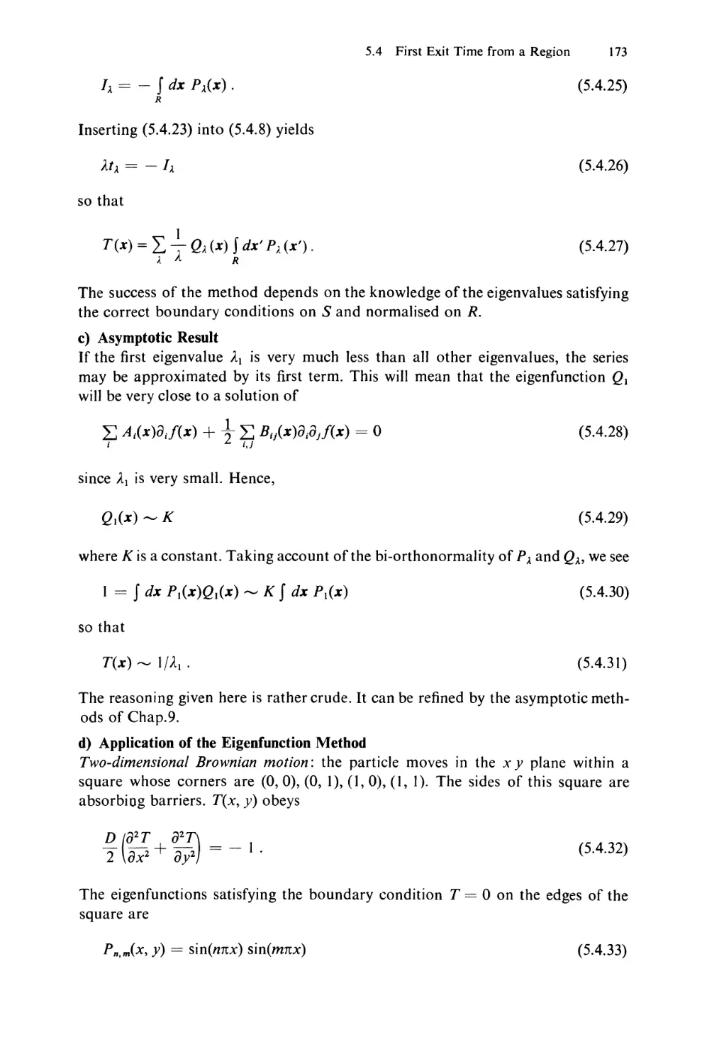
5.4 First Exit Time from a Region (Homogeneous Processes) 170
5.4.1 Solutions of Mean Exit Time Problems 171
5.4.2 Distribution of Exit Points 174
6. Approximation Methods for Diffusion Processes 177
6.1 Small Noise Perturbation Theories 177
6.2 Small Noise Expansions for Stochastic Differential Equations ... 180
6.2.1 Validity of the Expansion 182
6.2.2 Stationary Solutions (Homogeneous Processes) 183
6.2.3 Mean, Variance, and Time Correlation Function 184
6.2.4 Failure of Small Noise Perturbation Theories 185
6.3 Small Noise Expansion of the Fokker-Planck Equation 187
6.3.1 Equations for Moments and Autocorrelation Functions . . 189
6.3.2 Example 192
6.3.3 Asymptotic Method for Stationary Distributions 194
6.4 Adiabatic Elimination of Fast Variables 195
6.4.1 Abstract Formulation in Terms of Operators
and Projectors 198
6.4.2 Solution Using Laplace Transform 200
6.4.3 Short-Time Behaviour 203
6.4.4 Boundary Conditions 205
6.4.5 Systematic Perturbative Analysis 206
6.5 White Noise Process as a Limit of Nonwhite Process 210
6.5.1 Generality of the Result 215
6.5.2 More General Fluctuation Equations 215
6.5.3 Time Nonhomogencous Systems 216
6.5.4 Effect of Time Dependence in L, 217
6.6 Adiabatic Elimination of Fast Variables: The General Case .... 218
6.6.1 Example: Elimination of Short-Lived
Chemical Intermediates 218
6.6.2 Adiabatic Elimination in Haken's Model 223
6.6.3 Adiabatic Elimination of Fast Variables:
A Nonlinear Case 227
6.6.4 An Example with Arbitrary Nonlinear Coupling 232
7. Master Equations and Jump Processes 235
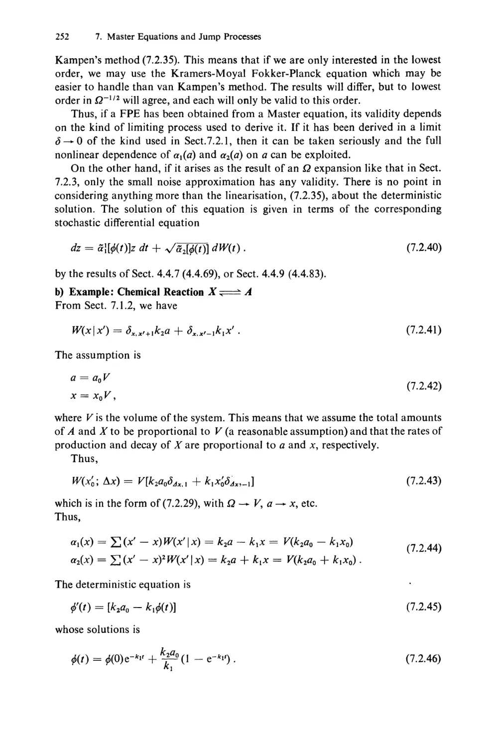
7.1 Birth-Death Master Equations—One Variable 236
7.1.1 Stationary Solutions 236
7.1.2 Example: Chemical Reaction X ;=± A 238
7.1.3 A Chemical Bistable System 241
7.2 Approximation of Master Equations by Fokker-Planck Equations . 246
7.2.1 Jump Process Approximation of a Diffusion Process .... 246
7.2.2 The Kramers-Moyal Expansion 245
7.2.3 Van Kampen's System Size Expansion 250

Contents
XV
7.2.4 Kurtz's Theorem 254
7.2.5 Critical Fluctuations 255
7.3 Boundary Conditions for Birth-Death Processes 257
7.4 Mean First Passage Times 259
7.4.1 Probability of Absorption 261
7.4.2 Comparison with Fokker-Planck Equation 261
7.5 Birth-Death Systems with Many Variables 262
7.5.1 Stationary Solutions when Detailed Balance Holds 263
7.5.2 Stationary Solutions Without Detailed Balance
(Kirchoff's Solution) 266
7.5.3 System Size Expansion and Related Expansions 266
7.6 Some Examples 267
7.6.1 X + A ^± 2X 267
7.6.2 X^Y^A 267
7.6.3 Prey-Predator System 268
7.6.4 Generating Function Equations 273
7.7 The Poisson Representation 277
7.7.1 Kinds of Poisson Representations 282
7.7.2 Real Poisson Representations 282
7.7.3 Complex Poisson Representations 282
7.7.4 The Positive Poisson Representation 285
7.7.5 Time Correlation Functions 289
7.7.6 Trimolecular Reaction 294
7.7.7 Third-Order Noise 299
8. Spatially Distributed Systems 303
8.1 Background 303
8.1.1 Functional Fokker-Planck Equations 305
8.2 Multivariate Master Equation Description 307
8.2.1 Diffusion 307
8.2.2 Continuum Form of Diffusion Master Equation 308
8.2.3 Reactions and Diffusion Combined 313
8.2.4 Poisson Representation Methods 314
8.3 Spatial and Temporal Correlation Structures 315
8.3.1 Reaction X^ Y 315
8.3.2 Reactions£ + X^C,A + X-+2X 319
8.3.3 A Nonlinear Model with a Second-Order Phase Transition . 324
8.4 Connection Between Local and Global Descriptions 328
8.4.1 Explicit Adiabatic Elimination of Inhomogeneous Modes . 328
8.5 Phase-Space Master Equation 331
8.5.1 Treatment of Flow 331
8.5.2 Flow as a Birth-Death Process 332
8.5.3 Inclusion of Collisions—the Boltzmann Master Equation . 336
8.5.4 Collisions and Flow Together 339

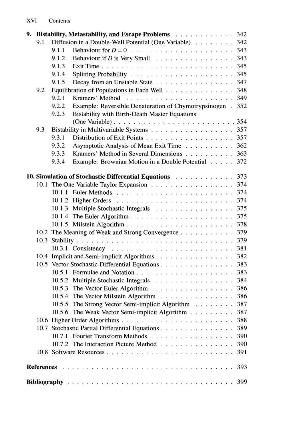
XVI Contents
9. Instability, Metastability, and Escape Problems 342
9.1 Diffusion in a Double-Well Potential (One Variable) 342
9.1.1 Behaviour forD = 0 343
9.1.2 Behaviour if D is Very Small 343
9.1.3 Exit Time 345
9.1.4 Splitting Probability 345
9.1.5 Decay from an Unstable State 347
9.2 Equilibration of Populations in Each Well 348
9.2.1 Kramers' Method 349
9.2.2 Example: Reversible Denaturation of Chymotrypsinogen . 352
9.2.3 Bistability with Birth-Death Master Equations
(One Variable) 354
9.3 Bistability in Multivariate Systems 357
9.3.1 Distribution of Exit Points 357
9.3.2 Asymptotic Analysis of Mean Exit Time 362
9.3.3 Kramers' Method in Several Dimensions 363
9.3.4 Example: Brownian Motion in a Double Potential 372
10. Simulation of Stochastic Differential Equations 373
10.1 The One Variable Taylor Expansion 374
10.1.1 Euler Methods 374
10.1.2 Higher Orders 374
10.1.3 Multiple Stochastic Integrals 375
10.1.4 The Euler Algorithm 375
10.1.5 Milstein Algorithm 378
10.2 The Meaning of Weak and Strong Convergence 379
10.3 Stability 379
10.3.1 Consistency 381
10.4 Implicit and Semi-implicit Algorithms 382
10.5 Vector Stochastic Differential Equations 383
10.5.1 Formulae and Notation 383
10.5.2 Multiple Stochastic Integrals 384
10.5.3 The Vector Euler Algorithm 386
10.5.4 The Vector Milstein Algorithm 386
10.5.5 The Strong Vector Semi-implicit Algorithm 387
10.5.6 The Weak Vector Semi-implicit Algorithm 387
10.6 Higher Order Algorithms 388
10.7 Stochastic Partial Differential Equations 389
10.7.1 Fourier Transform Methods 390
10.7.2 The Interaction Picture Method 390
10.8 Software Resources 391
References 393
Bibliography
399

Contents XVII
Symbol Index 403
Author Index 407
Subject Index 409

1. A Historical Introduction
1.1 Motivation
Theoretical science up to the end of the nineteenth century can be viewed as the
study of solutions of differential equations and the modelling of natural phenomena
by deterministic solutions of these differential equations. It was at that time
commonly thought that if all initial data could only be collected, one would be
able to predict the future with certainty.
We now know this is not so, in at least two ways. Firstly, the advent of quantum
mechanics within a quarter of a century gave rise to a new physics, and hence a
new theoretical basis for all science, which had as an essential basis a purely
statistical element. Secondly, more recently, the concept of chaos has arisen, in
which even quite simple differential equation systems have the rather alarming
property of giving rise to essentially unpredictable behaviour. To be sure, one can
predict the future of such a system given its initial conditions, but any error in the
initial conditions is so rapidly magnified that no practical predictability is left.
In fact, the existence of chaos is really not surprising, since it agrees with more of
our everyday experience than does pure predictability—but it is surprising perhaps
that it has taken so long for the point to be made.
0 2 4 6 8 10 12 14 16 18 20
Fig. 1.1. Stochastic simulation of an isomerisation reaction X-—* A

2 1. A Historical Introduction
Chaos and quantum mechanics are not the subject of this chapter. Here I wish
to give a semihistorical outline of how a phenomenological theory of fluctuating
phenomena arose and what its essential points are. The very usefulness of
predictable models indicates that life is not entirely chaos. But there is a limit to
predictability, and what we shall be most concerned with in this book are models of
limited predictability. The experience of careful measurements in science normally
gives us data like that of Fig. 1.1, representing the growth of the number of
molecules of a substance X formed by a chemical reaction of the form X ^± A. A quite
well defined deterministic motion is evident, and this is reproducible, unlike the
fluctuations around this motion, which are not.
1.2 Some Historical Examples
1.2.1 Brownian Motion
The observation that, when suspended in water, small pollen grains are found to
be in a very animated and irregular state of motion, was first systematically
investigated by Robert Brown in 1827, and the observed phenomenon took the
name Brownian Motion because of his fundamental pioneering work. Brown was
a botanist—indeed a very famous botanist—and of course tested whether this
motion was in some way a manifestation of life. By showing that the motion was
present in any suspension of fine particles—glass, minerals and even a fragment of
the sphinx—he ruled out any specifically organic origin of this motion. The motion
is illustrated in Fig. 1.2.
Fig. 1.2. Motion of a point undergoing Brownian
motion
The riddle of Brownian motion was not quickly solved, and a satisfactory
explanation did not come until 1905, when Einstein published an explanation under
the rather modest title "iiber die von der molekular-kinetischen Theorie der

1.2 Some Historical Examples 3
Warme geforderte Bewegung von in ruhenden Flussigkeiten suspendierten Teil-
chen" (concerning the motion, as required by the molecular-kinetic theory of heat,
of particles suspended in liquids at rest) [1.2]. The same explanation was
independently developed by Smoluchowski [1.3], who was responsible for much of the later
systematic development and for much of the experimental verification of Brownian
motion theory.
There were two major points in Einstein's solution to the problem of Brownian
motion.
(i) The motion is caused by the exceedingly frequent impacts on the pollen grain of
the incessantly moving molecules of liquid in which it is suspended,
(ii) The motion of these molecules is so complicated that its effect on the pollen
grain can only be described probabilistically in terms of exceedingly frequent
statistically independent impacts.
The existence of fluctuations like these ones calls out for a statistical explanation
of this kind of phenomenon. Statistics had already been used by Maxwell and
Boltzmann in their famous gas theories, but only as a description of possible states
and the likelihood of their achievement and not as an intrinsic part of the time
evolution of the system. Rayleigh [1.1] was in fact the first to consider a statistical
description in this context, but for one reason or another, very little arose out of
his work. For practical purposes, Einstein's explanation of the nature of Brownian
motion must be regarded as the beginning of stochastic modelling of natural
phenomena.
Einstein's reasoning is very clear and elegant. It contains all the basic concepts
which will make up the subject matter of this book. Rather than paraphrase a classic
piece of work, I shall simply give an extended excerpt from Einstein's paper (author's
translation):
"It must clearly be assumed that each individual particle executes a motion
which is independent of the motions of all other particles; it will also be considered
that the movements of one and the same particle in different time intervals are
independent processes, as long as these time intervals are not chosen too small.
"We introduce a time interval r into consideration, which is very small
compared to the observable time intervals, but nevertheless so large that in two
successive time intervals r, the motions executed by the particle can be thought of as
events which are independent of each other.
"Now let there be a total of n particles suspended in a liquid. In a time interval
t, the X-coordinates of the individual particles will increase by an amount A, where
for each particle A has a different (positive or negative) value. There will be a
certain frequency law for A; the number dn of the particles which experience a
shift which is between A and A + dA will be expressible by an equation of the form
dn = n$(A)dA, (1.2.1)
where
J <j>(A)dA = 1 (1.2.2)

4 1. A Historical Introduction
and j> is only different from zero for very small values of A, and satisifes the
condition
4(A) = ¢(- A). (1.2.3)
"We now investigate how the diffusion coefficient depends on <j>. We shall once
more restrict ourselves to the case where the number v of particles per unit volume
depends only on x and t.
"Let v = f(x, t) be the number of particles per unit volume. We compute the
distribution of particles at the time t + z from the distribution at time t. From the
definition of the function $(A), it is easy to find the number of particles which at
time t + r are found between two planes perpendicular to the x-axis and passing
through points x and x + dx. One obtains
f(x9 t + z)dx = dx] f(x + A, t)$(A)dA . (1.2.4)
But since z is very small, we can set
f(x,t + z)=f(x,t) + rft. (1.2.5)
Furthermore, we develop f(x + A, t) in powers of A:
r, t a x r, x , *df(X9t) , A2d2f(x,t) , /, - /-x
fix + A, t) =/(*, t) + A -^-; + ^- -%r- + ••' • 0-2-6)
We can use this series under the integral, because only small values of A contribute
to this equation. We obtain
f+ §£* = f ]j(^)dA + d£ ]^(A)dA + g \^<HA)dA . (1.2.7)
Because <f>(x) = <f>(-x), the second, fourth, etc., terms on the right-hand side vanish,
while out of the 1st, 3rd, 5th, etc., terms, each one is very small compared with the
previous. We obtain from this equation, by taking into consideration
J j>(A)dA = 1 (1.2.8)
and setting
- J 41j(A)dA=D, (1.2.9)
and keeping only the 1st and third terms of the right-hand side,
%-»%■■■■ <'-2-,o>

1.2 Some Historical Examples 5
This is already known as the differential equation of diffusion and it can be seen that
D is the diffusion coefficient. ...
"The problem, which corresponds to the problem of diffusion from a single
point (neglecting the interaction between the diffusing particles), is now
completely determined mathematically: its solution is
(1.2.11)
"We now calculate, with the help of this equation, the displacement lx in the
direction of the A'-axis that a particle experiences on the average or, more exactly,
the square root of the arithmetic mean of the square of the displacement in the
direction of the A'-axis; it is
K = VT2 = Vwt." (1.2.12)
Einstein's derivation is really based on a discrete time assumption, that impacts
happen only at times 0, r, 2t, 3t ... , and his resulting equation (1.2.10) for the
distribution function/(x, t) and its solution (1.2.11) are to be regarded as
approximations, in which t is considered so small that t may be considered as being
continuous. Nevertheless, his description contains very many of the major concepts
which have been developed more and more generally and rigorously since then,
and which will be central to this book. For example:
i) The Chapman-Kolmogorov Equation occurs as Einstein's equation (1.2.4). It
states that the probability of the particle being at point x at time t + z is given by
the sum of the probability of all possible "pushes" A from positions x + A,
multiplied by the probability of being at x + A at time t. This assumption is based on
the independence of the push A of any previous history of the motion: it is only
necessary to know the initial position of the particle at time t—not at any previous
time. This is the Markov postulate and the Chapman Kolmogorov equation, of
which (1.2.4) is a special form, is the central dynamical equation to all Markov
processes. These will be studied in detail in Chap. 3.
ii) The Fokker-Planck Equation: Eq. (1.2.10) is the diffusion equation, a special case
of the Fokker-Planck equation, which describes a large class of very interesting
stochastic processes in which the system has a continuous sample path. In this case,
that means that the pollen grain's position, if thought of as obeying a probabilistic
law given by solving the diffusion equation (1.2.10), in which time t is continuous
(not discrete, as assumed by Einstein), can be written x(t), where x(t) is a continuous
function of time-but a random function. This leads us to consider the possibility of
describing the dynamics of the system in some direct probabilistic way, so that we
would have a random or stochastic differential equation for the path. This procedure
was initiated by Langevin with the famous equation that to this day bears his name.
We will discuss this in detail in Chap. 4.
iii) The Kramers-Moyal and similar expansions are essentially the same as that
used by Einstein to go from (1.2.4) (the Chapman-Kolmogorov equation) to the

6 1. A Historical Introduction
diffusion equation (1.2.10). The use of this type of approximation, which effectively
replaces a process whose sample paths need not be continuous with one whose
paths are continuous, has been a topic of discussion in the last decade. Its use
and validity will be discussed in Chap. 7.
1.2.2 Langevin's Equation
Some time after Einstein's original derivation, Langevin [1.4] presented a new
method which was quite different from Einstein's and, according to him, "infinitely
more simple." His reasoning was as follows.
From statistical mechanics, it was known that the mean kinetic energy of the
Brownian particle should, in equilibrium, reach a value
^2mv2) = \kT (1.2.13)
(T\ absolute temperature, k; Boltzmann's constant). (Both Einstein and Smolucho-
wski had used this fact). Acting on the particle, of mass m there should be two
forces:
i) a viscous drag: assuming this is given by the same formula as in macroscopic
hydrodynamics, this is —6nrja dx/dt, rj being the viscosity and a the diameter of
the particle, assumed spherical.
ii) another fluctuating force X which represents the incessant impacts of the
molecules of the liquid on the Brownian particle. All that is known about it is that
fact, and that it should be positive and negative with equal probability. Thus, the
equation of motion for the position of the particle is given by Newton's law as
m^~= -6nrjajt + X (1.2.14)
and multiplying by x, this can be written
m d2 d(x2)
~^-2(x2) - mv2 = -Inna^2 + Xx , (1.2.15)
where v = dx/dt. We now average over a large number of different particles and use
(1.2.13) to obtain an equation for (x2):
m d2(x2) d(x2} n o ia\
y jti + 3n^adT ^ ' (1.2.16)
where the term (xX) has been set equal to zero because (to quote Langevin) "of
the irregularity of the quantity X". One then finds the general solution
^p = kT/Onrja) + C exp (-6nrjat/m), (1.2.17)

1.2 Some Historical Examples 7
where C is an arbitrary constant. Langevin estimated that the decaying exponential
approaches zero with a time constant of the order of 10~8 s, which for any practical
observation at that time, was essentially immediately. Thus, for practical purposes,
we can neglect this term and integrate once more to get
(x2) - <x02> = [kT/(3nrja)]t. (1.2.18)
This corresponds to (1.2.12) as deduced by Einstein, provided we identify
D = kT/(6nna)9 (1.2.19)
a result which Einstein derived in the same paper but by independent means.
Langevin's equation was the first example of the stochastic differential equation—
a differential equation with a random term X and hence whose solution is, in some
sense, a random function. Each solution of Langevin's equation represents a
different random trajectory and, using only rather simple properties of X (his
fluctuating force), measurable results can be derived.
One question arises: Einstein explicitly required that (on a sufficiently large time
scale) the change A be completely independent of the preceding value of A.
Langevin did not mention such a concept explicitly, but it is there, implicitly, when one
sets (Xx) equal to zero. The concept that X is extremely irregular and (which is not
mentioned by Langevin, but is implicit) that X and x are independent of each
other—that the irregularities in x as a function of time, do not somehow conspire
to be always in the same direction as those of A", so that the product could possibly
not be set equal to zero; these are really equivalent to Einstein's independence
assumption. The method of Langevin equations is clearly very much more direct,
at least at first glance, and gives a very natural way of generalising a dynamical
equation to a probabilistic equation. An adequate mathematical grounding for
the approach of Langevin, however, was not available until more than 40 years
later, when Ito formulated his concepts of stochastic differential equations. And
in this formulation, a precise statement of the independence of A' and x led to the
calculus of stochastic differentials, which now bears his name and which will be
fully developed in Chap. 4.
As a physical subject, Brownian motion had its heyday in the first two decades
of this century, when Smoluchowski in particular, and many others carried out
extensive theoretical and experimental investigations, which showed complete
agreement with the original formulation of the subject as initiated by himself and
Einstein, see [1.5]. More recently, with the development of laser light scattering
spectroscopy, Brownian motion has become very much more quantitatively
measurable. The technique is to shine intense, coherent laser light into a small
volume of liquid containing Brownian particles, and to study the fluctuations in the
intensity of the scattered light, which are directly related to the motions of the
Brownian particles. By these means it is possible to observe Brownian motion of
much smaller particles than the traditional pollen, and to derive useful data about
the sizes of viruses and macromolecules. With the preparation of more concentrated
suspensions, interactions between the particles appear, generating interesting and
quite complex problems related to macromolecular suspensions and colloids [1.6].

8 1. A Historical Introduction
The general concept of fluctuations describable by such equations has developed
very extensively in a very wide range of situations. The advantages of a continuous
description turn out to be very significant, since only a very few parameters are
required, i.e., essentially the coefficients of the derivatives in (1.2.7):
J Af(A)dA, and ] A2<j>{A)dA . (1.2.20)
It is rare to find a problem which cannot be specified, in at least some degree of
approximation, by such a system, and for qualitative simple analysis of problems it
is normally quite sufficient to consider an appropriate Fokker-Planck equation, of
a form obtained by allowing both coefficients (1.2.20) to depend on x, and in a space
of an appropriate number of dimensions.
1.3 Birth-Death Processes
A wide variety of phenomena can be modelled by a particular class of process called
a birth-death process. The name obviously stems from the modelling of human or
animal populations in which individuals are born, or die. One of the most
entertaining models is that of the prey-predator system consisting of two kinds of animal,
one of which preys on the other, which is itself supplied with an inexhaustible food
supply. Thus letting X symbolise the prey, Y the predator, and A the food of the
prey, the process under consideration might be
X+ A-+ 2X (1.3.1a)
X+ r—27 (1.3.1b)
Y-»B (1.3.1c)
which have the following naive, but charming interpretation. The first equation
symbolises the prey eating one unit of food, and reproducing immediately. The
second equation symbolises a predator consuming a prey (who thereby dies—this
is the only death mechanism considered for the prey) and immediately reproducing.
The final equation symbolises the death of the predator by natural causes. It is easy
to guess model differential equations for x and y, the numbers of X and Y. One
might assume that the first reaction symbolises a rate of production of X
proportional to the product of x and the amount of food; the second equation a
production of Y (and an equal rate of consumption of X) proportional to xy, and the last
equation a death rate of Y, in which the rate of death of Y is simply proportional to
y\ thus we might write
dx
-r = kxax — k2xy (1.3.2a)
^=k2xy-k3y. (1.3.2b)

1.3 Birth-Death Processes 9
The solutions of these equations, which were independently developed by Lotka
[1.7] and Volterra [1.8] have very interesting oscillating solutions, as presented in
Fig. 1.3a. These oscillations are qualitatively easily explicable. In the absence of
significant numbers of predators, the prey population grows rapidly until the
presence of so much prey for the predators to eat stimulates their rapid reproduction,
at the same time reducing the number of prey which get eaten. Because a large
number of prey have been eaten, there are no longer enough to maintain the
population of predators, which then die out, returning us to our initial situation.
The cycles repeat indefinitely and are indeed, at least qualitatively, a feature of
many real prey-predator systems. An example is given in Fig. 1.3b.
1500, 1
Fig. 1.3a-c. Time development in prey-predator systems, (a) Plot of solutions of the deterministic
equations (1.3.2) (x — solid line, y = dashed line), (b) Data for a real prey-predator system. Here
the predator is a mite (Eotetranychus sexmaculatus—dashed line) which feeds on oranges, and
the prey is another mite (Typhlodromus occidentalis). Data from [1.16, 17]. (c) Simulation of
stochastic equations (1.3.3)

10 1. A Historical Introduction
Of course, the realistic systems do not follow the solutions of differential
equations exactly—they fluctuate about such curves. One must include these
fluctuations and the simplest way to do this is by means of a birth-death master
equation. We assume a probability distribution, P(x, y, t), for the number of
individuals at a given time and ask for a probabilistic law corresponding to (1.3.2).
This is done by assuming that in an infinitesimal time At, the following transition
probability laws holds.
Prob (x -+ x+1; y -+ y) = kyaxAt, (1.3.3a)
Prob (x -+ x-\; y -+ y+1) - k2xyAt, (1.3.3b)
Prob (x -+ x\ y -+ y— 1) = k3yAt, (1.3.3c)
Prob (x -+ x\ y -+ y) = \-(kxax + k2xy + k3y)At. (1.3.3d)
Thus, we simply, for example, replace the simple rate laws by probability laws.
We then employ what amounts to the same equation as Einstein and others used,
i.e., the Chapman-Kolmogorov equation, namely, we write the probability at
t + At as a sum of terms, each of which represents the probability of a previous
state multiplied by the probability of a transition to the state (x, y). Thus, we
find
P{x,y,t + At)-P^y,t) = kMx _ {)p(x _Uytt) + Ux +X){y_ 1}
X P(x + 1, y - 1, t) + k3(y + \)P(x, ^+1,0- (kxax + k2xy + k3y)
X P(x9y,t) (1.3.4)
and letting At -+ 0, = dP(x, y, t)jdt. In writing the assumed probability laws
(1.3.3), we are assuming that the probability of each of the events occurring
can be determined simply from the knowledge of x and y. This is again the
Markov postulate which we mentioned in Sect. 1.2.1. In the case of Brownian
motion, very convincing arguments can be made in favour of this Markov
assumption. Here it is by no means clear. The concept of heredity, i.e., that the behaviour
of progeny is related to that of parents, clearly contradicts this assumption. How
to include heredity is another matter; by no means does a unique prescription
exist.
The assumption of the Markov postulate in this context is valid to the extent
that different individuals of the same species are similar; it is invalid to the extent
that, nevertheless, perceptible inheritable differences do exist.
This type of model has a wide application—in fact to any system to which a
population of indivuduals may be attributed, for example systems of molecules of
various chemical compounds, of electrons, of photons and similar physical
particles as well as biological systems. The particular choice of transition probabilities
is made on various grounds determined by the degree to which details of the
births and deaths involved are known. The simple multiplicative laws, as illustrated
in (1.3.3), are the most elementary choice, ignoring, as they do, almost all details of

1.4 Noise in Electronic Systems 11
the processes involved. In some of the physical processes we can derive the
transition probabilities in much greater detail and with greater precision.
Equation (1.3.4) has no simple solution, but one major property differentiates
equations like it from an equation of Langevin's type, in which the fluctuation term
is simply added to the differential equation. Solutions of (1.3.4) determine both
the gross deterministic motion and the fluctuations; the fluctuations are typically
of the same order of magnitude as the square roots of the numbers of individuals
involved. It is not difficult to simulate a sample time development of the process
as in Fig. 1.3c. The figure does show the correct general features, but the model is
so obviously simplified that exact agreement can never be expected. Thus, in
contrast to the situation in Brownian motion, we are not dealing here so much
with a theory of a phenomenon, as with a class of mathematical models, which
are simple enough to have a very wide range of approximate validity. We will see
in Chap. 7 that a theory can be developed which can deal with a wide range of
models in this category, and that there is indeed a close connection between this kind
of theory and that of stochastic differential equations.
1.4 Noise in Electronic Systems
The early days of radio with low transmission powers and primitive receivers,
made it evident to every ear that there were a great number of highly irregular
electrical signals which occurred either in the atmosphere, the receiver, or the
radio transmitter, and which were given the collective name of "noise", since this is
certainly what they sounded like on a radio. Two principal sources of noise are
shot noise and Johnson noise.
1.4.1 Shot Noise
In a vacuum tube (and in solid-state devices) we get a nonsteady electrical current,
since it is generated by individual electrons, which are accelerated across a distance
and deposit their charge one at a time on the anode. The electric current arising
from such a process can be written
/(0 = E *■('-'*)> (14.1)
tk
where F(t-tk) represents the contribution to the current of an electron which arrives
at time tk. Each electron is therefore assumed to give rise to the same shaped pulse,
but with an appropriate delay, as in Fig. 1.4.
A statistical aspect arises immediately we consider what kind of choice must be
made for tk. The simplest choice is that each electron arrives independently of the
previous one—that is, the times tk are randomly distributed with a certain average
number per unit time in the range (-oo, oo), or whatever time is under
consideration.

12
1. A Historical Introduction
Fig. 1.4. Illustration of shot
noise: identical electric pulses
arrive at random times
Time
The analysis of such noise was developed during the 1920's and 1930's and was
summarised and largely completed by Rice [1.9]. It was first considered as early as
1918 by Schottky[l.\0].
We shall find that there is a close connection between shot noise and processes
described by birth-death master equations. For, if we consider n, the number of
electrons which have arrived up to a time t, to be a statistical quantity described by
a probability P(n, t), then the assumption that the electrons arrive independently is
clearly the Markov assumption. Then, assuming the probability that an electron
will arrive in the time interval between t and t + Af is completely independent of t
and /i, its only dependence can be on At. By choosing an appropriate constant X, we
may write
Prob (n-+n + 1, in time At) = A At
so that
P(n, t + At) = P(n, t) (1 - XAt) + P(n - 1, t)XAt
and taking the limit At — 0
dP(n, t)
dt
'■=*.[P(n-l,t)-P(n9t)]
which is a pure birth process. By writing
G(s, t) = !>"/>(>*, t)
(1.4.2)
(1.4.3)
(1.4.4)
(1.4.5)
[here, G(s, t) is known as the generating function for P(«, t), and the particular
technique of solving (1.28) is very widely used], we find
^) = 1(,-1)^,0
so that
G(s, t) = exp [X(s- \)t]G(s, 0).
(1.4.6)
(1.4.7)
By requiring at time t = 0 that no electrons had arrived, it is clear that P(0, 0) is
1 and/»(«,0) is zero for all« ^ l,so that G(s,0) = 1. Expanding the solution (1.4.7)

1.4 Noise in Electronic Systems 13
in powers of s, we find
P(n,1) = exp (-Xt) (Xt)"/n\ (1.4.8)
which is known as a Poisson distribution (Sect. 2.8.3). Let us introduce the variable
N(t), which is to be considered as the number of electrons which have arrived up to
time t, and is a random quantity. Then,
P(n91) = Prob {N(t) = n), (1.4.9)
and N(t) can be called a Poisson process variable. Then clearly, the quantity /*(f),
formally defined by
M(t) - dN(t)/dt, (1.4.10)
is zero, except when N(t) increases by 1; at that stage it is a Dirac delta function,
i.e.,
M(t) = HW-t*)> (1.4.11)
k
where the tk are the times of arrival of the individual electrons. We may write
/(/)= ]jt'F(t - tWS) . (1.4.12)
A very reasonable restriction on F(t — t') is that it vanishes if t < t\ and that
for t —* oo, it also vanishes. This simply means that no current arises from an
electron before it arrives, and that the effect of its arrival eventually dies out. We
assume then, for simplicity, the very commonly encountered form
(1.4.13)
<w-_^^ dt, • (1.4.14)
We can derive a simple differential equation. We differentiate I(t) to obtain
+ J dt'i-aq^-^-'^^P (1.4.15)
so
F(t) =
=
qe-at
0
that (1.4.12) can
Ut\ =
f dt'n ft
O
(t<
be rewritten
-„„-,« dN(Q
0)
0)
as
dm
dt
that
dl(t)
dt
\gt-«u-.ndWy\
dt
-al(t) + q/x(t) .
»'-»
dt'
(1.4.16)

14 1. A Historical Introduction
This is a kind of stochastic differential equation, similar to Langevin's equation^ in
which, however, the fluctuating force is given by qju(t), where//(f) is the derivative
of the Poisson process, as given by (1.4.11). However, the mean of ju(t) is nonzero,
in fact, from (1.4.10)
(M(t)dt) = <</#(*)> = kdt (1.4.17)
([dN(t) - kdtf) = Idt (1.4.18)
from the properties of the Poisson distribution, for which the variance equals the
mean. Defining, then, the fluctuation as the difference between the mean value
and dN(t), we write
drj(t) = dN(t) - Xdt, (1.4.19)
so that the stochastic differential equation (1.4.16) takes the form
dl(t) = [Xq - al{t)} dt + qdnif) . (1.4.20)
Now how does one solve such an equation? In this case, we have an academic
problem anyway since the solution is known, but one would like to have a technique.
Suppose we try to follow the method used by Langevin—what will we get as an
answer? The short reply to this question is: nonsense. For example, using ordinary
calculus and assuming (J{t)drj{t)y = 0, we can derive
^^> = Xq- cr</(0> and (1.4.21)
Y^dT = ^</(0> - *</2(0> (1A22)
solving in the limit t — oo, where the mean values would reasonably be expected
to be constant one finds
(I(oo)) = Xq/a and (1.4.23)
</2(cx>)> = (W . (1.4.24)
The first answer is reasonable—it merely gives the average current through the
system in a reasonable equation, but the second implies that the mean square
current is the same as the square of the mean, i.e., the current at t —> oo does not
fluctuate! This is rather unreasonable, and the solution to the problem will show
that stochastic differential equations are rather more subtle than we have so far
presented.
Firstly, the notation in terms of differentials used in (1.4.17-20) has been chosen
deliberately. In deriving (1.4.22), one uses ordinary clalculus, i.e., one writes

1.4 Noise in Electronic Systems 15
d(i2) = (1+ diy -p = iidi + (diy (1.4.25)
and then one drops the (dl)2 as being of second order in dl. But now look at (1.4.18):
this is equivalent to
(drj(t)2} = Xdt (1.4.26)
so that a quantity of second order in drj is actually of first order in dt. The reason
is not difficult to find. Clearly,
drj(t) = dN(t) - Xdt, (1.4.27)
but the curve of N(t) is a step function, discontinuous, and certainly not differen-
tiable, at the times of arrival of the individual electrons. In the ordinary sense,
none of these calculus manipulations is permissible. But we can make sense out of
them as follows. Let us simply calculate (d(I2)) using (1.4.20, 25, 26):
(d(I)2} = 2(1 {[Xq - al]dt + q drj(t)}}
+ <P<7 - al]dt + qdrj(t)} 2> . (1.4.28)
We now assume again that (I(t)drj(t)) = 0 and expand, after taking averages
using the fact that (dn(t)2) = X dt, to 1st order in dt. We obtain
and this gives
Xq(» - a(P) + &
dt (1.4.29)
</2(c*>)> - </(«,)>* = p . (1.4.30)
la
Thus, there are fluctuations from this point of view, as t -+ oo. The extra term in
(1.4.29) as compared to (1.4.22) arises directly out of the statistical considerations
implicit in N(t) being a discontinuous random function.
Thus we have discovered a somewhat deeper way of looking at Langevin's kind
of equation—the treatment of which, from this point of view, now seems extremely
naive. In Langevin's method the fluctuating force X is not specified, but it will
become clear in this book that problems such as we have just considered are very
widespread in this subject. The moral is that random functions cannot normally
be differentiated according to the usual laws of calculus: special rules have to be
developed, and a precise specification of what one means by differentiation becomes
important. We will specify these problems and their solutions in Chap. 4 which will
concern itself with situations in which the fluctuations are Gaussian.
1.4.2 Autocorrelation Functions and Spectra
The measurements which one can carry out on fluctuating systems such as electric
circuits are, in practice, not of unlimited variety. So far, we have considered the

16 1. A Historical Introduction
distribution functions, which tell us, at any time, what the probability distribution
of the values of a stochastic quantity are. If we are considering a measureable
quantity x(t) which fluctuates with time, in practice we can sometimes determine the
distribution of the values of x, though more usually, what is available at one time
are the mean x(t) and the variance var {x(t).}
The mean and the variance do not tell a great deal about the underlying
dynamics of what is happening. What would be of interest is some quantity which is a
is a measure of the influence of a value of x at time t on the value at time t + z.
Such a quantity is the autocorrelation function, which was apparently first introduced
by Taylor [1.11] as
G(z) = lim ^ J dt x(t)x(t + z). (1.4.31)
This is the time average of a two-time product over an arbitrary large time T9
which is then allowed to become infinite.
Nowadays purpose built autocorrelators exist, which sample data and directly
construct the autocorrelation function of a desired process, from laser light
scattering signals to bacterial counts. It is also possible to construct autocorrelation
programs for high speed on line experimental computers. Further, for very fast
systems, there are clipped autocorrelators, which measure an approximation to
the autocorrelation function given by defining a variable c(t) such that
c(t) = 0 x(t) < I
= 1 x(t) > I (1.4.32)
and computing the autocorrelation function of that variable.
A more traditional approach is to compute the spectrum of the quantity x(t).
This is defined in two stages. First, define
^) = ^1 t"imx(t) (1.4.33)
o
then the spectrum is defined by
SM = lhn^bMI2. (1.4.34)
The autocorrelation function and the spectrum are closely connected. By a little
manipulation one finds
S(co) = lim
— J* cos (caz)dz — j x(t)x(t + z)dt
^0 ■* 0
(1.4.35)
and taking the limit T-^oo (under suitable assumptions to ensure the validity of
certain interchanges of order), one finds

1.4 Noise in Electronic Systems 17
S(co) = — J cos (coz)G(z)dz . (1.4.36)
K o
This is a fundamental result which relates the Fourier transform of the
autocorrelation function to the spectrum. The result may be put in a slightly different form
when one notices that
G(-t) = lim4J Xdt x(t + r)x(t) = G(t) (1.4.37)
so we obtain
SM = ^J t'imG(r)dr | (1.4.38)
with the corresponding inverse
G(t)= J timS(<o)d(o. | (1.4.39)
This result is known as the Wiener-Khinchin theorem [1.12,13] and has widespread
application.
It means that one may either directly measure the autocorrelation function of a
signal, or the spectrum, and convert back and forth, which by means of the fast
Fourier transform and computer is relatively straightforward.
1.4.3 Fourier Analysis of Fluctuating Functions: Stationary Systems
The autocorrelation function has been defined so far as a time average of a signal,
but we may also consider the ensemble average, in which we repeat the same
measurement many times, and compute averages, denoted by < >. It will be shown
that for very many systems, the time average is equal to the ensemble average;
such systems are termed ergodic (Sect. 3.7.1).
If we have such a fluctuating quantity x{t)9 then we can consider the average
(x(t)x(t + t)> = G(t), (1.4.40)
this result being the consequence of our ergodic assumption.
Now it is very natural to write a Fourier transform for the stochastic quantity
x(t)
x(t) = I dm c(co) eia" (1.4.41)
and consequently,
c(a>) = ±jdtx(t)e-l°". (1.4.42)

18 1. A Historical Introduction
Note that x(t) real implies
c((jo) = c*(-a>). (1.4.43)
If the system is ergodic, we must have a constant <x(0>> since the time average
is clearly constant. The process is then stationary by which we mean that all time-
dependent averages are functions only of time differences, i.e., averages of functions
xfa), x(t2), ... x(tn) are equal to those of x(tx + A), x(t2 + A), ... x(tn + A).
For convenience, in what follows we assume (x) = 0. Hence,
(c(co)) =^\dt (x)e-icot = 0 (1.4.44)
<c(w)c*(w')) = (-^ J J dt dt'e-^*>'<Xx(t)x(t')}
- ^- b(co - co') J dr ei(UTG(r)
= 5(co - <jo')S((d) . (1.4.45)
Here we find not only a relationship between the mean square (|c(a;)|2> and the
spectrum, but also the result that stationarity alone implies that c(co) and c*(a>')
are uncorrelated, since the term b(a> — co') arises because (x(t)x(t')) is a function
only of t — t'.
1.4.4 Johnson Noise and Nyquist's Theorem
Two brief and elegant papers appeared in 1928 in which Johnson [1.14]
demonstrated experimentally that an electric resistor automatically generated fluctuations
of electric voltage, and Nyquist [1.15] demonstrated its theoretical derivation, in
complete accordance with Johnson's experiment. The principle involved was
already known by Schottky [1.10] and is the same as that used by Einstein and
Langevin. This principle is that of thermal equilibrium. If a resistor R produces
electric fluctuations, these will produce a current which will generate heat. The heat
produced in the resistor must exactly balance the energy taken out of the
fluctuations. The detailed working out of this principle is not the subject of this section,
but we will find that such results are common throughout the physics and
chemistry of stochastic processes, where the principles of statistical mechanics, whose
basis is not essentially stochastic, are brought in to complement those of stochastic
processes. The experimental result found was the following. We have an electric
resistor of resistance R at absolute temperature T. Suppose by means of a suitable
filter we measure E(co)dco, the voltage across the resistor with angular frequency in
the range (a>, co + dco). Then, if k is Boltzmann's constant,

1.4 Noise in Electronic Systems 19
(E2(co)) = RkT/n . (1.4.46)
This result is known nowadays as Nyquist's theorem. Johnson remarked. "The
effect is one of the causes of what is called 'tube noise' in vacuum tube amplifiers.
Indeed, it is often by far the larger part of the 'noise' of a good amplifier."
Johnson noise is easily described by the formalism of the previous subsection.
The mean noise voltage is zero across a resistor, and the system is arranged so that
it is in a steady state and is expected to be well represented by a stationary process.
Johnson's quantity is, in practice, a limit of the kind (1.4.34) and may be
summarised by saying that the voltage spectrum S(co) is given by
S(co)= RkT/n , (1.4.47)
that is, the spectrum is flat, i.e., a constant function of co. In the case of light, the
frequencies correspond to different colours of light. If we perceive light to be white,
it is found that in practice all colours are present in equal proportions—the optical
spectrum of white light is thus flat—at least within the visible range. In analogy, the
term white noise is applied to a noise voltage (or any other fluctuating quantity)
whose spectrum is flat.
White noise cannot actually exist. The simplest demonstration is to note that
the mean power dissipated in the resistor in the frequency range (cou a>2) is given
by
(W2
j dco S(co)/R = kT{oj{-oj2)/n (1.4.48)
Q)l
so that the total power dissipated in all frequencies is infinite! Nyquist realised this,
and noted that, in practice, there would be quantum corrections which would,
at room temperature, make the spectrum flat only up to 7 x 1013 Hz, which is not
detectable in practice, in a radio situation. The actual power dissipated in the
resistor would be somewhat less than infinite, 10~10 W in fact! And in practice
there are other limiting factors such as the inductance of the system, which would
limit the spectrum to even lower frequencies.
From the definition of the spectrum in terms of the autocorrelation function
given in Sect. 1.4, we have
<£(f+ t)£(0> = G(t) (1.4.49)
= ^- J dcoQ-i0iT2R kT (1.4.50)
= 2RkTS(r), (1.4.51)
which implies that no matter how small the time difference r, E(t + r) and E(z)
are not correlated. This is, of course, a direct result of the flatness of the spectrum.
A typical model of S(co) that is almost flat is
S(oj) = RkT/[n{a? t2c+\)\ (1.4.52)

20 1. A Historical Introduction
.^
,G(t)
Fig. 1.5.a,b. Correlation Functions ( ) and corresponding spectra ( ) for (a) short
correlation time corresponding to an almost flat spectrum; (b) long correlation time, giving a
quite rapidly decreasing spectrum
This is flat provided a> <^ tc_1. The Fourier transform can be explicitly evaluated
in this case to give
<£(/ + r)E(t) > = (R kT/rc) exp (-t/tc) (1.4.53)
so that the autocorrelation function vanishes only for t ^> rc, which is called the
correlation time of the fluctuating voltage. Thus, the delta function correlation
function appears as an idealisation, only valid on a sufficiently long time scale.
This is very reminiscent of Einstein's assumption regarding Brownian motion
and of the behaviour of Langevin's fluctuating force. The idealised white noise will
play a highly important role in this book but, in just the same way as the fluctuation
term that arises in a stochastic differential equation is not the same as an ordinary
differential, we will find that differential equations which include white noise as a
driving term have to be handled with great care. Such equations arise very
naturally in any fluctuating system and it is possible to arrange by means of Stratono-
vich's rules for ordinary calculus rules to apply, but at the cost of imprecise
mathematical definition and some difficulties in stochastic manipulation. It turns out to
be far better to abandon ordinary calculus and use the Ito calculus, which is not
very different (it is, in fact, very similar to the calculus presented for shot noise)
and to preserve tractable statistical properties. All these matters will be discussed
thoroughly in Chap. 4.
White noise, as we have noted above, does not exist as a physically realisable
process and the rather singular behaviour it exhibits does not arise in any realisable
context. It is, however, fundamental in a mathematical, and indeed in a physical
sense, in that it is an idealisation of very many processes that do occur. The slightly
strange rules which we will develop for the calculus of white noise are not really
very difficult and are very much easier to handle than any method which always
deals with a real noise. Furthermore, situations in which white noise is not a good
approximation can very often be indirectly expressed quite simply in terms of
white noise. In this sense, white noise is the starting point from which a wide range
of stochastic descriptions can be derived, and is therefore fundamental to the
subject of this book.
k
\
\
^,S(u>)
\
\
k v
\ ^
\ ^
\ \
\ ^
/V ^
| G(t)\^^--
(b)

2. Probability Concepts
In the preceding chapter, we introduced probability notions without any definitions.
In order to formulate essential concepts more precisely, it is necessary to have
some more precise expression of these concepts. The intention of this chapter is to
provide some background, and to present a number of essential results. It is not a
thorough outline of mathematical probability, for which the reader is referred to
standard mathematical texts such as those by Feller [2.1] and Papoulis [2.2].
2.1 Events, and Sets of Events
It is convenient to use a notation which is as general as possible in order to describe
those occurrences to which we might wish to assign probabilities. For example,
we may wish to talk about a situation in which there are 6.4 x 1014 molecules in a
certain region of space; or a situation in which a Brownian particle is at a certain
point x in space; or possibly there are 10 mice and 3 owls in a certain region of a
forest.
These occurrences are all examples of practical realisations of events. More
abstractly, an event is simply a member of a certain space, which in the cases most
practically occuring can be characterised by a vector of integers
n = (nu n2,n3 ...) (2.1.1)
or a vector of real numbers
x = (xu x29 x3 ...). (2.1.2)
The dimension of the vector is arbitary.
It is convenient to use the language of set theory, introduce the concept of a set
of events, and use the notation
co<=A (2.1.3)
to indicate that the event co is one of events contained in A. For example, one
may consider the set A(25) of events in the ecological population in which there
are no more than 25 animals present; clearly the event co that there are 3 mice, a
tiger, and no other animals present satisfies
co e A(25).
(2.1.4)

22 2. Probability Concepts
More significantly, suppose we define the set of events A(r, AV) that a molecule
is within a volume element A V centred on a point r. In this case, the practical
significance of working in terms of sets of events becomes clear, because we should
normally be able to determine whether or not a molecule is within a neighbourhood
AKof r, but to determine whether the particle is exactly at r is impossible. Thus, if
we define the event co(y) that the molecule is at point y, it makes sense to ask
whether
co(y)^A(r, AV) (2.1.5)
and to assign a certain probability to the set A(r, AV), which is to be interpreted as
the probability of the occurrence of (2.1.5)
2.2 Probabilities
Most people have an intuitive conception of a probability, based on their own
experience. However, a precise formulation of intuitive concepts is fraught with
difficulties, and it has been found most convenient to axiomatise probability theory
as an essentially abstract science, in which a probability measure P(A) is assigned
to every set A9 in the space of events, including
the set of all events: Q (2.2.1)
the set of no events: 0 ; (2.2.2)
in order to define probability, we need our sets of events to form a closed system
(known by mathematicians as a a-algebra) under the set theoretic operations of
union and intersection.
2.2.1 Probability Axioms
We introduce the probability of A, P(A), as a function of A satisfying the following
probability axioms:
(i) P(A) > 0 for all A , (2.2.3)
(ii) P{Q) = 1 , (2.2.4)
(iii) if At(i=\, 2, 3, ...) is a countable (but possibly infinite) collection of
nonoverlapping sets, i.e., such that
At n Aj= 0 for all i^j, (2.2.5)
then
P(U A) = YiP(Ai). (2.2.6)
i i
These are all the axioms needed. Consequentially, however, we have:

2.2 Probabilities 23
(iv) if A is the complement of A, i.e., the set of all events not contained in A,
then
P(A) = 1 - P(A), (2.2.7)
(v) P(0) = 0. (2.2.8)
2.2.2 The Meaning of P(A)
There is no way of making probability theory correspond to reality without
requiring a certain degree of intuition. The probability P(A), as axiomatised above,
is the intuitive probability that an "arbitrary" event co, i.e., an event co "chosen at
random", will satisfy co e A. Or more explicitly, if we choose an event "at random"
from Q N times, the relative frequency that the particular event chosen will satisfy
co e A approaches P(A) as the number of times, N, we choose the event, approaches
infinity. The number of choices TV can be visualised as being done one after the
other ("independent" tosses of one die) or at the same time (N dice are thrown at the
same time "independently"). All definitions of this kind must be intuitive, as we
can see by the way undefined terms ("arbitrary", "at random", "independent") keep
turning up. By eliminating what we now think of as intuitive ideas and axiomatising
probability, Kolomogorov [2.3] cleared the road for a rigorous development of
mathematical probability. But the circular definition problems posed by wanting
an intuitive understanding remain. The simplest way of looking at axiomatic
probability is as a formal method of manipulating probabilities using the axioms. In
order to apply the theory, the probability space must be defined and the probability
measure P assigned. These are a priori probabilities, which are simply assumed.
Examples of such a priori probabilities abound in applied disciplines. For example,
in equilibrium statistical mechanics one assigns equal probabilities to equal volumes
of phase space. Einstein's reasoning in Brownian motion assigned a probability ¢(A)
to the probability of a "push" A from a position x at time t.
The task of applying probability is (i) to assume some set of a priori probabilities
which seem reasonable and to deduce results from this and from the structure of the
probability space, (ii) to measure experimental results with some apparatus which
is constructed to measure quantities in accordance with these a priori probabilities.
The structure of the probability space is very important, especially when the
space of events is compounded by the additional concept of time. This extension
makes the effective probability space infinite-dimensional, since we can construct
events such as "the particle was at points xn at times t„, n — 0, 1,2, ..., oo".
2.2.3 The Meaning of the Axioms
Any intuitive concept of probability gives rise to nonnegative probabilities, and the
probability that an arbitrary event is contained in the set of all events must be 1
no matter what our definition of the word arbitrary. Hence, axioms (i) and (ii) are
understandable. The heart of the matter lies in axiom (iii). Suppose we are dealing
with only 2 sets A and B, and A f] B = 0. This means there are no events con-

24 2. Probability Concepts
tained in both A and B. Therefore, the probability that co e A U B is the
probability that either co ^ A or co ^ B. Intuitive considerations tell us this probability is
the sum of the individual probabilities, i.e.,
P(A U B) = P{(co^ A) or (co e B)} = P(A) + P(B) (2.2.9)
(notice this is not a proof—merely an explanation).
The extension now to any finite number of nonoverlapping sets is obvious, but
the extension only to any countable number of nonoverlapping sets requires some
comment.
This extension must be made restrictive because of the existence of sets labelled
by a continuous index, for example, x, the position in space. The probability of a
molecule being in the set whose only element in x is zero; but the probability of
being in a region R of finite volume is nonzero. The region R is a union of sets of
the form {*} —but not a countable union. Thus axiom (iii) is not applicable and the
probability of being in R is not equal to the sum of the probabilities of being in {x}.
2.2.4 Random Variables
The concept of a random variable is a notational convenience which is central to
this book. Suppose we have an abstract probability space whose events can be
written x. Then we can introduce the random variable F(x) which is a function of
jc, which takes on certain values for each x. In particular, the identity function of
jc, written X(x) is of interest; it is given by
X(x) = x. (2.2.10)
We shall normally use capitals in this book to denote random variables and small
letters jc to denote their values whenever it is necessary to make a distinction.
Very often, we have some quite different underlying probability space Q with
values a>, and talk about X(co) which is some function of co, and then omit explicit
mention of co. This can be for either of two reasons:
i) we specify the events by the values of jc anyway, i.e., we identify x and co;
ii) the underlying events co are too complicated to describe, or sometimes, even
to know.
For example, in the case of the position of a molecule in a liquid, we really
should interpret each co as being capable of specifying all the positions, momenta,
and orientations of each molecule in that volume of liquid; but this is simply too
difficult to write down, and often unnecessary.
One great advantage of introducing the concept of a random variable is the
simplicity with which one may handle functions of random variables, e.g., X2,
sin(a • X), etc, and compute means and distributions of these. Further, by defining
stochastic differential equations, one can also quite simply talk about time
development of random variables in a way which is quite analogous to the classical
description by means of differential equations of nonprobabilistic systems.

2.3 Joint and Conditional Probabilities: Independence 25
2.3 Joint and Conditional Probabilities: Independence
2.3.1 Joint Probabilities
We explained in Sect. 2.2.3 how the occurrence of mutually exclusive events is related
to the concept of nonintersecting sets. We now consider the concept P(A f) B), where
A f] Bis nonempty. An event co which satisfies co ^ A will only satisfy co e A f) B
if co e B as well.
Thus, P(A (1 B) = P{(co e A) and (co <= 5)} (2.3.1)
and P(A f) ^) is called the joint probability that the event co is contained in both
classes, or, alternatively, that both the events co e A and co ^ B occur. Joint
probabilities occur naturally in the context of this book in two ways:
i) When the event is specified by a vector, e.g., m mice and n tigers. The probability
of this event is the joint probability of [m mice (and any number of tigers)] and
[n tigers (and any number of mice)]. All vector specifications are implicitly joint
probabilities in this sense.
ii) When more than one time is considered: what is the probability that (at time tx
there are mx tigers and nx mice) and (at time t2 there are m2 tigers and n2 mice).
To consider such a probability, we have effectively created out of the events at time
tx and events at time t2, joint events involving one event at each time. In essence,
there is no difference between these two cases except for the fundamental dynamical
role of time.
2.3.2 Conditional Probabilities
We may specify conditions on the events we are interested in and consider only
these, e.g., the probability of 21 buffaloes given that we know there are 100 lions.
What does this mean? Clearly, we will be interested only in those events contained
in the set B = {all events where exactly 100 lions occur}. This means that we to
define conditional probabilities, which are defined only on the collection of all sets
contained in B. we define the conditional probability as
P(A\B) = P(A n B)/P(B) (2.3.2)
and this satisfies our intuitive conception that the conditional probability that
co G A (given that we know co G B), is given by dividing the probability of joint
occurrence by the probability (co e B).
We can define in both directions, i.e., we have
P(A n B) - P(A | B)P(B) = P(B | A)P(A). (2.3.3)
There is no particular conceptual difference between, say, the probability of {(21
buffaloes) given (100 lions)} and the reversed concept. However, when two times

26 2. Probability Concepts
are involved, we do see a difference. For example, the probability that a particle is
at position xY at time tu given that it was at x2 at the previous time t29 is a very
natural thing to consider; indeed, it will turn out to be a central concept in this book.
The converse sounds strange, i.e., the probability that a particle is at position jc,
at time tl9 given that it will be at position x2 at a later time f2- It smacks of
clairvoyance—we cannot conceive of any natural way in which we would wish to
consider it, although it is, in principle, a quantity very similar to the "natural"
conditional probability, in which the condition precedes the events under consideration.
The natural definition has already occurred in this book, for example, the
<l>(A)dA of Einstein (Sect. 1.2.1.) is the probability that a particle at x at time t will
be in the range [x + A, x + A + dA] at time t + r, and similarly in the other
examples. Our intuition tells us as it told Einstein (as can be seen by reading the
extract from his paper) that this kind of conditional probability is directly related
to the time development of a probabilistic system.
2.3.3 Relationship Between Joint Probabilities of Different Orders
Suppose we have a collection of sets Bt such that
Btf] Bj= 0 (2.3.4)
U Bt = Q (2.3.5)
so that the sets divide up the space Q into nonoverlapping subsets.
Then
u (a n Bt) = An(u Bt) = Ano = A (2.3.6)
i i
Using now the probability axiom (iii), we see that A f) Bt satisfy the conditions
on the At used there, so that
2 P(A fl Bt) = P[U (A U B{)] (2.3.7)
= P(A) (2.3.8)
and thus
XP(A\Bt)P(Bt)=P(A) (2.3.9)
Thus, summing over all mutually exclusive possibilities of B in the joint probability
eliminates that variable.
Hence, in general.
x;/>04, n Bj n ck...) = p(Bj n c* n .)• (2.3.10)
The result (2.3.9) has very significant consequences in the development of the theory
of stochastic processes, which depends heavily on joint probabilities.

2.3 Joint and Conditional Probabilities: Independence 27
2.3.4 Independence
We need a probabilistic way of specifying what we mean by independent events.
Two sets of events A and B should represent independent sets of events if the
specification that a particular event is contained in B has no influence on the probability
of that event belonging to A. Thus, the conditional probability P(A\B) should be
independent of B, and hence
P(A n B) = P(A)P(B)
(2.3.11)
In the case of several events, we need a somewhat stronger specification. The events
(a> e A{) (i = 1,2, ..., n) will be considered to be independent if for any subset
0'i, **2, •-, ik) of the set (1,2, ..., n),
P(Ah n Ai2 ... Aik) = P(Aix)P(Ai2) ... P(Aik) .
(2.3.12)
It is important to require factorisation for all possible combinations, as in (2.3.12).
For example, for three sets Ah it is quite conceivable that
P(At n Aj) = P(AdP(A})
for all different i andy, but also that
ax n a2 = a2 n a3 = a3 n ax
This requires
(2.3.13)
(see Fig 2.1)
P(AX n^n A3) = P(A2 f] A3 f] A3) = P(A2 n A3) = P(A2)P(A3) (2.3.14)
=£ P(AX)P(A2)P(A3\
We can see that the occurrence of a> e A2 and a* e A3 necessarily implies the
occurrence of (o e Ax. In this sense the events are obviously not independent.
Random variables Xu X2, X3, ..., will be said to be independent random
variables, if for all sets of the form At = (x such that a( < x < bt) the events Xx e Au
/////A
/^^//A
V
\ ,
y
\/
A ■
y
V
A .
/
>
/
/
/
/
/
/
/
/
/
;
/
/
/
/
/
/
y
/
/
/
/
/
/
/
/
/
>
' V
A
y
/1
V
A
y
A
y
A
i
*3
A2
1
i
Fig. 2.1. Illustration of statistical independence
in pairs, but not in threes. In the three sets
Aj D A( is, in all cases, the central region. By
appropriate choice of probabilities, we can
arrange
P(A( fl Aj) = P(A()P(Aj)

28 2. Probability Concepts '
X2 e A2, X3 <= A3, ... are independent events. This will mean that all values of the
Xt are assumed independently of those of the remaining Xt.
2.4 Mean Values and Probability Density
The mean value of a random variable R(co) in which the basic events co are coun-
tably specifiable is given by
<R> = XP(co)R(o>), (2.4.1)
CO
where P(co) means the probability of the set containing only the single event co. In
the case of a continuous variable, the probability axioms above enable us to define
a probability density function p(co) such that if A(co0, dco0) is the set
(co0 < co < co0 + dco0), (2.4.2)
then
p(co0)dco0 = P[A(co0, dco0)] (2.4.3)
= p(co0y dco0). (2.4.4)
The last is a notation often used by mathematicians. Details of how this is done
have been nicely explained by Feller [2.1]. In this case,
<*> - J dco R(co)p(co) . (2.4.5)
One can often (as mentioned in Sect. 2.2.4) use R itself to specify the event, so we will
often write
</?> = jdR Rp(R). (2.4.6)
Obviously, p(R) is not the same function of R as p(co) is of co-more precisely
p(R0)dR0 = P[R0 <R<R0 + dR0)]. (2.4.7)
2.4.1 Determination of Probability Density by Means of Arbitrary Functions
Suppose for every function f(R) we know
(f(R)) = jdRf(R)p(R), (2.4.8)
then we know p(R). The proof follows by choosing
/(/0 = 1 R0<:R<R0 + dR0
= 0 otherwise.

2.5 Mean Values 29
Because the expectation of an arbitrary function is sometimes a little easier to work
with than a density, this relation will be used occasionally in this book.
2.4.2 Sets of Probability Zero
If a density p(R) exists, the probability that R is in the interval (R0, R0 + dR) goes to
zero with dR. Hence, the probability that R has exactly the value R0 is zero; and
similarly for any other value.
Thus, in such a case, there are sets £(/?,), each containing only one point Rh
which have zero probability. From probability axiom (iii), any countable union of
such sets, i.e., any set containing only a countable number of points (e.g., all
rational numbers) has probability zero. In general, all equalities in probability theory
are at best only "almost certainly true", i.e., they may be untrue on sets of
probability zero. Alternatively, one says, for example,
X= Y(with probability 1) (2.4.9)
which is by no means the same as saying that
X(R) = Y(R) for all R. (2.4.10)
Of course, (if the theory is to have any connection with reality) events with
probability zero do not occur.
In particular, notice that our previous result if inspected carefully, only implies
that we know p(R) only with probability 1, given that we know </(/?)> for all f(R).
2.5 Mean Values
The question of what to measure in a probabilistic system is nontrivial. In practice,
one measures either a set of individual values of a random variable (the number of
animals of a certain kind in a certain region at certain points in time; the electric
current passing through a given circuit element in each of a large number of replicas
of that circuit, etc.) or alternatively, the measuring procedure may implicitly
construct an average of some kind. For example, to measure an electric current, we may
measure the electric charge transferred and divide by the time taken—this gives a
measure of the average number of electrons transferred per unit time. It is
important to note the essential difference in this case, that it will not normally be
possible to measure anything other than a few selected averages and thus, higher
moments (for example) will be unavailable.
In contrast, when we measure individual events (as in counting animals), we can
then construct averages of the observables by the obvious method
XN=\jJ:X{n). (2.5.1)
The quantities X(ri) are the individual observed values of the quantity X. We expect

30 2. Probability Concepts
that as the number of samples TV becomes very large, the quantity XN approaches
the mean (X) and that, in fact,
lim j? £ f[X(n)] = lim f(X)N = </(*)> (2.5.2)
and such a procedure will determine the probability density function p(x) of X if
we carry out this procedure for all functions f. The validity of this procedure
depends on the degree of independence of the successive measurements and is dealt
with in Sect. 2.5.2.
In the case where only averages themselves are directly determined by the
measuring method, it will not normally be possible to measure X(n) and therefore, it will
not, in general, be possible to determine f(X)N. All that will be available will be
f(XN)—quite a different thing unless / is linear. We can often find situations in
which measurable quantities are related (by means of some theory) to mean values
of certain functions, but to hope to measure, for example, the mean value of an
arbitrary function of the number of electrons in a conductor is quite hopeless. The
mean number—yes, and indeed even the mean square number, but the measuring
methods available are not direct. We do not enumerate the individual numbers of
electrons at different times and hence arbitrary functions are not attainable.
2.5.1 Moments, Correlations, and Covariances
Quantities of interest are given by the moments (Xn) since these are often easily
calculated. However, probability densities must always vanish as x —+ ± °°» so we
see that higher moments tell us only about the properties of unlikely large values of
X. In practice we find that the most important quantities are related to the first
and second moments. In particular, for a single variable X, the variance defined by
var{Z} = {a[X]}> = <[*- (X)Y) , (2.5.3)
and as is well known, the variance var {X} or its square root the standard deviation
cr[X], is a measure of the degree to which the values of X deviate from the mean
value (X).
In the case of several variables, we define the covariance matrix as
<JT,, Xj) = <(*, - <*,» (Xj - (Xj))) ^ (XtXj) - (XtXXj) . (2.5.4)
Obviously,
(Xh X{) = var {X(} . (2.5.5)
If the variables are independent in pairs, the covariance matrix is diagonal.
2.5.2 The Law of Large Numbers
As an application of the previous concepts, let us investigate the following model
of measurement. We assume that we measure the same quantity N times, obtaining

2.5 Mean Values 31
sample values of the random variable X{n) {n = 1,2, ..., N). Since these are all
measurements of the same quantity at successive times, we assume that for every
n, X(n) has the same probability distribution but we do not assume the X(n) to be
independent. However, provided the covariance matrix (X(n), X(m)) vanishes
sufficiently rapidly as \n — m\ -+ oo, then defining
^ = ^2^), (2.5.6)
we shall show
lim XN = (X) . (2.5.7)
It is clear that
(XN) = (X) . (2.5.8)
We now calculate the variance of XN and show that as TV —* oo it vanishes under
certain conditions:
(XNXN) - {XNy = kt <Xn> Xm> • (2.5.9)
Provided (Xn, Xm) falls off sufficiently rapidly as \n — m\ —* oo, we find
lim(var{X„}) = 0 (2.5.10)
so that lim XN is a deterministic variable equal to (X) .
N— oo
Two models of (Xn, Xm) can be chosen.
a) (Xn,Xm}^KV^ (A< 1) (2.5.11)
for which one finds
,= , 2KlXN+2- NU- 1)- i\ K A ,.,,^
var{*„} =-2( (A 1 1)2 ) - ^-0. (2.5.12)
b) (Xni Xm}~ \n-m\~l (n^m) (2.5.13)
and one finds approximately
var{^} -^ log N -^-0. (2.5.14)
In both these cases, var {XN} -+ 0. The rate of convergence is very different. In-

32 2. Probability Concepts
terpreting n, m as the times at which the measurement is carried out, one sees than
even very slowly decaying correlations are permissible. The law of large numbers
comes in many forms, which are nicely summarised by Papoulis [2.2]. The central
limit theorem is an even more precise result in which the limiting distribution
function of XN — (X) is determined (see Sect. 2.8.2).
2.6 Characteristic Function
One would like a condition where the variables are independent, not just in pairs.
To this end (and others) we define the characteristic function.
If s is the vector (si9 sl9 ..., s„), and X the vector of random variables (Xl9 Xl9
..., Xn)9 then the characteristic function (or moment generating function) is defined
by
j£(s) = <exp (is • X)) = J" dx p(x) exp (is • jc) . (2.6.1)
The characteristic function has the following properties [Ref. 2.1, Chap. XV]
i) {5(0)=1
ii) l|(«)| < 1
iii) $(s) is a uniformly continuous function of its arguments for all finite real s [2.5].
iv) If the moments (Jl AV'> exist, then
(2.6.2)
5=0
v) A sequence of probability densities converges to limiting probability density if
and only if the corresponding characteristic functions converge to the corresponding
characteristic function of the limiting probability density.
vi) Fourier inversion formula
p(x) = (27u)-" j ds ^(s) exp (-ix • s) (2.6.3)
Because of this inversion formula, <j>{s) determines p(x) with probability 1. Hence,
the characteristic function does truly characterise the probability density.
vii) Independent random variables: from the definition of independent random
variables in Sect. 2.3.4, it follows that the variables Xu X2... are independent if
and only if
p(xl9 x29 ..., x„) = pl{xl)p2{x1)... pn(xn)9 (2.6.4)
<n */■*> =
ffHajf^
in which case,

2.7 Cumulant Generating Function: Correlation Functions and Cumulants 33
$(sl9 S29 ..., Sn) = ^,(^,)^2(^2) ••• Msn) (2.6.5)
(viii) Sum of independent random variables: if Xu X2, ..., are independent
random variables and if
Y = ^Xt9 (2.6.6)
1=1
and the characteristic function of Y is
&(j)=<exp(ijy», (2.6.7)
then
his) = f[ Ms). (2.6.8)
1=1
The characteristic function plays an important role in this book which arises from
the convergence property (v), which allows us to perform limiting processes on the
characteristic function rather than the probability distribution itself, and often makes
proofs easier. Further, the fact that the characteristic function is truly characteristic,
i.e., the inversion formula (vi), shows that different characteristic functions arise
from different distributions. As well as this, the straightforward derivation of the
moments by (2.6.2) makes any determination of the characteristic function directly
relevant to measurable quantities.
2.7 Cumulant Generating Function: Correlation Functions and
Cumulants
A further important property of the characteristic function arises by considering its
logarithm
0(s) = log ¢(5) (2.7.1)
which is called the cumulant generating function. Let us assume that all moments
exist so that ^(s) and hence, 0(s), is expandable in a power series which can be
written as
Sm\Sm2 Smn „
*« -SirS {XV X^ ... A») \ 2 '" n 8(r, 2 m,) , (2.7.2)
r=i (mi mx\m2\ ...mn\ /-1
where the quantities {XVX2 2 ... X%»} are called the cumulants of the variables
X. The notation chosen should not be taken to mean that the cumulants are
functions of the particular product of powers of the X; it rather indicates the moment
of highest order which occurs in their expression in terms of moments. Stratonovich

34 2. Probability Concepts
[2.4] also uses the term correlation functions, a term which we shall reserve for
cumulants which involve more than one X{. For, if the X are all independent, the
factorisation property (2.6.6) implies that 0(s) (the cumulant generating function)
is a sum of n terms, each of which is a function of only one st and hence the
coefficient of mixed terms, i.e., the correlation functions (in our terminology) are all zero
and the converse is also true. Thus, the magnitude of the correlation functions
is a measure of the degree of correlation.
The cumulants and correlation functions can be evaluated in terms of moments
by expanding the characteristic function as a power series:
m = E7T£ <x?lXz2 • • ■ *?•> m \m ■ ' »,»8^2m<)&& ■ ■ • tf-.(2-7-3)
r=i r\ (mi mx\m2\ ... mn\ ,=i
expanding the logarithm in a power series, and comparing it with (2.7.2) for <&{s)
No simple formula can be given, but the first few cumulants can be exhibited: we
find
((Xt)) = <*,> (2.7.4)
({XtXj} = (XtXj) - <*,><*,> (2.7.5)
{xtXjXk)) = (xtXjXky - (xixJ)(xk) - <*,><*,**>
- (XtXk)(Xj) + KXiXXjXX^ (2.7.6)
(here, all formulae are valid for any number of equal ij,k,l). An explicit general
formula can be given as follows. Suppose we wish to calculate the cumulant
((XlX2X3 ... Xn)). The procedure is the following:
i) write a sequence of n dots ;
ii) divide into p + 1 subsets by inserting angle brackets
<•••><••>< >••<••>;
iii) distribute the symbols X\ ... Xn in place of the dots in such a way that all
different expressions of this kind occur, e.g.,
<*i><*2*3> = <*i>cr3*2> * <jr3><-ri*a>;
iv) take the sum of all such terms for a given/?. Call this Cp(Xl9 X2, ..., Xn);
v) {Xx X2 ... Xn}} =*f:(-lYp\Cp(Xl9Xt9 ..., Xn). (2.7.7)
/>=0
A derivation of this formula was given by Meeron [2.6], The particular procedure
is due to van Kampen [2.7].
vi) Cumulants in which there is one or more repeated element, e.g., ((XIX3X2)):
simply evaluate (1,¾¾) and set XA = Xx in the resulting expression.

2.7 Cumulant Generating Function: Correlation Functions and Cumulants 35
2.7.1 Example: Cumulant of Order 4: {XlX1XiXA}
a)/7 = 0
only term is {XlX2XiX,} = C0(XiX2X3Xt).
b)p=l
partition <.><...>
Term {<*,><*,*,*«> + {X2){X,XiXi} + {Xi}{XiX,X2}
+ (x<y(x{x2x3y) = z>,
partition <..><..>
Term (X1X1)(X3Xi) + (X1X3)(X2X4) + (X.X^^X,} = D2.
Hence,
Dt+D2 = dlXtXtXiX.).
c)p = 2
partition <.><.><..>
Term <*,X*2><*,Ar4> + <*,><*,><*,*,> + <Jr,X*4X*i*3>
+ (^x^xa-.a-^ + <a-2><a-4> (XtX3) + ^x^xat, x2y
partition <.><.><.><•>
Term (Xl}(X2y(X3}(X4y = C3(XlX2X3X4).
Hence,
{XXX2X3X<} = Co - C, + 2C2 - 6C3 (2.7.8)
2.7.2 Significance of Cumulants*
From (2.7.4, 5) we see that the first two cumulants are the means (X() and co-
variances (Xh Xj). Higher-order cumulants contain information of decreasing
significance, unlike higher-order moments. We cannot set all moments higher than
a certain order equal to zero since (X2n) ^ (Xn)2 and thus, all moments contain
information about lower moments.
For cumulants, however, we can consistently set
<(*» = a
{(X-)) =0(n> 2),

36 2. Probability Concepts
and we can easily deduce by using the inversion formula for the characteristic
function that
p(x) = -^72^ exp[- (x - a)2/2a2], (2.7.9)
a Gaussian probability distribution. It does not, however, seem possible to give
more than this intuitive justification. Indeed, the theorem of Marcienkiewicz [2.8,9]
shows that the cumulant generating function cannot be a polynomial of degree
greater than 2, that is, either all but the first 2 cumulants vanish or there are an
infinite number of nonvanishing cumulants. The greatest significance of cumulants
lies in the definition of the correlation functions of different variables in terms of
them; this leads further to important approximation methods.
2.8 Gaussian and Poissonian Probability Distributions
2.8.1 The Gaussian Distribution
By far the most important probability distribution is the Gaussian, or normal
distribution. Here we collect together the most important facts about it.
If AT is a vector of n Gaussian random variables, the corresponding
multivariate probability density function can be written
p(x) = [(27i)" det(<7)]-1/2exp[-K* - x)Ta-l(x - x)] (2.8.1)
so that
(X) = jdxxp(x) = x (2.8.2)
(XXT) = j dx xxTp{x) = xxT + a (2.8.3)
and the characteristic function is given by
^(s) = <exp(isT X)) = exp(isT x - \sT as). (2.8.4)
This particularly simple characteristic function implies that all cumulants of higher
order than 2 vanish, and hence means that all moments of order higher than 2 are
expressible in terms of those of order 1 and 2. The relationship (2.8.3) means that a
is the covariance matrix (as defined in Sect. 2.5.1), i.e., the matrix whose elements
are the second-order correlation functions. Of course, a is symmetric.
The precise relationship between the higher moments and the covariance matrix
a can be written down straightforwardly by using the relationship between the
moments and the characteristic function [Sect.2.6 (iv)]. The formula is only simple
if x = 0, in which case the odd moments vanish and the even moments satisfy
(XtXjXk ...> = nN {aijaklamn ...}sym , (2.8.4)

2.8 Gaussian and Poissonian Probability Distributions 37
where the subscript "sym" means the symmetrised form of the product of cr's, and
IN is the order of the moment. For example,
4!
y [^12^34 + ^41^23 + O"l30"24]
\XiX2x3x4y — a 2i
— O"l20"34 + <741<723 + 0"l3^24 (2.8.5)
W)=4^,H} =3(7?,. (2.8.6)
2.8.2 Central Limit Theorem
The Gaussian distribution is important for a variety of reasons. Many variables are,
in practice, empirically well approximated by Gaussians and the reason for this
arises from the central limit theorem, which, roughly speaking, asserts that a random
variable composed of the sum of many parts, each independent but arbitrarily
distributed, is Gaussian. More precisely, let Xu X2, X3, ..., X„ be independent random
variables such that
<JT,> = 0, var{Jf,} = bj (2.8.7)
and let the distribution function of Xt be pt(xt).
Define
Sm = ±Xt9 (2.8.8)
and
<t„2 = var {Sn} =±bj. (2.8.9)
i=i
We require further the fulfilment of the Lindeberg condition:
l™ Zji] J" dxx2Pi(x)
„_«> \_a„ J==1 \x\>t<r„
(2.8.10)
for any fixed t > 0. Then, under these conditions, the distribution of the normalised
sums Sn/a„ tends to the Gaussian with zero mean and unit variance.
The proof of the theorem can be found in [2.1], It is worthwhile commenting on
the hypotheses, however. We first note that the summands Xt are required to be
independent. This condition is not absolutely necessary; for example, choose
*i = 'i:Yr (2.8.11)

38 2. Probability Concepts
where the Yj are independent. Since the sum of the A°s can be rewritten as a sum of
7's (with certain finite coefficients), the theorem is still true.
Roughly speaking, as long as the correlation between Xt and Xj goes to zero
sufficiently rapidly as | /—j| -*- oo, a central limit theorem will be expected. The Lin-
deberg condition (2.8.10) is not an obviously understandable condition but is the
weakest condition which expresses the requirement that the probability for | Xt |
to be large is very small. For example, if all the bt are infinite or greater than some
constant C, it is clear that o\ diverges as n — oo. The sum of integrals in (2.8.10)
is the sum of contributions to variances for all \Xt\ > ta„, and it is clear that as n
—+ oo, each contribution goes to zero. The Lindeberg condition requires the sum of
all the contributions not to diverge as fast as ol. In practice, it is a rather weak
requirement; satisfied if | X{ | < C for all Xi9 or ifpt(x) go to zero sufficiently rapidly
as x —- ± oo. An exception is
a(*) = *,[*(** + «2)]_I; (2.8.12)
the Cauchy, or Lorentzian distribution. The variance of this distribution is infinite
and, in fact, the sum of all the X( has a distribution of the same form as (2.8.12)
with a{ replaced by 2 #/• Obviously, the Lindeberg condition is not satisfied.
A related condition, also known as the Lindeberg condition, will arise in Sect.
3.3.1. where we discuss the replacement of a discrete process by one with
continuous steps.
2.8.3 The Poisson Distribution
A distribution which plays a central role in the study of random variables which
take on positive integer values is the Poisson distribution. If X is the relevant
variable the Poisson distribution is defined by
P(X =x) = P{x) = Q-aax/x\ (2.8.13)
and clearly, the factorial moments, defined by
(Xr)f = (x(x - 1) ... (x - r + 1)> , (2.8.14)
are given by
<Xr){ = ar , (2.8.15)
For variables whose range is nonnegative integral, we can very naturally define the
generating function
G(s) = f] s*P(x) = (sx) (2.8.16)
jc=0
which is related to the characteristic function by

2.9 Limits of Sequences of Random Variables 39
G(s) = ¢(-1 logs). (2.8.17)
The generating function has the useful property that
<-o. -
(£)'<*>
Jj-i
For the Poisson distribution we have
(2.8.18)
e-"(sa)x
G(s) = £ ^, = exP^ - 1)] • (2.8.19)
We may also define the factorial cumulant generating function g(s) by
g(s) = log G(s) (2.8.20)
and the factorial cumulants ((Xr}){ by
*=i ri
We see that the Poisson distribution has all but the first factorial cumulant zero.
The Poisson distribution arises naturally in very many contexts, for example,
we have already met it in Sect. 1.2.3 as the solution of a simple master equation.
It plays a similar central role in the study of random variables which take on integer
values to that occupied by the Gaussian distribution in the study of variables with
a continuous range. However, the only simple multivariate generalisation of the
Poisson is simply a product of Poissons, i.e., of the form
/>(*„ x2, x3, ...) = n —tr- • (2-8.21)
There is no logical concept of a correlated multipoissonian distribution, similar to
that of a correlated multivariate Gaussian distribution.
2.9 Limits of Sequences of Random Variables
Much of computational work consists of determining approximations to random
variables, in which the concept of a limit of a sequence of random variables naturally
arises. However, there is no unique way of defining such a limit.
For, suppose we have a probability space Q, and a sequence of random
variables X„ defined on Q. Then by the limit of the sequence as n -* oo
X=\\mXn, (2.9.1)
we mean a random variable A" which, in some sense, is approached by the sequence

40 2. Probability Concepts
of random variables X„. The various possibilities arise when one considers that the
probability space Q has elements co which have a probability density p(co). Then we
can choose the following definitions.
2.9.1 Almost Certain Limit
Xn converges almost certainly to X if, for all co except a set of probability zero
lim Xn(co) = X(co). (2.9.2)
n-*°o
Thus each realisation of X„ converges to X and we write
ac-lim X„ = X (2.9.3)
n-*oo
2.9.2 Mean Square Limit (Limit in the Mean)
Another possibility is to regard the X„(co) as functions of co, and look for the
mean square deviation of Xn(co) from X(co). Thus, we say that X„ converges to X in
the mean square if
lim J dcop(co)[X„(co) - X(co)]2 = lim ((Xn - X)2} = 0 (2.9.4)
This is the kind of limit which is well known in Hilbert space theory. We write
ms-lim Xn = X (2.9.5)
/I-»oo
2.9.3 Stochastic Limit, or Limit in Probability
We can consider the possibility that X„(co) approaches X because the probability of
deviation from X approaches zero: precisely, this means that if for any e > 0
lim P(\X„~ X\ > 8)==0 (2.9.6)
n-*oo
then the stochastic limit of X„ is X.
Note that the probability can be written as follows. Suppose /e(z) a function
such that
Xe(z)= 1 \z\ >e
= 0 \z\ <e (2.9.7)
Then
P(\Xn-X\>e) = jdoj p(oj)Xe(\Xn -X\). (2.9.8)

29. Limits of Sequences of Random Variables 41
In this case, we write
st-lim Xn = X (2.9.9)
n-*oo
2.9.4 Limit in Distribution
An even weaker form of convergence occurs if, for any continuous bounded
function/(x)
lim (f(Xn)} = </(*)> . (2.9.10)
n-»oo
In this case the convergence of the limit is said to be in distribution. In particular,
using exp(ixy) for f(x), we find that the characteristic functions approach each
other, and hence the probability density of X„ approaches that of A".
2.9.5 Relationship Between Limits
The following relations can be shown.
Almost certain convergence => stochastic convergence.
Convergence in mean square => stochastic convergence.
Stochastic convergence => convergence in distribution.
All of these limits have uses in applications.

3. Markov Processes
3.1 Stochastic Processes
All of the examples given in Chap. 1 can be mathematically described as stochastic
processes by which we mean, in a loose sense, systems which evolve probabilistically
in time or more precisely, systems in which a certain time-dependent random
variable X(t) exists. We can measure values x,, x2, x3, ..., etc., of X(t) at times /,,
/2, /3, ... and we assume that a set of joint probability densities exists
/>(x„/,;x2,/2;x3,/3; ...) (3.1.1)
which describe the system completely.
In terms of these joint probability density functions, one can also define
conditional probability densities:
p(xu /,,;x2, /2; ...|j>i,t,; j>2, r2; ...)
= />(x„/,;x2, /2; .-.; J>i,t,; j>2, t2; ---)//^1^1^2,^ ...). (3.1.2)
These definitions are valid independently of the ordering of the times, although it is
usual to consider only times which increase from right to left i.e.,
*i > h^t3^ ... >r, >r2^ .... (3.1.3)
The concept of an evolution equation leads us to consider the conditional
probabilities as predictions of the future values of X(t) (i.e., x,,x2, ... at times /,, /2, ...), given
the knowledge of the past (values ^,, j>2, ..., at times t,,t2, ...).
The concept of a general stochastic process is very loose. To define the process
we need to know at least all possible joint probabilities of the kind in (3.1.1). If such
knowledge does define the process, it is known as a separable stochastic process.
All the processes considered in this book will be assumed to be separable.
The most simple kind of stochastic process is that of complete independence:
/7(x1? /,; x2, /2; x3, /3; ...) = Jlp(xt,tt) (3.1 4)
which means that the value of X at time t is completely independent of its values in
the past (or future). An even more special case occurs when the p(xh /,-) are
independent of /,, so that the same probability law governs the process at all times. We
then have the Bernoulli trials, in which a probabilistic process is repeated at
successive times.

3.2 Markov Process 43
The next most simple idea is that of the Markov process in which knowledge of
only the present determines the future.
3.2 Markov Process
The Markov assumption is formulated in terms of the conditional probabilities. We
require that if the times satisfy the ordering (3.1.3), the conditional probability is
determined entirely by the knowledge of the most recent condition, i.e.,
p(xutx\ xl9 t2\ ... \yi,T\\y2,T2\ •••)
= p(xutx\x29t2\... |j>„t,). (3.2.1)
This is simply a more precise statement of the assumptions made by Einstein,
Smoluchowski and others. It is, even by itself, extremely powerful. For it means
that we can define everything in terms of the simple conditional probabilities
p(x\, ^1^1,^). For example, by definition of the conditional probability density
p(xi,tl9x29t2\yltTl) = p(xl9tl\x29 h\yu ?\)p(x2, t2 \ yu *i) and using the Markov
assumption (3.2.1), we find
p(xl9 h\ x29 t2;yl9 rl)=p(xl9tl\x2,t2)p(x29t2\yl9rl) (3.2.2)
and it is not difficult to see that an arbitrary joint probability can be expressed
simply as
p{x\,tl,x2,t2;x3,t3,... xn9 t„)
= p(xl9 r, |x29 t2)p(x2, t2\x3, t3)p(x3, t3\xt9 tA) ... (3.2.3)
..- Pi*n-1, t„-l\Xn9 tn)p(Xn9 tn)
provided
h > t2^ t3 > ... > tn_x > tn. (3.2.4)
3.2.1 Consistency—the Chapman-Kolmogorov Equation
From Sect.2.3.3 we require that summing over all mutually exclusive events of
one kind in a joint probability eliminates that variable, i.e.,
^p(a n b n c...) = p(a n c...); (3.2.5)
B
and when this is applied to stochastic processes, we get two deceptively similar
equations:
/>(*,, tx) = J" dx2 p(xl9 tx; x2912)
= \ dx2 p(xx, tx I x29 t2)p(x2, t2). (3.2.6)

44 3. Markov Processes
This equation is an identity valid for all stochastic processes and is the first in a
hierarchy of equations, the second of which is
p(xutx \x3,t3) = \ dx2p(xl,tl;x2,t2\x3,t3)
= J dx2 p(xx, tx |x2, t2; x3, t3)p(x29 t2\x3913). (3.2.7)
This equation is also always valid. We now introduce the Markov assumption. If
t\ ^ h ^ h-> we can drop the t3 dependence in the doubly conditioned probability
and write
p(xu tx |x3, t3) = I dx2p(xu t{\x2, t2)p(x2, t2\x3, t3) (3.2.8)
which is the Chapman-Kolmogorov equation.
What is the essential difference between (3.2.8) and (3.2.6)? The obvious answer
is that (3.2.6) is for unconditioned probabilities, whereas (3.2.7) is for conditional
probabilities. Equation (3.2.8) is a rather complex nonlinear functional equation
relating all conditional probabilities p(xh tt\Xj, tj) to each other, whereas (3.2.6)
simply constructs the one time probabilities in the future tx of t2, given the
conditional probability p(xu tx \ x2, t2).
The Chapman-Kolmogorov equation has many solutions. These are best
understood by deriving the differential form which is done in Sect. 3.4.1 under certain
rather mild conditions.
3.2.2 Discrete State Spaces
In the case where we have a discrete variable, we will use the symbol N = (TV,, N2,
N3 ...), where the N( are random variables which take on integral values. Clearly,
we now replace
J dx ~ 2 (3.2.9)
and we can now write the Chapman-Kolmogorov equation for such a process as
P(*i, U |»3, /3) = E P(»u tx I»2, h) P(n2, tz\n3, t3) . (3.2.10)
«2
This is now a matrix multiplication, with possibly infinite matrices.
3.2.3 More General Measures
A more general formulation would assume a measure dju(x) instead of dx where a
variety of choices can be made. For example, if ja(x) is a step function with steps at
integral values of jc, we recover the discrete state space form. Most mathematical
works attempt to be as general as possible. For applications, such generality can
lead to lack of clarity so, where possible, we will favour a more specific notation.

3.3 Continuity in Stochastic Processes 45
3.3 Continuity in Stochastic Processes
Whether or not the random variable X(t) has a continuous range of possible values
is a completely different question from whether the sample path of X(t) is a
continuous function oft. For example, in a gas composed of molecules with velocities V(t),
it is clear that all possible values of V(t) are in principle realisable, so that the range
of V(t) is continuous. However, a model of collisions in a gas of hard spheres as
occurring instantaneously is often considered, and in such a model the velocity
before the collision, vi9 will change instantaneously at the time of impact to another
value vf, so the sample path of V(t) is not continuous. Nevertheless, in such a
model, the position of a gas molecule X(t) would be expected to be continuous.
A major question now arises. Do Markov processes with continuous sample paths
actually exist in reality? Notice the combination of Markov and continuous. It is
almost certainly the case that in a classical picture (i.e., not quantum mechanical),
all variables with a continuous range have continuous sample paths. Even the hard
sphere gas mentioned above is an idealisation and more realistically, one should
allow some potential to act which would continuously deflect the molecules during
a collision. But it would also be the case that, if we observe on such a fine time scale,
the process will probably not be Markovian. The immediate history of the whole
system will almost certainly be required to predict even the probabilistic future.
This is certainly born out in all attempts to derive Markovian probabilistic
equations from mechanics. Equations which are derived are rarely truly Markovian—
rather there is a certain characteristic memory time during which the previous
history is important (Haake [3.1]).
This means that there is really no such thing as a Markov process; rather,
there may be systems whose memory time is so small that, on the time scale on
which we carry out observations, it is fair to regard them as being well
approximated by a Markov process. But in this case, the question of whether the sample
paths are actually continuous is not relevant. The sample paths of the
approximating Markov process certainly need not be continuous. Even if collisions of
molecules are not accurately modelled by hard spheres, during the time taken for a
collision, a finite change of velocity takes place and this will appear in the
approximating Markov process as a discrete step. On this time scale, even the position
may change discontinuously, thus giving the picture of Brownian motion as
modelled by Einstein.
In chemical reactions, for example, the time taken for an individual reaction to
proceed to completion—roughly of the same order of magnitude as the collision
time for molecules—provides yet another minimum time, since during this time,
states which cannot be described in terms of individual molecules exist. Here,
therefore, the very description of the state in terms of individual molecules requires a
certain minimum time scale to be considered.
However, Markov processes with continuous sample paths do exist
mathematically and are useful in describing reality. The model of the gas mentioned above
provides a useful example. The position of the molecule is indeed probably best

46 3. Markov Processes
modelled as changing discontinuously by discrete jumps. Compared to the distances
travelled, however, these jumps are infinitesimal and a continuous curve provides
a good approximation to the sample path. On the other hand, the velocities can
change by amounts which are of the same order of magnitude as typical values
attained in practice. The average velocity of a molecule in a gas is about 1000 m/s
and during a collision can easily reverse its sign. The velocities simply cannot reach
(with any significant probability) values for which the changes of velocity can be
regarded as very small. Hence, there is no sense in a continuous path description of
velocities in a gas.
3.3.1 Mathematical Definition of a Continuous Markov Process
For a Markov process, it can be shown [3.2] that with probability one, the sample
paths are continuous functions of t, if for any £>0we have
lim-f, J dxp(x,t + At\z,t) = 0 (3.3.1)
Ar-0m \x-z\>e
uniformly in z, t and At.
This means that the probability for the final position x to be finitely different
from z goes to zero faster that At, as At goes to zero. [Equation (3.3.1) is sometimes
called the Lindeberg condition.]
Examples
i) Einstein's solution for hisf(x, t) (Sect. 1.2.1) is really the conditional probability
p(x, t\0, 0). Following his method we would find
p(x, t + At\z,t) = (4nDAt)-1/2 exp [- (x - zfjADAt)] (3.3.2)
and it is easy to check that (3.3.1) is satisfied in this case. Thus, Brownian motion
in Einstein's formulation has continuous sample paths.
ii) Cauchy Process: Suppose
p(x, t + At\z, t) = — /[(x - z)2 + At2]. (3.3.3)
Then this does not satisfy (3.3.1) so the sample paths are discontinuous.
However, in both cases, we have as required for consistency
lim p(x, f + Af |z, 0 = 8(* — z), (3.3.4)
Ar-0
and it is easy to show that in both cases, the Chapman-Kolomogorov equation is
satisfied.
The difference between the two processes just described is illustrated in Fig. 3.1
in which simulations of both processes are given. The difference between the two is

3.4 Differential Chapman-Kolmogorov Equation 47
1 1
1
1
1
r—
1
1
1
1
1
1
W(t)
Fig. 3.1. Illustration of sample paths of
the Cauchy process X(t) ( ) and
Brownian motion W{t) ( )
striking. Notice, however, that even the Brownian motion curve is extremely
irregular, even though continuous—in fact it is nowhere differentiate. The Cauchy-
process curve is, of course, wildly discontinuous.
3.4 Differential Chapman-Kolmogorov Equation
Under appropriate assumptions, the Chapman-Kolmogorov equation can be
reduced to a differential equation. The assumptions made are closely connected with
the continuity properties of the process under consideration. Because of the form
of the continuity condition (3.3.1), one is led to consider a method of dividing
the differentiability conditions into parts, one corresponding to continuous motion
of a representative point and the other to discontinuous motion.
We require the following conditions for all e > 0:
i) lim p(x, t + At\z9 t)/At = W(x\z, t)
uniformly in jc, z, and /for |x — z| > e;
ii) lim -£- J dx (x{ - z,)/?(jc, t + At\z,t) = A((z, t) + 0(e) ;
Ar-0 Af |X_J
l<«
(3.4.1)
(3.4.2)
iii) lim -J- J dx (x, - zt) (xj - Zj)p(Xi t + At\z,t) = B^z, t) + 0(e); (3.4.3)
Af-0 i*1 \x-z\<e
the last two being uniform in z, e, and t.
Notice that all higher-order coefficients of the form in (3.4.2,3) must vanish. For
example, consider the third-order quantity defined by
lim ir* $ dx (xt — zt)(Xj — Zj)(xk — zk)p(x, t + At \ z, t)
11 At
= CtJk(z9 0 + 0(e).
(3.4.4)

48 3. Markov Processes
Since Cijk is symmetric in i,j, k, consider
2 apjakCjkiz, t) = C(or, z, t) (3.4.5)
ij.k
so that
Then,
1
|C(a,z, 01 <Hm ^- J |a.(x-z)|[a.(x-z)]2/7(x,f + ^|z,Orf*
Ar-0 a< |x-ii<,
+ 0(£)
< I a | e lim J [a • (x - z)]2p(x, / + Af | *, /)rfx + 0(e)
Ar-o
= e|a|[a,a,5l7(z, 0 + 0(e)] + 0(e)
= 0(e) (3.4.7)
so that C is zero. Similary, we can show that all corresponding higher-order
quantities also vanish.
According to the condition for continuity (3.3.1), the process can only have
continuous paths if W{x | z, t) vanishes for all x =£ z. Thus, this function must in some
way describe discontinuous motion, while the quantities At and BtJ must be
connected with continuous motion.
3.4.1 Derivation of the Differential Chapman-Kolmogorov Equation
We consider the time evolution of the expectation of a function f(z) which is
twice continuously differentiate.
Thus,
dt\dxf(x)p(x,t\y,tf)
= lim {J dxf(x)[p(x, t + Af | j, O - />(x, t\y91')]}/At (3.4.8)
Ar-0
= lim {j dx j dzf(x)p(x, t + Af|z, t)p(z,t\y,t')
Ar—0
- SdtJlz)p(i,t\y,n}IAt, (3.4.9)
where we have used the Chapman-Kolmogorov equation in the positive term of
(3.4.8) to produce the corresponding term in (3.4.9).
We now divide the integral over x into two regions |x — z\ > e and \x — z\
< e. When |x — z\ < £, since/(z) is, by assumption, twice continuously differen-
tiable, we may write

3.4 Differential Chapman-Kolmogorov Equation 49
/(*) =/«) + Zff ix, - z() + Sygg(*, - z()(x, - ,,)
+ |x-z|2/?(x,z),
where we have (again by the twice continuous differentiability)
\R(x, z)| — 0 as |x-*|—0.
Now substitute in (3.4.9):
(3.4.10)
(3.4.11)
(3.4.9) = limi-
Ar-0 Af
JJ rfx^Z
E(*, - *,) g + S y (*, - *,)(*, - */) 3¾
xp(x, / + At\z, t)p(z, t\y, t')
+ H dxdz | x - z 12*(*, zM*.' + A/1 z, 0/K*. /1 j>, f0
|jr-il<e
+ \l dxdzf(x)p(x,t + At\z,t)p(z,t\y,t')
+ |J dxdzf(z)p(x,t + At\z,t)p(z,t\y,t')
li-rl<«
- J J dxdzf(z)p(x, t + At\z, t)p(z, t\y, t')\
(3.4.12)
[notice that since p(x, t + Af |z, f) is a probability, the integral over jc in the last
term gives 1—this is simply the last term in (3.4.9)].
We now consider these line by line.
Lines 1,2: by the assumed uniform convergence, we take the limit inside the integral
to obtain [using conditions (ii) and (iii) of Sect. 3.4]
J dife Mi) J£ + y £ ^)9¾]^ t\y, t') + 0(e). (3.4.13)
Line 3: this is a remainder term and vanishes as e -* 0. For
1
1^ J dx\x-z\2R(x,z)p(x,t + At\z,t)\
^« lx-zl<e
<[-J- J rfx|x-z|2p(x,r + A/|z,ol Max|/?(x,z)|
I/*' lx-zl<e J lx-zl<e
- E *«(«, t) + 0(e)] {Max | R[x, z) |}.
i lx-z|<e
(3.4.14)
From (3.4.11) we can see that as e — 0, the factor in curly brackets vanishes.
Lines 4-6: We can put these all together to obtain
H dxdzf(z)[W(z\x, t)p(x, t\y9 tf) - W(x\z, t)p(z, t\y, t')). (3.4.15)
\x-z\>e

50 3. Markov Processes
The whole right-hand side of (3.4.12) is independent of e. Hence, taking the limit
e -— 0, we find
dt\dzf(z)p(z,t\y9 t') = \dz
p(z,t\y,0
+ jdzf(z){jdx[W(x\zit)p(x9t\y9tf)- W(x\z9t)p{z9t\y9t')]} . (3.4.16)
Notice, however, that we use the definition
lim \ dx F(x9 z) = jdx F(x, z) (3.4.17)
«^° lx-zl>e
for a principal value integral of a function F(x9 z). For (3.4.16) to have any meaning,
this integral should exist. Equation (3.4.1) defines W(x\z, t) only for x =fc z and
hence leaves open the possibility that it is infinite at x = z9 as is indeed the case
for the Cauchy process, discussed in Sect. 3.3.1, for which
W(x | z, t) = 1 /[n(x - z)2]. (3.4.18)
However, if p(x91 \ y91') is continuous and once differentiate, then the principal
value integral exists. In the remainder of the book we shall not write this integral
explicitly as a principal value integral since one rarely considers the singular cases
for which it is necessary.
The final step now is to integrate by parts. We find
\dzf{z)dtP{z9 t\y, O = jdzf(z) [-SJ^ifc. *)P(Z> t\y9 /')
+ jdx[W(z\x, t)p(x9 t\y9 /') - W(x\z, t)P(z, t\y,;')],
+ surface terms. (3.4.19)
We have not specified the range of the integrals. Suppose the process is confined to
a region R with surface S. Then clearly,
p(x, t\z9t') = 0 unless both x and z G R. (3.4.20)
It is clear that by definition we have
W(x | z91) = 0 unless both x and y <= a. (3.4.21)
But the conditions on A{(z91) and Btj(z91) can result in discontinuities in these
functions as defined by (3.4.2.3) since the conditional probability p(x91 + At\z91') can
very reasonably change discontinuously as z crosses the boundary of R, reflecting
the fact that no transitions are allowed from outside R to inside R.

3.5 Interpretation of Conditions and Results 51
In integrating by parts, we are forced to differentiate both At and Bi} and by our
reasoning above, one cannot assume that this is possible on the boundary of the
region. Hence, let us choose/(z) to be arbitrary but nonvanishing only in an
arbitrary region R! entirely contained in R. We can then deduce that for all z in the
interior of R,
d,/?(z,
t\y,
t') =
= -^[At(z,
1 32
ij 2 dZjdZj
+ \dx[W(z\
t)p(z, I
[B,j(z,
x, t)p(>
\y,t')]
t)p(z,t\y,
Ct\y,t')-
t')]
- W{x\z,
t)p(z,
t\y,
(3.4
'')]•
.22)
Surface terms do not arise, since they necessarily vanish.
This equation does not seem to have any agreed name in the literature. Since it
is purely a differential form of the Chapman-Kolmogorov equation, I propose to
call it the differential Chapman-Kolmogorov equation.
3.4.2 Status of the Differential Chapman-Kolmogorov Equation
From our derivation it is not clear to what extent solutions of the differential
Chapman-Kolmogorov equation are solutions of the Chapman-Kolmogorov
equation itself or indeed, to what extent solutions exist. It is certainly true, however,
that a set of conditional probabilities which obey the Chapman-Kolmogorov
equation does generate a Markov process, in the sense that the joint probabilities
so generated satisfy all probability axioms.
It can be shown [3.3] that, under certain conditions, if we specify A(x, t), B(x91)
(which must be positive semi-definite), and W{x \y, t) (which must be non-negative),
that a no/i-negative solution to the differential Chapman-Kolmogorov equation
exists, and this solution also satisfies the Chapman-Kolmogorov equation. The
conditions to be satisfied are the initial condition,
p(z,t\y,t) = b(y- z)
which follows from the definition of the conditional probability density, and any
appropriate boundary conditions. These are very difficult to specify in the full
equation, but in the case of the Fokker-Planck equation (Sect. 3.5.2) are given in
Chap. 5.
3.5 Interpretation of Conditions and Results
Each of the conditions (i), (ii), (iii) of Sect. 3.4 can now be seen to give rise to
a distinctive part of the equation, whose interpretation is rather straightforward.
We can identify three processes taking place, which are known as jumps, drift
and diffusion.

52 3. Markov Processes
3.5.1 Jump Processes: The Master Equation
We consider a case in which
At(z9t) = BtJ(z,t) = 0 (3.5.1)
so that we now have the Master equation:
dtP(z9 t\y, t') = J dx [W(z\x, t)p(x9t\y, tf) - W(x\z, t)p(z9 t\y, t')]. (3.5.2)
To first order in At we solve approximately, as follows. Notice that
P(z,t\y9t) = 5(y-z). (3.5.3)
Hence,
p(z, t + At\y91) = b(y - z)[\ - J dx W(x\y9 t)At] + W(z\y, t)At. (3.5.4)
We see that for any At there is a finite probability, given by the coefficient of the
Hy — z) in (3.5.4), for the particle to stay at the original position y. The
distribution of those particles which do not remain at y is given by W(z\y, t) after
appropriate normalisation. Thus, a typical path X(t) will consist of sections of
straight lines X(t) = constant, interspersed with discontinuous jumps whose
distribution is given by W(z\y, t). For this reason, the process is known as a jump
process. The paths are discontinuous at discrete points.
In the case where the state space consists of integers only, the Master equation
takes the form
dtP{n,t\n\ t') - 2 W(n\ m, t)P(m9t\n\ t') - W(m\n, t)P(n,t\n\ t')]. (3.5.5)
m
There is no longer any question that only jumps can occur, since only discrete values
of the state variable N(t) are allowed. It is most important, however, to be aware
that a pure jump process can occur even though the variable X{t) can take on a
continuous range of variables.
3.5.2 Diffusion Processes—the Fokker-Planck Equation
If we assume the quantities W(z \ x, t) to be zero, the differential Chapman-Kolmo-
gorov equation reduces to the Fokker-Planck equation:
+ y Sg^fc MM, t)p («, 11y, t')) (3.5.6)
and the corresponding process is known mathematically as a diffusion process. The
vector A(z, t) is known as the drift vector and the matrix B(z91) as the diffusion
matrix. The diffusion matrix is positive semidefinite and symmetric as a result of its

3.5 Interpretation of Conditions and Results 53
definition in (3.4.3). It is easy to see that from the definition of W(x\z, 0(3.4.1),
the requirement (3.3.1) for continuity of the sample paths is satisfied if W(x\z, t) is
zero. Hence, the Fokker-Planck equation describes a process in which X(t) has
continuous sample paths. In fact, we can heuristically give a much more definite
description of the process. Let us consider computing p(z, t + At\y, t), given that
p(z,t\y,t) = S(z-y). (3.5.7)
For a small At, the solution of the Fokker-Planck equation will still be on the
whole sharply peaked, and hence derivatives of A{(z, t) and i?j7(z, 0 will be
negligible compared to those of p. We are thus reduced to solving, approximately
dp(z,t\y,t')_ v ( AdP(z,t\y,Q 1 f,d2p(z,t\y,t')
(3.5.8)
where we have also neglected the time dependence of At and B(J for small t — t'.
Equation (3.5.8) can now be solved, subject to the initial condition (3.5.7), and
we get
p(z, t + At\y91) = (2n)-™{det[B(y, t)]}^[At]~^
1 lz-y- A(y, t)AtY[B(y, t)]~l[z -y- A(y, t)At])
X exp
At
(3.5.9)
that is, a Gaussian distribution with variance matrix B(y, t) and meany + A(y, t)At.
We get the picture of the system moving with a systematic drift, whose velocity is
A(y, t), on which is superimposed a Gaussian fluctuation with covariance matrix
B(y, t)At, that is, we can write
y(t + At) = y(t) + A(y(t), t)At + rj(t)At1'2, (3.5.10)
where <j/(0> = 0 (3.5.11)
(n(t)n(tyy = §(y,t). (3.5.12)
It is easy to see that this picture gives
i) sample paths which are always continuous — for, clearly, as At -+ 0, y(t + At)
-y(t);
ii) sample paths which are nowhere diffierentiable, because of the At112 occurring in
(3.5.10).
We shall see later, in Chap. 4 that the heuristic picture of (3.5.10) can be made
much more precise and leads to the concept of the stochastic differential equation.
3.5.3 Deterministic Processes—Liouville's Equation
It is possible that in the differential Chapman-Kolmogorov equation (3.4.22) only
the first term is nonzero, so we are led to the special case of a Liouville equation:

54 3. Markov Processes
fr**'^'0 = -£^M,(z, t)p(z, t\y, f)] (3.5.13)
which occurs in classical mechanics. This equation describes a completely
deterministic motion, i.e., if x(y, t) is the solution of the ordinary differential equation
d-^p = A[x(t),t] (3.5.14)
with x(y, t') = y, (3.5.15)
then the solution to (3.5.13) with initial condition
p(z,t'\y,t') = 8(z-y) (3.5.16)
is
p(z,t\y,t') = Z[z-x(y,t)]. (3.5.17)
The proof of this assertion is best obtained by direct substituion. For
-Il£;{^(z,05[z-*0>,0]} (3.5.18)
= -2¾ {Mx(y, t), tMz - x(y, /)]} (3.5.19)
= -E \a,[x(j, t), t]^8[z - x(y, t)]
(3.5.20)
and
|75[z - x(y, t)] = -2 A 8[z _ x{yt t)] ^£dl (3.5.21)
and by use of (3.5.14), we see that (3.5.20,21) are equal. Thus, if the particle is in a
well-defined initial position y at time /', it stays on the trajectory obtained by solving
the ordinary differential equation (3.5.14).
Hence, deterministic motion, as denned by a first-order differential equation of
the form (3.5.14), is an elementary form of Markov process. The solution (3.5.17)
is, of course, merely a special case of the kind of process approximated by equations
like (3.5.9) in which the Gaussian part is zero.
3.5.4 General Processes
In general, none of the quantities in A(z, t), B(z, t) and W(x \ z, t) need vanish, and
in this case we obtain a process whose sample paths are as illustrated in Fig. 3.2,
i.e., a piecewise continuous path made up of pieces which correspond to a diffusion
process with a nonzero drift, onto which is superimposed a fluctuating part.

3.6 Equations for Time Development in Initial Time-Backward Equations 55
Fig. 3.2. Illustration of a sample path
of a general Markov process, in which
drift, diffusion and jumps exist
Z(t)
J
y^\
A
Fig. 3.3. Sample path of a Markov
process with only drift and jumps
It is also possible that A(z, t) is nonzero, but B(z91) is zero and here the sample
paths are, as in Fig. 3.3, composed of pieces of smooth curve [solutions of (3.5.14)]
with discontinuities superimposed. This is very like the picture one would expect
in a dilute gas where the particles move freely between collisions which cause an
instantaneous change in momentum, though not position.
3.6 Equations for Time Development in Initial Time—Backward
Equations
We can derive much more simply than in Sect. 3.4, some equations which give the
time development with respect to the initial variables y91' of p(x, t\y, t').
We consider
Km tt>[/>(*> t\y, t' + At') - p(x, t\y, /')]
= lim -r-,\dzp(.z, t' + At'\y,t')[p(x,t\y,t' + At')
Ar'—0 l\1
p(x,t\z,t' + At')]
(3.6.1)
(3.6.2)
by use of the Chapman-Kolmogrov equation in the second term and by noting
that the first term gives 1 x p(x, t\y, t' + At').
The assumptions that are necessary are now the existence of all relevant deriva-

56 3. Markov Processes
tives, and that p(x9 t\y, t') is continuous and bounded in x,t,t' for some range
t — t' > 5 > 0. We may then write
= lim ~\ dzp(z, t' + At'\y, t')[p(x, t\y, t') - p(x, t\z, /')] (3-6.3)
Ar'—0 At
We now proceed using similar techniques to those used in Sect. 3.4.1 and finally
derive
dp(x,t\y,t') dp(x,t\y,t') 1 f,,d2p(x,t\y,t')
+ J dz W(z\y, O [p(x, t\y, t') - p(x,t\z, O] (3.6.4)
which will be called the backward differential Chapman-Kolmogorov equation. In
a mathematical sense, it is better defined than the corresponding forward equation
(3.4.22). The appropriate initial condition for both equation is
p(x, t\y, t) = 5(jc - y) for all t9 (3.6.5)
representing the obvious fact that if the particle is at y at time t, the probability
density for finding it at x at the same time is b(x—y).
The forward and the backward equations are equivalent to each other. For,
solutions of the forward equation, subject to the initial condition (3.6.5) [or 3.5.4],
and any appropriate boundary conditions, yield solutions of the Chapman-
Kolmogorov equation, as noted in Sect. 3.4.2. But these have just been shown to
yield the backward equation. (The relation between appropriate boundary
conditions for the Fokker-Planck equations is dealt with in Sect. 5.2.1,4). The basic
difference is which set of variables is held fixed. In the case of the forward equation,
we hold (j, f') fixed, and solutions exist for t ^ t\ so that (3.6.5) is an initial
condition for the forward equation. For the backward equation, solutions exist for t' < t,
so that since the backward equation expresses development in t\ (3.6.5) is really
better termed final condition in this case.
Since they are equivalent, the forward and backward equations are both useful.
The forward equation gives more directly the values of measurable quantities as a
function of the observed time, t, and tends to be used more commonly in
applications. The backward equation finds most application in the study of first passage
time or exit problems, in which we find the probability that a particle leaves a
region in a given time.
3.7 Stationary and Homogeneous Markov Processes
In Sect. 1.4.3 we met the concept of a stationary process, which represents the
stochastic motion of a system which has settled down to a steady state, and whose
stochastic properties are independent of when they are measured. Stationarity
can be defined in various degrees, but we shall reserve the term "stationary process*'

3.7 Stationary and Homogeneous Markov Processes 57
for a strict definition, namely, a stochastic process X(t) is stationary if X(t) and the
process X(t + e) have the same statistics for any e. This is equivalent to saying
that all joint probability densities satisfy time translation invariance, i.e.,
P\X\ > ^1 J X2i tl\ X3> ^3 j • • • j XTf> tn)
= />(*,, tx + e; x2, t2 + e; x3, f3 + e; ...; xB, tn + e) (3.7.1)
and hence such probabilities are only functions of the time differences, tt — tj. In
particular, the one-time probability is independent of time and can be simply
written as
Ps(x) (3.7.2)
and the two-time joint probability as
pJLxuh - f2;*2,0). (3.7.3)
Finally, the conditional probability can also be written as
pXxuh ~ '21*2,0). (3.7.4)
For a Markov process, since all joint probabilities can be written as products of the
two-time conditional probability and the one-time probability, a necessary and
sufficient condition for stationarity is the ability to write the one and two-time
probabilities in the forms given in (3.7.1-3).
3.7.1 Ergodic Properties
If we have a stationary process, it is reasonable to expect that average measurements
could be constructed by taking values of the variable x at successive times, and
averaging various functions of these. This is effectively a belief that the law of
large numbers (as explained in Sect. 2.5.2) applies to the variables defined by
successive measurements in a stochastic process.
Let us define the variable X(T) by
X(T) = ±]^tx(t), (3.7.5)
where x(t) is a stationary process, and consider the limit T—- 00. This represents a
possible model of measurement of the mean by averaging over all times. Clearly
(X(t)) = (x)s. (3.7.6)
We now calculate the variance of X(T). Thus,
(X(Tfy = ^ J ) dtxdt2 (x(tMh)> (3.7.7)

58 3. Markov Processes
and if the process is stationary,
<*('i) x(t2)) = /?(/, - t2) + (x)2, (3.7.8)
where R is the two-time correlation function. Hence,
_ 1 2T
(X(Tf) - <*>2 = ± \ dz R(z)(2T- |r|) (3.7.8)
4T2_
2T
where the last factor follows by changing variables to
r = /, - /2 (3.7.9)
* = 'i
and integrating t.
The left-hand side is now the variance of X(T) and one can show that under
certain conditions, this vanishes as T—+ oo. Most straightforwardly, all we require
is that
limy Jch (l - ^l)*(t) = 0 (3.7.10)
which is a little obscure. However, it is clear that a sufficient condition for this
limit to be zero is for
]dz \R(z)\ <oo, (3.7.11)
0
in which case, we simply require that the correlation function (xfo), x(t2)) should
tend to zero sufficiently rapidly as | tx —121 -* oo. In cases of interest it is frequently
found that the asymptotic behavior of R(z) is
R(z) — Re {A exp (-t/tc)} , (3.7.12)
where zc is a (possibly complex) parameter known as the correlation time. Clearly
the criterion of (3.7.11) is satisfied, and we find in this case that the variance in X(T)
approaches zero so that using (3.7.6) and (2.9.4), we may write
ms-limX(T)= (x)s. (3.7.13)
r-oo
This means that the averaging procedure (3.7.5) is indeed valid. It is not difficult to
extend the result to an average of an infinite set of measurements at discrete times
tn = t0 +nM.
Other ergodic hypotheses can easily be stated, and the two quantities that are of
most interest are the autocorrelation function and the distribution function.
As already mentioned in Sect. 1.4.2, the most natural way of measuring an
autocorrelation function is through the definition

3.7 Stationary and Homogeneous Markov Processes 59
G(z, T) = ~ J dt x(t)x(t + r) (3.7.14)
1 o
and we can rather easily carry through similar reasoning to show that
ms-lim G(r, T) = (x(t)x(t + r)>s, (3.7.15)
r—oo
provided the following condition is satisfied. Namely, define p(z, X) by
(x(t + X + r)x(t + X)x(t + t)x(0>s = />(t, X) + (x(t + T)x(t))2s . (3.7.16)
Then we require
lim ^ J (l - lj^j p(r, X)dX = 0 . (3.7.17)
We can see that this means that for sufficiently large X, the four-time average
(3.7.16) factorises into a product of two-time averages, and that the "error term"
p(z, X) must vanish sufficiently rapidly for A-* oo. Exponential behaviour, such
as given in (3.7.12) is sufficient, and usually found.
We similarly find that the spectrum, given by the Fourier transform
S(co) = -L J Q-^G(z)dz (3.7.18)
as in Sect. 1.4, is also given by the procedure
1 'r
5(C*) = 1™2ET
J dt Q-icotx(t)
(3.7.19)
Finally, the practical method of measuring the distribution function is to
consider an interval (xu x2) and measure x(t) repeatedly to determine whether it is in
this range or not. This gives a measure of J dx ps(x). Essentially, we are then meas-
uring the time average value of the function x(x) defined by
X(x) = 1 xx < x < x2 (3.7.20)
= 0 otherwise,
and we adapt the method of proving the ergodicity of (x) to find that the
distribution is ergodic provided
lim -L f A (l - M] }2 dx'ps(x') { f dx [p(x9 x \ x\ 0) - ps(x)]} = 0 . (3.7.21)
The most obvious sufficient condition here is that

60 3. Markov Processes
lim p(x, z | x\ 0) = ps(x) (3.7.22)
and that this limit is approached sufficiently rapidly. In practice, an exponential
approach is frequently found and this is, as in the case of the mean, quite sufficiently
rapid.
This condition is, in fact, sufficient for ergodicity of the mean and
autocorrelation function for a Markov process, since all means can be expressed in terms of
conditional probabilities and the sufficiently rapid achievement of the limit (3.7.22)
can be readily seen to be sufficient to guarantee both (3.7.17) and (3.7.10). We will
call a Markov process simply "ergodic" if this rather strong condition is satisfied.
3.7.2 Homogeneous Processes
If the condition (3.7.22) is satisfied for a stationary Markov process, then we clearly
have a way of constructing from the stationary Markov process a nonstationary
process whose limit as time becomes large is the stationary process. We simply
define the process for
t, t' > t0 (3.7.23)
by
p(x, t) = ps(x, 11 jc0, t0) and (3.7.24)
/>(*, 11 *', t') = ps(x, 11 x\ t') (3.7.25)
and all other joint probabilities are obtained from these in the usual manner for a
Markov process. Clearly, if (3.7.22) is satisfied, we find that as t -*- oo or as t0 -* — oo,
p(x,t)^ps(x)
and all other probabilities become stationary because the conditional probability
is stationary. Such a process is known as a homogeneous process.
The physical interpretation is rather obvious. We have a stochastic system
whose variable x is by some external agency fixed to have a value jc0 at time t0. It
then evolves back to a stationary system with the passage of time. This is how many
stationary systems are created in practice.
From the point of view of the differential Chapman-Kolmogorov equation, we
will find that the stationary distribution function ps(x) is a solution of the stationary
differential Chapman-Kolmogorov equation, which takes the form
o = -S^K(*)/>(«, 'I* Ol + y 2^ [**/(*)/>(*> *\y, 01
+ J dx [W(z\x)p(x, t\y9 O - W(x\z)p(z, t\y, t')], (3.7.26)
where we have used the fact that the process is homogeneous to note that A, B
and IV, as defined in (3.4.1-3), are independent oft. This is an alternative definition
of a homogeneous process.

3.7 Stationary and Homogeneous Markov Processes
3.7.3 Approach to a Stationary Process
61
A converse problem also exists. Suppose A, B and W are independent of time and
ps(z) satisfies (3.7.26). Under what conditions does a solution of the differential
Chapman-Kolmogorov equation approach the stationary solution />s(z)?
There does not appear to be a complete answer to this problem. However, we
can give a reasonably good picture as follows. We define a Lyapunov functional
K of any two solutions px and p2 of the differential Chapman-Kolgomorov equation
by
K = J" dx pi(x, t) log [/>,(*, t)/p2(x, t)]
(3.7.27)
and assume for the moment that neither />, nor p2 are zero anywhere. We will now
show that K is always positive and dKjdt is always negative.
Firstly, noting that both p2(x, t) and px(x, t) are normalised to one, we write
KlPuPz, t\=l dxPl(x, t) {log [/>,(*, t)lp2(x, t)]
+ p2(x, t)/Pl(x, t) - 1}
and use the inequality valid for all z > 0,
-logz + z- 1 >0,
(3.7.28)
(3.7.29)
to show that K > 0.
Let us now show that dKjdt < 0. We can write (using an abbreviated notation)
f=j*(^ nog*+ i-iog,j-^
[Pi/Pi
(3.7.30)
We now calculate one by one the contribution to dKjdt from drift, diffusion, and
jump terms in the differential Chapman-Kolmogorov equation:
(-)
\ dt I drift
Sj^|-[log(A/p2)+l]^(^i)
+ (PllPl)fam(AtP2)\
which can be rearranged to give
Similarly, we may calculate
(3.7.31)
(3.7.32)
(3.7.33)

62 3. Markov Processes
and after some rearranging we may write
dxj
Hog (PilPz)]
+ T2J<&;
Pi Btj log (pi/p2)
2 t? 3 "~ dx^Xj
Finally, we may calculate the jump contribution similarly:
ldK>
(3.7.34)
\ dt I jump J
dxdx'
[W(x\x')Pl(x', t) - W(x'\x)Pl(x, t)]
X {log [/>,(*, t)/p2(x, t)] + 1}
- [ ^(* I x')Pz(x', 0 - >F(*' I x)p2(x, t)]Pl(x, t)/p2(x, t)
and after some rearrangement,
dK>
(3.7.35)
(~) = \ dxdx' W(x | x') [p2(x\ tW log Wf\ -<j> + n, (3.7.36)
\Ul I jump
where
# = Pi(x, t)/p2(x, t)
(3.7.37)
and <j>' is similarly defined in terms of x'.
We now consider the simplest case. Suppose a stationary solution ps(x) exists
which is nonzero everywhere, except at infinity, where it and its first derivative
vanish. Then we may choose p2(x91) = ps(x). The contributions to dKjdt from
(3.7.32) and the second term in (3.7.34) can be integrated to give surface terms
which vanish at infinity so that we find
dK\
, dt I drift
dK
-0
(f) <°
(f) <°>
\Ul I jump
(3.7.38a)
(3.7.38b)
(3.7.38c)
where the last inequality comes by setting z = $'$ in (3.7.29).
We must now consider under what situations the equalities in (3.7.38) are
actually achieved. Inspection of (3.7.36) shows that this term will be zero if and only
if j> = ft for almost all x and x' which are such that W(x\x') =£ 0. Thus, if
W(x\x') is never zero, i.e., if transitions can take place in both directions between
any pair of states, the vanishing of the jump contribution implies that <f>(x) is
independent of x, i.e.,

3.7 Stationary and Homogeneous Markov Processes 63
P\(x, t)/ps(x) = constant. (3.7.39)
The constant must equal one since pi(x, t) and ps(x) are both normalised.
The term arising from diffusion will be strictly negative if Btj is almost
everywhere positive definite. Hence, we have now shown that under rather strong
conditions, namely,
ps(x) =£ 0 with probability 1
W(x\x') =£ 0 with probability 1, (3.7.40)
Bij(x) positive definite with probability 1,
that any solution of the differential Chapman-Kolmogorov equation approaches
the stationary solution ps(x) at t -— oo.
The result fails in two basic kinds of systems.
a) Disconnected State Space
The result is best illustrated when At and Bt] vanish, so we have a pure jump system.
Suppose the space divides into two regions Rx and R2 such that transitions from Rx
to R2 and back are impossible; hence, W(x\x') = 0 if x and x' are not both in
Rx or R2. Then it is possible to have dK/dt = 0 if
Pl(x, t) = XlPs(x) x(=Rx (3.7.41)
= hp£x) x <= R2
so that there is no unique stationary distribution. The two regions are disconnected
and separate stochastic processes take place in each, and in each of these, there is a
unique stationary solution. The relative probability of being Rx or R2 is not changed
by the process.
A similar result holds, in general, if as well we have BtJ and A{ vanishing
on the boundary between RY and R2.
b) Ps (x) Vanishes in Some Definite Region
If we have
ps(x) = 0 xG/?, (3.7.42)
=£ Q x e R2
and again At and Btj vanish, then it follows that, since ps(x) satisfies the stationary
equation (3.7.26),
W{x\y) = 0 x e Ruy e R2. (3.7.43)
In other words, no transitions are possible from the region R2 where the stationary
distribution is positive to Rx, where the stationary distribution vanishes.

64 3. Markov Processes
3.7.4 Autocorrelation Function for Markov Processes
For any Markov process, we can write a very elegant formula for the
autocorrelation function. We define
<*(0|[*o, 'o]> = j dxx />(x, f |*o, *o), (3.7.44)
then the autocorrelation matrix
(X(t)X(toyy = j dx dx0 xxlp(x, f; x0, t0) (3.7.45)
= J dx0 (X(t)| [x0, t0])xZp(x0, t0). (3.7.46)
Thus we see that (3.7.44) defines the mean of X(t) under the condition that X had
the vaue x0 at time t0, and (3.7.46) tells us that the autocorrelation matrix is
obtained by averaging this conditional average (multiplied by xj) at time t0. These
results are true by definition for any stochastic process.
In a Markov process we have, however, a unique conditional probability which
determines the whole process. Thus, for a Markov process, we can state that
(X(t) | [x0, t0]} is a uniquely defined quantity, since the knowledge of xQ at time tQ
completely determines the future of the process. The most notable use of this
property is in the computation of the stationary autocorrelation function. To
illustrate how this uniqueness is important, let us consider a non-Markov stationary
process with joint probabilities
P,(*i, h\x2,t2\... xn, tn\ (3.7.47)
which, of course, depend only on time differences. Let us now create a
corresponding nonstationary process by selecting only sample paths which pass through the
point x = a at time t = 0. Thus, we define
Pa(xi, f i; x2, t2; ... x„, tn) = ps(xx, tx, x2, t2; ... x„ tn \ a, 0). (3.7.48)
Then for this process we note that
<*(0|[*o, >o]>« = I dx xps(x, f |*0, t0; a, 0) (3.7.49)
which contains a dependence on a symbolised by the subscript a on the average
bracket. If the original stationary process possesses appropriate ergodic properties,
then
lim ps(x, t + t|x0, to + t; a,0) = ps(x, t - f0|*o, 0) (3.7.50)
:.o that we will also have a stationary conditional average of x
<*(0|[*o, >o]>s = lim (X(t + t)|[x0, to + r]>fl (3.7.51)
and the stationary autocorrelation matrix is given by

3.7 Stationary and Homogeneous Markov Processes 65
(X(t)X(t0Y)s = J dx0 xl(X(t) | [x0, t0])sPs(x0) (3.7.52)
= lim (X(t + x)X{t0 + t)t>„
T— oo
= lim J <fr0 x*<x(f + r) I [x0, t0 + t])oPo(x0, t0 + r). (3.7.53)
However, when the process is Markovian, this cumbersome limiting procedure is
not necessary since
Markov => <X(f)|[x0, 'J>, = <*(»|[*o, >o]>«
= <*(/) I [*o,'o]>. (3.7.54)
Equation(3.7.46) is a regression theorem when applied to a Markov process and is
the basis of a more powerful regression theorem for linear systems. By this we mean
systems such that a linear equation of motion exists for the means, i.e.,
d(X(t)\[x09 t0])/dt = -A(X(t)\[x0, t0]) (3.7.55)
which is very often the case in systems of practical interest, either as an exact result
or as an approximation. The initial conditions for(3.7.55) are clearly
(X(t0)\[x0, t0]) =x0. (3.7.56)
Then from (3.7.50, 59)
d
dt
(X(t)X(t0y) = -A(X(t)X(toyy (3.7.57)
with initial conditions (X(t0)X(t0)T}. The time correlation matrix
(X(t)X(t0y> - (X(t)}(X(t0yy = <*(/), x(t0yy (3.7.58)
obviously obeys the same equation, with the initial condition given by the
covariance matrix at time t0. In a stationary system, we have the result that if G(t) is the
stationary time correlation function and a the stationary covariance matrix, then
dG(t)/dt = -A G(t) (3.7.59)
and
G(0) = a (3.7.60)
or
G(t) = exp[-At]a (3.7.61)
which is the regression theorem in its simplest form. We again stress that it is valid
for the Markov processes in which the mean values obey linear evolution equations
like (3.7.55).

66 3. Markov Processes
For non-Markov processes there is no simple procedure. We must carry out the
complicated procedure implicit in (3.7.53).
3.8 Examples of Markov Processes
We present here for reference some fundamental solutions of certain cases of the
differential Chapman-Kolmogorov equation. These will have a wide application
throughout the remainder of this book.
3.8.1 The Wiener Process
This takes its name from N. Wiener who studied it extensively. From the point of
view of this chapter, it is the solution of the Fokker-Planck equation as discussed
in Sect.3.5.2, in which there is only one variable W(t), the drift coefficient is zero and
the diffusion coefficient is 1. Thus, the Fokker-Planck equation for this case is
dt
1 d2
/>(H\ 11 W0, t0) = y faiPfa * I wo, *o)
(3.8.1)
Utilising the initial condition
/>(vt>, t01 w0, to) = 8(w — w0) (3.8.2)
on the conditional probability, we solve (3.8.1) by use of the characteristic function
$(s, t) = J dw p(w, 11 w0, t0) exp Qsw) (3.8.3)
which satisfies
g~j*
so that
<f>(s, t) = exp — \ s\t — to)
$(s, t0) .
(3.8.4)
(3.8.5)
From (3.8.2), the initial condition is
(j>{s, to) = exp (iwo)
so that
<j>(s, t) = exp
\swo — i s\t - t0)
(3.8.6)

3.8 Examples of Markov Processes 67
Performing the Fourier inversion, we have the solution to (3.8.1):
P(w9 t\w0, t0) = [2jc(r - Jo)]-1'2 exp [-(w - w0)2/2(t - t0)}. (3.8.7)
This represents a Gaussian, with
(W(t)} = w0 (3.8.8)
<[W(t) - w0]2) = t - t0, (3.8.9)
so that an initially sharp distribution spreads in time, as graphed in Fig.3.4.
-J
L
Fig. 3.4. Wiener process: spreading of an
initially sharp distribution p(w, t\w0, t0)
with increasing time t — t0
Wo
A multivariate Wiener process can be defined as
^(0 = [^i(0, W2(t),...,Wm(t)]
which satisfies the multivariate Fokker-Planck equation
^/>(h>, t\w09 tQ) = y Eg^pto r|H,°j 'o)
whose solution is
/>(*, t\w0,t0) = [2n(t - to)Ynn exp [- (w - w0)2/2(t - t0)],
a multivariate Gaussian with
and
dWAf) - w0l] [Wj(t) - woj]> = (r - h)8tJ.
(3.8.10)
(3.8.11)
(3.8.12)
(3.8.13)
(3.8.14)

68 3. Markov Processes
The one-variable Wiener process is often simply called Brownian motion, since the
Wiener process equation (3.8.1) is exactly the same as the differential equation of
diffusion, shown by Einstein to be obeyed by Brownian motion, as we noted in
Sect. 1.2. The terminology is, however, not universal.
Points of note concerning the Wiener process are:
a) Irregularity of Sample Paths
Although the mean value of W(t) is zero, the mean square becomes infinite as t -—
oo. This means that the sample paths of W(t) are very variable, indeed surprisingly
so. In Fig. 3.5, we have given a few different sample paths with the same initial point
to illustrate the extreme non-reproducibility of the paths.
b) Non-differentiability of Sample Paths
The Wiener process is a diffusion process and hence the sample paths of W(t) are
continuous. However, they are not differentiate. Consider
Vvob{\[W(t + h) - W(t)]/h\ > k] .
From the solution for the conditional probability, this probability is
(3.8.15)
2 \dw(2nh)-
kh
W2,
exp (—wz/2h)
(3.8.16)
and in the limit as h — 0 this is one. This means that no matter what value of k
choose, \[W(t + h) — W(t)]jh\ is almost certain to be greater than this, i.e., the
derivative at any point is almost certainly infinite. This is in agreement with the
similar intuitive picture presented in Sect.3.5.2 and the simulated paths given in
Fig. 3.5 illustrate in point dramatically. This corresponds, of course, to the well-
known experimental fact that the Brownian particles have an exceedingly irregular
motion. However, this clearly an idealisation, since if W(t) represents the position
W(t)
t
Fig. 3.5. Three simulated sample paths of the Wiener process, illustrating their great variability

3.8 Examples of Markov Processes 69
of the Brownian particle, this means that its speed is almost certainly infinite. The
Ornstein-Uhlenbeck process is a more realistic model of Brownian motion (Sect.
3.8.4).
c) Independence of Increment
The Wiener process is fundamental to the study of diffusion processes, and by
means of stochastic differential equations, we can express any diffusion process in
terms of the Wiener process.
Of particular importance is the statistical independence of the increments of
W(t). More precisely, since the Wiener process is a Markov process, the joint
probability density can be written
p(wn, tn\ wn_u tn_i; uv-2, f„_2; ••• ; w0, t0)
n-\
= II P(wt+l9 tt+l | wt, tt)p(w0, t0), (3.8.17)
i=0
and using the explicit form of the conditional probabilities (3.8.7), we see that
p(wn, tH\ uv-i, tn-\\ wn-2> tn_2; ...; w0, t0)
= S {[2n(ti+l - tdV12 exp [-(wi+l - w{)2/2(ti+l - f,)]}/>K, /0) • (3.8.18)
i=0
If we define the variables
AWt= W(tt)- W(tt-i) (3.8.19)
A/, = tt- tt_x , (3.8.20)
then the joint probability density for the AWt is
p(Aw„; Avtv-i; Avy„„2; ... Aw,; w0)
= fl {(InAtt)-112 exp (-Awfl2Att)}p(wo910) (3.8.21)
i=i
which shows from the definition of statistical independence given in Sect.2.3.4,
that the variables AWt are independent of each other and of W(tQ).
The aspect of having independent increments AWt is very important in the
definition of stochastic integration which is carried out in Sect. 4.2.
d) Autocorrelation Functions
A quantity of great interest is the autocorrelation function, already discussed in
Sects. 1.4.2 and 3.7.4. The formal definition is
(W(t)W(s)\[w0, t0]) = J dwxdw2 w,W2/*w„ t\ w2, s\w09 /0), (3.8.22)
which is the mean product of W(t) and W(s) on the condition that the initial value is
W(tQ) = w0, and we can see, assuming t > s, that

70 3. Markov Processes
(W(t)W(s)\[w09 tQ]> = <[W(t) - W(s)]W(s)} + <[W(s)Y) . (3.8.23)
Using the independence of increments, the first average is zero and the second is
given by (3.8.9) so that we have, in general,
< W(t) W{s) | [w0, /0]> = min(/ - t09 s - t0) + w* (3.8.24)
which is correct for t > s and t < s.
3.8.2 The Random Walk in One Dimension
This is a very famous problem, which is now considered classical. A man moves
along a line, taking, at random, steps to the left or the right with equal probability.
The steps are of length / so that his position can take on only the value nl9 where n
is integral. We want to know the probability that he reaches a given point a
distance nl from the origin after a given elapsed time.
The problem can be defined in two ways. The first, which is more traditional, is
to allow the walker to take steps at times Nt (N integral) at which times he must
step either left or right, with equal probability. The second is to allow the walker to
take steps left or right with a probability per unit time d which means that the
walker waits at each point for a variable time. The second method is describable
by a Master equation.
To do a Master equation treatment of the problem, we consider that the
transition probability per unit time is given by the form
W(n + \\n,t) = W(n-\\n,t) = d; (3.8.25)
otherwise, W(n\m9 t) = 0 so that, according to Sect.3.5.1, the Master equation
for the man to be at the position nl, given that he started at /i7, is
dtP(n, t\n\ t') = d[P(n + 1, t\ri9 t') + P(n - 1, t\n\ t')
-2P(n,t\rit')]. (3.8.26)
The more classical form of the random walk does not assume that the man makes
his jump to the left or right according to a Master equaton, but that he jumps left
or right with equal probability at times ATr, so that time is a discrete variable. In
this case, we can write
P(n9 (N + \)r\n\ N't) = \ [P(n + 1, Nr\n\ N't)
+ P(n-\, Nr\n', N't)] . (3.8.27)
If t is small, we can view (3.8.26, 27) as approximations to each other by writing
P(n, (N + Or I n\ N't) ~ P(n, Nt \ n'9 N't) + TdtP(n, t \ ri91') (3.8.28)

3.8 Examples of Markov Processes 71
with t = Nz9 t' = N't and d = \t~\ so that the transition probability per unit
time in the Master equation model corresponds to half of the inverse waiting time
r in the discrete time model.
Both systems can be easily solved by introducing the characteristic function
G(s, t) = (eins) = 2 P(n9 t\n', t')ens (3.8.29)
n
in which case the Master equation gives
d,G(s, t) = </(e'» + e"" - 2)G(s, t) (3.8.30)
and the discrete time equation becomes
G(s, (AH- 1)t) = i(e" + e-'OGfe M-). (3.8.31)
Assuming the man starts at the origin n' = 0 at time t' = 0, we find
G(s, 0) = 1 (3.8.32)
in both cases, so that the solution to (3.8.30) is
G,(s, t) = exp [(e" + e"iJ - 2)td], (3.8.33)
and to (3.8.31)
G2(s, Nr) = [i(eu +e-")]w (3.8.34)
which can be written
G2(s, t) =
1 +^(e" + e-"-2)
(3.8.35)
Using the usual exponential limit
^(1+^)"=e°' <3-8-36>
we see that, provided s is sufficently small
Iim G2(s, t) = G{(s, t) (3.8.37)
7V-»oo
which, by the properties of the characteristic function (v) in Sect.2.6, means the
probability distributions approach each other.
The appropriate probability distributions can be obtained by expanding Gi(s9 Nz)
and G2(s, t) in powers of exp (\s)\ we find
Pi(/i, /10, 0) = e-2tdIn(4td) (3.8.38)

72 3. Markov Processes
/>2(n, JVt|0, 0) = (i)^JV!
FM'm
(3.8.39)
The discrete time distribution is also known as the Bernoulli distribution; it gives
the probability of a total of n heads in tossing an unbiased coin AT times.
The limit of continuous space is also of interest. If we set the distance travelled
as
x = nl (3.8.40)
so that the characteristic function of the distribution of x is
fas, t) = <elw> - G,(fa, 0 exp[(ei;* + e-"* - 2)td]. (3.8.41)
then the limit of infinitesimally small steps /-* 0 is
^(s, t) — exp (s2tD), (3.8.42)
where D = l\m(Pd). (3.8.43)
/-0
This is the characteristic function of a Gaussian (Sect.2.8.1) of the form
p(x, /|0, 0) = (471/)0-1/2 exp (-x2/4Dt) (3.8.44)
and is of course the distribution for the Wiener process (Sect.3.8.1) or Brownian
motion, as mentioned in Sect. 1.2. Thus, the Wiener process can be regarded as the
limit of a continuous time random walk in the limit of infinitesimally small step size.
The limit
/ - 0, t - 0, with D = lim (l2/z) (3.8.45)
/-0
of the discrete time random walk gives the same result. From this form, we see
clearly the expression of D as the mean square distance travelled per unit time.
We can also see more directly that expanding the right-hand side of (3.8.26)
as a function of x up to second order in / gives
dtp(x9110, 0) = (l2d)dlp(x, 110, 0). (3.8.46)
The three processes are thus intimately connected with each other at two levels,
namely, under the limits considered, the stochastic equations approach each other
and under those same limits, the solutions to these equations approach each
other. These limits are exactly those used by Einstein. Comparison with Sect. 1.2
shows that he modelled Brownian motion by a discrete time and space random
walk, but nevertheless, derived the Wiener process model by expanding the
equations for time development of the distribution function.

3.8 Examples of Markov Processes 73
The limit results of this section are a slightly more rigorous version of Einstein's
method. There are generalisations of these results to less specialised situations and it
is a fair statement to make that almost any jump process has some kind of limit
which is a diffusion process. However, the precise limits are not always so simple,
and there are limits in which certain jump processes become deterministic and
are governed by Liouville's equation (Sect.3.5.3) rather than the full Fokker-Planck
equation. These results are presented in Sect.7.2.
3.8.3 Poisson Process
We have already noted the Poisson process in Sect. 1.4.1. The process in which
electrons arrive at an anode or customers arrive at a shop with a probability per
unit time d of arriving, is governed by the Master equation for which
W(n+\\n,t) = d\ (3.8.47)
otherwise,
W(n\m,t) = 0. (3.8.48)
This Master equation becomes
dtP(n, 11 /i\ t') = d[P(n - 1, f | /i', f') - ?(n, * I n\ t')] (3.8.49)
and by comparison with (3.8.26) also represents a "one-sided" random walk, in
which the walker steps to the right only with probability per unit time equal to d.
The characteristic function equation is similar to (3.8.30):
dtG(s, t) - </[exp (is) - l]G(s, t) (3.8.50)
with the solution
G(s, t) = exp{fc/[exp (is) - 1] (3.8.51)
for the initial condition that there are initially no customers (or electrons) at time
t = 0, yielding
P(n, r|0, 0) = exp (- td)(td)n\n\, (3.8.52)
a Poisson distribution with mean given by
<7V(0> = td. (3.8.53)
In contrast to the random walk, the only limit that exists is /—* 0, with
dl=v (3.8.54)

74 3. Markov Processes
held fixed and the limiting characteristic function is
lim {exp [td{eh - 1)]} = exp (itvs) (3.8.55)
/-0
with the solution
p(x9t\09 0) = 5(x - vt). (3.8.56)
We also see that in this limit, we would obtain from the Master equation (3.8.49)
Liouville's equation, whose solution would be the deterministic motion we have
derived.
We can do a slightly more refined analysis. We expand the characteristic
function up to second order in s in the exponent and find
<f>(s9t) = G(ls9 t) - exp [t(lvs - s2D/2)] (3.8.57)
where, as in the previous section,
D = l2d.
This is the characteristic function of a Gaussian with variance Dt and mean vt,
so that we now have
p(x, t\09 0) ~ (2nDt)-112 exp [- (x - vt)2/2Dt] . (3.8.58)
It is also clear that this solution is the solution of
dtp(x9 t\09 0)= -v dxp(x9110,0) + \D d\p{x91\0, 0 (3.8.59)
which is obtained by expanding the Master equation (3.8.49) to order /2, by writing
Pin - 1, r|0, 0) = dp(x - /, f |0, 0)
~ dp(x, 110,0) - Iddxp(x9110,0) + y2dd2xp(x91 \ 0,0). (3.8.60)
However, this is an approximation or an expansion and not a limit. The limit /-^0
gives Liouville's equation with the purely deterministic solution (3.8.56). Effectively,
the limit / -* 0 with well-defined v corresponds to D = 0. The kind of
approximation just mentioned is a special case of van Kampen's system size expansion
which we treat fully in Sect.7.2.3.
3.8.4 The Ornstein-Uhlenbeck Process
All the examples so far have had no stationary distribution, that is, as t—+ oo, the
distribution at any finite point approaches zero and we see that, with probability
one, the point moves to infinity.
If we add a linear drift term to the Wiener process, we have a Fokker-Planck
equation of the form
dtp = dx(kxp) + \D d2xp ,
(3.8.61)

3.8 Examples of Markov Processes 75
where by p we mean p(x, t\x0, 0). This is the Ornstein-Uhlenbeck process [3.5]. The
equation for the characteristic function
j(s) = J eisxp(x, t\x0,0)dx is (3.8.62)
d$ + ksdrf = - i Ds2j . (3.8.63)
The method of characteristics can be used to solve this equation, namely, if
u(s, t,$) = a and v(s, t, ¢) = b (3.8.64)
are two integrals of the subsidary equation (with a and b arbitrary const)
(3.8.65)
dt
1
;n a
/(«
ks
general solution of (3.8.63) is
, v) = 0.
given
by
The particular integrals are readily found by integrating the equation involving dt
and ds and that involving ds and d<j>\ they are
u(s, t,<j>) = s exp (— kt) and (3.8.66)
v(s, t,$ = $ exp (Ds2/4k), (3.8.67)
and the general solution can clearly be put in the form v = g(u) with g(u) an
arbitrary function of u. Thus, the general solution is
$(s, t) = exp (-Ds2/4k)g[s exp (-kt)] (3.8.68)
The boundary condition
p(x, 01 jc0, 0) = 8(jc - jc0) (3.8.69)
clearly requires
0(j, 0) = exp (ix0s) (3.8.70)
and gives
g(s) = exp (Ds2/4k + ix0s),
and hence,
-Ds2
<f>(s, t) = exp
4k (1 - e"2*') + isx0e-kt
(3.8.71)

76 3. Markov Processes
which, from Sect.2.8.1, corresponds to a Gaussian with
(X(t)) = x0 exp (-hi) (3.8.72)
var {^(0} - £[1 - exp (-2*/)] • (3-8-73)
Clearly, as t — oo, the mean and variance approach limits 0 and D/2k,
respectively, which gives a limiting stationary solution. This solution can also be obtained
directly by requiring dtp = 0, so that p satisfies the stationary Fokker-Planck
equation
3J
kxp + \Ddxp
0 (3.8.74)
and integrating once, we find
\kxp + \DdxP\ = 0. (3.8.75)
L J-°°
The requirement that/? vanish at — oo together with its derivative, is necessary for
normalisation. Hence, we have
1 Jkx
±dxP=--^ (3.8.76)
so that pa(x) = (nD/k)-112 exp (-kx2/D) (3.8.77)
which is a Gaussian with mean 0 and variance D/2k, as predicted from the time-
dependent solution.
It is clear that a stationary solution can always be obtained for a one variable
system by this integration method if such a stationary solution exists. If a stationary
solution does not exist, this method gives an unnormalisable solution.
Time Correlation Functions for the Ornstein-Uhlenbeck Process. The time
correlation function analogous to that mentioned in connection with the Wiener process
can be calculated and is a measurable piece of data in most stochastic systems.
However, we have no easy way of computing it other than by definition
(X(t)X(s)\[x0, t0]) = jl dx{dx2 xxx2p(xu t\ x2is\xQi t0) (3.8.78)
and using the Markov property
= II dxxdx2 xxx2 p(xu 11 x2, s)p(x2, s \ x0, t0) (3.8.79)
on the assumption that
t > S ^ t0 .
(3.8.80)

3.8 Examples of Markov Processes 77
The correlation function with a definite initial condition is not normally of as
much interest as the stationary correlation function, which is obtained by allowing the
system to approach the stationary distribution. It is achieved by putting the initial
condition in the remote past, as pointed out in Sect. 3.7.2. Letting t0 -— — oo, we
find
lim p(x29s\x0910) = ps(x2) = (nD/k)-1'2 exp (- kx\\D) . (3.8.81)
r0-+-°o
and by straightforward substitution and integration and noting that the stationary
mean is zero, we get
(X(t)X(s))s = (X(t)9X(s)}s =ykexp(-k\t-s\). (3.8.82)
This result demonstrates the general property of stationary processes: that the
correlation functions depend only on time differences. It is also a general result
[3.6] that the process we have described in this section is the only stationary
Gaussian Markov process in one real variable.
The results of this subsection are very easily obtained by the stochastic
differential equation methods which will be developed in Chap.4.
The Ornstein-Uhlenbeck process is a simple, explicitly representable process,
which has a stationary solution. In its stationary state, it is often used to model a
realistic noise signal, in which X(t) and X(s) are only significantly correlated if
|/ — j| — 1/fc = t . (3.8.83)
(More precisely, t, known as the correlation time can be defined for arbitrary
processes X(s) by
r=]dt <X(t), *(0)>s/var {X}, (3.8.84)
0
which is independent of the precise functional form of the correlation function).
3.8.5 Random Telegraph Process
We consider a signal X(t) which can have either of two values a and b and switches
from one to the other with certain probabilities per unit time. Thus, we have a
Master equation
dtP(a9 t\x9 t0) = -XP(a9 t\x, t0) + fiP{b9 t\x, t0)
dtP(b, t\x, t0) = XP(a9t\x9 t0) - fiP(b9 t\x9 to)
for which the solution can simply be found by noting that
P(a9t\x,to) + P(b,t\x,to)= 1
(3.8.85)

78 3. Markov Processes
and that a simple equation can be derived for XP(a, t \ x, t0) — f*P(b, t \ x, t0), whose
solution is, because of the initial condition
P(x',t0\x,t0) = Sx,x,, (3.8.86)
XP(a, t\x, t0) - nP{b, t\x, t0) = exp [-(1 + n){t - t0)](XSa,x - nSbJ (3.8.87)
so that
P(a, t1 x, t0) - j£- + exp [-(X + /i) {t - t0)] (p— Sa>x - -^- S^ j
X+fi
X
P(b, 11 x, t0) = j^ - exp [-(X + ft) (t - t0)] (-^ Sa,x - -^ 6^
This process clearly has the stationary solution obtained by letting t0 —
Ps(a) - -£-
P£b) =
(3.8.88)
X + M
X
X + fi
(3.8.89)
which is, of course, obvious from the Master equation.
The mean of X(t) and its variance are straightforwardly computed:
(X(t) | [xQ, t0]> = 2 xP(x, 11 xQ, to)
aft + bX
= ajj^f + exp [-(A + „* - to)] (xo - a-ftf) (3.8
90)
so that
<*>.=
afi + bX
H + X
(3.8.91)
The variance can also be computed but is a very messy expression. The stationary
variance is easily computed to be
var{Z}s =
(a - bffiX
a + nf '
(3.8.92)
To compute the stationary time correlation function, we write (assuming t ^ s)
(X(t)X(s)\ = S xx'P(x, 11 *', s)Ps(x') (3.8.93)
XX*
= S x'<X(t) I [*', s]>Ps(x'). (3.8.94)
xf

3.8 Examples of Markov Processes 79
we now use (3.8.90-92) to obtain
(X(t)X(s)\ = <*>* + exp [-(A + fi)(t - s))((X*\ - <*>?) (3.8.95)
Ian + bX\ ■
\ n + x )
^+ ^2 + exp [-(A + m - s)] <%=£&. (3.8.96)
Hence,
(X(t),X(s)\ = (X(t)X(s)), - <X>\ = exp [-(A + n) | r - *| ] |^jjr • (3.8.97)
Notice that this time correlation function is of exactly the same form as that of the
Ornstein-Uhlenbeck process. Higher-order correlation functions are not the same
of course, but because of this simple correlation function and the simplicity of the
two state process, the random telegraph signal also finds wide application in
model building.

4. The Ito Calculus and Stochastic Differential Equations
4.1 Motivation
In Sect. 1.2.2 we met for the first time the equation which is the prototype of what
is now known as a Langevin equation, which can be described heuristically as an
ordinary differential equation in which a rapidly and irregularly fluctuating random
function of time [the term X(t) in Langevin's original equation] occurs. The
simplicity of Langevin's derivation of Einstein's results is in itself sufficient motivation
to attempt to put the concept of such an equation on a reasonably precise footing.
The simple-minded Langevin equation that turns up most often can be written
in the form
~ = a(x, t) + b(x, t)^t), (4.1.1)
where x is the variable of interest, a(x, t) and b(x, t) are certain known functions and
£(t) is the rapidly fluctuating random term. An idealised mathematical formulation
of the concept of a "rapidly varying, highly irregular function" is that for t =fc /', £(t)
and £,(t') are statistically independent. We also require <£(0> = 0, since any
nonzero mean can be absorbed into the definition of a(x, t), and thus require that
<«0«'0> = 8(f -/') (4.1.2)
which satisfies the requirement of no correlation at different times and furthermore,
has the rather pathological result that £(t) has infinite variance. From a realistic
point of view, we know that no quantity can have such an infinite variance, but
the concept of white noise as an idealisation of a realistic fluctuating signal does
have some meaning, and has already been mentioned in Sect. 1.4.2 in connection
with Johnson noise in electrical circuits. We have already met two sources which
might be considered realistic versions of almost uncorrelated noise, namely, the
Ornstein-Uhlenbeck process and the random telegraph signal. For both of these
the second-order correlation function can, up to a constant factor, be put in the
form
(X(t), X(t')) = V- e-»<-<" . (4.1.3)
Now the essential difference between these two is that the sample paths of the
random telegraph signal are discontinuous, while those of the Ornstein-Uhlenbeck
process are not. If (4.1.1) is to be regarded as a real differential equation, in which £(t)

4.1 Motivation 81
is not white noise with a delta function correlation, but rather a noise with a finite
correlation time, then the choice of a continuous function for £(t) seems essential
to make this equation realistic: we do not expect dx/dt to change discontinuously.
The limit as y — 0 of the correlation function (4.1.3) is clearly the Dirac delta
function since
] £-*->*'-"**'= 1 (4.1.4)
— oo -^
and for t =£ t',
lim Z- e^"-"1 = 0 . (4.1.5)
y—oo L
This means that a possible model of the ^(t) could be obtained by taking some
kind of limit as y -— oo of the Ornstein-Uhlenbeck process. This would
correspond, in the notation of Sect. 3.8.4, to the limit
A:—oo (4.1.6)
with D = k1. This limit simply does not exist. Any such limit must clearly be taken
after calculating measurable quantities. Such a procedure is possible but too
cumbersome to use as a calculational tool.
An alternative approach is called for. Since we write the differential equation
(4.1.1), we must expect it to be integrable and hence must expect that
u(t) = \ dt'<;{t') (4.1.7)
o
exists.
Suppose we now demand the ordinary property of an integral, that u(t) is a
continuous function of t. This implies that u(t) is a Markov process since we can write
i/(0 = /*«*)+}*«*) (4.1.8)
0 r
rjf&«j)i+j£fe«j) (4.1.9)
= lim
e-0
and for any e > 0, the £(s) in the first integral are independent of the £(s) in the
second integral. Hence, by continuity, u(t) and u(t') — u(t) are statistically
independent and further, u(tf) — u(t) is independent of u{t") for all t" < t. This means
that u{t') is fully determined (probabilistically) from the knowledge of the value of
u(t) and not by any past values. Hence, u(t) is a Markov process.
Since the sample functions of u(t) are continuous, we must be able to describe
u(t) by a Fokker-Planck equation. We can compute the drift and diffusion
coefficients for this process by using the formulae of Sect.3.5.2. We can write

82 4. The Ito Calculus and Stochastic Differential Equations
r+Af
<u(t + At) - uQ | [Wo, t]) = < J €(s)ds) = 0 (4.1.10)
and
r+Af r+Af
([u(t + At) - u0f\[u0, /]> = J * J ds'(t(s)t(s')> (4.1.11)
f+Af f+Ar
= J <& | *'5(s - s') = At (4.1.12)
f t
so that the drift and diffusion coefficients are
A(fht 0 = um <^ + Ar)-,0|Kr]> = Q
Af-0 A^
B(Wo, 0 = lim <[^ + Ar)-,0f|K?]> = j
Af-0 A^
Thus, the Fokker-Planck equation is that of the Wiener process and we can write
J £(/')*'= 40= W{t). (4.1.15)
o
Thus, we have the paradox that the integral of £(t) is W(t\ which is itself not
differentiate, as shown in Sect.3.8.1. This means that mathematically speaking, the
Langevin equation (4.1.1) does not exist. However, the corresponding integral
equation
x(t) - x(0) = j a[x(s), s]ds + J b[x(s), s]((s)ds (4.1.16)
0 0
can be interpreted consistently.
We make the replacement, which follows directly from the interpretation of the
integral of £(t) as the Wiener process W(t), that
dW(t) = W{t + dt)- W{t) = £(t)dt (4.1.17)
and thus write the second integral as
j b[x(s), s]dW(s), (4.1.18)
o
which is a kind of stochastic Stieltjes integral with respect to a sample function
W(t). Such an integral can be defined and we will carry this out in the next section.
Before doing so, it should be noted that the requirement that u(t) be continuous,
while very natural, can be relaxed to yield a way of defining jump processes as
stochastic differential equations. This has already been hinted at in the treatment of
shot noise in Sect. 1.4.1. However, it does not seem to be nearly so useful and will
not be treated in this book. The interested reader is referred to [4.1].

4.2 Stochastic Integration 83
As a final point, we should note that one normally assumes that £(t) is
Gaussian, and satisfies the conditions (4.1.2) as well. The above did not require this:
the Gaussian nature follows in fact from the assumed continuity of u(t). Which of
these assumptions is made is, in a strict sense, a matter of taste. However, the
continuity of u(t) seems a much more natural assumption to make than the
Gaussian nature of £(f), which involves in principle the determination of moments of
arbitrarily high order.
4.2 Stochastic Integration
4.2.1 Definition of the Stochastic Integral
Suppose G(t) is an arbitrary function of time and W{t) is the Wiener process. We
define the stochastic integral j* G(t')dW(t') as a kind of Riemann-Stieltjes integral.
Namely, we divide the interval [f0, t] into n subintervals by means of partitioning
points (as in Fig. 4.1)
tn-, I *
% r2 r3 % rn
Fig. 4.1. Partitioning of the time interval used in the definition of stochastic integration
tQ<ti <*»<- <'„-i< t, (4.2.1)
and define intermediate points x, such that
t,.x < t, < t,. (4.2.2)
The stochastic integral J G(t')dW(t') is defined as a limit of the partial sums.
S„ = ± Gix&WiU) - W(/,_,)]. (4.2.3)
It is heuristically quite easy to see that, in general, the integral defined as the limit of

84 4. The Ito Calculus and Stochastic Differential Equations
Sn depends on the particular choice of intermediate point rt. For, if we take the
choice of Gir^ = W{rt),
<sn> = < £ mrdimti) - mtt-i)]> (4.2.4)
= 2 [min(T„ r,) - min(T„ /,_,)] (4.2.5)
/=1
= £(*,-*,_.). (4-2.6)
.=1
If, for example, we choose for all i
r, = at, +(1- a)/,_, (0 < a < 1), (4.2.7)
then <S„> = 2 (/, - /,_,) « = (/-/„)« (4-2.8)
/=1
So that the mean value of the integral can be anything between zero and (t — t0)9
depending on the choice of intermediate points.
We therefore make the choice of intermediate points characterised by a = 0,
that is, we choose
t, = /,-, (4.2.9)
and thus define the Ito stochastic integral of the function G(t) by
/ G(t')dW(t') = ms -lim \± (7(/,.,)(^(0 - ^«,-,)]| •
By ms-lim we mean the mean square limit, as defined in Sect.2.9.2.
(4.2.10)
4.2.2 Example/ W{t)dW{t')
'0
An exact calculation is possible. We write [writing Wt for W(ti)]
Sn=± Wt_x {Wt - WM) = ± WMLWt (4.2.12)
/«i i=i
= i £ Wi-x + AW,)2 - W-,)2 ~ (MV,Y] (4.2.13)
/-1
= H^(o2-^o)2]-ii:(A^)2.
/»i
We can calculate the mean square limit of the last term. Notice that
<2 A^2> = 2 <(Wi - ^-i)2> = E d - 'i-i) = '-'<>. (4.2.14)
/ 1
Because of this,

4.2 Stochastic Integration 85
<EW- ^.-.)2 - (t - t0]2)
<£ (w, - wt_,r + 2EW- ws_xf (Wj - w,_tf
i i>j
- 2(t -/,)SW- ^,_,)2 + (* - M2>-
(4.2.15)
Notice the W, — Jf,., is a Gaussian variable and is independent of W, — Wj_x.
Hence, we can factorise. Thus,
<W - ^-i)2 W ~ W0-.)2> = (ti - >,-i) (0 - O-i) (4.2.16)
and also [using (2.8.6)]
<(Wt - W^yy = 3 <{Wt - ^,.,)2)2 = 3(/, - /,.,)2 (4.2.17)
which combined with (4.2.16) gives
<E (W, - W,_,) -(/- /0)]2> = 2 E (/, - /,_,)2 (4.2.18)
f t
+ S K'» - '•■-.) - (' - '«)] [(0 - *,_,) -(/- /„)]
= 2 S (r, - /,-,)2
0 as « —- oo.
Thus,
ms-lim2(^,- ^_i)2 = /-/o
by definition of the mean square limit, so
(4.2.19)
J W{f)dW{t') = J[ W - W{t0f -it- t0)}.
'0
(4.2.20)
Comments
i) <J W(t)dW(t)} = i [<W(/)*> - <^(/0)2> -(/- /0)] = 0
(4.2.21)
This is also obvious by definition, since in the individual terms we have
(Wi_x AW{) which vanishes because AWt is statistically independent of W(_u
as was demonstrated in Sect.3.8.1.
ii) The result for the integral is no longer the same as for the ordinary Riemann-Stielt-
jes integral in which the term (/ — /0) would be absent. The reason for this is that
| W{t + A/) — W(t) | is almost always of the order V7, so that in contrast to
ordinary integration, terms of second order in A W(t) do not vanish on taking the
limit.

86 4. The Ito Calculus and Stochastic Differential Equations
4.2.3 The Stratonovich Integral
An alternative definition was introduced by Stratonovich [4.2] as a stochastic integral
in. which the anomalous term (t -10) does not occur. We define this fully in
Sect. 4.3.6 - in the cases considered so far, it amounts to evaluating the integrand
as a function of W(t) at the value \ [W(tj) + W(ti-X)]. It is straightforward to show
S\ W(t')dW(t')
to
= ms-lim t ^ti)+W{,'-l) [ W(tt) - W(/,_,)] (4.2.22)
^[Witf-Wdtf]. (4.2.23)
However, the integral as defined by Stratonovich [which we will always designate
by a prefixed S as in (4.2.24)] has no general relationship with that defined by Ito.
That is, for arbitrary functions G(t), there is no connection between the two
integrals. [In the case, however, where we can specify that G(t) is related to some
stochastic differential equation, a formula can be given relating one to the other,
see Sect.4.3.6].
4.2.4 Nonanticipating Functions
The concept of a nonanticipating function can be easily made quite obscure by
complex notation, but is really quite simple. We have in mind a situation in which
all functions can be expressed as functions or functional of a certain Wiener
process W(t) through the mechanism of a stochastic differential (or integral)
equation of the form
x(t) - x(t0) = j a[x(t'), t']dt' + j b[x(t'\ t']d\V{t'). (4.2.24)
A function G(t) is called a nonanticipating function oft if for all s and t such that
t < s, G(t) is statistically independent of W(s) — W(t). This means that G(t) is
independent of the behaviour of the Wiener process in the future of t. This is clearly
a rather reasonable requirement for a physical function which could be a solution
of an equation like (4.2.24) in which it seems heruistically obvious that x(t) involves
W{tf) only for t' < t.
For example, specific nonanticipating functions of t are:
i) W{t)
ii) \ dt'F[W{t')]
'0
iii) / dW{t')F[W{t')}
•o

4.2 Stochastic Integration 87
iv) \dt'G{t')
v) \ dW(t')G(t')
when G(t) is itself a nonanticipating function
Results (iii) and (v) depend on the fact that the Ito stochastic integral, as defined
in (4.2.10), is a limit of the sequence in which only G{t') for t' < t and W(t') for
t' < t are involved.
The reasons for considering nonanticipating functions specifically are:
i) many results can be derived, which are only true for such functions;
ii) they occur naturally in situations, such as in the study of differential equations
involving time, in which some kind of causality is expected in the sense that the
unknown future cannot affect the present;
iii) the definition of stochastic differential equations requires such functions.
4.2.5 Proof that dW(tf = dt and dW(t)2+N = 0
The formulae in the heading are the key to the use of the Ito calculus as an ordinary
computational tool. However, as written they are not very precise and what is really
meant is
j [dW{t')]2+NG(t') = ms-lim £ GMMVf+N
= jdt'G(t') for N = 0 (4.2.25)
= 0 for N > 0
for an arbitrary nonanticipating function G(t).
The proof is quite straightforward. For N = 0, let us define
I = lim <E G,_i(A»7 - A/,)]2> (4.2.26)
n-*oo i
= Urn KXXC-.WAW? - A/,)2 + 2 2G(_,G,_,(AW7 - Atj)(AW? - A/,)>1.
Independent Independent (4.2.27)
The horizontal braces indicate factors which are statistically independent of each
other because of the properties of the Wiener process, and because the Gt are values
of a nonanticipating function which are independent of all AWt for/ > i.
Using this independence, we can factorise the means, and also using
i) <A»7> = A/,
ii) <(A Wf - Ati)2) = 2At? (from Gaussian nature of AIVt),
we find
/=21imKAr?<(<?,_,)1>]. (4.2.28)

88 4. The Ito Calculus and Stochastic Differential Equations
Under reasonably mild conditions on G(t) (e.g., boundedness), this means that
ms-lim (S GMLW} - £ G,_,Af,) = 0 (4.2.29)
n-*oo i i
and since
ms-lim £ G,_, Af, - J A'G(f') , (4.2.30)
we have
\[dW(t')?G{t') = \dt'G{t')
Comments
i) The proof J G(t)[dW(t)]2+N = 0 for TV > 0 is similar and uses the explicit ex-
'0
pressions for the higher moments of a Gaussian (Sect.2.8.1).
ii) d\V(t) only occurs in integrals so that when we restrict ourselves to nonantici-
pating functions, we can simply write
dW{tf = dt (4.2.31)
dW(t)2+N = 0 (N > 0). (4.2.32)
iii) The results are only valid for the Ito integral, since we have used the fact that
HWi is independent of (/,_,. In the Stratonovich integral,
AW, = W{tt) - Wiu-x) (4.2.33)
G,_, = G[tfff + /,.,)] (4.2.34)
and although G(t) is nonanticipating, this is not sufficient to guarantee the
independence of AW, and G,_, as thus defined.
iv) By similar methods one can prove that
J G{t')dt'dW{t') = ms-lim £ Gt_, A JVM = 0 (4.2.35)
and similarly for higher powers. The simplest way of characterising these results
is to say that dW(t) is an infinitesimal order of £ and that in calculating
differentials, infinitesimals of order higher than 1 are discarded.
4.2.6 Properties of the Ito Stochastic Integral
a) Existence
One can show that the Ito stochastic integral \ G(t')dW(t') exists whenever the
function G(t') is continuous and nonanticipating on the closed interval [/0, t] [4.3].

4.2 Stochastic Integration 89
b) Integration of Polynomials
We can formally use the result of Sect.4.2.5:
d[W(t)]m = [W(t) + d\V(t)]n - W(t)n = 2 H W{t)n-rdW(t)r
and using the fact that dW(t)r — 0 for all r > 2,
= nW{tf-xdW{t) + n^n ^ W(t)n-2dt
(4.2.36)
so that
J w(tydw(t') = —— [w(t)n+1 - w(t0y+l] -~\w{t'y-'dt'.
(4.2.37)
c) Two Kinds of Integral
We note that for each G(t) there are two kinds of integrals, namely,
\G(t')dt' and J G(t')dW(t'),
'o to
both of which occur in the previous equation. There is, in general, no connection
between these two kinds of integral.
d) General Differentiation Rules
In forming differentials [as in(b) above], one must keep all terms up to second order
in dW(t). This means that, for example,
</{exp [W(t)]} = exp [W(t) + dW(t)] - exp [^(0]
= exp [W(t)}[dW(t) + \dW{tf]
= zxp[W(t)][dW(t)+ \dt]
or more generally,
df[W{t\ t] = ffdt + \g{(<//)» + §£dW(0 + i%{dW{t)f
+ Wstdtdw^ + -
and we use (dt)2 — 0
dtdW(t) — 0 [Sect. 4.2.5, comment (iv)]
[dW(t)]2 = dt
and all higher powers vanish, to arrive at
(4.2.38)

90 4. The Ito Calculus and Stochastic Differential Equations
a/
df\w{t), n = |f + \ i£) at + g£^(o.
(4.2.39)
e) Mean Value Formula
For nonanticipating G(t),
(JG{t')dW(t'))=0.
•o
(4.2.40)
For, since G(t) is nonanticipating, in the definition of the stochastic integral,
<S G^AW.) = 2 <G,_,><AW,> = 0 (4.2.41)
i i
and we know from Sect. 2.9.5 that operations of ms-lim and < > may be
interchanged. Hence, taking the limit of (4.2.41), we have the result.
This result is not true for Stratonovich's integral, since the value of Gt_x is
chosen in the middle of the interval, and can be correlated with AWt.
f) Correlation Formula
If G(t) and H{t) are arbitrary continuous nonanticipating functions,
(4.2.42)
Proof. Notice that
i J i
+ <2«7,-,#,_, + Gj^H^AWjAW,) . (4.2.43)
In the second term, AW{ is independent of all other terms since y < /, and G and H
are nonanticipating. Hence, we may factorise out the term (AWt} = 0 so that this
term vanishes. Using
(j G(t')dW(t') j H{t')dW(t')} =
to '0
= jdt (G(t')H(t')} .
to
(AWf) = Ati
(4.2.44)
and interchanging mean and limit operations, the result follows.
Formally, this is equivalent to the idea that Langevin terms £(t) are delta
correlated and uncorrected with F(t) and G(t). For, rewriting
d\V(t) - £(t)dt,
(4.2.45)
it is clear that if F(t) and G(t) are nonanticipating, £(t) is independent of them, and
we get

4.2 Stochastic Integration 91
J df J ds' (G(t')H(s'WX(s')> = J J <&'«#<G(f')#(•)><«*')«•)>
= jdt'<G(t')H(t')} (4.2.46)
which implies
<«/)«*)> = 8(/ - s).
An important point of definition arises here, however. In integrals involving delta
functions, it frequently occurs in the study of stochastic differential equations
that the argument of the delta function is equal to either the upper or the lower
limit of the integral, that is, we find integrals like
h-ldtfitWt-n) (4.2.47)
or
]dtf(t)b(t-t2) (4.2.48)
h =
'1
and various conventions can be made concerning the value of such integrals. We
will show that in the present context, we must always make the interpretation
/i =M) (4.2.49)
h = 0 (4.2.50)
corresponding to counting all the weight of a delta function at the lower limit of an
integral, and none of the weight at the upper limit. To demonstrate this, note that
< J G(f')dW(t') [J H(st)dW(sf)X> = 0 (4.2.51)
This follows, since the function defined by the integral inside the square bracket is,
by Sect.4.2.4 comment (v), a nonanticipating function and hence the complete
integrand, [obtained by multiplying by G(t') which is also nonanticipating] is
itself nonanticipating. Hence the average vanishes by the result of Sect. 4.2.6e.
Now using the formulation in terms of the Langevin source <!;(/), we can rewrite
(4.2.51) as
/ dt' J ^'<G(r')//^/)>S(r' -/) = 0 (4.2.52)
which corresponds to not counting the weight of the delta function at the upper
limit. Consequently, the full weight must be counted at the lower limit.

92 4. The Ito Calculus and Stochastic Differential Equations
This property is a direct consequence of the definition of the Ito integral as in
(4.2.10), in which the increment points "towards the future". That is, we can
interpret
dW(t) = W(t + dt) - W(t). (4.2.53)
In the case of the Stratonovich integral, we get quite a different formula, which is
by no means as simple to prove as in the Ito case, but which amounts to choosing
(Stratonovich) (4.2.54)
This means that in both cases, the delta function occuring at the limit of an integral
has \ its weight counted. This formula, although intuitively more satisfying than
the Ito form, is more complicated to use, especially in the perturbation theory of
stochastic differential equations, where the Ito method makes very many terms
vanish.
4.3 Stochastic Differential Equations (SDE)
We concluded in Sect.4.1, that the most satisfactory interpretation of the Langevin
equation
^=a(x,t) + b(x,t)i(t) (4.3.1)
is a stochastic integral equation
x(t) - x(0) = j dt'a[x(t'\ t'] + j dW(t')b[x(t'), t']. (4.3.2)
o 0
Unfortunately, the kind of stochastic integral to be used is not given by the
reasoning of Sect.4.1. The Ito integral is mathematically and technically the most
satisfactory, but unfortunately, it is not always the most natural choice physically.
The Stratonovich integral is the natural choice for an interpretation which assumes
£(0 is a real noise (not a white noise) with finite correlation time, which is then
allowed to become infinitesimally small after calculating measurable quantities.
Furthermore, a Stratonovich interpretation enables us to use ordinary calculus,
which is not possible for an Ito interpretation.
From a mathematical point of view, the choice is made clear by the near
impossibility of carrying out proofs using the Stratonovich integral. We will therefore
define the Ito SDE, develop its equivalence with the Stratonovich SDE, and use
either form depending on circumstances. The relationship between white noise
stochastic differential equations and the real noise systems is explained in Sect.6.5.

4.3 Stochastic Differential Equations (SDE) 93
4.3.1 Ito Stochastic Differential Equation: Definition
A stochastic quantity x(t) obeys an Ito SDE written as
dx(t) = a[x(t), t]dt + b[x{t\ t]dW(t) (4.3.3)
if for all t and t09
x(t) = x(tQ) + \ dt' a[x{t'\ tf} + \ dW(t') b[x(t')91'].
(4.3.4)
Before considering what conditions must be satisfied by the coefficients in (4.3.4),
it is wise to consider what one means by a solution of such an equation and what
uniqueness of solution would mean in this context. For this purpose, we can
consider a discretised version of the SDE obtained by taking a mesh of points tt (as
illustrated in Fig. 4.2) such that
h<U<t2< ••• < *„_, <t„ = t
and writing the equation as
*/+i =xt + a(xi9 t,)Att + b(xh t^Wt
(4.3.5)
(4.3.6)
Fig. 4.2. Illustration of the Cauchy-Euler procedure for constructing an approximate solution of
the stochastic differential equation dx{t) = a[x(t), t]dt + b[x(t), t]dW(t)
Here,
xt = x(t()
Af,- = tt+l - U
A Wt - W(tM)- W(tt).
(4.3.7)
We see from (4.3.6) that an approximate procedure for solving the equation is to
calculate xt+l from the knowledge of xt by adding a deterministic term
a(xh tt)Att
(4.3.8)

94 4. The Ito Calculus and Stochastic Differential Equations
and a stochastic term
b(xt9tt)MVt. (4.3.9)
The stochastic term contains an element A Wu which is the increment of the Wiener
process, but is statistically independent of x{ if (i) x0 is itself independent of all
W(t) — W(tQ) for t > t0 (thus, the initial conditions if considered random, must
be nonanticipating) and (ii) a(x91) is a nonanticipating function of t for any fixed x.
Constructing an approximate solution iteratively by use of (4.3.6), we see that xt
is always independent of AWj fory > /.
The solution is then formally constructed by letting the mesh size go to zero.
To say that the solution is unique means that for a given sample function W(t) of
the random Wiener process W(t), the particular solution of the equation which
arises is unique. To say that the solution exists means that with probability one,
a solution exists for any choice of sample function W(t) of the Wiener process W{t).
The method of constructing a solution outlined above is called the Cauchy-
Euler method, and can be used to generate simulations.
However, this is not the way uniqueness and existence are usually demonstrated,
though it is possible to demonstrate these properties this way. Existence and
uniqueness will not be proved here. The interested reader will find proofs in [4.3].
The conditions which are required for existence and uniqueness in a time interval
[tQ, TJare:
i) Lipschitz condition: a K exists such that
\a(x, t) - a(y, /)1 + \Kx, t) - b(y, t)\ < K\x - y\ (4.3.10)
for all x and y, and all t in the range [/0, T\
ii) growth condition: a K exists such that for all t in the range [t0, T],
\a(x,t)\2+ \b(x9t)\2^K2(\ + |x|2). (4.3.11)
Under these conditions there will be a unique nonanticipating solution x(t) in the
range [t0, T\.
Almost every stochastic differential equation encountered in practice satisfies
the Lipschitz condition since it is essentially a smoothness condition. However,
the growth condition is often violated. This does not mean that no solution exists;
rather, it means the solution may "explode" to infinity, that is, the value of x can
become infinite in a finite time; in practice, a finite random time. This phenomenon
occurs in ordinary differential equations, for example,
di=ka* (4-3-,2>
has the general solution with an initial condition x = x0 at t = 0,
jc(0 = (- at + 1/xoV2 • (4.3.13)

4.3 Stochastic Differential Equations (SDE) 95
If a is positive, this becomes infinite when x0 = (at)~112 but if a is negative, the
solution never explodes. Failing to satisfy the Lipschitz condition does not guarantee
the solution will explode. More precise stability results are required for one to be
certain of that [4.3].
4.3.2 Markov Property of the Solution of an Ito Stochastic Differential Equation
We now show that x(t), the solution to the stochastic differential equation (4.3.4),
is a Markov Process. Heuristically, the result is obvious, since with a given initial
condition x(t0), the future time development is uniquely (stochastically)
determined, that is, x(t) for t > t0 is determined only by
i) the particular sample path of W(t) for t > t0 ;
ii) the value of x(t0).
Since x(t) is a nonanticipating function of t, W(t) for t > t0 is independent of x(t)
for t < t0. Thus, the time development of x(t) for t > t0 is independent of x(t) for
t < t0 provided x(t0) is known. Hence, x(t) is a Markov process. For a precise proof
see [4.3].
4.3.3 Change of Variables: Ito's Formula
Consider an arbitrary function of x(t): f[x(t)]. What stochastic differential
equation does it obey? We use the results of Sect.4.2.5 to expand df[x(t)] to second
order in dW(t):
df[x{t)] =/M0 + dx{t)} -f[x(t)]
= f'[x(t)]dx(t) + \f"[xi.t)]dx{tf + ...
= f'[x(t)]{4x(t), t]dt + b[x{t), t]dW{t)}
+ hf"[x{t)]b[x{t),tf[dW{t)f + ... ,
where all other terms have been discarded since they are of higher order. Now use
[dW{t)f = (/Mo obtain
df[x(t)] = {a[x(t), t]f'[x(t)] + \b[x{t), tff"[x{t)]}dt
+ b[x(t),t]f'[x(t)]dW(t).
This formula is known as Ito's formula and shows that changing variables is
not given by ordinary calculus unless/[.*(/)] is merely linear in x(t).
Many Variables. In practice, Ito's formula becomes very complicated and the
easiest method is to simply use the multivariate form of the rule that d\V(t) is an in-
finitesmial of order £. By similar methods to those used in Sect.4.2.5, we can show
that for an n dimensional Wiener process W(t),

96 4. The Ito Calculus and Stochastic Differential Equations
dlV^dWjit) = dtjdt
[dW((t)]N+2 = 0 (N>0)
dWt(t)dt - 0
dtl+N =0 (N>0).
(4.3.15a)
(4.3.15b)
(4.3.15c)
(4.3.15d)
which imply that dW{(t) is an infinitesimal of order £. Note, however, that (4.3.15a)
is a consequence of the independence of dWf(t) and dW}(t). To develop Ito's
formula for functions of an n dimensional vector x(t) satisfying the stochastic
differential equation
dx = A(x, t)dt + B{x, t)dW{t),
we simply follow this procedure. The result is
(4.3.16)
i U
u
(4.3.17)
4.3.4 Connection Between Fokker-Planck Equation and Stochastic
Differential Equation
We now consider the time development of an arbitrary f(x(t)). Using Ito's formula
<W0]>/*=(^) = |</W0]>
= <a[x(/), t]dxf + \b[x(t), tfdlf) . (4.3.18)
However, x(t) has a conditional probability density p(x, 11 x0, t0) and
jt </[*(')]> = J dxfW.pix, t\xB, t0)
= / dx[a(x, t)3xf+ tf(x, tfdlf]p(x,t\xQ, t0).
(4.3.19)
This is now of the same form as (3.4.16) Sect.3.4.1. Under the same conditions as
there, we integrate by parts and discard surface terms to obtain
j dxf(x)8,p = J dxf(x) {-dx[a(x, t)p] + \d\\Kx, tfp}}
and hence, since f(x) is arbitrary,
d,p(x, t\x0, t0) = -dx[a(x, t)p(x, t\x0, t0)] + {d\[b(x, tfp{x, t\x0, t0)]
(4.3.20)

4.3 Stochastic Differential Equations (SDE) 97
We have thus a complete equivalence to a diffusion process defined by a drift
coefficient a(x, t) and a diffusion coefficient b(x, t)2.
The results are precisely analogous to those of Sect.3.5.2, in which it was shown
that the diffusion process could be locally approximated by an equation resembling
an Ito stochastic differential equation.
4.3.5 Multivariate Systems
In general, many variable systems of stochastic differential equations can be defined
for n variables by
dx = A(x, i)dt + B(x9 t)dW(t), (4.3.21)
where dW(t) is an n variable Wiener process, as defined in Sect.3.8.1. The many
variable version of the reasoning used in Sect. 4.3.4 shows that the Fokker-Planck
equation for the conditional probability density p(x, t \ x0, tQ) = p is
d<P = -E dt[At(x9 t)p] + i E 3A {»(*, 0?T(x, t)]ijP}. (4.3.22)
t u
Notice that the same Fokker-Planck equation arises from all matrices B such that
BBT is the same. This means that we can obtain the same Fokker-Planck equation
by replacing B by BS where S is orthogonal, i.e., SST = 1. Notice that S may
depend on x(t). This can be seen more directly. Suppose S(t) is an orthogonal matrix
with an arbitrary nonanticipating dependence on t. Then define
dV(t) = S(t)dW{t). (4.3.23)
Now the vector dV(t) is a linear combination of Gaussian variables dW(t) with
coefficients S(t) which are independent of dW(t), since S(t) is nonanticipating. For any
fixed value of S(t), the dV(t) are thus Gaussian and their correlation matrix is
(dVt(t)dVj(t)> ^^SuiOSj^tKdWMdW^t)}
l,m
= S Sa(t)Ssi{t)dt = 8(Jdt (4.3.24)
since S(t) is orthogonal. Hence, all the moments are independent of S(t) and are
the same as those of dW(t), so dV(t) is itself Gaussian with the same correlation
matrix as dW(t). Finally, averages at different times factorise, for example, if
t > t' in
S ^^(OS/XOH^^aO^r')]") , (4.3.25)
i,k
we can factorise out the averages of dW((t) to various powers since dWt(t) is
independent of all other terms. Evaluating these we will find that the orthogonal
nature of S(t) gives, after averaging over dWt(t), simply

98 4. The Ito Calculus and Stochastic Differential Equations
2 <[dWj(t)r)([dWk(t')Skl(Or> (4.3.26)
k
which similarly gives ([dWj{t)]m[dWi{tr)]ny. Hence, the dV(t) are also increments of
a Wiener process. The orthogonal transformation simply mixes up different
sample paths of the process, without changing its stochastic nature.
Hence, instead of (4.3.21) we can write
dx = A(x9 t)dt + B(x, t)ST(t)S(t)dW(t) (4.3.27)
= A(x, t)dt + B(x, t)ST{t)dV(t), (4.3.28)
and since V(t) is itself simply a Wiener process, this equation is equivalent to
dx = A(x, t)dt + B(x, t)ST(t)dW(t) (4.3.29)
which has exactly the same Fokker-Planck equation (4.3.22).
We will return to some examples in which this identity is relevant in Sect.4.4.6.
4.3.6 Stratonovich's Stochastic Differential Equation
Stratonovich [4.2] has defined a stochastic integral of an integrand which is a
function of x (/) and t by
S $G[x(t% n d\V{t') = ms-lim £ G \X{U) +x(ti~l) ,/..,1 [^(/,)-^(/,-.,)]
/0 n-*co j=\ [ L )
(4.3.30)
It should be noted that only the dependence on x(t) is averaged. If G(z, /) is
differentiate in /, the integral is independent of the particular choice of value for t
in the range [/,_!,/,].
It is possible to write a stochastic differential equation (SDE) using
Stratonovich's integral
x(t) = x(t0) + j dt'a[x(t'\ /'] + S j dW(t')P[x{t'\ /'] , (4.3.31)
and we shall show that is equivalent to an appropriate Ito SDE.
Let us assume that x(t) is a solution of
dx(t) = a[x(t\ t]dt + b[x(t), t]dW(t) (4.3.32)
and deduce the corresponding a and /?. In both cases, the solution x(t) is the same
function. We first compute the connection between S J dW(t')f}[x(t'), /'] and
J dW(t')b[x{t'), /']. Then,
'0
s\dwit')p[x(f),t'\~Y,P
*(/,) + *(/,_,)
[W(r,)-^(/,-,)]. (4.3.33)

4.3 Stochastic Differential Equations (SDE)
99
In (4.3.33) we write
Jf(/,) = *(f.--|) +<fr(f<-i)
and use the Ito SDE (4.3.32) to write
dx (/,) =a [x (/,_,), /,-_, ](/,- -/,-,) + 6 [x (t,_,), t,_,] [ W(tt) - W{t,_,)]. (4.3.34)
Then, applying Ito's formula, we can write
A
x (/,) + *(/,-,)
,/,-
= A[x(7,-.)+T<M/,-lU-l]
= fi(/,_,) + [a(/,.,) <?xfi(//_,) +1 *2 (/,-,)] £ (/, - /,-,)]
+ 16(/,-.)^(/,-.)^(0-^,-,)]
(4.3.35)
(For simplicity, we write /?(/,) etc, instead of fi[x(t,), t,] wherever possible). Putting
all these back in the original equation (4.3.32) and dropping as usual dt1, dt dW, and
setting dW1 = dt, we find
SJ = Z PiU-x) {^(7,)-^(/,-.)}
/■
+ TS»('M)WH)('r'i-i).
Hence we derive
r0 '0 r0
(4.3.37)
This formula gives a connection between the Ito and Stratonovich integrals of
functions fi[x(t'),t']9 in which x(t') is the solution of the Ito SDE (4.3.31). It does
not give a general connection between the Ito and Stratonovich integrals of
arbitrary functions.
If we now make the choice
a(x, t) = a(x9 t) - \b{x9 t)dxb{x9 t)
fi(x9 t) = b(x9t)
We see that the Ito SDE dx = a dt + b dW(t\
is the same as the Stratonovich SDE dx = [a — \bdxb]dt + b d\V{t)9
(4.3.38)
(4.3.39a)
(4.3.39b)
or conversely,
the Stratonovich SDE
is the same as the Ito SDE
dx = a dt + 0 dW(t)
dx = [a + \PdJ]dt + P dW(t) .
(4.3.40a)
(4.3.40b)

100 4. The Ito Calculus and Stochastic Differential Equations
Comments
i) Using Ito's formula (4.3.14) we can show that the rule for a change of variables
in Stratonovich SDE is exactly the same as in ordinary calculus. Start with the
Stratonovich SDE (4.3.40a), and convert to the Ito SDE (4.3.40b). Change to the
new variable y = f(x) with the inverse x = g(y).
Define a(y) = a[g(y)]
fi(y) = P[g(y)].
Use Ito's formula and note that dfjdx = (dg/dy)~l to obtain the Ito SDE
*=HI)%iM#(l)--!|?($)>]*+(D-w.
Now convert back to a Stratonovich equation using (4.3.39); wc obtain
dy = (adt + fidlV) (¾
or
df[x(t)} = {a[x(t\ t)dt + P[x(t\ t]d\V(t)}f[x(t)] (4.3.41)
which is the same as in ordinary calculus.
ii) Many Variables. If a many variable Ito equation is
dx = A(x, t)dt +B(x, t)dW(t), (4.3.42)
then the corresponding Stratonovich equation can be shown similarly to be given
by replacing
Bh = BtJ . (4.3.43)
iii) Fokker-Planck Equation corresponding to the Stratonovich SDE,
(5) dx = As(x, t)dt + B(x, t)dW(t) (4.3.44)
can, by use of (4.3.43) and the known correspondence (Sect.4.3.5) between the
Ito SDE and Fokker-Planck equation, be put in the form
(4.3.45)
which is often known as the "Stratonovich form" of the Fokker-Planck equation.
In contrast to the two forms of the SDEs, the two forms of Fokker-Planck equation
have a different appearance but are (of course) interpreted with the same rules —

4.3 Stochastic Differential Equation (SDE) 101
those of ordinary calculus. We will find later that the Stratonovich form of the
Fokker-Planck equation does arise very naturally in certain contexts (Sect.6.6).
iv) Comparison of the Ito and Stratonovich Integrals. The Stratonovich integral as
defined in (4.3.30) is quite a specialised concept, for it can only be defined in terms
of a function G(z, t) of two variables. The more "obvious" definition in terms of
G(jc[y(// + f/_i)],}(// + //-1)) was not used by Stratonovich in his original
definition, although the view that this provides the definition of the Stratonovich
integral is widespread in the literature (including the first edition of this book).
Apparently, the more obvious definition cannot be proved to converge - see [4.6].
In practise, the precise definition of the Stratonovich integral from first principles
is of no great interest, whereas the property that the rule for change of variables is
given by ordinary calculus is of great significance, and this is ensured not so much
by the definition as by the relations (4.3.37, 43) between the two kinds of integral.
One could simply choose to define the Stratonovich integral as being given by
(4.3.37) when the function obeys the SDE (4.3.31), and this would be
mathematically completely satisfactory, and much less confusing.
4.3.7 Dependence on Initial Conditions and Parameters
In exactly the same way as in the case of deterministic differential equations, if
the functions which occur in a stochastic differential equation depend continuously
on parameters, then the solution normally depends continuously on that parameter.
Similarly, the solution depends continuously on the initial conditions. Let us
formulate this more precisely. Consider a one-variable equation
dx = a(X, x, t)dt + b{X, x9 t)dW(t) \
with initial condition (4.3.46)
x(t0) = c(X) J
where A is a parameter. Let the solution of (4.3.49) be x(X, t). Suppose
i) st-lim c(X) = c(XQ) ;
x-x0
ii) lim{sup /(E[/0, T][\a(X9 x, /) - a(X0, x, /)1 + \KK x, t) - b(X0, x, /)|]} = 0;
X-+X0 \x\<N
iii) a K independent of X exists such that
\a(X,x,t)\2 + \b(X,x,t)\2^K2(\ + \x2\).
Then,
st-lim{ sup \x(X, t) - x(X0, /)|} = 0 . (4.3.47)
X-Xq re[r0,r] '
For a proof see [4.1].

102 4. The Ito Calculus and Stochastic Differential Equations
Comments
i) Recalling the definition of stochastic limit, the interpretation of the limit (4.3.50)
is that as X — A0, the probability that the maximum deviation over any finite
interval [f0, T] between x(X91) and x(A0, t) is nonzero, goes to zero.
ii) Dependence on the initial condition is achieved by letting a and b be independent
of A.
iii) The result will be very useful in justifying perturbation expansions.
iv) Condition (ii) is written in the most natural form for the case that the functions
a{x, t) and b(x, t) are not themselves stochastic. It often arises that a(x, t) and
b(x, t) are themselves stochastic (nonanticipating) functions. In this case, condition
(ii) must be replaced by a probabilistic statement. It is, in fact, sufficient to replace
lim by st-lim.
A— Xq X-*Xq
4.4 Some Examples and Solutions
4.4.1 Coefficients Without x Dependence
The simple equation
dx = a(t)dt + b(t)dW(t) (4.4.1)
with a{t) and b{t) nonrandom functions of time, is solved simply by integrating
x(t) = x0 + / a(t')dt'+ j b(t')dW(t'). (4.4.2)
Here, x0 can be either a nonrandom initial condition or may be random, but must
be independent of W(t) — W(t0) for t > t0; otherwise, x(t) is not nonanticipating.
As constructed, x(t) is Gaussian, provided x0 is either nonrandom or itself
Gaussian, since
\b{t')dW(t')
is simply a linear combination of infinitesimal Gaussian variables.Further,
<*(/)> = <*o> +\a(t')dt'
to
(since the mean of the Ito integral vanishes)
and

4.4 Some Examples and Solutions 103
<[*(/) - <x(t))][x(s) - <*(*)>]> = (x(t), x(s)>
t s min(t,s)
= <J b(t')dW(t') J" b{s')dW{s')y = ] [b(t')fdt',
where we have used the result (4.2.42) with, however,
G(t') = b(t')
= 0
Hit1) = b(t')
= 0
t' <t
t' ^ t
1 t'<s
t'>s.
The process is thus completely determined.
4.4.2 Multiplicative Linear White Noise Process
The equation
dx = ex dW(t) (4.4.3)
is known as a multiplicative white noise process because it is linear in x, but the
"noise term" dW(t) multiplies x. We can solve this exactly by using Ito's formula.
Let us define a new variable by
y = log x , (4.4.4)
so that
dy = — dx — r—~ (dx)2
x 2x2
= cdW(t)- \c2dt. (4.4.5)
This equation can now be directly integrated, so we obtain
y(t) = y(t0) + c[W(t) - W(t0)] - \c\t - t0) (4.4.6)
and hence,
x(t) = x(t0) exp{c[W(t) - W(t0)] - \c\t - t0)}. (4.4.7)
We can calculate the mean by using the formula for any Gaussian variable z
with zero mean
<expz> =exp«z2>/2) (4.4.8)
so that

104 4. The Ito Calculus and Stochastic Differential Equations
(x(t)} = (x(tQ)} exp [\c\t - /0) - \c\t - /0)]
= (x(t0)> • (4.4.9)
This result is also obvious from definition, since
(dx) = (ex dW(t)) =0 so that
^ = 0.
dt
We can also calculate the autocorrelation function
(x(t)x(s)} = (x(t0)2}(exp{c[W(t) + W(s) - 2W(tQ)] - \c\t + s - 2f0)}>
= <^0)2>exp{ic2[<[^(0 + W(s) - 2W(t0)]2} -(t + s- 2t0)]}
= (x(t0)2}exp{{c2[t + s - 2tQ + 2min(f, s) - (t + s - 2t0)]}
= <x(/0)2>exp [c2mm(t - t0, s - t0)]. (4.4.10)
Stratonovich Interpretation. The solution of this equation interpreted as a
Stratonovich equation can also be obtained, but ordinary calculus would then be valid.
Thus, instead of (4.4.5) we would obtain
dy = c dW(t)
and hence,
x(t) = x(t0)exp{c[W(t) - W(t0)]} . (4.4.11)
In this case,
<x(0> = <*(f0)>exp lhc\t - t0)] (4.4.12)
and
(x(t)x(s)} = <x(r0)2>exp(ic2[/ + s-2t0 + 2min(f - t09 s - t0)]}. (4.4.13)
One sees that there is a clear difference between these two answers.
4.4.3 Complex Oscillator with Noisy Frequency
This is a simplification of a model due to Kubo [4.4] and is a slight generalisation of
the previous example for complex variables. We consider
jt =i[co + V2y€(t)1z (4.4.14)

4.4 Some Examples and Solutions 105
which formally represents a simple model of an oscillator with a mean frequency
co perturbed by a noise term £(/)•
Physically, this is best modelled by writing a Stratonovich equation
(S) dz = i[codt + ^/2ydW(t)]z (4.4.15)
which is equivalent to the Ito equation (from Sect. 4.3.6)
dz = [(i(» - y)dt + i y/Ty dW(t)]z . (4.4.16)
Taking the mean value, we see immediately that
^-/= (,co - y)<z> (4.4.17)
with the damped oscillatory solution
<z(0> = exp [(ico - y)f]<z(0)> . (4.4.18)
We shall show fully in Sect. 6.6, why the Stratonovich model is more appropriate.
The most obvious way to see this is to note that £(t) would, in practice, be somewhat
smoother than a white noise and ordinary calculus would apply, as is the case in the
Stratonovich interpretation.
Now in this case, the correlation function obtained from solving the original
Stratonovich equation is
(z(t)z(s)) = <z(0)2> exp [(\co - y)(t + s) - 2ymin(f, s)]. (4.4.19)
In the limit t, s -* oo, with t + z = s,
Um(z(t + z)z(t)) - 0 . (4.4.20)
r-»oo
However, the correlation function of physical interest is the complex correlation
<z(t)z*(s)) = <|z(0)|2><expMf -5) + WTy[W(t) - W(s)]})
= <|z(0)|2>exp{io;(/ - s) - y[t + s - 2min(f, s)}}
= <|z(0)|2>exp[iw(f -s)-y\t-s\]. (4.4.21)
Thus, the complex correlation function has a damping term which arises purely
from the noise. It may be thought of as a noise induced dephasing effect, whereby
for large time differences, z(t) and z*(s) become independent.
A realistic oscillator cannot be described by this model of a complex oscillator,
as discussed by van Kampen [4.5]. However the qualitative behaviour is very simi-

106 4. The Ito Calculus and Stochastic Differential Equations
lar, and this model may be regarded as a prototype model of oscillators with
noisy frequency.
4.4.4 Ornstein-Uhlenbeck Process
Taking the Fokker-Planck equation given for the Ornstein-Uhlenbeck process
(Sect.3.8.4), we can immediately write down the SDE using the result of Sect.4.3.4:
dx= -kxdt + V5 dW(t\ (4.4.22)
and solve this directly. Putting
y = xekt, (4.4.23)
then
dy = (dx)d(ekt) + (dx)tkt + xd(ekt)
= [~kx dt + VDdW(t)]k zktdt
+ \-kx dt + */D dW(t)]ekt + kx ektdt. (4.4.24)
We note that the first product vanishes, involving only dt2, and dW(t)dt (in fact, it
can be seen that this will always happen if we simply multiply x by a deterministic
function of time). We get
dy = ^D tktd\V(t) (4.4.25)
so that integrating and resubstituting for y, we get
x(t) = x(0)Q~kt + VDJ e-kU-tndW(t'). (4.4.26)
0
If the initial condition is deterministic or Gaussian distributed, then x(t) is clearly
Gaussian with mean and variance
<*(?)> = <*(0)>e-*' (4.4.27)
var{*(/)} = <{[x(0) - <*(0)>]e-*r + *Jd\e-kU-'ndW(t')}2> . (4.4.28)
0
Taking the initial condition to be nonanticipating, that is, independent of dW{t)
for t > 0, we can write using the result of Sect.4.2.6f
var {*(/)} = var {*(0)} e"2*' + o/e"2* "-"><//'

4.4 Some Examples and Solutions 107
= {[var{x(0)} - D/2k}e-2kt + D/2k . (4.4.29)
These equations are the same as those obtained directly by solving the Fokker-
Planck equation in Sect.3.8.4, with the added generalisation of a nonanticipating
random initial condition. Added to the fact that the solution is a Gaussian variable,
we also have the correct conditional probability.
The time correlation function can also be calculated directly and is,
(x(t),x(s)) = var{x(0)}e-*('+*> + D(j e-'^dWit') j e-ki<-sndW(s')}
= var{x(0)}e~kit+s) + Dj
min(t,s)
0
var{*(0)} - g
*~kit+s) + lle~*"~" • (4.4.30)
Notice that if k > 0, as t, s -* oo with finite 11 — s\, the correlation function
becomes stationary and of the form deduced in Sect.3.8.4.
In fact, if we set the initial time at — oo rather than 0, the solution (4.4.26)
becomes
x(t) = VD\ e-kl-'>dW(t') . (4.4.31)
in which the correlation function and the mean obviously assume their stationary
values. Since the process is Gaussian, this makes it stationary.
4.4.5 Conversion from Cartesian to Polar Coordinates
A model often used to describe an optical field is given by a pair of Ornstein-Uh-
lenbeck processes describing the real and imaginary components of the electric
field, i.e.,
dEx(t) = - yEx(t)dt + e dWx(t)
dE2(t) = - yE2(t) dt + e dW2(t). (4.4.32)
It is of interest to convert to polar coordinates. We set
E\{t) = a(t)cos <l>{t)
E2(t) = a(t)s'm ¢(0 (4.4.33)
and for simplicity, also define
fi(t) = log a(t) (4.4.34)

108 4. The Ito Calculus and Stochastic Differential Equations
so that
MO + i#0 = log [£,(/) + i£,(/)]. (4.4.35)
We then use the Ito calculus to derive
d(M + »0
</(£, + i£i) _ X [</(£, + i£2)]2
£, + i£2 2 (£, + \E2f
_ y(£,+ i£2) eldW.U) + \dW1{t)]
£, + i£2 ai + (£, + i£2)
1 e^dWtU) + i ^(f)]2
2 (£, + i£2)>
^2
(4.4.36)
and noting dW1(t)dW2(t) = 0, dWx(t)2 = dW2(t)2 = dt, it can be seen that the last
term vanishes, so we find
dWf) + #(f)] = -ydt + eexp [-//(0 - i#01 W(0 + i ^(0}. (4.4.37)
We now take the real part, set a(t) = exp [ju(t)] and using the Ito calculus find
da{t) = {-ya(t) + \e2ja(t)}dt + e{dWx(t)co^(t) + dW2(t)sm^t)]}. (4.4.38)
The imaginary part yields
d<j){t) = [e/a(t)] [-dW^Osin ¢(0 + d\V2cos ¢(()]. (4.4.39)
We now define
dWa(t) = dW^tycos ¢(0 + dW2(t)s\n ¢(0 1
(4.4.40)
dW^O = - dWx(0%m ¢(0 + dW2(0cos ¢(0 . )
We note that this is an orthogonal transformation of the kind mentioned in Sect.
4.3.5, so that we may take d\Va(t) and dW^t) as increments of independent Wiener
processes Wa(0 and W^t).
Hence, the stochastic differential equations for phase and amplitude are
dj(t) = [e/a(0]dWt(0 (4.4.41a)
da(0 = [-ya(0 + \?K0\dt + edWa(0 . (4.4.41b)
Comment. Using the rules given in Sect. 4.3.6 (ii), it is possible to convert both the
Cartesian equation (4.4.32) and the polar equations (4.4.41) to the Stratonovich
form, and to find that both are exactly the same as the Ito form. Nevertheless, a
direct conversion using ordinary calculus is not possible. Doing so we would get
the same result until (4.4.38) where the term [%e2/a(t)]dt would not be found.
This must be compensated by an extra term which arises from the fact that the
Stratonovich increments dW{(0 are correlated with ¢(0 and thus, dWa(t) and

4.4 Some Examples and Solutions 109
dW+(t) cannot simply be defined by (4.4.40). We see the advantage of the Ito
method which retains the statistical independence of dW{t) and variables evaluated
at time t.
Unfortunately, the equations in Polar form are not soluble, as the corresponding
Cartesian equations are. There is an advantage, however, in dealing with polar
equations in the laser, whose equations are similar, but have an added term
proportional to a(tfdt in (4.4.41b).
4.4.6 Multivariate Ornstein-Uhlenbeck Process
we define the process by the SDE
dx(t) = - Ax(t)dt + B dW(t), (4.4.42)
(A and B are constant matrices) for which the solution is easily obtained (as in Sect.
4.4.4):
x(t) = exp (-At)x(O) + j exp [-A(t - t')]B dW(t'). (4.4.43)
0
The mean is
<*(*)> = exp (-^)<*(0)> • (4.4.44)
The correlation function follows similarly
<*(o, *Ttf» = <[*(>) - <x(t)}][x(S) - <*oo>r>
= exp (-At)(x(0), xT(0)>exp (-As)
minU.s)
+ I exp [-A(t - t')]BBTexp [-AT(s - t')]dt'. (4.4.45)
0
The integral can be explicitly evaluated in certain special cases, and for particular
low-dimensional problems, it is possible to simply multiply everything out term
by term. In the remainder we set <jc(0), jct(0)> = 0, corresponding to a
deterministic initial condition, and evaluate a few special cases.
a) Suppose AAT = ATA
Then we can find a unitary matrix S such that
55+= 1
SAS+ = SATS+ = diagOl,, X2, ...A„). (4.4.46)
For simplicity, assume t > s. Then
(x(t\x'r(s)) = S+G(t,s)S9
where

110
4. The Ito Calculus and Stochastic Differential Equations
[G(t, s)]tJ = {j^f [exp (- A, 11 - s |) - exp (- X, t - X, s)\.
(4.4.47)
b) Variance in Stationary Solution
If A has only eigenvalues with positive real part, a stationary solution exists of
the form
x.(r) = \ exp [-A(t - t')]BdW(t').
— oo
We have of course
(4.4.48)
<*s(0> = 0
and
(4.4.49)
(4.4.50)
min(t,s)
<x.(r), x*(s)) = J exp [-A(t - 0]ABTexp [-^T0> - f)\it'
Let us define the stationary covariance matrix a by
<7=<*.(0,*!(0>.
Then the evaluation of this quantity can be achieved algebraically for
Ac + <tAt = \ A exp [-A(t - t')]BBTexp [-AT(t - t')]dt'
+ I exp [-A(t - t')]BBTexp [-AT(t - t')]ATdt'
= / ~ {exp [-A(t - 0]#*Texp [-A(t - /')»*' •
Carrying out the integral, we find that the lower limit vanishes by the assumed posi-
tivity of the eigenvalues of A and hence only the upper limit remains, giving
Ac + aAT = BBT
(4.4.51)
as an algebraic equation for the stationary covariance matrix.
c) Stationary Variance for Two Dimensions
We note that if A is a 2 X 2 matrix, it satisfies the characteristic equation
A2 - (Tr A)A + (Det A) = 0
(4.4.52)
and from (4.4.49) and the fact that (4.4.52) implies exp(—At) is a polynomial of
degree 1 in A, we must be able to write
a = aBBT + p(ABBT + BBTAT) + yABBTAT .
Using (4.4.52), we find (4.4.51) is satisfied if

4.4 Some Examples and Solutions 111
a + (Tr A)fi - (Det A)y = 0
2£(Det A)+\=0
P + (Tr A)y = 0.
From which,
a =
(Det A)BBT + [A- (Tr A)\]BBT[A - (Tr A)\y
2 (Tr A) (Det ^)
(4.4.53)
d) Time Correlation Matrix in the Stationary Sate
From the solution of (4.4.49), we see that if t > s,
(xs(t), xj(s)) = exp [-A(t - s)] j exp [-A(s - t')]BBTexp [~AT(s - t')]dt'
= exp [—A(t — s)]a t > s (4.4.54a)
and similarly,
= a exp [~AT(s - t)] t<s (4.4.54b)
which gives the dependence on s — t as expected of a stationary solution. Defining
then
Gs(t -s) = <*.(0, *JC0> ,
we see (remembering a = aT) that
Gs(t -s) = [Gs(s - or •
(4.4.55)
(4.4.56)
e) Spectrum Matrix in Stationary State
The spectrum matrix turns out to be rather simple. We define similarly to Sect.
1.4.2:
S(co) = T J* e~^Gs(z)dz
In
J_
In
(4.4.57)
J exp [— (ico + A)z]o dz + J a exp [(— \co + AT)z]dz
2tc
[{A + \(d)-xg + a(AT - \(o)~l]
1
Hence, (A + iaj)S(co)(AT — ia>) = — (aAT + Ao) and using (4.4.51), we get
S(co) = ^ (A + ico)-^5T(^T - ico)-1 . | (4.4.58)

112 4. The Ito Calculus and Stochastic Differential Equations
f) Regression Theorem
The result (4.4.54a) is also known as a regression theorem in that it states that the
time development Gs(z) is for r > 0 governed by the same law of time development
of the mean [e.g.,(4.4.44)]. It is a consequence of the Markovian linear nature of
the problem. For
~[Gs(r)]dT = ^(xXr),xl(0))dr
= <[-Ax.{r)<k + BdW{x)], *7(0)>
and since t > 0, dW(z) is uncorrelated with xTs(0), so
dx
[C.(t)J =-A Gs(t)
(4.4.59)
(4.4.59)
Thus, computation of <js(t) requires the knowledge of Gs(0) = a and the time
development equation of the mean. This result is similar to those of Sect.3.7.4.
4.4.7 The General Single Variable Linear Equation
a) Homogeneous Case
We consider firstly the homogeneous case
dx = [b(t)dt + g(t)dW(t)]x
and using the usual Ito rules, write
y = log x
so that
dy = dx/x - \(dxflx2
= [b{t)dt + g«)dlV(t)] - {g{tfdt,
and integrating and inverting (4.4*61), we get
x{t) = x(0) exp \j[b(t') - \g{t'YW + jg(t')dW(t')
lo 0
= x{0)t(t)
which serves to define $(t).
We note that [using (4.4.8)]
(4.4.60)
(4.4.61)
(4.4.62)
(4.4.63)
(4.4.64)
<MO]"> = <M0)]"> /exp \nj[b(t') - \g(ty]dt' + n\g{t')dW{t')^
= <W0)]"> exp In /b(t')dt' + \n{n - 1) jg(t')2dt' | . (4.4.65)

4.4 Some Examples and Solutions
113
b) Inhomogeneous Case
Now consider
dx = [a(t) + b{t)x]dt + [/(0 + g(t)x]dW(t)
and write
z(t) = x(t)[j(t)]-1
(4.4.66)
(4.4.67)
with <j>(t) as defined in (4.4.64) and a solution of the homogeneous equation
(4.4.60). Then we write
dz = dx[0(t)]~l + x dlfct)-1] + dx d[$(t)~l].
Noting that d[^(t)]'1 = -d<f>(t)[<f>(t)]~2 + [d^t)]2[^t)]'3 and using Ito rules, we
find
dz = {[a(t) -f(t)g(t)]dt +/(0^(0)^)-1 (4.4.68)
which is directly integrable. Hence, the solution is
X(t ) = m\ *(°) + / m~l {wo - /cmo] *' + xodw)} I • (4.4.69)
c) Moments and Autocorrelation
It is better to derive equations for the moments from (4.4.66) rather than calculate
moments and autocorrelation directly from the solution (4.4.69).
For we have
d[x(tf] = nx(t)"->dx(t) +^=-^ x(0"~W)F
= nx{t)"-ldx{t) + n("~ ]) x(tf-2[f(t) + g(t)x(t)fdt. (4.4.70)
Hence,
ft (x(tr) = <*(?)">
nb(t) +
n(n- 1)
g(tf
+ <x(0"->M0 + n(n - l)f(t)g(t)]
+ <x(0""2>
'^^W
(4.4.71)
These equations from a hierarchy in which the nth equation involves the solutions
of the previous two, and can be integrated successively.

114 4. The Ito Calculus and Stochastic Differential Equations
4.4.8 Multivariate Linear Equations
a) Homogeneous Case
The equation is
dx(t) = [B(t)dt + S G&t)dWA!)]x(t), (4.4.72)
where B(t), Gt(t) are matrices. The equation is not, in general, soluble in closed form
unless all the matrices B(t)9 Gt{t') commute at all times with each other, i.e.
G^Gjit') = GjiOGM
B(t)G((tf) = Gt{t')B(t) (4.4.73)
B{t)B{t') = B(t')B(t)
In this case, the solution is completely analogous to the one variable case and we
have
x(t) = 0(t)x(O)
with
0(t) = exp
J [B(t) - i 2 Gt(tf]dt + J 2 Gt(t)dWAt)
0 i 0 '
(4.4.74)
b) Inhomogeneous Case
We can reduce the inhomogeneous case to the homogeneous case in exactly the
same way as in one dimension. Thus, we consider
dx(t) = [A(t) + B(t)x]dt + 2 [F((t) + Gi(t)x]dW{t) (4.4.75)
i
and write
y(t) = v(trl*(t), (4.4.76)
where y/(t) is a matrix solution of the homogeneous equation (4.4.72). We first have
to evaluate d[y/~1]. For any matrix M we have MM~X = 1, so, expanding to second
order, Md[M~l] + dM M"1 + dM d[M~l] = 0.
Hence, d[M~l] = —[M + dM]~l dM M~l and again to second order
d[M~l] - -M~xdM M~l + M~ldM M~ldM AT1 (4.4.77)
and thus, since y/(t) satisfies the homogeneous equation,
d[Ht)~l] = KO"1 {[-*(') + S Gt(tf]dt - 2 Gt(t)dWt(t)} .
and, again taking differentials

4.4 Some Examples and Solutions 115
dy(t) = wit)'1 P(0 - £ Gt(t)F,{t)]dt + 2 Ft{t)dW,{t)} .
i i
Hence,
x(t) = Ht){x(0) + JHtT1 PC) - 2 g,(/')JW')]*' + S W^OH.
0 '
(4.4.78)
This solution is not very useful for practical purposes, even when the solution for
the homogeneous equation is known, because of the difficulty in evaluating means
and correlation functions.
4.4.9 Time-Dependent Ornstein-Uhlenbeck Process
This is a particular case of the previous general linear equation which is soluble. It
is a generalisation of the multivariate Ornstein-Uhlenbeck process (Sect.4.4.6) to
include time-dependent parameters, namely,
dx(t) = -A(t)x(t)dt + B(t)dW(t). (4.4.79)
This is clearly of the same form as (4.4.75) with the replacements
,4(0-0
B(t)^-A(t)
2 Ft(t)dW,(t) - B(t)dW(t) (4.4.80)
^,(0-0.
The corresponding homogeneous equation is simply the deterministic equation
dx(t)= - A(t)x(t)dt (4.4.81)
which is soluble provided A(t)A(t') = A(t')A(t) and has the solution
x(t) = y/(0*(0)
with
y/(t) = exp[-/ A(t')dt']. (4.4.82)
0
Thus, applying (4.4.78),
x(t) = exp [- / A{l')dt'}x(0) + / {exp [- / A(s)ds]} B(t')dW(t'). (4.4.83)
0 Of'
This is very similar to the solution of the time-independent Ornstein-Uhlenbeck
process, as derived in Sect. 4.4.6 (4.4.43).

116 4. The Ito Calculus and Stochastic Differential Equations
From this we have
<*(*)> = exp [- | A(t')dt'Kx(0)) (4.4.84)
0
<*(,), *T(0> = exp[- j A{t')dt'Kx(0), x(0yy exp [-j A*(t')dt']
0 0
+ / A'exp[- / A(s)ds]B(t')BT(t')Qxp[- j AT(s)ds]. (4.4.85)
0 t' t
The time-dependent Ornstein-Uhlenbeck process will arise very naturally in
connection with the development of asymptotic methods in low-noise systems.

5. The Fokker-Planck Equation
In this rather long chapter, the theory of continuous Markov processes is developed
from the point of view of the corresponding Fokker-Planck equation, which gives
the time evolution of the probability density function for the system. The chapter
divides into two main subjects—single variable and multivariate processes. There
are a large number of exact results for single variable systems, which makes the
separate treatment of such systems appropriate. Thus Sect. 5.2 and its subsections
treat all aspects of one variable systems, whereas Sect. 5.3 deals with multivariable
systems. However, the construction of appropriate boundary conditions is of
fundamental importance in both cases, and is carried out in general in Sect. 5.2.1.
A corresponding treatment for the boundary conditions on the backward Fokker-
Planck equation is given in Sect. 5.2.4. The remaining subsections of Sect. 5.2 are
devoted to a range of exact results, on stationary distribution functions, properties
of eigenfunctions, and exit problems, most of which can be explicitly solved in the
one variable case.
Section 5.3 and its subsections explore exact results for many variable systems.
These results are not as explicit as for the one variable case. An extra feature which
is included is the concept of detailed balance in multivariable systems, which is
almost trivial in one variable systems, but leads to very interesting conclusions in
multivariable systems.
The chapter concludes with a treatment of exact results in exit problems for
multivariable Fokker-Planck equations.
5.1 Background
We have already met the Fokker-Planck equation in several contexts, starting from
Einstein's original derivation and use of the diffusion equation (Sect. 1.2), again as
a particular case of the differential Chapman-Kolmogorov equation (Sect.3.5.2),
and finally, in connection with stochastic differential equations (Sect.4.3.4). There
are many techniques associated with the use of Fokker-Planck equations which lead
to results more directly than by direct use of the corresponding stochastic
differential equation; the reverse is also true. To obtain a full picture of the nature of
diffusion processes, one must study both points of view.
The origin of the name "Fokker-Planck Equation" is from the work of Fokker
(1914) [5.1] and Planck (1917) [5.2] where the former investigated Brownian
motion in a radiation field and the latter attempted to build a complete theory of
fluctuations based on it. Mathematically oriented works tend to use the term "Kolmo-
gorov's Equation" because of Kolmogorov's work in developing its rigorous basis

118 5. The Fokker-Planck Equation
[5.3]. Yet others use the term "Smoluchowski Equation" because of Smoluchowski's
original use of this equation. Without in any way assessing the merits of this
terminology, I shall use the term "Fokker-Planck equation" as that most commonly used
by the audience to which this book is addressed.
5.2 Fokker-Planck Equation in One Dimension
In one dimension, the Fokker-Planck equation (FPE) takes the simple form
3%^ = -lx[A(x,t)f(x9t)] + \^2[B(x9t)f(x,t)]. (5.2.1)
In Sects.3.4,5, the FPE was shown to be valid for the conditional probability,
that is, the choice
f(x9t)=p(x9t\x0,t0) (5.2.2)
for any initial xQ, t0, and with the initial condition
P(x, t01 x09 t0) = 8(x — Xo). (5.2.3)
However, using the definition for the one time probability
p(x, t) = J dx0 p(x91; xQ, tQ) = j dxo p(x, 11 xQ, t0)p(xQ, t0), (5.2.4)
we see that it is also valid for p(x, t) with the initial condition
p(x, t)\t=tQ = p(x, t0), (5.2.5)
which is generally less singular than (5.2.3).
From the result of Sect.4.3.4, we know that the stochastic process described
by a conditional probability satisfying the FPE is equivalent to the Ito stochastic
differential equation (SDE)
dx(t) = A[x(t), t]dt + VB[x(t), t]dW{t)
and that the two descriptions are to be regarded as complementary to each other.
We will see that perturbation theories based on the FPE are very different from
those based on the SDE and both have their uses.
5.2.1 Boundary Conditions
The FPE is a second-order parabolic partial differential equation, and for solutions
we need an initial condition such as (5.2.5) and boundary conditions at the end of
the interval inside which x is constrained. These take on a variety of forms.

5.2 Fokker-Planck Equation in One Dimension 119
It is simpler to derive the boundary conditions in general, than to restrict
consideration to the one variable situation. We consider the forward equation
dtp(z, t)=-Ti^Ai (z, t)p(z, 0 + yS 3¾ BtJ (z, t)p(z, t) (5.2.6)
We note that this can also be written
where we define the probability current
1 r)
Ji (z, t) = At («, t)p(z, t) - y 2 ^ Bi} (z, t)p{z, t) (5.2.8)
Equation (5.2.7) has the form of a local conservation equation, and can be written
in an integral form as follows. Consider some region R with a boundary S and
define
P(R,t) = jdzp(z,t)
R
then (5.2.7) is equivalent to
^1^=- ldSn.JU,t) (5.2.9)
ot s
where n is the outward pointing normal to 5. Thus (5.2.9) indicates that the total
loss of probability is given by the surface integral of/over the boundary of/?. We
can show as well that the current / does have the somewhat stronger property, that
a surface integral over any surface S gives the net flow of probability across that
surface.
Fig. 5.1. Regions used to demonstrate that the
probability current is the flow of probability
For consider two adjacent regions Rx and R2, separated by a surface Sn. Let
S{ and S2 be the surfaces which, together with 512, enclose respectively i?, and R2
(see Fig. 5.1).
Then the net flow of probability can be computed by noting that we are dealing
here with a process with continuous sample paths, so that, in a sufficiently short

120 5. The Fokker-PIanck Equation
time At, the probability of crossing SX2 from R2 to Rx is the joint probability of
being in R2 at time t and Rx at time t + At,
= \dx\ dyp(x,t + At;y,t).
The net flow of probability from R2 to Rx is obtained by subtracting from this the
probability of crossing in the reverse direction, and dividing by At; i.e.
lim j-A dx\ dy [p(x, t + At; y, t) - p(y, t + At; x, t)]. (5.2.10)
Ar-0 l-*1 Rx R2
Note that
Sdxjdyp(Xit;y,t) = 0
Rl R2
since this is the probability of being in Rx and R2 simultaneously. Thus, we can
write
(5.2.10) = jdx\dy [d„p(x, t';y, t) - dt,p(y, t'; x, /)]„.,
and using the Fokker-PIanck equation in the form (5.2.7)
= - J dx^^-J.ix, t; R2, t) + J dy^i-Jtiy, t; Rl91) (5.2.11)
where J{ (x, t; R2, t) is formed from
p(x,t;R2,t)= \ dy p{x,t;y,t)
Ri
in the same way as /(z, t) is formed fromp(z, t)\n (5.2.8) and J( (y, t;Ri,t)is defined
similarly. We now convert the integrals to surface integrals. The integral over S2
vanishes, since it will involve p(x, t; R2, t), with x not in R2 or on its boundary
(except for a set of measure zero.) Similarly the integral over Sx vanishes, but those
over 512 do not, since here the integration is simply over part of the boundaries of
Rx and R2.
Thus we find, the net flow from R2 to Rx is %
J dS n- {/(jc, t; Rx, t) + /(*, /; R2, t)}
s\i
and we finally conclude, since x belongs the union of Rx and R2, that the net flow
of probability per unit time from R2 to Rx
= lim J-/ dx I dy[p(x,t + At; y,t) - p(y,t + At;x,t)] - \ dS n-J(x, t)\
Ar-»0 ^1 Rx R2 ^12
where n points from R2 to Rx (5.2.12)

5.2 Fokker-Planck Equation in One Dimension 121
We can now consider the various boundary conditions separately.
a) Reflecting Barrier
We can consider the situation where the particle cannot leave a region R, hence
there is zero net flow of probability across S, the boundary of R. Thus we require
n-J(z91) = 0 for z e S, n = normal to S (5.2.13)
where /(z, 0 is given by (5.2.8).
Since the particle cannot cross S, it must be reflected there, and hence the
name reflecting barrjer for this condition.
b) Absorbing Barrier
Here, one assumes that the moment the particle reaches 5, it is removed from the
system, thus the barrier absorbs. Consequently, the probability of being on the
boundary is zero, i.e.
p(z,t) = 0 forzE5 (5.2.14)
c) Boundary Conditions at a Discontinuity
It is possible for both the At and BtJ coefficients to be discontinuous at a surface S,
but for there to be free motion across S. Consequently, the probability and the
normal component of the current must both be continuous across 5,
«-/(*)ls+ = *-/(z)ls- (5.2.15)
P(z)\s+=P(Z)\S_ (5.2.16)
where S+9 S_, as subscripts, mean the limits of the quantities from the left and right
hand sides of the surface.
The definition (5.2.8) of the current, indicates that the derivatives of p(z) are
not necessarily continuous at S.
d) Periodic Boundary Condition
We assume that the process takes place on an interval [a, b] in which the two end
points are identified with each other, (this occurs, for example, if the diffusion is
on a circle). Then we impose boundary conditions derived from those for a
discontinuity, i.e.,
I: \\mp(x, t) = \\mp(x9 t) (5.2.17)
jc—b— x-*a +
II: lim J(x, t) = lim J(x, t). (5.2.18)
jc—b— jc-»o +
Most frequently, periodic boundary conditions are imposed when the functions
A(x, t) and B(x, t) are periodic on the same interval so that we have
A(b,t) = A(a9t) (5.2.19)
B(b, t) = B(a, t)

122 5. The Fokker-Planck Equation
and this means that I and II simply reduce to an equality of p(x91) and its derivatives
at the points a and b.
e) Prescribed Boundaries
If the diffusion coefficient vanishes at a boundary, we have a situation in which
the kind of boundary may be automatically prescribed. Suppose the motion occurs
only for x > a. If a Lipschitz condition is obeyed by A (x, t) and J/ B (x, t) at x = a
(Sect. 4.3.1) and B (x, t) is differentiate at x = a then
dxB(a,t) = 0. (5.2.20)
The SDE then has solutions, and we may write
dx(0 =A(x91) dt + ]/B(xyt) d\V{t) (5.2.21)
In this rather special case, the situation is determined by the sign of A (x, /)• Three
cases then occur, as follows.
i) Exit boundary. In this case, we suppose
A (a, t) < 0 (5.2.22)
so that if the particle reaches the point <z, it will certainly proceed out of region to
x < a. Hence the name "exit boundary"
ii) Entrance boundary. Suppose
A(a,t)>0. (5.2.23)
In this case, if the particle reaches the point a, the sign of A (a, t) is such as to
return it to x > a; thus a particle placed to the right of a can never leave the region.
However, a particle introduced at x = a will certainly enter the region. Hence the
name, "entrance boundary".
iii) Natural boundary. Finally consider
,4(0,0 = 0. (5.2.24)
The particle, once it reaches x = a, will remain there. However it can be
demonstrated that it cannot ever reach this point. This is a boundary from which we can
neither absorb nor at which we can introduce any particles.
Feller [5.4] has shown that in general the boundaries can be assigned to one of
the four types; regular, entrance, exit and natural. His general criteria for the
classification of these boundaries are as follows. Define
f{x) =exp
2 \dsA(s)/B(s)
(5.2.25)

5.2 Fokker-Planck Equation in One Dimension 123
g(x) =2/[tf (*)/(*)] (5.2.26)
X
hl{x)=f{x)\g{s)ds (5.2.27)
X
h2(x)=g(x)if(s)ds. (5.2.28)
Here x0 e (a, 6), and is fixed. Denote by
S(xux2) (5.2.29)
the space of all functions integrable on the interval (xx, x2); then the boundary at a
can be classified as
I: Regular: if f(x) e S (ay x0), and g(x) e S (a, xQ)
II: Exit: if g(x) ¢ S (a, x0), and hx (x) e S (a, x0)
III: Entrance : if g(x) e S (a, x0), and h2 (x) e S (a, x0)
IV: Natural : all other cases.
It can be seen from the results of Sect. 5.2.2 that for an exit boundary there is no
normalisable stationary solution of the FPE, and that the mean time to reach the
boundary, (5.2.161), is finite. Similarly, if the boundary is exit, a stationary
solution can exist, but the mean time to reach the boundary is infinite. In the case
of a regular boundary, the mean time to reach the boundary is finite, but a
stationary solution with a reflecting boundary at a does exist. The case of natural
boundaries is harder to analyse. The reader is referred to [5.5] for a more complete
description.
f) Boundaries at Infinity
All of the above kinds of boundary can occur at infinity, provided we can
simultaneously guarantee the normalisation of the probability which, if p(x) is
reasonably well behaved, requires
limp(x9t) = 0. (5.2.30)
JC-*oo
If dxp(x) is reasonably well behaved (i.e., does not oscillate infinitely rapidly as
X-+ oo),
l\mdxp(x9t) = 0 (5.2.31)
JC-*oo
so that a nonzero current at infinity will usually require either A(x, t)or B(x, t)to
become infinite there. Treatment of such cases is usually best carried out by
changing to another variable which is finite at x = oo.
Where there are boundaries at x = ± oo and nonzero currents at infinity are
permitted, we have two possibilities which do not allow for loss of probability:

124 5. The Fokker-Planck Equation
i) J(± oo, 0 = 0 (5.2.32)
ii) /(+ oo, t) = /(-oo, t) . (5.2.33)
These are the limits of reflecting and periodic boundary conditions, respectively.
5.2.2 Stationary Solutions for Homogeneous Fokker-Planck Equations
We recall (Sect.3.7.2) that in a homogeneous process, the drift and diffusion
coefficients are time independent. In such a case, the equation satisfied by the stationary
distribution is
~ [A(x)ps(x)] -~^ [B(x)Ps(x)] = 0 (5.2.34)
which can also be written simply in terms of the current (as defined in Sect.5.2.1)
^ - 0 (5.2.35)
which clearly has the solution
J(x) = constant. (5.2.36)
Suppose the process takes place on an interval (a, b). Then we must have
J(a) = J(x) = J(b) = J (5.2.37)
and if one of the boundary conditions is reflecting, this means that both are
reflecting, and / = 0.
If the boundaries are not reflecting, (5.2.37) requires them to be periodic. We
then use the boundary conditions given by (5.2.17,18).
a) Zero Current—Potential Solution
Setting J = 0, we rewrite (5.2.37) as
A(x)pAx) = \fx [B(x)Ps(x)] = 0 (5.2.38)
for which the solution is
pAx) = ^- exp[2 J dx'A(x')IB(x')}, (5.2.39)
where ^is a normalisation constant such that
\dxps(x)=\. (5.2.40)

5.2 Fokker-Planck Equation in One Dimension 125
Such a solution is known as a potential solution, for various historical reasons, but
chiefly because the stationary solution is obtained by a single integration (the full
significance of this term will be treated in Sect.5.3.3).
b) Periodic Boundary Condition
Here we have nonzero current J and we rewrite (5.2.36) as
A(x)p.(x) -j£[B(x)ps(x)] = J.
(5.2.41)
However, J is not arbitrary, but is determined by normalisation and the periodic
boundary condition
PM = PM
J(a) = J(b).
For convenience, define
y/(x) = exp [2 f dx''A(x')lB(x')].
a
Then we can easily integrate (5.2.41) to get
ps(x)B(x)/y/(x) = ps(a)B(a)ly/(a) ~2j] dx'lw(x').
a
By imposing the boundary condition (5.2.42) we find that
J=[B(b)ly(b)-B(a)lrta)]p.(a)l
so that
\dx'lW{x')
Ps(x) = ps{a)
■f dx^_ Bip) i _cW_ B(a)
I V(x') v(b) i i//(x') y{a)
B{x)i dx'
y/(x)l y/(x')
(5.2.42)
(5.2.43)
(5.2.44)
(5.2.45)
(5.2.46)
(5.2.47)
c) Infinite Range and Singular Boundaries
In either of these cases, one or the other of the above possibilities may turn out to
be forbidden because of divergences, etc. A full enumeration of the possibilities is,
in general, very complicated. We shall demonstrate these by means of the examples
given in the next section.

126 5. The Fokker-Planck Equation
5.2.3 Examples of Stationary Solutions
a) Diffusion in a Gravitational Field
A strongly damped Brownian particle moving in a constant gravitational field is
often described by the SDE (Sect.6.4)
dx = -gdt + +JD dW(t) (5.2.48)
for which the Fokker-Planck equation is
On the interval (#, b) with reflecting boundary conditions, the stationary solution is
given by (5.2.39), i.e.
p£x) = JT exp [-IgxjD], (5.2.50)
where we have absorbed constant factors into the definition of JY*.
Clearly this solution is normalisable on (a, b) only if a a is finite, though b may
be infinite. The result is no more profound than to say that particles diffusing in a
beaker of fluid will fall down, and if the beaker is infinitely deep, they will never
stop falling! Diffusion upwards against gravity is possible for any distance but
with exponentially small probability.
Now assume periodic boundary conditions on {a, b). Substitution into (5.2.47)
yields
p,(x)=pu(a); (5.2.51)
a constant distribution.
The interpretation is that the particles pass freely from a to b and back.
b) Ornstein Uhlenbeck Process
We use the notation of Sect.3.8.4 where the Fokker-Planck equation was
whose stationary solution on the interval (a, b) with reflecting barriers is
ps(x) = JT exp (-kx2/D). (5.2.53)
Provided k > 0, this is normalisable on (— oo, oo). If k < 0, one can only make
sense of it on a finite interval.
Suppose
a = -b < 0 . (5.2.54)

5.2 Fokker-Planck Equation in One Dimension 127
Then in this case,
y/(x) = exp
-»1*-**
(5.2.55)
and if we consider the periodic boundary condition on this interval, by noting
V(a) = w(- a), (5.2.56)
we find that
Ps{x) = p£a)y/(x)/y/(a)
k
= ps(a) exp
-~ (*2 -fl»)
so that the symmetry yields the same solution as in the case of reflecting barriers.
Letting a -* oo, we see that we still have the same solution. The result is also true
if a —» oo independently of b —- — oo, provided k > 0.
c) A Chemical Reaction Model
Although chemical reactions are no/mally best modelled by a birth-death master
equation formalism (as in Chap. 7), approximate treatments are often given by
means of a FPE. The reaction
X + A
2X
(5.2.57)
is of interest since it possesses an exit boundary at x == 0 (where x is the number
of molecules of X). Clearly if there is no X, a collision between X and A cannot
occur so no more X is produced.
The FPE is derived in Sect.7.6.1 and is
dtp(x, t) = -dx[(ax - x2)p(x, 0] + i dl[(ax + x2)p(x, t)].
(5.2.58)
We introduce reflecting boundaries at x = a and x = ft. In this case, the stationary
solution is
p,(x) = e~2x(a + xYa~lx-
(5.2.59)
which is not normalisable if a = 0. The pole at x = 0 is a result of the absorption
there. In fact, comparing with (5.2.28), we see that
£(0, t) = (ax + x2)x=0 = 0
/4(0, t) = (ax - x2)x=Q = 0
dxB(091)= (a + 2x)x^ > 0
(5.2.60)
so we indeed have an exit boundary. The stationary solution has relevance only

128 5. The Fokker-Planck Equation
if a > 0 since it is otherwise not normalisable. The physical meaning of a reflecting
barrier is quite simple: whenever a molecule of A" disappears, we simply add
another one immediately. A plot of ps(x) is given in Fig. 5.2. The time for all x to
disappear is in practice extraordinarily long, and the stationary solution (5.2.59)
is, in practice, a good representation of the distribution except near x = 0.
Ps(x)
Fig. 5.2. Non-normalisable "stationary" ps(x) for the
reaction X + A ^==^ 2X
5.2.4 Boundary Conditions for the Backward Fokker-Planck Equation
We suppose that p(x, t\x', t') obeys the forward Fokker-Planck equation for a set
of x, t and x', t', and that the process is confined to a region R with boundary 5.
Then, if s is a time between t and t'
0 = jr-p(x9 t\x\ t') = —Jdyp(x,t\y9 s)p(y,s\xf, t'),
ds1
ds
(5.2.61)
where we have used the Chapman-Kolmogorov equation. We take the derivative
d/ds inside the integral, use the forward Fokker-Planck equation for the second
factor and the backward equation for the first factor. For brevity, let us write
p{y,s)=p{y,s\x\t')
p(y,s) =p(x9t\y,s).
(5.2.62)
Then,
R
+ \dy
and after some manipulation
(5.2.63)
Jrf;Sf
i idy,
-a,pp + \t,
p^{BilP)-pBitdp
dyj
dyj}\
(5.2.64)

5.2 Fokker-Planck Equation in One Dimension 129
= IIldS,
S
Atp+^^BliP)
-tJ?M? *'!>,)• (5-2-65)
We now treat the various cases individually.
a) Absorbing Boundaries
This requires p = 0 on the boundary. That it also requires p(y91) = 0 on the
boundary is easily seen to be consistent with (5.2.65) since on substituting p = 0 in that
equation, we get
0 = iPHdSlBtJjg. (5.2.66)
However, if the boundary is absorbing, clearly
/?0, t\y9 s) = 0, fory <= boundary (5.2.67)
since this merely states that the probability of X re-entering R from the boundary
is zero.
b) Reflecting Boundaries
Here the condition on the forward equation makes the first integral vanish in
(5.2.65). The final factor vanishes for arbitrary/? only if
S nAM ^ [P(x, t\y,s)] = 0. (5.2.68)
In one dimension this reduces to
fyP(x,t\y,s) = 0 (5.2.69)
unless B vanishes.
c) Other Boundaries
We shall not consider these in this section. For further details see [5.4].
5.2.5 Eigenfunction Methods (Homogeneous Processes)
We shall now show how, in the case of homogeneous processes, solutions can most
naturally be expressed in terms of eigenfunctions. We consider reflecting and
absorbing boundaries.
a) Eigenfunctions for Reflecting Boundaries
We consider a Fokker-Planck equation for a process on an interval (a, b) with
reflecting boundaries. We suppose the FPE to have a stationary solution ps(x) and
the form

130 5. The Fokker-Planck Equation
dtp(x, t) = -dx[A(x)p(x91)] + i dl [B(x)p(x91)]. (5.2.70)
We define a function q(x, t) by
p(x, t) = ps(x)q(x, t) (5.2.71)
and, by direct substitution, find that q(x, t) satisfies the backward equation
dtq(x, t) = A(x)dxq(x, t) + \ B(x)d2xq(x, t). (5.2.72)
We now wish to consider solutions of the form
p(x, t) = P,(x)e^ (5.2.73)
q{x, t) =Qx(x)e-Xt (5.2.74)
which obey the eigenfunction equations
-dx[A(x)Px(x)] + i 8l[B(x)Px(x)] = -XPx{x) (5.2.75)
A{x)dxQx,{x) + | B(x)dlQx,(x) = -X'QAx). (5.2.76)
Then we can straightforwardly show by partial integration that
(A' - A) \dxPx{x)Qx,(x) = [Qx,(x){-A(x)Px(x) + i dx[B(x)Px(x)]}
a
- J B(x)Px(x)dxQx,(x)]bai (5.2.77)
and using the reflecting boundary condition on the coefficient of Qxr(x)9 we see that
it vanishes. Further, using the definition of q(x, t) in terms of the stationary solution
(5.2.71), it is simple to show that
i B{x)dxQXf{x) = -A{x)Px,(x) + i dx[B(x)Px,(x)] (5.2.78)
so that term vanishes also. Hence, the Qx(x) and Px(x) form a bi-orthogonal system
jdxPx(x)Qx,(x) = 5w (5.2.79)
a
or, there are two alternative orthogonality systems,
fdx ps(x)Qx(x)Qx,(x) = bxx, (5.2.80)
a
fdx[Ps(x)]-lPx(x)Px,(x) = 5AA,. (5.2.81)

5.2 Fokker-Planck Equation in One Dimension 131
It should be noted that setting X = X' = 0 gives the normalisation of the stationary
solution ps(x) since
P0(x)=Ps(x) (5.2.82)
Goto = 1 • (5.2.83)
Using this orthogonality we can write any solution in terms of eigenfunctions. For if
/>(*, 0 = S AXPX(x)e-" , (5.2.84)
A
then
1 dx Qx(x)p(x, 0) = AX. (5.2.85)
a
For example, the conditional probability p(x9 t\x0, 0) is given by the initial
condition
p(x,0\x0,0) = b(x-xQ) (5.2.86)
so that
Ax = J </* CaW8(x - *o) - Qx(x0) (5.2.87)
a
and hence,
p{xt t\x9,0) = Z Px(x)Qx(x0)e-*>. (5.2.88)
A
We can write the autocorrelation function quite elegantly as
(x(t)x(O)} = j dx \ dx0 xx0p(x, 11 x0, 0)Ps(x) (5.2.89)
= Tt[[dx xPx(x)]2e~Xt, (5.2.90)
A
where we have used the definition of Qx(x) by (5.2.74).
b) Eigenfunctions for Absorbing Boundaries
This is very similar. We define Px and Qx as above, except that ps(x) is still the
stationary solution of the Fokker-Planck equation with reflecting boundary conditions.
With this definition, we find that we must have
Px(a) = Qx(a) = Px(b) = Qx{b) = 0 (5.2.91)

132 5. The Fokker-Planck Equation
and the orthogonality proof still follows through. Eigenfunctions are then
computed using this condition and the eigenfunction equations (5.2.75, 76) and all other
results look the same. However, the range of X does not include X = 0, and hence
p(x, 11 x0, 0) — 0 as t — oo.
5.2.6 Examples
a) A Wiener Process with Absorbing Boundaries
The Fokker-Planck equation
d,p = i dip (5.2.92)
it treated on the interval (0, 1). The absorbing boundary condition requires
p(0,t)=p(\,t) = 0 (5.2.93)
and the appropriate eigenfunctions are sin (nnx) so we expand in a Fourier sine
series
p(x, 0 = S bm(t) s'm(nnx) (5.2.94)
which automatically satisfies (5.2.93). The initial condition is chosen so that
p(x, 0) = 8(jc - x0) (5.2.95)
for which the Fourier coefficients are
i
bn(0) = 2j dx b(x — x0) sin (nnx) = 2 sin (nnx0). (5.2.96)
0
Substituting the Fourier expansion (5.2.94) into (5.2.92) gives
bn(t) = -KK(t) (5.2.97)
with
Xn = n2n2/2 (5.2.98)
and the solution
bn(t) = 6„(0)exp(- Xnt). (5.2.99)
So we have the solution [which by the initial condition (5.2.95) is for the conditional
probability p(x, 11 x0, 0)]
p(x, t\x0, 0) = 2 XI e*p(— ht) sin (nnx0) sin (nnx). (5.2.100)

5.2 Fokker-Planck Equation in One Dimension 133
b) Wiener Process with Reflecting Boundaries
Here the boundary condition reduces to [on the interval (0, 1)]
3^(0,0 = 3,/7(1,0 = 0 (5.2.101)
and the eigenfunctions are now cos (nnx), so we make a Fourier cosine expansion
p(x9t) = 4- a0 + S an(t) cos (mix) (5.2.102)
with the same initial condition
p(x,0) = 8(jc — x0) (5.2.103)
so that
i
a„(0) = 2 J dx cos (rmx)h(x — x0) = 2cos (htcx0) . (5.2.104)
0
In the same way as before, we find
an(t) = tfB(0) exp (- Xnt) (5.2.105)
with
Xn = n2n2l2 (5.2.106)
so that
p(x, t\x0, 0) = 1 + 2 J£ cos («ttx0) cos («tcx) exp (—A„t). (5.2.107)
As t —> oo, the process becomes stationary, with stationary distribution
ps(x) = lim p(x, r | jc0, 0) = 1 . (5.2.108)
We can compute the stationary autocorrelation function by
<jc(0*(0)>s = l)dx dx0 xxopix, t\x0, 0)ps(x) (5.2.109)
0 0
and carrying out the integrals explicitly,
<x(0*(0)>s = 1 + A £] exp(- ;.2|I+1/) (2a/ + I)"4. (5.2.110)
We see that as t —- oo, all the exponentials vanish and
<*(0*(0)>s - \ = [<x>s]2 (5.2.111)

134 5. The Fokker-PIanck Equation
and as t — 0,
<*(0*(0)>s -"}: + !* S (2n + I)"4 = ^- - <*?> (5.2.113)
when one takes account of the identity (from the theory of the Riemann zeta-func-
tion)
2(2»+1)- = ¾. (5.2.114)
n=0
96
c) Ornstein-Uhlenbeck Process
As in Sect.3.8.4, the Fokker-PIanck equation is
dtp(x, t) = dx[kxp(x, t)] + £ Dd2p(x, t) . (5.2.115)
The eigenfunction equation for Qx is
dlQx --j^dxQx+^Qx = 0 (5.2.116)
and this becomes the differential equation for Hermite polynomials [5.6] on making
the replacement
y = x^/kjD
d}Qx - 2ydyQk + (2X/k)Qx = 0 . (5.2.117)
We can write
Qx = (2"n\)-^Hn(xVk/D) > (5.2.118)
where
X = nk, (5.2.119)
and these solutions are normalised as in (5.2.79-81).
The stationary solution is, as previously found,
Ps(x) = (k/KDy2exp (- kx2/D) (5.2.120)
and a general solution can be written as
P(x, 0 = S V[k/(2nnlnD)]exp (-kx2ID)Hn(xVk/D)Q-"ktAn (5.2.121)
n
with
An=] dx Ax, 0)H„(xv/Jt75)(2"«!)-1'2. (5.2.122)

5.2 Fokker-Planck Equation in One Dimension 135
The result can also be obtained directly from the explicit solution for the
conditional probability given in Sect.3.8.4 by using generating functions for Hermite
polynomials. One sees that the time scale of relaxation to the stationary state is
given by the eigenvalues
Xn = nk. (5.2.123)
Here, k is the rate constant for deterministic relaxation, and it thus determines the
slowest time in the relaxation. One can also compute the autocorrelation function
directly using (5.2.90). We use the result [5.6] that
H,O0 = 2y (5.2.124)
so that the orthogonality property means that only the eigenfunction corresponding
to n = 1 has a nonzero coefficient.. We must compute
J xPkl(x)dx = ] Vk/(2nD) exp (-kx2ID)(2xVk/D)x (5.2.125)
= V~D]2k
so that
<*W0)). = |e-h, (5.2.126)
as found previously in Sects.3.8.4, 4.4.4.
d) Rayleigh Process
We take the model of amplitude fluctuations developed in Sect.4.4.5. The Fokker-
Planck equation is
dtp(x, t) = dx[(yx - iijx)p{x, t)] + fidlp(x91), (5.2.127)
where
li = e212. (5.2.128)
The range here is (0, oo) and the stationary solution (normalised)
ps(x) = (yxlfi) exp (-yx2/2»). (5.2.129)
The eigenfunction equation for the Qx(x) is
dlQx + 0/* - yxlM)dxQx + Wm)Qx == 0 . (5.2.130)
By setting
z = x2y/2[i, (5.2.131)

136 5. The Fokker-Planck Equation
we obtain
zd,2Qx + (1- z)d2Qx + (Wy)Qx = 0 . (5.2.132)
This is the differential equation for the Laguerre polynomials [5.6] provided
X = 2ny. (5.2.133)
We can write
Qx(x) = U(yx2l2fi) (5.2.134)
which is normalised. Hence, the conditional probability is
^,|Xo,0)=|o^exp(-g)L„@)L„(|2)e--. (5.2.135)
We can compute the autocorrelation function by the method of (5.2.90):
[H*?»p(ifV.(n
exp(-2«yr) (5.2.136)
(x(t)x(O)) = S
and using
f dz z"e-<L„(z) = (-1 yr(a + 1 )Q , (5.2.137)
we find for the autocorrelation function
<x(0*(0)> = y S -J (¾ 2exp(- 2nyt). (5.2.138)
5.2.7 First Passage Times for Homogeneous Processes
It is often of interest to know how long a particle whose position is described by
a Fokker-Planck equation remains in a certain region of x. The solution of this
problem can be achieved by use of the backward Fokker-Planck equation, as
described in Sect. 3.6.
a) Two Absorbing Barriers
Let the particle be initially at x at time t = 0 and let us ask how long it remains
in the interval (a, b) which is assumed to contain x:
a^x^b (5.2.139)
We erect absorbing barriers at a and b so that the particle is removed from the
system when it reaches a or b. Hence, if it is still in the interval {a, b), it has never
left that interval.
Under these conditions, the probability that at time t the particle is still in
(flf, b) is

5.2 Fokker-Planck Equation in One Dimension 137
f dx'p(x', 11 x, 0) = G(x, t). (5.2.140)
a
Let the time that the particle leaves (a, b) be T. Then we can rewrite (5.2.140) as
Prob(r > r) = } <&>(*', f | jc, 0) (5.2.141)
a
which means that G(x, t) is the same as Prob(T > t). Since the system is time
homogeneous, we can write
p(x\ f | jc, 0) = p(x\ 0|jc, -0 (5.2.142)
and the backward Fokker-Planck equation can be written
dtp(x', 11 x, 0) = ^)3,/^, /1 x, 0) + i B(x)d2xp(x\ t\x,0) (5.2.143)
and hence, G(x, 0 obeys the equation
dtG(x, t) = A(x)dxG(x, 0 + 1 B(x)d2xG(x, t). (5.2.144)
The boundary conditions are clearly that
p(x',0\x,0) = b(x- x')
and hence,
G(x,0)=\ a^x^b (5.2.145)
= 0 elsewhere
and if x = a or b, the particle is absorbed immediately, so
Prob(7 ^ t) = 0 when x = a or b , i.e.,
G(*, 0 = G(M) = 0. (5.2.146)
Since G(x, t) is the probability that T > f, the mean of any function of T is
</(n>^-J/(0^(x,r). (5.2.147)
o
Thus, the mean first passage time
T(x) = <r> (5.2.148)
is given by
T(x) = - f t dtG(x9 t)dt (5.2.149)

138 5. The Fokker-Planck Equation
= J G(x, t)dt
0
after integrating by parts.
Similarly, defining
Tm(x) = (T») ,
we find
(5.2.150)
(5.2.151)
Tn{x) = ]tn"lG{x,t)dt.
(5.2.152)
We can derive a simple ordinary differential equation for T(x) by using (5.2.150)
and integrating (5.2.144) over (0, oo). Noting that
J dt G(x, t)dt = G(x, oo) - G(x, 0) = -1 ,
0
we derive
A(x)dxT(x) + i B(x)dlT(x) = -1
with the boundary condition
T(a) = r(Z>) = 0 .
Similarly, we see that
- nT_x{x) = A(x)dxTn(x) + \ B{x)dlT„(x)
(5.2.153)
(5.2.154)
(5.2.155)
(5.2.156)
which means that all the moments of the first passage time can be found by repeated
integration.
Solutions of the Equations. Equation (5.2.154) can be solved directly by integration.
The solution, after some manipulation, can be written in terms of
y/(x) = exp
j dx'[2A(x')/B(x')]
(5.2.157)
We find
T(x)
li dy\\ dy' Kdzyjz) /» dy \i dy' Kdzyjz)
\l HyV I W(y') I B(z) \l W(y)) j y,(y') J B(z)
\dy_
I w(y)
(5.2.158)

5.2 Fokker-Planck Equation in One Dimension 139
b) One Absorbing Barrier
We consider motion still in the interval (a, b) but suppose the barrier at a to be
reflecting. The boundary conditions then become
dxG(a, 0 = 0
G(b, 0 = 0
(5.2.159a)
(5.2.159b)
which follow from the conditions on the backward Fokker-Planck equation
derived in Sect.5.2.4. We solve (5.2.154) with the corresponding boundary
condition and obtain
b j y ( \ a ^fleeting
^ = 2¾^¾¾^ b absorbin8
a < b
¥(y)iB{2)
(5.2.160)
Similarly, one finds
b reflecting
a absorbing
a < b
(5.2.161)
c) Application—Escape Over a Potential Barrier
We suppose that a point moves according to the Fokker-Planck equation
d(p(x, t) = dx[U'(x)p(x, 0] + Dd2xP(x, 0 • (5.2.162)
The potential has maxima and minima, as shown in Fig. 5.3. We suppose that
motion is on an infinite range, which means the stationary solution is
ps(x) = ^exp[-U(x)/D]
(5.2.163)
which is bimodal (as shown in Fig. 5.3) so that there is a relatively high probability
of being on the left or the right of b, but not near b. What is the mean escape time
from the left hand well? By this we mean, what is the mean first passage time from
a to x , where x is in the vicinity of bl We use (5.2.160) with the substitutions
b — x0
a—* —oo
x —+ a
(5.2.164)
so that
1 xr°
T(a -x0) = jr\dy exp [U(y)ID] j exp [- U(z)/D]dz
■*-s a —oo
(5.2.165)

140 5. The Fokker-Planck Equation
(b)
Ps(X)
(c)
T(a-x)
Fig. 5.3. (a) Double well potential U(x);
(b) Stationary distribution ps(x)\
(c) Mean first passage time from a to x, T(a
x0)
If the central maximum of U(x) is large and D is small, then exp [U(y)/D] is sharply
peaked at x = b, while exp[— U(z)/D] is very small near z = b. Therefore,
J-oo exP [— U(z)/D]dz is a very slowly varying function of y near y = b. This means
that the value of the integral jy_m exp [— U(z)/D]dz will be approximately constant
for those values of y which yield a value of exp [U(y)/D] which is significantly
different from zero. Hence, in the inner integral, we can set y = b and remove
the resulting constant factor from inside the integral with respect to y. Hence,
we can approximate (5.2.165) by
T(a - x0) = \- J dy exp [- U(z)/D]\ f dy exp [U(y)/D]
(5.2.166)
Notice that by the definition ofps(x) in (5.2.163), we can say that
f dy exp[- U(z)/D] = nJJT (5.2.167)
which means that na is the probability that the particle is to the left of b when the
system is stationary.
A plot of T(a — xQ) against x0 is shown in Fig. 5.3 and shows that the mean first
passage time to x0 is quite small for x0 in the left well and quite large for x0 in the

5.2 Fokker-Planck Equation in One Dimension 141
right well. This means that the particle, in going over the barrier to the right well,
takes most of the time in actually surmounting the barrier. It is quite meaningful
to talk of the escape time as that time for the particle, initially at a, to reach a point
near c, since this time is quite insensitive to the exact location of the initial and
final points. We can evaluate this by further assuming that near b we can write
U(x) = U(b)
and near a
1 ix
2
r-?-*)'
W*>=tf<«>+y(V)
The constant factor in (5.2.166) is evaluated as
J dzexp[-U(z)/D]~ $ dzexp
— oo —oo
~ <xV2jzD exp [- U(a)/D]
U(a) (z - a)2'
D 2Da2
(5.2.168)
(5.2.169)
(5.2.170)
(5.2.171)
and the inner factor becomes, on assuming xQ is well to the right of the central point
b,
~U(b) (y - b)2
D
j dy exp U(y)/D ~ \ dy exp
2/)(52
= Ax/ScD exp [U(b)/D].
Putting both of these in (5.2.166), we get
T(a — x0) - 2aSn exp {[U(b) - U(a)]/D}.
(5.2.172)
(5.2.173)
(5.2.174)
This is the classical Arrhenius formula of chemical reaction theory. In a chemical
reaction, we can model the reaction by introducing a coordinate such that x — a
is species A and x = c is species C. The reaction is modelled by the above diffusion
process and the two distinct chemical species are separated by the potential barrier
at b. In the chemical reaction, statistical mechanics gives the value
D = kT ,
(5.2.175)
where k is Boltzmann's constant and T is the absolute temperature. We see that the
most important dependence on temperature comes from the exponential factor
which is often written
exp (AE/kT)
(5.2.176)
and predicts a very characteristic dependence on temperature. Intuitively, the
answer is obvious. The exponential factor represents the probability that the energy

142 5. The Fokker-Planck Equation
will exceed that of the barrier when the system is in thermal equilibrium. Those
molecules that reach this energy then react, with a certain finite probability.
We will come back to problems like this in great detail in Chap.9.
5.2.8 Probability of Exit Through a Particular End of the Interval
What is the probability that the particle, initially at x in (a, b), exits through a,
and what is the mean exit time?
The total probability that the particle exits through a after time t is given by
the time integral of the probability current at a. We thus define this probability by
*.(*,')= -]dt'J(a,t'\x,0) (5.2.177)
= ]dt'{-A(a)p(a, t'\x, 0) + \da[B{a)p(a, t'\x, 0)]} (5.2.178)
t
(the negative sign is chosen since we need the current pointing to the left) and
gb(x, t) = ] dt'{A(b)p(b, t'\x, 0) - \db[B(b)p(b, t'\x9 0)]}. (5.2.179)
t
These quantities give the probabilities that the particle exits through a or b after
time /, respectively. The probability that (given that it exits through a) it exits after
time t is
Prob(rfl > 0 = ga(x, t)/ga(x, 0) .
(5.2.180)
We now find an equation for ga(x, t). We use the fact that p(a, t\x, 0) satisfies a
backward Fokker-Planck equation. Thus,
00
A(x)dxga{x, t) + \B{x)dlga(x, t)=- Sdt'd„J(a, t'\x, 0)
= J(a, t\x, 0)
= d,ga(x, t).
The mean exit time, given that exit is through a, is
T(a, x) = -]td,Prob (T. >t)dt= ]ga(x, t)dt/ga{x, ~).
o o
Simply integrating (5.2.181) with respect to t, we get
(5.2.181)
(5.2.182)
A(x)dAna(x)T(a, x)] + ±B(x)dl[na(x)T(a, x)] = -na(x),
where we define
i«(*) — (probability of exit through a) = ga(x, 0)
(5.2.183)
(5.2.184)

5.3 Fokker-Planck Equations in Several Dimensions 143
The boundary conditions on (5.2.183) are quite straightforward since they follow
from those for the backward Fokker-Planck equation, namely,
na(a)T(a, a) = na(b)T(a9 b) = 0
(5.2.185)
In the first of these clearly T(a, a) is zero (the time to reach a from a is zero) and in
the second, njjb) is zero (the probability of exiting through a, starting from b, is
zero).
By letting /-+0 in (5.2.181), we see that J(a,0\x,0) must vanish if a j= x. since.
p(a,0\x,0) = S{x-a). Hence, the right-hand side tends to zero and we get
A(x)dxna(x) + \B(x)dlna{x) = 0 ,
(5.2.186)
the boundary condition this time being
na(a) = 1
na(b) = 0.
(5.2.187)
The solution of (5.2.186) subject to this boundary condition and the condition
na(x) + nb(x) = 1 (5.2.188)
is
na(x) = [jdyy/(y)]ljdyy/(y)
x a
x b
nb(x) = [jdy \f/(y)]l \ dy y/(y)
(5.2.189)
(5.2.190)
with y/(x) as defined in (5.2.157).
These formulae find application in the problem of relaxation of a distribution
initially concentrated at an unstable stationary point (Sect.9.1.4).
5.3 Fokker-Planck Equations in Several Dimensions
In many variable situations, Fokker-Planck equations take on an essentially more
complex range of behaviour than is possible in the case of one variable. Boundaries
are no longer simple end points of a line but rather curves or surfaces, and the
nature of the boundary can change from place to place. Stationary solutions even
with reflecting boundaries can correspond to nonzero probability currents and
eigenfunction methods are no longer so simple.

144 5. The Fokker-Planck Equation
Nevertheless, the analogies between one and many dimensions are useful, and
this section will follow the same general outline as that on one-variable situations.
5.3.1 Change of Variables
Suppose we have a Fokker-Planck equation in variable xt,
dtP(x, t) = - s dt[At(x)p(x91] + i s a,ay[5l7(jcMjc, oi (5.3.1)
and we want to know the corresponding equation for the variables
y,=Mx), (5.3.2)
where/, are certain differentiable independent functions. Let us denote by p(y, t)
the probability density for the new variable, which is given by
p(y,t)=p(x,t)
9(*i,*2 •••)
d(jW2-..)
(5.3.3)
The simplest way to effect the change of variables is to use Ito's formula on the
corresponding SDE
dx(t) = A(x)dt + VB(x) dW(t)
(5.3.4)
and then recompute the corresponding FPE for p(y, t) from the resulting SDE as
derived in Sect. 4.3.4.
The result is rather complicated. In specific situations, direct implementation
(5.3.3) may be preferable. There is no way of avoiding a rather messy calculation
unless full use of symmetries and simplifications is made.
Example: Cartesian to Polar Coordinates. As an example, one can consider the
transformation to polar coordinates of the Rayleigh process, previously done by
the SDE method in Sect.4.4.5. Thus, the Fokker-Planck equation is
dtP{Eu E2, t) = y^ ElP + y-E2p + -^-- + g—)
and we want to find the FPE for a and <j> defined by
Ex = a cos^
E2 = a sin^ .
The Jacobian is
11 ~~3(M)
= a .
cos^
sin ¢5
—a sin ^
a cos^
(5.3.5)
(5.3.6)
(5.3.7)

5.3 Fokker-Planck Equations in Several Dimensions 145
We use the polar form of the Laplacian to write
dE\ + BE2 a2 d<f>2 + adaV da) (5*3'8)
and inverting (5.3.6)
a = VE2 + E\
<f> = tan"1^/^),
we note
da E}
dEx VE2 + E\
Similarly,
da
COS (j> .
dE2
sin
(5.3.9)
(5.3.10)
and
8E2 ~E\ + E\
= cos 6 a .
Similarly,
3¾ = - Sin *'a ■
(5.3.11)
Hence,
a
dElE'P + dEzE^
= ?„ -4- F id-l — 4-^ W] 4- F /^i^-J-^-M
P ~*~ ' \dadE, ~*~ dABEJ % \dadEz ^ 3ddE2
d<j>
(5.3.12)
Let us use the symbol p(a, ¢) for the density function in terms of a and <j>. The Jaco-
bian formula (5.5.3) tells us that
p(a, ¢) =
d(E„E2)
P(EU E2) = ap{Eu E2).
8(a, ¢)
Putting together (5.3.5, 8, 12, 13), we get
(5.3.13)
dp
8t
d_
da
(5.3.14)

146 5. The Fokker-Planck Equation
which (of course) is the FPE, corresponding to the two SDE's in Sect.4.4.5, which
were derived by changing variables according to Ito's formula.
5.3.2 Boundary Conditions
We have already touched on boundary conditions in general in Sect.5.2.1 where
they were considered in terms of probability current. The full range of boundary
conditions for an arbitrary multidimensional Fokker-Planck equation does not
seem to have been specified yet. In this book we shall therefore consider mostly
reflecting barrier boundary conditions at a surface S, namely,
/1./ = 0 on 5, (5.3.15)
where n is the normal to the surface and
/,(*, t) = A{(x, t)p(x, t) - y 2 ^ BtJ(x, t)p(x, t) (5.3.16)
and absorbing barrier boundary conditions
p(x,t) = 0 for x on 5. (5.3.17)
In practice, some part of the surface may be reflecting and another absorbing.
At a surface S on which At or Btj are discontinuous, we enforce
nJx=nJ2 onS (5.3.18)
Pi(x) = Pi(*) x on 5.
The tangential current component is permitted to be discontinuous.
The boundary conditions on the backward equation have already been derived
in Sect.5.2.4. For completeness, they are
Absorbing Boundary p(x, t\y9t') = 0 y <= S (5.3.19)
Reflecting Boundary 2 ntBtJ(y) -^p(x, t\y,t') = 0 y <= S . (5.3.20)
u
dyj
5.3.3 Stationary Solutions: Potential Conditions
A large class of interesting systems is described by Fokker-Planck equations which
permit a stationary distribution for which the probability current vanishes for
all x in R. Assuming this to be the case, by rearranging the definition of/(5.3.16),
we obtain a completely equivalent equation
1 >n o ,-^P*(x)
2 ? *»<*> %- = PM [AM -J^ *"<*>
1 ^ 3
(5.3.21)

5.3 Fokker-PJanck Equations in Several Dimensions
If the matrix Btj{x) has an inverse for all x, we can rewrite (5.3.21)
147
= Zt[A, B, x]
2Mx)-Y>^Bkj{x)
(5.3.22)
(5.3.23)
This equation cannot be satisfied for arbitrary Btj(x) and At(x) since the left-hand
side is explicitly a gradient. Hence, Zt must also be a gradient, and a necessary and
sufficient condition for that is the vanishing of the curl, i.e.,
dxj dxt'
(5.3.24)
If this condition is satisfied, the stationary solution can be obtained by simple
integration of (5.3.22):
Ps(x) = exp{]dx''Z[A,B9x']}.
(5.3.25)
The conditions (5.3.24) are known as potential conditions since we derive the
quantities Zt from derivatives of log [ps(x)], which, therefore, is often thought of as a
potential — ^(jc) so that more precisely,
p,(x) = exp [-#(*)]
and
0(,) = -]dx'-Z[A,B,x'].
Example: Rayleigh Process in Polar Coordinates. From (5.3.14) we find
A =
B =
— ya + e2/2a
0
0
e2/a\
(5.3.26)
(5.3.27)
(5.3.28)
(5.3.29)
from which
£to/*'-?feA'-°
(5.3.30)
so that
Z=2 BlA
-2ya/e2 + \\a
0
(5.3.31)

148 5. The Fokker-Planck Equation
and clearly
oj> da
The stationary solution is then
pa(a, ¢) = exp [°f(d<f> Z4 + da Za)] (5.3.33)
- JTexp (-^+ log a\ (5.3.34)
= ^flexp(-^j. (5.3.35)
5.3.4 Detailed Balance
a) Definition of Detailed Balance
The fact that the stationary solution of certain Fokker-Planck equations
corresponds to a vanishing probability current is a particular version of the physical
phenomenon of detailed balance. A Markov process satisfies detailed balance if,
roughly speaking, in the stationary situation each possible transition balances
with the reversed transition. The concept of detailed balance comes from physics,
so let us explain more precisely with a physical example. We consider a gas of
particles with positions r and velocities v. Then a transition corresponds to a
particle at some time t with position velocity (r, v) having acquired by a later
time t + r position and velocity (r', v'). The probability density of this transition
is the joint probability density p(r\ v\ t + r;r, v, t).
We may symbolically write this transition as
(r,v9t)-+(r',v\t + r). (5.3.36)
The reversed transition is not given simply by interchanging primed and unprimed
quantities Rather, it is
(r',-i/, 0 —(r, -v,t + z). (5.3.37)
It corresponds to the time reversed transition and requires the velocities to be
reversed because the motion from r' to r is in the opposite direction from that from
r to r'.
The probability density for the reversed transition is thus the joint probability
density
p(r, -v9t + r; r\ - v\ t). (5.3.38)
The principle of detailed balance requires the equality of these two joint probabilities
when the system is in a stationary state. Thus, we may write

5.3 Fokker-Planck Equations in Several Dimensions 149
ps(r\ v'9 r; r, v, 0) = p£r, -v, r; r', -v', 0) (5.3.39)
(The principle can be derived under certain conditions from the laws of physics,
see [5.7] and Sect.5.3.6b.)
More explicitly, for a Markov process we can rewrite (5.3.39)
/>(r', i/, r|r, v, 0)ps(r, v) = p(r, -v,x\r',- v', 0)ps(r\ - v'), (5.3.40)
where the conditional probabilities now apply to the corresponding homogeneous
Makov process (if the process was not Markov, the conditional probabilities would
be for the stationary system only).
In its general form, detailed balance is formulated in terms of arbitrary variables
xt, which under time reversal, transform to the reversed variables according to the rule
x{ —> SiXi (5.3.41)
et=±l (5.3.42)
depending on whether the variable is odd or even under time reversal. In the above,
r is even, v is odd.
Then by detailed balance we require
ps(x, t + r; jc', 0 = ps(ex\ t + r; ex, t) . (5.3.43)
By ex, we mean (¢,^,, e2x2* ...)•
Notice that setting r = 0 in (5.3.43) we obtain
5(jc - *')/>.(*') = Hex - ex')Ps(ex). (5.3.44)
The two delta functions are equal since only sign changes are involved. Hence,
ps(x)=ps(ex) (5.3.45)
is a consequence of the formulation of detailed balance by (5.3.43). Rewriting now
in terms of conditional probabilities, we have
p(x, t | x', 0)ps(x') = p(exf, r | ex, 0)p£x).
(5.3.46)
b) General Consequences of Detailed Balance
An important consequence of (5.3.45) is that
<jc>s = e(x)s (5.3.47)
(hence all odd variables have zero stationary mean), and for the autocorrelation
function
C(t) = <Jc(r)*T(0)>s

150 5. The Fokker-Planck Equation
we have
G(r) = 8(x(0W(t))s8 ,
hence,
G(r) = eGT(z)e
(5.3.48)
and setting t = 0 and noting that the covariance matrix a satisfies a = <rT,
ae = ea. (5.3.49)
For the spectrum matrix
S(co) = ±]j-^G(t) ,
we find from (5.3.48) that
S(co) = eST(co)e . (5.3.50)
c) Situations in Which Detailed Balance must be Generalised
It is possible that there exist several stationary solutions to a Markov process,
and in this situation, a weaker form of detailed balance may hold, namely, instead
of (5.3.43), we have
pl(x, t + t; jc', t) = p\(ex\ t + r; ex, t) (5.3.51)
where the superscripts 1 and 2 refer to two different stationary solutions. Such a
situation can exist if one of the variables is odd under time reversal, but does not
change with time; for example, in a centrifuge the total angular momentum has this
property. A constant magnetic field acts the same way.
Mostly, one writes the detailed balance conditions in such situations as
/>*(*, t + t; jc1, t) - p°s\ex', + t; ex, t) (5.3.52)
where A is a vector of such constant quantities, which change to gA under time
reversal. According to one point of view, such a situation does not represent detailed
balance; since in a given stationary situation, the transitions do not balance in
detail. It is perhaps better to call the property (5.3.52) time reversal invariance.
In the remainder of our considerations, we shall mean by detailed balance the
situation (5.3.45), since no strong consequences arise from the form (5.3.52).
5.3.5 Consequences of Detailed Balance
The formulation of detailed balance for the Fokker-Planck equation was done
by van Kampen [5.7] and independently by Uhlhorn [5.8], and Graham and Haken

5.3 Fokker-Planck Equations in Several Dimensions 151
[5.9]. We will formulate the conditions in a slightly more direct and more general
way. We want necessary and sufficient conditions on the drift and diffusion
coefficients and the jump probabilities for a homogeneous Markov process to have
stationary solutions which satisfy detailed balance. We shall show that necessary
and sufficient conditions are given by
(5.3.53)
The specialisation to a FPE is simply done by setting the jump probabilities W(x \ x')
equal to zero.
Necessary Conditions. It is simpler to formulate conditions for the differential Chap-
man-Kolmogorov equation than to restrict ourselves to the Fokker-Planck
equation. According to Sect. 3.4 which defines the quantities W{x\x'\ At(x) and
Btj(x) (all of course being time independent, since we are considering homogeneous
process), we have the trivial result that detailed balance requires, from (5.3.46)
0)
(ii)
(iii)
W(x\x')ps(x') =
e,A,(ex)ps(x) =
£fijBt](ex) = B,
= W(ex'\exMx)
-At(x)Ps{x) + 2
J
j(x).
dx,
[£„(*)/>,(*)]
W(x\x')ps(x')= W(sx'\sx)ps(x).
Consider now the drift coefficient. For simplicity write
x' = x + 6 .
Then from (5.3.46) we have
j dS dtpiex + eS, &t\ex, 0)ps(x)
\6\<K
= \ dS 6iP(x, At\x + S, 0)ps(x + S)
tSKK
(5.3.54)
(5.3.55)
(5.3.56)
(we use A" instead of e in the range of integration to avoid confusion with £,); divide
by At and take the limit At — 0, and the left-hand side yields
e!Ai{ex)Ps(x) + 0(K). (5.3.57)
On the right-hand side we write
p(x + S - S, At | x + 8, 0)Ps(x + 8)= p(x -8,At\ x, 0)Ps(x) (5.3.58)
+ S ^ 57 [p{x - 8, At\x, 0)Ps(x)] + 0(3')
so that the right-hand side is

152 5. The Fokker-PIanck Equation
lim 1 J dS^pix - S, At | x, 0)p5(x) + 2 ^- g| [/>(* - *, A/1*,0)/>,(*)]| + 0(K)
= -Aix)ps(x) + S^t^W^sW] + 0(JO s
(5.3.59)
where we have used the fact demonstrated in Sect. 3.4 that terms involving
higher powers of S than S2 are of order K. Letting K —- 0, we find
etA£ax)pu(x) = -i4,(*)/>.(x) + Sg^[WP.W]
(5.3.60)
The condition on 2?,/x) is obtained similarly, but in this case no term like the second
on the right of (5.3.60) arises, since the principal term is 0(32). We find
BfijB^tx) = Btj(x).
(5.3.61)
A third condition is, of course, that/?s(:c) be a stationary solution of the differential
Chapman-Kolmogorov equation. This is not a trivial condition, and is, in general,
independent of the others.
Sufficient Conditions. We now show that (5.3.53) are sufficient. Assume that these
conditions are satisfied, that ps(x) is a stationary solution of the differential
Chapman-Kolmogorov equation, and that /?(jc, t\x\ 0) is a solution of the differential
Chapman-Kolmogorov equation. We now consider a quantity
P(x, 11 *', 0) = p(ex\ 11 ex, 0)Ps(x)/Ps(x').
Clearly
P(x, 01 x\ 0) - 5(jc - x1) = p(x, 01 x\ 0).
(5.3.62)
(5.3.63)
We substitute p into the differential Chapman-Kolmogorov equation and show
that because p(x\ 11 x, 0) obeys the backward differential Chapman-Kolmogorov
equation in the variable x, the quantity p is a solution of the forward differential
Chapman-Kolmogorov equation.
We do this explicitly. The notation is abbreviated for clarity, so that we write
p for p(x, t\x',0)
ps for ps(x)
P* for ps(x')
p(x) for p(x'9t\x,0).
We proceed term by term,
i) Drift Term:
-2 i- (Atp) = -£ £ (AiP(ex)Ps/ps')
(5.3.64)
ldx{
idxt
(5.3.65)

5.3 Fokker-Planck Equations in Several Dimensions
153
= -£
' 7$ 7$
fa[A,ps]p(ex) + A,ps^p(ex)
IP.
ii) Diffusion Term:
1 32 1
2 tfdXidxj 2 u
a2
+ 2teSB«p;>te*Kx) + B'>p'axfixt
p(ex)
IPs'
(5.3.66)
iii) Jump Term:
\dz{W(x|z)p(z, t\x',0)-W(i\x)P(x, 11x', 0)]
= | rf«[»F(*|z)p.(*)p(8x', r|ez, 0) - W(z\x)Ps(x)p(ex', t\ex,0)]/ps ■ (5-3.67)
We now use the fact thatps(x) is a solution of the stationary differential Chapman-
Kolmogorov equation to write
\ky*>+^£s;r<>ri
\dzW{z\x)p£x)
= -\dzW{x\z)P£z)
and using the detailed balance condition (5.3.53(0) for W
= -\dzW(ez\tx)plx).
Now substitute
y = ex
y' = sx'
and all up all three contributions, taking care of (5.3.68, 69):
(5.3.68)
(5.3.69)
(5.3.70)
~T1e,Ai(sy)ps(y)
dy,
Ky)
+ "T S e,E,BtJ(ey)p,(y)
1 u
dy,dy,
+ Tl^j^r[Bij(sy)ps(y)]
P(y)
&,*y\
(5.3.71)
+ J dzl mey I z)pXz)p (/, 11 «*, 0) - w(v I <)p.(*)p(/, t\y, o)]| //>.(/).
We now substitute the detailed balance conditions (5.3.53).
Z ^/) |-/(/, ^, 0) + 15 Blj(y) ^pV, t \y, 0)
+ J <fc[W(zW/>(/, >|z,0) - W{z\y)P(y', t\y, 0) p^My1). (5.3.72)

154 5. The Fokker-Planck Equation
The term in the large curly brackets is now recognisable as the backward differential
Chapman-Kolmogorov operator [Sect.3.6, (3.6.4)]. Note that the process is
homogeneous, so that
P(y',t\y,0)=p(y90\y,-t).
We see that
(5.3.72) = ^[p(y',t\90)Ps(y)lps(y')] = ^P(x9t\x', 0) (5.3.73)
which means that p(x9 t\x\ 0), defined in (5.3.62), satisfies the forward differential
Chapman-Kolmogorov equation. Since the initial condition of p(x, t\x'9 0) and
p(x, t\x', 0) at t = 0 are the same (5.3.63) and the solutions are unique, we have
shown that provided the detailed balance conditions (5.3.53) are satisfied, detailed
balance is satisfied. Hence, sufficiency is shown.
Comments
i) Even variables only: the conditions are considerably simpler if all st are +1. In
this case, the conditions reduce to
(5.3.74)
(5.3.75)
(5.3.76)
the last of which is trivial. The condition (5.3.75) is exactly the same as the potential
condition (5.3.21) which expresses the vanishing of/, the probability current in the
stationary state.
The conditions (5.3.74, 75) taken together imply that/?s(jc) satisfies the stationary
differential Chapman-Kolmogorov equation, which is not the case for the general
conditions (5.3.53).
ii) Fokker-Planck equations: van Kampen, [5.7], and Graham and Haken [5.9]
introduced the concept of reversible and irreversible drift parts. The irreversible
drift is
D({x) = i [At(x) + 8Mb*)] (5.3.77)
and the reversible drift
/,(*) = J [At(x) - eMex]. (5.3.78)
Using again the potential defined by
/>,(*) = exp [-#*)], (5.3.79)
W(x|xO/>.(x') =
A,(x)ps(x) = y
2f,/x) = *(/x)
= W(x'
jdxj
\x)ps(x)
[BtjWpAx)]

5.3 Fokker-Planck Equations in Several Dimensions 155
we see that in the case of a Fokker-Planck equation, we can write the conditions for
detailed balance as
stelae) = Bt](x) (5.3.80)
'k«*-™*W\
(5.3.82)
where the last equation is simply the stationary FPE for ps(x), after substituting
(3.3.53(i)). As was the case for the potential conditions, it can be seen that (5.3.81)
gives an equation for d<f>/dxj which can only be satisfied provided certain conditions
on Dt(x) and B^x) are satisfied. If B^x) has an inverse, these take the form
where
£ = S B7k\x) \lDk{x) -2^ 5*/*)] (5.3.84)
and we have
Ps(x) = exp[-#x)] = exp(fdx'.2). (5.3.85)
Thus, as in the case of a vanishing probability current, p£x) can be determined
explicitly as an integral.
iii) Connection between backward and forward operators of differential Chapman-
Kolmogorov equations is provided by the detailed balance. The proof of sufficient
conditions amounts to showing that if/(x, t) is a solution of the forward differential
Chapman-Kolmogorov equation, then
f(x9t)=f(Bx9-t)lpXx) (5.3.86)
is a solution of the backward differential Chapman-Kolmogorov equation. This
relationship will be used in Sect.5.3.7 for the construction of eigenfunctions.
5.3.6 Examples of Detailed Balance in Fokker-Planck Equations
a) Kramers' Equation for Brownian Motion [5.10]
We take the motion of a particle in a fluctuating environment. The motion is in one
dimension and the state of the particle is described by its position x and velocity v.
This gives the differential equations

156 5. The Fokker-Planck Equation
£=• (5.3.87)
and
mTt = " V'(X) ~Pv + VJ^ i(t) (5'3M)
which are essentially Langevin's equations (1.2.14) in which for brevity, we write
6nr/a = ft
and V(x) is a potential whose gradient V'(x) gives rise to a force on the particle.
By making the assumption that the physical fluctuating force £(t) is to be interpreted
as
at)dt = d\V{t) (5.3.89)
as explained in Sect.4.1, we obtain SDE's
dx = v dt (5.3.90)
mdv= -[V\x) + fiv]dt + JlfkT dW(t) (5.3.91)
for which the corresponding FPE is
Sf- - s<"> + is i™ + « +¾¾ <"-'2>
The equation can be slightly simplified by introducing new scaled variables
(5.3.93)
(5.3.94)
(5.3.95)
(5.3.96)
so
y =
u =
x^/mjkT
Vy/mfkf
U(y) = V(x)/kT
y =
film
» that the FPE takes the form
dp
dt~
= " £<«*> +
lmy)p] +
d I
ydu\UP
OUj
(5.3.97)
which we shall call Kramers' equation.
Here, y (the position) is an even variable and w(the velocity) an odd variable, as
explained in Sect.5.3.4. The drift and diffusion can be written

5.3 Fokker-Planck Equations in Several Dimensions 157
A(y, u) =
?(y, u) =
r u
[- U'(y)
"0 0 "
.0 2y.
— yu_
(5.3.98)
(5.3.99)
and
(5.3.100)
We can check the conditions one by one.
The condition (5.3.53(iii)) is trivially satisfied. The condition (5.3.53(ii)) is
somewhat degenerate, since B is not invertible. It can be written
eA(y, - u)ps(y, u) = -A(y, u)p£y, u) +
or, more fully
0
2y
dps
du
(5.3.101)
U\y) - yu
Ps
U'(y) + yu
Pn +
2y
dp*
du
(5.3.102)
The first line is an identity and the second states
-up,(y>u)
dp*
du'
i.e.,
P*(y,u) = exp(-iw2)/(^)
(5.3.103)
(5.3.104)
which means that if ps(y,u) is written in the form (5.3.104), then the detailed
balance conditions are satisfied. One must now check whether (5.3.104) indeed gives
a stationary solution of Kramers' equation (5.3.97) by substitution. The final
bracket vanishes, leaving
0=-u&-U'(yW
which means
f(y) = ^cxp[-U(y)]
(5.3.105)
(5.3.106)
and

158 5. The Fokker-Planck Equation
P.(y, u) = ^exp [- U(y) - \u*\. (5.3.107)
In terms of the original (x, v) variables,
p£x, v) = ^exp
V(x) mv2'
kT ~ 2kT
(5.3.108)
which is the familiar Boltzmann distribution of statistical mechanics. Notice that
the denominators kT arise from the assumed coefficient ^/2pkf of the fluctuating
force in (5.3.88). Thus, we take the macroscopic equations and add a fluctuating
force, whose magnitude is fixed by the requirement that the solution be the
Boltzmann distribution corresponding to the temperature T.
But we have also achieved exactly the right distribution function. This means
that the assumption that Brownian motion is described by a Markov process of the
form (5.3.87, 88) must have considerable validity.
b) Deterministic Motion
Here we have BtJ(x) and W(x\x') equal to zero, so the detailed balance conditions
are simply
etAt(tx)= -Aj(x). (5.3.109)
Since we are now dealing with a Liouville equation (Sect.3.5.3), the motion of a
point whose coordinates are x is described by the ordinary differential equation
£x(t) = A[x(t)]. (5.3.110)
Suppose a solution of (5.3.110) which passes through the point y at t = 0 is
q[t,y] (5.3.111)
which therefore satisfies
q[0,y]=y. (5.3.112)
Then the relation (5.3.109) implies that the reversed solution
eq(-t,ey) (5.3.113)
is also a solution of (5.3.110), and since
«*(0, sy) = eey = y , (5.3.114)
i.e., the initial conditions are the same, these solutions must be identical, i.e.,
eq(-t,sy) = q(t9y). (5.3.115)
Now the joint probability in the stationary state can be written as

5.3 Fokker-PIanck Equations in Several Dimensions 159
p£x, t; x', t') = j dy pa(x91; x', t'; y9 0)
= J* 4> 8[x - q(t, y)]S[x' - q(t\ y)]ps(y) (5.3.116)
and
/>,(«', - f';ex, - 0 = J^8[«x - q(-t,y)]S[ex' - q(-t\y)]Ps(y). (5.3.117)
Change the variables from y to ey and note that />s(>0 = ps(sy), and rfe^ = dy, so
that
(5.3.117) = J dy 8[x - e*(-f, V)]8[x' - «*(-'', *>0]/>s(>0 (5.3.118)
and using (5.3.115),
= J dy 8[x - rf/, y)]8[x' - q(t', y)]ps(y) (5.3.119)
= />.(x,f;x',0. (5.3.120)
Using the stationarity property, that ps depends only on the time difference, we
see that detailed balance is satisfied.
This direct proof is, of course, unnecessary since the original general proof is
valid for this deterministic system. Furthermore, any system of deterministic first-
order differential equations can be transformed into a Liouville equation, so this
direct proof is in general unnecessary and it is included here merely as a matter of
interest.
However, it is important to give a brief summary of the philosophy behind
this demonstration of detailed balance. In physical systems, which are where
detailed balance is important, we often have an unbelievably large number of variables,
of the order of 1020 at least. These variables (say, momentum and velocity of the
particles in a gas) are those which occur in the distribution function which obeys a
Liouville equation for they follow deterministic equations of motion, like Newton's
laws of motion.
It can be shown directly that, for appropriate forms of interaction, Newton's
laws obey the principle of microscopic reversibility which means that they can be put
in the form (5.3.110), where A(x) obeys the reversibility condition (5.3.109).
The macroscopically observable quantities in such a system are functions of
these variables (for example, pressure, temperature, density of particles) and, by
appropriate changes of variable, can be represented by the first few components of
the vector x.
Thus, we assume x can be written
x = (a,x) (5.3.121)
where the vector a represents the macroscopically observable quantities and x is all
the others. Then, in practice, we are interested in
£(fli 9 *\\ «2, t2;a3913; ...)
= II ... J dxu dx2...p(xl9 tx\ x2, t2\ x3, t3; ...). (5.3.122)

160 5. The Fokker-Planck Equation
From the microscopic reversibility, it follows from our reasoning above that p, and
thus also p9 both obey the detailed balance conditions but, of course, p does not
obey a Liouville equation. If it turns out or can be proven that p obeys, to some degree
approximation, a Markov equation of motion, then we must preserve the detailed
balance property, which takes the same form for p as for/?. In this sense, the
condition (5.3.43) for detailed balance may be said to be derived from microscopic
reversibility of the equations of motion.
c) Ornstein-Uhlenbeck Process: Onsager Relations in Linear Systems
Most systems in which detailed balance is of interest can be approximated by an
Ornstein-Uhlenbeck process, i.e., this means we assume
Ai(x) = j:AijXj (5.3.123)
j
£„.(*) = 5,,. (5.3.124)
The detailed balance conditions are not trivial, however. Namely,
S (etjAtj + AtJ)xj = E^,7 log />,(*) (5.3.125)
j J OX]
and
eiejB.j = BiJ. (5.3.126)
Equation (5.3.125) has the qualitative implication that ps(x) is a Gaussian since
derivative of log ps(x) is linear in x. Furthermore, since the left-hand side contains
no constant term, this Gaussian must have zero mean, hence, we can write
ps(x) = ^rexp (- J xTa~lx). (5.3.127)
One can now substitute (5.3.127) in the stationary Fokker-Planck equation and
rearrange to obtain
-S A« ~ i 2 BtJajl + S(S a-k>A{j + J 2 a^Baa^)xkXj = 0 (5.3.128)
i i,j k,j i i,l
(we have used the symmetry of the matrix a). The quadratic term vanishes if
the symmetric part of its coefficient is zero. This condition may be written in
matrix form as
a~lA + ATa~l = -a~lBa~l (5.3.129)
or
Aa + aAT = -B. (5.3.130)
The constant term also vanishes if (5.3.129) is satisfied. Equation (5.3.130) is, of

5.3 Fokker-Planck Equations in Several Dimensions 161
course, exactly that derived by SDE techniques in Sect. 4.4.6 (4.4.51) with the
substitutions
A^-A (5.3.131)
BBT — B.
We can now write the detailed balance conditions in their most elegant form. We
define the matrix e by
« = diag(e„e2,fi3, ...) (5.3.132)
and clearly
e2= 1. (5.3.133)
Then the conditions (5.3.125, 126) become in matrix notation
eAe + A = -Ba~l (5.3.134)
eBe= B. (5.3.135)
The potential condition (5.3.83) is simply equivalent to the symmetry of a.
As noted in Sect.5.3.4 (5.3.49), detailed balance requires
ea = ae. (5.3.136)
Bearing this in mind, we take (5.3.130)
Ao + oAT = -B
and from (5.3.134)
eAea + Ao = -B (5.3.137)
which yield
eAeo = oAT (5.3.138)
and with (5.3.136)
e(Aa) = (Aa)Te. (5.3.139)
These are the celebrated Onsager relations; Onsager, [5.11]; Casimir, [5.12]. The
derivation closely follows van Kampen's [5.6] work.
The interpretation can be made simpler by introducing the phenomenological
forces defined as the gradient of the potential j> = log[/?s(jc)]:
F(x) = -V#x) = a~lx (5.3.140)

162 5. The Fokker-Planck Equation
(in physics, j>\kT is the entropy of the system). Because of the linear form of the
A((x) [(5.3.123)], the exact equations of motion for <jc> are
dt
<jc> = A(x) = A<jF((x}) .
(5.3.141)
Thus, if the fluxes d/dt(x} are related linearly to the forces F((x)) by a matrix L
defined by
L = Ao ,
then (5.3.139) says
sLe = U
or
(5.3.142)
(5.3.143)
LtJ — Lji
Notice also that
(e,- and Sj of the same sign)
LtJ = —Lji (Si and e, of different sign).
(5.3.144)
sBe
and
eaB = G
imply that BtJ and GtJ vanish if et and e, have opposite signs.
In the special case that all the et have the same sign, we find that
L = LT
(5.3.145)
(5.3.146)
and noting that, since a is symmetric and positive definite it has a real square root
a112, we find that
A = o-ll2Ao
-1/2 A-l/2 .
(5.3.147)
is symmetric, so that A is similar to a symmetric matrix. Hence, all the eigenvalues
of A are real.
d) Significance of the Onsager Relations: Fluctuation Dissipation Theorem
The Onsager relations are for a set of macroscopically observable quantities and thus
provide an easily observed consequence of detailed balance, which is itself a
consequence of the reversibility of microscopic equations of motion, as outlined in (b)
above. However, to check the validity in a given situation requires a knowledge of
the covariance matrix <r.
Fortunately, in such situations, statistical mechanics gives us the form of the
stationary distribution, provided this is thermodynamic equilibrium in which de-

5.3 Fokker-Planck Equations in Several Dimensions 163
tailed balance is always satisfied. The principle is similar to that used by Langevin
(Sect. 1.2.2). We shall illustrate with an example; the derivation of Nyquist's
formula
We assume an electric circuit as in Fig. 5.4 in which there is assumed to be a
fluctuating voltage arising from the system having a nonzero temperature, and a
fluctuating charge, which arises because the system is attached to a large neutral
charge reservoir, e.g., an ionic solution. The electrical equations arise from
conservation of an electric charge q and KirchofT's voltage law. The charge equation
takes the form
dq
dt
= i-yq + Aq(t)
(5.3.148)
in which we equate the rate of gain of charge on the capacitor to the current /, less a
leakage term yq into the reservoir, plus a fluctuating term Aq(t), which arises from
the reservoir, and whose magnitude will be shortly calculated.
L R
^JTvT^-AWV-
©*<t
Fig. 5.4. Electric circuit used in the derivation of
Nyquist's formula
KirchofT's voltage law is obtained by adding up all the voltages around the
circuit, including a possible fluctuating voltage AV(t):
* =1
dt L
--2-- iR + AV(t)
c
(5.3.149)
We now assume that Aq(t) and AV(t) are white noise. We can write in the most
general case,
Art0 = &ii£.(0 + *i2&(0
4-AK(0 = &,i£.(0 + *M«0
(5.3.150)
(5.3.151)
in which £,(/) and <!;2(<) are uncorrected Langevin sources, i.e.,
i,(t)dt = dWx{t)
Ut)dt = dW2(t),
(5.3.152)
(5.3.153)
where W{(t) and fV2(t) are independent Wiener processes.

164 5. The Fokker-Planck Equation
Thus, here
v -i
J_ R
LC £_
The total energy in the system is
(5.3.154)
E = ¥ + Tc*-
(5.3.155)
From statistical mechanics, we know that ps(q, i) is given by the Boltzmann
Distribution at temperature T, i.e.,
ps{q,i) = jrtxV(-EjkT)
where k is the Boltzmann constant, so that the covariance matrix is
a =
kTC 0
0 kT/L
(5.3.156)
(5.3.157)
The Onsager symmetry can now be checked:
ykTC -kT/L
kT/L RkT/L2
(5.3.158)
For this system q, the total charge is even under time inversion and /, the current, is
odd Thus,
c = diag(l, - 1)
and it is clear that
(/*<7)12 = - (Aa)2l
is the only consequence of the symmetry and is satisfied by (5.3.158).
Here, also,
(5.3.159)
(5.3.160)
B = - (Act + oAT) =
so that
bn = 62i = 0
bu = VlkTyC
b12 = s/WFRIL
= 2kT
-yC 0
0 R/L2
(5.3.161)
(5.3.162)
(5.3.163)

5.3 Fokker-Planck Equations in Several Dimensions 165
and we see that Bu = B2X = 0, as required by physical intuition, which suggests
that the two sources of fluctuations arise from different causes and should be
independent.
These results are fluctuation dissipation results. The magnitudes of the
fluctuations bij are determined by the dissipative terms y and R. In fact, the result (5.3.163)
is precisely Nyquist's theorem, which we discussed in Sect. 1.4.4. The noise voltage
in the circuit is given by
AV(t)=V2kTRU0 (5.3.164)
so that
(AV(t + r)AV(t)} = 2kTRS(r) (5.3.165)
which is Nyquists' theorem in the form quoted in (1.4.49).
The terms y and R are called dissipative because they give rise to energy
dissipation; in fact, deterministically (i.e. setting noise equal to 0),
§=-PR-l£ (5.3.166)
which explicitly exhibits the dissipation.
5.3.7 Eigenfunction Methods in Many Variables—Homogeneous Processes
Here we shall proceed similarly to Sect.5.2.5. We assume the existence of a complete
set of eigenfunctions Px(x) of the forward Fokker-Planck and a set Qx(x) of the
backward Fokker-Planck equation. Thus,
-E dilMx)Px(x)] + 1 S dflj[BtJ(x)Px(x)] = -XPx(x) (5.3.167)
i U
2 A,(x)dtQx,(x) + J 2 Bt,(x)dfljQk,(x) = -k'Qx,(x). (5.3.168)
Whether Qv(x) and Pk(x) satisfy absorbing or reflecting boundary conditions, one
can show, in a manner very similar to that used in Sect.5.2.4, that
-(A - A') \ dx Px(x)Qxr(x) = 0 (5.3.169)
R
so that the Px(x) and Qx>(x) form a bi-orthogonal set. However, the functional
relationship between the Px and the Qx only exists if detailed balance with all et = 1
is valid. We assume
J dx Px(x)Qx(x) = Sxx, , (5.3.170)
if the spectrum of eigenvalues X is discrete. [The Kronecker dX\> is to be replaced

166 5. The Fokker-Planck Equation
by b(X — Xf) when the spectrum is continuous, except where we have reflecting
boundary conditions, and X = 0 is stationary. The normalisation of ps(x)tnen gives
J dx P0(x)Q0(x) = J dx P0(x) = 1 (5.3.171)
so that there is also a discrete point with zero eigenvalue in the spectrum then.]
For, if detailed balance is valid, we have already noted in Sect.5.3.5 (iii) that
p(sx, - t)/ps(x) is a solution of the backward Fokker-Planck equation so that,
from the uniqueness of solutions, we can say
Qx(x) = rjxPx(ex)/ps(x). (5.3.172)
Here, rjx = ± 1 but is otherwise undetermined. For, if X = X', we can then write
(5.3.170) in the form
f Px(x)Px(sx)
idX P.(x) "^ (5-3*173)
We cannot determine r/x a priori, but by suitable normalisation it may be chosen
± 1. If, for example, all et are — 1 and Px(x)\s an odd function of x, it is clear that rjx
must be — 1.
i) Even Variables Only: Negativity of Eigenvalues. If all the et are equal to one,
then we can write
Qx(x) = Px(x)lpM(x) (5.3.174)
and rjx can always be set equal to one.
Hence, the expansions in eigenfunctions will be much the same as for the one-
variable case.
The completeness of the eigenfunctions is a matter for proof in each individual
case. If all the e{ are equal to one, then we can show that the Fokker-Planck
operator is self adjoint and negative semi-definite in a certain Hilbert space.
To be more precise, let us write the forward Fokker-Planck operator as
&(x) = -SJ dMx) + i 2 dfijB^x) (5.3.175)
and the backward Fokker-Planck operator as
&\x) - 2 At{x)dt + \ £ Btjixydfij. (5.3.176)
Then the fact that, if all et = 1, we can transform a solution of the forward FPE
to a solution of the backward FPE by dividing by ps(x) arises from the fact that for
any/(x),
&(x)[f(x)Ps(x)] = pAx)&*(x)[f(x)]. (5.3.177)

5.3 Fokker-Planck Equations in Several Dimensions 167
Define a Hilbert space of functions/(jc), g(x) ... by the scalar product
{f,S) = \dxf^f^. (5.3.178)
R PA*)
Then from (5.3.177),
R PA*)
= I dxf{x)S?*(x)
Ps(x)
Ps(x)
(5.3.179)
(5.3.180)
and integrating by parts, discarding surface terms by use of either reflecting or
absorbing boundary conditions
= Idxf&<?(xM*)]-
R P$\*)
Thus, in this Hilbert space,
(/, srg) = (g, s?f).
(5.3.181)
(5.3.182)
This condition is sufficient to ensure that the eigenvalues of 2?(x) are real. To
prove negative semi-definiteness, notice that for even variables only, [see(5.3:75)J
At{x) = '£dJ[BiJ{x)ps(x)]l2ps(x)
(5.3.183)
so that for any p(x),
2>(x)p(x) = s a.
djjBdxMxMx)
+ ia,[By(*)p(*)]
2Ps(x)
= JS3,- {B,j{x)pJix)dj[p(x)lp,{x)\}.
Hence,
(p, &p) = \\ dx pix)lp,(x) £ 3, {B!J(x)pXx)dJ[p(x)lps(x)]}
and integrating by parts (discarding surface terms),
(p, &p) = -l dxBtJ(.x)pt(x)dM*)IP.(.*M[p(*)lpJi*)]
since B,j(x) is positive semi-definite.
Hence, we conclude for any eigenfunction Pn{x) that A is real, and
(5.3.184)
(5.3.185)
X>0
(5.3.186)

168 5. The Fokker-Planck Equation
(remember that —A is the eigenvalue).
ii) A Variational Principle. Combined with this property is a variational principle.
For, suppose we choose any real function/(jc) and expand it in eigenfunctions
/(x) = S«^(x). (5.3.187)
X
Further, let us fix (/,/) = J dx/WlpJlx) = 1.
Then,
-(/, Sff) = 2 Xa\
x
and (5.3.188)
(/,/) = 2 «i-
X
Clearly — (/, &f) has its minimum of zero only if only the term X = 0 exists, i.e.,
aoiz° (5.3.189)
aA = 0 for I =£ 0 .
Now choose/(jc) orthogonal to P0(*) so a0 = 0> and we see that the minimum of
(/, ^/) occurs when
(5.3.190)
where Xx is the next smallest eigenvalue. This means that PXl(x) is obtained by
minimising — (p, Sfp) [which can be put in the form of (5.3.185)], subject to the
condition that
<*'>=1 (5.3.191)
(P, Po) = 0.
This method can yield a numerical way of estimating eigenfunctions in terms of
trial solutions and is useful particularly in bistability situations. It is, however, Jim-
ited to situations in which detailed balance is valid.
iii) Conditional Probability. Assuming completeness, we find that the conditional
probability can be written
p(x, 11 x0, 0) = 2 P,(x)Qx(xQ)c-><. (5.3.192)
x
«A, = 1
and
ax = 0
for all other A,
iv) Autocorrelation Matrix. If detailed balance is valid, for the stationary
autocorrelation matrix [using (5.3.172)] we have

5.3 Fokker-Planck Equations in Several Dimensions 169
G(t) = <*(/)*T(0)> = E ^e~A'[/ dx xPx(x)\ [J dx xPx(x)Ye (5.3.193)
which explicitly satisfies the condition
G(t) = eGT(t)s
derived in Sect. 5.3.4b.
v) Spectrum Matrix. The spectrum matrix is
(5.3.194)
±
2ji
S(co) = £ J e-"°'G(f )A
— oo
(J e-ia'G(t) dt + ] ei0" GT(0^
(5.3.195)
If we define, for convenience,
Ux = \dx xPx(x),
R
then
S(co)
>7a
A + ico
-^1* + 1-^^1^1
'/A
\co
(5.3.196)
(5.3.197)
If any of the X are complex, from the reality of 5?(x) we find that the eigenfunction
belonging to A* is [Px(x)]*, rjx = /7* and [Ux]* = Ux*. The spectrum is then
obtained by adding the complex conjugate of those terms involving complex
eigenvalues to (5.3.197).
In the case where e = 1 and hence r\x = 1, the spectrum matrix has the simpler
form
S(co)
1 v WXUJ
n Y X2 + co2
(5.3.198)
which is explicitly a positive definite matrix. The spectrum of a single variable
q made up as a linear combination of the x by a formula such as
q = mx
is given by
9 K x X2 + CD2
(5.3.199)
(5.3.200)
and is a strictly decreasing function of co.
In the case where s =£ 1, the positivity of the spectrum is no longer obvious,
though general considerations such as the result (3.7.19) show that it must be.

170 5. The Fokker-PIanck Equation
An important difference arises because the X now need not all be real, and this
means that denominators of the form
1/Ui + (co - Xj)2] (5.3.201)
can occur, giving rise to peaks in the spectrum away from co = 0.
5.4 First Exit Time from a Region (Homogeneous Processes)
We wish to treat here the multidimensional analogue of the first passage time
problem in one dimension, treated in Sect.5.2.7. As in that section, we will restrict
ourselves to homogeneous processes.
The analogous problem here is to compute the earliest time at which a particle,
initially inside a region R with boundary S, leaves that region.
As in the one-dimensional case, we consider the problem of solving the
backward Fokker-PIanck equation with an absorbing boundary condition on 5, namely,
/<x',/|x,0) = 0 (igS). (5.4.1)
The probability that the particle, initially at x, is somewhere within R after a time t
is
G(x,t)=$dx'p(x',t\x,0) (5.4.2)
R
and if T is the time at which the particle leaves R, then
Prob(r > t) = G(x, t) . (5.4.3)
Since the process is homogeneous, we find that G(x91) obeys the backward Fokker-
PIanck equation
dMx, 0 = E AJWdfiix, 0 + 22 BtJ(x)dfijG(x91). (5.4.4)
The initial conditions on (5.4.4) will arise from:
i) />(x',0|x,0) = 8(x-*') (5.4.5)
so that
G(jc, 0)-1 x e R (5.4.6)
= 0 elsewhere;
ii) the boundary condition (5.4.1) requires
G(x, 0 = 0 x e S. (5.4.7)

5.4 First Exit Time from a Region 171
As in Sect. 5.2.7, we find that these imply that the mean exit time from R starting at
jc, for which we shall use the symbol T(jc), satisfies
2 Aix)dtT(x) + 2 2 B^mx) = -1 (5.4.8)
with the boundary condition
T(x) = 0 xg5 (5.4.9)
and the nth moments
Tn(x) = <7-> = J r~lG(x, t)dt (5.4.10)
0
satisfy
- n Tn_x(x) = £ A£x)dtTH{x) + E B^dfijT^x) (5.4.11)
with the boundary conditions
r„(jc) = 0 jcg5. (5.4.12)
Inclusion of Reflecting Regions. It is possible to consider that S, the boundary of
R, is divided into two regions ST and 5a such that the particle is reflected when
it meets ST and is absorbed when it meets S&. The boundary conditions on G(x, t)
are then, from those derived in Sect. 5.2.4,
2 ntBtJ(x)djG(x9 0 = 0 (xGSr) (5.4.13)
iJ
C(x,0 = 0 (*eS.) (5.4.14)
and hence,
2 nfttxydiTJix) = 0 (, e 5r) (5.4.15)
Tn(x) = 0 (xe5a). (5.4.16)
5.4.1 Solutions of Mean Exit Time Problems
The basic partial differential equation for the mean first passage time is only simple
to solve in one dimension or in situations where there is a particular symmetry
available. Asymptotic approximations can provide very powerful results, but these
will be dealt with in Chap.9. We will illustrate some methods here with some
examples.

172 5. The Fokker-Planck Equation
a) Ornstein-Uhlenbeck Process in Two Dimensions (Rotationally Symmetric)
we suppose that a particle moves according to
dx = -kx dt + VD dW.it) 4
dy= -ky dt + V~D dW2(t)
and want to know the mean exit time from the region
x2 + y2^a2 (5.4.18)
given the initial position is at jt0, JV
This is easily reduced to the one-dimensional problem for the variable
r = V*2 + y2 (5.4.19)
by changing variables as in Sect.4.4.5, namely,
dr = (-kr + J D/r)dt + */D dW(t) (5.4.20)
and we want to know the mean exit time from the region (0, a). This can be solved
by using (5.2.165) with the replacements
U(x) — \kr2 - \D log r
D — £/>
x0 ^a
(5.4.21)
a — vxi + yl = 'o
— oo —o.
Thus, T(r0 — a)
= ^ J y~l exp[ky2/D]dy J z exp(-kz2/D)dz . (5.4.22)
The problem is thus essentially one dimensional. This does not often happen.
b) Application of Eigenfunctions
Suppose we use the eigenfunctions Qx(x) and Px(x) to expand the mean first passage
time as
T(x) = S *xQx(x). (5-4.23)
We suppose that the Px(x) and Q\(x) satisfy the boundary conditions required
for the particular exit problem being studied, so that T(x) as written in (5.4.23)
satisfies the appropriate boundary conditions.
We then expand
-1=2/*&(*), (5-4.24)
X
where

5.4 First Exit Time from a Region 173
h=-\dx Px{x). (5.4.25)
R
Inserting (5.4.23) into (5.4.8) yields
ktx = -h (5.4.26)
so that
T(x) = I -j- Qx (*) J dx* Pk (*'). (5.4.27)
X * R
The success of the method depends on the knowledge of the eigenvalues satisfying
the correct boundary conditions on S and normalised on R.
c) Asymptotic Result
If the first eigenvalue Xx is very much less than all other eigenvalues, the series
may be approximated by its first term. This will mean that the eigenfunction Q,
will be very close to a solution of
2 At(x)d{/{x) + 4- 2 BuWdfijJlx) = 0 (5.4.28)
L iJ
since Xx is very small. Hence,
Ci(*) - * (5.4.29)
where AT is a constant. Taking account of the bi-orthonormality of Px and Qki we see
\ = \dx Px(x)Qx(x) ~K\dx Px(x) (5.4.30)
so that
T(x)~ 1/A, . (5.4.31)
The reasoning given here is rather crude. It can be refined by the asymptotic
methods of Chap.9.
d) Application of the Eigenfunction Method
Two-dimensional Brownian motion', the particle moves in the xy plane within a
square whose corners are (0, 0), (0, 1), (1, 0), (1, 1). The sides of this square are
absorbiog barriers. T(x, y) obeys
(d2T d2T\
d id2T , a2r
2
The eigenfunctions satisfying the boundary condition T = 0 on the edges of the
square are
Pn.m(x, y) = s'm(nnx) s'm(mnx) (5.4.33)

174 5. The Fokker-Planck Equation
with
Qnm(x, y) = 4 sinf/mx) s'm(mnx)
and n, m positive and integral. The eigenvalues are
(5.4.34)
A„.m = ^(*2 + m2).
(5.4.35)
The coefficient
J* dx dy P„,m(x, y) = 0 (either n or m even)
R
4
Hence,
nx,y) = -kj:
mnn*
32
D iri n2 nm(m2 + n2)
odd
(m and n both odd)
sin(«7cx) sin(wTcy).
(5.4.36)
(5.4.37)
5.4.2 Distribution of Exit Points
This problem is the multidimensional analogue of that treated in Sect.5.2.8.
Namely, what is the probability of exiting through an element dS(a) at a of the
boundary S of the region R. We assume absorption on all S.
The probability that the particle exits through dS (a) after time t is
g(a9x,t)\dS(a)\ = -\dt'J(a,t'\x,0).dS(a)
(5.4.38)
Fig. 5.5. Region and surface considered in Sect. 5.4.2

5.4 First Exit Time from a Region 175
Similar reasoning to that in Sect.5.2.8 shows that g(a9 x, t) obeys the backward
Fokker-Planck equation
2 /f ,(x)3,g(«, x, /) + i S BuWdfijgia, x, t) = dtg(a9 x, r) . (5.4.39)
The boundary conditions follow by definition. Initially we have
g(a9 x, 0) = 0 for x =£ «, x e R (5.4.40)
and at all times
g(a9x9t) = 0 for Jc^fl,iG5. (5.4.41)
If jc = a, then exit through dS{d) is certain, hence,
g(a, a, t) dS(a) = 1 for all t (5.4.42)
or effectively
g(a9 x, t) = 5s(a - x) x e 5, for all /, (5.4.43)
where 5s(a — x) is an appropriate surface delta function such that
\\dS(a)\bs(a-x)=\. (5.4.44)
The probability of ultimate exit through dS{a) is
n(a9 x) | dS(a) | = g(a, x, 0) | dS(a) | . (5.4.45)
The mean exit time given that exit occurred at a is
T(a9 x) = ]dt g(a, x, t)/n(a, x) (5.4.46)
o
and in the same way as in Sect.5.2.8, we show that this satisfies
S At(x)dM*, x)T(a9 *)] + i S BtJ(x)dtdj[n(a9 x)T(a9 x)] = -n(a9 x)
(5.4.47)
and the boundary conditions is
n(a9 x)T(a, x) = 09 x <= S. (5.4.48)
Further, by letting t —* oo in the corresponding Fokker-Planck equation for
g(a9 x, t), we obtain the equation for n(a, x):

176 5. The Fokker-Planck Equation
2 AAx)dM; *)] + i S BtJ(x)dflM: *)1 = ° •
The boundary condition for (5.4.49) is
n(a, jc) = 0 0 =£ x, x e S
and
l\dS(a)\n(a,x)=l.
Thus, we can summarise this as
n(a9 x) = 8s(a — x) jcg5,
(5.4.49)
(5.4.50)
(5.4.51)
(5.4.52)
where 5s(a — x) is the surface delta function for the boundary S.

6. Approximation Methods for Diffusion Processes
The methods described in the previous two chapters have concentrated on exact
results, and of course the results available are limited in their usefulness.
Approximation methods are the essence of most applications, where some way of reducing a
problem to an exactly soluble one is always sought. It could even be said that most
work on applications is concerned with the development of various approximations.
There are two major approximation methods of great significance. The first is
the small noise expansion theory which gives solutions linearised about a
deterministic equation. Since noise is often small, this is a method of wide practical
application, the equations are reduced into a sequence of time-dependent Ornstein-
Uhlenbeck processes. Mostly the first order is used.
Another large class of methods is given by adiabatic elimination, in which
different time scales are identified and fast variables are eliminated completely. This
forms the basis of the second half of the chapter.
6.1 Small Noise Perturbation Theories
In many physical and chemical problems, the stochastic element in a dynamical
system arises from thermal fluctuations, which are always very small. Unless one
measures very carefully, it is difficult to detect the existence of fluctuations. In such a
case, the time development of the system will be almost deterministic and the
fluctuations will be a small perturbation.
With this in mind, we consider a simple linear example which is exactly soluble:
a one-variable Ornstein-Uhlenbeck process described by the stochastic differential
equation:
dx= -kxdt + edW(t) (6.1.1)
for which the Fokker-Planck equation is
3tp = 8x(kx p) + \e2d2xp. (6.1.2)
The solutions of these have been previously investigated in Sects. 3.8.4, 4.4.4. Here
e is a small parameter which is zero in the deterministic limit. However, the limit
e —- 0 is essentially different in the two cases.
In the stochastic differential equation (SDE) (6.1.1), as e—» 0, the differential
equation becomes nonstochastic but remains of first order in f, and the limit £ — 0
is therefore not singular. In contrast, in the Fokker-Planck equation (FPE) (6.1.2),

178 6. Approximation Methods for Diffusion Processes
the limit e -> 0 reduces a second-order differential equation to one of first order.
This limit is singular and any perturbation theory is a singular perturbation theory.
The solution to (6.1.1) is known exactly—it is (4.4.26)
xe(t) = cQ~kt + eje-k«-tndW(t') (6.1.3)
0
which can be written
*«(0 = *o(0 + <*,(/) (6.1.4)
and this is generic; that is, we can normally solve in a power series in the small
parameter e. Furthermore, the zero-order term xQ(t) is the solution of the equation
obtained by setting e = 0, i.e., of
dx = —kxdt. (6.1.5)
The situation is by no means so simple for the Fokker-Planck Equation (6.1.2).
Assuming the initial condition c is a nonstochastic variable, the exact solution is the
Gaussian with mean and variance given by
(X(t)) = a(t) = CQ~kt (6.1.6)
var {*(*)} = e2P(t) = e2(l - e~2k')l2k (6.1.7)
so that
pt(x, 11 c, 0) = — ,^-^-, exp
1 [x ~ ait)]*}
e2 2fi(t)
(6.1.8)
The solution for the conditional probability has the limiting form as e -— 0 of
Pe(x9t\c,0)^b[x-a(t)] (6.1.9)
which corresponds exactly to the first-order solution of the SDE, which is a
deterministic trajectory along the path x(t) = c exp (— kt). However, pe cannot be
expanded as a simple power series in e. To carry out a power series expansion, one
must define a scaled variable at each time;
y = [x-a(t)]/e (6.1.10)
so that a probability density for y is
dx
to'|0,0) = />e(x,f|c,0)g (6.1.11)

6.1 Small Noise Perturbation Theories 179
The probability density for the scaled variable y has no singularity; indeed, we have
no e dependence.
The transformation (6.1.10) can be rewritten as
x = a(t) + ey (6.1.13)
and is to be interpreted as follows. From (6.1.12) we see that the distribtuion of y is
Gaussian with mean zero, variance fi(t). Equation (6.1.13) says that the deviation of
x from a(t), the deterministic path, is of order e as e -> 0, and the coefficient is the
Gaussian random variable y. This is essentially the same conclusion as was reached
by the SDE method.
The general form of these results is the following. We have a system described
by the SDE
dx = a(x)dt + eb(x) dW(t). (6.1.14)
Then we can write the solution as
xe(t) = x0(t) + exx(t) + e2x2(t) + ... (6.1.15)
and solve successively for the x„(t). In particular, x0(t) is the solution of the
deterministic equation
dx = a(x)dt. (6.1.16)
Alternatively, we consider the Fokker-Planck equation
dtP = - dx[a(x)p] + \e2dl[b(xyP] . (6.1.17)
Then by changing the variable to the scaled variable and thus writing
y = [x-x0(t)]/e (6.1.18)
Pe(y,t)=ep(x9t\c,0), (6.1.19)
we can write the perturbation expansion
Ps(y, 0 = p0(y, t) + epx{y, t) + e2p2(y, t) + ... . (6.1.20)
Here we will find that p0(y, t) is indeed a genuine probability density, i.e., is positive
and normalised, while the higher-order terms are negative in some regions. Thus, it
can be said that the Fokker-Planck perturbation theory is not probabilistic. In
contrast, the SDE theory expands in a series of random variables xn(t)9 each of which
has its own probability distribution. At every stage, the system is probabilistic.
And finally, the most noticeable difference. The first term in the SDE
perturbation theory is xQ(t) which is the solution of the SDE obtained by setting e = 0 in
(6.1.1). In contrast, the first term p0(y, t) in (6.1.20) is not the solution of the equa-

180 6. Approximation Methods for Diffusion Processes
tion obtained by setting e = 0 in (6.1.2). In general, it is a limiting form of a FPE
for pe(y, t) obtained by setting e = 0 in the FPE for the scaled variable, y.
6.2 Small Noise Expansions for Stochastic Differential Equations
We consider a stochastic differential equation of the form
dx = a(x)dt + eb(x)dW(t) (6.2.1)
in which e is a small parameter. At this stage we exclude time dependence from a(x)
and b(x)9 which is only necessary in order to simplify the algebra. The results and
methods are exactly the same. We then assume that the solution x(t) of (6.2.1) can
be written
*(0 = *o(0 + e*i(0 + e2x2(0 + ... • (6.2.2)
We also assume that we can write
a(x) = a(x0 + e xx + e2x2 + ...) (6.2.3)
= tfoOo) + c «i(*o> *i) + ea*2(*o> xl9 x2) + .... (6.2.4)
The particular functional dependence in (6.2.4) is important and is easy to
demonstrate, for
a(x) = a(x0 + f] emxm)
m = \
= ±±d-^(±rx.Y- (6.2.5)
Formally resumming is not easy, but it is straightforward to compute the first few
powers of e and to obtain
<*o(x0) = tf(*0)
da(x0)
*i(*o, xx) = xx
dx0
a2(x09 xl9 x2) -Xl-1—+-Xl -—
v0
Mxp) , dWpc^ J_ 3 d3a(x0)
dx0 ^ *' 2 dxl + 6 *' dxl
ct3(x09 xl9 xl9 x3) — x3 —j^ \~ X\X2 , 2 ~^~ ~7T xi
Although it is not easy to write explicitly the full set of terms in general, it is easy to
see that we can always write for n ^ 1,
an(xQ9 xu...xH) = xH -^~ + An(xQ9 xl9 ... *„_,), (6.2.7)

6.2 Small Noise Expansions for Stochastic Differential Equations 181
where it is seen that A„ is independent of xn. In fact, it is easy to see directly from
(6.2.5) that the coefficient of e" can only involve xn if this is contributed from the
term /7=1, and the only other possibility for e" to arise is from terms with m < n,
which do not involve x„.
The form (6.2.7) for a„ is very important. It is clear that if we also require
b(x) = bQ(xQ) + e bx{x0, xx) + e2b2(x09 xu x2) + ..., (6.2.8)
then all the same conclusions apply. However, they are not so important in the
perturbation expansion.
We now substitute the expansions (6.2.2, 7, 8) in the stochastic differential
equation (6.2.1) and equate coefficients of like powers of e. We then obtain an infinite
set of SDE's. In these we use the notation
k(x0) = - ^) (6.2.9)
which simplifies the notation.
We obtain
dx0 = a(xQ)dt (6.2.10a)
dxn= [-k(xQ)xn + An(x0, ... xn_x)]dt + bn_}(x0, ... xn_x)dW(t). (6.2.10b)
These equations can now be solved sequentially. Equation (6.2.10a) is a (possibly
non-linear) ordinary differential equation whose solution is assumed to be known,
subject to an initial condition. It is of course possible to assume independent
nontrivial initial conditions for all the x„, but this is unnessarily complicated. It is
simplest to write (setting t — 0 as the initial time)
*0(0) = *(0) (6211)
xn(0) = 0 n > 1 .
Assuming that the solution of (6.2.9) is given by
Xo(t) = a(t)9 (6.2.12)
the equation (6.2.10a) for n = 1 can be written as
dxl = -k[a(t)]xxdt + b[a(t)]d\V(t) ,
(6.2.13)
where we have noted from (6.2.5) that A0 vanishes and bQ = b.
This equation, the first of a perturbation theory, is a time-dependent Ornstein-
Uhlenbeck process whose solution can be obtained straightforwardly by the
methods of Sect.4.4.9, reduced to one dimension. The solution is obtained simply
by multiplying by the integrating factor

182 6. Approximation Methods for Diffusion Processes
exp{jdt'k[a(t')]}
0
and is
*,(/) = J b[a(t')] exp {- / k[a(s)ds] dW(t') , (6.2.14)
o t>
where the initial condition x,(0) == 0 has been included.
For many purposes this form is quite adequate and amounts to a linearisation
of the original equation about the deterministic solution. Higher-order terms are
more complex because of the more complicated form of (6.2.10b) but are, in
essence, treated in exactly the same way. In order to solve the equation for xN(t),
we assume we know all the x„(t) for n < Nso that An and b„_x become known
(stochastic) functions of t after substituting these solutions. Then (6.2.10b) becomes
dxN = {-k[a(t)]xN + AN(t))dt + bN_x(t)dW(t) (6.2.15)
whose solution is obtained directly, or from Sect.4.4.9, as
xN{t) = j [AN(t')dtf + bN_x(t')dW(t')] exp {- / k[a(s))ds}. (6.2.16)
0 t'
Formally, the procedure is now complete. The range of validity of the method and
its practicability are yet unanswered. Like all perturbation theories, terms rapidly
become unwieldy with increasing order.
6.2.1 Validity of the Expansion
The expansion will not normally be a convergent power series. For (6.2.14) shows
that xx(t) is a Gaussian variable, being simply an Ito integral with nonstochastic
coefficients, and hence x{(t) can with finite probability assume a value greater than
any fixed value. Thus, only if all power series involved in the derivation of (6.2.5)
are convergent for all arguments, no matter how large, can we expect the method
to yield a convergent expansion.
We can, in fact, show that the expansion is asymptotic by using the results on
dependence on a parameter given in Sect.4.3.7.
we define a remainder by
yn(e, t) = [x(t) - £ erxr(t)Vs^ , (6.2.17)
r=0
where the xr(t) are solutions of the set of stochastic differential equations (6.2.10)
with initial conditions (6.2.11).
We then derive an equation for y„(t). We can write
a[x(t)] = a[£ erxr(t) + yn(e, t)e"+l] (6.2.18)
r*0

6.2 Small Noise Expansions for Stochastic Differential Equations 183
and we define a function an+l[XQ, Xu X2 -X, Y, e] by
<UiX,X^ - x> y> £1 = e~"~l W2 «X + en+1>1
r=0
-S ^,(^0,^,,...^,)}. (6.2.19)
We require that for all fixed A^, A^, ... XN9 Y,
\\man+l[X09Xu...Xn9Y,e] (6.2.20)
exists. We similarly define b„[X0, Xu...Xn, Y, e] and impose the same condition on it.
This condition is not probabilistic, but expresses required analytic properties
of the functions a(x) and b(x); it requires, in fact, that the expansions (6.2.4, 8)
be merely asymptotic expansions.
Now we can write the differential equation for y„(s, t) as
dy„ = fln+i[*0 (0, *i(0, •.. *n(0, yn, e] dt
+ b„[xQ(t), Xl(t), ... xn_x(t\ yn, e] d\V(t). (6.2.21)
The coefficients of dt and dW(t) are now stochastic functions because the xr(t) are
stochastic. However, the requirement (6.2.20) is now an almost certain limit, and
hence implies the existence of the stochastic limits
st-lim an+1[x0(t), *i(0, •• *»(0> yn, e] = an+l(t, yn) (6.2.22)
and
st-lim bn [x0(t)t x,(0, ... xn-x(t\yn, e] = 6m(t,y„) (6.2.23)
which is sufficient to satisfy the result of Sect.4.3.7 on the continuity of solutions
of the SDE (6.2.21) with respect to the parameter e, provided the appropriate Lip-
schitz conditions (ii) and (iii) of Sect.4.3.7 are satisfied. Thus, j>„(0, t) exists as a
solution of the SDE
dym(0, 0 = aH+l[t, ym(0, t)] + bn[t, yn(0, t)]dW(t) (6.2.24)
which, from the definition (6.2.17) shows that
x(t)-£erxr(t)~en+1 . (6.2.25)
Hence, the expansion in power of e is an asymptotic expansion.
6.2.2 Stationary Solutions (Homogeneous Processes)
A stationary solution is obtained by letting t -— oo. If the process is, as written,
homogeneous and ergodic, it does not matter what the initial condition is. In this

184 6. Approximation Methods for Diffusion Processes
case, one chooses x0(0) so that 4*o(0)] vanishes and the solution to (6.2.10a)
is
*o(*) = *o(0) = a (6.2.26)
[where we write simply a instead of a(t)].
Because of the initial condition 0, at t = the solution (6.2.14) to the equation of
order one is not a stationary process. One must either let t —* oo or set the initial
condition not at t = 0, but at t = — oo. Choosing the latter, we have
x\(t) = j b(a) exp [~(t - t')k(a)]dW(t'). (6.2.27)
Similarly,
K(0 = ( [A'XtW + K.x(t')dW{t')} exp [-(/ - t')k{a)] , (6.2.28)
where by As„ and bsn_x we mean the values of A„ and bn_x obtained by inserting the
stationary values of all arguments. From (6.2.28) it is clear that xsn(t) is, by
construction, stationary. Clearly the integrals in (6.2.27, 28) converge only if k(a) > 0,
which will mean that only a stable stationary solution of the deterministic process
generates a stationary solution by this method. This is rather obvious—the addition
of fluctuations to an unstable state derives the system away from that state.
6.2.3 Mean, Variance, and Time Correlation Function
If the series expansion in e is valid in some sense, it is useful to know the expansion
for mean and variance. Clearly
<*(>)> = ± e»(xn(t)> (6.2.29)
var{*(r)} = ± e" ± (xm(t)x„_m«)) - <*„,(0><*.-.(0>] • (6-2-30)
s=0 m=0
Since, however, we assume a deterministic initial condition and x0(t) is hence
deterministic, all terms involving x0(t) vanish. We can then work out that
var {*(?)} =£2var {*,(*)} + 2*3<x,(0, *2(0>
+ £4[2<x,(0, *,(/)> + var{*,(/)}] + ... (6.2.31)
and similarly,
(x(t), x(s)) = e2<x,(0, *i(*)> + e'Kxtit), x2(s)) + <*,(*), x2(t))]
+ £4[<^,(f), *3(*)> + <JCi(*), *s(0> + (x2(t), x2(s))]
+ ... . (6.2.32)

6.2 Small Noise Expansions for Stochastic Differential Equations 185
6.2.4 Failure of Small Noise Perturbation Theories
a) Example: Cubic Process and Related Behaviour
Consider the stochastic differential equation
dx = -x3dt + e dW(t) . (6.2.33)
It is not difficult to see that the expansion conditions (6.2.20) are trivially satisfied
for the coefficients of both dt and d\V(t\ and in fact for any finite t, an asymptotic
expansion with terms xN(t) given by (6.2.16) is valid. However, at x = 0, it is clear
that
-Oc3)
dxKX)
*=0
k(0) = 0 , (6.2.34)
and because x = 0 is the stationary solution of the deterministic equation, the
perturbation series for stationary solutions is not likely to converge since the
exponential time factors are all constant. For example, the first-order term in the stationary
expansion is, from (6.2.27),
x\(t) = j dW(t') = W(t) - ^(-oo) (6.2.35)
which is infinite with probability one (being a Gaussian variable with infinite
variance).
The problem is rather obvious. Near x = 0, the motion described by (6.2.33)
is simply not able to be approximated by an Ornstein-Uhlenbeck process. For
example, the stationary probability distribution, which is the stationary solution
oftheFPE
3,/> = dx(x*p) + \e2dlp , (6.2.36)
is given by
ps(x) = JTexp (~x4/2e2) (6.2.37)
and the moments are
(x") = (2e2Y14 r (^) \r (-j) (/i even)
(6.2.38)
= 0 (/! odd).
The lowest-order term of the expansion of the variance is proportional to e to the
first power, not e2 as in (6.2.31).
In this case, we must simply regard the cubic process described by (6.2.33) as a
fundamental process. If we introduce the new scaled variables through the
definitions

186 6. Approximation Methods for Diffusion Processes
x = VJy
t = z/e
and use
dW(r/e) = dW(r)/^/J9
then the cubic process can be recuced to a parameterless form
dy = -y*dz + dW(x) .
Regarding the solution of (6.2.41) as a known quantity, we can write
x(t)= VJy(et)
(6.2.39)
(6.2.40)
(6.2.41)
(6.2.42)
so that the limit £ —0 is approached like */~e, and also with a slower time scale.
This kind of scaling result is the basis of many critical phenomena.
A successful perturbation theory in the case where a(x) behaves like x3 near x = 0
must involve firstly the change of variables (6.2.39) then a similar kind of
perturbation theory to that already outlined—but in which the zero-order solution is
the cubic process. Thus, let us assume that we can write
a(x)
-x3c(x),
(6.2.43)
where c(x) is a smooth function with c(0) J= 0. Then, using the transformations
(6.2.39,40), we can rewrite the SDE as
dy = -fc(yVl)dr + b(y^T)dW(r)
(6.2.44)
If we expand y(t), c(y+/~e), b(y«y~s) as series in *S~e, we obtain a perturbation
theory. If we write
y(t) = 2 e",2yn(t),
n=0
then we get for the first two terms
dyQ = -ylc(0)dz + b(0)dW(z)
dyx = -yx
37oMO) + ^(0)
dz +
db
dx
(0)^o
dW{z).
(6.2.45)
(6.2.46)
(6.2.47)
We see that the equation for yx is in fact that of a time-dependent Ornstein-Uhlen-
beck process with stochastic coefficients. Thus, in principle, as long as the cubic
orocess is known, the rest is easily computed. In practice, not a great deal is in fact
cnown about the cubic process and this kind of perturbation is not very practical.

6.3 Small Noise Expansion of the Fokker-Planck Equation 187
b) Order v Processes (v odd)
If instead we have the Stochastic differential equation
dx = -xvdt + e dW{t), (6.2.48)
we find a stable deterministic state only if v is an odd integer. In this case we make
the transformation to scaled variables
x = vfi2/(i+p) (6.2.49)
r = Te2(i-v)/o+v) (6.2.50)
and follow very similar procedures to those used for the cubic process.
c) Bistable Systems
Suppose we have a system described by
dx = (x- x3)dt + e dW(t) (6.2.51)
for which there are three deterministic stationary states, at x = 0, ± 1. The
state at x = 0 is deterministically unstable, and we can see directly from the
perturbation theory that no stationary process arises from it, since the exponentials in
the perturbation series integrals (6.2.27, 28) have increasing arguments.
The solutions x0(t) of the deterministic differential equation
dx/dt = x — x3 (6.2.52)
divide into three classes depending on their behaviour as t — oo. Namely,
i) x0(t) <0=>x0(t)-~ — 1
ii) Xq(0) = 0 => x0(t) = 0 for all /
iii) x0(t) >0=>x0(t)-+ 1 .
Thus, depending on the initial condition, we get two different asymptotic
expansions, whose stationary limits represent the fluctuations about the two
deterministic stationary states. There is no information in these solutions about the
possible jump from the branch x = 1 to the branch x = — 1, or conversely - at least
not in any obvious form. In this sense the asymptotic expansion fails, since it does
not give a picture of the overall behaviour of the stationary state. We will see in
Chap. 9 that this results because an asymptotic expansion of behaviour
characteristic of jumps from one branch to the other is typically of the order of magnitude
of exp (— 1/e2), which approaches zero faster than any power as e — 0, and thus is
not represented in an expansion in powers of e.
6.3 Small Noise Expansion of the Fokker-Planck Equation
As mentioned in Sect. 6.1, a small noise expansion of a Fokker-Planck equation is
a singular expansion involving the introduction of scaled variables. Let us consider
how this is done.

188 6. Approximation Methods for Diffusion Processes
We consider the Fokker-Planck equation
dtP = -dx[A(x)p] + \e*dl[B{x)p} . (6.3.1)
We assume the solution of the deterministic equation to be a(t) so that
dta(t) = A[a(t)] . (6.3.2)
and introduce new variables (y, s) by
y = [x- a(t)Ve (6.3.3)
s = t (6.3.4)
and p(y9 s) = ep(x, t). (6.3.5)
We note that
a -/ x dP dy , dp ds
6(0 dp + dp
e dy ds
(6.3.6)
(6.3.7)
so that substituting into (6.3.1) we get, with the help of the equation of motion
(6.3.2) for a(t)
dp
ds
d_
dy
\A[a(s) + ey] - A[a(s)]
1 d
+ Y ^2 {B[a(s) + sy]p} . (6.3.
8)
We are now in a position to make an expansion in powers of e. We assume that A
and B have an expansion in powers of e of the form
A[a(s) + sy] - £ Ms)eny"
B[a(s) + ey] = £ B„(s)e"y"
(6.3.9)
(6.3.10)
and expand p in powers of e:
P = JlpJf-
(6.3.11)
Substituting these expansions into the FPE (6.3.8), we get by equating coefficients
dpo
ds
-Ms)~(yp0) + ±B0(s)d^f
dy
dy2
(6.3.12)

6.3 Small Noise Expansion of the Fokker-Planck Equation 189
|jr = - -lA^yp, + A2(s)y2p0] + ~^{B0(s)Pi + Us)yp0)
and, in general,
(6.3.13)
dpr
3s
d_
dy
S r
m=0
[Ar_m+l(s)pm
+ 7^5^---^-
(6.3.14)
Only the equation for/)0 is a FPE and, as mentioned in Sect.6.1, only p0 is a
probability. The first equation in the hierarchy, (6.3.12), is a time-dependent Ornstein-
Uhlenbeck process which corresponds exactly to (6.2.13), the first equation in the
hierarchy for the stochastic differential equation. Thereafter the correspondence
ceases.
The boundary conditions on the pr do present technical difficulties since the
transformation from x to y is time dependent, and a boundary at a fixed position in
the x variable corresponds to a moving boundary in the y variable. Further, a
boundary at x ■= a corresponds to one at
v =
[a - a(s)]
(6.3.15)
which approaches ± oo as e —* 0. There does not seem to be any known technique
of treating such boundaries, except when a = ± oo, so that the y boundary is also
at ±00 and hence constant. Boundary conditions then assume the same form in the
y variable as in the x variable.
In the case where the boundaries are at infinity, the result of the transformation
(6.3.3) is to change a singular perturbation problem (6.3.1). (in which the limit
£-+0 yields an equation of lower order) into an ordinary perturbation problem
(6.3.8) in which the coefficients of the equation depend smoothly on e, and the limit
e —* 0 is an equation of 2nd order. The validity of the expansion method will
depend on the form of the coefficients.
6.3.1 Equations for Moments and Autocorrelation Functions
The hierarchy (6.3.14) is not very tractable, but yields a relatively straightforward
procedure for computing the moments perturbatively. We assume that the
boundaries are at ± 00 so that we can integrate by parts and discard surface terms.
Then we define
<M0]"> = SfirAW).
Then clearly
M%t) = I dy yp^y, t)
(6.3.16)
(6.3.17)
Then using (6.3.12-14), we easily derive by integrating by parts

190 6. Approximation Methods for Diffusion Processes
1 (6.3.18)
dM"r(t) _ *
dt £<>
n Ir_ro+1(0 M"m+'-»(t) + n("2 l)Br_m(0 MT'm-2(t)
which is a closed hierarchy of equations, since the equation for M%t) can be solved
it all M£(/) are known for m < r and p < n + r.
Writing out the first few for the mean Ml(t) and mean square M?(f), we find
^P = i,(0AfJ(0 (6.3.19)
^P = I,(0M!(/) + A2{t)Ml(t) (6.3.20)
~fl = i«,(0JI/J(0 + ^(/)M?(r)+ ^OW) (6.3.21)
^112 = 2^,(r)Af3(0 + B0(t) (6.3.22)
^^ = 2l,(/)M?(/) + 2l2(r)M?(r) + 5,(r)MJ(r) (6.3.23)
^™ = 3^,(r)MS(0 + 350(0MJ(r) . (6.3.24)
In deriving the last two equations we note that
M%t) = \dypr{y,t) (6.3.25)
and using
J dyfi(y, 0 = 1 = S e^C) (6-3.26)
r
we see that
M°(0 = 1 (6.3.27)
M°r(t) = 0 r^l. (6.3.28)
The equations are linear ordinary differential equations with inhomogenieties that
are computed from lower equations in the hierarchy.
a) Stationary Moments
These are obtained by letting t—- oo and setting the left-hand side of (6.3.18) equal
to zero. (All coefficients, A, §, etc. are taken time independent.)
From (6.3.19-22) we find
MJ(oo) = 0
^8(00)=-^0/^

6.3 Small Noise Expansion of the Fokker-Planck Equation 191
M&oo) = 0
Mi(oo) = -A2M&oo)IAx = J A2BQj{Axy (6.3.29)
Mf(oo) = -A2Ml(oo)jAx = 0
Af J(°°) = -[AzMKoo) + ia^oofl/i, = 0 .
Thus, the stationary mean, variance, etc., are
(x)s = a + e[M&oo) + eMJ(oo) + e2M\(oo)]
= a + i£2l250/(ii)2 (6.3.30)
var{x}s = <x2>s - (xs)2
= ((a + ey)2)s - (a + ey>s2 = e2var{^}s
= -~ 50/I, to order e2 . (6.3.31)
The procedure can clearly be carried on to arbitrarily high order. Of course
in a one-variable system, the stationary distribution can be evaluated exactly and
the moments found by integration. But in many variable systems this is not always
possible, whereas the multivariate extension of this method is always able to be
carried out.
b) Stationary Autocorrelation Function
The autocorrelation function of x is simply related to that of y in a stationary
state by
<*(0*(0)>s - a2 + e2(y(t)y(0))s (6.3.32)
and a hierarchy of equations for (y(t)y(O)} is easily developed. Notice that
d / / x„ mvv AA[a + £y(t)] — A(a) , x .
jt <y(t)ny(0))s - < - ^ y-^ny(t)n l
+ \n(n- \)B[a + ey(t)]y(t)n
y(0))s (6.3.33)
which can be derived by using the FPE (6.3.1) for p(y, t\y0, t0) and integrating by
parts, or by using Ito's formula for the corresponding SDE.
Using the definition of A„ Br in (6.3.9.10) and expanding A and B in a power
series, we get
~ <y(t)y(0)>s = ± *
at q=Q
(6.3.34)
+ '*^l)^<_K,r,,-M0)>
These equations themselves form a hierarchy which can be simply solved in a power

192
6. Approximation Methods for Diffusion Processes
series in e. Normally one is most interested in (y(t)y(0}s, which can be calculated
to order eq, provided one knows (y(t)py(0)s) for p < q + 1. We have the initial
condition
0<owo)>s = <y+1>s
(6.3.35)
and the stationary moments can be evaluated from the stationary distribution,
or as has just been described.
6.3.2 Example
We consider the Fokker-Planck equation
dp 3 u , ,. , . e2 d2p
for which we have [in the stationary state a(t) = 0]
1, - -1
i2 = 0
A3 = -1
Aq = 0(q>3)
Bq = \8q. 0
a =0.
Using (6.3.30, 31) we have
var {x} s = e2/6 .
For convenience, let us use the notation
cJLt) = (yn(t)y(0)}s
so that the equations for the cx and c3 are
dcx
~di
dc3
~di
I
c3
(6.3.36)
(6.3.37)
(6.3.38)
(6.3.39)
(6.3.40)
[the equations for the c2n decouple from those for c2„+\ because B(x) is constant and
A(x) is an odd function of x].
It is simpler to solve (6.3.40) exactly than to perturb. The eigenvalues of the
matrix are

6.3 Small Noise Expansion of the Fokker-Planck Equation
193
A, = -2 + Vl
A2 = -2 -Vl - e2
and the corresponding eigenvectors
(6.3.41)
«i =
1 + Vl - £2
1
l - vn^T2
i
(6.3.42)
The solution of (6.3.40) can then be written
a,e"Al'«i + a2e~A2'«2 (t > 0).
c,(0
c3(0J
The initial condition is
C(0) = <J2>s
cs(0) = </>. •
(6.3.43)
(6.3.44)
We can compute (y4)s using the moment hierarchy (6.3.10) extended to MJ: we
find
M°- 2 1, -12
then </> = 1/12.
Hence, we obtain
(6.3.45)
1/6
1/12
= a,», + a2U2
(6.3.46)
a, =24(1 + Vl -e2)IVl -£2
which have the solutions
1
«2 = 24(-1 + -v/r^wr^T2.
The correlation function is, to 2nd order in £ (many terms cancel)
1
(6.3.47)
ci(0 = -^e-|Ai"
0
(6.3.48)
Notice that the eigenvalues A, and A2 depend on £2. Any attempt to solve the

194 6. Approximation Methods for Diffusion Processes
system (6.3.40) perturbatively would involve expanding exp {Xxt) and exp(A20 in
powers of e2 and would yield terms like fNexp (—It) which would not be an accurate
representation of the long-time behaviour of the autocorrelation function.
The x correlation function is
<*(0*(0)>s = c2c,(0 (6.3.49)
and the spectrum
S((jo) = e2] dt e-^'diOIln (6.3.50)
e2 1
12tc l\ + (jo2
(6.3.51)
6.3.3 Asymptotic Method for Stationary Distributions
For an arbitrary Fokker-Planck equation
dtP = ~ 2 dMx)p + he2 2 dfijBtJ(x)p , (6.3.52)
one can generate an asymptotic expansion for the stationary solution by setting
ps(x) = exp [-t(x)/e2] (6.3.53)
in terms of which we find
[2 MxW + i 2 B^xyajdjfl + e2[-2 M,W + 2 Wtfid
i iJ « i,J
+ 2 WAy(*)l = 0 . (6.3.54)
The first term, which is of order e°, is a Hamilton Jacobi equation. The main
significance of the result is that an asymptotic expansion for 0(x) can be, in
principle, developed:
fl*) = E **.(*) (6.3.55)
n
where <fi0(x) satisfies
2 Atxydjo + i 2 BtjixydjJdo = o (6.3.56)
Graham and 7W [6.8, 9] have recently shown how equation (6.3.56) may be solved
in the general case. Their main result is that solutions, though continuous, in
general have infinitely many discontinuities in their derivatives, except in certain
special cases, which are closely related to the situation in which the FPE satisfies
potential conditions.

6.4 Adiabatic Elimination of Fast Variables 195
6.4 Adiabatic Elimination of Fast Variables
It is very often the case that a dynamical system can be described by stochastic
equations which have widely different response times and in which the behaviour on a
very short time scale is not of interest. The most natural example of this occurs in
Brownian motion. Here it is normal to observe only the position of the Brownian
particle, but the fundamental equations involve the momentum as well, which is
normally unobservable. Thus, Langevin's equation (1.2.14) can be rewritten as an
equation for position and velocity as
£=« (6.4.1)
m jt = - pv + V2EJS7 «0 . (6.4.2)
If we interpret the equations as Ito stochastic differential equations, the method of
solution has already been given in Sect.4.4.6. However, it is simpler to integrate
(6.4.2) first to give the solution
v(t) = v(0) exp (-fit/m) + ^2kTP j exp [-fi(t - t')/m]£(t')dt'. (6.4.3)
YYl o
We now want to consider the situation in which the friction coefficient /? is not small
but the mass m is very small. Then for times t such that
/ > m/0 = t , (6.4.4)
the exponential in the first term will be negligible and the lower limit in the integral
will be able to be extended to — oo, without significant error. Hence,
v({) _V2kTfi | exp t_(, _ ,W(,V,-. (6A5)
m
Here r will be called relaxation time since it determines the time scale of relaxation
to (6.4.5).
Let us define
rj(t, t) = T"1 £ exp [-(t - t')/T]dW(t') (6.4.6)
which is, from Sect.4.4.4, a stationary Ornstein-Uhlenbeck process. The correlation
function is
<//(f, T)//(f', r)> = £ exp (- I / - /' I It) (6.4.7)
-8(/-0- (6.4.8)

196 6. Approximation Methods for Diffusion Processes
We see that the limit r —- 0 corresponds to a white noise limit in which the
correlation function becomes a delta function.
Thus, we can write (6.4.1) as
f = Vf*,t) (6A9)
and in the limit r -— 0, this should become
An alternative, and much more transparent way of looking at this is to say that in
(6.4.2) the limit m —- 0 corresponds to setting the left-hand side equal to zero, so
that
<0 = Jjf-t(t). (6.4.11)
The reasoning here is very suggestive but completely nonrigorous and gives no idea
of any systematic approximation method, which should presumably be some
asymptotic expansion in a small dimensionless parameter. Furthermore, there
does not seem to be any way of implementing such an expansion directly on the
stochastic differential equation—at least to the author's knowledge no one has
successfully developed such a scheme.
The Fokker-Planck equation equivalent to (6.4.1, 2) for the distribution
function p(x, v, t) is
dp 3...3 (vp\ . kT d2p ,, A 1/Vk
We define the position distribution function p(x, t) by
p(x,t) = J dvp(x,v9t). (6.4.13)
Then we expect that, corresponding to the "reduced" Langevin equation (6.4.10)
the FPE for p{x, t) is
dt P dx2' 10.4.1«;
We seek a way of deriving (6.4.14) from (6.4.12) in some perturbative manner, so
that we obtain higher corrections in powers of the appropriate small parameter.
More generally, we can consider Brownian motion in a potential for which the
Langevin equations are (Sect.5.3.6)

6.4 Adiabatic Elimination of Fast Variables 197
dx _
Tt~V (6.4.15)
mjt = - Pv - V'(x) + VWT&) •
The limit of large /? should result in very rapid relaxation of the second equation
to a quasistationary state in which dv/dt — 0. Hence, we assume that for large
enough /?,
v = ~J \V\x) - VWrti*)] (6.4.16)
and substituting in (6.4.15) we get
g= -rv\x) + J^Z(t) (6.4.17)
corresponding to a FPE for p(x) known as the Smoluchowski equation:
dt H
[d_
dx
v\x)p + krfx
(6.4.18)
In this case we have eliminated the fast variable v, which is assumed to relax
very rapidly to the value given by (6.4.16).
This procedure is the prototype of all adiabatic elimination procedures which
have been used as the basis of Haken's slaving principle [6.1]. The basic physical
assumption is that large /?(or, in general, short relaxation times) force the variables
governed by equations involving large /? (e.g., v) to relax to a value given by
assuming the slow variable (in this case x) to be constant. Such fast variables are then
effectively slaved by the slow variables.
Surprisingly, the problem of a rigorous derivation of the Smoluchowski
equation and an estimation of corrections to it, has only rather recently been solved.
The first treatment was by Brinkman [6.2] who only estimated the order of
magnitude of corrections to (6.4.18) but did not give all the correction terms to lowest
order. The first correct solution was by Stratonovich [Ref. 6.3, Chap. 4, Sect. 11.1].
Independently, Wilemski [6.4] and Titulaer [6.5] have also given correct treatments.
In the following sections we will present a systematic and reasonably general
theory of the problem of the derivation of the Smoluchowski equation and
corrections to it, and will then proceed to more general adiabatic elimination problems.
The procedure used is an adaptation of projection operator methods, which have
been used in statistical physics, quantum optics, and related fields for many years.
These methods can be formulated directly in the time domain, but we will find it
more convenient to use a Laplace transform method, which was that originally used
by Wilemski. The manner of presentation is similar to that of Papanicolaou [6.6],
who has given a rigorous basis to its use in some problems. However, the
demonstrations used here will be largely formal in character.

198 6. Approximation Methods for Diffusion Processes
6.4.1 Abstract Formulation in Terms of Operators and Projectors
Let us consider the rescaled form of the Fokker-Planck equation (6.4.12) derived
as (5.3.97) in Sect. 5.3.6, which we can write in the form
^=(yL1 + L2)p, (6.4.19)
where Lx and L2 are differential operators given by
l^Uu+B (6A20)
L* = -fyU+U'(y)L (6A21)
We would like to derive an equation for the distribution function in y,
P(y9t) = jdup(u,y9t) (6.4.22)
which would be valid in the limit where y becomes very large.
It is expected that an approximate solution to (6.4.19) would be obtained by
multiplying^^, t) by the stationary distribution of
d£=LlP, (6.4.23)
that is, by
(27E)-1/2exp(-iw2)- (6.4.24)
The reasoning is that for large y, the velocity distribution is very rapidly therma-
lised or, more crudely, we can in (6.4.19) neglect L2 compared to Lx and the
solution is a function of y multiplied by a solution of (6.4.23), which approaches a
stationary solution in a time of order y~l, which will be very small.
We formalise this by defining a projection operator P by
(Pf) (u, y) = (271)-1 " exp (- K) J duflu, y). (6.4.25)
where/(w, y) is an arbitrary function. The reader may easily check that
P2 = P . (6.4.26)
In terms of the vector space of all functions of u and y, P is an operator which
projects any vector into the subspace of all vectors which can be written in the form of
g(u, y) = (2k)- '2 exp (- W) §(y), (6.4.27)

6.4 Adiabatic Elimination of Fast Variables 199
where £(y) is an arbitrary function of y. However, functions of the form (6.4.27)
are all solutions of
Ltg = 09
(6.4.28)
that is, the space into which Pprojects is the null space ofLx. We may also note that
in this case
P = lim[exp(L,0]
(6.4.29)
To prove this, expand any function of u and y in eigenfunctions Px(u) of Lx as in
Sect.5.2.5:
f(u,y) = ?>Ax(y)Px(u), (6.4.30)
x
where
Ax(y) = iduQx(u)Au9y). (6.4.31)
Then
lim [exp (L, t)J(u9 y)] = 2 Ax(y) lim z~x<Px(u) (6.4.32)
r-»oo X t-*oo
= Po(u)jduQ0(u)f(u,y) (6.4.33)
and noting that for this process (Ornstein-Uhlenbeck)
P0(u) = (2n)~112 exp (- \u2) (6.4.34)
Qo(u) = 1 • (6.4.35)
We see that (6.4.29) follows.
In this case and in all other cases, we also have the essential relation
PL2P = 0 ,
(6.4.36)
For, considering PL2Pf(u, v), we see from the definition of L2, that L2Pf(u, y) is
proportional to
u exp(—\u2) oc Pi(u)
(6.4.37)
and
P Px(u) = 0
(6.4.38)

200
6. Approximation Methods for Diffusion Processes
either by explicit substitution or by noting that Px(u) is not in the null space of Lx.
Let us define
v = Pp
w = (1 - P)p
so that
p = v + vv
and v is in the null space of Ll9 while w is not in the null space of Lx.
We can now note that, from (6.4.29),
PL, = LxP = 0
and from the original equation we have
dv
(6.4.39)
(6.4.40)
(6.4.41)
dt
= P{yLx + L2)p
= P(yLx + L2)[Pp + (1- P)p)
= PL2(\ - P)p ,
[where we have used (6.4.41) and (6.4.36)] so that
dv
dt
PL2w.
(6.4.42)
Similarly,
dw
dt
= (\~ P)(yLx + L2)p = (1 - P)(yLx + L2)[Pp + (1- P)p]
= yLx{\ - P)p + (1- P)L2{\ - P)p + (1- P)L2Pp
and using PL2P = 0, we have
dw
-^- = yLxw + (1- P)L2w + L2v .
(6.4.43)
(6.4.44)
6.4.2 Solution Using Laplace Transform
The fundamental equations (6.4.42, 44) can be solved in a number of iterative ways.
However, since they are linear equations, a solution in terms of the Laplace
transform can be very appropriate and readily yields a perturbation expansion.

6.4 Adiabatic Elimination of Fast Variables 201
The Laplace transform of any function of time f(t) is defined by
/(5) = Je-V(0 (6.4.45)
0
and it may quite readily be defined for operators and abstract vectors in exactly the
same way. Our fundamental equations become, on using
J
dt
= sf(s)-f(0),
s v(s) = PL2w(s) + v(0),
s w(s) = [yLx + (1- P)L2]Ms) + L2v{s) + w(0).
(6.4.46)
(6.4.47)
These equations are linear operator equations, whose formal solution is
straightforward. For simplicity, let us first assume
w(0) = 0 (6.4.48)
which means that the initial distribution is assumed to be of the form
p(u, y, 0) - (2tu)-"2 exp (-^u2)p(y9 0), (6.4.49)
that is, the initial thermalisation of the velocity u is assumed. Then we have formally
w(j) = [s- yLx -(1- P)L2YlL2v(s) (6.4.50)
and hence,
s v(s) = PL2[s - yL, -(1- P)L2]~lL2v(s) + v(0)
(6.4.51)
We have here, at least formally, the complete solution of the problem. For any
finite s, we can take the large y limit to find
s v(s) - -y-lPL2L-x'L2v(s) + t<0).
Notice that L\x does not always exist. However, we know that
PL2v(s) = PL2Pp(s) = 0
(6.4.52)
(6.4.53)
from (6.4.36). Hence, L2v(s) contains no component in the null space of Lx and thus
LilL2v(s) exists.
In this case of Kramers' equation, let us now see what (6.4.52) looks like. It is
equivalent to the differental equation
dv
dt
-y~lPL2L\-lL2v.
(6.4.54)

202 6. Approximation Methods for Diffusion Processes
Now note that
L2v =
■fr + ™x
P0(u)jdu'p(u',y,t)
(6.4.55)
[with P0(u) defined by (6.4.34)].
For this problem is it useful to bring in the eigenfunctions of the Ornstein-Uh-
lenbeck process [Sect.5.2.6c] which for these parameters,
±D = k = 1
take the form
PJLu) = (2tt)-"2 exp (- K)0»
with
0„(m) = (2"«!)-"2H„(W/VT).
Using
LXPM = -nPn(u)
and the recursion formulae for Hermite polynomials
xH„(x) = iH„+,(x) + «H„_,(x)
^[e-rfH^)]=-e-»aH.+1(jf).
we see that
L2v = —
so that, using (6.4.59),
"'<>>+fe
P>(u)P(y)
L-tlL2v
U\y)
dy]
Pi(u)p(y) .
We now apply L2 once more and use the relations (6.4.60, 61) again.
We find
LiPiiu) = -
V 2 P2(u) + P0(u)
§}-VT PMU'(y)
PL2LT>L2v=-^
U'(y) +
dy.
P(y)P0(u)
(6.4.56)
(6.4.57)
(6.4.58)
(6.4.59)
(6.4.60)
(6.4.61)
(6.4.62)
(6.4.63)
(6.4.64)
(6.4.65)

6.4 Adiabatic Elimination of Fast Variables 203
and the equation of motion (6.4.54) takes the form [after cancelling the factor P0(u)]
d2= -iA
dy
dt
0V» + £
(6.4.66)
which is exactly the Smoluchowski equation, derived using the naive elimination
given in Sect. 6.4.
6.4.3 Short-Time Behaviour
One should note that the limit y — oo in (6.4.52) implies that s is finite, or roughly
speaking
7 > s . (6.4.67)
Thus, the solution for the Lapace transform will only be valid provided
s <y
or for the solution, this will mean that
t>y~l-
Let us define
Si = sy l
so that (6.4.51) becomes
ys,v = PL2[sxy - Lxy - (1 - P)L2]~lL2v + v(0) .
The limit y —- oo gives
ysxv - y-lPL2(sx - LxYxL2v + v(0).
Using the fact that L2v is proportional to Px(u) (6.4.62), we see that
ysxv == y-\sx + \yxPL\v + v(0).
Changing back to the variable s again and rearranging, we find
sv= yll—+ l) PL22v + v(0)
which is equivalent to
fit) f
^=jdt'exp[y(t'-t)]PLlv(t')dt.
(6.4.68)
(6.4.69)
(6.4.70)
(6.4.71)
(6.4.72)
(6.4.73)
(6.4.74)
(6.4.75)

204 6. Approximation Methods for Diffusion Processes
Alternatively, we can rewrite (6.4.74) in the form
J- [s2v - sv(0)] + [sv - v(0)] = y~xPL\v
(6.4.76)
which, using (6.4.46) and the same working out as in Sect. 6.4.2, is equivalent to the
equation for p:
1¾ . §£=v-iA
y d/2_r dt y dy
»v» + %
(6.4.77)
in which the initial condition
|<0) = 0
is implied because
Je-«/"W = *2/(*) - ^/(0) -/'(0)
and no constant term appears in the first bracket in (6.4.76). We may smiilarly
rewrite (6.4.75) or integrate (6.4.77) to get
dp=d_
dt dy
U'(y) +
dy\
\dt'exp[y(t'-t)]p(t').
(6.4.78)
Equations (6.4.77, 78) demonstrate a non-Markov nature, seen explicitly in (6.4.78)
which indicates that the prediction of p(t + At) requires the knowledge of p(t') for
0 < t' < t. However, the kernel exp [y{t' — t)] is significantly different from zero
only for \t' — t\ ~ y~l and on a time scale much longer than this, (6.4.78) is
approximated by the Smoluchowski equation (6.4.66). Formally, we achieve this by
integrating by parts in (6.4.78):
J dt' exp Mt' - t)] p(t')= JW-e-'WO) _ y_, j exp w _t)]dldt,. (6 A79)
o y o at
Neglecting the last term as being of order y~29 we find the Smoluchowski equation
replaced by
dp = l_
dt dy
U'(y) +
dy.
P{t)-e-'<p(p)
(6.4.80)
This equation is to lowest order in y equivalent to (6.4.78) for all times, that is, very
short (<y-1) and very long Oy-1) times. It shows the characteristic "memory
time", y~l, which elapses before the equation approaches the Smoluchowski form.

6.4 Adiabatic Elimination of Fast Variables 205
To this order then, the process can be approximated by a Markov process, but
to the same order, there are the alternative expressions (6.4.77, 78) which are not
Markov processes. Clearly, to any higher order, we must have a non-Markov pro-
ces.
6.4.4 Boundary Conditions
Let us consider a barrier to be erected at y = a with the particle confined to y < a.
The behaviors for u > 0 and u < 0 are distinct.
From the stochastic differential equations
dy = udt (6.4.81)
du = ~[U\y) + yu]dt + V2y d\V(t)
We see that
for u > 0, y — a is an exit boundary
for u < 0, y = a is an entrance boundary.
since a particle with u > 0 at y — a must proceed to y > a or be absorbed.
Similarly, particles to the left of the boundary can never reach y = a if u < 0.
Conventionally, we describe y = a as absorbing or reflecting as follows:
i) absorbing barrier: particle absorbed for u > 0, no particles with u < 0
=» p(u, a,t) = 0 u>0 (6.4.82)
= 0 u <0
The first condition is the usual absorbing boundary condition, as derived in Sect.
5.2.1. The second condition expresses the fact that any particle placed with u < 0
at y — a immediately proceeds to y < a, and no further particles are introduced.
The absorbing barrier condition clearly implies
P(a, 0 = 0 (6.4.83)
which is the usual absorbing barrier condition in a one variable Fokker-Planck
equation.
ii) "reflecting" barrier: physically, a reflection at y = a implies that the particle
reaches y — a with the velocity w, and is immediately reflected with a different
but negative veloicty. If we assume that
u —* — u ,
then we have a "periodic boundary condition" as in Sects. 5.2.1 and 5.3.2 This
means that
p(u,a,t)=p(-uia9t) (6.4.84)
and that the normal component of the current leaving at (w, a) is equal to that

206 6. Approximation Methods for Diffusion Processes
entering at (—u, a). However, since for this equation
J =
-up, [yu + U'(y)] p + Y^
(6.4.85)
and the normal component is the component along the direction y9 we see that
(6.4.84, 85) are equivalent.
This boundary condition leads very naturally to that for the Smoluchowski
equation.
(For (6.4.84) implies that only even-order eigenfunctions Pn(u) can occur in
the expansion of p(u, a, t). Hence,
(1 - P)p(u, a, t) = w(w, a, t) (6.4.86)
contains only even eigenfunctions, and the same is true of w(u, a, s), the Laplace
transform. But, from (6.4.50) we see that to lowest order in y~l
w(u, a, s) ~ (~y-lL~lL2v)(u, a, s) (6.4.87)
and using (6.4.63)
dp(yy\
= - Pi(u)y~l
U'(y)P(y) + dy j
(6.4.88)
Since this is proportional to the odd eigenfunction PY(u), it vanishes. Hence we
derive
u'iy)Ky) + Bm
dy \y=a
0 (6.4.89)
which is the correct reflecting barrier coundary condition for the Smoluchowski
equation.
It is not difficult to show similarly that the same boundary conditions can be
derived for the equations derived in Sect.6.4.3.
6.4.5 Systematic Perturbative Analysis
We return now to (6.4.47), but again with u>(0) = 0 for simplicity.
Then we have
$(s) = [s~ yLx -(1- P)L2]-lL2v(s) (6.4.90)
and
s v(s) = PL2[s - yLx - (1 - P)L2YlL2v(s) + v(0). (6.4.91)
We can straightforwardly expand the inverse in (6.5.91) in powers of y. However,
the order of magnitude of s in this expansion must be decided. From the previous
sections we see that there is a possibility of defining

6.4 Adiabatic Elimination of Fast Variables 207
Si = sy 1 , v — y lv (6.4.92)
which gives rise to an expansion in which the initial time behaviour in times of
order y~l is explicitly exhibited.
An alternative is to define
s2 = sy, v — yv (6.4.93)
which we will find yields an expansion in which only the long-time behaviour is
exhibited.
By substituting (6.4.93) we find that (6.4.91) takes the form
s2v = -PL2[LX + (1- P)L2y~l - s2y~2]-lL2v + v(0) (6.4.94)
and we may now write
s2v = - PL2L~xlL2v + v(0) (y -+ oo) (6.4.95)
whereas, without this substitution, the limit y —+ oo yields simply
sv = v(0). (6.4.96)
This, is in fact, in agreement with (6.4.52), where we did not actually go to the
limit y —- oo.
The substitution of s} = sy~l,
Slv = y~2PL2[sx -1,-(1- P)L2y-lrlL2v(s) + v(0) (6.4.97)
does not lead to a limit as y—+ oo. However, it does yield an expansion which is
similar to an ordinary perturbation problem, and, as we have seen, exhibits short-
time behaviour.
a) Long-Time Perturbation Theory
We can expand (6.4.94) to order y~2 in the form
s2v = [A + By~l + (C + Ds2)y~2]v + v(0) (6.4.98)
with
A == iLs2L,i Li2
B=PL2L-X\\-P)L2LSL2 (6499)
C = -PL2LT\\ - P)L2L-X\\ - P)L2L\'L2
d = -pl1l;1l1.
Rearranging (6.4.98) we have
J2O - 7~2D)v = [A+ By~l + Cy~2]v + v(0) (6.4.100)

208 6. Approximation Methods for Diffusion Processes
or, to order y~2,
s2v = [A + By~l + (C + DA)y~2]v + (1+ ra*>M0) .
(6.4.101)
This gives the Laplace transform of an equation of motion for v, in which the initial
condition is not v(0)9 but (1 + y~2D)v(0). Notice that this equation will be of first
order in time, since sn2 for n > 1 does not occur. This is not possible, of course, for
an expansion to higher powers of y.
b) Application to Brownian Motion
For Brownian motion we have already computed the operator A of (6.4.99); it is
given by (6.4.65)
A — JrL>2^i L"i
dy
U'(y) +
dy\
(6.4.102)
The other operators can be similarly calculated.
For example, from (6.4.63, 64),
LiL>\ L12 '■
Po(u)^ + V2P2(u)
u'^ + ry.
U'(y) +
dy\
Multiplying by (1 — P) simply removes the term involving P0, and multiplying by
Li1 afterwards multiplies by —J. Hence,
Lf'O - P)L2L^L2 = VT P2(u)
U'(y) +
dy]
We now use the Hermite polynomial recursion relations (6.4.60, 61) when
multiplying by L2: we derive
L2P2(u)
-k+U<
PA*)
(6.4.103)
- VT U'(y)P3(u) - 2-
V 3 PM + V2 Pt(u) .
Finally, multiplying by P annihilates all terms since P0(u) does not occur. Hence,
B = PL2L;\\ - P)L2LjlL2 = 0 .
(6.4.104)
The computation of C and DA follow similarly.
One finds that
C dy2
U'^+dy}
U'(y) +
dy]
(6.4.105)
and

6.4 Adiabatic Elimination of Fast Variables 209
DA = -~
dy
U'(y) + Wy[
U'(y) +
dy.
(6.4.106)
so that
C + DA = ^- C/"(^)
^+^
(6.4.107)
and (6.4.101) is equivalent to the differential equation
dp
dt
-'-[1 +r*U*(y)]
"W+f£
(6.4.108)
with the initial condition
f-0
'-^H + i7
P(y, 0)
(6.4.109)
This alteration of the initial condition is a reflection of a "layer" phenomenon.
Equation (6.4.108) is valid for t > y~l and is known as the corrected Smoluchowski
equation.
The exact solution would take account of the behaviour in the time up to t ~ y~l
in which terms like exp ( — yt) occur. Graphically, the situation is as in Fig. 6.1. the
changed initial condition accounts for the effect of the initial layer near t — y~l.
Ply.t
Fig. 6.1« Formation of a layer at a boundary. The exact
solution ( ) changes rapidly near the boundary on
the left. The approximation ( ) is good except near
the boundary. The appropriate boundary condition for
tne approximation is thus given by the smaller value,
where the dashed line meets the boundary
(c) Boundary Conditions
The higher order implementation of boundary conditions cannot be carried out by
the methods of this section, since a rapidly varying layer occurs in the variable x
near the boundaiy, and the assumption that the operator d/dy is bounded becomes
unjustified. Significant progress has been made by Titulaer and co-workers

210 6. Approximation Methods for Diffusion Processes
[6.10-12]. Suppose the boundary is at y = 0, then we can substitute z = yy, t = yt
into the Kramers equation (6.4.19) to obtain
dP
dx
d
du
I d \ d 1 1 dP
[u + —- )-u — \P + — U'(z/y)—- (6.4.110)
\ du J dz\ y du
so that the zero order problem is the solution of that part of the equation
independent of y: to this order the potential is irrelevant. Only the stationary
solution of (6.4.110) has so far been amenable to treatment. It can be shown that
the stationary solution to the y -► oo limit of (6.4.110) can be written in the form
00
P(u, z) = v()(u, z) + d*Qv(u, z) + Y. dl¥n(u9z) (6.4.111)
n=\
where
y/Q (w, z) = (2 71)- m exp (- ± u2) (6.4.112)
V/6(w,z)=(2 7r)-,/2(z-W)exp(-iW2) (6.4.113)
and the y/„(u, z) are certain complicated functions related to Hermite polynomials.
The problem of determining the coefficients df; is not straightforward, and the
reader is referred to [6.12] for a treatment. It is found that the solution has an
infinite derivative at z = 0, and for small z is of the form a + bzW2 .
6.5 White Noise Process as a Limit of Nonwhite Process
The relationship between real noise and white noise has been mentioned previously
in Sects. 1.4.4, 4.1. We are interested in a limit of a differential equation
dx
j% = a(x) + b(x)a0(t), (6.5.1)
where a0(t) is a stochastic source with some nonzero correlation time. We will show
that if a0(t) is a Markov process, then in the limit that it becomes a delta correlated
process, the differential equation becomes a Stratonovich stochastic differential
equation with the same coefficients, that is, it becomes
(S) dx - a(x)dt + b(x)d\V(t) (6.5.2)
which is equivalent to the Ito equation
dx = [a{x) + \b{x)b\x)]dt + b(x)dW(t). (6.5.3)
To achieve the limit of a delta correlated Markov process, we must take the large
y limit of
«o(0 = y«(ft) > (6-5-4)

6.5 White Noise Process as a Limit of Nonwhite Process 211
where a(z) is a stationary stochastic process with
<«(t)> = 0 (6.5.5)
(*W0)>S = g(r). (6.5.6)
Then,
<«0(0> = o
<a0(0«o(0)>. - y2g(y2t) • (6.5.7)
In the limit of infinite y, the correlation function becomes a delta function. More
precisely, suppose
]j(r)dT= 1 (6.5.8)
and
J \T\g(r)dT = Tc (6.5.9)
defines the correlation time of the process a(t). [If g(z) is exponential, then rc as
defined in (6.5.9) requires that
g(r) oc exp (-t/tc)
which agrees with the usage in Sects. 1.4.4, 3.7.1.]
Then clearly, the correlation time of a0(r) is rjy2, which becomes zero as y —- oo;
further,
lim <a0(0«o(0)>, = 0 (f =£ 0). (6.5.10)
But at all stages,
J <«o(0«o(0)>,A = J g(T)dr = 1 (6.5.11)
so that we can write
lim <a0(Oao(0)>. = <J(0 • (6-5.12)
y^oo
Therefore, the limit y —- oo of a0(t) does correspond to a normalised white noise
limit. The higher-order correlation functions might be thought to be important too,
but this turns out not to be the case.
We will give a demonstration in the case where a(z) is a Markov diffusion
process whose Fokker-Planck equation is

212
6. Approximation Methods for Diffusion Processes
This means that the FPE for the pair (x, a) is
dp(x,
dt
with
Lx =
L2 =
L3 =
-^ = (fL, + yL2 + L3)}
da
-g-xb(x)a
-dxa(x)-
t£*b>
(6.5.13)
(6.5.14)
(6.5.15)
The asymptotic analysis now proceeds similarly to that used in Sects.6.4.1, 6.4.3,
with a slight modification to take account of the operator L3. Analogously to Sect.
6.4.1, we define a projector P on the space of functions of x and a by
(Pf)(x, a) = ps(a) J da fix, a) ,
where ps(a) is the solution of
LlPs(a) = 0 .
(6.5.16)
(6.5.17)
We assume that in the stationary distribution of a, the mean <a>s is zero. This
means that the projection operator P satisfies the essential condition
PL2P = 0
Since
(6.5.18)
- fab(x)ap,(a)
J da'f(x, a')
(PL2Pf)(x,a)=ps(a)jda\
= -p£a)(a)s^b(x) J da'f(x, a') = 0
Also, it is obvious that
PL, = UP
and, as before,
PLX = /,,/> = ().
(6.5.19)
(6.5.20)
(6.5.21)

6.5 White Noise Process as a Limit of Nonwhite Process 213
Defining, as before
v = Pp (6.5.22)
w = (1 - P)p (6.5.23)
and using the symbols v, w for the corresponding Laplace transforms, we find
s v(s)= P(y*Lx + yL2 + L3)p(s) + v(0) (6.5.24)
= yPL2[Pp(s) + (1- P)p(s)) + L3Pp{s) + v(0)
so that
5 v(s) = yPL2w(s) + Z^C?) + v(0)
and similarly,
5 w(s) = [y2L, + Kl ~ /%2 + L3]w(s) + yL2v(5) + v<0)
(6.5.25)
(6.5.26)
which differ from (6.4.47) only by the existence of the L3v(s) term in (6.5.25) and
L3w in (6.5.26). We again assume vv(0) = 0, which means that a(t) is a stationary
Markov process, so that
sv(s) = L3v(s) - yPL2[-s + y2L, + y(\ - P)L2 + L3VyL2v(s) + v(0). (6.5.27)
Now the limit y —>- oo gives
j sv(s) ~ (L3 - P^Li'L^vis) + v(0).
now compute PL2Li1L2v. We write
v(s) = p(x)ps(a)
PLtL^ L2v = ps{a) \ da'
rfxb(x)a\
LV
[-fxw]
PsW)P(x).
(6.5.28)
(6.5.29)
(6.5.30)
We now need to evaluate
j da aL;laps(a) = - D (6.5.31)
and to do this we need a convenient expression for L\K Consider
JQxp(Llt,)dtf = L^QxpiL.t)- L\x (6.5.32)
0
and using (6.4.29)

214 6. Approximation Methods for Diffusion Processes
Jexp(L,0</'= -L~x\\ - P).
o
Since, by assumption,
Paps(a) = ps(a) J da'a'ps(af) = ps(a')(a)s = 0
we have
D = \ daa\ exp (Lxt)aps(a) dt
0
We note that
exp (L^apXa)
is the solution of the Fokker-Planck equation
dtf=LJ
with initial condition
f(a,0) = apu(a).
Hence,
exp (Lxt)ap9(a) = j da'p(a,t\a\ 0)a'p£a')
and substituting in (6.5.35), we find
D = jdt \da da aa'p(a\ t \ a, 0)ps(a) ,
o
i.e.,
D = ]dt(a(t)a(0))s
and from (6.5.8) and the symmetry of the correlation function,
D= 1/2.
Using (6.5.42) as the value of D9 we find
(6.5.33)
(6.5.34)
(6.5.35)
(6.5.36)
(6.5.37)
(6.5.38)
(6.5.39)
(6.5.40)
1 ?)
PLzLxlL2v = -j ps(a) ^
Kx)faKx)P(x)
(6.5.41)
(6.5.42)
(6.5.43)
so that the differential equation corresponding to (6.5.28) for

6.5 White Noise Process as a Limit of Nonwhite Process 215
P(x, t) = J dap(x, a) (6.5.44)
This is, of course, the FPE in the Stratonovich form which corresponds to
(S) dx = a(x)dt + b(x)d\V(t) (6.5.46)
or which has the Ito form
dx = [a(x) + \b\x)b(x)]dt + b(x)dW(t), (6.5.47)
as originally asserted.
6.5.1 Generality of the Result
A glance at the proof shows that all we needed was for a(t) to form a stationary
Markov process with zero mean and with an evolution equation of the form
d-^=LlP(a), (6.5.48)
where L, is a linear operator. This is possible for any kind of Markov process,
in particular, for example, the random telegraph process in which a(t) takes on
values ±a. In the limit y -+ oo, the result is still a Fokker-Planck equation. This is
a reflection of the central limit theorem. For, the effective Gaussian white noise is
made up of the sum of many individual components, as y —^ oo, and the net
result is still effectively Gaussian. In fact, Papanicolaou and Kohler [6.7] have
rigorously shown that the result is valid even if a(t) is a non-Markov process, provided it
is "strongly mixing" which, loosely speaking, means that all its correlation
functions decay rapidly for large time differences.
6.5.2 More General Fluctuation Equations
Notice that in (6.5.1), instead of defining a0(t) as simply ya(t/y2), we can use the
more general form
<*o(t, x) = yy/[x9 a(t/y2)] (6.5.49)
and now consider only b(x) = 1, since all x dependence can be included in y/.
We assume that
J da y/(x9 a)ps(a) = 0 (6.5.50)
in analogy to the previous assumption (a>s = 0.

216 6. Approximation Methods for Diffusion Processes
Then D becomes x dependent, and we have to use
D(x) = ]dt 0|>, a(t)]y/[x, a(0)]> (6.5.51)
o
and
E(x) = /^(¾ lx, «t)Mx, a(0)]) (6-5.52)
and the Fokker-Planck equation becomes
|f = - ^ [ {a(x) + E(x)}p] + £2 [D(x)p]. (6.5.53)
In this form we have agreement with the form derived by Stratonovich [Ref. 6.3,
Eq.(4.4.39)].
6.5.3 Time Nonhomogeneous Systems
If instead of (6.5.1) we have
dx
^ = a(x, t) + b(x, t)a0(t), (6.5.54)
the Laplace transform method cannot be used simply. We can evade this difficulty
by the following trick. Introduce the extra variable r so that the equations become
dx = [a(x, t) + yb{x, x)a]dt (6.5.55)
da = y2A(a)dt + yVW) dW{t) (6.5.56)
dr = dt. (6.5.57)
The final equation constrains t to be the same as r, but the system now forms a
homogeneous Markov process in the variables (x, a, r). Indeed, any
nonhomogeneous Markov process can be written as a homogeneous Markov process using
this trick.
The Fokker-Planck equation is now
^ = y*U + ?L2 + L3 (6.5.58)
with
da 2 da1
L, = - f A(a) +^-t> B(a) (6.5.59)

6.5 White Noise Process a Limit of Nonwhite Process
217
L2 =
dx
b(x, r)a
^ = -37-3^^-
Using the same procedure as before, we obtain
dp
dt
---a{x,r) + --b{x,T)¥xb{x,T)
which yields
dz = dt
so that we have, after eliminating r in terms of t,
dp
dt
-fxa{x,t) + \fxb(x,t)fxb(x,t)\p
(6.5.60)
(6.5.61)
(6.5.62)
(6.5.63)
(6.5.64)
in exact analogy to (6.5.45).
6.5.4 Effect of Time Dependence in L,
Suppose, in addition, that A and B depend on time as well, so that
l a2
3_
da
1« =- i^A(a, t) + Yda~2Bia' T)
(6.5.65)
In this case, we find P is a function of t and hence does not commute with L3. Thus,
PL3 * UP . (6.5.66)
Nevertheless, we can take care of this. Defining v(s) and w(s) as before, we have
s v(s) = P(yL2 + L3)w(s) + PL3v(s) + v(0) (6.5.67)
sw(s) = [y2L, + y(l - P)L2 + (1- P)L3]w(s) + yL2v(s) + (1- P)L&s)
(6.5.68)
so that
sv(s) = PL3v(s) + P(yL2 + L3)[s - y2Lx - y(\ - P)L2 -(1- P)L3]~l
X [yL2 + (1- P)L3]v(s) + v(0). (6.5.69)
We see that because L2 is multiplied by y and L3 is not, we get in the limit of large y
s v(s) ~ (PL3 - PULj'LJvis) + v(0). (6.5.70)

218 6. Approximation Methods for Diffusion Processes
In this case we will not assume that we can normalise the autocorrelation function
to a constant. The term — />L2Lj_1L2 gives
^b(x, r)~b(x, z)]dt(ar(t)ar(0)) , (6.5.71)
where by ax(t) we mean the random variable whose FPE is
dp
dt
faA{a'r) + i;&B(a'z)
p. (6.5.72)
Thus, the limit y — oo effectively makes the random motion of a infinitely faster
than the motion due to the time dependence of a arising from the time dependence
of A and B. Defining
D(r) = J *<«r(/K(0)> , (6.5.73)
0
we find, by eliminating r as before,
(6.5.74)
dp
dt
fxa(X,t) + D(t)fxt(X,t)lb(X,t)
6.6 Adiabatic Elimination of Fast Variables: The General Case
We now want to consider the general case of two variables x and a which are
coupled together in such a way that each affects the other. This is now a problem
analogous to the derivation of the Smoluchowski equation with nonvanishing
V'(x), whereas the previous section was a generalization of the same equation
with V'(x) set equal to zero.
The most general problem of this kind would be so complex and unwieldy as to
be incomprehensible. In order to introduce the concepts involved, we will first
consider an example of a linear chemical system and then develop a generalised theory.
6.6.1 Example: Elimination of Short-Lived Chemical Intermediates
We consider the example of a chemically reacting system
y k
X^=±Y^=±A (6.6.1)
k y
where X and Y are chemical species whose quantities vary, but A is by some means
held fixed. The deterministic rate equations for this system are
dx
— =-x + yy (6.6.2a)

6.6 Adiabatic Elimination of Fast Variables: The General Case 219
dy
dt
= — 2yy + x + a .
(6.6.2b)
Here x9 y, a, are the concentrations of X, Y, A. The rate constants have been
chosen so that k = 1, for simplicity.
The physical situation is often that Y is a very short-lived intermediate state
which can decay to X or A9 with time constant y~\ Thus, the limit of large y in
which the short-lived intermediate Y becomes even more short lived, and its
concentration negligible, is of interest. This results in the situation where we solve
(6.6.2b) with dy/dt = 0 so that
y = (x + a)j2y ,
and substitute this in (6.6.2a) to get
dx
dt
x
~2
a
~2'
(6.6.3)
(6.6.4)
The stochastic analogue of this procedure is complicated by the fact that the white
noises to be added to (6.6.2) are correlated, and the stationary distribution of y
depends on y. More precisely, the stochastic differential equations corresponding
to (6.3.2) are usually chosen to be (Sect.7.6.1)
dx = (-x + yy)dt + eBudWx(t) + eBX2dW2(t)
dy = (-2yy + x + a)dt + eB2XdWx{t) + eB22dW2(t)9
where the matrix B satisfies
(6.6.5)
BBT =
la
-2a
-la
4a
(6.6.6)
Here £ is a parameter, which is essentially the square root of the inverse volume of
the reacting system and is usually small, though we shall not make use of this fact
in what follows.
We wish to eliminate the variable y, whose mean value would be given by (6.6.3)
and becomes vanishingly small in the limit. It is only possible to apply the ideas we
have been developing if the variable being eliminated has a distribution function
in the stationary state which is independent of y. We will thus have to define a
new variable as a function of y and x which possesses this desirable property.
The Fokker-Planck equation corresponding to (6.6.5) is
dp
dt
dx
(x- yy) + 5-2£2a-2
dx1
d_
dy'
+ 57, (2yy — x — a) + 2e2a a 2
dxdy
dy1]
P ■
(6.6.7)
It seems reasonable to define a new variable z by

220 6. Approximation Methods for Diffusion Processes
z = 2yy — x — a
(6.6.8)
which is proportional to the difference between y and its stationary value. Thus, we
formally define a pair of new variables (xu z) by
xx = x
z
(6.6.9)
2yy - x - a y = (z + xx + a)/2y
so that we can transform the FPE using
d__
dx <
d__d_
5xi dz
d . d
Ty = lyTz
to obtain
dp
dt
' d [xi — a z '
3*i L 2 ~ T
+£2«s+^-2e2"-4^
+ Tz (2yz ~ *^T + f) + £(8eVa + £*a + 4y£2fl)
(6.6.10)
(6.6.11)
The limit of y —* oo does not yet give a Fokker-Planck operator in z, which is simply
proportional to a fixed operator: we see that the drift and diffusion terms for z
are proportional to y and y2, respectively.
However, the substitution
a = zy
(6.6.12)
changes this. In terms of a, the drift and diffusion coefficients become proportional
to y and we can see (now writing x instead of xx)
d^=[yLx + y"2L2{y) + L3]p
(6.6.13)
in which
T 9 9
U=1daa
L^=i
+ 8A£
-4s2fl; \a
da
daz da
f 3 32 d2)
+ -r1/2 Z-a - y-l2e2a^r- + 7"3/2^f-2
[da dxda da2\
-a\ , 2 a2
pc — a
[ 2
(6.6.14)
(6.6.15)
(6.6.16)

6.6 Adiabatic Elimination of Fast Variables: The General Case 221
Notice that L2(y) has a large y limit given by the first term of the first line of
(6.6.15). The only important property of L2 is that PL2P = 0. Defining P as usual
Pf(x, a) = ps(a) J da'f(x, af) (6.6.17)
where ps(a) is the stationary solution for L,, we see that for any operator beginning
with d/da [such as the y dependent part of L2(y)] we have
ptf== Ps{a) fda' hAx-a,) = ° * (6-6-18)
provided we can drop boundary terms. Hence, the y dependent part of L2(y)
satisfies PL2P = 0. Further, it is clear from (6.6.14) that (a)s = 0, so we find that the
first, y independent part, also satisfies this condition. Thus
PL2(y)P = 0. (6.6.19)
Nevertheless, it is worth commenting that the y dependent part of L2(y) contains
terms which look more appropriate to Lu that is, terms not involving any x
derivatives. However, by moving these terms into L2, we arrange for Lx to be independent
of y. Thus, P is independent of y and the limits are clearer.
The procedure is now quite straightforward. Defining, as usual
pp(s) = v(s) (6.6.20)
(1 - P)p(s) = w(s)
and assuming, as usual, w(0) = 0, we find
s v(s) = P[yLx + yl/2L2(y) + L3] [v(s) + w(s)] + v(0) (6.6.21)
and using
PL, =L,P = 0
PL2P = 0 (6.6.22)
PL3 = L3P,
we obtain
s v(s) = Pyll2L2(y)w(s) + L3v(s) + v(0) (6.6.23)
and similarly,
sw(s) = [yLx + y1/2(l - P)L2(y) + L3)w(s) + yl/2L2(y)v(s) (6.6.24)
so that

222 6. Approximation Methods for Diffusion Processes
sv(s) = {L3 + yPL2(y)[s - yLx - f'\\ - P)L2(y) - L3]-lL2}v(s)
+ v(0). (6.6.25)
Now taking the large y limit, we get
sv(s) ~ (L3 - PL2L-lL2)v{s) + v(0),
where
L*={z L^=U-4e2a £"H.
(6.6.26)
(6.6.27)
Equation (6.6.26) is of exactly the same form as (6.5.28) and indeed the formal
derivation from (6.6.7) is almost identical. The evaluation of PL2Li[lL2 is, however,
slightly different because of the existence of terms involving d/da. Firstly, notice that
since P d/da = 0, we can write
-PL2L^L2v = -ps(a) | da' (- \a>^Lf1 ^(-^a£, - w) PJWPM
(6.6.28)
and from the definition of ps(a) as satisfying Lips(a) — 0, we see from (6.6.14) that
ps{a) = -aps(a)l4era
da
and hence that
-PL2L^L2v = jP.(«)fii I da'a'LTWp£a')p(x)
= - \ Ps(a) d~l^ ] dt<«(/)«(0)>s,
(6.6.29)
(6.6.30)
(6.6.31)
where we have used the reasoning given in Sect.6.5 to write the answer in terms
of the correlation function. Here, Z,, is the generator of an Ornstein-Uhlenbeck
process (Sect 3.8.4) with k = 2, D = I6sza, so that from (3.8.2),
-PL2LVL2v = - 4-/>s(«)9-iSr 4£*fl J rf/e"*
dx1
(6.6.32)
= —-r era
I„»3W,
2"" dx- P°ia)-
Hence, from (6.6.26), the effective Fokker-Planck equation is
dp d x — a „, . , * 2 ~ ^
di = dx-2-pix) + ^£adx--
1 , d'P
(6.6.33)

6.6 Adiabatic Elimination of Fast Variables: The General Case 223
Comments
i) This is exactly the equation expected from the reaction
kll
X^=±A (6.6.34)
kll
(with k = 1) (Sect.7.5.3). It is expected because general principles tell us that the
stationary variance of the concentration fluctuations is given by
v<ir{x(t)}s = e\x)s. (6.6.35)
ii) Notice that the net effect of the adiabatic elimination is to reduce the coefficient
of d2/dx2, a result of the correlation between the noise terms in x and y in the
original equations.
iii) This result differs from the usual adiabatic elimination in that the noise term
in the eliminated variable is important. There are cases where this is not so; they
will be treated shortly.
6.6.2 Adiabatic Elimination in Haken's Model
Haken has introduced a simple model for demonstrating adiabatic elimination
[Ref. 6.1, Sect.7.2]. The deterministic version of the model is a pair of coupled
equations which may be written
x = — ex — axa (6.6.36)
d = -Ka + bx2. (6.6.37)
One assumes that if k is sufficiently large, we may, as before, replace a by the
stationary solution (6.6.37) in terms of x to obtain
a = — x2 (6.6.38)
x= -ex-~x3 . (6.6.39)
The essential aim of the model is to obtain the cubic form on the right-hand side of
(6.6.39).
In making the transition to a stochastic system, we find that there are various
possibilities available. The usual condition for the validity of adiabatic elimination
is
e <k .
(6.6.40)

224 6. Approximation Methods for Diffusion Processes
In a stochastic version, all other parameters come into play as well, and the
condition (6.6.40) is, in fact, able to be realised in at least three distinct ways with
characteristically different answers.
Let us write stochastic versions of (6.6.36, 37):
dx = -(ex + axa)dt + C dWx{i)
da = (-Ka + bx2)dt + D dW2(t)
(6.6.41)
and we assume here, for simplicity, that C and D are constants and Wx(t) and W2(t)
are independent of each other.
The Fokker-Planck equation is
dp
dt
Jx(eX + axa)+tC>£+llKa-bx>)+k*£
P ■
(6.6.42)
We wish to eliminate a. It is convenient to define a new variable /? by
P = a -—x1
(6.6.43)
so that, for fixed x, the quantity /? has zero mean. In terms of this variable, we can
write a FPE:
tip
dt
m + l° + i°)P
Lx 6pKP+ 2 dp
(6.6.44)
(6.6.45)
m " o 2ox a I , ab , , „\
c
./to
dfi\ k
dxdp + dxdfi
bx d
a
, _i!_ bx\ Ib^C1 d^
(6.6.46)
LR =
KM
+
C2_cP
2 dx1
(6.6.47)
In terms of these variables, the limit e —* 0 is not interesting since we simply get the
same system with e = 0. No elimination is possible since Lx is not multiplied by a
large parameter.
In order for the limit e -— 0 to have the meaning deterministically that (6.6.39)
is a valid limiting form, there must exist an A such that
ab
= eA,
as e
0.
(6.6.48)

6.6 Adiabatic Elimination of Fast Variables: The General Case
225
For this limit to be recognisable deterministically, it must not be swamped by
noise so one must also have
C2
= eB as e — 0
(6.6.49)
which means, as e —•> 0
a
7"°
dx(X + AS) + Bd-2
(6.6.50)
However, there are two distinct possibilities for L\. In order for L\ to be
independent of e, we must have k independent of e, which is reasonable. Thus, the
limit (6.6.48) must be achieved by the product ab being proportional to e. We
consider various possibilities.
a) The Silent Slave: a Proportional to e
We assume we can write
ea .
(6.6.51)
We see that L? is independent of e while L\ and L% are proportional to s. If we
rescale time by
T -
then
dp
where
et
= [^Lx + L2 + L^p,
L, = L?
L2 = L°2le
L3 = L°3ls .
Clearly, the usual elimination procedure gives to lowest order
(6.6.52)
(6.6.53)
(6.6.54)
Tt=Lip=z
'kx +**> + *&
P
(6.6.55)
since L2 does not become infinite as e -— 0.
This corresponds exactly to eliminating a adiabatically, ignoring the fluctuations
in a and simply setting the deterministic value in the x equation. I call it the 'silent
slave', since (in Haken's terminology) a is slaved by x and makes no contribution

226
6. Approximation Methods for Diffusion Processes
to the noise in the x equation. This is the usual form of slaving, as considered by
Haken.
b) The Noisy Slave: a Proportional to elt2
If we alternatively assume that both a and b are proportional to ell29 we can write
a = ael"
b = 6sl/2,
where
ah = kA .
L\ stays constant, L% is proportional to e and
L\ = ell2L2 + higher order terms in e,
where
L1 = aP¥xx.
(6.6.56)
(6.6.57)
(6.6.58)
(6.6.59)
Thus, the limiting equation is
d£ = (L3-PL2LT*L2)p.
The term PL2L\XL2 can be worked out as previously; we find
~?D2 d
PL2L^L2 -a 2K2dx*dx:
(6.6.60)
(6.6.61)
so
dp
dz
1 -
a2D2
2k2
+ Ax3
+
dx2
B +
a2D2x2
2k2
(6.6.62)
I call this the "noisy slave", since the slave makes his presence felt in the final
equation by adding noise (and affecting the drift, though this appears only in the Ito
form as written; as a Stratonovich form, there would be no extra drift).
c) The General Case
Because we assume ab oc e, it can be seen that the second two terms in (6.6.46) are
always proportional to ep, where p > 1, and hence are negligible (provided b is
bounded). Thus, the only term of significance in L\ is the first. Then it follows that if
a = erd ,

dP
rx{x+Ax)+wB+e awdkxTxx_
p-
6.6 Adiabatic Elimination of Fast Variables: The General Case 227
we have the following possibilities:
r > \\ no effect from L2: limiting equation is (6.6.55),
r = \\ limiting equation is (6.6.62)—a noisy slave,
r < \\ the term PL2L\lL2 becomes of order e2r_1 -* oo and is dominant.
The equation is asymptotically (for r < {)
These are quite distinct differences, all of which can be incorporated in the one
formula, namely, in general
(6.6.64)
In applying adiabatic elimination techniques, in general, one simply must take
particular care to ensure that the correct dependence on small parameters of all
constants in the system has been taken.
6.6.3 Adiabatic Elimination of Fast Variables: A Nonlinear Case
We want to consider the general case of two variables x and a which are coupled
together in such a way that each affects the other, though the time scale of a is
considerably faster than that of x.
Let us consider a system described by a pair of stochastic differential equations:
dx = [a(x) + b(x)a]dt + c(x)dWx(t) (6.6.65)
da = y2[A(a) - f(x)]dt + yy/2B(q) dW2(t) . (6.6.66)
If we naively follow the reasoning of Sect.6.4, we immediately meet trouble. For in
this limit, one would put
A(a)-f(X)=-J^d-^ (6.6.67)
on the assumption that for large a, (6.6.66) is always such that dajdt = 0. But then
to solve (6.6.67) for a in terms x yields, in general, some complicated nonlinear
function of x and dW2(t)/dt whose behaviour is inscrutable. However, if B(a) is zero,
then we can define u0(x) to be
A[u0(x)] = f(x) (6.6.68)
and substitute in (6.6.65) to obtain

228 6. Approximation Methods for Diffusion Processes
dx = [a(x) + b(x)u0(x)]dt + c(x)dWx(t). (6.6.69)
We shall devise a somewhat better procedure based on our previous methodology
which can also take the effect of fluctuations in (6.6.66) into account.
The Fokker-Planck equation equivalent to (6.6.65, 66) is
|J = (y2L, + L2 + L3)/>, (6.6.70)
where
Li=t[f(x) -A(a)]+£B(a) (6-6-7i)
and L2 and L3 are chosen with hindsight in order for the requirement PL2P = 0
to be satisfied. Firstly, we choose P, as usual, to be the projector into the null space
of L,. We write px(a) for the stationary solution i.e., the solution of
LlPx(a) = 0 (6.6.72)
so that px(a) explicitly depends on x, because Lx explicitly depends on x through the
function f(x). The projector P is defined by
(PF) (x, a) = pM) J dec' F(x, a') (6.6.73)
for any function F(x,a).
We now define the function u(x) as
u(x) = J da apx(a) = (a)x . (6.6.74)
Then we define
d
Ll~ dx
b(x)[a - u(x)]
(6.6.75)
u = ~Tx[a(x) + *Wm(*)] + T £lc(x)]2 (6-6-76)
so that the term {d/dx} b(x)u(x) cancels when these are added. Thus (6.6.70) is the
correct FPE corresponding to (6.6.65, 66).
Now we have
PL2PF = - px{a) J da' ^ {b{x)[a' - u(x)]}Px(a') J da" F(x, a") (6.6.77)
= 0
since J apx(a)da = u(x) .
It is of course true that

6.6 Adiabatic Elimination of Fast Variables: The General Case 229
PL, = L,P = 0
but
PL3 + L3P .
We now carry out the normal procedure. Writing, as usual,
Pp(s) = v(s)
(1 - P)p(s) = w(s)
(6.6.78)
(6.6.79)
(6.6.80)
and assuming w(0) = 0, we find
* v(s) = P(L2 + L3)w(s) + PL3v(s) + v(0)
s w(s) = [y2Lt + (1- P)L2 + (1- P)L3]w(s) + L2v{s) + (1- P)L3^) (6.6.81)
so that
j v(s) = PL3v(s) + P(L2 + L3)[* - y2Lt -(1- P)L2 -(1- P)L3]~l
X [I2 + (1- P^M*) + v(0). (6.6.-82)
To second order we have simply
sv(s) ~ {(PL3 - y~2P(L2 + L3)Lt*[L2 + (1- P)L3]}^) + v(0).
(6.6.83)
The term PL3v(s) is the most important term and yields the deterministic adiabatic
elimination result. Writing
t<0 = px(a)p(x),
we find
PL3v(t) = px(a) J da' (-J^ [a(x) + b(x)u(x)] + ~ £-2 [c(xf]
and since
J <fa /?,(«) = 1 ,
PL3v(t) = /7»
/>»/K*) (6.6.84)
- ^ [a(x) + b(x)u(x)] + y £-2 [c(*)>]
*(*)
(6.6.85)
so the lowest-order differential equation is
(6.6.86)

230 6. Approximation Methods for Diffusion Processes
which is equivalent to the stochastic differential equation
(6.6.87)
dx = [a(x) + b(x)u(x)]dt + c{x)d\V(t).
To this order, the equation of motion contains no fluctuating term whose origin
is in the equation for a. However, the effect of completely neglecting fluctuations is
given by (6.6.69) which is very similar to (6.6.87) but has uQ(x) instead of u(x). While
it is expected that the average value of a in the stationary state would be similar to
u0(x), it is not the same, and the similarity would only be close when the noise term
B(a) was small.
Second-Order Corrections
It is possible to evaluate (6.6.83) to order y~2. At first glance, the occurrence of 2nd
derivatives in L3 would seem to indicate that to this order, 4th derivatives occur
since L3 occurs twice. However, we can show that the fourth-order terms vanish.
Consider the expression
P(L2 + L3)L^[L2 + (1- P)L3]v(s) • (6.6.88)
We know
(6.6.89)
i) Pv(s) = v(s)
ii) (1 - P)L2Pv(s) = L2Pv(s),
where we have used PL2P = 0.
Thus, (6.6.88) becomes
P(L2 + L3)Lt\\ - P)(L2 + L3)Pv(s) = P{PL2 + [P, L3] + L3P)
X (1 - P)L-X\\ - P){L2P + [L3, P] + PL3}v(s) (6.6.90)
where the commutator [A, B] is defined by
[A, B] = AB - BA . (6.6.91)
We have noted that Lj"1 commutes with (1 — P) and used (1 — P)2 = (1 — P) in
(6.6.90) to insert another (1 — P) before L71. We have also inserted another P
in front of the whole expression, since P2 = P. Using now
P(l - P) = (1 - P)P = 0,
(6.6.90) becomes P{PL2 + [P, L3]}L^ (1 - P){L2 + [L3, P]}v(s). (6.6.92)
We will now compute [P, L3] :
(PL3f)(x, a) = px(a) j- ^[a(x) + b(x)u(x)]
+ T £ [c(x)]2\ f/(*'a,) da' (6-6-93)

6.6 Adiabatic Elimination of Fast Variables: The General Case
231
and
(L3P)Ax, a) =
- g]a(x) + b(x)u(x)]
+4-&M*)]3
2 dx
Subtracting these, and defining,
, , dpx(a)l . .
rx(a)= -~' px{a)
px(a) J da'f(x, a')
(6.6.94)
dx
d*px(a)
(6.6.95)
(6.6.96)
■**(«) = " £~'jpx(a).
One finds
([/>, L3]f) (x, a) = rx(a)[a(x) + b(x)u(x)]Pf(x, a)
- {sx(a)c{xfPf(x, a) - rx(a)P ^ [c(xff(x, a)] . (6.6.97)
The last term can be simplified even further since we are only interested in the case
where f(x, a) is v, i.e.,
f(x, a) = px(a)p(x) .
Then,
P^-xc{xfpx(.a)P{x)
Px(a)^.c(x)2 $ da'px(a')p(x)
'8x
px(a) ^ c{x)2p(x) .
We can further show that
P[P, L3] = 0 .
For since
J da px{a) = 1 ,
it follows that
J da rx(a)px(a) = J da sx(a)px(a) = 0
(6.6.98)
(6.6.99)
(6.6.100)
(6.6.101)
(6.6.102)
(6.6.103)
(6.6.104)

232 6. Approximation Methods for Diffusion Processes
which is sufficient to demonstrate (6.6.102). Hence, instead of (6.6.92) we may write
(6.6.92) in the form
PL2L-Xl {L2 + [L3, P]}v(s) (6.6.105)
and
[L3, P]v(s) = -Px(a){rx(a)[a(x) + b(x)u(x)] - ±sx(a)c(x)2} p(x)
+ Px(a)rx(a) ~ [c(xfp(x)] . (6.6.106)
6.6.4 An Example with Arbitrary Nonlinear Coupling
We consider the pair of equations
dx = yb(x)adt (6.6.107)
da = ~y2A(x, a, i)dt + yV2B(x9 a, y) dW{t)
and assume the existence of the following limits and asymptotic expansions
A(x, a, y) ~ f] An(x, a)y~n
"1° ' (6.6.108)
B(x, a, y) ~ f] Bn(x, a)y~n
n = 0
These expansions imply that there is an asymptotic stationary distribution of a
at fixed x given by
ps(a, x) = lim ps(a, x, y) (6.6.109)
ps(a, x) oc B0(x, a)'1 exp {J da[AQ(x, a)/B0(x9 a)]} . (6.6.110)
We assume that A0(x, a) and B0(x, a) are such that
<«(*)>„ = fda ap£a, x) = 0 (6.6.111)
so that we deduce from (6.6.108) that, for finite y
<«(*, 7)>s = I da aps(a, x, y) ~ a0(x)y~l (6.6.112)
where a0(x) can be determined from (6.6.108).
We define the new variables
£= a--£-«„<*) (66113)
X\ z— X .

6.6 Adiabatic Elimination of Fast Variables: The General Case
233
In terms of which the Fokker-Planck operator becomes (the Jacobian is a
constant, as usual) on changing xx back to x
L = - ^ «o(x)b(x)
Ypfxb(x) + j a0'(x)a0(x)b(x) ^ + ^pa0'(x)b(x)
+ f
d A (a0(x)
^ + A^)+aV(T + A*'')J (6.6.114)
and, by using the asymptotic expansions (6.6.108), we can write this as
(6.6.115)
L = U + yL2(y) + y2L{
with
d
L3
dx
a0(x)b(x)
L, = gpA^fi, x) + gp Ba(P, x)
Uv) = l2+ 0(7-1)
L2=-pfxb(x)-ffi
(6.6.116)
(6.6.117)
(6.6.118)
dp2
dA0(p, x)
. dp
dB0(p, x)
. dp
a0(x) + A{(p,x)
a0(x) + Bt(fi, x)
(6.6.119)
We note that L3 and L, do not commute, but, as in Sect. 6.5.4, this does not affect
the limiting result,
dp
dt
(L, - PL2L^L2)p .
(6.6.120)
The evaluation of the PL2LxiL2 term is straightforward, but messy. We note
that the terms involving djdp vanish after being operated on by P. From the explicit
form of ps{«, x) one can define G(P, x) by
dP(
dA0(p, x)
aP
a0(x) + At(P, x)
ps (P, x)
+
[dp2
dB0(p, x)
. dp
a0(x) + Bx(p, x)
pXP, x)= G(p, x)pXP, x)
(6.6.121)
and one finds that

234 6. Approximation Methods for Diffusion Processes
with
D(X)=] dtw\ m\*>
0
E(x)=]dt<P(t),G(P,x)\x}
A,WZ)W|^) + ^^)^)
(6.6.122)
(6.6.123)
where <... \x} indicates an average over /?s(/?, x). This is a rather strong adiabatic
elimination result, in which an arbitrary nonlinear elimination can be handled and
a finite resulting noise dealt with. The calculation is simpler than that in the
previous section, since the terms involving L3 are of lower order here than those
involving L2.

7. Master Equations and Jump Processes
It is very often the case that in systems involving numbers of particles, or individual
objects (animals, bacteria, etc) that a description in terms of a jump process can be
very plausibly made. In such cases we find, as first mentioned in Sect. 1.1, that in an
appropriate limit macroscopic deterministic laws of motion arise, about which the
random nature of the process generates a fluctuating part. However the
deterministic motion and the fluctuations arise directly out of the same description in terms
of individual jumps, or transitions. In this respect, a description in terms of a jump
process (and its corresponding master equation) is very satisfactory.
In contrast, we could model such a system approximately in terms of stochastic
differential equations, in which the deterministic motion and the fluctuations have a
completely independent origin. In such a model this independent description of
fluctuations and deterministic motion is an embarrassment, and fluctuation
dissipation arguments are necessary to obtain some information about the fluctuations.
In this respect the master equation approach is a much more complete description.
However the existence of the macroscopic deterministic laws is a very significant
result, and we will show in this chapter that there is often a limit in which the
solution of a master equation can be approximated asymptotically (in terms of a
large parameter Q describing the system size) by a deterministic part (which is the
solution of a deterministic differential equation), plus a fluctuating part, describa-
ble by a stochastic differential equation, whose coefficients are given by the original
master equation. Such asymptotic expansions have already been noted in Sect.
3.8.3, when we dealt with the Poisson process, a very simple jump process, and
are dealt with in detail in Sect. 7.2.
The result of these expansions is the development of rather simple rules for
writing Fokker-Planck equations equivalent (in an asymptotic approximation) to
master equations, and in fact it is often in practice quite simple to write down the
appropriate approximate Fokker-Planck equation without ever formulating the
master equation itself. There are several different ways of formulating the first-
order approximate Fokker-Planck equation, all of which are equivalent. However,
there is as yet only one way of systematically expanding in powers of Q~\ and that
is the system size expansion of van Kampen.
The chapter concludes with an outline of the Poisson representation, a method
devised by the author and co-workers, which, for a class of master equations,
sets up a Fokker-Planck equation exactly equivalent to the master equation. In this
special case, the system size expansion arises as a small noise expansion of the
Poisson representation Fokker-Planck equation.

236 7. Master Equations and Jump Processes
7.1 Birth-Death Master Equations—One Variable
The one dimensional prototype of all birth-death systems consists of a population
of individuals X in which the number that can occur is called x9 which is a non-
negative integer. We are led to consider the conditional probability P(x, t \ x\ t') and
its corresponding master equation. The concept of birth and death is usually that
only a finite number of X are created (born) or destroyed (die) in a given event. The
simplest case is when the X are born or die one at a time, with a time independent
probability so that the transition probabilities W(x\x\ t) can be written
W{x\x\ t) = t+(x')dx>x,+l + t-{x')dx<xf_x . (7.1.1)
Thus there are two processes,
x — x + 1: t+(x) = transition probability per unit time. (7.1.2)
x —+ x — 1: t~(x) — transition probability per unit time. (7.1.3)
The general master equation (3.5.5) then takes the form
dtP(x, t\x\ t') = t+(x - \)P(x - 1, t\x\ t') + t~(x + \)P(x + 1, t\x\ t')
- [t+(x) + t~(x)]P(x, t\x\ t'). (7.1.4)
There are no general methods of solving this equation, except in the
time-independent situation.
7.1.1 Stationary Solutions
We can write the equation for the stationary solution Ps(x) as
0 = J(X+ 1)- J(x) (7.1.5)
with
J(x) = r(x)Ps(x) - t+(x - \)Ps(x - 1). (7.1.6)
We now take note of the fact that x is a non-negative integer; we cannot have a
negative number of individuals. This requires
(i) f~(0) = 0: no probability of an individual dying if there are
none present; (7.1.7)
(ii) P(x, t\x\ t') -0 forx<0orx' <0. (7.1.8)
This means that
/(0) = r(0)Ps(0) - t\-\)Ps{-\) = 0 . (7.1.9)
We now sum (7.1.5) so

o = s [J (z +1) - Az)i = -hx) - m ■
2 = 0
Hence,
J(x) = 0
and thus
PM = t+(*l)Pu(x- 1)
7.1 Birth-Death Master Equations—One Variable 237
(7.1.10)
t~(x)
so that
x t+(z _ n
/»,(*)=f,(0)n ;* u.
2=1 t (Z)
(7.1.11)
(7.1.12)
(7.1.13)
a) Detailed Balance Interpretation
The condition J(x) = 0 can be viewed as a detailed balance requirement, in which x
is an even variable. For, it is clear that it is a form of the detailed balance condition
(5.3.74), which takes the form here of
P(x, z | *', 0)/>s(x') = P(x', r | x, 0)Ps(x),
(7.1.14)
Setting xf = x ± 1 and taking the limit r —* 0, and noting that by definition
(3A1),
W{x\x', t) = lim P{x, t + t\x', t)/z ,
the necessity of this condition is easily proved.
b) Rate Equations
We notice that the mean of x satisfies
9,<*(>)> =dtf]xP(x911 *',*')
jc = 0
= ± x[t+(x -l)P(x - 1, t\x'y t') - t+(x)P(x, t\x', t')]
jc=0
+ Z x[r(x + i)P(x + i,t\x',t') - r(x)P(x,t\x',t')]
= S K* + i)'+W - *>+W + (x - l)r(x)
jc=0
(7.1.15)
xr(*)]/>(x, t\x',t'),
i.e.,
^- <x(?)> = <t+[x(t))) - (r[x{t)]}
(7.1.16)
(7.1.17)
(7.1.18)
(7.1.19)

238 7. Master Equations and Jump Processes
The corresponding deterministic equation is that which would be obtained by
neglecting fluctuations, i.e.,
4*=t+(x)-r(x). (7.1.20)
Notice thata stationary state occurs deterministically when
t+(x) = r(x). (7.1.21)
Corresponding to this, notice that the maximum value of Ps(x) occurs when
Ps(x)/Ps(x-l)- 1, (7.1.22)
which from (7.1.12) corresponds to
t+(x- \) = r(x). (7.1.23)
Since the variable x takes on only integral values, for sufficiently large x (7.1.21) and
(7.1.23) are essentially the same.
Thus, the modal value of x, which corresponds to (7.1.23), is the stationary
stochastic analogue of the deterministic steady state which corresponds to (7.1.21).
7.1.2 Example: Chemical Reaction X^=± A
We treat the case of a reaction X *=± A in which it is assumed that A is a fixed
concentration. Thus, we assume
t+(x) = k2a (7.1.24)
r(x) = kxx (7.1.25)
so that the Master equation takes the simple form [in which we abbreviate
P(x,t\x\tf) to P(x9 t)]
dtP(x, t) = k2aP(x - 1, t) + kx(x + \)P(x +1,/)- (M + k2a)P(x91). (7.1.26)
a) Generating Function
To solve the equation, we introduce the generating function (c.f. Sects. 1.4.1, 3.8.2)
G(s,t) = Jts*P(x9t) (7.1.27)
so that
(7.1.28)
dtG(s91) - k2a(s - \)G(s, t) - kx(s - \)dsG(s, t).

7.1 Birth-Death Master Equations — One Variable 239
If we substitute
#j, t) = G(s, t) exp {-k2aslkx), (7.1.29)
(7.1.28) becomes
3f#j, 0=- *i(j - 1)3^(5, 0 • (7.1.30)
The further substitution s — 1 = ez,
¢5(5-, 0 = y/(z, 0
gives
3f^(z, 0 + *i3,Vfe 0 = 0 (7.1.3.
whose solution is an arbitrary function of kxt — z. For convenience, write this a:^
y/(z, 0 = F[exp (—fc,/ + z)] e-*2«/*i
- F[(s- l)e-*i']e-*2fl/*i
so
(7(5-, 0 =F[(j- l)e-*i'] exp [(s - 1 )^/^,] .
Normalisation requires (7(1, 0=1» anc* hence
F(0) = 1 .
b) Conditional Probability
The initial condition determines F\ this is (setting t' = 0)
P(x, 0\N, 0) = SxN
which means
G(s, 0) = sN = F(s - 1) exp [(s - l)M*i]
so that
\k2a
G(s, t) = exp
(^-1)(1- e-*'r)
[1+(^- Oe-*!']".
(7.I.J.
(7.1.33)
(7.1.34)
(7.1.35)
(7.1.36)
This can now be expanded in a power series in s giving
P(x, t\N90) = exp
x (1-
->
-e-*>')
k^N+x-ir^-kitr
e"^r)
(7.1.37)

240 7. Master Equations and Jump Processes
This very complicated answer is a complete solution to the problem but is of very
little practical use. It is better to work either directly from (7.1.36), the generating
function, or from the equations for mean values.
From the generating function we can compute
(7.1.38)
(7.1.39)
(7.1.40)
c) Moment Equations
From the differential equation (7.1.28) we have
dt[d"sG(s, t)] = {n[k2adrl - *,3;] + (j - \)[k2adns - left*1]} G(s91). (7.1.41)
Setting s = 1 and using
3IG(J, 01.-1 = <*(0">/, (7.1.42)
we find
<*(0>
1 <*(0M0-
var {*(?)}
= 3.G(j= 1,/) = ^(1 -e-*i«) +AT e-*"
- 1]> = d}G(s = I, 0 = (x(t))2 - Ne~2ki'
= (jVe-*>'+ ^)(1 -e-*i«).
ff <*(/)»>, = n[k2a(x(ty->)f - kx(x{tyyf]
(7.1.43)
and these equations form a closed hierarchy. Naturally, the mean and variance
solutions correspond to (7.1.38, 40).
d) Autocorrelation Function and Stationary Distribution
As t —» oo for any F, we find from (7.1.32, 33)
G(s, t -+ oo) = exp [ (s — \)k2a/kl]
corresponding to the Poissonian solution:
Ps(x) = exp (- k2alkx) (k2a/kl)x/x\.
(7.1.44)
(7.1.45)
Since the equation of time evolution for (x(t)) is linear, we can apply the methods
of Sect.3.7.4, namely, the regression theorem, which states that the stationary
autocorrelation function has the same time dependence as the mean, and its value
at t = 0 is the stationary variance. Hence,
(7.1.46)
(7.1.47)
(7.1.48)
<*(')>.
var{x(0}s
<x(0,*(0)>s
= k2a/kl
= k2ajkx
= e-k*k2alkx .
The Poissonian stationary solution also follows from (7.1.13) by direct substitution.

7.1 Birth-Death Master Equations—One Variable 241
e) Poissonian Time-Dependent Solutions
A very interesting property of this equation is the existence of Poissonian time-
dependent solutions. For if we choose
P(Xy0) = ~f-\ (7.1.49)
then
G(s,0) = exp[(s- l)a0] (7.1.50)
and from (7.1.32) we find
G(s, t) =• exp{(* - l)[a0e-*" +(Ar2a/^)(l -e"*'')JJ (7.1.51)
corresponding to
e-"wa(t)x
P(x,t) = -f^ (7.1.52)
with
a(t) = a0e-*|f +(*2*/*i)0-e~*'') . (7.1.53)
Here a(t) is seen to be the solution of the deterministic equation
dx
— = k2a-klX (7.1.54)
with the initial condition x(0) = a0. (7.1.55)
This result can be generalised to many variables and forms the rationale for the
Poisson representation which will be developed in Sect. 7.7. The existence of
Poissonian propagating solutions is a consequence of the linearity of the system.
7.1.3 A Chemical Bistable System
We consider the system
A+2X^3X (7.1.56)
k2
aJ^X (7.1.57)
which has been studied by many authors [7.1]. The concentration of A is held fixed
so that we have

242 7. Master Equations and Jump Processes
t+(x) = kxAx(x - 1) + M (7158)
t~(x) = k2x(x — 1) (x — 2) + kAx .
The corresponding deterministic equation is, of course,
-£=t+(x)-r(x)
(7.1.59)
— —k2x3 + A:,/4.x2 — k4x + &3/J ,
where it is assumed that x ^> 1 so that we set x(x — 1) (x — 2) — x3, etc. The
solution of this equation, with the initial condition x(0) = xQ, is given by
(X - Xy\ x3-*2 IX — X2\ x*-x* (X - X3\ x2-*l
\XQ X\j \xq X2J \xQ X3f
= exp [—k2(xl — x2)(x2 — x3)(x3 — xx)t] . (7.1.60)
Here, xl9 x2, x3 are roots of
k2x3 - kxAx2 + k*x -x3A=0 (7.1.61)
with x3 ^ x2 ^ xx.
Clearly these roots are the stationary values of the solutions x(t) of (7.1.59).
From (7.1.59) we see that
x < x{
X2 > X > xx
X3 > X > x2
x > x3
v dx A
v dx rt
=»f>°
=>s<°-
(7.1.62)
Thus, in the region x < x2, x(t) will be attracted to xx and in the region x > x2,
x(t) will be attracted to x3. The solution x(t) = x2 will be unstable to small
perturbations. This yields a system with two deterministically stable stationary states.
a) Stochastic Stationary Solution
From (7.1.13)
Ps(x) = />s(0) n
B[(z - 1) (z - 2) + P
[z(z - 1) (z - 2) + Rz
(7.1.63)
where

7.1 Birth-Death Master Equations—One Variable 243
B = kxAlk2
R = k4/k2
P = k3/kY .
(7.1.64)
Notice that if P = R, the solution (7.1.63) is Poissonian with mean B. In this case,
we have a stationary state in which reactions (7.1.56, 57) are simultaneously in
balance. This is chemical equilibrium, in which, as we will show later, there is always
a Poissonian solution (Sects. 7.5.1 and 7.7b). The maxima of (7.1.63) occur,
according to (7.1.21), when
B = x[(x - 1) (x - 2) + R]/[P + x(x - 1)].
(7.1.65)
The function x = x(B), found by inverting (7.1.65), gives the maxima (or minima)
corresponding to that value of B for a given P and R.
There are the two asymptotic forms:
x(B) ~ B large B
x(B) ~ PB/R small B
(7.1.66)
If R > 9P9 we can show that the slope of x(B) becomes negative for some range
of x > 0 and thus we get three solutions for a given B9 as shown in Fig. 7.1. The
transition from one straight line to the other gives the kink that can be seen.
Notice also that for the choice of parameters shown, the bimodal shape is
significant over a very small range of B. This range is very much narrower than the
range over which P(x) is two peaked, since the ratio of the heights of the peaks
can be very high.
2 000
X(B)
1000
1000
2 000
Fig. 7.1. Plot of x(B) against B,
as given by the solution of (7.1.65)
for various values of R/P, and
P = 10,000

244
7. Master Equations and Jump Processes
A more precise result can be given. Suppose the volume V of the system
becomes very large and the concentration y of A" given by
y = x/V9
is constant. Clearly the transition probabilities must scale like V, since the rate of
production of X will scale like x = yV.
Hence,
M
k3A
k2~
*♦-
~\\V
~ v
- \\v2
' 1
ich means that
B~
R~
P ~
V
V2
V2.
; then write
B =
R =
P =
BV
RV2
PV2
(7.1.67)
(7.1.68)
so that (7.1.65) becomes
B - y(y2 + R)/(y2 + P).
And if ^, and y2 are two values of y,
iog[P.(yi)IP.(yi)]= £ {\og§v + log {z* + Pv>)
z=y\V
- log [z(z2 + RV2)]}
and we now approximate by an integral
(7.1.69)
'Jdy\log(-
8( f + P)\
y(f + R) I
Hence,
PJiyi)
Psiyt)
exp
["M3£HB)]
(7.1.70)

7.1 Birth-Death Master Equations—One Variable 245
and as V —- oo, depending on the sign of the integral, this ratio becomes either
zero or infinity. Thus, in a large volume limit, the two peaks, unless precisely equal
in height, become increasingly unequal and only one survives.
The variance of the distribution can be obtained by a simple trick. Notice from
(7.1.63) that Ps(x) can be written
Ps(x) = BxG(x),
where G(x) is a function defined through (7.1.63). Then,
(7.1.71)
<**>
± B*G(x)V
*=0 J
and
*^<**> = <**+l> -<*><**>
(7.1.72)
so that
var {x}
BfB<X>
(7.1.73)
From this we note that as V —* oo,
var{j>}
■ — 0.
(7.1.74)
So a deterministic limit is approached. Further, notice that if (x) is proportional
to B, the variance is equal to the mean, in fact, we find on the two branches (7.1.66),
(x(B)) = var {x(B)} = B large B
(X(B)) = var {*(£)} = PB/R small B
which means that the distributions are roughly Poissonian on these limiting
branches.
The stochastic mean is not, in fact, given exactly by the peak values but
approximates it very well. Of course, for any B there is one well defined (x(B)}, not
three values. Numerical computations show that the mean closely follows the
lower branch and then suddenly makes a transition at Bc to the upper branch.
This will be the value at which the two maxima have equal height and canr in
principle, be determined from (7.1.70).
b) Time-Dependent Behaviour
This is impossible to deduce exactly. Almost all approximation methods depend
on the large volume limit, whose properties in a stationary situation have just been
noted and which will be dealt with systematically in the next section.

246 7. Master Equations and Jump Processes
7.2 Approximation of Master Equations by Fokker-Planck
Equations
The existence of the parameter V in terms of which well-defined scaling laws are
valid leads to the concept of system size expansions, first put on a systematic basis
by van Kampen [7.2]. There is a confused history attached to this, which arises out of
repeated attempts to find a limiting form of the Master equation in which a Fokker-
Planck equation arises. However, the fundamental result is that a diffusion proces~
can always be approximated by a jump process, not the reverse.
7.2.1 Jump Process Approximation of a Diffusion Process
The prototype result is that found for the random walk in Sect.3.8.2, that in the
limit of infinitely small jump size, the Master equation becomes a Fokker-Planck
equation. Clearly the jumps must become more probable and smaller, and this can
be summarised by a scaling assumption: that there is a parameter 3, such that the
average step size and the variance of the step size are proportional to <5, and such
that the jump probabilities increase as 3 becomes small.
We assume that the jump probabilities can be written
W5(x' \x) = 0 (*' - XV^A(X)S, *) S-312, (7.2.1)
where
j dy 0(y, x) = Q (7.2.2)
and
Sdyy(I>(y,x) = 0. (7.2.3)
This means that
a0(x) = \dx'W5{x'\x) = QI8
ax(x) = \ dx'(x' - x)W5(x'\x) = A(x)Q (7.2.4)
a2(x) = j dx\x' - x)2Ws(x' \x) = J dy y2<P(y, x) .
We further assume that 4>(y, x) vanishes sufficiently rapidly as y -— oo, so that
lim ^(y|jc)=.lim
<$-»0 y-+oo
fer9'*<**>
0 for x'^jc. (7.2.5)
The conditions (7.2.4, 5) are very similar to those in Sect.3.4, namely, (3.4.1, 4, 5)
and by taking a twice differentiate function/(z), one can carry out much the same
procedure as that used in Sect. 3.4 to show that

7.2 Approximation of Master Equations by Fokker-Planck Equations 247
implying that in the limit 8 —+ 0, the Master equation
^^ = J dx'[ W(x | x')P{x') - W(x' | x)P(x)\ (7.2.7)
becomes the FPE
^=-^ «.(*)^W + y £ «2Wx). (7.2.8)
Thus, given (7.2.8), one can always construct a Master equation depending on a
parameter £ which approximates it as closely as desired. Such a Master equation
will have transition probabilities which satisfy the criteria of (7.2.4). If they do not
satisfy these criteria, then this approximation is not possible. Some examples are
appropriate.
a) Random Walk (Sect.3.8.2)
Let x = nl, then
W(x\x') = d(Sx,,x_l + 6x,,x+l). (7.2.9)
Then
aQ(x) = Id
ai(x) = 0 (7.2.10)
a2(x) = 2l2d ;
let
6 = 11 (7.2.11)
and
D = l2d. (7.2.12)
Then all requirements are met, so the limiting equation is
dP = b^P
dt dx
= *>]b (7.2.13)
as found in Sect.3.8.2.
b) Poisson Process (Sect.3.8.3)
Here, letting x = nl,
W(x\x') = d6XtX,+l (7.2.14)

248 7. Master Equations and Jump Processes
and
aQ(x) = d
ax(x) = Id
a2(x) = l2d.
(7.2.15)
There is no way of parametrising / and d in terms of S such that / —* 0 and both
ax(x) and a2(x) are finite. In this case, there is no Fokker-Planck limit.
c) General Approximation of Diffusion Process by a Birth-Death Master Equation
Suppose we have a Master equation such that
W5(x \x) = 1-^- + -ffijOx'.x+s + I 2S~ ~*~ ~2$2]dx'>x-s (7.2.16)
so that for sufficiently small 3, W5(x'\x) is positive and we assume that this is
uniformly possible over the range of x of interest. The process then takes place on a
range of x composed of integral multiples of S. This is not of the form of (7.2.1)
but, nevertheless, in the limit £ — 0 gives a FPE. For
a0(x) = B(x)/S2
a{(x) = A(x)
a2(x) = B(x)
(7.2.17a)
(7.2.17b)
(7.2.17c)
and
lim 0^1^) = 0
6-+0
for
*'=£*.
(7.2.17d)
Here, however, aQ(x) diverges like l/S2, rather than like \/S as in (7.2.4) and the
picture of a jump taking place according to a smooth distribution is no longer valid.
The proof carries through, however, since the behaviour of a0(x) is irrelevant and
the limiting FPE is
dP(x)
dt
-1a(x)P(x) + ±-^B(x)P(x).
dx
2 dx2
(7.2.18)
In this form, we see that we have a possible tool for simulating a diffusion process
by an approximating birth-death process. The method fails if B(x) = 0 anywhere
in the range of x, since this leads to negative Ws(xf \ x). Notice that the stationary
solution of the Master equation in this case is
ps(x) = ps(o)n
2 = 1
SA(z -d)+ B(z - 6)
-8A(z) + B(z)
PM
-SA(0) + £(0)
8A(x) + B(x).
n
2 = 0
1 + dA(z)/B(z)
1 - SA(z)IB(z\
(7.2.19)

7.2 Approximation of Master Equations by Fokker-Planck Equations 249
so that, for small enough S
log Ps(x) — const - log B(x) + £ IS A(z)/B(z), (7.2.20)
i.e.,
p.
(*) - ^ exp [21 <fe ^(z)/5(z)] (7.2.21)
as required. The limit is clearly uniform in any finite interval of x provided A(x)/B(x)
is bounded there.
7.2.2 The Kramers-Moyal Expansion
A simple but nonrigorous derivation was given by Kramers [7.3] and considerably
improved by Moyal [7.4]. It was implicitly used by Einstein [7.5] as explained in
Sect. 1.2.1.
In the Master equation (7.2.7), we substitute x' by defining
y = x — x' in the first term, and
y = x' — x in the second term.
Defining
t(y,x) = W(x + y\x), (7.2.22)
the master equation becomes
dP(X)
dt
= | dy [t(y, x - y)P{x - y) - t(y, x)P(x)] . (7.2.23)
We now expand in power series,
= J dy £ (-^-" ^-n [t(y, x)P(x)) (7.2.24)
oo (—\y 5»
where
«.(*) = J ^(y - xy W(x'\x) = \dyyn t(y, x) . (7.2.26)
By terminating the series (7.2.25) at the second term, we obtain the Fokker-Planck
equation (7.2.8).
In introducing the system size expansion, van Kampen criticised this "proof",
because there is no consideration of what small parameter is being considered.

250 7. Master Equations and Jump Processes
Nevertheless, this procedure enjoyed wide popularity—mainly because of the
convenience and simplicity of the result. However, the demonstration in Sect.7.2.1
shows that there are limits to its validity. Indeed, if we assume that W(x'\x) has
the form(7.2.1), we find that
an{x) = Sn/2-1 j dy yn0(y, x). (7.2.27)
So that as £ — 0, terms higher than the second in the expansion (7.2.25) (the
Kramers-Moyal expansion) do vanish. And indeed in his presentation, Moyal
[7.4] did require conditions equivalent to (7.2.4, 5).
7.2.3 Van Kampen's System Size Expansion [7.2]
Birth-death master equations provide good examples of cases where the Kramers-
Moyal expansion fails, the simplest being the Poisson process mentioned in Sect.
7.2.1.
In all of these, the size of the jump is ±1 or some small integer, whereas typical
sizes of the variable may be large, e.g., the number of molecules or the position
of the random walker on a long lattice.
In such cases, we can introduce a system size parameter Q such that the
transition probabilities can be written in terms of the intensive variables x/Q etc. For
example, in the reaction of Sect.7.1.3, Q was the volume Fand x/Q the
concentration. Let us use van Kampen's notation:
a = extensive variable (number of molecules, etc oc Q)
x — ajQ intensive variable (concentration of molecules).
The limit of interest is large Q at fixed x. This corresponds to the approach to a
macroscopic system. We can rewrite the transition probability as
W(a\a')= W(a'\Aa)
Aa = a- a'. (7.2.28)
The essential point is that the size of the jump is expressed in terms of the extensive
quantity Aa, but the dependence on a' is better expressed in terms of the intensive
variable x.
Thus, we assume that we can write
W{d; Ad) = Qy/(^; Aa\. (7.2.29)
If this is the case, we can now make an expansion. We choose a new variable z so
that
a = Q<f>{t) + Ql'2z , (7.2.30)
where <j>{t) is a function to be determined. It will now be the case that the a„(a) are
proportional to Q: we will write

7.2 Approximation of Master Equations by Fokker-Planck Equations 251
a„(a) = QSJLx). (7.2.31)
We now take the Kramers-Moyal expansion (7.2.25) and change the variable to
get
3P(z, t) dP(z,t) _ - £>-»'2
3\"
x
(- ^) "*m) + Q-V2AP{z, <)• (7.2.32)
The terms of order Qxtl on either side will cancel if (j>{t) obeys
<J'(0 = 3dm] (7.2.33)
which is the deterministic equation expected. We expand a„[(j>{t) + Q~ll2z] in powers
of Q~in, rearrange and find
dP(z,t) ^ a
8t
(m-2) /2
00 Q~Km~l),L *» m\ ( (j\n
= E~ i S u „ei»)] Mr) z—P(z,r). (7.2.34)
Taking the large Q limit, only the m = 2 term survives giving
d^~ftl = - *! W01 £ * *>(*, 0 + y W)] J P(z, t)
(7.2.35)
a) Comparison with Kramers-Moyal Result
The Kramers-Moyal Fokker-Planck equation, obtained by terminating (7.2.25)
after two terms, is
^r = ~ L fow^J + y £ [^^ <7-2-36>
and changing variables to x = a/Q9 we get
We can now use the small noise theory of Sect. 6.3, with
£2 = £ (7.2.38)
and we find that substituting
z = Qll2[x - #/)], (7.2.39)
the lowest-order FPE for z is exactly the same as the lowest-order term in van

252 7. Master Equations and Jump Processes
Kampen's method (7.2.35). This means that if we are only interested in the lowest
order, we may use the Kramers-Moyal Fokker-Planck equation which may be
easier to handle than van Kampen's method. The results will differ, but to lowest
order in Q~ln will agree, and each will only be valid to this order.
Thus, if a FPE has been obtained from a Master equation, its validity depends
on the kind of limiting process used to derive it. If it has been derived in a limit
£--0 of the kind used in Sect.7.2.1, then it can be taken seriously and the full
nonlinear dependence of ax(a) and a2(a) on a can be exploited.
On the other hand, if it arises as the result of an Q expansion like that in Sect.
7.2.3, only the small noise approximation has any validity. There is no point in
considering anything more than the linearisation, (7.2.35), about the deterministic
solution. The solution of this equation is given in terms of the corresponding
stochastic differential equation
dz = a\[<t>{t)}z dt + y^pO] dW(t). (7.2.40)
by the results of Sect. 4.4.7 (4.4.69), or Sect. 4.4.9 (4.4.83).
b) Example: Chemical Reaction X^=± A
From Sect. 7.1.2, we have
W(x\x') = SXtX,+xk2a + Sx,x,_xkxx' . (7.2.41)
The assumption is
(7.2.42)
a = a0V
x = x0V,
where Kis the volume of the system. This means that we assume the total amounts
of A and X to be proportional to V (a reasonable assumption) and that the rates of
production and decay of X are proportional to a and x, respectively.
Thus,
W(x'0; Ax) = V[k2a0SJx,x + kxx'Qd,x,_x] (7.2.43)
which is in the form of (7.2.29), with Q -*■ V, a -+ x, etc.
Thus,
ct\(x) = XI (*' — x)W(x'\x) = k2a — kxx = V(k2a0 — kxxQ)
«i(x) = !](*' ~ x)2W{x'\x) = k2a + kxx = V(k2aQ + klXo).
(7.2.44)
The deterministic equation is
*'(') = [Mo - MO] (7.2.45)
whose solutions is
0(/) = #0)e-*i' +-^(1- e~*i'). (7.2.46)
Kx

7.2 Approximation of Master Equations by Fokker-PIanck Equations 253
The Fokker-PIanck equation is
^ = *, ^ zP{z) + yj [k2a0 + MOl^z) • (7.2.47)
From (4.4.84, 85) we can compute that
<z(/)> = z(0)e"fcif.
(7.2.48)
Usually, one would assume z(0) = 0, since the initial condition can be fully dealt
with by the initial condition on ¢. Assuming z(0) is zero, we find
,nr-0 + #0)e-*i'
L k\
(1 - e-*>')
var{z(0}
so that
<*(/)> = V<[>(t) = K^(0)e-^ + '-p 0 - e-fcO
\k2a
k2a t
var{x(r)} = Fvar{z(0} =
L/r,
+ K#(0)e-*i'
(1 - e-^)
(7.2.49)
(7.2.50)
(7.2.51)
With the identification V<j>(§) = N, these are exactly the same as the exact solutions
(7.1.38-40) in Sect. 7.1.2. The stationary solution of (7.2.47) is
w-'M-gs)
(7.2.52)
which is Gaussian approximation to the exact Poissonian.
The stationary solution of the Kramers-Moyal equation is
.o a2(x)
= JT(k2a + klX)-1+4k2a/kiQ-2x .
In fact, one can explicitly check the limit by setting
x = V{k2aQlkx) + S
so that
(7.2.53) ~ jr(2Vk2aQ + jfcl(^-i+"w*ie-2"2«o/*i-2*
Then,
log PM = const -^(3-^.
(7.2.53)
(7.2.54)
(7.2.55)
(7.2.56)

254 7. Master Equations and Jump Processes
Using the exact Poissonian solution, making the same substitution and using
Stirling's formula
log x\ — (x + {) log x — x + const, (7.2.57)
one finds the same result as (7.2.56), but the exact results are different, in the sense
that even the ratio of the logarithms is different.
The term linear in S is, in fact, of lower order in V: because using (7.2.39), we
find S = zVV and
loglW- const -^ (-^ -z>) (7.2.58)
so that in the large V limit, we have a simple Gaussian with zero mean.
c) Moment Hierarchy
From the expansion (7.2.34), we can develop equations for the moments
<z*> = \dz P(z, t)zk (7.2.59)
by direct substitution and integration by parts:
T- <**> = S i S "77 ^T777 Tl ^-"WOK^*-2") • (7.2.60)
One can develop a hierarchy by expanding <z*> in inverse powers of Q112:
<z*> = £]M*rrr/2. (7.2.61)
r=0
From such a hierarchy one can compute stationary moments and autocorrelation
functions using the same techniques as those used in handling the moment
hierarchy for the small noise expansion of the Fokker-Planck equation in Sect.6.3.1.
Van Kampen [7.2] has carried this out.
7.2.4 Kurtz's Theorem
Kurtz [7.6] has demonstrated that in a certain sense, the Kramers-Moyal expansion
can give rise to a slightly stronger result than van Kampen's expansion. For the
restricted class of birth-death processes with polynomial transition probabilities,
he has shown the following. We consider the stochastic process obeying a birth-
death master equation
dtP(a, /) = S W(a\a')P{a\ r) - S W(at\a)P(a, t) (7.2.62)
in which the scaling condition (7.2.29) is satisfied.

7.2 Approximation of Master Equations by Fokker-Planck Equations 255
Then the process b(t), satisfying the stochastic differential equation
db(t) = ax(b)dt + V^(bj d\V(t) (7.2.63)
exists, and to each sample path a(t) of (7.2.62) a sample path of 6(0 of (7.2.63)
exists such that
\b{t)-a(t)\ -log V (7.2.64)
for a\\ finite t.
This result implies the lowest order result of van Kampen. For, we make the
the substitution of the form (7.2.30)
a(t) = Vj(t) + Vll2z(t) (7.2.65)
6(0= V<}>{t)+ Vll2y(t). (7.2.66)
Then the characteristic function of z(t) is
<exp [ijz(/)]> = <exp [\sV~l/2a(t) - isVl,2$(t)]}
= exp [- ijKl/2#0]<exp [\sV~l/2b(t)]) + 0{V~XI2 log V)
= <exp [\sy(t)]} + 0(V-112 log V). (7.2.67)
Using now the asymptotic expansion for the FPE we know the distribution function
of y(t) approaches that of the FPE (7.2.35) to 0(V~112) and the result follows with,
however, a slightly weaker convergence because of the log V term involved. Thus,
in terms of quantities which can be calculated and measured, means, variances,
etc, Kurtz's apparently stronger result is equivalent to van Kampen's system size
expansion.
7.2.5 Critical Fluctuations
The existence of a system size expansion as outlined in Sect.7.2.3 depends on the
fact that a[(a) does not vanish. It is possible, however, for situations to arise where
a'i(« = 0 , (7.2.68)
where $£s is a stationary solution of the deterministic equation. This occurs, for
example, when we consider the reaction of Sect.7.1.3 for which (using the notation
of that section)
3i(y) = (By2 + p-y3- yR)k2,
where k2 = V2k2.
Two situations can occur, corresponding to A and B in Fig. 7.2. The situation
A corresponds to an unstable stationary state—any perturbation to the left will
eventually lead to C, but B is stable. Clearly the deterministic equation takes the
form

256 7. Master Equations and Jump Processes
Fig. 7.2. Graph showing different kinds of
behaviour of ax(y) which lead to a[(y) = 0
y = -k2(y - &)3
(7.2.69)
and we have a Master equation analogue of the cubic process of Sect.6.2.4a.
Van Kampen [7.13] has shown that in this case we should write
a = Q <j>(t) + Q*u
in which case (7.2.32) becomes
(7.2.70)
dt
*-w^=triP[-U W)+^'^o.(72
(7.2.71)
Suppose now that the first q — 1 derivatives of 3,(^) vanish. Then if we choose ¢,
for ¢(/), (7.2.71) becomes to lowest order
d-i^Jl =-1 fff>0.)G«-«> «-<" A {Z"p)
dt q\ ' —'- 3z'
+ W^O1-2"?! + higher terms.
To make sure z remains of order unity, set
(1 - q) (1 - n) = (1 - 2a«), i.e., H = -^:
so the result is
dt u \ q\ax dzzp + itt2dz2)
(7.2.72)
(7.2.73)
(7.2.74)
(where Sj*' and a2 are evaluated at ^s.) The fluctuations now vary on a slower time
scale t given by

7.3 Boundary Conditions for Birth-Death Processes 257
r = tQ-«-w+l) (7.2.75)
and the equation for the average is
*&> = ±-ap(x*y (7.2.76)
ax q\
which is no longer that associated with the linearised deterministic equation. Of
course, stability depends on the sign of a[q) and whether q is odd or even. The
simplest stable case occurs for q = 3 which occurs at the critical point B of Fig.7.2,
and in this case we have the cubic process of Sect.6.3.4a. The long-time scale is
t = Q~ll2t. (7.2.77)
We see that for large Q, the system's time dependence is given as a function of
r = Q~ll2t. Only for times t > Q112 does t become a significant size, and thus it
is only for very long times t that any significant time development of the system
takes place. Thus, the motion of the system becomes very slow at large Q.
The condition (7.2.68) is normally controllable by some external parameter,
(say, for example, the temperature), and the point in the parameter space where
(7.2.68) is satisfied is called a critical point. This property of very slow time
development at a critical point is known as critical slowing down.
7.3 Boundary Conditions for Birth-Death Processes
For birth-death processes, we have a rather simple way of implementing boundary
conditions. For a process confined within an interval [a, b], it is clear that reflecting
and absorbing boundary conditions are obtained by forbidding the exit from the
interval or the return to it, respectively. Namely,
Reflecting Absorbing
Boundary at a t~(a) = 0 t+(a — 1) = 0
Boundary at b t+(b) = 0 t~(b + 1) = 0.
It is sometimes useful, however, to insert boundaries in a process and, rather than
set certain transition probabilities equal to zero, impose boundary conditions
similar to those used for Fokker-Planck equations (Sect.5.2.1) so that the resulting
solution in the interval [a, b] is a solution of the Master equation with the
appropriate vanishing transition probabilities. This may be desired in order to
preserve the particular analytic form of the transition probabilities, which may have a
certain convenience.
a) Forward Master Equation
We can write the forward Master equation as
dtP(x, t\x\ tf) = t+(x - \)P(x - 1, t\x\ t') + t~(x + \)P(x + \,t\x', t')
- [t+(x) + r(x)]P(x911 x\ tf). (7.3.2)

258 7. Master Equations and Jump Processes
Suppose we want a reflecting barrier at x = a. Then this could be obtained by
requiring
r(a) = 0
and
P(a- l,f|x\O = 0.
(7.3.3)
The only equation affected by this requirement is that for dtP(a, t\x', t') for which
the same equation can be obtained by not setting t~(a) = 0 but instead introducing
a fictitious P{a — 1, t\x\ t') such that
t+(a - \)P(a -\,t\x\t') = r(a)P(a,t\x\ t').
(7.3.4)
This can be viewed as the analogue of the zero current requirement for a reflecting
barrier in a Fokker-Planck equation.
If we want an absorbing barrier at x = a, we can set
t+(a -1) = 0.
(7.3.5)
After reaching the point a — 1, the process never returns and its behaviour is now
of no interest. The only equation affected by this is that for dtP(a, 11 x'9 t') and the
same equation can be again obtained by introducing a fictitious P(a — 1, t\x\ t')
such that
P(a- l,t\x',t') = 0
(7.3.6)
Summarising, we have the alternative formulation of imposed boundary
conditions which yield the same effect in [a, b] as (7.3.1):
Foward Master Equation on interval [a, b]
Reflecting
Absorbing
Boundary at a
Boundary at b
t~(a)P(a) = t+(a - \)P(a - 1) P(a - 1) = 0
t+(b)P(b) = r(b + \)P(b + 1) P(b +1)-0
(7.3.7)
b) Backward Master Equation
The backward Master equation is (see Sect. 3.6)
dt,P(x9 t\x\ t') = t+(x')[P(x9 t\x' + 1, O - P(x,t\x', t')]
+ r(x'){P(x, t\x' - 1, t') - P(x,t\x', t')]
(7.3.8)
In the case of a reflecting barrier, at x = a, it is clear that t~(a) = 0 is equivalent to
constructing a fictitious P(x, t\a — 1, t') such that
P(x,t\a- \9t') = P(x9t\a9tf).
(7.3.9)

7.4 Mean First Passage Times 259
In the absorbing barrier case, none of the equations for P(x,t\x',tf) with
x,x' e [a, b] involve t+(a — 1). However, because t+(a — 1) = 0, the equations in
which x' < a — 1 will clearly preserve the condition
P(x, t\x', t') = 0, jfG[fl,J], x' <fl-l
and the effect of this on the equation with x' = a will be to impose
P(x, t\a- 1,0 = 0
which is therefore the required boundary condition. Summarising:
Backward Master Equation on interval [a, b]
Reflecting Absorbing
Boundary at a
Boundary at b
P(.\a- \) = P(-\a)
P(.\b+l) = P(.\b)
/>(• |«-1) = 0
P(-\b+ 1) = 0
(7.3.10)
(7.3.11)
(7.3.12)
7.4 Mean First Passage Times
The method for calculating these in the simple one-step case parallels that of the
Fokker-Planck equation (Sect.5.2.7) very closely. We assume the system is confined
to the range
a < x < b
(7.4.1)
and is abosrbed or reflected at either end, as the case may be. For definiteness we
take a system with
reflecting barrier at
absorbing state at
x = a;
x = b + 1.
The argument is essentially the same as that in Sect.5.2.7 and we find that T(x)9
the mean time for a particle initially at x to be absorbed, satisfies the equation
related to the backward Master equation (7.3.8):
t+(x)[T(x +1)- r(*)] + r(x)[T(x -1)- T(x)) = - 1 (7.4.2)
with the boundary condition corresponding to (5.2.159) and arising from (7.3.12):
T(a -1)- T(a) (7.4.3a)
T(b + 1) = 0 . (7.4.3b)

260 7. Master Equations and Jump Processes
Define
U(x) = T(x +1)- T(x) (7.4.4)
so (7.4.2) becomes
t+(x)U(x) - r(x)U(x - 1) = 1 . (7.4.5)
Define
«*)= ft jM and (7.4.6)
S(x) = U{x)l$x) (7.4.7)
then (7.4.5) is equivalent to
t+(x)0(x)[S(x) - S(x - 1)] = -1 (7.4.8)
with a solution
S(X) =-± l/[*+(zV(z)]. (7.4.9)
This satisfies the boundary condition (7.4.3a) which implies that
U(a - 1) = S(a - 1) = 0 . (7.4.10)
Hence,
T{x +1)- T(x) = -<f>{x) t ll[t+(zWz)] (7.4.11)
and
6
I
y = x
T(X) = z:t(y)z:ii[t+(zwz)]
a reflecting
b absorbing (7.4.12)
b > a
which also satisfies the boundary condition T(b + 1) = 0, (7.4.3b).
Similarly, if a is absorbing and b reflecting
W = S^)Si/[^+(^W]
y=a z=y
a absorbing
b reflecting (7.4.13)
b > a
and a formula corresponding to (5.2.158) for both a and b absorbing can be
similarly deduced.

7.4 Mean First Passage Times 261
7.4.1 Probability of Absorption
The mean time to absorption is always finite when a and b are finite. If, however,
b is at infinity and is reflecting, the mean time may diverge. This does not itself
mean that there is a finite probability of not being absorbed. The precise result [Ref.
7.7, Sect.4.7] is the following.
If the process takes place on the interval (a, oo) and a is absorbing, then the
probability of absorption into state a — 1 from state x is given as follows. Define
the function M(x) by
M(x) = £
£ *_!O0"
Then if M(x) < oo, the probability of absorption at a — 1, from state x, is
M(x)
1 + M(x)
(7.4.14)
(7.4.15)
and if M(x) = oo, this probability is one. If this probability is 1, then the mean
time to absorption is (7.4.13).
7.4.2 Comparison with Fokker-Planck Equation
The formulae (7.4.12, 13) are really very similar to the corresponding formulae
(7.4.1, 2) for a diffusion process. In fact, using the model of Sect. 7.2.1c it is not
difficult to show that in the limit £ — 0 the two become the same.
If we wish to deal with the kind of problem related to escape over a potential
barrier (Sect.5.2.7c) which turn up in the context of this kind of master equation,
for example, in the bistable reaction discussed in Sect.7.1.3, very similar
approximations can be made. In this example, let us consider the mean first passage time from
the stable stationary state xx to the other stable stationary state x3.
Then the point x = 0 is a reflecting barrier, so the interval under consideration
is (0, x3) with initial point xx. Notice that
* r(z) Ps(0)t+(0)
t(x)=U^)=m^W) (7A16)
so that
T(Xl -*,)=£; [Ps(y)t+(y))~l ± Ps{z). (7.4.17)
y=xx *=0
If we assume that /^00-1 has a sharp maximum at the unstable point x2, we can
set y = x2 in all other factors in (7.4.17) to obtain
T(Xl -* *3) ~ -£- S [Z^)]-1 , (7.4.18)
where

262 7. Master Equations and Jump Processes
«,=f^r) (7.4.19)
and is the total probability of being in the lower peak of the stationary distribution.
The result is a discrete analogue of those obtained in Sect. 5.2.7c.
7.5 Birth-Death Systems with Many Variables
There is a very wide class of systems whose time development can be considered as
the result of individual encounters between members of some population. These
include, for example,
—chemical reactions, which arise by transformations of molecules on collision;
—population systems, which die, give birth, mate and consume each other;
—systems of epidemics, in which diseases are transmitted from individual to
individual by contact.
All of these can usually be modelled by what I call combinatorial kinetics, in which
the transition probability for a certain transformation consequent on that
encounter is proportional to the number of possible encounters of that type.
For example, in a chemical reaction X^=±2Y, the reaction X —- 2Y occurs by
spontaneous decay, a degenerate kind of encounter, involving only one individual.
The number of encounters of this kind is the number of A"; hence, we say
t(x^x - 1,7 — y + 2) = kxx. (7.5.1)
For the reverse reaction, one can assemble pairs of molecules of Y in y(y — 1)/2
different ways. Hence
t(x^x+l,y^y-2) = k2y(y - 1) . (7.5.2)
In general, we can consider encounters of many kinds between molecules, species,
etc., of many kinds. Using the language of chemical reactions, we have the general
formulation as follows.
Consider an ^-component reacting system involving s different reactions:
k+
2 NAaXa ^ £ M*Xa (A = 1, 2, .... s). (7.5.3)
k~A *
The coefficient N* of Xa is the number of molecules of Xa involved on the left
and M* is the number involved on the right. We introduce a vector notation so that
if xa is the number of molecules of Xa, then
X = {Xi, x2, ..., xn)
NA = (JVf, NA2, .... NA„) (7.5.4)
MA = (Mi, MA, ..., Mi)
and we also define

7.5 Birth-Death Systems with Many Variables 263
rA = MA - NA . (7.5.5)
Clearly, as reaction A proceeds one step in the forward direction,
x -+ x + rA (7.5.6)
and in the backward direction,
x-+x-rA. (7.5.7)
The rate constants are defined by
t+A(x) = k+AT[
a
V-(x.-Ni)l
x.l
(x.-Mi)l
(7.5.8)
which are proportional, respectively, to the number of ways of choosing the
combination NA or MA from x molecules. The Master equation is thus
d,P(x, t) = Z{[rA(x + r')P(x + r\ t) - tf(x)P(x, t)]
A
+ [tA{x - rA)P(x - H, 0 - t-A(x)P(x, t)]}. (7.5.9)
This form is, of course, a completely general way of writing a time-homogeneous
Master equation for an integer variable x in which steps of size rA can occur. It is
only by making the special choice (7.5.8) for the transition probabilities per unit
time that the general combinatorial Master equation arises. Another name is the
chemical Master equation, since such equations are particularly adapted to chemical
reactions.
7.5.1 Stationary Solutions when Detailed Balance Holds
In general, there is no explicit way of writing the stationary solution in a practical
form. However, if detailed balance is satisfied, the stationary solution is easily
derived. The variable jc, being simply a vector of numbers, can only be an even
variable, hence, detailed balance must take the form (from Sect. 5.3.5)
t~A(x + rA)P£x + rA) = t+A(x)Ps(x) (7.5.10)
for all A. The requirement that this holds for all A puts quite stringent requirements
on the t^. This arises from the fact that (7.5.10) provides a way of calculating
^s(*o + nrA) for any n and any initial x0. Using this method for all available A, we
can generate Ps(x) on the space of all x which can be written
x = xQ + 2 nArA ; (nA integral) (7.5.11)
but the solutions obtained may be ambiguous since, for example, from (7.5.10) we
may write

264 7. Master Equations and Jump Processes
A{ + M + J " t~A{x + H) /i(x + rA + rB)
but
/>,[(* + rB) + i^]
i>.(s)/i(s)f3(s + i")
tB(x + rB)tA(x + rA + rB)
(7.5.12)
Using the combinatorial forms (7.5.8) and substituting in (7.5.12), we find that
this condition is automatically satisfied.
The condition becomes nontrivial when the same two points can be connected
to each other in two essentially different ways, i.e., if, for example,
NA jz NB
MA =£ MB
but rA = rB = r .
In this case, uniqueness of Ps(x + rA) in (7.5.10) requires
rt(x) = tj(x)
t~A(x + r) t~B(x + r)
and this means
r^A Kb
K A K a
(7.5.13)
(7.5.14)
(7.5.15)
If there are two chains A, B, C, ... , and A', B'y C, ..., of reactions such that
rA+ rB+rc + ...=rA'+ rB'+ 1°'+ .... ' (7.5.16)
Direct substitution shows that
Ps(jc + rA + rB + rc + ...) = Ps(x + rA' + rB' + rc' + ■••) (7.5.17)
only if
I-+ V+ lr+ L+ t+ k + I
(7.5.18)
*J
k~A
Kg
Kg
k+c
k-c
k\,
kA,
kBi
kct
Kq/
which is, therefore, the condition for detailed balance in a Master equation with
combinatorial kinetics.
A solution for Ps(x) in this case is a multivariate Poisson
pxx) = n ^-°
(7.5.19)

7.5 Birth-Death Systems with Many Variables 265
which we check by substituting into (7.5.10) which gives
g.(»«"fle-«« krA(xa + rj)\ ofte-* kAxa\
a (xa + rfi\ (xa + rAa-Mt)\ V xa\ {xa-Ni)\' l'^ZUj
Using the fact that
i a Jrj a 1J a »
we find that
« n «."• = fe n «/* . (7.5.21)
However, the most general solution will have this form only subject to
conservation laws of various kinds. For example, in the reaction
X^=±2Y, (7.5.22)
the quantity 2x + y is conserved. Thus, the stationary distribution is
e~gi a\ e~a2 ay2
x\ y\
f vT-*tf2x + y) (7.5.23)
where j> is an arbitrary function. Choosing $z5(2.x + y) = 1 gives the Poissonian
solution. Another choice is
j>{lx + y) = b(2x + y, N) (7.5.24)
which corresponds to fixing the total of 2x + y at N.
As a degenerate form of this, one sometimes considers a reaction written as
A^=±2Y (7.5.25)
in which, however, A is considered a fixed, deterministic number and the possible
reactions are
A-+2Y: t+(y) = kla (7.5.26)
2Y^A r(y) = k2y(y- 1).
In this case, the conservation law is now simply that y is always even, or always
odd. The stationary solution is of the form
PAy) = jiV(y,«) (7.5.27)
where y/(y, a) is a function which depends on y only through the evenness or oddness
of y.

266 7. Master Equations and Jump Processes
7.5.2 Stationary Solutions Without Detailed Balance (Kirchoff's Solution)
There is a method which, in principle, determines stationary solutions in general,
though it does not seem to have found great practical use. The interested reader
is referred to Haken [Ref. 7.8, Sect.4.8] and Schnakenberg [7.4] for a detailed
treatment. In general, however, approximation methods have more to offer.
7.5.3 System Size Expansion and Related Expansions
In general we find that in chemical Master equations a system size expansion does
exist. The rate of production or absorption is expected to be proportional to Q, the
size of the system. This means that as Q -+■ oo, we expect
Qp ,
(7.5.28)
where p is the set of chemical concentrations. Thus, we must have t^(x) proportional
to Q as Q —- oo, so that this requires
(7.5.29)
Under these circumstances, a multivariate form of van Kampen's system size
expansion can be developed. This is so complicated that it will not be explicitly derived
here, but as in the single variable case, we have a Kramers-Moyal expansion
whose first two terms give a diffusion process whose asymptotic form is the same as
that arising from a system size expansion.
The Kramers-Moyal expansion from (7.5.9) can be derived in exactly the same
way as in Sect.7.2.2, in fact, rather more easily, since (7.5.9) is already in the
appropriate form. Thus, we have
d,P(x, o = S
\(rA
n\
^[rA(x)P(x,t)] + (-
•V)"
n\
[tA(x)P(x,t)]
(7.5.30)
and we now truncate this to second order to obtain
d,P(x,
A £x) -
Bab(x)
o = -
A
= 2
A
-S da[Aa(x)P(x, 0] + i Z dMBJ.x)P(*>
a a,b
iltii*) - *;(*)] |
rirfttXx) + t~A{x)\. J
0],
(7.5.31)
(7.5.32)
In this form we have the chemical Fokker-Planck equation corresponding to the
Master equation. However, we note that this is really only valid as an approxima-

7.6 Some Examples 267
tion, whose large volume asymptotic expansion is identical to order l/Q with that
of the corresponding Master equation.
If one is satisfied with this degree of approximation, it is often simpler to use the
Fokker-Planck equation than the Master equation.
7.6 Some Examples
7.6.1 X + A ^=± IX
Here,
t+(x) = kxax
t~(x) = k2x{x — 1) .
Hence,
A(x) = kxax — k2x(x — 1) ~ kxax — k2x2 to order l/Q
B(x) = kxax + k2x(x — 1) ~ kxax + k2x2 to order l/Q .
(7.6.1)
(7.6.2)
7.6.2 X^Y
k
Here we have
tt(x) = yy
rr(jc) = kx
t+(x) = ka
k
y
A
rl
r2--
= 0,-1)
= (0, 1) .
fi(x) = yy J
Hence,
A(x)
-1
(yy - for) +
(foz - yy)
yy — kx
kx + ka — 2yy\
B(x) =
(1,-1)
(yy + kx) +
(0, 1)
(ka + yy)
yy + kx —yy — kx
-yy — kx 2yy + kx + ka
(7.6.3)
(7.6.4)
(7.6.5)
(7.6.6)
(7.6.7)
(7.6.8)

268 7. Master Equations and Jump Processes
If we now use the linearised form about the stationary state,
yy = kx = ka
Bs =
2ka —2ka
—2ka 4ka
(7.6.9)
(7.6.10)
7.6.3 Prey-Predator System
The prey-predator system of Sect. 1.3 provides a good example of the kind of system
in which we are interested. As a chemical reaction we can write it as
i) X+ A-+2X
ii) X + Y-+2Y
iii) 7— B
r1 = (1,0)
r2 = (-1,1)
r3 = (0,-1).
(7.6.11)
The reactions are all irreversible (though reversibility may be introduced) so we
have
t-A{x) = 0 04=1,2,3)
but
tt(x) = kta
yl-
(* -1)! y\
—. = kxax
t\{x) = /c2
(x-l)\(y-l)\
= kzxy
(7.6.12)
tl(x) = k3~,,/' , = k3y .
x\(y-l)l
The Master equation can now be explicitly written out using (7.5.9): one obtains
dtP(x9y) = kxa(x - \)P(x -l9y) + k2(x + 1)(^ - \)P(x + l,y-l)
+k3(y + 1) P(x, y+l)- (kxax + k2xy + k3y) P(x, y). (7.6.13)
There are no exact solutions of this equation, so approximation methods must be
used.
Kramers-Moyal. From (7.5.32)
A(x) =
T
.0.
kxax +
kxax — k2xy~
[k
lxy - k^
y _
1
1.
k2xy +
»
0"
.-1.
k3y
(7.6.14)
(7.6.15)

B(x) =
(l,0)kiax +
-1
1
(-\,])k2xy +
kxax + k2xy — k2xy
—k2xy kzxy + k3y
The deterministic equations are
7.6 Some Examples 269
(0,-l)k3y (7.6.16)
(7.6.17)
d_
dt
kxax — k2xy
\k2xy - k3y
(7.6.18)
Stationary State at
k,lk2 ■
k\alK
(7.6.19)
To determine the stability of this state, we check the stability of the linearised
deterministic equation
d_
dt
[Sy\ dxs dys
kxa - k2y,
0 -k3
\kxa 0 .
dx +
-k2xs
^2-^s ^3
5y
The eigenvalues of the matrix are
A= ± \{kxk,ay12
(7.6.20)
(7.6.21)
(7.6.22)
which indicates a periodic motion of any small deviation from the stationary state.
We thus have neutral stability, since the disturbance neither grows nor decays.
This is related to the existence of a conserved quantity
V = k2(x + y) — k3 log x — kxa log y
(7.6.23)
which can readily be checked to satisfy dV/dt = 0. Thus, the system conserves V
and this means that there are different circular trajectories of constant V.
Writing again
x = xs + Sx
y = y. + $y
(7.6.24)
and expanding to second order, we see that

270 7. Master Equations and Jump Processes
k\ ISx2
"-ft
Sy2
£2 + (lr.AV
(7.6.25)
so that the orbits are initially elliptical (this can also be deduced from the linearised
analysis).
As the orbits become larger, they become less elliptic and eventually either
x or y may become zero.
If x is the first to become zero (all the prey have been eaten), one sees that y
inevitably proceeds to zero as well. If y becomes zero (all predators have starved to
death), the prey grow unchecked with exponential growth.
Stochastic Behaviour. Because of the conservation of the quantity V, the orbits have
neutral stability which means that when the fluctuations are included, the system
will tend to change the size of the orbit with time. We can see this directly from the
equivalent stochastic differential equations
dx
dy\
kxax — k2xy
k2xy — k3y
dt + C(x, y)
dW^t)
dW1(t)
(7.6.26)
where
C{x,y)C{x,yY = B{x).
Then using Ito's formula
(7.6.27)
dV{x, y) = -^dx +
* + t(
1 ld2V
d2V
By"' ' 2\dx*dxl + 2^dxdy
' dxdy
dy2
dy\ (7.6.28)
so that
/dV dV
(dV(x, y)} = {-^{kxax - k2xy) + —(k2xy - k3y))dt
+ \B"2tf+B*2f
dt.
(7.6.29)
The first average vanishes since Kis deterministically conserved and we find
(dV(x v)> = — /k3kia + k3kiy + klkiax + k*k*a
' y>' 2 \ x x y y
(7.6.30)
All of these terms are of order Q~l and are positive when x and y are positive.
Thus, in the mean, V(x9 y) increases steadily. Of course, eventually one or other of
the axes is hit and similar effects occur to the deterministic case. We see that
when x or y vanish, V = oo.
Direct implementation of the system size expansion is very cumbersome in this
case, and moment equations prove more useful. These can be derived directly from
the Master equation or from the Fokker-Planck equation. The results differ slightly

7.6 Some Examples
271
from each other, by terms of order inverse volume. For simplicity, we use the FPE
so that
d_
dt
d_
dt
(x)
(y>
(xy)
kxa(x) - k2(xy)
k2(xy) - k3(y) J
dt
(2x dx + dx2)
(x dy + y dx + dx dy)
(2y dy + dy2)
2kia(x2) — 2k2(x2y) + kta(x) + k2(xy)'
k2(x2y - y2x) + {kxa - k3 - k2)(xy)
2k2(xy2) - 2k3(y2) + k2(xy) + k3(y) .
(7.6.31)
(7.6.32)
(7.6.33)
Knowing a system size expansion is valid means that we know all correlations and
variances are of order \jQ compared with the means.
We therefore write
x = (x) + dx
y = (y) + &y
(7.6.34)
and keep terms only of lowest order. Noting that terms arising from (dx2), (dxdy)
and (dy2) are one order in Q smaller than the others, we get
d_
dt
d_
dt
<*>
l(y>.
kxa(x) - k2(x)(y)
\k2(x)(y) - k3(x)(y).
+
—k2(dxdy)
k2(dxdy)
(7.6.35)
(dx2)
(dxdy)
,(dy2)
+
kxa(x) + k2(x)(y)
~k2(x)(y)
ki(x)(y) + k3(y)
2kxa - 2k2(y), -2k2(x) , 0
k2(y) , kla-k3 + k2((x)-(y)\ -k2(x)
P , 2k2(y) , 2k2(x) - 2k3\
(7.6.36)
(dx2) -
(dxdy)
.(Sy2) _
We note that the means, to lowest order, obey the deterministic equations, but to
next order, the term containing (SxSy) will contribute. Thus, let us choose a
simplified case in which
kxCl = ki=\, k2 = a (7.6.37)
which can always be done by rescaling variables. Also abbreviating
<*> - x, (y) -+ y, (Sx2) -+f, (SxSy) - g9 {dy2} -+ h , (7.6.38)

272 7. Master Equations and Jump Processes
we obtain
d
dt
d
dt
x\
V
g
A
=
=
x — axy\
axy — y\
~x + axy'
—axy
laxy + y_
+
+
—ag
_ ag.
"2 — lay —lax 0 ~|
ay a(x — y) —ax
0
lay lax — 2 J
\r
8
u.
(7.6.39)
We can attempt to solve these equations in a stationary state. Bearing in mind that
/, g, h, are a factor £2-1 smaller than x and y, this requires a to be of order Q~l [this
also follows from the scaling requirements (7.5.29)]. Hence a is small. To lowest
order one has
xs = ys = \/a .
But the equations for/, g, h in the stationary state then become
(7.6.40)
~2g -
h-f
L-2g .
=
1/a 1
-1/a
.2/«
(7.6.41)
which are inconsistent. Thus this method does not yield a stationary state.
Alternatively one can solve all of (7.6.39) in a stationary state.
After some manipulation one finds
x, = y,
gs = a~l(xs - ax*)
so that
f, = *.(- lax] + jc. (2 — or) — 1)/(2- 2a*s)
A. = xs{-2axl + xs(2 + a) + 1)/(2 - 2axs)
and the equation for g, gives
-axs2 + axs(fs - h3) = 0
giving a solution for xs, ys, etc.
*s = y, = 1
/. = i«/(« - 2)
£s = i(2 - a)/a
A.= -l/(a-2)
(7.6.42)
(7.6.43)
(7.6.44)
(7.6.45)

7.6 Some Examples 273
and for small a in which the method is valid, this leads to a negative value for/s,
which is by definition, postive. Thus there is no stationary solution.
By again approximating xs = ys = 1/a, the differential equations for/, g, and h
can easily be solved. We find, on assuming that initially the system has zero
variances and correlations,
/W=-L(cos2r-l) + ?L
g(0 =
2a
sin 2/
(7.6.46)
A(0=-^(cos2f-1) + ^
Notice that/(r) and h(t) are, in fact, always positive and increase steadily. The
solution is valid only for a short time since the increasing value of g(t) will eventually
generate a time-dependent mean.
7.6.4 Generating Function Equations
In the case of combinatorial kinetics, a relatively simple differential equation can be
derived for the generating function:
0(^) = 1(11^)^0. (7.6.47)
x a
For we note that
d,G(s, t) = d;G(s, t) + d;G(s, t) (7.6.48)
where the two terms correspond to the /+ and t~ parts of the master equation. Thus
A,x la
n
{x.-rl-Nf)\ ' J
P(x, t)
P(x - rA,t)
{x.-N*)\-
(7.6.49)
Changing the summation variable to x — rA and renaming this as x, in the first
term we find
3,+G(s, 0 =
Note that
s*ttx '
V (x. - N
A,x
tv.-1
x„\
?(jt.-Atf)!V " ?
{x.-Nt)\" \
n (aA?)^
P(x,t). (7.6.50)
(7.6.51)

274 7. Master Equations and Jump Processes
and that
so that
(7.6.52)
dtG(s, r) = 2 «(n s? - n ^') S.^Gfr 0. (7.6.53)
A \ a a I
Similarly, we derive a formula for d~G(s, t) and put these together to get
d,G(; o = s (n £°- n sNA fa n a.^- ^- n ^ g(*. o
.4 \ a a I \ a a I
(7.6.54)
which is the general formula for a generating function differential equation. We now
give a few examples.
a) An Exactly Soluble Model
Reactions: {A, B, Cheld fixed)
A + X J^2X + D Nl = \, Ml = 2;rl = \
(7.6.55)
B + X^ C
N2= 1, M2 = 0;r2= -1
Ar.fl
rt2 — ^3^ •
Hence, from (7.6.54), the generating function equation is
d,G = (s2 - s)(kiAdsG) + (1- s)(ktBdsG - fc3CG).
Solve by characteristics.
Set
*,£=£, M = ar, A:3C=y.
The characteristics are
dt
ds
dG
1 (l-s)(p-as) y(\-s)G
which have the solutions
(7.6.56)
(7.6.57)
(7.6.58)
(7.6.59)

(J -)eia-v = u
\P — asj
(P - as)ylaG = v .
The general solution can be written v = F(u), i.e.,
G = {p- as)-ylaF\
\P - as)
7.6 Some Examples 275
(7.6.60)
(7.6.61)
(7.6.62)
From this we can find various time-dependent solutions. The conditional
probability P(x, t\y,0) comes from the initial condition
G,(s, 0) = s"
=S> F(z) = (1 - Pz)>(\ - az)-"«-'08 - ay"
G,(s, t) = X>i°[P(\ - t~Xl) - s(a - jfc-*)]'
X [(P - ae~x') - as(l - e-*')]-yi<<-y
(7.6.63)
(7.6.64)
(7.6.65)
(with X = P — a).
As t — oo, a stationary state exists only if /? > a and is
Gy(s, oo) = (£ - as)-"a(P - a)""
r(X + y/cXaipy*
=> Ps(x) = -*
r(y/a)x\
(P - a)"" .
(7.6.66)
(7.6.67)
We can also derive moment equations from the generating function equations by
noting
3,G(M )l,-i = <*(')>
Proceeding this way we have
jt <x(0> = (M - *,*)<*(/)> + k3C
and
^ <40WO - l]> = 2(M - *i«)<Jf(/)M0 - i]>
+ 2M <*(')> + 2k3C(x(t)) .
These equations have a stable stationary solution provided
(7.6.68)
(7.6.69)
(7.6.70)

276 7. Master Equations and Jump Processes
k2A < kxB9 i.e., a < P .
In this case, the stationary mean and variance are
<*>s = k3C/(kxB - k2A)
var{x}s - kxk3BC/(k2A - kxB)2.
(7.6.71)
(7.6.72)
This model is a simple representation of the processes taking place in a nuclear
reactor. Here A" is a neutron. The first reaction represents the fission by absorption
of a neutron by A to produce residue(s) D plus two neutrons. The second
represents absorption of neutrons and production by means other than fission.
As k2A approaches kxB, we approach a critical situation where neutrons are
absorbed and created in almost equal numbers. For k2A > kxB, an explosive chain
reaction occurs. Notice that (xs) and var {x} s both become very large as a critical
point is approached and, in fact,
var [xs
<*>s
kxB
kxB — k2A
oo .
(7.6.73)
Thus, there are very large fluctuations in <xs> near the critical point.
Note also that the system has linear equations for the mean and is Markovian,
so the methods of Sect. 3.7.4 (the regression theorem) show that
(x(t\ x(0))s = exp [(M - M)f]var {*}
(7.6.74)
so that the fluctuations become vanishingly slow as the critical point is approached,
i.e., the time correlation function decays very slowly with time.
b) Chemical Reaction Xx ^==^ X2
k2
One reaction
N =
kt
1
0
kl9
M =
kT
-1
(7.6.75)
dtG(s{, s2> t) = (s2 - sM^ — k2dS2)G(su s2, t)
can be solved by characteristics. The generating function is an arbitrary function
of solutions of
1
dsx
ds2
ki(s2 - sx) k2{s2 — sxY
Two integrals are solutions of
k2dsx + kxds2 = 0 => k2sx + kxs2 = v ,
(7.6.76)
(7.6.77)

7.7 The Poisson Representation
277
(A, + k2)dt
d(s2 - sx)
*2 - ■*!
(S2— 5,)e-(fcl + fc2)f =: u
.'. G(Ji, J2, 0 =- F[k2sx + £,¾ (j2 - jOe"*^^'] •
The initial condition (Poissonian)
G(sl9 s29 0) = exp [a(s, -1) + P(s2 - 1)]
gives the Poissonian solution:
\k2p — kxa
(7.6.78)
(7.6.79)
(7.6.80)
G(su s2, t) = exp
+
kx +k2
(s2 - j,)e-(*1+*2)'
/Cj -f- /c^
[*i(*2 -0 + fc2(j, - 1)]
(7.6.81)
In this case, the stationary solution is not unique because x + y is a conserved
quantity. From (7.6.79) we see that the general stationary solution is of the form
G{su s2, oo) = F(k2sx + k{s2, 0)
Thus,
*1 3„n — K2 __y
ds\ ' 2 dsn7
which implies that, setting sx — s2 = 1,
k1\xiyf = k\ \xn2)f.
(7.6.82)
(7.6.83)
(7.6.84)
7.7 The Poisson Representation [7.10]
This is a particularly elegant technique which generates Fokker-Planck equations
which are equivalent to chemical Master equations of the form (7.5.9).
We assume that we can expand P(x, t) as a superposition of multivariate
uncorrected Poissons:
p{X, o = i rf« n e-^r-V(«, o • (7.7. l)
a Xa.
This means that the generating function G(s91) can be written
G(s, t)=\da exp [£ (sa - l)*J/(«, t). (7.7.2)
a
We substitute this in the generating function equation (7.6.54) to get

278
7. Master Equations and Jump Processes
X (hi n <*"J -k~AU a" ■) exp E (sa - l)a J/(a, t). (7.7.3)
\ a a I a J
We now integrate by parts, drop surface terms and finally equate coefficients of the
exponential to obtain
^-5(5(-^-11(-^ |
x \k% n <# - k-A n af-
/(«, r) •
(7.7.4)
a) Fokker-Planck Equations for Bimolecular Reaction Systems
This equation is of the Fokker-Planck form if we have, as is usual in real chemical
reactions,
a
(7.7.5)
which indicates that only pairs of molecules at the most participate in reactions.
The FPE can then be simplified as follows. Define the currents
^(«) = *in ^--^11^-,
the drifts
Aa[J(a)] = 2 riJA{a) ,
A
and the diffusion matrix elements by
Bab[J(a)] = 2 JA{a\M*aMt - N*aNAh - <UO
Then the Poisson representation FPE is
(7.7.6)
(7.7.7)
(7.7.8)
^~?£|-U««>W*.>1
+ iS
fc daadat
{BJJ(«)]f(*, ')} •
(7.7.9)
Notice also that if we use the explicit volume dependence of the parameters given
in Sect.7.5.3 (7.5.29) and define

n<, = oijv
e= V~112
7.7 The Poisson Representation 279
(7.7.10)
(7.7.11)
and F(t/, t) is the quasiprobability in the rj variable, then the FPE for the r\ variable
takes the form of
(7.7.12)
dF(r,, t)
dt
with
AM =
/.07) =
*M) =
adrj„
E r*SM
A
NA
Ki n t/la -
a
A
[Ao(tj)F(n,0] +
TT M*
a
AaMAh - NAaNi -
e> a2
2 a,bdtiadr]i
- Sa.brA) .
A
t(ti)F(n,
t)]\
(7.7.13a)
(7.7.13b)
(7.7.13c)
In this form we see how the system size expansion in V~l/2 corresponds exactly to
a small noise expansion in rj of the FPE (7.7.12). For such birth-death Master
equations, this method is technically much simpler than a direct system size
expansion.
b) Unimolecular Reactions
If for all A,
2 MAa < 1 and 2 NaA < 1,
a a
then it is easily checked that the diffusion coefficient Bab(rj) in (7.7.13) vanishes,
and we have a Liouville equation. An initially Poissonian P(x, t0), corresponds to a
delta function F(tj, to), and the time evolution generated by this Liouville equation
will generate a delta function solution, 5(j/ — fj(t)), where ij(t) is the solution of
dfj/dt = A(tj)
This means that P(jc, t) will preserve a Poissonian form, with mean equal to fj(t).
Thus we derive the general result, that there exist propagating multipoissonian
solutions for any unimolecular reaction system. Non Poissonian solutions also
exist—these correspond to initial F(tj9 t0) which are not delta functions.
c) Example
As an example, consider the reaction pair
i) a + X^=±2X
k4
ii) B+ X^=±C
*3
(7.7.14)

280 7. Master Equations and Jump Processes
Nl=\, M' = 2, kt=k2A, kj = kt
N2= 1, Af2= 0, k} = ktB, k2 = k,C
so that (7.7.4) takes the form
d\2 I. d<
dt
dt
('-£)-(■-£)
(k2Aa - k4a2)f
+
da,
(k^Ba - k3C)f
|- [k3C + (k2A - k,B)a - k4a2] + f-2 [k2Aa - kta2]
da aa
(7.7.15)
f (7.7.16)
which is of the Fokker-Planck form, provided k2Aa — k4a2 > 0. Furthermore,
there is the simple relationship between moments, which takes the form (in the
case of one variable)
<xr>f=Y>\da[x(x- 1) ... (jc — r + 1)'
X
= I da arf(a) = <ar) .
x\
/(")
(7.7.17)
This follows from the factorial moments of the Poisson distribution (Sect. 2.8.3).
However,/(af) is not a probability or at least, is not guaranteed to be a probability
in the simple minded way it is defined. This is clear, since any positive
superposition of Poisson distributions must have a variance at least as wide as the Poisson
distribution. Hence any P(x) for which the variance is less than that of the Poisson
distribution i.e., cannot be represented by a positive/(a).
A representation in terms of distributions is always possible, at least formally.
For if we define
fy(a) = (-\yby(a)ea, then
j dafy(a)e~aax/x\ = \ da ax (- j-\ * b(a)/x\
and integrating by parts
which means that we can write
P(x) = I da{e~°axlx\)[Y> (-1)'/W'(<r)e«]
(7.7.18)
(7.7.19)
(7.7.20)
(7.7.21)
so that in a formal sense, an f(a) can always be found for any P{x).
The rather singular form just given does not, in fact, normally arise since, for
example, we can find the stationary solution of the FPE (7.7.16) as the potential
solution (up to a normalisation)

7.7 The Poisson Representation 281
fu(a) = e"(M ~ kAaykiB/k*-k*c/k*A-x)akic/k2A-1 (7.7.22)
which is a relatively smooth function. However, an interpretation as a probability
is only possible iffs(a) is positive or zero and is normalisable.
If we define
3 = (M/*4 ~ ^C/M), (7.7.23)
then/s(ff) is normalisable on the interval (0, k2A/k4) provided that
8 > 0 (7.7.24)
k3 >0.
Clearly, by definition, k3 must be positive.
It must further be checked that the integrations by parts used to derive the FPE
(7.7.4) are such that under these conditions, surface terms vanish. For an interval
(a, b) the surface terms which would arise in the case of the reaction (7.7.14) can be
written
[{(k2Aa - k4a> - kxBa + k3C)f - da[(k2a - k4a2)f]} {e<*-»«}]?
+ [(k2a - k4a2)f[(s ~ l)e(s-,)a]]2 . (7.7.25)
Because of the extra factor (s — 1) on the second line, each line must vanish
separately. It is easily checked that on the interval (0, k2A/k4), each term vanishes at
each end of the interval for the choice (7.7.22) of/, provided 8 and k3 are both
greater than zero.
In the case where k3 and 8 are both positive, we have a genuine FPE equivalent
to the stochastic differential equation
da = [k3C + (k2A - kxB)a - k4a2]dt + V2(k2Aa - kAa2)dW(t) . (7.7.26)
The motion takes place on the range (0, k2A/k4) and both boundaries satisfy the
criteria for entrance boundaries, which means that it is not possible to leave the
range (0, k2A/k4) (Sect.5.2.1).
If either of the conditions (7.7.24) is violated, it is found that the drift vector is
such as to take the point outside the interval (0, k2A/k4). For example, near a = 0
we have
da - k3C dt (7.7.27)
and if k3C is negative, a will proceed to negative values. In this case, the coefficient
of d\V{t) in (7.7.26) becomes imaginary and interpretation is no longer possible
without further explanation.
Of course, viewed as a SDE in the complex variable
a = ax + \ay , (7.7.28)
the SDE is perfectly sensible and is really a pair of stochastic differential equations
for the two variables ax and ay. However, the corresponding FPE is no longer the

282 7. Master Equations and Jump Processes
one variable equation (7.7.16) but a two-variable FPE. We can derive such a FPE
in terms of variations of the Poisson representation, which we now treat.
7.7.1 Kinds of Poisson Representations
Let us consider the case of one variable and write
P(x) = J d»(a)(e-°a*lx\)f(a) . (7.7.29)
Then fi(a) is a measure which we will show may be chosen in three ways which all
lead to useful representations, and i^is the domain of integration, which can take
on various forms, depending on the choice of measure.
7.7.2 Real Poisson Representations
Here we choose
drfa) = da (7.7.30)
and @> is a section of the real line. As noted in the preceding example, this
representation does not always exist, but where it does, a simple interpretation in terms of
Fokker-Planck equations is possible.
7.7.3 Complex Poisson Representations
Here,
dv(a) = da (7.7.31)
and <& is a contour C in the complex plane. We can show that this exists under
certain restrictive conditions. For, instead of the form (7.7.18), we can choose
Ma)=£.a-"* e- (7.7.32)
and C to be a contour surrounding the origin. This means that
C
By appropriate summation, we may express a given P(x) in terms of an/(a) given by
A*) = 2^ S P(y)ra->-*y!. (7.7.34)
If the jP(j>)are such that for all y, y\P(y) is bounded, the series has a finite radius of
convergence outside which/(a) is analytic. By choosing C to be outside this circle of
convergence, we can take the integration inside the summation to find that P(x)
is given by

7.7 The Poisson Representation 283
P(x) = § da(Q~aax/x\)f(a) . (7.7.35)
c
a) Example: Reactions (1) A + X^=±2X, (2) B + X^=± C
We use the notation of Sect. 7.7 and distinguish three cases, depending on the
magnitude of 3. The quantity 3 gives a measure of the direction in which the
reaction system (7.7.14) is proceeding when a steady state exists. If 3 > 0, we find that
when x has its steady state value, reaction (1) is producing Awhile reaction (2)
consumes X. When 3 = 0, both reactions balance separately—thus we have
chemical equilibrium. When 3 < 0, reaction (1) consumes X while reaction (2)
produces X.
i) 3 > 0: according to (7.7.24), this is the condition for/s(a) to be a valid quasipro-
bability on the real interval (0, k2A/k4). In this range, the diffusion coefficient
(k2Aa — k4a2) is positive. The deterministic mean of a, given by
k2A - kxB + [(k2A - kxBf + 4k3k4CY»
a = ^ (7.7.36)
lies within the interval (0, k2A/k4). We are therefore dealing with the case of a
genuine FPE and/s(af) is a function vanishing at both ends of the interval and peaked
near the deterministic steady state.
ii) 3 = 0: since both reactions now balance separately, we expect a Poissonian
steady state. We note that/s(a) in this case has a pole at a = k2A/k4 and we choose
the range of a to be a contour in the complex plane enclosing this pole. Since this
is a closed contour, there are no boundary terms arising from partial integration
and Ps(x) given by choosing this type of Poisson representation clearly satisfies
the steady state Master equation. Now using the calculus of residues, we see that
Ps(x) = e~-° (7.7.37)
with
a0 = k2A/k4 .
iii) 3 < 0: when 3 < 0 we meet some very interesting features. The steady state
solution (7.7.22) now no longer satisfies the condition 3 > 0. However, if the range
of a is chosen to be a contour C in the complex plane (Fig. 7.3) and we employ
the complex Poisson representation, Ps(x) constructed as
P.(*) = J<fe/.(a)^p (7.7.38)
C X-
is a solution of the Master equation. The deterministic steady state now occurs
at a point on the real axis to the right of the singularity at a = k2A/k49 and
asymptotic evaluations of means, moments, etc., may be obtained by choosing C to pass
through the saddle point that occurs there. In doing so, one finds that the variance
of a, defined as

284 7. Master Equations and Jump Processes
Fig. 7.3. Contour C in the complex plane
for the evaluation of (7.7.38)
k2v/k4
var{ff} = (a2) — <or>2 ,
is negative, so that
var{jc} = (x2) - (x)2 = (a2) - (a)2 + <«r> < (x)
(7.7.39)
(7.7.40)
This means that the steady state is narrower than the Poissonian. Finally,
it should be noted that all three cases can be obtained from the contour C. In
the case where S = 0, the cut from the singularity at a = k2A/kA to — oo
vanishes and C may be distorted to a simple contour round the pole, while if S > 0,
the singularity at a = k2A/kA is now integrable so the contour may be collapsed
onto the cut and the integral evaluated as a discontinuity integral over the range
[0, k2A/k4]. (When S is a positive integer, this argument requires modification).
b) Example: Reactions B^LX,2X^LA
For which the Fokker-Planck equation is
a/fa Q
dt
£ [(ac, V - 2K2V-*a2)f(a, t)] - £* [(K2V-'a2)f(a9 /)], (7.7.41)
where kxV = kxB9 k2V~1 = k2 and Vis the system volume. Note that the diffusion
coefficient in the above FPE is negative on all the real lines.
The potential solution of (7.7.41) is (up to a normalisation factor)
f(a) = a-2 exp (2a + aV2/a)
(7.7.42)
with a = 2k2/ki and the a integration is to be performed along a closed contour
encircling the origin. Of course, in principle, there is another solution obtained by
solving the stationary FPE in full. However, only the potential solution is single
valued and allows us to choose an acceptable contour on which partial integration
is permitted.
Thus, by putting a = rjV, we get
<x>/ =
Vr § dr\^v{2^al^Y]T-2
j dr]Qyi2,'+al^rj~2
(7.7.43)
The function (2// + a/rj) does not have a maximum at the deterministic steady
state. In fact, it has a minimum at the deterministic steady state rj — + (a/2)in.

7.7 The Poisson Representation 285
However, in the complex rj plane this point is a saddle point and provides the
dominant contribution to the integral.
Thus, the negative diffusion coefficient in (7.7.41) reflects itself by giving rise to a
saddle point at the deterministic steady state, which results in the variance in X
being less than (x).
From (7.7.43) all the steady states moments can be calculated exactly. The
results are
<*r>/ =
\2/ J I,(2(2a)"2K) ' \i.i.i*)
where lr(2(2a)U2V) are the modified Bessel functions. Using the large-argument
expansion for lr(2(2a)lnV), we get
(x) = v(a/iy<2 + \ + oiuv)
var {*} = i V(a/2)112 -^ + 0(11V).
These asymptotic results can also be obtained by directly applying the method of
steepest descents to (7.7.43). In general, this kind of expansion will always be
possible after explicitly exhibiting the volume dependence of the parameters.
c) Summary of Advantages
The complex Poisson representation yields stationary solutions in analytic form to
which asymptotic or exact methods are easily applicable. It is not so useful in the
case of time-dependent solutions. The greatest advantages, however, occur in
quantum mechanical systems where similar techniques can be used for complex P
representations which can give information that is not otherwise extractable. These
are treated in Chap. 10.
7.7.4 The Positive Poisson Representation
Here we choose or to be a complex variable ax + \ay9
dn{a) = d2a = daxday , (7.7.46)
and @f is the whole complex plane. We show in Sect. 10.6.3 that for any P(x), a
positive f(a) exists such that
P(x) = $ d2a (Q-aaxlx\)f(a) ; (7.7.47)
thus, the positive P representation always exists. It is not unique, however. Foi
example, choose
f,(a) = (27KT2)-1 exp (- | a - a0 \ 2/2<x2) (7.7.48;
and note that if g(a) is any analytic function of or, we can write
g(") = g(«o) + S gin)(«o)(a - aoYlnl (7.7.49

286 7. Master Equations and Jump Processes
so that
J (2n<72yld2a exp (- | a - aQ \ 2/2a2)g(a) = g(a0) , (7.7.50)
since the terms with n > 1 vanish when integrated in (7.7.50). Noting that the
Poisson form e~aax/x\ is itself analytic in a, we obtain for any positive value of a2
P(X) = j d2afp(a)Q-aaxlx\ = t~a^axlx\ . (7.7.51)
In practice, this nonuniqueness is an advantage rather than a problem.
a) Fokker-Planck Equations
We make use of the analyticity of the Poisson and its generating function to produce
Fokker-Planck equations with positive diffusion matrices. A FPE of the form of
(7.7.9) arises from a generating function equation
3rG(s, t) = jd2af(a, t) (^ Aa £- + £ \ Bab~^j exp [£(*.- IK]. (7.7.52)
We now take explicit account of the fact that a is a complex variable
a = ax + \ay (7.7.53)
and also write
A(a) = Ax(a) + \Ay{a) . (7.7.54)
We further write
B(a) = C(a)CT(a) (7.7.55)
and
C(a) = Cx(a) + \Cy(a) (7.7.56)
For brevity we use
3; = d~ (7-7.57)
3> = —
Because of the analyticity of exp [XX5o — 1)¾]. >n tne generating function equation
(7.7.52) we can always make the interchangeable choice
3a ~ d*a ~ — idi . (7.7.58)
We then substitute the form (7.7.54) for Bab, and replace 3„ by either 3* or — i3£

7.7 The Poisson Representation
287
according to whether the corresponding index on A or C is x or y respectively. We
then derive
3,G(j, t) = J (Paf(a, t) {[£ (A.iXd* + Aa,,3Q
a
+ i S (Co,c;XCc,b.xdxadi + cfliC:ycCi6:jr9;9j
o. b, c
+ 20..,,,(:,.,,,¾¾] exp [£ (¾ - 1>J}. (7.7.59)
a
Integrating by parts and discarding the surface terms to get a FPE in the variables
(ax, ay),
dtf(a, t) = [-S (dxaAa;x+dyaAa;y) + \ S (K*XbCa%c,xCCtb,x
+ dyadybCa>c;yCCtb,y + 2dxadybCatC.xCCtb,y)]f(a, t) .
(7.7.60)
In the space of doubled dimensions, this is a FPE with positive semidefinite
diffusion. For, we have for the variable (ax, ay) the drift vector
Sf{a) = [Ax(a), Ay(a)]
and the diffusion matrix
where
ST(«) =
CXI
C CT
C CT
= %(a)%(aY
cx
(7.7.61)
(7.7.62)
(7.7.63)
so that S?(a) is explicitly positive semidefinite.
b) Stochastic Differential Equation (SDE)
Corresponding to the drift and diffusion (7.7.61,62) we have a stochastic differential
equation
dax
dav
Ax(a)
Ay(a)
dt +
CxdW(t)
CydW(t)
(7.7.64)
where W(t) is a Wiener process of the same dimension as ax. Note that the same
Wiener process occurs in both lines because of the two zero entries ^(a) as written
in (7.7.63).
Recombining real and imaginary parts, we find the SDE for the complex
variable a:
da - A(a)dt + C(a)dW(t) .
(7.7.65)
This is of course, exactly the same SDE which would arise if we used the usual
rules for converting Fokker-Planck equations to stochastic differential equations
directly on the Poisson representation FPE (7.7.9), and ignored the fact that C(a)

288 7. Master Equations and Jump Processes
so defined would have complex elements if B was not a positive semidefinite
diffusion matrix.
c) Examples of Stochastic Differential Equations in the Complex Plane
We again consider the reactions (sect. 7.7.b)
*2
A + X *— 2X
k4
B+ X*=±C.
k3
(7.7.66)
The use of the positive Poisson representation applied to this system yields the
SDE, arising from the FPE (7.7.16):
da = [k3C + (M - kxB)a - k4a2]dt + [2(k2Aa - k,a2)]l,2dW(t) . (7.7.67)
In the case S > 0, we note that the noise term vanishes at a = 0 and at
a = k2A/kA, is positive between these points and the drift term is such as to return
a to the range [0, k2A/kA] whenever it approaches the end points. Thus, for S > 0,
(7.7.67) represents a real SDE on the real interval [0, k2A/kA].
In the case S < 0, the stationary point lies outside the interval [0, k2A/k4]9 and
a point initially in this interval will move along this interval governed by (7.7.67)
until it meets the right-hand end, where the noise vanishes and the drift continues to
drive it towards the right. One leaving the interval, the noise becomes imaginary and
the point will follow a path like that shown in Fig. 7.4 until it eventually reaches
the interval [0, k2A/kA] again.
The case of S = 0 is not very dissimilar, except that once the point reaches the
right-hand end of the interval [0, k2A\k4\ both drift and diffusion vanish so it
remains there from then on.
In the case of the system
B-+ X
2X^A9
(7.7.68)
Fig. 7.4. Path followed by a point obeying the
stochastic differential equation (7.7.67)
Fig. 7.5. Simulation of the path of a point obeying
the stochastic differential equation (7.7.69) ►

7.7 The Poisson Representation 289
the SDE coming from the FPE (7.7.41) is
drj/dt = kt, — 2K2rj2 + i£(2*2) l,1rj^t) ,
where a = r/Vand e = V~112.
(7.7.69)
The SDE (7.7.69) can be computer simulated and a plot of motion in the
complex rj plane generated. Figure 7.5 illustrates the behaviour. The point is seen to
remain in the vicinity of Re [a] = (<z/2)1/2 but to fluctuate mainly in the imaginary
direction on either side, thus giving rise to a negative variance in a.
7.7.5 Time Correlation Functions
The time correlation function of a Poisson variable a is not the same as that for
the variable x. This can be seen, for example, in the case of a reaction X±=; Y which
gives a Poisson Representation Fokker-Planck equation with no diffusion term.
Hence, the Poisson variable does not fluctuate. We now show what the relationship
is. For clarity, the demonstration is carried out for one variable only.
We define
(a(t)a(s)} = J dn(a)dn(a')aa'f(a,t\a\ s)f(a\ s) .
We note that
f(a, s|or', s) = bM(a - a)
which means that
I dfi(a) e-a(ax/x\)f(a9s\a\ s) = Q~a,afx/x\
so that
J dii(a) af(a9 t \ a', s) = £ xP(x91 \ x\ s)e-°"cx'x'/x'!
x,xf
Hence,
(a(t)a(s)} = £ xP(x9 t\x'9 s) \ dM(af)(axf+^-af/xf\)f(a\ s)
x,xr
= 2 xP(x, 11 x', s) \ dfz(a')\ (-a' £-, + x] (a'*'e-<"/*'!)
x,xf L \ Ocx I
(7.7.70)
(7.7.71)
= E * x'P(x, 11 x', s)P{x', s)
x,xf
., 3
fW,s)
(7.7.72)
- f dfi(a')f(a', s)a' ^-, £ xP(x, t \ x', s)(a""e-"x!) . (7.7.73)
da x,x'
We define
<a(01 [a', s]) = J da af(a, t \ a', s) (7.7.74)

290 7. Master Equations and Jump Processes
as the mean of a(t) given the initial condition a' at s. Then the second term can be
written
J dnWW £7 <«(') I [«', *]>/(«', S) = (a' £p (a(t) | [a, sj>
so we have
(x(t)x(s)) = (a(t)a(s)} + (a' ^-, (a(t) \ [a, *]>) .
Taking into account a many-variable situation and noting that
<*(/)> = <«(0> always ,
we have
(7.7.75)
(7.7.76)
<*,(/), **(*)> = <«.(0, «*(*)> + ( a'h ^ <a-(/) | [«', j]>
(7.7.77)
This formula explicitly shows the fact that the Poisson representation gives a
process which is closely related to the Birth-Death Master equation, but not
isomorphic to it. The stochastic quantities of interest, such as time correlation
functions, can all be calculated but are not given directly by those of the Poisson
variable.
a) Interpretation in Terms of Statistical Mechanics
We assume for the moment that the reader is acquainted with the statistical
mechanics of chemical systems. If we consider a system composed of chemically
reacting components A, B, C, ..., the distribution function in the grand canonical
ensemble is given by
/>(/) = exp {P[Q + 2 iitx£l) - E(I)]},
(7.7.78)
where I is an index describing the microscopic state of the system, xt(I) is the
number of molecules of Xt in the state /, E(I) is the energy of the state, jzt is the
chemical potential of component Xh Q is a normalization factor, and
0= \/kT.
(7.7.79)
The fact that the components can react requires certain relationships between the
chemical potentials to be satisfied, since a state I can be transformed into a state
J only if
Etf*i(/) = Etf**GO> ^4 = 1,2,3,...
(7.7.80)
where vAa are certain integers. The relations (7.7.80) are the stoichiometric
constraints.

7.7 The Poisson Representation 291
The canonical ensemble for a reacting system is defined by requiring
SA//) = ^, (7.7.81)
for some rA, whereas the grand canonical ensemble is denned by requiring
2 P(D T, vtxAI) = 2 vf(xt> = f , (7.7.82)
Maximization of entropy subject to the constraint (7.7.82) (and the usual
constraints of fixed total probability and mean energy) gives the grand canonical
form (7.7.78) in which the chemical potentials also satisfy the relation
Mi = S kAvf . (7.7.83)
A
When one takes the ideal solution or ideal gas limit, in which interaction
energies (but not kinetic or internal energies) are neglected, there is no difference
between the distribution function for an ideal reacting system and an ideal nonre-
acting system, apart from the requirement that the chemical potentials be
expressible in the form of (7.7.83).
The canonical ensemble is not so simple, since the constraints must appear
explicitly as a factor of the form
n5E ^,(/),^] (7.7.84)
A i
and the distribution function is qualitatively different for every kind of reacting
system (including a nonreacting system as a special case).
The distribution in total numbers x of molecules of reacting components in the
grand canonical ensemble of an ideal reacting system is easily evaluated, namely,
P(x) = exp [P(Q + 2 iitXi)] S II 8[xf(/), *,] exp [-/?£(/)]. (7.7.85)
i i i
The sum over states is the same as that for the canonical ensemble of an ideal non-
reacting mixture so that
P(x) = exp [P(Q + 2 fitxt)] II -^ (S exp [-/?£*(/)]} *', (7.7.86)
i J x{\ k
where Ek(i) are the energy eigenstates of a single molecule of the substance A. This
result is a multivariate Poisson with mean numbers given by
log<x,.> = fi^ - log [£ e->**»] (7.7.87)
k
which, as is well known, when combined with the requirement (7.7.82) gives the
law of mass action.

292 7. Master Equations and Jump Processes
The canonical ensemble is obtained by maximizing entropy subject to the
stronger constraint (7.7.81), which implies the weak constraint (7.7.82). Thus,
the distribution function in total numbers for the canonical ensemble will simply
be given by
P(x)cc
i a,- I k
EStE^f]. (7.7.88)
In terms of the Poisson representation, we have just shown that in equilibrium
situations, the quasiprobability (in a grand canonical ensemble) is
f(a\q = 5[« - a(eq)\ (7.7.89)
since the at space distribution is Poissonian. For the time correlation functions there
are two results of this.
i) The variables a(t) and a(s) are nonfluctuating quantities with values a(eq). Thus,
<aXt),a&y>., = 0. (7.7.90)
ii) The equilibrium mean in the second term is trivial. Thus,
<jf.(0, *»(*)>
«; £; <«.(>) i [«',*]>
(7.7.91)
This result is, in fact, exactly that of Bernard and Callen [7.11] which relates a two-
time correlation function to a derivative of the mean of a quantity with respect to
a thermodynamically conjugate variable.
Consider a system in which the numbers of molecules of chemical species Xl9
X2, ... corresponding to a configuration I of the system are xx(I), x2(I). ... and it is
understood that these chemical species may react with each other. Then in a grand
canonical ensemble, as demonstrated above, the equilibrium distribution function is
Z-'(#0 exp [ {-£ mMD - £(/)} /kT\ (7.7.92)
i
with
Z(#0 = exp(-fl/f), (7.7.93)
where Z(ji) is the grand canonical partition function. As pointed out above, the
chemical potentials fit for a reacting system cannot be chosen arbitrarily but must
be related by the stoichiometric constraints (7.7.82) of the allowable reactions.
Now we further define the quantities
<Xi,t\lI,sJ> (7.7.94)
to be the mean values of the quantities xt at time t under the condition that the
system was in a configuration I at time s. Then a quantity of interest is the mean
value of (7.7.94) over the distribution (7.7.92) of initial conditions, namely,

7.7 The Poisson Representation 293
<*„ 11 in, s]) = s <*„ /1 [/,*]>z-l(#o
x exp
^E ^/(/)-£(/)]
(7.7.95)
When the chemical potentials satisfy the equilibrium constraints, this quantity will
be time independent and equal to the mean of x( in equilibrium, but otherwise it will
have a time dependence. Then, with a little manipulation one finds that
^<x„t\\M.sJ>
<*,(*), */*)>.
(7.7.96)
-l/l=ll(eq)
The left-hand side is a reponse function of the mean value to the change in the
chemical potentials around equilibrium and is thus a measure of dissipation, while
the right-hand side, the two-time correlation function in equilibrum, is a measure
of fluctuations.
To make contact with the Poisson representation result (7.7.91) we note that the
chemical potentials //, in ideal solution theory are given by
/*,«*» = kT log <*,> + const.
Using (7.7.97), we find that (7.7.96) becomes
a
<*,(>), *,(*)>
<*,>
3<*,>
<*„'I [**«*»,*]>
(7.7.97)
(7.7.98)
Since the ideal solution theory gives rise to a distribution in xt that is Poissonian, it
follows that in that limit
with a' = <x>. Thus, (7.7.98) becomes
(xt(t), Xj(s)) =
#j ^ <«(. * I [«'. ■*]>
af=*a(eq)
(7.7.99)
(7.7.100)
Thus, (7.7.91) is the ideal solution limit of the general result (7.7.98).
The general formula (7.7.77) can be considered as a generalization of the Bern-
ard-Callen result to systems that are not in thermodynamic equilibrium.
However, it is considerably different from the equilibrium result and the
two terms are directly interpretable. The second term is the equilibrium
contribution, a response function, but since the system is not in a well-defined equilibrium
state, we take the average of the equilibrium result over the various contributing a
space states. The first term is the contribution from the a-space fluctuations
themselves and is not directly related to a response function. It represents the fluctuations
in excess of equilibrium.

294 7. Master Equations and Jump Processes
b) Linearised Results
The general differential equation, arising from the use of the positive Poisson
representation, and corresponding to the FPE (7.7.12), is
dn = kn)dt + eC(rj)dW(t), (7.7.101)
where
CCT = B. (7.7.102)
We may now make a first-order small noise expansion about the stationary state
r\ by following the procedure of Sect.6.3. Thus, writing
*(0 = * + *li(0 (* = y~l,T) (7.7.103)
to lowest order we have
A(tj) = 0 (7.7.104)
dnx = -Fnxdt + GdW(t)
where
F„=-^Un) (7.7.105)
Q = C(ij).
Then,
<«,(/), a,(0)>. = V 2 [exp (-Ft)]r„ <*,,.„ ;/,,>, (7.7.106)
and
£> <«,(') I [«', 0]> = ^|- (^,,(/)1^:, 0]> = [exp (-Ft)]r,s. (7.7.107)
Hence,
(xr(t), xs(0))s = Vj: [exp (-Ft)]rr,[<1r,.>, ?,..>, + Sr,,3fjs) (7.7.108)
r'
= S exp (-F/),.„<*r, *.>. • (7.7.109)
Thus the linearised result is in agreement with the regression theorem of sect. 3.7.4
correlation functions for a variety of systems nave been computed in [7.10].
7.7.6 Trimolecular Reaction
In Sect. 7.1.3 we considered a reaction which included a part
,4 + 2*^=^3* (7.7.110)

7.7 The Poisson Representation 295
and set up an appropriate birth-death Master equation for this. However, it is well
known in chemistry that such trimolecular steps are of vanishingly small probability
and proceed in stages via a short-lived intermediate. Thus, the reaction (7.7.110)
presumably occurs as a two-state system
i) A + yJ^X+ Y (7.7.111a)
ii) Y ^-2X, (7.7.111b)
l
both of which are merely bimolecular, and we have set rate constants equal to one,
except for y (the decay constant of Y) which is assumed as being very large. Thus,
Y is indeed a short-lived intermediate. The deterministic rate equations are
-£ = ay - xy + 2(yy - x2)
ai (7.7.112)
dy 2
and the usual deterministic adiabatic elimination procedure sets y = x2/y and gives
g = (ax2 - x>)/y. (7.7.113)
Although this procedure is straightfoward deterministically, it is not clear that
the stochastic Master equation of the kind used in Sect.7.1.3 is a valid adiabatic
elimination limit. The adiabatic elimination techniques used in Chap. 6 are not easily
adapted to direct use on a Master equation but can be straightfowardly adapted
to the case of the Poisson representation Fokker-Planck equation.
a) Fokker-Planck Equation for Trimolecular Reaction
For the reaction (7.7.110) with forward and backward rate constants equal to \/y
to correspond to (7.7.113), the Poisson representation Fokker-Planck equation
becomes, from (7.7.4),
dt y
(-i+2i?-&Y*a-aM (7-7-114)
and contains third-order derivatives. There is no truly probabilistic interpretation
in terms of any real stochastic process in a space, no matter what kind of Poisson
representation is chosen. The concept of third-order noise will be explained in the
next section, which will show how probabilistic methods and stochastic differential
equations can still be used.
b) Adiabatic Elimination
Using the rules developed in (7.4.9), the Fokker-Planck equation for the system
(7.7.111) with the correspondence

296
7. Master Equations and Jump Processes
\x
a
is
fa = ~ t{{a ~ a)P + 2(yP ~ a2)] + lp{yP ~ a2)
(7.7.115)
Adiabatic elimination now proceeds as in Sect.6.6.1. We define new variables
(7.7.116)
x = a
y = yfi — a2
and consequently, changing variables with
— = — - 2x —
da dx dy
(7.7.117)
dp 73y'
the FPE becomes
df(x,y)
dt
\h-2xTy)
{a - x)(y + x1)
+ 2y
(7.7.118)
Since y is to be eliminated, there should be a well-defined limit of the Lx operator
which governs its motion at fixed x. However, this operator is
ydyyJrdy2 ^4*2y ~ 2xi<y + X^a ~ X^
and the large y limit turns this into deterministic motion. Setting
y = yy l'2
nsforms( 7.7.119) to
y^i(y) = y
ivv+^2xXx-a) + (4X>-
py
= yl
^i •
fvv + £2[2x>(x - a)]
- 2x)vy-112]
(7.7.119)
(7.7.120)
(7.7.121)

7.7 The Poisson Representation 297
With this substitution, we finally identify
y-'L3 = -y-1 ^[x2(a - x)\ (7.7.122)
Uy) = - fxKa - xW>» + 217-] - £x2x±v- 2*1 £1,
+ r"2|^+ yll2§-xfvl(« - *)(*2 + *r"2)] (7.7.123)
and
U = [y-'i, + ii(y) + ^,001/- (7.7.124)
The projection operator P will be onto the null space of Lx and because Lx depends
on x, we have
L3P^PLi. (7.7.125)
This means that the equation of motion for Pf = g is found by similar algebra to
that used in Sect. 6.5.4. We find
sg(s) = y~lPL3g(s) + P[L2(y) + y->L3][s - yL,-{\-P)L2{y)-y-\\ - /»)£,]"'
X [L2(y) + y-'(l - P)LM(s) + g(0). (7.7.126)
Notice, however, since for any function of v
PW)=pJiv)fdvftv) (7.7.127)
where px(v) satisfies
LlPx(v) = 0, (7.7.128)
that in PL2(y), all terms with djdv in them vanish. Thus, to highest order in y,
PL2(y) = y-V2 (_ 2v 1 + v ~^2) . (7.7.129)
The term [ ]_1 in(7.7.126) is asymptotic to — y~lL^1 and the only term in the
remaining bracket which can make the whole expression of order y~\ like the L3
term, is the term of order y112 in L2(y), i.e.,
y»*l[(a-x)x*]^. (7.7.130)
Thus, the large y limit of (7.7.126) is

298
7. Master Equations and Jump Processes
sg(s) = y'l\PL3g-P
dx dx2
vL\
dx
(a — x)x2
dv
Px(v)P
where we have written
g = Px(v)P, S = PxiV)P •
We are now lead to the central problem of the evaluation of
J dv'v'Lj1 ~-(a- x)x2 jr-,px{v')
dx
3v'
+ g(0)
(7.7.131)
(7.7.132)
(7.7.133)
which arises in the evaluation of the second part in the braces in (7.7.131). We wish
to bring the d/dx to the left outside the integral, but since 3/3.X and Lx do not
commute, this requires care. Now
L\\.
= ^71
■3*
and from (7.7.121),
dx
>U
%l***-6ax>]
Li1
^r1;
(7.7.134)
(7.7.135)
(7.7.133) =£ j dv'v'L^(a - x)x2£-fPx(v')
dx
dvr
+ J di/v'LTl £r2 V[(8*3 - 6ax2)(a - x)x2] £-,pxW). (7.7.136)
dv"
W
The second term vanishes, through the demonstration that this is so is rather
specialised. For, we know that Lx describes an Ornstein-Uhlenbeck process in v and that
px(v) is its stationary solution. The eigenfunction properties used in Sect.6.4.2 show
that
L*x j£hLix *:MV)
dv
dv1
(7.7.137)
is proportional to the third eigenfunction, which is orthogonal to v, the first
eigenfunction of the corresponding backward equation. The first term is now easily
computed using the fact that Lx involves the Ornstein-Uhlenbeck process. Using the
same techniques as in Sect.6.6.1, we find that all the x dependence arising from
px(v') vanishes, and hence
(7.7.133) = ~ (a-x)x2.
(7.7.138)
We similarly find

7.7 The Poisson Representation 299
PLJ = -Px(v) \ dv' -d-Wia - x)]px(v')p
= -PM yx ^ (o ~x)]p, (7.7.139)
so in the end
dp=\_
dt y
[-i+2k-k¥a-x)xl]p.
(7.7.140)
which is exactly the same as the trimolecular model Fokker-Planck equation
(7.7.114). This means the trimolecular Master equation is valid in the same limit.
c) Comments
i) Notice that this system gives an end result which is not in a Stratonovich form
but in the Ito form, with all derivatives to the left.
ii) The derivation of (7.7.140) means that techniques for understanding such non-
probabilistic Fokker-Planck equations are required. We outline a possible way
of doing this in the next section.
7.7.7 Third-Order Noise
To handle the third-order Fokker-Planck equations which arise with trimolecular
reactions, we introduce the stochastic variable V(t) whose conditional probability
density p(v, t) obeys the third-order partial differential equation
dp(v, /)/3/ =-i d3p(v, t)/dv3 . (7.7.141)
Since we have already shown in Sect.3.4 that no Markov process can possible give
a third-order term like this, some fundamental requirement must be violated by
p(v, t). It turns out that/?(?;, t) is not always positive, which is permissible in a quasi-
probability. We will see that in spite of this, the formal probabilistic analogy is
very useful.
We know that the solution of (7.7.141), subject to the boundary condition
p(v, t0) = b(v - v0), (7.7.142)
is given by Fourier transform methods as
p(v, 11 v09 t0) = (I/2k) ^ dq exp \\[q(v -^) + 1 q\t ~ /„)]} • (7.7.143)
The moments of V can be calculated, after a partial integration, to be
([V(t) - K0]"> == 0, n not a multiple of 3
<[V0) ~ Vo]3m> = [(t - /0)/6]"(3m)!/m! . (7.7.144)

300
7. Master Equations and Jump Processes
Further, we assume the process (7.7.141) is some kind of generalized Markov
process, for which the joint probability distribution is given by
p(v2t2: vxtx) = p(v2t21Viti)p(yi, U)
(7.7.145)
and from (7.7.142) we see that the first factor is a function of only v2 — vx and
t2 — tu so that the variable V(t2) — V(tx) is statistically independent of V(tx) and
that this process is a process with independent increments. Thus, dV(t) will be
independent of V(t).
The rigorous definition of stochastic integration with respect to V(t) is a task
that we shall not attempt at this stage. However, it is clear that it will not be too
dissimilar to Ito integration and, in fact, Hochberg [7.12] has rigorously defined
higher-order noises of even degree and carried out stochastic integration with
respect to them. We can show, however, that a stochastic differential equation of
the form
dy(t) = a(y)dt + b(y)dW(t) + c(y)dV(t)
(7.7.146)
[with W{t) and V(t) independent processes] is equivalent to a third-order Fokker-
Planck equation. It is clear that because W(t) and V(t) are processes with
independent increments, y(t) is a Markov process. We then calculate
lim<[XO-Xro)]"> = lim<[^)3!>!
t-*tQ t £0 dfQ—0 CHq
(7.7.147)
where y(t0) is a numerical initial value, not a stochastic variable. From (7.7.146),
y(t) depends on W(t') and V(t') for only t' < t and, since dW{t) and dV(t) are
independent of y(t)9 we find
<dy(t0)> = <a[y(t0)))dtQ + <b[y(t0)])(dW(t0)y + (c[y(t0)\)(dV(t0)}
= <a[y(t0)])dt0 = a[y(t0)]dt0 (7.7.148)
because y(t0) is a numerical initial value. Similarly, to lowest order in dt0
(dy(t0yy - b[y(t0W{dW(t0yy
= b[y(t0)Ydt0
<dy(toy) = c[y(t0)]\dV{tQy)
= c[y(t0)]3dt0.
Thus, we find
lim [<X0 - X'o)>/(' - >o)] - 4y(t0)]
lim [(MO - yit0)ry/(t - t0)] = b[y(t0)y
lim [<M0 - X>o)]3>/C - >„)] = c[y(t0)Y
<-'0
(7.7.149)
(7.7.150)
(7.7.151)

7.7 The Poisson Representation 301
and all higher powers give a zero result. By utilising a similar analysis to that of
Sect. 3.4, this is sufficient to show that y(t) is a generalized diffusion process whose
generalized FPE is
3%4 = -Ty[«0M + y jpl*yM -}§MyfP]■ (7.7.152)
We define a noise source C(0 by
dV(t)= C(t)dt, (7.7.153)
where
<C(0> = <C(0C(O> = 0 (7.7.154)
<C(0C(OC('")> = 8(r - f)8(f' - '") (7.7.155)
and higher moments can be readily calculated from the moments of dV{t). The
independence of increments means that, as with the Ito integral, integrals that
have a delta-function singularity at their upper limit are to be taken as zero.
Example of the Use of Third-Order Noise. Consider the chemical process
A + 2X^=±3X (7.7.156)
k2
k3
A^=±X
k4
whose Poisson representation FPE is
3¾^ = - Ya[KxV~la2 ~ KlV~2a3 + K*V~ K4a)f(a> t)]
+ y ^[4(KiV~l(x2 ~ ^F"v)/(^ oi
- ^j^M^V-1"2 - K2V~2a')f(a, t)] , (7.7.157)
where kxV~1 = kxA, k2V~2 = k2, k3V = k3, rc4 = k4.
In the steady state, (7.7.157) reduces to a linear second-order differential
equation which may be solved in terms of hypergeometric functions, and an asymptotic
expansion for the various moments can be obtained using steepest descent methods.
This procedure, although possible in principle, is not very practicable. It is in such
cases that the method of stochastic differential equations proves to be very useful
because of its ease of application.

302 7. Master Equations and Jump Processes
The stochastic differential equation equivalent to (7.7.157) is
drj{t)ldt = Kxrj{t)2 - K2ri(tf + k3 - K4q(t)
+ M3{4[Krtty-K2rj(ty]}l,2at)
+ ^{6[^^(02-^(03]},/3C(0,
(7.7.158)
where a = rjV, fx = v~X16 and the noise source £(t), henceforth referred to as the
"third-order noise", has been defined in (7.7.153-155)
Equation (7.7.158) may be solved iteratively by expanding rj(t):
tf(0 = Ut) + M%«) + /iVr) + M%(0 + tfriAt) + »9rj9(t) + ... (7.7.159)
which, when substituted in (7.7.158), yields the deterministic equation in the lowest
order and linear stochastic differential equations in the higher orders which may
be solved as in Sect.6.2.
In the stationary state the results are
<*> = V>1o + <tf6> + - = Via +
lab
+ ...
(7.7.160a)
<X2> _ <>2> = V{rj]y + [2<>M3> + 2(w4) + (rjl) - (rj6y + (rj6)] + ...
r2ai
= v
+
28 aW Sab2rj0 _ 36K2a2 Sab
.3 c4 + c3 c3 + c2
+ ...
<(* - (x)yy = v[(niy - 3<^><//6> + Xnf? + <>/o> + ...
Sa \2a2b ,
f - + rj0
+
(7.7.160b)
(7.7.160c)
where a = Kxrjl — k2y}\, b = 2k x — 3K2r/0, c = k4 — 2Kxrj0 + 3/c2//o and rj0 is the
solution of the steady-state deterministic equation
Ki>7o — Ki*ll + k3 - K4rj0 = 0 .
(7.7.161)
Here a few remarks are in order. The third-order noise £(0 contributes to 0(V~l) to
the mean and to 0(1) to the variance, but contributes to 0(F) to the skewness
coefficient. If one is only interested in calculating the mean and the variance
to 0(K), the third-order noise may be dropped from (7.7158) and the expansiou
carried out in powers of e = V~xn. Also note that as c —* 0, the variance and the
higher order corrections become divergent. This of, course, is due to the fact that in
this limit, the reaction system exhibits a first-order phase transition type behaviour.

8. Spatially Distributed Systems
Reaction diffusion systems are treated in this chapter as a prototype of the host
of spatially distributed systems that occur in nature. We introduce the subject
heuristically by means of spatially dependent Langevin equations, whose
inadequacies are explained. The more satisfactory multivariate master equation
description is then introduced, and the spatially dependent Langevin equations formulated
as an approximation to this description, based upon a system size expansion. It is
also shown how Poisson representation methods can give very similar spatially
dependent Langevin equations without requiring any approximation.
We next investigate the consequences of such equations in the spatial and
temporal correlation structures which can arise, especially near instability points.
The connection between local and global descriptions is then shown. The chapter
concludes with a treatment of systems described by a distribution in phase space
(i.e. the space of velocity and position). This is done by means of the Boltzmann
Master equation.
8.1 Background
The concept of space is central to our perception of the world, primarily because
well-separated objects do not, in general, have a great deal of influence on each
other. This leads to the description of the world, on a macroscopic deterministic
level, by local quantities such as local density, concentration, temperature,
electromagnetic potentials, and so on. Deterministically, these are normally thought of as
obeying partial differential equations such as the Navier-Stokes equations of
hydrodynamics, the reaction diffusion equations of chemistry or Maxwell's
equations of classical electromagnetism.
The simplest cases to consider are reaction diffusion equations, which describe
chemical reactions and which form the main topic of this chapter. In order to get
some feel of the concept, let us first consider a Langevin equation description for
the time evolution of the concentration p of a chemical substance. Then the
classical reaction-diffusion equation can be derived as follows. A diffusion current
j(r, t) exists such that
j(r,t)= -DFp(r,t) (8.1.1)
and (8.1.1) is called Fick's law. If there is no chemical reaction, this current obeys
a conservation equation. For, considering an arbitrary volume V, the total amount
of chemical in this volume can only change because of transport across the
boundary S, of V. Thus, if TV is the total amount in K,

304 8. Spatially Distributed Systems
dft= it Kr ^f)=~ [dS-xr>'> (81-2>
= - fd'rF-Hr.t).
V
Hence, since V is arbitrary,
3^0 + ^^,0 = 0. (8.1.3)
Substituting Fick's law (8.1.1) into the conservation equation (8.1.3) we get
dtp(r,t) = DF2p(r,t), (8.1.4)
the diffusion equation. Now how can one add fluctuations? First notice that the
conservation equation (8.1.3) is exact; this follows from its derivation. We cannot
add a fluctuating term to it. However, Fick's law could well be modified by adding
a stochastic source. Thus, we rewrite
j(r, t) = -DV p(r, t) + /d(r, t). (8.1.5)
Here, fd(r, t) is a vector Langevin source. The simplest assumption to make
concerning its stochastic properties is
</.(', ')> = 0
and
</d.,(r, 0/d./r\ '')> - Kd(r, t)StJS(r - r')5(f - /'), (8.1.6)
that is, the different components are independent of each other at the same time
and place, and all fluctuations at different times or places are independent. This is
a locality assumption. The fluctuating diffusion equation is then
dtP(r, 0 = Dr2p(r, 0 - F-/d(r, 0 . (8.1.7)
Notice that
<F-/d(r, t)F'-Mr', t')} = r-F'[KA(r9 /)8(r - r')]5(/ - /') . (8.1.8)
Now consider including a chemical reaction. Fick's law still applies, but instead
of the conservation equation we need an equation of the form
Tt=Ttld'r *r' t)=~l dS'i(r' ° + Id%r F[p(r't)]' (8>' -9)
where F[p(r, t)] is a function of the concentration and represents the production
of the chemical by a local chemical reaction.
Hence we find, before taking fluctuations into account,
dtp(r, 0 + F-j(r, 0 = F[p(r91)]. (8.1.10)

8.1 Background 305
The production of the chemical by a chemical reaction does generate fluctuations,
so we can add to (8.1.10) a term/c(r, t) which satisfies
</c(r'0>=° (8 111)
</c(r, 0/c(r', /')> = KG(r, /)8(r - r')5(/ - /') V * '
which expresses the fact that the reaction is local (i.e., fluctuations at different points
are uncorrelated) and Markov (delta correlated in time). The full reaction-diffusion
chemical equation now becomes
dtP(r, t) = DV2p(r, t) + F[p(r, t)] + g(r, t)
(8.1.12)
where
g(r, t) = -F-Mr, t) +/c(r, t) (8.1.13)
and
<£(', t)g(r\ t'))={Kc(r-r',t)b(r-r')+r.F'[Kd(r, t)b(r-r'))}8(t-t').
(8.1.14)
The simplest procedure for turning a classical reaction diffusion equation into a
Langevin equation yields a rather complex expression Further, we know nothing
about Kc{r) or Kd(r), and this procedure is based on very heuristic models.
Nevertheless, the form derived is essentially correct in that it agrees with the
results arising from a more microscopic approach based on Master equations,
which, however, specifies all arbitrary constants precisely.
8.1.1 Functional Fokker-Planck Equations
By writing a stochastic partial differential equation such as (8.1.12), we immediately
raise the question: what does the corresponding Fokker-Planck equation look like?
It must be a partial differential equation in a continuously infinite number of
variables /?(r), where r is the continuous index which distinguishes the various
variables. A simple-minded way of defining functional derivatives is as follows.
First, divide space into cubic cells of side / labelled i with position rt, and introduce
the variables
xi = Pp{ri) (8.1.15)
and consider functions of the variables x = {xj.
We now consider calculus of functions F(x) of all these cell variables. Partial
derivatives are easily defined in the usual way and we formally introduce the
functional derivative by
^ = lim/-a-fW. (8.1.16)

306 8. Spatially Distributed Systems
In what sense this limit exists is, in most applied literature, left completely
undefined. Precise definitions can be given and, as is usual in matters dealing with
functional, the precise definition of convergence is important. Further, the
"obvious" definition (8.1.16) is not used.
The precise formulation of functional calculus is not within the scope of this
book, but an indication of what is normally done by workers who write such
equations is appropriate. Effectively, the functional derivative is formally defined
by (8.1.16) and a corresponding discretised version of the stochastic differential
equation such as (8.1.12) is formulated. Using the same notation, this would be
dxt = E DijXj + P(Xt)] dt + Y* SijdWjit). (8.1.17)
« j
In this equation, DtJ are coefficients which yield a discretised approximation to DV1.
The coefficients F and g are chosen so that
F[p(rht)] = \imF(Xi)l-> (8.1.18)
/-+0
g(th t) = lim I" £ itJdWj(t). (8.1.19)
/-0 j
More precisely, we assume a more general correlation formula than (8.1.14), i.e.,
<g(r, t)g(r', /)> = G(r, r')5(f - /'), (8.1.20)
and require
G(rt, rj) = lim /~6 £ £lkgJk . (8.1.21)
/-0 k
In this case, the FPE for xt is
S,P(x) = -S ^ {[DljXj + <?,/(*,)]*>(*)} + 2j \ ~^t glkg]kP{x). (8.1.22)
Now consider the limit /3 —- 0. Some manipulation gives
d,P(p) = ~ \ d3'sp(r) {[DF2(r) + *WfMTO}
+ i JJrf'r dV
32 T^G{r,r')P(p)
SP(r)Sp(rf)
(8.1.23)
P(p) is now a kind of functional probability and the definition of its normalisation
requires a careful statement of the probability measure on p(r). This can be done
[8.1] but what is normally understood by (8.1.23) is really the discrete version
(8.1.22), and almost all calculations implicitly discretise.
The situation is clearly unsatisfactory. The formal mathematical existence of
stochastic partial differential equations and their solutions has now been
established, but as an everyday computational tool this has not been developed. We
refer the reader to [8.1] for more information on the mathematical formulation.
Since, however, most work is implicitly discretised, we will mostly formulate

8.2 Multivariate Master Equation Description 307
matters directly in a discretised form, using continuum notations simply as a
convenience in order to give a simpler notation.
8.2 Multivariate Master Equation Description
8.2.1 Diffusion
We assume that the space is divided into cubic cells of volume AFand side length
/. The cells are labelled by an index i and the number of molecules of a chemical
X inside cell i is called xt. Thus we introduce a multivariate probability
P(x9 t) = P(xu x2, ... ,0 = P(xt, x, 0 .
(8.2.1)
In the last expression, x means the vector of all x's not explicitly written.
We can model diffusion as a Markov process in which a molecule is transferred
from cell i to cell j with probability per unit time dijXt, i.e., the probability of
transfer is proportional to the number of molecules in the cell. For a strictly local
description, we expect that dtJ will be nonzero only when i andy are neighbouring
cells, but this is not necessary and will not always be assumed in what follows.
In terms of the notation of Sect. 7.5, we can write a birth-death Master equation
with parameters given by the replacements:
Nu.D = (o .
M"-" = (0 .
ru-» =(0..
ktn =*ij
*£/> =0.
• 0,
• 0,
• 0,
/
1,0,.
0,0,.
-1,0, .
j
..0,0,0,
..0,1,0,
• 0,1,0,
••)
••)
■•)
(8.2.2)
Hence, the Master equation becomes
dtP(x, 0 = £ dtjKxt + \)P(x, xt + 1, xj - 1, 0 - xtP(x91)]. (8.2.3)
This equation is a simple linear Master equation and can be solved by various
means.
Notice that since
r (,\y) =
r (;,«•)
Nuj) = Mij,0 9
(8.2.4)
we can also restrict to i > j and set kiu) = dJt. From (7.5.15,18) we see that in
this form, detailed balance is satisfied provided
dij<Xi>» = dji(xj}s
(8.2.5)

308 8. Spatially Distributed Systems
In a system which is diffusing, the stationary solution is homogenous, i.e.,
Hence, detailed balance requires
dtJ = dJt, (8.2.6)
and (8.2.3) possesses a multivariate Poisson stationary solution.
The mean-value equation is
d,<xt(t)> = 2 r^Kt+Xx) - tj-k(x))]
Hence,
4<*,(0> = 2 (dJt - SJt 2 dJkKxj(t)) (8.2.7)
J k
= 2 Djt<xj(t)> . (8.2.8)
j
8.2.2 Continuum Form of Diffusion Master Equation
Suppose the centre of cell i is located at rt and we make the replacement
*,(0 = Ppi'i, t) (8.2.9)
and assume that dtJ = 0 (/, y not nearest neighbours)
= d (/, j adjacent).
Then (8.2.8) becomes, in the limit /—*0,
d,<p(r, 0> = DV\p(r, /)> with (8.2.10)
D = l2d. (8.2.11)
Thus, the diffusion equation is recovered. We will generalise this result shortly.
a) Kramers-Moyal or System Size Expansion Equations
We need a parameter in terms of which the numbers and transition probabilities
scale appropriately. There are two limits which are possible, both of which
correspond to increasing numbers of molecules:
i) limit of large cells: /—* oo, at fixed concentration;
ii) limit of high concentration at fixed cell size.
The results are the same for pure diffusion. In either case,
tUx)-~oo (8.2.12)
and a system size expansion is possible. To lowest order, this will be equivalent to
a Kramers-Moyal expansion. From (7.5.31,32) we find

8.2 Multivariate Master Equation Description 309
AAx) = l,Dj,Xj (8.2.13)
j
B,m{x) = Slm 2 (D,jx, + Dj,xj) - Dlmx, - Dmlxm , (8.2.14)
j
where
Z>„ = </„-<$„ E 4* (8.2.15)
k
and thus, in this limit, P(x, t) obeys the Fokker-Planck equation
dtP = -S dlAl(x)P + J S dldmBlm(x)P . (8.2.16)
b) Continuum Form of Kramers-Moyal Expansion
The continuum form is introduced by associating a point r with a cell i and writing
/3E —J </3r (8.2.17)
Z)y, — D (/", #■) = B(t\ r - r') (8.2.18)
/-3^ — 8(r - r'). (8.2.19)
At this stage we make no particular symmetry assumptions on Dij9 etc, so that
anisotropic inhomogeneous diffusion is included.
However, there are some requirements brought about by the meaning of the
concept "diffusion."
i) Diffusion is observed only when a concentration gradient exists. This means that
the stationary state corresponds to constant concentration and from (8.2.13,15),
this means that
S DJi = 0 , (8.2.20)
j
i.e.,
£4i = E</iy. (8.2.21)
j j
Note that detailed balance (8.2.6) implies these.
ii) Diffusion does not change the total amount of substance in the system, i.e.,
^Z*/ = 0 (8.2.22)
and this must be true for any value of xt. From the equation for the mean values,
this requires
2 DtJ = 0 (8.2.23)
j
which follows from (8.2.15) and (8.2.21)
iii) In the continuum notation, (8.2.20) implies that for any r,

310 8. Spatially Distributed Systems
J d38 &f(r + 8, S) = 0 (8.2.24)
and from (8.2.23), we also have
J d3S &(r9 8) = 0. (8.2.25)
iv) If detailed balance is true, (8.2.24) is replaced by the equation obtained by
substituting (8.2.6) in the definition of D, i.e.,
DtJ = DJt (8.2.26)
which gives in the continuum form
&(r + 8, -8) = &(r, 8). (8.2.27)
The derivation of a continuum form now follows in a similar way to that of the
Kramers-Moyal expansion.
We define the derivate moments
M(r) = J d3S 8@>(r, 8) (8.2.28)
D(r) = {\d38 88&(r, 8) (8.2.29)
and it is assumed that derivate moments of higher order vanish in some
appropriate limit, similar to those used in the Kramers-Moyal expansion.
The detailed balance requirement (8.2.27) gives
M(r) = \d38 8&{r+ 8,-8)
= I d3S 6[Sf(r9 -8) + 8-V@{r, -8) + ...] (8.2.30)
= -M{r) + 2V-D{r) + ....
Hence, detailed balance requires
M(r)= F-D(r). (8.2.31)
The weaker requirement (8.2.24) similarly requires the weaker condition
V-[M{r) - P-D(r)] = 0 . (8.2.32)
We now can make the continuum form of At(x)\
Al(x)^jd38^(r,8)p(r + 8)
= M{r)-Vp(r) + D(r): VVp{r) (8.2.33)
If detailed balance is true, we can rewrite, from (8.2.31)
A^x^V-lDiryVpij-)]
(8.2.34)

8.2 Multivariate Master Equation Description 311
The general form, without detailed balance, can be obtained by defining
J(r) = M(r) - V-D(r) (8.2.35)
from (8.2.32)
F/(r)=0 (8.2.36)
so that we can write
J(r) = F-E(r), (8.2.37)
where E(r) is an antisymmetric tensor. Substituting, we find that by defining
H(r) = D(r) + E(r), (8.2.38)
we have defined a nonsymmetric diffusion tensor H(r) and that
At{x) - 7- \H(ryVpir,t)\ . (8.2.39)
This means that, deterministically,
d,p{r,t) = V-[H(&Vp{r,t)]
(8.2.40)
where H(r) is symmetric, if detailed balance holds.
We now come to the fluctuation term, given by (8.2.14). To compute B,m(x),
we first consider the limit of
/3 S B,Jm - | dr'B(r, r')$(r')
(8.2.41)
where <f>m is an arbitrary function. By similar, but much more tedious computation,
we eventually find
P S BtJm - -2V-[D{r)p{r)-V<Hr)]
m
so that
(8.2.42)
B(r, r') = 2VV: [D(r)p(r)b(r - r')]
(8.2.43)
The phenomenological theory of Sect. 8.1 now has a rational basis since (8.2.43)
is what arises from assuming

312 8. Spatially Distributed Systems
j(r, t) = -H{r)Vp{r, t) - «r, t)
in which
<£(r, t)ar', r')> = 25(/ - t')D(r)?,(r -
and hence,
dtP(r,t) = r-H(r)-rp + r-i(r,t).
- r')p(r)
(8.2.44)
(8.2.45)
(8.2.46)
This corresponds to a theory of inhomogeneous anisotropic diffusion without
detailed balance. This is usually simplified by setting
D(r) = Dl
(8.2.47)
and this gives a more familiar equation. Notice that according to (8.2.45),
fluctuations in different components of the current are in general correlated, unless D
is diagonal.
Comparison with Fluctuation-Dissipation Argument. The result (8.2.43) can almost
be obtained from a simple fluctuation-dissipation argument in the stationary state,
where we know the fluctuations are Poissonian. In that case,
(xt, Xj) = (Xl)StJ (8.2.48)
corresponding to
g{r, r') = {p{r\ p(r')) = 8(r - /)<p(r)> .
Since the theory is linear, we can apply (4.4.51) of Sect. 4.4.6. Here the matrices
A and AT become
A-^ -VH(r)-V
Ac^-F'-H(rJ)-F'.
(8.2.49)
Thus,
B(r, r') — BBT
= Aa + (rAT^[-r-H(r)■ V - V■ H(r')■ F']g(r, r') .
We note that in the stationary state, </?(/)> = </?>, independent of r. Thus,
B(r, r') = [-F-H(r)-r<P>Z(r - r') - V'■ 8(^)-F'<j>>$(r - r')\
= VV: {[H(r) + H?(r)](p)8(r - r')}
= 2FF':[p(r)(py5(r-r')].
(8.2.50)
(8.2.51)
However, this result is not as general as (8.2.43) since it is valid in the stationary
state only, nor is it the same in the stationary state because it includes (p}, not

8.2 Multivariate Master Equation Description 313
p(r). However, since the Fokker-Planck formalism is valid only as a large cell size
limit in which fluctuations are small, to this accuracy (8.2.51) agrees with (8.2.43)
8.2.3 Reactions and Diffusion Combined
We introduce reactions by assuming that molecules within a cell react with each
other according to a Master equation like those of Chap. 7. We wish to consider
several chemical components so we introduce the notation
X=(xux2, ...) (8.2.52)
where x{ represents a vector whose components xi>a are the numbers of molecules
of species Xa in cell i. Thus, we write
dtP(X, t) = ^(diffusion) + 2 {£ *+(*, - rA)P(xt - r\ X)
t A
+ t~A(Xi + r*)P(xt + r\ X) - [ti(xt) + tA(Xi)]P(X)} (8.2.53)
where the diffusion part has the form of (8.2.3), but is summed over the various
components.
This leads via a Kramers-Moyal expansion to a Fokker-Planck equation, with
the usual drift and diffusion as given by (7.5.32).
We can write equivalent stochastic partial differential equations in terms of a
spatially dependent Wiener process W(r, t) as follows: we consider an isotropic
constant diffusion tensor
D(r) = D\ (8.2.54)
dPa = [DaV2pa + £ rAa(K\ II pTa -KaTI pfa)¥t + dWa(r, t) (8.2.55)
A a a
with
dWa{r, t)dWh(r', t) = {2Sa,y.p[Dapa(rMt - r')]
+ 8(r - r') 2 riri{K\ II P?° + KaTI pf°)} dt. (8.2.56)
A a a
The validity of the Langevin equation depends on the system size expansion.
Equations (8.2.55,56) depend on the particular scaling of the chemical rate constants
with Q9 given in Sect. 7.5.3 (7.5.29). The only interpretation of Q which is valid in
this case is
q = P = volume of cell.
Notice, however, that at the same time, the diffusion part scales like /since /Vmust
remain equal to the diffusion coefficient while the terms arising from chemical
reactions scale like /3. This means that as cell volume is increased, we have less and
less effect from diffusion, but still more than the correction terms in the chemical
part which will be integral powers of P less than the first.

314 8. Spatially Distributed Systems
The precise method of comparing diffusion with reaction will be dealt with
later.
Example: Xl^=^2X2: for this chemical reaction, we find (using the methods of
Sect. 7.5)
N =
L M
r —
(8.2.57)
Thus, substituting
dpx(r) = (ZWi - KiPi + K2pl)dt + dWx{r, t)
dp2(r) = (D2V2p2 + 2kiPi - 2K2p22)dt + d\V2(r, t)
(8.2.58)
where dW(r, t)dWT(r\ /) =
\2V'V'lDlPfi(r-r>)] + 5(r-!•')[*,/>, + K2pH -2b(r-r')[KlPl + K2p*2]
-2b{r-r')[Klpx + K2pj], 2V-V'\D2p2h(r-r')\ + 4b(r-r')[KlPl + K2p2]
(8.2.59)
dt.
This equation is valid only as a system size expansion in Q~l, that is, the cell size,
and the continuum limit is to be regarded as a notation in which it is understood that
we really mean a cell model, and are working on a sufficiently large scale for the
cell size to appear small, though the cell itself is big enough to admit many
molecules.
Thus, this kind of equation is really only valid as a linearised equation about
the deterministic state which is the form in which Keizer [8.2] has formulated
chemical reactions. In this respect, the Poisson representation is better since it gives
equations exactly equivalent to the Master equation.
8.2.4 Poisson Representation Methods
Corresponding to a reaction with no more than bimolecular steps, we have from
(7.7.9) a rather simplified Fokker-Planck equation since for the spatial diffusion
[using the formulation (8.2.2)], we find the diffusion matrix vanishes. The
generalisation to a spatially dependent system is then carried out in the density variable
and we find
(8.2.60)
driJLr) = [DaP^a(t) + 2 riQc+A U r£° - k'a R t]?°)]dt + dWa(r, t) (8.2.61)
dWB(r, t)d\Vb(r\ t) = dt 5(r-/) 2(KJ n r -Kill *U°)
X {MiMi - N1N? - dabrt) .
(8.2.62)

8.3 Spatial and Temporal Correlation Structures 315
These equations are very similar to (8.2.55,56). When explicitly written out they
are simpler. For example, considering again XY *—; 2 X2, we get
drjx(r) = (DXF% - km + K2rjl)dt + dWx(r, t) (8.2.63)
dth{r) = (D2F2rj2 + 2^, - 2K2if2)dt + d\V2{r, t) (8.2.64)
TO 01
dW(r,t)dWT(r\ t) =
(k^ - K2ril)S(r - r')dt. (8.2.65)
The Simplicity of (8.2.63-65) when compared to their counterparts (8.2.57, 58)
is quite striking, and it is especially noteworthy that they are exactly equivalent
(in a continuum formulation) to the Master equation.
8.3 Spatial and Temporal Correlation Structures
We want to consider here various aspects of spatial, temporal and spatio-temporal
correlations in linear systems, which are of course all exactly soluble. The
correlations that are important are the factorial correlations which are defined in terms of
factorial moments in the same way as ordinary correlations are defined in terms
of moments. The equations which arise are written much more naturally in terms
of factorial moments, as we shall see in the next few examples.
8.3.1 Reaction X ^=^ Y
We assume homogenous isotropic diffusion with the same diffusion constant for
X and y, and since both the reaction and the diffusion are linear we find Poisson
representation Langevin equations for the concentration variables rj, p.
(corresponding, respectively, to X and Y) with no stochastic source, i.e.,
3,/7(r, 0 = DV2n - kYn + k2p 3 ^
dtp(r, t) = DV2p + kxn ~ k2p.
a) Spatial Correlations
We now note that
<//(!•, 0> = <J>x(r, 0>
<j*(r, 0> = <P,(r, /)> (8.3.2)
<//(r,0, rj(r\ t)} = (px(r,t), px(r', /)> - 8(r - r')(px(r, /)> = g(r, r\ t)
<rj(r,t), p{r\ /)> = <px(r9t), py(r\ 0> = f(r, r\ t)
<jt(r,t), Kr\ 0> = <P,(r9t), px(r\ t)) - 8(r - r')(py(r, /)> = A(r, r\ t),
which are all continuum notation versions of the fact that the Poissonian moments
are equal to the factorial moments of the actual numbers.

316 8. Spatially Distributed Systems
The equations for the mean concentrations are obviously exactly the same as
(8.3.1). Assuming now a homogeneous situation, so that we can assume
<Px(r, 0> = </>»(0>
<Py(r, 0> = <Py(t)>
g(r, r',t)= g(r -r',t)
f(r,r',t)=f(r-r',t)
h(ryr',t) = h{r-r',t)
(8.3.3)
and compute equations of motion for <//(r, t)rj(0, t)), etc, we quickly find
2DF2g(r, t) - 2klg(r, t) + 2k2f(r, t)
df(r, t)
dg(t, t)
dt
dl
dh(r, t)
= 2DV'f{r, t) - (*, + k2)f(t, t) + k2h(r, t) + k,g(r, t)
= 2DV1h(r, t) - 2k2h(t, t) + 2kJ(r, t) ,
(8.3.4)
dt
The stationary solution of these equations has the form
g(r) = &, f(t) = #,*„ h(r) = fr\
(8.3.5)
where £, is an arbitrary parameter. The corresponding stationary solutions for
the means are
<x(r,)> = Xk2, (y(rt)> = Xkt
(8.3.6)
where X is another arbitrary parameter. If £ = 0, we recover the Poissonian
situation where
<P*(r), />,(»•')> = <A«(r)> 8(r - r')
<PM Pr(r')) = </>»> 5(r - r')
</>», py(r')) = 0 .
(8.3.7)
(By choosing other values of A, different solutions corresponding to various
distributions over the total number of molecules in the system are obtained).
Time-dependent solutions for any initial condition can easily be developed.
In the case where the solutions are initially homogeneous, uncorrelated and
Poissonian, (8.3.7) is satisfied as an initial condition and thus/, g, and h are initially
all zero, and will remain so. Thus, an uncorrelated Poissonian form is preserved in
time, as has already been deduced in Sect. 7.7b.
The problem of relaxation to the Poisson is best dealt with by assuming a
specific form for the initial correlation function For example, an initially uncorrelated
but non-Poissonian system represented by
g(r, 0) = a 5(1-), /(r, 0) = /? 5(r), h(r, 0) = y 5(r).
(8.3.8)

8.3 Spatial and Temporal Correlation Structures
317
Time-dependent solutions are
I f(r, t)
iKr, 0.
where
exp(-r2/8Z)0
(ZnDt)3
k\ex — 2k2e2Q-{k^k^ + e3e-2(*i+*2>'
kxk2ex + (k2 - A:,)e2e-(fci+2)r - e3e-2(*i+*2><
(8.3.9)
el=(a + 2p + y)l(kx + k2f
^ -= [k2{P +7)- kx(a + /0]/(fc, + £2)2
£3 - [/rfa + k\y - 2kxk2$\\{kx + fc2)2.
(8.3.10)
Comments
i) The terms e,, e2, and £3 correspond, respectively, to deviations from an
uncorrelated Poissonian of the quantities <(*,• + yt), (xj + >>,)>, <(*, + yt), {kxyj — k2Xj)}9
and {(kxyi — k2x(), {kxyj — k2Xj)), which are essentially density fluctuations,
correlation between density fluctuation and chemical imbalance, and fluctuations
in chemical imbalance. We notice a characteristic diffusion form multiplying a
chemical time dependence appropriate to the respective terms,
ii) The time taken for the deviation from a Poissonian uncorrelated form given by
(8.3.8) to become negligible compared to the Poissonian depends, of course, on the
magnitude of the initial deviation. Assuming, however, that a, /?, y, <*,>, and
(yt) are all of comparable size, one can make a rough estimate as follows. We
consider a small spherical volume of radius R much larger, however, than our
basic cells. Then in this small volume V, we find that
war{x[V, 0]} = J </3r J d>r\px(r, 0), px(r\ 0)> ,
i.e.,
var{*[K,0]} = (x[V,0]) + aV
and similarly,
varWK,0]} = (y[V, 0]> + yV
<x[V,0ly[V,0])=/]V
while after a time t ;> R2/4D9 these quantities satisfy approximately
var{x[K, /]} ~(x[V9 /]>
F2
(8.3.11)
vzr{y[V9t]}
+ (SnDty12
K2
(ifcfo - 2&2e2e-(*i+*2>< + e3Q-2{k^k^)
+
(x[V9t]9y[V9 /]>
(8tiD03
F2
^(Arfe, + 2fc1e2e-(*i+/k2)' + e3e-2(*i+*2><)
(8tcZ>03/2
x [/r,^2£i + (^2
iti^e-^1"1"*2*' — £3e-2(*i+/:2><]
(8.3.12)

318 8. Spatially Distributed Systems
Thus, the diffusion has reduced the overall deviation from Poissonian uncorrelated
behaviour by a factor of the order of magnitude of R3/(Dt)312. However, notice
that in the case of an initial non-Poissonian, but also uncorrelated, situation,
corresponding to /? = 0, we find that a correlation has appeared between A'and Y,
which if the chemical rate constants are sufficiently large, can be quite substantial.
b) Space-Time Correlations
Since the equations of motion here are linear, we may use the linear theory
developed in Sect. 3.7.4. Define the stationary two-time correlation matrix <7(r, t) by
Qir, t) =
<P*(r, t), pjp, 0)>s
</>.(', 0, MO, 0)>s
(py(r, t), pjfi, 0)>
</>,(r, /), p,(0, 0)>
Then the equation corresponding to (3.7.63) is
\DV2 - kx k2
DV2 - k
d,G(r, t) =
G{r, t).
(8.3.13)
(8.3.14)
The solution can be obtained by Fourier transforming and solving the resultant
1st order differential matrix equation by standard methods, with boundary
conditions at t = 0 given by (3.3.7). The result is
•Yr t,_(<P*> + <Pr>YxP(->-2l4Dt)
-ir' l) [(^+ k2y ) (AnDty*
Ar,/t2(l - e-(*i+*2><)
k\ + kxk2t-«i+"i>'
\kl + A:,A:i8e-(*i+*2)'
[kik2(l - e-(*i+*2")
If we define variables
n(r, t) = px(r, t) + py(r, t)
c(r, t) = [klPx(r, t) - k2py(r, r)]/(*, + k2),
the solution (8.3.15) can be written as
exp (-/-74/)/)
<«(r, t), n(0, 0)>s = <«>s
(n(r, t), c(0, 0»,
<c(>, t), c(0, 0)>
(4nDty12
(c(r, t), «(0, 0)>s = 0
*■*!<">. exp(-r2/4Dt) (kl+kl)l
(*i + k2)2 {AnDtf12
(8.3.15)
(8.3.16)
(8.3.17)
(8.3.18)
(8.3.19)
(8.3.20)
The variables n and c correspond to total density and chemical imbalance density,
i.e., <c>s = 0. Thus we see that (8.3.18) gives the correlation for density
fluctuations which is the same as that arising from pure diffusion: (8.3.20) gives the
correlation of fluctuations in chemical imbalance, and (8.3.19) shows that these are
independent. A characteristic diffusion term multiplies all of these. The simplicity
of this result depends on the identity of diffusion constants for the different species.

8.3 Spatial and Temporal Correlation Structures 319
8.3.2 Reactions B + X *=± C, A + X—>2X
k3 k2
This reaction has already been treated in Sect. 7.6.4a without spatial dependence.
We find the Poisson representation equation for the concentration variable rj(r, t)
is [from (8.2.60-62), (7.6.55,56)]
dq(r9 t) = [DF2rj(r, t) + (K2 - K,)rj{r, t) + K3]dt + dW(r, t) (8.3.21)
dlV(r, t)d\V{r\ t) = 2dt 8(r - r')K2rj(r, t) , (8.3.22)
where
k3C = K3P |
k,B = K, (8.2.23)
k2A = K2. J
This system can be solved exactly since it is linear, but since the second reaction
destroys A" at a rate proportional to X, we do obtain a noise term in the Poisson
representation.
[In the Kramers-Moyal method, we would find an equation of the same form
as (8.3.21) for p(r, t\ but the dW(r, t) would satisfy
dW(r, t) dW(r\ t) = dt{2V'-V[Dp(r)h(r-r')]
+ 5(r-r')[(#2 + Kx)rj(r, t) + K3]} ]. (8.3.24)
a) Spatial Correlations
Define now
g(r, i-', 0 = </>(r, 0, P(r\ 0> - 8(r - r')</?(r, /)>
= Mr, 0, rj(r\ t)) = <,/(r, t)rj{r\ /)> - <^(r, t)}(rj{r\ /)> (8.3.25)
We consider the stationary homogeneous situation in which clearly
OK', OX = <p(r, 0>, = </>>. • (8.3.26)
Then,
dg(r, r\ t) = d(rj(r, t)rj(r\ t)}
= <//(r, t)drj(r\ r)> + <^(r, t)rj(rf /)> + <d/(r, 0<¥'', 0> (8-3.27)
and using the usual Ito rules and (8.3.21,22),
= [DV1 + DV'2 + 2(K2 - ^,)]<^(r, t)rj(r\ t)}
+ 2K3(p)sdt + 2tf25(r - i0</>>.*. (8.3.28)
Note that

320 8. Spatially Distributed Systems
</>>. = KM - K2) ,
(8.3.29)
and that in a spatially homogeneous situation, g(r, r', t) can only be a function of
r — r', which we call g(r, t).
Substitute using (8.3.25,26) to obtain
3,g(r, 0 = 2[DF2 + (K2 - AT,)]g(r, t) + 2K2(p\8(r)
(8.3.30)
The stationary solution g,(r) is best obtained by representing it as a Fourier
integral:
*.(') = I rf'f e-!*-'f.(f)
which, on using
8(1-) = (2n)~3 \ d3q e""" ,
gives
fS(*)=:
(2;t)3 Dq2 + Kx
whose inverse is given by
K2
*.«= *£&«P
4nDr
Ki — Ki\l
•is
(8.3.31)
(8.3.32)
(8.3.33)
(8.3.34)
Hence,
<p(r,tlp(r',t)ys = b(r-r'Kp}s
K2(p)s
+
4nD \r — r
7TexP
— \r — r
D
(8.3.35)
Comments
i) We note two distinct parts: a 5 correlated part which corresponds to Poissonian
fluctuations, independent at different space points, and added to this, a correlation
term with a characteristic correlation length
/c = VDKK, - K2).
(8.3.36)
ii) Approach to equilibrium: when K2—+ 0, we approach a simple reversible
reaction B + X^± C; one sees that the correlation in (8.3.34) becomes zero. However,
the correlation length itself does not vanish.
iii) Local and global fluctuations: a question raised originally by Nicolis [8.3] is
the following. Consider the total number of molecules in a volume V:
x[V, t] = J d'r p(r, t). (8.3.37)
V
Then we would like to know what is the variance of this number. We can easily see

8.3 Spatial and Temporal Correlation Structures 321
var{x(F)} . = 1^/ rfV<p(r, t), p(r', /)>.
(8.3.38)
and using (8.3.35),
<4K)>. +
4nD
J^3rJ^V|r-i-'|-1exp(-|r-r'|//c)
(8.3.39)
We can compute two limits to this. If V is much larger than /3, then, noting that
g(r) — 0 as r— oo, we integrate the stationary version of (8.3.30) and drop the
surface terms arising from integrating the Laplacian by parts:
0 = 2(K2 - Kt) J iPr J" dWg{r - r') + 2K2(p\ J dV .
V V V
Thus,
ff^r^r'g(r-r0~yx(7>s
so that
varWK)}s~f^>-*
(K>/3)
(8.3.40)
(8.3.41)
(8.3.42)
The small volume limit is somewhat more tricky. However, for a spherical volume
of radius R <^ /c, we can neglect the exponential in (8.3.39) and
\\ d3r d3r' | r - r' | ~' = J JV J 47tr2rfr d(cos9)(r2 + r'2 - 2rr'cos0)-"2
so that
= \d*r'\^dr{\r + r'\
V 0 r
= 2/?5(4ti)2/5
r'|)
(8.3.43)
varWK)}. ~ <x(K)>s (l + -^) {v = y k/?3 < /3.). (8.3.44)
Hence, we see in a small volume that the fluctuations are Poissonian, but in a large
volume the fluctuations are non-Poissonian, and in fact the variance is exactly
(7.6.72) given by the global Master equation for the same reaction.
In fact, for an arbitrary spherical volume, the variance can be evaluated directly
(by use of Fourier transform methods) and is given by
— e"
(8.3.45)
and this gives the more precise large volume asymptotic form

322 8. Spatially Distributed Systems
var WK)} ~ <x(K)> (^- - ^^¾) (K> ® . (8.3.46)
The result can also be illustrated by noting that the Fourier representation of
</>(r, f)> />(>', /)> is given by adding those of g,(r) and 5(1-)0), and is clearly
A72 + Kx
Dq2 + Kx- K2-
</>).(2n)-» "\ Z r ■ (8-3-47)
This means that for small q, i.e., long wavelength, this is approximately
</>>.(2*r3^z-^ (8.3.48)
which is the Fourier transform of
<p>sK^Y2b(r~rf) (8-3-49)
which corresponds to the same variance as the global Master equation.
For large q, i.e., small wavelengths, we fine
<A>s(2tu)-3 (8.3.50)
corresponding to
(p)Mr ~ r'), (8.3.51)
i.e., Poissonian fluctuations. Physically, the difference arises from the different
scaling of the diffusion and reaction parts of the master equation which was noted
in Sect. 8.2.3. Thus, in a small volume the diffusion dominates, since the fluctuations
arising from diffusion come about because the molecules are jumping back and
forth across the boundary of V. This is a surface area effect which becomes
relatively larger than the chemical reaction fluctuations, which arise from the bulk
reaction, and are proportional to volume. Conversely, for larger K, we find the
surface effect is negligible and only the bulk effect is important.
b) Space-Time Correlations
Since the system is linear, we can, as in Sect. 8.3.1, use the method of Sect. 3.7.4
Define
G(r, t) = <p(r, 0, />(0, 0»s . (8.3.52)
Then the linear equation corresponding to (3.7.63) is
dtG(r, t) = DF2G(r, t) - {Kx - K2)G{r, t) (8.3.53)
with an initial condition given by
G(r, 0) = (p(r), p(0)}s (8.3.54)

8.3 Spatial and Temporal Correlation Structures 323
which is given by (8.3.35). Representing G(r, t) as a Fourier integral
G(r, t) = J" d3q e-*" G(q, t), (8.3.55)
(8.3.53) becomes
d,G{q, t) = -{Dq1 + AT, - tf2)G(f, /) (8.3.56)
whose solution is, utilising the Fourier representation (8.3.47) of the initial
condition (8.3.54),
G(q, t) = (271)-
Dq1 + K.-K,
exp[-(Z)?2 + *,- *,)»].
(8.3.57)
If desired, this can be inverted by quite standard means though, in fact, the
Fourier transform correlation function is often what is desired in practical cases
and being usually easier to compute, it is favoured.
Thus, we have
(p) exv(-rV4Dt - DtlQ)
G(r' ° = (4ttD03'2
+
K2<P>
%nDr
+ [exp(r//c)] erfc
For small t we find
[exp(—a-//c)] erfc
(Dt)xn
(DtY
2(Dt)1
I
+
2(/)01
l=r)
(4nDt)-312 -
4K2(DtYl2l , K2(p)e-"'*
r'VS"
+
4nDr
(8.3.58)
(8.3.59)
(8.3.60)
G(r,0-<P> exP(4^j
while for large t,
c) Behaviour at the Instability Point
As Kx -* AT2, the reaction approaches instability, and when Kx = K2 there are no
longer any stationary solutions. We see that simultaneously,
i) the correlation length /c —* oo (8.3.36);
ii) the variance of the fluctuations in a volume V ;> /3 will become infinite [(8.3.42)].
However, as /c —* oo at finite K, one reaches a point at which /3 — Fand (8.3.42)
is no longer valid. Eventually /3 ^> V; the volume now appears small and the
fluctuations within it take the Poissonian form;
iii) the correlation time is best taken to be
rc = HID
(8.3.61)

324 8. Spatially Distributed Systems
being the coefficient of t in the exponent of the long-time behaviour of the space
time correlation function (8.3.60) (ignoring the diffusive part). Thus, rc —- oo also,
near the instability. We thus have a picture of long-range correlated slow
fluctuations. This behaviour is characteristic of many similar situations.
8.3.3 A Nonlinear Model with a Second-Order Phase Transition
We consider the reactions
A + X ^===^ 2X
k4
B + X^=±C
k4
(8.3.62)
considered previously in Sects. 7.7c, 7.7.3a, 7.7.4c. This model was first introduced
by Schlogl [8.4] and has since been treated by many others.
The deterministic equation is
3,/>(r, 0 = DV2p + kz + (k2 — Kx)p — K4p2
whose stationary solution is given by
p(r) = ps = [k2 - kx + vV2 - kx)2 + 4kak3]/2k4 .
(8.3.63)
(8.3.64)
[The k's are as defined by (7.5.29), with Q = /3]. For small kt3, this stationary
solution represents a transition behaviour as illustrated in Fig. 8.1.
The appropriate stochastic differential equation in the Poisson representation
is
Fig. 8.1. Plot of <x> vs k2
for the second-order phase
transition model
Kp—

8.3 Spatial and Temporal Correlation Structures 325
<*7(r, t) = [(£fri)(r9 t) + k3 + (k2 - Kx)rfa9 t) - K4rj\r, t)]dt
+ VTM(r, 0 - Ktf(r, t)Y»dW(r, t),
where
dW(r, t)d\V(r\ t) = 8(r - r')dt. (8.3.66)
Here we have not taken the continuum limit developed in Sect. 8.2.1 but have
preserved a possible nonlocality of diffusion, i.e.,
Cffity)(r, t) = - J* Sf(\r - r'|>/(r', /)rfV (8.3.67)
but we have considered only homogeneous isotropic diffusion.
In this form, there is no small parameter multiplying the noise term d\V(r, t)
and we are left without any obvious expansion parameter. We formally introduce a
parameter X in (8.3.65) as
dn(r, t) = [(SfrjKr, t) + k3 + (k2 - ic,)^(r, 0 - K4rj2(r, t)]dt
+ VT[#, 0 - Ktf(r9 t)]ll2dW(r, t) (8.3.68)
and expand rj(r, t) in powers of X to
//(i-, t) = //0(r, 0 + A*7,(r, /) + A2//2(r, /) + ... (8.3.69)
and set X equal to one at the end of the calculation. However, if it is understood
that all Fourier variable integrals have a cutoff/-1, this will still be in fact a (/3)-1
expansion.
Substituting (8.3.69) in (8.3.65), we get
dn^-L = (^7o)(r, 0 + *3 + (k2 - Kl)n0(r9 t) - K4rj20(r9 t) (8.3.70)
d*l\(r> 0 = {(&1i)(r, t) + [k2 -kx- 2K4nQ(r, /)]^(r, t)}dt
+ VIMo(r, t) - K4rjl(r, t)]ll2dW(r, t) (8.3.71)
dli(r, 0 = {(&*l2)(r, 0 + fo - *i - 2A:4^0(r, Oltofc 0 - /c^ftr, *)}*
fo - 2^ (r, /)h,(r, 0 ^ 0 (g 3 2)
Equation (8.3.70) has a homogeneous steady-state solution (8.3.64) so that
k2 - Kl - 2jc4*7o = * = [(*i - ^2)2 + 4*vc3]1/2 . (8.3.73)
Substituting this in (8.3.70-72) and taking the Fourier transforms, we get
1i(q, t) = (2Kxrjo)X12 /[exp{-[^(^2) + K](t - 0}]dW(q9 t') (8.3.74)

326 8. Spatially Distributed Systems
Mi, 0 = -k< j d39l J A'[exp{-[5'(flrO + K)(t - t'))]Uq - «„0«i(f.,'')
° f (8.3.75)
+ [2(^-^,1"» ' d'9i l l«P M W) + KK' - 0} W.(« - ft, ndWiMu t)
where
rftffo 0 = (—)' J exp(-\q-r)dW(r, t)d3r (8.3.76)
and
M*> t) = (^'2J exp (-i^-r)^(r, /)</3r , (8.3.77)
etc., and &(q2) is the Fourier transform <3t{\T — r'\\ We have left out the trivial
initial value terms in (8.3.74, 75).
To the lowest order, the mean concentration and the correlation function are
given by (in the stationary state)
</>(*% 0> = rjQ (8.3.78)
</>(r, t)p(r\ 0> - </>(r, t)}(p(r\ t)} = rj0b(r - r')
+ <tfi(r, t)mV, 0> • (8.3.79)
From (8.3.74) it follows that
<*i(f, t)Uq\ 0> =K{S[%XqK][X " exP(-2^^2) + *]'}] • (8.3.80)
Hence, the lowest-order contributions to the correlation function in the steady
state are given by
<p(r)p(r') - </>(r)> </>(/)> = r,0Hr + t')
(2k)3 j J?(#2) + K
If we assume that
{3r\\f) = DV2rj{r), (8.3.82)
then
&(q2) = Dq2 . (8.3.83)
Equation (8.3.81) then has exactly the same form as derived previously in
(8.3.35), namely,
(P(r\ pW\ = <P>oHr - r') + ^/^,, exp(- | r-r' | //c) (8.3.84)

83. Spatial and Temporal Correlation Structures 327
where
/c = (D/k)112 . (8.3.85)
All the same conclusions will follow concerning local and global fluctuations,
Poissonian and non-Poissonian fluctuations, since these are all consequences of the
form (8.3.84) and not of the particular values of the parameters chosen.
Notice that if kx = /c2, as k3 — 0 so does k —» 0, and hence /c—- oo, and the
same long-range correlation phenomena occur here as in that example.
Higher-Order Corrections: Divergence Problems. These are only lowest-order results,
which can be obtained equally well by a system size expansion, Kramers-Moyal
method, or by factorisation assumptions on correlation function equations.
The next order correction to the mean concentration is (rj2(r, 0)- Now from
(8.3.75)
<«i(f, 0> = - J <*3f i j df exp {-[W) + K](t - /')}
0
X <7i(f-fi,'')7i(fi.O>- (8.3.86)
In the steady state (8.3.86) gives
<Hl)> = -kmM) J ^^l— . (8.3.87)
For the choice of <2& given by (8.3.83,87) gives
and this integral is divergent. The problem lies in the continuum form chosen, for
if one preserves the discrete cells at all stages, one has two modifications:
i) J d3q is a sum over all allowed q which have a maximum value \q\ ~ 1//.
ii) &(q2) is some trigonometric function of q and /. If
d.. = 0 (/ not adjacent to j)
= d otherwise,
then &(q2) has the form
4D
I2
sin>(^)+sin»(^)+sin>(f)
In this form, no divergence arises since the sum is finite and for
/iti <i.
&(q2) — Dq2.

328 8. Spatially Distributed Systems
Nonlocal Reactions. The divergence, however, can also be avoided by preserving the
continuum but modifying the rj\r) term in the equations. This term represents a
collision picture of chemical reactions and will be nonlocal for a variety of reasons,
i) Molecules have a finite size, so a strictly local form ignores this,
ii) The time scale on which the system is Markovian is such that molecules will have
travelled a certain distance in this time; the products would be the result of
encounters at a variety of previous positions, and would be produced at yet
another position. By making the replacement
rj(r)2 — J d3r'd3r" m(r - r\ r - r'f)rj{r')rj{r'f), (8.3.89)
one finds that instead of (8.3.88) one has
KtKtfp f d3qm(q, -q)
where m(q, qr) is the fourier transform of m(r, r'). If m is sufficiently nonlocal, at
high q, m(q, —q) will decay and (rj2) will be finite.
8.4 Connection Between Local and Global Descriptions
We saw in Sect. 8.3.2 that the variance of the fluctuations in a volume element V is
Poissonian for small V and for sufficiently large V, approaches that corresponding
to the master equation without diffusion for the corresponding reaction. This arises
because the reactions give rise to fluctuations which add to each other whereas
diffusion, as a mere transfer of molecules from one place to another, has an effect
on the fluctuations in a volume which is effective only on the surface of the volume.
There is a precise theorem which expresses the fact that if diffusion is fast
enough, the molecules in a volume V will travel around rapidly and meet each
other very frequently. Hence, any molecule will be equally likely to meet any other
molecule. The results are summarised by Arnold [8.5] and have been proved quite
rigorously.
Basically, the method of proof depends on adiabatic elimination techniques as
developed in Chap. 5 and can be easily demonstrated by Poisson representation
methods.
8.4.1 Explicit Adiabatic Elimination of Inhomogeneous Modes
We suppose we are dealing with a single chemical species which diffuses and reacts
according to the cell model and thus has a Poisson representation Fokker-Planck
equation:
dP
dt '
hD"x'
+ s
ka(xt)+&tb{x'\
P. (8.4.1)
We introduce the eigenvectors ft(q) of Dtj, which satisfy

8.4 Connection Between Local and Global Descriptions 329
S A,/,(«) = -ZW(f)/,(f) • (8.4.2)
J
The precise nature of the eigenfunctions is not very important and will depend on
Dij. For the simplest form, with transfer only between adjacent cells and with
reflecting boundaries at the walls of the total system, assumed to be one
dimensional and of length L = Nl (with / the cell length), one has
fj(q) oc cos (qlj) (8.4.3)
and the reflecting boundary condition requires that q has the form
q = ^ (* = 0, 1,..., tf) (8.4.4)
and
Afo) = 4sin*(*f)//». (8.4.5)
Appropriate modifications must be made to take care of more dimensions, but the
basic structure is the same, namely,
^ = ° (8.4.6)
X(q) > 0 (fl =£ 0) and
/(0) = constant = N~112. (8.4.7)
This last result represents the homogeneous stationary state of diffusion with the
normalisation Nltz fixed by the completeness and orthogonality relations
£//?W) = <W .
' (8.4.8)
Q
We now introduce the variables
*fo) = E/yfo)*/ • (8.4.9)
j
The variable of interest is proportional to x(0), since
#) = r,,22^ (8.4.10)
j
is proportional to the total amount of substance in the system. The other variables
are to be adiabatically eliminated. In anticipation of an appropriate choice of
operators L,, L2, L3, we define

330 8. Spatially Distributed Systems
y{q) = x(q)y/D (q * 0)
x = x(0)ISN = AT1 2 Xj.
j
The various terms in the FPE can now be written
*kDi>x' = -D*Kq)m)y{q)-
Define now
v, = £/Mvfo)
q*0
then
+DP8j^)mfMx+^v)-
We now write this in decreasing powers of «/D ■ Thus, define
-X{q)dk)y{q)+m*Kx\
(8.4.11)
(8.4.12)
(8.4.13)
(8.4.14)
(8.4.15)
(8.4.16)
(8.4.17)
which is the coefficient of D in an expansion of the terms above (lower-order terms
are absorbed in L2). We also set
^=(11
(8.4.18)
where the average is over the stationary distribution of L,. As D becomes large,
L3 =
5 / X I 1 ^2 L/ \
+ °(^)-
(8.4.19)
We define L2 to order ^//) which can be computed to involve only terms in which
d/dy(q) stands to the left. Thus, in carrying out an adiabatic elimination of the

8.5 Phase-Space Master Equation 331
y(q) variables as D — oo to lowest order, there will be no PL2L\XL2 contribution
and we ultimately find the FPE
dP
dt Idx v ' ' n dx2
(8.4.20)
which corresponds to the global Master equation, since x is by (8.4.12) a
concentration. Notice that the condition for validity is that
DA(1)> K (8.4.21)
where K represents a typical rate of the chemical reaction, or noticing that
A(l)-(7u/7V/2),
KN2l2
D > ^r- (SA.22)
or
l>f (8A23>
/
The left-hand side, by definition of diffusion, represents the root mean square
distance travelled in the time scale of the chemical reaction, and the inequality
says this must be very much bigger than the length of the system. Thus, diffusion
must be able to homogenise the system. In [8.9] this result has been extended to
include homogenisation on an arbitrary scale.
8.5 Phase-Space Master Equation
The remainder of this chapter deals with a stochastic version of kinetic theory
and draws on the works of van Kampen [8.6] and van den Broek et al. [8.7].
We consider a gas in which molecules are described in terms of their positions
r and velocities v. The molecules move about and collide with each other. When a
collision between two molecules occurs, their velocities are altered by this collision
but their positions are not changed. However, between the collisions, the particles
move freely with constant velocity.
Thus, there are two processes—collision and flow. Each of these can be handled
quite easily in the absence of the other, but combining them is not straightforward.
8.5.1 Treatment of Flow
We suppose there is a large number of particles of mass m with coordinates r„ and
velocities vni which do not collide but move under the influence of an external
force field mA(r). The equations of motion are
K = Vn (8.5.1)
vn = A{rn) .

332 8. Spatially Distributed Systems
Then a phase-space density can be defined as
/(', v, t) = i; 8(r - r„(0)5(i> - i>B(0) (8.5.2)
so that
dtf(r, v, t) = 2 [r„.p5(r-rn(0)5(i;-i;n(0) + 8(r - rB(0)iV P.8(i> - *.(0)]
n
and using the properties of the delta function and the equations of motion (8.5.1),
we get
[dt + vF + A(r)-?v]f(r, v, t) = 0.
(8.5.3)
This is a deterministic flow equation for a phase-space density. If the particles are
distributed according to some initial probability distribution in position and velocity,
(8.5.3) is unaltered but/(r, v91) is to be interpreted as the average of/(r, v, t) as
defined in (8.5.2) over the initial positions and velocities.
Equation (8.5.3) is exact. The variable/(r, v, t) can be regarded as a random
variable whose time development is given by this equation, which can be regarded as
a stochastic differential equation with zero noise. The number of particles in a
phase cell, i.e., a six-dimensional volume element of volume At centred on the
phase-space coordinate (r,-, vt) is, of course,
X(rhvi) = jd3td'vf(r,v). (8.5.4)
8.5.2 Flow as a Birth-Death Process
For the purpose of compatibility with collisions, represented by a birth-death
Master equation, it would be very helpful to be able to represent flow as a birth-
death process in the cells At. This cannot be done for arbitrary cell size but, in the
limit of vanishingly small cell size, there is a birth-death representation of any flow
process.
To illustrate the point, consider a density p(r, t) in a one-dimensional system
which obeys the flow equation
dtp(r, t) = - Kdrp(r, 0 • (8.5.5)
This deterministic equation is the limit of a discrete equation for xh defined as
xi(t) = jdrp(r,t)~Xp(ri,t) (8.5.6)
a,
where A( is an interval of length X around a cell point at rt. The flow equation is
then the limit as X —* 0 of
d,xl(t) = ~[xi-l(t)-xl(t)], (8.5.7)

8.5 Phase-Space Master Equation 333
i.e.,
A3,/>(r„ 0 = y [Xp(r( - A, 0 - kpin, t))
(8.5.8)
whose limit as X —- 0 is the flow equation (8.5.5). A stochastic version is found by
considering particles jumping from cell i to cell i + 1 with transition probabilities
per unit time:
t+(x) = KXilk
r(x) = 0 .
(8.5.9)
This is of the form studied in Sect. 7.5, whose notation (7.5.4, 5) takes the form
here of
(8.5.10)
We consider the Kramers-Moyal expansion and show that in the limit X —* 0, all
derivate moments except those of first order vanish. The drift coefficient is given
by (7.5.32), i.e.,
da(x) = S (<*-.*+! - &a.t)KXtlk
— "T" \Xa-\ "~~ Xa)
and the diffusion matrix
Ba,,,(x) = -j-[(Sa,„ - (50_,,„)*„_, + ((J..* - (50, »_,)*„)].
We now set x, = p(rt) as in (8.5.6) and take a small A limit; one finds
A.(x) — j- [lp(ra - A, 0 - kp(r., t)]
— — hcdrp{r, t)
and the limiting value of BaJ>(x) is found similarly, but also using
8a,b — A 5(/-,, - r»)
/?„,»(*) - *A39ra„[8(r - r'Wr)] •
Thus, in this limit, p(r, t) obeys a stochastic differential equation
(8.5.11)
(8.5.12)
(8.5.13)
(8.5.14)
(8.5.15)
(8.5.16)

334 8. Spatially Distributed Systems
dp(r, 0=- KdrPir, t)dt + Xl/2dW(r, t)
where
dW(r9 t)dW(r\ t) = k dtdrdr,[d(r - r')p(r, t)].
(8.5.17)
(8.5.18)
We see that in the limit X —- 0, the noise term in (8.5.17) vanishes, leading to the
deterministic result as predicted.
It is interesting to ask why this deterministic limit occurs. It is not a system size
expansion in the usual sense of the word, since neither the numbers of particles xt
nor the transition probabilities t+(x) become large in the small X limit. However,
the transition probability for a single particle at rt to jump to the next cell does
become infinite in the small X limit, so in this sense, the motion becomes
deterministic.
The reader can also check that this result is independent of dimensionality of
space. Thus, we can find a representation of flow in phase space which, in the
limit of small cell size, does become equivalent to the flow equation (8.5.3).
Let us now consider a full phase-space formulation, including both terms of the
flow equation. The cells in phase space are taken to be six-dimensional boxes with
side length X in position coordinates and £ in velocity coordinates. We define the
phase-space density in terms of the total number of molecules X in a phase cell by
/(i* i*) - X(r\ v«)/?X3
(8.5.19)
We consider transitions of two types. For simplicity, consider these only in the
^-direction and define
A, = (A, 0,0).
Type 1: Flow in position space:
X(r', v') — X(r\ vl) - 1
and either
Z(r< + Xx, v<) - X(r< + JL„ <;<) + 1
or
(8.5.20)
(vx > 0)
(8.5.21)
X(? - 3LX9 <;') - XV - XX91/) + 1 (vx<0).
Then we make the labelling A —- (/, x9 1):
N (/,*,n = d(r\ra)d{v\va)
Ma,x,i) = sv - XX9 r^div1, va)
r(f.*.l) = M(i,x,l) _ NU,x,l)
(8.5.22)

ttl,x,l)(X)^X'\vx\X(r',v')IP
8.5 Phase-Space Master Equation 335
(8.5.23)
The form (8.5.23) is written to indicate explicitly that the transition probability is
the product of the end surface area of the cell (A2), the number of particles per
unit volume, and the x component of velocity, which is an approximation to the
rate of flow across this cell face.
Consequently, assuming vx > 0,
A™ = vx[X(r° + K, v°) ~ X(r\ v°))/X
= ?Vvx[f{r° + kX9 v°) -/(1-, V)]lk
^Pvx^f(r,v).
(8.5.24)
(8.5.25)
(8.5.26)
(8.5.27)
In a similar way to the previous example, the diffusion matrix Bab can be shown
to be proportional to X and hence vanishes as X —- 0.
Type 2: Flow in velocity space:
Define
ex = «, o, o).
Then we have
X(r\ vl) — X(r\ vl) - 1
and either
X(r\ i?' + ¢,) -* X(r\ & + ¢,) + 1 (Ax > 0)
or
X(r>, vl - ¢,) -* X(r>,v> - U + 1 (Ax < 0).
The labelling is
A - (i, x, 2)
N(J,X,2) ^^i^a^l^
(8.5.28)
r(i,jc,2) —
[6(v> - {„ V) - d(v<, v°)]d(r<, 1-)
ttt,x,2)(X) = ?\Ax(r>)\X(r<,v'W
n,x,2)(X) = 0 ■
(8.5.29)
Consequently, assuming Ax(r") > 0, the drift coefficient is

336 8. Spatially Distributed Systems
A. = [X(r°, v° + Zx)Ax(r°) - X{r\ v°)Ax{r°W (8.5.30)
= ?PAx(r°)[f(r°9 v° + ¢,) - /(r*,!>•)]/{ (8.5.31)
-£3AM,(r)^/(r,i>). (8.5.32)
Again, similar reasoning shows the diffusion coefficient vanishes as £ -+ 0.
Putting together (8.5.26, 32), one obtains the appropriate flow equation (8.5.3)
in the A, £, —- 0 limit.
8.5.3 Inclusion of Collisions—the Boltzmann Master Equation
We consider firstly particles in velocity space only and divide the velocity space
into cells as before. Let X(v) be the number of molecules with velocity v (where the
velocity is, of course, discretised).
A collision is then, represented by a "chemical reaction",
X(v() + X(vj) -+ X(vk) + X(vd . (8.5.33)
The collision is labelled by the index (i,j\ k91) and we have (using the notation of
Sect. 7.5)
NfM = SaJ + SOJ
M^kl = Sa,k + daJ (8.5.34)
and the transition probability per unit time is taken in the form
tlJLX) = Wh kl)X(vdX(Vj) (8 5 35)
trj,kl(x) = o.
There are five collisional invariants, that is, quantities conserved during a
collision, which arise from dynamics. These are:
i) the number of molecules—there are two on each side of (8.5.33);
ii) the three components of momentum: since all molecules here are the same, this
means in a collision
vt + Vj = vk + vt ; (8.5.36)
iii) the total energy: this means that
V} + Vj = vl + vj . (8.5.37)
The quantities v, and v2 are known as additive invariants and it can be shown that
any function which is similarly additively conserved is a linear function of them
(with a possible constant term) [8.8].

8.5 Phase-Space Master Equation 337
In all molecular collisons we have time reversal symmetry, which in this case
implies
R(ij9 kl) = R(kl9 ij) . (8.5.38)
Finally, because of the identity of all particles, we have
R{ij9 kl) = R(ji9 kl) = R(ij\ Ik), etc. (8.5.39)
We now have a variety of possible approaches. These are:
i) Attempt to work directly with the Master equation,
ii) System size expansion: we assume £3, the volume in phase space of the phase
cells is large, and we can write a FPE using the Kramers-Moyal expansion.
From (7.5.32), we can write a FPE with a drift term
Aa(X) = 2 (-<*.., - SaJ + <U + S.JXivdXivJRUJ, kl) (8.5.40)
and utilising all available symmetries,
= 2 2 R(aj9 kl) [X(pk)X(vt) - X(va)X(Vj)]. (8.5.41)
J,k,l
The diffusion coefficient can also be deduced;
Bab{X) = 2 rrlrfkl R(ij, kl)X(vt)X(Vj)
i,j,k,l
and again, utilising to the full all available symmetries,
Bab{X) = 26a,b 2 R(aj9 kl)[X(va)X(Vj) + X(vk)X(v,)]
j,k,l
+ 2 2 R(V, ab)[X(vt)X(Vj) + X(va)X(vb)]
-42 Rial, bl)[X(va)X(Vj) + X(vh)X(v,)]. (8.5.42)
These imply a stochastic differential equation
dX(va) = {2 2 *(«/, kl) [X(vk)X(vt) - X(va)X(vj)]}dt + dW(va91) (8.5.43)
j,k,l
where
d\V(va9 t)dW{vb, t) = dt Bab(X) . (8.5.44)
Neglecting the stochastic term, we recover the Boltzmann Equation for X(va) in a
discretised form. As always, this Kramers-Moyal equation is only valid in a small
noise limit which is equivalent to a system size expansion, the size being £3, the
volume of the momentum space cells.
iii)Poisson representation: the Boltzmann master equation is an ideal candidate for
a Poisson-representation treatment. Using the variable a(va) as usual, we can follow

338 8. Spatially Distributed Systems
through the results (7.7.6-9) to obtain a Poisson representation FPE with a drift
term
Aa(a) = 2 2 R(aj, kl) [a(vk)a(vt) - a(va)a(Vj)] (8.5.45)
J,k,l
and diffusion matrix
Bab(a) = 2dab 2 R(ij, kl)[a(vMvj) - "(»>("/)]
i.J.l
+ 2 2 R(if9 ab)[a(vMvj) - a(va)a(vb)]
- Sa,b 2 /*(q/, £/)[<*(<;>(<;,) - <*vb)a(Vi)] (8-5.46)
and the corresponding SDE is
da(va) = 2 2 /?(q/, kl) [a(vk)a(Vi) - a(va)a(P,)] + dW(va9 t) (8.5.47)
where
dW(vat t)dW(vbt t) = dt Bab(a). (8.5.48)
As emphasised previously, this Poisson representation stochastic differential equation
is exactly equivalent to the Boltzmann master equation assumed. Unlike the Kramers-
Moyal or system size expansions, it is valid for all sizes of velocity space cell £.
iv) Stationary solution of the Boltzmann master equation: we have chosen to
write the Boltzmann master equation with t^kl(X) zero, but we can alternatively
write
tr.kl(X) = t?jtkl(X) (8.5.49)
and appropriately divide all the R's by 2, since everything is now counted twice.
The condition for detailed balance (7.5.18) is trivially satisfied. Although we
have set t'(ij, kl) = 0, the reversed transition is actually given by t+(kl9 ij). Hence,
kthkl = kgu = R(ij, kl), (8.5.50)
provided the time-reversal symmetry (8.5.38) is satisfied.
Under these conditions, the stationary state has a mean (X) satisfying
a(vt)a(Vj) = aivjaiv,) . (8.5.51)
This means that log [a(v{)] is additively conserved and must be a function of the
invariants (8.5.36, 37) Hence,
a(v) = exp [~(v - Uy/mkT]. (8.5.52)
Here m is the mass of the molecules and U and kT are parameters which are of
course identified with the mean velocity of the molecules, and the absolute
temperature multiplied by Boltzmann's constant.

8.5 Phase-Space Master Equation 339
The stationary distribution is then a multivariate Poisson with mean values
given by (8.5.52). The fluctuations in number are uncorrelated for different
velocities.
8.5.4 Collisions and Flow Together
There is a fundamental difficulty in combining the treatment of flow and that of
collisions. It arises because a stochastic treatment of flow requires infinitesimally
small cells, whereas the Boltzmann master equation is better understood in terms
of cells of finite size. This means that it is almost impossible to write down
explicitly an exact stochastic equation for the system, except in the Poisson
representation which we shall shortly come to.
To formally write a multivariate phase-space master equation is, however,
straightforward when we assume we have phase-space cells of finite size A3£3. We
simply include all transitions available, i.e., those leading to flow in position space,
flow in velocity space and collisions. The resultant Master equation thus includes
the possible transitions specified in (8.5.22, 23, 29) and in a modified form (8.5.
34, 35). Here, however, we have collisions within each cell defined by the transition
probability per unit time
tiki*) = Sir* rj) S(rk, r,) «$(r„ rk) R(ij, kl)X(Xj . (8.5.53)
For finite A3£3, there will be an extra stochastic effect arising from the finite cell
size as pointed out in Sect. 8.5.2, which disappears in the limit of small X and £
when transfer from flow is purely deterministic.
The resulting master equation is rather cumbersome to write down and we
shall not do this explicitly. Most work that has been done with it has involved a
system size expansion or equivalently, a Kramers-Moyal approximation. The
precise limit in which this is valid depends on the system size dependence of R(ij, kl).
The system size in this case is the six-dimensional phase-space volume A3£3. In
order to make the deterministic equation for the density, defined by
/(r„ <;,.) = X(rt, vt)IW • (8.5.54)
independent of cell size, R(ij9 kl) as defined in (8.5.53) must scale like (A3£3)4, i.e.
R(ij\ kl) = R(ij\ kl) (A3£3)4 • (8.5.55)
This is interpretable as meaning that R(ij, kl) is the mean collision rate per phase-
space volume element in each of the arguments.
Taking the conservation law (8.5.36, 37) into account, we can then write
R(ij, kl) = 8<7[(i>, - Vj)\ (vt - Vj)-(vk - v,)]
X 8(1;? + v}-vl- vj) afa + Vj-vk~ Vl) (8.5.56)
and we have assumed that a is a function only of scalars. [The fact that a is only a

340 8. Spatially Distributed Systems
function of (f, — Vj)2 and (vt — v})'(vk — vt) is a result of scattering theory, and it
follows from invariance with respect to the Galilean group of transformations, i.e.,
rotational invariance, and the fact that the laws of physics do not depend on the
particular choice of unaccelerated frame of reference. We choose to keep the
dependence in terms of scalar products for simplicity of expression in the
fluctuation terms.]
a) Kramers-Moyal Expression
We now replace the summations by integrations according to
and change the variables by
Vj = v(
vk = \{P + *) (8.5.58)
^/ = h(p - 9) •
After a certain amount of manipulation in the collision term, the deterministic
equation comes out in the form [from (8.5.3.41)]
df(r, v) = \-v-rf{r9 v) - A.?vf(r, v)
+ J ^3»i J ^8(1 f I ~ \" ~ »i IM^f '(v-Vl)} (8.5.59)
X [/[r, \{v + i>, - q)]f[r, \{v + vx + q)] -/(r, <;)/(r, <;,)]
du
The stochastic differential equation, arising from a Kramers-Moyal expansion, is
obtained by adding a stochastic term dW(r, v, t) satisfying
dW(r, v, t) dW(r\ v\t) = 8(r - r')dt x
8(17-1/)/^08(^1-117-^1)
Xo(q\ q(v - Vl)]f[r, \{v + vx-q)]f[r, \{v + vx + q)] + f{r,v)f(r,vx)]
-2 J d*k b[(va - vb)-k] a[(va - vbf + \k\ -(va - vbf + \V]
X [f(va)f(vh - k) + f(vb)f(va - k)]
(8.5.60)
Using such a Kramers-Moyal method, van den Broek et al. [8.7] have been able
to apply a Chapman-Enskog expansion and have obtained fluctuating
hydrodynamics from it.
The validity of this method, which depends on the largeness of the cells for the
validity of the Kramers-Moyal expansion and the smallness of the cells for the
validity of the modelling of flow as a birth-death process, is naturally open to
question. However, since the Chapman-Enskog method is probably equivalent to
the adiabatic elimination of the variables governed by the Boltzmann collision term,

8.5 Phase-Space Master Equation 341
the result of adiabatic elimination is not likely to be very sensitive to the precise
form of this operator. Thus, the Kramers-Moyal approximation may indeed be
sufficiently accurate, even for very small cells.
b) Poisson Representation
The Poisson representation stochastic differential equation can be similarly
obtained from (8.5.45, 46). We use the symbol ^(r, v) defined by
j(r, v) = a(r9 v)l(V?). (8.5.61)
We find
d<f>(r, v) = dt (-<;.^(r, v) - A-F^r, v) + J d'vl^b(\q\ - \v - vx\)
X o\q\ q\v- v,)] [f[r, \(v + vx - q)]f[r, \{p + vx + q)]
-/(', v)f(r, i;,)]) + dW(r, v, t), (8.5.62)
where
(13
b(v-v,)jd3vly-Sb(\q\- \v-rx |)
X o[q\ q{v - v,)] {flr, \{p + i>, - q)} flr, \(p+vx + q)) - #r, v) #r, vx)}
+ J ^^(lfl - 1» - »11) ^.f •(»-»!)]
X fo[r, i(r + r' - q)] flr, ftv+V+q)] - flr, 1;) #r, 1;')}). (8.5.63)
The terms in (8.5.63) correspond to the first two terms in (8.5.46). The final term
gives zero contribution in the limit that ^P —* 0.
As always, we emphasise that this Poisson representation stochastic differential
equation is exactly equivalent to the small cell size limit of the Boltzmann Master
equation with flow terms added. Equations (8.5.62, 63) have not previously been
written down explicitly, and so far, have not been applied. By employing Chapman-
Enskog or similar techniques, one could probably deduce exact fluctuating hydro-
dynamic equations.

9. Instability, Metastability, and Escape Problems
This chapter is devoted to the asymptotic study of systems which can exist in at
least two stable states, and to some closely related problems. Such systems are of
great practical importance, e.g., switching and storage devices in computers are
systems which have this property. So do certain molecules which can isomerise,
and more recently, a large number of electronic, chemical and physical systems
which demonstrate related properties in rich variety have been investigated.
The problems of interest are:
i) How stable are the various states relative to each other?
ii) How long does it take for a system to switch spontaneously from one state
to another?
iii) How is the transfer made, i.e., through what path in the relevant state space?
iv) How does a system relax from an unstable state?
These questions can all be answered relatively easily for one-dimensional
diffusion processes—but the extension to several, but few dimensions is only recent.
The extension to infinitely many variables brings us to the field of the liquid-gas
transition and similar phase transitions where the system can be in one of two
phases and arbitrarily distributed in space. This is a field which is not ready to be
written down systematically from a stochastic point of view, and it is not treated
here.
The chapter is divided basically into three parts: single variable bistable
diffusion processes, one-step birth-death bistable systems and many-variable diffusion
processes. The results are all qualitatively similar, but a great deal of effort must be
invested for quantitative precision.
9.1 Diffusion in a Double-Well Potential (One Variable)
We consider once more the model of Sect. 5.2.7 where the probability density
p(x, t) of a particle obeys the Fokker-Planck equation
dtp(x, t) = dx[U'(x)p(x, t)] + Ddlp(x, t) . (9.1.1)
The shape of U(x) is as shown in Fig. 9.1. There are two minima at a and c and in
between, a local maximum. The stationary distribution is
Ps(x) = ^rtxp[-U(x)/D] (9.1.2)
and it is this that demonstrates the bistability. Corresponding to a, c and b are

9.1 Diffusion in a Double-Well Potential (One Variable)
343
Fig. 9.1. Plot of pB(x) and U(x) for a double well
potential
two maxima, and a central minimum as plotted in Fig. 9.1. The system is thus most
likely to be found at a or c.
9.1.1 Behaviour for D = 0
In this case, x(t) obeys the differential equation
dx
dt
Since
dU(x)
= -U'(x), x(0) = x0.
(9.1.3)
dx
dt = ^'W^= -^'W]2<0>
x(t) always moves in such a way as to minimise U(x), and stops only when U'(x)
is zero. Thus, depending on whether x0 is greater than or less than b, the particle
ends up at c or a, respectively. The motion follows the arrows on the figure.
Once the particle is at a or c it stays there. If it starts exactly at b, it also stays
there, though the slightest perturbation drives it to a or c. Thus, b is an unstable
stationary point and a and c are stable. There is no question of relative stability of
a and c.
9.1.2 Behaviour if D is Very Small
With the addition of noise, the situation changes. The stationary state can be
approximated asymptotically as follows. Assuming U(x) is everywhere sufficiently
smooth, we can write
U(x) - U(a) + J U"(a) (x - a)2
= U(c) + \U"(c)(x-cy
\x — a\ small
\x — c\ small.
(9.1.4)

344 9. Bistability, Metastability, and Escape Problems
If D is very small, then we may approximate
Ps(x) - JlTexp [- U(a)/D - \ U"(d) (x - a)2/D] \ x - a | small
~ JlT exp [- U(c)/D - \ U»(c) (x - c)2/Z)] | x - c | small (9.1.5)
=: 0 (elsewhere)
so that
jT-x ~ s-vmid ^/2nDIU"(a) + z~uic),D V2kD/U»(c) . (9.1.6)
Suppose, as drawn in the figure,
U(a)> U(c). (9.1.7)
Then for small enough D, the second term is overwhelmingly larger than the first
and Jtf~x can be approximated by it alone. Substituting into (9.1.5) we find
P'M = J1?^ exp [~ i^)(* ~ c)2/Z)] Ix ~ c I -^5
Z7C^ (9.1.8)
= 0 (otherwise).
This means that in the limit of very small Z), the deterministic stationary state at
which U(x) has an absolute minimum is the more stable state in the sense that in
the stochastic stationary state, ps(x) is very small everywhere except in its
immediate vicinity.
Of course this result disagrees with the previous one, which stated that each
state was equally stable. The distinction is one of time, and effectively we will show
that the deterministic behaviour is reproduced stochastically if we start the system
at x0 and consider the limit Z) — 0 of p(x, t) for any finite t. The methods of Sect.
6.3 show this as long as the expansion about the deterministic equation is valid.
Equation (6.3.10) shows that this will be the case provided U'(xQ) is nonzero, or,
in the case of any finite D, U'(xQ) is of order D° (here, D replaces the e2 in Sect. 6.3.)
This is true provided xQ is not within a neighbourhood of width of order D112 of
a, c, or b. This means that in the case of a and c, fluctuations take over and the
motion is given approximately by linearising the SDE around a or c. Around b,
the linearised SDE is unstable. The particle, therefore, follows the Ornstein-
Uhlenbeck Process until it leaves the immediate neighbourhood of x = b, at which
stage the asymptotic expansion in ^/~D takes over.
However, for t —» oo, the asymptotic expansion is no longer valid. Or, in other
words, the t —+ oo limit of the small noise perturbation theory does not reproduce
the D —+ 0 limit of the stationary state.
The process that can occur is that of escape over the central barrier. The noise
d\V(t) can cause the particle to climb the barrier at b and reach the other side. This
involves times of order exp(— const/D), which do not contribute to an asymptotic
expansion in powers of D since they go to zero faster than any power of D as D —0.

9.1 Diffusion in a Double-Well Potential (One Variable) 345
9.1.3 Exit Time
This was investigated in Sect. 5.2.7c. The time for the particle, initially near #, to
reach the central point b is
T(a -~ 6) = ti[| U"(b)\ U»(a)]-l>2 exp {[U(b) - U(a)]/D) (9.1.9)
(half as long as the time for the particle to reach a point well to the right of b). For
D —•> 0, this becomes exponentially large. The time taken for the system to reach
the stationary state will thus also become exponentially large, and on such a time
scale development of the solutions of the corresponding SDE in powers of Dxn
cannot be expected to be valid.
9.1.4 Splitting Probability
Suppose we put the particle at x0: what is the probability that it reaches a before c9
or c before a! This can be related to the problem of exit through a particular end of
an interval, studied in Sect. 5.2.8 We put absorbing barriers at x = a and x = c,
and using the results of that section, find na and nc, the "splitting probabilities" for
reaching a or c first. These are (noting that the diffusion coefficient is D, and hence
independent of x):
c ~]
J dxps(x)-ll
' X(P 1
J dxps(x) l \,
_ a J
rc
/\ \dxps(x)~x
L a
\jdxpAx~1)1
L a
The splitting probabilities na and nc can be viewed more generally as simply the
probability that the particle, started at x09 will fall into the left or right-hand well,
since the particle, having reached a, will remain on that side of the well for a time
of the same order as the mean exit time to b.
We now consider two possible asymptotic forms as D —+ 0.
a) jc0 a Finite Distance from b
We first evaluate
jdxps(x)-1 = \dxJf-x exp [U(x)/D]. (9.1.11)
a a
This is dominated by the behaviour at x — b. An asymptotic evaluation is
correctly obtained by setting
U(x) ~ U(b) - J | U\b) | jib - xf . (9.1.12)
As D —+ 0, the limits at x = a, c effectively recede to ±oo and we find

346 9. Bistability, Metastability, and Escape Problems
~2tu2T'
/*'■<*>-'--Wt^
(b)\
exp [U(b)/D].
(9.1.13)
Now suppose xQ < b. Then j dx p(x)~l can be evaluated by the substitution
with an inverse * = W(y) and is asymptotically
^T"1 J e>'° ^(yMv ~ jr~x D tvW>W'[U(xt)]
- £/'(*„) "
Thus,
,, L_ /it/^)i/> exD r^o) - cwi
(9.1.14)
(9.1.15)
and
7Tfl = 1 — 7TC .
(9.1.16)
(9.1.17)
We see here that the splitting probability depends only on x0 and b. Thus, the
probability of reaching c in this limit is governed entirely by the probability of jumping
the barrier at b. The points at a and c are effectively infinitely distant.
b) x0 Infinitesimally Distant from b
Suppose
x0 = b — y0 *J~D .
(9.1.18)
In this case, we can make the approximation (9.1.12) in both integrals. Defining
[9.1]
erf(x) = y^ jW'\
we find
nc = 1 - na ~ J{1 - erf[y0V\TTW\]}
= i!
1 - erf
(b
-W1^
Xb)\
(9.1.19)
(9.1.20)
(9.1.21)
Equation (9.1.21) is the result that would be obtained if we replaced U(x) by its
quadratic approximation (9.1.12) over the whole range.

9.1 Diffusion in a Double-Well Potential (One Variable) 347
c) Comparison of Two Regions
The two regions give different results, and we find that a simple linearisation of the
SDE [which is what replacing U(x) by a quadratic approximation amounts to] gives
the correct result only in the limit of large D and in a region of order of magnitude
-v/B^around the maximum b.
9.1.5 Decay from an Unstable State
The mean time for a particle placed at a point on a potential to reach one well or the
other is an object capable of being measured experimentally. If we use (9.1.1) for
the process, then the mean time to reach a ov c from b can be computed exactly
using the formulae of Sect. 5.2.8. The mean time to reach a from b is the solution of
- U'(x)dx[na(x)T(a9 x)] + Ddl[na(x)T(a, x)] = -na(x) (9.1.22)
with the boundary conditions
na(a)T(a, a) = na(c)T(a, c) = 0 (9.1.23)
and na(x) given by (9.1.10)
The solution to (9.1.22) is quite straightforward to obtain by direct integration,
but it is rather cumbersome. The solution technique is exactly the same as that used
for (5.2.158) and the result is similar. Even the case covered by (5.2.158) where we
do not distinguish between exit at the right or at the left, is very complicated.
For the record, however, we set down that
C Xf XX1
nc(x) \ dx'ps(x')~l J na(z)ps(z)dz-na(x) J dx'ps(x')-x J na(z)ps(z)dz
T(a x) = - -
{' ' Dna(x)
(9.1.24)
where one considers that na(x) is given by (9.1.10) and ps(z) by (9.1.2). It can be
seen that even for the simplest possible situation, namely,
U(x)= -\kx\ (9.1.25)
the expression is almost impossible to comprehend. An asymptotic treatment is
perhaps required. Fortunately, in the cases where /?s(z) is sharply peaked at a and c
with a sharp minimum at b, the problem reduces essentially to the problem of
relaxation to a or to c with a reflecting barrier at b.
To see this note that
i) the explicit solution for na(x) (9.1.10) means
na(x) - \ (x < b)
~\ (x = b) (9.1.26)
= 0 (x>b)

348 9. Bistability, Metastability, and Escape Problems
and the transition from 1 to 0 takes place over a distance of order VB, the width
of the peak in pAx)'1.
ii) In the integrals with integrand na(z)ps(z), we distinguish two cases.
x' > b: in this case the estimates allow us to say (9.1.27)
*j n0(z)Ps(z)dz ~ nJ2 , (9.1.29)
a
b
where na = j ps(z)dz and represents the probability of being in the left-hand well.
However, when x' < a, we may still approximate na(z) by 1, so we get
J na(z)Ps(z)dz ~ XjPs(z)dz = ^ - f ps(z)dz . (9.1.30)
a a ^ x1
Substituting these estimates into (9.1.24) we obtain
T(a, b) ~ D-> J dx'ps(x)-> J Ps(z)dz . (9.1.31)
a x'
which is the exact mean exit time from b to a in which there is a reflecting barrier at
b. Similarly,
T(c, b)^D~> I dx'pAxT' J Ps(z)dz . (9.1.32)
b b
9.2 Equilibration of Populations in Each Well
Suppose we start the system with the particle initially in the left-hand well at some
position x{ so that
p(x,0) = b(x-xi). (9.2.1)
If D is very small, the time for x to reach the centre is very long and for times small
compared with the first exit time, there will be no effect arising from the existence
of the well at c. We may effectively assume that there is a reflecting barrier at b.
The motion inside the left-hand well will be described simply by a small noise
expansion, and thus the typical relaxation time will be the same as that of the
deterministic motion. Let us approximate
U(x) ~ U(a) + \U"(a)x2 ;
then the system is now an Ornstein-Uhlenbeck process and the typical time scale is
of the order of [U"{a)Yx.
Thus, we expect a two time scale description. In the short term, the system
relaxes to a quasistationary state in the well in which it started. Then on a longer
time scale, it can jump over the maximum at b and the long-time bimodal stationary
distribution is approached.

9.2 Equilibration of Populations in Each Well 349
9.2.1 Kramers' Method
In 1940, Kramers [9.2] considered the escape problem from the point of view of
molecular transformation. He introduced what is called the Kramers equation
(Sect. 5.3.6a) in which he considered motion under the influence of a potential
V(x) which was double welled. In the case of large damping, he showed that a
corresponding Smoluchowski equation of the form found in (6.4.18) could be
used, and hence, fundamentally, the escape problem is reduced to the one
presently under consideration.
Kramers' method has been rediscovered and reformulated many times [9.3].
It will be presented here in a form which makes its precise range of validity
reasonably clear.
Using the notation of Fig. 9.1, define
M(x, t) = ] dx'p(x\ t) (9.2.2)
Na(t) = 1 - Nc(t) = M(b, t)
and (9.2.3)
NQ(t) = (c - a)p(xQit).
Further, define the corresponding stationary quantities by
c
na= 1 - nc= J ps(x')dx'
— oo
n0 = (c-a)ps(x0)
From the FPE (9.1.1) and the form of ps(x) given in (9.1.2) we can write
dtM(x, t) = D Ps(x)dx[p(x, t)/Ps(x)] (9.2.5)
which can be integrated to give
dt}° dx M(x, t)/p£x) = D[p(x0, t)/ps(x0) - p(a, t)/ps(a)] . (9.2.6)
a
This equation contains no approximations. We want to introduce some kind of
approximation which would be valid at long times.
We are forced to introduce a somewhat less rigorous argument than desirable
in order to present the essence of the method. Since we believe relaxation within
each well is rather rapid, we would expect the distribution in each well (in a time
of order of magnitude which is finite as D -* 0) to approach the same shape as the
stationary distribution, but the relative weights of the two peaks to be different.
This can be formalised by writing
p(x, t) = ps(x)Na(t)lna x < b
- ps(x)Nc(t)/nc x>b.
(9.2.4)

350
9. Instability, Metastability, and Escape Problems
This would be accurate to lowest order in D, except in a region of magnitude +/D
around b.
If we substitute these into (9.2.6), we obtain
<x0)Na(t) = D[N0(t)/n0 - Na(t)lna]
M(Xo)*c(t) = D[N0(t)/n0 - Nc(t)/nc]
(9.2.8)
with
*-0
k(*o) = J Ps(x) l[\ - y/(x)]dx
a
c
K*o) = j pa(x)~l[\ - y/M]dx
(9.2.9)
and
y/(x) = na l jps(z)dz x < b
X
X
= n~x \ps(z)dz x > b .
(9.2.10)
Note that if x is finitely different from a or c, then y/(x) vanishes exponentially as
Z) —0, as follows directly from the explicit form of ps(x). Hence, since x in both
integrals (9.2.9) satisfies this condition over the whole range of integration, we can
set
y/(x) = 0
and use
(9.2.11)
a) Three State Interpretation
Equations (9.2.8) correspond to a process able to be written as a chemical reaction
of the kind
k(x0) =
ri*o) =
= \ p
a
c
*0
.(*)"
.(*)"
ldx
ldx.
(9.2.12)
except that there is no equation for NQ, the number of X0. By noting that
N„ + Nc = 1, we find that
N0(t) = nMx0)N.(t) + K(x0)Nc(t)V[K(x0) + //(x0)]
(9.2.13)

9.2 Equilibration of Populations in Each Well 351
This is the same equation as would be obtained by adiabatically eliminating the
variable N0(t) from (9.2.8) and the further equation for N0(t)
N0(t) = D{Na(t)/[naK(Xo)} + Nc(t)/[ncn(x0)]}
- N0(t){[noK(x0)]-1 + K^o)]-1) • (9.2.14)
Since
n0 = PsM (c-d) = jr exp[- U(x0)/D] (c - a). (9.2.15)
we see that the limit D -+ 0 corresponds to n0 -+ 0, and hence the rate constant in
(9.2.14) multiplying N0(t) becomes exponentially large. Hence, adiabatic
elimination is valid.
This three-state interpretation is essentially the transition state theory of
chemical reactions proposed by Eyring [9.4].
b) Elimination of Intermediate States
Eliminating N0(t) from (9.2.8) by adding the two equations, we get
Na(t) = -Nc(0 = raNa(t) + rcN£t) (9.2.16)
with
ra = D[na\ dx ps(x)->]-1 rc = D[nc / dx aW"1]"1 , (9.2.17)
a a
where ra and rc are independent of *0. Thus, the precise choice of x0 does not
affect the interpeak relaxation.
Since Na + Nc = 1, the relaxation time constant, rr, is givenby
t;1 = ra + rc = ^- . (9.2.18)
nanc j dxps(x)~l
a
c) The Escape Probability Per Unit Time for a particle initially near a to reach x0
is the decay rate of Na(t) under the condition that an absorbing barrier is at x0.
This means that in (9.2.8) we set N0(0 = 0 [but note that/?s(x) is denned by (9.1.2)].
Similar reasoning gives us
Na(t) = -DN0(t)/naK(*o) (9.2.19)
so that the mean first passage time is given by
To = naD-l]0dxps(x)-1. (9.2.20)
a
This result is essentially that obtained in (5.2.166) by more rigorous reasoning.

352 9. Bistability, Metastability, and Escape Problems
d) Dependence of Relaxation Time on Peak Populations
Equation (9.2.18) looks at first glance like a simple formula relating the relaxation
time to na and nc = \ — na. One might think that all other factors were
independent of na and rr oc na{\ — na). However, a more careful evaluation shows this is
not so. If we use the asymptotic evaluation (9.1.13) we find
Tr=^y^wexp[c/(*)/z)] (9-2-2i)
and similarly, ^can be evaluated asymptotically by taking the contribution from
each peak. We obtain
JT-' = V2^D{[Uf'(a)]-ll2txp[-U(a)ID] + [U''(c)]-l>2exp[-U(c)/D]} (9.2.22)
and similarly, by definition (9.2.4) of na and «c,
~U(c) - U(a)l
njnc = VU''(c)/U"(a) exp
(9.2.23)
D
After a certain amount of algebra, one can rewrite (9.2.21) as
rr = 2tc H(b; a, c)[nanc]l/2 (9.2.24)
with H(b\ a, c) a function which depends on the height of U(b) compared to the
average of U(a) and U(c): explicitly,
H(b;a9 c)=[ \ U"{b) \ -ll2U"(aYXIAU"{c)-XIA] exp
2U(b) - U(a) - U(c)
2D
(9.2.25)
9.2.2 Example: Reversible Denaturation of Chymotrypsinogen
Chymotrypsinogen is a protein which can be transformed into a denatured form
by applying elevated pressures of up to several thousand atmospheres, as
demonstrated by Hawley [9.5]. Presumably the molecule collapses suddenly if sufficient
pressure is imposed.
A somewhat unrealistic, but simple, model of this process is given by the
equation.
dx = -u^) dt + y^r dW{t) ^ (9 2 26)
where x is the volume of a molecule, U(x) is the Gibbs Free energy per molecule and
kT/y takes the place of D. Here y is a friction constant, which would arise by an
adiabatic elimination procedure like that used to derive the Smoluchowski
equation in Sect. 6.4. The stationary distribution is then
ps(x) = JIT exp [- U(x)/JcT] (9.2.27)
as required by statistical mechanics.

9.2 Equilibration of Populations in Each Well 353
The explicit effect of the variation of pressure is included by writing
U(x) = UQ(x) + xSp (9.2.28)
where Sp is the pressure difference from the state in which na and nc are equal. The
term xSp changes the relative stability of the two minima and is equivalent to the
work done against the pressure dp. From (9.2.23) this requires U0(x) to satisfy
VU"0(a) exp [U0(a)/kT] = y/U&c) exp [U0(c)/kT] .
(9.2.29)
The maxima and minima of U(x) are slightly different from those of U0(x). If we
assume that higher derivatives of U0(x) are negligible, then the maxima and minima
of U(x) are at points where U'(x) = 0 and are given by a + Sa, b + Sb, c + Sc,
where
Sa = -Sp/U^a) = PaSp
5b = 8pl\K(b)\ =pbdp
6c = -dp/U'o(c) = pcSp.
(9.2.30)
We thus identify fia and /?c as the compressibilities dx/dp of the states a and c9 which
are negative, as required by stability. The quantity fih is some kind of incompressibi-
lity of the transition state. Since this is unstable, fib is positive.
The values of U(a), U(b), U(c) of these minima are
U(a + Sa) = U0(a + Sa) + (a + Sa)Sp
= UQ(a) + aSp + \pa(Spf
u(b + Sb) = u0(b) + bSp + \pb{sPy
U(c + Sc) = U0(c) + cSp + {PXSpf
and from (9.2.23) we obtain
(9.2.31)
— -= exp
-l*-ASp_[L=MiSpy
kT
2k T
(9.3.32)
This formula is exactly that obtained by thermodynamic reasoning and fits the
data well.
The relaxation time tr to the stationary distribution has also been measured.
We compute it using (9.2.24, 25). We find that
rr(0) = r'itA"2exp
■ £/W
kT
rr(<5/>) = («a«c)"2Tr(0)exp
—2kf~ P + 2kf^"~^°~W**
(9.2.33)

354 9. Instability, Metastability, and Escape Problems
Notice that, in principle, a and c, the volumes of the two states and fia and /?c, their
compressibilities, are all measurable directly. The transition state data b, U(b) and
ph are left as free parameters to be determined from lifetime measurements. Of
course, the quadratic terms will only be valid for sufficiently small dp and for
applications, it may be necessary to use a more sophisticated method.
In Fig. 9.2, rT(Sp) and najnc are plotted for a set of possible values of parameters,
as computed from (9.2.33).
2.00
-40 -30
-20 -10 0 10
ip (cal/cm3 )
20 30
40
Fig. 9.2. Relaxation rate zT((>p) and
ratio of concentrations of natural
and denatured forms of chymot-
rypsinogen according to (9.2.33).
Dashed line omits compressibility
corrections
Notice that the equilibration time reaches a maximum near the point at which
natural and denatured forms are in equal concentration. Some skewing, however,
can be induced by making the potential asymmetric. Hawley, in fact, notes that
measurements in this region are limited by "instrumental stability and the patience
of the investigator."
Finally, the curves with zero compressibility are given for comparison. The
difference is so large at the wings that it is clear that the quadratic correction
method is not valid for the Tr(dp) curve. However, the corrections almost cancel for
the najnc curve. A realistic treatment in which more variables are included preserves
the qualitative nature of this description, but permits as well the possibility fib < 0,
which is not possible here, as is shown in [9.9].
9.2.3 Bistability with Birth-Death Master Equations (One Variable)
The qualitative behaviour of bistable systems governed by one-step birth-death
Master equations is almost the same as that for Fokker-Planck equations.
Consider a one step process with transition probabilities t+(x), t~(x) so that
the Master equation can be written as
dP(x)
dt
= J(x-\- \,t)-J(x, t)
(9.2.34)

9.2 Equilibration of Populations in Each Well
355
with
j(x9 t) = r(x)P(x9 t) - t+(x-\)P(x-}, t) .
(9.2.35)
Suppose now that the stationary distribution has maxima at a, c and a minimum
at b, and in a similar way to that in Sect. 9.2.1, define
M(x, 0 = S P(*> 0
2 = 0
N.(t) = 1 - NjLt) = M(b, t)
and if x0 is a point near b,
N0{t) - P(x0, t) .
The corresponding stationary quantities are
«.= !-«, = 2 P.(z)
z-0
«0 = PS(X0) .
We now sum (9.2.34) from 0 to x — 1 to obtain
dM(x, t)
dt
J(x, t)
(9.2.36)
(9.2.37)
(9.2.38)
(9.2.39)
(9.2.40)
(9.2.41)
[since /(0, t) = 0]. We now use the fact that the stationary solution P,(x) is in a
one-step process obtained from the detailed balance equation
r(x)Ps(x) = t+(x-l)Ps(x-\)
to introduce an "integrating factor" for (9.2.41). Namely, define
ftx, t) = P(x, t)/Ps(x)
then (9.2.41) can be written
dM(x, t)
dt
■=Pt(x)r(xMx,t)-fi(x-l,t)]
(9.2.42)
(9.2.43)
(9.2.44)
so that
d_ is,
dt ,&,
M(z, t)
Ps(z)t-(z\
= fi(x0, t) - fi(a, t)
__ P(x0, t) P(a, t)
P£x0) Ps(a) ■
(9.2.45)

356 9. Bistability, Metastability, and Escape Problems
Equation (9.2.45) is now in almost precisely the form of (9.2.6) for the
corresponding Fokker-Planck process. It depends on the solution being obtained via a
detailed balance method (9.2.42).
We make the same assumptions as Kramers; namely, we assume that only
relaxation between peaks is now relevant and write
P(x, t) = Ps(x)Na(t)/na x<b (9.2.46)
= Ps(x)Nc(t)/nc x>b
and obtain relaxation equations exactly like those in (9.2.8)
«x0)N.(t) = N0(t)/nQ - Na(t)/na
M(xo)Xc(t) = N0(t)/n0 - Nc(t)/nc .
where
2=fl+1 (9.2.48)
»(*o)= ± [Ps(z)t~(z)r[\ - y,(z)]
with
Vfa) = nZlj±PJly) z<b
(9.2.49)
= n:1 s ps(y) z>b.
The only significant difference is that D appears on the right of (9.2.8) but is here
replaced by a factor t~(z)~l in the definitions of k(x0) and ^i(x0).
All the same approximations can be made, the only difficulty being a precise
reformulation of the Z)— 0 limit, which must here correspond to a large number
limit, in which all functions change smoothly as x changes by ±1. This is just the
limit of the system size expansion, in which a Fokker-Planck description can be
used anyway.
We shall not go into details, but merely mention that exact mean exit times
are obtainable by the method of Sect. 7.4. By adapting the methods of Sect. 5.2.8
to this system one finds the splitting probabilities that the system initially at x09
reaches points a, c are
*,= {£ [/>s(z>r(z)]-}/{ t [P.(z)r(z)D
r-*0+l r-a+1 (9.2.50)
«.= { 2 [JWton/f t [P.(z)t-{Z)]-*) .
2=0+1 2=0+1
Thus, for all practical considerations one might just as well model by means of a

9.3 Instability in Multivariate Systems 357
Fokker-Planck description. It is rare that one knows exactly what the underlying
mechanisms are, so that any equation written down can be no more than an
educated guess, for which purpose the simplest is the most appropriate.
9.3 Bistability in Multivariable Systems
There is a wide variety of possibilities when one deals with multivariable systems.
If the system is described by a Master equation, the possible variety of kinds of
transition and state space is so bewilderingly rich, that one can hardly imagine
where to start. However, since we saw in Sect. 9.2.4 that a Master equation
description is not very different from a Fokker-Planck description, it seems reasonable to
restrict oneself to these, which, it turns out, are already quite sufficiently
complicated.
The heuristic treatments of these problems, as developed mainly by the
physicists Langer, Landauer and Swanson [9.6] are now in the process of being made
rigorous by mathematical treatments by Schuss and Matkowsky [9.7] and others.
The first rigorous treatment was by Ventsel and Freidlin [9.8] which, however,
does not seem to have attracted much attention by applied workers since the rigour
is used only to confirm estimates that have long been guessed, rather than to
give precise asymptotic expansions, as do the more recent treatments.
We will consider here systems described in a space of / dimensions by a Fokker-
Planck equation which is conveniently written in the form
d<P = V'[-v(x)p + eD(x)'Fp] (9.3.1)
whose stationary solution is called ps(x) and which is assumed to be known in much
of what follows. It can, of course, be estimated asymptotically in the small e limit
by the method of Sect. 6.3.3.
9.3.1 Distribution of Exit Points
We will treat here only a simplified case of (9.3.1) in which D(x) is the identity:
D(x) = 1 . (9.3.2)
This does conceal features which can arise from strongly varying D but mostly, the
results are not greatly changed.
We suppose that the system is confined to a region R with boundary 5, and that
the velocity field v(x) points inwards to a stationary point a. The problem is the
asymptotic estimate of the distribution of points b on S at which the point escapes
from R. We use (5.4.49) for n(b, x) (the distribution of escape points on S, starting
from the point jc), which in this case takes the form
v(x) • Vn(b9 x) + EV2n(b, *) = 0 (9.3.3)
with boundary condition

358 9. Bistability, Metastability, and Escape Problems
n(b, 0) = 8s(b - «) (ieS). (9.3.4)
An asymptotic solution, valid for e —*- 0, is constructed, following the method of
Matkowsky and Schuss [9.7].
a) Solution Near x = u and in the Interior of R
Firstly one constructs a solution valid inside R. For e = 0 we have
i>(x)-P7r(*,x) = 0 (9.3.5)
which implies that 7i(£, x) is constant along the flow lines of v(x), since it simply
states that the derivative of n(b9 x) along these lines is zero. Since we assume all the
flow lines pass through a, we have
n(b9 x) = n(b, a) (9.3.6)
for any x inside. However, the argument is flawed by the fact that v(a) = 0 and
hence (9.3.5) is no longer an appropriate approximation.
We consider, therefore, the solution of (9.3.3) within a distance of order ^/~e
of the origin. To assist in this, we introduce new coordinates (z, yr) which are
chosen so that z measures the distance from a, while the^r are a set of / — 1
tangential variables measuring the orientation around a.
More precisely, choose z(x) and yr(x) so that
i;(x)-Fz(x)=-z(x)
i<*)-P>r(*) = <> (9.3.7)
z(a) = 0 .
The negative sign in the first of these equations takes account of the fact that a is
assumed stable, so that v(x) points towards a. Thus, z(x) increases as x travels
further from a.
Thus, we find, for any function/,
Vf = Vz{x) fz + 2 Vyr{x) & (9.3.8)
and hence,
v{x)-Vn=-zdg (9.3.9)
and
P2* = Vz{x) ■ Vz{x) S + 2 S Vz{x) ■ Vyr{x); ^
dz2 r dzdyr
+ S VyAxYVyi*)^ + FM*)| + S^*)^. (9-3.10)

9.3 Bistability in Multivariate Systems 359
We now evaluate n asymptotically by changing to the scaled (or stretched) variable
£ defined by
z-^7. (9.3.11)
Substituting (9.3.8-11) into (9.3.3) we find that, to lowest order in e,
-C£+Hu^=0
where (9.3.12)
H = Vz(d)*Vz{a).
We can now solve this equation getting
z/Vl
n(b, x) = Cx ] di exp (t2/2H) + n(b, a). (9.3.13)
o
Because H is positive, we can only match this solution for n with the constancy of
n(b, x) along flow lines for x =£ a if Cx = 0. Hence, for all x on the interior of R,
n(b,x) = n(b9a). (9.3.14)
[Notice that if v(x) points the other way, i.e., is unstable, we omit the negative sign
in (9.3.9) and find that n(b, x) is given by (9.3.3) with 7/- — H, and hence in a
distance of order «J~z of a, n(b9 x) changes its value].
b) Solution Near the Boundary S
We consider, with an eye to later applications, the solution of the slightly more
general equation
v(x)-Ff(x) + eF2f(x) = 0
with (9.3.15)
/(«) = g(u) (u €= S)
of which the boundary value problem (9.3.4) is a particular case. Two situations
arise.
i) v-i;(jc) =£ 0 on S or anywhere in R except x = a which is stable: clearly, in any
asymptotic method, the boundary condition (9.3.15) is not compatible with a
constant solution. Hence, there must be rapid changes at the boundary.
Near a point u on S we can write
v(u) • VAx) + eV2f(x) = 0 . (9.3.16)
Near S it is most convenient to introduce v(«), the normal (pointing out) at u to S,
and to define a variable p by

360 9. Bistability, Metastability, and Escape Problems
x = u — epv(u) (9.3.17)
and other variables yr parallel to S.
Then to lowest order in e, (9.3.16) reduces to (at a point near u on S)
]dP^ K 'dp1
[v.v(u)]°£+H{u)<LL = 0 (9.3.18)
with //(«) = v2 = 1.
The solution is then
/(*) = g(n) + C,(n) {1 - exp [-v-v(u)p]} . (9.3.19)
As p — oo, we approach a finite distance into the interior of R and thus
/(*)-g(«) + C,(«) = C0 (9.3.20)
from the analysis in (a), so
C,W = C0 - g(u). (9.3.22)
One must now fix C0, which is the principal quantity actually sought.
This can be done by means of Green's theorem. For let ps(x) be the usual
stationary solution of the forward Fokker-Planck equation. We know it can be
written
p£x) = exp
-jrlt(*) + 0(e)\
(9.3.23)
as has been shown in Sect. 6.3.3. We take (9.3.16), multiply by ps(x) and integrate
over R. Using the fact that ps(x) satisfies the forward Fokker-Planck equation, this
can be reduced to a surface integral
0 = $ dx Ps(x)[v(x) • Vf(x) + eV2f(x)} (9.3.24)
R
= J dS {Ps(x)v ■ v(x)f(x) + e[ps(x)v ■ Vf{x) - f(x)v■ FPs(x)]} . (9.3.25)
S
Noting that, to lowest order in e.
v-Vf{x) =-1^= -v.v{x)[C0 - g(x)} (9.3.26)
and
v• VPs{x) = - j- v• Ffrx) exp [-<f>(x)/e], (9.3.27)
we deduce that

9.3 Bistability in Multivariable Systems 361
Co
J dSe-W* [2v-v{x) + v-V<l>{x)]g{x)
]dSt-W*v-v(x) '
(9.3.28)
Recalling that for this problem, g(u) = 5S(« — b), we find that, if x is well in the
interior of R,
n(x, b) = C0 =
e-W*[2v.y(b) + v-Fftb)]
J* dSe-*(x)/'v.v(x)
(9.3.29)
We see here that the exit distribution is essentially exp [—$(b)/e], i.e., approximately
the stationary distribution. If the Fokker-Planck equation has a potential solution,
then
v(b) = -V<f>(b)
(9.3.30)
and
tt(jc, b) = e-*(*)/e v.v(b)/[ j dS e"*(*)/e v-i;(x)]
s
and we simply have a kind of average flow result.
ii) v>v(x) = 0 on S: this problem is more directly related to bistability, since
midway between two stable points a and c, a curve v-v(x) = 0 which separates the
two regions and is known as a separatrix is expected.
The method is much the same except that near u on 5, we expect
v • v(x) ~ v • (jc — u)k{u) .
(9.3.31)
where k(u) is a coefficient which depends on v(x) and is assumed to be nonzero.
The situation is now like that at x = a and it is appropriate to substitute
x = u - VT pv(u) (9.3.32)
and to lowest order in e (9.3.16) reduces to (at a point near u on S)
^1+8^=° (9i33)
so that
f[x) = g(u) + C,]dp exp [-W)P2]
(9.3.34)
and letting p — oo, we find

362 9. Bistability, Metastability, and Escape Problems
C, = [Co-«(.)] 7¾
The result for 7t(jc, b) is now completed as before: one gets
-ftb)/e
n(x, b) =
(^+J2jf))v-v(b) + v^(b)]
jdSe-WyJ2^vv(x)
(9.3.35)
(9.3.36)
9.3.2 Asymptotic Analysis of Mean Exit Time
From our experience in one-dimensional systems, we expect the mean exit time
from a point within R to be of order exp(A^/e); for some K > 0, as e -+ 0. We
therefore define
t(x) = exp (-K/e)T(x)
(9.3.37)
where T(x) is the mean escape time from R starting at x and r(x) satisfies (from
Sect. 5.4)
v(x)-7r(x) + eF2r(x) = -e~Kle
z(u) = 0 u e S.
(9.3.38)
If this scaling is correct, then any expansion of t(*) in powers of e will not see the
exponential, so the equation to lowest order in e will be essentially (9.3.16).
As in that case, we show that t(jc) is essentially constant in the interior of R and
can be written as [in the case v-v(x) ^ 0 on 5]
z(x)^C0{\ -exp[-v-v(u)p]}
(9.3.39)
near S.
We multiply (9.3.38) by ps(x) = exp[—<f>(x)/e] and use Green's theorem to
obtain [in much the same way as (9.3.25) but with t(jc) = 0 on 5]
-e-'* $ dx e-^*)/e = -j" dS e^{x)/e [C0v-v(x)],
(9.3.40)
i.e.,
C0 = J dx e-u"**^// dSe-*(x)/e v-v(x)
(9.3.41)
By hypothesis, C0 does not change exponentially like exp (A/e). In the numerator
of (9.3.41) the main contribution comes from the minimum of <j>(x) which occurs at
the point a, whereas in the denominator, it occurs at the point on S where <f>(x) is a
minimum, which we shall call jc0. Thus, the ratio behaves like

9.3 Bistability in Multivariate Systems 363
exp{W«)-^(*o)-*]/*} •
and hence for C0 to be asymptotically constant,
K=t(a)-<f>(x0) (9.3.42)
and, for x well into the interior of R9 we have
t(jc) = \dx e^'Vj dS [e-^)/e v-*;(*)]
In the case where v-v(x) = 0 on all of S, we now have
z(x) ^C0jdp exp 1-\k(u)p2]
(9.3.43)
(9.3.44)
and hence in the interior,
■w-s/s
2k(u)'
(9.3.45)
The analysis proceeds similarly and we find, for x well in the interior of R9
(x) ~ /-JL- f dx e*(*)/e/f dS e-*(*)/e.
(9.3.46)
9.3.3 Kramers9 Method in Several Dimensions
The generalisation of Kramers' method is relatively straightforward. We consider
a completely general Fokker-Planck equation in / dimensions [we use P(x) for the
probability density for notational ease]
dtP = P-[-v(x)P + eD(x)-7P]
(9.3.47)
whose stationary solution is to be called Ps(x) and can only be exhibited explicitly
if (9.3.47) satisfies potential conditions. We assume that Ps(x) has two well-defined
maxima at a and c and well-defined saddlepoint at b (Fig. 9.3). We assume that the
value at the saddlepoint is very much smaller than the values at a and c. We
introduce a family of (/ — 1) dimensional planes S(w)9 where w is a parameter which
labels the planes. We choose S(a) to pass through a, S(b) through b and S(c)
through c. The planes 5(w) are assumed to be oriented in such a way that Ps(x)
has a unique maximum when restricted to any one of them. We define, similarly
to Sect. 9.2.1
M[S(w)] = J dx P(x),
(9.3.48)

364
9. Bistability, Metastability, and Escape Problems
Fig. 9.3. Contours of the stationary
distribution function Pa(x). The plane S(w) is oriented
so that Ps(x) has a unique maximum there,
and the curve x = u(w) (dashed line) is the
locus of these maxima
where L(w) is the region of space to the left of the plane 5(w); then
M[S(w)] = J dS-[~v(x)P + sD(x)-VP]. (9.3.49)
SM
Current in stationary state is defined by
Js = -v(x)Ps + sD(x)-FPs. (9.3.50)
Assumption I: we exclude cases in which finite currents /s occur where Ps is very
small. Because of V-Js = 0, we can write
Js = -eF.(APs)
(9.3.51)
where A is an antisymmetric tensor. We require that A be of the some order of
magnitude as D(x)9 or smaller.
Relaxation equations are derived in two stages. Define a quantity /?(x) by
P{x) = P(xy t)/Ps(x) ~ Na(t)/na (x near a)
— Nc{t)jnc (jc near c).
(9.3.52)
This is the assumption that all relaxation within peaks has ceased. Substitute now
in (9.3.49), integrate by parts discarding terms at infinity and obtain
M[S(w)] = e $ dS-W(x).Vp] Ps(x)
S(w)
with
^(jc) = D(x) + A{x).
(9.3.53)
(9.3.54)
Assumption II: /^(jc) is sharply singly peaked on S(w) so we may make the
approximate evaluation

9.3 Bistability in Multivariate Systems 365
M[S(w)] = {eMw).&(x)-rp]»M + <5(w)} IJ dS Ps{x)\ , (9.3.55)
S(w)
where S(w) is expected to be very much smaller than the term in square brackets.
Here u(w) is the position at which Ps(x) has its maximum value when restricted to
S(w), and n(w) is the normal to S(w).
Assumption III: the direction of n(w) can be chosen so that &T(x)-n(w) is parallel
to the tangent at w to the curve x = u(w) — without violating the other
assumptions. Hence,
&T[u(w)] .»(w) = d(w)dwu(w) • (9.3.56)
Defining now
p(w)= \jdSPs(x)\ , (9.3.57)
S(w)
which is (up to a slowly varying factor) the probability density for the particle to
be on the plane S(w) and is expected to have a two-peaked shape with maxima at
w = a and w = c and a minimum at w = b.
Assumption IV: these are assumed to be sharp maxima and minima. Neglecting
S(w), making the choice (9.3.56) and noting
3*«(w) • VP[u(w)] = dj[u(w)}, (9.3.58)
we find
-j }° dw {M[S(w)]/[p(w)dM]} = /?(w0) - /?(«) . (9.3.59)
fc a
Using the sharp peaked nature of p(w)~l, (9.3.59) can now be approximated by
taking the value at the peak, using (9.3.52) and
N(a, t) = M[S(b\ t] (9.3.60)
as well as defining
K{wQ) = )\p{w)]-xdw (9.3.61)
a
A(w„) = J [p(w)]-ldw, (9.3.62)
WQ
to obtain the relaxation equations
<w0)NXO = ed(w0)[N0(t)/n0 - Na(t)M (9.3.63)
n(w0)Nc(t) = ed(w0)[N0(t)/n0 - Nc(t)lnc] . (9.3.64)

366 9. Bistability, Metastability, and Escape Problems
These are of exactly the same form as those in the one-variable case and all the
same interpretations can be made.
9.3.4 Example :Brownian Motion in a Double Potential
We consider Brownian motion in velocity and position as outlined in Sect. 5.3.6.
Thus, we consider the Fokker-Planck equation
dP(x,p,t)
8t
dP , ,,,, .dp ,
aP D,d2P-i.
In the notation of the previous section we have
x = (x, p)
i*x) = (P, -U\x)- yp)
£= 1
ro oi
[o y\
P.(x) = ^iexp[-ip*-£/(*)]
jr2 = (2k)-"2^
JTX = { J dxcxp[-U(x)]}~1 .
D(x)
(9.3.65)
(9.3.66)
Hence, we can write
0 -1
1 7.
v(x)
F(logPs)
and the current in the stationary state is
ro -l
o
/s = -vPs + D-rPs = -v
so that A exists, and
10 -11
1 0 '
Thus, Assumption 1 is satisfied.
The plane S(w) can be written in the form
Xx + p = w .
(9.3.67)
(9.3.68)
(9.3.69)
(9.3.70)
Assumption II requires us to maximise Ps(x) on this plane, i.e., to maximise
— \p-—U{x) on this plane. Using standard methods, we find that maxima must lie
along the curve u(w) given by

9.3 Bistability in Multivariate Systems
367
li(w)
x(w)
.P(w).
x(w)
w — Xx(w)
where x(w) satisfies
U'[x(w)] + X2x(w) - Xw = 0 ;
(9.3.71)
(9.3.72)
whether PS(X) is sharply peaked depends on the nature of U(x).
We now implement Assumption III.
The parameter A is a function of w on the particular set of planes which satisfy
(9.3.56). The tangent to u(w) is parallel to
dx dx dX
dw' dw dw
and differentiating (9.3.72) we have
dw
X-fwi2XX-W)
The normal to (9.3.70) is parallel to (A, 1). Hence,
(1 -i- A*)-
0 1
-1 7.
(1 + A2)"
y-K
and this is parallel to (9.3.73) if
dx
dw
/1 =
dx dX
"dw dw
l(y - A)
We can now solve (9.3.74, 76) simultaneously, to get
dx
dw
dX
dw
X
72
r U" -yl + X2
_x(U" + A2) - (2Xx
U"~Xy + P "1
"
— w)
.x(U" + X2) - (2Xx - w\
The saddle point is at (x, p) = (0, 0) and thus w = 0
(9.3.77) we see that we must have
x — wjy as w ~ 0 .
Near x =■ 0, we write approximately
U[x] ~ -\U2x2
and substituting (9.3.79, 80) in (9.3.72), we see that
(9.3.73)
(9.3.74)
(9.3.75)
(9.3.76)
(9.3.77)
(9.3.78)
x = 0. Using this in
(9.3.79)
(9.3.80)

368 9. Bistability, Metastability, and Escape Problems
A2 - yk + U"(0) = 0
which determines
A(0) =
i
$ + ¾.
(9.3.81)
(9.3.82)
We now see that (9.3.78) tells us that dXjdw = 0 when w = 0. Thus, X will not
change significantly from (9.3.82) around the saddle point, and we shall from now
on approximate X by (9.3.82).
Only one of the roots is acceptable and physically, this should be X —- oo in the
high friction limit which would give Kramers' result and requires the positive
sign. The other root corresponds to taking a plane such that we get a minimum of
Ps(jc) on it.
We now integrate (9.3.57) and determine d(w). Notice that d(w) must be defined
with n(w) a unit vector. Direct substitution in (9.3.75) and using (9.3.79)
(l + ^2)-1/2 = g(W = <M0) = y £/(0)
so that
d(Q) = y(\ + A2)~"2 ■
Further,
p{w) = J \dS P.(x)| = J Vdx* + dp2 P,(x, p)
SM SM
[I + A2]"2
(9.3.83)
(9.3.84)
= JTi
\dp^[-^-ui^)
(9.3.85)
An exact evaluation depends on the choice of U(x). Approximately, we use
U(x) -U0- \UzX2 (9.3.86)
and evaluate the result as a Gaussian: we get
p(w) = (1 + pU2 JTZ e- «o exp
and thus
L2(A2 - Uz).
Xy
et/0
(i+a2)"2vzt2
MO)
(9.3.87)
(9.3.88)
Thus, from (9.2.19) adapted to the many dimensional theory, we have for the
mean first passage time from one well to the point x = 0,

9.3 Bistability in Multivariate Systems 369
^:(0)^(0)-1 =-jeuojr
-i /2k
1 Vtf'
i.e.,
-m+ti+«)w&
(9.3.89)
(9.3.90)
Comparisons with Other Results
a) Exact One-Dimensional Mean First Passage Time (Smoluchowski's Equation)
One reduces Kramers equation in the large friction limit to the Smoluchowski
equation for
P(x, t) = I dv P(x, v9 t),
i.e.,
BPjxj) _ 1 3
dt y dx
U\x) P +
8P
dx
(9.3.91)
(9.3.92)
and the exact result for the mean first passage time from x = a to x = 0 for this
approximate equation is
tx = y] dx exp [U(x)] j dz exp [— U(z)].
(9.3.93)
This result can be evaluated numerically.
b) Kramers9 Result
This is obtained by applying our method to the one-dimensional Smoluchowski
equation (9.3.92) and making Gaussian approximations to all integrals. The
result is
T2 = \y^JT
■-V
2tt
U2
(9.3.94)
which differs from (9.3.90) for t0 by the replacement A — y, which is clearly valid in
a large y limit. In this limit,
r0~(\ + U2y-2)r2.
(9.3.95)
c) Corrected Smoluchowski
A more accurate equation than the Smoluchowski equation (9.3.1) is the corrected
Smoluchowski equation (6.4.108);
dP = J_d_
dt y dx
[1 + y-*U"(x)]
U'(x)P
3P
dx
(9.3.96)
One now calculates the exact mean first passage time for this equation using
standard theory; it is

370 9. Bistability, Metastability, and Escape Problems
r3 = yfdx[l+ y-2U'\x)] exp [£/(*)] | dz exp [- U(z)]. (9.3.97)
a —oo
Note however, that the principal contribution to the x integral comes from near
x = 0 so that the small correction term y~2U"(x) should be sufficiently accurately
evaluated by setting
U"(x) - £/"(0) = -U2 (9.3.98)
in (9.3.97). We then find the corrected Smoluchowski result,
z3 = (1 - r*U2yhx ~ (1 + y-2U2)rx . (9.3.99)
Notice that in this limit,
^ = ½ (9.3.100)
which means that in the limit that all integrals may be evaluated as sharply peaked
Gaussians, our result is in agreement with the corrected Smoluchowski.
d) Simulations
By computer simulation of the equivalent stochastic differential equations
dx=pdt (9.3.101)
dp = -[yp + U'(x)]dt + V2y dW(t), (9.3.102)
we can estimate the mean first passage time to the plane 50, i.e., to the line
p= -Xx. (9.3.103)
The results have to be computed for a given set of potentials. In order to assess the
effect of the sharpness of'peaking, we consider different temperatures T, i.e., we
consider
dx=pdt (9.3.104)
dp = -[yp + U'(x)]dt + V^TdW(t). (9.3.105)
By the substitutions
p-pTU2 (9.3.106)
x^xT1'2,
we obtain
dx = p dt I
(9.3.107)
dp =-bP+ V'{x, T)] + V2y dtV(t) J

9.3 Bistability in Multivariable Systems 371
where
V(x, T)= U(xT112).
The simulations were performed with
U(x) = \(x2 - \)2
(9.3.108)
(9.3.109)
and the results are shown in Fig. 9.4. They separate naturally into two sets: curved,
or straight lines. The best answer is the corrected Smoluchowski which agrees with
the simulations at all temperatures, and at low temperatures, agrees with our
method. Thus, we confirm the validity of the method in the region of validity
expected, since low temperature corresponds to sharply peaked distributions.
1000
500
100
50
1
500
100
50
One dimensional
Kramers
Our theory
Mean of 300
computer trials
— Corrected Smoluchowski
I
T = 1.0
#•
T = 0.2
T=0.15 I T=0.1
I I I II I U I 1 l_l l_
10 20
10 20
Fig. 9.4. Comparison of
various estimates of the mean exit
time from the double well
potential of Sect. 9.3.4

372 9. Bistability, Metastability, and Escape Problems
Notice also that the choice of the plane S0 as the separatrix is appropriate on
another ground. For, near to x — 0, p = 0, we can write
dx = pdt (9.3.110)
dp = (-yp + U2x)dt + VWdW(t). (9.3.111)
The condition that the deterministic part of (dx, dp), namely, (/?, —yp+ U2x) is in
the direction connecting the point (x, p) to the origin is
3777- = -- (9.3.112)
-yp + U2x p
Putting p = — X x, we find
P - Xy- U2 = 0 (9.3.113)
which is the same as (9.3.81) near x = 0. The two solutions correspond to the
deterministic motion pointing towards the origin (-fve root) or pointing away from
the origin (—ve root).
Thus, when the particle is on the separatrix, in the next time interval dt, only
the random term dW(t) will move it off this separatrix and it will move it right or
left with equal probability, i.e., this means that the splitting probability, to left
or right, should be 1:1 on this plane.
This separatrix definition also agrees with that of Sects. 9.1, 2 where the
v(x) should be perpendicular to the normal to S.

10. Simulation of Stochastic Differential Equations
Simulating stochastic differential equations is something that can now be
realistically attempted, in contrast to the situation when this book was first written. While
the dramatic increase in the power and availability of computers is the most
obvious reason, another is the development of a better understanding of the theoretical
basis and efficiency of algorithms for solving stochastic differential equations.
Unfortunately there is no easy adaptation of all but the simplest algorithms used for
ordinary differential equations to the solution of stochastic differential equations,
and it is also not possible to obtain the same order of convergence. However the
same basic theoretical approach to algorithms can be used, and the differences can
be made clear by quite straightforward arguments. As in the case of ordinary
differential equations, the three main issues are speed, accuracy and stability. The
first two of these are obvious requirements, and are of course connected with each
other—a highly accurate algorithm can be used with a larger time step than a less
accurate one, and thus the process of solution should proceed more rapidly. The
aspect of stability is less obvious, but soon becomes apparent in practice if an unstable
algorithm is used, in which errors in computation can become, often quite suddenly,
so large that the solution found bears no relation to the real one.
The major differences in the the simulation of stochastic differential equations
arise from the non differentiability of the noise term, rather than its stochastic nature,
and in this regard one has to keep a sense of realism, since the white noise which we
use is an idealisation of a physical noise which may have a finite correlation time and
may be differentiable. There is no point in trying to simulate accurately aspects of a
model system which are valid on a time scale much shorter than the correlation time
of the actual noise. The physical basis for the white noise limit, given in Chap. 6, can
be used to assess whether some implementation of a non-white noise source should
be used in a given case—very often the best way to implement the non-white noise
is to use a supplementary stochastic differential equation. We will find, however,
that there is one set of very important cases in which it is possible to use algorithms
appropriate to ordinary differential equations, and that is the case when the noise
terms are independent of the variable for which one is solving. In fact the class is
somewhat wider than that, and the noise form in this class is known as commutative
noise. As shown in Sect. 10.5.2c, there are non-trivial examples of equations of this
kind.
There are no extensive libraries of stochastic differential equation algorithms
available for use, and unfortunately uninformed intuition in this field can lead to
considerable difficulty, extensive waste of time or even complete failure to solve
the problem under study. This chapter is intended to address the main issues and
give some advice on appropriate algorithms and strategies. It is not a comprehen-

374 10. Simulation of Stochastic Differential Equations
sive study of either all possible algorithms or of the theory underlying them. The
theoretical basis is extensively canvassed in the books by Kloeden and Platen [ 10.1]
and by Kloeden, Platen and Schurz [10.2]. The reference section to this chapter
gives some sources which I hope will be helpful, and in the last section I have given
an assessment of possible sources of software.
10.1 The One Variable Taylor Expansion
Intuition is a bad guide in the development of simulation algorithms for stochastic
differential equations, so we develop the formal theoretical basis for them
immediately, with no further preliminaries.
For simplicity, we consider first a one-variable, time-homogeneous stochastic
differential equation, which can be written as the integral equation
t t
x(t)= x(t0) + ja(x(s))ds+jb(x(s))dW(s). (10.1.1)
'0 >0
Ito's formula (4.3.14) for an arbitrary function f(x(t)) can be written in integral form
as
f(x(s)) = f(x(ta)) + j [a(x(s'))f'(x(s'))+ ±b(x(s'))2f"(x(s'))] ds'
ta
S
+ \b(x(s'))f'(x(s'))dW(s'). (10.1.2)
ta
This formula now gives a procedure for an iterative solution by substituting for
a(x(s)) and b(x(s)) in the first equation in terms of a(x(0)) and a "remainder." This
proceeds in various orders.
10.1.1 Euler Methods
The lowest order approximation is to set ta —> t0, neglect the integrals in (10.1.2),
leading to the explicit Euler algorithm
x(t) « x(to) + a(x(t0))(t-t0) + b(x(t0))[W(t)- W(t0)]. (10.1.3)
10.1.2 Higher Orders
The next order is quite easy in principle, but it is best to use an abbreviated notation,
which we take in the form given by [10.2]. Introduce two operators
Lof = af'+±b2f", (10.1.4)
L\f = bf. (10.1.5)
In terms of these operators we find that (10.1.2) takes the form
f(x(s)) = f(x(ta)) + J L0 f(x(s')) ds' + J U f(x(s')) dW(s'). (10.1.6)

10.1 The One Variable Taylor Expansion 375
The strategy to be followed in developing an iterative expansion is governed by the
the fact that dW(t) is of order of magnitude yfdt. This means, roughly speaking,
that we should evaluate the stochastic integrals to twice the order of the ordinary
integrals. Therefore, one can use (10.1.6) to get the next higher order approximation
to the stochastic integral in (10.1.1), getting
t t t s
x(t) = x(t0) + a(x(t0)) \ds + b(x(t0)) j dW(s) + Lxb(x(tv)) j j dW(s) dW(s') + U.
to to to to
(10.1.7)
Here 71 is a remainder, and is given by
t s t s
U= \ds\ dW(s') U a(x(s')) + \ dW(s) \ ds' L0 b(x(s'))
to t0 t0 t0
t s s'
+ \ dW(s) \ dW(s') \ dW(s") (Lxfb(x{s"))
to to to
t s t s s'
+ j ds j ds' L0a(x(s')) + j dW(s) j dW(s') \ds" L0Lxb(x(s")). (10.1.8)
'o to to to to
10.1.3 Multiple Stochastic Integrals
The double stochastic integral in (10.1.7) can be evaluated explicitly as in Sect. 4.2.2
t s t
j j dW(s) dW(s') = j[W(s) - W(t0)] dW(s)
to to to
= }>{[W(t)-W(t0)]2-(t-t0)}. (10.1.9)
It is clear that further iterates of the process will lead to a variety of stochastic
integrals, such as
t s
\ds\dW(s'), (10.1.10)
t s
jdsjdW(s'), (10.1.11)
/o t0
t s s'
\ dW(s) \ dW(s') \ dW(s"), etc. (10.1.12)
t0 t0 t0
It may surprise the reader to be told that none of these can be expressed directly in
terms of Wiener process W(t). In practice this means that higher order simulations
must include an algorithm for computing at least some of these integrals.
Fortunately such algorithms have been developed by Kloeden and Platen [10.1,10.2].
10.1.4 The Euler Algorithm
The rigorous estimation of the accuracy of an algorithm is quite a complex and
detailed process, which is available in the book of Kloeden and Platen [10.1]—
here we give a non-rigorous estimation of the error. To implement the algorithm

376 10. Simulation of Stochastic Differential Equations
we consider the time interval (0, T) divided into N subintervals of size r = T/N at
points rn = nr, so that the function x{t) is to be evaluated at the points
To, T], T2, T3, . . . , Tyv-l, TN. (10.1.13)
The corresponding Wiener increments are
AWn = W(rn+l)-W(rn). (10.1.14)
Let us use the notation yn for the solutions of the algorithm, which can be written as
yn+i = yn+anT + bnAWn,
an = a(yn),
bn = b(yn).
(10.1.15)
(10.1.16)
(10.1.17)
The exact solution at the same points is written as xn = x(rn), which satisfies the
exact equation on the interval (rn,rn+i), which we can write approximately using
(10.1.7)
xn+] « xn+a(xn)r + b(xn)AWn + {L0b(xn)(AWn2-r\ (10.1.18)
where terms in the remainder 1Z are of higher order in r.
We can now consider at least two measures of the accuracy of the algorithm,
which are related to the different measures of convergence, as discussed in Sect. 2.9,
where four different definitions of convergence were presented,
a) Strong Order of Convergence: The most natural measure of the error is the
root mean square of the difference between the exact solution and the solution of
the Euler algorithm after a finite time interval T.
At the nth time step, the difference between the exact solution and the solution
of the Euler algorithm is
en = xn-yn. (10.1.19)
We can now subtract (10.1.15) from (10.1.18), to get
en+i = en + [a(yn + en) -an]r + [b(yn + en) - bn] AWn
+ ^LQb(yn^en)(AWn2-r). (10.1.20)
We now approximate using Taylor's theorem to lowest necessary order in each term
to get
en+l = ^(l+^r + ^AWn)+lLo^(AWn2-r). (10.1.21)
Notice that
i) (AW2n-r)=0;
ii) ((AW2n-r)2)=2r2;
iii) (AWn{AW2n-r)) =0;
iv) The solution of this equation makes en statistically independent of AW„.

10.1 The One Variable Taylor Expansion 377
Using these properties, we see that
(e2n+]) = (e2n) [(l+^r)2 + ^2r] +i(Lo^)2r2, (10.1.22)
< {e2n) [(\+At)2+Bt\ + Ct2, (10.1.23)
where A,B, C are the maxima of a'n,b'n , \{U)bn)2 over the range inside which the
solution takes place.
Using the initial condition eo = 0, we find (using N = T/t) that (ejj) has the
bound
~ \(1+At)2+Bt]T/t -1 7
(4> < Lr/1 ' Jn , Ct2, (10.1.24)
[(1+At)2+Bt]-1
exp [(2A + B)T] - 1
2A + B
Cr for sufficiently large N. (10.1.25)
We now take as a measure of the error in the solution at time T the root mean square
value
E(T) = y[(4) ~t1'2. (10.1.26)
Thus, we say the strong order of convergence of the Euler algorithm is r1/2.
b) Weak Order of Convergence: The measure of weak convergence is the rate at
which the average of a smooth function of the variable approaches its exact value,
and it is normally more rapid than the order of strong convergence.
First we consider the mean error; from (10.1.21), we note that the last term has
zero mean, so that we add in as well the contribution from 1Z in (10.1.8) to get
(en+l) « (en)(l+a'nT) + PnT2. (10.1.27)
The final term derives from (7Z)—it is easy to see from (10.1.8) that the only
nonzero contribution to the mean comes from the last two terms, both of which are of
order r2. Thus we can deduce that there is a constant D such that
\(en+i)\ < \(en)\\l+Dr\ + \P\T2. (10.1.28)
Carrying out reasoning similar to that used above for strong convergence, this shows
that
\{eN)\ - r. (10.1.29)
Now take a smooth function f(x) and consider the difference between its mean
as evaluated exactly, and as evaluated from the Euler algorithm
(f(xN)-f(yN)) ~ (f'(yN))(eN)+ i(/"(w))(4} + --- (10.1.30)
However, from (10.1.25,29) the terms on the right hand side are both of order r1,
so we deduce that the order of weak convergence of this algorithm is also r1.

378 10. Simulation of Stochastic Differential Equations
10.1.5 Milstein Algorithm
Neglecting the remainder 1Z gives us the Milstein algorithm
x(t) » x(t0)+[a(x(t0))- ±b(x(t0))b'(x(t0))] (t-t0)
+ b(x(t0)) [W(t)-W(t0)] + ±b(x(t0))b'(x(t0)) [W(t)-W(t0)f . (10.1.31)
The accuracy of the implementation of the Milstein algorithm can be evaluated in
much the same way as the Euler algorithm. The algorithm takes the form
yn+i = yn+anr + bnAWn+cn(AW2-r), (10.1.32)
c(x) = \L{b(x)= \b(x)b\x), (10.1.33)
cn = c(yn). (10.1.34)
(Rn)
(Rn2)
{RnAWn)
(Rn(Wn2-
-r)> ~
- PnT2,
- QnT\
- UnT2,
vn' >
For the exact solution we write
xn+i « xn+a(xn)T + b(xn)AWn+c(xn)[AWn2-T] + Rn. (10.1.35)
The remainder Rn is a stochastic quantity defined using (10.1.8) over the interval
(rn, rn+i), and it is easy to see that
(10.1.36)
(10.1.37)
(10.1.38)
(10.1.39)
in the sense that there are such quantities Pn, Qn, Un, Vn such that this gives the
typical leading behaviour for small r.
As for the Euler algorithm, we get the recursion relation
en+] « {l+a'nT + bfnAWn + c'n[AWn2-T]}en+Rn. (10.1.40)
The error term en is statistically independent of AWn, so we deduce
(en+l) = (\+a'nT)(en)+Pnr2 (10.1.41)
(en+l2) = [(l+<r)2 + ^2r + 2c:V] (en2)
+2[b'nUnT2 + c'nVnT3] (en) + Qnr\ (10.1.42)
From the first recursion relation we can deduce that (en) ~ r, so that the contribution
of the term in (en) in the second recursion relation is of order r3. Using the same
methods as for the Euler algorithm we can deduce that the error in the Milstein
algorithm is
E(T) = TM-r. (10.1.43)
This shows that the order of strong convergence is rl, and similar arguments to those
used for the Euler algorithm show that the order of weak convergence is also r1.

10.2 The Meaning of Weak and Strong Convergence 379
10.2 The Meaning of Weak and Strong Convergence
The fact that the Euler algorithm (and indeed other algorithms as well) has different
rates of convergence depending on the kind of convergence chosen is
mathematically not surprising, since we have already seen in Sect. 2.9 that there are several
different and inequivalent definitions of convergence for random variables. Clearly,
what is called "the order of strong convergence" in this chapter corresponds to the
mean square limit of Sect. 2.9, while "the order of weak convergence" corresponds
to the limit in distribution.
What does this mean intuitively? Consider a number of exact solution
trajectories xr(t) corresponding to different sample values Wr(t) of a Wiener process, and
the corresponding solutions yr(t) for a given time step value r, produced using the
Euler algorithm. The strong convergence criterion means essentially that the
average value of [xr(t) - yr(t)]2 ~ r; and this will mean that for most trajectories
xr(t)-yr(t)~±T1'2.
When we take averages of functions, our proof in Sect. 10.1.4b shows that the
positive and negative terms of order ir1/2 cancel, leaving only a residual error of
order r1. Using the Milstein algorithm gives a better estimate of the actual paths,
but does not improve the estimate of the averages.
The correspondence between reality and a stochastic differential equation is
most logically given in terms of averages, since these are all we can measure. The
precise trajectory of a given Wiener process used to generate a particular realisation
of a stochastic differential equation is completely unknown and unknowable. If one
looks carefully at the demonstration of the white noise limit of a non-white noise
stochastic differential equation in Sect. 6.5, it will be clear that the derivation uses
the limit in distribution. Thus, the trajectories of the physical non-white noise
process are, in general, not in correspondence with those of the white noise process; as
shown in Sect. 6.5.1, the same white noise stochastic differential equation can arise
from quite different underlying non-white noise processes.
10.3 Stability
In practical situations the concept of stability of an algorithm is very important. By
this is meant some measure of the extent to which an error in a solution will
propagate as the algorithm is iterated. In order to discuss this more precisely one needs
a definition of stability. To find a criterion which can be applied practically to all
situations is essentially impossible, and in practice one often uses a generalisation
of the concept of an A-stable algorithm, as adapted for stochastic differential
equations [10.1,10.2]. We consider the stability of a given algorithm when it is applied
to the complex-valued linear stochastic differential equation
dx(t) = \x(t) + dW(t). (10.3.1)
a) Stability of the Explicit Euler Algorithm: For the Euler algorithm we would
get from (10.1.15)
yn+l = (\ + \r)yn+AWn.
(10.3.2)

380 10. Simulation of Stochastic Differential Equations
b)
ilm(A)
Re(A)
Re(A)
Fig. 10.1 Regions of stability (shaded grey) of: a) The explicit Euler algorithm; b) The
semi-implicit algorithm; c) The fully implicit Euler algorithm.
If yn is a solution which starts at yo, then we can write
\yn+i-yn+i\= |l + Ar| |yn-jn|, (10.3.3)
so that
\yn-%\ = |l+Ar|>o-jo|. (10.3.4)
The difference \yo -yo\ can be seen as an error in the initial condition, and from this
equation we deduce that the error will increase exponentially unless
|l+Ar| < 1.
(10.3.5)
This is called the region of stability, and in the complex A-plane it is the interior of
a disc centred on A = -1/r and passing through the origin. As shown in Fig. 10.1a,
this is a relatively small region of the complex A-plane, but it is one which increases
as the time step r is reduced.
b) Stability of a Fully Implicit Euler Algorithm: In order to get a larger region
of stability, one can introduce implicit algorithms, in which the formula required to
compute the next value of jc depends on that next value. The simplest of these is the
fully implicit Euler algorithm, which comes from writing the approximation
x(t) « x(t0) + a(x(t))(t-to) + b(x(t))[W(t)-W(t0)l
(10.3.6)
To implement this algorithm for an arbitrary equation requires one to solve the
implicit equation for x(t) at every step, which in practice can only be done
approximately. The advantage of an implicit algorithm is its much greater stability—we can
show that the range of situations in which errors will start to grow uncontrollably is
rather limited.
For the implementation of the implicit scheme (10.3.6), we would write instead
of(10.1.15-17)
yn+\ = yn + tf/i+i t + bn+i AWn, (10.3.7)
an = a(yn), (10.3.8)
bn = b(yn). (10.3.9)
Applying this now to the test equation (10.3.1) we get in this case
yn+i = yn + \Tyn+l+AWn (10.3.10)

10.3 Stability 381
yn+i - yn^-
2
which gives
\yn-yn\ =
This is stable wh
1 + Ar/2
1 - Ar/2
en
leading to
\yn-yn\ = |l-Ar|->0-Jo|. (10.3.11)
The region of stability is now
|l-Ar| > 1, (10.3.12)
which is the exterior of a disk centred on A = l/r, and passing through the origin,
as shown in Fig. 10.1c.
c) Stability of a Semi-implicit Algorithm: Finally, one can introduce a
compromise semi-implicit algorithm corresponding to the average of the implicit and
explicit algorithms
.«*+ ^+1^½^^ (iQ3i3)
\yo-yo\- (10.3.14)
|l+Ar/2| < |l-Ar/2|, (10.3.15)
which corresponds to the left hand half plane, Re(A) < 0, as shown in Fig. 10.1b.
d) Definition of A-stability: An algorithm is said to be A-stable if the region
of stability of the test equation (10.3.1) includes the whole of the left half of the
complex A-plane. For this equation, this means that wherever the exact solution
does not grow, nor does the error, and we can see that both the fully implicit and
the semi-implicit algorithms are A-stable. In fact the fully implicit method is stable
even in regions where the solution itself can grow exponentially.
The implementation of any kind of implicit algorithm requires the introduction
of a method of solving the implicit equation—that is, the equations (10.3.7,13)—
for the update of xn —> xn+\ which occurs at each time step, and this itself can be a
nontrivial numerical problem. In practice, the semi-implicit concept appears to be
the best compromise [10.3,10.4,10.5], in that it is A-stable, and also it is in practice
more rapidly convergent than a fully implicit method.
10.3.1 Consistency
Kloeden and Platen [10.1] have introduced the term consistency to mean that the
algorithm should converge in the limit of zero time step to the correct solution. While
this seems an obvious requirement, it is in fact not satisfied by the implicit or the
semi-implicit algorithms as introduced above, unless b(x) is independent of x.
However, these algorithms can be corrected, and the correction required is essentially of
the same kind as used to relate the Ito to the Stratonovich version of the stochastic
differential equation.

382 10. Simulation of Stochastic Differential Equations
10.4 Implicit and Semi-implicit Algorithms
We consider an algorithm for the solution of the stochastic differential equation
(10.1.1) given by the rule
y„ = eyn+\ +(\-e)yn,
An = A(yn),
bn = b(yn),
yn+i = yn+AnT + bnAWn,
(10.4.1)
(10.4.2)
(10.4.3)
(10.4.4)
and here A(x) is a function which will be determined so as to give the correct solution
for the stochastic differential equation. The value of e will characterise the degree
of implicitness of the algorithm
To implement (10.4.4) requires us to solve the set of equations (10.4.1-4) for
yn+\ at each time step by some algorithm which we do not specify at this time.
The convergence of the algorithm can be investigated by solving the system
approximately to sufficient accuracy. Thus, if we write
zn = yn+\-yn, (10.4.5)
so that
yn = yn + ezn- (10.4.6)
We then expand in powers of zn
2 2
A(y„) = A(yn) + eznA'(yn) + c-^A"(yn\ (10.4.7)
2 2
b{yn) = b(yn) + eznb'{yn) + ^b"(yn). (10.4.8)
The set (10.4.1-8) yields a quadratic equation for zn, and this can be solved up to
second order to give
yn+i = yn + (An + ebnb'n) r + ebnb'n (AW2n -r)+bn AWn. (10.4.9)
The choice of A(x) is now determined as
A(x) = a(x)-eb(x)b'(x). (10.4.10)
a) Semi-implicit Algorithm: For ¢ = 1/2, this choice makes the algorithm exactly
equivalent to the Milstein algorithm (10.1.33); this is the correct form of the semi-
implicit algorithm. It clearly has the same weak and strong orders of convergence,
r1, as the Milstein algorithm.
b) Stratonovich Interpretation: If we take the Stratonovich stochastic differential
equation
Sdx = A(x)dt + b(x)dW(t), (10.4.11)

10.5 Vector Stochastic Differential Equations 383
then the semi-implicit algorithm corresponds to an algorithm of the same kind which
one would use for an ordinary differential equation, namely
yn = 5(yn+\+yn),
K = A(yn),
bn = b{yn),
yn+\ = yn+AnT + bnAWn.
(10.4.12)
(10.4.13)
(10.4.14)
(10.4.15)
It is clear too that this algorithm corresponds directly to the definitions of the Stra-
tonovich stochastic integral and the Stratonovich stochastic differential equation.
For convenience, we also rewrite the algorithm in a form which is more
explicitly as it would be executed on a computer
yn+l = yn + \A{yn)r + \b{yn)AWn, (10.4.16)
yn+x = 2yn-yn. (10.4.17)
In this form, it is clear that the first equation is an implicit equation for yn, which
must be solved by some root finding mechanism. Often simple iteration is used—
about three iterates are usually sufficient.
10.5 Vector Stochastic Differential Equations
The treatment of stochastic differential equations with several variables, and more
importantly, several noise terms, is not at all straightforward, and the development
of algorithms for them is still an active subject. In this section we shall not do much
more than sketch out the issues, and present the simpler algorithms. The
methodology for proving the orders of convergence of the simple algorithms presented here
is much the same as that for the one variable autonomous equations presented in the
earlier sections of this chapter—it is simply somewhat more tedious.
10.5.1 Formulae and Notation
We want to consider the simulation of systems of stochastic differential equations,
such as given in (4.3.21), but written in integral equation form
t t
x(t) = x(f0) + JA(x(s),s)ds+ JB(x(s),s) dW(s). (10.5.1)
to t0
We introduce the multidimensional operators, analogues of those defined in (10.1.4-
5),
d d d 1 d m d2
dt k=l dxk 2kJ=lj=l dxkdxi

384 10. Simulation of Stochastic Differential Equations
Here m is the dimension of the noise vector dW(t), while d is the dimension of the
variable x(t).
In the case of an arbitrary function f(x(t), t), Ito's formula (4.3.17) can be
written in integral form as
s m s
f(x(s)9s) = f(x(ta),ta) +JL0f(x(s'\s') ds' + £ \Ljf(x(s'\s') dWj(s').
ta 7=1 ta
(10.5.4)
The procedure now is the same as in Sect. 10.1.2; we obtain an expansion analogous
to (10.1.7)
t m t
xi(t) = Xi(t0) + At (x(t0), t0) j ds + £ Btj (x(t0), t0) \ dWj(s)
to J=l h
m t s
+ £ LfBij(x(to), t0) \ dWj(s) \ dWf(sf) + K. (10.5.5)
The remainder term is analogous to that in (10.1.7), but more difficult to write down.
10.5.2 Multiple Stochastic Integrals
There is a major qualitative difference in the many variable case, occasioned by the
appearance of the double stochastic integral
Iij(t,t0)= jdWi(s) ]dWj(sf). (10.5.6)
'o t0
Only if j =j' can this be explicitly evaluated as a function of the increments
t
AWj(t,t0) = jdWj(s), (10.5.7)
'0
as in (10.1.9).
The symmetrised integral can be evaluated, but the evaluation requires some
care, since we must use Ito integration. An adaptation of the proof in Sect. 4.2.2
gives the result
/lV(f, to) + Ij,i{U to) = j dW{{s) ) dWj(s') + J dWj(s) j dWi(s')9 (10.5.8)
to to to to
= \dWi{s)\dWj{s')-8ij{t-to), (10.5.9)
= AWKMo)AWy(Mo)-M'-'o). (10.5.10)
a) General Stochastic Multiple Integrals: This is only one of a whole class of
stochastic multiple integrals which arise in a general expansion to higher orders of

10.5 Vector Stochastic Differential Equations 385
(10.5.5). Following the formulation of Kloeden and Platen [10.1,10.2], these can
be concisely written by defining
Wo(Mo) = f-'o, (10.5.11)
and the general integral to be evaluated can be written
t S\ 52 5„_]
/(,-,.12.,-3...,/.)(^0)= \dWh{sx)\dWh{s2)\dWh{si)... J dWin(sn). (10.5.12)
'0 *0 *0 *0
There are also similarly defined Stratonovich multiple integrals, which are more
convenient for the development of higher order algorithms. Kloeden and Platen
give methods for their approximate evaluation in their books.
b) The Antisymmetric Second Order Integral: When account is taken of the
relationships (10.5.8-10) it is convenient in lower order algorithms to use the
definition
t s
Etj(t, t0) = j j [dWi(s)dWj(s') - dWj(s)dWi{s')\, (10.5.13)
'o'o
so that
/,-j(Mo) = ^{AW^^AWjiU^ + EijitJo)}- (10.5.14)
c) Commutative and Non-commutative Noise: The term involving the double
stochastic integral in (10.5.5) can be expressed in terms of Wiener increments if the
coefficient is symmetric
LfBij = LjBtj.. (10.5.15)
Using the definition (10.5.3), this requirement can be written
d /9/?. . d f)n. .,
E%? = E^irA (10.5.16)
k=l °xk k=\ °xk
and if this condition is satisfied, the set of equations is said to have commutative
noise. While not a particularly transparent condition, it is not uncommonly satisfied.
Most notable are the cases
i) When the coefficients Bij are independent of the variable x(t), but may have an
explicit time dependence. This is known as additive noise.
ii) When there is only one noise term, so that the indices jj' are given by j =/ = 1.
iii) If the noise coefficient can be written in the form
Bij(x) = XiGij9 (10.5.17)
where G/j is an arbitrary constant matrix, then
E^j-fl-^ = E^Gy^G^XiG^ = Y,Bk j-^. (10.5.18)
k VXk k k OXk
iv) There is the special case of the previous condition when d = m and G/j oc 6ij,
which is called diagonal noise by Kloeden and Platen.

386 10. Simulation of Stochastic Differential Equations
10.5.3 The Vector Euler Algorithm
With time steps at rn - nr, and corresponding Wiener increments
AWn = W(rn+l)-W(rn), (10.5.19)
we use the notation yn for the solutions of the algorithm. The vector Euler algorithm
is then defined by
yn+l = yn + AnT + BnAWn,
A" = A{y\rn\
Bn = B{y\Tn).
(10.5.20)
(10.5.21)
(10.5.22)
This algorithm has strong order of convergence r1/2, and weak order of convergence
r1. A proof along the lines of that given in Sect. 10.1.4 can be straightforwardly
developed.
10.5.4 The Vector Milstein Algorithm
The vector Milstein algorithm uses the stochastic integrals of Sect. 10.5.2
vTx = j{ + A»t + £ Blk AW»k + £ CQj. AWfr
* JJ'
In the last term we need the quantity
cuj' = L,Bkj'\y ,Tn)—— ,
k=i axk
and the stochastic integral, which is defined as
Tn+] S
AW?j, = \ dWj(s) j dWf(s').
It is more convenient to write the algorithm in terms of the symmetric and
antisymmetric parts of this quantity; thus we write
AWJj, = {{AW] AW], - t 6jj. + Elr } , (10.5.26)
in which we have used (10.5.10) for the symmetric part, and we define the
antisymmetric part by
7/1+1 S 7/1+1 s
Ely = \ dWj(s)\dWy(s')- \ dWy(s) \ dWj(s'). (10.5.27)
Provided one can simulate the antisymmetric stochastic integral EJy the Milstein
algorithm has both weak and strong order of convergence rx.
(10.5.23)
(10.5.24)
(10.5.25)

10.5 Vector Stochastic Differential Equations 387
10.5.5 The Strong Vector Semi-implicit Algorithm
There are two kinds of vector semi-implicit algorithm, known as weak and strong.
These semi-implicit algorithms have greater stability than the Euler and Milstein
algorithms, and thus are greatly preferred for practical implementation.
The strong vector semi-implicit algorithm can be put in the form
y» = 1(^+/),
fn = 5(rn+i+rn),
An = A(yn,fn),
j
B" = B(y",fn),
Q,j,f = Qjj(?,fn)
k
AWT
+ E
JJ'
c
Hi"
(10.5.28)
(10.5.29)
(10.5.30)
(10.5.31)
(10.5.32)
(10.5.33)
(10.5.34)
It can be shown to have both strong and weak order of convergence r1, but requires
one to simulate the antisymmetric stochastic integral E--, unless the condition of
commutative noise, ( 10.5.16), is satisfied.
10.5.6 The Weak Vector Semi-implicit Algorithm
The weak vector semi-implicit algorithm arises by noting that the mean of EJ1.,
vanishes, so omitting this term gives an algorithm which has weak order of convergence
r1; explicitly, using the same form as (10.4.16,17), it can be written
Tn = \ (Tn+\ + Tn) ,
An = A(y\fn),
An = 4«_ivr...
j
B" = B(y",fn),
QjJ = QjjiT,fn)
3T1 = fi+AniT + Y,K^n-
k
yn+l = 2yn-yn.
(10.5.35)
(10.5.36)
(10.5.37)
(10.5.38)
(10.5.39)
(10.5.40)
(10.5.41)
This algorithm has the significant advantage that the antisymmetric stochastic
integral does not need to be simulated.

388 10. Simulation of Stochastic Differential Equations
10.6 Higher Order Algorithms
a) Special Structural Features: There are quite a number of higher order
algorithms available, but the increased accuracy is obtained only at the cost of increasing
complexity and the requirement to compute stochastic multiple integrals—and the
number of different kinds of integrals which can turn up increases exponentially
with the order of convergence. The advice given by Kloeden [10.6] puts the
situation in perspective
Software for general SDEs is likely to be inefficient unless it takes into account special
structural features of specific SDEs which can avoid the need to generate all multiple
stochastic integrals in the scheme.
The principal "special structural features" which assist in this way arise from the
presence of commutative noise.
b) Simplified Noise for Weak Algorithms: There are weakly convergent
algorithms which replace the full Gaussian noise with a simplified noise, such as a
dichotomic random noise which takes on only the values dzl, thereby achieving a
speed advantage.
c) Computation of Derivatives: Computation of derivatives analytically is
something which it is often felt worthwhile avoiding, since they can produce expressions
of significant complexity. Thus, all but the Euler schemes discussed above require
the computation of Cijj>, as defined by (10.5.23). However, provided the noise is
commutative, and provided we are using a semi-implicit scheme, this only appears
in the coefficient of r, and is equivalent to the Ito correction required when
converting to a Stratonovich stochastic differential equation. In many situations in the
natural sciences the equation is in fact most naturally defined as a Stratonovich
stochastic differential equation, so in fact no derivatives need be computed. However,
such is not necessarily the case in the kinds of models used in finance.
d) Use of Higher-order Algorithms: One can probably conclude that higher order
algorithms are best left to experts in writing software. The collection of software
available in conjunction with [10.2] provides all the basic tools needed if it is felt
desirable to use such algorithms. On the other hand the XMDS package [10.7], which
can be used to simulate a wide (but not exhaustive) range of problems employs the
weak semi-implicit algorithm (10.5.35-41) for all stochastic differential equations
since:
i) This algorithm is strongly convergent for commutative noise;
ii) If the equation is posed in Stratonovich form, there is no need to compute
derivatives;
iii) The algorithm has good stability properties;
iv) The algorithm handles high dimensional situations very well, since it does not
need to compute stochastic integrals.
When one takes into account the rapidly increasing speed of modern computers,
and the time taken to write bug-free software, one comes to the conclusion that the
semi-implicit algorithm is by far the best general purpose choice.

10.7 Stochastic Partial Differential Equations 389
10.7 Stochastic Partial Differential Equations
Spatially distributed systems, such as those described in Chap. 8, naturally produce
stochastic partial differential equations of the kind
da(x,t) = \D ^* + f(a(x,t),x,t) 1 dt + g(a(x,t),x,t) dW(xJ\ (10.7.1)
and here the noise function satisfies the equation
dW(x, t) dW(x\ t) = H(x,x')dt. (10.7.2)
In Chap. 8 H(x,x') was typically a delta function, but we want to consider a more
general possibility here. In fact, as noted in Sect. 8.3.3, delta-function correlated
noise can give rise to divergences in some nonlinear cases, and therefore has to be
smoothed in some way. Thus (10.7.2) is much more realistic.
Similar kinds of equations appear in quantum optics and the physics of Bose-
Einstein condensation, though there these tend to be nonlinear versions of the Schro-
dinger equation with noise included, in contrast to the equations of Chap. 8, which
were nonlinear relatives of the diffusion equation. However, their basic structure is
the same, and the same kinds of algorithms are in general applicable. Even so, this
example should not be considered to be the most general—generalisations to include
higher dimensions and different orders of spatial derivatives are also possible.
In any numerical implementation of this sort of problem a spatial lattice of points
xi must be introduced, in which case the equation reduces to a vector stochastic
differential equation of the kind considered in Sect. 10.5. However, there are two
special features which must be taken into account, which make the treatment of this
kind of stochastic differential equation worthy of special attention.
i) The only operator which connects different points on the spatial lattice is the
spatial derivative, which is considerably simpler than a general function. The
most obvious benefit is the possibility of using the fast Fourier transform to
implement the derivative,
ii) The number of lattice points is normally quite large—in a two dimensional
system a lattice of 512 x 512 zz 250,000 points is quite common. This means
that an algorithm which requires the evaluation of the antisymmetric noise En •,
defined in (10.5.27) needs to compute not only 250,000 noise terms, but also
about 30,000,000,000 antisymmetric noises.
The extra speed gained by such an algorithm may well be destroyed by the
added labour of the evaluation of these antisymmetric noises. Higher order
algorithms which employ higher order stochastic integrals will behave even worse.
In this section we describe the procedure used by Drummond and co-workers [10.8],
which has been very successful in practice even in three dimensional situations,
and which has been implemented very conveniently in the package XMDS [10.7],in
a form which automatically produces fast code for a reasonably general class of
equations.

390 10. Simulation of Stochastic Differential Equations
10.7.1 Fourier Transform Methods
In any practical problem the range of x is finite, and we take it to be the interval
(-L/2, L/2). Correspondingly, the Fourier transform notation used is
1 Ly/2 / 27rr \
T[a](k)= -= j a(x)Q-lhcdx, [k= , rintegral) (10.7.3)
V2ttL_l/2 \ L )
= a(k). (10.7.4)
The corresponding inverse is written
f-][a]= _L=X)a(ik)eito. (10.7.5)
/2ttL
k
We can write derivative operators using the Fourier transform operator as, for
example
d2
_«(x) = T'x [-k2T[a]] (x). (10.7.6)
Such a Fourier transform can be carried out very quickly using a fast Fourier
transform method, and makes spatial derivative operators into relatively easily computed
linear operators. Of course in practical implementations the range of k must be
restricted, and this is enforced by the requirement that the lattice points xi must form
a discrete grid.
Although the time overhead is not much different from using a finite difference
method of sufficiently high order to be accurate—possibly up to order 10 or more—
in practice one finds that algorithms which use Fourier transform methods are more
stable than those that use finite difference methods.
10.7.2 The Interaction Picture Method
The name of this method comes from quantum mechanics, in which a similar
technique is used to simplify the description of a system described by the sum of two
Hamiltonians. Its application to the efficient numerical solution of partial
differential equations was made by Ballagh [10.9]. It is most convenient to take the equation
in the Stratonovich form, since this gives the most natural way of writing the semi-
implicit algorithm. Thus, we consider an equation of the form
Sda(xj)= {Ca(x,t) + f(a(x,t),x,t)} dt +g(a(x,t),x,t) dW(x,t), (10.7.7)
in which £ is a general partial differential operator with respect to x. The idea now
is to carry out the evolution induced by C exactly, in alternation with the remainder
of the evolution.
Thus, the solution of
dp(x,t) = Cp(x,t)dt (10.7.8)
can be written as
p(x,t)= exp{(t-t0)C}p(x,t0) (10.7.9)
= T~x [exp{(t-t0)C(k)}p(k,t0)], (10.7.10)

10.8 Software Resources 391
where C(k) is the Fourier transform expression of C We use this to define the
"interaction picture" function b(x, t) offset by an initial time T; thus
b(x,t) = exp{-(t-T)£}a(x,t). (10.7.11)
This satisfies the stochastic differential equation
Sdb(x,t) = exp{-(t-T)£} [f{a(x,t),x,t) dt + g{a{x,t),x,t) dW{x,t)].
(10.7.12)
To this equation we now apply the weak vector semi-implicit algorithm (10.5.35-
41). We choose the time T to be given by the mid-point time of the step
T = ln = tn+T-, (10.7.13)
since when we evaluate the functions / and g this will be at the mid point time, and
with this choice we have there
a{x~tn) = b(xjn), (10.7.14)
since the exponential in (10.7.11) becomes 1.
The algorithm then takes the form
exp{(tn-ln)£}a(x,tn), (10.7.15)
b(x,tn) + ±f(b(xJn\x,T)r+ \g{a{x,T),xrtn) A^W, (10.7.16)
2b(xJn)-b{x,tn), (10.7.17)
exp{(tn+l-ln)£}b(x,tn+l)- (10.7.18)
We remind the reader that this algorithm requires the original equation (10.7.7) to
be in the Stratonovich form. It is of strong order r1/2 and of weak order r1.
If the equation in the interaction picture satisfies the condition (10.5.16) for
commutative noise, we can expect the algorithm to be of strong order r1—but it
may not be easy to verify whether or not this condition is satisfied. However, it
seems likely that if the noise is commutative in the original equation( 10.7.1), then
the degree to which the noise is not commutative in the interaction picture would
be small.
10.8 Software Resources
There are no extensive libraries available for stochastic differential equations, so
one cannot expect to find a ready made package to solve a particular problem. The
following appear to be the major sources at the time of writing.
The major development of higher-order algorithms has been done by Kloeden,
Platen and co-workers, and is available via Kloeden's home page [10.10]. In
particular, one can find there the software (in Borland Pascal) for the book by Kloeden,
Platen and Schurz [10.2], as well as software for Maple [10.11]. Some rather
elementary software for Matlab is presented in [10.12] and somewhat more advanced
b(x,tn) =
b(xjn) =
b(x,tn+]) =
a(x,tn+i) =

392 10. Simulation of Stochastic Differential Equations
version for Matlab as well as Maple in [10.13], with software for both of these
downloadable from [10.14].
The XMDS package is a package designed for solving the kinds of ordinary
and partial differential equations, both stochastic and non-stochastic which turn up
in theoretical physics. The aim to is to provide high quality compiled C-code
programs using a markup language based on XML. The package and documentation are
available are downloadable from [10.7] and run on a variety of computer operating
systems.

References
Chapter 1
1.1 Lord Rayleigh, Scientific Papers HI (Cambridge University Press, Cambridge, 1899-
1920), p. 473 (Phil. Mag. 1891).
1.2 A. Einstein, Ann. Phys. (Leipzig) 17, 549 (1905).
1.3 M. von Smoluchowski, Ann. Phys. (Leipzig) 21, 756 (1906).
1.4 P. Langevin, Comptes Rendues 146, 530 (1906).
1.5 M. von Smoluchowski, Phys. Z. 16, 321 (1916); 17, 557 (1916).
1.6 B. J. Berne and R. Pecora, Dynamic Light Scattering (Wiley, New York, 1976).
1.7 A. J. Lotka, Elements of Physical Biology (Williams and Wilkins, Baltimore, 1925)
[Reissued as Elements of Mathematical Biology, Dover, 1956].
1.8 V. Volterra, Mem. Acad. Lincei 2, 31 (1926).
1.9 S. O. Rice, Bell Syst. Tech. J. 23, 282 (1944); 24, 46 (1945).
1.10 W Schottky, Ann. Phys. (Leipzig) 57, 541 (1918).
1.11 G. I. Taylor, Proc. London, math. Soc. 22, 196(1920).
1.12 N. Wiener, Acta. Math. 55, 117 (1930).
1.13 A. Khinchin, Math. Annalen 109, 604 (1934).
1.14 J. B. Johnson, Phys. Rev. 32, 97 (1928).
1.15 H. Nyquist, Phys. Rev. 32, 110 (1928).
1.16 C. G. Huffaker, Hilgardia 27, 343 (1958).
1.17 M. P. Hassell, The Dynamics of Arthropod Predator-Prey Systems Monographs in
Population Biology No. 13 (Princeton University Press, Princeton, 1978).
Chapter 2
2.1 W. Feller, An Introduction to Probability Theory and its Applications, 2nd ed. (Wiley,
New York, 1974).
2.2 A. Papoulis, Probability, Random Variables, and Stochastic Processes (McGraw-Hill,
New York, 1965, 1984,1991).
2.3 A. N. Kolmogorov, Foundations of the Theory of Probabilty (Chelsea, New York,
1950) [The German original appeared in 1933].
2.4 R. L. Stratonovich, Introduction to the Theory of Random Noise (Gordon and Breach,
New York, 1963).
2.5 B. V. Gnedenko, The Theory of Probability (Chelsea, New York, 1963).
2.6 E. Meeron, J. Chem. Phys 27, 1238 (1957).
2.7 N. G. van Kampen, Physica 74, 215 (1973); 74, 239 (1973).
2.8 J. Marcienkiewicz, Math. Z. 44, 612 (1939).
2.9 A. K. Rajagopal and E. C. G. Sudarshan, Phys. Rev. A 10, 1852 (1974).

394 References
Chapter 3
3.1 F. Haake, Springer Tracts in Modern Physics, Vol 66 (Springer, Berlin, Heidelberg,
New York, 1973).
3.2 I. F. Gihman and A. V. Skorokhod, The Theory of Stochastic Processes Vols. I, II, III.
(Springer, Berlin, Heidelberg, New York, 1975).
3.3 [Ref. 3.2, Vol II].
3.4 W. Feller, Ann. Math. 55, 227-246 (1952).
3.5 G. E. Uhlenbeck and L. S. Ornstein, Phys. Rev. 36, 823 (1930).
3.6 A. Papoulis, Probability, Random Variables, and Stochastic Processes (McGraw-Hill,
New York, 1965).
Chapter 4
4.1 I. F. Gihman and A. V Skorokhod, Stochastic Differential Equations (Springer,
Berlin, Heidelberg, New York, 1972).
4.2 R. L. Stratonovich, Introduction to the Theory of Random Noise (Gordon and Breach,
New York, London, 1963).
4.3 L. Arnold, Stochastic Differential Equations (Wiley-Interscience, New York, 1974,
reprinted by Krieger, Malabar Florida, 1991).
4.4 R. Kubo, in Stochastic Processes in Chemical Physics, edited by K. E. Shuler (Wiley-
Interscience, New York, 1969).
4.5 N. G. van Kampen, Phys. Rept 24C, 171-228(1976).
Chapter 5
5.1 A. D. Fokker, Ann. Phys. (Leipzig) 42, 310 (1915).
5.2 M. Planck, Sitzungsber. Preuss. Akad. Wiss. Phys. Math. Kl. 325 (1917).
5.3 A. N. Kolmogorov, Math. Ann. 104,415-418(1931).
5.4 W Feller, Ann. Math. 55, 227-246 (1952).
5.5 A. T. Bharucha-Reid, Elements of the Theory of Markov Processes and their
Application (McGraw-Hill, New York, 1960, reprinted by Dover, New York, 1997).
5.6 A.Erdelyi, Higher Transcendental Functions, Vols. I-III (McGraw-Hill, New York,
1953).
5.7 N.G. van Kampen, Physica 23, 707 (1957); 23, 816(1957).
5.8 U. Ulhorn, Ark. Fys. 17, 361 (1960).
5.9 R. Graham and H. Haken, Z. Phys. 243, 289-302 (1971).
5.10 H. Kramers, Physica 7, 284(1940).
5.11 L. Onsager, Phys. Rev 37, 405 (1931).
5.12 H. B. G. Casimir, Rev. Mod. Phys. 17, 343 (1945).
Chapter 6
6.1 H. Haken, Synergetics An Introduction (Springer, Heidelberg, New York, 1978, 1981,
1983).
6.2 H. C. Brinkman, Physica 22, 29 (1956).
6.3 R. L. Stratonovich, Introduction to the Theory of Random Noise (Gordon and Breach,
New York, London, 1963).

References 395
6.4 G. Wilemski, J. Stat. Phys. 14, 153-170(1976).
6.5 U. M. Titulaer, Physica 91 A, 321-344(1978).
6.6 G. C. Papanicolaou, in Modern Modelling of Continuum Phenomena, Lecture Notes
in Applied Maths. (Am. Math. Soc, Providence, Rhode Island, 1977), Vol. 16, p. 109.
6.7 G. C. Papanicolaou and W. Kohler, Comm. Pure Appl. Math. 27, 641-668 (1974).
6.8 R. Graham and T. Tel, J. Stat. Phys 35, 729 (1984).
6.9 R. Graham and T. Tel, Phys. Rev. A 31, 1109 (1985).
6.10 R. Beals and V. Protopescu, J. Stat. Phys 36, 293 (1983).
6.11 J. V. Selinger and U. M. Titulaer, J. Stat. Phys 36, 589 (1984).
6.12 U. M. Titulaer, J. Stat. Phys. 37, 589 (1985)
See also [6.13] for a treatment of partial absorption and [6.14] for an exact solution.
6.13 U. M. Titulaer, Phys. Lett. A 108, 19(1985).
6.14 T W. Marshall and E. J. Watson, J. Phys. A 18, 3531 (1985), A 20, 1345 (1987).
Chapter 7
7.1 I. S. Matheson, D. F. Walls, and C. W. Gardiner, J. Stat. Phys. 12, 21 (1975),
H. K. Janssen, Z. Phys. 260, 67 (1974).
7.2 N. G. van Kampen, Can. J. Phys. 39, 551-567 (1961).
7.3 H. Kramers, Physica 7, 284 (1940).
7.4 J. E. Moyal, J. R. Stat. Soc. 11, 151-210(1949).
7.5 A. Einstein, Ann. Phys. (Leipzig) 17, 549 (1905).
7.6 T G. Kurtz, J. Chem. Phys. 50, 460 (1969).
7.7 S. Karlin and H. M. Taylor, A First Course in Stochastic Processes (Academic Press,
New York, 1975).
7.8 H. Haken, Synergetics An Introduction (Springer, Heidelberg, New York, 1978).
7.9 J. Schnakenberg, Rev. Mod. Phys 48, 571-586 (1976).
7.10 C. W. Gardiner and S. Chaturvedi, J. Stat. Phys 17, 429^4-68 (1977).
7.11 W Bernard and H. B. Callen, Rev. Mod. Phys. 31, 1017 (1959),
W Bernard and H. B. Callen, Phys. Rev. 118, 1466 (1960).
7.12 K. Hochberg, Ann. Prob. 3, 433^4-58(1978).
7.13 N. G. van Kampen, Adv. Chem. Phys. 34, 245-309 (1976).
Chapter 8
8.1 R. F. Curtain, "Stochastic Partial Differential Equations", in Stochastic Nonlinear
Systems, edited by L. Arnold and R. Lefever (Springer, Berlin, Heidelberg, New York,
1981).
8.2 J. Keizer, J. Chem Phys. 64, 1679-1687(1976).
8.3 G. Nicolis, J. Stat. Phys. 6, 195 (1972).
8.4 F. Schlogl, Z. Phys. 253, 147 (1972).
8.5 L. Arnold, "Consistency of Models of Chemical reactions", in Dynamics ofSynergetic
Systems, edited by H. Haken (Springer, Berlin, Heidelberg, New York, 1980).

396 References
8.6 N. G. van Kampen, "Fluctutations in Continuous Systems", in Topics in Statistical
Mechanics and Biophysics, edited by R. A. Piccirelli (Am. Inst, of Physics, New York,
1976).
8.7 C. van den Broek, W. Horsthemke, and M. Malek-Mansour, Physica 89 A, 339-352
(1977),
L. Brenig and C van den Broek, Phys. Rev. A 21, 1039 (1980).
8.8 H. Grad, "Principles of the Kinetic Theory of Gases", in Handbuch der Physik, edited
by S. Flugge (Springer, Berlin, Gottingen, New York, 1958), Vol. 12.
8.9 C. W. Gardiner and M. L. Steyn-Ross, Phys. Rev. A 29, 2823 (1984).
Chapter 9
9.1 M. Abramowitz and I. Stegun, Handbook of Mathematical Functions (Dover, New
York, 1964).
9.2 H. Kramers, Physica 7, 284 (1940).
9.3 A summary of the situation is given in the appendix to M. Buttiker and R. Landauer,
"Transport and Fluctuations in Linear Arrays of Multistable Systems", in Nonlinear
Phenomena at Phase Transitions and Instabilities, edited by T. Riste (Plenum, New
York, London, 1982).
9.4 H. Eyring, J. Chem. Phys. 3, 1935 (1935).
9.5 S. A. Hawley, Biochem. 10, 2436 (1971),
S. A. Hawley and R. M. Mitchell, Biochem. 14, 3257 (1975).
9.6 J. S. Langer, Ann. Phys. N. Y 54, 258 (1969),
R. Landauer and J.A. Swanson, Phys. Rev. 121, 1668 (1961).
9.7 Z. Schuss, S.I.A.M. Rev. 22, 119 (1980),
B. J. Matkowsky and Z, Schuss, S.I.A.M. J. Appl. Math 33, 365 (1977).
9.8 A. D. Ventsel and M. I. Freidlin, Russian Math. Surveys 25, 1 (1970).
Chapter 10
10.1 P. E. Kloeden and E. Platen, Numerical Solution of Stochastic Differential Equations
(Springer, Berlin, Heidelberg, New York, 1992).
10.2 P. E. Kloeden, E. Platen, and H. Schurz, Numerical Solution ofSDE through Computer
Experiments (Springer, Berlin, Heidelberg, New York, 1994).
10.3 P. D. Drummondand I. K. Mortimer, J. Comp. Phys. 93, 144 (1991).
10.4 K. J. McNeil and I. J. D. Craig, Phys. Rev. A 41, 4009 (1990).
10.5 A. M. Smith and C. W. Gardiner, Phys. Rev. A 39, 3511 (1989).
10.6 P. E. Kloeden, "Stochastic differential equations and their numerical solution",
Durham Summer School 2000 Transparencies, available from [10.10], (2000).
10.7 XmdS extensible multi-dimensional Simulator, Available at
www.xmds. org and
sourceforge.net/projects/xmds, (2003).
10.8 M. J. Werner and P. D. Drummond, J. Comp. Phys. 131, 312 (1997).
10.9 R. J. Ballagh, "Computational Methods for Nonlinear Partial Differential Equations"
www. physics. otago. ac . nz/research/BEC/rk4ip. htm, (2003).
10.10 Peter Kloeden's home page
www.math.uni-frankfurt.de/~numerik/kloeden, (2003).

References 397
10.11 S. O. Cyganowski, L. Griine, and P. E. Kloeden, in Proceedings of the IX-th summer
school in Numerical Analysis, edited by J. F. Blowey, J. P. Coleman, and A. W. Craig
(Springer, Berlin, Heidelberg, NewYork, 2001), pp. 127-178.
10.12 D. J. Higham, SIAM Review 43, 525 (2001).
10.13 D. J. Higham and P. E. Kloeden, in Programming Languages and Systems in
Computational Economics and Finance, edited by S. S. Neilsen (Kluwer, Amsterdam, 2002),
pp. 233-270.
10.14 Available at
www.maths.strath.ac .uk/~aas96106/algfiles.html, (2003).

Bibliography
Aoki, Masanao, New approaches to macroeconomic modeling : evolutionary
stochastic dynamics, multiple equilibria, and externalities as field effects
(Cambridge University Press, Cambridge New York 1996)
Methods such as those used in statistical mechanics and as presented in Stochastic Methods
are developed in the context of macroeconomics.
Arnold, L., Stochastic Differential Equations—Theory and Applications (Wiley,
New York 1974)
The most readable mathematical test on stochastic differential equations. It is recommended
for readers interested in a rigorous, but understandable account of stochastic differential
equations.
Arnold, L. and Lefever, R. (eds.), Stochastic Nonlinear Systems (Springer, Berlin,
Heidelberg, New York 1981)
A coverage of the field of applied stochastic methods, with references to most relevant fields
of application.
Arnold, L., Random Dynamical Systems (Springer, Berlin Heidelberg 1998)
Contains, extends and unites various developments in the intersection of probability theory
and dynamical systems. Mainly rigorous mathematics, but pays considerable attention to
numerical and qualitative aspects, including aspects of bifurcation theory.
Beran, Jan, Statistics for long-memory processes (Chapman & Hall, New York
1994)
A specialised book covering a class of processes not covered in Stochastic Methods, or in
any standard book.
Bharucha-Reid, A. T., Elements of the Theory of Markov Processes and their
Applications (McGraw-Hill, New York 1960)
A useful book for applications, with a coverage of population biology, nuclear processes,
astronomy, chemistry, and queues. Many exact solutions given to models which approximate
real systems.
Cox, D. R. and Miller, H. D., The Theory of Stochastic Processes (Methuen,
London 1965)
A book in the English tradition, more oriented to applications in statistics rather than in
science. Very easy to read.

400 Bibliography
Feller, W., An Introduction to Probability Theory and its Applications, Vol. II, 2nd
ed. (Wiley, New York 1971)
A very readable and even entertaining book, mainly on the foundations of stochastic
processes, by one of those who created the subject. Not particularly useful for applications but
rather as a reminder to the applied worker of the beauty of the subject itself
Erdi, P. and Toth J., Mathematical models of chemical reactions: theory and
applications of deterministic and stochastic models (Princeton University Press,
Princeton, N.J. 1989)
A book which treats in much more depth the material on chemical reactions such as is
presented in chapter 7 of this Stochastic Methods .
Gammaitoni, L., Hanggi, P., Jung, P. and Marchesoni F., Stochastic Resonance
(Reviews of Modern Physics 70 223-287, 1998)
A major development in the field of dynamical systems over the last two decades has been
the field of stochastic resonance, in which the existence of noise can actually improve the
performance of a system. The archetypical model is that of simple symmetric bistable process
driven by both an additive random noise, for simplicity, white and Gaussian, and an external
sinusoidal bias. This is major review of the subject, with extensive references to the original
literature
Gihman, I. I. and Skorohod, A. V, Stochastic Differential Equations (Springer,
Berlin, Heidelberg, New York 1972)
A thorough Russian work. Not easy to read but worth the effort. Develops almost all Markov
process theory as stochastic differential equations, as well as some non-Markov processes.
Gihman, 1.1, and Skorohod, A. V., The Theory of Stochastic Processes, Vols. I-III
(Springer, Berlin, Heidelberg, New York 1974)
A massive work in the very thorough and rigorous Russian tradition. Not really useful in
applications, but can be regarded as the most modern rigorous work. With effort, it can be
understood by a non-mathematician.
Goel, N. S. and Richter-Dyn, N., Stochastic Models in Biology (Academic, New
York 1974)
An applied book, mainly on birth and death processes of populations. Does use some
approximate methods.
Graham, R., Statistical Theory of Instabilities in Stationary Nonequilibrium
Systems with Applications to Lasers and Non Linear Optics (Springer Tracts in
Modem Physics, Vol. 66) (Springer, Berlin, Heidelberg, New York 1973)
Applications of stochastic methods in quantum optics and other nonequilibrium systems.
Haken, H., Synergetics, An Introduction, 2nd ed. (Springer, Berlin, Heidelberg,
New York 1978)
A major reference on applications of stochastic processes to a wide variety of cooperative
phenomena. Many elementary examples, as well as advanced work.

Bibliography 401
Hanggi, P. and Thomas, H., Stochastic Processes: Time Evolution, Symmetries and
Linear Response (Physics Reports 88, 207-319, 1982)
A review of the application of Stochastic processes to physics. Contains some parts which
treat non-Markov processes.
Honerkamp, J., Stochastic dynamical systems: concepts, numerical methods, data
analysis (Wiley, New York 1994)
An interesting book which includes material on physical applications and algorithmic
methods.
Karlin, S., Taylor, H. M., A First Course in Stochastic Processes, 2nd ed.
(Academic, New York 1975)
Quite a readable mathematical book with many worked examples. Emphasis on Markov
chains and jump processes.
Kloeden, Peter E. and Platen, Eckhard, Numerical solution of stochastic differential
equations (Springer, Berlin New York 1992)
An exhaustive canvassing of numerical and simulation methods for stochastic differential
equations. This is a topic which is rarely covered in texts on stochastic processes, and one
whose relevance is now much more significant than formerly because of the availability of
sufficiently powerful computers at a reasonable price.
Lamberton, Damien, Introduction to stochastic calculus applied to finance
(Chapman and Hall, London 1995)
An advanced text which provides excellent introduction to the modern theory of financial
mathematics and in particular to the pricing of options, including the Black-Scholes formula
and its generalisations.
Lax, M., Classical Noise I—Rev. Mod. Phys. 32, 25 (I960); II—Phys. Chem.
Solids 14, 248 (1960) (with P. Mengert); III—Rev. Mod. Phys. 38, 359 (1966);
IV— Rev. Mod. Phys. 38, 541 (1966)
A pioneering, but rather discursive treatment, of the application of stochastic methods to
physical systems, with an emphasis on solid state physics.
Mikosch, Thomas, Elementary stochastic calculus with finance in view (World
Scientific, Singapore 1998)
An book written for commerce students who needed to know more about the application
of Stochastic methods to financial theory, and in particular, to the Black-Scholes theory of
option pricing. The treatment is on the whole at about the same level as Stochastic Methods.
Nicolis, G. and Prigogine, I., Self Organisation in Nonequilibiium Systems (Wiley,
New York 1977)
Mainly about self-organisation; this book does have a readable and useful account of the
stochastic methods of the Brussels school. Very recommendable as a source of actual current
work on applications of stochastic methods to reaction-diffusion systems and nonequilibrium
statistical mechanics.

402 Bibliography
Oppenheim, I., Shuler, K. E. and Weiss, G. H., Stochastic Processes in Chemical
Physics—the Master Equation (M.I.T. Press, Cambridge 1977)
A brief introduction to stochastic methods, followed by a very interesting and useful
compendium of basic papers on the subject, including the basic papers in which projection
techniques were first introduced by Zwanzig.
Papoulis, A., Probability, Random Variables, and Stochastic Processes (McGraw-
Hill, New York 1965)
An excellent reference for learning practical but reasonably rigorous probability methods.
Oriented mainly towards electrical engineering in terms of applications.
Paul, Wolfgang and Baschnagel, Jorg, Stochastic processes: from physics to
finance (Springer, Berlin New York 1999)
A book by physicists which extends the material of Stochastic Methods into the realm of
mathematical finance. It also includes material on Levy flights and their applications.
Risken, H., The Fokker Planck Equation (Springer, Berlin, Heidelberg, New York
1984)
A very thorough treatment of methods of solving and applying the Fokker-Planck equation.
Contains a treatment of continued fraction methods and motion in periodic potentials, and a
great deal of material not included in less specialised books.
Stratonovich, R. L., Topics in the Theory of Random Noise, Vols. I and II (Gordon
and Breach, New York 1963)
A compendium of a radio engineer's view of stochastic methods. Contains many beautiful
results in a characteristic style which is often very illuminating. Stochastic differential
equations are introduced as limits of real processes. One of the fundamental books on applied
stochastic differential equations.
Tapiero, Charles S., Applied stochastic models and control for finance and
insurance (Kluwer, Boston 1998)
A book on a similar level to Stochastic Methods, but with an emphasis on control theory,
optimisation and finance.
van Kampen, N. G., Stochastic Processes in Physics and Chemistry (North
Holland, Amsterdam, New York, Oxford 1981, 2001)
A book on the application of stochastic processes to physical and chemical phenomena.
Characterised by clear reasoning, and a precise style, with particular attention to evaluation of the
conditions of validity of approximations used commonly in physical and chemical
applications.
Wax N., Selected Papers on Noise and Stochastic Processes (Dover, New York
1954)
A fundamental historical reference, containing the original work of Uhlenbeck and Ornstein
on Brownian Motion, and Chandrasekhar's classic paper Stochastic Problems in Physics and
Astronomy, as well as other classic papers.

Symbol Index
The pages referred to are normally the first mention of the symbol in text. The order is
alphabetical, lower case first, and ignoring typeface. There are three parts to the index, Latin,
Greek, and Mathematical.
Latin Symbols
ac-lim Almost certain limit 40
A(z, t) Drift vector 47,52
Aa[J(®)] Drift vector in Poisson representation FPE 278
A(r]) Drift vector in Poisson representation 279
B(z, t) Diffusion matrix 47,52
Bab[J(a.)] Diffusion matrix in Poisson representation FPE 278
Bab(v) Diffusion matrix in the Poisson representation
after removing a factor e2 = V~l 280
dij Diffusion jump probability 307
dW(q, t) Fourier transform of local Wiener process 326
3 Domain of integration in Poisson representations 282
dW(r, t) Spatially dependent local Wiener process 314,315
D(r) Non-diagonal spatially dependent diffusion tensor 310
(3rj)(r) Nonlocal diffusion 325
Eij(t, to) Antisymmetric second order integral 385
X
erf (x) = \/\\dt e_r2 Error function 346
o
f(a, t) Poisson representation quasiprobability 289
f(a, t\af, t') Poisson representation conditional quasiprobability 277
T[a](k) Fourier transform of a{x) 390
G(s, t) Generating function 12,38,238
G(t) Autocorrelation function 16
Hn(x) Hermite polynomial 134
Iij(t, t0) Ito double integral 384
//, ,12,13,...,/« (*> to) Ito multiple integral 385
j(r, t) Diffusion current 303
J(x) Probability current in a jump process 236
J(z, 0 Probability current 119
J a (a) Probability current in Poisson representation 278
J a [rj] Probability current in the Poisson representation 279
k% Chemical master equation rate constant 263

404 Symbol Index
Lo,L\,Ln Evolution operators used in Taylor expansions
374,383,384
Ln(x)
ms-lim
MA
J
NA
p(X\,t\;X2,t2\---)
p(x],t,\x:
P(A\B)
P
P(x, t\x', I
Px(x)
q
Qx(x)
rA=MA-
st-lim
S(u>)
'*(*)
tt(*)
T(x)
var{X}
v9n
W(t)
W(t)
W(x\z,t)
x[Vj]=\
1J2)
>')
-NA
\ d?r p(r, t
Laguerre polynomial
Mean square limit
Final state parameter in chemical master equation
Normalisation constant
Initial state parameter in chemical master equation
Joint probability density
Conditional probability density
Conditional probability
Projection operator in adiabatic elimination
Conditional probability in a jump process
Eigenfunction in forward FP operator
Fourier transform variable
Eigenfunction in backward FP operator
Stochastic limit
Spectrum
Transition probability per unit time
for the jumps x —> x ± 1
Transition probability per unit time
in chemical master equations
Mean first passage time
Variance of X
System volume
Wiener process
Multivariate Wiener process
Jump probability
t) Number of molecules in a volume V
136
40
263
124
i 263
42
43
25
198,212
52, 236
130
326
130
263
41
16
236
263
263
137,259
30
277
66,67
67
47
320
Greek Symbols
a, a, a(t), ot{t) Poisson representation variable 277
an(x) n th derivate moment 249
6(x) Dirac delta function
6(m, n) = 6mn Kronecker delta 34
SF(P)
Functional derivative 305
6p(r)
77 Poisson representation concentration variable 279
/c^ Chemical rate constant in terms of concentrations 266
fi{a) Measure used in Poisson representations 282

Symbol Index 405
£(/) Fluctuating force 80
7ra(x) Probability of exit through through a 142
p(r, t) Concentration variable 304
o [X] Standard deviation of X 30
tc Correlation time 20
(j)(s) Moment generating function 32
$(s) Cumulant generating function 33
i?, V System size parameter 250
Mathematical Symbols
[A, B] = AB - BA Commutator of operators A, B 230
(¾.¾)
= (XiXj) - (Xi) {Xj) Covariance matrix of X; and Xj 30
(R) Mean of R 28
(Xr) f Factorial moment of X 38
(a(t)\[a', s]) Mean of a(t) under the initial condition a(s) = a' 289
((Xr))f Factorial cumulant of X 38
{{X™] X™2... X™n)) Cumulants of variables Xi, X2,... X„ 33
t
j G(t') dW(t') Ito stochastic integral 84
'0
t
S j G(t') dW(t') Stratonovich stochastic integral 86
oo
f(s) = j e~stf(t) dt Laplace transform of f(t) 201
o

Author Index
Ballagh, R. J. 390, 396
Beals, R. 395
Bernard, W. 292, 395
Boltzmann, L. 3
Brinkman, H. C. 197,394
Brown, R. 2
Callen, H. B. 292, 395
Casimir, H. B. G. 161,
394
Craig, I. J. D. 396
Cyganowski, S. O. 397
Drummond, P. D. 389,
396
Einstein, A. 2, 249,402,
393, 395
Feller, W. 21,393,394
Fokker, A. D. 117,394
Freidlin, M. I. 357, 396
Gardiner, C. W. 396
Graham, R. 154, 194,394
Griine, L. 397
Haken, H. 150, 154,223,
266, 395
Higham, D. J. 397
Hochberg, K. 300, 395
Johnson, J. B. 18,393
Keizer, J. 314,395
Khinchin, A. 17,393
Kloeden, P. E. 374, 375,
381,385,391,396,397
Kohler, W. 215
Kolmogorov, A. N. 23,
393, 394
Kramers, H. A. 155,249,
349, 394, 396
Kurtz, T. G. 254, 395
Landauer, R. 357, 396
Langer, J. S. 357, 396
Langevin, P. 5, 6, 393
Lotka, A. J. 9, 393
Marcienkiewiez, J. 36,
393
Matkowsky, B. J. 357,
358,396
McNeil, K. J. 396
Meeron, E. 34, 393
Mortimer, I. K. 396
Moyal, J. E. 249, 250,
395
Nyquist, H. 18,393
Onsager, L. 161,394
Ornstein, L. S. 75, 394
Papanicolaou, G. C. 197,
215,395
Papoulis,A. 21,393,394
Planck, M. 117,394
Platen, E. 374,375,381,
385,391,396
Protopescu, V. 395
Rayleigh, Lord 3, 393
Rice, S.O. 13,393
Schnakenberg, J. 266,
395
Schottky,W. 13,393
Schurz, H. 374,391,396
Schuss, Z. 357, 358, 396
Selinger, J. V. 395
Smith, A. M. 396
Smoluchowski, M. von 3,
7,393
Stratonovich, R. L. 34,
86, 197,216,393,394,
394
Taylor, G.I. 16,393
Tel, T. 209, 395
Titulaer, U. M. 197,209,
395
Uhlenbeck, G. E. 75, 394
Uhlhorn,U. 150,394
Van den Broek, C. 331,
396
Van Kampen, N. G. 34,
150, 154, 161,235,246,
331,393,394,395,396
Ventsel, A. D. 357, 396
Volterra, V 9, 393
Werner, M. J. 396
Wiener, N. 66, 393
Wilemski,G. 197,395

Subject Index
Absorbing boundary condition for
backward FPE 129
Additive invariants 336
Additive noise 385
Adiabatic elimination
diffusion systems 328 - 331
of fast variables 195-234
of inhomogeneous modes in reaction
diffusion systems 328 - 321
Algorithm 374
explicit Euler 382
higher order 378
Implicit 382
Milstein 382
semi-implicit 386,387
strong vector semi-implicit 387
vector Euler 388
vector Milstein 386
weak vector semi-implicit 388
weak, simplified noise for
Almost certain 29
Antisymmetric noise 385
Antisymmetric second order stochastic
integral 385
Arrhenius formula 141
A-stability 379
definition 381
A-stable, definition 381
Autocorrelation function 16, 58
and Poisson rep. 289 - 294
for Markov process 64 - 66
in terms of eigenfunctions 131
with detailed balance 149
Autocorrelation matrix
and eigenfunctions 168
stationary 65
Backward differential
Chapman-Kolmogorov equation 55
Backward FPE, boundary conditions for
128
Backward master equation, and first
passage times 259
Bernoulli distribution 72
Bernoulli trials 42
Birth-death master equation 10, 13
and bistability 354-357
one-variable 236 - 262
Birth-death process 8
boundary conditions for 257 - 259
for flow 332-336
Birth-death systems, many-variable
262 - 277
Bistability 342
in multivariable systems 357 - 371
with birth-death master equation
354-357
Bistable system, chemical 241 - 245
Boltzmann equation from Boltzmann
master equation 337
Boltzmann master equation 303,
336-339
in Poisson representation 338, 341
Boundary conditions
birth-death processes 257 - 259
for backward FPE 128
Kramers' equation 205
many-variable FPE 146
Smoluchowski equation 205
Boundary conditions for FPE 118 - 125
absorbing 121
at a discontinuity 121
at infinity 123
reflecting 121
Brownian motion 2
and adiabatic elimination 195
continuous sample path 46
corrections to Smoluchowski equation
206-210
in double potential 365 - 371
Kramers'equation for 155
Brownian particle 6

410 Subject Index
Cauchy process 46 - 47
Central limit theorem 37
Chaos 1
Chapman-Kolmogorov equation 5,
43-44
differential 47-51
Characteristic function 32
of a Gaussian 36
Chemical FPE 266
Chemical intermediates, elimination of
218
Chemical reaction, A + 2X ;=± 3X, A ;=± X
300-301
A + X ^ 2X, B + X ^± C, complex
Poisson rep. 283 - 284
A + X ^± 2X, B + X ;=± C, Poisson rep.
solution 279-281
A + X ^ 2X, £ + X ;=± C, positive
Poisson rep. 288
A + X ^± 2X, B + X ^ C, spatially
distributed 324 - 328
A + X^ 2X + D,B + X^± C, solution of
ME 274 - 276
A + Y ^± X + Y, Y ;=± 2X, elimination of
intermediate 295 - 299
A + 2X ;=± 3X, A ^± X, master equation
241
A + 2X ^ 3X, in Poisson rep. 294
B —> X, 2X —> A, and positive Poisson
rep. 288 - 289
B —► X, 2X —> A, complex Poisson rep.
284-285
£ + X ;=± C, A + X -* 2X, spatially
distributed 319-324
X ^ A, and system size expansion 252
X ;=± A, master equation 238
X ^ y, as reaction diffusion system
315-318
X +A ^ 2X, chemical FPE 267 - 273
X + A^±2X,FPE 127
X^±Y^±A 218
X^±Y^±A, chemical FPE 267 - 273
X! ^ 2X2, reaction diffusion equations
314
X\ ^ X2, solution of master equation
276-277
nonlocal 328
prey-predator system, FPE 268 - 273
unimolecular 279
Chemical reactions, transition state theory
351
Chymotrypsinogen, reversible denaturation
of 352
Collisions
and flow 339-341
Boltzmann master equation for
336-339
Combinatorial kinetics, defined 262
Commutative noise 373
385
Conditional probability 25
and eigenfunctions 131, 168
Consistency of algorithm for stochastic
differential equations, definition 381
Continuity in stochastic processes
45-46
Corrected Smoluchowski equation and
escape problem 369
Correlation 30
Correlation functions, defined 33
Correlation length 320
Correlation time 20, 58
Correlations, behaviour at instability
point 323
space-time 318
Covariance 30
Covariance matrix 30
Critical fluctuations 255
Critical slowing down 257
Cubic process 185
Cumulant 33 - 36
Cumulant generating function 33
factorial 39
Cumulant, factorial 39
Detailed balance 148-165
conditions for 151
defined 148
in birth-death master equation
237-238
in diffusion 307
Deterministic process 53
Diagonal noise 385
Differential Chapman-Kolmogorov
equation 47 - 51
backward 55

Subject Index 411
Diffusion
and detailed balance 307
coefficient 5
current, defined 303
equation 5
fluctuating partial differential equation
312
in a gravitational field 126
in multivariate master equation
307 - 308
inhomogeneous anisotropic 309
Diffusion master equation
continuum form of 308 - 313
system size expansion of 308
Diffusion matrix, defined 52
Diffusion process 52
approximation by jump process
246 - 249
Divergence problems in nonlinear reaction
diffusion systems 327
Double well potential 140
diffusion in 342 - 348
Drift vector, defined 52
Eigenfunctions
and autocorrelation matrix 168
and conditional probability 131, 168
and exit time 172
and spectrum matrix 169
for many-variable FPE 165
for one-variable FPE 129 - 136
Eigenfunctions for FPE, variational
principle for 168
Ensemble average 17
Entrance boundary for FPE 123
Equilibration of populations in bistable
system 348 - 357
Ergodic 17-18
Ergodic properties and stationary processes
57
Error, in the Milstein algorithm 376
Error measure, of Euler algorithm 377,
378
Escape 342
Escape probability of particle in a double
well 351
Escape time 141
Euler algorithm 380
explicit 381
explicit, stability of 375
fully implicit, stability of 374
semi-implicit, stability of 379
strong order of convergence 376
vector 386
weak order of convergence 377
Event 21
Exit boundary for FPE 123
Exit points, distribution of by asymptotic
method 357 - 362
Exit time, and eigenfunctions 172
asymptotic analysis of 362 - 363
from a region, many variable FPE
170-171
in a double well potential 345
see also first passage time
through a particular end of an interval
142
Explicit Euler algorithm 374
stability 379
Factorial correlation in reaction diffusion
system 315
Factorial cumulant 39
Factorial moment 38
Fast variable 197
Fick's law 303
with fluctuations 304
First passage time, for one dimensional
FPE 136-142
of particle in a double well 351
Flow, and collisions 339-341
as a birth death process 332 - 336
in position space 334
in velocity-space 334
Fluctuating force 6,15
Fluctuation dissipation theorem 162
Flux, phenomenological 162

412 Subject Index
Fokker-Planck equation (FPE) 5, 8,
117- 176
backward, boundary conditions 128
boundary conditions 118 - 125
chemical 266
connection with SDE 96
defined 52-53
from Poisson representation 278 - 285
functional 305
many dimensional 143 - 170
many variable, boundary conditions
146
many variables, eigenfunctions 165
one dimensional 117 - 143
one variable, eigenfunctions 129 - 13
small noise expansion for 187 - 194
stationary solution for one variable 124
Stratonovich form 100
for diffusing system 307 - 308
Force, phenomenological 161
Fourier analysis of fluctuating functions
17
Fourier transform methods for stochastic
partial differential equations 390
FPE, see Fokker Planck equation
Fully implicit Euler algorithm, stability
380
Functional derivative, defined 305
Functional FPE, for reaction diffusion
systems 305 - 307
Gaussian distribution 36 - 38
Gaussian random variable 36
Generating function 13
for birth-death master equation
273 - 274
for Poisson distribution 38
Haken's model 223
Hermite polynomials 134
in adiabatic elimination 202
Homogeneous Markov process 60
defined 56
Implicit algorithm 382
Implicit Euler algorithm, stability 380
Independence 7,27
Independent random variables 27
and characteristic function 32
Interaction picture method for simulating
stochastic partial differential equations
390
Ito stochastic integral, defined 84
properties of 88 - 92
Ito's formula, derivation of 95
Johnson noise 18 - 20
Joint probability 24
Jump process 52
Kramers' equation 155
boundary conditions 205
Kramers' method, for escape problems
349 - 352
in several dimensions 363 - 371
Kramers-Moyal expansion 5
and system size expansion 251
defined 249
in birth-death master equation 266
in Boltzmann master equation 337, 340
Kurtz's theorem 254
Laguerre polynomial 136
Langevin equation 11, 14, 80 - 83
Laplace transform and adiabatic elimination
200
Laser light scattering 7
Law of large numbers 30
Limit, almost certain 40
in distribution 41
in probability 41
mean square 40
stochastic 40
Limit in distribution, in convergence of
stochastic differential equation
simulations 379
Limit of sequence of random variables
39
Lindeberg condition 37, 46
Linear SDE, multivariable 113
single-variable 112
Liouville equation 53
Local and global descriptions of chemical
reaction, connection between
328-331
Local and global fluctuations 320
Maple software package 391, 392
Markov assumption 13, 43
Markov postulate 5,10

Subject Index 413
Markov process
autocorrelation for 64 - 66
continuous, defined 46
defined 43
homogeneous, defined 56
stationary, defined 56
Master equation 51, 235 - 301
approximation by Fokker-Planck
equation 246 - 257
many-variable 262 - 277
many-variable, Kramers-Moyal
expansion for 266
mean first passage times 259 - 262
one-variable, stationary solution of
236-238
phase space 331 - 341
stationary solutions without detailed
balance 266
Matlab software package 392
ME, see Master equation
Mean first passage time, for master
equations 259 - 262
in one-variable FPE 137
Mean square limit, in convergence of
stochastic differential equation
simulations 379
Mean square limit in definition of stochastic
integral 84
Mean value 28, 29
Metastability 342
Microscopic reversibility 159
Milstein algorithm 378
error in 378
vector 386
Moment 30
Moment generating function 32
Moments and characteristic function 32
Multiple integrals, Stratonovich 385
Multiple stochastic integrals 375
in vector stochastic differential equation
384
Multivariate master equation 303
Natural boundary for FPE 122
Noise 385
additive 385
antisymmetric 373
commutative 385
diagonal 373
non-differentiable 11
Nonanticipating function, defined 86
Nyquist's formula 163
Nyquist's theorem 18-20
Onsager relations 160 - 165
Ornstein-Uhlenbeck process 74 - 77
and Onsager relations 160
eigenfunctions 134
exit time from a circle 171
in small noise expansion of SDE 181
multivariate 109-111
SDE 106-107
spectrum matrix 111
stationary distribution 126
stationary variance 110
stationary variance in two dimensions
110
time correlation function 76
time correlation matrix in stationary state
111
time dependent 115
Oscillator, noisy 105
Partial stochastic differential equations,
algorithms for 389
Phase space master equation 331 - 341
Phase transition, second order, in reaction
diffusion system 324
Phenomenological flux 162
Phenomenological force 161
Poisson distribution 13, 14, 38 - 39
Poisson distribution relaxation in reaction
diffusion system 316-318
Poisson process 13, 72 - 75
Poisson representation 235, 277 - 301
and Boltzmann master equation 338,
341
and time correlation functions
289 - 294
and unimolecular reactions 279
complex, defined 282
in reaction diffusion system 314-315
positive, defined 285 - 289
real, defined 282
Poissonian time dependent solutions of
certain master equations 241
Potential barrier, escape over 138 - 141
Potential conditions, for many-variable
FPE 146
potential solution of one-variable FPE
124

414 Subject Index
Prey-predator system 8
chemical FPE for 268 - 273
Probability 22
a priori 23
conditional 25
joint 24
Probability axioms 22
Probability current, defined 119
Probability density 28
Projection operator in adiabatic elimination
198
Random telegraph process 77 - 79
Random variable 24
Gaussian 36
Random variables, independent 27
independent (and central limit theorem)
37
Random walk 70 - 73
approximation by FPE 247
Rayleigh process 144,147
eigenfunctions 135
Reaction diffusion chemical equation
305
Reaction diffusion master equation, defined
313
Reaction diffusion system 303
fluctuating partial differential equations
313
in Poisson representation 314
Reaction diffusion systems, divergence
problems 327
Reflecting boundary condition for
backward FPE 129
Regression theorem 65
Relaxation time, dependence on peak
populations 352
Sample path, continuous 5, 45 - 47
Scaling assumption in approximation of
master equation 246
SDE see Stochastic differential equation
Semi-implicit algorithm 382
Stratonovich interpretation 382
strong vector 387
weak vector 387
Semi-implicit Euler algorithm, stability
381
Separatrix 361
Set of events 21
Sets of probability zero 29
Shot noise 12
Sigma algebra 22
Simulation of stochastic differential
equations 373
meaning of strong and weak convergence
for 379
Slave, noisy 226
silent 225
Slaving principle 197
Small noise expansion, for SDE
180-187
of FPE 187-194
Smoluchowski equation 197
and escape problem 369
boundary conditions 205
corrected 209
corrections to 206 - 210
defined 197,203
for diffusion in a double well 349
Spatial correlations 315 - 328
Spectrum 16
flat 19
of Ornstein-Uhlenbeck process 111
Spectrum matrix, and eigenfunctions
169
with detailed balance 150
Splitting probability in double well
potential 345
Stability of algorithms for solution of
stochastic differential equations 379
Stability of the explicit Euler algorithm
379
Stability of the fully implicit Euler
algorithm 380
Stability of the semi-implicit Euler
algorithm 381
Standard deviation 30
Stationary 18
Stationary distribution of FPE, asymptotic
method for 194
Stationary Markov process, defined 56
Stationary process, approach to 61-63
Stationary solutions, many-variable FPE
146-148
Stationary systems 17
Statistical mechanics 6

Subject Index 415
Stochastic differential equation 5, 7,
14, 15,80-115
and positive Poisson rep. 287 - 289
as limit of nonwhite process 210-218
connection with FPE 96
definition and properties of 92 - 102
dependence of solutions on initial
conditions 101
dependence of solutions on parameters
101
partial 305
partial, algorithms for 389
simulating 373
small noise expansion for 180 - 187
vector 383
Stochastic integral, defined 83
Ito 84
multiple 375
second order, antisymmetric 385
Stratonovich 86
Stochastic partial differential equation
305
Stochastic process, defined 42
separable 42
Stratonovich SDE, as limit of nonwhite
process 210-218
definition and connection with Ito SDE
98-101
Stratonovich stochastic integral 86
Strong and weak convergence, meaning
of for simulation of stochastic differential
equations 379
Strong order of convergence, of the Euler
algorithm 376
System size 235
System size expansion, and critical
fluctuations 255
and Kramers-Moyal expansion 251
and Kurtz's theorem 254
in birth-death master equation 266
in Boltzmann master equation 337, 340
in reaction diffusion master equation
313
of master equation 250 - 257
Taylor expansion, one variable 374
Third-order noise 295
defined 299 - 300
Three-state interpretation of bistable system
350
Time correlation function,see
Autocorrelation function
Time reversal invariance 150
Transition probability 10
Transition state theory of chemical
reactions 351
Trimolecular reaction as a limit of
bimolecular reaction 294 - 299
Unimolecular reactions in Poisson
representation 279
Unstable state, decay from 347
Van Kampen's system size expansion
250
Variance 30
Variational principle for eigenfunctions of
FPE 168
Vector Euler algorithm 386
Vector Milstein algorithm 386
vector stochastic differential equation,
Multiple stochastic integrals in 384
Vector stochastic differential equations,
algorithms for 383
Viscosity 6
Volterra-Lotka system, see also
Prey-predator system
Weak and strong convergence, meaning
of for simulation of stochastic differential
equations 379
Weak order of convergence, of the Euler
algorithm 377
White noise 19 - 20, 80 - 83
as limit of nonwhite process 210-218
Wiener process 46, 47, 67 - 70
as limit of random walk 72
autocorrelation function 70
eigenfunctions 132
independence of increments 69
irregularity of sample paths 68
nondifferentiability of sample paths 68
Wiener-Khinchin theorem 17
XMDS software package 388, 389, 392

Springer Series in Synergetics
Synergetics An Introduction 3rd Edition
By H. Haken
Synergetics A Workshop
Editor: H. Haken
Synergetics Far from Equilibrium
Editors: A. Pacault, C. Vidal
Structural Stability in Physics
Editors: W. Giittinger, H. Eikemeier
Pattern Formation by Dynamic Systems
and Pattern Recognition
Editor: H. Haken
Dynamics of Synergetic Systems
Editor: H. Haken
Problems of Biological Physics
By L. A. Blumenfeld
Stochastic Nonlinear Systems
in Physics, Chemistry, and Biology
Editors: L. Arnold, R. Lefever
Numerical Methods in the Study
of Critical Phenomena
Editors: J. Delia Dora, J. Demongeot,
B. Lacolle
The Kinetic Theory of Electromagnetic
Processes By Yu. L. Klimontovich
Chaos and Order in Nature
Editor: H. Haken
Nonlinear Phenomena in Chemical
Dynamics Editors: C. Vidal, A. Pacault
Handbook of Stochastic Methods
for Physics, Chemistry, and the Natural
Sciences 3rd Edition
By C. W. Gardiner
Concepts and Models of a Quantitative
Sociology The Dynamics of Interacting
Populations By W. Weidlich, G. Haag
Noise-Induced Transitions Theory and
Applications in Physics, Chemistry, and
Biology By W. Horsthemke, R. Lefever
Physics of Bioenergetic Processes
By L. A. Blumenfeld
Evolution of Order and Chaos
in Physics, Chemistry, and Biology
Editor: H. Haken
The Fokker-Planck Equation
2nd Edition By H. Risken
Chemical Oscillations, Waves, and
Turbulence By Y. Kuramoto
Advanced Synergetics
2nd Edition By H. Haken
Stochastic Phenomena and Chaotic
Behaviour in Complex Systems
Editor: P. Schuster
Synergetics - From Microscopic to
Macroscopic Order Editor: E. Frehland
Synergetics of the Brain
Editors: E. Basar, H. Flohr, H. Haken,
A. J. Mandell
Chaos and Statistical Methods
Editor: Y. Kuramoto
Dynamics of Hierarchical Systems
An Evolutionary Approach
By J. S. Nicolis
Self-Organization and Management
of Social Systems Editors: H. Ulrich,
G. J. B. Probst
Non-Equilibrium Dynamics
in Chemical Systems
Editors: C. Vidal, A. Pacault
Self-Organization Autowaves and
Structures Far from Equilibrium
Editor: V I. Krinsky
Temporal Order Editors: L. Rensing,
N. I. Jaeger
Dynamical Problems in Soliton Systems
Editor: S. Takeno
Complex Systems - Operational
Approaches in Neurobiology, Physics,
and Computers Editor: H. Haken
Dimensions and Entropies in Chaotic
Systems Quantification of Complex
Behavior 2nd Corn Printing
Editor: G. Mayer-Kress
Selforganization by Nonlinear
Irreversible Processes
Editors: W Ebeling, H. Ulbricht
Instabilities and Chaos in Quantum Optics
Editors: F. T. Arecchi, R. G. Harrison
Nonequilibrium Phase Transitions
in Semiconductors Self-Organization
Induced by Generation and
Recombination Processes By E. Scholl
Temporal Disorder
in Human Oscillatory Systems
Editors: L. Rensing, U. an der Heiden,
M. C. Mackey

The Physics of Structure Formation
Theory and Simulation
Editors: W. Guttinger, G. Dangelmayr
Computational Systems - Natural and
Artificial Editor: H. Haken
From Chemical to Biological
Organization Editors: M. Markus,
S. C. Muller, G. Nicolis
Information and Self-Organization
A Macroscopic Approach to Complex
Systems 2nd Edition By H. Haken
Propagation in Systems Far from
Equilibrium Editors: J. E. Wesfreid,
H. R. Brand, P. Manneville, G. Albinet,
N. Boccara
Neural and Synergetic Computers
Editor: H. Haken
Cooperative Dynamics in Complex
Physical Systems Editor: H. Takayama
Optimal Structures in Heterogeneous
Reaction Systems Editor: P. J. Plath
Synergetics of Cognition
Editors: H. Haken, M. Stadler
Theories of Immune Networks
Editors: H. Atlan, I. R. Cohen
Relative Information Theories
and Applications By G. Jumarie
Dissipative Structures in Transport
Processes and Combustion
Editor: D. Meinkohn
Neuronal Cooperativity
Editor: J. Kriiger
Synergetic Computers and Cognition
A Top-Down Approach to Neural Nets
2nd edition By H. Haken
Foundations of Synergetics I
Distributed Active Systems 2nd Edition
By A. S. Mikhailov
Foundations of Synergetics II
Complex Patterns 2nd Edition
By A. S. Mikhailov, A. Yu. Loskutov
Synergetic Economics By W.-B. Zhang
Quantum Signatures of Chaos
2nd Edition By F. Haake
Rhythms in Physiological Systems
Editors: H. Haken, H. P. Koepchen
Quantum Noise 2nd Edition
By C. W. Gardiner, P. Zoller
Nonlinear Nonequilibrium
Thermodynamics I Linear and Nonlinear
Fluctuation-Dissipation Theorems
By R. Stratonovich
Self-organization and Clinical
Psychology Empirical Approaches
to Synergetics in Psychology
Editors: W. Tschacher, G. Schiepek,
E. J. Brunner
Nonlinear Nonequilibrium
Thermodynamics II Advanced Theory
By R. Stratonovich
Limits of Predictability
Editor: Yu. A. Kravtsov
On Self-Organization
An Interdisciplinary Search
for a Unifying Principle
Editors: R. K. Mishra, D. Maafi, E. Zwierlein
Interdisciplinary Approaches
to Nonlinear Complex Systems
Editors: H. Haken, A. Mikhailov
Inside Versus Outside
Endo- and Exo-Concepts of Observation
and Knowledge in Physics, Philosophy
and Cognitive Science
Editors: H. Atmanspacher, G. J. Dalenoort
Ambiguity in Mind and Nature
Mult is table Cognitive Phenomena
Editors: P. Kruse, M. Stadler
Modelling the Dynamics
of Biological Systems
Editors: E. Mosekilde, O. G. Mouritsen
Self-Organization in Optical Systems
and Applications in Information
Technology 2nd Edition
Editors: M.A. Vorontsov, W. B. Miller
Principles of Brain Functioning
A Synergetic Approach to Brain Activity,
Behavior and Cognition
By H. Haken
Synergetics of Measurement, Prediction
and Control By I. Grabec, W. Sachse
Predictability of Complex Dynamical Systems
By Yu. A. Kravtsov, J. B. Kadtke
Interfacial Wave Theory of Pattern Formation
Selection of Dentritic Growth and Viscous
Fingerings in Hele-Shaw Flow By Jian-Jun Xu
Asymptotic Approaches in Nonlinear Dynamics
New Trends and Applications
By J. Awrejcewicz, I. V. Andrianov,
L. I. Manevitch

Brain Function and Oscillations
Volume I: Brain Oscillations.
Principles and Approaches
Volume II: Integrative Brain Function.
Neurophysiology and Cognitive Processes
By E. Basar
Asymptotic Methods for the Fokker-Planck
Equation and the Exit Problem in Applications
By J. Grasman, O. A. van Herwaarden
Analysis of Neurophysiologies Brain
Functioning Editor: Ch. Uhl
Phase Resetting in Medicine and Biology
Stochastic Modelling and Data Analysis
By P. A. Tass
Self-Organization and the City By J. Portugali
Critical Phenomena in Natural Sciences
Chaos, Fractals, Selforganization and Disorder:
Concepts and Tools 2nd Edition By D. Sornette
Spatial Hysteresis and Optical Patterns
By N. N. Rosanov
Nonlinear Dynamics of Chaotic and Stochastic
Systems Tutorial and Modern Developments
By V. S. Anishchenko, V. V Astakhov,
A. B. Neiman, T. E. Vadivasova,
L. Schimansky-Geier
Synergetic Phenomena in Active Lattices
Patterns, Waves, Solitons, Chaos
By V I. Nekorkin, M. G. Velarde
Brain Dynamics
Synchronization and Activity Patterns
in Pulse-Coupled Neural Nets with Delays
and Noise By H. Haken
From Cells to Societies
Models of Complex Coherent Action
By A. S. Mikhailov, V Calenbuhr
Brownian Agents and Active Particles
Collective Dynamics in the Natural and Social
Sciences By F. Schweitzer
Nonlinear Dynamics of the Lithosphere
and Earthquake Prediction
By V I. Keilis-Borok, A. A. Soloviev (Eds.)
Nonlinear Fokker-Planck Equations
Fundamentals and Applications
By T. D. Frank

Springer: springer series
COMPLEXITY IN SYNERGETICS
Gardiner
Handbook of Stochastic Methods
The Handbook of Stochastic Methods covers
systematically and in simple language the foundations of
Markov systems, stochastic differential equations,
Fokker-Planck equations and stochastic master
equations. Strong emphasis is placed on systematic
approximation methods for solving problems. The
practical orientation and broad coverage will appeal to
researchers and academics working in theoretical
physics, physical chemistry and mathematical
finance.
The inclusion of a new chapter on the numerical
treatment of stochastic differential equations further
enhances the value of the third edition of this classic
text for practitioners.
FROM THE REVIEWS
"Extremely well written and informative... clear, complete, and
fairly rigorous treatment of a larger number of very basic
concepts in stochastic theory." (Journal of Quantum Electronics)
"A first class book." (Optica Acta)
"Ideal for people who need a clear introduction to stochastic
mathematics and their applications in physical sciences ... an
excellent self study and reference book." (Quantnotes.com)
"This well-established volume takes a supreme position
[among the many books on the subject]. This extremely
valuable contribution to the field of applied stochastic methods
can be recommended to graduate students, researchers, and
university teachers." (Optimization)
ISSN 0172-7389
ISBN 3-54O-20882-
y springeronline.com