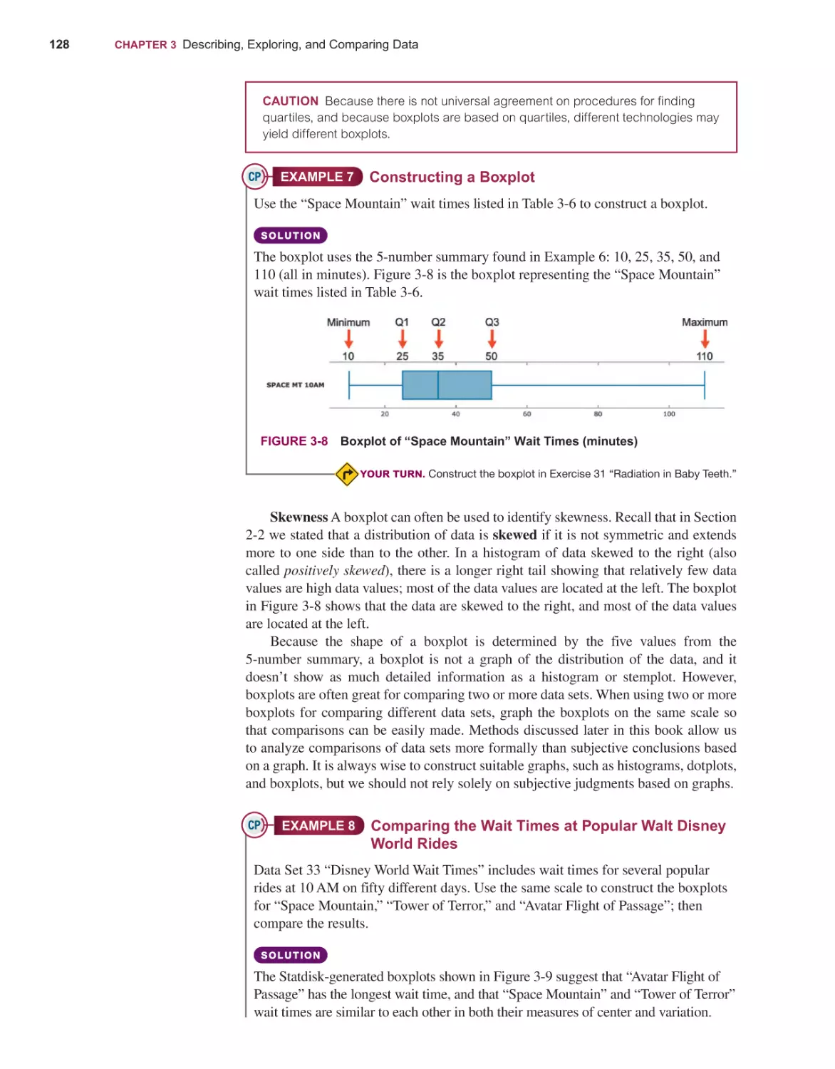
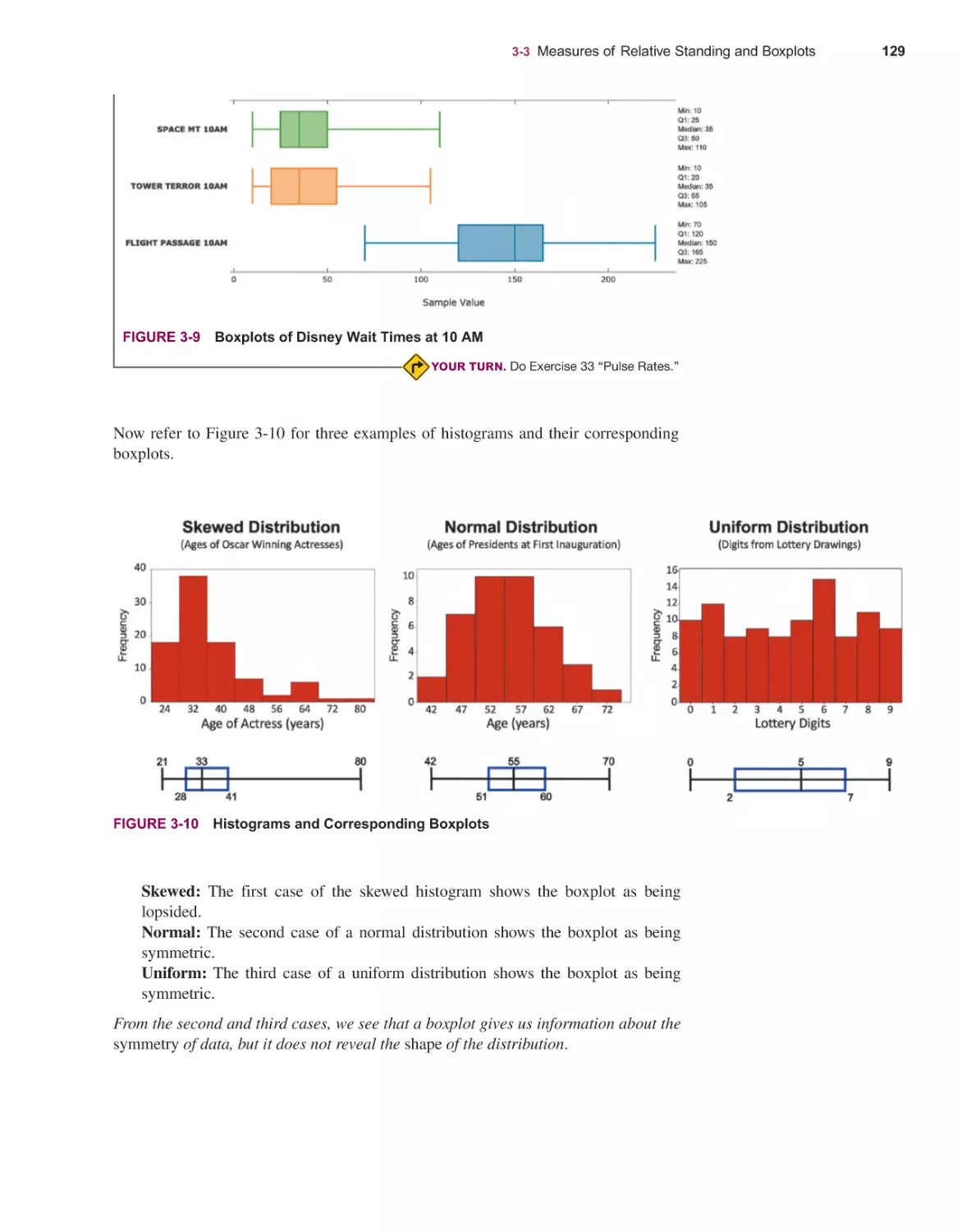
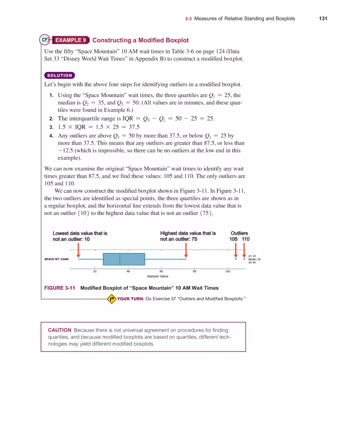
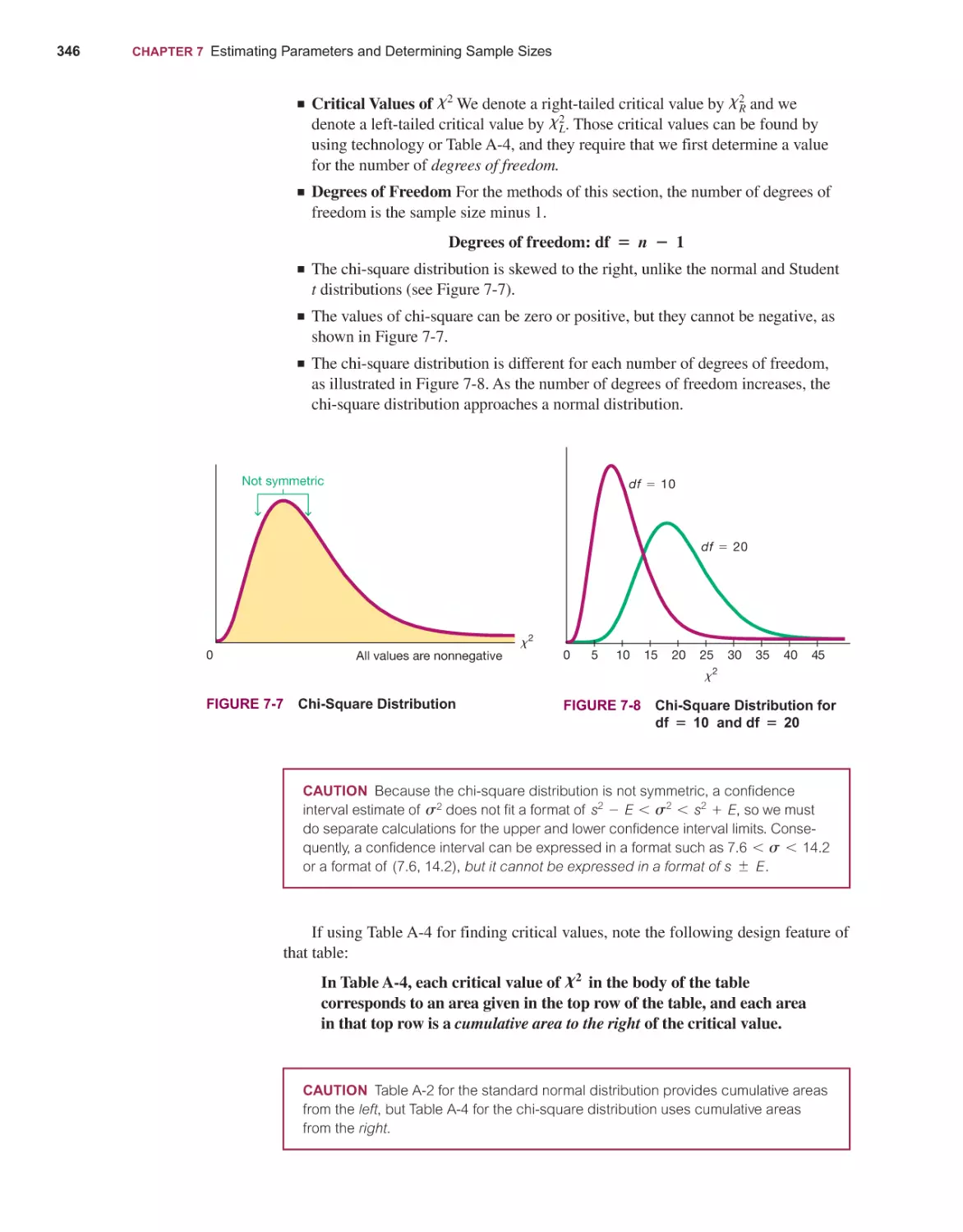
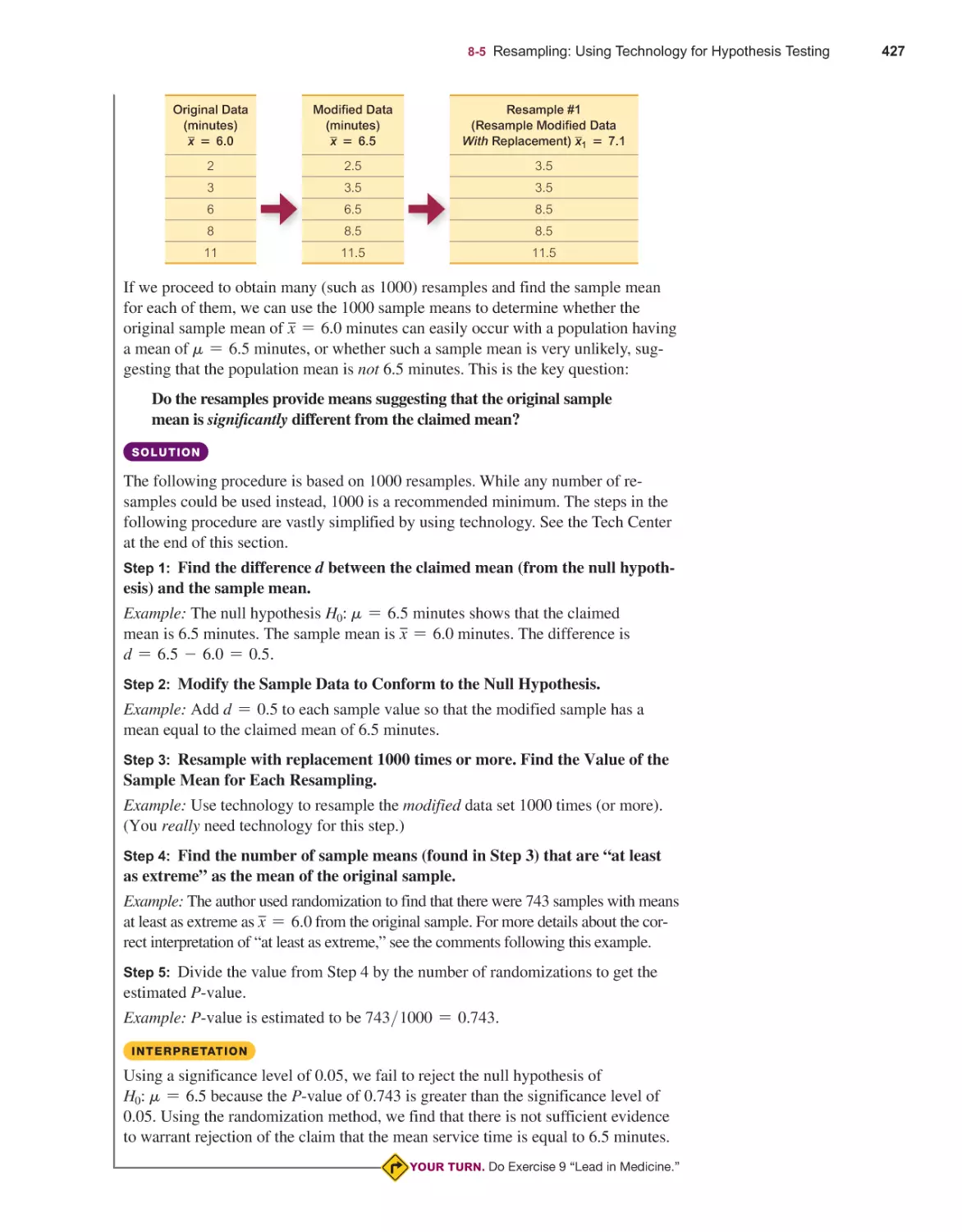
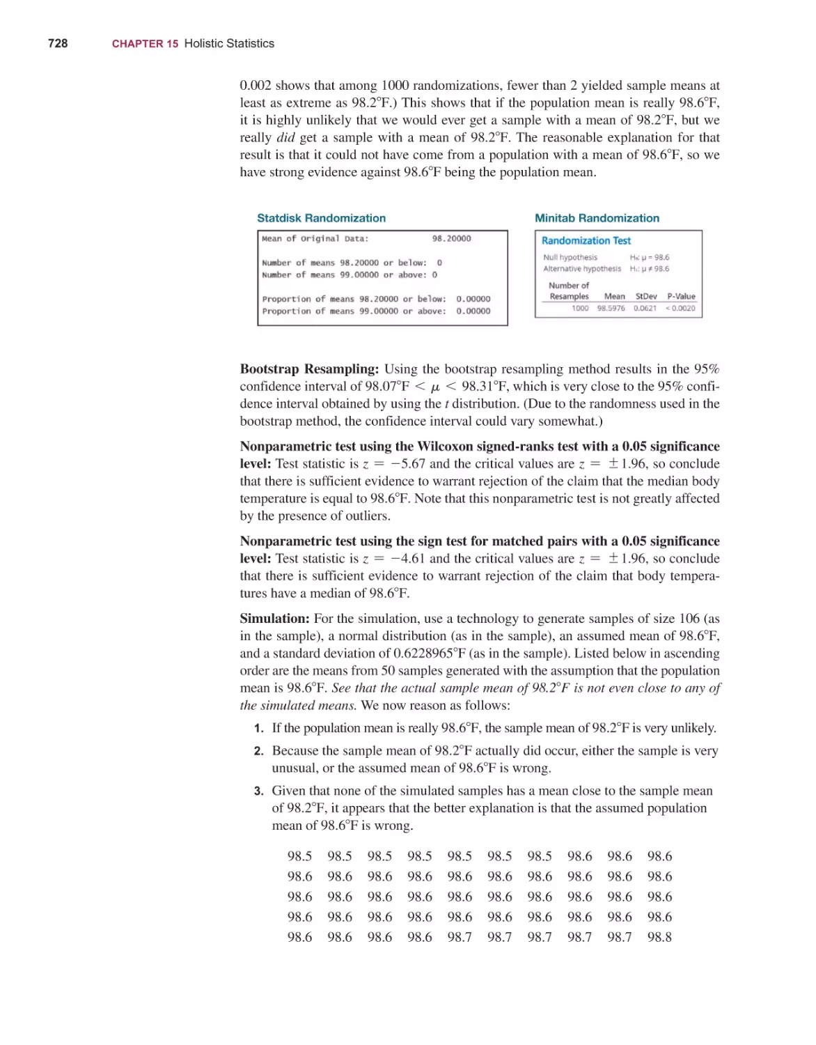
/


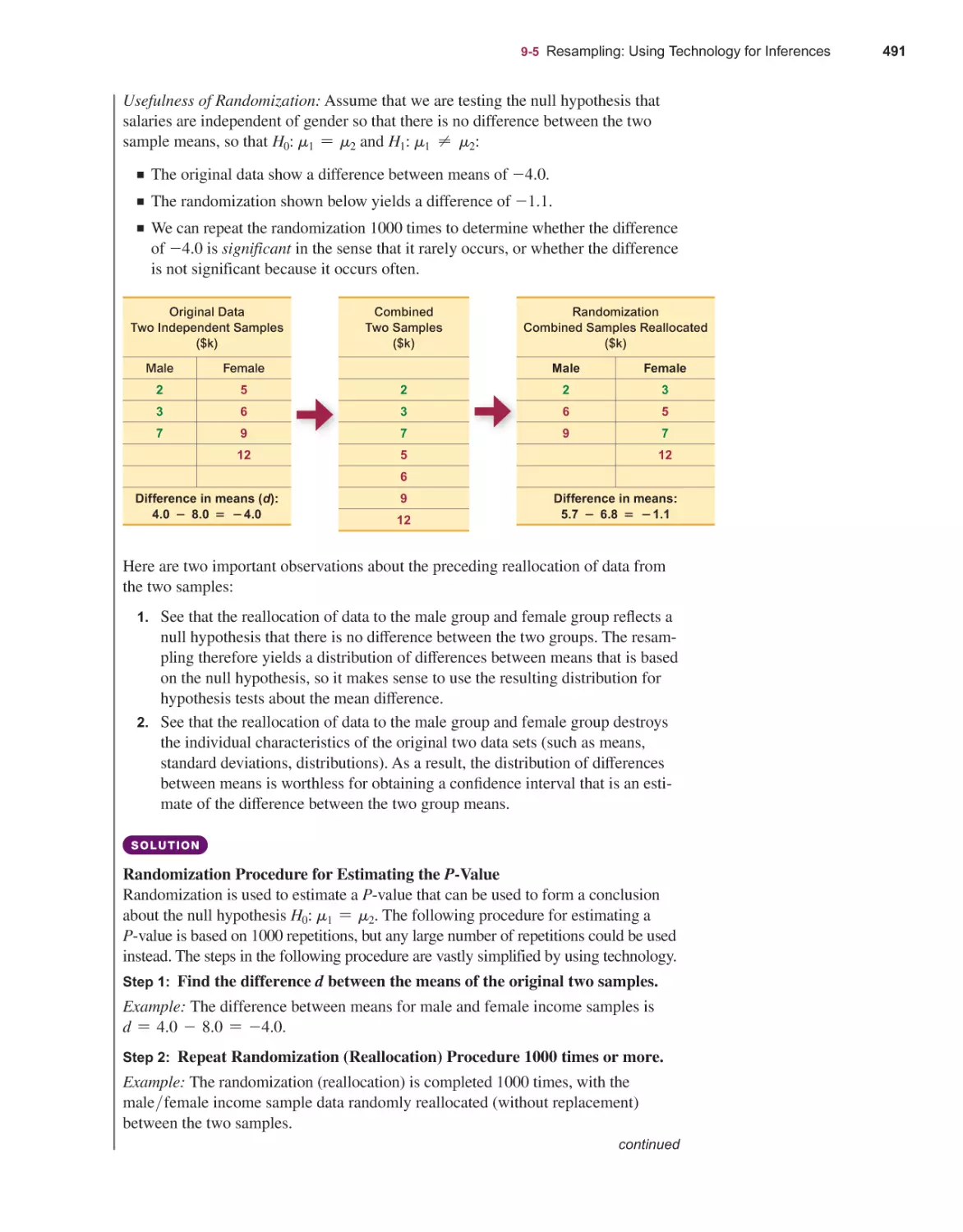


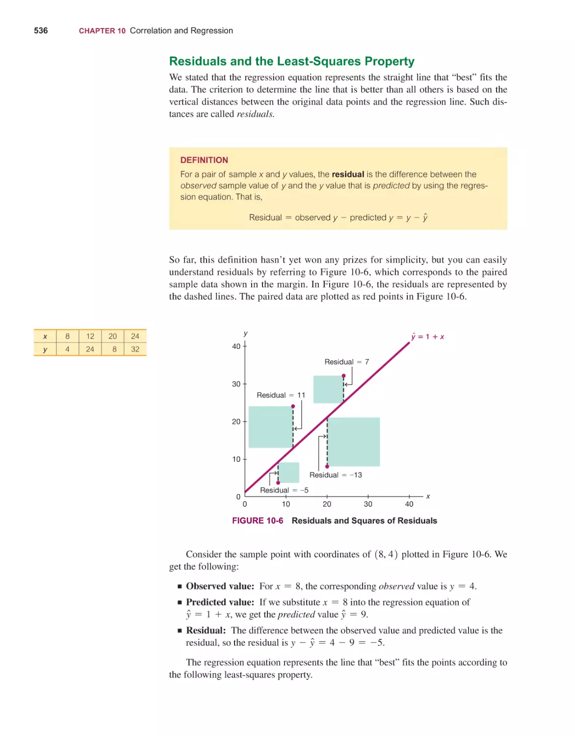


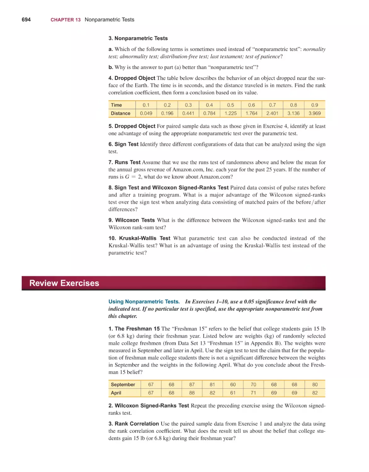


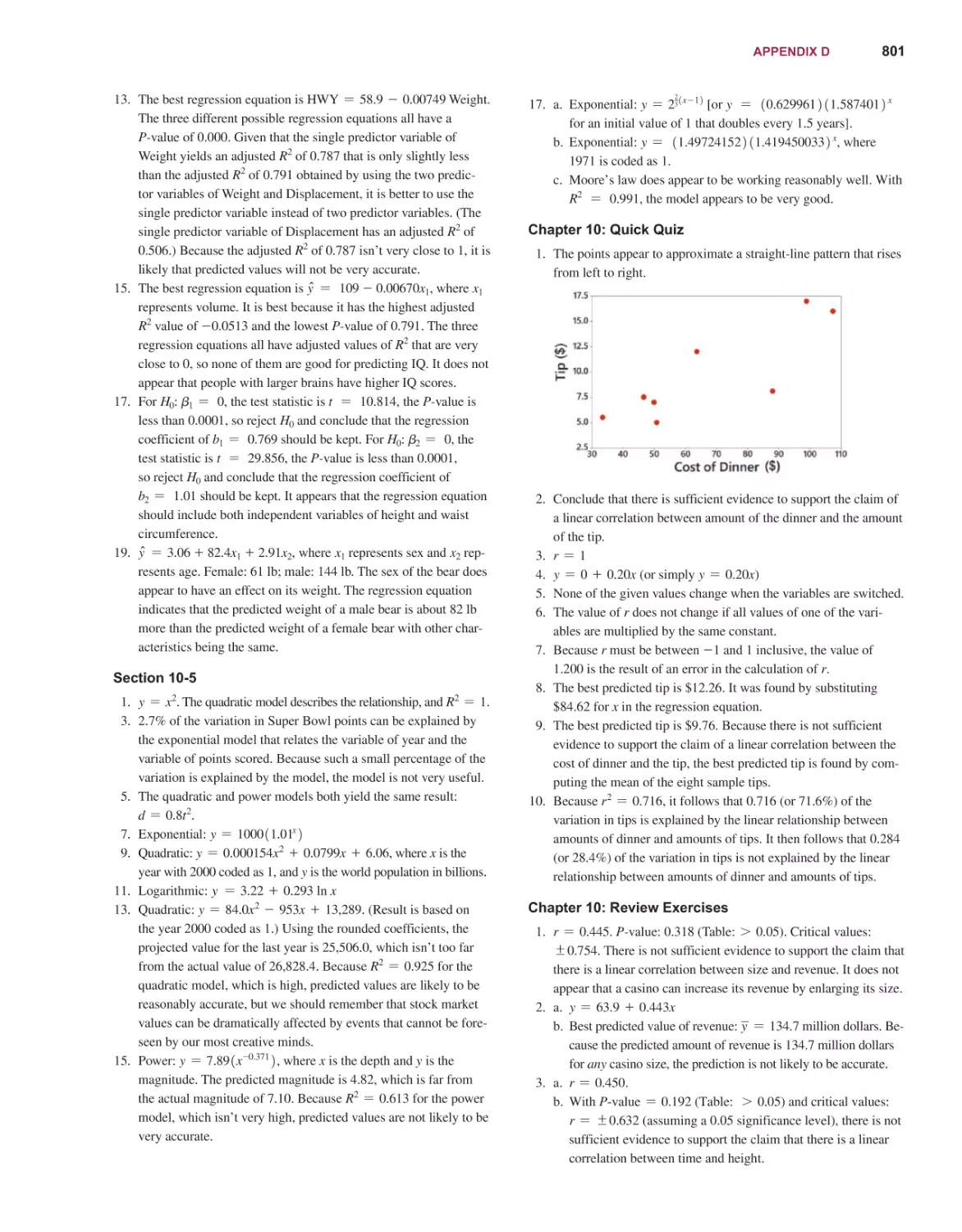


Текст
Elementary
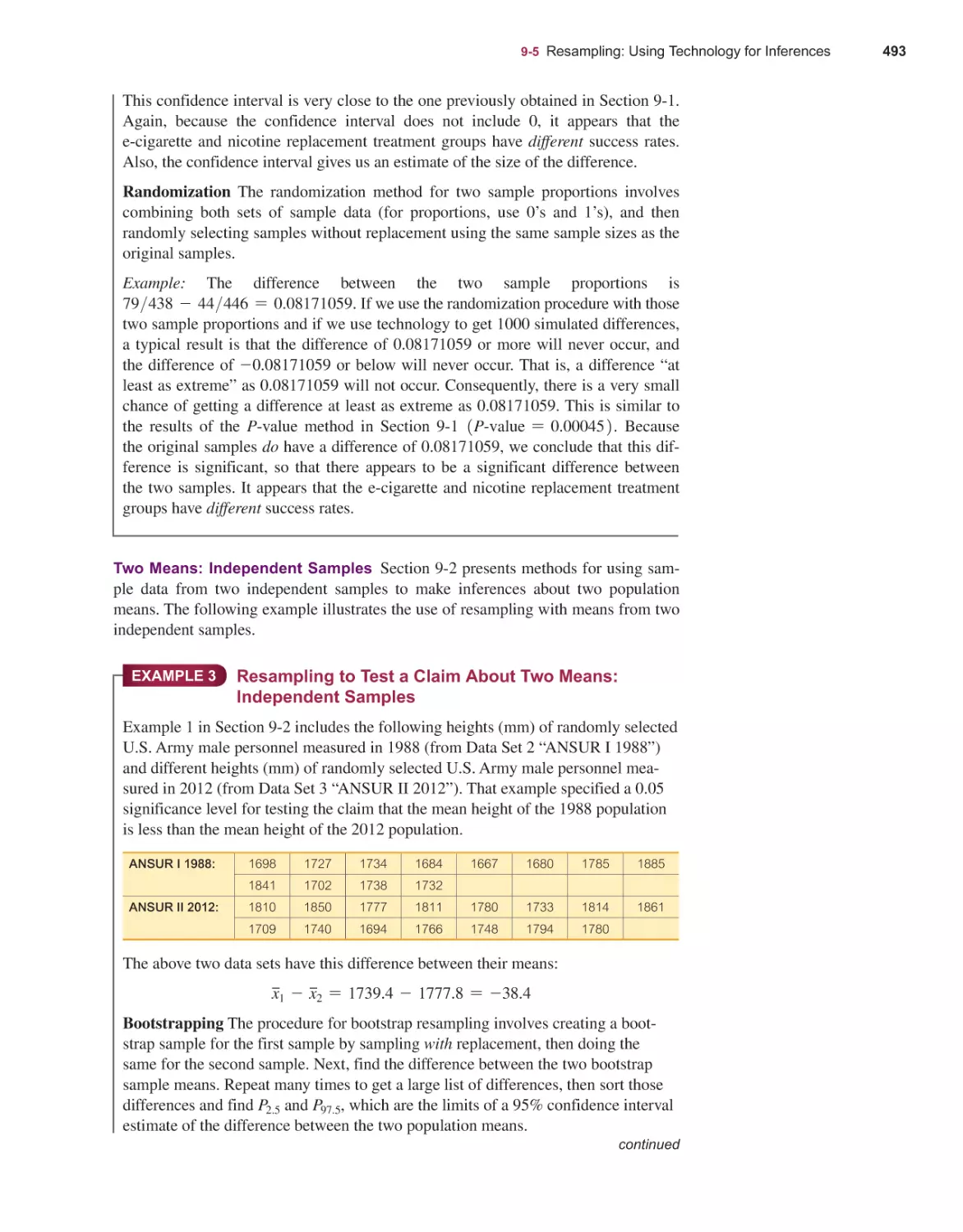
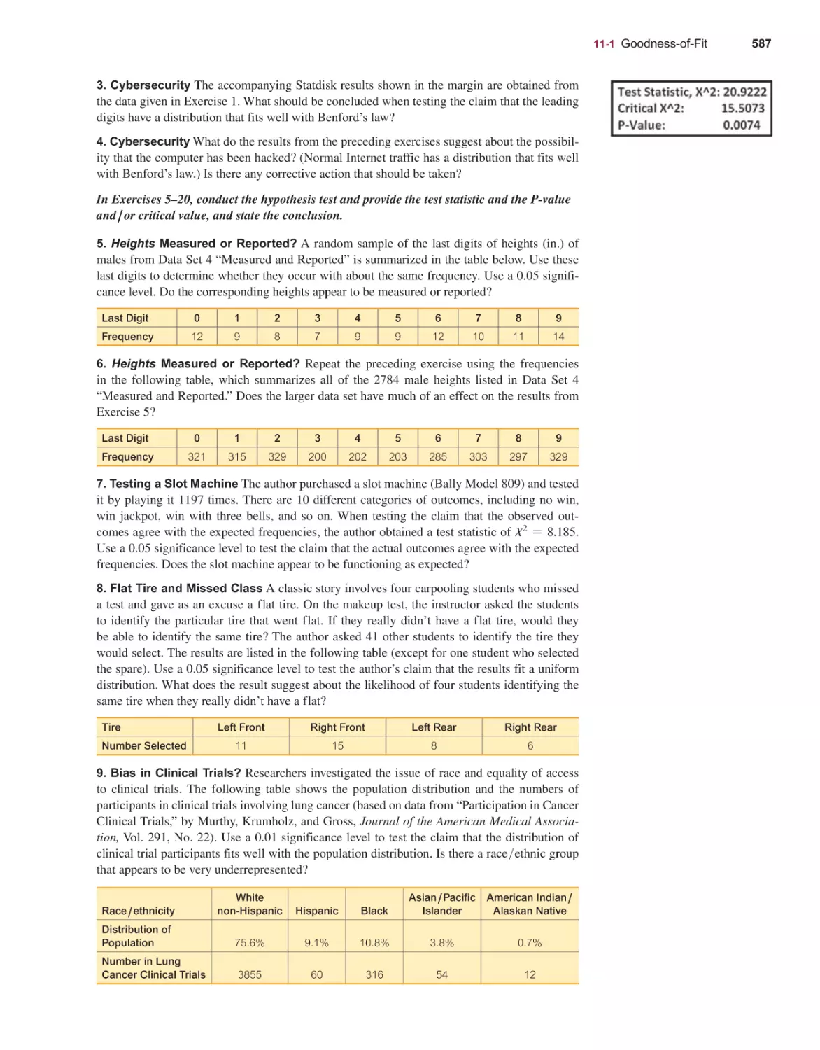
14E
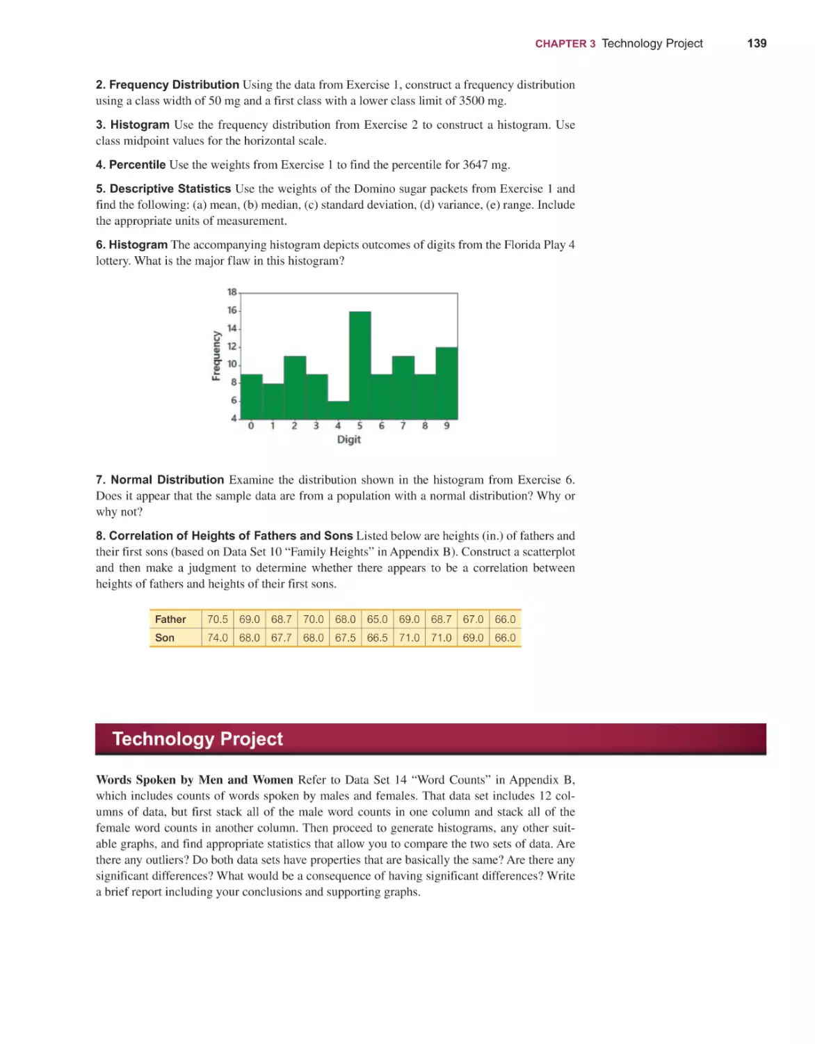
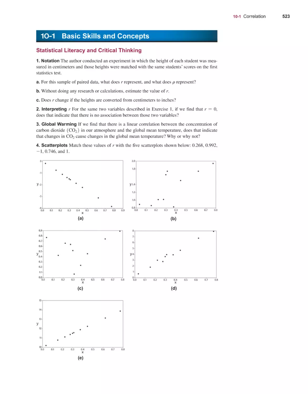
Stat st cs
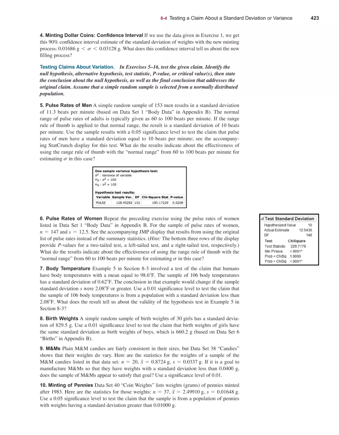
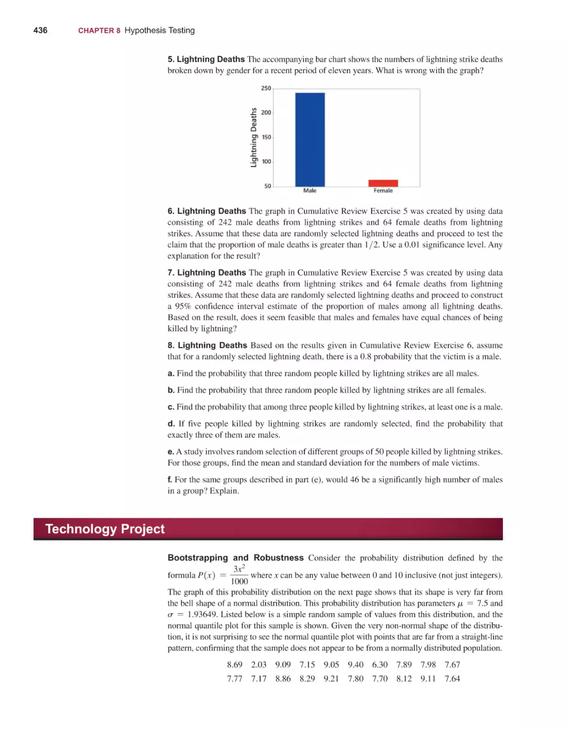
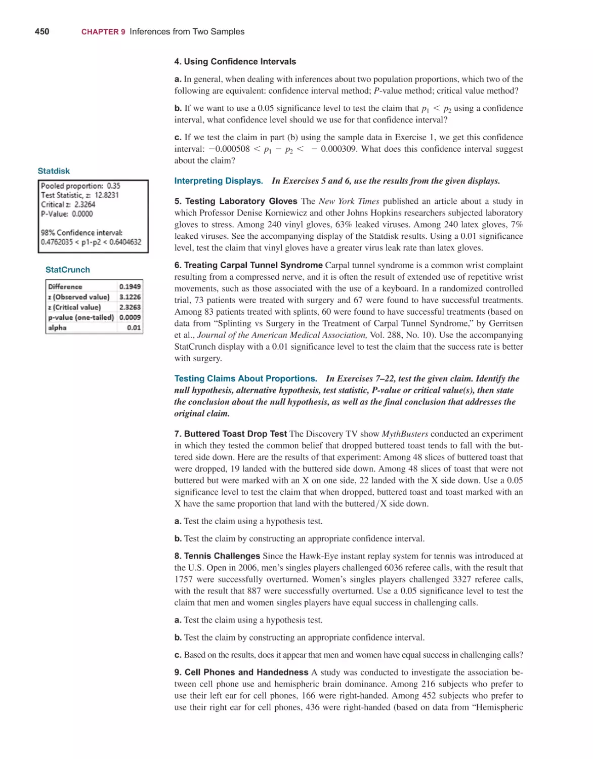
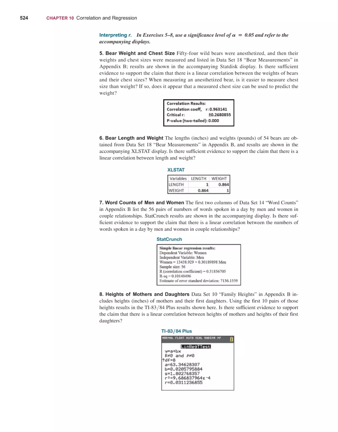
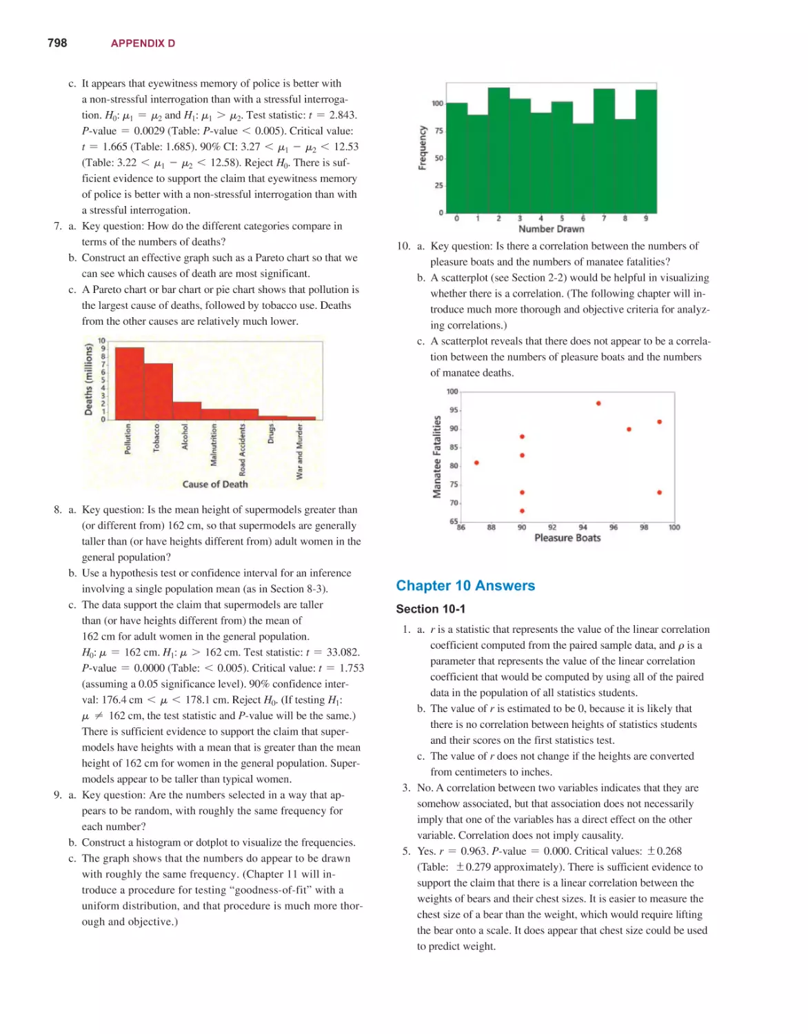
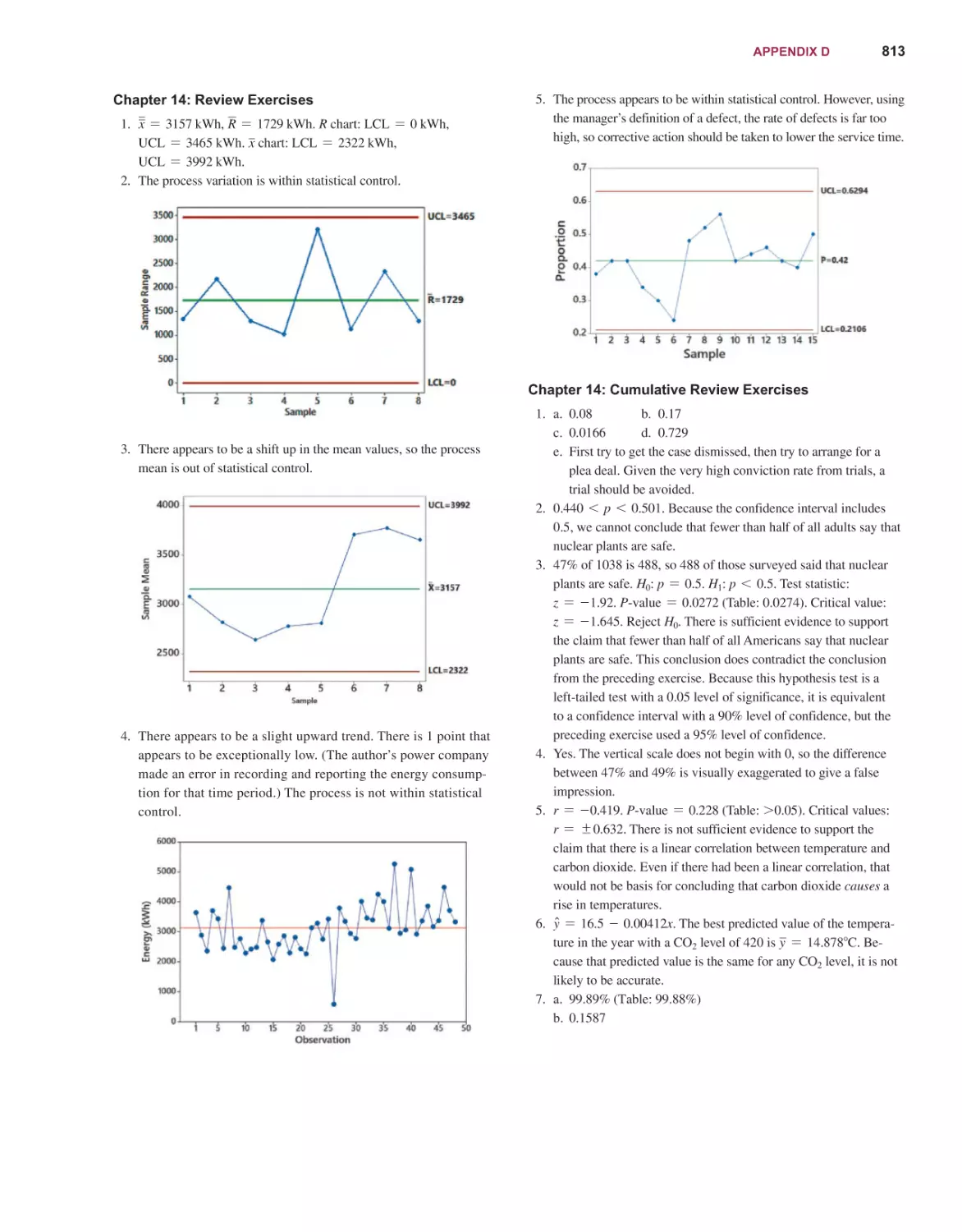
Mario F. Triola
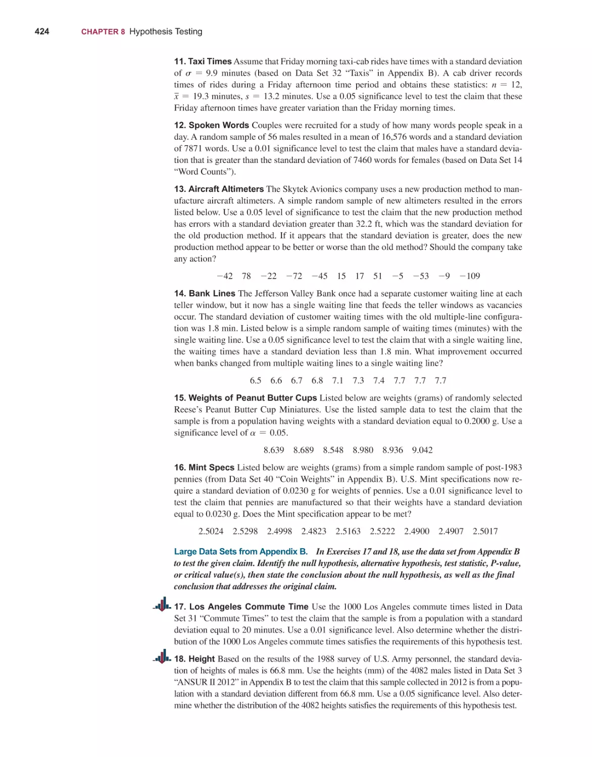
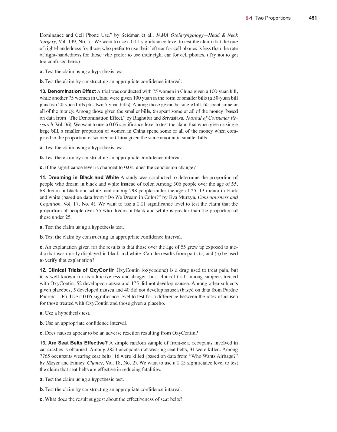
14th
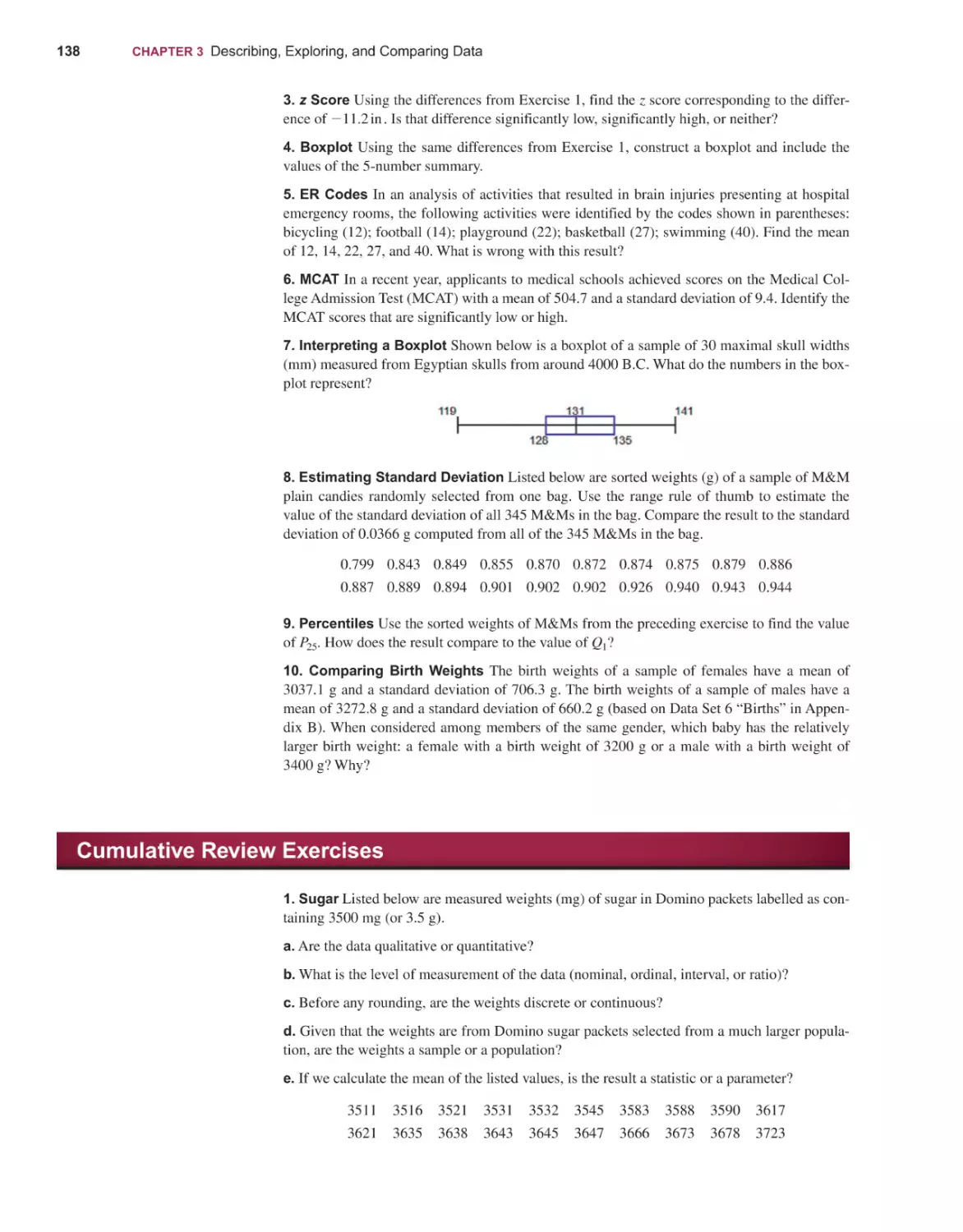
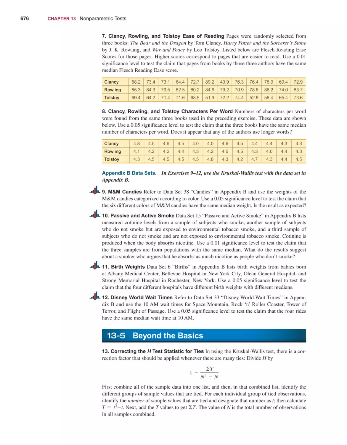
EDITION
ELEMENTARY
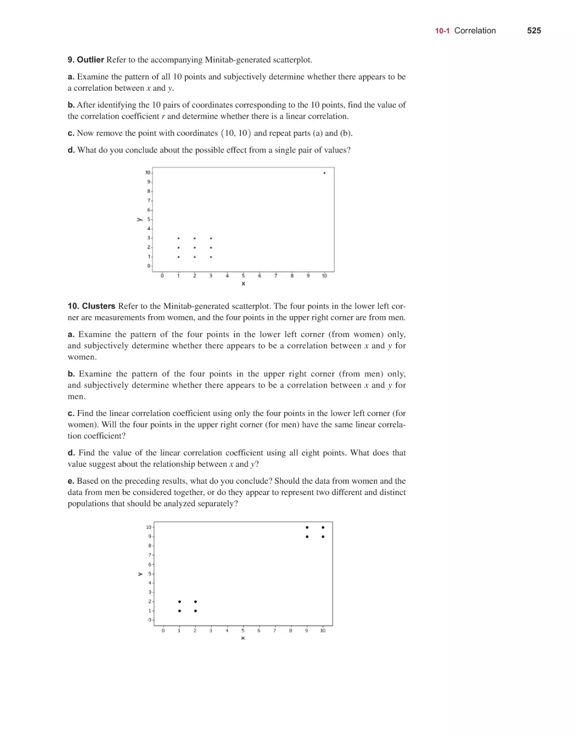
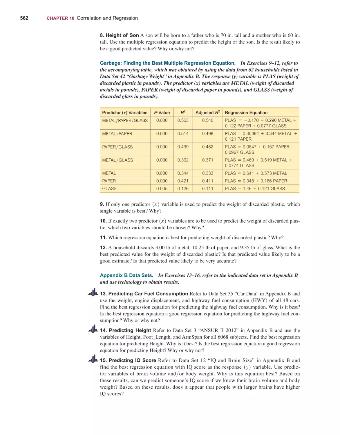
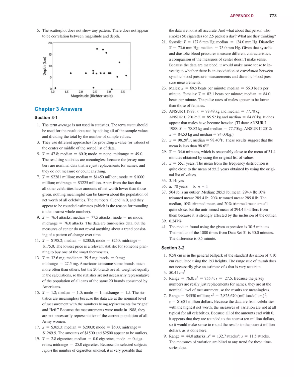
STATISTICS
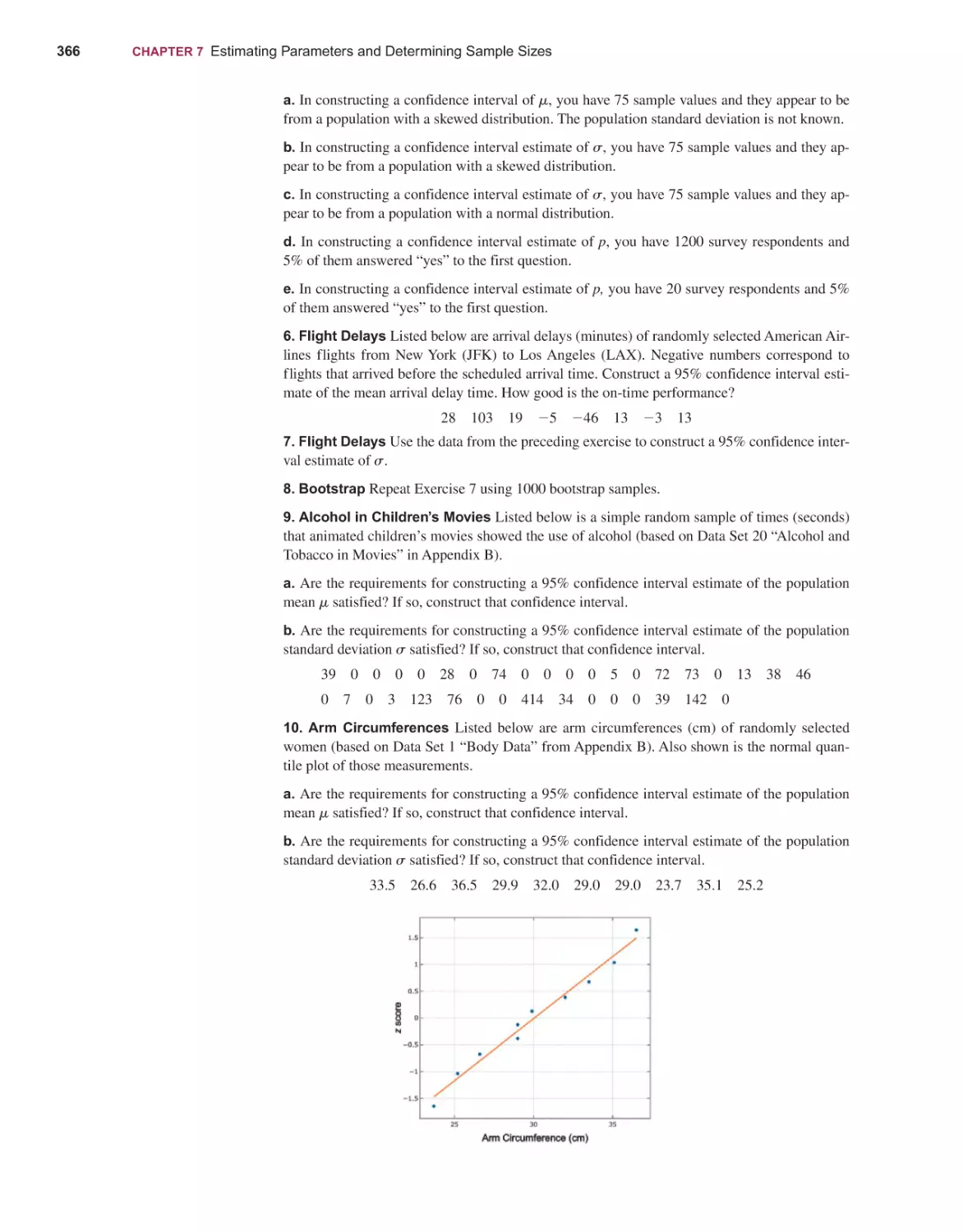
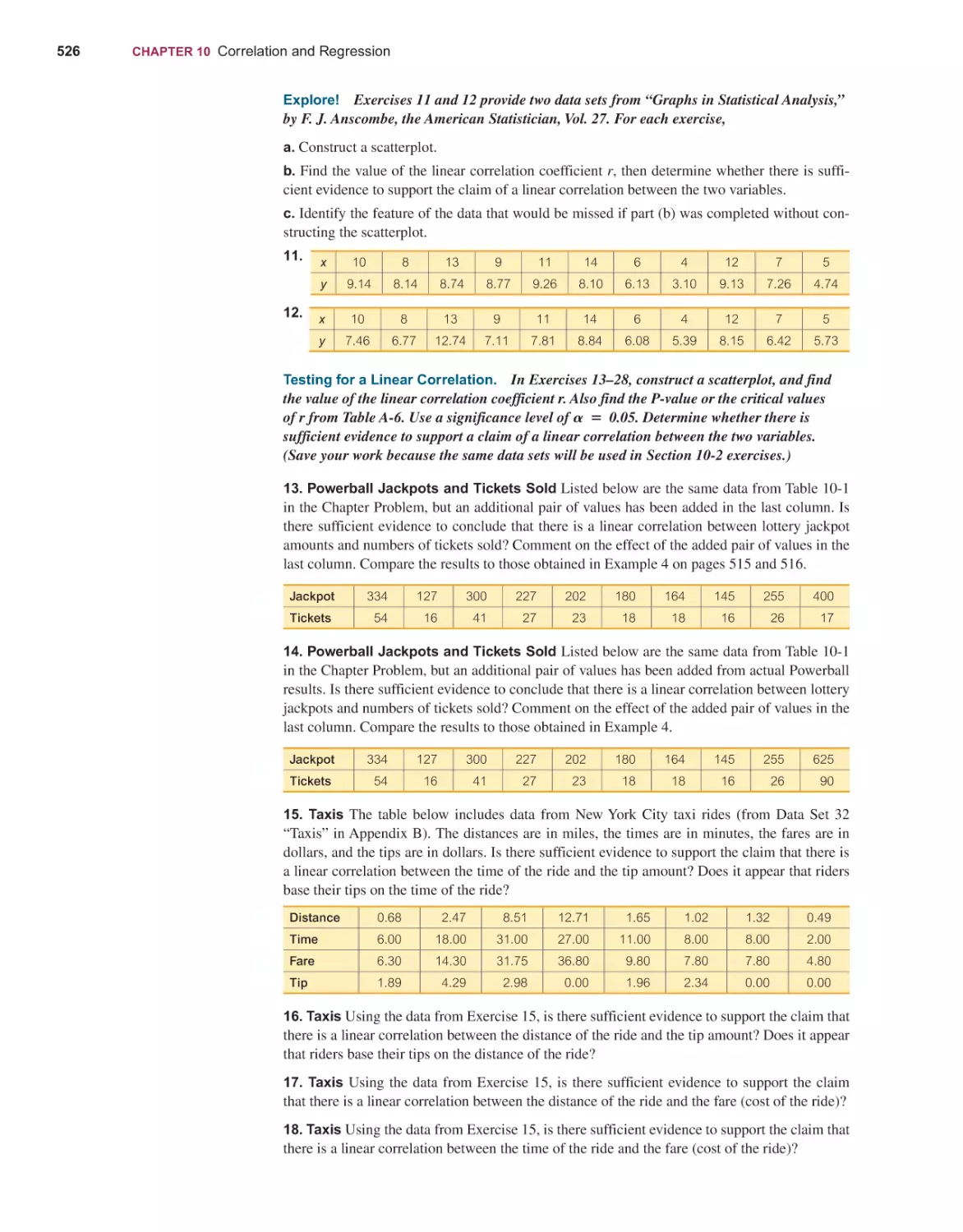
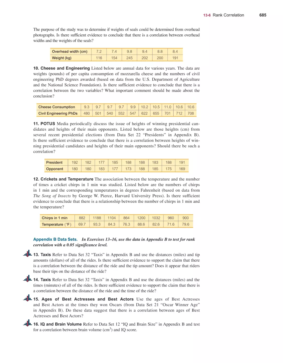
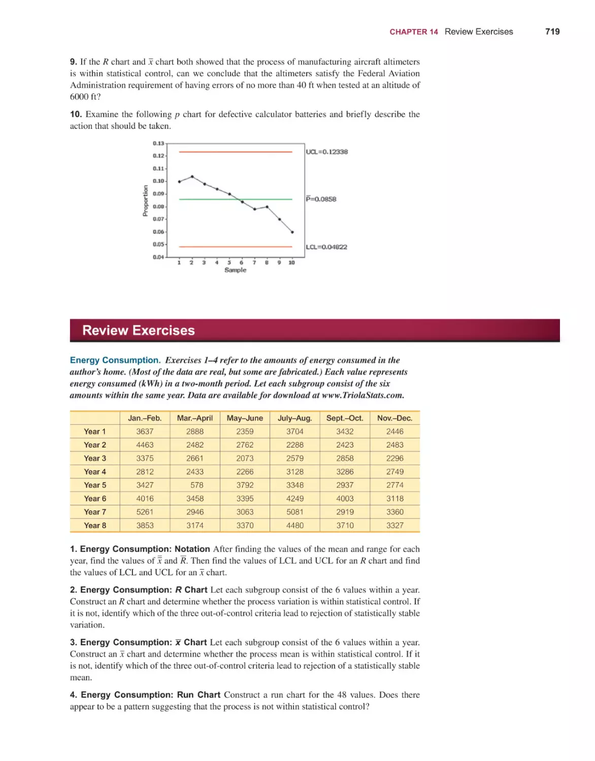
14th
EDITION
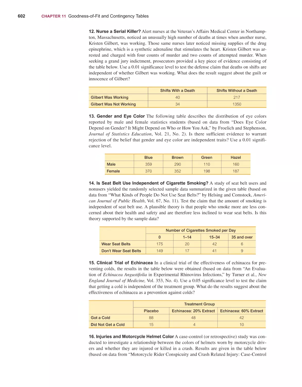
ELEMENTARY
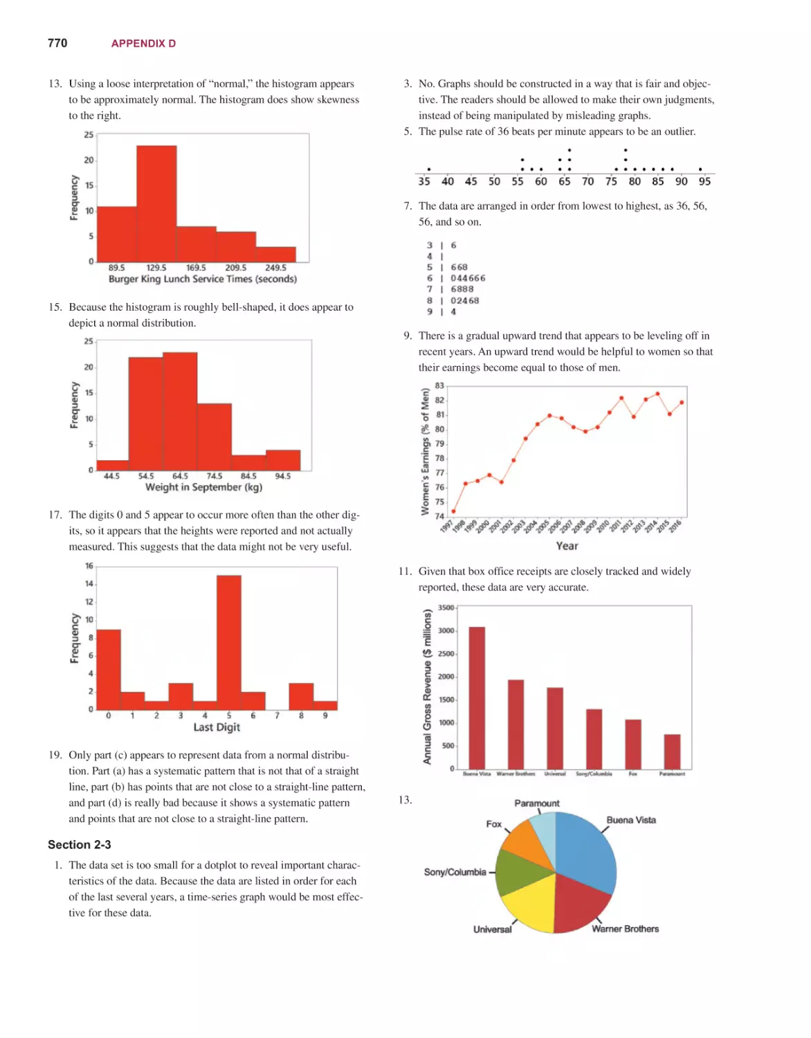
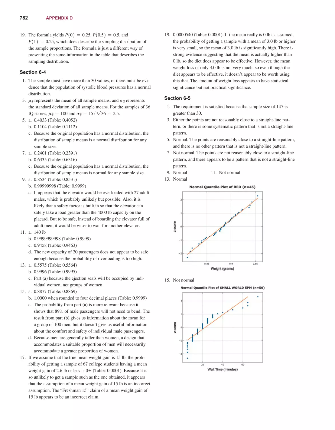
STATISTICS
MARIO F. TRIOLA
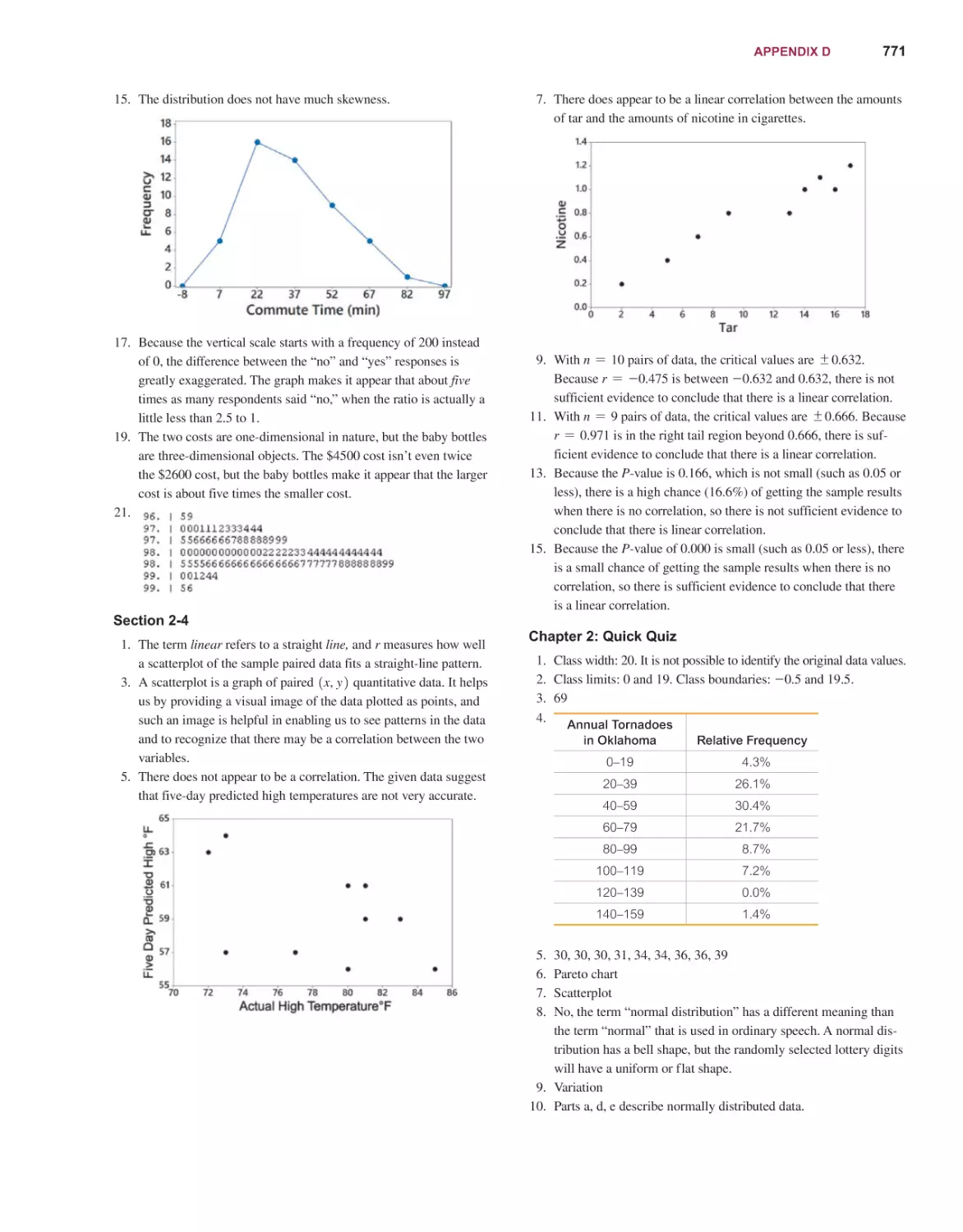
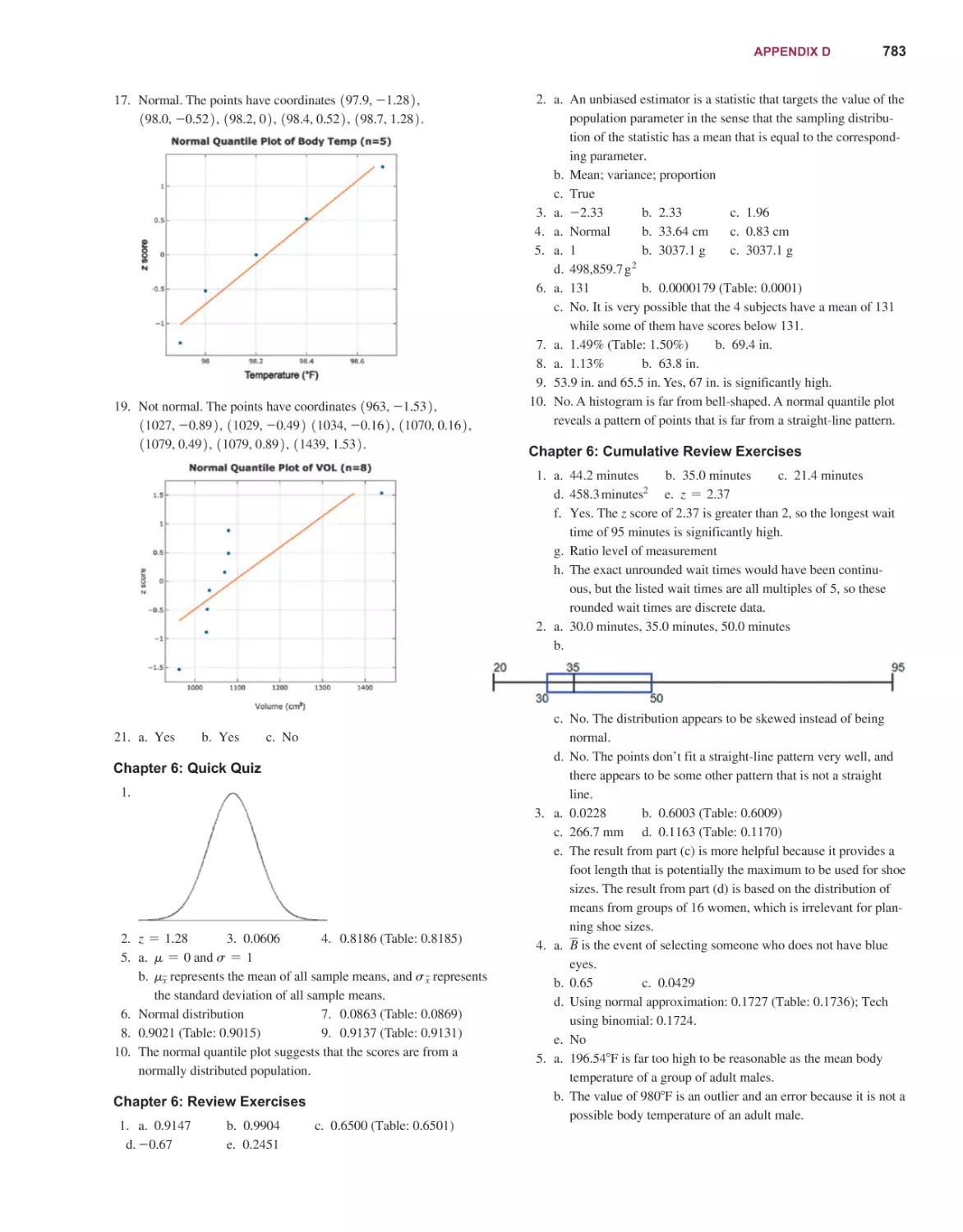
Content Development: Robert Carroll
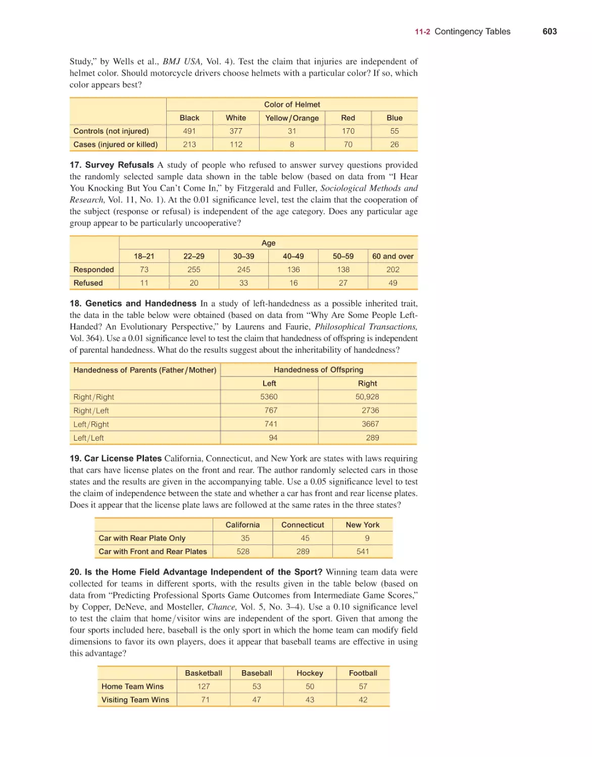
Content Management: Suzanna Bainbridge, Amanda Brands
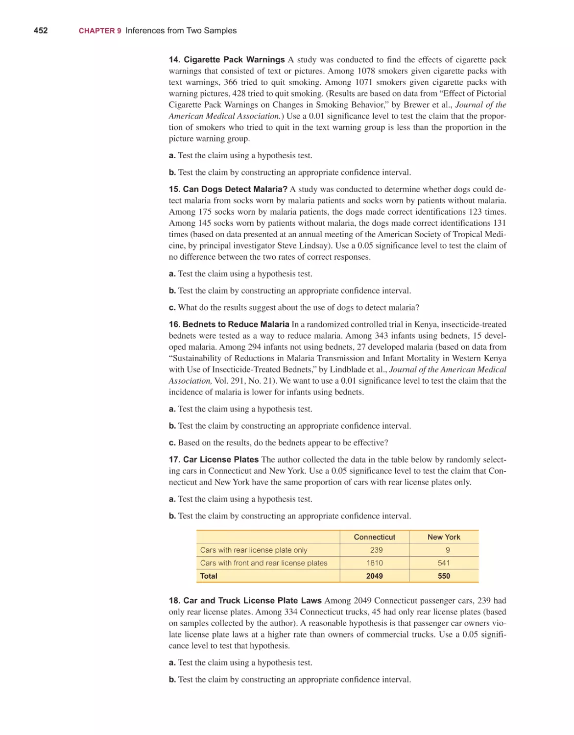
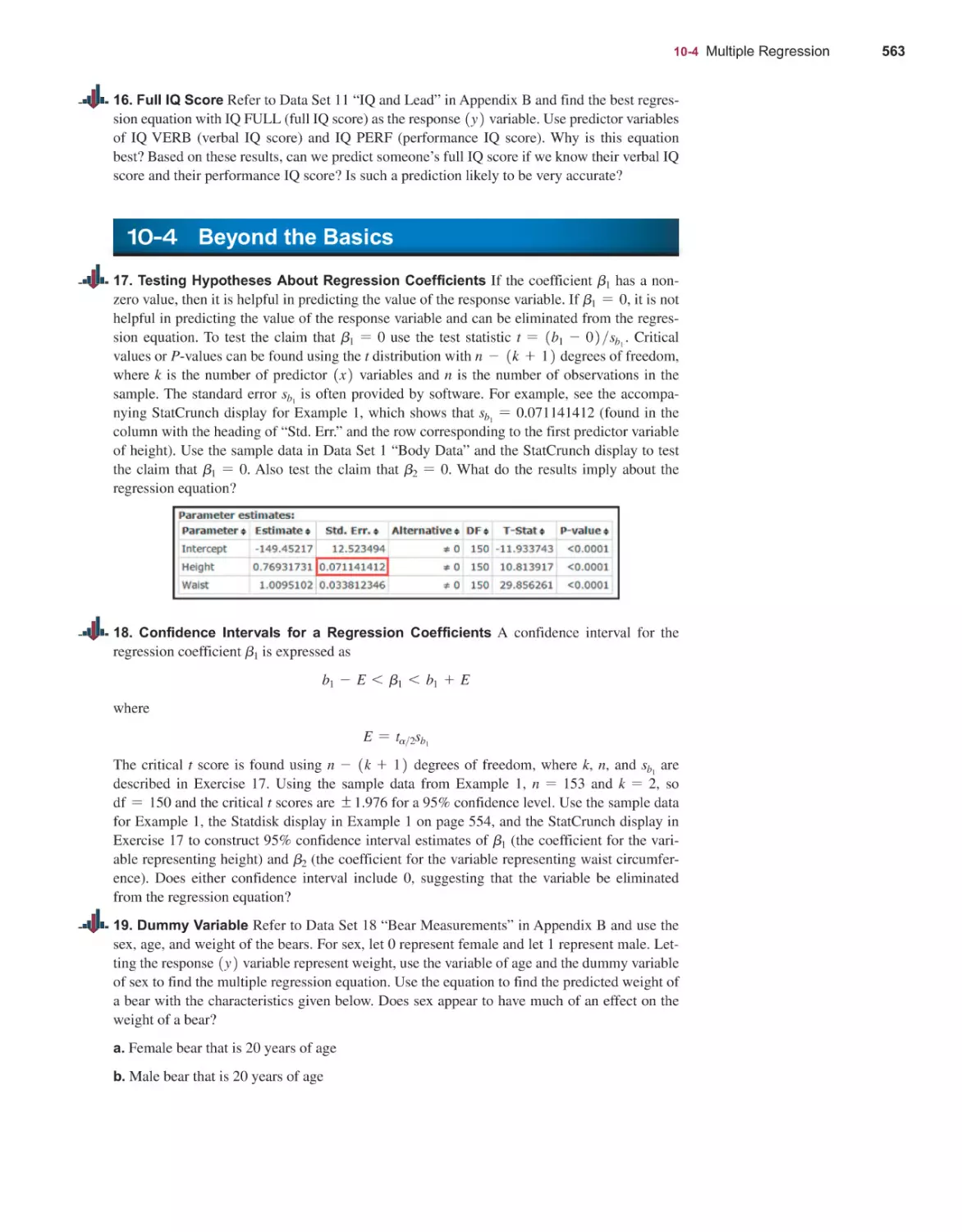
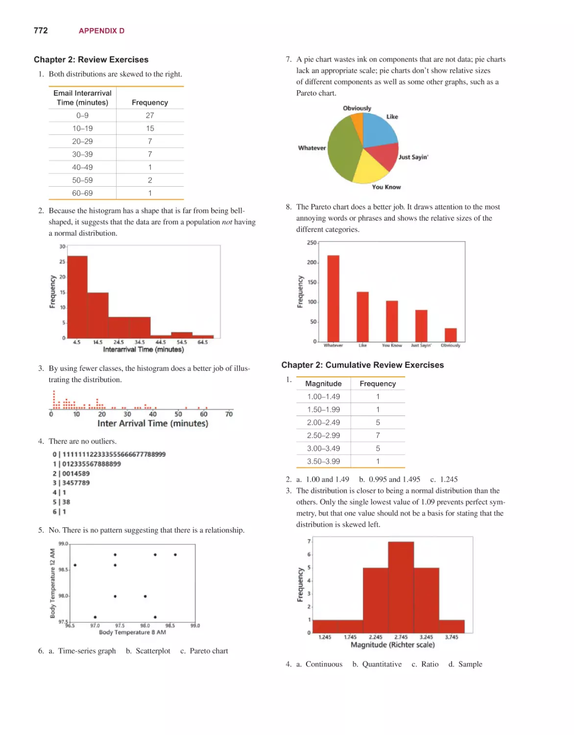
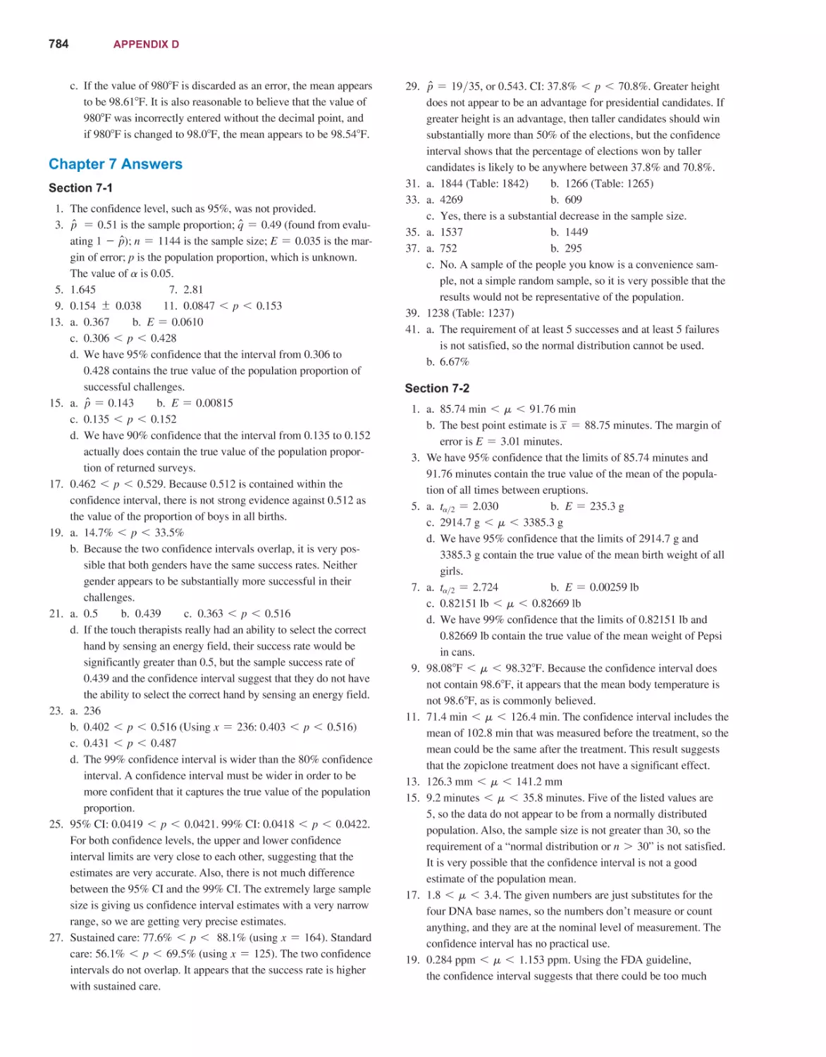
Content Production: Jean Choe, Peggy McMahon
Product Management: Karen Montgomery
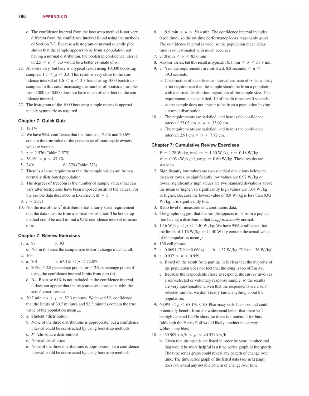
Product Marketing: Alicia Wilson
Rights and Permissions: Tanvi Bhatia/Anjali Singh
Please contact https://support.pearson.com/getsupport/s/ with any queries on this content.
Cover Image by Bim/Getty Images
Microsoft and/or its respective suppliers make no representations about the suitability of
the information contained in the documents and related graphics published as part of the
services for any purpose. All such documents and related graphics are provided “as is”
without warranty of any kind. Microsoft and/or its respective suppliers hereby disclaim
all warranties and conditions with regard to this information, including all warranties
and conditions of merchantability, whether express, implied or statutory, fitness for a
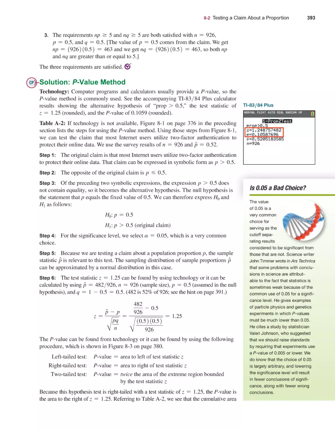
particular purpose, title and non-infringement. In no event shall Microsoft and/or its
respective suppliers be liable for any special, indirect or consequential damages or any
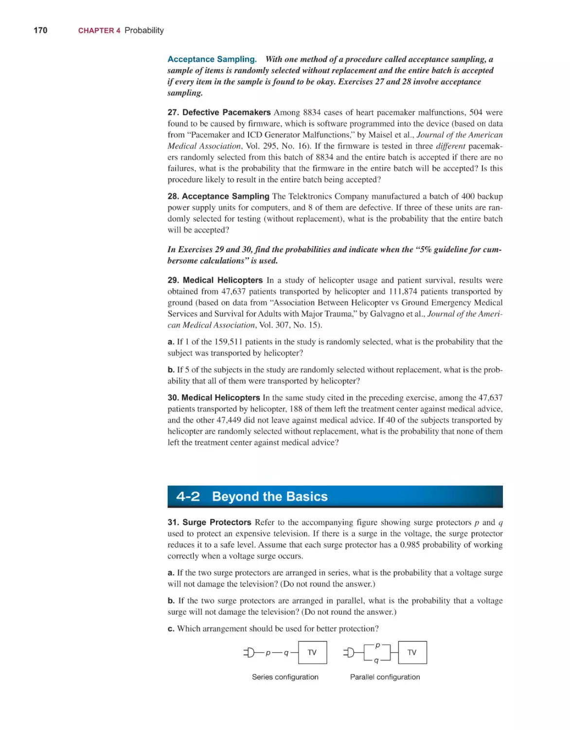
damages whatsoever resulting from loss of use, data or profits, whether in an action of
contract, negligence or other tortious action, arising out of or in connection with the use
or performance of information available from the services.
The documents and related graphics contained herein could include technical inaccuracies or typographical errors. Changes are periodically added to the information herein.
Microsoft and/or its respective suppliers may make improvements and/or changes in the
product(s) and/or the program(s) described herein at any time. Partial screen shots may
be viewed in full within the software version specified.
Microsoft® and Windows® are registered trademarks of the Microsoft Corporation in the
U.S.A. and other countries. This book is not sponsored or endorsed by or affiliated with
the Microsoft Corporation.
Copyright © 2022, 2018, 2014 by Pearson Education, Inc. or its affiliates, 221 River Street, Hoboken, NJ 07030. All Rights Reserved.
Manufactured in the United States of America. This publication is protected by copyright, and permission should be obtained from
the publisher prior to any prohibited reproduction, storage in a retrieval system, or transmission in any form or by any means, electronic, mechanical, photocopying, recording, or otherwise. For information regarding permissions, request forms, and the appropriate
contacts within the Pearson Education Global Rights and Permissions department, please visit www.pearsoned.com/permissions/.
Acknowledgments of third-party content appear on the appropriate page within the text, or in the Credits at the end of the book which
constitutes an extension of this copyright page.
PEARSON, ALWAYS LEARNING, and MYLAB are exclusive trademarks owned by Pearson Education, Inc., or its affiliates in the
U.S. and/or other countries.
Unless otherwise indicated herein, any third-party trademarks, logos, or icons that may appear in this work are the property of their
respective owners, and any references to third-party trademarks, logos, icons, or other trade dress are for demonstrative or descriptive
purposes only. Such references are not intended to imply any sponsorship, endorsement, authorization, or promotion of Pearson’s
products by the owners of such marks, or any relationship between the owner and Pearson Education, Inc., or its affiliates, authors,
licensees, or distributors.
Library of Congress Cataloging-in-Publication Data
Names: Triola, Mario F., author.
Title: Elementary statistics / Mario F. Triola.
Description: 14th edition, annotated instructor’s edition. | Hoboken :
Pearson, [2022] | Includes index. | Summary: “Step-by-step guide to the
important concepts of Statistics”-- Provided by publisher.
Identifiers: LCCN 2020040438 | ISBN 9780136803201 (hardcover)
Subjects: LCSH: Statistics--Textbooks.
Classification: LCC QA276.12 .T76 2022 | DDC 519.5--dc23
LC record available at https://lccn.loc.gov/2020040438
ScoutAutomatedPrintCode
Rental
ISBN-10: 0136803202
ISBN-13: 9780136803201
To Ginny
Marc, Dushana, and Marisa
Scott, Anna, Siena, and Kaia
ABOUT THE AUTHOR
Mario F. Triola is a Professor Emeritus of MathematCommunity
ics at Dutchess
College, where he has taught
statistics for over 30 years.
Marty is the author of Essentials of Statistics, 6th edition, Elementary Statistics
Using Excel™, 7th edition,
Elementary Statistics Using
the TI@83>84 Plus Calculator, 5th edition, and he is a coauthor of Biostatistics for the
Biological and Health Sciences, 2nd edition, Statistical
Reasoning for Everyday Life,
5th edition, and Business Statistics. Elementary Statistics is currently available as an
International Edition, and it has been translated into several foreign languages. Marty
designed the original Statdisk statistical software, and he has written several manuals
and workbooks for technology supporting statistics education. He has been a speaker
at many conferences and colleges. Marty’s consulting work includes the design of
casino slot machines and fishing rods. He has worked with attorneys in determining
probabilities in paternity lawsuits, analyzing data in medical malpractice lawsuits,
identifying salary inequities based on gender, and analyzing disputed election results.
He has also used statistical methods in analyzing medical school surveys, and in
analyzing survey results for the New York City Transit Authority, and analyzing
COVID-19 virus data for government officials. Marty has testified as an expert witness
in the New York State Supreme Court. The Text and Academic Authors Association
has awarded Marty a “Texty” for Excellence for his work on Elementary Statistics. As
of this writing, Marty’s Elementary Statistics book has been the #1 statistics book in
the United States for the past 25 consecutive years.
Celebrating the past 25 years as
the #1 statistics textbook author!
vii
CONTENTS
1
INTRODUCTION TO STATISTICS
2
EXPLORING DATA WITH TABLES AND GRAPHS
3
4
5
6
7
8
1-1
1-2
1-3
1-4
2-1
2-2
2-3
2-4
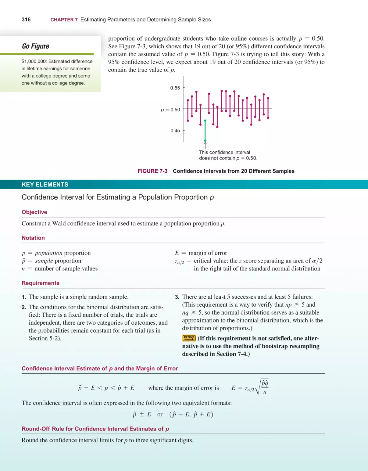
310
Estimating a Population Proportion 312
Estimating a Population Mean 329
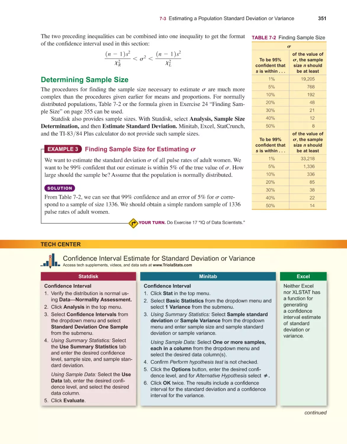
Estimating a Population Standard Deviation or Variance 345
Bootstrapping: Using Technology for Estimates 355
HYPOTHESIS TESTING
8-1
8-2
8-3
8-4
8-5
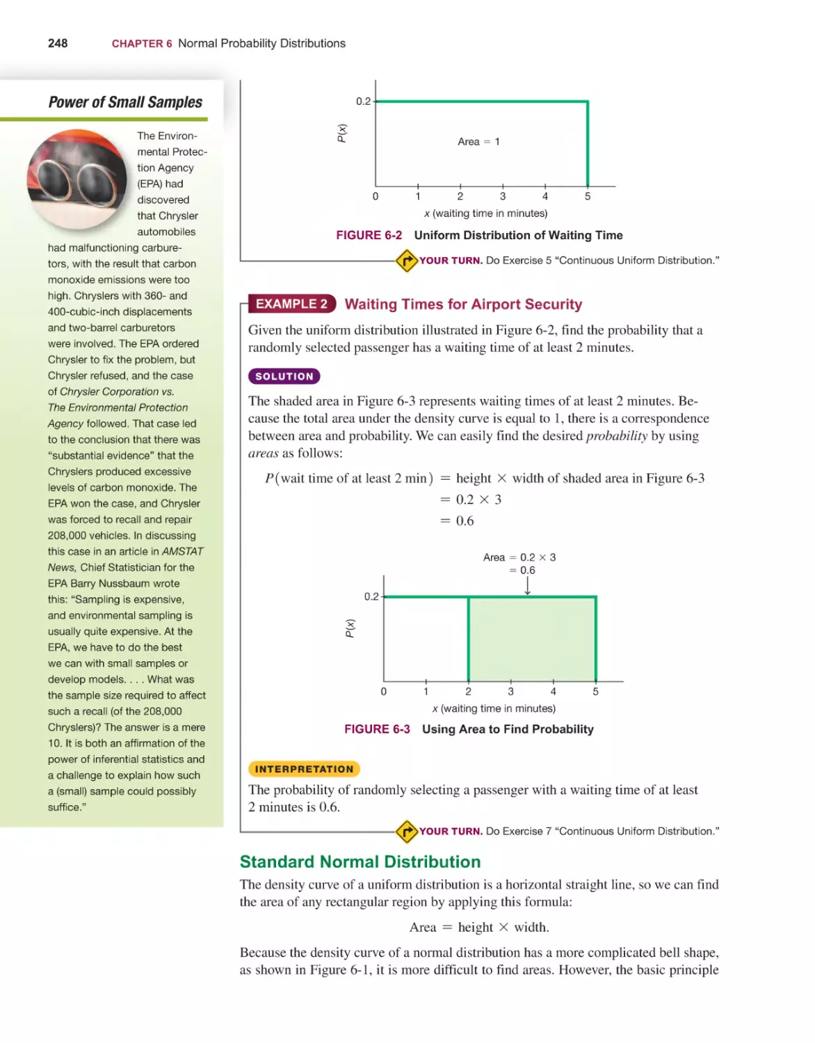
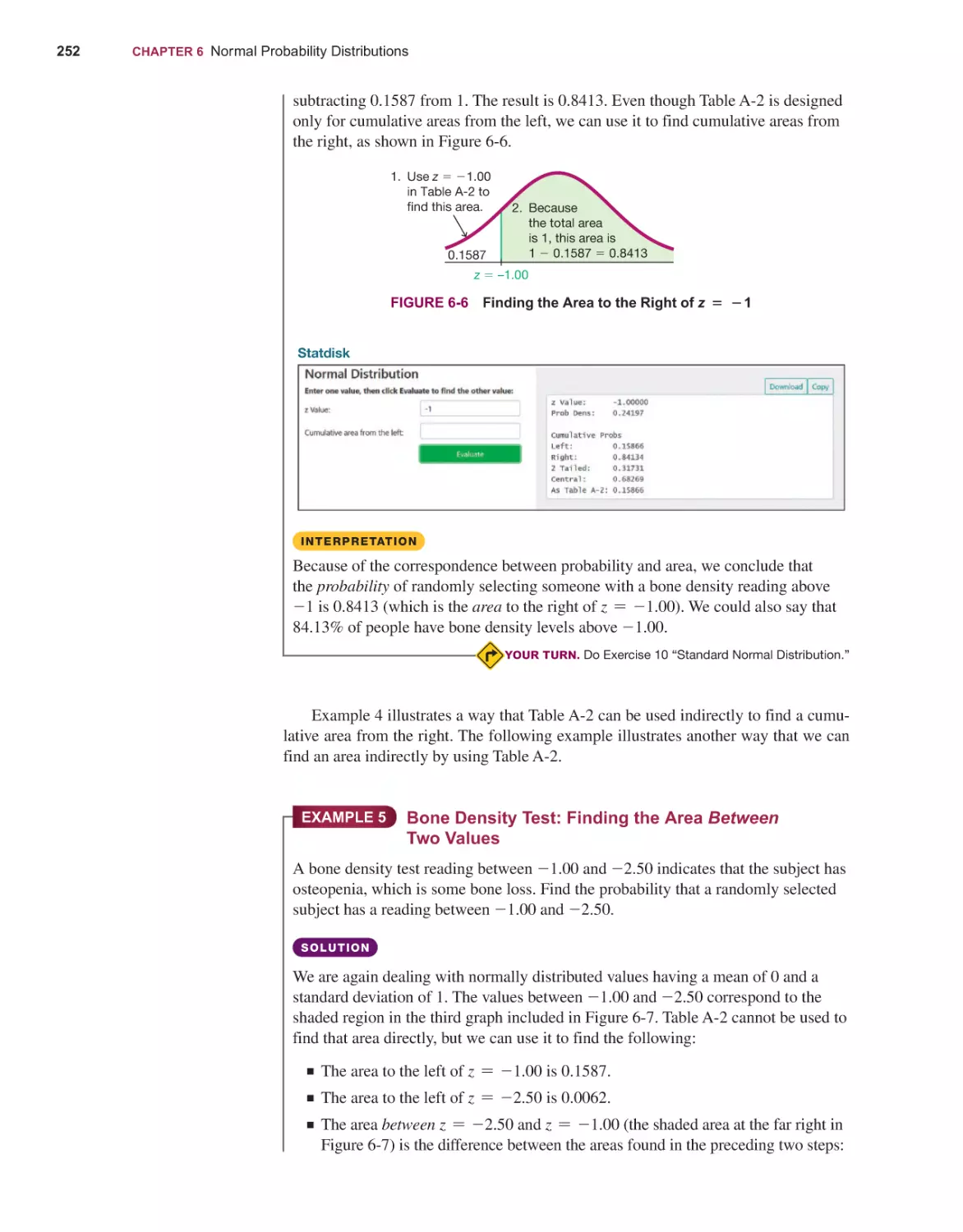
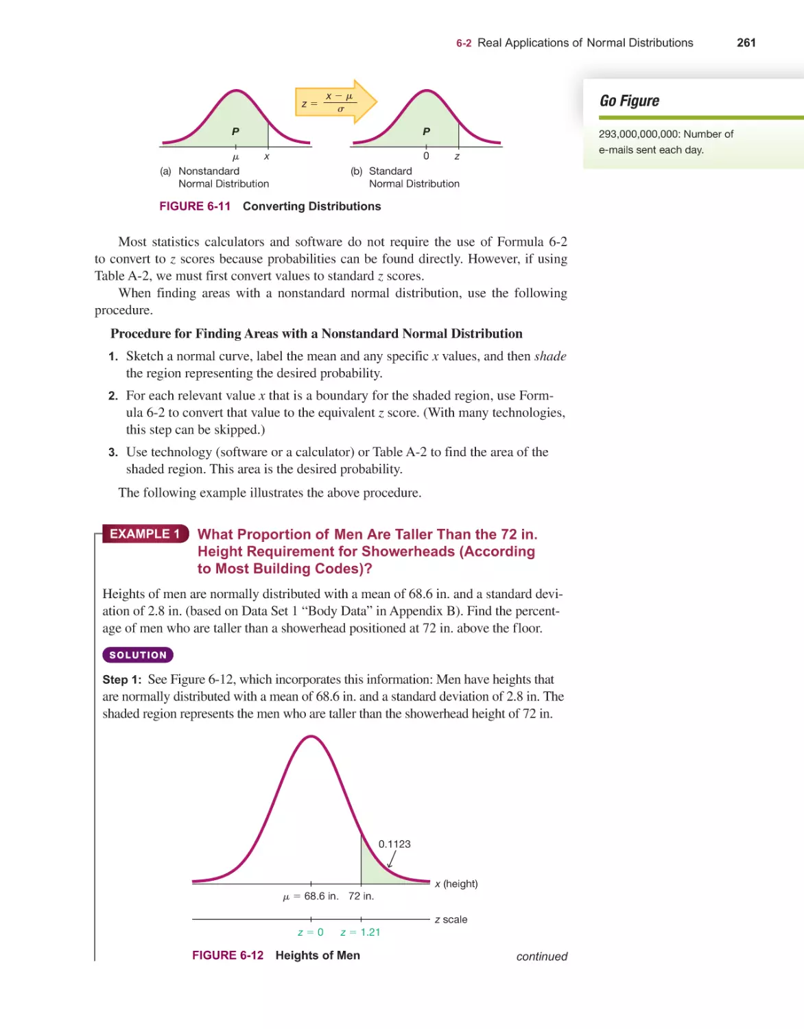
244
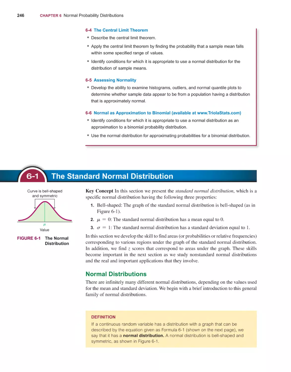
The Standard Normal Distribution 246
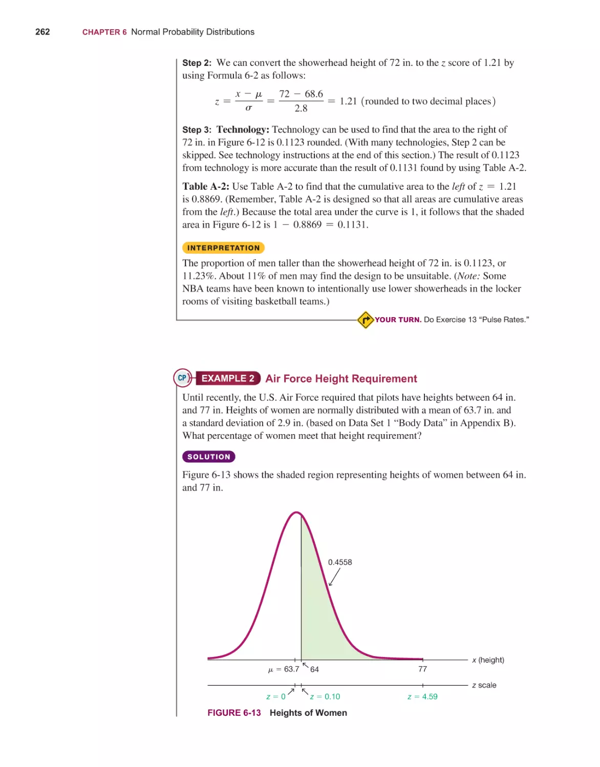
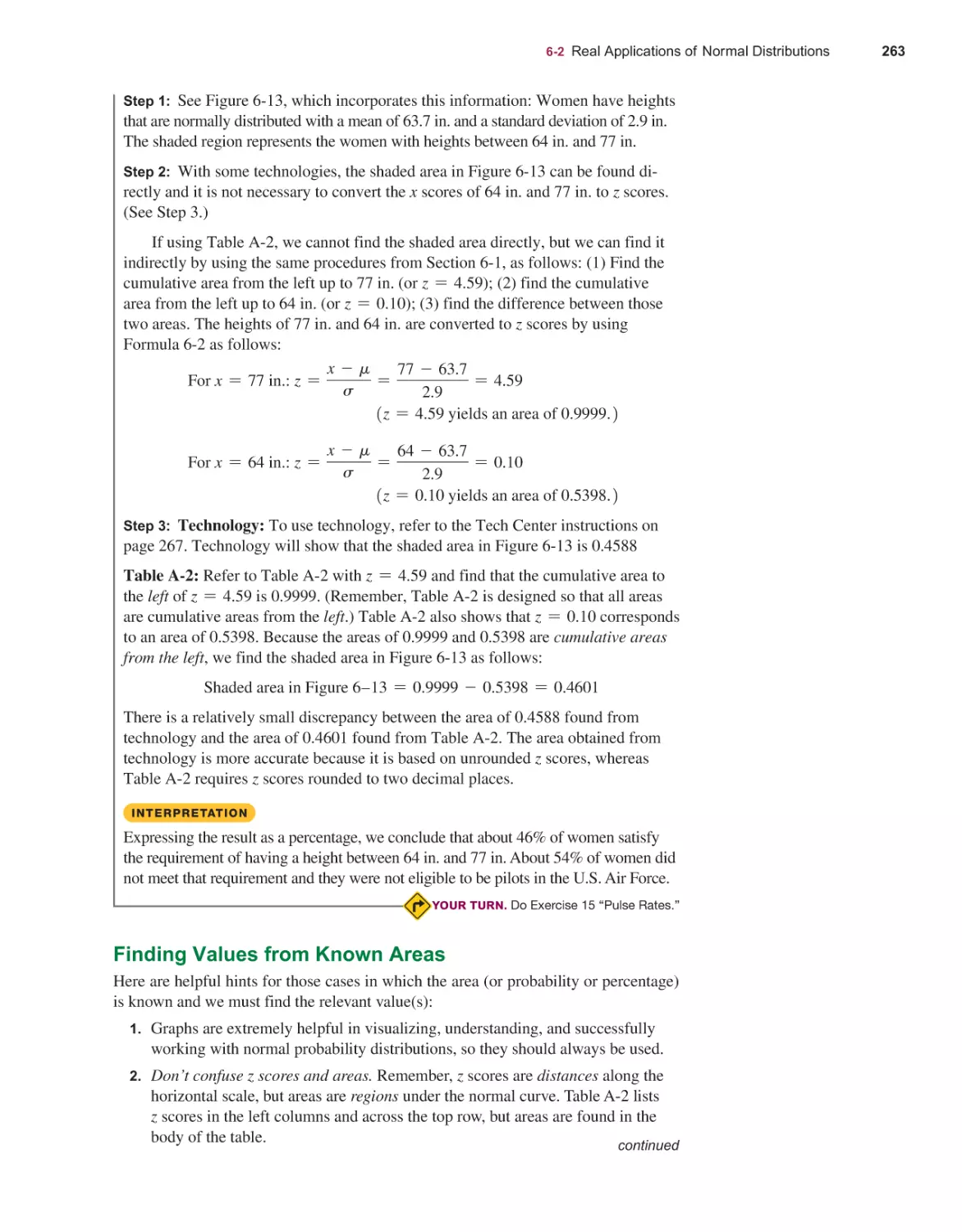
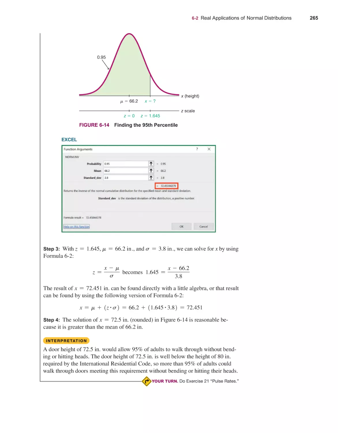
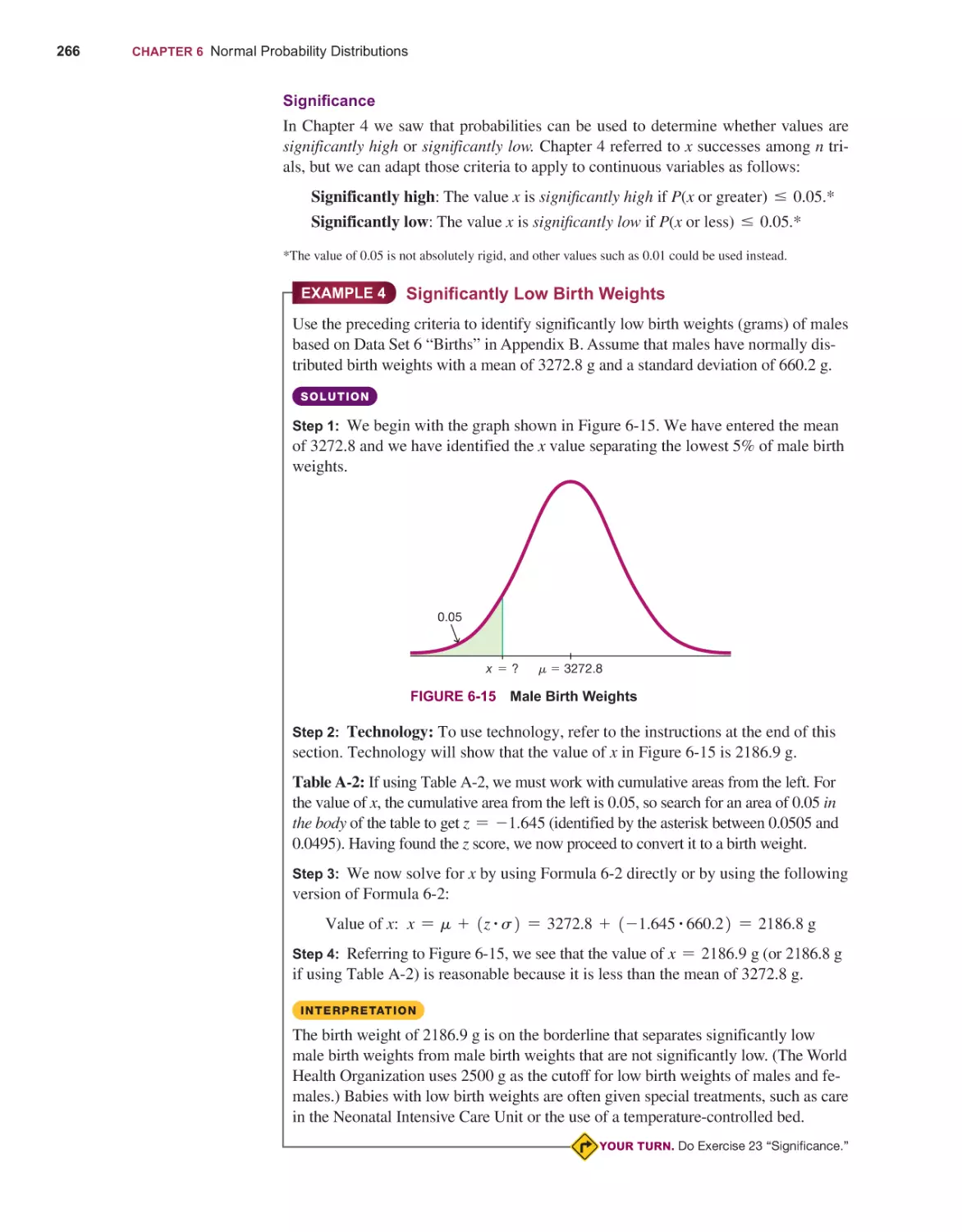
Real Applications of Normal Distributions 260
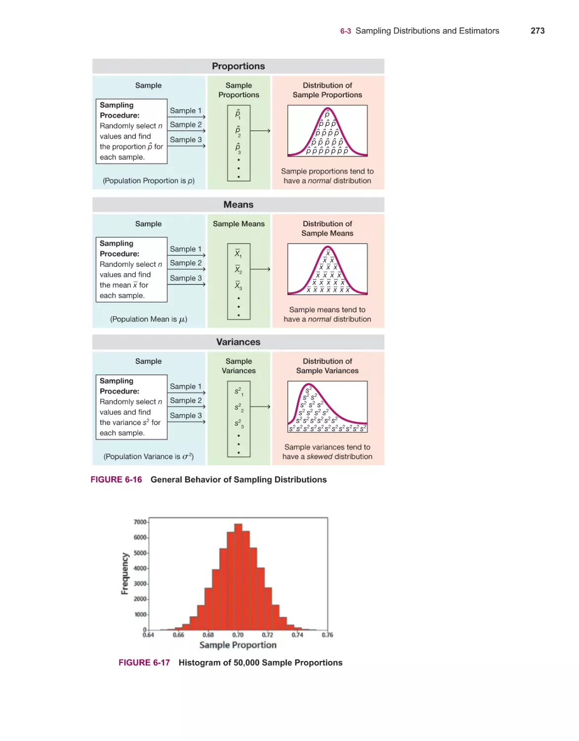
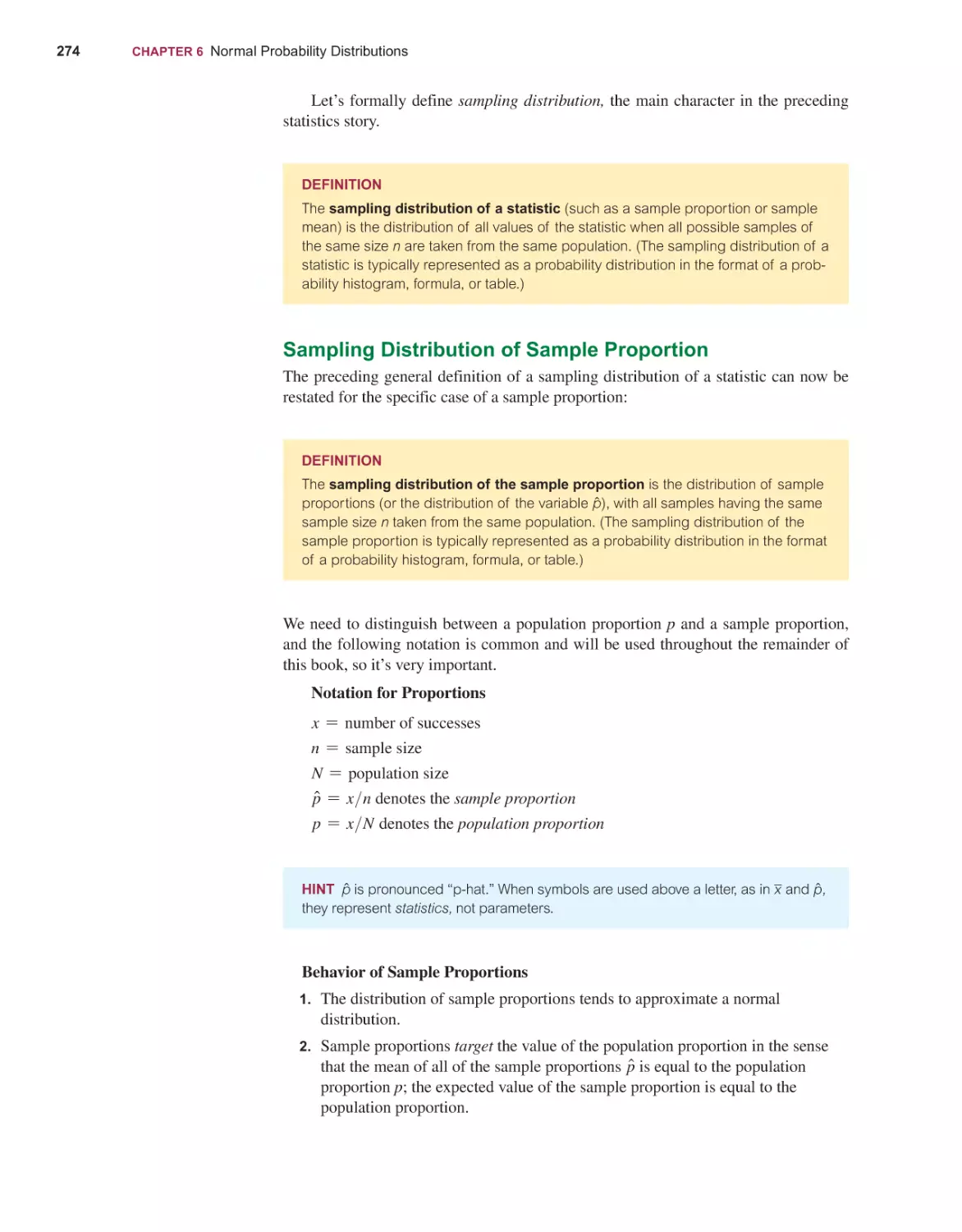
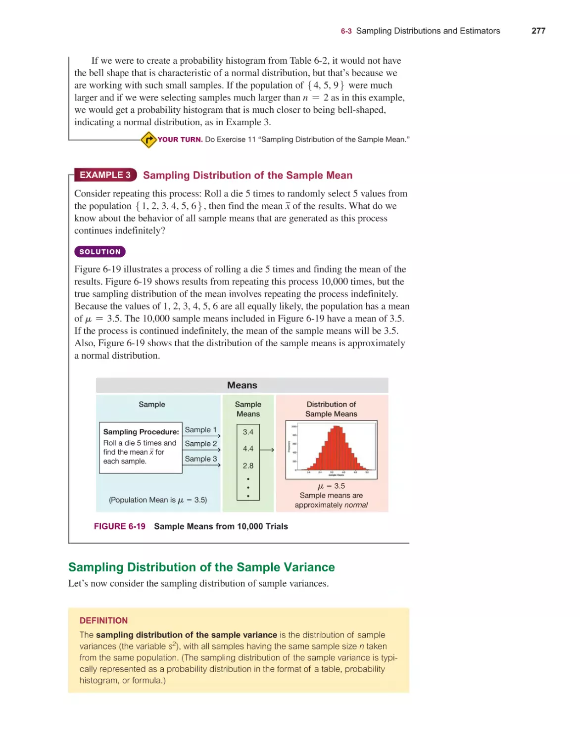
Sampling Distributions and Estimators 272
The Central Limit Theorem 283
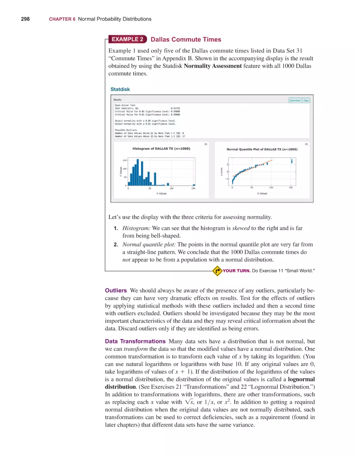
Assessing Normality 294
Normal as Approximation to Binomial (download only) 303
ESTIMATING PARAMETERS AND DETERMINING SAMPLE SIZES
7-1
7-2
7-3
7-4
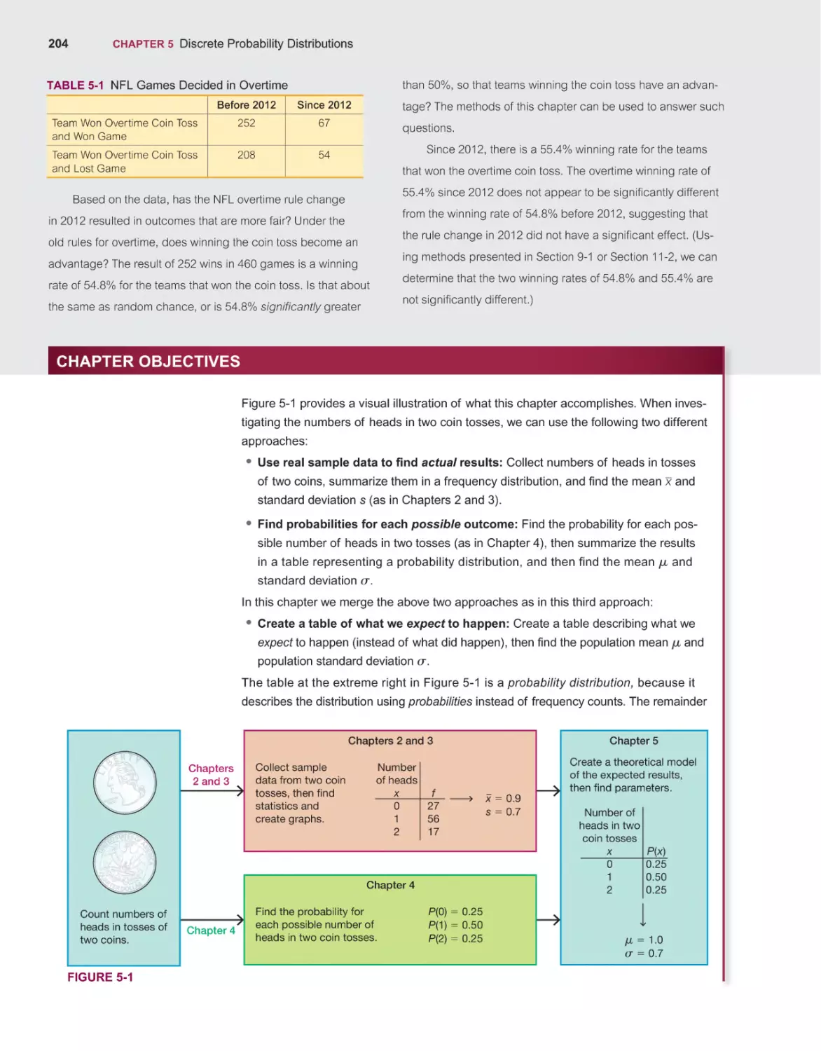
203
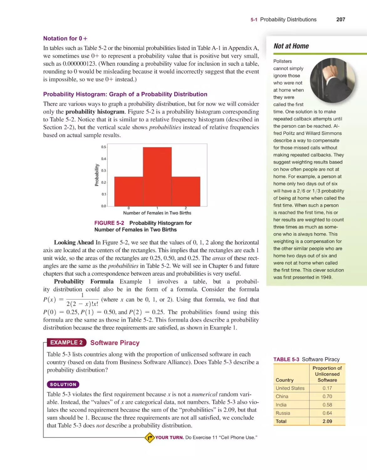
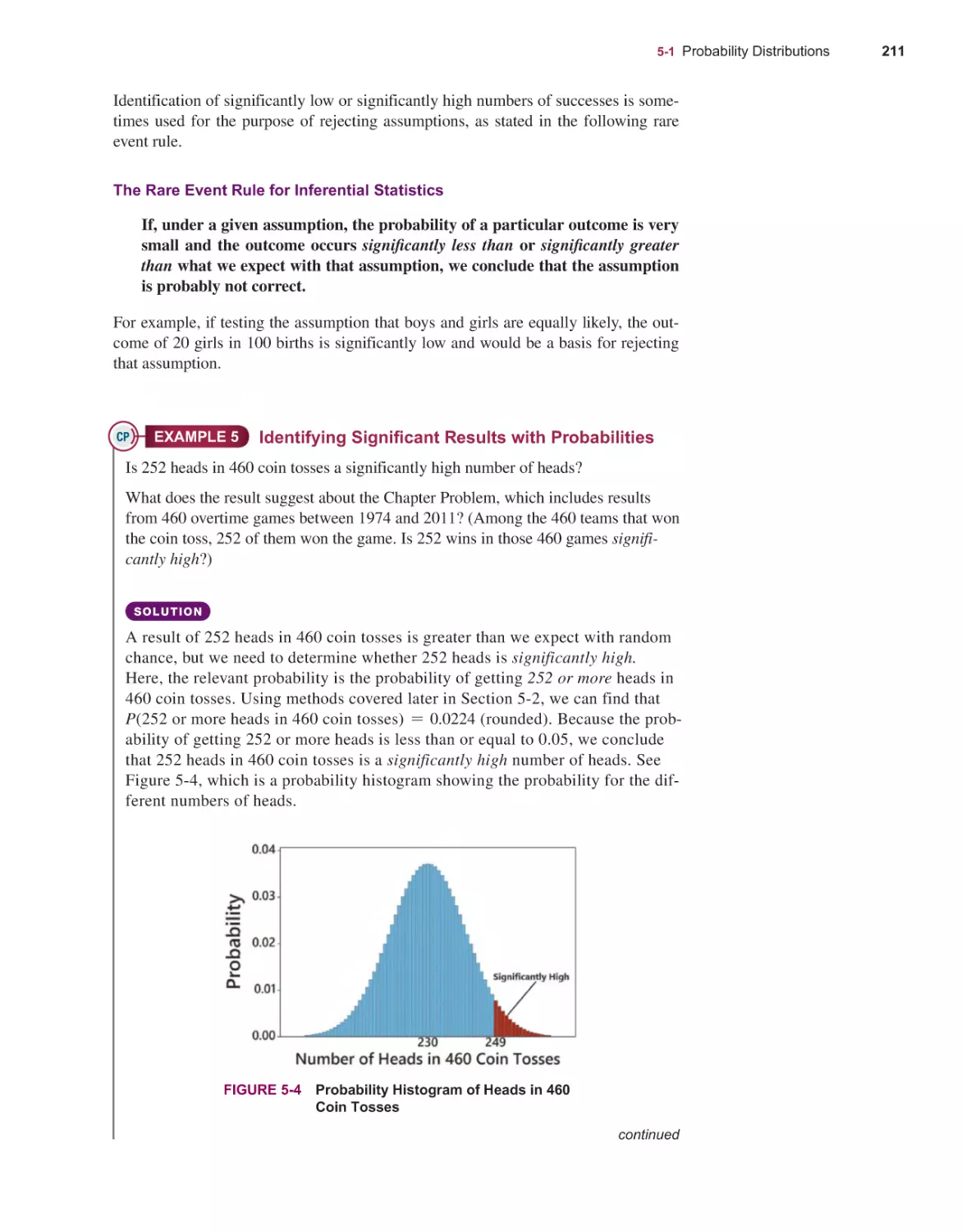
Probability Distributions 205
Binomial Probability Distributions 218
Poisson Probability Distributions 232
NORMAL PROBABILITY DISTRIBUTIONS
6-1
6-2
6-3
6-4
6-5
6-6
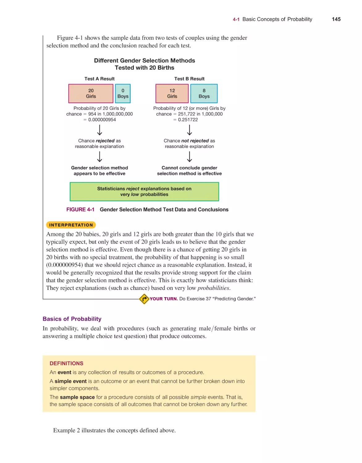
142
Basic Concepts of Probability 144
Addition Rule and Multiplication Rule 158
Complements, Conditional Probability, and Bayes’ Theorem 171
Counting 180
Simulations for Hypothesis Tests 190
DISCRETE PROBABILITY DISTRIBUTIONS
5-1
5-2
5-3
86
Measures of Center 88
Measures of Variation 104
Measures of Relative Standing and Boxplots 121
PROBABILITY
4-1
4-2
4-3
4-4
4-5
43
Frequency Distributions for Organizing and Summarizing Data 45
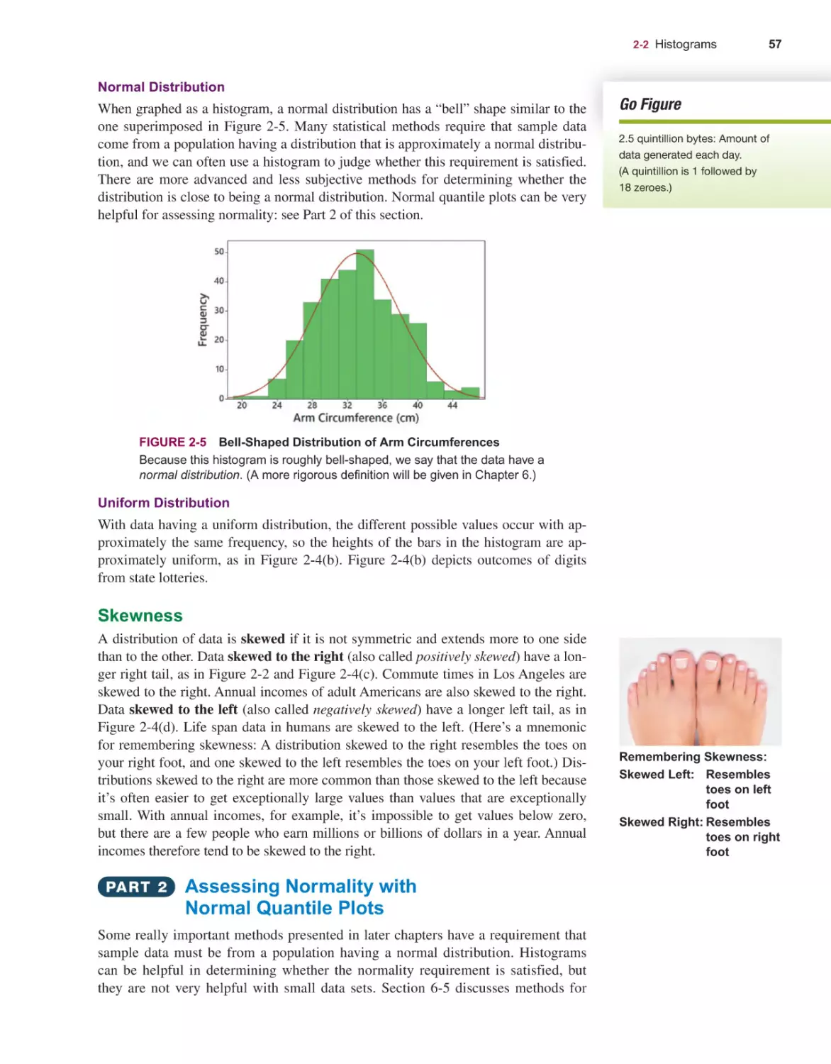
Histograms 55
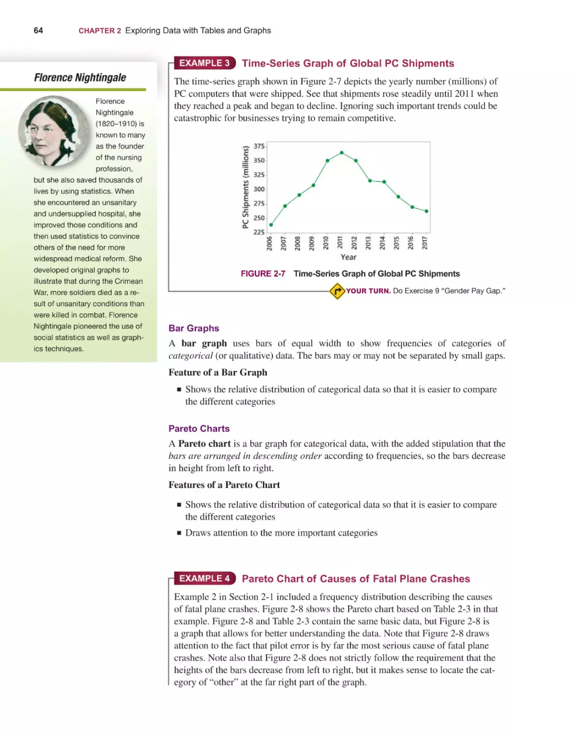
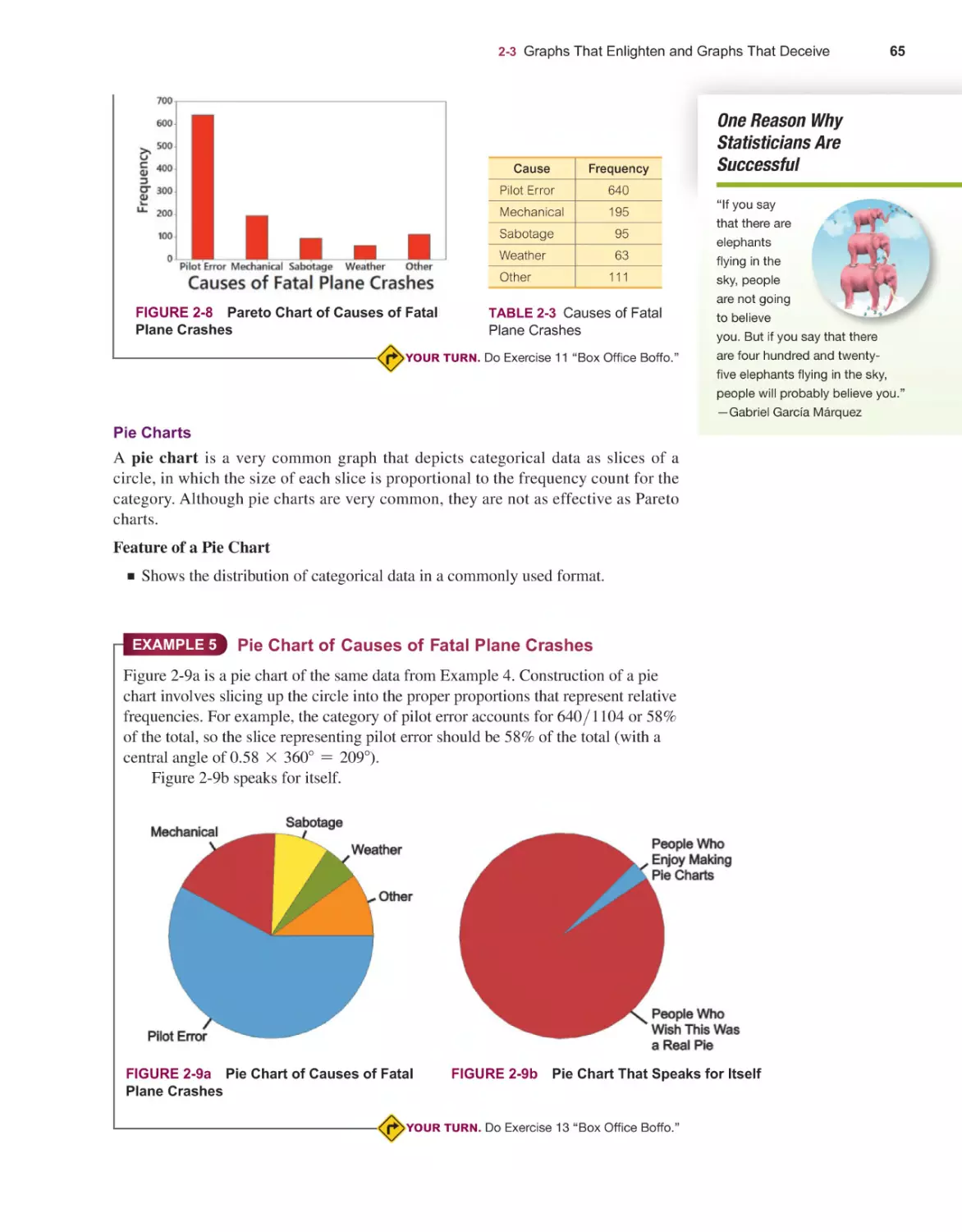
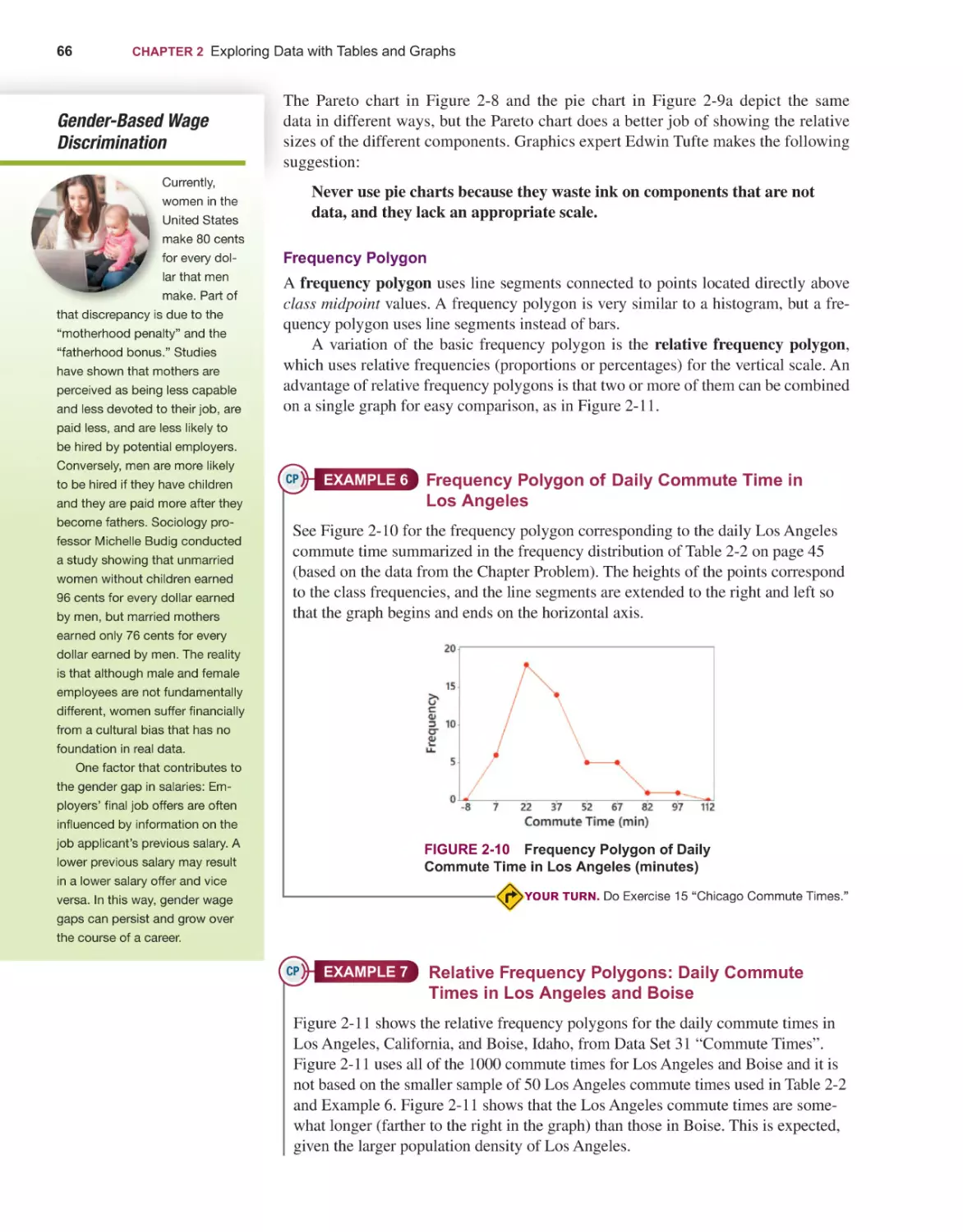
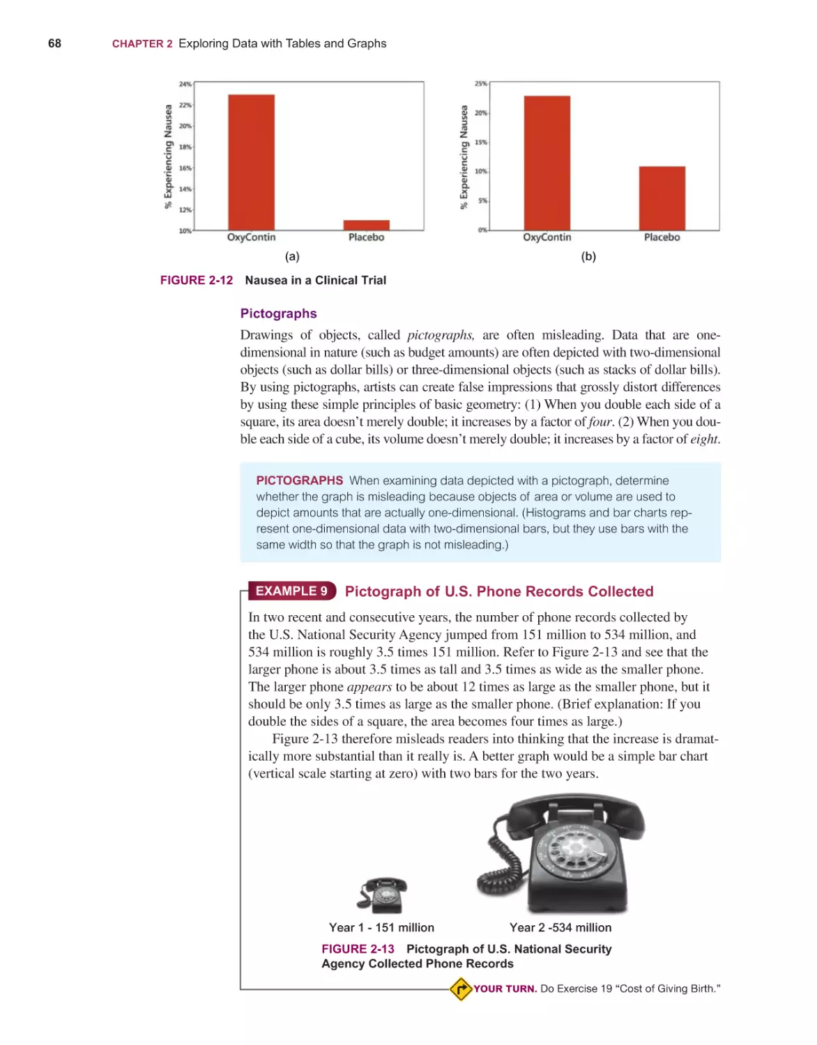
Graphs That Enlighten and Graphs That Deceive 62
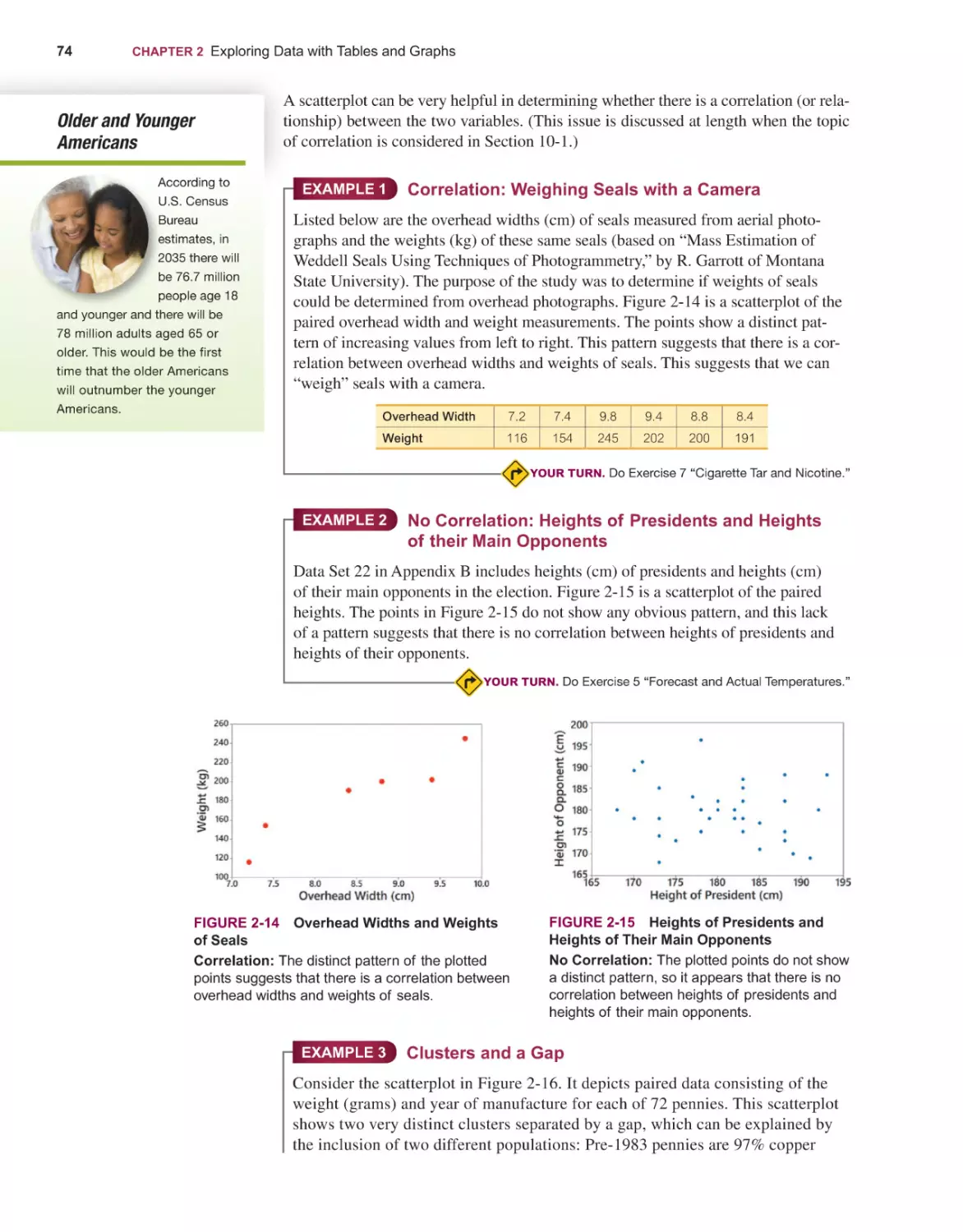
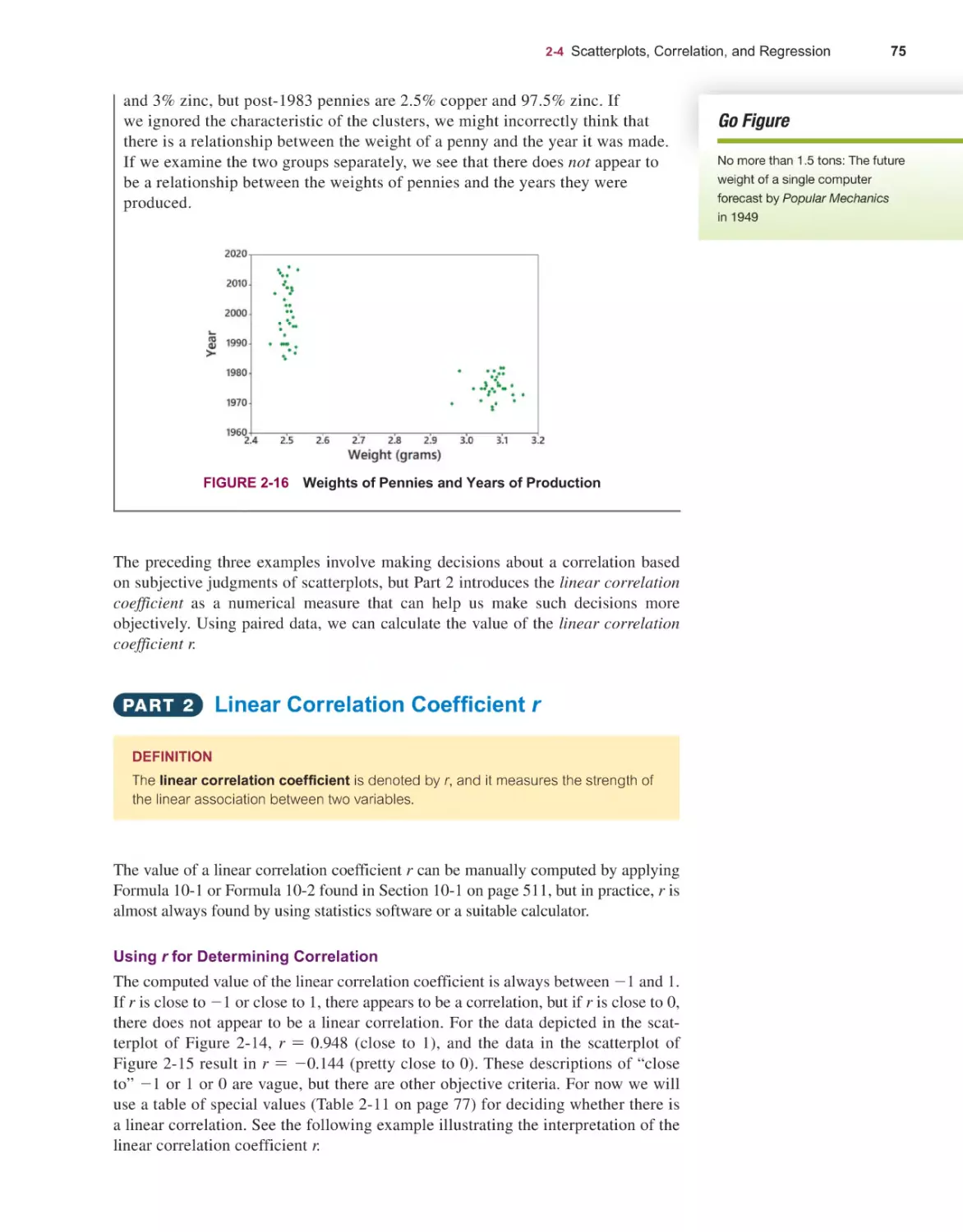
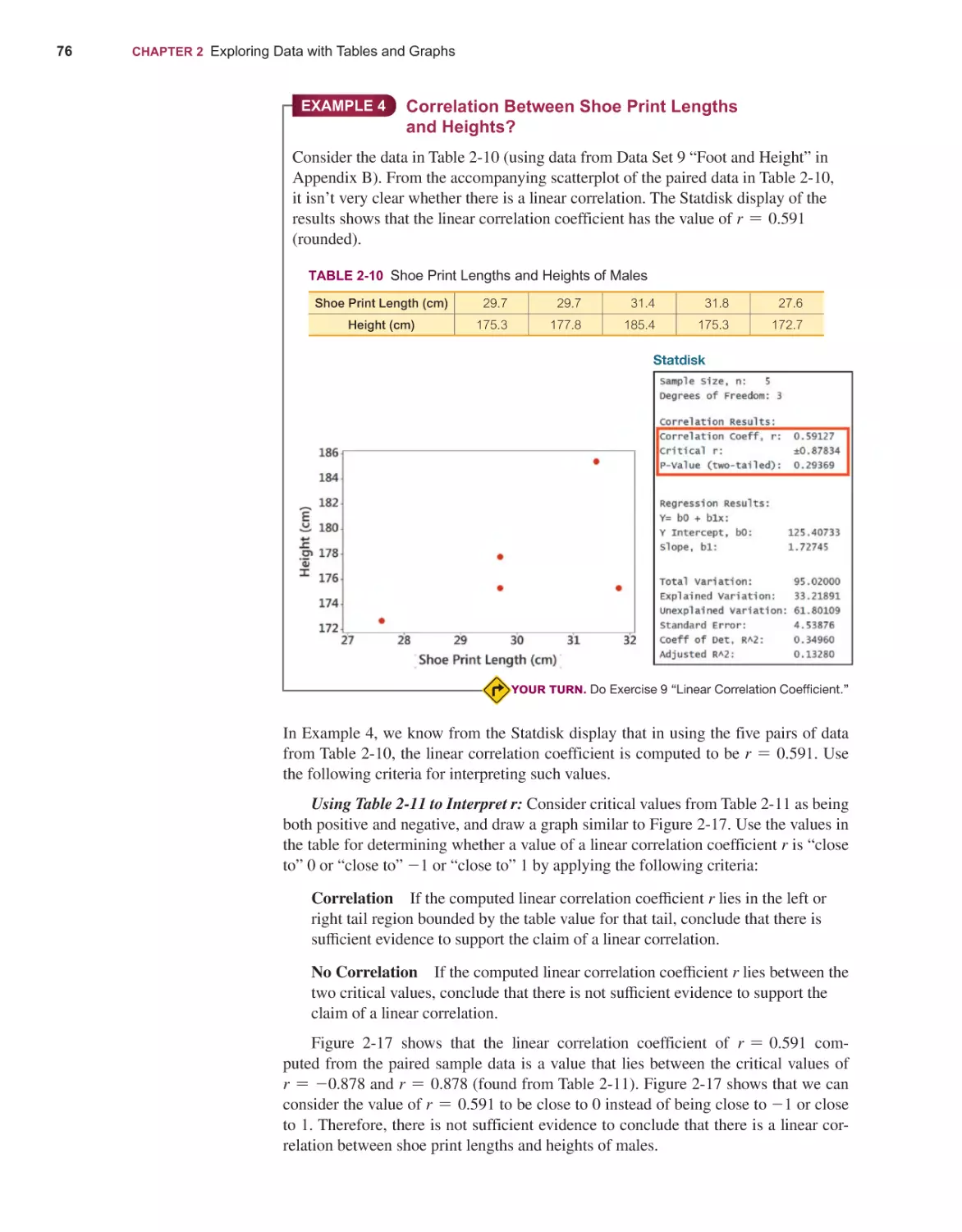
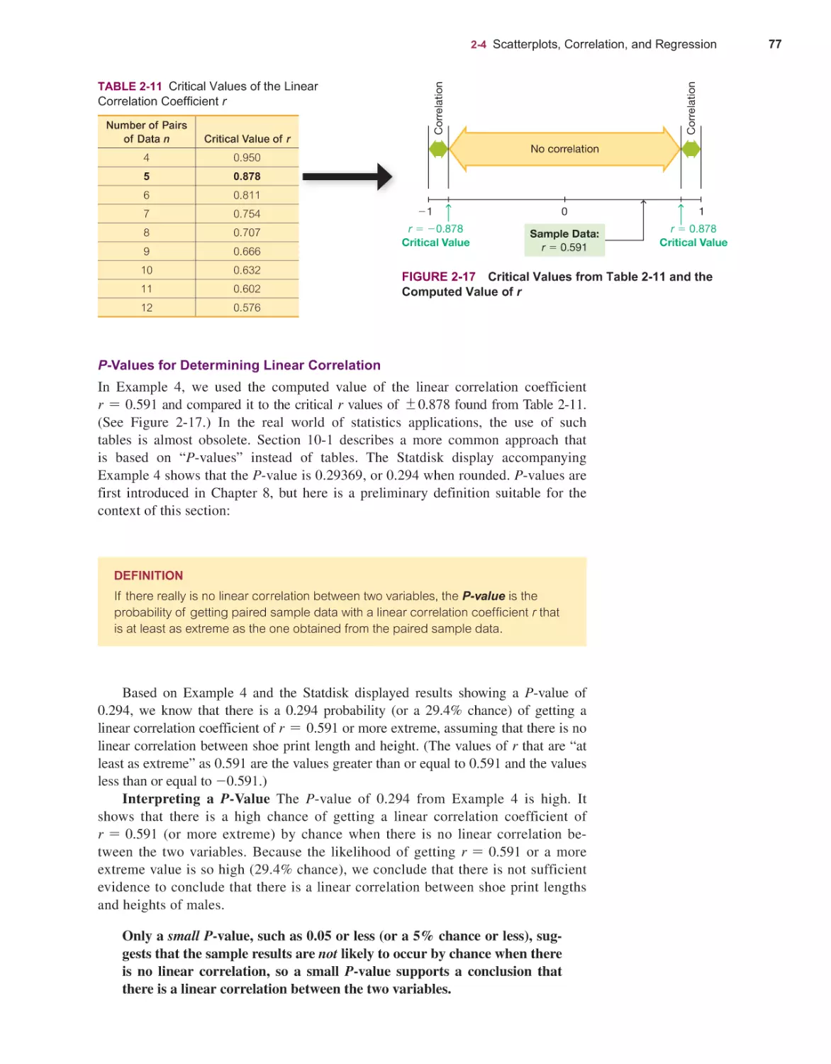
Scatterplots, Correlation, and Regression 73
DESCRIBING, EXPLORING, AND COMPARING DATA
3-1
3-2
3-3
1
Statistical and Critical Thinking 3
Types of Data 14
Collecting Sample Data 26
Ethics in Statistics (download only) 36
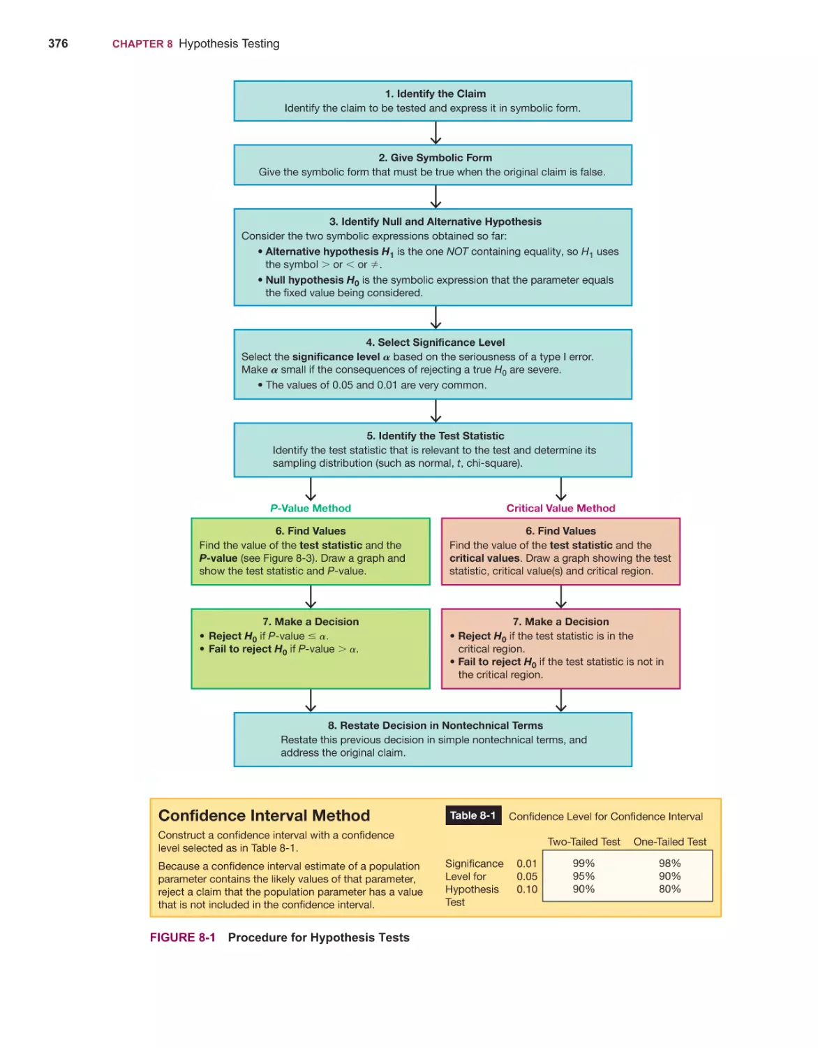
372
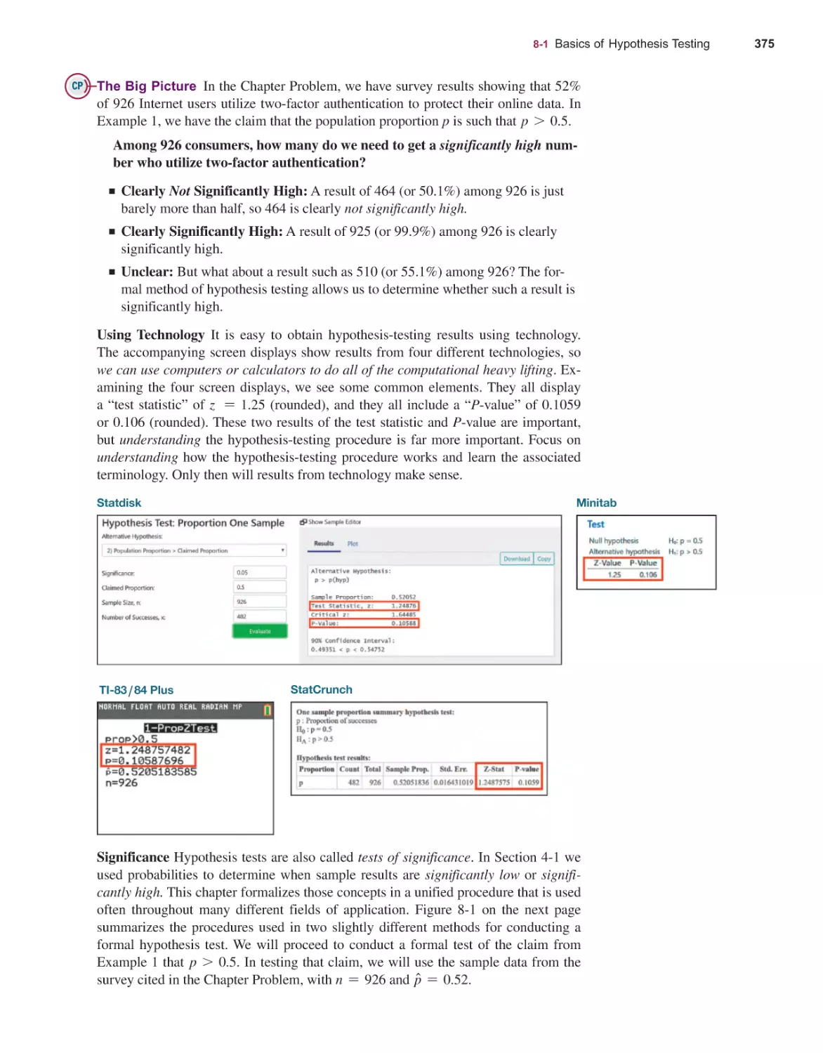
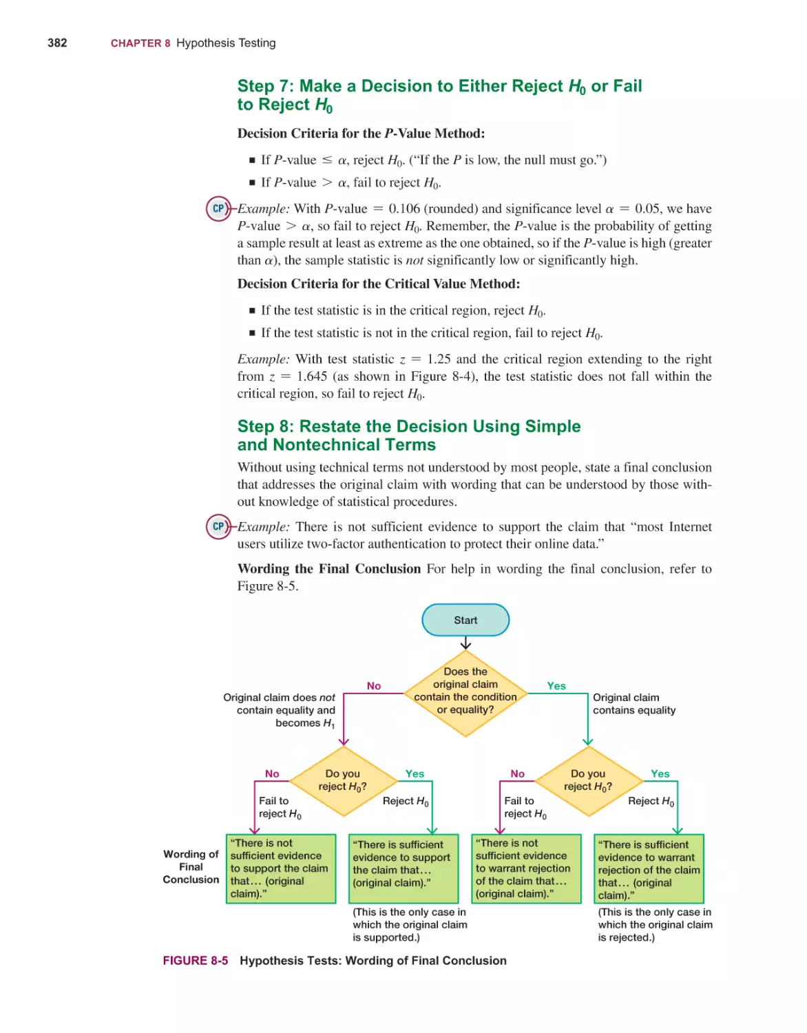
Basics of Hypothesis Testing 374
Testing a Claim About a Proportion 390
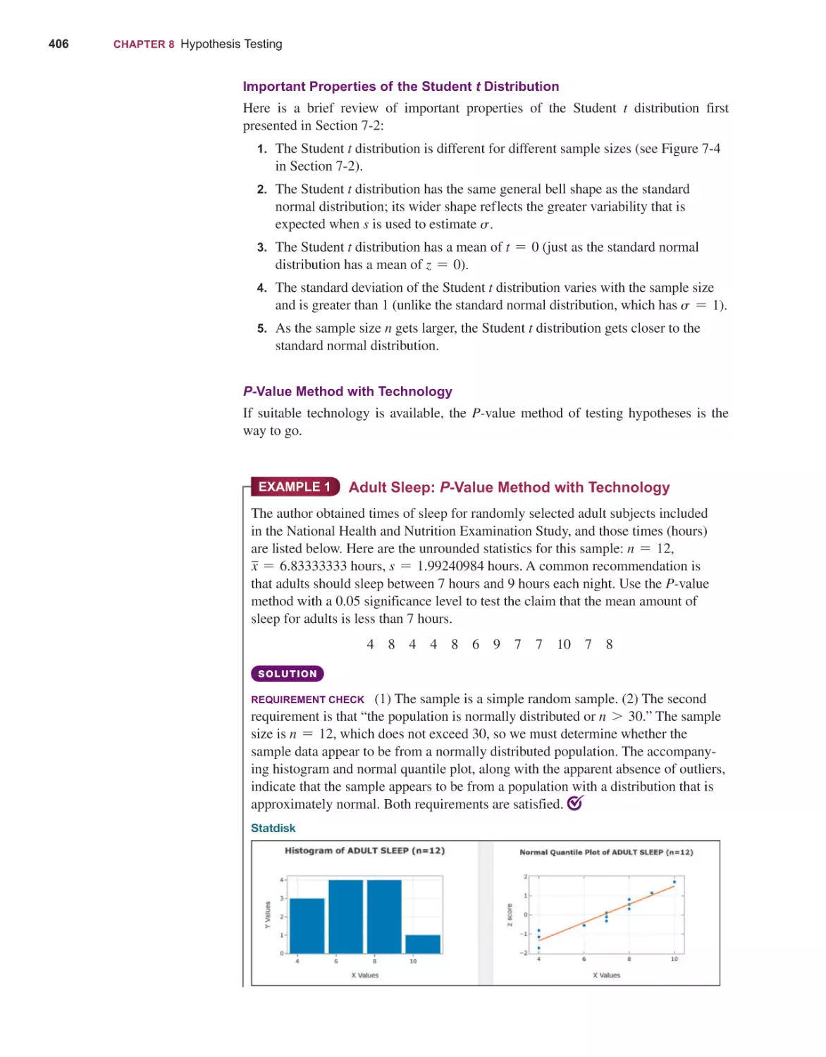
Testing a Claim About a Mean 404
Testing a Claim About a Standard Deviation or Variance 416
Resampling: Using Technology for Hypothesis Testing 425
ix
x
Contents
9
10
11
12
13
14
15
APPENDIX A
APPENDIX B
APPENDIX C
APPENDIX D
INFERENCES FROM TWO SAMPLES
9-1
9-2
9-3
9-4
9-5
CORRELATION AND REGRESSION
10-1
10-2
10-3
10-4
10-5
506
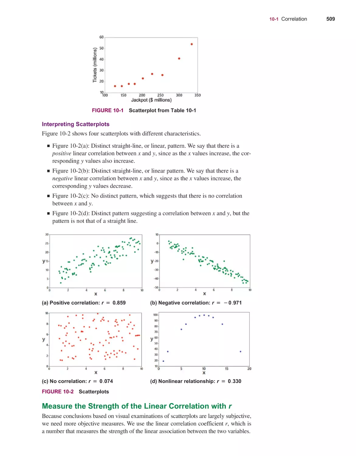
Correlation 508
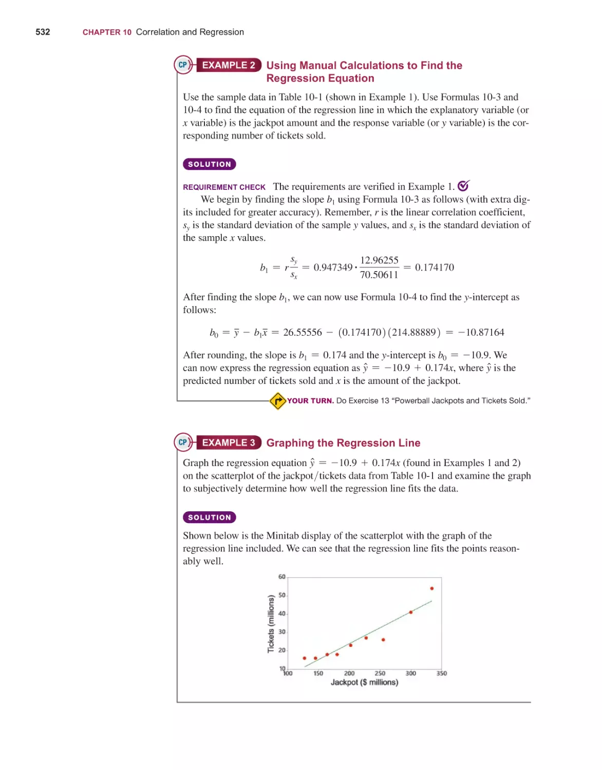
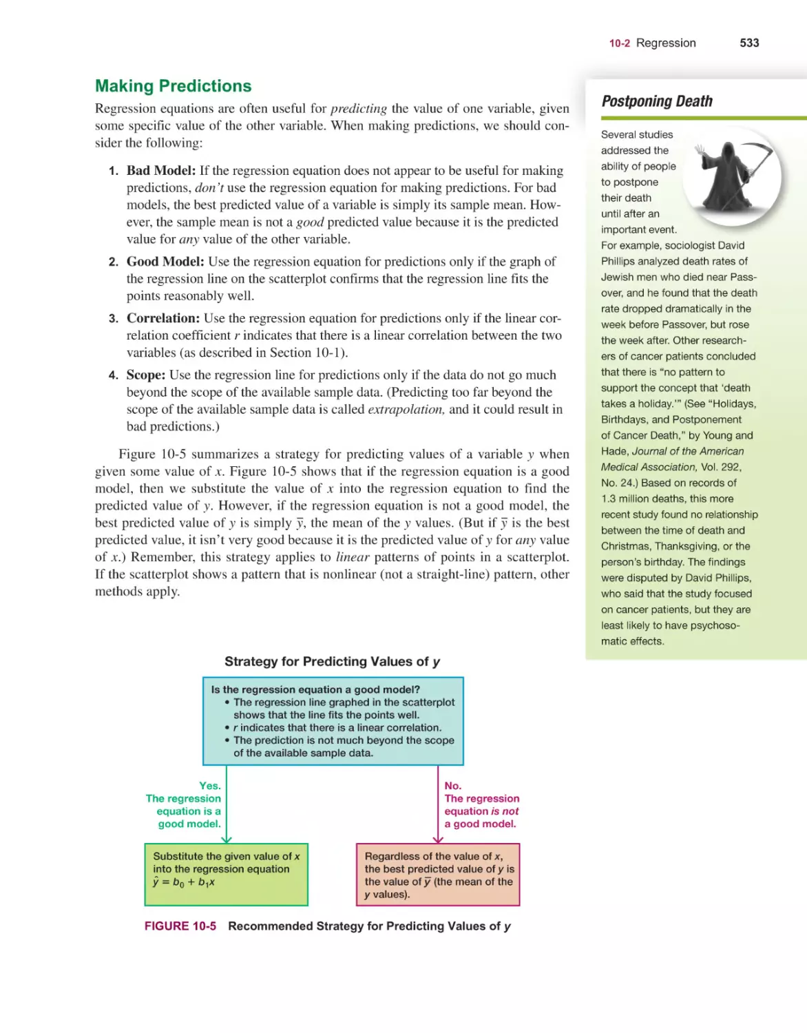
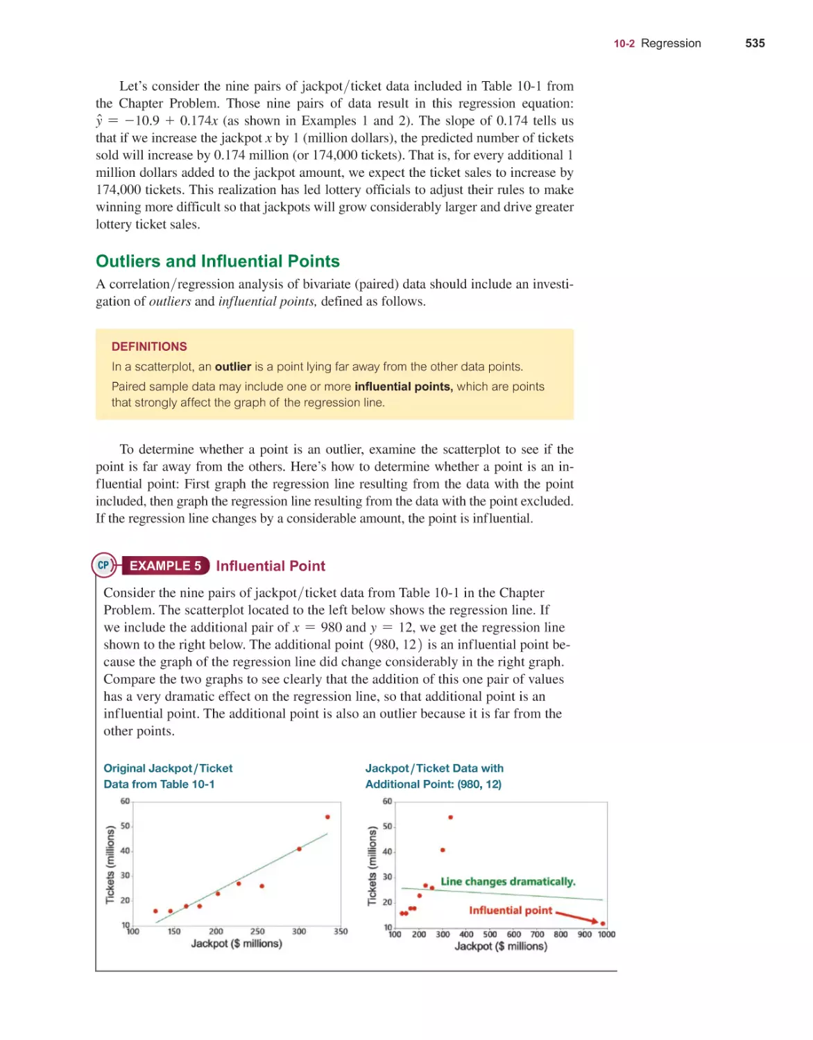
Regression 529
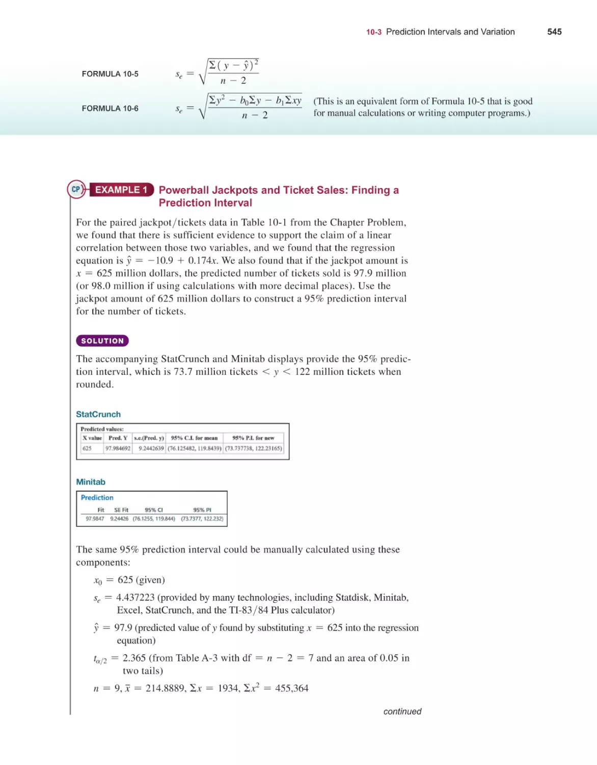
Prediction Intervals and Variation 544
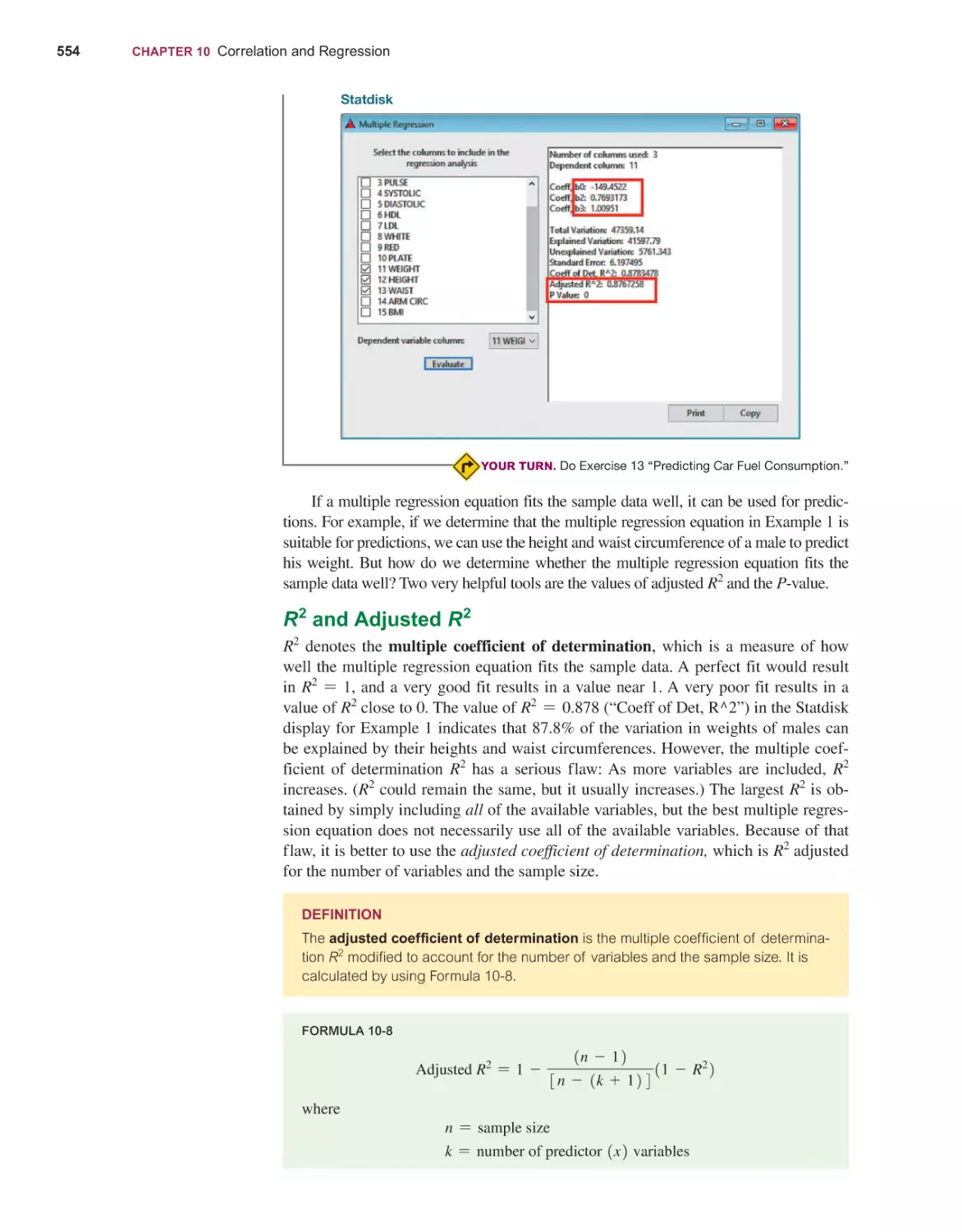
Multiple Regression 552
Nonlinear Regression 564
GOODNESS-OF-FIT AND CONTINGENCY TABLES
11-1
11-2
440
Two Proportions 442
Two Means: Independent Samples 454
Matched Pairs 469
Two Variances or Standard Deviations 480
Resampling: Using Technology for Inferences 490
576
Goodness-of-Fit 578
Contingency Tables 590
ANALYSIS OF VARIANCE
610
NONPARAMETRIC TESTS
642
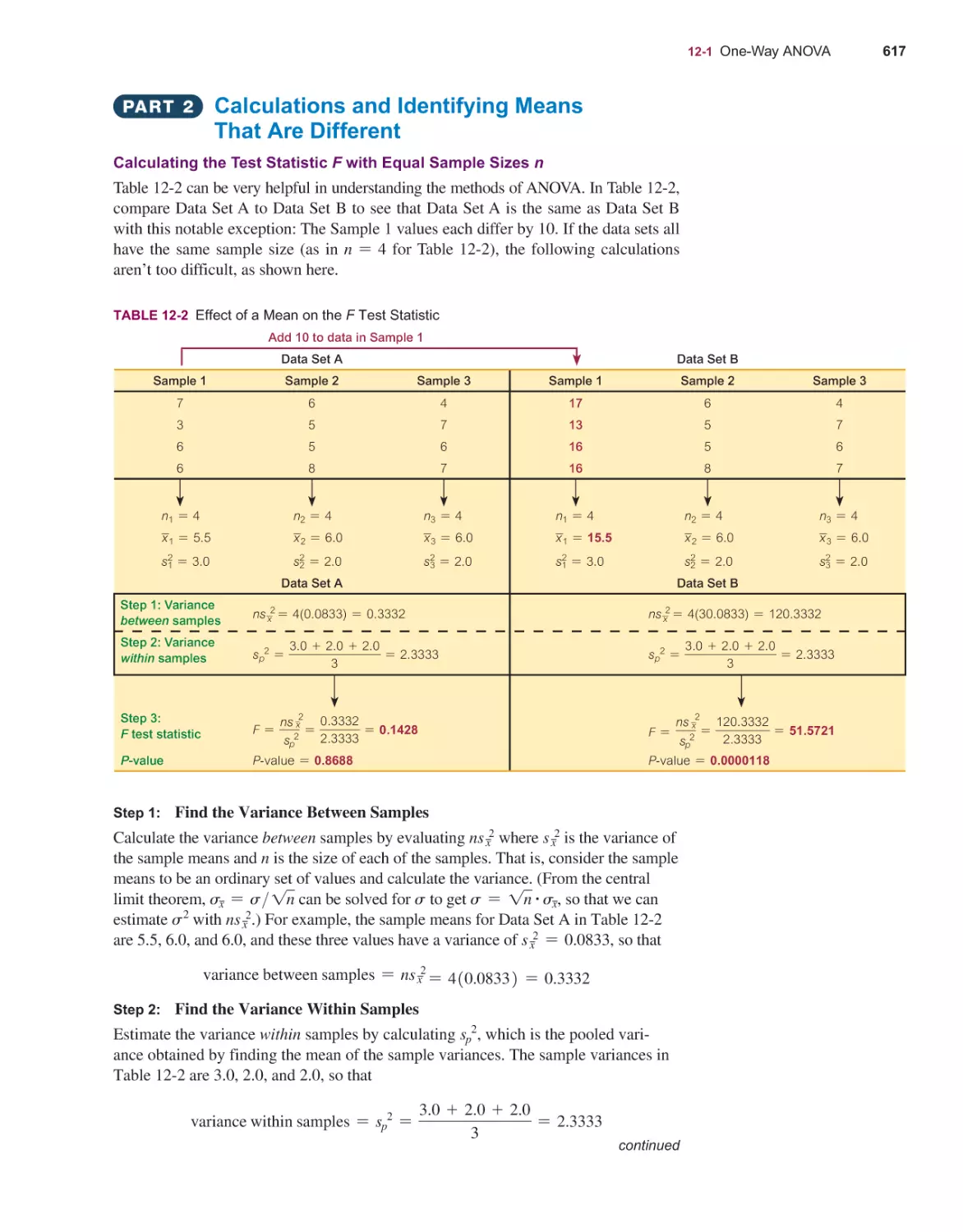
12-1 One-Way ANOVA 612
12-2 Two-Way ANOVA 626
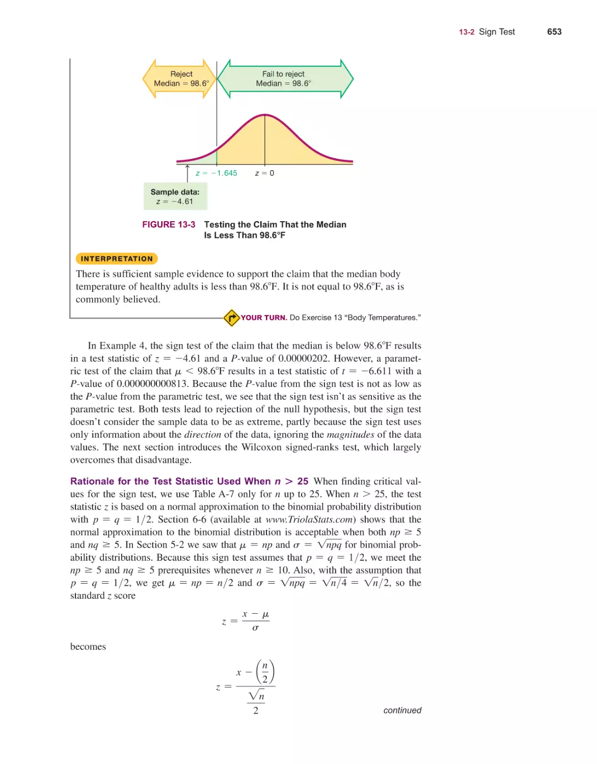
13-1
13-2
13-3
13-4
13-5
13-6
13-7
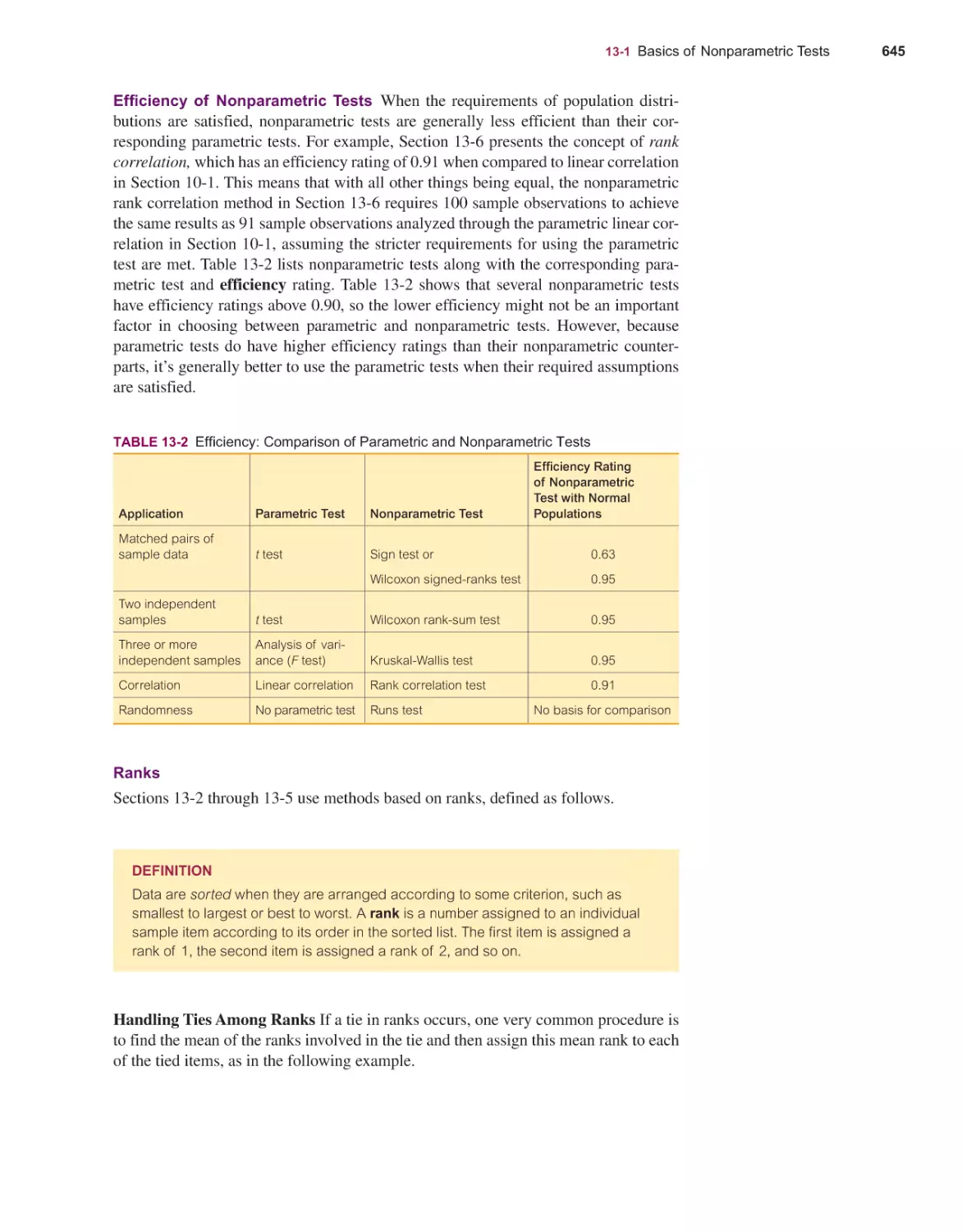
Basics of Nonparametric Tests 644
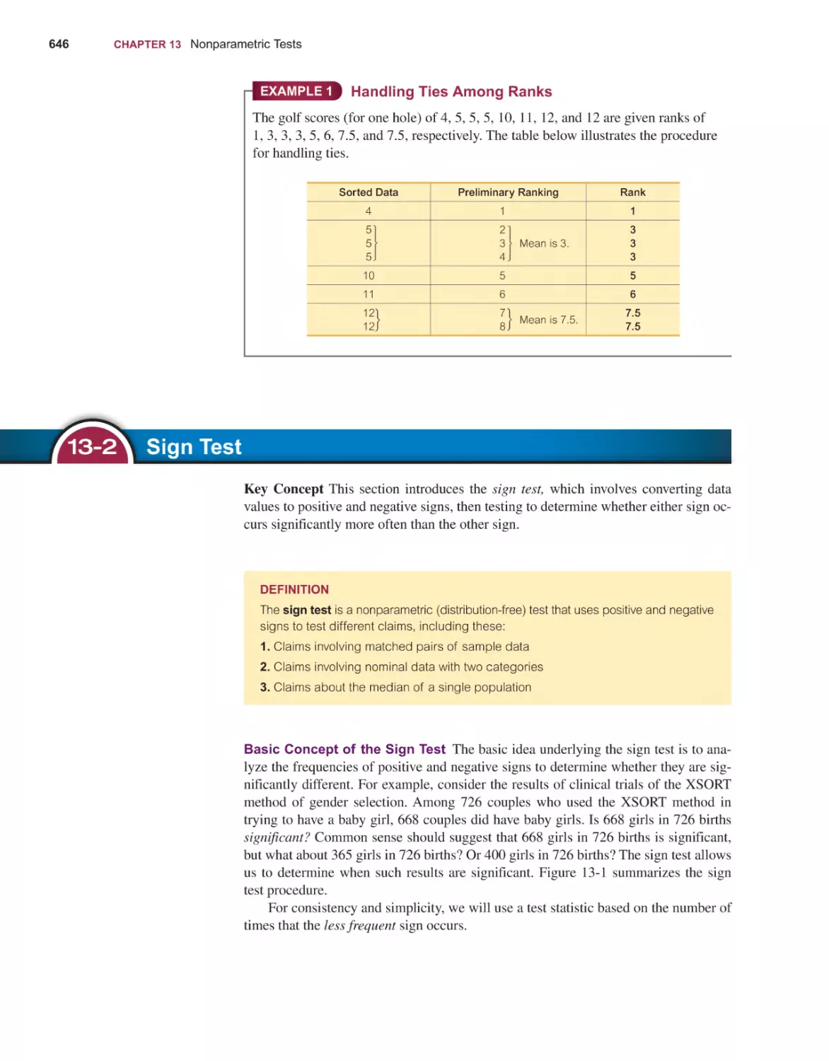
Sign Test 646
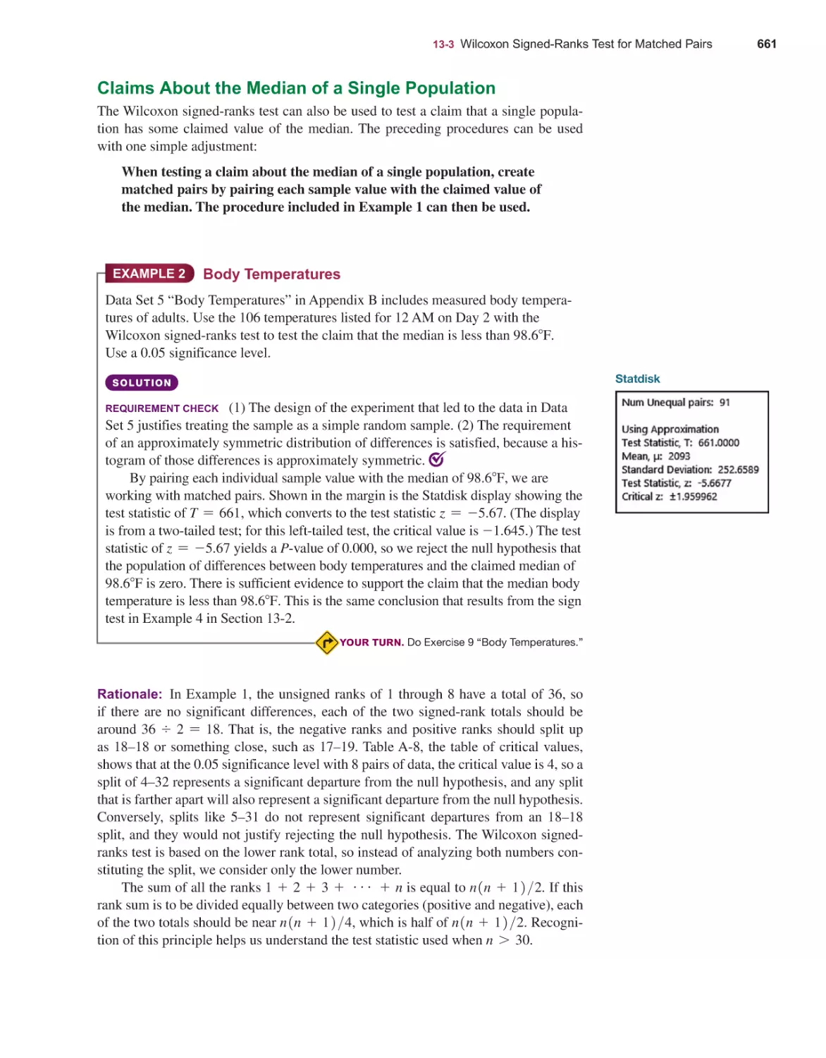
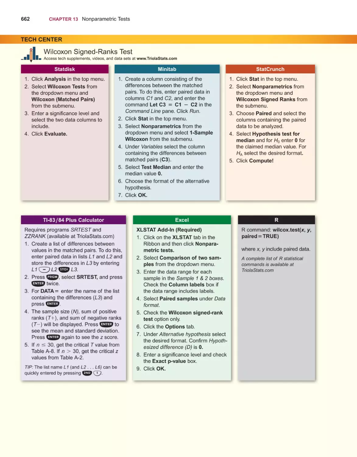
Wilcoxon Signed-Ranks Test for Matched Pairs 657
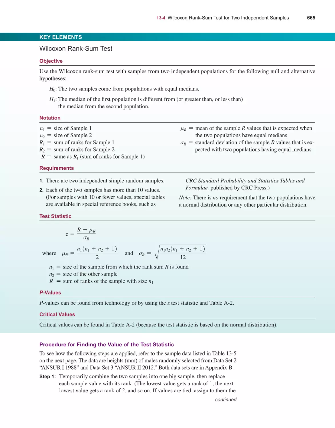
Wilcoxon Rank-Sum Test for Two Independent Samples 664
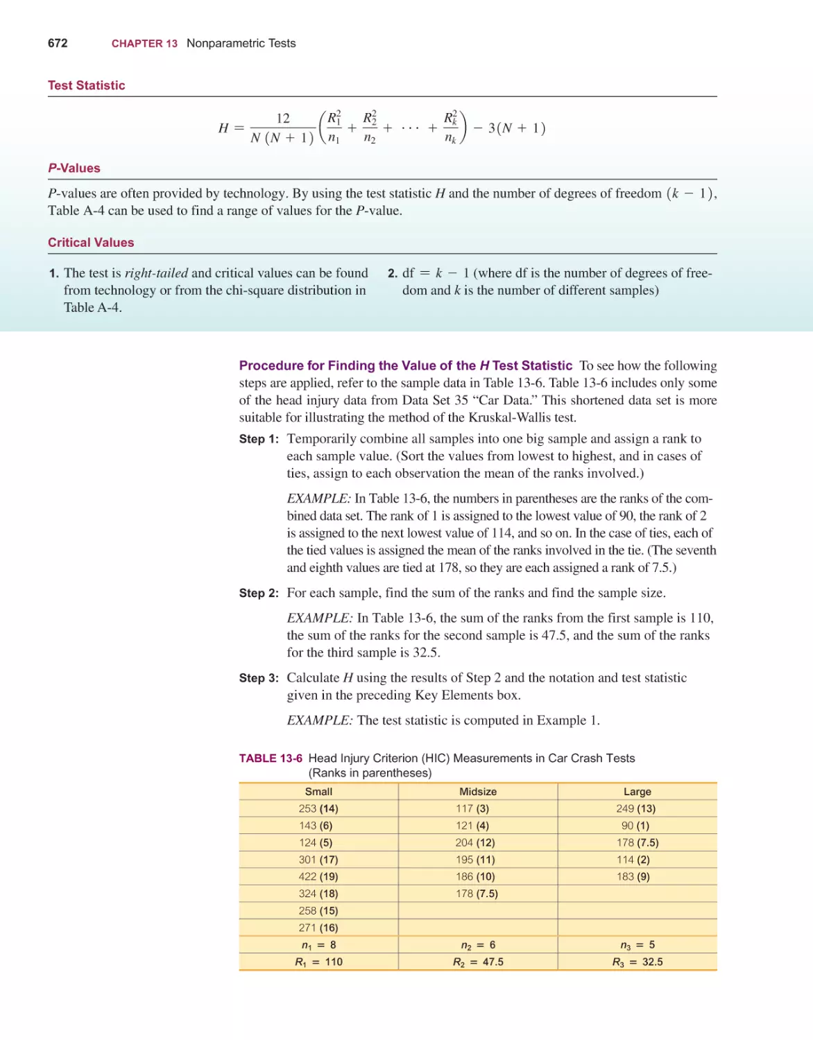
Kruskal-Wallis Test for Three or More Samples 671
Rank Correlation 677
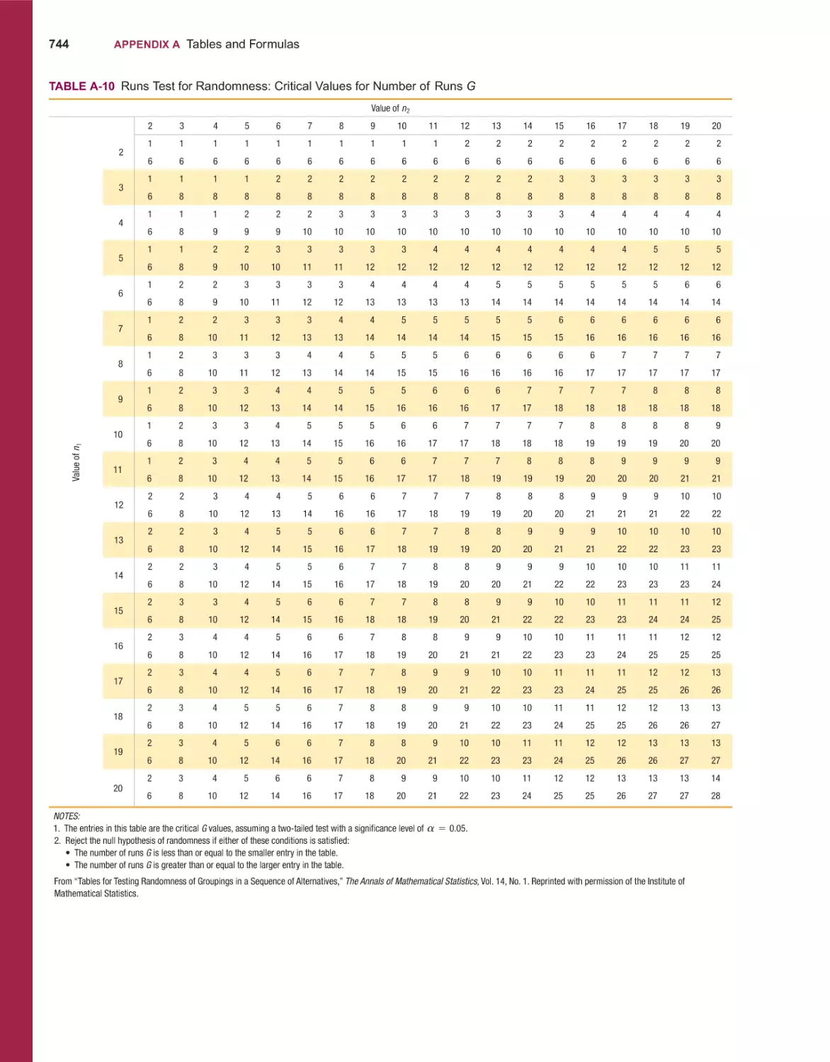
Runs Test for Randomness 686
STATISTICAL PROCESS CONTROL
700
HOLISTIC STATISTICS
TABLES AND FORMULAS
DATA SETS
WEBSITES AND BIBLIOGRAPHY OF BOOKS
ANSWERS TO ODD-NUMBERED SECTION EXERCISES
724
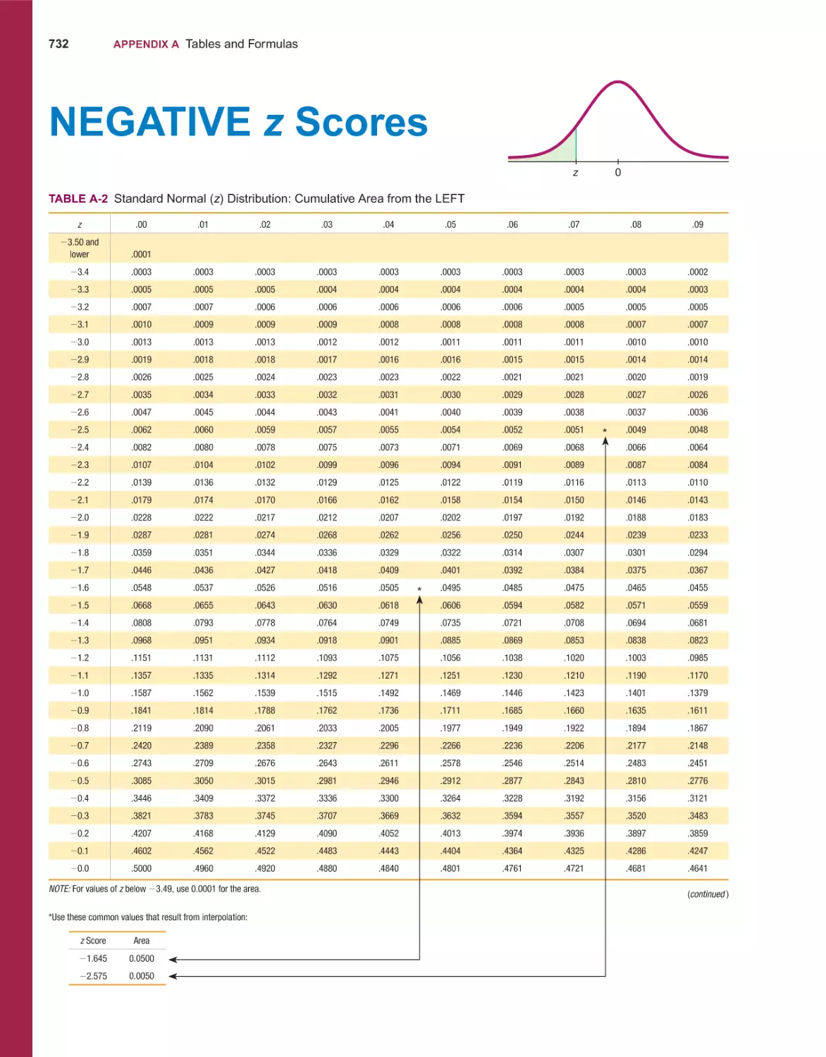
731
749
765
766
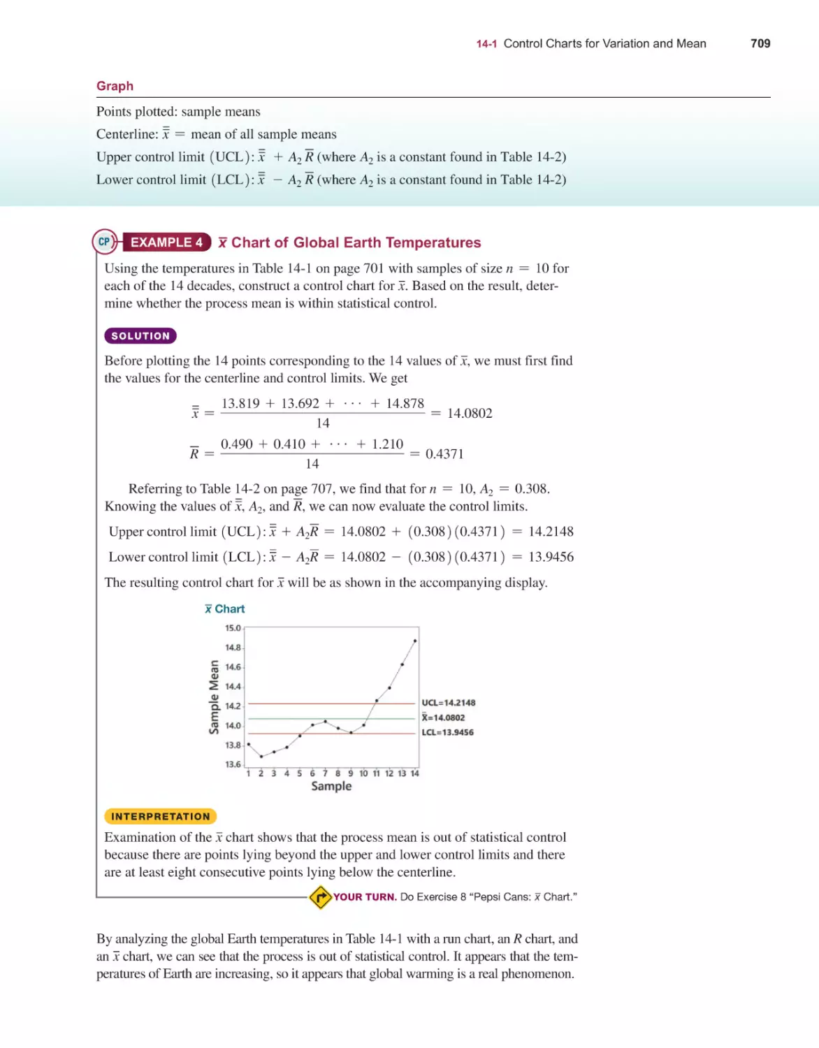
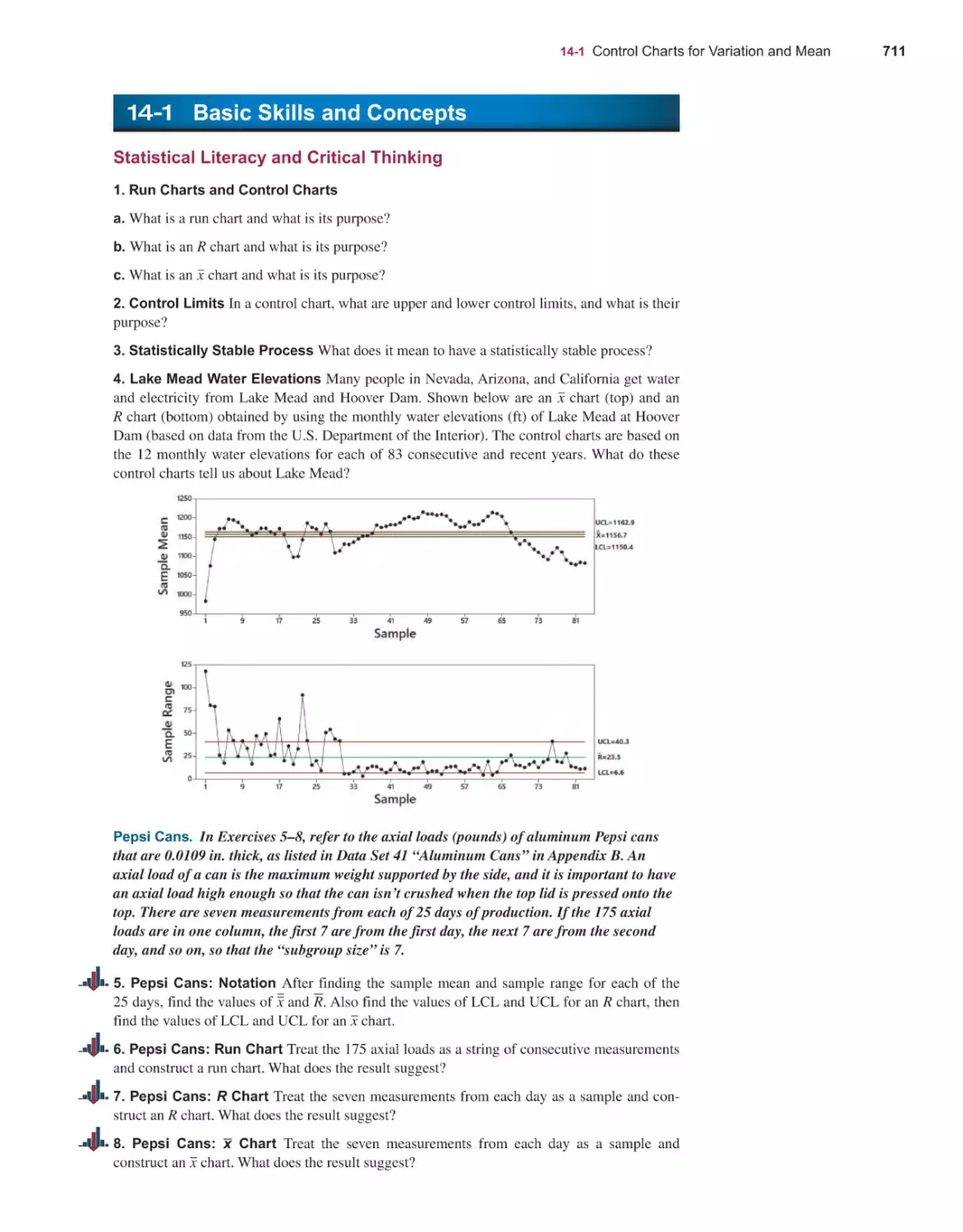
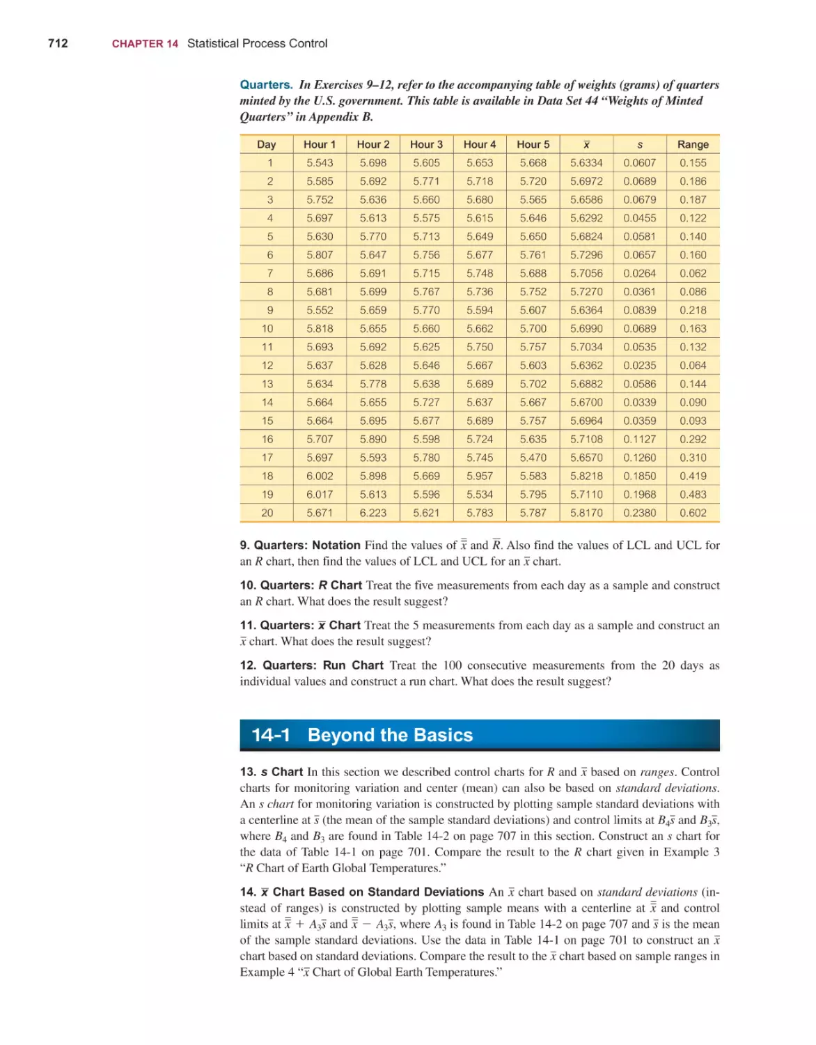
14-1 Control Charts for Variation and Mean 702
14-2 Control Charts for Attributes 713
(and all Quick Quizzes, all Review Exercises, and all Cumulative Review Exercises)
Credits 815
Subject Index 823
Applications Index 835
PREFACE
The ancient Chinese philosopher Lao Tzu famously wrote: A journey of a thousand
miles must begin with a single step. This textbook will lead you, step-by-step, on a
journey through the important concepts of statistics and if you’re reading this, you’ve
already taken the first step! Thankfully, our journey will be much less physically taxing than a “journey of a thousand miles” and will only require use of your feet for
determining skewness (see page 57).
We are now on the leading edge of a major revolution in technology, and the
content of this text is key to that revolution. Artificial intelligence, machine learning,
and deep learning are studied in data science, and the study of data science requires
study of the discipline of statistics. Data science is now experiencing unprecedented
growth. Projections indicate a 33% increased demand for statisticians in a few short
years, and there is a projected shortage of workers with statistical skills. Also, as in
past decades, statistics continues to be essential to a wide variety of disciplines, including medicine, polling, journalism, law, physical science, education, business, and
economics. It is a gross understatement to suggest that it is now very wise to initiate
a study of statistics.
Goals of This Fourteenth Edition
■■
■■
■■
■■
■■
■■
Foster personal growth of students through critical thinking, use of technology,
collaborative work, and development of communication skills.
Incorporate the latest and best methods used by professional statisticians.
Include features that address all of the recommendations included in the Guidelines for Assessment and Instruction in Statistics Education (GAISE) as recommended by the American Statistical Association.
Provide an abundance of new and interesting data sets, examples, and exercises,
such as those involving biometric security, cybersecurity, drones, and Internet
traffic.
Present topics used in data science and many other applications, and include very
large data sets that have become so important in our current culture.
Enhance teaching and learning with the most extensive and best set of supplements and digital resources.
Audience , Prerequisites
Elementary Statistics is written for students majoring in any subject. Algebra is used
minimally. It is recommended that students have completed at least an elementary
algebra course or that students should learn the relevant algebra components through
an integrated or co-requisite course available through MyLab Statistics. In many
cases, underlying theory is included, but this book does not require the mathematical
rigor more appropriate for mathematics majors. Instead of being a “cookbook” devoid of any theory, this book includes the mathematics underlying important statistical methods, but the focus is on understanding and applying those methods along with
interpreting results in a meaningful way.
xi
xii
Preface
Hallmark Features
Great care has been taken to ensure that each chapter of Elementary Statistics will
help students understand the concepts presented. The following features are designed
to help meet that objective of conceptual understanding.
Real Data
Thousands of hours have been devoted to finding data that are real, meaningful, and
interesting to students. 94% of the examples are based on real data, and 93% of the
exercises are based on real data. Some exercises refer to the 46 data sets listed in
Appendix B, and 20 of those data sets are new to this edition. Exercises requiring
use of the Appendix B data sets are located toward the end of each exercise set and
. These data sets are also available in
are marked with a special data set icon
MyLab Statistics, including data sets for StatCrunch.
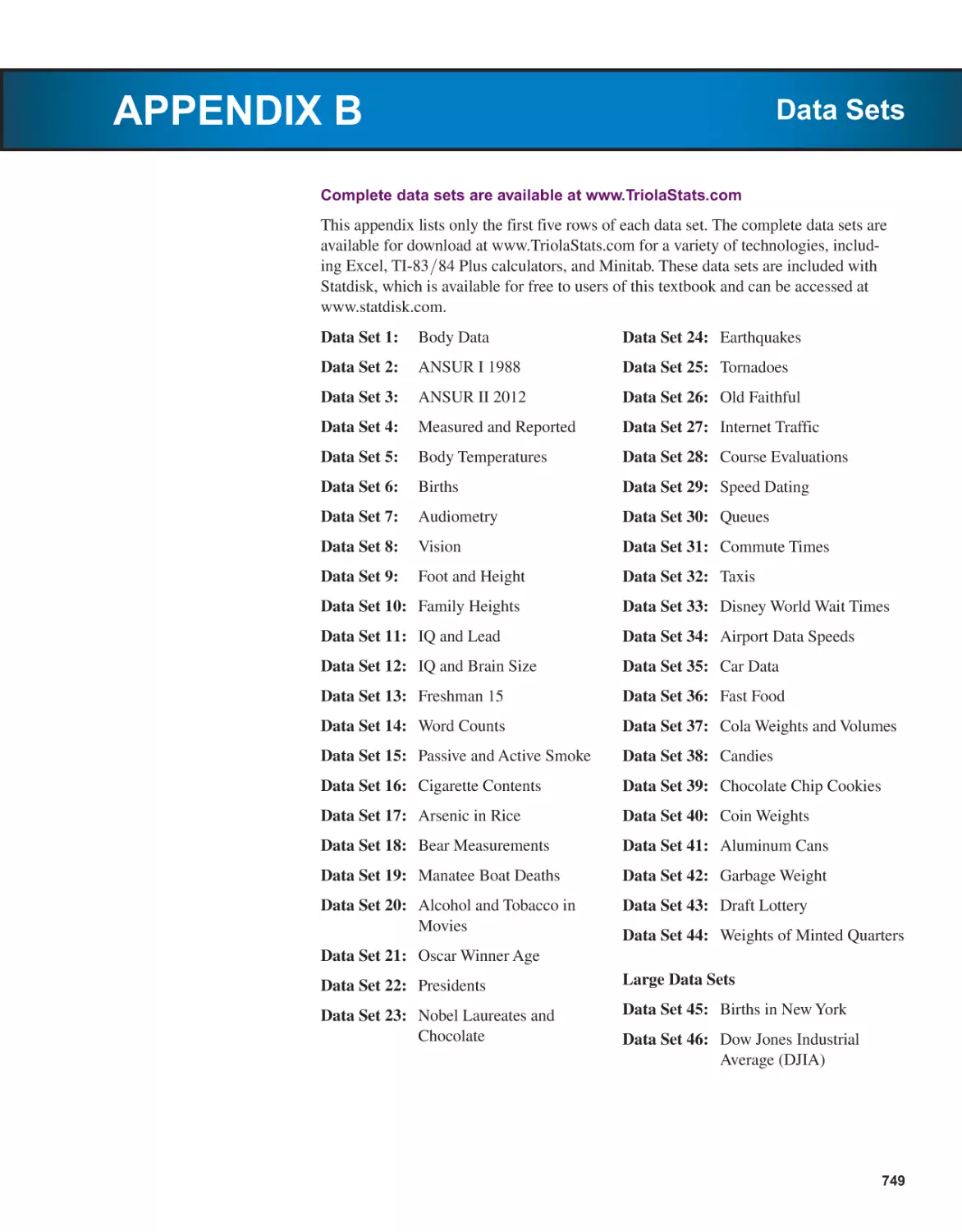
Appendix B includes descriptions of the 46 data sets that can be downloaded from
www.TriolaStats.com in formats for Excel™, Minitab™, JMP, SPSS, and TI-83>84™
Plus calculators. (Because TI-83>84 Plus calculators have limited memory, several
larger data sets have been truncated for TI users, and answers have been annotated
when appropriate.)
Readability
Great care, enthusiasm, and passion have been devoted to creating a book that is readable, understandable, interesting, and relevant. Students pursuing any major are sure
to find applications related to their future work.
Website
This textbook is supported by www.pearsonhighered.com/triola and the author’s
website www.TriolaStats.com which are continually updated to provide the latest
digital resources for the Triola Statistics Series, including:
■■
■■
■■
■■
■■
■■
Statdisk: A free and robust browser-based statistical program designed specifically for this book. This is the only statistics textbook with dedicated and comprehensive statistics software.
Downloadable Appendix B data sets in a variety of technology formats.
Downloadable textbook supplements including Section 1-4 Ethics in Statistics,
Section 6-6 Normal as Approximation to Binomial, Glossary of Statistical Terms,
and Formulas and Tables.
Interactive flow charts for key statistical procedures.
Online instructional videos created specifically for the 14th Edition that provide
step-by-step technology instructions.
Contact link providing one-click access for instructors and students to contact the
author, Marty Triola, with questions and comments.
Chapter Features
Chapter Opening Features
■■
■■
Chapters begin with a Chapter Problem that uses real data and motivates the
chapter material.
Chapter Objectives provide a summary of key learning goals for each section in
the chapter.
Preface
Exercises Many exercises require the interpretation of results. Great care has been
taken to ensure their usefulness, relevance, and accuracy. Exercises are arranged in
order of increasing difficulty and exercises are also divided into two groups: (1) Basic
Skills and Concepts and (2) Beyond the Basics. Beyond the Basics exercises address
more difficult concepts or require a stronger mathematical background. In a few cases,
these exercises introduce a new concept.
End-of-Chapter Features
■■
Chapter Quick Quiz provides 10 review questions that require brief answers.
■■
Review Exercises offer practice on the chapter concepts and procedures.
■■
Cumulative Review Exercises reinforce earlier material.
■■
■■
■■
■■
Technology Project provides an activity that can be used with a variety of
technologies.
Big (or Very Large) Data Projects encourage use of large data sets.
From Data to Decision is a capstone problem that requires critical thinking and
writing.
Cooperative Group Activities encourage active learning in groups.
Other Features
Margin Essays There are 133 margin essays designed to highlight real-world topics
and foster student interest. 36 of them are new to this edition. There are also many Go
Figure items that briefly describe interesting numbers or statistics.
Flowcharts The text includes flowcharts that simplify and clarify more complex concepts and procedures. Animated versions of the text’s flowcharts are available within
MyLab Statistics.
Formulas and Tables This summary of key formulas, organized by chapter, gives
students a quick reference for studying, or can be printed for use when taking tests
(if allowed by the instructor). It also includes the most commonly used tables. This
is available for download in MyLab Statistics, via pearson.com/math-stats-resources, or
TriolaStats.com.
Technology Integration
As in the preceding edition, there are many displays of screens from technology throughout the book, and some exercises are based on displayed results from technology. Where
appropriate, sections end with a Tech Center subsection that includes detailed instructions for Statdisk, Minitab®, Excel®, StatCrunch, R (new to this edition), or a TI@83>84
Plus® calculator. (Throughout this text, “TI@83>84 Plus” is used to identify a TI-83 Plus
or TI-84 Plus calculator). The Tech Centers also include references to new technologyspecific instructional videos. The end-of-chapter features include a Technology Project.
The Statdisk statistical software package is designed specifically for this textbook
and contains all Appendix B data sets. Statdisk is free to users of this book and it can
be accessed at www.Statdisk.com.
Changes to This 14th Edition
New Features
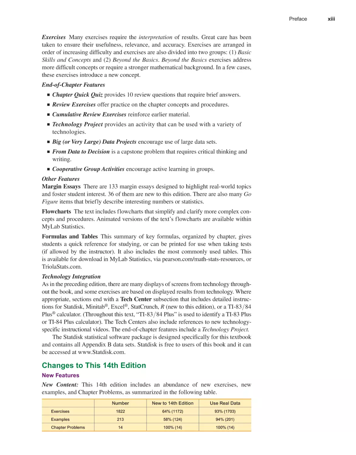
New Content: This 14th edition includes an abundance of new exercises, new
examples, and Chapter Problems, as summarized in the following table.
Number
New to 14th Edition
Use Real Data
Exercises
1822
64% (1172)
93% (1703)
Examples
213
58% (124)
94% (201)
Chapter Problems
14
100% (14)
100% (14)
xiii
xiv
Preface
New Data Sets: This book includes a rich data set library in Appendix B so that professors and students have ready access to real and interesting data. Appendix B has
been expanded from 32 data sets to 46 data sets. Twenty of those data sets are new,
including Internet Traffic, Queues, Car Data, Commute Times, Candies, Taxis, and
Disney World Wait Times.
Larger Data Sets: The largest data set in the previous edition had 600 cases. The data
set library in this 14th edition includes data sets with 6068, 3982, 5755, 8959, and
1000 cases. In addition, there are big data sets with 465,506 cases and 31,784 cases.
Working with such larger data sets is essential to students progressing into the age of
big data and data science.
New Types of Exercises: To foster the development of critical thinking, the Cumulative Review Exercises near the end of Chapters 9, 10, and 11 consist of open-ended
questions in which students are presented with a data set, and they are asked to pose
a key question relevant to the data, identify a procedure for addressing that question,
then analyze the data to form a conclusion.
New Margin Essays: This 14th edition of Elementary Statistics includes 36 new margin essays.
Big (or Very Large) Data Projects: New to this edition, these projects are located near
the end of each chapter and ask students to think critically while using large data sets.
New Chapter Problem Icon: Examples that relate to the Chapter Problem are now
highlighted with this icon CP to show how different statistical concepts and procedures can be applied to the real-world issue highlighted in the chapter.
Organization Changes
New Technology: The previous edition of Elementary Statistics introduced the
resampling method of bootstrapping in Section 7-4. This 14th edition of Elementary Statistics includes these methods of resampling using bootstrapping and
randomization:
Bootstrap One Proportion
Bootstrap Two Proportions
Bootstrap One Mean
Bootstrap Two Means
Bootstrap Matched Pairs
------------------------------------------Randomization One Proportion
Randomization Two Proportions
Randomization One Mean
Randomization Two Means
Randomization Matched Pairs
Randomization Correlation
New Section 4-5: Simulations for Hypothesis Tests
New Resampling Methods: Resampling methods are new to Sections 8-2, 8-3, 8-4,
8-5, 9-5, and 10-1.
New Section 8-5: Resampling: Using Technology for Hypothesis Testing
New Section 9-5: Resampling: Using Technology for Inferences
New Subsection 10-1, Part 3: Randomization Test ( for Correlation)
New Chapter 15: Holistic Statistics
Preface
Removed Section: The content of Section 6-6 (Normal as Approximation to Binomial)
has been removed from the text and is now available for download (MyLab Statistics,
pearson.com/math-stats-resources, or TriolaStats.com).
Removed Section: Ethics in Statistics has been moved from Chapter 15 to Section 1-4,
and is available for download (MyLab Statistics, pearson.com/math-stats-resources,
or TriolaStats.com).
Technology Changes
New to Statdisk: The previous version of Statdisk for Elementary Statistics included
bootstrap resampling, but the new version of Statdisk for the 14th edition also
includes all of the bootstrapping and randomization methods listed above under
“New Technology.”
Statdisk Online: Statdisk is now a browser-based program that can be used on any
device with a modern web browser, including laptops (Windows, macOS), Chromebooks, tablets and smartphones. Statdisk Online includes all of the statistical functions
from earlier versions of Statdisk and is continually adding new functions and features.
New Technology: Where it is appropriate, the end-of-section Tech Centers include
R as an additional technology. (The technologies of Statdisk, Excel, StatCrunch,
Minitab, and TI-83>84 Plus calculators continue to be included in the Tech Centers.)
Flexible Syllabus
This book’s organization reflects the preferences of most statistics instructors, but
there are two common variations:
■■
■■
Early Coverage of Correlation and Regression: Some instructors prefer to
cover the basics of correlation and regression early in the course. Section 2-4
includes basic concepts of scatterplots, correlation, and regression without the
use of formulas and greater depth found in Sections 10-1 (Correlation) and
10-2 (Regression).
Minimum Probability: Some instructors prefer extensive coverage of probability,
while others prefer to include only basic concepts. Instructors preferring minimum coverage can include Section 4-1 while skipping the remaining sections of
Chapter 4, as they are not essential for the chapters that follow. Many instructors
prefer to cover the fundamentals of probability along with the basics of the addition rule and multiplication rule (Section 4-2).
GAISE This book reflects recommendations from the American Statistical As-
sociation and its Guidelines for Assessment and Instruction in Statistics Education
(GAISE). Those guidelines suggest the following objectives and strategies.
1. Emphasize statistical literacy and develop statistical thinking: Each section
exercise set begins with Statistical Literacy and Critical Thinking exercises.
Many of the book’s exercises are designed to encourage statistical thinking
rather than the blind use of mechanical procedures.
2. Use real data: 94% of the examples and 93% of the exercises use real data.
3. Stress conceptual understanding rather than mere knowledge of procedures:
Instead of seeking simple numerical answers, most exercises and examples involve
conceptual understanding through questions that encourage practical interpretations of results. Also, each chapter includes a From Data to Decision project.
4. Foster active learning in the classroom: Each chapter ends with several
Cooperative Group Activities.
xv
xvi
Preface
5. Use technology for developing conceptual understanding and analyzing data:
Computer software displays are included throughout the book. Special Tech
Center subsections include instruction for using the software. Each chapter
includes a Technology Project. When there are discrepancies between answers
based on tables and answers based on technology, Appendix D provides both
answers. The website www.TriolaStats.com includes free text-specific software
(Statdisk), data sets formatted for several different technologies, and instructional videos for technologies. MyLab Statistics also includes support videos
for different statistical software applications.
6. Use assessments to improve and evaluate student learning: Assessment tools
include an abundance of section exercises, Chapter Quick Quizzes, Chapter
Review Exercises, Cumulative Review Exercises, Technology Projects, Big (or
Very Large) Data Projects, From Data to Decision projects, and Cooperative
Group Activities.
Acknowledgments
I would like to thank the thousands of statistics professors and students who have contributed to the success of this book. I thank the reviewers for their suggestions for this
fourteenth edition: Mary Kay Abbey, Vance Granville Community College; Kristin
Cook, College of Western Idaho; Celia Cruz, Lehman College of CUNY; Don Davis, Lakeland Community College; Jean Ellefson, Alfred University; Matthew Harris,
Ozarks Tech Community College; Stephen Krizan, Sait Polytechnic; Adam Littig, Los
Angeles Valley College; Dr. Rick Silvey, University of Saint Mary – Leavenworth;
Sasha Verkhovtseva, Anoka Ramsey Community College; William Wade, Seminole
Community College. Special thanks to Laura Iossi of Broward College for her contributions to the Triola Statistics Series.
Other recent reviewers have included Raid W. Amin, University of West Florida; Robert Black, United States Air Force Academy; James Bryan, Merced College;
Donald Burd, Monroe College; Keith Carroll, Benedictine University; Monte Cheney,
Central Oregon Community College; Christopher Donnelly, Macomb Community
College; Billy Edwards, University of Tennessee—Chattanooga; Marcos Enriquez,
Moorpark College; Angela Everett, Chattanooga State Technical Community College; Joe Franko, Mount San Antonio College; Rob Fusco, Broward College; Sanford
Geraci, Broward College; Eric Gorenstein, Bunker Hill Community College; Rhonda
Hatcher, Texas Christian University; Laura Heath, Palm Beach State College; Richard Herbst, Montgomery County Community College; Richard Hertz; Diane Hollister,
Reading Area Community College; Michael Huber, George Jahn, Palm Beach State
College; Gary King, Ozarks Technical Community College; Kate Kozak, Coconino
Community College; Dan Kumpf, Ventura College; Ladorian Latin, Franklin University; Mickey Levendusky, Pima County Community College; Mitch Levy, Broward
College; Tristan Londre, Blue River Community College; Alma Lopez, South Plains
College; Kim McHale, Heartland Community College; Carla Monticelli, Camden
County Community College; Ken Mulzet, Florida State College at Jacksonville; Julia
Norton, California State University Hayward; Michael Oriolo, Herkimer Community
College; Jeanne Osborne, Middlesex Community College; Joseph Pick, Palm Beach
State College; Ali Saadat, University of California—Riverside; Radha Sankaran, Passaic County Community College; Steve Schwager, Cornell University; Pradipta Seal,
Boston University; Kelly Smitch, Brevard College; Sandra Spain, Thomas Nelson
Community College; Ellen G. Stutes, Louisiana State University, Eunice; Sharon Testone, Onondaga Community College; Chris Vertullo, Marist College; Dave Wallach,
University of Findlay; Cheng Wang, Nova Southeastern University; Barbara Ward,
Preface
Belmont University; Richard Weil, Brown College; Lisa Whitaker, Keiser University;
Gail Wiltse, St. John River Community College; Claire Wladis, Borough of Manhattan Community College; Rick Woodmansee, Sacramento City College; Yong Zeng,
University of Missouri at Kansas City; Jim Zimmer, Chattanooga State Technical
Community College; Cathleen Zucco-Teveloff, Rowan University; Mark Z. Zuiker,
Minnesota State University, Mankato.
This fourteenth edition of Elementary Statistics is truly a team effort, and I consider myself fortunate to work with the dedication and commitment of the Pearson
team. I thank Suzy Bainbridge, Amanda Brands, Deirdre Lynch, Peggy McMahon,
Vicki Dreyfus, Jean Choe, Robert Carroll, Joe Vetere, and Rose Kernan of RPK Editorial Services.
I thank the following for their help in checking the accuracy of text and answers
in this 14th edition: Paul Lorczak, and Dirk Tempelaar.
I extend special thanks to Marc Triola, M.D., New York University School of
Medicine, for his outstanding work on creating the new Statdisk Online software.
I thank Scott Triola for his very extensive help throughout the entire production
process for this 14th edition.
M.F.T.
Madison, Connecticut
September 2020
xvii
Resources for Success
MyLab Statistics is available to accompany Pearson’s market-leading
text options, including Elementary Statistics, 14e by Mario F. Triola
(access code required).
MyLab™ is the teaching and learning platform that empowers you to reach every student.
MyLab Statistics combines trusted author content—including full eText and assessment
with immediate feedback—with digital tools and a flexible platform to personalize the
learning experience and improve results for each student. Integrated with StatCrunch®,
Pearson’s web-based statistical software program, students learn the skills they need to
interact with data in the real world.
Expanded objective-based exercise
coverage - Exercises in MyLab
Statistics are designed to reinforce and
support students’ understanding of key
statistical topics.
Enhanced video program to meet Introductory
Statistics needs:
• New! Animated Flow Charts - Animated flow
charts have been updated with a modern,
interactive interface with assignable auto-graded
assessment questions in MyLab Statistics.
• New! Tech-Specific Video Tutorials - These short,
topical videos show how to use common statistical
software to complete exercises.
• Updated! Chapter Review Exercise Videos - Watch
the Chapter Review Exercises come to life with new
review videos that help students understand key
chapter concepts.
Real-World Data Examples - Help
students understand how statistics
applies to everyday life through the
extensive current, real-world data
examples and exercises provided
throughout the text. MyLab Statistics
allows students to easily launch data
sets from their exercises to analyze
real-world data.
pearson.com/mylab/statistics
xviii
Resources for Success
Supplements
Student Resources
Student’s Solutions Manual, by James Lapp (Colorado Mesa University), provides detailed, worked-out
solutions to all odd-numbered text exercises. Available
for download in MyLab Statistics.
Student Workbook for the Triola Statistics Series,
by Laura Iossi (Broward College) offers additional examples, concept exercises, and vocabulary exercises
for each chapter. Available for download in MyLab Statistics. Can also be purchased separately.
ISBN: 0137363435 | 9780137363438
The following technology manuals include instructions, examples from the main text, and interpretations
to complement those given in the text. They are all
available for download in MyLab Statistics.
Excel Student Laboratory Manual and Workbook,
(Download Only) by Laurel Chiappetta (University of
Pittsburgh).
Graphing Calculator Manual for the TI-83 Plus,
TI-84 Plus, TI-84 Plus C and TI-84 Plus CE, (Download Only) by Kathleen McLaughlin (University of
Connecticut) & Dorothy Wakefield (University of Connecticut Health Center).
Statdisk Student Laboratory Manual and Workbook (Download Only), by Mario F. Triola. Available at
www.TriolaStats.com or within MyLab Statistics.
Instructor Resources
Annotated Instructor’s Edition, by Mario F. Triola,
contains answers to exercises in the margin, plus recommended assignments, and teaching suggestions.
(ISBN-13: 9780136803065; ISBN-10: 0136803067)
Instructor’s Solutions Manual (Download Only),
by James Lapp (Colorado Mesa University), contains
solutions to all the exercises. These files are available
to qualified instructors through Pearson Education’s
online catalog at www.pearsonhighered.com/irc or
within MyLab Statistics.
Insider’s Guide to Teaching with the Triola Statistics Series, (Download Only) by Mario F. Triola, contains sample syllabi and tips for incorporating projects,
as well as lesson overviews, extra examples, minimum
outcome objectives, and recommended assignments
for each chapter.
TestGen® Computerized Test Bank (www.pearsoned.
com/testgen), enables instructors to build, edit, print,
and administer tests using a computerized bank of
questions developed to cover all the objectives of
the text. TestGen is algorithmically based, allowing
instructors to create multiple but equivalent versions
of the same question or test with the click of a button. Instructors can also modify test bank questions
or add new questions. The software and testbank are
available for download from Pearson Education’s online catalog at www.pearsonhighered.com. Test Forms
(Download Only) are also available from the online
catalog.
PowerPoint® Lecture Slides: These files are available
to instructors through Pearson’s online catalog at www.
pearsonhighered.com/irc or within MyLab Statistics.
Accessibility—Pearson works continuously to ensure
our products are as accessible as possible to all students. Currently we work toward achieving WCAG 2.0
AA for our existing products (2.1 AA for future products) and Section 508 standards, as expressed in the
Pearson Guidelines for Accessible Educational Web
Media.
pearson.com/mylab/statistics
xix
GetMost
the Out
MostofOut of
Get the
MyLab
Statistics
MyStatLab
®
MyLab™ is the teaching and learning platform that empowers you to reach every
student. MyLab Statistics combines trusted author content — including full eText
and assessment with immediate feedback — with digital tools and a flexible
platform to personalize the learning experience and improve results for each
student. Integrated with StatCrunch®, Pearson’s web-based statistical software
program, students learn the skills they need to interact with data in the real world.
Integrated Review
Integrated Review in MyLab Statistics provides embedded and personalized review
of prerequisite topics within relevant chapters.
• S
tudents begin each chapter with a premade, assignable Skills Check assignment to check each student’s understanding of prerequisite skills needed to be
successful in that chapter.
• F
or any gaps in skill that are identified, a personalized review homework is populated. Students practice on the topics they need to focus on-no more, no less.
• A
suite of resources are available to help students understand the objectives
they missed on the Skills Check quiz, including worksheets and videos to help
remediate.
Integrated Review in the MyLab is ideal for corequisite courses, where students are
enrolled in a statistics course while receiving just-in-time remediation. But it can also
be used simply to get underprepared students up to speed on prerequisite skills in
order to be more successful in the Statistics content.
Used by nearly one million students a year, MyLab Statistics is the world’s leading
online program for teaching and learning statistics.
pearson.com/mylab/statistics
xx
1-1 Statistical and Critical
Thinking
1-2 Types of Data
1-3 Collecting Sample
Data
1-4 Ethics in Statistics
(available at
www.TriolaStats.com)
1
INTRODUCTION TO STATISTICS
CHAPTER
PROBLEM
Is YouTube Becoming a More Important Learning Tool?
Surveys provide data that enable us to better understand the
other topics, this survey asked respondents to identify their
world in which we live and identify changes in the opinions,
preferred learning tools, and YouTube was identified as one
habits, and behaviors of others. Survey data guide public
of the top tools by both Gen-Z and millennials. Figure 1-1 in-
policy, influence business and educational practices, and
cludes a graph that depicts the percentage of Gen-Z and mil-
affect many aspects of our daily lives. A recent Pearson survey,
lennials who identified YouTube as a preferred learning tool.
conducted by The Harris Poll, examined how technology has
Critical Thinking Figure 1-1 on the next page makes it ap-
shaped students’ learning habits and compared the responses
pear that Gen-Z is more than twice as likely to prefer YouTube as
from Gen-Z (ages 14–23) and millennials (ages 24–40). Among
a learning tool compared to millennials. A quick glance might also
1
2
CHAPTER 1 Introduction to Statistics
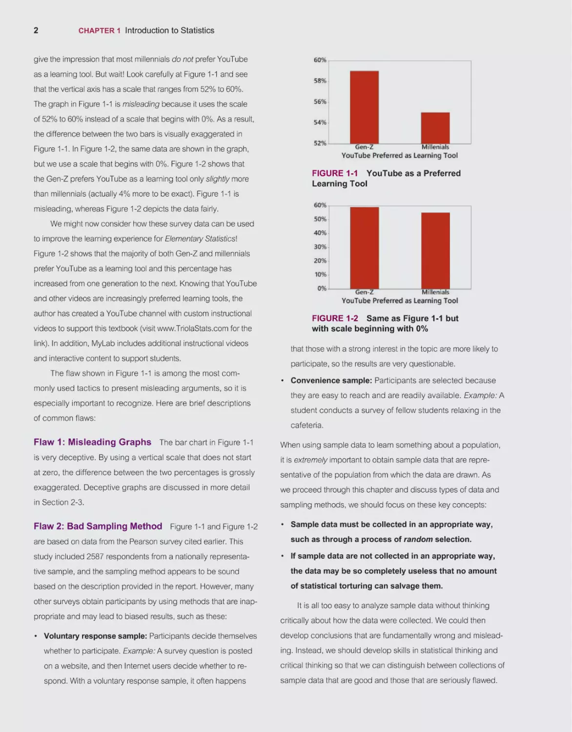
give the impression that most millennials do not prefer YouTube
as a learning tool. But wait! Look carefully at Figure 1-1 and see
that the vertical axis has a scale that ranges from 52% to 60%.
The graph in Figure 1-1 is misleading because it uses the scale
of 52% to 60% instead of a scale that begins with 0%. As a result,
the difference between the two bars is visually exaggerated in
Figure 1-1. In Figure 1-2, the same data are shown in the graph,
but we use a scale that begins with 0%. Figure 1-2 shows that
the Gen-Z prefers YouTube as a learning tool only slightly more
than millennials (actually 4% more to be exact). Figure 1-1 is
FIGURE 1-1 YouTube as a Preferred
Learning Tool
misleading, whereas Figure 1-2 depicts the data fairly.
We might now consider how these survey data can be used
to improve the learning experience for Elementary Statistics!
Figure 1-2 shows that the majority of both Gen-Z and millennials
prefer YouTube as a learning tool and this percentage has
increased from one generation to the next. Knowing that YouTube
and other videos are increasingly preferred learning tools, the
author has created a YouTube channel with custom instructional
videos to support this textbook (visit www.TriolaStats.com for the
link). In addition, MyLab includes additional instructional videos
and interactive content to support students.
The flaw shown in Figure 1-1 is among the most commonly used tactics to present misleading arguments, so it is
especially important to recognize. Here are brief descriptions
of common flaws:
FIGURE 1-2 Same as Figure 1-1 but
with scale beginning with 0%
that those with a strong interest in the topic are more likely to
participate, so the results are very questionable.
• Convenience sample: Participants are selected because
they are easy to reach and are readily available. Example: A
student conducts a survey of fellow students relaxing in the
cafeteria.
Flaw 1: Misleading Graphs The bar chart in Figure 1-1
When using sample data to learn something about a population,
is very deceptive. By using a vertical scale that does not start
it is extremely important to obtain sample data that are repre-
at zero, the difference between the two percentages is grossly
sentative of the population from which the data are drawn. As
exaggerated. Deceptive graphs are discussed in more detail
we proceed through this chapter and discuss types of data and
in Section 2-3.
sampling methods, we should focus on these key concepts:
Flaw 2: Bad Sampling Method Figure 1-1 and Figure 1-2
• Sample data must be collected in an appropriate way,
are based on data from the Pearson survey cited earlier. This
study included 2587 respondents from a nationally representa-
such as through a process of random selection.
• If sample data are not collected in an appropriate way,
tive sample, and the sampling method appears to be sound
the data may be so completely useless that no amount
based on the description provided in the report. However, many
of statistical torturing can salvage them.
other surveys obtain participants by using methods that are inappropriate and may lead to biased results, such as these:
• Voluntary response sample: Participants decide themselves
It is all too easy to analyze sample data without thinking
critically about how the data were collected. We could then
develop conclusions that are fundamentally wrong and mislead-
whether to participate. Example: A survey question is posted
ing. Instead, we should develop skills in statistical thinking and
on a website, and then Internet users decide whether to re-
critical thinking so that we can distinguish between collections of
spond. With a voluntary response sample, it often happens
sample data that are good and those that are seriously flawed.
1-1 Statistical and Critical Thinking
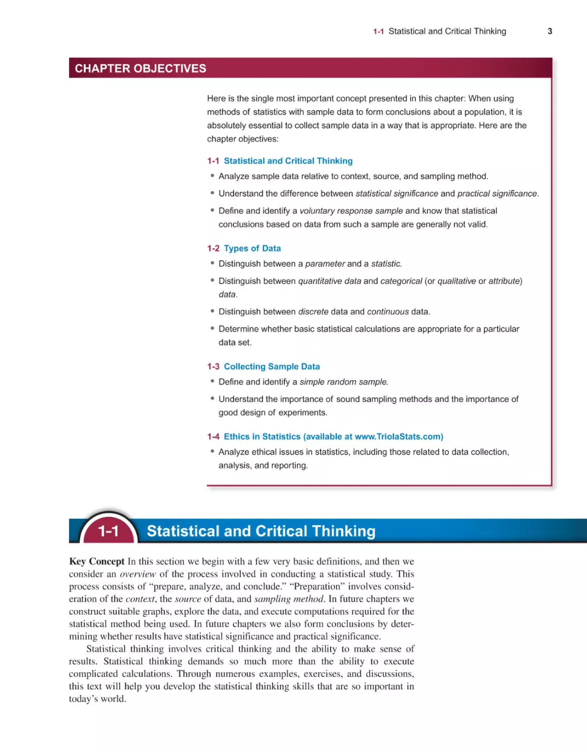
CHAPTER OBJECTIVES
Here is the single most important concept presented in this chapter: When using
methods of statistics with sample data to form conclusions about a population, it is
absolutely essential to collect sample data in a way that is appropriate. Here are the
chapter objectives:
1-1 Statistical and Critical Thinking
• Analyze sample data relative to context, source, and sampling method.
• Understand the difference between statistical significance and practical significance.
• Define and identify a voluntary response sample and know that statistical
conclusions based on data from such a sample are generally not valid.
1-2 Types of Data
• Distinguish between a parameter and a statistic.
• Distinguish between quantitative data and categorical (or qualitative or attribute)
data.
• Distinguish between discrete data and continuous data.
• Determine whether basic statistical calculations are appropriate for a particular
data set.
1-3 Collecting Sample Data
• Define and identify a simple random sample.
• Understand the importance of sound sampling methods and the importance of
good design of experiments.
1-4 Ethics in Statistics (available at www.TriolaStats.com)
• Analyze ethical issues in statistics, including those related to data collection,
analysis, and reporting.
1-1
Statistical and Critical Thinking
Key Concept In this section we begin with a few very basic definitions, and then we
consider an overview of the process involved in conducting a statistical study. This
process consists of “prepare, analyze, and conclude.” “Preparation” involves consideration of the context, the source of data, and sampling method. In future chapters we
construct suitable graphs, explore the data, and execute computations required for the
statistical method being used. In future chapters we also form conclusions by determining whether results have statistical significance and practical significance.
Statistical thinking involves critical thinking and the ability to make sense of
results. Statistical thinking demands so much more than the ability to execute
complicated calculations. Through numerous examples, exercises, and discussions,
this text will help you develop the statistical thinking skills that are so important in
today’s world.
3
4
CHAPTER 1 Introduction to Statistics
Importance of Accurate
Census Results
The United
States Constitu
tion requires a
census every
ten years. Some
factors affected
by census re
sults: Apportionment of congres
sional seats; distribution of bil
lions of dollars of federal funds to
states for transportation, schools,
and hospitals; locations of sites
for businesses and stores.
Although accuracy of census re
sults is extremely important, it is
becoming more difficult to collect
accurate census data due to the
growing diversity of cultures and
languages and increased distrust
of the government. No amount
of statistical analysis can salvage
poor data, so it is critical that the
census data is collected in an
appropriate manner.
We begin with some very basic definitions.
DEFINITIONS
Data are collections of observations, such as measurements, genders, or survey
responses. (A single data value is called a datum, a term rarely used. The term
“data” is plural, so it is correct to say “data are . . .” not “data is . . .”)
Statistics is the science of planning studies and experiments; obtaining data; and
organizing, summarizing, presenting, analyzing, and interpreting those data and
then drawing conclusions based on them.
A population is the complete collection of all measurements or data that are being
considered.
A census is the collection of data from every member of the population.
A sample is a subcollection of members selected from a population.
Because populations are often very large, a common objective of the use of statistics is to obtain data from a sample and then use those data to form a conclusion about
the population.
EXAMPLE 1
Watch What You Post Online
In a survey of 410 human resource professionals, 148 of them said that job candidates were disqualified because of information found on social media postings
(based on data from The Society for Human Resource Management). In this case,
the population and sample are as follows:
Population: All human resource professionals
Sample: The 410 human resource professionals who were surveyed
The objective is to use the sample as a basis for drawing a conclusion about the
population of all human resource professionals, and methods of statistics are helpful
in drawing such conclusions.
YOUR TURN. Do part (a) of Exercise 2 “Reported Versus Measured.”
We now proceed to consider the process involved in a statistical study. See
Figure 1-3 for a summary of this process and note that the focus is on critical thinking,
not mathematical calculations. Thanks to wonderful developments in technology, we
have powerful tools that effectively do the number crunching so that we can focus on
understanding and interpreting results.
Prepare
Go Figure
78%: The percentage of female
veterinarian students who are
women, according to The Herald
in Glasgow, Scotland.
Context Figure 1-3 suggests that we begin our preparation by considering the context of the data, so let’s start with context by considering the data in Table 1-1.
Table 1-1 includes shoe print lengths and heights of eight males. Forensic scientists measure shoe print lengths at burglary scenes and other crime scenes in order
to estimate the height of the criminal. The format of Table 1-1 suggests the following goal: Determine whether there is a relationship between shoe print lengths
1-1 Statistical and Critical Thinking
and heights of males. This goal suggests a reasonable hypothesis: Males with larger
shoe print lengths tend to be taller. (We are using data for males only because 84%
of burglaries are committed by males.)
TABLE 1-1 Shoe Print Lengths and Heights of Men
Shoe Print (cm)
27.6
29.7
29.7
31.0
31.3
31.4
31.8
34.5
Height (cm)
172.7
175.3
177.8
175.3
180.3
182.3
177.8
193.7
Source of the Data The second step in our preparation is to consider the source
(as indicated in Figure 1-3). The data in Table 1-1 are from Data Set 9 “Foot and
Height” in Appendix B, where the source is identified. The source certainly appears
to be reputable.
Sampling Method Figure 1-3 suggests that we conclude our preparation by considering the sampling method. For the data in Table 1-1, individuals were randomly
selected, so the sampling method appears to be sound.
Sampling methods and the use of random selection will be discussed in
Section 1-3, but for now, we stress that a sound sampling method is absolutely
essential for good results in a statistical study. It is generally a bad practice to use
voluntary response (or self-selected) samples, even though their use is common.
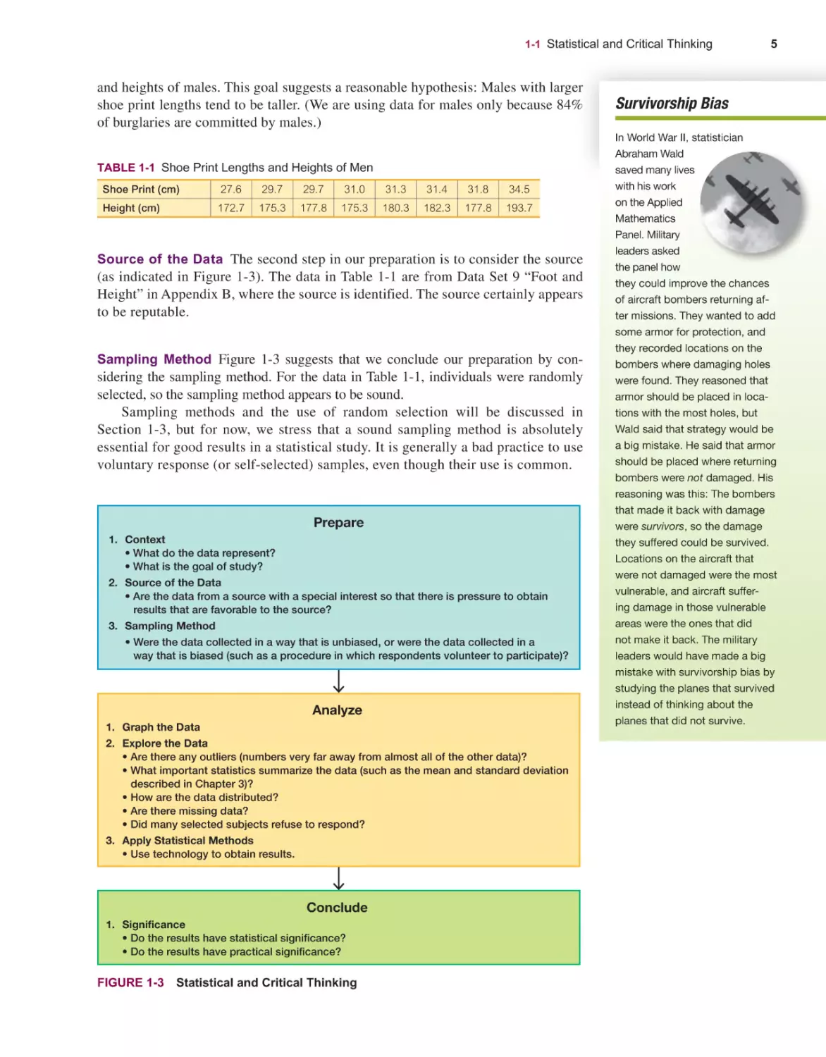
Prepare
1. Context
• What do the data represent?
• What is the goal of study?
2. Source of the Data
• Are the data from a source with a special interest so that there is pressure to obtain
results that are favorable to the source?
3. Sampling Method
• Were the data collected in a way that is unbiased, or were the data collected in a
way that is biased (such as a procedure in which respondents volunteer to participate)?
Analyze
1. Graph the Data
2. Explore the Data
• Are there any outliers (numbers very far away from almost all of the other data)?
• What important statistics summarize the data (such as the mean and standard deviation
described in Chapter 3)?
• How are the data distributed?
• Are there missing data?
• Did many selected subjects refuse to respond?
3. Apply Statistical Methods
• Use technology to obtain results.
Conclude
1. Significance
• Do the results have statistical significance?
• Do the results have practical significance?
FIGURE 1-3
Statistical and Critical Thinking
5
Survivorship Bias
In World War II, statistician
Abraham Wald
saved many lives
with his work
on the Applied
Mathematics
Panel. Military
leaders asked
the panel how
they could improve the chances
of aircraft bombers returning af
ter missions. They wanted to add
some armor for protection, and
they recorded locations on the
bombers where damaging holes
were found. They reasoned that
armor should be placed in loca
tions with the most holes, but
Wald said that strategy would be
a big mistake. He said that armor
should be placed where returning
bombers were not damaged. His
reasoning was this: The bombers
that made it back with damage
were survivors, so the damage
they suffered could be survived.
Locations on the aircraft that
were not damaged were the most
vulnerable, and aircraft suffer
ing damage in those vulnerable
areas were the ones that did
not make it back. The military
leaders would have made a big
mistake with survivorship bias by
studying the planes that survived
instead of thinking about the
planes that did not survive.
6
CHAPTER 1 Introduction to Statistics
Go Figure
17%: The percentage of U.S.
men between 20 and 40 years
of age and taller than 7 feet who
play basketball in the NBA.
Origin of “Statistics”
The word
statistics is
derived from
the Latin word
status (mean
ing “state”).
Early uses of
statistics involved compilations
of data and graphs describing
various aspects of a state or
country. In 1662, John Graunt
published statistical information
about births and deaths. Graunt’s
work was followed by studies
of mortality and disease rates,
population sizes, incomes, and
unemployment rates. House
holds, governments, and busi
nesses rely heavily on statistical
data for guidance. For example,
unemployment rates, inflation
rates, consumer indexes, and
birth and death rates are carefully
compiled on a regular basis,
and the resulting data are used
by business leaders to make
decisions affecting future hiring,
production levels, and expansion
into new markets.
DEFINITION
A voluntary response sample (or self-selected sample) is one in which the
respondents themselves decide whether to be included.
The following types of polls are common examples of voluntary response
samples. By their very nature, all are seriously flawed because we should not
make conclusions about a population on the basis of samples with a strong possibility of bias.
■■
Internet polls, in which people online decide whether to respond
■■
Mail-in polls, in which people decide whether to reply
■■
Telephone call-in polls, in which newspaper, radio, or television announcements
ask that you voluntarily call a special number to register your opinion
See the following Example 2.
EXAMPLE 2
Voluntary Response Sample
The ABC television show Nightline asked viewers to call with their opinion about
whether the United Nations headquarters should remain in the United States.
Viewers then decided themselves whether to call with their opinions, and 67%
of 186,000 respondents said that the United Nations should be moved out of the
United States. In a separate and independent survey, 500 respondents were randomly selected and surveyed, and 38% of this group wanted the United Nations
to move out of the United States. The two polls produced dramatically different
results. Even though the Nightline poll involved 186,000 volunteer respondents, the
much smaller poll of 500 randomly selected respondents is more likely to provide
better results because of the far superior sampling method.
YOUR TURN. Do Exercise 1 “Computer Virus.”
Analyze
Figure 1-3 indicates that after completing our preparation by considering the context,
source, and sampling method, we begin to analyze the data.
Graph and Explore An analysis should begin with appropriate graphs and explora-
tions of the data. Graphs are discussed in Chapter 2, and important statistics are discussed in Chapter 3.
Apply Statistical Methods Later chapters describe important statistical methods,
but application of these methods is often made easy with technology (calculators
and>or statistical software packages). A good statistical analysis does not require
strong computational skills. A good statistical analysis does require using common
sense and paying careful attention to sound statistical methods.
Conclude
Figure 1-3 shows that the final step in our statistical process involves conclusions, and
we should develop an ability to distinguish between statistical significance and practical significance.
1-1 Statistical and Critical Thinking
Statistical Significance Statistical significance is achieved in a study when we
get a result that is very unlikely to occur by chance. A common criterion has been this:
We have statistical significance if the likelihood of an event occurring by chance is 5%
or less.
■■
■■
Getting 98 girls in 100 random births is statistically significant because such an
extreme outcome is not likely to result from random chance.
Getting 52 girls in 100 births is not statistically significant because that event
could easily occur with random chance.
CAUTION An outcome can be statistically significant, and it may or may not be
important. Don’t associate statistical significance with importance.
Practical Significance It is possible that some treatment or finding is effective, but
common sense might suggest that the treatment or finding does not make enough of a
difference to justify its use or to be practical, as illustrated in Example 3.
EXAMPLE 3
Statistical Significance Versus Practical Significance
In a trial of weight loss programs, 21 subjects on the Atkins program lost an average
(mean) of 2.1 kg (or 4.6 lb) after one year (based on data from “Comparison of the
Atkins, Ornish, Weight Watchers, and Zone Diets for Weight Loss and Heart Disease Reduction,” by Dansinger et al., Journal of the American Medical Association,
Volume 93, Number 1). The results show that this loss is statistically significant and
is not likely to occur by chance. However, many dieters believe that after following
this diet for a year, a loss of only 2.1 kg is not worth the time, cost, and effort so
that for these people, this diet does not have practical significance.
YOUR TURN. Do Exercise 13 “Diet and Exercise Program.”
Example 3 includes a small sample of only 21 subjects, but with very large data
sets (e.g., “big data”), statistically significant differences can often be found with very
small differences. We should be careful to avoid the mistake of thinking that those
small differences have practical significance.
Analyzing Data: Potential Pitfalls
Here are a few more items that could cause problems when analyzing data.
Misleading Conclusions When forming a conclusion based on a statistical analysis,
we should make statements that are clear even to those who have no understanding of
statistics and its terminology. We should carefully avoid making statements not justified by the statistical analysis. For example, later in this book we introduce the concept
of a correlation, or association between two variables, such as shoe print lengths and
heights of males. A statistical analysis might justify the statement that there is a correlation between shoe print length and height, but it would not justify a statement that an
increase in the shoe print length causes an increase in height. Such a statement about
causality can be justified by physical evidence, not by statistical analysis.
Correlation does not imply causation.
Sample Data Reported Instead of Measured When collecting data from people,
it is better to take measurements yourself instead of asking subjects to report results.
Ask people what they weigh and you are likely to get their desired weights, not their
7
Publication Bias
There is a “publication bias” in
professional journals. It is the ten
dency to publish
positive results
(such as show
ing that some
treatment is
effective) much
more often than
negative results
(such as showing that some
treatment has no effect).
In the article “Registering Clinical
Trials” (Journal of the American
Medical Association, Vol. 290,
No. 4), authors Kay Dickersin
and Drummond Rennie state
that “the result of not knowing
who has performed what (clinical
trial) is loss and distortion of the
evidence, waste and duplica
tion of trials, inability of funding
agencies to plan, and a chaotic
system from which only certain
sponsors might benefit, and is
invariably against the interest
of those who offered to partici
pate in trials and of patients in
general.” They support a process
in which all clinical trials are
registered in one central system,
so that future researchers have
access to all previous studies,
not just the studies that were
published.
8
CHAPTER 1 Introduction to Statistics
Statistician Jobs
In a recent year,
U.S. News and
World Report
provided a list
of the top 10
best jobs. Here
are the first two
jobs at the top of the list: (1) Soft
ware developer; (2) Statistician.
It was noted that one reason
for this high ranking is that the
unemployment rate for statisti
cians is only 0.9 percent. That
unemployment rate is lower than
1 person in 100. Not to mention
how cool the contemporary disci
pline of statistics has become!
actual weights. People tend to round, usually down, sometimes way down. When
asked, someone with a weight of 187 lb might respond that he or she weighs 160 lb.
Accurate weights are collected by using a scale to measure weights, not by asking
people what they weigh.
Loaded Questions If survey questions are not worded carefully, the results of a
study can be misleading. Survey questions can be “loaded,” or intentionally worded
to elicit a desired response. Here are the actual rates of “yes” responses for the two
different wordings of a question:
97% yes: “Should the President have the line item veto to eliminate waste?”
57% yes: “Should the President have the line item veto, or not?”
Order of Questions Sometimes survey questions are unintentionally loaded by
such factors as the order of the items being considered. See the following two questions from a poll conducted in Germany, along with the very different response rates:
“Would you say that traffic contributes more or less to air pollution than industry?”
(45% blamed traffic; 27% blamed industry.)
“Would you say that industry contributes more or less to air pollution than traffic?”
(24% blamed traffic; 57% blamed industry.)
Go Figure
In addition to the order of items within a question, as illustrated above, the order of
separate questions could also affect responses.
Five out of four people have
some difficulty with statistics.
Nonresponse A nonresponse occurs when someone either refuses to respond to
a survey question or is unavailable. When people are asked survey questions, some
firmly refuse to answer. The refusal rate has been growing in recent years, partly because many persistent telemarketers try to sell goods or services by beginning with a
sales pitch that initially sounds as though it is part of an opinion poll. (This “selling
under the guise” of a poll is called sugging.) In Lies, Damn Lies, and Statistics, author
Michael Wheeler makes this very important observation:
People who refuse to talk to pollsters are likely to be different from those who
do not. Some may be fearful of strangers and others jealous of their privacy,
but their refusal to talk demonstrates that their view of the world around
them is markedly different from that of those people who will let poll-takers
into their homes.
Low Response Rates Related to the preceding item of nonresponses is the is-
sue of low response rates. If a survey has a low response rate, the reliability of the
results decreases. In addition to having a smaller sample size, there is an increased
likelihood of having a bias among those who do respond. Some steps to help prevent a low response rate: (1) A survey should present an engaging argument for
its importance; (2) a survey should not be very time consuming; (3) it is helpful to
provide a reward for completing a survey, such as cash or a chance to win a prize.
There are not definitive guidelines for acceptable response rates. A very good response rate is 80% or higher. Some suggest that response rates of at least 40% are
acceptable. Pew Research Center reports that its typical telephone surveys have
a response rate around 9%, but their surveys tend to be quite good. Sections 7-1,
7-2, and 7-3 include procedures for determining the sample size needed to estimate characteristics (proportion, mean, standard deviation) of a population, and
those methods require sound sampling methods.
1-1 Statistical and Critical Thinking
Percentages Some studies cite misleading or unclear percentages. Note that 100%
of some quantity is all of it, but if there are references made to percentages that exceed
100%, such references are often not justified. If an advertiser claims that your utility
costs can be reduced by 200%, that claim is misleading. Eliminating all utility costs
would be a reduction of 100%, and a reduction of 200% doesn’t make sense.
The following list identifies some key principles to apply when dealing with percentages. These principles all use the basic concept that % or “percent” really means
“divided by 100.” The first principle that follows is used often in this book.
Percentage of: To find a percentage of an amount, replace the % symbol with
division by 100, and then interpret “of” to be multiplication. This example shows
that 6% of 1200 is 72:
6, of 1200 responses =
6
* 1200 = 72
100
Decimal u Percentage: To convert from a decimal to a percentage, multiply by
100%. This example shows that 0.25 is equivalent to 25%:
0.25 S 0.25 * 100, = 25,
Fraction u Percentage: To convert from a fraction to a percentage, divide
the denominator into the numerator to get an equivalent decimal number; then
multiply by 100%. This example shows that the fraction 3>4 is equivalent to 75%:
3
= 0.75 S 0.75 * 100, = 75,
4
Percentage u Decimal: To convert from a percentage to a decimal number,
replace the % symbol with division by 100. This example shows that 85% is
equivalent to 0.85:
85
85, =
= 0.85
100
1-1 Basic Skills and Concepts
Statistical Literacy and Critical Thinking
1. Computer Virus In an AOL survey of Internet users, this question was posted online:
“Have you ever been hit by a computer virus?” Among the 170,063 responses, 63% answered “yes.” What term is used to describe this type of survey in which the people surveyed consist of those who chose to respond? What is wrong with this type of sampling
method?
2. Reported Versus Measured In a survey of 1046 adults conducted by Bradley C
orporation,
subjects were asked how often they wash their hands when using a public restroom, and 70% of
the respondents said “always.”
a. Identify the sample and the population.
b. Why would better results be obtained by observing the hand washing instead of asking about it?
3. Statistical Significance Versus Practical Significance When testing a new treatment,
what is the difference between statistical significance and practical significance? Can a treatment have statistical significance, but not practical significance?
9
10
CHAPTER 1 Introduction to Statistics
4. Correlation One study showed that for a recent period of 10 years, there was a strong correlation (or association) between the per capita consumption of margarine and the divorce rate
in Maine (based on data from National Vital Statistics reports and the U.S. Department of Agriculture). Does this imply that increasing margarine consumption is the cause of an increase in
the divorce rate in Maine? Why or why not?
In Exercises 5–8, determine whether the given source has the
potential to create a bias in a statistical study.
Consider the Source.
5. AAA The American Automobile Association (AAA) is a not-for-profit federation of motor
clubs that provides automotive and travel services. AAA conducts a survey of its members
about their use of public transportation versus private automobiles.
6. Body Data Data Set 1 “Body Data” in Appendix B includes pulse rates of subjects, and
those pulse rates were recorded by examiners as part of a study conducted by the National
Center for Health Statistics.
7. Brain Size A data set in Appendix B includes brain volumes from 10 pairs of monozygotic
(identical) twins. The data were collected by researchers at Harvard University, Massachusetts
General Hospital, Dartmouth College, and the University of California at Davis.
8. Chocolate An article in Journal of Nutrition (Vol. 130, No. 8) noted that chocolate is rich
in flavonoids. The article notes “regular consumption of foods rich in flavonoids may reduce
the risk of coronary heart disease.” The study received funding from Mars, Inc., the candy company, and the Chocolate Manufacturers Association.
Sampling Method. In Exercises 9–12, determine whether the sampling method appears
to be sound or is flawed.
9. Nuclear Power Plants In a survey of 1368 subjects, the following question was posted
on the USA Today website: “In your view, are nuclear plants safe?” The survey subjects were
Internet users who chose to respond to the question posted on the electronic edition of USA
Today.
10. Clinical Trials Researchers at Yale University conduct a wide variety of clinical trials by
using subjects who volunteer after reading advertisements soliciting paid volunteers.
11. Sharing Passwords In a Password Boss survey of 2030 randomly selected adults, 39%
said that they never share passwords with anyone.
12. Social Media Usage In a survey of social media usage, the Pew Research Center randomly selected 2002 adults in the United States.
Statistical Significance and Practical Significance. In Exercises 13–20, determine
whether the results appear to have statistical significance, and also determine whether the
results appear to have practical significance.
13. Diet and Exercise Program In a study of the Ornish weight loss program, 40 subjects
lost a mean of 3.3 lb after 12 months (based on data from “Comparison of the Atkins, Ornish,
Weight Watchers, and Zone Diets for Weight Loss and Heart Disease Risk Reduction,” by Dansinger et al., Journal of the American Medical Association, Vol. 293, No. 1). Methods of statistics can be used to show that if this diet had no effect, the likelihood of getting these results is
roughly 3 chances in 1000.
14. Surgery versus Splints A study compared surgery and splinting for subjects suffering
from carpal tunnel syndrome. It was found that among 73 patients treated with surgery, there
was a 92% success rate. Among 83 patients treated with splints, there was a 72% success rate.
Calculations using those results showed that if there really is no difference in success rates between surgery and splints, then there is about one chance in a thousand of getting success rates
like the ones obtained in this study.
1-1 Statistical and Critical Thinking
15. Mendel’s Genetics Experiments One of Gregor Mendel’s famous hybridization experi-
ments with peas yielded 580 offspring with 152 of those peas (or 26%) having yellow pods.
According to Mendel’s theory, 25% of the offspring peas should have yellow pods.
16. IQ Scores Most people have IQ scores between 70 and 130. For $39.99, you can purchase
a PC or Mac program from HighIQPro that is claimed to increase your IQ score by 10 to 20
points. The program claims to be “the only proven IQ increasing software in the brain training market,” but the author of your text could find no substantial data supporting that claim, so
let’s suppose that these results were obtained: In a study of 12 subjects using the program, the
average increase in IQ score is 3 IQ points. There is a 25% chance of getting such results if the
program has no effect.
17. Election Fraud The County Clerk in Essex County, New Jersey, was responsible for ran-
domly assigning the order in which candidates’ names appeared on a recent election ballot.
Among 41 different ballots, a Democrat was placed on the first line 40 times, and a Republican
was placed on the first line once.
18. Football Overtime Games In “The Overtime Rule in the National Football League:
Fair or Unfair?” by Gorgievski et al., MathAMATYC Educator, Vol. 2, No. 1, the authors
report that among 414 football games won in overtime (prior to the overtime rule change
in 2012), 235 were won by the team that won the coin toss at the beginning of overtime.
If winning the coin toss does not provide an advantage, there is a 0.3% chance of getting
such results.
19. Bias in Jury Selection In the case of Casteneda v. Partida, it was found that during a
period of 11 years in Hidalgo County, Texas, 870 people were selected for grand jury duty, and
39% of them were Americans of Mexican ancestry. Among the people eligible for grand jury
duty, 79.1% were Americans of Mexican ancestry.
20. Misleading Survey Responses In one presidential election, voting records showed
that 61% of eligible voters actually did vote. In a survey of 1002 people, 70% said that
they voted in that election (based on data from ICR Research Group). If survey respondents
answered honestly and with accurate recall, there is about a 0.0000006% chance of getting
such results.
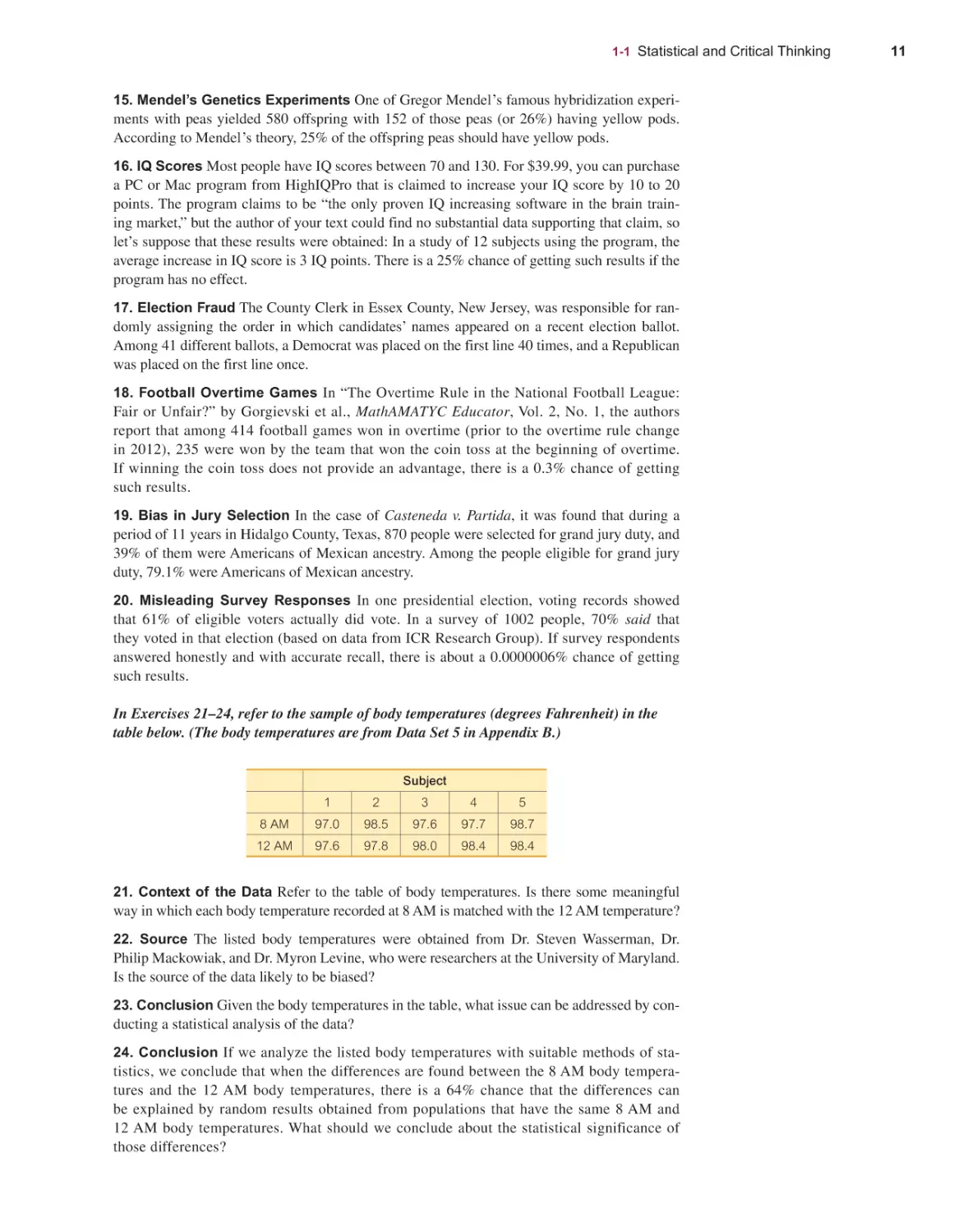
In Exercises 21–24, refer to the sample of body temperatures (degrees Fahrenheit) in the
table below. (The body temperatures are from Data Set 5 in Appendix B.)
Subject
1
2
3
4
5
8 AM
97.0
98.5
97.6
97.7
98.7
12 AM
97.6
97.8
98.0
98.4
98.4
21. Context of the Data Refer to the table of body temperatures. Is there some meaningful
way in which each body temperature recorded at 8 AM is matched with the 12 AM temperature?
22. Source The listed body temperatures were obtained from Dr. Steven Wasserman, Dr.
Philip Mackowiak, and Dr. Myron Levine, who were researchers at the University of Maryland.
Is the source of the data likely to be biased?
23. Conclusion Given the body temperatures in the table, what issue can be addressed by conducting a statistical analysis of the data?
24. Conclusion If we analyze the listed body temperatures with suitable methods of sta-
tistics, we conclude that when the differences are found between the 8 AM body temperatures and the 12 AM body temperatures, there is a 64% chance that the differences can
be explained by random results obtained from populations that have the same 8 AM and
12 AM body temperatures. What should we conclude about the statistical significance of
those differences?
11
12
CHAPTER 1 Introduction to Statistics
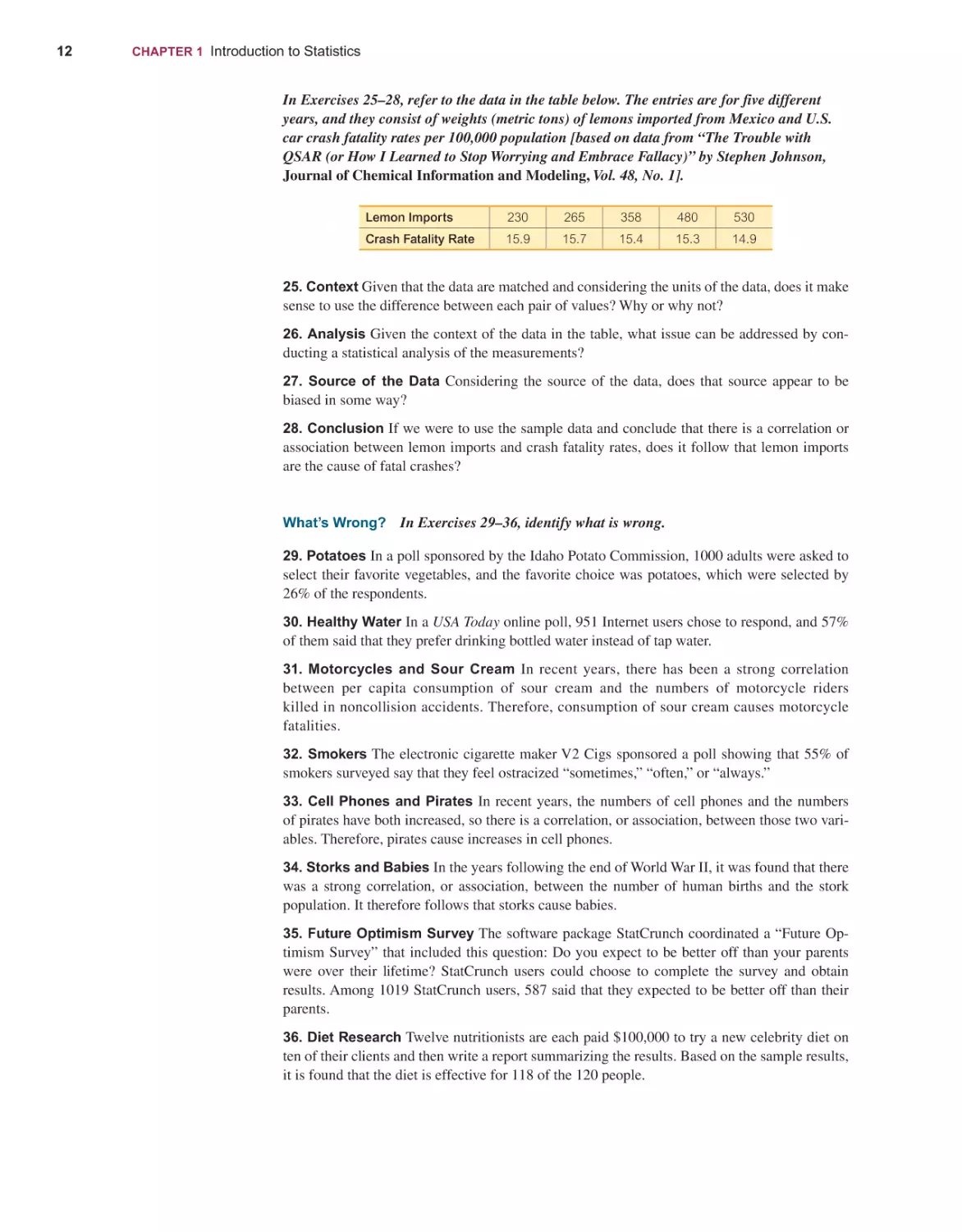
In Exercises 25–28, refer to the data in the table below. The entries are for five different
years, and they consist of weights (metric tons) of lemons imported from Mexico and U.S.
car crash fatality rates per 100,000 population [based on data from “The Trouble with
QSAR (or How I Learned to Stop Worrying and Embrace Fallacy)” by Stephen Johnson,
Journal of Chemical Information and Modeling, Vol. 48, No. 1].
Lemon Imports
230
265
358
480
530
Crash Fatality Rate
15.9
15.7
15.4
15.3
14.9
25. Context Given that the data are matched and considering the units of the data, does it make
sense to use the difference between each pair of values? Why or why not?
26. Analysis Given the context of the data in the table, what issue can be addressed by con-
ducting a statistical analysis of the measurements?
27. Source of the Data Considering the source of the data, does that source appear to be
biased in some way?
28. Conclusion If we were to use the sample data and conclude that there is a correlation or
association between lemon imports and crash fatality rates, does it follow that lemon imports
are the cause of fatal crashes?
What’s Wrong? In Exercises 29–36, identify what is wrong.
29. Potatoes In a poll sponsored by the Idaho Potato Commission, 1000 adults were asked to
select their favorite vegetables, and the favorite choice was potatoes, which were selected by
26% of the respondents.
30. Healthy Water In a USA Today online poll, 951 Internet users chose to respond, and 57%
of them said that they prefer drinking bottled water instead of tap water.
31. Motorcycles and Sour Cream In recent years, there has been a strong correlation
b etween per capita consumption of sour cream and the numbers of motorcycle riders
killed in noncollision accidents. Therefore, consumption of sour cream causes motorcycle
fatalities.
32. Smokers The electronic cigarette maker V2 Cigs sponsored a poll showing that 55% of
smokers surveyed say that they feel ostracized “sometimes,” “often,” or “always.”
33. Cell Phones and Pirates In recent years, the numbers of cell phones and the numbers
of pirates have both increased, so there is a correlation, or association, between those two variables. Therefore, pirates cause increases in cell phones.
34. Storks and Babies In the years following the end of World War II, it was found that there
was a strong correlation, or association, between the number of human births and the stork
population. It therefore follows that storks cause babies.
35. Future Optimism Survey The software package StatCrunch coordinated a “Future Optimism Survey” that included this question: Do you expect to be better off than your parents
were over their lifetime? StatCrunch users could choose to complete the survey and obtain
results. Among 1019 StatCrunch users, 587 said that they expected to be better off than their
parents.
36. Diet Research Twelve nutritionists are each paid $100,000 to try a new celebrity diet on
ten of their clients and then write a report summarizing the results. Based on the sample results,
it is found that the diet is effective for 118 of the 120 people.
1-1 Statistical and Critical Thinking
Percentages. In Exercises 37–44, answer the given questions, which are related to
percentages.
37. Workplace Attire In a survey conducted by Opinion Research Corporation, 1000 adults
were asked to identify “what is inappropriate in the workplace.” Of the 1000 subjects, 70% said
that miniskirts were not appropriate in the workplace.
a. What is 70% of 1000?
b. Among the 1000 respondents, 550 said that shorts are unacceptable in the workplace. What
percentage of respondents said that shorts are unacceptable in the workplace?
38. Checking Job Applicants In a study conducted by the Society for Human Resource
Management, 347 human resource professionals were surveyed. Of those surveyed, 73% said
that their companies conduct criminal background checks on all job applicants.
a. What is the exact value that is 73% of the 347 survey subjects?
b. Could the result from part (a) be the actual number of survey subjects who said that their
companies conduct criminal background checks on all job applicants? Why or why not?
c. What is the actual number of survey subjects who said that their company conducts criminal
background checks on all job applicants?
d. Assume that 112 of the survey subjects are females. What percentage of those surveyed are
females?
39. Marriage Proposals In a survey conducted by TheKnot.com, 1165 engaged or married
women were asked about the importance of a bended knee when making a marriage proposal.
Among the 1165 respondents, 48% said that the bended knee was essential.
a. What is the exact value that is 48% of 1165 survey respondents?
b. Could the result from part (a) be the actual number of survey subjects who said that a bended
knee is essential? Why or why not?
c. What is the actual number of survey respondents saying that the bended knee is essential?
d. Among the 1165 respondents, 93 said that a bended knee is corny and outdated. What percentage of respondents said that a bended knee is corny and outdated?
40. Texting While Driving USA Today reported results from an Arity survey in which 2018
drivers were asked if they text while driving.
a. Among the respondents, 42% said that they text while driving. What is the exact value that is
42% of the number of respondents?
b. Could the result from part (a) be the actual number of respondents who said that they text
while driving? Why or why not?
c. What is the actual number of respondents who said that they text while driving?
d. What do the results suggest about highway safety?
41. Percentages in Advertising An ad for Big Skinny wallets included the statement that one of
their wallets “reduces your filled wallet size by 50%–200%.” What is wrong with this statement?
42. Percentages in Advertising Continental Airlines ran ads claiming that lost baggage is
“an area where we’ve already improved 100% in the past six months.” What is wrong with this
statement?
43. Percentages in Advertising A New York Times editorial criticized a chart caption that
described a dental rinse as one that “reduces plaque on teeth by over 300%.” What is wrong
with this statement?
44. Percentages in Advertising In an actual ad for the Club, a device used to discourage car
thefts, it was stated that “The Club reduces your odds of car theft by 400%.” What is wrong
with this statement?
13
14
CHAPTER 1 Introduction to Statistics
1-1 Beyond the Basics
45. Percentages in Negotiations When the author was negotiating a contract for the faculty
and administration at a college, a dean presented the argument that if faculty receive a 4%
raise and administrators receive a 4% raise, that’s an 8% raise and it would never be approved.
What’s wrong with that argument?
46. What’s Wrong with This Picture? The Newport Chronicle ran a survey by ask-
ing readers to call in their response to this question: “Do you support the development of
atomic weapons that could kill millions of innocent people?” It was reported that 20 readers
responded and that 87% said “no,” while 13% said “yes.” Identify four major flaws in this
survey.
47. Falsifying Data A researcher at the Sloan-Kettering Cancer Research Center was once
criticized for falsifying data. Among his data were figures obtained from 6 groups of mice,
with 20 individual mice in each group. The following values were given for the percentage
of successes in each group: 53%, 58%, 63%, 46%, 48%, 67%. What’s wrong with those
values?
1-2
Types of Data
Key Concept Because a major use of statistics is to collect and use sample data to
make conclusions about populations, we should know and understand the meanings of
the terms statistic and parameter, as defined below. In this section we describe a few
different types of data. The type of data is one of the key factors that determine the
statistical methods we use in our analysis.
In Part 1 of this section we describe the basics of different types of data, and then
in Part 2 we consider “big data” and missing data.
PART 1
Basic Types of Data
Parameter , Statistic
DEFINITIONS
A parameter is a numerical measurement describing some characteristic of a
population.
A statistic is a numerical measurement describing some characteristic of a
sample.
HINT The alliteration in “population parameter” and “sample statistic” helps us
remember the meanings of these terms.
If we have more than one statistic, we have “statistics.” Another meaning of “statistics” was given in Section 1-1, where we defined statistics to be the science of planning studies and experiments; obtaining data; organizing, summarizing, presenting,
1-2 Types of Data
analyzing, and interpreting those data; and then drawing conclusions based on them.
We now have two different definitions of statistics, but we can determine which of
these two definitions applies by considering the context in which the term statistics
is used. The following example uses the first meaning of statistics as given on the
previous page.
EXAMPLE 1
Parameter , Statistic
There are 250,342,875 adults in the United States. In a survey of 1659 randomly
selected adults, 28% of them said that they own a credit card.
1. Parameter: The population size of 250,342,875 adults is a parameter,
because it is the entire population of all adults in the United States. (If we
somehow knew the percentage of all 250,342,875 adults who have a credit
card, that percentage would also be a parameter.)
2. Statistic: The sample size of 1659 adults is a statistic, because it is based on a
sample, not the entire population of all adults in the United States. The value
of 28% is another statistic, because it is also based on the sample, not on the
entire population.
YOUR TURN. Do Exercise 1 “Parameter and Statistic.”
15
Units of Measurement
The television
news show
60 Minutes
reported on the
increased risk
of cancer from
using certain
laminate flooring products made
in China and sold by Lumber Liq
uidators. The Centers for Disease
Control and Prevention (CDC)
stated that the risk of cancer was
actually three times higher than
had previously been reported.
The error occurred because in
some of the first calculations, the
CDC neglected to convert feet to
meters. Lumber Liquidators dis
continued sales of the problem
laminate flooring.
Quantitative , Categorical
Some data are numbers representing counts or measurements (such as heights of
adults), whereas others are attributes (such as eye color of green or brown) that are not
counts or measurements. The terms quantitative data and categorical data distinguish
between these types.
DEFINITIONS
Quantitative (or numerical) data consist of numbers representing counts or
measurements.
Categorical (or qualitative or attribute) data consist of names or labels (not
numbers that represent counts or measurements).
CAUTION Categorical data are sometimes coded with numbers, with those
numbers replacing names. Although such numbers might appear to be quantitative, they are actually categorical data. See the third part of Example 2 that
follows.
Include Units of Measurement With quantitative data, it is important to use the
appropriate units of measurement, such as dollars, hours, feet, or meters. We should
carefully observe information given about the units of measurement, such as “all
amounts are in thousands of dollars” or “all units are in kilograms.” Ignoring such
units of measurement can be very costly. The National Aeronautics and Space Administration (NASA) lost its $125 million Mars Climate Orbiter when the orbiter crashed
Go Figure
7 billion: The world population
that was exceeded in early 2012,
which is 13 years after it passed
6 billion.
16
CHAPTER 1 Introduction to Statistics
Validation Question
A question is
sometimes
used in a sur
vey to confirm
that a subject
is attempting
to seriously
complete the survey ques
tions instead of just mindlessly
checking off answers. Here is an
example:
This question is unlike the
others. To confirm that you have
read this question carefully,
please select “Don’t know” from
the following list.
• Definitely will
• Probably will
• Probably will not
• Definitely will not
• Don’t know
because the controlling software had acceleration data in English units, but they were
incorrectly assumed to be in metric units.
Hopefully, the day will soon come when the United States adopts the metric system and joins almost all of the rest of the countries on planet Earth.
Quantitative , Categorical
EXAMPLE 2
1. Quantitative Data: The ages (in years) of subjects enrolled in a clinical trial
Categorical Data as Labels: The genders (male>female) of subjects
enrolled in a clinical trial
3. Categorical Data as Numbers: The identification numbers 1, 2, 3, . . . , 25
are assigned randomly to the 25 subjects in a clinical trial. Those numbers
are substitutes for names. They don’t measure or count anything, so they are
categorical data.
2.
YOUR TURN. Do Exercise 2 “Quantitative/Categorical Data.”
Discrete , Continuous
Quantitative data can be further described by distinguishing between discrete and continuous types.
DEFINITIONS
Discrete data result when the data values are quantitative and the number of
values is finite, or “countable.” (If there are infinitely many values, the collection of
values is countable if it is possible to count them individually, such as the number
of tosses of a coin before getting tails.)
Continuous (numerical) data result from infinitely many possible quantitative
values, where the collection of values is not countable. (That is, it is impossible
to count the individual items because at least some of them are on a continuous
scale, such as the lengths of distances from 0 cm to 12 cm.)
CAUTION The concept of countable data plays a key role in the preceding definitions, but it is not a particularly easy concept to understand. Continuous data can
be measured, but not counted. If you select a particular data value from continuous
data, there is no “next” data value. See Example 3.
Continuous Data
Discrete Data
1-2 Types of Data
Discrete , Continuous
EXAMPLE 3
1. Discrete Data of the Finite Type: A statistics professor counts the number
of students in attendance at each of her classes. The numbers are discrete
because they are finite numbers resulting from a counting process.
2. Discrete Data of the Infinite Type: A statistics student plans to toss a fair
coin until it turns up heads. It is theoretically possible to toss the coin forever without ever getting heads, but the number of tosses can be counted,
even though the counting could go on forever. Because such numbers
result from a counting procedure, the numbers are discrete.
3. Continuous Data: Burmese pythons are invading Florida. Researchers
capture pythons and measure their lengths. So far, the largest python captured
in Florida was 17 feet long. If the python lengths are between 0 feet and 17
feet, there are infinitely many values between 0 feet and 17 feet. Because it is
impossible to count the number of different possible values on such a continuous scale, these lengths are continuous data.
YOUR TURN. Do Exercise 3 “Discrete/Continuous Data.”
GRAMMAR: FEWER VERSUS LESS When describing smaller amounts, it is correct
grammar to use “fewer” for discrete amounts and “less” for continuous amounts. It is
correct to say that we drank fewer cans of cola and that, in the process, we drank less
cola. The numbers of cans of cola are discrete data, whereas the volume amounts of
cola are continuous data.
Levels of Measurement
Another common way of classifying data is to use four levels of measurement: nominal, ordinal, interval, and ratio, all defined below. (Also see Table 1-2 on page 19 for brief descriptions of the four levels of measurements.) When we are applying statistics to real problems,
the level of measurement of the data helps us decide which procedure to use. There will be
references to these levels of measurement in this book, but the important point here is based
on common sense: Don’t do computations and don’t use statistical methods that are not appropriate for the data. For example, it would not make sense to compute an average (mean)
of Social Security numbers, because those numbers are data that are used for identification,
and they don’t represent measurements or counts of anything.
DEFINITION
The nominal level of measurement is characterized by data that consist of
names, labels, or categories only. The data cannot be arranged in some order
(such as low to high).
Nominal Level
EXAMPLE 4
Here are examples of sample data at the nominal level of measurement.
,
,
1. Yes No Undecided: Survey responses of yes, no, and undecided
2. Coded Survey Responses: For an item on a survey, respondents are given a
choice of possible answers, and they are coded as follows: “I agree” is coded
as 1; “I disagree” is coded as 2; “I don’t care” is coded as 3; “I refuse to
answer” is coded as 4; “Go away and stop bothering me” is coded as 5. The
numbers 1, 2, 3, 4, 5 don’t measure or count anything.
YOUR TURN. Do Exercise 21 “College Students.”
17
Measuring
Disobedience
How are data
collected about
something that
doesn’t seem to
be measurable,
such as
people’s level
of disobedience? Psychologist
Stanley Milgram devised the
following experiment: A researcher
instructed a volunteer subject to
operate a control board that gave
increasingly painful “electrical
shocks” to a third person.
Actually, no real shocks were
given, and the third person was
an actor. The volunteer began with
15 volts and was instructed to
increase the shocks by increments
of 15 volts. The disobedience
level was the point at which the
subject refused to increase the
voltage. Surprisingly, two-thirds of
the subjects obeyed orders even
when the actor screamed and
faked a heart attack.
18
CHAPTER 1 Introduction to Statistics
Big Data Study of Measles
Vaccine and Autism
In 2019, there
were measles
outbreaks
in U.S.
geographic
regions with
large numbers
of children who did not receive
the MMR (measles, mumps,
rubella) vaccine. Many parents
opposed those vaccinations
because they believed that they
were associated with autism.
Much of that belief was fueled
by a 1998 “study” of 12 subjects
showing an autism and MMR link
that was reported in Lancet, but
that article was later retracted.
Based on a new ten-year study
of 657,461 children, the Annals
of Internal Medicine reported that
the “MMR vaccination does not
increase the risk for autism, does
not trigger autism in susceptible
children, and is not associated
with clustering of autism cases
after vaccination.” An article in
The New York Times reported
about this study and emphasized
the key point with this head
line: “One More Time, With Big
Data: Measles Vaccine Doesn’t
Cause Autism.” In this case, the
use of big data is being used to
help overcome misunderstand
ings that result in unnecessary
measles outbreaks.
Because nominal data lack any ordering or numerical significance, they should
not be used for calculations. Numbers such as 1, 2, 3, and 4 are sometimes assigned
to the different categories (especially when data are coded for computers), but these
numbers have no real computational significance and any average (mean) calculated
from them is meaningless and possibly misleading.
DEFINITION
Data are at the ordinal level of measurement if they can be arranged in some
order, but differences (obtained by subtraction) between data values either cannot be
determined or are meaningless.
EXAMPLE 5
Ordinal Level
Here is an example of sample data at the ordinal level of measurement.
Course Grades: A college professor assigns grades of A, B, C, D, or F. These
grades can be arranged in order, but we can’t determine differences between the
grades. For example, we know that A is higher than B (so there is an ordering), but
we cannot subtract B from A (so the difference cannot be found).
YOUR TURN. Do Exercise 23 “Movie Ratings.”
Ordinal data provide information about relative comparisons but not the magnitudes of the differences. Ordinarily, ordinal data (such as course grades of A, B, C,
D, F) should not be used for calculations such as the average (mean), but calculations
are commonly used for some ordinal data, such as data from a survey question with
a rating scale of 0 to 10. (A Likert scale is used to measure attitudes or opinions with
a scale used for the level of agreement, usually with five to ten choices ranging from
one extreme opinion to the opposite extreme.)
DEFINITION
Data are at the interval level of measurement if they can be arranged in order, and
differences between data values can be found and are meaningful. Data at the interval
level do not have a natural zero starting point at which none of the quantity is present.
EXAMPLE 6
Interval Level
These examples illustrate the interval level of measurement.
1. Temperatures: The lowest and highest temperatures recorded on earth are
- 129°F and 134°F. Those values are examples of data at the interval level of measurement. Those values are ordered, and we can determine that their difference is
263°F. However, there is no natural starting point. The value of 0°F is arbitrary and
does not represent the total absence of heat (negative temperatures are common).
2. Years: The years 1492 and 1776 can be arranged in order, and the difference of 284 years can be found and is meaningful. However, time did not
begin in the year 0, so the year 0 is arbitrary instead of being a natural
zero starting point representing “no time.” The years of 1492 and 1776 are
therefore at the interval level of measurement.
3. Shoe Sizes: The shoe sizes of 10 and 5 can be arranged in order, and the difference is the same as the difference in shoe sizes of 8 and 13. However, size 0
is arbitrary.
YOUR TURN. Do Exercise 25 “Baseball.”
1-2 Types of Data
DEFINITION
Data are at the ratio level of measurement if they can be arranged in order, differences can be found and are meaningful, and there is a natural zero starting point
(where zero indicates that none of the quantity is present). For data at this level,
differences and ratios are both meaningful.
EXAMPLE 7
Ratio Level
The following are examples of data at the ratio level of measurement. Note the
presence of the natural zero value, and also note the use of meaningful ratios of
“twice” and “three times.”
1. Heights of Students: Heights of 180 cm and 90 cm for a high school student
and a preschool student (0 cm represents no height, and 180 cm is twice as tall
as 90 cm.)
2. Class Times: The times of 50 min and 100 min for a statistics class (0 min
represents no class time, and 100 min is twice as long as 50 min.)
YOUR TURN. Do Exercise 27 “Areas of States.”
TABLE 1-2 Levels of Measurement
Level of Measurement
Brief Description
Example
Ratio
There is a natural zero starting
point and ratios make sense.
Heights, lengths, distances,
volumes
Interval
Differences are meaningful,
but there is no natural zero
starting point and ratios are
meaningless.
Body temperatures in degrees
Fahrenheit or Celsius
Ordinal
Data can be arranged in order,
but differences either can’t be
found or are meaningless.
Ranks of colleges in U.S. News
& World Report
Nominal
Categories only. Data cannot
be arranged in order.
Eye colors
HINT The distinction between the interval and ratio levels of measurement can be a
bit tricky. Here are two tools to help with that distinction:
1. Ratio Test Focus on the term “ratio” and know that the term “twice” describes the
ratio of one value to be double the other value. To distinguish between the interval
and ratio levels of measurement, use a “ratio test” by asking this question: Does
use of the term “twice” make sense? “Twice” makes sense for data at the ratio
level of measurement, but it does not make sense for data at the interval level of
measurement.
2. True Zero For ratios to make sense, there must be a value of “true zero,” where the
value of zero indicates that none of the quantity is present, and zero is not simply
an arbitrary value on a scale. The temperature of 0°F is arbitrary and does not
indicate that there is no heat, so temperatures on the Fahrenheit scale are at the
interval level of measurement, not the ratio level.
19
Six Degrees of
Separation
Social
psychologists,
historians,
political
scientists, and
communications
specialists are
interested in “The Small World
Problem”: Given any two people
in the world, how many inter
mediate links are necessary to
connect the two original people?
In the 1950s and 1960s, social
psychologist Stanley Milgram
conducted an experiment in
which subjects tried to contact
other target people by mailing an
information folder to an acquain
tance who they thought would be
closer to the target. Among 160
such chains that were initiated,
only 44 were completed, so the
failure rate was 73%. Among
the successes, the number of
intermediate acquaintances
varied from 2 to 10, with a me
dian of 6 (hence “six degrees
of separation”). The experiment
has been criticized for its high
failure rate and its dispropor
tionate inclusion of subjects
with above-average incomes. A
more recent study conducted by
Microsoft researcher Eric Horvitz
and Stanford Assistant Professor
Jure Leskovec involved 30 billion
instant messages and 240 million
people. This study found that
for instant messages that used
Microsoft, the mean length of a
path between two individuals is
6.6, suggesting “seven degrees
of separation.” Work continues
in this important and interesting
field.
20
CHAPTER 1 Introduction to Statistics
Big Data Instead of a
Clinical Trial
Nicholas
Tatonetti of Co
lumbia Univer
sity searched
Food and Drug
Administration
databases for
adverse reactions in patients that
resulted from different pairings
of drugs. He discovered that the
Paxil (paroxetine) drug for de
pression and the pravastatin drug
for high cholesterol interacted
to create increases in glucose
(blood sugar) levels. When taken
separately by patients, neither
drug raised glucose levels, but
the increase in glucose levels
occurred when the two drugs
were taken together. This finding
resulted from a general database
search of interactions from many
pairings of drugs, not from a
clinical trial involving patients us
ing Paxil and pravastatin.
EXAMPLE 8
Distinguishing Between the Ratio Level
and Interval Level
For each of the following, determine whether the data are at the ratio level of measurement or the interval level of measurement:
a. Times (minutes) it takes students to complete a statistics test.
b. Body temperatures (Celsius) of statistics students.
S OLUTI ON
a. Apply the “ratio test” described in the preceding hint. If one student completes
the test in 40 minutes and another student completes the test in 20 minutes,
does it make sense to say that the first student used twice as much time? Yes!
So the times are at the ratio level of measurement. We could also apply the
“true zero” test. A time of 0 minutes does represent “no time,” so the value of
0 is a true zero indicating that no time was used.
b. Apply the “ratio test” described in the preceding hint. If one student has a
body temperature of 40°C and another student has a body temperature of
20°C, does it make sense to say that the first student is twice as hot as the second student? (Ignore subjective amounts of attractiveness and consider only
science.) No! So the body temperatures are not at the ratio level of measurement. Because the difference between 40°C and 20°C is the same as the difference between 90°C and 70°C, the differences are meaningful, but because
ratios do not make sense, the body temperatures are at the interval level of
measurement. Also, the temperature of 0°C does not represent “no heat” so
the value of 0 is not a true zero indicating that no heat is present.
YOUR TURN. Do Exercise 28 “Body Temperatures.”
PART 2
Big Data and Missing Data:
Too Much and Not Enough
When working with data, we might encounter some data sets that are ginormous, and
we might also encounter some data sets with individual elements missing. Here in
Part 2 we briefly discuss both cases.
Big Data
UPS delivers 20 million packages every day. UPS analyzes massive amounts of data
in order to optimize routes and plan maintenance for its truck and aircraft fleets. Data
analysis and optimization efforts to-date have enabled UPS to save 40 million gallons
of fuel and shorten travel distances by 370 million miles. The need to analyze large
data sets has led to the birth of data science. There is not universal agreement on the
following definitions, and various other definitions can be easily found elsewhere.
DEFINITIONS
Big data refers to data sets so large and so complex that their analysis is beyond
the capabilities of traditional software tools. Analysis of big data may require software simultaneously running in parallel on many different computers.
Data science involves applications of statistics, computer science, and software
engineering, along with some other relevant fields (such as sociology or finance).
1-2 Types of Data
Examples of Data Set Magnitudes We can see from the definition of big data that
there isn’t a fixed number that serves as an exact boundary for determining whether
a data set qualifies as being big data, but big data typically involves amounts of data
such as the following:
■■
Terabytes (1012 or 1,000,000,000,000 bytes) of data
■■
Petabytes (1015 bytes) of data
■■
Exabytes (1018 bytes) of data
■■
Zettabytes (1021 bytes) of data
■■
Yottabytes (1024 bytes) of data
Examples of Applications of Big Data The following are a few other examples
involving big data:
■■
■■
■■
■■
■■
■■
■■
Google provides live traffic maps by recording and analyzing GPS (global
positioning system) data collected from the smartphones of people traveling in
their vehicles.
Netflix collects data on viewing records and uses the data to create original programming as well as identifying which movies to acquire.
Attempts to forecast flu epidemics are made by analyzing Internet searches of
flu symptoms.
The Sloan Digital Sky Survey started in the year 2000, and it quickly collected
more astronomy data than in the history of mankind up to 2000. It now has more
than 140 terabytes of astronomy data.
Walmart processes 2.5 petabytes (2,500,000,000,000,000 bytes) of data every
hour. For online sales, Walmart developed the Polaris search engine that increased sales by 10% to 15%, worth billions of dollars.
Amazon monitors and tracks about 6 million items shipped daily from its stores
that are distributed across hundreds of fulfillment centers around the world.
Uber feeds driver and customer data into algorithms that identify the most profitable driver>passenger matches.
Examples of Jobs According to Analytic Talent, there are 6000 companies hiring
data scientists, and here are some job posting examples:
■■
Facebook: Data Scientist
■■
IBM: Data Scientist
■■
PayPal: Data Scientist
■■
The College Board: SAS Programmer>Data Scientist
■■
Netflix: Senior Data Engineer>Scientist
It was noted in the Preface that we are experiencing a new major revolution in technology that uses artificial intelligence, machine learning, and deep learning—topics studied
in Data Science, which requires a study of statistics. Data Science and statistics are now
experiencing unprecedented growth.
Statistics in Data Science The modern data scientist has a solid background in
statistics and computer systems as well as expertise in fields that extend beyond statistics. The modern data scientist might be skilled with software of R, Python or Hadoop.
The modern data scientist might also have a strong background in some other field
21
Statistics for Online
Dating
The four
founders of the
online dating
site OkCupid
are mathemati
cians who use
methods of
statistics to analyze results from
their website. The chief execu
tive officer of OkCupid has been
quoted as saying, “We’re not
psychologists. We’re math guys”
(from “Looking for a Date? A Site
Suggests You Check the Data,”
by Jenna Wortham, New York
Times). The OkCupid website is
unique in its use of methods of
statistics to match people more
effectively.
By analyzing the photos
and responses of 7000 users,
analysts at OkCupid found that
when creating a profile photo,
men should not look directly at
the camera, and they should not
smile. For women, the appear
ance of being interesting pro
duces much better results than
the appearance of being sexy.
They found that brevity is good
for the first posted message; the
ideal length of the first posted
message is 40 words—about
what a typical person can type in
1 minute.
22
CHAPTER 1 Introduction to Statistics
Hawthorne and
Experimenter
Effects
The wellknown
placebo
effect
occurs
when an
untreated
subject incorrectly believes that
he or she is receiving a real treat
ment and reports an improvement
in symptoms. The Hawthorne ef
fect occurs when treated subjects
somehow respond differently
simply because they are part of
an experiment. (This phenomenon
was called the “Hawthorne effect”
because it was first observed
in a study of factory workers at
Western Electric’s Hawthorne
plant.) An experimenter effect
(sometimes called a Rosenthal ef
fect) occurs when the researcher
or experimenter unintentionally
influences subjects through such
factors as facial expression, tone
of voice, or attitude.
such as psychology, biology, medicine, chemistry, or economics. Because of the wide
range of disciplines required, a data science project might typically involve a team of
collaborating individuals with expertise in different fields. An introductory statistics
course is a great first step in becoming a data scientist.
Missing Data
When collecting sample data, it is quite common to find that some values are missing. Ignoring missing data can sometimes create misleading results. If you make the
mistake of skipping over a few different sample values when you are manually typing
them into a statistics software program, the missing values are not likely to have a
serious effect on the results. However, if a survey includes many missing salary entries
because those with very low incomes are reluctant to reveal their salaries, those missing low values will have the serious effect of making salaries appear higher than they
really are.
For an example of missing data, see the following table. The body temperature for
Subject 2 at 12 AM on Day 2 is missing. (The table below includes the first three rows
of data from Data Set 5 “Body Temperatures” in Appendix B.)
Body Temperatures (in degrees Fahrenheit) of Healthy Adults
Temperature Day 1
Temperature Day 2
Subject
Sex
Smoke
8 AM
12 AM
8 AM
12 AM
1
M
Y
98.0
98.0
98.0
98.6
2
M
Y
97.0
97.6
97.4
----
3
M
Y
98.6
98.8
97.8
98.6
There are different categories of missing data, as described in the following
definitions.
DEFINITION
A data value is missing completely at random if the likelihood of its being missing is independent of its value or any of the other values in the data set. That is, any
data value is just as likely to be missing as any other data value.
(NOTE: More complete discussions of missing data will distinguish between
missing completely at random and missing at random, which means that the
likelihood of a value being missing is independent of its value after controlling
for another variable. There is no need to know this distinction in this book.)
Example of Missing Data—Random: When using a keyboard to manually enter
ages of survey respondents, the operator is distracted by a colleague singing “Daydream Believer” and makes the mistake of failing to enter the age of 37 years. This
data value is missing completely at random.
DEFINITION
A data value is missing not at random if the missing value is related to the reason
that it is missing.
1-2 Types of Data
Example of Missing Data—Not at Random A survey question asks each respon-
dent to enter his or her annual income, but respondents with very low incomes skip
this question because they find it embarrassing.
Biased Results? Based on the two definitions and examples from the previous
page, it makes sense to conclude that if we ignore data missing completely at random,
the remaining values are not likely to be biased and good results should be obtained.
However, if we ignore data that are missing not at random, it is very possible that the
remaining values are biased and results will be misleading.
Correcting for Missing Data There are different methods for dealing with missing
data.
1. Delete Cases: One very common method for dealing with missing data is to
delete all subjects having any missing values.
If the data are missing completely at random, the remaining values are not
likely to be biased and good results can be obtained, but with a smaller
sample size.
■■
■■
If the data are missing not at random, deleting subjects having any missing
values can easily result in a bias among the remaining values, so results can
be misleading.
2. Impute Missing Values: We “impute” missing data values when we substitute
values for them. There are different methods of determining the replacement
values, such as using the mean of the other values, or using a randomly selected
value from other similar cases, or using a method based on regression analysis
(which will make more sense after studying Chapter 10).
In this book we do not work much with missing data, but it is important to understand
this:
When analyzing sample data with missing values, try to determine why
they are missing, then decide whether it makes sense to treat the remaining values as being representative of the population. If it appears that there
are missing values that are missing not at random (that is, their values are
related to the reasons why they are missing), know that the remaining data
may well be biased and any conclusions based on those remaining values
may well be misleading.
1-2 Basic Skills and Concepts
Statistical Literacy and Critical Thinking
1. Parameter and Statistic In a Citrix Security survey of 1001 adults in the United States, it
was found that 69% of those surveyed believe that having their personal information stolen is
inevitable. Identify the population and sample. Is the value of 69% a statistic or a parameter?
2. Quantitative , Categorical Data Identify each of the following as quantitative data or
categorical data.
a. The platelet counts in Data Set 1 “Body Data” in Appendix B
b. The cigarette brands in Data Set 16 “Cigarette Contents” in Appendix B
c. The colors of the M&M candies in Data Set 38 “Candies” in Appendix B
d. The weights of the M&M candies in Data Set 38 “Candies” in Appendix B
23
Declining Response Rate
The Pew Research Center is now
using the Internet for most of its
surveys con
ducted in the
United States.
One major fac
tor precipitating
that change
is the low
and declining response rate of
telephone surveys. The response
rate for telephone surveys was
36% in 1997, but it has now
dropped to only 6%. A major
cause of this declining response
rate is the high and growing
use of robocalls. Public opinion
surveys conducted by telephone
usually appear as an unknown
source, so potential respon
dents are much more likely to
reject such calls. However, Pew
research has shown that low re
sponse rates do not cause inac
curate results. But low response
rates for telephone surveys do
result in higher survey costs.
24
CHAPTER 1 Introduction to Statistics
3. Discrete , Continuous Data Which of the following describe discrete data?
a. The exact heights of all NBA basketball players
b. The numbers of people surveyed in each of the Gallup polls preceding the next Presidential
election
c. The exact times that randomly selected students spend on smart phones during the preceding
week
4. E-Cigarette Survey In a survey of 36,000 adults, 3.7% said that they regularly use
E-cigarettes (based on data from the National Center for Health Statistics).
a. Identify the sample and population.
b. Is the value of 3.7% a statistic or parameter?
c. What is the level of measurement of the value of 3.7%? (nominal, ordinal, interval, ratio)
d. Are the numbers of subjects in such surveys discrete or continuous?
In Exercises 5–12, identify whether the given value is a statistic or a parameter.
5. Lost Wallets A survey of a sample of consumers in the United States showed that among
those who have found a wallet or purse, 89% either turned it in or located the owner (based on
a Toluna Quicksurveys poll).
6. Drivers According to the Federal Highway Administration, there are 212 million licensed
drivers in the United States.
7. Titanic Deaths The sinking of the Titanic on April 15, 1912, is one of the most infamous
disasters in history. A population of 1503 passengers and crew died when the Titanic sank approximately 400 miles south of Newfoundland, Canada.
8. Birth Weight In a study of a sample of babies born at hospitals in New York State, it was
found that the average (mean) weight at birth was 3152.0 grams.
9. Birth Genders In the same study cited in the preceding exercise, 51% of the babies were
girls.
10. Smart Phones In a Pew Research Center poll, a sample of adults in the United States was
obtained, and it was found that 72% of them own smart phones.
11. Super Bowl A study was conducted of all 70,081 people who attended Super Bowl LIII at
Mercedes-Benz Stadium in Atlanta, Georgia.
12. Prisoners According to the U.S. Bureau of Justice, there are 2,227,318 prisoners in the
United States.
In Exercises 13–20, determine whether the data are from a discrete or continuous data set.
13. Freshman 15 In a study of weight gains by college students in their freshman year,
researchers record the amounts of weight gained by randomly selected students (as in Data
Set 13 “Freshman 15” in Appendix B).
14. Fraud Detection While monitoring Internet traffic in order to detect fraudulent activity, a
researcher records the interarrival times (sec) between incoming Internet queries.
15. House Attendance The Clerk of the U.S. House of Representatives records the number of
representatives present at each session.
16. Students Your statistics professor records the number of students who pass each of her
courses.
17. Amazon Sales In a study of service times at an Amazon fulfillment center, the times
(minutes) it takes to process orders are recorded.
1-2 Types of Data
18. Texting Fatalities The Insurance Institute for Highway Safety collects data consisting of
the numbers of motor vehicle fatalities caused by driving while texting.
19. Statistics Classes In each of her classes, a statistics professor records the number of
students who earned a grade of A.
20. Criminal Forensics When studying the relationship between lengths of feet and heights
so that footprint evidence at a crime scene can be used to estimate the height of the suspect, a
researcher records the exact lengths of feet from a large sample of random subjects.
In Exercises 21–28, determine which of the four levels of measurement (nominal, ordinal,
interval, ratio) best describes the given data.
21. College Students In order to better plan for the incoming freshman class, a college
dean asks each newly admitted student to identify their likely major (physics, business, math,
psychology, engineering, law, etc.).
22. Medical School Rankings U.S. News & World Report periodically provides its rankings
of medical schools, and in a recent year the ranks for Harvard, Johns Hopkins, and New York
University were 1, 2, and 3, respectively.
23. Movie Ratings In a college film studies course, students rate ten documentaries using a
scale of 0 to 5 stars.
24. Criminology In a criminology study, the lengths of prison sentences are obtained for randomly selected subjects convicted of auto theft.
25. Baseball Baseball statistician Bill James records the years in which the baseball World
Series is won by a team from the National League.
26. Art History In an art history course, students are asked to identify the painting styles
(abstract, classical, expressionism, etc.) of several paintings.
27. Areas of States A data set consists of the areas 1km2 2 of each of the 50 United States.
28. Body Temperatures Body temperatures (in degrees Fahrenheit) listed in Data Set 5
“Body Temperatures” in Appendix B
In Exercises 29–32, identify the level of measurement of the data as nominal, ordinal,
interval, or ratio. Also, explain what is wrong with the given calculation.
29. Super Bowl The first Super Bowl attended by the author was Super Bowl XLVIII. On
the first play of the game, the Seattle defense scored on a safety. The defensive players wore
jerseys numbered 31, 28, 41, 56, 25, 54, 69, 50, 91, 72, 29, and the average (mean) of those
numbers is 49.6.
30. Social Security Numbers As part of a project in a statistics class, students report the last
four digits of their Social Security numbers, and the average (mean) of those digits is computed
to be 4.7.
31. Temperatures As this exercise is being written, it is 80°F in Paris, France, and it is 40°F in
Anchorage, Alaska, so it is twice as warm in Paris as it is in Anchorage.
32. College Ranks As of this writing, U.S. News & World Report ranked the best global
universities, including these results: Harvard (1), MIT (2), Stanford (3), University of
California at Berkeley (4), and University of Oxford (5). The difference between Harvard
and MIT is the same as the difference between Stanford and the University of California
at Berkeley.
25
26
CHAPTER 1 Introduction to Statistics
1-2 Beyond the Basics
33. Countable For each of the following, categorize the nature of the data using one of these
three descriptions: (1) discrete because the number of possible values is finite; (2) discrete
because the number of possible values is infinite but countable; (3) continuous because the
number of possible values is infinite and not countable.
a. Exact lengths of the feet of members of the band the Monkees
b. Shoe sizes of members of the band the Monkees (such as 9, 9½, and so on)
c. The number of albums sold by the Monkees band
d. The numbers of monkeys sitting at keyboards before one of them randomly types the lyrics
for the song “Daydream Believer.”
34. Directions in Degrees Standard navigation systems used for aviation and boating are
based on directions measured in degrees, with north represented by 0°. Relative to north, east
is 90°, south is 180°, and west is 270°. What is the level of measurement of such directions
measured in degrees?
1-3
Collecting Sample Data
Key Concept When analyzing sample data, it is essential to use an appropriate method
for collecting those sample data. This section includes comments about various
methods and sampling procedures. Of particular importance is the method of using a
simple random sample. We will make frequent use of this sampling method throughout
the remainder of this book.
As you read this section, remember this:
If sample data are not collected in an appropriate way, the data may be so
utterly useless that no amount of statistical torturing can salvage them.
PART 1
Basics of Design of Experiments
and Collecting Sample Data
The Gold Standard Randomness with placebo>treatment groups is sometimes
called the “gold standard” because it is so effective.
DEFINITION
A placebo is a harmless and ineffective pill, medicine, or procedure sometimes
used for psychological benefit or sometimes used by researchers for comparison to
other treatments.
The following example describes how the gold standard was used in the largest health
experiment ever conducted.
1-3 Collecting Sample Data
EXAMPLE 1
The Salk Vaccine Experiment
In 1954, an experiment was designed to test the effectiveness of the Salk vaccine in
preventing polio, which had killed or paralyzed thousands of children. By random
selection, 401,974 children were randomly assigned to two groups: (1) 200,745
children were given a treatment consisting of Salk vaccine injections; (2) 201,229
children were injected with a placebo that contained no drug. Children were assigned to the treatment or placebo group through a process of random selection,
equivalent to flipping a coin. Among the children given the Salk vaccine, 33 later
developed paralytic polio, and among the children given a placebo, 115 later
developed paralytic polio.
YOUR TURN. Do Exercise 1 “Magnet Treatment of Pain.”
Example 1 describes an experiment because subjects were given a treatment, but ethical, cost, time, and other considerations sometimes prohibit the use of an experiment.
We would never want to conduct a driving>texting experiment in which we ask subjects to text while driving—some of them could die. It would be far better to observe
past crash results to understand the effects of driving while texting. See the following
definitions.
DEFINITIONS
In an experiment, we apply some treatment and then proceed to observe its effects
on the individuals. (The individuals in experiments are called experimental units,
and they are often called subjects when they are people.)
In an observational study, we observe and measure specific characteristics, but
we don’t attempt to modify the individuals being studied.
Experiments are often better than observational studies because well-planned experiments typically reduce the chance of having the results affected by some variable that
is not part of a study. A lurking variable is one that affects the variables included in
the study, but it is not included in the study.
EXAMPLE 2
Ice Cream and Drownings
Observational Study: Observe past data to incorrectly conclude that ice cream
causes drownings (based on data showing that increases in ice cream sales are associated with increases in drownings). The mistake is to miss the lurking variable of
temperature and the failure to see that as the temperature increases, ice cream sales
increase and drownings increase because more people swim.
Experiment: Conduct an experiment with one group treated with ice cream
while another group gets no ice cream. We would see that the rate of drowning
victims is about the same in both groups, so ice cream consumption has no effect on drownings.
Here, the experiment is clearly better than the observational study.
YOUR TURN. Do Exercise 6 “Experiment or Observational Study.”
27
Clinical Trials Versus
Observational Studies
In a New York
Times article
about hormone
therapy for
women,
reporter Denise
Grady wrote
about randomized clinical trials that involve
subjects who were randomly
assigned to a treatment group
and another group not given the
treatment. Such randomized
clinical trials are often referred
to as the “gold standard” for
medical research. In contrast,
observational studies can involve
patients who decide themselves
to undergo some treatment.
Subjects who decide themselves
to undergo treatments are often
healthier than other subjects,
so the treatment group might
appear to be more successful
simply because it involves
healthier subjects, not necessarily because the treatment is
effective. Researchers criticized
observational studies of hormone
therapy for women by saying that
results might appear to make the
treatment more effective than it
really is.
28
CHAPTER 1 Introduction to Statistics
The Mode Effect
There is a
variety of dif
ferent ways
that polls can
be conducted,
and the way
that a particu
lar poll is conducted can strongly
influence the responses. Survey
questions on sensitive topics
can be greatly influenced by the
survey mode that was used.
For example, Pew reports that
when asked about their personal
financial situation, 20% of those
responding online reported that
it was in poor shape, but 14%
of those responding by phone
gave that same response. When
given multiple choices to a ques
tion, respondents tend to favor
the first choice when they are
reading it in an online poll, but
they tend to favor the last choice
when they hear the choices in a
live phone interview. These are
examples of the mode effect—
the way that a poll is conducted
has an effect on the responses
that people give.
Design of Experiments
Good design of experiments includes replication, blinding, and randomness.
■■
■■
■■
Replication is the repetition of an experiment on more than one individual.
Good use of replication requires sample sizes that are large enough so that we
can see effects of treatments. In the Salk experiment in Example 1, the experiment used sufficiently large sample sizes, so the researchers could see that the
Salk vaccine was effective.
Blinding is used when the subject doesn’t know whether he or she is receiving a
treatment or a placebo. Blinding is a way to get around the placebo effect, which
occurs when an untreated subject reports an improvement in symptoms. (The
reported improvement in the placebo group may be real or imagined.) The Salk
experiment in Example 1 was double-blind, which means that blinding occurred
at two levels: (1) The children being injected didn’t know whether they were
getting the Salk vaccine or a placebo, and (2) the doctors who gave the injections and evaluated the results did not know either. Codes were used so that the
researchers could objectively evaluate the effectiveness of the Salk vaccine.
Randomness is used when individuals are assigned to different groups through
a process of random selection, as in the Salk vaccine experiment in Example 1.
The logic behind randomness is to use chance as a way to create two groups that
are similar. The following definition refers to one common and effective way to
collect sample data in a way that uses randomness.
DEFINITION
A simple random sample of n subjects is selected in such a way that every possible sample of the same size n has the same chance of being chosen. (A simple
random sample is often called a random sample, but strictly speaking, a random
sample has the weaker requirement that all members of the population have the
same chance of being selected. That distinction is not so important in this text. See
Exercise 37 “Simple Random Sample vs. Random Sample”.)
Throughout, we will use various statistical procedures, and we often have a
requirement that we have collected a simple random sample, as defined above.
Unlike careless or haphazard sampling, random sampling usually requires very
careful planning and execution. Wayne Barber of Chemeketa Community College is
quite correct when he tells his students that “randomness needs help.”
Other Sampling Methods In addition to simple random sampling, here are some
other sampling methods commonly used for surveys. Figure 1-4 illustrates these different sampling methods.
DEFINITIONS
With systematic sampling, we select some starting point and then select every kth
(such as every 50th) element in the population.
With convenience sampling, we simply use data that are very easy to get.
With stratified sampling, we subdivide the population into at least two different subgroups (or strata) so that subjects within the same subgroup share the same characteristics (such as gender). Then we draw a sample from each subgroup (or stratum).
With cluster sampling, we first divide the population area into sections (or clusters). Then we randomly select some of those clusters and choose all the members
from those selected clusters.
1-3 Collecting Sample Data
555-867-5309
555-606-0842
555-777-9311
29
Simple Random Sample
A sample of n subjects is selected
so that every sample of the same
size n has the same chance of
being selected.
Systematic Sample
Select every kth subject.
3rd
6th
Convenience Sample
Use data that are very easy to get.
Men
Women
Stratified Sample
Subdivide population into strata
(groups) with the same
characteristics, then randomly
sample within those strata.
52
St.
th
82
St.
St.
nd
St.
43
rd
ER
ES
Wa
t.
FS
yS
t.
Cluster Sample
Partition the population in clusters
(groups), then randomly select
some clusters, then select all
members of the selected clusters.
5th
t.
St.
NT
He
ri
Sc tage
ho
ol
KW
Y
AS
t.
BS
t.
St.
t.
t.
St.
CS
DS
St.
KP
4th
MA
IN
CE
ML
3rd
2n
dS
1s
t.
tS
t.
No
rth
Pa
rk
St.
nd
36
FIGURE 1-4
Wording in Surveys Can
Affect Results
Common Sampling Methods
HINT Because it’s difficult to remember the distinction between stratified sampling
and cluster sampling, picture your entire class as one cluster among all classes at
your college. Remember the alliteration of “cluster class” to recall that with cluster
sampling, you choose all of the members of selected clusters. Associate “cluster”
with “all.” Then, stratified sampling is the other method of choosing samples from
selected classes or subgroups.
Multistage Sampling Professional pollsters and government researchers often col-
lect data by using some combination of the preceding sampling methods. In a multistage sample design, pollsters select a sample in different stages, and each stage might
use different methods of sampling, as in the following example.
EXAMPLE 3
Multistage Sample Design
The U.S. government’s unemployment statistics are based on surveys of households. It is impractical to personally survey each household in a simple random
sample, because they would be scattered all over the country, making it nearly
continued
Pew Research
Center pollsters
conduct experi
ments to better
understand how
wording in ques
tions can affect
the responses of survey subjects.
In a Pew Research Center survey
of 1505 adults in the United
States, half of the respondents
were asked about finding “jobs”
while the other half were asked
about “good jobs.” For the “jobs”
group, 33% said that jobs were
difficult to find. For the “good
jobs” group, 45% said that good
jobs were difficult to find.
30
CHAPTER 1 Introduction to Statistics
The Human Project
Started in
2014, the
Human Project
is a prospective study in
which 10,000
New Yorkers
will be followed for decades.
The goal of this ambitious study
is to “provide new insights and
understanding into how our
biology, our environment, and
our behavior interact to determine our health.” The subjects
in the study will be the basis
for collecting medical records,
education records, data from
physical examinations, patterns
of physical activity, environmental
measurements, and a wide vari
ety of other measurements. The
hope is that big data analysis will
enable researchers to generate
new insights into the biological,
behavioral, and environmental
factors that influence our health.
The Human Project was started
by the Kavli Foundation and the
New York University Institute for
Interdisciplinary Study of Deci
sion Making.
i mpossible to contact each of them. Instead, the U.S. Census Bureau and the
Bureau of Labor Statistics collaborate to conduct a survey called the Current
Population Survey. A recent survey incorporates a multistage sample design,
roughly following these steps:
1. The entire United States is partitioned into 2025 different regions called
primary sampling units (PSUs). The primary sampling units are metropolitan
areas, large counties, or combinations of smaller counties. The 2025 primary
sampling units are then grouped into 824 different strata.
2. In each of the 824 different strata, one of the primary sampling units is
selected so that the probability of selection is proportional to the size of
the population in each primary sampling unit.
3. Among the 824 selected primary sampling units, census data are used to
randomly select about 60,000 households.
4. A responsible person in each of the 60,000 selected households is interviewed
about the employment status of each household member of age 16 or older.
This multistage sample design includes a combination of random, stratified, and
cluster sampling at different stages. The end result is a very complicated sampling
design, but it is much more practical, less expensive, and faster than using a simpler
design, such as a simple random sample. (Using a simple random sample would result in households that are far apart and difficult to contact.)
PART 2
Beyond the Basics of Design of
Experiments and Collecting Sample Data
In Part 2 of this section, we discuss different types of observational studies and different ways of designing experiments.
Observational Studies The following definitions identify the standard terminology
used in professional journals for different types of observational studies. These definitions are illustrated in Figure 1-5.
Observational Study:
Observe and measure,
but do not modify.
When
are the
observations
made?
Past period of time
One point in time
Forward in time
Retrospective
(or case-control) study:
Go back in time to
collect data over some
past period.
Cross-sectional
study:
Data are
measured at one
point in time.
Prospective
(or longitudinal or cohort) study:
Go forward in time and observe
groups sharing common factors,
such as smokers and nonsmokers.
FIGURE 1-5 Types of Observational Studies
1-3 Collecting Sample Data
DEFINITIONS
In a cross-sectional study, data are observed, measured, and collected at one
point in time, not over a period of time.
In a retrospective (or case-control) study, data are collected from a past time
period by going back in time (through examination of records, interviews, and
so on).
In a prospective (or longitudinal or cohort) study, data are collected in the future
from groups that share common factors (such groups are called cohorts).
Experiments In an experiment, confounding occurs when we can see some effect, but we can’t identify the specific factor that caused it, as in the ice cream and
drowning observational study in Example 2. See also the bad experimental design
illustrated in Figure 1-6(a) on the next page, where confounding can occur when
the treatment group of women shows strong positive results. Because the treatment
group consists of women and the placebo group consists of men, confounding has
occurred because we cannot determine whether the positive results are attributable
to the treatment or to the gender of the subjects. The Salk vaccine experiment in
Example 1 illustrates one method for controlling the effect of the treatment variable: Use a completely randomized experimental design, whereby randomness is
used to assign subjects to the treatment group and the placebo group. A completely randomized experimental design is just one of the following methods that
are used to control effects of variables.
Completely Randomized Experimental Design: Assign subjects to different treatment groups through a process of random selection, as illustrated in
Figure 1-6(b) on the next page.
Randomized Block Design: See Figure 1-6c on the next page. A block is a group
of subjects that are similar, but blocks differ in ways that might affect the outcome
of the experiment. Use the following procedure, as illustrated in Figure 1-6(c):
1. Form blocks (or groups) of subjects with similar characteristics.
2. Randomly assign treatments to subjects within each block.
For example, in designing an experiment to test the effectiveness of aspirin treatments
on heart disease, we might form a block of men and a block of women, because it is
known that the hearts of men and women can behave differently. By controlling for
gender, this randomized block design eliminates gender as a possible source of confounding.
A randomized block design uses the same basic idea as stratified sampling, but
randomized block designs are used when designing experiments, whereas stratified
sampling is used for surveys.
Matched Pairs Design: Compare two treatment groups (such as treatment and
placebo) by using subjects matched in pairs that are somehow related or have
similar characteristics, as in the following cases.
■■
Before>After: Matched pairs might consist of measurements from subjects
before and after some treatment, as illustrated in Figure 1-6(d) on the next
page. Each subject yields a “before” measurement and an “after” measurement,
and each before>after pair of measurements is a matched pair.
31
Value of a Statistical Life
The value of a
statistical life
(VSL) is a mea
sure routinely
calculated and
used for making
decisions in
fields such as medicine, insur
ance, environmental health, and
transportation safety. As of this
writing, the value of a statistical
life is $7.4 million.
Many people oppose the
concept of putting a value on a
human life, but the word statistical in the “value of a statistical
life” is used to ensure that we
don’t equate it with the true
worth of a human life. Some
people legitimately argue that
every life is priceless, but others
argue that there are conditions in
which it is impossible or impracti
cal to save every life, so a value
must be somehow assigned to
a human life in order that sound
and rational decisions can be
made. Not far from the author’s
home, a parkway was modified
at a cost of about $3 million
to improve safety at a location
where car occupants had previ
ously died in traffic crashes. In
the cost-benefit analysis that led
to this improvement in safety,
the value of a statistical life was
surely considered.
32
CHAPTER 1 Introduction to Statistics
■■
Survey Pitfalls
Surveys constitute a huge and
growing business in the United
States, but
survey results
can be com
promised by
many factors.
A growing
number of
people refuse to respond; the
average response rate is now
about 22%, compared to 36%
around the year 2000. A grow
ing number of people are more
difficult to reach because they
use cell phones (no directories);
about 15% of adults now have
cell phones and no landlines,
and they tend to be younger than
average. There are obvious prob
lems associated with surveys
that ask respondents about drug
use, theft, or sexual behavior,
and a social desirability bias oc
curs when survey respondents
are not honest because they
don’t want to be viewed nega
tively by the person conducting
the interview.
Twins: A test of Crest toothpaste used matched pairs of twins, where one twin
used Crest and the other used another toothpaste.
Rigorously Controlled Design: Carefully assign subjects to different treatment
groups, so that those given each treatment are similar in the ways that are important to the experiment. This can be extremely difficult to implement, and often we
can never be sure that we have accounted for all of the relevant factors.
(a)
Treatment Group: Women
(b)
Treat all women subjects.
Placebo Group: Men
Treat these randomly
selected subjects and give
the others a placebo.
Give all men a placebo.
Completely randomized
experimental design:
Use randomness to
determine who gets the
treatment and who gets
the placebo.
Bad experimental design:
Treat all women subjects
and give the men a placebo.
(Problem: We don’t know if
effects are due to gender or
to treatment.)
(c)
Block of Women
(d)
Before
After
Alex
Treat randomly selected
women.
Block of Men
Bob
Chris
Treat randomly selected men.
Randomized block design:
1. Form a block of women
and a block of men.
2. Within each block,
randomly select subjects
to be treated.
Matched pairs design:
Get measurements from the
same subjects before and after
some treatment.
FIGURE 1-6 Designs of Experiments
Sampling Errors
In statistics, you could use a good sampling method and do everything correctly, and
yet it is possible to get wrong results. No matter how well you plan and execute the
sample collection process, there is likely to be some error in the results. The different
types of sampling errors are described here.
1-3 Collecting Sample Data
DEFINITIONS
A sampling error (or random sampling error) occurs when the sample has been
selected with a random method, but there is a discrepancy between a sample
result and the true population result; such an error results from chance sample
fluctuations.
A nonsampling error is the result of human error, including such factors as wrong
data entries, computing errors, questions with biased wording, false data provided
by respondents, forming biased conclusions, or applying statistical methods that
are not appropriate for the circumstances.
A nonrandom sampling error is the result of using a sampling method that is not
random, such as using a convenience sample or a voluntary response sample.
Experimental design requires much more thought and care than we can describe
in this relatively brief section. Taking a complete course in the design of experiments
is a good start in learning so much more about this important topic.
1-3 Basic Skills and Concepts
Statistical Literacy and Critical Thinking
1. Magnet Treatment of Pain Researchers conducted a study to determine whether magnets
are effective in treating back pain. Pain was measured using the visual analog scale, and the
results given below are among the results obtained in the study (based on data from “Bipolar
Permanent Magnets for the Treatment of Chronic Lower Back Pain: A Pilot Study,” by Collacott, Zimmerman, White, and Rindone, Journal of the American Medical Association, Vol. 283,
No. 10). Higher scores correspond to greater pain levels.
Reduction in Pain Level After Magnet Treatment: n = 20, x = 0.49, s = 0.96
Reduction in Pain Level After Sham Treatment: n = 20, x = 0.44, s = 1.4
Is this study an experiment or an observational study? Explain.
2. Blinding What does it mean when we say that the study cited in Exercise 1 was “double-
blind”?
3. Replication In what specific way was replication applied in the study cited in Exercise 1?
4. Sampling Method The patients were recruited among those at a Veterans Affairs hospital.
What type of sampling best describes the way in which the subjects were chosen: simple random sample, systematic sample, convenience sample, stratified sample, cluster sample? Does
the method of sampling appear to adversely affect the quality of the results?
Exercises 5–8 refer to the study of an association between which ear is used for cell phone
calls and whether the subject is left-handed or right-handed. The study is reported in
“Hemispheric Dominance and Cell Phone Use,” by Seidman et al., JAMA Otolaryngology—
Head & Neck Surgery, Vol. 139, No. 5. The study began with a survey e-mailed to 5000
people belonging to an otology online group, and 717 surveys were returned. (Otology
relates to the ear and hearing.)
5. Sampling Method What type of sampling best describes the way in which the 717 subjects were chosen: simple random sample, systematic sample, convenience sample, stratified
sample, cluster sample? Does the method of sampling appear to adversely affect the quality of
the results?
6. Experiment or Observational Study Is the study an experiment or an observational
study? Explain.
33
34
CHAPTER 1 Introduction to Statistics
7. Response Rate What percentage of the 5000 surveys were returned? Does that response
rate appear to be low? In general, what is a problem with a very low response rate?
8. Sampling Method Assume that the population consists of all students currently in your
statistics class. Describe how to obtain a sample of six students so that the result is a sample of
the given type.
a. Simple random sample
b. Systematic sample
c. Stratified sample
d. Cluster sample
e. Convenience sample
In Exercises 9–20, identify which of these types of sampling is used: random, systematic,
convenience, stratified, or cluster.
9. Cormorant Density Cormorant bird population densities were studied by using the “line
transect method” with aircraft observers flying along the shoreline of Lake Huron and collecting sample data at intervals of every 20 km (based on data from Journal of Great Lakes
Research).
10. Sexuality of Women The sexuality of women was discussed in Shere Hite’s book Women
and Love: A Cultural Revolution. Her conclusions were based on sample data that consisted of
4500 mailed responses from 100,000 questionnaires that were sent to women.
11. UFO Poll In a Kelton Research poll, 1114 Americans 18 years of age or older were called
after their telephone numbers were randomly generated by a computer, and 36% of the respondents said that they believe in the existence of UFOs.
12. Reported and Observed Results A Harris Interactive study involved 1013 adults who
were interviewed about washing their hands in restrooms and another 6336 adults who were
observed in public restrooms.
13. Books The author collected data by randomly selecting 35 pages from the previous edition
of this book and then counting the number of words on each of those pages.
14. Acupuncture Study In a study of treatments for back pain, 641 subjects were randomly
assigned to the four different treatment groups of individualized acupuncture, standardized
acupuncture, simulated acupuncture, and usual care (based on data from “A Randomized Trial
Comparing Acupuncture, Simulated Acupuncture, and Usual Care for Chronic Low Back
Pain,” by Cherkin et al., Archives of Internal Medicine, Vol. 169, No. 9).
15. Criminology Researchers randomly selected 50 convicted felons from each category of
burglary, auto theft, and assault.
16. Deforestation Rates Satellites are used to collect sample data for estimating deforestation rates. The Forest Resources Assessment of the United Nations (UN) Food and Agriculture
Organization uses a method of selecting a sample of a 10-km-wide square at every 1° intersection of latitude and longitude.
17. Testing Lipitor In a clinical trial of the cholesterol drug Lipitor (atorvastatin), subjects
were partitioned into groups given a placebo or Lipitor doses of 10 mg, 20 mg, 40 mg, or
80 mg. The subjects were randomly assigned to the different treatment groups (based on data
from Pfizer, Inc.).
18. Exit Polls During the last presidential election, CNN conducted an exit poll in which specific
polling stations were randomly selected and all voters were surveyed as they left the premises.
19. Literary Digest Poll In 1936, Literary Digest magazine mailed questionnaires to 10 mil-
lion people and obtained 2,266,566 responses. The responses indicated that Alf Landon would
win the presidential election. He didn’t.
1-3 Collecting Sample Data
20. Highway Strength The New York State Department of Transportation evaluated the
quality of the New York State Thruway by testing core samples collected at regular intervals
of 1 mile.
Critical Thinking: What’s Wrong? In Exercises 21–28, determine whether the study is
an experiment or an observational study, and then identify a major problem with the study.
21. Online News In a survey conducted by USA Today, 1465 Internet users chose to respond
to this question posted on the USA Today electronic edition: “Is news online as satisfying as
print and TV news?” 52% of the respondents said “yes.”
22. Physicians’ Health Study The Physicians’ Health Study involved 22,071 male physi-
cians. Based on random selections, 11,037 of them were treated with aspirin and the other
11,034 were given placebos. The study was stopped early because it became clear that aspirin
reduced the risk of myocardial infarctions by a substantial amount.
23. Drinking and Driving A researcher for a consortium of insurance companies plans to
test for the effects of drinking on driving ability by randomly selecting 1000 drivers and then
randomly assigning them to two groups: One group of 500 will drive in New York City after no
alcohol consumption, and the second group will drive in New York City after consuming three
shots of Jim Beam bourbon whiskey.
24. School Suspensions The Children’s Defense Fund reported that among secondary
school students suspended in one region, 67% were suspended at least three times. That statistic was based on three students.
25. Sleep Study When designing the study of a new treatment for insomnia in adults, researchers were criticized because their test subjects consisted of 75 college students. They then
expanded the study so that 750 college students were given the treatment.
26. Atkins Weight Loss Program An independent researcher tested the effectiveness of the
Atkins weight loss program by randomly selecting 1000 subjects using that program. Each of
the subjects was called to report their weight before the diet and after the diet.
27. Crime Research A sociologist has created a brief survey to be given to 2000 adults ran-
domly selected from the U.S. population. Here are her first two questions: (1) Have you ever
been the victim of a felony crime? (2) Have you ever been convicted of a felony?
28. Medications The Pharmaceutical Research and Manufacturers of America wants information about the consumption of various medications. An independent researcher conducts a
survey by mailing 10,000 questionnaires to randomly selected adults in the United States, and
she receives 152 responses.
1-3 Beyond the Basics
In Exercises 29–32, indicate whether the observational study used is cross-sectional, retrospective, or prospective.
29. Nurses’ Health Study II Phase II of the Nurses’ Health Study was started in 1989 with
116,000 female registered nurses. The study is ongoing.
30. Heart Health Study Samples of subjects with and without heart disease were selected,
and then researchers looked back in time to determine whether they took aspirin on a regular
basis.
31. Marijuana Study Researchers from the National Institutes of Health want to determine the
current rates of marijuana consumption among adults living in states that have legalized the use
of marijuana. They conduct a survey of 500 adults in those states.
32. Framingham Heart Study The Framingham Heart Study was started in 1948 and is ongoing. Its focus is on heart disease.
35
36
CHAPTER 1 Introduction to Statistics
In Exercises 33–36, identify which of these designs is most appropriate for the given experiment: completely randomized design, randomized block design, or matched pairs design.
33. Lunesta Lunesta is a drug designed to treat insomnia. In a clinical trial of Lunesta, amounts
of sleep each night are measured before and after subjects have been treated with the drug.
34. Lipitor A clinical trial of Lipitor treatments is being planned to determine whether its
effects on diastolic blood pressure are different for men and women.
35. West Nile Vaccine Currently, there is no approved vaccine for the prevention of infection
by West Nile virus. A clinical trial of a possible vaccine is being planned to include subjects
treated with the vaccine while other subjects are given a placebo.
36. HIV Vaccine The HIV Trials Network is conducting a study to test the effectiveness of two
different experimental HIV vaccines. Subjects will consist of 80 pairs of twins. For each pair
of twins, one of the subjects will be treated with the DNA vaccine and the other twin will be
treated with the adenoviral vector vaccine.
37. Simple Random Sample vs. Random Sample Refer to the definition of simple
random sample on page 28 and its accompanying definition of random sample enclosed within
parentheses. Determine whether each of the following is a simple random sample and a random
sample.
a. In Major League Baseball, there are 30 teams, each with an active roster of 25 players. The
names of the teams are printed on 30 separate index cards, the cards are shuffled, and one card
is drawn. The sample consists of the 25 players on the active roster of the selected team.
b. For the same Major League Baseball population described in part (a), the 750 names of the
players are printed on 750 separate index cards, and the cards are shuffled. Twenty-five different cards are selected from the top. The sample consists of the 25 selected players.
c. For the same Major League Baseball population described in part (a), a sample is constructed
by selecting the 25 youngest players.
1-4
Ethics in Statistics
The website www.TriolaStats.com includes a downloadable section that discusses
ethical issues in statistics, including those related to data collection, analysis, and
reporting.
Chapter Quick Quiz
1. Survey An example in this chapter referred to a survey of 410 human resource profession-
als. If those subjects are identified with numbers from 1 through 410, does it make sense to
calculate the average (mean) of those numbers?
2. Survey Which of the following best describes the level of measurement of the numbers 1, 2,
3, . . . , 410 described in Exercise 1: nominal, ordinal, interval, ratio?
3. Survey In the same survey cited in Exercise 1, are the exact unrounded ages of the 410
subjects discrete data or continuous data?
4. Survey In the same survey cited in Exercise 1, are the exact unrounded ages of the 410
subjects quantitative data or categorical data?
5. Survey Which of the following best describes the level of measurement of the exact
unrounded ages of the 410 survey subjects from Exercise 1: nominal, ordinal, interval, ratio?
CHAPTER 1 Review Exercises
6. Birth Weights For 100 randomly selected births from Bellevue Hospital Center, the birth
weights are added and then divided by 100. The result is 3240 g. Is the value of 3240 g a statistic or a parameter?
7. Birth Weights Refer to the sample described in Exercise 6. Because Bellevue Hospital
Center agreed to provide the 100 birth weights, does the sample of birth weights constitute a
voluntary response sample?
8. Birth Weights Are the data described in Exercise 6 the result of an observational study or
an experiment?
9. Physicians’ Health Study In the Physicians’ Health Study, some of the subjects were
treated with aspirin while others were given a placebo. For the subjects in this experiment,
what is blinding?
10. Sampling In a statistical study, which of the following types of samples is generally best:
convenience sample, voluntary response sample, simple random sample, biased sample?
Review Exercises
1. Online Medical Info USA Today posted this question on its website: “How often do you
seek medical information online?” Of 1072 Internet users who chose to respond, 38% of them
responded with “frequently.” What term is used to describe this type of survey in which the
people surveyed consist of those who decided to respond? What is wrong with this type of
sampling method?
2. Paying for First Dates USA Today posted this question on the electronic version of its
newspaper: “Should guys pay for the first date?” Of the 1148 subjects who decided to respond,
85% of them said “yes.”
a. What is wrong with this survey?
b. Is the value of 85% a statistic or a parameter?
c. Does the survey constitute an experiment or an observational study?
3. Sample Design Literacy In “High-Flow Oxygen for Treatment of Cluster Headache”
(Journal of the American Medical Association, Vol. 302, No. 22), the authors explain that 150
patients were treated with oxygen, and 148 patients were given a placebo. The authors summarize the sample design as “randomized and double-blind.” Describe the meaning of “randomized” and “double-blind” in the context of this study.
4. Divorces and Margarine One study showed that there is a very high correlation between
the divorce rate in Maine and per capita consumption of margarine in the United States. Can we
conclude that either one of those two variables is the cause of the other?
5. Sampling For each of the following, identify the term that best describes the type of sam-
ple: systematic, convenience, stratified, cluster, or simple random sample.
a. As Lipitor pills are being manufactured, a quality control plan is to select every 500th pill
and test it to confirm that it contains 80 mg of atorvastatin.
b. To test for a gender difference in the way that men and women make online purchases, Gal-
lup surveys 500 randomly selected men and 500 randomly selected women.
c. A list of all 1,736,997 adults in Manhattan is obtained; the list is numbered from 1 to
1,736,997; and then a computer is used to randomly generate 500 different numbers between 1
and 1,736,997. The sample consists of the adults corresponding to the selected numbers.
37
38
CHAPTER 1 Introduction to Statistics
d. A statistics student creates a survey and presents it to fellow statistics students.
e. The Commissioner of Major League Baseball obtains a sample by randomly selecting one
team from the American League and one team from the National League, and all players on the
selected teams are surveyed.
6. Defense of Marriage Act Both of the following questions are essentially the same. Does
the difference in wording seem as though it could affect the way that people respond?
• Are you in favor of the “Defense of Marriage Act”?
• Are you in favor of an act that for federal and state aid, only heterosexual marriages should
be recognized?
7. State Populations Currently, California has the largest population with 39,776,830 resi-
dents, and Wyoming has the smallest population with 573,520 residents.
a. Are the population sizes of the different states discrete or continuous?
b. What is the level of measurement for the numbers of residents in the different states? (nominal, ordinal, interval, ratio)
c. What is wrong with surveying state residents by mailing questionnaires to 10,000 of them
who are randomly selected?
d. If we randomly select 50 full-time workers in each of the 50 states, what type of sample is
obtained? (random, systematic, convenience, stratified, cluster)
e. If we randomly select two states and survey all of their adult residents, what type of sample
is obtained? (random, systematic, convenience, stratified, cluster)
8. Percentages
a. The labels on U-Turn protein energy bars include the statement that these bars contain
“125% less fat than the leading chocolate candy brands” (based on data from Consumer Reports magazine). What is wrong with that claim?
b. In a Pew Research Center poll on driving, 58% of the 1182 respondents said that they like to
drive. What is the actual number of respondents who said that they like to drive?
c. In a Pew Research Center poll on driving, 331 of the 1182 respondents said that driving is a
chore. What percentage of respondents said that driving is a chore?
9. Types of Data In each of the following, identify the level of measurement of the sample
data (nominal, ordinal, interval, ratio) and the type of sampling used to obtain the data (random, systematic, convenience, stratified, cluster).
a. At Albany Medical Center, every 10th newborn baby is selected and the body temperature is
measured (degrees Fahrenheit).
b. In each of the 50 states, 50 voters are randomly selected and their political party affiliations
are identified.
c. A pollster stops each person passing her office door and asks the person to rate the last
movie that he or she saw (on a scale of 1 star to 4 stars).
10. Statistical Significance and Practical Significance The Genetics and IVF Institute
developed a procedure designed to increase the likelihood that a baby would be a boy. In a
clinical trial of their procedure, 239 boys were born among 291 births. If the method has no
effect, there is less than a 1% chance that such extreme results would occur. Does the procedure appear to have statistical significance? Does the procedure appear to have practical
significance?
CHAPTER 1 Cumulative Review Exercises
Cumulative Review Exercises
For Chapter 2 through Chapter 14, the Cumulative Review Exercises include topics from
preceding chapters. For this chapter, we present a few calculator warm-up exercises, with
expressions similar to those found throughout this book. Use your calculator to find the
indicated values.
1. IQ Scores Listed below are the IQ scores of randomly selected statistics professors. What
value is obtained when those IQ scores are added and the total is divided by the number of
scores? (This result, called the mean, is discussed in Chapter 3.) What is notable about these
values?
135 149 145 129 118 119 115 133 107 188 127 131
2. Streak of Boys Jay and Kateri Schwandt had 13 children—all boys! The probability that
13 randomly selected children are all boys is found by evaluating 0.513. Find that value and
round the result to six decimal places.
3. LeBron James LeBron James, one of the best professional basketball players ever, has a
height of 203 cm. The expression below converts his height of 203 cm (or 6’ 8”) to a standardized
score. Find this value and round the result to two decimal places. Such standardized scores are
considered to be significantly high if they are greater than 2 or 3. Is the result significantly high?
203 - 176
6
4. Body Temperature The given expression is used for determining the likelihood that the
average (mean) human body temperature is different from the value of 98.6°F that is commonly
used. Find the given value and round the result to two decimal places.
98.2 - 98.6
0.62
2106
5. Determining Sample Size The given expression is used to determine the size of the sample necessary to estimate the proportion of college students who have the profound wisdom to
take a statistics course. Find the value and round the result up to the next larger whole number.
1.959962 # 0.25
0.032
6. Standard Deviation One way to get a very rough approximation of the value of a standard
deviation of sample data is to find the range, then divide it by 4. The range is the difference between the highest sample value and the lowest sample value. In using this approach, what value
is obtained from the sample data listed in Exercise 1 “IQ Scores”?
7. Standard Deviation The standard deviation is an extremely important concept introduced
in Chapter 3. Using the sample data from Exercise 1 “IQ Scores,” part of the calculation of
the standard deviation is shown in the expression below. Evaluate this expression and round
the result to three decimal places. (Fortunately, calculators and software are designed to automatically execute such expressions, so our future work with standard deviations will not be
burdened with cumbersome calculations.)
1135 - 133.02 2
11
8. Standard Deviation The given expression is used to compute the standard deviation of
three randomly selected body temperatures. Perform the calculation and round the result to two
decimal places.
C
198.4 - 98.62 2 + 198.6 - 98.62 2 + 198.8 - 98.62 2
3 - 1
39
40
CHAPTER 1 Introduction to Statistics
In Exercises 9–12, the given expressions are designed to yield
r esults expressed in a form of scientific notation. For example, the calculator-displayed
result of 1.23E5 can be expressed as 123,000, and the result of 1.23E-4 can be expressed
as 0.000123. Perform the indicated operation and express the result as an ordinary number
that is not in scientific notation.
Scientific Notation.
9. 0.36 10. 812 11. 856 12. 0.212
Technology Project
1. Missing Data The focus of this project is to download a data set and manipulate it to work
around the issue of missing data.
a. First, download Data Set 5 “Body Temperatures” in Appendix B from TriolaStats.com.
Choose the download format that matches your technology.
b. Some statistical procedures, such as those involved with correlation and regression
(discussed in later chapters) require data that consist of matched pairs of values, and those
procedures ignore pairs in which at least one of the data values in a matched pair is missing. Assume that we want to conduct analyses for correlation and regression on the last two
columns of data in Data Set 5: body temperatures measured at 8 AM on day 2 and again at 12 AM
on day 2. For those last two columns, identify the rows with at least one missing value. Note
that in some technologies, such as TI-83>84 Plus calculators, missing data must be represented
by a constant such as - 9 or 999.
c. Here are two different strategies for reconfiguring the data set to work around the missing
data in the last two columns (assuming that we need matched pairs of data with no missing
values):
i. Manual Deletion Highlight rows with at least one missing value in the last two columns,
then delete those rows. This can be tedious if there are many rows with missing data and those
rows are interspersed throughout instead of being adjacent rows.
ii. Sort Most technologies have a Sort feature that allows you to rearrange all rows using one
particular column as the basis for sorting (TI-83>84 Plus calculators do not have this type of
sort feature). The result is that all rows remain the same but they are in a different order. First
use the technology’s Sort feature to rearrange all rows using the “8 AM day 2” column as the
basis for sorting (so that all missing values in the “8 AM day 2” column are at the beginning);
then highlight and delete all of those rows with missing values in the “8 AM day 2” column.
Next, use the technology’s Sort feature to rearrange all rows using the “12 AM day 2” column
as the basis for sorting (so that all missing values in the “12 AM day 2” column are at the beginning); then highlight and delete all of those rows with missing values in the “12 AM day 2”
column. The remaining rows will include matched pairs of body temperatures, and those rows
will be suitable for analyses such as correlation and regression. Print the resulting reconfigured
data set that now has no missing data.
Big (or Very Large) Data Project
Refer to Data Set 45 “Births in New York” in Appendix B, with records from 465,506 births.
Find the number of males and find the number of females. What percentage of births are males?
How does that result compare to the value of 51.2%, which is believed to be the proportion of
male births in the population? Based on these results, does it appear that the sample accurately
reflects the population?
CHAPTER 1 Cooperative Group Activities
FROM DATA TO DECISION
Critical Thinking: Is Being a Student More Dangerous
or Unhealthy Than Being a Carpenter?
In 1835, the Swiss physician H. C. Lombard compiled longevity data for different professions. Over a period of 50
years, he collected 8496 death certificates from Geneva that
included name, age at death, and profession. He calculated
the average (mean) length of life for different professions,
and some of his results are listed on the right. The table
shows that among the five professions listed, being a student
is most dangerous or unhealthy with an average (mean) age
of death of only 20.2 years. Similar results would be obtained
if the same data were collected today. (See “A Selection of
Selection Anomalies” by Wainer, Palmer, and Bradlow in
Chance, Volume 11, No. 2.) Using common sense, the most
indispensable tool for statistical thinking, it should not seem
reasonable that being a student is substantially more dangerous or unhealthy than being a carpenter or barber.
Profession
Average (Mean) Age at Death
Carpenters
55.1
Bakers
49.8
Barbers
47.4
Shoemakers
54.2
Students
20.2
Analysis
1. Consider the population of students. About how many peo-
ple do you know who are students aged 50 years or older?
2. Estimate the age at which people stop being students.
3. Why is it that being a student is actually no more danger-
ous or unhealthy than being a carpenter or barber?
4. How are samples of carpenters, bakers, barbers, shoemak-
ers, and students fundamentally different?
Cooperative Group Activities
1. In-class activity For each student in the class, collect the number of children in his or
her immediate family, including the student. Combine the results and find the average (mean).
Compare the result to the value of 1.9 reported in the World Factbook by the Central Intelligence Agency. Use a class discussion to explain the discrepancy.
2. In-class activity Working in groups of three or four, design an experiment to determine
whether pulse rates of college students are the same while the students are standing and sitting.
Conduct the experiment and collect the data. Save the data so that they can be analyzed with
methods presented in the following chapters.
3. In-class activity Working in groups of three or four, construct a brief survey that includes
only a few questions that can be quickly asked. Include some objective questions along with
some that are biased, such as the first question below.
• Should your college force all students to pay a $100 activity fee?
• Should your college fund activities by collecting a $100 fee?
Conduct the survey and try to detect the effect that the biased wording has on the responses.
4. In-class activity Identify problems with a mailing from Consumer Reports magazine that
included an annual questionnaire about cars and other consumer products. Also included were
a request for a voluntary contribution of money and a voting ballot for the board of directors.
Responses were to be mailed back in envelopes that required postage stamps.
5. Out-of-class activity Find a report of a survey that used a voluntary response sample. De-
scribe how it is quite possible that the results do not accurately reflect the population.
6. Out-of-class activity Find a professional journal with an article that includes a statistical
analysis of an experiment. Describe and comment on the design of the experiment. Identify one
particular issue addressed by the study, and determine whether the results were found to be statistically significant. Determine whether those same results have practical significance.
41
42
CHAPTER 1 Introduction to Statistics
7. Out-of-class activity Obtain 18 straws from the cafeteria or supermarket. Cut 6 of them
in half, cut 6 of them into quarters, and leave the other 6 as they are. There should now be
42 straws of different lengths. Put them in a bag, mix them up, then select one straw, find its
length, then replace it. Repeat this until 20 straws have been selected. Important: Select the
straws without looking into the bag and select the first straw that is touched. Find the average
(mean) of the sample of 20 straws. Now remove all of the straws and find the average (mean) of
the population. Did the sample provide an average (mean) that was close to the true population
average (mean)? Why or why not?
2-1 Frequency
Distributions for
Organizing and
Summarizing Data
2-2 Histograms
2-3 Graphs That
Enlighten and
Graphs That Deceive
2-4 Scatterplots,
Correlation, and
Regression
2
EXPLORING DATA WITH TABLES
AND GRAPHS
CHAPTER
PROBLEM
Stuck in Traffic?
Does it seem like traffic is getting worse and that rush hour
more in traffic per year! Even minor changes in daily
has expanded to include most of the day? If your commute
commute times can have major impacts on productivity,
to work or college seems like it is getting longer, that’s because
the environment, mental health, and more.
it probably is! Recent data from the U.S. Census Bureau’s
In this Chapter Problem we will consider daily commute
American Community Survey found that the average
times in different cities. It is important that commute times be
American’s commute time increased from 26.6 minutes to
analyzed at both the national and local levels so that undesir-
26.9 minutes over a one-year period. That increase may seem
able trends can be identified and mitigated. Table 2-1 lists 50
small, but it means the average American spends 2.5 hours
reported daily commute times (to work) from residents of the
43
44
CHAPTER 2 Exploring Data with Tables and Graphs
city of Los Angeles, which is infamous for its traffic. These data
comparing such data to gain meaningful insights. In this chap-
are from Data Set 31 “Commute Times” in Appendix B.
ter we present methods that focus on organizing and summarizing the data and using graphs that enable us to understand
It is an exceptionally rare person who can simply look
at the data in Table 2-1 and form meaningful conclusions.
important characteristics of the data, especially the distribution
We mere mortals must work at describing, exploring, and
of the data.
TABLE 2-1 Daily Commute Time (minutes) in Los Angeles
18
25
45
75
60
40
25
8
50
10
10
30
15
25
50
20
30
20
45
30
60
30
20
15
30
60
30
15
35
40
5
30
40
20
10
45
30
15
25
25
5
90
30
15
60
20
60
30
25
25
CHAPTER OBJECTIVES
This chapter and the following chapter focus on important characteristics of data,
including the following:
HINT Remember the
sentence “Computer
Viruses Destroy Or
Terminate” to recall
the first letters of the
characteristics (CVDOT).
Important Characteristics of Data
1. Center: A representative value that shows us where the middle of the data set is
located.
2. Variation: A measure of the amount that the data values vary.
3. Distribution: The nature or shape of the spread of the data over the range of values
(such as bell-shaped).
4. Outliers: Sample values that lie very far away from the vast majority of the other
sample values.
5. Time: Any change in the characteristics of the data over time.
This chapter provides tools that enable us to gain insight into data by organizing, summarizing, and representing them in ways that enable us to see important characteristics
of the data. Here are the chapter objectives:
2-1 Frequency Distributions for Organizing and Summarizing Data
• Develop an ability to summarize data in the format of a frequency distribution and a
relative frequency distribution.
• For a frequency distribution, identify values of class width, class midpoint, class limits, and class boundaries.
2-2 Histograms
• Develop the ability to picture the distribution of data in the format of a histogram or
relative frequency histogram.
• Examine a histogram and identify common distributions, including a uniform distribution and a normal distribution.
2-3 Graphs That Enlighten and Graphs That Deceive
• Develop an ability to graph data using a dotplot, stemplot, time-series graph, Pareto
chart, pie chart, and frequency polygon.
• Determine when a graph is deceptive through the use of a nonzero axis or a pictograph that uses an object of area or volume for one-dimensional data.
45
2-1 Frequency Distributions for Organizing and Summarizing Data
2-4 Scatterplots, Correlation, and Regression
• Develop an ability to construct a scatterplot of paired data.
• Analyze a scatterplot to determine whether there appears to be a correlation
between two variables.
2-1
Frequency Distributions for Organizing
and Summarizing Data
Key Concept When working with large data sets, a frequency distribution (or
frequency table) is often helpful in organizing and summarizing data. A frequency
distribution helps us to understand the nature of the distribution of a data set. Also,
construction of a frequency distribution is often the first step in constructing a
histogram, which is a graph used to help visualize the distribution of data.
TABLE 2-2 Daily Commute
Time in Los Angeles
Daily Commute
Time in Los
Angeles
(minutes)
Frequency
0–14
6
DEFINITION
15–29
18
A frequency distribution (or frequency table) shows how data are partitioned
among several categories (or classes) by listing the categories along with the number (frequency) of data values in each of them.
30–44
14
45–59
5
60–74
5
75–89
1
90–104
1
Let’s use the commute times listed in Table 2-1 from the Chapter Problem. Table 2-2
is a frequency distribution summarizing those times. The frequency for a particular class
is the number of original values that fall into that class. For example, the first class in
Table 2-2 has a frequency of 6, so 6 of the commute times are between 0 and 14 minutes,
inclusive. Examining the list of frequencies, we see that the commute times are distributed with most of the times being at the lower end.
The following standard terms are often used in constructing frequency distributions and graphs.
DEFINITIONS
Lower class limits are the smallest numbers that can belong to each of the different classes. (Table 2-2 has lower class limits of 0, 15, 30, 45, 60, 75, and 90.)
Upper class limits are the largest numbers that can belong to each of the different
classes. (Table 2-2 has upper class limits of 14, 29, 44, 59, 74, 89, and 104.)
Class boundaries are the numbers used to separate the classes, but without the
gaps created by class limits. Figure 2-1 on the next page shows the gaps created
by the class limits from Table 2-2. In Figure 2-1 we see that the values of 14.5, 29.5,
44.5, 59.5, 74.5, and 89.5 are in the centers of those gaps. Following the pattern
of those class boundaries, we see that the lowest class boundary is -0.5 and the
highest class boundary is 104.5. The complete list of class boundaries is -0.5,
14.5, 29.5, 44.5, 59.5, 74.5, 89.5, and 104.5.
Class midpoints are the values in the middle of the classes. Table 2-2 has class
midpoints of 7, 22, 37, 52, 67, 82, and 97. Each class midpoint can be found by
adding the lower class limit to the upper class limit and dividing the sum by 2.
Class width is the difference between two consecutive lower class limits (or two consecutive lower class boundaries) in a frequency distribution. Table 2-2 uses a class
width of 15. (The first two lower class limits are 0 and 15, and their difference is 15.)
46
CHAPTER 2 Exploring Data with Tables and Graphs
No Phones or Bathtubs
Many statistical
analyses must
consider changing characteristics of populations over time.
Here are some
observations of life in the United
States from 100 years ago:
• 8% of homes had a telephone.
• 14% of homes had a bathtub.
• The mean life expectancy was
47 years.
• The mean hourly wage was 22
cents.
• There were approximately 230
annual murders in the entire
United States.
Although these observations
from 100 years ago are in stark
contrast to the United States of
today, statistical analyses should
always consider changing population characteristics that might
have more subtle effects.
CAUTION Finding the correct class width can be tricky. For class width, don’t
make the most common mistake of using the difference between a lower class limit
and an upper class limit. See Table 2-2 and note that the class width is 15, not 14.
CAUTION For class boundaries, remember that they split the difference between
the end of one class and the beginning of the next class, as shown in Figure 2-1.
STEP 1:
List the class limits
from Table 2-2.
0
STEP 2:
Split the difference
as shown.
STEP 3:
Find the first and
last values of 20.5
and 104.5 by
projecting the
same pattern from
Step 2.
14 15
29 30
44 45
59 60
74 75
14.5
29.5
44.5
59.5
74.5
89 90 104
89.5
20.5
104.5
FIGURE 2-1 Finding Class Boundaries from Class Limits in Table 2-2
Procedure for Constructing a Frequency Distribution
We construct frequency distributions to (1) summarize large data sets, (2) see the
distribution of the data, (3) identify outliers, and (4) have a basis for constructing graphs
(such as histograms, introduced in Section 2-2). Technology can generate frequency
distributions, but here are the steps for manually constructing them:
1. Select the number of classes, usually between 5 and 20. The number of classes
might be affected by the convenience of using round numbers. (According to
“Sturges’ guideline,” the ideal number of classes for a frequency distribution
can be approximated by 1 + 1log n2 > 1log 22 where n is the number of data
values. We don’t use this guideline in this book.)
2. Calculate the class width.
Class width ≈
1maximum data value2 - 1minimum data value2
number of classes
Round this result to get a convenient number. (It’s usually best to round up.) Using
a specific number of classes is not too important, and it’s usually wise to change the
number of classes so that they use convenient values for the class limits.
3. Choose the value for the first lower class limit by using either the minimum
value or a convenient value below the minimum.
4. Using the first lower class limit and the class width, list the other lower class
limits. (Do this by adding the class width to the first lower class limit to get the
second lower class limit. Add the class width to the second lower class limit to
get the third lower class limit, and so on.)
2-1 Frequency Distributions for Organizing and Summarizing Data
5. List the lower class limits in a vertical column and then determine and enter the
upper class limits.
6. Take each individual data value and put a tally mark in the appropriate class.
Add the tally marks to find the total frequency for each class.
When constructing a frequency distribution, be sure the classes do not overlap.
Each of the original values must belong to exactly one class. Include all classes, even
those with a frequency of zero. Try to use the same width for all classes, although it is
sometimes impossible to avoid open-ended intervals, such as “65 years or older.”
CP
EXAMPLE 1
Daily Commute Time in Los Angeles
Using the daily commute times in Los Angeles in Table 2-1 from the Chapter Problem,
follow the above procedure to construct the frequency distribution shown in
Table 2-2. Use seven classes.
S OL U TION
Step 1: Select 7 as the number of desired classes.
Step 2: Calculate the class width as shown below. Note that we round 12 up to 15,
which is a more convenient number for commute time measurements.
1maximum data value2 - 1minimum data value2
number of classes
90 - 5
=
= 12.1 ≈ 151rounded up to a more convenient number2
7
Class width ≈
Step 3: Let’s select 0 as the first lower class limit because it is below the value of 5
and is a very convenient starting point for commute time.
Step 4: Add the class width of 15 to the starting value of 0 to get the second lower
class limit of 15. Continue to add the class width of 15 until we have seven lower
class limits. The lower class limits are therefore 0, 15, 30, 45, 60, 75, and 90.
Step 5: List the lower class limits vertically, as shown in the margin. From this list,
we identify the corresponding upper class limits as 14, 29, 44, 59, 74, 89, and 104.
Step 6: Enter a tally mark for each data value in the appropriate class. Then add the
tally marks to find the frequencies shown in Table 2-2.
Categorical Data So far we have discussed frequency distributions using only quantitative data sets, but frequency distributions can also be used to summarize categorical (or qualitative or attribute) data, as illustrated in Example 2.
EXAMPLE 2
Authors Identified
In 1787–88
Alexander
Hamilton,
John Jay, and
James Madison
anonymously
published the
famous Federalist Papers in
an attempt to convince
New Yorkers that they should
ratify the Constitution. The
identity of most of the papers’
authors became known, but the
authorship of 12 of the papers
was contested. Through statistical analysis of the frequencies
of various words, we can now
conclude that James Madison is
likely to have been the author of
these 12 papers. For many of the
disputed papers, the evidence
in favor of Madison’s authorship
is overwhelming to the degree
that we can be almost certain of
being correct. Coincidentally, the
author of this book now lives in a
town called Madison.
0–
15–
30–
45–
60–
75–
90–
YOUR TURN. Do Exercise 13 “Chicago Commute Time.”
Causes of Fatal Plane Crashes
Table 2-3 on the next page lists data for the causes of fatal plane crashes from
1960 until a recent year. The causes are categorical data at the nominal level of
measurement, but we can create the frequency distribution as shown. We can see
that pilot error is the major cause of fatal plane crashes. Such information is helpful
to regulatory agencies, such as the Federal Aviation Administration, as they develop
strategies for reducing such crashes.
continued
47
48
CHAPTER 2 Exploring Data with Tables and Graphs
TABLE 2-3 Causes of Fatal Plane Crashes
Go Figure
Cause
14: The number of different
shapes of human noses, from
a study by Abrahim Tamir that
was published in the Journal of
Craniofacial Surgery.
Frequency
Pilot Error
640
Mechanical
195
Sabotage
95
Weather
63
Other
111
YOUR TURN. Do Exercise 27 “Software Piracy.”
Relative Frequency Distribution
A variation of the basic frequency distribution is a relative frequency distribution
or percentage frequency distribution, in which each class frequency is replaced by
a relative frequency (or proportion) or a percentage. In this text we use the term
“relative frequency distribution” whether we use relative frequencies or percentages.
Relative frequencies and percentages are calculated as follows.
Relative frequency for a class =
TABLE 2-4 Relative Frequency
Percentage for a class =
Distribution of Daily Commute
Times in Los Angeles
Daily Commute
Time in Los
Angeles (minutes)
Relative
Frequency
0–14
12%
15–29
36%
30–44
28%
45–59
10%
60–74
10%
75–89
2%
90–104
2%
frequency for a class
sum of all frequencies
frequency for a class
* 100,
sum of all frequencies
Table 2-4 is an example of a relative frequency distribution. It is a variation
of Table 2-2 in which each class frequency is replaced by the corresponding percentage value. The sum of the frequencies in Table 2-2 is 50, so the percentages
for the classes can be found by dividing each class frequency by 50, and then
multiplying by 100%. The first class of Table 2-2 has a frequency of 6, so divide
6 by 50 to get 0.12, and then multiply by 100% to get 12%. The sum of the percentages should be 100%, with a small discrepancy allowed for rounding errors, so
a sum such as 99% or 101% is usually acceptable. The sum of the percentages in
Table 2-4 is 100%.
The sum of the percentages in a relative frequency distribution must be very
close to 100% (with a little wiggle room for rounding errors).
Comparisons Example 3 illustrates this principle:
Combining two or more relative frequency distributions in one table makes
comparisons of different data sets much easier.
CP
EXAMPLE 3
Comparing Daily Commute Time in New York, NY
and Boise, ID
Now let’s shift gears (pun intended) and compare commute times of two different
cities. Table 2-5 shows the relative frequency distributions for 1000 commute times
in New York and Boise from Data Set 31. Because of the different sizes of these two
cities, we might expect the commute times to be very different. By comparing the
relative frequencies in Table 2-5, we see that there are major differences. The Boise
commute times appear to be lower than the New York commute times. (See that
for Boise, the lowest two classes have 75.8% of all commute times, compared
to only 28.9% for New York.) This is not surprising given the relative size and
population density of these cities.
2-1 Frequency Distributions for Organizing and Summarizing Data
TABLE 2-5 Daily Commute Times in New York, NY and Boise, ID (minutes)
Daily Commute Time (minutes)
New York, NY
Boise, ID
0–14
8.6%
30.3%
15–29
20.3%
45.5%
30–44
24.8%
17.0%
45–59
17.2%
3.5%
60–74
18.5%
2.2%
75–89
3.3%
0.3%
90–104
4.7%
0.3%
105–119
0.1%
0.0%
120–134
0.0%
0.0%
135–149
2.5%
0.9%
YOUR TURN. Do Exercise 23 “Oscar Winners.”
Cumulative Frequency Distribution
Another variation of a frequency distribution is a cumulative frequency distribution
in which the frequency for each class is the sum of the frequencies for that class and all
previous classes. Let’s return to the Los Angeles commute times provided at the beginning
of this chapter. Table 2-6 is the cumulative frequency distribution found from Table 2-2.
Using the original frequencies of 6, 18, 14, 5, 5, 1, 1, we add 6 + 18 to get the second
cumulative frequency of 24, then we add 6 + 8 + 14 to get the third, and so on. See
Table 2-6, and note that in addition to the use of cumulative frequencies, the class limits
are replaced by “less than” expressions that describe the new ranges of values.
TABLE 2-6 Cumulative Frequency Distribution of Daily
Commute Times in Los Angeles
Daily Commute Times in Los
Angeles (minutes)
Cumulative Frequency
Less than 15
6
Less than 30
24
Less than 45
38
Less than 60
43
Less than 75
48
Less than 90
49
Less than 105
50
Critical Thinking: Using Frequency Distributions
to Understand Data
At the beginning of this section we noted that a frequency distribution can help us understand the distribution of a data set, which is the nature or shape of the spread of the
data over the range of values (such as bell-shaped). In statistics we are often interested
in determining whether the data have a normal distribution. (Normal distributions are
discussed extensively in Chapter 6.) Data that have an approximately normal distribution are characterized by a frequency distribution with the following features.
Normal Distribution
1. The frequencies start low, then increase to one or two high frequencies, and
then decrease to a low frequency.
2. The distribution is approximately symmetric: Frequencies preceding the
aximum frequency should be roughly a mirror image of those that follow the
m
maximum frequency.
49
Growth Charts Updated
Pediatricians
typically use
standardized
growth charts to
compare their
patient’s weight
and height
to a sample of other children.
Children are considered to be in
the normal range if their weight
and height fall between the 5th
and 95th percentiles. If they fall
outside that range, they are often
given tests to ensure that there
are no serious medical problems.
Pediatricians became increasingly aware of a major problem
with the charts: Because they
were based on children living between 1929 and 1975, the growth
charts had become inaccurate.
To rectify this problem, the charts
were updated in 2000 to reflect
the current measurements of
millions of children. The weights
and heights of children are good
examples of populations that
change over time. This is the
reason for including changing
characteristics of data over time
as an important consideration for
a population.
50
CHAPTER 2 Exploring Data with Tables and Graphs
Table 2-7 satisfies these two conditions. The frequencies start low, increase to the
maximum of 18, and then decrease to a low frequency. Also, the frequencies of 2, 4,
and 10 that precede the maximum are a mirror image of the frequencies 10, 4, and 2
that follow the maximum. Real data sets are usually not so perfect as Table 2-7, and
judgment must be used to determine whether the distribution comes close enough to
satisfying those two conditions. (There are more objective procedures described later.)
If we consider the Los Angeles commute times from Table 2-1 and their frequency distribution summarized in Table 2-2, we see that the frequencies start low
at 6, increase to a maximum of 18 and then decrease to a low frequency of 1. The
distribution is far from symmetric, so the data do not satisfy the criteria for being a
normal distribution. The Los Angeles commute times have some other distribution
that is clearly not a normal distribution.
TABLE 2-7 Frequency Distribution Showing a Normal Distribution
Time
Frequency
0–14
2
15–29
4
30–44
10
45–59
18
60–74
10
75–89
4
90–104
2
Normal Distribution
d Frequencies start low, . . .
d Increase to this maximum, . . .
d Decrease to become low again.
Analysis of Last Digits Example 4 illustrates this principle:
Frequencies of last digits sometimes reveal how the data were collected
or measured.
EXAMPLE 4
TABLE 2-8 Last Digits of
Pulse Rates from the
National Health and
Examination Survey
Last Digit of
Pulse Rate
Frequency
0
455
1
0
2
461
3
0
4
479
5
0
6
425
7
0
8
399
9
0
Exploring Data: How Were the Pulse
Rates Measured?
Upon examination of measured pulse rates from 2219 adults included in the
National Health and Examination Survey, the last digits of the recorded pulse
rates are identified and the frequency distribution for those last digits is as
shown in Table 2-8. Here is an important observation of those last digits: All of
the last digits are even numbers. If the pulse rates were counted for 1 full minute,
there would surely be a large number of them ending with an odd digit. So what
happened?
One reasonable explanation is that even though the pulse rates are the number of heartbeats in 1 minute, they were likely counted for 30 seconds and the
number of beats was doubled. (The original pulse rates are not all multiples
of 4, so we can rule out a procedure of counting for 15 seconds and then
multiplying by 4.) Analysis of these last digits reveals to us the method used
to obtain these data.
In many surveys, we can determine that surveyed subjects were asked to report
some values, such as their heights or weights, because disproportionately many
values end in 0 or 5. This is a strong clue that the respondent is rounding instead of
being physically measured. Fascinating stuff!
YOUR TURN. Do Exercise 21 “Analysis of Last Digits.”
51
2-1 Frequency Distributions for Organizing and Summarizing Data
Gaps Example 5 illustrates this principle:
The presence of gaps can suggest that the data are from two or more different populations.
The converse of this principle is not true, because data from different populations do
not necessarily result in gaps.
TABLE 2-9 Randomly
EXAMPLE 5
Exploring Data: What Does a Gap Tell Us?
Table 2-9 is a frequency distribution of the weights (grams) of randomly selected
pennies. Examination of the frequencies reveals a large gap between the lightest
pennies and the heaviest pennies. This suggests that we have two different populations: Pennies made before 1983 are 95% copper and 5% zinc, but pennies made
after 1983 are 2.5% copper and 97.5% zinc, which explains the large gap between
the lightest pennies and the heaviest pennies represented in Table 2-9.
YOUR TURN. Do Exercise 21 “Analysis of Last Digits” and determine whether
there is a gap. If so, what is a reasonable explanation for it?
Selected Pennies
Weight
(grams) of
Penny
Frequency
2.40–2.49
18
2.50–2.59
19
2.60–2.69
0
2.70–2.79
0
2.80–2.89
0
2.90–2.99
2
3.00–3.09
25
3.10–3.19
8
TECH CENTER
Frequency Distributions
Access tech supplements, videos, and data sets at www.TriolaStats.com
Frequency distributions are often easy to obtain after generating a histogram, as described in Section 2-2. With Statdisk, for
example, we can generate a histogram with a desired starting point and class width, then move the cursor over the histogram
to see the frequency for each class. If histograms are not used, “sort” the data (arrange them in order) so that we can see the
maximum data value and the minimum data value used for computing the class width. Once the class limits are established, it
is easy to find the frequency for each class using sorted data. Every statistics software package includes a sort feature.
2-1 Basic Skills and Concepts
Statistical Literacy and Critical Thinking
1. Boston Commute Time The accompanying table summarizes daily commute times in
Boston. How many commute times are included in the summary? Is it possible to identify the
exact values of all of the original data amounts?
2. Boston Commute Time Refer to the accompanying frequency distribution. What problem
would be created by using classes of 0–30, 30–60, . . . , 120–150?
3. Relative Frequency Distribution Use percentages to construct the relative frequency dis-
tribution corresponding to the accompanying frequency distribution for daily commute time in
Boston.
Table for Exercises 1, 2 & 3.
Daily Commute
Time in Boston
(minutes)
Frequency
0–29
468
30–59
422
60–89
92
90–119
10
120–149
8
52
CHAPTER 2 Exploring Data with Tables and Graphs
Table for Exercise 4
Height (cm)
Relative
Frequency
130–144
23%
145–159
25%
160–174
22%
175–189
27%
190–204
28%
4. What’s Wrong? Heights of adult males are known to have a normal distribution, as de-
scribed in this section. A researcher claims to have randomly selected adult males and measured their heights with the resulting relative frequency distribution as shown in the margin.
Identify two major flaws with these results.
In Exercises 5–8, identify the class width, class midpoints, and class boundaries for the
given frequency distribution. Also identify the number of individuals included in the summary. The frequency distributions are based on real data from Appendix B.
5.
6.
Age (yr) of Best Actress
When Oscar Was Won
Frequency
Age (yr) of Best Actor
When Oscar Was Won
Frequency
20–29
31
20–29
1
30–39
34
30–39
29
40–49
15
40–49
38
50–59
3
50–59
16
60–69
6
60–69
6
70–79
1
70–79
1
80–89
1
8.
7.
Blood Platelet Count
of Males
Frequency
Blood Platelet Count
of Females
Frequency
1
100–199
25
100–199
51
200–299
92
200–299
90
300–399
28
300–399
10
400–499
0
400–499
0
500–599
2
500–599
0
600–699
1
0–99
Normal Distributions. In Exercises 9–12, using a loose interpretation of the criteria for
determining whether a frequency distribution is approximately a normal distribution, determine whether the given frequency distribution is approximately a normal distribution. Give
a brief explanation.
9. Best Actresses Refer to the frequency distribution from Exercise 5.
10. Best Actors Refer to the frequency distribution from Exercise 6.
11. Blood Platelet Counts of Males Refer to the frequency distribution from Exercise 7.
12. Blood Platelet Counts of Females Refer to the frequency distribution from Exercise 8.
In Exercises 13–20, use the indicated data to
construct the frequency distribution. (The data for Exercises 17–20 can be downloaded at
TriolaStats.com.)
Constructing Frequency Distributions.
13. Chicago Commute Time Listed below are the first 50 Chicago commute times from Data
Set 31. Construct a frequency distribution. Use a class width of 15 minutes and begin with
a lower class limit of 0 minutes. Do the data amounts appear to have a normal distribution?
Examine the data and identify anything appearing to be unique.
60
15
35
30
15
45
10
15
15
30
12
30
30
45
30
20
20
15
25
45
60
15
28
30
30
60
30
45
30
12
45
20
10
15
45
45
35
60
20
20
20
30
4
80
45
30
60
45
25
30
2-1 Frequency Distributions for Organizing and Summarizing Data
14. Presidents Listed below are the ages (years) of presidents of the United States at the
times of their first inaugurations (from Data Set 22 “Presidents” in Appendix B). Presidents
who took office as a result of an assassination or resignation are not included. The data are
current as of this writing. Use these ages to construct a frequency distribution. Use a class
width of 5 years and begin with a lower class limit of 40 years. Do the ages appear to have a
normal distribution?
57 61 57 57 58 57 61 54 68 49 64 48 65 52 46 54 49 47 55 54
42 51 56 55 51 54 51 60 62 43 55 56 52 69 64 46 54 47 70
15. Old Faithful Listed below are sorted duration times (seconds) of eruptions of the Old
Faithful geyser in Yellowstone National Park. Use these times to construct a frequency distribution. Use a class width of 25 seconds and begin with a lower class limit of 125 seconds.
125 203 205 221 225 229 233 233 235 236 236 237 238 238 239 240 240
240 240 241 241 242 242 242 243 243 244 245 245 245 245 246 246 248
248 248 249 249 250 251 252 253 253 255 255 256 257 258 262 264
16. Tornadoes Listed below are the F-scale intensities of recent tornadoes in the United
States. Construct a frequency distribution. Do the intensities appear to have a normal
distribution?
0
4
0
0
1
1
1
0
0
0
1
2
0
1
1
0
1
0
1
1
1
1
0
1
0
0
1
0
0
1
1
1
3
0
0
0
2
0
3
0
0
0
0
0
0
17. Burger King Lunch Service Times Refer to Data Set 36 “Fast Food” and use the drive-
through service times for Burger King lunches. Begin with a lower class limit of 70 seconds
and use a class width of 40 seconds.
18. Burger King Dinner Service Times Refer to Data Set 36 “Fast Food” and use the drive-
through service times for Burger King dinners. Begin with a lower class limit of 30 seconds
and use a class width of 40 seconds.
19. Freshman 15 Refer to Data Set 13 “Freshman 15” and use the second column, which lists
weights (kg) in September of college freshmen. Begin with a lower class limit of 40 kg and use
a class width of 10 kg. Does the distribution appear to be a normal distribution?
20. Hershey Kisses Refer to Data Set 38 “Candies” and use the weights (grams) of Hershey’s
Kisses. Begin with a lower class limit of 4.300 g and use a class width of 0.100 g. Does this
distribution appear to be a normal distribution?
21. Analysis of Last Digits Heights of statistics students were obtained by the author
as part of an experiment conducted for class. The last digits of those heights are listed below. Construct a frequency distribution with 10 classes. Based on the distribution, do the
heights appear to be reported or actually measured? Does there appear to be a gap in the
frequencies and, if so, how might that gap be explained? What do you know about the accuracy of the results?
0 0 0 0 0 0 0 0 0 1 1 2 3 3 3 4 5 5 5
5 5 5 5 5 5 5 5 5 5 5 5 6 6 8 8 8 9
22. Analysis of Last Digits Weights of respondents were recorded as part of the California
Health Interview Survey. The last digits of weights from 50 randomly selected respondents are
listed below. Construct a frequency distribution with 10 classes. Based on the distribution, do
the weights appear to be reported or actually measured? Does there appear to be a gap in the
frequencies and, if so, how might that gap be explained? What do you know about the accuracy
of the results?
5 0 1 0 2 0 5 0 5 0 3 8 5 0 5 0 5 6 0 0 0 0 0 0 8
5 5 0 4 5 0 0 4 0 0 0 0 0 8 0 9 5 3 0 5 0 0 0 5 8
53
54
CHAPTER 2 Exploring Data with Tables and Graphs
In Exercises 23 and 24, construct the relative
frequency distributions and answer the given questions.
Relative Frequencies for Comparisons.
23. Oscar Winners Construct one table (similar to Table 2-5 on page 49) that includes relative
frequencies based on the frequency distributions from Exercises 5 and 6, and then compare the
ages of Oscar-winning actresses and actors. Are there notable differences?
24. Blood Platelet Counts Construct one table (similar to Table 2-5 on page 49) that in-
cludes relative frequencies based on the frequency distributions from Exercises 7 and 8, and
then compare them. Are there notable differences?
Cumulative Frequency Distributions. In Exercises 25 and 26, construct the cumulative
frequency distribution that corresponds to the frequency distribution in the exercise indicated.
25. Exercise 5 (Age of Best Actress When Oscar Was Won)
26. Exercise 6 (Age of Best Actor When Oscar Was Won)
In Exercises 27 and 28, use the given categorical data to construct the
relative frequency distribution.
Categorical Data.
27. Software Piracy Here are the countries with the five highest estimated costs of software
piracy: United States ($9.1 billion), China ($8.7 billion), India ($2.7 billion), France ($2.1 billion), United Kingdom ($1.9 billion). Among these five countries, the United States has 37.1%
of the cost of piracy. Is it correct to conclude that the United States has 37.1% of the total cost
of piracy for all countries? What do these results tell us about the costs of piracy in the other
countries not included here?
28. Births Natural births randomly selected from four hospitals in New York State occurred on
the days of the week (in the order of Monday through Sunday) with these frequencies: 52, 66, 72,
57, 57, 43, 53. Does it appear that such births occur on the days of the week with equal frequency?
Large Data Sets. Exercises 29–34 involve large sets of data, so technology should be used.
Complete lists of the data are not listed in Appendix B, but they can be downloaded from the
website TriolaStats.com. Use the indicated data and construct the frequency distribution.
29. Los Angeles Commute Time Refer to Data Set 31 “Commute Times” in Appendix B
and use the 1000 Los Angeles commute times. Use a class width of 15 minutes and begin
with a lower class limit of 0 minutes. How does the frequency distribution compare to
Table 2-2?
30. Dallas Commute Time Refer to Data Set 31 “Commute Times” in Appendix B and use
the 1000 Dallas commute times. Use a class width of 30 minutes and begin with a lower class
limit of 0 minutes. How does the frequency distribution compare to the Boston commute time
frequency distribution given for Exercise 1?
31. Systolic Blood Pressure Use the systolic blood pressures of the 300 subjects included in
Data Set 1 “Body Data.” Use a class width of 20 mm Hg and begin with a lower class limit of
80 mm Hg. Does the frequency distribution appear to be a normal distribution?
32. Diastolic Blood Pressure Use the diastolic blood pressures of the 300 subjects included
in Data Set 1 “Body Data.” Use a class width of 15 mm Hg and begin with a lower class limit of
40 mm Hg. Does the frequency distribution appear to be a normal distribution?
33. Earthquake Magnitudes Use the magnitudes of the 600 earthquakes included in Data Set
24 “Earthquakes.” Use a class width of 0.5 and begin with a lower class limit of 1.00. Does the
frequency distribution appear to be a normal distribution?
34. Earthquake Depths Use the depths (km) of the 600 earthquakes included in Data Set 24
“Earthquakes.” Use a class width of 10.0 km and begin with a lower class limit of 0.0 km. Does
the frequency distribution appear to be a normal distribution?
2-2 Histograms
2-1 Beyond the Basics
35. Interpreting Effects of Outliers Refer to Data Set 41 “Aluminum Cans” in Appendix B
for the axial loads of aluminum cans that are 0.0111 in. thick. An axial load is the force at which
the top of a can collapses. The load of 504 lb is an outlier because it is very far away from all of
the other values. Construct a frequency distribution that includes the value of 504 lb, and then
construct another frequency distribution with the value of 504 lb excluded. In both cases, start
the first class at 200 lb and use a class width of 20 lb. State a generalization about the effect of
an outlier on a frequency distribution.
2-2
PART 1
Histograms
Basic Concepts of Histograms
Key Concept While a frequency distribution is a useful tool for summarizing data
and investigating the distribution of data, an even better tool is a histogram, which is a
graph that is easier to understand and interpret than a table of numbers.
DEFINITION
A histogram is a graph consisting of bars of equal width drawn adjacent to each
other (unless there are gaps in the data). The horizontal scale represents classes of
quantitative data values, and the vertical scale represents frequencies. The heights
of the bars correspond to frequency values.
Important Uses of a Histogram
■■
Visually displays the shape of the distribution of the data
■■
Shows the location of the center of the data
■■
Shows the spread of the data
■■
Identifies outliers
A histogram is basically a graph of a frequency distribution. For example,
Figure 2-2 on the next page shows the Minitab-generated histogram corresponding
to the frequency distribution given in Table 2-2 on page 45.
Class frequencies should be used for the vertical scale and that scale should be labeled as in Figure 2-2. There is no universal agreement on the procedure for selecting
which values are used for the bar locations along the horizontal scale, but it is common to use class midpoints (as shown in Figure 2-2) or class boundaries or class limits
or something else. It is often easier for us mere mortals to use class midpoints for the
horizontal scale. Histograms can usually be generated using technology.
Relative Frequency Histogram
A relative frequency histogram has the same shape and horizontal scale as a histogram, but the vertical scale uses relative frequencies (as percentages or proportions)
instead of actual frequencies. Figure 2-3 on the next page is the relative frequency
histogram corresponding to Figure 2-2.
55
56
CHAPTER 2 Exploring Data with Tables and Graphs
FIGURE 2-2 Histogram of Commute
Time in Los Angeles from Table 2-1
FIGURE 2-3 Relative Frequency
Histogram of Commute Time in Los
Angeles from Table 2-1
Critical Thinking: Interpreting Histograms
Even though creating histograms is more fun than human beings should be allowed
to have, the ultimate objective is to understand characteristics of the data. Explore
the data by analyzing the histogram to see what can be learned about “CVDOT”: the
center of the data, the variation (which will be discussed at length in Section 3-2),
the shape of the distribution, whether there are any outliers (values far away from
the other values), and time (whether there is any change in the characteristics of the
data over time). Examining Figure 2-2, we see that the histogram is centered roughly
around 30 minutes, and the shape of the distribution is a bit lopsided.
Common Distribution Shapes
The histograms shown in Figure 2-4 depict four common distribution shapes.
(a)
(b)
(c)
(d)
FIGURE 2-4 Common Distributions
2-2 Histograms
Normal Distribution
When graphed as a histogram, a normal distribution has a “bell” shape similar to the
one superimposed in Figure 2-5. Many statistical methods require that sample data
come from a population having a distribution that is approximately a normal distribution, and we can often use a histogram to judge whether this requirement is satisfied.
There are more advanced and less subjective methods for determining whether the
distribution is close to being a normal distribution. Normal quantile plots can be very
helpful for assessing normality: see Part 2 of this section.
57
Go Figure
2.5 quintillion bytes: Amount of
data generated each day.
(A quintillion is 1 followed by
18 zeroes.)
FIGURE 2-5 Bell-Shaped Distribution of Arm Circumferences
Because this histogram is roughly bell-shaped, we say that the data have a
normal distribution. (A more rigorous definition will be given in Chapter 6.)
Uniform Distribution
With data having a uniform distribution, the different possible values occur with approximately the same frequency, so the heights of the bars in the histogram are approximately uniform, as in Figure 2-4(b). Figure 2-4(b) depicts outcomes of digits
from state lotteries.
Skewness
A distribution of data is skewed if it is not symmetric and extends more to one side
than to the other. Data skewed to the right (also called positively skewed) have a longer right tail, as in Figure 2-2 and Figure 2-4(c). Commute times in Los Angeles are
skewed to the right. Annual incomes of adult Americans are also skewed to the right.
Data skewed to the left (also called negatively skewed) have a longer left tail, as in
Figure 2-4(d). Life span data in humans are skewed to the left. (Here’s a mnemonic
for remembering skewness: A distribution skewed to the right resembles the toes on
your right foot, and one skewed to the left resembles the toes on your left foot.) Distributions skewed to the right are more common than those skewed to the left because
it’s often easier to get exceptionally large values than values that are exceptionally
small. With annual incomes, for example, it’s impossible to get values below zero,
but there are a few people who earn millions or billions of dollars in a year. Annual
incomes therefore tend to be skewed to the right.
PART 2
Assessing Normality with
Normal Quantile Plots
Some really important methods presented in later chapters have a requirement that
sample data must be from a population having a normal distribution. Histograms
can be helpful in determining whether the normality requirement is satisfied, but
they are not very helpful with small data sets. Section 6-5 discusses methods for
Remembering Skewness:
Skewed Left: Resembles
toes on left
foot
Skewed Right: Resembles
toes on right
foot
58
CHAPTER 2 Exploring Data with Tables and Graphs
assessing normality—that is, determining whether the sample data are from a
normally distributed population. Section 6-5 includes a procedure for constructing
normal quantile plots, which are easy to generate using technology such as Statdisk,
Minitab, XLSTAT, StatCrunch, or a TI-83>84 Plus calculator. Interpretation of a
normal quantile plot is based on the following criteria:
Criteria for Assessing Normality with a Normal Quantile Plot
Normal Distribution: The population distribution is normal if the pattern of the
points in the normal quantile plot is reasonably close to a straight line, and the
points do not show some other systematic pattern that is not a straight-line pattern.
Not a Normal Distribution: The population distribution is not normal if the normal quantile plot has either or both of these two conditions:
■■
The points do not lie reasonably close to a straight-line pattern.
■■
The points show some systematic pattern that is not a straight-line pattern.
The following are examples of normal quantile plots. Procedures for creating such
plots are described in Section 6-5.
Normal Distribution: The points are
reasonably close to a straight-line pattern,
and there is no other systematic pattern
that is not a straight-line pattern.
Not a Normal Distribution: The
points do not lie reasonably close to a
straight line.
Not a Normal Distribution: The
points show a systematic pattern that
is not a straight-line pattern.
TECH CENTER
Histograms
Access tech supplements, videos, and data sets at www.TriolaStats.com
Statdisk
Minitab
StatCrunch
1. Click Data in top menu.
2. Select Histogram from the
dropdown menu.
3. Select the desired data column.
4. Click Plot.
5. Move the cursor over the
histogram to view frequencies.
6. Select User Defined under
Plot Options to use your own
class width and starting point.
1. Click Graph in top menu.
2. Select Histogram from the dropdown
menu.
3. Select Simple histogram and click OK.
4. Click on the desired data column, then
click Select and click OK.
5. Change default class width and starting point as needed by right-clicking on
the graph and selecting Edit Graph.
Right-click on the horizontal axis and
select Edit X Scale.
–Select the Scale tab to enter the location of the tick marks.
–Select the Binning tab to enter the
class midpoints.
1. Click Graph in the top menu.
2. Select Histogram from the
dropdown menu.
3. Select the desired data column.
4. To customize the histogram
enter desired starting point and
class width under Bins.
5. Click Compute!.
Tip: This procedure is also an easy
way to identify frequencies in a
frequency distribution.
2-2 Histograms
59
TECH CENTER continued
Histograms
Access tech supplements, videos, and data sets at www.TriolaStats.com
TI-83 , 84 Plus Calculator
1. Open the STAT PLOTS menu by pressing F, E.
2. Press [ to access the Plot 1 settings screen as shown:
a. Select ON and press [.
b. Select the bar chart option, then press [.
c. Enter the name of list containing data.
3. Press B, then 9 (ZoomStat) to generate the default histogram.
4. Press C and use f g to view the class boundaries and frequencies for
each class.
5. Press A to customize class width and boundaries. Press D to view histogram.
Tip: The list name L1 ( and L2 . . . L6) can be quickly entered by pressing F 1.
Excel
R
It is extremely difficult to generate histograms in Excel; the XLSTAT add-in
should be used:
1. Select the XLSTAT tab in the Ribbon.
2. Click the Visualizing Data button.
3. Select Histograms from the dropdown menu.
4. Enter the range of cells containing the desired data. Click Variable
labels if the first cell contains a data name.
5. Click OK to generate a default histogram.
R command: hist(x)
A complete list of R statistical commands
is available at TriolaStats.com
Tip: To customize, enter the desired class boundaries in a column, select the
Options tab, click User Defined, and enter the range of cells containing the
boundaries in the box.
2-2 Basic Skills and Concepts
Statistical Literacy and Critical Thinking
1. IQ Scores IQ scores of adults are normally distributed. If a large sample of adults is
randomly selected and the IQ scores are illustrated in a histogram, what is the shape of that
histogram?
2. More IQ Scores The population of IQ scores of adults is normally distributed. If we obtain
a voluntary response sample of 5000 of those IQ scores, will a histogram of the sample be bellshaped?
3. Cell Phone Radiation Listed below are radiation levels (W>kg) from Samsung Galaxy cell
phones (based on data from Samsung). Why does it not make sense to construct a histogram
for this data set?
0.87
1.18
1.47
1.25
1.59 1.55
4. Cell Phone Radiation If we collect a sample of cell phone radiation amounts much larger
than the sample included with Exercise 3, and if our sample includes a single outlier, how will
that outlier appear in a histogram?
60
CHAPTER 2 Exploring Data with Tables and Graphs
In Exercises 5–8, answer the questions by referring to the
following Minitab-generated histogram, which depicts the weights (grams) of all quarters
listed in Data Set 40 “Coin Weights” in Appendix B. (Grams are actually units of mass and
the values shown on the horizontal scale are rounded.)
Interpreting a Histogram.
5. Sample Size What is the approximate number of quarters depicted in the three bars farthest
to the left?
6. Class Width and Class Limits Give the approximate values of the class width, and the
lower and upper class limits of the class depicted in the bar farthest to the left.
7. Relative Frequency Histogram How would the shape of the histogram change if the
v ertical scale uses relative frequencies expressed in percentages instead of the actual frequency
counts as shown here?
8. Gap What is a reasonable explanation for the gap between the quarters with weights
b etween 5.5 grams and 5.8 grams and the group of quarters with weights between 6.0 grams
and 6.4 grams? (Hint: Refer to the columns of quarters in Data Set 40 “Coin Weights” in
Appendix B.)
Constructing Histograms. In Exercises 9–18, construct the histograms and answer the
given questions.
9. Chicago Commute Time Use the frequency distribution from Exercise 13 in Section 2-1
on page 52 to construct a histogram. Does it appear to be the graph of data from a population
with a normal distribution?
10. Presidents Use the frequency distribution from Exercise 14 in Section 2-1 on page 53 to
construct a histogram. Does it appear to be the graph of data from a population with a normal
distribution?
11. Old Faithful Use the frequency distribution from Exercise 15 in Section 2-1 on page 53 to
construct a histogram. Does it appear to be the graph of data from a population with a normal
distribution?
12. Tornadoes Use the frequency distribution from Exercise 16 in Section 2-1 on page 53
to construct a histogram. Does the histogram appear to be skewed? If so, identify the type of
skewness.
13. Burger King Lunch Service Times Use the frequency distribution from Exercise
17 in Section 2-1 on page 53 to construct a histogram. Does the histogram appear to be
normal?
2-2 Histograms
14. Burger King Dinner Service Times Use the frequency distribution from Exercise 18 in
Section 2-1 on page 53 to construct a histogram. Using a strict interpretation of the criteria for
being a normal distribution, does the histogram appear to depict data from a population with a
normal distribution?
15. Freshman 15 Use the frequency distribution from Exercise 19 in Section 2-1
on page 53 to construct a histogram. Does the histogram appear to depict a normal
distribution?
16. Hershey’s Kisses Use the frequency distribution from Exercise 20 in Section 2-1 on
page 53 to construct a histogram. In using a strict interpretation of the criteria for being
a normal distribution, does the histogram appear to depict data from a population with a
normal distribution?
17. Analysis of Last Digits Use the frequency distribution from Exercise 21 in
Section 2-1 on page 53 to construct a histogram. What can be concluded from the distribution
of the digits? Specifically, do the heights appear to be reported or actually measured?
18. Analysis of Last Digits Use the frequency distribution from Exercise 22 in Section 2-1
on page 53 to construct a histogram. What can be concluded from the distribution of the digits?
Specifically, do the heights appear to be reported or actually measured?
2-2 Beyond the Basics
19. Interpreting Normal Quantile Plots Which of the following normal quantile plots
appear to represent data from a population having a normal distribution? Explain.
a.
b.
c.
d.
20. Comparing Histograms Refer to the data in Data Set 20 “Alcohol and Tobacco in
Movies” and construct histograms for the movie lengths, the times of tobacco use, and
the times of alcohol use. Compare the three histograms. Are there any differences in the
distributions of the data?
61
62
CHAPTER 2 Exploring Data with Tables and Graphs
2-3
Graphs That Enlighten and Graphs That Deceive
Key Concept Section 2-2 introduced the histogram, and this section introduces other
common graphs that foster understanding of data. We also discuss some graphs that
are deceptive because they create impressions about data that are somehow misleading or wrong.
The era of charming and primitive hand-drawn graphs has passed, and technology
now provides us with powerful tools for generating a wide variety of graphs. Here we go.
The Power of a Graph
With annual
sales around
$13 billion and
with roughly
50 million
people using
it, Pfizer’s
prescription drug Lipitor (generic
name, atorvastatin) has become
the most profitable and most
widely used prescription drug
ever marketed. In the early
stages of its development, Lipitor
was compared to other drugs
(Zocor [simvastatin], Mevacor
[lovastatin], Lescol [fluvastatin],
and Pravachol [pravastatin]) in a
process that involved controlled
trials. The summary report included a graph showing a Lipitor
curve that had a steeper rise than
the curves for the other drugs,
visually showing that Lipitor
was more effective in reducing
cholesterol than the other drugs.
Pat Kelly, who was then a senior
marketing executive for Pfizer,
said, “I will never forget seeing
that chart . . . . It was like ‘Aha!’
Now I know what this is about.
We can communicate this!” The
Food and Drug Administration
approved Lipitor and allowed
Pfizer to include the graph with
each prescription. Pfizer sales
personnel also distributed the
graph to physicians.
Graphs That Enlighten
Dotplots
A dotplot consists of a graph of quantitative data in which each data value is plotted
as a point (or dot) above a horizontal scale of values. Dots representing equal values
are stacked.
Features of a Dotplot
■■
Displays the shape of the distribution of data.
■■
It is usually possible to recreate the original list of data values.
EXAMPLE 1
Dotplot of Pulse Rates of Males
Figure 2-6 shows a dotplot of the pulse rates (beats per minute) of males
from Data Set 1 “Body Data” in Appendix B. The two stacked dots above the
position at 50 indicate that two of the pulse rates are 50. (In this dotplot, the
horizontal scale allows even numbers only, but the original pulse rates are all
even numbers.)
For instructional purposes, this dotplot includes a fictional pulse rate of 10
beats per minute which is not part of the original data set. The lowest pulse rate ever
recorded in a living healthy person is 28 beats per minute, so this value is clearly
an error. In this case, the pulse rate of 10 beats per minute is an outlier, because it
is very far from the other data values. See how that outlier becomes easy to identify
when included as part of the dotplot.
In this example, the dotplot allows us to see that the general shape of the distribution is approximately normal, and there is an outlier present.
FIGURE 2-6 Dotplot of Pulse Rates of Males
YOUR TURN. Do Exercise 5 “Pulse Rates.”
2-3 Graphs That Enlighten and Graphs That Deceive
Jitter Some dotplots and other graphs don’t work too well when many data values are
the same. One way to improve these graphs is to add jitter, which randomly nudges
points so that they don’t overlap. Instead of the identical data values being plotted on
top of each other, adding jitter allows us to see them as separate points that are close
together.
Stemplots
A stemplot (or stem-and-leaf plot) represents quantitative data by separating
each value into two parts: the stem (such as the leftmost digit) and the leaf (such
as the rightmost digit). Better stemplots are often obtained by first rounding the
original data values. Also, stemplots can be expanded to include more rows and
can be condensed to include fewer rows, as in Exercise 21.
Features of a Stemplot
■■
Shows the shape of the distribution of the data.
■■
Retains the original data values.
■■
The sample data are sorted (arranged in order).
EXAMPLE 2
Stemplot of Male Pulse Rates
The following stemplot displays the pulse rates of the males in Data Set 1 “Body
Data” in Appendix B. (The fictional outlier of 10 beats per minute included in
Example 1 is not included in this example.) The lowest pulse rate of 40 is separated
into the stem of 4 and the leaf of 0. The stems and leaves are arranged in increasing
order, not the order in which they occur in the original list. If you turn the stemplot
on its side, you can see distribution of the pulse rates in the same way you would
see it in a histogram or dotplot.
See also that in the stemplot, the data are now sorted (arranged in order). It is
easy to see that the lowest value is 40 beats per minute and the highest value is
104 beats per minute. It is easy to see that the middle value of the sorted data is
around 68 beats per minute.
Pulse rates are 40 and 42
Pulse rates are 90, 92, 94, 96, 96
YOUR TURN. Do Exercise 7 “Pulse Rates.”
Time-Series Graph
A time-series graph is a graph of time-series data, which are quantitative data that
have been collected at different points in time, such as monthly or yearly.
Feature of a Time-Series Graph
■■
Reveals information about trends over time
63
The Texas Sharpshooter
Fallacy
The Texas
Sharpshooter
fallacy got its
name from
someone who
supposedly
randomly shot
at the side of a barn and then
proceeded to paint a bullseye
around the bullet holes that
appeared to be close together.
He then claimed to be a sharpshooter based on the number of
holes within the bullseye. This
fallacy is used in statistics when
a large amount of data is available, but only a small collection
of the data is used. When we
hear that “baseball player Aaron
Judge got a hit in 7 of his last 14
at-bats,” we should know that
this cluster has been carefully
selected to include disproportionately many hits, as can be
seen by the choice of 14 as the
number of at-bats to include.
Sometimes disease clusters can
be misleading when a boundary is drawn around the disease
occurrences, similar to the Texas
“sharpshooter” drawing a bullseye around a cluster of random
gunshots.
64
CHAPTER 2 Exploring Data with Tables and Graphs
EXAMPLE 3
Florence Nightingale
Florence
Nightingale
(1820–1910) is
known to many
as the founder
of the nursing
profession,
but she also saved thousands of
lives by using statistics. When
she encountered an unsanitary
and undersupplied hospital, she
improved those conditions and
then used statistics to convince
others of the need for more
widespread medical reform. She
developed original graphs to
illustrate that during the Crimean
War, more soldiers died as a result of unsanitary conditions than
were killed in combat. Florence
Nightingale pioneered the use of
social statistics as well as graphics techniques.
Time-Series Graph of Global PC Shipments
The time-series graph shown in Figure 2-7 depicts the yearly number (millions) of
PC computers that were shipped. See that shipments rose steadily until 2011 when
they reached a peak and began to decline. Ignoring such important trends could be
catastrophic for businesses trying to remain competitive.
FIGURE 2-7 Time-Series Graph of Global PC Shipments
YOUR TURN. Do Exercise 9 “Gender Pay Gap.”
Bar Graphs
A bar graph uses bars of equal width to show frequencies of categories of
categorical (or qualitative) data. The bars may or may not be separated by small gaps.
Feature of a Bar Graph
■■
Shows the relative distribution of categorical data so that it is easier to compare
the different categories
Pareto Charts
A Pareto chart is a bar graph for categorical data, with the added stipulation that the
bars are arranged in descending order according to frequencies, so the bars decrease
in height from left to right.
Features of a Pareto Chart
■■
■■
Shows the relative distribution of categorical data so that it is easier to compare
the different categories
Draws attention to the more important categories
EXAMPLE 4
Pareto Chart of Causes of Fatal Plane Crashes
Example 2 in Section 2-1 included a frequency distribution describing the causes
of fatal plane crashes. Figure 2-8 shows the Pareto chart based on Table 2-3 in that
example. Figure 2-8 and Table 2-3 contain the same basic data, but Figure 2-8 is
a graph that allows for better understanding the data. Note that Figure 2-8 draws
attention to the fact that pilot error is by far the most serious cause of fatal plane
crashes. Note also that Figure 2-8 does not strictly follow the requirement that the
heights of the bars decrease from left to right, but it makes sense to locate the category of “other” at the far right part of the graph.
2-3 Graphs That Enlighten and Graphs That Deceive
Cause
Frequency
Pilot Error
640
Mechanical
195
Sabotage
Weather
Other
FIGURE 2-8 Pareto Chart of Causes of Fatal
Plane Crashes
95
63
111
TABLE 2-3 Causes of Fatal
Plane Crashes
YOUR TURN. Do Exercise 11 “Box Office Boffo.”
One Reason Why
Statisticians Are
Successful
“If you say
that there are
elephants
flying in the
sky, people
are not going
to believe
you. But if you say that there
are four hundred and twentyfive elephants flying in the sky,
people will probably believe you.”
—Gabriel García Márquez
Pie Charts
A pie chart is a very common graph that depicts categorical data as slices of a
circle, in which the size of each slice is proportional to the frequency count for the
category. Although pie charts are very common, they are not as effective as Pareto
charts.
Feature of a Pie Chart
■■
Shows the distribution of categorical data in a commonly used format.
EXAMPLE 5
Pie Chart of Causes of Fatal Plane Crashes
Figure 2-9a is a pie chart of the same data from Example 4. Construction of a pie
chart involves slicing up the circle into the proper proportions that represent relative
frequencies. For example, the category of pilot error accounts for 640>1104 or 58%
of the total, so the slice representing pilot error should be 58% of the total (with a
central angle of 0.58 * 360° = 209°).
Figure 2-9b speaks for itself.
FIGURE 2-9a Pie Chart of Causes of Fatal
Plane Crashes
FIGURE 2-9b Pie Chart That Speaks for Itself
YOUR TURN. Do Exercise 13 “Box Office Boffo.”
65
66
CHAPTER 2 Exploring Data with Tables and Graphs
Gender-Based Wage
Discrimination
Currently,
women in the
United States
make 80 cents
for every dollar that men
make. Part of
that discrepancy is due to the
“motherhood penalty” and the
“fatherhood bonus.” Studies
have shown that mothers are
perceived as being less capable
and less devoted to their job, are
paid less, and are less likely to
be hired by potential employers.
Conversely, men are more likely
to be hired if they have children
and they are paid more after they
become fathers. Sociology professor Michelle Budig conducted
a study showing that unmarried
women without children earned
96 cents for every dollar earned
by men, but married mothers
earned only 76 cents for every
dollar earned by men. The reality
is that although male and female
employees are not fundamentally
different, women suffer financially
from a cultural bias that has no
foundation in real data.
One factor that contributes to
the gender gap in salaries: Employers’ final job offers are often
influenced by information on the
job applicant’s previous salary. A
lower previous salary may result
in a lower salary offer and vice
versa. In this way, gender wage
gaps can persist and grow over
the course of a career.
The Pareto chart in Figure 2-8 and the pie chart in Figure 2-9a depict the same
data in different ways, but the Pareto chart does a better job of showing the relative
sizes of the different components. Graphics expert Edwin Tufte makes the following
suggestion:
Never use pie charts because they waste ink on components that are not
data, and they lack an appropriate scale.
Frequency Polygon
A frequency polygon uses line segments connected to points located directly above
class midpoint values. A frequency polygon is very similar to a histogram, but a frequency polygon uses line segments instead of bars.
A variation of the basic frequency polygon is the relative frequency polygon,
which uses relative frequencies (proportions or percentages) for the vertical scale. An
advantage of relative frequency polygons is that two or more of them can be combined
on a single graph for easy comparison, as in Figure 2-11.
CP
EXAMPLE 6
Frequency Polygon of Daily Commute Time in
Los Angeles
See Figure 2-10 for the frequency polygon corresponding to the daily Los Angeles
commute time summarized in the frequency distribution of Table 2-2 on page 45
(based on the data from the Chapter Problem). The heights of the points correspond
to the class frequencies, and the line segments are extended to the right and left so
that the graph begins and ends on the horizontal axis.
FIGURE 2-10 Frequency Polygon of Daily
Commute Time in Los Angeles (minutes)
YOUR TURN. Do Exercise 15 “Chicago Commute Times.”
CP
EXAMPLE 7
Relative Frequency Polygons: Daily Commute
Times in Los Angeles and Boise
Figure 2-11 shows the relative frequency polygons for the daily commute times in
Los Angeles, California, and Boise, Idaho, from Data Set 31 “Commute Times”.
Figure 2-11 uses all of the 1000 commute times for Los Angeles and Boise and it is
not based on the smaller sample of 50 Los Angeles commute times used in Table 2-2
and Example 6. Figure 2-11 shows that the Los Angeles commute times are somewhat longer (farther to the right in the graph) than those in Boise. This is expected,
given the larger population density of Los Angeles.
2-3 Graphs That Enlighten and Graphs That Deceive
Go Figure
4,574,150,134: Number of
Internet users in the world.
FIGURE 2-11 Relative Frequency
Polygons for Commute Time in Los
Angeles and Boise (minutes)
Graphs That Deceive
Deceptive graphs are commonly used to mislead people, and we really don’t want
statistics students to be among those susceptible to such deceptions. Graphs should be
constructed in a way that is fair and objective. The readers should be allowed to make
their own judgments, instead of being manipulated by misleading graphs. We present
two of the ways in which graphs are commonly used to misrepresent data.
Nonzero Vertical Axis
A common deceptive graph involves using a vertical scale that starts at some value
greater than zero to exaggerate differences between groups.
NONZERO AXIS Always examine a graph carefully to see whether a vertical axis
begins at some point other than zero so that differences are exaggerated.
EXAMPLE 8
Nonzero Axis
Figure 2-12(a) and Figure 2-12(b) on the next page are based on the same data
from a clinical trial of OxyContin (oxycodone), a drug used to treat moderate to
severe pain. The results of that clinical trial included the percentage of subjects
who experienced nausea in an OxyContin treatment group and the percentage in
a group given a placebo.
By using a vertical scale that starts at 10% instead of 0%, Figure 2-12(a)
grossly exaggerates the difference between the two groups. Figure 2-12(a) makes it
appear that those using OxyContin experience nausea at a rate that is about 12 times
higher than the rate for those using a placebo, but Figure 2-12(b) shows that the true
ratio is about 2:1, not 12:1. Perhaps someone wants to discourage recreational use
of OxyContin by misleading people into thinking that the problem with nausea is
much greater than it really is. The objective might be sincere, but the use of a misleading graph is not the way to achieve that objective.
YOUR TURN. Do Exercise 17 “Self-Driving Vehicles.”
67
68
CHAPTER 2 Exploring Data with Tables and Graphs
(a)
(b)
FIGURE 2-12 Nausea in a Clinical Trial
Pictographs
Drawings of objects, called pictographs, are often misleading. Data that are one-
dimensional in nature (such as budget amounts) are often depicted with two-dimensional
objects (such as dollar bills) or three-dimensional objects (such as stacks of dollar bills).
By using pictographs, artists can create false impressions that grossly distort differences
by using these simple principles of basic geometry: (1) When you double each side of a
square, its area doesn’t merely double; it increases by a factor of four. (2) When you double each side of a cube, its volume doesn’t merely double; it increases by a factor of eight.
PICTOGRAPHS When examining data depicted with a pictograph, determine
whether the graph is misleading because objects of area or volume are used to
depict amounts that are actually one-dimensional. (Histograms and bar charts represent one-dimensional data with two-dimensional bars, but they use bars with the
same width so that the graph is not misleading.)
EXAMPLE 9
Pictograph of U.S. Phone Records Collected
In two recent and consecutive years, the number of phone records collected by
the U.S. National Security Agency jumped from 151 million to 534 million, and
534 million is roughly 3.5 times 151 million. Refer to Figure 2-13 and see that the
larger phone is about 3.5 times as tall and 3.5 times as wide as the smaller phone.
The larger phone appears to be about 12 times as large as the smaller phone, but it
should be only 3.5 times as large as the smaller phone. (Brief explanation: If you
double the sides of a square, the area becomes four times as large.)
Figure 2-13 therefore misleads readers into thinking that the increase is dramatically more substantial than it really is. A better graph would be a simple bar chart
(vertical scale starting at zero) with two bars for the two years.
Year 1 - 151 million
Year 2 -534 million
FIGURE 2-13 Pictograph of U.S. National Security
Agency Collected Phone Records
YOUR TURN. Do Exercise 19 “Cost of Giving Birth.”
2-3 Graphs That Enlighten and Graphs That Deceive
Concluding Thoughts
In addition to the graphs we have discussed in this section, there are many other
useful graphs—some of which have not yet been created. The world desperately
needs more people who can create original graphs that enlighten us about the nature
of data. In The Visual Display of Quantitative Information, Edward Tufte offers
these principles:
■■
■■
■■
■■
For small data sets of 20 values or fewer, use a table instead of a graph.
A graph of data should make us focus on the true nature of the data, not on
other elements, such as eye-catching but distracting design features (as in the
telephones in Figure 2-13).
Do not distort data; construct a graph to reveal the true nature of the data.
Almost all of the ink in a graph should be used for the data, not for other design
elements.
TECH CENTER
Graphing Capabilities
Access tech supplements, videos, and data sets at www.TriolaStats.com
Instead of listing instructions for each type of graph, the following lists identify the graphs that can be generated
with the different technologies.
Statdisk
• Histograms
• Scatterplots
Minitab
•
•
•
•
•
•
•
•
•
Histograms
Dotplots
Stemplots
Time-Series Graphs
Bar Graphs
Pareto Charts
Pie Charts
Frequency Polygons
Scatterplots
TI-83 , 84 Plus Calculator
•
•
•
•
Histograms
Time-Series Graphs
Frequency Polygons
Scatterplots
StatCrunch
•
•
•
•
•
•
Excel
•
•
•
•
•
•
Histograms
Time-Series Graphs
Bar Graphs
Pareto Charts
Pie Charts
Scatterplots
Histograms
Dotplots
Stemplots
Bar Graphs
Pie Charts
Scatterplots
R
•
•
•
•
•
•
•
•
•
Histograms
Dotplots
Stemplots
Time-Series Graphs
Bar Graphs
Pareto Charts
Pie Charts
Frequency Polygons
Scatterplots
69
70
CHAPTER 2 Exploring Data with Tables and Graphs
2-3 Basic Skills and Concepts
Statistical Literacy and Critical Thinking
1. Jaws Listed below are the numbers of unprovoked shark attacks worldwide for the last several years. Why is it that a dotplot of these data would not be very effective in helping us understand the data? Which of the following graphs would be most effective for these data: dotplot,
stemplot, time-series graph, Pareto chart, pie chart, frequency polygon?
70
54
68
82
79
83
76
73
98
81
2. Stemplot Construct a stemplot of the data listed in Exercise 1. If given only the stemplot,
can the original data values be found?
3. Ethics There are data showing that smoking is detrimental to good health. Given that people
could be helped and lives could be saved by reducing smoking, is it ethical to graph the data in
a way that is misleading by exaggerating the health risks of smoking?
4. Voluntary Response Data If we have a large voluntary response sample consisting of
weights of subjects who chose to respond to a survey posted on the Internet, can a graph help to
overcome the deficiency of having a voluntary response sample?
In Exercises 5 and 6, construct the dotplot.
Dotplots.
5. Pulse Rates Listed below are pulse rates (beats per minute) of females selected from Data
Set 1 “Body Data” in Appendix B. All of those pulse rates are even numbers. Is there a pulse
rate that appears to be an outlier? What is its value?
80 94 58 66 56 82 78 86 88 56 36 66 84 76 78 64 66 78 60 64
6. Diastolic Blood Pressure Listed below are diastolic blood pressure measurements
(mm Hg) of females selected from Data Set 1 “Body Data” in Appendix B. All of the values are
even numbers. Are there any outliers? If so, identify their values.
62 70 72 88 70 66 68 70 82 74 90 62
70 76 90 86 60 78 82 78 84 76 60 64
Stemplots.
In Exercises 7 and 8, construct the stemplot.
7. Pulse Rates Refer to the data listed in Exercise 5. How are the data sorted in the stemplot?
8. Diastolic Blood Pressure Refer to the data listed in Exercise 6. Identify the two values
that are closest to the middle when the data are sorted in order from lowest to highest. (These
values are often used to find the median, which is defined in Section 3-1.)
Time-Series Graphs.
In Exercises 9 and 10, construct the time-series graph.
9. Gender Pay Gap Listed below are women’s median earnings as a percentage of men’s
median earnings for recent years beginning with 1997 (listed in order by row). Is there a trend?
How does it appear to affect women?
74.4
76.3
76.5
76.9
76.4
77.9
79.4
80.4
81.0
80.8
80.2
79.9
80.2
81.2
82.2
80.9
82.1
82.5
81.1
81.9
10. Home Runs Listed below are the numbers of home runs in Major League Baseball for
each year beginning with 1993 (listed in order by row). Is there a trend?
4030 3306 4081 4962 4640 5064 5528 5693 5458 5059 5207 5451 5017
5386 4957 4878 5042 4613 4552 4934 4661 4186 4909 5610 6105
2-3 Graphs That Enlighten and Graphs That Deceive
Pareto Charts.
In Exercises 11 and 12 construct the Pareto chart.
11. Box Office Boffo Recent annual gross revenue (millions of dollars) for the leading movie
studios are as follows: 20th Century Fox (1082), Buena Vista (3092), Paramount (757),
Sony>Columbia (1304), Universal (1772), Warner Brothers (1941). Are these data likely to be
reasonably accurate?
12. Getting a Job In a survey, subjects seeking a job were asked to whom they should send a
thank-you note after having a job interview. Results were as follows: 40 said only the person
they spent the most time with, 396 said everyone they met, 40 said only the most senior-level
person, 15 said the person that they had the best conversation with, and 10 said that they don’t
send thank-you notes (based on data from TheLadders.com). Comment on the results.
Pie Charts.
In Exercises 13 and 14, construct the pie chart.
13. Box Office Boffo Use the data from Exercise 11 “Box Office Boffo.”
14. Getting a Job Use the data from Exercise 12 “Getting a Job.”
Frequency Polygon.
In Exercises 15 and 16, construct the frequency polygons.
15. Chicago Commute Times Use the frequency distribution from Exercise 13 in Section
2-1 on page 52 to construct a frequency polygon. Does the graph suggest that the distribution
is skewed? If so, how?
16. Presidents Use the frequency distribution from Exercise 14 in Section 2-1 on page 53 to
construct a frequency polygon. Does the graph suggest that the distribution is skewed? If so, how?
Deceptive Graphs.
In Exercises 17–20, identify how the graph is deceptive.
17. Self-Driving Vehicles In a survey of adults, subjects were asked if they felt comfortable
being in a self-driving vehicle. The accompanying graph depicts the results (based on data from
TE Connectivity).
18. Subway Fare In 1986, the New York City subway fare cost $1, and as of this writing, the
current cost is $2.50, so the 1986 price was multiplied by 2.5. In the accompanying graph, the
large bill is 2.5 times as tall and 2.5 times as wide as the smaller bill.
1986 Subway Fare
Current Subway Fare
71
72
CHAPTER 2 Exploring Data with Tables and Graphs
19. Cost of Giving Birth According to the Agency for Healthcare Research and
Quality Healthcare Cost and Utilization Project, the typical cost of a C-section baby delivery is $4500, and the typical cost of a vaginal delivery is $2600. See the following
illustration.
Cost of C-Section Delivery: $4500
Cost of Vaginal Delivery: $2600
20. Incomes and Academic Degrees The accompanying graph depicts workers with various academic degrees along with their income levels.
$
$
$
$
$24,544
No High School
Diploma
$33,852
High School
Diploma
$57,616
Bachelor’s
Degree
$80,877
Advanced
Degree
2-3 Beyond the Basics
21. Expanded Stemplots A stemplot can be condensed by combining adjacent rows.
We could use a stem of “6–7” instead of separate stems of 6 and 7. Every row in the
condensed stemplot should include an asterisk to separate digits associated with the different stem values. A stemplot can be expanded by subdividing rows into those with
leaves having digits 0 through 4 and those with leaves having digits 5 through 9. Using
the body temperatures from 12 AM on Day 2 listed in Data Set 5 “Body Temperatures”
in Appendix B, we see that the first three rows of an expanded stemplot have stems of 96
(for leaves between 5 and 9 inclusive), 97 (for leaves between 0 and 4 inclusive), and 97
(for leaves between 5 and 9 inclusive). Construct the complete expanded stemplot for the
body temperatures from 12 AM on Day 2 listed in Data Set 5 “Body Temperatures” in
Appendix B.
2-4 Scatterplots, Correlation, and Regression
22. TV and Digital Ads Listed below are amounts (billions of dollars) spent on TV and digital
advertising. The amounts are listed in order by year ending with the year 2022. The last few
years are projected amounts (based on data from Magna Global). Construct a graph that reveals
the story that the data are trying to tell. What story does the graph depict?
94.5
TV Ads:
133.1
179.8
106.3
151.2
183.8
103.7
157.3
180.0
109.6
165.6
183.4
114.3
169.7
125.5 131.0
176.2 176.2
137.6
178.4
142.0
178.5
143.2
183.0
Digital Ads:
4.8
9.3
52.7 62.6
263.9 291.3
8.5
75.5
319.4
8.1
89.0
347.7
11.1
105.2
15.5
125.6
32.0 43.3
178.4 208.8
50.6
236.8
2-4
22.2
150.7
Scatterplots, Correlation, and Regression
Key Concept This section introduces the analysis of paired sample data. In Part 1
of this section we discuss correlation and the role of a graph called a scatterplot. In
Part 2 we provide an introduction to the use of the linear correlation coefficient.
In Part 3 we provide a very brief discussion of linear regression, which involves the
equation and graph of the straight line that best fits the sample paired data.
All of the principles discussed in this section are discussed more fully in Chapter 10,
but this section serves as a quick introduction to some important concepts of correlation and regression. This section does not include details for executing manual calculations, which are rarely done. Instructions for using technology to obtain results are
included in Chapter 10.
PART 1
Scatterplot and Correlation
Our objective in this section is to explore whether there is a correlation, or association, between two variables. We begin with basic definitions.
DEFINITIONS
A correlation exists between two variables when the values of one variable are
somehow associated with the values of the other variable.
A linear correlation exists between two variables when there is a correlation and
the plotted points of paired data result in a pattern that can be approximated by a
straight line.
A scatterplot (or scatter diagram) is a plot of paired (x, y) quantitative data with
a horizontal x-axis and a vertical y-axis. The horizontal axis is used for the first variable (x), and the vertical axis is used for the second variable (y).
CAUTION The presence of a correlation between two variables is not evidence
that one of the variables causes the other. We might find a correlation between
beer consumption and weight, but we cannot conclude from the statistical
evidence that drinking beer has a direct effect on weight.
Correlation does not imply causality!
73
74
CHAPTER 2 Exploring Data with Tables and Graphs
Older and Younger
Americans
According to
U.S. Census
Bureau
estimates, in
2035 there will
be 76.7 million
people age 18
and younger and there will be
78 million adults aged 65 or
older. This would be the first
time that the older Americans
will outnumber the younger
Americans.
A scatterplot can be very helpful in determining whether there is a correlation (or relationship) between the two variables. (This issue is discussed at length when the topic
of correlation is considered in Section 10-1.)
EXAMPLE 1
Correlation: Weighing Seals with a Camera
Listed below are the overhead widths (cm) of seals measured from aerial photographs and the weights (kg) of these same seals (based on “Mass Estimation of
Weddell Seals Using Techniques of Photogrammetry,” by R. Garrott of Montana
State University). The purpose of the study was to determine if weights of seals
could be determined from overhead photographs. Figure 2-14 is a scatterplot of the
paired overhead width and weight measurements. The points show a distinct pattern of increasing values from left to right. This pattern suggests that there is a correlation between overhead widths and weights of seals. This suggests that we can
“weigh” seals with a camera.
Overhead Width
7.2
7.4
9.8
9.4
8.8
8.4
Weight
116
154
245
202
200
191
YOUR TURN. Do Exercise 7 “Cigarette Tar and Nicotine.”
EXAMPLE 2
No Correlation: Heights of Presidents and Heights
of their Main Opponents
Data Set 22 in Appendix B includes heights (cm) of presidents and heights (cm)
of their main opponents in the election. Figure 2-15 is a scatterplot of the paired
heights. The points in Figure 2-15 do not show any obvious pattern, and this lack
of a pattern suggests that there is no correlation between heights of presidents and
heights of their opponents.
YOUR TURN. Do Exercise 5 “Forecast and Actual Temperatures.”
FIGURE 2-14 Overhead Widths and Weights
of Seals
Correlation: The distinct pattern of the plotted
points suggests that there is a correlation between
overhead widths and weights of seals.
EXAMPLE 3
FIGURE 2-15 Heights of Presidents and
Heights of Their Main Opponents
No Correlation: The plotted points do not show
a distinct pattern, so it appears that there is no
correlation between heights of presidents and
heights of their main opponents.
Clusters and a Gap
Consider the scatterplot in Figure 2-16. It depicts paired data consisting of the
weight (grams) and year of manufacture for each of 72 pennies. This scatterplot
shows two very distinct clusters separated by a gap, which can be explained by
the inclusion of two different populations: Pre-1983 pennies are 97% copper
2-4 Scatterplots, Correlation, and Regression
and 3% zinc, but post-1983 pennies are 2.5% copper and 97.5% zinc. If
we ignored the characteristic of the clusters, we might incorrectly think that
there is a relationship between the weight of a penny and the year it was made.
If we examine the two groups separately, we see that there does not appear to
be a relationship between the weights of pennies and the years they were
produced.
FIGURE 2-16
Weights of Pennies and Years of Production
The preceding three examples involve making decisions about a correlation based
on subjective judgments of scatterplots, but Part 2 introduces the linear correlation
coefficient as a numerical measure that can help us make such decisions more
objectively. Using paired data, we can calculate the value of the linear correlation
coefficient r.
PART 2
Linear Correlation Coefficient r
DEFINITION
The linear correlation coefficient is denoted by r, and it measures the strength of
the linear association between two variables.
The value of a linear correlation coefficient r can be manually computed by applying
Formula 10-1 or Formula 10-2 found in Section 10-1 on page 511, but in practice, r is
almost always found by using statistics software or a suitable calculator.
Using r for Determining Correlation
The computed value of the linear correlation coefficient is always between - 1 and 1.
If r is close to - 1 or close to 1, there appears to be a correlation, but if r is close to 0,
there does not appear to be a linear correlation. For the data depicted in the scatterplot of Figure 2-14, r = 0.948 (close to 1), and the data in the scatterplot of
Figure 2-15 result in r = - 0.144 (pretty close to 0). These descriptions of “close
to” - 1 or 1 or 0 are vague, but there are other objective criteria. For now we will
use a table of special values (Table 2-11 on page 77) for deciding whether there is
a linear correlation. See the following example illustrating the interpretation of the
linear correlation coefficient r.
75
Go Figure
No more than 1.5 tons: The future
weight of a single computer
forecast by Popular Mechanics
in 1949
76
CHAPTER 2 Exploring Data with Tables and Graphs
EXAMPLE 4
Correlation Between Shoe Print Lengths
and Heights?
Consider the data in Table 2-10 (using data from Data Set 9 “Foot and Height” in
Appendix B). From the accompanying scatterplot of the paired data in Table 2-10,
it isn’t very clear whether there is a linear correlation. The Statdisk display of the
results shows that the linear correlation coefficient has the value of r = 0.591
(rounded).
TABLE 2-10 Shoe Print Lengths and Heights of Males
Shoe Print Length (cm)
29.7
29.7
31.4
31.8
27.6
Height (cm)
175.3
177.8
185.4
175.3
172.7
Statdisk
YOUR TURN. Do Exercise 9 “Linear Correlation Coefficient.”
In Example 4, we know from the Statdisk display that in using the five pairs of data
from Table 2-10, the linear correlation coefficient is computed to be r = 0.591. Use
the following criteria for interpreting such values.
Using Table 2-11 to Interpret r: Consider critical values from Table 2-11 as being
both positive and negative, and draw a graph similar to Figure 2-17. Use the values in
the table for determining whether a value of a linear correlation coefficient r is “close
to” 0 or “close to” - 1 or “close to” 1 by applying the following criteria:
Correlation If the computed linear correlation coefficient r lies in the left or
right tail region bounded by the table value for that tail, conclude that there is
sufficient evidence to support the claim of a linear correlation.
No Correlation If the computed linear correlation coefficient r lies between the
two critical values, conclude that there is not sufficient evidence to support the
claim of a linear correlation.
Figure 2-17 shows that the linear correlation coefficient of r = 0.591 computed from the paired sample data is a value that lies between the critical values of
r = - 0.878 and r = 0.878 (found from Table 2-11). Figure 2-17 shows that we can
consider the value of r = 0.591 to be close to 0 instead of being close to - 1 or close
to 1. Therefore, there is not sufficient evidence to conclude that there is a linear correlation between shoe print lengths and heights of males.
Correlation Coefficient r
Number of Pairs
of Data n
Critical Value of r
4
0.950
5
0.878
6
0.811
7
0.754
8
0.707
9
0.666
10
0.632
11
0.602
12
0.576
Correlation
TABLE 2-11 Critical Values of the Linear
Correlation
2-4 Scatterplots, Correlation, and Regression
No correlation
−1
r = −0.878
Critical Value
0
Sample Data:
r = 0.591
1
r = 0.878
Critical Value
FIGURE 2-17 Critical Values from Table 2-11 and the
Computed Value of r
P-Values for Determining Linear Correlation
In Example 4, we used the computed value of the linear correlation coefficient
r = 0.591 and compared it to the critical r values of { 0.878 found from Table 2-11.
(See Figure 2-17.) In the real world of statistics applications, the use of such
tables is almost obsolete. Section 10-1 describes a more common approach that
is based on “P-values” instead of tables. The Statdisk display accompanying
Example 4 shows that the P-value is 0.29369, or 0.294 when rounded. P-values are
first introduced in Chapter 8, but here is a preliminary definition suitable for the
context of this section:
DEFINITION
If there really is no linear correlation between two variables, the P-value is the
probability of getting paired sample data with a linear correlation coefficient r that
is at least as extreme as the one obtained from the paired sample data.
Based on Example 4 and the Statdisk displayed results showing a P-value of
0.294, we know that there is a 0.294 probability (or a 29.4% chance) of getting a
linear correlation coefficient of r = 0.591 or more extreme, assuming that there is no
linear correlation between shoe print length and height. (The values of r that are “at
least as extreme” as 0.591 are the values greater than or equal to 0.591 and the values
less than or equal to - 0.591.)
Interpreting a P-Value The P-value of 0.294 from Example 4 is high. It
shows that there is a high chance of getting a linear correlation coefficient of
r = 0.591 (or more extreme) by chance when there is no linear correlation between the two variables. Because the likelihood of getting r = 0.591 or a more
extreme value is so high (29.4% chance), we conclude that there is not sufficient
evidence to conclude that there is a linear correlation between shoe print lengths
and heights of males.
Only a small P-value, such as 0.05 or less (or a 5% chance or less), suggests that the sample results are not likely to occur by chance when there
is no linear correlation, so a small P-value supports a conclusion that
there is a linear correlation between the two variables.
77
78
CHAPTER 2 Exploring Data with Tables and Graphs
Police Deaths in Car
Chases
USA Today
investigated
the annual
reporting of
the numbers
of police who
were killed
during car chases. It was found
that the Federal Bureau of Investigation (FBI) counted 24 deaths
in the past 35 years, but other
records show that there were 371
deaths during that time period.
USA Today reporter Thomas
Frank wrote that “the undercount
is one of the most extreme examples of the federal government’s
inability to accurately track violent deaths and has led the FBI
to minimize the danger of police
chasing motorists.” Apparently,
the FBI was categorizing these
deaths as automobile accidents
instead of designating them as
police deaths that occurred during a car chase.
EXAMPLE 5
Correlation Between Shoe Print Lengths
and Heights?
Example 4 used only five pairs of data from Data Set 9 “Foot and Height” in
Appendix B. If we use the shoe print lengths and heights from all of the 40 subjects
listed in Data Set 9 in Appendix B, we get the scatterplot shown in Figure 2-18 and
we get the Minitab results shown in the accompanying display. The scatterplot does
show a distinct pattern instead of having points scattered about willy-nilly. Also, we
see that the value of the linear correlation coefficient is r = 0.813, and the P-value
is 0.000 when rounded to three decimal places. Because the P-value of 0.000 is
small, we have sufficient evidence to conclude that there is a linear correlation between shoe print lengths and heights.
In Example 4 with only five pairs of data, we did not have enough evidence to
conclude that there is a linear correlation, but in this example with 40 pairs of data,
we have sufficient evidence to conclude that there is a linear correlation between
shoe print lengths and heights.
Minitab
FIGURE 2-18 Scatterplot of 40 Pairs of Data
YOUR TURN. Do Exercise 13 “P-Values.”
PART 3
Regression
When we do conclude that there appears to be a linear correlation between two variables (as in Example 5), we can find the equation of the straight line that best fits the
sample data, and that equation can be used to predict the value of one variable when
given a specific value of the other variable. Based on the results from Example 5, we
can predict someone’s height given the length of their shoe print (which may have
been found at a crime scene).
Instead of using the straight-line equation format of y = mx + b that we have all
come to know and love from prior math courses, we use the format that follows.
DEFINITION
Given a collection of paired sample data, the regression line (or line of best fit, or
least-squares line) is the straight line that “best” fits the scatterplot of the data. (The
specific criterion for the “best”-fitting straight line is the “least squares” property
described in Section 10-2.)
2-4 Scatterplots, Correlation, and Regression
The regression equation
yn = b0 + b1x
where b0 is the y-intercept of the line and b1 is the slope of the line. This equation
algebraically describes the regression line.
Section 10-2 gives a good reason for using the format of yn = b0 + b1x instead of
the format of y = mx + b. Section 10-2 also provides formulas that could be used to
identify the values of the y-intercept b0 and the slope b1, but those values are usually
found by using statistics software or a suitable calculator.
EXAMPLE 6
Regression Line
Example 5 included a scatterplot of the 40 pairs of shoe print lengths and heights
from Data Set 9 “Foot and Height” in Appendix B. Figure 2-19 is that same scatterplot with the graph of the regression line included. Also shown is the Statdisk
display from the 40 pairs of data.
From the Statdisk display, we see that the general form of the regression equation has a y-intercept of b0 = 80.9 (rounded) and slope b1 = 3.22 (rounded), so the
equation of the regression line shown in Figure 2-19 is yn = 80.9 + 3.22x. It might
be helpful to express that equation more clearly by using the names of the variables:
Height = 80.9 + 3.22 1Shoe Print Length2
Note that the equation shows the y-intercept of 80.9 that does not appear on
the vertical scale in the graph. The leftmost vertical scale in Figure 2-19 is not the
actual y-axis that passes through 0 on the x-axis. If the graph were extended to the left,
the regression line would intercept the actual y-axis at the height of y = 80.9 cm.
Statdisk
FIGURE 2-19
Regression Line
2-4 Basic Skills and Concepts
Statistical Literacy and Critical Thinking
1. Linear Correlation In this section we use r to denote the value of the linear correlation
coefficient. Why do we refer to this correlation coefficient as being linear?
2. Causation A study has shown that there is a correlation between body weight and blood
pressure. Higher body weights are associated with higher blood pressure levels. Can we
c onclude that gaining weight is a cause of increased blood pressure?
79
80
CHAPTER 2 Exploring Data with Tables and Graphs
3. Scatterplot What is a scatterplot and how does it help us?
4. Estimating r For each of the following, estimate the value of the linear correlation coeffi-
cient r for the given paired data obtained from 50 randomly selected adults.
a. Their heights are measured in inches 1x2 and those same heights are recorded in centimeters 1y2.
b. Their IQ scores 1x2 are measured and their heights 1y2 are measured in centimeters.
c. Their pulse rates 1x2 are measured and their IQ scores are measured 1y2.
d. The 50 adults all drove cars from Jacksonville, Florida, to Richmond, Virginia. Their average
(mean) speeds 1x2 are recorded along with the times 1y2 it took to complete that trip.
In Exercises 5–8, use the sample data to construct a scatterplot. Use the
first variable for the x-axis. Based on the scatterplot, what do you conclude about a linear
correlation?
Scatterplot.
5. Forecast and Actual Temperatures The table lists actual high temperatures and the high
temperatures that were previously forecasted for these same days. The table includes data for
ten different days near the author’s home. What does the result suggest about the accuracy of
five-day predicted high temperatures?
Actual High
80
77
81
85
73
73
80
72
83
81
Predicted High
56
57
59
56
64
57
61
63
59
61
6. Airport Data Speeds Listed below are the cellular data speeds (Mbps) from Sprint and
erizon measured at nine different airports (based on data from CNN). What would the
V
presence of a correlation suggest about Sprint and Verizon?
Sprint
13.0
30.4
15.2
2.4
2.7
2.1
0.8
1.6
5.6
Verizon
38.5
55.6
22.4
14.1
23.1
24.5
6.5
21.5
25.7
7. Cigarette Tar and Nicotine The table below lists amounts of tar per cigarette (milligrams)
and amounts of nicotine (milligrams) from different cigarettes (from Data Set 16 “Cigarette
Contents”).
Tar
5.0
16
17.0
13.0
9.0
14
15.0
2.0
7.0
Nicotine
0.4
1
1.2
0.8
0.8
1
1.1
0.2
0.6
8. Pulse Rates The table lists pulse rates (beats per minute) from randomly selected females
and randomly selected males (based on Data Set 1 “Body Data”). What is a major and fundamental flaw with this exercise?
Female
66
56
82
78
86
88
56
36
84
76
Male
60
52
62
52
76
52
62
72
64
78
In Exercises 9–12, the linear correlation coefficient r is
provided. Use Table 2-11 on page 77 to find the critical values of r. Based on a comparison
of the linear correlation coefficient r and the critical values, what do you conclude about a
linear correlation?
Linear Correlation Coefficient
9. Using the data from Exercise 5 “Forecast and Actual Temperatures,” the linear correlation
coefficient is r = - 0.475.
10. Using the data from Exercise 6 “Airport Data Speeds,” the linear correlation coefficient is
r = 0.866.
11. Using the data from Exercise 7 “Cigarette Tar and Nicotine,” the linear correlation coefficient is r = 0.971.
12. Using the data from Exercise 8 “Pulse Rates,” the linear correlation coefficient is
r = - 0.076. As in Exercise 8, identify the major flaw with these data.
81
CHAPTER 2 Chapter Quick Quiz
2-4 Beyond the Basics
In Exercises 13–16, write a statement that interprets the P-value and includes a
conclusion about linear correlation.
P-Values
13. Using the data from Exercise 5 “Forecast and Actual Temperatures,” the P-value is 0.166.
14. Using the data from Exercise 6 “Airport Data Speeds,” the P-value is 0.003.
15. Using the data from Exercise 7 “Cigarette Tar and Nicotine,” the P-value is 0.000.
16. Using the data from Exercise 8 “Pulse Rates,” the P-value is 0.835.
Chapter Quick Quiz
1. Tornado Alley Refer to the accompanying frequency distribution that summarizes the number of tornadoes in Oklahoma in each year for the past several years. What is the class width? Is
it possible to identify the original data values?
2. Tornado Alley Using the same frequency distribution from Exercise 1, identify the class
limits of the first class and the class boundaries of the first class.
3. Tornado Alley Using the same frequency distribution from Exercise 1, how many years are
included?
4. Tornado Alley Construct the relative frequency distribution corresponding to the frequency
distribution in Exercise 1.
5. Tornado Alley A stemplot of the same data summarized in Exercise 1 is created, and one of the
rows of that stemplot is 3 | 000144669. Identify the values represented by that row of the stemplot.
6. Computers As a quality control manager at Texas Instruments, you find that defective calculators have various causes, including worn machinery, human error, bad supplies, and packaging mistreatment. Which of the following graphs would be best for describing the causes of
defects: histogram; scatterplot; Pareto chart; dotplot; pie chart?
7. Health Test In an investigation of a relationship between systolic blood pressure and diastolic blood pressure of adult females, which of the following graphs is most helpful: histogram; pie chart; scatterplot; stemplot; dotplot?
8. Lottery In Florida’s Play 4 lottery game, four digits between 0 and 9 inclusive are randomly selected each day. We normally expect that each of the 10 different digits will occur about 1>10 of the
time, and an analysis of last year’s results shows that this did happen. Because the results are what
we normally expect, is it correct to say that the distribution of selected digits is a normal distribution?
9. Seatbelts The Beams Seatbelts company manufactures—well, you know. When a sample
of seatbelts is tested for breaking point (measured in kilograms), the sample data are explored.
Identify the important characteristic of data that is missing from this list: center, distribution,
outliers, changing characteristics over time.
10. Normal Distribution If the following data are randomly selected, which are expected to
have a normal distribution?
a. Weights of Reese’s Peanut Butter Cups
b. Numbers selected in the Florida Pick 4 lottery, in which four whole numbers between 0 and
9 inclusive are randomly selected in each lottery
c. Numbers that turn up when a fair die is rolled
d. Exact volumes of Coke in 12 oz cans
e. Weights of McIntosh apples harvested from the same orchard
Annual
Tornadoes in
Oklahoma
Frequency
(Number of
Years)
0–19
3
20–39
18
40–59
21
60–79
15
80–99
6
100–119
5
120–139
0
140–159
1
82
CHAPTER 2 Exploring Data with Tables and Graphs
Review Exercises
1. Email Data Listed below are the interarrival times (minutes) of email arriving at the author’s
computer. Construct a frequency distribution. Use a class width of 10 minutes and begin with
a lower class limit of 0 minutes. Compare the distribution of these interarrival times to the
distribution of the commute times listed in the Chapter Problem (Table 2-1) and summarized in
the frequency distribution of Table 2-2.
19 58 39
3 61 17 21 13
1 20 16 18 37 25 15
19
6 37 18 24 53
1 20
1 12 13
1
1
6 29
5
1 41
2
6
9 35
9
5
7
8 33
3
2 34 18
3
7
7
5
6 38
1 10 11 28 15
8 18
9
2. Histogram of Interarrival Times Construct the histogram that corresponds to the fre-
quency distribution from Exercise 1. Use class midpoint values for the horizontal scale. Does
the histogram suggest that the data are from a population having a normal distribution? Why or
why not?
3. Dotplot of Interarrival Times Construct a dotplot of the interarrival times listed in
xercise 1. Which does a better job of illustrating the distribution of the data: the histogram
E
from Exercise 2 or the dotplot?
4. Stemplot of Interarrival Times Construct a stemplot of the interarrival times listed in
Exercise 1. Are there any outliers?
5. Body Temperatures Listed below are the temperatures from nine males measured at
8 AM and again at 12 AM (from Data Set 5 “Body Temperatures” in Appendix B). Construct a
scatterplot. Based on the graph, does there appear to be a relationship between 8 AM temperatures and 12 AM temperatures?
8 AM
98.0
97.0
98.6
97.4
97.4
98.2
98.2
96.6
97.4
12 AM
98.0
97.6
98.8
98.0
98.8
98.8
97.6
98.6
98.6
6. Environment
a. After collecting the average (mean) global temperatures for each of the most recent
100 years, we want to construct the graph that is most appropriate for these data. Which graph
is best?
b. After collecting the average (mean) global temperature and the amount of carbon monoxide
emissions for the most recent 100 years, we want to construct a graph to investigate the association between those two variables. Which graph is best?
c. An investigation of carbon monoxide sources includes motor vehicles, furnaces, fires, coalburning power plants, and tobacco smoke. If we want to construct a graph that illustrates the
relative importance of these sources, which graph is best?
7. It’s Like Time to Do This Exercise In a Marist survey of adults, these are the words or
phrases that subjects find most annoying in conversation (along with their frequencies of response): like (127); just sayin’ (81); you know (104); whatever (219); obviously (35). Construct
a pie chart. Identify one disadvantage of a pie chart.
8. Whatever Use the same data from Exercise 7 to construct a Pareto chart. Which graph does
a better job of illustrating the data: Pareto chart or pie chart?
83
CHAPTER 2 Technology Project
Cumulative Review Exercises
In Exercises 1–5, use the data listed in the margin, which are magnitudes (Richter scale)
and depths (km) of earthquakes from Data Set 24 “Earthquakes” in Appendix B.
Magnitude
Depth (km)
2.45
0.7
1. Frequency Distribution Construct a frequency distribution of the magnitudes. Use a class
3.62
6.0
width of 0.50 and use a starting value of 1.00.
3.06
7.0
3.30
5.4
1.09
0.5
3.10
0.0
2. Frequency Distribution For the frequency distribution from Exercise 1, find the following.
a. Class limits of the first class
b. Class boundaries of the first class
c. Class midpoint of the first class
2.99
7.0
2.58
17.6
2.44
7.0
2.91
15.9
3.38
11.7
2.83
7.0
2.44
7.0
4. Data Type
2.56
6.9
a. The listed earthquake depths (km) are all rounded to one decimal place. Before rounding, are
2.79
17.3
2.18
7.0
3.01
7.0
2.71
7.0
2.44
8.1
1.64
7.0
3. Histogram Construct the histogram corresponding to the frequency distribution from Ex-
ercise 1. For the values on the horizontal axis, use the class midpoint values. Which of the
following comes closest to describing the distribution: uniform, normal, skewed left, skewed
right?
the exact depths discrete data or continuous data?
b. For the listed earthquake depths, are the data categorical or quantitative?
c. Identify the level of measurement of the listed earthquake depths: nominal, ordinal, interval,
or ratio.
d. Given that the listed earthquake depths are part of a larger collection of depths, do the data
constitute a sample or a population?
5. Correlation Between Magnitudes and Depths Using the paired magnitude > depth
data, construct the graph that is helpful in determining whether there is a correlation between earthquake magnitudes and depths. Based on the result, does there appear to be a
correlation?
Technology Project
Graphs It was stated in this chapter that the days of charming and primitive hand-drawn graphs
are well behind us, and technology now provides us with powerful tools for generating a wide
variety of different graphs. This project therefore serves as a good preparation for professional
presentations that will be inevitably made in the future.
The complete data sets in Appendix B are already included in Statdisk. Also, those data
sets can be downloaded from www.TriolaStats.com. They can be opened by statistical software
packages, such as Minitab, Excel, SPSS, and JMP. Use a statistical software package to open
Data Set 1 “Body Data.” Use this software with the methods of this chapter to explore and
compare the pulse rates of females and the pulse rates of males.
• Obtain a printed copy of the two histograms. In both cases, use a class width of 10 beats per
minute and use 30 beats per minute as the lower class limit of the first class.
• Describe the natures of the two distributions (uniform, normal, skewed left, skewed right),
and identify possible outliers.
continued
84
CHAPTER 2 Exploring Data with Tables and Graphs
• Carefully identify the value at the center of each histogram. Does there appear to be a difference? (Such comparisons will become much easier and much less subjective in future chapters.)
• Write a brief description of your results.
Hint: The genders are coded as 1 for male and 0 for female, so sort (arrange in order) all of the
rows using the gender column as the basis for sorting. Then the rows for males can be separated
from the rows for females by using the copy/paste and cut functions of the software.
Big (or Very Large) Data Project
Refer to Data Set 45 “Births in New York” in Appendix B, which contains records from
465,506 births. Generate a histogram of the birth weights, then describe the shape of the
histogram.
FROM DATA TO DECISION
Were the subjects weighed or did they report their
weights?
One fascinating aspect of statistics is that we can sometimes learn how data were collected by analyzing the data.
Table 2-12 and Table 2-13 both include weights (pounds) of
50 randomly selected adult male subjects. When subjects are
included in the National Health and Interview Survey, there
is a requirement that subjects must be weighed on a scale.
TABLE 2-12 Weights (lbs) of 50 Adult Males
One of the two data sets was obtained by using a scale to
actually weigh the subjects, but the other data set consists of
weights that were reported by the subjects when they were
asked how much they weighed. With a clever use of common
sense, we know that when subjects report their weights, the
results are often rounded to a value conveniently ending in a
0 or 5. Given this, we are able to deduce how the data were
collected by analyzing the last digits of the weights.
TABLE 2-13 Weights (lbs) of 50 Adult Males
129
172
115
125
240
124
183
147
195
200
155
200
256
166
179
202
170
196
256
165
217
180
185
170
217
160
140
232
215
165
231
143
174
164
147
200
182
228
195
208
196
228
225
165
210
145
200
210
225
200
203
125
221
229
130
230
212
218
254
149
160
250
185
140
120
250
150
172
200
131
129
183
187
212
144
160
199
197
187
144
160
205
255
205
145
180
195
230
155
200
221
166
174
119
213
158
243
124
226
124
Critical Thinking
3. Compare the results from questions 1 and 2. Determine
Use the methods from this chapter to address the following
questions.
which table includes weights obtained by using a scale and
which table includes weights that were reported by the subjects.
1. Construct a frequency distribution and histogram of the
last digits of the weights in Table 2-12.
4. Which table appears to include data that are more accu-
2. Construct a frequency distribution and histogram of the
rate? Explain.
last digits of the weights in Table 2-13.
Cooperative Group Activities
1. Out-of-class activity Record the arrival times of your incoming emails (email timestamps
can be used). Then find your email interarrival times and compare the distribution to the author’s email interarrival times which are provided in Review Exercise 1 on page 82.
2. Out-of-class activity Data Set 36 “Fast Food” in Appendix B includes measured service
times of different fast food restaurants. Go to one or more fast food restaurants and collect your
own service times. Compare the results to those found in Data Set 36 in Appendix B.
CHAPTER 2 Cooperative Group Activities
3. In-class activity Using a package of purchased chocolate chip cookies, each student should
be given two or three cookies. Proceed to count the number of chocolate chips in each cookie.
Not all of the chocolate chips are visible, so “destructive testing” must be used through a
process involving consumption. Record the numbers of chocolate chips for each cookie and
combine all results. Construct a frequency distribution, histogram, dotplot, and stemplot of
the results. Given that the cookies were made through a process of mass production, we might
expect that the numbers of chips per cookie would not vary much. Is that indicated by the
results? Explain.
4. In-class activity For each student in the class, measure shoe print length and height.
Construct a scatterplot of the paired data. Does there appear to be a correlation? Explain.
5. In-class activity Divide into groups of 8 to 12 people. For each group member, measure
one or more of the distances below. Construct a scatterplot of the paired data for each type of
measurement. Does there appear to be a correlation?
• Measure each person’s height and also measure his or her navel height, which is the height
from the floor to the navel.
• Measure each person’s height and arm span. For the arm span, the subject should stand with
arms extended, like the wings on an airplane.
• Measure each person’s head circumference and forearm length using a string and ruler.
6. In-class activity Use a ruler as a device for measuring reaction time. One person should
suspend the ruler by holding it at the top while the subject holds his or her thumb and forefinger at the bottom edge, ready to catch the ruler when it is released. Record the distance that
the ruler falls before it is caught. Convert that distance to the time (in seconds) that it took the
subject to react and catch the ruler. (If the distance is measured in inches, use t = 2d>192. If
the distance is measured in centimeters, use t = 2d>487.68.) Test each subject once with the
right hand and once with the left hand, and record the paired data. Construct a scatterplot of the
paired data. Does there appear to be a correlation? Explain.
7. In-class activity In class, each student should record two pulse rates by counting the number of her or his heartbeats in 1 minute. The first pulse rate should be measured while the student is seated, and the second pulse rate should be measured while the student is standing. Using the pulse rates measured while seated, construct a frequency distribution and histogram for
the pulse rates of males, and then construct another frequency distribution and histogram for
the pulse rates of females. Using the pulse rates measured while standing, construct a frequency
distribution and histogram for the pulse rates of males, and then construct another frequency
distribution and histogram for the pulse rates of females. Compare the results. Do males and
females appear to have different pulse rates? Do pulse rates measured while seated appear to
be different from pulse rates measured while standing? Use an appropriate graph to determine
whether there is a relationship between sitting pulse rate and standing pulse rate.
8. Out-of-class activity Search newspapers and magazines to find an example of a graph that
is misleading. Describe how the graph is misleading. Redraw the graph so that it depicts the
information correctly. If possible, please submit your graph to www.TriolaStats.com.
9. Out-of-class activity Find Charles Joseph Minard’s graph describing Napoleon’s march to
Moscow and back, and explain why Edward Tufte says that “it may well be the best graphic
ever drawn.” (See The Visual Display of Quantitative Information by Edward Tufte, Graphics
Press). Minard’s graph can be seen at www.TriolaStats.com under “Textbook Supplements.”
10. Out-of-class activity In The Visual Display of Quantitative Information by Edward Tufte
(Graphics Press), find the graph that appeared in American Education, and explain why Tufte
says that “this may well be the worst graphic ever to find its way into print.” The graph can be
seen at www.TriolaStats.com under “Textbook Supplements.” Construct a graph that is effective in depicting the same data.
85
3-1 Measures of Center
3-2 Measures of Variation
3-3 Measures of Relative
Standing and Boxplots
3
DESCRIBING, EXPLORING,
AND COMPARING DATA
CHAPTER
PROBLEM
It’s a Small World After All!
Data Set 33 “Disney World Wait Times” in Appendix B includes
A queue is a line of people or vehicles or objects waiting to
wait times for several popular Walt Disney World rides at both
be serviced, and queueing theory is a complex but important field
10 AM and 5 PM. (The author collected these data using Disney’s
of study with applications that we all experience on a daily basis. It
“My Disney Experience” app.) What rides have the longest wait
should be noted that the psychology of queues (or waiting lines) is
times? How much do wait times vary for an individual ride? How
often more important than the statistics. Here are three examples:
do morning wait times compare to the evening wait times? These
• Airline passengers arriving at Houston International Airport
are important questions to Disney World visitors and those that
complained about the waiting time required to get their bag-
are responsible for its ongoing management and operation.
gage. Increasing the number of baggage handlers greatly
86
Chapter Objectives
87
reduced the waiting time, but complaints persisted. The
Examination of the dotplots in Figure 3-1 suggests that
airplane arrival gates were then moved farther away from
“Space Mountain” has a shorter wait time than “Avatar Flight of
the baggage claim area, so passengers had to walk farther.
Passage.” The difference between the minimum and maximum
Passengers now spend more time walking than waiting in
wait time for “Space Mountain” is also less than that for “Ava-
place, and complaints have fallen dramatically.
tar Flight of Passage.” Instead of relying solely on subjective
• Many DMV locations now provide visitors with an estimated
interpretations of a graph like Figure 3-1, this chapter intro-
wait time and queue number. The current status of the
duces measures that are essential to any study of statistics.
queue is displayed on clearly visible screens. Research has
This chapter introduces the mean, median, standard deviation,
shown that providing people with this queue information de-
and variance, which are among the most important statistics
fuses the stress, anxiety and uncertainty of waiting in line.
presented in this book, and they are essential to any study of
• The queue for Harry Potter and the Escape from Gringotts at
statistics. We will use these statistics for describing, exploring,
Universal Orlando Resort features many attractions including
and comparing the wait times for popular Disney World rides
the Great Hall of Gringotts bank with animatronic goblins, a
as listed in Data Set 33.
pre-ride show featuring the character of Bill Weasley, and an
elevator that creates the illusion of descending deep down into
underground vaults. All of these attractions keep guests happily distracted (and cool) as they wait in long summer lines.
We will proceed to examine the statistics of wait times, but we
should always keep in mind that many effective strategies require common sense in addition to a knowledge of statistics.
Let’s consider 10 AM wait times at two of the most popular
Disney World Rides: “Space Mountain” and “Avatar Flight of
FIGURE 3-1 Disney World Wait Times
Passage.”
CHAPTER OBJECTIVES
Critical Thinking and Interpretation: Going Beyond Formulas and Arithmetic
In this modern statistics course, the emphasis is not on memorizing formulas or manually doing messy arithmetic. We can get results with a calculator or software so that we
can focus on making practical sense of results through critical thinking. Although this
chapter includes detailed steps for important procedures, it isn’t always necessary to
master those steps. It is, however, generally helpful to perform a few manual calculations before using technology so that understanding is enhanced.
The methods and tools presented in this chapter are often called methods of
descriptive statistics, because they summarize or describe relevant characteristics
of data. In later chapters we use inferential statistics to make inferences, or
generalizations, about populations. Here are the chapter objectives:
3-1 Measures of Center
• Develop the ability to measure the center of data by finding the mean, median,
mode, and midrange.
>>>
• Determine whether an outlier has a substantial effect on the mean and median.
88
CHAPTER 3 Describing, Exploring, and Comparing Data
3-2 Measures of Variation
• Develop the ability to measure variation in a set of sample data by finding values of
the range, variance, and standard deviation.
• Develop the ability to interpret values of the standard deviation by applying the
range rule of thumb to determine whether a particular value is significantly low or
significantly high.
3-3 Measures of Relative Standing and Boxplots
• Develop the ability to compute a z score and use the result to determine whether a
given value x is significantly low or significantly high.
• Identify percentile values and quartile values from a set of data.
• Develop the ability to construct a boxplot from a set of data.
3-1
Measures of Center
Key Concept The focus of this section is to obtain a value that measures the center of
a data set. In particular, we present measures of center, including mean and median.
Our objective here is not only to find the value of each measure of center, but also
to interpret those values. Part 1 of this section includes core concepts that should be
understood before considering Part 2.
PART 1
Basic Concepts of Measures of Center
In Part 1 of this section, we introduce the mean, median, mode, and midrange as different
measures of center. Measures of center are widely used to provide representative
values that “summarize” data sets.
Go Figure
DEFINITION
A measure of center is a value at the center or middle of a data set.
$3.70: Mean amount left by the
tooth fairy, based on a survey by
Visa. An unlucky 10% of kids get
nothing.
There are different approaches for measuring the center, so we have different definitions for those different approaches. We begin with the mean.
Mean
The mean (or arithmetic mean) is generally the most important of all numerical measurements used to describe data, and it is what many people call an average.
CAUTION Never use the term average when referring to a measure of center.
The word average is often used for the mean, but it is sometimes used for other
measures of center. The term average is not used by statisticians and it will not be
used throughout the remainder of this book when referring to a specific measure
of center. The term average is not used by the statistics community or professional
journals. From this point forward, it would be wise to abandon use of the term
average when referring to a measure of center.
3-1 Measures of Center
DEFINITION
The mean (or arithmetic mean) of a set of data is the measure of center found by
adding all of the data values and dividing the total by the number of data values.
Important Properties of the Mean
■■
■■
■■
Sample means drawn from the same population tend to vary less than other measures of center.
The mean of a data set uses every data value.
A disadvantage of the mean is that just one extreme value (outlier) can change
the value of the mean substantially. (Using the following definition, we say that
the mean is not resistant.)
DEFINITION
A statistic is resistant if the presence of extreme values (outliers) does not cause it
to change very much.
Calculation and Notation of the Mean
The definition of the mean can be expressed as Formula 3-1, in which the Greek letter
Σ (uppercase sigma) indicates that the data values should be added, so Σx represents
the sum of all data values. The symbol n denotes the sample size, which is the number
of data values.
FORMULA 3-1
Mean =
Σ x d sum of all data values
n d number of data values
If the data are a sample from a population, the mean is denoted by x (pronounced “x-bar”);
if the data are the entire population, the mean is denoted by m (lowercase Greek mu).
NOTATION Hint: Sample statistics are usually represented by English letters, such
as x, and population parameters are usually represented by Greek letters, such as m.
Σ
denotes the sum of a set of data values.
x
is the variable usually used to represent the individual data values.
n
represents the number of data values in a sample.
N
represents the number of data values in a population.
Σx
n
Σx
m =
N
x =
is the mean of a set of sample values.
is the mean of all values in a population.
89
Class Size Paradox
There are at
least two ways
to obtain the
mean class
size, and they
can have
very different results. At one college, if we
take the numbers of students in
737 classes, we get a mean of
40 students. But if we were to
compile a list of the class sizes
for each student and use this list,
we would get a mean class size
of 147. This large discrepancy is
because there are many students
in large classes, while there are
few students in small classes.
Without changing the number
of classes or faculty, we could
reduce the mean class size experienced by students by making all
classes about the same size. This
would also improve attendance,
which is better in smaller classes.
90
CHAPTER 3 Describing, Exploring, and Comparing Data
Redefining Units of
Measure
In 1983, the
meter was
redefined to be
the distance
traveled by a
beam of light in
1>299,792,458
of a second. In 1967, the time
unit of one second was redefined
to be the amount of time it takes
an atom of cesium-133 to vibrate
9,192,631,770 times.
From 1889 to 2018, the kilogram was defined to be the mass
of the International Prototype
Kilogram—a chunk of platinumiridium metal that was stored in
a vault in Paris. The kilogram has
now been redefined in terms of
the Planck constant—a physical
constant in nature. The actual
definition is complicated, but
the new definition completes the
goal of having the basic units of
the International System of Units
(S.I.) defined by constants of nature instead of physical objects.
As of this writing, these are
the only countries that have not
yet adopted the S.I. system as
their official system of weights
and measures: Liberia, Myanmar,
and the United States!
EXAMPLE 1
CP
Mean
Data Set 33 “Disney World Wait Times” in Appendix B includes wait times
(minutes) for six popular rides. Find the mean of the first eleven wait times for
“Space Mountain” at 10 AM:
50 25 75 35 50 25 30 50 45 25 20
S OLUTI ON
The mean is computed by using Formula 3-1. First add the data values, and then divide by the number of data values:
Σx
50 + 25 + 75 + 35 + 50 + 25 + 30 + 50 + 45 + 25 + 20
=
n
11
430
=
= 39.1 min
11
The mean of the wait times for “Space Mountain” is 39.1 minutes.
x =
YOUR TURN. Find the mean in Exercise 5 “Super Bowl Jersey Numbers.”
Median
The median can be thought of loosely as a “middle value” in the sense that about half
of the values in a data set are less than the median and half are greater than the median. The following definition is more precise.
DEFINITION
The median of a data set is the measure of center that is the middle value when
the original data values are arranged in order of increasing (or decreasing)
magnitude.
Important Properties of the Median
■■
■■
The median does not change by large amounts when we include just a few extreme values, so the median is a resistant measure of center.
The median does not directly use every data value. (For example, if the largest
value is changed to a much larger value, the median does not change.)
Calculation and Notation of the Median
The median of a sample is sometimes denoted by ∼
x (pronounced “x-tilde”) or M or
Med; there isn’t a commonly accepted notation, and there isn’t a special symbol for
the median of a population. To find the median, first sort the values (arrange them in
order) and then follow one of these two procedures:
1. If the number of data values is odd, the median is the number located in the exact
middle of the sorted list.
2. If the number of data values is even, the median is found by computing the mean
of the two middle numbers in the sorted list.
3-1 Measures of Center
EXAMPLE 2
CP
Median with an Odd Number of Data Values
Find the median of the first eleven wait times (mins) for “Space Mountain” at 10 AM:
50 25 75 35 50 25 30 50 45 25 20
S OL U TION
First sort the data values by arranging them in ascending order, as shown below:
20 25 25 25 30 35 45 50 50 50 75
Because the number of data values is an odd number (11), the median is the data
value that is in the exact middle of the sorted list. The median is therefore 35.0
minutes. Note that the median of 35.0 minutes is different from the mean of 39.1
minutes found in Example 1.
YOUR TURN. Find the median in Exercise 17 “Diamonds at the Diamonds.”
EXAMPLE 3
CP
Median with an Even Number of Data Values
Repeat Example 2 after including the twelfth wait time for “Space Mountain” at
10 AM. That is, find the median of these wait times (minutes).
50 25 75 35 50 25 30 50 45 25 20 50
S OL U TION
First sort the data values by arranging them in ascending order, as shown below:
20 25 25 25 30 35 45 50 50 50 50 75
Because the number of data values is an even number (12), the median is found by
computing the mean of the two data values in the middle of the sorted list, which
are 35 and 45. The median is therefore 135 + 452 >2 = 40.0 minutes.
YOUR TURN. Find the median in Exercise 7 “Celebrity Net Worth.”
Mode
The mode isn’t used much with quantitative data, but it’s the only measure of center
that can be used with qualitative data (consisting of names, labels, or categories only).
DEFINITION
The mode of a data set is the value(s) that occur(s) with the greatest frequency.
Important Properties of the Mode
■■
The mode can be found with qualitative data.
■■
A data set can have no mode or one mode or multiple modes.
Finding the Mode: A data set can have one mode, more than one mode, or no mode.
■■
When two data values occur with the same greatest frequency, each one is a
mode, and the data set is said to be bimodal.
continued
91
What the Median Is Not
Harvard
biologist
Stephen Jay
Gould wrote,
“The Median Isn’t the
Message.” In
it, he describes how he learned
that he had abdominal mesothelioma, a form of cancer. He went
to the library to learn more, and
he was shocked to find that mesothelioma was incurable, with a
median survival time of only eight
months after it was discovered.
Gould wrote this: “I suspect that
most people, without training
in statistics, would read such a
statement as ‘I will probably be
dead in eight months’ - the very
conclusion that must be avoided,
since it isn’t so, and since attitude (in fighting the cancer) matters so much.” Gould went on to
carefully interpret the value of the
median. He knew that his chance
of living longer than the median was good because he was
young, his cancer was diagnosed
early, and he would get the best
medical treatment. He also reasoned that some could live much
longer than eight months, and
he saw no reason why he could
not be in that group. Armed with
this thoughtful interpretation of
the median and a strong positive
attitude, Gould lived for 20 years
after his diagnosis. He died of
another cancer not related to the
mesothelioma.
92
CHAPTER 3 Describing, Exploring, and Comparing Data
■■
The Changing Average
American
According
to The New
York Times,
the average
American
man weighs
198 pounds,
is 69 inches
tall, and has a 40-inch waist.
The average American woman
weighs 171 pounds, is 64 inches
tall, and has a 39-inch waist.
Since 1960, men have gained
an average of 32 pounds and
women gained an average of 31
pounds. It’s extremely important
to stay current with such averages, because they affect our
safety and comfort when designing airplanes, elevators, boats,
and many other devices.
Accurate data collection is
always important, and CDC epidemiologist Cynthia Ogden notes
that “people tend to overreport
their height and underreport their
weight.” Thankfully, the preceding averages are based on actual
physical measurements instead
of relying on measurements
reported by the study subjects.
When more than two data values occur with the same greatest frequency, each is
a mode, and the data set is said to be multimodal.
■■
When no data value is repeated, we say that there is no mode.
■■
When you have ice cream with your pie, it is “à la mode.”
EXAMPLE 4
CP
Mode
Find the mode of the first eleven wait times for “Tower of Terror” at 10 AM.
35 35 20 50 95 75 45 50 30 35 30
S OLUTI ON
Sort the list to make it easier to find values that occur more than once:
20 30 30 35 35 35 45 50 50 75 95
The mode is 35 minutes, because it is the value occurring most often (three times).
YOUR TURN. Find the mode in Exercise 7 “Celebrity Net Worth.”
In Example 4, the mode is a single value. Here are other possible circumstances:
Two modes: The wait times (mins) of 30, 30, 50, 50, and 75 have two modes:
30 mins and 50 mins.
No mode: The wait times (mins) of 20, 30, 35, 50, and 75 have no mode
because no value is repeated.
Midrange
Another measure of center is the midrange.
DEFINITION
The midrange of a data set is the measure of center that is the value midway between the maximum and minimum values in the original data set. It is found by adding the maximum data value to the minimum data value and then dividing the sum
by 2, as in the following formula:
Midrange =
maximum data value + minimum data value
2
Important Properties of the Midrange
■■
■■
Because the midrange uses only the maximum and minimum values, it is very
sensitive to those extremes so the midrange is not resistant.
In practice, the midrange is rarely used, but it has three redeeming features:
1. The midrange is very easy to compute.
2. The midrange helps reinforce the very important point that there are several
different ways to define the center of a data set.
3. The value of the midrange is sometimes used incorrectly for the median, so
confusion can be reduced by clearly defining the midrange along with the
median.
3-1 Measures of Center
EXAMPLE 5
CP
Midrange
Find the midrange of the first eleven wait times for “Space Mountain” at 10 AM
(from Example 1):
50 25 75 35 50 25 30 50 45 25 20
S OL U TION
The midrange is found as follows:
maximum data value + minimum data value
2
75 + 20
=
= 47.5 minutes
2
The midrange is 47.5 minutes.
Midrange =
YOUR TURN. Find the midrange in Exercise 7 “Celebrity Net Worth.”
Rounding Measures of Center
When calculating measures of center, we often need to round the result. We use the
following rule.
Round-Off Rules for Measures of Center:
• For the mean, median, and midrange, carry one more decimal place than is
present in the original set of values.
• For the mode, leave the value as is without rounding (because values of the
mode are the same as some of the original data values).
When applying any rounding rules, round only the final answer, not intermediate values that occur during calculations. See these examples:
■■
■■
The mean of 2, 3, and 5 is 3.333333 . . . , which is rounded to 3.3, which has one
more decimal place than the original values of 2, 3, and 5.
The mean of 80.4 and 80.6 is 80.50 (one more decimal place than was used for
the original values).
Mode: Because the mode is one or more of the original data values, we do not round
values of the mode; we simply use the same original values that are modes.
Critical Thinking
We can always calculate measures of center from a sample of numbers, but we should
always think about whether it makes sense to do that. In Section 1-2 we noted that it
makes no sense to do numerical calculations with data at the nominal level of measurement, because those data consist of names, labels, or categories only, so statistics
such as the mean and median are meaningless. We should also think about the sampling
method used to collect the data. If the sampling method is not sound, the statistics we
obtain may be very misleading.
93
Go Figure
Muhammad: The most common
first name in the world.
94
CHAPTER 3 Describing, Exploring, and Comparing Data
Simpson’s Paradox
Consider
these data:
When playing
a basketball
game, Bart
makes 4 of 10
shots in the
first half (40% success) and 3 of
4 shots in the second half (75%
success), while Homer makes 1
of 4 shots in the first half (25%
success) and 7 of 10 shots in
the second half (70% success).
See that Bart was better than
Homer in each half, but for the
entire game, Homer made 8 of
14 shots (57.1% success), while
Bart made 7 of 14 shots (50%
success). Bart was better than
Homer in each half, but Homer
was better overall. This is a good
example of Simpson’s paradox,
which states that groups can
have means that show one trend,
but the trend is reversed when
the groups are combined.
One classic and real situation
occurred when the Berkeley
graduate program admitted 44%
of male applicants and 35% of
female applicants (bias in favor
of males), but when looking at
individual departments, there
appeared to be a bias in favor of
female applicants.
EXAMPLE 6
Critical Thinking and Measures of Center
See each of the following illustrating situations in which the mean and median are
not meaningful statistics.
a. Zip codes of the Gateway Arch in St. Louis, White House, Air Force division
of the Pentagon, Empire State Building, and Statue of Liberty: 63102, 20500,
20330, 10118, 10004. (The zip codes don’t measure or count anything. The
numbers are just labels for geographic locations.)
b.
Ranks of selected medical schools of Harvard, Johns Hopkins, New York
University, Stanford University, and Duke University: 1, 2, 3, 4 10. (The
ranks reflect an ordering, but they don’t measure or count anything.)
c.
Numbers on the jerseys of the starting offense for the New England Patriots when they won Super Bowl LIII: 12, 26, 46, 15, 11, 87, 77, 62, 60, 69,
61. (The numbers on the football jerseys don’t measure or count anything;
they are just substitutes for names.)
d.
Top 5 annual compensation of chief executive officers (in millions of dollars): 513.3, 256.0, 146.6, 141.7, 130.7. (Such “top 5” or “top 10” lists
include data that are not at all representative of the larger population.)
e. The 50 mean ages computed from the means in each of the 50 states. (If you
calculate the mean of those 50 values, the result is not the mean age of people
in the entire United States. The population sizes of the 50 different states must
be taken into account, as described in the weighted mean introduced in Part 2
of this section.)
YOUR TURN. For Exercise 5 “Super Bowl Jersey Numbers,”
determine why the mean and median are not
meaningful.
In the spirit of describing, exploring, and comparing data, let’s examine the data
in Table 3-1 and their dotplots in Figure 3-2, which includes 10 AM wait times on different days for “Rock ‘n’ Roller Coaster” and “Tower of Terror.” These data are taken
from Data Set 33 “Disney World Wait Times” in Appendix B. The wait times for each
ride have been sorted from shortest to longest.
TABLE 3-1 Wait Times (min) For Rock ‘n’ Roller Coaster and Tower of Terror
Rock ‘n’ Roller Coaster
15
20
45
45
45
55
55
70
75
95
110
Tower of Terror
45
45
45
50
50
55
60
60
65
75
80
FIGURE 3-2 Dotplots of “Rock ‘n’ Roller Coaster”
and “Tower of Terror” Wait Times
Table 3-2 summarizes the different measures of center for the “Rock ‘n’ Roller
Coaster” and “Tower of Terror” wait times shown above.
3-1 Measures of Center
TABLE 3-2 Comparison of Disney Wait Times (minutes)
Mean
Median
Mode
Midrange
Rock ‘n’ Roller Coaster
57.3
55.0
45
62.5
Tower of Terror
57.3
55.0
45
62.5
Well, how can that be? The wait times for both rides have the same measures of center! Instead of being a phenomenon that commonly occurs, the wait times from Figure
3-2 have been carefully selected. Because the wait times for the two different rides
have the same measures of center, they appear to be behaving the same, but this is really, really important: Go back and examine the two sets of wait times in Figure 3-2
and try to identify a fundamental and dramatic difference that is not identified by the
measures of center. Find it? If not, SPOILER ALERT: Section 3-2 identifies and investigates this important difference. (See Example 8 on page 114.)
PART 2
Beyond the Basics of Measures of Center
Calculating the Mean from a Frequency Distribution
Formula 3-2 is the same calculation for the mean that was presented in Part 1, but it
incorporates this approach: When working with data summarized in a frequency distribution, we make calculations possible by pretending that all sample values in each
class are equal to the class midpoint. Formula 3-2 is not really a new concept; it is
simply a variation of Formula 3-1 (mean).
FORMULA 3-2
MEAN FROM A FREQUENCY DISTRIBUTION
First multiply each frequency and
class midpoint; then add the products.
T
Σ1 f # x2
x =
1Result is an approximation2
Σf
c
Sum of frequencies
1equal to n2
Example 7 illustrates the procedure for finding the mean from a frequency distribution.
EXAMPLE 7
Computing the Mean from a Frequency Distribution
The first two columns of Table 3-3 shown here are the same as the Los Angeles
commute time frequency distribution of Table 2-2 from Chapter 2. Use the frequency distribution in the first two columns of Table 3-3 to find the mean.
TABLE 3-3 Daily Commute Time in Los Angeles
Daily Commute Times in Los
Angeles (minutes)
Frequency ƒ
Class Midpoint x
ƒ
#
x
0–14
6
7.0
42.0
15–29
18
22.0
396.0
30–44
14
37.0
518.0
45–59
5
52.0
260.0
60–74
5
67.0
335.0
75–89
1
82.0
82.0
90–104
1
97.0
97.0
Totals:
a ƒ = 50
#
a 1ƒ x 2 = 1730.0
continued
Go Figure
1: The mean number of hours
Americans spend daily looking
for something.
95
96
CHAPTER 3 Describing, Exploring, and Comparing Data
Go Figure
4.77 hours: “Average” time adult
Americans watch TV each day
S OLUTI ON
Remember, when working with data summarized in a frequency distribution, we
make calculations possible by pretending that all sample values in each class are
equal to the class midpoint. For example, consider the first class interval of 0–14
with a frequency of 6. We pretend that each of the 6 commute times is 7 minutes
(the class midpoint). With the commute time of 7 minutes repeated 6 times, we have
a total of 7.0 # 6.0 = 42.0, as shown as the first entry in the rightmost column of
Table 3-3. We can then add those results to find the sum of all sample values.
The bottom row of Table 3-3 shows the two components we need for the
calculation of the mean (as in Formula 3-2): Σf = 50 and Σ1f # x2 = 1730.0. We
calculate the mean using Formula 3-2 as follows:
x =
Σ1f # x2
1730.0
=
= 34.6 minutes
Σf
50
The result of x = 34.6 minutes is an approximation because it is based on the use
of class midpoint values instead of the original list of 50 commute times. The mean
of 31.4 minutes (rounded from 31.42) found by using all of the original commute
times is a more accurate result.
YOUR TURN. Do Exercise 29 “Frequency Distribution.”
Calculating a Weighted Mean
When different x data values are assigned different weights w, we can compute a
weighted mean. Formula 3-3 can be used to compute the weighted mean.
FORMULA 3-3
Weighted mean: x =
Σ1w # x2
Σw
Formula 3-3 tells us to first multiply each weight w by the corresponding value x, then
to add the products, and then finally to divide that total by the sum of the weights, Σw.
EXAMPLE 8
Computing Grade-Point Average
In her first semester of college, a student of the author took five courses. Her
final grades, along with the number of credits for each course, were A (3 credits),
A (4 credits), B (3 credits), C (3 credits), and F (1 credit). The grading system
assigns quality points to letter grades as follows: A = 4; B = 3; C = 2; D = 1;
F = 0. Compute her grade-point average.
S OLUTI ON
Use the numbers of credits as weights: w = 3, 4, 3, 3, 1. Replace the letter grades
of A, A, B, C, and F with the corresponding quality points: x = 4, 4, 3, 2, 0. We
now use Formula 3-3 as shown below. The result is a first-semester grade-point
average of 3.07. (In using the preceding round-off rule, the result should be rounded
to 3.1, but it is common to round grade-point averages to two decimal places.)
Σ1w # x2
Σw
13 * 42 + 14 * 42 + 13 * 32 + 13 * 22 + 11 * 02
=
3 + 4 + 3 + 3 + 1
43
=
= 3.07
14
x =
YOUR TURN. Do Exercise 33 “Weighted Mean.”
3-1 Measures of Center
TECH CENTER
Descriptive Statistics Display Examples
Access tech supplements, videos, and data sets at www.TriolaStats.com
The following displays are based on Space Mountain 10AM wait times from Data Set 33 “Disney World Wait Times.”
Statdisk
TI-83 , 84 Plus
Minitab
R
StatCrunch
Excel - Data Analysis Toolpak
Excel - XLSTAT Add-In
97
98
CHAPTER 3 Describing, Exploring, and Comparing Data
TECH CENTER
Descriptive Statistics
Access tech supplements, videos, and data sets at www.TriolaStats.com
Statdisk
Minitab
StatCrunch
1. Click Data in the top
menu.
2. Select Explore DataDescriptive Statistics
from the dropdown menu.
3. Select the desired data
column.
4. Click Evaluate to view
descriptive statistics.
1. Click Stat in the top menu.
2. Select Basic Statistics from the dropdown menu, and then select Display
Descriptive Statistics.
3. Double click on the desired data column
so that it appears in the Variables window.
4. Click OK to view descriptive statistics.
1. Click on Stat in the top menu.
2. Select Summary Stats from
the dropdown menu, then
select Columns.
3. Select the desired data column.
4. Click Compute! to view descriptive statistics.
TIP: Click the Statistics button above OK to select
individual statistics you want displayed.
TIP: Customize descriptive statistics by
selecting items under Statistics.
TI-83 , 84 Plus Calculator
Excel
1. Press K, then select CALC from the
top menu.
2. Select 1-Var Stats and press [.
3. Enter the name of list that includes the
desired data (e.g., L1).
4. Select Calculate and press [ to
view descriptive statistics.
TIP: Press e to view additional statistics that
don't fit on the initial screen.
XLSTAT Add-In
1. Click on the XLSTAT tab in the Ribbon, and then
click Describing Data.
2. Select Descriptive statistics from the dropdown menu.
3. Check the Quantitative data box and enter the
desired data range. If the first row of data contains
a label, also check the Variable labels box.
4. Click OK to view descriptive statistics.
TIP: Click the Outputs tab to select which statistics are shown.
Excel Data Analysis Add-In
1. Click on the Data tab in the Ribbon, and then
select Data Analysis in the top menu.
2. Select Descriptive Statistics under Analysis Tools.
3. Enter the desired data range for Input Range. If
the first row of data contains a label, also check
the Labels in First Row box.
4. Check the Summary Statistics box and click OK to
view descriptive statistics.
R
R commands:
Mean, 5-Number Summary:
summary(x)
Standard Deviation:
sd(x)
Variance:
var(x)
A complete list of R statistical
commands is available at
TriolaStats.com
3-1 Basic Skills and Concepts
Statistical Literacy and Critical Thinking
1. Average The Social Security Administration lists “the national average wage index” for a
recent year as 50,321.89. What is the role of the term average in statistics? Should another term
be used in place of average?
2. What’s Wrong? Education Week magazine published a list consisting of the mean teacher
salary in each of the 50 states for a recent year. If we add the 50 means and then divide by 50,
we get $56,479. Is the value of $56,479 the mean teacher salary for the population of all teachers in the 50 United States? Why or why not?
3. Measures of Center In what sense are the mean, median, mode, and midrange measures
of “center”?
4. Resistant Measures Listed below are 10 wait times (minutes) for “Rock ‘n’ Roller
Coaster” at 10 AM (from Data Set 33 “Disney World Wait Times”). The data are listed in order
3-1 Measures of Center
from lowest to highest. Find the mean and median of these ten values. Then find the mean and
median after excluding the value of 180, which appears to be an outlier. Compare the two sets
of results. How much was the mean affected by the inclusion of the outlier? How much is the
median affected by the inclusion of the outlier?
15 20 25 30 30 35 45 50 50 180
Critical Thinking. For Exercises 5–20, watch out for these little buggers. Each of these
exercises involves some feature that is somewhat tricky. Find the (a) mean, (b) median,
(c) mode, (d) midrange, and then answer the given question.
5. Super Bowl Jersey Numbers Listed below are the jersey numbers of the 11 offensive
players on the starting roster of the New England Patriots when they won Super Bowl LIII.
Find the mean and median. What do the results tell us?
12 26 46 15 11 87 77 62 60 69 61
6. Super Bowl Ages Listed below are the ages of the same 11 players used in the preceding
exercise. How are the resulting statistics fundamentally different from those found in the preceding exercise?
41 24 30 31 32 29 25 26 26 25 30
7. Celebrity Net Worth Here are the celebrities with the top 8 net worths (in millions of dollars) in a recent year: George Lucas (5500), Steven Spielberg (3700), Oprah Winfrey (3200),
Michael Jordan (1700), Paul McCartney (1200), J. K. Rowling (1000), David Copperfield
(1000), and Jerry Seinfeld (950). Find the mean and median. What do the results tell us about
the population of all celebrities? Based on the nature of the amounts, what can be inferred
about their precision?
8. Geography Majors The data listed below are estimated incomes (dollars) of students who
graduated from the University of North Carolina (UNC) after majoring in geography. The data
are based on graduates in the year 1984. The income of basketball superstar Michael Jordan (a
1984 UNC graduate and geography major) is included. Does his income have much of an effect
on the measures of center? Based on these data, would the college have been justified by saying
that the mean income of a graduate in their geography program is greater than $250,000?
17,466 18,085 17,875 19,339 19,682 19,610 18,259 16,354 2,200,000
9. Jaws 2 Listed below are the number of unprovoked shark attacks worldwide for the last several years. What extremely important characteristic of the data is not considered when finding
the measures of center?
70 54 68 82 79 83 76 73 98 81
10. Peas in a Pod Biologists conducted experiments to determine whether a deficiency
of carbon dioxide in the soil affects the phenotypes of peas. Listed below are the phenotype codes, where 1 = smooth @ yellow, 2 = smooth @green, 3 = wrinkled @yellow, and
4 = wrinkled @green. Can the measures of center be obtained for these values? Do the results
make sense?
2 1 1 1 1 1 1 4 1 2 2 1 2 3 3 2 3 1 3 1 3 1 3 2 2
11. Smart Thermostats Listed below are selling prices (dollars) of smart thermostats tested
by Consumer Reports magazine. If you decide to buy one of these smart thermostats, what statistic is most relevant, other than the measures of central tendency?
250 170 225 100 250 250 130 200 150 250 170 200 180 250
12. Cell Phone Radiation Listed below are the measured radiation levels (in W/kg) corresponding to these cell phones: iPhone X, iPhone 7, Google Pixel, Samsung Galaxy S8, OnePlus 5, Motorola VE465, LG G3, and HTC Desire 310. The data are from the Federal Communications Commission. The media often report about the dangers of cell phone radiation as
99
100
CHAPTER 3 Describing, Exploring, and Comparing Data
a cause of cancer. The Federal Communications Commission (FCC) has a standard that a cell
phone radiation rate must be 1.6 W>kg or less. If you are planning to purchase a cell phone, are
any of the measures of center the most important statistic? Is there another statistic that is most
relevant? If so, which one?
0.97 1.38 0.93 1.52 1.37 1.09 0.48 0.65
13. Caffeine in Soft Drinks Listed below are measured amounts of caffeine (mg per 12 oz of
drink) obtained in one can from each of 20 brands (7-UP, A&W Root Beer, Cherry Coke, . . . ,
Tab). Are the statistics representative of the population of all cans of the same 20 brands
consumed by Americans?
0 0 34 34 34 45 41 51 55 36 47 41 0 0 53 54 38 0 41 47
14. Gender Pay Gap Listed below are women’s median earnings as a percentage of men’s
median earnings for recent years beginning with 1997 (listed in order by row). What extremely
important characteristic of the data is not considered when finding the measures of center?
74.4 76.3 76.5 76.9 76.4 77.9 79.4 80.4 81.0 80.8
80.2 79.9 80.2 81.2 82.2 80.9 82.1 82.5 81.1 81.9
15. Writing Hand Listed below are the writing hands (1 = right; 2 = left) of randomly selected Army women examined in 1988 for the Anthropometric Survey (ANSUR). Identify two
problems with the results.
1 1 1 1 1 1 1 1 2 2
16. Most Expensive Colleges Listed below are the annual costs (dollars) of tuition and fees
at the 10 most expensive colleges in the United States for a recent year (based on data from
U.S. News & World Report). The colleges listed in order are Columbia, Vassar, Harvey Mudd,
University of Chicago, Trinity, Franklin and Marshall, Tufts, Amherst, University of Southern
California, and Sarah Lawrence. What does this “top 10” list tell us about those costs for the
population of all U.S. college tuitions?
57,208 55,210 54,886 54,825 54,770 54,380 54,318 54,310 54,259 54,010
17. Diamonds at the Diamonds Listed below in dollars are the amounts it costs for marriage
proposal packages at the different Major League Baseball stadiums. Five of the teams don’t
allow proposals. Are there any outliers?
39
50
50
50
55
55
75
85
100
115
209
250
250
350
400
450
500
500
500
500
175
175
200
1500 2500
18. Sales of LP Vinyl Record Albums Listed below are annual U.S. sales of vinyl record albums (millions of units). The numbers of albums sold are listed in chronological order, and the
last entry represents the most recent year. Do the measures of center give us any information
about a changing trend over time?
0.3
0.6
0.8
1.1
1.1
1.4
1.4
1.5
1.2
1.3
1.4
1.0
1.9
2.5
2.8
3.9
4.6
6.1
9.2
11.9
13.1
14.3
1.2
0.9
0.9
19. California Smokers In the California Health Interview Survey, randomly selected adults
are interviewed. One of the questions asks how many cigarettes are smoked per day, and results
are listed below for 50 randomly selected respondents. How well do the results reflect the
smoking behavior of California adults?
9 10 10 20 40 50
0 0 0 0 0 0
0 0 0 0 0 0
0 0 0 0 0
0
0
0
0
0
0
0
0
0
0
0
0
0
0
0
0
0
0
0
0
0
0
0
0
0
0
0
3-1 Measures of Center
20. Big Mac Index Listed below in order are prices in dollars for a Big Mac hamburger in the
United States, Canada, Mexico, China, Japan, Russia, Switzerland, Italy, Spain, Britain, India,
and Egypt. Such data are used to compare currency exchange rates and the costs of goods in
different countries. Do these data suggest that the prices are roughly the same, or do they appear to vary by large amounts? Do any of the measures of center reveal anything about the
variation of the prices?
5.3 5.3 2.6 3.2 3.4 2.3 6.8 5.1 4.8 4.4 2.8 1.9
In Exercises 21–24, find the mean and median for each of the two samples, then compare
the two sets of results.
21. Blood Pressure A sample of blood pressure measurements is taken from Data Set 1 “Body
Data” in Appendix B, and those values (mm Hg) are listed below. The values are matched so
that 10 subjects each have systolic and diastolic measurements. (Systolic is a measure of the
force of blood being pushed through arteries, but diastolic is a measure of blood pressure when
the heart is at rest between beats.) Are the measures of center the best statistics to use with
these data? What else might be better?
Systolic:
118
128
158
96
156
122
116
136
126
120
Diastolic:
80
76
74
52
90
88
58
64
72
82
22. Parking Meter Theft Listed below are amounts (in millions of dollars) collected from
parking meters by Brinks and others in New York City during similar time periods. A larger
data set was used to convict five Brinks employees of grand larceny. The data were provided
by the attorney for New York City, and they are listed on the Data and Story Library (DASL)
website. Do the limited data listed here show evidence of stealing by Brinks employees?
Collection Contractor
Was Brinks
1.3 1.5 1.3 1.5 1.4 1.7 1.8 1.7 1.7 1.6
Collection Contractor
Was Not Brinks
2.2 1.9 1.5 1.6 1.5 1.7 1.9 1.6 1.6 1.8
23. Pulse Rates Listed below are pulse rates (beats per minute) from samples of adult males and
females (from Data Set 1 “Body Data” in Appendix B). Does there appear to be a difference?
Male:
86
72
64
72
72
54
66
56
80
72
64
64
96
58
66
Female: 64
84
82
70
74
86
90
88
90
90
94
68
90
82
80
24. It’s a Small Wait After All Listed below are the wait times (minutes) at 10 AM for the
rides “It’s a Small World” and “Avatar Flight of Passage.” These data are found in Data Set 33
“Disney World Wait Times.” Does a comparison between the means and medians reveal that
there is a difference between the two sets of data?
It’s a Small World
10
5
5 10 10 10 10 15 10 10 10 10 10 10
5 10 15
5
5 10
5
5
5 15 10 10 30 10
5 10 10 10
5
5
5 10 10
5 10
5 10 10 10
5 10 15 10 20 15 15
Avatar Flight of Passage 180 195 110 150 180 150 150 180 150 150 165 150 120 165 135
150 75 90 85 105 75 135 120 150 105 135 105 105 150 90 70 120 90 120 135
210 135 150 225 150 165 150 135 150 180 120 150 180 225 165
Large Data Sets from Appendix B. In Exercises 25–28, refer to the indicated data set in
Appendix B. Use software or a calculator to find the means and medians.
25. Weights Use the weights of the males listed in Data Set 2 “ANSUR I 1988,” which were
measured in 1988 and use the weights of the males listed in Data Set 3 “ANSUR II 2012,”
which were measured in 2012. Does it appear that males have become heavier?
101
102
CHAPTER 3 Describing, Exploring, and Comparing Data
26. Earthquakes Use the magnitudes (Richter scale) of the 600 earthquakes listed in Data
Set 24 “Earthquakes” in Appendix B. In 1989, the San Francisco Bay Area was struck with an
earthquake that measured 7.0 on the Richter scale. That earthquake occurred during the warmup period for the third game of the baseball World Series. Is the magnitude of that World Series
earthquake an outlier when considered in the context of the sample data given in Data Set 24?
Explain.
27. Body Temperatures Refer to Data Set 5 “Body Temperatures” in Appendix B and use the
body temperatures for 12:00 AM on day 2. Do the results support or contradict the common
belief that the mean body temperature is 98.6oF?
28. Births Use the birth weights (grams) of the 400 babies listed in Data Set 6 “Births” in
Appendix B. Examine the list of birth weights to make an observation about those numbers.
How does that observation affect the way that the results should be rounded?
In Exercises 29–32, compute the mean of the data summarized in the frequency distribution.
Also, compare the computed means to the actual means obtained by using the original list
of data values, which are as follows: (Exercise 29) 31.4 minutes; (Exercise 30) 140.6 minutes; (Exercise 31) 55.2 years; (Exercise 32) 240.2 seconds.
29.
31.
30. Avatar Flight of Passage
Daily Commute Time in
Los Angeles (minutes)
Frequency
0–14
6
15–29
18
30–44
14
45–59
5
60–74
5
75–89
1
90–104
1
32.
Wait Times 10 AM
(minutes)
Frequency
70–89
4
90–109
7
110–129
6
130–149
6
150–169
18
170–189
5
190–209
1
210–229
3
Age of President at First
Inauguration (years)
Frequency
Duration of Old Faithful
Eruptions (sec)
Frequency
40–44
2
125–149
1
45–49
7
150–174
0
50–54
10
175–199
0
55–59
10
200–224
3
60–64
6
225–249
34
65–69
3
250–274
12
70–74
1
33. Weighted Mean A student of the author earned grades of A, C, B, A, and D. Those courses
had these corresponding numbers of credit hours: 3, 3, 3, 4, and 1. The grading system assigns
quality points to letter grades as follows: A = 4; B = 3; C = 2; D = 1; F = 0. Compute the
grade-point average (GPA) and round the result with two decimal places. If the dean’s list requires a GPA of 3.00 or greater, did this student make the dean’s list?
34. Weighted Mean A student of the author earned grades of 63, 91, 88, 84, and 79 on her five
regular statistics tests. She earned grades of 86 on the final exam and 90 on her class projects.
Her combined homework grade was 70. The five regular tests count for 60% of the final grade,
the final exam counts for 10%, the project counts for 15%, and homework counts for 15%.
What is her weighted mean grade? What letter grade did she earn (A, B, C, D, or F)? Assume
that a mean of 90 or above is an A, a mean of 80 to 89 is a B, and so on.
3-1 Measures of Center
3-1 Beyond the Basics
35. Degrees of Freedom Five recent U.S. presidents had a mean age of 56.2 years at the time
of their inauguration. Four of these ages are 64, 46, 54, and 47.
a. Find the missing value.
b. We need to create a list of n values that have a specific known mean. We are free to select
any values we desire for some of the n values. How many of the n values can be freely assigned
before the remaining values are determined? (The result is referred to as the number of degrees
of freedom.)
36. Censored Data Data Set 22 “Presidents” in Appendix B lists the numbers of years that
U.S. presidents lived after their first inauguration. As of this writing, five of the presidents are
still alive, and after their first inauguration they have lived 44 years, 28 years, 20 years, 12
years, and 4 years so far. We might use the values of 44+ , 28+ , 20+ , 12+ , and 4+ , where the
positive signs indicate that the actual value is equal to or greater than the current value. (These
values are said to be censored at the current time that this list was compiled.) If you use the
values in Data Set 22 and ignore the presidents who are still alive, what is the mean? If you use
the values given in Data Set 22 along with the additional values of 44+ , 28+ , 20+ , 12+ , and
4+ , what do we know about the mean? Do the two results differ by much?
37. Trimmed Mean Because the mean is very sensitive to extreme values, we say that it is not
a resistant measure of center. By deleting some low values and high values, the trimmed mean
is more resistant. To find the 10% trimmed mean for a data set, first arrange the data in order,
then delete the bottom 10% of the values and delete the top 10% of the values, then calculate
the mean of the remaining values. Use the axial loads (pounds) of aluminum cans listed below
(from Data Set 41 “Aluminum Cans” in Appendix B) for cans that are 0.0111 in. thick. An axial
load is the force at which the top of a can collapses. Identify any outliers, then compare the
median, mean, 10% trimmed mean, and 20% trimmed mean.
247 260 268 273 276 279 281 283 284 285 286 288
289 291 293 295 296 299 310 504
38. Harmonic Mean The harmonic mean is often used as a measure of center for data sets
consisting of rates of change, such as speeds. It is found by dividing the number of values n by
the sum of the reciprocals of all values, expressed as
n
1
ax
(No value can be zero.)
a. A bicycle trip of 30 miles is traveled at a mean speed of 30 mi>h, and the return trip is trav-
eled at a mean speed of 10 mi>h. What is the total time required to travel the 60 miles? What
was the harmonic mean speed for the round trip?
b. The author drove 1163 miles to a conference in Orlando, Florida. For the trip to the conference, the author stopped overnight, and the mean speed from start to finish was 38 mi>h. For
the return trip, the author stopped only for food and fuel, and the mean speed from start to
finish was 56 mi>h. Find the harmonic mean of 38 mi>h and 56 mi>h. How does the result
compare to the (arithmetic) mean of 38 mi>h and 56 mi>h found using Formula 3-1? Which of
those two means is the actual mean speed for the round trip?
39. Geometric Mean The geometric mean is often used in business and economics for find-
ing average rates of change, average rates of growth, or average ratios. To find the geometric mean of n values (all of which are positive), first multiply the values, then find the nth
root of the product. For a 6-year period, money deposited in annual certificates of deposit had
annual interest rates of 0.58%, 0.29%, 0.13%, 0.14%, 0.15%, and 0.19%. Identify the single
103
104
CHAPTER 3 Describing, Exploring, and Comparing Data
p ercentage growth rate that is the same as the six consecutive growth rates by computing the
geometric mean of 1.0058, 1.0029, 1.0013, 1.0014, 1.0015, and 1.0019.
40. Quadratic Mean The quadratic mean (or root mean square, or R.M.S.) is used in physi-
cal applications, such as power distribution systems. The quadratic mean of a set of values is
obtained by squaring each value, adding those squares, dividing the sum by the number of values n, and then taking the square root of that result, as indicated below:
Quadratic mean =
Σx2
A n
Find the R.M.S. of these voltages measured from household current: 0, 60, 110, - 110, - 60, 0.
How does the result compare to the mean?
41. Median When data are summarized in a frequency distribution, the median can be found
by first identifying the median class, which is the class that contains the median. We then assume that the values in that class are evenly distributed and we interpolate. Letting n denote the
sum of all class frequencies, and letting m denote the sum of the class frequencies that precede
the median class, the median can be estimated as shown below.
(lower limit of median class) + (class width) °
n + 1
b - 1m + 12
2
¢
frequency of median class
a
Use this procedure to find the median of the frequency distribution given in Table 3-3 on
page 95. How far is that result from the median found from the original list of 1000 Los Angeles commute times listed in Data Set 31 “Commute Times” in Appendix B?
3-2
Measures of Variation
Key Concept Variation is the single most important topic in statistics, so this is the
single most important section in this book. This section presents three important measures of variation: range, standard deviation, and variance. These statistics are numbers, but our focus is not just computing those numbers but developing the ability to
interpret and understand them. This section is not a study of arithmetic; it is about understanding and interpreting measures of variation, especially the standard deviation.
STUDY HINT Part 1 of this section presents basic concepts of variation, and Part 2
presents additional concepts related to the standard deviation. Part 1 and Part 2
both include formulas for computation, but do not spend too much time memorizing formulas or doing arithmetic calculations. Instead, focus on understanding and
interpreting values of standard deviation.
PART 1
Basic Concepts of Variation
Visualizing Variation See Figure 3-3, which shows histograms and dotplots comparing volumes of cola in cans of (1) regular Coke and (2) Special Cola. (The volumes
of regular Coke are real data from Data Set 37 in Appendix B.) Recall from Section
2-3 that a dotplot is a graph of quantitative data in which each data value is plotted as
a point (or dot) above a horizontal scale of values, and dots representing equal values
are stacked vertically. To visualize the property of variation, refer to Figure 3-3 and
note these extremely important observations about the two data sets:
3-2 Measures of Variation
■■
■■
Both data sets have the same mean of 12.2 ounces.
The two data sets have very different amounts of variation, as indicated by the
dramatically different amounts of spread in the two histograms and the dramatically different amounts of spread in the two dotplots. (Compare the two dotplots
to see that the points in the dotplot of regular Coke volumes are very close together, but the points in the dotplot of Special Cola volumes are spread much
farther apart.)
FIGURE 3-3
Volumes of Regular Coke and Special Cola
The volumes of regular Coke appear to vary very little about the mean of 12.2 oz,
but the volumes of Special Cola appear to vary substantially about the mean of 12.2 oz.
Continuing production of the Special Cola with such excessive variation would eventually result in disaster for the Special Cola company. It is likely that the company
would not be able to stay in business with such a poor product. Consequently, companies often have this important goal:
Improve quality by reducing variation in goods and , or services.
We can subjectively compare the variation in the volumes of cola illustrated in
Figure 3-3, but this concept of variation is so critically important that we need objective measures instead of relying on subjective judgments. We will now proceed to
consider such measures of variation. To keep our round-off rules as consistent and as
simple as possible, we will round the measures of variation using this rule, which is
the same round-off rule used for the mean, median, and midrange:
ROUND-OFF RULE FOR MEASURES OF VARIATION When rounding the value of
a measure of variation, carry one more decimal place than is present in the original
set of data.
105
106
CHAPTER 3 Describing, Exploring, and Comparing Data
Got a Second?
The time unit
of 1 second is
defined to be
“the duration of
9,192,631,770
periods of the
radiation corresponding to
the transition
between the two hyperfine levels
of the ground state of the cesium-133 atom.” That definition
redefines time to be based on the
behavior of atoms instead of the
earth’s motion. It results in accuracy of {1 second in 10,000,000
years, which is the most accurate
measurement we use. Because
it is so accurate, the second
is being used to define other
quantities, such as the meter.
The meter was once defined as
1>10,000,000 of the distance
along the surface of the earth
between the North Pole and the
equator (passing through Paris).
The meter is now defined as the
length of the distance traveled by
light in a vacuum during a time
interval of 1>299,792,458 sec.
When dealing with time measurement devices, the traditional
standard deviation has been
found to be poor because of a
trend in which the mean changes
over time. Instead, other special
measures of variation are used,
such as Allan variance, total variance, and TheoH.
Unrelated to statistics but
nonetheless interesting is the
fact that ads for watches usually
show a watch with a time close
to 10:10. That time allows the
brand name to be visible, and it
creates a subliminal image of a
happy face. The time of 10:10
has been the industry standard
since the 1940s.
Range
Let’s begin with the range because it is quick and easy to compute, but it is not as important as other measures of variation.
DEFINITION
The range of a set of data values is the difference between the maximum data
value and the minimum data value.
Range = (maximum data value) − (minimum data value)
Important Property of the Range
■■
■■
CP
The range uses only the maximum and the minimum data values, so it is very
sensitive to extreme values. The range is not resistant.
Because the range uses only the maximum and minimum values, it does not take
every value into account and therefore does not truly reflect the variation among
all of the data values.
EXAMPLE 1
Range
Find the range of these wait times (minutes) for Space Mountain. (These are the
first eleven “Space Mountain” 10 AM wait times from Data Set 33 “Disney World
Wait Times” in Appendix B.)
50 25 75 35 50 25 30 50 45 25 20
S OLUTI ON
The range is found by subtracting the lowest value from the largest value, so we get
Range = 1maximum value2 - 1minimum value2 = 75 - 20 = 55.0 minutes
The range of 55.0 minutes is shown with one more decimal place than is present in
the original data values.
YOUR TURN. Find the range in Exercise 7 “Celebrity Net Worth.”
Standard Deviation of a Sample
The standard deviation is the measure of variation most commonly used in statistics.
DEFINITION
The standard deviation of a set of sample values, denoted by s, is a measure
of how much data values deviate away from the mean. It is calculated by using
Formula 3-4 or 3-5. Formula 3-5 is just a different version of Formula 3-4; both
formulas are algebraically the same.
The standard deviation found from sample data is a statistic denoted by s, but the
standard deviation found from population data is a parameter denoted by s. The formula for s is slightly different with division by the population size N used instead of
division by n - 1. The population standard deviation s will be discussed later.
Notation
s = sample standard deviation
s = population standard deviation
3-2 Measures of Variation
FORMULA 3-4
Σ1x - x22
s =
C n - 1
More Stocks, Less Risk
sample standard deviation
FORMULA 3-5
s =
n1Σ x2 2 - 1Σ x2 2
C
n1n - 12
s hortcut formula for sample standard
deviation (used by calculators and software)
Later we give the reasoning behind these formulas, but for now we recommend
that you use Formula 3-4 for an example or two, and then learn how to find standard
deviation values using a calculator or software.
Important Properties of Standard Deviation
■■
■■
The standard deviation is a measure of how much data values deviate away from
the mean.
The value of the standard deviation s is never negative. It is zero only when all of
the data values are exactly the same.
■■
Larger values of s indicate greater amounts of variation.
■■
The standard deviation s can increase dramatically with one or more outliers.
■■
■■
The units of the standard deviation s (such as minutes, feet, pounds) are the same
as the units of the original data values.
The sample standard deviation s is a biased estimator of the population standard
deviation s, which means that values of the sample standard deviation s do not
center around the value of s. (This is explained in Part 2.)
Example 2 illustrates a calculation using Formula 3-4 because that formula better
illustrates that the standard deviation is based on deviations of sample values away
from the mean.
CP
EXAMPLE 2
107
Calculating Standard Deviation with Formula 3-4
Use Formula 3-4 to find the standard deviation of these “Space Mountain” wait
times (minutes) from Example 1: 50, 25, 75, 35, 50, 25, 30, 50, 45, 25, 20.
S OL U TION
The left column of Table 3-4 on the next page summarizes the general procedure for
finding the standard deviation using Formula 3-4, and the right column illustrates
that procedure for the specific sample values 50, 25, 75, 35, 50, 25, 30, 50, 45, 25,
20. The result shown in Table 3-4 is 16.6 minutes, which is rounded to one more
decimal place than is present in the original list of sample values. Also, the units
for the standard deviation are the same as the units of the original data. Because the
original data all have units of minutes, the standard deviation is 16.6 minutes.
YOUR TURN. Find the standard deviation in Exercise 7 “Celebrity Net Worth.”
In their book
Investments,
authors Zvi
Bodie, Alex
Kane, and
Alan Marcus
state that
“the average standard deviation
for returns of portfolios composed of only one stock was
0.554. The average portfolio
risk fell rapidly as the number of
stocks included in the portfolio
increased.” They note that with
32 stocks, the standard deviation
is 0.325, indicating much less
variation and risk. They make the
point that with only a few stocks,
a portfolio has a high degree
of “firm-specific” risk, meaning
that the risk is attributable to the
few stocks involved. With more
than 30 stocks, there is very little
firm-specific risk; instead, almost
all of the risk is “market risk,”
attributable to the stock market
as a whole. They note that these
principles are “just an application of the well-known law of
averages.”
108
CHAPTER 3 Describing, Exploring, and Comparing Data
TABLE 3-4
Where Are the
0.400 Hitters?
The last baseball player to
hit above 0.400
was Ted Williams, who hit
0.406 in 1941.
There were
averages above 0.400 in 1876,
1879, 1887, 1894, 1895, 1896,
1897, 1899, 1901, 1911, 1920,
1922, 1924, 1925, and 1930,
but none since 1941. Are there
no longer great hitters? The late
Stephen Jay Gould of Harvard
University noted that the mean
batting average has been steady
at 0.260 for about 100 years, but
the standard deviation has been
decreasing from 0.049 in the
1870s to 0.031, where it is now.
He argued that today’s stars are
as good as those from the past,
but consistently better pitchers
now keep averages below 0.400.
General Procedure for Finding
Standard Deviation with Formula 3-4
Specific Example Using These Sample Values:
50, 25, 75, 35, 50, 25, 30, 50, 45, 25, 20
Step 1: Compute the mean x.
The sum of 50, 25, 75, 35, 50, 25, 30, 50, 45, 25, 20 is
430; therefore:
Σx
x =
n
50 + 25 + 75 + 35 + 50 + 25 + 30 + 50 + 45 + 25 + 20
=
11
430
=
= 39.1
11
Step 2: Subtract the mean from each
individual sample value. [The result is a
list of deviations of the form 1x - x2.]
Subtract the mean of 39.1 from each sample value to get
these deviations away from the mean: 10.9, - 14.1, 35.9,
- 4.1, 10.9, - 14.1, - 9.1, 10.9, 5.9, - 14.1, - 19.1.
Step 3: Square each of the deviations
obtained from Step 2. [This produces
numbers of the form 1x - x2 2.]
The squares of the deviations from Step 2 are: 118.81,
198.81, 1288.81, 16.81, 118.81, 198.81, 82.81, 118.81,
34.81, 198.81, 364.81.
Step 4: Add all of the squares obtained
from Step 3. The result is Σ1x - x2 2.
The sum of the squares from Step 3 is 2740.91.
Step 5: Divide the total from Step 4
by the number n - 1, which is 1 less
than the total number of sample values
present.
With n = 11 data values, n - 1 = 10, so we divide
2740.91
2740.91 by 10 to get this result:
= 274.091.
10
Step 6: Find the square root of the
result of Step 5. The result is the standard deviation, denoted by s.
The standard deviation is 2274.091 = 16.556.
Expressing the result with one more decimal place than
the original data, we get s = 16.6 minutes.
EXAMPLE 3
CP
Calculating Standard Deviation with Formula 3-5
Use Formula 3-5 to find the standard deviation of these ”Space Mountain” wait
times (minutes) from Example 1: 50, 25, 75, 35, 50, 25, 30, 50, 45, 25, 20.
S OLUTI ON
Here are the components needed in Formula 3-5.
n = 11 (because there are 11 values in the sample)
Σx = 430 (found by adding the original sample values)
Σ x2 = 19,550 (found by adding the squares of the sample values, as in
502 + 252 + 752 + 352 + 502 + 252 + 302 + 502 + 452 + 252 + 202
= 19,550)
Using Formula 3-5, we get
s =
n1Σx2 2 - 1Σx2 2
11119,5502 - 14302 2
30,150
=
=
= 16.6 minutes
C
n1n - 12
C
11111 - 12
C 110
The result of s = 16.6 minutes is the same as the result in Example 2. (Because
Formulas 3-4 and 3-5 are equivalent, those two results should always be the same.)
YOUR TURN. Find the standard deviation in Exercise 7 “Celebrity Net Worth.”
Range Rule of Thumb for Understanding Standard Deviation
The range rule of thumb is a crude but simple tool for understanding and interpreting standard deviation. It is based on the principle that for many data sets, the vast
majority (such as 95%) of sample values lie within 2 standard deviations of the mean.
We could improve the accuracy of this rule by taking into account such factors as the
size of the sample and its distribution, but here we sacrifice accuracy for the sake of
simplicity. The concept of significance that follows will be enhanced in later chapters,
3-2 Measures of Variation
especially those that include the topic of hypothesis tests, which are also called tests
of significance. The following range rule of thumb is based on the population mean m
and the population standard deviation s, but for large and representative samples, we
could use x and s instead.
Range Rule of Thumb for Identifying Significant Values
Significantly low values are m - 2s or lower.
Significantly high values are m + 2s or higher.
Values not significant: Between 1m - 2s2 and 1m + 2s2
See Figure 3-4, which illustrates the above criteria.
Significantly
low values
Values not significant
m − 2s
m
Significantly
high values
m + 2s
FIGURE 3-4 Range Rule of Thumb for Identifying
Significant Values
CAUTION An outcome can be statistically significant, and it may or may not be
important. Don’t associate statistical significance with importance.
Range Rule of Thumb for Estimating a Value of the Standard Deviation s
To roughly estimate the standard deviation from a collection of known sample
data, use
range
s ≈
4
EXAMPLE 4
Range Rule of Thumb for Interpreting s
Using the 147 pulse rates of females in Data Set 1 “Body Data” in Appendix B, the
mean is 74.0 beats per minute and the standard deviation is 12.5 beats per minute.
Use the range rule of thumb to find the limits separating values that are significantly
low or significantly high, and then determine whether the pulse rate of 102 beats per
minute is significantly high.
S OL U TION
With a mean of 74.0 and a standard deviation of 12.5, we use the range rule of
thumb to find the limits separating values that are significantly low or significantly
high, as follows:
Significantly low values are 174.0 - 2 * 12.52 or lower,
so significantly low values are 49.0 beats per minute or lower.
Significantly high values are 174.0 + 2 * 12.52 or higher,
so significantly high values are 99.0 beats per minute or higher.
Values not significant between 49.0 beats per minute and 99.0 beats per minute
IN TERPRETATION
Based on these results, we expect that typical pulse rates of females are between 49.0
beats per minute and 99.0 beats per minute. Because the given value of 102 beats per
minute falls above 99.0 beats per minute, we can consider it to be significantly high.
(The Mayo Clinic website states that “a normal resting heart rate for adults ranges
from 60 to 100 beats a minute.”)
YOUR TURN. Do Exercise 33 “U.S. Presidents.”
109
110
CHAPTER 3 Describing, Exploring, and Comparing Data
Variation in Faces
Researchers
commented
that “if every
one looked
more or less
the same,
there would be
total chaos.” They studied human
body measurements and found
that facial traits varied more
than other body traits, and the
greatest variation occurred within
the triangle formed by the eyes
and mouth. They learned that
facial traits vary independently of
each other. For example, there
is no relationship between the
distance between your eyes
and how big your mouth is. The
researchers stated that our facial
variation played an important
role in human evolution. (See
“Morphological and Population
Genomic Evidence That Human
Faces Have Evolved to Signal
Individual Identity,” by Sheehan
and Nachman, Nature Communications, Vol. 5, No. 4800.)
EXAMPLE 5
Range Rule of Thumb for Estimating s
Use the range rule of thumb to estimate the standard deviation of the sample of 147
pulse rates of females in Data Set 1 “Body Data” in Appendix B. Those 147 pulse
rates have a minimum of 36 beats per minute and a maximum of 104 beats per minute.
S OLUTI ON
The range rule of thumb indicates that we can estimate the standard deviation by
finding the range and dividing it by 4. With a minimum of 36 and a maximum of 104,
the range rule of thumb can be used to estimate the standard deviation s, as follows:
s ≈
range
104 - 36
=
= 17.0 beats per minute
4
4
INTERP RE TATI O N
The actual value of the standard deviation is s = 12.5 beats per minute, so the estimate of 17.0 beats per minute is in the general neighborhood of the exact result.
Because this estimate is based on only the minimum and maximum values, it is generally a rough estimate that could be off by a considerable amount.
YOUR TURN. Do Exercise 29 “Estimating Standard Deviation.”
Standard Deviation of a Population
The definition of standard deviation and Formulas 3-4 and 3-5 apply to the standard
deviation of sample data. A slightly different formula is used to calculate the standard
deviation s (lowercase sigma) of a population: Instead of dividing by n - 1, we divide by the population size N, as shown here:
Population standard deviation s =
Σ1x - m2 2
C
N
Because we generally deal with sample data, we will usually use Formula 3-4, in
which we divide by n - 1. Many calculators give both the sample standard deviation
and the population standard deviation, but they use a variety of different notations.
CAUTION When using a calculator to find standard deviation, identify the notation
used by your particular calculator so that you get the sample standard deviation,
not the population standard deviation.
Variance of a Sample and a Population
So far, we have used the term variation as a general description of the amount that
values vary among themselves. (The terms dispersion and spread are sometimes used
instead of variation.) The term variance has a specific meaning.
DEFINITION
The variance of a set of values is a measure of variation equal to the square of the
standard deviation.
• Sample variance: s2 = square of the standard deviation s.
• Population variance: s2 = square of the population standard deviation s.
3-2 Measures of Variation
Notation Here is a summary of notation for the standard deviation and variance:
s = sample standard deviation
s2 = sample variance
s = population standard deviation
2
s = population variance
ote: Articles in professional journals and reports often use SD for standard deN
viation and VAR for variance.
Important Properties of Variance
■■
■■
■■
■■
The units of the variance are the squares of the units of the original data values.
(If the original data values are in feet, the variance will have units of ft2; if the
original data values are in seconds, the variance will have units of sec2.)
The value of the variance can increase dramatically with the inclusion of outliers.
(The variance is not a resistant measure of variation.)
The value of the variance is never negative. It is zero only when all of the data
values are the same number.
The sample variance s2 is an unbiased estimator of the population variance s2,
as described in Part 2 of this section.
The variance is a statistic used in some statistical methods, but for our present purposes, the variance has the serious disadvantage of using units that are different than
the units of the original data set. This makes it difficult to understand variance as it
relates to the original data set. Because of this property, it is better to first focus on the
standard deviation when trying to develop an understanding of variation.
PART 2
Beyond the Basics of Variation
In Part 2, we focus on making sense of the standard deviation so that it is not some
mysterious number devoid of any practical significance. We begin by addressing common questions that relate to the standard deviation.
Why Is Standard Deviation Defined as in Formula 3-4?
In measuring variation in a set of sample data, it makes sense to begin with the individual amounts by which values deviate from the mean. For a particular data value x,
the amount of deviation is x - x. It makes sense to somehow combine those deviations into one number that can serve as a measure of the variation. Adding the deviations isn’t good, because the sum will always be zero. To get a statistic that measures
variation, it’s necessary to avoid the canceling out of negative and positive numbers.
One approach is to add absolute values, as in Σ x - x . If we find the mean of that
sum, we get the mean absolute deviation (or MAD), which is the mean distance of
the data from the mean:
Mean absolute deviation =
Σx - x
n
Why Not Use the Mean Absolute Deviation Instead of the Standard Deviation?
Computation of the mean absolute deviation uses absolute values, so it uses an operation that is not “algebraic.” (The algebraic operations include addition, multiplication,
extracting roots, and raising to powers that are integers or fractions.) The use of absolute values would be simple, but it would create algebraic difficulties in inferential
111
Geographical Center of
North America
Geography pro
fessor Peter Rogerson calculated
the geographical
center of North
America to be in
the aptly named
town of Center, North Dakota.
The method used by Dr. Rogerson involved finding the point at
which the sum of the squares of
the distances to all other points
in the region is the smallest possible sum. The calculation of the
standard deviation is based on a
sum of squares, as are some other
measures in statistics.
112
CHAPTER 3 Describing, Exploring, and Comparing Data
methods of statistics discussed in later chapters. The standard deviation has the advantage of using only algebraic operations. Because it is based on the square root of
a sum of squares, the standard deviation closely parallels distance formulas found in
algebra. There are many instances where a statistical procedure is based on a similar
sum of squares. Consequently, instead of using absolute values, we square all deviations 1x - x 2 so that they are nonnegative, and those squares are used to calculate the
standard deviation.
Why Divide by n − 1? After finding all of the individual values of 1x - x 2 2 we
combine them by finding their sum. We then divide by n - 1 because there are only
n - 1 values that can assigned without constraint. With a given mean, we can use any
numbers for the first n - 1 values, but the last value will then be automatically determined. With division by n - 1, sample variances s2 tend to center around the value of
the population variance s2; with division by n, sample variances s2 tend to underestimate the value of the population variance s2.
How Do We Make Sense of a Value of Standard Deviation? Part 1 of this
section included the range rule of thumb for interpreting a known value of a standard deviation or estimating a value of a standard deviation. (See Examples 4 and 5.)
Two other approaches for interpreting standard deviation are the empirical rule and
Chebyshev’s theorem.
Empirical (or 68-95-99.7) Rule for Data with a Bell-Shaped Distribution
A concept helpful in interpreting the value of a standard deviation is the empirical
rule. This rule states that for data sets having a distribution that is approximately bellshaped, the following properties apply. (See Figure 3-5.)
■■
About 68% of all values fall within 1 standard deviation of the mean.
■■
About 95% of all values fall within 2 standard deviations of the mean.
■■
About 99.7% of all values fall within 3 standard deviations of the mean.
99.7% of data are within 3 standard
deviations of the mean (x − 3s to x + 3s)
95% within
2 standard deviations
68% within
1 standard
deviation
34.13%
0.13%
34.13%
2.14%
2.14%
13.59%
x − 3s
x − 2s
x−s
0.13%
13.59%
x
x+s
x + 2s
x + 3s
FIGURE 3-5 The Empirical Rule
EXAMPLE 6
The Empirical Rule
IQ scores have a bell-shaped distribution with a mean of 100 and a standard deviation of 15. What percentage of IQ scores are between 70 and 130?
3-2 Measures of Variation
S OL U TION
The key to solving this problem is to recognize that 70 and 130 are each exactly 2
standard deviations away from the mean of 100, as shown below:
2 standard deviations = 2s = 2 1152 = 30
Therefore, 2 standard deviations from the mean is
100 - 30 = 70
or
100 + 30 = 130
The empirical rule tells us that about 95% of all values are within 2 standard deviations of the mean, so about 95% of all IQ scores are between 70 and 130.
YOUR TURN. Do Exercise 41 “The Empirical Rule.”
Another concept helpful in understanding or interpreting a value of a standard
deviation is Chebyshev’s theorem. The empirical rule applies only to data sets with
bell-shaped distributions, but Chebyshev’s theorem applies to any data set. Unfortunately, results from Chebyshev’s theorem are only approximate. Because the results
are lower limits (“at least”), Chebyshev’s theorem has limited usefulness.
Chebyshev’s Theorem
The proportion of any set of data lying within K standard deviations of the mean is
always at least 1 - 1>K 2, where K is any positive number greater than 1. For K = 2
and K = 3, we get the following statements:
■■
At least 3>4 (or 75%) of all values lie within 2 standard deviations of the mean.
■■
At least 8>9 (or 89%) of all values lie within 3 standard deviations of the mean.
EXAMPLE 7
Chebyshev’s Theorem
IQ scores have a mean of 100 and a standard deviation of 15. What can we conclude
from Chebyshev’s theorem?
S OL U TION
Applying Chebyshev’s theorem with a mean of 100 and a standard deviation of 15,
we can reach the following conclusions:
■■
■■
At least 3>4 (or 75%) of IQ scores are within 2 standard deviations of the mean
(between 70 and 130).
At least 8>9 (or 89%) of all IQ scores are within 3 standard deviations of the
mean (between 55 and 145).
YOUR TURN. Do Exercise 43 “Chebyshev’s Theorem.”
Comparing Variation in Different Samples or Populations
In Section 3-1 we included sample wait time data from “Rock ‘n’ Roller Coaster” and
“Tower of Terror,” and those two data sets had the same means, medians, modes, and
midranges. However, those two data sets have very different amounts of variation, as
illustrated in the following example.
113
114
CHAPTER 3 Describing, Exploring, and Comparing Data
CP
EXAMPLE 8 Wait Times for “Rock ‘n’ Roller Coaster” and
“Tower of Terror”
Table 3-5 includes measures of center and variation for the two data sets in Figure 3-2
on page 94. The measures of center fail to “see” the dramatic difference in variation
between the two data sets. The table shows that the measure of center are identical, but
the standard deviations of 28.8 and 12.1 are dramatically different. It would be
a major error to make the comparison based on measures of center alone.
TABLE 3-5 Comparison of Disney Wait Times (minutes)
Mode
Midrange
Rock ‘n’ Roller
Coaster
57.3
Mean
Median
55.0
45
62.5
Standard Deviation
28.8
Variance
831.8
Tower of Terror
57.3
55.0
45
62.5
12.1
146.8
It’s a good practice to compare two sample standard deviations only when the
sample means are approximately the same. When comparing variation in samples or
populations with very different means, it is better to use the coefficient of variation.
Also use the coefficient of variation to compare variation from two samples or populations with different scales or units of values, such as the comparison of variation of
heights of adult males and weights of adult males.
DEFINITION
The coefficient of variation (or CV) for a set of nonnegative sample or population data, expressed as a percent, describes the standard deviation relative to the
mean, and is given by the following:
Sample
CV =
s
x
#
100
Population
CV =
s
m
#
100
ROUND-OFF RULE FOR THE COEFFICIENT OF VARIATION Round the coefficient
of variation to one decimal place (such as 25.3%).
EXAMPLE 9
Heights of Adult Males and Weights of Adult Males
Use the data from Data Set 1 “Body Data” to compare the variation of heights
(cm) of adult males and weights (kg) of adult males. For the heights of the males
included in Data Set 1, x = 174.12 cm and s = 7.10 cm. For the weights of those
same adult males, x = 85.54 kg and s = 17.65 kg. Note that we want to compare
variation among heights (cm) and weights (kg), and we are working with different
units of measure.
S OLUTI ON
We can directly compare the standard deviations if the same scales and units are
used and the two means are approximately equal, but here we have different scales
and different units of measurement, so we use the coefficients of variation:
3-2 Measures of Variation
Heights: CV =
s #
7.10 cm
100% =
x
174.12 cm
Weights: CV =
s
x
# 100%
=
17.65 kg
85.54 kg
# 100%
# 100%
= 4.1%
= 20.6%
We can now see that the weights of adult males (with CV = 20.6%) vary considerably more than heights of adult males (with CV = 4.1%).
YOUR TURN. Do Exercise 21 “Blood Pressure.”
Biased and Unbiased Estimators
The sample standard deviation s is a biased estimator of the population standard deviation s, which means that values of the sample standard deviation s do not tend
to center around the value of the population standard deviation s. While individual
values of s could equal or exceed s, values of s generally tend to underestimate the
value of s. For example, consider an IQ test designed so that the population standard
deviation is 15. If you repeat the process of randomly selecting 100 subjects, giving
them IQ tests, and calculating the sample standard deviation s in each case, the sample
standard deviations that you get will tend to be less than 15, which is the population
standard deviation. There is no correction that allows us to fix the bias for all distributions of data. There is a correction that allows us to fix the bias for normally distributed populations, but it is rarely used because it is too complex and makes relatively
minor corrections.
The sample variance s2 is an unbiased estimator of the population variance s2,
which means that values of s2 tend to center around the value of s2 instead of systematically tending to overestimate or underestimate s2. Consider an IQ test designed so
that the population variance is 225. If you repeat the process of randomly selecting
100 subjects, giving them IQ tests, and calculating the sample variance s2 in each
case, the sample variances that you obtain will tend to center around 225, which is the
population variance.
Biased estimators and unbiased estimators will be discussed more in Section 6-3.
TECH CENTER
Measures of Variation
Access tech supplements, videos, and data sets at www.TriolaStats.com
Statdisk, Minitab, StatCrunch, Excel, R, and the TI-83>84 Plus Calculator can be used for the important calculations of this
section. Use the same Descriptive Statistics procedures given at the end of Section 3-1 on page 98.
3-2 Basic Skills and Concepts
Statistical Literacy and Critical Thinking
1. Range Rule of Thumb for Estimating s The 153 heights of males from Data Set 1 “Body
Data” in Appendix B vary from a low of 155.0 cm to a high of 193.3 cm. Use the range rule of
thumb to estimate the standard deviation s and compare the result to the standard deviation of
7.10 cm calculated using the 153 heights. What does the result suggest about the accuracy of
estimates of s found using the range rule of thumb?
115
116
CHAPTER 3 Describing, Exploring, and Comparing Data
2. Range Rule of Thumb for Interpreting s The 153 heights of males from Data Set 1
“Body Data” in Appendix B have a mean of 174.12 cm and a standard deviation of 7.10 cm.
Use the range rule of thumb to identify the limits separating values that are significantly low or
significantly high. For such data, would a height of 190 cm be significantly high?
3. Variance The 153 heights of males from Data Set 1 “Body Data” in Appendix B have a
standard deviation of 7.10 cm. What is the variance of their heights? Be sure to include the appropriate units with the result.
4. Symbols Identify the symbols used for each of the following: (a) sample standard deviation;
(b) population standard deviation; (c) sample variance; (d) population variance. If sample data
consist of weights measured in grams, what units are used for these statistics and parameters?
In Exercises 5–20, find the range, variance, and standard deviation for the given sample
data. Include appropriate units (such as “minutes”) in your results. (The same data were
used in Section 3-1, where we found measures of center. Here we find measures of variation.) Then answer the given questions.
5. Super Bowl Jersey Numbers Listed below are the jersey numbers of the 11 offensive
players on the starting roster of the New England Patriots when they won Super Bowl LIII.
What do the results tell us?
12 26 46 15 11 87 77 62 60 69 61
6. Super Bowl Ages Listed below are the ages of the same 11 players used in the preceding
exercise. How are the resulting statistics fundamentally different from those found in the preceding exercise?
41 24 30 31 32 29 25 26 26 25 30
7. Celebrity Net Worth Here are the celebrities with the top 8 net worths (in millions of dollars) in a recent year: George Lucas (5500), Steven Spielberg (3700), Oprah Winfrey (3200),
Michael Jordan (1700), Paul McCartney (1200), J. K. Rowling (1000), David Copperfield
(1000), and Jerry Seinfeld (950). What do the results tell us about the population of all celebrities? Based on the nature of the amounts, what can be inferred about their precision?
8. Geography Majors The data listed below are estimated incomes (dollars) of students who
graduated from the University of North Carolina (UNC) after majoring in geography. The data
are based on graduates from the year 1984, and the income of basketball superstar Michael
Jordan (a 1984 UNC graduate and geography major) is included. Does his income have much
of an effect on the results?
17,466 18,085 17,875 19,339 19,682 19,610 18,259 16,354 2,200,000
9. Jaws 3 Listed below are the number of unprovoked shark attacks worldwide for the last
s everal years. What extremely important characteristic of the data is not considered when finding the measures of variation?
70 54 68 82 79 83 76 73 98 81
10. Peas in a Pod Biologists conducted experiments to determine whether a deficiency of carbon
dioxide in the soil affects the phenotypes of peas. Listed below are the phenotype codes, where
1 = smooth@yellow, 2 = smooth@green, 3 = wrinkled@yellow, and 4 = wrinkled@green. Can
the measures of variation be obtained for these values? Do the results make sense?
2 1 1 1 1 1 1 4 1 2 2 1 2 3 3 2 3 1 3 1 3 1 3 2 2
11. Smart Thermostats Listed below are selling prices (dollars) of smart thermostats tested
by Consumer Reports magazine. Are any of the resulting statistics helpful in selecting a smart
thermostat for purchase?
250 170 225 100 250 250 130 200 150 250 170 200 180 250
12. Cell Phone Radiation Listed below are the measured radiation rates (in W>kg) corresponding to these cell phones: iPhone X, iPhone 7, Google Pixel, Samsung Galaxy S8, OnePlus 5,
3-2 Measures of Variation
Motorola VE465, LG G3, and HTC Desire 310. The data are from the Federal Communications
Commission. Are any of the resulting statistics helpful in selecting a cell phone for purchase?
0.97 1.38 0.93 1.52 1.37 1.09 0.48 0.65
13. Caffeine in Soft Drinks Listed below are measured amounts of caffeine (mg per 12 oz of
drink) obtained in one can from each of 20 brands (7-UP, A&W Root Beer, Cherry Coke, . . . ,
Tab). Are the statistics representative of the population of all cans of the same 20 brands consumed by Americans?
0 0 34 34 34 45 41 51 55 36 47 41 0 0 53 54 38 0 41 47
14. Gender Pay Gap Listed below are women’s median earnings as a percentage of men’s
median earnings listed in order by row for recent years beginning with 1997. What extremely
important characteristic of the data is not considered when finding the measures of variation?
74.4 76.3 76.5 76.9 76.4 77.9 79.4 80.4 81.0 80.8
80.2 79.9 80.2 81.2 82.2 80.9 82.1 82.5 81.1 81.9
15. Writing Hand Listed below are the writing hands (1 = right; 2 = left) of randomly
selected Army women examined in 1988 for the Anthropometric Survey (ANSUR). Are the
results useful?
1 1 1 1 1 1 1 1 2 2
16. Most Expensive Colleges Listed below are the annual costs (dollars) of tuition and fees
at the ten most expensive colleges in the United States for a recent year (based on data from
U.S. News & World Report). The colleges listed in order are Columbia, Vassar, Harvey Mudd,
University of Chicago, Trinity, Franklin and Marshall, Tufts, Amherst, University of Southern
California, and Sarah Lawrence. What do the results tell us about the variation of costs for the
population of all U.S. college tuitions?
57,208 55,210 54,886 54,825 54,770 54,380 54,318 54,310 54,259 54,010
17. Diamonds at the Diamonds Listed below are the amounts (dollars) it costs for marriage
proposal packages at the different Major League Baseball stadiums. Five of the teams don’t
allow proposals. Are there any outliers, and are they likely to have much of an effect on the
measures of variation?
39
50
50
50
55
55
75
85 100
209 250 250 350 400 450 500 500 500
115
175
175
200
500 1500 2500
18. Sales of LP Vinyl Record Albums Listed below are annual U.S. sales of vinyl record albums (millions of units). The numbers of albums sold are listed in chronological order, and the
last entry represents the most recent year. Do the measures of variation give us any information
about a changing trend over time?
0.3 0.6 0.8 1.1 1.1 1.4 1.4 1.5 1.2
1.3
1.4
1.2 0.9
0.9 1.0 1.9 2.5 2.8 3.9 4.6 6.1 9.2 11.9 13.1 14.3
19. California Smokers In the California Health Interview Survey, randomly selected adults
are interviewed. One of the questions asks how many cigarettes are smoked per day, and results
are listed below for 50 randomly selected respondents. How well do the results reflect the
smoking behavior of California adults?
9 10 10 20 40 50 0 0 0 0 0 0 0 0 0
0
0
0
0
0
0 0 0 0 0 0 0 0 0 0
0
0
0
0
0
0 0 0 0 0 0 0 0 0 0
0
0
0
0
0
20. Big Mac Index Listed below in order are prices in dollars for a Big Mac hamburger in the
United States, Canada, Mexico, China, Japan, Russia, Switzerland, Italy, Spain, Britain, India,
and Egypt. Such data are used to compare currency exchange rates and the costs of goods in
117
118
CHAPTER 3 Describing, Exploring, and Comparing Data
different countries. What do the measures of variation tell us about the prices of a Big Mac in
different countries?
5.3 5.3 2.6 3.2 3.4 2.3 6.8 5.1 4.8 4.4 2.8 1.9
In Exercises 21–24, find the coefficient of variation for each of the two samples; then compare the variation. (The same data were used in Section 3-1.)
21. Blood Pressure A sample of blood pressure measurements is taken from Data Set 1 “Body
Data” in Appendix B, and those values (mm Hg) are listed below. The values are matched so
that 10 subjects each have a systolic and diastolic measurement.
Systolic:
118
128
158
96
156
122
116
136
126
120
Diastolic:
80
76
74
52
90
88
58
64
72
82
22. Parking Meter Theft Listed below are amounts (in millions of dollars) collected from
parking meters by Brinks and others in New York City during similar time periods. A larger
data set was used to convict five Brinks employees of grand larceny. The data were provided
by the attorney for New York City, and they are listed on the Data and Story Library (DASL)
website. A difference in variation suggests theft may have occurred. Do the two samples appear
to have different amounts of variation?
Collection Contractor
Was Brinks
1.3 1.5 1.3 1.5 1.4 1.7 1.8 1.7 1.7 1.6
Collection Contractor
Was Not Brinks
2.2 1.9 1.5 1.6 1.5 1.7 1.9 1.6 1.6 1.8
23. Pulse Rates Listed below are pulse rates (beats per minute) from samples of adult males
and females (from Data Set 1 “Body Data” in Appendix B). Does there appear to be a d ifference?
Male:
86
72
64
72
72
54
66
56
80
72
64
64
96
58
66
Female:
64
84
82
70
74
86
90
88
90
90
94
68
90
82
80
24. It’s a Small Wait After All Listed below are the fifty wait times (minutes) at 10 AM for
the rides “It’s a Small World” and “Avatar Flight of Passage.” These data are found in Data Set
33 “Disney World Wait Times.” Do the two rides appear to have different amounts of variation?
It’s a Small World
10 5
5 10 10 10 10 15 10 10 10 10 10 10 5 10 10 10 5
5 10 15 5
5 10 5
5
5
5 10 10 5 10
5 15 10 10 30 10 5 10 10 10 5 10 15 10 20 15 15
Avatar Flight of Passage 180 195 110 150 180 150 150 180 150 150 165 150 120 165 135
150 75 90 85 105 75 135 120 150 105 135 105 105 150 90 70 120 90 120 135
210 135 150 225 150 165 150 135 150 180 120 150 180 225 165
Large Data Sets from Appendix B. In Exercises 25–28, refer to the indicated data
set in Appendix B. Use software or a calculator to find the range, variance, and standard
deviation. Express answers using appropriate units, such as “minutes.”
25. Body Temperatures Refer to Data Set 5 “Body Temperatures” in Appendix B and use the
body temperatures for 12:00 AM on day 2.
26. Earthquakes Use the magnitudes (Richter scale) of the 600 earthquakes listed in Data
Set 24 “Earthquakes” in Appendix B. In 1989, the San Francisco Bay Area was struck with an
earthquake that measured 7.0 on the Richter scale. If we add that value of 7.0 to those listed in
the data set, do the measures of variation change much?
27. Audiometry Use the hearing measurements from Data Set 7 “Audiometry.” Does it appear
that the amounts of variation are different for the right threshold measurements and the left
threshold measurements?
3-2 Measures of Variation
28. Weights Use the weights of the males listed in Data Set 2 “ANSUR I 1988,” which were
measured in 1988 and use the weights of the males listed in Data Set 3 “ANSUR II 2012,”
which were measured in 2012. Does it appear that amounts of variation have changed from
1988 to 2012?
Estimating Standard Deviation with the Range Rule of Thumb. In Exercises 29–32,
refer to the data in the indicated exercise. After finding the range of the data, use the range
rule of thumb to estimate the value of the standard deviation. Compare the result to the
standard deviation computed using all of the data.
29. Exercise 25 “Body Temperatures”
30. Exercise 26 “Earthquakes”
31. Exercise 27 “Audiometry”
32. Exercise 28 “Weights”
Identifying Significant Values with the Range Rule of Thumb. In Exercises 33–36,
use the range rule of thumb to identify the limits separating values that are significantly
low or significantly high.
33. U.S. Presidents Based on Data Set 22 “Presidents” in Appendix B, at the time of their
first inauguration, presidents have a mean age of 55.2 years and a standard deviation of 6.9
years. Is the minimum required 35-year age for a president significantly low?
34. Pulse Rates of Males Based on Data Set 1 “Body Data” in Appendix B, males have pulse
rates with a mean of 69.6 beats per minute and a standard deviation of 11.3 beats per minute. Is
a pulse rate of 50 beats per minute significantly low, significantly high, or neither? (All of these
pulse rates are measured at rest.) Explain.
35. Foot Lengths Based on Data Set 9 “Foot and Height” in Appendix B, adult males have
foot lengths with a mean of 27.32 cm and a standard deviation of 1.29 cm. Is the adult male
foot length of 30 cm significantly low, significantly high, or neither? Explain.
36. Body Temperatures Based on Data Set 5 “Body Temperatures” in Appendix B, body
temperatures of adults have a mean of 98.20°F and a standard deviation of 0.62°F. (The data
from 12 AM on day 2 are used.) Is an adult body temperature of 100oF significantly low,
significantly high, or neither?
Finding Standard Deviation from a Frequency Distribution. In Exercises 37–40, refer
to the frequency distribution in the given exercise and compute the standard deviation by using the formula below, where x represents the class midpoint, f represents the class frequency,
and n represents the total number of sample values. Also, compare the computed standard
deviations to these standard deviations obtained by using Formula 3-4 with the original
list of data values: (Exercise 37) 18.5 minutes; (Exercise 38) 36.7 minutes; (Exercise 39)
6.9 years; (Exercise 40) 20.4 seconds.
Standard deviation for frequency distribution
s =
37.
n3 Σ1f # x2 2 4 - 3 Σ1f # x2 4 2
C
n1n - 12
Daily Commute Time in Los
Angeles, CA (minutes)
38.
Frequency
“Avatar Flight of Passage”
Wait Times 10 AM (minutes)
Frequency
70–89
4
0–14
6
15–29
18
90–109
7
30–44
14
110–129
6
45–59
5
130–149
6
60–74
5
150–169
18
75–89
1
170–189
5
90–104
1
190–209
1
210–229
3
119
120
CHAPTER 3 Describing, Exploring, and Comparing Data
39.
40.
Age of President at First
Inauguration (years)
Frequency
Duration of Old Faithful
Eruptions (sec)
Frequency
40–44
2
125–149
1
45–49
7
150–174
0
50–54
10
175–199
0
55–59
10
200–224
3
60–64
6
225–249
34
65–69
3
250–274
12
70–74
1
41. The Empirical Rule Based on Data Set 1 “Body Data” in Appendix B, blood platelet
counts of women have a bell-shaped distribution with a mean of 255.1 and a standard deviation of 65.4. (All units are 1000 cells>mL.) Using the empirical rule, what is the approximate
percentage of women with platelet counts
a. within 2 standard deviations of the mean, or between 124.3 and 385.9?
b. between 189.7 and 320.5?
42. The Empirical Rule Based on Data Set 5 “Body Temperatures” in Appendix B, body
temperatures of healthy adults have a bell-shaped distribution with a mean of 98.20°F and a
standard deviation of 0.62°F. Using the empirical rule, what is the approximate percentage of
healthy adults with body temperatures
a. within 1 standard deviation of the mean, or between 97.58°F and 98.82°F?
b. between 96.34°F and 100.06°F?
43. Chebyshev’s Theorem Based on Data Set 1 “Body Data” in Appendix B, blood platelet counts of women have a bell-shaped distribution with a mean of 255.1 and a standard deviation of 65.4. (All units are 1000 cells>mL.) Using Chebyshev’s theorem, what do we know
about the percentage of women with platelet counts that are within 3 standard deviations of the
mean? What are the minimum and maximum platelet counts that are within 3 standard deviations of the mean?
44. Chebyshev’s Theorem Based on Data Set 5 “Body Temperatures” in Appendix B, body
temperatures of healthy adults have a bell-shaped distribution with a mean of 98.20°F and a
standard deviation of 0.62°F (using the data from 12 AM on day 2). Using Chebyshev’s theorem, what do we know about the percentage of healthy adults with body temperatures that are
within 2 standard deviations of the mean? What are the minimum and maximum body temperatures that are within 2 standard deviations of the mean?
3-2 Beyond the Basics
45. Why Divide by n − 1? Let a population consist of the values 9 cigarettes, 10 cigarettes,
and 20 cigarettes smoked in a day (based on data from the California Health Interview Survey).
Assume that samples of two values are randomly selected with replacement from this population. (That is, a selected value is replaced before the second selection is made.)
a. Find the variance s2 of the population {9 cigarettes, 10 cigarettes, 20 cigarettes}.
b. After listing the nine different possible samples of two values selected with replacement,
find the sample variance s2 (which includes division by n - 1) for each of them; then find the
mean of the nine sample variances s2.
c. For each of the nine different possible samples of two values selected with replacement, find
the variance by treating each sample as if it is a population (using the formula for population
variance, which includes division by n); then find the mean of those nine population variances.
3-3 Measures of Relative Standing and Boxplots
d. Which approach results in values that are better estimates of s2: part (b) or part (c)? Why?
When computing variances of samples, should you use division by n or n - 1?
e. The preceding parts show that s2 is an unbiased estimator of s2. Is s an unbiased estimator
of s? Explain.
46. Mean Absolute Deviation Use the same population of {9 cigarettes, 10 cigarettes,
20 cigarettes} from Exercise 45. Show that when samples of size 2 are randomly selected
with replacement, the samples have mean absolute deviations that do not center about the
value of the mean absolute deviation of the population. What does this indicate about a sample mean absolute deviation being used as an estimator of the mean absolute deviation of a
population?
3-3
Measures of Relative Standing and Boxplots
Key Concept This section introduces measures of relative standing, which are numbers showing the location of data values relative to the other values within the same
data set. The most important concept in this section is the z score, which will be used
often in following chapters. We also discuss percentiles and quartiles, which are
common statistics, as well as another statistical graph called a boxplot.
PART 1
Basics of z Scores, Percentiles, Quartiles,
and Boxplots
z Scores
A z score is found by converting a value to a standardized scale, as given in the following definition. This definition shows that a z score is the number of standard deviations that a data value is away from the mean. The z score is used often in C
hapter 6
and later chapters.
DEFINITION
A z score (or standard score or standardized value) is the number of standard
deviations that a given value x is above or below the mean. The z score is calculated by using one of the following:
Sample Population
x - m
x - x
z =
or z =
s
s
ROUND-OFF RULE FOR z SCORES Round z scores to two decimal places (such
as 2.31).
This round-off rule is motivated by the format of standard tables in which z scores
are expressed with two decimal places, as in Table A-2 in Appendix A. Example 1
illustrates how z scores can be used to compare values, even if they come from
different populations.
Important Properties of z Scores
1. A z score is the number of standard deviations that a given value x is above or
below the mean.
continued
121
122
CHAPTER 3 Describing, Exploring, and Comparing Data
2. z scores are expressed as numbers with no units of measurement.
3. Using the same range rule of thumb introduced in the preceding section, a data
value is significantly low if its z score is less than or equal to - 2 or the value is
significantly high if its z score is greater than or equal to + 2.
4. If an individual data value is less than the mean, its corresponding z score is a
negative number.
EXAMPLE 1 Comparing Adult Body Temperature and Weight
of a Quarter
Which of the following two data values is more extreme relative to the data set from
which it came?
■■
■■
The 99°F temperature of an adult (among 106 adults with sample mean
x = 98.20°F and sample standard deviation s = 0.62°F)
The 5.7790 g weight of a quarter (among 40 quarters with sample mean
x = 5.63930 g and sample standard deviation s = 0.06194 g)
S OLUTI ON
The 99°F body temperature and the 5.7790 g weight of a quarter can be standardized by converting each of them to z scores as shown below.
99°F body temperature:
z =
x - x
99oF - 98.20oF
=
= 1.29
s
0.62 oF
5.7790 g weight of a quarter:
z =
5.7790 g - 5.63930 g
x - x
= 2.26
=
s
0.06194 g
INTERP RE TATI O N
The z scores show that the 99°F body temperature is 1.29 standard deviations above
the mean, and the 5.7790 g weight of the quarter is 2.26 standard deviations above
the mean. Because the weight of the quarter is farther above the mean, it is the more
extreme value. A weight of 5.7790 g of a quarter is more extreme than a 99°F body
temperature.
YOUR TURN. Do Exercise 13 “Tallest and Shortest Men.”
Using z Scores to Identify Significant Values In Section 3-2 we used the range rule
of thumb to conclude that a value is significantly low or significantly high if it is
at least 2 standard deviations away from the mean. It follows that significantly low
values have z scores less than or equal to - 2 and significantly high values have z
scores greater than or equal to + 2, as illustrated in Figure 3-6. Using this criterion
with the two individual values used in Example 1, we see that the weight of the quarter is significantly high because its z score is greater than + 2, but the body temperature is neither significantly low nor significantly high because its z score is between
- 2 and + 2.
3-3 Measures of Relative Standing and Boxplots
Significantly
low values
−3
Significantly
high values
Values not significant
−2
−1
0
1
2
3
z
FIGURE 3-6
Interpreting z Scores Using the Range Rule of Thumb
• Significantly low values: z … - 2
• Significantly high values: z Ú 2
• Values not significant: -2 6 z 6 2
EXAMPLE 2 Is an Earthquake Magnitude of 4.01 Significantly
High?
Among the earthquakes listed in Data Set 24 “Earthquakes,” one of the stronger
earthquakes had a magnitude of 4.01. The magnitudes are measured on the Richter
scale, and only earthquakes of magnitude 1.00 or higher are included. The 600 magnitudes in the data set have a mean of 2.572 and a standard deviation of 0.651. For
this data set, is the magnitude of 4.01 significantly high?
S OL U TION
The magnitude of 4.01 is converted to a z score as shown below:
z =
x - x
4.01 - 2.572
=
= 2.21
s
0.651
IN TERPRETATION
The magnitude of 4.01 converts to the z score of 2.21. Because the z score of
2.21 is greater than or equal to + 2, that magnitude is significantly high. (Refer to
Figure 3-6.)
YOUR TURN. Do Exercise 9 “ACT.”
A z score is a measure of position, in the sense that it describes the location of a
value (in terms of standard deviations) relative to the mean. Percentiles and quartiles
are other measures of position useful for comparing values within the same data set or
between different sets of data.
Percentiles
Beyond the importance of their use in ordinary situations, percentiles play an important role in many resampling procedures, some of which are included in this book. It
is therefore important to develop an ability to find percentile values.
Percentiles are one type of quantiles—or fractiles—which partition data into
groups with roughly the same number of values in each group.
DEFINITION
Percentiles are measures of location, denoted P1, P2, c,P99, which divide a set of
data into 100 groups with about 1% of the values in each group.
123
Cost of Laughing Index
There really is a
Cost of Laughing Index (CLI),
which tracks
costs of such
items as rubber chickens,
Groucho Marx glasses, admissions to comedy clubs, and 13
other leading humor indicators.
This is the same basic approach
used in developing the Consumer
Price Index (CPI), which is based
on a weighted average of goods
and services purchased by typical consumers. While standard
scores and percentiles allow
us to compare different values,
they ignore any element of time.
Index numbers, such as the CLI
and CPI, allow us to compare
the value of some variable to its
value at some base time period.
The value of an index number is
the current value, divided by the
base value, multiplied by 100.
124
CHAPTER 3 Describing, Exploring, and Comparing Data
Go Figure
640K: The amount of computer
memory that in 1981 Microsoft
founder Bill Gates allegedly
thought would be “enough for
anybody.” Bill Gates: “I’ve said
some stupid things and some
wrong things, but not that.”
The 50th percentile, denoted P50, has about 50% of the data values below it and about
50% of the data values above it, so the 50th percentile is the same as the median.
There is not universal agreement on a single procedure for calculating percentiles, but
we will describe relatively simple procedures for (1) finding the percentile of a data
value and (2) converting a percentile to its corresponding data value. We begin with
the first procedure.
Finding the Percentile of a Data Value
he process of finding the percentile that corresponds to a particular data value x
T
is given by the following (round the result to the nearest whole number):
Percentile of value x =
EXAMPLE 3
CP
number of values less than x
total number of values
#
100
Finding a Percentile
Table 3-6 lists the fifty “Space Mountain” 10 AM wait times from Data Set 33
“Disney World Wait Times.” These wait times are arranged in increasing order in
Table 3-6. Find the percentile for the wait time of 45 minutes.
TABLE 3-6 Sorted “Space Mountain” 10 AM Wait Times
10
15
15
15
15
15
20
20
20
20
25
25
25
25
25
25
30
30
30
30
30
30
30
30
35
35
35
35
35
35
35
35
40
40
40
40
45
50
50
50
50
50
55
55
60
75
75
75
105
110
S OLUTI ON
From the sorted list of wait times in Table 3-6, we see that there are 36 wait times
less than 45 minutes, so
Percentile of 45 =
36 #
100 = 72
50
INTERP RE TATI O N
A wait time of 45 minutes is in the 72nd percentile. This can be interpreted loosely
as this: A wait time of 45 minutes separates the lowest 72% of values from the
highest 28% of values. We have P72 = 45 minutes.
YOUR TURN. Do Exercise 17 “Percentiles.”
Example 3 shows how to convert from a given sample value to the corresponding
percentile. There are several different methods for the reverse procedure of converting
a given percentile to the corresponding value in the data set. The procedure we will
use is summarized in Figure 3-7, which uses the following notation.
Notation
n
total number of values in the data set
k
percentile being used (Example: For the 25th percentile, k = 25.)
L locator that gives the position of a value (Example: For the 12th value in the
sorted list, L = 12.)
Pk kth percentile (Example: P25 is the 25th percentile.)
3-3 Measures of Relative Standing and Boxplots
Start
Sort the data.
(Arrange the data in order
of lowest to highest.)
Compute
k
L5
n where
100
n 5 number of values
k 5 percentile in question
Is L a whole
number?
Yes
The value of the kth percentile is
midway between the Lth value
and the next value in the sorted
set of data. Find Pk by adding
the Lth value and the next value
and dividing the total by 2.
No
Change L by rounding it
up to the next larger
whole number.
The value of Pk is the Lth
value, counting from
the lowest.
FIGURE 3-7 Converting from the kth percentile to the
corresponding data value
CP
EXAMPLE 4
Converting a Percentile to a Data Value
Refer to the fifty sorted “Space Mountain” wait times in Table 3-6 and use the procedure in Figure 3-7 to find the value of the 25th percentile, P25.
S OL U TION
From Figure 3-7, we see that the sample data are already sorted, so we can proceed
to find the value of the locator L. In this computation we use k = 25 because we are
trying to find the value of the 25th percentile. We use n = 50 because there are 50
data values.
k #
25 #
n =
50 = 12.5
100
100
Since L = 12.5 is not a whole number, we proceed to the next lower box in Figure
3-7, where we change L by rounding it up from 12.5 to the next larger whole number: 13. (In this book we typically round off the usual way, but this is one of two
cases where we round up instead of rounding off.) From the bottom box we see that
the value of P25 is the 13th value, counting from the lowest. In Table 3-6, the 13th
value is 25. That is, P25 = 25 minutes. Roughly speaking, about 25% of the wait
times are less than 25 minutes and 75% of the wait times are more than 25 minutes.
L =
YOUR TURN. Do Exercise 27 “Percentile.”
125
126
CHAPTER 3 Describing, Exploring, and Comparing Data
Nielsen Ratings for
College Students
The Nielsen
ratings are
one of the
most important measures
of television
viewing, and
they affect billions of dollars in
television advertising. In the past,
the television viewing habits of
college students were ignored,
with the result that a large segment of the important young
viewing audience was ignored.
Nielsen Media Research is now
including college students who
do not live at home.
Some television shows
have large appeal to viewers
in the 18-24 age bracket, and
the ratings of such shows have
increased substantially with the
inclusion of college students.
For males, NBC’s Sunday Night
Football broadcast had an increase of 20% after male college
students were included. Higher
ratings ultimately translate into
greater profits from charges to
commercial sponsors. These
ratings also give college students
recognition that affects the programming they receive.
CP
EXAMPLE 5
Converting a Percentile to a Data Value
Refer to the fifty sorted “Space Mountain” wait times in Table 3-6. Use Figure 3-7
to find the 90th percentile, denoted by P90.
S OLUTI ON
Referring to Figure 3-7, we see that the sample data are already sorted, so we can
proceed to compute the value of the locator L. In this computation, we use k = 90
because we are attempting to find the value of the 90th percentile, and we use
n = 50 because there are 50 data values.
L =
k #
90 #
n =
50 = 45
100
100
Since L = 45 is a whole number, we proceed to the box in Figure 3-7 located at
the right. We now see that the value of the 90th percentile is midway between the
Lth (45th) value and the next value in the original set of data. That is, the value of
the 90th percentile is midway between the 45th value and the 46th value. The 45th
value in Table 3-6 is 60 and the 46th value is 75, so the value midway between them
is 67.5 minutes. We conclude that the 90th percentile is P90 = 67.5 minutes.
YOUR TURN. Do Exercise 21 “Percentile.”
Quartiles
Just as there are 99 percentiles that divide the data into 100 groups, there are three
quartiles that divide the data into four groups.
DEFINITION
Quartiles are measures of location, denoted Q1, Q2, and Q3, which divide a set of
data into four groups with about 25% of the values in each group.
Here are descriptions of quartiles that are more accurate than those given in the
preceding definition:
Q1 (First quartile): Same value as P25. It separates the bottom 25% of the sorted
values from the top 75%. (To be more precise, at least 25%
of the sorted values are less than or equal to Q1, and at least
75% of the values are greater than or equal to Q1.)
Q2 (Second quartile): Same as P50 and same as the median. It separates the bottom 50% of the sorted values from the top 50%.
Q3 (Third quartile): Same as P75. It separates the bottom 75% of the sorted
values from the top 25%. (To be more precise, at least
75% of the sorted values are less than or equal to Q3, and
at least 25% of the values are greater than or equal to Q3.)
Q1 = P25
Q2 = P50
Q3 = P75
Finding values of quartiles can be accomplished with the same procedure used for
finding percentiles. Simply use the relationships shown in the margin. In Example 4
we found that P25 = 25 minutes, so it follows that Q1 = 25 minutes.
CAUTION Just as there is not universal agreement on a procedure for finding
percentiles, there is not universal agreement on a single procedure for calculating
quartiles, and different technologies often yield different results. If you use a calculator or software for exercises involving quartiles, you may get results that differ
somewhat from the answers obtained by using the procedures described here.
3-3 Measures of Relative Standing and Boxplots
In earlier sections of this chapter we described several statistics, including the
mean, median, mode, range, and standard deviation. Some other statistics are defined
using quartiles and percentiles, as in the following:
Interquartile range (or IQR) = Q3 - Q1
Semi-interquartile range
Midquartile
10–90 percentile range
Q3 - Q1
2
Q3 + Q1
=
2
= P90 - P10
=
5-Number Summary and Boxplot
The values of the minimum, maximum and three quartiles 1Q1, Q2, Q3 2 are used for
the 5-number summary and the construction of boxplot graphs.
DEFINITION
For a set of data, the 5-number summary consists of these five values:
1. Minimum
2. First quartile, Q1
3. Second quartile, Q2 (same as the median)
4. Third quartile, Q3
5. Maximum
CP
EXAMPLE 6
Finding a 5-Number Summary
Use the “Space Mountain” wait times in Table 3-6 to find the 5-number summary.
S OL U TION
Because the “Space Mountain” wait times in Table 3-6 are sorted, it is easy to see
that the minimum is 10 minutes and the maximum is 110 minutes. The value of
the first quartile is Q1 = 25 minutes (from Example 4). The median is equal to Q2,
and it is 35 minutes. Also, we can find that Q3 = 50 minutes by using the same
procedure for finding P75 (as summarized in Figure 3-7). The 5-number summary is
therefore 10, 25, 35, 50, and 110 (all in minutes).
YOUR TURN. Find the 5-number summary in Exercise 31 “Radiation in Baby Teeth.”
The values from the 5-number summary are used for the construction of a boxplot, defined as follows.
DEFINITION
A boxplot (or box-and-whisker diagram) is a graph of a data set that consists of a
line extending from the minimum value to the maximum value, and a box with lines
drawn at the first quartile Q1, the median, and the third quartile Q3. (See Figure 3-8
on the next page.)
Procedure for Constructing a Boxplot
1. Find the 5-number summary (minimum value, Q1, Q2, Q3, maximum value).
2. Construct a line segment extending from the minimum data value to the maxi-
mum data value.
3. Construct a box (rectangle) extending from Q1 to Q3, and draw a line in the box
at the value of Q2 (median).
127
128
CHAPTER 3 Describing, Exploring, and Comparing Data
CAUTION Because there is not universal agreement on procedures for finding
quartiles, and because boxplots are based on quartiles, different technologies may
yield different boxplots.
CP
EXAMPLE 7
Constructing a Boxplot
Use the “Space Mountain” wait times listed in Table 3-6 to construct a boxplot.
S OLUTI ON
The boxplot uses the 5-number summary found in Example 6: 10, 25, 35, 50, and
110 (all in minutes). Figure 3-8 is the boxplot representing the “Space Mountain”
wait times listed in Table 3-6.
FIGURE 3-8 Boxplot of “Space Mountain” Wait Times (minutes)
YOUR TURN. Construct the boxplot in Exercise 31 “Radiation in Baby Teeth.”
Skewness A boxplot can often be used to identify skewness. Recall that in S
ection
2-2 we stated that a distribution of data is skewed if it is not symmetric and extends
more to one side than to the other. In a histogram of data skewed to the right (also
called positively skewed), there is a longer right tail showing that relatively few data
values are high data values; most of the data values are located at the left. The boxplot
in Figure 3-8 shows that the data are skewed to the right, and most of the data values
are located at the left.
Because the shape of a boxplot is determined by the five values from the
5-number summary, a boxplot is not a graph of the distribution of the data, and it
doesn’t show as much detailed information as a histogram or stemplot. However,
boxplots are often great for comparing two or more data sets. When using two or more
boxplots for comparing different data sets, graph the boxplots on the same scale so
that comparisons can be easily made. Methods discussed later in this book allow us
to analyze comparisons of data sets more formally than subjective conclusions based
on a graph. It is always wise to construct suitable graphs, such as histograms, dotplots,
and boxplots, but we should not rely solely on subjective judgments based on graphs.
CP
EXAMPLE 8 Comparing the Wait Times at Popular Walt Disney
World Rides
Data Set 33 “Disney World Wait Times” includes wait times for several popular
rides at 10 AM on fifty different days. Use the same scale to construct the boxplots
for “Space Mountain,” “Tower of Terror,” and “Avatar Flight of Passage”; then
compare the results.
S OLUTI ON
The Statdisk-generated boxplots shown in Figure 3-9 suggest that “Avatar Flight of
Passage” has the longest wait time, and that “Space Mountain” and “Tower of Terror”
wait times are similar to each other in both their measures of center and variation.
3-3 Measures of Relative Standing and Boxplots
FIGURE 3-9 Boxplots of Disney Wait Times at 10 AM
YOUR TURN. Do Exercise 33 “Pulse Rates.”
Now refer to Figure 3-10 for three examples of histograms and their corresponding
boxplots.
FIGURE 3-10 Histograms and Corresponding Boxplots
Skewed: The first case of the skewed histogram shows the boxplot as being
lopsided.
Normal: The second case of a normal distribution shows the boxplot as being
symmetric.
Uniform: The third case of a uniform distribution shows the boxplot as being
symmetric.
From the second and third cases, we see that a boxplot gives us information about the
symmetry of data, but it does not reveal the shape of the distribution.
129
130
CHAPTER 3 Describing, Exploring, and Comparing Data
Outliers
When analyzing data, it is important to identify and consider outliers because they
can strongly affect values of some important statistics (such as the mean and standard
deviation), and they can also strongly affect important methods discussed later in this
book. In Chapter 2 we described outliers as sample values that lie very far away from
the vast majority of the other values in a set of data, but that description is vague and
it does not provide specific objective criteria. Part 2 of this section includes a description of modified boxplots along with a more precise definition of outliers used in the
context of creating modified boxplots.
CAUTION When analyzing data, always identify outliers and consider their effects,
which can be substantial.
PART 2
Outliers and Modified Boxplots
We noted that the description of outliers is somewhat vague, but for the purposes of
constructing modified boxplots, we can consider outliers to be data values meeting
specific criteria based on quartiles and the interquartile range. (The interquartile range
is often denoted by IQR, where IQR = Q3 - Q1.)
Identifying Outliers for Modified Boxplots
1. Find the quartiles Q1, Q2, and Q3.
2. Find the interquartile range (IQR), where IQR = Q3 - Q1.
3. Evaluate 1.5 * IQR.
4. In a modified boxplot, a data value is an outlier if it is
or
above Q3, by an amount greater than 1.5 * IQR
below Q1, by an amount greater than 1.5 * IQR
Modified Boxplots
The boxplots described earlier are called skeletal (or regular) boxplots, but some statistical software packages provide modified boxplots, which represent outliers as special
points. A modified boxplot is a regular boxplot constructed with these modifications:
1. A special symbol (such as an asterisk or point) is used to identify outliers as
defined above.
2. The solid horizontal line extends only as far as the minimum data value that is
not an outlier and the maximum data value that is not an outlier.
(Note: Exercises involving modified boxplots are found in the “Beyond the Basics”
exercises only.)
3-3 Measures of Relative Standing and Boxplots
CP
EXAMPLE 9
Constructing a Modified Boxplot
Use the fifty “Space Mountain” 10 AM wait times in Table 3-6 on page 124 (Data
Set 33 “Disney World Wait Times” in Appendix B) to construct a modified boxplot.
S OL U TION
Let’s begin with the above four steps for identifying outliers in a modified boxplot.
1. Using the “Space Mountain” wait times, the three quartiles are Q1 = 25, the
median is Q2 = 35, and Q3 = 50. (All values are in minutes, and these quartiles were found in Example 6.)
2. The interquartile range is IQR = Q3 - Q1 = 50 - 25 = 25.
3. 1.5 * IQR = 1.5 * 25 = 37.5
4. Any outliers are above Q3 = 50 by more than 37.5, or below Q1 = 25 by
more than 37.5. This means that any outliers are greater than 87.5, or less than
- 12.5 (which is impossible, so there can be no outliers at the low end in this
example).
We can now examine the original “Space Mountain” wait times to identify any wait
times greater than 87.5, and we find these values: 105 and 110. The only outliers are
105 and 110.
We can now construct the modified boxplot shown in Figure 3-11. In Figure 3-11,
the two outliers are identified as special points, the three quartiles are shown as in
a regular boxplot, and the horizontal line extends from the lowest data value that is
not an outlier 1102 to the highest data value that is not an outlier 1752.
FIGURE 3-11 Modified Boxplot of “Space Mountain” 10 AM Wait Times
YOUR TURN. Do Exercise 37 “Outliers and Modified Boxplots.”
CAUTION Because there is not universal agreement on procedures for finding
quartiles, and because modified boxplots are based on quartiles, different technologies may yield different modified boxplots.
131
132
CHAPTER 3 Describing, Exploring, and Comparing Data
TECH CENTER
Boxplots, 5-Number Summary, Outliers
Access tech supplements, videos, and data sets at www.TriolaStats.com
Statdisk
5-Number Summary
Use Descriptive Statistics procedure
given at the end of Section 3-1 on
page 98.
Boxplots
1. Click Data in the top menu.
2. Select Boxplot from the dropdown
menu.
3. Select the desired data columns.
4. Click Boxplot or Modified Boxplot.
Outliers
Create a modified boxplot using the
above procedure or sort as follows:
1. Click Data in the top menu.
2. Select Sort Data from the dropdown menu.
3. Click Sort after making desired
choices in the sort menu.
4. Examine minimum and maximum
values to determine if they are far
from other values.
StatCrunch
5-Number Summary
Use Descriptive Statistics procedure
given at the end of Section 3-1 on
page 98.
Boxplots
1. Click on Graph in the top menu.
2. Select Boxplot from the dropdown
menu.
3. Select the desired data column. For
a modified boxplot, check the Use
fences to idenfity outliers box.
4. Click Compute!
Outliers
Create a modified boxplot using the
above procedure or sort as follows:
1. Click Data in top menu.
2. Select Sort from the dropdown
menu.
3. Select the desired data column.
4. Click Compute!
5. Examine minimum and maximum
values to determine if they are far
from other values.
Minitab
5-Number Summary
Use Descriptive Statistics procedure given at the end of Section 3-1
on page 98.
Boxplots
1. Click Graph in the top menu
2. Select Boxplot from the dropdown menu
3. Select Simple option for one boxplot or multiple boxplots, then
click OK.
4. Double click on the desired data column(s) so that it appears in the
Graph variables window, then click OK.
Outliers
Create a modified boxplot using the above procedure or sort as follows:
1. Click Data in the top menu.
2. Select Sort from the dropdown menu.
3. Double click the desired data column so that it appears in the first
row of the Columns to sort by window.
4. Under Columns to sort select All columns. Click OK.
5. Examine minimum and maximum sorted values to determine if they
are far from other values.
TI-83 , 84 Plus Calculator
5-Number Summary
Use Descriptive Statistics
procedure given at the end of
Section 3-1 on page 98.
Boxplots
1. Open the STAT PLOTS menu
by pressing F, E
2. Press [ to access the Plot 1
settings screen as shown:
a. Select ON and press [.
b. Select the second boxplot icon, press [. Select the first boxplot
icon for a modified boxplot.
c. Enter name of list containing data.
3. Press B then 9 (ZoomStat) to display the boxplot.
4. Press C and use f g to view values.
Outliers
Create a modified boxplot using the above procedure or sort as follows:
1. Press K, select SortA (sort ascending) from the menu and press [.
2. Enter the name of the list to be sorted and press [.
3. To view the sorted list, press K, select Edit and press [.
4. Highlight the top cell in an empty column, enter the list name and press [.
5. Use h e to examine minimum and maximum values to determine if
they are far from other values.
TIP: The list name L1 (and L2 . . . L6) can be quickly entered by pressing F 1.
3-3 Measures of Relative Standing and Boxplots
133
TECH CENTER continued
Boxplots, 5-Number Summary, Outliers
Access tech supplements, videos, and data sets at www.TriolaStats.com
Excel
5-Number Summary
Use Descriptive Statistics procedure given at the end of Section 3-1 on page 98.
XLSTAT Add-In
• After Step 3 in the Descriptive Statistics procedure, click the Outputs tab and select Minimum, Maximum, 1st Quartile,
Median, 3rd Quartile. Click OK.
Excel
The Data Analysis add-in provides only the minimum, maximum and median. To obtain quartiles use the following procedure:
1. Click on Insert Function ƒx , select the category Statistical and select the function QUARTILE.INC.
2. Enter the range of data values in the Array box.
3. In the Quart box enter 0 to find the minimum, 1 to find the first 1st Quartile and 2,3,4 to find the remaining values.
Boxplots
XLSTAT Add-In (Required)
1. Click on the XLSTAT tab in the Ribbon and then click Describing Data.
2. Select Descriptive Statistics from the dropdown menu.
3. Check the Quantitative data box and enter the desired data range. Selecting two or more columns will generate multiple
boxplots. If the first row of data contains a label, also check the Variable labels box.
4. Click on the Charts (1) tab and checkmark the Box plots box under Quantitative data.
5. Click OK.
Outliers
Create a modified boxplot using the above XLSTAT procedure or sort as follows:
1. Click Data tab in the top menu and select the desired range of data values.
2. Click the Sort Smallest to Largest 1A S Z2 button in the ribbon.
3. Examine minimum and maximum values to determine if they are far from other values.
R
R commands:
5-Number Summary:
summary(x)
Boxplots:
boxplots(x,y,z)
Outliers:
Outliers are displayed on boxplots (see R command above), or sort data as follows:
1. Use sort(x) command to sort the data in ascending order.
2. Examine minimum and maximum values to determine if they are far from other values.
A complete list of R statistical commands is available at TriolaStats.com
134
CHAPTER 3 Describing, Exploring, and Comparing Data
3-3 Basic Skills and Concepts
Statistical Literacy and Critical Thinking
1. z Scores Professional football quarterback Tom Brady is 193 cm tall. Based on statistics
for the males from Data Set 1 “Body Data” in Appendix B, his height converts to the z score of
2.66. How many standard deviations is his height above the mean?
2. Waiting Times The boxplots shown below represent customer waiting times (minutes) for
two different waiting lines. Which line would you prefer, or does it not make a difference?
Explain.
3. Boxplot Comparison Refer to the boxplots shown below that are drawn on the same scale.
The top boxplot represents weights (kg) of male U.S. Army personnel in 1988, and the bottom
boxplot represents weights (kg) of male U.S. Army personnel in 2012. What story is told by
these boxplots?
4. z Scores If your score on your next statistics test is converted to a z score, which of these z
scores would you prefer: - 2.00, - 1.00, 0, 1.00, 2.00? Why?
z Scores. In Exercises 5–8, express all z scores with two decimal places.
5. Diastolic Blood Pressure of Females For the diastolic blood pressure measurements
of females listed in Data Set 1 “Body Data” in Appendix B, the highest measurement is
98 mm Hg. The 147 diastolic blood pressure measurements of females have a mean of
x = 70.2 mm Hg and a standard deviation of s = 11.2 mm Hg.
a. What is the difference between the highest diastolic blood pressure and the mean of the dia-
stolic blood pressures for females?
b. How many standard deviations is that [the difference found in part (a)]?
c. Convert the highest diastolic blood pressure to a z score.
d. Using the criteria summarized in Figure 3-6 on page 123, is the highest blood pressure sig-
nificantly low, significantly high, or neither?
6. Diastolic Blood Pressure of Males For the diastolic blood pressure measurements of
males listed in Data Set 1 “Body Data” in Appendix B, the lowest measurement is 40 mm Hg.
The 153 males have a mean of x = 71.3 mm Hg and a standard deviation of s = 12.0 mm Hg.
a. For males, what is the difference between the lowest diastolic blood pressure and the mean
of the diastolic blood pressures?
b. How many standard deviations is that [the difference found in part (a)]?
c. Convert the lowest diastolic blood pressure to a z score.
d. Using the criteria summarized in Figure 3-6 on page 123, is the lowest blood pressure
significantly low, significantly high, or neither?
3-3 Measures of Relative Standing and Boxplots
7. New York City Commute Time New York City commute times (minutes) are listed in Data
Set 31 “Commute Times” in Appendix B. The 1000 times have a mean of 42.6 minutes and a
standard deviation of 26.2 minutes. Consider the commute time of 95.0 minutes.
a. What is the difference between the commute time of 95.0 minutes and the mean commute
time?
b. How many standard deviations is that [the difference found in part (a)]?
c. Convert the commute time of 95.0 minutes to a z score.
d. Using the criteria summarized in Figure 3-6 on page 123, is the commute time of 95 minutes
significantly low, significantly high, or neither?
8. Word Counts Data Set 14 “Word Counts” includes counts of the numbers of words spoken
in a day by couples ranging in age from 18 to 29. The males have a mean of 16,576.1 words
with a standard deviation of 7871.5 words. The minimum for the males is 1411 words.
a. What is the difference between the 1411 words and the mean number of words?
b. How many standard deviations is that [the difference found in part (a)]?
c. Convert the count of 1411 words to a z score.
d. Using the criteria summarized in Figure 3-6 on page 123, is 1411 words significantly low,
significantly high, or neither?
Significant Values. In Exercises 9–12, use the range rule of thumb to identify (a) the
values that are significantly low, (b) the values that are significantly high, and (c) the values
that are neither significantly low nor significantly high.
9. ACT The ACT test is used to assess readiness for college. In a recent year, the mean ACT
score was 21.1 and the standard deviation was 5.2.
10. IQ Scores The Wechsler test is used to measure intelligence of adults aged 16 to 80. The
mean test score is 100 and the standard deviation is 15.
11. Designing a Work Station In designing a work desk, it is found that males have sitting
knee heights with a mean of 21.4 in. and a standard deviation of 1.2 in. (based on data from the
Department of Transportation).
12. Designing Aircraft Seats In the process of designing aircraft seats, it was found that men
have hip widths with a mean of 36.6 cm and a standard deviation of 2.5 cm (based on anthropometric survey data from Gordon, Clauser et al.).
Comparing Values.
In Exercises 13–16, use z scores to compare the given values.
13. Tallest and Shortest Men The tallest adult male was Robert Wadlow, and his height was
272 cm. The shortest adult male was Chandra Bahadur Dangi, and his height was 54.6 cm.
Heights of men have a mean of 174.12 cm and a standard deviation of 7.10 cm. Which of these
two men has the height that is more extreme?
14. Pulse Rates Based on Data Set 1 “Body Data” in Appendix B, males have pulse rates with
a mean of 69.6 and a standard deviation of 11.3; females have pulse rates with a mean of 74.0
and a standard deviation of 12.5. All pulse rates are measured in beats per minute. Which pulse
rate is more extreme: A male with a pulse rate of 50 or a female with a pulse rate of 99?
15. Birth Weights Based on Data Set 6 “Births” in Appendix B, newborn males have weights
with a mean of 3272.8 g and a standard deviation of 660.2 g. Newborn females have weights
with a mean of 3037.1 g and a standard deviation of 706.3 g. Who has the weight that is more
extreme relative to the group from which they came: a male who weighs 1500 g or a female
who weighs 1500 g?
16. Candy Based on Data Set 38 “Candies” in Appendix B, Hershey’s Kisses have a mean
weight of 4.5338 g and a standard deviation of 0.1039 g, and Reese’s Cups have a mean weight
135
136
CHAPTER 3 Describing, Exploring, and Comparing Data
of 8.8637 g and a standard deviation of 0.1608 g. Which candy has the more extreme weight: A
Hershey’s Kiss with a weight of 4.794 g or a Reese’s Cup with a weight of 8.413 g?
Percentiles. In Exercises 17–20, use the following radiation levels (in W , kg) for 50
different cell phones. Find the percentile corresponding to the given radiation level.
0.24 0.24 0.31 0.48 0.60 0.60 0.61 0.65 0.75 0.85
0.91 0.91 0.91 0.91 0.93 0.97 0.98 1.00 1.09 1.09
1.10 1.13 1.13 1.15 1.15 1.16 1.16 1.17 1.18 1.19
1.19 1.23 1.27 1.27 1.28 1.28 1.28 1.28 1.30 1.32
1.35 1.37 1.38 1.40 1.45 1.46 1.47 1.48 1.49 1.52
17. 0.48 W>kg
18. 1.47 W>kg
19. 1.10 W>kg
20. 0.98 W>kg
In Exercises 21–28, use the same list of cell phone radiation levels given for Exercises
17–20. Find the indicated percentile or quartile.
21. P30 22. Q1 23. Q3 24. P40 25. P50 26. P75 27. P25 28. P85
Boxplots. In Exercises 29–32, use the given data to construct a boxplot and identify the
5-number summary.
29. Speed Dating In a study of speed dating conducted at Columbia University, female sub-
jects were asked to rate the attractiveness of their male dates, and a sample of the results is
listed below (1 = not attractive; 10 = extremely attractive).
2.0 3.0 4.0 5.0 6.0 6.0 7.0 7.0 7.0 7.0 7.0 7.0 8.0 8.0 8.0 8.0 9.0 9.5 10.0 10.0
30. Taxis Listed below are times (minutes) of a sample of taxi rides in New York City. The data
are from the New York City Taxi and Limousine Commission.
15 12 31 3 11 33 62 4
31. Radiation in Baby Teeth Listed below are amounts of strontium-90 (in millibecquerels,
or mBq) in a simple random sample of baby teeth obtained from Pennsylvania residents born
after 1979 (based on data from “An Unexpected Rise in Strontium-90 in U.S. Deciduous Teeth
in the 1990s,” by Mangano et al., Science of the Total Environment).
128 130 133 137 138 142 142 144 147 149 151 151 151 155
156 161 163 163 166 172
32. Blood Pressure Measurements Fourteen different second-year medical students at
ellevue Hospital measured the blood pressure of the same person. The systolic readings
B
(mm Hg) are listed below.
138 130 135 140 120 125 120 130 130 144 143 140 130 150
Boxplots from Large Data Sets in Appendix B. In Exercises 33–36, use the given data
sets in Appendix B. Use the boxplots to compare the two data sets.
33. Pulse Rates Use the same scale to construct boxplots for the pulse rates of males and
females from Data Set 1 “Body Data” in Appendix B.
34. Ages of Oscar Winners Use the same scale to construct boxplots for the ages of the best
actresses and best actors from Data Set 21 “Oscar Winner Age” in Appendix B.
35. Weights Use the weights (kg) of males from Data Set 2 “ANSUR I 1988” and the weights
of males (kg) from Data Set 3 “ANSUR II 2012.” The ANSUR I data are from 1988 and the
ANSUR II data are from 2012.
36. Lead and IQ Use the same scale to construct boxplots for the full IQ scores (IQF) for the
low lead level group (group 1) and the high lead level group (group 3) in Data Set 11 “IQ and
Lead” in Appendix B. The low lead level group consists of children with low levels of lead in
their blood, and the high lead level group consists of children with high levels of lead in their
blood. What do the boxplots suggest about the effect of exposure to lead?
CHAPTER 3 Review Exercises
3-3 Beyond the Basics
37. Outliers and Modified Boxplots Repeat Exercise 33 “Pulse Rates” using modified box-
plots. Identify any outliers as defined in Part 2 of this section.
38. Outliers and Modified Boxplots Repeat Exercise 34 “Ages of Oscar Winners” using
modified boxplots. Identify any outliers as defined in Part 2 of this section.
Chapter Quick Quiz
1. Mean of Roller Coaster Speeds Listed below are maximum speeds (km>h) of randomly
selected roller coasters in the United States. Find the mean.
70
76
97
81
57
151
194
65
117
65
45
105
2. Median of Roller Coaster Speeds What is the median of the sample values listed in Exercise 1?
3. Mode of Roller Coaster Speeds What is the mode of the sample values listed in Exercise 1?
4. Variance of Roller Coaster Speeds The standard deviation of the sample values in Exercise 1 is 43.1 km>h. What is the variance (including units)?
5. Roller Coaster Speed Outlier Identify any outliers among the data listed for Exercise 1.
6. Roller Coaster z Score A larger sample of 92 roller coaster maximum speeds has a mean of
85.9 km>h and a standard deviation of 28.7 km>h. What is the z score for a speed of 34 km>h?
Does the z score suggest that the speed of 34 km>h is significantly low?
7. Q3 for Roller Coaster Speeds For the sample of 92 roller coaster maximum speeds, approximately how many of those speeds are less than Q3?
8. Roller Coaster Speed 5-Number Summary For the sample of 92 roller coaster maximum
speeds, give the names of the values that constitute the 5-number summary. (The actual values
can’t be identified; just give the names of those values.)
9. Estimating s The sample of 92 roller coaster maximum speeds includes values ranging
from a low of 10 km>h to a high of 194 km>h. Use the range rule of thumb to estimate the
standard deviation.
10. Roller Coaster Speed Notation Consider a sample of roller coaster maximum speeds
taken from the population of all roller coasters operating on our planet. Identify the symbols
used for the sample mean, population mean, sample standard deviation, population standard
deviation, sample variance, and the population variance.
Review Exercises
1. Reported and Measured Heights Listed below are self-reported heights of males aged 16
and over and their corresponding measured heights (based on data from the National Health and
Nutrition Examination Survey). All heights are in inches. First find the differences (reported
height–measured height), and then use those differences to find the (a) mean, (b) median,
(c) mode, (d) midrange, (e) range, (f) standard deviation, (g) variance, (h) Q1, (i) Q3.
Reported
68.0
71.0
63.0
70.0
71.0
60.0
65.0
64
54.0
63.0
66
72.0
Measured
67.9
69.9
64.9
68.3
70.3
60.6
64.5
67
55.6
74.2
65
70.8
2. Outliers Identify any of the differences found from Exercise 1 that appear to be outliers. For
any outliers, how much of an effect do they have on the mean, median, and standard deviation?
137
138
CHAPTER 3 Describing, Exploring, and Comparing Data
3. z Score Using the differences from Exercise 1, find the z score corresponding to the difference of - 11.2 in. Is that difference significantly low, significantly high, or neither?
4. Boxplot Using the same differences from Exercise 1, construct a boxplot and include the
values of the 5-number summary.
5. ER Codes In an analysis of activities that resulted in brain injuries presenting at hospital
emergency rooms, the following activities were identified by the codes shown in parentheses:
bicycling (12); football (14); playground (22); basketball (27); swimming (40). Find the mean
of 12, 14, 22, 27, and 40. What is wrong with this result?
6. MCAT In a recent year, applicants to medical schools achieved scores on the Medical College Admission Test (MCAT) with a mean of 504.7 and a standard deviation of 9.4. Identify the
MCAT scores that are significantly low or high.
7. Interpreting a Boxplot Shown below is a boxplot of a sample of 30 maximal skull widths
(mm) measured from Egyptian skulls from around 4000 B.C. What do the numbers in the boxplot represent?
8. Estimating Standard Deviation Listed below are sorted weights (g) of a sample of M&M
plain candies randomly selected from one bag. Use the range rule of thumb to estimate the
value of the standard deviation of all 345 M&Ms in the bag. Compare the result to the standard
deviation of 0.0366 g computed from all of the 345 M&Ms in the bag.
0.799 0.843 0.849 0.855 0.870 0.872 0.874 0.875 0.879 0.886
0.887 0.889 0.894 0.901 0.902 0.902 0.926 0.940 0.943 0.944
9. Percentiles Use the sorted weights of M&Ms from the preceding exercise to find the value
of P25. How does the result compare to the value of Q1?
10. Comparing Birth Weights The birth weights of a sample of females have a mean of
3037.1 g and a standard deviation of 706.3 g. The birth weights of a sample of males have a
mean of 3272.8 g and a standard deviation of 660.2 g (based on Data Set 6 “Births” in Appendix B). When considered among members of the same gender, which baby has the relatively
larger birth weight: a female with a birth weight of 3200 g or a male with a birth weight of
3400 g? Why?
Cumulative Review Exercises
1. Sugar Listed below are measured weights (mg) of sugar in Domino packets labelled as con-
taining 3500 mg (or 3.5 g).
a. Are the data qualitative or quantitative?
b. What is the level of measurement of the data (nominal, ordinal, interval, or ratio)?
c. Before any rounding, are the weights discrete or continuous?
d. Given that the weights are from Domino sugar packets selected from a much larger popula-
tion, are the weights a sample or a population?
e. If we calculate the mean of the listed values, is the result a statistic or a parameter?
3511
3516
3521
3531
3532
3545
3583
3588
3590
3617
3621
3635
3638
3643
3645
3647
3666
3673
3678
3723
CHAPTER 3 Technology Project
2. Frequency Distribution Using the data from Exercise 1, construct a frequency distribution
using a class width of 50 mg and a first class with a lower class limit of 3500 mg.
3. Histogram Use the frequency distribution from Exercise 2 to construct a histogram. Use
class midpoint values for the horizontal scale.
4. Percentile Use the weights from Exercise 1 to find the percentile for 3647 mg.
5. Descriptive Statistics Use the weights of the Domino sugar packets from Exercise 1 and
find the following: (a) mean, (b) median, (c) standard deviation, (d) variance, (e) range. Include
the appropriate units of measurement.
6. Histogram The accompanying histogram depicts outcomes of digits from the Florida Play 4
lottery. What is the major flaw in this histogram?
7. Normal Distribution Examine the distribution shown in the histogram from Exercise 6.
Does it appear that the sample data are from a population with a normal distribution? Why or
why not?
8. Correlation of Heights of Fathers and Sons Listed below are heights (in.) of fathers and
their first sons (based on Data Set 10 “Family Heights” in Appendix B). Construct a scatterplot
and then make a judgment to determine whether there appears to be a correlation between
heights of fathers and heights of their first sons.
Father
70.5
69.0
68.7
70.0
68.0
65.0
69.0
68.7
67.0
66.0
Son
74.0
68.0
67.7
68.0
67.5
66.5
71.0
71.0
69.0
66.0
Technology Project
Words Spoken by Men and Women Refer to Data Set 14 “Word Counts” in Appendix B,
which includes counts of words spoken by males and females. That data set includes 12 columns of data, but first stack all of the male word counts in one column and stack all of the
female word counts in another column. Then proceed to generate histograms, any other suitable graphs, and find appropriate statistics that allow you to compare the two sets of data. Are
there any outliers? Do both data sets have properties that are basically the same? Are there any
significant differences? What would be a consequence of having significant differences? Write
a brief report including your conclusions and supporting graphs.
139
140
CHAPTER 3 Describing, Exploring, and Comparing Data
Big (or Very Large) Data Project
a. Use the birth weights in Data Set 6 “Births” to complete the following table.
n
x
s
Minimum
Maximum
Male
Female
b. Repeat part (a) using Data Set 45 “Births in New York” in Appendix B, which contains
records from 465,506 births.
c. Use the preceding results to compare the birth weights of males and females.
d. Do the results from Data Set 6 “Births” differ much from the very large “Births in New
York” data set with 465,506 records?
FROM DATA TO DECISION
Second-Hand Smoke
Critical Thinking
Data Set 15 “Passive and Active Smoke” in Appendix B
lists measures of cotinine from three groups of subjects:
(1) smokers; (2) nonsmokers exposed to environmental
tobacco smoke; (3) nonsmokers not exposed to environmental tobacco smoke. Cotinine is an indicator of nicotine
absorption.
Use the methods from this chapter to explore and compare
the cotinine measures in the three groups. Are there any
notable differences? Are there any outliers? What do you
conclude about the effects that smokers have on nonsmokers? Write a brief report of your conclusions, and provide
supporting statistical evidence.
Cooperative Group Activities
1. In-class activity In class, each student should record two pulse rates by counting the num-
ber of heartbeats in 1 minute. The first pulse rate should be measured while the student is
seated, and the second pulse rate should be measured while the student is standing. Use the
methods of this chapter to compare results. Do males and females appear to have different
pulse rates? Do pulse rates measured while seated appear to be different from pulse rates measured while standing?
2. Out-of-class activity In the article “Weighing Anchors” in Omni magazine, author John
Rubin observed that when people estimate a value, their estimate is often “anchored” to (or
influenced by) a preceding number, even if that preceding number is totally unrelated to the
quantity being estimated. To demonstrate this, he asked people to give a quick estimate of
the value of 8 * 7 * 6 * 5 * 4 * 3 * 2 * 1. The mean of the answers given was 2250,
but when the order of the numbers was reversed, the mean became 512. Rubin explained that
when we begin calculations with larger numbers (as in 8 * 7 * 6), our estimates tend to be
larger. He noted that both 2250 and 512 are far below the correct product, 40,320. The article
suggests that irrelevant numbers can play a role in influencing real estate appraisals, estimates
of car values, and estimates of the likelihood of nuclear war. Conduct an experiment to test this
theory.
Record the estimates along with the particular order used. Carefully design the experiment
so that conditions are uniform and the two sample groups are selected in a way that minimizes
any bias. Don’t describe the theory to subjects until after they have provided their estimates.
Compare the two sets of sample results by using the methods of this chapter. Provide a printed
report that includes the data collected, the detailed methods used, the method of analysis, any
relevant graphs and/or statistics, and a statement of conclusions. Include a critique of the experiment, with reasons why the results might not be correct, and describe ways in which the
experiment could be improved.
CHAPTER 3 Cooperative Group Activities
3. In-class activity Each student should estimate the number of tennis balls that can fit in the
classroom that is currently being used. (A similar activity is often used to assess the problemsolving skills of job applicants.) Combine the estimates into one data set. Describe the distribution of the estimates, find the mean, and find the standard deviation. Is it likely that the mean of
the estimates is reasonably close to the correct number of tennis balls?
4. Out-of-class activity Each student should obtain a sample of pennies. For each penny, find
its age by subtracting the year that the penny was produced from the current year. Those ages
should be combined into one data set. Identify the distribution of the ages, then find the mean
and standard deviation. What do the results indicate about the pennies in circulation?
5. Out-of-class activity Each student should obtain a sample of data from a line of people
waiting for a service. For each person, record the arrival time, the time waiting in line, and the
time it took to complete the transaction. For each person, calculate the interarrival time, which
is the difference in time between the person’s arrival and the arrival of the preceding person.
For each of the following sets of sample data, describe the distribution and then find the mean
and standard deviation: interarrival times, waiting times, service times.
6. In-class activity Complete the following table, and then compare variation for each ride at
10 AM. See Data Set 33 “Disney World Wait Times.”
Space
Mountain
It’s a Small
World
Rock ‘n’ Roller
Coaster
Tower of
Terror
Avatar Flight
of Passage
Na’vi River
Journey
Standard
Deviation
Range
7. Out-of-class activity Record the times that cars are parked at a gas pump, and describe
important characteristics of those times.
8. Out-of-class activity Several websites, such as www.gasbuddy.com, are designed to provide a list of local gas prices. Obtain a list of local gas prices and explore the data using the
methods of this chapter and Chapter 2.
9. Out-of-class activity Data Set 39 “Chocolate Chip Cookies” in Appendix B includes counts
of chocolate chips in five different brands of cookies. Obtain your own sample of chocolate
chip cookies and proceed to count the number of chocolate chips in each cookie. Use the data
to generate a histogram and any other suitable graphs. Find the descriptive statistics. Compare
your chocolate chip counts to those given in Data Set 39. Are there any differences? Explain.
10. Out-of-class activity Appendix B includes many real and interesting data sets. In each
group of three or four students, select a data set from Appendix B and analyze it using the
methods discussed so far in this book. Write a brief report summarizing key conclusions.
11. Out-of-class activity In each group of three or four students, collect an original data set of
values at the interval or ratio level of measurement. Provide the following: (1) a list of sample
values; (2) software results of descriptive statistics and graphs; and (3) a written description of
the nature of the data, the method of collection, and important characteristics.
141
4-1 Basic Concepts of
Probability
4-2 Addition Rule and
Multiplication Rule
4-3 Complements,
Conditional
Probability, and
Bayes’ Theorem
4-4 Counting
4-5 Simulations for
Hypothesis Tests
4
PROBABILITY
CHAPTER
PROBLEM
Probability for Significance
In Chapter 3 we introduced the concepts of significantly low or
it is at least two standard deviations above the mean (or z Ú 2).
significantly high sample values. In that chapter, determination
Those criteria are based on the values of the mean and stan-
of whether values are significantly low or significantly high was
dard deviation, but those statistics could be greatly affected by
based on the range rule of thumb or the use of z scores. Both
outliers and the distributions of the data. In many cases (such
the range rule of thumb and the use of z scores indicate that a
as correlation), we don’t work with a single mean and standard
value is significantly low if it is at least two standard deviations
deviation, so the range rule of thumb can’t be used. We can
below the mean (or z … -2), and a value is significantly high if
better identify significant results by using probability values.
142
Chapter Objectives
143
Caution: An outcome can be statistically significant, and it may
For now, let’s consider this simpler problem that can be eas-
or may not be important. Don’t associate statistical significance
ily solved using the methods of this chapter: If a test of the XSORT
with importance.
method of gender selection involves 20 couples who give birth to
The Microsort XSORT gender selection technique was
20 babies, what is the probability that the 20 babies are all girls?
designed to increase the likelihood that a baby will be a girl.
Does the result of 20 girls suggest that the XSORT technique is
At one point before clinical trials of the XSORT gender selec-
effective? We will address these questions in this chapter.
tion technique were discontinued, 945 births consisted of 879
In addition to being great fun, the topic of probability is
baby girls and 66 baby boys (based on data from the Genet-
critically important because it serves as a foundation for later
ics & IVF Institute). The probability of getting such results by
concepts of statistics, such as hypothesis testing introduced
chance with no treatment is 0.00000000 when rounded to
in Chapter 8. Probability is not an independent and unrelated
eight decimal places. We can now interpret that probability
topic stuck in here for the sole purpose of being a fun distrac-
to conclude that 879 girls in 945 births is a significantly high
tion. Instead, probability plays an important role in helping us
number of girls.
to determine whether results are significant.
CHAPTER OBJECTIVES
The main objective of this chapter is to develop a sound understanding of probability
values, and then use those values to identify when results are significant. Probability
values constitute the underlying foundation on which methods of inferential statistics
are built. The important methods of hypothesis testing commonly use P-values, which
are probability values expressed as numbers between 0 and 1, inclusive. Smaller
probability values, such as 0.01, correspond to events that are very unlikely. Larger
probability values, such as 0.99, correspond to events that are very likely. Here are the
chapter objectives:
4-1 Basic Concepts of Probability
• Identify probabilities as values between 0 and 1, and interpret those values as expressions of likelihood of events.
• Develop the ability to calculate probabilities of events.
• Understand and apply the rare event rule for inferential statistics to determine when
results are significant.
• Define the complement of an event and calculate the probability of that
complement.
4-2 Addition Rule and Multiplication Rule
• Develop the ability to calculate the probability that in a single trial, some event A
occurs or some event B occurs or they both occur. Apply the addition rule by
correctly adjusting for events that are not disjoint (or are overlapping).
• Develop the ability to calculate the probability of an event A occurring in a first trial
and an event B occurring in a second trial. Apply the multiplication rule by adjusting
for events that are not independent.
>>>
• Distinguish between independent events and dependent events.
144
CHAPTER 4 Probability
4-3 Complements, Conditional Probability, and Bayes’ Theorem
• Compute the probability of “at least one” occurrence of an event A.
• Apply the multiplication rule by computing the probability of some event, given that
some other event has already occurred.
4-4 Counting
• Develop the ability to apply the fundamental counting rule, factorial rule, permutations rule, and combinations rule.
• Distinguish between circumstances requiring the permutations rule and those requiring the combinations rule.
4-5 Simulations for Hypothesis Tests
• Use simulations to determine when sample results are significantly low or significantly high, so that claims about population parameters can be tested.
4-1
Basic Concepts of Probability
Key Concept Part 1 of this section includes basic concepts of probability. The single
most important objective of this section is to learn how to interpret probability values,
which are expressed as values between 0 and 1. A small probability, such as 0.001,
corresponds to an event that rarely occurs. When interpreting probability values, it
is also important to understand the rare event rule for inferential statistics, which is
described later in Part 1 of this section.
Part 2 of this section includes odds and how they relate to probabilities. Concepts
related to odds are not needed for topics in the following chapters, but odds are commonly used in situations such as lotteries and gambling.
PART 1
Basic Concepts of Probability
Role of Probability in Statistics
Probability plays a central role in the important statistical method of hypothesis testing
introduced later in Chapter 8. Statisticians make decisions using data by rejecting explanations (such as chance) based on very low probabilities. See the following example
illustrating the role of probability and a fundamental way that statisticians think.
CP
EXAMPLE 1
Analyzing a Claim
Researchers have made this claim (really, they have):
Claim: “We have developed a gender selection method that greatly increases
the likelihood of a baby being a girl.”
Hypothesis Used When Testing the Preceding Claim: The method of gender
selection has no effect, so that for couples using this method, about 50% of the
births result in girls.
4-1 Basic Concepts of Probability
Figure 4-1 shows the sample data from two tests of couples using the gender
selection method and the conclusion reached for each test.
Different Gender Selection Methods
Tested with 20 Births
Test A Result
20
Girls
Test B Result
0
Boys
12
Girls
8
Boys
Probability of 20 Girls by
chance 5 954 in 1,000,000,000
5 0.000000954
Probability of 12 (or more) Girls by
chance 5 251,722 in 1,000,000
5 0.251722
Chance rejected as
reasonable explanation
Chance not rejected as
reasonable explanation
Gender selection method
appears to be effective
Cannot conclude gender
selection method is effective
Statisticians reject explanations based on
very low probabilities
FIGURE 4-1 Gender Selection Method Test Data and Conclusions
IN TERPRETATION
Among the 20 babies, 20 girls and 12 girls are both greater than the 10 girls that we
typically expect, but only the event of 20 girls leads us to believe that the gender
selection method is effective. Even though there is a chance of getting 20 girls in
20 births with no special treatment, the probability of that happening is so small
(0.000000954) that we should reject chance as a reasonable explanation. Instead, it
would be generally recognized that the results provide strong support for the claim
that the gender selection method is effective. This is exactly how statisticians think:
They reject explanations (such as chance) based on very low probabilities.
YOUR TURN. Do Exercise 37 “Predicting Gender.”
Basics of Probability
In probability, we deal with procedures (such as generating male>female births or
answering a multiple choice test question) that produce outcomes.
DEFINITIONS
An event is any collection of results or outcomes of a procedure.
A simple event is an outcome or an event that cannot be further broken down into
simpler components.
The sample space for a procedure consists of all possible simple events. That is,
the sample space consists of all outcomes that cannot be broken down any further.
Example 2 illustrates the concepts defined above.
145
146
CHAPTER 4 Probability
Probabilities That
Challenge Intuition
In certain
cases, our
subjective
estimates of
probability
values are dramatically different from the actual probabilities.
Here is a classical example: If
you take a deep breath, there is
better than a 99% chance that
you will inhale a molecule that
was exhaled in dying Caesar’s
last breath. In that same morbid
and unintuitive spirit, if Socrates’
fatal cup of hemlock was mostly
water, then the next glass of
water you drink will likely contain
one of those same molecules.
Here’s another, less morbid
example that can be verified: In
classes of 25 students, there is
better than a 50% chance that
at least 2 students will share the
same birthday (day and month).
1
Certain
Likely
EXAMPLE 2
CP
Simple Events and Sample Spaces
In the following display, we use “b” to denote a baby boy and “g” to denote a
baby girl.
Procedure
Example of Event
Sample Space: Complete
List of Simple Events
Single birth
1 girl (simple event)
{b, g}
3 births
2 boys and 1 girl
(bbg, bgb, and gbb are
all simple events resulting in 2 boys and 1 girl)
{bbb, bbg, bgb, bgg,
gbb, gbg, ggb, ggg}
Simple Events:
■■
■■
■■
With one birth, the result of 1 girl is a simple event and the result of 1 boy is
another simple event. They are individual simple events because they cannot be
broken down any further.
With three births, the result of 2 girls followed by a boy (ggb) is a simple event.
When rolling a single die, the outcome of 5 is a simple event, but the outcome
of an even number is not a simple event.
Not a Simple Event: With three births, the event of “2 girls and 1 boy” is
not a simple event because it can occur with these different simple events: ggb,
gbg, bgg.
Sample Space: With three births, the sample space consists of the eight different
simple events listed in the lower right cell of the above table.
YOUR TURN. Do Exercise 31 “Four Children.”
Three Common Approaches to Finding the Probability of an Event
We first list some basic notation, then we present three common approaches to finding
the probability of an event.
Notation for Probabilities
P denotes a probability.
A, B, and C denote specific events.
P1A2 denotes the “probability of event A occurring.”
0.5
50–50 Chance
The following three approaches for finding probabilities result in values between 0
and 1: 0 … P1A2 … 1. Figure 4-2 shows the possible values of probabilities and the
more familiar and common expressions of likelihood.
1. Relative Frequency Approximation of Probability Conduct (or observe) a
procedure and count the number of times that event A occurs. P1A2 is then
approximated as follows:
Unlikely
0
Impossible
FIGURE 4-2 Possible
Values for Probabilities
P1A2 =
number of times A occurred
number of times the procedure was repeated
When referring to relative frequency approximations of probabilities, this
text will not distinguish between results that are exact probabilities and
4-1 Basic Concepts of Probability
those that are approximations, so an instruction to “find the probability”
could actually mean “estimate the probability.”
2. Classical Approach to Probability (Requires Equally Likely Outcomes) If
a procedure has n different simple events that are equally likely, and if event A
can occur in s different ways, then
P1A2 =
number of ways A occurs
s
=
n
number of different simple events
CAUTION When using the classical approach, always confirm that the outcomes
are equally likely.
3. Subjective Probabilities P1A2, the probability of event A, is estimated by us-
ing knowledge of the relevant circumstances.
Figure 4-3 illustrates the approaches of the preceding three definitions.
1. Relative Frequency Approach: When trying
to determine the probability that an individual car
crashes in a year, we must examine past results
to determine the number of cars in use in a year
and the number of them that crashed; then we find
the ratio of the number of cars that crashed to the
total number of cars. For a recent year, the result
is a probability of 0.0480. (See Example 3.)
2. Classical Approach: When trying to determine the probability of winning the grand prize
in a lottery by selecting six different numbers between 1 and 60, each combination has an equal
chance of occurring. The probability of winning is
0.0000000200, which can be found by using methods presented in Section 4-4. (See Example 4.)
3. Subjective Probability: When trying to estimate the probability of getting stuck in the next
elevator that you ride, we know from personal
experience that the probability is quite small.
Let’s estimate it to be, say, 0.001 (equivalent to 1
chance in 1000). (See Example 5.)
FIGURE 4-3
Three Approaches to Finding a Probability
147
148
CHAPTER 4 Probability
Understanding Chances
of Winning the Lottery
In the New York
State Lottery
Mega Millions
game, you must
choose five different numbers
from 1 to 75,
and you must also select another
“Mega Ball” number from 1 to 15.
To win the jackpot, you must get
the correct five numbers and the
correct Mega Ball number. The
chance of winning the jackpot
with one ticket is 1>258,890,850.
Commercials for this lottery state
that “all you need is a little bit of
luck,” but in reality you need a
ginormous amount of luck. The
probability of 1>258,890,850 is
not so easy to understand, so
let’s consider a helpful analogy
suggested by Brother Donald
Kelly of Marist College. A stack
of 258,890,850 quarters is about
282 miles high. Commercial jets
typically fly about 7 miles high,
so this stack of quarters is about
40 times taller than the height
of a commercial jet when it is at
cruising altitude. The chance of
winning the Mega Millions lottery
game is equivalent to the chance
of randomly selecting one
specific quarter from that pile of
quarters that is 282 miles high.
Any of us who spend money on
this lottery should understand
that the chance of winning the
jackpot is very, very, very close
to zero.
Simulations Sometimes none of the preceding three approaches can be used. A simulation of a procedure is a process that behaves in the same ways as the procedure itself
so that similar results are produced. Probabilities can sometimes be found by using a
simulation. See Section 4-5.
ROUNDING PROBABILITIES
It is difficult to provide a universal rule for rounding probability values, but this
guide will apply to most problems in this text: When expressing the value of a probability, use this rounding rule: Either give the exact fraction or decimal, or round
off final decimal results to three significant digits.
(Suggestion: When a probability is not a simple fraction such as 2>3 or 5>9,
express it as a decimal so that the number can be better understood.) All digits in a
number are significant except for the zeros that are included for proper placement
of the decimal point. See the following examples.
■■
■■
■■
The probability of 0.1827259111333 (from Example 6) has thirteen significant
digits (1827259111333), and it can be rounded to three significant digits as 0.183.
The probability of 1>3 can be left as a fraction or rounded to 0.333. (Do not round
to 0.3, because 0.3 has only one significant digit instead of three.)
The probability of 2>8 can be expressed as 1>4 or 0.25. (Because 0.25 is exact,
there’s no need to express it with three significant digits as 0.250.)
Probabilities Expressed as Percentages? Mathematically, a probability of 0.25
is equivalent to 25%, but there are good reasons for working with fractions and decimals and not using percentages. Professional journals almost universally express
probabilities as decimals, not as percentages. Later in this book, we will use probability values generated from statistical software, and they will always be in the form
of decimals. Also, calculations using probability values, such as 0.25 * 0.25, are easy
when working with decimals, but 25, * 25, can cause major problems.
When finding probabilities with the relative frequency approach, we obtain an approximation instead of an exact value. As the total number of observations increases,
the corresponding approximations tend to get closer to the actual probability. This
property is commonly referred to as the law of large numbers.
LAW OF LARGE NUMBERS
As a procedure is repeated again and again, the relative frequency probability of
an event tends to approach the actual probability.
The law of large numbers tells us that relative frequency approximations tend to get
better with more observations. This law reflects a simple notion supported by common
sense: A probability estimate based on only a few trials can be off by a substantial amount,
but with a very large number of trials, the estimate tends to be much more accurate.
CAUTIONS
1. The law of large numbers applies to behavior over a large number of trials, and
it does not apply to any one individual outcome. Gamblers sometimes foolishly
lose large sums of money by incorrectly thinking that a string of losses increases
the chances of a win on the next bet, or that a string of wins is likely to continue.
2. If we know nothing about the likelihood of different possible outcomes, we
should not assume that they are equally likely. For example, we should not think
that the probability of passing the next statistics test is 1>2, or 0.5 (because we
either pass the test or do not). The actual probability depends on factors such
as the amount of preparation and the difficulty of the test.
4-1 Basic Concepts of Probability
EXAMPLE 3
Relative Frequency Probability: Airline Crashes
Find the probability that a commercial airliner will crash on any given flight.
S OL U TION
In a recent year, there were about 39 million commercial airline flights, and 16 of
them crashed. We use the relative frequency approach as follows:
P1airline crash2 =
number of airline crashes
16
=
= 0.000000410
total number of airline flights
39,000,000
Here, the classical approach cannot be used because the two outcomes (crashing,
not crashing) are not equally likely. A subjective probability can be estimated in the
absence of historical data.
YOUR TURN. Do Exercise 21 “YSORT Gender Selection.”
EXAMPLE 4
Classical Probability: Three Children of the
Same Gender
When three children are born, the sample space of genders is as shown in Example 2:
{bbb, bbg, bgb, bgg, gbb, gbg, ggb, ggg}. If boys and girls are equally likely, then those
eight simple events are equally likely. Assuming that boys and girls are equally likely,
find the probability of getting three children all of the same gender when three children
are born. (In reality, the probability of a boy is 0.512 instead of 0.5.)
S OL U TION
The sample space {bbb, bbg, bgb, bgg, gbb, gbg, ggb, ggg} includes eight equally
likely outcomes, and there are exactly two outcomes in which the three children are
of the same gender: bbb and ggg. We can use the classical approach to get
P1three children of the same gender2 =
2
1
= or 0 .25
8
4
YOUR TURN. Do Exercise 29 “Three Children.”
EXAMPLE 5
Subjective Probability: Earning a grade of
A in this Statistics Course
What is the probability that you will earn a grade of A in the statistics course you
are currently taking?
S OL U TION
Earning a grade of A depends on many factors including these: How much you
study; the difficulty of the tests; attendance in class; best in class textbook (✓); skill
of your professor. There is no way to calculate an accurate probability, so we use
subjective judgment. You might observe that you enjoy learning statistical concepts
and are highly motivated to master this valuable subject which has countless applications in today’s data-driven world! This passion for statistics and your success in
previous math courses might all suggest that there is a good chance of earning an A,
so you might assign a probability of 0.8 to that event.
YOUR TURN. Do Exercise 4 “Subjective Probability.”
149
How Probable?
How do we
interpret
such terms
as probable,
improbable,
or extremely
improbable?
The Federal Aviation Administration (FAA) interprets these terms
as follows.
• Probable: A probability on the
order of 0.00001 or greater
for each hour of flight. Such
events are expected to occur
several times during the operational life of each airplane.
• Improbable: A probability on
the order of 0.00001 or less.
Such events are not expected
to occur during the total
operational life of a single
airplane of a particular type,
but may occur during the total
operational life of all airplanes
of a particular type.
• Extremely improbable: A
probability on the order of
0.000000001 or less. Such
events are so unlikely that they
need not be considered to
ever occur.
150
CHAPTER 4 Probability
EXAMPLE 6
Ghosts!
In a Pew Research Center survey, randomly selected adults were asked if they have
seen or have been in the presence of a ghost. 366 of the respondents answered
“yes,” and 1637 of the respondents answered “no”. Based on these results, find the
probability that a randomly selected adult says that they have seen or been in the
presence of a ghost.
S OLUTI ON
CAUTION A common mistake is to blindly plug in numbers to get the wrong
probability of 366>1637 = 0.224. We should think carefully about what we are
doing, as follows.
Instead of trying to determine an answer directly from the given statement, first
summarize the information in a format that allows clear understanding, such as this
format:
366
responses of “yes”
1637
responses of “no”
2003
total number of responses
We can now use the relative frequency approach as follows:
P1response of ;yes<2 =
number of ;yes< responses
366
=
total number of responses
2003
= 0.183
INTE RP RE TATI O N
There is a 0.183 probability that a randomly selected adult says that they have seen
or been in the presence of a ghost.
YOUR TURN. Do Exercise 23 “Mendelian Genetics.”
CAUTION Don’t make the common mistake of finding a probability value by mindlessly dividing a smaller number by a larger number. Instead, think carefully about
the numbers involved and what they represent. Carefully identify the total number
of items being considered, as illustrated in Example 6.
EXAMPLE 7
Thanksgiving Day
If a year is selected at random, find the probability that Thanksgiving Day in the
United States will be (a) on a Wednesday or (b) on a Thursday.
S OLUTI ON
a. In the United States, Thanksgiving Day always falls on the fourth Thursday
in November. It is therefore impossible for Thanksgiving to be on a
Wednesday. When an event is impossible, its probability is 0. P(Thanksgiving
on Wednesday) = 0.
4-1 Basic Concepts of Probability
b. It is certain that a Thanksgiving Day in the United States will be on a
hursday. When an event is certain to occur, its probability is 1.
T
P (Thanksgiving on Thursday) = 1.
Because any event imaginable is impossible, certain, or somewhere in between, it
follows that the mathematical probability of any event A is 0, 1, or a number between 0 and 1 (as shown in Figure 4-2). For those of us into mathematical notation,
we can express this as 0 … P1A2 … 1.
YOUR TURN. Do Exercises 19 “Square Peg” and 20 “Death and Taxes.”
Complementary Events
Sometimes we need to find the probability that an event A does not occur.
DEFINITION
The complement of event A, denoted by A, consists of all outcomes in which event
A does not occur.
EXAMPLE 8
Complement of Internet User
In a Pew Research Center survey of 2002 randomly selected adults, 1782 of those
respondents said that they use the Internet. Find the probability that a randomly
selected adult does not use the Internet.
S OL U TION
Among 2002 survey subjects, 1782 use the Internet, so it follows that the other 220
do not use the Internet. We get the following
P1not using the Internet2 =
220
= 0.110
2002
IN TERPRETATION
The probability of randomly selecting an adult who does not use the Internet
is 0.110.
YOUR TURN. Do Exercise 25 “Social Networking.”
Relationship Between P1 A 2 and P1 A 2 If we denote the event of an adult using the
Internet by I, we get P1I2 = 1782>2002 = 0.890 and P1I2 = 0.110. P1I2 could be
found by just subtracting P1I2 from 1.
151
Go Figure
1080: Number of particles in the
observable universe. The probability of a monkey randomly hitting
keys and typing Shakespeare’s
Hamlet is 10-216,159.
152
CHAPTER 4 Probability
Gambling to Win
In the typical
state lottery, the
“house” has a
65% to 70%
advantage,
since only 30%
to 35% of the
money bet is returned as prizes.
The house advantage at racetracks is usually around 15%. In
casinos, the house advantage
is 5.26% for roulette, 1.4% for
craps, and 3% to 22% for slot
machines.
The house advantage is 5.9%
for blackjack, but some professional gamblers can systematically win with a 1% player
advantage by using complicated
card-counting techniques that
require many hours of practice.
If a card-counting player were to
suddenly change from small bets
to large bets, the dealer would
recognize the card counting and
the player would be ejected.
Card counters try to beat this
policy by working with a team.
When the count is high enough,
the player signals an accomplice
who enters the game with large
bets. A group of MIT students
supposedly won millions of
dollars by counting cards in
blackjack.
Identifying Significant Results with Probabilities:
The Rare Event Rule for Inferential Statistics
If, under a given assumption, the probability of a particular observed
event is very small and the observed event occurs significantly less than
or significantly greater than what we typically expect with that assumption, we conclude that the assumption is probably not correct.
We can use probabilities to identify values that are significantly low or significantly
high as follows.
Using Probabilities to Determine When Results Are Significantly High
or Significantly Low
■■
■■
Significantly high number of successes: x successes among n trials is a significantly high number of successes if the probability of x or more successes is unlikely with a probability of 0.05 or less. That is, x is a significantly high number
of successes if P1x or more2 … 0.05.*
Significantly low number of successes: x successes among n trials is a significantly low number of successes if the probability of x or fewer successes is unlikely with a probability of 0.05 or less. That is, x is a significantly low number
of successes if P1x or fewer2 … 0.05.*
*The value 0.05 is not absolutely rigid. Other values, such as 0.01, could be used to distinguish between
results that are not significant and those that are significantly high or low.
See Example 1 on pages 144–145, which illustrates the following:
■■
■■
Among 20 births, 20 girls is significantly high because the probability of 20 or
more girls is 0.000000954, which is less than or equal to 0.05 (so the gender
selection method appears to be effective).
Among 20 births, 12 girls is not significantly high because the probability of 12
or more girls is 0.251722, which is greater than 0.05 (so the gender selection
does not appear to be effective).
Probability Review
■■
The probability of an event is a fraction or decimal number between 0 and 1
inclusive.
■■
The probability of an impossible event is 0.
■■
The probability of an event that is certain to occur is 1.
■■
Notation: P1 A2 = the probability of event A.
■■
Notation: P1 A2 = the probability that event A does not occur.
PART 2
Odds
Expressions of likelihood are often given as odds, such as 50:1 (or “50 to 1”). Here are
advantages of probabilities and odds:
■■
■■
Odds make it easier to deal with money transfers associated with gambling. (That
is why odds are commonly used in casinos, lotteries, and racetracks.)
Probabilities make calculations easier. (That is why probabilities tend to be used
by statisticians, mathematicians, scientists, and researchers in all fields.)
4-1 Basic Concepts of Probability
In the three definitions that follow, the actual odds against and the actual odds in
favor reflect the actual likelihood of an event, but the payoff odds describe the payoff
amounts that are determined by casino, lottery, and racetrack operators. Racetracks
and casinos are in business to make a profit, so the payoff odds will not be the same as
the actual odds.
DEFINITIONS
The actual odds against event A occurring are the ratio P1A2 >P1A2, usually expressed in the form of a:b (or “a to b”), where a and b are integers. (Reduce using
the largest common factor; if a = 16 and b = 4, express the odds as 4:1 instead
of 16:4.)
The actual odds in favor of event A occurring are the ratio P1A2 >P1A2, which is
the reciprocal of the actual odds against that event. If the odds against an event
are a:b, then the odds in favor are b:a.
The payoff odds against event A occurring are the ratio of net profit (if you win) to
the amount bet:
Payoff odds against event A = 1net profit 2 : 1amount bet 2
EXAMPLE 9
Actual Odds Versus Payoff Odds
If you bet $5 on the number 13 in roulette, your probability of winning is 1>38, but
the payoff odds are given by the casino as 35:1.
a. Find the actual odds against the outcome of 13.
b. How much net profit would you make if you win by betting $5 on 13?
c. If the casino was not operating for profit and the payoff odds were changed
to match the actual odds against 13, how much would you win if the outcome
were 13?
S OL U TION
a. With P1132 = 1>38 and P1not 132 = 37>38, we get
Actual odds against 13 =
37>38
P1not 132
37
=
=
or 37:1
P1132
1>38
1
b. Because the casino payoff odds against 13 are 35:1, we have
35:1 = 1net profit2:1amount bet2
So there is a $35 profit for each $1 bet. For a $5 bet, the net profit is $175
(which is 5 * $35). The winning bettor would collect $175 plus the original
$5 bet. After winning, the total amount collected would be $180, for a net
profit of $175.
c. If the casino were not operating for profit, the payoff odds would be changed
to 37:1, which are the actual odds against the outcome of 13. With payoff
odds of 37:1, there is a net profit of $37 for each $1 bet. For a $5 bet, the net
profit would be $185. (The casino makes its profit by providing a profit of
only $175 instead of the $185 that would be paid with a roulette game that is
fair instead of favoring the casino.)
YOUR TURN. Do Exercise 41 “Florida Pick 3.”
153
154
CHAPTER 4 Probability
4-1 Basic Skills and Concepts
Statistical Literacy and Critical Thinking
1. California Lottery Let A denote the event of placing a $1 straight bet on the California
Daily 4 lottery and winning. There are 10,000 different ways that you can select the four digits
(with repetition allowed) in this lottery, and only one of those four-digit numbers will be the
winner. What is the value of P1A2? What is the value of P1A2?
2. Probability Rewrite the following statement so that the likelihood of rain is expressed as a
value between 0 and 1: “The probability of rain today is 25%.”
3. Dice and Coins
a. Find the probability that when a single six-sided die is rolled, the outcome is 5.
b. Find the probability that when a coin is tossed, the result is heads.
c. Find the probability that when a six-sided die is rolled, the outcome is 7.
4. Subjective Probability Estimate the probability that the next time that you approach an
escalator, you find it to be in operation.
5. Identifying Probability Values Which of the following are probabilities?
0 3>5 5>3
- 0.25 250, 7:3 1 50950 5:1 0.135 2.017
6. Penicillin “Who discovered penicillin: Marcel Bich, William Penn, Jonas Salk, Alexander
Fleming, or Louis Pasteur?” If you make a random guess for the answer to that question, what
is the probability that your answer is the correct answer of Alexander Fleming?
7. Planck’s Constant If you are asked on a quiz to give the first digit of the Planck c onstant
and, not knowing the answer, you make a random guess, what is the probability that your
answer is the correct answer of 6?
8. Sample Space for Births Example 2 in this section includes the sample space for genders
from three births. Identify the sample space for the genders from two births.
In Exercises 9–12, assume that 100 births are randomly selected. Use subjective judgment
to describe the given number of girls as (a) significantly low, (b) significantly high, or
(c) neither significantly low nor significantly high.
9. 53 girls.
10. 35 girls.
11. 75 girls.
12. 48 girls.
In Exercises 13–20, express the indicated degree of likelihood as a probability value
between 0 and 1.
13. Testing If you make a random guess for the answer to a true>false test question, there is a
50–50 chance of being correct.
14. SAT Test When making a random guess for an answer to a multiple choice question on an
SAT test, the possible answers are a, b, c, d, e, so there is 1 chance in 5 of being correct.
15. Movies Based on a study of the movies made in a recent year, 33 out of every 100 movies
have a female lead or co-lead.
16. Online Shopping Based on a National Retail Federation survey, 47% of consumers turn
down an online purchase if shipping is not free.
17. Randomness When using a computer to randomly generate the last digit of a phone num-
ber to be called for a survey, there is 1 chance in 10 that the last digit is zero.
18. Job Applicant Mistakes Based on an Adecco survey of hiring managers who were asked
to identify the biggest mistakes that job candidates make during an interview, there is a 50–50
chance that they will identify “inappropriate attire.”
4-1 Basic Concepts of Probability
19. Square Peg Sydney Smith wrote in “On the Conduct of the Understanding” that it is im-
possible to fit a square peg in a round hole.
20. Death and Taxes Benjamin Franklin said that death is a certainty of life.
In Exercises 21–28, find the probability and answer the questions.
21. YSORT Gender Selection MicroSort’s YSORT gender selection technique is designed
to increase the likelihood that a baby will be a boy. At one point before clinical trials of the
YSORT gender selection technique were discontinued, 291 births consisted of 239 baby
boys and 52 baby girls (based on data from the Genetics & IVF Institute). Based on these
results, what is the probability of a boy born to a couple using MicroSort’s YSORT method?
Does it appear that the technique is effective in increasing the likelihood that a baby will be
a boy?
22. Cash In a Circle survey of 3000 adults, it was found that 17% of the respondents do not
carry any cash. Based on these results, what is the probability that a randomly selected adult
carries no cash? Does it appear that most adults carry some cash?
23. Mendelian Genetics When Mendel conducted his famous genetics experiments with
peas, one sample of offspring consisted of 428 green peas and 152 yellow peas. Based on those
results, estimate the probability of getting an offspring pea that is green. Is the result reasonably
close to the expected value of 3>4, as Mendel claimed?
24. Guessing Birthdays On their first date, Kelly asks Mike to guess the date of her birth, not
including the year.
a. What is the probability that Mike will guess correctly? (Ignore leap years.)
b. Would it be unlikely for him to guess correctly on his first try?
c. If you were Kelly, and Mike did guess correctly on his first try, would you believe his claim that
he made a lucky guess, or would you be convinced that he already knew when you were born?
d. If Kelly asks Mike to guess her age, and Mike’s guess is too high by 15 years, what is the
probability that Mike and Kelly will have a second date?
25. Social Networking In a Pew Research Center survey of Internet users, 3732 respondents
say that they use social networking sites and 1380 respondents say that they do not use social
networking sites. What is the probability that a randomly selected person uses a social networking site? Does that result suggest that it is likely (with a probability of 0.5 or greater) for someone to use social networking sites?
26. Car Rollovers In a recent year in the United States, 83,600 passenger cars rolled over
when they crashed, and 5,127,400 passenger cars did not roll over when they crashed. Find the
probability that a randomly selected passenger car crash results in a rollover. Is it unlikely (with
a probability of 0.5 or less) for a car to roll over in a crash?
27. Genetics: Eye Color Each of two parents has the genotype brown>blue, which consists
of the pair of alleles that determine eye color, and each parent contributes one of those
alleles to a child. Assume that if the child has at least one brown allele, that color will
dominate and the eyes will be brown. (The actual determination of eye color is more
complicated than that.)
a. List the different possible outcomes. Assume that these outcomes are equally likely.
b. What is the probability that a child of these parents will have the blue>blue genotype?
c. What is the probability that the child will have brown eyes?
28. X-Linked Genetic Disease Men have XY (or YX) chromosomes and women have XX
chromosomes. X-linked recessive genetic diseases (such as juvenile retinoschisis) occur when
there is a defective X chromosome that occurs without a paired X chromosome that is not defective. In the following, represent a defective X chromosome with lowercase x, so a child with the
155
156
CHAPTER 4 Probability
xY or Yx pair of chromosomes will have the disease and a child with XX or XY or YX or xX or
Xx will not have the disease. Each parent contributes one of the chromosomes to the child.
a. If a father has the defective x chromosome and the mother has good XX chromosomes, what
is the probability that a son will inherit the disease?
b. If a father has the defective x chromosome and the mother has good XX chromosomes, what
is the probability that a daughter will inherit the disease?
c. If a mother has one defective x chromosome and one good X chromosome and the father has
good XY chromosomes, what is the probability that a son will inherit the disease?
d. If a mother has one defective x chromosome and one good X chromosome and the father has
good XY chromosomes, what is the probability that a daughter will inherit the disease?
Probability from a Sample Space. In Exercises 29–32, use the given sample space or
construct the required sample space to find the indicated probability.
29. Three Children Use this sample space listing the eight simple events that are possible when
a couple has three children (as in Example 2 on page 146): {bbb, bbg, bgb, bgg, gbb, gbg, ggb,
ggg}. Assume that boys and girls are equally likely, so that the eight simple events are equally
likely. Find the probability that when a couple has three children, there is exactly one girl.
30. Three Children Using the same sample space and assumption from Exercise 29, find the
probability that when a couple has three children, there are exactly two girls.
31. Four Children Exercise 29 lists the sample space for a couple having three children. After
identifying the sample space for a couple having four children, find the probability of getting
three girls and one boy (in any order).
32. Four Children Using the same sample space and assumption from Exercise 31, find the
probability that when a couple has four children, all four are of the same gender.
Using Probability for Signifiance. In Exercises 33–40, use the given probability value to
determine whether the sample results are significant.
33. Voting The County Clerk in Essex, New Jersey, was supposed to use randomness to assign
the order in which candidates’ names appeared on voting ballots. Among 41 different ballots,
Democratic candidate names were placed on the first line 40 times. The probability of a result
that high is 0.0000000000191. Assuming randomness was used, is the result of 40 Democratic
candidate names being placed on the first line significantly low, significantly high, or neither?
34. Voting Repeat the preceding Exercise 33 after replacing 40 Democrats being placed on the
first line of voting ballots with 26 Democrats being placed on the first line. The probability of
getting a result as high as 26 is 0.058638.
35. Voting Repeat Exercise 33 after replacing 40 Democrats being placed on the first line of
voting ballots with 14 Democrats being placed on the first line. The probability of getting a
result as low as 14 is 0.029792.
36. Voting Repeat Exercise 33 after replacing 40 Democrats being placed on the first line of
voting ballots with 27 Democrats being placed on the first line. The probability of getting a
result as high as 27 is 0.029792.
37. Predicting Gender A study addressed the issue of whether pregnant women can correctly predict the gender of their baby. Among 104 pregnant women, 57 correctly predicted the
gender of their baby (based on data from “Are Women Carrying ‘Basketballs’ . . . ,” by Perry,
DiPietro, Constigan, Birth, Vol. 26, No. 3). If pregnant women have no such ability, there is a
0.189 probability of getting 57 or more correct predictions in 104 births. Is 57 correct predictions significantly low, significantly high, or neither? What do you conclude about the ability of
pregnant women to correctly predict the gender of their baby?
38. Getting a Job In an SHRM survey of 410 human resource workers, it was found that 148 of
these workers have turned down job applicants because of information they found on social media.
4-1 Basic Concepts of Probability
A job recruiter claims that less than 50% of human resource professionals have turned down
job applicants because of information found on social media. If the true rate is 50%, there is a
0.00000000978 probability of getting 148 or fewer human resource professionals who turn down
job applicants because of information found on social media. If the true rate is 50%, is the result
of 148 significantly low? What does that suggest about the claim that the rate is less than 50%?
39. Online Friends In a Pew Research Center survey of 1060 teens aged 13 to 17, it was found
that 604 (or 57.0%) of those respondents have made new friends online. If the true rate is 50%,
there is a probability of 0.00000306 of getting 604 or more respondents who have made new
friends online. Is 604 significantly low, significantly high, or neither? What does the result suggest about the true rate being 50%?
40. Selfie Deaths Based on Priceonomics data describing 49 deaths while taking selfies, it
was found that 37 of those deaths were males. Assuming that males and females are equally
likely to have selfie deaths, there is a 0.000235 probability of getting 37 or more males. Is the
result of 37 males significantly low, significantly high, or neither? Does the result suggest that
male selfie deaths are more likely than female selfie deaths?
4-1 Beyond the Basics
Odds. In Exercises 41–44, answer the given questions that involve odds.
41. Florida Pick 3 In the Florida Pick 3 lottery, you can place a “straight” bet of $1 by select-
ing the exact order of three digits between 0 and 9 inclusive (with repetition allowed), so the
probability of winning is 1/1000. If the same three numbers are drawn in the same order, you
collect $500, so your net profit is $499.
a. Find the actual odds against winning.
b. Find the payoff odds.
c. Is there much of a difference between the actual odds against winning and the payoff odds?
42. Finding Odds in Roulette A roulette wheel has 38 slots. One slot is 0, another is 00, and
the others are numbered 1 through 36, respectively. You place a bet that the outcome is an odd
number.
a. What is your probability of winning?
b. What are the actual odds against winning?
c. When you bet that the outcome is an odd number, the payoff odds are 1:1. How much profit
do you make if you bet $18 and win?
d. How much profit would you make on the $18 bet if you could somehow convince the casino
to change its payoff odds so that they are the same as the actual odds against winning? (Recommendation: Don’t actually try to convince any casino of this; their sense of humor is remarkably absent when it comes to things of this sort.)
43. Kentucky Derby Odds When the horse Justify won the 144th Kentucky Derby, a $2 bet
on a Justify win resulted in a winning ticket worth $7.80.
a. How much net profit was made from a $2 win bet on Justify?
b. What were the payoff odds against a Justify win?
c. Based on preliminary wagering before the race, bettors collectively believed that Justify
had a 0.1935 probability of winning. Assuming that 0.1935 was the true probability of a Justify
victory, what were the actual odds against his winning?
d. If the payoff odds were the actual odds found in part (c), what would be the worth of a $2
win ticket after the Justify win?
157
158
CHAPTER 4 Probability
44. Relative Risk and Odds Ratio In a clinical trial of 2103 subjects treated with Nasonex,
26 reported headaches. In a control group of 1671 subjects given a placebo, 22 reported headaches. Denoting the proportion of headaches in the treatment group by pt and denoting the
proportion of headaches in the control (placebo) group by pc, the relative risk is pt >pc. The
relative risk is a measure of the strength of the effect of the Nasonex treatment. Another such
measure is the odds ratio, which is the ratio of the odds in favor of a headache for the treatment
group to the odds in favor of a headache for the control (placebo) group, found by evaluating
the following:
pt > 11 - pt 2
pc > 11 - pc 2
The relative risk and odds ratios are commonly used in medicine and epidemiological studies.
Find the relative risk and odds ratio for the headache data. What do the results suggest about
the risk of a headache from the Nasonex treatment?
4-2
Addition Rule and Multiplication Rule
Key Concepts In this section we present the addition rule as a tool for finding
P1A or B2, which is the probability that either event A occurs or event B occurs (or
they both occur) as the single outcome of a procedure. To find P1A or B2, we begin by
adding the number of ways that A can occur and the number of ways that B can occur,
but add without double counting. The word “or” in the addition rule is associated with
the addition of probabilities.
This section also presents the basic multiplication rule used for finding
P1A and B2, which is the probability that event A occurs and event B occurs. If
the outcome of event A somehow affects the probability of event B, it is important
to adjust the probability of B to reflect the occurrence of event A. The rule for
finding P1A and B2 is called the multiplication rule because it involves the multiplication of the probability of event A and the probability of event B (where, if
necessary, the probability of event B is adjusted because of the outcome of event
A). The word “and” in the multiplication rule is associated with the multiplication
of probabilities.
In Section 4-1 we considered only simple events, but in this section we consider
compound events.
DEFINITION
A compound event is any event combining two or more simple events.
Addition Rule
Notation for Addition Rule
P1A or B2 = P1in a single trial, event A occurs or event B occurs or they both occur2
The word “or” used in the preceding notation is the inclusive or, which means
either one or the other or both. The formal addition rule is often presented as a
formula, but blind use of formulas is not recommended. Instead, understand the
spirit of the rule and use that understanding, as in the intuitive addition rule that
follows.
4-2 Addition Rule and Multiplication Rule
INTUITIVE ADDITION RULE
To find P1A or B2, add the number of ways event A can occur and the number of
ways event B can occur, but add in such a way that every outcome is counted only
once. P1A or B2 is equal to that sum, divided by the total number of outcomes in
the sample space.
FORMAL ADDITION RULE
P1A or B2 = P1A2 + P1B2 - P1A and B2
where P1A and B2 denotes the probability that A and B both occur at the same time
as an outcome in a trial of a procedure.
One way to apply the addition rule is to add the probability of event A and the
probability of event B and, if there is any overlap that causes double-counting, compensate for it by subtracting the probability of outcomes that are included twice. This
approach is reflected in the above formal addition rule.
EXAMPLE 1
Drug Testing of Job Applicants
Refer to Table 4-1. If 1 subject is randomly selected from the 555 subjects given a
drug test, find the probability of selecting a subject who had a positive test result or
uses drugs.
TABLE 4-1 Results from Drug Tests of Job Applicants
Positive Test Result
(Test shows drug use.)
Negative Test Result
(Test shows no drug use.)
Subject Uses Drugs
45
(True Positive)
5
(False Negative)
Subject Does Not Use Drugs
25
(False Positive)
480
(True Negative)
*Numbers in red correspond to positive test results or subjects who use drugs, and the total of
those numbers is 75.
S OL U TION
Refer to Table 4-1 and carefully count the number of subjects who tested positive
(first column) or use drugs (first row), but be careful to count subjects exactly once,
not twice. When adding the frequencies from the first column and the first row,
include the frequency of 45 only once. In Table 4-1, there are 45 + 25 + 5 = 75
subjects who had positive test results or use drugs. We get this result:
P1positive test result or subject uses drugs2 = 75>555 = 0.135
YOUR TURN. Do Exercise 11 “Texting or Drinking.”
Disjoint Events and the Addition Rule
The addition rule is simplified when the events are disjoint.
DEFINITION
Events A and B are disjoint (or mutually exclusive) if they cannot occur at the
same time. (That is, disjoint events do not overlap.)
159
160
CHAPTER 4 Probability
Go Figure
EXAMPLE 2
Disjoint Events
Event A—Randomly selecting someone for a clinical trial who is a male
Disjoint events:
2300%: Increase in risk of crash
when texting and driving.
600%: Increase in risk of crash
when driving drunk.
Event B—Randomly selecting someone for a clinical trial who is a female
(The selected person cannot be both.)
Events that are not disjoint:
Event A—Randomly selecting someone taking a
statistics course
Event B—Randomly selecting someone who is a
female
(The selected person can be both.)
YOUR TURN. Do Exercise 12 “Texting or Not Drinking.”
Whenever A and B are disjoint, P1A and B2 becomes zero in the formal addition
rule, so for disjoint events A and B we have P1A or B2 = P1A2 + P1B2. But again,
instead of blind use of a formula, it is better to understand and use the intuitive
addition rule.
Here is a summary of the key points of the addition rule:
1. To find P1 A or B2 , first associate the word or with addition.
2. To find the value of P1 A or B2 , add the number of ways A can occur and
the number of ways B can occur, but be careful to add without double
counting.
Complementary Events and the Addition Rule
In Section 4-1 we used A to indicate that event A does not occur. Common sense
dictates this principle: We are certain (with probability 1) that either an event
A occurs or it does not occur, so it follows that P1A or A2 = 1. Because events
A and A must be disjoint, we can use the addition rule to express this principle as
follows:
P1A or A2 = P1A2 + P1A2 = 1
This result of the addition rule leads to the following three expressions that are “equivalent” in the sense that they are just different forms of the same principle.
RULE OF COMPLEMENTARY EVENTS
P1A2 + P1A2 = 1
EXAMPLE 3
P1A2 = 1 - P1A2
P1A2 = 1 - P1A2
Smartphone Home
Based on survey results from the Consumer Technology Association, the probability of randomly selecting a household in the United States and getting one with
a smartphone is 0.87, so P1smartphone2 = 0.87. If a household is randomly selected, find the probability of getting one that does not have a smartphone.
4-2 Addition Rule and Multiplication Rule
S OL U TION
Using the rule of complementary events, we get
P1household not having a smartphone2 = 1 - P1household with a smartphone2
= 1 - 0.87 = 0.13
The probability of randomly selecting a household not having a smartphone is 0.13.
YOUR TURN. Do Exercise 7 “Laundry Symbols.”
Multiplication Rule
Notation for Multiplication Rule
We begin with basic notation followed by the multiplication rule. We strongly suggest
using the intuitive multiplication rule, because it is based on understanding instead of
blind use of a formula.
Notation
P1A and B2 = P1event A occurs in a first trial and event B occurs in
a second trial2
P1B
A2 represents the probability of event B occurring after it is assumed that
event A has already occurred. (Interpret B
A as “event B occurs after event A has
already occurred.”)
CAUTION The notation P1A and B2 has two meanings, depending on its context.
For the multiplication rule, P1A and B2 denotes that event A occurs in one trial and
event B occurs in another trial; for the addition rule we use P1A and B2 to denote
that events A and B both occur in the same trial.
INTUITIVE MULTIPLICATION RULE
To find the probability that event A occurs in one trial and event B occurs in another
trial, multiply the probability of event A by the probability of event B, but be sure that
the probability of event B is found by assuming that event A has already occurred.
FORMAL MULTIPLICATION RULE
P1A and B2 = P1A2 # P1B
A2
Independence and the Multiplication Rule
When applying the multiplication rule and considering whether the probability of
event B must be adjusted to account for the previous occurrence of event A, we are
focusing on whether events A and B are independent.
DEFINITIONS
Two events A and B are independent if the occurrence of one does not affect the
probability of the occurrence of the other. (Several events are independent if the
occurrence of any does not affect the probabilities of the occurrence of the others.) If A and B are not independent, they are said to be dependent.
161
162
CHAPTER 4 Probability
Is Ryanair’s Seating
Allocation Random?
Ryanair is an
Irish airline
company that
supposedly assigns seats at
random when
passengers do
not pay extra to reserve a seat.
In one case, 15 women were
traveling as part of a bachelorette
party, and none of them paid for
reserved seats. The 15 women
were all separated, and they were
all given middle seats instead of
aisle or window seats. To test the
randomness claim of Ryanair,
four researchers were all sent on
four different Ryanair flights, and
every one of the 16 seat assignments was a middle seat. The
researchers were able to identify the available seats on these
flights and they found that on
each of these four flights, there
were fewer middle seats available
than aisle or window seats. Probability can be used to show that
Ryanair is not assigning seats
using a method of random selection. (See Review Exercise 11.)
CAUTION Don’t think that dependence of two events means that one is the direct
cause of the other. Having a working light in your kitchen and having a working
light in your bedroom are dependent events because they share the same power
source. One of the lights may stop working for many reasons, but if one light is out,
there is a higher probability that the other light will be out (because of the common
power source).
EXAMPLE 4
Drug Screening and the Basic Multiplication Rule
Let’s use only the 50 test results from the subjects who use drugs (from Table 4-1),
as shown below:
Positive Test Results:
45
Negative Test Results:
5
Total:
50
a. If 2 of these 50 subjects who use drugs are randomly selected with
replacement, find the probability that the first selected person had a positive
test result and the second selected person had a negative test result.
b. Repeat part (a) by assuming that the two subjects are selected without
replacement.
S OLUTI ON
a. With Replacement: First selection (with 45 positive results among 50 total
results):
P1positive test result2 =
45
50
Second selection (with 5 negative test results among the same 50 total
results):
P1negative test result2 =
5
50
We now apply the multiplication rule as follows:
P11st selection is positive and 2nd is negative2 =
45 # 5
= 0.0900
50 50
b. Without Replacement: Without replacement of the first subject, the calcula-
tions are the same as in part (a), except that the second probability must be
adjusted to reflect the fact that the first selection was positive and is not available for the second selection. After the first positive result is selected, we have
49 test results remaining, and 5 of them are negative. The second probability
is therefore 5>49, as shown below:
P11st selection is positive and 2nd is negative2 =
45 # 5
= 0.0918
50 49
YOUR TURN. Do Exercise 13 “Drinking and Driving.”
4-2 Addition Rule and Multiplication Rule
The key point of part (b) in Example 4 is this: We must adjust the probability of the
second event to reflect the outcome of the first event. Because selection of the second
subject is made without replacement of the first subject, the second probability must
take into account the fact that the first selection removed a subject who tested positive,
so only 49 subjects are available for the second selection, and 5 of them had a negative
test result. Part (a) of Example 4 involved sampling with replacement, so the events
are independent; part (b) of Example 4 involved sampling without replacement, so the
events are dependent. See the following.
Sampling
In the wonderful world of statistics, sampling methods are critically important, and
the following relationships hold:
■■
Sampling with replacement: Selections are independent events.
■■
Sampling without replacement: Selections are dependent events.
Exception: Treating Dependent Events as Independent
Some cumbersome calculations can be greatly simplified by using the common practice of treating events as independent when small samples are drawn without replacement from large populations. (In such cases, it is rare to select the same item twice.)
Here is a common guideline routinely used with applications such as analyses of survey results:
TREATING DEPENDENT EVENTS AS INDEPENDENT:
5% GUIDELINE FOR CUMBERSOME CALCULATIONS
When sampling without replacement and the sample size is no more than 5% of the
size of the population, treat the selections as being independent (even though they
are actually dependent).
Example 5 illustrates use of the above “5% guideline for cumbersome calculations”
and it also illustrates that the basic multiplication rule extends easily to three or more
events.
EXAMPLE 5
Drug Screening and the 5% Guideline for
Cumbersome Calculations
In a recent year, there were 130,639,273 full-time employees in the United States.
If one of those employees is randomly selected and tested for illegal drug use, there
is a 0.042 probability that the test will yield a positive result, indicating that the employee is using illegal drugs (based on data from Quest Diagnostics). Assume that
three employees are randomly selected without replacement from the 130,639,273
employees in the United States. Find the probability that the three selected
employees all test positive for drug use.
S OL U TION
Because the three employees are randomly selected without replacement, the three
events are dependent, but here we can treat them as being independent by applying
continued
163
Independent Jet Engines
Soon after
departing from
Miami, Eastern
Airlines Flight
855 had one
engine shut
down because
of a low oil pressure warning
light. As the L-1011 jet turned
to Miami for landing, the low
pressure warning lights for the
other two engines also flashed.
Then an engine failed, followed
by the failure of the last working engine. The jet descended
without power from 13,000 ft
to 4000 ft, when the crew was
able to restart one engine, and
the 172 people on board landed
safely. With independent jet engines, the probability of all three
failing is only 0.00013, or about
one chance in a trillion. The FAA
found that the same mechanic
who replaced the oil in all three
engines failed to replace the oil
plug sealing rings. The use of a
single mechanic caused the operation of the engines to become
dependent, a situation corrected
by requiring that the engines be
serviced by different mechanics.
164
CHAPTER 4 Probability
Redundancy
Reliability of
systems can
be greatly
improved with
redundancy of
critical components. Race
cars in the NASCAR Winston
Cup series have two ignition
systems so that if one fails, the
other will keep the car running.
Airplanes have two independent
electrical systems, and aircraft
used for instrument flight typically have two separate radios.
The following is from a Popular
Science article about stealth
aircraft: “One plane built largely
of carbon fiber was the Lear Fan
2100 which had to carry two radar transponders. That’s because
if a single transponder failed,
the plane was nearly invisible to
radar.” Such redundancy is an
application of the multiplication
rule in probability theory. If one
component has a 0.001 probability of failure, the probability
of two independent components
both failing is only 0.000001.
the 5% guideline for cumbersome calculations. The sample size of 3 is clearly no
more than 5% of the population size of 130,639,273. We get
P1all 3 employees test positive2 = P1first tests positive and second tests positive
and third tests positive2
= P1first tests positive2 # P1second tests
positive2 # P1third tests positive2
= 10.0422 10.0422 10.0422 = 0.0000741
There is a 0.0000741 probability that all three selected employees test positive.
YOUR TURN. Do Exercise 29 “Medical Helicopters.”
In Example 5, if we treat the events as dependent without using the 5% guideline,
we get the following cumbersome calculation that begins with 130,639,273 employees,
with 4.2% of them (or 5,486,849) testing positive:
a
5,486,848
5,486,847
5,486,849
ba
ba
b = 0.0000740879
130,639,273 130,639,272 130,639,271
= 0.00007411rounded2
Just imagine randomly selecting 1000 employees instead of just 3, as is commonly
done in typical polls. Extending the above calculation to include 1000 factors instead
of 3 factors: I mean, come on!
CAUTION In any probability calculation, it is extremely important to carefully
identify the event being considered. See Example 6, where parts (a) and (b) might
seem quite similar but their solutions are very different.
EXAMPLE 6
Birthdays
When two different people are randomly selected from those in your class or friend
group, find the indicated probability by assuming that birthdays occur on the days
of the week with equal frequencies.
a. Find the probability that the two people are born on the same day of the week.
b. Find the probability that the two people are both born on Monday.
S OLUTI ON
a. Because no particular day of the week is specified, the first person can be born
on any one of the seven weekdays. The probability that the second person
is born on the same day as the first person is 1>7. The probability that two
people are born on the same day of the week is therefore 1>7.
b. The probability that the first person is born on Monday is 1>7 and the prob-
ability that the second person is also born on Monday is 1>7. Because the two
events are independent, the probability that both people are born on Monday is
1#1
1
=
7 7
49
YOUR TURN. Do Exercise 13 “Drinking and Driving.”
4-2 Addition Rule and Multiplication Rule
WATCH YOUR LANGUAGE! Example 6 illustrates that finding correct or relevant
probability values often requires greater language skills than computational skills. In
Example 6, what exactly do we mean by “same day of the week”? See how parts (a)
and (b) in Example 6 are very different.
CP
EXAMPLE 7
Using Probability for Significance
Let’s now revisit the Chapter Problem and apply what we have learned about
independence and the multiplication rule. The Chapter Problem describes how
the XSORT method of gender selection was developed to help couples have baby
girls when they have children. If a test of the XSORT method of gender selection
involves 20 couples who give birth to 20 babies, what is the probability that the
20 babies are all girls? Does the result of 20 girls suggest that the XSORT technique is effective?
S OL U TION
We assume that the XSORT method has no effect so that P1girl2 = 1>2.
ecause the 20 births are all independent, we can apply the multiplication rule
B
as follows:
P120 girls2 = P11st baby is a girl2 # P12nd baby is a girl2
#
=
c # P120th baby is a girl2
1 # 1 # 1
2 2 2
#
c#
1
120 times2
2
1 20
= a b = 0.000000954
2
Notice that this result of 0.000000954 matches the probability given for the Test A
Result (probability of 20 girls born by chance) in Figure 4-1 on page 145. We
love it when a plan comes together!
Now we must make a decision: Is the result of 20 girls in 20 births likely to
occur with random chance, or does it appear that the XSORT method is effective
in enabling couples to have baby girls? Because the probability of getting 20 girls
by chance (with no effect from the XSORT method) is only 0.000000954, it makes
sense to eliminate chance as a viable explanation. The result of 20 girls in 20 births
is a significantly high number of girls (probability 0.05 or less), so it does appear
that the XSORT method is effective.
YOUR TURN. Do Exercise 4 “Probability for Significance.”
Redundancy: Important Application of Multiplication Rule
The principle of redundancy is used to increase the reliability of many systems. Our
eyes have passive redundancy in the sense that if one of them fails, we continue to see.
An important finding of modern biology is that genes in an organism can often work
in place of each other. Engineers often design redundant components so that the whole
system will not fail because of the failure of a single component, as in the following
example.
165
To Win, Bet Boldly
The New
York Times
published
an article
by Andrew
Pollack in
which he reported lower than expected earnings for the Mirage casino in Las
Vegas. He wrote that “winnings
for Mirage can be particularly
volatile, because it caters to high
rollers, gamblers who might bet
$100,000 or more on a hand
of cards. The law of averages
does not work as consistently
for a few large bets as it does for
thousands of smaller ones. . .”
This reflects the most fundamental principle of gambling: To
win, place one big bet instead
of many small bets! With the
right game, such as craps, you
have just under a 50% chance of
doubling your money if you place
one big bet. With many small
bets, your chance of doubling
your money drops substantially.
166
CHAPTER 4 Probability
Go Figure
13: Current record for the number of folds of a sheet of paper;
very thin paper was used and the
sheet was almost 2 miles long. If
you could fold a sheet of paper
42 times, it would have a height
that would reach to the moon. If
you could fold a sheet of paper
103 times, it would have a height
roughly equal to the diameter of
the observable universe.
EXAMPLE 8
Seagate Hard Drive: Redundancy for Better Reliability
The Seagate hard drive model ST4000DM000 has a failure rate of 2.89% in a year
(based on data from Backblaze, Inc.).
a. If your computer has only the Seagate hard drive model ST4000DM000, what
is the probability that it will work for a year?
b. If your computer has two Seagate model ST4000DM000 hard drives, what is
the probability at least one of them will work for a year?
S OLUTI ON
a. The failure rate of 2.89% converts to a probability of 0.0289 for failure, so the
probability that the hard drive will not fail during the year is found as follows:
P1hard drive does not fail2 = 1 - P1failure2 = 1 - 0.0289 = 0.971
b. With two independent hard drives, the computer will work if both hard drives
don’t fail. That is, the computer will work if at least one of the hard drive works.
P1at least one hard drive does not fail2 = 1 - P1both hard drives fail2
INTE RP RE TATI O N
= 1 - 10.02892 10.02892 = 0.999
With only one hard drive, there is a 0.0289 probability of failure, but with two independent hard drives, there is only a 0.001 probability that the computer will not
work with at least one operating hard drive. By using two hard drives instead of just
one, the risk of failure decreased by a factor of 1>28.9. By using two independent
hard drives, the risk of a serious failure is dramatically decreased and reliability of
the computer is dramatically increased. Redundancy at work!
YOUR TURN. Do Exercise 25 “Redundancy in Computer Hard Drives.”
Rationale for the Multiplication Rule
To see the reasoning that underlies the multiplication rule, consider a pop quiz consisting of these two questions:
1. True or false: A pound of feathers is heavier than a pound of gold.
2. Who said, “By a small sample, we may judge of the whole piece”? (a) Judge
Judy; (b) Judge Dredd; (c) Miguel de Cervantes; (d) George Gallup; (e) Gandhi
The answers are T (true) and c. (The first answer is true, because weights of feathers are in avoirdupois units where a pound is 453.59 g, but weights of gold and other
precious metals are in troy units where a pound is 373.24 g. The second answer is
from Don Quixote by Cervantes.)
Here is the sample space for the different possible answers:
Ta Tb Tc Td Te Fa Fb Fc Fd Fe
If both answers are random guesses, then the above 10 possible outcomes are equally
likely, so
1
= 0.1
10
With P1T and c2 = 1>10, P1T2 = 1>2, and P1c2 = 1>5, we see that
P1both correct2 = P1T and c2 =
1
1 1
= #
10
2 5
167
4-2 Addition Rule and Multiplication Rule
A tree diagram is a graph of the possible outcomes of a procedure, as in Figure 4-4.
Figure 4-4 shows that if both answers are random guesses, all 10 branches are equally
likely and the probability of getting the correct pair (T,c) is 1>10. For each response to
the first question, there are 5 responses to the second. The total number of outcomes
is 5 taken 2 times, or 10. The tree diagram in Figure 4-4 therefore provides a visual
illustration for using multiplication.
Summary of Addition Rule and Multiplication Rule
Addition Rule for P1 A or B2 : The word or suggests addition, and when adding
P1A2 and P1B2, we must add in such a way that every outcome is counted only
once.
Multiplication Rule for P1 A and B2 : The word and for two trials suggests
multiplication, and when multiplying P1A2 and P1B2, we must be sure that the
probability of event B takes into account the previous occurrence of event A.
4-2 Basic Skills and Concepts
Statistical Literacy and Critical Thinking
1. Notation When randomly selecting a new smartphone, D denotes the event that it has a
manufacturing defect. What do P1D2 and P1D2 represent?
2. Notation When randomly selecting adults, let M denote the event of randomly selecting
a male and let B denote the event of randomly selecting someone with blue eyes. What does
P1M
B2 represent? Is P1M
B2 the same as P1B
M2?
3. Sample for a Poll There are 30,488,983 Californians aged 18 or older. If The Gallup organization randomly selects 1068 adults without replacement, are the selections independent or
dependent? If the selections are dependent, can they be treated as being independent for the
purposes of calculations?
4. Probability for Significance The drug Lipitor (atorvastatin) is used to treat high cholesterol. In a clinical trial of Lipitor, 47 of 863 treated subjects experienced headaches (based on
data from Pfizer). A claim is made that fewer than 10% of subjects treated with Lipitor experience headaches. If the actual rate of headaches is 10%, there is a probability of 0.000000987 of
getting a result of 47 or lower. Does 47 appear to be significantly low? Does it appear that the
claim is supported by the data?
Finding Complements.
In Exercises 5–8, find the indicated complements.
5. Women in Movies In a recent year, speaking characters in movies were 68.2% male. What
is the probability of randomly selecting a character with a speaking part and getting a female?
What should be the value of that probability?
6. Smartwatch Based on a survey by Consumer Technology Association, smartwatches are
used in 18% of U.S. households. Find the probability that a randomly selected U.S. household
has no smartwatches.
7. Laundry Symbols Based on a New Generation of Stains survey, 13% of U.S. adults know
that the care-instruction symbol ∆ on clothing means that any bleach can be used. Find the
probability of randomly selecting an adult in the U.S. who does not know that.
8. Sobriety Checkpoint When the author observed a sobriety checkpoint conducted by the
Dutchess County Sheriff Department, he saw that 676 drivers were screened and 6 were arrested
for driving while intoxicated. Based on those results, we can estimate that P1I2 = 0.00888,
where I denotes the event of screening a driver and getting someone who is intoxicated. What
does P1I2 denote, and what is its value?
a
b
c
d
e
a
b
c
d
e
T
F
2
3
5
Ta
Tb
Tc
Td
Te
Fa
Fb
Fc
Fd
Fe
5
10
FIGURE 4-4 Tree Diagram
of Test Answers
168
CHAPTER 4 Probability
In Exercises 9–20, use the data in the following table, which lists survey results from
high school drivers at least 16 years of age (based on data from “Texting While Driving and Other Risky Motor Vehicle Behaviors Among U.S. High School Students,” by
O’Malley, Shults, and Eaton, Pediatrics, Vol. 131, No. 6). Assume that subjects are
randomly selected from those included in the table. Hint: Be very careful to read the
question correctly.
Drove When Drinking Alcohol?
Yes
No
Texted While Driving
731
3054
No Texting While Driving
156
4564
9. Drinking and Driving If one of the high school drivers is randomly selected, find the
probability of getting one who drove when drinking alcohol.
10. Texting and Driving If one of the high school drivers is randomly selected, find the
probability of getting one who did not text while driving.
11. Texting or Drinking If one of the high school drivers is randomly selected, find the
probability of getting one who texted while driving or drove when drinking alcohol.
12. Texting or Not Drinking If one of the high school drivers is randomly selected, find the
probability of getting one who did not text while driving or drove when drinking alcohol. Are
those two events disjoint?
13. Drinking and Driving If two of the high school drivers are randomly selected, find the
probability that they both drove when drinking alcohol.
a. Assume that the selections are made with replacement. Are the events independent?
b. Assume that the selections are made without replacement. Are the events independent?
c. Are the preceding results the same?
14. Texting While Driving If two of the high school drivers are randomly selected, find the
probability that they both texted while driving.
a. Assume that the selections are made with replacement. Are the events independent?
b. Assume that the selections are made without replacement. Are the events independent?
c. Are the preceding results the same?
15. Texting and Alcohol If two of the high school drivers are randomly selected from the
887 subjects who drove when drinking, find the probability that neither of them texted while
driving.
a. Assume that the selections are made with replacement. Are the events independent?
b. Assume that the selections are made without replacement. Are the events independent?
16. Texting and Alcohol If three of the high school drivers are randomly selected from the
4720 subjects who did not text while driving, find the probability that all three drove when
drinking.
a. Assume that the selections are made with replacement. Are the events independent?
b. Assume that the selections are made without replacement. Are the events independent?
17. Texting and Alcohol If one of the high school drivers is randomly selected, find the prob-
ability that the selected driver texted while driving and drove when drinking alcohol.
18. Texting and Alcohol If one of the high school drivers is randomly selected, find the prob-
ability that the selected driver did not text while driving and did not drive when drinking.
4-2 Addition Rule and Multiplication Rule
19. Texting and Alcohol If four different high school drivers are randomly selected, find the
probability that they all drove when drinking alcohol.
20. Texting and Alcohol If four different high school drivers are randomly selected, find the
probability that they all texted while driving.
In Exercises 21–24, use these results from the “1-Panel-THC” test for marijuana use, which
is provided by the company Drug Test Success: Among 143 subjects with positive test results,
there are 24 false positive (incorrect) results; among 157 negative results, there are 3 false
negative (incorrect) results. (Hint: Construct a table similar to Table 4-1 on page 159.)
21. Testing for Marijuana Use
a. How many subjects are included in the study?
b. How many of the subjects had a true negative result?
c. What is the probability that a randomly selected subject had a true negative result?
22. Testing for Marijuana Use If one of the test subjects is randomly selected, find the prob-
ability that the subject tested negative or used marijuana.
23. Testing for Marijuana Use If one of the test subjects is randomly selected, find the prob-
ability that the subject tested positive or did not use marijuana.
24. Testing for Marijuana Use If one of the test subjects is randomly selected, find the prob-
ability that the subject did not use marijuana. Do you think that the result reflects the general
population rate of subjects who do not use marijuana?
Redundancy. Exercises 25 and 26 involve redundancy.
25. Redundancy in Computer Hard Drives It is generally recognized that it is wise
to backup computer data. Assume that the following refer to use of Western Digital model
WD60EFRX hard drives, which have an annual failure rate of 3.66% (based on data from
Backblaze, Inc.).
a. If you store all of your computer data on a single hard drive, what is the probability that the
drive will fail during a year?
b. If all of your computer data are stored on a hard drive with a copy stored on a second hard
disk drive, what is the probability that both drives will fail during a year?
c. If copies of all of your computer data are stored on three independent hard drives, what is the
probability that all three will fail during a year?
d. Describe the improved reliability that is gained with backup drives.
26. Alarm Clock Life Hack Each of us must sometimes wake up early for something really
important, such as a final exam, job interview, or an early flight. (Professional golfer Jim
Furyk was disqualified from a tournament when his cellphone lost power and he overslept.)
Assume that a battery-powered alarm clock has a 0.005 probability of failure, a smartphone
alarm clock has a 0.052 probability of failure, and an electric alarm clock has a 0.001 probability of failure.
a. What is the probability that your single battery-powered alarm clock works successfully
when you need it?
b. If you use a battery-powered alarm clock and a smartphone alarm clock, what is the prob-
ability that they both fail? What is the probability that both of them do not fail?
c. If you use a battery-powered alarm clock and a smartphone alarm clock and an electric
alarm clock, what is the probability that they all fail? What is the probability that they don’t all
fail? Express both of these answers using eight decimal places.
d. What configuration gives you the best chance to wake up for something really important?
169
170
CHAPTER 4 Probability
Acceptance Sampling. With one method of a procedure called acceptance sampling, a
sample of items is randomly selected without replacement and the entire batch is accepted
if every item in the sample is found to be okay. Exercises 27 and 28 involve acceptance
sampling.
27. Defective Pacemakers Among 8834 cases of heart pacemaker malfunctions, 504 were
found to be caused by firmware, which is software programmed into the device (based on data
from “Pacemaker and ICD Generator Malfunctions,” by Maisel et al., Journal of the American
Medical Association, Vol. 295, No. 16). If the firmware is tested in three different pacemakers randomly selected from this batch of 8834 and the entire batch is accepted if there are no
failures, what is the probability that the firmware in the entire batch will be accepted? Is this
procedure likely to result in the entire batch being accepted?
28. Acceptance Sampling The Telektronics Company manufactured a batch of 400 backup
power supply units for computers, and 8 of them are defective. If three of these units are randomly selected for testing (without replacement), what is the probability that the entire batch
will be accepted?
In Exercises 29 and 30, find the probabilities and indicate when the “5% guideline for cumbersome calculations” is used.
29. Medical Helicopters In a study of helicopter usage and patient survival, results were
obtained from 47,637 patients transported by helicopter and 111,874 patients transported by
ground (based on data from “Association Between Helicopter vs Ground Emergency Medical
Services and Survival for Adults with Major Trauma,” by Galvagno et al., Journal of the American Medical Association, Vol. 307, No. 15).
a. If 1 of the 159,511 patients in the study is randomly selected, what is the probability that the
subject was transported by helicopter?
b. If 5 of the subjects in the study are randomly selected without replacement, what is the prob-
ability that all of them were transported by helicopter?
30. Medical Helicopters In the same study cited in the preceding exercise, among the 47,637
patients transported by helicopter, 188 of them left the treatment center against medical advice,
and the other 47,449 did not leave against medical advice. If 40 of the subjects transported by
helicopter are randomly selected without replacement, what is the probability that none of them
left the treatment center against medical advice?
4-2 Beyond the Basics
31. Surge Protectors Refer to the accompanying figure showing surge protectors p and q
used to protect an expensive television. If there is a surge in the voltage, the surge protector
reduces it to a safe level. Assume that each surge protector has a 0.985 probability of working
correctly when a voltage surge occurs.
a. If the two surge protectors are arranged in series, what is the probability that a voltage surge
will not damage the television? (Do not round the answer.)
b. If the two surge protectors are arranged in parallel, what is the probability that a voltage
surge will not damage the television? (Do not round the answer.)
c. Which arrangement should be used for better protection?
p
q
TV
Series configuration
p
q
TV
Parallel configuration
4-3 Complements, Conditional Probability, and Bayes’ Theorem
171
32. Same Birthdays If 25 people are randomly selected, find the probability that no 2 of them
have the same birthday. Ignore leap years.
33. Exclusive Or The exclusive or means either one or the other event occurs, but not both.
a. For the formal addition rule, rewrite the formula for P1A or B2 assuming that the addition
rule uses the exclusive or instead of the inclusive or.
b. Repeat Exercise 11 “Texting or Drinking” using the exclusive or instead of the inclusive or.
34. Complements and the Addition Rule Refer to the table used for Exercises 9–20.
ssume that one driver is randomly selected. Let A represent the event of getting a driver
A
who texted while driving and let B represent the event of getting a driver who drove when
drinking alcohol. Find P1A or B2, find P1A or B2, and then compare the results. In general,
does P1A or B2 = P1A or B2?
Complements, Conditional Probability,
4-3
and Bayes’ Theorem
Key Concept In Part 1 of this section we extend the use of the multiplication rule to
include the probability that among several trials, we get at least one of some specified
event. In Part 2 we consider conditional probability: the probability of an event occurring when we have additional information that some other event has already occurred.
In Part 3 we provide a brief introduction to Bayes’ theorem.
PART 1
Complements: The Probability
of “At Least One”
When finding the probability of some event occurring “at least once,” we should
understand the following:
■■
“At least one” = “one or more.”
■■
Complement of “at least one” particular event = no occurrences of that event.
For example, not getting at least 1 girl in 10 births is the same as getting no girls,
which is also the same as getting 10 boys.
Not getting at least 1 girl in 10 births = Getting no girls = Getting 10 boys
The following steps describe the details of finding the probability of getting at least
one of some event:
Finding the probability of getting at least one of some event:
1. Let A = getting at least one of some event.
2. Then A = getting none of the event being considered.
3. Find P1 A2 = probability that event A does not occur. (This is relatively
easy using the multiplication rule.)
4. Subtract the result from 1:
P1 at least one occurrence of event A2
= 1 − P1 no occurrences of event A2
Probability of an Event
That Has Never Occurred
Some events
are possible but
are so unlikely
that they have
never occurred.
Here is one
such problem
of great interest to political scientists: Estimate the probability that
your single vote will determine
the winner in a U.S. presidential
election. Andrew Gelman, Gary
King, and John Boscardin write
in the Journal of the American
Statistical Association (Vol. 93,
No. 441) that “the exact value of
this probability is of only minor
interest, but the number has
important implications for understanding the optimal allocation
of campaign resources, whether
states and voter groups receive
their fair share of attention from
prospective presidents, and how
formal ‘rational choice’ models of
voter behavior might be able to
explain why people vote at all.”
The authors show how the probability value of 1 in 10 million is
obtained for close elections.
172
CHAPTER 4 Probability
EXAMPLE 1
Manufacturing
A factory of the Global Manufacturing Company was manufacturing products with a
defect rate of 15% (based on data from the Harvard Business Review). If a customer purchases 12 of the products, what is the probability of getting at least one that is defective?
S OLUTI ON
Step 1: Let A = at least 1 of the 12 products is defective.
Step 2: Identify the event that is the complement of A.
A = not getting at least 1 defect among the 12 items
Convicted by Probability
A witness
described a
Los Angeles
robber as a
Caucasian
woman with
blond hair
in a ponytail who escaped in a
yellow car driven by an AfricanAmerican male with a mustache
and beard. Janet and Malcolm
Collins fit this description, and
they were convicted based on
testimony that there is only about
1 chance in 12 million that any
couple would have these characteristics. It was estimated that
the probability of a yellow car is
1>10, and the other probabilities
were estimated to be 1>10, 1>3,
1>10, and 1>1000. The convictions were later overturned when
it was noted that no evidence
was presented to support the
estimated probabilities or the independence of the events. Also,
because the couple was not randomly selected, a serious error
was made in not considering the
probability of other couples being
in the same region with the same
characteristics.
= all 12 items are good with no defects
Step 3: Find the probability of the complement by evaluating P1A2.
P1A2 = P1all 12 items are good2
= 0.85 # 0.85 # 0.85 # 0.85 # 0.85 # 0.85 # 0.85 # 0.85 # 0.85 # 0.85 # 0.85 # 0.85
= 0.8512 = 0.142
Step 4: Find P1A2 by evaluating 1 - P1A2.
P1A2 = 1 - P1A2 = 1 - 0.142 = 0.858
INTE RP RE TATI O N
For a group of 12 products, there is a 0.858 probability of getting at least 1 that is
defective. As quality control goes, this is too high. The company needs to improve
its manufacturing process so that the defect rate is lowered.
YOUR TURN. Do Exercise 7 “Births in the United States.”
PART 2
Conditional Probability
We now consider the principle that the probability of an event is often affected by
knowledge that some other event has occurred. According to Golf Digest, the probability of a golfer making a hole in one is 1>12,500, but if you have the additional
information that the golfer is a professional, the probability changes to 1>2500. In
general, a conditional probability of an event is used when the probability is calculated with some additional knowledge, such as the knowledge that some other event
has occurred. (Conditional probabilities were used in Section 4-2 with situations in
which samples were selected without replacement.)
DEFINITION
A conditional probability of an event is a probability obtained with the additional
information that some other event occurred.
Notation
P1B
A2 denotes the conditional probability of event B occurring, given that event A
has already occurred.
INTUITIVE APPROACH FOR FINDING P 1 B ∣ A 2
The conditional probability of B occurring given that A has occurred can be found
by assuming that event A occurred and then calculating the probability that event B
will occur, as illustrated in Example 2.
4-3 Complements, Conditional Probability, and Bayes’ Theorem
FORMAL APPROACH FOR FINDING P 1 B ∣ A 2
The probability P1B
A2 can be found by dividing the probability of events A and B
both occurring by the probability of event A:
P1B
A2 =
P1A and B2
P1A2
The preceding formula is a formal expression of conditional probability, but blind use
of formulas is not recommended. Instead, we recommend the intuitive approach, as
illustrated in Example 2.
EXAMPLE 2
Pre-Employment Drug Screening
Refer to Table 4-1 to find the following:
a. If 1 of the 555 test subjects is randomly selected, find the probability that the
subject had a positive test result, given that the subject actually uses drugs.
That is, find P(positive test result
subject uses drugs).
b. If 1 of the 555 test subjects is randomly selected, find the probability that the
subject actually uses drugs, given that he or she had a positive test result. That
is, find P(subject uses drugs
positive test result).
TABLE 4-1 Results from Drug Tests of Job Applicants
Positive Test Result
(Test shows drug use.)
Negative Test Result
(Test shows no drug use.)
Subject Uses Drugs
45
(True Positive)
5
(False Negative)
Subject Does Not Use Drugs
25
(False Positive)
480
(True Negative)
S OL U TION
a. Intuitive Approach: We want P(positive test result
subject uses drugs), the
probability of getting someone with a positive test result, given that the selected subject uses drugs. Here is the key point: If we assume that the selected
subject actually uses drugs, we are dealing only with the 50 subjects in the
first row of Table 4-1. Among those 50 subjects, 45 had positive test results,
so we get this result:
P1positive test result
subject uses drugs2 =
45
= 0.900
50
Formal Approach: The same result can be found by using the formula for
P1B
A2 given with the formal approach. We use the following notation.
P1B
A2 = P1positive test result
subject uses drugs2
where B = positive test result and A = subject uses drugs.
In the following calculation, we use P(subject uses drugs and had a positive test result) = 45>555 and P(subject uses drugs) = 50>555 to get the
following results:
P1B
A2 =
P1A and B2
P1A2
continued
173
Group Testing
During World
War II, the U.S.
Army tested
for syphilis
by giving
each soldier
an individual
blood test that was analyzed
separately. One researcher suggested mixing pairs of blood
samples. After the mixed pairs
were tested, those with syphilis
could be identified by retesting the few blood samples that
were in the pairs that tested
positive. Since the total number
of analyses was reduced by pairing blood specimens, why not
combine them in groups of three
or four or more? This technique
of combining samples in groups
and retesting only those groups
that test positive is known as
group testing or pooled testing,
or composite testing. University
of Nebraska statistician Christopher Bilder wrote an article about
this topic in Chance magazine,
and he cited some real applications. He noted that the American
Red Cross uses group testing
to screen for specific diseases,
such as hepatitis, and group testing is used by veterinarians when
cattle are tested for the bovine
viral diarrhea virus.
174
CHAPTER 4 Probability
The Prosecutor’s Fallacy
The incorrect
use of probabilities occurs
in court trials
when experts
confuse the
probability of
being guilty with the probability
of evidence found against the defendant. For example, the probability of a defendant matching
a description is not the same as
the probability that someone who
matches a description is guilty of
the charge. Although it is commonly referred to as “prosecutor’s fallacy,” the same errors are
often made by defense attorneys.
In such cases, attorneys must
be very careful with conditional
probability. For real examples,
see the Sally Clark case, the O.J.
Simpson case, and the People
vs. Collins case.
becomes
P1positive test result
subject uses drugs2
=
P1subject uses drugs and had a positive test result2
P1subject uses drugs2
=
45>555
= 0.900
50>555
By comparing the intuitive approach to the formal approach, it should be clear
that the intuitive approach is much easier to use, and it is also less likely to
result in errors. The intuitive approach is based on an understanding of conditional probability, instead of manipulation of a formula, and understanding is
so much better.
b. Here we want P(subject uses drugs
positive test result). This is the probabil-
ity that the selected subject uses drugs, given that the subject had a positive
test result. If we assume that the subject had a positive test result, we are
dealing with the 70 subjects in the first column of Table 4-1. Among those
70 subjects, 45 use drugs, so
P1subject uses drugs
positive test result2 =
45
= 0.643
70
Again, the same result can be found by applying the formula for conditional
probability, but we will leave that for those with a special fondness for manipulations with formulas.
INTE RP RE TATI O N
The first result of P(positive test result
subject uses drugs) = 0.900 indicates that
a subject who uses drugs has a 0.900 probability of getting a positive test result.
The second result of P(subject uses drugs
positive test result) = 0.643 indicates that for a subject who gets a positive test result, there is a 0.643 probability
that this subject actually uses drugs. Note that P(positive test result
subject uses
drugs) ≠ P(subject uses drugs
positive test result). This shows that in general,
P1B
A2 ≠ P1A
B2. See “Confusion of the Inverse” that follows.
YOUR TURN. Do Exercise 13 “Denomination Effect.”
Confusion of the Inverse
Note that in Example 2, P(positive test result
subject uses drugs) ≠ P(subject uses
drugs
positive test result). This example proves that in general, P1B
A2 ≠ P1A
B2.
There could be individual cases where P1A
B2 and P1B
A2 are equal, but they are
generally not equal.
DEFINITION
Confusion of the inverse is to incorrectly think that P1B
A2 and P1A
B2 are equal
or to incorrectly use one value in place of the other.
EXAMPLE 3
Confusion of the Inverse
Consider these events:
D: It is dark outdoors.
M: It is midnight.
4-3 Complements, Conditional Probability, and Bayes’ Theorem
In the following, we conveniently ignore the Alaskan winter and other such anomalies.
P1D M2 = 1 1It is certain to be dark given that it is midnight.2
P1M D2 = 0 1The probability that it is exactly midnight given
that it is dark is almost zero.2
Here, P1D M2 ≠ P1M D2. Confusion of the inverse occurs when we incorrectly
switch those probability values or think that they are equal.
PART 3
Bayes’ Theorem
In this section we extend the discussion of conditional probability to include applications of Bayes’ theorem (or Bayes’ rule), which we use for revising a probability value
based on additional information that is later obtained.
Let’s consider a study showing that physicians often give very misleading information when they experience confusion of the inverse. They tended to confuse
P(cancer positive test result) with P(positive test result cancer). (A positive test
result indicates the patient has cancer; a negative test result indicates the patient is
cancer-free.) About 95% of physicians estimated P(cancer positive test result) to be
about 10 times too high, with the result that patients were given diagnoses that were
very misleading, and patients were unnecessarily distressed by the incorrect information. Let’s take a closer look at this example, and let’s hope that we can give physicians information in a better format that is easy to understand.
EXAMPLE 4
Interpreting Medical Test Results
Assume cancer has a 1% prevalence rate, meaning that 1% of the population has
cancer. Denoting the event of having cancer by C, we have P1C2 = 0.01 for a
subject randomly selected from the population. This result is included with the following performance characteristics of the test for cancer (based on Probabilistic
Reasoning in Clinical Medicine by David Eddy, Cambridge University Press).
■■
■■
■■
P1C2 = 0.01 (There is a 1% prevalence rate of the cancer.)
The false positive rate is 10%. That is, P(positive test result given that cancer is
not present) = 0.10.
The true positive rate is 80%. That is, P(positive test result given that cancer is
present) = 0.80.
Find P(C positive test result). That is, find the probability that a subject actually has
cancer given that he or she has a positive test result.
S OL U TION
Using the given information, we can construct a hypothetical population with the
above characteristics. We can find the entries in Table 4-2 on the next page, as
follows.
■■
■■
Assume that we have 1000 subjects. With a 1% prevalence rate, 10 of the subjects are expected to have cancer. The sum of the entries in the first row of values is therefore 10.
The other 990 subjects do not have cancer. The sum of the entries in the second
row of values is therefore 990.
continued
175
Bayesian Statistics for
Saving Lives
A key characteristic of Bayesian
statistics is that
probabilities
can be updated
as additional
information
is acquired. The U.S. Coast
Guard has been using methods
of Bayesian statistics since
the 1970s. In one case, it was
reported that a fisherman fell
from his boat sometime between
9:00 PM and 6:00 AM the next
morning. The Coast Guard began
to enter data into their Search
and Rescue Optimal Planning
System (SAROPS). Additional
information, such as directions of
currents, was acquired and entered into SAROPS. The search
area could then be narrowed. A
helicopter rescued the fisherman
who was clinging to two buoys
after having been in the water for
12 hours.
176
CHAPTER 4 Probability
■■
Coincidences More
Likely Than They Seem
■■
Evelyn Evans
won $3.9 million
in the New
Jersey lottery,
then she won
another $1.5
million only
4 months later. The New York
Times reported that the chance
of that happening was only
1 in 17 trillion. But that likelihood is misleading because it
represents the chance of Evelyn
Evans winning with only one
ticket purchased in each of the
two specific lottery drawings. A
better question would be this:
What is the chance of someone
somewhere winning a lottery
twice? Statisticians George McCabe and Steve Samuels found
that over a 7-year span, there is a
53% chance of at least one past
lottery winner getting lucky with
another win. The chance of “1 in
17 trillion” is sensational, but the
more realistic chance is 53%.
■■
■■
Among the 990 subjects without cancer, 10% get positive test results, so 10%
of the 990 cancer-free subjects in the second row get positive test results. See
the entry of 99 in the second row.
For the 990 subjects in the second row, 99 test positive, so the other 891 must
test negative. See the entry of 891 in the second row.
Among the 10 subjects with cancer in the first row, 80% of the test results are
positive, so 80% of the 10 subjects in the first row test positive. See the entry of
8 in the first row.
The other 2 subjects in the first row test negative. See the entry of 2 in the
first row.
To find P(C
positive test result), see that the first column of values includes the
positive test results. In that first column, the probability of randomly selecting a
subject with cancer is 8>107 or 0.0748, so P(C
positive test result) = 0.0748.
INTE RP RE TATI O N
For the data given in this example, a randomly selected subject has a 1% chance
of cancer, but for a randomly selected subject given a test with a positive result,
the chance of cancer increases to 7.48%. Based on the data given in this example,
a positive test result should not be devastating news, because there is still a good
chance that the test is wrong.
YOUR TURN. Do Exercise 19 “Positive Predictive Value.”
TABLE 4-2 Test Results
Positive Test Result
(Test shows cancer.)
Negative Test Result
(Test shows no cancer.)
Total
Cancer
8
(True Positive)
2
(False Negative)
10
No Cancer
99
(False Positive)
891
(True Negative)
990
The solution in Example 4 is not very difficult. Another approach is to compute the
probability using this formula commonly given with Bayes’ theorem:
P1A
B2 =
P1A2 # P1B
A2
3 P1A2 # P1B
A2 4 + 3 P1A2 # P1B
A2 4
If we replace A with C and replace B with “positive,” we get this solution for Example 4:
P1C
positive2 =
=
P1C2 # P1positive
C2
P1C2 # P1positive
C2 + P1C2 # P1positive
C2
0.01 # 0.80
= 0.0748
+ 10.99 # 0.102
10.01 # 0.802
Study Results Here is a truly fascinating fact: When 100 physicians were given the information in Example 4, 95 of them estimated P(C
positive) to be around 0.70 to 0.80,
so they were wrong by a factor of 10. Physicians are extremely intelligent, but here
they likely suffered from confusion of the inverse. The given rate of 80% for positive
test results among those who are true positives implies that P(positive
C) = 0.80, but
this is very different from P(C
positive). The physicians would have done much better
if they had seen the given information in the form of a table like Table 4-2.
4-3 Complements, Conditional Probability, and Bayes’ Theorem
The importance and usefulness of Bayes’ theorem is that it can be used with sequential events, whereby new additional information is obtained for a subsequent
event, and that new information is used to revise the probability of the initial event. In
this context, the terms prior probability and posterior probability are commonly used.
DEFINITIONS
A prior probability is an initial probability value originally obtained before any
additional information is obtained.
A posterior probability is a probability value that has been revised by using additional information that is later obtained.
Relative to Example 4, P1C2 = 0.01, which is the probability that a randomly
selected subject has cancer. P1C2 is an example of a prior probability. Using the
additional information that the subject has received a positive test result, we found
that P1C
positive test result2 = 0.0748, and this is a posterior probability because it
uses that additional information of the positive test result.
4-3 Basic Skills and Concepts
Statistical Literacy and Critical Thinking
1. Language: Complement of “At Least One” Let A = the event of getting at least one
defective calculator when four are randomly selected with replacement from a batch. Write a
statement describing event A.
2. Probability of At Least One Let A = the event of getting at least 1 malfunctioning iPhone
when 3 iPhones are randomly selected with replacement from a batch. Based on data from
Statista, the malfunction rate is 7.5%. Which of the following are correct?
a. P1A2 = 10.9252 10.9252 10.9252 = 0.791
b. P1A2 = 1 - 10.9252 10.9252 10.9252 = 0.209
c. P1A2 = 10.0752 10.0752 10.0752 = 0.000422
3. Notation For a polygraph (lie detector) used when a subject is presented with a question, let
L = the subject lied and let Y = the polygraph indicated that the subject told a lie. Use your
own words to translate the notation P1Y 0 L2 into a verbal statement.
4. Confusion of the Inverse Using the same events L and Y described in Exercise 3, describe
confusion of the inverse.
At Least One. In Exercises 5–12, find the probability.
5. Four Girls Find the probability that when a couple has four children, at least one of them is
a girl. (Assume that boys and girls are equally likely.)
6. Probability of a Girl Assuming that boys and girls are equally likely, find the probability of a
couple having a boy when their third child is born, given that the first two children were both girls.
7. Births in the United States In the United States, the true probability of a baby being a boy
is 0.512 (based on the data available at this writing). For a family having three children, find
the following.
a. The probability that the first child is a girl.
b. The probability that all three children are boys.
continued
177
178
CHAPTER 4 Probability
c. The probability that all three children are girls.
d. The probability that at least one of the children is a girl.
8. Births in Vietnam In Vietnam, the probability of a baby being a boy is 0.526 (based on the
data available at this writing). For a family having four children, find the following.
a. The probability that the first child is a girl.
b. The probability that all four children are girls.
c. The probability that all four children are boys.
d. The probability that at least one of the children is a girl.
9. California Lottery In the California Daily 4 lottery, the probability of winning with one
ticket is 0.0001. Someone buys one ticket on each of 10 different days.
a. What is the probability that all ten tickets are losing tickets?
b. What is the probability that at least one of the tickets is a winner?
10. At Least One Correct Answer If you make random guesses for 10 multiple choice SAT
test questions (each with five possible answers), what is the probability of getting at least 1
correct? If these questions are part of a practice test and an instructor says that you must get at
least one correct answer before continuing, is there a good chance you will continue?
11. At Least One Defective iPhone It has been reported that 20% of iPhones manufactured
by Foxconn for a product launch did not meet Apple’s quality standards. An engineer needs at
least one defective iPhone so she can try to identify the problem(s). If she randomly selects 15
iPhones from a very large batch, what is the probability that she will get at least 1 that is defective? Is that probability high enough so that she can be reasonably sure of getting a defect for
her work?
12. Drunk Driving In the United States, 31% of road crash deaths involve alcohol (based on
data from the Global Status Report on Road Safety). What is the probability that among five
randomly selected road crash deaths, at least one involved alcohol? If a researcher plans to
conduct an in-depth study of road crash deaths that involve alcohol, can she be reasonably confident that the five road crash deaths will include at least one that involved alcohol?
Denomination Effect. In Exercises 13–16, use the data in the following table. In an ex-
periment to study the effects of using four quarters versus a $1 bill, some college students
were given four quarters and others were given a $1 bill, and they could either keep the
money or spend it on gum. The results are summarized in the table (based on data from
“The Denomination Effect,” by Priya Raghubir and Joydeep Srivastava, Journal of
Consumer Research, Vol. 36).
Purchased Gum
Kept the Money
Students Given Four Quarters
27
16
Students Given a $1 bill
12
34
13. Denomination Effect
a. Find the probability of randomly selecting a student who spent the money, given that the
student was given four quarters.
b. Find the probability of randomly selecting a student who kept the money, given that the student was given four quarters.
c. What do the preceding results suggest?
14. Denomination Effect
a. Find the probability of randomly selecting a student who spent the money, given that the
student was given a $1 bill.
4-3 Complements, Conditional Probability, and Bayes’ Theorem
b. Find the probability of randomly selecting a student who kept the money, given that the stu-
dent was given a $1 bill.
c. What do the preceding results suggest?
15. Denomination Effect
a. Find the probability of randomly selecting a student who spent the money, given that the
student was given four quarters.
b. Find the probability of randomly selecting a student who spent the money, given that the
student was given a $1 bill.
c. What do the preceding results suggest?
16. Denomination Effect
a. Find the probability of randomly selecting a student who kept the money, given that the stu-
dent was given four quarters.
b. Find the probability of randomly selecting a student who kept the money, given that the student was given a $1 bill.
c. What do the preceding results suggest?
In Exercises 17–20, refer to the accompanying table showing results from experiments conducted by researchers Charles R. Honts (Boise State University) and Gordon
H. Barland (Department of Defense Polygraph Institute). In each case, it was known
whether or not the subject lied, so the table indicates when the polygraph (lie detector)
test was correct.
Subject Did Not Lie
Subject Lied
Polygraph indicated that the
subject lied.
15
42
Polygraph indicated that the
subject did not lie.
32
9
17. False Positive Find the probability of selecting a subject with a positive polygraph test re-
sult, given that the subject did not lie. Why is this particular case problematic for test subjects?
18. False Negative Find the probability of selecting a subject with a negative polygraph result, given that the subject lied. What would be an unfavorable consequence of this error?
19. Positive Predictive Value Find the positive predictive value for the test. That is, find the
probability that a subject lied, given that the polygraph indicated lying. Does the result make
the polygraph appear to be effective?
20. Negative Predictive Value Find the negative predictive value for the polygraph. That is,
find the probability that a subject did not lie, given that the polygraph indicates that the subject
did not lie. Does the result make the test appear to be effective?
21. Redundancy in Computer Hard Drives The Seagate ST8000NM0055 hard drive has a
1.22% rate of failures in a year (based on data from Backblaze, Inc.). For the following, assume
that all hard drives are that Seagate model.
a. If all of your computer data are stored on a hard disk drive with a copy stored on a second
hard disk drive, what is the probability that during a year, you can avoid catastrophe with at
least one working drive? Express the result with six decimal places.
b. If copies of all of your computer data are stored on three independent hard disk drives, what
is the probability that during a year, you can avoid catastrophe with at least one working drive?
Express the result with six decimal places. What is wrong with using the usual round-off rule
for probabilities in this case?
179
180
CHAPTER 4 Probability
22. Redundancy in Stadium Generators Large stadiums rely on backup generators to pro-
vide electricity in the event of a power failure. Assume that emergency backup generators fail
22% of the times when they are needed (based on data from Arshad Mansoor, senior vice president with the Electric Power Research Institute). A stadium has three backup generators so that
power is available if at least one of them works in a power failure. Find the probability of having at least one of the backup generators working given that a power failure has occurred. Does
the result appear to be adequate for the stadium’s needs?
23. Composite Drug Test Based on the data in Table 4-1 on page 159, assume that the probability of a randomly selected person testing positive for drug use is 0.126. If drug screening
samples are collected from 5 random subjects and combined, find the probability that the combined sample will reveal a positive result. Is that probability low enough so that further testing
of the individual samples is rarely necessary?
24. Composite Water Samples The Fairfield County Department of Public Health tests wa-
ter for the presence of E. coli (Escherichia coli) bacteria. To reduce laboratory costs, water
samples from 10 public swimming areas are combined for one test, and further testing is done
only if the combined sample tests positive. Based on past results, there is a 0.005 probability of
finding E. coli bacteria in a public swimming area. Find the probability that a combined sample
from 10 public swimming areas will reveal the presence of E. coli bacteria. Is that probability
low enough so that further testing of the individual samples is rarely necessary?
4-3 Beyond the Basics
25. Shared Birthdays Find the probability that of 25 randomly selected people, at least 2
share the same birthday.
26. Unseen Coins A statistics professor tosses two coins that cannot be seen by any students.
One student asks this question: “Did one of the coins turn up heads?” Given that the professor’s
response is “yes,” find the probability that both coins turned up heads.
4-4
Counting
Key Concept Probability problems typically require that we know the total number of
simple events, but finding that number often requires one of the five rules presented in
this section. In Section 4-2 with the addition rule, multiplication rule, and conditional
probability, we encouraged intuitive rules based on understanding and we discouraged blind use of formulas, but this section requires much greater use of formulas as
we consider five different methods for counting the number of possible outcomes in a
variety of situations. Not all counting problems can be solved with these five methods,
but they do provide a strong foundation for the most common real applications.
1. Multiplication Counting Rule
The multiplication counting rule is used to find the total number of possibilities from
some sequence of events.
MULTIPLICATION COUNTING RULE
For a sequence of events in which the first event can occur n1 ways, the second
event can occur n2 ways, the third event can occur n3 ways, and so on, the total
number of outcomes is n1 # n2 # n3 c.
4-4 Counting
EXAMPLE 1
Multiplication Counting Rule: Hacker
Guessing a Password
A computer hacker finds that a password is entered as •••••, so the characters are
hidden, but we can see that there are five characters. We can use 92 different characters with a typical keyboard. How many different passwords are possible using
five characters? If the hacker starts to generate all different possibilities, what is the
probability of guessing the correct password on the first attempt?
S OL U TION
There are 92 different possibilities for each character, so the total number of
different possible passwords is n1 # n2 # n3 # n4 # n5 = 92 # 92 # 92 # 92 # 92 =
6,590,815,232.
Because all of the passcodes are equally likely, the probability of getting the
correct passcode on the first attempt is 1>6,590,815,232 or 0.000000000152. Unfortunately, there are sophisticated programs that allow hackers to try large numbers
of likely possibilities, beginning with the commonly used but highly ineffective
password of “password.”
YOUR TURN. Do Exercise 5 “Pin Numbers.”
2. Factorial Rule
The factorial rule is used to find the total number of ways that n different items can
be rearranged (order of items matters). The factorial rule uses the following notation.
NOTATION
The factorial symbol (!) denotes the product of decreasing positive whole numbers. For example, 4! = 4 # 3 # 2 # 1 = 24. By special definition, 0! = 1.
FACTORIAL RULE
The number of different arrangements (order matters) of n different items when all
n of them are selected is n!.
The factorial rule is based on the principle that the first item may be selected n different ways, the second item may be selected n - 1 ways, and so on. This rule is really the multiplication counting rule modified for the elimination of one item on each
selection.
EXAMPLE 2
Factorial Rule: Scrambling Letters
Some words consist of letters which can be rearranged to form other words. Consider the word “steam.”
a. How many different ways can the letters of “steam” be arranged?
b. If the letters of “steam” are arranged randomly, what is the probability that the
letters will be in alphabetical order?
c. How many different words can be formed with the letters in “steam”?
continued
181
Changes to Mega
Millions Lottery
The old Mega
Millions lottery cost $1
and a player
would select 5
numbers from
1 to 75 and
a Mega number from 1 to 15;
there is 1 chance in 258,890,850
of winning the jackpot. With the
new format introduced on October 28, 2017, a ticket costs $2
and a player selects 5 numbers
from 1 to 70 and a Mega number
from 1 to 25; there is 1 chance
in 302,575,350 of winning the
jackpot. The change was motivated by psychological factors
based on reasoning that with a
much lower chance of winning
the jackpot, the jackpot would
grow to much larger amounts.
Larger jackpots generate more
lottery ticket sales, resulting in
greater income from the lottery.
In October of 2018, one player
won the jackpot of $1.6 billion.
The winner taking the lump sum
payout would get about $904
million before taxes, and about
$500 million after taxes.
182
CHAPTER 4 Probability
The Random Secretary
One classical problem
of probability
goes like this:
A secretary
addresses
50 different
letters and envelopes to 50 different people, but the letters are
randomly mixed before being
put into envelopes. What is the
probability that at least one letter
gets into the correct envelope?
Although the probability might
seem as though it should be
small, it’s actually 0.632. Even
with a million letters and a million envelopes, the probability is
0.632. The solution is beyond the
scope of this text—way beyond.
S OLUTI ON
a. For the 5 different letters, the number of different arrangements is
5! = 5 # 4 # 3 # 2 # 1 = 120.
Note that this solution could have been done by applying the multiplication counting rule. The first letter can be any one of the 5 letters in
“steam,” the second letter can be any one of the 4 remaining letters, and so
on. The result is again 5 # 4 # 3 # 2 # 1 = 120. Use of the factorial rule has the
advantage of including the factorial symbol, which is sure to impress.
b. There is only one arrangement with the letters listed in alphabetical order
(aemst), so the probability is 1>120.
c. The letters of “steam” can be arranged to form these other words: teams,
meats, mates, and tames, so there are five different words that can be formed.
This is found by trial and error, and statistics is no help here.
YOUR TURN. Do Exercise 1 “Notation.”
Permutations and Combinations: Does Order Count?
When using different counting methods, it is essential to know whether different arrangements of the same items are counted only once or are counted separately. The
terms permutations and combinations are standard in this context, and they are defined as follows:
DEFINITIONS
How Many Shuffles?
After conducting extensive
research,
Harvard
mathematician
Persi Diaconis
found that it
takes seven shuffles of a deck of
cards to get a complete mixture.
The mixture is complete in the
sense that all possible arrangements are equally likely. More
than seven shuffles will not have
a significant effect, and fewer
than seven are not enough. Casino dealers rarely shuffle as often as seven times, so the decks
are not completely mixed. Some
expert card players have been
able to take advantage of the
incomplete mixtures that result
from fewer than seven shuffles.
Permutations of items are arrangements in which different sequences of the same
items are counted separately. (The letter arrangements of abc, acb, bac, bca, cab,
and cba are all counted separately as six different permutations.)
Combinations of items are arrangements in which different sequences of
the same items are counted as being the same. (The letter arrangements
of abc, acb, bac, bca, cab, and cba are all considered to be the same
combination.)
Mnemonics for Permutations and Combinations
■■
■■
Remember “Permutations Position,” where the alliteration reminds us that with
permutations, the positions of the items makes a difference.
Remember “Combinations Committee,” which reminds us that with members of
a committee, rearrangements of the same members result in the same committee,
so order does not count.
3. Permutations Rule (When All of the Items Are Different)
The permutations rule is used when there are n different items available for selection, we must select r of them without replacement, and the sequence of the items
matters. The result is the total number of arrangements (or permutations) that are
possible. (Remember, rearrangements of the same items are counted as different
permutations.)
4-4 Counting
PERMUTATIONS RULE
When n different items are available and r of them are selected without replacement, the number of different permutations (order counts) is given by
n!
nPr =
1n - r2!
EXAMPLE 3
Permutations Rule (with Different Items):
Trifecta Bet
In a horse race, a trifecta bet is won by correctly selecting the horses that finish first
and second and third, and you must select them in the correct order. The 144th running of the Kentucky Derby had a field of 20 horses.
a. How many different trifecta bets are possible?
b. If a bettor randomly selects three of those horses for a trifecta bet, what is the
probability of winning by selecting Justify to win, Good Magic to finish second, and Audible to finish third, as they did? Do all of the different possible
trifecta bets have the same chance of winning? (Ignore “dead heats” in which
horses tie for a win.)
S OL U TION
a. There are n = 20 horses available, and we must select r = 3 of them without
replacement. The number of different sequences of arrangements is found as
shown:
nPr
=
n!
20!
=
= 6840
1n - r2!
120 - 32!
b. There are 6840 different possible arrangements of 3 horses selected from the
20 that are available. If one of those arrangements is randomly selected, there
is a probability of 1>6840 that the winning arrangement is selected.
There are 6840 different possible trifecta bets, but not all of them have the same
chance of winning, because some horses tend to be faster than others. (Because the
“favorite” horses all finished in the top three, a winning $2 trifecta bet in this race
won only $282.80.)
YOUR TURN. Do Exercise 11 “Scheduling Routes.”
4. Permutations Rule (When Some Items Are Identical to Others)
When n items are all selected without replacement, but some items are identical, the
number of possible permutations (order matters) is found by using the following rule.
PERMUTATIONS RULE (WHEN SOME ITEMS ARE IDENTICAL TO OTHERS)
The number of different permutations (order counts) when n items are available
and all n of them are selected without replacement, but some of the items are identical to others, is found as follows:
n!
n1!n2! . . . nk!
where n1 are alike, n2 are alike, . . . , and nk are alike.
183
Bar Codes
In 1974,
the first
bar code
was scanned on a pack of Juicy
Fruit gum that cost 67¢. Now,
bar codes or “Universal Product
Codes” are scanned about 10
billion times each day. When
used for numbers, the bar code
consists of black lines that represent a sequence of 12 digits, so
the total number of different bar
code sequences can be found
by applying the fundamental
counting rule. The number of
different bar code sequences is
10 * 10 * 10 * 10 * 10 * 10
* 10 * 10 * 10 * 10 * 10 *
10 = 1012 = 1,000,000,000,000.
The effectiveness of bar codes
depends on the large number of
different possible products that
can be identified with unique
numbers.
When a bar code is scanned,
the detected number is not price;
it is a number that identifies the
particular product. The scanner
uses that identifying number to
look up the price in a central
computer. See the accompanying bar code representing the
author’s name, so that letters are
used instead of digits. There will
be no price corresponding to this
bar code, because this person is
priceless—at least according to
most members of his immediate
family.
184
CHAPTER 4 Probability
Choosing Personal
Security Codes
All of us use
personal security codes for
ATM machines,
Internet accounts, and
home security
systems. The safety of such codes
depends on the large number of
different possibilities, but hackers
now have sophisticated tools that
can largely overcome that obstacle. Researchers found that by
using variations of the user’s first
and last names along with 1800
other first names, they could identify 10% to 20% of the passwords
on typical computer systems.
When choosing a password, do
not use a variation of any name, a
word found in a dictionary, a password shorter than seven characters, telephone numbers, or social
security numbers. Do include
nonalphabetic characters, such as
digits or punctuation marks.
You Can Be Very Special!
If you take a
deck of 52
cards and
thoroughly
shuffle it, it is
extremely unlikely that the
order of the cards has occurred
in the past and it is extremely
unlikely that this order will occur
again in the future. Don’t believe
that? Well, there are 52! possible
arrangements of the deck, where
52! = 8.07 * 1067 (or the 68-digit
number 80,658,175, . . . ). If every
living human could shuffle a deck
every five seconds, the number
of centuries it would take all living
humans to do that many shuffles
would be a number that is
50 digits long. That is the power of
factorials!
EXAMPLE 4
Permutations Rule (with Some Identical Items):
Good Survey Design
When designing surveys, pollsters often repeat a question to see if a subject
is thoughtlessly providing answers just to finish quickly. For one survey
with 10 questions, 2 of the questions are identical to each other (with superficial
differences in wording), and 3 other questions are also identical to each other
(with superficial differences in w
ording). For this survey, how many different
arrangements are possible? Is it practical to survey enough subjects so that
every different possible arrangement is used?
S OLUTI ON
We have 10 questions with 2 that are identical to each other and 3 others that are
also identical to each other, and we want the number of permutations. Using the rule
for permutations with some items identical to others, we get
n!
10!
3,628,800
=
=
= 302,400
n1!n2! cnk!
2!3!
2#6
INTE RP RE TATI O N
There are 302,400 different possible arrangements of the 10 questions. It is not
practical to accommodate every possible permutation. For typical surveys, the number of respondents is somewhere around 1000.
YOUR TURN. Do Exercise 9 “Statistics Counts.”
5. Combinations Rule
The combinations rule is used when there are n different items available for selection,
only r of them are selected without replacement, and order does not matter. The result
is the total number of combinations that are possible. (Remember: Rearrangements of
the same items are considered to be the same combination.)
COMBINATIONS RULE
When n different items are available, but only r of them are selected without
replacement, the number of different combinations (order does not matter) is
found as follows:
nCr
EXAMPLE 5
=
n!
1n - r2!r!
Combinations Rule: Lottery
In Florida’s Cash 5 lottery game, winning the jackpot requires that you select
5 different numbers from 1 to 35, and the same 5 numbers must be drawn in the
lottery. The w
inning numbers can be drawn in any order, so order does not make
a difference.
a. How many different lottery tickets are possible?
b. Find the probability of winning the jackpot when one ticket is purchased.
4-4 Counting
S OL U TION
a. There are n = 35 different numbers available, and we must select r = 5 of
them without replacement (because the selected numbers must be different).
Because order does not count, we need to find the number of different possible combinations. We get
nCr
=
n!
35!
35!
=
=
= 324,632
1n - r2!r!
135 - 52!5!
30! # 5!
b. If you select one 5-number combination, your probability of winning is
1>324,632. Typical lotteries rely on the fact that people rarely know the value
of this probability and have no realistic sense for how small that probability is.
This is why the lottery is often called a “tax on people who are bad at math.”
YOUR TURN. Do Exercise 29 “Mega Millions.”
Permutations or Combinations? Because choosing between permutations and
combinations can often be tricky, we provide the following example that emphasizes
the difference between them.
EXAMPLE 6
Permutations and Combinations:
Corporate Officers and Committees
The Google company must appoint three corporate officers: chief executive officer
(CEO), executive chairperson, and chief operating officer (COO). It must also appoint a Planning Committee with three different members. There are eight qualified
candidates, and officers can also serve on the Planning Committee.
a. How many different ways can the officers be appointed?
b. How many different ways can the committee be appointed?
S OL U TION
Note that in part (a), order is important because the officers have very different
functions. However, in part (b), the order of selection is irrelevant because the committee members all serve the same function.
a. Because order does count, we want the number of permutations of r = 3
people selected from the n = 8 available people. We get
nPr
=
185
How to Choose Lottery
Numbers
Many books
and suppliers
of computer
programs claim
to be helpful
in predicting
winning lottery
numbers. Some use the theory
that particular numbers are “due”
(and should be selected) because
they haven’t been coming up
often; others use the theory that
some numbers are “cold” (and
should be avoided) because they
haven’t been coming up often;
and still others use astrology,
numerology, or dreams. Because
selections of winning lottery
number combinations are independent events, such theories
are worthless. A valid approach
is to choose numbers that are
“rare” in the sense that they are
not selected by other people,
so that if you win, you will not
need to share your jackpot with
many others. The combination
of 1, 2, 3, 4, 5, 6 is a poor choice
because many people tend to
select it. In a Florida lottery with
$105 million in prizes, 52,000
tickets had 1, 2, 3, 4, 5, 6; if
that combination had won, the
top prize would have been only
$1000. It’s wise to pick combinations not selected by many
others. Avoid combinations that
form a pattern on the entry card.
n!
8!
=
= 336
1n - r2!
18 - 32!
b. Because order does not count, we want the number of combinations of r = 3
people selected from the n = 8 available people. We get
nCr
=
n!
8!
=
= 56
1n - r2!r!
18 - 32!3!
With order taken into account, there are 336 different ways that the officers can
be appointed, but without order taken into account, there are 56 different possible
committees.
YOUR TURN. Do Exercise 23 “Corporate Officers and Committees.”
Go Figure
43,252,003,274,489,856,000:
Number of possible positions on
a Rubik’s cube.
186
CHAPTER 4 Probability
4-4 Basic Skills and Concepts
Statistical Literacy and Critical Thinking
1. Notation What does the symbol ! represent? The five starting players of an NBA basketball
team can stand in a line 5! different ways, so what is the actual number of ways that the five
players can stand in a line?
2. Delaware Multi-Win Lotto In the Delaware Multi-Win Lotto game, a bettor selects six dif-
ferent numbers, each between 1 and 35. Winning the top prize requires that the selected numbers match those that are drawn, but the order does not matter. Do calculations for winning this
lottery involve permutations or combinations? Why?
3. Delaware Play 3 In the Delaware Play 3 lottery game, a bettor selects three numbers be-
tween 0 and 9 and any selected number can be used more than once. Winning the top prize requires that the selected numbers match those and are drawn in the same order. Do calculations
for this lottery involve the combinations rule or either of the two permutation rules presented in
this section? Why or why not? If not, what rule does apply?
4. Combination Lock The typical combination lock uses three numbers, each between 0 and
49. Opening the lock requires entry of the three numbers in the correct order. Is the name
“combination” lock appropriate? Why or why not?
In Exercises 5–36, express all probabilities as fractions.
5. Pin Numbers Use of ATM cards and hotel safes typically requires a four-digit (each 0
through 9) code, such as 3312. Digits can be repeated, but they must be entered in the correct
order. If someone gains access and enters a code that was randomly selected, what is the probability of getting the correct code on the first try?
6. Social Security Numbers A Social Security number consists of nine digits in a particular
order, and repetition of digits is allowed. After seeing the last four digits printed on a receipt, if
you randomly select the other digits, what is the probability of getting the correct Social Security number of the person who was given the receipt?
7. Quinela In a horse race, a quinela bet is won if you selected the two horses that finish first
and second, and they can be selected in any order. The 144th running of the Kentucky Derby
had a field of 20 horses. What is the probability of winning a quinela bet if you randomly select
the horses?
8. Soccer Shootout In the FIFA Women’s World Cup 2019, a tie at the end of two overtime
periods leads to a “shootout” with five kicks taken by each team from the penalty mark. Each
kick must be taken by a different player. How many ways can 5 players be selected from the
11 eligible players? For the 5 selected players, how many ways can they be designated as first,
second, third, fourth, and fifth?
9. Statistics Counts How many different ways can the letters of “statistics” be arranged? If
the letters of “statistics” are arranged in a random order, what is the probability that the result
will be “statistics”?
10. Radio Station Call Letters Radio and Television station call letters must begin with either K (for stations west of the Mississippi River) or W (for stations east of the Mississippi
River) and must include either two or three additional letters. How many different possibilities
are there?
11. Scheduling Routes A presidential candidate plans to begin her campaign by visiting the
capitals of 4 of the 50 states. If the four capitals are randomly selected without replacement,
what is the probability that the route is Sacramento, Juneau, Hartford, and Bismarck, in that
order?
4-4 Counting
12. Survey Cross Validation One way to identify survey subjects who don’t take the survey
seriously is to repeat a question with similar wording. If a survey with 10 questions includes
three questions that are the same except for minor differences in wording, how many different
ways can the 10 questions be arranged?
13. Safety with Numbers The author owns a safe in which he stores all of his great ideas for
the next edition of this book. The safe “combination” consists of four numbers, with each number
from 0 to 99. The safe is designed so that numbers can be repeated. If another author breaks in and
tries to steal these ideas, what is the probability that he or she will get the correct combination on
the first attempt? Assume that the numbers are randomly selected. Given the number of possibilities, does it seem feasible to try opening the safe by making random guesses for the combination?
14. Electricity When testing for current in a cable with five color-coded wires, the author used
a meter to test two wires at a time. How many different tests are required for every possible
pairing of two wires?
15. Jumble Many newspapers carry “Jumble,” a puzzle in which the reader must unscramble
letters to form words. The letters MHRHTY were included in newspapers on the day this exercise was written. How many ways can those letters be arranged? Identify the correct unscrambling, then determine the probability of getting that result by randomly selecting one arrangement of the given letters.
16. DNA Nucleotides DNA (deoxyribonucleic acid) is made of nucleotides. Each nucleotide can contain any one of these nitrogenous bases: A (adenine), G (guanine), C (cytosine), T
(thymine). If one of those four bases (A, G, C, T) must be selected three times to form a linear
triplet, how many different triplets are possible? All four bases can be selected for each of the
three components of the triplet.
17. Powerball As of this writing, the Powerball lottery is run in 44 states. Winning the jackpot
requires that you select the correct five different numbers between 1 and 69 and, in a separate
drawing, you must also select the correct single number between 1 and 26. Find the probability
of winning the jackpot.
18. Teed Off When four golfers are about to begin a game, they often toss a tee to randomly
select the order in which they tee off. What is the probability that they tee off in alphabetical
order by last name?
19. ZIP Code If you randomly select five digits, each between 0 and 9, with repetition allowed,
what is the probability you will get the author’s ZIP code?
20. Age Discrimination The Cytertonics Communications Company reduced its management
staff from 15 managers to 10. The company claimed that five managers were randomly selected
for job termination. However, the five managers chosen are the five oldest managers among the
15 that were employed. Find the probability that when five managers are randomly selected
from a group of 15, the five oldest are selected. Is that probability low enough to charge that
instead of using random selection, the company actually fired the oldest employees?
21. Phone Numbers Current rules for telephone area codes allow the use of digits 2–9 for
the first digit, and 0–9 for the second and third digits, but the last two digits cannot both be
1 (to avoid confusion with area codes such as 911). How many different area codes are possible
with these rules? That same rule applies to the exchange numbers, which are the three digits
immediately preceding the last four digits of a phone number. Given both of those rules, how
many 10-digit phone numbers are possible? Given that these rules apply to the United States
and Canada and a few islands, are there enough possible phone numbers? (Assume that the
combined population is about 400,000,000.)
22. One Mississippi The counting sequence of “one Mississippi, two Mississippi, three Mississippi, . . .” is often used because saying a number with “Mississippi” takes about one second.
A classic counting problem is to determine the number of different ways that the letters of
“Mississippi” can be arranged. Find that number. If the letters are mixed up in a random sequence, what is the probability that the letters will be in alphabetical order?
187
188
CHAPTER 4 Probability
23. Corporate Officers and Committees The Self Driving Unicycle Company was recently
successfully funded via Kickstarter and must now appoint a president, chief executive officer
(CEO), chief operating officer (COO), and chief financial officer (CFO), and chief human
resources officer (CHR). It must also appoint a strategic planning committee with five different
members. There are 15 qualified candidates, and officers can also serve on the committee.
a. How many different ways can the five officers be appointed?
b. How many different ways can a committee of five be appointed?
c. What is the probability of randomly selecting the committee members and getting the five
youngest of the qualified candidates?
24. ATM You want to obtain cash by using an ATM, but it’s dark and you can’t see your card
when you insert it. The card must be inserted with the front side up and the printing configured
so that the beginning of your name enters first.
a. What is the probability of selecting a random position and inserting the card with the result
that the card is inserted correctly?
b. What is the probability of randomly selecting the card’s position and finding that it is incorrectly inserted on the first attempt, but it is correctly inserted on the second attempt? (Assume
that the same position used for the first attempt could also be used for the second attempt.)
c. How many random selections are required to be absolutely sure that the card works because
it is inserted correctly?
25. Is the Researcher Cheating? You become suspicious when a genetics researcher “ran-
domly” selects numerous groups of 20 newborn babies and seems to consistently get 10 girls
and 10 boys. The researcher claims that it is common to get 10 girls and 10 boys in such cases.
a. If 20 newborn babies are randomly selected, how many different gender sequences are
possible?
b. How many different ways can 10 girls and 10 boys be arranged in sequence?
c. What is the probability of getting 10 girls and 10 boys when 20 babies are born?
d. Based on the preceding results, do you agree with the researcher’s explanation that it is com-
mon to get 10 girls and 10 boys when 20 babies are randomly selected?
26. Identity Theft with Credit Cards Credit card numbers typically have 16 digits, but not all
of them are random.
a. What is the probability of randomly generating 16 digits and getting your MasterCard
number?
b. Receipts often show the last four digits of a credit card number. If only those last four digits
are known, what is the probability of randomly generating the other digits of your MasterCard
number?
c. Discover cards begin with the digits 6011. If you know that the first four digits are 6011 and
you also know the last four digits of a Discover card, what is the probability of randomly generating the other digits and getting all of them correct? Is this something to worry about?
27. What a Word! One of the longest words in standard statistics terminology is “homoscedasticity.” How many ways can the letters in that word be arranged?
28. Phase I of a Clinical Trial A clinical test on humans of a new drug is normally done in
three phases. Phase I is conducted with a relatively small number of healthy volunteers. For
example, a phase I test of bexarotene involved only 14 subjects. Assume that we want to treat
14 healthy humans with this new drug and we have 16 suitable volunteers available.
a. If the subjects are selected and treated one at a time in sequence, how many different sequential arrangements are possible if 14 people are selected from the 16 that are available?
4-4 Counting
b. If 14 subjects are selected from the 16 that are available, and the 14 selected subjects are all
treated at the same time, how many different treatment groups are possible?
c. If 14 subjects are randomly selected and treated at the same time, what is the probability of
selecting the 14 youngest subjects?
29. Mega Millions As of this writing, the Mega Millions lottery is run in 44 states. Winning
the jackpot requires that you select the correct five different numbers from 1 to 70 and, in a
separate drawing, you must also select the correct single number from 1 to 25.
a. Find the probability of winning the jackpot.
b. How does the result compare to the probability of being struck by lightning in a year, which
the National Weather Service estimates to be 1>960,000?
c. How does the probability compare to the probability for the old Mega Millions game which
involved the selection of five different numbers between 1 and 75 and a separate single number
between 1 and 15?
30. Medicare Identifiers In 2019, the Social Security Numbers used on Medicare cards were
replaced with new Medicare Benefit Identifiers (MBI). Here is the format for these new MBIs:
• Each MBI consists of 11 characters.
• The character in position 1 will be a digit 1 through 9.
• The characters in positions 4, 7, 10, 11 will be digits 0 through 9.
• The characters in positions 2, 5, 8, and 9 will be uppercase letters, but the letters S, L, O, I,
B, Z will not be used.
The characters in positions 3 and 6 can be digits or letters (excluding S, L, O, I, B, Z).
How many different MBIs are possible? Given that the current population of the United States
is around 325,000,000, is the number of different possible MBIs sufficient? How does the number of different possible MBIs compare to the number of different possible Social Security
Numbers used for Medicare cards before 2019? What is a major advantage of the new MBIs?
31. Morse Codes The International Morse code is a way of transmitting coded text by using
sequences of on>off tones. Each character is 1 or 2 or 3 or 4 or 5 segments long, and each segment is either a dot or a dash. For example, the letter G is transmitted as two dashes followed
by a dot, as in — — • . How many different characters are possible with this scheme? Are there
enough characters for the alphabet and numbers?
32. Mendel’s Peas Mendel conducted some of his famous experiments with peas that were
either smooth yellow plants or wrinkly green plants. If four peas are randomly selected from a
batch consisting of four smooth yellow plants and four wrinkly green plants, find the probability that the four selected peas are of the same type.
33. Change for a Quarter How many different ways can you make change for a quarter?
(Different arrangements of the same coins are not counted separately.)
34. Counting with Fingers How many different ways can you touch two or more fingers to
each other on one hand?
35. Design Your Own Lottery You have been given the task of creating a new lottery. For
each $1 ticket, the player will select 6 different numbers from 1 to 25 (without replacement),
and the only prize will be the jackpot won by players who select the six numbers (in any order)
that are later drawn.
a. What is the probability of winning with one ticket?
b. What should be the winning prize if you want to average a profit of 50%, which is common
for lotteries?
c. Would this lottery have much appeal?
189
190
CHAPTER 4 Probability
36. Design Your Own Lottery Repeat the preceding exercise for a lottery with 6 numbers
selected from 1 to 50.
a. What is the probability of winning with one ticket?
b. What should be the winning prize if you want to average a profit of 50%, which is common
for lotteries?
c. Would this lottery have much appeal?
4-4 Beyond the Basics
37. Computer Variable Names A common computer programming rule was that names of
variables must be between one and eight characters long. The first character can be any of the
26 letters, while successive characters can be any of the 26 letters or any of the 10 digits. For
example, allowable variable names include A, BBB, and M3477K. How many different variable names are possible? (Ignore the difference between uppercase and lowercase letters.)
38. High Fives
a. Ten “mathletes” celebrate after solving a particularly challenging problem during competition. If each mathlete high fives each other mathlete exactly once, what is the total number of
high fives?
b. If n mathletes shake hands with each other exactly once, what is the total number of handshakes?
c. How many different ways can ten mathletes be seated at a round table? (Assume that if
everyone moves to the right, the seating arrangement is the same.)
d. How many different ways can n mathletes be seated at a round table?
39. Pick 10 Lottery For the New York Pick 10 lottery, the player first selects 10 numbers from
1 to 80. Then there is an official drawing of 20 numbers from 1 to 80. The prize of $500,000 is
won if the 10 numbers selected by the player are all included in the 20 numbers that are drawn.
Find the probability of winning that prize.
40. Stirling’s Approximation Stirling’s approximation given below can be used to approximate values of factorials. Use it to approximate the number of different ways that 60 ticket holders can stand in a line. How does the result compare to the exact value of 8.320987113 * 1081?
n n
Stirling’s approximation: n! ≈ 22pn a b where e = 2.718281828459 c
e
4-5
Simulations for Hypothesis Tests
Key Concept In this section we use simulations as one approach to determining when
sample results are significantly low or high, so that claims about population parameters
can be tested. Simulations can also be used for solving many probability problems
that cannot be easily solved using the methods from the preceding sections of this
chapter.
We begin by defining a simulation.
DEFINITION
A simulation of a procedure is a process that behaves the same way as the procedure, so that similar results are produced.
4-5 Simulations for Hypothesis Tests
Here are two good uses of simulations:
1. Test a Claim Use a simulation to test some claim about a population parameter.
(Example: Use the body temperatures from Data Set 5 “Body Temperatures” to
test the common belief that the mean body temperature is 98.6°F. See Example 1.)
2. Find a Probability Use a simulation to find a probability that would be diffi-
cult to find using the methods presented earlier in this chapter. (Example: Find
the probability that among 100 randomly selected people, at least three of them
share the same birthday. See Example 2.)
EXAMPLE 1
Test the Claim That the Mean Body
Temperature is 98.6°F
Data Set 5 “Body Temperatures” includes samples of body temperatures. Using the
last column of body temperatures, we get the following:
n = 106
x = 98.20°F s = 0.62°F Distribution: Approximately normal
If humans have a mean body temperature of 98.6°F as is commonly believed, is the
above sample result of x = 98.20°F significantly low? If x = 98.20°F is significantly low, what does that suggest about the common belief that the mean body
temperature is 98.6°F?
Simulation Method Used in This Example:
1. Assume that the mean body temperature is 98.6°F and randomly generate
many samples of 106 body temperatures from a normal distribution. (Random
generators in technology typically require that we specify the normal distribution, the mean, the standard deviation, and the sample size. For the mean,
enter the assumed value of 98.6, for the standard deviation enter the value of
0.62 from the sample in Data Set 5, and enter 106 for the sample size.)
2. Find the mean x for each generated sample and construct a list of those sample
means.
3. Examine the list of sample means to see whether the sample mean of 98.2°F
can easily occur or whether a value such as 98.2°F is very unlikely, so that
98.2°F appears to be significantly low.
4. If it appears that a sample mean such as 98.2°F is significantly low, then its
actual occurrence suggests that the assumed mean of 98.6°F is likely to be
incorrect. (Chapter 8 will introduce another procedure for testing the belief
that 98.6°F is the mean body temperature.)
S OL U TION
Use a technology to repeat the process of randomly generating samples from a
normally distributed population having the assumed mean of 98.6°F, the standard
deviation of 0.62°F, and the sample size of n = 106. Obtain the mean of each generated sample.
Using the above procedure, we obtain 50 sample means that have been sorted
and listed below.
98.5
98.5
98.5
98.5
98.5
98.5
98.5
98.5
98.5
98.6
98.6
98.6
98.6
98.6
98.6
98.6
98.6
98.6
98.6
98.6
98.6
98.6
98.6
98.6
98.6
98.6
98.6
98.6
98.6
98.6
98.6
98.6
98.6
98.6
98.6
98.6
98.6
98.6
98.7
98.7
98.7
98.7
98.7
98.7
98.7
98.7
98.7
98.7
98.7
98.7
continued
191
Cheating the Lottery
Eddie Tipton
was hired as
director of
security for
the MultiState Lottery
Association,
even though he was a known
convicted felon. Tipton managed
to write and install a computer
program for generating “random”
lottery numbers, and this allowed
him to reduce his odds against
winning from 5 million to 1 down
to 200 to 1. He was then able to
acquire more than $24 million
in winnings. He was caught and
sentenced to up to 25 years in
prison. Better luck next time,
Eddie!
192
CHAPTER 4 Probability
Examine this list of 50 simulated sample means with this question in mind: “How
common is the Data Set 5 sample mean of 98.2°F?” The list of 50 sample means
shows that if the population mean is actually 98.6°F as assumed, then such means
will typically fall between 98.5°F and 98.7°F, so the sample mean of 98.2°F appears
to be significantly low. It appears that if the population mean is actually 98.6°F, then
a sample mean of 98.2°F is highly unlikely.
Probability Value We can also use the 50 sample means listed above to estimate the probability of getting a sample mean of 98.20°F or lower, assuming that
the population mean is equal to 98.6°F. Because none of the 50 sample means is
98.2°F or lower, the estimated probability of getting a sample mean of 98.2°F or
lower is 0>50 = 0. Using more advanced methods, the actual probability can be
found to be 0.00000000002.
INTE RP RE TATI O N
With the assumption that the mean body temperature is 98.6°F, we have found that
the sample mean of 98.2°F is highly unlikely and is significantly low. Because we did
get the sample mean of 98.2°F from Data Set 5, we have strong evidence suggesting
that the assumed population mean of 98.6°F is likely to be wrong!
YOUR TURN. Do Exercise 9 “Body Temperatures.”
The simulation method used in Example 1 can be generalized as follows.
Simulation Method for Testing a Claim About a Population Mean
1. Assume that the population mean is the value that is being claimed. Obtain the
sample statistics of n, x, s, and identify the distribution (such as normal). Use
technology to randomly generate many samples with these properties: The
sample size is n (same as the sample being used), the standard deviation is s
(the same standard deviation as the sample being used), and use the same distribution (such as normal) that was identified from the sample. For the mean, use
the assumed (or claimed) value of the population mean.
2. Find the mean x for each generated sample, and construct a list of those sample
means.
3. Examine the list of sample means to see whether the value of x from the sample
can easily occur or whether the value of x is significantly low or significantly
high (because it rarely occurs in the randomly generated samples). Hint: Sort
the means from the randomly generated samples.
4. If it appears that a sample mean of x is significantly low or significantly high,
then its occurrence suggests that the assumed mean is likely to be incorrect.
The following example illustrates the use of a simulation for finding a probability that
would be very difficult to find using the methods presented in the preceding sections
of this chapter.
EXAMPLE 2
Probability of Three Birthdays That Are the Same
Find the probability that among 100 randomly selected people, at least three share
the same birthday.
S OLUTI ON
Although the probability problem is easy to state and understand, its solution can be
quite difficult using the methods discussed in the previous sections of this chapter.
Instead, a simulation can be used whereby different samples of 100 birthdays are
4-5 Simulations for Hypothesis Tests
193
randomly generated, then the samples are analyzed to determine whether three or
more birthdays are the same. Instead of using actual birthdays, we can use the integers
1, 2, 3, . . . , 365, where 1 = January 1, 2 = January 2, . . . , 365 = December 31.
A computer can be used to generate such samples of 100 simulated birthdays. (Most
statistics software packages provide a feature for generating random integers.) Here
is one sample, with the simulated birthdays sorted so that it becomes easy to see
whether three or more are the same:
4
7
7
9
10
11
14
15
16
18
21
25
34
36
37
45
46
61
65
70
75
79
87
92
97
101
105
107
109
110
113
113
113
114
116
123
130
139
142
142
148
149
157
162
173
173
174
174
181
183
185
186
192
192
192
197
201
203
206
211
215
215
225
234
234
235
237
238
240
241
243
245
247
247
252
265
269
270
272
272
273
273
304
315
318
320
321
321
323
327
332
333
337
340
340
357
358
361
363
364
Because the birthdays have been sorted, it is easy to scan through the above sample
to see that there are three (or more) simulated birthdays that are the same. (For this
sample, there are two birthdays that occur three times: 113 and 192). We could
now continue to generate more samples and, in each case, determine whether three
or more birthdays are the same. We can repeat as often as needed to get a good
estimate of the probability that among 100 randomly selected people, at least three
share the same birthday.
YOUR TURN. Do Exercise 13 “Simulating the Monty Hall Problem.”
TECH CENTER
Generating Simulated Data
Access tech supplements, videos, and data sets at www.TriolaStats.com
Statdisk
Minitab
StatCrunch
1. Click Data in the top menu.
2. Select the desired type of data
generator from the dropdown
menu. Options include:
• Normal Generator
• Uniform Generator
• Binomial Generator
3. Enter the required inputs (varies depending on the type of
generator selected).
4. Click Generate.
1. Click Calc in the top menu.
2. Select Random Data from the dropdown
menu.
3. Select the desired type of data generator from the dropdown menu. Options
include:
•
Normal
•
Uniform
•
Integer (uniform distribution)
•
Binomial
4. Enter the required inputs (varies
depending on the type of generator
selected).
5. Click OK.
1. Click Data in the top menu.
2. Select Simulate in the dropdown menu.
3. Select the desired type of data
generator from the dropdown
menu. Options include:
•
Normal
•
Uniform
•
Binomial
4. Enter the required inputs (varies
depending on the type of generator selected).
5. Click Compute.
continued
194
CHAPTER 4 Probability
TECH CENTER continued
Generating Simulated Data
Access tech supplements, videos, and data sets at www.TriolaStats.com
TI-83 , 84 Plus Calculator
Excel
1. Press L then select PROB
(or PRB) from the menu.
2. Select the desired type of data
generator from the dropdown
menu. Options include:
• randNorm (normal distribution)
• randInt (uniform distribution)
• randBin (binomial distribution)
3. Enter the required inputs
(varies depending on the type
of generator selected). See tip
below for TI-83 plus calculators.
4. Select Paste and press [
twice.
XLSTAT Add-In
1. Click the XLSTAT tab in the Ribbon and
then click Preparing data.
2. Select Distribution sampling from
dropdown menu.
3. In the Theoretical distribution box, select the desired type of data generator.
Options include:
Normal
•
•
Uniform and Uniform Discrete
• Binomial
4. Enter the required inputs (varies depending on the type of generator selected).
5. Click OK.
TIP: Use the following format for TI-83
Plus calculators: randNorm(M, S,
trials); randInt(lower, upper, n);
randBin(n, p, repetitions). Press
[ when complete.
Excel
1. Click on Insert Function ƒx, select the
category Math & Trig and select the
function RANDBETWEEN.
2. Enter the desired bottom and top values
and click OK. One random value will be
generated.
3. Copy the cell with the random data value
to additional cells as needed.
R
R commands:
Normal Distribution:
rnorm(n, mean, sd)
Uniform Distribution:
runif (n, min, max)
Binomial Distribution:
rbinom(n, size, prob)
A complete list of R statistical
commands is available at
TriolaStats.com
4-5 Basic Skills and Concepts
Statistical Literacy and Critical Thinking
1. Simulating Dice When two dice are rolled, the total is between 2 and 12 inclusive.
A student simulates the rolling of two dice by randomly generating numbers between 2
and 12. Does this simulation behave in a way that is similar to actual dice? Why or
why not?
2. Simulating Dice Assume that you have access to a computer that can randomly generate
whole numbers between any two values. Describe how this computer can be used to simulate
the rolling of a pair of dice.
3. Simulating Birthdays A student wants to conduct the simulation described in Example
2, but no calculator or computer is available, so the student uses 365 individual index cards to
write the individual numbers between 1 and 365. The student then shuffles the cards, selects
one, and records the result. That card is replaced, the cards are again shuffled and a second
number is drawn. This process is repeated until 100 birthdays are generated. Does this simulation behave the same way as the process of selecting 100 people and recording their birthdays?
Why or why not?
4-5 Simulations for Hypothesis Tests
4. Simulating Body Temperatures If Example 1 is repeated with a different sample and
it is found that for 100 randomly generated samples, 40 of these generated samples have a
mean that is as extreme as the mean of the actual sample, what should be concluded about the
assumed mean of 98.6°F?
In Exercises 5–8, describe the simulation procedure. (For example, to simulate 10 births,
use a random number generator to generate 10 integers between 0 and 1 inclusive, and
consider 0 to be a male and 1 to be a female.)
5. Brand Recognition The probability of randomly selecting an adult who recognizes the
brand name of McDonald’s is 0.95 (based on data from Franchise Advantage). Describe a procedure for using software or a TI-83/84 Plus calculator to simulate the random selection of
50 adult consumers. Each individual outcome should be an indication of one of two results:
(1) The consumer recognizes the brand name of McDonald’s; (2) the consumer does not
recognize the brand name of McDonald’s.
6. Lefties Ten percent of people are left-handed. In a study of dexterity, 15 people are randomly selected. Describe a procedure for using software or a TI-83>84 Plus calculator to simulate the random selection of 15 people. Each of the 15 outcomes should be an indication of one
of two results: (1) Subject is left-handed; (2) subject is not left-handed.
7. Tom Brady Tom Brady gained fame as the quarterback for the New England Patriots until
2020 when he left. As of this writing, he threw 9375 passes and 6004 of them were caught, so
his success rate is 0.640. Describe a procedure for using software or a TI-83>84 Plus calculator
to simulate his next pass. The outcome should be an indication of one of two results: (1) The
pass is caught; (2) the pass is not caught.
8. Simulating Hybridization When Mendel conducted his famous hybridization experiments,
he used peas with green pods and yellow pods. One experiment involved crossing peas in such
a way that 75% of the offspring peas were expected to have green pods, and 25% of the offspring peas were expected to have yellow pods. Describe a procedure for using software or a
TI-83>84 Plus calculator to simulate 20 peas in such a hybridization experiment. Each of the
20 individual outcomes should be an indication of one of two results: (1) The pod is green;
(2) the pod is yellow.
In Exercises 9–12, use a suitable technology to conduct the simulation.
9. Body Temperatures Repeat Example 1 using these statistics from the 8 AM temperatures
on Day 2 from Data Set 5 “Body Temperatures”: n = 70, x = 97.49°F, s = 0.70°F. As in
xample 1, assume that the temperatures are from a normally distributed population.
E
10. Body Temperatures Repeat Example 1 using these statistics from hypothetical data with
these statistics: n = 50, x = 98.5°F, s = 0.7°F. Assume that the sample temperatures are from
a normally distributed population.
11. Got a Minute? Students of the author estimated the length of one minute without refer-
ence to a watch or clock, and the times (seconds) are listed below. Assuming that the times are
from a normally distributed population, use a simulation to determine whether these times are
from a population with a mean equal to 60 seconds.
69
81
39
65
42
21
60
63
66
48
64
70
96
91
65
12. IQ Scores New York City cab drivers are randomly selected for IQ tests, and the re-
sults are listed below. Assuming that IQ scores are from a normally distributed population,
use a simulation to determine whether these IQ scores are from a population with a mean
equal to 100.
88 115 74 123 93 98 99 93 82 106
195
196
CHAPTER 4 Probability
4-5 Beyond the Basics
13. Simulating the Monty Hall Problem A problem that once attracted much attention is
the Monty Hall problem, based on the old television game show Let’s Make a Deal, hosted
by Monty Hall. Suppose you are a contestant who has selected one of three doors after being
told that two of them conceal nothing, but that a new red Corvette is behind one of the three.
Next, the host opens one of the doors you didn’t select and shows that there is nothing behind
it. He then offers you the choice of sticking with your first selection or switching to the other
unopened door. Should you stick with your first choice or should you switch? Develop a simulation of this game and determine whether you should stick or switch. (According to Chance
magazine, business schools at such institutions as Harvard and Stanford use this problem to
help students deal with decision making.)
14. Simulating Birthdays
a. Develop a simulation for finding the probability that when 50 people are randomly selected,
at least 2 of them have the same birth date. Describe the simulation and estimate the probability.
b. Develop a simulation for finding the probability that when 50 people are randomly se-
lected, at least 3 of them have the same birth date. Describe the simulation and estimate the
probability.
15. Genetics: Simulating Population Control A classical probability problem involves a
king who wanted to increase the proportion of women by decreeing that after a mother gives
birth to a son, she is prohibited from having any more children. The king reasons that some
families will have just one boy, whereas other families will have a few girls and one boy, so the
proportion of girls will be increased. Conduct a simulation to determine whether his reasoning
is correct, and to determine whether the proportion of girls will increase.
Chapter Quick Quiz
1. ESP A psychologist tells you that in an ESP (extrasensory perception) experiment, there is a 20%
chance of answering a question correctly. What is the probability of answering a question correctly?
2. Standard Tests Standard tests, such as the SAT or ACT or MCAT, tend to make extensive
use of multiple-choice questions because they are easy to grade using software. If one such
multiple choice question has possible correct answers of a, b, c, d, e, what is the probability of
a wrong answer if the answer is a random guess?
3. Birthday If a day of a year (not a leap year) is randomly selected, what is the probability it
is the author’s birthday?
4. Online Courses Based on data from a survey sponsored by Sallie Mae, 10% of undergrad-
uate students take online courses only. If two undergraduate students are randomly selected,
what is the probability that they both take online courses only?
5. Subjective Probability Estimate the probability that the next time you watch a TV news
report, it includes a story about a plane crash.
In Exercises 6–10, use the following results from tests of an experiment to test the effectiveness of an experimental vaccine for children (based on data from USA Today). Express all
probabilities in decimal form.
Developed Flu
Did Not Develop Flu
Vaccine Treatment
14
1056
Placebo
95
437
6. If 1 of the 1602 subjects is randomly selected, find the probability of getting 1 that developed flu.
CHAPTER 4 Review Exercises
7. If 1 of the 1602 subjects is randomly selected, find the probability of getting 1 who had the
vaccine treatment or developed flu.
8. If 1 of the 1602 subjects is randomly selected, find the probability of getting 1 who had the
vaccine treatment and developed flu.
9. Find the probability of randomly selecting 2 subjects without replacement and finding that
they both developed flu.
10. Find the probability of randomly selecting 1 of the subjects and getting 1 who developed
flu, given that the subject was given the vaccine treatment.
Review Exercises
In Exercises 1–10, use the data in the accompanying table and express all results in decimal form. (The data are from “The Left-Handed: Their Sinister History,” by Elaine Fowler
Costas, Education Resources Information Center, Paper 399519.)
Writes with Left Hand?
Yes
No
Male
23
217
Female
65
455
1. Female If one of the subjects in the study is randomly selected, find the probability of g
etting
a female. Does it appear that the proportion of females is reasonably close to the proportion of
females in the general population?
2. Lefty Given Female Find the probability of randomly selecting one of the study subjects
and getting someone who writes with their left hand given that the selected person is a
female.
3. Female Given Lefty Find the probability of randomly selecting one of the study subjects
and getting a female given that the selected person writes with their left hand.
4. Lefty or Female Find the probability of randomly selecting one of the study subjects and
getting someone who writes with their left hand or is a female.
5. Lefty or Male Find the probability of randomly selecting one of the study subjects and getting someone who writes with their left hand or is a male.
6. Both Lefties If two of the study subjects are randomly selected without replacement, find
the probability that they both write with their left hand.
7. Both Lefties If two of the study subjects are randomly selected with replacement, find the
probability that they both write with their left hand.
8. Complement If L represents the event of randomly selecting one of the study subjects
and getting someone who writes with their left hand, what does L represent? Find the value
of P1L2.
9. Complement If M represents the event of randomly selecting one of the study subjects and
getting someone who is a male, what does M represent? Find the value of P1M2.
10. All Three Lefties If three of the study subjects are randomly selected without replacement, find the probability that they all write with their left hand. If we did get three lefties
when three subjects were randomly selected, would that be a significantly high number
of lefties?
197
198
CHAPTER 4 Probability
11. Random Seats on Ryanair When four researchers checked into a Ryanair flight
from Manchester to Dublin, there were 65 seats available, and 15 of them were middle
seats (based on data from “How ‘Random’ is Ryanair’s Seating Allocation” by Jennifer
Rogers, Significance). All four researchers were assigned middle seats. If the four researchers were assigned seats randomly, what is the probability that they are all given
middle seats? What does the result suggest about Ryanair’s claim that seats are randomly
assigned?
12. Vision Correction About 75% of the U.S. population uses some type of vision correction
(such as glasses or contact lenses).
a. If someone is randomly selected, what is the probability that he or she does not use vision
correction?
b. If four different people are randomly selected, what is the probability that they all use vision
correction?
c. What is the general criterion for using probability to determine whether a number of successes among n trials is significantly high?
d. If you randomly select four people, is a result of all four using vision correction significantly
high? Why or why not?
13. National Statistics Day
a. If a person is randomly selected, find the probability that his or her birthday is October 18,
which is National Statistics Day in Japan. Ignore leap years.
b. If a person is randomly selected, find the probability that his or her birthday is in October.
Ignore leap years.
c. Estimate a subjective probability for the event of randomly selecting an adult American and
getting someone who knows that October 18 is National Statistics Day in Japan.
d. If ten adult Americans are randomly selected and nine of them know that October 18 is
National Statistics Day in Japan, is that result of nine significantly high?
14. Composite Sampling for Diabetes Currently, the rate for new cases of diabetes in
a year is 4.3 per 1000 (based on data from the Centers for Disease Control and Prevention). When testing for the presence of diabetes, the Newport Diagnostics Laboratory saves
money by combining blood samples for tests. The combined sample tests positive if at
least one person has diabetes. If the combined sample tests positive, then the individual
blood tests are performed. In a test for diabetes, blood samples from 10 randomly selected
subjects are combined. Find the probability that the combined sample tests positive with
at least 1 of the 10 people having diabetes. Is it likely that such combined samples test
positive?
15. Texas Two Step In the Texas Two Step lottery, winning the top prize requires that you
select the correct four different numbers from 1 to 35 (in any order and without replacement) and you must also select the correct additional “Bonus Ball” number between 1 and
35, which is drawn separately. The additional Bonus Ball number could be the same as
one of the first four selected numbers. What is the probability of winning the top prize?
(Express the answer as a fraction.) As this exercise was written, the jackpot was advertised to
be $200,000; does that seem fair?
CHAPTER 4 Cumulative Review Exercises
Cumulative Review Exercises
1. Cloud Seeding The “Florida Area Cumulus Experiment” was conducted by using silver
iodide to seed clouds with the objective of increasing rainfall. For the purposes of this exercise,
let the daily amounts of rainfall be represented by units of rnfl. (The actual rainfall amounts are
in cubic meters * 10,000,000 or m3 * 107.)
Find the value of the following statistics and include appropriate units based on rnfl as the unit
of measurement.
15.53 7.27 7.45 10.39 4.70 4.50 3.44 5.70 8.24 7.30 4.05 4.46
a. mean
b. median
c. midrange
d. range
e. standard deviation
f. variance
2. Cloud Seeding Use the same data given in Exercise 1.
a. Identify the 5-number summary. As in Exercise 1, use rnfl to represent the units of measurement.
b. Construct a boxplot.
c. Identify any values that appear to be outliers.
3. Organ Donors USA Today provided information about a survey (conducted for Donate Life
America) of 5100 adult Internet users. Of the respondents, 2346 said they are willing to donate
organs after death. In this survey, 100 adults were surveyed in each state and the District of
Columbia, and results were weighted to account for the different state population sizes.
a. What percentage of respondents said that they are willing to donate organs after death?
b. Based on the poll results, what is the probability of randomly selecting an adult who is will-
ing to donate organs after death?
c. What term is used to describe the sampling method of randomly selecting 100 adults from
each state and the District of Columbia?
4. Sampling Eye Color Based on a study by Dr. P. Sorita Soni at Indiana University, assume
that eye colors in the United States are distributed as follows: 40% brown, 35% blue, 12%
green, 7% gray, 6% hazel.
a. A statistics instructor collects eye color data from her students. What is the name for this
type of sample?
b. Identify one factor that might make the sample from part (a) biased and not representative of
the general population of people in the United States.
c. If one person is randomly selected, what is the probability that this person will have brown
or blue eyes?
d. If two people are randomly selected, what is the probability that at least one of them has
brown eyes?
5. Heights of Presidents Theories have been developed about the heights of winning candi-
dates for the U.S. presidency and the heights of candidates who were runners up. Listed below
are heights (cm) from recent presidential elections. Construct a graph suitable for exploring an
association between heights of presidents and the heights of the presidential candidates who
were runners-up. What does the graph suggest about that association?
Winner
182
177
185
188
188
183
188
191
Runner-Up
180
183
177
173
188
185
175
169
199
200
CHAPTER 4 Probability
Technology Project
Simulations Calculating probabilities are sometimes painfully difficult, but simulations provide us with a very practical alternative to calculations based on formal rules. A simulation
of a procedure is a process that behaves the same way as the procedure so that similar results
are produced. Instead of calculating the probability of getting exactly 5 boys in 10 births, you
could repeatedly toss 10 coins and count the number of times that exactly 5 heads (or simulated
“boys”) occur. Better yet, you could do the simulation with a random number generator on a
computer or calculator to randomly generate 1s (or simulated “boys”) and 0s (or simulated
“girls”). Let’s consider this probability exercise:
Find the probability that among 40 randomly selected people, at least 3 have the
same birthday.
For the above problem, a simulation begins by representing birthdays by integers from 1
through 365, where 1 represents a birthday of January 1, and 2 represents January 2, and so
on. We can simulate 40 birthdays by using a calculator or computer to generate 40 random
numbers (with repetition allowed) between 1 and 365. Those numbers can then be sorted, so
it becomes easy to examine the list to determine whether any 3 of the simulated birth dates are
the same. (After sorting, equal numbers are adjacent.) We can repeat the process as many times
as we wish, until we are satisfied that we have a good estimate of the probability. Use technology to simulate 20 different groups of 40 birthdays. Use the results to estimate the probability
that among 40 randomly selected people, at least 3 have the same birthday.
Summary of Simulation Functions (see Tech Center at the end of Section 4-5):
Statdisk: Select Data from the top menu, select Uniform Generator from the
dropdown menu.
Excel: Click Insert Function fx, select Math & Trig, select
RANDBETWEEN. Copy to additional cells.
TI-83 , 84 Plus: Press L, select PROB from the top menu, select randInt
from the menu.
StatCrunch: Select Data from the top menu, select Simulate from the dropdown
menu, select Uniform or Discrete Uniform from the submenu.
Minitab: Select Calc from the top menu, select Random Data from the
dropdown menu, select Integer from the submenu.
Big (or Very Large) Data Project
a. Use Data Set 6 “Births” from Appendix B to estimate the following probabilities.
P(male with a birth weight greater than 3200 grams)
P(female with a birth weight greater than 3200 grams)
b. Repeat part (a) using Data Set 45 “Births in New York” from Appendix B, which contains
records from 465,506 births.
c. Compare the results from the relatively small sample in part (a) to the results from the large
sample in part (b). Does the larger data set have much of an effect on the results?
CHAPTER 4 Cooperative Group Activities
201
FROM DATA TO DECISION
Critical Thinking: Interpreting results from a test
for smoking
It is estimated that roughly half of smokers lie when asked
about their smoking involvement. Pulse CO-oximeters may
be a way to get information about smoking without relying on patients’ statements. Pulse CO-oximeters use light
that shines through a fingernail, and it measures carbon
monoxide in blood. These devices are used by firemen and
emergency departments to detect carbon monoxide poisoning, but they can also be used to identify smokers. The
accompanying table lists results from people aged 18–44
when the pulse CO-oximeter is set to detect a 6% or higher
level of carboxyhemoglobin (based on data from “Carbon
Monoxide Test Can Be Used to Identify Smoker,” by Patrice Wendling, Internal Medicine News, Vol. 40., No. 1,
and Centers for Disease Control and Prevention).
CO-Oximetry Test for Smoking
Positive Test
Result
Negative Test
Result
Smoker
49
57
Nonsmoker
24
370
Analyzing the Results
7. Positive Predictive Value Find the positive predictive
1. False Positive Based on the results in the table, find the
value of the test by finding the probability that the subject
smokes, given that the test yields a positive result.
probability that a subject is not a smoker, given that the test
result is positive.
2. True Positive Based on the results in the table, find the
probability that a subject smokes, given that the test result is
positive.
8. Negative Predictive Value Find the negative predictive value of the test by finding the probability that
the subject does not smoke, given that the test yields a
negative result.
3. False Negative Based on the results in the table, find the
9. Confusion of the Inverse Find the following values,
probability that a subject smokes, given that the test result is
negative.
then compare them. In this case, what is confusion of the
inverse?
4. True Negative Based on the results in the table, find the
• P(smoker
positive test result)
probability that a subject does not smoke, given that the test
result is negative.
• P(positive test result
smoker)
5. Sensitivity Find the sensitivity of the test by finding the
probability of a true positive, given that the subject actually
smokes.
10. Effectiveness of the Test Based on the results found,
what do you conclude about the effectiveness of pulse
CO-oximeters used to identify smokers?
6. Specificity Find the specificity of the test by finding the
probability of a true negative, given that the subject does not
smoke.
Cooperative Group Activities
1. Out-of-class activity Divide into groups of three or four and create a new carnival game.
Determine the probability of winning. Determine how much money the operator of the game
can expect to gain each time the game is played.
2. In-class activity Divide into groups of three or four and use coin flipping to develop a simula-
tion that emulates the kingdom that abides by this decree: After a mother gives birth to a son, she
will not have any other children. If this decree is followed, does the proportion of girls increase?
3. In-class activity Divide into groups of three or four and use actual thumbtacks or Hershey’s
Kisses candies or paper cups to estimate the probability that when dropped, they will land with
the point (or open side) up. How many trials are necessary to get a result that appears to be reasonably accurate when rounded to the first decimal place?
202
CHAPTER 4 Probability
4. Out-of-class activity Marine biologists often use the capture-recapture method as a way
to estimate the size of a population, such as the number of fish in a lake. This method involves
capturing a sample from the population, tagging each member in the sample, then returning
it to the population. A second sample is later captured, and the tagged members are counted
along with the total size of this second sample. The results can be used to estimate the size of
the population.
Instead of capturing real fish, simulate the procedure using some uniform collection of
items such as colored beads, M&Ms, or index cards. Start with a large collection of at least 200
of such items. Collect a sample of 50 and use a marker to “tag” each one. Replace the tagged
items, mix the whole population, then select a second sample and proceed to estimate the population size. Compare the result to the actual population size obtained by counting all of the items.
5. Out-of-class activity Divide into groups of three or four. First, use subjective estimates for
the probability of randomly selecting a car and getting each of these car colors: black, white,
blue, red, silver, other. Then design a sampling plan for obtaining car colors through observation. Execute the sampling plan and obtain revised probabilities based on the observed results.
Write a brief report of the results.
6. In-class activity The manufacturing process for a new computer integrated circuit has a
yield of 1>6, meaning that 1>6 of the circuits are good and the other 5>6 are defective. Use
a die to simulate this manufacturing process, and consider an outcome of 1 to be a good integrated circuit, while outcomes of 2, 3, 4, 5, or 6 represent defective integrated circuits. Find the
mean number of circuits that must be manufactured to get one that is good.
7. Out-of-class activity In Cumulative Review Exercise 4, it was noted that eye colors
in the United States are distributed as follows: 40% brown, 35% blue, 12% green, 7% gray,
6% hazel. That distribution can form the basis for probabilities. Conduct a survey by asking
fellow students to identify the color of their eyes. Does the probability of 0.4 for brown eyes
appear to be consistent with your results? Why would a large sample be required to confirm
that P(hazel eyes) = 0.06?
8. In-class activity Each student should survey people to determine whether they have the
ability to raise one eyebrow without raising the other. All results can be combined to estimate
the probability that a randomly selected person can raise one eyebrow without raising the other.
9. Out-of-class activity Have each student announce the 4th and 5th digits of their Social Security numbers. After all of those numbers have been recorded, analyze them and try to identify
any features suggesting that those numbers are not random.
5-1 Probability
Distributions
5-2 Binomial Probability
Distributions
5-3 Poisson Probability
Distributions
5
DISCRETE PROBABILITY
DISTRIBUTIONS
CHAPTER
PROBLEM
Is the NFL Overtime Coin-Toss Rule Fair?
Overtime in National Football League (NFL) football games
same team that won the overtime coin toss; the teams that lost
begin with a coin toss. The team winning this coin toss has the
the overtime coin toss went on to win 208 games. The NFL
option of receiving the ball or kicking the ball. Between 1974
overtime rules were changed in 2012 to be more fair, and as of
and 2011, there were 477 overtime games, and 17 of them
this writing, there have been 121 games since 2012 with win-
ended in a tie after overtime play. Here, we consider the 460
ners decided in overtime. 67 of the teams that won in overtime
overtime games that did not end in a tie. Among those 460
also won the overtime coin toss. These results are shown in
games that were decided in overtime, 252 were won by the
Table 5-1 on the next page.
continued
203
204
CHAPTER 5 Discrete Probability Distributions
than 50%, so that teams winning the coin toss have an advan-
TABLE 5-1 NFL Games Decided in Overtime
Before 2012
Since 2012
Team Won Overtime Coin Toss
and Won Game
252
67
Team Won Overtime Coin Toss
and Lost Game
208
54
tage? The methods of this chapter can be used to answer such
questions.
Since 2012, there is a 55.4% winning rate for the teams
that won the overtime coin toss. The overtime winning rate of
55.4% since 2012 does not appear to be significantly different
Based on the data, has the NFL overtime rule change
from the winning rate of 54.8% before 2012, suggesting that
in 2012 resulted in outcomes that are more fair? Under the
the rule change in 2012 did not have a significant effect. (Us-
old rules for overtime, does winning the coin toss become an
ing methods presented in Section 9-1 or Section 11-2, we can
advantage? The result of 252 wins in 460 games is a winning
determine that the two winning rates of 54.8% and 55.4% are
rate of 54.8% for the teams that won the coin toss. Is that about
not significantly different.)
the same as random chance, or is 54.8% significantly greater
CHAPTER OBJECTIVES
Figure 5-1 provides a visual illustration of what this chapter accomplishes. When investigating the numbers of heads in two coin tosses, we can use the following two different
approaches:
• Use real sample data to find actual results: Collect numbers of heads in tosses
of two coins, summarize them in a frequency distribution, and find the mean x and
standard deviation s (as in Chapters 2 and 3).
• Find probabilities for each possible outcome: Find the probability for each possible number of heads in two tosses (as in Chapter 4), then summarize the results
in a table representing a probability distribution, and then find the mean m and
standard deviation s.
In this chapter we merge the above two approaches as in this third approach:
• Create a table of what we expect to happen: Create a table describing what we
expect to happen (instead of what did happen), then find the population mean m and
population standard deviation s.
The table at the extreme right in Figure 5-1 is a probability distribution, because it
describes the distribution using probabilities instead of frequency counts. The remainder
Chapters 2 and 3
Chapters
2 and 3
Collect sample
data from two coin
tosses, then find
statistics and
create graphs.
Number
of heads
x
f
0
27
1
56
2
17
Chapter 4
Count numbers of
heads in tosses of
two coins.
FIGURE 5-1
Chapter 4
Find the probability for
each possible number of
heads in two coin tosses.
P(0) 5 0.25
P(1) 5 0.50
P(2) 5 0.25
Chapter 5
x 5 0.9
s 5 0.7
Create a theoretical model
of the expected results,
then find parameters.
Number of
heads in two
coin tosses
x
0
1
2
P(x)
0.25
0.50
0.25
m 5 1.0
s 5 0.7
5-1 Probability Distributions
of this book and the core of inferential statistics are based on applications of probability
distributions. In this chapter we focus on discrete probability distributions.
Here are the chapter objectives:
5-1 Probability Distributions
• Define random variable and probability distribution.
• Determine whether the requirements of a probability distribution are satisfied when
given values of a random variable along with their corresponding probabilities.
• Compute the mean and standard deviation of a probability distribution. The mean
and standard deviation can then be used to determine whether results are significantly low or significantly high.
5-2 Binomial Probability Distributions
• Describe a binomial probability distribution and find probability values for a binomial
distribution.
• Compute the mean and standard deviation for a binomial distribution, and then use
those results to determine whether results are significantly low or significantly high.
5-3 Poisson Probability Distributions
• Describe a Poisson probability distribution and find probability values for a Poisson
distribution.
5-1
Probability Distributions
Key Concept This section introduces the concept of a random variable and the concept of a probability distribution. We illustrate how a probability histogram is a graph
that visually depicts a probability distribution. We show how to find the important
parameters of mean, standard deviation, and variance for a probability distribution.
Most importantly, we describe how to determine whether outcomes are significantly
low or significantly high or neither. We begin with the related concepts of random
variable and probability distribution.
PART 1
Basic Concepts of a Probability Distribution
DEFINITIONS
A random variable is a variable (typically represented by x) that has a single
numerical value, determined by chance, for each outcome of a procedure.
A probability distribution is a description that gives the probability for each value of
the random variable. It is often expressed in the format of a table, formula, or graph.
In Section 1-2 we made a distinction between discrete and continuous data. Random variables may also be discrete or continuous, and the following two definitions
are consistent with those given in Section 1-2.
205
206
CHAPTER 5 Discrete Probability Distributions
DEFINITIONS
A discrete random variable has a collection of values that is finite or countable.
(If there are infinitely many values, the number of values is countable if it is
possible to count them individually, such as the number of tosses of a coin before
getting heads.)
A continuous random variable has infinitely many values, and the collection
of values is not countable. (That is, it is impossible to count the individual items
because at least some of them are on a continuous scale, such as body
temperatures.)
This chapter deals exclusively with discrete random variables, but the following
chapters deal with continuous random variables.
Probability Distribution: Requirements
Every probability distribution must satisfy each of the following three requirements.
1. There is a numerical (not categorical) random variable x, and its numerical values
are associated with corresponding probabilities.
2. ΣP1x2 = 1 where x assumes all possible values. (The sum of all probabilities
must be 1, but sums such as 0.999 or 1.001 are acceptable because they result
from rounding errors.)
3. 0 … P1x2 … 1 for every individual value of the random variable x. (That is,
each probability value must be between 0 and 1 inclusive.)
The second requirement comes from the simple fact that the random variable x
represents all possible events in the entire sample space, so we are certain (with probability 1) that one of the events will occur. The third requirement comes from the basic
principle that any probability value must be 0 or 1 or a value between 0 and 1.
EXAMPLE 1
Births
For the purposes of this example, assume that male births and female births are
equally likely. [In reality, P1male birth2 = 0.512.] Let’s consider two births, with
the following random variable:
x = number of females when two babies are born
TABLE 5-2 Probability
Distribution for the Number of
Females in Two Births
x: Number of
Females in
Two Births
P (x)
0
0.25
1
0.50
2
0.25
The above x is a random variable because its numerical values depend on chance.
With two births, the number of females can be 0, 1, or 2, and Table 5-2 is a probability distribution because it gives the probability for each value of the random
variable x and it satisfies the three requirements listed earlier:
1. The variable x is a numerical random variable, and its values are associated
with probabilities, as in Table 5-2.
2. ΣP1x2 = 0.25 + 0.50 + 0.25 = 1
3. Each value of P1x2 is between 0 and 1. (Specifically, 0.25 and 0.50 and 0.25
are each between 0 and 1 inclusive.)
The random variable x in Table 5-2 is a discrete random variable, because it has
three possible values 10, 1, 22, and three is a finite number, so this satisfies the
requirement of being finite or countable.
YOUR TURN. Do Exercise 7 “Plane Crashes.”
207
5-1 Probability Distributions
Notation for 0 +
In tables such as Table 5-2 or the binomial probabilities listed in Table A-1 in Appendix A,
we sometimes use 0 + to represent a probability value that is positive but very small,
such as 0.000000123. (When rounding a probability value for inclusion in such a table,
rounding to 0 would be misleading because it would incorrectly suggest that the event
is impossible, so we use 0 + instead.)
Probability Histogram: Graph of a Probability Distribution
There are various ways to graph a probability distribution, but for now we will consider
only the probability histogram. Figure 5-2 is a probability histogram corresponding
to Table 5-2. Notice that it is similar to a relative frequency histogram (described in
Section 2-2), but the vertical scale shows probabilities instead of relative frequencies
based on actual sample results.
FIGURE 5-2 Probability Histogram for
Number of Females in Two Births
Looking Ahead In Figure 5-2, we see that the values of 0, 1, 2 along the horizontal
axis are located at the centers of the rectangles. This implies that the rectangles are each 1
unit wide, so the areas of the rectangles are 0.25, 0.50, and 0.25. The areas of these rectangles are the same as the probabilities in Table 5-2. We will see in Chapter 6 and future
chapters that such a correspondence between areas and probabilities is very useful.
Probability Formula Example 1 involves a table, but a probability distribution could also be in the form of a formula. Consider the formula
1
P1x2 =
(where x can be 0, 1, or 2). Using that formula, we find that
212 - x2!x!
P102 = 0.25, P112 = 0.50, and P122 = 0.25. The probabilities found using this
formula are the same as those in Table 5-2. This formula does describe a probability
distribution because the three requirements are satisfied, as shown in Example 1.
EXAMPLE 2
Not at Home
Pollsters
cannot simply
ignore those
who were not
at home when
they were
called the first
time. One solution is to make
repeated callback attempts until
the person can be reached. Alfred Politz and Willard Simmons
describe a way to compensate
for those missed calls without
making repeated callbacks. They
suggest weighting results based
on how often people are not at
home. For example, a person at
home only two days out of six
will have a 2>6 or 1>3 probability
of being at home when called the
first time. When such a person
is reached the first time, his or
her results are weighted to count
three times as much as someone who is always home. This
weighting is a compensation for
the other similar people who are
home two days out of six and
were not at home when called
the first time. This clever solution
was first presented in 1949.
Software Piracy
Table 5-3 lists countries along with the proportion of unlicensed software in each
country (based on data from Business Software Alliance). Does Table 5-3 describe a
probability distribution?
TABLE 5-3 Software Piracy
Country
S OL U TION
Table 5-3 violates the first requirement because x is not a numerical random variable. Instead, the “values” of x are categorical data, not numbers. Table 5-3 also violates the second requirement because the sum of the “probabilities” is 2.09, but that
sum should be 1. Because the three requirements are not all satisfied, we conclude
that Table 5-3 does not describe a probability distribution.
YOUR TURN. Do Exercise 11 “Cell Phone Use.”
Proportion of
Unlicensed
Software
United States
0.17
China
0.70
India
0.58
Russia
0.64
Total
2.09
208
CHAPTER 5 Discrete Probability Distributions
Jerry and Marge Beat
the Lottery
Jerry and
Marge Selbee
made $26
million in lottery
winnings, and
it wasn’t due
to an abundance of good luck. Jerry saw a
brochure for a Michigan lottery
game called Winfall and quickly
realized that because the jackpot
kept building, the expected value
of a ticket actually became positive once the jackpot reached
$5 million. With this jackpot size,
it became profitable to buy a
large number of lottery tickets.
Initially, Jerry and Marge invested
$515,000 in Winfall tickets and
got back $853,000 in winnings.
They then moved on to play
the similar Cash WinFall game
in Massachusetts. In total, they
spent $18 million on losing
tickets in the process of winning
their $26 million. And it was all
legal—they just did the math!
Parameters of a Probability Distribution
Remember that with a probability distribution, we have a description of a population
instead of a sample, so the values of the mean, standard deviation, and variance are
parameters, not statistics. The mean, variance, and standard deviation of a discrete
probability distribution can be found with the following formulas:
FORMULA 5-1 Mean M for a probability distribution
m = Σ 3 x # P1x2 4
FORMULA 5-2 Variance S 2 for a probability distribution
s2 = Σ 3 1x - m2 2 # P1x2 4 (This format is easier to understand.)
FORMULA 5-3 Variance S 2 for a probability distribution
s2 = Σ 3 x2 # P1x2 4 - m2 (This format is easier for manual calculations.)
FORMULA 5-4 Standard deviation S for a probability distribution
s = 2Σ 3 x2 # P1x2 4 - m2
When applying Formulas 5-1 through 5-4, use the following rule for rounding results.
Round-Off Rule for M, S, and S 2 from a Probability Distribution
Round results by carrying one more decimal place than the number of decimal
places used for the random variable x. If the values of x are integers, round m, s,
and s2 to one decimal place.
Exceptions to Round-Off Rule In some special cases, the above round-off rule results
in values that are misleading or inappropriate. For example, with four-engine jets the
mean number of jet engines working successfully throughout a flight is 3.999714286,
which becomes 4.0 when rounded, but that is misleading because it suggests that all
jet engines always work successfully. Here we need more precision to correctly reflect
the true mean, such as the precision in 3.999714.
Expected Value
The mean of a discrete random variable x is the theoretical mean outcome for
infinitely many trials. We can think of that mean as the expected value in the sense
that it is the average value that we would expect to get if the trials could continue
indefinitely.
DEFINITION
The expected value of a discrete random variable x is denoted by E, and it is the
mean value of the outcomes, so E = m and E can also be found by evaluating
E = Σ 3x # P1x2 4 , as in Formula 5-1.
5-1 Probability Distributions
CAUTION An expected value need not be a whole number, even if the different
possible values of x might all be whole numbers. The expected number of girls in
five births is 2.5, even though five particular births can never result in 2.5 girls. If we
were to survey many couples with five children, we expect that the mean number
of girls will be 2.5.
EXAMPLE 3
Finding the Mean, Variance, and Standard Deviation
Table 5-2 on page 206 describes the probability distribution for the number of
females in two births. Find the mean, variance, and standard deviation for the
probability distribution described in Table 5-2 from Example 1.
S OL U TION
In Table 5-4, the two columns at the left describe the probability distribution given
earlier in Table 5-2. We create the two columns at the right for the purposes of the
calculations required.
Using Formulas 5-1 and 5-2 and the table results, we get
Mean: m = Σ 3 x # P1x2 4 = 1.0
Variance: s2 = Σ 3 1x - m2 2 # P1x2 4 = 0.5
The standard deviation is the square root of the variance, so
Standard deviation: s = 20.5 = 0.707107 = 0.7 1rounded2
Rounding: In Table 5-4, we use m = 1.0. If m had been the value of 1.23456, we
might round m to 1.2, but we should use its unrounded value of 1.23456 in Table 5-4
calculations. Rounding in the middle of calculations can lead to results with errors
that are too large.
TABLE 5-4 Calculating
x
P(x)
0
0.25
1
0.50
2
0.25
Total
m and s for a Probability Distribution
x ~ P1x 2
0 # 0.25 = 0.00
1 # 0.50 = 0.50
2 # 0.25 = 0.50
1.00
c
m = Σ 3 x # P1x2 4
1x − M 2 2 ~ P1x 2
10 - 1 .02 2 # 0 .25 = 0 .25
11 - 1 .02 2 # 0 .50 = 0 .00
12 - 1 .02 2 # 0 .25 = 0 .25
0 .50
c
s2 = Σ 3 1x - m2 2 # P1x2 4
IN TERPRETATION
In two births, the mean number of females is 1.0 female, the variance is
0.5 female2, and the standard deviation is 0.7 female. Also, the expected value for
the number of females in two births is 1.0 female, which is the same value as the
mean. If we were to collect data on a large number of trials with two births in each
trial, we expect to get a mean of 1.0 female.
YOUR TURN. Do Exercise 15 “Mean and Standard Deviation.”
Making Sense of Results: Significant Values
We present the following two different approaches for determining whether a value of
a random variable x is significantly low or significantly high.
209
Meta-Analysis
The term metaanalysis refers
to a technique
of conducting a study
that essentially combines
results of other studies. It has the
advantage that separate smaller
samples can be combined into
one big sample, making the
collective results more meaningful. It also has the advantage
of using work that has already
been done. Meta-analysis has
the disadvantage of being only
as good as the studies that are
used. If the previous studies are
flawed, the “garbage in, garbage
out” phenomenon can occur. The
use of meta-analysis is currently
popular in medical research and
psychological research. As an
example, a study of migraine
headache treatments was based
on data from 46 other studies.
(See “Meta-Analysis of Migraine
Headache Treatments: Combining Information from Heterogeneous Designs,” by Dominici
et al., Journal of the American
Statistical Association, Vol. 94,
No. 445.)
210
CHAPTER 5 Discrete Probability Distributions
Identifying Significant Results with the Range Rule of Thumb
The following range rule of thumb (from Section 3-2) is based on the principle that
the vast majority of values should lie within 2 standard deviations of the mean.
Range Rule of Thumb for Identifying Significant Values
Significantly low values are 1m - 2s2 or lower.
Significantly high values are m + 2s or higher.
Values not significant: Between 1m - 2s2 and 1m + 2s2
Figure 5-3 (repeated from Figure 3-4 in Section 3-2) illustrates the above criteria:
Significantly
low values
Values not significant
m − 2s
m
Significantly
high values
m + 2s
FIGURE 5-3 Range Rule of Thumb for Identifying
Significant Values
CAUTION Know that the use of the number 2 in the range rule of thumb is somewhat arbitrary, and this is a guideline, not an absolutely rigid rule.
EXAMPLE 4
Identifying Significant Results with the Range
Rule of Thumb
In Example 3 we found that for two births, the mean number of females is m = 1.0
female and the standard deviation is s = 0.7 female. Use those results and the
range rule of thumb to determine if 2 females in 2 births is significantly high.
S OLUTI ON
Using the range rule of thumb, the outcome of 2 females is significantly high if it is
greater than or equal to m + 2s. With m = 1.0 female and s = 0.7 female, we get
m + 2s = 1 + 210.72 = 2.4 females
Significantly high numbers of females are 2.4 and above.
INTE RP RE TATI O N
Based on these results, we conclude that 2 females is not a significantly high number
of females (because 2 is not greater than or equal to 2.4).
YOUR TURN. Do Exercise 17 “Range Rule of Thumb for Significant Events.”
Identifying Significant Results with Probabilities:
■■
■■
Significantly high number of successes: x successes among n trials is a significantly
high number of successes if the probability of x or more successes is 0.05 or less.
That is, x is a significantly high number of successes if P(x or more) … 0.05.*
Significantly low number of successes: x successes among n trials is a significantly low number of successes if the probability of x or fewer successes is 0.05 or
less. That is, x is a significantly low number of successes if P(x or fewer) … 0.05.*
*The value 0.05 is not absolutely rigid. Other values, such as 0.01, could be used to distinguish between
results that are significant and those that are not significant.
5-1 Probability Distributions
Identification of significantly low or significantly high numbers of successes is sometimes used for the purpose of rejecting assumptions, as stated in the following rare
event rule.
The Rare Event Rule for Inferential Statistics
If, under a given assumption, the probability of a particular outcome is very
small and the outcome occurs significantly less than or significantly greater
than what we expect with that assumption, we conclude that the assumption
is probably not correct.
For example, if testing the assumption that boys and girls are equally likely, the outcome of 20 girls in 100 births is significantly low and would be a basis for rejecting
that assumption.
CP
EXAMPLE 5
Identifying Significant Results with Probabilities
Is 252 heads in 460 coin tosses a significantly high number of heads?
What does the result suggest about the Chapter Problem, which includes results
from 460 overtime games between 1974 and 2011? (Among the 460 teams that won
the coin toss, 252 of them won the game. Is 252 wins in those 460 games significantly high?)
S OL U TION
A result of 252 heads in 460 coin tosses is greater than we expect with random
chance, but we need to determine whether 252 heads is significantly high.
Here, the relevant probability is the probability of getting 252 or more heads in
460 coin tosses. Using methods covered later in Section 5-2, we can find that
P(252 or more heads in 460 coin tosses) = 0.0224 (rounded). Because the probability of getting 252 or more heads is less than or equal to 0.05, we conclude
that 252 heads in 460 coin tosses is a significantly high number of heads. See
Figure 5-4, which is a probability histogram showing the probability for the different numbers of heads.
FIGURE 5-4 P
robability Histogram of Heads in 460
Coin Tosses
continued
211
212
CHAPTER 5 Discrete Probability Distributions
INTE RP RE TATI O N
It is unlikely that we would get 252 or more heads in 460 coin tosses by chance. It
follows that 252 wins by teams that won the overtime coin toss is significantly high,
so winning the coin toss is an advantage. This is justification for changing the overtime rules, as was done in 2012.
YOUR TURN. Do Exercise 19 “Using Probabilities for Significant Events.”
Not Exactly, but “At Least as Extreme”
It should be obvious that among 1000 tosses of a coin, 502 heads is not significantly
high, whereas 900 heads is significantly high. What makes 900 heads significantly
high while 502 heads is not significantly high? It is not the exact probabilities of 900
heads and 502 heads (they are both less than 0.026). It is the fact that the probability
of 502 or more heads 10.4622 is not low, but the probability of 900 or more heads
10+ 2 is very low.
PART 2
Expected Value and Rationale for Formulas
Expected Value
In Part 1 of this section we noted that the expected value of a random variable x is equal
to the mean m. We can therefore find the expected value by computing Σ 3 x # P1x2 4 ,
just as we do for finding the value of m. We also noted that the concept of expected
value is used in decision theory. In Example 6 we illustrate this use of expected value
with a situation in which we must choose between two different bets. Example 6
involves a real and practical decision.
EXAMPLE 6
Be a Better Bettor
You have $5 to place on a bet in the Golden Nugget casino in Las Vegas. You have
narrowed your choice to one of two bets:
Roulette: Bet on the number 7 in roulette.
Craps: Bet on the “pass line” in the dice game of craps.
a. If you bet $5 on the number 7 in roulette, the probability of losing $5 is 37>38
and the probability of making a net gain of $175 is 1>38. (The prize is $180,
including your $5 bet, so the net gain is $175.) Find your expected value if
you bet $5 on the number 7 in roulette.
b. If you bet $5 on the pass line in the dice game of craps, the probability of losing
$5 is 251>495 and the probability of making a net gain of $5 is 244>495. (If
you bet $5 on the pass line and win, you are given $10 that includes your bet, so
the net gain is $5.) Find your expected value if you bet $5 on the pass line.
Which of the preceding two bets is better in the sense of producing higher expected
value?
S OLUTI ON
a. Roulette The probabilities and payoffs for betting $5 on the number 7 in
roulette are summarized in Table 5-5. Table 5-5 also shows that the expected
value is Σ 3 x # P1x2 4 = - 26.. That is, for every $5 bet on the number 7,
you can expect to lose an average of 26..
5-1 Probability Distributions
TABLE 5-5 Roulette
Event
x
P(x)
Lose
- $5
37>38
Win (net gain)
$175
1>38
Total
x ~ P1x 2
- $4.868421
$4.605263
- $0.26 (rounded)
(or - 26.)
b. Craps Game The probabilities and payoffs for betting $5 on the pass line in
craps are summarized in Table 5-6. Table 5-6 also shows that the expected
value is Σ 3 x # P1x2 4 = - 7.. That is, for every $5 bet on the pass line, you
can expect to lose an average of 7..
TABLE 5-6 Craps Game
Event
x
P(x)
Lose
- $5
251>495
$5
244>495
Win (net gain)
Total
x ~ P1x 2
- $2.535353
$2.464646
- $0.07 (rounded)
(or - 7.)
IN TERPRETATION
The $5 bet in roulette results in an expected value of - 26. and the $5 bet in craps
results in an expected value of - 7.. Because you are better off losing 7. instead of
losing 26., the craps game is better in the long run, even though the roulette game
provides an opportunity for a larger payoff when playing the game once.
YOUR TURN. Do Exercise 29 “Expected Value for the Florida Pick 3 Lottery.”
Rationale for Formulas 5-1 Through 5-4
Instead of blindly accepting and using formulas, it is much better to have some
understanding of why they work. When computing the mean from a frequency distribution, f represents class frequency and N represents population size. In the
expression that follows, we rewrite the formula for the mean of a frequency table
so that it applies to a population. In the fraction f>N, the value of f is the frequency
with which the value x occurs and N is the population size, so f>N is the probability for the value of x. When we replace f>N with P1x2, we make the transition
from relative frequency based on a limited number of observations to probability
based on infinitely many trials. This result shows why Formula 5-1 is as given earlier in this section.
m =
Σ1f # x2
f#x
f
= ac
d = a c x # d = Σ 3 x # P1x2 4
N
N
N
Similar reasoning enables us to take the variance formula from Chapter 3 and
apply it to a random variable for a probability distribution; the result is Formula 5-2.
Formula 5-3 is a shortcut version that will always produce the same result as Formula 5-2.
Although Formula 5-3 is usually easier to work with, Formula 5-2 is easier to understand directly. Based on Formula 5-2, we can express the standard deviation as
s = 2Σ 3 1x - m2 2 # P1x2 4
or as the equivalent form given in Formula 5-4.
213
214
CHAPTER 5 Discrete Probability Distributions
5-1 Basic Skills and Concepts
Statistical Literacy and Critical Thinking
1. Random Variable The accompanying table lists probabilities for the corresponding numbers of unlicensed software packages when four software packages are randomly selected in
China. What is the random variable, what are its possible values, and are its values numerical?
Number of Unlicensed
Software Packages x
P(x)
0
0.008
1
0.076
2
0.265
3
0.412
4
0.240
2. Discrete or Continuous? Is the random variable given in the table from Exercise 1 d
iscrete
or continuous? Explain.
3. Probability Distribution For the table from Exercise 1, is the sum of the values of P1x2
equal to 1, as required for a probability distribution? Does the table describe a probability
distribution?
4. Significant For 100 births, P(exactly 56 girls) = 0.0390 and P(56 or more girls) = 0.136.
Is 56 girls in 100 births a significantly high number of girls? Which probability is relevant to
answering that question?
Identifying Discrete and Continuous Random Variables. In Exercises 5 and 6, refer
to the given values, then identify which of the following is most appropriate: discrete random variable, continuous random variable, or not a random variable.
5. a. IQ scores of statistics students
b. Exact heights of statistics students
c. Shoe sizes (such as 8 or 8½) of statistics students
d. Majors (such as history) of statistics students
e. The number of rolls of a die required for a statistics student to get the number 4
6.a. Numbers of students in statistics classes
b. Grades (A, B, C, D, F) earned in statistics classes
c. Number of times a statistic student must draw a card from a shuffled deck before getting an ace
d. Social Security numbers of statistics students
e. Exact unrounded ages of statistics students
Identifying Probability Distributions. In Exercises 7–14, determine whether a probability
distribution is given. If a probability distribution is given, find its mean and standard
deviation. If a probability distribution is not given, identify the requirements that are not
satisfied.
7. Plane Crashes The table lists causes of fatal plane
crashes with their corresponding probabilities.
Cause
Probability
Pilot Error
0.58
Mechanical
0.17
Weather
0.06
Sabotage
0.09
Other
0.10
5-1 Probability Distributions
8. Password Protection Results from a survey of mobile device
users are listed in the table, where x is the number in a group who
said that they do not use passwords to protect their mobile devices
(based on data from a Kaspersky Lab survey).
9. Online Courses College students are randomly selected and
arranged in groups of three. The random variable x is the number in
the group who say that they take one or more online courses (based
on data from Sallie Mae).
10. Genetic Disorder Five males with an X-linked genetic disorder have one child each. The random variable x is the number of
children among the five who inherit the X-linked genetic disorder.
11. Cell Phone Use In a survey, cell phone users were asked
which ear they use to hear their cell phone, and the table is based on
their responses (based on data from “Hemispheric Dominance and
Cell Phone Use,” by Seidman et al., JAMA Otolaryngology—Head
& Neck Surgery, Vol. 139, No. 5).
12. Fear of Heights The table lists results from a survey of 285
subjects who were asked, “Are you afraid of heights in tall buildings?”
The results are from USA Today.
13. Printer Usage Households are randomly selected and parti-
tioned into groups of four. For those groups, the random variable x
is the number of households with a printer (based on data from the
Consumer Technology Association).
14. Self-Driving Vehicle Groups of adults are randomly selected
and arranged in groups of three. The random variable x is the number
in the group who say that they would feel comfortable in a selfdriving vehicle (based on a TE Connectivity survey).
x
P(x)
0
0.012
1
0.079
2
0.215
3
0.311
x
P(x)
0
0.104
1
0.351
2
0.396
3
0.149
x
P(x)
0
0.031
1
0.156
2
0.313
3
0.313
4
0.156
5
0.031
P(x)
Left
0.636
Right
0.304
No
preference
0.060
Response x
P(x)
Yes
0.46
No
0.54
x
P(x)
0
0.023
1
0.145
2
0.340
3
0.354
4
0.138
x
P(x)
0
0.358
1
0.439
2
0.179
3
0.024
215
216
CHAPTER 5 Discrete Probability Distributions
In Exercises 15–20, refer to the accompanying
table, which describes probabilities for the California Daily
4 lottery. The player selects four digits with repetition
allowed, and the random variable x is the number of digits
that match those in the same order that they are drawn (for
a “straight” bet).
Lottery.
15. Mean and Standard Deviation Find the mean and stan-
dard deviation for the numbers of correct matches.
Number of
Matching Digits
P(x)
0
0.656
1
0.292
2
0.049
3
0.004
4
0+
16. Range Rule of Thumb for Significant Events Use the range rule of thumb to determine
whether 0 matches is a significantly low number of matches.
17. Range Rule of Thumb for Significant Events Use the range rule of thumb to determine
whether 4 matches is a significantly high number of matches.
18. Using Probabilities for Significant Events
a. Find the probability of getting exactly 2 matches.
b. Find the probability of getting 2 or more matches.
c. Which probability is relevant for determining whether 2 is a significantly high number of
matches: the result from part (a) or part (b)?
d. Is 2 a significantly high number of matches? Why or why not?
19. Using Probabilities for Significant Events
a. Find the probability of getting exactly 3 matches.
b. Find the probability of getting 3 or more matches.
c. Which probability is relevant for determining whether 3 is a significantly high number of
matches: the result from part (a) or part (b)?
d. Is 3 a significantly high number of matches? Why or why not?
20. Using Probabilities for Significant Events
a. Find the probability of getting exactly 1 match.
b. Find the probability of getting 1 or fewer matches.
c. Which probability is relevant for determining whether 1 is a significantly low number of
matches: the result from part (a) or part (b)?
d. Is 1 a significantly low number of matches? Why or why not?
Texting and Driving. In Exercises 21–26, refer to the
accompanying table, which describes probabilities for
groups of five drivers. The random variable x is the number
of drivers in a group who say that they text while driving
(based on data from an Arity survey of drivers).
21. Mean and Standard Deviation For groups of five
drivers, find the mean and standard deviation for the numbers of drivers who say that they text while driving.
Number of Drivers
Who Say That They
Text While Driving
P(x)
0
0.066
1
0.238
2
0.344
3
0.249
4
0.090
5
0.013
5-1 Probability Distributions
22. Range Rule of Thumb for Significant Events Use the range rule of thumb to determine
whether 4 is a significantly high number of drivers who say that they text while driving.
23. Range Rule of Thumb for Significant Events Use the range rule of thumb to determine
whether 1 is a significantly low number of drivers who say that they text while driving.
24. Using Probabilities for Significant Events
a. Find the probability of getting exactly 3 drivers who say that they text while driving.
b. Find the probability of getting 3 or more drivers who say that they text while driving.
c. Which probability is relevant for determining whether 3 is a significantly high number of
drivers who say that they text while driving: the result from part (a) or part (b)?
d. Is 3 a significantly high number of drivers who say that they text while driving? Why or why not?
25. Using Probabilities for Significant Events
a. Find the probability of getting exactly 2 drivers who say that they text while driving.
b. Find the probability of getting 2 or fewer drivers who say that they text while driving.
c. Which probability is relevant for determining whether 2 is a significantly low number of
drivers who say that they text while driving: the result from part (a) or part (b)?
d. Is 2 a significantly low number of drivers who say that they text while driving? Why or why
not?
26. Using Probabilities for Significant Events
a. Find the probability of getting exactly 4 drivers who say that they text while driving.
b. Find the probability of getting 4 or more drivers who say that they text while driving.
c. Which probability is relevant for determining whether 4 is a significantly high number of
drivers who say that they text while driving: the result from part (a) or part (b)?
d. Is 4 a significantly high number of drivers who say that they text while driving? Why or
why not?
27. Biometric Security In a USA Today survey of 510 people, 270 (or 53%) said that we
should replace passwords with biometric security, such as fingerprints. Use the following probabilities related to determining whether the result of 270 is significantly high (assuming the
true rate is 50%). Is 270 significantly high? What should be concluded about the claim that
the majority of the population says that we should replace passwords with biometric security?
Explain.
• P1respondent says to use biometrics2 = 0.5
• P1among 510, exactly 270 say to use biometrics2 = 0.0146
• P1among 510, 270 or more say to use biometrics2 = 0.0995.
28. Stem Cell Survey In a Newsweek poll of 882 adults, 481 (or 55%) said that they were
in favor of using federal tax money to fund medical research using stem cells obtained from
human embryos. A politician claims that people don’t really understand the stem cell issue
and their responses to such questions are random responses equivalent to a coin toss. Use the
following probabilities related to determining whether the result of 481 is significantly high
(assuming the true rate is 50%). Is 481 significantly high? What should be concluded about the
politician’s claim? Explain.
• P1respondent says to use the federal tax money2 = 0.5
• P1among 882, exactly 481 say to use federal tax money2 = 0.000713
• P1among 882, 481 or more say to use federal tax money2 = 0.00389
217
218
CHAPTER 5 Discrete Probability Distributions
5-1 Beyond the Basics
29. Expected Value for the Florida Pick 3 Lottery In the Florida Pick 3 lottery, you can
bet $1 by selecting three digits, each between 0 and 9 inclusive. If the same three numbers are
drawn in the same order, you win and collect $500.
a. How many different selections are possible?
b. What is the probability of winning?
c. If you win, what is your net profit?
d. Find the expected value for a $1 bet.
e. If you bet $1 on the pass line in the casino dice game of craps, the expected value is - 1.4¢.
Which bet is better in the sense of producing a higher expected value: a $1 bet in the Florida
Pick 3 lottery or a $1 bet on the pass line in craps?
30. Expected Value in North Carolina’s Pick 4 Game In North Carolina’s Pick 4 lottery
game, you can pay $1 to select a four-digit number from 0000 through 9999. If you select the
same sequence of four digits that are drawn, you win and collect $5000.
a. How many different selections are possible?
b. What is the probability of winning?
c. If you win, what is your net profit?
d. Find the expected value.
e. If you bet $1 in North Carolina’s Pick 3 game, the expected value is - 50.. Which bet is bet-
ter in the sense of a producing a higher expected value: A $1 bet in the North Carolina Pick 4
game or a $1 bet in the North Carolina Pick 3 game?
31. Expected Value in Roulette When playing roulette at the Venetian casino in Las Vegas,
a gambler is trying to decide whether to bet $5 on the number 27 or to bet $5 that the outcome
is any one of these five possibilities: 0, 00, 1, 2, 3. The expected value of the $5 bet for a single
number is - 26.. For the $5 bet that the outcome is 0, 00, 1, 2, or 3, there is a probability of
5>38 of making a net profit of $30 and a 33>38 probability of losing $5.
a. Find the expected value for the $5 bet that the outcome is 0, 00, 1, 2, or 3.
b. Which bet is better: a $5 bet on the number 27 or a $5 bet that the outcome is any one of the
numbers 0, 00, 1, 2, or 3? Why?
32. Life Insurance There is a 0.99963 probability that a randomly selected 20-year-old female lives through the year (based on data from the U.S. Department of Health and Human
Services). An insurance company wants to offer her a one-year policy with a death benefit of
$1,000,000. How much should the company charge for this policy if it wants an expected return
of $400 from all similar policies?
5-2
Binomial Probability Distributions
Key Concept Section 5-1 introduced the important concept of a discrete probability
distribution. Among the various discrete probability distributions that exist, the focus
of this section is the binomial probability distribution. Part 1 of this section introduces
the binomial probability distribution along with methods for finding probabilities.
Part 2 presents easy methods for finding the mean and standard deviation of a binomial
distribution. As in other sections, we stress the importance of interpreting probability
values to determine whether events are significantly low or significantly high.
5-2 Binomial Probability Distributions
PART 1
Basics of Binomial Probability Distribution
Binomial probability distributions allow us to deal with circumstances in which the
outcomes belong to two categories, such as heads>tails or acceptable>defective or
survived>died.
DEFINITION
A binomial probability distribution results from a procedure that meets these four
requirements:
1. The procedure has a fixed number of trials. (A trial is a single observation.)
2. The trials must be independent, meaning that the outcome of any individual trial
doesn’t affect the probabilities in the other trials.
3. Each trial must have all outcomes classified into exactly two categories, commonly referred to as success and failure (but a “success” is not necessarily
something good).
4. The probability of a success remains the same in all trials.
Notation for Binomial Probability Distributions
S and F (success and failure) denote the two possible categories of all outcomes.
P1S2 = p
P1F2 = 1 - p = q
n
x
p
q
P1x2
1p = probability of a success2
1q = probability of a failure2
the fixed number of trials
a specific number of successes in n trials, so x can be any
whole number between 0 and n, inclusive
probability of success in one of the n trials
probability of failure in one of the n trials
probability of getting exactly x successes among the n trials
CAUTION The word success as used here is arbitrary and does not necessarily
represent something good. Either of the two possible categories may be called the
success S as long as its probability is identified as p. (The value of q can always
be found from q = 1 - p. If p = 0.95, then q = 1 - 0.95 = 0.05.)
CAUTION When using a binomial probability distribution, always be sure that x
and p are consistent in the sense that they both refer to the same category being
called a success.
EXAMPLE 1
Cash
When an adult smartphone owner is randomly selected (with replacement), there is a
0.05 probability that this person is cashless (never carries cash) (based on a U.S. Bank
survey of over 2003 adult smartphone owners in the U.S.). We want to find the probability that among ten randomly selected adults, exactly two of them are cashless.
a. Does this procedure result in a binomial distribution?
b. If this procedure does result in a binomial distribution, identify the values of
continued
n, x, p, and q.
219
Go Figure
9,000,000: Number of other
people with the same birthday
as you.
220
CHAPTER 5 Discrete Probability Distributions
“How Statistics Can Help
Save Failing Hearts”
A New York
Times article
by David Leonhardt featured
the headline
of “How
Statistics
Can Help Save Failing Hearts.”
Leonhardt writes that patients
have the best chance of recovery
if their clogged arteries are
opened within two hours of a
heart attack. In 2005, the U.S.
Department of Health and Human Services began posting
hospital data on its website
www.hospitalcompare.hhs.gov,
and it included the percentage
of heart attack patients who
received treatment for blocked
arteries within two hours of arrival
at the hospital. Not wanting to be
embarrassed by poor data, doctors and hospitals are reducing
the time it takes to unblock those
clogged arteries. Leonhardt
writes about the University of
California, San Francisco Medical
Center, which cut its time in half
from almost three hours to about
90 minutes. Effective use of
simple statistics can save lives.
S OLUTI ON
a. This procedure does satisfy the requirements for a binomial distribution, as
shown below.
1. The number of trials (10) is fixed.
2. The 10 trials are independent because the probability of any random adult
smartphone owner being cashless is not affected by the results from the
other randomly selected adults.
3. Each of the 10 trials has two categories of outcomes: The selected person is
either cashless or is not.
4. For each randomly selected adult smartphone owner, there is a 0.05 probability that this person is cashless, and that probability remains the same for
each of the ten selected people.
b. Having concluded that the given procedure does result in a binomial distribu-
tion, we now proceed to identify the values of n, x, p, and q.
1. With ten randomly selected adults, we have n = 10.
2. We want the probability of exactly two who are cashless, so x = 2.
3. The probability of success (getting someone who is cashless) for one selec-
tion is 0.05, so p = 0.05.
4. The probability of failure (not getting someone who is cashless) is 0.95, so
q = 0.95.
Consistent Notation Again, it is very important to be sure that x and p both refer
to the same concept of “success.” In this example, we use x to count the number
of people who are cashless, so p must be the probability that the selected person is
cashless. Therefore, x and p do use the same concept of success: being cashless.
YOUR TURN. Do Exercise 5 “Pew Survey.”
Treating Dependent Events as Independent
When selecting a sample (as in a survey), we usually sample without replacement. Sampling without replacement results in dependent events, which violates
a requirement of a binomial distribution. However, we can often treat the events
as if they were independent by applying the following 5% guideline introduced in
Section 4-2:
5% Guideline for Cumbersome Calculations
When sampling without replacement and the sample size is no more than
5% of the size of the population, treat the selections as being independent
(even though they are actually dependent).
Methods for Finding Binomial Probabilities
We now proceed with three methods for finding the probabilities corresponding to the
random variable x in a binomial distribution. The first method involves calculations
using the binomial probability formula and is the basis for the other two methods.
The second method involves the use of software or a calculator, and the third method
involves the use of the Appendix Table A-1. (With technology so widespread, such
tables are becoming obsolete.) If using technology that automatically produces binomial probabilities, we recommend that you solve one or two exercises using Method 1
to better understand the basis for the calculations.
5-2 Binomial Probability Distributions
Method 1: Using the Binomial Probability Formula In a binomial probability
distribution, probabilities can be calculated by using Formula 5-5.
FORMULA 5-5 Binomial Probability Formula
P1x2 =
where
n!
# px # qn - x
1n - x2!x!
for x = 0, 1, 2, c , n
n = number of trials
x = number of successes among n trials
p = probability of success in any one trial
q = probability of failure in any one trial 1q = 1 - p2
Fun Stuff for Formula-Loving Readers
Formula 5-5 can also be expressed as P1x2 = nCx px qn - x. With x items identical to
themselves, and n - x other items identical to themselves, the number of permutations
is nCx = n!> 3 1n - x2!x! 4 , so the two sides of this equation are interchangeable. The
factorial symbol !, introduced in Section 4-4, denotes the product of decreasing factors.
Two examples of factorials are 3! = 3 # 2 # 1 = 6 and 0! = 1 (by definition).
EXAMPLE 2
Cash
Given that there is a 0.05 probability that a randomly selected adult smartphone
owner is cashless, use the binomial probability formula to calculate the probability
that when ten adults are randomly selected, exactly two of them are cashless. That
is, apply the binomial probability formula (Formula 5-5) to find P122 given that
n = 10, x = 2, p = 0.05, and q = 0.95.
SOL U TION
Using the given values of n, x, p, and q in the binomial probability formula
(Formula 5-5), we get
10!
# 0.052 # 0.9510-2
110 - 22!2!
10! #
=
0.0025 # 0.663420
8!2!
= 1452 10.00252 10.6634202 = 0.074635
P122 =
= 0.0746 1rounded to three significant digits2
The probability of getting exactly two cashless adults is 0.0746.
YOUR TURN. Do Exercise 13 “Guessing Answers.”
Calculation hint: When computing a probability with the binomial probability formula, it’s helpful to get a single number for n!> 3 1n - x2!x! 4 or nCx, a single number
for px, and a single number for qn - x, then simply multiply the three factors together as
shown in the third line of the calculation in the preceding example. Don’t round when
you find those three factors; round only at the end, and round the final result to three
significant digits.
221
222
CHAPTER 5 Discrete Probability Distributions
Method 2: Using Technology Technologies can be used to find binomial
probabilities. The screen displays list binomial probabilities for n = 10 and p = 0.05,
as in Example 2. Notice that in each display, the probability distribution is given as a
table. Example 2 showed that P122 = 0.0746, and that same result can be easily
obtained from technology; see the probability of 0.0746 corresponding to 2 successes
in the displays.
Statdisk
Minitab
Excel
TI-85 Plus CE
CP
EXAMPLE 3
Overtime Rule in Football
In the Chapter Problem, we noted that between 1974 and 2011, there were 460 NFL
football games decided in overtime, and 252 of them were won by the team that
won the overtime coin toss. Is the result of 252 wins in the 460 games equivalent to
random chance, or is 252 wins significantly high? We can answer that question by
finding the probability of 252 wins or more in 460 games, assuming that wins and
losses are equally likely.
S OLUTI ON
Using the notation for binomial probabilities, we have n = 460, p = 0.5, q = 0.5,
and we want to find the sum of all probabilities for each value of x from 252
through 460. The formula is not practical here, because we would need to apply it
209 times—we don’t want to go there. Table A-1 (Binomial Probabilities) doesn’t
apply because n = 460, which is way beyond the scope of that table. Instead, we
wisely choose to use technology.
The Statdisk display on the next page shows that the probability of 252 or
more wins in 460 overtime games is 0.0224 (rounded), which is low (such as less
than 0.05). This shows that it is unlikely that we would get 252 or more wins by
chance. If we effectively rule out chance, we are left with the more reasonable
explanation that the team winning the overtime coin toss has a better chance of
winning the game.
5-2 Binomial Probability Distributions
Statdisk
YOUR TURN. Do Exercise 27 “Internet Voting.”
Example 3 illustrates the power and ease of using technology. Example 3 also illustrates the rare event rule of statistical thinking: If under a given assumption (such as
the assumption that winning the overtime coin toss has no effect), the probability of a
particular observed event (such as 252 or more wins in 460 games) is extremely small
(such as 0.05 or less), we conclude that the assumption is probably not correct.
Method 3: Using Table A-1 in Appendix A This method can be skipped if tech-
nology is available. Table A-1 in Appendix A lists binomial probabilities for select
values of n and p. Table A-1 cannot be used if n 7 8 or if the probability p is not one
of the 13 values included in the table.
To use Table A-1 we must first locate n and the desired corresponding value of x. At
this stage, one row of numbers should be isolated. Now align that row with the desired
probability of p by using the column across the top. The isolated number represents the
desired probability. A very small probability, such as 0.000064, is indicated by 0 + .
EXAMPLE 4
Veggies
Based on a Gallup poll, 5% of U.S. adults are vegetarians. If we randomly select
five adults, find the following probabilities by using Table A-1.
a. The probability that exactly two of the five adults are vegetarians
b. The probability that there are fewer than three vegetarians
S OL U TION
a. The following excerpt from Table A-1 shows that when n = 5 and p = 0.05,
the probability for x = 2 is given by P122 = 0.021.
TABLE A-1 Binomial Probabilities
p
n
x
.01
.05
.10
x
P (x )
5
0
.951
.774
.590
0
.774
1
.048
.204
.328
1
.204
2
.001
.021
.073
2
.021
3
0+
.001
.008
3
.001
4
0+
0+
0+
4
0+
5
0+
0+
0+
5
0+
continued
223
224
CHAPTER 5 Discrete Probability Distributions
b. The phrase “fewer than three” vegetarians means that the number of vegetar-
Proportions of
Males>Females
It is well
known that
when a baby
is born, boys
and girls are
not equally
likely. It is
currently
believed that 105 boys are born
for every 100 girls, so the probability of a boy is 0.512. Kristen
Navara of the University of Georgia conducted a study showing
that around the world, more
boys are born than girls, but the
difference becomes smaller as
people are located closer to the
equator. She used latitudes, temperatures, unemployment rates,
gross and national products from
200 countries and conducted a
statistical analysis showing that
the proportions of boys appear
to be affected only by latitude
and its related weather. So far, no
one has identified a reasonable
explanation for this phenomenon.
ians is 0 or 1 or 2. (See the bottom of the preceding page for the probability
values.)
P1fewer than 3 vegetarians2 = P10 or 1 or 22
= P102 + P112 + P122
= 0.774 + 0.204 + 0.021
= 0.999
YOUR TURN. Do Exercise 15 “Cashless Society” using Table A-1.
PART 2
1
Using Mean and Standard Deviation
for Critical Thinking
Section 5-1 included formulas for finding the mean, variance, and standard deviation
from any discrete probability distribution. A binomial distribution is a particular type
of discrete probability distribution, so we could use those same formulas, but if we
know the values of n and p, it is much easier to use the following:
For Binomial Distributions
FORMULA 5-6
Mean:
FORMULA 5-7
Variance:
FORMULA 5-8
Standard Deviation: s = 1npq
m = np
s2 = npq
As in earlier sections, finding values for m and s can be great fun, but it is especially
important to interpret and understand those values, so the range rule of thumb and the
rare event rule for inferential statistics can be very helpful. Here is a brief summary
of the range rule of thumb: Values are significantly low or high if they differ from the
mean by more than 2 standard deviations, as described by the following:
Range Rule of Thumb
Significantly low values … 1m - 2s2
Significantly high values Ú 1m + 2s2
Values not significant: Between 1m - 2s2 and 1m + 2s2
CP
EXAMPLE 5
Using Parameters to Determine Significance
The Chapter Problem and Example 3 involve n = 460 overtime wins in NFL football games. We get p = 0.5 and q = 0.5 by assuming that winning the overtime
coin toss does not provide an advantage, so both teams have the same 0.5 chance of
winning the game in overtime.
a. Find the mean and standard deviation for the number of wins in groups of
460 games.
b. Use the range rule of thumb to find the values separating the numbers of wins
that are significantly low or significantly high.
c. Is the result of 252 overtime wins in 460 games significantly high?
5-2 Binomial Probability Distributions
S OL U TION
a. With n = 460, p = 0.5, and q = 0.5, Formulas 5-6 and 5-8 can be applied
as follows:
m = np = 14602 10.52 = 230.0 games
s = 1npq = 214602 10.52 10.52 = 10.7 games 1rounded2
For random groups of 460 overtime games, the mean number of wins is
230.0 games, and the standard deviation is 10.7 games.
b. The values separating numbers of wins that are significantly low or signifi-
cantly high are the values that are two standard deviations away from the
mean. With m = 230.0 games and s = 10.7 games, we get
Significantly low … m - 2s = 230.0 - 2110.72 = 208.6 games
Significantly high Ú m + 2s = 230.0 + 2110.72 = 251.4 games
Significantly low numbers of wins are 208.6 games or fewer, significantly
high numbers of wins are 251.4 games or greater, and values not significant
are between 208.6 games and 251.4 games.
c. The result of 252 wins is significantly high because it is greater than the value
of 251.4 games found in part (b).
YOUR TURN. Do Exercise 29 “Gender Selection.”
Instead of the range rule of thumb, we could also use probabilities to determine when
values are significantly high or low.
Using Probabilities to Determine When Results Are Significantly High or Low
■■
■■
Significantly high number of successes: x successes among n trials is significantly high if the probability of x or more successes is 0.05 or less. That is, x is a
significantly high number of successes if P(x or more) … 0.05.*
Significantly low number of successes: x successes among n trials is significantly low if the probability of x or fewer successes is 0.05 or less. That is, x is a
significantly low number of successes if P(x or fewer) … 0.05.*
*The value 0.05 is not absolutely rigid. Other values, such as 0.01, could be used to distinguish between
results that are significant and those that are not significant.
Rationale for the Binomial Probability Formula
The binomial probability formula is the basis for all three methods presented in this
section. Instead of accepting and using that formula blindly, let’s see why it works.
In Example 2, we used the binomial probability formula to find the probability of getting exactly two adult smartphone owners who are cashless (never use cash) when ten adult
smartphone owners are randomly selected. With P1one person is cashless2 = 0.05, we
can use the multiplication rule from Section 4-2 to find the probability that the first two
adults are cashless and the last eight adults are not cashless. We get the following result:
P12 adults are cashless followed by 8 adults who are not cashless2
= 0.05 # 0.05 # 0.95 # 0.95 # 0.95 # 0.95 # 0.95 # 0.95 # 0.95 # 0.95
= 0.052 # 0.958
= 0.00165855
This result gives a probability of randomly selecting ten adult smartphone owners and
finding that the first two are cashless and the last eight are not. However, the probability of
225
Go Figure
$5: Cost of the ticket on the first
commercial airline flight in the
United States in 1914, which flew
21 miles.
226
CHAPTER 5 Discrete Probability Distributions
0.00165855 is not the probability of getting exactly two adults who are cashless because it
was found by assuming a particular sequence. Other different sequences are possible.
In Section 4-4 we saw that with two subjects identical to each other (such as
adults who are cashless) and eight other subjects identical to each other (such as
adults who are not cashless), the total number of arrangements, or permutations, is
10!> 3 110 - 22! 2! 4 or 45. Each of those 45 different arrangements has a probability
of 0.052 # 0.958, so the total probability is as follows:
P12 adults are cashless among 102 =
10!
# 0.052 # 0.958 = 0.0746
110 - 22!2!
This particular result can be generalized as the binomial probability formula (Formula 5-5). That is, the binomial probability formula is a combination of the multiplication
rule of probability and the counting rule for the number of arrangements of n items when x
of them are identical to each other and the other n - x are identical to each other.
The number of outcomes with
exactly x successes among n trials
2
P 1x2 =
TECH CENTER
The probability of x successes among
n trials for any one particular order
2
n!
# px # qn - x
1n - x2!x!
Binomial Distributions
Access tech supplements, videos, and data sets at www.TriolaStats.com
Statdisk
1. Click Analysis in the top menu.
2. Select Probability Distributions
from the dropdown menu and
select Binomial Distribution
from the submenu.
3. Enter the values for n, p and
click Evaluate.
Tip: Enter a specific value for x to get a
single probability.
Minitab
StatCrunch
1. Enter the values of x for which you want
probabilities (such as 0, 1, 2, 3, 4, 5) in
column C1.
2. Select Calc from the top menu.
3. Select Probability Distributions from
the dropdown menu and Binomial from
the submenu.
4. Select Probability, enter the number
of trials, enter the event probability, and
select C1 for Input Column.
5. Click OK.
1. Click Stat in the top menu.
2. Select Calculators from the
dropdown menu and Binomial
from the submenu.
3. In the dialog box, enter the
desired values for n, p, x. Select
= or the desired inequality for x.
4. Click Compute.
TI-83>84 Plus Calculator
Excel
1. Press F then O keys to access the
DISTR (distributions) menu.
2. Select binompdf and click [.
3. Enter the values for trials n, probability p,
and number of successes x to complete the
command binompdf(n, p, x). Press [.
1. Enter the values of x for which you want
probabilities (such as 0, 1, 2, 3, 4, 5) in column A.
2. Select cell B1, click Insert Function ƒx , select the
category Statistical, select the function BINOM.DIST
and click OK.
3. Enter A1 for Number_s and then enter the
number of trials n and probability p.
4. Enter 0 in the Cumulative box.
5. Click OK and the probability will appear in cell B1.
6. Copy B1 down the column to obtain the
probability for each value of x listed in column A.
Tip: Omitting a value for x provides a list for all
probabilities corresponding to x = 0, 1, 2…n.
Press Y then F then 2 to save the
probabilities as list L2. You can then manually
enter the values of x in list L1 for calculations.
Tip: Select binomcdf in Step 2 for cumulative
probabilities.
Tip: Enter 1 in Step 4 for the cumulative binomial distribution.
R
R command:
dbinom(x,n,p)
TIP: Use the
R command
pbinom(x,n,p)
for cumulative
probabilities.
A complete list of
R statistical commands is available
at TriolaStats.com
5-2 Binomial Probability Distributions
5-2 Basic Skills and Concepts
Statistical Literacy and Critical Thinking
1. Movies When randomly selecting a speaking character in a movie, the probability of get-
ting a female is 0.331 (based on data from “Inequality in 1200 Popular Films,” by Smith, et al.,
Annenberg Foundation). If we want to find the probability that among five randomly selected
speaking characters in movies, there are exactly two females, what is wrong with this solution:
P12 females among 5 speaking characters2 =
P1female2 # P1female2 # P1male2 # P1male2 # P1male2 =
10.3312 10.3312 11 - 0.3312 11 - 0.3312 11 - 0.3312 = 0.0328
2. Notation Assume that we want to find the probability that when five speaking characters in
movies are randomly selected, exactly two of them are females. Also assume that when randomly selecting a speaking character in a movie, the probability of getting a female is 0.331.
Identify the values of n, x, p, and q.
3. Independent Events Again assume that when randomly selecting a speaking character in a
movie, the probability of getting a female is 0.331, as in Exercise 1. If we want to find the probability of 20 females when 50 different speaking characters are randomly selected from a population of 1500 speaking characters, are the 50 selections independent? Using the 5% guideline
for cumbersome calculations, can they be treated as being independent?
4. Notation of 0+ Using the same survey described in Exercise 1, the probability of randomly
selecting 50 speaking characters from movies and getting 40 females is expressed as 0+ . Does
0+ indicate that it is impossible to get 40 females among the 50 speaking characters? What
does 0+ indicate?
Identifying Binomial Distributions. In Exercises 5–12, determine whether the given proce-
dure results in a binomial distribution or a distribution that can be treated as binomial (by
applying the 5% guideline for cumbersome calculations). For those that are not binomial
and cannot be treated as binomial, identify at least one requirement that is not satisfied.
5. Pew Survey In a Pew Research Center survey of 3930 subjects, the ages of the respondents
are recorded.
6. Pew Survey In a Pew Research Center survey, 3930 subjects were asked if they have ever
fired a gun, and the responses consist of “yes” or “no.”
7. LOL In a U.S. Cellular survey of 500 smartphone users, subjects are asked if they find abbreviations (such as LOL or BFF) annoying, and each response was recorded as “yes,” “no,” or “not sure.”
8. Clinical Trial of YSORT The YSORT method of gender selection, developed by the Genetics & IVF Institute, was designed to increase the likelihood that a baby will be a boy. When
291 couples use the YSORT method and give birth to 291 babies, the genders of the babies are
recorded.
9. Surveying Senators The Senate members of the 116th Congress include 75 males and 25
females. Forty different senators are randomly selected without replacement, and the gender of
each selected senator is recorded.
10. Surveying Senators Ten different senators from the 116th Congress are randomly
selected without replacement, and the numbers of terms that they have served are recorded.
11. Smart TV In a comScore survey, 3600 different households were randomly selected without replacement, and respondents were asked whether the household had a smart TV. Answers
of “yes” and “no” were recorded.
12. Credit Cards In a CreditCards.com survey, 1659 different adults with credit cards were
randomly selected without replacement, and respondents were asked if they have ever changed
their primary credit card. Responses of “yes” and “no” were recorded.
227
228
CHAPTER 5 Discrete Probability Distributions
Binomial Probability Formula. In Exercises 13 and 14, answer the questions designed to
help understand the rationale for the binomial probability formula.
13. Guessing Answers Standard tests, such as the SAT, ACT, or Medical College Admission
Test (MCAT), typically use multiple choice questions, each with five possible answers (a, b, c,
d, e), one of which is correct. Assume that you guess the answers to the first three questions.
a. Use the multiplication rule to find the probability that the first two guesses are wrong and the third
is correct. That is, find P(WWC), where W denotes a wrong answer and C denotes a correct answer.
b. Beginning with WWC, make a complete list of the different possible arrangements of two
wrong answers and one correct answer, and then find the probability for each entry in the list.
c. Based on the preceding results, what is the probability of getting exactly one correct answer
when three guesses are made?
14. Porch Pirates An InsuranceQuotes.com survey showed that 8% of Americans had a holiday
package stolen from outside their front door. Consider the random selection of four Americans.
a. Use the multiplication rule to find the probability that the first three did not have a package
stolen from outside their front door and the fourth subject did have a package stolen from outside their front door. That is, find P(NNNS), where N denotes that no package was stolen and S
indicates that a package was stolen.
b. Beginning with NNNS, make a complete list of the different possible arrangements of those
four letters, then find the probability for each entry in the list.
c. Based on the preceding results, what is the probability of getting exactly three Americans
who did not have a package stolen from outside their front porch and one American who did
have a package stolen from outside their front porch.
40% of consumers believe that cash will be obsolete in the next
20 years (based on a survey by J.P. Morgan Chase). In each of Exercises 15–20, assume
that 8 consumers are randomly selected. Find the indicated probability.
Cashless Society.
15. Find the probability that exactly 6 of the selected consumers believe that cash will be obsolete in the next 20 years.
16. Find the probability that at least 6 of the selected consumers believe that cash will be obsolete in the next 20 years.
17. Find the probability that fewer than 3 of the selected consumers believe that cash will be
obsolete in the next 20 years.
18. Find the probability that no more than 3 of the selected consumers believe that cash will be
obsolete in the next 20 years.
19. Find the probability that none of the selected consumers believes that cash will be obsolete
in the next 20 years.
20. Find the probability that at least one of the selected consumers believes that cash will be
obsolete in the next 20 years.
In Exercises 21–24, assume that when human resource managers are randomly selected, 65%
of them say that after submitting a résumé, job applicants should follow up within two weeks.
21. If 10 human resource managers are randomly selected, find the probability that exactly 6 of
them say job applicants should follow up within two weeks.
22. If 16 human resource managers are randomly selected, find the probability that exactly 12
of them say job applicants should follow up within two weeks.
23. If 20 human resource managers are randomly selected, find the probability that at least 18
of them say job applicants should follow up within two weeks.
24. If 14 human resource managers are randomly selected, find the probability that fewer than
3 of them say job applicants should follow up within two weeks.
5-2 Binomial Probability Distributions
In Exercises 25–28, find the probabilities and answer the questions.
25. Whitus v. Georgia In the classic legal case of Whitus v. Georgia, a jury pool of 90 peo-
ple was supposed to be randomly selected from a population in which 27% were minorities.
Among the 90 people selected, 7 were minorities. Find the probability of getting 7 or fewer minorities if the jury pool was randomly selected. Is the result of 7 minorities significantly low?
What does the result suggest about the jury selection process?
26. Social Media and Job Applicants Based on a Society for Human Resource Management
survey, 36% of human resource professionals are at companies that rejected job candidates
because of information found on their social media. If 25 human resource professionals are
randomly selected, would 14 be a significantly high number to be at companies that rejected
job candidates because of information found on their social media? Why or why not?
27. Internet Voting Based on a Consumer Reports survey, 39% of likely voters would be willing to vote by Internet instead of the in-person traditional method of voting. For each of the
following, assume that 15 likely voters are randomly selected.
a. What is the probability that exactly 12 of those selected would do Internet voting?
b. If 12 of the selected voters would do Internet voting, is 12 significantly high? Why or why not?
c. Find the probability that at least one of the selected likely voters would do Internet voting.
28. Too Young to Tat Based on a Harris poll, among adults who regret getting tattoos, 20%
say that they were too young when they got their tattoos. Assume that five adults who regret
getting tattoos are randomly selected, and find the indicated probability.
a. Find the probability that none of the selected adults say that they were too young to get tattoos.
b. Find the probability that exactly one of the selected adults says that he or she was too young to
get tattoos.
c. Find the probability that the number of selected adults saying they were too young is 0 or 1.
d. If we randomly select five adults, is 1 a significantly low number who say that they were too
young to get tattoos?
Significance with Range Rule of Thumb. In Exercises 29 and 30, assume that different
groups of couples use the XSORT method of gender selection and each couple gives birth
to one baby. The XSORT method is designed to increase the likelihood that a baby will be a
girl, but assume that the method has no effect, so the probability of a girl is 0.5.
29. Gender Selection Assume that the groups consist of 36 couples.
a. Find the mean and standard deviation for the numbers of girls in groups of 36 births.
b. Use the range rule of thumb to find the values separating results that are significantly low or
significantly high.
c. Is the result of 26 girls a result that is significantly high? What does it suggest about the effectiveness of the XSORT method?
30. Gender Selection Assume that the groups consist of 16 couples.
a. Find the mean and standard deviation for the numbers of girls in groups of 16 births.
b. Use the range rule of thumb to find the values separating results that are significantly low or
significantly high.
c. Is the result of 11 girls a result that is significantly high? What does it suggest about the effectiveness of the XSORT method?
Significance with Range Rule of Thumb. In Exercises 31 and 32, assume that hybridization experiments are conducted with peas having the property that for offspring, there is
a 0.75 probability that a pea has green pods (as in one of Mendel’s famous experiments).
31. Hybrids Assume that offspring peas are randomly selected in groups of 10.
a. Find the mean and standard deviation for the numbers of peas with green pods in the groups of 10.
229
230
CHAPTER 5 Discrete Probability Distributions
b. Use the range rule of thumb to find the values separating results that are significantly low or
significantly high.
c. Is the result of 9 peas with green pods a result that is significantly high? Why or why not?
32. Hybrids Assume that offspring peas are randomly selected in groups of 16.
a. Find the mean and standard deviation for the numbers of peas with green pods in the groups of 16.
b. Use the range rule of thumb to find the values separating results that are significantly low or
significantly high.
c. Is a result of 7 peas with green pods a result that is significantly low? Why or why not?
Exercises 33 and 34 involve the method of composite sampling,
whereby a medical testing laboratory saves time and money by combining blood samples for
tests so that only one test is conducted for several people. A combined sample tests positive
if at least one person has the disease. If a combined sample tests positive, then individual
blood tests are used to identify the individual with the disease or disorder.
Composite Sampling.
33. HIV It is estimated that in the United States, the proportion of people infected with the
human immunodeficiency virus (HIV) is 0.00343. In tests for HIV, blood samples from 50 different people are combined. What is the probability that the combined sample tests positive for
HIV? Is it unlikely for such a combined sample to test positive?
34. Workplace Drug Testing Workplace drug tests have an annual positive rate of 4.2%
(based on data from Quest Diagnostics). Given that the rate is quite low, samples can be combined into groups of 100 and tested together. If the group fails, the individual samples can be
retested to identify the particular workers who have positive test results. What is the probability
that a combination of 100 samples yields a positive result? Based on the resulting probability,
does it seem wise to combine 100 samples into one sample?
Acceptance Sampling. Exercises 35 and 36 involve the method of acceptance sampling.
With acceptance sampling, a large shipment of items is accepted or rejected based on test
results from a sample drawn from the shipment.
35. Historical Use of Acceptance Sampling Methods of acceptance sampling were first
used by the U.S. Army in World War II when batches of ammunition were accepted or rejected
based on results from samples. A common World War II rifle was the M1, and it used 30 caliber ammunition, and an ammo can contains 500 rounds. Use this sampling plan: Randomly select and test 5 rounds from an ammo can, then accept the whole can if the number of defects is
0 or 1. If the true defect rate is 4%, what is the probability that an ammo can will be accepted?
Based on the result, does it appear that there is a production problem with the ammo?
36. AAA Batteries AAA batteries are made by companies including Duracell, Energizer,
Eveready, and Panasonic. When purchasing bulk orders of AAA batteries, a toy manufacturer
uses this acceptance sampling plan: Randomly select 50 batteries and determine whether each
is within specifications. The entire shipment is accepted if at most 2 batteries do not meet
specifications. A shipment contains 2000 AAA batteries, and 2% of them do not meet specifications. What is the probability that this whole shipment will be accepted? Will almost all such
shipments be accepted, or will many be rejected?
Exercises 37–40 involve finding binomial probabilities,
finding parameters, and determining whether values are significantly high or low by using
the range rule of thumb and probabilities.
Ultimate Binomial Exercises!
37. M&Ms Data Set 38 “Candies” in Appendix B includes data from 345 M&M candies, and 36
of them are brown. Mars, Inc. claims that 13% of its plain M&M candies are brown. For the following, assume that the claim of 13% is true, and assume that a sample consists of 345 M&Ms.
a. For the 345 M&Ms, use the range rule of thumb to identify the limits separating numbers
of brown M&Ms that are significantly low and those that are significantly high. Based on the
results, is the result of 36 brown M&Ms significantly low?
5-2 Binomial Probability Distributions
b. Find the probability of exactly 36 brown M&Ms.
c. Find the probability of 36 or fewer brown M&Ms.
d. Which probability is relevant for determining whether the result of 36 brown M&Ms is significantly low: the probability from part (b) or part (c)? Based on the relevant probability, is the
result of 36 brown M&Ms significantly low?
e. What do the results suggest about the 13% claim by Mars, Inc.?
38. Politics The County Clerk in Essex, New Jersey, was accused of cheating by not using ran-
domness in assigning the order in which candidates’ names appeared on voting ballots. Among
41 different ballots, Democrats were assigned the desirable first line 40 times. Assume that
Democrats and Republicans are assigned the first line using a method of random selection so
that they are equally likely to get that first line.
a. Use the range rule of thumb to identify the limits separating values that are significantly
low and those that are significantly high. Based on the results, is the result of 40 first lines for
Democrats significantly high?
b. Find the probability of exactly 40 first lines for Democrats.
c. Find the probability of 40 or more first lines for Democrats.
d. Which probability is relevant for determining whether 40 first lines for Democrats is signifi-
cantly high: the probability from part (b) or part (c)? Based on the relevant probability, is the
result of 40 first lines for Democrats significantly high?
e. What do the results suggest about how the clerk met the requirement of using a random
method to assign the order of candidates’ names on voting ballots?
39. Perception and Reality In a presidential election, 611 randomly selected voters were surveyed, and 308 of them said that they voted for the winning candidate (based on data from ICR
Survey Research Group). The actual percentage of votes for the winning candidate was 43%.
Assume that 43% of voters actually did vote for the winning candidate, and assume that 611
voters are randomly selected.
a. Use the range rule of thumb to identify the limits separating values that are significantly low
and those that are significantly high. Based on the results, is the 308 voters who said that they
voted for the winner significantly high?
b. Find the probability of exactly 308 voters who actually voted for the winner.
c. Find the probability of 308 or more voters who actually voted for the winner.
d. Which probability is relevant for determining whether the value of 308 voters is significantly
high: the probability from part (b) or part (c)? Based on the relevant probability, is the result of
308 voters who said that they voted for the winner significantly high?
e. What is an important observation about the survey results?
40. Hybrids One of Mendel’s famous experiments with peas resulted in 580 offspring, and
152 of them were yellow peas. Mendel claimed that under the same conditions, 25% of offspring peas would be yellow. Assume that Mendel’s claim of 25% is true, and assume that a
sample consists of 580 offspring peas.
a. Use the range rule of thumb to identify the limits separating values that are significantly low
and those that are significantly high. Based on the results, is the result of 152 yellow peas either
significantly low or significantly high?
b. Find the probability of exactly 152 yellow peas.
c. Find the probability of 152 or more yellow peas.
d. Which probability is relevant for determining whether 152 peas is significantly high: the
probability from part (b) or part (c)? Based on the relevant probability, is the result of 152 yellow peas significantly high?
e. What do the results suggest about Mendel’s claim of 25%?
231
232
CHAPTER 5 Discrete Probability Distributions
5-2 Beyond the Basics
41. Geometric Distribution If a procedure meets all the conditions of a binomial distribution
except that the number of trials is not fixed, then the geometric distribution can be used. The
probability of getting the first success on the xth trial is given by P1x2 = p11 - p2 x - 1, where
p is the probability of success on any one trial. Subjects are randomly selected for the National
Health and Nutrition Examination Survey conducted by the National Center for Health Statistics, Centers for Disease Control and Prevention. The probability that someone is a universal
donor (with group O and type Rh negative blood) is 0.06. Find the probability that the first
subject to be a universal blood donor is the fifth person selected.
42. Multinomial Distribution The binomial distribution applies only to cases involving two
types of outcomes, whereas the multinomial distribution involves more than two categories.
Suppose we have three types of mutually exclusive outcomes denoted by A, B, and C. Let
P1A2 = p1, P1B2 = p2, and P1C2 = p3. In n independent trials, the probability of x1 outcomes of type A, x2 outcomes of type B, and x3 outcomes of type C is given by
n!
# p x1 # p x22 # p x33
1x1 2!1x2 2!1x3 2! 1
A roulette wheel in the Venetian casino in Las Vegas has 18 red slots, 18 black slots, and 2
green slots. If roulette is played 15 times, find the probability of getting 7 red outcomes, 6
black outcomes, and 2 green outcomes.
43. Hypergeometric Distribution If we sample from a small finite population without re-
placement, the binomial distribution should not be used because the events are not independent. If sampling is done without replacement and the outcomes belong to one of two types, we
can use the hypergeometric distribution. If a population has A objects of one type (such as
lottery numbers you selected), while the remaining B objects are of the other type (such as lottery numbers you didn’t select), and if n objects are sampled without replacement (such as six
drawn lottery numbers), then the probability of getting x objects of type A and n - x objects
of type B is
P1x2 =
1A + B2!
A!
B!
#
,
1A - x2!x! 1B - n + x2!1n - x2!
1A + B - n2!n!
In New Jersey’s Pick 6 lottery game, a bettor selects six numbers from 1 to 49 (without
repetition), and a winning six-number combination is later randomly selected. Find the probability of getting exactly four winning numbers with one ticket.
5-3
Poisson Probability Distributions
Key Concept In Section 5-1 we introduced general discrete probability distributions
and in Section 5-2 we considered binomial probability distributions, which is one
particular category of discrete probability distributions. In this section we introduce
Poisson probability distributions, which are another category of discrete probability
distributions.
The following definition states that Poisson distributions are used with occurrences of an event over a specified interval, and here are some applications:
■■
Number of automobile accidents in a day
■■
Number of patients arriving at an emergency room in one hour
■■
Number of Internet users logging onto a website in one day
5-3 Poisson Probability Distributions
■■
Number of Atlantic hurricanes in one year
■■
Number of speling errors on a page
■■
Number of machine failures in a month
Go Figure
DEFINITION
A Poisson probability distribution is a discrete probability distribution that applies
to occurrences of some event over a specified interval. The random variable x
is the number of occurrences of the event in an interval. The interval can be time,
distance, area, volume, or some similar unit. The probability of the event occurring
x times over an interval is given by Formula 5-9.
FORMULA 5-9
Poisson Probability Distribution
P1x2 =
mx # e-m
x!
where e ≈ 2.71828
m = mean number of occurrences of the event in the intervals
Requirements for the Poisson Probability Distribution
1. The random variable x is the number of occurrences of an event in some interval.
2. The occurrences must be random.
3. The occurrences must be independent of each other.
4. The occurrences must be uniformly distributed over the interval being used.
Parameters of the Poisson Probability Distribution
• The mean is m.
• The standard deviation is s = 1m.
Properties of the Poisson Probability Distribution
1. A particular Poisson distribution is determined only by the mean μ.
2. A Poisson distribution has possible x values of 0, 1, 2, . . . with no upper limit.
EXAMPLE 1
233
Atlantic Hurricanes
There have been 652 Atlantic hurricanes during the 118-year period starting in
1900. Assume that the Poisson distribution is a suitable model.
a. Find m, the mean number of hurricanes per year.
b. Find the probability that in a randomly selected year, there are exactly 6 hur
ricanes. That is, find P162, where P1x2 is the probability of x Atlantic hurricanes in a year.
continued
53: Number of years before we
run out of oil.
234
CHAPTER 5 Discrete Probability Distributions
c. In this 118-year period, there were actually 16 years with 6 Atlantic hurricanes.
How does this actual result compare to the probability found in part (b)? Does
the Poisson distribution appear to be a good model in this case?
S OLUTI ON
a. The Poisson distribution applies because we are dealing with the occurrences
of an event (hurricanes) over some interval (a year). The mean number of hurricanes per year is
m =
number of hurricanes
652
=
= 5.5
number of years
118
b. Using Formula 5-9, the probability of x = 6 hurricanes in a year is as follows
(with x = 6, m = 5.5, and e = 2.71828):
P162 =
127,680.642 10.00408678662
mx # e-m
5.56 # 2.71828-5.5
=
=
= 0.157
x!
6!
720
The probability of exactly 6 hurricanes in a year is P162 = 0.157.
c. The probability of P162 = 0.157 from part (b) is the likelihood of getting 6
Atlantic hurricanes in 1 year. In 118 years, the expected number of years with
6 Atlantic hurricanes is 118 * 0.157 = 18.5 years. The expected number of
years with 6 hurricanes is 18.5, which is reasonably close to the 16 years that
actually had 6 hurricanes, so in this case, the Poisson model appears to work
quite well.
YOUR TURN. Do Exercise 5 “Hurricanes.”
Poisson Distribution as Approximation to Binomial
The Poisson distribution is sometimes used to approximate the binomial distribution
when n is large and p is small. One rule of thumb is to approximate the binomial distribution by using the Poisson distribution when the following two requirements are
both satisfied.
Requirements for Using Poisson as an Approximation to Binomial
1. n Ú 100
2. np … 10
If both requirements are satisfied and we want to use the Poisson distribution as an
approximation to the binomial distribution, we need a value for m. That value can be
calculated by using Formula 5-6 (from Section 5-2):
FORMULA 5-6
Mean for Poisson as an Approximation to Binomial
m = np
EXAMPLE 2
Maine Pick 4
In the Maine Pick 4 game, you pay 50. to select a sequence of four digits (0–9)
with repetition allowed, such as 1377. If you play this game once every day, find the
probability of winning at least once in a year with 365 days.
235
5-3 Poisson Probability Distributions
S OL U TION
The time interval is a day, and playing once each day results in n = 365 games.
Because there is one winning set of numbers among the 10,000 that are possible
(from 0000 to 9999), the probability of a win is p = 1>10,000. With n = 365 and
p = 1>10,000, the conditions n Ú 100 and np … 10 are both satisfied, so we can
use the Poisson distribution as an approximation to the binomial distribution. We
first need the value of m, which is found as follows:
m = np = 365 #
1
= 0.0365
10,000
Having found the value of m, we can proceed to find the probability for specific
values of x. Because we want the probability that x is “at least 1,” we will use the
clever strategy of first finding P102, the probability of no wins in 365 days. The
probability of at least one win can then be found by subtracting that result from 1.
We find P102 by using x = 0, m = 0.0365, and e = 2.71828, as shown here:
P102 =
mx # e-m
0.03650 # 2.71828-0.0365
1 # 0.9642
=
=
= 0.9642
x!
0!
1
Using the Poisson distribution as an approximation to the binomial distribution, we
find that there is a 0.9642 probability of no wins, so the probability of at least one
win is 1 - 0.9642 = 0.0358. If we use the binomial distribution, we get a probability of 0.0358, so the Poisson distribution works quite well here.
YOUR TURN. Do Exercise 17 “Mega Millions Lottery: Poisson Approximation to Binomial.”
TECH CENTER
Poisson Distributions
Access tech supplements, videos, and data sets at www.TriolaStats.com
Statdisk
1. Click Analysis in the top
menu.
2. Select Probability Distributions
from the dropdown menu and
select Poisson Distribution
from the submenu.
3. Enter the value of the mean
and click Evaluate.
TI-83>84 Plus Calculator
1. Press F then O keys to access
the DISTR (distributions) menu.
2. Select poissonpdf and press [.
3. Enter the values for mean (m)
and x to complete the command
poissonpdf (M, x). Press [.
Tip: Select poissoncdf in Step 2 for
cumulative probability.
Minitab
StatCrunch
1. Enter the values of x for which you
want probabilities (such as 0, 1, 2, 3,
4, 5) in column C1.
2. Select Calc from the top menu.
3. Select Probability Distributions from
the dropdown menu and Poisson from
the submenu.
4. Select Probability, enter the mean,
and select C1 for Input Column.
5. Click OK .
1. Click Stat in the top menu.
2. Select Calculators from the
dropdown menu and Poisson
from the submenu.
3. In the dialog box enter the value
of the mean and the value of x.
Select = or the desired inequality
for x.
4. Click Compute.
Excel
1. Enter the values of x for which you want
probabilities (such as 0, 1, 2, 3, 4, 5) in column A.
2. Select cell B1, click Insert Function ƒx ,
select the category Statistical, select the function
POISSON.DIST and click OK.
3. Enter A1 for X and then enter the value of the mean.
4. Enter 0 in the Cumulative box.
5. Click OK and the probability will appear in cell B1.
6. Copy B1 down the column to obtain the
probability for each value of x listed in column A.
Tip: Enter 1 in Step 4 for the cumulative Poisson distribution.
R
R command:
dpois(x, M).
TIP: Use the
R command
ppois(x, M) for cumulative probabilities.
A complete list of R
statistical commands
is available at
TriolaStats.com
236
CHAPTER 5 Discrete Probability Distributions
5-3 Basic Skills and Concepts
Statistical Literacy and Critical Thinking
1. Internet Traffic Data Set 27 “Internet Traffic” includes 9000 arrivals of Internet traffic at
the Digital Equipment Corporation, and those 9000 arrivals occurred over a period of 19,130
thousandths of a minute. Let the random variable x represent the number of such Internet traffic arrivals in one thousandth of a minute. It appears that these Internet arrivals have a Poisson
distribution. If we want to use Formula 5-9 to find the probability of exactly 2 arrivals in one
thousandth of a minute, what are the values of m, x, and e that would be used in that formula?
2. Internet Arrivals For the random variable x described in Exercise 1, what are the possible
values of x? Is the value of x = 4.8 possible? Is x a discrete random variable or a continuous
random variable?
3. Internet Traffic For the distribution described in Exercise 1, find the probability of exactly 2
arrivals in one thousandth of a minute.
4. Probability if 0 For the random variable x described in Exercise 1, use Formula 5-9 to evalu-
ate P102. For any Poisson probability distribution, simplify Formula 5-9 for the case of x = 0.
Hurricanes. In Exercises 5–8, assume that the Poisson distribution applies; assume that
the mean number of Atlantic hurricanes in the United States is 5.5 per year, as in Example 1;
and proceed to find the indicated probability.
5. Hurricanes
a. Find the probability that in a year, there will be 7 hurricanes.
b. In a 118-year period, how many years are expected to have 7 hurricanes?
c. How does the result from part (b) compare to the recent period of 118 years in which
14 years had 7 hurricanes? Does the Poisson distribution work well here?
6. Hurricanes
a. Find the probability that in a year, there will be no hurricanes.
b. In a 118-year period, how many years are expected to have no hurricanes?
c. How does the result from part (b) compare to the recent period of 118 years in which there
were 2 years without any hurricanes? Does the Poisson distribution work well here?
7. Hurricanes
a. Find the probability that in a year, there will be 3 hurricanes.
b. In a 118-year period, how many years are expected to have 3 hurricanes?
c. How does the result from part (b) compare to the recent period of 118 years in which
17 years had 3 hurricanes? Does the Poisson distribution work well here?
8. Hurricanes
a. Find the probability that in a year, there will be 10 hurricanes.
b. In a 118-year period, how many years are expected to have 10 hurricanes?
c. How does the result from part (b) compare to the recent period of 118 years in which 4 years
had 10 hurricanes? Does the Poisson distribution work well here?
In Exercises 9–16, use the Poisson distribution to find the indicated probabilities.
9. Births In a recent year (365 days), NYU-Langone Medical Center had 5942 births.
a. Find the mean number of births per day.
b. Find the probability that in a single day, there are 16 births.
5-3 Poisson Probability Distributions
c. Find the probability that in a single day, there are no births. Would 0 births in a single day be
a significantly low number of births?
10. Murders In a recent year (365 days), there were 650 murders in Chicago. Find the mean
number of murders per day, then use that result to find the probability that in a single day, there
are no murders. Would 0 murders in a single day be a significantly low number of murders?
11. Radioactive Decay Radioactive atoms are unstable because they have too much energy.
When they release their extra energy, they are said to decay. When studying cesium-137, a
nuclear engineer found that over 365 days, 1,000,000 radioactive atoms decayed to 977,287
radioactive atoms; therefore 22,713 atoms decayed during 365 days.
a. Find the mean number of radioactive atoms that decayed in a day.
b. Find the probability that on a given day, exactly 50 radioactive atoms decayed.
12. Deaths from Horse Kicks A classical example of the Poisson distribution involves the
number of deaths caused by horse kicks to men in the Prussian Army between 1875 and 1894.
Data for 14 corps were combined for the 20-year period, and the 280 corps-years included a total of 196 deaths. After finding the mean number of deaths per corps-year, find the probability
that a randomly selected corps-year has the following numbers of deaths: (a) 0, (b) 1, (c) 2, (d) 3,
(e) 4. The actual results consisted of these frequencies: 0 deaths (in 144 corps-years); 1 death
(in 91 corps-years); 2 deaths (in 32 corps-years); 3 deaths (in 11 corps-years); 4 deaths (in 2
corps-years). Compare the actual results to those expected by using the Poisson probabilities.
Does the Poisson distribution serve as a good tool for predicting the actual results?
13. World War II Bombs In analyzing hits by V-1 buzz bombs in World War II, South London
was partitioned into 576 regions, each with an area of 0.25 km2. A total of 535 V-1 buzz bombs
hit the combined area of 576 regions.
a. Find the probability that a randomly selected region had exactly 2 hits.
b. Among the 576 regions, find the expected number of regions with exactly 2 hits.
c. How does the result from part (b) compare to this actual result: There were 93 regions that
had exactly 2 hits?
14. Disease Cluster Neuroblastoma, a rare form of cancer, occurs in 11 children in a mil-
lion, so its probability is 0.000011. Four cases of neuroblastoma occurred in Oak Park, Illinois,
which had 12,429 children.
a. Assuming that neuroblastoma occurs as usual, find the mean number of cases in groups of
12,429 children.
b. Using the unrounded mean from part (a), find the probability that the number of neuroblastoma cases in a group of 12,429 children is 0 or 1.
c. What is the probability of more than one case of neuroblastoma?
d. Does the cluster of four cases appear to be attributable to random chance? Why or why not?
15. Chocolate Chip Cookies In the production of chocolate chip cookies, we can consider
each cookie to be the specified interval unit required for a Poisson distribution, and we can
consider the variable x to be the number of chocolate chips in a cookie.
a. Refer to Data Set 39 “Chocolate Chip Cookies,” and find the mean number of chocolate
chips in the 34 Keebler cookies.
b. Assume that the Poisson distribution applies. Find the probability that a Keebler cookie will
have 26 chocolate chips.
c. Find the expected number of Keebler cookies with 26 chocolate chips among 34 different Keebler
cookies. Compare the result to the actual number of Keebler cookies with 26 chocolate chips.
16. Chocolate Chip Cookies Repeat Exercise 15 using 30 chocolate chips instead of 26
chocolate chips. In Data Set 39 “Chocolate Chip Cookies,” six of the Keebler cookies have 30
chocolate chips.
237
238
CHAPTER 5 Discrete Probability Distributions
5-3 Beyond the Basics
17. Mega Millions Lottery: Poisson Approximation to Binomial There is a 1>302,575,350
probability of winning the Mega Millions lottery jackpot with a single ticket. Assume that you
purchase a single ticket in each of the next 5200 different Mega Millions games that are run
over the next 50 years (with drawings twice each week). Find the probability of winning the
jackpot with at least one of those tickets. Is there a good chance that you would win the jackpot
at least once in 50 years? How many years of playing would be required to reach a 10% chance
of winning the jackpot at least once?
Chapter Quick Quiz
1. What does the probability of P1A2 = 0+ indicate? Does it indicate that it is impossible for
event A to occur?
2. Is a probability distribution defined if the only possible values of a random variable are 0, 1,
2, and P102 = P112 = P122 = 0.5?
3. Is a probability distribution defined if P1x2 = 0.2, where the only possible values of x are
1, 2, 3, 4, 5?
4. Find the mean of the random variable x described in the preceding exercise.
5. Is the mean found in the preceding exercise a statistic or a parameter?
In Exercises 6–10, refer to the accompanying table, which
describes the numbers of adults in groups of five who reported
sleepwalking (based on data from “Prevalence and Comorbidity
of Nocturnal Wandering In the U.S. Adult General Population,”
by Ohayon et al., Neurology, Vol. 78, No. 20).
x
P (x)
0
0.172
1
0.363
2
0.306
3
0.129
6. Does the table describe a probability distribution?
4
0.027
7. Probability Find the probability that at least one of the subjects
5
0.002
is a sleepwalker.
8. Mean Find the mean for the numbers of sleepwalkers in groups of five.
9. Standard Deviation The unrounded standard deviation is s = 1.019041635 sleepwalkers.
Find the rounded variance and include appropriate units.
10. Significant Events Is 4 a significantly high number of sleepwalkers in a group of 5
adults? Explain.
Review Exercises
In Exercises 1–5, assume that 4.2% of workers test positive when tested for illegal drugs
(based on data from Quest Diagnostics). Assume that a group of ten workers is randomly
selected.
1. Workplace Drug Testing Find the probability that exactly two of the ten workers test
positive for illegal drugs.
2. Workplace Drug Testing Find the probability that at least one of the ten workers tests
positive for illegal drugs.
239
CHAPTER 5 Cumulative Review Exercises
3. Workplace Drug Testing Find the mean and standard deviation for the numbers of workers
in groups of ten who test positive for illegal drugs.
4. Workplace Drug Testing If none of the ten workers tests positive for illegal drugs, is that
a significantly low result?
5. Workplace Drug Testing If four of the ten workers test positive for illegal drugs, is that a
significantly high result?
6. Acrophobia USA Today reported results from a survey in which subjects were asked if they
are afraid of heights in tall buildings. The results are summarized in the accompanying table.
Does this table describe a probability distribution? Why or why not?
7. Brand Recognition In a study of brand recognition of Sony, groups of four consumers are
Response
P(x)
Yes
0.46
No
0.54
interviewed. If x is the number of people in the group who recognize the Sony brand name, then x
can be 0, 1, 2, 3, or 4, and the corresponding probabilities are 0.0016, 0.0250, 0.1432, 0.3892, and
0.4096. Does the given information describe a probability distribution? Why or why not?
8. Family>Partner Groups of people aged 15–65 are randomly selected and arranged in
groups of six. The random variable x is the number in the group who say that their family
and>or partner contribute most to their happiness (based on a Coca-Cola survey). The accompanying table lists the values of x along with their corresponding probabilities. Does the table
describe a probability distribution? If so, find the mean and standard deviation.
9. Detecting Fraud The Brooklyn District Attorney’s office analyzed the leading (leftmost)
digits of check amounts in order to identify fraud. The leading digit of 1 is expected to occur
30.1% of the time, according to “Benford’s law,” which applies in this case. Among 784 checks
issued by a suspect company, there were none with amounts that had a leading digit of 1.
a. If there is a 30.1% chance that the leading digit of the check amount is 1, what is the
expected number of checks among 784 that should have a leading digit of 1?
b. Assume that groups of 784 checks are randomly selected. Find the mean and standard deviation for the numbers of checks with amounts having a leading digit of 1.
c. Use the results from part (b) and the range rule of thumb to identify the values that are significantly low.
d. Given that the 784 actual check amounts had no leading digits of 1, is there very strong
evidence that the suspect checks are very different from the expected results? Why or why not?
10. Poisson: Deaths Currently, an average of 7 residents of the village of Westport (popula-
tion 760) die each year (based on data from the U.S. National Center for Health Statistics).
a. Find the mean number of deaths per day.
b. Find the probability that on a given day, there are no deaths.
c. Find the probability that on a given day, there is more than one death.
d. Based on the preceding results, should Westport have a contingency plan to handle more
than one death per day? Why or why not?
Cumulative Review Exercises
1. Planets The planets of the solar system have the numbers of moons listed below in order
from the sun. (Pluto is not included because it was uninvited from the solar system party in
2006.) Include appropriate units whenever relevant.
0 0 1 2 17 28 21 8
a. Find the mean.
b. Find the median.
continued
x
P(x)
0
0+
1
0.003
2
0.025
3
0.111
4
0.279
5
0.373
6
0.208
240
CHAPTER 5 Discrete Probability Distributions
c. Find the mode.
d. Find the range.
e. Find the standard deviation.
f. Find the variance.
g. Use the range rule of thumb to identify the values separating significant values from those
that are not significant.
h. Based on the result from part (g), do any of the planets have a number of moons that is sig-
nificantly low or significantly high? Why or why not?
i. What is the level of measurement of the data: nominal, ordinal, interval, or ratio?
j. Are the data discrete or continuous?
2. Kentucky Pick 4 In the Kentucky Pick 4 lottery game, you can pay $1 for a “straight” bet
in which you select four digits with repetition allowed. If you buy only one ticket and win, your
prize is $2500.
a. If you buy one ticket, what is the probability of winning?
b. If you play this game once every day, find the mean number of wins in years with exactly
365 days.
c. If you play this game once every day, find the probability of no wins in 365 days.
d. Find the expected value for the purchase of one ticket.
3. Tennis Challenge In a recent U.S. Open tennis tournament, there were 945 challenges
made by singles players, and 255 of them resulted in referee calls that were overturned. The
accompanying table lists the results by gender.
Challenge Upheld with
Overturned Call
Challenge Rejected with
No Change
Challenges by Men
160
398
Challenges by Women
95
292
a. If 1 of the 945 challenges is randomly selected, what is the probability that it resulted in an
overturned call?
b. If one of the overturned calls is randomly selected, what is the probability that the challenge
was made by a woman?
c. If two different challenges are randomly selected without replacement, find the probability
that they both resulted in an overturned call.
d. If 1 of the 945 challenges is randomly selected, find the probability that it was made by a
man or was upheld with an overturned call.
e. If one of the challenges is randomly selected, find the probability that it was made by a man,
given that the challenge was upheld with an overturned call.
4. Salary Negotiations In a Jobvite survey, 2287 adult workers were randomly selected and
asked about salary negotiations.
a. 29% of the respondents reported that they negotiated salary at their latest job. What is the
number of respondents who reported that they negotiated salary?
b. Among those who negotiated salary, 84% received higher pay. How many received higher
pay?
c. What percentage of the 2287 respondents received higher pay?
d. Is the value of 29% given in part (a) a parameter or a statistic?
CHAPTER 5 Technology Project
5. Bar Graph Fox News broadcast a graph similar to the one shown here. The graph is intended
to compare the number of people actually enrolled in a government health plan (left bar) and
the goal for the number of enrollees (right bar). Does the graph depict the data correctly or is it
somehow misleading? Explain.
6. Roulette A casino gambler plays roulette 50 times with a bet on the number 7 every time.
To finish with a profit, at least 2 games must be won. For each game, P172 = 1>38. For the
50 games, P1exactly 2 wins2 = 0.236 and P12 or more wins2 = 0.380. For the 50 games, is
2 wins a significantly high number? Why or why not? How do things look for this gambler?
7. Washing Hands Based on results from a Bradley Corporation poll, assume that 70% of
adults always wash their hands after using a public restroom.
a. Find the probability that among 8 randomly selected adults, exactly 5 always wash their
hands after using a public restroom.
b. Find the probability that among 8 randomly selected adults, at least 7 always wash their
hands after using a public restroom.
c. For groups of 8 randomly selected adults, find the mean and standard deviation of the num-
bers in the groups who always wash their hands after using a public restroom.
d. If 8 adults are randomly selected and it is found that exactly 1 of them washes hands after
using a public restroom, is that a significantly low number?
8. Happiness In a survey sponsored by Coca-Cola, subjects were asked what contributes most
to their happiness, and the table summarizes their responses. Does the table represent a probability distribution? Explain.
x
P(x)
Family>partner
0.77
Friends
0.15
Other
0.08
Technology Project
Overbooking Flights Delta Airlines Flight 2673 from New York’s JFK airport to San Fran-
cisco’s SFO airport uses the Boeing 757-200 with 180 seats available for passengers. Delta can
overbook by accepting more reservations than there are seats available. If the flight is not overbooked, the airline loses revenue from empty seats, but if too many seats are sold, the airline
loses money from the compensation it must pay to the bumped passengers. Airlines calculate
expected “no show” rates for each route and class of ticket, but for simplicity, assume that there
is a 0.0995 probability that a passenger with a reservation will not show up for the flight (based
on data from the IBM research paper “Passenger-Based Predictive Modeling of Airline No-Show
continued
241
242
CHAPTER 5 Discrete Probability Distributions
Rates,” by Lawrence, Hong, and Cherrier). Also assume that Delta Airlines accepts 200 reservations for the 180 seats that are available.
• Find the probability that when 200 reservations are accepted for Delta Airlines Flight 2673,
there are more passengers showing up than there are seats available. Is the probability of overbooking small enough so that it does not happen very often, or does it seem too high so that
changes must be made to make it lower?
• Use trial and error to find the maximum number of reservations that could be accepted so that
the probability of having more passengers than seats is 0.05 or less.
Big (or Very Large) Data Project
Refer to Data Set 45 “Births in New York” from Appendix B.
a. Find the number of male births and find the number of female births. (Manual counting of
those numbers is totally impractical given the sample size of n = 465,506.) Assuming that
0.512 of births are males (as is commonly believed), find the probability of getting a number
of male births that is at least as extreme as the number of male births in the data set. What
does the result suggest about the common belief that 0.512 of births are male births?
b. Construct a frequency distribution with the values of x consisting of the different lengths
of stay paired with their corresponding frequencies. How many different values are there for
lengths of stay?
c. Investigate whether the lengths of stay have a distribution that is approximately a Poisson
distribution. Explain the approach used and state a conclusion.
FROM DATA TO DECISION
Critical Thinking: Using probability to test a claim
a. Among the 2515 survey subjects, what is the actual num-
Consider a Kaspersky Lab survey of 2515 adult Internet users
in the United States and Canada. Among those 2515 survey
subjects, 46% said that they experienced at least one cybersecurity issue within the past five years. The cybersecurity issues
include problems such as viruses, ransomware attacks, or malicious email. Here is a key question about this survey:
ber of them who said that they experienced at least one cybersecurity issue within the past five years?
Do the survey data support a claim that fewer than half
(or fewer than 50%) of adult Internet users have experienced cybersecurity issues within the past five years?
Clearly, 46% is less than 50%, but is 46% significantly less
than 50%? Use the methods of this chapter to determine
whether 46% is significantly less than 50% in this case.
Address these questions:
b. Given the context of the Kaspersky Lab survey, is 46%
significantly less than 50% in this case? Explain using relevant probabilities.
c. Based on the results from part (b), what should be con-
cluded about the claim that fewer than half (or fewer than
50%) of adult Internet users have experienced cybersecurity
issues within the past five years?
d. For this survey, would a result of 49.9% be significantly
less than 50%?
e. For this survey, would a result of 10% be significantly less
than 50%?
Cooperative Group Activities
1. In-class activity Win $1,000,000! The James Randi Educational Foundation offered a
$1,000,000 prize to anyone who can show “under proper observing conditions, evidence of
any paranormal, supernatural, or occult power or event.” (That prize was discontinued in 2015.)
Divide into groups of three. Select one person who will be tested for extrasensory perception
(ESP) by trying to correctly identify a digit (0–9) randomly selected by another member of the
CHAPTER 5 Cooperative Group Activities
group. Conduct at least 20 trials. Another group member should record the randomly selected
digit, the digit guessed by the subject, and whether the guess was correct or wrong. Construct
the table for the probability distribution of randomly generated digits, construct the relative
frequency table for the random digits that were actually obtained, and construct a relative frequency table for the guesses that were made. After comparing the three tables, what do you
conclude? What proportion of guesses is correct? Does it seem that the subject has the ability to
select the correct digit significantly more often than would be expected by chance?
2. In-class activity See the preceding activity and design an experiment that would be effective in testing someone’s claim that he or she has the ability to identify the color of a card
selected from a standard deck of playing cards. Describe the experiment with great detail. Because the prize of $1,000,000 is at stake, we want to be careful to avoid the serious mistake of
concluding that the person has a paranormal power when that power is not actually present.
There will likely be some chance that the subject could make random guesses and be correct
every time, so identify a probability that is reasonable for the event of the subject passing the
test with random guesses. Be sure that the test is designed so that this probability is equal to or
less than the probability value selected.
3. In-class activity Suppose we want to identify the probability distribution for the number
of children in families with at least one child. For each student in the class, find the number
of brothers and sisters and record the total number of children (including the student) in each
family. Construct the relative frequency table for the result obtained. (The values of the random
variable x will be 1, 2, 3, . . . .) What is wrong with using this relative frequency table as an estimate of the probability distribution for the number of children in randomly selected families?
4. Out-of-class activity The analysis of the last digits of data can sometimes reveal whether
the data have been collected through actual measurements or reported by the subjects. Refer to
an almanac or the Internet and find a collection of data (such as lengths of rivers in the world),
and then analyze the distribution of last digits to determine whether the values were obtained
through actual measurements.
5. Out-of-class activity In the past, leading (leftmost) digits of the amounts on checks have
been analyzed for fraud. For checks not involving fraud, the leading digit of 1 is expected about
30.1% of the time. Obtain a random sample of actual check amounts and record the leading
digits. Compare the actual number of checks with amounts that have a leading digit of 1 to the
30.1% rate expected. Do the actual checks conform to the expected rate, or is there a substantial
discrepancy? Explain.
6. In-class activity Survey the class by asking this question: “Which man is named Bob and
which man is named Tim?” Do the respondents appear to give results significantly different
from what is expected with random guesses? (See “Who Do You Look Like? Evidence of Facial Stereotypes for Male Names,” by Lea, Thomas, Lamkin, and Bell, Psychonomic Bulletin &
Review, Vol. 14, Issue 5.)
243
6-1 The Standard Normal
Distribution
6-2 Real Applications of
Normal Distributions
6-3 Sampling
Distributions and
Estimators
6-4 The Central Limit
Theorem
6-5 Assessing Normality
6-6 Normal as
Approximation to
Binomial (available at
www.TriolaStats.com)
6
NORMAL PROBABILITY DISTRIBUTIONS
CHAPTER
PROBLEM
So, You Want to Fly a U.S. Air Force Jet?
Do you satisfy the U.S. Air Force requirement of having a
of the basic tools introduced in this chapter will enable us to
height between 64 inches and 77 inches? What percentage of
solve many problems related to ergonomics, such as those
adult males satisfy this height requirement? What percentage
involving the following requirements.
of adult females satisfy this height requirement?
• The U.S. Air Force requires that its pilots must have heights
Ergonomics 101 Ergonomics is a discipline focused on
the design of tools and equipment so that they can be used
safely, comfortably, and efficiently. The design of civilian and
military aircraft makes extensive use of ergonomics. Some
244
between 64 inches and 77 inches. (This requirement was
being changed at the time of this writing.)
• The U.S. Army requires that women must be between 58 in.
and 80 in. tall.
Chapter Objectives
• Section 4.4.2 of the Americans with Disabilities Act relates
245
Ergonomic problems often involve extremely important safety
to height clearances with this statement: “Walks, halls, corri-
issues, and here are real cases that proved to be fatal:
dors, passageways, aisles, or other circulation spaces shall
• “We have an emergency for Air Midwest fifty-four eighty,”
have 80 in. (2030 mm) minimum clear head room.”
said pilot Katie Leslie, just before her Beech plane crashed
• The elevator in the San Francisco Airport rental car facility
in Charlotte, North Carolina, resulting in the death of all
has a placard indicating a maximum load of 4000 lb or
21 crew and passengers. Excessive total weight of the
27 passengers.
passengers was suspected as a factor that contributed to
• A Disney requirement for someone wanting to be employed
as the Tinkerbell character is that they must have a height
the crash.
• After 20 passengers perished when the Ethan Allen
tour boat capsized on New York’s Lake George, an
between 58 inches and 62 inches.
• Radio City Music Hall Rockette dancers must be females
with heights between 66 inches and 70.5 inches.
• The Bombardier Dash 8 aircraft can carry 37 passengers,
and the fuel and baggage allow for a total passenger load
investigation showed that although the number of passengers was below the maximum allowed, the boat
should have been certified for a much smaller number of
passengers.
• A water taxi sank in Baltimore’s Inner Harbor, killing 5 of
of 6200 lb.
• When women were finally allowed to become pilots of
the 25 people on board. The boat was certified to carry
fighter jets, engineers needed to redesign the ejection
25 passengers, but their total weight exceeded the safe
seats because they had been originally designed for men
load of 3500 lb, so the number of passengers should have
weighing between 140 lb and 211 lb.
been limited to 20.
CHAPTER OBJECTIVES
Chapter 5 introduced discrete probability distributions, but in this chapter we introduce continuous probability distributions. Most of this chapter focuses on normal distributions, which
are the most important distributions in the field of statistics. Here are the chapter objectives:
6-1 The Standard Normal Distribution
• Describe the characteristics of a standard normal distribution.
• Find the probability of some range of z scores in a standard normal distribution.
• Find z scores corresponding to regions under the curve representing a standard
normal distribution.
6-2 Real Applications of Normal Distributions
• Develop the ability to describe a normal distribution (not necessarily a standard
normal distribution).
• Find the probability of some range of values in a normal distribution.
• Find x scores corresponding to regions under the curve representing a normal distribution, and solve real problems using this skill.
6-3 Sampling Distributions and Estimators
population parameter.
>>>
• Develop the ability to describe a sampling distribution of a statistic.
• Determine whether a sample statistic serves as a good estimator of the corresponding
246
CHAPTER 6 Normal Probability Distributions
6-4 The Central Limit Theorem
• Describe the central limit theorem.
• Apply the central limit theorem by finding the probability that a sample mean falls
within some specified range of values.
• Identify conditions for which it is appropriate to use a normal distribution for the
distribution of sample means.
6-5 Assessing Normality
• Develop the ability to examine histograms, outliers, and normal quantile plots to
determine whether sample data appear to be from a population having a distribution
that is approximately normal.
6-6 Normal as Approximation to Binomial (available at www.TriolaStats.com)
• Identify conditions for which it is appropriate to use a normal distribution as an
approximation to a binomial probability distribution.
• Use the normal distribution for approximating probabilities for a binomial distribution.
6-1
The Standard Normal Distribution
Curve is bell-shaped
and symmetric
Key Concept In this section we present the standard normal distribution, which is a
specific normal distribution having the following three properties:
1. Bell-shaped: The graph of the standard normal distribution is bell-shaped (as in
Figure 6-1).
m
Value
FIGURE 6-1 The Normal
Distribution
2. m = 0: The standard normal distribution has a mean equal to 0.
3. s = 1: The standard normal distribution has a standard deviation equal to 1.
In this section we develop the skill to find areas (or probabilities or relative frequencies)
corresponding to various regions under the graph of the standard normal distribution.
In addition, we find z scores that correspond to areas under the graph. These skills
become important in the next section as we study nonstandard normal distributions
and the real and important applications that they involve.
Normal Distributions
There are infinitely many different normal distributions, depending on the values used
for the mean and standard deviation. We begin with a brief introduction to this general
family of normal distributions.
DEFINITION
If a continuous random variable has a distribution with a graph that can be
described by the equation given as Formula 6-1 (shown on the next page), we
say that it has a normal distribution. A normal distribution is bell-shaped and
symmetric, as shown in Figure 6-1.
6-1 The Standard Normal Distribution
FORMULA 6-1
y =
1 x-m 2
s
e- 2 1
2
s 22p
Fortunately, we won’t actually use Formula 6-1, but examining the right side of the
equation reveals that any particular normal distribution is determined by two parameters: the population mean, m, and population standard deviation, s. (In Formula 6-1,
x is a variable, p = 3.14159 c and e = 2.71828 c.) Once specific values are
selected for m and s, Formula 6-1 is an equation relating x and y, and we can graph
that equation to get a result that will look like Figure 6-1. And that’s about all we need
to know about Formula 6-1!
Uniform Distributions
The major focus of this chapter is the concept of a normal probability distribution, but
we begin with a uniform distribution so that we can see the following two very important properties:
1. The area under the graph of a continuous probability distribution is equal to 1.
2. There is a correspondence between area and probability, so probabilities can be
found by identifying the corresponding areas in the graph using this formula
for the area of a rectangle:
Area = height * width
DEFINITION
A continuous random variable has a uniform distribution if its values are equally
spread over the range of possible values. The graph of a uniform distribution
results in a rectangular shape.
Density Curve The graph of any continuous probability distribution is called a
density curve, and any density curve must satisfy the requirement that the total area
under the curve is exactly 1. This requirement that the area must equal 1 simplifies
probability problems, so the following statement is really important:
Because the total area under any density curve is equal to 1, there is a
correspondence between area and probability.
EXAMPLE 1
Waiting Times for Airport Security
During certain time periods at JFK airport in New York City, passengers arriving at
the security checkpoint have waiting times that are uniformly distributed between 0
minutes and 5 minutes, as illustrated in Figure 6-2 on the next page.
Refer to Figure 6-2 to see these properties:
■■
■■
■■
All of the different possible waiting times are equally likely.
Waiting times can be any value between 0 min and 5 min, so it is possible to
have a waiting time of 1.234567 min.
By assigning the probability of 0.2 to the height of the vertical line in
Figure 6-2, the enclosed area is exactly 1. (In general, we should make the
height of the vertical line in a uniform distribution equal to 1>range.)
continued
247
248
CHAPTER 6 Normal Probability Distributions
Power of Small Samples
P(x)
Area 5 1
0
1
2
3
4
5
x (waiting time in minutes)
FIGURE 6-2 Uniform Distribution of Waiting Time
YOUR TURN. Do Exercise 5 “Continuous Uniform Distribution.”
EXAMPLE 2
Waiting Times for Airport Security
Given the uniform distribution illustrated in Figure 6-2, find the probability that a
randomly selected passenger has a waiting time of at least 2 minutes.
S OLUTI ON
The shaded area in Figure 6-3 represents waiting times of at least 2 minutes. Because the total area under the density curve is equal to 1, there is a correspondence
between area and probability. We can easily find the desired probability by using
areas as follows:
P1wait time of at least 2 min2 = height * width of shaded area in Figure 6-3
= 0.2 * 3
= 0.6
Area 5 0.2 3 3
5 0.6
0.2
P(x)
The Environmental Protection Agency
(EPA) had
discovered
that Chrysler
automobiles
had malfunctioning carburetors, with the result that carbon
monoxide emissions were too
high. Chryslers with 360- and
400-cubic-inch displacements
and two-barrel carburetors
were involved. The EPA ordered
Chrysler to fix the problem, but
Chrysler refused, and the case
of Chrysler Corporation vs.
The Environmental Protection
Agency followed. That case led
to the conclusion that there was
“substantial evidence” that the
Chryslers produced excessive
levels of carbon monoxide. The
EPA won the case, and Chrysler
was forced to recall and repair
208,000 vehicles. In discussing
this case in an article in AMSTAT
News, Chief Statistician for the
EPA Barry Nussbaum wrote
this: “Sampling is expensive,
and environmental sampling is
usually quite expensive. At the
EPA, we have to do the best
we can with small samples or
develop models. . . . What was
the sample size required to affect
such a recall (of the 208,000
Chryslers)? The answer is a mere
10. It is both an affirmation of the
power of inferential statistics and
a challenge to explain how such
a (small) sample could possibly
suffice.”
0.2
0
1
2
3
4
5
x (waiting time in minutes)
FIGURE 6-3 Using Area to Find Probability
INTE RP RE TATI O N
The probability of randomly selecting a passenger with a waiting time of at least
2 minutes is 0.6.
YOUR TURN. Do Exercise 7 “Continuous Uniform Distribution.”
Standard Normal Distribution
The density curve of a uniform distribution is a horizontal straight line, so we can find
the area of any rectangular region by applying this formula:
Area = height * width.
Because the density curve of a normal distribution has a more complicated bell shape,
as shown in Figure 6-1, it is more difficult to find areas. However, the basic principle
6-1 The Standard Normal Distribution
is the same: There is a correspondence between area and probability. In Figure 6-4
we show that for a standard normal distribution, the area under the density curve is
equal to 1. In Figure 6-4, we use “z Score” as a label for the horizontal axis, and this is
common for the standard normal distribution, defined as follows.
Area 5 1
23
22
21
0
1
2
3
z Score
FIGURE 6-4
Standard Normal Distribution
DEFINITION
The standard normal distribution is a probability distribution with these properties:
• The distribution is a normal distribution, so it is bell-shaped as in Figure 6-4.
• The population parameter of the mean has the specific value of m = 0.
• The population parameter of the standard deviation has the specific value of
s = 1.
• The total area under its density curve is equal to 1 (as in Figure 6-4).
Finding Probabilities When Given z Scores
It is not easy to manually find areas in Figure 6-4, but we can find areas (or probabilities) for many different regions in Figure 6-4 by using technology, or we can also use
Table A-2 (in Appendix A). Key features of the different methods are summarized in
Table 6-1, which follows. (StatCrunch provides options for a cumulative left region, a
cumulative right region, or the region between two boundaries.) Because calculators and
software generally give more accurate results than Table A-2, we strongly recommend
using technology. (When there are discrepancies, answers in Appendix D will generally
include results based on technology as well as answers based on Table A-2.)
If using Table A-2, it is essential to understand these points:
1. Table A-2 is designed only for the standard normal distribution, which is a nor-
mal distribution with a mean of 0 and a standard deviation of 1.
2. Table A-2 is on two pages, with the left page for negative z scores and the right
page for positive z scores.
3. Each value in the body of the table is a cumulative area from the left up to a
vertical boundary above a specific z score.
4. When working with a graph, avoid confusion between z scores and areas.
z score:
D
istance along the horizontal scale of the standard normal distribution (corresponding to the number of standard deviations
above or below the mean); refer to the leftmost column and top
row of Table A-2.
Area:
Region under the curve; refer to the values in the body of Table A-2.
5. The part of the z score denoting hundredths is found across the top row of
Table A-2.
249
250
CHAPTER 6 Normal Probability Distributions
Go Figure
134: The number of times
people check their smartphones
every day, according to a Dignity
Health survey of 2000 smartphone
users.
TABLE 6-1 Formats Used for Finding Normal Distribution Areas
Cumulative Area from the Left
The following provide the cumulative area from
the left up to a vertical line above a specific value
of z:
•
Table A-2
•
Statdisk
•
Minitab
•
Excel
•
StatCrunch
z
Cumulative Left Region
Area Between Two Boundaries
The following provide the area bounded on the
left and bounded on the right by vertical lines
above specific values.
• TI-83 , 84 Plus calculator
• StatCrunch
Lower
Upper
Area Between Two Boundaries
CAUTION When working with a normal distribution, be careful to avoid confusion
between z scores and areas.
ROUND-OFF RULE FOR z SCORES Round z scores to two decimal places, such
as 2.31. (Table A-2 includes z scores rounded to two decimal places.)
The following examples illustrate procedures that can be used with real and
important applications introduced in the following sections.
EXAMPLE 3
Bone Density Test
A bone mineral density test can be helpful in identifying the presence or susceptibility to osteoporosis, a disease that causes bones to become more fragile and more
likely to break. The result of a bone density test is commonly measured as a z score.
The population of z scores is normally distributed with a mean of 0 and a standard
deviation of 1, so these test results meet the requirements of a standard normal distribution, and the graph of the bone density test scores is as shown in Figure 6-5.
A randomly selected adult undergoes a bone density test. Find the probability
that this person has a bone density test score less than 1.27.
S OLUTI ON
Note that the following are the same (because of the aforementioned correspondence between probability and area):
■■
Probability that the bone density test score is less than 1.27
■■
Shaded area shown in Figure 6-5
So we need to find the area in Figure 6-5 below z = 1.27. If using technology, see
the Tech Center instructions included at the end of this section. If using Table A-2,
begin with the z score of 1.27 by locating 1.2 in the left column; next find the value
251
6-1 The Standard Normal Distribution
in the adjoining row of probabilities that is directly below 0.07, as shown in the accompanying excerpt. Table A-2 shows that there is an area of 0.8980 corresponding
to z = 1.27. We want the area below 1.27, and Table A-2 gives the cumulative area
from the left, so the desired area is 0.8980. Because of the correspondence between
area and probability, we know that the probability of a z score below 1.27 is 0.8980.
IN TERPRETATION
The probability that a randomly selected person has a bone density test result below
1.27 is 0.8980, shown as the shaded region in Figure 6-5. Another way to interpret
this result is to conclude that 89.80% of people have bone density levels below 1.27.
Area 5 0.8980
(from Table A-2)
z 5 1.27
0
FIGURE 6-5
Finding Area to the Left of z = 1.27
TABLE A-2 (continued) Cumulative Area from the LEFT
z
.00
.01
.02
.03
.04
.05
.06
.07
.08
.09
0.0
.5000
.5040
.5080
.5120
.5160
.5199
.5239
.5279
.5319
.5359
0.1
.5398
.5438
.5478
.5517
.5557
.5596
.5636
.5675
.5714
.5753
0.2
.5793
.5832
.5871
.5910
.5948
.5987
.6026
.6064
.6103
.6141
1.0
.8413
.8438
.8461
.8485
.8508
.8531
.8554
.8577
.8599
.8621
1.1
.8643
.8665
.8686
.8708
.8729
.8749
.8770
.8790
.8810
.8830
1.2
.8849
.8869
.8888
.8907
.8925
.8944
.8962
.8980
.8997
.9015
1.3
.9032
.9049
.9066
.9082
.9099
.9115
.9131
.9147
.9162
.9177
1.4
.9192
.9207
.9222
.9236
.9251
.9265
.9279
.9292
.9306
.9319
YOUR TURN. Do Exercise 9 “Standard Normal Distribution.”
EXAMPLE 4
Bone Density Test: Finding the Area to the Right
of a Value
Using the same bone density test from Example 3, find the probability that a randomly selected person has a result above - 1.00. A value above - 1.00 is considered
to be in the “normal” range of bone density readings.
S OL U TION
We again find the desired probability by finding a corresponding area. We are looking for the area of the region to the right of z = - 1.00 that is shaded in Figure 6-6
on the next page. The Statdisk display on the next page shows that the area to the
right of z = - 1.00 is 0.841345.
If we use Table A-2, we should know that it is designed to apply only to cumulative areas from the left. Referring to the page with negative z scores, we find that the
cumulative area from the left up to z = - 1.00 is 0.1587, as shown in Figure 6-6.
Because the total area under the curve is 1, we can find the shaded area by
continued
252
CHAPTER 6 Normal Probability Distributions
subtracting 0.1587 from 1. The result is 0.8413. Even though Table A-2 is designed
only for cumulative areas from the left, we can use it to find cumulative areas from
the right, as shown in Figure 6-6.
1. Use z 5 21.00
in Table A-2 to
find this area.
0.1587
2. Because
the total area
is 1, this area is
1 2 0.1587 5 0.8413
z 5 –1.00
FIGURE 6-6 Finding the Area to the Right of z = −1
Statdisk
INTE RP RE TATI O N
Because of the correspondence between probability and area, we conclude that
the probability of randomly selecting someone with a bone density reading above
- 1 is 0.8413 (which is the area to the right of z = - 1.00). We could also say that
84.13% of people have bone density levels above - 1.00.
YOUR TURN. Do Exercise 10 “Standard Normal Distribution.”
Example 4 illustrates a way that Table A-2 can be used indirectly to find a cumulative area from the right. The following example illustrates another way that we can
find an area indirectly by using Table A-2.
EXAMPLE 5
Bone Density Test: Finding the Area Between
Two Values
A bone density test reading between - 1.00 and - 2.50 indicates that the subject has
osteopenia, which is some bone loss. Find the probability that a randomly selected
subject has a reading between - 1.00 and - 2.50.
S OLUTI ON
We are again dealing with normally distributed values having a mean of 0 and a
standard deviation of 1. The values between - 1.00 and - 2.50 correspond to the
shaded region in the third graph included in Figure 6-7. Table A-2 cannot be used to
find that area directly, but we can use it to find the following:
■■
The area to the left of z = - 1.00 is 0.1587.
■■
The area to the left of z = - 2.50 is 0.0062.
■■
The area between z = - 2.50 and z = - 1.00 (the shaded area at the far right in
Figure 6-7) is the difference between the areas found in the preceding two steps:
6-1 The Standard Normal Distribution
minus this area
2 0.0062
This area
0.1587
0.0062
0.1587
0.1525
z 5 22.50
z 5 21.00
equals this area
5 0.1525
22.50 21.00
FIGURE 6-7 Finding the Area Between Two z Scores
IN TERPRETATION
Using the correspondence between probability and area, we conclude that there is a
probability of 0.1525 that a randomly selected subject has a bone density reading between - 1.00 and - 2.50. Another way to interpret this result is to state that 15.25%
of people have osteopenia, with bone density readings between - 1.00 and - 2.50.
YOUR TURN. Do Exercise 11 “Standard Normal Distribution.”
Example 5 can be generalized as the following rule:
The area corresponding to the region between two z scores can be found
by finding the difference between the two areas found in Table A-2.
Figure 6-8 illustrates this general rule. The shaded region B can be found by c alculating
the difference between two areas found from Table A-2.
HINT Don’t try to memorize a rule or formula for this case. Focus on understanding
by using a graph. Draw a graph, shade the desired area, and then get creative to
think of a way to find the desired area by working with cumulative areas from the left.
B
A
z Left
0
z Right
Shaded area B 5 (areas A and B combined) — (area A)
FIGURE 6-8
Finding the Area Between Two z Scores
Probabilities such as those in the preceding examples can also be expressed with
the following notation.
Notation
P1a 6 z 6 b2
denotes the probability that the z score is between a and b.
P1z 7 a2
denotes the probability that the z score is greater than a.
P1z 6 a2
denotes the probability that the z score is less than a.
With this notation, P1 - 2.50 6 z 6 - 1.002 = 0.1525, states in symbols that the
probability of a z score falling between - 2.50 and - 1.00 is 0.1525 (as in Example 5).
253
254
CHAPTER 6 Normal Probability Distributions
Finding z Scores from Known Areas
Examples 3, 4, and 5 all involved the standard normal distribution, and they were all
examples with this same format: Given z scores, find areas (or probabilities). In many
cases, we need a method for reversing the format: Given a known area (or probability), find the corresponding z score. In such cases, it is really important to avoid confusion between z scores and areas. Remember, z scores are distances along the horizontal scale, but areas (or probabilities) are regions under the density curve. (Table A-2
lists z-scores in the left column and across the top row, but areas are found in the body
of the table.) We should also remember that z scores positioned in the left half of the
curve are always negative. If we already know a probability and want to find the corresponding z score, we use the following procedure.
Procedure for Finding a z Score from a Known Area
1. Draw a bell-shaped curve and identify the region under the curve that corre-
sponds to the given probability. If that region is not a cumulative region from the
left, work instead with a known region that is a cumulative region from the left.
2. Use technology or Table A-2 to find the z score. With Table A-2, use the cumu-
lative area from the left, locate the closest probability in the body of the table,
and identify the corresponding z score.
Special Cases in Table A-2
z Score
Cumulative
Area from the
Left
1.645
0.9500
- 1.645
0.0500
2.575
0.9950
- 2.575
0.0050
Above 3.49
0.9999
Below - 3.49
0.0001
Special Cases In the solution to Example 6 that follows, Table A-2 leads to a
z score of 1.645, which is midway between 1.64 and 1.65. When using Table A-2, we
can usually avoid interpolation by simply selecting the closest value. The accompanying table lists special cases that are often used in a wide variety of applications. (For
one of those special cases, the value of z = 2.576 gives an area slightly closer to the
area of 0.9950, but z = 2.575 has the advantage of being the value exactly midway
between z = 2.57 and z = 2.58.) Except in these special cases, we can usually select
the closest value in the table. (If a desired value is midway between two table values,
select the larger value.) For z scores above 3.49, we can use 0.9999 as an approximation of the cumulative area from the left; for z scores below - 3.49, we can use 0.0001
as an approximation of the cumulative area from the left.
EXAMPLE 6
Bone Density Test: Finding a Test Score
Use the same bone density test scores used in earlier examples. Those scores are
normally distributed with a mean of 0 and a standard deviation of 1, so they meet
the requirements of a standard normal distribution. Find the bone density score corresponding to P95, the 95th percentile. That is, find the bone density score that separates the bottom 95% from the top 5%. See Figure 6-9.
Area 5 0.95
0
z5?
FIGURE 6-9 Finding the 95th Percentile
S OLUTI ON
Figure 6-9 shows the z score that is the 95th percentile, with 95% of the area (or
0.95) below it.
6-1 The Standard Normal Distribution
Technology: We could find the z score using technology. The accompanying Excel display shows that the z score with an area of 0.95 to its left is
z = 1.644853627, or 1.645 when rounded.
Excel
Table A-2: If using Table A-2, search for the area of 0.95 in the body of the
table and then find the corresponding z score. In Table A-2 we find the areas of
0.9495 and 0.9505, but there’s an asterisk with a special note indicating that 0.9500
corresponds to a z score of 1.645. We can now conclude that the z score in Figure 6-9
is 1.645, so the 95th percentile is z = 1.645.
IN TERPRETATION
For bone density test scores, 95% of the scores are less than or equal to 1.645, and
5% of them are greater than or equal to 1.645.
YOUR TURN. Do Exercise 37 “Finding Bone Density Scores.”
EXAMPLE 7
Bone Density Test
Using the same bone density test described in Example 3, we have a standard normal
distribution with a mean of 0 and a standard deviation of 1. Find the bone density test
score that separates the bottom 2.5% and find the score that separates the top 2.5%.
S OL U TION
The required z scores are shown in Figure 6-10. Those z scores can be found
using technology. If using Table A-2 to find the z score located to the left, we search
the body of the table for an area of 0.025. The result is z = - 1.96. To find the
z score located to the right, we search the body of Table A-2 for an area of 0.975.
(Remember that Table A-2 always gives cumulative areas from the left.) The result
is z = 1.96. The values of z = - 1.96 and z = 1.96 separate the bottom 2.5%
and the top 2.5%, as shown in Figure 6-10.
Area 5 0.025
Area 5 0.025
z 5 21.96
FIGURE 6-10
0
z 5 1.96
To find this z score,
locate the cumulative
area to the left in
Table A–2. Locate 0.975
in the body of Table A–2.
Finding z Scores
continued
255
Lefties Die Sooner?
A study by
psychologists
Diane Halpern
and Stanley
Coren received
considerable
media attention and generated considerable
interest when it concluded that
left-handed people don’t live as
long as right-handed people.
Based on their study, it appeared
that left-handed people live an
average of nine years less than
righties. The Halpern>Coren
study has been criticized for
using flawed data. They used
second-hand data by surveying
relatives about people who had
recently died. The myth of lefties
dying younger became folklore
that has survived many years.
However, more recent studies
show that left-handed people do
not have shorter lives than those
who are right-handed.
256
CHAPTER 6 Normal Probability Distributions
New Technology,
New Data, New Insight
Residents of
New York City
believed that
taxi cabs became scarce
around rush
hour in the
late afternoon. Their complaints
could not be addressed, because
there were no data to support
that alleged shortage. However,
GPS units were installed on cabs
and officials could then track
their locations. After analyzing
the GPS data, it was found that
20% fewer cabs were in service
between 4:00 pm and 5:00 pm
than in the preceding hour.
Subjective beliefs and anecdotal
stories were now substantiated
with objective data.
Two factors were found to be
responsible for the late afternoon
cab shortage. First, the 12-hour
shifts were scheduled to change
at 5:00 pm so that drivers on both
shifts would get an equal share
at a rush hour. Second, rising
rents in Manhattan forced many
cab companies to house their
cabs in Queens, so drivers had
to start returning around 4:00 pm
so that they could make it back
in time and avoid fines for being
late. In recent years, the shortage
of cabs has been alleviated with
the growth of companies such as
Uber and Lyft.
INTE RP RE TATI O N
For the population of bone density test scores, 2.5% of the scores are equal to or
less than - 1.96 and 2.5% of the scores are equal to or greater than 1.96. Another interpretation is that 95% of all bone density test scores are between - 1.96 and 1.96.
YOUR TURN. Do Exercise 39 “Finding Bone Density Scores.”
Critical Values
DEFINITION
For the standard normal distribution, a critical value is a z score on the borderline
separating those z scores that are significantly low or significantly high.
Common critical values are z = - 1.96 and z = 1.96, and they are obtained as
shown in Example 7. In Example 7, values of z = - 1.96 or lower are significantly
low because only 2.5% of the population have scores at or below - 1.96, and the values at or above z = 1.96 are significantly high because only 2.5% of the population
have scores at or above 1.96. Only 5% of all bone density scores are either - 1.96 or
lower or 1.96 or higher. Critical values will become extremely important in subsequent chapters. The following notation is used for critical z values found by using the
standard normal distribution.
Notation
The expression za denotes the z score with an area of a to its right. (a is the Greek
letter alpha.)
EXAMPLE 8
Finding the Critical Value zA
Find the value of z0.025. (Let a = 0.025 in the expression za.)
S OLUTI ON
The notation of z0.025 is used to represent the z score with an area of 0.025 to its
right. Refer to Figure 6-10 and note that the value of z = 1.96 has an area of 0.025
to its right, so z0.025 = 1.96. Note that z0.025 corresponds to a cumulative left area
of 0.975.
YOUR TURN. Do Exercise 41 “Critical Values.”
CAUTION When finding a value of za for a particular value of a, note that a is the
area to the right of za, but Table A-2 and some technologies give cumulative areas
to the left of a given z score. To find the value of za, resolve that conflict by using
the value of 1 - a. For example, to find z0.1, refer to the z score with an area of 0.9
to its left.
Examples 3 through 7 in this section are based on the real application of the bone
density test, with scores that are normally distributed with a mean of 0 and standard deviation of 1, so that these scores have a standard normal distribution. Apart from the bone
density test scores, it is rare to find such convenient parameters, because typical normal
distributions have means different from 0 and standard deviations different from 1. In the
next section we present methods for working with such normal distributions.
6-1 The Standard Normal Distribution
257
TECH CENTER
Finding z Scores>Areas (Standard Normal)
Access tech supplements, videos, and data sets at www.TriolaStats.com
Statdisk
Minitab
StatCrunch
1. Click Analysis in the
top menu.
2. Select Probability
Distributions from
the dropdown menu
and select Normal
Distribution from the
submenu.
3. Enter the desired z score
or cumulative area from
the left of the z score
and click Evaluate.
1. Click Calc in the top menu.
2. Select Probability Distributions from the
dropdown menu and select Normal from the
submenu.
Finding Cumulative Area to the Left of a z Score
• Select Cumulative probability, enter mean of
0 and standard deviation of 1.
• Select Input Constant, enter the desired z
score, and click OK.
1. Click Stat in the top menu.
2. Select Calculators from the
dropdown menu and Normal
from the submenu.
3. In the calculator box enter
mean of 0 and standard deviation of 1.
4. Enter the desired z score (middle box) or known probability>
area (rightmost box). Select the
desired inequality.
5. Click Compute.
Finding z Score from a Known Probability
• Select Inverse cumulative probability, enter
mean of 0 and standard deviation of 1.
• Select Input Constant, enter the total area to
the left of the z score, and click OK.
TI-83 , 84 Plus Calculator
Unlike most other technologies, the TI-83>84 Plus bases areas on the region between two z scores, rather than cumulative
regions from the left.
Finding Area Between Two z Scores
1. Press F then O keys to access the DISTR (distributions) menu.
2. Select normalcdf and press [.
3. Enter the desired lower z score and upper z score. Enter 0 for m and 1 for s to complete the command
normalcdf(lower z,upper z,M,S). Press [.
TIP: If there is no lower z score, enter - 99999999; if there is no upper z score, enter 99999999.
Finding z Score from a Known Probability
1. Press F then O keys to access the DISTR (distributions) menu.
2. Select invNorm and press [.
3. Enter the area to the left or right of the z score, 0 for m, and 1 for s. For Tail select the tail where the area is located (Left
or Right). The completed command is InvNorm(area,0,1,TAIL). Press [.
TIP: The TI-83 Plus only calculates area to the left of the z score. The completed command is InvNorm(area,0,1).
Excel
Finding Cumulative Area to the Left of a z Score
1. Click Insert Function ƒx, select the category Statistical, select the
function NORM.DIST, and click OK.
2. For x enter the z score, enter 0 for Mean, enter 1 for Standard_dev,
and enter 1 for Cumulative.
3. Click OK.
Finding z Score from a Known Probability
1. Click Insert Function ƒx, select the category
Statistical, and select the function NORM.INV.
2. Enter the probability, enter 0 for Mean, and enter 1 for Standard_dev.
3. Click OK.
R
R command not available at time of
publication.
R is rapidly evolving, and an updated list
of statistical commands is available at
TriolaStats.com
258
CHAPTER 6 Normal Probability Distributions
6-1 Basic Skills and Concepts
Statistical Literacy and Critical Thinking
1. Normal Distribution What’s wrong with the following statement? “Because the digits 0, 1,
2, . . . , 9 are the normal results from lottery drawings, such randomly selected numbers have a
normal distribution.”
2. Normal Distribution A normal distribution is informally described as a probability distribution that is “bell-shaped” when graphed. Draw a rough sketch of a curve having the bell
shape that is characteristic of a normal distribution.
3. Standard Normal Distribution Identify the values of the mean and standard deviation for
a normal distribution that is a standard normal distribution.
4. Notation What does the notation za indicate?
P(x)
Area 5 1
0 1 2 3 4 5
x (waiting time in minutes)
FIGURE 6-2
In Exercises 5–8, refer to the continuous uniform
distribution depicted in Figure 6-2 and described in Example 1. Assume that a passenger is
randomly selected, and find the probability that the waiting time is within the given range.
Continuous Uniform Distribution.
0.2
5. Greater than 3.00 minutes
6. Less than 4.00 minutes
7. Between 2 minutes and 3 minutes
8. Between 2.5 minutes and 4.5 minutes
Standard Normal Distribution. In Exercises 9–12, find the area of the shaded region.
The graph depicts the standard normal distribution of bone density scores with mean 0 and
standard deviation 1.
9.
10.
z 5 0.44
z 5 21.04
11.
12.
z 5 20.84
z 5 21.07
z 5 1.28
z 5 0.67
Standard Normal Distribution. In Exercises 13–16, find the indicated z score. The graph
depicts the standard normal distribution of bone density scores with mean 0 and standard
deviation 1.
13.
14.
0.8907
0.3050
0
z
z 0
6-1 The Standard Normal Distribution
15.
16.
0.9265
0.2061
z
0
0
z
Standard Normal Distribution. In Exercises 17–36, assume that a randomly selected
subject is given a bone density test. Those test scores are normally distributed with a mean
of 0 and a standard deviation of 1. In each case, draw a graph, then find the probability of
the given bone density test scores. If using technology instead of Table A-2, round answers
to four decimal places.
17. Less than - 2.00
18. Less than - 0.50
19. Less than 1.33
20. Less than 2.33
21. Greater than 1.00
22. Greater than 2.33
23. Greater than - 1.75
24. Greater than - 2.09
25. Between 1.50 and 2.00
26. Between 1.37 and 2.25
27. Between - 1.22 and - 2.36
28. Between - 0.45 and - 2.08
29. Between - 1.55 and 1.55
30. Between - 0.77 and 1.42
31. Between - 2.00 and 3.50
32. Between - 3.52 and 2.53
33. Greater than - 3.77
34. Less than - 3.93
35. Between - 4.00 and 4.00
36. Between - 3.67 and 4.25
In Exercises 37–40 assume that a randomly selected subject is given a bone density test. Bone density test scores are normally distributed with a mean
of 0 and a standard deviation of 1. In each case, draw a graph, then find the bone density test
score corresponding to the given information. Round results to two decimal places.
Finding Bone Density Scores.
37. Find P99, the 99th percentile. This is the bone density score separating the bottom 99%
from the top 1%.
38. Find P15, the 15th percentile. This is the bone density score separating the bottom 15%
from the top 85%.
39. If bone density scores in the bottom 1% and the top 1% are used as cutoff points for levels
that are too low or too high, find the two readings that are cutoff values.
40. Find the bone density scores that are the quartiles Q1, Q2, and Q3.
Critical Values. In Exercises 41–44, find the indicated critical value. Round results to two
decimal places.
41. z0.25
42. z0.90
43. z0.02
44. z0.05
In Exercises 45–48, find
the indicated area under the curve of the standard normal distribution; then convert it to a
percentage and fill in the blank. The results form the basis for the range rule of thumb and
the empirical rule introduced in Section 3-2.
Basis for the Range Rule of Thumb and the Empirical Rule.
45. About
of the mean).
% of the area is between z = - 1 and z = 1 (or within 1 standard deviation
259
260
CHAPTER 6 Normal Probability Distributions
46. About
of the mean).
47. About
of the mean).
% of the area is between z = - 2 and z = 2 (or within 2 standard deviations
% of the area is between z = - 3 and z = 3 (or within 3 standard deviations
% of the area is between z = - 3.5 and z = 3.5 (or within 3.5 standard deviations of the mean).
48. About
6-1 Beyond the Basics
49. Significance For bone density scores that are normally distributed with a mean of 0 and a
standard deviation of 1, find the percentage of scores that are
a. significantly high (or at least 2 standard deviations above the mean).
b. significantly low (or at least 2 standard deviations below the mean).
c. not significant (or less than 2 standard deviations away from the mean).
50. Distributions In a continuous uniform distribution,
m =
minimum + maximum
2
and s =
range
212
a. Find the mean and standard deviation for the distribution of the waiting times represented in
Figure 6-2, which accompanies Exercises 5–8.
b. For a continuous uniform distribution with m = 0 and s = 1, the minimum is - 23 and
the maximum is 23. For this continuous uniform distribution, find the probability of randomly
selecting a value between –1 and 1, and compare it to the value that would be obtained by incorrectly treating the distribution as a standard normal distribution. Does the distribution affect
the results very much?
6-2
Real Applications of Normal Distributions
Key Concept Most of the preceding section dealt with the real-world application of
bone density scores, which have a normal distribution with m = 0 and s = 1. However, it is rare to find other real applications of a standard normal distribution. We now
extend the methods of the previous section so that we can work with any nonstandard
normal distribution (with a mean different from 0 and>or a standard deviation different from 1). The key is a simple conversion (Formula 6-2) that allows us to “standardize” any normal distribution so that x values can be transformed to z scores; then the
methods of the preceding section can be used.
FORMULA 6-2
z =
x - m
s
1round z scores to 2 decimal places2
Figure 6-11 illustrates the conversion from a nonstandard to a standard normal
distribution. The area in any normal distribution bounded by some score x (as in
Figure 6-11a) is the same as the area bounded by the corresponding z score in the
standard normal distribution (as in Figure 6-11b).
6-2 Real Applications of Normal Distributions
z5
x2m
s
Go Figure
P
P
0
z
(b) Standard
Normal Distribution
m
x
(a) Nonstandard
Normal Distribution
FIGURE 6-11
293,000,000,000: Number of
e-mails sent each day.
Converting Distributions
Most statistics calculators and software do not require the use of Formula 6-2
to convert to z scores because probabilities can be found directly. However, if using
Table A-2, we must first convert values to standard z scores.
When finding areas with a nonstandard normal distribution, use the following
procedure.
Procedure for Finding Areas with a Nonstandard Normal Distribution
1. Sketch a normal curve, label the mean and any specific x values, and then shade
the region representing the desired probability.
2. For each relevant value x that is a boundary for the shaded region, use Form
ula 6-2 to convert that value to the equivalent z score. (With many technologies,
this step can be skipped.)
3. Use technology (software or a calculator) or Table A-2 to find the area of the
shaded region. This area is the desired probability.
The following example illustrates the above procedure.
EXAMPLE 1
What Proportion of Men Are Taller Than the 72 in.
Height Requirement for Showerheads (According
to Most Building Codes)?
Heights of men are normally distributed with a mean of 68.6 in. and a standard deviation of 2.8 in. (based on Data Set 1 “Body Data” in Appendix B). Find the percentage of men who are taller than a showerhead positioned at 72 in. above the floor.
S OL U TION
Step 1: See Figure 6-12, which incorporates this information: Men have heights that
are normally distributed with a mean of 68.6 in. and a standard deviation of 2.8 in. The
shaded region represents the men who are taller than the showerhead height of 72 in.
0.1123
m 5 68.6 in. 72 in.
z50
FIGURE 6-12
z 5 1.21
Heights of Men
x (height)
z scale
continued
261
262
CHAPTER 6 Normal Probability Distributions
Step 2: We can convert the showerhead height of 72 in. to the z score of 1.21 by
using Formula 6-2 as follows:
z =
x - m
72 - 68.6
=
= 1.21 1rounded to two decimal places2
s
2.8
Step 3: Technology: Technology can be used to find that the area to the right of
72 in. in Figure 6-12 is 0.1123 rounded. (With many technologies, Step 2 can be
skipped. See technology instructions at the end of this section.) The result of 0.1123
from technology is more accurate than the result of 0.1131 found by using Table A-2.
Table A-2: Use Table A-2 to find that the cumulative area to the left of z = 1.21
is 0.8869. (Remember, Table A-2 is designed so that all areas are cumulative areas
from the left.) Because the total area under the curve is 1, it follows that the shaded
area in Figure 6-12 is 1 - 0.8869 = 0.1131.
INTE RP RE TATI O N
The proportion of men taller than the showerhead height of 72 in. is 0.1123, or
11.23%. About 11% of men may find the design to be unsuitable. (Note: Some
NBA teams have been known to intentionally use lower showerheads in the locker
rooms of visiting basketball teams.)
YOUR TURN. Do Exercise 13 “Pulse Rates.”
CP
EXAMPLE 2
Air Force Height Requirement
Until recently, the U.S. Air Force required that pilots have heights between 64 in.
and 77 in. Heights of women are normally distributed with a mean of 63.7 in. and
a standard deviation of 2.9 in. (based on Data Set 1 “Body Data” in Appendix B).
What percentage of women meet that height requirement?
S OLUTI ON
Figure 6-13 shows the shaded region representing heights of women between 64 in.
and 77 in.
0.4558
m 5 63.7
64
z50
z 5 0.10
77
x (height)
z scale
FIGURE 6-13 Heights of Women
z 5 4.59
6-2 Real Applications of Normal Distributions
Step 1: See Figure 6-13, which incorporates this information: Women have heights
that are normally distributed with a mean of 63.7 in. and a standard deviation of 2.9 in.
The shaded region represents the women with heights between 64 in. and 77 in.
Step 2: With some technologies, the shaded area in Figure 6-13 can be found di-
rectly and it is not necessary to convert the x scores of 64 in. and 77 in. to z scores.
(See Step 3.)
If using Table A-2, we cannot find the shaded area directly, but we can find it
indirectly by using the same procedures from Section 6-1, as follows: (1) Find the
cumulative area from the left up to 77 in. (or z = 4.59); (2) find the cumulative
area from the left up to 64 in. (or z = 0.10); (3) find the difference between those
two areas. The heights of 77 in. and 64 in. are converted to z scores by using
Formula 6-2 as follows:
x - m
77 - 63.7
For x = 77 in.: z =
=
= 4.59
s
2.9
1z = 4.59 yields an area of 0.9999.2
For x = 64 in.: z =
x - m
64 - 63.7
=
= 0.10
s
2.9
1z = 0.10 yields an area of 0.5398.2
Step 3: Technology: To use technology, refer to the Tech Center instructions on
page 267. Technology will show that the shaded area in Figure 6-13 is 0.4588
Table A-2: Refer to Table A-2 with z = 4.59 and find that the cumulative area to
the left of z = 4.59 is 0.9999. (Remember, Table A-2 is designed so that all areas
are cumulative areas from the left.) Table A-2 also shows that z = 0.10 corresponds
to an area of 0.5398. Because the areas of 0.9999 and 0.5398 are cumulative areas
from the left, we find the shaded area in Figure 6-13 as follows:
Shaded area in Figure 6913 = 0.9999 - 0.5398 = 0.4601
There is a relatively small discrepancy between the area of 0.4588 found from
technology and the area of 0.4601 found from Table A-2. The area obtained from
technology is more accurate because it is based on unrounded z scores, whereas
Table A-2 requires z scores rounded to two decimal places.
IN TERPRETATION
Expressing the result as a percentage, we conclude that about 46% of women satisfy
the requirement of having a height between 64 in. and 77 in. About 54% of women did
not meet that requirement and they were not eligible to be pilots in the U.S. Air Force.
YOUR TURN. Do Exercise 15 “Pulse Rates.”
Finding Values from Known Areas
Here are helpful hints for those cases in which the area (or probability or percentage)
is known and we must find the relevant value(s):
1. Graphs are extremely helpful in visualizing, understanding, and successfully
working with normal probability distributions, so they should always be used.
2. Don’t confuse z scores and areas. Remember, z scores are distances along the
horizontal scale, but areas are regions under the normal curve. Table A-2 lists
z scores in the left columns and across the top row, but areas are found in the
body of the table.
continued
263
264
CHAPTER 6 Normal Probability Distributions
3. Choose the correct (right> left) side of the graph. A value separating the
top 10% from the others will be located on the right side of the graph, but
a value separating the bottom 10% will be located on the left side of the
graph.
4. A z score must be negative whenever it is located in the left half of the normal
distribution.
5. Areas (or probabilities) are always between 0 and 1, and they are never
negative.
Procedure for Finding Values from Known Areas or Probabilities
1. Sketch a normal distribution curve, write the given probability or percent-
age in the appropriate region of the graph, and identify the x value(s) being
sought.
2. If using technology, refer to the Tech Center instructions at the end of this sec-
tion. If using Table A-2, refer to the body of Table A-2 to find the area to the left
of x, then identify the z score corresponding to that area.
3. If you know z and must convert to the equivalent x value, use Formula 6-2 by
entering the values for m, s, and the z score found in Step 2, then solve for x.
Based on Formula 6-2, we can solve for x as follows:
x = m + 1z # s2
1another form of Formula 6922
(If z is located to the left of the mean, be sure that it is a negative number.)
4. Refer to the sketch of the curve to verify that the solution makes sense in the
context of the graph and in the context of the problem.
The following example uses this procedure for finding a value from a known area.
EXAMPLE 3
Designing a Front Door for a Home
When designing equipment, one common criterion is to use a design that accommodates at least 95% of the population. What is the height of a door that would allow
95% of adults to walk through the doorway without bending or hitting their heads?
Based on Data Set 1 “Body Data” in Appendix B, assume that heights of adults are
normally distributed with a mean of 66.2 in. and a standard deviation of 3.8 in. How
does the result compare to the door height of 80 in. required by the International
Residential Code?
S OLUTI ON
Step 1: Figure 6-14 on the next page shows the normal distribution with the height
x that we want to identify. The shaded area represents the shortest 95% of adults.
Step 2: Technology: Technology will provide the value of x in Figure 6-14. For
example, see the Excel display on the next page showing that x = 72.45044378 in.,
or 72.5 in. when rounded.
Table A-2: If using Table A-2, search for an area of 0.9500 in the body of the table.
(The area of 0.9500 shown in Figure 6-14 is a cumulative area from the left, and
that is exactly the type of area listed in Table A-2.) The area of 0.9500 is between
the Table A-2 areas of 0.9495 and 0.9505, but there is an asterisk and footnote indicating that an area of 0.9500 corresponds to z = 1.645.
6-2 Real Applications of Normal Distributions
0.95
FIGURE 6-14
m 5 66.2
x5?
z50
z 5 1.645
x (height)
z scale
Finding the 95th Percentile
EXCEL
Step 3: With z = 1.645, m = 66.2 in ., and s = 3.8 in ., we can solve for x by using
Formula 6-2:
z =
x - m
x - 66.2
becomes 1.645 =
s
3.8
The result of x = 72.451 in. can be found directly with a little algebra, or that result
can be found by using the following version of Formula 6-2:
x = m + 1z # s2 = 66.2 + 11.645 # 3.82 = 72.451
Step 4: The solution of x = 72.5 in. (rounded) in Figure 6-14 is reasonable be-
cause it is greater than the mean of 66.2 in.
IN TERPRETATION
A door height of 72.5 in. would allow 95% of adults to walk through without bending or hitting heads. The door height of 72.5 in. is well below the height of 80 in.
required by the International Residential Code, so more than 95% of adults could
walk through doors meeting this requirement without bending or hitting their heads.
YOUR TURN. Do Exercise 21 “Pulse Rates.”
265
266
CHAPTER 6 Normal Probability Distributions
Significance
In Chapter 4 we saw that probabilities can be used to determine whether values are
significantly high or significantly low. Chapter 4 referred to x successes among n trials, but we can adapt those criteria to apply to continuous variables as follows:
Significantly high: The value x is significantly high if P(x or greater) … 0.05.*
Significantly low: The value x is significantly low if P(x or less) … 0.05.*
*The value of 0.05 is not absolutely rigid, and other values such as 0.01 could be used instead.
EXAMPLE 4
Significantly Low Birth Weights
Use the preceding criteria to identify significantly low birth weights (grams) of males
based on Data Set 6 “Births” in Appendix B. Assume that males have normally distributed birth weights with a mean of 3272.8 g and a standard deviation of 660.2 g.
S OLUTI ON
Step 1: We begin with the graph shown in Figure 6-15. We have entered the mean
of 3272.8 and we have identified the x value separating the lowest 5% of male birth
weights.
0.05
x5?
m 5 3272.8
FIGURE 6-15 Male Birth Weights
Step 2: Technology: To use technology, refer to the instructions at the end of this
section. Technology will show that the value of x in Figure 6-15 is 2186.9 g.
Table A-2: If using Table A-2, we must work with cumulative areas from the left. For
the value of x, the cumulative area from the left is 0.05, so search for an area of 0.05 in
the body of the table to get z = - 1.645 (identified by the asterisk between 0.0505 and
0.0495). Having found the z score, we now proceed to convert it to a birth weight.
Step 3: We now solve for x by using Formula 6-2 directly or by using the following
version of Formula 6-2:
Value of x: x = m + 1z # s2 = 3272.8 + 1 - 1.645 # 660.22 = 2186.8 g
Step 4: Referring to Figure 6-15, we see that the value of x = 2186.9 g (or 2186.8 g
if using Table A-2) is reasonable because it is less than the mean of 3272.8 g.
INTE RP RE TATI O N
The birth weight of 2186.9 g is on the borderline that separates significantly low
male birth weights from male birth weights that are not significantly low. (The World
Health Organization uses 2500 g as the cutoff for low birth weights of males and females.) Babies with low birth weights are often given special treatments, such as care
in the Neonatal Intensive Care Unit or the use of a temperature-controlled bed.
YOUR TURN. Do Exercise 23 “Significance.”
6-2 Real Applications of Normal Distributions
267
TECH CENTER
Finding x Values>Areas
Access tech supplements, videos, and data sets at www.TriolaStats.com
Statdisk
Minitab
1. Click Analysis in the top menu.
2. Select Probability Distributions from the dropdown menu
and select Normal Distribution from the submenu.
3. Enter the desired z value or
cumulative area from the left of
the z score and click Evaluate.
TIP: Statdisk does not work directly
with nonstandard normal distributions,
so use corresponding z scores.
StatCrunch
1. Click Calc in the top menu.
2. Select Probability Distributions from
the dropdown menu and select Normal
from the submenu.
Finding Cumulative Area to the Left of
an x Value
3. Select Cumulative probability, enter the
mean and standard deviation.
4. Select Input constant, enter the desired
x value, and click OK.
1. Click Stat in the top menu.
2. Select Calculators from the
dropdown menu and Normal
from the submenu.
3. In the calculator box enter the
mean and standard deviation.
4. Enter the desired x value
(middle box) or probability
(rightmost box).
5. Click Compute.
Finding x Value from a Known
Probability
3. Select Inverse cumulative probability,
enter the mean and standard deviation.
4. Select Input constant, enter the total area
to the left of the x value, and click OK.
TI-83 , 84 Plus Calculator
Unlike most other technologies, the TI-83>84 Plus bases areas on the region between two z scores, rather than cumulative
regions from the left.
Finding Area Between Two x Values
1. Press F then O keys to access the DISTR (distributions) menu.
2. Select normalcdf and press [.
3. Enter the desired lower x value and upper x value. Enter the mean 1m 2 and standard deviation 1s 2 to complete the
command normalcdf(lower x,upper x, M, S). Press [.
TIP: If there is no lower x value, enter - 99999999; if there is no upper x value, enter 99999999.
Finding x Value Corresponding to a Known Area
1. Press F then O keys to access the DISTR (distributions) menu.
2. Select invNorm and press [.
3. Enter the area to the left or right of the x value, enter the mean 1m 2, and the standard deviation 1s 2. For Tail select the
tail where the area is located (Left or Right) relative to the x value. The completed command is InvNorm(area, M, S,TAIL).
Press [.
TIP: The TI-83 Plus only calculates area to the left of the x score. The completed command is InvNorm(area, M, S).
Excel
Finding Cumulative Area to the Left of an x Value
1. Click Insert Function ƒx, select the category Statistical, select the
function NORM.DIST, and click OK.
2. For x enter the x value, enter Mean, enter Standard_dev, and enter 1
for Cumulative.
3. Click OK.
Finding x Value Corresponding to a Known Probability
1. Click Insert Function ƒx, select the category Statistical, select the
function NORM.INV, and click OK.
2. Enter the probability or the area to the left of the desired x value, enter
Mean, and enter Standard_dev.
3. Click OK.
R
R command not available at time of
publication.
R is rapidly evolving, and an updated
list of statistical commands is available
at TriolaStats.com
268
CHAPTER 6 Normal Probability Distributions
6-2 Basic Skills and Concepts
Statistical Literacy and Critical Thinking
1. Hershey Kisses Based on Data Set 38 “Candies” in Appendix B, weights of the chocolate
in Hershey Kisses are normally distributed with a mean of 4.5338 g and a standard deviation
of 0.1039 g.
a. What are the values of the mean and standard deviation after converting all weights of
Hershey Kisses to z scores using z = 1x - m2 >s?
b. The original weights are in grams. What are the units of the corresponding z scores?
2. Hershey Kisses Based on Data Set 38 “Candies” in Appendix B, weights of the chocolate
in Hershey Kisses are normally distributed with a mean of 4.5338 g and a standard deviation
of 0.1039 g.
a. For the bell-shaped graph of the normal distribution of weights of Hershey Kisses, what is
the area under the curve?
b. What is the value of the median?
c. What is the value of the mode?
d. What is the value of the variance?
3. Normal Distributions Is the distribution described in the preceding exercise a standard
normal distribution? Why or why not?
4. Mega Millions The Mega Millions lottery game requires that a number between 1 and 25 is
randomly selected. What is the shape of the distribution of those selected numbers? Is it correct
to say that because these selected numbers are the result of the normal selection procedure used
for every drawing, the distribution of the selected numbers is a normal distribution?
IQ Scores. In Exercises 5–8, find the area of the shaded region. The graphs depict IQ
scores of adults, and those scores are normally distributed with a mean of 100 and a standard deviation of 15 (as on the Wechsler IQ test).
5.
6.
118
91
7.
8.
79
133
112 124
6-2 Real Applications of Normal Distributions
IQ Scores. In Exercises 9–12, find the indicated IQ score and round to the nearest whole
number. The graphs depict IQ scores of adults, and those scores are normally distributed
with a mean of 100 and a standard deviation of 15 (as on the Wechsler IQ test).
9.
10.
0.9918
0.1587
x
x
11.
12.
0.9099
0.9798
x
x
Pulse Rates. In Exercises 13–24, use the data in the table below for pulse rates of adult
males and females (based on Data Set 1 “Body Data” in Appendix B). Hint: Draw a graph
in each case.
Pulse Rate (beats per minute)
Mean
St. Dev.
Distribution
Males
69.6
11.3
Normal
Females
74.0
12.5
Normal
13. Find the probability that a male has a pulse rate less than 60 beats per minute.
14. Find the probability that a female has a pulse rate less than 60 beats per minute.
15. Find the probability that a female has a pulse rate greater than 80 beats per minute.
16. Find the probability that a male has a pulse rate greater than 80 beats per minute.
17. Find the probability that a female has a pulse rate between 70 beats per minute and 90 beats
per minute.
18. Find the probability that a male has a pulse rate between 65 beats per minute and 85 beats
per minute.
19. Find the probability that a male has a pulse rate between 70 beats per minute and 90 beats
per minute.
20. Find the probability that a female has a pulse rate between 60 beats per minute and 70 beats
per minute.
21. For males, find P90, which is the pulse rate separating the bottom 90% from the top 10%.
22. For females, find the first quartile Q1, which is the pulse rate separating the bottom 25%
from the top 75%.
23. Significance Instead of using 0.05 for identifying significant values, use the criteria that
a value x is significantly high if P(x or greater) … 0.01 and a value is significantly low if
P(x or less) … 0.01. Find the pulse rates for males that separate significant pulse rates from
those that are not significant. Using these criteria, is a male pulse rate of 90 beats per minute
significantly high?
269
270
CHAPTER 6 Normal Probability Distributions
24. Significance Instead of using 0.05 for identifying significant values, use the criteria
that a value x is significantly high if P(x or greater) … 0.025 and a value is significantly low
if P(x or less) … 0.025. Find the female pulse rates separating significant values from those
that are not significant. Using these criteria, is a female pulse rate of 48 beats per minute
significantly low?
In Exercises 25–28, use these parameters (based on Data Set 1 “Body Data” in Appendix B):
• Men’s heights are normally distributed with mean 68.6 in. and standard deviation 2.8 in.
• Women’s heights are normally distributed with mean 63.7 in. and standard deviation 2.9 in.
25. Navy Pilots The U.S. Navy requires that fighter pilots have heights between 62 in. and 78 in.
a. Find the percentage of women meeting the height requirement. Are many women not quali-
fied because they are too short or too tall?
b. If the Navy changes the height requirements so that all women are eligible except the shortest 3% and the tallest 3%, what are the new height requirements for women?
26. Air Force Pilots The U.S. Air Force required that pilots have heights between 64 in. and 77 in.
a. Find the percentage of men meeting the height requirement.
b. If the Air Force height requirements are changed to exclude only the tallest 2.5% of men and
the shortest 2.5% of men, what are the new height requirements?
27. Mickey Mouse Disney World requires that people employed as a Mickey Mouse character
must have a height between 56 in. and 62 in.
a. Find the percentage of men meeting the height requirement. What does the result suggest
about the genders of the people who are employed as Mickey Mouse characters?
b. If the height requirements are changed to exclude the tallest 50% of men and the shortest 5%
of men, what are the new height requirements?
28. Snow White Disney World requires that women employed as a Snow White character
must have a height between 64 in. and 67 in.
a. Find the percentage of women meeting the height requirement.
b. If the height requirements are changed to exclude the shortest 40% of women and the tallest
5% of women, what are the new height requirements?
29. Designing Helmets Engineers must consider the circumferences of adult heads when de-
signing motorcycle helmets. Adult head circumferences are normally distributed with a mean
of 570.0 mm and a standard deviation of 18.3 mm (based on Data Set 3 “ANSUR II 2012”).
Due to financial constraints, the helmets will be designed to fit all adults except those with head
circumferences that are in the smallest 5% or largest 5%. Find the minimum and maximum
head circumferences that the helmets will fit.
30. Designing a Desk A common design requirement is that an environment must fit the
range of people who fall between the 5th percentile for women and the 95th percentile for men.
In designing a desk, we must consider sitting knee height, which is the distance from the bottom
of the feet to the top of the knee. Males have sitting knee heights that are normally distributed
with a mean of 21.4 in. and a standard deviation of 1.2 in.; females have sitting knee heights
that are normally distributed with a mean of 19.6 in. and a standard deviation of 1.1 in. (based
on data from the Department of Transportation).
a. What is the minimum desk clearance height required to satisfy the requirement of fitting
95% of men? Why is the 95th percentile for women ignored in this case?
b. The author is writing this exercise at a desk with a clearance of 23.5 in. above the floor.
What percentage of men fit this desk, and what percentage of women fit this desk? Does the
desk appear to be made to fit almost everyone?
6-2 Real Applications of Normal Distributions
31. Aircraft Seat Width Engineers want to design seats in commercial aircraft so that they are
wide enough to fit 99% of all adults. (Accommodating 100% of adults would require very wide
seats that would be much too expensive.) Assume adults have hip widths that are normally distributed with a mean of 14.3 in. and a standard deviation of 0.9 in. (based on data from Applied
Ergonomics). Find P99. That is, find the hip width for adults that separates the smallest 99%
from the largest 1%.
32. Freshman 15 The term “Freshman 15” refers to the claim that college students typically
gain 15 lb during their freshman year at college. Assume that the amounts of weight that male
college students gain during their freshman year are normally distributed with a mean of 2.6 lb
and a standard deviation of 10.8 lb (based on Data Set 13 “Freshman 15”). Find the probability
that a randomly selected male college student gains 15 lb or more during his freshman year.
What does the result suggest about the claim of the “Freshman 15”?
33. Durations of Pregnancies The lengths of pregnancies are normally distributed with a
mean of 268 days and a standard deviation of 15 days.
a. In a letter to “Dear Abby,” a wife claimed to have given birth 308 days after a brief visit from
her husband, who was working in another country. Find the probability of a pregnancy lasting
308 days or longer. What does the result suggest?
b. If we stipulate that a baby is premature if the duration of pregnancy is in the lowest 3%,
find the duration that separates premature babies from those who are not premature. Premature
babies often require special care, and this result could be helpful to hospital administrators in
planning for that care.
34. Body Temperatures Based on the sample results in Data Set 5 “Body Temperatures” in
Appendix B, assume that human body temperatures are normally distributed with a mean of
98.20°F and a standard deviation of 0.62°F.
a. According to emedicinehealth.com, a body temperature of 100.4°F or above is considered
to be a fever. What percentage of normal and healthy persons would be considered to have a
fever? Does this percentage suggest that a cutoff of 100.4°F is appropriate?
b. Physicians want to select a minimum temperature for requiring further medical tests. What
should that temperature be, if we want only 2.0% of healthy people to exceed it? (Such a result
is a false positive, meaning that the test result is positive, but the subject is not really sick.)
35. Designing Cars The sitting height of drivers must be considered in the design of a new
car. The sitting height is measured from the seat to the top of the driver’s head, and adults have
sitting heights that are normally distributed with a mean of 35.4 in. and a standard deviation
of 1.8 in. (based on Data Set 3 “ANSUR II 2012”). Engineers have provided plans that can
accommodate adults with sitting heights up to 38.9 in., but taller adults cannot fit. Find the
percentage of adults with sitting heights that fit this car. Based on the result, is the engineering
design feasible?
36. Water Taxi Safety When a water taxi sank in Baltimore’s Inner Harbor, an investigation
revealed that the safe passenger load for the water taxi was 3500 lb. It was also noted that the
mean weight of a passenger was assumed to be 140 lb. Assume a “worst-case” scenario in
which all of the passengers are adult men. Assume that weights of men are normally distributed
with a mean of 188.6 lb and a standard deviation of 38.9 lb (based on Data Set 1 “Body Data”
in Appendix B).
a. If one man is randomly selected, find the probability that he weighs less than 174 lb (the new
value suggested by the National Transportation and Safety Board).
b. With a load limit of 3500 lb, how many male passengers are allowed if we assume a mean
weight of 140 lb?
c. With a load limit of 3500 lb, how many male passengers are allowed if we assume the
updated mean weight of 188.6 lb?
d. Why is it necessary to periodically review and revise the number of passengers that are
allowed to board?
271
272
CHAPTER 6 Normal Probability Distributions
6-2 Beyond the Basics
37. Curving Test Scores A professor gives a test and the scores are normally distributed with
a mean of 60 and a standard deviation of 12. She plans to curve the scores.
a. If she curves by adding 15 to each grade, what is the new mean and standard deviation?
b. Is it fair to curve by adding 15 to each grade? Why or why not?
c. If the grades are curved so that grades of B are given to scores above the bottom 70% and
below the top 10%, find the numerical limits for a grade of B.
d. Which method of curving the grades is fairer: adding 15 to each original score or using a
scheme like the one given in part (c)? Explain.
38. Outliers For the purposes of constructing modified boxplots as described in Section 3-3,
outliers are defined as data values that are above Q3 by an amount greater than 1.5 * IQR or
below Q1 by an amount greater than 1.5 * IQR, where IQR is the interquartile range. Using
this definition of outliers, find the probability that when a value is randomly selected from a
normal distribution, it is an outlier.
6-3
Sampling Distributions and Estimators
Key Concept We now consider the concept of a sampling distribution of a statistic.
Instead of working with values from the original population, we want to focus on
the values of statistics (such as sample proportions or sample means) obtained from
the population. Figure 6-16 shows the key points that we need to know, so try really,
really hard to understand the story that Figure 6-16 tells.
A Statistics Story Among the population of all adults, exactly 70% do not
feel comfortable in a self-driving vehicle (the author just knows this). In a TE
Connectivity survey of 1000 adults, 69% said that they did not feel comfortable
in a self-driving vehicle. Empowered by visions of multitudes of driverless cars,
50,000 people became so enthusiastic that they each conducted their own individual survey of 1000 randomly selected adults on the same topic. Each of these
50,000 newbie surveyors reported the percentage that they found, with results such
as 68%, 72%, 70%. The author obtained each of the 50,000 sample p ercentages,
he changed them to proportions, and then he constructed the histogram shown in
Figure 6-17. Notice anything about the shape of the histogram? It’s normal
(unlike the 50,000 newbie surveyors). Notice anything about the mean of the sample proportions? They are centered about the value of 0.70, which happens to be
the population proportion. Moral:
When samples of the same size are taken from the same population, the
following two properties apply:
1. Sample proportions tend to be normally distributed.
2. The mean of sample proportions is the same as the population mean.
The implications of the preceding properties will be extensive in the chapters that
follow. What a happy ending!
6-3 Sampling Distributions and Estimators
Proportions
Sample
Sampling
Sample 1
Procedure:
Randomly select n Sample 2
values and find
Sample 3
the proportion p
ˆ for
each sample.
(Population Proportion is p)
Sample
Proportions
Distribution of
Sample Proportions
p̂
p̂
p p̂ p̂
p̂
ˆ
p̂ p̂ p̂ p̂
p̂ p̂ p̂ p̂ p̂
p̂ p̂ p̂ p̂ p̂ p̂ p̂
1
p̂
2
p̂
3
•
•
•
Sample proportions tend to
have a normal distribution
Means
Sample
Sampling
Procedure:
Randomly select n
values and find
the mean x for
each sample.
Sample 1
Sample 2
Sample 3
(Population Mean is m)
Sample Means
Distribution of
Sample Means
X1
x
x x
x x x
x x x x
x x x x x
xxxxxxx
X2
X3
•
•
•
Sample means tend to
have a normal distribution
Variances
Sample
Sampling
Procedure:
Randomly select n
values and find
the variance s2 for
each sample.
Sample 1
Sample 2
Sample 3
(Population Variance is s 2)
Sample
Variances
Distribution of
Sample Variances
s21
s2
s2 s2
s2 s2 s2
s2 s2 s2 s2
s2 s2 s2 s2 s2 s2
s2 s2 s2 s2 s2 s2 s2 s2 s2 s2 s2
s22
s23
•
•
•
Sample variances tend to
have a skewed distribution
FIGURE 6-16 General Behavior of Sampling Distributions
FIGURE 6-17
Histogram of 50,000 Sample Proportions
273
274
CHAPTER 6 Normal Probability Distributions
Let’s formally define sampling distribution, the main character in the preceding
statistics story.
DEFINITION
The sampling distribution of a statistic (such as a sample proportion or sample
mean) is the distribution of all values of the statistic when all possible samples of
the same size n are taken from the same population. (The sampling distribution of a
statistic is typically represented as a probability distribution in the format of a probability histogram, formula, or table.)
Sampling Distribution of Sample Proportion
The preceding general definition of a sampling distribution of a statistic can now be
restated for the specific case of a sample proportion:
DEFINITION
The sampling distribution of the sample proportion is the distribution of sample
n ), with all samples having the same
proportions (or the distribution of the variable p
sample size n taken from the same population. (The sampling distribution of the
sample proportion is typically represented as a probability distribution in the format
of a probability histogram, formula, or table.)
We need to distinguish between a population proportion p and a sample proportion,
and the following notation is common and will be used throughout the remainder of
this book, so it’s very important.
Notation for Proportions
x = number of successes
n = sample size
N = population size
pn = x>n denotes the sample proportion
p = x>N denotes the population proportion
n is pronounced “p-hat.” When symbols are used above a letter, as in x and p
n,
HINT p
they represent statistics, not parameters.
Behavior of Sample Proportions
1. The distribution of sample proportions tends to approximate a normal
distribution.
2. Sample proportions target the value of the population proportion in the sense
that the mean of all of the sample proportions pn is equal to the population
proportion p; the expected value of the sample proportion is equal to the
population proportion.
6-3 Sampling Distributions and Estimators
EXAMPLE 1
Sampling Distribution of the Sample Proportion
Consider repeating this process: Roll a die 5 times and find the proportion of odd
numbers (1 or 3 or 5). What do we know about the behavior of all sample proportions that are generated as this process continues indefinitely?
S OL U TION
Figure 6-18 illustrates a process of rolling a die 5 times and finding the proportion of
odd numbers. (Figure 6-18 shows results from repeating this process 10,000 times,
but the true sampling distribution of the sample proportion involves repeating the
process indefinitely.) Figure 6-18 shows that the sample proportions are approximately normally distributed. (Because the values of 1, 2, 3, 4, 5, 6 are all equally
likely, the proportion of odd numbers in the population is 0.5, and Figure 6-18 shows
that the sample proportions have a mean of 0.50.)
Proportions
Sample
Sampling Procedure: Sample 1
Roll a die 5 times and Sample 2
find the proportion p
ˆ
of odd numbers for
Sample 3
each sample.
(Population Proportion is p 5 0.5)
Sample
Proportions
Distribution of
Sample Proportions
0.2
0.4
0.8
•
•
•
p 5 0.5
Sample proportions are
approximately normal
FIGURE 6-18 Sample Proportions from 10,000 Trials
YOUR TURN. Do Exercise 10 “Sampling Distribution of the Sample Proportion.”
Sampling Distribution of the Sample Mean
We now consider sample means.
DEFINITION
The sampling distribution of the sample mean is the distribution of all possible
sample means (or the distribution of the variable x), with all samples having the
same sample size n taken from the same population. (The sampling distribution of
the sample mean is typically represented as a probability distribution in the format
of a probability histogram, formula, or table.)
Behavior of Sample Means
1. The distribution of sample means tends to be a normal distribution. (This
will be discussed further in the following section, but the distribution tends to
become closer to a normal distribution as the sample size increases.)
2. The sample means target the value of the population mean. (That is, the mean
of the sample means is the population mean. The expected value of the sample
mean is equal to the population mean.)
275
Go Figure
90%: Percentage of the world’s
data that have been generated in
the past two years (according to
Science Daily).
276
CHAPTER 6 Normal Probability Distributions
EXAMPLE 2
Sampling Distribution of the Sample Mean
A friend of the author has three children with ages of 4, 5, and 9. Let’s consider the
population consisting of 5 4, 5, 96. (We don’t usually know all values in a population, and we don’t usually work with such a small population, but it works well for
the purposes of this example.) If two ages are randomly selected with replacement
from the population 5 4, 5, 96, identify the sampling distribution of the sample
mean by creating a table representing the probability distribution of the sample
mean. Do the values of the sample mean target the value of the population mean?
S OLUTI ON
If two values are randomly selected with replacement from the population
5 4, 5, 96 , the leftmost column of Table 6-2 lists the nine different possible samples.
The second column lists the corresponding sample means. The nine samples are
equally likely with a probability of 1>9. We saw in Section 5-1 that a probability
distribution is a description that gives the probability for each value of a random
variable, as in the second and third columns of Table 6-2. The second and third
columns of Table 6-2 constitute a probability distribution for the random variable
representing sample means, so the second and third columns represent the sampling
distribution of the sample mean. In Table 6-2, some of the sample mean values are
repeated, so we combined them in Table 6-3.
TABLE 6-2 Sampling Distribution
of Mean
TABLE 6-3 Sampling Distribution
of Mean (Condensed)
Sample
Mean x
Sample Mean x
Probability
Sample
Probability
4, 4
4.0
4.0
1>9
1>9
4, 5
4.5
4.5
1>9
2>9
4, 9
6.5
5.0
1>9
1>9
5, 4
4.5
6.5
1>9
2>9
5, 5
5.0
7.0
1>9
2>9
5, 9
7.0
9.0
1>9
1>9
9, 4
6.5
1>9
9, 5
7.0
1>9
9, 9
9.0
1>9
INTE RP RE TATI O N
Because Table 6-3 lists the possible values of the sample mean along with their
corresponding probabilities, Table 6-3 is an example of a sampling distribution of a
sample mean.
The value of the mean of the population 5 4, 5, 96 is m = 6.0. Using either
Table 6-2 or 6-3, we could calculate the mean of the sample values and we get 6.0.
Because the mean of the sample means (6.0) is equal to the mean of the population
(6.0), we conclude that the values of the sample mean do target the value of the
population mean. It’s unfortunate that this sounds so much like doublespeak, but
this illustrates that the mean of the sample means is equal to the population mean m.
HINT Read the last sentence of the above paragraph a few times until it makes
sense.
6-3 Sampling Distributions and Estimators
If we were to create a probability histogram from Table 6-2, it would not have
the bell shape that is characteristic of a normal distribution, but that’s because we
are working with such small samples. If the population of 5 4, 5, 96 were much
larger and if we were selecting samples much larger than n = 2 as in this example,
we would get a probability histogram that is much closer to being bell-shaped,
indicating a normal distribution, as in Example 3.
YOUR TURN. Do Exercise 11 “Sampling Distribution of the Sample Mean.”
EXAMPLE 3
Sampling Distribution of the Sample Mean
Consider repeating this process: Roll a die 5 times to randomly select 5 values from
the population 51, 2, 3, 4, 5, 66 , then find the mean x of the results. What do we
know about the behavior of all sample means that are generated as this process
continues indefinitely?
S OL U TION
Figure 6-19 illustrates a process of rolling a die 5 times and finding the mean of the
results. Figure 6-19 shows results from repeating this process 10,000 times, but the
true sampling distribution of the mean involves repeating the process indefinitely.
Because the values of 1, 2, 3, 4, 5, 6 are all equally likely, the population has a mean
of m = 3.5. The 10,000 sample means included in Figure 6-19 have a mean of 3.5.
If the process is continued indefinitely, the mean of the sample means will be 3.5.
Also, Figure 6-19 shows that the distribution of the sample means is approximately
a normal distribution.
Means
Sample
Sampling Procedure: Sample 1
Roll a die 5 times and Sample 2
find the mean x for
Sample 3
each sample.
(Population Mean is m 5 3.5)
Sample
Means
Distribution of
Sample Means
3.4
4.4
2.8
•
•
•
m 5 3.5
Sample means are
approximately normal
FIGURE 6-19 Sample Means from 10,000 Trials
Sampling Distribution of the Sample Variance
Let’s now consider the sampling distribution of sample variances.
DEFINITION
The sampling distribution of the sample variance is the distribution of sample
variances (the variable s2), with all samples having the same sample size n taken
from the same population. (The sampling distribution of the sample variance is typically represented as a probability distribution in the format of a table, probability
histogram, or formula.)
277
278
CHAPTER 6 Normal Probability Distributions
CAUTION When working with population standard deviations or variances, be
sure to evaluate them correctly. In Section 3-2 we saw that the computations for
population standard deviations or variances involve division by the population size
N instead of n - 1, as shown here.
Population standard deviation:
s =
s2 =
Population variance:
2
a 1x - m2
E
N
2
a 1x - m2
N
Caution: Because the calculations are typically performed with software or calculators, be careful to correctly distinguish between the variance of a sample and the variance of a population.
Behavior of Sample Variances
1. The distribution of sample variances tends to be a distribution skewed to the right.
2. The sample variances target the value of the population variance. (That is, the
mean of the sample variances is the population variance. The expected value of
the sample variance is equal to the population variance.)
EXAMPLE 4
Sampling Distribution of the Sample Variance
Consider repeating this process: Roll a die 5 times and find the variance s 2 of the
results. What do we know about the behavior of all sample variances that are generated as this process continues indefinitely?
S OLUTI ON
Figure 6-20 illustrates a process of rolling a die 5 times and finding the variance of the
results. Figure 6-20 shows results from repeating this process 10,000 times, but the
true sampling distribution of the sample variance involves repeating the process indefinitely. Because the values of 1, 2, 3, 4, 5, 6 are all equally likely, the population has a
variance of s2 = 2.9, and the 10,000 sample variances included in Figure 6-20 have a
mean of 2.9. If the process is continued indefinitely, the mean of the sample variances
will be 2.9. Also, Figure 6-20 shows that the distribution of the sample variances is a
skewed distribution, not a normal distribution with its characteristic bell shape.
Variances
Sample
Sample
Variances
Sampling Procedure: Sample 1
Roll a die 5 times and Sample 2
find the variance s 2
Sample 3
for each sample.
(Population Variance is s2 5 2.9)
Distribution of
Sample Variances
1.8
2.3
2.2
•
•
•
s2 5 2.9
Sample variances tend to
have a skewed distribution
FIGURE 6-20 Sample Variances from 10,000 Trials
YOUR TURN. Do Exercise 14 “Sampling Distribution of the Variance.”
6-3 Sampling Distributions and Estimators
Estimators: Unbiased and Biased
The preceding examples show that sample proportions, means, and variances tend to
target the corresponding population parameters. More formally, we say that sample
proportions, means, and variances are unbiased estimators. See the following two
definitions.
DEFINITIONS
An estimator is a statistic used to infer (or estimate) the value of a population
parameter.
An unbiased estimator is a statistic that targets the value of the corresponding
population parameter in the sense that the sampling distribution of the statistic has
a mean that is equal to the corresponding population parameter.
Unbiased Estimators These statistics are unbiased estimators. That is, they each
target the value of the corresponding population parameter (with a sampling distribution having a mean equal to the population parameter):
■■
Proportion pn
■■
Mean x
■■
Variance s 2
Biased Estimators These statistics are biased estimators. That is, they do not target
the value of the corresponding population parameter:
■■
Median
■■
Range
■■
Standard deviation s
Important Note: The sample standard deviations do not target the population
standard deviation s, but the bias is relatively small in large samples, so
s is often used to estimate S even though s is a biased estimator of s.
EXAMPLE 5
Sampling Distribution of the Sample Range
As in Example 2, consider samples of size n = 2 randomly selected from the
population 54, 5, 96.
a. List the different possible samples along with the probability of each sample,
then find the range for each sample.
b. Describe the sampling distribution of the sample range in the format of a table
summarizing the probability distribution.
c. Based on the results, do the sample ranges target the population range, which
is 9 - 4 = 5?
d. What do these results indicate about the sample range as an estimator of the
population range?
S OL U TION
a. In Table 6-4 on the next page we list the nine different possible samples of size
n = 2 selected with replacement from the population 5 4, 5, 96. The nine
samples are equally likely, so each has probability 1>9. Table 6-4 also shows
the range for each of the nine samples.
continued
279
280
CHAPTER 6 Normal Probability Distributions
TABLE 6-4 Sampling Distribution of Range
Sample
Sample Range
Probability
4, 4
0
1>9
4, 5
1
1>9
4, 9
5
1>9
5, 4
1
1>9
5, 5
0
1>9
5, 9
4
1>9
9, 4
5
1>9
9, 5
4
1>9
9, 9
0
1>9
b. The last two columns of Table 6-4 list the values of the range along with the
corresponding probabilities, so the last two columns constitute a table summarizing the probability distribution. Table 6-4 therefore describes the sampling
distribution of the sample range.
c. The mean of the sample ranges in Table 6-4 is 20>9 or 2.2. The population of
5 4, 5, 96 has a range of 9 - 4 = 5. Because the mean of the sample ranges
(2.2) is not equal to the population range (5), the sample ranges do not target
the value of the population range.
d. Because the sample ranges do not target the population range, the sample
range is a biased estimator of the population range.
INTE RP RE TATI O N
Because the sample range is a biased estimator of the population range, a sample
range should generally not be used to estimate the value of the population range.
YOUR TURN. Do Exercise 13 “Sampling Distribution of the Range.”
Why Sample with Replacement? All of the examples in this section involved sam-
pling with replacement. Sampling without replacement would have the very practical
advantage of avoiding wasteful duplication whenever the same item is selected more
than once. Many of the statistical procedures discussed in the following chapters are
based on the assumption that sampling is conducted with replacement because of the
following two very important reasons.
Reasons for Sampling with Replacement
1. When selecting a relatively small sample from a large population, it makes no sig-
nificant difference whether we sample with replacement or without replacement.
2. Sampling with replacement results in independent events that are unaffected by
previous outcomes, and independent events are easier to analyze and result in
simpler calculations and formulas.
6-3 Basic Skills and Concepts
Statistical Literacy and Critical Thinking
1. Fatal Car Crashes There are about 15,000 car crashes each day in the United States, and
the proportion of car crashes that are fatal is 0.00559 (based on data from the National Highway Traffic Safety Administration). Assume that each day, 1000 car crashes are randomly
selected and the proportion of fatal car crashes is recorded.
a. What do you know about the mean of the sample proportions?
b. What do you know about the shape of the distribution of the sample proportions?
6-3 Sampling Distributions and Estimators
2. Sampling with Replacement The Pew Research Center conducts many different surveys
in the United States each year.
a. Do you think that for each individual survey, the respondents are randomly selected with
replacement or without replacement?
b. Give two reasons why statistical methods tend to be based on the assumption that sampling
is conducted with replacement, instead of without replacement.
3. Unbiased Estimators Data Set 1 “Body Data” in Appendix B includes systolic blood pressure measurements from 147 adult females. If we compute the values of sample statistics from
that sample, which of the following statistics are unbiased estimators of the corresponding
population parameters: sample mean; sample median; sample range; sample variance; sample
standard deviation; sample proportion?
4. Sampling Distribution Data Set 1 “Body Data” in Appendix B includes systolic blood
pressure measurements from 147 adult females. If we explore this sample by constructing a
histogram and finding the mean and standard deviation, do those results describe the sampling
distribution of the mean? Why or why not?
5. Good Sample? An economist is investigating the incomes of college students. Because she
lives in Maine, she obtains sample data from that state. Is the resulting mean income of college
students a good estimator of the mean income of college students in the United States? Why or
why not?
6. College Presidents There are about 4200 college presidents in the United States, and they
have annual incomes with a distribution that is skewed instead of being normal. Many different
samples of 40 college presidents are randomly selected, and the mean annual income is computed for each sample.
a. What is the approximate shape of the distribution of the sample means (uniform, normal,
skewed, other)?
b. What value do the sample means target? That is, what is the mean of all such sample means?
In Exercises 7–10, use the same population of {4, 5, 9} that was used in Examples 2 and 5.
As in Examples 2 and 5, assume that samples of size n = 2 are randomly selected with
replacement.
7. Sampling Distribution of the Sample Variance
a. Find the value of the population variance s2.
b. Table 6-2 describes the sampling distribution of the sample mean. Construct a similar table
representing the sampling distribution of the sample variance s 2. Then combine values of s 2
that are the same, as in Table 6-3 (Hint: See Example 2 on page 276 for Tables 6-2 and 6-3,
which describe the sampling distribution of the sample mean.)
c. Find the mean of the sampling distribution of the sample variance.
d. Based on the preceding results, is the sample variance an unbiased estimator of the popula-
tion variance? Why or why not?
8. Sampling Distribution of the Sample Standard Deviation For the following, round
results to three decimal places.
a. Find the value of the population standard deviation s.
b. Table 6-2 describes the sampling distribution of the sample mean. Construct a similar table
representing the sampling distribution of the sample standard deviation s. Then combine values
of s that are the same, as in Table 6-3 (Hint: See Example 2 on page 276 for Tables 6-2 and 6-3,
which describe the sampling distribution of the sample mean.)
c. Find the mean of the sampling distribution of the sample standard deviation.
d. Based on the preceding results, is the sample standard deviation an unbiased estimator of the
population standard deviation? Why or why not?
281
282
CHAPTER 6 Normal Probability Distributions
9. Sampling Distribution of the Sample Median
a. Find the value of the population median.
b. Table 6-2 describes the sampling distribution of the sample mean. Construct a similar table
representing the sampling distribution of the sample median. Then combine values of the median that are the same, as in Table 6-3. (Hint: See Example 2 on page 276 for Tables 6-2 and
6-3, which describe the sampling distribution of the sample mean.)
c. Find the mean of the sampling distribution of the sample median.
d. Based on the preceding results, is the sample median an unbiased estimator of the population
median? Why or why not?
10. Sampling Distribution of the Sample Proportion
a. For the population, find the proportion of odd numbers.
b. Table 6-2 describes the sampling distribution of the sample mean. Construct a similar table
representing the sampling distribution of the sample proportion of odd numbers. Then combine
values of the sample proportion that are the same, as in Table 6-3. (Hint: See Example 2 on
page 276 for Tables 6-2 and 6-3, which describe the sampling distribution of the sample mean.)
c. Find the mean of the sampling distribution of the sample proportion of odd numbers.
d. Based on the preceding results, is the sample proportion an unbiased estimator of the popu-
lation proportion? Why or why not?
In Exercises 11–14, use the population of {2, 3, 5, 9} of the lengths of hospital stay (days) of
mothers who gave birth, found from Data Set 6 “Births” in Appendix B. Assume that random samples of size n = 2 are selected with replacement.
11. Sampling Distribution of the Sample Mean
a. After identifying the 16 different possible samples, find the mean of each sample, and then
construct a table representing the sampling distribution of the sample mean. In the table,
combine values of the sample mean that are the same. (Hint: See Table 6-3 in Example 2 on
page 276.)
b. Compare the mean of the population {2, 3, 5, 9} to the mean of the sampling distribution of
the sample mean.
c. Do the sample means target the value of the population mean? In general, do sample means
make good estimators of population means? Why or why not?
12. Sampling Distribution of the Median Repeat Exercise 11 using medians instead of
means.
13. Sampling Distribution of the Range Repeat Exercise 11 using ranges instead of means.
14. Sampling Distribution of the Variance Repeat Exercise 11 using variances instead of
means.
15. Births: Sampling Distribution of Sample Proportion When two births are randomly
selected, the sample space for genders is bb, bg, gb, and gg (where b = boy and g = girl). Assume that those four outcomes are equally likely. Construct a table that describes the sampling
distribution of the sample proportion of girls from two births. Does the mean of the sample
proportions equal the proportion of girls in two births? Does the result suggest that a sample
proportion is an unbiased estimator of a population proportion?
16. Births: Sampling Distribution of Sample Proportion Repeat Exercise 15 using three
births instead of two births.
17. MCAT The Medical College Admissions Test (MCAT) is used to help screen applicants to
medical schools. Like many such tests, the MCAT uses multiple-choice questions with each
6-4 The Central Limit Theorem
question having five choices, one of which is correct. Assume that you must make random
guesses for two such questions. Assume that both questions have correct answers of “a.”
a. After listing the 25 different possible samples, find the proportion of correct answers in each
sample, then construct a table that describes the sampling distribution of the sample proportions of correct responses.
b. Find the mean of the sampling distribution of the sample proportion.
c. Is the mean of the sampling distribution [from part (b)] equal to the population proportion of
correct responses? Does the mean of the sampling distribution of proportions always equal the
population proportion?
18. Hybridization A hybridization experiment begins with four peas having yellow pods and
one pea having a green pod. Two of the peas are randomly selected with replacement from this
population.
a. After identifying the 25 different possible samples, find the proportion of peas with yellow
pods in each of them, then construct a table to describe the sampling distribution of the proportions of peas with yellow pods.
b. Find the mean of the sampling distribution.
c. Is the mean of the sampling distribution [from part (b)] equal to the population proportion of
peas with yellow pods? Does the mean of the sampling distribution of proportions always equal
the population proportion?
6-3 Beyond the Basics
19. Using a Formula to Describe a Sampling Distribution Exercise 15 “Births” requires
the construction of a table that describes the sampling distribution of the proportions of girls
from two births. Consider the formula shown here, and evaluate that formula using sample proportions (represented by x) of 0, 0.5, and 1. Based on the results, does the formula describe the
sampling distribution? Why or why not?
P1x2 =
1
212 - 2x2!12x2!
where x = 0, 0.5, 1
20. Mean Absolute Deviation Is the mean absolute deviation of a sample a good statistic
for estimating the mean absolute deviation of the population? Why or why not? (Hint: See
Example 5.)
6-4
The Central Limit Theorem
Key Concept In the preceding section we saw that the sampling distribution of
sample means tends to be a normal distribution as the sample size increases. In this
section we introduce and apply the central limit theorem. The central limit theorem allows us to use a normal distribution for some very meaningful and important
applications.
Given any population with any distribution (uniform, skewed, whatever), the distribution of sample means x can be approximated by a normal distribution when the
samples are large enough with n 7 30. (There are some special cases of very nonnormal distributions for which the requirement of n 7 30 isn’t quite enough, so the
number 30 should be higher in those cases, but those cases are rare.)
283
284
CHAPTER 6 Normal Probability Distributions
CENTRAL LIMIT THEOREM
For all samples of the same size n with n 7 30, the sampling distribution of x can be
approximated by a normal distribution with mean m and standard deviation s > 2n.
EXAMPLE 1
Boston Commute Times
Figures 6-21 and 6-22 illustrate the central limit theorem.
■■
■■
Original Data: Figure 6-21 is a histogram of 1000 Boston commute times
(minutes) from Data Set 31 “Commute Times” in Appendix B.
Sample Means: Figure 6-22 is a histogram of 1000 sample means, where each
of the 1000 samples includes 50 Boston commute times (randomly selected
from Data Set 31 “Commute Times” in Appendix B).
FIGURE 6-21 Nonnormal Distribution:
1000 Boston Commute Times
FIGURE 6-22 Approximately Normal
Distribution of 1000 Sample Means
INTE RP RE TATI O N
The original Boston commute times depicted in Figure 6-21 have a skewed distribution, but when we collect samples and compute their means, those sample means
tend to have a distribution that is normal, as in Figure 6-22.
A Universal Truth Example 1 and the central limit theorem are truly remarkable
because they describe a rule of nature that works throughout the universe. If we could
send a spaceship to a distant planet “in a galaxy far, far away,” and if we collect samples of rocks (all of the same large sample size) and weigh them, the sample means
would have a distribution that is approximately normal. Think about the significance
of that!
The following key points form the foundation for estimating population parameters and hypothesis testing—topics discussed at length in the following chapters.
6-4 The Central Limit Theorem
285
KEY ELEMENTS
Central Limit Theorem and the Sampling Distribution of x
Given
1. Population (with any distribution) has mean m and
2. Simple random samples all of the same size n are
standard deviation s.
selected from the population.
Practical Rules for Real Applications Involving a Sample Mean x
Requirements: Population has a normal distribution or n + 30:
Mean of all values of x:
mx = m
Standard deviation of all values of x:
sx =
z score conversion of x:
s
1n
x - m
z =
s
1n
Original population is not normally distributed and n " 30: The distribution of x cannot be approximated well by
a normal distribution, and the methods of this section do not apply. Use other methods, such as nonparametric methods
(Chapter 13) or bootstrapping methods (Section 7-4).
Considerations for Practical Problem Solving
1. Check Requirements: When working with the mean from a sample, verify that the normal distribution can be used
by confirming that the original population has a normal distribution or the sample size is n 7 30.
2. Individual Value or Mean from a Sample? Determine whether you are using a normal distribution with a single
value x or the mean x from a sample of n values. See the following.
•• Individual value: When working with an individual value from a normally distributed population, use the methods of
x - m
Section 6-2 with z =
.
s
•• Mean from a sample of values: When working with a mean for some sample of n values, be sure to use the value of
x - m
.
s> 1n for the standard deviation of the sample means, so use z =
s
1n
The following new notation is used for the mean and standard deviation of the distribution of x.
NOTATION FOR THE SAMPLING DISTRIBUTION OF x
If all possible simple random samples of size n are selected from a population with
mean m and standard deviation s, the mean of all sample means is denoted by mx
and the standard deviation of all sample means is denoted by s x.
Mean of all values of x:
mx = m
Standard deviation of all values of x:
sx =
s
2n
Note: s x is called the standard error of the mean and is sometimes denoted as SEM.
286
CHAPTER 6 Normal Probability Distributions
Applying the Central Limit Theorem
Many practical problems can be solved with the central limit theorem. Example 2
is a good illustration of the central limit theorem because we can see the difference
between working with an individual value in part (a) and working with the mean for
a sample in part (b). Study Example 2 carefully to understand the fundamental difference between the procedures used in parts (a) and (b). In particular, note that when
x - m
working with an individual value, we use z =
, but when working with the
s
x - m
mean x for a collection of sample values, we use z =
.
s> 2n
EXAMPLE 2
Boeing 737 Airline Seats
American Airlines uses Boeing 737 jets with 126 seats in the main cabin. In an attempt to create more room, an engineer is considering a reduction of the seat width
from 16.6 in. to 16.0. in. Adult males have hip widths that are normally distributed
with a mean of 14.3 in. and a standard deviation of 0.9 in. (based on data from
Applied Ergonomics).
a. Find the probability that a randomly selected adult male has a hip width
greater than the seat width of 16.0 in.
b. Find the probability that 126 main cabin seats are all occupied by males with
a mean hip width greater than the seat width of 16.0 in.
c. For the design of the aircraft seats, which is more relevant: The result from
part (a) or the result from part (b)? Why? What do the results suggest about
the reduction of the seat width to 16.0 in.?
S OLUTI ON
Sample means of hip
widths of adult males
Individual hip widths of
adult males
m = 14.3
(s = 0.9)
x = 16.0
(a)
FIGURE 6-23 Hip Widths of Adult Males
mx = 14.3
(sx = 0.1)
(b)
x = 16.0
6-4 The Central Limit Theorem
a. Approach Used for an Individual Value: Use the methods presented in Sec
tion 6-2 because we are dealing with an individual value from a normally distributed population. We seek the area of the green-shaded region in Figure 6-23(a).
Technology: If using technology (as described at the end of Section 6-2), we
find that the green-shaded area is 0.0295.
Table A-2: If using Table A-2, we convert the hip width of 16.0 in. to the corresponding z score of z = 1.89, as shown here:
z =
x - m
16.0 - 14.3
=
= 1.89
s
0.9
We refer to Table A-2 to find that the cumulative area to the left of
z = 1.89 is 0.9706, so the green-shaded area in Figure 6-23 is
1 - 0.9706 = 0.0294. The result of 0.0295 from technology is more
accurate.
b. Approach Used for the Mean of Sample Values: Because we are dealing
with the mean of a sample of 126 males and not an individual male, use the
central limit theorem.
We can use the normal distribution if the original
population is normally distributed or n 7 30. The sample size is greater than 30, so
samples of any size will yield means that are normally distributed.
Because we are now dealing with a distribution of sample means, we must use
the parameters mx and sx, which are evaluated as follows:
REQUIREMENT CHECK FOR PART B
mx = m = 14.3
s
0.9
= 0.1
2n
2126
We want to find the green-shaded area shown in Figure 6-23(b). (Note: Figure 6-23(b)
is not drawn to scale. If Figure 6-23(b) had been true to scale, the green-shaded area
would not be visible and the normal curve would be much thinner and taller.)
sx =
=
Technology: If using technology, the green-shaded area in Figure 6-23(b) is 0 + ,
which is a really small positive number.
Table A-2: If using Table A-2, we convert the value of x = 16.0 to the corresponding z score of z = 17.00, as shown here:
x - mx
16.0 - 14.3
= 17.00
sx
0.1
From Table A-2 we find that the cumulative area to the left of z = 17 is 0.9999,
so the green-shaded area of Figure 6-23(b) is 1 - 0.9999 = 0.0001. It is highly
unlikely that the 126 adult males will have a mean hip width greater than 16.0 in.
z =
=
IN TERPRETATION
The result from part (a) is more relevant for the design of the aircraft seats. Individual seats will be occupied by individual passengers, not groups of passengers. The
result from part (a) shows that with a 0.0295 probability, approximately 3% of adult
males would have hip widths greater than the seat width. Although 3% appears to
be small, that would result in several passengers on every flight that would somehow require a special accommodation, and that would likely lead to significant challenges for passengers and the flight crew. The reduction of the seat width to 16.0 in.
does not appear to be feasible.
YOUR TURN. Do Exercise 5 “Using the Central Limit Theorem.”
287
The Fuzzy Central Limit
Theorem
In The Cartoon
Guide to Statistics, by Gonick
and Smith,
the authors
describe the
Fuzzy Central
Limit Theorem as follows: “Data
that are influenced by many small
and unrelated random effects
are approximately normally
distributed. This explains why
the normal is everywhere: stock
market fluctuations, student
weights, yearly temperature
averages, SAT scores: All are the
result of many different effects.”
People’s heights, for example,
are the results of hereditary
factors, environmental factors,
nutrition, health care, geographic
region, and other influences,
which, when combined, produce
normally distributed values.
288
CHAPTER 6 Normal Probability Distributions
Example 2 shows that we can use the same basic procedures from Section 6-2,
but we must remember to correctly adjust the standard deviation when working
with a sample mean instead of an individual sample value. The calculations used in
Example 2 are exactly the type of calculations used by engineers when they design
elevators, ski lifts, escalators, airplanes, boats, amusement park rides, and other devices
that carry people.
Introduction to Hypothesis Testing
Carefully examine the conclusions that are reached in the next example illustrating
the type of thinking that is the basis for the important procedure of hypothesis testing
(formally introduced in Chapter 8). Example 3 uses the rare event rule for inferential
statistics, first presented in Section 4-1:
Identifying Significant Results with Probabilities: The Rare Event Rule for
Inferential Statistics
If, under a given assumption, the probability of a particular observed
event is very small and the observed event occurs significantly less than or
significantly greater than what we typically expect with that assumption,
we conclude that the assumption is probably not correct.
The following example illustrates the above rare event rule and it uses the author’s alltime favorite data set. This example also illustrates the type of reasoning that is used for
the important method of hypothesis testing, which is formally introduced in Chapter 8.
EXAMPLE 3
Body Temperatures
Assume that the population of human body temperatures has a mean of 98.6°F,
as is commonly believed. Also assume that the population standard deviation is
0.62°F (based on Data Set 5 “Body Temperatures” in Appendix B). A sample of size
n = 106 subjects was randomly selected and the mean body temperature of 98.2°F
was obtained. If the mean body temperature is really 98.6°F, find the probability
of getting a sample mean of 98.2°F or lower for a sample of size 106. Based on the
result, is 98.2°F significantly low? What do these results suggest about the common
belief that the mean body temperature is 98.6°F?
S OLUTI ON
We work under the assumption that the population of human body temperatures has
a mean of 98.6°F. We weren’t given the distribution of the population, but because
the sample size n = 106 exceeds 30, we use the central limit theorem and conclude
that the distribution of sample means is a normal distribution with these parameters:
mx = m = 98.6 (by assumption)
sx =
s
2n
=
0.62
2106
= 0.0602197
Figure 6-24 shows the shaded area (see the tiny left tail of the graph) corresponding to the probability we seek. Having already found the parameters that apply to
the distribution shown in Figure 6-24, we can now find the shaded area by using the
same procedures developed in Section 6-2.
Technology: If we use technology to find the shaded area in Figure 6-24, we get
0.0000000000155, which can be expressed as 0 + .
6-4 The Central Limit Theorem
Table A-2: If we use Table A-2 to find the shaded area in Figure 6-24, we must first
convert the sample mean of x = 98.2°F to the corresponding z score:
z =
x - mx
sx
=
98.2 - 98.6
= - 6.64
0.0602197
Referring to Table A-2, we find that z = - 6.64 is off the chart, but for values
of z below - 3.49, we use an area of 0.0001 for the cumulative left area up
to z = - 3.49. We therefore conclude that the shaded region in Figure 6-24
is 0.0001.
0.0001
x 5 98.2
mx 5 98.6
26.64
0
z
FIGURE 6-24 M
eans of Body Temperatures from
Samples of Size n = 106
IN TERPRETATION
The result shows that if the mean of our body temperatures is really 98.6°F, as
we assumed, then there is an extremely small probability of getting a sample
mean of 98.2°F or lower when 106 subjects are randomly selected. The sample
mean of 98.2°F is significantly low. University of Maryland researchers did obtain such a sample mean, and after confirming that the sample is sound, there
are two feasible explanations: (1) The population mean really is 98.6°F and their
sample represents a chance event that is extremely rare; (2) the population mean
is actually lower than the assumed value of 98.6°F and so their sample is typical.
Because the probability is so low, it is more reasonable to conclude that the common belief of 98.6°F for the mean body temperature is a belief that is incorrect.
Based on the sample data, we should reject the belief that the mean body temperature is 98.6°F.
YOUR TURN. Do Exercise 9 “Safe Loading of Elevators.”
Not Exactly, but “At Least as Extreme”
In Example 3, we assumed that the mean body temperature is m = 98.6°F, and we
determined that the probability of getting the sample mean of x = 98.2°F or lower
is 0.0001, which suggests that the true mean body temperature is actually less than
98.6°F. In the context of Example 3, the sample mean of 98.2°F is significantly low
not because the probability of exactly 98.2°F is low, but because the probability of
98.2°F or lower is small. (See Section 5-1 for the discussion of “Not Exactly, but At
Least as Extreme.”)
Correction for a Finite Population
In applying the central limit theorem, our use of s x = s> 1n assumes that the
p opulation has infinitely many members. When we sample with replacement, the
289
290
CHAPTER 6 Normal Probability Distributions
population is effectively infinite. When sampling without replacement from a finite
population, we may need to adjust s x. Here is a common rule:
When sampling without replacement and the sample size n is greater
than 5% of the finite population size N (that is, n + 0.05N), adjust the
standard deviation of sample means S x by multiplying it by this finite
population correction factor:
N - n
AN - 1
Except for Exercise 21 “Correcting for a Finite Population,” the examples and exercises in this section assume that the finite population correction factor does not apply,
because we are sampling with replacement, or the population is infinite, or the sample
size doesn’t exceed 5% of the population size.
6-4 Basic Skills and Concepts
Statistical Literacy and Critical Thinking
1. Requirements Medical researchers once conducted experiments to determine whether
Lisinopril is a drug that is effective in lowering systolic blood pressure of patients. Patients in a
treatment group had their systolic blood pressure measured after being treated with Lisinopril.
Under what conditions can the mean systolic blood pressure of this sample be treated as a value
that is from a population having a normal distribution?
2. Small Sample Weights of M&M plain candies are normally distributed. Twelve M&M plain
candies are randomly selected and weighed, and then the mean of this sample is calculated. Is
it correct to conclude that the resulting sample mean cannot be considered to be a value from a
normally distributed population because the sample size of 12 is too small? Explain.
3. Notation In general, what do the symbols m x and s x represent? What are the values of mx
and s x for samples of size 36 randomly selected from the population of IQ scores with population mean of 100 and standard deviation of 15?
4. Incomes of Statistics Students Annual incomes of statistics students are known to have
a distribution that is skewed to the right instead of being normally distributed. Assume that we
collect a random sample of annual incomes of 50 statistics students. Can the distribution of
incomes in that sample be approximated by a normal distribution because the sample is large?
Why or why not?
Using the Central Limit Theorem. In Exercises 5–8, assume that the amounts of weight
that male college students gain during their freshman year are normally distributed with a
mean of 1.2 kg and a standard deviation of 4.9 kg (based on Data Set 13 “Freshman 15” in
Appendix B).
5. a. If 1 male college student is randomly selected, find the probability that he has no weight
gain during his freshman year. (That is, find the probability that during his freshman year, his
weight gain is less than or equal to 0 kg.)
b. If 25 male college students are randomly selected, find the probability that their mean weight
gain during their freshman year is less than or equal to 0 kg.
c. Why can the normal distribution be used in part (b), even though the sample size does not
exceed 30?
6-4 The Central Limit Theorem
6. a. If 1 male college student is randomly selected, find the probability that he gains at least
2.0 kg during his freshman year.
b. If 16 male college students are randomly selected, find the probability that their mean weight
gain during their freshman year is at least 2.0 kg.
c. Why can the normal distribution be used in part (b), even though the sample size does not
exceed 30?
7. a. If 1 male college student is randomly selected, find the probability that he gains between
0 kg and 3 kg during freshman year.
b. If 9 male college students are randomly selected, find the probability that their mean weight
gain during freshman year is between 0 kg and 3 kg.
c. Why can the normal distribution be used in part (b), even though the sample size does not
exceed 30?
8. a. If 1 male college student is randomly selected, find the probability that he gains between
0.5 kg and 2.5 kg during freshman year.
b. If 4 male college students are randomly selected, find the probability that their mean weight
gain during freshman year is between 0.5 kg and 2.5 kg.
c. Why can the normal distribution be used in part (b), even though the sample size does not
exceed 30?
Ergonomics. Exercises 9–16 involve applications to ergonomics, as described in the
Chapter Problem.
9. Safe Loading of Elevators The elevator in the car rental building at San Francisco International Airport has a placard stating that the maximum capacity is “4000 lb—27 passengers.”
Because 4000>27 = 148, this converts to a mean passenger weight of 148 lb when the elevator
is full. We will assume a worst-case scenario in which the elevator is filled with 27 adult males.
Based on Data Set 1 “Body Data” in Appendix B, assume that adult males have weights that
are normally distributed with a mean of 189 lb and a standard deviation of 39 lb.
a. Find the probability that 1 randomly selected adult male has a weight greater than 148 lb.
b. Find the probability that a sample of 27 randomly selected adult males has a mean weight
greater than 148 lb.
c. What do you conclude about the safety of this elevator?
10. Designing Manholes According to the website www.torchmate.com, “manhole covers
must be a minimum of 22 in. in diameter, but can be as much as 60 in. in diameter.” Assume
that a manhole is constructed to have a circular opening with a diameter of 22 in. Men have
shoulder widths that are normally distributed with a mean of 18.2 in. and a standard deviation
of 1.0 in. (based on data from the National Health and Nutrition Examination Survey).
a. What percentage of men will fit into the manhole?
b. Assume that the Connecticut’s Evergreen company employs 36 men who work in manholes.
If 36 men are randomly selected, what is the probability that their mean shoulder width is less
than 18.5 in.? Does this result suggest that money can be saved by making smaller manholes
with a diameter of 18.5 in.? Why or why not?
11. Water Taxi Safety Passengers died when a water taxi sank in Baltimore’s Inner Harbor.
Men are typically heavier than women and children, so when loading a water taxi, assume a
worst-case scenario in which all passengers are men. Assume that weights of men are normally
distributed with a mean of 189 lb and a standard deviation of 39 lb (based on Data Set 1 “Body
Data” in Appendix B). The water taxi that sank had a stated capacity of 25 passengers, and the
boat was rated for a load limit of 3500 lb.
a. Given that the water taxi that sank was rated for a load limit of 3500 lb, what is the maxi-
mum mean weight of the passengers if the boat is filled to the stated capacity of 25 passengers?
291
292
CHAPTER 6 Normal Probability Distributions
b. If the water taxi is filled with 25 randomly selected men, what is the probability that their
mean weight exceeds the value from part (a)?
c. After the water taxi sank, the weight assumptions were revised so that the new capacity be-
came 20 passengers. If the water taxi is filled with 20 randomly selected men, what is the probability that their mean weight exceeds 175 lb, which is the maximum mean weight that does
not cause the total load to exceed 3500 lb?
d. Is the new capacity of 20 passengers safe?
12. Loading a Tour Boat The Ethan Allen tour boat capsized and sank in Lake George, New
York, and 20 of the 47 passengers drowned. Based on a 1960 assumption of a mean weight of
140 lb for passengers, the boat was rated to carry 50 passengers. After the boat sank, New York
State changed the assumed mean weight from 140 lb to 174 lb.
a. Given that the boat was rated for 50 passengers with an assumed mean of 140 lb, the boat
had a passenger load limit of 7000 lb. Assume that the boat is loaded with 50 male passengers,
and assume that weights of men are normally distributed with a mean of 189 lb and a standard
deviation of 39 lb (based on Data Set 1 “Body Data” in Appendix B). Find the probability that
the boat is overloaded because the 50 male passengers have a mean weight greater than 140 lb.
b. The boat was later rated to carry only 14 passengers, and the load limit was changed to 2436 lb.
If 14 passengers are all males, find the probability that the boat is overloaded because their mean
weight is greater than 174 lb (so that their total weight is greater than the maximum capacity of
2436 lb). Do the new ratings appear to be safe when the boat is loaded with 14 male passengers?
13. Redesign of Ejection Seats When women were finally allowed to become pilots of
fighter jets, engineers needed to redesign the ejection seats because they had been originally
designed for men only. The ACES-II ejection seats were designed for men weighing between
140 lb and 211 lb. Weights of women are now normally distributed with a mean of 171 lb and a
standard deviation of 46 lb (based on Data Set 1 “Body Data” in Appendix B).
a. If 1 woman is randomly selected, find the probability that her weight is between 140 lb and
211 lb.
b. If 25 different women are randomly selected, find the probability that their mean weight is
between 140 lb and 211 lb.
c. When redesigning the fighter jet ejection seats to better accommodate women, which prob-
ability is more relevant: the result from part (a) or the result from part (b)? Why?
14. Loading Aircraft Before every flight, the pilot must verify that the total weight of the load
is less than the maximum allowable load for the aircraft. The Bombardier Dash 8 aircraft can
carry 37 passengers, and a flight has fuel and baggage that allows for a total passenger load
of 6200 lb. The pilot sees that the plane is full and all passengers are men. The aircraft will be
overloaded if the mean weight of the passengers is greater than 6200 lb>37 = 167.6 lb. What
is the probability that the aircraft is overloaded? Should the pilot take any action to correct for
an overloaded aircraft? Assume that weights of men are normally distributed with a mean of
189 lb and a standard deviation of 39 lb (based on Data Set 1 “Body Data” in Appendix B).
15. Doorway Height The Boeing 757-200 ER airliner carries 200 passengers and has doors
with a height of 72 in. Heights of men are normally distributed with a mean of 68.6 in. and a
standard deviation of 2.8 in. (based on Data Set 1 “Body Data” in Appendix B).
a. If a male passenger is randomly selected, find the probability that he can fit through the
doorway without bending.
b. If half of the 200 passengers are men, find the probability that the mean height of the 100
men is less than 72 in.
c. When considering the comfort and safety of passengers, which result is more relevant: the
probability from part (a) or the probability from part (b)? Why?
d. When considering the comfort and safety of passengers, why are women ignored in this case?
6-4 The Central Limit Theorem
16. Aircraft Cockpit The overhead panel in an aircraft cockpit typically includes controls for
such features as landing lights, fuel booster pumps, and oxygen. It is important for pilots to
be able to reach those overhead controls while sitting. Seated adult males have overhead grip
reaches that are normally distributed with a mean of 51.6 in. and a standard deviation of 2.2 in.
a. If an aircraft is designed for pilots with an overhead grip reach of 53 in., what percentage
of adult males would not be able to reach the overhead controls? Is that percentage too high?
b. If the cockpit is designed so that 95% of adult males would be able to reach the overhead
controls, what is the overhead grip reach distance?
c. A small regional airline employs 40 male pilots. An engineer wants to design for an overhead grip
reach that satisfies this criterion: There is a 0.95 probability that 40 randomly selected male pilots
have a mean overhead grip reach that is greater than or equal to the designed overhead reach distance. What overhead grip reach distance satisfies that design? Why should this engineer be fired?
In Exercises 17–20, apply the central limit theorem to test the given
claim. (Hint: See Example 3.)
Hypothesis Testing.
17. Freshman 15 The term “Freshman 15” refers to the claim that college students gain 15 lb
during their freshman year at college. Data Set 13 “Freshman 15” includes measurements from
67 college students from their freshman year, and they had weight gains with a mean of 2.6 lb
and a standard deviation of 8.6 lb. Assume that the mean weight gain really is 15 lb and find
the probability that a random sample of 67 college students would have a mean weight gain of
2.6 lb or less. What does the result suggest about the claim of the “Freshman 15”?
18. Adult Sleep Times (hours) of sleep for randomly selected adult subjects included in
the National Health and Nutrition Examination Study are listed below. Here are the statistics for this sample: n = 12, x = 6.8 hours, s = 2.0 hours. The times appear to be from a
normally distributed population. A common recommendation is that adults should sleep
between 7 hours and 9 hours each night. Assuming that the mean sleep time is 7 hours, find
the probability of getting a sample of 12 adults with a mean of 6.8 hours or less. What does
the result suggest about a claim that “the mean sleep time is less than 7 hours”?
4 8 4 4 8 6 9 7 7 10 7 8
19. Weight Watchers Diet When 40 people used the Weight Watchers diet for one year,
their mean weight loss was 3.0 lb, and the standard deviation was 4.9 lb (based on data from
“Comparison of the Atkins, Ornish, Weight Watchers, and Zone Diets for Weight Loss and
Heart Disease Reduction,” by Dansinger et al., Journal of the American Medical Association,
Vol. 293, No. 1). Assuming that the diet has no effect so the true mean amount of lost weight
is 0 lb, find the probability of getting a sample of 40 subjects with a mean weight loss of 3.0 lb
or higher. Based on the result, is the mean weight loss of 3.0 lb significantly high? What do the
results suggest about the effectiveness of the diet?
6-4 Beyond the Basics
20. Correcting for a Finite Population In a study of babies born with very low birth weights,
275 children were given IQ tests at age 8, and their scores approximated a normal distribution
with m = 95.5 and s = 16.0 (based on data from “Neurobehavioral Outcomes of School-age
Children Born Extremely Low Birth Weight or Very Preterm,” by Anderson et al., Journal of
the American Medical Association, Vol. 289, No. 24). Fifty of those children are to be randomly selected without replacement for a follow-up study.
a. When considering the distribution of the mean IQ scores for samples of 50 children ran-
domly selected from a population of 275 children, should s x be corrected by using the finite
population correction factor? Why or why not? What is the value of s x ?
b. Find the probability that the mean IQ score of the follow-up sample is between 95 and 105.
293
294
CHAPTER 6 Normal Probability Distributions
6-5
Assessing Normality
Key Concept The following chapters include important statistical methods requiring
that sample data are from a population having a distribution that is approximately normal. In this section we present these steps for determining whether sample data satisfy
the requirement of a normal distribution:
1. Construct a histogram and determine whether it is roughly bell-shaped.
2. Construct a normal quantile plot and use the criteria given later in this section.
PART 1
Basic Concepts of Assessing Normality
When trying to determine whether a collection of data has a distribution that is approximately normal, we can visually inspect a histogram to see if it is approximately
bell-shaped (as discussed in Section 2-2), and we can also use a normal quantile plot
(discussed briefly in Section 2-2).
DEFINITION
A normal quantile plot (or normal probability plot) is a graph of points 1x, y2
where each x value is from the original set of sample data, and each y value is the
corresponding z score that is expected from the standard normal distribution.
Procedure for Determining Whether It Is Reasonable to Assume That Sample
Data Are from a Population Having a Normal Distribution
1. Histogram: Construct a histogram. If the histogram departs dramatically from a
bell shape, conclude that the data do not have a normal distribution.
2. Normal quantile plot: If the histogram is basically symmetric, use technology
to generate a normal quantile plot. Apply the following criteria to determine
whether the distribution is normal. (These criteria can be used loosely for small
samples, but they should be used more strictly for large samples.)
Normal Distribution: The population distribution is normal if the pattern of
the points is reasonably close to a straight line and the points do not show some
systematic pattern that is not a straight-line pattern.
Not a Normal Distribution: The population distribution is not normal if either
or both of these two conditions applies:
■■ The points do not lie reasonably close to a straight-line pattern.
■■
The points show some systematic pattern that is not a straight-line pattern.
Advanced Methods: In addition to using histograms and normal quantile plots, there
are other more advanced procedures for assessing normality, such as the Ryan-Joiner
test (discussed briefly in Part 2 of this section). Other tests for normality include
(insert drum roll here) the Shapiro-Wilk test, D’Agostino-Pearson test, chi-square
goodness-of-fit test, Kolmogorov-Smirnov test, Lillefors corrected K-S test, Cramervon Mises test, Anderson-Darling test, the Jarque-Bera test, and the Anscombe-Glynn
kurtosis test.
6-5 Assessing Normality
Histograms and Normal Quantile Plots
In Part 2 of this section we describe the process of constructing a normal quantile
plot, but for now we focus on interpreting a normal quantile plot. The following
displays show histograms of data and the corresponding normal quantile plots.
Normal: The first case shows a histogram of IQ scores that is close to being bellshaped, so the histogram suggests that the IQ scores are from a normal distribution.
The corresponding normal quantile plot shows points that are reasonably close to a
straight-line pattern, and the points do not show any other systematic pattern that is
not a straight line. It is safe to assume that these IQ scores are from a population that
has a normal distribution.
Uniform: The second case shows a histogram of data having a uniform (rectangular) distribution. The corresponding normal quantile plot suggests that the points
are not normally distributed. Although the pattern of points is reasonably close to a
straight-line pattern, there is another systematic pattern that is not a straight-line pattern. We conclude that these sample values are from a population having a distribution
that is not normal.
Skewed: The third case shows a histogram of the amounts of rainfall (in inches)
in Boston for every Monday in one year. The shape of the histogram is skewed to the
right, not bell-shaped. The corresponding normal quantile plot shows points that are
not at all close to a straight-line pattern. These rainfall amounts are from a population
having a distribution that is not normal.
295
296
CHAPTER 6 Normal Probability Distributions
PART 2
Manual Construction of Normal Quantile Plots
The following is a relatively simple procedure for manually constructing a normal
quantile plot, and it is the same procedure used by Statdisk and the TI-83>84 Plus calculator. Some statistical packages use various other approaches, but the interpretation
of the graph is essentially the same.
Manual Construction of a Normal Quantile Plot
Step 1:
First sort the data by arranging the values in order from lowest to highest.
Step 2:
With a sample of size n, each value represents a proportion of 1>n of the
1 3 5
, 2n , 2n , and so
sample. Using the known sample size n, find the values of 2n
on, until you get n values. These values are the cumulative areas to the left
of the corresponding sample values.
Step 3:
Use the standard normal distribution (software or a calculator or Table A-2)
to find the z scores corresponding to the cumulative left areas found in
Step 2. (These are the z scores that are expected from a normally distributed sample.)
Step 4:
Match the original sorted data values with their corresponding z scores
found in Step 3, then plot the points 1x, y2, where each x is an original
sample value and y is the corresponding z score.
Step 5:
Examine the normal quantile plot and use the criteria given in Part 1.
onclude that the population has a normal distribution if the pattern of the
C
points is reasonably close to a straight line and the points do not show some
systematic pattern that is not a straight-line pattern.
EXAMPLE 1
Dallas Commute Times
Data set 31 “Commute Times” in Appendix B includes commute times (minutes)
obtained from Dallas, Texas. Let’s consider this sample of the first five commute
times: 20, 16, 25, 10, 30. With only five sample values, a histogram will not be
very helpful here. Instead, construct a normal quantile plot for these five values
and determine whether they appear to be from a population that is normally
distributed.
S OLUTI ON
The following steps correspond to those listed in the procedure above for constructing a normal quantile plot.
Step 1: First, sort the data by arranging them in order. We get 10, 16, 20, 25, 30.
Step 2: With a sample of size n = 5, each value represents a proportion of 1>5
of the sample, so we proceed to identify the cumulative areas to the left of the
corresponding sample values. The cumulative left areas, which are expressed in
1 3 5
, 2n , 2n, and so on, become these specific areas for this example with
general as 2n
1 3 5 7 9
n = 5: 10
, 10 , 10 , 10, 10. These cumulative left areas expressed in decimal form are
0.1, 0.3, 0.5, 0.7, and 0.9.
Step 3: We now use technology (or Table A-2) with the cumulative left areas of
0.1000, 0.3000, 0.5000, 0.7000, and 0.9000 to find these corresponding z scores:
- 1.28, - 0.52, 0, 0.52, and 1.28. (For example, the z score of - 1.28 has an area of
0.1000 to its left.)
6-5 Assessing Normality
Step 4: We now pair the original sorted Dallas commute times with their corre-
sponding z scores. We get these 1x, y2 coordinates, which are plotted in the accompanying Statdisk display:
110, - 1.282, 116, - 0.522, 120, 02, 125, 0.522, 130, 1.282
Statdisk
IN TERPRETATION
We examine the normal quantile plot in the Statdisk display. The points do appear to
lie reasonably close to the straight line, so we conclude that the sample of five commute times does appear to be from a normally distributed population.
YOUR TURN. Do Exercise 5 “Ages of Presidents.”
Ryan-Joiner Test The Ryan-Joiner test is one of several formal tests of normality,
each having its own advantages and disadvantages. Statdisk has a feature of Normality Assessment that displays a histogram, normal quantile plot, the number of potential outliers, and results from the Ryan-Joiner test.
297
298
CHAPTER 6 Normal Probability Distributions
EXAMPLE 2
Dallas Commute Times
Example 1 used only five of the Dallas commute times listed in Data Set 31
“Commute Times” in Appendix B. Shown in the accompanying display is the result
obtained by using the Statdisk Normality Assessment feature with all 1000 Dallas
commute times.
Statdisk
Let’s use the display with the three criteria for assessing normality.
1. Histogram: We can see that the histogram is skewed to the right and is far
from being bell-shaped.
2. Normal quantile plot: The points in the normal quantile plot are very far from
a straight-line pattern. We conclude that the 1000 Dallas commute times do
not appear to be from a population with a normal distribution.
YOUR TURN. Do Exercise 11 “Small World.”
Outliers We should always be aware of the presence of any outliers, particularly because they can have very dramatic effects on results. Test for the effects of outliers
by applying statistical methods with these outliers included and then a second time
with outliers excluded. Outliers should be investigated because they may be the most
important characteristics of the data and they may reveal critical information about the
data. Discard outliers only if they are identified as being errors.
Data Transformations Many data sets have a distribution that is not normal, but
we can transform the data so that the modified values have a normal distribution. One
common transformation is to transform each value of x by taking its logarithm. (You
can use natural logarithms or logarithms with base 10. If any original values are 0,
take logarithms of values of x + 1). If the distribution of the logarithms of the values
is a normal distribution, the distribution of the original values is called a lognormal
distribution. (See Exercises 21 “Transformations” and 22 “Lognormal Distribution.”)
In addition to transformations with logarithms, there are other transformations, such
as replacing each x value with 1x, or 1>x, or x2. In addition to getting a required
normal distribution when the original data values are not normally distributed, such
transformations can be used to correct deficiencies, such as a requirement (found in
later chapters) that different data sets have the same variance.
6-5 Assessing Normality
299
TECH CENTER
Normal Quantile Plots
Access tech supplements, videos, and data sets at www.TriolaStats.com
Statdisk
1. Click Data in the top
menu.
2. Select Normal Quantile
Plot from the dropdown
menu.
3. Select the desired data
column and click Plot.
TIP: Select Normality Assessment in the dropdown menu
under Data to obtain the
normal quantile plot along
with other results helpful in
assessing normality.
Minitab
StatCrunch
Minitab generates a probability plot that is similar
to the normal quantile plot and can be interpreted
using the same criteria given in this section.
Probability Plot
1. Click Stat in the top menu.
2. Select Basic Statistics from the dropdown
menu and select Normality Test from the submenu.
3. Select the desired column in the Variable box
and click OK.
Probability Plot with Boundaries
1. Click Graph in the top menu.
2. Select Probability Plot from the dropdown
menu, select Single,and click OK.
3. Select the desired column in the Graph variables
box and click OK.
4. If the points all lie within the boundaries, conclude that the data are normally distributed. If
points are outside the boundaries, conclude that
the data are not normally distributed.
StatCrunch generates a QQ
Plot that is similar to the normal quantile plot and can be
interpreted using the same
criteria given in this section.
1. Click Graph in the top
menu.
2. Select QQ Plot in the
dropdown menu.
3. Select the desired data
column.
4. Click Compute!
TI-83 , 84 Plus Calculator
1. Open the STAT PLOTS menu by pressing F, E.
2. Press [ to access the Plot 1 settings screen as shown:
a. Select ON and press [.
b. Select last graph type, press [.
c. Enter name of list containing data.
d. For Data Axis select X.
3. Press B then 9 (ZoomStat) to generate the normal quantile plot.
4. Press A to customize graph and then press D to view the normal
quantile plot.
Excel
XLSTAT Add-In (Required)
1. Click on the XLSTAT tab in the Ribbon and then click
Describing Data.
2. Select Normality tests from the dropdown menu.
3. Enter the desired data range in the Data box. If the first row of
data contains a label, check the Sample labels box.
4. Click the Charts tab and confirm that the Normal Q-Q plots
box is checked.
5. Click OK and scroll down the results to view the Normal
Q-Q plot.
R
R command: qqnorm(x)
TIP: The R command qqline(x) can be used to
add a reference line.
A complete list of R statistical commands is
available at TriolaStats.com
300
CHAPTER 6 Normal Probability Distributions
6-5 Basic Skills and Concepts
Statistical Literacy and Critical Thinking
1. Satisfying Requirements Data Set 1 “Body Data” in Appendix B includes a sample
of 147 pulse rates of randomly selected women. Does that sample satisfy the following
r equirement: (1) The sample appears to be from a normally distributed population; or (2) the
sample has a size of n 7 30?
2. Histogram and Normal Quantile Plot Pulse rates of women are normally distributed. If
we construct a histogram and normal quantile plot using the same sample of 147 pulse rates
described in the preceding exercise, describe the appearance of those two graphs.
3. Normal Quantile Plot After constructing a histogram of the ages of the 147 women
included in Data Set 1 “Body Data” in Appendix B, you see that the histogram is far
from being bell-shaped. What do you now know about the pattern of points in the normal
quantile plot?
4. Assessing Normality The accompanying histogram is constructed from the pulse rates of
the 153 men included in Data Set 1 “Body Data” in Appendix B. If you plan to conduct further
statistical tests and there is a requirement of a normally distributed population, what do you
conclude about the population distribution based on this histogram?
Interpreting Normal Quantile Plots. In Exercises 5–8, examine the normal quantile
plot and determine whether the sample data appear to be from a population with a normal
distribution.
5. Ages of Presidents The normal quantile plot represents the ages of presidents of the
United States at the times of their inaugurations. The data are from Data Set 22 “Presidents” in
Appendix B.
6-5 Assessing Normality
6. Diet Pepsi The normal quantile plot represents weights (pounds) of the contents of cans of
Diet Pepsi (from Data Set 37 “Cola Weights and Volumes” in Appendix B).
7. Dunkin’ Donuts Service Times The normal quantile plot represents service times during
the dinner hours at Dunkin’ Donuts (from Data Set 36 “Fast Food” in Appendix B).
8. Tornadoes The normal quantile plot represents the distances (miles) that tornadoes traveled
(from Data Set 25 “Tornadoes” in Appendix B).
301
302
CHAPTER 6 Normal Probability Distributions
In Exercises 9–12, refer to the indicated sample data and determine whether they appear to be from a population with a normal distribution. Assume that
this requirement is loose in the sense that the population distribution need not be exactly
normal, but it must be a distribution that is roughly bell-shaped.
Determining Normality.
9. M&Ms The weights (grams) of the red M&M plain candies, as listed in Data Set 38 “Can-
dies” in Appendix B
10. Taxi Trips The distances (miles) traveled by New York City taxis transporting customers,
as listed in Data Set 32 “Taxis” in Appendix B
11. Small World The waiting times (minutes) for the Disney World ride Small World at
5:00 PM, as listed in Data Set 33 “Disney World Wait Times” in Appendix B
12. Dunkin’ Donuts The drive-through service times (seconds) of Dunkin’ Donuts lunch customers, as listed in Data Set 36 “Fast Food” in Appendix B
Using Technology to Generate Normal Quantile Plots. In Exercises 13–16, use the
data from the indicated exercise in this section. Use software (such as Statdisk, Minitab,
Excel, or StatCrunch) or a TI-83 , 84 Plus calculator to generate a normal quantile plot.
Then determine whether the data come from a normally distributed population.
13. Exercise 9 “M&Ms”
14. Exercise 10 “Taxi Trips”
15. Exercise 11 “Small World”
16. Exercise 12 “Dunkin’ Donuts”
Constructing Normal Quantile Plots. In Exercises 17–20, use the given data values to
identify the corresponding z scores that are used for a normal quantile plot, then identify
the coordinates of each point in the normal quantile plot. Construct the normal quantile plot, then determine whether the data appear to be from a population with a normal
distribution.
17. Body Temperatures A sample of body temperatures 1°F2 of women from Data Set 5
“Body Temperatures” in Appendix B: 98.7, 98.4, 98.0, 97.9, 98.2
18. Earthquake Depths A sample of depths (km) of earthquakes is obtained from Data Set 24
“Earthquakes” in Appendix B: 17.3, 7.0, 7.0, 7.0, 8.1, 6.8.
19. Brain Volumes A sample of human brain volumes 1cm3 2 is obtained from those listed in
Data Set 12 “IQ and Brain Size” in Appendix B: 1027, 1029, 1034, 1070, 1079, 1079, 963, 1439.
20. Ages of Oscar-Winning Actresses A sample of the ages (years) of actresses who won Os-
cars, as listed in Data Set 21 “Oscar Winner Age” in Appendix B: 25, 24, 41, 30, 27, 35, 33, 29, 80
6-5 Beyond the Basics
21. Transformations The heights (in inches) of women listed in Data Set 1 “Body Data” in
Appendix B have a distribution that is approximately normal, so it appears that those heights
are from a normally distributed population.
a. If 2 inches is added to each height, are the new heights also normally distributed?
b. If each height is converted from inches to centimeters, are the heights in centimeters also
normally distributed?
c. Are the logarithms of the normally distributed heights also normally distributed?
22. Lognormal Distribution The following are the values of net worth (in millions of dol-
lars) of recent members of the executive branch of the U.S. government. Test these values for
normality, then take the logarithm of each value and test for normality. What do you conclude?
1297 15.8 7.08 1.05 0.73 0.08 0.23 0.19
CHAPTER 6 Chapter Quick Quiz
Normal as Approximation to Binomial
6-6
(available at www.TriolaStats.com)
Because of our ability to use technology to find exact values of binomial probabilities,
the use of a normal approximation to a binomial distribution has become largely obsolete, so this section is included on the website www.TriolaStats.com.
Here are two key points:
■■
Given probabilities p and q (where q = 1 - p) and sample size n, if the conditions np Ú 5 and nq Ú 5 are both satisfied, then probabilities from a binomial
probability distribution can be approximated reasonably well by using a normal
distribution having these parameters:
m = np
■■
s = 2npq
The binomial probability distribution is discrete (with whole numbers for the
random variable x), but the normal approximation is continuous. To compensate,
we use a “continuity correction” with each whole number x represented by the
interval from x - 0.5 to x + 0.5.
Chapter Quick Quiz
In Exercises 1–4, assume that scores on a bone mineral density test
are normally distributed with a mean of 0 and a standard deviation of 1.
Bone Density Test.
1. Bone Density Sketch a graph showing the shape of the distribution of bone density test
scores.
2. Bone Density Find the bone density score that is the 90th percentile, which is the score
separating the lowest 90% from the top 10%.
3. Bone Density For a randomly selected subject, find the probability of a bone density score
greater than 1.55.
4. Bone Density For a randomly selected subject, find the probability of a bone density score
between - 1.00 and 2.00.
5. Notation
a. Identify the values of m and s for the standard normal distribution.
b. What do the symbols mx and sx represent?
6. Salaries It is known that salaries of college professors have a distribution that is skewed. If
we repeat the process of randomly selecting 50 college professors and find the mean of each
sample, what is the distribution of these sample means?
Seat Designs. In Exercises 7–9, assume that when seated, adult males have back-to-knee
lengths that are normally distributed with a mean of 23.5 in. and a standard deviation of
1.1 in. (based on anthropometric survey data from Gordon, Churchill, et al.). These data
are used often in the design of different seats, including aircraft seats, train seats, theater
seats, and classroom seats.
7. Find the probability that a male has a back-to-knee length greater than 25.0 in.
8. Find the probability that a male has a back-to-knee length between 22.0 in. and 26.0 in.
303
304
CHAPTER 6 Normal Probability Distributions
9. Find the probability that nine males have back-to-knee lengths with a mean greater than 23.0 in.
10. War and Peace The accompanying normal quantile plot was constructed from the Flesch-
Kincaid Grade Level scores for pages randomly selected from Leo Tolstoy’s classic novel
War and Peace. (Flesch-Kincaid Grade Level scores are measures of the U.S. grade level of
education that the reader should have to understand the text.) What does the graph tell us about
those scores?
Review Exercises
1. Bone Density Test A bone mineral density test is used to identify a bone disease. The result
of a bone density test is commonly measured as a z score, and the population of z scores is normally distributed with a mean of 0 and a standard deviation of 1.
a. For a randomly selected subject, find the probability of a bone density test score greater than
- 1.37.
b. For a randomly selected subject, find the probability of a bone density test score less than 2.34.
c. For a randomly selected subject, find the probability of a bone density test score between
- 0.67 and 1.29.
d. Find Q1, the bone density test score separating the bottom 25% from the top 75%.
e. If the mean bone density test score is found for 9 randomly selected subjects, find the prob-
ability that the mean is greater than 0.23.
2. Unbiased Estimators
a. What is an unbiased estimator?
b. For the following statistics, identify those that are unbiased estimators: mean, median, range,
variance, proportion.
c. Determine whether the following statement is true or false: “The sample standard deviation
is a biased estimator, but the bias is relatively small in large samples, so s is often used to
estimate s.”
3. Critical Values
a. Find the standard z score with a cumulative area to its left of 0.01.
b. Find the standard z score with a cumulative area to its right of 0.01.
c. Find the value of z 0.025.
CHAPTER 6 Review Exercises
4. Arm Circumferences Arm circumferences of adult men are normally distributed with a mean
of 33.64 cm and a standard deviation of 4.14 cm (based on Data Set 1 “Body Data” in Appendix B).
A sample of 25 men is randomly selected and the mean of the arm circumferences is obtained.
a. Describe the distribution of such sample means.
b. What is the mean of all such sample means?
c. What is the standard deviation of all such sample means?
5. Birth Weights Based on Data Set 6 “Births” in Appendix B, birth weights of girls are normally distributed with a mean of 3037.1 g and a standard deviation of 706.3 g.
a. For the bell-shaped graph, what is the area under the curve?
b. What is the value of the median?
c. What is the value of the mode?
d. What is the value of the variance?
6. Mensa Membership in Mensa requires a score in the top 2% on a standard intelligence test.
The Wechsler IQ test is designed for a mean of 100 and a standard deviation of 15, and scores
are normally distributed.
a. Find the minimum Wechsler IQ test score that satisfies the Mensa requirement.
b. If 4 randomly selected adults take the Wechsler IQ test, find the probability that their mean
score is at least 131.
c. If 4 subjects take the Wechsler IQ test and they have a mean of 131 but the individual scores
are lost, can we conclude that all 4 of them have scores of at least 131?
7. Tall Clubs The social organization Tall Clubs International has a requirement that women
must be at least 70 in. tall. Assume that women have normally distributed heights with a mean
of 63.7 in. and a standard deviation of 2.9 in. (based on Data Set 1 “Body Data” in Appendix B).
a. Find the percentage of women who satisfy the height requirement.
b. If the height requirement is to be changed so that the tallest 2.5% of women are eligible,
what is the new height requirement?
In Exercises 8 and 9, assume that women have standing eye heights that are normally distributed with a mean of 59.7 in. and a standard deviation of 2.5 in. (based on anthropometric survey data from Gordon, Churchill, et al.).
8. Biometric Security In designing a security system based on eye (iris) recognition, we must
consider the standing eye heights of women.
a. If an eye recognition security system is positioned at a height that is uncomfortable for
women with standing eye heights less than 54 in., what percentage of women will find that
height uncomfortable?
b. In positioning the eye recognition security system, we want it to be suitable for the lowest
95% of standing eye heights of women. What standing eye height of women separates the
lowest 95% of standing eye heights from the highest 5%?
9. Significance Instead of using 0.05 for identifying significant values, use the criteria that
a value x is significantly high if P1x or greater2 … 0.01 and a value is significantly low if
P1x or less2 … 0.01. Find the standing eye heights of women that separate significant values
from those that are not significant. Using these criteria, is a woman’s standing eye height of 67 in.
significantly high?
10. Assessing Normality Listed below are the recent salaries (in millions of dollars) of
p layers on the LA Lakers professional basketball team. Do these salaries appear to come from
a population that has a normal distribution? Why or why not?
35.6 14.4 12.0 9.0 7.5 5.8 4.4 3.5 2.4 1.8 1.7 1.7 1.5 1.5 1.0 0.1 0.1
305
306
CHAPTER 6 Normal Probability Distributions
Cumulative Review Exercises
In Exercises 1 and 2, use the following wait times (minutes) at 10:00 AM for the Tower of
Terror ride at Disney World (from Data Set 33 “Disney World Wait Times” in Appendix B).
35 35 20 50 95 75 45 50 30 35 30 30
1. Tower of Terror Wait Times
a. Find the mean x.
b. Find the median.
c. Find the standard deviation s.
d. Find the variance.
e. Convert the longest wait time to a z score.
f. Based on the result from part (e), is the longest wait time significantly high?
g. What level of measurement (nominal, ordinal, interval, ratio) describes this data set?
h. Are the wait times discrete data or continuous data?
2. Tower of Terror Wait Times
a. Find Q1, Q2, and Q3.
b. Construct a boxplot.
c. Based on the boxplot from part (b), do the sample data appear to be from a normally distrib-
uted population?
d. The accompanying normal quantile plot is obtained by using all 50 wait times at 10:00 AM
for the Tower of Terror ride at Disney World. Based on this normal quantile plot, do the sample
data appear to be from a normally distributed population?
3. Foot Lengths of Women Assume that foot lengths of adult females are normally distributed with a mean of 246.3 mm and a standard deviation of 12.4 mm (based on Data Set 3
“ANSUR II 2012” in Appendix B).
a. Find the probability that a randomly selected adult female has a foot length less than 221.5 mm.
b. Find the probability that a randomly selected adult female has a foot length between 220 mm
and 250 mm.
c. Find P95.
d. Find the probability that 16 adult females have foot lengths with a mean greater than 250 mm.
e. Which is more helpful in planning for production of shoes for adult females: The result from
part (c) or the result from part (d)? Why?
CHAPTER 6 Big (or Very Large) Data Project
4. Blue Eyes Assume that 35% of us have blue eyes (based on a study by Dr. P. Soria at Indiana University).
a. Let B denote the event of selecting someone who has blue eyes. What does the event B denote?
b. Find the value of P1B2.
c. Find the probability of randomly selecting three different people and finding that all of them
have blue eyes.
d. Find the probability that among 100 randomly selected people, at least 40 have blue eyes.
e. If 35% of us really do have blue eyes, is a result of 40 people with blue eyes among 100 ran-
domly selected people a result that is significantly high?
5. Body Temperatures Listed below are body temperatures 1°F2 of adult males (based on
Data Set 5 “Body Temperatures” in Appendix B).
97.6 98.2 99.6 98.7 99.4 98.2 980 98.6 98.6
a. Find the mean. Does the result seem reasonable?
b. Identify a characteristic of the data that is very notable.
c. Based on the result from part (b), what appears to be the mean body temperature of adult males?
Technology Project
Testing a Claim Using a Simulation Based on the Normal Distribution When 40 people
used the Weight Watchers diet for one year, their mean weight loss was 3.0 lb and the standard
deviation was 4.9 lb (based on data from “Comparison of the Atkins, Ornish, Weight Watchers,
and Zone Diets for Weight Loss and Heart Disease Reduction,” by Dansinger et al., Journal of
the American Medical Association, Vol. 293, No. 1).
Make the following assumptions:
• The amounts of weight lost on the Weight Watchers diet are normally distributed.
• The diet has no effect, so the mean amount of weight lost is 0 lb.
• The standard deviation of amounts of lost weight is 4.9 lb.
• Samples of size n = 40 are randomly selected.
Use a technology capable of randomly generating values from a normal distribution with a
desired sample size, mean, and standard deviation. Use the technology to randomly generate different samples with the preceding four assumptions. Find the mean of each generated
sample.
a. Does it appear that the actual sample mean weight loss of 3.0 lb is significantly high?
Explain.
b. Based on the values of the simulated sample means, what do you conclude about the
effectiveness of the diet? Explain.
Big (or Very Large) Data Project
Refer to Data Set 45 “Births in New York” in Appendix B. Using the 465,506 birth weights
(grams), test for normality. Do the histogram of the birth weights and the normal q uantile plot
of the birth weights suggest the same conclusion about normality?
307
308
CHAPTER 6 Normal Probability Distributions
FROM DATA TO DECISION
a. First, elevators commonly have a 25% margin of error,
Critical Thinking: Designing a campus
dormitory elevator
so they can safely carry a load that is 25% greater than the
stated load. What amount is 25% greater than 2500 pounds?
Let’s refer to this amount as “the maximum safe load”
while the 2500 pound limit is the “placard maximum load.”
An Ohio college student died when he tried to escape from
a dormitory elevator that was overloaded with 24 passengers. The elevator was rated for a maximum weight of 2500
pounds. Let’s consider this elevator with an allowable weight
of 2500 pounds. Let’s also consider parameters for weights
of adults, as shown in the accompanying table (based on
Data Set 1 “Body Data” in Appendix B).
b. Now we need to determine the maximum number of passengers that should be allowed. Should we base our calculations on the maximum safe load or the 2500 pound placard
maximum load?
Weights of Adults
c. The weights given in the accompanying table are weights
M
Males
Females
189 lb
171 lb
S
39 lb
46 lb
Distribution
Normal
Normal
We could consider design features such as the type of music
that could be played on the elevator. We could select songs
such as “Imagine,” or “Daydream Believer.” Instead, we will
focus on the critical design feature of weight.
of adults not including clothing or textbooks. Add another
10 pounds for each student’s clothing and textbooks. What is
the maximum number of elevator passengers that should be
allowed?
d. Do you think that weights of college students are different
from weights of adults from the general population? If so,
how? How would that affect the elevator design?
Cooperative Group Activities
1. In-class activity Each student states the last four digits of their Social Security number. For
privacy concerns, those four digits can be given in any order. Construct a dotplot of the digits.
What is the distribution of those digits? What value is the approximate center of the distribution? Then, each student calculates the mean of their four digits. Construct another dotplot for
these means. What is the distribution of the means? What value is the approximate center of the
distribution? Compare the variation in the original dotplot to the variation in the dotplot representing the sample means. What conclusions follow?
2. Out-of-class activity Use the Internet to find “Pick 4” lottery results for 50 different
drawings. Find the 50 different means. Graph a histogram of the original 200 digits that were
selected, and graph a histogram of the 50 sample means. What important principle do you observe?
3. In-class activity Divide into groups of three or four students and address these issues affecting the design of manhole covers.
• Which of the following is most relevant for determining whether a manhole cover diameter of
24 in. is large enough: weights of men, weights of women, heights of men, heights of women,
hip widths of men, hip widths of women, shoulder widths of men, shoulder widths of women?
• Why are manhole covers usually round? (This was once a popular interview question asked
of applicants at IBM, and there are at least three good answers. One good answer is sufficient
here.)
4. Out-of-class activity Divide into groups of three or four students. In each group, develop
an original procedure to illustrate the central limit theorem. The main objective is to show that
when you randomly select samples from a population, the means of those samples tend to be
normally distributed, regardless of the nature of the population distribution. For this illustration, begin with some population of values that does not have a normal distribution.
CHAPTER 6 Cooperative Group Activities
5. In-class activity Divide into groups of three or four students. Using a coin to simulate
births, each individual group member should simulate 25 births and record the number of simulated girls. Combine all results from the group and record n = total number of births and x =
number of girls. Given batches of n births, compute the mean and standard deviation for the
number of girls. Is the simulated result unusual? Why or why not?
6. In-class activity Divide into groups of three or four students. Select a set of data from one
of these data sets in Appendix B: 2, 3, 4, 6, 7, 8, 9, 10, 11, 13, 14, 15, 16, 17, 18, 19, 20, 23,
26, 27, 28, 29, 30, 34, 35, 39, 40, 41, 42, 43. (These are the data sets that were not used in examples or exercises in Section 6-5). Use the methods of Section 6-5 to construct a histogram
and normal quantile plot, then determine whether the data set appears to come from a normally
distributed population.
7. Out-of-class activity Divide into groups of three or four students and have each group
collect an original data set of values at the interval or ratio level of measurement. Test for
normality and provide reasons why the data set does or does not appear to be from a normally
distributed population.
8. In-class activity Divide into groups of three or four students. In each group, develop an
original procedure to illustrate that the median is a biased estimator.
9. In-class activity Divide into groups of three or four students. In each group, develop an
original procedure to illustrate that the range is a biased estimator.
309
7-1 Estimating a
Population Proportion
7-2 Estimating a
Population Mean
7-3 Estimating a
Population Standard
Deviation or Variance
7-4 Bootstrapping: Using
Technology for
Estimates
7
ESTIMATING PARAMETERS AND
DETERMINING SAMPLE SIZES
CHAPTER
PROBLEM
Surveys: The Window to Evolving Technologies
Importance of Surveys In our relatively new data-driven world,
• In a Pearson survey, 59% of Gen-Z respondents (ages
it is essential that we have the ability to analyze and under-
14–23) identified YouTube as a preferred learning tool (see
stand the polls and surveys that play a critical role in guiding
Chapter 1 Problem). Good to know for college professors
just about every facet of our lives. This chapter presents the
and textbook authors!
tools for developing that ability. Listed below are some recent
• In a National Center for Health Statistics survey of 16,113
surveys that focus on evolving technologies, and it doesn’t take
subjects, 53.9% of them lived in homes with no landline
much imagination to recognize that each of these surveys re-
phones. Good to know for those providing landline phone
veals results with serious implications.
service and emergency responders.
310
Chapter Objectives
• In a Mobile Banking Study of 2000 adults, 91% prefer using
should analyze them by considering issues such as the
an app for banking instead of going to a physical bank.
following:
Good to know for bank officials.
• What method was used to select the survey subjects?
• In a Sallie Mae survey of 950 undergraduate students, 53%
• How do we use sample results to estimate values of
take online courses. Good to know for college officials.
• In a Society for Human Resource Management survey of
3490 human resource professionals, 60% of employers
311
population parameters?
• How accurate are survey sample results likely to be?
• Typical media reports about surveys are missing an
offered telecommuting to employees. Good to know for
extremely important element of relevant information. What is
business owners.
usually missing?
• Biometric Security: In a USA Today survey of 510 people,
• How do we correctly interpret survey results?
53% said that we should replace passwords with biometric
For example, the “biometric security” poll cited above is based
security, such as fingerprints. Good to know for computer,
on a voluntary response sample (described in Section 1-1), so
smartphone, and tablet manufacturers.
its fundamental validity is very questionable. The other surveys
Because surveys are now so pervasive and extensive, and
all involve sound sampling methods, so with these surveys we
because they are often accepted without question, we
can proceed to consider the other issues listed above.
CHAPTER OBJECTIVES
The preceding chapters focused on methods of descriptive statistics, but in this chapter
we begin the study of methods of inferential statistics. The following are the major activities of inferential statistics, and this chapter introduces methods for the first activity
of using sample data to estimate population parameters. Chapter 8 will introduce basic
methods for testing claims (or hypotheses) about population parameters.
Major Activities of Inferential Statistics
1. Use sample data to estimate values of population parameters (such as a population
proportion or population mean).
2. Use sample data to test hypotheses (or claims) made about population parameters.
Here are the chapter objectives:
7-1 Estimating a Population Proportion
• Construct a confidence interval estimate of a population proportion and interpret
such confidence interval estimates.
• Identify the requirements necessary for the procedure that is used, and determine
whether those requirements are satisfied.
• Develop the ability to determine the sample size necessary to estimate a population
proportion.
7-2 Estimating a Population Mean
• Construct a confidence interval estimate of a population mean, and be able to interpret such confidence interval estimates.
>>>
• Determine the sample size necessary to estimate a population mean.
312
CHAPTER 7 Estimating Parameters and Determining Sample Sizes
7-3 Estimating a Population Standard Deviation or Variance
• Develop the ability to construct a confidence interval estimate of a population
standard deviation or variance, and be able to interpret such confidence interval
estimates.
7-4 Bootstrapping: Using Technology for Estimates
• Develop the ability to use technology with the bootstrapping method to construct
a confidence interval estimate of a population proportion, population mean, and
population standard deviation and population variance.
7-1
Estimating a Population Proportion
Key Concept This section presents methods for using a sample proportion to make
an inference about the value of the corresponding population proportion. This section
focuses on the population proportion p, but we can also work with probabilities or
percentages. When working with percentages, we will perform calculations with the
equivalent proportion value. Here are the three main concepts included in this section:
■■
■■
■■
Point Estimate: The sample proportion (denoted by pn ) is the best point estimate
(or single value estimate) of the population proportion p.
Confidence Interval: We can use a sample proportion pn to construct a confidence interval estimate of the true value of a population proportion p, and we
should know how to construct and interpret such confidence intervals.
Sample Size: We should know how to find the sample size necessary to estimate
a population proportion p.
The concepts presented in this section are used in the following sections and chapters,
so it is important to understand this section quite well. Below are the key notations that
will be referenced.
Notation:
x = number of successes
n = sample size
N = population size
pn = x>n denotes the sample proportion
p = x>N denotes the population proportion
PART 1
Point Estimate, Confidence Interval,
and Sample Size
Point Estimate
If we want to estimate a population proportion with a single value, the best estimate
is the sample proportion pn . Because pn consists of a single value that is equivalent to a
point on a line, it is called a point estimate.
DEFINITION
A point estimate is a single value used to estimate a population parameter.
7-1 Estimating a Population Proportion
The sample proportion pn is the best point estimate of the population
proportion p.
Unbiased Estimator We use pn as the point estimate of p because it is unbiased and
it is the most consistent of the estimators that could be used. (An unbiased estimator is a statistic that targets the value of the corresponding population parameter in
the sense that the sampling distribution of the statistic has a mean that is equal to the
corresponding population parameter. The statistic pn targets the population proportion p.)
The sample proportion pn is the most consistent estimator of p in the sense that the
standard deviation of sample proportions tends to be smaller than the standard deviation of other unbiased estimators of p.
CP
EXAMPLE 1
Online Courses
The Chapter Problem included reference to a Sallie Mae survey of 950 undergraduate college students, and 53% of them said that they take online courses. Based on
that result, find the best point estimate of the proportion of all undergraduate college
students who take online courses.
S OL U TION
Because the sample proportion is the best point estimate of the population proportion, we conclude that the best point estimate of p is 0.53. (If using the sample
results to estimate the percentage of all undergraduate college students who take
online courses, the best point estimate is 53%.)
YOUR TURN. Find the point estimate in Exercise 13 “Tennis Challenges.”
Confidence Interval
Why Do We Need Confidence Intervals? In Example 1 we saw that 0.53 is our best
point estimate of the population proportion p, but we have no indication of how good
that “best” estimate is. By giving us a range of values associated with a probability, a
confidence interval gives us a much better sense of how good an estimate is.
DEFINITION
A confidence interval (or interval estimate) is a range (or an interval) of values
used to estimate the true value of a population parameter. A confidence interval is
sometimes abbreviated as CI.
Here’s an example of a confidence interval illustrated later in Example 2:
The 0.95 (or 95%) confidence interval estimate of a population
proportion p is 0.499 * p * 0.562.
Two key elements of a confidence interval are (1) the confidence level and the associated
critical value, and (2) the margin of error. These key elements are described as follows.
Confidence Level
DEFINITION
The confidence level is the probability 1 - a (such as 0.95, or 95%) that the confidence interval actually does contain the population parameter, assuming that the
estimation process is repeated a large number of times. (The confidence level is
also called the degree of confidence, or the confidence coefficient.)
313
Push Polling
Push polling is
the practice of
political campaigning under
the guise of a
poll. Its name
is derived from
its objective of pushing voters
away from opposition candidates
by asking loaded questions
designed to discredit them. This
survey question was used in one
campaign: “Please tell me if you
would be more likely or less likely
to vote for Roy Romer if you
knew that Governor Romer appoints a parole board which has
granted early release to an average of four convicted felons per
day every day since Romer took
office.” The National Council on
Public Polls says that push polls
are unethical. Reputable pollsters
do not approve of push polling.
314
CHAPTER 7 Estimating Parameters and Determining Sample Sizes
The following table shows the relationship between the confidence level and the corresponding value of a. The confidence level of 95% is the value used most often.
Most Common Confidence Levels
Corresponding Values of A
90% (or 0.90) confidence level:
a = 0.10
95% (or 0.95) confidence level:
a = 0.05
99% (or 0.99) confidence level:
a = 0.01
Critical Value After selecting the confidence level, the associated critical value must
a/2
a/2
z50
za/2
Found from
technology or
Table A-2
FIGURE 7-1 Critical Value
zA,2 in the Standard Normal
Distribution
Internet Surveys
Internet usage
among adults
has grown
from 14%
in 1996 to
90% today,
and surveys
are being dramatically affected
by that increase in Internet
usage. Internet surveys are
faster, cheaper, and enable more
efficient analysis of the data
collected. Important research
has shown that for most types
of survey questions, Internet
responses are not much different
from those obtained through
mail or telephone calls. However,
some topics, such as those that
involve technology, can have a
strong bias if respondents are
limited to Internet users. Those
conducting surveys through the
Internet alone should be aware
of potential pitfalls. See “Coverage Error in Internet Surveys”
provided by the Pew Research
Center (pewresearch.org).
be determined. The critical value, sample size, and sample proportion are used to evaluate the margin of error. We will use the following definition of critical value, which
was first presented in Section 6-1, and this definition uses a z score from the standard
normal distribution.
DEFINITION
For the standard normal distribution, a critical value is a z score on the borderline
separating those z scores that are significantly low or significantly high.
The number za>2 separates an area of a>2 in the right tail of the standard normal distribution. See Figure 7-2, showing that if a = 0.05, then za>2 = 1.96 (as shown in
Example 8 in Section 6-1).
Note that when finding the critical z score for a 95% confidence level, we use a
cumulative left area of 0.9750 (not 0.95). See Figure 7-2 and think of it this way:
This is our
The area in both The area in the right The cumulative area from the left,
confidence level:
tails is:
tail is:
excluding the right tail, is:
95%
u
A = 0.05
u
A , 2 = 0.025
u
1 − 0.025 = 0.975
Confidence Level: 95%
a/2 5 0.025
a/2 5 0.025
2za/2 5 21.96
z50
za/2 5 1.96
The total area to the
left of this boundary
is 0.975.
FIGURE 7-2 F
inding the Critical Value zA,2 for a 95%
Confidence Level
The accompanying table lists the most commonly used critical values.
Confidence Level
A
90%
0.10
Critical Value, zA,2
95%
0.05
1.96
99%
0.01
2.575
1.645
7-1 Estimating a Population Proportion
Margin of Error We now formally define the margin of error E that we have all en-
countered so often in media reports.
DEFINITION
When using a sample statistic to estimate a population parameter, the margin of
error, denoted by E, is the maximum likely amount of error (the amount by which
the sample statistic misses the population parameter).
When using a sample proportion pn to estimate a population proportion p, the difference between pn and the actual value of p is an error, and the margin of error is the
maximum likely amount of that error. The margin of error E can be found by multiplying the critical value and the estimated standard deviation of sample proportions, as
shown in Formula 7-1. (This estimate of a standard deviation of a sampling distribution of proportions is called a standard error of the sample proportions.)
FORMULA 7-1
MARGIN OF ERROR E FOR PROPORTIONS
E = za>2
4
pn qn
B n
c
Critical value
c
Estimated standard deviation of sample proportions
Wald Confidence Interval When constructing a confidence interval using the margin
of error E given in Formula 7-1, the result is called a Wald confidence interval. Part 2
of this section will discuss other methods for constructing a confidence interval.
Interpreting a Confidence Interval
We must be careful to interpret confidence intervals correctly. There is a correct interpretation and many different and creative incorrect interpretations of the confidence
interval 0.499 6 p 6 0.562.
Correct:
Wrong:
Wrong:
“We are 95% confident that the interval from 0.499 to 0.562 actually does contain the true value of the population proportion p.”
This is a short and acceptable way of saying that if we were to select
many different random samples of size 950 and construct the corresponding confidence intervals, 95% of them would contain the population proportion p. In this correct interpretation, the confidence level
of 95% refers to the success rate of the process used to estimate the
population proportion.
“There is a 95% chance that the true value of p will fall between
0.499 and 0.562.”
This is wrong because p is a population parameter with a fixed value;
it is not a random variable with values that vary.
“95% of sample proportions will fall between 0.499 and 0.562.”
This is wrong because the values of 0.499 and 0.562 result from
one sample; they are not parameters describing the behavior of all
samples.
Confidence Level: The Process Success Rate A confidence level of 95% tells us that
the process we are using should, in the long run, result in confidence interval limits
that contain the true population proportion 95% of the time. Suppose that the true
315
Shakespeare’s
Vocabulary
According to
Bradley Efron
and Ronald
Thisted,
Shakespeare’s
writings included 31,534
different words. They used probability theory to conclude that
Shakespeare probably knew at
least another 35,000 words that
he didn’t use in his writings. The
problem of estimating the size
of a population is an important
problem often encountered in
ecology studies, but the result
given here is another interesting
application. (See “Estimating the
Number of Unseen Species: How
Many Words Did Shakespeare
Know?”; in Biometrika, Vol. 63,
No. 3.)
316
CHAPTER 7 Estimating Parameters and Determining Sample Sizes
Go Figure
$1,000,000: Estimated difference
in lifetime earnings for someone
with a college degree and someone without a college degree.
proportion of undergraduate students who take online courses is actually p = 0.50.
See Figure 7-3, which shows that 19 out of 20 (or 95%) different confidence intervals
contain the assumed value of p = 0.50. Figure 7-3 is trying to tell this story: With a
95% confidence level, we expect about 19 out of 20 confidence intervals (or 95%) to
contain the true value of p.
0.55
p 5 0.50
0.45
This confidence interval
does not contain p 5 0.50.
FIGURE 7-3 Confidence Intervals from 20 Different Samples
KEY ELEMENTS
Confidence Interval for Estimating a Population Proportion p
Objective
Construct a Wald confidence interval used to estimate a population proportion p.
Notation
p = population proportion
pn = sample proportion
n = number of sample values
E = margin of error
za>2 = critical value: the z score separating an area of a>2
in the right tail of the standard normal distribution
Requirements
1. The sample is a simple random sample.
3. There are at least 5 successes and at least 5 failures.
(This requirement is a way to verify that np Ú 5 and
nq Ú 5, so the normal distribution serves as a suitable
approximation to the binomial distribution, which is the
distribution of proportions.)
2. The conditions for the binomial distribution are satis-
fied: There is a fixed number of trials, the trials are
independent, there are two categories of outcomes, and
the probabilities remain constant for each trial (as in
Section 5-2).
(If this requirement is not satisfied, one alternative is to use the method of bootstrap resampling
described in Section 7-4.)
Confidence Interval Estimate of p and the Margin of Error
pn - E 6 p 6 pn + E
where the margin of error is
E = za>2
The confidence interval is often expressed in the following two equivalent formats:
pn { E or
Round-Off Rule for Confidence Interval Estimates of p
1 pn - E, pn + E2
Round the confidence interval limits for p to three significant digits.
pn qn
Bn
7-1 Estimating a Population Proportion
Procedure for Constructing a Confidence Interval for p
1. Verify that the requirements in the preceding Key Elements box are satisfied.
2. Use technology or Table A-2 to find the critical value za>2 that corresponds to
the desired confidence level.
n qn >n.
3. Evaluate the margin of error E = za>2 2p
4. Using the value of the calculated margin of error E and the value of the sample
proportion pn , find the values of the confidence interval limits pn - E and pn + E.
Substitute those values in the general format for the confidence interval.
5. Round the resulting confidence interval limits to three significant digits.
CP
EXAMPLE 2
Constructing a Confidence Interval: Online Courses
In the Chapter Problem, we noted that in a Sallie Mae survey of 950 undergraduate
students, 53% take online courses. The sample results are n = 950 and pn = 0.53.
a. Find the margin of error E that corresponds to a 95% confidence level.
b. Find the 95% confidence interval estimate of the population proportion p.
c. Based on the results, can we safely conclude that more than 50% of under-
graduates take online courses?
d. Assuming that you are an online reporter, write a brief statement that accu-
rately describes the results, and include all of the relevant information.
S OL U TION
REQUIREMENT CHECK (1) The polling methods used by the Sallie Mae organization
result in samples that can be considered to be simple random samples. (2) The conditions for a binomial experiment are satisfied because there is a fixed number of
trials (950), the trials are independent (because the response from one undergraduate
doesn’t affect the probability of the response from another undergraduate), there are
two categories of outcome (an undergraduate either takes online courses or does not),
and the probability remains constant, because P(undergraduate takes online courses)
is fixed for a given point in time. (3) With 53% of the 950 undergraduates taking
online courses, the number taking online courses is 53% of 950, which is 504 (from
0.53 * 950). If 504 of the 950 undergraduates take online courses, the other 446 do
not, so the number of “successes” (504) and the number of “failures” (446) are both at
least 5, as required. The check of requirements has been successfully completed.
Technology The confidence interval and margin of error can be easily found using
technology. From the Statdisk display we can see the required entries on the left and
the results displayed on the right. Like most technologies, Statdisk requires a value for
the number of successes, so we find 53% of 950 and round the result of 503.5 to the
whole number 504. The results show that the margin of error is E = 0.03174, and the
confidence interval is 0.499 6 p 6 0.562 (rounded). (The Wilson Score confidence
interval included in the display will be discussed later in Part 2 of this section.)
Statdisk
continued
317
Bias in Internet
Surveys?
Capitalizing on
the widespread
use of technology and social
media, there is a
growing trend to
conduct surveys
using only the Internet instead
of using in-person interviews or
phone calls to randomly selected
subjects. Internet surveys are
faster and much less expensive,
and they provide important
advantages in survey design and
administration. But are Internet
surveys biased because they use
only subjects randomly selected
from the 90% of the U.S. population that uses the Internet? The
Pew Research Center studied
this issue by comparing results
from online polls to polls that
included the offline population.
It was found that the differences
were generally quite small, but
topics related to the Internet and
technology resulted in much
larger differences. We should be
careful to consider consequences
of bias with Internet surveys.
318
CHAPTER 7 Estimating Parameters and Determining Sample Sizes
Manual Calculation Here is how to find the confidence interval with manual
calculations:
a. The margin of error is found by using Formula 7-1 with za>2 = 1.96,
pn = 0.53, qn = 0.47, and n = 950.
10.532 10.472
pn qn
= 1.96
= 0.0317381
Bn
950
B
b. Constructing the confidence interval is really easy now that we know that
pn = 0.53 and E = 0.0317381. Simply substitute those values to obtain this
result:
E = za>2
pn - E 6 p 6 pn + E
0.53 - 0.0317381 6 p 6 0.53 + 0.0317381
0.498 6 p 6 0.562
1rounded to three significant digits2
This same result could be expressed in the format of 0.53 { 0.032 or
10.498, 0.5622. If we want the 95% confidence interval for the true population percentage, we could express the result as 49.8, 6 p 6 56.2,.
Note that these expressions resulting from manual calculations differ
slightly from the expression obtained using technology. The reason for the
discrepancy is that the manual calculations are based on the critical value
of z 0.025 = 1.96, but technology uses the more accurate critical value of
z 0.025 = 1.959963986.
c. Based on the confidence interval obtained in part (b), we cannot safely con-
clude that more than 50% of undergraduates take online courses. Because the
confidence interval ranges from 0.499 to 0.562, it is possible that the population percentage is below 50%.
d. Here is one statement that summarizes the results: 53% of undergraduates
take online courses. That percentage is based on a Sallie Mae survey of
950 randomly selected undergraduates. In theory, in 95% of such polls, the
percentage should differ by no more than 3.2 percentage points in either
direction from the percentage that would be found by interviewing all
undergraduates.
YOUR TURN. Find the confidence interval in Exercise 13 “Tennis Challenges.”
Bootstrap Resampling for Constructing Confidence Intervals Section 7-4 describes the method of bootstrap resampling for constructing a confidence interval estimate of a population parameter. The basic approach is to use technology such as Statdisk to “resample” the sample data many times (such as 1000), then use the sorted list of
1000 results to find the confidence interval. If we repeat Example 2 using the bootstrap
resampling method, here is a typical result: 0.498 6 p 6 0.561. Because of the randomness used in the procedure, the resulting confidence interval may differ somewhat.
Analyzing Polls Example 2 deals with a typical poll. When analyzing results from
polls, consider the following:
1. The sample should be a simple random sample, not an inappropriate sample
(such as a voluntary response sample).
2. The confidence level should be provided. (It is often 95%, but media reports
usually fail to identify the confidence level.)
3. The sample size should be provided. (It is often provided by the media, but not
always.)
7-1 Estimating a Population Proportion
4. Except for relatively rare cases, the quality of the poll results depends on the
sampling method and the size of the sample, but the size of the population is
usually not a factor.
CAUTION Never think that poll results are unreliable if the sample size is a small
percentage of the population size. The population size is usually not a factor in determining the reliability of a poll.
Finding the Point Estimate and E from a Confidence Interval
Sometimes we want to better understand a confidence interval that might have been
obtained from a journal article or technology. If we already know the confidence interval limits, the sample proportion (or the best point estimate) pn and the margin of error
E can be found as follows:
Point estimate of p:
pn =
(upper confidence interval limit) + (lower confidence interval limit)
2
Margin of error:
E =
(upper confidence interval limit) - (lower confidence interval limit)
2
EXAMPLE 3
Finding the Sample Proportion and Margin of Error
The article “High-Dose Nicotine Patch Therapy,” by Dale, Hurt, et al. (Journal of
the American Medical Association, Vol. 274, No. 17) includes this statement: “Of
the 71 subjects, 70% were abstinent from smoking at 8 weeks (95% confidence
interval [CI], 58% to 81%).” Use that statement to find the point estimate pn and the
margin of error E.
S OL U TION
We get the 95% confidence interval of 0.58 6 p 6 0.81 from the given statement
of “58% to 81%.” The point estimate pn is the value midway between the upper and
lower confidence interval limits, so we get
(upper confidence limit) + (lower confidence limit)
2
0.81 + 0.58
=
= 0.695
2
np =
The margin of error can be found as follows:
(upper confidence limit) - (lower confidence limit)
2
0.81 - 0.58
=
= 0.115
2
E =
Using Confidence Intervals for Hypothesis Tests
A confidence interval can be used to address some claim made about a population proportion. For example, if sample results consist of 70 heads in 100 tosses of a coin, the
resulting 95% confidence interval of 0.610 6 p 6 0.790 is evidence supporting the
claim that the proportion of heads is different from 50% (because 0.50 is not contained
within the confidence interval).
319
Author Testifying in Court
The author
testified as an
expert witness
in New York
State Supreme
Court. He
testified on
behalf of a former student who
lost an election apparently due
to a misleading ballot format in
one district. The author used a
confidence interval as one item
of evidence. When questioned
about the confidence interval, the attorney opposing the
former student argued that for
my confidence interval, the 95%
confidence level corresponded
to a 5% error rate, and if you add
that 5% to the margin of error of
3 percentage points, you get a
total of 8%, which is far too high.
That argument made no sense
because the “5% error rate” and
the “3 percentage point margin
of error” are two totally different
measures and it would be absurd
to add them. In this case, lack
of basic knowledge of statistics
severely damaged the opposing
attorney’s arguments, and my
former student won his case.
320
CHAPTER 7 Estimating Parameters and Determining Sample Sizes
Determining Sample Size
When planning to collect sample data in order to estimate some population proportion
p, we must first determine the sample size, which is the number of sample units that
must be collected. If we solve the formula for the margin of error E (Formula 7-1) for
the sample size n, we get Formula 7-2 below. Formula 7-2 requires pn as an estimate
of the population proportion p, but if no such estimate is known (as is often the case),
we replace pn by 0.5 and replace qn by 0.5, with the result given in Formula 7-3. Replacing pn and qn with 0.5 results in the largest possible sample size, so we are sure that the
sample size is adequate for estimating p.
KEY ELEMENTS
Finding the Sample Size Required to Estimate a Population Proportion
Objective
Determine how large the sample size n should be in order to estimate the population proportion p.
Notation
p = population proportion
pn = sample proportion
n = number of sample values
E = desired margin of error
za>2 = z score separating an area of a>2 in the right tail of the standard normal distribution
Requirements
The sample must be a simple random sample of independent sample units.
When an estimate pn is known:
Formula 7-2
n =
3 za>2 4 2 pn qn
When no estimate pn is known:
Formula 7-3
n =
3 za>2 4 2 0.25
E2
E2
If a reasonable estimate of pn can be made by using previous samples, a pilot study, or someone’s expert knowledge, use
Formula 7-2. If nothing is known about the value of pn , use Formula 7-3.
Round-Off Rule for Determining Sample Size
If the computed sample size n is not a whole number, round the value of n up to the next larger whole number, so the
sample size is sufficient instead of being slightly insufficient. For example, round 708.135 to 709.
EXAMPLE 4 What Percentage of Adults Make Online Purchases?
A 2016 Pew Research Center survey of 4787 randomly selected U.S. adults showed
that 79% of the respondents shop online. If we want to conduct a new survey to
determine whether that percentage has changed, how many adults must be surveyed
in order to be 95% confident that the sample percentage is in error by no more than
three percentage points?
a. Assume that 79% of adults make online purchases (as in the earlier Pew survey).
b. Assume that we have no prior information suggesting a possible value of the
population proportion.
7-1 Estimating a Population Proportion
S OL U TION
a. With a 95% confidence level, we have a = 0.05, so za>2 = 1.96. Also,
the margin of error is E = 0.03, which is the decimal equivalent of “three
percentage points.” The prior survey suggests that pn = 0.79, so qn = 0.21
(found from qn = 1 - 0.79). Because we have an estimated value of pn , we use
Formula 7-2 as follows:
n =
3 za>2 4 2 pn qn
=
3 1.964 2 10.792 10.212
E2
0.032
= 708.135 = 709 1rounded up2
We must obtain a simple random sample that includes at least 709 adults.
n (or qn ), we use Formula 7-3 as follows:
b. With no prior knowledge of p
n =
3 za>2 4 2 # 0.25
=
3 1.964 2 # 0.25
E2
0.032
= 1067.11 = 1068 1rounded up2
We must obtain a simple random sample that includes at least 1068 adults.
IN TERPRETATION
To be 95% confident that our sample percentage is within three percentage points of
the true percentage for all adults, we should obtain a simple random sample of 1068
adults, assuming no prior knowledge. By comparing this result to the sample size
of 709 found in part (a), we can see that if we have no knowledge of a prior study, a
larger sample is required to achieve the same results as when the value of pn can be
estimated.
YOUR TURN. Do Exercise 31 “Wiggle Your Ears.”
CAUTION Try to avoid these three common errors when calculating sample size:
1. Don’t make the mistake of using E = 3 as the margin of error corresponding to
“three percentage points.” If the margin of error is three percentage points, use
E = 0.03.
2. Be sure to substitute the critical z score for za>2. For example, when working with
95% confidence, be sure to replace za>2 with 1.96. Don’t make the mistake of
replacing za>2 with 0.95 or 0.05.
3. Be sure to round up to the next higher integer; don’t round off using the usual
round-off rules. Round 708.135 to 709.
Role of the Population Size N Formulas 7-2 and 7-3 are remarkable because they show
that the sample size does not depend on the size (N) of the population; the sample size
depends on the desired confidence level, the desired margin of error, and sometimes the
known estimate of pn . (See Exercise 39 “Finite Population Correction Factor” for dealing with cases in which a relatively large sample is selected without replacement from a
finite population, so the sample size n does depend on the population size N.)
PART 2
Better-Performing Confidence Intervals
Disadvantage of Wald Confidence Interval
Wald Coverage Probability Is Too Liberal A concept used to gauge the quality of a
confidence interval is the coverage probability, defined as follows.
321
Curbstoning
The glossary
for the Census
defines curbstoning as “the
practice by
which a census
enumerator
fabricates a questionnaire for a
residence without actually visiting
it.” Curbstoning occurs when
a census enumerator sits on a
curbstone (or anywhere else) and
fills out survey forms by making
up responses. Because data
from curbstoning are not real,
they can affect the validity of the
Census. The extent of curbstoning has been investigated in
several studies, and one study
showed that about 4% of Census
enumerators practiced curbstoning at least some of the time. The
methods of Section 7-1 assume
that the sample data have been
collected in an appropriate way,
so if much of the sample data
have been obtained through
curbstoning, then the resulting
confidence interval estimates
might be very flawed.
322
CHAPTER 7 Estimating Parameters and Determining Sample Sizes
Real-World Margin
of Error
The New
York Times
reported on
research
showing that
the margin
of error in a
typical survey is about twice as
large as we might expect with
our theoretical calculations. In
a typical survey, we say that we
have 95% confidence that the
margin of error is three percentage points, but David Rothschild
and Sharad Goel say that the
real-world margin of error is
about six percentage points.
They base that conclusion on
an analysis of 4221 surveys
conducted late in election campaigns. They compared survey
results to actual election results
to identify the larger margin of
error. Two explanations: (1) There
is a discrepancy between those
who are surveyed and those who
actually vote; (2) There is a nonresponse error that occurs when
the likelihood of responding to
the survey is somehow related
to how the survey questions are
answered. They found that those
who support a trailing candidate
are less likely to respond to the
survey. There is also bias created with the wording of survey
questions. These are very real
factors that could create a large
discrepancy between a margin of
error that we theoretically expect
and the real-world margin of error
that actually occurs.
DEFINITION
The coverage probability of a confidence interval estimate of the population proportion p is the actual proportion of such confidence intervals that contain the true
population proportion.
If we select a specific confidence level, such as 0.95 (or 95%), we would like to get the
actual coverage probability equal to our desired confidence level.
Disadvantage of the Wald Confidence Interval (described in Part 1):
Too “Liberal”: The coverage probability of a Wald confidence interval is
usually less than or equal to the selected confidence level.
For example, if we select a 95% confidence level, we usually get 95% or fewer of
confidence intervals containing the population proportion p. For this reason, the
Wald confidence interval is rarely used in professional applications and professional
journals.
Better-Performing Confidence Intervals
Important note about exercises: Except for some Beyond the Basics exercises,
the exercises for this Section 7-1 are based on the method for constructing a Wald
confidence interval as described in Part 1, not the confidence intervals described here.
It is recommended that students learn the methods presented earlier, but recognize that
there are better methods available, and they can be used with suitable technology.
Plus Four Method The plus four confidence interval performs better than the Wald
confidence interval in the sense that its coverage probability is closer to the confidence level that is used.
Procedure for the Plus Four Method
1. Add 2 to the number of successes x.
2. Add 2 to the number of failures (so the number of trials n is increased by 4).
3. Proceed to find the confidence interval using the same method described in Part 1.
The plus four confidence interval has coverage probabilities similar to those for the
Wilson score confidence interval that follows.
Wilson Score Another confidence interval that performs better than the Wald CI is the
Wilson score confidence interval. The upper and lower confidence interval limits are
calculated using the following:
z2a>2
pn qn +
pn +
{ za>2
B
n
2n
1 +
z2a>2
4n
z2a>2
n
The Wilson score confidence interval performs better than the Wald CI in the sense
that the coverage probability is closer to the confidence level. Given its calculation
complexity, it is easy to see why this superior Wilson score confidence interval is not
used much in introductory statistics courses. The complexity of the above expression can be circumvented by using some technologies, such as Statdisk, that provide
Wilson score confidence interval results.
7-1 Estimating a Population Proportion
323
Clopper-Pearson Method The Clopper-Pearson method is an “exact” method in the
sense that it is based on the exact binomial distribution instead of an approximation of
a distribution.
Disadvantage of the Clopper-Pearson Confidence Interval
Too “Conservative”: The coverage probability is usually greater than or
equal to the selected confidence level.
Calculations with the Clopper-Pearson method are too messy to consider here.
Which Method Is Best? There are other methods for constructing confidence intervals that are not discussed here. There isn’t universal agreement on which method is
best for constructing a confidence interval estimate of p.
■■
■■
The Wald confidence interval is best as a teaching tool for introducing students to
confidence intervals.
The plus four confidence interval is almost as easy as Wald and it performs better
than Wald by having a coverage probability closer to the selected confidence level.
Again, note that except for some Beyond the Basic exercises, the exercises that follow
are based on the Wald confidence interval given earlier, not the better-performing
confidence intervals discussed here.
TECH CENTER
Proportions: Confidence Intervals and Sample Size Determination
Access tech supplements, videos, and data sets at www.TriolaStats.com
Statdisk
Confidence Interval
1. Click Analysis in the top menu.
2. Select Confidence Intervals from the
dropdown menu and select Proportion One
Sample from the submenu.
3. Enter the confidence level, sample size, and
number of successes.
4. Click Evaluate.
Sample Size Determination
1. Click Analysis in the top menu.
2. Select Sample Size Determination from
the dropdown menu and select Estimate
Proportion from the submenu.
3. Enter the confidence level, margin of error E,
estimate of p if known, and population size if
known.
4. Click Evaluate.
Minitab
Confidence Interval
1. Click Stat in the top menu.
2. Select Basic Statistics from the dropdown menu and select
1 Proportion from the submenu.
3. Select Summarized data in the dropdown window and enter
the number of events (successes) and number of trials.
Confirm Perform hypothesis test is not checked.
4. Click the Options button and enter the desired confidence
level. For Alternative Hypothesis select 3 and for Method
select Normal approximation for the methods of this section.
5. Click OK twice.
Sample Size Determination
Minitab determines sample size using the binomial distribution
(not normal distribution), so the results will differ from those found
using the methods of this section.
1. Click Stat in the top menu.
2. Select Power and Sample Size from the dropdown menu and
select Sample Size for Estimation from the submenu.
3. For Parameter select Proportion (Binomial) and enter an
estimate of the proportion if known or enter 0.5 if not known.
4. Select Estimate sample sizes from the dropdown menu and
enter the margin of error for confidence intervals.
5. Click the Options button to enter the confidence level and
select a two-sided confidence interval.
6. Click OK twice.
continued
324
CHAPTER 7 Estimating Parameters and Determining Sample Sizes
TECH CENTER continued
Proportions: Confidence Intervals and Sample Size Determination
Access tech supplements, videos, and data sets at www.TriolaStats.com
TI-83 , 84 Plus Calculator
StatCrunch
Confidence Interval
1. Click Stat in the top menu.
2. Select Proportion Stats from the dropdown menu and select One
Sample—With Summary from the submenu.
3. Enter the number of successes and number of observations.
4. Select Confidence interval for p and enter the confidence level.
Select the Standard-Wald method.
5. Click Compute!
Sample Size Determination
Not available.
Confidence Interval
1. Press K, then select TESTS in the top
menu.
2. Select 1-PropZInt in the menu and
press [.
3. Enter the number of successes x, number
of observations n, and confidence level
(C-Level).
4. Select Calculate and press [.
Sample Size Determination
Not available.
Excel
R
XLSTAT Add-In (Required)
1. Click on the XLSTAT tab in the Ribbon and then click
Parametric tests.
2. Select Tests for one proportion from the dropdown menu.
3. Under Data format select Frequency if you know the number of successes x or select Proportion if you know the
sample proportion pn .
4. Enter the frequency or sample proportion, sample size, and
0.5 for Test proportion.
5. Check z test and uncheck Continuity correction.
6. Click the Options tab.
7. Under Alternative hypothesis select 3 D. Enter 0 for Hypothesized difference and enter the desired significance level (enter 5 for 95% confidence interval). Under Variance (confidence
interval) select Sample and under Confidence interval select
Wald.
8. Click OK to display the result under “confidence interval on
the proportion (Wald).”
R command not available at time of publication.
R is rapidly evolving, and an updated list of statistical
commands is available at TriolaStats.com.
Sample Size Determination
Not available.
7-1 Basic Skills and Concepts
Statistical Literacy and Critical Thinking
1. Poll Results in the Media USA Today provided results from a survey of 1144 Americans
who were asked if they approve of Brett Kavanaugh as the choice for Supreme Court justice.
51% of the respondents said that they did approve, and the margin of error was given as plus or
minus 3.5 percentage points. What important element of the survey was omitted?
2. Margin of Error For the poll described in Exercise 1, describe what is meant by the statement that “the margin of error was given as { 3.5 percentage points.”
7-1 Estimating a Population Proportion
3. Notation For the poll described in Exercise 1, what values do pn , qn , n, E, and p represent? If
the confidence level is 95%, what is the value of a?
4. Confidence Levels Given specific sample data, such as the data given in Exercise 1, which
confidence interval is wider: the 95% confidence interval or the 80% confidence interval? Why
is it wider?
Finding Critical Values. In Exercises 5–8, find the critical value zA,2 that corresponds to
the given confidence level.
5. 90% 6. 99% 7. 99.5% 8. 98%
Formats of Confidence Intervals. In Exercises 9–12, express the confidence interval
using the indicated format. (The confidence intervals are based on the proportions of red,
orange, yellow, and blue M&Ms in Data Set 38 “Candies” in Appendix B.)
9. Green M&Ms Express 0.116 6 p 6 0.192 in the form of pn { E.
10. Orange M&Ms Express 0.193 6 p 6 0.283 in the form of pn { E.
11. Yellow M&Ms Express the confidence interval 10.0847, 0.1532 in the form of
pn - E 6 p 6 pn + E.
12. Blue M&Ms Express the confidence interval 0.255 { 0.046 in the form of
pn - E 6 p 6 pn + E.
Constructing and Interpreting Confidence Intervals. In Exercises 13–16, use the given
sample data and confidence level. In each case, (a) find the best point estimate of the population proportion p; (b) identify the value of the margin of error E; (c) construct the confidence interval; (d) write a statement that correctly interprets the confidence interval.
13. Tennis Challenges In a recent U.S. Open tennis tournament, men playing singles matches
used challenges on 240 calls made by the line judges. Among those challenges, 88 were found
to be successful with the call overturned. Construct a 95% confidence interval for the proportion of successful challenges.
14. Eliquis The drug Eliquis (apixaban) is used to help prevent blood clots in certain patients.
In clinical trials, among 5924 patients treated with Eliquis, 153 developed the adverse reaction
of nausea (based on data from Bristol-Myers Squibb Co.). Construct a 99% confidence interval
for the proportion of adverse reactions.
15. Survey Return Rate In a study of cell phone use and brain hemispheric dominance, an
Internet survey was e-mailed to 5000 subjects randomly selected from an online group involved
with ears. 717 surveys were returned. Construct a 90% confidence interval for the proportion of
returned surveys.
16. Medical Malpractice In a study of 1228 randomly selected medical malpractice lawsuits,
it was found that 856 of them were dropped or dismissed (based on data from the Physicians
Insurers Association of America). Construct a 95% confidence interval for the proportion of
medical malpractice lawsuits that are dropped or dismissed.
Critical Thinking. In Exercises 17–28, use the data and confidence level to construct a
confidence interval estimate of p, then address the given question.
17. Births A random sample of 860 births in New York State included 426 boys. Construct a 95%
confidence interval estimate of the proportion of boys in all births. It is believed that among all births,
the proportion of boys is 0.512. Do these sample results provide strong evidence against that belief?
18. Mendelian Genetics One of Mendel’s famous genetics experiments yielded 580 peas,
with 428 of them green and 152 yellow.
a. Find a 99% confidence interval estimate of the percentage of green peas.
continued
325
326
CHAPTER 7 Estimating Parameters and Determining Sample Sizes
b. Based on his theory of genetics, Mendel expected that 75% of the offspring peas would be
green. Given that the percentage of offspring green peas is not 75%, do the results contradict
Mendel’s theory? Why or why not?
19. Tennis Challenges In a recent U. S. Open tennis tournament, women playing singles
matches used challenges on 137 calls made by the line judges. Among those challenges, 33
were found to be successful with the call overturned.
a. Construct a 99% confidence interval for the percentage of successful challenges.
b. Compare the result from part (a) to this 99% confidence interval for the percentage of successful challenges made by the men playing singles matches: 28.7% 6 p 6 44.7%. Does it
appear that either gender is more successful than the other?
20. OxyContin The drug OxyContin (oxycodone) is used to treat pain, but it is dangerous
b ecause it is addictive and can be lethal. In clinical trials, 227 subjects were treated with
OxyContin and 52 of them developed nausea (based on data from Purdue Pharma L.P.).
a. Construct a 95% confidence interval estimate of the percentage of OxyContin users who
develop nausea.
b. Compare the result from part (a) to this 95% confidence interval for 5 subjects who developed
nausea among the 45 subjects given a placebo instead of OxyContin: 1.93% 6 p 6 20.3%.
What do you conclude?
21. Touch Therapy When she was 9 years of age, Emily Rosa did a science fair experiment in
which she tested professional touch therapists to see if they could sense her energy field. She
flipped a coin to select either her right hand or her left hand, and then she asked the therapists
to identify the selected hand by placing their hand just under Emily’s hand without seeing it
and without touching it. Among 280 trials, the touch therapists were correct 123 times (based
on data in “A Close Look at Therapeutic Touch,” Journal of the American Medical Association,
Vol. 279, No. 13).
a. Given that Emily used a coin toss to select either her right hand or her left hand, what proportion of correct responses would be expected if the touch therapists made random guesses?
b. Using Emily’s sample results, what is the best point estimate of the therapists success rate?
c. Using Emily’s sample results, construct a 99% confidence interval estimate of the proportion
of correct responses made by touch therapists.
d. What do the results suggest about the ability of touch therapists to select the correct hand by
sensing an energy field?
22. Internet Use A random sample of 5005 adults in the United States includes 751 who do
not use the Internet (based on three Pew Research Center polls). Construct a 95% confidence
interval estimate of the percentage of U.S. adults who do not use the Internet. Based on the
result, does it appear that the percentage of U.S. adults who do not use the Internet is different
from 48%, which was the percentage in the year 2000?
23. Job Interviews In a Harris poll of 514 human resource professionals, 45.9% said that body
piercings and tattoos were big personal grooming red flags.
a. Among the 514 human resource professionals who were surveyed, how many of them said
that body piercings and tattoos were big personal grooming red flags?
b. Construct a 99% confidence interval estimate of the proportion of all human resource professionals believing that body piercings and tattoos are big personal grooming red flags.
c. Repeat part (b) using a confidence level of 80%.
d. Compare the confidence intervals from parts (b) and (c) and identify the interval that is
wider. Why is it wider?
7-1 Estimating a Population Proportion
24. Job Interviews In a Harris poll of 514 human resource professionals, 90% said that the
appearance of a job applicant is most important for a good first impression.
a. Among the 514 human resource professionals who were surveyed, how many of them said
that the appearance of a job applicant is most important for a good first impression?
b. Construct a 99% confidence interval estimate of the proportion of all human resource professionals believing that the appearance of a job applicant is most important for a good first
impression.
c. Repeat part (b) using a confidence level of 80%.
d. Compare the confidence intervals from parts (b) and (c) and identify the interval that is
wider. Why is it wider?
25. Really Large Sample A Quest Diagnostics analysis of 10 million drug tests revealed that
4.2% of them tested positive for illegal drugs. Construct a 95% confidence interval estimate of
the positive test rate, and construct a 99% confidence interval estimate of that rate. Comment
on the results.
26. Gender Selection Before its clinical trials were discontinued, the Genetics & IVF Insti-
tute conducted a clinical trial of the XSORT method designed to increase the probability of
conceiving a girl and, among the 945 babies born to parents using the XSORT method, there
were 879 girls. The YSORT method was designed to increase the probability of conceiving a
boy and, among the 291 babies born to parents using the YSORT method, there were 239 boys.
Construct the two 95% confidence interval estimates of the percentages of success. Compare
the results. What do you conclude?
27. Smoking Stopped In a program designed to help patients stop smoking, 198 patients were
given sustained care, and 82.8% of them were no longer smoking after one month. Among 199
patients given standard care, 62.8% were no longer smoking after one month (based on data
from “Sustained Care Intervention and Postdischarge Smoking Cessation Among Hospitalized
Adults,” by Rigotti et al., Journal of the American Medical Association, Vol. 312, No. 7). Construct the two 95% confidence interval estimates of the percentages of success. Compare the
results. What do you conclude?
28. Measured Results vs. Reported Results The same study cited in the preceding exercise
produced these results after six months for the 198 patients given sustained care: 25.8% were
no longer smoking, and these results were biochemically confirmed, but 40.9% of these patients
reported that they were no longer smoking. Construct the two 95% confidence intervals. Compare the results. What do you conclude?
Using Appendix B Data Sets. In Exercises 29 and 30, use the indicated data set in
Appendix B.
29. Heights of Presidents Refer to Data Set 22 “Presidents” in Appendix B. Treat the data as
a sample and find the proportion of presidents who were taller than their opponents. Use that
result to construct a 95% confidence interval estimate of the population percentage. Based on
the result, does it appear that greater height is an advantage for presidential candidates? Why
or why not?
30. Green M&Ms Data Set 38 “Candies” in Appendix B includes data from 345 M&M plain
candies, and 53 of them are green. The Mars candy company claims that 16% of its M&M
plain candies are green. Use the sample data to construct a 95% confidence interval estimate of
the percentage of green M&Ms. What do you conclude about the claim of 16%?
Determining Sample Size. In Exercises 31–38, use the given data to find the minimum
sample size required to estimate a population proportion or percentage.
31. Wiggle Your Ears Find the sample size needed to estimate the percentage of adults who can
wiggle their ears. Use a margin of error of 3 percentage points and use a confidence level of 99%.
continued
327
328
CHAPTER 7 Estimating Parameters and Determining Sample Sizes
a. Assume that pn and qn are unknown.
b. Assume that 22% of adults can wiggle their ears (based on data from Soul Publishing).
32. Touch Your Nose With Your Tongue Find the sample size needed to estimate the
p ercentage of adults who can touch their nose with their tongue. Use a margin of error of
2 percentage points and use a confidence level of 90%.
a. Assume that pn and qn are unknown.
b. Assume that a previous study showed that 10% of adults can touch their nose with their
tongue (based on data from Onedio).
c. Does the use of the results from the previous study have much of an effect on the sample size?
33. E-Cigarettes A New York Times article reported that a survey conducted in 2014 included
36,000 adults, with 3.7% of them being regular users of e-cigarettes. Because e-cigarette use is
relatively new, there is a need to obtain today’s usage rate. How many adults must be surveyed
now if we want a confidence level of 95% and a margin of error of 1.5 percentage points?
a. Assume that nothing is known about the rate of e-cigarette usage among adults.
b. Use the results from the 2014 survey.
c. Does the use of the result from the 2014 survey have much of an effect on the sample size?
34. Astrology A sociologist plans to conduct a survey to estimate the percentage of adults who
believe in astrology. How many people must be surveyed if we want a confidence level of 99%
and a margin of error of four percentage points?
a. Assume that nothing is known about the percentage to be estimated.
b. Use the information from a previous Harris survey in which 26% of respondents said that
they believed in astrology.
35. Airline Seating You are the operations manager for American Airlines and you are
c onsidering a higher fare level for passengers in aisle seats. You want to estimate the percentage
of passengers who now prefer aisle seats. How many randomly selected air passengers must
you survey? Assume that you want to be 95% confident that the sample percentage is within
2.5 percentage points of the true population percentage.
a. Assume that nothing is known about the percentage of passengers who prefer aisle seats.
b. Assume that a prior survey suggests that about 38% of air passengers prefer an aisle seat
(based on a 3M Privacy Filters survey).
36. Online Gambling Some states now allow online gambling. As a marketing manager for a
casino, you need to determine the percentage of adults in those states who gamble online. How
many adults must you survey in order to be 99% confident that your estimate is in error by no
more than two percentage points?
a. Assume that nothing is known about the percentage of adults who gamble online.
b. Assume that 18% of all adults gamble online (based on 2017 data from a Gambling Commis-
sion study in Great Britain).
37. Smart Phone Apple is planning for the launch of a new and improved iPhone. The marketing
team wants to know the worldwide percentage of consumers who intend to purchase the new model,
so a survey is being planned. How many people must be surveyed in order to be 90% confident that
the estimated percentage is within three percentage points of the true population percentage?
a. Assume that nothing is known about the worldwide percentage of consumers who intend to
buy the new model.
b. Assume that 11% of consumers have a smartphone and plan to upgrade to a new model.
c. Given that the required sample size is relatively small, could you simply survey the people
that you know?
7-2 Estimating a Population Mean
38. Women Who Give Birth An epidemiologist plans to conduct a survey to estimate the
percentage of women who give birth. How many women must be surveyed in order to be 99%
confident that the estimated percentage is in error by no more than two percentage points?
a. Assume that nothing is known about the percentage to be estimated.
b. Assume that a prior study conducted by the U.S. Census Bureau showed that 82% of women
give birth.
c. What is wrong with surveying randomly selected adult women?
7-1 Beyond the Basics
39. Finite Population Correction Factor For Formulas 7-2 and 7-3 we assume that the population is infinite or very large and that we are sampling with replacement. When we sample
without replacement from a relatively small population with size N, we modify E to include the
finite population correction factor shown here, and we can solve for n to obtain the result given
here. Use this result to repeat part (b) of Exercise 38, assuming that we limit our population to a
county with 2500 women who have completed the time during which they can give birth.
E = za>2
pn qn N - n
B n BN - 1
n =
Npn qn 3za>2 4 2
pn qn 3za>2 4 2 + 1N - 12E 2
40. One-Sided Confidence Interval A one-sided claim about a population proportion is a
claim that the proportion is less than (or greater than) some specific value. Such a claim can
be formally addressed using a one-sided confidence interval for p, which can be expressed as
p 6 pn + E or p 7 pn - E, where the margin of error E is modified by replacing za>2 with za.
(Instead of dividing a between two tails of the standard normal distribution, put all of it in one
tail.) The Chapter Problem refers to a Sallie Mae survey of 950 undergraduate students, and
53% of the survey subjects take online courses. Use that data to construct a one-sided 95% confidence interval that would be suitable for helping to determine whether the percentage of all
undergraduates who take online courses is greater than 50%.
41. No Failures According to the Rule of Three, when we have a sample size n with x = 0 suc-
cesses, we have 95% confidence that the true population proportion has an upper bound of 3>n.
(See “A Look at the Rule of Three,” by Jovanovic and Levy, American Statistician, Vol. 51, No. 2.)
a. If n independent trials result in no successes, why can’t we find confidence interval limits by
using the methods described in this section?
b. In a study of failure rates of computer hard drives, 45 Toshiba model MD04ABA500V hard
drives were tested and there were no failures. What is the 95% upper bound for the percentage
of failures for the population of all such hard drives?
7-2
Estimating a Population Mean
Key Concept The main goal of this section is to present methods for using a sample
mean x to make an inference about the value of the corresponding population mean m.
There are three main concepts included in this section:
Point Estimate: The sample mean x is the best point estimate (or single value
estimate) of the population mean m.
■■ Confidence Interval: Use sample data to construct and interpret a confidence
interval estimate of the true value of a population mean m.
■■ Sample Size: Find the sample size necessary to estimate a population mean.
■■
329
330
CHAPTER 7 Estimating Parameters and Determining Sample Sizes
Estimating a Population Mean
It’s rare that we want to estimate the unknown value of a population mean m but we
somehow know the value of the population standard deviation s, so we now focus on
the realistic situation in which s is not known.
Point Estimate As discussed in Section 6-3, the sample mean x is an unbiased estimator
of the population mean m. Also, for many populations, sample means tend to vary less than
other measures of center. For these reasons, the sample mean x is usually the best point
estimate of the population mean m.
The sample mean x is the best point estimate of the population mean M.
Because even the best point estimate gives us no indication of how accurate it is, we
use a confidence interval (or interval estimate), which consists of a range (or an interval) of values instead of just a single value.
Confidence Interval The accompanying box includes the key elements for con-
structing a confidence interval estimate of a population mean m in the common situation where s is not known.
KEY ELEMENTS
Confidence Interval for Estimating a Population Mean with s Not Known
Objective
Construct a confidence interval used to estimate a population mean.
Notation
m = population mean
x = sample mean
s = sample standard deviation
n = number of sample values
E = margin of error
Requirements
1. The sample is a simple random sample.
2. Either or both of these conditions are satisfied: The
population is normally distributed or n 7 30.
If the second requirement is not satisfied, one
alternative is to use the method of bootstrap resampling described in Section 7-4.
Confidence Interval
Formats: x - E 6 m 6 x + E or x { E or 1x
s
• Margin of Error: E = ta>2 #
(Use df = n - 1.)
•
2n
• Confidence Level: The confidence interval is associated with a confidence level, such as 0.95 (or 95%),
•
and a is the complement of the confidence level. For
a 0.95 (or 95%) confidence level, a = 0.05.
- E, x + E2
Critical Value: ta>2 is the critical t value separating
an area of a>2 in the right tail of the Student t
distribution.
Degrees of Freedom: df = n - 1 is the number
of degrees of freedom used when finding the critical
value.
Round-Off Rule
1. Original Data: When using an original set of data val-
ues, round the confidence interval limits to one more
decimal place than is used for the original set of data.
2. Summary Statistics: When using the summary statistics
of n, x, and s, round the confidence interval limits to the
same number of decimal places used for the sample mean.
7-2 Estimating a Population Mean
Requirement of “Normality or n + 30”
Normality Requirement with Large Samples 1 n + 30 2 : It is common to consider
the normality requirement to be satisfied if the sample is large 1n 7 302, because we
know from the central limit theorem that for such large samples, the distribution of
the sample means will tend to approximate a normal distribution. (For some population distributions that are extremely far from normal, the sample size might need to be
much larger than 30.)
Normality Requirement with Small Samples 1 n " 30 2 : With small samples, the
method for finding a confidence interval estimate of m is robust against a departure
from normality, which means that the normality requirement is loose. The distribution
need not be perfectly bell-shaped (it never is), but it should satisfy these conditions:
1. The distribution of the sample data should be somewhat close to being
symmetric.
2. The distribution of the sample data should have one mode.
3. The sample data should not include any outliers.
Interpreting the Confidence Interval The confidence interval is associated with a
confidence level, such as 0.95 (or 95%). When interpreting a confidence interval estimate of m, know that the confidence level gives us the success rate of the procedure
used to construct the confidence interval. For example, the 95% confidence interval
estimate of 8.5901 g 6 m 6 9.0213 g can be interpreted as follows:
“We are 95% confident that the interval from 8.5901 g to 9.0213 g
actually does contain the true value of M.”
By “95% confident” we mean that if we were to select many different samples of the
same size and construct the corresponding confidence intervals, in the long run, 95%
of the confidence intervals should contain the value of m.
Student t Distribution
In this section we use a Student t distribution, which is commonly referred to as a
“t distribution.” It was developed by William Gosset (1876–1937), who was a Guinness
Brewery employee who needed a distribution that could be used with small samples.
The brewery prohibited publication of research results, but Gosset got around this by
publishing under the pseudonym “Student.” (Strictly in the interest of better serving
his readers, the author visited the Guinness Brewery and felt obligated to sample some
of the product.) Here are some key points about the Student t distribution:
■■
Student t Distribution If a population has a normal distribution, then the distribution of
t =
x - m
s
2n
is a Student t distribution for all samples of size n. A Student t distribution is
commonly referred to as a t distribution.
■■
Degrees of Freedom Finding a critical value ta>2 requires a value for the degrees
of freedom (or df). In general, the number of degrees of freedom for a collection
of sample data is the number of sample values that can vary after certain restrictions have been imposed on all data values. (Example: If 10 test scores have the
restriction that their mean is 80, then their sum must be 800, and we can freely
assign values to the first 9 scores, but the 10th score would then be determined,
331
332
CHAPTER 7 Estimating Parameters and Determining Sample Sizes
so in this case there are 9 degrees of freedom.) For the methods of this section,
the number of degrees of freedom is the sample size minus 1.
Estimating Wildlife
Population Sizes
The National
Forest Management Act
protects endangered species,
including the
northern spotted owl, with the result that the
forestry industry was not allowed
to cut vast regions of trees in
the Pacific Northwest. Biologists
and statisticians were asked to
analyze the problem, and they
concluded that survival rates and
population sizes were decreasing for the female owls, known to
play an important role in species
survival. Biologists and statisticians also studied salmon in the
Snake and Columbia rivers in
Washington State, and penguins
in New Zealand. In the article
“Sampling Wildlife Populations” (Chance, Vol. 9, No. 2),
authors Bryan Manly and Lyman
McDonald comment that in such
studies, “biologists gain through
the use of modeling skills that are
the hallmark of good statistics.
Statisticians gain by being introduced to the reality of problems
by biologists who know what the
crucial issues are.”
Degrees of freedom = n − 1
■■
■■
Finding Critical Value tA,2 A critical value ta>2 can be found using technology
or Table A-3. Technology can be used with any number of degrees of freedom,
but Table A-3 can be used for select numbers of degrees of freedom only. If using
Table A-3 to find a critical value of ta>2, but the table does not include the exact
number of degrees of freedom, you could use the closest value, or you could be
conservative by using the next lower number of degrees of freedom found in the
table, or you could interpolate.
The Student t distribution is different for different sample sizes. (See Figure 7-4
for the cases n = 3 and n = 12.)
Standard
normal
distribution
Student t
distribution
with n 5 12
Student t
distribution
with n 5 3
0
FIGURE 7-4 Student t Distributions for n = 3 and n = 12
The Student t distribution has the same general shape and
symmetry as the standard normal distribution, but it has the
greater variability that is expected with small samples.
■■
■■
■■
■■
The Student t distribution has the same general symmetric bell shape as the
standard normal distribution, but has more variability (with wider distributions),
as we expect with small samples.
The Student t distribution has a mean of t = 0 (just as the standard normal distribution has a mean of z = 0).
The standard deviation of the Student t distribution varies with the sample size, but
it is greater than 1 (unlike the standard normal distribution, which has s = 1).
As the sample size n gets larger, the Student t distribution gets closer to the standard normal distribution.
Procedure for Constructing a Confidence Interval for M
Confidence intervals can be easily constructed with technology or they can be manually constructed by using the following procedure.
1. Verify that the two requirements are satisfied: The sample is a simple random
sample and the population is normally distributed or n 7 30.
2. With s unknown (as is usually the case), use n - 1 degrees of freedom and use
technology or a t distribution table (such as Table A-3) to find the critical value
ta>2 that corresponds to the desired confidence level.
7-2 Estimating a Population Mean
#
3. Evaluate the margin of error using E = ta>2 s> 1n.
4. Using the value of the calculated margin of error E and the value of the sample
mean x, substitute those values in one of the formats for the confidence interval:
x - E 6 m 6 x + E or x { E or 1x - E, x + E2.
5. Round the resulting confidence interval limits as follows: With an original set of
data values, round the confidence interval limits to one more decimal place than
is used for the original set of data, but when using the summary statistics of n, x,
and s, round the confidence interval limits to the same number of decimal places
used for the sample mean.
EXAMPLE 1
Finding a Critical Value tA,2
Find the critical value ta>2 corresponding to a 95% confidence level, given that the
sample has size n = 6.
S OL U TION
Because n = 6, the number of degrees of freedom is n - 1 = 5. The 95% confidence level corresponds to a = 0.05, so there is an area of 0.025 in each of the
two tails of the t distribution, as shown in Figure 7-5.
Using Technology Technology can be used to find that for 5 degrees of freedom and
an area of 0.025 in each tail, the critical value is ta>2 = t0.025 = 2.571.
Using Table A-3 To find the critical value using Table A-3, use the column with
0.05 for the “Area in Two Tails” (or use the same column with 0.025 for the “Area
in One Tail”). The number of degrees of freedom is df = n - 1 = 5. We get
ta>2 = t0.025 = 2.571.
0.025
0.025
t50
FIGURE 7-5
ta/2 5 2.571
Critical Value tA,2
YOUR TURN. Find the critical value for Exercise 2 “Degrees of Freedom.”
EXAMPLE 2
Confidence Interval Using Peanut Butter Cups
Listed below are weights (grams) of randomly selected Reese’s Peanut Butter Cups
Miniatures. They are from a package of 38 cups, and the package label states that
the total weight is 12 oz, or 340.2 g. If the 38 cups have a total weight of 340.2 g,
then the cups should have a mean weight of 340.2 g>38 = 8.953 g.
a. Use the listed sample data to find the point estimate of the mean weight of a
Reese’s Peanut Butter Cup Miniatures.
b. Use the listed sample data to construct a 95% confidence interval estimate of
the mean weight of Reese’s Peanut Butter Cup Miniatures.
continued
333
Estimating Sugar
in Oranges
In Florida,
members
of the citrus
industry make
extensive use
of statistical
methods. One
particular application involves the
way in which growers are paid
for oranges used to make orange
juice. An arriving truckload of
oranges is first weighed at the receiving plant, and then a sample
of about a dozen oranges is
randomly selected. The sample is
weighed and then squeezed, and
the amount of sugar in the juice
is measured. Based on the sample results, an estimate is made
of the total amount of sugar in
the entire truckload. Payment
for the load of oranges is based
on the estimate of the amount of
sugar because sweeter oranges
are more valuable than those less
sweet, even though the amounts
of juice may be the same.
334
CHAPTER 7 Estimating Parameters and Determining Sample Sizes
Captured Tank Serial
Numbers Reveal
Population Size
Based on the preceding results, does it seem that the packages are being filled so
that the total package weight is 340.2 g as indicated by the label?
8.639 8.689 8.548 8.980 8.936 9.042
S OLUTI ON
During World
War II, Allied
intelligence
specialists
wanted to
determine
the number
of tanks Germany was producing. Traditional spy techniques
provided unreliable results, but
statisticians obtained accurate
estimates by analyzing serial
numbers on captured tanks. As
one example, records show that
Germany actually produced 271
tanks in June 1941. The estimate
based on serial numbers was
244, but traditional intelligence
methods resulted in the extreme
estimate of 1550. (See “An
Empirical Approach to Economic
Intelligence in World War II,” by
Ruggles and Brodie, Journal
of the American Statistical
Association, Vol. 42.)
a. The point estimate of the data is the sample mean x, which is 8.8057 g.
b. REQUIREMENT CHECK Before constructing the 95% confidence interval, we
must first verify that the requirements are satisfied. (1) The sample is a simple
random sample. (2) Because the sample size is n = 6, the requirement that
“the population is normally distributed or the sample size is greater than 30”
can be satisfied only if the sample data appear to be from a normally distributed population, so we need to investigate normality. In the accompanying
normal quantile plot, the points appear to fit a straight-line pattern, so the
sample data appear to be from a normally distributed population. This second
requirement is satisfied.
Using Technology Technology can be used to automatically construct the confidence interval. (See instructions near the end of this section.) Shown here is the
StatCrunch display resulting from the six weights. The display shows the lower confidence interval limit (L. Limit) and the upper confidence interval limit (U. Limit).
After rounding to four decimal places (one more than the original data), we can
express the confidence interval as 8.5901 g 6 m 6 9.0213 g.
StatCrunch
Manual Calculation First find the critical value t0.025 = 2.571 from Table A-3
using n - 1 = 5 degrees of freedom (as shown in Example 1). Find the standard
deviation s = 0.2054 g from the original sample values. Now find the margin of
error E:
E = ta>2
s
2n
= 2.571 #
0.2054
26
= 0.215589
7-2 Estimating a Population Mean
With x = 8.8057 g and E = 0.215589 g, we construct the confidence interval as
follows:
x - E 6 m 6 x + E
8.8057 - 0.215589 6 m 6 8.8057 + 0.215589
8.5901 g 6 m 6 9.0213 g 1rounded to four decimal places2
IN TERPRETATION
We are 95% confident that the limits of 8.5901 g and 9.0213 g actually do contain
the value of the population mean m. If we were to collect many different random
samples of 6 Reese’s Peanut Butter Cup Miniatures and find the mean weight of
each sample, about 95% of the corresponding confidence intervals should contain
the mean weight of all such peanut butter cups.
We noted earlier that the sample is from a bag of 38 cups and the bag is labeled
as containing a total weight of 340.2 g, so the mean weight of a cup should be
340.2 g>38 = 8.953 g. The confidence interval limits do contain the desired mean
of 8.953 g, so the package appears to have been filled with candy in an acceptable
way. (It would have been better to obtain a simple random sample of six Reese’s
miniature peanut butter cups from six different bags from different regions of the
country, but the author didn’t have time for that—he needed to rotate his car tires.)
YOUR TURN. Do Exercise 13 “Archeology.”
Bootstrap Resampling for Constructing Confidence Intervals Section 7-4 describes the method of bootstrap resampling for constructing a confidence interval estimate of a population parameter. The basic approach is to use technology such as
Statdisk to “resample” the sample data many times (such as 1000), then use the sorted
list of 1000 results to find the confidence interval. If we repeat Example 2 using the
bootstrap resampling method, here is a typical result: 8.6551 g 6 m 6 8.9468 g. Because of the randomness used in the procedure, the resulting confidence interval may
differ somewhat.
EXAMPLE 3
Critical Thinking: Sales of Vinyl Records
Listed below are sales (millions) of vinyl LP units in the United States. The sales
numbers are listed in order by year beginning with 1993.
a. Use the listed sample data to construct a 95% confidence interval estimate of
the population mean.
b. Is the confidence interval method described in this section a good tool for
gaining insight into the nature of the sample data?
c. Apart from the confidence interval, is there some other tool that would be bet-
ter for gaining insight into the nature of the sample data? What is most notable
about the sales numbers?
0.3 0.6 0.8 1.1 1.1 1.4 1.4 1.5 1.2 1.3 1.4 1.2 0.9 0.9
1.0 1.9 2.5 2.8 3.9 4.6 6.1 9.2 11.9 13.1 14.3 16.8
S OL U TION
a. Using the methods of this chapter, the 95% confidence interval is found to be
2.02 million 6 m 6 5.92 million.
continued
335
Estimating Crowd Size
There are
sophisticated
methods of
analyzing
the size of a
crowd. Aerial
photographs
and measures of people density
can be used with reasonably
good accuracy. However,
reported crowd size estimates
are often simple guesses. After
the Boston Red Sox won the
World Series for the first time in
86 years, Boston city officials
estimated that the celebration
parade was attended by 3.2 million
fans. Boston police provided
an estimate of around 1 million,
but it was admittedly based on
guesses by police commanders.
A photo analysis led to an estimate of around 150,000. Boston
University Professor Farouk ElBaz used images from the U.S.
Geological Survey to develop an
estimate of at most 400,000. MIT
physicist Bill Donnelly said that
“it’s a serious thing if people are
just putting out any number. It
means other things aren’t being
vetted that carefully.”
336
CHAPTER 7 Estimating Parameters and Determining Sample Sizes
Benchmarking Survey
Questions
Pew Research
Center sometimes includes
“benchmarking questions”
designed to
help confirm
the accuracy of survey data.
Benchmarking questions often
involve lifestyle characteristics
for which government statistics
are known. For example, a survey might include the question,
“Are you married?”. The U.S.
Census Bureau reports that 48%
of adults in the United States
are married, so the responses
to the survey question can be
compared to the benchmark of
48%. Serious questions would
be raised about a survey in which
the percentage of respondents
saying they are married differs from 48% by a significant
amount. One common solution is
to use weighting so that underrepresented groups are correctly
accounted for.
b. A check of the requirements will show that the sample is small 1n … 302 and
the data do not appear to be from a population having a normal distribution, so
the requirements are not satisfied. The confidence interval is not a good tool
for gaining insight into the nature of the data.
c. Because the sales numbers are listed in order by year, a time series graph
should be helpful in revealing the nature of the data. The accompanying time
series graph clearly shows this notable feature: There is a distinct pattern of
increasing sales over recent years. This shows that the population is changing over time, but the confidence interval does not reveal that trend. This also
shows that instead of blindly applying statistical methods, we should always
think about what we are doing!
YOUR TURN. Do Exercise 19 “Mercury in Sushi.”
Finding a Point Estimate and Margin of Error E from a Confidence Interval
Technology and journal articles often express a confidence interval in a format such
as 110.0, 30.02. The sample mean x is the value midway between those limits, and the
margin of error E is one-half the difference between those limits (because the upper
limit is x + E and the lower limit is x - E, the distance separating them is 2E).
(upper confidence limit) + (lower confidence limit )
2
(upper confidence limit) - (lower confidence limit)
Margin of error: E =
2
Point estimate of m: x =
For example, the confidence interval 110.0, 30.02 yields x = 20.0 and E = 10.0.
Using Confidence Intervals to Describe, Explore, or Compare Data
In some cases, confidence intervals might be among the different tools used to describe, explore, or compare data sets, as in the following example.
EXAMPLE 4
Second-Hand Smoke
Figure 7-6 shows graphs of confidence interval estimates of the mean cotinine level
in each of three samples: (1) people who smoke; (2) people who don’t smoke but are
exposed to tobacco smoke at home or work; (3) people who don’t smoke and are not
exposed to smoke. (These confidence intervals are based on samples of data taken
from Data Set 15 “Passive and Active Smoke” in Appendix B.) Because cotinine is
produced by the body when nicotine is absorbed, cotinine is a good indication of
nicotine intake. Figure 7-6 helps us see the effects of second-hand smoke. In Fig
ure 7-6, we see that the confidence interval for smokers does not overlap the other
confidence intervals, so it appears that the mean cotinine level of smokers is different from that of the other two groups. The two nonsmoking groups have confidence
7-2 Estimating a Population Mean
intervals that do overlap, so it is possible that they have the same mean cotinine
level. It is helpful to compare confidence intervals or their graphs, but such comparisons should not be used for making formal and final conclusions about equality
of means. Chapters 9 and 12 introduce better methods for formal comparisons of
means.
Smokers
People exposed to smoke
People not exposed to smoke
225
0
25
50
75
100
125
150
175
200
225
Cotinine (ng/mL)
FIGURE 7-6
Comparing Confidence Intervals
YOUR TURN. Do Exercise 30 “Second-Hand Smoke.”
Estimating a Population Mean When S Is Known
In the real world of professional statisticians and professional journals and reports, it is
extremely rare that we want to estimate an unknown value of a population mean m but
we somehow know the value of the population standard deviation s. If we somehow do
know the value of s, the confidence interval is constructed using the standard normal
distribution instead of the Student t distribution, so the same procedure from “Estimating
a Population Mean” provided earlier in this section can be used with this margin of error:
E = za>2 #
s
2n
(used with known s)
The requirements for using this margin of error are the same as those listed earlier for
the t distribution: The sample should be a simple random sample and either n 7 30 or
the sample appears to be from a normally distributed population.
Choosing the Correct Distribution
When constructing a confidence interval estimate of the population mean m, it is
important to use the correct distribution. Table 7-1 summarizes the key points to
consider.
TABLE 7-1 Choosing the Correct Distribution
Conditions
Method
s not known and normally distributed population Use Student t distribution with
or
s not known and n 7 30
E = ta>2
s
2n
s known and n 7 30
(In reality, s is rarely known.)
Use normal (z) distribution with
s
E = za>2 #
2n
Population is not normally distributed and
n … 30.
Use the bootstrapping method (Section 7-4) or
some other nonparametric method.
s known and normally distributed population
or
Determining Sample Size
If we want to collect a sample to be used for estimating a population mean m, how
many sample values do we need? When determining the sample size needed to estimate a population mean, we must have an estimated or known value of the population
standard deviation s, so that we can use Formula 7-4 shown in the Key Elements box
on the next page.
337
Go Figure
Gazillion: An extremely large
number that doesn’t have a
specific value. It is now accepted
as a valid word.
338
CHAPTER 7 Estimating Parameters and Determining Sample Sizes
KEY ELEMENTS
Finding the Sample Size Required to Estimate a Population Mean
Objective
Determine the sample size n required to estimate the value of a population mean m.
Notation
m = population mean
E = desired margin of error
s = population standard deviation
za>2 = z score separating an area of a>2 in the right
tail of the standard normal distribution
x = sample mean
Requirement
The sample must be a simple random sample.
Sample Size
The required sample size is found by using Formula 7-4.
Formula 7-4
Round-Off Rule
n = c
za>2s
E
d
2
If the computed sample size n is not a whole number, round the value of n up to the next larger whole number.
Population Size Formula 7-4 does not depend on the size (N) of the population (except for cases in which a relatively large sample is selected without replacement from
a finite population).
Rounding The sample size must be a whole number because it is the number of sample values that must be found, but Formula 7-4 usually gives a result that is not a whole
number. The round-off rule is based on the principle that when rounding is necessary,
the required sample size should be rounded upward so that it is at least adequately
large instead of being slightly too small.
Dealing with Unknown S When Finding Sample Size Formula 7-4 requires that
we substitute a known value for the population standard deviation s, but in reality,
it is usually unknown. When determining a required sample size (not constructing a
confidence interval), here are some ways that we can work around the problem of not
knowing the value of s:
1. Range Rule of Thumb Use the range rule of thumb (see Section 3-2) to es-
timate the standard deviation as follows: s ≈ range>4, where the range is
determined from sample data. (With a sample of 87 or more values randomly
selected from a normally distributed population, range>4 will yield a value that
is greater than or equal to s at least 95% of the time.)
2. Start and Improve Start the sample collection process without knowing s and,
using the first several values, calculate the sample standard deviation s and use
it in place of s. The estimated value of s can then be improved as more sample
data are obtained, and the required sample size can be adjusted as you collect
more sample data.
7-2 Estimating a Population Mean
3. Use Prior Results Estimate the value of s by using the results of some other ear-
lier study. In addition, we can sometimes be creative in our use of other known
results. For example, Wechsler IQ tests are designed so that the standard deviation is 15. Statistics students have IQ scores with a standard deviation less than
15, because they are a more homogeneous group than people randomly selected
from the general population. We do not know the specific value of s for statistics
students, but we can be safe by using s = 15. Using a value for s that is larger
than the true value will make the sample size larger than necessary, but using
a value for s that is too small would result in a sample size that is inadequate.
When determining the sample size n, any errors should always be conservative in
the sense that they make the sample size too large instead of too small.
EXAMPLE 5
339
Go Figure
Robocalls: In a recent year,
there were 1517 robocalls
made every second. There were
47,839,232,200 robocalls made
in the year. 39.36% of the robocalls were scams.
IQ Scores of Statistics Students
Assume that we want to estimate the mean IQ score for the population of statistics
students. How many statistics students must be randomly selected for IQ tests if we want
95% confidence that the sample mean is within 3 IQ points of the population mean?
S OL U TION
For a 95% confidence interval, we have a = 0.05, so za>2 = 1.96. Because we
want the sample mean to be within 3 IQ points of m, the margin of error is E = 3.
Also, we can assume that s = 15 (see the discussion that immediately precedes
this example). Using Formula 7-4, we get
n = c
za>2s
IN TERPRETATION
E
2
d = c
1.96 # 15 2
d = 96.04 = 97 (rounded up)
3
Among the thousands of statistics students, we need to obtain a simple random
sample of at least 97 of their IQ scores. With a simple random sample of only 97
statistics students, we will be 95% confident that the sample mean x is within 3 IQ
points of the true population mean m.
YOUR TURN. Do Exercise 23 “Ages of Moviegoers.”
TECH CENTER
Means: Confidence Intervals and Sample Size Determination
Access tech supplements, videos, and data sets at www.TriolaStats.com
Statdisk
Confidence Interval
1. Click Analysis in the top menu.
2. Select Confidence Intervals from the dropdown menu
and select Mean One Sample from the submenu.
3. Using Summary Statistics: Select the Use Summary
Statistics tab and enter the desired confidence level,
sample size, sample mean, and sample standard deviation.
Using Sample Data: Select the Use Data tab and select
the desired data column.
4. Click Evaluate.
Sample Size Determination
1. Click Analysis in the top menu.
2. Select Sample Size Determination from the dropdown
menu and select Estimate Mean from the submenu.
3. Enter the confidence level, margin of error E, and population standard deviation. Also enter the known population size if you are sampling without replacement from a
finite population.
4. Click Evaluate.
TIP: Statdisk will automatically choose between the normal and
t distributions, depending on whether a value for the population
standard deviation is entered.
continued
340
CHAPTER 7 Estimating Parameters and Determining Sample Sizes
TECH CENTER continued
Means: Confidence Intervals and Sample Size Determination
Access tech supplements, videos, and data sets at www.TriolaStats.com
Minitab
Confidence Interval
1. Click Stat in the top menu.
2. Select Basic Statistics from the dropdown menu and
select 1-Sample t from the submenu.
3. Using Summary Statistics: Select Summarized data
from the dropdown menu and enter the sample size,
sample mean, and standard deviation.
Using Sample Data: Select One or more samples, each
in a column from the dropdown menu and select the
desired data column(s).
4. Confirm Perform hypothesis test is not checked.
5. Click the Options button and enter the confidence level.
For Alternative Hypothesis select 3.
6. Click OK twice.
Sample Size Determination
1. Click Stat in the top menu.
2. Select Power and Sample Size from the dropdown
menu and select Sample Size for Estimation from the
submenu.
3. For Parameter select Mean (Normal) and enter the standard deviation.
4. Select Estimate sample sizes from the dropdown menu
and enter the desired margin of error for confidence
intervals.
5. Click the Options button to enter the confidence level
and select a two-sided confidence interval.
6. Click OK twice.
StatCrunch
Confidence Interval
1. Click Stat in the top menu.
2. Select T Stats in the dropdown menu, then select One Sample from the submenu.
3. Using Summary Statistics: Select With Summary from the submenu and enter the sample mean, sample standard
deviation, and sample size.
Using Sample Data: Select With Data from the submenu and select the desired data column(s).
4. Select Confidence interval for μ and enter the desired confidence level.
5. Click Compute!
Sample Size Determination
Not available.
TI-83 , 84 Plus Calculator
Excel
R
Confidence Interval
1. Press K, then select TESTS
in the top menu.
2. Select TInterval from the menu
if s is not known. (Choose
ZInterval if s is known.)
3. Using Summary Statistics: Select
stats, press [, and enter the
values for sample mean x,
sample standard deviation Sx,
and sample size n.
Using Sample Data: Select Data,
press [, and enter the name
of the list containing the sample
data. Freq should be set to 1.
4. Enter the desired confidence
level, C-Level.
5. Select Calculate and
press [.
Confidence Interval
XLSTAT Add-In (Required)
Requires original sample data, does not work
with summary data.
1. Click on the XLSTAT tab in the Ribbon and
then click Parametric tests.
2. Select One-sample t-test and z-test from
the dropdown menu.
3. Under Data enter the range of cells containing the sample data. For Data format select
One sample. If the first row of data contains
a label, also check the Column labels box.
4. Select Student’s t test.
5. Click the Options tab.
6. Under Alternative hypothesis select 3
Theoretical mean. Enter 0 for Theoretical
mean and enter the desired significance level
(enter 5 for 95% confidence interval).
7. Click OK to display the result under
“confidence interval on the mean.”
R command not available
at time of publication.
Sample Size Determination
Not available.
Sample Size Determination
Not available.
R is rapidly evolving, and
an updated list of statistical
commands is available at
TriolaStats.com.
7-2 Estimating a Population Mean
7-2 Basic Skills and Concepts
Statistical Literacy and Critical Thinking
In Exercises 1–4, refer to the accompanying screen display that results from a simple random sample of times (minutes) between eruptions of the Old Faithful geyser. The confidence
level of 95% was used.
1. Old Faithful Refer to the accompanying screen display.
a. Express the confidence interval in the format that uses the “less than” symbol. Round the con-
fidence interval limits given that the original times are all rounded to one decimal place.
b. Identify the best point estimate of m and the margin of error.
2. Degrees of Freedom
a. What is the number of degrees of freedom that should be used for finding the critical value ta>2?
b. Find the critical value ta>2 corresponding to a 95% confidence level.
c. Give a brief general description of the number of degrees of freedom.
3. Interpreting a Confidence Interval The results in the screen display are based on a 95%
confidence level. Write a statement that correctly interprets the confidence interval.
4. Requirements
a. What are the requirements for using the methods of this section to construct a confidence
interval estimate of a population mean?
b. What does it mean when we say that the confidence interval methods of this section are
robust against departures from normality?
c. Does the sample used for the accompanying screen display satisfy the requirements for con-
structing a confidence interval estimate of the population mean m? Explain.
In Exercises 5–8, (a) identify the critical value tA,2 used for finding the margin of error,
(b) find the margin of error, (c) find the confidence interval estimate of m, and (d) write a
brief statement that interprets the confidence interval.
5. Birth Weights Here are summary statistics for randomly selected weights of newborn girls:
n = 36, x = 3150.0 g, s = 695.5 g (based on Data Set 6 “Births” in Appendix B). Use a
confidence level of 95%.
6. Hershey Kisses Here are summary statistics for randomly selected weights of Hershey
Kisses: n = 32, x = 4.5210 g, s = 0.1077 g (based on a sample from Data Set 38 “Candies”
in Appendix B). Use a confidence level of 99%.
7. Pepsi Weights Here are summary statistics for the weights of Pepsi in randomly selected
cans: n = 36, x = 0.82410 lb, s = 0.00570 lb (based on Data Set 37 “Cola Weights and
Volumes” in Appendix B). Use a confidence level of 99%.
8. Airport Data Speeds Here are summary statistics for the phone data speeds of Verizon in
different airports: n = 38, x = 18.86 Mbps, s = 15.66 Mbps (based on a sample from Data
Set 34 “Airport Data Speeds” in Appendix B). Use a confidence level of 95%.
Confidence Intervals. In Exercises 9–20, construct the confidence interval estimate of
the mean.
9. Mean Body Temperature Data Set 5 “Body Temperatures” in Appendix B includes a sample
of 106 body temperatures having a mean of 98.20°F and a standard deviation of 0.62°F. Construct
a 95% confidence interval estimate of the mean body temperature for the entire population. What
does the result suggest about the common belief that 98.6°F is the mean body temperature?
TI-83 , 84 Plus
341
342
CHAPTER 7 Estimating Parameters and Determining Sample Sizes
10. Atkins Weight Loss Program In a test of weight loss programs, 40 adults used the Atkins
weight loss program. After 12 months, their mean weight loss was found to be 2.1 lb, with a
standard deviation of 4.8 lb. Construct a 90% confidence interval estimate of the mean weight
loss for all such subjects. Does the Atkins program appear to be effective? Does it appear to be
practical?
11. Insomnia Treatment A clinical trial was conducted to test the effectiveness of the drug
zopiclone for treating insomnia in older subjects. Before treatment with zopiclone, 16 subjects
had a mean wake time of 102.8 min. After treatment with zopiclone, the 16 subjects had a mean
wake time of 98.9 min and a standard deviation of 42.3 min (based on data from “Cognitive Behavioral Therapy vs Zopiclone for Treatment of Chronic Primary Insomnia in Older Adults,” by
Sivertsen et al., Journal of the American Medical Association, Vol. 295, No. 24). Assume that
the 16 sample values appear to be from a normally distributed population and construct a 98%
confidence interval estimate of the mean wake time for a population with zopiclone treatments.
What does the result suggest about the mean wake time of 102.8 min before the treatment?
Does zopiclone appear to be effective?
12. Garlic for Reducing Cholesterol In a test of the effectiveness of garlic for lowering
cholesterol, 49 subjects were treated with raw garlic. Cholesterol levels were measured before
and after the treatment. The changes (before minus after) in their levels of LDL cholesterol
(in mg>dL) had a mean of 0.4 and a standard deviation of 21.0 (based on data from “Effect of
Raw Garlic vs Commercial Garlic Supplements on Plasma Lipid Concentrations in Adults with
Moderate Hypercholesterolemia,” by Gardner et al., Archives of Internal Medicine, Vol. 167).
Construct a 98% confidence interval estimate of the mean net change in LDL cholesterol after
the garlic treatment. What does the confidence interval suggest about the effectiveness of garlic
in reducing LDL cholesterol?
13. Archeology Archeologists have studied sizes of Egyptian skulls in an attempt to determine whether breeding occurred between different cultures. Listed below are the widths (mm)
of skulls from 150 A.D. (based on data from Ancient Races of the Thebaid by Thomson and
Randall-Maciver). Construct a 99% confidence interval estimate of the mean skull width.
128 138 126 132 143 135 139 129
14. Minting Quarters Listed below are weights (grams) of quarters minted after 1964
(based on Data Set 40 “Coin Weights” in Appendix B). Construct a 95% confidence interval
estimate of the mean weight of all quarters minted after 1964. Specifications require that
the quarters have a weight of 5.670 g. What does the confidence interval suggest about that
specification?
5.7790 5.5928 5.6486 5.6661 5.5491 5.7239 5.5591 5.5864 5.6872 5.6274
15. Los Angeles Commute Time Listed below are 15 Los Angeles commute times (based
on a sample from Data Set 31 “Commute Times” in Appendix B). Construct a 99% confidence
interval estimate of the population mean. Is the confidence interval a good estimate of the population mean?
5 25 45 5 5 40 25 8 50 5 5 30 15 25 50
16. Los Angeles Commute Time Repeat the preceding exercise using these 32 Los Angeles
commute times:
5 25 45
5
5 40 25
25 45 75 60 40 25
8 50
5
5 30 15 25 50 18
8 50 10 10 30 15 25 50 20 30
17. Genes Samples of DNA are collected, and the four DNA bases of A, G, C, and T are coded
as 1, 2, 3, and 4, respectively. The results are listed below. Construct a 95% confidence interval
estimate of the mean. What is the practical use of the confidence interval?
2 2 1 4 3 3 3 3 4 1
7-2 Estimating a Population Mean
18. Arsenic in Rice Listed below are amounts of arsenic (μg, or micrograms, per serving) in
samples of brown rice from California (based on data from the Food and Drug Administration).
Use a 90% confidence level. The Food and Drug Administration also measured amounts of arsenic in samples of brown rice from Arkansas. Can the confidence interval be used to describe
arsenic levels in Arkansas?
5.4 5.6 8.4 7.3 4.5 7.5 1.5 5.5 9.1 8.7
19. Mercury in Sushi An FDA guideline is that the mercury in fish should be below 1 part per
million (ppm). Listed below are the amounts of mercury (ppm) found in tuna sushi sampled at
different stores in New York City. The study was sponsored by the New York Times, and the stores
(in order) are D’Agostino, Eli’s Manhattan, Fairway, Food Emporium, Gourmet Garage, Grace’s
Marketplace, and Whole Foods. Construct a 98% confidence interval estimate of the mean amount
of mercury in the population. Does it appear that there is too much mercury in tuna sushi?
0.56 0.75 0.10 0.95 1.25 0.54 0.88
20. Caffeine in Soft Drinks Listed below are measured amounts of caffeine (mg per 12 oz of
drink) obtained in one can from each of 20 brands (7UP, A&W Root Beer, Cherry Coke, . . . ,
TaB). Use a confidence level of 99%. Does the confidence interval give us good information
about the population of all cans of the same 20 brands that are consumed? Does the sample
appear to be from a normally distributed population? If not, how are the results affected?
0 0 34 34 34 45 41 51 55 36 47 41 0 0 53 54 38 0 41 47
Sample Size. In Exercises 21–29, find the sample size required to estimate the population
mean.
21. Mean IQ of Statistics Students The Wechsler IQ test is designed so that the mean is
100 and the standard deviation is 15 for the population of normal adults. Find the sample size
necessary to estimate the mean IQ score of statistics students. We want to be 95% confident that
our sample mean is within 3 IQ points of the true mean. The mean for this population is clearly
greater than 100. The standard deviation for this population is less than 15 because it is a group
with less variation than a group randomly selected from the general population; therefore, if we
use s = 15 we are being conservative by using a value that will make the sample size at least
as large as necessary. Assume then that s = 15 and determine the required sample size. Does
the sample size appear to be practical?
22. Mean IQ of Data Scientists See the preceding exercise, in which we can assume that
s = 15 for the IQ scores. Data scientists are a group with IQ scores that vary less than the IQ
scores of the general population. Find the sample size needed to estimate the mean IQ of data
scientists, given that we want 98% confidence that the sample mean is within 2 IQ points of the
population mean. Does the sample size appear to be practical?
23. Ages of Moviegoers Find the sample size needed to estimate the mean age of movie
patrons, given that we want 98% confidence that the sample mean is within 1.5 years of the
population mean. Assume that s = 19.6 years, based on a previous report from the Motion
Picture Association of America. Could the sample be obtained from one movie at one theater?
24. Lengths of Songs The manager for a radio station wants to estimate the mean length of
all songs published after 1960. How many songs should be in the sample if we want 99% confidence that the sample mean is within 15 seconds of the population mean? Use the range rule
of thumb to estimate s, assuming that the shortest and longest songs are 1.5 minutes and 12
minutes long.
25. Mean Pulse Rate of Males Data Set 1 “Body Data” in Appendix B includes pulse rates
of 153 randomly selected adult males, and those pulse rates vary from a low of 40 bpm to a
high of 104 bpm. Find the minimum sample size required to estimate the mean pulse rate of
adult males. Assume that we want 99% confidence that the sample mean is within 2 bpm of the
population mean.
continued
343
344
CHAPTER 7 Estimating Parameters and Determining Sample Sizes
a. Find the sample size using the range rule of thumb to estimate s.
b. Assume that s = 11.3 bpm, based on the value of s = 11.3 bpm for the sample of 153 male
pulse rates.
c. Compare the results from parts (a) and (b). Which result is likely to be better?
26. Mean Pulse Rate of Females Data Set 1 “Body Data” in Appendix B includes pulse rates
of 147 randomly selected adult females, and those pulse rates vary from a low of 36 bpm to a
high of 104 bpm. Find the minimum sample size required to estimate the mean pulse rate of
adult females. Assume that we want 99% confidence that the sample mean is within 2 bpm of
the population mean.
a. Find the sample size using the range rule of thumb to estimate s.
b. Assume that s = 12.5 bpm, based on the value of s = 12.5 bpm for the sample of 147 f emale
pulse rates.
c. Compare the results from parts (a) and (b). Which result is likely to be better?
27. Mean Grade-Point Average Assume that all grade-point averages are to be standard-
ized on a scale between 0 and 4. How many grade-point averages must be obtained so that the
sample mean is within 0.01 of the population mean? Assume that a 95% confidence level is desired. If we use the range rule of thumb, we can estimate s to be range>4 = 14 - 02 >4 = 1.
If conducting a telephone survey, does the sample size seem practical?
28. Mean Body Temperature Data Set 5 “Body Temperatures” in Appendix B includes 106
body temperatures of adults for Day 2 at 12 AM, and they vary from a low of 96.5°F to a high
of 99.6°F. Find the minimum sample size required to estimate the mean body temperature of
all adults. Assume that we want 98% confidence that the sample mean is within 0.1°F of the
population mean.
a. Find the sample size using the range rule of thumb to estimate s.
b. Assume that s = 0.62°F, based on the value of s = 0.62°F for the sample of 106 body
temperatures.
c. Compare the results from parts (a) and (b). Which result is likely to be better?
Appendix B Data Sets. In Exercises 29–32, use the Appendix B data sets to construct the
confidence interval estimates of the mean.
29. Pulse Rates Refer to Data Set 1 “Body Data” and construct a 95% confidence interval
estimate of the mean pulse rate of adult females; then do the same for adult males. Compare the
results.
30. Second-Hand Smoke Refer to Data Set 15 “Passive and Active Smoke” and construct
a 95% confidence interval estimates of the mean cotinine level in each of three samples:
(1) people who smoke; (2) people who don’t smoke but are exposed to tobacco smoke at home
or work; (3) people who don’t smoke and are not exposed to smoke. Measuring cotinine in people’s blood is the most reliable way to determine exposure to nicotine. What do the confidence
intervals suggest about the effects of smoking and second-hand smoke?
31. New York Commute Time Refer to Data Set 31 “Commute Times” and use the 1000 New
York commute times to construct a 95% confidence interval estimate of the population mean.
32. Los Angeles Commute Time Repeat Exercise 15 using all of the 1000 Los Angeles
c ommute times from Data Set 31 “Commute Times” to construct a 99% confidence interval
estimate of m.
7-3 Estimating a Population Standard Deviation or Variance
345
7-2 Beyond the Basics
33. Ages of Prisoners The accompanying frequency distribution summarizes sample data consisting of ages of randomly selected inmates in federal prisons (based on data
from the Federal Bureau of Prisons). Use the data to construct a 95% confidence interval estimate of the mean age of
all inmates in federal prisons.
34. Finite Population Correction Factor If a simple
Age (years)
Number
16–25
13
26–35
61
36–45
66
46–55
36
56–65
14
Over 65
5
random sample of size n is selected without replacement
from a finite population of size N, and the sample size is more than 5% of the population size
1n 7 0.05N2, better results can be obtained by using the finite population correction factor, which involves multiplying the margin of error E by 21N - n2 > 1N - 12. Refer to the
weights of the M&M candies in Data Set 38 “Candies” in Appendix B.
a. Use only the red M&Ms and treat that sample as a simple random sample from a very large pop-
ulation of M&Ms. Find the 95% confidence interval estimate of the mean weight of all M&Ms.
b. Use only the red M&Ms and treat that sample as a simple random sample selected from the
population of the 345 M&Ms listed in the data set. Find the 95% confidence interval estimate
of the mean weight of all 345 M&Ms. Compare the result to the actual mean of the population
of all 345 M&Ms.
c. Compare the confidence intervals from parts (a) and (b).
7-3
Estimating a Population Standard Deviation or Variance
Key Concept This section presents methods for using a sample standard deviation s (or a
sample variance s2) to estimate the value of the corresponding population standard deviation s (or population variance s2). Here are the main concepts included in this section:
■■
■■
Point Estimate: The sample variance s2 is the best point estimate (or single
value estimate) of the population variance s2. The sample standard deviation s is
commonly used as a point estimate of s, even though it is a biased estimator, as
described in Section 6-3.
Confidence Interval: When constructing a confidence interval estimate of a population standard deviation (or population variance), we construct the confidence
interval using the x2 distribution. (The Greek letter x is pronounced “kigh.”)
Chi-Square Distribution
Here are key points about the x2 (chi-square or chi-squared) distribution:
■■
In a normally distributed population with variance s2, if we randomly select independent samples of size n and, for each sample, compute the sample variance
s2, the sample statistic x2 = (n - 1) s2 >s2 has a sampling distribution called the
chi-square distribution, as shown in Formula 7-5.
FORMULA 7-5
x2 =
1n - 12s2
s2
346
CHAPTER 7 Estimating Parameters and Determining Sample Sizes
■■
■■
Critical Values of x2 We denote a right-tailed critical value by x2R and we
denote a left-tailed critical value by x2L. Those critical values can be found by
using technology or Table A-4, and they require that we first determine a value
for the number of degrees of freedom.
Degrees of Freedom For the methods of this section, the number of degrees of
freedom is the sample size minus 1.
Degrees of freedom: df = n − 1
■■
■■
■■
The chi-square distribution is skewed to the right, unlike the normal and Student
t distributions (see Figure 7-7).
The values of chi-square can be zero or positive, but they cannot be negative, as
shown in Figure 7-7.
The chi-square distribution is different for each number of degrees of freedom,
as illustrated in Figure 7-8. As the number of degrees of freedom increases, the
chi-square distribution approaches a normal distribution.
Not symmetric
df 5 10
df 5 20
0
All values are nonnegative
x2
0
5
10
15
20
25
30
35
40
45
x2
FIGURE 7-7 Chi-Square Distribution
FIGURE 7-8 C
hi-Square Distribution for
df = 10 and df = 20
CAUTION Because the chi-square distribution is not symmetric, a confidence
interval estimate of s2 does not fit a format of s2 - E 6 s2 6 s2 + E, so we must
do separate calculations for the upper and lower confidence interval limits. Consequently, a confidence interval can be expressed in a format such as 7.6 6 s 6 14.2
or a format of (7.6, 14.2), but it cannot be expressed in a format of s { E.
If using Table A-4 for finding critical values, note the following design feature of
that table:
In Table A-4, each critical value of X2 in the body of the table
corresponds to an area given in the top row of the table, and each area
in that top row is a cumulative area to the right of the critical value.
CAUTION Table A-2 for the standard normal distribution provides cumulative areas
from the left, but Table A-4 for the chi-square distribution uses cumulative areas
from the right.
7-3 Estimating a Population Standard Deviation or Variance
Finding Critical Values of X2
EXAMPLE 1
A simple random sample of 22 pulse rates is obtained (as in Example 2, which
follows). Construction of a confidence interval for the population standard deviation
s requires the left and right critical values of x2 corresponding to a confidence level
of 95% and a sample size of n = 22. Find x2L (the critical value of x2 separating an
area of 0.025 in the left tail), and find x2R (the critical value of x2 separating an area
of 0.025 in the right tail).
S OL U TION
With a sample size of n = 22, the number of degrees of freedom is df = n - 1 = 21.
See Figure 7-9.
0.025
0
0.025
x2L 5 10.283
x2R 5 35.479
2
x
(df 5 21)
Table A-4:
Use df 5 21 and
a cumulative right
area of 0.975.
Table A-4:
Use df 5 21 and
a cumulative right
area of 0.025.
FIGURE 7-9 Finding Critical Values of X2
The critical value to the right (x2R = 35.479) is obtained from Table A-4 in a
straightforward manner by locating 21 in the degrees-of-freedom column at the
left and 0.025 across the top row. The leftmost critical value of x2L = 10.283 also
corresponds to 21 in the degrees-of-freedom column, but we must locate 0.975
(or 1 - 0.025) across the top row because the values in the top row are always
areas to the right of the critical value. Refer to Figure 7-9 and see that the total area
to the right of x2L = 10.283 is 0.975.
YOUR TURN. Find the critical values in Exercise 5 “Nicotine in Menthol Cigarettes.”
When obtaining critical values of x2 from Table A-4, if a number of degrees of
freedom is not found in the table, you can be conservative by using the next lower
number of degrees of freedom, or you can use the closest critical value in the table, or
you can get an approximate result with interpolation. For numbers of degrees of freedom greater than 100, use the equation given in Exercise 23 “Finding Critical Values”
on pages 354–355, or use a more extensive table, or use technology.
Although s2 is the best point estimate of s2, there is no indication of how good
it is, so we use a confidence interval that gives us a range of values associated with a
confidence level.
347
348
CHAPTER 7 Estimating Parameters and Determining Sample Sizes
KEY ELEMENTS
Confidence Interval for Estimating a Population Standard Deviation or Variance
Objective
Construct a confidence interval estimate of a population standard deviation or variance.
Notation
s = population standard deviation
s2 = population variance
s = sample standard deviation
s2 = sample variance
n = number of sample values
x2L = left-tailed critical value of x2
E = margin of error
x2R = right-tailed critical value of x2
Requirements
1. The sample is a simple random sample.
2. The population must have normally distributed values (even if the sample is large). The requirement of a normal
distribution is much stricter here than in earlier sections, so large departures from normal distributions can result in
large errors.
(If this requirement is not satisfied, use the bootstrap method described in Section 7-4.)
Confidence Interval Estimate of the Population Variance S2
1n - 12 s2
1n - 12s2
2
6 s 6
x2R
x2L
Confidence Interval Estimate of the Population Standard Deviation S
Round-Off Rule
1n - 12 s2
1n - 12 s2
6
s
6
x2R
x2L
B
B
1. Original Data: When using the original set of data values, round the confidence interval limits to one more decimal
place than is used for the original data.
2. Summary Statistics: When using the summary statistics (n, s), round the confidence interval limits to the same num-
ber of decimal places used for the sample standard deviation.
Procedure for Constructing a Confidence Interval for S or S2
Confidence intervals can be easily constructed with technology or they can be
constructed by using Table A-4 with the following procedure.
1. Verify that the two requirements are satisfied: The sample is a random sample
from a normally distributed population.
2. Using n - 1 degrees of freedom, find the critical values x2R and x2L that corre-
spond to the desired confidence level (as in Example 1).
3. To get a confidence interval estimate of s2, use the following:
1n - 12s2
1n - 12s2
2
6
s
6
x2R
x2L
7-3 Estimating a Population Standard Deviation or Variance
4. To get a confidence interval estimate of s, take the square root of each compo-
nent of the above confidence interval.
5. Round the confidence interval limits using the round-off rule given in the pre-
ceding Key Elements box.
Using Confidence Intervals for Comparisons or Hypothesis Tests
Comparisons Confidence intervals can be used informally to compare the variation in
different data sets, but the overlapping of confidence intervals should not be used for
making formal and final conclusions about equality of variances or standard deviations.
EXAMPLE 2
Confidence Interval Estimate of S for Pulse Rates
Listed below is a simple random sample of pulse rates (beats per minute or bpm)
obtained from adult females (based on Data Set 1 “Body Data” in Appendix B).
Construct a 95% confidence interval estimate of s.
76 76 86 74 66 62 78 68 62 62 74
80 54 74 74 84 60 52 84 66 56 66
S OL U TION
REQUIREMENT CHECK
Step 1: Check requirements. (1) The sample is a simple random sample. (2) The
accompanying normal quantile plot suggests that the sample is from a normally
distributed population (because the points are close to a straight-line pattern).
Step 2: Using Technology The confidence interval can be found using technology. The Statdisk display shows the confidence interval estimates of the population standard deviation s and the population variance s2. Rounding the confidence
interval limits to one decimal place, we get this 95% confidence interval estimate of
s: 7.6 bpm 6 s 6 14.2 bpm.
Statdisk
continued
349
Go Figure
1 minute and 41 seconds: The
mean time it takes to talk to a
human customer service representative when calling an 800
number at one of the top 100
Internet retailers.
350
CHAPTER 7 Estimating Parameters and Determining Sample Sizes
Using Table A-4 If using Table A-4 , we first use the sample size of n = 22 to
find degrees of freedom: df = n - 1 = 21. In Table A-4 , refer to the row corresponding to 21 degrees of freedom, and refer to the columns with areas of 0.975
and 0.025. (For a 95% confidence level, we divide a = 0.05 equally between the
two tails of the chi-square distribution, and we refer to the values of 0.975 and
0.025 across the top row of Table A-4 .) The critical values are x2L = 10.283 and
x2R = 35.479 (as shown in Example 1).
Step 3: Using the critical values of x2L = 10.283 and x2R = 35.479, the sample
standard deviation of s = 9.91959 and the sample size of n = 22, we construct the
95% confidence interval by evaluating the following:
1n - 12s2
1n - 12s2
2
6
s
6
x2R
x2L
122 - 12 19.919592 2
122 - 12 10.919592 2
6 s2 6
35.479
10.283
Step 4: Evaluating the expression above results in 58.2419 6 s2 6 200.9495.
Finding the square root of each part and rounding the result to one decimal place,
we get this 95% confidence interval estimate of the population standard deviation
s: 7.6 bpm 6 s 6 14.2 bpm.
INTERP RE TATI O N
Based on this result, we have 95% confidence that the limits of 7.6 bpm and
14.2 bpm contain the true value of s. The confidence interval can also be expressed
as (7.6 bpm, 14.2 bpm), but it cannot be expressed in a format of s { E.
YOUR TURN. Find the confidence interval in Exercise 5 “Nicotine in Menthol Cigarettes.”
Bootstrap Resampling for Constructing Confidence Intervals Section 7-4
describes the method of bootstrap resampling for constructing a confidence interval
estimate of a population parameter. A technology such as Statdisk can be used to
“resample” the sample data many times (such as 1000), then use the sorted list of
1000 results to find the confidence interval. If we repeat Example 2 using the bootstrap resampling method, here is a typical result: 7.2 bpm 6 s 6 11.5 bpm. Because
of the randomness used in the procedure, the resulting confidence interval may differ
somewhat.
Rationale for the Confidence Interval See Figure 7-9 on page 347 to make
sense of this statement: If we select random samples of size n from a normally distributed population with variance s2, there is a probability of 1 - a that the statistic
1n - 12s2 >s2 will fall between the critical values of x2L and x2R. It follows that there is
a 1 - a probability that both of the following are true:
1n - 12s2
1n - 12s2
x2R and
6
7 x2L
s2
s2
Multiply both of the preceding inequalities by s2, then divide each inequality by the
appropriate critical value of x2, so the two preceding inequalities can be expressed in
these equivalent forms:
1n - 12s2
1n - 12s2
2
6
s
and
7 s2
x2R
x2L
351
7-3 Estimating a Population Standard Deviation or Variance
The two preceding inequalities can be combined into one inequality to get the format
of the confidence interval used in this section:
TABLE 7-2 Finding Sample Size
1n - 12s2
1n - 12s2
2
6
s
6
x2R
x2L
Determining Sample Size
The procedures for finding the sample size necessary to estimate s are much more
complex than the procedures given earlier for means and proportions. For normally
distributed populations, Table 7-2 or the formula given in Exercise 24 “Finding Sample Size” on page 355 can be used.
Statdisk also provides sample sizes. With Statdisk, select Analysis, Sample Size
Determination, and then Estimate Standard Deviation. Minitab, Excel, StatCrunch,
and the TI-83>84 Plus calculator do not provide such sample sizes.
Finding Sample Size for Estimating S
EXAMPLE 3
We want to estimate the standard deviation s of all pulse rates of adult women. We
want to be 99% confident that our estimate is within 5% of the true value of s. How
large should the sample be? Assume that the population is normally distributed.
S OL U TION
From Table 7-2, we can see that 99% confidence and an error of 5% for s correspond to a sample of size 1336. We should obtain a simple random sample of 1336
pulse rates of adult women.
S
To be 95%
confident that
s is within . . .
of the value of
S, the sample
size n should
be at least
1%
19,205
5%
768
10%
192
20%
48
30%
21
40%
12
50%
8
To be 99%
confident that
s is within . . .
of the value of
S, the sample
size n should
be at least
1%
33,218
5%
1,336
10%
336
20%
85
30%
38
40%
22
50%
14
YOUR TURN. Do Exercise 17 “IQ of Data Scientists.”
TECH CENTER
Confidence Interval Estimate for Standard Deviation or Variance
Access tech supplements, videos, and data sets at www.TriolaStats.com
Statdisk
Minitab
Excel
Confidence Interval
1. Verify the distribution is normal using Data—Normality Assessment.
2. Click Analysis in the top menu.
3. Select Confidence Intervals from
the dropdown menu and select
Standard Deviation One Sample
from the submenu.
4. Using Summary Statistics: Select
the Use Summary Statistics tab
and enter the desired confidence
level, sample size, and sample standard deviation.
Confidence Interval
1. Click Stat in the top menu.
2. Select Basic Statistics from the dropdown menu and
select 1 Variance from the submenu.
3. Using Summary Statistics: Select Sample standard
deviation or Sample Variance from the dropdown
menu and enter sample size and sample standard
deviation or sample variance.
Neither Excel
nor XLSTAT has
a function for
generating
a confidence
interval estimate
of standard
deviation or
variance.
Using Sample Data: Select the Use
Data tab, enter the desired confidence level, and select the desired
data column.
5. Click Evaluate.
Using Sample Data: Select One or more samples,
each in a column from the dropdown menu and
select the desired data column(s).
4. Confirm Perform hypothesis test is not checked.
5. Click the Options button, enter the desired confidence level, and for Alternative Hypothesis select 3 .
6. Click OK twice. The results include a confidence
interval for the standard deviation and a confidence
interval for the variance.
continued
352
CHAPTER 7 Estimating Parameters and Determining Sample Sizes
TECH CENTER continued
Confidence Interval Estimate for Standard Deviation or Variance
Access tech supplements, videos, and data sets at www.TriolaStats.com
StatCrunch
TI-83>84 Plus Calculator
Confidence Interval
1. Click Stat in the top menu.
2. Select Variance Stats in the dropdown
menu, then select One Sample from the
submenu.
3. Using Summary Statistics: Select With
Summary from the submenu and enter the
sample variance and sample size.
1. Download and install the Michael Lloyd
programs S2INT and ZZINEWT
(available at www.TriolaStats.com) on
your TI-83>84 Plus Calculator.
2. Press N, select S2INT from the menu,
and press [ twice.
3. Enter the sample variance Sx 2, sample
size n, and confidence level C-Level.
Press [ after each entry.
4. Wait for the sx 2 confidence interval to
be displayed. (Be patient; it may take a
while!).
5. Press [ to view the sx confidence
interval.
Using Sample Data: Select With Data from
the submenu and select the desired data
column(s).
4. Select Confidence interval for S2 and
enter the desired confidence level.
5. Click Compute!
R
R command not
available at time of
publication.
R is rapidly evolving,
and an updated list
of statistical commands is available at
TriolaStats.com.
7-3 Basic Skills and Concepts
Statistical Literacy and Critical Thinking
1. Margin of Error
a. Why does “margin of error” have no relevance for confidence interval estimates of s or s2?
b. What is wrong with expressing the confidence interval of 7.6 bpm 6 s 6 14.2 bpm (from
Example 2) as 10.9 bpm { 3.3 bpm?
2. Requirements
a. What are the requirements for constructing a confidence interval estimate of s or s2?
b. How do the requirements from part (a) differ from the requirements for constructing a confidence interval estimate of m?
c. In the California Daily 4 lottery, 4 numbers from 0 to 9 are randomly selected with replace-
ment. Can the methods of this section be used to estimate s for the numbers that are selected in
this lottery? Why or why not?
3. Red Blood Cell Count Here is a 95% confidence interval estimate of s obtained by using
the red blood cell counts of adult females listed in Data Set 1 “Body Data” in Appendix B:
0.360 1million cells>mL2 6 s 6 0.454 1million cells>mL2. Identify the corresponding confidence interval estimate of s2 and include the appropriate units.
4. Critical Values A sample consists of 20 weights of McDonald’s French fries. Find the criti-
cal values x2L and x2R used to construct a 95% confidence interval estimate of s.
Finding Critical Values and Confidence Intervals. In Exercises 5–8, use the given information to find the number of degrees of freedom, the critical values X2L and X2R, and the confidence interval estimate of S. The samples are from Appendix B and it is reasonable to assume
that a simple random sample has been selected from a population with a normal distribution.
5. Nicotine in Menthol Cigarettes 95% confidence; n = 25, s = 0.24 mg.
6. Weights of Dollar Coins 95% confidence; n = 20, s = 0.04111 g.
7-3 Estimating a Population Standard Deviation or Variance
7. White Blood Counts of Women 99% confidence; n = 147, s = 1.96 11000 cells>mL2.
8. Heights of Men 99% confidence; n = 153, s = 7.10 cm.
Finding Confidence Intervals. In Exercises 9–16, assume that each sample is a simple
random sample obtained from a population with a normal distribution.
9. Body Temperature Data Set 5 “Body Temperatures” in Appendix B includes a sample of
106 body temperatures having a mean of 98.20°F and a standard deviation of 0.62°F (for day 2
at 12 AM). Construct a 95% confidence interval estimate of the standard deviation of the body
temperatures for the entire population.
10. Atkins Weight Loss Program In a test of weight loss programs, 40 adults used the Atkins
weight loss program. After 12 months, their mean weight loss was found to be 2.1 lb, with a
standard deviation of 4.8 lb. Construct a 90% confidence interval estimate of the standard deviation of the weight loss for all such subjects. Does the confidence interval give us information
about the effectiveness of the diet?
11. Insomnia Treatment A clinical trial was conducted to test the effectiveness of the drug
zopiclone for treating insomnia in older subjects. After treatment with zopiclone, 16 subjects had
a mean wake time of 98.9 min and a standard deviation of 42.3 min (based on data from “Cognitive Behavioral Therapy vs Zopiclone for Treatment of Chronic Primary Insomnia in Older
Adults,” by Sivertsen et al., Journal of the American Medical Association, Vol. 295, No. 24).
Assume that the 16 sample values appear to be from a normally distributed population and construct a 98% confidence interval estimate of the standard deviation of the wake times for a population with zopiclone treatments. Does the result indicate whether the treatment is effective?
12. Garlic for Reducing Cholesterol In a test of the effectiveness of garlic for lowering
cholesterol, 49 subjects were treated with raw garlic. Cholesterol levels were measured before
and after the treatment. The changes (before minus after) in their levels of LDL cholesterol
(in mg>dL) had a mean of 0.4 and a standard deviation of 21.0 (based on data from “Effect
of Raw Garlic vs Commercial Garlic Supplements on Plasma Lipid Concentrations in Adults
with Moderate Hypercholesterolemia,” by Gardner et al., Archives of Internal Medicine,
Vol. 167). Construct a 98% confidence interval estimate of the standard deviation of the
changes in LDL cholesterol after the garlic treatment. Does the result indicate whether the
treatment is effective?
13. Heights of Female Soccer Players Listed below are the heights (in.) of players on the
U.S. Women’s National Soccer Team (at the time of this writing). Use those heights as a sample
of the heights of all professional women soccer players to construct a 95% confidence interval
estimate of s. If we assume that the standard deviation of heights of the population of U.S.
women is 2.9 in. (based on the data in Data Set 1 “Body Data”), what does the confidence interval suggest about this claim: The heights of women who are professional soccer players vary
less than women in the general population?
67 67 70 61 67 69 69 66 69 66 64 68
68 71 72 67 69 65 66 64 67 67 67
14. Mint Specs Listed below are weights (grams) from a simple random sample of pennies
produced after 1983 (from Data Set 40 “Coin Weights” in Appendix B). Construct a 95% confidence interval estimate of s for the population of such pennies. What does the confidence interval suggest about the U.S. Mint specifications that now require a standard deviation of 0.0230 g
for weights of pennies?
2.5024 2.5298 2.4998 2.4823 2.5163 2.5222 2.4900 2.4907 2.5017
15. Professor Evaluation Scores Listed below are student evaluation scores of professors
from Data Set 28 “Course Evaluations” in Appendix B. Construct a 95% confidence interval
estimate of s for each of the two data sets. Does there appear to be a difference in variation?
Female
4.4
3.4
4.8
2.9
4.4
4.9
3.5
3.7
3.4
4.8
Males
4.0
3.6
4.1
4.1
3.5
4.6
4.0
4.3
4.5
4.3
353
354
CHAPTER 7 Estimating Parameters and Determining Sample Sizes
16. Comparing Waiting Lines
a. The values listed below are waiting times (in minutes) of customers at the Jefferson Valley
Bank, where customers enter a single waiting line that feeds three teller windows. Construct a
95% confidence interval for the population standard deviation s.
6.5 6.6 6.7 6.8 7.1 7.3 7.4 7.7 7.7 7.7
b. The values listed below are waiting times (in minutes) of customers at the Bank of
Providence, where customers may enter any one of three different lines that have formed at three
teller windows. Construct a 95% confidence interval for the population standard deviation s.
4.2 5.4 5.8 6.2 6.7 7.7 7.7 8.5 9.3 10.0
c. Interpret the results found in parts (a) and (b). Do the confidence intervals suggest a difference
in the variation among waiting times? Which arrangement seems better: the single-line system or
the multiple-line system?
Determining Sample Size. In Exercises 17–20, assume that each sample is a simple ran-
dom sample obtained from a normally distributed population. Use Table 7-2 on page 351 to
find the indicated sample size.
17. IQ of Data Scientists You want to estimate s for the population of IQ scores of data
scientists. Find the minimum sample size needed to be 99% confident that the sample standard
deviation s is within 20% of s. Is this sample size practical?
18. Blood Pressure You want to estimate s for the population of diastolic blood pressures
of air traffic controllers in the United States. Find the minimum sample size needed to be 95%
confident that the sample standard deviation s is within 1% of s. Is this sample size practical?
19. Aspirin Tablets You want to estimate s for the population of weights of the aspirin in
Bayer tablets. Find the minimum sample size needed to be 95% confident that the sample standard deviation s is within 10% of s. Is this sample size practical?
20. Pulse Rates You want to estimate s for the population of pulse rates for the population of
marathon runners. Find the minimum sample size needed to be 99% confident that the sample
standard deviation s is within 50% of s. Is this sample size practical?
Large Data Sets from Appendix B. In Exercises 21 and 22, use the data set in
Appendix B. Assume that each sample is a simple random sample obtained from a
population with a normal distribution.
21. Comparing Waiting Lines Refer to Data Set 30 “Queues” in Appendix B. Construct separate 95% confidence interval estimates of s using the two-line wait times and the single-line wait
times. Do the results support the expectation that the single line has less variation? Do the wait
times from both line configurations satisfy the requirements for confidence interval estimates of s?
22. Birth Weights Refer to Data Set 6 “Births” in Appendix B.
a. Use the 205 birth weights of girls to construct a 95% confidence interval estimate of the
standard deviation of the population from which the sample was obtained.
b. Repeat part (a) using the 195 birth weights of boys.
c. Compare the results from part (a) and part (b).
7-3 Beyond the Basics
23. Finding Critical Values In constructing confidence intervals for s or s2, Table A-4 can
be used to find the critical values x2L and x2R only for select values of n up to 101, so the number
of degrees of freedom is 100 or smaller. For larger numbers of degrees of freedom, we can approximate x2L and x2R by using
x2 = 1 3{ za>2 + 22k - 1 4 2
2
7-4 Bootstrapping: Using Technology for Estimates
where k is the number of degrees of freedom and za>2 is the critical z score described in
Section 7-1. Use this approximation to find the critical values x2L and x2R for Exercise 9 “Body
Temperature,” where the sample size is 106 and the confidence level is 95%. How do the results
compare to the actual critical values of x2L = 78.536 and x2R = 135.247?
24. Finding Sample Size Instead of using Table 7-2 for determining the sample size required
to estimate a population standard deviation s, the following formula can also be used
n =
1 za>2 2
b
a
2 d
where za>2 corresponds to the confidence level and d is the decimal form of the percentage error.
For example, to be 95% confident that s is within 15% of the value of s, use za>2 = 1.96 and
d = 0.15 to get a sample size of n = 86. Find the sample size required to estimate the standard
deviation of IQ scores of data scientists, assuming that we want 98% confidence that s is within
5% of s.
7-4
Bootstrapping: Using Technology for Estimates
Key Concept The preceding sections presented methods for estimating population
proportions, means, and standard deviations (or variances). All of those methods have
certain requirements that limit the situations in which they can be used. When some of
the requirements are not satisfied, we can often use the bootstrap method to estimate a
parameter with a confidence interval. The bootstrap method typically requires the use
of software such as Statdisk.
The bootstrap resampling method described in this section has these
requirements:
1. The sample must be collected in an appropriate way, such as a simple
random sample. (If the sample is not collected in an appropriate way, there’s
a good chance that nothing can be done to get a usable confidence interval
estimate of a parameter.)
2. When generating statistics using bootstrap resampling, the distribution of
those statistics should be approximately symmetric.
The preceding methods of this chapter also have these requirements:
■■
■■
■■
CI for Proportion (Section 7-1): There are at least 5 successes and at least
5 failures, or np Ú 5 and nq Ú 5.
CI for Mean (Section 7-2): The population is normally distributed or n 7 30.
CI for S or S 2 (Section 7-3): The population must have normally distributed
values, even if the sample is large.
When the above requirements are not satisfied, we should not use the methods presented in the preceding sections of this chapter, but we can use the bootstrap method
instead. The bootstrap method does not require large samples. This method does not
require the sample to be collected from a normal or any other particular distribution,
and so the bootstrap method is called a nonparametric or distribution-free method;
other nonparametric methods are included in Chapter 13.
355
356
CHAPTER 7 Estimating Parameters and Determining Sample Sizes
How Many People
Do You Know
It’s difficult
for anyone
to count the
number of
people he or
she knows,
but statistical methods can be used to
estimate the mean number of
people that we all know. The
simple approach of just asking
someone how many people are
known has worked poorly in the
past. A much better approach is
to select a representative sample
of people and ask each person
how many people he or she
knows who are named Mario,
Ginny, Rachel, or Todd. (Uncommon names are more effective
because people with more
common names are more difficult
to accurately recall.) Responses
are then used to project the total
number of people that are known.
(If sample subjects know a mean
of 1.76 people with those names,
and we know that 0.288% of the
population has those names,
then the mean number of people
known is 1.76>0.00288 = 611.)
According to one estimate, the
mean number of people known
is 611, and the median is 472.
(See “How Many People Do
You Know? Efficiently Estimating Personal Network Size,” by
McCormick, Salganik, and Zheng,
Journal of the American Statistical
Association, Vol. 105, No. 4.)
DEFINITION
Given a simple random sample of size n, a bootstrap sample is another random
sample of n values obtained with replacement from the original sample.
Without replacement, every sample would be identical to the original sample, so the
proportions or means or standard deviations or variances would all be the same, and
there would be no confidence “interval.”
CAUTION Note that a bootstrap sample involves sampling with replacement, so
that when a sample value is selected, it is replaced before the next selection is
made.
Advantage of Bootstrapping Bootstrap resampling gives us a reasonable estimate of
how the point estimate of the parameter varies. With enough bootstrap samples, the
resulting distribution of the sample statistic tends to be a reasonable approximation of
the true distribution.
Disadvantage of Bootstrapping It should be noted that with this bootstrap method,
many samples are generated, and those samples are then used to generate the statistic being used to estimate a parameter. The sampling distribution of those statistics is
centered around the sample statistic of the original sample data, not the population parameter being estimated. If we have a sample with a point estimate that is a very poor
estimate of the population parameter, the bootstrap method will not make that point
estimate any better.
Limitation of Percentile Bootstrapping Confidence Interval The method of bootstrapping presented in this section involves resampling a data set then constructing a
confidence interval by finding percentile values of the statistic being analyzed. The
result is a confidence interval estimate of a parameter. This approach of constructing
a confidence interval using percentile values is not ideal. There are more advanced
methods, such as the bias-corrected BC bootstrap confidence interval, that yield better
confidence intervals, but they are beyond the scope of this text.
EXAMPLE 1
Bootstrap Sample of Incomes
When the author collected annual incomes of current statistics students, he obtained
these results (in thousands of dollars): 0, 2, 3, 7.
Original Sample
0
2
3
7
Bootstrap Sample
7
2
2
3
The sample of 5 7, 2, 2, 36 is one bootstrap sample obtained from the original
sample. Other bootstrap samples may be different.
Incomes tend to have distributions that are skewed instead of being normal, so
we should not use the methods of Section 7-2 with a small sample of incomes. This
is a situation in which the bootstrap method comes to the rescue.
7-4 Bootstrapping: Using Technology for Estimates
Why Is It Called “Bootstrap”? The term “bootstrap” is used because the data “pull
themselves up by their own bootstraps” to generate new data sets. In days of yore,
“pulling oneself up by one’s bootstraps” meant that an impossible task was somehow
accomplished, and the bootstrap method described in this section might seem impossible, but it works!
How Many? In the interest of providing manageable examples that don’t occupy multiple pages each, the examples in this section involve very small data sets and no more
than 20 bootstrap samples, but we should use at least 1000 bootstrap samples when we
use bootstrap methods in serious applications. Professional statisticians commonly use
10,000 or more bootstrap samples.
Bootstrap Procedure for a Confidence Interval Estimate of a Parameter
1. Given a simple random sample of size n, obtain many (such as 1000 or more)
bootstrap samples of the same size n.
2. For the parameter to be estimated, find the corresponding statistic for each
of the bootstrap samples. (Example: For a confidence estimate of m, find the
s ample mean x from each bootstrap sample.)
3. Sort the list of sample statistics from low to high.
4. Using the sorted list of the statistics, create the confidence interval by finding
corresponding percentile values. Procedures for finding percentiles are given
in Section 3-3. (Example: Using a list of sorted sample means, the 90% confidence interval limits are P5 and P95. The 90% confidence interval estimate of
m is P5 6 m 6 P95, where P5 and P95 are replaced with the actual percentile
values calculated from the sample data.)
Limitations of the Following Examples For the purpose of illustrating the bootstrap
procedure, Examples 2, 3, and 4 all involve very small samples with only 20 bootstrap samples. Consequently, the resulting confidence intervals include almost the entire range of sample values, and those confidence intervals are not very useful. Larger
samples with 1000 or more bootstrap samples will provide much better results than
those from Examples 2, 3, and 4.
Proportions
When working with proportions, it is very helpful to represent the data from the two
categories by using 0’s and 1’s, as in the following example.
EXAMPLE 2
Eye Color Survey: Bootstrap CI for Proportion
In a survey, four randomly selected subjects were asked if they have brown eyes, and here are the results: 0,
0, 1, 0 (where 0 = no and 1 = yes). Use the bootstrap resampling procedure to construct a 90% confidence
interval estimate of the population proportion p, the proportion of people with brown eyes in the population.
S OL U TION
The sample is a simple random sample. (There is no requirement of at least
5 successes and at least 5 failures or np Ú 5 and nq Ú 5. There is no requirement that the sample
must be from a normally distributed population.)
The four solution steps are on the next page:
REQUIREMENT CHECK
continued
357
358
CHAPTER 7 Estimating Parameters and Determining Sample Sizes
Step 1: In Table 7-3, we created 20 bootstrap samples from
TABLE 7-3 Bootstrap Samples for p
the original sample of 0, 0, 1, 0.
Bootstrap Sample
Step 2: Because we want a confidence interval estimate of
1
0
0
1
0.50
0.00
1
0
1
0
0.50
0.00
0
1
1
1
0.75
0.00
the population proportion p, we want the sample proportion
pn for each of the 20 bootstrap samples, and those sample
proportions are shown in the column to the right of the
bootstrap samples.
Step 3: The column of data shown farthest to the right is a
list of the 20 sample proportions arranged in order (“sorted”)
from lowest to highest.
Step 4: Because we want a confidence level of 90%, we
want to find the percentiles P5 and P95. Recall that P5 separates the lowest 5% of values, and P95 separates the top 5%
of values. Using the methods from Section 3-3 for finding
percentiles, we use the sorted list of bootstrap sample proportions to find that P5 = 0.00 and P95 = 0.75. The 90%
confidence interval estimate of the population proportion is
0.00 6 p 6 0.75.
I N T ER PR ETATION
The confidence interval of 0.00 6 p 6 0.75 is quite wide.
After all, every confidence interval for every proportion
must fall between 0 and 1, so the 90% confidence interval of
0.00 6 p 6 0.75 doesn’t seem to be helpful, but it is based
on only four sample values.
Sorted pn
pn
0
0
0
0
0.00
0.00
0
1
0
0
0.25
0.25
1
0
0
0
0.25
0.25
0
1
0
1
0.50
0.25
1
0
0
0
0.25
0.25
P5 = 0.00
0
0
0
0
0.00
0.25
0
0
1
1
0.50
0.25
90% Confidence Interval:
0
0
0
1
0.25
0.25
0.00 6 p 6 0.75
0
0
1
0
0.25
0.25
1
1
1
0
0.75
0.50
0
0
0
0
0.00
0.50
0
0
0
0
0.00
0.50
0
1
1
0
0.50
0.50
0
0
1
0
0.25
0.50
1
0
0
0
0.25
0.75
1
1
1
0
0.75
0.75
0
0
0
1
0.25
0.75
P95 = 0.75
YOUR TURN. Do Exercise 5 “Online Buying.”
HINT: Example 2 uses only 20 bootstrap samples, but effective use of the bootstrap
method typically requires the use of software to generate 1000 or more bootstrap
samples.
Means
In Section 7-2 we noted that when constructing a confidence interval estimate of a
population mean, there is a requirement that the sample is from a normally distributed
population or the sample size is greater than 30. The bootstrap method can be used
when this requirement is not satisfied.
EXAMPLE 3
Incomes: Bootstrap CI for Mean
When the author collected a simple random sample of annual incomes of his statistics students, he
obtained these results (in thousands of dollars): 0, 2, 3, 7. Use the bootstrap resampling procedure to
construct a 90% confidence interval estimate of the mean annual income of the population of all of the
author’s statistics students.
SOLU TI O N
The sample is a simple random sample and there is no requirement that the sample must be
from a normally distributed population. Because distributions of incomes are typically skewed instead of normal,
we should not use the methods of Section 7-2 for finding the confidence interval, but the bootstrap method can be
used.
REQUIREMENT CHECK
7-4 Bootstrapping: Using Technology for Estimates
Step 1: In Table 7-4, we created 20 bootstrap samples
359
TABLE 7-4 Bootstrap Samples for m
(with replacement!) from the original sample of 0, 2, 3,
7. (Here we use only 20 bootstrap samples so we have
a manageable example that doesn’t occupy many pages
of text, but we usually want at least 1000 bootstrap
samples.)
Step 2: Because we want a confidence interval estimate
of the population mean m, we want the sample mean x
for each of the 20 bootstrap samples, and those sample
means are shown in the column to the right of the bootstrap samples.
Bootstrap Sample
Sorted x
x
3
3
0
2
2.00
1.75
0
3
2
2
1.75
1.75
7
0
2
7
4.00
1.75
3
2
7
3
3.75
2.00
0
0
7
2
2.25
2.00
7
0
0
3
2.50
2.25
P5 = 1.75
3
0
3
2
2.00
2.50
3
7
3
7
5.00
2.50
0
3
2
2
1.75
2.50
Step 3: The column of data shown farthest to the right is
a list of the 20 sample means arranged in order (“sorted”)
from lowest to highest.
0
3
7
0
2.50
2.75
90% Confidence Interval:
0
7
2
2
2.75
3.00
1.75 6 m 6 4.875
7
2
2
3
3.50
3.25
Step 4: Because we want a confidence level of 90%,
7
2
3
7
4.75
3.25
we want to find the percentiles P5 and P95. Recall that P5
separates the lowest 5% of values, and P95 separates the
top 5% of values. Using the methods from Section 3-3
for finding percentiles, we use the sorted list of bootstrap
sample means to find that P5 = 1.75 and P95 = 4.875. The
90% confidence interval estimate of the population mean
is 1.75 6 m 6 4.875, where the values are in thousands of
dollars.
2
7
2
7
4.50
3.50
0
7
2
3
3.00
3.75
7
3
7
2
4.75
4.00
3
7
0
3
3.25
4.50
0
0
3
7
2.50
4.75
3
3
7
0
3.25
4.75
2
0
2
3
1.75
5.00
YOUR TURN. Do Exercise 7 “Freshman 15.”
Standard Deviations
In Section 7-3 we noted that when constructing confidence interval estimates of population standard deviations or variances, there is a requirement that the sample must be
from a population with normally distributed values. Even if the sample is large, this
normality requirement is much stricter than the normality requirement used for estimating population means. Consequently, the bootstrap method becomes more important for confidence interval estimates of s or s2.
EXAMPLE 4
Incomes: Bootstrap CI for Standard Deviation
Use these same incomes (thousands of dollars) from Example 3: 0, 2, 3, 7. Use the
bootstrap resampling procedure to construct a 90% confidence interval estimate of
the population standard deviation s, the standard deviation of the annual incomes of
the population of the author’s statistics students.
S OL U TION
The same requirement check used in Example 3 applies here.
The same basic procedure used in Example 3 is used here. Example 3 already includes 20 bootstrap samples, so here we find the standard deviation of each bootstrap
sample, and then we sort them to get this sorted list of sample standard deviations:
REQUIREMENT CHECK
1.26
2.87
1.26
2.87
1.26
2.89
1.41
2.94
1.41
2.99
2.22
3.30
2.31
3.32
2.38
3.32
P95 = 4.875
2.63
3.32
2.63
3.56
The 90% confidence interval limits are found from this sorted list of standard deviations by finding P5 and P95. Using the methods from Section 3-3, we get P5 = 1.26
and P95 = 3.44. The 90% confidence interval estimate of the population standard
deviation s is 1.26 6 s 6 3.44, where the values are in thousands of dollars.
YOUR TURN. Do part (b) of Exercise 8 “Cell Phone Radiation.”
360
CHAPTER 7 Estimating Parameters and Determining Sample Sizes
Again, know that for practical reasons, the examples of this section involved very
small data sets and no more than 20 bootstrap samples, but use at least 1000 bootstrap
samples. The use of 10,000 or more bootstrap samples is common.
TECH CENTER
Bootstrap Resampling
Access tech supplements, videos, and data sets at www.TriolaStats.com
Statdisk
1. Click Resampling in the top
menu.
2. Select the desired type of randomization from the dropdown
menu. Options include:
- Bootstrap One Proportion
- Bootstrap Two Proportions
- Bootstrap One Mean
- Bootstrap Two Means
- Bootstrap Matched Pairs
3. Enter the required inputs
which include the confidence
level and desired number of
resamplings.
4. Click Evaluate.
5. The sorted results are listed in
the Sample Editor.
TI-83 , 84 Plus Calculator
Not available.
Minitab
StatCrunch
1. Click Calc in the top menu.
2. Select Resampling from the
dropdown menu and select
Bootstrapping for 1-Sample
Function from the submenu.
3. For Statistic, select the desired
parameter from the dropdown
menu.
4. In the Sample box, enter the column containing the sample data.
5. In the Number of Resamples
box, enter the desired number of
resamples.
6. Click the Options button and
enter the confidence level.
7. Click OK twice. The results will
include the confidence interval.
1. Click Applets in the top menu.
2. Select Resampling – Bootstrap a
statistic in the dropdown menu.
3. Using Summary Statistics: Select
Proportion from summary and enter
the number of successes and number
of observations.
Using Sample Data: Select From data
table, select the column containing
the sample data and select the
desired statistic (e.g. Mean).
4. Click Compute! and the applet window will appear.
5. Click 1000 times for 1000 resamplings. The confidence interval limits
will be displayed.
Excel
XLSTAT Add-In (Required)
1. Click on the XLSTAT tab in the Ribbon and then
click Describing data.
2. Select Resampled statistics from the dropdown
menu.
3. Under Quantitative Data enter the range of cells
containing the sample values. If the first row
contains a label, check the Sample labels box.
4. Under Method select Bootstrap.
5. Enter the desired number of samples.
6. Click the Outputs tab and enter the confidence
interval (%) of 95; confirm Standard bootstrap
interval is selected. Also select Mean and
Standard deviation (n−1).
7. Click OK.
R
R command not available
at time of publication.
R is rapidly evolving, and
an updated list of statistical
commands is available at
TriolaStats.com.
7-4 Basic Skills and Concepts
Statistical Literacy and Critical Thinking
1. Bootstrap Requirements Listed below are sample times (seconds) that animated children’s
movies showed the use of tobacco (based on Data Set 20 “Alcohol and Tobacco in Movies” in
Appendix B). If we plan to use the bootstrap method to construct a 95% confidence interval
estimate of the population mean m, what two requirements must be satisfied?
0 0 299 37 0 0 0 24 158 0 162 24 74 37 0
7-4 Bootstrapping: Using Technology for Estimates
2. Bootstrap Sample For the sample data given in Exercise 1, what is a bootstrap sample?
3. How Many? The examples in this section all involved no more than 20 bootstrap samples.
How many should be used in real applications?
4. Mean Assume that we want to use the sample data given in Exercise 1 with the bootstrap
method to estimate the population mean. The mean of the values in Exercise 1 is 54.3 seconds,
and the mean of all of the tobacco times in Data Set 20 “Alcohol and Tobacco in Movies”
from Appendix B is 57.4 seconds. If we use 1000 bootstrap samples and find the corresponding
1000 means, do we expect that those 1000 means will target 54.3 seconds or 57.4 seconds?
What does that result suggest about the bootstrap method in this case?
In Exercises 5–8, use the relatively small number of given bootstrap samples to construct the
confidence interval.
5. Online Buying In a Consumer Reports Research Center survey, women were asked if they
purchase books online, and responses included these: no, yes, no, no. Letting “yes” = 1 and
letting “no” = 0, here are ten bootstrap samples for those responses: 50, 0, 0, 06, 51, 0, 1, 06,
51, 0, 1, 06, 50, 0, 0, 06, 50, 0, 0, 06, 50, 1, 0, 06, 50, 0, 0, 06, 50, 0, 0, 06, 50, 1, 0, 06,
51, 1, 0, 06. Using only the ten given bootstrap samples, construct a 90% confidence interval
estimate of the proportion of women who said that they purchase books online.
6. Seating Choice In a 3M Privacy Filters poll, respondents were asked to identify their favorite seat when they fly, and the results include these responses: window, window, other, other.
Letting “window” = 1 and letting “other” = 0, those four responses can be represented as
{1, 1, 0, 0}. Here are ten bootstrap samples for those responses: 50, 0, 0, 06, 50, 1, 0, 06,
50, 1, 0, 16, 50, 0, 1, 06, 51, 1, 1, 06, 50, 1, 1, 06, 51, 0, 0, 16, 50, 1, 1, 16, 51, 0, 1, 06,
51, 0, 0, 16. Using only the ten given bootstrap samples, construct an 80% confidence interval
estimate of the proportion of respondents who indicated their favorite seat is “window.”
7. Freshman 15 Here is a sample of amounts of weight change (kg) of college students in
their freshman year (from Data Set 13 “Freshman 15” in Appendix B): 11, 3, 0, - 2, where - 2
represents a loss of 2 kg and positive values represent weight gained. Here are ten bootstrap
samples: 511, 11, 11, 06, 511, - 2, 0, 116, 511, - 2, 3, 06, 53, - 2, 0, 116, 50, 0, 0, 36,
53, - 2, 3, - 26, 511, 3, - 2, 06, 5 - 2, 3, - 2, 36, 5 - 2, 0, - 2, 36, 53, 11, 11, 116.
a. Using only the ten given bootstrap samples, construct an 80% confidence interval estimate of
the mean weight change for the population.
b. Using only the ten given bootstrap samples, construct an 80% confidence interval estimate of
the standard deviation of the weight changes for the population.
8. Cell Phone Radiation Here is a sample of measured radiation emissions (cW/kg) for
cell phones (based on data from the Environmental Working Group): 38, 55, 86, 145. Here
are ten bootstrap samples: 538, 145, 55, 866, 586, 38, 145, 1456, 5145, 86, 55, 556,
555, 55, 55, 1456, 586, 86, 55, 556, 538, 38, 86, 866, 5145, 38, 86, 556, 555, 86, 86, 866,
5145, 86, 55, 866, 538, 145, 86, 556.
a. Using only the ten given bootstrap samples, construct an 80% confidence interval estimate of
the population mean.
b. Using only the ten given bootstrap samples, construct an 80% confidence interval estimate of
the population standard deviation.
In Exercises 9–24, use technology to create the large number of bootstrap samples.
9. Freshman 15 Repeat Exercise 7 “Freshman 15” using a confidence level of 90% for parts
(a) and (b) and using 1000 bootstrap samples instead of the 10 that were given in Exercise 7.
10. Cell Phone Radiation Repeat Exercise 8 “Cell Phone Radiation” using a confidence level
of 90% for parts (a) and (b) and using 1000 bootstrap samples instead of the 10 that were given
in Exercise 8.
361
362
CHAPTER 7 Estimating Parameters and Determining Sample Sizes
11. Archeology Archeologists have studied sizes of Egyptian skulls in an attempt to determine
whether breeding occurred between different cultures. Listed below are the widths (mm) of skulls
from 150 A.D. (based on data from Ancient Races of the Thebaid by Thomson and Randall-Maciver).
a. Use 1000 bootstrap samples to construct a 99% confidence interval estimate of the mean
skull width.
b. How does the result compare to the confidence interval found in Exercise 13 in Section 7-2?
128 138 126 132 143 135 139 129
12. Minting Quarters Listed below are weights (grams) of quarters minted after 1964 (based
on Data Set 40 “Coin Weights” in Appendix B).
a. Use 1000 bootstrap samples to construct a 95% confidence interval estimate of the mean
weight of all quarters minted after 1964.
b. Specifications require that the quarters have a weight of 5.670 g. What does the confidence
interval suggest about that specification?
c. How does the confidence interval compare to the result found in Exercise 14 in Section 7-2
on page 342?
5.7790 5.5928 5.6486 5.6661 5.5491 5.7239 5.5591 5.5864 5.6872 5.6274
13. Los Angeles Commute Time Listed below are 15 Los Angeles commute times (based on
a sample from Data Set 31 “Commute Times” in Appendix B).
a. Use 1000 bootstrap samples to construct a 99% confidence interval estimate of the popula-
tion mean.
b. Given that Exercise 15 in Section 7-2 used the same data for a 99% confidence interval based
on use of the t distribution, and given that the data do not appear to be from a normally distributed population, which confidence interval is likely to be better: The confidence interval from
part (a) or the confidence interval found in Exercise 15 in Section 7-2?
5
25 45
5
5
40 25
8
50
5
5
30 15 25 50
14. Los Angeles Commute Time Listed below are 32 Los Angeles commute times (based on
a sample from Data Set 31 “Commute Times” in Appendix B).
a. Use 1000 bootstrap samples to construct a 99% confidence interval estimate of the popula-
tion mean.
b. How does the result compare to the confidence interval found in Exercise 16 in Section 7-2?
5
25
45
5
5
40
25
8
50
5
5
30
15
25 50
18
25
45
75
60
40
25
8
50
10
10
30
15
25
50 20
30
15. Heights of Female Soccer Players Listed below are the heights (in.) of players on the
U.S. Women’s National Soccer Team (at the time of this writing). Use those heights as a sample
of the heights of all professional women soccer players.
a. Use 1000 bootstrap samples to construct a 95% confidence interval estimate of s.
b. How does the result compare to the confidence interval found in Exercise 13 in Section 7-3?
67 67 70 61 67 69 69 66 69 66 64 68
68 71 72 67 69 65 66 64 67 67 67
16. Mint Specs Listed below are weights (grams) from a simple random sample of pennies
produced after 1983 (from Data Set 40 “Coin Weights” in Appendix B).
a. Use 1000 bootstrap samples to construct a 95% confidence interval estimate of s.
b. How does the result compare to the confidence interval found in Exercise 14 in Section 7-3?
2.5024 2.5298 2.4998 2.4823 2.5163 2.5222 2.4900 2.4907 2.5017
7-4 Bootstrapping: Using Technology for Estimates
17. Brain Volumes Use these measures of brain volumes 1cm3 2 from Data Set 12 “IQ and
Brain Size” in Appendix B. Use the bootstrap method with 1000 bootstrap samples.
1005 963 1035 1027 1281 1272 1051 1079 1034 1070
1173 1079 1067 1104 1347 1439 1029 1100 1204 1160
a. Use 1000 bootstrap samples to construct a 90% confidence interval estimate of the popula-
tion mean.
b. Use 1000 bootstrap samples to construct a 90% confidence interval estimate of the popula-
tion standard deviation.
18. Caffeine in Soft Drinks Listed below are measured amounts of caffeine (mg per 12 oz of
drink) obtained in one can from each of 20 brands (7UP, A&W Root Beer, Cherry Coke, . . . ,
TaB).
a. Use 1000 bootstrap samples to construct a 99% confidence interval estimate of the mean
amount of caffeine in cans of soft drinks.
b. Given that Exercise 20 in Section 7-2 used the same data for a 99% confidence interval based
on use of the t distribution, and given that the data do not appear to be from a normally distributed population, which confidence interval is likely to be better: The confidence interval from
part (a) or the confidence interval found in Exercise 20 in Section 7-2?
c. How does the result compare to the confidence interval found in Exercise 20 in Section 7-2
on page 343?
0 0 34 34 34 45 41 51 55 36 47 41 0 0 53 54 38 0 41 47
19. Survey Return Rate In a study of cell phone use and brain hemispheric dominance, an
I nternet survey was e-mailed to 5000 subjects randomly selected from an online otological group
(focused on ears), and 717 surveys were returned. Use the bootstrap method to construct a 90%
confidence interval estimate of the proportion of returned surveys. Use 1000 bootstrap samples.
How does the result compare to the confidence interval found in Exercise 15 “Survey Return
Rate” from Section 7-1 on page 325?
20. Medical Malpractice In a study of 1228 randomly selected medical malpractice lawsuits,
it was found that 856 of them were dropped or dismissed (based on data from the Physicians
Insurers Association of America). Use the bootstrap method to construct a 95% confidence interval estimate of the proportion of lawsuits that are dropped or dismissed. Use 1000 bootstrap
samples. How does the result compare to the confidence interval found in Exercise 16 “Medical
Malpractice” from Section 7-1 on page 325?
21. Eliquis The drug Eliquis (apixaban) is used to help prevent blood clots in certain patients.
In clinical trials, among 5924 patients treated with Eliquis, 153 developed the adverse reaction of nausea (based on data from Bristol-Myers Squibb Co.). Use the bootstrap method to
construct a 99% confidence interval estimate of the proportion patients who experience nausea.
Use 1000 bootstrap samples. How does the result compare to the confidence interval found in
Exercise 14 “Eliquis” from Section 7-1 on page 325?
22. Job Interviews In a Harris poll of 514 human resource professionals, 463 said that the ap-
pearance of a job applicant is most important for a good first impression. Use 1000 bootstrap
samples to construct a 99% confidence interval estimate of the proportion of all human resource
professionals believing that the appearance of a job applicant is most important for a good
first impression. How does the result compare to the confidence interval found in Exercise 24
part (b) in Section 7-1 on page 327?
23. Analysis of Last Digits Weights of respondents were recorded as part of the California
Health Interview Survey. The last digits of weights from 50 randomly selected respondents are
listed below.
5
0
1
0
2
0
5
0
5
0
3
8
5
0
5
0
5
6
0
0
0
0
0
0
8
5
5
0
4
5
0
0
4
0
0
0
0
0
8
0
9
5
3
0
5
0
0
0
5
8
continued
363
364
CHAPTER 7 Estimating Parameters and Determining Sample Sizes
a. Use the bootstrap method with 1000 bootstrap samples to find a 95% confidence interval
estimate of s.
b. Find the 95% confidence interval estimate of s found by using the methods of Section 7-3.
c. Compare the results. If the two confidence intervals are different, which one is better? Why?
24. Analysis of Last Digits Repeat Exercise 23 “Analysis of Last Digits” using the mean in-
stead of the standard deviation. Compare the confidence interval to the one that would be found
using the methods of Section 7-2.
7-4 Beyond the Basics
25. Effect of the Number of Bootstrap Samples Repeat Exercise 23 “Analysis of Last
Digits” using 10,000 bootstrap samples instead of 1000. What happens?
26. Distribution Shapes Use the sample data given in Exercise 23 “Analysis of Last Digits.”
a. Do the original sample values appear to be from a normally distributed population? Explain.
b. Do the 1000 bootstrap samples appear to have means that are from a normally distributed
population? Explain.
c. Do the 1000 bootstrap samples appear to have standard deviations that are from a normally
distributed population? Explain.
27. Confirming the Requirement of Symmetry Use the sample data listed in Exercise 1 to
generate 1000 bootstrap samples, then find the mean in each of those samples. Construct a histogram
of the 1000 bootstrap sample means. Does it appear to be approximately symmetric as required?
28. Estimating the Median Use the sample data listed in Exercise 1 “Bootstrap Requirements”
to generate 1000 bootstrap samples, and find the median in each of those samples. After obtaining
the 1000 sample medians, find the 95% confidence interval estimate of the population median by
evaluating P2.5 and P97.5 from the sorted 1000 medians. Given that the sample times in Exercise 1
are from the 50 times in Data Set 20 “Alcohol and Tobacco in Movies” and those 50 times have
a median of 5.5, how well did the bootstrap method work to create a “good” confidence interval?
Chapter Quick Quiz
1. Female Motorcycle Owners Here is a 95% confidence interval estimate of the percentage of
motorcycle owners who are female: 17.5% 6 p 6 20.6% (based on data from the Motorcycle
Industry Council). What is the best point estimate of the percentage of motorcycle owners who
are women?
2. Interpreting CI Write a brief statement that correctly interprets the confidence interval given
in Exercise 1 “Female Motorcycle Owners.”
3. Critical Value For the survey described in Exercise 1 “Female Motorcycle Owners,” find
the critical value that would be used for constructing a 99% confidence interval estimate of the
population proportion.
4. Loose Change USA Today reported that 40% of people surveyed planned to use accumu-
lated loose change for paying bills. The margin of error was given as { 3.1 percentage points.
Identify the confidence interval that corresponds to that information.
5. Sample Size for Proportion Find the sample size required to estimate the percentage of statistics students who take their statistics course online. Assume that we want 95% confidence that
the proportion from the sample is within two percentage points of the true population percentage.
6. Sample Size for Mean Find the sample size required to estimate the mean IQ of airline
pilots. Assume that we want 99% confidence that the mean from the sample is within two IQ
points of the true population mean. Also assume that s = 15.
CHAPTER 7 Review Exercises
7. Requirements A construction quality control analyst has collected a random sample of six
concrete road barriers, and she plans to weigh each of them and construct a 95% confidence interval estimate of the mean weight of all such barriers. What requirements must be satisfied in order
to construct the confidence interval with the method from Section 7-2 that uses the t distribution?
8. Degrees of Freedom In general, what does “degrees of freedom” refer to? For the sample
data described in Exercise 7 “Requirements,” find the number of degrees of freedom, assuming
that you want to construct a confidence interval estimate of m using the t distribution.
9. Critical Value Refer to Exercise 7 “Requirements” and assume that the requirements are
satisfied. Find the critical value that would be used for constructing a 95% confidence interval
estimate of m using the t distribution.
10. Which Method? Refer to Exercise 7 “Requirements” and assume that sample of six weights
appears to be from a population having a distribution that is substantially far from being normal.
Should a 95% confidence interval estimate of s be constructed using the x2 distribution? If not,
what other method could be used to find a 95% confidence interval estimate of s?
Review Exercises
1. Bachelor’s Degree in Four Years In a study of government financial aid for college stu-
dents, it becomes necessary to estimate the percentage of full-time college students who earn a
bachelor’s degree in four years or less. Find the sample size needed to estimate that percentage.
Use a 0.1 margin of error, and use a confidence level of 95%.
a. Assume that nothing is known about the percentage to be estimated.
b. Assume that prior studies have shown that about 40% of full-time students earn bachelor’s
degrees in four years or less.
c. Does the added knowledge in part (b) have much of an effect on the sample size?
2. Bachelor’s Degree The president of Brown University wants to estimate the mean time
(years) it takes students to earn a bachelor’s degree. How many students must be surveyed in
order to be 95% confident that the estimate is within 0.2 year of the true population mean?
Assume that the population standard deviation is s = 1.3 years.
3. Voting Survey In a survey of 1002 people, 70% said that they voted in a recent presidential
election (based on data from ICR Research Group). Voting records show that 61% of eligible
voters actually did vote.
a. Among the 1002 people surveyed, what is the actual number of people who said that they voted?
b. Find a 95% confidence interval estimate of the percentage of people who say that they voted.
c. Fill in the blanks for this statement that a typical reporter might write: Based on a survey,
_____ percent of those surveyed say that they voted in the presidential election, and the survey
has a margin of error of __________.
d. Are the survey results consistent with the actual voter turnout of 61%? Why or why not?
4. Space Mountain Use the following wait times (minutes) for the Space Mountain ride at
Disney World (from Data Set 33 “Disney World Wait Times” in Appendix B). Construct a 95%
confidence interval estimate of the mean of all wait times. Write a brief statement that interprets
that confidence interval.
40 35 40 40 25 80 50 30 35 40
5. Distributions Identify the distribution (normal, Student t, chi-square) that should be used
in each of the following situations. If none of the three distributions can be used, what other
method could be used?
continued
365
366
CHAPTER 7 Estimating Parameters and Determining Sample Sizes
a. In constructing a confidence interval of m, you have 75 sample values and they appear to be
from a population with a skewed distribution. The population standard deviation is not known.
b. In constructing a confidence interval estimate of s, you have 75 sample values and they appear to be from a population with a skewed distribution.
c. In constructing a confidence interval estimate of s, you have 75 sample values and they appear to be from a population with a normal distribution.
d. In constructing a confidence interval estimate of p, you have 1200 survey respondents and
5% of them answered “yes” to the first question.
e. In constructing a confidence interval estimate of p, you have 20 survey respondents and 5%
of them answered “yes” to the first question.
6. Flight Delays Listed below are arrival delays (minutes) of randomly selected American Airlines flights from New York (JFK) to Los Angeles (LAX). Negative numbers correspond to
flights that arrived before the scheduled arrival time. Construct a 95% confidence interval estimate of the mean arrival delay time. How good is the on-time performance?
28 103 19
-5
- 46 13
- 3 13
7. Flight Delays Use the data from the preceding exercise to construct a 95% confidence inter-
val estimate of s.
8. Bootstrap Repeat Exercise 7 using 1000 bootstrap samples.
9. Alcohol in Children’s Movies Listed below is a simple random sample of times (seconds)
that animated children’s movies showed the use of alcohol (based on Data Set 20 “Alcohol and
Tobacco in Movies” in Appendix B).
a. Are the requirements for constructing a 95% confidence interval estimate of the population
mean m satisfied? If so, construct that confidence interval.
b. Are the requirements for constructing a 95% confidence interval estimate of the population
standard deviation s satisfied? If so, construct that confidence interval.
39 0 0 0 0 28 0 74 0 0 0 0 5 0 72 73 0 13 38 46
0 7 0 3 123 76 0 0 414 34 0 0 0 39 142 0
10. Arm Circumferences Listed below are arm circumferences (cm) of randomly selected
women (based on Data Set 1 “Body Data” from Appendix B). Also shown is the normal quantile plot of those measurements.
a. Are the requirements for constructing a 95% confidence interval estimate of the population
mean m satisfied? If so, construct that confidence interval.
b. Are the requirements for constructing a 95% confidence interval estimate of the population
standard deviation s satisfied? If so, construct that confidence interval.
33.5 26.6 36.5 29.9 32.0 29.0 29.0 23.7 35.1 25.2
CHAPTER 7 Cumulative Review Exercises
Cumulative Review Exercises
Cell Phone Radiation. Listed below are amounts of cell phone radiation (W , kg) mea-
sured from randomly selected cell phones (based on data from the Federal Communications
Commission). Use these values for Exercises 1–6.
1.5 0.9 1.3 1.5 1.3 1.2 1.4 1.1 1.3 1.4 1.2
1. Statistics Find the mean, median, standard deviation, variance, and range. Are the results
statistics or parameters?
2. Significance Use the results from Exercise 1 with the range rule of thumb to find amounts
of radiation separating those that are significantly low and those that are significantly high. Is
the lowest listed value significantly low?
3. Level of Measurement What is the level of measurement of these data (nominal, ordinal, in-
terval, ratio)? Are the original unrounded amounts of radiation continuous data or discrete data?
4. Normality The accompanying graphs are a normal quantile plot and a histogram of the radiation amounts. What do these graphs suggest about the distribution of the population of cell
phone radiation amounts?
5. Confidence Interval Use the radiation amounts to construct a 95% confidence interval esti-
mate of the population mean m. Write a brief statement that interprets that confidence interval.
6. Sample Size Find the sample size necessary to estimate the mean amount of cell phone radiation. Assume that we want 95% confidence that the sample mean is in error by no more than
0.05 W>kg. Based on a larger sample than the one given for the preceding exercises, assume
that all cell phones have a standard deviation of 0.29 W>kg.
7. Normal Distribution Using a larger data set than the one given for the preceding exercises,
assume that cell phone radiation amounts are normally distributed with a mean of 1.17 W>kg
and a standard deviation of 0.29 W>kg.
a. Find the probability that a randomly selected cell phone has a radiation amount that exceeds
the U.S. standard of 1.6 W>kg or less.
b. Find the value of Q3, the cell phone radiation amount that is the third quartile.
8. Controversial Song The song “Baby It’s Cold Outside” generated much controversy be-
cause of its lyrics and tone. CBS New York conducted a survey by asking viewers to use the Internet to respond to a question asking whether that song was really too offensive to play. Among
1043 Internet users who chose to respond, 986 said that the song was not too offensive, and 57
of the respondents said that the song was too offensive.
a. Construct a 95% confidence interval estimate of the proportion of the population having the
belief that the song is not too offensive.
continued
367
368
CHAPTER 7 Estimating Parameters and Determining Sample Sizes
b. Based on the result from part (a), is it safe to say that the majority of the population does not
feel that the song is too offensive.
c. What is wrong with this survey? Based on this survey, what do we really know about the
population?
9. Flu Shots CVS Pharmacy sponsored a Harris survey of 2,020 adults, and 66% of them said
that they plan to get a flu shot this year. Construct a 95% confidence interval estimate of the
percentage of all adults who plan to get a flu shot this year. Is there anything about the survey
that is questionable?
10. Tour de France Listed below are the average speeds (km>h) of winners of the Tour de
France men’s bicycle race. The speeds are listed in order by year, beginning with the year 2000.
a. Construct a 95% confidence interval estimate of the population mean.
b. Is a confidence interval the best tool for gaining insight into the data? Investigate the data
using another tool that would be more helpful. What do you conclude?
39.56 40.02 39.93 40.94 40.55 41.65 40.78 38.98 40.50 40.31
39.59 39.79 39.88 40.54 40.69 39.64 39.62 41.00 40.21
Technology Project
Chicago Commute Time Data Set 31 “Commute Times” from Appendix B includes 1000
commute times (minutes) in Chicago. Use the 1000 commute times for the following.
a. Find the mean and standard deviation.
b. Generate a histogram and normal quantile plot. Does it appear that the commute times are
from a population having a normal distribution?
c. In obtaining a 95% confidence interval estimate of the commute times for the population of
Chicago, are the requirements for using the t distribution satisfied? Explain.
d. Find the 95% confidence interval estimate of the population mean m by using the t distribution.
e. Find the 95% confidence interval estimate of the population mean by using 1000 bootstrap
samples.
f. Compare the results from parts (d) and (e). Which confidence interval is likely to be better?
Given that the confidence intervals from parts (d) and (e) are obtained from dramatically different methods, do the two confidence intervals appear to be very different?
Big (or Very Large) Data Project
Refer to Data Set 45 “Births in New York” in Appendix B, which contains records from
465,506 births.
a. Use the birth weights (grams) of males to construct a 95% confidence interval estimate of the
mean birth weight of all males.
b. Use the birth weights (grams) of females to construct a 95% confidence interval estimate of
the mean birth weight of all females.
c. Compare the results from parts (a) and (b).
CHAPTER 7 Cooperative Group Activities
369
FROM DATA TO DECISION
Critical Thinking: What does the survey tell us?
Surveys have become an integral part of our lives. Because it is
so important that every citizen has the ability to interpret survey
results, surveys are the focus of this project. Use the following.
A Gallup poll of 3297 U.S. adults showed that 54% of
the respondents said it is unlikely that they would use
a self-driving car.
Analyzing the Data
1. Use the survey results to construct a 95% confidence interval estimate of the percentage of all U.S. adults who say they
are unlikely to use self-driving cars.
6. In reference to another survey, the president of a company
wrote to the Associated Press about a nationwide survey of
1223 subjects. Here is what he wrote:
When you or anyone else attempts to tell me and my
associates that 1223 persons account for our opinions
and tastes here in America, I get mad as hell! How
dare you! When you or anyone else tells me that 1223
people represent America, it is astounding and unfair
and should be outlawed.
2. Find the margin of error for this survey. How does it com-
pare to this statement from Gallup: “For results based on the
total sample of 3297 U.S. adults, the margin of sampling error is { 2 percentage points at the 95% confidence level.”?
3. Explain why or why not an online news website would be
justified in publishing this claim: “Most U.S. adults say they
are unlikely to use self-driving cars.”
4. Assume that you are an online reporter. Write a description
of the survey results for your website.
5. A common criticism of surveys is that they poll only a very
small percentage of the population and therefore cannot be
accurate. Given that a sample of size 3297 from a population
of 256,338,241 adults is a sample that is only 0.001% of the
population, is that sample size too small? Write a brief explanation of why the sample size of 3297 is or is not too small.
The writer of that letter then proceeds to claim that because
the sample size of 1223 people represents 120 million
people, his single letter represents 98,000 (120 million divided
by 1223) who share the same views. Do you agree or disagree
with this claim? Write a response that either supports or refutes
this claim.
Cooperative Group Activities
1. Out-of-class activity Collect sample data, and use the methods of this chapter to construct
confidence interval estimates of population parameters. Here are some suggestions for p arameters:
• Proportion of students at your college who can touch their nose with their tongue
• Proportion of students at your college who can raise one eyebrow without raising the other
eyebrow
• Mean age of cars driven by statistics students and/or the mean age of cars driven by faculty
• Mean length of words in New York Times editorials and mean length of words in editorials
found in your local newspaper
• Proportion of students at your college who can correctly identify the president, vice president,
and secretary of state
• Proportion of students at your college who are over the age of 18 and are registered to vote
• Mean age of full-time students at your college
• Mean number of hours that students at your college study each week
• Proportion of student cars that are painted white
• Proportion of cars that are red
370
CHAPTER 7 Estimating Parameters and Determining Sample Sizes
2. In-class activity Without using any measuring device, each student should draw a line believed to be 3 in. long and another line believed to be 3 cm long. Then use rulers to measure
and record the lengths of the lines drawn. Find the means and standard deviations of the two
sets of lengths. Use the sample data to construct a confidence interval for the length of the line
estimated to be 3 in., and then do the same for the length of the line estimated to be 3 cm. Do
the confidence interval limits actually contain the correct length? Compare the results. Do the
estimates of the 3-in. line appear to be more accurate than those for the 3-cm line?
3. In-class activity Assume that a method of gender selection can affect the probability of a
baby being a girl, so that the probability becomes 1/4. Each student should simulate 20 births
by drawing 20 cards from a shuffled deck. (Which design better simulates reality: sampling the
cards with replacement, or sampling the cards without replacement?) Consider the hearts to
be girls and consider all other cards to be boys. After making 20 selections and recording the
“genders” of the babies, construct a confidence interval estimate of the proportion of girls.
Does the result appear to be effective in identifying the true value of the population proportion?
(If decks of cards are not available, use some other way to simulate the births, such as using
the random number generator on a calculator or using digits from phone numbers or Social
Security numbers.)
4. Out-of-class activity Groups of three or four students should go to the library and collect a
sample consisting of the ages of books (based on copyright dates). Plan and describe the sampling procedure, execute the sampling procedure, then use the results to construct a confidence
interval estimate of the mean age of all books in the library.
5. In-class activity Each student should write an estimate of the age of the current president of
the United States. All estimates should be collected, and the sample mean and standard deviation should be calculated. Then use the sample results to construct a confidence interval. Do the
confidence interval limits contain the correct age of the president?
6. In-class activity A class project should be designed to conduct a test in which each student
is given a taste of Coke and a taste of Pepsi. The student is then asked to identify which sample
is Coke. After all of the results are collected, analyze the claim that the success rate is better
than the rate that would be expected with random guesses.
7. In-class activity Each student should estimate the length of the classroom. The values
should be based on visual estimates, with no actual measurements being taken. After the estimates have been collected, construct a confidence interval, then measure the length of the room.
Does the confidence interval contain the actual length of the classroom? Is there a “collective
wisdom,” whereby the class mean is approximately equal to the actual room length?
8. In-class activity Divide into groups of three or four. Examine a sample of different issues
of a current magazine and find the proportion of pages that include advertising. Based on the
results, construct a 95% confidence interval estimate of the percentage of all such pages that
have advertising. Compare results with other groups.
9. In-class activity Divide into groups of two. First find the sample size required to estimate
the proportion of times that a coin turns up heads when tossed, assuming that you want 80%
confidence that the sample proportion is within 0.08 of the true population proportion. Then
toss a coin the required number of times and record your results. What percentage of such
confidence intervals should actually contain the true value of the population proportion, which
we know is p = 0.5? Verify this last result by comparing your confidence interval with the
confidence intervals found in other groups.
10. Out-of-class activity Identify a topic of general interest and coordinate with all members
of the class to conduct a survey. Instead of conducting a “scientific” survey using sound principles of random selection, use a convenience sample consisting of respondents who are readily
available, such as friends, relatives, and other students. Analyze and interpret the results. Identify the population. Identify the shortcomings of using a convenience sample, and try to identify
how a sample of subjects randomly selected from the population might be different.
CHAPTER 7 Cooperative Group Activities
11. Out-of-class activity Each student should find an article in a professional journal that includes a confidence interval of the type discussed in this chapter. Write a brief report describing
the confidence interval and its role in the context of the article.
12. In-class activity Each student should first estimate the height of the current U.S. president
in (a) feet; (b) meters. Combine all estimates to create a data set of estimates in feet and a second data set with estimates in meters. For each of the two data sets, (a) describe the distribution
of estimates, (b) find the mean and standard deviation, and (c) construct a 95% confidence
interval estimate of the mean of the population of all such estimates. Find the actual height of
the president and compare it to the confidence interval estimates. Finally, identify the countries
that are not on the metric system.
13. Out-of-class activity Working in groups of three or four students, each group should make
observations and collect data to estimate the proportion of cars that fail to come to a complete
stop at a particular stop sign. Use the sample data to construct a 95% confidence interval estimate of that proportion.
14. In-class activity Each student should estimate the current age of the person in the accom-
panying photograph. All of the estimates should be collected and a 95% confidence interval
estimate should be found from the results. Does the 95% confidence interval estimate capture
the true age of the person in the photograph?
371
8-1 Basics of Hypothesis
Testing
8-2 Testing a Claim
About a Proportion
8-3 Testing a Claim
About a Mean
8-4 Testing a Claim
About a Standard
Deviation or Variance
8-5 Resampling: Using
Technology for
Hypothesis Testing
8
HYPOTHESIS TESTING
CHAPTER
PROBLEM
Cybersecurity: Do Most Internet Users Utilize Two-Factor
Authentication to Protect Their Online Data?
Cyberattacks and data breaches are now too common
(such as a username and password) with something you
in our digital and networked world. Protecting data from
have (your smartphone, fingerprint scan, face identification).
cybercriminals becomes increasingly important as we continue
Two-factor authentication is increasingly available on popular
to put more personal information online. One of the first lines
websites (e.g., Google, Apple, Amazon, Twitter) and should
of defense against hackers is account passwords, but
be used to protect accounts whenever available. In a recent
passwords alone are vulnerable to hackers. A much more
effective method of protecting online information is “two-
Pew Research Center survey, 52% of Internet users 1n = 9262
factor authentication,” which combines something you know
one online account. With this survey result, can we be justified
372
reported that they utilize two-factor authentication with at least
Chapter Objectives
373
in making this claim: “Most Internet users utilize two-factor
will present the standard methods for testing such claims. It’s
authentication to protect their online data.” (We interpret “most”
important to note that the methods of hypothesis testing are
to mean the majority, or more than half, or more than 50%.)
not unique to statistics; methods of hypothesis testing are used
The claim about “most Internet users” is a claim that can
in many different disciplines, including those with applications
be addressed by using the method of hypothesis testing that
to health and medicine, business, and advertising. It would
is presented in this chapter. We have the claim that p 7 0.5,
be a challenge to identify a discipline in which methods of
which is the symbolic form of the verbal claim that most (or
hypothesis testing are not used. Consequently, the content of
the majority or more than half) of Internet users utilize two-
this chapter has broad application outside of the subject
factor authentication to protect their online data. This chapter
of statistics.
CHAPTER OBJECTIVES
Here are the chapter objectives:
8-1 Basics of Hypothesis Testing
• Develop the ability to identify the null and alternative hypotheses when given
some claim about a population parameter (such as a proportion, mean, standard
deviation, or variance).
• Develop the ability to calculate a test statistic, find critical values, calculate P-values,
and state a final conclusion that addresses the original claim. Here are the components that should be included in the hypothesis test:
• Statements of the null and alternative hypotheses expressed in symbolic form
• Value of the test statistic
• Selection of the sampling distribution to be used for the hypothesis test
• Identification of a P-value and>or critical value(s)
• Statement of one of these conclusions: Reject the null hypothesis, or fail to reject
the null hypothesis
• Statement of a final conclusion that uses simple and nontechnical terms to
address the original claim
8-2 Testing a Claim About a Proportion
• Develop the ability to use sample data to conduct a formal hypothesis test of a claim
about a population proportion. The procedure should include the components listed
above with the objectives for Section 8-1.
8-3 Testing a Claim About a Mean
• Develop the ability to use sample data to conduct a formal hypothesis test of a claim
made about a population mean. The procedure should include the same components listed above with the objectives for Section 8-1.
8-4 Testing a Claim About a Standard Deviation or Variance
• Develop the ability to use sample data to conduct a formal hypothesis test of a claim
include the same components listed above with the objectives for Section 8-1.
>>>
made about a population standard deviation or variance. The procedure should
374
CHAPTER 8 Hypothesis Testing
8-5 Resampling: Using Technology for Hypothesis Testing
• Use the resampling methods of bootstrapping and randomization to test a claim
about a population proportion, population mean, and population standard deviation or variance.
8-1
Basics of Hypothesis Testing
Key Concept In this section we present key components of a formal hypothesis test.
The concepts in this section are general and apply to hypothesis tests involving proportions, means, or standard deviations or variances. In Part 1, we begin with the “big
picture” to understand the basic underlying approach to hypothesis tests. Then we
describe null and alternative hypotheses, significance level, types of tests (two-tailed,
left-tailed, right-tailed), test statistic, P-value, critical values, and statements of
conclusions. In Part 2 we describe types of errors (type I and type II). In Part 3 we
describe the power of a hypothesis test.
PART 1
Basic Concepts of Hypothesis Testing
We begin with two very basic definitions.
DEFINITIONS
In statistics, a hypothesis is a claim or statement about a property of a population.
A hypothesis test (or test of significance) is a procedure for testing a claim about
a property of a population.
The “property of a population” referred to in the preceding definitions is often the
value of a population parameter, so here are some examples of typical hypotheses
(or claims):
■■
■■
■■
CP
p 7 0.5 “Most Internet users (more than half) utilize two-factor authentication
to protect their online data.”
m 6 98.6°F “The mean body temperature of humans is less than 98.6°F.”
s = 15 “The population of college students has IQ scores with a standard deviation equal to 15.”
EXAMPLE 1
Most Internet Users Utilize Two-Factor
Authentication to Protect Their Online Data
Consider the claim from the Chapter Problem that “most Internet users utilize twofactor authentication to protect their online data.” Using p to denote the proportion
of Internet users who utilize two-factor authentication, the claim that “most”
Internet users (or the “majority”) is equivalent to the claim that the proportion is
greater than half, or p 7 0.5. The expression p 7 0.5 is the symbolic form of the
original claim.
8-1 Basics of Hypothesis Testing
CP
The Big Picture In the Chapter Problem, we have survey results showing that 52%
of 926 Internet users utilize two-factor authentication to protect their online data. In
Example 1, we have the claim that the population proportion p is such that p 7 0.5.
Among 926 consumers, how many do we need to get a significantly high number who utilize two-factor authentication?
■■
■■
■■
Clearly Not Significantly High: A result of 464 (or 50.1%) among 926 is just
barely more than half, so 464 is clearly not significantly high.
Clearly Significantly High: A result of 925 (or 99.9%) among 926 is clearly
significantly high.
Unclear: But what about a result such as 510 (or 55.1%) among 926? The formal method of hypothesis testing allows us to determine whether such a result is
significantly high.
Using Technology It is easy to obtain hypothesis-testing results using technology.
The accompanying screen displays show results from four different technologies, so
we can use computers or calculators to do all of the computational heavy lifting. Examining the four screen displays, we see some common elements. They all display
a “test statistic” of z = 1.25 (rounded), and they all include a “P-value” of 0.1059
or 0.106 (rounded). These two results of the test statistic and P-value are important,
but understanding the hypothesis-testing procedure is far more important. Focus on
understanding how the hypothesis-testing procedure works and learn the associated
terminology. Only then will results from technology make sense.
Statdisk
TI-83 , 84 Plus
Minitab
StatCrunch
Significance Hypothesis tests are also called tests of significance. In Section 4-1 we
used probabilities to determine when sample results are significantly low or significantly high. This chapter formalizes those concepts in a unified procedure that is used
often throughout many different fields of application. Figure 8-1 on the next page
summarizes the procedures used in two slightly different methods for conducting a
formal hypothesis test. We will proceed to conduct a formal test of the claim from
Example 1 that p 7 0.5. In testing that claim, we will use the sample data from the
survey cited in the Chapter Problem, with n = 926 and pn = 0.52.
375
376
CHAPTER 8 Hypothesis Testing
1. Identify the Claim
Identify the claim to be tested and express it in symbolic form.
2. Give Symbolic Form
Give the symbolic form that must be true when the original claim is false.
3. Identify Null and Alternative Hypothesis
Consider the two symbolic expressions obtained so far:
• Alternative hypothesis H1 is the one NOT containing equality, so H1 uses
the symbol . or , or Þ.
• Null hypothesis H0 is the symbolic expression that the parameter equals
the fixed value being considered.
4. Select Significance Level
Select the significance level A based on the seriousness of a type I error.
Make A small if the consequences of rejecting a true H0 are severe.
• The values of 0.05 and 0.01 are very common.
5. Identify the Test Statistic
Identify the test statistic that is relevant to the test and determine its
sampling distribution (such as normal, t, chi-square).
P-Value Method
Critical Value Method
6. Find Values
Find the value of the test statistic and the
P-value (see Figure 8-3). Draw a graph and
show the test statistic and P-value.
6. Find Values
Find the value of the test statistic and the
critical values. Draw a graph showing the test
statistic, critical value(s) and critical region.
7. Make a Decision
• Reject H0 if P-value # a.
• Fail to reject H0 if P-value . a.
7. Make a Decision
• Reject H0 if the test statistic is in the
critical region.
• Fail to reject H0 if the test statistic is not in
the critical region.
8. Restate Decision in Nontechnical Terms
Restate this previous decision in simple nontechnical terms, and
address the original claim.
Confidence Interval Method
Table 8-1
Confidence Level for Confidence Interval
Construct a confidence interval with a confidence
level selected as in Table 8-1.
Because a confidence interval estimate of a population
parameter contains the likely values of that parameter,
reject a claim that the population parameter has a value
that is not included in the confidence interval.
FIGURE 8-1 Procedure for Hypothesis Tests
Significance
Level for
Hypothesis
Test
0.01
0.05
0.10
Two-Tailed Test
One-Tailed Test
99%
95%
90%
98%
90%
80%
8-1 Basics of Hypothesis Testing
Importance of Terminology This chapter introduces several terms that should be
known because they are the same terms used in many different fields, not just s tatistics.
For example, when learning the meaning of “null hypothesis” and “alternative h ypothesis”
and “P-value,” you are learning terminology used in medicine, advertising, criminology,
law, and many other disciplines. These terms are not unique to statistics.
Steps 1, 2, 3: Use the Original Claim to Create a Null
Hypothesis H0 and an Alternative Hypothesis H1
The objective of Steps 1, 2, 3 is to identify the null hypothesis and alternative hypothesis so that the formal hypothesis test includes these standard components that are
often used in many different disciplines. The null hypothesis includes the working assumption for the purposes of conducting the test.
DEFINITIONS
The null hypothesis (denoted by H0) is a statement that the value of a population
parameter (such as proportion, mean, or standard deviation) is equal to some
claimed value.
The alternative hypothesis (denoted by H1 or Ha or HA) is a statement that the
arameter has a value that somehow differs from the null hypothesis. For the methp
ods of this chapter, the symbolic form of the alternative hypothesis must use one of
these symbols: 6, 7, ≠.
HINT Think of the null hypothesis as a “working assumption” (that you may or may
not believe).
The term null is used to indicate no change or no effect or no difference. We conduct
the hypothesis test by assuming that the parameter is equal to some specified value so
that we can work with a single distribution having a specific value.
Example: Here is an example of a null hypothesis involving a proportion:
H0: p = 0.5
Example: Here are different examples of alternative hypotheses involving proportions:
H1: p 7 0.5 H1: p 6 0.5 H1: p ≠ 0.5
Given the claim from Example 1 that “most Internet users utilize two-factor authentication to protect their online data,” we can apply Steps 1, 2, and 3 in Figure 8-1 as follows.
Step 1: Identify the claim to be tested and express it in symbolic form. Using p to
denote the probability of selecting an Internet user utilizing two-factor authentication,
the claim that “most Internet users utilize two-factor authentication” can be expressed
in symbolic form as p 7 0.5.
Step 2: Give the symbolic form that must be true when the original claim is false. If
the original claim of p 7 0.5 is false, then p … 0.5 must be true.
Step 3: This step is in two parts: Identify the alternative hypothesis H1 and identify
the null hypothesis H0.
■■
Identify H1: Using the two symbolic expressions p 7 0.5 and p … 0.5, the
a lternative hypothesis H1 is the one that does not contain equality. Of those two
expressions, p 7 0.5 does not contain equality, so we get
H1: p 7 0.5
continued
377
378
CHAPTER 8 Hypothesis Testing
■■
Identify H0: The null hypothesis H0 is the symbolic expression that the parameter
equals the fixed value being considered, so we get
H0: p = 0.5
The first three steps yield the null and alternative hypotheses:
H0: p = 0.5 1null hypothesis2
H1: p 7 0.5 1alternative hypothesis2
Note About Forming Your Own Claims (Hypotheses) If you are conducting a study
and want to use a hypothesis test to support your claim, your claim must be worded
so that it becomes the alternative hypothesis (and can be expressed using only the
symbols 6, 7, or ≠ ). You can never support a claim that a parameter is equal to a
specified value.
Step 4: Select the Significance Level A
DEFINITION
The significance level a for a hypothesis test is the probability value used as the
cutoff for determining when the sample evidence constitutes significant evidence
against the null hypothesis. By its nature, the significance level a is the probability
of mistakenly rejecting the null hypothesis when it is true:
Significance level A = P 1 rejecting H0 when H0 is true2
Go Figure
140,000,000,000,000,000,000
miles: The distance you can see
with your naked eye. What you
see is light from 2.4 million
years ago.
The significance level a is the same a introduced in Section 7-1, where we defined
“critical value.” Common choices for a are 0.05, 0.01, and 0.10; 0.05 is most common.
Step 5: Identify the Statistic Relevant to the Test and
Determine Its Sampling Distribution (such as normal,
t, or X2)
Table 8-2 lists parameters along with the corresponding sampling distributions.
Example: The claim p 7 0.5 is a claim about the population proportion p, so use
the normal distribution, provided that the requirements are satisfied. (With n = 926,
p = 0.5, and q = 0.5 from Example 1, np Ú 5 and nq Ú 5 are both true.)
TABLE 8-2 Parameters and Corresponding Test Statistics
Parameter
Sampling Distribution
Requirements
Proportion p
Normal (z)
np Ú 5 and nq Ú 5
Mean m
t
s not known and normally
distributed population
Test Statistic
z =
t =
n - p
p
pq
A n
x - m
s
or
2n
s not known and n 7 30
Mean m
Normal (z)
s known and normally
distributed population
z =
x - m
or
2n
s known and n 7 30
St. dev. s or
variance s2
x2
Strict requirement: normally
distributed population
s
x2 =
1n - 12s2
s2
8-1 Basics of Hypothesis Testing
379
Step 6: Find the Value of the Test Statistic, Then Find
Either the P-Value or the Critical Value(s)
The test statistic gives us a measure of the amount of the discrepancy between a sample statistic and the claimed value of the population parameter assumed in the null
hypothesis. For proportions, the test statistic is a measure of the discrepancy between
the sample proportion pn and the claimed proportion p.
DEFINITION
The test statistic is a value used in making a decision about the null hypothesis. It
n , x, or s) to a score (such as z,
is found by converting the sample statistic (such as p
t, or x2) with the assumption that the null hypothesis is true.
In this chapter we use the test statistics listed in the last column of Table 8-2.
CP
Example: From Example 1 we have a claim made about the population proportion p,
we have n = 926 and pn = 0.52. With the null hypothesis of H0: p = 0.5, we are
working with the assumption that p = 0.5, and it follows that q = 1 - p = 0.5. We
can evaluate the test statistic as shown below (or technology can find the test statistic
for us). The test statistic of z = 1.25 from each of the previous technology displays
is more accurate than the result of z = 1.22 shown below. (If we replace 0.52 with
482>926 = 0.5205183585, we get z = 1.25.)
pn - p
0.52 - 0.5
=
= 1.22
pq
10.52 10.52
An
B
926
Finding the P-value and>or critical value(s) requires that we first consider whether the
hypothesis test is two-tailed, left-tailed, or right-tailed, which are described as follows.
z =
Two-Tailed, Left-Tailed, Right-Tailed
Sign used in H1: Þ
Two-tailed test
DEFINITION
The critical region (or rejection region) is the area corresponding to all values of
the test statistic that cause us to reject the null hypothesis.
Sign used in H1: ,
Left-tailed test
Depending on the claim being tested, the critical region could be in the two extreme
tails, it could be in the left tail, or it could be in the right tail.
■■
■■
■■
Two-tailed test: The critical region is in the two extreme regions (tails) under
the curve (as in the top graph in Figure 8-2).
Left-tailed test: The critical region is in the extreme left region (tail) under the
curve (as in the middle graph in Figure 8-2).
Right-tailed test: The critical region is in the extreme right region (tail) under
the curve (as in the bottom graph in Figure 8-2).
HINT Look at the symbol used in the alternative hypothesis H1.
• The symbol 7 points to the right and the test is right-tailed.
• The symbol 6 points to the left and the test is left-tailed.
• The symbol ≠ is used for a two-tailed test.
Example: With H0: p = 0.5 and H1: p 7 0.5, we reject the null hypothesis and
s upport the alternative hypothesis only if the sample proportion is greater than
0.5 by a significant amount, so the hypothesis test in this case is right-tailed.
Sign used in H1: .
Right-tailed test
FIGURE 8-2 Critical Region
in Two-Tailed, Left-Tailed,
and Right-Tailed Tests
380
CHAPTER 8 Hypothesis Testing
P-Value Method
With the P-value method of testing hypotheses, we make a decision by comparing
the P-value to the significance level.
DEFINITION
In a hypothesis test, the P-value is the probability of getting a value of the test statistic that is at least as extreme as the test statistic obtained from the sample data,
assuming that the null hypothesis is true.
CAUTION Don’t confuse the following notation:
• P@value = probability of getting a test statistic at least as extreme as the one
found from the sample data, assuming that the null hypothesis H0 is true
• p = population proportion
n = sample proportion
• p
To find the P-value, first find the area beyond the test statistic, (using technology or
Table A-2), then use the procedure given in Figure 8-3. That procedure can be summarized as follows:
■■
Critical region in left tail:
■■
Critical region in right tail: P@value = area to the right of the test statistic
■■
P@value = area to the left of the test statistic
Critical region in two tails: P@value = twice the area in the tail beyond the
test statistic
FIGURE 8-3
Finding P-Values
Start
Left-tailed
Right-tailed
What type
of test?
Two-tailed
Is the test
statistic to the
right or left of
center?
Left
P-value 5 area to
the left of the
test statistic
P-value
P-value 5 twice the
area to the left of
the test statistic
P-value is
twice this area.
Test statistic
Right
P-value 5 twice the
area to the right of
the test statistic
P-value 5 area to
the right of the
test statistic
P-value is
twice this area.
Test statistic Test statistic
P-value
Test statistic
8-1 Basics of Hypothesis Testing
CP
Example: Using the data from the Chapter Problem, the test statistic is z = 1.25, and
the area to the right of that test statistic is 1 - 0.8944 = 0.1056 (using Table A-2), so
a right-tailed test with test statistic z = 1.25 has a P@value = 0.1056. The P-value of
0.1056 differs slightly from the P-value of 0.1059 in the different technology displays
shown earlier. The discrepancy between 0.1056 and 0.1059 is small, and it is due to
the use of the rounded z scores in Table A-2. The P-value of 0.1059 from technology
is more accurate.
P-Value and Hypothesis Testing Controversy
The standard method of testing hypotheses and the use of P-values have very widespread acceptance and use, but not everyone is convinced that these methods are
sound. Editors of the Journal of Basic and Applied Social Psychology took a strong
stand when they said that they would no longer publish articles that included P-values.
They said that P-values are an excuse for lower-quality research and the P-value criterion is too easy to pass. In the past, P-values have been misinterpreted and misused,
so a serious and important statistical analysis should not rely solely on P-value results.
See Chapter 15 “Holistic Statistics” for a discussion of other aspects that should be
considered. Some of those other aspects are included in this chapter.
Critical Value Method
With the critical value method (or traditional method) of testing hypotheses, we
make a decision by comparing the test statistic to the critical value(s).
DEFINITION
In a hypothesis test, the critical value(s) separates the critical region (where we
reject the null hypothesis) from the values of the test statistic that do not lead to
rejection of the null hypothesis.
Critical values depend on the null hypothesis, the sampling distribution, and the
significance level a.
CP
Example: The critical region in Figure 8-4 is shaded in green. Figure 8-4 shows that
with a significance level of a = 0.05, the critical value is z = 1.645.
Critical region:
Area of a 5 0.05 used to
identify significantly high
sample proportions
p 5 0.5
or
z50
Critical
Value:
z 5 1.645
Sample proportion:
p̂ 5 0.52
or
z 5 1.25
FIGURE 8-4
Critical Region, Critical Value, and Test Statistic
381
Journal Bans P-Values!
The P-value
method of testing hypotheses
has received
widespread
acceptance in
the research
community, but the editors of the
journal Basic and Applied Social
Psychology took a dramatic
stance when they said that they
would no longer publish articles
that included P-values. In an
editorial, David Trafimow and
Michael Marks stated their belief
that “the P-value bar is too easy
to pass and sometimes serves
as an excuse for lower quality
research.” David Trafimow stated
that he did not know which
statistical method should replace
the use of P-values.
Many reactions to the P-value
ban acknowledged that although
P-values can be misused and
misinterpreted, their use as a
valuable research tool remains.
382
CHAPTER 8 Hypothesis Testing
Step 7: Make a Decision to Either Reject H0 or Fail
to Reject H0
Decision Criteria for the P-Value Method:
CP
■■
If P-value … a, reject H0. (“If the P is low, the null must go.”)
■■
If P-value 7 a, fail to reject H0.
Example: With P@value = 0.106 (rounded) and significance level a = 0.05, we have
P@value 7 a, so fail to reject H0. Remember, the P-value is the probability of getting
a sample result at least as extreme as the one obtained, so if the P-value is high (greater
than a), the sample statistic is not significantly low or significantly high.
Decision Criteria for the Critical Value Method:
■■
If the test statistic is in the critical region, reject H0.
■■
If the test statistic is not in the critical region, fail to reject H0.
Example: With test statistic z = 1.25 and the critical region extending to the right
from z = 1.645 (as shown in Figure 8-4), the test statistic does not fall within the
critical region, so fail to reject H0.
Step 8: Restate the Decision Using Simple
and Nontechnical Terms
Without using technical terms not understood by most people, state a final conclusion
that addresses the original claim with wording that can be understood by those without knowledge of statistical procedures.
CP
Example: There is not sufficient evidence to support the claim that “most Internet
users utilize two-factor authentication to protect their online data.”
Wording the Final Conclusion For help in wording the final conclusion, refer to
Figure 8-5.
Start
Original claim does not
contain equality and
becomes H1
No
Fail to
reject H0
Wording of
Final
Conclusion
No
Do you
reject H0?
“There is not
sufficient evidence
to support the claim
that . . . (original
claim).”
Does the
original claim
contain the condition
or equality?
Yes
Reject H0
“There is sufficient
evidence to support
the claim that . . .
(original claim).”
No
Fail to
reject H0
Hypothesis Tests: Wording of Final Conclusion
Original claim
contains equality
Do you
reject H0?
“There is not
sufficient evidence
to warrant rejection
of the claim that . . .
(original claim).”
(This is the only case in
which the original claim
is supported.)
FIGURE 8-5
Yes
Yes
Reject H0
“There is sufficient
evidence to warrant
rejection of the claim
that . . . (original
claim).”
(This is the only case in
which the original claim
is rejected.)
8-1 Basics of Hypothesis Testing
“Accept” Is Misleading We should say that we “fail to reject the null hypothesis”
instead of saying that we “accept the null hypothesis.” The term accept is misleading,
because it implies incorrectly that the null hypothesis has been proved or is somehow
being supported, but we can never prove a null hypothesis. The phrase fail to reject
says more correctly that the available evidence isn’t strong enough to warrant rejection of the null hypothesis.
Multiple Negatives Final conclusions can include as many as three negative terms.
(Example: “There is not sufficient evidence to warrant rejection of the claim of no difference between 0.5 and the population proportion.”) For such confusing conclusions,
it is better to restate them to be understandable. Instead of saying that “there is not
sufficient evidence to warrant rejection of the claim of no difference between 0.5 and
the population proportion,” a better statement would be this: “Until stronger evidence
is obtained, continue to assume that the population proportion is equal to 0.5.” It is
important to effectively communicate the correct conclusion.
CAUTION Never conclude a hypothesis test with a statement of “reject the
null hypothesis” or “fail to reject the null hypothesis.” Always make sense of the
conclusion with a statement that uses simple nontechnical wording that addresses
the original claim.
Confidence Intervals for Hypothesis Tests
In this section we have described the individual components used in a hypothesis test,
but the following sections will combine those components in comprehensive procedures. We can test claims about population parameters by using the P-value method
or the critical value method summarized in Figure 8-1, or we can use confidence
intervals.
A confidence interval estimate of a population parameter contains the likely values of that parameter. If a confidence interval does not include a claimed value of a
population parameter, reject that claim. For two-tailed hypothesis tests, construct a
confidence interval with a confidence level of 1 - a, but for a one-tailed hypothesis
test with significance level a, construct a confidence interval with a confidence level
of 1 - 2a. (See Table 8-1 on page 376 for common cases.) After constructing the
confidence interval, use this criterion:
A confidence interval estimate of a population parameter contains the
likely values of that parameter. We should therefore reject a claim that
the population parameter has a value that is not included in the confidence interval.
Equivalent Methods
Caution: In some cases, a conclusion based on a confidence interval may be different
from a conclusion based on a hypothesis test. The P-value method and critical value
method are equivalent in the sense that they always lead to the same conclusion. The following table shows that for the methods included in this chapter, a confidence interval estimate of a proportion might lead to a conclusion different from that of a hypothesis test.
Parameter
Is a confidence interval equivalent to a hypothesis test in the
sense that they always lead to the same conclusion?
Proportion
No
Mean
Yes
Standard deviation or variance
Yes
383
Aspirin Not Helpful for
Geminis and Libras
Physician
Richard Peto
submitted an
article to Lancet,
a British medical journal. The
article showed
that patients had a better chance
of surviving a heart attack if
they were treated with aspirin
within a few hours of their heart
attacks. Lancet editors asked
Peto to break down his results
into subgroups to see if recovery
worked better or worse for different groups, such as males
or females. Peto believed that
he was being asked to use too
many subgroups, but the editors
insisted. Peto then agreed, but
he supported his objections by
showing that when his patients
were categorized by signs of the
zodiac, aspirin was useless for
Gemini and Libra heart attack patients, but aspirin is a lifesaver for
those born under any other sign.
This shows that when conducting multiple hypothesis tests with
many different subgroups, there
is a very large chance of getting
some wrong results.
384
CHAPTER 8 Hypothesis Testing
Sham Surgery as a
Placebo
Sham surgery
is used as
a control in
clinical trials
of surgical
interventions
(similar to use
of a placebo in drug trials). With
sham or fake surgery, patients
undergo the same pre- and
post-surgery procedures as
real surgery. They fast, they are
given anesthesia, and incisions
are made to mimic real surgery,
but the actual surgery is not performed. Surprisingly, one study
of 53 trials showed that sham
surgery worked as well as real
surgery in about half of the cases.
Meniscus surgery had results that
were no better than those from
sham surgery. This shows that
some surgeries are often not as
effective as believed, and there
can be some real benefit from
sham surgery. Because of ethical
considerations, sham surgeries are conducted only with the
patient’s approval.
Resampling Methods (See Section 8-5) In addition to the P-value method, criti-
cal value method, and the use of confidence intervals, another approach for testing
claims about population parameters is to use resampling methods that involve the
use of technology to “resample” the original sample data many times. Section 8-5 is
focused on these resampling methods:
■■
■■
Bootstrap The bootstrap resampling method was introduced in Section 7-4,
and it is used to construct a confidence interval that could be used to estimate a
population parameter. The confidence interval can then be used to address the
claim being tested.
Randomization The randomization method involves resampling after the sample data have been modified to reflect the value of the population parameter that
is assumed in the null hypothesis. The resamples help us to determine whether a
sample statistic is consistent with the claimed value of a parameter or whether it
contradicts the claimed value of a parameter.
PART 2
Type I and Type II Errors
When testing a null hypothesis, we arrive at a conclusion of rejecting it or failing to
reject it. Our conclusions are sometimes correct and sometimes wrong (even if we apply all procedures correctly). With a hypothesis test, it is not simply a matter of being
right or wrong. Different types of errors can have dramatically different consequences,
and that is why we distinguish between type I errors and type II errors. For example,
consider the dramatic difference between these two errors:
■■
Conclude that a new medicine is effective when in reality it is not effective.
■■
Conclude that a new medicine is not effective when in reality it is effective.
Table 8-3 includes two different types of errors and we distinguish between them by
calling them type I and type II errors, as described here:
■■
■■
Type I error: The mistake of rejecting the null hypothesis when it is actually
true. The symbol a (alpha) is used to represent the probability of a type I error.
A = P1 type I error 2 = P1 rejecting H0 when H0 is true 2
Type II error: The mistake of failing to reject the null hypothesis when it is
actually false. The symbol b (beta) is used to represent the probability of a
type II error.
B = P1 type II error 2 = P1 failing to reject H0 when H0 is false 2
TABLE 8-3 Type I and Type II Errors
True State of Nature
Reject H0
Preliminary
Conclusion
Fail to reject H0
Null hypothesis is true
Null hypothesis is false
Type I error:
Reject a true H0.
P (type I error) =
Correct decision
Correct decision
✓
a
✓
Type II error:
Fail to reject a false H0.
P (type II error) = b
8-1 Basics of Hypothesis Testing
385
MEMORY HINT FOR TYPE I AND TYPE II ERRORS Remember “routine for fun,”
and use the consonants from those words (RouTiNe FoR FuN) to remember that a
type I error is RTN: Reject True Null (hypothesis), and a type II error is FRFN: Fail to
Reject a False Null (hypothesis).
HINT FOR DESCRIBING TYPE I AND TYPE II ERRORS Descriptions of a
type I error and a type II error refer to the null hypothesis being true or false, but
when wording a statement representing a type I error or a type II error, be sure
that the conclusion addresses the original claim (which may or may not be the null
hypothesis). See Example 2.
EXAMPLE 2
Describing Type I and Type II Errors
Consider the claim that a medical procedure designed to increase the likelihood of
a baby girl is effective, so that the probability of a baby girl is p 7 0.5. Given the
following null and alternative hypotheses, write statements describing (a) a type I
error, and (b) a type II error.
H0: p = 0.5
H1: p 7 0.5 1original claim that will be addressed in the final conclusion2
S OL U TION
a. Type I Error: A type I error is the mistake of rejecting a true null hypothesis,
so the following is a type I error: In reality p = 0.5, but sample evidence
leads us to conclude that p 7 0.5. (In this case, a type I error is to conclude
that the medical procedure is effective when in reality it has no effect.)
b. Type II Error: A type II error is the mistake of failing to reject the null hypoth
esis when it is false, so the following is a type II error: In reality p 7 0.5, but
we fail to support that conclusion. (In this case, a type II error is to conclude that
the medical procedure has no effect, when it really is effective in increasing the
likelihood of a baby girl.)
YOUR TURN. Do Exercise 25 “Type I and Type II Errors.”
Controlling Type I and Type II Errors Step 4 in our standard procedure for testing
hypotheses is to select a significance level a (such as 0.05), which is the probability
of a type I error. The values of a, b, and the sample size n are all related, so if you
choose any two of them, the third is automatically determined (although b can’t be
determined until an alternative value of the population parameter has been specified
along with a and n).
Good Practices
■■
■■
■■
Consider the seriousness of a type I error (with probability a) and also consider
the seriousness of a type II error (with probability b).
One common practice is to select the significance level a, then select a sample
size that is practical, so the value of b is determined.
If it’s important to reduce the probability a (the probability of a Type I error) and
the probability b (the probability of a Type II error), select a and b accordingly
and then the required sample size n is automatically determined.
P-Hacking
Researchers
often feel strong
pressure to
obtain meaningful results, such
as a result that
a potential drug
is effective. When conducting
an experiment, “P-hacking” is
cheating to obtain such meaningful results. Some of the methods
used to P-hack: Repeat the
experiment many times, but
include only those cases with
a P-value less than 0.05; throw
out any sample data that cause
the P-value to exceed 0.05;
discontinue sampling once a
P-value less than 0.05 has been
obtained. One effective way
to prevent P-hacking is to use
“preregistration,” whereby a detailed research plan is prepared
in advance and preregistered at
an online registry, such as Open
Science Framework.
386
CHAPTER 8 Hypothesis Testing
Power of a Hypothesis Test
PART 3
We use b to denote the probability of failing to reject a false null hypothesis, so P(type II
error) = b. It follows that 1 - b is the probability of rejecting a false null hypothesis,
so 1 - b is a probability that is one measure of the effectiveness of a hypothesis test.
DEFINITION
The power of a hypothesis test is the probability 1 - b of rejecting a false null
hypothesis. The value of the power is computed by using a particular significance
level a and a particular value of the population parameter that is an alternative to
the value assumed true in the null hypothesis.
Because determination of power requires a particular value that is an alternative to the
value assumed in the null hypothesis, a hypothesis test can have many different values
of power, depending on the particular values of the population parameter chosen as
alternatives to the null hypothesis.
EXAMPLE 3
Power of a Hypothesis Test
Consider these preliminary results from the XSORT method of gender selection:
There were 13 girls among the 14 babies born to couples using the XSORT method.
If we want to test the claim that girls are more likely 1p 7 0.52 with the XSORT
method, we have the following null and alternative hypotheses:
H0: p = 0.5 H1: p 7 0.5
Let’s use a significance level of a = 0.05. In addition to all of the given test
c omponents, finding power requires that we select a particular value of p that is an
alternative to the value assumed in the null hypothesis H0: p = 0.5. Find the values
of power corresponding to these alternative values of p: 0.6, 0.7, 0.8, and 0.9.
S OLUTI ON
The values of power in the following table were found by using Minitab, and
exact calculations are used instead of a normal approximation to the binomial
distribution.
Specific Alternative Value of p
B
Power of Test = 1 − B
0.6
0.820
0.180
0.7
0.564
0.436
0.8
0.227
0.773
0.9
0.012
0.988
INTE RP RE TATI O N
On the basis of the power values listed above, we see that this hypothesis test
has power of 0.180 (or 18.0%) of rejecting H0: p = 0.5 when the population
proportion p is actually 0.6. That is, if the true population proportion is actu
ally equal to 0.6, there is an 18.0% chance of making the correct conclusion
of rejecting the false null hypothesis that p = 0.5. That low power of 18.0% is
not so good.
8-1 Basics of Hypothesis Testing
There is a 0.436 probability of rejecting p = 0.5 when the true value of p is
actually 0.7. It makes sense that this test is more effective in rejecting the claim
of p = 0.5 when the population proportion is actually 0.7 than when the population proportion is actually 0.6. (When identifying animals assumed to be horses,
there’s a better chance of rejecting an elephant as a horse—because of the greater
difference—than rejecting a mule as a horse.) In general, increasing the difference
between the assumed parameter value and the actual parameter value results in an
increase in power, as shown in the table above.
YOUR TURN. Do Exercise 30 “Calculating Power.”
Because the calculations of power are quite complicated, the use of technology
is strongly recommended. (In this section, only Exercises 29, 30, and 31 involve
power.)
Power and the Design of Experiments
Just as 0.05 is a common choice for a significance level, a power of at least 0.80 is a
common requirement for determining that a hypothesis test is effective. (Some statisticians argue that the power should be higher, such as 0.85 or 0.90.) When designing an experiment, we might consider how much of a difference between the claimed
value of a parameter and its true value is an important amount of difference. If testing
the effectiveness of the XSORT gender selection method, a change in the proportion
of girls from 0.5 to 0.501 is not very important, whereas a change in the proportion of
girls from 0.5 to 0.9 would be very important. Such magnitudes of differences affect
power. When designing an experiment, a goal of having a power value of at least 0.80
can often be used to determine the minimum required sample size, as in the following
example.
EXAMPLE 4
Finding the Sample Size Required to
Achieve 80% Power
Here is a statement similar to one in an article from the Journal of the American
Medical Association: “The trial design assumed that with a 0.05 significance level,
153 randomly selected subjects would be needed to achieve 80% power to detect a
reduction in the coronary heart disease rate from 0.5 to 0.4.” From that statement,
we know the following:
■■
■■
■■
Before conducting the experiment, the researchers selected a significance
level of 0.05 and a power of at least 0.80.
The researchers decided that a reduction in the proportion of coronary heart
disease from 0.5 to 0.4 is an important difference that they wanted to detect
(by correctly rejecting the false null hypothesis).
Using a significance level of 0.05, power of 0.80, and the alternative proportion
of 0.4, technology such as Minitab is used to find that the required minimum
sample size is 153.
The researchers can then proceed by obtaining a sample of at least 153 randomly
selected subjects. Because of factors such as dropout rates, the researchers are likely
to need somewhat more than 153 subjects. (See Exercise 31.)
YOUR TURN. Do Exercise 31 “Finding Sample Size to Achieve Power.”
387
Process of Drug
Approval
Gaining Food
and Drug
Administration
(FDA) approval
for a new drug
is expensive
and timeconsuming. Here are the different
stages of getting approval for a
new drug:
• Phase I study: The safety of
the drug is tested with a small
(20–100) group of volunteers.
• Phase II: The drug is tested
for effectiveness in randomized trials involving a larger
(100–300) group of subjects.
This phase often has subjects
randomly assigned to either a
treatment group or a placebo
group.
• Phase III: The goal is to better
understand the effectiveness of the drug as well as its
adverse reactions. This phase
typically involves 1,000–3,000
subjects, and it might require
several years of testing.
Lisa Gibbs wrote in Money
magazine that “the (drug) industry points out that for every 5,000
treatments tested, only 5 make it
to clinical trials and only 1 ends
up in drugstores.” Total cost
estimates vary from a low of $40
million to as much as $1.5 billion.
388
CHAPTER 8 Hypothesis Testing
8-1 Basic Skills and Concepts
Statistical Literacy and Critical Thinking
1. Mean Wait Time at Space Mountain A formal hypothesis test is to be conducted to test
the claim that the wait times at the Space Mountain ride in Walt Disney World have a mean
equal to 40 minutes.
a. What is the null hypothesis, and how is it denoted?
b. What is the alternative hypothesis, and how is it denoted?
c. What are the possible conclusions that can be made about the null hypothesis?
d. Is it possible to conclude that “there is sufficient evidence to support the claim that the mean
wait time is equal to 40 minutes”?
2. Estimates vs. Hypothesis Tests Labels on cans of Dr. Pepper soda indicate that they
contain 12 oz of the drink. We could collect samples of those cans and accurately measure the
actual contents, then we could use methods of Section 7-2 for making an estimate of the mean
amount of Dr. Pepper in cans, or we could use those measured amounts to test the claim that
the cans contain a mean of 12 oz. What is the difference between estimating the mean and testing a hypothesis about the mean?
3. Interpreting P-value The Ericsson method is one of several methods claimed to increase the
likelihood of a baby girl. In a clinical trial, results could be analyzed with a formal hypothesis
test with the alternative hypothesis of p 7 0.5, which corresponds to the claim that the method
increases the likelihood of having a girl, so that the proportion of girls is greater than 0.5. If
you have an interest in establishing the success of the method, which of the following P-values
would you prefer as a result in your hypothesis test: 0.999, 0.5, 0.95, 0.05, 0.01, 0.001? Why?
4. Vitamin C vs. Lisinopril A bottle contains a label stating that it contains Spring Valley pills
with 500 mg of vitamin C, and another bottle contains a label stating that it contains Merck
pills with 40 mg of lisinopril that is used to treat high blood pressure. Identify which one of the
following errors is most serious, explain why it is most serious, and characterize the error as
being a type I error or a type II error.
i. For lisinopril, fail to reject H0: m = 40 mg when the mean is actually different from 40 mg.
ii. For lisinopril, reject H0: m = 40 mg when the mean is actually equal to 40 mg.
iii. For vitamin C, fail to reject H0: m = 500 mg when the mean is actually different from 500 mg.
iv. For vitamin C, reject H0: m = 500 mg when the mean is actually equal to 500 mg.
Identifying H0 and H1.
In Exercises 5–8, do the following:
a. Express the original claim in symbolic form.
b. Identify the null and alternative hypotheses.
5. Landline Phones Claim: Fewer than 10% of homes have only a landline telephone and no
wireless phone. Sample data: A survey by the National Center for Health Statistics showed that
among 16,113 homes, 5.8% had landline phones without wireless phones.
6. Light Year Claim: Most adults know that a light year is a measure of distance. Sample data:
A Pew Research Center survey of 3278 adults showed that 72% knew that a light year is a measure of distance.
7. Systolic Blood Pressure Claim: The mean systolic blood pressure of a healthy adult is
less than 123 mm Hg. Sample data: Data Set 1 “Body Data” in Appendix B shows that for 300
healthy adults, the mean systolic blood pressure level is 122.96 mm Hg and the standard deviation is 15.85 mm Hg.
8-1 Basics of Hypothesis Testing
8. Systolic Blood Pressure Claim: Healthy adults have systolic blood pressure levels with a
standard deviation greater than 5 mm Hg. Sample data: Data Set 1 “Body Data” in Appendix B
shows that for 300 healthy adults, the systolic blood pressure amounts have a standard deviation
of 15.85 mm Hg.
Test Statistics. In Exercises 9–12, refer to the exercise identified and find the value of
the test statistic. (Refer to Table 8-2 on page 378 to select the correct expression for evaluating the test statistic.)
9. Exercise 5 “Landline Phones”
10. Exercise 6 “Light Year”
11. Exercise 7 “Systolic Blood Pressure”
12. Exercise 8 “Systolic Blood Pressure”
Finding P-Values.
In Exercises 13–16, do the following:
a. Identify the hypothesis test as being two-tailed, left-tailed, or right-tailed.
b. Find the P-value. (See Figure 8-3 on page 380.)
c. Using a significance level of a = 0.05, should we reject H0 or should we fail to reject H0?
13. The test statistic of z = - 0.75 is obtained when testing the claim that p 6 1>3.
14. The test statistic of z = 2.00 is obtained when testing the claim that p 7 0.25.
15. The test statistic of z = 1.80 is obtained when testing the claim that p ≠ 0.314.
16. The test statistic of z = - 1.60 is obtained when testing the claim that p ≠ 0.455.
Finding Critical Values. In Exercises 17–20, refer to the information in the given exercise and use a 0.05 significance level for the following.
a. Find the critical value(s).
b. Should we reject H0 or should we fail to reject H0?
17. Exercise 13
18. Exercise 14
19. Exercise 15
20. Exercise 16
Final Conclusions. In Exercises 21–24, use a significance level of A = 0.05 and use the
given information for the following:
a. State a conclusion about the null hypothesis. (Reject H0 or fail to reject H0.)
b. Without using technical terms or symbols, state a final conclusion that addresses the original
claim.
21. Original claim: More than 58% of adults would erase all of their personal information
online if they could. The hypothesis test results in a P-value of 0.3257.
22. Original claim: More than 35% of air travelers would choose another airline to have access
to inflight Wi-Fi. The hypothesis test results in a P-value of 0.00001.
23. Original claim: The mean pulse rate (in beats per minute) of adult males is 72 bpm. The
hypothesis test results in a P-value of 0.0095.
24. Original claim: The standard deviation of pulse rates of adult males is more than 11 bpm.
The hypothesis test results in a P-value of 0.3045.
389
390
CHAPTER 8 Hypothesis Testing
Type I and Type II Errors. In Exercises 25–28, provide statements that identify the type
I error and the type II error that correspond to the given claim. (Although conclusions are
usually expressed in verbal form, the answers here can be expressed with statements that
include symbolic expressions such as p = 0.1.)
25. The proportion of people who write with their left hand is equal to 0.1.
26. The proportion of people who know that water boils at a lower temperature at high altitudes
is equal to 0.34.
27. The proportion of drivers who make angry gestures is greater than 0.25.
28. The proportion of job interviews that result from online applications is less than 1>2.
8-1 Beyond the Basics
29. Interpreting Power Chantix (varenicline) tablets are used as an aid to help people stop
smoking. In a clinical trial, 129 subjects were treated with Chantix twice a day for 12 weeks,
and 16 subjects experienced abdominal pain (based on data from Pfizer, Inc.). If someone
claims that more than 8% of Chantix users experience abdominal pain, that claim is supported
with a hypothesis test conducted with a 0.05 significance level. Using 0.18 as an alternative
value of p, the power of the test is 0.96. Interpret this value of the power of the test.
30. Calculating Power Consider a hypothesis test of the claim that the Ericsson method of
gender selection is effective in increasing the likelihood of having a baby girl, so that the claim
is p 7 0.5. Assume that a significance level of a = 0.05 is used, and the sample is a simple
random sample of size n = 64.
a. Assuming that the true population proportion is
0.65, find the power of the test, which is the probability of rejecting the null hypothesis when it
is false. (Hint: With a 0.05 significance level, the
critical value is z = 1.645, so any test statistic in
the right tail of the accompanying top graph is in
the rejection region where the claim is supported.
Find the sample proportion pn in the top graph, and
use it to find the power shown in the bottom graph.)
b. Explain why the green-shaded region of the
bottom graph represents the power of the test.
a 5 0.05
p 5 0.5
z 5 1.645
Power
b
p 5 0.65
31. Finding Sample Size to Achieve Power Researchers plan to conduct a test of a gender
selection method. They plan to use the alternative hypothesis of H1: p 7 0.5 and a significance
level of a = 0.05. Find the sample size required to achieve at least 80% power in detecting an
increase in p from 0.50 to 0.55. (This is a very difficult exercise. Hint: See Exercise 30.)
32. “At Least” and “At Most” Repeat Exercise 5 after changing the claim to this: “At most
10% of homes have only a landline telephone and no wireless phone.” What do you conclude
about this new claim of “at most 10%” if the null hypothesis is rejected? What do you conclude
about this new claim of “at most 10%” if we fail to reject the null hypothesis?
8-2
Testing a Claim About a Proportion
Key Concept This section describes a complete hypothesis testing procedure for testing a claim made about a population proportion p. We illustrate hypothesis testing
with these three methods: (1) the P-value method, (2) the critical value method, (3) the
8-2 Testing a Claim About a Proportion
use of confidence intervals. In addition, Section 8-5 describes the alternative resampling methods of bootstrapping and randomization. The methods of this section can
be used with claims about population proportions, probabilities, or the decimal equivalents of percentages.
There are different methods for testing a claim about a population proportion.
Part 1 of this section is based on the use of a normal approximation to a binomial
distribution, and this method serves well as an introduction to basic concepts, but it
is not a method used by professional statisticians. Part 2 discusses other methods that
might require the use of technology.
HINT: FINDING THE NUMBER OF SUCCESSES When using technology for
hypothesis tests of proportions, we must usually enter the sample size n and the
n is often
number of successes x, but in real applications the sample proportion p
given instead of x. The number of successes x can be easily found by evaluating
n . If 52% of 926 survey respondents answer “yes” to a question, the number
x = np
n = 1926210.522 = 481.52, which we must round to
who answered “yes” is x = n # p
x = 482. (481.52 must be rounded to a whole number because it is a count of the
number of people among 926, and also because technology typically requires entry
of a whole number.)
Caution: When conducting hypothesis tests of claims about proportions, slightly
different results can be obtained when calculating the test statistic using a given
sample proportion instead of using a rounded value of x found by using
n.
x = np
PART 1
Normal Approximation Method
The box on the next page includes the key elements used for testing a claim about
a population proportion. The following procedure is based on the use of a normal
distribution as an approximation to a binomial distribution. When obtaining sample
proportions from samples that all have the same size n, and if n is large enough, the
distribution of the sample proportions is approximately a normal distribution.
Equivalent Methods
When testing claims about proportions, the P-value method and the critical value
method are equivalent to each other in the sense that they both lead to the same conclusion. However, the confidence interval method is not equivalent to them. (Both
the P-value method and the critical value method use the same standard deviation
based on the claimed proportion p, but the confidence interval method uses an estimated standard deviation based on the sample proportion.) So the confidence interval
method could result in a different conclusion.
Recommendation: Use the P-value method or critical value method for testing a
claim about a proportion (see Exercise 34), but use a confidence interval to estimate a
population proportion.
391
392
CHAPTER 8 Hypothesis Testing
KEY ELEMENTS
Testing a Claim About a Population Proportion (Normal Approximation Method)
Objective
Conduct a formal hypothesis test of a claim about a population proportion p.
Notation
n = sample size or number of trials
p = population proportion (p is the value used in the statement
of the null hypothesis)
x
pn = (sample proportion)
q = 1 - p
n
Requirements
1. The sample observations are a simple random sample.
3. The conditions np Ú 5 and nq Ú 5 are both satisfied,
so the binomial distribution of sample proportions
can be approximated by a normal distribution with
m = np and s = 1npq (as described in Section 6-6).
Note that p used here is the assumed proportion used in
the claim, not the sample proportion pn .
2. The conditions for a binomial distribution are satisfied:
•• There is a fixed number of trials.
•• The trials are independent.
•• Each trial has two categories of “success” and
“failure.”
•• The probability of a success remains the same in all
trials.
(If this requirement is not satisfied, test the
claim using a confidence interval obtained by using
the resampling methods of bootstrapping, or use
randomization described in Section 8-5, or use an
exact method described in Part 2 of this section, or
use the sign test described in Section 13-2.)
Test Statistic for Testing a Claim About a Proportion
z =
pn - p
pq
An
CP
P-values: P-values are automatically provided by tech
nology. If technology is not available, use the standard
normal distribution (Table A-2) and refer to Figure 8-3
on page 380.
Critical values: Use the standard normal distribution
(Table A-2).
Claim: Most Internet Users Utilize Two-Factor
Authentication to Protect Their Online Data
The Chapter Problem cited a Pew Research Center survey in which 926 Internet users
were asked if they utilize two-factor authentication on at least one online account, and
52% of them responded with “yes.” Use this result to test the claim that most Internet
users utilize two-factor authentication to protect their online data.
REQUIREMENT CHECK
We first check the three requirements.
1. The 926 consumers are randomly selected.
2. There is a fixed number (926) of independent trials with two categories (the
respondent either utilizes two-factor authentication or does not).
8-2 Testing a Claim About a Proportion
393
3. The requirements np Ú 5 and nq Ú 5 are both satisfied with n = 926,
p = 0.5, and q = 0.5. [The value of p = 0.5 comes from the claim. We get
np = 19262 10.52 = 463 and we get nq = 19262 10.52 = 463, so both np
and nq are greater than or equal to 5.]
The three requirements are satisfied.
CP
Solution: P-Value Method
Technology: Computer programs and calculators usually provide a P-value, so the
P-value method is commonly used. See the accompanying TI-83>84 Plus c alculator
results showing the alternative hypothesis of “prop 7 0.5,” the test statistic of
z = 1.25 (rounded), and the P-value of 0.1059 (rounded).
TI-83 , 84 Plus
Table A-2: If technology is not available, Figure 8-1 on page 376 in the preceding
section lists the steps for using the P-value method. Using those steps from Figure 8-1,
we can test the claim that most Internet users utilize two-factor authentication to
protect their online data. We use the survey results of n = 926 and pn = 0.52.
Step 1: The original claim is that most Internet users utilize two-factor authentication
to protect their online data. That claim can be expressed in symbolic form as p 7 0.5.
Step 2: The opposite of the original claim is p … 0.5.
Step 3: Of the preceding two symbolic expressions, the expression p 7 0.5 does
not contain equality, so it becomes the alternative hypothesis. The null hypothesis is
the statement that p equals the fixed value of 0.5. We can therefore express H0 and
H1 as follows:
H0: p = 0.5
H1: p 7 0.5 (original claim)
Step 4: For the significance level, we select a = 0.05, which is a very common
choice.
Step 5: Because we are testing a claim about a population proportion p, the sample
statistic pn is relevant to this test. The sampling distribution of sample proportions pn
can be approximated by a normal distribution in this case.
Step 6: The test statistic z = 1.25 can be found by using technology or it can be
c alculated by using pn = 482>926, n = 926 (sample size), p = 0.5 (assumed in the null
hypothesis), and q = 1 - 0.5 = 0.5. (482 is 52% of 926; see the hint on page 391.)
482
- 0.5
np - p
926
z =
=
= 1.25
pq
10.52 10.52
An
B
926
The P-value can be found from technology or it can be found by using the following
procedure, which is shown in Figure 8-3 on page 380.
Left-tailed test:
P-value = area to left of test statistic z
Right-tailed test:
P-value = area to right of test statistic z
Two-tailed test:
P-value = twice the area of the extreme region bounded
by the test statistic z
Because this hypothesis test is right-tailed with a test statistic of z = 1.25, the P-value is
the area to the right of z = 1.25. Referring to Table A-2, we see that the cumulative area
Is 0.05 a Bad Choice?
The value
of 0.05 is a
very common
choice for
serving as the
cutoff separating results
considered to be significant from
those that are not. Science writer
John Timmer wrote in Ars Technica
that some problems with conclusions in science are attributable to the fact that statistics is
sometimes weak because of the
common use of 0.05 for a significance level. He gives examples
of particle physics and genetics
experiments in which P-values
must be much lower than 0.05.
He cites a study by statistician
Valen Johnson, who suggested
that we should raise standards
by requiring that experiments use
a P-value of 0.005 or lower. We
do know that the choice of 0.05
is largely arbitrary, and lowering
the significance level will result
in fewer conclusions of significance, along with fewer wrong
conclusions.
394
CHAPTER 8 Hypothesis Testing
to the left of z = 1.25 is 0.8944 (see Table A-2 row “1.2” and column “.05”), so the area
to the right of that test statistic is 1 - 0.8944 = 0.1056. We get P@value = 0.1056.
Figure 8-6 shows the test statistic and P-value for this example. (If using technology, the
P-value is 0.1059. This P-value is more accurate because it is found using an unrounded
test statistic instead of the rounded value of z = 1.25.)
Step 7: Because the P-value of 0.1056 (or 0.1059 from technology) is greater than
the significance level of a = 0.05, we fail to reject the null hypothesis.
Step 8: Because we fail to reject H0: p = 0.5, we do not support the alternative
hypothesis of p 7 0.5. Here is the conclusion: There is not sufficient sample
evidence to support the claim that most Internet users utilize two-factor authentication to protect their online data.
P-value 5 0.1056
a 5 0.05
p 5 0.5
or
z50
FIGURE 8-6
CP
p 5 0.5
or
z50
pˆ 5 482/926
or
z = 1.25
P-Value Method
Critical Value:
z 5 1.645
Test Statistic:
z 5 1.25
FIGURE 8-7
Critical Value Method
Solution: Critical Value Method
The critical value method of testing hypotheses is summarized in Figure 8-1 on
page 376. When using the critical value method with the claim given in Section 8-1
Example 1, “Most Internet users utilize two-factor authentication to protect their
online data,” Steps 1 through 5 are the same as in Steps 1 through 5 for the P-value
method, as shown on the previous pages. We continue with Step 6 of the critical
value method.
Step 6: The test statistic is computed to be z = 1.25, as shown for the preceding
P-value method. With the critical value method, we now find the critical values
(instead of the P-value). This is a right-tailed test, so the area of the critical region
is an area of a = 0.05 in the right tail. Referring to Table A-2 and applying the
methods of Section 6-1, we find that the critical value is z = 1.645, which is at the
boundary of the critical region, as shown in Figure 8-7.
Step 7: Because the test statistic does not fall within the critical region, we fail to
reject the null hypothesis.
Step 8: Because we fail to reject H0: p = 0.5, we conclude that there is not sufficient
sample evidence to support the claim that most Internet users utilize two-factor authentication to protect their online data. (It is very important to use the correct wording for
this final statement. See Figure 8-5 for help with wording this final conclusion.)
8-2 Testing a Claim About a Proportion
CP
Solution: Confidence Interval Method
The claim given in Section 8-1 Example 1, “Most Internet users utilize two-factor
authentication to protect their online data,” can be tested with a 0.05 significance level
by constructing a 90% confidence interval. (See Table 8-1 on page 376 to see why
this right-tailed test with a 0.05 significance level corresponds to a 90% confidence
interval.)
The 90% confidence interval estimate of the population proportion p is found
using the sample data consisting of n = 926 and x = 482 (found from pn = 0.52).
Using the methods of Section 7-1 we get this confidence interval:
0.494 * p * 0.548
This confidence interval shows us that it is likely that the true value of the population
proportion p can be anywhere between 0.494 and 0.548, so it could be less than 0.5
and it could be equal to 0.5. Therefore, we can’t conclude that p 7 0.5 and we can’t
conclude that most Internet users utilize two-factor authentication. In this case, the conclusion is the same as with the P-value method and the critical value method, but that is
not always the case. It is possible that a conclusion based on the confidence interval can
be different from the conclusion based on the P-value method or critical value method.
CP
Alternative Methods: Resampling Methods of
Bootstrapping and Randomization
The claim given in the Chapter Problem, “Most Internet users utilize two-factor
authentication to protect their online data,” can be tested by using the resampling
methods of bootstrapping and randomization. See Section 8-5 “Resampling: Using
Technology for Hypothesis Testing.”
Left-Tailed Test The preceding discussions in this section illustrated the method of
hypothesis testing for a claim made about a proportion, and those preceding discussions are based on a right-tailed test. The following example illustrates a left-tailed test.
EXAMPLE 1
Fewer Than 30% of Adults Have Sleepwalked?
A study of sleepwalking or “nocturnal wandering” was described in Neurology
magazine, and it included information that 29.2% of 19,136 American adults have
sleepwalked. Would a reporter be justified in stating that “fewer than 30% of adults
have sleepwalked”? Let’s use a 0.05 significance level to test the claim that for the
adult population, the proportion of those who have sleepwalked is less than 0.30.
S OL U TION
REQUIREMENT CHECK (1) The sample is a simple random sample. (2) There is a
fixed number (19,136) of independent trials with two categories (a subject has
sleepwalked or has not). (3) The requirements np Ú 5 and nq Ú 5 are both satisfied with n = 19,136 and p = 0.30. The three requirements are all satisfied.
Step 1: The original claim is expressed in symbolic form as p 6 0.30.
Step 2: The opposite of the original claim is p Ú 0.30.
Step 3: Because p 6 0.30 does not contain equality, it becomes H1. We get
H0: p = 0.30 1null hypothesis2
H1: p 6 0.30 1alternative hypothesis and original claim2
continued
395
396
CHAPTER 8 Hypothesis Testing
Lie Detectors and the Law
Why not simply
require all
criminal suspects to take
polygraph (lie
detector) tests
and eliminate
trials by jury? According to the
Council of Scientific Affairs of the
American Medical Association,
when lie detectors are used to
determine guilt, accuracy can
range from 75% to 97%. However, a high accuracy rate of 97%
can still result in a high percentage of false positives, so it is
possible that 50% of innocent
subjects incorrectly appear to
be guilty. Such a high chance of
false positives rules out the use
of polygraph tests as the single
criterion for determining guilt.
Step 4: The significance level is a = 0.05.
Step 5: Because the claim involves the proportion p, the statistic relevant to this
test is the sample proportion pn and the sampling distribution of sample proportions
can be approximated by the normal distribution.
Step 6: Technology If using technology, the test statistic and the P-value will be
provided. See the accompanying results from StatCrunch showing that the test
statistic is z = - 2.41 (rounded) and the P@value = 0.008.
StatCrunch
Table A-2 If technology is not available, proceed as follows to conduct the hypothesis test using the P-value method summarized in Figure 8-1 on page 376.
The test statistic z = - 2.41 is calculated as follows:
z =
pn - p
0.292 - 0.30
=
= - 2.41
pq
10.302 10.702
An
B 19,136
Refer to Figure 8-3 on page 380 for the procedure for finding the P-value. For this
left-tailed test, the P-value is the area to the left of the test statistic. Using Table A-2,
we see that the area to the left of z = - 2.41 is 0.0080, so the P-value is 0.0080.
Step 7: Because the P-value of 0.0080 is less than or equal to the significance level
of 0.05, we reject the null hypothesis.
INTE RP RE TATI O N
Because we reject the null hypothesis, we support the alternative hypothesis. We
therefore conclude that there is sufficient evidence to support the claim that fewer
than 30% of adults have sleepwalked.
YOUR TURN. Do Exercise 9 “Cursed Movie.”
Critical Value Method If we were to repeat Example 1 using the critical value
method of testing hypotheses, we would see that in Step 6 the critical value is
z = - 1.645, which can be found from technology or Table A-2. In Step 7 we would
reject the null hypothesis because the test statistic of z = - 2.41 would fall within
the critical region bounded by z = - 1.645. We would then reach the same conclusion given in Example 1.
Confidence Interval Method If we were to repeat Example 1 using the confidence interval method, we would use a 90% confidence level because we
have a left-tailed test. (See Table 8-1.) We get this 90% confidence interval:
0.287 6 p 6 0.297. Because the entire range of the confidence interval falls below 0.30, there is sufficient evidence to support the claim that fewer than 30% of
adults have sleepwalked.
8-2 Testing a Claim About a Proportion
PART 2
Exact Methods for Testing Claims About a
Population Proportion p
Instead of using the normal distribution as an approximation to the binomial distribution, we can get exact results by using the binomial probability distribution
itself. Binomial probabilities are a real nuisance to calculate manually, but technology makes this approach quite simple. Also, this exact approach does not require that np Ú 5 and nq Ú 5, so we have a method that applies when that requirement is not satisfied. To test hypotheses using the exact method, find P-values as
follows:
Exact Method Identify the sample size n, the number of successes x, and
the claimed value of the population proportion p (used in the null hypothesis);
then find the P-value by using technology for finding binomial probabilities as
follows:
Left-tailed test:
P@value = P1x or fewer successes among n trials2
Right-tailed test:
P@value = P1x or more successes among n trials2
Two-tailed test:
P-value = twice the smaller of the preceding left-tailed
and right-tailed values
Note: There is no universally accepted method for the two-tailed exact case, so this
case can be treated with other different approaches, some of which are quite complex.
For example, Minitab uses a “likelihood ratio test” that is different from the above
approach that is commonly used.
EXAMPLE 2
Using the Exact Method
In Example 1 we have n = 19,136 subjects and 29.2% of them (or 5588) have
sleepwalked. In Example 1 we used a hypothesis test to determine whether
29.2% is significantly less than 30% (or to determine whether 5588 is significantly low). Here, we can use the binomial probability distribution to find the
probability of getting 5588 or fewer sleepwalkers when 19,136 subjects are randomly selected. Shown here is a portion of the Statdisk results obtained when
finding binomial probabilities with n = 19,136 and p = 0.30. This Statdisk
result shows that the probability of 5588 sleepwalkers or fewer is 0.0080286,
which is the P-value. (This is the P-value because it is the probability of getting
a result “at least as extreme” as the result of 5588 sleepwalkers that was obtained.) Given that the P-value is 0.0080286 and the significance level is 0.05,
we reject the null hypothesis as we did in Example 1. We support the alternative
hypothesis and we conclude that there is sufficient evidence to support the claim
that fewer than 30% of adults have sleepwalked.
Statdisk
YOUR TURN. Do Exercise 33 “Exact Method.”
397
398
CHAPTER 8 Hypothesis Testing
Consequence of a False
Positive
One week
before his
scheduled
release from
prison, Michael
Kearney was
informed that
he tested positive for use of an
illegal painkiller, and he was then
sentenced to 120 days in solitary
confinement. Seven months later,
it was found that the test result
was a false positive. Michael
Kearney spent those 120 days
in solitary confinement knowing
that he had not used any drugs.
Improving the Exact Method A criticism of the exact method is that it is too conservative in the sense that the actual probability of a type I error is always less than or
equal to a, and it could be much lower than a.
With the exact method, the actual probability of a type I error is less
than or equal to A, which is the desired probability of a type I error.
A simple continuity correction improves the conservative behavior of the exact
method with an adjustment to the P-value that is obtained by subtracting from it the
value that is one-half the binomial probability at the boundary, as shown below. (See
Exercise 33 “Exact Method.”) This method is easy to apply if technology is available
for finding binomial probabilities.
Simple Continuity Correction to the Exact Method
Left-tailed test:
Right-tailed test:
Two-tailed test:
1
P1exactly x2
2
1
P@value = P1x or more2 - P1exactly x2
2
P-value = twice the smaller of the preceding left-tailed and
right-tailed values
P@value = P1x or fewer2 -
The above “simple continuity correction” is described in “Modifying the Exact Test for a
Binomial Proportion and Comparisons with Other Approaches,” by Alan Huston, Journal of Applied Statistics, Vol. 33, No. 7. For another improvement that uses weighted tail
areas based on a measure of skewness, see the preceding article by Alan Huston.
TECH CENTER
Hypothesis Test: Proportion
Access tech supplements, videos, and data sets at www.TriolaStats.com
Statdisk
Minitab
StatCrunch
1. Click Analysis in the top menu.
2. Select Hypothesis Testing
from the dropdown menu and
select Proportion One Sample from the submenu.
3. Under Alternative Hypothesis
select the format used for the
alternative hypothesis, enter
significance level, claimed proportion (from null hypothesis),
sample size, and number of
successes.
4. Click Evaluate.
1. Click Stat in the top menu.
2. Select Basic Statistics from the dropdown menu and select 1 Proportion
from the submenu.
3. Select Summarized data from the
dropdown menu and enter number of
events and number of trials (n).
4. Check the Perform hypothesis test
box and enter the proportion used in
the null hypothesis.
5. Click the Options button and enter the
confidence level. (Enter 95.0 for a significance level of 0.05.) For Alternative
Hypothesis select the format used for
the alternative hypothesis.
6. For Method select Normal approximation to use the same method in this
Section and click OK twice.
1. Click Stat in the top menu.
2. Select Proportion Stats from
the dropdown menu, then select
One Sample—With Summary
from the submenu.
3. Enter the number of successes
and number of observations (n).
4. Select Hypothesis test for p
and for H0 enter the claimed
value of the population proportion (from the null hypothesis).
For HA select the format used
for the alternative hypothesis.
5. Click Compute!
8-2 Testing a Claim About a Proportion
399
TECH CENTER
Hypothesis Test: Proportion
Access tech supplements, videos, and data sets at www.TriolaStats.com
TI-83 , 84 Plus Calculator
Excel
1. Press K, then
select TESTS in the
top menu.
2. Select 1-PropZTest in
the menu and press
[.
3. Enter the claimed
population proportion
p0, number of successes x, and sample
size n. For prop select
the format used
for the alternative
hypothesis.
4. Select Calculate and
press [.
XLSTAT Add-In (Required)
1. Click on the XLSTAT tab in the Ribbon and then click
Parametric tests.
2. Select Tests for one proportion from the dropdown
menu.
3. Under Data format select Frequency if you know the
number of successes x or select Proportion if you
know the sample proportion pn .
4. Enter the frequency or sample proportion, sample size,
and claimed value for the population proportion (Test
proportion).
5. Check z test and uncheck Continuity correction for
the methods of this section.
6. Click the Options tab.
7. Under Alternative hypothesis select the format used
for the alternative hypothesis. For Hypothesized difference enter 0 and enter the desired significance level
(enter 5 for a 0.05 significance level). Under Variance
(confidence interval) select Test proportion and under
Confidence Interval select Wald.
8. Click OK to display the result. The test statistic is
labeled z (Observed value) and the P-value is below
that. Critical values will also be displayed.
8-2 Basic Skills and Concepts
Statistical Literacy and Critical Thinking
In Exercises 1–4, use the results from a Hankook Tire Gauge Index survey of a simple random sample of 1020 adults. Among the 1020 respondents, 86% rated themselves as above
average drivers. We want to test the claim that more than 3 , 4 of adults rate themselves as
above average drivers.
1. Number and Proportions
a. Identify the actual number of respondents who rated themselves as above average drivers.
b. Identify the sample proportion and use the symbol that represents it.
c. For the hypothesis test, identify the value used for the population proportion and use the
symbol that represents it.
2. Null and Alternative Hypotheses and Test Statistic
a. Identify the null hypothesis and the alternative hypothesis.
b. Find the value of the test statistic.
3. Requirements Are the requirements of the hypothesis test all satisfied? Explain.
R
R command:
prop.test(x, n, p =
NULL, alternative =
c(“two.sided”, “less”,
“greater”), conf.level =
0.95, correct = FALSE)
TIP: To test the Chapter
Problem claim: prop.test
(482, 926, 0.5, alternative =
“greater”, 0.95, correct =
FALSE)
A complete list of R
statistical commands is
available at TriolaStats.com
400
CHAPTER 8 Hypothesis Testing
4. Equivalence, P-Value, and Significance Level
a. Regardless of the conclusion reached from the hypothesis test, is it possible that more than
3>4 of adults can be above average drivers?
b. If we use the same significance level to conduct the hypothesis test using the P-value method,
the critical value method, and a confidence interval, which method is not always equivalent to
the other two?
c. It was stated that we can easily remember how to interpret P-values with this: “If the P is
low, the null must go.” What does this mean?
d. Another memory trick sometimes used is this: “If the P is high, the null will fly.” Given that
a hypothesis test never results in a conclusion of proving or supporting a null hypothesis, how
is this memory trick misleading?
e. Common significance levels are 0.01 and 0.05. Why would it be unwise to use a significance
level with a number like 0.0483?
In Exercises 5–8, identify the indicated values or interpret the
given display. Use the normal distribution as an approximation to the binomial distribution, as described in Part 1 of this section. Use a 0.05 significance level and answer the
following:
Using Technology.
a. Is the test two-tailed, left-tailed, or right-tailed?
b. What is the test statistic?
c. What is the P-value?
d. What is the null hypothesis, and what do you conclude about it?
e. What is the final conclusion?
TI-83 , 84 Plus
5. Adverse Reactions to Drug The drug Lipitor (atorvastatin) is used to treat high
c holesterol. In a clinical trial of Lipitor, 47 of 863 treated subjects experienced headaches (based on data from Pfizer). The accompanying TI@83>84 Plus calculator display
shows results from a test of the claim that fewer than 10% of treated subjects experience
headaches.
6. Smartphone Protections In a Pew Research Center survey of 1040 smartphone owners,
28% of them said that they have no lock screen on their phones. The accompanying StatCrunch
display results from testing the claim that more than 1>4 of smartphone owners have no lock
screen on their phones.
StatCrunch
Minitab
7. Online Selfie A Domain.ME survey of 1000 adults showed that 40% of the respondents
searched for themselves online. The accompanying Minitab display results from a test of the
claim that fewer than 50% of adults search for themselves online.
Statdisk
8. Biometric Security In a USA Today survey of 510 people, 53% said that we should replace
passwords with biometric security, such as fingerprints. The accompanying Statdisk display
results from a test of the claim that half of us say that we should replace passwords with biometric security.
8-2 Testing a Claim About a Proportion
In Exercises 9–32, test the given claim. Identify the
null hypothesis, alternative hypothesis, test statistic, P-value, or critical value(s), then state
the conclusion about the null hypothesis, as well as the final conclusion that addresses the
original claim. Use the P-value method unless your instructor specifies otherwise. Use the
normal distribution as an approximation to the binomial distribution, as described in Part 1
of this section.
Testing Claims About Proportions.
9. Cursed Movie Released in 1956, the movie The Conqueror attracted considerable atten-
tion because many members of the cast and crew died from cancer supposedly resulting from
exposure to radioactive fallout. The movie was shot a short distance from a site in Nevada
where above-ground tests of atomic weapons were conducted. Among the 220 cast and crew
members, 91 developed cancer. According to the National Cancer Institute, for that time period and for the age cohort, the incidence of cancer was about 40%. Use a 0.05 significance
level to test the claim that the sample of cast and crew members is from a population in
which the rate of cancer is greater than 40%. What do you conclude about the movie being
a curse?
10. MythBusters The Discovery channel television show MythBusters conducted an experiment to study what happens when buttered toast is dropped on the floor. When 48 buttered
slices of toast were dropped, 29 of them landed with the buttered side up and 19 landed with
the buttered side down. Use a 0.05 significance level to test the claim that toast will land with
the buttered side down 50% of the time. Write a conclusion that addresses the intent of the
experiment.
11. Clothing Care Instructions For clothing, the accompanying symbol has been
designated to indicate that the product should be dry-cleaned only. In a survey of
2005 Americans, 11% correctly knew what the symbol designated. Use a 0.01 significance level to test the claim that fewer than half of all Americans know what the
symbol designates. What do these results suggest about this symbol?
12. M&Ms Data Set 38 “Candies” in Appendix B lists data from 345 M&Ms, and 25.5% of
them are blue. The Mars candy company claims that the percentage of blue M&Ms is equal to
24%. Use a 0.05 significance level to test that claim. Should Mars take corrective action?
13. OxyContin The drug OxyContin (oxycodone) is used to treat pain, but it is dangerous
because it is addictive and can be lethal. In clinical trials, 227 subjects were treated with
OxyContin and 52 of them developed nausea (based on data from Purdue Pharma L.P.). Use
a 0.05 significance level to test the claim that more than 20% of OxyContin users develop
nausea. Does the rate of nausea appear to be too high?
14. Medical Malpractice In a study of 1228 randomly selected medical malpractice lawsuits,
it was found that 856 of them were dropped or dismissed (based on data from the Physicians
Insurers Association of America). Use a 0.01 significance level to test the claim that most medical malpractice lawsuits are dropped or dismissed. Should this be comforting to physicians?
15. News Media A Pew Research Center poll of 4581 Americans showed that 47% of the respondents prefer to watch the news rather than read or listen to it. Use those results with a 0.01
significance level to test the claim that fewer than half of Americans prefer to watch the news
rather than read or listen to it.
16. Internet Use A random sample of 5005 adults in the United States includes 751 who do
not use the Internet (based on three Pew Research Center polls). Use a 0.05 significance level
to test the claim that the percentage of U.S. adults who do not use the Internet is now less
than 48%, which was the percentage in the year 2000. If there appears to be a difference, is it
dramatic?
17. Births A random sample of 860 births in New York State included 426 boys. Use a 0.05
significance level to test the claim that 51.2% of newborn babies are boys. Do the results support the belief that 51.2% of newborn babies are boys?
401
402
CHAPTER 8 Hypothesis Testing
18. Mendelian Genetics When Mendel conducted his famous genetics experiments with
peas, one sample of offspring consisted of 428 green peas and 152 yellow peas. Use a 0.01
significance level to test Mendel’s claim that under the same circumstances, 25% of offspring
peas will be yellow. What can we conclude about Mendel’s claim?
19. Lie Detectors Trials in an experiment with a polygraph yield 98 results that include 24
cases of wrong results and 74 cases of correct results (based on data from experiments conducted by researchers Charles R. Honts of Boise State University and Gordon H. Barland of
the Department of Defense Polygraph Institute). Use a 0.05 significance level to test the claim
that such polygraph results are correct less than 80% of the time. Based on the results, should
polygraph test results be prohibited as evidence in trials?
20. Tennis Instant Replay The Hawk-Eye electronic system is used in tennis for displaying
an instant replay that shows whether a ball is in bounds or out of bounds so players can challenge calls made by referees. In a recent U.S. Open, singles players made 1569 challenges and
446 of them were successful, with the call overturned. Use a 0.01 significance level to test the
claim that less than 30% of the challenges are successful. What do the results suggest about the
ability of players to see calls better than referees?
21. Touch Therapy When she was 9 years of age, Emily Rosa did a science fair experiment in
which she tested professional touch therapists to see if they could sense her energy field. She
flipped a coin to select either her right hand or her left hand, and then she asked the therapists
to identify the selected hand by placing their hand just under her hand without seeing it and
without touching it. Among 280 trials, the touch therapists were correct 123 times (based on
data in “A Close Look at Therapeutic Touch,” Journal of the American Medical Association,
Vol. 279, No. 13). Use a 0.10 significance level to test the claim that touch therapists use a
method equivalent to random guesses. Do the results suggest that touch therapists are effective?
22. Online Friends A Pew Research Center poll of 1060 teens aged 13 to 17 showed that 57%
of them have made new friends online. Use a 0.01 significance level to test the claim that half
of all teens have made new friends online.
23. Road Rage In a survey of 2705 licensed drivers aged 16 and older, 33% of those respon-
dents reported that they make angry gestures while driving (based on data from the Automobile
Association of America). Use a 0.05 significance level to test the claim that among licensed
drivers aged 16 and older, the percentage who make angry gestures while driving is equal to
35%. Does the conclusion change if the significance level is changed to 0.01?
24. Internet-Connected TV Penetration In a Leichtman Research Group survey of 1150 TV
households, 74% of them had at least one Internet-connected TV device (e.g., Smart TV, standalone streaming device, connected video game console). A marketing executive wants to convey
high penetration of Internet-connected TV devices, so he makes the claim that the percentage
of all homes with at least one Internet-connected TV device is equal to 80%. Test that claim
using a 0.05 significance level.
25. Super Bowl Wins Through the sample of the first 53 Super Bowls, 27 of them were won
by teams in the National Football Conference (NFC). Use a 0.05 significance level to test the
claim that NFC teams win the majority of Super Bowl games.
26. Supreme Court When Brett Kavanaugh was nominated to be a Supreme Court justice, a
survey of 1144 Americans showed that 51% of them disapproved of Kavanaugh (based on a
poll by the Washington Post and ABC News). USA Today published an article with this headline: “Majority of Americans Disapprove of Kavanaugh.” Use a 0.05 significance level to test
the claim made in that headline.
27. Overtime Rule in Football Before the overtime rule in the National Football League was
changed in 2011, among 460 overtime games, 252 were won by the team that won the coin toss
at the beginning of overtime. Using a 0.05 significance level, test the claim that the coin toss is
fair in the sense that neither team has an advantage by winning it. Did the coin toss appear to be
fair prior to the overtime rule change?
8-2 Testing a Claim About a Proportion
28. Postponing Death An interesting and popular hypothesis is that individuals can tempo-
rarily postpone death to survive a major holiday or important event such as a birthday. In a
study, it was found that there were 6062 deaths in the week before Thanksgiving, and 5938
deaths the week after Thanksgiving (based on data from “Holidays, Birthdays, and Postponement of Cancer Death,” by Young and Hade, Journal of the American Medical Association,
Vol. 292, No. 24). If people can postpone death until after Thanksgiving, then the proportion
of deaths in the week before should be less than 0.5. Use a 0.05 significance level to test the
claim that the proportion of deaths in the week before Thanksgiving is less than 0.5. Based on
the result, does there appear to be any indication that people can temporarily postpone death to
survive the Thanksgiving holiday?
29. Belief in Ghosts In a Harris Interactive poll of 2250 adults, 42% of the respondents said
that they believe in ghosts. Use a 0.01 significance level to test the claim that more than 1>3 of
adults believe in ghosts.
30. Smoking Stopped In a program designed to help patients stop smoking, 198 patients were
given sustained care, and 82.8% of them were no longer smoking after one month (based on
data from “Sustained Care Intervention and Postdischarge Smoking Cessation Among Hospitalized Adults,” by Rigotti et al., Journal of the American Medical Association, Vol. 312, No. 7).
Use a 0.01 significance level to test the claim that 80% of patients stop smoking when given
sustained care. Does sustained care appear to be effective?
31. Bias in Jury Selection In the case of Casteneda v. Partida, it was found that during a
period of 11 years in Hidalgo County, Texas, 870 people were selected for grand jury duty
and 39% of them were Americans of Mexican ancestry. Among the people eligible for grand
jury duty, 79.1% were Americans of Mexican ancestry. Use a 0.01 significance level to test the
claim that the selection process is biased against Americans of Mexican ancestry. Does the jury
selection system appear to be biased?
32. Legalization of Marijuana In 1969, only 12% of Americans were in favor of legalizing
marijuana. A recent Pew Research Center poll of 1201 adults showed that 57% of them
supported the legalization of marijuana. Use a 0.01 significance level to test the claim that the
current rate of support is greater than the 12% level in 1969.
8-2 Beyond the Basics
33. Exact Method For each of the three different methods of hypothesis testing (identified
in the left column), enter the P-values corresponding to the given alternative hypothesis and
sample data. Use a 0.05 significance level. Note that the entries in the last column correspond
to the Chapter Problem. How do the results agree with the large sample size?
H1: p 3 0.5
n = 10, x = 9
H1: p 3 0.4
n = 10, x = 9
H1: p + 0.5
n = 926, x = 482
Normal approximation
Exact
Exact with simple
continuity correction
34. Using Confidence Intervals to Test Hypotheses When analyzing the last digits of tele-
phone numbers in Port Jefferson, it is found that among 1000 randomly selected digits, 119 are
zeros. If the digits are randomly selected, the proportion of zeros should be 0.1.
a. Use the critical value method with a 0.05 significance level to test the claim that the propor-
tion of zeros equals 0.1.
b. Use the P-value method with a 0.05 significance level to test the claim that the proportion of
zeros equals 0.1.
continued
403
404
CHAPTER 8 Hypothesis Testing
c. Use the sample data to construct a 95% confidence interval estimate of the proportion of
zeros. What does the confidence interval suggest about the claim that the proportion of zeros
equals 0.1?
d. Compare the results from the critical value method, the P-value method, and the confidence
interval method. Do they all lead to the same conclusion?
35. Power For a hypothesis test with a specified significance level a, the probability of a type I
error is a, whereas the probability b of a type II error depends on the particular value of p that
is used as an alternative to the null hypothesis.
a. Using an alternative hypothesis of p 6 0.4, using a sample size of n = 50, and assuming
that the true value of p is 0.25, find the power of the test. See Exercise 30 “Calculating Power”
in Section 8-1. [Hint: Use the values p = 0.25 and pq>n = 10.252 10.752 >50.]
b. Find the value of b, the probability of making a type II error.
c. Given the conditions cited in part (a), find the power of the test. What does the power tell us
about the effectiveness of the test?
36. Claim of “At Least” or “At Most”
How do the following results change?
a. Chapter Problem claim is changed to this: “At least 50% of Internet users utilize two-factor
authentication to protect their online data.”
b. Exercise 15 “News Media” claim is changed to this: “At most half of Americans prefer to
watch the news rather than read or listen to it.”
8-3
Testing a Claim About a Mean
Key Concept Testing a claim about a population mean is one of the most important methods presented in this book. This section deals with the very realistic and
commonly used case in which the population standard deviation s is not known.
(There is a brief discussion of the procedure used when s is known, which is very rare.)
Testing a Claim About M with S Not Known
In reality, it is very rare that we test a claim about an unknown value of a population
mean m but we somehow know the value of the population standard deviation s. The
realistic situation is that we test a claim about a population mean and the value of the
population standard deviation s is not known. When s is not known, we estimate it
with the sample standard deviation s. From the central limit theorem (Section 6-4),
we know that the distribution of sample means x is approximately a normal distribution with mean mx = m and standard deviation sx = s> 1n, but if s is unknown, we
estimate it with s> 1n, which is used in the test statistic for a “t test.” This test statistic has a distribution called the Student t distribution. The requirements, test statistic,
P-value, and critical values are summarized in the Key Elements box that follows.
Equivalent Methods
For the t test described in this section, the P-value method, the critical value method,
and the confidence interval method are all equivalent in the sense that they all lead to
the same conclusions.
8-3 Testing a Claim About a Mean
405
KEY ELEMENTS
Testing Claims About a Population Mean with s Not Known
Objective
Use a formal hypothesis test to test a claim about a population mean m.
Notation
n = sample size
s = sample standard deviation
x = sample mean
mx = population mean (this value is taken from the claim and is used in the
statement of the null hypothesis H0)
Requirements
1. The sample is a simple random sample.
2. Either or both of these conditions are satisfied: The
population is normally distributed or n 7 30.
(If the second requirement is not satisfied, test
the claim using a resampling method of bootstrapping or randomization described in Section 8-5,
or use a nonparametric method such as the sign
test (Section 13-2) or Wilcoxon signed-ranks test
(Section 13-3).)
Test Statistic for Testing a Claim About a Mean
t =
x - mx
(Round t to three decimal places, as in
s
Table A-3.)
2n
P-values: Use technology or use the Student t distribution (Table A-3) with degrees of freedom given by
df = n - 1. (Figure 8-3 on page 380 summarizes the
procedure for finding P-values.)
Critical values: Use the Student t distribution (Table A-3)
with degrees of freedom given by df = n - 1. (When
Table A-3 doesn’t include the number of degrees of freedom,
you could be conservative by using the next lower number
of degrees of freedom found in the table, you could use the
closest number of degrees of freedom in the table, or you
could interpolate.)
Requirement of “Normality or n + 30”
Normality requirement with Large Samples 1 n + 30 2 : It is common to consider
the normality requirement to be satisfied if the sample is large 1n 7 302, because we
know from the central limit theorem that for such large samples, the distribution of
the sample means will tend to approximate a normal distribution. (For some population distributions that are extremely far from normal, the sample size might need to be
much larger than 30.)
Normality requirement with Small Samples 1 n " 30 2 : With small samples, the
method for finding a confidence interval estimate of m is robust against a departure from normality, which means that the normality requirement is loose. The
distribution need not be perfectly bell-shaped (it never is), but it should satisfy
these conditions:
1. The distribution of the sample data should be somewhat close to being
symmetric.
2. The distribution of the sample data should have one mode.
3. The sample data should not include any outliers.
Go Figure
There are now 2.7 zettabytes
11021 2 of data in our digital
universe.
406
CHAPTER 8 Hypothesis Testing
Important Properties of the Student t Distribution
Here is a brief review of important properties of the Student t distribution first
presented in Section 7-2:
1. The Student t distribution is different for different sample sizes (see Figure 7-4
in Section 7-2).
2. The Student t distribution has the same general bell shape as the standard
n ormal distribution; its wider shape reflects the greater variability that is
expected when s is used to estimate s.
3. The Student t distribution has a mean of t = 0 (just as the standard normal
distribution has a mean of z = 0).
4. The standard deviation of the Student t distribution varies with the sample size
and is greater than 1 (unlike the standard normal distribution, which has s = 1).
5. As the sample size n gets larger, the Student t distribution gets closer to the
standard normal distribution.
P-Value Method with Technology
If suitable technology is available, the P-value method of testing hypotheses is the
way to go.
EXAMPLE 1
Adult Sleep: P-Value Method with Technology
The author obtained times of sleep for randomly selected adult subjects included
in the National Health and Nutrition Examination Study, and those times (hours)
are listed below. Here are the unrounded statistics for this sample: n = 12,
x = 6.83333333 hours, s = 1.99240984 hours. A common recommendation is
that adults should sleep between 7 hours and 9 hours each night. Use the P-value
method with a 0.05 significance level to test the claim that the mean amount of
sleep for adults is less than 7 hours.
4 8 4 4 8 6 9 7 7 10 7 8
S OLUTI ON
(1) The sample is a simple random sample. (2) The second
requirement is that “the population is normally distributed or n 7 30.” The sample
size is n = 12, which does not exceed 30, so we must determine whether the
sample data appear to be from a normally distributed population. The accompanying histogram and normal quantile plot, along with the apparent absence of outliers,
indicate that the sample appears to be from a population with a distribution that is
approximately normal. Both requirements are satisfied.
REQUIREMENT CHECK
Statdisk
8-3 Testing a Claim About a Mean
Here are the steps that follow the procedure summarized in Figure 8-1 on page 376.
Step 1: The claim that “the mean amount of adult sleep is less than 7 hours”
becomes m 6 7 hours when expressed in symbolic form.
Step 2: The alternative (in symbolic form) to the original claim is m Ú 7 hours.
Step 3: Because the statement m 6 7 hours does not contain the condition of
equality, it becomes the alternative hypothesis H1. The null hypothesis H0 is the
statement that m = 7 hours.
H0: m = 7 hours 1null hypothesis2
H1: m 6 7 hours 1alternative hypothesis and original claim2
Step 4: As specified in the statement of the problem, the significance level is
a = 0.05.
Step 5: Because the claim is made about the population mean m, the sample statis-
tic most relevant to this test is the sample mean x, and we use the t distribution.
Step 6: The sample statistics of n = 12, x = 6.83333333 hours, s = 1.99240984 hours
are used to calculate the test statistic as follows, but technologies provide the test
statistic of t = - 0.290. In calculations such as the following, it is good to carry
extra decimal places and not round.
t =
x - mx
6.83333333 - 7
=
= - 0.290
s
1.99240984
2n
212
P-Value with Technology We could use technology to obtain the P-value. Shown
below and on the next page are results from several technologies, and we can
see that the P-value is 0.3887 (rounded). (SPSS shows a two-tailed P-value of
0.777, so it must be halved for this one-tailed test.)
Step 7: Because the P-value of 0.3887 is greater than the significance level of
a = 0.05, we fail to reject the null hypothesis.
IN TERPRETATION
Step 8: Because we fail to reject the null hypothesis, we conclude that there is not
sufficient evidence to support the claim that the mean amount of adult sleep is less
than 7 hours.
YOUR TURN. Do Exercise 13 “Systolic Blood Pressure.”
TI-83 , 84 Plus
Statdisk
Excel (XLSTAT)
continued
407
Go Figure
Mastercard alone receives about
three Internet attack attempts
every second.
408
CHAPTER 8 Hypothesis Testing
Minitab
JMP
Holistic Statistics
Instead of
using only
the P-value
method of
testing a claim
about a population mean, it
is wise to use holistic statistics
with a variety of different approaches. Begin with an analysis
of the sampling method, and explore the sample data looking for
outliers, the nature of the distribution, and anything else notable
about the data. In addition to the
t-test described in this section,
construct a confidence interval
(Section 7-2), use the sign test
(Section 13-2), Wilcoxon SignedRanks test (Section 13-3), use
bootstrapping to obtain a confidence interval estimate of the
population mean (Section 7-4),
and use the resampling method
of randomization (Section 8-5).
This holistic approach is much
more likely to provide us with
clear understanding of the claim
being tested. See Chapter 15.
StatCrunch
SPSS
Examine the technology displays to see that only two of them include critical values,
but they all include P-values. This is a major reason why the P-value method of testing hypotheses has become so widely used in recent years.
P-Value Method Without Technology
If suitable technology is not available, we can use Table A-3 to identify a range of
values containing the P-value. In using Table A-3, keep in mind that it is designed for
positive values of t and right-tail areas only, but left-tail areas correspond to the same
t values with negative signs.
EXAMPLE 2
Adult Sleep: P-Value Method Without Technology
Example 1 is a left-tailed test with a test statistic of t = - 0.290 (rounded) and a
sample size of n = 12, so the number of degrees of freedom is df = n - 1 = 11.
Using the test statistic of t = - 0.290 with Table A-3, examine the values of t in
the row for df = 11 to see that 0.290 is less than all of the listed t values in the row,
which indicates that the area in the left tail below the test statistic of t = - 0.290 is
greater than 0.10. In this case, Table A-3 allows us to conclude that P@value 7 0.10,
but technology provided the P@value of 0.3887. With the P@value 7 0.10, the
conclusions are the same as in Example 1.
YOUR TURN. Do Exercise 21 “Lead in Medicine.”
HINT Because using Table A-3 to find a range of values containing the P-value
can be a bit tricky, the critical value method (see Example 3) might be easier than
the P-value method if suitable technology is not available.
8-3 Testing a Claim About a Mean
Critical Value Method
EXAMPLE 3
Practical Significance
Adult Sleep: Critical Value Method
Example 1 is a left-tailed test with test statistic t = - 0.290 (rounded). The
sample size is n = 12, so the number of degrees of freedom is df = n - 1 = 11.
Given the significance level of a = 0.05, refer to the row of Table A-3 corresponding to 11 degrees of freedom, and refer to the column identifying an “area
in one tail” of 0.05 (the significance level). The intersection of the row and column yields the critical value of t = 1.796, but this test is left-tailed, so the actual
critical value is t = - 1.796. Figure 8-8 shows that the test statistic of t = - 0.290
does not fall within the critical region bounded by the critical value t = - 1.796,
so we fail to reject the null hypothesis. The conclusions are the same as those
given in Example 1.
a 5 0.05
m 5 7 or t 5 0
Critical Value:
t 5 21.796
Sample mean:
x 5 6.833 hours
or
t 5 20.290
FIGURE 8-8 t Test: Critical Value Method
Confidence Interval Method
EXAMPLE 4
409
Adult Sleep: Confidence Interval Method
Example 1 is a left-tailed test with significance level a = 0.05, so we should
use 90% as the confidence level (as indicated by Table 8-1 on page 376). For the
sample data given in Example 1, here is the 90% confidence interval estimate of
m: 5.8 hours 6 m 6 7.9 hours. In testing the claim that m 6 7 hours, we use
H0: m = 7 hours, but the assumed value of m = 7 hours is contained within the
confidence interval limits, so the confidence interval is telling us that 7 hours
could be the value of m. We don’t have sufficient evidence to reject H0: m = 7 hours,
so we fail to reject this null hypothesis and we get the same conclusions given in
Example 1.
Alternative Methods Used When Population Is Not Normal and n " 30
The methods of this section include two requirements: (1) The sample is a simple
random sample; (2) either the population is normally distributed or n 7 30. If we
have sample data that are not collected in an appropriate way, such as a voluntary
response sample, it is likely that there is nothing that can be done to salvage the data,
and the methods of this section should not be used. If the data are a simple random
Merck conducted clinical trials
of its sleep-aid
drug Belsomra. Some
key findings:
(1) Subjects
taking Belsomra fell asleep six
minutes faster than those taking
a placebo; (2) Belsomra subjects
slept 16 minutes longer than the
placebo subjects; (3) the preceding two results were found to
have statistical significance.
Merck proceeded to spend
$96 million in one year for the
promotion of Belsomra, and
Merck expected to eventually
have more Belsomra sales than
Ambien and Lunesta, the current
market leaders. Belsomra costs
around $12 per pill and was met
with negative reviews and poor
sales given the high cost and
potential side effects. Given the
relatively small effects on sleep,
it appears that Belsomra has
statistical significance, but not
practical significance.
410
CHAPTER 8 Hypothesis Testing
Human Lie Detectors
Researchers
tested 13,000
people for
their ability
to determine
when someone
is lying. They
found 31 people with exceptional
skills at identifying lies. These
human lie detectors had accuracy rates around 90%. They
also found that federal officers
and sheriffs were quite good
at detecting lies, with accuracy
rates around 80%. Psychology
Professor Maureen O’Sullivan
questioned those who were
adept at identifying lies, and
she said that “all of them pay
attention to nonverbal cues and
the nuances of word usages and
apply them differently to different people. They could tell you
eight things about someone after
watching a two-second tape. It’s
scary, the things these people
notice.” Methods of statistics can
be used to distinguish between
people unable to detect lying and
those with that ability.
sample but the second condition is violated, there are alternative methods that could
be used, including these three alternative methods:
■■
■■
Bootstrap Resampling Use the confidence interval method of testing hypotheses, but obtain the confidence interval using bootstrap resampling, introduced in
Section 7-4. See Section 8-5 for more detail about using this resampling method.
Randomization This method involves resampling (with replacement) after the
sample data have been modified to reflect the value of the population parameter
that is assumed in the null hypothesis. See Section 8-5 for more details about using this resampling method.
■■
Sign Test See Section 13-2.
■■
Wilcoxon Signed-Ranks Test See Section 13-3.
Two-Tailed Test
The preceding examples are based on the same left-tailed test. The following example
illustrates a hypothesis test of a claim about a mean using a two-tailed test.
EXAMPLE 5
Is the Mean Body Temperature Really 98.6°F?
Data Set 5 “Body Temperatures” in Appendix B includes measured body temperatures with these statistics for 12 AM on day 2: n = 106, x = 98.20°F, s = 0.62°F.
(This is the author’s favorite data set.) Use a 0.05 significance level to test the common belief that the population mean is 98.6°F.
S OLUTI ON
REQUIREMENT CHECK (1) With the study design used, we can treat the sample as a
simple random sample. (2) The second requirement is that “the population is normally distributed or n 7 30.” The sample size is n = 106, so the second requirement is satisfied and there is no need to investigate the normality of the data. Both
requirements are satisfied.
Here are the steps that follow the procedure summarized in Figure 8-1.
Step 1: The claim that “the population mean is 98.6°F” becomes m = 98.6°F when
expressed in symbolic form.
Step 2: The alternative (in symbolic form) to the original claim is m ≠ 98.6°F.
Step 3: Because the statement m ≠ 98.6°F does not contain the condition of equality, it becomes the alternative hypothesis H1. The null hypothesis H0 is the statement that m = 98.6°F.
H0: m = 98.6°F 1null hypothesis and original claim2
H1: m ≠ 98.6°F 1alternative hypothesis2
Step 4: As specified in the statement of the problem, the significance level is a = 0.05.
Step 5: Because the claim is made about the population mean m, the sample statistic
most relevant to this test is the sample mean x. We use the t distribution because the relevant sample statistic is x and the requirements for using the t distribution are satisfied.
Step 6: The sample statistics are used to calculate the test statistic as follows, but
technologies use unrounded values to provide the test statistic of t = - 6.61.
t =
x - mx
98.20 - 98.6
=
= - 6.64
s
0.62
2n
2106
8-3 Testing a Claim About a Mean
P-Value: The P-value is 0.0000 or 0 + (or “less than 0.01” if using Table A-3).
Critical Values: The critical values are { 1.983 (or { 1.984 if using Table A-3).
Confidence Interval: The 95% confidence interval is 98.08°F 6 m 6 98.32°F,
which does not contain 98.6°F.
411
Go Figure
Americans spend 37 billion hours
in line each year.
Step 7: All three approaches lead to the same conclusion: Reject H0.
■■
■■
■■
P-Value: The P-value of 0.0000 is less than the significance level of
a = 0.05.
Critical Values: The test statistic t = - 6.64 falls in the critical region
bounded by { 1.983.
Confidence Interval: The claimed mean of 98.6°F does not fall within the
confidence interval of 98.08°F 6 m 6 98.32°F.
IN TERPRETATION
Step 8: There is sufficient evidence to warrant rejection of the common belief that
the population mean is 98.6°F.
YOUR TURN. Do Exercise 23 “Cell Phone Radiation.”
Testing a Claim About M When S Is Known
In reality, it is very rare to test a claim about an unknown population mean while the
population standard deviation is somehow known. For this case of known s, the procedure is essentially the same as earlier in this section, the requirements are the same,
but the test statistic, P-value, and critical values are as shown below.
CAUTION In days of yore preceding the widespread availability of good technology, this “s known” case was commonly used with this practice: If n 7 30, treat
the sample standard deviation s as if it were the known value of s. Because we
now have such great technology, we can use the t distribution instead of the normal
distribution. Consequently, this “s known” approach is now effectively obsolete.
KEY ELEMENTS
Testing a Claim About a Mean (When s Is Known)
Requirements
(1) The sample is a simple random sample, (2) the population standard deviation s is known, and (3) either or both
of these conditions is satisfied: the sample is large 1n 7 302 or the sample is from a normally distributed population.
Test Statistic
z =
x - mx
s
2n
P-value: Provided by technology, or use the standard normal distribution (Table A-2)
with the procedure in Figure 8-3 on page 380.
Critical values: Use the standard normal distribution (Table A-2).
412
CHAPTER 8 Hypothesis Testing
TECH CENTER
Hypothesis Test: Mean
Access tech supplements, videos, and data sets at www.TriolaStats.com
Statdisk
Minitab
1. Click Analysis in the top menu.
2. Select Hypothesis Testing from the
dropdown menu and select Mean One
Sample from the submenu.
3. Select the desired format for the Alternative
Hypothesis, enter the desired significance
level and claimed mean (from the null
hypothesis).
4. Using Summary Statistics: Select the Use
Summary Statistics tab and enter the
sample size, sample mean, and sample
standard deviation.
Using Sample Data: Select the Use Data tab
and select the desired data column.
5. Click Evaluate.
1. Click Stat in the top menu.
2. Select Basic Statistics from the dropdown menu and select
1-Sample t from the submenu.
3. Using Summary Statistics: Select Summarized data from the
dropdown menu and enter the sample size, sample mean, and
sample standard deviation.
Using Sample Data: Select One or more samples, each in a column from the dropdown menu and select the desired data column.
4. Check the Perform hypothesis test box and enter the mean
used in the null hypothesis.
5. Click the Options button and enter the confidence level. (Enter
95.0 for a significance level of 0.05.) For Alternative hypothesis
select the format used for the alternative hypothesis.
6. Click OK twice.
TIP: Another procedure is to click on Assistant in the top menu, then select
Hypothesis Tests and 1-Sample t. Complete the dialog box to get results,
including P-value and other helpful information.
StatCrunch
TI-83>84 Plus Calculator
1. Click Stat in the top menu.
2. Select T Stats from the dropdown menu, then select
One Sample from the submenu.
3. Using Summary Statistics: Select With Summary
from the submenu and enter the sample mean,
sample standard deviation, and sample size.
Using Sample Data: Select With Data from the
submenu and select the desired data column.
4. Select Hypothesis test for M and for H0 enter the
claimed value of the population mean (from the null
hypothesis). For HA select the format used for the
alternative hypothesis.
5. Click Compute!
Press K, then select TESTS in the top menu.
Select T-Test in the menu and press [.
Enter the claimed value of the population mean m0.
Using Summary Statistics: Select Stats, press [
and enter the sample mean x, sample standard deviation Sx, and sample size n.
Using Sample Data: Select Data, press [, and enter
the name of the list containing the sample data. Freq
should be set to 1.
5. For m select the format used for the alternative hypothesis.
6. Select Calculate and press [.
1.
2.
3.
4.
Excel
XLSTAT Add-In (Required)
Requires original sample data; does not work with summary data.
1. Click on the XLSTAT tab in the Ribbon and then click Parametric tests.
2. Select One-Sample t-test and z-test from the dropdown menu.
3. Under Data enter the range of cells containing the sample data. For Data format
select One sample. If the first row of data contains a label, also check the Column
labels box.
4. Check the Student’s t test box.
5. Click the Options tab.
6. Under Alternative hypothesis select the desired format (3 for two-tailed test, *
for left-tailed test, + for right-tailed test).
7. For Theoretical mean, enter the claimed value of the population mean (from the
null hypothesis). Enter the desired significance level (enter 5 for a significance
level of 0.05).
8. Click OK to display the results. The test statistic is identified as t(Observed value)
or z(Observed value). The P-value and critical value(s) are also displayed.
R
R command:
t.test(x, alternative = c(“two.
sided”, “less”, “greater”),
mu = 0, conf.level = 0.95)
TIP: For Example 1: t.test(x,
alternative = “less”, mu = 7,
conf.level = 0.95)
A complete list of R statistical
commands is available at
TriolaStats.com
8-3 Testing a Claim About a Mean
8-3 Basic Skills and Concepts
Statistical Literacy and Critical Thinking
1. Basketball Player Salaries Listed below are salaries (millions of dollars) of professional
basketball players in a recent year. What requirements must be satisfied to test the claim that
the salaries are from a population with a mean greater than 5 million dollars? Are those requirements satisfied?
1 1 2 2 2 2 2 2 4 4 6 7 9 12 36
2. df If we are using the sample data from Exercise 1 for a t test of the claim that the population
mean is greater than $5 million, what does df denote, and what is its value?
3. t Test Exercise 2 refers to a t test. What is a t test? Why is the letter t used? What is unrealis-
tic about the z test method described at the end of this section?
4. Test Statistic and Critical Value The statistics for the sample data in Exercise 1 are
n = 15, x = 6.133333, and s = 8.862978, where the units are millions of dollars. Find the
test statistic and critical value(s) for a test of the claim that the salaries are from a population with a mean greater than 5 million dollars. Assume that a 0.05 significance level is
used.
Finding P-values. In Exercises 5–8, either use technology to find the P-value or use
Table A-3 to find a range of values for the P-value. Based on the result, what is the final
conclusion?
5. Weights of Quarters The claim is that weights (grams) of quarters made after 1964 have
a mean equal to 5.670 g as required by mint specifications. The sample size is n = 40 and the
test statistic is t = - 3.135.
6. Weights of Pennies The claim is that weights (grams) of pennies made after 1983 have a
mean equal to 2.500 g as required by mint specifications. The sample size is n = 37 and the
test statistic is t = - 0.331.
7. Cotinine in Smokers The claim is that smokers have a mean cotinine level greater than the
level of 2.84 ng>mL found for nonsmokers. (Cotinine is used as a biomarker for exposure to
nicotine.) The sample size is n = 902 and the test statistic is t = 56.319.
8. Body Temperatures The claim is that for 8 AM body temperatures of males, the mean is
less than 98.6°F. The sample size is n = 33 and the test statistic is t = - 4.411.
Statdisk
Technology. In Exercises 9–12, test the given claim by using the display provided from
technology. Use a 0.05 significance level. Identify the null and alternative hypotheses, test
statistic, P-value (or range of P-values), or critical value(s), and state the final conclusion
that addresses the original claim.
9. Peanut Butter Cups Data Set 38 “Candies” includes weights of Reese’s peanut butter
Minitab
cups. The accompanying Statdisk display results from using all 38 weights to test the claim that
the sample is from a population with a mean equal to 8.953 g.
10. Taxi Times Data Set 32 “Taxis” in Appendix B includes times (minutes) of taxi cab rides
in New York City. Using the first 36 times to test the claim that the mean of all such times is
less than 15 minutes, the accompanying Minitab display is obtained.
11. Tower of Terror Data Set 33 “Disney World Wait Times” includes wait times (min-
utes) for the Tower of Terror ride at 5:00 PM. Using the first 40 times to test the claim that
the mean of all such wait times is more than 30 minutes, the accompanying Excel display
is obtained.
Excel (XLSTAT)
413
414
JMP
CHAPTER 8 Hypothesis Testing
12. Service Times Data Set 30 “Queues” in Appendix B includes service times (seconds) of cars
being serviced at a Delaware inspection center. Using the first 33 times to test the claim that the
mean of all such times is less than 5 minutes or 300 seconds, the accompanying display is obtained.
Testing Hypotheses. In Exercises 13–24, assume that a simple random sample has been
selected and test the given claim. Unless specified by your instructor, use either the P-value
method or the critical value method for testing hypotheses. Identify the null and alternative
hypotheses, test statistic, P-value (or range of P-values), or critical value(s), and state the
final conclusion that addresses the original claim.
13. Systolic Blood Pressure Systolic blood pressure levels above 120 mm Hg are considered
to be high. For the 300 systolic blood pressure levels listed in Data Set 1 “Body Data” from
Appendix B, the mean is 122.96000 mm Hg and the standard deviation is 15.85169 mm Hg.
Use a 0.01 significance level to test the claim that the sample is from a population with a mean
greater than 120 mm Hg.
14. Diastolic Blood Pressure Diastolic blood pressure levels of 60 mm Hg or lower are
c onsidered to be too low. For the 300 diastolic blood pressure levels listed in Data Set 1 “Body Data”
from Appendix B, the mean is 70.75333 mm Hg and the standard deviation is 11.61618 mm Hg.
Use a 0.01 significance level to test the claim that the sample is from a population with a mean
greater than 60 mm Hg.
15. IQ and Lead Exposure Standard IQ tests are designed to yield a population mean of 100.
Data Set 11 “IQ and Lead” in Appendix B includes IQ scores of 21 children with high exposure to lead. For this group, the IQ scores have a mean of 86.90476 and a standard deviation of
8.988352. Use a 0.05 significance level to test the claim that this sample is from a population
with mean IQ equal to 100. Do the results prove that exposure to lead has an adverse effect on
IQ scores of children?
16. Taxi Fares For the first 40 taxi fares (dollars) listed in Data Set 32 “Taxis” from Appendix B,
the mean is $12.035 and the standard deviation is $8.361. Use a 0.05 significance level to test
the claim that the mean cost of a taxicab ride in New York City is less than $15.00.
17. Is the Diet Practical? When 40 people used the Weight Watchers diet for one year,
their mean weight loss was 3.0 lb and the standard deviation was 4.9 lb (based on data from
“Comparison of the Atkins, Ornish, Weight Watchers, and Zone Diets for Weight Loss and
Heart Disease Reduction,” by Dansinger et al., Journal of the American Medical Association,
Vol. 293, No. 1). Use a 0.01 significance level to test the claim that the mean weight loss is
greater than 0. Based on these results, does the diet appear to have statistical significance?
Does the diet appear to have practical significance?
18. How Many English Words? A simple random sample of 10 pages from Merriam-Webster’s
Collegiate Dictionary is obtained. The numbers of words defined on those pages are found,
with these results: n = 10, x = 53.3 words, s = 15.7 words. Given that this dictionary has
1459 pages with defined words, the claim that there are more than 70,000 defined words is
equivalent to the claim that the mean number of words per page is greater than 48.0 words. Assume a normally distributed population. Use a 0.01 significance level to test the claim that the
mean number of words per page is greater than 48.0 words. What does the result suggest about
the claim that there are more than 70,000 defined words?
19. Cans of Coke Data Set 37 “Cola Weights and Volumes” in Appendix B includes volumes
(ounces) of a sample of cans of regular Coke. The summary statistics are n = 36, x = 12.19 oz,
s = 0.11 oz. Use a 0.05 significance level to test the claim that cans of Coke have a mean
volume of 12.00 ounces. Does it appear that consumers are being cheated?
20. Insomnia Treatment A clinical trial was conducted to test the effectiveness of the drug
zopiclone for treating insomnia in older subjects. Before treatment with zopiclone, 16 subjects
had a mean wake time of 102.8 min. After treatment with zopiclone, the 16 subjects had a mean
wake time of 98.9 min and a standard deviation of 42.3 min (based on data from “Cognitive
Behavioral Therapy vs Zopiclone for Treatment of Chronic Primary Insomnia in Older Adults,”
8-3 Testing a Claim About a Mean
by Sivertsen et al., Journal of the American Medical Association, Vol. 295, No. 24). Assume
that the 16 sample values appear to be from a normally distributed population, and test the
claim that after treatment with zopiclone, subjects have a mean wake time of less than 102.8 min.
Does zopiclone appear to be effective?
21. Lead in Medicine Listed below are the lead concentrations (in mg>g) measured in different Ayurveda medicines. Ayurveda is a traditional medical system commonly used in India. The
lead concentrations listed here are from medicines manufactured in the United States (based on
data from “Lead, Mercury, and Arsenic in US and Indian Manufactured Ayurvedic Medicines
Sold via the Internet,” by Saper et al., Journal of the American Medical Association, Vol. 300,
No. 8). Use a 0.05 significance level to test the claim that the mean lead concentration for all
such medicines is less than 14 mg>g.
3.0 6.5 6.0 5.5 20.5 7.5 12.0 20.5 11.5 17.5
22. Got a Minute? Students of the author estimated the length of one minute without refer-
ence to a watch or clock, and the times (seconds) are listed below. Use a 0.05 significance level
to test the claim that these times are from a population with a mean equal to 60 seconds. Does
it appear that students are reasonably good at estimating one minute?
69 81 39 65 42 21 60 63 66 48 64 70 96 91 65
23. Cell Phone Radiation Listed below are the measured radiation levels (in W>kg) corre
sponding to these cell phones: iPhone X, iPhone 7, Google Pixel, Samsung Galaxy S8,
OnePlus 5, Motorola VE465, LG G3, and HTC Desire 310. The data are from the Federal
Communications Commission. The Federal Communications Commission (FCC) has a standard that a cell phone radiation level must be 1.6 W>kg or less. Use a 0.01 significance level to
test the claim that the sample is from a population of cell phones with a mean amount of radiation that is less than the FCC standard of 1.6 W>kg.
0.97 1.38 0.93 1.52 1.37 1.09 0.48 0.65
24. Dollar Coins Listed below are weights (grams) of dollar coins from Data Set 40 “Coin
Weights” in Appendix B. Use a 0.01 significance level to test the claim that the sample is from
a population with a mean equal to 8.1 grams, which is the weight specified by the mint. What is
a reasonable explanation for the result?
8.1008
8.1281
8.1072
8.0307
8.0271
8.0719
8.0813
8.0345
8.0241
8.0775
8.0510
8.1384
7.9817
8.1041
8.0954
8.0894
8.0658
8.0538
8.1238
8.0342
Large Data Sets from Appendix B. In Exercises 25–28, use the data set from Appendix B
to test the given claim. Use the P-value method unless your instructor specifies otherwise.
25. Los Angeles Commute Time Use the 1000 Los Angeles Commute times listed in Data
Set 31 “Commute Times” to test the claim that the mean Los Angeles commute time is less
than 35 minutes. Use a 0.01 significance level. Compare the sample mean to the claimed mean
of 35 minutes. Is the difference between those two values statistically significant? Does the
difference between those two values appear to have practical significance?
26. Taxi Fares Repeat Exercise 16 using all 703 of the New York City taxi fares listed in Data
Set 32 “Taxis” from Appendix B.
27. Arm Span Use the arm span distances (mm) of the 4082 males listed in Data Set 3
“ ANSUR II 2012” in Appendix B to test the claim that the sample is from a population with
a mean less than 1818 mm. Use a 0.01 significance level. Compare the sample mean to the
claimed mean of 1818 mm. Is the difference between those two values statistically significant?
Does the difference between those two values appear to have practical significance?
28. Army Height Based on the results of the 1988 survey of U.S. Army personnel, the mean
height of males is 1755.8 mm. Use the heights (mm) of the 4082 males listed in Data Set 3
“ANSUR II 2012” in Appendix B to test the claim that this sample collected in 2012 is from a
population with a mean greater than 1755.8 mm. Use a 0.05 significance level. Does it appear
that male army personnel were taller in 2012 than in 1988?
415
416
CHAPTER 8 Hypothesis Testing
8-3 Beyond the Basics
29. Large Sample and a Small Difference It has been said that with really large samples,
even very small differences between the sample mean and the claimed population mean can
appear to be significant, but in reality they are not significant. Test this statement using the
claim that the mean IQ score of adults is 100, given the following sample data: n = 1,000,000,
x = 100.05, s = 15. Based on this sample, is the difference between x = 100.05 and the
claimed mean of 100 statistically significant? Does that difference have practical significance?
30. Interpreting Power For the sample data in Exercise 23 “Cell Phone Radiation,” the hy-
pothesis test has power of 0.9127 of supporting the claim that m 6 1.6 W>kg when the actual
population mean is 1.0 W>kg. Interpret this value of the power, then identify the value of b and
interpret that value. (For the t test in this section, a “noncentrality parameter” makes calculations of power much more complicated than the process described in Section 8-1, so software
is recommended for power calculations.)
31. Finding Critical t Values When finding critical values, we often need significance levels other
than those available in Table A-3. Some computer programs approximate critical t values by calculat-
ing t = 3df # 1eA >df - 12 where df = n - 1, e = 2.718, A = z18 # df + 32 > 18 # df + 12,
and z is the critical z score. Use this approximation to find the critical t score for Exercise 28
“Army Height,” using a significance level of 0.05. Compare the results to the critical t score of
1.645 found from technology. Does this approximation appear to work reasonably well?
2
32. Hypothesis Test with Known S
a. How do the results from Example 1 in this section change if s is known to be 1.99240984 g?
Does the knowledge of s have much of an effect on the results of this hypothesis test?
b. In general, can knowledge of s have much of an effect on the results of a hypothesis test of
a claim about a population mean m?
8-4
Testing a Claim About a Standard Deviation or Variance
Key Concept An important goal of business and industry is to improve quality of goods
and>or services by reducing variation. A hypothesis test can be used to confirm that an
improvement has occurred by confirming that a relevant standard deviation has been lowered. This section presents methods for conducting a formal hypothesis test of a claim
made about a population standard deviation s or population variance s2. The methods
of this section use the chi-square distribution that was first introduced in Section 7-3. The
assumptions, test statistic, P-value, and critical values are summarized as follows.
KEY ELEMENTS
Testing Claims About s or s2
Objective
Conduct a hypothesis test of a claim made about a population standard deviation s or population variance s2.
Notation
n = sample size
s = sample standard deviation
s = population standard deviation
s2 = sample variance
s2 = population variance
8-4 Testing a Claim About a Standard Deviation or Variance
417
Requirements
1. The sample is a simple random sample.
2. There is a fairly strict requirement that the population
has a normal distribution.
(If the second requirement is not satisfied, one
alternative is to use the confidence interval method
of testing hypotheses, but obtain the confidence
interval using the bootstrap resampling method
described in Section 8-5.)
Test Statistic
x2 =
1n - 12s2
s2
(round to three decimal places, as in Table A-4)
P-values: Use technology or Table A-4 with degrees of freedom: df = n - 1.
See “Hint: P-Value in Two-Tailed Tests” that follows.
Critical values: Use Table A-4 with degrees of freedom df = n - 1.
CAUTION The x2 (chi-square) test of this section is not robust against a departure
from normality, meaning that the test does not work well if the population has a distribution that is far from normal. The condition of a normally distributed population is
therefore a much stricter requirement when testing claims about s or s2 than when
testing claims about a population mean m.
Equivalent Methods
When testing claims about s or s2, the P-value method, the critical value method, and
the confidence interval method will always lead to the same conclusion.
Properties of the Chi-Square Distribution
The chi-square distribution was introduced in Section 7-3, where we noted the following
important properties.
1. All values of x2 are nonnegative, and the distribution is not symmetric (see
Figure 8-9).
2. There is a different x2 distribution for each number of degrees of freedom (see
Figure 8-10).
3. The critical values are found in Table A-4 using
degrees of freedom = n − 1
Not symmetric
df 5 10
df 5 20
0
All values are nonnegative
FIGURE 8-9 P
roperties of the Chi-Square
Distribution
x2
0
5
10
15
20
25
30
35
40
45
FIGURE 8-10 C
hi-Square Distribution for
df = 10 and df = 20
x2
418
CHAPTER 8 Hypothesis Testing
Here is an important note if using Table A-4 for finding critical values:
In Table A-4, each critical value of x2 in the body of the table corresponds to an area given in the top row of the table, and each area in that
top row is a cumulative area to the right of the critical value.
CAUTION Table A-4 for the chi-square distribution uses cumulative areas from the
right (unlike Table A-2 for the standard normal distribution, which provides cumulative areas from the left.) See Example 1 in Section 7-3.
EXAMPLE 1
Minting Quarters
U.S. Mint specifications require that quarters manufactured after 1964 have weights
with a mean of 5.670 g and a standard deviation of 0.062 g. Listed below are
weights (grams) of a simple random sample of quarters made with a new minting
process designed to reduce the standard deviation so that weights of quarters are
more consistent. Use a 0.05 significance level to test the claim that these weights
are from a population with a standard deviation that is less than 0.062 g.
5.7424 5.7328 5.7268 5.5938 5.6342 5.6839 5.6651 5.6925
5.6803 5.6245 5.7985 5.7180 5.7299 5.6582 5.7360 5.6546
5.7222 5.6619 5.7041 5.6528 5.6210 5.6613 5.6484 5.6502
S OLUTI ON
REQUIREMENT CHECK (1) The sample is a simple random sample. (2) In checking for
normality, we see that the sample has no outliers, the accompanying normal quantile
plot shows points that are reasonably close to a straight-line pattern, and there is no
other pattern that is not a straight line. Both requirements are satisfied.
Technology Technology capable of conducting this test will typically display the
P-value. Statdisk can be used as described at the end of this section, and the result
will be as shown in the accompanying display. The display shows that the test statistic
is x2 = 13.795 (rounded) and the P-value is 0.0674.
Statdisk
Step 1: The claim that “the standard deviation is less than 0.062 g” is expressed in
symbolic form as s 6 0.062 g.
Step 2: If the original claim is false, then s Ú 0.062 g.
8-4 Testing a Claim About a Standard Deviation or Variance
Step 3: The expression s 6 0.062 g does not contain equality, so it becomes the
alternative hypothesis. The null hypothesis is the statement that s = 0.062 g.
H0: s = 0.062 g
H1: s 6 0.062 g
Step 4: The significance level is a = 0.05.
Step 5: Because the claim is made about s, we use the x2 (chi-square) distribution.
Step 6: The Statdisk display shows the test statistic of x2 = 13.795 (rounded) and
it shows that the P-value is 0.0674.
Step 7: Because the P-value is greater than the significance level of a = 0.05, we
fail to reject H0.
IN TERPRETATION
Step 8: There is not sufficient evidence to support the claim that the listed weights
are from a population with a standard deviation that is less than 0.062 g. There isn’t
enough evidence to show that the new minting procedure is achieving the goal of
reducing the variation of weights of quarters.
YOUR TURN. Do Exercise 7 “Body Temperature.”
Critical Value Method
Technology typically provides a P-value, so the P-value method is used. If technology
is not available, the P-value method of testing hypotheses is a bit challenging because
Table A-4 allows us to find only a range of values for the P-value. Instead, we could
use the critical value method. Steps 1 through 5 in Example 1 would be the same. In
Step 6, the test statistic is calculated by using s = 0.062 g (as assumed in the null
hypothesis in Example 1), n = 24, and s = 0.0480164 g, which is the unrounded standard deviation computed from the original list of 24 weights. We get this test statistic:
x2 =
1n - 12s2
s2
=
124 - 12 10.048016422
0.0622
= 13.795
The critical value of x2 = 13.091 is found from Table A-4, and it corresponds to
23 degrees of freedom and an “area to the right” of 0.95 (based on the significance
level of 0.05 for a left-tailed test). See Figure 8-11. In Step 7 we fail to reject the
null hypothesis because the test statistic of x2 = 13.795 does not fall in the critical
region, as shown in Figure 8-11. We conclude that there is not sufficient evidence
to support the claim that the listed weights are from a population with a standard
deviation that is less than 0.062 g.
a 5 0.05
Critical Value:
x 2 5 13.091
Test Statistic:
x 2 5 13.795
FIGURE 8-11 Testing the Claim That S * 0.062 g
419
420
CHAPTER 8 Hypothesis Testing
Confidence Interval Method
As stated earlier, when testing claims about s or s2, the P-value method, the critical
value method, and the confidence interval method are all equivalent in the sense that
they will always lead to the same conclusion. See Example 2.
EXAMPLE 2
Minting Quarters: Confidence Interval Method
Repeat the hypothesis test in Example 1 by constructing a suitable confidence interval.
S OLUTI ON
First, we should be careful to select the correct confidence level. Because the hypothesis test is left-tailed and the significance level is 0.05, we should use a confidence level of 90%, or 0.90. (See Table 8-1 on page 376 for help in selecting the
correct confidence level.)
Using the methods described in Section 7-3, we can use the sample data
listed in Example 1 to construct a 90% confidence interval estimate of s. We use
n = 24, s = 0.0480164 g, x2L = 13.091, and x2R = 35.172. (The critical values
x2L and x2R are found in Table A-4. Use the row with df = n - 1 = 23. The 0.90
confidence level corresponds to a = 0.10 and we divide that area of 0.10 equally
between the two tails so that the areas to the right of the critical values are 0.95
and 0.05. Refer to Table A-4 and use the columns with areas of 0.95 and 0.05 and
use the 23rd row.)
1n - 12s2
1n - 12s2
6
s
6
x2R
x2L
B
B
124 - 12 10.04801642 2
124 - 12 10.04801642 2
6 s 6
35.172
13.091
B
B
0.03883 g 6 s 6 0.06365 g
With this confidence interval, we cannot support the claim that s 6 0.062 g
because the value of 0.062 g is contained within the confidence interval. The
confidence interval is telling us that s can be any value between 0.03883 g and
0.06365 g; the confidence interval is not telling us that s is less than 0.062 g. We
reach the same conclusion found with the P-value method and the critical value
method.
FINDING P-VALUES IN TWO-TAILED TESTS Because the x2 distribution is not symmetric, P-values in two-tailed tests are extremely difficult to find. A common procedure
is to approximate P-values in two-tailed hypothesis tests by doubling the tail areas, as
we have done in the preceding sections of this chapter. Because the x2 distribution
becomes more symmetric for larger sample sizes, such approximations get better for
larger sample sizes. Doubling the tail areas is the procedure used by Minitab, XLSTAT,
Statdisk, and StatCrunch. (SPSS and JMP don’t do hypothesis tests for a claim about
the standard deviation or variance.) For two-tailed tests, we always have the option of
using the critical value method of testing hypotheses of claims about s or s2.
8-4 Testing a Claim About a Standard Deviation or Variance
421
Alternative Method Used When Population Is Not Normal
The methods of this section include two requirements: (1) The sample is a simple random sample; (2) the population is normally distributed. If sample data are
not collected in a random manner, the methods of this section do not apply. If
the sample appears to be from a population not having a normal distribution,
we could use the confidence interval method of testing hypotheses, but obtain
the confidence interval using bootstrap resampling, as described in Section 8-5.
We could also use the resampling method of randomization. See Exercise 13 in
Section 8-5.
TECH CENTER
Hypothesis Test: Standard Deviation or Variance
Access tech supplements, videos, and data sets at www.TriolaStats.com
Statdisk
Minitab
1. Click Analysis in the top menu.
2. Select Hypothesis Testing from the dropdown menu and select Standard Deviation
One Sample from the submenu.
3. Select the desired format for the Alternative
Hypothesis, then enter the desired significance level and claimed standard deviation
(from the null hypothesis).
4. Using Summary Statistics: Select the Use
Summary Statistics tab and enter the sample
size and sample standard deviation.
1. Click Stat in the top menu.
2. Select Basic Statistics from the dropdown menu and select
1 Variance from the submenu.
3. Using Summary Statistics: Select Sample standard deviation
(or variance) from the dropdown menu and enter the sample size
and sample standard deviation (or variance).
Using sample data: Select the Use Data tab
and select the desired data column.
5. Click Evaluate.
Using Sample Data: Select One or more samples, each in a
column from the dropdown menu and select the desired data
column.
4. Check the Perform hypothesis test box and enter the standard
deviation (or variance) used in the null hypothesis.
5. Click the Options button and enter the confidence level. (Enter
95.0 for a significance level of 0.05.) For Alternative hypothesis
select the format used for the alternative hypothesis.
6. Click OK twice.
TIP: Another procedure is to click on Assistant in the top menu, then select
Hypothesis Tests and 1-Sample Standard Deviation. Complete the dialog
box to get results, including P-value and other helpful information.
StatCrunch
TI-83 , 84 Plus Calculator
1. Click Stat in the top menu.
2. Select Variance Stats from the dropdown menu, then
select One Sample from the submenu.
3. Using Summary Statistics: Select With Summary
from the submenu and enter the sample variance and
sample size.
1. Download and install the Michael Lloyd programs
S2TEST and ZZINEWT (available at www.TriolaStats.
com) on your TI-83>84 Plus Calculator.
2. Press the N button, then select S2TEST from the
menu and press [ twice.
3. Enter the population variance sx2, sample variance
Sx 2, and sample size n. Press [ after each entry.
4. For SIGMA2 select the desired format for the alternative hypothesis (3 for two-tailed test, * for left-tailed
test, + for right-tailed test).
5. Press [ and the test statistic and the P-value will
be provided.
Using Sample Data: Select With Data from the submenu and select the desired data column.
4. Select Hypothesis test for s2 and for H0 enter the
claimed value of the population variance. For HA select
the format used for the alternative hypothesis.
5. Click Compute!
continued
422
CHAPTER 8 Hypothesis Testing
TECH CENTER continued
Hypothesis Test: Standard Deviation or Variance
Access tech supplements, videos, and data sets at www.TriolaStats.com/ES13
Excel
R
XLSTAT Add-In (Required)
Requires original sample data; does not work with summary data.
1. Click on the XLSTAT tab in the Ribbon and then click Parametric
tests.
2. Select One-sample variance test from the dropdown menu.
3. Under Data enter the range of cells containing the sample data. For
Data format select One column per sample. If the first row of data
contains a label, also check the Column labels box.
4. For Range, enter a cell location such as D5 where the results will be
displayed.
5. Click the Options tab.
6. Under Alternative hypothesis select the desired format (3 for
two-tailed test, * for left-tailed test, + for right-tailed test).
7. For Theoretical variance, enter the claimed value of the population
variance. Enter the desired significance level (enter 5 for a significance
level of 0.05).
8. Click OK to display the results. The test statistic is identified as Chisquare (Observed value). The P-value is also displayed.
R command not available at time of
publication.
R is rapidly evolving, and an updated list
of statistical commands is available at
TriolaStats.com.
TIP: The above procedure is based on testing a claim about a population variance;
to test a claim about a population standard deviation, use the same procedure and
enter s2 for the Theoretical Variance.
8-4 Basic Skills and Concepts
Statistical Literacy and Critical Thinking
1. Minting Dollar Coins Assume that the U.S. Mint manufactures dollar coins so that the
s tandard deviation is 0.04000 g (based on Data Set 40 “Coin Weights” in Appendix B). Listed
below are weights (grams) of dollar coins manufactured with a new process designed to decrease the standard deviation so that it is less than 0.04000 g. This sample has these summary statistics: n = 16, x = 8.06576 g, s = 0.02176 g. If we want to use a 0.05 significance
level to test the claim that the sample is from a population with a standard deviation less than
0.04000 g, what requirements must be satisfied? How does the normality requirement for a
hypothesis test of a claim about a standard deviation differ from the normality requirement for
a hypothesis test of a claim about a mean?
8.0652
8.0730
8.0548
8.1084
8.0754 8.0545 8.0334 8.0126 8.0758 8.0517
8.0678 8.0808 8.0680 8.0818 8.0684 8.0806
2. Minting Dollar Coins Use the data and the claim given in Exercise 1 to identify the null
and alternative hypotheses and the test statistic. What is the sampling distribution of the test
statistic?
3. Minting Dollar Coins For the sample data from Exercise 1, we get a P-value of 0.0041 when
testing the claim that s 6 0.04000 g.
a. What should we conclude about the null hypothesis?
b. What should we conclude about the original claim?
c. What do these results suggest about the new minting process?
8-4 Testing a Claim About a Standard Deviation or Variance
4. Minting Dollar Coins: Confidence Interval If we use the data given in Exercise 1, we get
this 90% confidence interval estimate of the standard deviation of weights with the new minting
process: 0.01686 g 6 s 6 0.03128 g. What does this confidence interval tell us about the new
filling process?
Testing Claims About Variation. In Exercises 5–16, test the given claim. Identify the
null hypothesis, alternative hypothesis, test statistic, P-value, or critical value(s), then state
the conclusion about the null hypothesis, as well as the final conclusion that addresses the
original claim. Assume that a simple random sample is selected from a normally distributed
population.
5. Pulse Rates of Men A simple random sample of 153 men results in a standard deviation
of 11.3 beats per minute (based on Data Set 1 “Body Data” in Appendix B). The normal
range of pulse rates of adults is typically given as 60 to 100 beats per minute. If the range
rule of thumb is applied to that normal range, the result is a standard deviation of 10 beats
per minute. Use the sample results with a 0.05 significance level to test the claim that pulse
rates of men have a standard deviation equal to 10 beats per minute; see the accompanying StatCrunch display for this test. What do the results indicate about the effectiveness of
using the range rule of thumb with the “normal range” from 60 to 100 beats per minute for
estimating s in this case?
6. Pulse Rates of Women Repeat the preceding exercise using the pulse rates of women
listed in Data Set 1 “Body Data” in Appendix B. For the sample of pulse rates of women,
n = 147 and s = 12.5. See the accompanying JMP display that results from using the original
list of pulse rates instead of the summary statistics. (Hint: The bottom three rows of the display
provide P-values for a two-tailed test, a left-tailed test, and a right-tailed test, respectively.)
What do the results indicate about the effectiveness of using the range rule of thumb with the
“normal range” from 60 to 100 beats per minute for estimating s in this case?
7. Body Temperature Example 5 in Section 8-3 involved a test of the claim that humans
have body temperatures with a mean equal to 98.6°F. The sample of 106 body temperatures
has a standard deviation of 0.62°F. The conclusion in that example would change if the sample
standard deviation s were 2.08°F or greater. Use a 0.01 significance level to test the claim that
the sample of 106 body temperatures is from a population with a standard deviation less than
2.08°F. What does the result tell us about the validity of the hypothesis test in Example 5 in
Section 8-3?
8. Birth Weights A simple random sample of birth weights of 30 girls has a standard deviation of 829.5 g. Use a 0.01 significance level to test the claim that birth weights of girls have
the same standard deviation as birth weights of boys, which is 660.2 g (based on Data Set 6
“Births” in Appendix B).
9. M&Ms Plain M&M candies are fairly consistent in their sizes, but Data Set 38 “Candies”
shows that their weights do vary. Here are the statistics for the weights of a sample of the
M&M candies listed in that data set: n = 20, x = 0.8724 g, s = 0.0337 g. If it is a goal to
manufacture M&Ms so that they have weights with a standard deviation less than 0.0400 g,
does the sample of M&Ms appear to satisfy that goal? Use a significance level of 0.01.
10. Minting of Pennies Data Set 40 “Coin Weights” lists weights (grams) of pennies minted
after 1983. Here are the statistics for those weights: n = 37, x = 2.49910 g, s = 0.01648 g.
Use a 0.05 significance level to test the claim that the sample is from a population of pennies
with weights having a standard deviation greater than 0.01000 g.
423
424
CHAPTER 8 Hypothesis Testing
11. Taxi Times Assume that Friday morning taxi-cab rides have times with a standard deviation
of s = 9.9 minutes (based on Data Set 32 “Taxis” in Appendix B). A cab driver records
times of rides during a Friday afternoon time period and obtains these statistics: n = 12,
x = 19.3 minutes, s = 13.2 minutes. Use a 0.05 significance level to test the claim that these
Friday afternoon times have greater variation than the Friday morning times.
12. Spoken Words Couples were recruited for a study of how many words people speak in a
day. A random sample of 56 males resulted in a mean of 16,576 words and a standard deviation
of 7871 words. Use a 0.01 significance level to test the claim that males have a standard deviation that is greater than the standard deviation of 7460 words for females (based on Data Set 14
“Word Counts”).
13. Aircraft Altimeters The Skytek Avionics company uses a new production method to man-
ufacture aircraft altimeters. A simple random sample of new altimeters resulted in the errors
listed below. Use a 0.05 level of significance to test the claim that the new production method
has errors with a standard deviation greater than 32.2 ft, which was the standard deviation for
the old production method. If it appears that the standard deviation is greater, does the new
production method appear to be better or worse than the old method? Should the company take
any action?
- 42 78
- 22
- 72
- 45 15 17 51
-5
- 53
-9
- 109
14. Bank Lines The Jefferson Valley Bank once had a separate customer waiting line at each
teller window, but it now has a single waiting line that feeds the teller windows as vacancies
occur. The standard deviation of customer waiting times with the old multiple-line configuration was 1.8 min. Listed below is a simple random sample of waiting times (minutes) with the
single waiting line. Use a 0.05 significance level to test the claim that with a single waiting line,
the waiting times have a standard deviation less than 1.8 min. What improvement occurred
when banks changed from multiple waiting lines to a single waiting line?
6.5 6.6 6.7 6.8 7.1 7.3 7.4 7.7 7.7 7.7
15. Weights of Peanut Butter Cups Listed below are weights (grams) of randomly selected
Reese’s Peanut Butter Cup Miniatures. Use the listed sample data to test the claim that the
sample is from a population having weights with a standard deviation equal to 0.2000 g. Use a
significance level of a = 0.05.
8.639 8.689 8.548 8.980 8.936 9.042
16. Mint Specs Listed below are weights (grams) from a simple random sample of post-1983
pennies (from Data Set 40 “Coin Weights” in Appendix B). U.S. Mint specifications now require a standard deviation of 0.0230 g for weights of pennies. Use a 0.01 significance level to
test the claim that pennies are manufactured so that their weights have a standard deviation
equal to 0.0230 g. Does the Mint specification appear to be met?
2.5024 2.5298 2.4998 2.4823 2.5163 2.5222 2.4900 2.4907 2.5017
Large Data Sets from Appendix B. In Exercises 17 and 18, use the data set from Appendix B
to test the given claim. Identify the null hypothesis, alternative hypothesis, test statistic, P-value,
or critical value(s), then state the conclusion about the null hypothesis, as well as the final
conclusion that addresses the original claim.
17. Los Angeles Commute Time Use the 1000 Los Angeles commute times listed in Data
Set 31 “Commute Times” to test the claim that the sample is from a population with a standard
deviation equal to 20 minutes. Use a 0.01 significance level. Also determine whether the distribution of the 1000 Los Angeles commute times satisfies the requirements of this hypothesis test.
18. Height Based on the results of the 1988 survey of U.S. Army personnel, the standard deviation of heights of males is 66.8 mm. Use the heights (mm) of the 4082 males listed in Data Set 3
“ANSUR II 2012” in Appendix B to test the claim that this sample collected in 2012 is from a population with a standard deviation different from 66.8 mm. Use a 0.05 significance level. Also determine whether the distribution of the 4082 heights satisfies the requirements of this hypothesis test.
8-5 Resampling: Using Technology for Hypothesis Testing
425
8-4 Beyond the Basics
19. Finding Critical Values of X2 For large numbers of degrees of freedom, we can approximate critical values of x2 as follows:
x2 = 1 1z + 22k - 12 2
2
Here k is the number of degrees of freedom and z is the critical value(s) found from technology
or Table A-2. In Exercise 12 “Spoken Words” we have df = 55, so Table A-4 does not list an
exact critical value. If we want to approximate a critical value of x2 in the right-tailed hypothesis test with a = 0.01 and a sample size of 56, we let k = 55 with z = 2.33 (or the more
accurate value of z = 2.326348 found from technology). Use this approximation to estimate
the critical value of x2 for Exercise 12. How close is it to the critical value of x2 = 82.292
obtained by using Statdisk and Minitab?
20. Finding Critical Values of X2 Repeat Exercise 19 using this approximation (with k and z
as described in Exercise 19):
2 3
x2 = k a1 - 2 + z
b
9k
A 9k
8-5
Resampling: Using Technology for Hypothesis Testing
Key Concept The preceding sections of this chapter included three methods for testing claims about a population proportion, population mean and population standard
deviation or variance. Those methods have certain requirements that limit the situations in which they can be used. When some of the requirements are not satisfied, we
can often use resampling methods that involve the use of technology to “resample” the
original sample data many times. Even when requirements are satisfied, resampling
methods can be used along with other methods to provide an additional perspective
and insight into the data. It is wise to use “holistic statistics” by applying two or more
different methods. Resampling methods can serve as a good “second opinion.”
Usefulness of Resampling Methods
Resampling methods have the following advantages:
1. There is no requirement about the underlying distribution of data. There is no
requirement that the data must be from a normally distributed population.
2. There is no requirement of a minimum sample size.
Most of the methods used in the preceding sections of this chapter cannot be used
with small samples selected from populations not having normal distributions, but
resampling methods can be used instead. See the Technology Project near the end of
this chapter for a small sample randomly selected from a population with a distribution that is far from normal.
426
CHAPTER 8 Hypothesis Testing
In this section we include these resampling methods:
■■
■■
Bootstrap The bootstrap resampling method is used to construct a confidence
interval that could be used to test a claim about a population parameter. See
Section 7-4 for more detail on bootstrap resampling.
Randomization Randomization, which is used for hypothesis testing, is another
method of resampling. While bootstrapping generates resamples of the same
original data, randomization requires that the sample data be modified to agree
with the assumption used in the null hypothesis.
The bootstrap resampling method was first introduced in Section 7-4. We now introduce the randomization method of resampling. Randomization applies to tests of claims
about a population proportion, population mean, or population standard deviation.
Randomization
DEFINITION
Randomization is a method of hypothesis testing that involves resampling (with
replacement) after the sample data have been modified to conform to the value of
the population parameter that is assumed in the null hypothesis.
Resample with Replacement? When using randomization for a hypothesis test of a
claim about one proportion, mean, or standard deviation, resampling from one sample
without replacement would result in the same generated sample every time, which is
not useful. Instead, when working with one sample, we resample with replacement.
POOR TERMINOLOGY Because we have already used the terms of “random” and
“randomness” to describe sampling methods in Chapter 1, it is poor terminology
to use “randomization” for a method of resampling, but that is the term now in use.
Another term for a randomization test is a “permutation test,” but that is also poor
terminology because combinations are used instead of permutations. A good term
for randomization would be “resampling for hypothesis tests,” but apparently that is
not snappy enough.
The following example illustrates randomization with one sample.
EXAMPLE 1
Randomization Method
Assume that we want to use randomization to test the claim that the mean service
time (minutes) at Mario’s Pizza food truck is equal to 6.5 minutes. That claim results
in the following hypotheses
H0: m = 6.5 minutes
H1: m ≠ 6.5 minutes
Shown on the next page in the leftmost column is this sample of five wait times
(minutes): 2, 3, 6, 8, 11. Because this sample has a mean of x = 6.0 minutes but the
hypothesis test is conducted with the assumption that m = 6.5 minutes, we modify
the original data set by adding 0.5 minute to each value so that the mean becomes
x = 6.5 minutes as assumed. We then resample the modified data, and one such
resampling is shown on the next page in the rightmost column.
8-5 Resampling: Using Technology for Hypothesis Testing
Original Data
(minutes)
x = 6.0
Modified Data
(minutes)
x = 6.5
Resample #1
(Resample Modified Data
With Replacement) x1 = 7.1
2
2.5
3.5
3
3.5
3.5
6
6.5
8.5
8
8.5
8.5
11
11.5
11.5
If we proceed to obtain many (such as 1000) resamples and find the sample mean
for each of them, we can use the 1000 sample means to determine whether the
original sample mean of x = 6.0 minutes can easily occur with a population having
a mean of m = 6.5 minutes, or whether such a sample mean is very unlikely, suggesting that the population mean is not 6.5 minutes. This is the key question:
Do the resamples provide means suggesting that the original sample
mean is significantly different from the claimed mean?
S OL U TION
The following procedure is based on 1000 resamples. While any number of re
samples could be used instead, 1000 is a recommended minimum. The steps in the
following procedure are vastly simplified by using technology. See the Tech Center
at the end of this section.
Step 1: Find the difference d between the claimed mean (from the null hypoth-
esis) and the sample mean.
Example: The null hypothesis H0: m = 6.5 minutes shows that the claimed
mean is 6.5 minutes. The sample mean is x = 6.0 minutes. The difference is
d = 6.5 - 6.0 = 0.5.
Step 2: Modify the Sample Data to Conform to the Null Hypothesis.
Example: Add d = 0.5 to each sample value so that the modified sample has a
mean equal to the claimed mean of 6.5 minutes.
Step 3: Resample with replacement 1000 times or more. Find the Value of the
Sample Mean for Each Resampling.
Example: Use technology to resample the modified data set 1000 times (or more).
(You really need technology for this step.)
Step 4: Find the number of sample means (found in Step 3) that are “at least
as extreme” as the mean of the original sample.
Example: The author used randomization to find that there were 743 samples with means
at least as extreme as x = 6.0 from the original sample. For more details about the correct interpretation of “at least as extreme,” see the comments following this example.
Step 5: Divide the value from Step 4 by the number of randomizations to get the
estimated P-value.
Example: P-value is estimated to be 743>1000 = 0.743.
IN TERPRETATION
Using a significance level of 0.05, we fail to reject the null hypothesis of
H0: m = 6.5 because the P-value of 0.743 is greater than the significance level of
0.05. Using the randomization method, we find that there is not sufficient evidence
to warrant rejection of the claim that the mean service time is equal to 6.5 minutes.
YOUR TURN. Do Exercise 9 “Lead in Medicine.”
427
428
CHAPTER 8 Hypothesis Testing
HINT Technologies such as Statdisk will automatically execute the steps listed in the
preceding example, so enter and use the original unmodified data. There is no need
to manually perform the calculations illustrated in the preceding example.
Criteria for “At Least As Extreme” The following criteria for “at least as extreme”
are based on means, but proportions or standard deviations could also be addressed
using these same criteria.
In the following, x is the original sample mean found from the unmodified original sample, and m is the value of the population mean assumed in the null hypothesis.
“Values” refers to the sample mean for each resampling.
■■
■■
■■
Left-tailed test: Values at least as extreme as the original sample mean x are
sample means that are less than or equal to x.
Right-tailed test: Values at least as extreme as x are sample means that are
greater than or equal to x.
Two-tailed test: Find the difference d between x and m (the claimed value of
the population parameter used in the null hypothesis), and express d as a positive
value. That is, d = x - m . Using that difference d, values at least as extreme
as x are those that are . . .
less than or equal to 1m - d2
or greater than or equal to 1m + d2
In Example 1 we have a sample with x = 6.0 and we have a two-tailed hypothesis
test in which we assume that m = 6.5. For Example 1, d = 6.0 - 6.5 = 0.5. The
value of m - d is 6.5 - 0.5 = 6.0; the value of m + d is 6.5 + 0.5 = 7.0. So values
that are at least as extreme as x are those that are
less than or equal to 6.0
or greater than or equal to 7.0
How Many Randomizations? It would be wise to repeat the randomization at least
1000 times. Professional statisticians commonly resample 10,000 or more times. It is
obviously impractical to resample that many times using any manual procedure, so
the use of software such as Statdisk is very strongly recommended.
Testing a Claim About a Proportion Section 8-2 presents methods for testing a
claim made about a population proportion. Example 2 shows how resampling can be
used to test such claims.
CP
EXAMPLE 2
Resampling to Test a Claim About a Proportion
The claim given in the Chapter Problem, “Most Internet users utilize two-factor
authentication to protect their online data,” can be tested by using the resampling
methods of bootstrapping (introduced in Section 7-4) and randomization.
Bootstrapping The confidence interval obtained from the bootstrap resampling
method can be used to determine the likely values of the population proportion p,
and that can be used to form a conclusion about the claim being tested.
Example: Using bootstrap resampling to find the 90% confidence interval limits
for the Chapter Problem 1n = 926; x = 4822 yields the result of approximately
0.495 6 p 6 0.548. Because of the random nature of this process, your resulting
8-5 Resampling: Using Technology for Hypothesis Testing
confidence interval might be somewhat different. The confidence interval of
0.495 6 p 6 0.548 shows that it is likely that the true value of the population
proportion p can be anywhere between 0.495 6 p 6 0.548, so it could be less than
or equal to 0.5 and we can’t conclude that p 7 0.5. We can’t support the conclusion
that most Internet users utilize two-factor authentication to protect their online data.
Randomization Modify the original sample data to have the same value of the
proportion claimed in the null hypothesis. (Use a column of 0s and 1s, where the
proportion of 1s is the proportion claimed in the null hypothesis.) Next, resample
with replacement to determine the likelihood of getting a sample proportion at least
as extreme as the one obtained.
Example: In this example, we use technology to modify the original sample data
1n = 926; x = 4822 to have a sample proportion of 0.5 (as defined by the null
hypothesis) and then generate 1000 resampled data sets using this modified data set.
A typical result is that among these 1000 resampled data sets, there are 114 sample
proportions that are at least 0.52, so there appears to be about a 0.114 chance of
getting a sample proportion of 0.52 or greater. It appears that the sample proportion
of 0.52 can easily occur with a population proportion of 0.5. That is, the sample
proportion of 0.52 does not appear to be significantly high, so there is not sufficient
evidence to support the claim that p 7 0.5. There is not sufficient sample evidence
to support the claim that most Internet users utilize two-factor authentication to
protect their online data.
YOUR TURN. Do Exercise 5 “Cursed Movie.”
Testing a Claim About a Mean Section 8-3 presents methods for testing a claim
made about a population mean. Example 3 illustrates the use of resampling for testing
such claims.
EXAMPLE 3
Adult Sleep: Resampling Methods
The first example in Section 8-3 included the following sample data consisting of
hours slept in one night for randomly selected adults. That example specified that a
0.05 significance level be used to test the claim that the mean amount of sleep for
adults is less than 7 hours. This claim can be tested by using the resampling methods of bootstrapping and randomization.
4 8 4 4 8 6 9 7 7 10 7 8
Bootstrapping The confidence interval obtained from the bootstrap resampling
method can be used to determine the likely values of the population mean m, and
that can be used to form a conclusion about the claim being tested.
Example: Using technology for bootstrapping to find the 90% confidence interval limits for this example, we get a confidence interval of approximately
5.9 hours 6 m 6 7.8 hours, which is quite close to the confidence interval of
5.8 hours 6 m 6 7.9 hours obtained using the methods of Section 8-3. The confidence interval shows that there is not sufficient evidence to support the conclusion
that the population mean m is less than 7 hours.
Randomization Modify the sample data to have the same mean claimed in the null
hypothesis, then resample with replacement to determine the likelihood of getting a
sample mean at least as extreme as the one obtained.
continued
429
430
CHAPTER 8 Hypothesis Testing
Example: In this example, we use technology to modify the original sample
(n = 12, x = 6.83333333 hours) to have a sample mean of 7.0 hours, and then
generate 1000 resampled data sets using this modified data set. A typical result
is that among 1000 resampled data sets, there are 377 sample means that are
at 6.83333333 or lower, so there appears to be about a 0.377 chance of getting a sample mean of 6.83333333 or lower. It appears that the sample mean of
6.83333333 can easily occur with a population mean of 7.0. The sample mean
of 6.83333333 does not appear to be significantly low, so there is not sufficient
evidence to support the claim that m 6 7 hours. There is not sufficient sample
evidence to support the claim that the mean amount of sleep for adults is less
than 7 hours.
YOUR TURN. Do Exercise 11 “Cell Phone Radiation.”
Testing a Claim About a Standard Deviation or Variance Section 8-4 presents
methods for testing a claim made about a population standard deviation or variance.
Example 4 shows how resampling can be used to test such claims.
EXAMPLE 4
Minting Quarters: Bootstrap Resampling Method
The first example in Section 8-4 included the following sample data consisting of
weights of randomly selected quarters. That example specified that a 0.05 significance level be used to test the claim that these weights are from a population with
a standard deviation that is less than 0.062 g. This claim can be tested by using the
resampling method of bootstrapping.
5.7424
5.6803
5.7222
5.7328
5.6245
5.6619
5.7268
5.7985
5.7041
5.5938
5.7180
5.6528
5.6342
5.7299
5.6210
5.6839
5.6582
5.6613
5.6651
5.7360
5.6484
5.6925
5.6546
5.6502
Bootstrapping The confidence interval obtained from the bootstrap resampling
method can be used to determine the likely values of the population standard
deviation or variance, and that can be used to form a conclusion about the claim
being tested.
Example: Using technology with bootstrapping to obtain the 90% confidence
interval using the bootstrap resampling method (from Section 7-4), we get this
approximate confidence interval: 0.03374 g 6 s 6 0.05851 g. Because of the randomness used, this confidence interval might differ somewhat. In testing the claim
that “the standard deviation is less than 0.062 g,” we see that the assumed value of
s = 0.062 g is not contained within the confidence interval and all values of the
confidence interval are less than 0.062 g, so we support the claim that the sample
weights are from a population with a standard deviation less than 0.062 g. This conclusion is different than the one reached in Example 2 in Section 8-4.
Randomization As of this writing, there is no statistical software that does randomization for a standard deviation or variance. See Exercise 13 for an approach used
by the author.
8-5 Resampling: Using Technology for Hypothesis Testing
431
TECH CENTER
Randomization – One Sample (See Section 7-4 for “Bootstrap Resampling” Tech Center)
Access tech supplements, videos, and data sets at www.TriolaStats.com
Statdisk
1. Click Resampling in the
top menu.
2. Select the desired type of
randomization from the
dropdown menu. Options
include:
• Randomization One
Proportion
• Randomization One
Mean
3. Enter the required inputs
which include the claimed
value of population mean
or proportion and desired
number of resamplings.
4. Click Evaluate.
TI-83 , 84 Plus Calculator
Not available.
Minitab
StatCrunch
1. Click Calc in the top menu.
2. Select Resampling from
dropdown menu.
3. Select the desired type of
randomization from the
dropdown menu. Options
include:
• Randomization Test for
1-Sample Mean
• Randomization Test for
1-Sample Proportion
4. Enter the required inputs
which include the hypothesized mean or proportion
and the desired number of
resamplings.
5. Click the Options button
and select the format of the
alternative hypothesis.
6. Click OK twice.
1. Modify the sample data to conform to the null
hypothesis (See Examples 1 & 2 for procedure).
Enter the modified data in a column such as var3.
2. Click Stat in the top menu.
3. Select Resample in the dropdown menu and
Statistic in the submenu.
4. Select the column that contains the modified
sample data, such as var3.
5. For Statistic enter mean(var3).
6. For the Resampling method select Bootstrap
– with replacement. For the Type of resample
select Univariate – resample columns at
different rows.
7. For Number of resamples, enter the desired
number of resamples, such as 1000.
8. For Other options select Store resampled
statistics in data table.
9. Click Compute!
10. A column of means (or proportions) will be generated. Sort the column and find the number of
the resampled values that are at least as extreme
as the original sample mean (or proportion).
Excel
XLSTAT Add-In
1. Modify the sample data to conform to the
null hypothesis (See Examples 1 & 2 for
procedure). Enter the modified data in a
column such as C.
2. Click the XLSTAT tab in the Ribbon and then
click Describing data.
3. Select Resampled statistics from dropdown
menu.
4. For Quantitative data, enter the cell range for
the modified sample data.
5. For Method, select Bootstrap and enter the
desired number of resamples, such as 1000.
6. Click the Outputs tab and confirm Mean and
Standard deviation (n-1) are selected under
Quantitative data. Also check the Resampled
statistics box.
7. Click OK.
8. Results include a list of the resampled statistics. Sort this list and find the number of the
resampled values that are at least as extreme
as the original sample mean (or proportion).
R
R command not available at
time of publication.
R is rapidly evolving, and an
updated list of statistical
commands is available at
TriolaStats.com.
432
CHAPTER 8 Hypothesis Testing
8-5 Basic Skills and Concepts
Statistical Literacy and Critical Thinking
1. Resampling
a. In general, what does it mean to “resample” the following data set consisting of wait times
(minutes) of customers waiting in line for the Space Mountain ride at Walt Disney World:
50, 25, 75, 35, 50?
b. When resampling from the data set given in part (a), is it done with replacement or without
replacement? Why?
c. When testing a claim about a proportion or mean or standard deviation, what is an important
advantage of using a resampling method instead of the parametric method described in the preceding sections of this chapter?
2. Bootstrapping and Randomization When dealing with one sample of individual data
values, what is the fundamental difference between the resampling methods of bootstrapping
and randomization?
3. At Least As Extreme A random sample of 860 births in New York State included 426 boys,
and that sample is to be used for a test of the common belief that the proportion of male births
in the population is equal to 0.512.
a. In testing the common belief that the proportion of male babies is equal to 0.512, identify the
values of pn and p.
b. For random samples of size 860, what sample proportions of male births are at least as extreme as the sample proportion of 426>860?
c. In using the method of randomization with 1000 resamples, it is found that 310 of them have
sample proportions that are at least as extreme as 426>860. What should be concluded about
the claim that the proportion of male births is equal to 0.512?
4. At Least As Extreme
a. Data Set 5 “Body Temperatures” includes a column of 38 body temperatures with a mean
of 98.13°F, and that sample is to be used to test the claim that the population has a mean body
temperature equal to 98.6°F. For random samples of 38 body temperatures, what sample means
are at least as extreme as the sample mean of 98.13°F?
b. In using the method of randomization with 1000 resamples, it is found that none of the
resampled data sets have sample means that are at least as extreme as 98.13°F. What should
be concluded about the claim that the population has a mean body temperature equal to
98.6°F?
Randomization: Testing a Claim About a Proportion. In Exercises 5–8, use the ran-
domization procedure for the indicated exercise.
5. Section 8-2, Exercise 9 “Cursed Movie”
6. Section 8-2, Exercise 10 “MythBusters”
7. Section 8-2, Exercise 11 “Clothing Care Instructions”
8. Section 8-2, Exercise 12 “M&Ms”
Randomization: Testing a Claim About a Mean.
tion procedure for the indicated exercise.
9. Section 8-3, Exercise 21 “Lead in Medicine”
10. Section 8-3, Exercise 22 “Got a Minute?”
In Exercises 9–12, use the randomiza-
CHAPTER 8 Chapter Quick Quiz
11. Section 8-3, Exercise 23 “Cell Phone Radiation”
12. Section 8-3, Exercise 24 “Dollar Coins”
8-5 Beyond the Basics
13. Randomization with Standard Deviation When dealing with a single list of sample
data, hypothesis testing with randomization requires that we modify the original sample data
to conform to the assumption used for the null hypothesis. When testing a claim about s
with sample data having standard deviation s, we can multiply each sample data value by
s>s so that the sample has a standard deviation of s as required. We can then resample the
modified data set to find the number of resamples having standard deviations that are at least
as extreme as the value of s from the original sample. Apply this method to repeat Example 4
using randomization. How do the results using randomization compare to those obtained
from Example 1 in Section 8-4? What does that comparison suggest about the effectiveness
of randomness in this case?
14. Randomization Data Set The solution to Exercise 9 included the count of 53 as the
number of resamplings with a mean of 11.05 mg>g or less. Repeat Exercise 9 many more times
(such as 100) and record the counts of the numbers of resamplings with a mean of 11.05 mg>g
or less. Explore this new data set and identify the mean, standard deviation, range, minimum,
maximum, nature of the distribution, and identify any outliers. Comment on the results.
Chapter Quick Quiz
1. Discarded Plastic Data Set 42 “Garbage Weight” includes weights (pounds) of discarded
plastic from 62 different households. Those 62 weights have a mean of 1.911 pounds and a
standard deviation of 1.065 pounds. We want to use a 0.05 level of significance to test the claim
that this sample is from a population with a mean less than 2.000 pounds. Identify the null
hypothesis and alternative hypothesis.
2. Discarded Plastic Find the test statistic used for the hypothesis test described in Exercise 1.
3. Discarded Plastic
a. What distribution is used for the hypothesis test described in Exercise 1?
b. For the hypothesis test described in Exercise 1, is it necessary to determine whether the
62 weights appear to be from a population having a normal distribution? Why or why not?
4. Discarded Plastic The P-value for the hypothesis test described in Exercise 1 is 0.2565.
a. What should be concluded about the null hypothesis?
b. What is the final conclusion that addresses the original claim?
5. Streaming Devices A Leichtman Research Group survey of 1150 TV households showed
that 49% of them had at least one stand-alone streaming device. We want to use these results
with a 0.01 significance level to test the claim that for the population of all homes, more than
45% have streaming devices. Identify the null hypothesis and alternative hypothesis.
6. Streaming Devices Find the test statistic used for the hypothesis test described in Exercise 5.
7. Streaming Devices The P-value for the hypothesis test described in Exercise 5 is 0.0029.
a. What should be concluded about the null hypothesis?
b. What is the final conclusion that addresses the original claim?
433
434
CHAPTER 8 Hypothesis Testing
8. Distributions Using the methods of this chapter, identify the distribution that should be used for
testing a claim about the given population parameter, assuming that the requirements are satisfied.
a. Mean
b. Proportion
c. Standard deviation
9. True or False Determine whether the given statements are true or false.
a. In hypothesis testing, it is never valid to form a conclusion of supporting the null hypothesis.
b. The conclusion of “fail to reject the null hypothesis” has exactly the same meaning as
“accept the null hypothesis.”
c. If correct methods of hypothesis testing are used with a large simple random sample that
satisfies the test requirements, the conclusion will always be true.
d. When conducting a hypothesis test about the claimed proportion of adults who have current
driving licenses, the problems with a convenience sample can be overcome by using a larger
sample size.
e. When repeating the same hypothesis test with different random samples of the same size, the
conclusions will all be the same.
10. Robust Explain what is meant by the statements that the t test for a claim about m is
robust, but the x2 test for a claim about s is not robust.
Review Exercises
1. Job Search A Gallup poll of 195,600 employees showed that 51% of them were actively
searching for new jobs. Use a 0.01 significance level to test the claim that the majority of employees are searching for new jobs.
2. Tour de France Listed below are the mean speeds (km/h) of recent winners of the Tour de
France bicycle race. Use these speeds with a 0.05 significance level to test the claim that these
recent mean winning speeds are not significantly different from the 27.2 km>h mean winning
speed from the first few Tour de France races in the early 20th century.
40.3 39.6 40.0 39.9 40.9 40.6 41.7 40.8 39.0 40.5
40.3 39.6 39.8 39.9 40.5 40.7 39.6 39.6 41.0 40.2
3. Red Blood Cell Count A simple random sample of 40 adult males is obtained, and the
red blood cell count (in cells per microliter) is measured for each of them, with these results:
n = 40, x = 4.932 million cells per microliter, s = 0.504 million cells per microliter (from
Data Set 1 “Body Data” in Appendix B). Use a 0.01 significance level to test the claim that
the sample is from a population with a mean less than 5.4 million cells per microliter, which is
often used as the upper limit of the range of normal values. Does the result suggest that each of
the 40 males has a red blood cell count below 5.4 million cells per microliter?
4. Perception and Reality In a presidential election, 308 out of 611 voters surveyed said that
they voted for the candidate who won (based on data from ICR Survey Research Group). Use
a 0.05 significance level to test the claim that among all voters, the percentage who believe that
they voted for the winning candidate is equal to 43%, which is the actual percentage of votes
for the winning candidate. What does the result suggest about voter perceptions?
5. Type I Error and Type II Error
a. In general, what is a type I error? In general, what is a type II error?
b. For the hypothesis test in Exercise 4 “Perception and Reality,” write a statement that would
be a type I error, and write another statement that would be a type II error.
CHAPTER 8 Cumulative Review Exercises
6. True , False Determine whether the given statements are true or false.
a. In a hypothesis test, a very high P-value indicates strong support of the alternative
hypothesis.
b. The Student t distribution can be used to test a claim about a population mean whenever the
sample data are randomly selected from a normally distributed population.
c. When using a x2 distribution to test a claim about a population standard deviation, there
is a very loose requirement that the sample data are from a population having a normal
distribution.
d. When testing a claim about a population proportion, the normal distribution can be used
regardless of the sample size.
e. In a test of the claim that s = 15 for the population of IQ scores of current statistics students, we find that the rightmost critical value is x2R = 83.298, so the leftmost critical value is
x2L = - 83.298.
Cumulative Review Exercises
1. Lightning Deaths Listed below are the numbers of deaths from lightning strikes in the
United States each year for a sequence of recent and consecutive years. Find the values of the
indicated statistics.
46 51 44 51 43 32 38 48 45 27 34 29 26 28 23 26 28 40 16 20
a. Mean
b. Median
c. Standard deviation
d. Variance
e. Range
f. What important feature of the data is not revealed from an examination of the statistics,
and what tool would be helpful in revealing it? What does a quick examination of the data
reveal?
2. Lightning Deaths Refer to the sample data in Cumulative Review Exercise 1.
a. What is the level of measurement of the data (nominal, ordinal, interval, ratio)?
b. Are the values discrete or continuous?
c. Are the data categorical or quantitative?
d. Is the sample a simple random sample?
3. Confidence Interval for Lightning Deaths
a. Use the sample values given in Cumulative Review Exercise 1 to construct a 99% con-
fidence interval estimate of the population mean. Assume that the population has a normal
distribution.
b. Write a brief statement that interprets the confidence interval.
c. Is the confidence interval estimate of m good for predicting the number of lightning deaths
10 years into the future? Why or why not?
4. Hypothesis Test for Lightning Deaths Refer to the sample data given in Cumulative
Review Exercise 1 and consider those data to be a random sample of annual lightning
deaths from recent years. Use those data with a 0.01 significance level to test the claim that
the mean number of annual lightning deaths is less than the mean of 72.6 deaths from the
1980s. If the mean is now lower than in the past, identify one of the several factors that
could explain the decline.
435
436
CHAPTER 8 Hypothesis Testing
5. Lightning Deaths The accompanying bar chart shows the numbers of lightning strike deaths
broken down by gender for a recent period of eleven years. What is wrong with the graph?
6. Lightning Deaths The graph in Cumulative Review Exercise 5 was created by using data
consisting of 242 male deaths from lightning strikes and 64 female deaths from lightning
strikes. Assume that these data are randomly selected lightning deaths and proceed to test the
claim that the proportion of male deaths is greater than 1>2. Use a 0.01 significance level. Any
explanation for the result?
7. Lightning Deaths The graph in Cumulative Review Exercise 5 was created by using data
consisting of 242 male deaths from lightning strikes and 64 female deaths from lightning
strikes. Assume that these data are randomly selected lightning deaths and proceed to construct
a 95% confidence interval estimate of the proportion of males among all lightning deaths.
Based on the result, does it seem feasible that males and females have equal chances of being
killed by lightning?
8. Lightning Deaths Based on the results given in Cumulative Review Exercise 6, assume
that for a randomly selected lightning death, there is a 0.8 probability that the victim is a male.
a. Find the probability that three random people killed by lightning strikes are all males.
b. Find the probability that three random people killed by lightning strikes are all females.
c. Find the probability that among three people killed by lightning strikes, at least one is a male.
d. If five people killed by lightning strikes are randomly selected, find the probability that
exactly three of them are males.
e. A study involves random selection of different groups of 50 people killed by lightning strikes.
For those groups, find the mean and standard deviation for the numbers of male victims.
f. For the same groups described in part (e), would 46 be a significantly high number of males
in a group? Explain.
Technology Project
Bootstrapping and Robustness Consider the probability distribution defined by the
3x2
formula P1x2 =
where x can be any value between 0 and 10 inclusive (not just integers).
1000
The graph of this probability distribution on the next page shows that its shape is very far from
the bell shape of a normal distribution. This probability distribution has parameters m = 7.5 and
s = 1.93649. Listed below is a simple random sample of values from this distribution, and the
normal quantile plot for this sample is shown. Given the very non-normal shape of the distribution, it is not surprising to see the normal quantile plot with points that are far from a straight-line
pattern, confirming that the sample does not appear to be from a normally distributed population.
8.69 2.03 9.09 7.15 9.05 9.40 6.30 7.89 7.98 7.67
7.77 7.17 8.86 8.29 9.21 7.80 7.70 8.12 9.11 7.64
CHAPTER 8 Big (or Very Large) Data Project
P 1x 2 =
3x 2
defined on [0, 10]
1000
Normal Quantile Plot of 20 Sample Values
a. Mean Test the claim that the 20 given sample values are from a population having a mean
equal to 7.5, which is the known population mean. Because the sample is not from a normally
distributed population and because n = 20 does not satisfy the requirement of n 7 30, we
should not use the methods of Section 8-3. Instead, test the claim by using (a) the confidence
interval method based on a bootstrap sample of size 1000 (see Section 7-4), and (b) the ran
domization method. Use a 0.05 significance level. What do the resampling methods of bootstrapping and randomization suggest about the claim that the sample is from a population with
a mean of 7.5?
b. Standard Deviation Test the claim that the 20 sample values are from a population with a
standard deviation equal to 1.93649, which is the known population standard deviation. Use the
confidence interval method based on a bootstrap sample of size 1000. (See Section 7-4.) Use
a 0.05 significance level. Does the bootstrap confidence interval contain the known population
standard deviation of 1.93649? Is the bootstrap method effective for this test? What happens if
we conduct the test by throwing all caution to the wind and constructing the 95% confidence
interval by using the x2 distribution as described in Section 7-3?
Big (or Very Large) Data Project
Refer to Data Set 45 “Births in New York” in Appendix B. Use all 465,506 birth weights
to test the claim that babies have a mean birth weight less than 3255 grams. Use a 0.05
significance level.
FROM DATA TO DECISION
Critical Thinking: Did the Official Cheat?
A county clerk in Essex County, New Jersey, had the responsibility of selecting the order in which candidates’ names
appeared on election ballots. Being placed first on the ballot
is generally recognized as an advantage. The clerk was supposed to use random selection for those ballot placements.
Here are the clerk’s results:
Democrats were selected first in 40 of 41 ballots.
Republicans claimed that instead of using randomness, the
clerk cheated by using a method that favored Democrats.
Analyzing the Results
a. In testing the claim made by the Republicans, choose
b etween a significance level of 0.01 or 0.05. Consider the
seriousness of the two types of errors. Explain your choice.
b. Analyze the result of Democrats getting the top line in 40
of 41 ballots. Describe the method used and the conclusions
reached.
c. Assume that you are preparing an argument that will be
presented in court. Is there strong evidence to support the
claim that the clerk cheated? This is serious stuff, so write a
thorough description of your analysis.
437
438
CHAPTER 8 Hypothesis Testing
Cooperative Group Activities
1. In-class activity The “psychic staring effect”: Can you sense when someone is staring at
you? Pair off students and conduct an experiment to test this effect. For each pair of students,
one student is the subject being stared at, and the other is the student who does (or does not)
stare and cannot be seen by the subject. Each pair of students should conduct ten trials in which
some of the trials involve staring and the others do not. In each trial, the subject must identify
whether staring is occurring. Select the trials using random selection, such as tossing a coin to
determine when staring is used. Combine all of the results and use them to test the claim that
the proportion of correct responses by the subjects is p = 0.5, which corresponds to random
guesses. What do you conclude about the psychic staring effect?
2. Out-of-class activity The author was told that 1962 pennies are biased in this sense: When
they are made to stand on the edge and the table is bumped, heads will occur 80% of the time.
Obtaining a sample of 1962 pennies may be challenging, so groups of three or four students
may use a sample of any pennies to test that claim. What do you conclude?
3. Out-of-class activity Exercise 10 in Section 8-2 deals with results from the MythBusters
television show in which buttered toast was dropped. The goal was to determine whether
dropped buttered toast lands with the buttered side down at a rate significantly different from
50%. In groups of three or four, replicate the MythBusters experiment by creating your own
experiment to test the claim that buttered toast lands with the buttered side down at a rate significantly different from 50%.
4. Out-of-class activity How do you draw the letter X? Working in groups of three or four,
randomly select subjects and ask them to draw the letter X. Observe how the X is drawn, and
record whether it is drawn by starting at the top left side and drawing ∖ , then starting at the top
right side and drawing >. Test the claim that the majority of people draw the X as described here.
5. Out-of-class activity Here is the breakdown of the most common car colors from PPG Industries: 23% are white, 18% are black, 16% are gray, 15% are silver, and 10% are red. After selecting
one of the given colors, groups of three or four students should go to the college parking lot and
randomly select cars to test the claim that the percentage for the chosen color is as claimed.
6. Out-of-class activity In the United States, 40% of us have brown eyes, according to
Dr. P. Sorita Soni at Indiana University. Groups of three or four students should randomly
select people and identify the color of their eyes. The claim that 40% of us have brown eyes can
then be tested.
7. In-class activity Without using any measuring device, each student should draw a line believed to be 3 in. long and another line believed to be 3 cm long. Then use rulers to measure and
record the lengths of the lines drawn. Find the means and standard deviations of the two sets
of lengths. Test the claim that the lines estimated to be 3 in. have a mean length that is equal to
3 in. Test the claim that the lines estimated to be 3 cm have a mean length that is equal to 3 cm.
Compare the results. Do the estimates of the 3-in. line appear to be more accurate than those
for the 3-cm line? What do these results suggest?
8. In-class activity Assume that a method of gender selection can affect the probability of a
baby being a girl so that the probability becomes 1>4. Each student should simulate 20 births
by drawing 20 cards from a shuffled deck. Replace each card after it has been drawn, then
reshuffle. Consider the hearts to be girls and consider all other cards to be boys. After making
20 selections and recording the “genders” of the babies, use a 0.10 significance level to test the
claim that the proportion of girls is equal to 1>4. How many students are expected to get results
leading to the wrong conclusion that the proportion is not 1>4? How does that relate to the
probability of a type I error? Does this procedure appear to be effective in identifying the effectiveness of the gender selection method? (If decks of cards are not available, use some other
way to simulate the births, such as using the random number generator on a calculator or using
digits from phone numbers or Social Security numbers.)
CHAPTER 8 Cooperative Group Activities
9. Out-of-class activity Groups of three or four students should go to the library and collect a
sample consisting of the ages of books (based on copyright dates). Plan and describe the sampling plan, execute the sampling procedure, and then use the results to test the claim that the
mean age of books in the library is greater than 20 years.
10. In-class activity Each student should write an estimate of the age of the current president of the United States. All estimates should be collected, and the sample mean and standard
deviation should be calculated. Then test the hypothesis that the mean of all such estimates is
equal to the actual current age of the president.
11. In-class activity A class project should be designed to conduct a test in which each student
is given a taste of Coke and a taste of Pepsi. The student is then asked to identify which sample
is Coke. After all of the results are collected, test the claim that the success rate is better than the
rate that would be expected with random guesses.
12. In-class activity Each student should estimate the length of the classroom. The values
should be based on visual estimates, with no actual measurements being taken. After the estimates have been collected, measure the length of the room, then test the claim that the sample
mean is equal to the actual length of the classroom. Is there a “collective wisdom,” whereby the
class mean is approximately equal to the actual room length?
13. Out-of-class activity Using one wristwatch that is reasonably accurate, set the time to be
exact. Visit www.time.gov to set the exact time. If you cannot set the time to the nearest second, record the error for the watch you are using. Now compare the time on this watch to the
time on other watches that have not been set to the exact time. Record the errors with negative
signs for watches that are ahead of the actual time and positive signs for those watches that are
behind the actual time. Use the data to test the claim that the mean error of all wristwatches is
equal to 0. Do we collectively run on time, or are we early or late? Also test the claim that the
standard deviation of errors is less than 1 min. What are the practical implications of a standard
deviation that is excessively large?
14. In-class activity In a group of three or four people, conduct an extrasensory perception
(ESP) experiment by selecting one of the group members as the subject. Draw a circle on one
small piece of paper and draw a square on another sheet of the same size. Repeat this experiment 20 times: Randomly select the circle or the square and place it in the subject’s hand behind his or her back so that it cannot be seen, then ask the subject to identify the shape (without
seeing it); record whether the response is correct. Test the claim that the subject has ESP because the proportion of correct responses is significantly greater than 0.5.
15. In-class activity After dividing into groups of between 10 and 20 people, each group
member should record the number of heartbeats in a minute. After calculating the sample mean
and standard deviation, each group should proceed to test the claim that the mean is greater
than 48 beats per minute, which is the author’s result. (When people exercise, they tend to have
lower pulse rates, and the author runs 5 miles a few times each week. What a guy!)
16. Out-of-class activity In groups of three or four, collect data to determine whether subjects
have a Facebook page, then combine the results and test the claim that more than 3>4 of students
have a Facebook page.
17. Out-of-class activity Each student should find an article in a professional journal that
includes a hypothesis test of the type discussed in this chapter. Write a brief report describing
the hypothesis test and its role in the context of the article.
439
9-1 Two Proportions
9-2 Two Means:
Independent
Samples
9-3 Matched Pairs
9-4 Two Variances or
Standard Deviations
9-5 Resampling: Using
Technology for
Inferences
9
INFERENCES FROM TWO SAMPLES
CHAPTER
PROBLEM
To Stop Smoking, Which is Better: E-Cigarettes or Nicotine Replacement?
Researchers conducted a trial in which 884 smokers were
From Table 9-1 we can see that the success rates are
randomly placed in one of two different groups for smok-
18.0% for the e-cigarette group and 9.9% for the nicotine
ing cessation treatment with either e-cigarettes or nicotine
replacement group. Clearly, 18.0% is higher than 9.9%, but
replacement (nicotine patch, nicotine gum, etc.). Table 9-1
is the difference statistically significant? This chapter will in-
shows the results obtained 52 weeks after the treatment
troduce methods for answering such questions. In this case,
(based on “A Randomized Trial of E-Cigarettes versus
the answer will reveal whether the e-cigarette is a more ef-
Nicotine-Replacement Therapy,” by Hajek, et al., New England
fective smoking cessation aid than the nicotine replacement
Journal of Medicine).
treatment.
440
Chapter Objectives
441
TABLE 9-1 Results of Smoking Cessation Trials
E-Cigarettes
Nicotine Replacement
Not smoking after 52 weeks
79
44
Number of subjects
438
446
In addition to using the data in Table 9-1 to evaluate the
addiction, harm the respiratory system, and may impair brain
effectiveness of e-cigarettes as an aid to stop smoking, we
development. While e-cigarettes may be used as an aid to
must also consider other factors such as health and behav-
stop smoking, the use of e-cigarettes should never be consid-
ioral risks. E-cigarettes can contain harmful ingredients, cause
ered a healthy behavior.
CHAPTER OBJECTIVES
Inferential statistics involves forming conclusions (or inferences) about a population
parameter. Two major activities of inferential statistics are estimating values of population
parameters using confidence intervals (as in Chapter 7) and testing claims made about
population parameters (as in Chapter 8). Chapters 7 and 8 both involved methods for
dealing with a sample from one population, and this chapter extends those methods to
situations involving two populations. Here are the chapter objectives:
9-1 Two Proportions
• Conduct a formal hypothesis test of a claim made about two population proportions.
• Construct a confidence interval estimate of the difference between two population
proportions.
9-2 Two Means: Independent Samples
• Distinguish between a situation involving two independent samples and a situation
involving two samples that are not independent.
• Conduct a formal hypothesis test of a claim made about two means from independent populations.
• Construct a confidence interval estimate of the difference between two population means.
9-3 Matched Pairs
• Identify sample data consisting of matched pairs.
• Conduct a formal hypothesis test of a claim made about the mean of the differences
between matched pairs.
• Construct a confidence interval estimate of the mean difference between matched pairs.
9-4 Two Variances or Standard Deviations
• Develop the ability to conduct a formal hypothesis test of a claim made about two
population variances or standard deviations.
9-5 Resampling: Using Technology for Inferences
• Use the resampling methods of bootstrapping and randomization for inferences
about two proportions, two means from independent populations, two means from
matched pairs, or two population standard deviations or variances.
442
CHAPTER 9 Inferences from Two Samples
9-1
Two Proportions
Key Concept In this section we present methods for (1) testing a claim made about
two population proportions and (2) constructing a confidence interval estimate of the
difference between two population proportions. The methods of this section can also
be used with probabilities or the decimal equivalents of percentages.
KEY ELEMENTS
Inferences About Two Proportions
Objectives
1. Hypothesis Test: Conduct a hypothesis test of a claim
about two population proportions.
2. Confidence Interval: Construct a confidence interval esti-
mate of the difference between two population proportions.
Notation for Two Proportions
For population 1 we let
x1
(sample proportion)
n1
p1 = population proportion
pn1 =
n1 = size of the first sample
qn1 = 1 - pn1 (complement of pn1)
x1 = number of successes in the first sample
The corresponding notations p2, n2, x2, pn2, and qn2 apply to population 2.
Pooled Sample Proportion
The pooled sample proportion is denoted by p and it combines the two sample proportions into one proportion, as
shown here:
x1 + x2
n1 + n2
q = 1 - p
p =
Requirements
1. The sample proportions are from two simple random
samples.
2. The two samples are independent. (Samples are
independent if the sample values selected from one
population are not related to or somehow naturally
paired or matched with the sample values from the
other population.)
3. For each of the two samples, there are at least 5 successes
and at least 5 failures. (That is, npn Ú 5 and nqn Ú 5 for
each of the two samples).
(If the third requirement is not satisfied, alternatives include the resampling methods of bootstrapping
or randomization described in Section 9-5, or Fisher’s
exact test described in Section 11-2.)
Test Statistic for Two Proportions (with H0: p1 = p2)
z =
1pn1 - pn2 2 - 1p1 - p2 2
pq
pq
+
n
n2
A 1
Where p =
x1 + x2
n1 + n2
where p1 - p2 = 0 (assumed in the null hypothesis)
(pooled sample proportion)
and q = 1 - p
9-1 Two Proportions
P-Value:
443
P-values are automatically provided by technology. If technology is
not available, use Table A-2 (standard normal distribution) and find
the P-value using the procedure given in Figure 8-3 on page 380.
Critical Values: Use Table A-2. (Based on the significance level a, find critical
values by using the same procedures introduced in Section 8-1.)
Confidence Interval Estimate of p1 − p2
The confidence interval estimate of the difference p1 - p2 is
1pn1 - pn2 2 - E 6 1p1 - p2 2 6 1pn1 - pn2 2 + E
where the margin of error E is given by E = za>2
pn2qn2
pn1qn1
.
+
A n1
n2
Rounding: Round the confidence interval limits to three significant digits.
Equivalent Methods
Is the Cure Worse Than
the Disease?
When testing a claim about two population proportions:
■■
■■
The P-value method and the critical value method are equivalent.
The confidence interval method is not equivalent to the P-value method or the
critical value method.
Recommendation: If you want to test a claim about two population proportions, use
the P-value method or critical value method; if you want to estimate the difference
between two population proportions, use the confidence interval method.
Hypothesis Tests
For tests of hypotheses made about two population proportions, we consider only tests
having a null hypothesis of p1 = p2 (so the null hypothesis is H0: p1 = p2). With the
assumption that p1 = p2, the estimates of pn1 and pn2 are combined to provide the best
estimate of the common value of pn1 and pn2, and that combined value is the pooled
sample proportion p given in the preceding Key Elements box. The following example will help clarify the roles of x1, n1, pn1, p, and so on. Note that with the assumption
of equal population proportions, the best estimate of the common population proportion is obtained by pooling both samples into one big sample, so that p is the estimator
of the common population proportion.
P-Value Method
CP
EXAMPLE 1
Is There a Difference Between Success Rates of
E-Cigarettes and Nicotine Replacement for Smokers
Who Try to Stop Smoking?
Table 9-1 in the Chapter Problem includes these two sample proportions of success
for the e-cigarette treatment group and the nicotine replacement treatment group.
Proportion of Success (not smoking after 52 weeks)
E-Cigarette Group: pn1 = 79>438 = 0.180
Nicotine Replacement Group:
pn2 = 44>446 = 0.099
Use a 0.05 significance level and the P-value method to test the claim that there is
no difference in success rates between the two treatment groups.
continued
This chapter
includes
methods
showing
that for the
accompanying Chapter
Problem, e-cigarettes are more
effective than nicotine replacement treatments for smokers
trying to stop smoking. However,
critical thinking requires that we
should look at the larger picture
and ask whether it is wise to
use e-cigarettes as a treatment.
Both regular cigarettes and
e-cigarettes contain nicotine,
which is an addictive toxic substance that raises blood pressure
and increases heart rate. As this
is being written, there have been
reports of deaths and sickness
that appear to be related to the
use of e-cigarettes. Massachusetts has placed a temporary
ban on the sale of e-cigarettes.
Based on the evidence available
at the time of this writing, it appears that the use of e-cigarettes
should not be recommended.
444
CHAPTER 9 Inferences from Two Samples
The Lead Margin of Error
Authors
Stephen
Ansolabehere
and Thomas
Belin wrote
in their article
“Poll Faulting”
(Chance magazine) that “our
greatest criticism of the reporting
of poll results is with the margin
of error of a single proportion
(usually {3,) when media
attention is clearly drawn to the
lead of one candidate.” They
point out that the lead is really
the difference between two proportions (p1 - p2) and go on to
explain how they developed the
following rule of thumb: The lead
is approximately 23 times larger
than the margin of error for any
one proportion. For a typical
pre-election poll, a reported {3,
margin of error translates to
about {5, for the lead of one
candidate over the other. They
write that the margin of error for
the lead should be reported.
S OLUTI ON
We first verify that the three necessary requirements are
satisfied. (1) The description of the selection of study subjects and the random
assignment to groups confirms that the two samples can be treated as simple
random samples for the purposes of this analysis. (2) The two samples are
independent because subjects in the samples are not matched or paired in any
way. (3) Consider a “success” to be a smoker who is not smoking after
52 weeks. For the e-cigarette group, the number of successes is 79 and the
number of failures is 438 - 79 = 359, so they are both at least 5. For the
nicotine replacement group, the number of successes is 44 and the number of
failures 446 - 44 = 402, so they are both at least 5. The requirements are
satisfied.
The following steps are from the P-value method of testing hypotheses, which
is summarized in Figure 8-1 on page 376.
REQUIREMENT CHECK
Step 1: The claim of no significance difference between the two treatment groups
can be expressed as p1 = p2.
Step 2: If p1 = p2 is false, then p1 ≠ p2.
Step 3: Because the claim of p1 ≠ p2 does not contain equality, it becomes the
alternative hypothesis. The null hypothesis is the statement of equality, so we have
H0: p1 = p2 H1: p1 ≠ p2
Step 4: The significance level was specified as a = 0.05, so we use a = 0.05.
(Who are we to argue?)
Step 5: Using Technology Steps 5 and 6 can be skipped when using technology; see the accompanying Statdisk display showing the test statistic and
P-value.
Statdisk
Manual Calculation If not using technology, we use the normal distribution (with
the test statistic given in the Key Elements box) as an approximation to the binomial
distribution. We estimate the common value of p1 and p2 with the pooled sample
estimate p calculated as shown below, with extra decimal places used to minimize
rounding errors in later calculations.
p =
x1 + x2
79 + 44
=
= 0.13914027
n1 + n2
438 + 446
With p = 0.13914027, it follows that q = 1 - 0.13914027 = 0.86085973.
9-1 Two Proportions
Step 6: Because we assume in the null hypothesis that p1 = p2, the value of
p1 - p2 is 0 in the following calculation of the test statistic:
z =
=
1pn1 - pn2 2 - 1p1 - p2 2
pq
pq
+
n
n2
A 1
a
79
44
b - 0
438
446
10.139140272 10.860859732
10.139140272 10.860859732
+
438
446
B
= 3.51
This is a two-tailed test, so the P-value is twice the area to the right of the test statistic z = 3.51 as shown in Figure 8-3 on page 380. Refer to Table A-2 and find that
the area to the right of z = 3.51 is 0.0001, so the P-value is 210.00012 = 0.0002.
Technology provides a more accurate P-value of 0.00045 (as shown in the preceding Statdisk display). The test statistic and P-value are shown in Figure 9-1(a).
P-value:
For a two-tailed test,
double this area.
p1 2 p2 5 0
or
z50
Test Statistic:
z 5 3.51
(a) P-Value Method
a/2 5 0.025
a/2 5 0.025
z 5 21.96
p1 2 p2 5 0
or
z50
z 5 1.96
(b) Critical Value Method
FIGURE 9-1 Hypothesis Test with Two Proportions
Step 7: Because the P-value of 0.00045 is less than the significance level of a = 0.05,
we reject the null hypothesis of p1 = p2. (“If the P is low, the null must go.”)
IN TERPRETATION
We must address the original claim that there is no difference in success rates
between the two treatment groups. Because we reject the null hypothesis, we conclude that there is sufficient evidence to warrant rejection of the claim that p1 = p2.
It appears that there is a significant difference between success rates in the two
treatment groups.
But wait, we’re not done. Based on this hypothesis test, it appears that the
e-cigarette treatment is better than the nicotine replacement treatment. We can verify
that with a right-tailed test of p1 7 p2, the test statistic is the same z = 3.51 and
the P-value will be 0.00022 (the P-value is 0.00045 for the two-tailed test, and it
is 0.00022 for the right-tailed test). However, even the e-cigarette treatment has a
success rate of only 18.0%, indicating that smokers using this treatment have less
than a 20% chance of success in their attempt to stop smoking. The e-cigarette
treatment might be better, but it is not that effective.
YOUR TURN. Do Part (a) of Exercise 7 “Buttered Toast Drop Test.”
Test Statistic:
z 5 3.51
445
446
CHAPTER 9 Inferences from Two Samples
Polio Experiment
In 1954 an
experiment
was conducted
to test the
effectiveness
of the Salk
vaccine as protection against the devastating
effects of polio. Approximately
200,000 children were injected
with an ineffective salt solution,
and 200,000 other children were
injected with the vaccine. The
experiment was “double blind”
because the children being
injected didn’t know whether they
were given the real vaccine or the
placebo, and the doctors giving
the injections and evaluating the
results didn’t know either. Only
33 of the 200,000 vaccinated
children later developed paralytic
polio, whereas 115 of the 200,000
injected with the salt solution
later developed paralytic polio.
Statistical analysis of these and
other results led to the conclusion
that the Salk vaccine was indeed
effective against paralytic polio.
Critical Value Method
The critical value method of testing hypotheses (see Figure 8-1 on page 376) can
also be used for Example 1. In Step 6, instead of finding the P-value, find the critical values. With a significance level of a = 0.05 in a two-tailed test based on the
normal distribution, we refer to Table A-2 and find that an area of a = 0.05 divided
equally between the two tails corresponds to the critical values of z = { 1.96. In
Figure 9-1(b) on the preceding page we can see that the test statistic of z = 3.51 falls
within the critical region beyond the critical value of 1.96. We again reject the null
hypothesis. The conclusions are the same as in Example 1.
Confidence Intervals
Using the format given in the preceding Key Elements box, we can construct a confidence interval estimate of the difference between population proportions 1p1 - p2 2. If a
confidence interval estimate of p1 - p2 does not include 0, we have evidence suggesting that p1 and p2 have different values. The confidence interval uses a standard deviation based on estimated values of the population proportions, whereas a hypothesis test
uses a standard deviation based on the assumption that the two population proportions
are equal. Consequently, a conclusion based on a confidence interval might be different
from a conclusion based on a hypothesis test. See the caution that follows Example 2.
CP
Confidence Interval for Claim About
Two Treatment Groups
EXAMPLE 2
Use the sample data given in Example 1 to construct a 95% confidence interval estimate of the difference between the two population proportions. What does the result
suggest about the claim that there is no difference in success rates between the two
treatment groups?
S OLUTI ON
We are using the same data from Example 1, and the same requirement check applies here, so the requirements are satisfied.
The confidence interval can be found using technology; see the preceding Statdisk
display. If not using technology, proceed as follows.
With a 95% confidence level, za>2 = 1.96 (from Table A-2). We first calculate
the value of the margin of error E as shown here.
REQUIREMENT CHECK
79
359
44
402
ba
b
a
ba
b
pn2qn2
pn1qn1
438 438
446 446
E = za>2
+
= 1.96
+
n2
438
446
B n1
T
a
= 0.04541521
With pn1 = 79>438 = 0.18036530 and pn2 = 44>446 = 0.09865471, we get
pn1 - pn2 = 0.08171059. With pn1 - pn2 = 0.08171059 and E = 0.04541521, the
confidence interval is evaluated as follows, with the confidence interval limits
rounded to three significant digits.
1pn1 - pn2 2 - E 6 p1 - p2 6 1pn1 - pn2 2 + E
0.08171059 - 0.04541521 6 p1 - p2 6 0.08171059 + 0.04541521
0.0363 6 p1 - p2 6 0.127
See the preceding Statdisk display in Example 1 showing that after rounding, we
get the same confidence interval obtained here.
9-1 Two Proportions
IN TERPRETATION
The confidence interval limits do not contain 0, suggesting that it is very unlikely
that pn1 - pn2 = 0, so there is a significant difference between the two proportions.
We should therefore reject the null hypothesis of pn1 = pn2. It appears that the
e-cigarette and nicotine replacement treatment groups have different success rates.
YOUR TURN. Do Part (b) of Exercise 7 “Buttered Toast Drop Test.”
CAUTION Use of One Confidence Interval Don’t test for equality of two population proportions by determining whether there is an overlap between two individual
confidence interval estimates of the two individual population proportions. When
compared to the confidence interval estimate of p1 - p2, the analysis of overlap
between two individual confidence intervals is more conservative (by rejecting
equality less often), and it has less power (because it is less likely to reject p1 - p2
when in reality p1 ≠ p2). See Exercise 25 “Overlap of Confidence Intervals.”
CP
Alternative Methods: Resampling Methods of Bootstrapping and
Randomization
The claim that there is no difference in success rates between the E-cigarette group
and nicotine replacement group can be tested by using the resampling methods of
bootstrapping and randomization. See Section 9-5 “Resampling: Using Technology
for Inferences.”
Rationale: Why Do the Procedures of This Section Work?
Hypothesis Tests With n1pn1 Ú 5 and n1qn1 Ú 5, the distribution of pn1 can be approximated by a normal distribution with mean p1, standard deviation 1p1q1 >n1, and variance p1q1 >n1 (based on Sections 6-6 and 7-1). This also applies to the second sample.
The distributions of pn1 and pn2 are each approximated by a normal distribution, so
the difference pn1 - pn2 will also be approximated by a normal distribution with mean
p1 - p2 and variance
p1q1
p2q2
s21pn1 - np22 = sn2p1 + sn2p2 =
+
n1
n2
(The result above is based on this property: The variance of the differences between
two independent random variables is the sum of their individual variances.)
The pooled estimate of the common value of p1 and p2 is p =
1x1 + x2 2 > 1n1 + n2 2. If we replace p1 and p2 by p and replace q1 and q2 by
q = 1 - p, the variance above leads to the following standard deviation:
s1pn1 - np22 =
pq
pq
+
n2
A n1
We now know that the distribution of pn1 - pn2 is approximately normal, with mean
p1 - p2 and standard deviation as shown above, so the z test statistic has the form given
in the Key Elements box near the beginning of this section.
Confidence Interval The form of the confidence interval requires an expression for
the variance different from the one given above. When constructing a confidence
447
Survey Combined with
Genetics
USA Today
reported
that among
Americans,
53% of women
and 26% of
men can hear
a musical note and match its
pitch. That was based on a
study conducted by the genetics
and biotechnology company
23andMe, named for the fact that
a normal human cell has 23 pairs
of chromosomes. Two facets of
the study are quite interesting:
(1) The large difference between
the results from women and men,
and (2) the fact that the researchers obtained their results by
combining survey responses and
genetic data from 539,725 customers who did genetic testing.
448
CHAPTER 9 Inferences from Two Samples
interval estimate of the difference between two proportions, we don’t assume that the
two proportions are equal, and we estimate the standard deviation as
Go Figure
Scam calls: It has been estimated that in a recent year, 44.6% of
total mobile calls were scam calls
(based on a First Orion study of
50 billion mobile calls).
pn2qn2
pn1qn1
+
n2
B n1
In the test statistic
z =
1pn1 - pn2 2 - 1p1 - p2 2
pn2qn2
pn1qn1
+
n2
B n1
use the positive and negative values of z (for two tails) and solve for p1 - p2. The
results are the limits of the confidence interval given in the Key Elements box near the
beginning of this section.
TECH CENTER
Inferences with Two Proportions
Access tech supplements, videos, and data sets at www.TriolaStats.com
Statdisk
Hypothesis Testing
1. Click Analysis in the top menu.
2. Select Hypothesis Testing from the dropdown
menu and Proportion Two Samples from the
submenu.
3. Select the desired format for Alternative Hypothesis
and enter the significance level. For both samples,
enter sample size and number of successes.
4. Click Evaluate.
Confidence Intervals
1. Click Analysis in the top menu.
2. Select Confidence Intervals from the dropdown menu
and Proportion Two Samples from the submenu.
3. Enter the desired confidence level. For both samples, enter sample size and number of successes.
4. Click Evaluate.
Minitab
1. Click Stat in the top menu.
2. Select Basic Statistics from the dropdown menu and select 2 Proportions from the submenu.
3. Select Summarized data from the dropdown menu and
enter the number of events and number of trials for both
samples.
4. Click the Options button and enter the confidence level.
If testing a hypothesis, enter 0 for Hypothesized differ
ence and select the desired format for the Alternative
hypothesis.
5. For Test method select Use the pooled estimate of the
proportion.
6. Click OK twice.
TIP: Another procedure is to click on Assistant in the top menu,
then select Hypothesis Tests and 2-Sample % Defective.
Complete the dialog box to get results, including P-value and other
helpful information.
StatCrunch
TI-83 , 84 Plus Calculator
1. Click Stat in the top menu.
2. Select Proportion Stats from the dropdown menu, then select Two Sample—With
Summary from the submenu.
3. Enter the number of successes and number of
observations for both samples.
4. Hypothesis Testing: Select Hypothesis
test for p1@p2. Enter 0 for the hypothesized
difference 1H0 2 and select the desired format
for the alternative hypothesis 1HA 2.
Hypothesis Testing:
1. Press K, then select TESTS in the top menu.
2. Select 2-PropZTest in the menu and press [.
3. Enter the number of successes (x) and number of observations
(n) for both samples. Select the desired format for the alternative hypothesis (p1).
4. Select Calculate and press [.
Confidence Intervals: Select Confidence
interval for p1@p2 and enter the confidence
level.
5. Click Compute!
Confidence Intervals:
1. Press K, then select TESTS in the top menu.
2. Select 2-PropZInt in the menu and press [.
3. Enter the number of successes (x) and number of observations
(n) for both samples. Enter the desired confidence level (C-Level).
4. Select Calculate and press [.
9-1 Two Proportions
449
TECH CENTER continued
Inferences with Two Proportions
Access tech supplements, videos, and data sets at www.TriolaStats.com
Excel
XLSTAT Add-In (Required)
1. Click on the XLSTAT tab in the Ribbon and then click
Parametric tests.
2. Select Tests for two proportions from the dropdown menu.
3. Under Data Format select Frequencies if you know the number
of successes x or select Proportions if you know the sample
n.
proportion p
4. Enter the frequency or sample proportion and sample size for both
samples.
5. Check z test, uncheck Continuity Correction, and uncheck
Monte Carlo method.
6. Click the Options tab.
7. Hypothesis Testing:
Under Alternative hypothesis select the desired format (3 for
two-tailed test, * for left-tailed test, + for right-tailed test). For
Hypothesized difference enter 0. Enter the desired significance
level (enter 5 for 0.05 significance level). Under Variance select
pq 1 1 , n1 + 1 , n22 .
Confidence Intervals:
Under Alternative hypothesis select 3 D for a two-tailed test.
For Hypothesized difference enter 0. Enter the desired significance
level (enter 5 for a 95% confidence level). Under Variance select
p1q1 , n1 + p2q2 , n2.
8. Click OK to display the results that include the test statistic labeled
z(Observed value), P-value, and confidence interval.
R
R command:
prop.test(x, y, alternative = c(“two.sided”,
“less”, “greater”), conf.level = 0.95,
correct = FALSE)
where x is a vector of successes in group 1
and 2 and y is a vector of the sample sizes of
group 1 and 2.
TIP: The results include the x2 (X-squared) statistic.
The z-statistic can be found by taking the square root
of the x2 statistic.
TIP: For Example 1: prop.test(x, y, alternative = “two.
sided”, conf.level = 0.95, correct = FALSE2; where
x = c179,442 and y = c1438,4462.
A complete list of R statistical commands is available
at TriolaStats.com
9-1 Basic Skills and Concepts
Statistical Literacy and Critical Thinking
1. Salk Vaccine: Verifying Requirements In the largest clinical trial ever conducted,
401,974 children were randomly assigned to two groups. The treatment group consisted of
201,229 children given the Salk vaccine for polio, and 33 of those children developed polio. The other 200,745 children were given a placebo, and 115 of those children developed
polio. If we want to use the methods of this section to test the claim that the rate of polio is
less for children given the Salk vaccine, are the requirements for a hypothesis test satisfied?
Explain.
2. Notation For the sample data given in Exercise 1, consider the Salk vaccine treatment group
to be the first sample. Identify the values of n1, pn 1, qn1, n2, pn2, qn2, p, and q. Round all values so
that they have six significant digits.
3. Hypotheses and Conclusions Refer to the hypothesis test described in Exercise 1.
a. Identify the null hypothesis and the alternative hypothesis.
b. If the P-value for the test is reported as “less than 0.001,” what should we conclude about the
original claim?
450
CHAPTER 9 Inferences from Two Samples
4. Using Confidence Intervals
a. In general, when dealing with inferences about two population proportions, which two of the
following are equivalent: confidence interval method; P-value method; critical value method?
b. If we want to use a 0.05 significance level to test the claim that p1 6 p2 using a confidence
interval, what confidence level should we use for that confidence interval?
c. If we test the claim in part (b) using the sample data in Exercise 1, we get this confidence
interval: - 0.000508 6 p1 - p2 6 - 0.000309. What does this confidence interval suggest
about the claim?
Statdisk
Interpreting Displays.
In Exercises 5 and 6, use the results from the given displays.
5. Testing Laboratory Gloves The New York Times published an article about a study in
which Professor Denise Korniewicz and other Johns Hopkins researchers subjected laboratory
gloves to stress. Among 240 vinyl gloves, 63% leaked viruses. Among 240 latex gloves, 7%
leaked viruses. See the accompanying display of the Statdisk results. Using a 0.01 significance
level, test the claim that vinyl gloves have a greater virus leak rate than latex gloves.
StatCrunch
6. Treating Carpal Tunnel Syndrome Carpal tunnel syndrome is a common wrist complaint
resulting from a compressed nerve, and it is often the result of extended use of repetitive wrist
movements, such as those associated with the use of a keyboard. In a randomized controlled
trial, 73 patients were treated with surgery and 67 were found to have successful treatments.
Among 83 patients treated with splints, 60 were found to have successful treatments (based on
data from “Splinting vs Surgery in the Treatment of Carpal Tunnel Syndrome,” by Gerritsen
et al., Journal of the American Medical Association, Vol. 288, No. 10). Use the accompanying
StatCrunch display with a 0.01 significance level to test the claim that the success rate is better
with surgery.
Testing Claims About Proportions. In Exercises 7–22, test the given claim. Identify the
null hypothesis, alternative hypothesis, test statistic, P-value or critical value(s), then state
the conclusion about the null hypothesis, as well as the final conclusion that addresses the
original claim.
7. Buttered Toast Drop Test The Discovery TV show MythBusters conducted an experiment
in which they tested the common belief that dropped buttered toast tends to fall with the buttered side down. Here are the results of that experiment: Among 48 slices of buttered toast that
were dropped, 19 landed with the buttered side down. Among 48 slices of toast that were not
buttered but were marked with an X on one side, 22 landed with the X side down. Use a 0.05
significance level to test the claim that when dropped, buttered toast and toast marked with an
X have the same proportion that land with the buttered>X side down.
a. Test the claim using a hypothesis test.
b. Test the claim by constructing an appropriate confidence interval.
8. Tennis Challenges Since the Hawk-Eye instant replay system for tennis was introduced at
the U.S. Open in 2006, men’s singles players challenged 6036 referee calls, with the result that
1757 were successfully overturned. Women’s singles players challenged 3327 referee calls,
with the result that 887 were successfully overturned. Use a 0.05 significance level to test the
claim that men and women singles players have equal success in challenging calls.
a. Test the claim using a hypothesis test.
b. Test the claim by constructing an appropriate confidence interval.
c. Based on the results, does it appear that men and women have equal success in challenging calls?
9. Cell Phones and Handedness A study was conducted to investigate the association be-
tween cell phone use and hemispheric brain dominance. Among 216 subjects who prefer to
use their left ear for cell phones, 166 were right-handed. Among 452 subjects who prefer to
use their right ear for cell phones, 436 were right-handed (based on data from “Hemispheric
9-1 Two Proportions
Dominance and Cell Phone Use,” by Seidman et al., JAMA Otolaryngology—Head & Neck
Surgery, Vol. 139, No. 5). We want to use a 0.01 significance level to test the claim that the rate
of right-handedness for those who prefer to use their left ear for cell phones is less than the rate
of right-handedness for those who prefer to use their right ear for cell phones. (Try not to get
too confused here.)
a. Test the claim using a hypothesis test.
b. Test the claim by constructing an appropriate confidence interval.
10. Denomination Effect A trial was conducted with 75 women in China given a 100-yuan bill,
while another 75 women in China were given 100 yuan in the form of smaller bills (a 50-yuan bill
plus two 20-yuan bills plus two 5-yuan bills). Among those given the single bill, 60 spent some or
all of the money. Among those given the smaller bills, 68 spent some or all of the money (based
on data from “The Denomination Effect,” by Raghubir and Srivastava, Journal of Consumer Research, Vol. 36). We want to use a 0.05 significance level to test the claim that when given a single
large bill, a smaller proportion of women in China spend some or all of the money when compared to the proportion of women in China given the same amount in smaller bills.
a. Test the claim using a hypothesis test.
b. Test the claim by constructing an appropriate confidence interval.
c. If the significance level is changed to 0.01, does the conclusion change?
11. Dreaming in Black and White A study was conducted to determine the proportion of
people who dream in black and white instead of color. Among 306 people over the age of 55,
68 dream in black and white, and among 298 people under the age of 25, 13 dream in black
and white (based on data from “Do We Dream in Color?” by Eva Murzyn, Consciousness and
Cognition, Vol. 17, No. 4). We want to use a 0.01 significance level to test the claim that the
proportion of people over 55 who dream in black and white is greater than the proportion of
those under 25.
a. Test the claim using a hypothesis test.
b. Test the claim by constructing an appropriate confidence interval.
c. An explanation given for the results is that those over the age of 55 grew up exposed to me-
dia that was mostly displayed in black and white. Can the results from parts (a) and (b) be used
to verify that explanation?
12. Clinical Trials of OxyContin OxyContin (oxycodone) is a drug used to treat pain, but
it is well known for its addictiveness and danger. In a clinical trial, among subjects treated
with OxyContin, 52 developed nausea and 175 did not develop nausea. Among other subjects
given placebos, 5 developed nausea and 40 did not develop nausea (based on data from Purdue
Pharma L.P.). Use a 0.05 significance level to test for a difference between the rates of nausea
for those treated with OxyContin and those given a placebo.
a. Use a hypothesis test.
b. Use an appropriate confidence interval.
c. Does nausea appear to be an adverse reaction resulting from OxyContin?
13. Are Seat Belts Effective? A simple random sample of front-seat occupants involved in
car crashes is obtained. Among 2823 occupants not wearing seat belts, 31 were killed. Among
7765 occupants wearing seat belts, 16 were killed (based on data from “Who Wants Airbags?”
by Meyer and Finney, Chance, Vol. 18, No. 2). We want to use a 0.05 significance level to test
the claim that seat belts are effective in reducing fatalities.
a. Test the claim using a hypothesis test.
b. Test the claim by constructing an appropriate confidence interval.
c. What does the result suggest about the effectiveness of seat belts?
451
452
CHAPTER 9 Inferences from Two Samples
14. Cigarette Pack Warnings A study was conducted to find the effects of cigarette pack
warnings that consisted of text or pictures. Among 1078 smokers given cigarette packs with
text warnings, 366 tried to quit smoking. Among 1071 smokers given cigarette packs with
warning pictures, 428 tried to quit smoking. (Results are based on data from “Effect of Pictorial
Cigarette Pack Warnings on Changes in Smoking Behavior,” by Brewer et al., Journal of the
American Medical Association.) Use a 0.01 significance level to test the claim that the proportion of smokers who tried to quit in the text warning group is less than the proportion in the
picture warning group.
a. Test the claim using a hypothesis test.
b. Test the claim by constructing an appropriate confidence interval.
15. Can Dogs Detect Malaria? A study was conducted to determine whether dogs could de-
tect malaria from socks worn by malaria patients and socks worn by patients without malaria.
Among 175 socks worn by malaria patients, the dogs made correct identifications 123 times.
Among 145 socks worn by patients without malaria, the dogs made correct identifications 131
times (based on data presented at an annual meeting of the American Society of Tropical Medicine, by principal investigator Steve Lindsay). Use a 0.05 significance level to test the claim of
no difference between the two rates of correct responses.
a. Test the claim using a hypothesis test.
b. Test the claim by constructing an appropriate confidence interval.
c. What do the results suggest about the use of dogs to detect malaria?
16. Bednets to Reduce Malaria In a randomized controlled trial in Kenya, insecticide-treated
bednets were tested as a way to reduce malaria. Among 343 infants using bednets, 15 developed malaria. Among 294 infants not using bednets, 27 developed malaria (based on data from
“Sustainability of Reductions in Malaria Transmission and Infant Mortality in Western Kenya
with Use of Insecticide-Treated Bednets,” by Lindblade et al., Journal of the American Medical
Association, Vol. 291, No. 21). We want to use a 0.01 significance level to test the claim that the
incidence of malaria is lower for infants using bednets.
a. Test the claim using a hypothesis test.
b. Test the claim by constructing an appropriate confidence interval.
c. Based on the results, do the bednets appear to be effective?
17. Car License Plates The author collected the data in the table below by randomly selecting cars in Connecticut and New York. Use a 0.05 significance level to test the claim that Connecticut and New York have the same proportion of cars with rear license plates only.
a. Test the claim using a hypothesis test.
b. Test the claim by constructing an appropriate confidence interval.
Connecticut
Cars with rear license plate only
New York
239
9
Cars with front and rear license plates
1810
541
Total
2049
550
18. Car and Truck License Plate Laws Among 2049 Connecticut passenger cars, 239 had
only rear license plates. Among 334 Connecticut trucks, 45 had only rear license plates (based
on samples collected by the author). A reasonable hypothesis is that passenger car owners violate license plate laws at a higher rate than owners of commercial trucks. Use a 0.05 significance level to test that hypothesis.
a. Test the claim using a hypothesis test.
b. Test the claim by constructing an appropriate confidence interval.
9-1 Two Proportions
19. Blue Eyes and Gender Professors collected data consisting of eye color and gender of
statistics students. Among 1107 female students, 370 had blue eyes. Among 919 male students,
359 had blue eyes (based on data from “Does Eye Color Depend on Gender? It Might Depend
on Who or How You Ask,” by Froelich and Stephenson, Journal of Statistics Education, Vol. 21,
No. 2). Use a 0.01 significance level to test the claim that the proportions of blue eyes are the
same for females and males.
a. Test the claim using a hypothesis test.
b. Test the claim by constructing an appropriate confidence interval.
c. What is the type of sampling used? Is it likely that the sample is biased?
20. Brown Eyes and Gender Professors collected data consisting of eye color and gender
of statistics students. Among 1107 female students, 352 had brown eyes. Among 919 male
students, 290 had brown eyes (based on data from “Does Eye Color Depend on Gender? It
Might Depend on Who or How You Ask,” by Froelich and Stephenson, Journal of Statistics
Education, Vol. 21, No. 2). Use a 0.01 significance level to test the claim that the proportions of
brown eyes are the same for females and males.
a. Test the claim using a hypothesis test.
b. Test the claim by constructing an appropriate confidence interval.
c. What is the type of sampling used? Is it likely that the sample is biased?
21. Lefties In a random sample of males, it was found that 23 write with their left hands and 217
do not. In a random sample of females, it was found that 65 write with their left hands and 455
do not (based on data from “The Left-Handed: Their Sinister History,” by Elaine Fowler Costas,
Education Resources Information Center, Paper 399519). We want to use a 0.01 significance level
to test the claim that the rate of left-handedness among males is less than that among females.
a. Test the claim using a hypothesis test.
b. Test the claim by constructing an appropriate confidence interval.
c. Based on the results, is the rate of left-handedness among males less than the rate of
left-handedness among females?
22. Ground vs. Helicopter for Serious Injuries A study investigated rates of fatalities
among patients with serious traumatic injuries. Among 61,909 patients transported by helicopter, 7813 died. Among 161,566 patients transported by ground services, 17,775 died (based
on data from “Association Between Helicopter vs. Ground Emergency Medical Services and
Survival for Adults With Major Trauma,” by Galvagno et al., Journal of the American Medical
Association, Vol. 307, No. 15). Use a 0.01 significance level to test the claim that the rate of
fatalities is higher for patients transported by helicopter.
a. Test the claim using a hypothesis test.
b. Test the claim by constructing an appropriate confidence interval.
c. Considering the test results and the actual sample rates, is one mode of transportation better
than the other? Are there other important factors to consider?
9-1 Beyond the Basics
23. Determining Sample Size The sample size needed to estimate the difference between
two population proportions to within a margin of error E with a confidence level of 1 - a can
be found by using the following expression:
E = za>2
p2q2
p1q1
+
n2
A n1
continued
453
454
CHAPTER 9 Inferences from Two Samples
Replace n1 and n2 by n in the preceding formula (assuming that both samples have the same
size) and replace each of p1, q1, p2, and q2 by 0.5 (because their values are not known). Solving
for n results in this expression:
n =
z2a>2
2E 2
Use this expression to find the size of each sample if you want to estimate the difference
between the proportions of men and women who shop online. Assume that you want 95%
confidence that your error is no more than 0.02.
24. Yawning and Fisher’s Exact Test In one segment of the TV series MythBusters, an experiment was conducted to test the common belief that people are more likely to yawn when
they see others yawning. In one group, 34 subjects were exposed to yawning, and 10 of them
yawned. In another group, 16 subjects were not exposed to yawning, and 4 of them yawned. We
want to test the belief that people are more likely to yawn when they are exposed to yawning.
a. Why can’t we test the claim using the methods of this section?
b. If we ignore the requirements and use the methods of this section, what is the P-value? How
does it compare to the P-value of 0.5128 that would be obtained by using Fisher’s exact test?
c. Comment on the conclusion of the MythBusters segment that yawning is contagious.
25. Overlap of Confidence Intervals In the article “On Judging the Significance of Differences by Examining the Overlap Between Confidence Intervals,” by Schenker and Gentleman
(American Statistician, Vol. 55, No. 3), the authors consider sample data in this statement:
“Independent simple random samples, each of size 200, have been drawn, and 112 people in
the first sample have the attribute, whereas 88 people in the second sample have the attribute.”
a. Use the methods of this section to construct a 95% confidence interval estimate of the
difference p1 - p2. What does the result suggest about the equality of p1 and p2?
b. Use the methods of Section 7-1 to construct individual 95% confidence interval estimates
for each of the two population proportions. After comparing the overlap between the two confidence intervals, what do you conclude about the equality of p1 and p2?
c. Use a 0.05 significance level to test the claim that the two population proportions are equal.
What do you conclude?
d. Based on the preceding results, what should you conclude about the equality of p1 and p2?
Which of the three preceding methods is least effective in testing for the equality of p1 and p2?
26. Equivalence of Hypothesis Test and Confidence Interval Two different simple ran-
dom samples are drawn from two different populations. The first sample consists of 20 people
with 10 having a common attribute. The second sample consists of 2000 people with 1404 of
them having the same common attribute. Compare the results from a hypothesis test of p1 = p2
(with a 0.05 significance level) and a 95% confidence interval estimate of p1 - p2.
27. Large Data Sets Use a 0.01 significance level to test the claim that the proportion of
males in the sample in Data Set 2 “ANSUR I 1988” is the same as the proportion of males in
the sample in Data Set 3 “ANSUR II 2012.”
9-2
Two Means: Independent Samples
Key Concept This section presents methods for using sample data from two independent samples to (1) test hypotheses made about two population means or to (2) construct confidence interval estimates of the difference between two population means.
In Part 1 we discuss situations in which the standard deviations of the two populations
are unknown and are not assumed to be equal. In Part 2 we briefly discuss two other
9-2 Two Means: Independent Samples
455
situations: (1) The two population standard deviations are unknown but are assumed
to be equal; (2) the unrealistic case in which two population standard deviations are
both known.
PART 1
Independent Samples: S1 and S2 Unknown
and Not Assumed Equal
This section involves two independent samples, and the following section deals with
samples that are dependent because they consist of matched pairs. It is important to
know the difference between independent samples and dependent samples.
DEFINITIONS
Two samples are independent if the sample values from one population are not
related to or somehow naturally paired or matched with the sample values from the
other population.
Two samples are dependent (or consist of matched pairs) if the sample values
are somehow matched, where the matching is based on some inherent relationship. (That is, each pair of sample values consists of two measurements from the
same subject—such as before>after data—or each pair of sample values consists
of matched pairs—such as husband>wife data—where the matching is based on
some meaningful relationship.) Caution: “Dependence” does not require a direct
cause>effect relationship.
HINT If the two samples have different sample sizes with no missing data, they must
be independent. If the two samples have the same sample size, the samples may or
may not be independent.
Here is an example of independent samples and another example of dependent samples
consisting of matched pairs:
■■
Independent Samples: Heights of Men and Women Data Set 1 “Body Data” in
Appendix B includes the following heights (cm) of samples of men and women,
and the two samples are not matched according to some inherent relationship.
They are actually two independent samples that just happen to be listed in a way
that might cause us to incorrectly think that they are matched.
Heights (cm) of Men
Heights (cm) of Women
■■
172
186
154
161
156
179
158
167
169
179
Dependent Samples: Heights of Husbands and Wives Students of the author collected data consisting of the heights (cm) of husbands and the heights (cm) of their
wives. Five of those pairs of heights are listed below. These two samples are dependent, because the height of each husband is matched with the height of his wife.
Height (cm) of Husband
Height (cm) of Wife
175
160
180
165
173
163
176
162
178
166
For inferences about means from two independent populations, the following box
summarizes key elements of a hypothesis test and a confidence interval estimate of the
difference between the population means.
Do Real Estate Agents
Get You the Best Prices?
When a real
estate agent
sells a home,
does he or she
get the best
price for the
seller? This
question was addressed by Steven Levitt and Stephen Dubner
in Freakonomics. They collected
data from thousands of homes
near Chicago, including homes
owned by the agents themselves.
Here is what they write: “There’s
one way to find out: measure the
difference between the sales
data for houses that belong to
real-estate agents themselves and
the houses they sold on behalf of
clients. Using the data from the
sales of those 100,000 Chicago
homes, and controlling for any
number of variables—location,
age and quality of the house, aesthetics, and so on—it turns out
that a real-estate agent keeps their
own home on the market an average of ten days longer and sells
it for an extra 3-plus percent, or
$10,000 on a $300,000 house.”
A conclusion such as this can be
obtained by using the methods of
this section.
456
CHAPTER 9 Inferences from Two Samples
KEY ELEMENTS
Inferences About Two Means: Independent Samples
Objectives
1. Hypothesis Test: Conduct a hypothesis test of a claim
about two independent population means.
2. Confidence Interval: Construct a confidence interval
estimate of the difference between two independent
population means.
Notation
For population 1 we let
m1 = population mean
x1 = sample mean
s1 = population standard deviation
s1 = sample standard deviation
n1 = size of the first sample
The corresponding notations m2, s2, x2, s2, and n2, apply to population 2.
Requirements
small samples, the normality requirement is loose in
the sense that the procedures perform well as long as
there are no outliers and departures from normality
are not too extreme.)
1. The values of s1 and s2 are unknown and we do not
assume that they are equal.
2. The two samples are independent.
3. Both samples are simple random samples.
4. Either or both of these conditions are satisfied: The
two sample sizes are both large (with n1 7 30 and
n2 7 30) or both samples come from populations
having normal distributions. (The methods used here
are robust against departures from normality, so for
(If the third requirement is not satisfied,
alternatives for hypothesis tests include the resampling methods of bootstrapping and randomization described in Section 9-5, or the Wilcoxon
rank-sum test described in Section 13-4.)
Hypothesis Test Statistic for Two Means: Independent Samples (with H0: M1 =
t =
1x1 - x2 2 - 1m1 - m2 2
s21
s22
+
n2
B n1
M2)
1where m1 - m2 is often assumed to be 02
Degrees of Freedom When finding critical values or
P-values, use the following for determining the number
of degrees of freedom, denoted by df. (Although these
two methods typically result in different numbers of degrees of freedom, the conclusion of a hypothesis test is
rarely affected by the choice.)
1. Use this simple and conservative estimate:
df = smaller of n1 − 1 and n2 − 1
2. Technologies typically use the more accurate but
more difficult estimate given in Formula 9-1.
FORMULA 9-1
df =
1A + B2 2
A2
B2
+
n1 - 1
n2 - 1
where A =
s21
n1
and B =
s22
n2
Note: Answers in Appendix D include technology answers based on Formula 9-1 along with “Table” answers
based on using Table A-3 with the simple estimate of df
given in option 1 at the left.
P-Values:
P
-values are automatically provided by technology. If technology is not available, refer to the
t distribution in Table A-3. Use the procedure summarized in Figure 8-3 on page 380.
Critical Values:
Refer to the t distribution in Table A-3.
9-2 Two Means: Independent Samples
Confidence Interval Estimate of
M1 − M2: Independent Samples
The confidence interval estimate of the difference m1 - m2 is
1x1 - x2 2 - E 6 1m1 - m2 2 6 1x1 - x2 2 + E
where
s21
s22
E = ta>2
+
n2
B n1
and the number of degrees of freedom df is as described for hypothesis tests.
(In this book, we use df = smaller of n1 - 1 and n2 - 1.)
Equivalent Methods
The P-value method of hypothesis testing, the critical value method of hypothesis
testing, and confidence intervals all use the same distribution and standard error, so
they are all equivalent in the sense that they result in the same conclusions.
P-Value Method
EXAMPLE 1
Are People Getting Taller?
Listed below are heights (mm) of randomly selected U.S. Army male personnel
measured in 1988 (from Data Set 2 “ANSUR I 1988”) and different heights (mm)
of randomly selected U.S. Army male personnel measured in 2012 (from Data Set 3
“ANSUR II 2012”). Use a 0.05 significance level to test the claim that the mean
height of the 1988 population is less than the mean height of the 2012 population.
ANSUR I 1988
1698
1727
1734
1684
1667
1680
1785
1885
1841
1702
1738
1732
ANSUR II 2012
1810
1850
1777
1811
1780
1733
1814
1861
1709
1740
1694
1766
1748
1794
1780
S OL U TION
(1) The values of the two population standard deviations are
not known and we are not making an assumption that they are equal. (2) The two
samples are independent because the measurements are from different people, and
they are not matched or paired in any way. (3) The samples are simple random
samples. (4) Both samples are small (30 or fewer), so we need to determine whether
both samples come from populations having normal distributions. Normal quantile plots of the two samples suggest that the samples are from populations having
distributions that are not far from normal. The requirements are all satisfied.
Using the P-value method summarized in Figure 8-1 on page 376, we can test
the claim as follows.
REQUIREMENT CHECK
Step 1: The claim that “the mean height of the 1988 population is less than the
mean height of the 2012 population” can be expressed as m1 6 m2.
Step 2: If the original claim is false, then m1 Ú m2.
Step 3: The alternative hypothesis is the expression not containing equality, and the
null hypothesis is an expression of equality, so we have
H0: m1 = m2 H1: m1 6 m2
We now proceed with the assumption that m1 = m2, or m1 - m2 = 0.
continued
457
458
CHAPTER 9 Inferences from Two Samples
Expensive Diet Pill
There are
many past
examples in
which ineffective treatments
were marketed
for substantial
profits. Capsules of “Fat Trapper” and “Exercise in a Bottle,”
manufactured by the Enforma
Natural Products company, were
advertised as being effective
treatments for weight reduction.
Advertisements claimed that after
taking the capsules, fat would be
blocked and calories would be
burned, even without exercise.
Because the Federal Trade Commission identified claims that
appeared to be unsubstantiated,
the company was fined $10 million
for deceptive advertising.
The effectiveness of such
treatments can be determined
with experiments in which one
group of randomly selected
subjects is given the treatment,
while another group of randomly
selected subjects is given a
placebo. The resulting weight
losses can be compared using
statistical methods, such as
those described in this section.
Step 4: The significance level is a = 0.05.
Step 5: Using Technology Steps 5 and 6 can be skipped when using technology;
see the accompanying Statdisk display showing the test statistic and P-value.
Statdisk
Manual Calculation If not using technology, we use the t distribution with the
test statistic given in the Key Elements box.
Step 6: The test statistic is calculated using these statistics (with extra decimal
places) obtained from the listed sample data:
ANSUR I 1988: n = 12, x = 1739.417 mm, s = 66.6012 mm
ANSUR II 2012: n = 15, x = 1777.8 mm, s = 47.86618 mm
t =
1x1 - x2 2 - 1m1 - m2 2
s21
s22
+
B n1 n2
=
11739.417 - 1777.82 - 0
66.60122
47.866182
+
15
B 12
= - 1.679
P-Value With test statistic t = - 1.679, we refer to Table A-3 (t distribution). The
number of degrees of freedom is the smaller of n1 - 1 and n2 - 1, or the smaller
of 112 - 12 and 115 - 12, which is 11. With df = 11 and a left-tailed test,
Table A-3 indicates that the P-value is greater than 0.05 (and less than 0.10).
Technology will provide the P-value of 0.0546 when using the original data or
unrounded sample statistics.
Step 7: Because the P-value is greater than the significance level of 0.05, we fail
to reject the null hypothesis. (“If the P is low, the null must go.” Here, the P-value
is not low, so it doesn’t go.)
INTE RP RE TATI O N
Step 8: There is not sufficient evidence to support the claim that the mean height of
the 1988 male population is less than the mean height of the 2012 male population.
Are people getting taller? Maybe, maybe not, but the given data do not provide
enough evidence to support that claim. The sample mean from 1988 is 1739.4 mm
and the sample mean from 2012 is 1777.8 mm, so the 2012 sample mean is larger.
Perhaps a larger sample might provide sufficient evidence to support the claim.
Also, the sample data are from U.S. male Army personnel, and this sample might be
from a population that is different from the general population.
YOUR TURN. Do Part (a) of Exercise 5 “Better Tips by Giving Candy.”
Critical Value Method
If technology is not available, the critical value method of testing a claim about two means
is generally easier than the P-value method. Example 1 can be solved using the critical
value method. When finding critical values in Table A-3, we use df = smaller of n1 - 1
and n2 - 1 as a relatively easy way to avoid using the r eally messy calculation required
with Formula 9-1. In Example 1 with sample sizes of n1 = 12 and n2 = 15, the n umber
9-2 Two Means: Independent Samples
of degrees of freedom is 11, which is the smaller of 11 and 14. In Table A-3 with df = 11
and a = 0.05 in the left tail, we get a critical value of t = - 1.796. (Table A-3 gives us
t = 1.796, but we must make it negative because this is a left-tailed test.) Technology can
be used to find the more accurate critical value of t = - 1.727 (as shown in the preceding Statdisk display). Figure 9-2 shows the more accurate critical value of t = - 1.727.
Figure 9-2 shows that the test statistic does not fall within the critical region, so we fail to
reject the null hypothesis, as we did in Example 1.
a 5 0.05
t 5 21.727
t50
Test Statistic:
t 5 21.679
FIGURE 9-2
Hypothesis Test of Means from Two Independent Populations
Confidence Intervals
Confidence Interval Estimate of Difference Between
1988 Heights and 2012 Heights
EXAMPLE 2
Repeat Example 1 by constructing a confidence interval estimate of the difference
between the mean height in 1988 and the mean height in 2012.
S OL U TION
First, we must be careful to use the appropriate confidence level. The test in
Example 1 is left-tailed with a 0.05 significance level, so we should construct the
confidence interval using a confidence level of 90%. (See Table 8-1 on page 376,
which shows that for a significance level of 0.05 in a one-tailed test, we should use
a 90% confidence interval.)
Because we are using the same data from Example 1, the
same requirement check applies here, so the requirements are satisfied.
REQUIREMENT CHECK
Technology Technology can be used to find this 90% confidence interval estimate
of the difference between the two populations: - 77.9 mm 6 m1 - m2 6 1.1 mm
(as shown in the Statdisk display included with Example 1).
Manual Calculations For manual calculations, we must first find the value of the
margin of error E. In Table A-3 with df = 11 and a = 0.05 in one tail, we get
the critical value of t = 1.796. (Technology can be used to find the more accurate
critical value of t = 1.727.) We use the critical value of t = 1.796 and the sample
statistics n1 = 12, s1 = 66.6012 mm, n2 = 15, and s2 = 47.86618 mm to evaluate
the margin of error as follows.
s21
s22
66.60122
47.866182
+
= 1.796
+
= 41.049035
15
B n1 n2
B 12
E = ta>2
continued
459
Super Bowls
Students were
invited to a
Super Bowl
game, and half
of them were
given large
4-liter snack
bowls while the other half were
given smaller 2-liter bowls. Those
using the large bowls consumed
56% more than those using
the smaller bowls. (See “Super
Bowls: Serving Bowl Size and
Food Consumption,” by Wansink
and Cheney, Journal of the
American Medical Association,
Vol. 293, No. 14.)
A separate study showed that
there is “a significant increase
in fatal motor vehicle crashes
during the hours following the
Super Bowl telecast in the United
States.” Researchers analyzed
20,377 deaths on 27 Super Bowl
Sundays and 54 other Sundays
used as controls. They found a
41% increase in fatalities after
Super Bowl games. (See “Do
Fatal Crashes Increase Following a Super Bowl Telecast?” by
Redelmeier and Stewart, Chance,
Vol. 18, No. 1.)
460
CHAPTER 9 Inferences from Two Samples
Using E = 41.049035, x1 = 1739.417, and x2 = 1777.8, we can now use simple
substitution to find the confidence interval as shown here:
1x1 - x2 2 - E 6 m1 - m2 6 1x1 - x2 2 + E
- 79.4 mm 6 m1 - m2 6 2.7 mm
The confidence interval limits of (- 77.9 mm, 1.1 mm) found from technology are
more accurate, but we can see that the manual calculations give us a result that is
reasonably good, even though we used a simplified method for finding the number
of degrees of freedom (instead of getting more accurate results by using Formula 9-1
to compute the number of degrees of freedom).
INTE RP RE TATI O N
We are 90% confident that the confidence interval actually does contain the difference between the mean height in 1988 and the mean height in 2012. Because the
confidence interval does contain 0, it suggests that there is not a significant difference between the mean height in 1988 and the mean height in 2012.
YOUR TURN. Do Part (b) of Exercise 5 “Better Tips by Giving Candy.”
Alternative Methods: Resampling Methods of Bootstrapping and
Randomization
The claim that the mean height of U.S. Army male personnel in 1988 is less than the
mean height of this population in 2012 can be tested by using the resampling methods
of bootstrapping and randomization. See Section 9-5 “Resampling: Using Technology
for Inferences.”
PART 2
Alternative Methods
Part 1 of this section dealt with situations in which the two population standard deviations are unknown and are not assumed to be equal. In Part 2 we address two other
situations:
1. The two population standard deviations are unknown but are assumed to be
equal.
2. The two population standard deviations are both known.
Alternative Method: Assume That S1 = S2 and Pool the Sample Variances
Even when the specific values of s1 and s2 are not known, if it can be assumed that
they have the same value, the sample variances s21 and s22 can be pooled to obtain an
estimate of the common population variance s2. The pooled estimate of S 2 is denoted by s2p and is a weighted average of s21 and s22, which is used in the test statistic
for this case:
Test Statistic
where
s2p
t =
1x1 - x2 2 - 1m1 - m2 2
s2p
s2p
+
B n1
n2
1n1 - 12s21 + 1n2 - 12s22
=
1n1 - 12 + 1n2 - 12
(pooled sample variance)
and the number of degrees of freedom is df = n1 + n2 - 2.
9-2 Two Means: Independent Samples
The requirements for this case are the same as in Part 1, except the first requirement
is that s1 and s2 are not known but they are assumed to be equal. Confidence intervals are found by evaluating 1x1 - x2 2 - E 6 m1 - m2 6 1x1 - x2 2 + E with the
following margin of error E.
s2p
s2p
Margin of Error for Confidence Interval E = ta>2
+
B n1
n2
2
where sp is as given in the test statistic above, and df = n1 + n2 - 2.
When Should We Assume That S1 = S2? If we use randomness to assign
subjects to treatment and placebo groups, we know that the samples are drawn
from the same population. So if we conduct a hypothesis test assuming that two
population means are equal, it is reasonable to assume that the samples are from
populations with the same standard deviations (but we should still check that
assumption).
Advantage of Pooling Sample Variances The advantage of this alternative method of
pooling sample variances is that the number of degrees of freedom is a little higher, so
hypothesis tests have more power and confidence intervals are a little narrower.
Alternative Method Used When S1 and S2 Are Known
In reality, the population standard deviations s1 and s2 are almost never known, but
if they are somehow known, the test statistic and confidence interval are based on the
normal distribution instead of the t distribution. The requirements are the same as
those given in Part 1, except for the first requirement that s1 and s2 are known. Critical values and P-values are found using technology or Table A-2, and the test statistic
for this case is as follows:
Test Statistic
z =
1x1 - x2 2 - 1m1 - m2 2
s21
s22
+
n2
B n1
Confidence intervals are found by evaluating
1x1 - x2 2 - E 6 m1 - m2 6 1x1 - x2 2 + E, where:
Margin of Error for Confidence Interval
s21
s22
E = za>2
+
n2
B n1
What if One Standard Deviation Is Known and the Other Is Unknown? If s1
is known but s2 is unknown, use the procedures in Part 1 of this section with these
changes: Replace s1 with the known value of s1 and use the number of degrees
of freedom found from the expression below. (See “The Two-Sample t Test with
One Variance Unknown,” by Maity and Sherman, The American Statistician,
Vol. 60, No. 2.)
df =
a
s21
s22 2
+ b
n1
n2
1s22 >n2 2 2
n2 - 1
Recommended Strategy for Two Independent Means
Here is the recommended strategy for the methods of this section:
Assume that S1 and S2 are unknown, do not assume that S1 = S2, and
use the test statistic and confidence interval given in Part 1 of this section.
461
Using Statistics to
Identify Thieves
Methods of
statistics can
be used to
determine that
an employee
is stealing, and
they can also
be used to estimate the amount
stolen. For comparable time periods, samples of sales have means
that are significantly different. The
mean sale amount decreases
significantly. There is a significant
increase in “no sale” register
openings. There is a significant decrease in the ratio of cash receipts
to checks. (See “How to Catch a
Thief,” by Manly and Thomson,
Chance, Vol. 11, No. 4.)
462
CHAPTER 9 Inferences from Two Samples
TECH CENTER
Inferences with Two Means: Independent Samples
Access tech supplements, videos, and data sets at www.TriolaStats.com
Minitab
Statdisk
Hypothesis Testing
1. Click Analysis in the top menu.
2. Select Hypothesis Testing from the dropdown menu
and Mean Two Independent Samples from the
submenu.
3. Select the desired format for Alternative Hypothesis
and enter the significance level. For both samples
enter the sample statistics, or click the Use Data tab
to use columns of data.
4. Under Method of Analysis select Unequal variances:
No Pool.
5. Click Evaluate.
Confidence Intervals
1. Click Analysis in the top menu.
2. Select Confidence Intervals from the dropdown
menu and Mean Two Independent Samples from
the submenu.
3. Enter the desired confidence level. For both samples
enter the sample statistics, or click the Use Data tab
to use columns of data.
4. Under Method of Analysis select Unequal variances:
No Pool.
5. Click Evaluate.
StatCrunch
1. Click Stat in the top menu.
2. Select T Stats from the dropdown menu,
then select Two Sample from the submenu.
3. Using Summary Statistics: Select With
Summary from the submenu and enter the
sample mean, sample standard deviation,
and sample size for each sample.
Using Sample Data: Select With Data from
the submenu and select the desired data
column for each sample.
4. Leave Pool variances unchecked. Check
this box only if you want to assume the
populations have equal variances—this is
not recommended.
5. Hypothesis Testing: Select Hypothesis test
for M1 − M2. For hypothesized difference
1H0 2 enter 0 and select the desired format
for the alternative hypothesis 1HA 2.
Confidence Intervals: Select Confidence
interval for M1 − M2 and enter the confidence level.
6. Click Compute!
1. Click Stat in the top menu.
2. Select Basic Statistics from the dropdown menu and
select 2-sample t from the submenu.
3. Using Summary Statistics: Select Summarized data
from the dropdown menu and enter the sample size,
sample mean, and sample standard deviation for each
sample.
Using Sample Data: Select Each sample is in its own
column from the dropdown menu and select the desired
data columns.
4. Click the Options button and enter the confidence level.
Enter 0 for Hypothesized difference and select the desired format for the Alternative hypothesis.
5. Leave Assume equal variances unchecked. Check this
box only if you want to assume the populations have
equal variances—this is not recommended.
6. Click OK twice.
Tip: Another procedure is to click on Assistant in the top menu,
select Hypothesis Tests and 2-Sample t. Complete the dialog box
to get results, including P-value and other helpful information.
TI-83 , 84 Plus Calculator
Hypothesis Testing:
1. Press K, then select TESTS in the top menu.
2. Select 2-SampTTest in the menu and press [.
3. Select Data if you have sample data in lists or Stats if you have
summary statistics. Press [ and enter the list names (leave
Freq = 1) or summary statistics.
4. For m1 select the desired format for the alternative hypothesis.
5. For pooled select No. Select Yes only if the population variances
are believed to be equal.
6. Select Calculate and press [.
Confidence Intervals:
1. Press K, then select TESTS in the top menu.
2. Select 2-SampTInt in the menu and press [.
3. Select Data if you have sample data in lists or Stats if you have
summary statistics. Press [ and enter the list names (leave
Freq = 1) or summary statistics.
4. For C-Level enter the desired confidence level.
5. For pooled select No. Select Yes only if the population variances
are believed to be equal.
6. Select Calculate and press [.
9-2 Two Means: Independent Samples
463
TECH CENTER continued
Inferences with Two Means: Independent Samples
Access tech supplements, videos, and data sets at www.TriolaStats.com
Excel
Hypothesis Test
XLSTAT Add-In
Requires original sample data; does not work with summary data.
1. Click on the XLSTAT tab in the Ribbon and then click Parametric tests.
2. Select Two-sample t-test and z-test from the dropdown menu.
3. For Data format select One column per sample. Under Sample 1 & 2 enter the range of cells containing the
sample data.
4. Select Student’s t test.
5. If the first row of data contains a label, check the Column labels box.
6. Click the Options tab.
7. Under Alternative hypothesis select the desired format (3 for two-tailed test, * for left-tailed test, + for right-tailed
test). Enter 0 for Hypothesized difference (D) and enter the desired significance level (enter 5 for 0.05 significance
level). Select Asymptotic p-value.
8. Uncheck the Assume equality box and uncheck the Cochran-Cox box. Uncheck the Use an F-test box.
9. Click OK to display the test statistic (labeled t Observed value) and P-value.
Excel (Data Analysis Add-In)
1. Click on Data in the ribbon, then click on the Data Analysis tab.
2. Select t-Test: Two-Sample Assuming Unequal Variances and click OK.
3. Enter the data range for each variable in the Variable Range boxes. If the first row contains a label, check the
Labels box.
4. Enter 0 for Hypothesized Mean Difference.
5. Enter the desired significance level in the Alpha box and click OK. The test statistic is labeled t Stat and P-value is
labeled P.
Confidence Interval
XLSTAT Add-In (Required)
Requires original sample data; does not work with summary data.
1-5. Follow above Steps 1–5 for Hypothesis Test using XLSTAT Add-In.
6. Click the Options tab.
7. Under Alternative hypothesis select the two-tailed option 3 . Enter 0 for Hypothesized difference (D) and enter the
desired significance level (enter 5 for 95% confidence level). Select Asymptotic p-value.
8. Uncheck the Assume equality box and uncheck the Cochran-Cox box. Uncheck the Use an F-test box.
9. Click OK to display the confidence interval.
R
R command: t.test(x, y, alternative= c(“two.sided”, “less”, “greater”), paired =FALSE, conf.level=0.952
where x is a vector of group 1 sample data and y is a vector of group 2 sample data.
TIP: For Example 1: t.test(x, y, alternative = “less”, paired=FALSE, conf.level =0.90 2
A complete list of R statistical commands is available at TriolaStats.com
464
CHAPTER 9 Inferences from Two Samples
9-2 Basic Skills and Concepts
Statistical Literacy and Critical Thinking
1. Independent Samples Which of the following involve independent samples?
a. Data Set 4 “Measured and Reported” includes measured heights matched with the heights
that were reported when the subjects were asked for those values.
b. Data Set 6 “Births” includes birth weights of a sample of baby boys and a sample of baby
girls.
c. Data Set 1 “Body Data” includes a sample of pulse rates of 147 women and a sample of
pulse rates of 153 men.
2. Pulse Rates of Women and Men Using the samples of women and men included in Data
Set 1 “Body Data,” we get this 95% confidence interval estimate of the difference between the
population mean of pulse rates (bpm) of women and the population mean of pulse rates (bpm)
of men: 1.7 bpm 6 m1 - m2 6 7.2 bpm. In this confidence interval, women correspond to
population 1 and men correspond to population 2.
a. What does the confidence interval suggest about equality of the mean pulse rate of women
and the mean pulse rate of men?
b. Write a brief statement that interprets the confidence interval.
c. Express the confidence interval with measures from men being population 1 and measures
from women being population 2.
3. Hypothesis Tests and Confidence Intervals for Pulse Rates
a. Exercise 2 includes a confidence interval. If you use the P-value method or the critical value
method from Part 1 of this section to test the claim that women and men have the same mean
pulse rates, will the hypothesis tests and the confidence interval result in the same conclusion?
b. In general, if you conduct a hypothesis test using the methods of Part 1 of this section, will
the P-value method, the critical value method, and the confidence interval method result in the
same conclusion?
c. Assume that you want to use a 0.01 significance level to test the claim that the mean pulse
rate of women is greater than the mean pulse rate of men. What confidence level should be
used if you want to test that claim using a confidence interval?
4. Degrees of Freedom For Example 1 on page 457, we used df = smaller of n1 - 1 and
n2 - 1, we got df = 11, and the corresponding critical value is t = - 1.796 (found from
Table A-4). If we calculate df using Formula 9-1, we get df = 19.370, and the corresponding
critical value is t = - 1.727. How is using the critical value of t = - 1.796 “more conservative”
than using the critical value of t = - 1.727?
In Exercises 5–20, assume that the two samples are independent simple random samples
selected from normally distributed populations, and do not assume that the population standard deviations are equal. (Note: Answers in Appendix D include technology answers based
on Formula 9-1 along with “Table” answers based on Table A-3 with df equal to the smaller
of n1 − 1 and n2 − 1.)
5. Better Tips by Giving Candy An experiment was conducted to determine whether giving
candy to dining parties resulted in greater tips. The mean tip percentages and standard deviations are given below along with the sample sizes (based on data from “Sweetening the Till:
The Use of Candy to Increase Restaurant Tipping,” by Strohmetz et al., Journal of Applied
Social Psychology, Vol. 32, No. 2).
a. Use a 0.05 significance level to test the claim that giving candy does result in greater tips.
9-2 Two Means: Independent Samples
b. Construct the confidence interval suitable for testing the claim in part (a).
No Candy:
n = 20, x = 18.95, s = 1.50
Two candies:
n = 20, x = 21.62, s = 2.51
6. Readability of Font On a Computer Screen The statistics shown below were obtained
from a standard test of readability of fonts on a computer screen (based on data from “Reading
on the Computer Screen: Does Font Type Have Effects on Web Text Readability?” by Ali et al.,
International Education Studies, Vol. 6, No. 3). Reading speed and accuracy were combined
into a readability performance score (x), where a higher score represents better font readability.
a. Use a 0.05 significance level to test the claim that there is no significant difference in read-
ability between Roman and Arial fonts.
b. Construct the confidence interval suitable for testing the claim in part (a).
Roman:
n = 24, x = 66.25, s = 12.96
Arial:
n = 24, x = 65.62, s = 9.93
7. Hand Cleansing An experiment was conducted to determine whether there is a difference between washing hands with antiseptic soap and rubbing hands with an alcohol based
solution. Hand bacteria counts were measured in colony forming units (cfu) with the results
summarized below (based on data from “Efficacy of Handrubbing With Alcohol Based Solution versus Standard Handwashing with Antiseptic Soap,” by Girou et al., British Medical
Journal).
a. Use a 0.01 significance level to test the claim that rubbing with alcohol results in a lower
bacteria count.
b. Construct the confidence interval suitable for testing the claim in part (a).
c. Does the conclusion change if the significance level is changed to 0.05?
Washing With Soap:
n = 55, x = 69, s = 106
Rubbing With Alcohol:
n = 59, x = 35, s = 59
8. Birth Weights Listed below are birth weight statistics from Data Set 6 “Births” in Appendix B.
a. Use a 0.01 significance level to test the claim that at birth, girls have a lower mean weight
than boys.
b. Construct the confidence interval suitable for testing the claim in part (a).
Girls:
n = 205, x = 3037.1 g, s = 706.3 g
Boys:
n = 195, x = 3272.8 g, s = 660.2 g
9. Color and Cognition Researchers from the University of British Columbia conducted a
study to investigate the effects of color on cognitive tasks. Words were displayed on a computer
screen with background colors of red and blue. Results from scores on a test of word recall are
given below. Higher scores correspond to greater word recall.
a. Use a 0.05 significance level to test the claim that the samples are from populations with the
same mean.
b. Construct a confidence interval appropriate for the hypothesis test in part (a). What is it
about the confidence interval that causes us to reach the same conclusion from part (a)?
c. Does the background color appear to have an effect on word recall scores? If so, which color
appears to be associated with higher word memory recall scores?
Red Background
n = 35, x = 15.89, s = 5.90
Blue Background
n = 36, x = 12.31, s = 5.48
465
466
CHAPTER 9 Inferences from Two Samples
10. Color and Creativity Researchers from the University of British Columbia conducted trials
to investigate the effects of color on creativity. Subjects with a red background were asked to
think of creative uses for a brick; other subjects with a blue background were given the same
task. Responses were scored by a panel of judges and results from scores of creativity are given
below. Higher scores correspond to more creativity. The researchers make the claim that “blue
enhances performance on a creative task.”
a. Use a 0.01 significance level to test the claim that blue enhances performance on a
creative task.
b. Construct the confidence interval appropriate for the hypothesis test in part (a). What is it
about the confidence interval that causes us to reach the same conclusion from part (a)?
Red Background:
n = 35, x = 3.39, s = 0.97
Blue Background:
n = 36, x = 3.97, s = 0.63
11. Magnet Treatment of Pain People spend around $5 billion annually for the purchase
of magnets used to treat a wide variety of pains. Researchers conducted a study to determine whether magnets are effective in treating back pain. Pain was measured using the visual analog scale, and the results given below are among the results obtained in the study
(based on data from “Bipolar Permanent Magnets for the Treatment of Chronic Lower
Back Pain: A Pilot Study,” by Collacott, Zimmerman, White, and Rindone, Journal of the
American Medical Association, Vol. 283, No. 10). Higher scores correspond to greater
pain levels.
a. Use a 0.05 significance level to test the claim that those treated with magnets have a greater
mean reduction in pain than those given a sham treatment (similar to a placebo).
b. Construct the confidence interval appropriate for the hypothesis test in part (a).
c. Does it appear that magnets are effective in treating back pain? Is it valid to argue that mag-
nets might appear to be effective if the sample sizes are larger?
Reduction in Pain Level After Magnet Treatment: n = 20, x = 0.49, s = 0.96
Reduction in Pain Level After Sham Treatment: n = 20, x = 0.44, s = 1.4
12. Second-Hand Smoke Samples from Data Set 15 “Passive and Active Smoke” in Appen-
dix B include cotinine levels measured in a group of nonsmokers exposed to tobacco smoke
(n = 40, x = 60.58 ng>mL, s = 138.08 ng>mL) and a group of nonsmokers not exposed to
tobacco smoke (n = 40, x = 16.35 ng>mL, s = 62.53 ng>mL). Cotinine is a metabolite of
nicotine, meaning that when nicotine is absorbed by the body, cotinine is produced.
a. Use a 0.05 significance level to test the claim that nonsmokers exposed to tobacco smoke
have a higher mean cotinine level than nonsmokers not exposed to tobacco smoke.
b. Construct the confidence interval appropriate for the hypothesis test in part (a).
c. What do you conclude about the effects of second-hand smoke?
13. Bicycle Commuting A researcher used two different bicycles to commute to work. One
bicycle was steel and weighed 30.0 lb; the other was carbon and weighed 20.9 lb. The commuting times (minutes) were recorded with the results shown below (based on data from “Bicycle
Weights and Commuting Time,” by Jeremy Groves, British Medical Journal).
a. Use a 0.05 significance level to test the claim that the mean commuting time with the heavier
bicycle is the same as the mean commuting time with the lighter bicycle.
b. Construct the confidence interval suitable for testing the claim in part (a).
Heavier Bicycle:
n = 30, x = 107.8 min, s = 4.9 min
Lighter Bicycle:
n = 26, x = 108.4 min, s = 6.3 min
9-2 Two Means: Independent Samples
14. IQ and Lead Exposure Data Set 11 “IQ and Lead” in Appendix B lists full IQ scores for
a random sample of subjects with low lead levels in their blood and another random sample of
subjects with high lead levels in their blood. The statistics are summarized below.
a. Use a 0.05 significance level to test the claim that the mean IQ score of people with low
blood lead levels is higher than the mean IQ score of people with high blood lead levels.
b. Construct a confidence interval appropriate for the hypothesis test in part (a).
c. Does exposure to lead appear to have an effect on IQ scores?
Low Blood Lead Level:
n = 78, x = 92.88462, s = 15.34451
High Blood Lead Level:
n = 21, x = 86.90476, s = 8.988352
15. Are Quarters Now Lighter? Weights of quarters are carefully considered in the design
of the vending machines that we have all come to know and love. Data Set 40 “Coin Weights”
in Appendix B includes weights of a sample of pre-1964 quarters (n = 40, x = 6.19267 g,
s = 0.08700 g) and weights of a sample of post-1964 quarters (n = 40, x = 5.63930 g,
s = 0.06194 g).
a. Use a 0.05 significance level to test the claim that pre-1964 quarters have a mean weight that
is greater than the mean weight of post-1964 quarters.
b. Construct a confidence interval appropriate for the hypothesis test in part (a).
c. Do post-1964 quarters appear to weigh less than before 1964? If so, why aren’t vending
machines affected very much by the difference?
16. Bad Stuff in Children’s Movies Data Set 20 “Alcohol and Tobacco in Movies” in Appendix B
includes lengths of times (seconds) of tobacco use shown in animated children’s movies. For the
Disney movies, n = 33, x = 61.6 sec, s = 118.8 sec. For the other movies, n = 17, x = 49.3 sec,
s = 69.3 sec. The sorted times for the non-Disney movies are listed below.
a. Use a 0.05 significance level to test the claim that Disney animated children’s movies and
other animated children’s movies have the same mean time showing tobacco use.
b. Construct a confidence interval appropriate for the hypothesis test in part (a).
c. Conduct a quick visual inspection of the listed times for the non-Disney movies and com-
ment on the normality requirement. How does the normality of the 17 non-Disney times affect
the results?
0 0 0 0 0 0 1 5 6 17 24 55 91 117 155 162 205
17. Are Weights Changing Over Time? Listed below are weights (kg) of randomly selected
U.S. Army male personnel measured in 1988 (from Data Set 2 “ANSUR I 1988”) and different
weights (kg) of randomly selected U.S. Army male personnel measured in 2012 (from Data
Set 3 “ANSUR II 2012”).
a. Use a 0.05 significance level to test the claim that the mean weight of the 1988 population is
less than the mean weight of the 2012 population.
b. Construct a confidence interval appropriate for the hypothesis test in part (a).
ANSUR I 1988
76.9
85.2
97.9
69.4
71.2
77.7
78.2
75.6
84.4
72.0
60.6
83.0
ANSUR II 2012
79.2
91.5
96.5
67.5
107.3
79.3
78.2
88.2
71.5
94.7
66.5
87.9
67.5
88.4
69.5
18. Queues Listed on the next page are waiting times (seconds) of observed cars at a Delaware
inspection station. The data from two waiting lines are real observations, and the data from the
single waiting line are modeled from those real observations. These data are from Data Set 30
“Queues” in Appendix B. The data were collected by the author.
continued
467
468
CHAPTER 9 Inferences from Two Samples
a. Use a 0.01 significance level to test the claim that cars in two queues have a mean waiting
time equal to that of cars in a single queue.
b. Construct the confidence interval suitable for testing the claim in part (a).
64
Two Lines
One Line
216
86
340
200
630
333
329
915
553
597
865
1090
663
518
566
268
350
95
100
163
101
64
157
142
279
253
476
478
474
402
722
761
692
837
903
734
606
268
310
129
133
122
129
233
461
482
518
509
580
19. Regular Coke and Diet Coke Listed below are weights (lb) of samples of the contents
of cans of regular Coke and Diet Coke (from Data Set 37 “Cola Weights and Volumes” in
Appendix B).
a. Use a 0.01 significance level to test the claim that the contents of cans of regular Coke have
weights with a mean that is greater than the mean for Diet Coke.
b. Construct the confidence interval appropriate for the hypothesis test in part (a).
c. Can you explain why cans of regular Coke would weigh more than cans of Diet Coke?
Regular
Diet
0.8192
0.8150
0.8163
0.8211
0.8181
0.8247
0.8062
0.8128
0.8172
0.8110
0.8251
0.8264
0.7773
0.7758
0.7896
0.7868
0.7844
0.7861
0.7806
0.7830
0.7852
0.7879
0.7881
0.7826
0.7923
0.7852
0.7872
0.7813
20. Blanking Out on Tests Many students have had the unpleasant experience of panick-
ing on a test because the first question was exceptionally difficult. The arrangement of test
items was studied for its effect on anxiety. The following scores are measures of “debilitating
test anxiety,” which most of us call panic or blanking out (based on data from “Item Arrangement, Cognitive Entry Characteristics, Sex and Test Anxiety as Predictors of Achievement in
Examination Performance,” by Klimko, Journal of Experimental Education, Vol. 52, No. 4.) Is
there sufficient evidence to support the claim that the two populations of scores have different
means? Is there sufficient evidence to support the claim that the arrangement of the test items
has an effect on the score? Is the conclusion affected by whether the significance level is 0.05
or 0.01?
Questions Arranged from Easy to Difficult
Questions Arranged from Difficult to Easy
24.64
39.29
16.32
32.83
28.02
33.62
34.02
26.63
30.26
33.31
20.60
21.13
26.69
28.90
35.91
26.68
29.49
35.32
26.43
24.23
7.10
32.86
21.06
27.24
32.34
29.34
33.53
28.89
28.71
31.73
30.02
21.96
27.62
42.91
30.20
32.54
25.49
38.81
27.85
30.29
30.72
Larger Data Sets. In Exercises 21–24, use the indicated Data Sets in Appendix B. The
complete data sets can be found at www.TriolaStats.com. Assume that the two samples are
independent simple random samples selected from normally distributed populations. Do not
assume that the population standard deviations are equal.
21. Are We Getting Heavier? Exercise 17 used weights of small samples of males from Data
Set 2 “ANSUR I 1988” and from Data Set 3 “ANSUR II 2012.” Repeat Exercise 17 using the
1774 weights of males from the ANSUR I 1988 data set and the 4082 weights of males from
the ANSUR II 2012 data set.
9-3 Matched Pairs
22. Are We Getting Taller? Example 1 used heights of small samples of males from Data Set 2
“ANSUR I 1988” and from Data Set 3 “ANSUR II 2012.” Repeat Example 1 using the 1774 heights
of males from the ANSUR I 1988 data set and the 4082 heights of males from the ANSUR II 2012
data set. Do the larger samples provide sufficient evidence to suggest that people are getting taller?
23. Do Men Talk Less Than Women? Refer to Data Set 14 “Word Counts” and use the measured word counts from men in the third column (“M2”) and the measured word counts from
women in the fourth column (“F2”). Use a 0.05 significance level to test the claim that men talk
less than women.
24. Queues Repeat Exercise 18 using all of the waiting times from the two line configuration
and the single line configuration in Data Set 30 “Queues” in Appendix B.
9-2 Beyond the Basics
25. Pooling Repeat Exercise 14 “IQ and Lead Exposure” by assuming that the two population
standard deviations are equal, so s1 = s2. Use the appropriate method from Part 2 of this section. Does pooling the standard deviations yield results showing greater significance?
26. Degrees of Freedom In Exercise 20 “Blanking Out on Tests,” using the “smaller of
n1 - 1 and n2 - 1” for the number of degrees of freedom results in df = 15. Find the number
of degrees of freedom using Formula 9-1. In general, how are hypothesis tests and confidence
intervals affected by using Formula 9-1 instead of the “smaller of n1 - 1 and n2 - 1”?
27. No Variation in a Sample An experiment was conducted to test the effects of alcohol. Researchers measured the breath alcohol levels for a treatment group of people who drank ethanol
and another group given a placebo. The results are given below (based on data from “Effects of
Alcohol Intoxication on Risk Taking, Strategy, and Error Rate in Visuomotor Performance,” by
Streufert et al., Journal of Applied Psychology, Vol. 77, No. 4). Use a 0.05 significance level to
test the claim that the two sample groups come from populations with the same mean.
Treatment Group: n1 = 22, x1 = 0.049, s1 = 0.015
Placebo Group: n2 = 22, x2 = 0.000, s2 = 0.000
9-3
Matched Pairs
Key Concept This section presents methods for testing hypotheses and constructing
confidence intervals involving the mean of the differences of the values from two populations that consist of matched pairs. The pairs must be matched according to some
relationship, such as these:
■■
Before>after measurements from the same subjects
■■
IQ scores of husbands and wives
■■
Measured and reported weights from a sample of subjects
Good Experimental Design
Many experiments have been conducted to test the effectiveness of drug treatments in
lowering blood pressure. When designing such experiments to test the effectiveness of
a treatment, there are different approaches that could be taken, such as these:
1. Measure the blood pressure of each subject before and after the treatment, then
analyze the “before – after” differences.
continued
469
470
CHAPTER 9 Inferences from Two Samples
2. For the entire sample of subjects, find the mean blood pressure before the treat-
ment and then find the mean after the treatment.
3. Obtain a random sample of subjects and use randomness to separate them into
one sample given the treatment and another sample given a placebo.
An advantage of using the matched pairs from the first approach is that we reduce the
extraneous variation, which could easily occur with different independent samples.
The strategy for designing an experiment can be generalized by the following principle of good design:
When designing an experiment or planning an observational study,
using matched pairs is generally better than using two independent
samples.
Déjà Vu All Over Again The methods of hypothesis testing in this section are the
same methods for testing a claim about a population mean (Section 8-3), except that
here we use the differences from the matched pairs of sample data.
There are no exact procedures for dealing with matched pairs, but the following
approximation methods are commonly used.
KEY ELEMENTS
Inferences About Differences from Matched Pairs
Objectives
1. Hypothesis Test: Use the differences from matched
pairs to test a claim about the mean of the population of
all such differences.
2. Confidence Interval: Use the differences from matched
pairs to construct a confidence interval estimate of the
mean of the population of all such differences.
Notation for Matched Pairs
d = individual difference between the two values in a single matched pair
md = mean value of the differences d for the population of all matched pairs of data
d = mean value of the differences d for the paired sample data
sd = standard deviation of the differences d for the paired sample data
n = number of pairs of sample data
Requirements
1. The sample data are matched pairs.
These methods are robust against departures for normality, so the normality requirement is loose.
2. The matched pairs are a simple random sample.
3. Either or both of these conditions are satisfied: The
number of pairs of sample data is large (n 7 30) or the
pairs of values have differences that are from a population having a distribution that is approximately normal.
(If the third requirement is not satisfied, alternatives include the resampling methods of bootstrapping
and randomization as described in Section 9-5, or the
Sign test as described in Section 13-2.)
Test Statistic for Matched Pairs (with H0: Md = 0)
t =
d - md
sd
2n
9-3 Matched Pairs
P-Values:
P-values are automatically provided by technology or the t distribution
in Table A-3 can be used. Use the procedure given in Figure 8-3 on page 380.
Critical Values:
Use Table A-3 (t distribution). For degrees of freedom, use df = n - 1.
471
Confidence Intervals for Matched Pairs
where
d - E 6 md 6 d + E
sd
E = ta>2
(Degrees of freedom: df = n - 1.)
2n
Procedures for Inferences with Matched Pairs
1. Verify that the sample data consist of matched pairs, and verify that the require-
ments in the preceding Key Elements box are satisfied.
2. Find the difference d for each pair of sample values. (Caution: Be sure to
subtract in a consistent manner, such as “before – after”).
3. Find the value of d (mean of the differences) and sd (standard deviation of the
differences).
4. For hypothesis tests and confidence intervals, use the same t test procedures
used for a single population mean (described in Section 8-3).
Equivalent Methods
Because the hypothesis test and confidence interval in this section use the same distribution and standard error, they are equivalent in the sense that they result in the same
conclusions. Consequently, a null hypothesis that the mean difference equals 0 can be
tested by determining whether the confidence interval includes 0.
EXAMPLE 1
Are People Honest About their Weight?
It is a common belief that if you ask someone how much they weigh, you tend to
get a number that is somewhat lower than the number that you would get by using a
scale to actually weigh them. Listed below are measured and reported weights (lb) of
random male subjects (from Data Set 4 “Measured and Reported” in Appendix B).
Use a 0.05 significance level to test the claim that for males, the measured weights
tend to be higher than the reported weights.
TABLE 9-2 Measured and Reported Weights (lb)
Subject
1
2
3
4
5
6
7
8
Measured Weight (lb)
152.6
149.3
174.8
119.5
194.9
180.3
215.4
239.6
Reported Weight (lb)
150
148
170
119
185
180
224
239
S OL U TION
We address the three requirements listed earlier in the Key Elements box. (1) The data are matched pairs because each pair of values is from the
same subject. (2) The pairs of data are randomly selected. We will consider the data
to be a simple random sample. (3) Because the number of pairs of data is n = 8,
which is not large, we should check for normality of the differences and we should
check for outliers. There are no outliers, and a normal quantile plot shows that the
points approximate a straight-line pattern with no other pattern, so the differences
satisfy the loose requirement of being from a normally distributed population. All
requirements are satisfied.
REQUIREMENT CHECK
continued
Matched Pairs
In the late
1950s, Procter
& Gamble introduced Crest
toothpaste as
the first such
product with
fluoride. To test the effectiveness
of Crest in reducing cavities,
researchers conducted experiments with several sets of twins.
One of the twins in each set was
given Crest with fluoride, while
the other twin continued to use
ordinary toothpaste without
fluoride. It was believed that each
pair of twins would have similar
eating, brushing, and genetic
characteristics. Results showed
that the twins who used Crest
had significantly fewer cavities
than those who did not. This
use of twins as matched pairs
samples allowed the researchers
to control many of the different
variables affecting cavities.
472
CHAPTER 9 Inferences from Two Samples
Twins in Twinsburg
During the first
weekend in
August of each
year, Twinsburg,
Ohio, celebrates
its annual
“Twins Days in
Twinsburg” festival. Thousands
of twins from around the world
have attended this festival in the
past. Scientists saw the festival
as an opportunity to study identical twins. Because they have the
same basic genetic structure,
identical twins are ideal for studying the different effects of heredity and environment on a variety
of traits, such as male baldness,
heart disease, and deafness—
traits that were recently studied
at one Twinsburg festival. A study
of twins showed that myopia
(near-sightedness) is strongly affected by hereditary factors, not
by environmental factors such as
watching television, surfing the
Internet, or playing computer or
video games.
We will follow the same method of hypothesis testing that we used for testing a
claim about a mean (see Figure 8-1 on page 376), but we use differences instead of
the original raw sample data.
Step 1: The claim that the measured weights tend to be higher than the reported
weights can be expressed as md 7 0 lb.
Step 2: If the original claim is not true, we have md … 0 lb.
Step 3: The null hypothesis must express equality and the alternative hypothesis
cannot include equality, so we have
H0: md = 0 lb H1: md 7 0 lb 1original claim2
Step 4: The significance level is a = 0.05.
Step 5: Using Technology Steps 5 and 6 can be done with technology. Shown here
is the Excel (XLSTAT) display for this hypothesis test, and it shows the test statistic is t = 0.778 (“observed value”) and the P-value is 0.231.
Excel (XLSTAT)
Manual Calculation If not using technology, we use the Student t distribution with
the differences.
Step 6: Manual Calculations From Table 9-2 we get these “measured –
r eported” differences: 2.6, 1.3, 4.8, 0.5, 9.9, 0.3, - 8.6, 0.6. We use this list
of differences to find these unrounded sample statistics: n = 8, d = 1.425 lb,
sd = 5.181216 lb. Using these sample statistics and the assumption from the
null hypothesis that md = 0 lb, we can now find the value of the test statistic as
shown below.
t =
d - md
1.425 - 0
=
= 0.778
sd
5.181216
2n
28
P-Value Method Because we are using a t distribution, we refer to Table A-3 for
the row with df = 7 and we see that the test statistic t = 0.778 corresponds to an
“Area in One Tail” that is greater than 0.10, so P@value 7 0.10. (The preceding
XLSTAT display shows that P@value = 0.231.)
Critical Value Method Refer to Table A-3 to find the critical value of t = 1.895
as follows: Use the column for 0.05 (Area in One Tail), and use the row with
degrees of freedom of n - 1 = 7. We get the critical value of t = 1.895. See
Figure 9-3(b).
Step 7: If we use the P-value method, we fail to reject H0 because the P-value
of 0.231 is greater than the significance level of 0.05. If we use the critical value
method, we fail to reject H0 because the test statistic of t = 0.778 does not fall in
the critical region.
9-3 Matched Pairs
473
P-value:
0.231
a 5 0.05
t50
t50
Test Statistic:
t 5 0.778
(b) Critical Value Method
(a) P-Value Method
FIGURE 9-3
Critical Value:
t 5 1.895
Test Statistic:
t 5 0.778
Hypothesis Test with Matched Pairs
IN TERPRETATION
We conclude that there is not sufficient evidence to support md 7 0 lb. There is not
sufficient evidence to support the claim that for males, the measured weights tend to
be higher than the reported weights. Based on the very small sample, it appears that
males do not tend to report weights that are much lower than their actual weights. It
is possible that a much larger sample would lead to a different conclusion.
YOUR TURN. Do Part (a) of Exercise 5 “Measured and Reported Weights.”
EXAMPLE 2
Confidence Interval for Estimating the Mean of
the Differences Between Measured Weights and
Reported Weights of Males
Using the same sample data in Table 9-2, construct a 90% confidence interval estimate of md, which is the mean of the differences between measured weights and
reported weights of males. By using a confidence level of 90%, we get a result that
could be used for the hypothesis test in Example 1. (Because the hypothesis test
is one-tailed with a significance level of a = 0.05, the confidence level should be
90%. See Table 8-1 on page 376.)
S OL U TION
The solution for Example 1 includes verification that the
requirements are satisfied.
Some technologies such as Statdisk, Minitab, XLSTAT, and the TI-83>84 Plus
calculator will provide the confidence interval when asked politely.
To manually find the confidence interval, use these sample statistics found in Example 1: n = 8, d = 1.425 lb, sd = 5.181216 lb and use the critical value of t = 1.895
(also found in Example 1). We first calculate the value of the margin of error E.
REQUIREMENT CHECK
E = ta>2
sd
2n
= 1.895 #
We now find the confidence interval.
5.181216
28
= 3.4713301
d - E 6 md 6 d + E
1.425 - 3.4713301 6 md 6 1.425 + 3.4713301
- 2.05 lb 6 md 6 4.90 lb
continued
Gender Gap in Drug
Testing
A study of
the relationship between
heart attacks
and doses of
aspirin involved
22,000 male
physicians. This study, like
many others, excluded women.
The General Accounting Office
criticized the National Institutes
of Health for not including both
genders in many studies because
results of medical tests on males
do not necessarily apply to
females. For example, women’s
hearts are different from men’s
in many important ways. When
forming conclusions based on
sample results, we should be
wary of an inference that extends
to a population larger than the
one from which the sample was
drawn.
474
CHAPTER 9 Inferences from Two Samples
INTE RP RE TATI O N
We have 90% confidence that the limits of - 2.05 lb and 4.90 lb contain the true
value of the mean of the “measured – reported” differences. In the long run, 90%
of such samples will lead to confidence interval limits that actually do contain the
true population mean of those differences. See that the confidence interval includes
the value of 0 lb, so it is very possible that the mean of the differences is equal to
0 lb, indicating that there is no significant difference between measured weights and
reported weights. Remember, this conclusion is based on the very small sample
included in Table 9-2.
YOUR TURN. Do Part (b) of Exercise 5 “Measured and Reported Weights.”
Alternative Methods: Resampling Methods of Bootstrapping and Randomization
The claim that the measured weights of males tend to be higher than the reported
weights can be tested by using the resampling methods of bootstrapping and randomization. See Section 9-5 “Resampling: Using Technology for Inferences.”
TECH CENTER
Inferences with Two Means: Matched Pairs
Access tech supplements, videos, and data sets at www.TriolaStats.com
Statdisk
Minitab
Requires paired sample data entered in columns.
Hypothesis Testing
1. Click Analysis in the top menu.
2. Select Hypothesis Testing from the dropdown menu
and Mean Matched Pairs from the submenu.
3. Select the desired format for Alternative Hypothesis,
enter the significance level, and select the data columns
to compare.
4. Click Evaluate.
Confidence Intervals
1. Click Analysis in the top menu.
2. Select Confidence Intervals from the dropdown menu
and Mean Matched Pairs from the submenu.
3. Enter the desired confidence level and select the data
columns to compare.
4. Click Evaluate.
Requires paired sample data entered in columns.
1. Click Stat in the top menu.
2. Select Basic Statistics from the dropdown menu and
select Paired t from the submenu.
3. Select Each sample is in a column from the dropdown menu and select the desired data columns.
4. Click the Options button and enter the confidence
level. Enter 0 for the Hypothesized difference and select the desired format for the Alternative hypothesis.
5. Click OK twice.
StatCrunch
Requires paired sample data entered in columns.
1. Click Stat in the top menu.
2. Select T Stats from the dropdown menu, then select Paired from the submenu.
3. Select the columns containing paired sample data.
4. Hypothesis Testing: Select Hypothesis test for MD = M1 − M2. For hypothesized difference 1H0 2 enter 0 and select
the desired format for the alternative hypothesis 1HA 2.
Confidence Intervals: Select Confidence interval for MD = M1 − M2 and enter the confidence level.
5. Click Compute!
475
9-3 Matched Pairs
TECH CENTER continued
Inferences with Two Means: Matched Pairs
Access tech supplements, videos, and data sets at www.TriolaStats.com
TI-83 , 84 Plus Calculator
Caution: Do not use the menu item 2-SampTTest because it applies only to independent samples.
1. Enter the data for the first variable in list L1 and the data for the second variable in list L2.
2. Create a list of differences and store the list in L3 by entering L1 c L2 Y L3 [.
3. Press K, then select TESTS in the top menu.
Hypothesis Testing
1. Choose T-Test and press [.
2. Select Data and press [.
3. For m0 enter 0.
4. For List enter L3 (leave Freq = 1).
5. For m select the desired format for the alternative hypothesis.
6. Select Calculate and press [.
Confidence Interval
1. Choose TInterval and press [.
2. Select Data, press [, and enter L3 for list name (leave Freq = 1).
3. Enter the desired confidence level C-Level.
4. Select Calculate and press [.
TIP: The list name L1 (and L2 . . . L6) can be quickly entered by pressing F 1.
Excel
Requires paired sample data entered in columns.
Hypothesis Test
XLSTAT Add-In
1. Click on the XLSTAT tab in the Ribbon and then click Parametric tests.
2. Select Two-sample t-test and z-test from the dropdown menu.
3. For Data format select Paired samples. Under Sample 1 & 2, enter the range of cells containing the paired sample data.
4. Select Student’s t test.
5. If the first row of data contains a label, check the Column labels box.
6. Click the Options tab.
7. Under Alternative hypothesis select the desired format (3 for two-tailed test, * for left-tailed test, + for right-tailed
test). Enter 0 for Hypothesized difference (D) and enter the desired significance level (enter 5 for 0.05 significance level).
Select Asymptotic p-value.
8. Click OK to display the test statistic (labeled t Observed value) and P-value.
Excel (Data Analysis Add-In)
1. Click on Data in the ribbon, then click on the Data Analysis tab.
2. Select t-Test: Paired Two Sample for Means and click OK.
3. Enter the data range for each variable in the Variable Range boxes. If the first row contains a label, check the Labels box.
4. Enter 0 for Hypothesized Mean Difference.
5. Enter the desired significance level in the Alpha box.
6. Click OK. The results include the test statistic (labeled t Stat), P-values for a one-tail and two-tail test, and critical values
for one-tail and two-tail test.
Confidence Interval
XLSTAT Add-In (Required)
1–5. Follow above Steps 1–5 for Hypothesis Test using the XLSTAT Add-In.
6. Click the Options tab.
7. Under Alternative hypothesis select the two-tailed option 3. Enter 0 for Hypothesized difference (D) and enter the
desired significance level (enter 5 for 95% confidence level). Select Asymptotic p-value.
8. Click OK to display the confidence interval.
continued
476
CHAPTER 9 Inferences from Two Samples
TECH CENTER continued
Inferences with Two Means: Matched Pairs
Access tech supplements, videos, and data sets at www.TriolaStats.com
R
R command: t.test(x, y, alternative= c(“two.sided”, “less”, “greater”), paired = TRUE, conf.level = 0.95)
where x and y are each vectors of matched pairs of sample data.
TIP: For Example 1: t.test(x, y, alternative = “greater”, paired =TRUE, conf.level=0.95)
A complete list of R statistical commands is available at TriolaStats.com
9-3 Basic Skills and Concepts
Statistical Literacy and Critical Thinking
1. Is Friday the 13th Unlucky? Listed below are numbers of hospital admissions in one
region due to traffic accidents on different Fridays falling on the 6th day of a month and the
following 13th day of the month (based on data from “Is Friday the 13th Bad for Your Health,”
by Scanlon et al., British Medical Journal, Vol. 307). Assume that we want to use a 0.05 significance level to test the claim that the data support the claim that fewer hospital admissions
due to traffic accidents occur on Friday the 6th than on the following Friday the 13th. Identify
the null hypothesis and alternative hypothesis.
Friday 6th
9
6
11
11
3
5
Friday 13th
13
12
14
10
4
12
2. Friday the 13th Refer to the sample data from Exercise 1.
a. Find the differences d, then find the values of d and sd.
b. In general, what does md represent?
3. Confidence Interval Assume that we want to use the sample data in Exercise 1 for con-
structing a confidence interval to be used for testing the given claim.
a. What is the confidence level that should be used for the confidence interval?
b. What is the critical t value that should be used for finding the margin of error E?
c. If the resulting confidence interval is - 5.8 admissions 6 md 6 - 0.9 admissions, what do
you conclude?
4. True or False For the methods of this section, determine whether the following statements
are true or false.
a. When testing a claim with matched pairs of data, hypothesis tests using the P-value method,
critical value method, and confidence interval method will all result in the same conclusion.
b. If a simple random sample of 50 matched pairs of data yields differences with a distribution
that is far from normal, then the methods of this section should not be used.
c. The methods of this section can be used with pulse rates of 100 randomly selected adult
women and 100 randomly selected adult men.
d. If using the methods of this section to test a claim that md ≠ 0 and it is found that the 95%
confidence interval does not include 0, then the P-value must be 0.05 or less.
e. If the methods of this section are used with pulse rates of 100 subjects before and after exer-
cise, the sample size is n = 200.
9-3 Matched Pairs
In Exercises 5–16, use the listed paired sample data, and assume that the samples are
simple random samples and that the differences have a distribution that is approximately
normal.
5. Measured and Reported Weights Listed below are measured and reported weights (lb) of
random female subjects (from Data Set 4 “Measured and Reported” in Appendix B).
a. Use a 0.05 significance level to test the claim that for females, the measured weights tend to
be higher than the reported weights.
b. Construct the confidence interval that could be used for the hypothesis test described in
part (a). What feature of the confidence interval leads to the same conclusion reached in part (a)?
Measured
147.3
268.7
213.4
201.3
107.1
172.0
187.4
132.5
122.1
151.9
Reported
142
267
210
204
107
176
187
135
122
150
6. Do Men Talk Less than Women? Listed below are word counts of males and females in
couple relationships (from Data Set 14 “Word Counts” in Appendix B).
a. Use a 0.05 significance level to test the claim that men talk less than women.
b. Construct the confidence interval that could be used for the hypothesis test described in part (a).
What feature of the confidence interval leads to the same conclusion reached in part (a)?
Men
13,560
18,876
13,825
9274
20,547
17,190
Women
21,261
12,964
33,789
8709
10,508
11,909
7. The Freshman 15 The “Freshman 15” refers to the belief that college students gain 15 lb
(or 6.8 kg) during their freshman year. Listed below are weights (kg) of randomly selected
male college freshmen (from Data Set 13 “Freshman 15” in Appendix B). The weights were
measured in September and later in April.
a. Use a 0.01 significance level to test the claim that for the population of freshman male col-
lege students, the weights in September are less than the weights in the following April.
b. Construct the confidence interval that could be used for the hypothesis test described in part (a).
What feature of the confidence interval leads to the same conclusion reached in part (a)?
c. What do you conclude about the Freshman 15 belief?
September
67
68
87
81
60
70
68
68
80
April
67
68
88
82
61
71
69
69
82
8. QWERTY vs Dvorak Currently, keyboards have the keys configured in an arrangement re-
ferred to as “QWERTY” because of the placement of those particular letters on the second row
from the top. Supposedly, that configuration was designed to slightly slow typing so that keys
would not jam in typewriters commonly used in days of yore. The Dvorak keyboard configuration is claimed to be more efficient by arranging keys according to frequency of use. Listed
below are difficulty ratings of typing different words on each of the two keyboards (based on
data collected by the author). The data are paired according to the same word used on both keyboards, and higher numbers correspond to words that are more difficult to type.
a. Use a 0.01 significance level to test the claim that word difficulty scores are higher with the
QWERTY keyboard.
b. Construct the confidence interval that could be used for the hypothesis test described in
part (a). What feature of the confidence interval leads to the same conclusion reached in part (a)?
QWERTY
5
6
6
8
10
7
2
2
10
5
8
2
5
4
2
Dvorak
3
3
1
3
5
4
2
0
5
1
4
0
3
5
0
477
478
CHAPTER 9 Inferences from Two Samples
9. Audiometry Listed below are results from subjects tested for hearing in the right ear and
left ear (based on data from the National Center for Health Statistics). Values are in decibels
Hearing Level (db HL) which represent the quietest sound level subjects can hear at a specific
frequency.
a. Use a 0.05 significance level to test the claim that the population of such differences has a
mean equal to 0.
b. Construct the confidence interval that could be used for the hypothesis test described in
part (a). What feature of the confidence interval leads to the same conclusion reached in part (a)?
Right Ear
5
10
5
5
40
10
45
15
30
5
20
5
Left Ear
5
10
15
5
25
5
35
10
15
10
25
10
10. Vision Test Listed below are results from subjects tested for visual acuity in the right eye
and left eye (based on data from the National Center for Health Statistics). Lower values represent better vision.
a. Use a 0.05 significance level to test the claim that the population of such differences has a
mean equal to 0.
b. Construct the confidence interval that could be used for the hypothesis test described in
part (a). What feature of the confidence interval leads to the same conclusion reached in part (a)?
Right Eye
30
25
20
20
25
50
20
20
25
25
Left Eye
20
25
25
20
25
40
20
20
20
30
11. Oscars Listed below are ages of actresses and actors when they won Academy Awards for
their performances (from Data Set 21 “Oscar Winner Age” in Appendix B). Each pair of ages
is from the same year.
a. Use a 0.05 significance level to test the claim that Oscar-winning actresses tend to be
younger than Oscar-winning actors.
b. Construct the confidence interval that could be used for the hypothesis test described in
part (a). What feature of the confidence interval leads to the same conclusion reached in part (a)?
Actress (years)
28
28
31
29
35
26
26
41
30
34
Actor (years)
62
37
36
38
29
34
51
39
37
42
12. Heights of Presidents A popular theory is that presidential candidates have an advantage
if they are taller than their main opponents. Listed are heights (cm) of presidents along with the
heights of their main opponents (from Data Set 22 “Presidents” in Appendix B).
a. Use the sample data with a 0.05 significance level to test the claim that for the population of
heights of presidents and their main opponents, the differences have a mean greater than 0 cm.
b. Construct the confidence interval that could be used for the hypothesis test described in
part (a). What feature of the confidence interval leads to the same conclusion reached in part (a)?
Height (cm) of President
185
178
175
183
193
173
Height (cm) of Main Opponent
171
180
173
175
188
178
13. Heights of Mothers and Daughters Listed below are heights (in.) of mothers and their
first daughters. The data are from a journal kept by Francis Galton. (See Data Set 10 “Family
Heights” in Appendix B.) Use a 0.05 significance level to test the claim that there is no difference in heights between mothers and their first daughters.
Height of Mother
68.0
60.0
61.0
63.5
69.0
64.0
69.0
64.0
63.5
66.0
Height of Daughter
68.5
60.0
63.5
67.5
68.0
65.5
69.0
68.0
64.5
63.0
9-3 Matched Pairs
14. Heights of Fathers and Sons Listed below are heights (in.) of fathers and their first
sons. The data are from a journal kept by Francis Galton. (See Data Set 10 “Family Heights”
in Appendix B.) Use a 0.05 significance level to test the claim that there is no difference in
heights between fathers and their first sons.
Height of Father
72.0
66.0
69.0
70.0
70.0
70.0
70.0
75.0
68.2
65.0
Height of Son
73.0
68.0
68.0
71.0
70.0
70.0
71.0
71.0
70.0
63.0
15. Hypnotism for Reducing Pain A study was conducted to investigate the effectiveness
of hypnotism in reducing pain. Results for randomly selected subjects are given in the accompanying table (based on “An Analysis of Factors That Contribute to the Efficacy of Hypnotic Analgesia,” by Price and Barber, Journal of Abnormal Psychology, Vol. 96, No. 1).
The values are before and after hypnosis; the measurements are in centimeters on a pain
scale. Higher values correspond to greater levels of pain. Construct a 95% confidence interval for the mean of the “before>after” differences. Does hypnotism appear to be effective in
reducing pain?
Subject
A
B
C
D
E
F
G
H
Before
6.6
6.5
9.0
10.3
11.3
8.1
6.3
11.6
After
6.8
2.4
7.4
8.5
8.1
6.1
3.4
2.0
16. Gosset Data Listed below are paired data from W. S. Gosset, who introduced us to the
famous t distribution. The values are hours of sleep gained or lost by 10 patients after each
of two different sleep treatments (based on data from “Probable Error of the Mean,” by
W. S. Gosset, Biometrica, Vol. 6).
a. Use a 0.01 significance level to test the claim that both sleep treatments have the same
effect.
b. Construct the confidence interval that could be used for the hypothesis test described in
part (a). What feature of the confidence interval leads to the same conclusion reached in
part (a)?
Dextro
0.7
- 1.6
- 0.2
- 1.2
- 1.0
3.4
3.7
0.8
0.0
2.0
Laevo
1.9
0.8
1.1
0.1
- 0.1
4.4
5.5
1.6
4.6
3.4
Larger Data Sets. In Exercises 17–24, use the indicated Data Sets from Appendix B.
The complete data sets can be found at www.TriolaStats.com. Assume that the paired
sample data are simple random samples and the differences have a distribution that is
approximately normal.
17. Measured and Reported Weights Repeat Exercise 5 using all of the 2971 measured and
reported weights (lb) of females listed in Data Set 4 “Measured and Reported” in Appendix B.
Did the larger data set have much of an effect on the results?
18. Measured and Reported Weights Repeat Example 1 using all of the 2784 measured and
reported weights of males listed in Data Set 4 “Measured and Reported” in Appendix B. Did
the larger data set have much of an effect on the results?
19. Oscars Repeat Exercise 11 “Oscars” using all of the sample data from Data Set 21
“Oscar Winner Age” in Appendix B. Note that the pairs of data consist of ages that are
matched according to the year in which the Oscars were won. Again use a significance
level of 0.05.
20. Heights of Presidents Repeat Exercise 12 “Heights of Presidents” using all of the sample data from Data Set 22 “Presidents” in Appendix B.
479
480
CHAPTER 9 Inferences from Two Samples
21. Height and Arm Span Supposedly, a person’s height is approximately equal to their arm
span. Refer the Data Set 3 “ANSUR II 2012” and use the heights and arm spans (cm) of the
4082 males. Use a 0.05 significance level to test the claim that for males, their height is the
same as their arm span.
22. Do Men Talk Less than Women? Repeat Exercise 6 “Do Men Talk Less than Women”
using all of the data in the first two columns of Data Set 14 “Word Counts” in Appendix B.
23. Heights of Mothers and Daughters Repeat Exercise 13 “Heights of Mothers and
Daughters” using all of the heights of mothers and daughters listed in Data Set 10 “Family
Heights” in Appendix B.
24. Heights of Fathers and Sons Repeat Exercise 14 “Heights of Fathers and Sons” using
all of the heights of fathers and sons listed in Data Set 10 “Family Heights” in Appendix B.
9-3 Beyond the Basics
25. Heights of Fathers and Sons
a. Repeat Exercise 14 using a confidence interval constructed with the methods of this section.
b. Repeat Exercise 14 using a confidence interval constructed by using the bootstrap method
described in Section 7-4.
c. Compare the results from parts (a) and (b).
9-4
Two Variances or Standard Deviations
Key Concept In this section we present the F test for testing claims made about two
population variances (or standard deviations). The F test (named for statistician Sir
Ronald Fisher) uses the F distribution introduced in this section. The F test requires
that both populations have normal distributions. Instead of being robust, this test is
very sensitive to departures from normal distributions, so the normality requirement is
quite strict. Part 1 describes the F test procedure for conducting a hypothesis test, and
Part 2 gives a brief description of two alternative methods for comparing variation in
two samples.
PART 1
F Test with Two Variances or Standard
Deviations
The following Key Elements box includes elements of a hypothesis test of a claim
about two population variances or two population standard deviations. The procedure
is based on using the two sample variances, but the same procedure is used for claims
made about two population standard deviations.
The actual F test could be two-tailed, left-tailed, or right-tailed, but we can make
computations much easier by stipulating that the larger of the two sample variances is
denoted by s21. It follows that the smaller sample variance is denoted as s22. This stipulation of denoting the larger sample variance by s21 allows us to avoid the somewhat
messy problem of finding a critical value of F for the left tail.
9-4 Two Variances or Standard Deviations
481
KEY ELEMENTS
Hypothesis Test with Two Variances or Standard Deviations
Objective
Conduct a hypothesis test of a claim about two population
variances or standard deviations. (Any claim made about
two population standard deviations can be restated with an
equivalent claim about two population variances, so the
same procedure is used for two population standard deviations or two population variances.)
Notation
s21 = larger of the two sample variances
n1 = size of the sample with the larger variance
s21 = variance of the population from which the sample
with the larger variance was drawn
The symbols s22, n2, and s22 are used for the other sample
and population.
Requirements
1. The two populations are independent.
2. The two samples are simple random samples.
3. Each of the two populations must be normally
distributed, regardless of their sample sizes. This
F test is not robust against departures from normality,
so it performs poorly if one or both of the populations
have a distribution that is not normal. The requirement
of normal distributions is quite strict for this F test.
(If the third requirement is not satisfied, alternative
methods include the count five method, the LeveneBrown-Forsythe test, and resampling methods.)
Test Statistic for Hypothesis Tests with Two Variances (with H0: S21 = S22)
s21
(where s21 is the larger of the two sample variances)
s22
area of 0.025 or 0.05, depending on the type of test, as
shown below:
P-Values: P-values are automatically provided by technology.
If technology is not available, use the computed value of the
F test statistic with Table A-5 to find a range for the P-value.
•• Two-tailed test: Use Table A-5 with 0.025 in the right
tail. (The significance level of 0.05 is divided between
the two tails, so the area in the right tail is 0.025.)
Critical Values: Use Table A-5 to find critical F values that
are determined by the following:
•• One-tailed test: Use Table A-5 with a = 0.05 in the
right tail.
1. The significance level a (Table A-5 includes critical
Find the critical F value for the right tail: Because we
are stipulating that the larger sample variance is s21, all
one-tailed tests will be right-tailed and all two-tailed
tests will require that we find only the critical value
located to the right. (We have no need to find the critical value at the left tail, which is not very difficult. See
Exercise 19 “Finding Lower Critical F Values.”)
F =
values for a = 0.025 and a = 0.05.)
2. Numerator degrees of freedom = n1 − 1
(determines column of Table A-5)
3. Denominator degrees of freedom = n2 − 1
(determines row of Table A-5) For significance level
a = 0.05, refer to Table A-5 and use the right-tail
Explore the Data! Because the F test requirement of normal distributions is quite
strict, be sure to examine the distributions of the two samples using histograms and
normal quantile plots, and confirm that there are no outliers. (See “Assessing Normality” in Section 6-5.)
482
CHAPTER 9 Inferences from Two Samples
F Distribution
For two normally distributed populations with equal variances 1s21 = s22 2, the
sampling distribution of the test statistic F = s21 >s22 is the F distribution shown in
Figure 9-4 (provided that we have not yet imposed the stipulation that the larger
sample variance is s21). If you repeat the process of selecting samples from two normally
distributed populations with equal variances, the distribution of the ratio s21 >s22 is the
F distribution.
Not symmetric
(skewed to the right)
a
0
Nonnegative
values only
Value of F 5
F
s12
s22
FIGURE 9-4 F Distribution
There is a different F distribution for each different pair of degrees of freedom for the
numerator and denominator.
See Figure 9-4 and note these properties of the F distribution:
■■
The F distribution is not symmetric.
■■
Values of the F distribution cannot be negative.
■■
The exact shape of the F distribution depends on the two different degrees of
freedom.
Interpreting the Value of the F Test Statistic
If the two populations have equal variances, then the ratio s21 >s22 will tend to be close to 1.
Because we are stipulating that s21 is the larger sample variance, the ratio s21 >s22 will
be a large number whenever s21 and s22 are far apart in value. Consequently, a value of
F near 1 will be evidence in favor of s21 = s22, but a large value of F will be evidence
against s21 = s22.
Large values of F are evidence against s21 = s22.
EXAMPLE 1
Weights of Male Army Personnel
Listed below are weights (kg) of randomly selected male U.S. Army personnel from
Data Set 2 “ANSUR I 1988” and Data Set 3 “ANSUR II 2012.” Use a 0.05 significance
level to test the claim that the variation among weights did not change from the
ANSUR I study in 1988 to the ANSUR II study in 2012.
ANSUR I 1988
63.0 88.9
71.1 83.6 84.2 76.3 69.5 74.4
81.4 72.0 85.5 111.1
ANSUR II 2012
90.8 86.1 101.1 76.9 63.0 98.4 83.5 65.1 111.5 78.0
9-4 Two Variances or Standard Deviations
S OL U TION
(1) The two populations are independent of each other. The
two samples are not matched in any way. (2) Given the design for the study, we assume that the two samples can be treated as simple random samples. (3) A normal
quantile plot of each set of sample weights shows that both samples appear to be
from populations with a normal distribution. The requirements are satisfied.
Here are the statistics for the above data sets:
REQUIREMENT CHECK
■■
ANSUR I 1988: n = 12, s = 12.4194 kg
■■
ANSUR II 2012: n = 10, s = 15.5306 kg
Because we stipulate that in this section the larger variance is denoted by s21, we
switch the above two data sets and we let s21 = 15.53062 and n1 = 10. By default,
s22 = 12.41942 and n2 = 12.
Step 1: The claim that the variation did not change from ANSUR I 1988 to ANSUR II
2012 can be expressed symbolically as s21 = s22 or as s1 = s2. We will use s1 = s2.
Step 2: If the original claim is false, then s1 ≠ s2.
Step 3: Because the null hypothesis is the statement of equality and because the alternative hypothesis cannot contain equality, we have
H0: s1 = s2 (original claim)
H1: s1 ≠ s2
Step 4: The significance level is a = 0.05.
Step 5: Using Technology Steps 5 and 6 can be skipped using technology. See the
accompanying StatCrunch display showing that the test statistic is F = 1.5637842
and the P-value is 0.4779.
StatCrunch
Manual Calculations If technology is not available, first note that because this test
involves two population variances, we use the F distribution.
Step 6: The test statistic is
F =
s21
15.53062
=
= 1.5638
s22
12.41942
P-Value Method Due to the format of Table A-5, the P-value method is a bit tricky
without technology, but here we go. For a two-tailed test with significance level
0.05, there is an area of 0.025 in the right tail, so we use the two pages for the F
distribution (Table A-5) with “0.025 in the right tail.” The degrees of freedom are
found as follows:
■■
Numerator degrees of freedom = n1 - 1 = 10 - 1 = 9
■■
Denominator degrees of freedom = n2 - 1 = 12 - 1 = 11
With numerator degrees of freedom = 9 and denominator degrees of freedom = 11, we find that the critical value of F is 3.5879. The test statistic of
F = 1.5638 is not greater than the critical value, so we know that the area to the
right of the test statistic is more than 0.025, and it follows that for this two-tailed
test, P@value 7 0.05.
continued
483
484
CHAPTER 9 Inferences from Two Samples
Go Figure
12,386,344: Number of different
possible plays in every baseball
game.
9: Number of different possible
ways that a batter can get to first
base.
5 to 7: Number of pitches that
a typical baseball is used in a
major league game.
Critical Value Method As with the P-value method, we find that the critical value
is 3.5879. The test statistic F = 1.5638 is not greater than the critical value, so the
test statistic does not fall in the critical region. See Figure 9-5.
Step 7: Figure 9-5 shows that the test statistic F = 1.5638 does not fall within the
critical region, so we fail to reject the null hypothesis of equal variances. There is not
sufficient evidence to warrant rejection of the claim of equal standard deviations.
a/2 5
0.025
a/2 5 0.025
0
Upper Critical Value
Lower
F 5 3.5879
Critical
Value
Test Statistic:
F 5 0.2556
F 5 1.5638
FIGURE 9-5 F-Test of Equal Standard Deviations
INTE RP RE TATI O N
Step 8: There is not sufficient evidence to warrant rejection of the claim that the
two standard deviations are equal. It appears that the variation among weights of
male U.S. Army personnel did not change from 1988 to 2012.
YOUR TURN. Do Exercise 5 “Minting of Quarters.”
Caution: Part 2 of Section 9-2 includes methods for testing claims about two population
means, and one of those methods has a requirement that s1 = s2. Using the F test is
not recommended as a way to decide whether this requirement is met. For Section 9-2,
using the F test runs the risk of using differences that are too small to have an effect
on the t test for two independent samples. That approach is often described as being
analogous to sending someone out to sea in a rowboat (the preliminary F test) to
determine whether the sea is safe for an ocean liner (the t test).
PART 2
Alternative Methods
Part 1 of this section presents the F test for testing claims made about the standard
deviations (or variances) of two independent populations. Because that test is so sensitive to departures from normality, we now briefly describe alternative methods that
are not so sensitive to departures from normality.
Count Five
The count five method is a relatively simple alternative to the F test, and it does not
require normally distributed populations. (See “A Quick, Compact, Two-Sample Dispersion Test: Count Five,” by McGrath and Yeh, American Statistician, Vol. 59, No. 1.)
If the two sample sizes are equal, and if one sample has at least five of the largest
mean absolute deviations (MAD), then we conclude that its population has a larger
variance. See Exercise 17 “Count Five Test” for the specific procedure.
485
9-4 Two Variances or Standard Deviations
Levene-Brown-Forsythe Test
The Levene-Brown-Forsythe test (or modified Levene’s test) is another alternative to
the F test, and it is much more robust against departures from normality. This test
begins with a transformation of each set of sample values. Within the first sample,
replace each x value with x - median , and apply the same transformation to the
second sample. Using the transformed values, conduct a t test of equality of means for
independent samples, as described in Part 1 of Section 9-2. Because the transformed
values are now deviations, the t test for equality of means is actually a test comparing
variation in the two samples. See Exercise 18 “Levene-Brown-Forsythe Test.”
There are other alternatives to the F test, as well as adjustments that improve the
performance of the F test. See “Fixing the F Test for Equal Variances,” by Shoemaker,
American Statistician, Vol. 57, No. 2.
Go Figure
Every minute there are more
than 350,000 tweets, 212 million
e-mails, and 16 million text
messages.
TECH CENTER
Inferences from Two Standard Deviations
Access tech supplements, videos, and data sets at www.TriolaStats.com
Statdisk
Minitab
1. Click Analysis in the top menu.
2. Select Hypothesis Testing
from the dropdown menu and
Standard Deviation Two
Samples from the submenu.
3. Using Summary Statistics:
Select the Use Summary
Statistics tab and enter the
sample size and sample standard deviation for each sample.
1. Click Stat in the top menu.
2. Select Basic Statistics from the dropdown menu and select 2 Variances
from the submenu.
3. Using Summary Statistics: Select Sample variances or Sample standard
deviations from the dropdown menu and enter the sample sizes and
sample variances or standard deviations.
Using Sample Data: Select the
Use Data tab and select the
desired data columns.
4. Select the desired format for
Alternative Hypothesis and
enter the significance level.
5. Click Evaluate.
Using sample data: Select Each sample is in its own column from the
dropdown menu and select the desired data columns.
4. Click the Options button and select the desired ratio. Enter the desired
confidence level and enter 1 for Hypothesized ratio. Select the desired
format for the Alternative hypothesis.
5. Check the box labeled Use test and confidence intervals based on
normal distribution.
6. Click OK twice.
TIP: Another procedure is to click on Assistant in the top menu, then select
Hypothesis Tests and 2-Sample Standard Deviation. Complete the dialog box to
get results, including P-value and other helpful information.
StatCrunch
1. Click Stat in the top menu.
2. Select Variance Stats from the dropdown
menu, then select Two Sample from the
submenu.
3. Using Summary Statistics: Select With
Summary from the submenu and enter the
sample variances and sample sizes.
Using Sample Data: Select With Data from
the submenu and select the desired data
column for each sample.
4. Select Hypothesis test for S12 , S22.
Enter 1 for the hypothesized ratio 1H0 2 and
select the desired format for the alternative
hypothesis 1HA 2.
5. Click Compute!
TI-83>84 Plus Calculator
1. Press K, then select TESTS in the top menu.
2. Select 2-SampFTest in the menu and press [.
3. Select Data if you have sample data in lists or Stats if you
have summary statistics. Press [ and enter the list
names (leave Freq = 1) or summary statistics.
4. For s1 select the desired format for the alternative
hypothesis.
5. Select Calculate and press [.
continued
486
CHAPTER 9 Inferences from Two Samples
TECH CENTER continued
Inferences from Two Standard Deviations
Access tech supplements, videos, and data sets at www.TriolaStats.com
Excel
XLSTAT Add-In
Requires original sample data, does not work with summary data.
1. Click on the XLSTAT tab in the Ribbon and then click Parametric tests.
2. Select Two-sample comparison of variances from the dropdown menu.
3. Under Sample 1 & 2 enter the range of cells containing the sample data. For
Data format select One column per sample. If the first row of data contains a
label, also check the Column labels box.
4. Select Fisher’s F-test.
5. Click the Options tab.
6. Under Alternative hypothesis select the desired format (3 for two-tailed test,
* for left-tailed test, + for right-tailed test). Enter the Hypothesized ratio
(usually 1) and enter the desired significance level (enter 5 for 0.05 significance
level). Select Asymptotic p-value.
7. Click OK to display the test statistic (labeled F Observed value) and P-value.
R
R command not available at
time of publication.
R is rapidly evolving, and an updated list of statistical commands
is available at TriolaStats.com.
Excel (Data Analysis Add-In)
1. Click on Data in the ribbon, then click on the Data Analysis tab.
2. Select F-Test Two-Sample for Variances and click OK.
3. Enter the data range for each variable in the Variable Range boxes. If the first
row contains a label, check the Labels box.
4. Enter the desired significance level in the Alpha box and click OK. The results
include the F test statistic, P-value for a one-tail test, and critical value for a
one-tail test.
TIP: For a two-tailed test make two adjustments: (1) Enter the value that is half the
significance level (Step 4) and (2) double the P-value given in the results.
9-4 Basic Skills and Concepts
Statistical Literacy and Critical Thinking
1. F Test Statistic
a. If s21 represents the larger of two sample variances, can the F test statistic ever be less than 1?
b. Can the F test statistic ever be a negative number?
c. If testing the claim that s21 ≠ s22, what do we know about the two samples if the test statistic
F is very close to 1?
d. Is the F distribution symmetric, skewed left, or skewed right?
2. F Test Using sample data from Data Set 2 “ANSUR I 1988” and Data Set 3 “ANSUR II
2012” for a test of the claim that heights of female U.S. Army personnel in 1988 and 2012 have
different amounts of variation, we find that s = 63.6 cm for 1988 and s = 64.2 cm for 2012.
a. Find the values of s21 and s22 and express them with appropriate units of measure.
b. Identify the null and alternative hypotheses.
c. Find the value of the F test statistic and round it to four decimal places.
d. The P-value for this test is 0.6695. What do you conclude about the stated claim?
9-4 Two Variances or Standard Deviations
3. Test for Normality For the hypothesis test described in Exercise 2, the sample sizes are
n1 = 2208 and n2 = 1986. When using the F test with these data, is it correct to reason that
there is no need to check for normality because both samples have sizes that are greater than 30?
4. Robust What does it mean when we say that the F test described in this section is not robust
against departures from normality?
In Exercises 5–16, test the given claim.
5. Minting of Quarters Before 1964, quarters were 90% silver and 10% copper. After 1964,
quarters were made with a copper-nickel alloy. Using the data from Data Set 40 “Coin Weights”
we get the statistics shown below. Use a 0.05 significance level to test the claim that the variation of weights before 1964 is greater than the variation of weights after 1964. If that claim is
supported, what is an advantage of the change?
Before 1964:
n = 40, s = 0.086995 g
After 1964:
n = 40, s = 0.061937 g
6. Minting of Pennies Before 1983, pennies were 97% copper and 3% zinc, but after 1983
they are 3% copper and 97% zinc. Using the data from Data Set 40 “Coin Weights” we get
the statistics shown below. Use a 0.05 significance level to test the claim that the variation
of weights before 1983 is greater than the variation of weights after 1983. If that claim is
supported, what is an advantage of the change?
Before 1983:
n = 35, s = 0.03910 g
After 1983:
n = 37, s = 0.01648 g
7. Color and Creativity Researchers from the University of British Columbia conducted trials
to investigate the effects of color on creativity. Subjects with a red background were asked to
think of creative uses for a brick; other subjects with a blue background were given the same
task. Responses were scored by a panel of judges and results from scores of creativity are given
below. Use a 0.05 significance level to test the claim that creative task scores have the same
variation with a red background and a blue background.
Red Background:
n = 35, x = 3.39, s = 0.97
Blue Background:
n = 36, x = 3.97, s = 0.63
8. Color and Recall Researchers from the University of British Columbia conducted trials to
investigate the effects of color on the accuracy of recall. Subjects were given tasks consisting
of words displayed on a computer screen with background colors of red and blue. The subjects
studied 36 words for 2 minutes, and then they were asked to recall as many of the words as they
could after waiting 20 minutes. Results from scores on the word recall test are given below.
Use a 0.05 significance level to test the claim that variation of scores is the same with the red
background and blue background.
Accuracy Scores
Red Background:
n = 35, x = 15.89, s = 5.90
Blue Background:
n = 36, x = 12.31, s = 5.48
9. Testing Effects of Alcohol Researchers conducted an experiment to test the effects of
alcohol. Errors were recorded in a test of visual and motor skills for a treatment group of 22
people who drank ethanol and another group of 22 people given a placebo. The errors for the
treatment group have a standard deviation of 2.20, and the errors for the placebo group have
a standard deviation of 0.72 (based on data from “Effects of Alcohol Intoxication on Risk
Taking, Strategy, and Error Rate in Visuomotor Performance,” by Streufert et al., Journal of
Applied Psychology, Vol. 77, No. 4). Use a 0.05 significance level to test the claim that both
groups have the same amount of variation among the errors.
487
488
CHAPTER 9 Inferences from Two Samples
10. Second-Hand Smoke Samples from Data Set 15 “Passive and Active Smoke” include coti-
nine levels measured in a group of smokers (n = 40, x = 172.48 ng>mL, s = 119.50 ng>mL)
and a group of nonsmokers not exposed to tobacco smoke (n = 40, x = 16.35 ng>mL,
s = 62.53 ng>mL). Cotinine is a metabolite of nicotine, meaning that when nicotine is absorbed by the body, cotinine is produced.
a. Use a 0.05 significance level to test the claim that the variation of cotinine in smokers is
greater than the variation of cotinine in nonsmokers not exposed to tobacco smoke.
b. The 40 cotinine measurements from the nonsmoking group consist of these values (all
in ng > mL): 1, 1, 90, 244, 309, and 35 other values that are all 0. Does this sample appear
to be from a normally distributed population? If not, how are the results from part (a)
affected?
11. Bicycle Commuting A researcher used two different bicycles to commute to work.
One bicycle was carbon and weighed 20.9 lb; the other bicycle was steel and weighed 30.0 lb.
The commuting times (minutes) were recorded with the results shown below (based on data
from “Bicycle Weights and Commuting Time,” by Jeremy Groves, British Medical Journal).
Use a 0.05 significance level to test the claim that commuting times with the lighter bicycle
have more variation than commuting times with the heavier bicycle.
Lighter Bicycle:
n = 26, x = 108.4 min, s = 6.3 min
Heavier Bicycle:
n = 30, x = 107.8 min, s = 4.9 min
12. Birth Weights Listed below are birth weight statistics from Data Set 6 “Births” in Ap-
pendix B. Use a 0.05 significance level to test the claim that at birth, weights of girls have more
variation than weights of boys.
Girls:
n = 205, x = 3037.1 g, s = 706.3 g
Boys:
n = 195, x = 3272.8 g, s = 660.2 g
13. Female and Male Pulse Rates Listed below are pulse rates of randomly selected sub-
jects from Data Set 1 “Body Data.” Use a 0.05 significance level to test the claim that the variation among pulse rates of females is greater than the variation among males.
Female
56
54
72
70
80
72
62
96
72
Male
76
78
78
84
74
72
60
70
66
60
98
72
14. Weights of Female Army Personnel Listed below are weights (kg) of randomly selected
female U.S. Army personnel from Data Set 2 “ANSUR I 1988” and Data Set 3 “ANSUR II
2012.” Use a 0.05 significance level to test the claim that the variation among weights did not
change from the ANSUR I study in 1988 to the ANSUR II study in 2012.
ANSUR I 1988:
70.1
65.6
62.2
59.6
57.3
67.7
59.2
57.3
57.0
66.2
ANSUR II 2012:
71.2
72.2
61.0
81.7
79.9
60.2
58.4
60.1
83.4
97.3
68.4
51.5
15. IQ and Lead Exposure Data Set 11 “IQ and Lead” in Appendix B lists full IQ scores for a
random sample of subjects with medium lead levels in their blood and another random sample
of subjects with high lead levels in their blood. Those IQ scores are listed below. Use a 0.05
significance level to test the claim that IQ scores of subjects with medium lead levels vary more
than IQ scores of subjects with high lead levels.
Medium:
High:
72
90
92
71
86
79
83
114
100
93
91
46
85
82
97
91
92
77
111
78
82
93
85
75
85
80
101
89
80
94
104
88
88
83
104
96
76
80
79
75
91
88
98
9-4 Two Variances or Standard Deviations
16. Blanking Out on Tests Many students have had the unpleasant experience of panicking
on a test because the first question was exceptionally difficult. The arrangement of test items
was studied for its effect on anxiety. The following scores are measures of “debilitating test
anxiety,” which most of us call panic or blanking out (based on data from “Item Arrangement,
Cognitive Entry Characteristics, Sex and Test Anxiety as Predictors of Achievement in Examination Performance,” by Klimko, Journal of Experimental Education, Vol. 52, No. 4.) Using a
0.05 significance level, test the claim that the two populations of scores have different amounts
of variation.
Questions Arranged from Easy to Difficult
24.64
39.29
16.32
33.31
20.60
21.13
26.43
24.23
7.10
28.89
28.71
31.73
25.49
38.81
27.85
32.83
Questions Arranged from Difficult to Easy
28.02
33.62
34.02
26.63
30.26
26.69
28.90
35.91
26.68
29.49
35.32
32.86
21.06
27.24
32.34
29.34
33.53
30.02
21.96
27.62
42.91
30.20
32.54
30.29
30.72
9-4 Beyond the Basics
17. Count Five Test for Comparing Variation in Two Populations Repeat Exercise 16
“Blanking Out on Tests,” but instead of using the F test, use the following procedure for the
“count five” test of equal variations (which is not as complicated as it might appear).
a. For each value x in the first sample, find the absolute deviation x - x , then sort the abso-
lute deviation values. Do the same for the second sample.
b. Let c1 be the count of the number of absolute deviation values in the first sample that
are greater than the largest absolute deviation value in the other sample. Also, let c2 be the
count of the number of absolute deviation values in the second sample that are greater than
the largest absolute deviation value in the other sample. (One of these counts will always
be zero.)
c. If the sample sizes are equal 1n1 = n2 2, use a critical value of 5. If n1 ≠ n2, calculate the
critical value shown below.
log1a>22
log a
n1
b
n1 + n2
d. If c1 Ú critical value, then conclude that s21 7 s22. If c2 Ú critical value, then conclude that
s22 7 s21. Otherwise, fail to reject the null hypothesis of s21 = s22.
18. Levene-Brown-Forsythe Test Repeat Exercise 16 “Blanking Out on Tests” using the
Levene-Brown-Forsythe test.
19. Finding Lower Critical F Values For hypothesis tests that are two-tailed, the methods of
Part 1 require that we need to find only the upper critical value. Let’s denote the upper critical
value by FR, where the subscript indicates the critical value for the right tail. The lower critical
value FL (for the left tail) can be found as follows: (1) Interchange the degrees of freedom used
for finding FR, then (2) using the degrees of freedom found in Step 1, find the F value from
Table A-5; (3) take the reciprocal of the F value found in Step 2, and the result is FL. Find the
critical values FLand FR for Exercise 16 “Blanking Out on Tests.”
489
490
CHAPTER 9 Inferences from Two Samples
9-5
Resampling: Using Technology for Inferences
Key Concept The preceding sections of this chapter included methods for testing claims
about two proportions, two independent means, means of differences from matched
pairs, and two standard deviations (or variances). Those methods have certain requirements that limit the situations in which they can be used. When some of the requirements
are not satisfied, we can often use resampling methods of bootstrapping or randomization. Even when requirements are satisfied, resampling methods can be used in addition
to other methods to provide an additional perspective and insight into the data. These
methods typically require the use of software such as Statdisk (www.statdisk.com).
For this section, here are key differences between bootstrap resampling and randomization:
■■
■■
Bootstrap: Construct a confidence interval by resampling with
replacement.
Randomization: Test a claim by resampling without replacement.
Bootstrapping with Two Samples
The basic concept of bootstrap resampling with one sample was introduced in
Section 7-4. The procedure for Bootstrapping with two samples is similar but requires
some additional steps based on the claims being tested. These steps are summarized in
this section and are also illustrated with examples.
Randomization with Two Samples
Randomization for one sample was introduced in Section 8-5, and we now introduce
the randomization method for two samples.
DEFINITION
Randomization of sample data from two samples occurs when we randomly reassign the data to the two samples without replacement.
The following example is designed to illustrate this central concept of randomization
with two samples:
If there is no difference between two groups, any individual sample
value is just as likely to be in one group as in the other group.
How Many Times to Resample? It would be wise to repeat a resampling at least
1000 times. Professional statisticians commonly resample 10,000 or more times. It
is obviously impractical to resample that many times using any manual procedure, so
the use of software such as Statdisk is very strongly recommended.
EXAMPLE 1
Randomization with Two Samples
Illustrated below is a randomization of income data (thousands of dollars) from two
samples of college students arranged according to gender. See that the data have
been randomly reallocated between the two samples, and the random selections
were made without replacement. Also note that the original sample sizes of 3 and 4
are the same in the randomization.
9-5 Resampling: Using Technology for Inferences
Usefulness of Randomization: Assume that we are testing the null hypothesis that
salaries are independent of gender so that there is no difference between the two
sample means, so that H0: m1 = m2 and H1: m1 ≠ m2:
■■
The original data show a difference between means of - 4.0.
■■
The randomization shown below yields a difference of - 1.1.
■■
We can repeat the randomization 1000 times to determine whether the difference
of - 4.0 is significant in the sense that it rarely occurs, or whether the difference
is not significant because it occurs often.
Original Data
Two Independent Samples
($k)
Combined
Two Samples
($k)
Randomization
Combined Samples Reallocated
($k)
Male
Female
Male
Female
2
5
2
2
3
3
6
3
6
5
7
9
7
9
12
5
7
12
6
Difference in means (d):
4.0 − 8.0 = −4.0
9
12
Difference in means:
5.7 − 6.8 = −1.1
Here are two important observations about the preceding reallocation of data from
the two samples:
1. See that the reallocation of data to the male group and female group reflects a
null hypothesis that there is no difference between the two groups. The resampling therefore yields a distribution of differences between means that is based
on the null hypothesis, so it makes sense to use the resulting distribution for
hypothesis tests about the mean difference.
2. See that the reallocation of data to the male group and female group destroys
the individual characteristics of the original two data sets (such as means,
standard deviations, distributions). As a result, the distribution of differences
between means is worthless for obtaining a confidence interval that is an estimate of the difference between the two group means.
S OL U TION
Randomization Procedure for Estimating the P-Value
Randomization is used to estimate a P-value that can be used to form a conclusion
about the null hypothesis H0: m1 = m2. The following procedure for estimating a
P-value is based on 1000 repetitions, but any large number of repetitions could be used
instead. The steps in the following procedure are vastly simplified by using technology.
Step 1: Find the difference d between the means of the original two samples.
Example: The difference between means for male and female income samples is
d = 4.0 - 8.0 = - 4.0.
Step 2: Repeat Randomization (Reallocation) Procedure 1000 times or more.
Example: The randomization (reallocation) is completed 1000 times, with the
male>female income sample data randomly reallocated (without replacement)
between the two samples.
continued
491
492
CHAPTER 9 Inferences from Two Samples
Step 3: Find the difference between the means for each randomization sample,
then sort these means in ascending order.
Example: The difference between the male/female means for each of the 1000 randomization samples is calculated and sorted.
Step 4: Find the number of randomization sample mean differences (found in
Step 3) that are “at least as extreme” as d = − 4.0 found in Step 1.
To determine the number of differences that are “at least as extreme” as - 4.0, find
the number of differences less than or equal to - 4 and greater than or equal to 4.
Example: Among 1000 resamplings, there are 89 with sample mean differences of
- 4 or lower, and there are 90 sample differences greater than or equal to 4.
Step 5: Add the two values from Step 4 and divide by the number of randomizations (from Step 2) to get the estimated P-value.
Example: P-Value is estimated to be 189 + 902 >1000, or 0.179.
INTE RP RE TATI O N
Using a significance level of 0.05, we fail to reject the null hypotheses of
H0: m1 = m2 because the estimated P-value of 0.179 is greater than the significance
level of 0.05. Using the randomization method, we find that there is not sufficient
evidence to warrant rejection of the claim that the mean income of males is different
from the mean income of females.
YOUR TURN. Do Exercise 9 “Are Weights Changing Over Time?”
Two Proportions Section 9-1 presents methods for making inferences about two
population proportions. The following example illustrates how resampling can be
used to construct confidence intervals and test hypotheses.
CP
EXAMPLE 2
Resampling to Test a Claim About Two Proportions
The first example in Section 9-1 included the following sample data. That example
specified a 0.05 significance level for testing the claim that there is no difference in
success rates between the two smoking cessation treatment groups.
Proportion of Success (not smoking after 52 weeks)
E-Cigarette Group: pn1 = 79>438 = 0.180
Nicotine Replacement Group:
pn2 = 44>446 = 0.099
The above two samples have this difference between the proportions:
pn1 - pn2 = 0.180 - 0.099 = 0.081
Bootstrapping The procedure for bootstrap resampling with two samples involves
creating a bootstrap sample for the first sample by sampling with replacement, then
doing the same for the second sample. Next, find the difference between the two
unsorted bootstrap sample means. Repeat many times to get a large list of differences, then sort those differences and find P2.5 and P97.5, which are the confidence
interval limits of a 95% confidence interval estimate of the difference between the
two population proportions.
Example: Using the bootstrap procedure with the sample proportions of 79>438 and
44>446, a typical result is this 95% confidence interval: 0.0363 6 p1 - p2 6 0.123.
9-5 Resampling: Using Technology for Inferences
This confidence interval is very close to the one previously obtained in Section 9-1.
Again, because the confidence interval does not include 0, it appears that the
e-cigarette and nicotine replacement treatment groups have different success rates.
Also, the confidence interval gives us an estimate of the size of the difference.
Randomization The randomization method for two sample proportions involves
combining both sets of sample data (for proportions, use 0’s and 1’s), and then
randomly selecting samples without replacement using the same sample sizes as the
original samples.
Example: The difference between the two sample proportions is
79>438 - 44>446 = 0.08171059. If we use the randomization procedure with those
two sample proportions and if we use technology to get 1000 simulated differences,
a typical result is that the difference of 0.08171059 or more will never occur, and
the difference of - 0.08171059 or below will never occur. That is, a difference “at
least as extreme” as 0.08171059 will not occur. Consequently, there is a very small
chance of getting a difference at least as extreme as 0.08171059. This is similar to
the results of the P-value method in Section 9-1 1P@value = 0.000452. Because
the original samples do have a difference of 0.08171059, we conclude that this difference is significant, so that there appears to be a significant difference between
the two samples. It appears that the e-cigarette and nicotine replacement treatment
groups have different success rates.
Two Means: Independent Samples Section 9-2 presents methods for using sam-
ple data from two independent samples to make inferences about two population
means. The following example illustrates the use of resampling with means from two
independent samples.
EXAMPLE 3
Resampling to Test a Claim About Two Means:
Independent Samples
Example 1 in Section 9-2 includes the following heights (mm) of randomly selected
U.S. Army male personnel measured in 1988 (from Data Set 2 “ANSUR I 1988”)
and different heights (mm) of randomly selected U.S. Army male personnel measured in 2012 (from Data Set 3 “ANSUR II 2012”). That example specified a 0.05
significance level for testing the claim that the mean height of the 1988 population
is less than the mean height of the 2012 population.
ANSUR I 1988:
1698
1727
1734
1684
1667
1680
1785
1885
1841
1702
1738
1732
ANSUR II 2012:
1810
1850
1777
1811
1780
1733
1814
1861
1709
1740
1694
1766
1748
1794
1780
The above two data sets have this difference between their means:
x1 - x2 = 1739.4 - 1777.8 = - 38.4
Bootstrapping The procedure for bootstrap resampling involves creating a bootstrap sample for the first sample by sampling with replacement, then doing the
same for the second sample. Next, find the difference between the two bootstrap
sample means. Repeat many times to get a large list of differences, then sort those
differences and find P2.5 and P97.5, which are the limits of a 95% confidence interval
estimate of the difference between the two population means.
continued
493
494
CHAPTER 9 Inferences from Two Samples
Example: A 90% confidence interval is required for this left-tailed case, so we
create a large list of differences (1000 resamples) and then find the confidence
interval limits of P0.05 and P0.95. A typical result is a 90% confidence interval:
- 74.1 mm 6 m1 - m2 6 0.683 mm. This result is similar to the confidence interval found in Example 2 in Section 9-2. Because the confidence interval does include
0, it appears that there is not a significant difference between the mean height in
1988 and the mean height in 2012. (Note: Repeating this bootstrap procedure several
times will easily lead to confidence interval limits that do not include 0, so it could
easily appear that there is a significant difference between the mean height in 1988
and the mean height in 2012. The P-value of 0.0546 from the t-test from Example 1
in Section 9-2 also confirms that the sample data are close to the borderline between
supporting and failing to support the claim that the mean height of the 1988 population is less than the mean height of the 2012 population. In this case, the sample
data do not provide compelling evidence in favor or against that claim.)
Randomization As previously described, the randomization procedure involves
combining both sets of sample data, then randomly selecting samples without replacement using the same sample sizes as the original samples. Find the difference
in sample means, and then repeat many times to determine whether the original
difference rarely occurs or commonly occurs.
Example: Using the sample data, we get x1 - x2 = 1739.4 - 1777.8 = - 38.4 mm.
If we use the randomization procedure described in Example 1 with the two sets of
sample data to generate 1000 simulated differences, a typical result is that the difference of - 38.4 mm or below will occur 51 times (for a proportion of 0.051). This is
quite close to the P-value of 0.0546 from Example 1 in Section 9-2. As in Example 1,
we conclude that there is not sufficient evidence to support the claim that the mean
height of the 1988 male population is less than the mean height of the 2012 male
population. (Note: As in the preceding bootstrapping example, the sample data
are close to the borderline between supporting and failing to support the claim that
the mean height of the 1988 population is less than the mean height of the 2012
population. The sample data do not provide compelling evidence in favor or against
that claim.)
YOUR TURN. Do Exercise 11 “Regular Coke and Diet Coke.”
HINT For the randomization in Example 3, it was found that there were 51 differences of -38.4 mm or below. Instead of getting a result of 51 each time, repeating
that randomization process will result in counts typically ranging from about 35 to 65.
In such cases, answers in Appendix B include the statement that “results vary.” Know
that such results can vary by somewhat substantial amounts.
Matched Pairs Section 9-3 presents methods for making inferences about matched
pairs. The following example illustrates the use of resampling with matched pairs.
EXAMPLE 4
Resampling with Matched Pairs
Examples 1 and 2 in Section 9-3 use the following eight measured and reported
weights to test the claim that for males, the measured weights tend to be higher than
the reported weights. Use a 0.05 significance level.
9-5 Resampling: Using Technology for Inferences
TABLE 9-2 Measured and Reported Weights (lb)
Subject
1
2
3
4
5
6
7
8
Measured Weight (lb)
152.6
149.3
174.8
119.5
194.9
180.3
215.4
239.6
Reported Weight (lb)
150
148
170
119
185
180
224
239
Bootstrapping For the bootstrap resampling procedure with matched pairs, first
find the differences d between the matched pairs of data, and then use the same
bootstrapping procedure described in Section 7-4 for one mean.
Example: The matched pairs of data have these “measured – reported” differences:
2.6, 1.3, 4.8, 0.5, 9.9, 0.3, - 8.6, 0.6. A 90% confidence interval is required, so we
find the confidence interval limits of P0.05 and P0.95. A typical result is the confidence interval: - 1.46 lb 6 md 6 4.08 lb. This confidence interval is reasonably
close to the confidence interval obtained in Section 9-3. Because the confidence
interval does include 0, it appears that there is no significant difference between
measured weights and reported weights.
Randomization For the randomization procedure for matched pairs, we are assuming in the null hypothesis that md = 0, so each pair of values can occur in any
order. We therefore randomly select the order for each pair of values, then find the
difference d, then find the mean d. We repeat that procedure many times, such as
1000, and we proceed to find the number of d values that are at least as extreme as
the original value of d found from the original sample values.
Example: Using the sample data, we get d = 1.425 lb. We use the randomization
procedure to find the likelihood of getting a value d Ú 1.425 (or at least as extreme as
the value of 1.425 that was obtained) for this right-tailed test. Here is a typical result:
With 1000 resamples, the mean of 1.425 or greater occurs 222 times so its likelihood
is about 0.222. This is similar to the P@value = 0.231 found in Section 9-3. This
shows that d = 1.425 is not rare and can easily occur by chance, so it appears that
there is no significant difference between measured weights and reported weights.
YOUR TURN. Do Exercise 13 “Measured and Reported Weights.”
Two Variances or Standard Deviations Section 9-4 presents methods for making
inferences about two population variances (or standard deviations). For our resampling methods involving two variances or standard deviations, we will use these same
two stipulations:
1. Let the first sample be the one with the larger standard deviation (or variance).
2. Use the test statistic format of F = s21 >s22.
EXAMPLE 5
Resampling With Two Variances or Standard Deviations
Example 1 in Section 9-4 tested the claim that the variation among male U.S. Army
personnel weights did not change from the ANSUR I study in 1988 to the ANSUR II
study in 2012, and that example used a 0.05 significance level. Here are the data
used in that example after the two samples have been switched so that the first sample has the larger standard deviation.
ANSUR II 2012
90.8 86.1 101.1 76.9 63.0 98.4 83.5 65.1 111.5 78.0
ANSUR I 1988
63.0 88.9
71.1 83.6 84.2 76.3 69.5 74.4
81.4 72.0 85.5 111.1
continued
495
496
CHAPTER 9 Inferences from Two Samples
Bootstrap Resampling with Two Standard Deviations or Two Variances The
bootstrap method can be applied as follows: (1) Generate separate bootstrap samples
from each of the two sets of sample data; (2) obtain the standard deviation from each of
the bootstrap samples; (3) Using the two lists of unsorted standard deviations, divide the
first list by the second list to obtain a list of ratios of the type s1 >s2; (4) sort those ratios;
(5) find the percentile values (such as P2.5 and P97.5) from the sorted list of ratios. If the
confidence interval includes the ratio of 1 (indicating that s1 = s2), that is evidence that
there is not a significant difference between s1 and s2. If the confidence interval does
not include 1, that suggests that there is a significant difference between s1 and s2.
As of this writing, it is rare to find statistics software that does bootstrapping
with two standard deviations or variances, but we can apply the bootstrap method
using any software capable of bootstrapping one sample and generating standard
deviations or variances. Statdisk, Minitab, and StatCrunch generate such bootstrap
samples, and they can be used for the above procedure.
Example: Using the above procedure with the samples, a typical result is this 95% confidence interval: 0.67 6 s1 >s2 6 2.72. Because the confidence interval does include
the ratio of 1, conclude that there is not sufficient evidence to warrant rejection of the
claim that the two standard deviations (or variances) are equal. It appears that the variation among weights of male U.S. Army personnel did not change from 1988 to 2012.
Randomization with Two Standard Deviations or Two Variances Randomization
would first require that the two samples be combined into one big sample, random
samples of the same sizes are then drawn without replacement, and the ratio s21 >s22
is found. That process is repeated many times (such as 1000). We can then find the
number of ratios s21 >s22 that are at least as extreme as the ratio s21 >s22 found from the
original two samples. We can then determine whether the two variances (or standard
deviations) are significantly different.
As of this writing, it is rare to find statistics software that does randomization
with two standard deviations or variances.
TECH CENTER
Bootstrapping and Randomization – Two Samples
Access tech supplements, videos, and data sets at www.TriolaStats.com
Statdisk
Minitab
StatCrunch
1. Click Resampling in the top
menu.
2. Select the desired type of
bootstrapping or randomization from the dropdown
menu. Options include:
– Bootstrap Two Proportions
– Bootstrap Two Means
– Randomization Two
Proportions
–Randomization Two Means
– Randomization Matched
Pairs
3. Enter the required inputs
which includes the desired
number of resamplings.
4. Click Evaluate.
1. Click Calc in the top menu.
2. Select Resampling from dropdown menu.
3. Select the desired resampling function
from the submenu:
– Bootstrapping for 2-Sample Means
– Randomization Test for 2-Sample
Means
4. Enter the required inputs which includes
the desired number of resamplings.
5. Click the Options button. For randomiza
tion, select the format of the alternative
hypothesis. For bootstrapping, enter the
desired confidence level.
6. Click OK twice.
1. Click Applets in the top menu.
2. Select Resampling in the
dropdown menu and select the
desired randomization from the
submenu. Options include:
– Randomization test for two
proportions
– Randomization test for two
means
3. Enter the required Sample 1
and Sample 2 data.
4. Click Compute! and the applet
window will appear.
5. Click 1000 times for 1000
resamplings. The results will be
displayed.
TIP: If bootstrapping and/or randomization is
desired for two proportions, enter two columns of
0’s and 1’s that represent the two sample proportions, then proceed to use the bootstrapping and
randomization functions for two means.
StatCrunch does not currently
have a function for bootstrapping
two proportions or two means.
9-5 Resampling: Using Technology for Inferences
497
TECH CENTER continued
Bootstrapping and Randomization – Two Samples
Access tech supplements, videos, and data sets at www.TriolaStats.com
TI-83 , 84 Plus Calculator
Excel
Not available.
R
R command not available at time of
publication.
Not available.
R is rapidly evolving, and an updated
list of statistical commands is avail
able at TriolaStats.com.
9-5 Basic Skills and Concepts
Statistical Literacy and Critical Thinking
1. Bootstrapping and Randomization When resampling data from two independent sam-
ples, what is the fundamental difference between bootstrapping and randomization?
2. Sampling Methods A student obtains a sample of responses to the question “Do you plan
to take or have you taken a statistics course?” A second student obtains a sample of responses
to the same question. The first student surveys only males at the same college, and the second
student surveys only females at the same college. What is wrong with the samples? Can randomization be used to overcome the flaws of those samples?
3. Randomization with Commute Times Given the two samples of commute times (min-
utes) shown here, which of the following are randomizations of them?
Boston:
5
10
25
New York:
10
20
60
30
45
a. Boston: 10 10 60. New York: 5 20 25 30 45.
b. Boston: 10 10 60 20 25. New York: 5 30 45.
c. Boston: 5 10 25 25 60. New York: 5 30 30 60.
d. Boston: 10 10 60. New York: 5 20 25 30 45.
e. Boston: 10 10 10 10 10. New York: 60 60 60.
4. Randomization vs t Test Two samples of commute times from Boston and New York are
randomly selected and it is found that the samples sizes are n1 = 8 and n2 = 12 and each of the
two samples appears to be from a population with a distribution that is dramatically far from
normal. Which method is more likely to yield better results for testing m1 ≠ m2: Hypothesis test
using the t distribution (as in Section 9-2) or the resampling method?
Two Proportions. In Exercises 5–8, use (a) randomization and (b) bootstrapping for the
indicated exercise from Section 9-1. Compare the results to those obtained in the original
exercise.
5. Exercise 7 in Section 9-1 “Buttered Toast Drop”
6. Exercise 8 in Section 9-1 “Tennis Challenges”
7. Exercise 9 in Section 9-1 “Cell Phones and Handedness”
8. Exercise 10 in Section 9-1 “Denomination Effect”
498
CHAPTER 9 Inferences from Two Samples
Two Means. In Exercises 9–12, use (a) randomization and (b) bootstrapping for the
indicated exercise from Section 9-2. Compare the results to those obtained in the original
exercise.
9. Exercise 17 in Section 9-2 “Are Weights Changing Over Time?”
10. Exercise 18 in Section 9-2 “Queues”
11. Exercise 19 in Section 9-2 “Regular Coke and Diet Coke”
12. Exercise 20 in Section 9-2 “Blanking Out on Tests” (use randomization only.)
Matched Pairs. In Exercises 13–16, use (a) randomization and (b) bootstrapping for the
indicated exercise from Section 9-3. Compare the results to those obtained in the original
exercise.
13. Exercise 5 in Section 9-3 “Measured and Reported Weights”
14. Exercise 6 in Section 9-3 “Do Men Talk Less than Women?”
15. Exercise 7 in Section 9-3 “The Freshman 15”
16. Exercise 8 in Section 9-3 “QWERTY vs Dvorak”
9-5 Beyond the Basics
17. Effect of the Number of Bootstrap Samples Use the weights (lb) of regular Coke
and diet Coke from Data Set 37 “Cola Weights and Volumes.” Use resampling to find a 95%
confidence interval estimate of the difference between the two population means. Use 1000
bootstrap samples, then use 10,000 resamples. Does the larger number of resamples have much
of an effect on the results?
18. Bootstrapping with Two Standard Deviations Use the weights (lb) of regular Coke and
diet Coke from Data Set 37 “Cola Weights and Volumes.” Use bootstrap resamples to construct
a 95% confidence interval estimate of the ratio of the two variances. What does the confidence
interval suggest about the variation in the two populations?
Chapter Quick Quiz
1. Identifying Hypotheses In a randomized clinical trial of adults with an acute sore throat,
288 were treated with the drug dexamethasone and 102 of them experienced complete resolution; 277 were treated with a placebo and 75 of them experienced complete resolution
(based on data from “Effect of Oral Dexamethasone Without Immediate Antibiotics vs
Placebo on Acute Sore Throat in Adults,” by Hayward et al., Journal of the American Medical Association). Identify the null and alternative hypotheses corresponding to the claim
that patients treated with dexamethasone and patients given a placebo have the same rate of
complete resolution.
2. Test Values Find the values of pn1, pn2, and the pooled proportion p obtained when testing the
claim given in Exercise 1.
3. P-Value The test statistic of z = 2.14 is obtained when using the data from Exercise 1 and
testing the claim that patients treated with dexamethasone and patients given a placebo have the
same rate of complete resolution.
a. Find the P-value for the test.
b. If a significance level of 0.05 is used to test the claim, what should be concluded?
CHAPTER 9 Review Exercises
4. Confidence Interval When using the given sample results and the claim given in Exercise 1,
the 95% confidence interval of 10.00732, 0.1592 is obtained.
a. Express the confidence interval in the format of an inequality that uses the symbol 6 .
b. What feature of the confidence interval is a basis for deciding whether there is a significant
difference between the success rate in the treatment group and the success rate in the placebo
group?
5. Coke and Diet Coke Data Set 37 “Cola Weights and Volumes” in Appendix B includes the
weights (in pounds) of cola for a sample of cans of regular Coke 1n = 36, x = 0.81682 lb,
s = 0.00751 lb2 and the weights of cola for a sample of cans of Diet Coke 1n = 36,
x = 0.78479 lb, s = 0.00439 lb2.
a. Are the two samples independent or are they dependent? Explain.
b. If we want to test the claim that the weights of regular Coke and the weights of Diet Coke
have the same mean, what is the value of the test statistic?
6. Variation Find the value of the test statistic used for testing the claim that the two samples
from Exercise 5 are from populations having the same variation.
7. Body Temperatures Listed below are body temperatures from six different subjects measured at two different times in a day (from Data Set 5 “Body Temperatures” in Appendix B).
a. Are the two sets of data independent or dependent? Explain.
b. Identify the null and alternative hypotheses for using the sample data to test the claim that
the differences between 8 AM temperatures and 12 AM temperatures are from a population
with a mean equal to 0°F.
Temperature 1 °F 2 at 8 AM
Temperature 1 °F 2 at 12 AM
98.2
97.4
97.8
98.4
97.6
96.2
98.0
98.2
98.0
98.0
97.0
97.2
8. Body Temperatures Technology is used to test the claim that for the sample data from
Exercise 7, the differences between 8 AM temperatures and 12 AM temperatures are from
a population with a mean equal to 0°F. Technology provides this 95% confidence interval:
- 0.82°F 6 md 6 0.55°F. What does this confidence interval suggest about the data?
9. True? Determine whether the following statement is true: When random samples of 250
men and 250 women are obtained and we want to test the claim that men and women have the
same mean SAT scores, there is no need to confirm that the samples are from populations with
normal distributions.
10. True? When we collect random samples to test the claim that the proportion of female sta-
tistics professors is equal to the proportion of female physics professors, there is a requirement
that np Ú 30 and nq Ú 30.
Review Exercises
1. Denomination Effect In the article “The Denomination Effect” by Priya Raghubir and
Joydeep Srivastava, Journal of Consumer Research, Vol. 36, researchers reported results from
studies conducted to determine whether people have different spending characteristics when
they have larger bills, such as a $20 bill, instead of smaller bills, such as twenty $1 bills. In
one trial, 89 undergraduate business students from two different colleges were randomly assigned to two different groups. In the “dollar bill” group, 46 subjects were given dollar bills;
the “quarter” group consisted of 43 subjects given quarters. All subjects from both groups were
given a choice of keeping the money or buying gum or mints. The article includes the claim
499
500
CHAPTER 9 Inferences from Two Samples
that “money in a large denomination is less likely to be spent relative to an equivalent amount
in smaller denominations.” Test that claim using a 0.05 significance level with the following
sample data from the study.
Group 1
Group 2
Subjects Given $1 Bill
Subjects Given 4 Quarters
Spent the money
x1 = 12
x2 = 27
Subjects in group
n1 = 46
n2 = 43
2. Denomination Effect Construct the confidence interval that could be used to test the
claim in Exercise 1. What feature of the confidence interval leads to the same conclusion from
Exercise 1?
3. Forecast and Actual Temperatures Listed below are actual temperatures 1°F2
along with the temperatures that were forecast five days earlier (data collected by the
author). Use a 0.05 significance level to test the claim that differences between actual
temperatures and temperatures forecast five days earlier are from a population with a
mean of 0°F.
Actual Temperature 1 °F 2
Temperature 1 °F 2 Forecast Five Days Earlier
80
77
81
85
73
73
80
72
83
81
80
80
79
80
79
82
76
73
77
83
4. Forecast and Actual Temperatures Construct the confidence interval that could be used
to test the claim in Exercise 3. What feature of the confidence interval leads to the same conclusion from Exercise 3? Based on these results, does it appear that weather forecasters are doing
a good job?
5. Smoking Cessation Programs Among 198 smokers who underwent a “sustained care”
program, 51 were no longer smoking after six months. Among 199 smokers who underwent a “standard care” program, 30 were no longer smoking after six months (based on
data from “Sustained Care Intervention and Postdischarge Smoking Cessation Among
Hospitalized Adults,” by Rigotti et al., Journal of the American Medical Association,
Vol. 312, No. 7). We want to use a 0.01 significance level to test the claim that the rate of
success for smoking cessation is greater with the sustained care program. Test the claim
using a hypothesis test.
6. Smoking Cessation Programs
a. Construct the confidence interval that could be used to test the claim in Exercise 5. What
feature of the confidence interval leads to the same conclusion from Exercise 5?
b. Does the difference between the success rate of the sustained care program and the standard
care program appear to have practical significance?
c. Does the more successful program appear to have practical significance?
7. Seat Belts A study of seat belt use involved children who were hospitalized after motor
vehicle crashes. For a group of 123 children who were wearing seat belts, the number of days
in intensive care units (ICU) has a mean of 0.83 and a standard deviation of 1.77. For a group
of 290 children who were not wearing seat belts, the number of days spent in ICUs has a mean
of 1.39 and a standard deviation of 3.06 (based on data from “Morbidity Among Pediatric
Motor Vehicle Crash Victims: The Effectiveness of Seat Belts,” by Osberg and Di Scala,
American Journal of Public Health, Vol. 82, No. 3). Use a 0.05 significance level to test the
claim that children wearing seat belts have a lower mean length of time in an ICU than the
mean for children not wearing seat belts.
8. Seat Belts Construct the confidence interval that could be used to test the claim in
Exercise 7. What feature of the confidence interval leads to the same conclusion from
Exercise 7?
CHAPTER 9 Cumulative Review Exercises
9. Waist Circumferences Listed below are waist circumferences (mm) of randomly
s elected U.S. Army male personnel measured in 1988 (from Data Set 2 “ANSUR I 1988”)
and waist circumferences (mm) of different randomly selected U.S. Army male personnel measured in 2012 (from Data Set 3 “ANSUR II 2012”). Use a 0.05 significance level
to test the claim that the differences between the pairs of data are from a population with
a mean of 0 mm, indicating that there is no change. What is seriously wrong with this
question?
Waist (1988)
808
852
729
841
825
903
874
935
Waist (2012)
787
938
933
986
946
748
934
802
10. Variation of Hospital Times Use the sample data given in Exercise 7 “Seat Belts” and
test the claim that for children hospitalized after motor vehicle crashes, the numbers of days in
intensive care units for those wearing seat belts and for those not wearing seat belts have the
same variation. Use a 0.05 significance level.
Cumulative Review Exercises
In Exercises 1–10, based on the nature of the given data, do the following:
a. Pose a key question that is relevant to the given data.
b. Identify a procedure or tool from this chapter or the preceding chapters to address the key
question from part (a).
c. Analyze the data and state a conclusion.
1. Video Games The graph below shows percentages of people aged 18–29 who say that they
play video games often or sometimes (based on data from Pew Research Center).
2. Video Games In a survey of subjects aged 18–29, subjects were asked if they play video
games often or sometimes. Among 984 females, 49% answered “yes” (based on data from a
Pew Research Center survey).
3. Video Games In a survey of subjects aged 18–29, subjects were asked if they play video
games often or sometimes. Among 1017 males, 72% answered “yes.” Among 984 females,
49% answered “yes” (based on data from a Pew Research Center survey).
4. IQ Scores of Twins Listed below are IQ scores of twins listed in Data Set 12 “IQ and Brain
Size” in Appendix B. The data are pairs of IQ scores from ten different families.
First Born
96
87
101
103
127
101
93
94
97
113
Second Born
89
87
103
96
126
96
88
85
114
124
501
502
CHAPTER 9 Inferences from Two Samples
5. CD Sales Listed below are amounts of CD sales in billions of dollars (based on data from
the Recording Industry Association of America). The amounts are listed in order by year beginning with the year 1999.
12.8
13.2
12.9
12.0
11.2
11.4
10.5
9.4
7.5
5.5
4.3
3.4
3.1
2.3
2.1
1.8
1.4
1.1
1.1
0.9
6. Eyewitness Accuracy of Police An experiment tested eyewitness memory of police one
week after a non-stressful interrogation of a cooperative suspect and one week after a stressful
interrogation of an uncooperative and belligerent suspect. The numbers of details recalled one
week after the incident were recorded, and the summary statistics are given below (based on
data from “Eyewitness Memory of Police Trainees for Realistic Role Plays,” by Yuille et al.,
Journal of Applied Psychology, Vol. 79, No. 6). Higher values for x represent better memory
recall.
Non-stressful interrogation:
n = 40, x = 53.3, s = 11.6
Stressful interrogation:
n = 40, x = 45.4, s = 13.2
7. Deaths from Risk Factors Here are estimated numbers of global deaths for common risk
factors in a recent year: alcohol (2.3 million), drug use (0.5 million), total pollution (9.2 million),
road accidents (1.4 million), tobacco smoking (7.2 million), malnutrition (1.4 million), war and
murder (0.4 million).
8. Heights of Supermodels Adult women from the general population have a mean height
of 162 cm. Listed below are the heights (cm) for the simple random sample of female supermodels Lima, Bundchen, Ambrosio, Ebanks, Iman, Rubik, Kurkova, Kerr, Kroes, Swanepoel,
Prinsloo, Hosk, Kloss, Robinson, Heatherton, and Refaeli.
178 177 176 174 175 178 175 178 178 177 180 176 180 178 180 176
9. Daily 4 Lottery Numbers The table below summarizes results from 250 drawings for the
California Daily 4 lottery game.
Number Selected
Frequency
0
1
2
3
4
5
6
7
8
9
101
90
115
105
92
102
82
114
86
113
10. Manatees Listed below are numbers of registered pleasure boats in Florida (tens of thousands) and the numbers of manatee fatalities from encounters with boats in Florida for each of
several recent years.
Pleasure Boats
99
99
97
95
90
90
87
90
90
Manatee Fatalities
92
73
90
97
83
88
81
73
68
Technology Project
Queues Listed on the next page are ten pairs of waiting line times (sec) from Data Set 30
“Queues” in Appendix B. The first row lists actual wait times of drivers in two lines at a
Delaware vehicle inspection station, and the second row lists modeled times for the same drivers
assuming that they used a single common waiting line for the same two inspection stations.
a. Do the differences appear to satisfy the requirement of being from a normally distributed
population or n 7 30?
b. Use a 95% confidence level and use the methods of this chapter to construct a confidence
interval for testing the claim that there is no difference in wait times between the two-line configuration and the single-line configuration.
CHAPTER 9 Big (or Very Large) Data Project
503
c. Use a 95% confidence level and use the bootstrap method to construct a confidence interval
for testing the claim that there is no difference in wait times between the two-line configuration
and the single-line configuration.
d. Repeat Part (a) using all 85 of the two-line wait times and single-line wait times listed in
Data Set 30 “Queues” from Appendix B.
e. Repeat Part (b) using all 85 of the two-line wait times and single-line wait times listed in
Data Set 30 “Queues” from Appendix B.
f. Repeat Part (c) using all 85 of the two-line wait times and single-line wait times listed in Data
Set 30 “Queues” from Appendix B.
g. What do you conclude?
Two Lines
113
225
270
393
506
574
675
579
351
347
Single Line
113
225
270
390
504
574
610
455
482
346
Big (or Very Large) Data Project
Refer to Data Set 45 “Births in New York.” Separate the 465,506 birth weights (grams) into
two samples according to gender. Use a 0.05 significance level to test the claim that males
have a mean birth weight that is greater than the mean birth weight of females.
FROM DATA TO DECISION
What Is the Effect of the NFL Overtime Rule Change?
The National Football League (NFL) changed the overtime rules in 2012. Before 2012, games tied at the end of
regulation play continued with a coin toss to determine
which team would receive the ball, then “sudden death”
was put into place so that the first team that scored won
the game. Beginning in 2012, that rule was modified so
that if a team scored with a field goal, the opposing team
would get possession of the ball in an attempt to either
tie or win. The goal was to make the overtime rules more
fair. Listed in the table below (from the Chapter 5 Problem) are results for games played before and after the
overtime rule change in 2012. (The data for the games
after 2012 are current up to the time of this writing.) The
table does not include games that ended in a tie after the
overtime period ended.
TABLE 5-1 NFL Games Decided in Overtime
Before 2012
Since 2012
Team Won Overtime Coin Toss and
Won Game
252
67
Team Won Overtime Coin Toss and
Lost Game
208
54
Analysis
1. Is there a significant difference between win rates by overtime coin toss winners before 2012 and after 2012?
2. Was the overtime rule change effective in improving the fairness of the game by eliminating the advantage that the coin
toss could give?
3. Was the pre-2012 win rate by coin toss winners significantly better than 50%, so that the rule change was really necessary?
4. Is the post-2012 game win rate by coin toss winners significantly better than 50%?
5. Bottom line: Did the 2012 overtime rule change accomplish anything, or was it a waste of time and effort?
504
CHAPTER 9 Inferences from Two Samples
Cooperative Group Activities
1. Out-of-class activity Exercise 7 in Section 9-1 included data from a MythBusters episode
involving a drop test of buttered toast and toast that was marked with an X on one side (but not
buttered). Construct your own experiment to replicate the one televised on MythBusters. What
do you conclude about the results?
2. Out-of-class activity Working in groups of three or four students, each group should make
observations and collect data to determine whether there is a cost difference between genders
for a particular product or service, such as prices of haircuts or the cost of dry cleaning men’s
and women’s pants or shirts.
3. Out-of-class activity Pedometers are used to count the number of steps that a person
walks. Those steps are often converted to distances, often by calibrating the pedometer. High
school and college running tracks are typically either 400 meters in length or 440 yards in
length. Use such a track with a known length and conduct an experiment to test the accuracy
of a pedometer. Some pedometers are inexpensive, such as less than $1. Others, such as a
Fitbit, are much more expensive. Also, there are free smartphone apps that can function as
pedometers.
4. Out-of-class activity Exercise 17 in Section 9-1 is based on observations of cars with only
rear license plates in states with laws that require both front and rear license plates. Work together in groups of three or four and collect data in your state. Use a hypothesis test to test the
claim that in your state, the proportion of cars with only rear license plates is the same as the
proportion of 239>2049 from Connecticut. (Connecticut students can compare the proportion
they get to the proportion of 239>2049 obtained by the author.)
5. Out-of-class activity Survey couples and record the number of credit cards each person
has. Analyze the paired data to determine whether the males in couple relationships have more
credit cards than the females. Try to identify reasons for any discrepancy.
6. Out-of-class activity Measure and record the height of the male and the height of the
female from each of several different couples. Estimate the mean of the differences. Compare
the result to the difference between the mean height of men and the mean height of women included in Data Set 1 “Body Data” in Appendix B. Do the results suggest that height is a factor
when people select couple partners?
7. Out-of-class activity Are estimates influenced by anchoring numbers? Refer to the related
Chapter 3 Cooperative Group Activity on page 140. In Chapter 3 we noted that, according to
author John Rubin, when people must estimate a value, their estimate is often “anchored” to
(or influenced by) a preceding number. In that Chapter 3 activity, some subjects were asked
to quickly estimate the value of 8 * 7 * 6 * 5 * 4 * 3 * 2 * 1, and others were asked to
quickly estimate the value of 1 * 2 * 3 * 4 * 5 * 6 * 7 * 8. In Chapter 3, we could compare the two sets of results by using statistics (such as the mean) and graphs (such as boxplots).
The methods of this chapter now allow us to compare the results with a formal hypothesis test.
Specifically, collect your own sample data and test the claim that when we begin with larger
numbers (as in 8 * 7 * 6), our estimates tend to be larger.
8. In-class activity Divide into groups according to gender, with about 10 or 12 students in
each group. Each group member should record his or her pulse rate by counting the number
of heartbeats in 1 minute, then the group statistics 1n, x, s2 should be calculated. The groups
should test the null hypothesis of no difference between their mean pulse rate and the mean of
the pulse rates for the population from which subjects of the same gender were selected for
Data Set 1 “Body Data” in Appendix B.
CHAPTER 9 Cooperative Group Activities
9. Out-of-class activity Randomly select a sample of male students and a sample of female
students and ask each selected person a yes>no question, such as whether they support a death
penalty for people convicted of murder, or whether they believe that the federal government
should fund stem cell research. Record the response, the gender of the respondent, and the
gender of the person asking the question. Use a formal hypothesis test to determine whether
there is a difference between the proportions of yes responses from males and females. Also,
determine whether the responses appear to be influenced by the gender of the interviewer.
10. Out-of-class activity Construct a short survey of just a few questions, including a ques-
tion asking the subject to report his or her height. After the subject has completed the survey,
measure the subject’s height (without shoes) using an accurate measuring system. Record the
gender, reported height, and measured height of each subject. Do male subjects appear to exaggerate their heights? Do female subjects appear to exaggerate their heights? Do the errors for
males appear to have the same mean as the errors for females?
11. In-class activity Without using any measuring device, ask each student to draw a line believed to be 3 in. long and another line believed to be 3 cm long. Then use rulers to measure and
record the lengths of the lines drawn. Record the errors along with the genders of the students
making the estimates. Test the claim that when estimating the length of a 3-in. line, the mean
error from males is equal to the mean error from females. Also, do the results show that we
have a better understanding of the British system of measurement (inches) than the SI system
(centimeters)?
12. Out-of-class activity Obtain simple random samples of cars in the student and faculty
parking lots, and test the claim that students and faculty have the same proportions of foreign
cars.
13. Out-of-class activity Obtain sample data to test the claim that in the college library, science books have a mean age that is less than the mean age of fiction novels.
14. Out-of-class activity Conduct experiments and collect data to test the claim that there are
no differences in taste between ordinary tap water and different brands of bottled water.
15. Out-of-class activity Collect sample data and test the claim that people who exercise tend
to have pulse rates that are lower than those who do not exercise.
16. Out-of-class activity Collect sample data and test the claim that the proportion of female
students who smoke is equal to the proportion of male students who smoke.
17. Out-of-class activity Collect sample data to test the claim that women carry more pocket
change than men.
505
10-1 Correlation
10-2 Regression
10-3 Prediction Intervals
and Variation
10-4 Multiple Regression
10-5 Nonlinear Regression
10
CORRELATION AND REGRESSION
CHAPTER
PROBLEM
Are Powerball Ticket Lines Longer When the Jackpot is Higher?
Table 10-1 lists paired data consisting of amounts of Powerball lottery jackpots (millions of dollars) and numbers of lottery
tickets sold (millions). Many of us have seen that ticket lines for
• Is there a correlation between lottery jackpot amounts and
numbers of tickets sold?
• If there is a correlation between lottery jackpot amounts
lotteries often grow large when the jackpot is high. Is that just
and numbers of tickets sold, can we describe it with an
anecdotal evidence, or are there data to support the theory
equation so that we can predict the numbers of tickets sold
that more lottery tickets are sold when the jackpot is higher?
when given the lottery jackpot amount?
We will analyze the data in Table 10-1 to address questions
such as these:
506
• Will increasing the lottery jackpot cause an increase in sales
of lottery tickets?
Chapter Objectives
TABLE 10-1 Powerball Tickets Sold and Jackpot Amounts
507
imply causality.” Maybe increasing a lottery jackpot will cause
Jackpot
334
127
300
227
202
180
164
145
255
an increase in sales of lottery tickets, but there is no way that
Tickets
54
16
41
27
23
18
18
16
26
we can make that conclusion based on a statistical analysis.
When considering the first two of the preceding questions, it is
The last of the preceding questions involves at least as
important to recognize that a correlation between two variables
much common sense as statistical knowledge. Like every topic
does not necessarily imply that one of the variables is the
in statistics, common sense or critical thinking proves to be an
cause of the other. One of the most memorable quotes from
indispensable tool.
introductory statistics courses is that “correlation does not
CHAPTER OBJECTIVES
A major focus of this chapter is to analyze paired sample data. In Section 9-3 we
considered sample data consisting of matched pairs, but the goal in Section 9-3 was
to make inferences about the mean of the differences from the matched pairs. In this
chapter we again consider paired sample data, but the objective is fundamentally different from that of Section 9-3. In this chapter we present methods for determining
whether there is a correlation, or association, between two variables. For linear correlations, we can identify an equation of a straight line that best fits the data, and we can
use that equation to predict the value of one variable given the value of the other variable. Here are the chapter objectives:
10-1 Correlation
• Use paired data to find the value of the linear correlation coefficient r.
• Determine whether there is sufficient evidence to support a conclusion that there is
a linear correlation between two variables.
• Use the resampling method of randomization to test a null hypothesis of no
correlation.
10-2 Regression
• Use paired sample data to find the equation of the regression line.
• Find the best predicted value of a variable given some value of the other variable.
10-3 Prediction Intervals and Variation
• Use paired sample data to determine the value of the coefficient of determination
r 2, and to interpret that value.
• Use a given value of one variable to find a prediction interval for the other variable.
10-4 Multiple Regression
• Interpret results from technology to determine whether a multiple regression
equation is suitable for making predictions.
combination that results in the best multiple regression equation.
>>>
• Compare results from different combinations of predictor variables and identify the
508
CHAPTER 10 Correlation and Regression
10-5 Nonlinear Regression
• Use paired data to identify the linear, quadratic, logarithmic, exponential, and power
models.
• Determine which model best fits the paired data.
10-1
Correlation
Key Concept In Part 1 we introduce the linear correlation coefficient r, which is a
number that measures how well paired sample data fit a straight-line pattern when
graphed. We use the sample of paired data (sometimes called bivariate data) to find
the value of r (usually using technology), and then we use that value to decide whether
there is a linear correlation between the two variables. In this section we consider
only linear relationships, which means that when graphed in a scatterplot, the points
approximate a straight-line pattern. In Part 2, we discuss methods for conducting a
formal hypothesis test that can be used to decide whether there is a linear correlation
between all population values for the two variables. Finally, in Part 3 we discuss a
method of randomization whereby we resample many times to test the null hypothesis
of no correlation.
PART 1
Basic Concepts of Correlation
We begin with the basic definition of correlation, a term commonly used in the context of an association between two variables.
DEFINITIONS
A correlation exists between two variables when the values of one variable are
somehow associated with the values of the other variable.
A linear correlation exists between two variables when there is a correlation and
the plotted points of paired data result in a pattern that can be approximated by a
straight line.
Table 10-1, for example, includes paired sample data consisting of lottery jackpot
amounts and numbers of tickets sold for nine different Powerball lotteries. We will determine whether there is a linear correlation between the variable x (jackpot amount)
and the variable y (number of tickets sold). Instead of blindly jumping into the calculation of the linear correlation coefficient r, it is wise to first explore the data.
Explore!
Because it is always wise to explore sample data before applying a formal statistical procedure, we should use a scatterplot to graph the paired data in Table 10-1 and
observe if there is a distinct pattern in the plotted points. (Scatterplots were first introduced in Section 2-4.) The scatterplot is shown in Figure 10-1 and there does appear
to be a distinct pattern of increasing Powerball ticket sales corresponding to increasing jackpot amounts. There do not appear to be any outliers, which are data points that
are far away from the other data points.
10-1 Correlation
FIGURE 10-1
Scatterplot from Table 10-1
Interpreting Scatterplots
Figure 10-2 shows four scatterplots with different characteristics.
■■
■■
■■
■■
Figure 10-2(a): Distinct straight-line, or linear, pattern. We say that there is a
positive linear correlation between x and y, since as the x values increase, the corresponding y values also increase.
Figure 10-2(b): Distinct straight-line, or linear pattern. We say that there is a
negative linear correlation between x and y, since as the x values increase, the
corresponding y values decrease.
Figure 10-2(c): No distinct pattern, which suggests that there is no correlation
between x and y.
Figure 10-2(d): Distinct pattern suggesting a correlation between x and y, but the
pattern is not that of a straight line.
(a) Positive correlation: r = 0.859
(b) Negative correlation: r = −0.971
(c) No correlation: r = 0.074
(d) Nonlinear relationship: r = 0.330
FIGURE 10-2
Scatterplots
Measure the Strength of the Linear Correlation with r
Because conclusions based on visual examinations of scatterplots are largely subjective,
we need more objective measures. We use the linear correlation coefficient r, which is
a number that measures the strength of the linear association between the two variables.
509
510
CHAPTER 10 Correlation and Regression
Go Figure
15 Billion: The number of years
it would take the atomic clock in
Boulder, Colorado, to be off by
one second.
DEFINITION
The linear correlation coefficient r measures the strength of the linear correlation
between the paired quantitative x values and y values in a sample. The linear correlation coefficient r is computed by using Formula 10-1 or Formula 10-2, included
in the following Key Elements box. [The linear correlation coefficient is sometimes
referred to as the Pearson product moment correlation coefficient in honor of
Karl Pearson (1857–1936), who originally developed it.]
Because the linear correlation coefficient r is calculated using sample data, it is a
sample statistic used to measure the strength of the linear correlation between x and y. If
we had every pair of x and y values from an entire population, the result of Formula 10-1
or Formula 10-2 would be a population parameter, represented by r (Greek letter rho).
KEY ELEMENTS
Calculating and Interpreting the Linear Correlation Coefficient r
Objective
Determine whether there is a linear correlation between two variables.
Notation for the Linear Correlation Coefficient
n
number of pairs of sample data.
Σ
denotes addition of the items indicated.
Σx
sum of all x values.
2
Σx
indicates that each x value should be squared and then those squares added.
1Σx2 2 indicates that the x values should be added and the total then squared. Avoid confusing Σx2 and 1Σx2 2.
Σxy indicates that each x value should first be multiplied by its corresponding y value. After obtaining all such
products, find their sum.
r
linear correlation coefficient for sample data.
r
linear correlation coefficient for a population of paired data.
Requirements
Given any collection of sample paired quantitative data,
the linear correlation coefficient r can always be computed, but the following requirements should be satisfied
when using the sample paired data to make a conclusion
about linear correlation in the corresponding population
of paired data.
1. The sample of paired 1x, y2 data is a simple random sam-
ple of quantitative data. (It is important that the sample
data have not been collected using some inappropriate
method, such as using a voluntary response sample.)
2. Visual examination of the scatterplot must confirm
that the points approximate a straight-line pattern.*
3. Because results can be strongly affected by the pres-
ence of outliers, any outliers must be removed if they
are known to be errors. The effects of any other outliers should be considered by calculating r with and
without the outliers included.*
*Note: Requirements 2 and 3 above are simplified attempts at checking this formal requirement: The pairs of
1x, y2 data must have a bivariate normal distribution.
Normal distributions are discussed in Chapter 6, but this
assumption basically requires that for any fixed value of
x, the corresponding values of y have a distribution that
is approximately normal, and for any fixed value of y, the
values of x have a distribution that is approximately normal. This requirement is usually difficult to check, so for
now, we will use Requirements 2 and 3 as listed above.
Alternatives If the first requirement is violated
and the data have been collected using an inappropriate
method, it is likely that nothing can be done to conduct a
reasonable analysis of correlation. If other requirements
are violated, possible alternatives include using rank correlation (Section 13-6) or a randomization test, which is
discussed later in Part 3 of this section.
10-1 Correlation
511
Formulas for Calculating r
FORMULA 10-1
r =
FORMULA 10-2
2
n1Σxy2 - 1Σx2 1Σy2
2n1Σx 2 - 1Σx2 2 2n1Σy 2 2 - 1Σy2 2
r =
Σ1zx zy 2
n - 1
1Good format for calculations2
1Good format for understanding2
where zx denotes the z score for an individual sample value x and zy is the z score for the corresponding sample value y.
Rounding the Linear Correlation Coefficient r
Round the linear correlation coefficient r to three decimal places so that its value can be directly compared to critical
values in Table A-6.
Interpreting the Linear Correlation Coefficient r
•• Using P-Value from Technology to Interpret r: Use the P-value and significance level a as follows:
P@value … a: Supports the claim of a linear correlation.
P@value 7 a: Does not support the claim of a linear correlation.
•• Using Table A-6 to Interpret r: Consider critical values from Table A-6 or technology as being both positive and
negative, draw a graph similar to Figure 10-3 shown below and used in Example 4 on page 516, and then use the
following decision criteria:
Correlation If the computed linear correlation coefficient r lies in the left tail at or below the leftmost critical
value or if it lies in the right tail at or above the rightmost critical value (that is,
r
Ú critical value), conclude
that there is sufficient evidence to support the claim of a linear correlation.
No Correlation If the computed linear correlation coefficient lies between the two critical values (that is,
r
6 critical value), conclude that there is not sufficient evidence to support the claim of a linear correlation.
Correlation
−1
No correlation
Correlation
0
r = −0.666
Critical Value
1
r = 0.666
Critical Value
Sample Data:
r = 0.947
FIGURE 10-3 Critical r Values and the Computed r Value
CAUTION Remember, the methods of this section apply to a linear correlation. If
you conclude that there does not appear to be a linear correlation, it is possible
that there might be some other association that is not linear, as in Figure 10-2(d).
Always generate a scatterplot to see relationships that might not be linear.
512
CHAPTER 10 Correlation and Regression
Properties of the Linear Correlation Coefficient r
1. The value of r is always between - 1 and 1 inclusive. That is, - 1 … r … 1.
2. If all values of either variable are converted to a different scale, the value of r
does not change.
3. The value of r is not affected by the choice of x or y. Interchange all x values
and y values, and the value of r will not change.
4. r measures the strength of a linear relationship. It is not designed to measure
the strength of a relationship that is not linear [as in Figure 10-2(d)].
5. r is very sensitive to outliers in the sense that a single outlier could dramatically
affect its value.
Calculating the Linear Correlation Coefficient r
The following three examples illustrate three different methods for finding the value
of the linear correlation coefficient r, but you need to use only one method. The use
of technology (as in Example 1) is strongly recommended. If manual calculations are
absolutely necessary, Formula 10-1 is recommended (as in Example 2). If a better understanding of r is desired, Formula 10-2 is recommended (as in Example 3).
CP
EXAMPLE 1
Finding r Using Technology
Use technology to find the value of the linear correlation coefficient r for the
Powerball jackpot amounts and numbers of tickets listed in Table 10-1.
TABLE 10-1 Powerball Tickets Sold and Jackpot Amounts
Jackpot
334
127
300
227
202
180
164
145
255
Tickets
54
16
41
27
23
18
18
16
26
S OLUTI ON
The value of r will be automatically calculated with software or a calculator. See
the accompanying technology displays showing that r = 0.947 (rounded to three
decimal places).
Statdisk
StatCrunch
TI-83 , 84 Plus
Minitab
XLSTAT
JMP
10-1 Correlation
513
SPSS
Speeding Out-of-Towners
Ticketed More?
YOUR TURN. Do Exercise 13 “Powerball Jackpots and Tickets Sold.”
CP
EXAMPLE 2
Finding r Using Formula 10-1
Use Formula 10-1 to find the value of the linear correlation coefficient r for the
Powerball jackpot amounts and numbers of tickets listed in Table 10-1.
S OL U TION
Using Formula 10-1, the value of r is calculated as shown below. Here, the variable x
is used for the jackpot amount, and the variable y is used for the numbers of lottery
tickets. Because there are 9 pairs of data, n = 9, and the other required values are
computed in Table 10-2.
TABLE 10-2 Calculating r with Formula 10-1
x (Jackpot)
y (Tickets)
x2
y2
xy
334
54
111,556
2916
18,036
127
16
16,129
256
2032
300
41
90,000
1681
12,300
227
27
51,529
729
6129
202
23
40,804
529
4646
180
18
32,400
324
3240
164
18
26,896
324
2952
145
16
21,025
256
2320
255
26
Σx = 1934
Σy = 239
65,025
2
Σx = 455,364
676
6630
Σy = 7691
Σxy = 58,285
2
Using Formula 10-1 with the paired data from Table 10-1, r is calculated as follows:
r =
=
=
2
nΣxy - 1Σx2 1Σy2
2n1Σx 2 - 1Σx2 2 2n1Σy 2 2 - 1Σy2 2
9158,2852 - 119342 12392
291455,3642 - 119342 2 29176912 - 12392 2
62,339
2357,920212,098
= 0.947
YOUR TURN. Do Exercise 13 “Powerball Jackpots and Tickets Sold.”
Are police
more likely to
issue a ticket
to a speeding
driver who is
out-of-town
than to a
local driver? George Mason
University researchers Michael
Makowsky and Thomas Stratmann addressed this question
by examining more than 60,000
warnings and tickets issued by
Massachusetts police in one
year. They found that out-of-town
drivers from Massachusetts were
10% more likely to be ticketed
than local drivers, and the 10%
figure rose to 20% for out-ofstate drivers. They also found a
statistical association between
a town’s finances and speeding
tickets. When compared to local
drivers, out-of-town drivers had
a 37% greater chance of being
ticketed when speeding in a town
in which voters had rejected a
proposition to raise taxes more
than the 2.5% amount allowed
by the state levy limit.
514
CHAPTER 10 Correlation and Regression
Go Figure
15 Billion: The number of years
it would take the atomic clock in
Boulder, Colorado, to be off by
one second.
CP
EXAMPLE 3
Finding r Using Formula 10-2
Use Formula 10-2 to find the value of the linear correlation coefficient r for the
Powerball jackpot amounts and numbers of tickets listed in Table 10-1.
S OLUTI ON
If manual calculations are absolutely necessary, Formula 10-1 is much easier than
Formula 10-2, but Formula 10-2 has the advantage of making it easier to understand
how r works. (See the rationale for r discussed later in this section.) As in Example 2,
the variable x is used for the jackpot amount, and the variable y is used for the
numbers of lottery tickets sold. In Formula 10-2, each sample value is replaced by
its corresponding z score. For example, using unrounded numbers, the jackpots have
a mean of x = 214.8889 and a standard deviation of sx = 70.5061, so the first x
value of 334 is converted to a z score of 1.6894, as shown here:
x - x
334 - 214.8889
=
= 1.6894
sx
70.5061
zx =
Table 10-3 lists the z scores for all of the jackpot amounts (see the third column)
and the z scores for all of the numbers of tickets (see the fourth column). The last
column of Table 10-3 lists the products zx # zy.
TABLE 10-3 Calculating r with Formula 10-2
x (Jackpot)
y (Tickets)
334
54
1.6894
2.1172
3.57680
127
16
- 1.2465
- 0.8143
1.01502
300
41
1.2071
1.1143
1.34507
227
27
0.1718
0.0343
0.00589
202
23
- 0.1828
- 0.2743
0.05014
180
18
- 0.4948
- 0.6600
0.32657
164
18
- 0.7218
- 0.6600
0.47639
145
16
- 0.9912
- 0.8143
0.80713
255
26
0.5689
- 0.0429
- 0.02441
zx
zy
zx ~ zy
Σ zx # zy = 7.57862
Using Σ1zx # zy 2 = 7.57862 from Table 10-3, the value of r is calculated by using
Formula 10-2, as shown below.
r =
Σ1zx # zy 2
n - 1
=
7.57862
= 0.947
9 - 1
YOUR TURN. Do Exercise 13 “Powerball Jackpots and Tickets Sold.”
Is There a Linear Correlation?
We know from the preceding three examples that the value of the linear correlation
coefficient is r = 0.947 for the data in Table 10-1. We now proceed to interpret the
meaning of r = 0.947 from the nine pairs of data listed in Table 10-1, and our goal
in this section is to decide whether there appears to be a linear correlation between
lottery jackpot amounts and numbers of tickets sold. Using the criteria given in the
preceding Key Elements box, we can base our interpretation on a P-value or a critical
value from Table A-6. (See the criteria for “Interpreting the Linear Correlation Coefficient r” given in the preceding Key Elements box on page 511.)
10-1 Correlation
EXAMPLE 4
CP
Is There a Linear Correlation?
Using the value of r = 0.947 for the nine pairs of data in Table 10-1 and using
a significance level of 0.05, is there sufficient evidence to support a claim that
there is a linear correlation between Powerball jackpot amounts and numbers of
tickets sold?
S OL U TION
The data are a simple random sample, so the first requirement is satisfied. The second requirement of a scatterplot showing a straight-line
pattern is satisfied. See the scatterplot in Figure 10-1 on page 509. The scatterplot
of Figure 10-1 also shows that the third requirement of no outliers is satisfied.
We can base our conclusion about correlation on either the P-value obtained
from technology or the critical value found in Table A-6. (See the criteria for
“Interpreting the Linear Correlation Coefficient r” given in the preceding Key
Elements box.)
REQUIREMENT CHECK
■■
Using P-Value from Technology to Interpret r: Use the P-value and significance level a as follows:
P@value … a: Supports the claim of a linear correlation.
P@value 7 a: Does not support the claim of a linear correlation.
The Statdisk display shows that the P-value is 0.0001. Because that P-value
is less than or equal to the significance level of 0.05, we conclude that
there is sufficient evidence to support the conclusion that there is a linear
correlation between Powerball lottery jackpot amounts and numbers of
tickets sold.
Statdisk
■■
Using Table A-6 to Interpret r: Consider critical values from Table A-6 as
being both positive and negative, and draw a graph similar to Figure 10-3 on
the next page. For the 9 pairs of data in Table 10-1, Table A-6 yields a critical
value of r = 0.666; technology yields a critical value of r = 0.666. We
can now compare the computed value of r = 0.947 to the critical values of
r = { 0.666, as shown in Figure 10-3.
Correlation If the computed linear correlation coefficient r lies in the left or
right tail region at or beyond the critical value for that tail, conclude that there
is sufficient evidence to support the claim of a linear correlation.
No Correlation If the computed linear correlation coefficient lies between the
two critical values, conclude that there is not sufficient evidence to support the
claim of a linear correlation.
Because Figure 10-3 shows that the computed value of r = 0.947 lies beyond
the upper critical value, we conclude that there is sufficient evidence to support the
claim of a linear correlation between Powerball jackpot amounts and numbers of
lottery tickets sold.
continued
515
Teacher Evaluations
Correlate with Grades
Student evaluations of faculty
are often used
to measure
teaching effectiveness.
Many studies
reveal a correlation, with higher
student grades being associated
with higher faculty evaluations.
One study at Duke University
involved student evaluations
collected before and after final
grades were assigned. The study
showed that “grade expectations or received grades caused
a change in the way students
perceived their teacher and
the quality of instruction.” It
was noted that with student
evaluations, “the incentives for
faculty to manipulate their grading policies in order to enhance
their evaluations increase.” It
was concluded that “the ultimate
consequence of such manipulations is the degradation of the
quality of education in the United
States.” (See “Teacher Course
Evaluations and Student Grades:
An Academic Tango,” by Valen
Johnson, Chance, Vol. 15, No. 3.)
516
CHAPTER 10 Correlation and Regression
Go Figure
300,000: The average number of
items in a home in America.
INTE RP RE TATI O N
It appears that there is a linear correlation between lottery jackpot amounts and
numbers of tickets sold. It appears that higher jackpots correspond to more tickets
sold. In addition to the numbers, common sense and critical thinking also support
this finding.
Although we have found a linear correlation, we should not conclude that one
of the variables is a cause of the other. It is reasonable to believe that larger jackpots
cause higher ticket sales, but that belief is not justified by the statistical analysis.
Correlation does not imply causation.
No correlation
Correlation
−1
Correlation
0
1
r = −0.666
Critical Value
r = 0.666
Critical Value
Sample Data:
r = 0.947
FIGURE 10-3 Critical r Values and the Computed r Value
YOUR TURN. Do Exercise 15 “Taxis.”
EXAMPLE 5
Spurious Correlation
Table 10-4 lists paired data consisting of per capita consumption of margarine
(pounds) in the United States and the divorce rate in Maine (divorces per 1000
people in Maine). Each pair of data is from a different year. The data are from
the U.S. Census Bureau and the U.S. Department of Agriculture. Is there a linear
correlation? What do you conclude?
TABLE 10-4 U.S. Margarine Consumption and Divorces in Maine
Margarine
8.2
7.0
6.5
5.3
5.2
4.0
4.6
4.5
4.2
3.7
Divorces
5.0
4.7
4.6
4.4
4.3
4.1
4.2
4.2
4.2
4.1
S OLUTI ON
Here are the key points about the data in Table 10-4:
■■
■■
The requirements appear to be satisfied.
A scatterplot shows a very clear pattern of points that is close to a straight-line
pattern, and there are no outliers.
■■
The linear correlation coefficient r is equal to 0.993.
■■
The P-value is 0.000.
■■
The critical values are r = { 0.632 (assuming a 0.05 significance level).
Based on these results, we should support a claim that there is a linear correlation between margarine consumption and the divorce rate in Maine. But, come on!
Common sense strongly suggests that there is no real association between those
two variables. It would be totally ridiculous to argue that one of the variables is the
cause of the other. Statistics is so much more than blindly running data through
formulas and procedures—it requires critical thinking!
YOUR TURN. Do Exercise 25 “Car Sales and the Super Bowl.”
10-1 Correlation
DEFINITION
A spurious correlation is a correlation that doesn’t have an actual association, as
in Example 5.
Spurious correlations will become more common with the increased use of big data,
and they are more likely to occur with time-series data that have similar trends.
Interpreting r: Explained Variation
If we conclude that there is a linear correlation between x and y, we can find a linear
equation that expresses y in terms of x, and that equation can be used to predict values
of y for given values of x. In Section 10-2 we will describe a procedure for finding
such equations and show how to predict values of y when given values of x. But a
predicted value of y will not necessarily be the exact result that occurs because in
addition to x, there are other factors affecting y, such as random variation and other
characteristics not included in the study. In Section 10-3 we will present a rationale
and more details about this principle:
The value of r 2 is the proportion of the variation in y that is explained by
the linear relationship between x and y.
CP
EXAMPLE 6
Explained Variation
Using the 9 pairs of data from Table 10-1 included with the Chapter Problem,
we get a linear correlation coefficient of r = 0.947. What proportion of the variation in the numbers of tickets sold can be explained by the variation in jackpot
amounts?
S OL U TION
With r = 0.947, we get r 2 = 0.897.
IN TERPRETATION
We conclude that 0.897 (or about 90%) of the variation in the numbers of tickets
sold can be explained by the linear relationship between jackpot amounts and
numbers of tickets sold. This implies that about 10% of the variation in the
numbers of tickets sold cannot be explained by the linear correlation between the
two variables.
Interpreting r with Causation: Don’t Go There!
In Example 4 we concluded that there is sufficient evidence to support the claim of
a linear correlation between lottery jackpot amounts and numbers of tickets sold. We
should not make any conclusion that includes a statement about a cause-effect relationship between the two variables. We should not conclude that an increase in the
jackpot amount will cause ticket sales to increase. See the first of the following common
errors, and know this:
Correlation does not imply causality!
517
518
CHAPTER 10 Correlation and Regression
Common Errors Involving Correlation
Here are three of the most common errors made in interpreting results involving
correlation:
1. Assuming that correlation implies causality. One classic example involves
paired data consisting of the stork population in Oldenburg, Germany and the
number of human births. For the years of 1930 to 1936, the data suggested a
linear correlation. Bulletin: Storks do not actually cause births, and births do
not cause storks. Both variables were affected by another variable lurking in the
background. (A lurking variable is one that affects the variables being studied
but is not included in the study.) Here, an increasing human population resulted
in more births and increased construction of thatched roofs that attracted storks!
2. Using data based on averages. Averages suppress individual variation and may
inflate the correlation coefficient. One study produced a 0.4 linear correlation
coefficient for paired data relating income and education among individuals, but
the linear correlation coefficient became 0.7 when regional averages were used.
3. Ignoring the possibility of a nonlinear relationship. If there is no linear correlation,
there might be some other correlation that is not linear, as in Figure 10-2(d).
PART 2
Formal Hypothesis Test
Hypotheses If conducting a formal hypothesis test to determine whether there is a significant linear correlation between two variables, use the following null and alternative
hypotheses that use r to represent the linear correlation coefficient of the population:
H0 : r = 0 1No correlation2
Null Hypothesis
Alternative Hypothesis H1 : r ≠ 0 1Correlation2
Test Statistic The same methods of Part 1 can be used with the test statistic r, or the t
test statistic can be found using the following:
Test Statistic t =
r
1 - r2
Bn - 2
1with n - 2 degrees of freedom2
If the above t test statistic is used, P-values and critical values can be found using
technology or Table A-3 as described in earlier chapters. See the following example.
CP
Hypothesis Test Using the P-Value from the t Test
EXAMPLE 7
Use the paired data from Table 10-1 on page 507 to conduct a formal hypothesis
test of the claim that there is a linear correlation between lottery jackpot amounts
and numbers of tickets sold. Use a 0.05 significance level with the P-value method
of testing hypotheses.
S OLUTI ON
In Example 4 we noted that the requirements appear to be
satisfied.
To claim that there is a linear correlation is to claim that the population linear correlation coefficient r is different from 0. We therefore have the following hypotheses:
REQUIREMENT CHECK
H0 : r = 0
H1 : r ≠ 0
1There is no linear correlation.2
1There is a linear correlation.2
10-1 Correlation
The linear correlation coefficient is r = 0.947 and n = 9 (because there are 9 pairs
of sample data), so the test statistic is
t =
r
1 - r2
Bn - 2
=
0.947
1 - 0.9472
B 9 - 2
= 7.800
With n - 2 = 7 degrees of freedom, Table A-3 shows that the test statistic of
t = 7.800 yields a P-value that is less than 0.01. Technologies show that the
P-value is 0.000 when rounded. Because the P-value of 0.000 is less than the
significance level of 0.05, we reject H0. (“If the P is low, the null must go.” Yup, the
P-value of 0.000 is low.)
IN TERPRETATION
This formal hypothesis test results in the same conclusion as Example 4. It appears
that there is a linear correlation between lottery jackpots amounts and numbers of
tickets sold. It appears that higher jackpots correspond to more tickets sold.
YOUR TURN. Do Exercise 17 “Taxis.”
One-Tailed Tests The examples and exercises in this section generally involve two-
tailed tests, but one-tailed tests can occur with a claim of a positive linear correlation
or a claim of a negative linear correlation. In such cases, the hypotheses will be as
shown here.
Claim of Negative Correlation
(Left-Tailed Test)
Claim of Positive Correlation
(Right-Tailed Test)
H0: r = 0
H0: r = 0
H1: r 6 0
H1: r 7 0
For these one-tailed tests, the P-value method can be used as in earlier chapters.
Rationale for Methods of This Section We have presented Formulas 10-1 and
10-2 for calculating r and have illustrated their use. Those formulas are given below
along with some other formulas that are “equivalent,” in the sense that they all produce the same values.
FORMULA 10-1
r =
FORMULA 10-2
r =
2
nΣxy - 1Σx21Σy2
2n1Σx 2 - 1Σx2 2 2n1Σy 2 2 - 1Σy2 2
Σ1zx zy 2
n - 1
Σ1x - x2 1y - y2
r =
1n - 12sx sy
r =
r =
ac
1x - x2 1y - y2
d
sx
sy
n - 1
sxy
1sxx 1syy
We will use Formula 10-2 to help us understand the reasoning that underlies the
development of the linear correlation coefficient. Because Formula 10-2 uses z scores,
the value of Σ1zxzy 2 does not depend on the scale that is used for the x and y values.
Figure 10-4 shows the scatterplot of the paired data from Table 10-1 after the original
519
Palm Reading
Some people
believe that the
length of their
palm’s lifeline
can be used to
predict longevity. In a letter
published in the Journal of the
American Medical Association,
authors M. E. Wilson and L. E.
Mather refuted that belief with a
study of cadavers. Ages at death
were recorded, along with the
lengths of palm lifelines. The
authors concluded that there
is no correlation between age
at death and length of lifeline.
Palmistry lost, hands down.
520
CHAPTER 10 Correlation and Regression
Go Figure
Smallest country in the world:
Vatican City with an area of 0.2
square miles.
jackpot>ticket data values have been converted to z scores. Figure 10-4 is essentially
the same scatterplot as Figure 10-1, except that Figure 10-4 uses different scales. The
red lines in Figure 10-4 form the same coordinate axes that we have all come to know
and love from earlier mathematics courses. Those red lines partition Figure 10-4 into
four quadrants.
FIGURE 10-4 Scatterplot of z Scores from the
Data in Table 10-1
If the points of the scatterplot approximate an uphill line (as in Figure 10-4),
individual values of the product zx # zy tend to be positive (because most of the points
are found in the first and third quadrants, where the values of zx and zy are either both
positive or both negative), so Σ1zx zy 2 tends to be positive. If the points of the scatterplot approximate a downhill line, most of the points are in the second and fourth quadrants, where zx and zy are opposite in sign, so Σ1zx zy 2 tends to be negative. Points that
follow no linear pattern tend to be scattered among the four quadrants, so the value of
Σ1zx zy 2 tends to be close to 0.
Using Σ1zx zy 2 as a measure of how the points are configured among the four
quadrants, we get the following:
■■
■■
■■
Positive Correlation: A large positive value of Σ1zx zy 2 suggests that the points
are predominantly in the first and third quadrants (corresponding to a positive
linear correlation).
Negative Correlation: A large negative value of Σ1zx zy 2 suggests that the
points are predominantly in the second and fourth quadrants (corresponding to a
negative linear correlation).
No Correlation: A value of Σ1zx zy 2 near 0 suggests that the points are scattered among the four quadrants (with no linear correlation).
We divide Σ1zx zy 2 by n - 1 to get an average instead of a statistic that becomes
larger simply because there are more data values. (The reasons for dividing by n - 1
instead of n are essentially the same reasons that relate to the standard deviation.) The
end result is Formula 10-2, which can be algebraically manipulated into any of the
other expressions for r.
PART 3
Randomization Test
When listing the requirements for an analysis of correlation, we noted that alternatives
to the method presented in Part 1 are to use rank correlation (Section 13-6) or the resam
pling method of randomization. The randomization method is based on the principle
that when assuming a null hypothesis of no correlation, we can resample by holding
the x data values fixed while randomly shuffling the order of the y data values. We
do the shuffling without replacement, so we are working with a randomization test
that can be used to test the assumption (null hypothesis) of no correlation.
10-1 Correlation
521
Shown below is Table 10-1 from the Chapter Problem, followed by two resamplings in which the ticket data are shuffled in a random order. Such shuffles are based
on the null hypothesis of no correlation, and if we calculate the linear correlation coefficient r for each new shuffle, we get a list of r values that can be used to determine
whether the actual r = 0.947 from the original data in Table 10-1 is significant in the
sense that it is not likely to occur by chance when there really is no correlation.
TABLE 10-1 Lottery Tickets Sold and Jackpot Amounts
Jackpot
334
127
300
227
202
180
164
145
255
Tickets
54
16
41
27
23
18
18
16
26
16
26
18
27
41
23
18
27
41
23
18
16
26
Random shuffling of ticket data:
Tickets
16
54
Another random shuffling of ticket data:
Tickets
18
16
54
Using the paired data in Table 10-1, we can use technology to create 1000 samples
using the preceding method of shuffling. Here is one result from technology: Among
the 1000 values of r created by shuffling the ticket values as described above, none
of them are at least as extreme as the value of r = 0.947 found from the original data
in Table 10-1. Because a result of r = 0.947 never occurred among 1000 samples, it
appears that the likelihood of such an extreme value is around 0.000. This shows that
a value such as r = 0.947 is significant in the sense that it is not likely to occur by
chance. This suggests that there is a correlation between the jackpot amounts and the
numbers of tickets sold.
TECH CENTER
Correlation
Access tech supplements, videos, and data sets at www.TriolaStats.com
Statdisk
Minitab
StatCrunch
1. Click Analysis in the top
menu.
2. Select Correlation and
Regression from the dropdown menu.
3. Enter the desired significance level and select the
columns to be evaluated.
4. Click Evaluate.
5. Click Scatterplot to obtain
a scatterplot with the regression line included.
1. Click Stat in the top menu.
2. Select Basic Statistics from the dropdown menu
and select Correlation from the submenu.
3. Select the columns to be evaluated under Variables.
4. Click the Options button, select Pearson correlation for Method and enter the desired confidence level.
5. Click OK twice.
1. Click Stat in the top menu.
2. Select Regression from
the dropdown menu, then
select Simple Linear from
the submenu.
3. Select the columns to be
used for the x variable and
y variable.
4. Click Compute!
5. Click the arrow at the bottom of the results window
to view the scatterplot.
Scatterplot
1. Click Stat in the top menu.
2. Select Regression—Fitted Line Plot from the
dropdown menu.
3. Select the desired columns for the y variable and
x variable.
4. Select Linear under Type of Regression Model
and click OK.
TIP: Another procedure is to click on Assistant in the top
menu, then select Regression and Simple Regression.
Complete the dialog box to get results.
continued
522
CHAPTER 10 Correlation and Regression
TECH CENTER continued
Correlation
Access tech supplements, videos, and data sets at www.TriolaStats.com
TI-83 , 84 Plus Calculator
1. Press K, then select TESTS in the top menu.
2. Select LinRegTTest in the menu and press [.
3. Enter the list names for the x and y variables. Enter 1 for Freq and for b & r select 3 0 to test the
null hypothesis of no correlation.
4. Select Calculate and press [.
Scatterplot
1. Open the STAT PLOTS menu by pressing F, E.
2. Press [ to access the Plot 1 settings screen as shown:
a. Select ON and press [.
b. Select first chart option (scatterplot), then press [.
c. Enter names of lists containing data for the x and y variables.
3. Press B then 9 (ZoomStat) to generate the scatterplot.
Excel
XLSTAT Add-In
1. Click on the XLSTAT tab in the Ribbon and then click Modeling data.
2. Select Linear regression from the dropdown menu.
3. Enter the range of cells containing the Y>Dependent variable data and
X>Explanatory variable data. Check the Quantitative box under
X>Explanatory variable. If the first data row includes a label, check the
Variable labels box.
4. Click the Outputs tab and ensure Correlations and Analysis of
variance are both checked.
5. Click OK, and the linear correlation coefficient, P-value, a scatterplot,
and hypothesis test results will be displayed. The linear coefficient r is
found in the Correlation matrix and the P-value is found in the Analysis
of Variance table under Pr 7 F.
Excel
1. Click Insert Function ƒx, select the category Statistical, and select
the function CORREL. Click OK.
2. For Array1 enter the data range for the independent x variable. For
Array2 enter the data range for the dependent y variable.
3. Click OK for the linear correlation coefficient r.
Scatterplot (Excel)
1. Select the data range.
2. Click the Insert tab in the Ribbon.
3. In the Charts section of the top menu select the Scatter chart type.
4. Right click on the chart to customize.
R
R commands:
Correlation: cor(x,y)
Scatterplot: plot(x,y)
Add Regression Line to Scatterplot:
abline(lm 1y=x2 )
A complete list of R statistical commands is
available at TriolaStats.com
10-1 Correlation
10-1 Basic Skills and Concepts
Statistical Literacy and Critical Thinking
1. Notation The author conducted an experiment in which the height of each student was mea-
sured in centimeters and those heights were matched with the same students’ scores on the first
statistics test.
a. For this sample of paired data, what does r represent, and what does r represent?
b. Without doing any research or calculations, estimate the value of r.
c. Does r change if the heights are converted from centimeters to inches?
2. Interpreting r For the same two variables described in Exercise 1, if we find that r = 0,
does that indicate that there is no association between those two variables?
3. Global Warming If we find that there is a linear correlation between the concentration of
carbon dioxide 1CO2 2 in our atmosphere and the global mean temperature, does that indicate
that changes in CO2 cause changes in the global mean temperature? Why or why not?
4. Scatterplots Match these values of r with the five scatterplots shown below: 0.268, 0.992,
- 1, 0.746, and 1.
(a)
(b)
(c)
(d)
(e)
523
524
CHAPTER 10 Correlation and Regression
Interpreting r. In Exercises 5–8, use a significance level of A = 0.05 and refer to the
accompanying displays.
5. Bear Weight and Chest Size Fifty-four wild bears were anesthetized, and then their
weights and chest sizes were measured and listed in Data Set 18 “Bear Measurements” in
Appendix B; results are shown in the accompanying Statdisk display. Is there sufficient
evidence to support the claim that there is a linear correlation between the weights of bears
and their chest sizes? When measuring an anesthetized bear, is it easier to measure chest
size than weight? If so, does it appear that a measured chest size can be used to predict the
weight?
6. Bear Length and Weight The lengths (inches) and weights (pounds) of 54 bears are obtained from Data Set 18 “Bear Measurements” in Appendix B, and results are shown in the
accompanying XLSTAT display. Is there sufficient evidence to support the claim that there is a
linear correlation between length and weight?
XLSTAT
7. Word Counts of Men and Women The first two columns of Data Set 14 “Word Counts”
in Appendix B list the 56 pairs of numbers of words spoken in a day by men and women in
couple relationships. StatCrunch results are shown in the accompanying display. Is there sufficient evidence to support the claim that there is a linear correlation between the numbers of
words spoken in a day by men and women in couple relationships?
StatCrunch
8. Heights of Mothers and Daughters Data Set 10 “Family Heights” in Appendix B includes heights (inches) of mothers and their first daughters. Using the first 10 pairs of those
heights results in the TI-83>84 Plus results shown here. Is there sufficient evidence to support
the claim that there is a linear correlation between heights of mothers and heights of their first
daughters?
TI-83 , 84 Plus
10-1 Correlation
9. Outlier Refer to the accompanying Minitab-generated scatterplot.
a. Examine the pattern of all 10 points and subjectively determine whether there appears to be
a correlation between x and y.
b. After identifying the 10 pairs of coordinates corresponding to the 10 points, find the value of
the correlation coefficient r and determine whether there is a linear correlation.
c. Now remove the point with coordinates 110, 102 and repeat parts (a) and (b).
d. What do you conclude about the possible effect from a single pair of values?
10. Clusters Refer to the Minitab-generated scatterplot. The four points in the lower left cor-
ner are measurements from women, and the four points in the upper right corner are from men.
a. Examine the pattern of the four points in the lower left corner (from women) only,
and subjectively determine whether there appears to be a correlation between x and y for
women.
b. Examine the pattern of the four points in the upper right corner (from men) only,
and subjectively determine whether there appears to be a correlation between x and y for
men.
c. Find the linear correlation coefficient using only the four points in the lower left corner (for
women). Will the four points in the upper right corner (for men) have the same linear correlation coefficient?
d. Find the value of the linear correlation coefficient using all eight points. What does that
value suggest about the relationship between x and y?
e. Based on the preceding results, what do you conclude? Should the data from women and the
data from men be considered together, or do they appear to represent two different and distinct
populations that should be analyzed separately?
525
526
CHAPTER 10 Correlation and Regression
Explore! Exercises 11 and 12 provide two data sets from “Graphs in Statistical Analysis,”
by F. J. Anscombe, the American Statistician, Vol. 27. For each exercise,
a. Construct a scatterplot.
b. Find the value of the linear correlation coefficient r, then determine whether there is sufficient evidence to support the claim of a linear correlation between the two variables.
c. Identify the feature of the data that would be missed if part (b) was completed without con-
structing the scatterplot.
11.
12.
x
10
8
13
9
11
14
6
4
12
7
5
y
9.14
8.14
8.74
8.77
9.26
8.10
6.13
3.10
9.13
7.26
4.74
x
10
8
13
9
11
14
6
4
12
7
5
y
7.46
6.77
12.74
7.11
7.81
8.84
6.08
5.39
8.15
6.42
5.73
Testing for a Linear Correlation. In Exercises 13–28, construct a scatterplot, and find
the value of the linear correlation coefficient r. Also find the P-value or the critical values
of r from Table A-6. Use a significance level of A = 0.05. Determine whether there is
sufficient evidence to support a claim of a linear correlation between the two variables.
(Save your work because the same data sets will be used in Section 10-2 exercises.)
13. Powerball Jackpots and Tickets Sold Listed below are the same data from Table 10-1
in the Chapter Problem, but an additional pair of values has been added in the last column. Is
there sufficient evidence to conclude that there is a linear correlation between lottery jackpot
amounts and numbers of tickets sold? Comment on the effect of the added pair of values in the
last column. Compare the results to those obtained in Example 4 on pages 515 and 516.
Jackpot
334
127
300
227
202
180
164
145
255
400
Tickets
54
16
41
27
23
18
18
16
26
17
14. Powerball Jackpots and Tickets Sold Listed below are the same data from Table 10-1
in the Chapter Problem, but an additional pair of values has been added from actual Powerball
results. Is there sufficient evidence to conclude that there is a linear correlation between lottery
jackpots and numbers of tickets sold? Comment on the effect of the added pair of values in the
last column. Compare the results to those obtained in Example 4.
Jackpot
334
127
300
227
202
180
164
145
255
625
Tickets
54
16
41
27
23
18
18
16
26
90
15. Taxis The table below includes data from New York City taxi rides (from Data Set 32
“Taxis” in Appendix B). The distances are in miles, the times are in minutes, the fares are in
dollars, and the tips are in dollars. Is there sufficient evidence to support the claim that there is
a linear correlation between the time of the ride and the tip amount? Does it appear that riders
base their tips on the time of the ride?
Distance
0.68
2.47
8.51
12.71
1.65
1.02
1.32
0.49
Time
6.00
18.00
31.00
27.00
11.00
8.00
8.00
2.00
Fare
6.30
14.30
31.75
36.80
9.80
7.80
7.80
4.80
Tip
1.89
4.29
2.98
0.00
1.96
2.34
0.00
0.00
16. Taxis Using the data from Exercise 15, is there sufficient evidence to support the claim that
there is a linear correlation between the distance of the ride and the tip amount? Does it appear
that riders base their tips on the distance of the ride?
17. Taxis Using the data from Exercise 15, is there sufficient evidence to support the claim
that there is a linear correlation between the distance of the ride and the fare (cost of the ride)?
18. Taxis Using the data from Exercise 15, is there sufficient evidence to support the claim that
there is a linear correlation between the time of the ride and the fare (cost of the ride)?
10-1 Correlation
19. Oscars Listed below are ages of recent Oscar winners matched by the years in which the
awards were won (from Data Set 21 “Oscar Winner Age” in Appendix B). Is there sufficient
evidence to conclude that there is a linear correlation between the ages of Best Actresses and
Best Actors? Should we expect that there would be a correlation?
Best Actor
32
33
45
29
62
22
44
54
26
28
60
45
Best Actress
50
48
60
50
39
55
44
33
41
41
59
37
20. POTUS Media periodically discuss the issue of heights of winning presidential candidates
and heights of their main opponents. Listed below are those heights (cm) from several recent
presidential elections (from Data Set 22 “Presidents” in Appendix B). Is there sufficient evidence to conclude that there is a linear correlation between heights of winning presidential
candidates and heights of their main opponents? Should there be such a correlation?
President
192
182
177
185
188
188
183
188
191
Opponent
180
180
183
177
173
188
185
175
169
21. Prices of Pizza and Subway Rides The “pizza connection” is the principle that the
price of a slice of pizza in New York City is always about the same as the subway fare. Use the
pizza and subway cost data in the table below to determine whether there is a linear correlation
between these two items.
Year
1960
1973
1986
1995
2002
2003
2009
2013
2015
2019
Pizza Cost
0.15
0.35
1.00
1.25
1.75
2.00
2.25
2.30
2.75
3.00
Subway Fare
0.15
0.35
1.00
1.35
1.50
2.00
2.25
2.50
2.75
2.75
CPI
29.6
44.4
109.6
152.4
180.0
184.0
214.5
233.0
237.0
252.2
22. Subway and the CPI Use subway fare>CPI data from the preceding exercise to determine
whether there is a significant linear correlation between the subway fare and the CPI (Consumer Price Index).
23. CSI Statistics Police crime scene investigators sometimes measure footprints at crime
scenes so that they can learn something about criminals. Listed below are foot lengths (mm)
and heights (mm) of males (from Data Set 3 “ANSUR II 2012” in Appendix B). Is there sufficient evidence to conclude that there is a linear correlation between foot lengths and heights of
males? Based on these results, does it appear that police can use a footprint length to estimate
the height of a male?
Foot Length
282
278
253
259
279
258
274
262
Height
1785
1771
1676
1646
1859
1710
1789
1737
24. Crickets and Temperature A classic application of correlation involves the association
between the temperature and the number of times a cricket chirps in a minute. Listed below
are the numbers of chirps in 1 min and the corresponding temperatures in °F (based on data
from The Song of Insects, by George W. Pierce, Harvard University Press). Is there sufficient
evidence to conclude that there is a linear correlation between the number of chirps in 1 min
and the temperature?
Chirps in 1 min
882
1188
1104
864
1200
1032
960
900
Temperature 1 °F 2
69.7
93.3
84.3
76.3
88.6
82.6
71.6
79.6
25. Car Sales and the Super Bowl Listed below are annual data for various years. The data
are the numbers of cars sold (thousands) and the numbers of points scored in the Super Bowl.
Is there sufficient evidence to conclude that there is a linear correlation between those two variables? Would it be reasonable to expect a correlation?
Car Sales
Super Bowl Points
8175
8213
8518
8991
8635
8527
8272
8142
61
69
43
75
44
56
55
53
527
528
CHAPTER 10 Correlation and Regression
26. Cheese and Engineering Listed below are annual data for various years. The data are
weights (pounds) of per capita consumption of mozzarella cheese and the numbers of civil
engineering PhD degrees awarded (based on data from the U.S. Department of Agriculture and
the National Science Foundation). Is there sufficient evidence to conclude that there is a linear
correlation between the two variables? Do the results suggest that consumption of mozzarella
cheese causes people to earn PhD degrees in civil engineering?
Cheese Consumption
9.3
9.7
9.7
9.7
9.9
10.2
10.5
11.0
10.6
10.6
Civil Engineering PhDs
480
501
540
552
547
622
655
701
712
708
27. Lemons and Car Crashes Listed below are annual data for various years. The data are
weights (metric tons) of lemons imported from Mexico and U.S. car crash fatality rates per
100,000 population [based on data from “The Trouble with QSAR (or How I Learned to Stop
Worrying and Embrace Fallacy),” by Stephen Johnson, Journal of Chemical Information and
Modeling, Vol. 48, No. 1]. Is there sufficient evidence to conclude that there is a linear correlation between weights of lemon imports from Mexico and U.S. car fatality rates? Do the results
suggest that imported lemons cause car fatalities?
Lemon Imports
230
265
358
480
530
Crash Fatality Rate
15.9
15.7
15.4
15.3
14.9
28. Weighing Seals with a Camera Listed below are the overhead widths (cm) of seals
measured from photographs and the weights (kg) of the seals (based on “Mass Estimation of
Weddell Seals Using Techniques of Photogrammetry,” by R. Garrott of Montana State University).
The purpose of the study was to determine if weights of seals could be determined from
overhead photographs. Is there sufficient evidence to conclude that there is a linear correlation
between overhead widths of seals from photographs and the weights of the seals?
Overhead Width
7.2
7.4
9.8
9.4
8.8
8.4
Weight
116
154
245
202
200
191
Appendix B Data Sets. In Exercises 29–32, use the data from Appendix B to construct a
scatterplot, find the value of the linear correlation coefficient r, and find either the P-value or the
critical values of r from Table A-6 using a significance level of A = 0.05. Determine whether
there is sufficient evidence to support the claim of a linear correlation between the two variables.
29. Taxis Repeat Exercise 15 using all of the time>tip data from the 703 taxi rides listed in
Data Set 32 “Taxis” from Appendix B. Compare the results to those found in Exercise 15.
30. Taxis Repeat Exercise 16 using all of the distance>tip data from the 703 taxi rides listed
in Data Set 32 “Taxis” from Appendix B. Compare the results to those found in Exercise 16.
31. Taxis Repeat Exercise 17 using all of the distance>fare data from the 703 taxi rides listed
in Data Set 32 “Taxis” from Appendix B. Compare the results to those found in Exercise 17.
32. Taxis Repeat Exercise 18 using all of the time>fare data from the 703 taxi rides listed in
Data Set 32 “Taxis” from Appendix B. Compare the results to those found in Exercise 18.
10-1 Beyond the Basics
For Exercises 33–36, repeat the indicated exercise using the resampling
method of randomization.
Randomization.
33. Powerball Jackpots and Tickets Sold Exercise 13
34. Powerball Jackpots and Tickets Sold Exercise 14
35. Taxis Exercise 15
36. Taxis Exercise 16
10-2 Regression
37. Finding Critical r Values Table A-6 lists critical values of r for selected values of n and a.
More generally, critical r values can be found by using the formula
r =
t
2
2t + n - 2
where the t value is found from the table of critical t values (Table A-3) assuming a
two-tailed case with n - 2 degrees of freedom. Use the formula for r given here and in
Table A-3 (with n - 2 degrees of freedom) to find the critical r values corresponding to
H1: r ≠ 0, a = 0.05, and n = 703 as in Exercises 29–32.
10-2
Regression
Key Concept This section presents methods for finding the equation of the straight
line that best fits the points in a scatterplot of paired sample data. That best-fitting
straight line is called the regression line, and its equation is called the regression equation. We can use the regression equation to make predictions for the value of one of
the variables, given some specific value of the other variable. In Part 2 of this section
we discuss marginal change, influential points, and residual plots as tools for analyzing correlation and regression results.
PART 1
Basic Concepts of Regression
In some cases, two variables are related in a deterministic way, meaning that given a value
for one variable, the value of the other variable is exactly determined without any error,
as in the equation y = 2.54x for converting a distance x from inches to centimeters. Such
equations are considered in algebra courses, but statistics courses focus on probabilistic
models, which are equations with a variable that is not determined completely by the
other variable. For example, the height of a child cannot be determined completely by the
height of the father and>or mother. Sir Francis Galton (1822–1911) studied the phenomenon of heredity and showed that when tall or short couples have children, the heights
of those children tend to regress, or revert to the more typical mean height for people of
the same gender. We continue to use Galton’s “regression” terminology, even though our
data do not involve the same height phenomena studied by Galton.
DEFINITIONS
Given a collection of paired sample data, the regression line (or line of best fit, or leastsquares line) is the straight line that “best” fits the scatterplot of the data. (The specific
criterion for the “best-fitting” straight line is the “least-squares” property described later.)
The regression equation
yn = b0 + b1x
algebraically describes the regression line. The regression equation expresses a
relationship between x (called the explanatory variable, or predictor variable, or
independent variable) and yn (called the response variable or dependent variable).
The preceding definition shows that in statistics, the typical equation of a straight
line y = mx + b is expressed in the form yn = b0 + b1x, where b0 is the y-intercept
and b1 is the slope. The values of the slope b1 and y-intercept b0 can be easily found
by using any one of the many computer programs and calculators designed to provide
those values, as illustrated in Example 1. The values of b1 and b0 can also be found
with manual calculations, as shown in Example 2.
529
530
CHAPTER 10 Correlation and Regression
KEY ELEMENTS
Finding the Equation of the Regression Line
Objective
Find the equation of a regression line.
Notation for the Equation of a Regression Line
Sample Statistic
Population Parameter
b0
b0
y-intercept of regression line
Slope of regression line
Equation of the regression line
b1
b1
yn = b0 + b1x
y = b0 + b1x
Requirements
1. The sample of paired 1x, y2 data is a random sample of
quantitative data.
2. Visual examination of the scatterplot shows that the
points approximate a straight-line pattern.*
3. Outliers can have a strong effect on the regression
e quation, so remove any outliers if they are known to be
errors. Consider the effects of any outliers that are not
known errors. In particular, consider the effects of any
outliers that dramatically affect the regression line.*
*Note: Requirements 2 and 3 above are simplified
attempts at checking these formal requirements for
regression analysis:
•• For each fixed value of x, the corresponding values
of y have a normal distribution.
•• For the different fixed values of x, the distributions
of the corresponding y-values all have the same
standard deviation. (This is violated if part of the
scatterplot shows points very close to the regression line while another portion of the scatterplot
shows points that are much farther away from the
regression line. See the discussion of residual plots
in Part 2 of this section.)
•• For the different fixed values of x, the distributions
of the corresponding y values have means that lie
along the same straight line.
The methods of this section are not seriously affected if
departures from normal distributions and equal standard
deviations are not too extreme.
Formulas for Finding the Slope b1 and y-Intercept b0 in the Regression Equation yn = b0 + b1x
sy
sx
FORMULA 10-3
Slope:
FORMULA 10-4
y-intercept: b0 = y - b1x
b1 = r
where r is the linear correlation coefficient, sy is
the standard deviation of the y values, and sx is the
standard deviation of the x values.
The slope b1 and y-intercept b0 can also be found using the following formulas that are useful for manual calculations or
writing computer programs:
b1 =
n1Σxy2 - 1Σx2 1Σy2
n1Σx2 2 - 1Σx2 2
Rounding the Slope b1 and the y-Intercept b0
b0 =
1Σy2 1Σx2 2 - 1Σx2 1Σxy2
n1Σx2 2 - 1Σx2 2
Round b1 and b0 to three significant digits. It’s difficult to provide a simple universal rule for rounding values of b1
and b0, but this rule will work for most situations in this book. (Depending on how you round, this book’s answers to
examples and exercises may be slightly different from your answers.)
10-2 Regression
CP
EXAMPLE 1
Using Technology to Find the Regression Equation
Table 10-1 from the Chapter Problem is reproduced here. (Jackpot amounts are in
millions of dollars and numbers of tickets sold are in millions.) Use technology to
find the equation of the regression line in which the explanatory variable (or x variable) is the amount of the lottery jackpot and the response variable (or y variable) is
the corresponding number of lottery tickets sold.
TABLE 10-1 Lottery Tickets Sold and Jackpot Amounts
Jackpot
334
127
300
227
202
180
164
145
255
Tickets
54
16
41
27
23
18
18
16
26
S OL U TION
(1) The data are a simple random sample. (2) The scatterplot
in Figure 10-1 on page 509 shows that the pattern of points is reasonably close to
a straight-line pattern. (3) The scatterplot also shows that there are no outliers. The
requirements are satisfied.
REQUIREMENT CHECK
Technology The use of technology is recommended for finding the equation of a regression line. Shown below are the results from different technologies. Minitab and
XLSTAT provide the actual equation; the other technologies list the values of the
y-intercept and the slope. All of these technologies show that the regression equation can be expressed as yn = - 10.9 + 0.174x, where yn is the predicted number of
tickets sold and x is the amount of the jackpot.
Statdisk
TI-83 , 84 Plus
Excel (XLSTAT)
Minitab
SPSS
JMP
StatCrunch
We should know that the regression equation is an estimate of the true regression equation for the population of paired data. This estimate is based on one
particular set of sample data, but another sample drawn from the same population
would probably lead to a slightly different equation.
YOUR TURN. Do Exercise 13 “Powerball Jackpots and Tickets Sold.”
531
532
CHAPTER 10 Correlation and Regression
CP
Using Manual Calculations to Find the
Regression Equation
EXAMPLE 2
Use the sample data in Table 10-1 (shown in Example 1). Use Formulas 10-3 and
10-4 to find the equation of the regression line in which the explanatory variable (or
x variable) is the jackpot amount and the response variable (or y variable) is the corresponding number of tickets sold.
S OLUTI ON
The requirements are verified in Example 1.
We begin by finding the slope b1 using Formula 10-3 as follows (with extra digits included for greater accuracy). Remember, r is the linear correlation coefficient,
sy is the standard deviation of the sample y values, and sx is the standard deviation of
the sample x values.
REQUIREMENT CHECK
b1 = r
sy
12.96255
= 0.947349 #
= 0.174170
sx
70.50611
After finding the slope b1, we can now use Formula 10-4 to find the y-intercept as
follows:
b0 = y - b1x = 26.55556 - 10.1741702 1214.888892 = - 10.87164
After rounding, the slope is b1 = 0.174 and the y-intercept is b0 = - 10.9. We
can now express the regression equation as yn = - 10.9 + 0.174x, where yn is the
predicted number of tickets sold and x is the amount of the jackpot.
YOUR TURN. Do Exercise 13 “Powerball Jackpots and Tickets Sold.”
CP
EXAMPLE 3
Graphing the Regression Line
Graph the regression equation yn = - 10.9 + 0.174x (found in Examples 1 and 2)
on the scatterplot of the jackpot>tickets data from Table 10-1 and examine the graph
to subjectively determine how well the regression line fits the data.
S OLUTI ON
Shown below is the Minitab display of the scatterplot with the graph of the
regression line included. We can see that the regression line fits the points reasonably well.
10-2 Regression
Making Predictions
Regression equations are often useful for predicting the value of one variable, given
some specific value of the other variable. When making predictions, we should consider the following:
1. Bad Model: If the regression equation does not appear to be useful for making
predictions, don’t use the regression equation for making predictions. For bad
models, the best predicted value of a variable is simply its sample mean. However, the sample mean is not a good predicted value because it is the predicted
value for any value of the other variable.
2. Good Model: Use the regression equation for predictions only if the graph of
the regression line on the scatterplot confirms that the regression line fits the
points reasonably well.
3. Correlation: Use the regression equation for predictions only if the linear cor-
relation coefficient r indicates that there is a linear correlation between the two
variables (as described in Section 10-1).
4. Scope: Use the regression line for predictions only if the data do not go much
beyond the scope of the available sample data. (Predicting too far beyond the
scope of the available sample data is called extrapolation, and it could result in
bad predictions.)
Figure 10-5 summarizes a strategy for predicting values of a variable y when
given some value of x. Figure 10-5 shows that if the regression equation is a good
model, then we substitute the value of x into the regression equation to find the
predicted value of y. However, if the regression equation is not a good model, the
best predicted value of y is simply y, the mean of the y values. (But if y is the best
predicted value, it isn’t very good because it is the predicted value of y for any value
of x.) Remember, this strategy applies to linear patterns of points in a scatterplot.
If the scatterplot shows a pattern that is nonlinear (not a straight-line) pattern, other
methods apply.
Strategy for Predicting Values of y
Is the regression equation a good model?
• The regression line graphed in the scatterplot
shows that the line fits the points well.
• r indicates that there is a linear correlation.
• The prediction is not much beyond the scope
of the available sample data.
Yes.
The regression
equation is a
good model.
No.
The regression
equation is not
a good model.
Substitute the given value of x
into the regression equation
yˆ 5 b0 1 b1x
FIGURE 10-5
Regardless of the value of x,
the best predicted value of y is
the value of y (the mean of the
y values).
Recommended Strategy for Predicting Values of y
533
Postponing Death
Several studies
addressed the
ability of people
to postpone
their death
until after an
important event.
For example, sociologist David
Phillips analyzed death rates of
Jewish men who died near Passover, and he found that the death
rate dropped dramatically in the
week before Passover, but rose
the week after. Other researchers of cancer patients concluded
that there is “no pattern to
support the concept that ‘death
takes a holiday.’” (See “Holidays,
Birthdays, and Postponement
of Cancer Death,” by Young and
Hade, Journal of the American
Medical Association, Vol. 292,
No. 24.) Based on records of
1.3 million deaths, this more
recent study found no relationship
between the time of death and
Christmas, Thanksgiving, or the
person’s birthday. The findings
were disputed by David Phillips,
who said that the study focused
on cancer patients, but they are
least likely to have psychosomatic effects.
534
CHAPTER 10 Correlation and Regression
Machine Learning
CP
EXAMPLE 4
Making Predictions
a. Use the jackpot>tickets data from Table 10-1 on page 507 to predict the
A relatively
new and
growing field is
machine learning. Machine
learning in a
system (such
as a self-driving car) uses
artificial intelligence (AI) in a way
that enables the system to learn
from experience instead of direct
human intervention. This new
field requires the use of statistics,
including topics such as descriptive statistics, outlier detection,
data sampling, experimental
design, determining when results
are significant, normal distributions, correlation, confidence
intervals, and hypothesis testing. Because these topics are
included in this book, this book
becomes a great beginning in the
study of machine learning.
n umber of lottery tickets sold when the jackpot is $625 million. How close is
the predicted value to the actual value of 90 million tickets that were actually
sold when the Powerball lottery had a jackpot of $625 million?
b. Predict the IQ score of an adult who is exactly 175 cm tall.
S OLUTI ON
a. Good Model: Use the Regression Equation for Predictions. The
r egression line fits the points well, as shown in Example 3. Also, there is
a linear correlation between Powerball jackpot amounts and numbers of
tickets sold, as shown in Section 10-1. Because the regression equation
yn = - 10.9 + 0.174x is a good model, substitute x = 625 into the regression equation to get a predicted value of 97.9 million tickets sold. The actual
number of tickets sold was 90 million, so the predicted value of 97.9 million
tickets is pretty good.
b. Bad Model: Use y for predictions. There is no correlation between
height and IQ score, so we know that a regression equation is not a good
model. Therefore, the best predicted IQ score value is the mean IQ score,
which is 100.
INTE RP RE TATI O N
Note that in part (a), the paired data result in a good regression model, so the predicted number of tickets sold is found by substituting the value of x = 625 into the
regression equation. However, in part (b) there is no correlation between height and
IQ, so the best predicted IQ score is the mean IQ score of y = 100.
Key point: Use the regression equation for predictions only if it is a good model.
If the regression equation is not a good model, use y for the predicted value of y.
YOUR TURN. Do Exercise 5 “Cars.”
PART 2
Beyond the Basics of Regression
In Part 2 we consider the concept of marginal change, which is helpful in interpreting
a regression equation; then we consider the effects of outliers and special points called
influential points. We also consider residual plots.
Interpreting the Regression Equation: Marginal Change
We can use the regression equation to see the effect on one variable when the other
variable changes by some specific amount.
DEFINITION
In working with two variables related by a regression equation, the marginal
change in a variable is the amount that it changes when the other variable changes
by exactly one unit. The slope b1 in the regression equation represents the marginal
change in y that occurs when x changes by one unit.
10-2 Regression
Let’s consider the nine pairs of jackpot>ticket data included in Table 10-1 from
the Chapter Problem. Those nine pairs of data result in this regression equation:
yn = - 10.9 + 0.174x (as shown in Examples 1 and 2). The slope of 0.174 tells us
that if we increase the jackpot x by 1 (million dollars), the predicted number of tickets
sold will increase by 0.174 million (or 174,000 tickets). That is, for every additional 1
million dollars added to the jackpot amount, we expect the ticket sales to increase by
174,000 tickets. This realization has led lottery officials to adjust their rules to make
winning more difficult so that jackpots will grow considerably larger and drive greater
lottery ticket sales.
Outliers and Influential Points
A correlation>regression analysis of bivariate (paired) data should include an investigation of outliers and influential points, defined as follows.
DEFINITIONS
In a scatterplot, an outlier is a point lying far away from the other data points.
Paired sample data may include one or more influential points, which are points
that strongly affect the graph of the regression line.
To determine whether a point is an outlier, examine the scatterplot to see if the
point is far away from the others. Here’s how to determine whether a point is an influential point: First graph the regression line resulting from the data with the point
included, then graph the regression line resulting from the data with the point excluded.
If the regression line changes by a considerable amount, the point is influential.
CP
EXAMPLE 5
Influential Point
Consider the nine pairs of jackpot> ticket data from Table 10-1 in the Chapter
Problem. The scatterplot located to the left below shows the regression line. If
we include the additional pair of x = 980 and y = 12, we get the regression line
shown to the right below. The additional point 1980, 122 is an influential point because the graph of the regression line did change considerably in the right graph.
Compare the two graphs to see clearly that the addition of this one pair of values
has a very dramatic effect on the regression line, so that additional point is an
influential point. The additional point is also an outlier because it is far from the
other points.
Original Jackpot , Ticket
Data from Table 10-1
Jackpot , Ticket Data with
Additional Point: (980, 12)
535
536
CHAPTER 10 Correlation and Regression
Residuals and the Least-Squares Property
We stated that the regression equation represents the straight line that “best” fits the
data. The criterion to determine the line that is better than all others is based on the
vertical distances between the original data points and the regression line. Such distances are called residuals.
DEFINITION
For a pair of sample x and y values, the residual is the difference between the
observed sample value of y and the y value that is predicted by using the regression equation. That is,
Residual = observed y - predicted y = y - yn
So far, this definition hasn’t yet won any prizes for simplicity, but you can easily
understand residuals by referring to Figure 10-6, which corresponds to the paired
sample data shown in the margin. In Figure 10-6, the residuals are represented by
the dashed lines. The paired data are plotted as red points in Figure 10-6.
x
y
8
4
12
24
20
8
y
24
yˆ = 1 + x
40
32
Residual = 7
30
Residual = 11
20
10
Residual = –13
0
Residual = –5
0
10
20
30
40
x
FIGURE 10-6 Residuals and Squares of Residuals
Consider the sample point with coordinates of 18, 42 plotted in Figure 10-6. We
get the following:
■■
■■
■■
Observed value: For x = 8, the corresponding observed value is y = 4.
Predicted value: If we substitute x = 8 into the regression equation of
yn = 1 + x, we get the predicted value yn = 9.
Residual: The difference between the observed value and predicted value is the
residual, so the residual is y - yn = 4 - 9 = - 5.
The regression equation represents the line that “best” fits the points according to
the following least-squares property.
10-2 Regression
DEFINITION
A straight line satisfies the least-squares property if the sum of the squares of the
residuals is the smallest sum possible.
From Figure 10-6, we see that the residuals are - 5, 11, - 13, and 7, so the sum of
their squares is
1 - 52 2 + 112 + 1 - 132 2 + 72 = 364
We can visualize the least-squares property by referring to Figure 10-6, where the
squares of the residuals are represented by the shaded square areas. The sum of the
shaded square areas is 364, which is the smallest sum possible. Use any other straight
line, and the shaded squares will combine to produce an area larger than the combined
shaded area of 364.
Fortunately, we need not deal directly with the least-squares property when
we want to find the equation of the regression line. Calculus has been used
to build the least-squares property into Formulas 10-3 and 10-4. Because the
derivations of these formulas require calculus, we don’t include the derivations in
this text.
Residual Plots
In this section and the preceding section we listed simplified requirements for the
effective analyses of correlation and regression results. We noted that we should
always begin with a scatterplot, and we should verify that the pattern of points is approximately a straight-line pattern. We should also consider outliers. A residual plot
can be another helpful tool for analyzing correlation and regression results and for
checking the requirements necessary for making inferences about correlation and
regression.
DEFINITION
A residual plot is a scatterplot of the 1x, y2 values after each of the
y-coordinate values has been replaced by the residual value y - yn (where
yn denotes the predicted value of y). That is, a residual plot is a graph of the
points 1x, y - yn 2.
To construct a residual plot, draw a horizontal reference line through the residual value of 0, then plot the paired values of 1x, y - yn 2. Because the manual
construction of residual plots can be tedious, the use of technology is strongly
recommended.
Usefulness of a Residual Plot
■■
■■
A residual plot helps us determine whether the regression line is a good model of
the sample data.
A residual plot helps us to check the requirement that for different values of x,
the corresponding y values all have the same standard deviation.
continued
537
538
CHAPTER 10 Correlation and Regression
Criteria for Residual Plot
■■
■■
CP
The residual plot should not have any obvious pattern (not even a straight-line
pattern). (This lack of a pattern confirms that a scatterplot of the sample data is a
straight-line pattern instead of some other pattern.)
The residual plot should not become much wider (or thinner) when viewed from
left to right. (This confirms the requirement that for the different fixed values
of x, the distributions of the corresponding y values all have the same standard
deviation.)
EXAMPLE 6
Residual Plot
The jackpot > ticket data from Table 10-1 are used to obtain the accompanying
Statdisk-generated residual plot, which is a plot of the 1x, y - yn 2 values. See
that this residual plot satisfies the preceding two general criteria for residual
plots.
Statdisk
See the three residual plots below. The leftmost residual plot suggests that the
regression equation is a good model. The middle residual plot shows a distinct pattern,
suggesting that the sample data do not follow a straight-line pattern as required. The
rightmost residual plot becomes thicker, which suggests that the requirement of equal
standard deviations is violated.
Residual Plot Suggesting That the
Regression Equation Is a Good Model
Residual Plot with an Obvious Pattern,
Suggesting That the Regression
Equation Is Not a Good Model
Residual Plot That Becomes Wider,
Suggesting That the Regression
Equation Is Not a Good Model
10-2 Regression
539
TECH CENTER
Regression
Access tech supplements, videos, and data sets at www.TriolaStats.com
Statdisk
Minitab
StatCrunch
1. Click Analysis in the
top menu.
2. Select Correlation
and Regression
from the dropdown
menu.
3. Enter the desired
significance level and
select the columns to
be evaluated.
4. Click Evaluate.
5. Click Scatterplot to
obtain a scatterplot
with the regression
line.
1. Click Stat in the top menu.
2. Select Regression from the dropdown menu and select
Regression—Fit Regression Model from the submenu.
3. Under Responses select the column that contains the dependent y values. Under Continuous predictors select the
column that contains the independent x values.
4. Click OK. The regression equation is included in the results.
1. Click Stat in the top
menu.
2. Select Regression
from the dropdown
menu, then select
Simple Linear from
the submenu.
3. Select the columns to
be used for the x variable and y variable.
4. Click Compute!
5. Click the arrow at the
bottom of the results
window to view the
scatterplot with
regression line.
Scatterplot
1. Click Stat in the top menu.
2. Select Regression—Fitted Line Plot from the dropdown
menu.
3. Select the desired columns for the y variable and x variable.
4. Select Linear under Type of Regression Model and click OK.
TIP: Another procedure is to click on Assistant in the top menu, then
select Regression, and Simple Regression. Complete the dialog
box to get results, including the regression equation.
TI-83 , 84 Plus Calculator
1. Press K, then select TESTS in the top menu.
2. Select LinRegTTest in the menu and press [.
3. Enter the list names for the x and y variables. Enter 1 for Freq and for b & r select 3 0 to test the null hypothesis of no
correlation.
4. Select Calculate and press [ to view results, which include the y-intercept (a) and slope (b) of the regression equation.
Excel
XLSTAT Add-In
1. Click on the XLSTAT tab in the Ribbon and then click Modeling data.
2. Select Linear regression from the dropdown menu.
3. Enter the range of cells containing the Y>Dependent variable data and X>Explanatory
variable data. Check the Quantitative box under X>Explanatory variable. If the first
data row includes a label, check the Variable labels box.
4. Click the Outputs tab and ensure Correlations and Analysis of variance and
Prediction and residuals are checked.
5. Click OK, and the equation of the regression line will be displayed in the results.
Excel (Data Analysis Add-In)
1. Click on the Data tab in the Ribbon and then click the Data Analysis tab.
2. Select Regression under Analysis Tools and click OK.
3. For Input Y Range enter the data range for the dependent y variable. For Input X
Range enter the data range for the independent x variable.
4. Check the Labels box if the first row contains a label.
5. Check the Line Fit Plots box and Residuals Plots box and click OK to display the
results. In the Coefficients table, the slope is labeled X Variable (or data label) and the
y-intercept is labeled Intercept.
TIP: The displayed graph will include a scatterplot of the original sample points along with the points
that would be predicted by the regression equation. You can obtain the regression line by connecting the “predicted y” points.
R
R commands:
Regression results (y intercept
and slope): lm 1y=x2
Additional regression details:
summary1 lm1 y=x2 2
A complete list of R statistical
commands is available at
TriolaStats.com
540
CHAPTER 10 Correlation and Regression
10-2 Basic Skills and Concepts
Statistical Literacy and Critical Thinking
1. Notation Using the weights (lb) and highway fuel consumption amounts (mi>gal) of the
48 cars listed in Data Set 35 “Car Data” of Appendix B, we get this regression equation:
yn = 58.9 - 0.00749x, where x represents weight.
a. What does the symbol yn represent?
b. What are the specific values of the slope and y-intercept of the regression line?
c. What is the predictor variable?
d. Assuming that there is a significant linear correlation between weight and highway fuel consump-
tion, what is the best predicted value of highway fuel consumption of a car that weighs 3000 lb?
2. Notation What is the difference between the regression equation yn = b0 + b1x and the
regression equation y = b0 + b1x?
3. Best-Fit Line
a. What is a residual?
b. In what sense is the regression line the straight line that “best” fits the points in a scatterplot?
4. Correlation and Slope What is the relationship between the linear correlation coefficient r
and the slope b1 of a regression line?
In Exercises 5–8, let the predictor variable x be the first variable
given. Use the given data to find the regression equation and the best predicted value of the
response variable. Be sure to follow the prediction procedure summarized in Figure 10-5 on
page 533. Use a 0.05 significance level.
Making Predictions.
5. Cars For the 12 small cars included in Data Set 35 “Car Data” from Appendix B, the weights
of the cars 1x2 are paired with the highway fuel consumption 1y2. The 12 paired values yield
x = 2817.7 lb, y = 37.3 mi>gal, r = - 0.395, P@value = 0.203, and the regression equation
is yn = 53.7 - 0.00580x. Find the best predicted value of the highway fuel consumption for a
small car that weighs 2500 lb.
6. Bear Measurements Head widths (in.) and weights (lb) were measured for 20 randomly se-
lected bears (from Data Set 18 “Bear Measurements” in Appendix B). The 20 pairs of measurements yield x = 6.9 in., y = 214.3 lb, r = 0.879, P-value = 0.000, and yn = - 212 + 61.9x.
Find the best predicted weight of a bear given that the bear has a head width of 6.5 in.
7. Height and Weight Heights (cm) and weights (kg) are measured for 100 randomly selected
adult males (from Data Set 1 “Body Data” in Appendix B). The 100 paired measurements yield
x = 173.79 cm, y = 85.93 kg, r = 0.418, P-value = 0.000, and yn = - 106 + 1.10x. Find
the best predicted weight given an adult male who is 180 cm tall.
8. Cigarette Tar and Nicotine For 25 king-size cigarettes listed in Data Set 16 “Cigarette
Contents” in Appendix B, the amount 1x2 of tar (mg) and the amount 1y2 of nicotine (mg) are
listed for each cigarette. The 25 paired amounts yield x = 21.1 mg, y = 1.26 mg, r = 0.245,
P@value = 0.237, and the regression equation is yn = 0.883 + 0.0177x. Find the best predicted
amount of nicotine for a cigarette with 10 mg of tar.
In Exercises 9 and 10, use the given
data to find the equation of the regression line. Examine the scatterplot and identify a
characteristic of the data that is ignored by the regression line.
Finding the Equation of the Regression Line.
9.
x
10
8
13
9
11
14
6
4
12
7
5
y
9.14
8.14
8.74
8.77
9.26
8.10
6.13
3.10
9.13
7.26
4.74
10-2 Regression
10.
x
10
8
13
9
11
14
6
4
12
7
5
y
7.46
6.77
12.74
7.11
7.81
8.84
6.08
5.39
8.15
6.42
5.73
11. Effects of an Outlier Refer to the Minitab-generated scatterplot given in Exercise 9 of
Section 10-1 on page 525.
a. Using the pairs of values for all 10 points, find the equation of the regression line.
b. After removing the point with coordinates 110, 102, use the pairs of values for the remaining
9 points and find the equation of the regression line.
c. Compare the results from parts (a) and (b).
12. Effects of Clusters Refer to the Minitab-generated scatterplot given in Exercise 10 of
Section 10-1 on page 525.
a. Using the pairs of values for all 8 points, find the equation of the regression line.
b. Using only the pairs of values for the 4 points in the lower left corner, find the equation of
the regression line.
c. Using only the pairs of values for the 4 points in the upper right corner, find the equation of
the regression line.
d. Compare the results from parts (a), (b), and (c).
Regression and Predictions.
Exercises 13–28 use the same data sets as Exercises 13–28
in Section 10-1.
(a) Find the regression equation, letting the first variable be the predictor (x) variable.
(b) Find the indicated predicted value by following the prediction procedure summarized in
Figure 10-5 on page 533.
13. Powerball Jackpots and Tickets Sold Listed below are the same data from Table 10-1
in the Chapter Problem, but an additional pair of values has been added in the last column.
(Jackpot amounts are in millions of dollars, ticket sales are in millions.) Find the best predicted
number of tickets sold when the jackpot was actually 625 million dollars. How does the result
compare to the value of 90 million tickets that were actually sold?
Jackpot
334
127
300
227
202
180
164
145
255
400
Tickets
54
16
41
27
23
18
18
16
26
17
14. Powerball Jackpots and Tickets Sold Listed below are the same data from Table 10-1
in the Chapter Problem, but an additional pair of values has been added from actual Powerball
results. (Jackpot amounts are in millions of dollars, ticket sales are in millions.) Find the best
predicted number of tickets sold when the jackpot was actually 345 million dollars. How does
the result compare to the value of 55 million tickets that were actually sold?
Jackpot
334
127
300
227
202
180
164
145
255
625
Tickets
54
16
41
27
23
18
18
16
26
90
15. Taxis Use the time >tip data from the table below, which includes data from New York
City taxi rides (from Data Set 32 “Taxis” in Appendix B). (The distances are in miles, the
times are in minutes, the fares are in dollars, and the tips are in dollars.) Find the best predicted tip for a ride that takes 20 minutes. How does the result compare to the actual tip
amount of $4.55?
Distance
0.68
2.47
8.51
12.71
1.65
1.02
1.32
0.49
Time
6.00
18.00
31.00
27.00
11.00
8.00
8.00
2.00
Fare
6.30
14.30
31.75
36.80
9.80
7.80
7.80
4.80
Tip
1.89
4.29
2.98
0.00
1.96
2.34
0.00
0.00
541
542
CHAPTER 10 Correlation and Regression
16. Taxis Use the distance>tip data from Exercise 15. Find the best predicted tip for a ride that
is 3.10 miles. How does the result compare to the actual tip of $4.55?
17. Taxis Use the distance>fare data from Exercise 15 and find the best predicted fare amount
for a distance of 3.10 miles. How does the result compare to the actual fare of $15.30?
18. Taxis Use the time>fare data from Exercise 15 and find the best predicted fare amount for
a time of 20 minutes. How does the result compare to the actual fare of $15.30?
19. Oscars Listed below are ages of recent Oscar winners matched by the years in which the
awards were won (from Data Set 21 “Oscar Winner Age” in Appendix B). Find the best predicted age of an Oscar-winning actress given that the Oscar winner for best actor is 59 years of
age. How does the result compare to the actual actress age of 60 years?
Best Actor
32
33
45
29
62
22
44
54
26
28
60
45
Best Actress
50
48
60
50
39
55
44
33
41
41
59
37
20. POTUS Listed below are the heights (cm) of winning presidential candidates and
their main opponents from several recent presidential elections (from Data Set 22
“Presidents” in Appendix B). Find the best predicted height of an opponent given that the
president had a height of 191 cm. How close is the result to the actual opponent height of
169 cm?
President
192
182
177
185
188
188
183
188
191
Opponent
180
180
183
177
173
188
185
175
169
21. Prices of Pizza and Subway Rides In the table below, use the pizza cost and the subway
fare. (Pizza cost is in dollars per slice, subway fare and CPI are in dollars.) What is the best
predicted subway fare when pizza costs $4.00 per slice?
Year
1960
1973
1986
1995
2002
2003
2009
2013
2015
2019
Pizza Cost
0.15
0.35
1.00
1.25
1.75
2.00
2.25
2.30
2.75
3.00
Subway Fare
0.15
0.35
1.00
1.35
1.50
2.00
2.25
2.50
2.75
2.75
CPI
29.6
44.4
109.6
152.4
180.0
184.0
214.5
233.0
237.0
252.2
22. Subway and the CPI Use the subway>CPI data from the preceding exercise. What is the
best predicted value of the CPI when the subway fare is $3.00?
23. CSI Statistics Listed below are foot lengths (mm) and heights (mm) of males (from Data
Set 3 “ANSUR II 2012” in Appendix B). Find the best predicted height of a male with a foot
length of 273 mm. How does the result compare to the actual height of 1776 mm?
Foot Length
Height
282
278
253
259
279
258
274
262
1785
1771
1676
1646
1859
1710
1789
1737
24. Crickets and Temperature Find the best predicted temperature at a time when a cricket
chirps 3000 times in 1 minute. What is wrong with this predicted temperature?
Chirps in 1 min
882
1188
1104
864
1200
1032
960
900
Temperature 1 °F 2
69.7
93.3
84.3
76.3
88.6
82.6
71.6
79.6
25. Cars Sales and the Super Bowl Listed below are the annual numbers of cars sold (thou-
sands) and the numbers of points scored in the Super Bowl that same year. What is the best
predicted number of Super Bowl points in a year with sales of 8423 thousand cars? How close
is the predicted number to the actual result of 37 points?
Car Sales
Super Bowl Points
8175
8213
8518
8991
8635
8527
8272
8142
61
69
43
75
44
56
55
53
10-2 Regression
26. Cheese and Engineering Listed below are weights (pounds) of per capita consumption of mozzarella cheese and the numbers of civil engineering PhD degrees awarded in
various years (based on data from the U.S. Department of Agriculture and the National
Science Foundation). What is the best predicted number of civil engineering PhD degrees
awarded in a year when per capita cheese consumption is 12.0 pounds? Is that prediction
likely to be accurate?
Cheese Consumption
9.3
9.7
9.7
9.7
9.9
10.2
10.5
11.0
10.6
10.6
Civil Engineering PhDs
480
501
540
552
547
622
655
701
712
708
27. Lemons and Car Crashes Listed below are annual data for weights (metric tons) of
lemons imported from Mexico and U.S. car crash fatalities per 100,000 population. Using these
data, find the best predicted crash fatality rate for a year in which there are 500 metric tons of
lemon imports. Is the prediction worthwhile?
Lemon Imports
230
265
358
480
530
Crash Fatality Rate
15.9
15.7
15.4
15.3
14.9
28. Weighing Seals with a Camera Listed below are the overhead widths (cm) of seals
measured from photographs and weights (kg) of the seals. Using the listed data, find the best
predicted weight of a seal if the overhead width measured from a photograph is 2 cm. Can the
prediction be correct? If not, what is wrong?
Overhead Width
7.2
7.4
9.8
9.4
8.8
8.4
Weight
116
154
245
202
200
191
Exercises 29–32 use the same Appendix B data sets as Exercises 29–32
in Section 10-1. In each case, find the regression equation, letting the first variable be the
predictor (x) variable. Find the indicated predicted values following the prediction procedure summarized in Figure 10-5 on page 533.
Large Data Sets.
29. Taxis Repeat Exercise 15 using all of the time>tip data from the 703 taxi rides listed in
Data Set 32 “Taxis” from Appendix B.
30. Taxis Repeat Exercise 16 using all of the distance>tip data from the 703 taxi rides listed in
Data Set 32 “Taxis” from Appendix B.
31. Taxis Repeat Exercise 17 using all of the distance>fare data from the 703 taxi rides listed
in Data Set 32 “Taxis” from Appendix B.
32. Taxis Repeat Exercise 18 using all of the time>fare data from the 703 taxi rides listed in
Data Set 32 “Taxis” from Appendix B.
10-2 Beyond the Basics
33. Least-Squares Property According to the least-squares property, the regression line minimizes the sum of the squares of the residuals. Refer to the jackpot>tickets data in Table 10-1 on
page 507 and use the regression equation yn = - 10.9 + 0.174x that was found in Examples 1
and 2 of this section.
a. Identify the nine residuals.
b. Find the sum of the squares of the residuals.
c. Show that the equation yn = - 10.0 + 0.200x results in a larger sum of squares of residuals.
543
544
CHAPTER 10 Correlation and Regression
10-3
Prediction Intervals and Variation
Key Concept In Section 10-2 we presented a method for using a regression equation to find a predicted value of y, but it would be great to have a way of determining
the accuracy of such predictions. In this section we introduce the prediction interval,
which is an interval estimate of a predicted value of y. See the following definitions
for the distinction between confidence interval and prediction interval.
DEFINITIONS
A prediction interval is a range of values used to estimate a variable (such as a
predicted value of y in a regression equation).
A confidence interval is a range of values used to estimate a population parameter (such as p or m or s).
In Example 4(a) from the preceding section, we showed that when using the 9 pairs of
jackpot>tickets data from Table 10-1, the regression equation is yn = - 10.9 + 0.174x,
and for a jackpot of x = 625 million dollars, the predicted value of y is 97.9 million
tickets (which is found by substituting x = 625 in the regression equation).
For x = 625, the “best” predicted value of y is 97.9, but we have no sense of the
accuracy of that estimate, so we need an interval estimate. A prediction interval estimate of a predicted value yn can be found using the components in the following Key
Elements box. Given the nature of the calculations, the use of technology is strongly
recommended. Minitab and StatCrunch can be used to automatically generate 95%
prediction intervals.
KEY ELEMENTS
Prediction Intervals
Objective
Find a prediction interval, which is an interval estimate of a predicted value of y.
Requirement
For each fixed value of x, the corresponding sample values of y are normally distributed about the regression line, and
those normal distributions have the same variance.
Formulas for Creating a Prediction Interval
Given a fixed and known value x0, the prediction interval for an individual y value is
where the margin of error is
yn - E 6 y 6 yn + E
n1x0 - x 22
1
E = ta>2 se 1 +
+
n
B
n1Σx2 2 - 1Σx22
and x0 is a given value of x, ta>2 has n - 2 degrees of freedom, and se is the standard error of estimate found from
Formula 10-5 or Formula 10-6. (The standard error of estimate se is a measure of variation of the residuals, which
are the differences between the observed sample y values
and the predicted values yn that are found from the regression equation.)
10-3 Prediction Intervals and Variation
CP
FORMULA 10-5
se =
FORMULA 10-6
se =
EXAMPLE 1
Σ1 y - yn 2 2
B n - 2
Σy 2 - b0 Σy - b1 Σxy
B
n - 2
( This is an equivalent form of Formula 10-5 that is good
for manual calculations or writing computer programs.)
Powerball Jackpots and Ticket Sales: Finding a
Prediction Interval
For the paired jackpot > tickets data in Table 10-1 from the Chapter Problem,
we found that there is sufficient evidence to support the claim of a linear
correlation between those two variables, and we found that the regression
equation is yn = - 10.9 + 0.174x. We also found that if the jackpot amount is
x = 625 million dollars, the predicted number of tickets sold is 97.9 million
(or 98.0 million if using calculations with more decimal places). Use the
jackpot amount of 625 million dollars to construct a 95% prediction interval
for the number of tickets.
S OL U TION
The accompanying StatCrunch and Minitab displays provide the 95% prediction interval, which is 73.7 million tickets 6 y 6 122 million tickets when
rounded.
StatCrunch
Minitab
The same 95% prediction interval could be manually calculated using these
components:
x0 = 625 (given)
se = 4.437223 (provided by many technologies, including Statdisk, Minitab,
Excel, StatCrunch, and the TI-83>84 Plus calculator)
yn = 97.9 (predicted value of y found by substituting x = 625 into the regression
equation)
ta>2 = 2.365 (from Table A-3 with df = n - 2 = 7 and an area of 0.05 in
two tails)
n = 9, x = 214.8889, Σx = 1934, Σx2 = 455,364
continued
545
546
CHAPTER 10 Correlation and Regression
INTE RP RE TATI O N
The 95% prediction interval is 73.7 million tickets * y * 122 million tickets
(which does contain the value of 90 million tickets that were actually sold in
this particular lottery). This means that if we select some particular lottery with
a jackpot of 625 million dollars 1x = 6252, we have 95% confidence that the
limits of
73.7 million tickets and 122 million tickets
contain the actual ticket sales in millions. That is a wide range of values. The prediction interval would be much narrower and our estimated number of tickets would
be much better if the margin of error E was not so large (due to the small sample
size and the large difference between the outlier jackpot of x = 625 million dollars
and x = 214.8889 million dollars).
YOUR TURN. Do Exercise 13 “Cars.”
Explained and Unexplained Variation
Assume that we have a sample of paired data having the following properties shown
in Figure 10-7:
■■
There is sufficient evidence to support the claim of a linear correlation between x
and y.
■■
The equation of the regression line is yn = 3 + 2x.
■■
The mean of the y values is given by y = 9.
■■
One of the pairs of sample data is x = 5 and y = 19.
■■
The point (5, 13) is one of the points on the regression line, because substituting
x = 5 into the regression equation of yn = 3 + 2x yields yn = 13.
y
20
19
18
17
16
15
14
13
12
11
10
9
8
7
6
5
4
3
2
1
0
(5, 19)
Total
deviation
(y – y )
Unexplained
deviation
ˆ
( y – y)
(5, 13)
Explained
deviation
( yˆ – y)
y=9
(5, 9)
yˆ = 3 + 2 x
0
1
2
3
4
5
6
7
8
9
x
FIGURE 10-7 Total, Explained, and Unexplained Deviation
10-3 Prediction Intervals and Variation
Figure 10-7 shows that the point (5, 13) lies on the regression line, but the point
(5, 19) from the original data set does not lie on the regression line. If we completely
ignore correlation and regression concepts and want to predict a value of y given a
value of x and a collection of paired 1x, y2 data, our best guess would be the mean
y = 9. But in this case there is a linear correlation between x and y, so a better way to
predict the value of y when x = 5 is to substitute x = 5 into the regression equation
to get yn = 13. We can explain the discrepancy between y = 9 and yn = 13 by noting
that there is a linear relationship best described by the regression line. Consequently,
when x = 5, the predicted value of y is 13, not the mean value of 9. For x = 5, the
predicted value of y is 13, but the observed sample value of y is actually 19. The discrepancy between yn = 13 and y = 19 cannot be explained by the regression line, and
it is called a residual or unexplained deviation, which can be expressed in the general
format of y - yn.
As in Section 3-2, where we defined the standard deviation, we again consider a
deviation to be a difference between a value and the mean. (In this case, the mean is
y = 9.) Examine Figure 10-7 carefully and note these specific deviations from y = 9:
Total deviation 1from y = 92 of the point 15, 192 = y - y = 19 - 9 = 10
Explained deviation 1from y = 92 of the point 15, 192 = yn - y = 13 - 9 = 4
Unexplained deviation 1from y = 92 of the point 15, 192 = y - yn = 19 - 13 = 6
These deviations from the mean are generalized and formally defined as follows.
DEFINITIONS
Assume that we have a collection of paired data containing the sample point 1x, y2,
that yn is the predicted value of y (obtained by using the regression equation), and
that the mean of the sample y values is y.
The total deviation of 1x, y2 is the vertical distance y - y, which is the distance between the point 1x, y2 and the horizontal line passing through the sample mean y.
The explained deviation is the vertical distance yn - y, which is the distance between the predicted y value and the horizontal line passing through the sample
mean y.
The unexplained deviation is the vertical distance y - yn , which is the vertical distance between the point 1x, y2 and the regression line. (The distance y - yn is also
called a residual, as defined in Section 10-2.)
In Figure 10-7 we can see the following relationship for an individual point 1x, y2:
1total deviation2 = 1explained deviation2 + 1unexplained deviation2
1y - y 2
=
1yn - y2
+
1y - yn 2
The expression above involves deviations away from the mean, and it applies to
any one particular point 1x, y2. If we sum the squares of deviations using all points
1x, y2, we get amounts of variation. The same relationship applies to the sums of
squares shown in Formula 10-7, even though the expression above is not algebraically
equivalent to Formula 10-7. In Formula 10-7, the total variation is the sum of the
547
548
CHAPTER 10 Correlation and Regression
squares of the total deviation values, the explained variation is the sum of the squares
of the explained deviation values, and the unexplained variation is the sum of the
squares of the unexplained deviation values.
FORMULA 10-7
1total variation2 = 1explained variation2 + 1unexplained variation2
Σ1y - y2 2
=
Σ1yn - y2 2
+
Σ1y - yn 2 2
Coefficient of Determination
In Section 10-1 we saw that the linear correlation coefficient r can be used to find the
proportion of the total variation in y that can be explained by the linear correlation.
This statement was made in Section 10-1:
The value of r 2 is the proportion of the variation in y that is explained by
the linear relationship between x and y.
This statement about the explained variation is formalized with the following
definition.
DEFINITION
The coefficient of determination is the proportion of the variation in y that is explained by the regression line. It is computed as
r2 =
explained variation
total variation
We can compute r 2 by using the formula given in the preceding definition (along
with Formula 10-7), or we can simply square the linear correlation coefficient r. Go
with squaring r.
CP
EXAMPLE 2
Jackpot , Tickets Data: Finding the Coefficient of
Determination
If we use the nine pairs of jackpot>tickets data from Table 10-1, we find that the linear correlation coefficient is r = 0.947. Find the coefficient of determination. Also,
find the percentage of the total variation in y (tickets) that can be explained by the
linear correlation between the jackpot amount and number of tickets sold.
S OLUTI ON
With r = 0.947 the coefficient of determination is r 2 = 0.897.
INTE RP RE TATI O N
Because r 2 is the proportion of total variation that can be explained, we conclude
that 89.7% of the total variation in tickets sold can be explained by the amount of
the jackpot, and the other 10.3% cannot be explained by the jackpot. The other
10.3% might be explained by some other factors and>or random variation.
YOUR TURN. Do Exercise 5 “Times of Taxi Rides and Tips.”
10-3 Prediction Intervals and Variation
549
TECH CENTER
Prediction Intervals
Access tech supplements, videos, and data sets at www.TriolaStats.com
Statdisk
Minitab
StatCrunch
Statdisk provides the intercept and
slope of the regression equation,
the standard error of estimate
(labeled “Standard Error”), and
the coefficient of determination.
These results are helpful in finding
a prediction interval, but the actual
prediction interval is not provided.
1. Click Analysis in the top menu.
2. Select Correlation and Regression from the dropdown menu.
3. Enter the desired significance
level and select the two columns to be evaluated.
4. Click Evaluate.
1. Complete the Minitab Regression procedure from Section 10-2 to get the regression equation. Minitab will automatically
use this equation in this procedure.
2. Click Stat in the top menu.
3. Select Regression from the dropdown
menu and select Regression—Predict
from the submenu.
4. Select Enter individual values from
the dropdown menu.
5. Enter the desired value(s) for the
x variable.
6. Click the Options button and change
the confidence level to the desired value.
7. Click OK twice.
1. Click Stat in the top menu.
2. Select Regression from the
dropdown menu, then select
Simple Linear from the
submenu.
3. Select the columns to be used
for the x variable and y variable.
4. For Prediction of Y enter the
desired x value(s) and significance level.
5. Click Compute!
TI-83 , 84 Plus Calculator
TI-83>84 Plus results include the intercept (a) and slope of the regression equation (b), the standard error of estimate (s),
and the coefficient of determination 1r 2 2. These results are helpful in finding a prediction interval, but the actual prediction
interval is not provided.
1. Press K, then select TESTS in the top menu.
2. Select LinRegTTest in the menu and press [.
3. Enter the list names for the x and y variables. Enter 1 for Freq and for b & r select 3 0 to test the null hypothesis of no correlation.
4. Select Calculate and press [ to view results.
Excel
XLSTAT Add-In
1. Enter the sample data in columns of the worksheet.
2. Enter the desired value(s) for x to be used for the prediction interval in a column.
3. Click on the XLSTAT tab in the Ribbon and then click Modeling data.
4. Select Linear regression from the dropdown menu.
5. Enter the range of cells containing the Y>Dependent variable data and X>Explanatory
variable data. Check the Quantitative box under X>Explanatory variable. If the first data
row includes a label, check the Variable labels box.
6. Click the Options tab and enter the desired confidence interval, such as 95.
7. Click the Prediction tab.
8. Check the Prediction box and in the Quantitative box enter the cell range containing the desired value(s) of x from Step 2. The first cell in the range must contain a value, not a label.
9. Click OK. The prediction interval(s) are in the Predictions for the new observations table.
Excel (Data Analysis Add-In)
Excel provides the intercept and slope of the regression equation, the standard error of estimate
se (labeled “Standard Error”), and the coefficient of determination (labeled “R Square”). These
results are helpful in finding a prediction interval, but the actual prediction interval is not provided.
1. Click on the Data tab in the Ribbon and then click the Data Analysis tab.
2. Select Regression under Analysis Tools and click OK.
3. For Input Y Range enter the data range for the dependent y variable. For Input X Range
enter the data range for the independent x variable.
4. Check the Labels box if the first row contains a label.
5. Click OK to display the results.
R
R command:
predict(lm(y~x), interval = “confidence”,
conf.level =0.95)
TIP: Results provided for
each value of x and in
same order that x values
occur in data set.
A complete list of R statistical commands is available
at TriolaStats.com
550
CHAPTER 10 Correlation and Regression
10-3 Basic Skills and Concepts
Statistical Literacy and Critical Thinking
1. se Notation Using Data Set 1 “Body Data” in Appendix B, if we let the predictor variable
x represent heights of males and let the response variable y represent weights of males, the
sample of 153 heights and weights results in se = 16.27555 cm. In your own words, describe
what that value of se represents.
2. Prediction Interval Using the heights and weights described in Exercise 1, a height of
180 cm is used to find that the predicted weight is 91.3 kg, and the 95% prediction interval
is (59.0 kg, 123.6 kg). Write a statement that interprets that prediction interval. What is the
major advantage of using a prediction interval instead of simply using the predicted weight of
91.3 kg? Why is the terminology of prediction interval used instead of confidence interval?
3. Coefficient of Determination Using the heights and weights described in Exercise 1, the
linear correlation coefficient r is 0.394. Find the value of the coefficient of determination. What
practical information does the coefficient of determination provide?
4. Standard Error of Estimate A random sample of 118 different female statistics students
is obtained and their weights are measured in kilograms and in pounds. Using the 118 paired
weights (weight in kg, weight in lb), what is the value of se? For a female statistics student who
weighs 100 lb, the predicted weight in kilograms is 45.4 kg. What is the 95% prediction interval?
Interpreting the Coefficient of Determination. In Exercises 5–8, use the value of the
linear correlation coefficient r to find the coefficient of determination and the percentage of
the total variation that can be explained by the linear relationship between the two variables.
5. Times of Taxi Rides and Tips r = 0.298 (x = time in minutes, y = amount of tip in
dollars)
6. Distances of Taxi Rides and Tips r = - 0.114 (x = distance in miles, y = amount of
tip in dollars)
7. Distances of Taxi Rides and Fares r = 0.986 (x = distance in miles, y = fare in dollars)
8. Times of Taxi Rides and Fares r = 0.953 (x = time in minutes, y = fare in dollars)
Interpreting a Computer Display. In Exercises 9–12, refer to the display obtained
by using the paired data consisting of weights (pounds) and highway fuel consumption
amounts (mi , gal) of the large cars included in Data Set 35 “Car Data” in Appendix B.
Along with the paired weights and fuel consumption amounts, StatCrunch was also given
the value of 4000 pounds to be used for predicting highway fuel consumption.
StatCrunch
9. Testing for Correlation Use the information provided in the display to determine the value
of the linear correlation coefficient. Is there sufficient evidence to support a claim of a linear
correlation between weights of large cars and the highway fuel consumption amounts?
10. Identifying Total Variation What percentage of the total variation in highway fuel
consumption can be explained by the linear correlation between weight and highway fuel
consumption?
10-3 Prediction Intervals and Variation
11. Predicting Highway Fuel Consumption Using a car weight of x = 4000 (pounds),
what is the single value that is the best predicted amount of highway fuel consumption?
12. Finding a Prediction Interval For a car weighing 4000 pounds 1x = 40002, identify the
95% prediction interval estimate of the highway fuel consumption. Write a statement interpreting that interval.
Finding a Prediction Interval. In Exercises 13–16, use the following paired data consisting of weights of large cars (pounds) and highway fuel consumption (mi , gal) from
Data Set 35 “Car Data” in Appendix B. (These are the same data used in Exercises 9-12.)
Let x represent the weight of the car and let y represent the corresponding highway fuel
consumption. Use the given weight and the given confidence level to construct a prediction
interval estimate of highway fuel consumption.
Weight
3608
3962
4253
4006
3754
3859
3874
4674
4321
4346
3891
3957
32
27
25
31
28
30
30
24
27
26
33
31
Highway
13. Cars Use x = 3500 pounds with a 95% confidence level.
14. Cars Use x = 4200 pounds with a 99% confidence level.
15. Cars Use x = 3800 pounds with a 99% confidence level.
16. Cars Use x = 3750 pounds with a 95% confidence level.
Variation and Prediction Intervals. In Exercises 17–20, find the (a) explained variation, (b) unexplained variation, and (c) indicated prediction interval. In each case, there is
sufficient evidence to support a claim of a linear correlation, so it is reasonable to use the
regression equation when making predictions.
17. Altitude and Temperature Listed below are altitudes (thousands of feet) and outside
air temperatures (°F) recorded by the author during Delta Flight 1053 from New Orleans to
Atlanta. For the prediction interval, use a 95% confidence level with the altitude of 6327 ft
(or 6.327 thousand feet).
Altitude (thousands of feet)
Temperature (°F)
3
10
14
22
28
31
33
57
37
24
-5
- 30
- 41
- 54
18. Town Courts Listed below are amounts of court income and salaries paid to the town justices (based on data from the Poughkeepsie Journal). All amounts are in thousands of dollars,
and all of the towns are in Dutchess County, New York. For the prediction interval, use a 99%
confidence level with a court income of $800,000.
Court Income
65
404
1567
1131
272
252
111
154
32
Justice Salary
30
44
92
56
46
61
25
26
18
19. Crickets and Temperature The table below lists numbers of cricket chirps in 1 minute
and the temperature in °F. For the prediction interval, use 1000 chirps in 1 minute and use a
90% confidence level.
Chirps in 1 min
882
1188
1104
864
1200
1032
960
900
Temperature 1 °F 2
69.7
93.3
84.3
76.3
88.6
82.6
71.6
79.6
20. Weighing Seals with a Camera The table below lists overhead widths (cm) of seals
measured from photographs and the weights (kg) of the seals (based on “Mass Estimation of
Weddell Seals Using Techniques of Photogrammetry,” by R. Garrott of Montana State University). For the prediction interval, use a 99% confidence level with an overhead width of 9.0 cm.
Overhead Width
7.2
7.4
9.8
9.4
8.8
8.4
Weight
116
154
245
202
200
191
551
552
CHAPTER 10 Correlation and Regression
10-3 Beyond the Basics
21. Confidence Interval for Mean Predicted Value Example 1 in this section illustrated the
procedure for finding a prediction interval for an individual value of y. When using a specific
value x0 for predicting the mean of all values of y, the confidence interval is as follows:
yn - E 6 y 6 yn + E
where
E = ta>2 # se
n1x0 - x2 2
1
+
Bn
n1Σx2 2 - 1Σx2 2
The critical value ta>2 is found with n - 2 degrees of freedom. Using the 9 pairs of
jackpot > tickets data from Table 10-1 on page 507, find a 95% confidence interval estimate
of the mean number of tickets sold when the jackpot is 625 million dollars.
10-4
Multiple Regression
Key Concept So far in this chapter we have discussed the linear correlation between
two variables, but this section presents methods for analyzing a linear relationship
with more than two variables. We focus on these two key elements: (1) finding the
multiple regression equation, and (2) using the value of adjusted R2 and the P-value as
measures of how well the multiple regression equation fits the sample data. Because
the required calculations are so difficult, manual calculations are impractical and a
threat to mental health, so this section emphasizes the use and interpretation of results
from technology.
PART 1
Basic Concepts of a Multiple
Regression Equation
As in the preceding sections of this chapter, we will consider linear relationships only.
The following multiple regression equation describes linear relationships involving
more than two variables.
DEFINITION
A multiple regression equation expresses a linear relationship between a response variable y and two or more predictor variables (x1, x2, . . . , xk ). The general
form of a multiple regression equation obtained from sample data is
yn = b0 + b1x1 + b2x2 + g + bkxk
The following Key Elements box includes the key components of this section. For
notation, see that the coefficients b0, b1, b2, c, bk are sample statistics used to estimate the corresponding population parameters b0, b1, b2, c, bk. Also, note that the
multiple regression equation is a natural extension of the format yn = b0 + b1x1 used in
Section 10-2 for regression equations with a single independent variable x1. In Sec
tion 10-2, it would have been reasonable to question why we didn’t use the more common and familiar format of y = mx + b, and we can now see that using yn = b0 + b1x1
allows us to easily extend that format to include additional predictor variables.
10-4 Multiple Regression
553
KEY ELEMENTS
Finding a Multiple Regression Equation
Objective
Use sample matched data from three or more variables to find a multiple regression equation that is useful for predicting
values of the response variable y.
Notation
yn = b0 + b1x1 + b2x2 + g + bk xk (multiple regression equation found from sample data)
y = b0 + b1x1 + b2x2 + g + bk xk (multiple regression equation for the population of data)
yn = predicted value of y (computed using the multiple regression equation)
k = number of predictor variables (also called independent variables or x variables)
n = sample size (number of values for any one of the variables)
Requirements
For any specific set of x values, the regression equation is associated with a random error often denoted by e. We assume
that such errors are normally distributed with a mean of 0 and a standard deviation of s and that the random errors are
independent.
Procedure for Finding a Multiple Regression Equation
Manual calculations are not practical, so technology must be used. (See the “Tech Center” instructions at the end of this
section.)
In 1886, Francis Galton was among the first to study genetics using the methods of regression we are now considering. He wrote the article “Regression Towards
Mediocrity in Hereditary Stature,” claiming that heights of offspring regress or revert
back toward a mean. Although we continue to use the term “regression,” current applications extend far beyond those involving heights.
EXAMPLE 1
Predicting Weight
Data Set 1 “Body Data” in Appendix B includes heights (cm), waist circumferences
(cm), and weights (kg) from a sample of 153 males. Find the multiple regression
equation in which the response variable 1y2 is the weight of a male and the predictor
variables are height 1x1 2 and waist circumference 1x2 2.
S OL U TION
Using Statdisk with the sample data in Data Set 1, we obtain the results shown in
the display on the top of the next page. The coefficients b0, b1, and b2 are used in the
multiple regression equation:
yn = - 149 + 0.769x1 + 1.01x2
or
Weight = - 149 + 0.769 Height + 1.01 Waist
The obvious advantage of the second format above is that it is easier to keep track
of the roles that the variables play.
continued
554
CHAPTER 10 Correlation and Regression
Statdisk
YOUR TURN. Do Exercise 13 “Predicting Car Fuel Consumption.”
If a multiple regression equation fits the sample data well, it can be used for predictions. For example, if we determine that the multiple regression equation in Example 1 is
suitable for predictions, we can use the height and waist circumference of a male to predict
his weight. But how do we determine whether the multiple regression equation fits the
sample data well? Two very helpful tools are the values of adjusted R2 and the P-value.
R 2 and Adjusted R 2
R2 denotes the multiple coefficient of determination, which is a measure of how
well the multiple regression equation fits the sample data. A perfect fit would result
in R2 = 1, and a very good fit results in a value near 1. A very poor fit results in a
value of R2 close to 0. The value of R2 = 0.878 (“Coeff of Det, R^2”) in the Statdisk
display for Example 1 indicates that 87.8% of the variation in weights of males can
be explained by their heights and waist circumferences. However, the multiple coefficient of determination R2 has a serious flaw: As more variables are included, R2
increases. (R2 could remain the same, but it usually increases.) The largest R2 is obtained by simply including all of the available variables, but the best multiple regression equation does not necessarily use all of the available variables. Because of that
flaw, it is better to use the adjusted coefficient of determination, which is R2 adjusted
for the number of variables and the sample size.
DEFINITION
The adjusted coefficient of determination is the multiple coefficient of determination R2 modified to account for the number of variables and the sample size. It is
calculated by using Formula 10-8.
FORMULA 10-8
Adjusted R2 = 1 where
1n - 12
11 - R2 2
3 n - 1k + 12 4
n = sample size
k = number of predictor 1x2 variables
10-4 Multiple Regression
The preceding Statdisk display shows the adjusted coefficient of determination as
“Adjusted R^2” = 0.877 (rounded). If we use Formula 10-8 with R2 = 0.8783478,
n = 153, and k = 2, we get adjusted R2 = 0.877 (rounded). When comparing this
multiple regression equation to others, it is better to use the adjusted R2 of 0.877.
When considering the adjusted R2 of 0.877 by itself, we see that it is fairly high (close
to 1), suggesting that the regression equation is a good fit with the sample data.
P-Value
The P-value is a measure of the overall significance of the multiple regression equation. The displayed P-value of 0 (rounded) is small, indicating that the multiple regression equation has good overall significance and is usable for predictions. We can
predict weights of males based on their heights and waist circumferences. Like the
adjusted R2, this P-value is a good measure of how well the equation fits the sample
data. The P-value results from a test of the null hypothesis that b1 = b2 = 0. Rejection of b1 = b2 = 0 implies that at least one of b1 and b2 is not 0, indicating that this
regression equation is effective in predicting weights of males. A complete analysis
of results might include other important elements, such as the significance of the individual coefficients, but we are keeping things simple (!) by limiting our discussion
to the three key components—multiple regression equation, adjusted R2, and P-value.
Finding the Best Multiple Regression Equation
When trying to find the best multiple regression equation, we should not necessarily
include all of the available predictor variables. Finding the best multiple regression
equation requires abundant use of judgment and common sense, and there is no exact
and automatic procedure that can be used to find the best multiple regression equation. Determination of the best multiple regression equation is often quite difficult and
is beyond the scope of this section, but the following guidelines are helpful.
Guidelines for Finding the Best Multiple Regression Equation
1. Use common sense and practical considerations to include or exclude
variables. For example, when trying to find a good multiple regression equation
for predicting the height of a daughter, we should exclude the height of the phy
sician who delivered the daughter, because that height is obviously irrelevant.
2. Consider the P-value. Select an equation having overall significance, as deter-
mined by a low P-value found in the technology results display.
3. Consider equations with high values of adjusted R2, and try to include only
a few variables. Instead of including almost every available variable, try to include relatively few predictor 1x2 variables. Use these guidelines:
■■
■■
■■
Select an equation having a value of adjusted R2 with this property: If an
additional predictor variable is included, the value of adjusted R2 does not
increase very much.
For a particular number of predictor 1x2 variables, select the equation with
the largest value of adjusted R2.
In excluding predictor 1x2 variables that don’t have much of an effect on the
response 1y2 variable, it might be helpful to find the linear correlation coefficient r for each pair of variables being considered. If two predictor values
have a very high linear correlation coefficient (called multicollinearity), there
is no need to include them both, and we should exclude the variable with the
lower value of adjusted R2.
555
556
CHAPTER 10 Correlation and Regression
The following example illustrates that common sense and critical thinking are
essential tools for effective use of methods of statistics.
EXAMPLE 2
Predicting Height from Footprint Evidence
Data Set 9 “Foot and Height” in Appendix B includes the age, foot length, shoe
print length, shoe size, and height for each of 40 different subjects. Using those
sample data, find the regression equation that is best for predicting height. Is the
“best” regression equation a good equation for predicting height?
S OLUTI ON
Using the response variable of height and possible predictor variables of age, foot
length, shoe print length, and shoe size, there are 15 different possible combinations
of predictor variables. Table 10-5 includes key results from five of those combinations. Blind and thoughtless application of regression methods would suggest that
the best regression equation uses all four of the predictor variables, because that
combination yields the highest adjusted R2 value of 0.7585. However, given the
objective of using evidence to estimate the height of a suspect, we use critical
thinking as follows.
1. Delete the variable of age, because criminals rarely leave evidence identifying
their ages.
2. Delete the variable of shoe size, because it is really a rounded form of foot length.
3. For the remaining variables of foot length and shoe print length, use only foot
length because its adjusted R2 value of 0.7014 is greater than 0.6520 for shoe
print length, and it is not very much less than the adjusted R2 value of 0.7484
for both foot length and shoe print length. In this case, it is better to use one
predictor variable instead of two.
4. Although it appears that the use of the single variable of foot length is best,
we also note that criminals usually wear shoes, so shoe print lengths are more
likely to be found than foot lengths.
TABLE 10-5 Select Key Results from Data Set 9 “Foot and Height” in Appendix B
Adjusted R 2
P-Value
Age
0.1772
0.004
d Not best: Adjusted R2 is far less than
0.7014 for Foot Length.
Foot Length
0.7014
0.000
d Best: High adjusted R2 and lowest
P-value.
Shoe Print Length
0.6520
0.000
d Not best: Adjusted R2 is less than
0.7014 for Foot Length.
Foot Length>Shoe
Print Length
0.7484
0.000
d Not best: The adjusted R2 value is not
very much higher than 0.7014 for the single
variable of Foot Length.
Age>Foot Length>
Shoe Print Length>
Shoe Size
0.7585
0.000
d Not best: There are other cases using
fewer variables with adjusted R2 that are
not too much smaller.
Predictor Variables
INTE RP RE TATI O N
Blind use of regression methods suggests that when estimating the height of a
subject, we should use all of the available data by including all four predictor
variables of age, foot length, shoe print length, and shoe size, but practical considerations suggest that it is best to use the single predictor variable of foot length. So
the best regression equation appears to be: Height = 64.1 + 4.29 (Foot Length).
10-4 Multiple Regression
However, given that criminals usually wear shoes, it is best to use the single
predictor variable of shoe print length, so the best practical regression
equation appears to be this: Height = 80.9 + 3.22 (Shoe Print Length). The
P-value of 0.000 suggests that the regression equation yields a good model for
estimating height.
Because the results of this example are based on sample data from only 40
subjects, estimates of heights will not be very accurate. As is usually the case, better
results could be obtained by using larger samples.
YOUR TURN. Do Exercise 13 “Predicting Car Fuel Consumption.”
Tests of Regression Coefficients The preceding guidelines for finding the best
multiple regression equation are based on the adjusted R2 and the P-value, but we
could also conduct individual hypothesis tests based on values of the regression coefficients. Consider the regression coefficient of b1. A test of the null hypothesis b1 = 0
can tell us whether the corresponding predictor variable should be included in the
regression equation. Rejection of b1 = 0 suggests that b1 has a nonzero value and is
therefore helpful for predicting the value of the response variable. Procedures for such
tests are described in Exercise 17.
Predictions With Multiple Regression
When we discussed regression in Section 10-2, we listed (on page 533) four points
to consider when using regression equations to make predictions. These same points
should be considered when using multiple regression equations.
PART 2
Dummy Variables and Logistic Regression
So far in this chapter, all variables have represented continuous data, but many situations involve a variable with only two possible qualitative values (such as male>female
or dead>alive or cured>not cured). To obtain regression equations that include such
variables, we must somehow assign numbers to the two different categories. A common procedure is to represent the two possible values by 0 and 1, where 0 represents a
“failure” and 1 represents a “success.” For disease outcomes, 1 is often used to represent the event of the disease or death, and 0 is used to represent the nonevent.
DEFINITION
A dummy variable is a variable having only the values of 0 and 1 that are used to
represent the two different categories of a qualitative variable.
A dummy variable is sometimes called a dichotomous variable. The word “dummy”
is used because the variable does not actually have any quantitative value, but we use
it as a substitute to represent the different categories of the qualitative variable.
Dummy Variable as a Predictor Variable
Procedures of regression analysis differ dramatically, depending on whether the
dummy variable is a predictor 1x2 variable or the response 1y2 variable. If we include
a dummy variable as another predictor 1x2 variable, we can use the same methods of
Part 1 in this section, as illustrated in Example 3.
557
558
CHAPTER 10 Correlation and Regression
Icing the Kicker
Just as a kicker
in football
is about to
attempt a
field goal, it
is a common
strategy for
the opposing coach to call a
time-out to “ice” the kicker. The
theory is that the kicker has time
to think and become nervous
and less confident, but does the
practice actually work? In “The
Cold-Foot Effect” by Scott M.
Berry in Chance magazine, the
author wrote about his statistical analysis of results from two
National Football League (NFL)
seasons. He uses a logistic
regression model with variables
such as wind, clouds, precipitation, temperature, the pressure
of making the kick, and whether
a time-out was called prior to the
kick. He writes that “the conclusion from the model is that icing
the kicker works—it is likely icing
the kicker reduces the probability
of a successful kick.”
EXAMPLE 3
Using a Dummy Variable as a Predictor Variable
Table 10-6 is adapted from Data Set 10 “Family Heights” in Appendix B and it is in
a more convenient format for this example. Use the dummy variable of sex (coded
as 0 = female, 1 = male). Given that a father is 69 in. tall and a mother is 63 in.
tall, find the multiple regression equation and use it to predict the height of (a) a
daughter and (b) a son.
TABLE 10-6 Heights (inches) of Fathers, Mothers, and Their Children
Height of Father
Height of Mother
Height of Child
Sex of Child (1 = Male)
66.5
62.5
70.0
1
70.0
64.0
68.0
1
67.0
65.0
69.7
1
68.7
70.5
71.0
1
69.5
66.0
71.0
1
70.0
65.0
73.0
1
69.0
66.0
70.0
1
68.5
67.0
73.0
1
65.5
60.0
68.0
1
69.5
66.5
70.5
1
70.5
63.0
64.5
0
71.0
65.0
62.0
0
70.5
62.0
60.0
0
66.0
66.0
67.0
0
68.0
61.0
63.5
0
68.0
63.0
63.0
0
71.0
62.0
64.5
0
65.5
63.0
63.5
0
64.0
60.0
60.0
0
71.0
63.0
63.5
0
S OLUTI ON
Using the methods of multiple regression from Part 1 of this section and computer
software, we get this regression equation:
Height of child = 36.5 - 0.0336 1Height of father2
+ 0.461 1Height of mother2 + 6.14 1Sex2
where the value of the dummy variable of sex is either 0 for a daughter or 1 for a son.
a. To find the predicted height of a daughter, we substitute 0 for the sex variable,
and we also substitute 69 in. for the father’s height and 63 in. for the mother’s
height. The result is a predicted height of 63.2 in. for a daughter.
b. To find the predicted height of a son, we substitute 1 for the sex variable, and
we also substitute 69 in. for the father’s height and 63 in. for the mother’s
height. The result is a predicted height of 69.4 in. for a son.
The coefficient of 6.14 in the regression equation shows that when given the height
of a father and the height of a mother, a son will have a predicted height that is
6.14 in. more than the height of a daughter.
YOUR TURN. Do Exercise 19 “Dummy Variable.”
10-4 Multiple Regression
559
Logistic Regression In Example 3, we could use the same methods of Part 1 in
this section because the dummy variable of sex is a predictor variable. However, if the
dummy variable is the response 1y2 variable, we cannot use the methods in Part 1 of
this section, and we should use a different method known as logistic regression. This
section does not include detailed procedures for using logistic regression, but many
books are devoted to this topic. Example 4 briefly illustrates the method of logistic
regression.
Logistic Regression
EXAMPLE 4
Let a sample data set consist of the heights (cm) and arm circumferences (cm)
of women and men as listed in Data Set 1 “Body Data” in Appendix B. Let the
response y variable represent gender (0 = female, 1 = male). Using the gender
values of y and the combined list of corresponding heights and arm circumferences,
logistic regression could be used to obtain this model:
ln a
p
b = - 40.6 + 0.2421HT2 + 0.0001291ArmCirc2
1 - p
In the expression above, p is the probability of a male, so p = 1 indicates that the
subject is definitely a male, and p = 0 indicates that the subject is definitely not a
male (so the subject is a female). [To solve for p, substitute values for height and
arm circumference to get a value v, then p = ev > 11 + ev 2.] See the following two
sets of results.
■■
■■
If we use the model above and substitute a height of 183 cm (or 72.0 in.) and an
arm circumference of 33 cm (or 13.0 in.), we can solve for p to get p = 0.976,
indicating that such a person has a 97.6% chance of being a male.
In contrast, a smaller person with a height of 150 cm (or 59.1 in.) and an arm
circumference of 20 cm (or 7.9 in.) results in a probability of p = 0.0134, indicating that such a small person is very unlikely to be a male.
TECH CENTER
Multiple Regression
Access tech supplements, videos, and data sets at www.TriolaStats.com
Statdisk
Minitab
StatCrunch
1. Click Analysis in the top menu.
2. Select Multiple Regression
from the dropdown menu.
3. Select the columns to be
included in the regression
analysis. For Dependent variable column, select the column
to be used for the dependent y
variable.
4. Click Evaluate.
1. Click Stat in the top menu.
2. Select Regression from the dropdown
menu and select Regression—Fit
Regression Model from the submenu.
3. Under Responses select the column
that contains the dependent y values.
Under Continuous predictors select the
columns that contain the variables you
want included as predictor x variables.
4. Click OK. The regression equation is
included in the results.
1. Click Stat in the top menu.
2. Select Regression from the
dropdown menu, then select
Multiple Linear from the
submenu.
3. Select the column to be used for
the y variable and columns to
be used for the x variable.
4. Click Compute!
continued
560
CHAPTER 10 Correlation and Regression
TECH CENTER continued
Multiple Regression
Access tech supplements, videos, and data sets at www.TriolaStats.com
TI-83 , 84 Plus Calculator
Requires program A2MULREG (available at TriolaStats.com)
1. Data must be entered as columns in Matrix D, with the first column containing values of the dependent y variable:
Manually enter data: Press F then Q to get to the MATRIX menu, select EDIT from the top menu, select [D], and
press [. Enter the number of rows and columns needed, press [, and proceed to enter the sample
values.
2.
3.
4.
5.
Using existing lists: Lists can be combined and stored in Matrix D. Press F then Q to get to the MATRIX menu,
select MATH from the top menu, and select the item List S matr. Enter the list names (the first list must contain values
for the dependent y variable), followed by the matrix name [D], all separated by ,.
Important: The matrix name must be entered by pressing F then Q, selecting [D], and pressing [. The
following is a summary of the commands used to create a matrix from three lists (L1, L2, L3):
List S matr(L1, L2, L3, [D]).
Press N, select A2MULREG, press [ three times, select MULT REGRESSION, and press [.
Enter the number of independent x variables, then enter the column number of each independent x variable.
Press [ after each entry.
The results will be displayed, including P-value and adjusted R 2. Press [ to view additional results, including values
used in the multiple regression equation.
Press [ to select the QUIT option.
TIP: The list name L1 (and L2 . . . L6) can be quickly entered by pressing F 1.
Excel
XLSTAT Add-In
1. Click on the XLSTAT tab in the Ribbon and then click Modeling
data.
2. Select Linear regression from the dropdown menu.
3. Enter the range of cells containing the Y>Dependent variable data
and X>Explanatory variable data (multiple columns). Check the
Quantitative box under X>Explanatory variable. If the first data row
includes a label, check the Variable labels box.
4. Click the Outputs tab and ensure Correlations and Analysis of
variance are both checked.
5. Click OK, and the equation of the multiple regression line will be
displayed in the results.
Excel (Data Analysis Add-In)
1. Click on the Data tab in the Ribbon and then click the Data Analysis tab. Select Regression under Analysis Tools.
2. For Input Y Range enter the data range for the dependent y
variable. For Input X Range enter the data range for the independent x variables. The x variable data must be located in adjacent
columns.
3. Check the Labels box if the first row contains a label.
4. Click OK to display the results.
R
R commands:
Regression results (y intercept and slope):
lm 1y=x+z2
Additional regression details:
summary1lm 1y=x+z2 2
Predictions of y: predict 1 lm 1y=x+z2 ,
interval = “confidence”, conf.level = 0.95)
Where y is the dependent variable.
TIP: Additional independent variables can be added
to the above formulas as needed.
A complete list of R statistical commands is available
at TriolaStats.com
10-4 Multiple Regression
10-4 Basic Skills and Concepts
Statistical Literacy and Critical Thinking
1. Response and Predictor Variables Using all of the Tour de France bicycle race re-
sults up to a recent year, we get this multiple regression equation: Speed = 29.2 0.00260 Distance + 0.540 Stages + 0.0570 Finishers, where Speed is the mean speed of the
winner (km>h), Distance is the length of the race (km), Stages is the number of stages in the
race, and Finishers is the number of bicyclists who finished the race. Identify the response and
predictor variables.
2. Best Multiple Regression Equation For the multiple regression equation given in
xercise 1, the P-value is 0.000 and the adjusted R2 value is 0.894. If we were to include
E
an additional predictor variable of the number of bicyclists who entered the race, the
P-value is 0.000 and the adjusted R2 is again 0.894. Is it correct to reason that we should
include the number of bicyclists who entered the race because the adjusted R2 remains the
same but the multiple regression equation gives us more information because it includes
another variable? Explain.
3. Adjusted Coefficient of Determination For Exercise 2, why is it better to use values of
adjusted R2 instead of simply using values of R2?
4. Interpreting R2 For the multiple regression equation given in Exercise 1, we get R2 = 0.897.
What does that value tell us?
Interpreting a Computer Display. In Exercises 5–8, we want to consider the correla-
tion between heights of fathers and mothers and the heights of their sons. Refer to the
StatCrunch display and answer the given questions or identify the indicated items. The
display is based on Data Set 10 “Family Heights” in Appendix B. (The response y variable
represents heights of sons.)
5. Height of Son Identify the multiple regression equation that expresses the height of a son in
terms of the height of his father and mother.
6. Height of Son Identify the following:
a. The P-value corresponding to the overall significance of the multiple regression equation
b. The value of the multiple coefficient of determination R2
c. The adjusted value of R2
7. Height of Son Should the multiple regression equation be used for predicting the height of
a son based on the height of his father and mother? Why or why not?
561
562
CHAPTER 10 Correlation and Regression
8. Height of Son A son will be born to a father who is 70 in. tall and a mother who is 60 in.
tall. Use the multiple regression equation to predict the height of the son. Is the result likely to
be a good predicted value? Why or why not?
Garbage: Finding the Best Multiple Regression Equation. In Exercises 9–12, refer to
the accompanying table, which was obtained by using the data from 62 households listed in
Data Set 42 “Garbage Weight” in Appendix B. The response (y) variable is PLAS (weight of
discarded plastic in pounds). The predictor (x) variables are METAL (weight of discarded
metals in pounds), PAPER (weight of discarded paper in pounds), and GLASS (weight of
discarded glass in pounds).
Predictor (x) Variables
P-Value
R2
Adjusted R2
METAL>PAPER>GLASS
0.000
0.563
0.540
PLAS = - 0.170 + 0.290 METAL +
0.122 PAPER + 0.0777 GLASS
METAL >PAPER
0.000
0.514
0.498
PLAS = 0.00394 + 0.344 METAL +
0.121 PAPER
PAPER >GLASS
0.000
0.499
0.482
PLAS = 0.0647 + 0.157 PAPER +
0.0967 GLASS
METAL >GLASS
0.000
0.392
0.371
PLAS = 0.469 + 0.519 METAL +
0.0774 GLASS
METAL
0.000
0.344
0.333
PLAS = 0.641 + 0.573 METAL
PAPER
0.000
0.421
0.411
PLAS = 0.348 + 0.166 PAPER
GLASS
0.005
0.126
0.111
PLAS = 1.46 + 0.121 GLASS
Regression Equation
9. If only one predictor 1x2 variable is used to predict the weight of discarded plastic, which
single variable is best? Why?
10. If exactly two predictor 1x2 variables are to be used to predict the weight of discarded plastic, which two variables should be chosen? Why?
11. Which regression equation is best for predicting weight of discarded plastic? Why?
12. A household discards 3.00 lb of metal, 10.25 lb of paper, and 9.35 lb of glass. What is the
best predicted value for the weight of discarded plastic? Is that predicted value likely to be a
good estimate? Is that predicted value likely to be very accurate?
Appendix B Data Sets. In Exercises 13–16, refer to the indicated data set in Appendix B
and use technology to obtain results.
13. Predicting Car Fuel Consumption Refer to Data Set 35 “Car Data” in Appendix B and
use the weight, engine displacement, and highway fuel consumption (HWY) of all 48 cars.
Find the best regression equation for predicting the highway fuel consumption. Why is it best?
Is the best regression equation a good regression equation for predicting the highway fuel consumption? Why or why not?
14. Predicting Height Refer to Data Set 3 “ANSUR II 2012” in Appendix B and use the
variables of Height, Foot_Length, and ArmSpan for all 6068 subjects. Find the best regression
equation for predicting Height. Why is it best? Is the best regression equation a good regression
equation for predicting Height? Why or why not?
15. Predicting IQ Score Refer to Data Set 12 “IQ and Brain Size” in Appendix B and
find the best regression equation with IQ score as the response 1y2 variable. Use predictor variables of brain volume and > or body weight. Why is this equation best? Based on
these results, can we predict someone’s IQ score if we know their brain volume and body
weight? Based on these results, does it appear that people with larger brains have higher
IQ scores?
10-4 Multiple Regression
16. Full IQ Score Refer to Data Set 11 “IQ and Lead” in Appendix B and find the best regres
sion equation with IQ FULL (full IQ score) as the response 1y2 variable. Use predictor variables
of IQ VERB (verbal IQ score) and IQ PERF (performance IQ score). Why is this equation
best? Based on these results, can we predict someone’s full IQ score if we know their verbal IQ
score and their performance IQ score? Is such a prediction likely to be very accurate?
10-4 Beyond the Basics
17. Testing Hypotheses About Regression Coefficients If the coefficient b1 has a non-
zero value, then it is helpful in predicting the value of the response variable. If b1 = 0, it is not
helpful in predicting the value of the response variable and can be eliminated from the regression equation. To test the claim that b1 = 0 use the test statistic t = 1b1 - 02 >sb1 . Critical
values or P-values can be found using the t distribution with n - 1k + 12 degrees of freedom,
where k is the number of predictor 1x2 variables and n is the number of observations in the
sample. The standard error sb1 is often provided by software. For example, see the accompanying StatCrunch display for Example 1, which shows that sb1 = 0.071141412 (found in the
column with the heading of “Std. Err.” and the row corresponding to the first predictor variable
of height). Use the sample data in Data Set 1 “Body Data” and the StatCrunch display to test
the claim that b1 = 0. Also test the claim that b2 = 0. What do the results imply about the
regression equation?
18. Confidence Intervals for a Regression Coefficients A confidence interval for the
regression coefficient b1 is expressed as
b1 - E 6 b1 6 b1 + E
where
E = ta>2sb1
The critical t score is found using n - 1k + 12 degrees of freedom, where k, n, and sb1 are
described in Exercise 17. Using the sample data from Example 1, n = 153 and k = 2, so
df = 150 and the critical t scores are { 1.976 for a 95% confidence level. Use the sample data
for Example 1, the Statdisk display in Example 1 on page 554, and the StatCrunch display in
Exercise 17 to construct 95% confidence interval estimates of b1 (the coefficient for the variable representing height) and b2 (the coefficient for the variable representing waist circumference). Does either confidence interval include 0, suggesting that the variable be eliminated
from the regression equation?
19. Dummy Variable Refer to Data Set 18 “Bear Measurements” in Appendix B and use the
sex, age, and weight of the bears. For sex, let 0 represent female and let 1 represent male. Letting the response 1y2 variable represent weight, use the variable of age and the dummy variable
of sex to find the multiple regression equation. Use the equation to find the predicted weight of
a bear with the characteristics given below. Does sex appear to have much of an effect on the
weight of a bear?
a. Female bear that is 20 years of age
b. Male bear that is 20 years of age
563
564
CHAPTER 10 Correlation and Regression
10-5
Nonlinear Regression
Key Concept The preceding sections of this chapter deal with linear relationships
only, but not all in the world is linear. This section is a brief introduction to methods
for finding some nonlinear functions that fit sample data. We focus on the use of technology because the required calculations are quite complex.
Shown below are five basic generic models considered in this section. Each of the
five models is given with a generic formula along with an example of a specific function and its graph.
Linear: y = a + bx
Example: y = 1 + 2x
Logarithmic: y = a + b In x
Example: y = 1 + 2 In x
Quadratic: y = ax2 + bx + c
Example: y = x2 − 8x + 18
Exponential: y = abx
Example: y = 2x
Power: y = axb
Example: y = 3x2.5
Here are three basic rules for identifying a good mathematical model:
1. Look for a pattern in the graph. Construct a graph, compare it to those shown
here, and identify the model that appears to be most similar.
2. Compare values of R2. For each model being considered, use technology to
find the value of the coefficient of determination R2. Choose functions that
result in larger values of R2, because such larger values correspond to functions
that better fit the observed sample data.
■■ Don’t place much importance on small differences, such as the difference
between R2 = 0.984 and R2 = 0.989.
■■
■■
Unlike in Section 10-4, we don’t need to use values of adjusted R2. Because
the examples of this section all involve a single predictor variable, it makes
sense to compare values of R2.
In addition to R2, another measure used to assess the quality of a model is the
sum of squares of the residuals. See Exercise 18 “Sum of Squares Criterion.”
3. Think. Use common sense. Don’t use a model that leads to predicted values
that are unrealistic. Use the model to calculate future values, past values, and
values for missing data, and then determine whether the results are realistic and
make sense. Don’t go too far beyond the scope of the available sample data.
10-5 Nonlinear Regression
Finding the Best Population Model
EXAMPLE 1
Table 10-7 lists the population of the United States for different 20-year intervals.
Find a mathematical model for the population size, then predict the size of the U.S.
population in the year 2040.
TABLE 10-7 Population (in millions) of the United States
Year
1800 1820 1840 1860 1880 1900 1920 1940 1960 1980 2000 2020
Coded Year
1
2
3
4
5
6
7
8
9
10
11
12
Population
5
10
17
31
50
76
106
132
179
227
281
335
S OL U TION
First, we “code” the year values by using 1, 2, 3, . . . , instead of 1800, 1820, 1840, . . . .
The reason for this coding is to use values of x that are much smaller and much less
likely to cause computational difficulties.
1. Look for a pattern in the graph. Examine the pattern of the data values in
the TI-83> 84 Plus display (shown in the margin), and compare that pattern
to the generic models shown earlier in this section. The pattern of those
points is clearly not a straight line, so we rule out a linear model. Good
candidates for the model appear to be the quadratic, exponential, and
power functions.
2. Find and compare values of R2. The TI-83>84 display for the quadratic model
is shown in the margin. For the quadratic model, R2 = 0.9995 (rounded),
which is quite high. Table 10-8 includes this result with results from two other
potential models. In comparing the values of the coefficient R2, it appears that
the quadratic model is best because it has the highest value of 0.9995. If we
select the quadratic function as the best model, we conclude that the equation
y = 2.75x2 - 5.80x + 9.66 best describes the relationship between the year
x (coded with x = 1 representing 1800, x = 2 representing 1820, and so on)
and the population y (in millions).
Based on its R2 value of 0.9995, the quadratic model appears to be best,
but the other values of R2 are also quite high. Our general knowledge of
population growth might suggest that the exponential model is most appropriate. (With a constant birth rate and no limiting factors, population will grow
exponentially.)
TABLE 10-8 Models for the Population Data
R2
Equation
Quadratic
0.9995
y = 2.75x2 - 5.80x + 9.66
Exponential
0.9573
Power
0.9779
y = 5.7611.45x 2
Model
y = 3.26x1.79
To predict the U.S. population for the year 2040, first note that the
year 2040 is coded as x = 13 (see Table 10-7). Substituting x = 13 into
the quadratic model of y = 2.75x2 - 5.80x + 9.66 results in y = 399,
which indicates that the U.S. population is estimated to be 399 million in
the year 2040.
continued
565
Clinical Trial Cut Short
What do you
do when you’re
testing a new
treatment and,
before your
study ends,
you find that it
is clearly effective? You should
cut the study short and inform
all participants of the treatment’s
effectiveness. This happened
when hydroxyurea was tested as
a treatment for sickle cell anemia.
The study was scheduled to
last about 40 months, but the
effectiveness of the treatment
became obvious and the study
was stopped after 36 months.
(See “Trial Halted as Sickle Cell
Treatment Proves Itself,” by
Charles Marwick, Journal of the
American Medical Association,
Vol. 273, No. 8.)
TI-83 , 84 Plus
566
CHAPTER 10 Correlation and Regression
3. Think. The forecast result of 399 million in 2040 seems reasonable. (As of this
writing, the latest figures from the U.S. Bureau of the Census use much more
sophisticated methods to project that the U.S. population in 2040 will be
373 million.) However, there is considerable danger in making estimates
for times that are beyond the scope of the available data. For example, the
quadratic model suggests that in 1492, the U.S. population was 663 million,
which is a result statisticians refer to as ridiculous. The quadratic model appears to be good for the available data (1800–2020), but other models might
be better if it is necessary to make future population estimates.
YOUR TURN. Do Exercise 5 “Landing on the Moon.”
EXAMPLE 2
Interpreting R 2
In Example 1, we obtained the value of R2 = 0.9995 for the quadratic model. Interpret that value as it relates to the predictor variable of year and the response variable
of population size.
S OLUTI ON
In the context of the year>population data from Table 10-7, the value of R2 = 0.9995
can be interpreted as follows: 99.95% of the variation in the population size can be
explained by the quadratic regression equation (given in Example 1) that relates year
and population size.
YOUR TURN. Do Exercise 3 “Interpreting R2.”
EXAMPLE 3
COVID-19 Virus Pandemic
As this was being written in 2020, the COVID-19 virus was sweeping the world.
In the United States and many other countries, residents were instructed to stay at
home. Restaurants, movie theaters, and many other nonessential businesses were
ordered closed. The 2020 Olympics were postponed for a year, and many other professional sports were cancelled or postponed.
Listed below are numbers of deaths in the United States resulting from the virus.
The deaths occurred on consecutive days beginning with March 16, 2020, which was
very early in the growth of the virus. Predicting future deaths becomes critical because
those predictions could determine the distribution of important resources, such as hospital ventilators used in attempts to prevent deaths. Modeling the data became important as we all sought a return to normal life. Consequently, there were extensive and intensive efforts to develop and revise models. Use the listed data to find a mathematical
model and use it to predict the number of deaths on the following day. How accurate is
the prediction when compared to the actual number of 367 deaths that did occur?
19 22 48 59 53 126 73 203 225 264
S OLUTI ON
Use the days coded as 1, 2, 3, . . . . The quadratic and exponential models are very close
with R2 values of 0.918817 and 0.918732, respectively. Given that populations tend to
grow exponentially, we choose the exponential model of y = 15.111.34x 2 as best, even
though its R2 value is very slightly lower than that of the quadratic model. The prediction
for the next day is 378 deaths (388 if using unrounded coefficients), which is close to the
actual number of 367 deaths. The quadratic model yields a prediction of 329 deaths.
YOUR TURN. Do Exercise 7 “CD Yields.”
10-5 Nonlinear Regression
567
TECH CENTER
Nonlinear Regression
Access tech supplements, videos, and data sets at www.TriolaStats.com
Statdisk
Minitab
StatCrunch
Statdisk can find the quadratic model using
the Multiple Regression function. The following
procedure features data from Table 10-7.
1. Enter the population data from Table 10-7 in
column 1 of the Sample Editor.
2. Enter the corresponding coded year values
(1, 2, 3 . . . , 12) in column 2.
3. Enter the squares of the coded year values
(1, 4, 9, . . . , 144) in column 3.
4. Click Analysis in the top menu.
5. Select Multiple Regression from the dropdown menu.
6. Select columns 1, 2, 3 and select column 1
as the dependent variable.
7. Click Evaluate. Statdisk provides the coefficients for the regression equation and value
for R 2.
1. Click Stat in the top menu.
2. Select Regression from the
dropdown menu and select
Fitted Line Plot from the
submenu.
3. Select the column to be used
for the Response y variable
and the column to be used
for the Predictor x variable.
4. Choose the desired type of
regression model: Linear,
Quadratic or Cubic.
5. Click OK.
StatCrunch can find the model
for a quadratic function (polynomial of order 2).
1. Click Stat in the top menu.
2. Select Regression from the
dropdown menu, then select
Polynomial from the submenu.
3. Select the column to be
used for the x variable and y
variable.
4. For a quadratic function
select 2 under Poly. order.
5. Click Compute!
TI-83 , 84 Plus Calculator
Excel
R
1. Turn on the Stat Diagnostics feature
by pressing the G button, scrolling down to Stat Diagnostics, highlighting ON, and pressing [.
2. Press K, then select CALC in the
top menu.
3. Select the desired model from the list
of available options, then press [.
4. Enter the desired data list names for
x and y variables (for TI-83 calculators, enter the list names separated
by ,).
5. Select Calculate and press [.
The XLSTAT add-in cannot be
used to create nonlinear regression models, so Excel itself must
be used.
1. Select the range of cells
containing paired data.
2. Click the Insert tab in the
Ribbon and select Scatter in
the Charts section.
3. Right-click on any data point
on the scatterplot and select
Add Trendline . . .
4. Selected desired model and
check Display Equation
on chart and Display
R-squared value on chart.
The basic syntax for creating a nonlinear least square test in R is provided
below.
TIP: For TI-83 Plus calculators, turn Stat
Diagnostics ON by pressing F 0 for the
Catalog menu. Scroll down to DiagnosticON
and press [ twice.
R command: nls(formula, data, start)
Where
- formula is a nonlinear model formula
including variables and parameters.
- data is an optional data frame used
to evaluate the variables in the
formula.
- start is a named list or named
numeric vector of starting estimates.
A complete list of R statistical commands is
available at TriolaStats.com
10-5 Basic Skills and Concepts
Statistical Literacy and Critical Thinking
1. Identifying a Model and R 2 Samples of different square circuit boards are obtained. The
sides of the squares are measured in cm (centimeters) and the areas are measured in cm2. Let x
represent the side of a square, and let y represent its area. What formula best describes the relationship between x and y? Which of the five models describes this relationship? What should
be the value of R2?
568
CHAPTER 10 Correlation and Regression
2. Super Bowl and R 2 Let x represent years coded as 1, 2, 3, . . . for years starting in 1980,
and let y represent the numbers of points scored in each annual Super Bowl beginning in 1980.
Using the data from 1980 to the last Super Bowl at the time of this writing, we obtain the
following values of R2 for the different models: linear: 0.008; quadratic: 0.023; logarithmic:
0.0004; exponential: 0.027; power: 0.007. Based on these results, which model is best? Is the
best model a good model? What do the results suggest about predicting the number of points
scored in a future Super Bowl game?
3. Interpreting R 2 In Exercise 2, the exponential model results in R2 = 0.027. Identify the
percentage of the variation in Super Bowl points that can be explained by the exponential
model relating the variable of year and the variable of points scored. (Hint: See Example 2.)
What does the result suggest about the usefulness of the exponential model?
4. Interpreting a Graph The accompanying graph plots the numbers of points scored in
each Super Bowl from the first Super Bowl in 1967 (coded as year 1) to the last Super
Bowl at the time of this writing. The graph of the quadratic equation that best fits the data
is also shown in red. What feature of the graph justifies the value of R2 = 0.205 for the
quadratic model?
Finding the Best Model. In Exercises 5–16, construct a scatterplot and identify the
mathematical model that best fits the given data. Assume that the model is to be used only
for the scope of the given data, and consider only linear, quadratic, logarithmic, exponential, and power models.
5. Landing on the Moon When the Apollo spacecraft landed on the Moon, the rocket
engine would typically cut off at about 1.3 meters above the surface so that hot gases
and dust and other surface materials would not cause damage. The landing module was in
freefall starting at about 1 meter above the surface. The table below lists the time t (seconds) after being dropped and the distance d (meters) travelled by an object dropped near
the surface of the Moon.
t
0.1
0.2
0.3
0.4
0.5
0.6
0.7
0.8
d
0.008
0.032
0.072
0.128
0.200
0.288
0.392
0.512
6. Dirt Cheap The Cherry Hill Construction company in Branford, CT sells screened topsoil
by the “yard,” which is actually a cubic yard. Let the variable x be the length (yd) of each side
of a cube of screened topsoil. The table below lists the values of x along with the corresponding
cost (dollars).
x
1
2
3
4
5
6
7
8
Cost
22
176
594
1408
2750
4752
7646
11,264
7. CD Yields The table lists the value y (in dollars) of $1000 deposited in a certificate of
deposit at Bank of New York (based on rates currently in effect).
Year
1
2
3
4
5
6
10
Value
1010.00
1020.10
1030.30
1040.60
1051.01
1061.52
1104.62
10-5 Nonlinear Regression
8. Sound Intensity The table lists intensities of sounds as multiples of a basic reference
sound. A scale similar to the decibel scale is used to measure the sound intensity.
Sound Intensity
316
500
750
2000
5000
Scale Value
25.0
27.0
28.75
33.0
37.0
9. Population Growth Here are the values of the world population (billions) beginning with
the year 2000:
6.15
6.22
6.30
6.38
6.46
6.54
6.62
6.71
6.79
6.87
6.96
7.04
7.13
7.21
7.30
7.38
7.47
7.55
7.63
7.71
10. Deaths from Motor Vehicle Crashes Listed below are the numbers of deaths in the
United States resulting from motor vehicle crashes. Use the best model to find the projected
number of such deaths for the year 2025.
1975
1980
1985
1990
1995
2000
2005
2010
2015
44,525
51,091
43,825
44,599
41,817
41,945
43,443
32,708
35,485
Year
Deaths
11. Richter Scale The table lists different amounts (metric tons) of the explosive TNT and
the corresponding value measured on the Richter scale resulting from explosions of the
TNT.
2
10
15
50
100
500
3.4
3.9
4.0
4.4
4.6
5.0
TNT
Richter Scale
12. Detecting Fraud Leading digits of check amounts are often analyzed for the purpose of
detecting fraud. The accompanying table lists frequencies of leading digits from checks written
by the author (an honest guy).
Leading Digit
1
2
3
4
5
6
7
8
9
Frequency
83
58
27
21
21
21
6
4
9
13. Stock Market Listed below in order by row are the annual high values of the Dow Jones
Industrial Average for each year beginning with 2000. Find the best model and then predict the
value for the last year listed. Is the predicted value close to the actual value of 26,828.4?
11723.0
11337.9
10635.3
10453.9
10854.5
10940.5
12510.6
14164.5
13058.2
10548.5
11585.4
12810.5
13610.2
16576.7
18053.7
18312.4
19974.6
24837.5
26828.4
14. Sunspot Numbers Listed below in order by row are annual sunspot numbers beginning
with 1980. Is the best model a good model? Carefully examine the scatterplot and identify the
pattern of the points. Which of the models fits that pattern?
154.6
140.5
115.9
66.6
45.9
17.9
142.6
119.6
16.5
13.4
29.2
100.2
157.6
145.7
94.3
54.6
29.9
123.3
123.3
65.9
40.4
17.5
8.6
21.5
64.3
93.3
29.8
15.2
7.5
2.9
55.7
57.6
64.7
79.3
3.1
44.6
24.5
13.8
4.0
15. Earthquakes Listed below are earthquake depths (km) and magnitudes (Richter scale)
of different earthquakes. Find the best model and then predict the magnitude for the last
earthquake with a depth of 3.78 km. Is the predicted value close to the actual magnitude
of 7.1?
Depth
6.00
7.00
5.4
17.60
15.90
11.70
17.30
22.40
15.90
3.78
Magnitude
3.62
3.06
3.3
2.58
2.91
3.38
2.79
2.61
3.13
7.10
569
570
CHAPTER 10 Correlation and Regression
16. Global Warming Listed below are mean annual temperatures (°C) of the earth for each
decade, beginning with the decade of the 1880s. Find the best model and then predict the value
for 2090–2099. Comment on the result.
13.819
13.692
13.741
13.788
13.906
14.016
13.983
13.938
14.014
14.264
14.396
14.636
14.052
10-5 Beyond the Basics
17. Moore’s Law In 1965, Intel cofounder Gordon Moore initiated what has since become
known as Moore’s law: The number of transistors per square inch on integrated circuits will
double approximately every 18 months. In the table below, the first row lists different years and
the second row lists the number of transistors (in thousands) for different years.
1971 1974 1978 1982 1985 1989 1993 1997
2.3
5
29
120
275
2000
2002
2003
2007
2011
2018
1180 3100 7500 42,000 220,000 410,000 789,000 2,600,000 19,200,000
a. Ignoring the listed data and assuming that Moore’s law is correct and transistors per square
inch double every 18 months, which mathematical model best describes this law: linear, quadratic, logarithmic, exponential, power? What specific function describes Moore’s law?
b. Which mathematical model best fits the listed sample data?
c. Compare the results from parts (a) and (b). Does Moore’s law appear to be working reason-
ably well?
18. Sum of Squares Criterion In addition to the value of R2, another measurement used to
assess the quality of a model is the sum of squares of the residuals. Recall from Section 10-2
that a residual is y - yn (the difference between an observed y value and the value predicted
from the model). Better models have smaller sums of squares. Refer to the U.S. population data
in Table 10-7 on page 565.
a. Find Σ1y - yn 2 2, the sum of squares of the residuals resulting from the linear model.
b. Find the sum of squares of residuals resulting from the quadratic model.
c. Verify that according to the sum of squares criterion, the quadratic model is better than the
linear model.
Chapter Quick Quiz
Exercises 1–10 are based on the following sample data consisting of costs of dinner
(dollars) and the amounts of tips (dollars) left by diners. The data were collected by students
of the author.
Cost of Dinner (dollars)
Tip (dollars)
46.60
33.46
50.68
87.92
98.84
63.60
107.34
49.88
7.50
5.50
5.00
8.08
17.00
12.00
16.00
7.00
1. Scatterplot Construct a scatterplot and comment on the pattern of points.
2. Conclusion The linear correlation coefficient r is found to be 0.846, the P-value is 0.008,
and the critical values for a 0.05 significance level are { 0.707. What should you conclude?
3. Fixed Percentage If a restaurant were to change its tipping policy so that a constant tip of
20% of the bill is added to the cost of the dinner, what would be the value of the linear correlation coefficient for the paired amounts of dinners>tips?
CHAPTER 10 Review Exercises
4. Fixed Percentage If a restaurant were to change its tipping policy so that a constant tip of
20% of the bill is added to the cost of the dinner, what would be the linear regression equation
relating the cost of the dinner 1x2 and the amount of the tip 1y2?
5. Switched Variables Which of the following values change if the two variables of dinner
cost and amount of tip are switched: the value of r = 0.846, the P-value of 0.008, the critical
values of { 0.707?
6. Change in Scale Exercise 1 stated that for the given paired data, r = 0.846. How does that
value change if all of the amounts of dinners are left unchanged but all of the tips are expressed
in cents instead of dollars?
7. Values of r If you had computed the value of the linear correlation coefficient to be 1.200,
what should you conclude?
8. Predictions The sample data result in a linear correlation coefficient of r = 0.846 and the
regression equation yn = - 0.00777 + 0.145x. What is the best predicted amount of tip, given
that the cost of dinner was $84.62? How was the predicted value found?
9. Predictions Repeat the preceding exercise assuming that the linear correlation coefficient
is r = 0.132.
10. Explained Variation Given that the linear correlation coefficient r is found to be 0.846,
what is the proportion of the variation in tips that is explained by the linear relationship
between amounts of dinner and amounts of tips? What is the proportion of the variation that
cannot be explained by that linear relationship?
Review Exercises
1. Casino Size and Revenue Listed below are sizes (in thousands of square feet) and revenue
(in millions of dollars) from casinos in Atlantic City (based on data from the New York Times).
Is there sufficient evidence to conclude that there is a linear correlation between size and revenue of casinos? Can a casino increase its revenue by enlarging its physical size?
Size
160
227
140
144
161
147
141
Revenue
189
157
140
127
123
106
101
2. Casino Size and Revenue Use the same paired data from the preceding exercise.
a. Find the linear regression equation.
b. What is the best predicted amount of revenue for a casino with a size of 200 thousand square
feet? Is it likely that the best predicted amount of revenue will be accurate?
3. Time and Motion In a physics experiment at Doane College, a soccer ball was thrown upward from the bed of a moving truck. The table below lists the time (sec) that has lapsed from
the throw and the corresponding height (m) of the soccer ball.
a. Find the value of the linear correlation coefficient r.
b. Based on the result from part (a), what do you conclude about a linear correlation between
time and height?
c. What horrible mistake would be easy to make if the analysis is conducted without a
scatterplot?
Time (sec)
0.0
0.2
0.4
0.6
0.8
1.0
1.2
1.4
1.6
1.8
Height (m)
0.0
1.7
3.1
3.9
4.5
4.7
4.6
4.1
3.3
2.1
571
572
CHAPTER 10 Correlation and Regression
4. Multiple Regression with Cigarette Contents The table below lists measured amounts
(mg) of tar, carbon monoxide (CO), and nicotine in king size cigarettes of different brands
(from Data Set 16 “Cigarette Contents” in Appendix B).
a. Find the multiple regression equation with the response 1y2 variable of amount of nicotine
and predictor 1x2 variables of amounts of tar and carbon monoxide.
b. Identify the value of the multiple coefficient of determination R2, the adjusted R2, and the
P-value representing the overall significance of the multiple regression equation.
c. Use a 0.05 significance level and determine whether the multiple regression equa-
tion can be used to predict the amount of nicotine given the amounts of tar and carbon
monoxide.
d. The Raleigh brand king size cigarette is not included in the table, and it has 23 mg of tar
and 15 mg of carbon monoxide. What is the best predicted amount of nicotine? How does the
predicted amount compare to the actual amount of 1.3 mg of nicotine?
Tar
25
27
20
24
20
20
21
24
CO
18
16
16
16
16
16
14
17
Nicotine
1.5
1.7
1.1
1.6
1.1
1.0
1.2
1.4
Cumulative Review Exercises
In Exercises 1–8, based on the nature of the given data, do the following:
a. Pose a key question that is relevant to the given data.
b. Identify a procedure or tool from this chapter or the preceding chapters to address the key
question from part (a).
c. Analyze the data and state a conclusion.
1. IQ Scores In the table below, the values of x are IQ scores from randomly selected airline
passengers and the values of y are IQ scores from randomly selected police officers.
x
105
103
118
137
95
89
89
79
103
103
y
111
108
112
107
108
110
110
109
118
110
2. IQ Scores Use the same table of values from Cumulative Review Exercise 1, but assume
that the data are from ten randomly selected college students and for each student, the IQ score
is measured before taking a training course and the IQ score is measured again after completion of the course. Each x value is the pre-course IQ score and each y value is the corresponding
post-course IQ score.
3. Jockey Weight and IQ Score Use the same table of values from Cumulative Review
xercise 1, but assume that ten professional horse jockeys are randomly selected and their
E
weights (lb) are measured along with the number of times they finished a race in the top three
positions (i.e., “in the money”). Each x value is the weight of a horse jockey and each y value is
their number of top three race finishes.
4. Digital Buyers A digital buyer is someone who purchases goods and services predomi-
nantly online. The table below lists the worldwide numbers (billions) of digital buyers for each
of several recent years (based on data from eMarketer). What consequence do the data suggest
for the business community?
Year
2014
2015
2016
2017
2018
2019
Digital Buyers (billions)
1.32
1.46
1.61
1.77
1.91
2.07
CHAPTER 10 Big (or Very Large) Data Project
5. Wireless Earbuds In a survey of n = 2016 adults, the respondents were asked if they had
wireless earbuds and 30% of them said “yes” (based on data from the Consumer Technology
Association).
6. Height of Stephen Curry Heights of adult males are normally distributed with a mean of
174.12 cm and a standard deviation of 7.10 cm (based on Data Set 1 “Body Data” in Appendix B).
Professional basketball player Stephen Curry has a height of 191 cm.
7. Cans of Motor Oil Automobile motor oil is commonly sold in plastic containers labelled
as containing 16 ounces. A new motor oil filling device is being tested and listed below are the
amounts (ounces) that the device poured in a sample of 16 containers.
15.7 19.2 16.0 17.8 15.4 18.4 17.7 16.5 17.3 12.6 16.1 19.0 14.2 15.1
8. Drug Screening The company Drug Test Success provides a “1-Panel-THC” test for mari-
juana usage. Among 300 tested subjects, results from 27 subjects were wrong (either a false
positive or a false negative).
Technology Project
Queues Data Set 30 “Queues” in Appendix B includes waiting times (seconds) from drivers
in two lines (or queues) at a Delaware Department of Motor Vehicle emissions testing facility.
Two-line wait times are actual times cars spent waiting in a line. Single-line wait times are
modeled by assuming that there was a single line feeding the two service bays. Interarrival
times are times (sec) since the previous car entered a line. Service times (sec) are times starting
with a car entering a service bay and ending when it leaves the bay.
a. Using the actual two-line wait times and the modeled single-line wait times, generate a scat-
terplot and test for a correlation.
b. Using the independent variable of the two-line wait times and the dependent variable of the
single-line wait times, find the equation of the regression line. How well does the regression
line fit the data?
c. Using the independent variables of the interarrival times and the two-line wait times, and
u sing the dependent variable of the single line wait times, find the best multiple regression
equation. How well does the multiple regression equation fit the sample data?
d. Is the multiple regression equation from Part (c) better than the regression equation found in
Part (b)? Why or why not?
Big (or Very Large) Data Project
Refer to Data Set 45 “Births in New York” in Appendix B, which contains records from
465,506 births.
a. Test for a correlation between birth weight and length of stay.
b. Find the equation of the regression line using length of stay as the independent x variable
and using birth weight as the dependent y variable.
c. Can the regression equation from part (b) be used to predict birth weight based on length of
stay? Why or why not?
573
574
CHAPTER 10 Correlation and Regression
FROM DATA TO DECISION
Critical Thinking: Do we report body measurements
that are different from the actual measurements?
Use Data Set 4 “Measured and Reported’ in Appendix B to
address the following.
1. Correlation with Weights
b. For females, is there a significant linear correlation
between measured heights and reported heights?
3. Conclusions
a. Does it appear that data are distorted when reported
values are used in place of actual measurements?
a. For males, is there a significant linear correlation
between measured weights and reported weights?
b. For females, is there a significant linear correlation
between measured weights and reported weights?
2. Correlation with Heights
b. Does there appear to be a difference between males and
females in how they report weights?
c. Does there appear to be a difference between males and
females in how they report heights?
a. For males, is there a significant linear correlation
between measured heights and reported heights?
Cooperative Group Activities
1. In-class activity For each student in the class, measure shoe print length and height. Test
for a linear correlation and identify the equation of the regression line. Measure the shoe print
length of the professor and use it to estimate his or her height. How close is the estimated
height to the actual height?
2. Out-of-class activity Each student should estimate the number of footsteps that he or she
would walk between the door of the classroom and the door used to exit the building. After
recording all of the estimates, each student should then count the number of footsteps while
walking from the classroom door to the door most students use to exit the building. After all of
the estimates and actual counts have been compiled, explore correlation and regression using
the tools presented in this chapter.
3. In-class activity Divide into groups of 8 to 12 people. For each group member, measure
the person’s height and also measure his or her navel height, which is the height from the floor
to the navel. Is there a correlation between height and navel height? If so, find the regression
equation with height expressed in terms of navel height. According to one theory, the average
person’s ratio of height to navel height is the golden ratio: 1 1 + 25 2 >2 ≈ 1.6. Does this
theory appear to be reasonably accurate?
4. In-class activity Divide into groups of 8 to 12 people. For each group member, use a string
and ruler to measure head circumference and forearm length. Is there a relationship between
these two variables? If so, what is it?
5. In-class activity Leonardo DaVinci did extensive research on human bodies and he formed
many different conclusions including this one: “Length of arm span is equal to height.” Arm
span is the distance between the ends of the fingers when the arms are extended like the wings
on an airplane. Divide into groups of two and use the ANSUR II data to investigate that claim.
Is there a correlation between height and arm span? If so, find the regression equation with
height expressed in terms of arm span. Can arm span be used as a reasonably good predictor of
height?
6. In-class activity Divide into groups of 8 to 12 people. For each group member, measure
height and arm span. For the arm span, the subject should stand with arms extended, like the
wings on an airplane. Using the paired sample data, is there a correlation between height and
arm span? If so, find the regression equation with height expressed in terms of arm span. Can
arm span be used as a reasonably good predictor of height?
CHAPTER 10 Cooperative Group Activities
7. In-class activity Leonardo DaVinci did extensive research on human bodies and he formed
many different conclusions including this one: “Length of foot is one seventh of height.” Divide
into groups of two and use the ANSUR II data to investigate that claim.
8. In-class activity Use a ruler as a device for measuring reaction time. One person should
suspend the ruler by holding it at the top while the subject holds his or her thumb and forefinger at the bottom edge, ready to catch the ruler when it is released. Record the distance that
the ruler falls before it is caught. Convert that distance to the time (in seconds) that it took the
subject to react and catch the ruler. (If the distance is measured in inches, use t = 2d>192. If
the distance is measured in centimeters, use t = 2d>487.68.) Test each subject once with the
right hand and once with the left hand, and record the paired data. Test for a correlation. Find
the equation of the regression line. Does the equation of the regression line suggest that the
dominant hand has a faster reaction time?
9. In-class activity Divide into groups of 8 to 12 people. Record the pulse rate of each group
member while he or she is seated. Then record the pulse rate of each group member while he or
she is standing. Is there a relationship between sitting and standing pulse rate? If so, what is it?
10. Out-of-class activity Each student should use a sheet of paper and a paperclip to construct a “whirlybird” such as the one shown here. Instructions can be found on the Internet using the search term “make a whirlybird from paper.” Each whirlybird should be dropped from
a height of six feet and a stopwatch should be used to record the time it takes to reach the floor.
For each whirlybird, record the time it takes to fall and the length of its wings. Test for a correlation between the times and the lengths of wings.
11. In-class activity Divide into groups of three or four people. Appendix B includes many
data sets not yet included in examples or exercises in this chapter. Search Appendix B for a pair
of variables of interest, then investigate correlation and regression. State your conclusions and
try to identify practical applications.
12. Out-of-class activity Divide into groups of three or four people. Investigate the relationship between two variables by collecting your own paired sample data and using the methods
of this chapter to determine whether there is a significant linear correlation. Also identify the
regression equation and describe a procedure for predicting values of one of the variables when
given values of the other variable. Suggested topics:
• Is there a relationship between taste and cost of different brands of chocolate chip cookies (or
colas)? Taste can be measured on some number scale, such as 1 to 10.
• Is there a relationship between salaries of professional baseball (or basketball or football)
players and their season achievements?
• Is there a relationship between student grade-point averages and the amount of television
watched? If so, what is it?
575
11-1 Goodness-of-Fit
11-2 Contingency Tables
11
GOODNESS-OF-FIT AND
CONTINGENCY TABLES
CHAPTER
PROBLEM
Is There a Link Between the Measles Vaccine and Autism?
The World Health Organization reports that prior to mass
The link between the vaccine and autism was fueled in
vaccinations in the 1980s, measles killed around 2,600,000
part by research conducted by gastroenterologist Andrew
people each year. As this is being written, about 100,000 people
Wakefield. In 1998, Wakefield and colleagues published
die from measles each year, and there is currently an outbreak
of measles in the United States. Based on a belief that there is a
results showing a vaccine >autism link in Lancet. Their small
link between the MMR (measles, mumps, rubella) vaccine and
nature of their conclusions led to retraction of their published
autism, some parents continue to prevent their children from
results, and those authors were accused of ethical violations,
being vaccinated.
falsification of data, and fraud.
576
sample size of n = 12, the design of their studies, and the
Chapter Objectives
577
authors of the study stated “these findings indicate no harmful
Table 11-1 includes more recent data (based on “Autism
Occurrence by MMR Vaccine Status Among U.S. Children
association between MMR vaccine receipt and ASD (autism
with Older Siblings With and Without Autism,” by Jain et al.,
spectrum disorder) even among children already at higher risk
Journal of the American Medical Association, Vol. 313, No. 15).
for ASD.” Do the data in Table 11-1 support this conclusion?
The 1878 subjects included in Table 11-1 were all children
That is, among four-year-old children, does having autism
of age 4 with an older sibling having autism, and those who
appear to be independent of whether the children are unvac-
were vaccinated received one dose of the vaccine MMR
cinated or vaccinated?
(for measles, mumps, and rubella). In their conclusion, the
TABLE 11-1 Results From a Study of a Link Between the MMR Vaccine and Autism
Unvaccinated
25
64
362
1427
Autism
No Autism
Vaccinated
CHAPTER OBJECTIVES
Chapters 7 and 8 introduced important methods of inferential statistics, including
confidence intervals for estimating population parameters (Chapter 7) and methods
for testing hypotheses or claims (Chapter 8). In Chapter 9 we considered inferences
involving two populations, and in Chapter 10 we considered inferences involving correlation and regression with paired data. In this chapter we use statistical methods
for analyzing categorical (or qualitative, or attribute) data that can be separated into
different cells. The methods of this chapter use the same x2 (chi-square) distribution that was introduced in Section 7-3 and again in Section 8-4. See Section 7-3
or Section 8-4 for a quick review of properties of the x2 distribution. Here are the
chapter objectives:
11-1 Goodness-of-Fit
• Use frequency counts of categorical data partitioned into different categories and
determine whether the data fit some claimed distribution.
11-2 Contingency Tables
• Use categorical data summarized as frequencies in a two-way table with at least two
rows and at least two columns to conduct a formal test of independence between
the row variable and column variable.
• Be able to conduct a formal test of a claim that different populations have the same
proportions of some characteristics.
578
CHAPTER 11 Goodness-of-Fit and Contingency Tables
11-1
Goodness-of-Fit
Key Concept By “goodness-of-fit” we mean that sample data consisting of observed
frequency counts arranged in a single row or column (called a one-way frequency
table) agree with some particular distribution (such as normal or uniform) being considered. We will use a hypothesis test for the claim that the observed frequency counts
agree with the claimed distribution.
DEFINITION
A goodness-of-fit test is used to test the hypothesis that an observed frequency
distribution fits (or conforms to) some claimed distribution.
KEY ELEMENTS
Testing for Goodness-of-Fit
Objective
Conduct a goodness-of-fit test, which is a hypothesis test to determine whether a single row (or column) of frequency
counts agrees with some specific distribution (such as uniform or normal).
Notation
O represents the observed frequency of an outcome, found from the sample data.
E represents the expected frequency of an outcome, found by assuming that the distribution is as claimed.
k represents the number of different categories or cells.
n represents the total number of trials (or the total of observed sample values).
p represents the probability that a sample value falls within a particular category.
Requirements
1. The data have been randomly selected.
2. The sample data consist of frequency counts for each of the different categories.
3. For each category, the expected frequency is at least 5. (The expected frequency for a category is the frequency that
would occur if the data actually have the distribution that is being claimed. There is no requirement that the observed
frequency for each category must be at least 5.)
Null and Alternative Hypotheses
H0: The frequency counts agree with the claimed distribution.
H1: The frequency counts do not agree with the claimed distribution.
Test Statistic for Goodness-of-Fit Tests
x2 =
a
1O - E2 2
E
P-values: P-values are typically provided by technology, or a range of P-values can be found from Table A-4.
Critical values:
1. Critical values are found in Table A-4 by using k - 1 degrees of freedom, where k is the number of categories.
2. Goodness-of-fit hypothesis tests are always right-tailed.
11-1 Goodness-of-Fit
Finding Expected Frequencies
Conducting a goodness-of-fit test requires that we identify the observed frequencies
denoted by O, then find the frequencies expected (denoted by E) with the claimed
distribution. There are two different approaches for finding expected frequencies E:
■■
■■
Equal Expected Frequencies: If the expected frequencies are all equal, the
expected frequency for each category (or cell) is E = n>k.
Unequal Expected Frequencies: If the expected frequencies are not all equal, find
the expected frequency for each individual category (or cell) by evaluating E = np
(where n is the total sample size and p is the probability for the individual category).
As good as these two preceding formulas for E might be, it is better to use an informal
approach by simply asking,
“How can the observed frequencies be split up among the different categories so that there is perfect agreement with the claimed distribution?”
Note: The observed frequencies must all be whole numbers because they represent
actual counts, but the expected frequencies need not be whole numbers.
Examples:
a. Equally Likely A single die is rolled 45 times with the following results.
Assuming that the die is fair and all outcomes are equally likely, find the
expected frequency E for each empty cell.
Outcome
Observed Frequency O
1
2
3
4
5
6
13
6
12
9
3
2
Expected Frequency E
With n = 45 outcomes and k = 6 categories, the expected frequency for each
cell is the same: E = n>k = 45>6 = 7.5. If the die is fair and the outcomes are
all equally likely, we expect that each outcome should occur about 7.5 times.
b. Not Equally Likely Using the same results from part (a), suppose that
we claim that instead of being fair, the die is loaded so that the outcome
of 1 occurs 50% of the time and the other five outcomes occur 10% of
the time. The probabilities are listed in the second row below. Using
n = 45 and the probabilities listed below, we find that for the first cell,
E = np = 145210.52 = 22.5. Each of the other five cells will have the
expected value of E = np = 145210.12 = 4.5.
Outcome
Probability
1
2
3
4
5
6
0.5
0.1
0.1
0.1
0.1
0.1
Observed Frequency O
13
6
12
9
3
2
Expected Frequency E
22.5
4.5
4.5
4.5
4.5
4.5
Measuring Disagreement with the Claimed Distribution
We know that sample frequencies typically differ somewhat from the values we theoretically expect, so we consider the key question:
Are the differences between the actual observed frequencies O and the
theoretically expected frequencies E significant?
To measure the discrepancy between the O and E values, we use the test statistic given
in the preceding Key Elements box. (Later we will explain how this test statistic was
developed, but it has differences of O - E as a key component.)
x2 =
a
1O - E2 2
E
579
580
CHAPTER 11 Goodness-of-Fit and Contingency Tables
Compare the observed O
values to the corresponding
expected E values.
Go Figure
3.141592653: The first 10 digits
of p, which is a number with an
infinite number of digits that have
no pattern of repetition.
Os and Es
are close
Os and Es
are far apart
Small x 2 value, large P-value
Large x 2 value, small P-value
x 2 here
x 2 here
“If the P is low,
the null must go.”
Fail to reject H0
Reject H0
Good fit with assumed
distribution
Not a good fit with
assumed distribution
FIGURE 11-1
Relationships Among the X2 Test Statistic, P-Value,
and Goodness-of-Fit
The x2 test statistic is based on differences between the observed and expected
values. If the observed and expected values are close, the x2 test statistic will be small
and the P-value will be large. If the observed and expected frequencies are far apart,
the x2 test statistic will be large and the P-value will be small. Figure 11-1 summarizes
this relationship. The hypothesis tests of this section are always right-tailed, because
the critical value and critical region are located at the extreme right of the distribution.
If you are confused, just remember this mnemonic:
“If the P is low, the null must go.”
(If the P-value is small, reject the null hypothesis that the distribution
is as claimed.)
EXAMPLE 1
Measured or Reported?
It is well known that when people report data, the results can be very different from
those that are measured, especially when sensitive data such as weights or heights
are involved. When weights of people are measured, the last digits of those weights
tend to occur with about the same frequency. Data Set 4 “Measured and Reported”
includes weights of subjects that were both reported and measured, and the data
are from the National Center for Health Statistics. The last digits of weights (lb)
of males are summarized in Table 11-2. Test the claim that the sample is from a
population of weights in which the last digits do not occur with the same frequency.
Based on the results, does it appear that the weights were reported or measured?
TABLE 11-2 Last Digits of Weights of Males
Last Digit
0
1
2
3
4
5
6
7
8
9
Frequency
1175
44
169
111
112
731
96
110
171
65
11-1 Goodness-of-Fit
S OL U TION
(1) The data come from randomly selected subjects.
(2) The data do consist of frequency counts, as shown in Table 11-2. (3) If the 2784
last digits are in 10 categories that are equally likely, each expected frequency is
2784>10 = 278.4, so each expected frequency does satisfy the requirement of
being a value that is at least 5. All of the requirements are satisfied.
The claim that the digits do not occur with the same frequency is equivalent to
the claim that the relative frequencies or probabilities of the 10 cells 1p0, p1, c, p9 2
are not all equal. (This is equivalent to testing the claim that the distribution of
digits is not a uniform distribution.)
REQUIREMENT CHECK
Step 1: The original claim is that the digits do not occur with the same frequency.
That is, at least one of the probabilities, p0, p1, c, p9, is different from the others.
Step 2: If the original claim is false, then all of the probabilities are the same. That
is, p0 = p1 = p2 = p3 = p4 = p5 = p6 = p7 = p8 = p9.
Step 3: The null hypothesis must contain the condition of equality, so we have
H0: p0 = p1 = p2 = p3 = p4 = p5 = p6 = p7 = p8 = p9
H1: At least one of the probabilities is different from the others.
Step 4: No significance level was specified, so we select the common choice of
a = 0.05.
Step 5: Because we are testing a claim about the distribution of the last digits being
a uniform distribution (with all of the digits having the same probability), we use
the goodness-of-fit test described in this section. The x2 distribution is used with
the test statistic given in the preceding Key Elements box.
Step 6: The observed frequencies O are listed in Table 11-2. Each corresponding
e xpected frequency E is equal to 2784>10 = 278.4 (because the 2784 last digits
would be uniformly distributed among the 10 categories). The Excel add-in XLSTAT
is used to obtain the results shown in the accompanying screen display, and
Table 11-3 shows the manual computation of the x2 test statistic. The test statistic
is x2 = 4490.174, the P-value is less than 0.0001, the critical value is x2 = 16.919
(found in Table A-4 with a = 0.05 in the right tail and degrees of freedom equal to
k - 1 = 10 - 1 = 9). The test statistic and critical value are shown in Figure 11-2.
TABLE 11-3 Calculating the x2 Test Statistic for the Last Digits of Weights
Last Digit
Observed
Frequency O
Expected
Frequency E
0
1175
278.4
1
44
2
3
1O − E2 2
896.6
1O − E2 2
803,891.56
2887.5415
278.4
- 234.4
54,943.36
197.3540
169
278.4
- 109.4
11,968.36
42.9898
111
278.4
- 167.4
28,022.76
100.6565
4
112
278.4
- 166.4
27,688.96
99.4575
5
731
278.4
452.6
204,846.76
735.8001
6
96
278.4
- 182.4
33,269.76
119.5034
7
110
278.4
- 168.4
28,358.56
101.8626
8
171
278.4
- 107.4
11,534.76
41.4323
9
65
278.4
- 213.4
45,539.56
163.5760
O − E
x2 =
a
E
1O - E2 2
E
= 4490.174
continued
XLSTAT
581
582
CHAPTER 11 Goodness-of-Fit and Contingency Tables
Which Car Seats
Are Safest?
Many people
believe that the
back seat of a
car is the safest
place to sit, but
is it? University of Buffalo
researchers analyzed more
than 60,000 fatal car crashes
and found that the middle back
seat is the safest place to sit in
a car. They found that sitting in
that seat makes a passenger
86% more likely to survive than
those who sit in the front seats,
and they are 25% more likely to
survive than those sitting in either
of the back seats nearest the
windows. An analysis of seat belt
use showed that when not wearing a seat belt in the back seat,
passengers are three times more
likely to die in a crash than those
wearing seat belts in that same
seat. Passengers concerned with
safety should sit in the middle
back seat and wear a seat belt.
Fail to reject
p0 5 p15 • • • 5 p9
Reject
p 0 5 p15 • • • 5 p 9
Critical
Region
0
Critical Value:
x 2 5 16.919
Test Statistic:
x 2 5 4490.174
FIGURE 11-2 Test of p0 = p1 = p2 = p3 = p4 = p5 = p6 = p7 = p8 = p9
Step 7: If we use the P-value method of testing hypotheses, we see that the P-value
is small (less than 0.0001), so we reject the null hypothesis. If we use the critical
value method of testing hypotheses, Figure 11-2 shows that the test statistic falls in
the critical region, so there is sufficient evidence to reject the null hypothesis.
Step 8: There is sufficient evidence to support the claim that the last digits do not
occur with the same relative frequency.
INTE RP RE TATI O N
This goodness-of-fit test suggests that the last digits do not provide a good fit with
the claimed uniform distribution of equally likely frequencies. Instead of actually
weighing the subjects, it appears that the subjects reported their weights. Visual
examination of the frequencies in Table 11-2 reveals that the two highest frequencies correspond to the last digits of 0 and 5, and that also strongly suggests that the
weights were reported instead of being measured. Because the weights are reported,
the reliability of the data is questionable.
YOUR TURN. Do Exercise 5 “Heights: Measured or Reported?”
Example 1 involves a situation in which the expected frequencies E for the
different categories are all equal. The methods of this section can also be used
when the expected frequencies are different, as in Example 2.
Benford’s Law
According to Benford’s law, many data sets have the property that the leading (leftmost) digits of numbers have a distribution described by the top two rows of Table 11-4
in the following example. Data sets with values having leading digits that conform to
Benford’s law include numbers of Twitter followers, stock market prices, population
sizes, amounts on tax returns, lengths of rivers, and check amounts. The real-world
applications of Benford’s law are widespread. In the New York Times article “Following Benford’s Law, or Looking Out for No. 1,” Malcolm Browne writes that “the income tax agencies of several nations and several states, including California, are using
detection software to identify fraud based on Benford’s Law. Many accounting firms
and other large businesses use Benford’s law to identify corporate fraud.
11-1 Goodness-of-Fit
Cybersecurity Benford’s law is also being used to detect cyberattacks on computer systems by analyzing Internet traffic in real time based on the time between the
arrival of consecutive data packets, or “interarrival time.” The basic idea is to detect
anomalies in times of Internet traffic flow by analyzing leading digits of those times
and determining whether the distribution of those leading digits is a significant departure from the distribution that follows Benford’s law. Normal Internet traffic follows
Benford’s law, while a significant departure from Benford’s law may indicate a cyberattack. (See “Benford’s Law Behavior of Internet Traffic,” by Arshadi and Jahangir,
Journal of Network and Computer Applications, Vol. 40, No. 2014.) Major advantages
of this approach are that it is relatively simple, it doesn’t require difficult computations, it can be done in real time, and hackers would not be able to configure their
malware to avoid detection.
EXAMPLE 2
Benford’s Law: Detecting Computer Intrusions
The bottom row of Table 11-4 lists a sample of 271 leading digits of interarrival
times of Internet traffic flow. Do these 271 leading digits appear to provide a good
fit with the distribution indicated by Benford’s law (as in the top two rows of
Table 11-4)? What does the result suggest about a potential cyberattack?
TABLE 11-4 Leading Digits of Internet Traffic Interarrival Times
Leading Digit
Benford’s Law: Distribution
of Leading Digits
Sample 2 of Leading Digits
1
2
3
4
5
6
7
8
30.1% 17.6% 12.5% 9.7% 7.9% 6.7% 5.8% 5.1%
69
40
42
26
25
16
16
9
4.6%
17
20
S OL U TION
(1) The sample data are randomly selected from a larger
p opulation. (2) The sample data do consist of frequency counts. (3) Each expected
frequency is at least 5. Because there are 271 leading digits and the lowest expected
percentage is 4.6%, the lowest expected frequency is 271 # 0.046 = 12.466. All of
the requirements are satisfied.
REQUIREMENT CHECK
Step 1: The original claim is that the leading digits fit the distribution given as
enford’s law. Using subscripts corresponding to the leading digits, we can express
B
this claim as p1 = 0.301 and p2 = 0.176 and p3 = 0.125 and . . . and p9 = 0.046.
Step 2: If the original claim is false, then at least one of the proportions does not
have the value as claimed.
Step 3: The null hypothesis must contain the condition of equality, so we have
H0: p1 = 0.301 and p2 = 0.176 and p3 = 0.125 and c and p9 = 0.046.
H1: At least one of the proportions is not equal to the given claimed value.
Step 4: The significance level is not specified, so we use the common choice of
a = 0.05.
Step 5: Because we are testing a claim that the distribution of leading digits fits the
distribution given by Benford’s law, we use the goodness-of-fit test described in
this section. The x2 distribution is used with the test statistic given in the preceding
Key Elements box.
continued
583
584
CHAPTER 11 Goodness-of-Fit and Contingency Tables
TI-84 Plus CE
Step 6: Table 11-5 shows the calculations of the components of the x2 test statistic
for the leading digits of 1 and 2. If we include all nine leading digits, we get the test
statistic of x2 = 11.2792, as shown in the accompanying TI-84 Plus CE calculator
display. The critical value is x2 = 15.507 (found in Table A-4, with a = 0.05 in
the right tail and degrees of freedom equal to k - 1 = 8). The TI-84 Plus CE
calculator display shows the value of the test statistic as well as the P-value of
0.186. (The entire bottom row of the display can be viewed by scrolling to the right.
CNTRB is an abbreviated form of “contribution,” and the values are the individual
contributions to the total value of the x2 test statistic.)
Mendel’s Data Falsified?
Because some
of Mendel’s data
from his famous
genetics experiments seemed
too perfect to
be true, statistician R. A. Fisher concluded that
the data were probably falsified.
He used a chi-square distribution
to show that when a test statistic
is extremely far to the left and
results in a P-value very close to
1, the sample data fit the claimed
distribution almost perfectly, and
this is evidence that the sample
data have not been randomly
selected. It has been suggested
that Mendel’s gardener knew
what results Mendel’s theory
predicted, and subsequently
adjusted results to fit that theory.
Ira Pilgrim wrote in The
Journal of Heredity that this use
of the chi-square distribution
is not appropriate. He notes
that the question is not about
goodness-of-fit with a particular
distribution, but whether the
data are from a sample that is
truly random. Pilgrim used the
binomial probability formula
to find the probabilities of the
results obtained in Mendel’s experiments. Based on his results,
Pilgrim concludes that “there is
no reason whatever to question
Mendel’s honesty.” It appears
that Mendel’s results are not too
good to be true, and they could
have been obtained from a truly
random process.
TABLE 11-5 Calculating the x2 Test Statistic for Leading Digits in Table 11-4
Leading Digit
Observed
Frequency O
1
69
2
40
Expected Frequency
E = np
271 # 0.301 = 81.5710
271 # 0.176 = 47.6960
(O − E )2
2
O − E
(O − E)
- 12.5710
158.0300
1.9373
- 7.6960
59.2284
1.2418
E
Step 7: The P-value of 0.186 is greater than the significance level of 0.05, so there
is not sufficient evidence to reject the null hypothesis. (Also, the test statistic of
x2 = 11.2792 does not fall in the critical region bounded by the critical value of
15.507, so there is not sufficient evidence to reject the null hypothesis.)
Step 8: There is not sufficient evidence to warrant rejection of the claim that the
271 leading digits fit the distribution given by Benford’s law.
INTE RP RE TATI O N
The sample of leading digits does not provide enough evidence to conclude that the
Benford’s law distribution is not being followed. There is not sufficient evidence to
support a conclusion that the leading digits are from interarrival times that are not
from normal traffic, so there is not sufficient evidence to conclude that a cyberattack
has occurred.
YOUR TURN. Do Exercise 21 “Detecting Fraud.”
In Figure 11-3 we use a green line to graph the expected proportions given by
Benford’s law (as in Table 11-4) along with a red line for the observed proportions from
Table 11-4. Figure 11-3 allows us to visualize the “goodness-of-fit” between the distribution given by Benford’s law and the frequencies that were observed. In Figure 11-3,
the green and red lines agree reasonably well, so it appears that the observed data fit the
expected values reasonably well.
FIGURE 11-3 Interarrival Times: Observed Proportions
and Proportions Expected with Benford’s Law
11-1 Goodness-of-Fit
585
Rationale for the Test Statistic Examples 1 and 2 show that the x2 test statis-
tic is a measure of the discrepancy between observed and expected frequencies.
Simply summing the differences O - E between observed and expected values
tells us nothing because that sum is always 0. Squaring the O - E values gives
us a better statistic. (The reasons for squaring the O - E values are essentially
the same as the reasons for squaring the x - x values in the formula for standard
deviation.) The value of Σ1O - E2 2 measures only the magnitude of the differences, but we need to find the magnitude of the differences relative to what was
expected. We need a type of average instead of a cumulative total. This relative
magnitude is found through division by the expected frequencies, as in the test
statistic Σ1O - E2 2 >E.
The theoretical distribution of Σ1O - E2 2 >E is a discrete distribution because
the number of possible values is finite. The distribution can be approximated by a
chi-square distribution, which is continuous. This approximation is generally considered acceptable, provided that all expected values E are at least 5. (There are
ways of circumventing the problem of an expected frequency that is less than 5,
such as combining some categories so that all expected frequencies are at least 5.
Also, there are different procedures that can be used when not all expected frequencies are at least 5.)
The number of degrees of freedom reflects the fact that we can freely assign frequencies to k - 1 categories before the frequency for every category is
determined. (Although we say that we can “freely” assign frequencies to k - 1
categories, we cannot have negative frequencies, nor can we have frequencies so
large that their sum exceeds the total of the observed frequencies for all categories
combined.)
TECH CENTER
Goodness-of-Fit Test
Access tech supplements, videos, and data sets at www.TriolaStats.com
Statdisk
Minitab
StatCrunch
1. Click Analysis in the top menu.
2. Select Goodness-of-Fit from
the dropdown menu.
3. Select Equal Expected
Frequencies or Unequal
Expected Frequencies.
4. Enter the desired significance
level and select the column
containing the observed
frequencies. For Unequal
Expected Frequencies also indicate if data are in the format
of counts or proportions and
select the column containing
expected data.
5. Click Evaluate.
1. Click Stat in the top menu.
2. Select Tables from the dropdown menu
and select Chi-Square Goodness-ofFit Test from the submenu.
3. Click Observed Counts and select
the column containing the observed
frequencies.
4. Under Test select Equal proportions
if expected frequencies are all equal.
For unequal expected frequencies or
proportions, select Proportions specified by historical counts and select
the column containing the expected
frequencies or proportions.
5. Click OK.
1. Click Stat in the top menu.
2. Select Goodness-of-fit from
the dropdown menu, then
select Chi-Square Test from
the submenu.
3. Select the column with the
observed frequencies.
4. Select the column containing
the expected frequencies if expected frequencies are not all
equal. Otherwise, click All cells
in equal proportion.
5. Click Compute!
continued
586
CHAPTER 11 Goodness-of-Fit and Contingency Tables
TECH CENTER continued
Goodness-of-Fit Test
Access tech supplements, videos, and data sets at www.TriolaStats.com
TI-83 , 84 Plus Calculator
Excel
TI-83>84 calculators require
xpected frequencies. Expected
e
proportions cannot be used.
1. Enter the observed values in a
list (L1) and expected frequencies in a separate list (L2).
2. Press K, then select TESTS
in the top menu.
3. Select X2 GOF-Test in the menu
and press [.
4. Enter the list names for the
observed and expected frequencies. For df enter the degrees of
freedom, which is 1 less than the
number of categories.
5. Select Calculate and press
[.
XLSTAT Add-In
1. Click on the XLSTAT tab in the Ribbon
and then click Parametric tests.
2. Select Multinomial goodness of fit
test from the dropdown menu.
3. Under Data format, select Frequencies
or Proportions for the expected data
format.
4. In the Frequencies box enter the range
of cells containing the observed frequencies. In the Expected frequencies/
proportions box enter the range of cells
containing the expected data.
5. Check the Chi-square test box.
6. Enter a significance level and click OK.
The test statistic is labeled Chi-Square
(Observed Value).
TIP: TI-83 calculators require the
program X2GOF, which is available at
TriolaStats.com.
Excel
1. Click Insert Function ƒx, select the category Statistical, and select the function CHISQ.TEST.
2. For Actual_range enter the cell
range for observed frequencies. For
Expected_range enter the cell range for
the expected frequencies.
3. Click OK for the P-value.
R
R commands:
Equal expected frequencies:
chisq.test 1x2
Unequal expected frequencies:
chisq.test 1x, p =y2
where x are the observed
values and y are the expected
proportions.
A complete list of R statistical
commands is available at
TriolaStats.com
11-1 Basic Skills and Concepts
Statistical Literacy and Critical Thinking
1. Cybersecurity The table below lists the frequency of leading digits of Internet traffic interarrival times for a computer, along with the percentages of each leading digit expected with
Benford’s law.
a. Identify the general notation used for observed and expected values.
b. Identify the observed and expected values for the leading digit of 2.
c. Use the results from part (b) to find the contribution to the x2 test statistic from the category
representing the leading digit of 2.
Leading Digit
1
2
3
4
5
6
7
8
9
Benford’s Law
30.1%
17.6%
12.5%
9.7%
7.9%
6.7%
5.8%
5.1%
4.6%
76
62
29
33
19
27
28
21
22
Leading Digits of
Interarrival Traffic Times
2. Cybersecurity When using the data from Exercise 1 to test for goodness-of-fit with the
distribution described by Benford’s law, identify the null and alternative hypotheses.
11-1 Goodness-of-Fit
3. Cybersecurity The accompanying Statdisk results shown in the margin are obtained from
the data given in Exercise 1. What should be concluded when testing the claim that the leading
digits have a distribution that fits well with Benford’s law?
4. Cybersecurity What do the results from the preceding exercises suggest about the possibil-
ity that the computer has been hacked? (Normal Internet traffic has a distribution that fits well
with Benford’s law.) Is there any corrective action that should be taken?
In Exercises 5–20, conduct the hypothesis test and provide the test statistic and the P-value
and , or critical value, and state the conclusion.
5. Heights Measured or Reported? A random sample of the last digits of heights (in.) of
males from Data Set 4 “Measured and Reported” is summarized in the table below. Use these
last digits to determine whether they occur with about the same frequency. Use a 0.05 significance level. Do the corresponding heights appear to be measured or reported?
Last Digit
0
1
2
3
4
5
6
7
8
9
Frequency
12
9
8
7
9
9
12
10
11
14
6. Heights Measured or Reported? Repeat the preceding exercise using the frequencies
in the following table, which summarizes all of the 2784 male heights listed in Data Set 4
“Measured and Reported.” Does the larger data set have much of an effect on the results from
Exercise 5?
Last Digit
0
1
2
3
4
5
6
7
8
9
Frequency
321
315
329
200
202
203
285
303
297
329
7. Testing a Slot Machine The author purchased a slot machine (Bally Model 809) and tested
it by playing it 1197 times. There are 10 different categories of outcomes, including no win,
win jackpot, win with three bells, and so on. When testing the claim that the observed outcomes agree with the expected frequencies, the author obtained a test statistic of x2 = 8.185.
Use a 0.05 significance level to test the claim that the actual outcomes agree with the expected
frequencies. Does the slot machine appear to be functioning as expected?
8. Flat Tire and Missed Class A classic story involves four carpooling students who missed
a test and gave as an excuse a flat tire. On the makeup test, the instructor asked the students
to identify the particular tire that went flat. If they really didn’t have a flat tire, would they
be able to identify the same tire? The author asked 41 other students to identify the tire they
would select. The results are listed in the following table (except for one student who selected
the spare). Use a 0.05 significance level to test the author’s claim that the results fit a uniform
distribution. What does the result suggest about the likelihood of four students identifying the
same tire when they really didn’t have a flat?
Tire
Number Selected
Left Front
Right Front
Left Rear
Right Rear
11
15
8
6
9. Bias in Clinical Trials? Researchers investigated the issue of race and equality of access
to clinical trials. The following table shows the population distribution and the numbers of
participants in clinical trials involving lung cancer (based on data from “Participation in Cancer
Clinical Trials,” by Murthy, Krumholz, and Gross, Journal of the American Medical Association, Vol. 291, No. 22). Use a 0.01 significance level to test the claim that the distribution of
clinical trial participants fits well with the population distribution. Is there a race>ethnic group
that appears to be very underrepresented?
Race , ethnicity
Distribution of
Population
Number in Lung
Cancer Clinical Trials
White
non-Hispanic
Hispanic
Black
Asian , Pacific
Islander
American Indian ,
Alaskan Native
75.6%
9.1%
10.8%
3.8%
0.7%
3855
60
316
54
12
587
588
CHAPTER 11 Goodness-of-Fit and Contingency Tables
10. Loaded Die The author drilled a hole in a die and filled it with a lead weight, then proceeded to roll it 200 times. Here are the observed frequencies for the outcomes of 1, 2, 3, 4, 5,
and 6, respectively: 27, 31, 42, 40, 28, and 32. Use a 0.05 significance level to test the claim
that the outcomes are not equally likely. Does it appear that the loaded die behaves differently
than a fair die?
11. Mendelian Genetics Experiments are conducted with hybrids of two types of peas. If
the offspring follow Mendel’s theory of inheritance, the seeds that are produced are yellowsmooth, green-smooth, yellow-wrinkled, and green-wrinkled, and they should occur in the ratio
of 9:3:3:1, respectively. An experiment is designed to test Mendel’s theory, with the result that
the offspring seeds consist of 307 that are yellow-smooth, 77 that are green-smooth, 98 that are
yellow-wrinkled, and 18 that are green-wrinkled. Use a 0.05 significance level to test the claim
that the results contradict Mendel’s theory.
12. Do World War II Bomb Hits Fit a Poisson Distribution? In analyzing hits by V-1
buzz bombs in World War II, South London was subdivided into regions, each with an area
of 0.25 km2. Shown below is a table of actual frequencies of hits and the frequencies expected with the Poisson distribution. (The Poisson distribution is described in Section 5-3.)
Use the values listed and a 0.05 significance level to test the claim that the actual frequencies fit a Poisson distribution. Does the result prove that the data conform to the Poisson
distribution?
Number of Bomb Hits
Actual Number of Regions
Expected Number of Regions
(from Poisson Distribution)
0
1
2
3
4 or more
229
211
93
35
8
227.5
211.4
97.9
30.5
8.7
13. Kentucky Derby The table below lists the frequency of wins for different post positions
through the 144th running of the Kentucky Derby horse race. A post position of 1 is closest to
the inside rail, so the horse in that position has the shortest distance to run. (Because the number of horses varies from year to year, only the first 10 post positions are included.) Use a 0.05
significance level to test the claim that the likelihood of winning is the same for the different
post positions. Based on the result, should bettors consider the post position of a horse racing
in the Kentucky Derby?
Post Position
1
2
3
4
5
6
7
8
9
10
Wins
19
14
11
15
16
7
9
12
5
11
14. Super Bowl Betting Pools Super Bowl parties often have a betting pool based on the last
digits of scores at the end of each quarter. The table below lists the last digits of scores for all
quarters of the Super Bowls up to the time of this writing. Using a 0.05 significance level, test
the claim that the last digits occur with the same frequency. What do the results suggest about
a betting strategy?
Last Digit
0
1
2
3
4
5
6
7
8
9
Frequency
113
25
12
68
46
10
34
80
16
20
15. World Series Games The table below lists the numbers of games played in 110 Major
League Baseball (MLB) World Series. This table also includes the expected proportions for the
numbers of games in a World Series, assuming that in each series, both teams have about the
same chance of winning. Use a 0.05 significance level to test the claim that the actual numbers
of games fit the distribution indicated by the expected proportions.
Games Played
World Series Contests
Expected Proportion
4
5
6
7
21
26
24
39
2>16
4>16
5>16
5>16
11-1 Goodness-of-Fit
16. Baseball Player Births In his book Outliers, author Malcolm Gladwell argues that more
baseball players have birth dates in the months immediately following July 31, because that
was the age cutoff date for non-school baseball leagues. Here is a sample of frequency counts
of months of birth dates of American-born Major League Baseball players starting with January: 387, 329, 366, 344, 336, 313, 313, 503, 421, 434, 398, 371. Using a 0.05 significance
level, is there sufficient evidence to warrant rejection of the claim that American-born Major
League Baseball players are born in different months with the same frequency? Do the sample
values appear to support Gladwell’s claim?
Exercises 17–20 are based on data sets included in Appendix B. The complete data sets can
be found at www.TriolaStats.com.
17. Admissions for Birth Data Set 6 “Births” includes the days of the weeks that prospec-
tive mothers were admitted to a hospital to give birth. A physician claims that because many
births are induced or involve cesarean section, they are scheduled for days other than Saturday
or Sunday, so births do not occur on the seven different days of the week with equal frequency.
Use a 0.01 significance level to test that claim.
18. Discharges After Birth Data Set 6 “Births” includes the days of the weeks that newborn
babies were discharged from the hospital. A hospital administrator claims that such discharges
occur on the seven different days of the week with equal frequency. Use a 0.01 significance
level to test that claim.
19. M&M Candies Mars, Inc. claims that its M&M plain candies are distributed with the fol-
lowing color percentages: 16% green, 20% orange, 14% yellow, 24% blue, 13% red, and 13%
brown. Refer to Data Set 38 “Candies” in Appendix B and use the sample data to test the claim
that the color distribution is as claimed by Mars, Inc. Use a 0.05 significance level.
20. Last Digits of Weights Data Set 1 “Body Data” in Appendix B includes weights (kg) of
300 subjects. Use a 0.05 significance level to test the claim that the sample is from a population
of weights in which the last digits do not occur with the same frequency. Do the results suggest
that the weights were reported?
Benford’s Law. According to Benford’s law, a variety of different data sets include
numbers with leading (first) digits that follow the distribution shown in the table below. In
Exercises 21–24, test for goodness-of-fit with the distribution described by Benford’s law.
Leading Digit
Benford’s Law: Distribution
of Leading Digits
1
2
3
4
5
6
7
8
9
30.1%
17.6%
12.5%
9.7%
7.9%
6.7%
5.8%
5.1%
4.6%
21. Detecting Fraud When working for the Brooklyn district attorney, investigator Robert
Burton analyzed the leading digits of the amounts from 784 checks issued by seven suspect
companies. The frequencies were found to be 0, 15, 0, 76, 479, 183, 8, 23, and 0, and those
digits correspond to the leading digits of 1, 2, 3, 4, 5, 6, 7, 8, and 9, respectively. If the observed
frequencies are substantially different from the frequencies expected with Benford’s law, the
check amounts appear to result from fraud. Use a 0.01 significance level to test for goodnessof-fit with Benford’s law. Does it appear that the checks are the result of fraud?
22. Author’s Check Amounts Exercise 21 lists the observed frequencies of leading digits
from amounts on checks from seven suspect companies. Here are the observed frequencies of
the leading digits from the amounts on 300 of the most recent checks written by the author at
the time this exercise was created: 102, 45, 30, 34, 20, 27, 12, 18, 12. (Those observed frequencies correspond to the leading digits of 1, 2, 3, 4, 5, 6, 7, 8, and 9, respectively.) Using a 0.01
significance level, test the claim that these leading digits are from a population of leading digits
that conform to Benford’s law.
23. Tax Cheating? Frequencies of leading digits from IRS tax files are 152, 89, 63, 48, 39, 40, 28,
25, and 27 (corresponding to the leading digits of 1, 2, 3, 4, 5, 6, 7, 8, and 9, respectively, based on
data from Mark Nigrini, who provides software for Benford data analysis). Using a 0.05 significance
level, test for goodness-of-fit with Benford’s law. Does it appear that the tax entries are legitimate?
589
590
CHAPTER 11 Goodness-of-Fit and Contingency Tables
24. Author’s Computer Files The author recorded the leading digits of the sizes of the electronic document files for the current edition of this book. The leading digits have frequencies of
112, 28, 62, 47, 32, 40, 24, 11, and 11 (corresponding to the leading digits of 1, 2, 3, 4, 5, 6, 7, 8,
and 9, respectively). Using a 0.05 significance level, test for goodness-of-fit with Benford’s law.
11-1 Beyond the Basics
25. Testing Goodness-of-Fit with a Normal Distribution Refer to Data Set 1 “Body Data”
in Appendix B for the heights of females.
Height (cm)
Less than 155.45
155.45 − 162.05
162.05 − 168.65
Greater than 168.65
Frequency
a. Enter the observed frequencies in the table above.
b. Assuming a normal distribution with mean and standard deviation given by the sample mean
and standard deviation, use the methods of Chapter 6 to find the probability of a randomly
selected height belonging to each class.
c. Using the probabilities found in part (b), find the expected frequency for each category.
d. Use a 0.01 significance level to test the claim that the heights were randomly selected from
a normally distributed population. Does the goodness-of-fit test suggest that the data are from a
normally distributed population?
26. Weights Measured or Reported? Use the last digits of reported weights (lb) of females
from Data Set 4 “Measured and Reported” and test to determine whether they occur with about
the same frequency. Use a 0.05 significance level. How do the results confirm that the weights
were reported and not measured? Also, what is it about the measured weights (lb) of females
that strongly suggests that they were in fact measured and not reported?
11-2
Contingency Tables
Key Concept We now consider methods for analyzing contingency tables (or twoway frequency tables), which include frequency counts for categorical data arranged
in a table with at least two rows and at least two columns. In Part 1 of this section,
we present a method for conducting a hypothesis test of the null hypothesis that the
row and column variables are independent of each other. This test of independence is
widely used in real-world applications. In Part 2, we will consider three variations of
the basic method presented in Part 1: (1) test of homogeneity, (2) Fisher’s exact test,
and (3) McNemar’s test for matched pairs.
PART 1
Basic Concepts of Testing for Independence
In this section we use standard statistical methods to analyze frequency counts in a
contingency table (or two-way frequency table).
DEFINITION
A contingency table (or two-way frequency table) is a table consisting of
frequency counts of categorical data corresponding to two different variables.
(One variable is used to categorize rows, and a second variable is used to
categorize columns.)
11-2 Contingency Tables
591
The word contingent has a few different meanings, one of which refers to a
dependence on some other factor. We use the term contingency table because we test
for independence between the row and column variables. We first define a test of independence and we provide key elements of the test in the Key Elements box that follows.
DEFINITION
In a test of independence, we test the null hypothesis that in a contingency table,
the row and column variables are independent. (That is, there is no dependency
between the row variable and the column variable.)
KEY ELEMENTS
Contingency Table
Objective
Conduct a hypothesis test of independence between the row variable and column variable in a contingency table.
Notation
O
E
r
c
represents the observed frequency in a cell of a contingency table.
represents the expected frequency in a cell, found by assuming that the row and column variables are independent.
represents the number of rows in a contingency table (not including labels or row totals).
represents the number of columns in a contingency table (not including labels or column totals).
Requirements
1. The sample data are randomly selected.
2. The sample data are represented as frequency counts in a two-way table.
3. For every cell in the contingency table, the expected frequency E is at least 5. (There is no requirement that every
observed frequency must be at least 5.)
Null and Alternative Hypotheses
Test Statistic for a Test of Independence
x2 =
a
The null and alternative hypotheses are as follows:
H0: The row and column variables are independent.
H1: The row and column variables are dependent.
1O - E2 2
E
where O is the observed frequency in a cell and E is the
expected frequency in a cell that is found by evaluating
E =
P-values
1row total2 1column total2
1grand total2
P-values are typically provided by technology, or a range of P-values can be found from Table A-4.
Critical values:
1. The critical values are found in Table A-4 using
Degrees of freedom = 1 r − 1 2 1 c − 1 2
where r is the number of rows of data and c is the number of columns of data (not including labels).
2. Tests of independence with a contingency table are always right-tailed.
592
CHAPTER 11 Goodness-of-Fit and Contingency Tables
Caution
■■
■■
If the P-value is greater than the significance level a, do not accept independence. Instead, conclude that there is not sufficient evidence to reject
independence.
If the P-value is less than or equal to the significance level a, do not conclude that
one of the variables is the direct cause of the other variable.
The distribution of the test statistic x2 can be approximated by the chi-square
distribution, provided that all cells have expected frequencies that are at least 5. The
number of degrees of freedom 1r - 12 1c - 12 reflects the fact that because we know
the total of all frequencies in a contingency table, we can freely assign frequencies to
only r - 1 rows and c - 1 columns before the frequency for every cell is determined.
However, we cannot have negative frequencies or frequencies so large that any row (or
column) sum exceeds the total of the observed frequencies for that row (or column).
Observed and Expected Frequencies The test statistic allows us to measure the
amount of disagreement between the frequencies actually observed and those that
we would theoretically expect when the two variables are independent. Large values
of the x2 test statistic are in the rightmost region of the chi-square distribution, and
they reflect significant differences between observed and expected frequencies. As in
Section 11-1, if observed and expected frequencies are close, the x2 test statistic will
be small and the P-value will be large. If observed and expected frequencies are far
apart, the x2 test statistic will be large and the P-value will be small. These relationships are summarized and illustrated in Figure 11-4.
Compare the observed O
values to the corresponding
expected E values.
Os and Es
are close
Os and Es
are far apart
2
Small x value, large P-value
x 2 here
Large x 2 value, small P-value
x 2 here
Fail to reject
independence
Reject
independence
“If the P is low,
independence
must go.”
FIGURE 11-4 R
elationships Among Key Components in a
Test of Independence
Finding Expected Values E
An individual expected frequency E for a cell can be found by simply multiplying the
total of the row frequencies by the total of the column frequencies, then dividing by
the grand total of all frequencies, as shown in Example 1.
E =
1row total2 1column total2
1grand total2
11-2 Contingency Tables
CP
Finding Expected Frequency
EXAMPLE 1
Table 11-1 from the Chapter Problem is shown below. Also shown are the row
totals and column totals. Find the expected frequency E for the cell with an
observed frequency of 25.
TABLE 11-1 Results From a Study of a Link Between the MMR Vaccine and Autism
Unvaccinated
Autism
No Autism
Total
Vaccinated
Total
25 1E = ?2
64
89
362
1427
1789
387
1491
1878
S OL U TION
The cell with the frequency of 25 lies in the first row (with a total frequency of 89)
and in the first column (with total frequency of 387). The “grand total” is the sum
of all frequencies in the table, which is 1878. For that first cell with an observed frequency of 25, the expected frequency is
E =
1row total2 1column total2
1892 13872
= 18.340
=
1grand total2
1878
Using this formula, the expected frequency for the remaining three cells can be
found. These expected frequencies are shown in Table 11-6.
TABLE 11-6 Expected Frequencies from Table 11-1
Unvaccinated
Autism
No Autism
Vaccinated
251E = 18.3402
641E = 70.6602
3621E = 368.6602
14271E = 1420.3402
IN TERPRETATION
We know that the first cell has an observed frequency of O = 25 and an expected
frequency of E = 18.340. We can interpret the expected value by stating that if we
assume that autism is independent of vaccine, then we expect to find that 18.340 of
the subjects would be unvaccinated and they would have autism. There is a discrepancy between O = 25 and E = 18.340, and such discrepancies are key components
of the test statistic that is a collective measure of the overall disagreement between
the observed frequencies and the frequencies expected with independence between
the row and column variables.
YOUR TURN. Exercise 1: “Dogs Detecting Malaria.”
CP
EXAMPLE 2
Is There a Link Between the MMR Vaccine
and Autism?
Use the same sample data from Example 1 with a 0.05 significance level to test the
claim that autism is independent of the MMR (measles, mumps, rubella) vaccine.
S OL U TION
(1) On the basis of the study description, we will treat the subjects as being randomly selected and randomly assigned to the different treatment
groups. (2) The results are expressed as frequency counts in Table 11-6 in Example 1.
(3) Table 11-6 shows that the expected frequencies are all at least 5. (The lowest
expected frequency is 18.340.) The requirements are satisfied.
REQUIREMENT CHECK
continued
593
Go Figure
$178,201: The annual salary that
a mother staying at home would
earn if she were being paid for her
work. 96: The number of hours
worked each week by the typical
mother who stays at home.
594
CHAPTER 11 Goodness-of-Fit and Contingency Tables
The null hypothesis and alternative hypothesis are as follows:
H0: Autism is independent of the MMR vaccine .
H1: Autism and the MMR vaccine are dependent .
The significance level is a = 0.05.
Because the data in Table 11-6 are in the form of a contingency table, we use
the x2 distribution with this test statistic:
x2 =
a
125 - 18.3402 2
11427 - 1420.3402 2
1O - E2 2
=
+ g +
E
18.340
1420.340
= 3.198
TI-83 , 84
P-Value from Technology If using technology, results typically include the x2 test
statistic and the P-value. For example, see the accompanying TI-83>84 Plus display
showing the test statistic is x2 = 3.198 and the P-value is 0.074.
P-Value from Table A-4 If using Table A-4 instead of technology, first find
the number of degrees of freedom: 1r - 12 1c - 12 = 12 - 12 12 - 12 = 1
degree of freedom. Because the test statistic of x2 = 3.198 is less than 3.841
in Table A-4 for the row corresponding to 1 degree of freedom, we know that
P@value 7 0.05.
Because the P-value is greater than the significance level of 0.05, we fail to
reject the null hypothesis of independence between autism and the vaccine.
Critical Value If using the critical value method of hypothesis testing, the critical value of x2 = 3.841 is found from Table A-4, with
a = 0.05 in the right tail and the number of degrees of freedom given by
1r - 12 1c - 12 = 12 - 12 12 - 12 = 1. The test statistic of x2 = 3.198
does not fall in the critical region bounded by the critical value x2 = 3.841, so
we fail to reject the null hypothesis of independence between autism and the
vaccine.
INTE RP RE TATI O N
Based on the data in Table 11-1, it appears that autism is not linked to the MMR
vaccine. The data support the conclusion of the study that “these findings indicate
no harmful association between MMR vaccine receipt and ASD (autism spectrum
disorder) even among children already at higher risk for ASD.” Within days of this
writing, Peter Marks, director of the Center for Biologics Evaluation and Research
for the FDA said that “vaccinating against measles, mumps and rubella not only
protects us and our children, it protects people who can’t be vaccinated, including
children with compromised immune systems due to illness and its treatment, such
as cancer.”
YOUR TURN. Do Exercise 5 “Lie Detector.”
2 : 2 Contingency Table vs Two Proportions The data in Table 11-1 can be
expressed as two proportions:
■■
Unvaccinated Group: P(autism) = 25>387
■■
Vaccinated Group: P(autism) = 64>1491
Because we now have two proportions, why can’t we use the methods of Section 9-1
“Two Proportions” instead of the methods of this section? Well, we can! See Exer
cise 21 for verifying that results from the two different methods are equivalent.
11-2 Contingency Tables
Rationale for Expected Frequencies E To better understand expected frequen-
cies, pretend that we know only the row and column totals in Table 11-6. Let’s assume
that the row and column variables are independent and that 1 of the 1878 study subjects is randomly selected. First, note that 89 of the 1878 subjects had autism, and 387
of the 1878 subjects were unvaccinated, so we have the following:
P1autism2 = 89>1878 and P1unvaccinated2 = 387>1878.
If the row and column variables are independent, as we are assuming in the null hypothesis, we can use the multiplication rule for independent events (see Section 4-2)
as follows:
P1autism and unvaccinated2 =
89 # 387
= 0.00976584
1878 1878
With a probability of 0.00976584 for the first cell, we expect that among 1878 subjects, there are 1878 # 0.00976584 = 18.340 subjects in the first cell. If we generalize
these calculations, we get the following:
Expected frequency E = 1grand total2
This expression can be simplified to
E =
PART 2
#
1row total2 1column total2
#
1grand total2 1grand total2
1row total2 1column total2
1grand total2
Test of Homogeneity, Fisher’s Exact Test,
and McNemar’s Test for Matched Pairs
Test of Homogeneity
In Part 1 of this section, we focused on the test of independence between the row and
column variables in a contingency table. In Part 1, the sample data are from one population, and individual sample results are categorized with the row and column variables. In a chi-square test of homogeneity, we have samples randomly selected from
different populations, and we want to determine whether those populations have the
same proportions of some characteristic being considered. (The word homogeneous
means “having the same quality,” and in this context, we are testing to determine
whether the proportions are the same.) Section 9-1 presented a procedure for testing a
claim about two populations with categorical data having two possible outcomes, but
a chi-square test of homogeneity allows us to use two or more populations with outcomes from several categories.
DEFINITION
A chi-square test of homogeneity is a test of the claim that different populations
have the same proportions of some characteristics.
Sampling from Different Populations In a typical test of independence, as de-
scribed in Part 1 of this section, sample subjects are randomly selected from one population (such as people treated for stress fractures in a foot bone) and values of two
different variables are observed (such as success>failure for people receiving different
treatments). In a typical chi-square test of homogeneity, subjects are randomly selected from the different populations separately.
595
Alternative to
Clinical Trials
Rheumatologist Jennifer Frankovich
diagnosed a
patient with
lupus, but
she noticed a
specific combination of symptoms that had led to blood clots
in the past. Her colleagues at
the Stanford Packard Children’s
Hospital recommended that she
not treat with anti-clotting drugs,
so she did research but could
find no relevant studies. She then
retrieved the data from all lupus
patients treated in the hospital
over the last five years and used
basic statistics to find that her
patient did have a higher risk
of blood clots, so she then proceeded to treat with anti-clotting
drugs. A randomized clinical
trial with treatment and placebo
groups would be better, but such
trials are rarely conducted for
such specific complications.
596
CHAPTER 11 Goodness-of-Fit and Contingency Tables
Safest Seats in a
Commercial Jet
A study by
aviation writer
and researcher
David Noland
showed that
sitting farther
back in a
commercial jet will increase your
chances of surviving in the event
of a crash. The study suggests
that the chance of surviving is
not the same for each seat, so a
goodness-of-fit test would lead
to rejection of the null hypothesis
that every seat has the same pro
bability of a passenger surviving.
Records from the 20 commercial
jet crashes that occurred since
1971 were analyzed. It was found
that if you sit in business or first
class, you have a 49% chance
of surviving a crash; if you sit in
coach over the wing or ahead
of the wing, you have a 56%
chance of surviving; and if you sit
in the back behind the wing, you
have a 69% chance of surviving.
In commenting on this study,
David Noland stated that he does
not seek a rear seat when he flies.
He says that because the chance
of a crash is so small, he doesn’t
worry about where he sits, but he
prefers a window seat.
StatCrunch
Procedure In conducting a test of homogeneity, we can use the same notation, re-
quirements, test statistic, critical value, and procedures given in the Key Elements
box from Part 1 on page 591 of this section, with this exception: Instead of testing
the null hypothesis of independence between the row and column variables, we test
the null hypothesis that the different populations have the same proportion of some
characteristic.
EXAMPLE 3
The Lost Wallet Experiment
Table 11-7 lists results from a Reader’s Digest experiment in which 12 wallets were
intentionally lost in each of 16 different cities, including New York City, London,
Amsterdam, and so on. Use a 0.05 significance level with the data from Table 11-7
to test the null hypothesis that the cities have the same proportion of returned wallets. The Reader’s Digest headline “Most Honest Cities: The Reader’s Digest Lost
Wallet Test” implies that whether a wallet is returned is dependent on the city in
which it was lost. Test the claim that the proportion of returned wallets is not the
same in the 16 different cities.
TABLE 11-7 Lost Wallet Experiment
City
A
B
C
D
E
F
G
H
I
J
K
L
M
N
O
P
Wallet
Returned
8
5
7
11
5
8
6
7
3
1
4
2
4
6
4
9
Wallet Not
Returned
4
7
5
1
7
4
6
5
9
11
8
10
8
6
8
3
S OLUTI ON
(1) Based on the description of the study, we will treat the
subjects as being randomly selected and randomly assigned to the different cities.
(2) The results are expressed as frequency counts in Table 11-7. (3) The expected
frequencies are all at least 5. (All expected values are either 5.625 or 6.375.) The
requirements are satisfied.
The null hypothesis and alternative hypothesis are as follows:
REQUIREMENT CHECK
H0: Whether a lost wallet is returned is independent of the city in which it was lost.
H1: A lost wallet being returned depends on the city in which it was lost.
The accompanying StatCrunch display shows the test statistic of x2 = 35.388
(rounded) and the P-value of 0.002 (rounded). Because the P-value of 0.002 is less
than the significance level of 0.05, we reject the null hypothesis of independence
between the two variables. (“If the P is low, the null must go.”)
INTE RP RE TATI O N
We reject the null hypothesis of independence, so it appears that the proportion of
returned wallets depends on the city in which they were lost. There is sufficient
evidence to conclude that the proportion of returned wallets is not the same in the
16 different cities.
Fisher’s Exact Test
The procedures for testing hypotheses with contingency tables have the requirement
that every cell must have an expected frequency of at least 5. This requirement is necessary for the x2 distribution to be a suitable approximation to the exact distribution
of the x2 test statistic. Fisher’s exact test is often used for a 2 * 2 contingency table
11-2 Contingency Tables
with one or more expected frequencies that are below 5. Fisher’s exact test provides
an exact P-value and does not require an approximation technique. Because the calculations are quite complex, it’s a good idea to use technology when using Fisher’s
exact test. Statdisk, Minitab, XLSTAT, and StatCrunch all have the ability to perform
Fisher’s exact test.
EXAMPLE 4
Does Yawning Cause Others to Yawn?
The MythBusters show on the Discovery Channel tested the theory that when someone yawns, others are more likely to yawn. The results are summarized in Table 11-8.
The methods of Part 1 in this Section should not be used because one of the cells
has an expected frequency of 4.480, which violates the requirement that every cell
must have an expected frequency E of at least 5. Using Fisher’s exact test results
in a P-value of 0.513, so there is not sufficient evidence to support the myth that
people exposed to yawning actually yawn more than those not exposed to yawning.
(For testing the claim of no difference, the P-value is 1.000, indicating that there is
not a significant difference between the two groups.)
TABLE 11-8 Yawning Theory Experiment
Subject Exposed to Yawning?
Yes
Did Subject Yawn?
No
Yes
10
4
No
24
12
McNemar’s Test for Matched Pairs
The methods in Part 1 of this section are based on independent data. For 2 * 2 tables
consisting of frequency counts that result from matched pairs, the frequency counts
within each matched pair are not independent and, for such cases, we can use
McNemar’s test of the null hypothesis that the frequencies from the discordant
(different) categories occur in the same proportion.
Table 11-9 shows a general format for summarizing results from data consisting
of frequency counts from matched pairs. Table 11-9 refers to two different treatments
(such as two different eyedrop solutions) applied to two different parts of each subject
(such as left eye and right eye). We should be careful when reading a table such as
Table 11-9. If a = 100, then 100 subjects were cured with both treatments. If b = 50
in Table 11-9, then each of 50 subjects had no cure with treatment X but they were
each cured with treatment Y. The total number of subjects is a + b + c + d, and
each of those subjects yields results from each of two parts of a matched pair. Remember, the entries in Table 11-9 are frequency counts of subjects, not the total number of
individual components in the matched pairs. If 500 people have each eye treated with
two different ointments, the value of a + b + c + d is 500 (the number of subjects),
not 1000 (the number of treated eyes).
TABLE 11-9 2 * 2 Table with Frequency Counts from Matched Pairs
Treatment X
Treatment Y
Cured
Not Cured
Cured
a
b
Not Cured
c
d
continued
597
598
CHAPTER 11 Goodness-of-Fit and Contingency Tables
McNemar’s test requires that for a table such as Table 11-9, the frequencies are
such that b + c Ú 10. The test is a right-tailed chi-square test with the following test
statistic:
x2 =
1
b - c
- 12 2
b + c
P-values are typically provided by software, and critical values can be found in
Table A-4 using 1 degree of freedom. Caution: When applying McNemar’s test, be
careful to use only the two frequency counts from discordant (different) pairs, such as
the frequency b in Table 11-9 (with different pairs of cured>not cured) and frequency
c in Table 11-9 (with different pairs of not cured>cured).
EXAMPLE 5
Are Hip Protectors Effective?
A randomized controlled trial was designed to test the effectiveness of hip protectors in preventing hip fractures in the elderly. Nursing home residents each wore
protection on one hip, but not the other. Results are summarized in Table 11-10
(based on data from “Efficacy of Hip Protector to Prevent Hip Fracture in Nursing
Home Residents,” by Kiel et al., Journal of the American Medical Association,
Vol. 298, No. 4). McNemar’s test can be used to test the null hypothesis that the
following two proportions are the same:
■■
■■
The proportion of subjects with no hip fracture on the protected hip and a hip
fracture on the unprotected hip.
The proportion of subjects with a hip fracture on the protected hip and no hip
fracture on the unprotected hip.
TABLE 11-10 Randomized Controlled Trial of Hip Protectors
No Hip Protector Worn
Hip Protector Worn
No Hip Fracture
Hip Fracture
No Hip Fracture
309
10
Hip Fracture
15
2
Using the discordant (different) pairs with the general format from Table 11-9 we
have b = 10 and c = 15, so the test statistic is calculated as follows:
x2 =
1
b - c
- 12 2
1
10 - 15
- 12 2
=
= 0.640
b + c
10 + 15
With a 0.05 significance level and degrees of freedom given by df = 1, we refer to
Table A-4 to find the critical value of x2 = 3.841 for this right-tailed test. The test
statistic of x2 = 0.640 does not exceed the critical value of x2 = 3.841, so we fail
to reject the null hypothesis. (Also, the P-value is 0.424, which is greater than 0.05,
indicating that we fail to reject the null hypothesis.) The proportion of hip fractures
with the protectors worn is not significantly different from the proportion of hip
fractures without the protectors worn. The hip protectors do not appear to be effective in preventing hip fractures.
11-2 Contingency Tables
599
TECH CENTER
Contingency Tables
Access tech supplements, videos, and data sets at www.TriolaStats.com
Statdisk
Minitab
StatCrunch
1. Click Analysis in the top menu.
2. Select Contingency Tables
from the dropdown menu.
3. Enter the desired significance
level and select the columns to
be included in the analysis.
4. Click Evaluate.
1. Click Stat in the top menu.
2. Select Tables from the dropdown
menu and select Chi-Square Test
for Association.
3. Select Summarized data in a twoway table from the dropdown box.
4. Select the columns containing the
observed frequencies.
5. Click OK.
1. Click Stat in the top menu.
2. Select Tables from the dropdown
menu, then select Contingency—
With Summary from the submenu.
3. Select the columns of data to be
included in the analysis.
4. For Row labels select the column
containing the row names.
5. Click Compute! The test statistic
and P-value are displayed at the
bottom of the results.
TIP: Observed frequencies must be entered
in columns just as they appear in the contingency table.
TI-83 , 84 Plus Calculator
Excel
1. Enter the contingency data as a matrix:
Manually enter data: Press F then Q to get to the MATRIX menu,
select EDIT from the top menu, select a matrix letter, and press [.
Enter the number of rows and columns needed, press [, and proceed to enter the sample values.
2.
3.
4.
5.
TIP: You must enter row names in the first
column.
Using existing lists: Lists can be combined and stored in a matrix. Press
F then Q to get to the MATRIX menu, select MATH from the top
menu, and select the item List S matr. Enter the list names (the first list
must contain values for the dependent y variable), followed by the
matrix name, all separated by commas. Important: The matrix name must
be entered by pressing F then Q, selecting the matrix letter, and
pressing [. The following is a summary of the commands used to
create a matrix from three lists (L1, L2, L3): List S matr(L1, L2, L3,[D]).
Press K, then select TESTS in the top menu.
Select X2-Test in the menu and press [.
For Observed enter the matrix created in Step 1 by pressing F then
Q and selecting the matrix letter. Expected shows the matrix that will be
used to automatically store the expected frequencies that are calculated.
Select Calculate and press [.
XLSTAT Add-In
1. Click on the XLSTAT tab in the
Ribbon and then click Correlation ,
Association tests.
2. Select Tests on contingency tables
from the dropdown menu.
3. Under Data format select
Contingency table.
4. In the Contingency table box enter
the range of cells containing the
frequency counts of the contingency
table. If the range includes data labels, check the Labels included box.
5. Click the Options tab.
6. Check the Chi-square test box
and enter a significance level if that
option is available. If not, a 0.05 significance level will be used.
7. Click OK to display the results.
TIP: The list name L1 (and L2 . . . L6) can be quickly entered by pressing F 1.
R
R command:
Equal expected frequencies: chisq.test(Con_Table, correct =FALSE)
where Con_Table is the contingency table name in R.
TIP: correct = FALSE results in no Yates’s continuity correction being applied. correct = TRUE applies Yates’s continuity correction.
A complete list of R statistical commands is available at TriolaStats.com
600
CHAPTER 11 Goodness-of-Fit and Contingency Tables
11-2 Basic Skills and Concepts
Statistical Literacy and Critical Thinking
1. Dogs Detecting Malaria The following table lists results from an experiment designed to
test the ability of dogs to use their extraordinary sense of smell to detect malaria in samples of
children’s socks (based on data presented at an annual meeting of the American Society of Tropical
Medicine, by principal investigator Steve Lindsay). Assuming that the dog being correct is independent of whether malaria is present, find the expected value for the observed frequency of 123.
Malaria Was Present
Malaria Was Not Present
Dog Was Correct
123
131
Dog Was Wrong
52
14
2. Identifying Hypotheses Refer to the data given in Exercise 1 and assume that the require-
ments are all satisfied and we want to conduct a hypothesis test of independence using the
methods of this section. Identify the null and alternative hypotheses.
3. Hypothesis Test The accompanying TI-83>84 Plus calculator display shows the results
from the experiment described in Exercise 1. Assume that the hypothesis test requirements are
all satisfied.
a. Identify the test statistic and the P-value (expressed in standard form and rounded to three
decimal places), and then state the conclusion about the null hypothesis.
b. Does rejection of the null hypothesis of independence imply that dogs are good at identifying malaria?
4. Right-Tailed, Left-Tailed, Two-Tailed Is the hypothesis test described in Exercise 1 righttailed, left-tailed, or two-tailed? Explain your choice.
In Exercises 5–18, test the given claim.
5. Lie Detector The table below includes results from polygraph (lie detector) experiments
conducted by researchers Charles R. Honts (Boise State University) and Gordon H. Barland
(Department of Defense Polygraph Institute). In each case, it was known if the subject lied or
did not lie, so the table indicates when the polygraph test was correct. Use a 0.05 significance
level to test the claim that whether a subject lies is independent of the polygraph test indication.
Do the results suggest that polygraphs are effective in distinguishing between truths and lies?
Did the Subject Actually Lie?
No (Did Not Lie)
Yes (Lied)
Polygraph test indicated that
the subject lied.
15
42
Polygraph test indicated that
the subject did not lie.
32
9
6. Ghosts The following table summarizes results from a Pew Research Center survey in
which subjects were asked whether they had seen or been in the presence of a ghost. Use a 0.01
significance level to test the claim that gender is independent of response. Does the conclusion
change if the significance level is changed to 0.05?
Yes
No
Male
138
724
Female
228
913
7. Texting and Drinking In a study of high school students at least 16 years of age, researchers
obtained survey results summarized in the accompanying table (based on data from “Texting
While Driving and Other Risky Motor Vehicle Behaviors Among U.S. High School Students,”
11-2 Contingency Tables
by O’Malley, Shults, and Eaton, Pediatrics, Vol. 131, No. 6). Use a 0.05 significance level to
test the claim of independence between texting while driving and driving when drinking alcohol. Are those two risky behaviors independent of each other?
Drove When Drinking Alcohol?
Yes
No
Texted While Driving
731
3054
No Texting While Driving
156
4564
8. Accuracy of Fingerprint Identifications An experiment was conducted to compare the
accuracy of fingerprint experts to the accuracy of novices (based on data from “Identifying
Fingerprint Expertise,” by Tangen, Thompson, and McCarthy, Psychological Science, Vol. 22,
No. 8). The data in the table are based on trials in which the evaluators were given matching
fingerprints. Use a 0.05 significance level to determine whether correct identification is independent of whether the evaluator is an expert or a novice.
Correct
Wrong
Novice
331
113
Expert
409
35
9. Four Quarters the Same as $1? In a study of the “denomination effect,” 43 college students were each given one dollar in the form of four quarters, while 46 other college students
were each given one dollar in the form of a dollar bill. All of the students were then given
two choices: (1) keep the money; (2) spend the money on gum. The results are given in the
accompanying table (based on “The Denomination Effect,” by Priya Raghubir and Joydeep
Srivastava, Journal of Consumer Research, Vol. 36.) Use a 0.05 significance level to test the
claim that whether students purchased gum or kept the money is independent of whether they
were given four quarters or a $1 bill. Is there a “denomination effect”?
Purchased Gum
Kept the Money
Students Given Four Quarters
27
16
Students Given a $1 Bill
12
34
10. Effect of the Football Overtime Coin Toss The accompanying table lists results of
overtime football games before and after the overtime rule was changed in the National Football League in 2011. The data are current as of this writing. Use a 0.05 significance level to test
the claim of independence between winning an overtime game and whether playing under the
old rule or the new rule. What do the results suggest about the effectiveness of the rule change?
Before Rule Change
After Rule Change
Overtime Coin Toss Winner
Won the Game
252
59
Overtime Coin Toss Winner
Lost the Game
208
52
11. Hawk-Eye and Tennis Challenges In 2006, use of the Hawk-Eye computer system was
initiated at U.S. Open tennis matches. Players could challenge chair umpire and line judge
calls, and the Hawk-Eye system was used to decide whether the call was correct or wrong. The
table below shows results of player challenges in men’s and women’s singles games in which
the Hawk-Eye system was used. The data are current at the time of this writing. Use a 0.05
significance level to test the claim that the gender of the tennis player is independent of whether
the call is overturned. Do players of either gender appear to be better at challenging calls?
Was the Challenge to the Call Successful?
Men
Women
Yes
No
1757
4279
887
2440
601
602
CHAPTER 11 Goodness-of-Fit and Contingency Tables
12. Nurse a Serial Killer? Alert nurses at the Veteran’s Affairs Medical Center in Northamp-
ton, Massachusetts, noticed an unusually high number of deaths at times when another nurse,
Kristen Gilbert, was working. Those same nurses later noticed missing supplies of the drug
epinephrine, which is a synthetic adrenaline that stimulates the heart. Kristen Gilbert was arrested and charged with four counts of murder and two counts of attempted murder. When
seeking a grand jury indictment, prosecutors provided a key piece of evidence consisting of
the table below. Use a 0.01 significance level to test the defense claim that deaths on shifts are
independent of whether Gilbert was working. What does the result suggest about the guilt or
innocence of Gilbert?
Shifts With a Death
Shifts Without a Death
Gilbert Was Working
40
217
Gilbert Was Not Working
34
1350
13. Gender and Eye Color The following table describes the distribution of eye colors
reported by male and female statistics students (based on data from “Does Eye Color
Depend on Gender? It Might Depend on Who or How You Ask,” by Froelich and Stephenson,
Journal of Statistics Education, Vol. 21, No. 2). Is there sufficient evidence to warrant
rejection of the belief that gender and eye color are independent traits? Use a 0.01 significance level.
Blue
Brown
Green
Hazel
Male
359
290
110
160
Female
370
352
198
187
14. Is Seat Belt Use Independent of Cigarette Smoking? A study of seat belt users and
nonusers yielded the randomly selected sample data summarized in the given table (based on
data from “What Kinds of People Do Not Use Seat Belts?” by Helsing and Comstock, American Journal of Public Health, Vol. 67, No. 11). Test the claim that the amount of smoking is
independent of seat belt use. A plausible theory is that people who smoke more are less concerned about their health and safety and are therefore less inclined to wear seat belts. Is this
theory supported by the sample data?
Number of Cigarettes Smoked per Day
0
1–14
15–34
35 and over
Wear Seat Belts
175
20
42
6
Don’t Wear Seat Belts
149
17
41
9
15. Clinical Trial of Echinacea In a clinical trial of the effectiveness of echinacea for preventing colds, the results in the table below were obtained (based on data from “An Evaluation of Echinacea Angustifolia in Experimental Rhinovirus Infections,” by Turner et al., New
England Journal of Medicine, Vol. 353, No. 4). Use a 0.05 significance level to test the claim
that getting a cold is independent of the treatment group. What do the results suggest about the
effectiveness of echinacea as a prevention against colds?
Treatment Group
Placebo
Echinacea: 20% Extract
Echinacea: 60% Extract
Got a Cold
88
48
42
Did Not Get a Cold
15
4
10
16. Injuries and Motorcycle Helmet Color A case-control (or retrospective) study was conducted to investigate a relationship between the colors of helmets worn by motorcycle drivers and whether they are injured or killed in a crash. Results are given in the table below
(based on data from “Motorcycle Rider Conspicuity and Crash Related Injury: Case-Control
11-2 Contingency Tables
Study,” by Wells et al., BMJ USA, Vol. 4). Test the claim that injuries are independent of
helmet color. Should motorcycle drivers choose helmets with a particular color? If so, which
color appears best?
Color of Helmet
Black
White
Controls (not injured)
491
377
Cases (injured or killed)
213
112
Yellow , Orange
Red
Blue
31
170
55
8
70
26
17. Survey Refusals A study of people who refused to answer survey questions provided
the randomly selected sample data shown in the table below (based on data from “I Hear
You Knocking But You Can’t Come In,” by Fitzgerald and Fuller, Sociological Methods and
Research, Vol. 11, No. 1). At the 0.01 significance level, test the claim that the cooperation of
the subject (response or refusal) is independent of the age category. Does any particular age
group appear to be particularly uncooperative?
Age
18–21
22–29
30–39
40–49
50–59
60 and over
Responded
73
255
245
136
138
202
Refused
11
20
33
16
27
49
18. Genetics and Handedness In a study of left-handedness as a possible inherited trait,
the data in the table below were obtained (based on data from “Why Are Some People LeftHanded? An Evolutionary Perspective,” by Laurens and Faurie, Philosophical Transactions,
Vol. 364). Use a 0.01 significance level to test the claim that handedness of offspring is independent
of parental handedness. What do the results suggest about the inheritability of handedness?
Handedness of Parents (Father , Mother)
Handedness of Offspring
Right >Right
Left
Right
5360
50,928
767
2736
741
3667
94
289
Right >Left
Left >Right
Left >Left
19. Car License Plates California, Connecticut, and New York are states with laws requiring
that cars have license plates on the front and rear. The author randomly selected cars in those
states and the results are given in the accompanying table. Use a 0.05 significance level to test
the claim of independence between the state and whether a car has front and rear license plates.
Does it appear that the license plate laws are followed at the same rates in the three states?
California
Car with Rear Plate Only
Car with Front and Rear Plates
Connecticut
New York
35
45
9
528
289
541
20. Is the Home Field Advantage Independent of the Sport? Winning team data were
collected for teams in different sports, with the results given in the table below (based on
data from “Predicting Professional Sports Game Outcomes from Intermediate Game Scores,”
by Copper, DeNeve, and Mosteller, Chance, Vol. 5, No. 3–4). Use a 0.10 significance level
to test the claim that home>visitor wins are independent of the sport. Given that among the
four sports included here, baseball is the only sport in which the home team can modify field
dimensions to favor its own players, does it appear that baseball teams are effective in using
this advantage?
Home Team Wins
Visiting Team Wins
Basketball
Baseball
Hockey
Football
127
53
50
57
71
47
43
42
603
604
CHAPTER 11 Goodness-of-Fit and Contingency Tables
11-2 Beyond the Basics
21. Equivalent Tests A x2 test involving a 2 * 2 table is equivalent to the test for the dif-
ference between two proportions, as described in Section 9-1. Using Table 11-1 on page 577
from the Chapter Problem, verify that the x2 test statistic and the z test statistic (found from the
test of equality of two proportions) are related as follows: z2 = x2. Also show that the critical
values have that same relationship.
22. Using Yates’s Correction for Continuity The chi-square distribution is continuous,
whereas the test statistic used in this section is discrete. Some statisticians use Yates’s correction for continuity in cells with an expected frequency of less than 10 or in all cells of a contingency table with two rows and two columns. With Yates’s correction, we replace
a
1O - E2 2
E
with
a
1
O - E
- 0.52 2
E
Given the contingency table in Exercise 9 “Four Quarters the Same as $1?” find the value of the
x2 test statistic using Yates’s correction in all cells. What effect does Yates’s correction have?
Chapter Quick Quiz
Exercises 1–5 refer to the sample data in the following table, which summarizes the frequencies of 500 digits randomly generated by Statdisk. Assume that we want to use a 0.05
significance level to test the claim that Statdisk generates the digits in a way that they are
equally likely.
Last Digit
0
1
2
3
4
5
6
7
8
9
Frequency
45
45
54
61
45
43
48
53
50
56
1. What are the null and alternative hypotheses corresponding to the stated claim?
2. When testing the claim in Exercise 1, what are the observed and expected frequencies for the
first digit of 0?
3. Is the hypothesis test left-tailed, right-tailed, or two-tailed?
4. If using a 0.05 significance level to test the stated claim, find the number of degrees of
freedom.
5. Given that the P-value for the hypothesis test is 0.720, what do you conclude? Does it appear
that Statdisk generates the digits so that they are equally likely?
Questions 6–10 refer to the sample data in the following table, which describes the fate of
the passengers and crew aboard the Titanic when it sank on April 15, 1912. Assume that
the data are a sample from a large population and we want to use a 0.05 significance level
to test the claim that surviving is independent of whether the person is a man, woman, boy,
or girl.
Men
Women
Boys
Girls
Survived
332
318
29
27
Died
1360
104
35
18
6. Identify the null and alternative hypotheses corresponding to the stated claim.
7. What distribution is used to test the stated claim (normal, t, F, chi-square, uniform)?
8. Is the hypothesis test left-tailed, right-tailed, or two-tailed?
CHAPTER 11 Review Exercises
9. Find the number of degrees of freedom.
10. Given that the P-value for the hypothesis test is 0.000 when rounded to three decimal
places, what do you conclude? What do the results indicate about the rule that women and children should be the first to be saved?
Review Exercises
1. Weather-Related Deaths For the most recent year as of this writing, the numbers of
weather-related U.S. deaths for each month were 61, 14, 22, 26, 29, 42, 93, 49, 47, 35, 96,
16, listed in order beginning with January (based on data from the National Weather Service).
Use a 0.01 significance level to test the claim that weather-related deaths occur in the different
months with the same frequency. Provide an explanation for the result.
2. Benford and Cheating in Badminton According to Benford’s law, for many data sets the
leading digits of individual sample values follow the distribution shown in the first two rows of
the following table. In normal and fair badminton play, leading digits in the numbers of rallies
tend to follow the distribution of Benford’s law. In a study of leading digits for the numbers
of badminton rallies in international tournaments, the frequencies in the bottom row of the
table were obtained (based on data from “Preliminary Study to Detect Match-Fixing: Benford’s
Law in Badminton Rally Data,” by Park et al., Journal of Physical Education and Sports
Management, Vol. 3, No. 1). Does it appear that the observed frequencies fit the distribution
from Benford’s law? What does the result suggest about cheating in those matches?
Leading Digit
1
2
3
4
5
6
7
8
9
Benford’s Law: Distribution
of Leading Digits
0.301
0.176
0.125
0.097
0.079
0.067
0.058
0.051
0.046
Leading Digits of Numbers
of Rallies
3679
1515
974
898
866
757
740
743
649
3. Splint or Surgery? A randomized controlled trial was designed to compare the effectiveness of splinting versus surgery in the treatment of carpal tunnel syndrome. Results are given in
the table below (based on data from “Splinting vs. Surgery in the Treatment of Carpal Tunnel
Syndrome,” by Gerritsen et al., Journal of the American Medical Association, Vol. 288,
No. 10). The results are based on evaluations made one year after the treatment. Using a 0.01
significance level, test the claim that success is independent of the type of treatment. What do
the results suggest about treating carpal tunnel syndrome?
Successful Treatment
Unsuccessful Treatment
Splint Treatment
60
23
Surgery Treatment
67
6
4. Does the Treatment Affect Success? The following table lists frequencies of successes
and failures for different treatments used for a stress fracture in a foot bone (based on data from
“Surgery Unfounded for Tarsal Navicular Stress Fracture,” by Bruce Jancin, Internal Medicine
News, Vol. 42, No. 14). Use a 0.05 significance level to test the claim that success of the treatment is independent of the type of treatment. What does the result indicate about the increasing
trend to use surgery?
Success
Failure
Surgery
54
12
Weight-Bearing Cast
41
51
Non–Weight-Bearing Cast for 6 Weeks
70
3
Non–Weight-Bearing Cast for Less Than 6 Weeks
17
5
605
606
CHAPTER 11 Goodness-of-Fit and Contingency Tables
Cumulative Review Exercises
In Exercises 1–4, based on the nature of the given data, do the following:
a. Pose a key question that is relevant to the given data.
b. Identify a procedure or tool from this chapter or the preceding chapters to address the key
question from part (a).
c. Analyze the data and state a conclusion.
1. Manual Dexterity In the following table, each column lists scores on a test of manual dexterity for brother/sister fraternal twins. The females are listed in the top row, and their corresponding brothers are listed in the bottom row.
14
22
11
12
18
20
15
16
17
15
2. Last Digits Use the same data from Exercise 1, but assume that the ten values are frequen-
cies of last digits of weights of salmon captured in the Columbia River between Oregon and
Washington. The frequencies are listed in order by row and they correspond to the last digits of
0, 1, 2, 3, 4, 5, 6, 7, 8, and 9.
3. Marathon Runners Use the same data from Exercise 1, but assume that the values in the
top row are distances (miles) run by five randomly selected male runners and the values in the
bottom row are distances (miles) run by five randomly selected female runners.
4. Last Digits Use the same data from Exercise 1, but assume that the columns correspond
to the variable of day of the week (Monday, Tuesday, Wednesday, Thursday, Friday) and the
rows correspond to the work shift (morning, afternoon) at an automobile brake manufacturer.
The entries in the table are numbers of defective brake linings found during quality assurance
inspections.
5. One Big Bill or Many Smaller Bills In a study of the “denomination effect,” 150 women
in China were given either a single 100 yuan bill or a total of 100 yuan in smaller bills. The
value of 100 yuan is about $15. The women were given the choice of spending the money on
specific items or keeping the money. The results are summarized in the table below (based on
“The Denomination Effect,” by Priya Raghubir and Joydeep Srivastava, Journal of Consumer
Research, Vol. 36). Use a 0.05 significance level to test the claim that the form of the 100 yuan
is independent of whether the money was spent. What does the result suggest about a denomination effect?
Spent the Money
Kept the Money
Women Given a Single 100-Yuan Bill
60
15
Women Given 100 Yuan in Smaller Bills
68
7
6. Probability Refer to the results from the 150 subjects in Cumulative Review Exercise 5.
a. Find the probability that if 1 of the 150 subjects is randomly selected, the result is a woman
who spent the money.
b. Find the probability that if 1 of the 150 subjects is randomly selected, the result is a woman
who spent the money or was given a single 100-yuan bill.
c. If two different women are randomly selected, find the probability that they both spent the
money.
CHAPTER 11 Big (or Very Large) Data Project
Technology Project
Data Set 3 “ANSUR II 2012” includes measurements from n = 6068 U.S. Army personnel.
Use software to find the frequencies in the following table. After finding those frequencies, test
to determine whether handedness (right, left, or both) is independent of gender.
Right-Handed
Left-Handed
Ambidextrous (Both Right and Left)
Female
Male
Big (or Very Large) Data Project
Refer to Data Set 45 “Births in New York” in Appendix B. Fill in the following table with
the counts corresponding to gender and the given lengths of stay, then test the claim that the
length of stay is independent of gender of the baby.
Two Days
Three Days
Four Days
Males
Females
FROM DATA TO DECISION
Critical Thinking: Was Allstate wrong?
The Allstate insurance company once issued a press release
listing zodiac signs along with the corresponding numbers of
automobile crashes, as shown in the first and last columns in
the table below.
In the original press release, Allstate included comments such as one stating that Virgos are worried and shy,
Zodiac Sign
and they were involved in 211,650 accidents, making them
the worst offenders. Allstate quickly issued an apology
and retraction. In a press release, Allstate included this:
“Astrological signs have absolutely no role in how we base
coverage and set rates. Rating by astrology would not be
actuarially sound.”
Dates
Length (days)
Crashes
Capricorn
Jan. 18–Feb. 15
29
128,005
Aquarius
Feb. 16–March 11
24
106,878
Pisces
March 12–April 16
36
172,030
Aries
April 17–May 13
27
112,402
Taurus
May 14–June 19
37
177,503
Gemini
June 20–July 20
31
136,904
Cancer
July 21–Aug. 9
20
101,539
Leo
Aug. 10–Sept. 15
37
179,657
Virgo
Sept. 16–Oct. 30
45
211,650
Libra
Oct. 31–Nov. 22
23
110,592
26,833
Scorpio
Nov. 23–Nov. 28
6
Ophiuchus
Nov. 29–Dec. 17
19
83,234
Sagittarius
Dec. 18–Jan. 17
31
154,477
Analyzing the Results
The original Allstate press release did not include the lengths
(days) of the different zodiac signs. The preceding table lists
those lengths in the third column. A reasonable explanation
for the different numbers of crashes is that they should be
proportional to the lengths of the zodiac signs. For example,
people are born under the Capricorn sign on 29 days out of
the 365 days in the year, so they are expected to have
29>365 of the total number of crashes. Use the methods of
this chapter to determine whether this appears to explain the
results in the table. Write a brief report of your findings.
607
608
CHAPTER 11 Goodness-of-Fit and Contingency Tables
Cooperative Group Activities
1. Out-of-class activity Divide into groups of four or five students. Example 2 in Section 11-1
noted that according to Benford’s law, a variety of different data sets include numbers with
leading (first) digits that follow the distribution shown in the table below. Collect original data
and use the methods of Section 11-1 to support or refute the claim that the data conform reasonably well to Benford’s law. Here are some suggestions: (1) leading digits of smartphone
passcodes; (2) leading digits of the prices of stocks; (3) leading digits of the numbers of Facebook friends; (5) leading digits of the lengths of rivers in the world; (6) leading digits of the
amounts of checks written by each individual.
Leading Digit
1
2
3
4
5
6
7
8
9
Benford’s Law
30.1%
17.6%
12.5%
9.7%
7.9%
6.7%
5.8%
5.1%
4.6%
2. Out-of-class activity Divide into groups of four or five students and collect past results
from a state lottery. Such results are often available on websites for individual state lotteries.
Use the methods of Section 11-1 to test the claim that the numbers are selected in such a way
that all possible outcomes are equally likely.
3. Out-of-class activity Divide into groups of four or five students. Each group member
should survey at least 15 male students and 15 female students at the same college by asking
three questions: (1) Which political party does the subject favor most? (2) If the subject were
to make up an absence excuse of a flat tire, which tire would he or she say went flat if the instructor asked? (See Exercise 8 in Section 11-1.) (3) What is the eye color of the subject? (See
Exercise 13 in Section 11-2.) Ask the subject to write the three responses on an index card, and
also record the gender of the subject and whether the subject wrote with the right or left hand.
Use the methods of this chapter to analyze the data collected. Include these claims:
• The four possible choices for a flat tire are selected with equal frequency.
• The tire identified as being flat is independent of the gender of the subject.
• Political party choice is independent of the gender of the subject.
• Political party choice is independent of whether the subject is right- or left-handed.
• The tire identified as being flat is independent of whether the subject is right- or left-handed.
• Gender is independent of whether the subject is right- or left-handed.
• Eye color is independent of gender.
• Political party choice is independent of the tire identified as being flat.
4. Out-of-class activity Divide into groups of four or five students. Each group member
should select about 15 other students and first ask them to “randomly” select four digits each.
After the four digits have been recorded, ask each subject to write the last four digits of his or
her Social Security number (for security, write these digits in any order). Take the “random”
sample results of individual digits and mix them into one big sample, then mix the individual
Social Security digits into a second big sample. Using the “random” sample set, test the claim
that students select digits randomly. Then use the Social Security digits to test the claim that
they come from a population of random digits. Compare the results. Does it appear that students can randomly select digits? Are they likely to select any digits more often than others?
Are they likely to select any digits less often than others? Do the last digits of Social Security
numbers appear to be randomly selected?
5. In-class activity Divide into groups of three or four students. Each group should be given
a die along with the instruction that it should be tested for “fairness.” Is the die fair or is it biased? Describe the analysis and results.
CHAPTER 11 Cooperative Group Activities
6. Out-of-class activity Divide into groups of two or three students. The analysis of last digits
of data can sometimes reveal whether values are the results of actual measurements or whether
they are reported estimates. Find the lengths of rivers in the world, then analyze the last digits
to determine whether those lengths appear to be actual measurements or whether they appear
to be reported estimates. Instead of lengths of rivers, you could use other variables, such as the
following:
• Heights of mountains
• Heights of tallest buildings
• Lengths of bridges
• Heights of roller coasters
7. Out-of-class activity Divide into groups of two or three students. Each group should con-
duct a survey by asking subjects to draw the letter X. Observe how the X is drawn and identify
it as one of those shown below or some other approach. Using the four different configurations
shown below and a fifth category of “other,” test the claim that the five different categories are
all equally likely.
2
1
(a)
1
2
(b)
(c)
1
2
2
1
(d)
609
12-1 One-Way ANOVA
12-2 Two-Way ANOVA
12
ANALYSIS OF VARIANCE
CHAPTER
PROBLEM
Are Larger Cars Safer in Crashes?
It is a common belief that larger cars are safer in crashes.
a higher probability of head injury in a crash. The data in
Table 12-1 lists measurements of head injuries in car crash
Table 12-1 list HIC measures for a sample of different car
tests. These data are taken from Data Set 35 “Car Data” in
models in four vehicle size categories: small, midsize, large,
Appendix B. Head injuries are the leading cause of death
and SUV.
and disability in motor vehicle crashes. In car crash tests,
Before jumping into the application of a particular statisti-
head injuries are measured using HIC (“head injury crite-
cal method, we should first explore the data. Sample statistics
rion”), which is a measure of the likelihood of head injury
are included in the table on the next page. See also the box-
arising from an impact. A higher HIC measure represents
plots of the four vehicle size categories of HIC measurements.
610
Chapter Problem
611
TABLE 12-1 Measurements of Head Injuries (HIC) in Car Crash Tests
Small
Midsize
Large
SUV
253
117
249
121
143
121
90
112
124
204
178
261
301
195
114
145
422
186
183
198
324
178
87
193
258
157
180
193
271
203
103
111
467
132
154
276
298
212
129
156
315
229
266
213
304
235
338
143
Informal and subjective comparisons show that the “small”
we need to compare means from samples collected from
cars have a mean that is somewhat higher than the means
four different populations. When we have samples from three
of the “midsize,” “large,” and “SUV” vehicles. The boxplots
or more populations, we can test for equality of the population
overlap, so differences do not appear to be dramatic. But
means by using the method of analysis of variance, to be in-
we need more formal methods that allow us to recognize any
troduced in Section 12-1. In Section 12-1, we will use analysis
significant differences. We could use the methods of Section 9-2
of variance to test the claim that the four samples are from
“Two Means: Independent Samples” to compare means from
populations with the same mean.
samples collected from two different populations, but here
Small
Midsize
Large
SUV
n
12
12
12
12
x
290.0
180.8
172.6
176.8
s
Distribution
Outliers
96.7
40.6
77.9
55.1
Normal
Normal
Normal
Normal
Low outliers of 124 and
143 and high outlier of 467
0
0
0
612
CHAPTER 12 Analysis of Variance
CHAPTER OBJECTIVES
Section 9-2 includes methods for testing equality of means from two independent
populations, but this chapter presents a method for testing equality of three or more
population means. Here are the chapter objectives:
12-1 One-Way ANOVA
• Apply the method of one-way analysis of variance to conduct a hypothesis test of
equality of three or more population means. The focus of this section is the interpretation of results from technology.
12-2 Two-Way ANOVA
• Analyze sample data from populations separated into categories using two characteristics (or factors), such as gender and eye color.
• Apply the method of two-way analysis of variance to the following: (1) test for an
interaction between two factors, (2) test for an effect from the row factor, and (3) test
for an effect from the column factor. The focus of this section is the interpretation of
results from technology.
12-1
One-Way ANOVA
Key Concept In this section we introduce the method of one-way analysis of
variance, which is used for tests of hypotheses that three or more populations
have means that are all equal, as in H0: m1 = m2 = m3. Because the calculations
are very complicated, we emphasize the interpretation of results obtained by using
technology.
F Distribution
The analysis of variance (ANOVA) methods of this chapter require the F distribution,
which was first introduced in Section 9-4. In Section 9-4 we noted that the F distribution has the following properties (see Figure 12-1):
Not symmetric
(skewed to the right)
1. There is a different F distribution for each different pair of degrees of freedom
for numerator and denominator.
2. The F distribution is not symmetric. It is skewed right.
3. Values of the F distribution cannot be negative.
a
0
Nonnegative
values only
Value of F 5
s12
s22
FIGURE 12-1 F Distribution
4. The exact shape of the F distribution depends on the two different degrees of
F
freedom.
12-1 One-Way ANOVA
PART 1
613
Basics of One-Way Analysis of Variance
When testing for equality of three or more population means, use the method of
one-way analysis of variance.
DEFINITION
One-way analysis of variance (ANOVA) is a method of testing the equality of
three or more population means by analyzing sample variances. One-way analysis
of variance is used with data categorized with one factor (or treatment), so there
is one characteristic used to separate the sample data into the different categories.
The term treatment is used because early applications of analysis of variance involved agricultural experiments in which different plots of farmland were treated with
different fertilizers, seed types, insecticides, and so on. Table 12-1 uses the one “treatment” (or factor) of size category of the automobile. That factor of size has four different
categories: small, midsize, large, and SUV.
KEY ELEMENTS
One-Way Analysis of Variance for Testing Equality of Three or More Population Means
Objective
Use samples from three or more different populations to test a claim that the populations all have the same mean.
Requirements
1. The populations have distributions that are approximately
normal. This is a loose requirement, because the method
works well unless a population has a distribution that is
very far from normal.
If a population does have a distribution that is far
from normal, use the Kruskal-Wallis test described in
Section 13-5.
2
2. The populations have the same variance s (or standard
deviation s). This is a loose requirement, because the
method works well unless the population variances
differ by large amounts. Statistician George E. P. Box
showed that as long as the sample sizes are equal (or
nearly equal), the largest variance can be up to nine
times the smallest variance and the results of ANOVA
will continue to be essentially reliable.
3. The samples are simple random samples of quantitative
data.
4. The samples are independent of each other. (The
samples are not matched or paired in any way.)
5. The different samples are from populations that are
categorized in only one way.
Procedure for Testing H0: M1 = M2 = M3 = P = Mk
1. Use technology to obtain results that include the test
statistic and P-value.
2. Identify the P-value from the display. (The ANOVA
test is right-tailed because only large values of the test
statistic cause us to reject equality of the population
means.)
3. Form a conclusion based on these criteria that use the
significance level a:
•• Reject: If the P@value … a, reject the null hypothesis
of equal means and conclude that at least one of the
population means is different from the others.
•• Fail to Reject: If the P@value 7 a, fail to reject the
null hypothesis of equal means.
614
CHAPTER 12 Analysis of Variance
Because the calculations required for one-way analysis of variance are messy, we
recommend using technology with this study strategy:
1. Understand that a small P-value (such as 0.05 or less) leads to rejection of the
null hypothesis of equal means. (“If the P is low, the null must go.”) With a
large P-value (such as greater than 0.05), fail to reject the null hypothesis of
equal means.
2. Develop an understanding of the underlying rationale by studying the examples
in this section.
CP
EXAMPLE 1
Size of Vehicle and Head Injury Measurements
Use the head injury criterion (HIC) measurements listed in Table 12-1 and use a
significance level of a = 0.5 to test the claim that the four samples come from
populations with means that are all equal.
S OLUTI ON
(1) Based on the four samples listed in Table 12-1, the four
populations appear to have distributions that are approximately normal, as indicated
by normal quantile plots that are not shown here. (2) The four samples in Table 12-1
have standard deviations that differ by considerable amounts, but those differences
are not substantial, so we can consider the four population variances to be about
the same. (3) On the basis of the study design, we can treat the samples as simple
random samples. (4) The samples are independent of each other; the HIC measurements are not matched in any way. (5) The four samples are from populations categorized according to the single factor of vehicle size (small, midsize, large, SUV).
The requirements are satisfied.
The null hypothesis and the alternative hypothesis are as follows:
REQUIREMENT CHECK
H0: m1 = m2 = m3 = m4
H1: At least one of the means is different from the others
The significance level is a = 0.05.
Step 1: Use technology to obtain ANOVA results, such as one of those shown in
the accompanying displays.
Statdisk
Excel
Minitab
12-1 One-Way ANOVA
StatCrunch
TI-83 , 84 Plus
SPSS
JMP
Step 2: In addition to the test statistic of F = 7.6853, the displays all show that the
P-value is 0.000 when rounded.
Step 3: Because the P-value of 0.000 is less than the significance level of a = 0.05,
we reject the null hypothesis of equal means. (If the P is low, the null must go.)
IN TERPRETATION
There is sufficient evidence to warrant rejection of the claim that the four samples
come from populations with means that are all equal. Using the samples of measurements listed in Table 12-1, we conclude that those values come from populations having means that are not all the same. On the basis of this ANOVA test, we
cannot conclude that any particular mean is different from the others, but we can
informally note that the sample mean for the small cars is higher than the means for
the midsize, large, and SUV vehicles. It appears that in crash tests, small cars are
associated with higher head injury measurements.
YOUR TURN. Do Exercise 5 “Car Size and Left Femur in Crash Tests.”
CAUTION When we conclude that there is sufficient evidence to reject the claim of
equal population means, we cannot conclude from ANOVA that any particular mean
is different from the others. (There are several other methods that can be used to
identify the specific means that are different, and some of them are discussed in
Part 2 of this section.)
How is the P-Value Related to the Test Statistic? Larger values of the test statistic
result in smaller P-values, so the ANOVA test is right-tailed. Figure 12-2 on the next
page shows the relationship between the F test statistic and the P-value. Assuming that
the populations have the same variance s2 (as required for the test), the F test statistic is
the ratio of these two estimates of s2: (1) variation between samples (based on variation
among sample means); and (2) variation within samples (based on the sample variances).
615
616
CHAPTER 12 Analysis of Variance
Why 0.05?
In 1925,
R. A. Fisher
F Distrib
-5
A
le
Tab
2
published
1
a book that
799.50
79
647.
39.00
1
38.506
16.04 introduced
2
17.443
10.64
3
12.218
8.4 the method
4
0 007
of analysis of
variance, and he needed a table
of critical values based on numerator degrees of freedom and
denominator degrees of freedom,
as in Table A-5 in Appendix A.
Because the table uses two different degrees of freedom, it becomes very long if many different
critical values are used, so Fisher
included a table using 0.05 only.
In a later edition he also included
the significance level of 0.01.
Stephen Stigler, a notable
historian of statistics, wrote in
Chance magazine that the choice
of a significance level of 0.05 is
a convenient round number that
is somewhat arbitrary. Although
it is arbitrary, the choice of 0.05
accomplishes the following
important goals. (1) The value of
a 0.05 significance level results in
sample sizes that are reasonable
and not too large. (2) The choice
of 0.05 is large enough to give us
a reasonable chance of identifying important effects (by correctly
rejecting a null hypothesis of no
effect when there really is an effect). (3) The choice of 0.05 is not
so small that it forces us to miss
important effects (by making the
mistake of failing to reject a null
hypothesis of no effect when
there really is an effect).
= 0.
ution (a
Sample means
are all close
At least one sample
mean is very different
Small F test statistic,
large P-value
Large F test statistic,
small P-value
F here
F here
Fail to reject equality of
population means
Reject equality of
population means
FIGURE 12-2 R
elationship Between the F Test Statistic
and the P-Value
Test Statistic for One-Way ANOVA: F =
variance between samples
variance within samples
The numerator of the F test statistic measures variation between sample means. The
estimate of variance in the denominator depends only on the sample variances and is
not affected by differences among the sample means. Consequently, sample means
that are close in value to each other result in a small F test statistic and a large P-value,
so we conclude that there are no significant differences among the sample means.
Sample means that are very far apart in value result in a large F test statistic and a
small P-value, so we reject the claim of equal means.
Why Not Just Test Two Samples at a Time? If we want to test for equality among
three or more population means, why do we need a new procedure when we can test
for equality of two means using the methods presented in Section 9-2? For example,
if we want to use the sample data from Table 12-1 to test the claim that the four populations have the same mean, why not simply pair them off and test two at a time by
testing each of the following:
H0: m1 = m2
H0: m1 = m3
H0: m1 = m4
H0: m2 = m3
H0: m2 = m4
H0: m3 = m4
For the data in Table 12-1, the approach of testing equality of two means at a time requires six different hypothesis tests. If we use a 0.05 significance level for each of those
six hypothesis tests, the actual overall confidence level could be as low as 0.956 (or
0.735). In general, as we increase the number of individual tests of significance, we increase the risk of finding a difference by chance alone (instead of a real difference in the
means). The risk of a type I error—finding a difference in one of the pairs when no such
difference actually exists—is far too high. The method of analysis of variance helps us
avoid that particular pitfall (rejecting a true null hypothesis) by using one test for equality of several means, instead of several tests that each compare two means at a time.
CAUTION When testing for equality of three or more populations, use analysis of
variance. (Using multiple hypothesis tests with two samples at a time could adversely affect the significance level.)
617
12-1 One-Way ANOVA
Calculations and Identifying Means
That Are Different
PART 2
Calculating the Test Statistic F with Equal Sample Sizes n
Table 12-2 can be very helpful in understanding the methods of ANOVA. In Table 12-2,
compare Data Set A to Data Set B to see that Data Set A is the same as Data Set B
with this notable exception: The Sample 1 values each differ by 10. If the data sets all
have the same sample size (as in n = 4 for Table 12-2), the following calculations
aren’t too difficult, as shown here.
TABLE 12-2 Effect of a Mean on the F Test Statistic
Add 10 to data in Sample 1
Data Set A
Data Set B
Sample 1
Sample 2
Sample 3
Sample 1
Sample 2
Sample 3
7
6
4
17
6
4
3
5
7
13
5
7
6
5
6
16
5
6
6
8
7
16
8
7
n1 = 4
n2 = 4
n3 = 4
n1 = 4
n2 = 4
n3 = 4
x 1 = 5.5
x 2 = 6.0
x 3 = 6.0
x 1 = 15.5
x 2 = 6.0
x 3 = 6.0
s21 = 3.0
s22 = 2.0
s23 = 2.0
s21 = 3.0
s22 = 2.0
s23 = 2.0
Data Set A
Step 1: Variance
between samples
ns x2 = 4(0.0833) = 0.3332
Step 2: Variance
within samples
sp2 =
Step 3:
F test statistic
F =
P-value
P@value = 0.8688
Data Set B
ns x2 = 4(30.0833) = 120.3332
3.0 + 2.0 + 2.0
= 2.3333
3
2
0.3332
ns x
= 0.1428
=
2
2.3333
sp
3.0 + 2.0 + 2.0
= 2.3333
3
sp2 =
2
F =
ns x
sp2
120.3332
= 51.5721
2.3333
P@value = 0.0000118
Step 1: Find the Variance Between Samples
Calculate the variance between samples by evaluating ns x2 where s x2 is the variance of
the sample means and n is the size of each of the samples. That is, consider the sample
means to be an ordinary set of values and calculate the variance. (From the central
limit theorem, sx = s> 1n can be solved for s to get s = 1n # sx, so that we can
estimate s2 with ns x2.) For example, the sample means for Data Set A in Table 12-2
are 5.5, 6.0, and 6.0, and these three values have a variance of s x2 = 0.0833, so that
variance between samples = ns x2 = 410.08332 = 0.3332
Step 2: Find the Variance Within Samples
Estimate the variance within samples by calculating sp2, which is the pooled variance obtained by finding the mean of the sample variances. The sample variances in
Table 12-2 are 3.0, 2.0, and 2.0, so that
variance within samples = sp2 =
=
3.0 + 2.0 + 2.0
= 2.3333
3
continued
618
CHAPTER 12 Analysis of Variance
Step 3: Calculate the Test Statistic
Evaluate the F test statistic as follows:
F =
variance between samples
ns 2 0.3332
= x2 =
= 0.1428
variance within samples
2.3333
sp
Finding the Critical Value
The critical value of F is found by assuming a right-tailed test because large values of
F correspond to significant differences among means. With k samples each having n
values, the numbers of degrees of freedom are as follows.
Degrees of Freedom 1 using k = number of samples and n = sample size 2
Numerator degrees of freedom = k - 1
Denominator degrees of freedom = k1n - 12
For Data Set A in Table 12-2, k = 3 and n = 4, so the degrees of freedom are 2 for
the numerator and 314 - 12 = 9 for the denominator. With a = 0.05, 2 degrees of
freedom for the numerator, and 9 degrees of freedom for the denominator, the critical F value from Table A-5 is 4.2565. If we were to use the critical value method of
hypothesis testing with Data Set A in Table 12-2, we would see that this right-tailed
test has a test statistic of F = 0.1428 and a critical value of F = 4.2565, so the test
statistic is not in the critical region. We therefore fail to reject the null hypothesis of
equal means.
Understanding the Effect of a Mean on the F Test Statistic To really understand how the method of analysis of variance works, consider Data Set A and Data
Set B in Table 12-2 and note the following.
■■
■■
■■
■■
■■
■■
■■
The three samples in Data Set A are identical to the three samples in Data Set B,
except for this: Each value in Sample 1 of Data Set B is 10 more than the corresponding value in Data Set A.
Adding 10 to each data value in the first sample of Data Set A has a significant
effect on the test statistic, with F changing from 0.1428 to 51.5721.
Adding 10 to each data value in the first sample of Data Set A has a dramatic
effect on the P-value, which changes from 0.8688 (not significant) to 0.0000118
(significant).
The three sample means in Data Set A (5.5, 6.0, 6.0) are very close, but the
sample means in Data Set B (15.5, 6.0, 6.0) are not close.
The three sample variances in Data Set A are identical to those in Data Set B.
The variance between samples in Data Set A is 0.3332, but for Data Set B it is
120.3332 (indicating that the sample means in B are farther apart).
The variance within samples is 2.3333 in both Data Set A and Data Set B,
because the variance within a sample isn’t affected when we add a constant to
every sample value. The change in the F test statistic and the P-value is attributable only to the change in x1. This illustrates the key point underlying the method
of one-way analysis of variance:
The F test statistic is very sensitive to sample means, even though it is
obtained through two different estimates of the common population
variance.
12-1 One-Way ANOVA
Calculations with Unequal Sample Sizes
While the calculations for cases with equal sample sizes are somewhat reasonable,
they become much more complicated when the sample sizes are not all the same, but
the same basic reasoning applies. Instead of providing the relevant messy formulas
required for cases with unequal sample sizes, we wisely and conveniently assume that
technology should be used to obtain the P-value for the analysis of variance. We become unencumbered by complex computations and we can focus on checking requirements and interpreting results.
We calculate an F test statistic that is the ratio of two different estimates of the
common population variance s2. With unequal sample sizes, we must use weighted
measures that take the sample sizes into account. The test statistic is essentially the
same as the one given earlier, and its interpretation is also the same as described earlier.
Designing Experiments
With one-way (or single-factor) analysis of variance, we use one factor as the basis
for partitioning the data into different categories. If we conclude that the differences
among the means are significant, we can’t be absolutely sure that the differences can
be explained by the factor being used. It is possible that the variation of some other
unknown factor is responsible. One way to reduce the effect of the extraneous factors is to design the experiment so that it has a completely randomized design, in
which each sample value is given the same chance of belonging to the different factor
groups. For example, you might assign subjects to two different treatment groups and
a third placebo group through a process of random selection equivalent to picking
slips of paper from a bowl. Another way to reduce the effect of extraneous factors is
to use a rigorously controlled design, in which sample values are carefully chosen
so that all other factors have no variability. In general, good results require that the
experiment be carefully designed and executed.
Identifying Which Means Are Significantly Different
After conducting an analysis of variance test, we might conclude that there is sufficient evidence to reject a claim of equal population means, but we cannot conclude
from ANOVA that any particular means are significantly different from the others.
There are several formal and informal procedures that can be used to identify the specific means that are significantly different. Here are two informal methods for comparing means:
■■
■■
Construct boxplots of the different samples and examine any overlap to see if one
or more of the boxplots is very different from the others.
Construct confidence interval estimates of the means for each of the different
samples, then compare those confidence intervals to see if one or more of them
does not overlap with the others.
There are several formal procedures for identifying which means are significantly different. Some of the tests, called range tests, allow us to identify subsets of
means that are not significantly different from each other. Other tests, called multiple
comparison tests, use pairs of means, but they make adjustments to overcome the
problem of having a significance level that increases as the number of individual tests
increases. There is no consensus on which test is best, but some of the more common
tests are the Duncan test, Student-Newman-Keuls test (or SNK test), Tukey test (or
Tukey honestly significant difference test), Scheffé test, Dunnett test, least significant
difference test, and the Bonferroni test. Let’s consider the Bonferroni test to see one
example of a multiple comparison test. Here is the procedure.
619
Go Figure
$7000: The extra cost incurred
by a private employer each year
attributable to an employee who
smokes. That total includes the
costs of smoking breaks and
health care costs due to the
larger number of health problems
suffered by smokers.
620
CHAPTER 12 Analysis of Variance
Bonferroni Multiple Comparison Test
Step 1: Do a separate t test for each pair of samples, but make the adjustments
described in the following steps.
Step 2: For an estimate of the variance s2 that is common to all of the involved
populations, use the value of MS(error), which uses all of the available
sample data. The value of MS(error) is typically obtained with the results
when conducting the analysis of variance test. Using the value of MS(error),
calculate the value of the test statistic t, as shown below. The particular test
statistic calculated below is based on the choice of Sample 1 and Sample 2;
change the subscripts and use another pair of samples until all of the different possible pairs of samples have been tested.
x1 - x2
t =
A
MS1error2 # a
1
1
+ b
n1
n2
Step 3: After calculating the value of the test statistic t for a particular pair of sam-
ples, find either the critical t value or the P-value, but make the following
adjustment so that the overall significance level does not increase.
P-Value Use the test statistic t with df = N - k, where N is the total number of sample values and k is the number of samples, and find the P-value
using technology or Table A-3, but adjust the P-value by multiplying it by
the number of different possible pairings of two samples. (For example,
with three samples, there are three different possible pairings, so adjust the
P-value by multiplying it by 3.)
Critical Value When finding the critical value, adjust the significance
level a by dividing it by the number of different possible pairings of two
samples. (For example, with three samples, there are three different possible pairings, so adjust the significance level by dividing it by 3.)
Note that in Step 3 of the preceding Bonferroni procedure, either an individual test is conducted with a much lower significance level or the P-value is greatly increased. Rejection of
equality of means therefore requires differences that are much farther apart. This adjustment
in Step 3 compensates for the fact that we are doing several tests instead of only one test.
CP
EXAMPLE 2
Bonferroni Test
Example 1 in this section used analysis of variance with the sample data in Table 12-1.
We concluded that there is sufficient evidence to warrant rejection of the claim of equal
means. Use the Bonferroni test with a 0.05 significance level to identify which mean is
significantly different from the others.
S OLUTI ON
The Bonferroni test requires a separate t test for each of six different possible pair
of samples. Here are the null hypotheses to be tested:
H0: m1 = m2
H0: m1 = m3
H0: m1 = m4
H0: m2 = m3
H0: m2 = m4
H0: m3 = m4
We begin with H0: m1 = m2. Using the sample data given in Table 12-1, we have
n1 = 12 and x1 = 290.0. Also, n2 = 12 and x2 = 180.75. From the technology
results shown in Example 1 we also know that MS1error2 = 5026.337121.
12-1 One-Way ANOVA
We now evaluate the test statistic using the unrounded sample means:
x1 - x2
t =
=
B
MS1error2 # a
B
1
5026.337121 # a
1
1
+ b
n1
n2
290.0 - 180.75
1
b
+
12
12
= 3.775
The number of degrees of freedom is df = N - k = 48 - 4 = 44. (N = 48 because there are 48 different sample values in all four samples combined, and k = 4
because there are four different samples.) With a test statistic of t = 3.775 and with
df = 44, the two-tailed P-value is 0.000476, but we adjust this P-value by multiplying it by 6 (the number of different possible pairs of samples) to get a final adjusted
P-value of 0.002856 or 0.003 when rounded. Because this P-value is small (less
than 0.05), we reject the null hypothesis. It appears that Samples 1 and 2 do have
significantly different means.
Instead of continuing with separate hypothesis tests for the other five pairings,
see the SPSS display showing all of the Bonferroni test results. In these results,
the vehicle size categories are represented as follows: 1 = small, 2 = midsize,
3 = large, 4 = SUV. The first row of results corresponds to the results found here;
see the P-value of 0.003 that was previously calculated and see the same significance
(“Sig”) value of 0.003 shown in the display. Consequently, there is a significance
difference between small cars and medium cars. In addition, the SPSS display shows
that the pairing of small>large yields a P-value of 0.001, so there is a significant difference between small cars and large cars. Also, the pairing of small>SUV yields a
P-value of 0.002, so there is a significant difference between small cars and SUVs.
SPSS Bonferroni Results
IN TERPRETATION
Although the analysis of variance test tells us that at least one of the means is significantly different from the others, the Bonferroni test results do show that the first
sample (small cars) has HIC values with a mean that is significantly different from
the three other means. Examining all of the P-values (“Sig”) in the last column of
the SPSS display, we see that the only significant differences in means occur when
one of the means is from the small cars. None of the other three samples yields a
mean that is significantly different. In this case, the Bonferroni test results did identify which mean appears to be significantly different from the others.
YOUR TURN. Do Exercise 18 “Bonferroni Test.”
621
Go Figure
Since the beginning of humankind, about 100 billion humans
have been born. There are
roughly 7 billion humans alive
now, so about 7% of all humans
are still alive.
622
CHAPTER 12 Analysis of Variance
TECH CENTER
One-Way Analysis of Variance
Access tech supplements, videos, and data sets at www.TriolaStats.com
Statdisk
Minitab
1. Click Analysis in the top menu.
2. Select One-Way Analysis of
Variance from the dropdown
menu.
3. Enter the desired significance
level and select at least 3
columns to be included in the
analysis.
4. Click Evaluate.
1. Click Stat in the top menu.
2. Select ANOVA from the dropdown
menu and select One-Way from the
submenu.
3. Select Response data are in a separate column for each factor level.
4. In the Responses box select the columns to be included in the analysis.
5. Click the Options button and check
the Assume equal variances box.
6. Click OK twice.
StatCrunch
1. Click Stat in the top menu.
2. Select ANOVA from the dropdown menu, then select One
Way from the submenu.
3. Select the columns to be included in the analysis.
4. Click Compute!
TI-83 , 84 Plus Calculator
Excel
1. Press K, then select TESTS in the
top menu.
2. Select ANOVA in the menu and press
[.
3. Enter list names that include the
data to be included in the analysis.
Separate list names with , so
the command appears in the format
ANOVA(L1, L2, L3).
4. Press [ and use the arrow buttons to scroll through the results.
XLSTAT Add-In
Data can be in the format of columns or a table. The procedure below is for
the default “column” format which requires all data to be stacked in a single
column with the corresponding category name for each data value in a
separate column.
1. Click on the XLSTAT tab in the Ribbon and then click Modeling data.
2. Select ANOVA from the dropdown menu.
3. Enter the range of cells containing the Y>Dependent variable data values.
4. Select Qualitative box and enter the range of cells containing the qualitative values (category names) for the X>Explanatory variable.
5. If the first data row includes a label, check the Variable labels box.
6. Click OK. The Analysis of Variance table includes the F test statistic and
P-value.
TIP: The list name L1 (and L2 . . . L6) can be
quickly entered by pressing F 1.
Excel Data Analysis Add-In
1. Click on the Data tab in the Ribbon and then select Data Analysis in the
top menu.
2. Select Anova: Single Factor under Analysis Tools and click OK.
3. Enter the desired data range for Input Range.
4. For Grouped By select Columns if data for each category are contained
in separate columns; select Rows if data are organized by rows.
5. Check the Labels in First Row box if the first cell contains a category
label.
6. Click OK for the results, including the F test statistic and P-value.
R
Requires all data to be stacked in a single vector with the corresponding category name for each data value in a
separate vector.
R command: aov1 y=x2
Additional ANOVA details: summary(aov 1 y=x2 )
Where y contains the data values and x contains the corresponding category names.
A complete list of R statistical commands is available at TriolaStats.com
12-1 One-Way ANOVA
12-1 Basic Skills and Concepts
Statistical Literacy and Critical Thinking
In Exercises 1–4, use the following listed measured amounts of chest compression (mm)
from car crash tests (from Data Set 35 “Car Data” in Appendix B). Also shown are the SPSS
results from analysis of variance. Assume that we plan to use a 0.05 significance level to test
the claim that the different car sizes have the same mean amount of chest compression.
Small
29
31
35
33
26
32
21
26
25
34
26
34
Midsize
32
28
26
23
25
26
19
29
26
20
22
22
Large
27
32
39
27
31
26
34
30
34
26
24
31
SUV
24
31
31
25
30
39
22
33
34
35
29
26
SPSS
1. ANOVA
a. What characteristic of the data above indicates that we should use one-way analysis of
variance?
b. If the objective is to test the claim that the four car sizes have the same mean chest compression, why is the method referred to as analysis of variance?
2. Why Not Test Two at a Time? Refer to the sample data given in Exercise 1. If we want to
test for equality of the four means, why don’t we use the methods of Section 9-2 “Two Means:
Independent Samples” for the following six separate hypothesis tests?
H0: m1 = m2
H0: m1 = m3
H0: m1 = m4
H0: m2 = m3
H0: m2 = m4
H0: m3 = m4
3. Test Statistic What is the value of the test statistic? What distribution is used with the test
statistic?
4. P-Value If we use a 0.05 significance level in analysis of variance with the sample data
given in Exercise 1, what is the P-value? What should we conclude? If the four populations
have means that do not appear to be the same, does the analysis of variance test enable us to
identify which populations have means that are significantly different?
In Exercises 5–16, use analysis of variance for the indicated test.
5. Car Size and Left Femur in Crash Tests Example 1 used measured amounts of chest
compression from car crash tests for four different vehicle size categories. If we use the same
four categories of vehicle size with measured amounts of left leg femur force (kN), we get the
following Minitab display. (The data are listed in Data Set 35 “Car Data” in Appendix B.) Using a 0.05 significance level, test the claim that the four vehicle size categories have the same
mean force on the femur of the left leg. Does size of the car appear to have an effect on the
force on the left femur in crash tests?
623
624
CHAPTER 12 Analysis of Variance
6. Does Candy Increase Restaurant Tips? A study was conducted to determine whether
amounts of tips left for servers are affected by giving guests free candy along with the bill.
Four different groups were used: (1) No candy, (2) one piece of candy, (3) two pieces of
candy, (4) the offer of an additional piece of candy after the customer selected one piece of
candy. The results of analysis of variance are shown in the accompanying TI-83 > 84 Plus
display (based on data from “Sweetening the Till: The Use of Candy to Increase Restaurant Tipping,” by Strohmetz et al., Journal of Applied Social Psychology, Vol. 32, No. 2).
Use a 0.05 significance level to test the claim that tip amounts are affected by giving
guests candy.
7. Chocolate Chip Cookies Data Set 39 “Chocolate Chip Cookies” in Appendix B includes
the counts of chocolate chips from the three different types of Chips Ahoy cookies. The accompanying StatCrunch display results from analysis of variance used with those three types
of cookies. Use a 0.05 significance level to test the claim that the three different types of Chips
Ahoy cookies have the same mean number of chocolate chips.
8. Secondhand Smoke Data Set 15 “Passive and Active Smoke” in Appendix B includes
measured serum cotinine levels (mg>mL) from the three groups of subjects: 902 smokers, 433
nonsmokers exposed to tobacco smoke, and 358 nonsmokers not exposed to tobacco smoke.
When nicotine is absorbed by the body, cotinine is produced. The results from analysis of variance
are shown in the accompanying XLSTAT display. Use a 0.05 significance level to test the claim
that the three samples are from populations with the same mean. What do the results suggest
about the effects of secondhand smoke?
9. Clancy, Rowling, and Tolstoy Ease of Reading Pages were randomly selected from
three books: The Bear and the Dragon by Tom Clancy, Harry Potter and the Sorcerer’s Stone
by J.K. Rowling, and War and Peace by Leo Tolstoy. Listed below are Flesch Reading Ease
Scores for those pages. Use a 0.05 significance level to test the claim that pages from books by
those three authors have the same mean Flesch Reading Ease score. Given that higher scores
correspond to text that is easier to read, which author appears to be different, and how is that
author different?
Clancy
58.2
73.4
73.1
64.4
72.7
89.2
43.9
76.3
76.4
78.9
69.4
72.9
Rowling
85.3
84.3
79.5
82.5
80.2
84.6
79.2
70.9
78.6
86.2
74.0
83.7
Tolstoy
69.4
64.2
71.4
71.6
68.5
51.9
72.2
74.4
52.8
58.4
65.4
73.6
12-1 One-Way ANOVA
10. Clancy, Rowling, and Tolstoy Characters per Word Numbers of characters per word
were found from the same three books used in the preceding exercise. Use a 0.05 significance
level to test the claim that the three books have the same mean number of characters per word.
Does it appear that any of the authors use words with more characters?
Clancy
4.8
4.5
4.6
4.5
4.0
4.0
4.6
4.5
4.4
4.4
4.3
4.3
Rowling
4.1
4.2
4.2
4.4
4.3
4.2
4.5
4.5
4.3
4.0
4.4
4.3
Tolstoy
4.3
4.5
4.5
4.5
4.5
4.8
4.3
4.2
4.7
4.3
4.4
4.5
11. Triathlon Times Jeff Parent is a statistics instructor who participates in triathlons. Listed
below are times (in minutes and seconds) he recorded while riding a bicycle for five stages
through each mile of a 3-mile loop. Use a 0.05 significance level to test the claim that it takes
the same time to ride each of the miles. Does one of the miles appear to have a hill?
Mile 1
3:15
3:24
3:23
3:22
3:21
Mile 2
3:19
3:22
3:21
3:17
3:19
Mile 3
3:34
3:31
3:29
3:31
3:29
12. Arsenic in Rice Listed below are amounts of arsenic in samples of brown rice from three
different states. The amounts are in micrograms of arsenic and all samples have the same serving size. The data are from the Food and Drug Administration. Use a 0.05 significance level to
test the claim that the three samples are from populations with the same mean. Do the amounts
of arsenic appear to be different in the different states? Given that the amounts of arsenic in the
samples from Texas have the highest mean, can we conclude that brown rice from Texas poses
the greatest health problem?
Arkansas
4.8
4.9
5.0
5.4
5.4
5.4
5.6
5.6
5.6
5.9
6.0
6.1
California
1.5
3.7
4.0
4.5
4.9
5.1
5.3
5.4
5.4
5.5
5.6
5.6
Texas
5.6
5.8
6.6
6.9
6.9
6.9
7.1
7.3
7.5
7.6
7.7
7.7
In Exercises 13–16, use the data set in Appendix B.
13. Size of Vehicle and Head Injury Measurements Repeat Example 1 in this section after
excluding the HIC measurements from small cars. The data are listed in Table 12-1 and Data
Set 35 “Car Data.”
14. M&M Candies Refer to Data Set 38 “Candies” in Appendix B and use the weights of the
M&M candies for each of the six colors. Use a 0.05 significance level to test the claim that the
six different colors of M&M candies have the same mean weight. Is the result as expected?
15. Disney World Wait Times Refer to Data Set 33 “Disney World Wait Times” in Appen
dix B and use the 10 AM wait times for Space Mountain, Rock ‘n’ Roller Coaster, Tower of
Terror, and Flight of Passage. Use a 0.05 significance level to test the claim that the four rides
have the same mean wait time at 10 AM.
16. Disney World Wait Times Repeat the preceding exercise using the wait times at 5 PM
instead of at 10 AM.
12-1 Beyond the Basics
17. Tukey Test A display of the Bonferroni test results from Table 12-1 (which is part of
the Chapter Problem) is provided on page 621. Shown on the top of the next page is the
SPSS-generated display of results from the Tukey test using the same data. Compare the Tukey
test results to those from the Bonferroni test.
continued
625
626
CHAPTER 12 Analysis of Variance
SPSS
18. Bonferroni Test Shown below are weights (kg) of poplar trees obtained from trees planted in
a rich and moist region. The trees were given different treatments identified in the table below. The
data are from a study conducted by researchers at Pennsylvania State University and were provided
by Minitab, Inc. Also shown are partial results from using the Bonferroni test with the sample data.
No Treatment
1.21
0.57
0.56
0.13
1.30
Fertilizer
0.94
0.87
0.46
0.58
1.03
Irrigation
0.07
0.66
0.10
0.82
0.94
Fertilizer and Irrigation
0.85
1.78
1.47
2.25
1.64
a. Use a 0.05 significance level to test the claim that the different treatments result in the same
mean weight.
b. What do the displayed Bonferroni SPSS results tell us?
c. Use the Bonferroni test procedure with a 0.05 significance level to test for a significant dif-
ference between the mean amount of the irrigation treatment group and the group treated with
both fertilizer and irrigation. Identify the test statistic and either the P-value or critical values.
What do the results indicate?
Bonferroni Results from SPSS
12-2
Two-Way ANOVA
Key Concept Section 12-1 considered data partitioned using one factor, but this section describes the method of two-way analysis of variance, which is used with data
partitioned into categories according to two factors. The method of this section requires that we first test for an interaction between the two factors; then we test for an
effect from the row factor, and we test for an effect from the column factor.
Table 12-3 includes data of the measured force on femurs (or thighbones) in car
crash tests. The data are measured in kilonewtons 1kN2. Table 12-3 has data categorized according to the two factors:
1. Femur Side: One factor is whether the femur is in the left leg or the right leg.
2. Vehicle Size Category: The second factor is the vehicle size category (small,
midsize, large, SUV).
12-2 Two-Way ANOVA
TABLE 12-3 Crash Test Force on Femur with Two Factors: Femur Side and Vehicle
Size Category
Small
Midsize
Large
SUV
Left Femur
1.6 1.4 0.5 0.2 0.4 0.4 0.7 1.1 0.7 0.5 0.6 1.8 0.3 1.3 1.1 0.4 0.4 0.6 0.2 0.2
Right Femur
2.8 1.0 0.3 0.3 0.2 0.6 0.8 1.3 0.5 1.1 1.5 1.7 0.2 0.6 0.9 0.7 0.7 3.0 0.2 0.2
The subcategories in Table 12-3 are called cells, so Table 12-3 has eight cells containing five values each.
In analyzing the sample data in Table 12-3, we have already discussed one-way
analysis of variance for a single factor (Section 12-1), so it might seem reasonable to
simply proceed with one-way ANOVA for the factor of femur side and another oneway ANOVA for the factor of vehicle size category. However, that approach wastes
information and totally ignores a very important feature: the possible effect of an
interaction between the two factors.
DEFINITION
There is an interaction between two factors if the effect of one of the factors
changes for different categories of the other factor.
As an example of an interaction between two factors, consider food pairings. P
eanut
butter and jelly interact well, but ketchup and ice cream interact in a way that results in
a bad taste, so we rarely see someone eating ice cream topped with ketchup. In general,
consider an interaction to be an effect due to the combination of the two factors.
Explore Data with Means and an Interaction Graph
Let’s explore the data in Table 12-3 by calculating the mean for each cell and by constructing a graph. The individual cell means are shown in Table 12-4. Those means
vary from a low of 0.68 to a high of 1.02, so they vary considerably. Figure 12-3 is an
interaction graph, which shows graphs of those means. We can interpret an interaction graph as follows:
■■
■■
Interaction Effect: An interaction effect is suggested when line segments are far
from being parallel.
No Interaction Effect: If the line segments are approximately parallel, as in
Figure 12-3, it appears that the different categories of a variable have the same
effect for the different categories of the other variable, so there does not appear to
be an interaction effect.
TABLE 12-4 Means of Cells from Table 12-3
Small
Midsize
Large
SUV
Left Femur
0.82
0.68
1.02
0.36
Right Femur
0.92
0.86
0.98
0.96
FIGURE 12-3 Interaction Graph of Femur Side and
Vehicle Size Category from Table 12-4
627
628
CHAPTER 12 Analysis of Variance
Instead of relying only on subjective judgments made by examining the means in
Table 12-4 and the interaction graph in Figure 12-3, we will proceed with the more
objective procedure of two-way analysis of variance. Here are the requirements and
basic procedure for two-way analysis of variance (ANOVA). The procedure is also
summarized in Figure 12-4, which follows the Key Elements box.
KEY ELEMENTS
Two-Way Analysis of Variance
Objective
With sample data categorized with two factors (a row variable and a column variable), use two-way analysis of variance
to conduct the following three tests:
1. Test for an effect from an interaction between the row factor and the column factor.
2. Test for an effect from the row factor.
3. Test for an effect from the column factor.
Requirements
1. Normality For each cell, the sample values come from
a population with a distribution that is approximately
normal. (This procedure is robust against reasonable
departures from normal distributions.)
2. Variation The populations have the same variance s2
(or standard deviation s). (This procedure is robust
against reasonable departures from the requirement of
equal variances.)
3. Sampling The samples are simple random samples of
quantitative data.
4. Independence The samples are independent of each
other. (This procedure does not apply to samples lacking independence.)
5. Two-Way The sample values are categorized two ways.
(This is the basis for the name of the method: two-way
analysis of variance.)
6. Balanced Design All of the cells have the same number
of sample values. (This is called a balanced design. This
section does not include methods for a design that is not
balanced.)
Procedure for Two-Way ANOVA (See Figure 12-4)
Step 1: Interaction Effect: In two-way analysis of variance, begin by testing the null hypothesis that there is no interaction between the two factors. Use technology to find the P-value corresponding to the following test statistic:
F =
MS1interaction2
MS1error2
Conclusion:
•• Reject: If the P-value corresponding to the above test
statistic is small (such as less than or equal to 0.05),
reject the null hypothesis of no interaction. Conclude
that there is an interaction effect.
•• Fail to Reject: If the P-value is large (such as greater
than 0.05), fail to reject the null hypothesis of no interaction between the two factors. Conclude that there is
no interaction effect.
Step 2: Row , Column Effects: If we conclude that there is an interaction effect, then we should stop now; we should
not proceed with the two additional tests. (If there is an interaction between factors, we shouldn’t consider the effects of
either factor without considering those of the other.)
If we conclude that there is no interaction effect, then we should proceed with the following two hypothesis tests.
Row Factor
For the row factor, test the null hypothesis H0: There are no effects from the row factor (that is, the row values are from
populations with the same mean). Find the P-value corresponding to the test statistic F = MS1row2 >MS1error2.
12-2 Two-Way ANOVA
Conclusion:
•• Reject: If the P-value corresponding to the test statistic
is small (such as less than or equal to 0.05), reject the
null hypothesis of no effect from the row factor. Conclude that there is an effect from the row factor.
629
•• Fail to Reject: If the P-value is large (such as greater
than 0.05), fail to reject the null hypothesis of no effect
from the row factor. Conclude that there is no effect
from the row factor.
Column Factor
For the column factor, test the null hypothesis H0: There are no effects from the column factor (that is, the column values are
from populations with the same mean). Find the P-value corresponding to the test statistic F = MS(column)>MS(error).
Conclusion:
•• Reject: If the P-value corresponding to the test statistic
is small (such as less than or equal to 0.05), reject the
null hypothesis of no effect from the column factor.
Conclude that there is an effect from the column factor.
•• Fail to Reject: If the P-value is large (such as greater
than 0.05), fail to reject the null hypothesis of no effect
from the column factor. Conclude that there is no effect
from the column factor.
Start
Test for an interaction between the two factors.
Use the P-value for the test statistic
F5
MS (interaction)
MS (error)
If the P-value is small (such as less than 0.05),
conclude that there is an interaction effect.
Is there an effect
due to interaction between
the two factors?
Yes
(Reject H0 of
no interaction
effect.)
Stop. Don’t consider the
effects of either factor
without considering the
effects of the other.
No
(Fail to reject H0 of
no interaction effect.)
Test for effect from row factor using the P-value
for the test statistic
F5
MS (row factor)
MS (error)
If the P-value is small (such as less than 0.05),
conclude that there is an effect from the
row factor.
Test for effect from column factor using the
P-value for the test statistic
F5
MS (column factor)
MS (error)
If the P-value is small (such as less than 0.05),
conclude that there is an effect from the
column factor.
FIGURE 12-4
Procedure for Two-Way Analysis of Variance
630
CHAPTER 12 Analysis of Variance
CP
EXAMPLE 1
Femur Impact in Car Crash Tests
Given the Table 12-3 measurements of crash forces on the left and right femurs in
car crash tests, use two-way analysis of variance to test for an interaction effect,
an effect from the row factor of femur side (left, right), and an effect from the
column factor of vehicle size category (small, midsize, large, SUV). Use a 0.05
significance level.
S OLUTI ON
(1) Except for the right > small and right > SUV cells, the
sample values appear to be from populations with distributions that are approximately normal, as indicated by normal quantile plots. The right > small and
right>SUV cells appear to be normal using a 0.01 significance level, so they don’t
deviate from normal distributions by substantial amounts. (2) The variances
of the cells (0.40, 0.07, 0.35, 0.03, 1.21, 0.11, 0.39, 1.36) differ considerably,
but the test is robust against departures from equal variances. (3) The samples
are simple random samples of vehicles. (4) The samples are independent of
each other; the vehicles are not matched in any way. (5) The sample values
are categorized in two ways (femur side and vehicle size category). (6) All of
the cells have the same number (five) of sample values. The requirements are
satisfied.
The calculations are quite involved, so we use technology. The StatCrunch twoway analysis of variance display for the data in Table 12-3 is shown here.
REQUIREMENT CHECK
StatCrunch
Step 1: Interaction Effect: We begin by testing the null hypothesis that there is no
interaction between the two factors. Using StatCrunch for the data in Table 12-3,
we get the results shown in the preceding StatCrunch display, and we can see that
the test statistic for the interaction is F = 0.3872. This test statistic can be calculated as follows:
F =
MS1interaction2
0.18966667
=
= 0.3872
MS1error2
0.489875
Interpretation: The corresponding P-value is shown in the StatCrunch display as
0.763, so we fail to reject the null hypothesis of no interaction between the two
factors. It does not appear that femur crash force measurements are affected by an
interaction between the femur side (left, right) and vehicle size category. There does
not appear to be an interaction effect.
12-2 Two-Way ANOVA
,
Step 2: Row Column Effects: Because there does not appear to be an interaction
effect, we proceed to test for effects from the row and column factors. The two
hypothesis tests use these null hypotheses:
H0: There are no effects from the row factor 1that is, the row values
are from populations with equal means2.
H0: There are no effects from the column factor 1that is, the column values
are from populations with equal means2.
Row Factor: For the row factor (femur side), we refer to the preceding StatCrunch
display of results to see that the test statistic for the row factor is F = 0.9002
(rounded). This test statistic can be calculated as follows:
F =
MS1leg side2
0.441
=
= 0.9002
MS1error2
0.489875
Conclusion: The corresponding P-value is shown in the StatCrunch display as
0.3498. Because that P-value is greater than the significance level of 0.05, we fail to
reject the null hypothesis of no effects from femur side. That is, the car crash force
measurements do not appear to be affected by whether the femur is in the left leg or
right leg.
Column Factor: For the column factor (vehicle size category), we refer to the
preceding StatCrunch display of results to see that the test statistic for the column
factor is F = 0.4280 (rounded). This test statistic can be calculated as follows:
F =
MS1size2
0.2096667
=
= 0.4280
MS1error2
0.489875
Conclusion: The corresponding P-value is shown in the StatCrunch display as
0.7343. Because that P-value is not less than the significance level of 0.05, we
fail to reject the null hypothesis of no effects from vehicle size category. The
femur crash force measurements do not appear to be affected by the size of the
vehicle.
IN TERPRETATION
On the basis of the sample data in Table 12-3, we conclude that the crash force measurements on the femur are not affected by an interaction between the femur side
(left, right) and the vehicle size category, they are not affected by the femur side
(left, right), and they are not affected by the vehicle size category.
YOUR TURN. Do Exercise 5 “Car Crash Test Measurements.”
CAUTION Two-way analysis of variance is not one-way analysis of variance done
twice. When conducting a two-way analysis of variance, be sure to test for an
interaction between the two factors.
631
632
CHAPTER 12 Analysis of Variance
TECH CENTER
Two-Way Analysis of Variance
Access tech supplements, videos, and data sets at www.TriolaStats.com
Statdisk
1. Click Analysis in the top
menu.
2. Select Two-Way Analysis of Variance from the
dropdown menu.
3. Enter the number of categories for row variables
and column variables.
4. Enter the number of
values in each cell and
click Generate Table.
5. In the table, enter or
paste the data in the
Value column.
6. Click Evaluate.
Minitab
StatCrunch
1. Enter all of the sample values in column C1.
2. Enter the corresponding row numbers
(or names) in column C2.
3. Enter the corresponding column numbers
(or names) in column C3.
4. Click Stat in the top menu.
5. Select ANOVA from the dropdown menu
and select General Linear Model—Fit
General Linear Model.
6. For Responses select C1 and select C2 and
C3 as Factors.
7. Click the Model button.
8. Under Factors and covariates select C2 and
C3 and click the Add button.
9. Click OK twice. See Analysis of Variance in
the results.
1. Enter all sample values in one
column named “Responses.”
2. Enter corresponding row numbers (or names) in a second
column named “Row Factor.”
3. Enter the corresponding column
numbers (or names) in a third
column named “Column Factor.”
4. Click Stat in the top menu.
5. Select ANOVA from the dropdown menu, then select Two
Way from the submenu.
6. Select the columns to be used
for responses, row factor and
column factor.
7. Click Compute!
TIP: Use descriptive labels rather than C1, C2, and
C3 to avoid confusion.
TI-83 , 84 Plus Calculator
Requires program A1ANOVA (available at www.TriolaStats.com).
1. The program A1ANOVA requires that we first create a Matrix [D] containing the sample data:
Manually enter data: Press F then Q to get to the MATRIX menu, select EDIT from the top menu, select [D],
and press [.
Enter the number of rows and columns needed, press [, and proceed to enter the sample values.
Using existing lists: Lists can be combined and stored in a matrix. Press F then Q to get to the MATRIX menu,
select MATH from the top menu, and select the item List u matr. Enter the list names, followed by the matrix name [D],
all separated by commas. Important: The matrix name must be entered by pressing F then Q, selecting [D], and
pressing [. The following is a summary of the commands used to create a matrix from three lists (L1, L2, L3):
List u matr(L1, L2, L3,[D]).
2. Press N, then select A1ANOVA and press [ twice.
3. Select RAN BLOCK DESIGN and press [ twice. Select Continue and press [.
4. The program will work with data in Matrix [D] and display the results. The results do not fit on a single screen, so press
[ to see the remaining results.
TIP: In the results, F(A) is the F test statistic for the row factor, F(B) is the F test statistic for the column factor, and F(AB) is the F test
statistic for the interaction effect.
12-2 Two-Way ANOVA
633
TECH CENTER continued
Two-Way Analysis of Variance
Access tech supplements, videos, and data sets at www.TriolaStats.com
Excel
XLSTAT Add-In
Data can be in the format of columns or a table. The procedure below is for the default “column” format which requires
all data to be stacked in a single column with the corresponding category names for each data value in two separate and
adjacent columns. The row names should be in one of those columns and the column names should be in the other column.
1. Click on the XLSTAT tab in the Ribbon and then click Modeling data.
2. Select ANOVA from the dropdown menu.
3. Enter the range of cells containing sample values in the Y>Dependent variables box.
4. Select Qualitative box and enter the range of cells containing the row and column names in the X>Explanatory
variables box, such as B1:C30.
5. If a variable label is included in the data range, check the Variable labels box.
6. Click the Options tab and confirm the Interactions , Level box is checked and set to 2.
7. Click the Outputs tab and check the box labeled Type I , II , III SS.
8. Click OK. Click All in the Factors and interactions window and click OK for the results. Look for key results under the
heading of “Type I Sum of Squares analysis.” P-values are labeled Pr 7 F.
Excel Data Analysis Add-In
More than one entry per cell
For two-way tables with more than one entry per cell, entries from the same cell must be listed down a column, not across a
row. Enter the labels corresponding to the data set in column A and row 1, as shown in this example:
A
C
D
Low
Medium
High
2
Male
85
78
93
3
Male
90
107
97
f
f
f
f
f
1
1.
2.
3.
4.
5.
B
Click on the Data tab in the Ribbon and then select Data Analysis in the top menu.
Select Anova: Two-Factor With Replication under Analysis Tools and click OK.
Enter the desired data range for Input Range.
In Rows per sample enter the number of values in each cell.
Click OK.
R
Requires all data to be stacked in a single vector with the corresponding row category names in a separate vector and the
corresponding column category names in a separate vector
R command: aov1 y=x1+x2+x1*x22
Additional Two-Way ANOVA details: summary(aov 1y=x1+x2+x1*x22 )
where y contains the data values and x1, x2 contain the corresponding row and column category names.
TIP: x1*x2 tests for an interaction effect.
A complete list of R statistical commands is available at TriolaStats.com
634
CHAPTER 12 Analysis of Variance
12-2 Basic Skills and Concepts
Statistical Literacy and Critical Thinking
1. Two-Way ANOVA The measurements of crash test forces on the femur in Table 12-3 from
Example 1 are reproduced below with fabricated measurement data (in red) used for the left
femur in a small car. What characteristic of the data suggests that the appropriate method of
analysis is two-way analysis of variance? That is, what is “two-way” about the data entered in
this table?
Small
Midsize
Large
SUV
Left Femur
8.0 7.0 2.5 1.0 2.0
0.4 0.7 1.1 0.7 0.5
0.6 1.8 0.3 1.3 1.1
0.4 0.4 0.6 0.2 0.2
Right Femur
2.8 1.0 0.3 0.3 0.2
0.6 0.8 1.3 0.5 1.1
1.5 1.7 0.2 0.6 0.9
0.7 0.7 3.0 0.2 0.2
2. Two-Way ANOVA If we have a goal of using the data given in Exercise 1 to
(1) determine whether the femur side (left, right) has an effect on the crash force measurements and (2) to determine whether the vehicle size has an effect on the crash force measurements, should we use one-way analysis of variance for the two individual tests? Why
or why not?
3. Interaction
a. What is an interaction between two factors?
b. In general, when using two-way analysis of variance, if we find that there is an interaction
effect, how does that affect the procedure?
c. Shown below is an interaction graph constructed from the data in Exercise 1. What does the
graph suggest?
4. Balanced Design Does the table given in Exercise 1 constitute a balanced design? Why or
why not?
5. Car Crash Test Measurements If we use the data given in Exercise 1 with two-way analy-
sis of variance and a 0.05 significance level, we get the accompanying display. What do you
conclude?
Statdisk
12-2 Two-Way ANOVA
6. Weights from ANSUR I and ANSUR II The following table lists weights (kg) of randomly
selected U.S. Army personnel obtained from the ANSUR I study conducted in 1988 and the
ANSUR II study conducted in 2012. If we use the data with two-way analysis of variance and a
0.05 significance level, we get the accompanying display. What do you conclude?
ANSUR I - 1998
ANSUR II - 2012
Female
72.6
56.0 66.7 53.6
54.5
77.9
57.3
58.2
55.3
69.8
64.0
59.0
Male
70.7
77.1 77.3 74.4
75.4
83.0
82.4
65.0
96.1
97.9
54.0
60.8
XLSTAT
7. Distance Between Pupils The following table lists distances (mm) between pupils of randomly selected U.S. Army personnel collected as part of the ANSUR II study. Results from
two-way analysis of variance are also shown. Use the displayed results and use a 0.05 significance level. What do you conclude? Are the results as you would expect?
Right-Handed
Left-Handed
Female
65
64
60 59
56
71
63
62
70
63
Male
66 63
67 69
70
68
68
64
67
65
Statdisk
8. Pancake Experiment Listed below are ratings of pancakes made by experts (based on
data from Minitab). Different pancakes were made with and without a supplement and with
different amounts of whey. The results from two-way analysis of variance are shown. Use the
displayed results and a 0.05 significance level. What do you conclude?
Whey
0%
10%
20%
30%
No Supplement
4.4
4.5
4.3
4.6 4.5
4.8
4.5
4.8
4.8
4.6
4.7
5.1
Supplement
3.3
3.2
3.1
3.8 3.7
3.6
5.0
5.3
4.8
5.4
5.6
5.3
Minitab
9. Sitting Heights The sitting height of a person is the vertical distance between the sitting
surface and the top of the head. The following table lists sitting heights (mm) of randomly
s elected U.S. Army personnel collected as part of the ANSUR II study. Using the data with a
0.05 significance level, what do you conclude? Are the results as you would expect?
Right-Handed
Left-Handed
Female
857
878 875
786
897
871
Male
944
908 902
913
946
1001
858 885
846
812
917
977
1030
915
635
636
CHAPTER 12 Analysis of Variance
10. Smoking, Gender, and Body Temperature The table below lists body temperatures
obtained from randomly selected subjects (based on Data Set 5 “Body Temperatures” in
Appendix B). Using a 0.05 significance level, test for an interaction between gender and smoking, test for an effect from gender, and test for an effect from smoking. What do you conclude?
Smokes
Does not smoke
Male
98.8
97.6
98.0
98.5
98.4
97.8
98.0
97.0
Female
98.0
98.5
98.3
98.7
97.7
98.0
98.2
99.1
12-2 Beyond the Basics
11. Transformations of Data Example 1 illustrated the use of two-way ANOVA to analyze
the sample data in Table 12-3 on page 627. How are the results affected in each of the following cases?
a. The same constant is added to each sample value.
b. Each sample value is multiplied by the same nonzero constant.
c. The format of the table is transposed so that the row and column factors are interchanged.
d. The first sample value in the first cell is changed so that it becomes an outlier.
Chapter Quick Quiz
1. Cola Weights Data Set 37 “Cola Weights and Volumes” in Appendix B lists the weights (lb)
of the contents of cans of cola from four different samples: (1) regular Coke, (2) Diet Coke,
(3) regular Pepsi, and (4) Diet Pepsi. The results from analysis of variance are shown in the
Minitab display below. What is the null hypothesis for this analysis of variance test? Based on
the displayed results, what should you conclude about H0? What do you conclude about equality of the mean weights from the four samples?
Minitab
2. Cola Weights For the four samples described in Exercise 1, the sample of regular Coke
has a mean weight of 0.81682 lb, the sample of Diet Coke has a mean weight of 0.78479 lb,
the sample of regular Pepsi has a mean weight of 0.82410 lb, and the sample of Diet Pepsi has
a mean weight of 0.78386 lb. If we use analysis of variance and reach a conclusion to reject
equality of the four sample means, can we then conclude that any of the specific samples have
means that are significantly different from the others?
3. Cola Weights For the analysis of variance test described in Exercise 1, is that test left-tailed,
right-tailed, or two-tailed?
4. Cola Weights Identify the value of the test statistic in the display included with Exercise 1.
In general, do larger test statistics result in larger P-values, smaller P-values, or P-values that
are unrelated to the value of the test statistic?
5. Cola Weights The displayed results from Exercise 1 are from one-way analysis of variance.
What is it about this test that characterizes it as one-way analysis of variance instead of two-way
analysis of variance?
6. One-Way ANOVA In general, what is one-way analysis of variance used for?
CHAPTER 12 Review Exercises
7. One vs. Two What is the fundamental difference between one-way analysis of variance and
two-way analysis of variance?
8. Pulse Rates Shown below are pulse rates from Data Set 1 “Body Data” in Appendix B,
and the StatCrunch display from two-way analysis of variance of these data. In analyzing these
data, what important feature is addressed with two-way analysis of variance that is not addressed with two separate tests of (1) difference between mean pulse rates based on gender, or
(2) differences among the mean pulse rates in the different age brackets?
Female
Male
18–29
104 82 80 78 80 84 82 66 70
78
72
64 72 64 64 70 72 64 54 52
30–49
66 74 96 86 98 88 82 72 80
80
80
90 58 74 96 72 58 66 80 92
50–80
94 72 82 86 72 90 64 72 72 100
54 102 52 52 62 82 82 60 52 74
9. Interaction
a. Based on the display included with the preceding exercise, what do you conclude about an
interaction between gender and age bracket?
b. If there does appear to be an interaction between gender and age bracket, how should we
continue with the procedure for two-way analysis of variance?
10. Gender and Age Bracket Based on the display included with Exercise 8, what are the
final conclusions?
Review Exercises
1. Cholesterol If we record all of the LDL cholesterol measures from Data Set 1: “Body
Data” that fall into the four age brackets of 20–29, 30–39, 40–49, and 50–59, we obtain the
Statdisk analysis of variance results shown below. What do you conclude?
2. Cholesterol Listed below are LDL cholesterol measurements (mg>dL) from subjects in
four different age brackets. Use a 0.05 significance level to test the claim that subjects in those
different age brackets have the same mean cholesterol level.
Age
20-29
144
104
116
52
124
102
117
30-39
150
137
118
104
94
69
103
40-49
60
68
94
57
75
136
119
50-59
152
91
147
130
140
84
122
56
66
637
638
CHAPTER 12 Analysis of Variance
3. Birth Weights Data Set 6 “Births” includes birth weights (g), hospitals, and the day of the
week that mothers were admitted to the hospital. Using rows to represent the four hospitals
(Albany Medical Center, Bellevue Hospital Center, Olean General Hospital, Strong Memorial
Hospital), and using columns to represent the seven different days of the week, a two-way table
has 28 individual cells. Using five birth weights for each of those 28 cells and using StatCrunch
for two-way analysis of variance, we get the results displayed below. What do you conclude?
4. Birth Weights The table below lists some of the same data used in the preceding exercise,
but the seven days of the week are combined into weekday (Monday, Tuesday, Wednesday,
Thursday, Friday) and weekend days (Saturday, Sunday). Also, the birth weights are converted
to kilograms. What do you conclude?
Weekday
Weekend
Albany
3.5
3.4
3.3
2.8
3.3
3.1
3.6
3.5
0.3
1.7
Bellevue
3.4
3.0
3.2
0.6
3.2
3.5
2.5
3.1
1.0
3.2
Olean
2.6
2.6
3.2
2.9
3.2
3.3
3.0
3.1
3.5
3.7
Strong
2.9
3.4
2.7
3.5
3.3
3.6
2.8
2.3
3.3
2.7
Cumulative Review Exercises
In Exercises 1–5, refer to the following list of numbers of years that deceased U.S. presidents, popes, and British monarchs lived after their inauguration, election, or coronation,
respectively. (As of this writing, the last president is George H. W. Bush, the last pope is
John Paul II, and the last British monarch is George VI.) Assume that the data are samples
from larger populations.
Longevity (years)
Presidents
Popes
Monarchs
10
29
26
28
15
23
17
25
4
10
17
16
12
28
3
16
0
20
4
1
24
16
12
0
7
24
9
25
23
12
4
18
21
11
2
9
36
32
30
25
23
6
2
15
32
63
9
25
36
15
2
9
21
3
6
10
18
11
6
25
11
8
17
19
5
15
0
26
17
6
13
12
13
33
59
10
7
1. Exploring the Data Include appropriate units in all answers.
a. Find the mean for presidents, find the mean for popes, and find the mean for the monarchs.
b. Find the standard deviation for presidents, find the standard deviation for popes, and find the
standard deviation for monarchs.
c. Find the variances for presidents, popes, and monarchs.
d. Are there any obvious outliers?
e. What is the level of measurement of the data (nominal, ordinal, interval, ratio)?
2. Comparing Two Means Treating the data as samples from larger populations, test the claim
that there is a significant difference between the mean of presidents and the mean of popes.
CHAPTER 12 Cumulative Review Exercises
3. Normal Quantile Plot The accompanying normal quantile plot was obtained from the longevity times of presidents. What does this graph tell us?
4. Confidence Interval Use the longevity times of presidents and construct a 95% confidence
interval estimate of the population mean. Write a brief statement that interprets the confidence
interval.
5. ANOVA The XLSTAT display below results from using the one-way analysis of variance
test with the three samples.
a. What is the null hypothesis?
b. Assuming a 0.05 significance level, what conclusion is indicated by the displayed results?
6. Quarters Assume that weights of quarters minted after 1964 are normally distributed with a
mean of 5.670 g and a standard deviation of 0.062 g (based on U.S. Mint specifications).
a. Find the probability that a randomly selected quarter weighs between 5.600 g and 5.700 g.
b. If 25 quarters are randomly selected, find the probability that their mean weight is greater
than 5.675 g.
c. Find the probability that when eight quarters are randomly selected, they all weigh less than
5.670 g.
d. If a vending machine is designed to accept quarters with weights above the 10th percentile
P10, find the weight separating acceptable quarters from those that are not acceptable.
7. Concussions The following table summarizes results from a study of concussions
in children (based on data from “Association Between Early Participation in Physical
Activity Following Acute Concussion and Persistent Postconcussive Symptoms in C
hildren
and Adolescents,” by Grool et al., Journal of the American Medical Association, Vol. 216,
No. 23). Use a 0.05 significance level and determine whether physical activity within
7 days after an acute concussion appears to have an effect on symptoms 28 days after a
concussion.
Symptoms 28 days after concussion?
Physical activity
within 7 days after
acute concussion?
Yes
No
Yes
413
1264
No
320
416
639
640
CHAPTER 12 Analysis of Variance
8. Win 4 Lottery Shown below is a histogram of digits selected in California’s Win 4 lottery.
Each drawing involves the random selection (with replacement) of four digits between 0 and 9
inclusive.
a. What is fundamentally wrong with the graph?
b. Does the display depict a normal distribution? Why or why not? What should be the shape
of the histogram?
c. Identify the frequencies, then test the claim that the digits are selected from a population in
which the digits are all equally likely. Is there a problem with the lottery?
Technology Project
Does Weight Change with Age? Refer to Data Set 1 “Body Data” in Appendix B and use the
weights of males partitioned into the three different age brackets of 18–25, 26–40, and 41–80.
Test the claim that men in those three age brackets have the same mean weight.
Sorting One challenge in this project is identifying the weights of men in the three age
brackets. First, use the sort feature of your technology to sort all of the columns using Gender
as the basis for sorting. You can then delete all of the rows representing females. Next, sort all
of the columns using Age as the basis for sorting. It will then be much easier to identify the
weights in the different age brackets.
Big (or Very Large) Data Project
Refer to Data Set 46 “Dow Jones Industrial Average (DJIA)” in Appendix B. That data set
includes 31,784 records of opening, high, low, and closing values of the Dow Jones Industrial
Average. Test the claim that the values from those four variables have the same mean.
FROM DATA TO DECISION
Critical Thinking: Does Exposure to Lead Affect IQ
Scores of Children?
An important environment>health study involved children
who lived within 7 km (about 4 miles) of a large ore smelter
in El Paso, Texas. A smelter is used to melt the ore in order
to separate the metals in it. Because the smelter emitted
lead pollution, there was concern that these children would
somehow suffer negative health effects. Data from the study
are included in Data Set 11 “IQ and Lead” in Appendix B.
The focus of this Project is to investigate the possible effect
of lead exposure on IQ scores as measured by the Wechsler
intelligence scale.
CHAPTER 12 Cooperative Group Activities
Data Set 11 “IQ and Lead” includes the following IQ scores:
• Verbal IQ: Measured verbal IQ scores
• Performance IQ: Measured with a performance test that
includes components such as picture analysis, picture arrangement, and matching patterns
• Full IQ: The full IQ score is a combination of the verbal
IQ score and the performance IQ score.
641
Based on measured blood lead levels, the children were
partitioned into a low lead level group, a medium lead level
group, or a high lead level group.
First explore the data using sample statistics. Then use
analysis of variance to investigate the effect of lead on verbal
IQ scores, performance IQ scores, and full IQ scores. What
do you conclude?
Cooperative Group Activities
1. Out-of-class activity Flesch Reading Ease scores and Flesch-Kincaid Grade Level scores
measure readability of text. Some programs, such as Microsoft Word, include features that allow you to automatically obtain readability scores. Divide into groups of three or four students.
Using at least three different writing samples, such as the New York Times, USA Today, and the
Onion, obtain readability scores for ten samples of text from each source. Use the methods of
this chapter to determine whether there are any differences.
2. In-class activity Divide the class into three groups. One group should record the pulse rate
of each member while he or she remains seated. The second group should record the pulse rate
of each member while he or she is standing. The third group should record the pulse rate of
each member immediately after he or she stands and sits 10 times. Analyze the results. What do
the results indicate?
3. In-class activity Ask each student in the class to estimate the length of the classroom. Specify
that the length is the distance between the whiteboard and the opposite wall. On the same sheet of
paper, each student should also write his or her gender (male>female) and major. Then divide into
groups of three or four, and use the data from the entire class to address these questions:
• Is there a significant difference between the mean estimate for males and the mean estimate
for females?
• Is there sufficient evidence to reject equality of the mean estimates for different majors? Describe how the majors were categorized.
• Does an interaction between gender and major have an effect on the estimated length?
• Does gender appear to have an effect on estimated length?
• Does major appear to have an effect on estimated length?
4. Out-of-class activity Biographyonline.net includes information on the lives of notable artists, politicians, scientists, actors, and others. Design and conduct an observational study that
begins with choosing samples from select groups, followed by a comparison of life spans of
people from the different groups. Do any particular groups appear to have life spans that are
different from those of the other groups? Can you explain such differences?
5. Out-of-class activity Divide into groups of three or four students. Each group should sur-
vey other students at the same college by asking them to identify their major and gender. You
might include other factors, such as employment (none, part-time, full-time) and age (under
21, 21–30, over 30). For each surveyed subject, determine the number of Twitter followers or
Facebook friends.
• Does gender appear to have an effect on the number of followers>friends?
• Does major have an effect on the number of followers>friends?
• Does an interaction between gender and major have an effect on the number of followers>
friends?
13-1 Basics of
Nonparametric Tests
13-2 Sign Test
13-3 Wilcoxon SignedRanks Test for
Matched Pairs
13-4 Wilcoxon Rank-Sum
Test for Two
Independent Samples
13-5 Kruskal-Wallis Test
for Three or More
Samples
13-6 Rank Correlation
13-7 Runs Test for
Randomness
13
NONPARAMETRIC TESTS
CHAPTER
PROBLEM
Do Better Smartphones Cost More?
Table 13-1 lists ranks and costs (dollars) of smartphones
It would be wise to begin the analysis with a basic
(based on data from Consumer Reports). Lower rank numbers
exploration of the data. Because we want to address the
correspond to better smartphones, based on quality scores
issue of correlation, we create the scatterplot shown below.
determined by Consumer Reports. Among the smartphones
There appears to be a straight-line pattern, so there does
included in Table 13-1, the best smartphone has a rank of 1,
appear to be a linear correlation. We could move beyond
and its cost is $1000. Is there a correlation between ranks and
this subjective judgment and proceed to compute a linear
cost? If so, does it appear that better smartphones cost more?
correlation coefficient r, but let’s consider the nature of the
Do you get what you pay for?
data. Specifically, the ranks simply identify an order, and
642
Chapter Objectives
643
they do not really measure or count anything. Instead of us-
We can then provide objective results that are better than a
ing the linear correlation method from Section 10-1, we can
subjective judgment.
use the rank correlation method described in Section 13-6.
TABLE 13-1 Ranks and Costs of Smartphones
Rank
1
2
3
4
5
6
7
8
9
10
Cost (dollars) 1000 1100 900 1000 750 1000 900 700 750 600
CHAPTER OBJECTIVES
Here are the chapter objectives:
13-1 Basics of Nonparametric Tests
• Develop the ability to describe the difference between parametric tests and
nonparametric tests.
• Identify advantages and disadvantages of nonparametric tests.
• Know how nonparametric tests are generally less efficient than the corresponding
parametric tests.
• Develop the ability to convert data into ranks.
13-2 Sign Test
• Develop the ability to conduct a sign test for claims involving matched pairs of
sample data, or claims involving nominal data, or claims made about the median of
a population.
13-3 Wilcoxon Signed-Ranks Test for Matched Pairs
• Develop the ability to apply the Wilcoxon signed-ranks test for sample data consisting of matched pairs.
13-4 Wilcoxon Rank-Sum Test for Two Independent Samples
• Develop the ability to apply the Wilcoxon rank-sum test for sample data from two
independent populations.
13-5 Kruskal-Wallis Test for Three or More Samples
• Develop the ability to apply the Kruskal-Wallis test for sample data from three or
more independent populations.
13-6 Rank Correlation
• Develop the ability to compute the value of the rank correlation coefficient rs, and
use it to determine whether there is a correlation between two variables.
>>>
644
CHAPTER 13 Nonparametric Tests
13-7 Runs Test for Randomness
• Develop the ability to use the runs test for randomness to determine whether sample
data occur in a random sequence.
13-1
Basics of Nonparametric Tests
This chapter introduces methods of nonparametric tests, which do not have the
stricter requirements of corresponding parametric tests, which are based on samples
from populations with specific parameters such as m or s.
DEFINITIONS
Parametric tests have requirements about the distribution of the populations involved; nonparametric (or distribution-free) tests do not require that
samples come from populations with normal distributions or any other particular
distributions.
Misleading Terminology The term distribution-free test correctly indicates
that a test does not require a particular distribution. The term nonparametric tests
is misleading in the sense that it suggests that the tests are not based on a param
eter, but there are some nonparametric tests that are based on a parameter such
as the median. Due to the widespread use of the term nonparametric test, we use
that terminology, but we define it to be a test that does not require a particular
distribution.
Advantages and Disadvantages
Advantages of Nonparametric Tests
1. Because nonparametric tests have less rigid requirements than parametric tests,
they can be applied to a wider variety of situations.
2. Nonparametric tests can be applied to more data types than parametric
tests. For example, nonparametric tests can be used with data consisting of
ranks, and they can be used with categorical data, such as genders of survey
respondents.
Disadvantages of Nonparametric Tests
1. Nonparametric tests tend to waste information because exact numerical
data are often reduced to a qualitative form. For example, with the nonpara
metric sign test (Section 13-2), weight losses by dieters are recorded sim
ply as negative signs, and the actual magnitudes of the weight losses are
ignored.
2. Nonparametric tests are not as efficient as parametric tests, so a nonparametric
test generally needs stronger evidence (such as a larger sample or greater differ
ences) in order to reject a null hypothesis.
13-1 Basics of Nonparametric Tests
Efficiency of Nonparametric Tests When the requirements of population distri
butions are satisfied, nonparametric tests are generally less efficient than their cor
responding parametric tests. For example, Section 13-6 presents the concept of rank
correlation, which has an efficiency rating of 0.91 when compared to linear correlation
in Section 10-1. This means that with all other things being equal, the nonparametric
rank correlation method in Section 13-6 requires 100 sample observations to achieve
the same results as 91 sample observations analyzed through the parametric linear cor
relation in Section 10-1, assuming the stricter requirements for using the parametric
test are met. Table 13-2 lists nonparametric tests along with the corresponding para
metric test and efficiency rating. Table 13-2 shows that several nonparametric tests
have efficiency ratings above 0.90, so the lower efficiency might not be an important
factor in choosing between parametric and nonparametric tests. However, because
parametric tests do have higher efficiency ratings than their nonparametric counter
parts, it’s generally better to use the parametric tests when their required assumptions
are satisfied.
TABLE 13-2 Efficiency: Comparison of Parametric and Nonparametric Tests
Efficiency Rating
of Nonparametric
Test with Normal
Populations
Application
Parametric Test
Nonparametric Test
Matched pairs of
sample data
t test
Sign test or
0.63
Wilcoxon signed-ranks test
0.95
Two independent
samples
t test
Wilcoxon rank-sum test
0.95
Three or more
independent samples
Analysis of variance (F test)
Kruskal-Wallis test
0.95
Correlation
Linear correlation
Rank correlation test
0.91
Randomness
No parametric test
Runs test
No basis for comparison
Ranks
Sections 13-2 through 13-5 use methods based on ranks, defined as follows.
DEFINITION
Data are sorted when they are arranged according to some criterion, such as
smallest to largest or best to worst. A rank is a number assigned to an individual
sample item according to its order in the sorted list. The first item is assigned a
rank of 1, the second item is assigned a rank of 2, and so on.
Handling Ties Among Ranks If a tie in ranks occurs, one very common procedure is
to find the mean of the ranks involved in the tie and then assign this mean rank to each
of the tied items, as in the following example.
645
646
CHAPTER 13 Nonparametric Tests
EXAMPLE 1
Handling Ties Among Ranks
The golf scores (for one hole) of 4, 5, 5, 5, 10, 11, 12, and 12 are given ranks of
1, 3, 3, 3, 5, 6, 7.5, and 7.5, respectively. The table below illustrates the procedure
for handling ties.
Sorted Data
Rank
1
5
5
5
2
3
4
10
5
5
11
6
6
12
f
12
7
f Mean is 7.5.
8
1
$1%1&
$1%1&
13-2
Preliminary Ranking
4
Mean is 3.
3
3
3
7.5
7.5
Sign Test
Key Concept This section introduces the sign test, which involves converting data
values to positive and negative signs, then testing to determine whether either sign oc
curs significantly more often than the other sign.
DEFINITION
The sign test is a nonparametric (distribution-free) test that uses positive and negative
signs to test different claims, including these:
1. Claims involving matched pairs of sample data
2. Claims involving nominal data with two categories
3. Claims about the median of a single population
Basic Concept of the Sign Test The basic idea underlying the sign test is to ana
lyze the frequencies of positive and negative signs to determine whether they are sig
nificantly different. For example, consider the results of clinical trials of the XSORT
method of gender selection. Among 726 couples who used the XSORT method in
trying to have a baby girl, 668 couples did have baby girls. Is 668 girls in 726 births
significant? Common sense should suggest that 668 girls in 726 births is significant,
but what about 365 girls in 726 births? Or 400 girls in 726 births? The sign test allows
us to determine when such results are significant. Figure 13-1 summarizes the sign
test procedure.
For consistency and simplicity, we will use a test statistic based on the number of
times that the less frequent sign occurs.
13-2 Sign Test
Start
Assign positive and negative signs
and discard any zeros.
Let n equal the total number of signs.
Let the test statistic x equal the
number of the less frequent sign.
Yes
Do the sample
data contradict
H1?
No
Is n ◊ 25?
No
Convert the test statistic x to
the test statistic
z5
(x 1 0.5) 2 (n/2)
Ïn/2
Yes
Find the critical value
from Table A-7.
Find the critical z value(s) from
Table A-2 in the usual way.
Is the
test statistic
less than or equal
to the critical
value(s)?
Yes
No
Fail to reject the null
hypothesis.
FIGURE 13-1
Sign Test Procedure
Reject the null
hypothesis.
647
648
CHAPTER 13 Nonparametric Tests
KEY ELEMENTS
Sign Test
Objective
Use positive and negative signs to test a claim falling into one of the following three categories:
3. Median of a Single Population
1. Matched Pairs
•• Subtract the median from each sample value, record
the sign of the difference, and ignore any 0s.
•• Subtract the second value in each pair from the first,
record the sign of the difference, and ignore any 0s.
2. Nominal Data with Two Categories
•• Represent each member of one category by a posi
tive sign and represent each member of the other
category by a negative sign.
Notation
x = the number of times the less frequent sign occurs
n = the total number of positive and negative signs combined
Requirements
The sample data are a simple random sample.
Note: There is no requirement that the sample data come from a population with a particular distribution, such as
a normal distribution.
Test Statistic
If n … 25: Test statistic is x = the number of times the less frequent sign occurs.
If n 7 25: Test statistic is
z =
n
1x + 0.52 - a b
2
2n
2
P-Values
P-values are often provided by technology, or P-values can often be found using the z test statistic.
Critical Values
1. If n … 25, critical x values are found in Table A-7.
2. If n 7 25, critical z values are found in Table A-2.
Hint: Because x or z is based on the less frequent sign, all one-sided tests are treated as if they were left-tailed tests.
CAUTION When using the sign test in a one-tailed test, be very careful to avoid
making the wrong conclusion when one sign occurs significantly more often or less
often than the other sign, but the sample data contradict the alternative hypothesis.
A sample of 7% boys can never be used to support the claim that boys occur more
than 50% of the time, as in Example 1.
13-2 Sign Test
EXAMPLE 1
Data Contradicting the Alternative Hypothesis
Among 945 couples who used the XSORT method of gender selection, 66 had
boys, so the sample proportion of boys is 66>945, or 0.0698 (based on data from
the Genetics & IVF Institute). Consider the claim that the XSORT method of gender
selection increases the likelihood of baby boys so that the probability of a boy is
p 7 0.5. This claim of p 7 0.5 becomes the alternative hypothesis.
Using common sense, we see that with a sample proportion of boys of 0.0698, we
can never support a claim that p 7 0.5. (We would need a sample proportion of boys
greater than 0.5 by a significant amount.) Here, the sample proportion of 66>945, or
0.0698, contradicts the alternative hypothesis because it is not greater than 0.5.
IN TERPRETATION
An alternative hypothesis can never be supported with data that contradict it. The
sign test will show that 66 boys in 945 births is significant, but it is significant in the
wrong direction. We can never support a claim that p 7 0.5 with a sample propor
tion of 66>945, or 0.0698, which is less than 0.5.
YOUR TURN. Exercise 3 “Contradicting H1.”
Claims About Matched Pairs
When using the sign test with data that are matched pairs, we convert the raw data to
positive and negative signs as follows:
1. Subtract each value of the second variable from the corresponding value of the
first variable.
2. Record only the sign of the difference found in Step 1. Exclude ties by deleting
any matched pairs in which both values are equal.
The main concept underlying this use of the sign test is as follows:
If the two sets of data have equal medians, the number of positive signs
should be approximately equal to the number of negative signs.
EXAMPLE 2
Is There a Difference Between Measured and
Reported Weights?
Listed below are measured and reported weights (lb) of random male subjects (from
Data Set 4 “Measured and Reported” in Appendix B). Use a 0.05 significance level
to test the claim that for males, the differences “measured weight–reported weight”
have a median equal to 0.
TABLE 13-3 Measured and Reported Male Weights
Measured
220.0 268.7 213.4 201.3 107.1 172.0 187.4 132.5 122.1 151.9
Reported
220
267
210
204
107
176
187
135
122
150
0
+
+
-
+
-
+
-
+
+
Sign of Difference
S OL U TION
The only requirement of the sign test is that the sample data
are a simple random sample, and that requirement is satisfied.
If there is no difference between measured weights and reported weights, the num
bers of positive and negative signs should be approximately equal. In Table 13-3 we
have 6 positive signs, 3 negative signs, and 1 difference of 0. We discard the difference
of 0 and proceed using only the 6 positive signs and 3 negative signs. The sign test tells
us whether or not the numbers of positive and negative signs are approximately equal.
REQUIREMENT CHECK
continued
649
650
CHAPTER 13 Nonparametric Tests
The null hypothesis is the claim of no difference between measured weights
and reported weights of males, and the alternative hypothesis is the claim that there
is a difference.
H0: There is no difference. 1The median of the differences is equal to 0.2
H1: There is a difference. 1The median of the differences is not equal to 0.2
Following the sign test procedure summarized in Figure 13-1, we let n = 9 (the
total number of positive and negative signs) and we let x = 3 (the number of the
less frequent sign, or the smaller of 3 and 6).
The sample data do not contradict H1, because there is a difference between the
6 positive signs and the 3 negative signs. The sample data show a difference, and we
need to continue with the test to determine whether that difference is significant.
Figure 13-1 shows that with n = 9, we should proceed to find the critical value
from Table A-7. We refer to Table A-7, where the critical value of 1 is found for
n = 9 and a = 0.05 in two tails.
Since n … 25, the test statistic is x = 3 (and we do not convert x to a z score). With
a test statistic of x = 3 and a critical x value of 1, we fail to reject the null hypothesis
of no difference. (See Note 2 included with Table A-7: “Reject the null hypothesis if the
number of the less frequent sign (x) is less than or equal to the value in the table.”
Because x = 3 is not less than or equal to the critical value of 1, we fail to reject the null
hypothesis.) There is not sufficient evidence to warrant rejection of the claim that for
males, the median of the differences “measured weight – reported weight” is equal to 0.
INTE RP RE TATI O N
We conclude that there is not sufficient evidence to reject the claim that for males,
there is no difference between measured weights and reported weights.
YOUR TURN. Do Exercise 5 “Measured and Reported Weights.”
Claims Involving Nominal Data with Two Categories
In Chapter 1 we defined nominal data to be data that consist of names, labels, or cat
egories only. The nature of nominal data limits the calculations that are possible, but
we can identify the proportion of the sample data that belong to a particular category,
and we can test claims about the corresponding population proportion p. The follow
ing example uses nominal data consisting of genders (girls>boys). The sign test is
used by representing girls with positive 1 + 2 signs and boys with negative 1 - 2 signs.
(Those signs are chosen arbitrarily—honest.)
EXAMPLE 3
Gender Selection
The Genetics & IVF Institute conducted a clinical trial of its methods for gender se
lection for babies. Before the clinical trials were concluded, 879 of 945 babies born
to parents using the XSORT method of gender selection were girls. Use the sign test
and a 0.05 significance level to test the claim that this method of gender selection is
effective in increasing the likelihood of a baby girl.
S OLUTI ON
The only requirement is that the sample is a simple random
sample. Based on the design of this experiment, we can assume that the sample data
are a simple random sample.
Let p denote the population proportion of baby girls. The claim that girls are
more likely with the XSORT method can be expressed as p 7 0.5, so the null and
alternative hypotheses are as follows:
REQUIREMENT CHECK
13-2 Sign Test
H0: p = 0.5 1the proportion of girls is equal to 0.52
H1: p 7 0.5 1girls are more likely2
Denoting girls by positive signs 1 + 2 and boys by negative signs 1 - 2, we have 879
positive signs and 66 negative signs. Using the sign test procedure summarized in
Figure 13-1, we let the test statistic x be the smaller of 879 and 66, so x = 66 boys.
Instead of trying to determine whether 879 girls is high enough to be significantly
high, we proceed with the equivalent goal of trying to determine whether 66 boys is
low enough to be significantly low, so we treat the test as a left-tailed test.
The sample data do not contradict the alternative hypothesis because the sample
proportion of girls is 879> 945, or 0.930, which is greater than 0.5, as in the above
alternative hypothesis. Continuing with the procedure in Figure 13-1, we note that
the value of n = 945 is greater than 25, so the test statistic x = 66 is converted
(using a correction for continuity) to the test statistic z as follows:
z =
=
n
1x + 0.52 - a b
2
2n
2
166 + 0.52 - a
2945
2
945
b
2
= - 26.41
P-Value We could use the test statistic of z = - 26.41 to find the left-tailed P-value
of 0.0000 (Table: 0.0001). That low P-value causes us to reject the null hypothesis.
Critical Value With a = 0.05 in a left-tailed test, the critical value is z = - 1.645.
Figure 13-2 shows that the test statistic z = - 26.41 is in the critical region bounded by
z = - 1.645, so we reject the null hypothesis that the proportion of girls is equal to 0.5.
There is sufficient sample evidence to support the claim that girls are more
likely with the XSORT method.
Fail to reject
p 5 0. 5
Reject
p 5 0. 5
z 5 21.645
z50
Sample data:
z 5 –26.41
FIGURE 13-2 T
esting Effectiveness of the XSORT Gender
Selection Method
IN TERPRETATION
The XSORT method of gender selection does appear to be associated with an increase in the likelihood of a girl, so this method appears to be effective (but this hypothesis test does not prove that the XSORT method is the cause of the increase).
YOUR TURN. Do Exercise 9 “Buttered Toast Drop Test.”
651
652
CHAPTER 13 Nonparametric Tests
Claims About the Median of a Single Population
The next example illustrates the procedure for using the sign test in testing a claim
about the median of a single population. See how the negative and positive signs are
based on the claimed value of the median.
EXAMPLE 4
Body Temperatures
Data Set 5 “Body Temperatures” in Appendix B includes measured body tempera
tures of adults. Use the 106 temperatures listed for 12 AM on Day 2 with the sign
test to test the claim that the median is less than 98.6°F. Use a 0.05 significance
level. Of the 106 subjects, 68 had temperatures below 98.6°F, 23 had temperatures
above 98.6°F, and 15 had temperatures equal to 98.6°F.
S OLUTI ON
The only requirement is that the sample is a simple random
sample. Based on the design of this experiment, we assume that the sample data are
a simple random sample.
The claim that the median is less than 98.6°F is the alternative hypothesis, while
the null hypothesis is the claim that the median is equal to 98.6°F.
REQUIREMENT CHECK
H0: Median is equal to 98.6°F. 1median = 98.6°F2
H1: Median is less than 98.6°F. 1median 6 98.6°F2
Following the procedure outlined in Figure 13-1, we use a negative sign to
represent each temperature below 98.6°F, and we use a positive sign for each
temperature above 98.6°F. We discard the 15 data values of 98.6, since they
result in differences of zero. We have 68 negative signs and 23 positive signs, so
n = 91 and x = 23 (the number of the less frequent sign). The sample data do
not contradict the alternative hypothesis, because most of the 91 temperatures are
below 98.6 °F. The value of n exceeds 25, so we convert the test statistic x to the
test statistic z:
z =
=
n
1 x + 0.52 - a b
2
2n
2
123 + 0.52 - a
291
2
91
b
2
= - 4.61
P-Value In this left-tailed test, the test statistic of z = - 4.61 yields a P-value
of 0.0000 (Table: 0.0001). Because that P-value is so small, we reject the null
hypothesis.
Critical Value In this left-tailed test with a = 0.05, use Table A-2 to get the critical
z value of - 1.645. From Figure 13-3 on the next page we see that the test statistic
of z = - 4.61 is within the critical region, so reject the null hypothesis.
13-2 Sign Test
Reject
Median 5 98. 68
Fail to reject
Median 5 98. 68
z 5 21. 645
z50
Sample data:
z 5 24. 61
FIGURE 13-3
esting the Claim That the Median
T
Is Less Than 98.6°F
I N TERPRETATION
There is sufficient sample evidence to support the claim that the median body
temperature of healthy adults is less than 98.6°F. It is not equal to 98.6°F, as is
commonly believed.
YOUR TURN. Do Exercise 13 “Body Temperatures.”
In Example 4, the sign test of the claim that the median is below 98.6°F results
in a test statistic of z = - 4.61 and a P-value of 0.00000202. However, a paramet
ric test of the claim that m 6 98.6°F results in a test statistic of t = - 6.611 with a
P-value of 0.000000000813. Because the P-value from the sign test is not as low as
the P-value from the parametric test, we see that the sign test isn’t as sensitive as the
parametric test. Both tests lead to rejection of the null hypothesis, but the sign test
doesn’t consider the sample data to be as extreme, partly because the sign test uses
only information about the direction of the data, ignoring the magnitudes of the data
values. The next section introduces the Wilcoxon signed-ranks test, which largely
overcomes that disadvantage.
Rationale for the Test Statistic Used When n + 25 When finding critical val
ues for the sign test, we use Table A-7 only for n up to 25. When n 7 25, the test
statistic z is based on a normal approximation to the binomial probability distribution
with p = q = 1>2. Section 6-6 (available at www.TriolaStats.com) shows that the
normal approximation to the binomial distribution is acceptable when both np Ú 5
and nq Ú 5. In Section 5-2 we saw that m = np and s = 1npq for binomial prob
ability distributions. Because this sign test assumes that p = q = 1>2, we meet the
np Ú 5 and nq Ú 5 prerequisites whenever n Ú 10. Also, with the assumption that
p = q = 1>2, we get m = np = n>2 and s = 1npq = 1n>4 = 1n>2, so the
standard z score
z =
x - m
s
becomes
z =
n
x - a b
2
2n
2
continued
653
654
CHAPTER 13 Nonparametric Tests
We replace x by x + 0.5 as a correction for continuity (as discussed in Section 6-6).
That is, the values of x are discrete, but since we are using a continuous probability
distribution, a discrete value such as 10 is actually represented by the interval from 9.5
to 10.5. Because x represents the less frequent sign, we act conservatively by concern
ing ourselves only with x + 0.5; we get the test statistic z shown below and in the Key
Elements box.
z =
n
1 x + 0.52 - a b
2
2n
2
TECH CENTER
Sign Test
Access tech supplements, videos, and data sets at www.TriolaStats.com
Statdisk
Minitab
StatCrunch
1. Click Analysis in the top menu.
2. Select Sign Test from the
dropdown menu.
3. Known number of signs
Select Given Number of
Signs, choose the format for
the claim, enter the significance
level and numbers of positive
and negative signs.
Minitab requires a single column of values.
Matched pairs: Enter a column consisting of the differences.
Nominal data in two categories: Enter
a 1 for each value of one category
and - 1 for each value of the other
category. Enter 0 for the claimed
value of the median.
Individual values to be tested with
claimed median: Enter sample
values in a single column.
1. Click Stat in the top menu.
2. Select Nonparametrics from the dropdown menu and select 1-Sample Sign
from the submenu.
3. Under Variables select the column
containing the data to be analyzed.
4. Select Test Median and enter the
claimed median value.
5. Choose the format of the alternative
hypothesis.
6. Click OK.
StatCrunch is able to test the claim
that a single list of values is from a
population with a median equal to
some specified value.
1. Click Stat in the top menu.
2. Select Nonparametrics from
the dropdown menu and Sign
Test from the submenu.
3. Select the column containing
the data to be analyzed.
4. Select Hypothesis test for
median and for H0 enter the
claimed median value. For HA
select the desired format.
5. Click Compute!
Pairs of values
Select Given Pairs of
Values, choose the format for
the claim, enter the significance
level, and select the two data
columns to include.
4. Click Evaluate.
TI-83 , 84 Plus Calculator
The TI-83>84 Plus calculator does not have a function dedicated to the sign test, but the calculator’s binomcdf function can
be used to find the P-value for a sign test.
1. Press F then O keys to access the DISTR (distributions) menu.
2. Select binomcdf and click [.
3. Enter the values for trials n, p, and x to complete the command binomcdf(n,p,x). For trials enter the total number of
positive and negative signs. For p enter 0.5. For x enter the number of the less frequent sign.
4. Press [. The result is the probability of getting x or fewer trials. Double this value for two-tailed tests.
TIP: The final result is the P-value, so reject the null hypothesis if the P-value is less than or equal to the significance level. Otherwise, fail
to reject the null hypothesis.
13-2 Sign Test
655
TECH CENTER continued
Sign Test
Access tech supplements, videos, and data sets at www.TriolaStats.com
Excel
R
XLSTAT Add-In
1. Click on the XLSTAT tab in the Ribbon and then click Nonparametric
tests.
2. Select Comparison of two samples from the dropdown menu.
3. Enter the data range for each sample in the Sample 1 & 2 boxes. Check
the Column labels box if the data range includes labels.
4. Select Paired samples under Data format.
5. Check the Sign test option only.
6. Click the Options tab.
7. Under Alternative hypothesis select Sample 1 −Sample 2 3 D.
Confirm Hypothesized difference (D) is 0.
8. Enter a significance level and check the Exact p-value box.
9. Click OK.
R does not have a function dedicated to the
sign test, but the binom.test command can
be used to find the P-value for a sign test.
Excel
Excel does not have a function dedicated to the sign test, but can be used
to find the P-value for a sign test.
1. Click on the Insert Function ƒx button, select the category Statistical,
and select the function BINOM.DIST and click OK.
2. For Number_s enter the number of times the less frequent sign occurs.
For Trials enter the total number of positive and negative signs. For
probability_s enter 0.5. For Cumulative enter 1 for “True.”
3. Click OK. The single-tail P-value will be displayed. Double this value for
two-tailed tests.
R command: binom.test(x, n, p =0.5,
alternative=c(“less” or “two.sided”)
where x is the number of the less frequent
sign and n is the number of positive and
negative signs.
TIP: The final result is the P-value, so reject
the null hypothesis if the P-value is less than or
equal to the significance level. Otherwise, fail to
reject the null hypothesis.
A complete list of R statistical commands is
available at TriolaStats.com
TIP: The final result is the P-value, so reject the null hypothesis if the P-value is less
than or equal to the significance level. Otherwise, fail to reject the null hypothesis.
13-2 Basic Skills and Concepts
Statistical Literacy and Critical Thinking
1. Is Friday the 13th Unlucky? Listed below are numbers of hospital admissions in one
region due to traffic accidents on different Fridays falling on the 6th day of a month and the following 13th day of the month (based on data from “Is Friday the 13th Bad for Your Health,” by
Scanlon et al., British Medical Journal, Vol. 307). Assume that we plan to use the sign test to
test the claim of no difference between traffic accidents that occur on Friday the 6th and those
that occur on the following Friday the 13th.
a. What requirements must be satisfied for this test?
b. Is there any requirement that the samples must be from populations having a normal distribution or any other specific distribution?
c. In what sense is this sign test a “distribution-free test”?
Friday 6th
9
6
11
11
3
5
8
Friday 13th
13
12
14
10
4
12
8
2. Identifying Signs For the sign test described in Exercise 1, identify the number of positive
signs, the number of negative signs, the number of ties, the sample size n that is used for the
sign test, and the value of the test statistic.
656
CHAPTER 13 Nonparametric Tests
3. Contradicting H1 An important step in conducting the sign test is to determine whether the
sample data contradict the alternative hypothesis H1. For the sign test described in Exercise 1,
identify the null hypothesis and the alternative hypothesis, and explain how the sample data
contradict or do not contradict the alternative hypothesis.
4. Efficiency of the Sign Test Refer to Table 13-2 on page 645 and identify the efficiency of
the sign test. What does that value tell us about the sign test?
Matched Pairs. In Exercises 5–8, use the sign test for the data consisting of matched pairs.
5. Measured and Reported Weights Listed below are measured and reported weights (lb)
of random female subjects (from Data Set 4 “Measured and Reported” in Appendix B). Use a
0.05 significance level to test the claim that for females, there is no difference between mea
sured weights and reported weights.
Measured
147.3
268.7
213.4
201.3
107.1
172.0
187.4
132.5
122.1
151.9
Reported
142
267
210
204
107
176
187
135
122
150
6. Do Men and Women Talk the Same Amount? Listed below are word counts of males
and females in couple relationships (from Data Set 14 “Word Counts” in Appendix B). Use a
0.05 significance level to test the claim that there is no significant difference between the num
bers of words spoken by males and females in couple relationships.
Men
13,560
18,876
13,825
9274
20,547
17,190
Women
21,261
12,964
33,789
8709
10,508
11,909
7. Do Men and Women Talk the Same Amount? Repeat Exercise 6 using all of the paired
word counts of males and females in couple relationships listed in the first two columns from
Data Set 14 “Word Counts” in Appendix B.
8. Oscars Refer to Data Set 21 “Oscar Winner Age” in Appendix B and use all of the
ages of actresses and actors when they won Academy Awards for their performances. Each
pair of ages is from the same year. Use a 0.05 significance level to test the claim that there is
no significant difference between ages of Oscar-winning actresses and Oscar-winning actors.
Nominal Data.
In Exercises 9–12, use the sign test for the claim involving nominal data.
9. Buttered Toast Drop Test The Discovery channel television show MythBusters conducted
an experiment to study what happens when buttered toast is dropped on the floor. When 48 but
tered slices of toast were dropped, 29 of them landed with the buttered side up and 19 landed
with the buttered side down. Use a 0.05 significance level to test the claim that toast will land
with the buttered side down 50% of the time.
10. Medical Malpractice In a study of 1228 randomly selected medical malpractice lawsuits,
it was found that 856 of them were dropped or dismissed (based on data from the Physicians
Insurers Association of America). Use a 0.01 significance level to test the claim that there is a
difference between the rate of medical malpractice lawsuits that go to trial and the rate of such
lawsuits that are dropped or dismissed.
11. Overtime Rule in Football Before the overtime rule in the National Football League was
changed in 2011, among 460 overtime games, 252 were won by the team that won the coin
toss at the beginning of overtime. Using a 0.05 significance level, test the claim that the coin
toss is fair in the sense that neither team has an advantage by winning it. Does the coin toss
appear to be fair?
12. Overtime Rule in Football Repeat the preceding exercise using these results from 111
overtime games (excluding ties) played after the overtime rule in the National Football League
was changed in 2011: Among 111 overtime games, 59 were won by the team that won the coin
toss at the beginning of overtime, and 52 were lost by the team that won the coin toss at the
beginning of overtime. These results are current as of this writing.
13-3 Wilcoxon Signed-Ranks Test for Matched Pairs
Appendix B Data Sets. In Exercises 13–16, refer to the indicated data set in Appendix B
and use the sign test for the claim about the median of a population.
13. Body Temperatures Data Set 5 “Body Temperatures” in Appendix B includes measured
body temperatures of adults. Use the body temperatures listed for 12 AM on Day 1 with the
sign test to test the claim that the median is equal to 98.6°F. Use a 0.01 significance level.
14. Peanut Butter Cups Data Set 38 “Candies” includes weights (grams) of randomly se
lected Reese’s Peanut Butter Cup Miniatures. They are from a package of 38 cups, and the
package label states that the total weight is 12 oz, or 340.2 g. If the 38 cups have a total weight
of 340.2 g, then the cups should have a median weight of 340.2 g>38 = 8.953 g. Use the listed
sample data to test the claim that the sample is from a population with a median weight equal to
8.953 g. Use a significance level of a = 0.05.
15. Cotinine in Smokers Data Set 15 “Passive and Active Smoke” includes cotinine measure
ments from 902 smokers. Cotinine is a biomarker of nicotine in the body. Use a 0.01 signifi
cance level to test the claim that smokers have cotinine levels with a median of 2.84 ng/mL,
which is the median for nonsmokers not exposed to tobacco smoke.
16. Tower of Terror Data Set 33 “Disney World Wait Times” includes wait times (minutes)
for the Tower of Terror ride at 5:00 PM. Use those times to test the claim that the median of all
such wait times is equal to 30 minutes. Use a 0.01 significance level.
13-2 Beyond the Basics
17. Procedures for Handling Ties In the sign test procedure described in this section, we
exclude ties (represented by 0 instead of a sign of + or - ). A second approach is to treat half
of the 0s as positive signs and half as negative signs. (If the number of 0s is odd, exclude one
so that they can be divided equally.) With a third approach, in two-tailed tests make half of the
0s positive and half negative; in one-tailed tests make all 0s either positive or negative, which
ever supports the null hypothesis. Repeat Example 4 “Body Temperatures” using the second
and third approaches to handling ties, and use a significance level of 0.05. Do the different
approaches lead to very different test statistics, P-values, and conclusions?
18. Finding Critical Values Table A-7 lists critical values for limited choices of a. Use Ta
ble A-1 to add a new column in Table A-7 (from n = 1 to n = 8) that represents a significance
level of 0.03 in one tail or 0.06 in two tails. For any particular n, use p = 0.5, because the sign
test requires the assumption that P(positive sign) = P(negative sign) = 0.5. The probability of
x or fewer like signs is the sum of the probabilities for values up to and including x.
13-3
Wilcoxon Signed-Ranks Test for Matched Pairs
Key Concept This section introduces the Wilcoxon signed-ranks test, which begins
with the conversion of the sample data into ranks. This test can be used for the two
different applications described in the following definition.
DEFINITION
The Wilcoxon signed-ranks test is a nonparametric test that uses ranks for these
applications:
1. Testing a claim that a population of matched pairs has the property that the
matched pairs have differences with a median equal to zero
2. Testing a claim that a single population of individual values has a median equal
to some claimed value
657
658
CHAPTER 13 Nonparametric Tests
When testing a claimed value of a median for a population of individual values, we
create matched pairs by pairing each sample value with the claimed median, so the
same procedure is used for both of the applications above.
Claims Involving Matched Pairs
The sign test (Section 13-2) can be used with matched pairs, but the sign test uses only
the signs of the differences. By using ranks instead of signs, the Wilcoxon signedranks test takes the magnitudes of the differences into account, so it includes and uses
more information than the sign test and therefore tends to yield conclusions that better
reflect the true nature of the data.
KEY ELEMENTS
Wilcoxon Signed-Ranks Test
Objective: Use the Wilcoxon signed-ranks test for the following tests:
•• Matched Pairs: Test the claim that a population of
matched pairs has the property that the matched pairs
have differences with a median equal to zero.
•• One Population of Individual Values: Test the
claim that a population has a median equal to some
claimed value. (By pairing each sample value with the
claimed median, we again work with matched pairs.)
Notation
T = the smaller of the following two sums:
1. The sum of the positive ranks of the nonzero
differences d
2. The absolute value of the sum of the negative ranks of
the nonzero differences d
(Details for evaluating T are given in the procedure following this Key Elements box.)
Requirements
1. The data are a simple random sample.
2. The population of differences has a distribution that is
pair; for a sample of individual values, obtain differ
ences by subtracting the value of the claimed median
from each sample value.)
approximately symmetric, meaning that the left half of
its histogram is roughly a mirror image of its right half. Note: There is no requirement that the data have a normal
(For a sample of matched pairs, obtain differences by
distribution.
subtracting the second value from the first value in each
Test Statistic
If n … 30, the test statistic is T.
T If n 7 30, the test statistic is z =
P-Values
n 1n + 12
4
n 1n + 12 12n + 12
B
24
P-values are often provided by technology, or P-values can be found using the z test statistic and Table A-2.
Critical Values
1. If n … 30, the critical T value is found in Table A-8.
2. If n 7 30, the critical z values are found in Table A-2.
13-3 Wilcoxon Signed-Ranks Test for Matched Pairs
Wilcoxon Signed-Ranks Procedure The following example includes the eight
steps of the Wilcoxon signed-ranks procedure. This procedure requires that you sort
data, then assign ranks. When working with larger data sets, sorting and ranking be
come tedious, but technology can be used to automate that process. Stemplots can
also be very helpful in sorting data.
EXAMPLE 1
Measured and Reported Weights
The first two rows of Table 13-4 include measured and reported weights from a
simple random sample of eight different male subjects (from Data Set 4 “Measured
and Reported” in Appendix B). The data are matched, so each measured weight
is paired with the corresponding reported weight. Assume that we want to use the
Wilcoxon signed-ranks test with a 0.05 significance level to test the claim that
there is a significant difference between measured weights and reported weights
of males. That is, assume that we want to test the null hypothesis that the matched
pairs are from a population of matched pairs with differences having a median
equal to zero.
TABLE 13-4 Measured and Reported Weights (kg)
Measured Weights
152.6
149.3
174.8
119.5
194.9
180.3
215.4
239.6
Reported Weights
150
148
170
119
185
180
224
239
- 8.6
d (difference)
2.6
1.3
4.8
0.5
9.9
0.3
Rank of |d |
5
4
6
2
8
1
7
3
Signed rank
5
4
6
2
8
1
-7
3
0.6
S OL U TION
(1) The data are a simple random sample, as required.
(2) The second requirement is that the population of differences has a distribu
tion that is approximately symmetric, meaning that the left half of its histogram is
roughly a mirror image of its right half. A histogram of the differences in the third
row of Table 13-4 shows that the difference between the left and right sides is not
too extreme, so we will consider this requirement to be satisfied.
REQUIREMENT CHECK
Wilcoxon Signed-Ranks Procedure
Step 1: For each pair of data, find the difference d by subtracting the second value
from the first value. Discard any pairs that have a difference of 0.
EXAMPLE: The third row of Table 13-4 lists the differences found by
subtracting the reported weights from the measured weights. Ignore any
differences equal to 0.
Step 2: Ignore the signs of the differences, then sort the differences from lowest to
highest and replace the differences by the corresponding rank value (as de
scribed in Section 13-1). When differences have the same numerical value,
assign to them the mean of the ranks involved in the tie.
EXAMPLE: The fourth row of Table 13-4 shows the ranks of the values of
d . The smallest value of d is 0.3, so it is assigned the rank of 1. The
next smallest value of d is 0.5, so it is assigned the rank of 2. If there
had been any ties, they would have been assigned the mean of the ranks
involved in the tie.
continued
659
660
CHAPTER 13 Nonparametric Tests
Step 3: Attach to each rank the sign of the difference from which it came. That is,
insert the signs that were ignored in Step 2.
EXAMPLE: The bottom row of Table 13-4 lists the same ranks found in
the fourth row, but the signs of the differences shown in the third row are
inserted.
Step 4: Find the sum of the ranks that are positive. Also find the absolute value of
the sum of the negative ranks.
EXAMPLE: The bottom row of Table 13-4 lists the signed ranks. The
sum of the positive ranks is 5 + 4 + 6 + 2 + 8 + 1 + 3 = 29. The
sum of the negative ranks is - 7, and the absolute value of this sum is 7.
The two rank sums are 29 and 7.
Step 5: Let T be the smaller of the two sums found in Step 4. Either sum could be
used, but for a simplified procedure we arbitrarily select the smaller of the
two sums.
EXAMPLE: The data in Table 13-4 result in the rank sums of 29 and 7, so
the smaller of those two sums is 7.
Step 6: Let n be the number of pairs of data for which the difference d is not 0.
EXAMPLE: The data in Table 13-4 have 8 differences that are not 0, so
n = 8.
Step 7: Determine the test statistic and critical values based on the sample size, as
shown in the preceding Key Elements box.
EXAMPLE: For the data in Table 13-4 the test statistic is T = 7. The sample
size is n = 8, so the critical value is found in Table A-8. Using a 0.05 sig
nificance level with a two-tailed test, the critical value from Table A-8 is 4.
Step 8: Reject the null hypothesis if the sample data lead to a test statistic that is in
the critical region—that is, the test statistic is less than or equal to the criti
cal value(s). Otherwise, fail to reject the null hypothesis.
EXAMPLE: For the sample of matched pairs in the first two rows of
Table 13-4, the test statistic is T = 7 and the critical value is 4, so the test
statistic is not less than or equal to the critical value. Consequently, we fail
to reject the null hypothesis that the matched pairs are from a population of
matched pairs with differences having a median equal to zero.
Conclusion Table A-8 includes a note stating that we should reject the null hypoth
esis if the test statistic T is less than or equal to the critical value. Because the test
statistic of T = 7 is not less than or equal to the critical value of 4, we fail to reject
the null hypothesis.
INTE RP RE TATI O N
We conclude that there is not sufficient evidence to support the claim that for males,
there is a significant difference between measured weights and reported weights.
Based on the very small sample, it appears that males do not tend to report weights
that are much different from their actual weights. It is possible that a much larger
sample would lead to a different conclusion.
YOUR TURN. Do Exercise 5 “Measured and Reported Weights.”
13-3 Wilcoxon Signed-Ranks Test for Matched Pairs
Claims About the Median of a Single Population
The Wilcoxon signed-ranks test can also be used to test a claim that a single popula
tion has some claimed value of the median. The preceding procedures can be used
with one simple adjustment:
When testing a claim about the median of a single population, create
matched pairs by pairing each sample value with the claimed value of
the median. The procedure included in Example 1 can then be used.
EXAMPLE 2
Body Temperatures
Data Set 5 “Body Temperatures” in Appendix B includes measured body tempera
tures of adults. Use the 106 temperatures listed for 12 AM on Day 2 with the
Wilcoxon signed-ranks test to test the claim that the median is less than 98.6°F.
Use a 0.05 significance level.
Statdisk
S OL U TION
(1) The design of the experiment that led to the data in Data
Set 5 justifies treating the sample as a simple random sample. (2) The requirement
of an approximately symmetric distribution of differences is satisfied, because a his
togram of those differences is approximately symmetric.
By pairing each individual sample value with the median of 98.6°F, we are
working with matched pairs. Shown in the margin is the Statdisk display showing the
test statistic of T = 661, which converts to the test statistic z = - 5.67. (The display
is from a two-tailed test; for this left-tailed test, the critical value is - 1.645.) The test
statistic of z = - 5.67 yields a P-value of 0.000, so we reject the null hypothesis that
the population of differences between body temperatures and the claimed median of
98.6°F is zero. There is sufficient evidence to support the claim that the median body
temperature is less than 98.6°F. This is the same conclusion that results from the sign
test in Example 4 in Section 13-2.
REQUIREMENT CHECK
YOUR TURN. Do Exercise 9 “Body Temperatures.”
Rationale: In Example 1, the unsigned ranks of 1 through 8 have a total of 36, so
if there are no significant differences, each of the two signed-rank totals should be
around 36 , 2 = 18. That is, the negative ranks and positive ranks should split up
as 18–18 or something close, such as 17–19. Table A-8, the table of critical values,
shows that at the 0.05 significance level with 8 pairs of data, the critical value is 4, so a
split of 4–32 represents a significant departure from the null hypothesis, and any split
that is farther apart will also represent a significant departure from the null hypothesis.
Conversely, splits like 5–31 do not represent significant departures from an 18–18
split, and they would not justify rejecting the null hypothesis. The Wilcoxon signedranks test is based on the lower rank total, so instead of analyzing both numbers con
stituting the split, we consider only the lower number.
The sum of all the ranks 1 + 2 + 3 + g + n is equal to n1n + 12 >2. If this
rank sum is to be divided equally between two categories (positive and negative), each
of the two totals should be near n1n + 12 >4, which is half of n1n + 12 >2. Recogni
tion of this principle helps us understand the test statistic used when n 7 30.
661
662
CHAPTER 13 Nonparametric Tests
TECH CENTER
Wilcoxon Signed-Ranks Test
Access tech supplements, videos, and data sets at www.TriolaStats.com
Statdisk
1. Click Analysis in the top menu.
2. Select Wilcoxon Tests from
the dropdown menu and
Wilcoxon (Matched Pairs)
from the submenu.
3. Enter a significance level and
select the two data columns to
include.
4. Click Evaluate.
Minitab
1. Create a column consisting of the
differences between the matched
pairs. To do this, enter paired data in
columns C1 and C2, and enter the
command Let C3 = C1 − C2 in the
Command Line pane. Click Run.
2. Click Stat in the top menu.
3. Select Nonparametrics from the
dropdown menu and select 1-Sample
Wilcoxon from the submenu.
4. Under Variables select the column
containing the differences between
matched pairs (C3).
5. Select Test Median and enter the
median value 0.
6. Choose the format of the alternative
hypothesis.
7. Click OK.
StatCrunch
1. Click Stat in the top menu.
2. Select Nonparametrics from
the dropdown menu and
Wilcoxon Signed Ranks from
the submenu.
3. Choose Paired and select the
columns containing the paired
data to be analyzed.
4. Select Hypothesis test for
median and for H0 enter 0 for
the claimed median value. For
HA select the desired format.
5. Click Compute!
TI-83 , 84 Plus Calculator
Excel
R
Requires programs SRTEST and
ZZRANK (available at TriolaStats.com)
1. Create a list of differences between
values in the matched pairs. To do this,
enter paired data in lists L1 and L2 and
store the differences in L3 by entering
L1 c L2 Y L3.
2. Press N, select SRTEST, and press
[ twice.
3. For DATA = enter the name of the list
containing the differences (L3) and
press [.
4. The sample size (N), sum of positive
ranks (T + ), and sum of negative ranks
(T- ) will be displayed. Press [ to
see the mean and standard deviation.
Press [ again to see the z score.
5. If n … 30, get the critical T value from
Table A-8. If n 7 30, get the critical z
values from Table A-2.
XLSTAT Add-In (Required)
1. Click on the XLSTAT tab in the
Ribbon and then click Nonparametric tests.
2. Select Comparison of two samples from the dropdown menu.
3. Enter the data range for each
sample in the Sample 1 & 2 boxes.
Check the Column labels box if
the data range includes labels.
4. Select Paired samples under Data
format.
5. Check the Wilcoxon signed-rank
test option only.
6. Click the Options tab.
7. Under Alternative hypothesis select
the desired format. Confirm Hypothesized difference (D) is 0.
8. Enter a significance level and check
the Exact p-value box.
9. Click OK.
R command: wilcox.test(x, y,
paired =TRUE)
TIP: The list name L1 (and L2 . . . L6) can be
quickly entered by pressing F 1.
where x, y include paired data.
A complete list of R statistical
commands is available at
TriolaStats.com
13-3 Wilcoxon Signed-Ranks Test for Matched Pairs
13-3 Basic Skills and Concepts
Statistical Literacy and Critical Thinking
1. Is Friday the 13th Unlucky? Listed below are numbers of hospital admissions in one region
due to traffic accidents on different Fridays falling on the 6th day of a month and the following
13th day of the month (based on data from “Is Friday the 13th Bad for Your Health,” by Scanlon et al.,
British Medical Journal, Vol. 307). Assume that we want to use the Wilcoxon signed-ranks test to
test the claim of no difference between traffic accidents that occur on Friday the 6th and those that
occur on the following Friday the 13th. Identify the null hypothesis and alternative hypothesis.
a. What requirements must be satisfied for this test?
b. Is there any requirement that the samples must be from populations having a normal distri
bution or any other specific distribution?
c. In what sense is the Wilcoxon signed-ranks test a “distribution-free test”?
Friday 6th
9
6
11
11
3
5
Friday 13th
13
12
14
10
4
12
2. Hospital Admissions For the matched pairs listed in Exercise 1, identify the following
components used in the Wilcoxon signed-ranks test:
a. Differences d
b. The ranks corresponding to the nonzero values of d
c. The signed ranks
d. The sum of the positive ranks and the sum of the absolute values of the negative ranks
e. The value of the test statistic T
f. The critical value of T (assuming a 0.05 significance level in a test of no difference between
hospital admissions of Friday 6th and the following Friday 13th).
3. Sign Test vs. Wilcoxon Signed-Ranks Test Using the data in Exercise 1, we can test for
no difference between hospital admissions on Friday 6th and Friday 13th by using the sign test
or the Wilcoxon signed-ranks test. In what sense does the Wilcoxon signed-ranks test incorpo
rate and use more information than the sign test?
4. Efficiency of the Wilcoxon Signed-Ranks Test Refer to Table 13-2 on page 645 and iden
tify the efficiency of the Wilcoxon signed-ranks test. What does that value tell us about the test?
Using the Wilcoxon Signed-Ranks Test. In Exercises 5–8, refer to the sample data for
the given exercises in Section 13-2 on page 656. Use the Wilcoxon signed-ranks test to test
the claim that the matched pairs have differences that come from a population with a median equal to zero. Use a 0.05 significance level.
5. Exercise 5 “Measured and Reported Weights”
6. Exercise 6 “Do Men and Women Talk the Same Amount?”
7. Exercise 7 “Do Men and Women Talk the Same Amount?”
8. Exercise 8 “Oscars”
In Exercises 9–12, refer to the sample data from the given exercises in Section 13-2 on
page 657. Use the Wilcoxon signed-ranks test for the claim about the median of a population.
9. Exercise 13 “Body Temperatures”
10. Exercise 14 “Peanut Butter Cups”
11. Exercise 15 “Cotinine in Smokers”
12. Exercise 16 “Tower of Terror”
663
664
CHAPTER 13 Nonparametric Tests
13-3 Beyond the Basics
13. Rank Sums Exercise 12 uses Data Set 33 “Disney World Wait Times” in Appendix B, and
the sample size for the 5:00 PM Tower of Terror wait times is n = 50.
a. If we have sample paired data with 50 nonzero differences, what are the smallest and largest
possible values of T?
b. If we have sample paired data with 50 nonzero differences, what is the expected value of T if
the population consists of matched pairs with differences having a median of 0?
c. If we have sample paired data with 50 nonzero differences and the sum of the positive ranks
is 165, find the absolute value of the sum of the negative ranks.
d. If we have sample paired data with n nonzero differences and one of the two rank sums is k,
find an expression for the other rank sum.
13-4
Wilcoxon Rank-Sum Test for Two Independent Samples
Key Concept This section describes the Wilcoxon rank-sum test, which uses ranks of
values from two independent samples to test the null hypothesis that the samples are
from populations having equal medians. The Wilcoxon rank-sum test is equivalent to
the Mann-Whitney U test (see Exercise 13), which is included in some textbooks and
technologies (such as Minitab, StatCrunch, and XLSTAT). Here is the basic idea under
lying the Wilcoxon rank-sum test: If two samples are drawn from identical populations
and the individual values are all ranked as one combined collection of values, then the
high and low ranks should fall evenly between the two samples. If the low ranks are
found predominantly in one sample and the high ranks are found predominantly in the
other sample, we have an indication that the two populations have different medians.
Unlike the parametric t tests for two independent samples in Section 9-2, the
Wilcoxon rank-sum test does not require normally distributed populations and it can
be used with data at the ordinal level of measurement, such as data consisting of ranks.
In Table 13-2 we noted that the Wilcoxon rank-sum test has a 0.95 efficiency rating
when compared to the parametric test. Because this test has such a high efficiency
rating and involves easier calculations, it is often preferred over the parametric t test,
even when the requirement of normality is satisfied.
CAUTION Don’t confuse the Wilcoxon rank-sum test for two independent samples
with the Wilcoxon signed-ranks test for matched pairs. Use “Internal Revenue
Service” as the mnemonic for IRS to remind yourself of “Independent: Rank Sum.”
DEFINITION
The Wilcoxon rank-sum test is a nonparametric test that uses ranks of sample
data from two independent populations to test this null hypothesis:
H0: Two independent samples come from populations with equal medians.
(The alternative hypothesis H1 can be any one of the following three possibilities:
The two populations have different medians, or the first population has a median
greater than the median of the second population, or the first population has a median less than the median of the second population.)
13-4 Wilcoxon Rank-Sum Test for Two Independent Samples
665
KEY ELEMENTS
Wilcoxon Rank-Sum Test
Objective
Use the Wilcoxon rank-sum test with samples from two independent populations for the following null and alternative
hypotheses:
H0: The two samples come from populations with equal medians.
H1: The median of the first population is different from (or greater than, or less than)
the median from the second population.
Notation
n1
n2
R1
R2
R
=
=
=
=
=
size of Sample 1
size of Sample 2
sum of ranks for Sample 1
sum of ranks for Sample 2
same as R1 (sum of ranks for Sample 1)
mR = m
ean of the sample R values that is expected when
the two populations have equal medians
sR = standard deviation of the sample R values that is expected with two populations having equal medians
Requirements
1. There are two independent simple random samples.
2. Each of the two samples has more than 10 values.
(For samples with 10 or fewer values, special tables
are available in special reference books, such as
CRC Standard Probability and Statistics Tables and
Formulae, published by CRC Press.)
Note: There is no requirement that the two populations have
a normal distribution or any other particular distribution.
Test Statistic
z =
where mR =
R - mR
sR
n1 1n1 + n2 + 12
2
and sR =
n1n2 1n1 + n2 + 12
B
12
n1 = size of the sample from which the rank sum R is found
n2 = size of the other sample
R = sum of ranks of the sample with size n1
P-Values
P-values can be found from technology or by using the z test statistic and Table A-2.
Critical Values
Critical values can be found in Table A-2 (because the test statistic is based on the normal distribution).
Procedure for Finding the Value of the Test Statistic
To see how the following steps are applied, refer to the sample data listed in Table 13-5
on the next page. The data are heights (mm) of males randomly selected from Data Set 2
“ANSUR I 1988” and Data Set 3 “ANSUR II 2012.” Both data sets are in Appendix B.
Step 1: Temporarily combine the two samples into one big sample, then replace
each sample value with its rank. (The lowest value gets a rank of 1, the next
lowest value gets a rank of 2, and so on. If values are tied, assign to them the
continued
666
CHAPTER 13 Nonparametric Tests
TABLE 13-5 Heights (mm) of
Males from ANSUR I and ANSUR II
ANSUR I 1988
ANSUR II 2012
1698 (5)
1810 (21)
1727 (8)
1850 (25)
1734 (11)
1777 (16)
1684 (3)
1811 (22)
1667 (1)
1780 (17.5)
1680 (2)
1733 (10)
1785 (19)
1814 (23)
1885 (27)
1861 (26)
1841 (24)
1709 (7)
1702 (6)
1740 (13)
1738 (12)
1694 (4)
1732 (9)
1766 (15)
1748 (14)
1794 (20)
1780 (17.5)
n1 = 12
n2 = 15
R1 = 127
R2 = 251
mean of the ranks involved in the tie. See Section 13-1 for a description of
ranks and the procedure for handling ties.)
EXAMPLE: In Table 13-5, the ranks of the 27 male heights are shown in pa
rentheses. The rank of 1 is assigned to the lowest sample value of 1667, the
rank of 2 is assigned to the next lowest value of 1680, and the rank of 3 is
assigned to the next lowest value of 1684. The 17th and 18th values are tied
at 1780, so we assign the rank of 17.5 to both of those tied values.
Step 2: Find the sum of the ranks for either one of the two samples.
EXAMPLE: In Table 13-5, the sum of the ranks from the first sample is 127.
(That is, R1 = 5 + 8 + 11 + g + 9 = 127.) The sum of the ranks from
the second sample is 251.
Step 3: Calculate the value of the z test statistic as shown in the preceding Key
Elements box, where either sample can be used as “Sample 1.” (If both
sample sizes are greater than 10, then the sampling distribution of R is
approximately normal with mean mR and standard deviation sR, and the
test statistic is as shown in the preceding Key Elements box.)
EXAMPLE: Calculations of mR and sR and z are shown in Example 1,
which follows.
EXAMPLE 1
Heights of Males from ANSUR I 1988 and
ANSUR II 2012
Table 13-5 lists samples of heights of males from the ANSUR I 1988 and
ANSUR II 2012 data sets. Use a 0.05 significance level to test the claim that the two
samples are from populations with the same median.
S OLUTI ON
(1) The sample data are two independent simple random sam
ples. (2) The sample sizes are 12 and 15, so both sample sizes are greater than 10.
The requirements are satisfied.
The null and alternative hypotheses are as follows:
REQUIREMENT CHECK
H0: The two samples are from populations with the same median.
H1: The two samples are from populations with different medians.
Rank the combined list of all 27 male heights, beginning with a rank of 1 (assigned
to the lowest value of 1667). The ranks corresponding to the individual sample
values are shown in parentheses in Table 13-5. R denotes the sum of the ranks for
the sample we choose as Sample 1. If we choose the ANSUR I 1988 sample, we get
R = 5 + 8 + 11 + g + 9 = 127
Because there are 12 heights in the first sample, we have n1 = 12. Also, n2 = 15
because there are 15 heights in the second sample. The values of mR and sR and the
test statistic z can now be found as follows.
mR =
sR =
z =
n1 1n1 + n2 + 12
12112 + 15 + 12
=
= 168
2
2
n1n2 1n1 + n2 + 12
1122 1152 112 + 15 + 12
=
= 20.4939
B
12
B
12
R - mR
127 - 168
=
= - 2.00
sR
20.4939
13-4 Wilcoxon Rank-Sum Test for Two Independent Samples
The test is two-tailed because a large positive value of z would indicate that dispro
portionately more higher ranks are found in Sample 1, and a large negative value of
z would indicate that disproportionately more lower ranks are found in Sample 1. In
either case, we would have strong evidence against the claim that the two samples
come from populations with equal medians.
The significance of the test statistic z can be treated as in previous chapters.
We are testing (with a = 0.05) the hypothesis that the two populations have equal
medians, so we have a two-tailed test.
P-Value: Using the unrounded z score, the P-value is 0.045, so we reject the null
hypothesis that the two samples are from populations with the same median.
Critical Values: If we use the critical values of z = { 1.96, we see that
the test statistic of z = - 2.00 does fall within the critical region, so we reject
the null hypothesis that the two samples are from populations with the same
median.
IN TERPRETATION
There is sufficient evidence to warrant rejection of the claim that the sample of
male heights from ANSUR I 1988 and the sample of male heights from ANSUR II
2012 are from populations with the same median. It appears that the medians are
different. Based on the listed sample data, it appears that the heights from 1988 are
different than the heights from 2012. Because the heights from 2012 have a larger
median, it appears that males became taller as time passed from 1988 to 2012, al
though a one-sided hypothesis test would be better for testing that conclusion. A
one-sided test would lead to the conclusion that the 2012 heights are significantly
larger than the 1988 heights.
YOUR TURN. Do Exercise 5 “Heights of Females from ANSUR I and ANSUR II.”
In Example 1, if we interchange the two sets of sample values and consider the
ANSUR II 2012 heights to be the first sample, then R = 251, mR = 210, sR =
20.4939, and z = 2.00, so the conclusion is exactly the same.
EXAMPLE 2
Large Samples of Heights of Males from
ANSUR I (in 1988) and ANSUR II (in 2012)
Example 1 uses samples of sizes 12 and 15. Data Set 2 “ANSUR I 1988”
includes 1774 heights of males and Data Set 3 “ANSUR II 2012” includes
4082 heights of males. Repeating the manual calculations of Example 1 using
these much larger samples would not be much fun. But alas, technology comes
to the rescue. If we use Statdisk to repeat Example 1 with the much larger
data sets, we get the accompanying display. We can see that the test statistic is
z = - 0.11 rounded. The unrounded test statistic of z = - 0.10546 can be used
to find that the P-value in this two-tailed test is 0.9160. Although Example 1
led to a conclusion of a difference between the two population medians, the
larger data sets lead to a conclusion of no significant difference between the
two population medians.
YOUR TURN. Do Exercise 9 “Queues.”
Statdisk
667
668
CHAPTER 13 Nonparametric Tests
TECH CENTER
Wilcoxon Rank-Sum Test
Access tech supplements, videos, and data sets at www.TriolaStats.com
Statdisk
Minitab
StatCrunch
1. Click Analysis in the top menu.
2. Select Wilcoxon Tests from
the dropdown menu and
Wilcoxon (Independent
Samples) from the submenu.
3. Enter a significance level and
select the two data columns to
include.
4. Click Evaluate.
1. Enter the two sets of sample data into
columns C1 and C2.
2. Click Stat in the top menu.
3. Select Nonparametrics from the dropdown menu and select Mann-Whitney
from the submenu.
4. For First Sample select C1 and for
Second Sample select C2.
5. Enter the confidence level (95.0
corresponds to a significance level
of a = 0.05).
6. For Alternative, choose the format of the
alternative hypothesis (not equal corresponds to a two-tailed hypothesis test).
7. Click OK.
1. Click Stat in the top menu.
2. Select Nonparametrics
from the dropdown menu
and Mann-Whitney from the
submenu.
3. Select the columns to be used
for the two samples.
4. Select Hypothesis test for
m1-m2 and for H0 enter the
value of the claimed difference.
For HA select the desired format.
5. Click Compute!
TI-83 , 84 Plus Calculator
Excel
R
Requires programs RSTEST and
ZZRANK (available at TriolaStats.
com)
1. Enter the two sets of sample data
in list L1 and L2.
2. Press N, select RSTEST, and
press [ twice.
3. For GROUP A = enter L1 and
press [. For GROUP B =
enter L2 and press [.
4. The rank sum R, mean, standard deviation and test statistic
z will be calculated based on the
sample with the fewer number of
values. Press [ again to get
the test statistic z. Find the critical
value by referring to Table A-2 or
using the normalcdf function as
described in the Tech Center in
Section 6-1.
XLSTAT Add-In (Required)
1. Click on the XLSTAT tab in the Ribbon and
then click Nonparametric tests.
2. Select Comparison of two samples from
the dropdown menu.
3. Enter the data range for each sample in the
Sample 1 & 2 boxes. Check the Column
labels box if the data range includes labels.
4. Select One column per sample under
Data format.
5. Check the Mann-Whitney test option only.
6. Click the Options tab.
7. Under Alternative hypothesis select
Sample 1 – Sample 2 3 D. Confirm
Hypothesized difference (D) is 0.
8. Enter a significance level and check the
Exact p-value box.
9. Click OK.
R command: wilcox.test(x, y,
paired =FALSE)
TIP: The list name L1 (and L2 . . . L6) can
be quickly entered by pressing F 1.
where x, y include independent data.
A complete list of R statistical
commands is available at
TriolaStats.com
TIP: Because XLSTAT uses a different procedure
than the one described in this section, results may
be somewhat different, especially for small samples.
13-4 Basic Skills and Concepts
Statistical Literacy and Critical Thinking
1. Heights of Females from ANSUR I and ANSUR II Example 1 in this section used samples of heights of males from Data Set 1 “ANSUR I 1988” and Data Set 2 “ANSUR II 2012.”
Listed below are samples of heights (mm) of females from those same data sets. Are the requirements for using the Wilcoxon rank-sum test satisfied? Why or why not?
13-4 Wilcoxon Rank-Sum Test for Two Independent Samples
ANSUR I 1988
1620
1693
1558
1783
1609
1640
1660
1597
1569
ANSUR II 2012
1672
1621
1623
1633
1526
1637
1718
1588
1520
1618
1649
1628
1597
1570
1616
1690
1631
1642
2. Rank Sum After ranking the combined list of female heights given in Exercise 1, find the
sum of the ranks for the ANSUR I sample.
3. What Are We Testing? Refer to the sample data in Exercise 1. Assuming that we use the
Wilcoxon rank-sum test with those data, identify the null hypothesis and all possible alternative
hypotheses.
4. Efficiency Refer to Table 13-2 on page 645 and identify the efficiency of the Wilcoxon
rank-sum test. What does that value tell us about the test?
Wilcoxon Rank-Sum Test.
In Exercises 5–8, use the Wilcoxon rank-sum test.
5. Heights of Females from ANSUR I and ANSUR II Use the sample data given in Exercise 1
and test the claim that the sample of female heights from ANSUR I and the sample of female
heights from ANSUR II are from populations with the same median. Use a 0.05 significance level.
6. Radiation in Baby Teeth Listed below are amounts of strontium-90 (in millibecquerels, or
mBq, per gram of calcium) in a simple random sample of baby teeth obtained from Pennsyl
vania residents and New York residents born after 1979 (based on data from “An Unexpected
Rise in Strontium-90 in U.S. Deciduous Teeth in the 1990s,” by Mangano et al., Science of the
Total Environment). Use a 0.05 significance level to test the claim that the median amount of
strontium-90 from Pennsylvania residents is the same as the median from New York residents.
Pennsylvania
155
142
149
130
151
163
151
142
156
133
138
161
New York
133
140
142
131
134
129
128
140
140
140
137
143
7. Clinical Trials of Lipitor The sample data below are changes in LDL cholesterol levels in
clinical trials of Lipitor (atorvastatin). It was claimed that Lipitor had an effect on LDL choles
terol. (The data are based on results given in a Parke-Davis memo from David G. Orloff, M.D.,
the medical team leader for clinical trials of Lipitor. Pfizer declined to provide the author with the
original data values.) Negative values represent decreases in LDL cholesterol. Use a 0.05 signifi
cance level to test the claim that for those treated with 20 mg of Lipitor and those treated with
80 mg of Lipitor, changes in LDL cholesterol have the same median. What do the results suggest?
Group Treated with 20 mg of Lipitor:
- 28
- 32
- 29
- 39
- 31
- 35
- 25
- 36
- 35
- 26
- 29
- 34
- 30
- 41
- 37
- 34
Group Treated with 80 mg of Lipitor:
- 42
- 41
- 38
- 42
- 41
- 41
- 40
- 44
- 32
- 37
- 31
8. Queues Listed below are observed waiting times (seconds) of cars at a Delaware vehicle
inspection station. The data from two waiting lines are real observations and the data from the
single waiting line are modeled from those real observations. These data are from Data Set 30
“Queues” in Appendix B. The data were collected by the author. Use a 0.01 significance level
to test the claim that cars in two lines have a median waiting time equal to that of cars in a
single common line.
Two Lines
One Line
64
216
86
340
200
630
333
329
915
553
597
865
1090
663
518
566
268
350
95
100
163
101
64
157
142
279
253
476
478
474
402
722
761
692
837
903
734
606
268
310
129
133
122
129
233
461
482
518
509
580
669
670
CHAPTER 13 Nonparametric Tests
Appendix B Data Sets. In Exercises 9–12, refer to the indicated data set in Appendix B
and use the Wilcoxon rank-sum test.
9. Queues Repeat Exercise 8 using all of the waiting times from the two line configuration and
the single line configuration. The data are from Data Set 30 “Queues” in Appendix B.
10. Do Men and Women Talk the Same Amount? Refer to Data Set 14 “Word Counts” in
Appendix B and use the measured word counts from men in the third column (“M2”) and the
measured word counts from women in the fourth column (“F2”). Use a 0.01 significance level
to test the claim that contrary to a popular belief, the median of the numbers of words spoken
by men in a day is the same as the median of the numbers of words spoken by women in a day.
11. IQ and Lead Exposure Data Set 11 “IQ and Lead” in Appendix B lists full IQ scores for
a random sample of subjects with “medium” lead levels in their blood and another random
sample of subjects with “high” lead levels in their blood. Use a 0.05 significance level to test
the claim that subjects with medium lead levels have a higher median of the full IQ scores than
subjects with high lead levels. Does lead level appear to affect full IQ scores?
12. IQ and Lead Exposure Data Set 11 “IQ and Lead” in Appendix B lists performance IQ
scores for a random sample of subjects with low lead levels in their blood and another random
sample of subjects with high lead levels in their blood. Use a 0.05 significance level to test the
claim that subjects with low lead levels have a higher median of the performance IQ score than
those with high lead levels. Does lead exposure appear to have an adverse effect?
13-4 Beyond the Basics
13. Using the Mann-Whitney U Test The Mann-Whitney U test is equivalent to the
Wilcoxon rank-sum test for independent samples in the sense that they both apply to the same
situations and always lead to the same conclusions. In the Mann-Whitney U test we calculate
U z =
B
where
n1n2
2
n1n2 1n1 + n2 + 12
12
U = n1n2 +
n1 1n1 + 12
2
- R
and R is the sum of the ranks for Sample 1. Use the male height values in Table 13-5 on page 666
to find the z test statistic for the Mann-Whitney U test. Compare this value to the z test statistic
found using the Wilcoxon rank-sum test.
14. Finding Critical Values Assume that we have two treatments (A and B) that produce
quantitative results, and we have only two observations for treatment A and two observations
for treatment B. We cannot use the Wilcoxon signed-ranks test given in this section because
both sample sizes do not exceed 10.
Rank Sum for
Treatment A
Rank
1
2
3
4
A
A
B
B
3
a. Complete the accompanying table by listing the five rows corresponding to the other five
possible outcomes, and enter the corresponding rank sums for treatment A.
b. List the possible values of R and their corresponding probabilities. (Assume that the rows of
the table from part (a) are equally likely.)
c. Is it possible, at the 0.10 significance level, to reject the null hypothesis that there is no dif
ference between treatments A and B? Explain.
671
13-5 Kruskal-Wallis Test for Three or More Samples
13-5
Kruskal-Wallis Test for Three or More Samples
Key Concept This section describes the Kruskal-Wallis test, which uses ranks of data
from three or more independent simple random samples to test the null hypothesis
that the samples come from populations with the same median.
Section 12-1 described one-way analysis of variance (ANOVA) as a method for
testing the null hypothesis that three or more populations have the same mean, but that
ANOVA procedure requires that all of the involved populations have normal distribu
tions. The Kruskal-Wallis test for equal medians does not require normal distributions,
so it is a distribution-free or nonparametric test.
DEFINITION
The Kruskal-Wallis test (also called the H test) is a nonparametric test that uses
ranks of combined simple random samples from three or more independent populations to test the null hypothesis that the populations have the same median. (The alternative hypothesis is the claim that the populations have medians that are not all equal.)
In applying the Kruskal-Wallis test, we compute the test statistic H, which has a dis
tribution that can be approximated by the chi-square distribution provided that each
sample has at least five observations. (For a quick review of the key features of the
chi-square distribution, see Section 7-3.)
The H test statistic measures the variance of the rank sums R1, R2, c,Rk from the dif
ferent samples. If the ranks are distributed evenly among the sample groups, then H should
be a relatively small number. If the samples are very different, then the ranks will be exces
sively low in some groups and high in others, with the net effect that H will be large. Con
sequently, only large values of H lead to rejection of the null hypothesis that the samples
come from identical populations. The Kruskal-Wallis test is therefore a right-tailed test.
KEY ELEMENTS
Kruskal-Wallis Test
Objective
Use the Kruskal-Wallis test with simple random samples from three or more independent populations for the following
null and alternative hypotheses:
H0: The samples come from populations with the same median.
H1: The samples come from populations with medians that are not all equal.
Notation
N
k
R1
n1
=
=
=
=
total number of observations in all samples combined
number of different samples
sum of ranks for Sample 1
number of observations in Sample 1
For Sample 2, the sum of ranks is R2 and the number of
observations is n2, and similar notation is used for the other
samples.
Requirements
1. We have at least three independent simple random samples.
2. Each sample has at least five observations. (If samples
have fewer than five observations, refer to special tables
of critical values, such as CRC Standard Probability
and Statistics Tables and Formulae, published by
CRC Press.)
Note: There is no requirement that the populations have
a normal distribution or any other particular distribution.
continued
672
CHAPTER 13 Nonparametric Tests
Test Statistic
H =
P-Values
R2k
R22
R21
12
a
+
+ g +
b - 31N + 12
n2
nk
N 1N + 12 n1
P-values are often provided by technology. By using the test statistic H and the number of degrees of freedom 1k - 12,
Table A-4 can be used to find a range of values for the P-value.
Critical Values
1. The test is right-tailed and critical values can be found
from technology or from the chi-square distribution in
Table A-4.
2. df = k - 1 (where df is the number of degrees of free
dom and k is the number of different samples)
Procedure for Finding the Value of the H Test Statistic To see how the following
steps are applied, refer to the sample data in Table 13-6. Table 13-6 includes only some
of the head injury data from Data Set 35 “Car Data.” This shortened data set is more
suitable for illustrating the method of the Kruskal-Wallis test.
Step 1: Temporarily combine all samples into one big sample and assign a rank to
each sample value. (Sort the values from lowest to highest, and in cases of
ties, assign to each observation the mean of the ranks involved.)
EXAMPLE: In Table 13-6, the numbers in parentheses are the ranks of the com
bined data set. The rank of 1 is assigned to the lowest value of 90, the rank of 2
is assigned to the next lowest value of 114, and so on. In the case of ties, each of
the tied values is assigned the mean of the ranks involved in the tie. (The seventh
and eighth values are tied at 178, so they are each assigned a rank of 7.5.)
Step 2: For each sample, find the sum of the ranks and find the sample size.
EXAMPLE: In Table 13-6, the sum of the ranks from the first sample is 110,
the sum of the ranks for the second sample is 47.5, and the sum of the ranks
for the third sample is 32.5.
Step 3: Calculate H using the results of Step 2 and the notation and test statistic
given in the preceding Key Elements box.
EXAMPLE: The test statistic is computed in Example 1.
TABLE 13-6 Head Injury Criterion (HIC) Measurements in Car Crash Tests
(Ranks in parentheses)
Small
Midsize
Large
253 (14)
117 (3)
249 (13)
143 (6)
121 (4)
90 (1)
124 (5)
204 (12)
178 (7.5)
301 (17)
195 (11)
114 (2)
422 (19)
186 (10)
183 (9)
324 (18)
178 (7.5)
258 (15)
271 (16)
n1 = 8
n2 = 6
n3 = 5
R1 = 110
R2 = 47.5
R3 = 32.5
13-5 Kruskal-Wallis Test for Three or More Samples
Head Injuries in Small, Midsize, and Large Cars
EXAMPLE 1
Table 13-6 lists head injury criterion (HIC) measurements of small, midsize,
and large car crash tests. Use a 0.05 significance level to test the claim that the
three samples of HIC measurements are from populations with medians that are
all equal.
(1) Each of the three samples is a simple random independent
sample. (2) Each sample size is at least 5. The requirements are satisfied.
The null and alternative hypotheses are as follows:
REQUIREMENT CHECK
H0: The populations of small cars, midsize cars, and large cars all have the same
median HIC measurement in crash tests.
H1: The three populations of small, midsize, and large cars have median HIC
measurements that are not all the same.
Test Statistic First combine all of the sample data and rank them, then find the sum
of the ranks for each category. In Table 13-6, ranks are shown in parentheses next
to the original sample values. Next, find the sample size (n) and sum of ranks (R)
for each sample. Those values are shown at the bottom of Table 13-6. Because the
total number of observations is 19, we have N = 19. We can now evaluate the test
statistic as follows:
H =
=
R2k
R22
R21
12
a
+
+ g + b - 31N + 12
n2
nk
N1N + 12 n1
1102
12
47.52
32.52
a
+
+
b - 3119 + 12
19119 + 12
8
6
5
= 6.309
Because each sample has at least five observations, the distribution of H is approxi
mately a chi-square distribution with k - 1 degrees of freedom. The number of
samples is k = 3, so we have 3 - 1 = 2 degrees of freedom.
P-Value With H = 6.309 and df = 2, Table A-4 shows that the P-value is less
than 0.05. Using technology, we get P@value = 0.043. Because the P-value is
less than the significance level of 0.05, we reject the null hypothesis of equal
population medians.
Critical Value Refer to Table A-4 to find the critical value of 5.991, which cor
responds to 2 degrees of freedom and a 0.05 significance level (with an area of
0.05 in the right tail). In this right-tailed test with test statistic H = 6.309 and
critical value of 5.991, the test statistic does exceed the critical value, so it does
fall within the critical region. We reject the null hypothesis of equal population
medians.
IN TERPRETATION
There is sufficient evidence to reject the claim that the three samples of HIC mea
surements come from populations with medians that are all equal. At least one of
the population medians appears to be different from the others.
YOUR TURN. Do Exercise 5 “HIC Measurements.”
673
674
CHAPTER 13 Nonparametric Tests
Rationale: The Kruskal-Wallis H test statistic is the rank version of the F test statis
tic used in analysis of variance discussed in Chapter 12. When we deal with ranks R
instead of original values x, many components are predetermined. For example, the
sum of all ranks can be expressed as N1N + 12 >2, where N is the total number of
values in all samples combined. The expression
H =
where
Ri =
12
Σni 1Ri - R2 2
N1N + 12
Ri
ni
and
R =
ΣRi
Σni
combines weighted variances of ranks to produce the H test statistic given here, and
this expression for H is algebraically equivalent to the expression for H given earlier
as the test statistic.
TECH CENTER
Kruskal-Wallis Test
Access tech supplements, videos, and data sets at www.TriolaStats.com
Statdisk
Minitab
1. Click Analysis in the top menu.
2. Select Kruskal-Wallis Test
from the dropdown menu.
3. Enter a significance level and
select the columns to be included in the analysis.
4. Click Evaluate.
1. List all of the sample data in column
C1 and identify the sample (using
names or numbers) for the corresponding value in a second column C2.
• For the data of Table 13-6 in this
section, enter the 19 sample values in
C1 and in C2 enter eight 1s followed
by six 2s followed by five 3s.
2. Click Stat in the top menu.
3. Select Nonparametrics from the dropdown menu and select Kruskal-Wallis
from the submenu.
4. For Response select column C1 and
for Factor select column C2.
5. Click OK.
StatCrunch
1. Click Stat in the top menu.
2. Select Nonparametrics in the
dropdown menu and KruskalWallis in the submenu.
3. Select the columns to be used
in the analysis.
4. Check Adjust for ties under
Options.
5. Click Compute!
TIP: Checking Adjust for ties provides
more accurate results that may be
different from those in this section of
the textbook.
TI-83 , 84 Plus Calculator
Requires programs KWTEST and ZZRANK (available at TriolaStats.com)
1. Data must be entered as columns in Matrix A:
Manually enter data: Press F then Q to get to the MATRIX menu, select EDIT from the top menu, select [A], and
press [.
Enter the number of rows and columns needed, press [, and proceed to enter the sample values.
Using existing lists: Lists can be combined and stored in Matrix A. Press F then Q to get to the MATRIX menu,
select MATH from the top menu, and select the item List S matr. Enter the list names followed by the matrix name
[A], all separated by commas. Important: The matrix name must be entered by pressing F then Q, selecting [A],
and pressing [. The following is a summary of the commands used to create a matrix from three lists (L1, L2, L3):
List S matr(L1, L2, L3, [A]).
2. Press N, select KWTEST, and press [ twice. The value of the H test statistic and the number of degrees of freedom will be provided. Refer to Table A-4 to find the critical value.
TIP: If the samples have different sizes, some of the matrix entries will be zeros. If any of the original data values are zero, add some
convenient constant to all of the sample values so that no zeros are present among the original data values.
13-5 Kruskal-Wallis Test for Three or More Samples
675
TECH CENTER continued
Kruskal-Wallis Test
Access tech supplements, videos, and data sets at www.TriolaStats.com
Excel
R
XLSTAT Add-In (Required)
1. Click the XLSTAT tab in the Ribbon and click Nonparametric tests.
2. Select Comparison of k samples from the dropdown menu.
3. In the Samples box enter the data range for the sample values. If the
range includes labels, check the Column labels box.
4. Select One column per sample under Data format.
5. Check the Kruskal-Wallis test option only.
6. Click the Options tab, enter a significance level and check the Asymptotic
p-value box.
7. Click the Missing Data tab and select Ignore missing data if the data
samples do not have an equal number of observations.
8. Click OK.
R command: kruskal.test(list(x, y, z))
A complete list of R statistical commands
is available at TriolaStats.com
13-5 Basic Skills and Concepts
Statistical Literacy and Critical Thinking
1. HIC Measurements Listed below are head injury criterion (HIC) measurements from crash
tests of small, midsize, large, and SUV vehicles. In using the Kruskal-Wallis test, we must rank
all of the data combined, and then we must find the sum of the ranks for each sample. Find the
sum of the ranks for each of the four samples.
Small
29
31
35
33
26
32
Midsize
32
28
26
23
25
Large
27
32
39
27
31
26
SUV
24
31
31
25
30
39
21
22
2. Requirements Assume that we want to use the data from Exercise 1 with the
Kruskal-Wallis test. Are the requirements satisfied? Explain.
3. Notation For the data given in Exercise 1, identify the values of n1, n2, n3, and N.
4. Efficiency Refer to Table 13-2 on page 645 and identify the efficiency of the Kruskal-Wallis
test. What does that value tell us about the test?
Using the Kruskal-Wallis Test. In Exercises 5–8, use the Kruskal-Wallis test.
5. HIC Measurements Use the sample data from Exercise 1 with a 0.05 significance level to
test the claim that small, midsize, large, and SUV vehicles have the same median HIC measurement in car crash tests.
6. Arsenic in Rice Listed below are amounts of arsenic in samples of brown rice from three
different states. The amounts are in micrograms of arsenic and all samples have the same serving size. The data are from the Food and Drug Administration. Use a 0.01 significance level to
test the claim that the three samples are from populations with the same median.
Arkansas
4.8
4.9
5.0
5.4
5.4
5.4
5.6
5.6
5.6
5.9
6.0
6.1
California
1.5
3.7
4.0
4.5
4.9
5.1
5.3
5.4
5.4
5.5
5.6
5.6
Texas
5.6
5.8
6.6
6.9
6.9
6.9
7.1
7.3
7.5
7.6
7.7
7.7
676
CHAPTER 13 Nonparametric Tests
7. Clancy, Rowling, and Tolstoy Ease of Reading Pages were randomly selected from
three books: The Bear and the Dragon by Tom Clancy, Harry Potter and the Sorcerer’s Stone
by J. K. Rowling, and War and Peace by Leo Tolstoy. Listed below are Flesch Reading Ease
Scores for those pages. Higher scores correspond to pages that are easier to read. Use a 0.01
significance level to test the claim that pages from books by those three authors have the same
median Flesch Reading Ease score.
Clancy
58.2
73.4
73.1
64.4
72.7
89.2
43.9
76.3
76.4
78.9
69.4
72.9
Rowling
85.3
84.3
79.5
82.5
80.2
84.6
79.2
70.9
78.6
86.2
74.0
83.7
Tolstoy
69.4
64.2
71.4
71.6
68.5
51.9
72.2
74.4
52.8
58.4
65.4
73.6
8. Clancy, Rowling, and Tolstoy Characters Per Word Numbers of characters per word
were found from the same three books used in the preceding exercise. These data are shown
below. Use a 0.05 significance level to test the claim that the three books have the same median
number of characters per word. Does it appear that any of the authors use longer words?
Clancy
4.8
4.5
4.6
4.5
4.0
4.0
4.6
4.5
4.4
4.4
4.3
4.3
Rowling
4.1
4.2
4.2
4.4
4.3
4.2
4.5
4.5
4.3
4.0
4.4
4.3
Tolstoy
4.3
4.5
4.5
4.5
4.5
4.8
4.3
4.2
4.7
4.3
4.4
4.5
Appendix B Data Sets.
In Exercises 9–12, use the Kruskal-Wallis test with the data set in
Appendix B.
9. M&M Candies Refer to Data Set 38 “Candies” in Appendix B and use the weights of the
M&M candies categorized according to color. Use a 0.05 significance level to test the claim that
the six different colors of M&M candies have the same median weight. Is the result as expected?
10. Passive and Active Smoke Data Set 15 “Passive and Active Smoke” in Appendix B lists
measured cotinine levels from a sample of subjects who smoke, another sample of subjects
who do not smoke but are exposed to environmental tobacco smoke, and a third sample of
subjects who do not smoke and are not exposed to environmental tobacco smoke. Cotinine is
produced when the body absorbs nicotine. Use a 0.01 significance level to test the claim that
the three samples are from populations with the same median. What do the results suggest
about a smoker who argues that he absorbs as much nicotine as people who don’t smoke?
11. Birth Weights Data Set 6 “Births” in Appendix B lists birth weights from babies born
at Albany Medical Center, Bellevue Hospital in New York City, Olean General Hospital, and
Strong Memorial Hospital in Rochester, New York. Use a 0.05 significance level to test the
claim that the four different hospitals have different birth weights with different medians.
12. Disney World Wait Times Refer to Data Set 33 “Disney World Wait Times” in Appen
dix B and use the 10 AM wait times for Space Mountain, Rock ‘n’ Roller Coaster, Tower of
Terror, and Flight of Passage. Use a 0.05 significance level to test the claim that the four rides
have the same median wait time at 10 AM.
13-5 Beyond the Basics
13. Correcting the H Test Statistic for Ties In using the Kruskal-Wallis test, there is a cor
rection factor that should be applied whenever there are many ties: Divide H by
1 -
ΣT
N3 - N
First combine all of the sample data into one list, and then, in that combined list, identify the
different groups of sample values that are tied. For each individual group of tied observations,
identify the number of sample values that are tied and designate that number as t; then calculate
T = t 3 - t. Next, add the T values to get ΣT. The value of N is the total number of observations
in all samples combined.
13-6 Rank Correlation
677
Listed below are performance (non-verbal) IQ scores from samples of subjects with low
blood lead level, medium blood lead level, and high blood lead level (from Data Set 11 “IQ and
Lead” in Appendix B). For the test of equal medians, find the value of the test statistic H using
the methods of this section, and then find the corrected value of H using the above correction
factor. Does the corrected value of H differ substantially from the uncorrected value?
Low
85
Medium
High
13-6
90
107
85
100
97
78
97
107
80
90
83
93
100
97
79
97
101
64
Rank Correlation
Key Concept This section describes the nonparametric method of the rank correlation test, which uses ranks of paired data to test for an association between two vari
ables. In Section 10-1, paired sample data were used to compute values for the linear
correlation coefficient r, but in this section we use ranks as the basis for computing
the rank correlation coefficient rs. As in Chapter 10, we should begin an analysis of
paired data by exploring with a scatterplot so that we can identify any patterns in the
data as well as outliers.
DEFINITION
The rank correlation test (or Spearman’s rank correlation test) is a nonparametric test that uses ranks of sample data consisting of matched pairs. It is used to
test for an association between two variables.
We use the notation rs for the rank correlation coefficient so that we don’t confuse
it with the linear correlation coefficient r. The subscript s does not refer to a standard
deviation; it is used in honor of Charles Spearman (1863–1945), who originated the
rank correlation approach. In fact, rs is often called Spearman’s rank correlation
coefficient. Key components of the rank correlation test are given in the following
Key Elements box, and the procedure is summarized in Figure 13-4 on page 679.
KEY ELEMENTS
Rank Correlation
Objective
Compute the rank correlation coefficient rs and use it to
test for an association between two variables. The null and
alternative hypotheses are as follows:
H0: rs = 0 (There is no correlation.)
H1: rs ≠ 0 (There is a correlation.)
Notation
rs = r ank correlation coefficient for sample paired data
(rs is a sample statistic)
rs = rank correlation coefficient for all the population
data (rs is a population parameter)
n = number of pairs of sample data
d = d ifference between ranks for the two values within an
individual pair
continued
678
CHAPTER 13 Nonparametric Tests
Requirements
1. The paired data are a simple random sample.
2. The data are ranks or can be converted to ranks.
Note: Unlike the parametric methods of Section 10-1,
there is no requirement that the sample pairs of data have a
bivariate normal distribution (as described in Section 10-1 ).
There is no requirement of a normal distribution for any
population.
Test Statistic
Within each sample, first convert the data to ranks,
then find the exact value of the rank correlation coef
ficient rs by using Formula 10-1:
FORMULA 10-1
rs =
2
n1Σxy2 - 1Σx2 1Σy2
Simpler Test Statistic if There Are No Ties: After con
verting the data in each sample to ranks, if there are no
ties among ranks for the first variable and there are no ties
among ranks for the second variable, the exact value of the
test statistic can be calculated using Formula 10-1 or with
the following relatively simple formula, but it is probably
easier to use Formula 10-1 with technology:
2n1Σx 2 - 1Σx2 2 2n1Σy 2 2 - 1Σy2 2
rs = 1 -
6Σd 2
n1n2 - 12
P-Values
P-values are sometimes provided by technology, but use them only if they result from Spearman’s rank correlation.
(Caution: Do not use P-values from linear correlation for methods of rank correlation. When working with data hav
ing ties among ranks, the rank correlation coefficient rs can be calculated using Formula 10-1. Technology can be used
instead of manual calculations with Formula 10-1, but the displayed P-values from linear correlation do not apply to the
methods of rank correlation.)
Critical Values
1. If n … 30, critical values are found in Table A-9.
2. If n 7 30, critical values of rs are found using
Formula 13-1.
FORMULA 13-1
rs =
{z
2n - 1
1critical values for n 7 302
where the value of z corresponds to the significance
level. (For example, if a = 0.05, z = 1.96.)
Advantages of Rank Correlation: Rank correlation has these advantages over the
parametric methods discussed in Chapter 10:
1. Rank correlation can be used with paired data that are ranks or can be converted
to ranks. Unlike the parametric methods of Chapter 10, the method of rank
correlation does not require a normal distribution for any population.
2. Rank correlation can be used to detect some (not all) relationships that are
not linear.
Disadvantage of Rank Correlation: Efficiency A minor disadvantage of rank
correlation is its efficiency rating of 0.91, as described in Section 13-1. This effi
ciency rating shows that with all other circumstances being equal, the nonparametric
approach of rank correlation requires 100 pairs of sample data to achieve the same
results as only 91 pairs of sample observations analyzed through the parametric ap
proach, assuming that the stricter requirements of the parametric approach are met.
13-6 Rank Correlation
Start
Are the n pairs of
data in the form of
ranks?
No
Convert the data of the first sample to
ranks from 1 to n and then do the same
for the second sample.
No
Calculate the difference d for each pair
of ranks by subtracting the lower rank
from the higher rank.
Yes
Does either variable
have ties among
its ranks?
Yes
Calculate rs using Formula 10-1 with
the ranks:
rs 5
nΣxy – (Σx) (Σy)
Ïn(Σx 2 ) – (Σx) 2 Ïn(Σy 2 ) – (Σy) 2
Square each difference d and then find
the sum of those squares to get Σ(d 2).
Complete the computation of
6Σd 2
rs 5 1 2
n(n2 – 1)
to get the test statistic.
Is n ◊ 30?
No
Yes
Calculate the
critical values
z
rs 5 6
Ïn – 1
where z
corresponds
to the
significance level.
Find the negative and
positive critical values
of rs from Table A-9.
• If rs is between the negative and positive critical values, fail to reject the null
hypothesis rs 5 0 (no correlation).
• If rs is not between the negative and positive critical values, reject the null hypothesis
rs 5 0 and conclude that there is sufficient evidence to support a claim of a correlation.
FIGURE 13-4
Rank Correlation Procedure for Testing H0: Rs = 0
679
680
CHAPTER 13 Nonparametric Tests
CP
Do Better Smartphones Cost More?
EXAMPLE 1
Table 13-1 from the Chapter Problem lists ranks and costs (dollars) of smartphones
(based on data from Consumer Reports). Lower ranks correspond to better smart
phones. Find the value of the rank correlation coefficient and use it to determine
whether there is sufficient evidence to support the claim of a correlation between
quality and price. Use a 0.05 significance level. Based on the result, does it appear
that you get a better quality smartphone by spending more?
TABLE 13-1 Ranks and Costs of Smartphones
Quality Rank
1
2
3
4
5
6
7
8
9
10
Cost (dollars)
1000
1100
900
1000
750
1000
900
700
750
600
S OLUTI ON
The sample data are a simple random sample from the smart
phones that were tested. The data are ranks or can be converted to ranks.
The quality ranks are consecutive integers and are not from a population that is
normally distributed, so we use the rank correlation coefficient instead of the linear
correlation coefficient to test for a relationship between quality and price. The null
and alternative hypotheses are as follows:
REQUIREMENT CHECK
H0: rs = 0 1There is no correlation between quality and price.2
H1: rs ≠ 0 1There is a correlation between quality and price.2
Following the procedure of Figure 13-4, we begin by converting the costs in
Table 13-1 into their corresponding ranks shown in Table 13-7. The lowest cost of
$600 in Table 13-1 is assigned a rank of 1, the next lowest cost of $700 is assigned a
rank of 2, and so on. When ties occur, each of the tied values is assigned the mean of
the ranks involved in the tie. For example, there are two costs of $750 and they are
tied for the ranks of 3 and 4, so they are both assigned a rank of 3.5. The ranks cor
responding to the costs from Table 13-1 are shown in the second row of Table 13-7.
TABLE 13-7 Ranks of All Data from Table 13-1
Quality Rank
1
2
3
4
5
6
7
8
9
10
Cost Rank
8
10
5.5
8
3.5
8
5.5
2
3.5
1
Because there are ties among ranks, we must use Formula 10-1 to find that the
rank correlation coefficient rs is equal to - 0.796.
FORMULA 10-1
rs =
=
2
nΣxy - 1Σx21Σy2
2n1Σx 2 - 1Σx2 2 2n1Σy 2 2 - 1Σy2 2
1012382 - 15521552
21013852 - 1552 2 21013822 - 1552 2
= -0.796
Now we refer to Table A-9 to find the critical values of { 0.648 (based on a = 0.05
and n = 10). Because the test statistic rs = - 0.796 is outside of the range between
the critical values of - 0.648 and 0.648, we reject the null hypothesis. There is suf
ficient evidence to support a claim of a correlation between quality and cost. It ap
pears that you do get better quality by paying more, but this conclusion incorrectly
implies causation.
YOUR TURN. Do Exercise 7 “Colombian Coffee.”
13-6 Rank Correlation
CP
EXAMPLE 2
Large Sample Case
Example 1 used a sample size of n = 10, but if we use 33 smartphones, we get
the following costs (dollars) that correspond to ranks of 1 through 33, respectively.
Use a 0.05 significance level to test the claim that there is a correlation between the
quality rank and the costs of these smartphones.
1000
1100
900
1000
750
1000
900
700
750
600
550
700
600
470
900
850
800
400
400
800
490
470
230
850
500
255
800
400
330
800
550
850
120
S OL U TION
REQUIREMENT CHECK
The data are a simple random sample and can be converted
to ranks.
Test Statistic The value of the rank correlation coefficient is rs = - 0.572, which
can be found by using technology.
Critical Values Because there are 33 pairs of data, we have n = 33. Because n
exceeds 30, we find the critical values from Formula 13-1 instead of Table A-9.
With a = 0.05 in two tails, we let z = 1.96 to get the critical values of - 0.346 and
0.346, as shown below.
rs =
{z
2n - 1
=
{ 1.96
233 - 1
= { 0.346
The test statistic of rs = - 0.572 falls outside of the range between the critical
values of - 0.346 and 0.346, so we reject the null hypothesis of rs = 0. There is
sufficient evidence to support the claim that there is a correlation between costs of
smartphones and their quality.
YOUR TURN. Do Exercise 13 “Taxis.”
Detecting Nonlinear Patterns Rank correlation methods sometimes allow us to de
tect relationships that we cannot detect with the linear correlation methods of Chapter 10.
See scatterplot on the following page, which shows an S-shaped pattern of points sug
gesting that there is a correlation between x and y. The methods of Chapter 10 result
in the linear correlation coefficient of r = 0.627 and critical values of { 0.632, sug
gesting that there is not sufficient evidence to support the claim of a linear correlation
between x and y. If we use rank correlation and the methods of this section, we get
r = 0.997 and critical values of { 0.648, suggesting that there is sufficient evidence
to support the claim of a correlation between x and y. Linear correlation missed it, but
rank correlation recognized it.
With rank correlation, we can sometimes detect relationships that are
not linear.
681
Direct Link Between
Smoking and Cancer
When we find
a statistical
correlation
between two
variables,
we must be
extremely
careful to avoid the mistake of
concluding that there is a causeeffect link. The tobacco industry
has consistently emphasized
that correlation does not imply
causality as they denied that
tobacco products cause cancer.
However, Dr. David Sidransky of
Johns Hopkins University and
other researchers found a direct
physical link that involves mutations of a specific gene among
smokers. Molecular analysis of
genetic changes allows researchers to determine whether
cigarette smoking is the cause
of a cancer. (See “Association
Between Cigarette Smoking
and Mutation of the p53 Gene in
Squamous-Cell Carcinoma of the
Head and Neck,” by Brennan,
Boyle, et al., New England
Journal of Medicine, Vol 332,
No. 11.) Although statistical
methods cannot prove that
smoking causes cancer, statistical methods can be used to identify an association, and physical
proof of causation can then be
sought by researchers.
682
CHAPTER 13 Nonparametric Tests
Nonlinear Pattern
TECH CENTER
Rank Correlation
Access tech supplements, videos, and data sets at www.TriolaStats.com
Statdisk
Minitab
StatCrunch
1. Click Analysis from the top
menu.
2. Select Rank Correlation from
the dropdown menu.
3. Enter a significance level and
select the two data columns to
be included.
4. Click Evaluate.
1. Enter the paired data in columns C1
and C2.
2. Click Stat in the top menu.
3. Select Basic Statistics from the dropdown menu and select Correlation
from the submenu.
4. Select the columns C1 and C2 to be
included under Variables.
5. Click the Options button, select
Spearman correlation for Method and
enter the desired confidence level.
6. Click OK twice.
1. Click Stat in the top menu.
2. Select Nonparametrics from
the dropdown menu and
Spearman’s Correlation from
the submenu.
3. Select the columns to be used
in the analysis.
4. Under Display check Two-sided
P-value.
5. Click Compute!
TI-83 , 84 Plus Calculator
The TI-83>84 Plus calculator is not designed to calculate rank correlation, but we can replace each value with its corresponding rank and calculate the value of the linear correlation coefficient r.
1. Replace each sample value with its corresponding rank and enter the paired ranks in lists L1 and L2.
2. Press K, then select TESTS in the top menu.
3. Select LinRegTTest in the menu and press [.
4. Enter the list names for the x and y variables. Enter 1 for Freq and for b & r select 3 0 to test the null hypothesis of no
correlation.
5. Select Calculate and press [. Because the calculation of r is done using ranks, the value shown as r is actually the
rank correlation coefficient rs. Ignore the P-value because it is using the methods of Chapter 10, not the methods of
this section.
13-6 Rank Correlation
683
TECH CENTER continued
Rank Correlation
Access tech supplements, videos, and data sets at www.TriolaStats.com
Excel
R
XLSTAT Add-In
1. Click on the XLSTAT tab in the Ribbon and then click
Correlation , Association tests.
2. Select Correlation tests from the dropdown menu.
3. For Observations , Quantitative variables enter the cell range for the
data values. If the data range includes a data label, check the Variable
labels box.
4. For Type of correlation select Spearman.
5. Enter the desired significance level.
6. Click OK. The rank correlation coefficient is displayed in the Correlation
Matrix. If the value displayed is in bold font, we can reject the claim of
no correlation.
R command:
cor.test(x, y, method = “spearman”)
A complete list of R statistical commands
is available at TriolaStats.com
Excel
Excel does not have a function that calculates the rank correlation coefficient from the original sample values, but the following procedure can be
used.
1. Replace each of the original sample values with its corresponding rank.
2. Click Insert Function ƒx, select the category Statistical, select the
function CORREL, and click OK.
3. For Array1 enter the data range for the first variable. For Array2 enter
the data range for the second variable.
4. Click OK for the rank correlation coefficient rs.
13-6 Basic Skills and Concepts
Statistical Literacy and Critical Thinking
1. Lottery Tickets Sold and Jackpot Amounts The following table includes the same
paired data used for the Chapter Problem at the beginning of Chapter 10. The table lists paired
data consisting of Powerball lottery jackpot amounts (millions of dollars) and numbers of lot
tery tickets sold (millions). Convert the data to ranks that would be used for finding the rank
correlation coefficient.
Jackpot
334
127
300
227
202
180
164
145
255
Tickets
54
16
41
27
23
18
18
16
26
2. Rank Correlation Use the ranks from Exercise 1 to find the value of the rank correlation
coefficient. Also, use a 0.05 significance level and find the critical value of the rank correlation
coefficient. What do you conclude about correlation?
3. Notation What do r, rs, r, and rs denote? Why is the subscript s used? Does the subscript s
represent the same standard deviation s introduced in Section 3-2?
4. Efficiency Refer to Table 13-2 on page 645 and identify the efficiency of the rank correla
tion test. What does that value tell us about the test?
684
CHAPTER 13 Nonparametric Tests
In Exercises 5 and 6, use the scatterplot to find the value of the rank correlation coefficient
rs and the critical values corresponding to a 0.05 significance level used to test the null
hypothesis of Rs = 0. Determine whether there is a correlation.
5. Altitude and Temperature Shown below is a scatterplot of altitudes (thousands of feet)
and outside air temperatures (degrees Fahrenheit) recorded by the author during a Delta flight
from New Orleans to Atlanta.
6. First Moon Landing Shown below is a scatterplot of vertical distance traveled (meters) and
time of travel (seconds) during the final descent of the Apollo 11 Lunar Module when it first
landed on the Moon.
Testing for Rank Correlation. In Exercises 7–12, use the rank correlation coefficient to
test for a correlation between the two variables. Use a significance level of A = 0.05.
7. Colombian Coffee The following table lists quality rankings and costs (dollars) for a pound
of different brands of Colombian coffee (based on data from Consumer Reports). Lower values
of the quality rankings correspond to better coffee. Do the more expensive brands appear to
have better quality?
Rank
1
2
3
4
5
6
7
8
9
10
Cost
23
16
10
25
14
9
13
5
9
11
8. Computers The following table lists quality rankings and costs (dollars) for different brands
of laptop computers with 12 in. or 13 in. screens (based on data from Consumer Reports).
Lower values of the quality rankings correspond to better computers. Do the more expensive
brands appear to have better quality?
Rank
1
2
3
4
5
6
7
8
9
10
Cost
1800
950
1265
1260
1200
1500
1200
880
1600
800
9. Measuring Seals from Photos Listed below are the overhead widths (cm) of seals measured
from photographs and the weights of the seals (kg). The data are based on “Mass Estimation of
Weddell Seals Using Techniques of Photogrammetry,” by R. Garrott of Montana State University.
13-6 Rank Correlation
The purpose of the study was to determine if weights of seals could be determined from overhead
photographs. Is there sufficient evidence to conclude that there is a correlation between overhead
widths and the weights of the seals?
Overhead width (cm)
7.2
7.4
9.8
9.4
8.8
8.4
Weight (kg)
116
154
245
202
200
191
10. Cheese and Engineering Listed below are annual data for various years. The data are
weights (pounds) of per capita consumption of mozzarella cheese and the numbers of civil
engineering PhD degrees awarded (based on data from the U.S. Department of Agriculture
and the National Science Foundation). Is there sufficient evidence to conclude that there is a
correlation between the two variables? What important comment should be made about the
conclusion?
Cheese Consumption
9.3
9.7
9.7
9.7
9.9
10.2
10.5
11.0
10.6
10.6
Civil Engineering PhDs
480
501
540
552
547
622
655
701
712
708
11. POTUS Media periodically discuss the issue of heights of winning presidential can
didates and heights of their main opponents. Listed below are those heights (cm) from
several recent presidential elections (from Data Set 22 “Presidents” in Appendix B).
Is there sufficient evidence to conclude that there is a correlation between heights of win
ning presidential candidates and heights of their main opponents? Should there be such a
correlation?
President
192
182
177
185
188
188
183
188
191
Opponent
180
180
183
177
173
188
185
175
169
12. Crickets and Temperature The association between the temperature and the number
of times a cricket chirps in 1 min was studied. Listed below are the numbers of chirps
in 1 min and the corresponding temperatures in degrees Fahrenheit (based on data from
The Song of Insects by George W. Pierce, Harvard University Press). Is there sufficient
evidence to conclude that there is a relationship between the number of chirps in 1 min and
the temperature?
Chirps in 1 min
882
1188
1104
864
1200
1032
960
900
Temperature 1°F2
69.7
93.3
84.3
76.3
88.6
82.6
71.6
79.6
Appendix B Data Sets. In Exercises 13–16, use the data in Appendix B to test for rank
correlation with a 0.05 significance level.
13. Taxis Refer to Data Set 32 “Taxis” in Appendix B and use the distances (miles) and tip
amounts (dollars) of all of the rides. Is there sufficient evidence to support the claim that there
is a correlation between the distance of the ride and the tip amount? Does it appear that riders
base their tips on the distance of the ride?
14. Taxis Refer to Data Set 32 “Taxis” in Appendix B and use the distances (miles) and the
times (minutes) of all of the rides. Is there sufficient evidence to support the claim that there is
a correlation between the distance of the ride and the time of the ride?
15. Ages of Best Actresses and Best Actors Use the ages of Best Actresses
and Best Actors at the times they won Oscars (from Data Set 21 “Oscar Winner Age”
in Appendix B). Do these data suggest that there is a correlation between ages of Best
Actresses and Best Actors?
16. IQ and Brain Volume Refer to Data Set 12 “IQ and Brain Size” in Appendix B and test
for a correlation between brain volume (cm3) and IQ score.
685
686
CHAPTER 13 Nonparametric Tests
13-6 Beyond the Basics
17. Finding Critical Values An alternative to using Table A-9 to find critical values for rank
correlation is to compute them using this approximation:
rs = {
t2
Bt + n - 2
2
Here, t is the critical t value from Table A-3 corresponding to the desired significance level and
n - 2 degrees of freedom. Use this approximation to find critical values of rs for Exercise 15
“Ages of Best Actresses and Best Actors.” How do the resulting critical values compare to the
critical values that would be found by using Formula 13-1 on page 678?
13-7
Runs Test for Randomness
Key Concept This section describes the runs test for randomness, which is used to
determine whether a sequence of sample data has a random order. This test requires a
criterion for categorizing each data value into one of two separate categories, and it an
alyzes runs of those two categories to determine whether the runs appear to result from
a random process, or whether the runs suggest that the order of the data is not random.
DEFINITIONS
After characterizing each data value as one of two separate categories,
a run is a sequence of data having the same characteristic; the sequence is
preceded and followed by data with a different characteristic or by no data at all.
The runs test uses the number of runs in a sequence of sample data to test for
randomness in the order of the data.
Fundamental Principle of the Runs Test
Here is the key idea underlying the runs test:
Reject randomness if the number of runs is very low or very high.
■■
■■
Example: The sequence of genders FFFFFMMMMM is not random because it
has only 2 runs, so the number of runs is very low.
Example: The sequence of genders FMFMFMFMFM is not random because
there are 10 runs, which is very high.
The exact criteria for determining whether a number of runs is very high or low are
found in the Key Elements box. The procedure for the runs test for randomness is also
summarized in Figure 13-5.
CAUTION The runs test for randomness is based on the order in which the data
occur; it is not based on the frequency of the data. For example, a sequence of 3
men and 20 women might appear to be random, but the issue of whether 3 men
and 20 women constitute a biased sample (with disproportionately more women) is
not addressed by the runs test.
13-7 Runs Test for Randomness
687
KEY ELEMENTS
Runs Test for Randomness
Objective
Apply the runs test for randomness to a sequence of sample data to test for randomness in the order of the data. Use the
following null and alternative hypotheses:
H0: The data are in a random order.
H1: The data are in an order that is not random.
Notation
n1 = n umber of elements in the sequence that have one particular characteristic. (The characteristic chosen
for n1 is arbitrary.)
n2 = number of elements in the sequence that have the other characteristic
G = number of runs
Requirements
1. The sample data are arranged according to some order
ing scheme, such as the order in which the sample val
ues were obtained.
2. Each data value can be categorized into one of two
separate categories (such as male>female).
Test Statistic and Critical Values
For Small Samples and A = 0.05: If n1 … 20 and n2 … 20 and the significance level is a = 0.05, the test statistic,
critical values, and decision criteria are as follows:
•• Test statistic: number of runs G
•• Critical values of G: Use Table A-10.
•• Decision criteria: Reject randomness if the number
of runs G is such that
•• G … smaller critical value found in Table A-10.
•• or G Ú larger critical value found in Table A-10.
For Large Samples or A 3 0 .05: If n1 7 20 or n2 7 20 or a ≠ 0.05, the test statistic, critical values, and decision
criteria are as follows:
G - mG
•• Test statistic: z =
sG
•• Critical values of z: Use Table A-2.
2n1n2
where mG =
+ 1
•• Decision criteria: Reject randomness if the test
n1 + n2
statistic z is such that
and sG =
12n1n2 2 12n1n2 - n1 - n2 2
2
B 1n1 + n2 2 1n1 + n2 - 12
•• z … negative critical z score (such as - 1.96).
•• or z Ú positive critical z score (such as 1.96).
688
CHAPTER 13 Nonparametric Tests
Sports Hot Streaks
It is a common
belief that
athletes often
have “hot
streaks”—
that is, brief
periods of
extraordinary success. Stanford
University psychologist Amos
Tversky and other researchers
used statistics to analyze the
thousands of shots taken by the
Philadelphia 76ers for one full
season and half of another. They
found that the number of “hot
streaks” was no different than
you would expect from random
trials with the outcome of each
trial independent of any preceding results. That is, the probability of making a basket doesn’t
depend on the preceding make
or miss.
Start
Identify a sequence of two
different characteristics.
Determine the value of n1, the number
of elements of the first type.
Determine the value of n2, the number
of elements of the second type.
Determine the value of G, the
number of runs.
Is n1 > 20?
Yes
No
Is n2 > 20?
Yes
Calculate
2n1n2
mG 5 n 1 n 1 1
1
2
No
Does
No
a 5 0.05?
Calculate
sG 5
Î
2n1n2(2n1n2 2 n1 2 n2)
(n1 1 n2) 2 (n1 1 n2 2 1)
Yes
The test statistic is G. Use Table A-10 to
get the critical values.
Calculate the test statistic
z5
Reject randomness if the test statistic
is less than or equal to the smaller critical
value or greater than or equal to the larger
critical value. Otherwise, fail to reject the
null hypothesis of randomness.
G 2 mG
sG
Determine the critical values
of z from Table A-2 as usual.
(If a 5 0.05, the critical
values are 21.96 and 1.96.)
FIGURE 13-5 Procedure for Runs Test for Randomness
13-7 Runs Test for Randomness
Testing for Randomness Above and Below the Mean or Median
Some sequential data are naturally categorized according to two characteristics, such as a se
quence of male and female genders from consecutive births. (See Example 1.) Additionally,
we can also test for randomness in the way numerical data fluctuate above or below a
mean or median. To test for randomness above and below the median, for example, use
the sample data to find the value of the median, then replace each individual value with the
letter A if it is above the median and replace it with B if it is below the median. Delete any
values that are equal to the median. (It is helpful to write the A’s and B’s directly above or
below the numbers they represent because this makes checking easier and also reduces the
chance of having the wrong number of letters.) After finding the sequence of A and B let
ters, we can proceed to apply the runs test as described earlier. (See Example 2.)
Economists use the runs test for randomness above and below the median to iden
tify trends or cycles. An upward economic trend would contain a predominance of
B’s at the beginning and A’s at the end, so the number of runs would be very small. A
downward trend would have A’s dominating at the beginning and B’s at the end, with
a small number of runs. A cyclical pattern would yield a sequence that systematically
changes, so the number of runs would tend to be large.
EXAMPLE 1
Small Sample: Political Parties of Presidents
Listed below are the political parties of the past 15 presidents of the United States
(as of this writing). The letter R represents a Republican president and the letter D
represents a Democratic president. Use a 0.05 significance level to test for random
ness in the sequence.
R D D R D D R R D R R D R D R
S OL U TION
(1) The data are arranged in order. (2) Each data value is
categorized into one of two separate categories (Republican>Democrat). The
requirements are satisfied.
We will follow the procedure summarized in Figure 13-5. The sequence of two
characteristics (Republican>Democrat) has been identified. We must now find the
values of n1, n2, and the number of runs G. The sequence is shown below with spac
ing adjusted to better identify the different runs.
REQUIREMENT CHECK
R ()*
DD ()*
R ()*
DD ()*
RR ()*
D ()*
RR ()*
D ()*
R ()*
D ()*
R
()*
1st run 2nd run 3rd run 4th run 5th run 6th run 7th run 8th run 9th run 10th run 11th run
The above display shows that there are 8 Republican presidents and 7 Democratic
presidents, and the number of runs is 11. We represent those results with the follow
ing notation.
n1 = number of Republican presidents = 8
n2 = number of Democratic presidents = 7
G = number of runs = 11
Because n1 … 20 and n2 … 20 and the significance level is a = 0.05, the test sta
tistic is G = 11 (the number of runs), and we refer to Table A-10 to find the critical
values of 4 and 13. Because G = 11 is neither less than or equal to the lower criti
cal value of 4, nor is it greater than or equal to the upper critical value of 13, we do
not reject randomness. There is not sufficient evidence to reject randomness in the
sequence of political parties of recent presidents. Based on the given data, it appears
that Republicans and Democrats become presidents in random order.
YOUR TURN. Do Exercise 5 “Law Enforcement Fatalities.”
689
690
CHAPTER 13 Nonparametric Tests
EXAMPLE 2
Large Sample: Testing Temperatures for Randomness
Above and Below the Mean
Use the following mean global temperatures 1°C2 for 50 recent and consecutive
years to test for randomness above and below the mean. Use a 0.05 significance
level. The data are listed in order by row.
13.98
14.04
14.27
14.49
14.41
14.10
13.90
14.40
14.44
14.56
14.05
13.95
14.10
14.16
14.70
14.03
14.18
14.34
14.18
14.64
13.65
13.94
14.16
14.31
14.60
13.75
13.98
14.13
14.47
14.77
13.93
13.79
14.19
14.36
14.64
13.98
14.16
14.35
14.40
14.66
13.91
14.07
14.42
14.71
14.68
14.00
14.13
14.28
14.44
14.70
S OLUTI ON
(1) The data are arranged in order. (2) Each data value can be
categorized into one of two separate categories: below the mean or above the mean.
The requirements are satisfied.
The null and alternative hypotheses are as follows:
REQUIREMENT CHECK
H0: The sequence is random.
H1: The sequence is not random.
The mean of those 50 temperatures is 14.250°C. If we replace each temperature
with B if it is below the mean and A if it is above the mean, we get the follow
ing sequence. For example, the first temperature of 13.98°C is below the mean of
14.250°C, so 13.98 is replaced with B.
B
B
B
B
B
B
B
B
B
B
B
B
B
B
B
B
B
B
B
B
A
A
B
A
B
B
B
A
A
A
A
A
B
B
A
A
A
A
A
A
A
A
A
A
A
A
A
A
A
A
Examination of the sequence of B’s and A’s shows that the letter B occurs 26 times,
the letter A occurs 24 times, and the number of runs is 8, so we have the following:
n1 = number of B>s = 26
n2 = number of A>s = 24
G = number of runs = 8
Since, n1 7 20, we need to calculate the test statistic z, so we must first evaluate mG
and sG as follows:
mG =
sG =
=
21262 1242
2n1n2
+ 1 =
+ 1 = 25.96
n1 + n2
26 + 24
12n1n2 2 12n1n2 - n1 - n2 2
B 1n1 + n2 2 2 1n1 + n2 - 12
B
122 1262 1242 3 21262 1242 - 26 - 24 4
126 + 242 2 126 + 24 - 12
= 3.49355558
We now find the test statistic:
z =
G - mG
8 - 25.96
=
= - 5.14
sG
3.49355558
We can use the test statistic z = - 5.14 to find that the P-value is 0.000, which is less
than the significance level of a = 0.05, so we reject the null hypothesis of randomness.
13-7 Runs Test for Randomness
691
Also, because the significance level is a = 0.05 and we have a two-tailed test,
the critical values are z = - 1.96 and z = 1.96. The test statistic of z = - 5.14 does
fall within the critical region, so we again reject the null hypothesis of randomness.
IN TERPRETATION
We have sufficient evidence to reject randomness of the sequence of 50 mean global
temperatures. If we simply examine the list of B’s and A’s, we see that the B’s are
mostly in the beginning of the sequence and the A’s are mostly at the end, suggest
ing that over this period of 50 years, the mean global temperature is increasing.
YOUR TURN. Do Exercise 9 “Testing for Randomness of Super Bowl Victories.”
TECH CENTER
Runs Test for Randomness
Access tech supplements, videos, and data sets at www.TriolaStats.com
Statdisk
Minitab
1. Determine the number of elements in the first category, the
number of elements in the
second category, and count the
number of runs.
2. Click Analysis in the top menu.
3. Select Runs Test for Randomness from the dropdown menu.
4. Enter a significance level and
the values for number of runs,
number of elements in the
first category (Element 1), and
number of elements in the second category (Element 2).
5. Click Evaluate.
Minitab will do a runs test with a sequence of numerical data only. The
Minitab Student Laboratory Manual and
Workbook provides additional information
on how to circumvent this constraint.
1. Enter numerical data in column C1.
2. Click Stat in the top menu.
3. Select Nonparametrics from the dropdown menu and select Runs Test from
the submenu.
4. Select column C1 under Variables.
5. Select to test above and below the mean
or enter a desired value to be used.
6. Click OK.
TI-83 , 84 Plus Calculator
Not available.
StatCrunch
Not available.
Excel
Not available.
R
R command not available at time of
publication.
R is rapidly evolving, and an updated list
of statistical commands is available at
TriolaStats.com.
13-7 Basic Skills and Concepts
Statistical Literacy and Critical Thinking
In Exercises 1–4, use the following sequence of political party affiliations of recent presidents of the United States, where R represents Republican and D represents Democrat.
R R R D R D R R R D R R R D D R D D R R D R R D R D R
1. Testing for Bias Can the runs test be used to show the proportion of Republicans is signifi
cantly greater than the proportion of Democrats?
692
CHAPTER 13 Nonparametric Tests
2. Notation Identify the values of n1, n2, and G that would be used in the runs test for
randomness.
3. Runs Test If we use a 0.05 significance level to test for randomness, what are the critical
values from Table A-10? Based on those values and the number of runs from Exercise 2, what
should be concluded about randomness?
4. Good Sample? Given the sequence of data, if we fail to reject randomness, does it follow
that the sampling method is suitable for statistical methods? Explain.
Using the Runs Test for Randomness. In Exercises 5–8, use the runs test with a significance level of A = 0.05. (All data are listed in order by row.)
5. Law Enforcement Fatalities Listed below are numbers of law enforcement fatalities for
recent and consecutive years. First find the median, and then test for randomness above and
below the median. Is there a trend?
196
195
162
149
163
158
179
184
140
174
172
146
162
242
159
151
167
166
160
203
159
139
171
185
141
120
148
160
159
129
6. Odd and Even Digits in Pi A New York Times article about the calculation of decimal
places of p noted that “mathematicians are pretty sure that the digits of p are indistinguishable
from any random sequence.” Given below are the first 25 decimal places of p. Test for random
ness in the way that odd (O) and even (E) digits occur in the sequence. Based on the result,
does the statement from the New York Times appear to be accurate?
1 4 1 5 9 2 6 5 3 5 8 9 7 9 3 2 3 8 4 6 2 6 4 3 3
7. Draft Lottery In 1970, a lottery was used to determine who would be drafted into the U.S.
Army. The 366 dates in the year were placed in individual capsules, they were mixed, and then
capsules were selected to identify birth dates of men to be drafted first. The first 30 results are
listed below. Test for randomness before and after the middle of the year, which is July 1.
Sept. 14
Apr. 24
Dec. 30
Feb. 14
Oct. 18
Sept. 6
Oct. 26
Sept. 7
Nov. 22
Dec. 6
Aug 31
Dec. 7
July 8
Apr. 11
July 12
Dec. 29
Jan. 15
Sept. 26
Nov. 1
June 4
Aug. 10
June 26
July 24
Oct. 5
Feb. 19
Dec. 14
July 21
June 5
Mar. 2
Mar. 31
8. CD Sales Listed below are amounts of CD sales in billions of dollars (based on data from
the Recording Industry Association of America). The amounts are listed in order by year begin
ning with the year 1984. First find the mean, identify each value as being above the mean (A)
or below the mean (B), then test for randomness above and below the mean. Is there a trend?
0.1
0.4
0.9
1.6
2.1
2.6
3.5
4.3
5.3
6.5
8.5
9.4
9.9
9.9
11.4
12.8
13.2
12.9
12.0
11.2
11.4
10.5
9.4
7.5
5.5
4.3
3.4
3.1
2.3
2.1
1.8
1.4
1.1
1.1
0.9
In Exercises 9–12, use the runs test with a significance
level of A = 0.05. (All data are listed in order by row.)
Runs Test with Large Samples.
9. Testing for Randomness of Super Bowl Victories Listed below are the conference des
ignations of teams that won the Super Bowl, where N denotes a team from the NFC and A
denotes a team from the AFC. Do the results suggest that either conference is superior?
N N A A A N A A A A A N A A A N N A N N N N N N N N N
N N N N A A N A A N A A A A N A N N N A N A A A N
A
CHAPTER 13 Chapter Quick Quiz
10. Baseball World Series Victories Test the claim that the sequence of World Series wins
by American League and National League teams is random. Given are recent results, with
A = American League and N = National League.
A
N
A
N
N
N
A
A
A
N
N
A
A
A
N
A
A
N
A
N
N
A
N
N
A
N
A
A
A
N
N
N
N
A
A
N
A
A
N
A
N
A
A
A
A
A
N
N
A
A
A
A
N
A
A
A
A
A
N
N
A
N
N
N
A
N
A
N
N
N
A
A
N
N
N
N
A
A
N
N
A
A
A
N
N
N
A
A
N
A
A
A
N
A
A
A
N
A
A
A
A
A
A
N
A
A
A
N
N
A
N
A
A
A
11. Stock Market: Testing for Randomness Above and Below the Median Listed below
are the annual high values of the Dow Jones Industrial Average for a recent sequence of years.
Find the median, then test for randomness below and above the median. What does the result
suggest about the stock market as an investment consideration?
969
995
943
985
969
842
951
1036
1052
892
882
1015
2722
2184
1000
908
898
1000
1024
1071
1287
1287
1553
1956
2791
3000
3169
3413
3794
3978
5216
6561
8259
9374 11568 11401
11350 10635 10454 10855 10941 12464 14198 13279 10580 11625 12929 13589
16577 18054 18312 19975 24838 26828
12. Kentucky Derby Listed below are the post positions of Kentucky Derby winners arranged
in order by year. Find the mean, then test for randomness above and below the mean. Is there
any other analysis that would be better for bettors?
7
5
13
11
8
10
5
1
1
5
1
4
3
5
4
12
2
13
1
2
14
9
1
10
7
8
1
6
2
9
9
14
4
1
7
8
12
7
13
8
2
12
9
10
2
3
2
4
2
3
10
7
18
10
15
10
1
3
11
10
8
5
10
6
8
16
15
5
3
16
15
16
5
5
13
10
8
7
20
8
4
16
19
15
5
15
13
13-7 Beyond the Basics
13. Finding Critical Values
a. Using all of the elements A, A, A, B, B, B, B, B, B, list the 84 different possible sequences.
b. Find the number of runs for each of the 84 sequences.
c. Use the results from parts (a) and (b) to find your own critical values for G.
d. Compare your results to those given in Table A-10.
Chapter Quick Quiz
1. Nicotine in Cigarettes Some of the nonparametric methods in this chapter use ranks of
data. Find the ranks corresponding to the following amounts (milligrams) of nicotine in kingsized cigarettes (from Data Set 16 “Cigarette Contents” in Appendix B).
1.1 1.7 1.7 1.1 1.4 1.0 1.2 1.8 1.6 1.1
2. Efficiency What does it mean when we say that the rank correlation test has an efficiency
rating of 0.91 when compared to the parametric test for linear correlation?
693
694
CHAPTER 13 Nonparametric Tests
3. Nonparametric Tests
a. Which of the following terms is sometimes used instead of “nonparametric test”: normality
test; abnormality test; distribution-free test; last testament; test of patience?
b. Why is the answer to part (a) better than “nonparametric test”?
4. Dropped Object The table below describes the behavior of an object dropped near the sur
face of the Earth. The time is in seconds, and the distance traveled is in meters. Find the rank
correlation coefficient, then form a conclusion based on its value.
Time
Distance
0.1
0.2
0.3
0.4
0.5
0.6
0.7
0.8
0.9
0.049
0.196
0.441
0.784
1.225
1.764
2.401
3.136
3.969
5. Dropped Object For paired sample data such as those given in Exercise 4, identify at least
one advantage of using the appropriate nonparametric test over the parametric test.
6. Sign Test Identify three different configurations of data that can be analyzed using the sign
test.
7. Runs Test Assume that we use the runs test of randomness above and below the mean for
the annual gross revenue of Amazon.com, Inc. each year for the past 25 years. If the number of
runs is G = 2, what do we know about Amazon.com?
8. Sign Test and Wilcoxon Signed-Ranks Test Paired data consist of pulse rates before
and after a training program. What is a major advantage of the Wilcoxon signed-ranks
test over the sign test when analyzing data consisting of matched pairs of the before > after
differences?
9. Wilcoxon Tests What is the difference between the Wilcoxon signed-ranks test and the
Wilcoxon rank-sum test?
10. Kruskal-Wallis Test What parametric test can also be conducted instead of the
ruskal-Wallis test? What is an advantage of using the Kruskal-Wallis test instead of the
K
parametric test?
Review Exercises
In Exercises 1–10, use a 0.05 significance level with the
indicated test. If no particular test is specified, use the appropriate nonparametric test from
this chapter.
Using Nonparametric Tests.
1. The Freshman 15 The “Freshman 15” refers to the belief that college students gain 15 lb
(or 6.8 kg) during their freshman year. Listed below are weights (kg) of randomly selected
male college freshmen (from Data Set 13 “Freshman 15” in Appendix B). The weights were
measured in September and later in April. Use the sign test to test the claim that for the popula
tion of freshman male college students there is not a significant difference between the weights
in September and the weights in the following April. What do you conclude about the Fresh
man 15 belief?
September
67
68
87
81
60
70
68
68
80
April
67
68
88
82
61
71
69
69
82
2. Wilcoxon Signed-Ranks Test Repeat the preceding exercise using the Wilcoxon signed-
ranks test.
3. Rank Correlation Use the paired sample data from Exercise 1 and analyze the data using
the rank correlation coefficient. What does the result tell us about the belief that college stu
dents gain 15 lb (or 6.8 kg) during their freshman year?
CHAPTER 13 Cumulative Review Exercises
4. Length of Hospital Stay Listed below are lengths of stay (days) for mothers who gave
birth at Albany Medical Center, Bellevue Hospital Center, and Olean General Hospital (based
on Data Set 6 “Births” from Appendix B). Use a 0.05 significance level to test the claim that
the lengths of stay at the three hospitals have the same median.
Albany
2
2
36
5
2
4
3
2
2
2
19
3
2
Bellevue
2
3
53
2
3
2
6
44
3
3
2
3
2
Olean
3
2
2
3
2
4
3
4
2
2
2
3
3
5. World Series The last 114 baseball World Series ended with 66 wins by American League
teams and 48 wins by National League teams. Use the sign test to test the claim that in each
World Series, the American League team has a 0.5 probability of winning.
6. Taxis In a study of the length of time for a taxi ride in New York City, the following sample
of times (minutes) was obtained (from Data Set 32 “Taxis” in Appendix B). Use the sign test to
test the claim that the sample is from a population with a median equal to 15 minutes.
38 4 7 16 13 20 4 7 10 12
7. Taxis Repeat the preceding Review Exercise 6 using the Wilcoxon signed-ranks test.
8. California Lottery Listed below are consecutive first-digits drawn in the California Daily
4 lottery. Test for randomness of even and odd integers. Does the lottery appear to be working
as it should?
8 7 7 8 0 5 7 4 7 0 0 3 1 2 9 4 7 7 0 4 9 5 1 7 8 8 5 5 8 2
9. Old Faithful Listed below are time intervals (min) between eruptions of the Old Faithful
geyser. The “recent” times are within the past few years, and the “past” times are from 1995.
Test the claim that the two samples are from populations with the same median. Does the con
clusion change with a 0.01 significance level?
Recent
78
91
89
79
57 100 62
87
70
88
82
83
Past (1995)
89
88
97
98
64
96
87
95
90
95
85
85
56
81
74 102 61
10. Student and U.S. News & World Report Rankings of Colleges Each year, U.S. News
& World Report publishes rankings of colleges based on statistics such as admission rates,
graduation rates, class size, faculty–student ratio, faculty salaries, and peer ratings of adminis
trators. Economists Christopher Avery, Mark Glickman, Caroline Minter Hoxby, and Andrew
Metrick took an alternative approach of analyzing the college choices of 3240 high-achieving
school seniors. They examined the colleges that offered admission along with the colleges that
the students chose to attend. The table below lists rankings for a small sample of colleges. Find
the value of the rank correlation coefficient and use it to determine whether there is a correla
tion between the student rankings and the rankings of the magazine.
Student ranks
1
2
3
4
5
6
7
8
U.S. News & World Report ranks
1
2
5
4
7
6
3
8
Cumulative Review Exercises
Hershey’s Kisses In Exercises 1–10, use the following weights (g) of Hershey’s Kisses
from Data Set 38 “Candies” in Appendix B.
4.488
4.781
4.697
4.54
4.458
4.524
4.395
4.513
4.512
4.666
1. Statistics Find the mean, median, range, standard deviation, and variance. Include appro
priate units in the answers.
2. Normality Do the weights appear to be from a population having a normal distribution?
Explain.
695
696
CHAPTER 13 Nonparametric Tests
3. t Test The bag of Hershey’s Kisses includes 75 of the candies. According to the label, the
total weight is 340 g, so the candies should have a mean weight of 340>75 = 4.5333 g. Use
the sample of weights listed above to test the claim that they are from a population with a mean
of 4.5333 g. Use a 0.05 significance level with a t test. What does the conclusion suggest about
the claim of 340 g printed on the label?
4. Sign Test Repeat Exercise 3 using the sign test to test the claim that the sample of weights
is from a population with a median of 4.5333 g.
5. Wilcoxon Signed-Ranks Test Repeat Exercise 3 using the Wilcoxon signed-ranks test to
test the claim that the sample of weights is from a population with a median of 4.5333 g.
6. Confidence Interval Use the sample of Hershey’s Kisses weights on the previous page to
construct a 95% confidence interval estimate of the population mean μ. What does the confi
dence interval suggest about the claim that Hershey’s Kisses have a mean weight of 4.5333 g?
7. Bootstrap Resampling Use the bootstrap resampling method with the sample of Hershey’s
Kisses weights to construct a 95% confidence interval estimate of the population mean μ. What
does the confidence interval suggest about the claim that Hershey’s Kisses have a mean weight
of 4.5333 g?
8. Randomness Refer to the following ages at inauguration of the elected presidents of the
United States (from Data Set 22 “Presidents” in Appendix B). Test for randomness above and
below the mean. Do the results suggest an upward trend or a downward trend?
57
61
57
57
58
57
61
54
68
49
64
48
65
52
46
54
49
47
55
54
42
51
56
55
51
54
51
60
62
43
55
56
52
69
64
46
54
47
70
9. Sample Size Advances in technology are dramatically affecting different aspects of our
lives. For example, the number of daily print newspapers is decreasing because of easy
access to Internet and television news. To help address such issues, we want to estimate
the percentage of adults in the United States who use a computer at least once each day.
Find the sample size needed to estimate that percentage. Assume that we want 95% con
fidence that the sample percentage is within two percentage points of the true population
percentage.
10. Cell Phones and Crashes: Analyzing Newspaper Report In an article from the Asso
ciated Press, it was reported that researchers “randomly selected 100 New York motorists who
had been in an accident and 100 who had not been in an accident. Of those in accidents, 13.7
percent owned a cellular phone, while just 10.6 percent of the accident-free drivers had a phone
in the car.” What is wrong with these results?
Technology Project
Past attempts to identify or contact extraterrestrial intelligent life have involved efforts to send
radio messages carrying information about us earthlings. Dr. Frank Drake of Cornell Univer
sity developed such a radio message that could be transmitted as a series of pulses and gaps.
The pulses and gaps can be considered to be 1s and 0s. Listed on the next page is a message
consisting of 77 entries of 0s and 1s. If we factor 77 into the prime numbers of 7 and 11 and
then make an 11 * 7 grid and put a dot at those positions corresponding to a pulse of 1, we
can get a simple picture of something. Assume that the sequence of 77 entries of 1s and 0s is
sent as a radio message that is intercepted by extraterrestrial life with enough intelligence to
have studied this book. If the radio message is tested using the methods of this chapter, will the
CHAPTER 13 Big (or Very Large) Data Project
697
sequence appear to be “random noise” or will it be identified as a pattern that is not random?
Also, construct the image represented by the digits and identify it.
0
0
1
1
1
0
0
0
0
1
1
1
0
0
0
0
0
1
0
0
0
1
1
1
1
1
1
1
0
0
1
1
1
0
0
0
0
1
1
1
0
0
0
0
1
1
1
0
0
0
1
0
0
0
1
0
1
0
0
0
0
1
0
1
0
0
0
0
1
0
1
0
0
0
0
1
0
Big (or Very Large) Data Project
Data Set 25 “Tornadoes” in Appendix B includes lengths (miles) and widths (yards) of 63,160
tornadoes. Use rank correlation to test for an association between those two variables.
FROM DATA TO DECISION
Critical Thinking: Was the draft lottery random?
Analyzing the Results
On December 1, 1969, during the Vietnam War, a lottery
was used to determine who would be drafted into the U.S.
Army, but the lottery generated considerable controversy.
The different dates in a year were placed in 366 individual
capsules. First, the 31 January capsules were placed in a
box; then the 29 February capsules were added and the two
months were mixed. Next, the 31 March capsules were added
and the three months were mixed. This process continued
until all months were included. The first capsule selected was
September 14, so men born on that date were drafted first.
The accompanying list shows the 366 priority dates in the or
der of selection. These data are available in Appendix B Data
Set 43 “Draft Lottery.”
a. Use the runs test to test the sequence for randomness
Day
Jan.
Feb.
Mar.
1
2
305
86
159
144
3
251
4
5
above and below the median of 183.5.
b. Use the Kruskal-Wallis test to test the claim that the
12 months had priority numbers drawn from the same population.
c. Calculate the 12 monthly means. Then plot those 12 means on
a graph. (The horizontal scale lists the 12 months, and the vertical
scale ranges from 100 to 260.) Note any pattern suggesting that
the original priority numbers were not randomly selected.
d. Based on the results from parts (a), (b), and (c), decide
whether this particular draft lottery was fair. Write a state
ment explaining why you believe that it was or was not fair.
If you decided that this lottery was unfair, describe a process
for selecting lottery numbers that would have been fair.
Apr.
May
Jun.
Jul.
Aug.
Sep.
Oct.
Nov.
Dec.
108
32
330
29
271
298
249
93
111
225
359
19
129
228
350
45
161
125
34
297
267
83
328
40
301
115
261
49
244
348
157
215
210
275
101
214
293
81
276
20
279
145
232
202
266
165
269
364
28
188
54
82
24
310
56
6
224
347
139
7
306
91
122
253
155
110
327
114
6
87
76
10
147
35
85
50
168
8
234
51
12
8
199
181
9
194
338
213
312
321
366
13
48
184
283
97
105
317
219
197
335
277
106
263
342
80
43
10
325
11
329
216
323
218
65
206
284
21
71
220
282
41
150
136
14
37
134
248
324
158
237
46
39
12
13
221
68
300
346
133
272
15
142
242
72
66
314
318
152
259
124
295
69
42
307
175
138
126
14
163
238
4
354
231
178
356
331
198
1
294
127
26
continued
698
CHAPTER 13 Nonparametric Tests
Day
Jan.
Feb.
Mar.
Apr.
May
Jun.
Jul.
Aug.
Sep.
Oct.
Nov.
Dec.
320
15
17
89
169
273
130
180
322
102
113
171
131
16
121
212
166
148
55
274
120
44
207
254
107
96
17
235
189
33
260
112
73
98
154
255
288
143
304
18
140
292
332
90
278
341
190
141
246
5
146
128
19
58
25
200
336
75
104
227
311
177
241
203
240
20
280
302
239
345
183
360
187
344
63
192
185
135
21
186
363
334
62
250
60
27
291
204
243
156
70
22
337
290
265
316
326
247
153
339
160
117
9
53
23
118
57
256
252
319
109
172
116
119
201
182
162
24
59
236
258
2
31
358
23
36
195
196
230
95
25
52
179
343
351
361
137
67
286
149
176
132
84
26
92
365
170
340
357
22
303
245
18
7
309
173
27
355
205
268
74
296
64
289
352
233
264
47
78
28
77
299
223
262
308
222
88
167
257
94
281
123
29
349
285
362
191
226
353
270
61
151
229
99
16
30
164
217
208
103
209
287
333
315
38
174
3
31
211
30
193
11
313
79
100
Cooperative Group Activities
1. Out-of-class activity Half of the students should make up results for 200 coin flips and
the other half should collect results from 200 actual tosses of a coin. Then use the runs test to
determine whether the results appear to be random.
2. In-class activity Use the existing seating arrangement in your class and apply the runs test
to determine whether the students are arranged randomly according to gender. After recording
the seating arrangement, analysis can be done in subgroups of three or four students.
3. In-class activity Divide into groups of 8 to 12 people. For each group member, measure his
or her height and measure his or her arm span. For the arm span, the subject should stand with
arms extended, like the wings on an airplane. Divide the following tasks among subgroups of
three or four people.
a. Use rank correlation with the paired sample data to determine whether there is a correlation
between height and arm span.
b. Use the sign test to test for a difference between the two variables.
c. Use the Wilcoxon signed-ranks test to test for a difference between the two variables.
4. In-class activity Do Activity 3 using pulse rate instead of arm span. Measure pulse rates by
counting the number of heartbeats in 1 min.
CHAPTER 13 Cooperative Group Activities
5. Out-of-class activity Divide into groups of three or four students. Investigate the relation
ship between two variables by collecting your own paired sample data and using the methods
of Section 13-6 to determine whether there is a correlation. Suggested topics:
• Is there a correlation between taste and cost of different brands of chocolate chip cookies (or
colas)? (Taste can be measured on some number scale, such as 1 to 10.)
• Is there a correlation between salaries of professional baseball (or basketball or football)
players and their season achievements (such as batting average or points scored)?
• Is there a correlation between car fuel consumption rates and car weights?
• Is there a correlation between the lengths of men’s (or women’s) feet and their heights?
• Is there a correlation between student grade-point averages and the amount of television
watched?
• Is there a correlation between heights of fathers (or mothers) and heights of their first sons
(or daughters)?
6. Out-of-class activity See this chapter’s “From Data to Decision” project, which involves
analysis of the 1970 lottery used for drafting men into the U.S. Army. Because the 1970 results
raised concerns about the randomness of selecting draft priority numbers, design a new proce
dure for generating the 366 priority numbers. Use your procedure to generate the 366 numbers
and test your results using the techniques suggested in parts (a), (b), and (c) of the “From Data
to Decision” project. How do your results compare to those obtained in 1970? Does your ran
dom selection process appear to be better than the one used in 1970? Write a report that clearly
describes the process you designed. Also include your analyses and conclusions.
7. Out-of-class activity Divide into groups of three or four. Survey other students by asking
them to identify their major and gender. For each surveyed subject, determine the number of
Twitter followers or Facebook friends. Use the sample data to address these questions:
• Do the numbers of Twitter followers or Facebook friends appear to be the same for both
genders?
• Do the numbers of Twitter followers or Facebook friends appear to be the same for the dif
ferent majors?
8. In-class activity Divide into groups of 8 to 12 people. For each group member, measure
the person’s height and also measure his or her navel height, which is the height from the floor
to the navel. Use the rank correlation coefficient to determine whether there is a correlation
between height and navel height.
9. In-class activity Divide into groups of three or four people. Appendix B includes many
data sets not yet addressed by the methods of this chapter. Search Appendix B for variables of
interest, then investigate using appropriate methods of nonparametric statistics. State your con
clusions and try to identify practical applications.
699
14-1 Control Charts for
Variation and Mean
14-2 Control Charts for
Attributes
14
STATISTICAL PROCESS CONTROL
CHAPTER
PROBLEM
Global Warming: Is It Real?
The principles of statistical process control are widely used
for the last two years. This data set is based on measurements
to monitor the quality of services and manufactured goods.
provided by NASA Goddard’s Global Surface Temperature
Scientists also use statistical process control in the monitor-
Analysis (GISTEMP).
ing of global temperatures to better understand and predict
Note: Annual global temperature is calculated by com-
atmospheric and climatic changes. In this Chapter Problem,
paring each daily measurement to what is “normal” for that
we consider the process of monitoring the surface temperature
specific location and time. For the GISS analysis, “normal”
of Earth. Table 14-1 lists the global mean surface temperature
is defined as the mean temperature for the 30-year period
(in °C) of Earth for each year from 1880, with projections used
1951–1980. The differences are called “anomalies,” and it
700
701
Chapter Objectives
is these anomalies that scientists monitor and evaluate. The
warming and claim that human activity is not driving an
data in Table 14-1 are not actual global temperature data,
increase in global temperature. We will see how methods of
but are based on data from NASA’s Goddard Institute for
statistics can be used to monitor and evaluate trends in the
Space Studies (GISS).
Earth’s temperature. Specifically, we will determine whether
Most scientists agree that global warming is occurring
the Earth’s temperature results from a process that is out of
and that this increase in temperature is caused by an in-
control, or whether the Earth’s temperature is behaving as it
crease in greenhouse gases (e.g., CO2 ). Others deny global
should.
TABLE 14-1 Annual Temperatures 1°C2 of Earth
0
1
2
3
4
5
6
7
8
9
x
Range
1880s
13.88
13.88
14.00
13.96
13.59
13.77
13.75
13.55
13.77
14.04
13.819
0.490
1890s
13.78
13.44
13.60
13.61
13.68
13.68
13.73
13.85
13.79
13.76
13.692
0.410
1900s
13.95
13.95
13.70
13.64
13.58
13.75
13.85
13.60
13.70
13.69
13.741
0.370
1910s
13.79
13.74
13.67
13.72
13.98
14.06
13.80
13.54
13.67
13.91
13.788
0.520
1920s
13.85
13.95
13.91
13.84
13.89
13.85
14.04
13.95
14.00
13.78
13.906
0.260
1930s
13.97
14.03
14.04
13.89
14.05
13.92
14.01
14.12
14.15
13.98
14.016
0.260
1940s
14.14
14.11
14.10
14.06
14.11
13.99
14.01
14.12
13.97
13.91
14.052
0.230
1950s
13.83
13.98
14.03
14.12
13.91
13.91
13.82
14.08
14.10
14.05
13.983
0.300
1960s
13.98
14.10
14.05
14.03
13.65
13.75
13.93
13.98
13.91
14.00
13.938
0.450
1970s
14.04
13.90
13.95
14.18
13.94
13.98
13.79
14.16
14.07
14.13
14.014
0.390
1980s
14.27
14.40
14.10
14.34
14.16
14.13
14.19
14.35
14.42
14.28
14.264
0.320
1990s
14.49
14.44
14.16
14.18
14.31
14.47
14.36
14.40
14.71
14.44
14.396
0.550
2000s
14.41
14.56
14.70
14.64
14.60
14.77
14.64
14.66
14.68
14.70
14.636
0.360
2010s
14.52
14.40
14.60
14.81
14.59
14.96
14.83
15.61
15.49
14.97
14.878
1.210
CHAPTER OBJECTIVES
This chapter presents methods for constructing and interpreting control charts that
are commonly used to monitor changing characteristics of data over time. A control
chart is a graph with a centerline, an upper control limit, and a lower control limit.
A control chart can be used to determine whether a process is statistically stable
(or within statistical control) with only natural variation and no patterns, cycles, or
unusual points.
Here are the chapter objectives:
14-1 Control Charts for Variation and Mean
within statistical control.
>>>
• Develop the ability to construct a run chart.
• Develop the ability to construct a control chart for R (range).
• Develop the ability to construct a control chart for x.
• Identify out-of-control criteria and apply them to determine whether process data are
702
CHAPTER 14 Statistical Process Control
14-2 Control Charts for Attributes
• Develop the ability to construct a control chart for p, the proportion corresponding to
some attribute, such as being a defect.
• Identify out-of-control criteria and apply them to determine whether attribute data
are within statistical control with only natural variation and no patterns, cycles, or
unusual points.
14-1
Control Charts for Variation and Mean
Key Concept This section presents run charts, R charts, and x charts as tools that enable us to monitor characteristics of data over time. We can use such charts to determine whether a process is statistically stable (or within statistical control).
Process Data
The following definition formally describes the type of data that will be considered in
this chapter.
DEFINITION
Process data are data arranged according to some time sequence. They are measurements of a characteristic of goods or services that result from some combination of equipment, people, materials, methods, and conditions.
CP
EXAMPLE 1
Global Temperatures of Earth as Process Data
Table 14-1 includes process data consisting of the measured global temperatures 1°C2
of Earth. Because the values in Table 14-1 are arranged according to the time at which
they were measured, they are process data.
Continuous process monitoring is critical for identifying problems before they get
out of hand. Countless companies have gone bankrupt because they allowed manufacturing processes to deteriorate without constant monitoring. This section introduces
three tools commonly used to monitor process data: run charts, R charts, and x charts.
We begin with run charts.
Run Chart
A run chart is one of several different tools commonly used to monitor a process to
ensure that desired characteristics don’t change. A run chart is basically the same as a
time-series graph, which was introduced in Section 2-3.
DEFINITION
A run chart is a sequential plot of individual data values over time. One axis
(usually the vertical axis) is used for the data values, and the other axis (usually
the horizontal axis) is used for the time sequence. Run charts are used to monitor
process data for any patterns of changes over time.
14-1 Control Charts for Variation and Mean
CP
Run Chart of Earth Temperatures
EXAMPLE 2
Treating the 140 global Earth temperatures from Table 14-1 as a string of
consecutive measurements, construct a run chart using the vertical axis for the
temperatures and the horizontal axis to identify the chronological order of the
temperatures.
S OL U TION
Figure 14-1 is the Minitab-generated run chart for the data in Table 14-1. In Fig
ure 14-1, the horizontal scale identifies the sample number, so the number 1
corresponds to the first temperature measurement in 1880, the number 2 corresponds
to the second temperature measurement in 1881, and so on. The vertical scale
represents the mean global temperatures 1°C2.
FIGURE 14-1 Run Chart of Earth Temperatures
IN TERPRETATION
Examine Figure 14-1 and try to identify any patterns. From Figure 14-1 we see that
as time progresses from left to right, the points appear to be rising. If this pattern
continues, rising temperatures will cause melting of large ice formations, widespread flooding, and many other climatic changes. Figure 14-1 is evidence of global
warming, which threatens us in many different ways.
YOUR TURN. Do Exercise 6 “Pepsi Cans: Run Chart.”
DEFINITION
A process is statistically stable (or within statistical control) if it has only natural
variation, with no patterns, cycles, or unusual points.
Interpreting Run Charts
A run chart with no obvious pattern suggests that the data are from a process that is
statistically stable, and the data can be treated as if they came from a population with a
constant mean, standard deviation, distribution, and other characteristics. Figure 14-1
shows a pattern of increasing values, and that is one of several criteria for determining
that a process is not statistically stable (or out of statistical control). Violating one or
more of the following criteria indicates that a process is not statistically stable or out of
statistical control.
703
Flynn Effect: Upward
Trend of IQ Scores
An IQ (Intelligence Quotient)
is measured
from standard
tests of intelligence. A run
chart or control
chart of IQ scores would reveal
that they exhibit an upward trend,
because IQ scores have been
steadily increasing from about
1930. The trend is worldwide,
and it is the same for different
types of IQ tests, even those
that rely heavily on abstract and
nonverbal reasoning with minimal
cultural influence. This upward
trend has been named the Flynn
effect, because political scientist
James R. Flynn discovered it
in his studies of U.S. military
recruits. The amount of the increase is quite substantial: Based
on a current mean IQ score of
100, it is estimated that the mean
IQ in 1920 would be about 77.
The typical student of today is
therefore brilliant when compared
to his or her great-grandparents.
It is not yet clear whether the
upward trend in IQ scores indicates an increasingly intelligent
population or whether there are
problems with the methods used
for IQ testing.
704
CHAPTER 14 Statistical Process Control
Improving Quality in Cars
by Reducing Variation
Ford and
Mazda were
producing similar transmissions that were
supposed to
be made with
the same specifications, but it
soon became apparent that the
Ford transmissions required
many more warranty repairs
than the Japanese-made Mazda
transmissions. Ford researchers
investigated this and found that
their transmissions were meeting
the required specifications, but
the variation in the Ford transmissions was much greater than
those from Mazda. Mazda was
using a better and more expensive grinder, but the increased
cost was offset through fewer
warranty repairs. Armed with
these important results, Ford
made changes and proceeded
not only to meet the required
specifications but also to improve
quality by reducing variation. (See
Taguchi Techniques for Quality
Engineering by Phillip J. Ross.)
Out of Control Criteria
■■
■■
■■
■■
■■
Increasing Variation: As the run chart proceeds from left to right, the vertical
variation of the points is increasing, so the corresponding data values are experiencing an increase in variation. This is a common problem in quality control.
The net effect is that products vary more and more until almost all of them are
considered defective.
Upward Trend: The points are rising from left to right, (as in Figure 14-1), so
the corresponding values are increasing over time.
Downward Trend: The points are falling from left to right, so the corresponding values are decreasing over time.
Upward Shift: The points near the beginning are noticeably lower than those
near the end, so the corresponding values have shifted upward.
Downward Shift: The points near the beginning are noticeably higher than
those near the end, so the corresponding values have shifted downward.
■■
Exceptional Value: There is a single point that is exceptionally high or low.
■■
Cyclical Pattern: There is a repeating cycle.
Causes of Variation
Many different methods of quality control attempt to reduce variation in the product
or service. Variation in a process can result from two types of causes as defined below.
DEFINITIONS
Random variation is due to chance; it is the type of variation inherent in any
process that is not capable of producing every good or service exactly the same
way every time.
Assignable variation results from causes that can be identified (such as defective
machinery or untrained employees).
Later in the chapter we will consider ways to distinguish between assignable variation
and random variation.
The run chart is one tool for monitoring the stability of a process. We will now
consider control charts, which are also useful for monitoring the stability of a process.
Control Charts
Because control charts were first introduced by Walter Shewhart in 1924, they are
sometimes called Shewhart charts. We begin with a basic definition.
DEFINITION
A control chart (or Shewhart chart or process-behavior chart) of a process
characteristic (such as mean or variation) consists of values plotted sequentially
over time, and it includes a centerline as well as a lower control limit (LCL) and
an upper control limit (UCL). The centerline represents a central value of the
characteristic measurements, whereas the control limits are boundaries used
to separate and identify any points considered to be significantly high or
significantly low.
14-1 Control Charts for Variation and Mean
705
We will assume that the population standard deviation s is not known as we now
consider two of several different types of control charts:
1. R charts (or range charts) used to monitor variation
2. x charts used to monitor means
When using control charts to monitor a process, it is common to consider R charts
and x charts together, because a statistically unstable process may be the result of
increasing variation, changing means, or both.
Interpreting Control Charts
When interpreting control charts, the following caution is important:
CAUTION Upper and lower control limits of a control chart are based on the
actual behavior of the process, not the desired behavior. Upper and lower control
limits do not correspond to any process specifications that may have been decreed
by the manufacturer.
When investigating the quality of some process, typically two key questions need
to be addressed:
1. Based on the current behavior of the process, can we conclude that the process
is within statistical control?
2. Do the process goods or services meet design specifications?
Don’t Tamper!
In this chapter we address the first question, but not the second; we are focusing on the
behavior of the process with the objective of determining whether the process is within
statistical control. Also, we should clearly understand the following specific criteria for
determining whether a process is in statistical control (or is statistically stable).
Out-of-Control-Criteria
DEFINITION
A process is not statistically stable or is out of statistical control if one or more
of the following out-of-control criteria are satisfied.
1. There is a pattern, trend, or cycle that is obviously not random.
2. There is at least one point above the upper control limit or at least one point below the lower control limit.
3. Run of 8 Rule: There are at least eight consecutive points all above or all below
the centerline. (With a statistically stable process, there is a 0.5 probability that
a point will be above or below the centerline, so it is very unlikely that eight consecutive points will all be above the centerline or all below it.)
In this book we will use only the three out-of-control criteria listed above, but some
companies use additional criteria such as these:
■■
■■
There are at least six consecutive points all increasing or all decreasing.
There are at least 14 consecutive points all alternating between up and down
(such as up, down, up, down, and so on).
continued
Nashua
Corp. had
trouble with its
paper-coating
machine and
considered
spending a
million dollars to replace it. The
machine was working well with a
stable process, but samples were
taken every so often and, based
on the results, unnecessary
adjustments were made. These
overadjustments, called tampering, caused shifts away from
the distribution that had been
good. The effect was an increase
in defects. When statistician
and quality expert W. Edwards
Deming studied the process, he
recommended that no adjustments be made unless warranted
by a signal that the process had
shifted or had become unstable.
The company was better off with
no adjustments than with the
tampering that took place.
706
CHAPTER 14 Statistical Process Control
■■
■■
Two out of three consecutive points are beyond control limits that are 2 standard
deviations away from the centerline.
Four out of five consecutive points are beyond control limits that are 1 standard
deviation away from the centerline.
Control Chart for Monitoring Variation: The R Chart
DEFINITION
An R chart (or range chart) is a plot of sample ranges instead of individual sample values. In addition to plotting the values of the ranges, we include a centerline
located at R, which denotes the mean of all sample ranges, as well as another line
for the lower control limit and a third line for the upper control limit. It is used to
monitor the variation in a process.
For monitoring variation in a process, it might make more sense to use standard deviations, but range charts are quite effective for cases in which the size of the samples (or
subgroups) is 10 or fewer. If the samples all have a size greater than 10, the use of an
s chart is recommended instead of an R chart. (See Exercise 13.) The following is a
summary of notation and the components of the R chart.
KEY ELEMENTS
Monitoring Process Variation: Control Chart for R
Objective
Construct a control chart for R (or an “R chart”) that can be used to determine whether the variation of process data is
within statistical control.
Requirements
1. The data are process data consisting of a sequence of
samples all of the same size n.
2. The distribution of the process data is essentially normal.
3. The individual sample data values are independent.
Notation
n = size of each sample or subgroup
R = mean of the sample ranges (the sum of the sample ranges divided by the number of samples)
Graph
Points plotted: sample ranges (each point represents the range for each subgroup)
Centerline: R (the mean of the sample ranges)
Upper control limit 1UCL2: D4 R (where D4 is a constant found in Table 14-2)
Lower control limit 1LCL2: D3 R (where D3 is a constant found in Table 14-2)
14-1 Control Charts for Variation and Mean
TABLE 14-2 Control Chart Constants
n: Number of
Observations
in Subgroup
R Chart
x Chart
Costly Assignable
Variation
s Chart
D3
D4
A2
A3
B3
B4
2
0.000
3.267
1.880
2.659
0.000
3.267
3
0.000
2.574
1.023
1.954
0.000
2.568
4
0.000
2.282
0.729
1.628
0.000
2.266
5
0.000
2.114
0.577
1.427
0.000
2.089
6
0.000
2.004
0.483
1.287
0.030
1.970
7
0.076
1.924
0.419
1.182
0.118
1.882
8
0.136
1.864
0.373
1.099
0.185
1.815
9
0.184
1.816
0.337
1.032
0.239
1.761
10
0.223
1.777
0.308
0.975
0.284
1.716
Source: Adapted from ASTM Manual on the Presentation of Data and Control Chart Analysis,
© 1976 ASTM, pp. 134–136. Reprinted with permission of American Society for Testing and Materials.
The values of D4 and D3 are constants computed by quality-control experts, and
they are intended to simplify calculations. The upper and lower control limits of D4R
and D3R are values that are roughly equivalent to 99.7% confidence interval limits. It
is therefore highly unlikely that values from a statistically stable process would fall
beyond those limits. If a value does fall beyond the control limits, it’s very likely that
the process is not statistically stable.
CP
EXAMPLE 3
R Chart of Earth Global Temperatures
Construct a control chart for R using the temperatures listed in Table 14-1. Use the
samples of size n = 10 for each of the decades.
S OL U TION
Refer to Table 14-1 in the Chapter Problem on page 701 to see the column of sample ranges R. The value of R is the mean of those 14 sample ranges, so its value is
found as follows:
R =
707
0.490 + 0.410 + g + 1.210
= 0.4371
14
The centerline for our R chart is therefore located at R = 0.4371°C. To find the
upper and lower control limits, we must first find the values of D3 and D4. Referring
to Table 14-2 for n = 10, we get D4 = 1.777 and D3 = 0.223, so the control limits
are as follows:
Upper control limit 1UCL2: D4R = 11.7772 10.43712 = 0.7767
Lower control limit 1LCL2: D3R = 10.2232 10.43712 = 0.0975
Using a centerline value of R = 0.4371 and control limits of 0.7767 and
0.0975, we now proceed to plot the 14 sample ranges as 14 individual points. The
result is shown in the following display.
continued
The Mars
Climate Orbiter
was launched
by NASA and
sent to Mars,
but it was
destroyed when
it flew too close to Mars. The loss
was estimated at $125 million.
The cause of the crash was
found to be confusion over the
units used for calculations.
Acceleration data were provided
in the English units of pounds
of force, but the Jet Propulsion
Laboratory assumed that those
units were in metric “newtons”
instead of pounds. The thrusters
of the spacecraft subsequently
provided wrong amounts of force
in adjusting the position of the
spacecraft. The errors caused by
the discrepancy were fairly small
at first, but the cumulative error
over months of the spacecraft’s
journey proved to be fatal to its
success.
In 1962, the rocket carrying the Mariner 1 satellite was
destroyed by ground controllers
when it went off course due to a
missing minus sign in a computer
program.
708
CHAPTER 14 Statistical Process Control
R Chart
Bribery Detected with
Control Charts
Control charts
were used to
help convict
a person who
bribed Florida
jai alai players
to lose. (See
“Using Control Charts to Corroborate Bribery in Jai Alai,”
by Charnes and Gitlow, The
American Statistician, Vol. 49,
No. 4.) An auditor for one jai alai
facility noticed that abnormally
large sums of money were wagered for certain types of bets,
and some contestants didn’t
win as much as expected when
those bets were made. R charts
and x charts were used in court
as evidence of highly unusual
patterns of betting. Examination of the control charts clearly
shows points well beyond the
upper control limit, indicating that
the process of betting was out of
statistical control. The statistician was able to identify a date
at which assignable variation appeared to stop, and prosecutors
knew that it was the date of the
suspect’s arrest.
INTE RP RE TATI O N
Examination of the R chart shows that there is a point that lies beyond the upper
control limit, so we conclude that the variation of the process is out of statistical
control.
YOUR TURN. Do Exercise 7 “Pepsi Cans: R Chart.”
Control Chart for Monitoring Means: The x Chart
DEFINITION
An x chart is a plot of sample means. It includes a centerline located at x, which
denotes the mean of all sample means (equal to the mean of all sample values
combined), as well as another line for the lower control limit and a third line for the
upper control limit. It is used to monitor the center in a process.
Using the approach common in business and industry, the control limits are based on
ranges instead of standard deviations. (See Exercise 14 for an x chart based on standard deviations.)
KEY ELEMENTS
Monitoring Process Mean: Control Chart for x
Objective
Construct a control chart for x (or an x chart) that can be used to determine whether the center of process data is within
statistical control.
Requirements
1. The data are process data consisting of a sequence of
3. The individual sample data values are independent.
samples all of the same size n.
2. The distribution of the process data is essentially normal.
Notation
n = size of each sample, or subgroup
x = mean of all sample means (equal to the mean of all sample values combined)
14-1 Control Charts for Variation and Mean
Graph
Points plotted: sample means
Centerline: x = mean of all sample means
Upper control limit 1UCL2: x + A2 R (where A2 is a constant found in Table 14-2)
Lower control limit 1LCL2: x - A2 R (where A2 is a constant found in Table 14-2)
CP
x Chart of Global Earth Temperatures
EXAMPLE 4
Using the temperatures in Table 14-1 on page 701 with samples of size n = 10 for
each of the 14 decades, construct a control chart for x. Based on the result, determine whether the process mean is within statistical control.
S OL U TION
Before plotting the 14 points corresponding to the 14 values of x, we must first find
the values for the centerline and control limits. We get
13.819 + 13.692 + g + 14.878
= 14.0802
14
0.490 + 0.410 + g + 1.210
R =
= 0.4371
14
x =
Referring to Table 14-2 on page 707, we find that for n = 10, A2 = 0.308.
Knowing the values of x, A2, and R, we can now evaluate the control limits.
Upper control limit 1UCL2: x + A2R = 14.0802 + 10.3082 10.43712 = 14.2148
Lower control limit 1LCL2: x - A2R = 14.0802 - 10.3082 10.43712 = 13.9456
The resulting control chart for x will be as shown in the accompanying display.
x Chart
IN TERPRETATION
Examination of the x chart shows that the process mean is out of statistical control
because there are points lying beyond the upper and lower control limits and there
are at least eight consecutive points lying below the centerline.
YOUR TURN. Do Exercise 8 “Pepsi Cans: x Chart.”
By analyzing the global Earth temperatures in Table 14-1 with a run chart, an R chart, and
an x chart, we can see that the process is out of statistical control. It appears that the temperatures of Earth are increasing, so it appears that global warming is a real phenomenon.
709
710
CHAPTER 14 Statistical Process Control
TECH CENTER
Control Charts
Access tech supplements, videos, and data sets at www.TriolaStats.com
Statdisk
Minitab
StatCrunch
Visit TriolaStats.com
for detailed
instructions.
Run Chart
1. Enter all of the sample data in column C1.
2. Click Stat in the top menu.
3. Select Quality Tools from the dropdown menu and select Run
Chart from the submenu.
4. In the Single column box enter C1. In Subgroup size enter 1.
5. Click OK.
1. Click Stat in the top
menu.
2. Select Control
Charts from the
dropdown menu and
X-bar, R from the
submenu.
3. Select the columns to
be used.
4. Click Compute!
5. Click the arrow
buttons to switch
between the charts
and numerical results.
R Chart and x Chart
1. Enter sample values sequentially in column C1 or enter the
sample values in columns or rows as in Table 14-1.
2. Click Stat in the top menu.
3. Select Control Charts from the dropdown menu and select
Variables Charts for Subgroups
4. Select Xbar-R from the submenu.
5. Select the format of data entered in Step 1 and then select the
appropriate columns in the entry box.
6. Enter the subgroup size if all observations are in one column.
7. Click the Xbar-R Options button and then click the Estimate
tab and select Rbar.
8. Click OK twice.
TI-83 , 84 Plus Calculator
Creating Run Charts, R
Charts, and Charts using
a TI-83>84 Plus calculator is possible but not
recommended due to
the complex procedures
required and limited
information displayed.
Visit TriolaStats.com for
detailed instructions.
Excel
R
XLSTAT Add-In (not available with all XLSTAT licenses)
1. Click on the XLSTAT tab in the Ribbon and then click SPC.
2. Select Subgroup charts from the dropdown menu.
3. For Chart Family click Subgroup charts and select
X-bar–R chart under Chart type.
4. Click the General tab.
5. Under Data format select Column if the data are listed
in separate columns or One column if the data are
stacked in a single column.
6. If One column is selected, enter the sample size common to all data entries under Common subgroup size.
7. In the Data box enter the cell range of the data. If the data
range includes a label, check the Column labels box.
8. Click the Estimation tab and select R bar.
9. Click OK twice.
R command not available
at time of publication.
Control charts are available in some R packages.
R is rapidly evolving, and
an updated list of statistical commands is available
at TriolaStats.com.
14-1 Control Charts for Variation and Mean
14-1 Basic Skills and Concepts
Statistical Literacy and Critical Thinking
1. Run Charts and Control Charts
a. What is a run chart and what is its purpose?
b. What is an R chart and what is its purpose?
c. What is an x chart and what is its purpose?
2. Control Limits In a control chart, what are upper and lower control limits, and what is their
purpose?
3. Statistically Stable Process What does it mean to have a statistically stable process?
4. Lake Mead Water Elevations Many people in Nevada, Arizona, and California get water
and electricity from Lake Mead and Hoover Dam. Shown below are an x chart (top) and an
R chart (bottom) obtained by using the monthly water elevations (ft) of Lake Mead at Hoover
Dam (based on data from the U.S. Department of the Interior). The control charts are based on
the 12 monthly water elevations for each of 83 consecutive and recent years. What do these
control charts tell us about Lake Mead?
Pepsi Cans. In Exercises 5–8, refer to the axial loads (pounds) of aluminum Pepsi cans
that are 0.0109 in. thick, as listed in Data Set 41 “Aluminum Cans” in Appendix B. An
axial load of a can is the maximum weight supported by the side, and it is important to have
an axial load high enough so that the can isn’t crushed when the top lid is pressed onto the
top. There are seven measurements from each of 25 days of production. If the 175 axial
loads are in one column, the first 7 are from the first day, the next 7 are from the second
day, and so on, so that the “subgroup size” is 7.
5. Pepsi Cans: Notation After finding the sample mean and sample range for each of the
25 days, find the values of x and R. Also find the values of LCL and UCL for an R chart, then
find the values of LCL and UCL for an x chart.
6. Pepsi Cans: Run Chart Treat the 175 axial loads as a string of consecutive measurements
and construct a run chart. What does the result suggest?
7. Pepsi Cans: R Chart Treat the seven measurements from each day as a sample and con-
struct an R chart. What does the result suggest?
8. Pepsi Cans: x Chart Treat the seven measurements from each day as a sample and
construct an x chart. What does the result suggest?
711
712
CHAPTER 14 Statistical Process Control
Quarters. In Exercises 9–12, refer to the accompanying table of weights (grams) of quarters
minted by the U.S. government. This table is available in Data Set 44 “Weights of Minted
Quarters” in Appendix B.
Day
Hour 1
Hour 2
Hour 3
Hour 4
Hour 5
x
s
Range
1
5.543
5.698
5.605
5.653
5.668
5.6334
0.0607
0.155
2
5.585
5.692
5.771
5.718
5.720
5.6972
0.0689
0.186
3
5.752
5.636
5.660
5.680
5.565
5.6586
0.0679
0.187
4
5.697
5.613
5.575
5.615
5.646
5.6292
0.0455
0.122
5
5.630
5.770
5.713
5.649
5.650
5.6824
0.0581
0.140
6
5.807
5.647
5.756
5.677
5.761
5.7296
0.0657
0.160
7
5.686
5.691
5.715
5.748
5.688
5.7056
0.0264
0.062
8
5.681
5.699
5.767
5.736
5.752
5.7270
0.0361
0.086
9
5.552
5.659
5.770
5.594
5.607
5.6364
0.0839
0.218
10
5.818
5.655
5.660
5.662
5.700
5.6990
0.0689
0.163
11
5.693
5.692
5.625
5.750
5.757
5.7034
0.0535
0.132
12
5.637
5.628
5.646
5.667
5.603
5.6362
0.0235
0.064
13
5.634
5.778
5.638
5.689
5.702
5.6882
0.0586
0.144
14
5.664
5.655
5.727
5.637
5.667
5.6700
0.0339
0.090
15
5.664
5.695
5.677
5.689
5.757
5.6964
0.0359
0.093
16
5.707
5.890
5.598
5.724
5.635
5.7108
0.1127
0.292
17
5.697
5.593
5.780
5.745
5.470
5.6570
0.1260
0.310
18
6.002
5.898
5.669
5.957
5.583
5.8218
0.1850
0.419
19
6.017
5.613
5.596
5.534
5.795
5.7110
0.1968
0.483
20
5.671
6.223
5.621
5.783
5.787
5.8170
0.2380
0.602
9. Quarters: Notation Find the values of x and R. Also find the values of LCL and UCL for
an R chart, then find the values of LCL and UCL for an x chart.
10. Quarters: R Chart Treat the five measurements from each day as a sample and construct
an R chart. What does the result suggest?
11. Quarters: x Chart Treat the 5 measurements from each day as a sample and construct an
x chart. What does the result suggest?
12. Quarters: Run Chart Treat the 100 consecutive measurements from the 20 days as
individual values and construct a run chart. What does the result suggest?
14-1 Beyond the Basics
13. s Chart In this section we described control charts for R and x based on ranges. Control
charts for monitoring variation and center (mean) can also be based on standard deviations.
An s chart for monitoring variation is constructed by plotting sample standard deviations with
a centerline at s (the mean of the sample standard deviations) and control limits at B4s and B3s,
where B4 and B3 are found in Table 14-2 on page 707 in this section. Construct an s chart for
the data of Table 14-1 on page 701. Compare the result to the R chart given in Example 3
“R Chart of Earth Global Temperatures.”
14. x Chart Based on Standard Deviations An x chart based on standard deviations (instead of ranges) is constructed by plotting sample means with a centerline at x and control
limits at x + A3s and x - A3s, where A3 is found in Table 14-2 on page 707 and s is the mean
of the sample standard deviations. Use the data in Table 14-1 on page 701 to construct an x
chart based on standard deviations. Compare the result to the x chart based on sample ranges in
Example 4 “x Chart of Global Earth Temperatures.”
14-2 Control Charts for Attributes
14-2
713
Control Charts for Attributes
Key Concept This section presents a method for constructing a control chart to
monitor the proportion p for some attribute, such as whether a service or manufactured item is defective or nonconforming. (A good or a service is nonconforming if
it doesn’t meet specifications or requirements. Nonconforming goods are sometimes
discarded, repaired, or called “seconds” and sold at reduced prices.) The control chart
is interpreted using the same three out-of-control criteria from Section 14-1 to determine whether the process is statistically stable:
Out-of-Control-Criteria
DEFINITION
A process is not statistically stable or is out of statistical control if one or more
of the following out-of-control criteria are satisfied.
1. There is a pattern, trend, or cycle that is obviously not random.
2. There is at least one point above the upper control limit or at least one point below the lower control limit.
3. Run of 8 Rule: There are at least eight consecutive points all above or all below
the centerline. (With a statistically stable process, there is a 0.5 probability that
a point will be above or below the centerline, so it is very unlikely that eight
consecutive points will all be above the centerline or all below it.)
As in Section 14-1, we select samples of size n at regular time intervals and plot points
in a sequential graph with a centerline and control limits. (There are ways to deal with
samples of different sizes, but we don’t consider them here.)
DEFINITION
A control chart for p (or p chart) is a graph of proportions of some attribute (such
as whether products are defective) plotted sequentially over time, and it includes a
centerline, a lower control limit (LCL), and an upper control limit (UCL).
The notation and control chart values are as summarized in the following Key
Elements box. In this box, the attribute of “defective” can be replaced by any other
relevant attribute (so that each sample item belongs to one of two distinct categories).
KEY ELEMENTS
Monitoring a Process Attribute: Control Chart for p
Objective
Construct a control chart for p (or a “p chart”) that can be used to determine whether the proportion of some attribute
(such as whether products are defective) from process data is within statistical control.
Requirements
1. The data are process data consisting of a sequence of
3. The individual sample data values are independent.
samples all of the same size n.
2. Each sample item belongs to one of two categories
(such as defective or not defective).
continued
714
CHAPTER 14 Statistical Process Control
Notation
p = estimate of the proportion of defective items in the process
=
total number of defects found among all items sampled
total number of items sampled
q = estimate of the proportion of process items that are not defective
= 1 - p
n = size of each individual sample or subgroup
Graph
Points plotted: proportions from the individual samples of size n
Centerline: p
Upper control limit: p + 3
pq
(Use 1 if this result is greater than 1.)
A n
Lower control limit: p - 3
pq
(Use 0 if this result is less than 0.)
A n
CAUTION Note this distinction in the calculations: When evaluating p, divide the
total number of defects by the total number of items sampled. The computations
for UCL and LCL, however, require division by n, the size of each individual sample.
We use p for the centerline because it is the best estimate of the proportion of
defects from the process. The expressions for the control limits correspond to 99.7%
confidence interval limits for the confidence intervals described in Section 7-1.
(Section 7-1 did not include any 99.7% confidence intervals, but the z score used for a
99.7% confidence interval is z = 2.97, which is rounded to 3 in the expressions used
for the LCL and UCL in this section.)
EXAMPLE 1
Defective Aircraft Altimeters
The accuracy of aircraft altimeters is important because pilots rely on this instrument to maintain safe altitudes at all times. Pilots and passengers have been killed
in crashes caused by wrong altimeter readings that led pilots to believe that they
were safely above the ground when they were actually flying dangerously low.
Because aircraft altimeters are so critically important to aviation safety, their
accuracy is carefully controlled by government regulations. Federal Aviation Administration (FAA) Regulation 91.411 requires periodic testing of aircraft altimeters, and
those altimeters must comply with specifications included in Appendix E to Part 43 of
the FAA regulations. One of those FAA specifications is that an altimeter must give a
reading with an error of no more than 30 ft when tested for an altitude of 2000 ft.
The Orange Avionics Company manufactures altimeters in batches of 100, and
each altimeter is tested and determined to be acceptable or defective. Listed below are
the numbers of defective altimeters in successive batches of 100. Construct a control
chart for the proportion p of defective altimeters and determine whether the process is
within statistical control. If not, identify which of the three out-of-control criteria apply.
Defects: 2 0 1 3 1 2 2 4 3 5 12 7
14-2 Control Charts for Attributes
S OL U TION
The centerline for the control chart is located by the value of p:
p =
=
total number of defects from all samples combined
,
total number of altimeters sampled
2 + 0 + 1 + g + 7
42
=
= 0.035
12 # 100
1200
Because p = 0.035, it follows that q = 1 - p = 0.965. Using p = 0.035,
q = 0.965, and n = 100, we find the control limits as follows:
Upper control limit:
p + 3
Lower control limit:
p - 3
10.0352 10.9652
pq
= 0.035 + 3
= 0.090
B n
B
100
10.0352 10.9652
pq
= 0.035 - 3
= - 0.020
B n
B
100
Because the lower control limit is less than 0, we use 0 instead.
Having found the values for the centerline and control limits, we can proceed
to plot the control chart for proportions of defective altimeters. The Minitab control
chart for p is shown in the accompanying display.
Minitab
IN TERPRETATION
We can interpret the control chart for p by considering the three out-of-control criteria listed earlier in this section. Using those criteria, we conclude that this process is
out of statistical control for these reasons: There appears to be an upward trend, and
there is point lying beyond the upper control limit. The company should take immediate corrective action.
YOUR TURN. Do Exercise 5 “Euro Coins.”
CAUTION Upper and lower control limits of a control chart for a proportion p are
based on the actual behavior of the process, not the desired behavior. Upper and
lower control limits are totally unrelated to any process specifications that may have
been decreed by the manufacturer.
715
Quality Control at
Perstorp
Perstorp
Components,
Inc., uses a
computer
that automatically generates
control charts
to monitor the thicknesses of
the floor insulation the company
makes for Ford Rangers and
Jeep Grand Cherokees. The
$20,000 cost of the computer
was offset by a first-year savings
of $40,000 in labor, which had
been used to manually generate control charts to ensure
that insulation thicknesses were
between the specifications
of 2.912 mm and 2.988 mm.
Through the use of control charts
and other quality-control methods, Perstorp reduced its waste
by more than two-thirds.
716
CHAPTER 14 Statistical Process Control
TECH CENTER
Control Chart for p
Access tech supplements, videos, and data sets at www.TriolaStats.com
Statdisk
Visit TriolaStats.com
for detailed instructions.
Minitab
StatCrunch
1. Enter the numbers of defects (or items
with any particular attribute) in column C1.
2. Click Stat in the top menu.
3. Select Control Charts from the dropdown
menu and select Attribute Charts and
P from the submenu.
4. In the Variables box enter column C1.
5. In Subgroup sizes enter the size of the
individual samples.
6. Click OK.
1. Click Stat in the top menu.
2. Select Control Charts from the dropdown menu and p from the submenu.
3. Select the column to be used, select
Constant, and enter the size of the individual samples.
4. Click Compute!
5. Click the arrow buttons to switch between the chart and numerical results.
TI-83 , 84 Plus Calculator
Not available.
Excel
R
XLSTAT Add-In (not available with all XLSTAT
licenses)
1. Click on the XLSTAT tab in the Ribbon and then
click SPC.
2. Select Attribute charts from the dropdown menu.
3. For Chart Family click Attribute charts and
select P chart under Chart type.
4. Click the General tab.
5. In the Data box enter the cell range of the data.
If the data range includes a label, check the
Column labels box.
6. In the Common subgroup size box enter the sample size that is common to all data entries.
7. Click OK. The results include a p chart.
R command not available at
time of publication. Control
charts are available in some
R packages.
R is rapidly evolving, and
an updated list of statistical
commands is available at
TriolaStats.com.
14-2 Basic Skills and Concepts
Statistical Literacy and Critical Thinking
1. Minting Quarters Specifications for a quarter require that it be 8.33% nickel and 91.67% copper; it must weigh 5.670 g and have a diameter of 24.26 mm and a thickness of 1.75 mm; and it
must have 119 reeds on the edge. A quarter is considered to be defective if it deviates substantially
from those specifications. A production process is monitored, defects are recorded and the accompanying control chart is obtained. Does this process appear to be within statistical control? If not,
identify any out-of-control criteria that are satisfied. Is the manufacturing process deteriorating?
14-2 Control Charts for Attributes
2. Notation The control chart for Exercise 1 shows a value of p = 0.0975. What does that
value denote, and how is it obtained? What do UCL and LCL indicate?
3. Control Limits In constructing a control chart for the proportions of defective dimes, it is
found that the lower control limit is - 0.00325. How should that value be adjusted?
4. Euro Coins After constructing a control chart for the proportions of defective one-euro
coins, it is concluded that the process is within statistical control. Does it follow that almost all
of the coins meet the desired specifications? Explain.
Control Charts for p. In Exercises 5–12, use the given process data to construct a control
chart for p. In each case, use the three out-of-control criteria listed near the beginning
of this section and determine whether the process is within statistical control. If it is not,
identify which of the three out-of-control criteria apply.
5. Euro Coins Consider a process of minting coins with a value of one euro. Listed below
are the numbers of defective coins in successive batches of 10,000 coins randomly selected on
consecutive days of production.
32 21 25 19 35 34 27 30 26 33
6. Euro Coins Repeat Exercise 5, assuming that the size of each batch is 100 instead of
10,000. Compare the control chart to the one found for Exercise 5. Comment on the general
quality of the manufacturing process described in Exercise 5 compared to the manufacturing
process described in this exercise.
7. Aspirin Tablets Bottles of aspirin tablets typically have labels indicating that each tablet
contains 325 mg of aspirin, but the actual amounts can vary between 315 mg and 335 mg. A
tablet is defective if it has less than 315 mg of aspirin or more than 335 mg of aspirin. Listed
below are numbers of defects found in batches of 1000 tablets.
16 18 13 9 10 8 6 5 5 3
8. Defibrillators At least one corporation was sued for manufacturing defective heart defibril-
lators. Listed below are the numbers of defective defibrillators in successive batches of 1000.
Construct a control chart for the proportion p of defective defibrillators and determine whether
the process is within statistical control. If not, identify which of the three out-of-control criteria
apply.
8 5 6 4 9 3 12 7 8 5 22 4 9 10 11 8 7 6 8 5
9. Voting Rate In each of recent and consecutive years of national elections held every two
years, 1000 people of voting age in the United States were randomly selected and the number
who voted was determined, with the results listed below. Comment on the voting behavior of
the population.
549 725 560 780 576 660 516 638 453 688 475 644 486 644 425 654
10. Car Batteries Defective car batteries are a nuisance because they can strand and inconvenience drivers, and drivers could be put in danger. A car battery is considered to be defective if
it fails before its warranty expires. Defects are identified when the batteries are returned under
the warranty program. The Powerco Battery corporation manufactures car batteries in batches
of 250, and the numbers of defects are listed below for each of 12 consecutive batches. Does
the manufacturing process require correction?
3 4 2 5 3 6 8 9 12 14 17 20
11. Motor Oil Motor oil is commonly provided in cans labeled as containing 1 quart of the
oil. It is common for a car to require 6 quarts of motor oil. If cans are underfilled or overfilled,
engine damage can occur. Consider a can to be defective if it contains less than 0.95 qt or more
than 1.05 qt. Listed below are numbers of defects in batches of 100 cans randomly selected on
15 different days of production. What action should be taken?
9 6 12 14 8 7 11 11 7 8 9 12 10 5 8
717
718
CHAPTER 14 Statistical Process Control
12. Li-ion Batteries Rechargeable lithium ion batteries are used for mobile computing devices
and portable power systems. Consider batteries manufactured to provide a capacity of 2200 mAh
(milliampere hour) with a minimum of 2150 mAh. Batteries not meeting those specifications
are defects. Listed below are numbers of defects in batches of 300 randomly selected batteries
in each of 12 consecutive days of production. What action should be taken?
4 3 5 8 12 7 11 9 9 7 6 19
14-2 Beyond the Basics
13. np Chart A variation of the control chart for p is the np chart, in which the actual numbers
of defects are plotted instead of the proportions of defects. The np chart has a centerline value
of np, and the control limits have values of np + 31np q and np - 31np q. The p chart and
the np chart differ only in the scale of values used for the vertical axis. Construct the np chart for
Example 1 “Defective Aircraft Altimeters” in this section. Compare the np chart to the control
chart for p given in this section.
Chapter Quick Quiz
1. What are process data?
2. What is the difference between random variation and assignable variation?
3. Identify three specific criteria for determining when a process is out of statistical control.
4. What is the difference between an R chart and an x chart?
In Exercises 5–8, use the following two control charts that result from testing batches of
newly manufactured aircraft altimeters, with 100 in each batch. The original sample values
are errors (in feet) obtained when the altimeters are tested in a pressure chamber that simulates an altitude of 6000 ft. The Federal Aviation Administration requires an error of no
more than 40 ft at that altitude.
5. Is the process variation within statistical control? Why or why not?
6. What is the value of R? In general, how is a value of R obtained?
7. Is the process mean within statistical control? Why or why not?
8. What is the value of x? In general, how is a value of x found?
CHAPTER 14 Review Exercises
9. If the R chart and x chart both showed that the process of manufacturing aircraft altimeters
is within statistical control, can we conclude that the altimeters satisfy the Federal Aviation
Administration requirement of having errors of no more than 40 ft when tested at an altitude of
6000 ft?
10. Examine the following p chart for defective calculator batteries and briefly describe the
action that should be taken.
Review Exercises
Energy Consumption. Exercises 1–4 refer to the amounts of energy consumed in the
a uthor’s home. (Most of the data are real, but some are fabricated.) Each value represents
energy consumed (kWh) in a two-month period. Let each subgroup consist of the six
amounts within the same year. Data are available for download at www.TriolaStats.com.
Jan.–Feb.
Mar.–April
May–June
July–Aug.
Sept.–Oct.
Nov.–Dec.
Year 1
3637
2888
2359
3704
3432
2446
Year 2
4463
2482
2762
2288
2423
2483
Year 3
3375
2661
2073
2579
2858
2296
Year 4
2812
2433
2266
3128
3286
2749
Year 5
3427
578
3792
3348
2937
2774
Year 6
4016
3458
3395
4249
4003
3118
Year 7
5261
2946
3063
5081
2919
3360
Year 8
3853
3174
3370
4480
3710
3327
1. Energy Consumption: Notation After finding the values of the mean and range for each
year, find the values of x and R. Then find the values of LCL and UCL for an R chart and find
the values of LCL and UCL for an x chart.
2. Energy Consumption: R Chart Let each subgroup consist of the 6 values within a year.
Construct an R chart and determine whether the process variation is within statistical control. If
it is not, identify which of the three out-of-control criteria lead to rejection of statistically stable
variation.
3. Energy Consumption: x Chart Let each subgroup consist of the 6 values within a year.
Construct an x chart and determine whether the process mean is within statistical control. If it
is not, identify which of the three out-of-control criteria lead to rejection of a statistically stable
mean.
4. Energy Consumption: Run Chart Construct a run chart for the 48 values. Does there
appear to be a pattern suggesting that the process is not within statistical control?
719
720
CHAPTER 14 Statistical Process Control
5. Service Times A manager of a McDonald’s franchise has developed a service criterion
whereby a dinner order is considered to be defective if it takes longer than 180 seconds. Listed
below are numbers of such defects among groups of 50 different customers on each of several
consecutive days (based on Data Set 36 “Fast Food” in Appendix B). Construct an appropriate
control chart and determine whether the process is within statistical control. What should the
manager conclude from the result?
19 21 21 17 15 12 24 26 28 21 22 23 21 20 25
Cumulative Review Exercises
1. Federal Criminal Defendants The following graph depicts results from a study of defen-
dants in federal crime cases (based on data from the Administrative Office of the U.S. Courts).
a. If a defendant is randomly selected what is the probability that this person had their case
dismissed before going to trial?
b. If a defendant goes to trial, what is the probability of an acquittal from the trial?
c. If a defendant is randomly selected, what is the probability of getting someone who went to
trial and was subsequently convicted?
d. If three defendants are randomly selected, what is the probability that they all pleaded guilty?
e. If a defense attorney is assigned a random defendant, what seems like a reasonable strategy
for the client?
2. Are Nuclear Plants Safe? In a Gallup poll of 1038 adults, 47% said that nuclear plants
are safe, 49% said that they are not safe, and 4% had no opinion. Construct a 95% confidence
interval estimate of the proportion of all adults who say that nuclear plants are safe. Based on
the result, can we conclude that fewer than half of all adults say that nuclear plants are safe?
3. Are Nuclear Plants Safe? Use the data from the preceding exercise to test the claim that
fewer than half of all adults say that nuclear plants are safe. Use a 0.05 significance level. Does
the conclusion contradict the conclusion from the preceding exercise?
4. Are Nuclear Plants Safe? Using the survey results from Exercise 2 and ignoring those
respondents with no opinion, is the following graph somehow misleading? If so, how?
CHAPTER 14 Technology Project
5. Carbon Dioxide and Temperature The table below lists the annual amount of carbon
dioxide (parts per million) and the mean annual temperature 1°C2 of Earth for several different
years. Is there a correlation? Can we conclude that human activity that increases carbon dioxide emissions is the cause of the rise in temperatures?
CO2
Temp.
390
392
394
397
399
401
404
407
273
415
14.52
14.4
14.6
14.81
14.59
14.96
14.83
15.61
15.49
14.97
6. Carbon Dioxide and Temperature Use the sample data from the preceding exercise to
find the equation of the regression line. What is the best predicted temperature for a year with a
CO2 level of 420? Is that predicted value likely to be accurate?
7. Heights On the basis of Data Set 1 “Body Data” in Appendix B, assume that heights of men
are normally distributed, with a mean of 68.6 in. and a standard deviation of 2.8 in.
a. The U.S. Coast Guard requires that men must have a height between 60 in. and 80 in. Find
the percentage of men who satisfy that height requirement.
b. Find the probability that 4 randomly selected men have heights with a mean greater than 70 in.
8. Defective Child Restraint Systems The Tracolyte Manufacturing Company produces
plastic frames used for child booster seats in cars. During each week of production, 120 frames
are selected and tested for conformance to all regulations by the Department of Transportation.
Frames are considered defective if they do not meet all requirements. Listed below are the
numbers of defective frames among the 120 that are tested each week. Use a control chart for p
to verify that the process is within statistical control. If it is not in control, explain why it is not.
3 2 4 6 5 9 7 10 12 15
9. Child Restraint Systems Use the numbers of defective child restraint systems given in
Exercise 8. Find the mean, median, and standard deviation. What important characteristic of
the sample data is missed if we explore the data using those statistics?
10. Eyewitness Accuracy of Police Does stress affect the recall ability of police eyewit-
nesses? This issue was studied in an experiment that tested police eyewitness memory a week
after a non-stressful interrogation of a cooperative suspect and a stressful interrogation of an
uncooperative and belligerent suspect. The numbers of details recalled a week after the incident
were recorded, and the summary statistics are given below (based on data from “Eyewitness
Memory of Police Trainees for Realistic Role Plays,” by Yuille et al., Journal of Applied
Psychology, Vol. 79, No. 6). Use a 0.01 significance level to test the claim in the article that
“stress decreases the amount recalled.”
Nonstress:
n = 40, x = 53.3, s = 11.6
Stress:
n = 40, x = 45.3, s = 13.2
Technology Project
Carbon Dioxide Listed below are annual mean amounts of carbon dioxide (parts per million)
measured at the Mauna Loa Observatory in Hawaii. The amounts are listed in order starting
with 1960. Construct and print a run chart. Then use subgroups consisting of the decades and
construct and print an R chart and an x chart. What do you conclude?
1960s:
317 318 318 319 320 320 321 322 323 325
1970s:
326 326 327 330 330 331 332 334 335 337
1980s:
339 340 341 343 345 346 347 349 352 353
1990s:
354 356 356 357 359 361 363 364 367 368
2000s:
370 371 373 376 378 380 382 384 386 387
2010s:
390 392 394 397 399 401 404 407 273 415
721
722
CHAPTER 14 Statistical Process Control
Big (or Very Large) Data Project
Refer to Data Set 46 “Dow Jones Industrial Average” in Appendix B. This data set includes
opening values, high values, low values, and closing values for each day from May 27, 1896
to December 28, 2018, and there are records for 31,784 days. Use the closing values to construct a run chart, and comment on the result. Hint: For a technology that does not include
a function for generating a run chart, create a new column of consecutive integers from 1 to
31,784, then construct a scatterplot using the consecutive integers for x (horizontal scale) and
use the closing values for y (vertical scale).
FROM DATA TO DECISION
Critical Thinking: Are the axial loads within statisti
cal control? Is the process of manufacturing cans
proceeding as it should?
Exercises 5–8 in Section 14-1 used process data from the
manufacture of 0.0109-in.-thick aluminum cans. Refer to
Data Set 41 “Aluminum Cans” in Appendix B and conduct
an analysis of the process data for the cans that are 0.0111 in.
thick. The values in the data set are the measured axial loads of
cans, and the top lids are pressed into place with pressures that
vary between 158 lb and 165 lb. The 175 axial loads are in one
column, the first 7 are from the first day, the next 7 are from the
second day, and so on, so that the “subgroup size” is 7.
Analyzing the Results
Based on the given process data, should the company take
any corrective action? Write a report summarizing your conclusions. Address not only the issue of statistical stability but
also the ability of the cans to withstand the pressures applied
when the top lids are pressed into place. Also compare the
behavior of the 0.0111-in. cans to the behavior of the
0.0109-in. cans, and recommend which thickness should
be used.
Cooperative Group Activities
1. Out-of-class activity Collect your own process data and analyze them using the methods
of this chapter. It would be ideal to collect data from a real manufacturing process, but that
might be difficult. Instead, consider using a simulation or referring to published data. Obtain a
copy of computer results and write a brief report summarizing your conclusions. Here are some
suggestions:
• Shoot five basketball foul shots (or shoot five crumpled sheets of paper into a wastebasket)
and record the number of shots made; then repeat this procedure 20 times. Use a p chart to test
for statistical stability in the proportion of shots made.
• Measure your pulse rate by counting the number of times your heart beats in 1 min. Measure your pulse rate four times each hour for several hours, then construct appropriate control
charts. What factors contribute to random variation? Assignable variation?
• Search the Internet and record the closing of the Dow Jones Industrial Average (DJIA) for
each business day of the past 12 weeks. Use run and control charts to explore the statistical
stability of the DJIA. Identify at least one practical consequence of having this process statistically stable, and identify at least one practical consequence of having this process out of
statistical control.
CHAPTER 14 Cooperative Group Activities
• Find the marriage rate per 10,000 population for several years. Assume that in each year
10,000 people were randomly selected and surveyed to determine whether they were married.
Use a p chart to test for statistical stability of the marriage rate. (Other possible rates: death,
accident fatality, crime.)
• Search the Internet and find the numbers of runs scored by your favorite baseball team in
recent games, then use run and control charts to explore statistical control.
2. In-class activity If the instructor can distribute the numbers of absences for each class
meeting, groups of three or four students can analyze them for statistical stability and make
recommendations based on the conclusions.
3. Out-of-class activity Conduct research to find a description of Deming’s funnel experi-
ment, then use a funnel and marbles to collect data for the different rules for adjusting the funnel location. Construct appropriate control charts for the different rules of funnel adjustment.
What does the funnel experiment illustrate? What do you conclude?
4. Out-of-class activity This chapter included annual global mean temperatures and annual
carbon dioxide amounts. Identify another factor that should be considered in an investigation of
global warming. Find annual data and use the methods of this chapter to conduct an analysis.
723
15
HOLISTIC STATISTICS
CHAPTER
PROBLEM
Is the Body Temperature of 98.6°F a Myth?
In this final chapter, we revisit the process of statistical
method. Explore the data with relevant graphs, identify any
and critical thinking that was introduced in Chapter 1.
outliers and important statistics. Use two or more technolo-
See Figure 1-3 for a summary of this process and note that
gies to obtain results. Form a conclusion and determine
the focus is on critical thinking, not mathematical calcula-
whether the results have statistical significance and > or
tions. Instead of jumping into an analysis of data with one
particular statistical method, it is wise to begin by consider-
practical significance.
In this chapter, we will apply statistical and critical thinking
ing what the data represent and identifying the goal of the
to investigate the following question: Is the body temperature
study. Question the source of the data and the sampling
of 98.6°F a myth?
724
Chapter Objectives
725
Prepare
1. Context
• What do the data represent?
• What is the goal of study?
2. Source of the Data
• Are the data from a source with a special interest so that there is pressure to obtain
results that are favorable to the source?
3. Sampling Method
• Were the data collected in a way that is unbiased, or were the data collected in a
way that is biased (such as a procedure in which respondents volunteer to participate)?
Analyze
1. Graph the Data
2. Explore the Data
• Are there any outliers (numbers very far away from almost all of the other data)?
• What important statistics summarize the data (such as the mean and standard deviation
described in Chapter 3)?
• How are the data distributed?
• Are there missing data?
• Did many selected subjects refuse to respond?
3. Apply Statistical Methods
• Use technology to obtain results.
Conclude
1. Significance
• Do the results have statistical significance?
• Do the results have practical significance?
FIGURE 1-3
Statistical and Critical Thinking
CHAPTER OBJECTIVES
Here are the chapter objectives:
Approach an application of statistics by using appropriate statistical methods.
Be thorough by using a variety of methods.
• Begin by considering the context of the data, the source of the data, and the sampling method. Explore the data and include relevant graphs.
• Use a variety of different relevant statistical methods, and use at least two different
technologies to generate graphs and conduct data analyses.
• Write a conclusion that highlights the most important features of the data. Address
the issues of statistical significance and practical significance.
• Start from the beginning and replicate the study by collecting new sample data, then
repeat the entire process of analyzing the data. Confirm that the results of the original study continue to appear to be valid.
726
CHAPTER 15 Holistic Statistics
Is the Body Temperature of 98.6°F a Myth?
Let’s consider the common belief that us humans have a body temperature of 98.6°F.
Data Set 5 “Body Temperatures” includes body temperatures collected as part of a
study reported in the article “A Critical Appraisal of 98.6 Degrees F, the Upper Limit
of the Normal Body Temperature, and Other Legacies of Carl Reinhold August Wunderlich,” by Mackowiak, Wasserman, and Levine, Journal of the American Medical
Association, Volume 268, Number 12. Data Set 5 “Body Temperatures” includes
four columns of body temperatures, but for the purposes of this analysis, we will use
only the values included in the last column, which are body temperatures collected at
12 AM on the second day (Day 2) of the study.
Prepare
Context The data represent body temperatures 1°F2 measured from subjects who
participated in the study. The subjects were healthy volunteers recruited for inpatient
vaccine trials that were conducted at the Center for Vaccine Development, University
of Maryland School of Medicine. Temperatures were measured during a two-day
period preceding treatment with a vaccine.
Source The source of the measured body temperatures is from the authors
(Mackowiak, Wasserman, Levine) of the journal article cited above. The study was
supported by the U.S. Department of Veterans Affairs and the U.S. Army. The source
of the data does not appear to be at all questionable.
Sampling Method The subjects were recruited for a study of a vaccine. A substan-
tial issue would have been hospitalized patients who were not healthy and may have
abnormal body temperatures, but the recruited subjects were healthy. Also, the temperatures were measured by the researchers instead of being reported by the subjects.
The sampling method appears to be sound.
Analyze
Graph the Data Shown below are a histogram and boxplot (Figure 15-1), and normal
quantile plot (Figure 15-2) of the sample of body temperatures. The histogram and
normal quantile plot suggest that the data are from a normally distributed population.
FIGURE 15-1 Histogram and Boxplot of Body
Temperatures 1 °F 2
FIGURE 15-2 N
ormal Quantile Plot of Body
Temperatures 1 °F 2
Is the Body Temperature of 98.6°F a Myth?
Explore the Data Here are important statistics from the sample of measured body
temperatures. Note that the sample mean is 98.2°F, not 98.6°F.
Any Outliers? Examination of the normal quantile plot and the minimum and maximum body temperatures reveals that there is one potential outlier: the minimum body
temperature of 96.5°F. But when viewed as part of the lowest ten body temperatures
(96.5, 96.9, 97.0, 97.0, 97.0, 97.1, 97.1, 97.1, 97.2, 97.3), the minimum of 96.5°F does
not appear to be very far from the other lowest values, so that minimum value is not
likely to have much of an impact on results.
Apply Statistical Methods
Hypothesis test using the parametric t test with a 0.05 significance level: Example
5 in Section 8-3 involved a hypothesis test of the common belief that the population
mean is equal to 98.6°F. Results: With H0: m = 98.6°F and H1: m ≠ 98.6°F, the test
statistic is t = - 6.611, the P-value is 0.0000 (Table: P@value 6 0.005), the critical
values are t = { 1.983, so we reject H0 and conclude that there is sufficient evidence
to warrant rejection of the common belief that the mean body temperature is equal to
98.6°F. (See the following Statdisk and Minitab displays for this hypothesis test.)
Statdisk Results
Minitab Results
95% confidence interval using the t distribution: Based on the preceding hypothesis test, we rejected the common belief that the mean body temperature is equal to
98.6°F, but that begs this question: If the mean body temperature is not 98.6°F, then
what is it? A confidence interval gives us valuable information about that mean. The
95% confidence interval estimate of m is 98.08°F 6 m 6 98.32°F. We have 95% confidence that the mean body temperature is between 98.08°F and 98.32°F. Because the
confidence interval does not include 98.6°F, we have strong evidence suggesting that
the mean body temperature is not equal to 98.6°F.
Randomization: Using the resampling method of randomization, shift the sample
values so that the sample mean changes from 98.2°F to the claimed value of 98.6°F,
and then use bootstrapping to generate 1000 samples. Using the sorted 1000 sample
means, find the number of those sample means that are at least as extreme as 98.2°F.
A typical randomization procedure will yield 1000 sample means such that the
number of sample means that are at least as extreme as 98.2°F is 0 or close to 0. See
the following displays from Statdisk and Minitab. (The Minitab P-value of less than
continued
727
728
CHAPTER 15 Holistic Statistics
0.002 shows that among 1000 randomizations, fewer than 2 yielded sample means at
least as extreme as 98.2°F.) This shows that if the population mean is really 98.6°F,
it is highly unlikely that we would ever get a sample with a mean of 98.2°F, but we
really did get a sample with a mean of 98.2°F. The reasonable explanation for that
result is that it could not have come from a population with a mean of 98.6°F, so we
have strong evidence against 98.6°F being the population mean.
Statdisk Randomization
Minitab Randomization
Bootstrap Resampling: Using the bootstrap resampling method results in the 95%
confidence interval of 98.07°F 6 m 6 98.31°F, which is very close to the 95% confidence interval obtained by using the t distribution. (Due to the randomness used in the
bootstrap method, the confidence interval could vary somewhat.)
Nonparametric test using the Wilcoxon signed-ranks test with a 0.05 significance
level: Test statistic is z = - 5.67 and the critical values are z = { 1.96, so conclude
that there is sufficient evidence to warrant rejection of the claim that the median body
temperature is equal to 98.6°F. Note that this nonparametric test is not greatly affected
by the presence of outliers.
Nonparametric test using the sign test for matched pairs with a 0.05 significance
level: Test statistic is z = - 4.61 and the critical values are z = { 1.96, so conclude
that there is sufficient evidence to warrant rejection of the claim that body temperatures have a median of 98.6°F.
Simulation: For the simulation, use a technology to generate samples of size 106 (as
in the sample), a normal distribution (as in the sample), an assumed mean of 98.6°F,
and a standard deviation of 0.6228965°F (as in the sample). Listed below in ascending
order are the means from 50 samples generated with the assumption that the population
mean is 98.6°F. See that the actual sample mean of 98.2°F is not even close to any of
the simulated means. We now reason as follows:
1. If the population mean is really 98.6°F, the sample mean of 98.2°F is very unlikely.
2. Because the sample mean of 98.2°F actually did occur, either the sample is very
unusual, or the assumed mean of 98.6°F is wrong.
3. Given that none of the simulated samples has a mean close to the sample mean
of 98.2°F, it appears that the better explanation is that the assumed population
mean of 98.6°F is wrong.
98.5
98.6
98.6
98.6
98.6
98.5
98.6
98.6
98.6
98.6
98.5
98.6
98.6
98.6
98.6
98.5
98.6
98.6
98.6
98.6
98.5
98.6
98.6
98.6
98.7
98.5
98.6
98.6
98.6
98.7
98.5
98.6
98.6
98.6
98.7
98.6
98.6
98.6
98.6
98.7
98.6
98.6
98.6
98.6
98.7
98.6
98.6
98.6
98.6
98.8
There’s More to the Story
Conclusion
Statistical and Practical Significance The preceding results use a variety of different approaches, and they are all in agreement that the population does not have a
mean body temperature equal to 98.6°F. Because there is sufficient evidence to warrant rejection of the common belief that the mean body temperature is 98.6°F, the
results do have statistical significance. Based on the sample mean of 98.20°F and the
preceding confidence intervals, the discrepancy between 98.6°F and the actual mean
appears to be somewhere between 0.28°F and 0.55°F, and that difference is fairly substantial, so the difference does appear to have practical significance.
There’s More to the Story
Replication The preceding example led to the conclusion that the mean body temperature is not 98.6°F. Also, the preceding results suggest that the actual population mean
is likely to be somewhere between 98.08°F and 98.32°F. These results are based on the
1992 study conducted by Mackowiak, Wasserman, and Levine. A more recent study
conducted by Jonathan Hausmann et al. used smartphone crowdsourcing to collect a
sample of 5038 body temperatures from 329 subjects. The subjects used a variety of
different thermometers and an app to manually report their temperatures. The results
from this 2018 study suggest that the population mean body temperature is 97.7°F.
(See “Using Smartphone Crowdsourcing to Redefine Normal and Febrile Temperatures in Adults: Results from the Feverprints Study,” by Jonathan S. Hausmann et al.,
in Journal of General Internal Medicine.) Therefore, we don’t have agreement on the
true value of the mean body temperature, but there is agreement that it is not 98.6°F.
There is also agreement that there isn’t a single value that should be used for the “normal” body temperature. Body temperatures vary throughout the day, and they vary for
different people.
Where Did 98.6°F Come From?
The value of 98.6°F came from the nineteenth century German physician Carl
Wunderlich. He collected data from 25,000 patients by holding a foot-long thermometer in patients’ armpits for 20 minutes. His value of 98.6°F was used until the 1992
study by Mackowiak et al. Current thermometers are more accurate, and they are typically placed in the patient’s mouth instead of the armpit, so results are more reliable.
Even though we now have better data showing that the value of 98.6°F is wrong, many
people continue to believe that 98.6°F is the correct value.
Key Takeaways
The preceding analyses illustrate the different approaches that can be used. Here are
some important takeaways for conducting an important statistical analysis:
■■
■■
Preliminary Analysis Start by questioning what the data represent, and identifying the goal of the study. Question the source of the data and the sampling
method. Explore the data with relevant graphs, identify any outliers and important statistics.
Go Beyond the P-Value! It is wise to not rely solely on a conclusion suggested
by a P-value. The P-value leads us to a binary conclusion equivalent to either
rejecting the null hypothesis or failing to reject the null hypothesis, but a confidence interval can give us information about the size of an effect, and graphs
729
730
CHAPTER 15 Holistic Statistics
can give us deep insight that might not be otherwise obtained. Instead of relying
on a single statistical method, use a variety of different methods. Use parametric
methods if they satisfy distribution requirements, and also use nonparametric
methods that don’t require particular distributions. Use randomization and bootstrapping methods.
■■
■■
Multiple Technologies It is wise to not rely solely on a single technology. Some
technologies are a bit quirky and can provide results that can be easily misunderstood or misinterpreted.
Replicate Repeat the entire study after collecting a new set of sample data. Compare results from the original study and the new study.
Holistic Exercises
1. Differences from Matched Pairs Use the second-day 8 AM temperatures paired with the
second-day 12 AM temperatures from Data Set 5 “Body Temperatures.” Test the null hypothesis that the matched pairs have differences with a mean equal to 0°F. Use relevant parametric
and nonparametric methods.
2. Differences from Matched Pairs Use the first-day 12 AM temperatures paired with the
second-day 12 AM temperatures from Data Set 5 “Body Temperatures.” Test the null hypothesis that the matched pairs have differences with a mean equal to 0°F. Use relevant parametric
and nonparametric methods.
3. Correlation Use the second-day 8 AM temperatures paired with the second-day 12 AM
temperatures from Data Set 5 “Body Temperatures.” Test for a correlation using the linear correlation coefficient r and the rank correlation coefficient rs.
4. Correlation Use the first-day 12 AM temperatures paired with the second-day 12 AM tem-
peratures from Data Set 5 “Body Temperatures.” Test for a correlation using the linear correlation coefficient r and the rank correlation coefficient rs.
5. Fevers Use the sample statistics from the study conducted by Mackowiak et al. (x = 98.20°F
and s = 0.62°F). Find the 99th percentile to be used as the cutoff for determining that a patient
has a fever. Compare the result to the 99th percentile that would be obtained by using the mean
of 98.6°F instead of 98.2°F. Compare the results.
The body temperatures included in this chapter used only the values of the 12 AM temperatures
from the second day (Day 2) as listed in Data Set 5 “Body Temperatures.” For Exercises 6-8,
use the indicated samples of temperatures from Data Set 5 “Body Temperatures” and repeat
the test of the claim that the mean body temperature is equal to 98.6 °F using at least several
different methods. Also, compare the results to those found previously in this chapter.
6. Replication Use the 8 AM temperatures from the second day to test the claim that the mean
body temperature is 98.6°F.
7. Replication Use the 12 AM temperatures from the first day (Day 1).
8. Replication Use the 8 AM temperatures from the first day (Day 1).
9. Simulation This chapter included a simulation method for testing the claim that the mean
body temperature is equal to 98.6°F. Use a technology to generate samples of size 106 (as in
the sample), a normal distribution (as in the sample), an assumed mean of 98.6°F, and a standard deviation of 0.6228965°F (as in the sample). Find the means of the simulated samples,
then arrange them in ascending order, and determine how many of the simulated means are
at least as extreme as the sample mean of 98.2°F that was obtained in the 1992 study. Write a
conclusion and provide an explanation justifying the conclusion.
APPENDIX A
Tables and Formulas
TABLE A-1 Binomial Probabilities
p
n
x
.01
.05
.10
.20
.30
.40
.50
.60
.70
.80
.90
.95
.99
x
2
0
.980
.903
.810
.640
.490
.360
.250
.160
.090
.040
.010
.003
0+
0
1
.020
.095
.180
.320
.420
.480
.500
.480
.420
.320
.180
.095
.020
1
2
0+
.003
.010
.040
.090
.160
.250
.360
.490
.640
.810
.903
.980
2
3
4
5
6
7
8
0
.970
.857
.729
.512
.343
.216
.125
.064
.027
.008
.001
0+
0+
0
1
.029
.135
.243
.384
.441
.432
.375
.288
.189
.096
.027
.007
0+
1
2
0+
.007
.027
.096
.189
.288
.375
.432
.441
.384
.243
.135
.029
2
3
0+
0+
.001
.008
.027
.064
.125
.216
.343
.512
.729
.857
.970
3
0
0
.961
.815
.656
.410
.240
.130
.063
.026
.008
.002
0+
0+
0+
1
.039
.171
.292
.410
.412
.346
.250
.154
.076
.026
.004
0+
0+
1
2
.001
.014
.049
.154
.265
.346
.375
.346
.265
.154
.049
.014
.001
2
3
0+
0+
.004
.026
.076
.154
.250
.346
.412
.410
.292
.171
.039
3
4
0+
0+
0+
.002
.008
.026
.063
.130
.240
.410
.656
.815
.961
4
0
.951
.774
.590
.328
.168
.078
.031
.010
.002
0+
0+
0+
0+
0
1
.048
.204
.328
.410
.360
.259
.156
.077
.028
.006
0+
0+
0+
1
2
.001
.021
.073
.205
.309
.346
.313
.230
.132
.051
.008
.001
0+
2
3
0+
.001
.008
.051
.132
.230
.313
.346
.309
.205
.073
.021
.001
3
4
0+
0+
0+
.006
.028
.077
.156
.259
.360
.410
.328
.204
.048
4
5
0+
0+
0+
0+
.002
.010
.031
.078
.168
.328
.590
.774
.951
5
0
.941
.735
.531
.262
.118
.047
.016
.004
.001
0+
0+
0+
0+
0
1
.057
.232
.354
.393
.303
.187
.094
.037
.010
.002
0+
0+
0+
1
2
.001
.031
.098
.246
.324
.311
.234
.138
.060
.015
.001
0+
0+
2
3
0+
.002
.015
.082
.185
.276
.312
.276
.185
.082
.015
.002
0+
3
4
0+
0+
.001
.015
.060
.138
.234
.311
.324
.246
.098
.031
.001
4
5
0+
0+
0+
.002
.010
.037
.094
.187
.303
.393
.354
.232
.057
5
6
0+
0+
0+
0+
.001
.004
.016
.047
.118
.262
.531
.735
.941
6
0
.932
.698
.478
.210
.082
.028
.008
.002
0+
0+
0+
0+
0+
0
1
.066
.257
.372
.367
.247
.131
.055
.017
.004
0+
0+
0+
0+
1
2
.002
.041
.124
.275
.318
.261
.164
.077
.025
.004
0+
0+
0+
2
3
0+
.004
.023
.115
.227
.290
.273
.194
.097
.029
.003
0+
0+
3
4
0+
0+
.003
.029
.097
.194
.273
.290
.227
.115
.023
.004
0+
4
5
0+
0+
0+
.004
.025
.077
.164
.261
.318
.275
.124
.041
.002
5
6
0+
0+
0+
0+
.004
.017
.055
.131
.247
.367
.372
.257
.066
6
7
0+
0+
0+
0+
0+
.002
.008
.028
.082
.210
.478
.698
.932
7
0
.923
.663
.430
.168
.058
.017
.004
.001
0+
0+
0+
0+
0+
0
1
.075
.279
.383
.336
.198
.090
.031
.008
.001
0+
0+
0+
0+
1
2
.003
.051
.149
.294
.296
.209
.109
.041
.010
.001
0+
0+
0+
2
3
0+
.005
.033
.147
.254
.279
.219
.124
.047
.009
0+
0+
0+
3
4
0+
0+
.005
.046
.136
.232
.273
.232
.136
.046
.005
0+
0+
4
5
0+
0+
0+
.009
.047
.124
.219
.279
.254
.147
.033
.005
0+
5
6
0+
0+
0+
.001
.010
.041
.109
.209
.296
.294
.149
.051
.003
6
7
0+
0+
0+
0+
.001
.008
.031
.090
.198
.336
.383
.279
.075
7
0+
0+
0+
0+
0+
.001
.004
.017
.058
.168
.430
.663
.923
8
8
NOTE: 0 + represents a positive probability value less than 0.0005.
From Frederick C. Mosteller, Robert E. K. Rourke, and George B. Thomas, Jr., Probability with Statistical Applications, 2nd ed., © 1970. Reprinted and electronically
reproduced by permission of Pearson Education, Inc., Upper Saddle River, New Jersey.
731
732
APPENDIX A Tables and Formulas
NEGATIVE z Scores
z
0
TABLE A-2 Standard Normal (z) Distribution: Cumulative Area from the LEFT
.01
.02
.03
.04
.05
.06
.07
.08
.09
.0003
.0003
.0003
.0003
.0003
.0003
.0003
.0003
.0003
.0002
- 3.3
.0005
.0005
.0005
.0004
.0004
.0004
.0004
.0004
.0004
.0003
- 3.2
.0007
.0007
.0006
.0006
.0006
.0006
.0006
.0005
.0005
.0005
- 3.1
.0010
.0009
.0009
.0009
.0008
.0008
.0008
.0008
.0007
.0007
- 3.0
.0013
.0013
.0013
.0012
.0012
.0011
.0011
.0011
.0010
.0010
- 2.9
.0019
.0018
.0018
.0017
.0016
.0016
.0015
.0015
.0014
.0014
- 2.8
.0026
.0025
.0024
.0023
.0023
.0022
.0021
.0021
.0020
.0019
- 2.7
.0035
.0034
.0033
.0032
.0031
.0030
.0029
.0028
.0027
.0026
- 2.6
.0047
.0045
.0044
.0043
.0041
.0040
.0039
.0038
.0037
.0036
- 2.5
.0062
.0060
.0059
.0057
.0055
.0054
.0052
.0051
.0049
.0048
- 2.4
.0082
.0080
.0078
.0075
.0073
.0071
.0069
.0068
.0066
.0064
- 2.3
.0107
.0104
.0102
.0099
.0096
.0094
.0091
.0089
.0087
.0084
- 2.2
.0139
.0136
.0132
.0129
.0125
.0122
.0119
.0116
.0113
.0110
- 2.1
.0179
.0174
.0170
.0166
.0162
.0158
.0154
.0150
.0146
.0143
- 2.0
.0228
.0222
.0217
.0212
.0207
.0202
.0197
.0192
.0188
.0183
- 1.9
.0287
.0281
.0274
.0268
.0262
.0256
.0250
.0244
.0239
.0233
- 1.8
.0359
.0351
.0344
.0336
.0329
.0322
.0314
.0307
.0301
.0294
- 1.7
.0446
.0436
.0427
.0418
.0409
.0401
.0392
.0384
.0375
.0367
- 1.6
.0548
.0537
.0526
.0516
.0505
.0495
.0485
.0475
.0465
.0455
- 1.5
.0668
.0655
.0643
.0630
.0618
.0606
.0594
.0582
.0571
.0559
- 1.4
.0808
.0793
.0778
.0764
.0749
.0735
.0721
.0708
.0694
.0681
- 1.3
.0968
.0951
.0934
.0918
.0901
.0885
.0869
.0853
.0838
.0823
- 1.2
.1151
.1131
.1112
.1093
.1075
.1056
.1038
.1020
.1003
.0985
- 1.1
.1357
.1335
.1314
.1292
.1271
.1251
.1230
.1210
.1190
.1170
- 1.0
.1587
.1562
.1539
.1515
.1492
.1469
.1446
.1423
.1401
.1379
- 0.9
.1841
.1814
.1788
.1762
.1736
.1711
.1685
.1660
.1635
.1611
- 0.8
.2119
.2090
.2061
.2033
.2005
.1977
.1949
.1922
.1894
.1867
- 0.7
.2420
.2389
.2358
.2327
.2296
.2266
.2236
.2206
.2177
.2148
- 0.6
.2743
.2709
.2676
.2643
.2611
.2578
.2546
.2514
.2483
.2451
- 0.5
.3085
.3050
.3015
.2981
.2946
.2912
.2877
.2843
.2810
.2776
- 0.4
.3446
.3409
.3372
.3336
.3300
.3264
.3228
.3192
.3156
.3121
- 0.3
.3821
.3783
.3745
.3707
.3669
.3632
.3594
.3557
.3520
.3483
- 0.2
.4207
.4168
.4129
.4090
.4052
.4013
.3974
.3936
.3897
.3859
- 0.1
.4602
.4562
.4522
.4483
.4443
.4404
.4364
.4325
.4286
.4247
- 0.0
.5000
.4960
.4920
.4880
.4840
.4801
.4761
.4721
.4681
.4641
z
.00
- 3.50 and
lower
.0001
- 3.4
NOTE: For values of z below - 3.49, use 0.0001 for the area.
*Use these common values that result from interpolation:
z Score
Area
- 1.645
0.0500
- 2.575
0.0050
*
*
(continued )
733
APPENDIX A Tables and Formulas
POSITIVE z Scores
0
z
TABLE A-2 (continued) Cumulative Area from the LEFT
z
.00
.01
.02
.03
.04
.05
.06
.07
.08
.09
0.0
.5000
.5040
.5080
.5120
.5160
.5199
.5239
.5279
.5319
.5359
0.1
.5398
.5438
.5478
.5517
.5557
.5596
.5636
.5675
.5714
.5753
0.2
.5793
.5832
.5871
.5910
.5948
.5987
.6026
.6064
.6103
.6141
0.3
.6179
.6217
.6255
.6293
.6331
.6368
.6406
.6443
.6480
.6517
0.4
.6554
.6591
.6628
.6664
.6700
.6736
.6772
.6808
.6844
.6879
0.5
.6915
.6950
.6985
.7019
.7054
.7088
.7123
.7157
.7190
.7224
0.6
.7257
.7291
.7324
.7357
.7389
.7422
.7454
.7486
.7517
.7549
0.7
.7580
.7611
.7642
.7673
.7704
.7734
.7764
.7794
.7823
.7852
0.8
.7881
.7910
.7939
.7967
.7995
.8023
.8051
.8078
.8106
.8133
0.9
.8159
.8186
.8212
.8238
.8264
.8289
.8315
.8340
.8365
.8389
1.0
.8413
.8438
.8461
.8485
.8508
.8531
.8554
.8577
.8599
.8621
1.1
.8643
.8665
.8686
.8708
.8729
.8749
.8770
.8790
.8810
.8830
1.2
.8849
.8869
.8888
.8907
.8925
.8944
.8962
.8980
.8997
.9015
1.3
.9032
.9049
.9066
.9082
.9099
.9115
.9131
.9147
.9162
.9177
1.4
.9192
.9207
.9222
.9236
.9251
.9265
.9279
.9292
.9306
.9319
1.5
.9332
.9345
.9357
.9370
.9382
.9394
.9406
.9418
.9429
.9441
1.6
.9452
.9463
.9474
.9484
.9495
.9505
.9515
.9525
.9535
.9545
1.7
.9554
.9564
.9573
.9582
.9591
.9599
.9608
.9616
.9625
.9633
1.8
.9641
.9649
.9656
.9664
.9671
.9678
.9686
.9693
.9699
.9706
1.9
.9713
.9719
.9726
.9732
.9738
.9744
.9750
.9756
.9761
.9767
2.0
.9772
.9778
.9783
.9788
.9793
.9798
.9803
.9808
.9812
.9817
2.1
.9821
.9826
.9830
.9834
.9838
.9842
.9846
.9850
.9854
.9857
2.2
.9861
.9864
.9868
.9871
.9875
.9878
.9881
.9884
.9887
.9890
2.3
.9893
.9896
.9898
.9901
.9904
.9906
.9909
.9911
.9913
.9916
2.4
.9918
.9920
.9922
.9925
.9927
.9929
.9931
.9932
.9934
.9936
2.5
.9938
.9940
.9941
.9943
.9945
.9946
.9948
.9949
.9951
.9952
2.6
.9953
.9955
.9956
.9957
.9959
.9960
.9961
.9962
.9963
.9964
2.7
.9965
.9966
.9967
.9968
.9969
.9970
.9971
.9972
.9973
.9974
2.8
.9974
.9975
.9976
.9977
.9977
.9978
.9979
.9979
.9980
.9981
2.9
.9981
.9982
.9982
.9983
.9984
.9984
.9985
.9985
.9986
.9986
3.0
.9987
.9987
.9987
.9988
.9988
.9989
.9989
.9989
.9990
.9990
3.1
.9990
.9991
.9991
.9991
.9992
.9992
.9992
.9992
.9993
.9993
3.2
.9993
.9993
.9994
.9994
.9994
.9994
.9994
.9995
.9995
.9995
3.3
.9995
.9995
.9995
.9996
.9996
.9996
.9996
.9996
.9996
.9997
3.4
.9997
.9997
.9997
.9997
.9997
.9997
.9997
.9997
.9997
.9998
3.50 and up
.9999
NOTE: For values of z above 3.49, use 0.9999 for the area.
*Use these common values that result from interpolation:
z Score
Area
1.645
0.9500
2.575
0.9950
*
*
Common Critical Values
Confidence
Level
Critical
Value
0.90
1.645
0.95
1.96
0.99
2.575
734
APPENDIX A Tables and Formulas
TABLE A-3 t Distribution: Critical t Values
Left tail
0.005
Degrees of
Freedom
1
a
Critical t value
(negative)
Right tail
a
Critical t value
(positive)
Two tails
a 2
Critical t value
(negative)
a 2
Critical t value
(positive)
0.01
63.657
0.01
Area in One Tail
0.025
0.02
Area in Two Tails
0.05
31.821
12.706
0.05
0.10
0.10
0.20
6.314
3.078
2
9.925
6.965
4.303
2.920
1.886
3
5.841
4.541
3.182
2.353
1.638
4
4.604
3.747
2.776
2.132
1.533
5
4.032
3.365
2.571
2.015
1.476
6
3.707
3.143
2.447
1.943
1.440
7
3.499
2.998
2.365
1.895
1.415
8
3.355
2.896
2.306
1.860
1.397
9
3.250
2.821
2.262
1.833
1.383
10
3.169
2.764
2.228
1.812
1.372
11
3.106
2.718
2.201
1.796
1.363
12
3.055
2.681
2.179
1.782
1.356
13
3.012
2.650
2.160
1.771
1.350
14
2.977
2.624
2.145
1.761
1.345
15
2.947
2.602
2.131
1.753
1.341
16
2.921
2.583
2.120
1.746
1.337
17
2.898
2.567
2.110
1.740
1.333
18
2.878
2.552
2.101
1.734
1.330
19
2.861
2.539
2.093
1.729
1.328
20
2.845
2.528
2.086
1.725
1.325
21
2.831
2.518
2.080
1.721
1.323
22
2.819
2.508
2.074
1.717
1.321
23
2.807
2.500
2.069
1.714
1.319
24
2.797
2.492
2.064
1.711
1.318
25
2.787
2.485
2.060
1.708
1.316
26
2.779
2.479
2.056
1.706
1.315
27
2.771
2.473
2.052
1.703
1.314
28
2.763
2.467
2.048
1.701
1.313
29
2.756
2.462
2.045
1.699
1.311
30
2.750
2.457
2.042
1.697
1.310
31
2.744
2.453
2.040
1.696
1.309
32
2.738
2.449
2.037
1.694
1.309
33
2.733
2.445
2.035
1.692
1.308
34
2.728
2.441
2.032
1.691
1.307
35
2.724
2.438
2.030
1.690
1.306
36
2.719
2.434
2.028
1.688
1.306
37
2.715
2.431
2.026
1.687
1.305
38
2.712
2.429
2.024
1.686
1.304
39
2.708
2.426
2.023
1.685
1.304
40
2.704
2.423
2.021
1.684
1.303
45
2.690
2.412
2.014
1.679
1.301
50
2.678
2.403
2.009
1.676
1.299
60
2.660
2.390
2.000
1.671
1.296
70
2.648
2.381
1.994
1.667
1.294
80
2.639
2.374
1.990
1.664
1.292
90
2.632
2.368
1.987
1.662
1.291
100
2.626
2.364
1.984
1.660
1.290
200
2.601
2.345
1.972
1.653
1.286
300
2.592
2.339
1.968
1.650
1.284
400
2.588
2.336
1.966
1.649
1.284
500
2.586
2.334
1.965
1.648
1.283
1000
2.581
2.330
1.962
1.646
1.282
2000
2.578
2.328
1.961
1.646
1.282
Large
2.576
2.326
1.960
1.645
1.282
APPENDIX A Tables and Formulas
TABLE A-4 Chi-Square 1x2 2 Distribution
735
Area to the Right of the Critical Value
Degrees of
Freedom
0.995
0.99
0.975
0.95
0.90
0.10
0.05
1
—
—
0.001
0.004
0.016
2.706
3.841
5.024
6.635
7.879
2
0.010
0.020
0.051
0.103
0.211
4.605
5.991
7.378
9.210
10.597
0.025
0.01
0.005
3
0.072
0.115
0.216
0.352
0.584
6.251
7.815
9.348
11.345
12.838
4
0.207
0.297
0.484
0.711
1.064
7.779
9.488
11.143
13.277
14.860
5
0.412
0.554
0.831
1.145
1.610
9.236
11.071
12.833
15.086
16.750
6
0.676
0.872
1.237
1.635
2.204
10.645
12.592
14.449
16.812
18.548
7
0.989
1.239
1.690
2.167
2.833
12.017
14.067
16.013
18.475
20.278
8
1.344
1.646
2.180
2.733
3.490
13.362
15.507
17.535
20.090
21.955
9
1.735
2.088
2.700
3.325
4.168
14.684
16.919
19.023
21.666
23.589
10
2.156
2.558
3.247
3.940
4.865
15.987
18.307
20.483
23.209
25.188
11
2.603
3.053
3.816
4.575
5.578
17.275
19.675
21.920
24.725
26.757
12
3.074
3.571
4.404
5.226
6.304
18.549
21.026
23.337
26.217
28.299
13
3.565
4.107
5.009
5.892
7.042
19.812
22.362
24.736
27.688
29.819
14
4.075
4.660
5.629
6.571
7.790
21.064
23.685
26.119
29.141
31.319
15
4.601
5.229
6.262
7.261
8.547
22.307
24.996
27.488
30.578
32.801
16
5.142
5.812
6.908
7.962
9.312
23.542
26.296
28.845
32.000
34.267
17
5.697
6.408
7.564
8.672
10.085
24.769
27.587
30.191
33.409
35.718
18
6.265
7.015
8.231
9.390
10.865
25.989
28.869
31.526
34.805
37.156
19
6.844
7.633
8.907
10.117
11.651
27.204
30.144
32.852
36.191
38.582
20
7.434
8.260
9.591
10.851
12.443
28.412
31.410
34.170
37.566
39.997
21
8.034
8.897
10.283
11.591
13.240
29.615
32.671
35.479
38.932
41.401
22
8.643
9.542
10.982
12.338
14.042
30.813
33.924
36.781
40.289
42.796
23
9.260
10.196
11.689
13.091
14.848
32.007
35.172
38.076
41.638
44.181
24
9.886
10.856
12.401
13.848
15.659
33.196
36.415
39.364
42.980
45.559
25
10.520
11.524
13.120
14.611
16.473
34.382
37.652
40.646
44.314
46.928
26
11.160
12.198
13.844
15.379
17.292
35.563
38.885
41.923
45.642
48.290
27
11.808
12.879
14.573
16.151
18.114
36.741
40.113
43.194
46.963
49.645
28
12.461
13.565
15.308
16.928
18.939
37.916
41.337
44.461
48.278
50.993
29
13.121
14.257
16.047
17.708
19.768
39.087
42.557
45.722
49.588
52.336
30
13.787
14.954
16.791
18.493
20.599
40.256
43.773
46.979
50.892
53.672
40
20.707
22.164
24.433
26.509
29.051
51.805
55.758
59.342
63.691
66.766
50
27.991
29.707
32.357
34.764
37.689
63.167
67.505
71.420
76.154
79.490
60
35.534
37.485
40.482
43.188
46.459
74.397
79.082
83.298
88.379
91.952
70
43.275
45.442
48.758
51.739
55.329
85.527
90.531
95.023
100.425
104.215
80
51.172
53.540
57.153
60.391
64.278
96.578
101.879
106.629
112.329
116.321
90
59.196
61.754
65.647
69.126
73.291
107.565
113.145
118.136
124.116
128.299
100
67.328
70.065
74.222
77.929
82.358
118.498
124.342
129.561
135.807
140.169
Source: Donald B. Owen, Handbook of Statistical Tables.
Degrees of Freedom
n - 1
Confidence interval or hypothesis test for a standard deviation s or variance s2
k - 1
Goodness-of-fit test with k different categories
(r - 1)(c - 1)
Contingency table test with r rows and c columns
k - 1
Kruskal-Wallis test with k different samples
736
APPENDIX A Tables and Formulas
0.025
F
TABLE A-5 F Distribution (a = 0.025 in the right tail)
Numerator degrees of freedom (df1)
1
2
3
4
5
6
7
8
9
647.79
799.50
864.16
899.58
921.85
937.11
948.22
956.66
963.28
2
38.506
39.000
39.165
39.248
39.298
39.331
39.335
39.373
39.387
3
17.443
16.044
15.439
15.101
14.885
14.735
14.624
14.540
14.473
4
12.218
10.649
5
10.007
6
Denominator degrees of freedom (df2)
1
8.8131
9.9792
9.6045
9.3645
9.1973
9.0741
8.9796
8.9047
8.4336
7.7636
7.3879
7.1464
6.9777
6.8531
6.7572
6.6811
7.2599
6.5988
6.2272
5.9876
5.8198
5.6955
5.5996
5.5234
7
8.0727
6.5415
5.8898
5.5226
5.2852
5.1186
4.9949
4.8993
4.8232
8
7.5709
6.0595
5.4160
5.0526
4.8173
4.6517
4.5286
4.4333
4.3572
9
7.2093
5.7147
5.0781
4.7181
4.4844
4.3197
4.1970
4.1020
4.0260
10
6.9367
5.4564
4.8256
4.4683
4.2361
4.0721
3.9498
3.8549
3.7790
11
6.7241
5.2559
4.6300
4.2751
4.0440
3.8807
3.7586
3.6638
3.5879
12
6.5538
5.0959
4.4742
4.1212
3.8911
3.7283
3.6065
3.5118
3.4358
13
6.4143
4.9653
4.3472
3.9959
3.7667
3.6043
3.4827
3.3880
3.3120
14
6.2979
4.8567
4.2417
3.8919
3.6634
3.5014
3.3799
3.2853
3.2093
15
6.1995
4.7650
4.1528
3.8043
3.5764
3.4147
3.2934
3.1987
3.1227
16
6.1151
4.6867
4.0768
3.7294
3.5021
3.3406
3.2194
3.1248
3.0488
17
6.0420
4.6189
4.0112
3.6648
3.4379
3.2767
3.1556
3.0610
2.9849
18
5.9781
4.5597
3.9539
3.6083
3.3820
3.2209
3.0999
3.0053
2.9291
19
5.9216
4.5075
3.9034
3.5587
3.3327
3.1718
3.0509
2.9563
2.8801
20
5.8715
4.4613
3.8587
3.5147
3.2891
3.1283
3.0074
2.9128
2.8365
21
5.8266
4.4199
3.8188
3.4754
3.2501
3.0895
2.9686
2.8740
2.7977
22
5.7863
4.3828
3.7829
3.4401
3.2151
3.0546
2.9338
2.8392
2.7628
23
5.7498
4.3492
3.7505
3.4083
3.1835
3.0232
2.9023
2.8077
2.7313
24
5.7166
4.3187
3.7211
3.3794
3.1548
2.9946
2.8738
2.7791
2.7027
25
5.6864
4.2909
3.6943
3.3530
3.1287
2.9685
2.8478
2.7531
2.6766
26
5.6586
4.2655
3.6697
3.3289
3.1048
2.9447
2.8240
2.7293
2.6528
27
5.6331
4.2421
3.6472
3.3067
3.0828
2.9228
2.8021
2.7074
2.6309
28
5.6096
4.2205
3.6264
3.2863
3.0626
2.9027
2.7820
2.6872
2.6106
29
5.5878
4.2006
3.6072
3.2674
3.0438
2.8840
2.7633
2.6686
2.5919
30
5.5675
4.1821
3.5894
3.2499
3.0265
2.8667
2.7460
2.6513
2.5746
40
5.4239
4.0510
3.4633
3.1261
2.9037
2.7444
2.6238
2.5289
2.4519
60
5.2856
3.9253
3.3425
3.0077
2.7863
2.6274
2.5068
2.4117
2.3344
120
5.1523
3.8046
3.2269
2.8943
2.6740
2.5154
2.3948
2.2994
2.2217
∞
5.0239
3.6889
3.1161
2.7858
2.5665
2.4082
2.2875
2.1918
2.1136
(continued )
737
APPENDIX A Tables and Formulas
TABLE A-5 (continued) F Distribution (a = 0.025 in the right tail)
Numerator degrees of freedom (df1)
Denominator degrees of freedom (df2)
1
10
12
15
20
24
968.63
976.71
984.87
993.10
997.25
30
1001.4
40
1005.6
60
1009.8
120
1014.0
∞
1018.3
2
39.398
39.415
39.431
39.448
39.456
39.465
39.473
39.481
39.490
39.498
3
14.419
14.337
14.253
14.167
14.124
14.081
14.037
13.992
13.947
13.902
4
8.8439
8.7512
8.6565
8.5599
8.5109
8.4613
8.4111
8.3604
8.3092
8.2573
5
6.6192
6.5245
6.4277
6.3286
6.2780
6.2269
6.1750
6.1225
6.0693
6.0153
6
5.4613
5.3662
5.2687
5.1684
5.1172
5.0652
5.0125
4.9589
4.9044
4.8491
7
4.7611
4.6658
4.5678
4.4667
4.4150
4.3624
4.3089
4.2544
4.1989
4.1423
8
4.2951
4.1997
4.1012
3.9995
3.9472
3.8940
3.8398
3.7844
3.7279
3.6702
9
3.9639
3.8682
3.7694
3.6669
3.6142
3.5604
3.5055
3.4493
3.3918
3.3329
10
3.7168
3.6209
3.5217
3.4185
3.3654
3.3110
3.2554
3.1984
3.1399
3.0798
11
3.5257
3.4296
3.3299
3.2261
3.1725
3.1176
3.0613
3.0035
2.9441
2.8828
12
3.3736
3.2773
3.1772
3.0728
3.0187
2.9633
2.9063
2.8478
2.7874
2.7249
13
3.2497
3.1532
3.0527
2.9477
2.8932
2.8372
2.7797
2.7204
2.6590
2.5955
14
3.1469
3.0502
2.9493
2.8437
2.7888
2.7324
2.6742
2.6142
2.5519
2.4872
15
3.0602
2.9633
2.8621
2.7559
2.7006
2.6437
2.5850
2.5242
2.4611
2.3953
16
2.9862
2.8890
2.7875
2.6808
2.6252
2.5678
2.5085
2.4471
2.3831
2.3163
17
2.9222
2.8249
2.7230
2.6158
2.5598
2.5020
2.4422
2.3801
2.3153
2.2474
18
2.8664
2.7689
2.6667
2.5590
2.5027
2.4445
2.3842
2.3214
2.2558
2.1869
19
2.8172
2.7196
2.6171
2.5089
2.4523
2.3937
2.3329
2.2696
2.2032
2.1333
20
2.7737
2.6758
2.5731
2.4645
2.4076
2.3486
2.2873
2.2234
2.1562
2.0853
21
2.7348
2.6368
2.5338
2.4247
2.3675
2.3082
2.2465
2.1819
2.1141
2.0422
22
2.6998
2.6017
2.4984
2.3890
2.3315
2.2718
2.2097
2.1446
2.0760
2.0032
23
2.6682
2.5699
2.4665
2.3567
2.2989
2.2389
2.1763
2.1107
2.0415
1.9677
24
2.6396
2.5411
2.4374
2.3273
2.2693
2.2090
2.1460
2.0799
2.0099
1.9353
25
2.6135
2.5149
2.4110
2.3005
2.2422
2.1816
2.1183
2.0516
1.9811
1.9055
26
2.5896
2.4908
2.3867
2.2759
2.2174
2.1565
2.0928
2.0257
1.9545
1.8781
27
2.5676
2.4688
2.3644
2.2533
2.1946
2.1334
2.0693
2.0018
1.9299
1.8527
28
2.5473
2.4484
2.3438
2.2324
2.1735
2.1121
2.0477
1.9797
1.9072
1.8291
29
2.5286
2.4295
2.3248
2.2131
2.1540
2.0923
2.0276
1.9591
1.8861
1.8072
30
2.5112
2.4120
2.3072
2.1952
2.1359
2.0739
2.0089
1.9400
1.8664
1.7867
40
2.3882
2.2882
2.1819
2.0677
2.0069
1.9429
1.8752
1.8028
1.7242
1.6371
60
2.2702
2.1692
2.0613
1.9445
1.8817
1.8152
1.7440
1.6668
1.5810
1.4821
120
2.1570
2.0548
1.9450
1.8249
1.7597
1.6899
1.6141
1.5299
1.4327
1.3104
∞
2.0483
1.9447
1.8326
1.7085
1.6402
1.5660
1.4835
1.3883
1.2684
1.0000
Based on data from Maxine Merrington and Catherine M. Thompson, “Tables of Percentage Points of the Inverted Beta (F ) Distribution,” Biometrika 33 (1943): 80–84.
738
APPENDIX A Tables and Formulas
0.05
F
TABLE A-5 (continued) F Distribution (a = 0.05 in the right tail)
Numerator degrees of freedom (df1)
1
2
3
4
5
6
7
8
161.45
199.50
215.71
224.58
230.16
233.99
236.77
238.88
2
18.513
3
10.128
4
Denominator degrees of freedom (df2)
1
7.7086
19.000
19.164
19.247
19.296
19.330
19.353
19.371
9
240.54
19.385
9.5521
9.2766
9.1172
9.0135
8.9406
8.8867
8.8452
8.8123
6.9443
6.5914
6.3882
6.2561
6.1631
6.0942
6.0410
6.9988
5
6.6079
5.7861
5.4095
5.1922
5.0503
4.9503
4.8759
4.8183
4.7725
6
5.9874
5.1433
4.7571
4.5337
4.3874
4.2839
4.2067
4.1468
4.0990
7
5.5914
4.7374
4.3468
4.1203
3.9715
3.8660
3.7870
3.7257
3.6767
8
5.3177
4.4590
4.0662
3.8379
3.6875
3.5806
3.5005
3.4381
3.3881
9
5.1174
4.2565
3.8625
3.6331
3.4817
3.3738
3.2927
3.2296
3.1789
10
4.9646
4.1028
3.7083
3.4780
3.3258
3.2172
3.1355
3.0717
3.0204
11
4.8443
3.9823
3.5874
3.3567
3.2039
3.0946
3.0123
2.9480
2.8962
12
4.7472
3.8853
3.4903
3.2592
3.1059
2.9961
2.9134
2.8486
2.7964
13
4.6672
3.8056
3.4105
3.1791
3.0254
2.9153
2.8321
2.7669
2.7144
14
4.6001
3.7389
3.3439
3.1122
2.9582
2.8477
2.7642
2.6987
2.6458
15
4.5431
3.6823
3.2874
3.0556
2.9013
2.7905
2.7066
2.6408
2.5876
16
4.4940
3.6337
3.2389
3.0069
2.8524
2.7413
2.6572
2.5911
2.5377
17
4.4513
3.5915
3.1968
2.9647
2.8100
2.6987
2.6143
2.5480
2.4943
18
4.4139
3.5546
3.1599
2.9277
2.7729
2.6613
2.5767
2.5102
2.4563
19
4.3807
3.5219
3.1274
2.8951
2.7401
2.6283
2.5435
2.4768
2.4227
20
4.3512
3.4928
3.0984
2.8661
2.7109
2.5990
2.5140
2.4471
2.3928
21
4.3248
3.4668
3.0725
2.8401
2.6848
2.5727
2.4876
2.4205
2.3660
22
4.3009
3.4434
3.0491
2.8167
2.6613
2.5491
2.4638
2.3965
2.3419
23
4.2793
3.4221
3.0280
2.7955
2.6400
2.5277
2.4422
2.3748
2.3201
24
4.2597
3.4028
3.0088
2.7763
2.6207
2.5082
2.4226
2.3551
2.3002
25
4.2417
3.3852
2.9912
2.7587
2.6030
2.4904
2.4047
2.3371
2.2821
26
4.2252
3.3690
2.9752
2.7426
2.5868
2.4741
2.3883
2.3205
2.2655
27
4.2100
3.3541
2.9604
2.7278
2.5719
2.4591
2.3732
2.3053
2.2501
28
4.1960
3.3404
2.9467
2.7141
2.5581
2.4453
2.3593
2.2913
2.2360
29
4.1830
3.3277
2.9340
2.7014
2.5454
2.4324
2.3463
2.2783
2.2229
30
4.1709
3.3158
2.9223
2.6896
2.5336
2.4205
2.3343
2.2662
2.2107
40
4.0847
3.2317
2.8387
2.6060
2.4495
2.3359
2.2490
2.1802
2.1240
60
4.0012
3.1504
2.7581
2.5252
2.3683
2.2541
2.1665
2.0970
2.0401
120
3.9201
3.0718
2.6802
2.4472
2.2899
2.1750
2.0868
2.0164
1.9588
∞
3.8415
2.9957
2.6049
2.3719
2.2141
2.0986
2.0096
1.9384
1.8799
(continued )
739
APPENDIX A Tables and Formulas
TABLE A-5 (continued) F Distribution (a = 0.05 in the right tail)
Numerator degrees of freedom (df1)
Denominator degrees of freedom (df2)
10
12
15
20
24
30
40
60
120
∞
1
241.88
243.91
245.95
248.01
249.05
250.10
251.14
252.20
253.25
254.31
2
19.396
19.413
19.429
19.446
19.454
19.462
19.471
19.479
19.487
19.496
3
8.7855
8.7446
8.7029
8.6602
8.6385
8.6166
8.5944
8.5720
8.5494
8.5264
4
5.9644
5.9117
5.8578
5.8025
5.7744
5.7459
5.7170
5.6877
5.6581
5.6281
5
4.7351
4.6777
4.6188
4.5581
4.5272
4.4957
4.4638
4.4314
4.3985
4.3650
6
4.0600
3.9999
3.9381
3.8742
3.8415
3.8082
3.7743
3.7398
3.7047
3.6689
7
3.6365
3.5747
3.5107
3.4445
3.4105
3.3758
3.3404
3.3043
3.2674
3.2298
8
3.3472
3.2839
3.2184
3.1503
3.1152
3.0794
3.0428
3.0053
2.9669
2.9276
9
3.1373
3.0729
3.0061
2.9365
2.9005
2.8637
2.8259
2.7872
2.7475
2.7067
10
2.9782
2.9130
2.8450
2.7740
2.7372
2.6996
2.6609
2.6211
2.5801
2.5379
11
2.8536
2.7876
2.7186
2.6464
2.6090
2.5705
2.5309
2.4901
2.4480
2.4045
12
2.7534
2.6866
2.6169
2.5436
2.5055
2.4663
2.4259
2.3842
2.3410
2.2962
13
2.6710
2.6037
2.5331
2.4589
2.4202
2.3803
2.3392
2.2966
2.2524
2.2064
14
2.6022
2.5342
2.4630
2.3879
2.3487
2.3082
2.2664
2.2229
2.1778
2.1307
15
2.5437
2.4753
2.4034
2.3275
2.2878
2.2468
2.2043
2.1601
2.1141
2.0658
16
2.4935
2.4247
2.3522
2.2756
2.2354
2.1938
2.1507
2.1058
2.0589
2.0096
17
2.4499
2.3807
2.3077
2.2304
2.1898
2.1477
2.1040
2.0584
2.0107
1.9604
18
2.4117
2.3421
2.2686
2.1906
2.1497
2.1071
2.0629
2.0166
1.9681
1.9168
19
2.3779
2.3080
2.2341
2.1555
2.1141
2.0712
2.0264
1.9795
1.9302
1.8780
20
2.3479
2.2776
2.2033
2.1242
2.0825
2.0391
1.9938
1.9464
1.8963
1.8432
21
2.3210
2.2504
2.1757
2.0960
2.0540
2.0102
1.9645
1.9165
1.8657
1.8117
22
2.2967
2.2258
2.1508
2.0707
2.0283
1.9842
1.9380
1.8894
1.8380
1.7831
23
2.2747
2.2036
2.1282
2.0476
2.0050
1.9605
1.9139
1.8648
1.8128
1.7570
24
2.2547
2.1834
2.1077
2.0267
1.9838
1.9390
1.8920
1.8424
1.7896
1.7330
25
2.2365
2.1649
2.0889
2.0075
1.9643
1.9192
1.8718
1.8217
1.7684
1.7110
26
2.2197
2.1479
2.0716
1.9898
1.9464
1.9010
1.8533
1.8027
1.7488
1.6906
27
2.2043
2.1323
2.0558
1.9736
1.9299
1.8842
1.8361
1.7851
1.7306
1.6717
28
2.1900
2.1179
2.0411
1.9586
1.9147
1.8687
1.8203
1.7689
1.7138
1.6541
29
2.1768
2.1045
2.0275
1.9446
1.9005
1.8543
1.8055
1.7537
1.6981
1.6376
30
2.1646
2.0921
2.0148
1.9317
1.8874
1.8409
1.7918
1.7396
1.6835
1.6223
40
2.0772
2.0035
1.9245
1.8389
1.7929
1.7444
1.6928
1.6373
1.5766
1.5089
60
1.9926
1.9174
1.8364
1.7480
1.7001
1.6491
1.5943
1.5343
1.4673
1.3893
120
1.9105
1.8337
1.7505
1.6587
1.6084
1.5543
1.4952
1.4290
1.3519
1.2539
∞
1.8307
1.7522
1.6664
1.5705
1.5173
1.4591
1.3940
1.3180
1.2214
1.0000
Based on data from Maxine Merrington and Catherine M. Thompson, “Tables of Percentage Points of the Inverted Beta (F) Distribution,” Biometrika 33 (1943): 80–84.
740
APPENDIX A Tables and Formulas
TABLE A-6 Critical Values of the
Pearson Correlation
Coefficient r
n
a = .05
a = .01
4
.950
.990
5
.878
.959
6
.811
.917
7
.754
.875
8
.707
.834
9
.666
.798
10
.632
.765
11
.602
.735
12
.576
.708
13
.553
.684
14
.532
.661
15
.514
.641
16
.497
.623
17
.482
.606
18
.468
.590
19
.456
.575
20
.444
.561
25
.396
.505
30
.361
.463
35
.335
.430
40
.312
.402
45
.294
.378
50
.279
.361
60
.254
.330
70
.236
.305
80
.220
.286
90
.207
.269
100
.196
.256
NOTE: To test H 0: r = 0 (no correlation) against
H 1: r ≠ 0 (correlation), reject H 0 if the absolute value of r
is greater than or equal to the critical value in the table.
APPENDIX A Tables and Formulas
TABLE A-7 Critical Values for the Sign Test
a
n
.005
(one tail)
.01
(one tail)
.025
(one tail)
.05
(one tail)
.01
(two tails)
.02
(two tails)
.05
(two tails)
.10
(two tails)
1
*
*
*
*
2
*
*
*
*
3
*
*
*
*
4
*
*
*
*
5
*
*
*
0
6
*
*
0
0
7
*
0
0
0
8
0
0
0
1
9
0
0
1
1
10
0
0
1
1
11
0
1
1
2
12
1
1
2
2
13
1
1
2
3
14
1
2
2
3
15
2
2
3
3
16
2
2
3
4
17
2
3
4
4
18
3
3
4
5
19
3
4
4
5
20
3
4
5
5
21
4
4
5
6
22
4
5
5
6
23
4
5
6
7
24
5
5
6
7
25
5
6
7
7
NOTES:
1. *indicates that it is not possible to get a value in the critical region, so fail to reject the
null hypothesis.
2. Reject the null hypothesis if the number of the less frequent sign (x) is less than or
equal to the value in the table.
3. For values of n greater than 25, a normal approximation is used with
n
1x + 0.52 - a b
2
z =
1n
2
741
742
APPENDIX A Tables and Formulas
TABLE A-8 Critical Values of T for the Wilcoxon Signed-Ranks Test
a
n
.005
(one tail)
.01
(one tail)
.025
(one tail)
.05
(one tail)
.01
(two tails)
.02
(two tails)
.05
(two tails)
.10
(two tails)
5
*
*
*
1
6
*
*
1
2
7
*
0
2
4
8
0
2
4
6
9
2
3
6
8
10
3
5
8
11
11
5
7
11
14
12
7
10
14
17
13
10
13
17
21
14
13
16
21
26
15
16
20
25
30
16
19
24
30
36
17
23
28
35
41
18
28
33
40
47
19
32
38
46
54
20
37
43
52
60
21
43
49
59
68
22
49
56
66
75
23
55
62
73
83
24
61
69
81
92
25
68
77
90
101
26
76
85
98
110
27
84
93
107
120
28
92
102
117
130
29
100
111
127
141
30
109
120
137
152
NOTES:
1. *indicates that it is not possible to get a value in the critical region, so fail to reject the null
hypothesis.
2. Conclusions:
Reject the null hypothesis if the test statistic T is less than or equal to the critical value found in
this table.
Fail to reject the null hypothesis if the test statistic T is greater than the critical value found
in the table.
Based on data from Some Rapid Approximate Statistical Procedures, Copyright © 1949, 1964
Lederle Laboratories Division of American Cyanamid Company.
APPENDIX A Tables and Formulas
a 2
21
a 2
rs
2rs
1
TABLE A-9 Critical Values of Spearman’s Rank
Correlation Coefficient rs
n
a = 0.10
a = 0.05
a = 0.02
5
.900
—
—
—
6
.829
.886
.943
—
a = 0.01
7
.714
.786
.893
.929
8
.643
.738
.833
.881
9
.600
.700
.783
.833
10
.564
.648
.745
.794
11
.536
.618
.709
.755
12
.503
.587
.678
.727
13
.484
.560
.648
.703
14
.464
.538
.626
.679
15
.446
.521
.604
.654
16
.429
.503
.582
.635
17
.414
.485
.566
.615
18
.401
.472
.550
.600
19
.391
.460
.535
.584
20
.380
.447
.520
.570
21
.370
.435
.508
.556
22
.361
.425
.496
.544
23
.353
.415
.486
.532
24
.344
.406
.476
.521
25
.337
.398
.466
.511
26
.331
.390
.457
.501
27
.324
.382
.448
.491
28
.317
.375
.440
.483
29
.312
.368
.433
.475
30
.306
.362
.425
.467
NOTES:
1. For n 7 30 use rs = {z> 1n - 1, where z corresponds to the level of
significance. For example, if a = 0.05, then z = 1.96.
2. If the absolute value of the test statistic rs is greater than or equal to the positive
critical value, then reject H 0: rs = 0 and conclude that there is sufficient evidence to
support the claim of a correlation.
Based on data from Biostatistical Analysis, 4th edition © 1999, by Jerrold Zar, Prentice
Hall, Inc., Upper Saddle River, New Jersey, and “Distribution of Sums of Squares of Rank
Differences to Small Numbers with Individuals,” The Annals of Mathematical Statistics,
Vol. 9, No. 2.
743
744
APPENDIX A Tables and Formulas
TABLE A-10 Runs Test for Randomness: Critical Values for Number of Runs G
Value of n 2
2
2
3
4
5
6
7
8
9
Value of n 1
10
11
12
13
14
15
16
17
18
19
20
3
4
5
6
7
8
9
10
11
12
13
14
15
16
17
18
19
20
1
1
1
1
1
1
1
1
1
1
2
2
2
2
2
2
2
2
2
6
6
6
6
6
6
6
6
6
6
6
6
6
6
6
6
6
6
6
1
1
1
1
2
2
2
2
2
2
2
2
2
3
3
3
3
3
3
6
8
8
8
8
8
8
8
8
8
8
8
8
8
8
8
8
8
8
1
1
1
2
2
2
3
3
3
3
3
3
3
3
4
4
4
4
4
6
8
9
9
9
10
10
10
10
10
10
10
10
10
10
10
10
10
10
1
1
2
2
3
3
3
3
3
4
4
4
4
4
4
4
5
5
5
6
8
9
10
10
11
11
12
12
12
12
12
12
12
12
12
12
12
12
1
2
2
3
3
3
3
4
4
4
4
5
5
5
5
5
5
6
6
6
8
9
10
11
12
12
13
13
13
13
14
14
14
14
14
14
14
14
1
2
2
3
3
3
4
4
5
5
5
5
5
6
6
6
6
6
6
6
8
10
11
12
13
13
14
14
14
14
15
15
15
16
16
16
16
16
1
2
3
3
3
4
4
5
5
5
6
6
6
6
6
7
7
7
7
6
8
10
11
12
13
14
14
15
15
16
16
16
16
17
17
17
17
17
1
2
3
3
4
4
5
5
5
6
6
6
7
7
7
7
8
8
8
6
8
10
12
13
14
14
15
16
16
16
17
17
18
18
18
18
18
18
1
2
3
3
4
5
5
5
6
6
7
7
7
7
8
8
8
8
9
6
8
10
12
13
14
15
16
16
17
17
18
18
18
19
19
19
20
20
1
2
3
4
4
5
5
6
6
7
7
7
8
8
8
9
9
9
9
6
8
10
12
13
14
15
16
17
17
18
19
19
19
20
20
20
21
21
2
2
3
4
4
5
6
6
7
7
7
8
8
8
9
9
9
10
10
6
8
10
12
13
14
16
16
17
18
19
19
20
20
21
21
21
22
22
2
2
3
4
5
5
6
6
7
7
8
8
9
9
9
10
10
10
10
6
8
10
12
14
15
16
17
18
19
19
20
20
21
21
22
22
23
23
2
2
3
4
5
5
6
7
7
8
8
9
9
9
10
10
10
11
11
6
8
10
12
14
15
16
17
18
19
20
20
21
22
22
23
23
23
24
2
3
3
4
5
6
6
7
7
8
8
9
9
10
10
11
11
11
12
6
8
10
12
14
15
16
18
18
19
20
21
22
22
23
23
24
24
25
2
3
4
4
5
6
6
7
8
8
9
9
10
10
11
11
11
12
12
6
8
10
12
14
16
17
18
19
20
21
21
22
23
23
24
25
25
25
2
3
4
4
5
6
7
7
8
9
9
10
10
11
11
11
12
12
13
6
8
10
12
14
16
17
18
19
20
21
22
23
23
24
25
25
26
26
2
3
4
5
5
6
7
8
8
9
9
10
10
11
11
12
12
13
13
6
8
10
12
14
16
17
18
19
20
21
22
23
24
25
25
26
26
27
2
3
4
5
6
6
7
8
8
9
10
10
11
11
12
12
13
13
13
6
8
10
12
14
16
17
18
20
21
22
23
23
24
25
26
26
27
27
2
3
4
5
6
6
7
8
9
9
10
10
11
12
12
13
13
13
14
6
8
10
12
14
16
17
18
20
21
22
23
24
25
25
26
27
27
28
a
= 0.05.
NOTES:
1. The entries in this table are the critical G values, assuming a two-tailed test with a significance level of
2. Reject the null hypothesis of randomness if either of these conditions is satisfied:
• The number of runs G is less than or equal to the smaller entry in the table.
• The number of runs G is greater than or equal to the larger entry in the table.
From “Tables for Testing Randomness of Groupings in a Sequence of Alternatives,” The Annals of Mathematical Statistics, Vol. 14, No. 1. Reprinted with permission of the Institute of
Mathematical Statistics.
APPENDIX A Tables and Formulas
Formulas by Mario F. Triola
Copyright 2022 Pearson Education, Inc.
Ch. 3: Descriptive Statistics
Ch. 7: Confidence Intervals (one population)
Σx
Mean
n
Σ 1f # x2
x =
Mean (frequency table)
Σf
pn - E 6 p 6 pn + E
x =
s =
s =
B
B
Σ 1x - x2 2
n - 1
Standard deviation
n 1Σx2 2 - 1Σx2 2
n 1n - 12
Standard deviation (shortcut)
n 3 Σ 1f # x2 2 4 - 3 Σ 1f # x2 4 2 Standard deviation
s =
(frequency table)
n 1n - 12
B
variance = s2
Ch. 4: Probability
P1A or B2 = P1A2 + P1B2 if A, B are mutually exclusive
P1A or B2 = P1A2 + P1B2 - P1A and B2
if A, B are not mutually exclusive
P1A and B2 = P1A2 # P1B2 if A, B are independent
P1A and B2 = P1A2 # P1B 0 A2 if A, B are dependent
P1A2 = 1 - P1A2 Rule of complements
n!
Permutations (no elements alike)
nPr =
1n - r2!
n!
Permutations (n1 alike, c)
n1! n2! c nk!
n!
Combinations
nCr =
1n - r2! r!
x - E 6 m 6 x + E Mean
s
(s unknown)
1n
s
(s known)
or E = za>2
1n
where E = ta>2
1n - 12s2
1n - 12s2
2
6
s
6
x2R
x2L
s = 2Σ 3x
P1x2 =
2
Mean (prob. dist.)
# P1x2 4 - m2 Standard deviation (prob. dist.)
n!
# px # qn - x Binomial probability
1n - x2! x!
m = n#p
s2 = n # p # q
s = 1n # p # q
mx # e-m
P1x2 =
x!
Mean (binomial)
Variance (binomial)
Standard deviation (binomial)
Poisson distribution where
e = 2.71828
Ch. 6: Normal Distribution
x - m
x - x
or
Standard score
s
s
mx = m Central limit theorem
s
sx =
Central limit theorem (Standard error)
2n
z =
Variance
Ch. 7: Sample Size Determination
3za>2 4 20.25
n =
E2
3za>2 4 2pn qn
n =
n = J
E2
za>2s
E
R
Proportion
Proportion (pn and qn are known)
2
Mean
Ch. 8: Test Statistics (one population)
z =
t =
Ch. 5: Probability Distributions
m = Σ 3x # P1x2 4
Proportion
pn qn
where E = za>2
Bn
z =
pn - p
pq
Bn
x - m
s
1n
x - m
s
1n
x2 =
Proportion—one population
Mean—one population (s unknown)
Mean—one population (s known)
1n - 12s2
s2
tandard deviation or variance—
S
one population
745
746
APPENDIX A Tables and Formulas
Formulas by Mario F. Triola
Copyright 2022 Pearson Education, Inc.
Ch. 9: Confidence Intervals (two populations)
Ch. 10: Linear Correlation/Regression
1 pn1 - pn2 2 - E 6 1 p1 - p2 2 6 1 pn1 - pn2 2 + E
Correlation r =
where E = za>2
pn1qn1
pn2qn2
+
B n1
n2
E = ta>2
B n1
s2p =
s2p
+
n2
1df = n1 + n2 - 22
1n1 - 12s21 + 1n2 - 12s22
1n1 - 12 + 1n2 - 12
(s1 and s2 unknown but assumed equal)
s21
s22
+
n2
B n1
(s1, s2 known)
where E = ta>2
sd
1df = n - 12
Ch. 9: Test Statistics (two populations)
z =
t =
1pn1 - pn2 2 - 1p1 - p2 2
pq
pq
+
B n1
n2
Two proportions
x1 + x2
p =
n1 + n2
1x1 - x2 2 - 1m1 - m2 2 df = smaller of
n1 - 1, n2 - 1
s21
s22
+
B n1 n2
Two means—independent; s1 and s2 unknown, and not
assumed equal.
t =
1x1 - x2 2 - 1m1 - m2 2
s2p
B n1
+
s2p
n2
1df = n1 + n2 - 22
s2p =
1n1 - 12s21 + 1n2 - 12s22
n1 + n2 - 2
Two means—independent; s1 and s2 unknown, but
assumed equal.
z =
t =
1x1 - x2 2 - 1m1 - m2 2
s21
s22
+
n2
B n1
Two means—independent;
s1, s2 known.
d - md
Two means—matched pairs (df = n - 1)
sd
1n
F =
s21
s22
b1 =
y-Intercept:
nΣxy - 1Σx2 1Σy2
2
n 1Σx 2 - 1Σx2
b0 = y - b1x or b0 =
yn = b0 + b1x
r2 =
where zx = z score for x
zy = z score for y
2
or b1 = r
sy
sx
1Σy2 1Σx2 2 - 1Σx2 1Σxy2
n 1Σx2 2 - 1Σx2 2
Estimated eq. of regression line
explained variation
total variation
B
Σ 1y - yn 2 2
n - 2
or
Σy 2 - b0 Σy - b1 Σxy
n - 2
B
yn - E 6 y 6 yn + E Prediction interval
(Matched pairs)
1n
Slope:
se =
E = za>2
d - E 6 md 6 d + E
n - 1
(Indep.)
s21
s22 (df = smaller of
where E = ta>2
+
n - 1, n2 - 1)
B n1 n2 1
(s1 and s2 unknown and not assumed equal)
s2p
g 1zx zy 2
or r =
1x1 - x2 2 - E 6 1m1 - m2 2 6 1x1 - x2 2 + E
nΣxy - 1Σx2 1Σy2
2n1Σx2 2 - 1Σx2 2 2n1Σy 2 2 - 1Σy2 2
tandard deviation or variance—
S
two populations (where s21 Ú s22)
where E = ta>2se
B
1 +
n1x0 - x2 2
1
+
n
n1Σx2 2 - 1Σx2 2
Ch. 11: Goodness-of-Fit and Contingency Tables
x2 = g
x2 = g
1O - E2 2
E
1O - E2 2
E
Contingency table [df = (r - 1)(c - 1)]
1row total2 1column total2
where E =
x2 =
1 0 b - c 0 - 12
b + c
Goodness-of-fit (df = k - 1)
2
1grand total2
McNemar’s test for matched pairs 1df = 12
Ch. 12: One-Way Analysis of Variance
Procedure for testing H0: m1 = m2 = m3 = c
1. Use software or calculator to obtain results.
2. Identify the P-value.
3. Form conclusion:
If P-value … a, reject the null hypothesis
of equal means.
If P-value 7 a, fail to reject the null hypothesis
of equal means.
Ch. 12: Two-Way Analysis of Variance
Procedure:
1. Use software or a calculator to obtain results.
2. Test H0: There is no interaction between the row factor and
column factor.
3. Stop if H0 from Step 2 is rejected.
If H0 from Step 2 is not rejected (so there does not appear to be an
interaction effect), proceed with these two tests:
Test for effects from the row factor.
Test for effects from the column factor.
747
APPENDIX A Tables and Formulas
Formulas by Mario F. Triola
Copyright 2022 Pearson Education, Inc.
Ch. 13: Nonparametric Tests
z =
1x + 0.52 - 1n>22
z =
T - n 1n + 12 >4
1n
2
B
Ch. 14: Control Charts
R chart: Plot sample ranges
Sign test for n 7 25
UCL: D4R
Centerline: R
LCL: D3R
Wilcoxon signed ranks
(matched pairs and n 7 30)
n 1n + 12 12n + 12
x chart: Plot sample means
24
R - mR
z =
=
sR
R B
UCL: x + A2R
n1 1n1 + n2 + 12
2
n1n2 1n1 + n2 + 12
Wilcoxon rank-sum
(two independent
samples)
12
LCL: p - 3
2
Rank correlation
G - mG
sG
=
pq
B n
pq
B n
{ z
b
1n - 1
acritical values for n 7 30:
z =
p chart: Plot sample proportions
Centerline: p
Kruskal-Wallis (chi-square df = k - 1)
6Σd
n1n2 - 12
LCL: x - A2R
UCL: p + 3
R2k
R22
R21
12
H =
a
+
+ g +
b - 31N + 12
N1N + 12 n1
n2
nk
rs = 1 -
Centerline: x
G - a
2n1n2
+ 1b
n1 + n2
12n1n2 2 12n1n2 - n1 - n2 2
Control Chart Constants
Runs test
for n 7 20
B 1n1 + n2 2 2 1n1 + n2 - 12
Subgroup Size
n
D3
D4
A2
2
0.000
3.267
1.880
1.023
3
0.000
2.574
4
0.000
2.282
0.729
5
0.000
2.114
0.577
6
0.000
2.004
0.483
7
0.076
1.924
0.419
Inferences about M: choosing between t and normal distributions
t distribution:
Normal distribution:
or
s not known and normally distributed population
s not known and n 7 30
or
s known and normally distributed population
s known and n 7 30
Nonparametric method or bootstrapping: Population not normally distributed and n … 30
748
Procedure for Hypothesis Tests
1. Identify the Claim
Identify the claim to be tested and express it in symbolic form.
Hypothesis Tests:
Wording of Final
Conclusion
2. Give Symbolic Form
Give the symbolic form that must be true when the original claim is false.
Original claim does not
contain equality and
becomes H1
3. Identify Null and Alternative Hypothesis
Consider the two symbolic expressions obtained so far:
• Alternative hypothesis H1 is the one NOT containing equality, so H1 uses
the symbol . or , or Þ.
• Null hypothesis H0 is the symbolic expression that the parameter equals
the fixed value being considered.
4. Select Significance Level
Select the significance level A based on the seriousness of a type I error.
Make A small if the consequences of rejecting a true H0 are severe.
• The values of 0.05 and 0.01 are very common.
No
Fail to
reject H0
Wording of
Final
Conclusion
“There is not
sufficient evidence
to support the claim
that . . . (original
claim).”
Does the
original claim
contain the condition
or equality?
No
Do you
reject H0?
Start
Yes
Yes
No
Fail to
reject H0
Reject H0
“There is sufficient
evidence to support
the claim that ...
(original claim).”
Original claim
contains equality
Do you
reject H0?
“There is not
sufficient evidence
to warrant rejection
of the claim that ...
(original claim).”
Yes
Reject H0
“There is sufficient
evidence to warrant
rejection of the claim
that ... (original
claim).”
(This is the only case in
which the original claim
is rejected.)
(This is the only case in
which the original claim
is supported.)
5. Identify the Test Statistic
Identify the test statistic that is relevant to the test and determine its
sampling distribution (such as normal, t, chi-square).
P-Value Method
Critical Value Method
6. Find Values
Find the value of the test statistic and
the P-value (see Figure 8-3). Draw a
graph and show the test statistic and
P-value.
6. Find Values
Find the value of the test statistic and
the critical values. Draw a graph
showing the test statistic, critical
value(s) and critical region.
Finding P-Values
Start
Left-tailed
7. Make a Decision
• Reject H0 if P-value # a.
• Fail to reject H0 if P-value . a.
7. Make a Decision
• Reject H0 if the test statistic is in the
critical region.
• Fail to reject H0 if the test statistic is
not in the critical region.
8. Restate Decision in Nontechnical Terms
Restate this previous decision in simple nontechnical terms, and
address the original claim.
Right-tailed
What type
of test?
Two-tailed
Left
P-value 5 area to the left
of the test statistic
Is the test
statistic to the
right or left of
center?
P-value 5 twice the area to
the left of the test statistic
Right
P-value 5 twice the area to
the right of the test statistic
P-value 5 area to the right
of the test statistic
APPENDIX B
Data Sets
Complete data sets are available at www.TriolaStats.com
This appendix lists only the first five rows of each data set. The complete data sets are
available for download at www.TriolaStats.com for a variety of technologies, including Excel, TI-83>84 Plus calculators, and Minitab. These data sets are included with
Statdisk, which is available for free to users of this textbook and can be accessed at
www.statdisk.com.
Data Set 1:
Body Data
Data Set 24: Earthquakes
Data Set 2:
ANSUR I 1988
Data Set 25: Tornadoes
Data Set 3:
ANSUR II 2012
Data Set 26: Old Faithful
Data Set 4:
Measured and Reported
Data Set 27: Internet Traffic
Data Set 5:
Body Temperatures
Data Set 28: Course Evaluations
Data Set 6:
Births
Data Set 29: Speed Dating
Data Set 7:
Audiometry
Data Set 30: Queues
Data Set 8:
Vision
Data Set 31: Commute Times
Data Set 9:
Foot and Height
Data Set 32: Taxis
Data Set 10: Family Heights
Data Set 33: Disney World Wait Times
Data Set 11: IQ and Lead
Data Set 34: Airport Data Speeds
Data Set 12: IQ and Brain Size
Data Set 35: Car Data
Data Set 13: Freshman 15
Data Set 36: Fast Food
Data Set 14: Word Counts
Data Set 37: Cola Weights and Volumes
Data Set 15: Passive and Active Smoke
Data Set 38: Candies
Data Set 16: Cigarette Contents
Data Set 39: Chocolate Chip Cookies
Data Set 17: Arsenic in Rice
Data Set 40: Coin Weights
Data Set 18: Bear Measurements
Data Set 41: Aluminum Cans
Data Set 19: Manatee Boat Deaths
Data Set 42: Garbage Weight
Data Set 20: A
lcohol and Tobacco in
Movies
Data Set 43: Draft Lottery
Data Set 44: Weights of Minted Quarters
Data Set 21: Oscar Winner Age
Data Set 22: Presidents
Large Data Sets
Data Set 23: N
obel Laureates and
Chocolate
Data Set 45: Births in New York
Data Set 46: D
ow Jones Industrial
Average (DJIA)
749
750
APPENDIX B Data Sets
Data Set 1: Body Data
(1000 cells>mL), RED is red blood cell count (million cells>mL),
PLATE is platelet count (1000 cells>mL), WEIGHT is weight (kg),
HEIGHT is height (cm), WAIST is waist circumference (cm), ARM
CIRC is arm circumference (cm), and BMI is body mass index
1kg>m2 2. Data are from the National Center for Health Statistics.
Body and exam measurements are from 300 subjects (first five
rows shown here). AGE is in years, for GENDER 1 = male and
0 = female, PULSE is pulse rate (beats per minute), SYSTOLIC
is systolic blood pressure (mm Hg), DIASTOLIC is diastolic
blood pressure (mm Hg), HDL is HDL cholesterol (mg/dL), LDL
is LDL cholesterol (mg/dL), WHITE is white blood cell count
TI-83 , 84 list names AGE, GENDR, PULSE, SYS, DIAS, HDL,
(BODY): LDL, WHITE, REDBC, PLATE, WT, HT,
WAIST, ARMC, BMI
AGE
GENDER (1 = M)
PULSE
SYSTOLIC
DIASTOLIC
HDL
LDL
WHITE
RED
PLATE
WEIGHT
HEIGHT
WAIST
ARM CIRC
BMI
43
0
80
100
70
73
68
8.7
4.80
319
98.6
172.0
120.4
40.7
33.3
57
1
84
112
70
35
116
4.9
4.73
187
96.9
186.0
107.8
37.0
28.0
38
0
94
134
94
36
223
6.9
4.47
297
108.2
154.4
120.3
44.3
45.4
80
1
74
126
64
37
83
7.5
4.32
170
73.1
160.5
97.2
30.3
28.4
34
1
50
114
68
50
104
6.1
4.95
140
83.1
179.0
95.1
34.0
25.9
Data Set 2: ANSUR I 1988
ANSUR is an abbreviation of “anthropometric survey.” The ANSUR I
study was conducted in 1988. (See also the following ANSUR II
data set.) This data set consists of body measurements from 3982
U.S. Army personnel (first five rows shown here, not all data columns
shown). AGE is in years, WEIGHT is in kilograms (kg), for GENDER 1 = male and 0 = female, for WRITING HAND 1 = right
and 2 = left and 3 = both, and the other body measurements are in
AGE
HEIGHT
WEIGHT
FOOT LENGTH
HEAD CIRC
CHEST CIRC
illimeters (mm). Additional detail on body measurements in this data
m
set can be found at TriolaStats.com/ansur. Data are from the U.S. Army.
TI-83 , 84 list names A1AGE, A1HT, A1WGT, A1FTL, A1HC, A1CC,
(ANSUR1)*: A1NC, A1WC, A1SW, A1SH, A1SKH, A1SEH,
A1NHT, A1PPD, A1ARM, A1WH, A1GND
*NOTE: TI lists are limited to 500 rows due to calculator memory
constraints.
SHOULDER WIDTH
SITTING HT
ARM SPAN
WRITING HAND
GENDER (1 = M)
34
1735
88.3
260
572
1052
490
888
1813
1
1
37
1830
86.5
290
590
1029
485
905
1916
1
1
38
1726
71.3
254
572
995
500
907
1827
1
1
33
1783
81.6
271
593
966
484
948
1846
1
1
42
1669
75.6
240
546
1032
479
856
1712
1
1
Data Set 3: ANSUR II 2012
ANSUR is an abbreviation of “anthropometric survey.” The ANSUR II
study was conducted in 2012. (See also the preceding ANSUR I
data set.) This data set consists of body measurements from 6068
U.S. Army personnel (first five rows shown here, not all data columns
shown). AGE is in years, WEIGHT is in kilograms (kg), for GENDER 1 = male and 0 = female, for WRITING HAND 1 = right
and 2 = left and 3 = both, and the other body measurements are in
millimeters (mm). Additional detail on body measurements can be
found at TriolaStats.com/ansur. Data are from the U.S. Army.
TI-83 , 84 list names A2AGE, A2HT, A2WGT, A2FTL, A2HC,
(ANSUR2)*: A2CC, A2NC, A2WC, A2SW, A2SH,
A2SKH, A2SEH, A2NHT, A2PPD, A2ARM,
A2WH, A2GND
*NOTE: TI lists are limited to 500 rows due to calculator memory
constraints.
AGE
HEIGHT
WEIGHT
FOOT LENGTH
HEAD CIRC
CHEST CIRC
SHOULDER WIDTH
SITTING HT
ARM SPAN
WRITING HAND
GENDER (1 = M)
41
1776
81.5
273
583
1074
493
928
1782
1
1
35
1702
72.6
263
568
1021
479
884
1745
2
1
42
1735
92.9
270
573
1120
544
917
1867
2
1
31
1655
79.4
267
576
1114
518
903
1708
1
1
21
1914
94.6
305
566
1048
524
919
2035
1
1
(Complete data sets available at www.TriolaStats.com)
751
APPENDIX B Data Sets
Data Set 4: Measured and Reported
kilograms. Heights are given in inches and centimeters. Data are from
the National Center for Health Statistics.
Measured weights and heights matched with the weights and heights
that were reported when 5755 subjects (first five rows shown here)
aged 16 and over were asked for those values. Values are given in
both Imperial and metric systems. Weights are given in pounds and
GENDER (1 = M)
MEASURED
WEIGHT (LB)
REPORTED
WEIGHT (LB)
MEASURED
HEIGHT (IN)
TI-83 , 84 list names MRGND, MWTLB, RWLB, MHTIN, RHTIN,
(MESREPT)*: MWTKG, RWKG, MHTCM, RHTCM
*NOTE: TI lists are limited to 500 rows due to calculator memory
constraints.
REPORTED
HEIGHT (IN)
MEASURED
WEIGHT (KG)
REPORTED
WEIGHT (KG)
MEASURED
HEIGHT (CM)
REPORTED
HEIGHT (CM)
1
209.0
212
72.6
74
94.8
96.2
184.5
188.0
1
199.3
193
67.5
68
90.4
87.5
171.4
172.7
1
183.9
182
67.0
69
83.4
82.6
170.1
175.3
0
242.1
220
63.3
64
109.8
99.8
160.9
162.6
0
121.7
125
64.9
64
55.2
56.7
164.9
162.6
TI-83 , 84 Plus list names D1T8, D1T12, D2T8, D2T12 (no list for
(BODYTEMP): SEX and SMOKE). Missing data values
are represented by 9999.
Data Set 5: Body Temperatures
Body temperatures 1°F2 are from 107 subjects taken on two consecutive days at 8 AM and 12 AM (first five rows shown here). SEX is
gender of subject, and SMOKE indicates if subject smokes (Y) or
does not smoke (N). Data provided by Dr. Steven Wasserman,
Dr. Philip Mackowiak, and Dr. Myron Levine of the University of
Maryland.
SEX
SMOKE
DAY 1—8 AM
DAY 1—12 AM
DAY 2—8 AM
DAY 2—12 AM
M
Y
98.0
98.0
98.0
98.6
M
Y
97.0
97.6
97.4
—
M
Y
98.6
98.8
97.8
98.6
M
N
97.4
98.0
97.0
98.0
M
N
98.2
98.8
97.0
98.0
TI-83 , 84 list names FLOS, MLOS, FBWT, MBWT, FCHRG,
(BIRTHS): MCHRG [Separate lists provided for female
(F) and male (M) babies. No list for
FACILITY, INSURANCE, ADMITTED, and
DISCHARGED]
Data Set 6: Births
Data are from 400 births (first five rows shown here). For GENDER
1 = male and 0 = female. LENGTH OF STAY is in days, BIRTH
WEIGHT is in grams, and TOTAL CHARGES are in dollars.
FACILITY
Albany Medical Center Hospital
INSURANCE
GENDER (1 = M)
LENGTH OF STAY
ADMITTED
DISCHARGED
BIRTH WEIGHT
TOTAL CHARGES
Insurance Company
0
2
FRI
SUN
3500
13986
Albany Medical Center Hospital
Blue Cross
1
2
FRI
SUN
3900
3633
Albany Medical Center Hospital
Blue Cross
0
36
WED
THU
800
359091
Albany Medical Center Hospital
Insurance Company
1
5
MON
SAT
2800
8537
Albany Medical Center Hospital
Insurance Company
1
2
FRI
SUN
3700
3633
(Complete data sets available at www.TriolaStats.com)
752
APPENDIX B Data Sets
Data Set 7: Audiometry
sounds sent through earphones. Intensity of sound is varied until hearing threshold at frequency of 1000 Hz (db) is identified. Data are from
the National Center for Health Statistics.
Data are from 350 subjects (first five rows shown here). AGE is in
years, for GENDER 0 = female and 1 = male, and RIGHT/LEFT
THRESHOLD are hearing measurements in each ear using pure tone
TI-83 , 84 list names
(AUDIO):
AUDAG, AUDGN, AUDRT, AUDLT
AGE
GENDER
RIGHT THRESHOLD
42
1
5
5
46
0
5
15
51
0
5
10
70
0
15
20
78
1
5
10
Data Set 8: Vision
Data are from 300 subjects (first five rows shown here). AGE is in
years, for GENDER 0 = female and 1 = male, and RIGHT/LEFT
EYE is measure of visual acuity with “usual correction,” which could
AGE
GENDER
LEFT THRESHLOD
be eyeglasses, contacts, or no correction. Data are from the National
Center for Health Statistics.
TI-83 , 84 list names
(VISION):
RIGHT EYE
LEFT EYE
39
1
20
20
48
1
20
20
84
0
25
20
55
0
25
20
41
1
50
50
Data Set 9: Foot and Height
Foot and height measurements are from 40 subjects (first five rows
shown here). SEX is gender of subject, AGE is age in years, FOOT
LENGTH is length of foot (cm), SHOE PRINT is length of shoe
(cm), SHOE SIZE is reported shoe size, and HEIGHT is height (cm)
of the subject.
VISAG, VISGN, VISRT, VISLT
Data from Rohren, Brenda, “Estimation of Stature from Foot and
Shoe Length: Applications in Forensic Science.” Copyright © 2006.
Reprinted by permission of the author. Brenda Rohren (MA, MFS,
LIMHP, LADC, MAC) was a graduate student at Nebraska Wesleyan
University when she conducted the research and wrote the report.
TI-83 , 84 list names
(FOOTHT):
FTSEX (1 = male), FTAGE, FTLN, SHOPT,
SHOSZ, FHT
SEX
AGE
FOOT LENGTH
SHOE PRINT
SHOE SIZE
M
67
27.8
31.3
11.0
HEIGHT
180.3
M
47
25.7
29.7
9.0
175.3
M
41
26.7
31.3
11.0
184.8
M
42
25.9
31.8
10.0
177.8
M
48
26.4
31.4
10.0
182.3
(Complete data sets available at www.TriolaStats.com)
APPENDIX B Data Sets
Data Set 10: Family Heights
Height data are from 134 families (first five rows shown here). Heights
are in inches. Only families with at least one child of each gender
are included, and only heights of the first son and first daughter are
included. The data are from a journal of Francis Galton (1822–1911),
753
who developed the concepts of standard deviation, regression line, and
correlation between two variables.
TI-83 , 84 list names
(FAMHT):
DAD, MOM, SON1, DGHT1
FATHER
MOTHER
FIRST SON
FIRST DAUGHTER
70.0
64.0
68.0
65.0
71.0
65.5
72.0
66.0
69.0
63.5
70.5
65.0
69.5
66.0
71.0
66.5
70.0
58.0
72.0
66.0
Data Set 11: IQ and Lead
YEAR1 is blood lead level in first year, and YEAR2 is blood lead level
in second year. IQ VERB is measured verbal IQ score. IQ PERF is
measured performance IQ score. IQ FULL is measured full IQ score.
Data are from “Neuropsychological Dysfunction in Children
with Chronic Low-Level Lead Absorption,” by P. J. Landrigan,
R. H. Whitworth, R. W. Baloh, N. W. Staehling, W. F Barthel, and
B. F. Rosenblum, Lancet, Vol. 1, No. 7909.
Data are from 121 subjects (first five rows shown here). Data are
measured from children in two consecutive years, and the children
were living close to a lead smelter. LEAD is blood lead level group
[1 = low lead level (blood lead levels 6 40 micrograms>100 mL
in both years), 2 = medium lead level (blood lead levels
Ú 40 micrograms>100 mL in exactly one of two years), 3 = high
lead level (blood lead level Ú 40 micrograms>100 mL in both years)].
AGE is age in years, SEX is sex of subject (1 = male; 2 = female).
TI-83 , 84 list names
(IQLEAD):
LEAD, IQAGE, IQSEX, YEAR1, YEAR2,
IQV, IQP, IQF
LEAD
AGE
SEX
YEAR1
YEAR2
IQ VERB
IQ PERF
IQ FULL
1
11
1
25
18
61
85
70
1
9
1
31
28
82
90
85
1
11
1
30
29
70
107
86
1
6
1
29
30
72
85
76
1
11
1
2
34
72
100
84
Data Set 12: IQ and Brain Size
left and right cerebral hemispheres) surface area 1cm2 2, CIRC is head
circumference (cm), and WT is body weight (kg).
Data provided by M. J. Tramo, W. C. Loftus, T. A. Stukel,
J. B. Weaver, M. S. Gazziniga. See “Brain Size, Head Size, and IQ in
Monozygotic Twins,” Neurology, Vol. 50.
Data are from 20 monozygotic (identical) twins (first five rows shown
here). PAIR identifies the set of twins, SEX is the gender of the subject
(1 = male, 2 = female), ORDER is the birth order, IQ is measured
full IQ score, VOL is total brain volume 1cm3 2, AREA is total brain
surface area 1cm2 2, CCSA is corpus callosum (fissure connecting
TI-83 , 84 list names
(IQBRAIN):
PAIR, SEX, ORDER, IQ, VOL, AREA,
CCSA, CIRC, BWT
PAIR
SEX (1 = M)
ORDER
IQ
VOL
AREA
CCSA
CIRC
WT
1
2
1
96
1005
1913.88
6.08
54.7
57.607
1
2
2
89
963
1684.89
5.73
54.2
58.968
2
2
1
87
1035
1902.36
6.22
53.0
64.184
2
2
2
87
1027
1860.24
5.80
52.9
58.514
3
2
1
101
1281
2264.25
7.99
57.8
63.958
(Complete data sets available at www.TriolaStats.com)
754
APPENDIX B Data Sets
Data Set 13: Freshman 15
Women in the First Year of College: A Study of the ‘Freshman 15.’”
Journal of American College Health, July 1, 2006, Vol. 55, No. 1,
p. 41. Copyright © 2006. Reprinted by permission.
Weights of 67 college students are provided (first five rows shown
here). SEX is gender of subject, WT is weights in kilograms, and
BMI is measured body mass index. Measurements were made in
September of freshman year and then later in April of freshman year.
Results are published in Hoffman, D. J., Policastro, P., Quick, V.,
and Lee, S. K.: “Changes in Body Weight and Fat Mass of Men and
TI-83 , 84 list names
(FRESH15):
WTSP, WTAPR, BMISP, BMIAP
(no list for SEX)
SEX
WT SEPT
WT APRIL
BMI SEPT
BMI APRIL
M
72
59
22.02
18.14
M
97
86
19.70
17.44
M
74
69
24.09
22.43
M
93
88
26.97
25.57
F
68
64
21.51
20.10
Data Set 14: Word Counts
Sample 4: Students recruited in introductory psychology classes,
aged 17 to 22
Sample 5: Students recruited in introductory psychology classes,
aged 18 to 26
Sample 6: Students recruited in introductory psychology classes,
aged 17 to 23
Results were published in “Are Women Really More Talkative Than
Men?” by Mehl, Vazire, Ramirez-Esparza, Slatcher, Pennebaker, Science, Vol. 317, No. 5834.
Data are from counts of the numbers of words spoken in a day by
396 male (M) and female (F) subjects in six different sample groups
(first five rows shown here). Column M1 denotes the word counts for
males in Sample 1, F1 is the count for females in Sample 1, and so on.
Sample 1: Recruited couples ranging in age from 18 to 29
Sample 2: Students recruited in introductory psychology classes,
aged 17 to 23
Sample 3: Students recruited in introductory psychology classes in
Mexico, aged 17 to 25
TI-83 , 84 list names
(WORDS):
M1, F1, M2, F2, M3, F3, M4, F4, M5, F5,
M6, F6.
M1
F1
M2
F2
M3
F3
M4
F4
M5
F5
M6
F6
27531
20737
23871
16109
21143
6705
47016
11849
39207
15962
28408
15357
15684
24625
5180
10592
17791
21613
27308
25317
20868
16610
10084
13618
5638
5198
9951
24608
36571
11935
42709
40055
18857
22497
15931
9783
27997
18712
12460
13739
6724
15790
20565
18797
17271
5004
21688
26451
25433
12002
17155
22376
15430
17865
21034
20104
10171
37786
12151
Data Set 15: Passive and Active Smoke
a metabolite of nicotine. (When nicotine is absorbed by the body, cotinine is produced.) Data are from the U.S. Department of Health and
Human Services, National Center for Health Statistics, Third National
Health and Nutrition Examination Survey.
Data are from 1693 subjects (first five rows shown here) in three
groups: SMOKER includes subjects who reported smoking at least
one cigarette every day, ETS (Exposed to Tobacco Smoke) includes
nonsmokers who reported living in a household with at least one
smoker, NOETS (Nonsmoker and No Exposure to Tobacco Smoke)
includes nonsmokers who reported living in a household with no
smokers and had no exposure to second-hand smoke over the last seven
days. All values are measured levels of serum cotinine (in ng/mL),
SMOKER
TI-83 , 84 Plus list names
(SMOKE)*:
SMKR, ETS, NOETS
*NOTE: TI lists are limited to 500 rows due to calculator memory
constraints.
ETS
NOETS
362
1.700
0.046
210
0.029
0.124
400
0.042
0.030
520
28.700
0.011
360
0.520
0.011
(Complete data sets available at www.TriolaStats.com)
APPENDIX B Data Sets
Data Set 16: Cigarette Contents
TAR is the amount of tar per cigarette (milligrams), NICOTINE
is the amount of nicotine per cigarette (milligrams), and CO is the
amount of carbon monoxide per cigarette (milligrams). Data are from
the Federal Trade Commission.
Data are from 75 cigarettes (first five rows shown here) from three
categories: KING includes king-sized cigarettes that are nonfiltered,
nonmenthol, and nonlight; MENTH includes menthol cigarettes
that are 100 mm long, filtered, and nonlight; and 100 includes
100-mm-long cigarettes that are filtered, nonmenthol, and nonlight.
TI-83 , 84 list names
(CIGARET):
KGTAR, KGNIC, KGCO, MNTAR,
MNNIC, MNCO, FLTAR, FLNIC, FLCO
KING TAR
KING NICOTINE
KING CO
MENTH TAR
MENTH NICOTINE
MENTH CO
100 TAR
100 NICOTINE
20
1.1
16
16
1.1
15
5
0.4
4
27
1.7
16
13
0.8
17
16
1.0
19
27
1.7
16
16
1.0
19
17
1.2
17
100 CO
20
1.1
16
9
0.9
9
13
0.8
18
20
1.1
16
14
0.8
17
13
0.8
18
Data Set 17: Arsenic in Rice
are in micrograms 1mg2 per serving. Data are from the U.S. Food and
Drug Administration.
Measures of inorganic arsenic from samples of brown rice in California, Arkansas, and Texas (first five rows shown here). All values are
based on samples of the same serving size, and amounts of arsenic
CALIFORNIA
TI-83 , 84 list names
(ARSENIC):
ARKANSAS
1.5
4.8
5.6
4.9
5.8
4.0
5.0
6.6
4.5
5.4
6.9
4.9
5.4
6.9
length of body (inches), CHEST is distance around chest (inches),
and WEIGHT is measured in pounds. Data are from Gary Alt and
Minitab, Inc.
Data are from 54 anesthetized wild bears (first five rows shown
here). AGE is in months, MONTH is the month of measurement 1 = January, SEX is coded with 0 = female and 1 = male,
HEADLEN is head length (inches), HEADWDTH is width of head
(inches), NECK is distance around neck (in inches), LENGTH is
MONTH
SEX (1 = M)
HEADLEN
ARSCA, ARSAK, ARSTX
TEXAS
3.7
Data Set 18: Bear Measurements
AGE
755
TI-83 , 84 list names BAGE, BSEX, BHDLN, BHDWD,
(BEARS): BNECK, BLEN, BCHST, BWGHT (no list
for MONTH)
HEADWDTH
NECK
LENGTH
CHEST
WEIGHT
19
7
1
11.0
5.5
16.0
53.0
26.0
80
55
7
1
16.5
9.0
28.0
67.5
45.0
344
81
9
1
15.5
8.0
31.0
72.0
54.0
416
115
7
1
17.0
10.0
31.5
72.0
49.0
348
104
8
0
15.5
6.5
22.0
62.0
35.0
166
(Complete data sets available at www.TriolaStats.com)
756
APPENDIX B Data Sets
Data Set 19: Manatee Boat Deaths
boats (tens of thousands), FLORIDA POP is the Florida population (millions).
Annual Florida data for 28 years are provided (first five rows
shown here). DEATHS is the annual number of Manatee deaths
caused by boats, BOATS is the number of registered pleasure
TI-83 , 84 list names
(MANATEE):
DEATH, BOATS, FLPOP (no list for YEAR)
YEAR
DEATHS
BOATS
FLORIDA POP
1991
53
68
13.3
1992
38
68
13.5
1993
35
67
13.7
1994
49
70
14.0
1995
42
71
14.3
Data Set 20: Alcohol and Tobacco in Movies
Animated Films.” Journal of the American Medical Association,
March 24/31, 1999, Vol. 281, No. 12, p. 1132. Copyright © 1999.
All rights reserved.
Data are from 50 animated children’s movies (first five rows shown
here). LENGTH is movie length in minutes, TOBACCO is tobacco
use time in seconds, and ALCOHOL is alcohol use time in seconds.
The data are based on Goldstein, Adam O., Sobel, Rachel A.,
Newman, Glen R., “Tobacco and Alcohol Use in G-Rated Children’s
TI-83 , 84 list names
(CHMOVIE):
CHLEN, CHTOB, CHALC (no list for
MOVIE and STUDIO)
MOVIE
STUDIO
LENGTH (MIN)
Snow White
Disney
83
0
0
Pinocchio
Disney
88
223
80
Fantasia
Disney
120
0
0
Dumbo
Disney
64
176
88
Bambi
Disney
69
0
0
Data Set 21: Oscar Winner Age
Data are from 91 years (first five rows shown here). Data values are
ages (years) of actresses and actors at the times that they won Oscars
in the categories of Best Actress and Best Actor. The ages are listed in
chronological order by row, so that each row has paired ages from the
same year. (Note: In 1968 there was a tie in the Best Actress category,
and the mean of the two ages is used; in 1932 there was a tie in the
Best Actor category, and the mean of the two ages is used).
TOBACCO (SEC)
ALCOHOL (SEC)
These data are suggested by the article “Ages of Oscar-Winning
Best Actors and Actresses,” by Richard Brown and Gretchen Davis,
Mathematics Teacher magazine. In that article, the year of birth of the
award winner was subtracted from the year of the awards ceremony,
but the ages listed here are calculated from the birth date of the winner
and the date of the awards ceremony.
TI-83 , 84 list names
(OSCARS):
ACTRESSES
ACTORS
22
44
37
41
28
62
63
52
32
41
OSCRF, OSCRM
(Complete data sets available at www.TriolaStats.com)
APPENDIX B Data Sets
Data Set 22: Presidents
(cm) of the president. HEIGHT OPP is the height (cm) of the major
opponent for the presidency.
Data are from 39 presidents of the United States (first five rows shown
here). Presidents who took office as the result of an assassination or
resignation are not included. AGE is age in years at time of inauguration. DAYS is the number of days served as president. YEARS is the
number of years lived after the first inauguration. HEIGHT is height
PRESIDENT
AGE
TI-83 , 84 list names PRAGE, DAYS, YEARS, PRHT, HTOPP
(POTUS): (no list for PRESIDENT). Missing data
values are represented by 9999.
DAYS
YEARS
HEIGHT
HEIGHT OPP
Washington
57
2864
10
188
J. Adams
61
1460
29
170
189
Jefferson
57
2921
26
189
170
Madison
57
2921
28
163
Monroe
58
2921
15
183
Data Set 23: Nobel Laureates and Chocolate
The data are from “The Real Secret to Genius? Reading Between
the Lines,” by McClintock, Stangle, and Cetinkaya-Rundel, Chance,
Vol. 27, No. 1; and “Chocolate Consumption, Cognitive Function, and
Nobel Laureates,” by Franz Messerli, New England Journal of Medicine, Vol. 367, No. 16.
Data are from 23 countries (first five rows shown here).
CHOCOLATE includes chocolate consumption (kg per capita),
NOBEL includes the numbers of Nobel Laureates (per 10 million
people), POPULATION includes population (in millions), and
INTERNET includes the number of Internet users per 100 people.
COUNTRY
CHOCOLATE
Australia
TI-83 , 84 list names
(NOBEL):
NOBEL
CHOC, NOBEL, POPUL, INTNT
(no list for COUNTRY)
POPULATION
INTERNET
22
79.5
24.3
8
79.8
8.6
11
78.0
2.9
0.1
197
45.0
3.9
6.1
34
83.0
4.5
5.5
Austria
10.2
Belgium
4.4
Brazil
Canada
Data Set 24: Earthquakes
Data are from 600 matched pairs (first five rows shown here) of
magnitude/depth measurements randomly selected from 10,594 earthquakes recorded in one year from a location in southern California.
Only earthquakes with a magnitude of at least 1.00 are used.
757
MAGNITUDE is magnitude measured on the Richter scale and
DEPTH is depth in km. The magnitude and depth both describe the
source of the earthquake. The data are from the Southern California
Earthquake Data Center.
TI-83 , 84 list names
(QUAKE):
MAGNITUDE
DEPTH
2.45
0.7
3.62
6.0
3.06
7.0
3.30
5.4
1.09
0.5
MAG, DEPTH
(Complete data sets available at www.TriolaStats.com)
758
APPENDIX B Data Sets
TI-83 , 84 list names FSCAL, FATAL, TLEN, TWDTH
(TORNADO)*: (no list for YEAR and MONTH). Missing
F-scale values are represented by 9999.
Data Set 25: Tornadoes
Data are from 63,160 tornadoes (first five rows shown here)
arranged chronologically. MONTH is the month of the tornado
11 = January2, F SCALE is the Fujita scale rating of tornado
intensity, FATALITIES is number of deaths caused by the tornado,
LENGTH (MI) is the distance the tornado traveled in miles, and
WIDTH (YD) is the tornado width in yards. Data are from the
National Weather Service.
*NOTE: TI lists are limited to 500 rows due to calculator memory
constraints.
YEAR
MONTH
F SCALE
FATALITIES
LENGTH (MI)
1950
1
3
0
9.5
WIDTH (YD)
150
1950
1
3
0
3.6
130
1950
1
1
0
0.1
10
1950
1
3
1
0.6
17
1950
1
2
0
2.3
300
Data Set 26: Old Faithful
is the error (min) of the predicted time of eruption. Based on data
from the Geyser Observation and Study Association.
Data are from 250 eruptions (first five rows shown here) of the Old
Faithful geyser in Yellowstone National Park. INT BEFORE is the
time interval (min) before the eruption, DURATION is the time (sec)
of the eruption, INT AFTER is the time interval (min) after the eruption, HEIGHT (ft) is the height of the eruption, and PRED ERROR
TI-83 , 84 list names
(OLDFAITH):
INTBF, DUR, INTAF, OFHT, PRED
INT BEFORE (MIN)
DURATION (SEC)
INT AFTER (MIN)
HEIGHT (FT)
82
251
83
130
4
99
243
76
125
- 13
88
250
86
120
-2
92
240
82
120
-6
86
243
87
130
0
TI-83 , 84 list names
(INTERNET)*:
Data Set 27: Internet Traffic
Data from 9000 arrivals of Internet traffic at Digital Equipment Corporation (first five rows shown here). ARRIVAL TIME is in thousandths of a minute. INTERARRIVAL TIME is the time between
consecutive traffic arrivals, in thousandths of a minute. DATA are the
numbers of bytes, where a byte is a letter or digit or symbol.
PRED ERROR (MIN)
ARRVL, INTER, BYTES
*NOTE: TI lists are limited to 500 rows due to calculator memory
constraints.
ARRIVAL TIME
INTERARRIVAL TIME
DATA (BYTES)
419
2
421
2
5
427
6
512
427
0
512
428
1
512
0
(Complete data sets available at www.TriolaStats.com)
759
APPENDIX B Data Sets
Data Set 28: Course Evaluations
Based on data from Andrew Gelman and Jennifer Hill, 2007,
“Replication Data for Data Analysis Using Regression Multilevel/Hierarchical Models,” http://hdl.handle.net/1902.1/10285.
Data are from 93 college student course evaluations (first five rows
shown here). COURSE EVAL includes the mean course rating,
PROF EVAL includes the mean professor rating, PROF AGE includes the professor age in years, SIZE includes the number of course
evaluations per course, PROF BEAUTY includes the mean beauty
rating based on the professor’s photo.
TI-83 , 84 list names CEVAL, PEVAL, PAGE, SIZE, PBTY
(EVALS): (no list for PROF, PROF GENDER, PROF
PHOTO, and CLASS LEVEL)
PROF
COURSE EVAL
PROF EVAL
PROF GENDER
PROF AGE
SIZE
PROF BEAUTY
PROF PHOTO
CLASS LEVEL
1
4.3
4.7
female
36
24
5.000
color
upper
2
4.5
4.6
male
59
17
3.000
color
upper
3
3.7
4.1
male
51
55
3.333
color
upper
4
4.3
4.5
female
40
40
3.167
color
upper
5
4.4
4.8
female
31
42
7.333
color
upper
Data Set 29: Speed Dating
female of male. Data for males use corresponding descriptors. Higher
scale ratings correspond to more positive impressions.
Based on replication data from Data Analysis Using Regression
and Multilevel/Hierarchical Models, by Andrew Gelman and Jennifer
Hill, Cambridge University Press.
Data are from 199 dates (first five rows shown here). DEC BY FEM
is decision (1 = yes) of female to date again, AGE FEM is age of
female, LIKE BY FEM is “like” rating by female of male (scale
of 1-10), ATTRACT BY FEM is “attractive” rating by female of
male (scale of 1-10), ATTRIB BY FEM is sum of ratings of five
attributes (sincerity, intelligence, fun, ambitious, shared interests) by
TI-83 , 84 list names
(DATE):
DBYF, DBYM, AGEF, AGEM, LBYF,
LBYM, ABYF, ABYM, ATBYF, ATBYM
DEC BY FEM
DEC BY MALE
AGE FEM
AGE MALE
LIKE BY FEM
LIKE BY MALE
ATTRACT BY FEM
ATTRACT BY MALE
ATTRIB BY FEM
ATTRIB BY MALE
0
1
27
28
7
7
5
8
38
36
0
0
24
26
7
7
7
6
36
38
1
0
26
28
6
3
7
8
29
35
1
0
34
27
8
6
8
6
38
28
1
0
22
25
5
5
7
5
33
34
Data Set 30: Queues
Data from 85 drivers (first five rows shown here) waiting in two queues
(or lines) at a Delaware Department of Motor Vehicle emissions testing
facility. All times are in seconds. The data for a single line are modeled
from the actual times and are based on the assumption that all drivers
enter a single waiting line and then move to one of the service stations as
vacancies become available. Data observed and collected by the author.
CAR is the sequence number for each vehicle based on arrival
time. INTERARRIVAL TIME is the time (sec) since the previous
car entered a line. SERVICE TIME is the time (sec) starting with a
CAR
1
ARRIVAL TIME
0
TWO LINE
WAIT - ACTUAL
car entering a service bay and ending when it leaves the bay. TWO
LINE WAIT - ACTUAL is the actual time (sec) a car spent waiting
in a line. TWO-LINE BAY - ACTUAL indicates whether a car
entered the left or right service bay. SINGLE LINE WAIT –
MODELED is modeled by assuming that there was a single line
feeding the two service bays. SINGLE LINE BAY - MODELED
is the modeled service bay (left or right) that the car entered from a
single line feeding two service bays.
TI-83 , 84 list names
(QUEUES):
TWO LINE
BAY - ACTUAL (1 = L)
QCAR, QARRV, QINTA, QSERV, Q2WAT,
Q2BAY, Q1WAT, Q1BAY
SINGLE LINE
WAIT - MODELED
SINGLE LINE
BAY - MODELED (1 = L)
INTERARRIVAL TIME
SERVICE TIME
94
102
64
1
64
1
2
9
9
223
216
2
157
1
3
83
74
177
86
1
142
2
4
110
27
342
340
2
279
1
5
149
39
239
200
1
253
2
(Complete data sets available at www.TriolaStats.com)
760
APPENDIX B Data Sets
Data Set 31: Commute Times
Reported daily commute times (minutes) to work from 7494 workers
(first five rows shown here) of age 16 and older in different cities. Data
are from the U.S. Census Bureau’s 2017 American Community Survey.
BOSTON MA
NEW YORK NY
LOS ANGELES CA
CHICAGO IL
TI-83 , 84 list names
(COMMUTE)*:
BOSTN, NYNY, LACA, CHCGO, DALLS,
BOISE, POK, BURLT
*NOTE: TI lists are limited to 500 rows due to calculator memory
constraints.
DALLAS TX
BOISE ID
POUGHKEEPSIE NY
10
10
18
60
20
45
10
45
30
20
25
15
16
30
15
60
45
60
45
35
25
151
38
10
20
25
75
30
10
10
30
30
5
20
60
15
30
25
25
15
Data Set 32: Taxis
NYC Taxi and Limousine Commission data from 703 taxicab rides
(first five rows shown here) in New York City yellow cabs during a
Friday morning of the same day in a recent year. The fare structure is
somewhat complicated and includes such items as a $2.50 fee upon
entry, a 50¢ New York State tax surcharge, a 30¢ fee for “improve-
DISTANCE (MI)
ment,” a 50¢ fee for each one-fifth of a mile while the taxi is going at
least 6 mi/h, and a 50¢ fee for each minute the taxi is going less than
6 mi/h. There is a flat fare of $52.80 for a trip to or from JFK International Airport.
TI-83 , 84 list names
(TAXI):
TIME (MIN)
FARE ($)
6
6.3
0
1.89
8.19
2.47
18
14.3
0
4.29
18.59
8.51
31
31.75
0
2.98
34.73
12.71
27
36.8
5.76
0
42.56
1.65
11
9.8
0
1.96
11.76
Wait times (minutes) from six rides located in three different Walt
Disney World theme parks: Magic Kingdom, Hollywood Studios, and
Animal Kingdom (first five rows shown here). Wait times were reported by Disney and wait times at 10 AM and 5 PM were recorded on
50 different days. Magic Kingdom rides include Space Mountain and
SPACE MT
5PM
SMALL
WORLD
10AM
50
70
25
110
75
TOLLS ($)
TXDIS, TXTIM, TXFAR, TXTOL, TXTIP,
TXPAY
0.68
Data Set 33: Disney World Wait Times
TIP ($)
TOTAL PAID ($)
It’s a Small World; Hollywood Studios rides include Rock ‘n’ Roller
Coaster and Tower of Terror; Animal Kingdom rides include Avatar
Flight of Passage and Na’vi River Journey.
TI-83 , 84 list names SPM10, SPM5, SMW10, SMW5, RRC10,
(DISNY): RRC5, TOT10, TOT5, FOP10, FOP5, NAV10,
NAV5
SMALL
WORLD
5PM
ROCK N
ROLLER
10AM
ROCK N
ROLLER
5PM
TOWER
TERROR
10AM
TOWER
TERROR
5PM
FLIGHT
PASSAGE
10AM
10
30
55
65
35
45
5
35
50
70
35
50
45
5
25
75
75
20
35
45
10
25
50
85
50
110
10
45
60
45
SPACE MT
10AM
BURLINGTON VT
FLIGHT
PASSAGE
5PM
NAVI RIVER
10AM
NAVI RIVER
5PM
180
95
70
70
195
125
50
70
30
110
90
60
45
50
35
150
85
60
75
95
55
180
115
60
75
(Complete data sets available at www.TriolaStats.com)
761
APPENDIX B Data Sets
TI-83 , 84 list names
(DATASPED):
Data Set 34: Airport Data Speeds
Data are from 50 airports (first five rows shown here) consisting of
data speeds (Mbps) from four different cell phone carriers. Based on
data from CNN.
VRZN, SPRNT, ATT, TMOBL (no list for
AIRPORT CODE)
AIRPORT CODE
VERIZON
SPRINT
RSW
38.5
13.0
9.7
ORD
55.6
30.4
8.2
7.0
SNA
22.4
15.2
7.1
18.5
MEM
14.1
2.4
14.4
16.7
MKE
23.1
2.7
13.4
5.6
Data Set 35: Car Data
Measurements and crash test results from 48 cars (first five shown
here). There are 12 cars in each category of small, midsize, large, and
SUV. Crash test results are from cars crashed into a fixed barrier at
35 mi/h with a crash test dummy in the driver’s seat. For car measurements, WEIGHT is car weight (lb), LENGTH is car length (inches),
BRAKING is braking distance (feet) from 60 mi/h, CYLINDERS is
the number of cylinders, DISPLACEMENT is the engine displacement (liters), CITY is the fuel consumption (mi/gal) for city driving
conditions, HWY is highway fuel consumption (mi/gal) for highway
driving conditions, and GHG is a measure of greenhouse gas emissions (in tons/year, expressed as CO2 equivalents). For crash test
ATT
T-MOBILE
8.6
results, HIC is a measurement of a standard “head injury criterion,”
CHEST is chest maximum compression (mm), LEFT FEMUR is
left leg femur force (in kilonewtons, kN), RIGHT FEMUR is right
leg femur force (kN), MAXIMUM NIJ is a measure of “neck injury
criteria.” Data are from the National Highway Traffic Safety Administration, the Insurance Institute for Highway Safety, the Environmental
Protection Agency, and Consumer Reports.
TI-83 , 84 list names CWGT, CLNGT, CBRAK, CCYL, CDISPL,
(CARDATA): CCITY, CHWY, CGHG, CHIC, CCHST,
CLFEM, CRFEM, CNIJ (no list for
MODEL and SIZE)
MODEL
SIZE
WEIGHT
LENGTH
BRAKING
CYLINDERS
DISPLACEMENT
CITY
HWY
GHG
HIC
CHEST
LEFT FEMUR
Toyota Corolla
Small
2844
183
138
4
1.8
29
36
4.6
253
29
1.6
RIGHT FEMUR MAXIMUM NIJ
2.8
0.27
Subaru Impreza
Small
3109
176
124
4
2.0
28
38
4.7
143
31
1.4
1.0
0.28
Mazda 3
Small
2870
180
133
4
2.0
30
41
4.4
124
35
0.5
0.3
0.24
Volkswagen Golf
Small
3095
168
130
4
2.0
25
33
5.3
301
33
0.2
0.3
0.33
Honda Civic
Small
2915
182
129
4
1.5
31
42
4.2
422
26
0.4
0.2
0.20
Data Set 36: Fast Food
Data are from 400 observations (first five rows shown here) of drivethru service times (sec) at different fast-food restaurants. Times begin
when a vehicle stops at the order window and end when the vehicle
leaves the pickup window. Lunch times were measured between
MCDONALDS
LUNCH
11:00 AM and 2:00 PM, and dinner times were measured between
4:00 PM and 7:00 PM. Data collected by the author.
TI-83 , 84 list names
(FASTFOOD):
MCDL, MCDD, BKL, BKD, WL, WD,
DDL, DDD
MCDONALDS
DINNER
BURGER KING
LUNCH
BURGER KING
DINNER
WENDYS LUNCH
WENDYS DINNER
DUNKIN DONUTS
LUNCH
DUNKIN DONUTS
DINNER
107
84
116
101
466
139
121
131
126
387
56
86
181
82
201
197
119
147
153
50
368
120
179
177
209
146
120
116
219
116
131
107
281
266
126
175
177
121
126
68
(Complete data sets available at www.TriolaStats.com)
762
APPENDIX B Data Sets
TI-83 , 84 list names
(COLA):
Data Set 37: Cola Weights and Volumes
Data are from 144 cans of cola (first five rows shown here). WT is
weight in pounds and VOL is volume in ounces.
CRGWT, CRGVL, CDTWT, CDTVL,
PRGWT, PRGVL, PDTWT, PDTVL
COKE REG WT
COKE REG VOL
COKE DIET WT
COKE DIET VOL
PEPSI REG WT
PEPSI REG VOL
PEPSI DIET WT
PEPSI DIET VOL
0.8192
12.3
0.7773
12.1
0.8258
12.4
0.7925
12.3
0.8150
12.1
0.7758
12.1
0.8156
12.2
0.7868
12.2
0.8163
12.2
0.7896
12.3
0.8211
12.2
0.7846
12.2
0.8211
12.3
0.7868
12.3
0.8170
12.2
0.7938
12.3
0.8181
12.2
0.7844
12.2
0.8216
12.2
0.7861
12.2
TI-83 , 84 list names
(CANDY):
Data Set 38: Candies
Weights (grams) from M&M plain candies listed by color, Hershey’s
Kisses, and Reese’s Peanut Butter Cup Miniatures (first five rows
shown here). Data collected and later eaten by the author.
MMRED, MMORG, MMYEL, MMBWN,
MMBLU, MMGRN, HKISS, PBCUP
RED
ORANGE
YELLOW
BROWN
BLUE
GREEN
HERSHEYS KISSES
REESES PB CUPS
0.889
0.976
0.853
0.874
0.843
0.892
4.488
9.029
0.937
0.878
0.822
0.842
0.845
0.861
4.781
8.689
0.877
0.886
0.875
0.907
0.829
0.968
4.697
8.909
0.839
0.867
0.855
0.904
0.880
0.968
4.540
8.969
0.810
0.858
0.934
0.877
0.871
0.905
4.458
9.012
Data Set 39: Chocolate Chip Cookies
numbers of chocolate chips in each cookie. Data collected by
the author.
Data are from 170 chocolate chip cookies (first five rows shown
here). Brands are Chips Ahoy regular, Chips Ahoy Chewy, Chips
Ahoy Reduced Fat, Keebler, and Hannaford. Values are counts of
TI-83 , 84 list names
(CHIPS):
CAREG, CACHW, CARF, KEEB, HANNA.
CHIPS AHOY REG
CHIPS AHOY CHEWY
CHIPS AHOY RED FAT
KEEBLER
HANNAFORD
22
21
13
29
13
22
20
24
31
15
26
16
18
25
16
24
17
16
32
21
23
16
21
27
15
Data Set 40: Coin Weights
Data are from 222 coins (first five rows shown here) consisting of coin
weights (grams). The “pre-1983 pennies” were made after the Indian
and wheat pennies, and they are 97% copper and 3% zinc. The “post1983 pennies” are 3% copper and 97% zinc. The “pre-1964 silver
quarters” are 90% silver and 10% copper. The “post-1964 quarters”
are made with a copper-nickel alloy.
TI-83 , 84 list names
(COINS):
CPIND, CPWHT, CPPRE, CPPST, CPCAN,
CQPRE, CQPST, CDOL
INDIAN PENNIES
WHEAT PENNIES
PRE-1983 PENNIES
POST-1983 PENNIES
CANADIAN PENNIES
PRE-1964 QUARTERS
POST-1964 QUARTERS
3.0630
3.1366
3.1582
2.5113
3.2214
6.2771
5.7027
DOLLAR COINS
8.1008
3.0487
3.0755
3.0406
2.4907
3.2326
6.2371
5.7495
8.1072
2.9149
3.1692
3.0762
2.5024
2.4662
6.1501
5.7050
8.0271
3.1358
3.0476
3.0398
2.5298
2.8357
6.0002
5.5941
8.0813
2.9753
3.1029
3.1043
2.4950
3.3189
6.1275
5.7247
8.0241
(Complete data sets available at www.TriolaStats.com)
763
APPENDIX B Data Sets
Data Set 41: Aluminum Cans
that are 0.0109 inch thick, and CANS 111 includes cans that are
0.0111 inch thick.
Data are from 350 cans (first five rows shown here) consisting of
measured maximum axial loads (pounds). Axial loads are applied
when the tops are pressed into place. CANS 109 includes cans
TI-83 , 84 list names
(CANS):
CANS 109
CANS 111
270
287
273
216
258
260
204
291
254
210
TI-83 , 84 list names
(GARBAGE):
Data Set 42: Garbage Weight
Data are from 62 households (first five rows shown here) consisting
of weights (pounds) of discarded garbage in different categories.
HH SIZE is household size. Data provided by Masakuza Tani, the
Garbage Project, University of Arizona.
CN109, CN111
HHSIZ, METAL, PAPER, PLAS, GLASS,
FOOD, YARD, TEXT, OTHER, TOTAL
HH SIZE
METAL
PAPER
PLASTIC
GLASS
FOOD
YARD
TEXTILE
OTHER
TOTAL
2
1.09
2.41
0.27
0.86
1.04
0.38
0.05
4.66
10.76
3
1.04
7.57
1.41
3.46
3.68
0.00
0.46
2.34
19.96
3
2.57
9.55
2.19
4.52
4.43
0.24
0.50
3.60
27.60
6
3.02
8.82
2.83
4.92
2.98
0.63
2.26
12.65
38.11
4
1.50
8.72
2.19
6.31
6.30
0.15
0.55
2.18
27.90
Data Set 43: Draft Lottery
based on the order in which their birthday was drawn. See “From Data
to Decision” in Chapter 13 for more information.
Data are from the 1969 Vietnam War U.S. Army draft lottery (first five
rows shown here). The data represent the order in which dates were
drawn from a box (1 is the first date drawn of September 14; 366 is
the last date drawn of June 8). Men were drafted into the U.S. Army
DAY
JAN
FEB
MAR
1
2
305
86
159
144
3
251
4
5
TI-83 , 84 list names DRDAY, DRJAN, DRFEB, DRMAR, DRAPR,
(DRAFT): DRMAY, DRJUN, DRJUL, DRAUG, DRSEP,
DROCT, DRNOV, DRDEC
APR
MAY
JUNE
JULY
AUG
SEPT
OCT
NOV
DEC
108
32
330
29
271
298
249
93
111
225
359
19
129
228
350
45
161
125
34
297
267
83
328
40
301
115
261
49
244
348
157
215
210
275
101
214
293
81
276
20
279
145
232
202
266
165
269
364
28
188
54
82
24
310
56
(Complete data sets available at www.TriolaStats.com)
764
APPENDIX B Data Sets
TI-83 , 84 list names
(QUARTER):
Data Set 44: Weights of Minted Quarters
Data are the weights (grams) of quarters selected during each of the
first 5 hours of U.S. Mint production on each of 25 consecutive days
(first five rows shown here).
MQDAY, MQHR1, MQHR2, MQHR3,
MQHR4, MQHR5, MQXBR, MQS, MQRNG.
DAY
HOUR 1
HOUR 2
HOUR 3
HOUR 4
HOUR 5
x
s
1
5.543
5.698
5.605
5.653
5.668
5.6334
0.060690
RANGE
0.155
2
5.585
5.692
5.771
5.718
5.720
5.6972
0.068947
0.186
3
5.752
5.636
5.660
5.680
5.565
5.6586
0.067925
0.187
4
5.697
5.613
5.575
5.615
5.646
5.6292
0.045499
0.122
5
5.630
5.770
5.713
5.649
5.650
5.6824
0.058140
0.140
TI-83 , 84 list names
(BIRTHS)*:
Data Set 45: Births in New York
Data are from 465,506 births (first five rows shown here) in New
York State hospitals. GENDER is the gender of the baby, LENGTH
OF STAY is the number of days the mother remained in the hospital,
BIRTH WEIGHT is the weight of the baby at birth in grams.
BBLOS, BBWGT (no list for GENDER)
*NOTE: TI lists are limited to 500 rows due to calculator memory constraints.
GENDER
LENGTH OF STAY
BIRTH WEIGHT
M
3
2500
F
1
3400
F
2
3000
M
4
2800
M
2
2900
Data Set 46: Dow Jones Industrial
Average (DJIA)
TI-83 , 84 list names
(DJIA)*:
Data are from the Dow Jones Industrial Average (DJIA) on 31,784
days (first five rows shown here) dating back to May 1896. For each
date, OPEN is the opening DJIA value, HIGH is the maximum
DJIA value reached, LOW is the minimum DJIA value reached, and
CLOSE is the DJIA value when the stock market closed.
*NOTE: TI lists are limited to 500 rows due to calculator memory constraints.
DJOPN, DJHI, DJLOW, DJCLS
(No list for DATE)
DATE
OPEN
HIGH
LOW
CLOSE
1896-05-27
29.39
29.39
29.39
29.39
1896-05-28
29.11
29.11
29.11
29.11
1896-05-29
29.43
29.43
29.43
29.43
1896-06-01
29.40
29.40
29.40
29.40
1896-06-02
29.00
29.00
29.00
29.00
(Complete data sets available at www.TriolaStats.com)
APPENDIX C
Websites
Triola Stats: www.TriolaStats.com
Access continually updated digital resources for the Triola Statistics Series, including downloadable data sets, textbook supplements, online instructional videos, and more.
Statdisk: www.Statdisk.com
Access the free Statdisk statistical software that is designed specifically for this book and contains all Appendix B data sets.
StatCrunch: www.statcrunch.com
Books
*An
asterisk denotes a book recommended for reading. Other
books are recommended as reference texts.
Bennett, D. 1998. Randomness. Cambridge, Mass.: Harvard University
Press.
*Best, J. 2012. Damned Lies and Statistics. Berkeley, Calif.: University
of California Press.
*Best, J. 2004. More Damned Lies and Statistics. Berkeley, Calif.: University of California Press.
*Campbell, S. 2004. Flaws and Fallacies in Statistical Thinking. Mineola, N.Y.: Dover Publications.
*Crossen, C. 1996. Tainted Truth: The Manipulation of Fact in America. New York: Simon & Schuster.
*Freedman, D., R. Pisani, R. Purves, and A. Adhikari. 2007. Statistics.
4th ed. New York: W. W. Norton & Company.
*Gonick, L., and W. Smith. 1993. The Cartoon Guide to Statistics.
New York: Harper Collins.
*Heyde, C., and E. Seneta, eds. 2001. Statisticians of the Centuries.
New York: Springer-Verlag.
*Hollander, M., and F. Proschan. 1984. The Statistical Exorcist: Dispelling Statistics Anxiety. New York: Marcel Dekker.
*Holmes, C. 1990. The Honest Truth About Lying with Statistics.
Springfield, Ill.: Charles C Thomas.
*Hooke, R. 1983. How to Tell the Liars from the Statisticians. New
York: Marcel Dekker.
*Huff, D. 1993. How to Lie with Statistics. New York: W. W. Norton
& Company.
*Jaffe, A., and H. Spirer. 1998. Misused Statistics. New York: Marcel
Dekker.
Kaplan, M. 2007. Chances Are. New York: Penguin Group.
Websites and
Bibliography of Books
Kotz, S., and D. Stroup. 1983. Educated Guessing—How to Cope in an
Uncertain World. New York: Marcel Dekker.
Lapp, James. 2022. Student Solutions Manual to Accompany Elementary Statistics. 14th ed. Boston: Pearson.
Mlodinow, L. 2009. The Drunkard’s Walk. New York: Vintage Books.
*Moore, D., and W. Notz. 2017. Statistics: Concepts and Controversies. 9th ed. San Francisco: Freeman.
*Paulos, J. 2001. Innumeracy: Mathematical Illiteracy and Its
Consequences. New York: Hill and Wang.
*Reichmann, W. 1981. Use and Abuse of Statistics. New York: P
enguin.
*Rossman, A., and B. Chance. 2011. Workshop Statistics: Discovery
with Data. 4th ed. Emeryville, Calif.: Key Curriculum Press.
*Salsburg, D. 2001. The Lady Tasting Tea: How Statistics Revolutionized the Twentieth Century. New York: W. H. Freeman.
Sheskin, D. 2011. Handbook of Parametric and Nonparametric Statistical Procedures. 5th ed. Boca Raton, Fla.: CRC Press.
*Silver, N. 2015. The Signal and the Noise. New York: Penguin Books.
Simon, J. 1997. Resampling: The New Statistics. 2nd ed. Arlington,
Va.: Resampling Stats.
Spiegelhalter, D. 2019. The Art of Statistics: How to Learn from Data.
New York: Hachette Book Group.
*Stigler, S. 1986. The History of Statistics. Cambridge, Mass.: Harvard
University Press.
Stigler, S. 2016. The Seven Pillars of Statistical Wisdom. Cambridge,
Mass.: Harvard University Press.
Taleb, N. 2010. The Black Swan. 2nd ed. New York: Random House.
Triola, M. 2022. Statdisk Student Laboratory Manual and Workbook.
14th ed. Boston: Pearson.
Triola, M., and L. Franklin. 1994. Business Statistics. Boston:
Addison-Wesley.
Triola, M., M. Triola, and J. Roy. 2018. Biostatistics for the Biological
and Health Sciences. 2nd ed. Boston: Pearson.
*Tufte, E. 2001. The Visual Display of Quantitative Information.
2nd ed. Cheshire, Conn.: Graphics Press.
Tukey, J. 1977. Exploratory Data Analysis. Boston: Pearson.
Vickers, A. 2009. What Is a P-Value Anyway? Boston: Pearson.
Whelan, C. 2013. Naked Statistics. New York: W. W. Norton &
Company.
Zwillinger, D., and S. Kokoska. 2000. CRC Standard Probability and
Statistics Tables and Formulae. Boca Raton, Fla.: CRC Press.
765
APPENDIX D
Chapter 1 Answers
Section 1-1
1. The respondents are a voluntary response sample or a self-selected
sample. Because those with strong interests in the topic are more
likely to respond, it is very possible that their responses do not
reflect the opinions or behavior of the general population.
3. Statistical significance is indicated when methods of statistics are
used to reach a conclusion that a treatment is effective, but common
sense might suggest that the treatment does not make enough of a
difference to justify its use or to be practical. Yes, it is possible for a
study to have statistical significance, but not practical significance.
5. Yes, there does appear to be a potential to create a bias.
7. No, there does not appear to be a potential to create a bias.
9. The sample is a voluntary response sample and has strong potential to be flawed.
11. The sampling method appears to be sound.
13. The Ornish weight loss program has statistical significance,
because the results are so unlikely (3 chances in 1000) to occur
by chance. It does not have practical significance because the
amount of lost weight (3.3 lb) is so small.
15. The difference between Mendel’s 25% rate and the result of 26% is
not statistically significant. According to Mendel’s theory, 145 of the
580 peas would have yellow pods, but the results consisted of 152
peas with yellow pods. The difference of 7 peas with yellow pods
among the 580 offspring does not appear to be statistically significant. The difference does not appear to have practical significance.
17. With 40 out of 41 ballots having the Democrat first, it appears that
the result is statistically significant. Because of the great advantage
enjoyed by Democrats, the results also have practical significance.
19. There appears to be statistical significance given the large discrepancy
between 79.1% and 39%. Because the results are so far from yielding
a jury of peers, it appears that the results have practical significance.
21. Yes. Each column of 8 AM and 12 AM temperatures is recorded
from the same subject, so each pair is matched.
23. The data can be used to address the issue of whether there is a
correlation between body temperatures at 8 AM and at 12 AM.
Also, the data can be used to determine whether there are differences between body temperatures at 8 AM and at 12 AM.
25. No. The lemon imports are weights in metric tons and the crash
fatality rates are fatalities per 100,000 population, so their differences are meaningless.
27. No. The author of an article for the Journal of Chemical Information and Modeling has no reason to collect or present the data in a
way that is biased.
29. It is questionable that the sponsor is the Idaho Potato Commission and the favorite vegetable is potatoes.
31. The correlation, or association, between two variables does not
mean that one of the variables is the cause of the other. Correlation does not imply causation. Clearly, sour cream consumption
is not directly related in any way to motorcycle fatalities.
766
Answers to Odd-Numbered Section Exercises, plus
Answers to All Chapter Quick Quizzes, Chapter
Review Exercises, and Cumulative Review Exercises
33. The correlation, or association, between two variables does not
mean that one of the variables is the cause of the other. Correlation does not imply causation.
35. The sample is a voluntary response sample, so there is a good
chance that the results do not accurately reflect the larger
population.
37. a. 700 adults b. 55%
39. a. 559.2 respondents
b. No. Because the result is a count of respondents among the
1165 engaged or married women who were surveyed, the result must be a whole number.
c. 559 respondents d. 8%
41. Because a reduction of 100% would eliminate all of the size, it is
not possible to reduce the size by 100% or more.
43. Because a reduction of 100% would eliminate all plaque, it is not
possible to reduce it by more than 100%.
45. If one subgroup receives a 4% raise and another subgroup receives
a 4% raise, the combined group will receive a 4% raise, not an 8%
raise. The percentages should not be added in this case.
47. All percentages of success should be multiples of 5. The given
percentages cannot be correct.
Section 1-2
1. The population consists of all adults in the United States, and the
sample is the 1001 adults who were surveyed. Because the value
of 69% refers to the sample, it is a statistic.
3. Only part (b) describes discrete data.
5. Statistic
7. Parameter
9. Statistic
11. Parameter
13. Continuous
15. Discrete
17. Continuous
19. Discrete
21. Nominal
23. Ordinal
25. Interval
27. Ratio
29. The numbers are not counts or measures of anything. They are at
the nominal level of measurement, and it makes no sense to compute the average (mean) of them.
31. The temperatures are at the interval level of measurement. Because there is no natural starting point with 0°F representing “no
heat,” ratios such as “twice” make no sense, so it is wrong to say
that it is twice as warm in Paris as it is in Anchorage.
33. a. Continuous, because the number of possible values is infinite
and not countable
b. Discrete, because the number of possible values is finite
c. Discrete, because the number of possible values is finite
d. Discrete, because the number of possible values is infinite and
countable
Section 1-3
1. The study is an experiment because subjects were given treatments.
3. The group sample sizes are large enough so that the researchers
could see the effects of the two treatments, but it would have been
better to have larger samples.
APPENDIX D
5. The sample appears to be a convenience sample. By e-mailing the
survey to a readily available group of Internet users, it was easy
to obtain results. Although there is a real potential for getting a
sample group that is not representative of the population, indications of which ear is used for cell phone calls and which hand
is dominant do not appear to be factors that would be distorted
much by a sample bias.
7. With 717 responses, the response rate is 14%, which does appear
to be quite low. In general, a very low response rate creates a
serious potential for getting a biased sample that consists of those
with a special interest in the topic.
9. Systematic
11. Random
13. Cluster
15. Stratified
17. Random
19. Convenience
21. Observational study. The sample is a convenience sample consisting of subjects who decided themselves to respond. Such voluntary response samples have a high chance of not being representative of the larger population, so the sample may well be biased.
The question was posted in an electronic edition of a newspaper,
so the sample is biased from the beginning.
23. Experiment. This experiment would create an extremely dangerous and illegal situation that has a real potential to result in injury
or death. It’s difficult enough to drive in New York City while being completely sober.
25. Experiment. The biased sample created by using a small sample
of college students cannot be fixed by using a larger sample. The
larger sample will still be a biased sample that is not representative of the population of all adults.
27. Observational study. Respondents who have been convicted of
felonies are not likely to respond honestly to the second question.
The survey will suffer from a “social desirability bias” because
subjects will tend to respond in ways that will be viewed favorably by those conducting the survey.
29. Prospective study
31. Cross-sectional study
33. Matched pairs design
35. Completely randomized design
37. a. Not a simple random sample, but it is a random sample.
b. Simple random sample and also a random sample.
c. Not a simple random sample and not a random sample.
Chapter 1: Quick Quiz
1.
2.
5.
8.
9.
No. The numbers do not measure or count anything.
Nominal
3. Continuous
4. Quantitative data
Ratio
6. Statistic
7. No
Observational study
The subjects did not know whether they were getting aspirin or
the placebo.
10. Simple random sample
Chapter 1: Review Exercises
1. The respondents are a voluntary response sample or a self-
selected sample. Because those with strong interests in the topic
are more likely to respond, it is very possible that their responses
do not reflect the opinions or behavior of the general population.
2. a. The sample is a voluntary response sample, so the results are
questionable.
b. Statistic c. Observational study
767
3. Randomized: Subjects were assigned to the different groups
through a process of random selection, whereby they had the
same chance of belonging to each group. Double-blind: The subjects did not know which of the two groups they were in, and the
people who evaluated results did not know either.
4. No. Correlation does not imply causality.
5. a. Systematic
b. Stratified
c. Simple random sample d. Convenience
e. Cluster
6. Yes. The two questions give the false impression that they are
addressing very different issues. Most people would be in favor
of defending marriage, so the first question is likely to receive a
substantial number of “yes” responses. The second question better describes the issue and subjects are much more likely to have
varied responses.
7. a. Discrete b. Ratio
c. The mailed responses would be a voluntary response sample,
so those with strong opinions or greater interest in the topics
are more likely to respond. It is very possible that the results
do not reflect the true opinions of the population of all state
residents.
d. Stratified e. Cluster
8. a. If they have no fat at all, they have 100% less than any other
amount with fat, so the 125% figure cannot be correct.
b. 686 c. 28%
9. a. Interval data; systematic sample
b. Nominal data; stratified sample
c. Ordinal data; convenience sample
10. Because there is less than a 1% chance of getting the results by
chance, the method does appear to have statistical significance.
The result of 239 boys in 291 births is a rate of 82% so it is above
the 50% rate expected by chance, and it does appear to be high
enough to have practical significance. The procedure appears to
have both statistical significance and practical significance.
Chapter 1: Cumulative Review Exercises
1. 133.0. The IQ score of 188 appears to be substantially higher
than the other IQ scores.
2. 0.000122
3. 4.50 is a significantly high value.
5. 1068
4. -6.64
6. 20.25
7. 0.364
8. 0.20
9. 0.000729
10. 68,719,476,736 (or about 68,719,477,000)
11. 377,149,515,625 (or about 377,149,520,000)
12. 0.000000004096
Chapter 2 Answers
Section 2-1
1. The table summarizes 1000 commute times. It is not possible to
identify the exact values of all of the original data amounts.
768
3.
APPENDIX D
Daily Commute Time
in Boston (minutes)
19. The distribution does appear to be a normal distribution.
Relative Frequency
0–29
46.8%
30–59
42.2%
60–89
9.2%
90–119
1.0%
120–149
0.8%
5. Class width: 10. Class midpoints: 24.5, 34.5, 44.5, 54.5, 64.5,
74.5, 84.5. Class boundaries: 19.5, 29.5, 39.5, 49.5, 59.5, 69.5,
79.5, 89.5. Number: 91.
7. Class width: 100. Class midpoints: 49.5, 149.5, 249.5, 349.5,
449.5, 549.5, 649.5. Class boundaries: -0.5, 99.5, 199.5, 299.5,
399.5, 499.5, 599.5, 699.5. Number: 153.
9. No. The maximum frequency is in the second class instead of
being near the middle, so the frequencies below the maximum do
not mirror those above the maximum.
11. Yes. Except for the single value that lies between 600 and 699, the
frequencies start low, reach a maximum of 90, and then decrease.
The values below the maximum are very roughly a mirror image of
those above it. (That single value between 600 and 699 is an outlier
that makes the determination of a normal distribution somewhat
questionable, but using a loose interpretation of the criteria for normality, it is reasonable to conclude that the distribution is normal.)
13. The data amounts do not appear to have a normal distribution.
The distribution does not appear to be symmetric because the
frequencies preceding the maximum frequency of 16 are far outweighed by the frequencies following the maximum.
15.
17.
Weight (kg)
Frequency
40–49
2
50–59
22
60–69
23
70–79
13
80–89
3
90–99
4
21. Because there are disproportionately more 0s and 5s, it appears
that the heights were reported instead of measured. It is likely
that the results are not very accurate.
Last Digit
Frequency
0
9
1
2
2
1
3
3
4
1
5
15
6
2
7
0
8
3
9
1
23. The actresses appear to be generally younger than the actors.
Daily Commute Time
in Chicago (Minutes)
Age (yr)
Actresses
Frequency
20–29
34.1%
1.1%
0–14
5
30–39
37.4%
31.9%
15–29
16
40–49
16.5%
41.8%
30–44
14
50–59
3.3%
17.6%
45–59
9
60–69
6.6%
6.6%
60–74
5
70–79
1.1%
1.1%
75–89
1
80–89
1.1%
0.0%
25.
Actors
Duration (sec)
Frequency
125–149
1
Age (yr) of Best Actress
When Oscar Was Won
Cumulative Frequency
150–174
0
Less than 30
31
175–199
0
Less than 40
65
200–224
3
Less than 50
80
225–249
34
Less than 60
83
250–274
12
Less than 70
89
Less than 80
90
Less than 90
91
Burger King Lunch
Service Times (sec)
Frequency
70–109
11
110–149
23
150–189
7
190–229
6
230–269
3
769
APPENDIX D
27. No. The United States has 37.1% of the cost of piracy for only
the five countries listed, not the total cost of piracy for all countries. Because only the top five costs of piracy are listed, we
know only that any other country must have a cost less than
$1.9 billion.
Country
Relative Frequency
United States
37.1%
China
35.5%
India
11.0%
France
8.6%
United Kingdom
7.8%
29. It is very similar to Table 2-2. Both frequency distributions begin
with a low frequency in the first class, followed by the maximum
frequency in the second class, and the frequencies are generally
lower as you progress from top to bottom in the table. (TI data:
Frequencies are 79, 148, 157, 43, 49, 6, 9, 0, 0, 9.)
Daily Commute Time in
Los Angeles (minutes)
Frequency
0–14
157
15–29
324
30–44
282
45–59
103
60–74
98
75–89
7
90–104
18
105–119
0
120–134
0
135–149
11
35. An outlier can dramatically increase the number of classes.
Weight (lb)
With Outlier
Without Outlier
200–219
6
6
220–239
5
5
240–259
12
12
260–279
36
36
280–299
87
87
300–319
28
28
320–339
0
340–359
0
360–379
0
380–399
0
400–419
0
420–439
0
440–459
0
460–479
0
480–499
0
500–519
1
Section 2-2
1. The histogram should be bell-shaped.
3. With a data set that is so small, the true nature of the distribution
cannot be seen with a histogram.
5. 40
7. The shape of the graph would not change. The vertical scale
would be different, but the relative heights of the bars would be
the same.
9. Because the data are skewed to the right, the histogram does not
appear to depict data from a population with a normal distribution.
31. Yes, the frequency distribution appears to be a normal distribution.
Systolic Blood Pressure
(mm Hg)
Frequency
80–99
11
100–119
116
120–139
131
140–159
34
160–179
7
180–199
1
33. Yes, the frequency distribution appears to be a normal distribution.
Magnitude
Frequency
1.00–1.49
19
1.50–1.99
97
2.00–2.49
187
2.50–2.99
147
3.00–3.49
100
3.50–3.99
38
4.00–4.49
8
4.50–4.99
4
11. Because it is far from being bell-shaped, the histogram does not
appear to depict data from a population with a normal distribution.
770
APPENDIX D
13. Using a loose interpretation of “normal,” the histogram appears
to be approximately normal. The histogram does show skewness
to the right.
3. No. Graphs should be constructed in a way that is fair and objective. The readers should be allowed to make their own judgments,
instead of being manipulated by misleading graphs.
5. The pulse rate of 36 beats per minute appears to be an outlier.
7. The data are arranged in order from lowest to highest, as 36, 56,
56, and so on.
15. Because the histogram is roughly bell-shaped, it does appear to
depict a normal distribution.
9. There is a gradual upward trend that appears to be leveling off in
recent years. An upward trend would be helpful to women so that
their earnings become equal to those of men.
17. The digits 0 and 5 appear to occur more often than the other digits, so it appears that the heights were reported and not actually
measured. This suggests that the data might not be very useful.
11. Given that box office receipts are closely tracked and widely
reported, these data are very accurate.
19. Only part (c) appears to represent data from a normal distribution. Part (a) has a systematic pattern that is not that of a straight
line, part (b) has points that are not close to a straight-line pattern,
and part (d) is really bad because it shows a systematic pattern
and points that are not close to a straight-line pattern.
Section 2-3
1. The data set is too small for a dotplot to reveal important characteristics of the data. Because the data are listed in order for each
of the last several years, a time-series graph would be most effective for these data.
13.
APPENDIX D
15. The distribution does not have much skewness.
17. Because the vertical scale starts with a frequency of 200 instead
of 0, the difference between the “no” and “yes” responses is
greatly exaggerated. The graph makes it appear that about five
times as many respondents said “no,” when the ratio is actually a
little less than 2.5 to 1.
19. The two costs are one-dimensional in nature, but the baby bottles
are three-dimensional objects. The $4500 cost isn’t even twice
the $2600 cost, but the baby bottles make it appear that the larger
cost is about five times the smaller cost.
21.
Section 2-4
1. The term linear refers to a straight line, and r measures how well
a scatterplot of the sample paired data fits a straight-line pattern.
3. A scatterplot is a graph of paired 1x, y2 quantitative data. It helps
us by providing a visual image of the data plotted as points, and
such an image is helpful in enabling us to see patterns in the data
and to recognize that there may be a correlation between the two
variables.
5. There does not appear to be a correlation. The given data suggest
that five-day predicted high temperatures are not very accurate.
771
7. There does appear to be a linear correlation between the amounts
of tar and the amounts of nicotine in cigarettes.
9. With n = 10 pairs of data, the critical values are { 0.632.
Because r = -0.475 is between -0.632 and 0.632, there is not
sufficient evidence to conclude that there is a linear correlation.
11. With n = 9 pairs of data, the critical values are { 0.666. Because
r = 0.971 is in the right tail region beyond 0.666, there is sufficient evidence to conclude that there is a linear correlation.
13. Because the P-value is 0.166, which is not small (such as 0.05 or
less), there is a high chance (16.6%) of getting the sample results
when there is no correlation, so there is not sufficient evidence to
conclude that there is linear correlation.
15. Because the P-value of 0.000 is small (such as 0.05 or less), there
is a small chance of getting the sample results when there is no
correlation, so there is sufficient evidence to conclude that there
is a linear correlation.
Chapter 2: Quick Quiz
1. Class width: 20. It is not possible to identify the original data values.
2. Class limits: 0 and 19. Class boundaries: -0.5 and 19.5.
3. 69
4.
Annual Tornadoes
in Oklahoma
5.
6.
7.
8.
Relative Frequency
0–19
4.3%
20–39
26.1%
40–59
30.4%
60–79
21.7%
80–99
8.7%
100–119
7.2%
120–139
0.0%
140–159
1.4%
30, 30, 30, 31, 34, 34, 36, 36, 39
Pareto chart
Scatterplot
No, the term “normal distribution” has a different meaning than
the term “normal” that is used in ordinary speech. A normal distribution has a bell shape, but the randomly selected lottery digits
will have a uniform or flat shape.
9. Variation
10. Parts a, d, e describe normally distributed data.
772
APPENDIX D
Chapter 2: Review Exercises
1. Both distributions are skewed to the right.
Email Interarrival
Time (minutes)
Frequency
0–9
27
10–19
15
20–29
7
30–39
7
40–49
1
50–59
2
60–69
1
2. Because the histogram has a shape that is far from being bellshaped, it suggests that the data are from a population not having
a normal distribution.
3. By using fewer classes, the histogram does a better job of illustrating the distribution.
4. There are no outliers.
5. No. There is no pattern suggesting that there is a relationship.
6. a. Time-series graph
b. Scatterplot
7. A pie chart wastes ink on components that are not data; pie charts
lack an appropriate scale; pie charts don’t show relative sizes
of different components as well as some other graphs, such as a
Pareto chart.
8. The Pareto chart does a better job. It draws attention to the most
annoying words or phrases and shows the relative sizes of the
different categories.
Chapter 2: Cumulative Review Exercises
1.
Magnitude
Frequency
1.00–1.49
1
1.50–1.99
1
2.00–2.49
5
2.50–2.99
7
3.00–3.49
5
3.50–3.99
1
2. a. 1.00 and 1.49 b. 0.995 and 1.495 c. 1.245
3. The distribution is closer to being a normal distribution than the
others. Only the single lowest value of 1.09 prevents perfect symmetry, but that one value should not be a basis for stating that the
distribution is skewed left.
c. Pareto chart
4. a. Continuous
b. Quantitative
c. Ratio
d. Sample
APPENDIX D
5. The scatterplot does not show any pattern. There does not appear
to be correlation between magnitude and depth.
21.
23.
Chapter 3 Answers
25.
Section 3-1
1. The term average is not used in statistics. The term mean should
be used for the result obtained by adding all of the sample values
and dividing the total by the number of sample values.
3. They use different approaches for providing a value (or values) of
the center or middle of the sorted list of data.
5. x = 47.8; median = 60.0; mode = none; midrange = 49.0.
The resulting statistics are meaningless because the jersey numbers are nominal data that are just replacements for names, and
they do not measure or count anything.
7. x = $2281 million; median = $1450 million; mode = $1000
million; midrange = $3225 million. Apart from the fact that
all other celebrities have amounts of net worth lower than those
given, nothing meaningful can be known about the population of
net worth of all celebrities. The numbers all end in 0, and they
appear to be rounded estimates (which is the reason for rounding
to the nearest whole number).
9. x = 76.4 attacks; median = 77.5 attacks; mode = no mode;
midrange = 76.0 attacks. The data are time-series data, but the
measures of center do not reveal anything about a trend consisting of a pattern of change over time.
11. x = $198.2; median = $200.0; mode = $250; midrange =
$175.0. The lowest price is a relevant statistic for someone planning to buy one of the smart thermostats.
13. x = 32.6 mg; median = 39.5 mg; mode = 0 mg;
midrange = 27.5 mg. Americans consume some brands much
more often than others, but the 20 brands are all weighted equally
in the calculations, so the statistics are not necessarily representative
of the population of all cans of the same 20 brands consumed by
Americans.
15. x = 1.2; median = 1.0; mode = 1; midrange = 1.5. The statistics are meaningless because the data are at the nominal level
of measurement with the numbers being replacements for “right”
and “left.” Because the measurements were made in 1988, they
are not necessarily representative of the current population of all
Army women.
17. x = $365.3; median = $200.0; mode = $500; midrange =
$1269.5. The amounts of $1500 and $2500 appear to be outliers.
19. x = 2.8 cigarettes; median = 0.0 cigarettes; mode = 0 cigarettes; midrange = 25.0 cigarettes. Because the selected subjects
report the number of cigarettes smoked, it is very possible that
27.
29.
31.
33.
35.
37.
39.
41.
773
the data are not at all accurate. And what about that person who
smokes 50 cigarettes (or 2.5 packs) a day? What are they thinking?
Systolic: x = 127.6 mm Hg; median = 124.0 mm Hg. Diastolic:
x = 73.6 mm Hg; median = 75.0 mm Hg. Given that systolic
and diastolic blood pressures measure different characteristics,
a comparison of the measures of center doesn’t make sense.
Because the data are matched, it would make more sense to investigate whether there is an association or correlation between
systolic blood pressure measurements and diastolic blood pressure measurements.
Males: x = 69.5 beats per minute; median = 66.0 beats per
minute. Females: x = 82.1 beats per minute; median = 84.0
beats per minute. The pulse rates of males appear to be lower
than those of females.
ANSUR I 1988: x = 78.49 kg and median = 77.70 kg.
ANSUR II 2012: x = 85.52 kg and median = 84.60 kg. It does
appear that males have become heavier. (TI data: ANSUR I
1988: x = 78.82 kg and median = 77.70 kg. ANSUR II 2012:
x = 84.53 kg and median = 84.00 kg.)
x = 98.20°F; median = 98.40°F. These results suggest that the
mean is less than 98.6°F.
x = 34.6 minutes, which is reasonably close to the mean of 31.4
minutes obtained by using the original list of values.
x = 55.1 years. The mean from the frequency distribution is
quite close to the mean of 55.2 years obtained by using the original list of values.
3.14; yes
a. 70 years b. n - 1
504 lb is an outlier. Median: 285.5 lb; mean: 294.4 lb; 10%
trimmed mean: 285.4 lb; 20% trimmed mean: 285.8 lb. The
median, 10% trimmed mean, and 20% trimmed mean are all
quite close, but the untrimmed mean of 294.4 lb differs from
them because it is strongly affected by the inclusion of the outlier.
0.247%
The median found using the given expression is 30.5 minutes.
The median of the 1000 times from Data Set 31 is 30.0 minutes.
The difference is 0.5 minute.
Section 3-2
1. 9.58 cm is in the general ballpark of the standard deviation of 7.10
cm calculated using the 153 heights. The range rule of thumb does
not necessarily give an estimate of s that is very accurate.
3. 50.41 cm2
5. Range = 76.0; s2 = 755.4; s = 27.5. Because the jersey
numbers are really just replacements for names, they are at the
nominal level of measurement, so the results are meaningless.
7. Range = $4550 million; s2 = 2,825,670 1million dollars2 2;
s = $1681 million dollars. Because the data are from celebrities
with the highest net worth, the measures of variation are not at all
typical for all celebrities. Because all of the amounts end with 0,
it appears that they are rounded to the nearest ten million dollars,
so it would make sense to round the results to the nearest million
dollars, as is done here.
9. Range = 44.0 attacks; s2 = 132.7 attacks2; s = 11.5 attacks.
The measures of variation are blind to any trend for these timeseries data.
774
APPENDIX D
11. Range = $150.0; s2 = 2513.9 dollars2; s = $50.1. These statistics are measuring variation among the sample of prices. The
minimum price would be a particularly helpful statistic, but none
of these statistics is helpful for selecting a smart thermostat for
purchase.
13. Range = 55.0 mg; s2 = 413.4 mg 2; s = 20.3 mg. Americans
consume some brands much more often than others, but the 20
brands are all weighted equally in the calculations, so the statistics are not necessarily representative of the population of all cans
of the same 20 brands consumed by Americans.
15. Range = 1.0; s2 = 0.2; s = 0.4. Because the numbers are replacements for “right” and “left,” they are at the nominal level of
measurement, and the results are meaningless.
17. Range = $2461.0; s2 = 290,400.4 1dollars2 2; s = $538.9. The
amounts of $1500 and $2500 appear to be outliers, and it is likely
that they have a large effect on the measures of variation.
19. Range = 50.0 cigarettes; s2 = 89.7 cigarettes2; s = 9.5 cigarettes. Because the selected subjects report the number of cigarettes smoked, it is very possible that the data are not at all accurate, so the results might not reflect the actual smoking behavior
of California adults.
21. Systolic: 14.6%. Diastolic: 16.9%. The variation is roughly about
the same.
23. Males: 16.2%. Females: 11.2%. Pulse rates of males appear to
vary more than pulse rates of females.
25. Range = 3.10°F; s2 = 0.391°F2 2; s = 0.62°F
27. Right Threshold: Range = 70.0; s2 = 160.7; s = 12.7.
Left Threshold: Range = 75.0; s2 = 164.9; s = 12.8. Amounts
of variation for the left and right thresholds do not appear to be
very different.
29. 0.78°F, which is not substantially different from s = 0.62°F
found using all of the data.
31. Right Threshold: 17.5, which is reasonably close to s = 12.7
found using all of the data.
Left Threshold: 18.8, which is in the ballpark of 12.8 found using
all of the data.
33. Significantly low values are less than or equal to 41.4 years, and
significantly high values are greater than or equal to 69.0 years.
An age of 35 years would be significantly low.
35. Significantly low values are less than or equal to 24.74 cm, and
significantly high values are greater than or equal to 29.90 cm. A
foot length of 30 cm is significantly high.
37. s = 20.4 minutes is very close to the exact value of 18.5 minutes.
39. s = 7.1 years is very close to the exact value of 6.9 years.
41. a. 95% b. 68%
43. At least 89% of women have platelet counts within 3 standard
deviations of the mean. The minimum is 58.9 and the maximum
is 451.3.
45. a. 24.7 cigarettes2 b. 24.7 cigarettes2 c. 12.3 cigarettes2
d. Part (b), because repeated samples result in variances that
target the same value 124.7 cigarettes2 2 as the population variance. Use division by n - 1.
e. No. The mean of the sample variances 124.7 cigarettes2 2
equals the population variance 124.7 cigarettes2 2, but the
mean of the sample standard deviations (3.5 cigarettes) does
not equal the population standard deviation (5.0 cigarettes).
Section 3-3
1. Brady’s height is 2.66 standard deviations above the mean.
3. It appears that weights of U.S. Army males increased from 1988
to 2012.
5. a. 27.8 mm Hg b. 2.48 standard deviations c. z = 2.48
d. The diastolic blood pressure of 98 mm Hg is significantly
high.
7. a. 52.4 minutes b. 2.00 standard deviations c. z = 2.00
d. The commute time of 95.0 minutes is significantly high because z Ú 2.0.
9. Significantly low values are less than or equal to 10.7; significantly high values are greater than or equal to 31.5; values that
are not significant are between 10.7 and 31.5.
11. Significantly low values are less than or equal to 19.0 in.; significantly high values are greater than or equal to 23.8 in.; values that
are not significant are between 19.0 in. and 23.8 in.
13. With z scores of 13.79 and –16.83, the z score of –16.83 is farther
from the mean, so Chandra Bahadur Dangi has a height that is
more extreme.
15. Male: z score = -2.69; female: z score = -2.18. The male has
the more extreme weight.
17. 6th percentile
19. 40th percentile
21. 0.95 W>kg (Tech: Minitab: 0.942 W>kg; Excel: 0.958 W>kg)
23. 1.28 W>kg (Tech: Minitab: 1.285 W>kg)
25. 1.155 W>kg
27. 0.91 W>kg
29. 5-number summary: 2, 6.0, 7.0, 8.0, 10.
31. 5-number summary: 128 mBq, 140.0 mBq, 150.0 mBq,
158.5 mBq, 172 mBq (Tech: Minitab yields Q1 = 139.0 mBq
and Q3 = 159.75 mBq. Excel yields Q1 = 141.0 mBq and
Q3 = 157.25 mBq.)
33. The top boxplot represents males. Males appear to have slightly
lower pulse rates than females. (Tech: For males, Minitab yields
Q3 = 77.)
35. The top boxplot represents the weights from ANSUR I 1988
and the bottom boxplot represents weights from ANSUR II
2012. It appears that the weights of male Army personnel increased somewhat from 1988 to 2012. (Tech: For ANSUR II
2012, Minitab yields Q1 = 75.575 and Q3 = 94.425. TI data:
The values of the five-number summary for ANSUR I are
APPENDIX D
49.8, 70.7, 77.7, 86.0, 116.9, and for ANSUR II those values
are 47.8, 75.2, 84.0, 93.2, 137.1.)
37. Top boxplot represents males. Males appear to have slightly
lower pulse rates than females. Outliers for males: 40 beats per
minute, 102 beats per minute, 104 beats per minute. Outliers for
females: 36 beats per minute.
775
6. Significantly low values are less than or equal to 485.9; significantly high values are greater than or equal to 523.5.
7. The minimum is 119 mm, the first quartile Q1 is 128 mm, the
second quartile Q2 (or median) is 131 mm, the third quartile Q3 is
135 mm, and the maximum is 141 mm.
8. With a minimum of 0.799 g and a maximum of 0.944 g, s is
estimated to be range>4 = 0.0363 g, which is very close to the
standard deviation of 0.0366 g.
9. P25 = 0.871 g. The value of P25 is the same as the value of Q1.
(Tech: Minitab yields 0.8705 and Excel yields 0.8715.)
10. The female has the larger relative birth weight because her z
score of 0.23 is larger than the z score of 0.19 for the male.
Chapter 3: Cumulative Review Exercises
1. a. Quantitative
d. Sample
2.
Chapter 3: Quick Quiz
1. 93.6 km>h
2. 78.5 km>h
4. 1857.6 1km>h2 2
3. 65 km>h
5. The speed of 194 km>h appears to be an outlier because it is substantially greater than the other speeds.
6. -1.81; no
7. About 75% or 69 speeds are less than Q3.
8. Minimum, first quartile Q1, second quartile Q2 (or median), third
quartile Q3, maximum
10. x , m, s, s, s2, s2
9. 46.0 km>h (from range>4)
Chapter 3: Review Exercises
1. a. -1.00 in.
b. 0.30 in.
c. None
d. -4.75 in.
e. 12.90 in.
f. 3.52 in.
g. 12.39 in.2
h. -1.75 in. (Tech: Minitab: -1.83 in.; Excel: -1.675 in.)
i. 1.05 in. (Tech: Minitab: 1.07 in.; Excel: 1.025 in.)
2. The difference of -11.2 in. appears to be an outlier. If that outlier
is excluded, the mean changes from -1.00 in. to -0.07 in., the
median changes from 0.30 in. to 0.50 in., and the standard deviation
changes from 3.52 in. to 1.51 in. The outlier has a strong effect on
the mean and standard deviation, but very little effect on the median.
3. z = -2.90. The difference of -11.2 in. is significantly low
(because its z score is less than or equal to -2).
4. 5-number summary: -11.2 in., -1.75 in., 0.30 in., 1.05 in., 1.70 in.
(Tech: Minitab yields Q1 = -1.83 in. and Q3 = 1.07 in. Excel
yields Q1 = -1.675 in. and Q3 = 1.025 in.)
5. 23.0. The numbers don’t measure or count anything. They are
used as replacements for the names of the categories, so the
numbers are at the nominal level of measurement. In this case the
mean is a meaningless statistic.
b. Ratio level of measurement
e. Statistic
Weight (mg)
Frequency
3500–3549
6
3550–3599
3
3600–3649
7
3650–3699
3
3700–3749
1
c. Continuous
3.
4.
5.
6.
75th percentile
a. 3605.2 mg
b. 3619.0 mg
c. 62.4 mg
e. 212.0 mg
d. 3895.3 mg 2
The vertical scale does not begin at 0, so the differences among
the different outcomes are exaggerated.
7. No. A normal distribution would appear in a histogram as being
bell-shaped, but the histogram is not bell-shaped.
8. Based on the scatterplot, there does appear to be a correlation
between heights of fathers and heights of their first sons. Because
the points are not very close to a straight-line pattern, the correlation does not appear to be very strong.
776
APPENDIX D
Chapter 4 Answers
Section 4-1
1.
3.
5.
9.
11.
13.
17.
21.
23.
25.
P1A2 = 1>10,000, or 0.0001. P1A2 = 9999>10,000, or 0.9999.
a. 1>6 or 0.167 b. 1>2 or 0.5 c. 0
0, 3>5, 1, 0.135 7. 1>10 or 0.1
Neither significantly low nor significantly high
Significantly high
1>2 or 0.5
15. 0.33
1>10 or 0.1
19. 0
239>291 or 0.821. Yes, the technique appears to be effective.
428>580 or 0.738; yes
0.730. The result suggests that it is likely for someone to use a
social networking site.
27. a. brown>brown, brown>blue, blue>brown, blue>blue
c. 3>4
b. 1>4
29. 3>8 or 0.375
31. 4>16 or 1>4 or 0.25.
33. Because the probability of a result such as 40 is small (less than
or equal to 0.05), and because 40 is much higher than what is
expected with randomness, the result of 40 is significantly high.
35. Because the probability of a result as low as 14 is 0.029792, that
probability is small (less than or equal to 0.05). The result of 14
Democrats being placed on the first line is significantly low.
37. If pregnant women have no ability to predict the genders of their
babies, then among 104 predictions, we expect about half of them
(or 52) to be correct. The 57 correct predictions is greater than
52. The high probability of 0.189 is greater than 0.05, so 57 correct predictions is not significantly high (and it is not significantly
low). It does not appear that pregnant women can correctly predict the genders of their babies.
39. Because the probability of getting 604 or more respondents who
have made new friends online is 0.00000306 (less than or equal
to 0.05), it appears that 604 is significantly high. This suggests
that the true rate is not 50%.
41. a. 999:1
b. 499:1
c. Yes. If payoffs were made according to the actual odds, the
payoff for a winning ticket would be a profit of $999 instead
of only $499.
43. a. $5.80
b. 5.80:2 or 29:10 (or roughly 3:1)
c. 4.168:1 (or roughly 4:1)
d. $10.34 or about $10 (instead of the actual payoff of $7.80)
Section 4-2
1. P1D2 represents the probability of selecting a smartphone with
a manufacturing defect, and P1D2 represents the probability that
the selected smartphone does not have a manufacturing defect.
3. Because the selections are made without replacement, the events
are dependent. Because the sample size of 1068 is less than 5%
of the population size of 30,488,983, the selections can be treated
as being independent (based on the 5% guideline for cumbersome
calculations).
5. 0.318; 0.5 7. 0.87
11. 3941>8505 or 0.463
9. 887>8505 or 0.104
13. a. 0.0109. Yes, the events are independent.
b. 0.0109. The events are dependent, not independent.
c. In this case, the results are the same when rounded to three
significant digits, but with more significant digits, the results
of 0.0108767364 and 0.0108657516 are different.
15. a. 0.0309. Yes, the events are independent.
b. 0.0308. The events are dependent, not independent.
19. 0.000118
17. 731>8505 or 0.0859
21. a. 300
b. 154
c. 0.513
23. 0.990
25. a. 0.0366
b. 0.00133956 or 0.00134 rounded
c. 0.000049027896 or 0.0000490 rounded
d. By using one drive without a backup, the probability of total failure is 0.0366, and with three independent drives, the
probability drops to 0.0000490 (rounded). By changing from
one drive to three, the probability of total failure drops from
0.0366 to 0.0000490, and that is a very substantial improvement in reliability. Back up your data!
27. 0.838. The probability of 0.838 is high, so it is likely that the
entire batch will be accepted, even though it includes many firmware defects.
29. a. 0.299
b. Using the 5% guideline for cumbersome calculations: 0.00239
[using the rounded result from part (a)] or 0.00238
31. a. 0.999775
b. 0.970225
c. The series arrangement provides better protection.
33. a. P1A or B2 = P1A2 + P1B2 - 2P1A and B2
b. 3210>8505 or 0.377
Section 4-3
1. The event of not getting at least 1 defect among the 4 calculators,
which means that all 4 calculators are good.
3. The probability that the polygraph indicated a lie given that the
subject did tell a lie.
5. 15>16 or 0.938
7. a. 0.488 b. 0.134 c. 0.116 d. 0.866
9. a. 0.999 b. 0.00100
11. 0.965. The probability is high enough so that she can be reasonably sure of getting a defect for her work.
13. a. 27>43 or 0.628 b. 16>43 or 0.372
c. It appears that when students are given four quarters, they are
more likely to spend the money than keep it.
15. a. 27>43 or 0.628 b. 12>46 or 0.261
c. It appears that students are more likely to spend the money
when given four quarters than when given a $1 bill.
17. 15>47 or 0.319. This is the probability of the polygraph making
it appear that the subject lied when the subject did not lie, so the
subject would be unfairly characterized as a liar.
19. 42>57 or 0.737. To be truly effective, the probability should be
much higher. There is not sufficient evidence to conclude that the
polygraph is effective.
21. a. 0.999851
b. 0.999998. The usual round-off rule for probabilities would result in a probability of 1.00, which would incorrectly indicate
that we are certain to have at least one working hard drive.
23. 0.490. The probability is not low, so further testing of the individual samples will be necessary in 49% of the combined samples.
25. 0.569
APPENDIX D
Section 4-4
1. The symbol ! is the factorial symbol, which represents
the product of decreasing whole numbers, as in
5! = 5 # 4 # 3 # 2 # 1 = 120. Five NBA players can stand in line
120 different ways.
3. Because repetition is allowed, numbers are selected with replacement, so the combinations rule and the two permutation rules do
not apply. The multiplication counting rule can be used to show
that the number of possible outcomes is 10 # 10 # 10 = 1000.
5. 1>10,000 7. 1>190
9. 50,400; 1>50,400
11. 1>5,527,200
13. 1>100,000,000. No, there are far too many different possibilities.
15. 360; 1>360 (RHYTHM)
19. 1>100,000
17. 1>292,201,338
21. Area codes: 792. Phone numbers: 6,272,640,000. Yes. (With a
total population of about 400,000,000, there would be roughly 16
phone numbers for every adult and child.)
23. a. 360,360
b. 3003
c. 1>3003
25. a. 1,048,576 b. 184,756
c. 0.176
d. With a probability of 0.176, the result is common, but it
should not happen consistently.
27. 653,837,184,000
29. a. 1>302,575,350
b. There is a much better chance of being struck by lightning.
c. Probability for the old Mega Millions game: 1>258,890,850.
The current Mega Millions game has a substantially lower
probability of winning when compared to the old Mega
Millions game.
31. There are 62 different possible characters. The alphabet requires
26 characters and there are 10 digits, so the Morse code system is
more than adequate.
33. 12
b. $88,550
35. a. 1>177,100
c. No, because the jackpot is too small.
37. 2,095,681,645,538 (about 2 trillion)
39. 0.000000112 3from 120C10 2 > 180C10 2 4
Section 4-5
1. No. The generated numbers between 2 and 12 would be equally
likely, but they are not equally likely with actual dice.
3. Yes, it does. Each of the 365 birthdays has the same chance of being selected, and the cards are replaced, so it is possible to select
the same birthday more than once.
5. Randomly generate 50 integers, with each integer between 1
and 100. Consider the numbers 1 through 95 to be adults who
recognize the brand name of McDonald’s, while the numbers 96
through 100 represent adults who do not recognize McDonald’s.
7. Randomly generate an integer between 1 and 1000 inclusive.
Consider an outcome of 1 through 640 to be a pass that was
caught and consider an outcome between 641 and 1000 to be a
pass that was not caught.
9. Answers vary, but here is a typical result: Among 100 generated
samples, the sample mean of x = 97.49°F or lower never
occurred, so the conclusions are essentially the same as in
Example 1: With the assumption that the mean body temperature
is 98.6°F, we have found that the sample mean of 97.49°F is
777
highly unlikely and is significantly low. Because we did get the
sample mean of 97.49°F from Data Set 5, we have strong evidence suggesting that the assumed population mean of 98.6°F is
likely to be wrong.
11. Sample statistics: n = 15, x = 62.7 seconds, s = 19.5 seconds.
Generate random samples from a normally distributed population with the assumed mean of 60 seconds, a standard deviation
of 19.5 seconds, and a sample size of n = 15. Answers vary, but
here is a typical result: Among 100 generated samples, the sample mean of x = 62.7 seconds or higher occurred 33 times, so
62.7 seconds is not significantly high. The sample mean of 62.7
seconds could easily occur with a population mean of 60 seconds,
so there isn’t strong evidence against 60 seconds as the population mean.
13. With switching, P1win2 = 2>3. With sticking, P1win2 = 1>3.
15. The reasoning is not correct. The proportion of girls will not
increase.
Chapter 4: Quick Quiz
1. 0.2 or 1>5
2. 4>5 or 0.8
3. 1>365
4. 1>100 or 0.01
5. Answer varies, but the probability should be somewhat low, such
as 0.02.
6. 0.0680
7. 0.727
8. 0.00874
9. 0.00459
10. 0.0131
Chapter 4: Review Exercises
1. 0.684, which does not appear to be reasonably close to the proportion of females in the general population. It does not seem
that the study subjects were randomly selected from the general
population.
2. 0.125
3. 0.739
4. 0.714
5. 0.401
6. 0.0133
7. 0.0134
8. L is the event of randomly selecting one of the study subjects
and getting someone who does not write with their left hand.
P1L2 = 0.884.
9. M is the event of randomly selecting one of the study subjects
and getting someone who is not a male. P1M2 = 0.684.
10. 0.00151. Yes, because the probability of getting three lefties is so
small.
11. 115>652 114>642 113>632 112>622 = 32,760>16,248,960 =
0.00202. Because that probability is so low, it is very unlikely
that the seats were randomly assigned.
12. a. 0.25
b. 0.316
c. A result of x successes among n trials is a significantly high
number of successes if the probability of x or more successes
is unlikely with a probability of 0.05 or less. That is, x is a significantly high number of successes if P(x or more) … 0.05.
(The value 0.05 is not absolutely rigid. Other values, such
as 0.01, could be used to distinguish between results that are
significant and those that are not significant.)
d. No, the probability of getting all four people using vision correction is 0.316, which is not unlikely with a small probability
such as 0.05 or less. Because the probability of four people using vision correction is so high, that event can easily occur and
it is not a significant event.
778
APPENDIX D
b. 31>365
13. a. 1>365
c. Answer varies, but it is probably quite small, such as 0.01 or
less.
d. Yes
14. 0.0422. No.
15. 1>1,832,600. No, the jackpot seems disproportionately small
given the probability of winning it. But then, no lotteries are fair.
5.
7.
Chapter 4: Cumulative Review Exercises
13.
15.
17.
1. a. 6.919 rnfl
b. 6.485 rnfl
c. 9.485 rnfl
d. 12.090 rnfl
e. 3.400 rnfl
f. 11.558 rnfl2
2. a. 3.44 rnfl, 4.480 rnfl, 6.485 rnfl, 7.845 rnfl, 15.53 rnfl
b.
9.
11.
19.
3.
4.
c.
a.
a.
b.
The amount of 15.53 rnfl appears to be an outlier.
46% b. 0.460 c. Stratified sample
Convenience sample
If the students at the college are mostly from a surrounding region
that includes a large proportion of one ethnic group, the results
might not reflect the general population of the United States.
c. 0.75
d. 0.64
5. Based on the scatterplot, it is reasonable to conclude that there
is no association between heights of presidents and the heights
of the presidential candidates who were runners-up. It is also
reasonable to conclude that there is a very weak association
with increasing heights of winners corresponding to decreasing
heights of runners-up. (More objective criteria will be introduced
in Chapter 10.)
21.
23.
25.
27.
29.
31.
a. Discrete random variable b. Continuous random variable
c. Discrete random variable d. Not a random variable
e. Discrete random variable
Not a probability distribution because the causes are not values of
a numerical random variable.
Probability distribution with m = 1.6, s = 0.9.
Not a probability distribution because the responses are not
values of a numerical random variable.
Probability distribution with m = 2.4, s = 1.0.
m = 0.4, s = 0.6
Significantly high numbers of matches are greater than or equal
to m + 2s, and m + 2s = 0.4 + 210.62 = 1.6 matches.
Because 4 matches is greater than or equal to 1.6 matches, it is a
significantly high number of matches.
a. 0.004 b. 0.004 c. Part (b)
d. Yes, because the probability of 0.004 is low (less than or equal
to 0.05).
m = 2.1, s = 1.1
Significantly low numbers of drivers who say that they text while
driving is less than or equal to m -2s = 2.1-211.12 = -0.1.
Because 1 driver is not less than or equal to -0.1, 1 is not a
significantly low number of drivers who say that they text while
driving.
a. 0.344 b. 0.648 c. Part (b)
d. No, because the probability of 2 or fewer drivers who say that
they text while driving is not low (less than or equal to 0.05).
Because the probability of 270 or more saying that we should
use biometrics is 0.0995, which is not low (less than or equal
to 0.05), 270 is not significantly high. Given that 270 is not significantly greater than 50%, there is not sufficient evidence to
conclude that the majority of the population says that we should
replace passwords with biometric security.
a. 1000 b. 1>1000 c. $499 d. -50.
e. The $1 bet on the pass line in craps is better because its expected value of -1.4. is much greater than the expected value
of -50. for the Florida Pick 3 lottery.
a. -39.
b. The bet on the number 27 is better because its expected value
of -26. is greater than the expected value of -39. for the
other bet.
Section 5-2
Chapter 5 Answers
Section 5-1
1. The random variable is x, which is the number of unlicensed software packages. The possible values of x are 0, 1, 2, 3, and 4. The
values of the random variable x are numerical.
3. ΣP1x2 = 0.008 + 0.076 + 0.265 + 0.412 + 0.240 = 1.001.
The sum is not exactly 1 because of a round-off error. The sum is
close enough to 1 to satisfy the requirement. Also, the variable x
is a numerical random variable and its values are associated with
probabilities, and each of the probabilities is between 0 and 1
inclusive, as required. The table does describe a probability distribution.
1. The given calculation assumes that the first two speaking characters are females and the last three are not females, but there are
other arrangements consisting of two females and three males.
The probabilities corresponding to those other arrangements
should also be included in the result.
3. Because the 50 selections are made without replacement, they are
dependent, not independent. Based on the 5% guideline for cumbersome calculations, the 50 selections can be treated as being
independent. (The 50 selections constitute 3.33% of the population of 1500 speaking characters, and 3.33% is not more than 5%
of the population.)
5. Not binomial. Each of the ages has more than two possible outcomes.
APPENDIX D
7. Not binomial. Each response has more than two possible
outcomes.
9. Not binomial. Because the senators are selected without replacement, the selections are not independent. (The 5% guideline
for cumbersome calculations should not be used because the
40 selected senators constitute 40% of the population of 100
senators, and 40% exceeds 5%.)
11. Binomial. Although the events are not independent, they can be
treated as being independent by applying the 5% guideline for
cumbersome calculations. The sample size of 3600 is not more
than 5% of the population of all households.
13. a. 0.128 b. WWC, WCW, CWW; 0.128 for each
c. 0.384
15. 0.0413 (Table: 0.041)
17. 0.315 (Table: 0.316)
19. 0.0168 (Table: 0.017) 21. 0.238
23. 0.0121
25. 0.00000451. The result of 7 minorities is significantly low. The
probability shows that it is very highly unlikely that a process
of random selection would result in 7 or fewer minorities. (The
Supreme Court rejected the claim that the process was random.)
27. a. 0.00128
b. Yes, because the probability of 12 or more is 0.00149, which
is low (such as less than 0.05).
c. 0.999
29. a. m = 18.0 girls; s = 3.0 girls
b. Values of 12.0 girls or fewer are significantly low, values of
24.0 girls or greater are significantly high, and values between
12.0 girls and 24.0 girls are not significant.
c. Yes, because the result of 26 girls is greater than or equal to
24.0 girls. A result of 26 girls would suggest that the XSORT
method is effective.
31. a. m = 7.5 peas; s = 1.4 peas
b. Values of 4.7 or less are significantly low, values of 10.3 or
greater are significantly high, and values between 4.7 and 10.3
are not significant.
c. No, because the result of 9 peas with green pods is not greater
than or equal to 10.3.
33. With a probability of 0.158 that the combined sample tests positive,
it is not unlikely because the probability of 0.158 is not very low.
35. 0.985. The high probability shows that a high percentage of
ammo cans will be accepted, so it does not appear that there is a
production problem.
37. a. 32.4 and 57.3 (or 32.5 and 57.3 if using the rounded s). The
result of 36 brown M&Ms lies between those limits, so it is
neither significantly low nor significantly high.
b. 0.0241
c. The probability of 36 or fewer brown M&Ms is 0.0878.
d. The probability from part (c) is relevant. The result of 36
brown M&Ms is not significantly low.
e. The results do not provide strong evidence against the claim
that 13% of M&Ms are brown.
39. a. 238.3 and 287.2 (or 287.1 if using the rounded s). Because
308 is greater than 287.2, the value of 308 is significantly high.
b. 0.0000369
c. The probability of 308 or more is 0.000136.
d. The probability from part (c) is relevant. The result of 308 voters who voted for the winner is significantly high.
779
e. The results suggest that the surveyed voters either lied or had
defective memory of how they voted.
41. 0.0468
43. 0.000969 (Use A = 6, B = 43, n = 6, and x = 4.)
Section 5-3
1. m = 0.470 arrivals; x = 2 arrivals; e ≈ 2.71828, which is a
constant used in all applications of Formula 5-9.
3. The probability of exactly 2 Internet arrivals in one thousandth
of a minute is P1x2 = 0.0690 (or 0.0691 if using the unrounded
value of m).
5. a. P142 = 0.123
b. In 118 years, the expected number of years with 7 hurricanes
is 14.5.
c. The expected value of 14.5 years is very close to the actual
value of 14 years, so in this case the Poisson distribution
works quite well.
7. a. P132 = 0.113
b. In 118 years, the expected number of years with 3 hurricanes
is 13.3.
c. The expected value of 13.3 years is close to the actual value of
17 years, so in this case the Poisson distribution works well.
9. a. 16.3 births
b. 0.0989 (or 0.0990 if using the unrounded mean)
c. 0+ (or 0.0000000834 or 0.0000000851 if using the unrounded
mean). Yes, 0 births in a day would be a significantly low
number of births.
11. a. 62.2
b. 0.0155 (0.0156 using the rounded mean)
13. a. 0.170
b. The expected number is between 97.9 and 98.2, depending on
rounding.
c. The expected number of regions with 2 hits is close to 93,
which is the actual number of regions with 2 hits.
15. a. m = 30.41176471 chocolate chips (or 30.4 rounded).
b. P1262 = 0.0557 (or 0.0558 if using the rounded mean).
c. Expected number: 1.9 cookies. The expected number of
cookies is 1.9, and that is very close to the actual number of
cookies with 26 chocolate chips, which is 2.
17. 0.0000172. No, it is highly unlikely that at least one jackpot win
will occur in 50 years. You would need to play for more than
306,534 years to reach a 10% chance of winning at least one
jackpot. Don’t hold your breath.
Chapter 5: Quick Quiz
1. 0+ indicates that the probability is a very small positive number.
It does not indicate that it is impossible for event A to occur.
2. No, the sum of the probabilities is 1.5, which is greater than 1.
3. Yes. The random variable x has numerical values, the sum of the
probabilities is 1, and each probability is between 0 and 1.
4. m = 3.0
5. The mean is a parameter.
6. Yes. The sum of the probabilities is 0.999, but because of rounding errors, it can be considered to be 1.
7. 0.827 or 0.828
8. m = 1.5 sleepwalkers
9. 1.0 sleepwalker2
780
APPENDIX D
10. Yes. If using the range rule of thumb, significantly high
numbers of sleepwalkers are greater than or equal to
m + 2s = 1.5 + 211.02 = 3.5 sleepwalkers, and 4 sleepwalkers is greater than or equal to 3.5 sleepwalkers. If using probabilities, the probability of 4 or more sleepwalkers is 0.029, which is
small (less than 0.05).
Chapter 5: Review Exercises
1. 0.0563
2. 0.349
3. m = 0.4 workers and s = 0.6 workers.
4. No, 0 is not significantly low. If using the range rule of thumb
with m = 0.4 workers and s = 0.6 workers, values are significantly low if they are less than or equal to m - 2s = -0.8, but 0
is not less than or equal to -0.8. If using probabilities, the probability of 0 workers testing positive is 0.651, which is not low
(less than or equal to 0.05).
5. Yes, 4 is significantly high. If using the range rule of thumb with
m = 0.4 workers and s = 0.6 workers, values are significantly
high if they are greater than or equal to m + 2 s = 1.6, and 4 is
greater than or equal to 1.6. If using probabilities, the probability
of 4 or more workers testing positive is 0.000533, which is low
(less than or equal to 0.05).
6. No. The responses are not numerical as required.
7. No, because ΣP1x2 = 0.9686, but the sum should be 1. (There
is a little leeway allowed for rounding errors, but the sum of
0.9686 is too far from 1.)
8. Yes, probability distribution with m = 4.6 people, s = 1.0
people. (The sum of the probabilities is 0.999, but that is due to
rounding errors.)
9. a. 236.0 checks
b. m = 236.0 checks and s = 12.8 checks
c. 210.4 checks (or 210.3 checks if using the unrounded s)
d. Yes, because 0 is less than or equal to 210.4 checks (or 210.3
checks).
10. a. 7>365 or 0.0192 b. 0.981 c. 0.000182
d. No, because the event is so rare. (But it is possible that more
than one death occurs in a car crash or some other such event,
so it might be wise to consider a contingency plan.)
Chapter 5: Cumulative Review Exercises
1. a.
d.
g.
h.
2.
3.
4.
5.
9.6 moons
b. 5.0 moons
c. 0 moons
28.0 moons
e. 11.0 moons
f. 120.3 moons2
-12.4 moons, 31.6 moons
No, because none of the planets have a number of moons less
than or equal to -12.4 moons (which is impossible, anyway)
and none of the planets have a number of moons equal to or
greater than 31.6 moons.
i. Ratio
j. Discrete
b. 0.0365
a. 1>10,000 or 0.0001
c. 0.964
d. -75.
a. 0.270 b. 0.373 c. 0.0726 d. 0.691 e. 0.627
a. 663
b. 557
c. 24.4%
d. Statistic
No vertical scale is shown, but a comparison of the numbers
shows that 7,066,000 is roughly 1.2 times the number 6,000,000;
however, the graph makes it appear that the goal of 7,066,000
people is roughly 3 times the number of people enrolled. The
graph is misleading in the sense that it creates the false impression that actual enrollments are far below the goal, which is not
the case. Fox News apologized for their graph and provided a
corrected graph.
6. Two wins is not significantly high because
P12 or more wins2 = 0.380, which is not low (0.05 or less). The
probability of making a profit with two or more wins is 0.380,
which is not very likely. Things aren’t looking too good for this
gambler.
7. a. 0.254 b. 0.255 (Table: 0.256)
c. m = 5.6 adults, s = 1.3 adults
d. Yes. Using the range rule of thumb, 1 is less than
m - 2s = 3.0; using probabilities, the probability of 1 or
fewer is 0.00129 (Table: 0.001), which is low, such as less
than 0.05.
8. Not a probability distribution because the responses are not
values of a numerical random variable.
Chapter 6 Answers
Section 6-1
1. The word “normal” has a special meaning in statistics. It refers to
a specific bell-shaped distribution that can be described by Formula 6-1. The lottery digits do not have a normal distribution.
3. The mean is m = 0 and the standard deviation is s = 1.
5. 0.4 7. 0.2 9. 0.6700 11. 0.6993 (Table: 0.6992)
13. 1.23
15. -1.45 17. 0.0228 19. 0.9082 21. 0.1587
23. 0.9599
25. 0.0441 (Table: 0.0440)
27. 0.1021
29. 0.8789 (Table: 0.8788)
31. 0.9770 (Table: 0.9771)
33. 0.9999 (Table: 0.9999 or 0.9998)
35. 0.9999 (Table: 0.9998) 37. 2.33 39. -2.33, 2.33
41. 0.67
43. 2.05
45. 68.27% (Table: 68.26%)
47. 99.73% (Table: 99.74%)
49. a. 2.28% b. 2.28% c. 95.45% (Table: 95.44%)
Section 6-2
1. a. m = 0; s = 1
b. The z scores are numbers without units of measurement.
3. No. A standard normal distribution has a mean of 0 and a standard deviation of 1, but the distribution described in the preceding exercise has a mean different from 0 and a standard deviation
different from 1. The distribution is a normal distribution, but not
a standard normal distribution.
5. 0.8849
7. 0.9053 9. 136
11. 69
13. 0.1978 (Table: 0.1977)
15. 0.3156
17. 0.5252
19. 0.4504 (Table: 0.4489)
21. 84.1 beats per minute
23. 43.3 beats per minute and 95.9 beats per minute. No, 90 beats per
minute is not significantly high.
25. a. 72.11% (Table: 72.23%). Yes, about 28% of women are not
qualified because of their heights.
b. 58.2 in. to 69.2 in.
27. a. 0.92% (Table: 0.90%). Because so few men can meet the
height requirement, it is likely that most Mickey Mouse characters are women.
b. 64.0 in. to 68.6 in.
29. 539.9 mm and 600.1 mm
31. 16.4 in.
APPENDIX D
33. a. 0.0038; either a very rare event occurred or the husband is not
the father.
b. 240 days
35. 97.41% (Table: 97.38%). The design is feasible if the loss of
2.59% (Table: 2.62%) of adult drivers is acceptable.
37. a. 75; 12
b. No, the conversion should also account for variation.
c. B grade: 66.3 to 75.4 (Table: 66.2 to 75.4)
d. Use a scheme like the one given in part (c), because variation
is included in the curving process.
Section 6-3
1. a. In the long run, the sample proportions will have a mean of
0.00559.
b. The sample proportions will tend to have a distribution that is
approximately normal.
3. Sample mean; sample variance; sample proportion
5. No. The sample is not a simple random sample from the population of all college students in the United States. It is very possible
that incomes of college students in Maine differ substantially
from the incomes of college students in the other states.
7. a. 4.7
b.
Sample Variance
s2
Probability
0.0
3>9
0.5
2>9
8.0
2>9
12.5
2>9
c. 4.7
d. Yes. The mean of the sampling distribution of the sample
variances (4.7) is equal to the value of the population variance
(4.7), so the sample variances target the value of the population variance.
9. a. 5
b. Sample Median Probability
11. a.
Probability
x
2
2.5
1 >16
3
1>16
3.5
2>16
4
2>16
5
1>16
5.5
2>16
6
2>16
7
2>16
9
1>16
2>16
b. The mean of the population is 4.75 and the mean of the sample
means is also 4.75.
c. The sample means target the population mean. Sample means
make good estimators of population means because they target
the value of the population mean instead of systematically
underestimating or overestimating it.
13. a.
Range
Probability
0
4>16
1
2 >16
2
2 >16
3
2 >16
4
2 >16
6
2 >16
7
2 >16
b. The range of the population is 7.0, but the mean of the sample
ranges is 2.875. Those values are not equal.
c. The sample ranges do not target the population range of 7.0,
so sample ranges do not make good estimators of population
ranges.
15. Proportion of Girls Probability
1>9
0
0.25
4.5
2>9
0.5
0.50
5.0
1>9
1
0.25
6.5
2>9
7.0
2>9
9.0
1>9
4.0
c. 6.0
d. No. The mean of the sampling distribution of the sample medians is 6.0, and it is not equal to the value of the population
median (5.0), so the sample medians do not target the value of
the population median.
781
Yes. The proportion of girls in 2 births is 0.5, and the mean of the
sample proportions is 0.5. The result suggests that a sample proportion is an unbiased estimator of a population proportion.
17. a.
Proportion Correct
Probability
0
16>25
0.5
8>25
1
1>25
b. 0.2
c. Yes. The sampling distribution of the sample proportions has a
mean of 0.2 and the population proportion is also 0.2 (because
there is 1 correct answer among 5 choices). Yes, the mean of
the sampling distribution of the sample proportions is always
equal to the population proportion.
782
APPENDIX D
19. The formula yields P102 = 0.25, P10.52 = 0.5, and
P112 = 0.25, which does describe the sampling distribution of
the sample proportions. The formula is just a different way of
presenting the same information in the table that describes the
sampling distribution.
Section 6-4
1. The sample must have more than 30 values, or there must be evidence that the population of systolic blood pressures has a normal
distribution.
3. m x represents the mean of all sample means, and s x represents
the standard deviation of all sample means. For the samples of 36
IQ scores, m x = 100 and s x = 15> 236 = 2.5.
5. a. 0.4033 (Table: 0.4052)
b. 0.1104 (Table: 0.1112)
c. Because the original population has a normal distribution, the
distribution of sample means is a normal distribution for any
sample size.
7. a. 0.2401 (Table: 0.2391)
b. 0.6335 (Table: 0.6316)
c. Because the original population has a normal distribution, the
distribution of sample means is normal for any sample size.
9. a. 0.8534 (Table: 0.8531)
b. 0.99999998 (Table: 0.9999)
c. It appears that the elevator would be overloaded with 27 adult
males, which is probably unlikely but possible. Also, it is
likely that a safety factor is built in so that the elevator can
safely take a load greater than the 4000 lb capacity on the
placard. But to be safe, instead of boarding the elevator full of
adult men, it would be wiser to wait for another elevator.
11. a. 140 lb
b. 0.9999999998 (Table: 0.9999)
c. 0.9458 (Table: 0.9463)
d. The new capacity of 20 passengers does not appear to be safe
enough because the probability of overloading is too high.
13. a. 0.5575 (Table: 0.5564)
b. 0.9996 (Table: 0.9995)
c. Part (a) because the ejection seats will be occupied by individual women, not groups of women.
15. a. 0.8877 (Table: 0.8869)
b. 1.0000 when rounded to four decimal places (Table: 0.9999)
c. The probability from part (a) is more relevant because it
shows that 89% of male passengers will not need to bend. The
result from part (b) gives us information about the mean for
a group of 100 men, but it doesn’t give us useful information
about the comfort and safety of individual male passengers.
d. Because men are generally taller than women, a design that
accommodates a suitable proportion of men will necessarily
accommodate a greater proportion of women.
17. If we assume that the true mean weight gain is 15 lb, the probability of getting a sample of 67 college students having a mean
weight gain of 2.6 lb or less is 0+ (Table: 0.0001). Because it is
so unlikely to get a sample such as the one obtained, it appears
that the assumption of a mean weight gain of 15 lb is an incorrect
assumption. The “Freshman 15” claim of a mean weight gain of
15 lb appears to be an incorrect claim.
19. 0.0000540 (Table: 0.0001). If the mean really is 0 lb as assumed,
the probability of getting a sample with a mean of 3.0 lb or higher
is very small, so the mean of 3.0 lb is significantly high. There is
strong evidence suggesting that the mean is actually higher than
0 lb, so the diet does appear to be effective. However, the mean
weight loss of only 3.0 lb is not very much, so even though the
diet appears to be effective, it doesn’t appear to be worth using
this diet. The amount of weight loss appears to have statistical
significance but not practical significance.
Section 6-5
1. The requirement is satisfied because the sample size of 147 is
greater than 30.
3. Either the points are not reasonably close to a straight-line pattern, or there is some systematic pattern that is not a straight-line
pattern.
5. Normal. The points are reasonably close to a straight-line pattern,
and there is no other pattern that is not a straight-line pattern.
7. Not normal. The points are not reasonably close to a straight-line
pattern, and there appears to be a pattern that is not a straight-line
pattern.
9. Normal
11. Not normal
13. Normal
15. Not normal
APPENDIX D
17. Normal. The points have coordinates 197.9, -1.282,
198.0, -0.522, 198.2, 02, 198.4, 0.522, 198.7, 1.282.
19. Not normal. The points have coordinates 1963, -1.532,
11027, -0.892, 11029, -0.492 11034, -0.162, 11070, 0.162,
11079, 0.492, 11079, 0.892, 11439, 1.532.
21. a. Yes b. Yes c. No
Chapter 6: Quick Quiz
1.
2. z = 1.28
3. 0.0606 4. 0.8186 (Table: 0.8185)
5. a. m = 0 and s = 1
b. mx represents the mean of all sample means, and s x represents
the standard deviation of all sample means.
6. Normal distribution 7. 0.0863 (Table: 0.0869)
8. 0.9021 (Table: 0.9015) 9. 0.9137 (Table: 0.9131)
10. The normal quantile plot suggests that the scores are from a
normally distributed population.
Chapter 6: Review Exercises
1. a. 0.9147
d. -0.67
b. 0.9904
e. 0.2451
c. 0.6500 (Table: 0.6501)
783
2. a. An unbiased estimator is a statistic that targets the value of the
population parameter in the sense that the sampling distribution of the statistic has a mean that is equal to the corresponding parameter.
b. Mean; variance; proportion
c. True
b. 2.33
c. 1.96
3. a. -2.33
4. a. Normal
b. 33.64 cm
c. 0.83 cm
5. a. 1
b. 3037.1 g
c. 3037.1 g
d. 498,859.7 g 2
6. a. 131
b. 0.0000179 (Table: 0.0001)
c. No. It is very possible that the 4 subjects have a mean of 131
while some of them have scores below 131.
7. a. 1.49% (Table: 1.50%) b. 69.4 in.
8. a. 1.13%
b. 63.8 in.
9. 53.9 in. and 65.5 in. Yes, 67 in. is significantly high.
10. No. A histogram is far from bell-shaped. A normal quantile plot
reveals a pattern of points that is far from a straight-line pattern.
Chapter 6: Cumulative Review Exercises
1. a. 44.2 minutes b. 35.0 minutes c. 21.4 minutes
d. 458.3 minutes2 e. z = 2.37
f. Yes. The z score of 2.37 is greater than 2, so the longest wait
time of 95 minutes is significantly high.
g. Ratio level of measurement
h. The exact unrounded wait times would have been continuous, but the listed wait times are all multiples of 5, so these
rounded wait times are discrete data.
2. a. 30.0 minutes, 35.0 minutes, 50.0 minutes
b.
c. No. The distribution appears to be skewed instead of being
normal.
d. No. The points don’t fit a straight-line pattern very well, and
there appears to be some other pattern that is not a straight
line.
3. a. 0.0228
b. 0.6003 (Table: 0.6009)
c. 266.7 mm d. 0.1163 (Table: 0.1170)
e. The result from part (c) is more helpful because it provides a
foot length that is potentially the maximum to be used for shoe
sizes. The result from part (d) is based on the distribution of
means from groups of 16 women, which is irrelevant for planning shoe sizes.
4. a. B is the event of selecting someone who does not have blue
eyes.
b. 0.65
c. 0.0429
d. Using normal approximation: 0.1727 (Table: 0.1736); Tech
using binomial: 0.1724.
e. No
5. a. 196.54°F is far too high to be reasonable as the mean body
temperature of a group of adult males.
b. The value of 980°F is an outlier and an error because it is not a
possible body temperature of an adult male.
784
APPENDIX D
c. If the value of 980°F is discarded as an error, the mean appears
to be 98.61°F. It is also reasonable to believe that the value of
980°F was incorrectly entered without the decimal point, and
if 980°F is changed to 98.0°F, the mean appears to be 98.54°F.
Chapter 7 Answers
Section 7-1
1. The confidence level, such as 95%, was not provided.
3. pn = 0.51 is the sample proportion; qn = 0.49 (found from evaluating 1 - pn ); n = 1144 is the sample size; E = 0.035 is the margin of error; p is the population proportion, which is unknown.
The value of a is 0.05.
5. 1.645 7. 2.81
11. 0.0847 6 p 6 0.153
9. 0.154 { 0.038
13. a. 0.367 b. E = 0.0610
c. 0.306 6 p 6 0.428
d. We have 95% confidence that the interval from 0.306 to
0.428 contains the true value of the population proportion of
successful challenges.
15. a. pn = 0.143 b. E = 0.00815
c. 0.135 6 p 6 0.152
d. We have 90% confidence that the interval from 0.135 to 0.152
actually does contain the true value of the population proportion of returned surveys.
17. 0.462 6 p 6 0.529. Because 0.512 is contained within the
confidence interval, there is not strong evidence against 0.512 as
the value of the proportion of boys in all births.
19. a. 14.7% 6 p 6 33.5%
b. Because the two confidence intervals overlap, it is very possible that both genders have the same success rates. Neither
gender appears to be substantially more successful in their
challenges.
21. a. 0.5 b. 0.439 c. 0.363 6 p 6 0.516
d. If the touch therapists really had an ability to select the correct
hand by sensing an energy field, their success rate would be
significantly greater than 0.5, but the sample success rate of
0.439 and the confidence interval suggest that they do not have
the ability to select the correct hand by sensing an energy field.
23. a. 236
b. 0.402 6 p 6 0.516 (Using x = 236: 0.403 6 p 6 0.516)
c. 0.431 6 p 6 0.487
d. The 99% confidence interval is wider than the 80% confidence
interval. A confidence interval must be wider in order to be
more confident that it captures the true value of the population
proportion.
25. 95% CI: 0.0419 6 p 6 0.0421. 99% CI: 0.0418 6 p 6 0.0422.
For both confidence levels, the upper and lower confidence
interval limits are very close to each other, suggesting that the
estimates are very accurate. Also, there is not much difference
between the 95% CI and the 99% CI. The extremely large sample
size is giving us confidence interval estimates with a very narrow
range, so we are getting very precise estimates.
27. Sustained care: 77.6% 6 p 6 88.1% (using x = 164). Standard
care: 56.1% 6 p 6 69.5% (using x = 125). The two confidence
intervals do not overlap. It appears that the success rate is higher
with sustained care.
29. pn = 19>35, or 0.543. CI: 37.8% 6 p 6 70.8%. Greater height
does not appear to be an advantage for presidential candidates. If
greater height is an advantage, then taller candidates should win
substantially more than 50% of the elections, but the confidence
interval shows that the percentage of elections won by taller
candidates is likely to be anywhere between 37.8% and 70.8%.
31. a. 1844 (Table: 1842)
b. 1266 (Table: 1265)
33. a. 4269
b. 609
c. Yes, there is a substantial decrease in the sample size.
35. a. 1537
b. 1449
37. a. 752
b. 295
c. No. A sample of the people you know is a convenience sample, not a simple random sample, so it is very possible that the
results would not be representative of the population.
39. 1238 (Table: 1237)
41. a. The requirement of at least 5 successes and at least 5 failures
is not satisfied, so the normal distribution cannot be used.
b. 6.67%
Section 7-2
1. a. 85.74 min 6 m 6 91.76 min
b. The best point estimate is x = 88.75 minutes. The margin of
error is E = 3.01 minutes.
3. We have 95% confidence that the limits of 85.74 minutes and
91.76 minutes contain the true value of the mean of the population of all times between eruptions.
b. E = 235.3 g
5. a. ta>2 = 2.030
c. 2914.7 g 6 m 6 3385.3 g
d. We have 95% confidence that the limits of 2914.7 g and
3385.3 g contain the true value of the mean birth weight of all
girls.
b. E = 0.00259 lb
7. a. ta>2 = 2.724
c. 0.82151 lb 6 m 6 0.82669 lb
d. We have 99% confidence that the limits of 0.82151 lb and
0.82669 lb contain the true value of the mean weight of Pepsi
in cans.
9. 98.08°F 6 m 6 98.32°F. Because the confidence interval does
not contain 98.6°F, it appears that the mean body temperature is
not 98.6°F, as is commonly believed.
11. 71.4 min 6 m 6 126.4 min. The confidence interval includes the
mean of 102.8 min that was measured before the treatment, so the
mean could be the same after the treatment. This result suggests
that the zopiclone treatment does not have a significant effect.
13. 126.3 mm 6 m 6 141.2 mm
15. 9.2 minutes 6 m 6 35.8 minutes. Five of the listed values are
5, so the data do not appear to be from a normally distributed
population. Also, the sample size is not greater than 30, so the
requirement of a “normal distribution or n 7 30” is not satisfied.
It is very possible that the confidence interval is not a good
estimate of the population mean.
17. 1.8 6 m 6 3.4. The given numbers are just substitutes for the
four DNA base names, so the numbers don’t measure or count
anything, and they are at the nominal level of measurement. The
confidence interval has no practical use.
19. 0.284 ppm 6 m 6 1.153 ppm. Using the FDA guideline,
the confidence interval suggests that there could be too much
APPENDIX D
21.
23.
25.
27.
29.
31.
33.
ercury in fish because it is possible that the mean is greater than
m
1 ppm. Also, one of the sample values exceeds the FDA guideline
of 1 ppm, so at least some of the fish have too much mercury.
The sample size is 97, and it does appear to be very practical.
925 (Table: 927). The sample should not be obtained from one
movie at one theater, because that sample could be easily biased.
Instead, a simple random sample of the broader population should
be obtained.
a. 425
b. 212
c. The result from part (a) is substantially larger than the result
from part (b). The result from part (b) is likely to be better
because it uses s instead of the estimated s obtained from the
range rule of thumb.
The required sample size is 38,415 (Table: 38,416). The sample
appears to be too large to be practical for a telephone survey.
Females: 72.0 bpm 6 m 6 76.1 bpm.
Males: 67.8 bpm 6 m 6 71.4 bpm. Adult females appear to
have a mean pulse rate that is higher than the mean pulse rate of
adult males. Good to know.
41.0 minutes 6 m 6 44.3 minutes
(TI data: 40.0 minutes 6 m 6 44.9 minutes)
Using the class limits of 66-75 for the “over 65” group, the summary statistics are n = 195, x = 40.1 years, s = 11.3 years.
CI: 38.5 years 6 m 6 41.7 years.
Section 7-3
1. a. Unlike confidence interval estimates of p or m, confidence
interval estimates of s or s2 are not created using a distribution that is symmetric, so there is no “{ E” as in confidence
interval estimates of p or m.
b. The format of 10.9 bpm { 3.3 bpm implies that s = 10.9 bpm,
which is not the case. Because the chi-square distribution
is not symmetric, confidence interval estimates of s or s2
cannot be expressed in the format of s { E.
3. 0.130 1million cells>mL2 2 6 s2 6 0.206 1million cells>mL2 2
5. df = 24. x2L = 12.401 and x2R = 39.364. CI: 0.19 mg 6 s 6
0.33 mg.
7. df = 146. x2L = 105.741 (Table: 67.328)
and x2R = 193.761 (Table: 140.169).
CI: 1.70 11000 cells>mL2 6 s 6 2.30 11000 cells>mL2.
[Table: 2.00 11000 cells>mL2 6 s 6 2.89 11000 cells>mL2.]
9. 0.55°F 6 s 6 0.72°F (Table: 0.56°F 6 s 6 0.74°F)
11. 29.6 min 6 s 6 71.6 min. No, the confidence interval does not
indicate whether the treatment is effective.
13. 1.9 in. 6 s 6 3.4 in. Because the confidence interval includes
the value of 2.9 in., it is very possible that the standard deviation
of heights of women who are professional soccer players is the
same as the standard deviation of heights of women in the general
population. There is not sufficient evidence to support the claim
that women who are professional soccer players have heights that
vary less than women in the general population.
15. Female: 0.50 6 s 6 1.32. Male: 0.24 6 s 6 0.64. Because
the two confidence intervals overlap, it is possible that females
and males have the same amount of variation, so there does not
appear to be a significant difference in variation.
17. The sample size is 85, which is very practical.
785
19. The sample size is 192, which is practical.
21. Two-line wait times: 208.8 sec 6 s 6 283.0 sec
(Table: 213.3 sec 6 s 6 291.3 sec.)
Single-line wait times: 174.3 sec 6 s 6 236.3 sec
(Table: 178.0 sec 6 s 6 243.2 sec.)
Because the confidence intervals overlap, it is possible that the
different line configurations have the same variation, so these
results do not support the expectation that the single line has
less variation. Requirements: The strict normality requirement is
questionable for both data sets, especially the two-line wait times.
23. x2L = 78.085 and x2R = 134.756.
The values from the given approximation are quite close to the
actual critical values.
Section 7-4
1. (1) The sample must be collected in an appropriate way, such as
a simple random sample. (2) The sample means found from the
generated bootstrap samples should have a distribution that is
approximately symmetric.
3. There is no universal exact number, but there should be at
least 1000 bootstrap samples, and the use of 10,000 or more is
common.
5. 0.000 6 p 6 0.500
b. 1.9 kg 6 s 6 6.3 kg
7. a. 0.1 kg 6 m 6 8.6 kg
9. Answers vary, but here are typical answers.
a. -0.8 kg 6 m 6 7.8 kg
b. 1.2 kg 6 s 6 7.0 kg
11. a. Answers vary, but here is a typical answer:
128.4 mm 6 m 6 139.3 mm.
b. The confidence interval obtained from the bootstrap method
is very close to this confidence interval from Exercise 13 in
Section 7-2: 126.3 mm 6 m 6 141.2 mm.
13. a. Answers vary, but here is a typical answer:
11.9 minutes 6 m 6 34.3 minutes.
b. The confidence interval given in part (a) is likely to be better. Given that the sample data do not appear to be from a
normally distributed population, the use of the t distribution is
questionable, so the confidence interval found in Exercise 15
in Section 7-2 might not be a good estimate of m.
15. a. Answers vary, but here is a typical answer:
1.5 in. 6 s 6 3.1 in.
b. The confidence interval obtained from the bootstrap method is
close to this confidence interval from Exercise 13 in Section
7-3: 1.9 in. 6 s 6 3.4 in.
17. a. Answers vary, but here is a typical answer:
1080.0 cm3 6 m 6 1169.0 cm3
b. Answers vary, but here is a typical answer:
79.0 cm3 6 s 6 152.8 cm3
19. Answers vary, but here is a typical result: 0.135 6 p 6 0.152.
The result is essentially the same as the confidence interval of
0.135 6 p 6 0.152 found in Exercise 15 from Section 7-1.
21. Answers vary, but here is a typical result: 0.0208 6 p 6 0.0317.
This is quite close to the confidence interval of 0.0205 6 p 6
0.0311 found in Exercise 14 from Section 7-1.
23. a. Answers vary, but here is a typical result: 2.5 6 s 6 3.3.
b. 2.4 6 s 6 3.7
786
APPENDIX D
c. The confidence interval from the bootstrap method is not very
different from the confidence interval found using the methods
of Section 7-3. Because a histogram or normal quantile plot
shows that the sample appears to be from a population not
having a normal distribution, the bootstrap confidence interval
of 2.5 6 s 6 3.3 would be a better estimate of s.
25. Answers vary, but here is a typical result using 10,000 bootstrap
samples: 1.7 6 m 6 3.3. This result is very close to the confidence interval of 1.6 6 m 6 3.3 found using 1000 bootstrap
samples. In this case, increasing the number of bootstrap samples
from 1000 to 10,000 does not have much of an effect on the confidence interval.
27. The histogram of the 1000 bootstrap sample means is approximately symmetric as required.
Chapter 7: Quick Quiz
1. 19.1%
2. We have 95% confidence that the limits of 17.5% and 20.6%
contain the true value of the percentage of motorcycle owners
who are women.
3. z = 2.576 (Table: 2.575)
4. 36.9% 6 p 6 43.1%
5. 2401
6. 374 (Table: 373)
7. There is a loose requirement that the sample values are from a
normally distributed population.
8. The degrees of freedom is the number of sample values that can
vary after restrictions have been imposed on all of the values. For
the sample data described in Exercise 7, df = 5.
9. t = 2.571
10. No, the use of the x2 distribution has a fairly strict requirement
that the data must be from a normal distribution. The bootstrap
method could be used to find a 95% confidence interval estimate
of s.
Chapter 7: Review Exercises
1. a. 97
b. 93
c. No, in this case the sample size doesn’t change much at all.
2. 163
3. a. 701
b. 67.1% 6 p 6 72.8%
c. 70%; { 2.8 percentage points [or { 2.9 percentage points if
using the confidence interval limits from part (b)]
d. No. Because 61% is not included in the confidence interval,
it does not appear that the responses are consistent with the
actual voter turnout.
4. 30.7 minutes 6 m 6 52.3 minutes. We have 95% confidence
that the limits of 30.7 minutes and 52.3 minutes contain the true
value of the population mean m.
5. a. Student t distribution
b. None of the three distributions is appropriate, but a confidence
interval could be constructed by using bootstrap methods.
c. x2 (chi-square distribution)
d. Normal distribution
e. None of the three distributions is appropriate, but a confidence
interval could be constructed by using bootstrap methods.
6. -19.9 min 6 m 6 50.4 min. The confidence interval includes
0 (on time), so the on-time performance looks reasonably good.
The confidence interval is wide, so the population mean delay
time is not estimated with much accuracy.
7. 27.8 min 6 s 6 85.6 min
8. Answer varies, but this result is typical: 10.1 min 6 s 6 58.8 min.
9. a. Yes, the requirements are satisfied. 8.8 seconds 6 m 6
59.3 seconds.
b. Construction of a confidence interval estimate of s has a fairly
strict requirement that the sample should be from a population
with a normal distribution, regardless of the sample size. That
requirement is not satisfied. 19 of the 36 times are 0 seconds,
so the sample does not appear to be from a population having
a normal distribution.
10. a. The requirements are satisfied, and here is the confidence
interval: 27.03 cm 6 m 6 33.07 cm.
b. The requirements are satisfied, and here is the confidence
interval: 2.91 cm 6 s 6 7.72 cm.
Chapter 7: Cumulative Review Exercises
1. x = 1.28 W>kg, median = 1.30 W>kg, s = 0.18 W>kg,
s2 = 0.03 1W>kg2 2, range = 0.60 W>kg. These results are
statistics.
2. Significantly low values are two standard deviations below the
mean or lower, so significantly low values are 0.92 W>kg or
lower; significantly high values are two standard deviations above
the mean or higher, so significantly high values are 1.64 W>kg
or higher. Because the lowest value of 0.9 W>kg is less than 0.92
W>kg, it is significantly low.
3. Ratio level of measurement; continuous data.
4. The graphs suggest that the sample appears to be from a population having a distribution that is approximately normal.
5. 1.16 W>kg 6 m 6 1.40 W>kg. We have 95% confidence that
the limits of 1.16 W>kg and 1.40 W>kg contain the actual value
of the population mean m.
6. 130 cell phones
7. a. 0.0691 (Table: 0.0694) b. 1.37 W>kg (Table: 1.36 W>kg)
8. a. 0.932 6 p 6 0.959
b. Based on the result from part (a), it is clear that the majority of
the population does not feel that the song is too offensive.
c. Because the respondents chose to respond, the survey involves
a self-selected or voluntary response sample, so the results
are very questionable. Given that the respondents are a selfselected sample, we don’t really know anything about the
population.
9. 63.9% 6 p 6 68.1%. CVS Pharmacy sells flu shots and could
potentially benefit from the widespread belief that there will
be high demand for flu shots, so there is a potential for bias
(although the Harris Poll would likely conduct the survey
without any bias).
10. a. 39.909 km>h 6 m 6 40.531 km>h
b. Given that the speeds are listed in order by year, another tool
that would be more helpful is a time series graph of the speeds.
The time series graph could reveal any pattern of change over
time. The time series graph of the listed data (see next page)
does not reveal any notable pattern of change over time.
APPENDIX D
787
Section 8-2
Chapter 8 Answers
Section 8-1
1. a. H0: m = 40 minutes
b. H1: m ≠ 40 minutes
c. Reject the null hypothesis or fail to reject the null hypothesis.
d. No. In this case, the original claim becomes the null hypothesis.
For the claim that the mean wait time is equal to 40 minutes, we
can either reject that claim or fail to reject it, but we cannot state
that there is sufficient evidence to support that claim.
3. The P-value of 0.001 is preferred because it corresponds to
the sample evidence that most strongly supports the alternative
hypothesis that the method is effective.
b. H0: p = 0.10; H1: p 6 0.10
5. a. p 6 0.10
7. a. m 6 123 mm Hg
b. H0: m = 123 mm Hg; H1: m 6 123 mm Hg
9. z = -17.77 (or z = -17.76 if using x = 935)
11. t = -0.044
13. a. Left-tailed
b. P@value = 0.2266 c. Fail to reject H0.
15. a. Two-Tailed
b. P@value = 0.0719 (Table: 0.0718)
c. Fail to reject H0.
b. Fail to reject H0.
17. a. z = -1.645
b. Fail to reject H0.
19. a. z = { 1.96
21. a. Fail to reject H0.
b. There is not sufficient evidence to support the claim that more
than 58% of adults would erase all of their personal information online if they could.
23. a. Reject H0.
b. There is sufficient evidence to warrant rejection of the claim
that the mean pulse rate (in beats per minute) of adult males is
72 bpm.
25. Type I error: In reality p = 0.1, but we reject the claim that
p = 0.1. Type II error: In reality p ≠ 0.1, but we fail to reject
the claim that p = 0.1.
27. Type I error: In reality p = 0.25, but we support the claim that
p 7 0.25. Type II error: In reality p 7 0.25, but we fail to support that claim.
29. The power of 0.96 shows that there is a 96% chance of rejecting
the null hypothesis of p = 0.08 when the true proportion is actually 0.18. That is, if the proportion of Chantix users who experience abdominal pain is actually 0.18, then there is a 96% chance
of supporting the claim that the proportion of Chantix users who
experience abdominal pain is greater than 0.08.
31. 617 (or 618 or 619 depending on precision used)
1. a. 877 b. pn = 0.86 c. p = 3>4 or 0.75
3. (1) It was stated that the sample is a simple random sample. (2)
There is a fixed number of trials (1020), the trials are independent
because any respondent is independent of the others, there are
two categories of success, and the probability remains the same
for all respondents. (3) With n = 1020 and p = 3>4, the conditions np Ú 5 and nq Ú 5 are both satisfied (because 765 and 255
are both greater than 5).
5. a. Left-tailed b. z = -4.46 c. P-value: 0.000004
d. H0: p = 0.10. Reject the null hypothesis.
e. There is sufficient evidence to support the claim that fewer
than 10% of treated subjects experience headaches.
7. a. Left-tailed. b. z = -6.32 c. P-value: 0.000
d. H0: p = 0.50. Reject the null hypothesis.
e. There is sufficient evidence to support the claim that fewer
than 50% of adults search for themselves online.
9. H0: p = 0.40. H1: p 7 0.40. Test statistic: z = 0.41.
P@value = 0.3399 (Table: 0.3409). Critical value: z = 1.645.
Fail to reject H0. There is not sufficient evidence to support the
claim that the sample of cast and crew members is from a population in which the rate of cancer is greater than 40%. There is not
sufficient evidence to support a conclusion that the movie was
cursed because of a significantly high number of cancer cases.
11. 11% of 2005 is 221, so 221 of those surveyed knew what the
symbol designates. H0: p = 0.5. H1: p 6 0.5. Test statistic:
z = -34.91. P@value = 0.0000 (Table: 0.0001). Critical value:
z = -2.33. Reject H0. There is sufficient evidence to support the
claim that fewer than half of all Americans know what the symbol designates. Because it appears that so few Americans know
what the symbol designates, the symbol should be replaced with
one that is much more obvious.
13. H0: p = 0.20. H1: p 7 0.20. Test statistic: z = 1.10.
P-value = 0.1367 (Table: 0.1357). Critical value: z = 1.645. Fail
to reject H0. There is not sufficient evidence to support the claim
that more than 20% of OxyContin users develop nausea. However,
with pn = 0.229, we see that a large percentage of OxyContin
users experience nausea, so that rate does appear to be very high.
15. H0: p = 0.50. H1: p 6 0.50. Test statistic: z = -4.06.
P@value = 0.00002 (Table: 0.0001). Critical value z = -2.33.
Reject H0. There is sufficient evidence to support the claim that
fewer than half of Americans prefer to watch the news rather than
read or listen to it.
17. H0: p = 0.512. H1: p ≠ 0.512. Test statistic: z = -0.98.
P-value = 0.3286 (Table: 0.3270). Critical values: z = { 1.96.
Fail to reject H0. There is not sufficient evidence to warrant
rejection of the claim that 51.2% of newborn babies are boys.
The results do not support the belief that 51.2% of newborn
babies are boys; the results merely show that there is not strong
evidence against the rate of 51.2%.
19. H0: p = 0.80. H1: p 6 0.80. Test statistic: z = -1.11. P-value
= 0.1332 (Table: 0.1335). Critical value: z = -1.645. Fail to reject H0. There is not sufficient evidence to support the claim that
the polygraph results are correct less than 80% of the time. However, based on the sample proportion of correct results in 75.5%
of the 98 cases, polygraph results do not appear to have the high
788
21.
23.
25.
27.
29.
31.
33.
35.
APPENDIX D
degree of reliability that would justify the use of polygraph results in court, so polygraph test results should be prohibited as
evidence in trials.
H0: p = 0.5. H1: p ≠ 0.5. Test statistic: z = -2.03.
P-value = 0.0422 (Table: 0.0424). Critical values: z = { 1.645.
Reject H0. There is sufficient evidence to warrant rejection of the
claim that touch therapists use a method equivalent to random
guesses. However, their success rate of 123>280, or 43.9%, indicates that they performed worse than random guesses, so they do
not appear to be effective.
H0: p = 0.35. H1: p ≠ 0.35. Test statistic: z = -2.17.
P@value = 0.0303 (Table: 0.0300). Critical values: z = { 1.96.
Reject H0. There is sufficient evidence to warrant rejection of the
claim that the percentage who make angry gestures while driving
is equal to 35%. If the significance level is changed to 0.01, the
conclusion does change to this: “There is not sufficient evidence
to warrant rejection of the claim that the percentage who make
angry gestures while driving is equal to 35%.”
H0: p = 0.5. H1: p 7 0.5. Test statistic: z = 0.14.
P@value = 0.4454 (Table: 0.4443). Critical value: z = 1.645.
Fail to reject H0. There is not sufficient evidence to support the
claim that NFC teams win the majority of Super Bowl games.
H0: p = 0.5. H1: p ≠ 0.5. Test statistic: z = 2.05. P-value =
0.0402 (Table: 0.0404). Critical values: z = { 1.96. Reject H0.
There is sufficient evidence to warrant rejection of the claim that
the coin toss is fair in the sense that neither team has an advantage by winning it. The coin toss rule does not appear to be fair.
This helps explain why the overtime rules were changed.
H0: p = 1>3. H1: p 7 1>3. Test statistic: z = 8.72.
P@value = 0.0000 (Table: 0.0001). Critical value: z = 2.33.
Reject H0. There is sufficient evidence to support the claim that
more than 1>3 of adults believe in ghosts.
H0: p = 0.791. H1: p 6 0.791. Test statistic: z = -29.09 (using
pn = 0.39) or z = -29.11 (using x = 339). P-value = 0.0000
(Table: 0.0001). Critical value: z = -2.33. Reject H0. There is
sufficient evidence to support the claim that the percentage of selected Americans of Mexican ancestry is less than 79.1%, so the
jury selection process appears to be biased.
The P-values agree reasonably well with the large sample size of
n = 926. The normal approximation to the binomial distribution
works better as the sample size increases. Normal approximation entries: 0.0114, 0.0012, 0.1059. Exact entries: 0.0215, 0.0034, 0.1120.
Exact with simple continuity correction: 0.0117, 0.0018, 0.1060.
a. 0.7219 (Table: 0.7224)
b. 0.2781 (Table: 0.2776)
c. The power of 0.7219 shows that there is a reasonably good
chance of making the correct decision of rejecting the false
null hypothesis. It would be better if the power were even
higher, such as greater than 0.8 or 0.9.
3.
5.
7.
9.
11.
13.
15.
17.
19.
Section 8-3
1. Requirement: (1) the sample must be a simple random sample,
and (2) either or both of these conditions must be satisfied: The
population is normally distributed or n > 30. There is not enough
information given to determine whether the sample is a simple
random sample. Because the sample size is not greater than 30,
we must check for normality, but the value of $36 million appears
21.
to be an outlier, and a normal quantile plot or histogram suggests
that the sample does not appear to be from a normally distributed
population. The requirements are not satisfied.
A t test is a hypothesis test that uses the Student t distribution,
such as the method of testing a claim about a population mean as
presented in this section. The letter t is used in reference to the
Student t distribution, which is used in a t test. The z test methods
require a known value of s, but it would be very rare to conduct
a hypothesis test for a claim about an unknown value of m while
we somehow know the value of s.
P@value = 0.0033 (Table: P@value 6 0.01). There is sufficient
evidence to warrant rejection of the claim that the mean weight of
quarters is equal to 5.670 g.
P@value = 0.0000 (Table: P@value 6 0.005). There is sufficient
evidence to support the claim that the mean cotinine level of
smokers is greater than 2.84 ng>mL.
H0: m = 8.953 g. H1: m ≠ 8.953 g. Test statistic: t = -3.423.
P@value = 0.0015. Critical values assuming a 0.05 significance
level: t = { 2.026. Reject H0. There is sufficient evidence to
warrant rejection of the claim that the sample is from a population with a mean equal to 8.953 g.
H0: m = 30 min. H1: m 7 30 min. Test statistic: t = 0.940.
P@value = 0.177. Critical value assuming a 0.05 significance
level: t = 1.685. Fail to reject H0. There is not sufficient evidence
to support the claim that the mean wait time is more than 30 min.
H0: m = 120 mm Hg. H1: m 7 120 mm Hg. Test statistic:
t = 3.234. P@value = 0.0007 (Table: P@value 6 0.005). Critical
value: t = 2.339. Reject H0. There is sufficient evidence to support the claim that the sample is from a population with a mean
greater than 120 mm Hg.
H0: m = 100. H1: m ≠ 100. Test statistic: t = -6.676.
P@value = 0.0000 (Table: P@value 6 0.01). Critical values:
t = { 2.086. Reject H0. There is sufficient evidence to warrant
rejection of the claim that the sample of children is from a population with mean IQ equal to 100. These results do not “prove” that
exposure to lead has an adverse effect on IQ scores of children, but
it strongly suggests that such an adverse effect is very possible.
H0: m = 0 lb. H1: m 7 0 lb. Test statistic: t = 3.872. P-value =
0.0002 (Table: 60.005). Critical value: t = 2.426. Reject H0.
There is sufficient evidence to support the claim that the mean
weight loss is greater than 0. Although the diet appears to have
statistical significance, it does not appear to have practical significance, because the mean weight loss of only 3.0 lb does not seem
to be worth the effort and cost.
H0: m = 12.00 oz. H1: m ≠ 12.00 oz. Test statistic: t = 10.364.
P-value = 0.0000 (Table: 60.01). Critical values: t = { 2.030.
Reject H0. There is sufficient evidence to warrant rejection of
the claim that the mean volume is equal to 12.00 oz. Because the
mean appears to be greater than 12.00 oz, consumers are not being cheated because they are getting slightly more than 12.00 oz.
The sample data meet the loose requirement of having a normal
distribution. H0: m = 14 mg>g. H1: m 6 14 mg>g. Test statistic:
t = -1.444. P-value = 0.0913 (Table: 70.05). Critical value:
t = -1.833. Fail to reject H0. There is not sufficient evidence to
support the claim that the mean lead concentration for all such
medicines is less than 14 mg>g.
APPENDIX D
23. H0: m = 1.6 W>kg. H1: m 6 1.6 W>kg. Test statistic:
t = -4.256. P@value = 0.0019 (Table: P@value 6 0.005). Critical value: t = -2.998. Reject H0. There is sufficient evidence
to support the claim that the sample is from a population of cell
phones with a mean amount of radiation that is less than the FCC
standard of 1.6 W>kg.
25. H0: m = 35 minutes. H1: m 6 35 minutes. Test statistic:
t = -5.820. P@value = 0.000 (Table: P@value 6 0.005). Critical value: t = -2.330. Reject H0. There is sufficient evidence
to support the claim that the mean commute time is less than 35
minutes. The sample mean is 31.0 minutes, and the claimed mean
is 35 minutes. That difference is statistically significant, but does
not appear to have much practical significance. (TI data: Test
statistic is t = -2.62 and P@value = 0.005.)
27. H0: m = 1818 mm. H1: m 6 1818 mm. Test statistic: t = -2.903.
P@value = 0.0019 (Table: P@value 6 0.005). Critical value:
t = -2.327 (Table: -2.326). Reject H0. There is sufficient evidence
to support the claim that the sample is from a population with a mean
arm span less than 1818 mm. The sample mean is 1814.154 mm, and
the claimed mean is 1818 mm. The difference of 3.846 mm (or 0.15
in.) is statistically significant, but does not appear to have practical
significance. (TI data: Test statistic: t = 0.126, P@value = 0.550,
critical value: t = -2.334. Fail to reject H0. There is not sufficient
evidence to support the claim that the sample is from a population
with a mean arm span less than 1818 mm.)
29. The hypothesis test yields a P-value of 0.0009, so the difference
between x = 100.05 and the claimed mean of 100 is statistically
significant, but that difference is so small that it does not have
practical significance.
31. The critical t score found using the given approximation is 1.645,
which is the same value of 1.645 found from technology. The approximation appears to work quite well, and it provides us with a
method for finding critical t scores when the number of degrees
of freedom cannot be found from Table A-3 and suitable technology is unavailable.
Section 8-4
1. The sample must be a simple random sample, and the sample
must be from a normally distributed population. The normality
requirement for a hypothesis test of a claim about a standard
deviation is different in these ways: (1) It is much more strict,
meaning that the distribution of the population must be much
closer to a normal distribution; (2) the normality requirement applies for any sample size, not just for small samples with n … 30.
3. a. Reject H0.
b. There is sufficient evidence to support the claim that the standard deviation is less than 0.04000 g.
c. It appears that with the new minting process, the variation
among weights has decreased, so the weights are more consistent. The new minting process appears to be better than the
original minting process.
5. H0: s = 10 bpm. H1: s ≠ 10 bpm. Test statistic: x2 = 195.172.
P-value = 0.0208. Reject H0. There is sufficient evidence to warrant rejection of the claim that pulse rates of men have a standard
deviation equal to 10 beats per minute. Using the range rule of
thumb with the normal range of 60 to 100 beats per minute is not
very good for estimating s in this case.
789
7. H0: s = 2.08°F. H1: s 6 2.08°F. Test statistic: x2 = 9.329.
P-value = 0.0000 (Table: 60.005). Critical value: x2 = 74.252
(Table: 70.065 approximately). Reject H0. There is sufficient evidence to support the claim that body temperatures have a standard
deviation less than 2.08°F. It is very highly unlikely that the conclusion in the hypothesis test in Example 5 from Section 8-3 would
change because of a standard deviation from a different sample.
9. H0: s = 0.0400 g. H1: s 6 0.0400 g. Test statistic:
x2 = 13.486. P@value = 0.1872. Critical value: x2 = 7.633.
Fail to reject H0. There is not sufficient evidence to support a
claim that M&Ms are manufactured so that they have weights
with a standard deviation less than 0.0400 g. It does not appear
that the goal is being satisfied.
11. H0: s = 9.9 min. H1: s 7 9.9 min. Test statistic: x2 = 19.556.
P@value = 0.0518 (Table: 0.05 6 P@value 6 0.10). Critical
value: x2 = 19.675. Fail to reject H0. There is not sufficient
evidence to support a claim that Friday afternoon ride times have
greater variation than the Friday morning ride times.
13. H0: s = 32.2 ft. H1: s 7 32.2 ft. Test statistic: x2 = 29.176.
P-value: 0.0021. Critical value: x2 = 19.675. Reject H0. There is
sufficient evidence to support the claim that the new production
method has errors with a standard deviation greater than 32.2 ft.
The variation appears to be greater than in the past, so the new
method appears to be worse because there will be more altimeters
that have larger errors. The company should take immediate action to reduce the variation.
15. H0: s = 0.2000 g. H1: s ≠ 0.2000 g. Test statistic: x2 = 5.275.
P@value = 0.7664 (Table: P@value 7 0.20). Critical values:
0.831, 12.833. Fail to reject H0. There is not sufficient evidence
to warrant rejection of the claim that the sample is from a population having weights with a standard deviation equal to 0.2000 g.
17. H0: s = 20 minutes. H1: s ≠ 20 minutes. Test statistic:
x2 = 1153.950. P@value = 0.0009. Critical values: 887.620,
1117.889. Reject H0. There is sufficient evidence to warrant rejection of the claim that the sample is from a population with a
standard deviation equal to 20 minutes. A histogram or normal
quantile plot shows that the distribution is far from being normal, so a requirement of the hypothesis test is violated and the
results of this hypothesis test are not necessarily valid. (TI data:
Test statistic: x2 = 679.168, P@value = 0.0000. Critical values:
421.384, 584.125.)
19. Critical x2 = 81.540 (or 81.494 if using z = 2.326348 found
from technology), which is close to the value of 82.292 obtained
from Statdisk and Minitab.
Section 8-5
1. a. A sample of the same size 1n = 52 is randomly selected from
the given sample.
b. The sampling is done with replacement. If we were to sample
without replacement, we would always obtain the same sample consisting of the same five waiting times, and those results
would have no real value.
c. A resampling method does not require that the sample data
are from a population having a particular distribution (such
as normal) or that the sample size meets some minimum
requirement.
790
APPENDIX D
3. a. pn = 426>860 = 0.495 and p = 0.512.
b. The sample proportions that are at least as extreme as
pn = 0.495 are those that are 0.495 or lower and those that are
0.529 or higher.
c. The result of 310 samples (among 1000) with a proportion at
least as extreme as 426 >860 shows that the event of getting
such a sample proportion is quite common and can easily occur. It appears that there is not sufficient evidence to warrant
rejection of the claim that the proportion of male births is
equal to 0.512.
5. Answers vary, but the following is typical. Resample 1000
times to find that 364 of the results have a proportion of
91>220 = 0.414 or greater. There is a likelihood of 0.364 of
getting a sample proportion that is at least as extreme as the one
obtained, so there is not sufficient evidence to support the claim
that the sample of cast and crew members is from a population in
which the rate of cancer is greater than 40%.
7. Answers vary, but the following is typical. Create a column of
2005 ones and zeros, with 0.5 of them being 1 (as assumed in the
null hypothesis). The sample proportion is 0.11, so in this lefttailed case, the values “at least as extreme” as 0.11 are those that
are 0.11 or lower. Resample 1000 times to find that none of the
results have a proportion of 0.11 or lower. There is a very small
likelihood of getting a sample proportion that is at least as extreme as the one obtained, so there is sufficient evidence to support the claim that fewer than half of all Americans know what
the symbol designates.
9. Answers vary, but the following is typical. With x = 11.05 mg>g
and m = 14 mg>g (as assumed in the null hypothesis), add
2.95 mg>g to each sample value (as Statdisk does) so that the
sample has the claimed mean of 14 mg>g. Resample the modified sample 1000 times to find that 53 of the results have a mean
of 11.05 mg>g or less. There appears to be a likelihood of 0.053
of getting a sample mean of 11.05 mg>g or lower, so there is not
sufficient evidence to support the claim that the mean lead concentration for all such medicines is less than 14 mg>g. (Note: Because the likelihood of 0.053 is so close to the significance level
of 0.05, it is very possible to find that the likelihood is less than
0.05, so the conclusion would be that there is sufficient evidence
to support the claim.)
11. Answers vary, but the following is typical. With x = 1.04875 W>kg
and m = 1.6 W>kg (as assumed in the null hypothesis), add
0.55125 W>kg to each sample value (as Statdisk does) so that the
sample has the claimed mean of 1.6 W>kg. Resample the modified sample 1000 times. The sample means at least as extreme as
1.04875 W>kg are those that are 1.04875 W>kg or lower. Among
the 1000 generated samples, there are none that are at least as
extreme as 1.04875 W>kg, so there appears to be a likelihood of
0.000 of getting a sample mean at least as extreme as 1.04875 W>kg.
There is sufficient evidence to support the claim that the sample is
from a population of cell phones with a mean amount of radiation
that is less than the FCC standard of 1.6 W>kg.
13. For the data in Example 4, s = 0.0480164 g. For testing
the claim that s 6 0.062 g, we assume in the null hypothesis that s = 0.062 g. To modify the data set so that
s becomes 0.062 g, multiply each of the data values by
s>s = 0.062>0.0480164 = 1.2912255, then resample 1000
times. A typical result is that among the 1000 resulting values
of s, 69 of them are 0.0480164 or lower. That is, 69 of the 1000
resamples are at least as extreme as the value of s = 0.0480164 g
that was obtained. That result corresponds to an estimated
P-value of 0.069, which is greater than the significance level of
0.05 used in Example 4. We therefore conclude that there is not
sufficient evidence to support the claim that the listed weights are
from a population with a standard deviation that is less than
0.062 g. These results from randomization agree quite well with
those from Example 1 in Section 8-4, and this suggests that randomization is very effective in this case.
Chapter 8: Quick Quiz
H0: m = 2.000 pounds. H1: m 6 2.000 pounds.
t = -0.658
a. t distribution
b. No. The relevant requirement is that the population is normally distributed or n 7 30. With n = 62, that requirement is
satisfied and it is not necessary to test for normality.
4. a. Fail to reject H0.
b. There is not sufficient evidence to support the claim that
the sample is from a population with a mean less than 2.000
pounds.
6. z = 2.76
5. H0: p = 0.45. H1: p 7 0.45.
7. a. Reject H0.
b. There is sufficient evidence to support the claim that for the
population of all TV households, more than 45% have at least
one stand-alone streaming device.
8. a. t distribution
b. Normal distribution
c. Chi-square distribution
9. a. True b. False c. False d. False e. False
10. The t test requires that the sample is from a normally distributed
population, and the test is robust in the sense that the test works
reasonably well if the departure from normality is not too extreme. The x2 (chi-square) test is not robust against a departure
from normality, meaning that the test does not work well if the
population has a distribution that is far from normal.
1.
2.
3.
Chapter 8: Review Exercises
1. H0: p = 0.50. H1: p 7 0.50. Test statistic: z = 8.85.
P@value = 0.0000 (Table: 0.0001). Critical value: z = 2.33. Reject H0. There is sufficient evidence to support the claim that the
majority of employees are searching for new jobs.
2. H0: m = 27.2 km>h. H1: m ≠ 27.2 km>h. Test statistic:
t = 92.116. P@value = 0.0000 (Table: 0.0002). Critical values:
t = { 2.093. Reject H0. There is sufficient evidence to reject the
claim that current winning speeds are not significantly different
from the 27.2 km>h overall speed of winners from the first few
races. Current winning speeds appear to be significantly higher.
3. H0: m = 5.4 million cells per microliter. H1: m 6 5.4 million
cells per microliter. Test statistic: t = -5.873. P-value = 0.0000
(Table: 60.005). Critical value: t = -2.426. Reject H0. There is
sufficient evidence to support the claim that the sample is from
a population with a mean less than 5.4 million cells per microliter. The test deals with the distribution of sample means, not
APPENDIX D
4.
5.
6.
individual values, so the result does not suggest that each of the
40 males has a red blood cell count below 5.4 million cells per
microliter.
H0: p = 0.43. H1: p ≠ 0.43. Test statistic: z = 3.70. P-value:
0.0002. Critical values: z = { 1.96. Reject H0. There is sufficient
evidence to warrant rejection of the claim that the percentage
who believe that they voted for the winning candidate is equal to
43%. There appears to be a substantial discrepancy between how
people said that they voted and how they actually did vote.
a. A type I error is the mistake of rejecting a null hypothesis
when it is actually true. A type II error is the mistake of failing
to reject a null hypothesis when in reality it is false.
b. Type I error: In reality, the percentage who voted for the
winning candidate is equal to 43%, but we conclude that the
percentage is different from 43%. Type II error: In reality, the
percentage who voted for the winning candidate is different
from 43%, but we fail to support that claim that the percentage
is different from 43%.
a. False b. True c. False d. False e. False
Chapter 8: Cumulative Review Exercises
1. a. 34.8 deaths
b. 33.0 deaths
c. 10.7 deaths
e. 35.0 deaths
d. 114.7 deaths2
f. The pattern of the data over time is not revealed by the statistics. A time-series graph would be very helpful in understanding the pattern over time. The data appear to be trending
downward.
2. a. Ratio
b. Discrete
c. Quantitative
d. No. The data are from recent and consecutive years, so they
are not randomly selected.
3. a. 27.9 deaths 6 m 6 41.6 deaths.
b. We have 99% confidence that the limits of 27.9 deaths and
41.6 deaths contain the value of the population mean.
c. No. The data appear to be trending downward. Instead of having a stable population, the population characteristics appear
to be changing over time.
4. H0: m = 72.6 deaths. H1: m 6 72.6 deaths. Test statistic:
t = -15.804. P@value = 0.0000 (Table: P@value 6 0.005). Critical value: t = -2.539. Reject H0: m = 72.6 deaths. There is
sufficient evidence to support the claim that the mean number of
annual lightning deaths is now less than the mean of 72.6 deaths
from the 1980s. Possible factors: Shift in population from rural to
urban areas; better lightning protection and grounding in electric
and cable and phone lines; better medical treatment of people
struck by lightning; fewer people use phones attached to cords;
better weather predictions.
5. Because the vertical scale starts at 50 and not at 0, the difference
between the number of males and the number of females is exaggerated, so the graph is deceptive by creating the false impression
that males account for nearly all lightning strike deaths. A comparison of the numbers of deaths shows that the number of male
deaths is roughly 4 times the number of female deaths, but the
graph makes it appear that the number of male deaths is around
12 times the number of female deaths.
791
6. H0: p = 0.5. H1: p 7 0.5. Test statistic: z = 10.18.
P-value = 0.0000 (Table: 0.0001). Critical value: z = 2.33.
Reject H0. There is sufficient evidence to support the claim that
the proportion of male deaths is greater than 1>2. More males are
involved in certain outdoor activities such as construction, fishing, and golf.
7. 0.745 6 p 6 0.836. Because the entire confidence interval is
greater than 0.5, it does not seem feasible that males and females
have equal chances of being killed by lightning. The confidence
interval indicates that the proportion of male lightning deaths is
substantially greater than 0.5.
8. a. 0.512 b. 0.008 c. 0.992 d. 0.205
e. m = 40.0 males; s = 2.8 males
f. Yes. Using the range rule of thumb, significantly high values
are m + 2s or greater. With m + 2s = 45.6, values above
45.6 are significantly high, so 46 would be a significantly high
number of male victims in a group of 50. Using probabilities,
P(46 or more male victims among 50) = 0.0185, which is
very small, suggesting that 46 is significantly high.
Chapter 9 Answers
Section 9-1
1. The samples are simple random samples that are independent.
For each of the two groups, the number of successes is at least
5 and the number of failures is at least 5. (Depending on what
we call a success, the four numbers are 33, 115, 201,196, and
200,630 and all of those numbers are at least 5.) The requirements are satisfied.
3. a. H0: p1 = p2. H1: p1 6 p2.
b. There is sufficient evidence to support the claim that the rate
of polio is less for children given the Salk vaccine than for
children given a placebo. The Salk vaccine appears to be
effective.
5. H0: p1 = p2. H1: p1 7 p2. Test statistic: z = 12.82. P-value:
0.0000. Critical value: z = 2.33. Reject H0. There is sufficient
evidence to support the claim that vinyl gloves have a greater
virus leak rate than latex gloves.
7. a. H0: p1 = p2. H1: p1 ≠ p2. Test statistic: z = -0.62. P-value:
0.5359 (Table: 0.5352). Critical values: z = { 1.96. Fail to
reject H0. There is not sufficient evidence to warrant rejection of the claim that when dropped, buttered toast and toast
marked with an X have the same proportion that land with the
buttered>X side down.
b. 95% CI: -0.260 6 p1 - p2 6 0.135. Because the confidence interval limits do contain 0, there is a not a significant
difference between the two sample proportions. There is not
sufficient evidence to warrant rejection of the claim that when
dropped, buttered toast and toast marked with an X have the
same proportion that land with the buttered>X side down.
9. a. H0: p1 = p2. H1: p1 6 p2. Test statistic: z = -7.94. P-value:
0.0000 (Table: 0.0001). Critical value: z = -2.33. Reject H0.
There is sufficient evidence to support the claim that the rate
of right-handedness for those who prefer to use their left ear
for cell phones is less than the rate of right-handedness for
those who prefer to use their right ear for cell phones.
792
APPENDIX D
b. 98% CI: -0.266 6 p 6 -0.126. Because the confidence interval limits do not contain 0, there is a significant difference
between the two proportions. Because the interval consists of
negative numbers only, it appears that the claim is supported.
The difference between the populations does appear to have
practical significance.
11. a. H0: p1 = p2. H1: p1 7 p2. Test statistic: z = 6.44. P-value
= 0.0000 (Table: 0.0001). Critical value: z = 2.33. Reject
H0. There is sufficient evidence to support the claim that the
proportion of people over 55 who dream in black and white is
greater than the proportion of those under 25.
b. 98% CI: 0.117 6 p1 - p2 6 0.240. Because the confidence
interval limits do not include 0, it appears that the two proportions are not equal. Because the confidence interval limits
include only positive values, it appears that the proportion of
people over 55 who dream in black and white is greater than
the proportion of those under 25.
c. The results suggest that the proportion of people over 55 who
dream in black and white is greater than the proportion of
those under 25, but the results cannot be used to verify the
cause of that difference.
13. a. H0: p1 = p2. H1: p1 7 p2. Test statistic: z = 6.11. P-value =
0.0000 (Table: 0.0001). Critical value: z = 1.645. Reject H0.
There is sufficient evidence to support the claim that the fatality rate is higher for those not wearing seat belts.
b. 90% CI: 0.00559 6 p1 - p2 6 0.0123. Because the confidence interval limits do not include 0, it appears that the two
fatality rates are not equal. Because the confidence interval
limits include only positive values, it appears that the fatality
rate is higher for those not wearing seat belts.
c. The results suggest that the use of seat belts is associated with
fatality rates lower than those associated with not using seat
belts.
15. a. H0: p1 = p2. H1: p1 ≠ p2. Test statistic: z = -4.41. P-value:
0.00001 (Table: 0.0002). Critical values: z = { 1.96. Reject
H0. There is sufficient evidence to reject the claim of no difference between the two rates of correct responses. It appears
that the dogs do a better job of correctly identifying subjects
without malaria.
b. 95% CI: -0.284 6 p1 -p2 6 -0.118. Because the confidence
interval limits do not contain 0, there is a significant difference
between the two sample proportions. Because the confidence
interval consists of negative values only, it appears that the
proportion of correct identifications made with subjects having
malaria is less than the proportion of correct identifications
made with subjects not having malaria.
c. With correct identification rates of 70.3% and 90.3%, the dogs
are doing quite well for subjects with malaria and subjects
without malaria, but they do a much better job of correctly
identifying patients without malaria.
17. a. H0: p1 = p2. H1: p1 ≠ p2. Test statistic: z = 7.11. P-value:
0.0000 (Table: 0.0002). Critical values: z = { 1.96. Reject
H0. There is sufficient evidence to warrant rejection of the
claim that Connecticut and New York have the same proportion of cars with rear license plates only.
b. 95% CI: 0.0828 6 p1 -p2 6 0.118. Because the confidence
interval limits do not contain 0, there is sufficient evidence to
warrant rejection of the claim that Connecticut and New York
have the same proportion of cars with rear license plates only.
There appears to be a significant difference between the proportions of cars with rear license plates only.
19. a. H0: p1 = p2. H1: p1 ≠ p2. Test statistic: z = -2.63. P-value:
0.0085 (Table: 0.0086). Critical values: z = { 2.575. Reject
H0. There is sufficient evidence to reject the claim that the
proportions of blue eyes are the same for females and males.
b. 99% CI: -0.112 6 p1 - p2 6 -0.00116. Because the confidence interval limits do not contain 0, there appears to be
a significant difference between the two sample proportions.
Because the confidence interval consists of negative values
only, it appears that the proportion of blue eyes among females is less than the proportion of blue eyes among males.
c. The professors used a convenience sample of their students.
Convenience samples are typically problematic for making inferences about population parameters, but in this case
there isn’t anything about eye color that would seem to make
someone more or less likely to be a student in a statistics class,
so the data do not appear to have the typical bias of a convenience sample.
21. a. H0: p1 = p2. H1: p1 6 p2. Test statistic: z = -1.17. P-value
= 0.1214 (Table: 0.1210). Critical value: z = -2.33. Fail to
reject H0. There is not sufficient evidence to support the claim
that the rate of left-handedness among males is less than that
among females.
b. 98% CI: -0.0848 6 p1 - p2 6 0.0264 (Table: -0.0849 6
p1 - p2 6 0.0265). Because the confidence interval limits
include 0, there does not appear to be a significant difference
between the rate of left-handedness among males and the rate
among females. There is not sufficient evidence to support the
claim that the rate of left-handedness among males is less than
that among females.
c. The rate of left-handedness among males does not appear to
be less than the rate of left-handedness among females.
23. The samples should include 4802 men and 4802 women.
25. a. 0.0227 6 p1 - p2 6 0.217; because the confidence interval
limits do not contain 0, it appears that p1 = p2 can be rejected.
b. 0.491 6 p1 6 0.629; 0.371 6 p2 6 0.509; because the confidence intervals do overlap, it appears that p1 = p2 cannot be
rejected.
c. H0: p1 = p2. H1: p1 ≠ p2. Test statistic: z = 2.40. P-value:
0.0164. Critical values: z = { 1.96. Reject H0. There is sufficient evidence to reject p1 = p2.
d. Reject p1 = p2. Least effective method: Using the overlap between the individual confidence intervals.
27. ANSUR I 1988: pn1 = 1774>3982. ANSUR II 2012:
pn2 = 4082>6068.
H0: p1 = p2. H1: p1 ≠ p2. Test statistic: z = -22.59. P-value:
0.0000 (Table: 0.0002). Critical values: z = { 2.575. 99% CI:
-0.253 6 p1 -p2 6 -0.202. Reject H0. There is sufficient
evidence to warrant rejection of the claim that the proportion of
males in the sample in Data Set 1 “ANSUR I 1988” is the same
as the proportion of males in the sample in Data Set 2 “ANSUR
APPENDIX D
II 2012.” The proportion of males in ANSUR II 2012 appears
to be significantly higher than in ANSUR I 1988. (TI data: With
sample proportions of 227>500 and 319>500, test statistic is
z = -5.84, P@value = 0.0000, and the confidence interval is
-0.264 6 p1 -p2 6 -0.104.)
Section 9-2
1. Only parts (b) and (c) describe independent samples.
3. a. Yes
b. Yes
c. 98%
5. a. H0: m1 = m2. H1: m1 6 m2. Test statistic: t = -4.084.
P@value = 0.0001 (Table: P@value 6 0.005). Critical value:
t = -1.695 (Table: -1.729). Reject H0. There is sufficient
evidence to support the claim that giving candy does result in
greater tips.
b. 90% CI: -3.78 6 m1 - m2 6 -1.56
(Table: -3.80 6 m1 - m2 6 -1.54)
7. a. H0: m1 = m2. H1: m1 7 m2. Test statistic: t = 2.095.
P@value = 0.0196 (Table: P@value 7 0.01). Critical value:
t = 2.372 (Table: 2.403). Fail to reject H0. There is not sufficient evidence to support the claim that rubbing with alcohol
results in a lower bacteria count.
b. 98% CI: -4 6 m1 - m2 6 72 (Table: -5 6 m1 - m2 6 73)
c. Yes, the null hypothesis is rejected with a 0.05 significance
level, so the conclusion changes to this: There is sufficient
evidence to support the claim that rubbing with alcohol results
in a lower bacteria count.
9. a. H0: m1 = m2. H1: m1 ≠ m2. Test statistic: t = 2.647.
P@value = 0.0101 (Table: 6 0.02). Critical values:
t = { 1.995 (Table: { 2.032). Reject H0. There is sufficient
evidence to warrant rejection of the claim that the samples are
from populations with the same mean. Color does appear to
have an effect on word recall scores. Red appears to be associated with higher word memory recall scores.
b. 95% CI: 0.88 6 m1 - m2 6 6.28 (Table:
0.83 6 m1 - m2 6 6.33). The confidence interval includes
positive numbers only, so the mean score with a red background
appears to be greater than the mean score with a blue background.
c. The background color does appear to have an effect on word
recall scores. Red appears to be associated with higher word
memory recall scores.
11. a. H0: m1 = m2. H1: m1 7 m2. Test statistic: t = 0.132.
P-value = 0.4480 (Table: 7 0.10). Critical value: t = 1.691
(Table: 1.729). Fail to reject H0. There is not sufficient evidence to support the claim that the magnets are effective in
reducing pain.
b. 90, CI: -0.59 6 m1 - m2 6 0.69
(Table: -0.61 6 m1 - m2 6 0.71).
c. Magnets do not appear to be effective in treating back pain. It
is valid to argue that the magnets might appear to be effective
if the sample sizes were larger.
13. a. H0: m1 = m2. H1: m1 ≠ m2. Test statistic: t = -0.393.
P@value = 0.6959 (Table: P@value 7 0.20). Critical value:
t = { 2.012 (Table: { 2.060). Fail to reject H0. There is not
sufficient evidence to warrant rejection of the claim that the
mean commuting time with the heavier bicycle is the same as
the mean commuting time with the lighter bicycle.
b. 95% CI: -3.7 min 6 m1 - m2 6 2.5 min
793
15. a. H0: m1 = m2. H1: m1 7 m2. Test statistic: t = 32.771.
P@value = 0.0000 (Table: 6 0.005). Critical value:
t = 1.667 (Table: 1.685). Reject H0. There is sufficient evidence
to support the claim that pre-1964 quarters have a mean weight
that is greater than the mean weight of post-1964 quarters.
b. 90% CI: 0.52522 lb 6 m1 - m2 6 0.58152
(Table: 0.52492 lb 6 m1 - m2 6 0.58182)
c. Yes. Vending machines are not affected very much because
pre-1964 quarters are mostly out of circulation.
17. a. H0: m1 = m2. H1: m1 6 m2. Test statistic: t = -1.085.
P@value = 0.1442 (Table: P@value 7 0.10). Critical value:
t = -1.708 (Table: -1.796). Fail to reject H0. There is not
sufficient evidence to support the claim that the mean weight
of the 1988 male population is less than the mean weight of
the 2012 male population.
b. 90% CI: -11.77 kg 6 m1 - m2 6 2.63 kg
(Table: -12.14 kg 6 m1 - m2 6 3.00 kg)
19. a. H0: m1 = m2. H1: m1 7 m2. Test statistic: t = 16.084.
P@value = 0.0000 (Table: 6 0.005). Critical value:
t = 2.538 (Table: 2.718). Reject H0. There is sufficient evidence to support the claim that the contents of cans of regular
Coke have weights with a mean that is greater than the mean
for Diet Coke.
b. 98% CI: 0.02794 lb 6 m1 - m2 6 0.03841 lb
(Table: 0.02756 lb 6 m1 - m2 6 0.03878 lb)
c. The contents in cans of regular Coke appear to weigh more,
probably due to the sugar present in regular Coke but not diet
Coke.
21. a. H0: m1 = m2. H1: m1 6 m2. Test statistic: t = -20.393.
P@value = 0.0000 (Table: P@value 6 0.005). Critical value:
t = -1.645. Reject H0. There is sufficient evidence to support
the claim that the mean weight of the 1988 male population is
less than the mean weight of the 2012 male population. It does
appear that the male population is getting heavier. (TI data:
Test statistic is t = -5.282, P-value is 0.0000, critical value
is t = -1.648.)
b. 90% CI: -7.60 kg 6 m1 - m2 6 -6.47 kg
(TI data: -7.50 kg 6 m1 - m2 6 -3.93 kg)
23. H0: m1 = m2. H1: m1 6 m2. Test statistic: t = -0.132. P-value
= 0.4477 (Table: 70.10). Critical value: t = -1.669
(Table: -1.688). Fail to reject H0. There is not sufficient
evidence to support the claim that men talk less than women.
25. With pooling, df increases dramatically to 97, but the test
statistic decreases from 2.282 to 1.705 (because the estimated
standard deviation increases from 2.620268 to 3.507614), the
P-value increases to 0.0457, and the 90% confidence interval becomes wider. With pooling, these results do not show
greater significance.
27. H0: m1 = m2. H1: m1 ≠ m2. Test statistic: t = 15.322.
P@value = 0.0000 (Table: P@value 6 0.01). Critical values:
t = { 2.080. Reject H0. There is sufficient evidence to warrant rejection of the claim that the two populations have the
same mean.
794
APPENDIX D
Section 9-3
1. H0: md = 0. H1: md 6 0.
3. a. 90%
b. 2.015
c. Because the confidence interval limits do not include 0 admissions and the range of values consists of negative values only,
there is sufficient evidence to support the claim that fewer
hospital admissions due to traffic accidents occur on Friday
the 6th than on the following Friday the 13th.
5. a. H0: md = 0. H1: md 7 0. Test statistic: t = 0.407.
P@value = 0.3469 (Table: P@value 7 0.10). Critical value:
t = 1.833. Fail to reject H0. There is not sufficient evidence to
support the claim that for females, the measured weights tend
to be higher than the reported weights.
b. 90% CI: -1.30 lb 6 md 6 2.04 lb. Because the confidence
interval includes 0, fail to reject H0. There is not sufficient
evidence to support the claim that for females, the measured
weights tend to be higher than the reported weights.
7. a. H0: md = 0. H1: md 6 0. Test statistic: t = -4.438.
P@value = 0.0011 (Table: P@value 6 0.005). Critical value:
t = -2.896. Reject H0. There is sufficient evidence to support the claim that for the population of freshman male college
students, the weights in September are less than the weights in
the following April.
b. 98% CI: -1.5 kg 6 md 6 -0.3 kg. Because the confidence
interval does not include 0 kg, reject H0. There is sufficient
evidence to support the claim that for the population of freshman male college students, the weights in September are less
than the weights in the following April.
c. The test does not address the specific weight gain of 15 lb, but
it does suggest that males gain weight during their freshman
year.
9. a. H0: md = 0. H1: md ≠ 0. Test statistic: t = 0.890.
P@value = 0.3924 (Table: P@value 7 0.20). Critical values:
t = { 2.201. Fail to reject H0. There is not sufficient evidence
to warrant rejection of the claim that the population of differences has a mean equal to 0.
b. 95% CI: -3.1 6 md 6 7.2. Because the confidence interval
includes 0, fail to reject H0. There is not sufficient evidence
to warrant rejection of the claim that the population of differences has a mean equal to 0.
11. a. H0: md = 0 year. H1: md 6 0 year. Test statistic: t = -2.609.
P@value = 0.0142 (Table: 6 0.025). Critical value:
t = -1.833. Reject H0. There is sufficient evidence to support
the claim that for the population of ages of Best Actresses and
Best Actors, the differences have a mean less than 0. There is
sufficient evidence to conclude that Best Actresses are generally younger than Best Actors.
b. 90% CI: -16.5 years 6 md 6 -2.9 years. The confidence interval consists of negative numbers only and does not include 0.
13. H0: md = 0 in. H1: md ≠ 0 in. Test statistic: t = -1.379.
P-value = 0.2013 (Table: 70.20). Critical values: t = { 2.262.
Fail to reject H0. There is not sufficient evidence to warrant rejection of the claim that there is no difference in heights between
mothers and their first daughters.
15. 0.69 6 md 6 5.56. Because the confidence interval limits do not
contain 0 and they consist of positive values only, it appears that
the “before” measurements are greater than the “after” measurements, so hypnotism does appear to be effective in reducing pain.
17. The larger data set changed the results and conclusion.
a. H0: md = 0. H1: md 7 0. Test statistic: t = 17.611.
P@value = 0.0000 (Table: P@value 6 0.005). Critical value:
t = 1.645. Reject H0. There is sufficient evidence to support the
claim that for females, the measured weights tend to be higher
than the reported weights. (TI data: Test statistic is t = 4.864,
the critical value is t = 1.651, and the P-value is 0.0000.)
b. 90% CI: 2.94 lb 6 md 6 3.55 lb. Because the confidence
interval does not include 0 lb, reject H0. There is sufficient
evidence to support the claim that for females, the measured
weights tend to be higher than the reported weights. (TI data:
1.02 lb 6 md 6 2.08 lb.)
19. a. H0: md = 0 year. H1: md 6 0 year. Test statistic: t = -5.269.
P@value = 0.0000 (Table: 6 0.005). Critical value:
t = -1.662. Reject H0. There is sufficient evidence to support
the claim that actresses are generally younger than actors.
b. 90% CI: -10.2 years 6 md 6 -5.3 years. The confidence interval consists of negative numbers only and does not include 0.
21. a. H0: md = 0. H1: md ≠ 0. Test statistic: t = -77.006.
P@value = 0.0000 (Table: P@value 6 0.005). Critical values:
t = { 1.961. Reject H0. There is sufficient evidence to warrant rejection of the claim that for males, their height is the
same as their arm span. (TI data: Test statistic is t = -22.16,
critical values are t = { 1.967, and the P-value is 0.0000.)
23. H0: md = 0 in. H1: md ≠ 0 in. Test statistic: t = -4.090.
P-value = 0.0001 (Table: 60.01). Critical values: t = { 1.978
(Table: { 1.984 approximately). Reject H0. There is sufficient
evidence to warrant rejection of the claim of no difference in
heights between mothers and their first daughters.
25. a. 95% CI: -1.31 in. 6 md 6 1.35 in. Because the confidence
interval includes the value of 0 in., fail to reject H0. There is
not sufficient evidence to warrant rejection of the claim of
no difference in heights between fathers and their first sons.
There does not appear to be a significant difference.
b. Answers vary, but here is a typical 95% confidence interval:
-0.98 in. 6 md 6 1.20 in. Because the confidence interval
includes the value of 0 in., fail to reject H0. There is not sufficient evidence to warrant rejection of the claim of no difference in heights between fathers and their first sons. There does
not appear to be a significant difference.
c. The two confidence intervals do not differ by amounts that
are very substantial. The conclusions from the two confidence
intervals are the same. It appears that the confidence interval
constructed using the t distribution and the confidence interval
constructed using the bootstrap method are reasonably consistent with each other.
Section 9-4
1. a. No.
b. No.
c. The two samples have standard deviations (or variances) that
are very close in value.
d. Skewed right
APPENDIX D
3. No. Unlike some other tests that have a requirement that samples
must be from normally distributed populations or the samples
must have more than 30 values, the F test has a requirement that
the samples must be from normally distributed populations, regardless of how large the samples are.
5. H0: s1 = s2 and H1: s1 7 s2. Test statistic: F = 1.9728.
P-value: 0.0184. Critical F value is 1.7045 (Table: Approximately
1.6928). Reject H0. There is sufficient evidence to support the
claim that the variation of weights before 1964 is greater than
the variation of weights after 1964. Here is one advantage of the
change in variation: Weights of quarters now have less variation
than they did before 1964, so vending machines can be calibrated
to accept a narrower range of weights, and counterfeit coins will
be less likely to be accepted.
7. H0: s1 = s2. H1: s1 ≠ s2. Test statistic: F = 2.3706. P-value:
0.0129. Upper critical F value: 1.9678 (Table: Upper critical
F value is between 1.8752 and 2.0739). Reject H0. There is sufficient evidence to warrant rejection of the claim that creative task
scores have the same variation with a red background and a blue
background.
9. H0: s1 = s2 and H1: s1 ≠ s2. Test statistic: F = 9.3364.
P-value: 0.0000. Critical F value is 2.4086 (Table: Critical F
value is between 2.3675 and 2.4247). Reject H0. There is sufficient evidence to reject the claim that the treatment and placebo
groups have the same amount of variation among the errors.
11. H0: s1 = s2 and H1: s1 7 s2. Test statistic: F = 1.6531.
P-value: 0.0966. Critical F value is 1.8915 (Table: Between
1.8543 and 1.9005). Fail to reject H0. There is not sufficient evidence to support the claim that commuting times with the lighter
bicycle have more variation than commuting times with the
heavier bicycle.
13. H0: s1 = s2 and H1: s1 7 s2. Test statistic: F = 3.8134.
P-value: 0.0340. Critical F value is 3.3129 (Table: Between
3.3472 and 3.2839). Reject H0. There is sufficient evidence to
support the claim that the variation among pulse rates of females
is greater than the variation among males.
15. H0: s1 = s2 and H1: s1 7 s2. Test statistic: F = 2.5285.
P-value: 0.0213. Critical F value is 2.1124 (Table: Critical F
value is between 2.0825 and 2.1242). Reject H0. There is sufficient evidence to support the claim that IQ scores of subjects with
medium lead levels vary more than IQ scores of subjects with
high lead levels.
17. c1 = 3, c2 = 0, critical value is 7.4569. Fail to reject H0. There is
not sufficient evidence to support a claim that the two populations
of scores have different amounts of variation.
19. FL = 0.4103; FR = 2.7006
Section 9-5
1. Bootstrapping is used for obtaining a confidence interval estimate, and it involves sampling with replacement of selected sample values. Randomization is used for testing hypotheses. When
working with two independent samples, randomization involves
sampling without replacement; when working with matched
pairs, randomization involves sampling with replacement.
3. Only part (b) is a randomization. Only part (b) has the same original
sample sizes with the sample data selected without replacement.
795
5. a. Randomization: The difference between the two sample
proportions is 0.0625. Results vary but this is typical: Among
1000 resamplings, differences at least as extreme as 0.0625
occurred 695 times. It appears that by chance, it is easy to get
a difference like the one obtained, so there is not sufficient
evidence to warrant rejection of the claim that when dropped,
buttered toast and toast marked with an X have the same proportion that land with the buttered >X side down.
b. Bootstrapping: Results vary but this is typical: 95% CI:
-0.250 6 p1 -p2 6 0.125. Because the confidence interval
limits do contain 0, there is a not a significant difference
between the two sample proportions. There is not sufficient
evidence to warrant rejection of the claim that when dropped,
buttered toast and toast marked with an X have the same proportion that land with the buttered>X side
7. a. Randomization: The difference between the two sample proportions is 0.196. Results vary but this is typical: Among 1000
resamplings, differences at least as extreme as -0.196 never
occurred. It appears that by chance, it is very difficult to get a
difference like the one obtained, so there is sufficient evidence
to support the claim that the rate of right-handedness for those
who prefer to use their left ear for cell phones is less than the
rate of right-handedness for those who prefer to use their right
ear for cell phones.
b. Bootstrapping: Results vary but this is typical: 98% CI:
-0.266 6 p1 - p2 6 -0.127. Because the confidence interval limits do not contain 0, there is a significant difference between the two sample proportions. There is sufficient evidence
to support the claim that the rate of right-handedness for those
who prefer to use their left ear for cell phones is less than the
rate of right-handedness for those who prefer to use their right
ear for cell phones.
9. a. Randomization: Using the sample data, we get
x1 -x2 = -4.57 kg. If we use randomization with the two
sets of sample data to generate 1000 simulated differences, a
typical result is that 150 of those differences will be -4.57 kg
or below, so it appears that such differences can easily occur.
There is not sufficient evidence to support the claim that the
mean weight of the 1988 male population is less than the mean
weight of the 2012 male population.
b. Bootstrapping: Results vary but this is typical: 90% CI:
-11.38 kg 6 m1 - m2 6 2.21 kg. Because the confidence
interval does include 0, it appears that there is not a significant
difference between the mean weight in 1988 and the mean
weight in 2012. There is not sufficient evidence to support the
claim that the mean weight of the 1988 male population is less
than the mean weight of the 2012 male population.
11. a. Randomization: Using the sample data, we get
x1 - x2 = 0.03317 lb. If we use randomization to generate
1000 simulated differences, a typical result is that none of
those differences will be at least as extreme as 0.03317 lb, so
it appears that such differences are very rare. There is sufficient evidence to support the claim that the contents of cans of
regular Coke have weights with a mean that is greater than the
mean for Diet Coke.
796
APPENDIX D
b. Bootstrapping: Results vary but this is typical: 98% CI:
0.02844 lb 6 m1 - m2 6 0.03773 lb. Because the confidence
interval does not include 0, it appears that there is a significant
difference between the two sample means. There is sufficient
evidence to support the claim that the contents of cans of
regular Coke have weights with a mean that is greater than the
mean for Diet Coke.
13. a. Randomization: Typical result: With 1000 resamples, 336 of
the values of d are 0.37 lb or greater, so the value of d = 0.37
lb can easily occur by chance. There is not sufficient evidence
to support the claim that for females, the measured weights
tend to be higher than the reported weights.
b. Bootstrapping: Typical result: 90% CI:
-1.02 lb 6 md 6 1.78 lb. Because the confidence interval
does include 0, there is not sufficient evidence to support the
claim that for females, the measured weights tend to be higher
than the reported weights.
15. a. Randomization: Typical result: With 1000 resamples, 5
of the values of d are -0.889 kg or less, so the value of
d = -0.889 kg is very unlikely to occur by chance. There is
sufficient evidence to support the claim that for the population
of freshman male college students, the weights in September
are less than the weights in the following April.
b. Bootstrapping: Typical result: 98% CI:
-1.3 kg 6 md 6 -0.4 kg. Because the confidence interval
does not include 0 and consists of negative values only, there
is sufficient evidence to support the claim that for the population of freshman male college students, the weights in September are less than the weights in the following April.
17. Typical result from 1000 resamples: 95% CI:
0.02909 lb 6 m1 - m2 6 0.03478 lb. Typical result from 10,000
resamples: 0.02908 lb 6 m1 - m2 6 0.03474 lb. The differences
are very small, so the larger number of resamples does not have
much of an effect on the results.
Chapter 9: Quick Quiz
1. H0: p1 = p2. H1: p1 ≠ p2.
2. pn1 = 102>288 = 0.354, pn2 = 75>277 = 0.271, p = 0.313
3. a. 0.0324
b. Reject H0 and conclude that there is sufficient evidence to
warrant rejection of the claim that patients treated with dexamethasone and patients given a placebo have the same rate of
complete resolution. It appears that the rates of complete resolution are different.
4. a. 95% CI: 0.00732 6 p1 - p2 6 0.159
b. The confidence interval does not include 0, so it appears that
the two proportions are not equal. There appears to be a significant difference between the success rate in the treatment
group and the success rate in the placebo group.
5. a. The two samples are independent because they are not
matched or paired in any way.
b. t = 22.092 (or 22.095 if using original data)
6. F = 2.9265 (or 2.9233 if using original data)
7. a. Because each pair of data is matched by the same subject, the
two sets of data are dependent.
b. H0: md = 0°F. H1: md ≠ 0°F.
8. Because the confidence interval includes the value of 0°F, it
appears that there is not a significant difference between the
temperatures at 8 AM and the temperatures at 12 AM.
9. True
10. False
Chapter 9: Review Exercises
1. H0: p1 = p2. H1: p1 6 p2. Test statistic: z = -3.49. P-value:
0.0002. Critical value: z = -1.645. Reject H0. There is sufficient
evidence to support the claim that money in a large denomination is less likely to be spent relative to an equivalent amount in
smaller denominations.
2. 90% CI: -0.528 6 p1 - p2 6 -0.206. The confidence interval
limits do not contain 0, so it appears that there is a significant
difference between the two proportions. Because the confidence
interval consists of negative values only, it appears that p1 is less
than p2, so it appears that money in a large denomination is less
likely to be spent relative to an equivalent amount in smaller denominations.
3. H0: md = 0°F. H1: md ≠ 0°F. Test statistic: t = -0.262.
P@value = 0.7995 (Table: P@value 7 0.10). Critical values:
t = { 2.262. Fail to reject H0. There is not sufficient evidence
to warrant rejection of the claim that differences between actual
temperatures and temperatures forecast five days earlier are from
a population with a mean of 0°F. There does not appear to be a
difference between actual temperatures and temperatures forecast
five days earlier.
4. 95% CI: -3.9°F 6 md 6 3.1°F. Because the confidence interval
includes 0°F, fail to reject H0. There is not sufficient evidence
to warrant rejection of the claim that differences between actual
temperatures and temperatures forecast five days earlier are from
a population with a mean of 0°F. There does not appear to be a
difference between actual temperatures and temperatures forecast
five days earlier. It appears that weather forecasters are doing a
good job.
5. a. H0:p1 = p2. H1:p1 7 p2. Test statistic: z = 2.64. P-value:
0.0041. Critical value: z = 2.33. Reject H0. There is sufficient
evidence to support the claim that the rate of success for smoking
cessation is greater with the sustained care program.
6. a. 98% CI: 0.0135 6 p1 - p2 60.200 (Table: 0.0134 6 p 6
0.200). Because the confidence interval limits do not contain
0, there is a significant difference between the two proportions. Because the interval consists of positive numbers only,
it appears that the success rate for the sustained care program
is greater than the success rate for the standard care program.
b. Based on the samples, the success rates of the programs are
25.8% (sustained care) and 15.1% (standard care). That difference does appear to be substantial, so the difference between
the programs does appear to have practical significance.
c. The more successful of the two programs has a success rate of
only 25.8%, so there is a failure rate of about 74% for those
who try to stop smoking with the sustained care program. The
time required and cost of the sustained program relative to
standard care must be considered when determining practical
significance. If sustained care is much more time consuming
and expensive, the practical significance will be lower.
APPENDIX D
7. H0: m1 = m2 H1: m1 6 m2 Test statistic: t = -2.330.
P@value = 0.0102 (Table: 6 0.025). Critical value: t = -1.649
(Table: -1.660). Reject H0. There is sufficient evidence to support the claim that children wearing seat belts have a lower mean
length of time in an ICU than the mean for children not wearing
seat belts. Buckle up!
8. 90% CI: -0.96 day 6 m1 - m2 6 -0.16 day. The confidence interval does not include 0 days, so there appears to be a significant
difference. Because the confidence interval consists of negative
values only, it appears that children wearing seat belts spend less
time in intensive care units than children who don’t wear seat
belts. Children should wear seat belts (except for young children
who should use properly installed car seats).
9. The waist circumferences from 1988 are measured from eight
males, and the waist circumferences from 2012 are from eight
different males, so the data are not paired or matched in any
meaningful way. The stated claim makes no sense for these two
independent samples. Here are the results that would be obtained by blindly following the instruction to test the claim that
the differences between the pairs of data are from a population
with a mean of 0 mm: H0: md = 0. H1: md ≠ 0. Test statistic:
t = -0.834. P@value = 0.4320 (Table: P@value 7 0.20). Critical values: t = { 2.365. Fail to reject H0. There is not sufficient
evidence to warrant rejection of the claim that the differences
between the pairs of data are from a population with a mean of 0
mm. However, these results are not valid and they make no sense
with the two independent samples.
10. H0: s1 = s2. H1: s1 ≠ s2. Test statistic: F = 2.9888. P-value:
0.0000. Upper critical F value: 1.3630. Reject H0. There is sufficient evidence to warrant rejection of the claim that for children
hospitalized after motor vehicle crashes, the numbers of days in
intensive care units for those wearing seat belts and for those not
wearing seat belts have the same variation.
Chapter 9: Cumulative Review Exercises
1. a. Key question: Does the bar graph correctly depict the data
or is it somehow misleading? (Another reasonable question
would be to ask whether significantly more males play video
games than females, but no sample sizes are provided to help
address that question.)
b. Just examine the graph to determine whether it is misleading.
c. Because the vertical scale begins with 40% instead of 0%, the
bottom portion of the bar graph is cut off, so the differences
are visually exaggerated. The graph makes it appear that about
3.5 times as many males play video games as females, but
examination of the percentage values shows that the ratio is
closer to 1.5.
2. a. Key question: Estimate the proportion of all females aged 18–
29 who play video games. Another reasonable question is this:
Are females aged 18–29 who play video games in the minority
(with a proportion less than 0.5 or 50%)?
b. The population proportion can be estimated with a confidence
interval. Determination of whether the population proportion
is less than 0.5 can be addressed with a hypothesis test of the
claim that p 6 0.5.
797
c. The 95% confidence interval estimate of the population
proportion is 0.459 6 p 6 0.521. For determining whether
the proportion of females aged 18–29 who play video games
is less than 0.5, the test statistic is z = -0.64 and the Pvalue is 0.2619 (Table: 0.2611), and these values show that
the sample proportion of 0.49 is not significantly below
0.5. There is not sufficient evidence to support a claim that
the proportion is less than 0.5. (Also, there is not sufficient
evidence to support a claim that the proportion is significantly
different from 0.5.)
3. a. Key question: Do significantly more males play video games
than females? Or is there a significant difference between the
proportion of male video game players and the proportion of
female video game players?
b. Use a hypothesis test or confidence interval with two proportions (as in Section 9-1).
c. Conclude that the proportion of male video game players
is greater than (or different from) the proportion of female
video game players. Using the methods of Section 9-1,
the test statistic of z = 10.53 and the P-value of 0.0000
support that claim. Or the 95% confidence interval of
0.188 6 p1 - p2 6 0.272 consists of positive values only,
which also supports that claim.
4. a. Key question: Based on the differences between the IQ scores
of each matched pair in the sample, is there no difference between the IQ scores of pairs of twins in the population?
b. Use the methods of Section 9-3 for matched pairs.
c. There does not appear to be a difference between the IQ scores
of first-born and second-born twins in the population. Use
H0: md = 0 and H1: md ≠ 0. Fail to reject H0. Test statistic:
t = 0.150. P@value = 0.8843 (Table: P@value 7 0.20).
Critical values: { 2.262 (assuming a 0.05 significance level).
95% CI: -5.6 6 md 6 6.4.
5. a. The data are time series data. Key question: What is the trend
of the data over time?
b. A time series graph would reveal a trend over time.
c. A time series graph clearly shows that there is a distinct trend
of declining sales of CDs.
6. a. Key question: Is eyewitness memory of police better (or the
same as) with a non-stressful interrogation than with a stressful interrogation?
b. Use the methods for inferences from two independent means
(Section 9-2).
798
APPENDIX D
c. It appears that eyewitness memory of police is better with
a non-stressful interrogation than with a stressful interrogation. H0: m1 = m2 and H1: m1 7 m2. Test statistic: t = 2.843.
P@value = 0.0029 (Table: P@value 6 0.005). Critical value:
t = 1.665 (Table: 1.685). 90% CI: 3.27 6 m1 - m2 6 12.53
(Table: 3.22 6 m1 - m2 6 12.58). Reject H0. There is sufficient evidence to support the claim that eyewitness memory
of police is better with a non-stressful interrogation than with
a stressful interrogation.
7. a. Key question: How do the different categories compare in
terms of the numbers of deaths?
b. Construct an effective graph such as a Pareto chart so that we
can see which causes of death are most significant.
c. A Pareto chart or bar chart or pie chart shows that pollution is
the largest cause of deaths, followed by tobacco use. Deaths
from the other causes are relatively much lower.
8. a. Key question: Is the mean height of supermodels greater than
(or different from) 162 cm, so that supermodels are generally
taller than (or have heights different from) adult women in the
general population?
b. Use a hypothesis test or confidence interval for an inference
involving a single population mean (as in Section 8-3).
c. The data support the claim that supermodels are taller
than (or have heights different from) the mean of
162 cm for adult women in the general population.
H0: m = 162 cm. H1: m 7 162 cm. Test statistic: t = 33.082.
P@value = 0.0000 (Table: 6 0.005). Critical value: t = 1.753
(assuming a 0.05 significance level). 90% confidence interval: 176.4 cm 6 m 6 178.1 cm. Reject H0. (If testing H1:
m ≠ 162 cm, the test statistic and P-value will be the same.)
There is sufficient evidence to support the claim that supermodels have heights with a mean that is greater than the mean
height of 162 cm for women in the general population. Supermodels appear to be taller than typical women.
9. a. Key question: Are the numbers selected in a way that appears to be random, with roughly the same frequency for
each number?
b. Construct a histogram or dotplot to visualize the frequencies.
c. The graph shows that the numbers do appear to be drawn
with roughly the same frequency. (Chapter 11 will introduce a procedure for testing “goodness-of-fit” with a
uniform distribution, and that procedure is much more thorough and objective.)
10. a. Key question: Is there a correlation between the numbers of
pleasure boats and the numbers of manatee fatalities?
b. A scatterplot (see Section 2-2) would be helpful in visualizing
whether there is a correlation. (The following chapter will introduce much more thorough and objective criteria for analyzing correlations.)
c. A scatterplot reveals that there does not appear to be a correlation between the numbers of pleasure boats and the numbers
of manatee deaths.
Chapter 10 Answers
Section 10-1
1. a. r is a statistic that represents the value of the linear correlation
coefficient computed from the paired sample data, and r is a
parameter that represents the value of the linear correlation
coefficient that would be computed by using all of the paired
data in the population of all statistics students.
b. The value of r is estimated to be 0, because it is likely that
there is no correlation between heights of statistics students
and their scores on the first statistics test.
c. The value of r does not change if the heights are converted
from centimeters to inches.
3. No. A correlation between two variables indicates that they are
somehow associated, but that association does not necessarily
imply that one of the variables has a direct effect on the other
variable. Correlation does not imply causality.
5. Yes. r = 0.963. P-value = 0.000. Critical values: { 0.268
(Table: { 0.279 approximately). There is sufficient evidence to
support the claim that there is a linear correlation between the
weights of bears and their chest sizes. It is easier to measure the
chest size of a bear than the weight, which would require lifting
the bear onto a scale. It does appear that chest size could be used
to predict weight.
APPENDIX D
7. Yes. r = 0.319 and with n = 56, the critical values are { 0.263
(Table: { 0.254 approximately). There is sufficient evidence to
support the claim that there is a linear correlation between the
numbers of words spoken in a day by men and women in couple
relationships.
9. a. Answer varies. Because there appears to be an upward pattern,
it is reasonable to think that there is a linear correlation.
b. r = 0.906. P-value = 0.000 (Table: 60.01). Critical values:
r = { 0.632 (for a 0.05 significance level). There is sufficient
evidence to support the claim of a linear correlation.
c. r = 0. P-value = 1.000 (Table: 70.05). Critical values:
r = { 0.666 (for a 0.05 significance level). There is not sufficient evidence to support the claim of a linear correlation.
d. The effect from a single pair of values can be very substantial,
and it can change the conclusion.
11. a.
21.
23.
25.
27.
29.
b. r = 0.816. P-value = 0.002 (Table: 60.01). Critical values:
r = { 0.602 assuming a 0.05 significance level. There is sufficient evidence to support the claim of a linear correlation
between the two variables.
c. The scatterplot reveals a distinct pattern that is not a straightline pattern.
13. r = 0.532. P@value = 0.114 (Table: 70.05). Critical values:
r = { 0.632. There is not sufficient evidence to support the
claim that there is a linear correlation between lottery jackpots
and numbers of tickets sold. The pair of data in the last column
correspond to a point in the scatterplot that is an outlier. The
outlier had a significant effect on the results and the conclusion
changed from the one reached in Example 4. Also, the added pair
of values represent a huge jackpot of 400 million dollars, but
the relatively low number of ticket sales is not consistent with
known lottery behavior. It appears that the added pair of values
is in error.
15. r = 0.298. P@value = 0.473 (Table: 70.05). Critical values:
r = { 0.707. There is not sufficient evidence to support the
claim that there is a linear correlation between the time of the ride
and the tip amount. It does not appear that riders base their tips
on the time of the ride.
17. r = 0.986. P@value = 0.000 (Table: 60.01). Critical values:
r = { 0.707. There is sufficient evidence to support the claim
that there is a linear correlation between the distance of the ride
and the fare.
19. r = -0.139. P@value = 0.667 (Table: 70.05). Critical values:
r = { 0.576. There is not sufficient evidence to support the
claim that there is a significant linear correlation between the
ages of Best Actresses and Best Actors. Because Best Actresses
31.
33.
35.
799
and Best Actors typically appeared in different movies, we should
not expect that there would be a correlation between their ages at
the time that they won the awards.
r = 0.990. P@value = 0.000 (Table: 60.01). Critical values:
r = { 0.632. There is sufficient evidence to support the claim
that there is a linear correlation between New York City prices of
a slice of pizza and a subway ride.
r = 0.857. P@value = 0.007 (Table: 60.01). Critical values:
r = { 0.707. There is sufficient evidence to support the claim
that there is a linear correlation between footprint lengths and
heights of males. The given results suggest that police can use a
footprint length to estimate the height of a male.
r = 0.174. P@value = 0.681 (Table: 70.05). Critical values:
r = { 0.707. There is not sufficient evidence to support the
claim that there is a linear correlation between the numbers of
cars sold (thousands) and the numbers of points scored in the Super Bowl. Common sense suggests that it would be unreasonable
to expect a correlation between car sales and points scored in the
Super Bowl.
r = -0.959. P-value = 0.010. Critical values: r = { 0.878.
There is sufficient evidence to support the claim that there is
a linear correlation between weights of lemon imports from
Mexico and U.S. car fatality rates. The results do not suggest any
cause-effect relationship between the two variables.
r = 0.571. P@value = 0.000 (Table: 60.05). Critical values
found from technology: r = { 0.074. There is sufficient evidence to support the claim that there is a linear correlation between the time of the ride and the tip amount. It does appear that
riders base their tips on the time of the ride. While the smaller
sample of eight pairs of data listed in Exercise 15 did not provide
sufficient evidence to support a claim of a linear correlation, the
larger data set of 703 pairs of data does provide sufficient evidence to support that claim.
r = 0.934. P@value = 0.000 (Table: 60.05). Critical values
found from technology: r = { 0.074. There is sufficient evidence to support the claim that there is a linear correlation between the distance of the ride and the fare. The smaller sample of
eight pairs of data leads to the same conclusion as the larger data
set of 703 pairs of data, and the values of the linear correlation
coefficient r are not dramatically different.
Answers vary, but the following is typical. Resampling 1000
times, there are 108 results that are at least as extreme as
r = 0.532 found from the sample data. (The results “at least as
extreme” are those with r = 0.532 or greater and those that with
r = -0.532 or lower.) It appears that the likelihood of getting a
result at least as extreme as the one obtained is 0.108, so there is
not sufficient evidence to support the claim that there is a linear
correlation between lottery jackpots and numbers of tickets sold.
Answers vary, but the following is typical. Resampling 1000
times, there are 473 results that are at least as extreme as
r = 0.298 found from the sample data. (The results “at least as
extreme” are those with r = 0.298 or greater and those that with
r = -0.298 or lower.) It appears that the likelihood of getting a
result at least as extreme as the one obtained is 0.473, so there is
not sufficient evidence to support the claim that there is a linear
correlation between the time of the ride and the tip amount.
800
APPENDIX D
37. With n = 703, there are 701 degrees of freedom. From Table
A-3 use the closest t value of 1.965 in the given formula to get
the critical values of { 0.074. Using a more accurate value of
t = 1.963354 from technology leads to the same critical values
of { 0.074.
Section 10-2
1. a.
b.
c.
d.
3. a.
yn represents the predicted value of highway fuel consumption.
Slope: -0.00749; y-intercept: 58.9
The predictor variable is weight which is represented by x.
36.4 mi>gal
A residual is a value of y - yn, which is the difference between
an observed value of y and a predicted value of y.
b. The regression line has the property that the sum of squares of
the residuals is the lowest possible sum.
5. With no significant linear correlation, the best predicted value is
y = 37.3 mi>gal.
7. With a significant linear correlation, the best predicted value is
92.0 kg.
9. yn = 3.00 + 0.500x. The data have a pattern that is not a straight
line.
11. a. yn = 0.264 + 0.906x
b. yn = 2 + 0x 1or yn = 22
c. The results are very different, indicating that one point can
dramatically affect the regression equation.
13. yn = 7.97 + 0.0756x. Best predicted value: y = 25.6 million
tickets. The best predicted value is very different from the actual
value of 90 million tickets that were sold.
15. yn = 1.06 + 0.0452x. Best predicted value: y = $1.68. The best
predicted value is very different from the actual tip of $4.55.
17. yn = 5.19 + 2.70x. Best predicted value: $13.55 1or $13.562.
The best predicted value is close to the actual fare of $15.30.
19. yn = 50.0 - 0.0886x. Best predicted value: y = 46.4 years. The
best predicted value isn’t close to the actual value of 60 years.
21. yn = 0.0329 + 0.969x. Best predicted value: $3.91.
23. yn = 350 + 5.21x. Best predicted value: 1772 mm. The best predicted height is close to the actual height.
25. yn = 0.923 + 0.00665x. Best predicted value: y = 57 points.
The best predicted value isn’t close to the actual value of 37
points.
27. yn = 16.5 - 0.00282x. Best predicted value: 15.1 fatalities per
100,000 population. Common sense suggests that the prediction
doesn’t make much sense.
29. yn = 0.174 + 0.116x. Best predicted value: $2.49. (Unlike Exercise 15, this larger data set results in a significant linear correlation, so the predicted value is not y.) The best predicted value
isn’t very close to the actual tip of $4.55.
31. yn = 5.95 + 2.86x. Best predicted value: $14.80 (or $14.82). The
best predicted value is close to the actual fare of $15.30.
33. a. 6.784, 4.802, -0.300, -1.598, -1.248, -2.420, 0.364, 1.670,
-7.470
b. 137.862
c. Using yn = -10.0 + 0.200x, the sum of squares of the residuals is 535.560, which is larger than 137.862, which is the sum
of squares of the residuals for the regression line.
Section 10-3
1. The value of se = 16.27555 cm is the standard error of estimate,
which is a measure of the differences between the observed
weights and the weights predicted from the regression equation.
It is a measure of the variation of the sample points about the regression line.
3. The coefficient of determination is r 2 = 0.155. We know that
15.5% of the variation in weight is explained by the linear correlation between height and weight, and 84.5% of the variation in
weight is explained by other factors and>or random variation.
5. r 2 = 0.089. 8.9% of the variation in tips is explained by the linear correlation between times and tips, and 91.1% of the variation
in tips is explained by other factors and>or random variation.
7. r 2 = 0.972. 97.2% of the variation in fares is explained by the
linear correlation between distances and fares, and 2.8% of the
variation in fares is explained by other factors and>or random
variation.
9. r = -0.788. Critical values: r = { 0.576, assuming a 0.05
significance level. There is sufficient evidence to support a claim
of a linear correlation between weights of large cars and the highway fuel consumption amounts.
11. 29.0 mi>gal
13. 27.9 mi>gal 6 y 6 37.7 mi>gal
15. 24.2 mi>gal 6 y 6 36.9 mi>gal
17. a. 10,626.59
b. 68.83577
c. 38.0°F 6 y 6 60.4°F
19. a. 352.7278
b. 109.3722
c. 71.09°F 6 y 6 88.71°F
21. 76.1 million tickets 6 y 6 120 million tickets
Section 10-4
1. The response variable is Speed (the mean speed of the winner)
and the predictor variables are Distance, the number of Stages,
and the number of Finishers.
3. The unadjusted R2 increases (or remains the same) as more variables are included, but the adjusted R2 is adjusted for the number
of variables and sample size. The unadjusted R2 incorrectly suggests that the best multiple regression equation is obtained by
including all of the available variables, but by taking into account
the sample size and number of predictor variables, the adjusted
R2 is much more helpful in weeding out variables that should not
be included.
5. Son = 18.0 + 0.504 Father+0.277 Mother
7. P-value less than 0.0001 is low, but the values of R2 10.36492 and
adjusted R2 10.35522 are not high. Although the multiple regression equation fits the sample data best, it is not a good fit, so it
should not be used for predicting the height of a son based on the
height of his father and the height of his mother.
9. The weight of discarded paper, because it has the best combination of small P-value (0.000) and highest adjusted R2 (0.411).
11. PLAS = -0.170 + 0.290 METAL + 0.122 PAPER +
0.0777 GLASS. That equation has a low P-value of 0.000 and
its adjusted R2 value of 0.540 is the largest and it is substantially higher than any of the other values of adjusted R2.
APPENDIX D
13. The best regression equation is HWY = 58.9 - 0.00749 Weight.
The three different possible regression equations all have a
P-value of 0.000. Given that the single predictor variable of
Weight yields an adjusted R2 of 0.787 that is only slightly less
than the adjusted R2 of 0.791 obtained by using the two predictor variables of Weight and Displacement, it is better to use the
single predictor variable instead of two predictor variables. (The
single predictor variable of Displacement has an adjusted R2 of
0.506.) Because the adjusted R2 of 0.787 isn’t very close to 1, it is
likely that predicted values will not be very accurate.
15. The best regression equation is yn = 109 - 0.00670x1, where x1
represents volume. It is best because it has the highest adjusted
R2 value of -0.0513 and the lowest P-value of 0.791. The three
regression equations all have adjusted values of R2 that are very
close to 0, so none of them are good for predicting IQ. It does not
appear that people with larger brains have higher IQ scores.
17. For H0: b1 = 0, the test statistic is t = 10.814, the P-value is
less than 0.0001, so reject H0 and conclude that the regression
coefficient of b1 = 0.769 should be kept. For H0: b2 = 0, the
test statistic is t = 29.856, the P-value is less than 0.0001,
so reject H0 and conclude that the regression coefficient of
b2 = 1.01 should be kept. It appears that the regression equation
should include both independent variables of height and waist
circumference.
19. yn = 3.06 + 82.4x1 + 2.91x2, where x1 represents sex and x2 represents age. Female: 61 lb; male: 144 lb. The sex of the bear does
appear to have an effect on its weight. The regression equation
indicates that the predicted weight of a male bear is about 82 lb
more than the predicted weight of a female bear with other characteristics being the same.
Section 10-5
1. y = x2. The quadratic model describes the relationship, and R2 = 1.
3. 2.7% of the variation in Super Bowl points can be explained by
the exponential model that relates the variable of year and the
variable of points scored. Because such a small percentage of the
variation is explained by the model, the model is not very useful.
5. The quadratic and power models both yield the same result:
d = 0.8t 2.
7. Exponential: y = 100011.01x 2
9. Quadratic: y = 0.000154x2 + 0.0799x + 6.06, where x is the
year with 2000 coded as 1, and y is the world population in billions.
11. Logarithmic: y = 3.22 + 0.293 ln x
13. Quadratic: y = 84.0x2 - 953x + 13,289. (Result is based on
the year 2000 coded as 1.) Using the rounded coefficients, the
projected value for the last year is 25,506.0, which isn’t too far
from the actual value of 26,828.4. Because R2 = 0.925 for the
quadratic model, which is high, predicted values are likely to be
reasonably accurate, but we should remember that stock market
values can be dramatically affected by events that cannot be foreseen by our most creative minds.
15. Power: y = 7.891x -0.371 2, where x is the depth and y is the
magnitude. The predicted magnitude is 4.82, which is far from
the actual magnitude of 7.10. Because R2 = 0.613 for the power
model, which isn’t very high, predicted values are not likely to be
very accurate.
801
2
17. a. Exponential: y = 23 1x - 12 [or y = 10.6299612 11.5874012 x
for an initial value of 1 that doubles every 1.5 years].
b. Exponential: y = 11.497241522 11.4194500332 x, where
1971 is coded as 1.
c. Moore’s law does appear to be working reasonably well. With
R2 = 0.991, the model appears to be very good.
Chapter 10: Quick Quiz
1. The points appear to approximate a straight-line pattern that rises
from left to right.
2. Conclude that there is sufficient evidence to support the claim of
a linear correlation between amount of the dinner and the amount
of the tip.
3. r = 1
4. y = 0 + 0.20x (or simply y = 0.20x)
5. None of the given values change when the variables are switched.
6. The value of r does not change if all values of one of the variables are multiplied by the same constant.
7. Because r must be between -1 and 1 inclusive, the value of
1.200 is the result of an error in the calculation of r.
8. The best predicted tip is $12.26. It was found by substituting
$84.62 for x in the regression equation.
9. The best predicted tip is $9.76. Because there is not sufficient
evidence to support the claim of a linear correlation between the
cost of dinner and the tip, the best predicted tip is found by computing the mean of the eight sample tips.
10. Because r 2 = 0.716, it follows that 0.716 (or 71.6%) of the
variation in tips is explained by the linear relationship between
amounts of dinner and amounts of tips. It then follows that 0.284
(or 28.4%) of the variation in tips is not explained by the linear
relationship between amounts of dinner and amounts of tips.
Chapter 10: Review Exercises
1. r = 0.445. P-value: 0.318 (Table: 7 0.05). Critical values:
{ 0.754. There is not sufficient evidence to support the claim that
there is a linear correlation between size and revenue. It does not
appear that a casino can increase its revenue by enlarging its size.
2. a. y = 63.9 + 0.443x
b. Best predicted value of revenue: y = 134.7 million dollars. Because the predicted amount of revenue is 134.7 million dollars
for any casino size, the prediction is not likely to be accurate.
3. a. r = 0.450.
b. With P@value = 0.192 (Table: 7 0.05) and critical values:
r = { 0.632 (assuming a 0.05 significance level), there is not
sufficient evidence to support the claim that there is a linear
correlation between time and height.
802
APPENDIX D
c. Although there is no linear correlation between time and height,
the scatterplot shows a very distinct pattern revealing that time
and height are associated by some function that is not linear.
(The scatterplot appears to depict a parabola. The quadratic regression equation is y = -4.44x2 + 9.13x + 0.0482.)
4. a. NICOTINE = -0.443 + 0.0968 TAR - 0.0262 CO, or
yn = -0.443 + 0.0968x1 -0.0262x2.
b. R2 = 0.936; adjusted R2 = 0.910; P-value = 0.001.
c. With high values of R2 and adjusted R2 and a small P-value
of 0.001, it appears that the regression equation can be used
to predict the amount of nicotine given the amounts of tar and
carbon monoxide.
d. The predicted value is 1.39 mg or 1.4 mg rounded, which is
close to the actual value of 1.3 mg of nicotine.
3. a. For professional horse jockeys, is there a correlation between
weight and number of top three race finishes?
b. Use the methods of Section 10-1 to test for a linear correlation.
c. r = -0.060. P@value = 0.869 (Table: 7 0.05). Critical values (assuming a 0.05 significance level): r = { 0.632. There
is not sufficient evidence to support the claim that there is a
linear correlation between weight and the number of top three
race finishes.
4. a. Because the table lists time series data, a key question is this:
What is the trend of the data over time?
b. Use the methods of Section 2-3 to construct a time series
graph that would reveal a trend of the data over time.
c. A time series graph clearly shows that there is a distinct trend
of steadily increasing numbers of digital buyers over time.
Businesses should ensure they can market and sell their goods
and services online.
Chapter 10: Cumulative Review Exercises
1. a. Is there a difference between the mean IQ score of airline passengers and the mean IQ score of police officers?
b. Test for a difference between the means of two independent
populations using the methods of Section 9-2.
c. H0: m1 = m2. H1: m1 ≠ m2. Test statistic: t = -1.557.
P@value = 0.1516 (Table: P@value 7 0.05). Critical values
(assuming a 0.05 significance level): t = { 2.239 (Table:
{ 2.262). Fail to reject H0. There is not sufficient evidence
to support the claim that there is a difference between the
mean IQ score of airline passengers and the mean IQ of police
officers. (This 95% confidence interval could also be used:
-20.0 6 m1 - m2 6 3.59. Because the confidence interval
includes 0, there is not sufficient evidence to support the claim
that there is a difference between the mean IQ score of airline
passengers and the mean IQ of police officers.)
2. a. Was the training course effective in raising the IQ scores? That
is, do the “before - after” differences have a mean that is less
than 0, showing that the course is effective in raising IQ scores?
b. Use the methods of Section 9-3 to test the claim that the mean
of the “before - after” differences is less than 0, showing that
the course is effective with larger “after” scores.
c. H0: md = 0. H1: md 6 0. Test statistic: t = -1.541.
P@value = 0.0789 (Table: P@value 7 0.05). Critical value (assuming a 0.05 significance level): t = -1.833. Fail to reject
H0. There is not sufficient evidence to support the claim that
the course is effective with higher “after” scores. (This 90%
confidence interval could also be used: -18.0 6 md 6 1.56).
Because the confidence interval includes 0, there is not sufficient evidence to support the claim that the course is effective
with higher “after” scores.
5. a. What is an estimate of the proportion of all adults who have
wireless earbuds?
b. Use the methods of Section 7-1 to construct a confidence interval estimate of the proportion of all adults who use wireless
earbuds.
c. 95% confidence interval estimate of p: 0.280 6 p 6 0.320.
With 95% confidence, it is estimated that between 28.0% and
32.0% of all adults have wireless earbuds.
(It would also be reasonable to conduct a hypothesis test,
such as a test of the claim that fewer than 50% of adults have
wireless earbuds. For that test, the test statistic is z = -17.95
and the P-value is 0.0000 so there is sufficient evidence to
support the claim that fewer than 50% of adults have wireless
earbuds.)
6. a. Is Stephen Curry significantly tall in the population of adult
males?
b. Using the methods of Section 3-3, convert Stephen Curry’s
height to a z score and use the range rule of thumb to determine whether his height is significantly high.
c. Converting Stephen Curry’s height to a z score, we get
z = 1x - m2 >s = 1191 - 174.122 >7.10 = 2.38. Stephen
Curry’s height is 2.38 standard deviations above the mean, so
his height is significantly high.
7. a. Is the mean amount provided by the new device equal to 16
ounces? Is there anything else about the data suggesting that
there is a problem with the new device?
b. Explore the sample data to see if there are any undesirable
characteristics. Use the methods of Section 8-3 to test the
claim that the mean of the amounts is equal to 16 ounces.
APPENDIX D
c. H0: m = 16 oz. H1: m ≠ 16 oz. Test statistic: t = 0.998.
P@value = 0.3363 (Table: P@value 7 0.20). Critical values
(assuming a 0.05 significance level): t = { 2.160. Fail to reject
H0. There is not sufficient evidence to warrant rejection of the
claim that the mean is equal to 16 oz. (This 95% confidence interval could also be used: 15.42 oz 6 m 6 17.58 oz. Because
the confidence interval includes 16 oz, there is not sufficient
evidence to reject the claim that the mean is equal to 16 oz.).
Although the mean appears to be OK, exploring the data reveals that the variation appears to be too high. The minimum
sample value is 12.6 oz and the maximum is 19.2 oz, and they
show that the amount of variation is far too high. Some containers would be dramatically underfilled while others would
be overflowing. The filling device must be modified to correct
the unacceptably high amount of variation.
8. a. What is an estimate of the proportion of wrong results in the
population of all of the drug tests?
b. Use the methods of Section 7-1 to construct a confidence
interval estimate of the proportion p of wrong results in the
population of all of the drug tests. Decide whether the proportion of wrong results is acceptable.
c. 95% confidence interval estimate: 0.0576 6 p 6 0.122.
This shows that we have 95% confidence that the percentage
of wrong test results is between 5.76% and 12.2%. Because
wrong test results could possibly have adverse implications,
such as unfair rejection of job applicants, it appears that the
proportion of wrong results is unacceptably high.
Chapter 11 Answers
Section 11-1
1. a. Observed values are represented by O and expected values are
represented by E.
b. For the leading digit of 2, O = 62
and E = 13172 10.1762 = 55.792.
c. For the leading digit of 2, (O - E)2 >E = 0.691.
3. There is sufficient evidence to warrant rejection of the claim that the
leading digits have a distribution that fits well with Benford’s law.
5. Test statistic: x2 = 4.050. P@value = 0.908 (Table: 7 0.10).
Critical value: x2 = 16.919. There is not sufficient evidence to
warrant rejection of the claim that the last digits of the reported
heights occur with about the same frequency. There is not sufficient evidence to conclude that the heights were reported instead
of being measured.
7. P-value = 0.516 (Table: 70.10). Critical value: x2 = 16.919.
There is not sufficient evidence to warrant rejection of the claim
that the observed outcomes agree with the expected frequencies.
The slot machine appears to be functioning as expected.
9. Test statistic: x2 = 524.713. P@value = 0.0000 (Table: 60.005).
Critical value: x2 = 13.277. There is sufficient evidence to warrant rejection of the claim that the distribution of clinical trial
participants fits well with the population distribution. Hispanics
have an observed frequency of 60 and an expected frequency
of 391.027, so they are very underrepresented. Also, the Asian>
Pacific Islander subjects have an observed frequency of 54 and an
expected frequency of 163.286, so they are also underrepresented.
803
11. Test statistic: x2 = 11.161. P-value = 0.011 (Table: 60.025).
Critical value: x2 = 7.815. There is sufficient evidence to support the claim that the results contradict Mendel’s theory.
13. Test statistic: x2 = 13.689. P@value = 0.134 (Table: 7 0.10).
Critical value: x2 = 16.919. There is not sufficient evidence to warrant rejection of the claim that the likelihood of winning is the same
for the different post positions. Based on these results, post position
should not be considered when betting on the Kentucky Derby.
15. Test statistic: x2 = 7.658. P@value = 0.054 (Table: 7 0.05).
Critical value: x2 = 7.815. There is not sufficient evidence to
warrant rejection of the claim that the actual numbers of games
fit the distribution indicated by the proportions listed in the given
table. It appears that the actual games conform reasonably well
with the results expected by theory.
17. Test statistic: x2 = 9.500. P-value = 0.147 (Table: 70.10).
Critical value: x2 = 16.812. There is not sufficient evidence to
support the claim that births do not occur on the seven different
days of the week with equal frequency.
19. Test statistic: x2 = 5.714. P@value = 0.335 (Table: 7 0.10).
Critical value: x2 = 11.071. There is not sufficient evidence to warrant rejection of the claim that the color distribution is as claimed.
21. Test statistic: x2 = 3650.251. P-value = 0.000 (Table: 60.005).
Critical value: x2 = 20.090. There is sufficient evidence to warrant rejection of the claim that the leading digits are from a population with a distribution that conforms to Benford’s law. It does
appear that the checks are the result of fraud (although the results
cannot confirm that fraud is the cause of the discrepancy between
the observed results and the expected results).
23. Test statistic: x2 = 1.762. P-value = 0.988 (Table: 70.10).
Critical value: x2 = 15.507. There is not sufficient evidence to
warrant rejection of the claim that the leading digits are from a
population with a distribution that conforms to Benford’s law.
The tax entries do appear to be legitimate.
25. a. 26, 46, 49, 26
b. 0.2023, 0.3171, 0.3046, 0.1761 (Table: 0.2033, 0.3166,
0.3039, 0.1762)
c. 29.7381, 46.6137, 44.7762, 25.8867 (Table: 29.8851, 46.5402,
44.6733, 25.9014)
d. Test statistic: x2 = 0.877 (Using probabilities from table:
0.931). P-value = 0.831 (Table: 70.10). Critical value:
x2 = 11.345. There is not sufficient evidence to warrant rejection of the claim that heights were randomly selected from
a normally distributed population. The test suggests that we
cannot rule out the possibility that the data are from a normally distributed population.
Section 11-2
1. E = 138.906
3. a. Test statistic: x2 = 19.490. P-value: 0.000. Reject the null hypothesis of independence between whether the dog is correct
and whether malaria is present.
b. No. It is possible that the dogs are wrong significantly more
than they are correct. However, with the given data, dogs were
correct 70.3% of the time when malaria was present, and they
were correct 90.3% of the time when malaria was not present,
so they do appear to be effective in their identifications.
804
APPENDIX D
5. Test statistic: x2 = 25.571. P-value = 0.000 (Table: 60.005).
Critical value: x2 = 3.841. There is sufficient evidence to warrant rejection of the claim that whether a subject lies is independent of the polygraph test indication. The results suggest that
polygraphs are effective in distinguishing between truths and lies,
but there are many false positives and false negatives, so they are
not highly reliable.
7. Test statistic: x2 = 576.224. P-value = 0.000 (Table: 60.005).
Critical value: x2 = 3.841. There is sufficient evidence to warrant rejection of the claim of independence between texting while
driving and driving when drinking alcohol. Those two risky behaviors appear to be somehow related.
9. Test statistic: x2 = 12.162. P-value = 0.001 (Table: 60.005).
Critical value: x2 = 3.841. There is sufficient evidence to warrant rejection of the claim that whether students purchased gum
or kept the money is independent of whether they were given four
quarters or a $1 bill. It appears that there is a denomination effect.
11. Test statistic: x2 = 6.343. P@value = 0.012 (Table: 60.05).
Critical value: x2 = 3.841. There is sufficient evidence to warrant rejection of the claim of independence between gender and
success in challenging referee calls. However, with success rates
of 29.1% for men and 26.7% for women, the difference does not
appear to have practical significance.
13. Test statistic: x2 = 16.091. P@value = 0.001 (Table: 60.005).
Critical value: x2 = 11.345. There is sufficient evidence to warrant rejection of the claim of independence between gender and
eye color. However, because the sample data were reported, it is
possible that the sample is not representative of the population.
15. Test statistic: x2 = 2.925. P-value = 0.232 (Table: 70.10).
Critical value: x2 = 5.991. There is not sufficient evidence to
warrant rejection of the claim that getting a cold is independent
of the treatment group. The results suggest that echinacea is not
effective for preventing colds.
17. Test statistic: x2 = 20.271. P-value = 0.0011 (Table: 60.005).
Critical value: x2 = 15.086. There is sufficient evidence to
warrant rejection of the claim that cooperation of the subject is
independent of the age category. The age group of 60 and over
appears to be particularly uncooperative.
19. Test statistic: x2 = 50.446. P-value = 0.000 (Table: 60.005).
Critical value: x2 = 5.991. There is sufficient evidence to warrant rejection of the claim of independence between the state and
whether a car has front and rear license plates. It does not appear
that the license plate laws are followed at the same rates in the
three states.
21. Unrounded test statistics: x2 = 3.197517514 and
z = 1.788160371 so that x2 = z2. Critical values: x2 = 3.841
and z = { 1.96 (or { 1.959963986 from technology), so
x2 = z2.
Chapter 11: Quick Quiz
1. H0: p0 = p1 = g = p9. H1: At least one of the probabilities is
different from the others.
2. O = 45 and E = 50.
3. Right-tailed.
4. df = 9
5. There is not sufficient evidence to warrant rejection of the null
hypothesis that the digits are all equally likely. Although we cannot conclude that the sample data support the claim that the digits
are equally likely (because we can’t support a null hypothesis),
it does appear that Statdisk generates the digits so that they are
equally likely.
6. H0: Surviving the sinking is independent of whether the person is
a man, woman, boy, or girl.
H1: Surviving the sinking and whether the person is a man,
woman, boy, or girl are somehow related.
7. Chi-square distribution.
8. Right-tailed.
9. df = 3
10. There is sufficient evidence to warrant rejection of the claim that
surviving the sinking is independent of whether the person is a
man, woman, boy, or girl. Most of the women survived, 45% of the
boys survived, and most girls survived, but only about 20% of the
men survived, so it appears that the rule was followed quite well.
Chapter 11: Review Exercises
1. Test statistic: x2 = 186.332. P@value = 0.000 (Table: 60.005).
Critical value: x2 = 24.725. There is sufficient evidence to warrant rejection of the claim that weather-related deaths occur in the
different months with the same frequency. The warmer months
appear to have disproportionately more weather-related deaths,
and that is likely due to the fact that vacations and outdoor activities are much greater during those months.
2. Test statistic: x2 = 396.014. Critical value: x2 = 15.507 (assuming a 0.05 significance level). P-value: 0.000 (Table: 60.005).
There is sufficient evidence to warrant rejection of the claim that
the observed frequencies fit the distribution from Benford’s law.
It appears that the data are from matches in which cheating may
have occurred.
3. Test statistic: x2 = 9.750. P@value = 0.002 (Table: 60.005).
Critical value: x2 = 6.635. There is sufficient evidence to warrant rejection of the claim that success is independent of the type
of treatment. The results suggest that the surgery treatment is
better.
4. Test statistic: x2 = 58.393. Critical value: x2 = 7.815. P-value:
0.000 (Table: 60.005). There is sufficient evidence to warrant rejection of the claim that success is independent of the treatment.
Although these results of this test do not tell us which treatment
is best, we can see from the table that the success rates of 81.8%,
44.6%, 95.9%, and 77.3% suggest that the best treatment is to use
a non-weight-bearing cast for 6 weeks. These results suggest that
the increasing use of surgery is a treatment strategy that is not
supported by the evidence.
Chapter 11: Cumulative Review Exercises
1. a. Here are two different key questions that are appropriate for the
data: (1) Is there a correlation between the scores of the females
and the scores of their brothers? (2) For the paired scores, is
there a significant difference between the scores of the siblings?
b. (1) Use the linear correlation coefficient, as in Section 10-1.
(2) Use the methods for inferences about differences from
matched pairs, as in Section 9-3.
APPENDIX D
c. (1) Using correlation: r = -0.481, P@value = 0.412
(Table: 70.05), critical values: r = { 0.878 (assuming a 0.05 significance level). There is not sufficient evidence to support a claim of a correlation. (2) Test statistic:
t = -0.459, P@value = 0.670 (Table: 70.20), critical values:
t = { 2.776 (assuming a 0.05 significance level). There is not
sufficient evidence to support a claim of a difference between
the scores of the siblings.
2. a. Are the last digits from a population in which they all occur
with the same frequency?
b. Use the goodness-of-fit test, as in Section 11-1.
c. Test statistic: x2 = 6.500. P@value = 0.689 (Table: 70.10).
Critical value: x2 = 16.919 (assuming a 0.05 significance level).
Fail to reject the null hypothesis that the last digits are from a
population in which they all occur with the same frequency.
3. a. Is there a significant difference between the distances run by
males and the distances run by females?
b. Use the test for a difference between the means of two independent populations, as in Section 9-2.
c. H0: m1 = m2. H1: m1 ≠ m2. Test statistic: t = -0.536.
P@value = 0.613 (Table: P@value 70.20). Critical values
(assuming a 0.05 significance level): t = { 2.492
(Table: { 2.776). Fail to reject the null hypothesis of no difference. There is not sufficient evidence to reject the claim of
no significant difference between the distances run by males
and females. (The same conclusion results from a 95% confidence interval: -6.8 miles 6 m1 - m2 6 4.4 miles.)
4. a. Are the variables of workday and shift independent?
b. Use the x2 test for a contingency table, as in Section 11-2.
c. Test statistic: x2 = 4.225. P@value = 0.376 (Table: 70.10).
Critical value: x2 = 9.488 (assuming a 0.05 significance
level). There is not sufficient evidence to warrant rejection of
the claim of independence between shift and day of the week.
5. Test statistic: x2 = 3.409. P-value = 0.0648 (Table: 70.05).
Critical value: x2 = 3.841. There is not sufficient evidence to
warrant rejection of the claim that the form of the 100-yuan gift
is independent of whether the money was spent. There is not sufficient evidence to support the claim of a denomination effect.
Women in China do not appear to be affected by whether 100
yuan are in the form of a single bill or several smaller bills.
b. 143>150 = 0.953
6. a. 128>150 = 0.853
c. 0.727 (not 0.728)
Chapter 12 Answers
Section 12-1
1. a. The chest compression amounts are categorized according to
the one characteristic of vehicle size category.
b. The terminology of analysis of variance refers to the method
used to test for equality of the four population means. That
method is based on two different estimates of a common
population variance.
3. The test statistic is F = 3.815, and the F distribution applies.
5. Test statistic: F = 0.57. P-value: 0.638. Fail to reject
H0: m1 = m2 = m3 = m4. There is not sufficient evidence to warrant rejection of the claim that the four vehicle size categories
have the same mean force on the left femur in crash tests. Size
7.
9.
11.
13.
15.
17.
805
of the car does not appear to have an effect on the force on the
femur of the left leg in crash tests.
Test statistic: F = 28.1666. P@value 6 0.0001. Reject
H0: m1 = m2 = m3. There is sufficient evidence to warrant rejection of the claim that the three different types of Chips Ahoy
cookies have the same mean number of chocolate chips.
Test statistic: F = 9.4695. P-value: 0.001. Reject
H0: m1 = m2 = m3. There is sufficient evidence to warrant rejection of the claim that pages from books by Clancy, Rowling, and
Tolstoy have the same mean Flesch Reading Ease score. It appears that at least one of the authors has a mean Flesch Reading
Ease score that is different from the others. With means of 70.73,
80.75, and 66.15, it appears that Rowling is different by having the
highest Flesch Reading Ease score, but ANOVA does not justify a
conclusion that any particular mean is different from the others.
Test statistic: F = 27.2474. P-value: 0.000. Reject H0: m1 =
m2 = m3. There is sufficient evidence to warrant rejection of the
claim that the three different miles have the same mean time.
These data suggest that the third mile appears to take longer, and
a reasonable explanation is that the third mile has a hill.
Test statistic: F = 0.0558. P-value: 0.946. Fail to reject
H0: m1 = m2 = m3. There is not sufficient evidence to warrant
rejection of the claim that the three vehicle size categories (midsize, large, SUV) have the same mean head injury criterion (HIC)
measurements in crash tests. For midsize, large, and SUV cars,
size category of the car does not appear to have an effect on the
HIC measurements.
Test statistic: F = 144.4462. P-value: 0.000. Reject
H0: m1 = m2 = m3 = m4. There is sufficient evidence to warrant
rejection of the claim that the four rides have the same mean wait
time. At least one of the rides has a mean 10 AM wait time that is
different from the others.
The Tukey test results show different P-values, but they are not
dramatically different. The Tukey results suggest the same conclusions as the Bonferroni test.
Section 12-2
1. The measurements are categorized using two different factors of
(1) femur side (left, right) and (2) vehicle size (small, midsize,
large, SUV).
3. a. An interaction between two factors or variables occurs if the
effect of one of the factors changes for different categories of
the other factor.
b. If there is an interaction effect, we should not proceed with individual tests for effects from the row factor and column factor.
If there is an interaction, we should not consider the effects of
one factor without considering the effects of the other factor.
c. The lines are not too far from being parallel except for the
mean for the left femur in small cars. That large difference
does suggest that there is an interaction effect between femur
side and size of vehicle.
5. For interaction, the test statistic is F = 4.4313 and the P-value is
0.0103, so there is sufficient evidence to warrant rejection of the
null hypothesis of no interaction effect. Because there appears to
be an interaction between femur side (left, right) and vehicle size
category, we should not proceed with a test for an effect from
806
7.
9.
11.
APPENDIX D
the femur side (left>right) and a test for an effect from vehicle
size category. It appears that an interaction between the femur
side and vehicle size category has an effect on the force measurements. (Remember, these results are based on fabricated data
used in one of the cells, so this conclusion does not necessarily
apply to real data.)
For interaction, the test statistic is F = 3.6296 and the P-value
is 0.0749, so there is not sufficient evidence to warrant rejection
of the null hypothesis of no interaction effect. For the row variable of gender, the test statistic is F = 5.3519 and the P-value is
0.0343, so there does appear to be an effect from gender. For the
column variable of handedness, the test statistic is F = 2.2407
and the P-value is 0.1539, so there does not appear to be an effect
from handedness. It appears that the distance between pupils is
affected by gender. For distances between pupils, we expect the
following: (1) No interaction between genders; (2) No effect from
handedness (right, left); (3) There could be differences based on
gender. The results are as expected.
For interaction, the test statistic is F = 2.1727 and the P-value is
0.1599, so there is not sufficient evidence to warrant rejection of
the null hypothesis of no interaction effect. For the row variable
of gender, the test statistic is F = 27.8569 and the P-value is
0.0001, so there does appear to be an effect from gender. For the
column variable of handedness, the test statistic is F = 1.4991
and the P-value is 0.2385, so there does not appear to be an effect
from handedness. It appears that sitting height is affected by gender. For sitting heights, it is reasonable to not expect an interaction between genders and handedness, it is reasonable to not expect that handedness (right, left) would affect sitting heights, and
it is reasonable to expect that there could be differences based on
gender, so the results are as expected.
a. Test statistics and P-values do not change.
b. Test statistics and P-values do not change.
c. Test statistics and P-values do not change.
d. An outlier can dramatically affect and change test statistics
and P-values.
Chapter 12: Quick Quiz
1. H0: m1 = m2 = m3 = m4. Because the displayed P-value of 0.000
is small, reject H0. There is sufficient evidence to warrant rejection of
the claim that the four samples have the same mean weight.
2. No. It appears that mean weights of Diet Coke and Diet Pepsi are
lower than the mean weights of regular Coke and regular Pepsi,
but the method of analysis of variance does not justify a conclusion
that any particular means are significantly different from the others.
3. Right-tailed.
4. Test statistic: F = 503.06. Larger test statistics result in smaller
P-values.
5. The four samples are categorized using only one factor: the type
of cola (regular Coke, Diet Coke, regular Pepsi, Diet Pepsi).
6. One-way analysis of variance is used to test a null hypothesis that
three or more samples are from populations with equal means.
7. With one-way analysis of variance, data from the different
samples are categorized using only one factor, but with two-way
analysis of variance, the sample data are categorized into different cells determined by two different factors.
8. Two-way analysis of variance includes a test for an interaction
between gender and age bracket, but the two separate tests fail to
include that test for an interaction.
9. a. Because the effect from an interaction has a P-value of
0.3973, conclude that there is not sufficient evidence to warrant rejection of the null hypothesis of no interaction. Pulse
rates do not appear to be affected by an interaction between
gender and age bracket.
b. If there does appear to be an interaction, we should not proceed to test for an effect from the row factor of age bracket
and we should not proceed to test for an effect from the column factor of gender. If there is an interaction, we should not
consider the effect of either factor without also considering the
effect of the other factor.
10. Pulse rates do not appear to be affected by an interaction between
gender and age bracket, they do not appear to be affected by age
bracket, but they do appear to be affected by gender.
Chapter 12: Review Exercises
1. With test statistic F = 2.1436 and P-value 0.096, fail to reject
H0: m1 = m2 = m3 = m4. Conclude that there is not sufficient
evidence to warrant rejection of the claim that subjects in the four
age brackets have the same mean cholesterol level. It appears that
for the given age brackets, age does not have a significant effect
on cholesterol.
2. Test statistic: F = 2.3831. P-value: 0.092. Fail to reject
H0: m1 = m2 = m3 = m4. There is not sufficient evidence to warrant rejection of the claim that subjects in the four different age
brackets have the same mean cholesterol level. It appears that
for those four age brackets, age does not have an effect on LDL
cholesterol.
3. For interaction, the test statistic is F = 0.8476 and the P-value
is 0.6413, so there is not sufficient evidence to warrant rejection
of the null hypothesis of no interaction effect. For the row variable of hospital, the test statistic is F = 0.3549 and the P-value
is 0.7857, so there does not appear to be an effect from hospital.
For the column variable of day of the week, the test statistic is
F = 0.8386 and the P-value is 0.5426, so there does not appear
to be an effect from day of the week. It appears that birth weights
are not affected by an interaction between hospital and day of
the week, they are not affected by the hospital, and they are not
affected by the day of the week.
4. For interaction, the test statistic is F = 1.0605 and the P-value
is 0.3795, so there is not sufficient evidence to warrant rejection
of the null hypothesis of no interaction effect. For the row variable of hospital, the test statistic is F = 0.6423 and the P-value
is 0.5935, so there does not appear to be an effect from hospital.
For the column variable of day of weekday>weekend, the test
statistic is F = 0.4097 and the P-value is 0.5267, so there does
not appear to be an effect from whether the day is a weekday or
weekend day. It appears that birth weights are not affected by an
interaction between hospital and weekday>weekend, they are not
affected by the hospital, and they are not affected by whether the
day is a weekday or weekend day.
APPENDIX D
Chapter 12: Cumulative Review Exercises
Chapter 13 Answers
1. a.
b.
c.
d.
Section 13-2
15.9 years, 13.1 years, 22.7 years
9.9 years, 9.0 years, 18.6 years
97.4 years2, 80.3 years2, 346.1 years2
Visual inspection of the data shows that among the monarchs,
the values of 59 years and 63 years appear to be possible outliers, but they are not outliers according to the criterion of being
above the third quartile Q3 by more than 1.5 times the interquartile range.
e. Ratio level of measurement
2. Test statistic: t = 1.136. P@value = 0.2610 (Table: 70.20).
Critical values assuming a 0.05 significance level: t = { 2.006
(Table: { 2.069). Fail to reject H0: m1 = m2. There is not sufficient evidence to support the claim that there is a difference
between the mean longevity times of presidents and popes.
3. Because the pattern of the points is reasonably close to a straightline pattern, the longevity times of presidents do appear to be
from a population with a normal distribution.
4. 12.7 years 6 m 6 19.1 years. We have 95% confidence that the
limits of 12.7 years and 19.1 years contain the value of the population mean for longevity times of presidents.
5. a. H0: m1 = m2 = m3
b. Because the P-value of 0.054 is greater than the significance
level of 0.05, fail to reject the null hypothesis of equal means.
There is not sufficient evidence to warrant rejection of the
claim that the three means are equal. The three populations do
not appear to have means that are significantly different.
6. a. 0.5563 (Table: 0.5552)
b. 0.3434 (Table: 0.3446)
c. 1>256 or 0.00391
d. 5.591 g
7. Test statistic: x2 = 85.945. P-value: 0.000 (Table: 60.005).
Critical value: x2 = 3.841. Reject the null hypothesis of independence between physical activity within 7 days after an acute
concussion and symptoms 28 days after the concussion. It appears that early physical activity during the week after a concussion does have an effect on symptoms 28 days after a concussion.
8. a. Because the vertical scale begins at 15 instead of 0, the graph
is deceptive by exaggerating the differences among the frequencies.
b. No. A normal distribution is approximately bell-shaped, but
the given histogram is far from being bell-shaped. Because the
digits are supposed to be equally likely, the histogram should
be flat with all bars having approximately the same height.
c. The frequencies are 19, 21, 22, 21, 18, 23, 16, 16, 22, 22.
Test statistic: x2 = 3.000. P@value = 0.964 (Table: 70.95).
Critical value: x2 = 16.919 (assuming a 0.05 significance
level). There is not sufficient evidence to warrant rejection
of the claim that the digits are selected from a population in
which the digits are all equally likely. There does not appear
to be a problem with the lottery.
807
1. a. The only requirement for the matched pairs is that they constitute a simple random sample.
b. There is no requirement of a normal distribution or any other
specific distribution.
c. The sign test is “distribution-free” in the sense that it does not
require a normal distribution or any other specific distribution.
3. H0: There is no difference between hospital admissions due
to traffic accidents that occur on Friday the 6th and those that
occur on the following Friday the 13th. H1: There is a difference between hospital admissions due to traffic accidents that
occur on Friday the 6th and those that occur on the following
Friday the 13th. The sample data do not contradict H1 because
the numbers of positive signs (1) and negative signs (5) are not
exactly the same.
5. The test statistic of x = 3 is not less than or equal to the critical value of 1 (from Table A-7). There is not sufficient evidence
to warrant rejection of the claim of no difference. Based on the
given data, there does not appear to be a significant difference
between measured weights and reported weights.
7. The test statistic of z = -1.47 results in a P-value of
0.1416, and it does not fall in the critical region bounded
by z = -1.96 and 1.96. There is not sufficient evidence to
warrant rejection of the claim that there is no significant difference between the numbers of words spoken by males and
females in couple relationships. Based on the given data, there
does not appear to be a significant difference.
9. The test statistic of z = -1.30 results in a P-value of 0.1936, and
it is not in the critical region bounded by z = -1.96 and 1.96.
There is not sufficient evidence to warrant rejection of the claim
that toast will land with the buttered side down 50% of the time.
11. The test statistic of z = -2.00 results in a P-value of 0.0455, and
it is in the critical region bounded by z = -1.96 and 1.96. There
is sufficient evidence to warrant rejection of the claim that the
coin toss is fair in the sense that neither team has an advantage by
winning it. The coin toss does not appear to be fair.
13. The test statistic of z = -4.91 results in a P-value of 0.0000,
and it is in the critical region bounded by z = -2.575 and 2.575.
There is sufficient evidence to warrant rejection of the claim that
the median is equal to 98.6°F.
15. The test statistic of z = -29.67 results in a P-value of 0.0000,
and it is in the critical region bounded by z = -2.575 and 2.575.
There is sufficient evidence to warrant rejection of the claim that
smokers have a median cotinine level equal to 2.84 ng>mL.
17. Second approach: The test statistic of z = -4.29 results in a
P-value of 0.0000, and it is in the critical region bounded by
z = -1.645, so the conclusions are the same as in Example 4.
Third approach: The test statistic of z = -2.82 results in a
P-value of 0.0024, and it is in the critical region bounded by
z = -1.645, so the conclusions are the same as in Example 4.
The different approaches can lead to very different results; see the
test statistics of -4.21, -4.29, and -2.82. The conclusions are
the same in this case, but they could be different in other cases.
808
APPENDIX D
Section 13-3
1. a. The only requirements are that the matched pairs be a simple
random sample and the population of differences be approximately symmetric.
b. There is no requirement of a normal distribution or any other
specific distribution.
c. The Wilcoxon signed-ranks test is “distribution-free” in the
sense that it does not require a normal distribution or any other
specific distribution.
3. The sign test uses only the signs of the differences, but the
Wilcoxon signed-ranks test uses ranks that are affected by the
magnitudes of the differences.
5. Test statistic: T = 22. Critical value: T = 8. Fail to reject the
null hypothesis that the population of differences has a median
of 0. There is not sufficient evidence to warrant rejection of the
claim of no difference between measured weights and reported
weights of females.
7. Convert T = 612 to the test statistic z = -1.52. P-value: 0.1285
(Table: 0.1286). Critical values: z = { 1.96. There is not sufficient evidence to warrant rejection of the claim of no significant
difference between the numbers of words spoken by males and
females in couple relationships. Based on the given data, there
does not appear to be a significant difference.
9. Convert T = 491.5 to the test statistic z = -5.77. P-value:
0.0000. Critical values: z = { 2.575. There is sufficient evidence to warrant rejection of the claim that the median is equal
to 98.6°F.
11. Convert T = 19 to the test statistic z = -26.01. P-value: 0.0000.
Critical values: z = { 2.575. There is sufficient evidence to warrant rejection of the claim that smokers have a median cotinine
level equal to 2.84 ng>mL.
13. a. 0 and 1275
b. 637.5
n1n + 12
- k
c. 1110 d.
2
Section 13-4
1. Yes. The two samples are independent. (The heights from
ANSUR I and ANSUR II are not matched in any way.) Each
sample has more than 10 values.
3. H0: The sample of heights from ANSUR I and the sample of
heights from ANSUR II are from populations with the same
median.
H1: The sample of heights from ANSUR I and the sample of
heights from ANSUR II are from populations with different
medians.
H1: The ANSUR I sample is from a population with a lower
median than the median of the second population.
H1: The ANSUR I sample is from a population with a higher
median than the median of the second population.
5. R1 = 172, R2 = 206, mR = 168, sR = 20.4939, test statistic:
z = 0.20. P-value: 0.845. Critical values: z = { 1.96. Fail to
reject the null hypothesis that the populations have the same median. There is not sufficient evidence to warrant rejection of the
claim that the sample of female heights from ANSUR I and the
sample of female heights from ANSUR II are from populations
with the same median.
7. R1 = 253.5, R2 = 124.5, mR = 182, sR = 20.607, test statistic:
z = 3.47. P-value: 0.0005. Critical values: z = { 1.96. Reject
the null hypothesis that the populations have the same median.
There is sufficient evidence to reject the claim that for those
treated with 20 mg of Lipitor and those treated with 80 mg of
Lipitor, changes in LDL cholesterol have the same median. It
appears that the dosage amount does have an effect on the change
in LDL cholesterol.
9. R1 = 7236.5, R2 = 7298.5, mR = 7267.5, sR = 320.868,
test statistic: z = -0.10. P-value: 0.923. Critical values:
z = { 2.575. Fail to reject the null hypothesis that the populations have the same median. There is not sufficient evidence to
warrant rejection of the claim that cars in two lines have a median
waiting time equal to that of cars in a single line.
11. R1 = 501, R2 = 445, mR = 484, sR = 41.15823, test statistic: z = 0.41. P-value: 0.3409. Critical value: z = 1.645. Fail
to reject the null hypothesis that the populations have the same
median. There is not sufficient evidence to support the claim that
subjects with medium lead levels have a higher median of the
full IQ scores than subjects with high lead levels. Based on these
data, it does not appear that lead level affects full IQ scores.
13. Using n1 = 12 and n2 = 15, we get U = 131 and z = 2.00. The
test statistic from the Mann-Whitney U test is the same test statistic from the Wilcoxon rank-sum test but with opposite sign.
Section 13-5
1. R1 = 103.5, R2 = 48.5, R3 = 90, R4 = 83
3. n1 = 7, n2 = 5, n3 = 6, n4 = 7, and N = 25
5. Test statistic: H = 2.029. Critical value: x2 = 7.815. (Tech:
P@value = 0.566.) Fail to reject the null hypothesis of equal medians. There is not sufficient evidence to warrant rejection of the
claim that small, midsize, large, and SUV vehicles have the same
median HIC measurement in car crash tests.
7. Test statistic: H = 16.949. Critical value: x2 = 9.210 (Tech:
P@value = 0.0002.) Reject the null hypothesis of equal medians.
There is sufficient evidence to warrant rejection of the claim that
pages from books by those three authors have the same median
Flesch Reading Ease score. At least one of the books has a median different from the others.
9. Test statistic: H = 2.745. Critical value: x2 = 11.071. (Tech:
P@value = 0.739.) Fail to reject the null hypothesis of equal medians. There is not sufficient evidence to warrant rejection of the
claim that the six different colors of M&M candies have the same
median weight. It does not seem feasible that the color would
have much of an effect on the weight, so the result is as expected.
11. Test statistic: H = 2.5999. Critical value: x2 = 7.815. (Tech:
P-value = 0.458.) Fail to reject the null hypothesis of equal medians. It appears that the four hospitals have birth weights with
the same median.
13. The values of t are 2, 2, 2, 2, and 4, so the values of T are 6, 6,
6, 6, and 60 and ΣT = 84. Using ΣT = 84 and N = 19, the
corrected value of H is 0.703, which is not substantially different
from the uncorrected value of 0.694. In this case, the large
numbers of ties do not appear to have a dramatic effect on the
test statistic H.
APPENDIX D
Section 13-6
1.
Jackpot
9
1
8
6
5
4
3
2
7
Tickets
9
1.5
8
7
5
3.5
3.5
1.5
6
3. r represents the linear correlation coefficient computed from
sample paired data; r represents the parameter of the linear correlation coefficient computed from a population of paired data;
rs denotes the rank correlation coefficient computed from sample
paired data; rs represents the rank correlation coefficient computed from a population of paired data. The subscript s is used
so that the rank correlation coefficient can be distinguished from
the linear correlation coefficient r. The subscript does not represent the standard deviation s. It is used in recognition of Charles
Spearman, who introduced the rank correlation method.
5. rs = -1. Critical values are -0.786 and 0.786. Reject the null
hypothesis of rs = 0 (no correlation). There is sufficient evidence to support a claim of a correlation between altitude and
temperature.
7. rs = -0.644. Critical values: -0.648 and 0.648. Fail to reject the
null hypothesis of rs = 0. There is not sufficient evidence to support the claim of a correlation between the quality ranks and the
costs. It does not appear that more expensive brands have better
quality.
9. rs = 1. Critical values: -0.886, 0.886. Reject the null hypothesis
of rs = 0. There is sufficient evidence to conclude that there is a
correlation between overhead widths of seals from photographs
and the weights of the seals.
11. rs = -0.434. Critical values: -0.700 and 0.700. Fail to reject
the null hypothesis of rs = 0. There is not sufficient evidence
to support the claim of a correlation between heights of winning
presidential candidates and heights of their main opponents.
Hopefully, we do not elect our presidents based on heights or any
other physical appearance.
13. rs = 0.429. Critical values: -0.074 and 0.074. Reject the null
hypothesis of rs = 0. There is sufficient evidence to support
the claim of a correlation between distance of the ride and the
amount of the tip. It does appear that riders base their tips on the
distance of the ride.
15. rs = 0.024. Critical values: -0.207 and 0.207. Fail to reject the
null hypothesis of rs = 0. There is not sufficient evidence to
support the claim of a correlation between ages of Best Actresses
and Best Actors at the times they won Oscars. There does not appear to be a correlation between ages of Best Actresses and Best
Actors.
17. With n = 91, the number of degrees of freedom is 89. Use
t = 1.987 to get critical values of -0.206 and 0.206, which are
very close to the critical values of -0.207 and 0.207 found by
using Formula 13-1 on page 678.
Section 13-7
1. No. The runs test can be used to determine whether the sequence
of political parties is not random, but the runs test does not show
whether the proportion of Republicans is significantly greater
than the proportion of Democrats.
809
3. The critical values are 8 and 19. Because G = 17 is not less than
or equal to 8 nor is G = 17 greater than or equal to 19, fail to
reject randomness. There is not sufficient evidence to conclude
that the sequence of political parties is not random. The sequence
appears to be random.
5. The median is 161.0. n1 = 15, n2 = 15, G = 16. From
Table A-10, the critical values are 10 and 22. There is not
sufficient evidence to reject randomness. There does not appear
to be a trend of increasing or decreasing values.
7. n1 = 20, n2 = 10, G = 16, critical values: 9, 20. Fail to reject
randomness. There is not sufficient evidence to reject the claim
that the dates before and after July 1 are randomly selected.
9. n1 = 27, n2 = 26, G = 22, mG = 27.49057, sG = 3.603576.
Test statistic: z = -1.52. P-value: 0.1276. Critical values:
z = { 1.96. Fail to reject randomness. There is not sufficient
evidence to reject randomness. The runs test does not test for disproportionately more occurrences of one of the two categories, so
the runs test does not suggest that either conference is superior.
11. The median is 3291.0. n1 = 27, n2 = 27, G = 2, mG = 28,
sG = 3.639407. Test statistic: z = -7.14. Tech: P@value = 0.0000.
Critical values: z = { 1.96. There is sufficient evidence to reject
randomness. All of the values below the median occur at the beginning and all of the values above the median occur at the end,
so there appears to be an upward trend, and the stock market
appears to be a profitable investment for the long term.
13. b. The 84 sequences yield these results: 2 sequences have
2 runs, 7 sequences have 3 runs, 20 sequences have 4 runs,
25 sequences have 5 runs, 20 sequences have 6 runs, and 10
sequences have 7 runs.
c. With P12 runs2 = 2>84, P13 runs2 = 7>84, P14 runs2 =
20 >84, P15 runs2 = 25 >84, P16 runs2 = 20 >84, and
P17 runs2 = 10 >84, each of the G values of 3, 4, 5, 6, 7
can easily occur by chance, whereas G = 2 is unlikely because P12 runs2 is less than 0.025. The lower critical value
of G is therefore 2, and there is no upper critical value that
can be equaled or exceeded.
d. Critical value of G = 2 agrees with Table A-10. The table
lists 8 as the upper critical value, but it is impossible to get 8
runs using the given elements.
Chapter 13: Quick Quiz
1. 3, 8.5, 8.5, 3, 6, 1, 5, 10, 7, 3
2. The efficiency rating of 0.91 indicates that with all other factors
being the same, rank correlation requires 100 pairs of sample observations to achieve the same results as 91 pairs of observations
with the parametric test for linear correlation, assuming that the
stricter requirements for using linear correlation are met.
3. a. Distribution-free test
b. The term “distribution-free test” suggests correctly that the
test does not require that a population must have a particular
distribution, such as a normal distribution. The term “nonparametric test” incorrectly suggests that the test is not based on
a parameter, but some nonparametric tests are based on the
median, which is a parameter; the term “distribution-free test”
is better because it does not make that incorrect suggestion.
810
APPENDIX D
4. rs = 1. There is sufficient evidence to conclude that there is a
correlation between the time of travel and the distance traveled.
5. Rank correlation can be used in a wider variety of circumstances
than linear correlation. Rank correlation does not require a
normal distribution for any population. Rank correlation can be
used to detect some (not all) relationships that are not linear.
6. The sign test can be used to test claims involving matched pairs
of sample data, it can be used to test claims involving nominal
data with two categories, and it can be used to test claims about
the median of a single population.
7. Because there are only two runs, all of the values below the mean
occur at the beginning and all of the values above the mean occur
at the end, or vice versa. This indicates the presence of an upward
(or downward) trend.
8. Because the sign test uses only signs of differences while the Wilcoxon signed-ranks test uses ranks of the differences, the Wilcoxon
signed-ranks test uses more information about the data and tends to
yield conclusions that better reflect the true nature of the data.
9. The Wilcoxon signed-ranks test is used to test a claim that a
population of matched pairs has the property that they have differences with a median equal to zero or to test a claim that a
single population of individual values has a median equal to some
claimed value, whereas the Wilcoxon rank-sum test is used to test
the null hypothesis that two independent samples are from populations having equal medians.
10. One-way analysis of variance can be used instead of the KruskalWallis test. Like many other nonparametric tests, the KruskalWallis test has no requirement that the populations have a normal
distribution or any other particular distribution.
Chapter 13: Review Exercises
1. The test statistic of x = 0 is less than or equal to the critical value
of 0 (from Table A-7). There is sufficient evidence to warrant rejection of the claim that for the population of freshman male college
students, there is not a significant difference between the weights
in September and the weights in the following April. Based on the
given data, there does appear to be a significant difference. The test
does not address the specific weight gain of 15 lb.
2. T = 0. The critical value is T = 2. There is sufficient evidence to
warrant rejection of the claim that the median of the differences is
equal to 0. There does appear to be a difference. The test does not
address the specific weight gain of 15 lb.
3. rs = 0.983. Critical values: -0.700 and 0.700. Reject the null
hypothesis of rs = 0. There is sufficient evidence to support
the claim of a correlation between the September weights and
the April weights. The presence of a correlation tells us nothing
about the belief that college students gain 15 lb (or 6.8 kg) during
their freshman year.
4. Test statistic: H = 0.465. Critical value: x2 = 5.991 (Tech:
P@value = 0.792.) Fail to reject the null hypothesis of equal medians. There is not sufficient evidence to warrant rejection of the claim
that the lengths of stay at the three hospitals have the same median.
5. Test statistic: z = -1.59. P@value = 0.1113. The P-value is not
small, so fail to reject the null hypothesis of p = 0.5. There is
not sufficient evidence to warrant rejection of the claim that in
each World Series, the American League team has a 0.5 probability of winning.
6. The test statistic of x = 3 is not less than or equal to the critical
value of 1 (from Table A-7). There is not sufficient evidence to
warrant rejection of the claim that the sample is from a population with a median equal to 15 minutes.
7. Test statistic T = 15.5 is not less than or equal to the critical
value of 8. There is not sufficient evidence to warrant rejection
of the claim that the sample is from a population with a median
equal to 15 minutes.
8. n1 = 14, n2 = 16, G = 17, critical values: 10, 22. Fail to reject
randomness. There is not sufficient evidence to warrant rejection
of the claim that odd and even digits occur in random order. The
lottery appears to be working as it should.
9. R1 = 204.5, R2 = 230.5, mR = 255, sR = 22.58318, test statistic: z = -2.24. Tech: P-value: 0.025. Critical values: z = {1.96.
Reject the null hypothesis that the populations have the same median. There is sufficient evidence to warrant rejection of the claim
that the recent eruptions and past eruptions have the same median
time interval between eruptions. The conclusion does change
with a 0.01 significance level.
10. rs = 0.714. Critical values: { 0.738. Fail to reject the null hypothesis of rs = 0. There is not sufficient evidence to support
the claim that there is a correlation between the student ranks
and the magazine ranks. When ranking colleges, students and the
magazine do not appear to agree.
Chapter 13: Cumulative Review Exercises
1. x = 4.5574 g, median = 4.5185 g, range = 0.3860 g,
s = 0.1192 g, s2 = 0.0142 g 2
2. The normal quantile plot shows that the points approximate a
straight-line pattern, so the weights do appear to be from a population having a normal distribution.
3. H0: m = 4.5333 g. H1: m ≠ 4.5333 g. Test statistic: t = 0.640.
P@value = 0.5384 (Table: P@value 7 0.20). Critical values:
t = { 2.262. Fail to reject H0. There is not sufficient evidence
to warrant rejection of the claim that the sample is from a population with mean equal to 4.533 g. The claim of 340 g appears
to be valid.
4. The test statistic of x = 4 is not less than or equal to the critical
value of 1 (from Table A-7). There is not sufficient evidence to
warrant rejection of the claim that the sample of weights is from
a population with a median of 4.5333 g.
APPENDIX D
5. Test statistic: T = 27. Critical value: T = 8. Fail to reject the
null hypothesis that the population has a median of 4.5333 g.
6. 4.4722 g 6 m 6 4.6426 g. Because the confidence interval
contains the claimed mean of 4.5333 g, there is not sufficient evidence to warrant rejection of the claim that the population mean
is equal to 4.5333 g.
7. Answers vary, but here is a typical answer:
4.4924 g 6 m 6 4.6293 g. Because the confidence interval
contains the claimed mean of 4.5333 g, there is not sufficient evidence to warrant rejection of the claim that the population mean
is equal to 4.5333 g.
8. The sample mean is 55.15 years. n1 = 22, n2 = 17, and the
number of runs is G = 17. mG = 20.17949, sG = 3.029127.
Test statistic: z = -1.05. Tech: P@value = 0.2939. Critical values: z = { 1.96. Fail to reject the null hypothesis of randomness.
There is not sufficient evidence to warrant rejection of the claim
that the sequence of ages is random relative to values above and
below the mean. The results do not suggest that there is an upward trend or a downward trend.
9. 2401
10. There must be an error, because the rates of 13.7% and 10.6% are
not possible with samples of size 100.
811
9. x = 5.6955 g, R = 0.2054 g. For R chart: LCL = 0.0000 g
and UCL = 0.4342 g. For x chart: LCL = 5.5770 g and
UCL = 5.8140 g.
11. There are points lying beyond the upper control limit, so the
process mean appears to be out of statistical control.
13. Except for a different vertical scale, the s chart is nearly identical
to the R chart shown in Example 3.
Chapter 14 Answers
Section 14-1
1. a. A run chart is a sequential plot of individual data values over
time. It is used to monitor process data for any patterns of
changes over time.
b. An R chart is a plot of sample ranges. It is used to monitor the
variation in a process.
c. An x chart is a plot of sample means. It is used to monitor the
center in a process.
3. A process is statistically stable (or within statistical control) if
it has only natural variation, with no patterns, cycles, or significantly low or significantly high points.
5. x = 267.11 lb, R = 54.96 lb. For R chart: LCL = 4.18 lb
and UCL = 105.74 lb. For x chart: LCL = 244.08 lb and
UCL = 290.14 lb.
7. The R chart does not meet any of the three out-of-control criteria,
so the variation of the process appears to be within statistical
control.
Section 14-2
1. No, the process appears to be out of statistical control. There is a
downward trend and there are at least eight consecutive points all
lying above the centerline. Because the proportions of defects are
decreasing, the manufacturing process is not deteriorating; it is
improving.
3. Because the value of -0.00325 is negative and the actual proportion of defects cannot be less than 0, we should replace that value
with 0.
5. The process appears to be within statistical control. (Considering
a shift up, note that the first and last points are about the same.)
812
APPENDIX D
7. The process appears to be out of statistical control because
of a downward trend, but the number of defects appears to be
decreasing, so the process is improving. Causes for the declining number of defects should be identified so that they can be
continued.
13. Except for a different vertical scale, the basic control chart is
identical to the one given for Example 1.
Chapter 14: Quick Quiz
9. The process is out of statistical control because there are points
lying beyond the upper control limit and there are points lying
beyond the lower control limit. The graph shows a “sawtooth”
pattern because presidential elections held every four years tend
to attract many more voters than the national elections that do not
include a presidential election.
11. Based on the control chart for p it appears that the process is
within statistical control. However, the numbers of defects in
batches of 100 are significantly high. Although the process is
within statistical control, immediate corrective action should be
taken to reduce the large numbers of defects.
1. Process data are data arranged according to some time sequence.
They are measurements of a characteristic of goods or services
that result from some combination of equipment, people, materials, methods, and conditions.
2. Random variation is due to chance, but assignable variation results from causes that can be identified, such as defective machinery or untrained employees.
3. There is a pattern, trend, or cycle that is obviously not random.
There is a point lying outside the region between the upper and
lower control limits. There are at least eight consecutive points all
above or all below the centerline.
4. An R chart uses ranges to monitor variation, but an x chart uses
sample means to monitor the center (mean) of a process.
5. No. The R chart has at least eight consecutive points all lying
below the centerline, there are at least eight consecutive points
all lying above the centerline, there are points lying beyond the
upper and lower control limits, and there is a pattern showing
that the ranges have jumped in value for the more recent samples.
What a mess!
6. R = 67.0 ft. In general, a value of R is found by first finding the
range for the values within each individual subgroup; the mean of
those ranges is the value of R.
7. No. The x chart has a point lying beyond the upper control limit,
and there are at least eight consecutive points lying below the
centerline.
8. x = -2.24 ft. In general, a value of x is found by first finding
the mean of the values within each individual subgroup; the mean
of those subgroup means is the value of x .
9. No. The control charts can be used to determine whether
the mean and variation are within statistical control, but
they do not reveal anything about specifications or
requirements.
10. Because there is a downward trend, the process is out of statistical control, but the rate of defects is decreasing, so we should
investigate and identify the cause of that trend so that it can be
continued.
APPENDIX D
Chapter 14: Review Exercises
1. x = 3157 kWh, R = 1729 kWh. R chart: LCL = 0 kWh,
UCL = 3465 kWh. x chart: LCL = 2322 kWh,
UCL = 3992 kWh.
2. The process variation is within statistical control.
813
5. The process appears to be within statistical control. However, using
the manager’s definition of a defect, the rate of defects is far too
high, so corrective action should be taken to lower the service time.
Chapter 14: Cumulative Review Exercises
3. There appears to be a shift up in the mean values, so the process
mean is out of statistical control.
4. There appears to be a slight upward trend. There is 1 point that
appears to be exceptionally low. (The author’s power company
made an error in recording and reporting the energy consumption for that time period.) The process is not within statistical
control.
1. a. 0.08
b. 0.17
c. 0.0166
d. 0.729
e. First try to get the case dismissed, then try to arrange for a
plea deal. Given the very high conviction rate from trials, a
trial should be avoided.
2. 0.440 6 p 6 0.501. Because the confidence interval includes
0.5, we cannot conclude that fewer than half of all adults say that
nuclear plants are safe.
3. 47% of 1038 is 488, so 488 of those surveyed said that nuclear
plants are safe. H0: p = 0.5. H1: p 6 0.5. Test statistic:
z = -1.92. P@value = 0.0272 (Table: 0.0274). Critical value:
z = -1.645. Reject H0. There is sufficient evidence to support
the claim that fewer than half of all Americans say that nuclear
plants are safe. This conclusion does contradict the conclusion
from the preceding exercise. Because this hypothesis test is a
left-tailed test with a 0.05 level of significance, it is equivalent
to a confidence interval with a 90% level of confidence, but the
preceding exercise used a 95% level of confidence.
4. Yes. The vertical scale does not begin with 0, so the difference
between 47% and 49% is visually exaggerated to give a false
impression.
5. r = -0.419. P@value = 0.228 (Table: 70.05). Critical values:
r = { 0.632. There is not sufficient evidence to support the
claim that there is a linear correlation between temperature and
carbon dioxide. Even if there had been a linear correlation, that
would not be basis for concluding that carbon dioxide causes a
rise in temperatures.
6. yn = 16.5 - 0.00412x. The best predicted value of the temperature in the year with a CO2 level of 420 is y = 14.878°C. Because that predicted value is the same for any CO2 level, it is not
likely to be accurate.
7. a. 99.89% (Table: 99.88%)
b. 0.1587
814
APPENDIX D
8. There is a pattern of an upward trend, so the process is out of
statistical control.
3.
5.
9. x = 7.3, median = 6.5, s = 4.2. These statistics do not convey
information about the changing pattern of the data over time.
10. H0: m1 = m2. H1: m1 7 m2. Test statistic: t = 2.879.
P@value = 0.0026 (Table: 60.005).
Critical value: t = 2.376 (Table: 2.426). Reject H0. There is
sufficient evidence to support the claim that the mean number
of details recalled is lower for the stress group. It appears that
“stress decreases the amount recalled,” but we should not conclude that stress is the cause of the decrease.
7.
Chapter 15 Answers
Holistic Exercises
1. Test statistic from parametric t test (Section 9-3):
t = -8.484, critical values are t = { 1.996 (Table:
{ 2.000), P@value = 0.000 and 95% confidence interval is
-1.05°F 6 md 6 -0.65°F. Nonparametric sign test: Test statistic is z = -5.86, critical values are { 1.96, P@value = 0.000.
Nonparametric Wilcoxon signed-ranks test: Test statistic is
9.
z = -5.98, critical values are { 1.96, P@value = 0.000. Randomization test with 1000 resamplings yields no results at least as
extreme as d = -0.85072°F. Bootstrap 95% confidence interval:
-1.04°F 6 md 6 -0.66°F (which can vary). All of the results
suggest rejection of H0: md = 0°F. There appears to be a significant difference between the 8 AM and 12 AM second-day temperatures. It appears that there is generally a significant difference
between body temperatures measured at 8 AM and at 12 AM.
r = 0.206 and critical values are { 0.237 which suggests no
correlation. rs = 0.252 and critical values are { 0.238 which
suggests that there is a correlation. These results conflict, but a
scatterplot shows no clear pattern, so conclude that there is not a
correlation.
Using 98.20°F we get P99 = 99.64°F. Using 98.6°F we get
P99 = 100.04°F. The difference is 0.40°F, which is not insignificant, but it probably does not make too much of a difference in
practice.
Test statistic from parametric t test (Section 8-2):
t = -7.102, critical values are t = { 1.986 (Table:
{ 1.987), P@value = 0.000 and 95% confidence interval is
97.99°F 6 m 6 98.26°F. Nonparametric sign test: Test statistic is z = -4.91, critical values are { 1.96, P@value = 0.000.
Nonparametric Wilcoxon signed-ranks test: Test statistic is
z = -5.77, critical values are { 1.96, P@value = 0.000. Results
can vary, but a randomization test with 1000 resamplings yields
no results at least as extreme as 98.12366°F. Bootstrap 95% confidence interval: 97.99°F 6 md 6 97.25°F (which can vary). All
of the results suggest rejection of H0: m = 98.6°F. It appears that
the mean body temperature at 12 AM is different from 98.6°F.
Typical results are shown in this chapter in the discussion of
simulations. It would be very rare to get a simulated sample with
a mean as extreme as 98.2°F, and this shows that the assumption
of a mean equal to 98.6°F is probably an incorrect assumption. It
appears that the mean body temperature is not 98.6°F.
CREDITS
Cover Image:
Bim/Getty Images
Chapter 1: Image Credits
Shutterstock: GongTo/Shutterstock 1; Shutterstock: Gary Blakeley/Shutterstock 5; Shutterstock: USBFCO/
Shutterstock 6; Shutterstock: Wavebreakmedia/Shutterstock 7; Shutterstock: Suppakij1017/Shutterstock 15;
Shutterstock: Khamidulin Sergey/Shutterstock 15; Shutterstock: Ollyy/Shutterstock 17; Alamy Stock Photo: Allstar
Picture Library/Alamy Stock Photo 19; Shutterstock: 18percentgrey/Shutterstock 20; Shutterstock: Lucky Business/
Shutterstock 21; Getty Images: Andersen Ross/Stockbyte/Getty Images 27; Shutterstock: Triff/Shutterstock 22; Shutterstock:
Pixsooz/Shutterstock 29; Shutterstock: Fujji/Shutterstock 31; Shutterstock: Dotshock/Shutterstock 32; Shutterstock:
Shutterstock 1; Shutterstock: Stephen VanHorn/Shutterstock 8; Shutterstock: Dmitry Naumov/Shutterstock 16; 123RF:
Andriy Popov/123RF 28; 123RF: Pavlo Vakhrushev/123RF 30; 123RF: Sam74100/123RF 23; Shutterstock: Juan Camilo
Bernal/Shutterstock 4; Shutterstock: Oleg Golovnev/Shutterstock 29; 123RF: Mihtiander/123RF 15; 123RF: Sherry Yates
Young/123RF 18
Chapter 1: Text Credits
Society for Human Resource Management: Based on data from The Society for Human Resource Management 4;
American Medical Association: From “Registering Clinical Trials” by Kay Dickersin and Drummond Rennie in Journal
of American Medical Association, Vol 290, No: 4,pp: 516-523. Published by Journal of American Medical Association,
© 2003. 7; American Medical Association: Based on data from “Comparison of the Atkins, Ornish, Weight Watchers,
and Zone Diets for Weight Loss and Heart Disease Reduction,” by Dansinger, et al, Journal of the American Medical Association, Volume 93, Number 1 7; Dell Publishing: From Lies, Damn Lies, And Statistics: The Manipulation Of Public
Opinion In America. Published by Dell Publishing, © 1976. 8; U.S. Department of Health & Human Services: Based on
data from National Vital Statistics reports 10; Oxford University Press: Based on Teresa L. Dillinger et al., 2000, Food of
the Gods: Cure for Humanity? A Cultural History of the Medicinal and Ritual Use of Chocolate, Journal of Nutrition, Vol.
130, No. 8. 10; American Medical Association: Based on data from “Comparison of the Atkins, Ornish, Weight Watchers,
and Zone Diets for Weight Loss and Heart Disease Risk Reduction,” by Dansinger et al., Journal of the American Medical
Association, Vol. 293, No. 1 10; National Council of Teachers of Mathematics.: The Overtime Rule in the National
Football League: Fair or Unfair?” by Gorgievski et al, MathAMATYC Educator, Vol. 2, No. 1 11; International Cement
Review Publishers Limited: Based on data from ICR Research Group 11; American Chemical Society: Based on data
from “The Trouble with QSAR (or How I Learned to Stop Worrying and Embrace Fallacy)” by Stephen Johnson, Journal
of Chemical Information and Modeling, Vol. 48, No. 1 12; The New York Times Company: From Looking for a Date? A
Site Suggests You Check the Data by Jenna Wortham in New York Times. Published by The New York Times Company,
© 2010. 21; National Center for Health Statistics: Based on data from the National Center for Health Statistics 24; Toluna
Quicksurveys poll: Based on a Toluna Quicksurveys poll 24; Great Lakes Research: Based on Brian S. Dorr et al., 2010,
Management Effects on Breeding and Foraging Numbers and Movements of Double-Crested Comorants in the Les Cheneaux Islands, Lake Huron, Michigan, Journal of Great Lakes Research, Vol. 36, No. 2. 32; American Medical Association: Based on data from “Bipolar Permanent Magnets for the Treatment of Chronic Lower Back Pain: A Pilot Study,” by
Collacott, Zimmerman, White, and Rindone, Journal of the American Medical Association, Vol. 283, No. 10 33; American
Medical Association: Based on data from “A Randomized Trial Comparing Acupuncture, Simulated Acupuncture, and
Usual Care for Chronic Low Back Pain,” by Cherkin et al., Archives of Internal Medicine, Vol. 169, No. 9. 34; Pfizer Inc:
Based on data from Pfizer, Inc. 34; USA Today: USA Today” 37; American Medical Association: High-Flow Oxygen for
Treatment of Cluster Headache” (Journal of the American Medical Association, Vol. 302, No. 22), 37; Consumer Reports
magazine.: Based on data from Consumer Reports magazine. 38; Taylor & Francis Group: “A Selection of Selection
Anomalies” by Wainer, Palmer, and Bradlow in Chance, Volume 11, No. 2. 41; Starch Research: Roper Starch Worldwide, 1991 39
Chapter 2: Image Credits
Shutterstock: GongTo/Shutterstock 43; Shutterstock: Gallofoto/Shutterstock 46; Shutterstock: Valua Vitaly/Shutterstock
57; Getty Images: Stockbyte/Getty Images 62; Shutterstock: Dmitriy Eremenkov/Shutterstock 78; Texas Instruments
Inc: Courtesy of Texas Instruments. Used by permission of Texas Instrument. 54; Shutterstock: Prachaya Roekdeethaweesab/Shutterstock 47; Shutterstock: Blend Images/Shutterstock 49; Shutterstock: Prachaya Roekdeethaweesab/Shutterstock 64; Shutterstock: DeawSS/Shutterstock 71; Shutterstock: DeawSS/Shutterstock 71; Shutterstock: laymul/Shutterstock 72; Shutterstock: laymul/Shutterstock 72; 123RF: Welcomia/123RF 43; Shutterstock: Antoniodiaz/Shutterstock 66;
Shutterstock: Shutterstock 74; Shutterstock: Karyna Che/Shutterstock 63; Shutterstock: Ganna Demchenko/Shutterstock 65;
Shutterstock: Milos Luzanin/Shutterstock 68
Chapter 2: Text Credits
Samsung: Based on data from Samsung 59; TE Connectivity survey.: Based on data from TE Connectivity. 71;
The Ladders.: Based on data from The Ladders. 71; Magna Global Inc: Based on data from Magna Global 73; USA
Today: From USA TODAY: FBI Vastly Understates Police Deaths in Chases by Thomas Frank in USA Today. Published
by USA Today, © 2015. 73; Cable News Network: Based on data from CNN 80; Gabriel García Márquez: Gabriel
García Márquez 65
Chapter 3: Image Credits
Shutterstock: GongTo/Shutterstock 86; Shutterstock: Wavebreakmedia/Shutterstock 89; Shutterstock: Image Point
Fr/Shutterstock 91; StatCrunch: Courtesy of StatCrunchTM. Used with permission. 97; Shutterstock: Kitch Bain/
Shutterstock 106; Shutterstock: Alfredo Ragazzoni/Shutterstock 107; Shutterstock: Ariwasabi/Shutterstock 110;
815
816
Credits
Shutterstock: VINCENT GIORDANO PHOTO/Shutterstock 123; Shutterstock: Poleze/Shutterstock 126; Texas
Instruments Inc: Courtesy of Texas Instruments. Used by permission of Texas Instrument. 97; Texas Instruments
Inc: Courtesy of Texas Instruments. Used by permission of Texas Instrument. 97; Minitab Corporation: Courtesy of
Minitab Corporation. Used by permission of Minitab Corporation. 97; Texas Instruments Inc: Courtesy of Texas Instruments. Used by permission of Texas Instrument. 132; Shutterstock: Todd Taulman/Shutterstock 108; Getty Images:
Melvyn Longhurst/The Image Bank Unreleased/Getty Images 86; Shutterstock: ZM_Photo/Shutterstock 90; Shutterstock: Forestpath/Shutterstock 92; Shutterstock: Dotshock/Shutterstock 94; Shutterstock: Leigh/Shutterstock 111
Chapter 3: Text Credits
Stephen Jay Gould: From The Median isn’t the Message by Stephen Jay Gould. Published by Stephen Jay Gould. 84;
McGraw-Hill Education: From Investments by Zvi Bodie; Alex Kane and Alan Marcus. Published by McGraw-Hill Education, © 2013. 99; California Health Interview Survey.: Based on data from the California Health Interview Survey. 112;
Elsevier: Based on data from “An Unexpected Rise in Strontium-90 in U.S. Deciduous Teeth in the1990s,” by Mangano et.
al., Science of the Total Environment. 126; U.S. News & World Report: Based on data from U.S. News & World Report
93; U.S. News & World Report: Based on data from U.S. News & World Reports 109; US Department of Transportation: Based on data from the Department of Transportation 124; American Medical Association: Based on anthropometric
survey data from Gordon, Clauser et al. 124; Centers for Disease Control and Prevention: Based on data from the National Health and Nutrition Examination Survey 127; Federal Communications Commission: Data are from the Federal
Communications Commission 91
Chapter 4: Image Credits
Shutterstock: GongTo/Shutterstock 142; Shutterstock: Photomatz/Shutterstock 146; Getty Images: Dansin/E+/Getty
Images 147; Shutterstock: Pakhnyushcha/Shutterstock 147; Shutterstock: Worker/Shutterstock 147; Shutterstock: PeJo/
Shutterstock 148; Shutterstock: Ssuaphotos/Shutterstock 149; Shutterstock: Bochkarev Photography/Shutterstock 150;
Shutterstock: Nomad_Soul/Shutterstock 152; Shutterstock: Dgbomb/Shutterstock 153; Shutterstock: Ssuaphotos/
Shutterstock 163; Shutterstock: Jim Barber/Shutterstock 164; Shutterstock: Chepe Nicoli/Shutterstock 165; Getty Images:
Srischivan/E+/Getty Images 172; Shutterstock: Africa Studio/Shutterstock; Shutterstock: Alexander Raths/Shutterstock
173; Shutterstock: Philip Gangler/Shutterstock 171; Shutterstock: Stephen VanHorn/Shutterstock 176; Shutterstock:
Bioraven/Shutterstock 182; Shutterstock: Serg Shalimoff/Shutterstock 170; 123RF: Zentilia/123RF 185; Stats, Triola:
©Triola Stats. All Rights Reserved. 183; Shutterstock: Pshenina_m/Shutterstock 142; 123RF: Ikiryo/123RF 174; 123RF:
Vitaly Yamzin/123RF 162; Shutterstock: EPG_EuroPhotoGraphics/Shutterstock 175; Shutterstock: Jason Stitt/Shutterstock 184; 123RF: Zentilia/123RF 181; Shutterstock: 123dartist/Shutterstock 191
Chapter 4: Text Credits
Genetics & IVF Institute: Based on data from the Genetics & IVF Institute 143; Conestoga College: Based on data from
“Are Women Carrying ‘Basketballs’ . . . ,” by Perry, DiPietro, Constigan, Birth, Vol. 26, No. 3 156; Quest Diagnostics
Incorporated: Based on data from Quest Diagnostics 163; Bonnier Corporation: From Popular Science Magazine
Vol. 233, No. 1. Published by Bonnier Corporation, © 1988. 164; The New York Times Company: From BUSINESS; In the
Gaming Industry, the House Can Have Bad Luck, Too by Andrew Pollack. Published by The New York Times Company,
© 1999. 165; Backblaze, Inc.: Based on data from Backblaze, Inc. 166; Pfizer Inc: Based on data from Pfizer 167; American
Academy of Pediatrics: Based on data from “Texting While Driving and Other Risky Motor Vehicle Behaviors Among
U.S. High School Students,” by O’Malley, Shults, and Eaton, Pediatrics, Vol. 131, No. 6 167; Backblaze, Inc.: Based on
data from Backblaze, Inc. 169; American Medical Association: Based on data from “Pacemaker and ICD Generator Malfunctions,” by Maisel et al., Journal of the American Medical Association, Vol. 295, No. 16. 170; American Medical
Association: Based on data from “Association Between Helicopter vs Ground Emergency Medical Services and Survival for
Adults With Major Trauma,” by Galvagno et al., Journal of the American Medical Association, Vol. 307, No. 15. 170; Harvard Business Review: Based on data from the Harvard Business Review 175; Cambridge University Press: Based on
Probabilistic Reasoning in Clinical Medicine by David Eddy, Cambridge University Press. 171; Taylor & Francis Group:
From “Estimating the Probability of Events That have Never Occurred: When is Your Vote Decisive?” by Andrew Gelman,
Gary King & W. John Boscardin in Journal of American Statistical Association, Vol: 93, pp: 1-28. Published by Taylor &
Francis group, © 2012. 171; Statista Inc: Based on data from Statista 177; World Health Organization: Based on data
from the Global Status Report on Road Safety 177; Oxford University Press: Based on data from “The Denomination Effect” by Priya Raghubir and Joydeep Srivastava, Journal of Consumer Research, Vol. 36. 178; Electric Power Research
Institute.: Based on data from Arshad Mansoor, Senior Vice President with the Electric Power Research Institute. 180;
Charles R. Honts: Charles R. Honts (Boise State University) and Gordon H. Barland (Department of Defense Polygraph
Institute) 180; USA Today: Based on data from USA Today. 196; Franchise Gator: Based on data from Franchise Advantage 197; Sallie Mae: Based on data from a survey sponsored by Sallie Mae 197; U.S. Department of Education: The data
are from “The Left-Handed: Their Sinister History,” by Elaine Fowler Costas, Education Resources Information Center,
Paper 399519 197; John Wiley & Sons: Based on data from “How ‘Random’ is Ryanair’s Seating Allocation” by Jennifer Rogers, Significance 197; Centers for Disease Control and Prevention: Based on data from the Centers for Disease
Control and Prevention 197; Centers for Disease Control and Prevention: Based on data from “Carbon Monoxide Test
Can Be Used to Identify Smoker,” by Patrice Wendling, Internal Medicine News, Vol. 40., No. 1, and Centers for Disease
Control and Prevention. 201
Chapter 5: Image Credits
Getty Images: Fuse/Corbis/Getty Images 203; Shutterstock: GongTo/Shutterstock 203; Shutterstock: JHDT Productions/
Shutterstock 207; Shutterstock: Laborant/Shutterstock 209; Shutterstock: B Calkins/Shutterstock 220; Stats, Triola:
© Triola Stats. All Rights Reserved. 222; Microsoft Corporation: © Microsoft Corporation 222; Stats, Triola: © Triola
Stats. All Rights Reserved. 222; Shutterstock: Vitalinka/Shutterstock 222; Minitab Corporation: Courtesy of Minitab
Corporation. Used by permission of Minitab Corporation. 222; Texas Instruments Inc: Courtesy of Texas Instruments.
Used by permission of Texas Instrument. 222; Shutterstock: Iurii Stepanov/Shutterstock 225; Shutterstock: Upthebanner/
Shutterstock 225; Shutterstock: Andy Dean Photography/Shutterstock 208
Credits
Chapter 5: Text Credits
Chapter 6: Image Credits
Chapter 6: Text Credits
Chapter 7: Image Credits
Chapter 7: Text Credits
817
Business Software Alliance: Based on data from Business Software Alliance 204; American Statistical Association:
From “Meta-Analysis of Migraine Headache Treatments: Combining Information from Heterogeneous Designs,” by
Francesca Dominici, Giovanni Parmigiani, Robert L. Wolpert and Vic Hasselblad in Journal of the American Statistical
Association, Vol. 94, No. 445, pp: 16-28. Published by American Statistical Association, © 1999. 209; TE Connectivity
survey.: Based on a TE Connectivity survey. 214; Kaspersky Labsurvey: Based on data from a Kaspersky Labsurvey
215; Sallie Mae: Based on data from Sallie Mae 215; Consumer Technology Association: Based on data from the Consumer Technology Association 215; American Medical Association: Based on data from “Hemispheric Dominance and
Cell Phone Use,” by Seidman et al., JAMA Otolaryngology—Head & Neck Surgery, Vol. 139, No. 5. 215; Arity survey
of drivers: Based on data from an Arity survey of drivers 215; U.S. Department of Health & Human Services: Based on
data from the U.S. Department of Health and Human Services 215; U.S. Bank: Based on a U.S. Bank survey of over 2003
adult smartphone owners in the .S. 219; ICR Research Group: Based on data from ICR Survey Research Group. 231;
American Academy of Neurology: Based on data from “Prevalence and Comorbidity of Nocturnal Wandering In the U.S.
Adult General Population,” by Ohayon et al., Neurology, Vol. 78, No. 20 238; Quest Diagnostics Incorporated: Based
on data from Quest Diagnostics 238; Coca-Cola survey.: Based on a Coca-Cola survey. 221; U.S. National Center for
Health Statistics.: Based on data from the U.S. National Center for Health Statistics. 239; American Medical Association:
Based on data from ES14 Chapter 5: Discrete Probability Distributions — “Hemispheric Dominance and Cell Phone Use,”
by Seidman et al., JAMA Otolaryngology—Head & Neck Surgery, Vol. 139, No. 5 215; HSS: HSS 223; Association for
Computing Machinery Inc: Based on data from the IBM research paper “Passenger-Based Predictive Modeling of Airline
No-Show Rates,” by Lawrence, Hong, and Cherrier 241
Shutterstock: GongTo/Shutterstock 244; 123RF: Rui Santos/123RF 248; Stats, Triola: ©Triola Stats. All Rights
Reserved. 252; Microsoft Corporation: © Microsoft Corporation 255; Shutterstock: Elena Stepanova/Shutterstock 255;
Shutterstock: Elena Yakusheva/Shutterstock 256; Microsoft Corporation: © Microsoft Corporation 265; Shutterstock:
Ciurea Adrian/Shutterstock 287; Stats, Triola: ©Triola Stats. All Rights Reserved. 298; Stats, Triola: ©Triola Stats.
All Rights Reserved. 297; Stats, Triola: ©Triola Stats. All Rights Reserved. 297; Shutterstock: Derek Gordon/
Shutterstock 244
American Statistical Association: From Statisticians and the EPA: What’s the Connection Issue -371 by Barry D. Nussbaum. Published by American Statistical Association, © 2008. 248; StatPearls Publishing LLC.: Based on anthropometric
survey data from Gordon, Churchill, et al. 270; Elsevier: Based on data from Applied Ergonomics 271; StatPearls Publishing LLC.: Based on anthropometric survey data from Gordon, Clauser, et al. 271; National Highway Traffic Safety
Administration: Based on data from the National Highway Traffic Safety Administration 280; Elsevier: Based on data
from Applied Ergonomics 286; HarperCollins Publishers: From The Cartoon Guide to Statistics by Larry Gonick and
Woollcott Smith. Published by Harper and Collins, © 1993. 287; Centers for Disease Control and Prevention: Based
on data from the National Health and Nutrition Examination Survey. 291; American Medical Association: Based on data
from “Neurobehavioral Outcomes of School-age Children Born Extremely Low Birth Weight or Very Preterm,” by Anderson et al., Journal of the American Medical Association, Vol. 289, No. 24. 293; StatPearls Publishing LLC.: Based
on anthropometric survey data from Gordon, Clauser, et al 293; American Medical Association: Based on data from
“Comparison of the Atkins, Ornish, Weight Watchers, and Zone Diets for Weight Loss and Heart Disease Reduction,” by
Dansinger et al., Journal of the American Medical Association, Vol. 293, No. 1 293; StatPearls Publishing LLC.: Based
on anthropometric survey data from Gordon, Churchill, et al. 303; StatPearls Publishing LLC.: Based on anthropometric
survey data from Gordon, Churchill, et al. 305; Indiana University: Based on a study by Dr. P. Soria at Indiana University.
306; American Medical Association: Based on data from “Comparisonof the Atkins, Ornish, Weight Watchers, and Zone
Diets for Weight Loss and HeartDisease Reduction,” by Dansinger et al., Journal of the American Medical Association,
Vol. 293, No. 1” 307
Shutterstock: GongTo/Shutterstock 310; Shutterstock: Mike Flippo/Shutterstock 313; Shutterstock: Stocksnapper/
Shutterstock 315; Shutterstock: Mama_Mia/Shutterstock 317; Stats, Triola: ©Triola Stats. All Rights Reserved. 317;
Shutterstock: Juan Camilo Bernal/Shutterstock 371; Shutterstock: Robin W/Shutterstock 333; Stats, Triola: ©Triola Stats.
All Rights Reserved. 349; Shutterstock: Gary Blakeley/Shutterstock 335; Shutterstock: Rafael Ramirez Lee/Shutterstock 335;
Shutterstock: ESB Basic/Shutterstock 356; Texas Instruments Inc: Courtesy of Texas Instruments. Used by permission
of Texas Instrument. 341; Shutterstock: Marut Sayannikroth/Shutterstock 332; 123RF: Teerawut Masawat/123RF 321;
123RF: Wavebreak Media Ltd/123RF 319; Shutterstock: Alphaspirit/Shutterstock 322; 123RF: Sjenner13/123RF 314;
Shutterstock: Dmytro Sheremeta/Shutterstock 336
The New York Times Company: From How the Poll Was Conducted in New York Times. Published by The Newyork
Times Company, © 2016. 305; American Medical Association: From “High-Dose Nicotine Patch Therapy,” by Lowell C
Dale; Richard D Hurt; Kenneth P Offord; Lawson G M; Croghan I T and Schroeder D R in Journal of the American Medical Association. Published by American Medical Association, © 1995. 319; Bristol-Myers Squibb Co: Based on data from
Bristol-Myers Squibb Co. 325; Physicians Insurers Association of America.: Based on data from the Physicians Insurers
Association of America. 325; Purdue Pharma L.P.: Based on data from Purdue Pharma L.P. 328; American Medical Association: Based on data in “A Close Look at Therapeutic Touch,” Journal of the American Medical Association, Vol. 279,
No. 13. 326; Pew Research Centre: Based on three Pew Research Center polls 328; Soul Publishing: Based on data from
Soul Publishing 327; Onedio: Based on data from Onedio 327; Gambling Commission: Based on 2017 data from Gambling Commission study in Great Britain 328; ICR Research Group: Based on data from “Sustained Care Intervention and
Postdischarge Smoking Cessation Among Hospitalized Adults,” by Rigotti et al., Journal of the American Medical Association, Vol. 312, No. 7. 327; American Statistical Association: From “Sampling Wildlife Populations” by Bryan Manly and
Lyman McDonald in Chance, Vol.9, No. 2,pp: 9-19. Published by American Statistical Association, © 2012. 332;
818
Credits
American Medical Association: Based on data from “Cognitive Behavioral Therapy vs Zopiclone for Treatment of
Chronic Primary Insomnia in Older Adults,” by Sivertsen et al., Journal of the American Medical Association, Vol. 295,
No. 24. 342; American Medical Association: Based on data from “Effect of Raw Garlic vs Commercial Garlic Supplements on Plasma Lipid Concentrations in Adults with Moderate Hypercholesterolemia,” by Gardner et al., Archives of Internal Medicine, Vol. 167. 342; Food and Drug Administration.: Based on data from the Food and Drug Administration.
343; Nabu Press: Based on data from Ancient Races of the Thebaid by Thomson and Randall-Maciver 362; American
Medical Association: Based on data from “Cognitive Behavioral Therapy vs Zopiclone for Treatment of Chronic Primary
Insomnia in Older Adults,” by Sivertsen et al., Journal of the American Medical Association, Vol. 295, No. 24. 353; American Medical Association: Based on data from “Effect of Raw Garlic vs Commercial Garlic Supplements on Plasma Lipid
Concentrations in Adults with Moderate Hypercholesterolemia,” by Gardner et al., Archives of Internal Medicine, Vol. 167.
353; Bristol-Myers Squibb Co: Based on data from Bristol-Myers Squibb Co. 348; Nabu Press: Based on data from Ancient Races of the Thebaid by Thomson and Randall-Maciver 362; Physicians Insurers Association of America.: Based
on data from the Physicians Insurers Association of America. 363; Motorcycle Industry Council: Based on data from the
Motorcycle Industry Council 364; ICR Research Group: Based on data from ICR Research Group 365; Government
Printing Office: Based on data from the Federal Communications Commission 367
Chapter 8: Image Credits
Shutterstock: GongTo/Shutterstock 372; Shutterstock: Azuzl/Shutterstock 381; Shutterstock: Wikki/Shutterstock 383;
Shutterstock: David H.Seymour/Shutterstock 387; Shutterstock: Suravid/Shutterstock 393; StatCrunch: Courtesy of
StatCrunchTM. Used with permission. 375; 123RF: Alexey Burmakin/123RF 396; Stats, Triola: ©Triola Stats. All Rights
Reserved. 375; Shutterstock: Boscorelli/Shutterstock 398; International Business Machines Corporation: Reprint Courtesy of International Business Machines Corporation, © SPSS, Inc., an IBM Company. 407; SAS Institute, Inc.: Created
using JMP® software. Copyright © SAS Institute Inc. SAS and all other SAS Institute Inc. product or service names are
registered trademarks or trademarks of SAS Institute Inc., Cary, NC, USA. 407; StatCrunch: Courtesy of StatCrunchTM.
Used with permission. 407; Microsoft Corporation: © Microsoft Corporation 407; Stats, Triola: ©Triola Stats. All Rights
Reserved. 413; Shutterstock: Zentilia/Shutterstock 410; SAS Institute, Inc.: Created using JMP® software. Copyright ©
SAS Institute Inc. SAS and all other SAS Institute Inc. product or service names are registered trademarks or trademarks
of SAS Institute Inc., Cary, NC, USA. 413; Stats, Triola: ©Triola Stats. All Rights Reserved. 413; Minitab Corporation:
Courtesy of Minitab Corporation. Used by permission of Minitab Corporation. 407; Texas Instruments Inc: Courtesy of
Texas Instruments. Used by permission of Texas Instrument. 407; Texas Instruments Inc: Courtesy of Texas Instruments.
Used by permission of Texas Instrument. 408; Minitab Corporation: Courtesy of Minitab Corporation. Used by permission of Minitab Corporation. 408; Texas Instruments Inc: Courtesy of Texas Instruments. Used by permission of Texas
Instrument. 408; Texas Instruments Inc: Courtesy of Texas Instruments. Used by permission of Texas Instrument. 408;
Minitab Corporation: Courtesy of Minitab Corporation. Used by permission of Minitab Corporation. 413; Texas Instruments Inc: Courtesy of Texas Instruments. Used by permission of Texas Instrument. 413; Shutterstock: Wright Studio/
Shutterstock 372; Shutterstock: Beerkoff/Shutterstock 384; 123RF: James Steidl/123RF 385; Shutterstock: Digital
Genetics/Shutterstock 408; Shutterstock: Nadya Lukic/Shutterstock 409
Chapter 8: Text Credits
Trafimow, David: From “Psychology Journal Bans P Values” by David Trafimow quoted in Chris Woolston in Nature,
Vol: 519, Issue: 7541. Published by David Trafimow, © 2015. 381; Gibbs, Lisa: Quote by Lisa Gibbs from Money
Magazine. 387; Pfizer Inc: Based on data from Pfizer, Inc. 390; Pfizer Inc: Based on data from Pfizer, Inc. 400; Purdue
Pharma L.P.: Based on data from Purdue Pharma L.P. 401; Pew Research Centre: Based on three Pew Research Center polls 401; Physicians Insurers Association of America.: Based on data from the Physicians Insurers Association of
America. 401; Department of Defense Polygraph Institute.: Based on data from experiments conducted by researchers
Charles R. Honts of Boise State University and Gordon H. Barland of the Department of Defense Polygraph Institute. 402;
American Medical Association: Based on data in “A Close Look at Therapeutic Touch,” Journal of the American Medical
Association, Vol. 279, No. 13. 402; Washington Post: Based on a poll by the Washington Post 402; American Medical
Association: Based on data from “Holidays, Birthdays, and Postponement of Cancer Death,” by Young and Hade, Journal
of the American Medical Association, Vol. 292, No. 24. 403; American Medical Association: Based on data from “Sustained Care Intervention and Postdischarge Smoking Cessation Among Hospitalized Adults,” by Rigotti et al., Journal of the
American Medical Association, Vol. 312, No. 7. 403; O’Sullivan, Maureen: From Discover Your Inner Economist: Use
Incentives to Fall in Love, Survive Your Next Meeting, and Motivate Your Dentist by Tyler Cowen. Published by Penguin
Random House, © 2008. 410; American Medical Association: Based on data from “Comparison of the Atkins, Ornish,
Weight Watchers, and Zone Diets for Weight Loss and Heart Disease Reduction,” by Dansinger et al., Journal of the American Medical Association, Vol. 293, No. 1. 414; American Medical Association: Based on data from “Cognitive Behavioral
Therapy vs Zopiclone for Treatment of Chronic Primary Insomnia in Older Adults,” by Sivertsen et al., Journal of the
American Medical Association, Vol. 295, No. 24. 414; American Medical Association: Based on data from “Lead, Mercury, and Arsenic in US and Indian Manufactured Ayurvedic Medicines Sold via the Internet,” by Saper et al., Journal of
the American Medical Association, Vol. 300, No. 8. 415; Payscale: Based on data from payscale.com. 415; ICR Research
Group: Based on data from ICR Survey Research Group. 434
Chapter 9: Image Credits
Shutterstock: GongTo/Shutterstock 440; Shutterstock: Sirtravelalot/Shutterstock 444; Shutterstock: Sergei Telegin/Shutterstock 446; Shutterstock: Alex Staroseltsev/Shutterstock 421; Stats, Triola: ©Triola Stats. All Rights Reserved. 444;
StatCrunch: Courtesy of StatCrunchTM. Used with permission. 450; Shutterstock: GJS/Shutterstock 455; Shutterstock:
Amy Walters/Shutterstock 458; Shutterstock: David Lee/Shutterstock 459; Shutterstock: Christy Thompson/Shutterstock
461; Shutterstock: Spayder pauk_79/Shutterstock 471; Shutterstock: Andrey Arkusha/Shutterstock 472; Shutterstock:
Pressmaster/Shutterstock 473; Stats, Triola: ©Triola Stats. All Rights Reserved. 469; Shutterstock: Andrey_Popov/Shutterstock 440; Shutterstock: Vertes Edmond Mihai/Shutterstock 443; 123RF: Zamfir Cristian Ion/123RF 447
Credits
819
Chapter 9: Text Credits
Massachusetts Medical Society: Based on “A Randomized Trial of Ecigarettes versus Nicotine-Replacement Therapy” by
Hajek, et al, New England Journal of Medicine 467; Chance Magazine: From “Poll Faulting” by Ansolabehere S, Belin
TR in Chance, Vol:6, pp:22-8. Published by Chance, © 1993. 444; American Medical Association: Based on data from
“Effect of Pictorial Cigarette Pack Warnings on Changes in Smoking Behavior” by Brewer et al, Journal of the American
Medical Association. 452; American Society of Tropical Medicine: Based on data presented at an annual meeting of the
American Society of Tropical Medicine, by principal investigator Steve Lindsay 452; American Statistical Association:
Based on data from “Does Eye Color Depend on Gender? It Might Depend on Who or How You Ask” by Froelich and
Stephenson, Journal of Statistics Education, Vol. 21, No. 2 453; American Statistical Association: Based on data from
“Does Eye Color Depend on Gender? It Might Depend on Who or How You Ask” by Froelich and Stephenson, Journal
of Statistics Education, Vol. 21, No. 2 453; American Psychological Association: Based on data from “Do We Dream in
Color?” by Eva Murzyn, Consciousness and Cognition, Vol. 17, No. 4. 451; Purdue Pharma L.P.: Based on data from
Purdue Pharma L.P. 451; American Psychological Association: Based on data from “Who Wants Airbags?” by Meyer and
Finney, Chance, Vol. 18, No. 2. 451; American Medical Association: Based on data from “Sustainability of Reductions in
Malaria Transmission and Infant Mortality in Western Kenya with Use of Insecticide-Treated Bednets,” by Lindblade et al.,
Journal of the American Medical Association, Vol. 291, No. 21. 452; American Medical Association: Based on data from
“Hemi-spheric Dominance and Cell Phone Use,” by Seidman et al., JAMA Otolaryngology—Head & Neck Surgery, Vol.
139, No. 5. 450; Oxford University Press: Based on data from “The Denomination Effect” by Priya Raghubir and Joydeep
Srivastava, Journal of Consumer Research, Vol. 36. 451; U.S. Department of Education: Based on data from “The LeftHanded: Their Sinister History,” by Elaine Fowler Costas, Education Resources Information Center, Paper 399519. 453;
American Medical Association: Based on data from “Association Between Helicopter vs Ground Emergency Medical
Services and Survival for Adults With Major Trauma,” by Galvagno et al., Journal of the American Medical Association,
Vol. 307, No. 15. 453; Penguin Random House: From Freakonomics by Steven D. Levitt, Stephen J. Dubner. Published by
Penguin Random House, © 2010. 455; John Wiley & Sons: Based on data from “Sweetening the Till: The Use of Candy
to Increase Restaurant Tipping” by Strohmetz et al, Journal of Applied Social Psychology, Vol. 32, No. 2 454; Canadian
Center of Science and Education: Based on data from “Reading on the Computer Screen: Does Font Type Have Effects
on Web Text Readability?” by Ali et al, International Education Studies, Vol. 6, No. 3 465; British Medical Association:
Based on data from “Efficacy of Handrubbing With Alcohol Based Solution versus Standard Handwashing with Antiseptic
Soap” by Girou et al, British Medical Journal 465; British Medical Association: Based on data from “Bicycle Weights
and Commuting Time” by Jeremy Groves, British Medical Journal 466; American Medical Association: Based on data
from “Bipolar Permanent Magnets for the Treatment of Chronic Lower Back Pain: A Pilot Study,” by Collacott, Zimmerman, White, and Rindone, Journal of the American Medical Association, Vol. 283, No. 10. 466; Taylor & Francis Group:
Based on data from “Item Arrangement, Cognitive Entry Characteristics, Sex and Test Anxiety as Predictors of Achievement in Examination Performance,” by Klimko, Journal of Experimental Education, Vol. 52, No. 4. 468; Oxford university
Press: Based on data from “Effects of Alcohol Intoxication on Risk Taking, Strategy, and Error Rate in Visuomotor Performance,” by Streufert et al., Journal of Applied Psychology, Vol. 77, No. 4. 469; American Psychological Association:
Based on “An Analysis of Factors That Contribute to the Efficacy of Hypnotic An-algesia,” by Price and Barber, Journal
of Abnormal Psychology, Vol. 96, No. 1. 479; British Medical Association: Based on data from “Bicycle Weights and
Commuting Time” by Jeremy Groves, British Medical Journal 488; American Psychological Association: Based on data
from “Effects of Alcohol Intoxication on Risk Taking, Strategy, and Error Rate in Visuomotor Performance,” by Streufert
et al., Journal of Applied Psychology, Vol. 77, No. 4. 487; Oxford University Press: Based on data from “Item Arrangement, Cognitive Entry Characteristics, Sex and Test Anxiety as Predictors of Achievement in Examination Performance,”
by Klimko, Journal of Experimental Education, Vol. 52, No. 4. 489; American Medical Association: Based on data from
“Effect of Oral Dexamethasone Without Immediate Antibiotics vs Placebo on Acute Sore Throat in Adults” by Hayward et
al, Journal of the American Medical Association 498; American Medical Association: Based on data from “Sustained Care
Intervention and Postdischarge Smoking Cessation Among Hospitalized Adults,” by Rigotti et al., Journal of the American
Medical Association, Vol. 312, No. 7 500; American Public Health Association: Based on data from “Morbidity Among
Pediatric Motor Vehicle Crash Victims: The Effectiveness of Seat Belts,” by Osberg and Di Scala, American Journal of
Public Health, Vol. 82, No. 3 500; Pew Research Centre: Based on data from a Pew Research Center survey 501; Pew Research Centre: Based on data from a Pew Research Center survey 501; Kazaa publisher: Based on data from the Recording Industry Association of America 502; American Psychological Association: Based on data from “Eyewitness Memory
of Police Trainees for Realistic Role Plays,” by Yuille et al., Journal of Applied Psychology, Vol. 79, No. 6 502; British
Medical Association: Based on data from “Is Friday the 13th Bad for Your Health” by Scanlon, et al, British Medical Journal, Vol. 307 476; National Center for Health Statistics: Based on data from the National Center for Health Statistics 478;
National Center for Health Statistics: Based on data from the National Center for Health Statistics 478; Oxford university Press: Based on data from “Probable Error of the Mean” by W. S. Gosset, Biometrica, Vol. 6 478
Chapter 10: Image Credits
Shutterstock: GongTo/Shutterstock 506; SAS Institute, Inc.: Created using JMP® software. Copyright © SAS Institute
Inc. SAS and all other SAS Institute Inc. product or service names are registered trademarks or trademarks of SAS Institute
Inc., Cary, NC, USA. 531; International Business Machines Corporation: Reprint Courtesy of International Business
Machines Corporation, © SPSS, Inc., an IBM Company. 531; Shutterstock: John Roman Images/Shutterstock 513;
Shutterstock: Alexander Raths/Shutterstock 515; Shutterstock: Africa Studio/Shutterstock 519; SAS Institute, Inc.: Created
using JMP® software. Copyright © SAS Institute Inc. SAS and all other SAS Institute Inc. product or service names are
registered trademarks or trademarks of SAS Institute Inc., Cary, NC, USA. 531; International Business Machines Corporation: Reprint Courtesy of International Business Machines Corporation, © SPSS, Inc., an IBM Company. 531; Shutterstock: Zffoto/Shutterstock 533; Stats, Triola: ©Triola Stats. All Rights Reserved. 531; Stats, Triola: ©Triola Stats. All
Rights Reserved. 531; Getty Images: David Madison/Photodisc/Getty Images 558; Shutterstock: Leah-Anne Thompson/
Shutterstock 565; International Business Machines Corporation: Reprint Courtesy of International Business Machines
820
Credits
Corporation, © SPSS, Inc., an IBM Company. 531; Texas Instruments Inc: Courtesy of Texas Instruments. Used by permission of Texas Instrument. 565; Texas Instruments Inc: Courtesy of Texas Instruments. Used by permission of Texas
Instrument. 565; Texas Instruments Inc: Courtesy of Texas Instruments. Used by permission of Texas Instrument. 565;
Texas Instruments Inc: Courtesy of Texas Instruments. Used by permission of Texas Instrument. 565; Minitab Corporation: Courtesy of Minitab Corporation. Used by permission of Minitab Corporation. 522; Texas Instruments Inc: Courtesy
of Texas Instruments. Used by permission of Texas Instrument. 524; Texas Instruments Inc: Courtesy of Texas Instruments. Used by permission of Texas Instrument. 524; Shutterstock: Stephen VanHorn/Shutterstock 506; Shutterstock:
VLADGRIN/Shutterstock 534
Chapter 10: Text Credits
Chance Magazine: From “Teacher Course Evaluations and Student Grades: An Academic Tango,” by Valen Johnson in
Chance, Vol. 15, No. 3, pp:9-16. Published by Chance, © 2012. 515; American Chemical Society: Based on data from
“The Trouble with QSAR (or How I Learned to Stop Worrying and Embrace Fallacy)” by Stephen Johnson, Journal of
Chemical Information and Modeling, Vol. 48, No. 1. 528; Harvard University Press.: Based on data from The Song of
Insects by George W. Pierce, Harvard University Press. 542; Montana State University.: Based on “Mass Estimation of
Weddell Seals Using Techniques of Photogrammetry,” by R. Garrott of Montana State University. 543; Montana State
University.: Based on data from the U. S Department of Agriculture and the National Science Foundation 527; U. S.
Department of Agriculture: Based on data from the U. S. Department of Agriculture 528; Chance Magazine: From “Poll
Faulting” by Ansolabehere S, Belin TR in Chance, Vol:6, pp:22-8. Published by Chance, © 1993. 551; Montana State
University.: Based on “Mass Estimation of Weddell Seals Using Techniques of Photogrammetry,” by R. Garrott of Montana
State University. 551; New York Times: Based on data from the New York Times 571; eMarketer: Based on data from
eMarketer 572; Consumer Technology Association: Based on data from the Consumer Technology Association 573
Chapter 11: Image Credits
Shutterstock: GongTo/Shutterstock 576; Shutterstock: AlexKalashnikov/Shutterstock 582; Shutterstock: Serhiy Shullye/Shutterstock 584; Shutterstock: Lenetstan/Shutterstock 595; Shutterstock: Dundanim/Shutterstock 596; StatCrunch:
Courtesy of StatCrunchTM. Used with permission. 596; Texas Instruments Inc: Courtesy of Texas Instruments. Used by
permission of Texas Instrument. 600; Texas Instruments Inc: Courtesy of Texas Instruments. Used by permission of Texas
Instrument. 594; Texas Instruments Inc: Courtesy of Texas Instruments. Used by permission of Texas Instrument. 594;
Shutterstock: Rohane Hamilton/Shutterstock 576
Chapter 11: Text Credits
American Medical Association: Based on “Autism Occurrence by MMR Vaccine Status Among U. S. Children with Older
Siblings With and Without Autism” by Jain et al, Journal of the American Medical Association, Vol. 313, No. 15 577;
Oxford University Press: From “A Solution to the Too-Good-to-be-True Paradox and Gregor Mendel” by Ira Pilgrim in The
Journal of Heredity Vol: 77, Vol: 3, pp: 218-220. Published by Oxford University Press, © 1986. 584; American Medical
Association: Based on data from “Participation in Cancer Clinical Trials,” by Murthy, Krumholz, and Gross, Journal of
the American Medical Association, Vol. 291, No. 22. 587; American Medical Association: Based on data from “Efficacy
of Hip Protector to Prevent Hip Fracture in Nursing Home Residents,” by Kiel et al., Journal of the American Medical Association, Vol. 298, No. 4. 598; Sage Publications: Based on data from “Identifying Fingerprint Expertise” by Tangen,
Thompson, and McCarthy, Psychological Science, Vol. 22, No. 8 601; American Statistical Association: Based on data
from “Does Eye Color Depend on Gender? It Might Depend on Who or How You Ask,” by Froelich and Stephenson, Journal of Statistics Education, Vol. 21, No. 2 602; Oxford university Press: Based on data from “Texting While Driving and
Other Risky Motor Vehicle Behaviors Among U.S. High School Students,” by O’Malley, Shults, and Eaton, Pediatrics,
Vol. 131, No. 6. 600; Oxford University Press: Based on “The Denomination Effect,” by Priya Raghubir and Joydeep
Srivastava, Journal of Consumer Research, Vol. 36. 601; Royal Society: Based on data from “Why Are Some People LeftHanded? An Evolutionary Perspective,” by Laurens and Faurie, Philosophical Transactions, Vol. 364 603; American Public Health Association: Based on data from “What Kinds of People Do Not Use Seat Belts?” by Helsing and Comstock,
American Journal of Public Health, Vol. 67, No. 11. 602; British Medical Association: Based on data from “An Evaluation
of Echinacea Angustifolia in Experimental Rhinovirus Infections,” by Turner et al., New England Journal of Medicine,
Vol. 353, No. 4. 602; British Medical Association: Based on data from “Motorcycle Rider Conspicuity and Crash Related
Injury: Case-Control Study,” by Wells et al., BMJ USA, Vol. 4. 602; Sage Publications: Based on data from “I Hear You
Knocking But You Can’t Come In,” by Fitzgerald and Fuller, Sociological Methods and Research, Vol. 11, No.1. 603; Copper Cauldron Publishing: Based on data from “Predicting Professional Sports Game Outcomes from Intermediate Game
Scores,” by Copper, DeNeve, and Mosteller, Chance, Vol. 5, No. 3–4. 603; National Weather Service: Based on data from
the National Weather Service 605; American Resaerch Institute: Based on data from “Preliminary Study to Detect MatchFixing: Benford’s Law in Badminton Rally Data” by Park et al, Journal of Physical Education and Sports; Management,
Vol. 3, No. 1” 605; Oxford University Press: Based on “The Denomination Effect” by Priya Raghubir and Joydeep Srivastava, Journal of Consumer Research, Vol. 36. 606; American Medical Association: Based on data from “Splinting vs.
Surgery in the Treatment of Carpal Tunnel Syndrome,” by Gerritsen et al., Journal of the American Medical Association,
Vol. 288, No. 10 598; Frontline Medical Communication: Based on data from “Surgery Unfounded for Tarsal Navicular
Stress Fracture,” by Bruce Jancin, Internal Medicine News, Vol. 42, No. 14 600
Chapter 12: Image Credits
Shutterstock: GongTo/Shutterstock 610; SAS Institute, Inc.: Created using JMP® software. Copyright © SAS Institute
Inc. SAS and all other SAS Institute Inc. product or service names are registered trademarks or trademarks of SAS Institute
Inc., Cary, NC, USA. 615; International Business Machines Corporation: Reprint Courtesy of International Business
Machines Corporation, © SPSS, Inc., an IBM Company. 615; StatCrunch: Courtesy of StatCrunchTM. Used with permission. 586; International Business Machines Corporation: Reprint Courtesy of International Business Machines Corporation, © SPSS, Inc., an IBM Company. 623; International Business Machines Corporation: Reprint Courtesy of International Business Machines Corporation, © SPSS, Inc., an IBM Company. 621; Stats, Triola: ©Triola Stats. All Rights
Reserved. 624; Texas Instruments Inc: Courtesy of Texas Instruments. Used by permission of Texas Instrument. 615;
Credits
821
Texas Instruments Inc: Courtesy of Texas Instruments. Used by permission of Texas Instrument. 615; Minitab Corporation: Courtesy of Minitab Corporation. Used by permission of Minitab Corporation. 614; Minitab Corporation: Courtesy
of Minitab Corporation. Used by permission of Minitab Corporation. 614; Shutterstock: Benoist/Shutterstock 610
Chapter 13: Image Credits
Shutterstock: GongTo/Shutterstock 642; Stats, Triola: ©Triola Stats. All Rights Reserved. Multi; Stats, Triola: ©Triola
Stats. All Rights Reserved. Multi; Shutterstock: Sinisa Botas/Shutterstock 681; Shutterstock: ESB Professional/Shutterstock 688; Stats, Triola: ©Triola Stats. All Rights Reserved. Multi; Shutterstock: Igor Kardasov/Shutterstock 642
Chapter 13: Text Credits
Consumers Union: Based on data from Consumer Reports 680; Genetics & IVF Institute: Based on data from the Genetics & IVF Institute. 649; British Medical Association: Based on data from “Is Friday the 13th Bad for Your Health” by
Scanlon, et al, British Medical Journal, Vol. 307 655; Physicians Insurers Association of America.: Based on data from
the Physicians Insurers Association of America. 656; British Medical Association: Based on data from “Is Friday the 13th
Bad for Your Health” by Scanlon, et al, British Medical Journal, Vol. 307 663; Elsevier: Based on data from “An Unexpected Rise in Strontium-90 in U.S. Deciduous Teeth in the1990s,” by Mangano et. al., Science of the Total Environment.
669; Montana State University.: Based on “Mass Estimation of Weddell Seals Using Techniques of Photogrammetry,”
by R. Garrott of Montana State University. 684; Consumers Union: Based on data from Consumer Reports 684; Consumers Union: Based on data from Consumer Reports 684; U. S. Department of Agriculture: Based on data from the U. S.
Department of Agriculture 685; Harvard University Press.: Based on data from The Song of Insects by George W. Pierce,
Harvard University Press. 685; Kazaa publisher: Based on data from the Recording Industry Association of America 692
Chapter 14: Image Credits
Shutterstock: GongTo/Shutterstock 700; Shutterstock: Getmilitaryphotos/Shutterstock 703; Shutterstock: Blaz Kure/
Shutterstock 704; Shutterstock: Michael Rosskothen/Shutterstock 707; Shutterstock: Moreno Soppelsa/Shutterstock 705;
SuperStock: Age Fotostock/SuperStock 708; Shutterstock: Tupungato/Shutterstock 715; Minitab Corporation: Courtesy
of Minitab Corporation. Used by permission of Minitab Corporation. Multi; Shutterstock: ChameleonsEye/Shutterstock 700
Chapter 14: Text Credits
NASA: Based on data from NASA’s Goddard Institute for Space Studies (GISS) 701; American Society for Testing and
Materials: Adapted from ASTM Manual on the Presentation of Data and Control Chart Analysis, © 1976 ASTM, pp.
134–136. Reprinted with permission of American Society for Testing and Materials. 707; U.S. Department of the Interior:
Based on data from the U.S. Department of the Interior 711; U.S. Courts: Based on data from the Administrative Office of
the U.S. Courts 720; American Psychological Association: Based on data from “Eyewitness Memory of Police Trainees
for Realistic Role Plays,” by Yuille et al., Journal of Applied Psychology, Vol. 79, No. 6 721
Chapter 15: Image Credits
Shutterstock: eskay lim/123RF 724; Stats, Triola: ©Triola Stats. All Rights Reserved. 727; Stats, Triola: ©Triola Stats.
All Rights Reserved. 728; Minitab Corporation: Courtesy of Minitab Corporation. Used by permission of Minitab Corporation. Multi; Shutterstock: Focal point/Shutterstock 724
Appendix A: Text Credits
Pearson Education: Mosteller, Probability With Statistical Applications, 2nd Ed., © 1970. Reprinted and Electronically
reproduced by permission of Pearson Education, Inc. Upper Saddle River, New Jersey. 731; Addison Wesley Publishing:
From Donald B. Owen, Handbook of Statistical Tables. 735; Oxford University Press: Based on data from Maxine Merrington and Catherine M. Thompson, “Tables of Percentage Points of the Inverted Beta (F)Distribution,” Biometrika 33
(1943): 80–84. 736; American Cyanamid Company: Based on data from Some Rapid Approximate Statistical Procedures,
Copyright © 1949, 1964 Lederle Laboratories Division of American Cyanamid Company. 740; Institute of Mathematical Statistics: From Tables for Testing Randomness of Grouping in a Sequence of Alternatives by Frieda S. Swed and
C. Eisenhart in The Annals of Mathematical Statistics, Vol. 14, No.1, pp. 66–87. Copyright © Institute of Mathematical
Statistics. 741; Oxford University Press: Based on data from Maxine Merrington and Catherine M. Thompson, “Tables of
Percentage Points of the Inverted Beta (F)Distribution,” Biometrika 33 (1943): 80–84. 739
Appendix B: Text Credits
Elsevier: Data are from “Neuropsychological Dysfunction in Children with Chronic Low-Level Lead Absorption,” by
P. J. Landrigan, R. H. Whitworth, R. W. Baloh, N. W. Staehling, W. F Barthel, and B. F. Rosenblum, Lancet, Vol. 1,
No. 7909. 753; National Center for Health Statistics.: Data are from the National Center for Health Statistics. 750;
U.S. Army.: Data are from the U.S. Army. 750; U.S. Army.: Data are from the U.S. Army. 750; National Center for Health
Statistics.: Data are from the National Center for Health Statistics. 751; National Center for Health Statistics.: Data are
from the National Center for Health Statistics. 751; National Center for Health Statistics.: Data are from the National
Center for Health Statistics. 751; Rohren, Brenda: Rohren, Brenda, “Estimation of Stature from Foot and Shoe Length:
Applications in Forensic Science.” Copyright © 2006. Reprinted by permission of the author. 752; Elsevier: Data are
from “Neuropsychological Dysfunction in Children with Chronic Low-Level Lead Absorption,” by P. J. Landrigan, R. H.
Whitworth, R. W. Baloh, N. W. Staehling, W. F Barthel, and B. F. Rosenblum, Lancet, Vol. 1, No. 7909. 752; American
Academy of Neurology: Data provided by M. J. Tramo, W. C. Loftus, T. A. Stukel, J. B. Weaver, M. S. Gazziniga. See
“Brain Size, Head Size, and IQ in Monozygotic Twins,” Neurology, Vol. 50. 752; Taylor & Francis Group: Based on
Hoffman, D. J., Policastro, P., Quick, V., and Lee, S. K.: “Changes in Body Weight and Fat Mass of Men and Women
in the First Year of College: A Study of the ‘Freshman 15.’” Journal of American College Health, July 1, 2006, Vol. 55,
No. 1, p. 41. 754; National Center for Health Statistics.: Data are from the National Center for Health Statistics. 754;
U.S. Food and Drug Administration.: Data are from the U.S. Food and Drug Administration. 754; National Weather
Service: Data are from the National Weather Service 755; U.S. Census Bureau: Data are from the U.S. Census Bureau’s
2017 American Community Survey. 758; National Highway Traffic Safety Administration: Data are from the
National Highway Traffic Safety Administration 761; U.S. Army.: Data are from the 1969 Vietnam War U.S. Army
draft lottery 763; Masakuza Tani: Data provided by Masakuza Tani, the Garbage Project, University of Arizona. 763;
822
Credits
Southern California Earthquake Data Center: The data are from the Southern California Earthquake Data Center. 757;
Massachusetts Medical Society: Data are from “The Real Secret to Genius? Reading Between the Lines,” by McClintock,
Stangle, and Cetinkaya-Rundel, Chance, Vol. 27, No. 1; and “Chocolate Consumption, Cognitive Function, and Nobel
Laureates,” by Franz Messerli, New England Journal of Medicine, Vol. 367, No. 16. 757; Cambridge University Press:
Based on replication data from Data Analysis Using Regression and Multilevel/Hierarchical Models, by Andrew Gelman
and Jennifer Hill, Cambridge University Press. 759; Harvard University Press.: Based on data from Andrew Gelman,
Jennifer Hill, 2007, “Replication data for Data Analysis Using Regression Multilevel/Hierarchical Models,”http://hdl.
handle.net/1902.1/10285. 759; JAMA: Based on Goldstein, Adam O., Sobel, Rachel A., Newman, Glen R., “Tobacco
and Alcohol Use in G-Rated Children’s Animated Films.” Journal of the American Medical Association, March 24 > 31,
1999, Vol. 281, No. 12, p. 1132. Copyright © 1999. All rights reserved. 756; Mathematics Teacher magazine.: “Ages
of Oscar-Winning Best Actors and Actresses,” by Richard Brown and Gretchen Davis, Mathematics Teacher magazine.
756; Cambridge University Press: “Are Women Really More Talkative Than Men?” by Mehl, Vazire, Ramirez-Esparza,
Slatcher, Pennebaker, Science, Vol. 317, No. 5834. 754; Cable News Network: Based on data from CNN. 754
SUBJECT INDEX
A
Acceptance sampling, 170
Actual odds against, 153
Actual odds in favor, 153
Addition rule
complementary events and, 160–161
defining, 158
disjoint events and, 159–160
formal, 158–159
intuitive, 159
notation for, 158–159
summary of, 167
Adjusted coefficient of determination,
554–555
Airport data speeds, 757
Alcohol and tobacco in movies, 752
a, 256
Alternative hypothesis, 518
contingency tables, 591
defining, 377
goodness-of-fit and, 578
original claim for, 377–378
Aluminum cans, 759
Analysis of data, 6
potential pitfalls, 7–9
Analysis of variance (ANOVA)
history of, 616
interaction in, 627
one-way, 612–626
two-way, 626–636
Area
between boundaries, 250
known, 254–256
with nonstandard normal
distribution, 260–262
probability and, 247, 250–253
z scores and, 249, 250–253
Arsenic in rice, 751
Aspirin, 383
Assignable variation, 704, 707
Attributes, control charts for, 713
Audiometry, 748
Autism, 576–577
Average, 88, 518
Axis, nonzero vertical, 67–68
B
b1 slope, 529, 530
Balanced design, 628
Bar codes, 183
Bar graphs, 64
Bayes’ theorem, 175–177
Bear measurements, 751
Benford’s law, 582–584
Bell-shaped distribution, 246
b, 384
Bias
in internet surveys, 314, 317
in missing data, 23
publication, 7
survivorship, 5
Biased estimators, 107, 115, 279–280
Big data, 14, 18, 20–22
applications of, 21
Bimodal, 91
Binomial probabilities, 731
Binomial probability distribution,
218–226
defining, 219
finding, 220–224
formula, 220–221
normal distribution approximation
of, 303–304
notation, 219, 303
rationale for, 225–226
software/calculator results, 226
Births, 747, 760
Bivariate normal distribution, 510
Blinding, 28
Blocks, 31–32
Body data, 746
Body temperatures, 724, 726–730, 747
Bonferroni multiple comparison test
critical values in, 620
one-way ANOVA, 620
P-values in, 620
Bootstrap resampling
for claims testing, 395–396, 410, 426
for constructing confidence intervals,
318, 335, 350
in holistic statistics, 728
in hypothesis testing, 384
for matched pairs, 474, 495
randomization vs., 490
software/calculator results, 360,
496–497
for two-samples inferences, 447, 460,
474, 490, 492–494, 496
Bootstrap sample
for confidence interval, 356, 357
defining, 356
means and, 358–359
proportions and, 357–358
requirements, 355
standard deviation and, 359
Box, George E. P., 613
Boxplots, 121–130
constructing, 127–128
defining, 127
for mean, 619
modified, 130–131
skeletal, 130
skewness in, 128
software/calculator results, 132–133
Bribery, 708
C
Callbacks, repeated, 207
Cancer, 681
Candies data set, 758
Car chases, 78
Car crash tests, 610–611
Car data set, 757
Car seats, 582
Case-control study, 30–31
Categorical data, 15–16
in frequency distributions, 47–48
Causation
correlation and, 7, 73, 517–518
interpretation with, 517
Censored data, 103
Census, 4
Centerline, 704
Central Limit Theorem, 283–288
applications of, 286–288
defining, 284
fuzzy, 287
sample mean and, 285
sampling distribution and, 285
universal truths and, 284
Chebyshev’s theorem, 113
Chi-square distribution, 345–347, 735
critical values in, 346
degrees of freedom in, 346
formula, 345
properties of, 417–419
Chi-square test of homogeneity, 595–596
Chocolate chip cookies, 758
Cigarette contents, 751
Claimed distribution
disagreement with, 579–582
in goodness-of-fit, 579–582
Claims testing
with abnormal populations, 421
bootstrap resampling for, 395–396,
410, 426
confidence interval for, 395, 405,
409, 420
critical values for, 392, 405, 409
critical values in, 418
degrees of freedom in, 417
equivalent methods, 417
exact methods, 397–398
important properties of, 406
for non-normal population, 409–410
normal approximation method, 391–396
notation, 405, 416
about population means, 404–416, 429–430
823
824
Subject Index
Claims testing (continued)
about population proportion, 390–404,
428–429
P-value in, 391–393, 406–408
requirements, 405, 411, 417
sign test for, 410
simulations for, 191
about standard deviation, 416–425, 430
technology for, 406–408
test statistic, 405, 411, 417
about variance, 416–425, 430
Wilcoxon signed-ranks test for, 410
Class
boundaries, 45, 46
midpoints, 45
size, 89
width, 45, 46
Classical approach to probability, 147
Clinical trials, 16
alternatives to, 595
observational studies compared with, 27
short cuts, 565
Clopper-Pearson method, 323
Cluster sampling, 28, 29
Coefficient
confidence, 313
linear correlation, 75, 510–514
Pearson correlation, 740
Pearson product moment correlation, 510
regression, 557
Spearman’s rank correlation, 677, 743
of variation, 114
Coefficient of determination, 548
adjusted, 554–555
multiple, 554–555
Coefficient of variation (CV)
defining, 114
round-off rule for, 114
Cohort study, 30–31
Coincidences, 176
Coin toss, 203–204
Coin weights, 758
Cola weights, 758
Column factor, 629
Combinations
defining, 182
mnemonics for, 182
permutations and, 185
rule, 184–185
Commercial jet safety, 596
Commute times, 756
Complementary event
addition rule and, 160–161
defining, 151
probability and, 151
rule of, 160
Complements
of “at least one”, 171–172
multiplication rule of, 171
probability and, 171–172
Completely randomized design, 31, 619
Composite sampling, 180
Conclusions, 6–7
misleading, 7
Conditional probability, 172–175
defining, 172
formal approach for, 173
intuitive approach for, 172–173
notation, 172–173
Confidence coefficient, 313
Confidence interval, 312
analyzing polls, 318–319
better-performing, 321–323
bootstrap sample for, 335, 350, 356, 357
for claims testing, 395, 396, 405,
409, 420
Clopper-Pearson method, 323
for comparisons, 349–350
constructing, 317, 348–349
critical values, 314–315
data comparisons with, 336–337
defining, 313, 544
as equivalent method, 471
for hypothesis tests, 319, 349–350, 376,
383–384
in independent samples, 457, 459–460
interpreting, 315–316, 331
manual calculation, 318
margin of error and, 336–337, 461
for matched pairs, 471
for mean, 619
notation, 316
one-sided, 329
plus four method, 322
point estimate and, 319, 336–337
for population mean, 329–330
for population proportion, 316–317
for population standard deviation, 348
population variance, 348
procedure for, 332–333
rationale for, 350–351, 447–448
requirement check, 316, 317
round-off rule, 316
software/calculator results, 351–352,
448–449
technology and, 317
for two dependent samples, 471
in two proportions, 443, 446–448
Wald, 321–322
Wilson score, 322
Confidence level
defining, 313
process success rate, 315–316
Confounding, 31
Confusion of the inverse, 174–175
Constitution, 47
Context, 3–5
Contingency tables
alternative hypothesis, 591
basic concepts, 590–595
critical thinking, 600–603
critical values in, 591
defining, 590
degrees of freedom in, 591
expected frequencies in, 592
expected value in, 592–593
notation, 591
null hypothesis, 591
observed frequencies in, 592
P-values in, 591
requirements, 591
software/calculator results, 599
test statistic in, 591
2 * 2, 594
Continuity correction, 303
Continuous data, 16–17
Continuous random variable, 206
Control charts, 704–710
for attributes, 713–716
constants, 707
defining, 704
graphs, 706, 709
interpreting, 705–706
for mean, 708–709
notation, 706, 708
for p, 713–716
requirements, 706, 708
software/calculator results, 710
for variation, 706–708
Convenience sampling, 28, 29
Convictions, 172
Correlation, 73–79
basic concepts of, 508–518
causation and, 7, 73, 517–518
common errors involving, 518
defining, 73, 508
determining, 75–77
formal hypothesis test and, 518–520
linear, 73, 77–78, 508–517, 678
negative, 509
nonlinear relationship in, 518
positive, 509
randomization test for, 520–521
rank, 677–686
regression and, 533
software/calculator results for, 521–522
spurious, 516–517
Count five
for standard deviation, 484
for variance, 484
Course evaluations, 755
Coverage probability, 321–322
COVID-19 virus pandemic, 566
Critical region, 379
Critical thinking
contingency tables, 600–603
goodness-of-fit and, 586–590
Kruskal-Wallis test, 675–676
one-way ANOVA, 623–625
sign test, 655–657
standard deviation for, 224–226
in two-way ANOVA, 634–636
Wilcoxon rank-sum test, 668–670
Critical values, 734
in Bonferroni multiple comparison
test, 620
Subject Index
in chi-square distribution, 346
for claims testing, 392, 394, 405, 409
in claims testing, 396, 418
confidence interval, 314–315
in contingency tables, 591
decision criteria for, 382, 687
defining, 256, 314
finding, 332
for goodness-of-fit, 578
in hypothesis testing, 379, 381
in independent samples, 456, 458–459
Kruskal-Wallis test, 672
in one-way ANOVA, 618
in population means, 332
rank correlation, 678
runs test, 687, 744
in sign test, 648, 741
in standard deviation, 481
in two proportions, 443, 446
in variance, 481
Wilcoxon rank-sum test, 665
Wilcoxon signed-ranks test, 658, 742
Cross-sectional study, 30–31
Crowd size, 335
Cumbersome calculations, 163–164
Cumulative frequency distribution, 49
Curbstoning, 321
CV. See Coefficient of variation
Cybersecurity, 372–373
Cyclical pattern, 704
D
Data
analysis of, 6
basic types of, 14–23
big, 14, 20–22
body, 746
categorical, 15–16, 47–48
censored, 103
center of, 55
confidence intervals, 336–337
continuous, 16–17
defining, 4
discrete, 16–17
distribution of, 55
falsification of, 584
genetic, 447
magnitude in sets of, 21
missing, 22–23
nominal, 648, 650–651
process, 702
quantitative, 15–16
science, 20–22
sources of, 3, 5
spread of, 55
Data transformation, 298
Death, 533
Decimals, 9
Degree of confidence, 313
Degrees of freedom (df), 103
in chi-square distribution, 346
in claims testing, 417
in contingency tables, 591
in independent samples, 456
one-way ANOVA, 618
in population means, 331–332
two means and, 456
Denomination effect, 178–179, 499–500
Density curve, 247
Dependence, 162
independence and, 220
Dependent samples
confidence interval for, 471
defining, 455
experimental design for, 469–470
hypothesis test for, 470
notation for, 470
test statistics for, 470–471
Dependent variable, 529
Descriptive statistics, 87
df. See Degrees of freedom
Dichotomous variable, 557
Diet pills, 458
Discordant categories, 597
Discrete data, 16–17
finite type, 17
infinite type, 17
Discrete random variable, 206
Discrimination, gender-based
wage, 66
Disjoint events, 159–160
Disney World wait times, 756
Disobedience, 17
Dispersion. See Variation
Distance, 249
Distribution-free method, 355
Distribution-free tests, 644
Dotplot, 62
Double-blind, 28
Dow Jones Industrial Average
(DJIA), 760
Downward shift, 704
Downward trend, 704
Draft lottery, 759
Drake, Frank, 696
Driving tickets, 513
Drug approval, 387
Dummy variables
logistic regression and, 557–559
as predictor, 557–559
Duncan test, 619
E
Earthquakes, 753
E-cigarettes, 440–441, 443
Efficiency rating, 645
Empirical rule, 112–113
Employees, theft by, 461
Equally likely, 579
Ergonomics, 244–245
Estimators
biased, 107, 115, 279–280
defining, 279
unbiased, 111, 115, 279–280, 313
Ethics, 36
Events
complementary, 151, 160–161
defining, 145
disjoint, 159–160
probability of, 146–151
rare, 152–153, 211, 288
sequential, 177
simple, 145
Exact methods
claims testing, 397–398
improving, 398
simple continuity correction, 398
Exceptional value, 704
Expected frequencies
in contingency tables, 592
equal, 579
finding, 579
in goodness-of-fit, 579
rationale for, 595
Expected value, 208–209
in contingency tables, 592–593
defining, 208
rationale for formulas, 212–213
Experimental units, 27
Experiment design, 26–30
advanced, 30–33
blinding in, 28
completely randomized, 31, 619
defining, 27
for dependent samples, 469–470
gold standard of, 26–27
hypothesis testing and, 387
matched pairs, 31–32
for matched pairs, 469–470
one-way ANOVA and, 619
randomization in, 27
replication in, 28
rigorously controlled, 32
Experimenter effects, 22
Expert witness testimony, 319
Explained deviation, 547
Explained variation, 546–548
Explanatory variable, 529
Extrapolation, 533
F
Factorial rule
defining, 181
notation, 181
False positive/negative, 175, 179, 398
Falsified data, 584
Family heights, 749
Fast food, 757
F distribution, 736–739
one-way ANOVA, 612
in standard deviation, 482
in variance, 482
Federalist Papers, 47
Fewer, 17
Finite population, 289–290
Fisher, R. A., 616
825
826
Subject Index
Fisher’s exact test, 596–597
Fitted line plot, 521
5-number summary
defining, 127
finding, 127
software/calculator results, 132–133
Fluoride, 471
Flynn effect, 703
Foot and height, 748
Football kickers, 558
Formal addition rule, 158–159
Formal hypothesis test, 518–520
Formal multiplication rule, 161
Fractions, 9
Frequency
defining, 45
expected, 579, 592, 595
observed, 592
Frequency distribution, 46–51
cumulative, 49
defining, 45
last digits in, 50
mean calculated from, 95–96
normal, 49–50
procedure for constructing, 46–48
relative, 48–49
Frequency polygon, 66–67
Freshman 15, 750
F test
interpreting, 482–484
for standard deviations, 480–484
for variances, 480–484
Fuzzy Central Limit Theorem, 287
G
Galton, Francis, 553
Gambling, 165
Garbage weight, 759
Gender gap, 473
Genetic data, 447
Geometric distribution, 232
Geometric mean, 103–104
Global warming, 700–701
Goodness-of-fit
alternative hypothesis and, 578
Benford’s law and, 582–584
claimed distribution in, 579–582
critical thinking and, 586–590
critical values for, 578
defining, 578
expected frequencies in, 579
notation, 578
null hypothesis and, 578
P-values for, 578
requirement check, 581
requirements, 578
software/calculator results, 585–586
testing for, 578
test statistic for, 578, 585
Gosset, William, 331
Gould, Stephen Jay, 91
correlation and, 518–520
critical region in, 379
critical values in, 379, 381
defining, 374
for dependent samples, 470
as equivalent method, 471–474
experiment design and, 387
final conclusion, 382–383
formal, 518–520
for independent samples, 456
for matched pairs, 470
for means, 456
memory hints for, 385
multiple negatives in, 383
one-tailed, 519
for proportions, 443
P-value in, 379–381
rare event rule and, 288
rationale for, 447
rejection in, 381–382
restating, 382–383
sampling distributions in, 378
for significance, 375
significance level and, 378
simulations for, 190–193
software/calculator results, 398–399,
412, 421–422, 448–449
for standard deviation, 481
test statistic in, 378, 518
type I errors, 384–385
type II errors, 384–385
for variances, 481
Graphs
analysis using, 6
bar, 64
control charts, 706, 709
deceptive, 67–68
enlightening, 62–69
frequency polygon, 66–67
in holistic statistics, 726
interaction, 627–628
of means, 627–628
with nonzero vertical axis, 67–68
Pareto charts, 64–65
p chart, 714
pictographs, 68
pie charts, 65–66
R chart, 706
regression line, 532
software/calculator results, 69
time-series, 63–64
Graunt, John, 6
Group testing, 173
Growth charts, 49
H
Hamilton, Alexander, 47
Harmonic mean, 103
Hawthorne effect, 22
Height data set, 747
Histogram, 298
Histograms, 55–59, 272, 273
basic concepts of, 55–57
defining, 55
distribution shapes, 56–57
important uses of, 55
interpreting, 56
normal distribution, 57, 294
normal quantile plots and,
294, 295
probability, 207
relative frequency, 55–56
skewness of, 295
uniform distribution, 57
Holistic statistics, 408, 724–730
Homogeneity, test of, 595–596
chi-square, 595–596
procedure, 596
Horvitz, Eric, 19
Hot streaks, 688
H test. See Kruskal-Wallis test
Human Project, 30
Hybridization, 231, 283
Hypergeometric distribution, 232
Hypothesis, 374
alternative, 377–378, 518, 578, 591
null, 377–378, 518, 578, 591
Hypothesis testing, 288–289. See also Test
statistic
basic concepts of, 374–387
big picture, 375
confidence intervals for, 319, 349–350,
383–384
I
Imputing missing data, 23
Inclusive or, 158
Independence
dependence and, 220
key components in test of, 592
multiplication rule and, 161–165
testing for, 590–595
test statistic for tests of, 591
in two-way ANOVA, 628
Independent events, 161
Independent samples, 454–469
alternative methods, 460–461
confidence interval in, 457, 459–460
critical values in, 456, 459–460
defining, 455
degrees of freedom in, 456
hypothesis testing for, 456
notation, 456
P-values in, 456, 457–458
requirements, 456
software/calculator results for, 462–463
standard deviation for, 461
Wilcoxon rank-sum test for, 664–670
Independent variable, 529
Inferences
about matched pairs, 470–471
software/calculator results, 448–449
Subject Index
from standard deviations, 485–486
about two means, 456
about two proportions, 442–443
Inferential statistics, 87, 152–153
rare event rule for, 211
Influential points, 535
Interactions
in ANOVA, 627
defining, 627
effect, 627
graphs, 627–628
Internet traffic, 754
Interquartile range, 127, 130
Interval, 313
level, 18, 19
prediction, 544–552
Interval Estimate. See Confidence interval
Intuitive addition rule, 159
Intuitive multiplication rule, 161
IQ
brain size and, 749
lead and, 749
scores, 703
J
Jay, John, 47
Jet engine problems, 163
Jobs, 21
K
Known area, 254–256
Kruskal-Wallis test
critical thinking, 675–676
critical values, 672
defining, 671
key elements, 671–672
notation, 671
P-values, 672
rationale, 674
requirements, 671
right-tailed, 672
software/calculator results, 674–675
test statistic, 672
L
Labels, categorical data as, 16
Law of large numbers, 148
LCL. See Lower control limit
Lead margin of error, 444
Least-squares property, 536–537
Left-handedness, 255
Left-tailed test, 379, 395–396
Less, 17
Levene-Brown-Forsythe test
for standard deviation, 485
for variance, 485
Lie detectors, 396, 410
Lies, Damn Lies, and Statistics (Wheeler), 8
Likert scale, 18
Linear correlation
defining, 73, 508
determining, 77–78
finding, 514–517
P-values for, 77–78, 678
strength of, 509–510
variation in, 517
Linear correlation coefficient, 75–75
calculation of, 510–514
defining, 510
formulas, 511
interpreting, 511
notation, 510
properties of, 512
P-values for, 511
requirements, 510
rounding, 511
Loaded questions, 8
Logistic regression, 557–559
Lognormal distribution, 298, 302
Longitudinal study, 30–31
Lottery, 176, 181, 185, 191, 506–507
Lower class limits, 45
Lower control limit (LCL), 704
Lurking variables, 27, 518
M
MAD. See Mean absolute deviation
Madison, James, 47
Magnitudes, 18
Manatee deaths, 752
Mann-Whitney U test, 664, 670
Manual construction, 296–298
Margin of error
confidence interval and, 336–337, 461
defining, 315
lead, 444
prediction interval, 544
real-world, 322
Matched pairs, 469–480
bootstrap resampling for, 474
claims about, 649–650, 658–660
confidence interval for, 471
defining, 455
equivalent methods for, 471–474
hypothesis test for, 470
inferences about, 470–471
McNemar’s test for, 597–598
notation for, 470
requirements, 470
resampling with, 494–495
sign test for, 648
software/calculator results for, 474–475
test statistic for, 470–471
Wilcoxon signed-ranks test for, 657–664
Matched pairs design, 31–32
experimental, 469–470
Mathematical models, 564
McNemar’s test for matched pairs, 597–598
Mean absolute deviation (MAD), 111, 283
Means, 88–90, 454–469. See also
Population mean
alternative methods of finding, 460–461
bootstrap sample and, 358–359
827
boxplots for, 619
calculation of, 89–90
calculation of, from frequency
distribution, 95–96
comparing, 619
confidence interval estimates for, 619
control charts for, 708–709
critical thinking using, 224–226
defining, 89
degrees of freedom and, 456
geometric, 103–104
graph of, 627–628
harmonic, 103
hypothesis testing in, 456
identifying different, 617–621
inferences about, 456
informal methods of comparing, 619
interaction graphs for, 627–628
notation, 89–90
for Poisson probability distribution, 233
of probability distribution, 208
properties of, 89
quadratic, 104
runs test for randomness above or
below, 689–691
sampling distributions and, 272–273
software/calculator results for, 339–340,
412, 462–463
standard deviation for, 461
standard error of, 285
test statistics affected by, 618
trimmed, 103
two, 454–469, 493–494
weighted, 96
Measurement
of disobedience, 17
interval level, 18, 19
levels of, 17–20
nominal level, 17–18, 19
ordinal level, 18, 19
ratio level, 19
units of, 15–16
Measures of center, 88–104. See also
specific types
advanced concepts, 95–98
basic concepts, 88–95
critical thinking and, 93–95
defining, 88
rounding, 93
software/calculator results, 97–98
Median, 104
calculation of, 90–91
defining, 90
notation of, 90–91
properties of, 90
runs test for randomness above or
below, 689–691
of single population, 648, 652–654
Median class, 104
Mendel, Gregor, 231, 325–326, 584
Meta-analysis, 209
828
Subject Index
Microsoft XSORT gender selection
technique, 143
Midrange
defining, 92
properties of, 92–93
Milgram, Stanley, 17
Misleading conclusions, 7
Missing data, 22–23
bias in, 23
completely at random, 22
correcting, 23
not at random, 22–23
Marginal change, 534–535
Measles vaccine, 576–577
Midquartile, 127
Minted quarters weights, 760
Mode
defining, 91
important properties of, 91
Modified boxplots
constructing, 130–131
outliers and, 130–131
Monte Carlo method, 449
Multimodal, 92
Multinomial distribution, 232
Multiple coefficient of determination,
554–555
Multiple comparison tests, 619
Multiple regression equation
basic concepts, 552–557
best, 555–557
defining, 552
finding, 553
guidelines for, 555–557
notation, 553
predictions with, 557
P-values in, 555
requirements, 553
software/calculator results, 559–560
Multiplication counting rule, 180–181
Multiplication rule
of complements, 171
formal, 161
independence and, 161–165
intuitive, 161
notation for, 161
rationale for, 166–167
redundancy and, 165–166
summary of, 167
Multistage sampling, 29–30
N
Negatively skewed, 57
Nielsen ratings, 126
Nightingale, Florence, 64
Nobel laureates, 753
Nominal data, 648
in sign test, 650–651
with two categories, 650–651
Nominal level, 17–18, 19
Nonlinear patterns, 681–682
Nonlinear regression, 564–570
software/calculator results, 567
Nonlinear relationship, 509
in correlation, 518
Nonparametric method, 355
Nonparametric tests
advantages of, 644
basics of, 644–646
defining, 644
disadvantages of, 644
efficiency of, 644–645
misleading terminology, 644
ranks, 645–646
Nonrandom sampling error, 33
Nonresponse, 8
Nonsampling error, 33
Nonstandard normal distribution,
260–262
Nonzero vertical axis, 67–68
Normal approximation, 303–304
for claims testing, 391–396
Normal distribution, 49–50
advanced methods, 294
binomial distribution approximated
with, 303–304
bivariate, 510
conversions of, 260
defining, 246
formulas for, 247, 260
of normal quantile plots, 294–298
populations with, 294
significance and, 266
skewness and, 295
software/calculator results, 267
standard, 246–260
values from known areas, 263–266
Normal distribution histograms, 57, 295
Normality
assessing, 294–298
assessment of, with normal quantile
plots, 57–59
claims testing and, 405
histogram and, 298
normal quantile plots and, 298
outliers and, 298
for population means, 331
in two-way ANOVA, 628
Normality assessment, 297
Normal probability plot. See Normal
quantile plots
Normal quantile plots
assessing normality with, 57–59
defining, 294
histograms and, 295
manual construction of, 296–298
normal distribution of, 294–298
normality and, 298
software/calculator results, 299
Not equally likely, 579
Not statistically stable, 705, 713
np chart, 718
Null hypothesis, 518
contingency tables, 591
defining, 377
goodness-of-fit and, 578
original claim for, 377–378
Numerical random variable, 206
O
Observational studies, 30–32
case-control, 30–31
clinical trials compared with, 27
cohort, 30–31
cross-sectional, 30–31
longitudinal, 30–31
prospective, 30–31
retrospective, 30–31
types of, 30–30
Observed frequencies, 592
Odds, 152–153
actual, against, 153
actual, in favor, 153
payoff, 153
Old faithful, 754
One-sided confidence interval, 329
One-tailed test, 519
One-way ANOVA, 612–626
basics of, 613–616
Bonferroni multiple comparison
test, 620
completely randomized design, 619
critical thinking, 623–625
critical values in, 618
defining, 613
degrees of freedom, 618
experiment design and, 619
fail to reject, 613
F distribution, 612
multiple comparison tests and, 619
procedure for, 613
P-value, 613–614
range tests and, 619
reject, 613
requirements, 613
rigorously controlled design in, 619
software/calculator results, 622
for testing population means, 613
test statistic in, 616
Online dating, 21
Orange sugar content, 333
Order of questions, 8
Ordinal level, 18, 19
Oscar winner age, 752
Outliers, 55, 130–131
in correlation/regression analysis, 535
in holistic statistics, 727
modified boxplots and, 130–131
normality and, 298
software/calculator results, 132–133
Out-of-control-criteria, 704, 705–706, 713
Out of statistical control, 705, 713
Out-of-town drivers, 513
Subject Index
P
Palm reading, 519
Parameters, 14–15
Parametric tests
defining, 644
efficiency of, 645
Pareto charts, 64–65
Passive and active smoke, 750
Payoff odds, 153
p chart, 713–716
graphs, 714
key elements, 713–714
notation, 714
requirements, 713
software/calculator results, 716
Pearson correlation coefficient, 740
Pearson product moment correlation
coefficient, 510
Percentage frequency distribution, 48–49
Percentages
conversion to, from fractions, 9
conversion to decimals, 9
probabilities as, 148
Percentiles, 121–130, 265
conversion of, 125–126
defining, 123
finding, 124
Permutations
combinations and, 185
defining, 182
mnemonics for, 182
Permutations rule, 182–184
with different items, 182–183
with some identical items, 183–184
Personal security codes, 184
Pew Research Center, 23
P-hacking, 385
Pi, 580
Pictographs, 68
Pie charts, 65–66
Placebo effect, 22, 26, 27
Plus four method, 322
Point estimate, 312–313
confidence interval and, 319, 336–337
defining, 312
population mean, 329–330
sample proportion as, 312
Poisson probability distribution, 232–235
as approximation to binomial,
234–235
defining, 233
formula, 233
mean for, 233
parameters of, 233
properties of, 233
requirements, 233
software/calculator results, 235
Polio experiment, 446
Pooled estimate, 460–461
Pooled sample proportion, 442
Pooling, 460–461
Population
abnormal, 421
changes over time in, 46
defining, 4
finite, 289–290
median of single, 648, 652–654, 661
models, 565–566
with normal distribution, 294
standard deviation of, 110
variance of, 110–111
Population mean
appropriate distribution for, 337
claims testing about, 404–416,
429–430
confidence interval, 329–330
critical values in, 332
degrees of freedom in, 331–332
with known variables, 337
normality for, 331
notation, 330
one-way ANOVA for, 613
point estimate, 329–330
requirements, 330
round-off rule, 330
sample size and, 329, 337–338
simulation for testing a claim
about, 192
student t distribution, 331–332
Population proportion
claims testing about, 390–404, 428–429
confidence interval for, 316–317
sample size and, 320–321
Population size, 319
determining, 338
role of, 321
Population standard deviation,
345–352
confidence interval for, 348
notation, 348
requirements, 348
resampling for two, 495–496
round-off rule, 348
Population variance, 345–352
confidence interval, 348
notation, 348
requirements, 348
resampling for two, 495–496
Positively skewed, 57
Posterior probability, 177
Practical significance, 7, 409
Prediction interval, 544–552
defining, 544
formulas for, 544–545
margin of error, 544
requirement, 544
standard error of estimate, 544
Predictor variable, 529
Presidents, 753
Primary sampling units (PSUs), 30
Prior probability, 177
Probabilistic models, 529
829
Probability
area and, 247, 250–253
basic concepts of, 144–153
binomial, 731
classical approach to, 147
complementary events and, 151
complements and, 171–172
conditional, 172–175
convictions and, 172
of events, 146–151
of event that has never occurred, 171
finding values from, 263–266
intuition and, 146
notation for, 146
as percentages, 148
posterior, 177
prior, 177
relative frequency approximation
of, 146–147
rounding in, 148
for significance, 142–143
significant results and, 288
simulations, 148, 191
in statistics, 144–145
subjective, 147
with z scores, 249–253
Probability distribution
basic concepts of, 205–212
binomial, 218–226
defining, 205
mean of, 208
parameters of, 208
Poisson, 232–235
requirements, 206
round-off rule for, 208
standard deviation for, 208
variance for, 208
Probability formula, 207
Probability histogram, 207
Process data, 702
Proportion, 442–454
bootstrap sample and, 357–358
confidence interval in, 443, 446–448
critical values in, 443, 446
hypothesis testing in, 443
inferences, 442–443
notation for, 274, 442
pooled sample, 442
population. See Population proportion
P-value in, 443–445
requirements, 442
rounding, 443
sampling distributions and, 272–273
software/calculator results for, 323–324,
398–399, 448–449
technology and, 444
two, 442–454, 492–493, 594
Prosecutors’ fallacy, 174
Prospective study, 30–31
Publication bias, 7
Push polling, 313
830
Subject Index
P-values
0.05 vs. 0.005, 393
in Bonferroni multiple comparison
test, 620
for claims testing, 391–393
in claims testing, 406–408
in contingency tables, 591
controversy over, 381
defining, 77, 380
for goodness-of-fit, 578
in hypothesis testing, 379–381
in independent samples, 456,
457–458
interpreting, 77
Kruskal-Wallis test, 672
for linear correlation, 77–78, 678
for linear correlation coefficient, 511
in multiple regression equation, 555
in one-way ANOVA, 613–614
randomization to estimate, 491–492
rank correlation, 678
in Sign test, 648
in Standard deviation, 481
from technology, 594
without technology, 408
technology and, 515
test statistics and, 615–616
in two proportions, 443–445
in two-tailed tests, 420
in variance, 481
Wilcoxon rank-sum test, 665
Wilcoxon signed-ranks test, 658
Q
Quadratic mean, 104
Qualitative data, 15
Quality control, 715
Quantiles, 123
Quantitative data, 15–16
Quartiles, 121–130
defining, 126
Questions
loaded, 8
order of, 8
Queueing theory, 86–87
Queues, 755
R
Randomization, 27, 28
bootstrap resampling vs., 490
in claims testing, 395–396, 410
correlation analysis using, 520–521
defining, 426, 490
in holistic statistics, 727–728
in hypothesis testing, 384
for matched pairs, 495
P-value estimation using, 491–492
software/calculator results, 496–497
for two-samples inferences, 447, 460,
490–492, 493, 496
usefulness of, 491
Randomized block design, 31–32
Random sample, 28
Random sampling error, 32–33
Random variable
continuous, 206
defining, 205
discrete, 206
numerical, 206
Random variation, 704
Range, 106
Range chart. See R chart
Range rule of thumb, 210, 224
for sample size, 338
for significant values, 109, 210
for standard deviation, 108–110
Range tests, 619
Rank correlation, 677–686
advantages of, 678
critical values, 678
defining, 677
disadvantage of, 678
efficiency, 678
nonlinear patterns, 681–682
notation, 677
procedure, 679
P-value, 678
requirements, 678
software/calculator results, 682–683
test statistic, 678
Ranks
defining, 645–646
handling ties among, 645–646
in nonparametric tests, 645–646
Rare event rule, 152–153
hypothesis testing and, 288
for inferential statistics, 211
Ratio test, 19
R chart, 706
graphs, 706
notation, 706
requirements, 706
Real estate agents, 455
Redundancy, 164
multiplication rule and, 165–166
Region, 249
Regression, 73–79
advanced concepts, 534–538
bad models, 533, 534
basic concepts of, 529–534
correlation and, 533
defining, 78
equation, 79, 529
fitted line plot, 521
good models, 533, 534
influential points in, 535
least-squares property, 536–537
logistic, 557–559
nonlinear, 564–570
outliers in, 535
predictions from, 533–534
residuals in, 536–537
scope, 533
software/calculator results, 539
Regression coefficients, 557
Regression equation
interpreting, 534–535
slope in, 530
technology and, 531
y-intercept in, 530
Regression line, 529
equation of, 530
formulas for, 530
graphing, 532
notation, 530
requirements, 530
Rejection region, 379
Relative frequency approximation,
146–147
Relative frequency distribution, 48–49
Relative frequency histogram, 55–56
Relative frequency polygon, 66
Replacements
sampling with, 163, 280
sampling without, 163, 280
Replication, 28, 729
in experiment design, 28
Resampling, 425–433
bootstrap. See Bootstrap resampling
claim testing using, 428–430,
492–494
with matched pairs, 494–495
randomization. See Randomization
with replacement, 426
software/calculator results, 431
usefulness of, 425–426
Residual plot, 537–538
Residuals, 536–537
Resistant statistics, 89, 103
Response rates
declining, 23
low, 8
Response variable, 529
Retrospective study, 30–31
Rice, arsenic in, 751
Right-tailed test, 379
Rigorously controlled design, 32
one-way ANOVA in, 619
Robocalls, 23, 339
Root mean square (RMS), 104
Rosenthal effect, 22
Rounding
errors, 93
linear correlation coefficient, 511
measures of center, 93
in probabilities, 148
sample size, 338
slope, 530
two proportions, 443
y-intercept, 530
Round-off rules
for coefficient of variation, 114
confidence interval, 316
Subject Index
for measures of center, 93
for measures of variation, 105
population mean, 330
population standard deviation, 348
for probability distribution, 208
for sample size, 320, 338
for z scores, 121, 250
Row factor, 628–629
Rubik’s cube, 185
Rule of complementary events, 160
Run, defining, 686
Run chart, 702–704
defining, 702
interpreting, 703
out of control criteria, 704
variations in, 704
Run of 8 rule, 705, 713
Runs test for randomness, 686–693
above and below mean, 689–691
above and below median, 689–691
critical values, 687, 744
defining, 686
fundamental principle of, 686–691
notation for, 687
procedure for, 688
requirements, 687
software/calculator results, 691
test statistic, 687
Ryan-Joiner test, 297
S
Salaries, 593
Salk Vaccine experiment, 27
Sample. See also Bootstrap sample
defining, 4
independent, 454–469, 664–670
measurement of, 7–8
reporting, 7–8
self-selected, 6
simple random, 26, 28
small, 248
space, 145
test statistic for large, 687
test statistic for small, 687
variance of, 110–111, 616–618
voluntary response, 6
Sample data
advanced methods, 30–33
basics of, 26–27
collecting, 26–33
Sample mean
behavior of, 275
Central Limit Theorem and, 285
sampling distributions of, 275–277
Sample proportion
behavior of, 274
as point estimate, 312
sampling distributions of,
274–275
Sample range, sampling distribution
of, 279–280
Sample size
determining, 320–321, 337–339, 351
notation, 320
population mean and, 337–339
population proportion and, 312,
320–321
requirements, 320
round-off rule for, 320, 338
software/calculator results, 323–324
unequal, 619
Sample standard deviation. See standard
deviation
Sample variance
behavior of, 278
sampling distributions of, 277–278
Sampling. See also Bootstrap resampling
cluster, 28
convenience, 28, 29
errors, 32–33
multistage, 29–30
with replacement, 163, 280
without replacement, 163, 280
stratified, 28, 29
systematic, 28, 29
in two-way ANOVA, 628
Sampling distribution, 285
defining, 274
determining, 378
general behavior of, 273
in hypothesis testing, 378
mean and, 272–273
notation for, 285
proportions and, 272–273
of sample mean, 275–277
of sample proportion, 274–275
of sample range, 279–280
of sample variance, 277–278
of statistics, 274
variance and, 273
Sampling method, 3, 5
common, 29
Scatterplots, 73–79
defining, 73
interpreting, 509
of z scores, 521
Scheffé test, 619
Self-selected samples, 6
Semi-interquartile range, 127
Sequential events, 177
Shakespeare’s vocabulary, 315
Shewhart chart. See control charts
Shuffles, 182
Significance, 270
in holistic statistics, 729
hypothesis testing for, 375
normal distribution and, 266
practical, 7, 409
probability for, 142–143
statistical, 7
Significance level
0.05, 393
831
defining, 378
hypothesis testing and, 378
Significantly high, 266
Significantly low, 266
Significant results
identifying, 210–211
probability and, 288
Significant values, 109, 122–123,
209–212
Sign test, 646–657
basic concept of, 646–648
for claims testing, 410
critical thinking, 655–657
critical values in, 648, 741
defining, 646
in holistic statistics, 728
matched pairs for, 648
nominal data in, 650–651
notation, 648
procedure, 647
P-values in, 648
requirements, 648
software/calculator results, 654–655
test statistic in, 648, 653–654
Simple continuity correction, 398
Simple events, 145
Simple random sample, 26, 28, 29, 456
Simpson’s paradox, 94
Simulations, 148
defining, 190
in holistic statistics, 728
for hypothesis tests, 190–193
software/calculator results, 193–194
uses of, 191
Single population
median of, 648, 652–654, 661
Wilcoxon signed-ranks test and, 661
Skeletal boxplots, 130
Skewness
in boxplots, 128
of histograms, 295
to left, 57
normal distribution and, 295
to right, 57
Slope
formulas for, 530
in regression equation, 530
rounding, 530
Small samples, 248
Smartphones, 642–643
Smoking, 619
cancer and, 681
cessation treatment, 440–441
Software/calculator results
binomial probability distribution, 226
boxplots, 132–133
confidence interval, 351–352
contingency tables, 599
control charts, 710
for correlation, 521–522
for dependent samples, 474–475
832
Subject Index
Software/calculator results (continued)
5-number summary, 132–133
goodness-of-fit, 585–586
graphing, 69
hypothesis testing, 398–399, 412,
421–422, 448–449
for independent samples, 462–463
inferences, 448–449
Kruskal-Wallis test, 674–675
for matched pairs, 474–475
for means, 339–340, 412
measures of center, 97–98
measures of variation, 115
multiple regression equations
and, 559–560
nonlinear regression, 567
normal distribution, 267
normal quantile plots, 299
one-way ANOVA, 622
outliers, 132–133
p chart, 716
Poisson probability distribution, 235
prediction intervals, 549
for proportions, 323–324, 398–399,
448–449
rank correlation, 682–683
regression, 539
runs test, 691
sample size, 323–324
sign test, 654–655
standard deviation, 351–352,
421–422
for standard deviations, 485–486
for two means, 462–463
in two-way ANOVA, 632–633
for variance, 485–486
Wilcoxon rank-sum test, 668
Wilcoxon signed-ranks test, 662
z scores, 257
Sort data, 40
Spearman’s rank correlation coefficient,
677, 743. See also Rank correlation
Speed dating, 755
Spurious correlation, 516–517
Standard deviation, 106–110
bootstrap sample and, 359
Chebyshev’s theorem, 113
claims testing about, 416–425, 430
count five for, 484
for critical thinking, 224–226
critical values in, 481
defining, 106, 111
F distribution in, 482
formula for, 107–108
hypothesis test for, 481
for independent samples, 461
Levene-Brown-Forsythe test for, 485
notation, 106, 481
population, 345–352
of population, 110
for probability distribution, 208
properties of, 107
P-values in, 481
range rule of thumb for, 108–110
requirements in, 481
resampling for two, 495–496
of a sample, 106–110
software/calculator results, 351–352,
421–422
technology for, 485–486
test statistic for, 481
for two means, 461
Standard deviations
F test for, 480–484
inferences from, 485–486
software/calculator results for, 485–486
Standard error of estimate, 544
Standard error of the mean, 285
Standardized score. See z score
Standard normal distribution, 246–260
Statistically stable, 703
Statistical methods, 6
Statistical significance, 7
Statistics. See also specific types
in data science, 20–22
defining, 4, 14
holistic, 408
inferential, 152–153
origins of, 6
probability in, 144–145
resistant, 89, 103
sampling distributions of, 274
Stemplots, 63
Stigler, Stephen, 616
Stocks, 107
Stratified sampling, 28, 29
Student t distribution, 331–332, 734
in holistic statistics, 727
important properties of, 406
Subgroup, 706
Subjective probabilities, 147
Subjects, 27
Sugging, 8
Surgery, sham, 384
Surveys
low response rates, 8
pitfalls, 32
telephone, 23
wording in, 29
Survivorship bias, 5
Systematic sampling, 28, 29
T
Tampering, 705
Tank serial numbers, 334
t distribution, 331–332, 734
student, 331–332
t test. See Student t distribution
Taxis, 756
Teacher evaluations, 515
Technology. See also Software/calculator
results
for claims testing, 406–408
confidence interval and, 317
hypothesis-testing results using, 375
for inferences, 490–497
learning habits and, 1–2
projects, 696–697
P-values and, 515, 594
regression equation and, 531
for standard deviation, 485–486
two proportions and, 444
for variances, 485–486
Telephone surveys, 23
Testimony, expert witness, 319
Test of homogeneity, 595
Test of independence, defining, 591
Test of significance. See Hypothesis testing
Test statistic. See also Hypothesis testing
calculation of, 618
claims testing, 405, 411, 417
in contingency tables, 591
defining, 379
effect of mean on, 618
for goodness-of-fit, 578, 585
in hypothesis testing, 378, 518
Kruskal-Wallis test, 672
for large samples, 687
for matched pairs, 470–471
notation, 481
for one-way ANOVA, 616
P-value and, 615–616
rank correlation, 678
runs test, 687
in sign test, 648, 653–654
for small samples, 687
for standard deviation, 481
for tests of independence, 591
for two dependent samples, 470–471
for two means, 456
for two proportions, 442–443
value of, 672
for variances, 481
Wilcoxon rank-sum test, 665
Wilcoxon signed-ranks test, 658
Time-series graph, 63–64
Tornadoes, 754
Total deviation, 547
Total variation, 547
Tree diagram, 167
Trimmed mean, 103
True positive/negative, 175, 179
True zero, 19
Tukey test, 625
Twins, 471, 472
Two-factor authentication, 372–373,
392–396
Two-tailed test, 379, 410–411
P-values in, 420
Two-way ANOVA, 626–636
balanced design in, 628
column factor, 629
critical thinking, 634–636
Subject Index
fail to reject, 628, 629
independence in, 628
normality in, 628
procedure for, 628–629
rejection, 628, 629
requirements, 628
row factor, 628–629
sampling in, 628
software/calculator results in, 632–633
variation in, 628
Two-way frequency table. See Contingency
tables
Type I errors, 384
Type II errors, 384
U
UCL. See Upper control limit
Unbiased estimators, 111, 115, 279–280
defining, 279
in point estimates, 313
Unequal sample size, 619
Unexplained deviation, 547
Unexplained variation, 546–548
Uniform, 295
Uniform distribution, 247–248, 295
Uniform distribution histograms, 57
Upper class limits, 45
Upper control limit (UCL), 704
Upward shift, 704
Upward trend, 704
V
Value of a statistical life (VSL), 31
Variables
advanced concepts, 111–115
continuous random, 206
dependent, 529
discrete random, 206
dummy, 557–559
explanatory, 529
independent, 529
lurking, 27, 518
marginal change in, 534–535
numerical random, 206
predictor, 529
random, 205
response, 529
Variance. See also Analysis of variance
(ANOVA)
claims testing about, 416–425, 430
count five for, 484
critical values in, 481
F distribution in, 482
F test for, 480–484
hypothesis test for, 481
Levene-Brown-Forsythe test for, 485
population, 345–352
for probability distribution, 208
requirements in, 481
resampling for two, 495–496
of samples, 110–111, 616–618
sampling distributions and, 273
software/calculator results
for, 485–486
technology for, 485–486
test statistic for, 481
Variation
assignable, 704, 707
basic concepts of, 104–111
coefficient of, 114
comparing, 113–115
control charts for, 706–708
explained, 546–548
in faces, 110
increasing, 704
in linear correlation, 517
measures of, 104–121
of population, 110–111
properties of, 111
random, 704
reduction of, 704
in run charts, 704
software/calculator results, 115
total, 547
in two-way ANOVA, 628
unexplained, 546–548
Vertical axis, nonzero, 67–68
Vision data set, 748
Voluntary response sample, 6
W
Wage discrimination, gender-based, 66
Wait times, statistics of, 87
Wald confidence interval, 321–322
Weight data set, 747
Weighted means, 96
Wheeler, Michael, 8
Wilcoxon rank-sum test
critical thinking, 668–670
critical values, 665
defining, 664
in holistic statistics, 728
for independent samples, 664–670
key elements, 665
notation, 665
P-values, 665
requirements, 665
software/calculator results, 668
test statistic, 665
Wilcoxon signed-ranks test
for claims testing, 410
critical values, 658, 742
defining, 657
for matched pairs, 657–664
notation, 658
procedure, 659
P-value, 658
rationale for, 661
requirement, 658
single population and, 661
software/calculator results, 662
test statistic, 658
Wildlife, 332
Wilson score confidence interval, 322
Witnesses, expert, 319
Word counts, 750
Wording in surveys, 29
X
x, 89
x chart, 708–709
Y
Yates’s correction for continuity, 604
y-intercept
formulas for, 530
in regression equation, 530
rounding, 530
YouTube, 1–2
Z
0+, 207
Zeros, true, 19
z scores, 121–130
area and, 249, 250–253
defining, 121
known area and, 254–256
negative, 732
positive, 733
probability with, 249–253
properties of, 121–122
round-off rule for, 121, 250
scatterplots of, 520
significant values and, 122–123
software/calculator results, 257
833
APPLICATIONS INDEX
Agriculture
Hybridization, 229–230, 283
Irrigation and Fertilization, 626
Phenotypes of Peas, 99, 116
Topsoil, 568
Archeology
Skull Widths, 342, 362
Biology
Bear Data, 524, 540, 563, 751
Blinding in Clinical Trials, 33
Blood Cell Counts, 52, 54, 120, 352, 353, 434
Blood Lead Levels, 467
Blood Platelet Counts, 52, 120
Body Temperatures, 11, 20, 25, 39, 72,
82, 102, 118, 119, 120, 122, 191–192,
195, 271, 288–289, 302, 307, 341, 344,
353, 410–411, 413, 423, 432, 499, 636,
652–653, 657, 661, 724–725, 730, 747
Brain Volume and IQ, 302, 363, 562, 685, 749
Brain Volumes, 10, 302, 363, 685
Capture-Recapture Method, 202
Cricket Chirps and Temperature, 527, 542,
551, 685
Data Falsification, 584
DNA Nucleotides, 187
Eyebrow, 202
Eye Color, 155, 199, 202, 357–358, 438,
453, 602
Gender Selection, 38, 39
Genes, 342
Genetic Disorder, 215
Genetics: Eye Color, Age, and Gender, 155,
199, 357–358, 453, 602
Genetics and Handedness, 603
LDL Cholesterol Measurements, 342
Low-Birth Weight Babies, 266, 293
Manatee Deaths, 502, 752
Mendelian Genetics, 11, 155, 189, 195, 231,
325–326, 402, 584, 588
Mendel’s Data Falsified, 584
Proportions of Girls from Two Births, 282, 283
Simulating Population Control, 196
Skull Widths, 138, 342, 362
Universal Blood Donor, 232
Weights Changing over Time, 467, 468, 640
Weights of Seals, 74, 528, 543, 551, 684–685
Wildlife Population Sizes, 332
Business and Economics
Advertising, 13, 126, 370, 458
Amazon.com, Inc. Sales, 24
Annual Gross Revenue of Amazon.com,
Inc. 694
Bar Codes, 183
Better Tips by Giving Candy, 464–465, 624
Brand Recognition, 195, 239
Car Sales and the Super Bowl, 527
Casino Size and Revenue, 571
CD Sales, 502, 692
Computer Integrated Circuit
Manufacturing, 202
Corporate Officials and Committees, 185, 188
Cost Difference between Genders, 504
Customer Waiting Times, 86–87, 134, 141,
306, 354, 365, 388, 413, 424, 432,
467–468, 469, 502–503, 573, 669, 670
Defective Items, 81, 170, 172, 178,
714–715, 717, 718, 719, 721
Dow Jones Industrial Average, 569, 640,
693, 722, 760
Drug Screening, 162, 163–164
Gender Pay Gap, 70, 100, 117
Job Applicant Background Check, 13, 229
Job Search, 434
Letters in Envelopes, 182
Moore’s Law, 570
Online Shopping, 154, 320–321, 361
Paper-Coating Machine, 705
PC Shipments, 64
Percentages in Advertising, 13
Pre-Employment Drug Screening, 159
Quality Control, 172, 715
Real Estate Agents, 455
Service Times of Customers, 53, 60–61, 84,
301, 302, 414, 426–427, 720
Stock Market, 107, 569, 693
Subway Fare, 71
Tax Cheating, 589
Tipping Policy, 570–571
Education
Absences, 723
Blanking out on Tests, 468, 489
Class Attendance, 17
Class Seating Arrangement, 698
Class Size, 89
Class Times, 19
College Major, 25
College Ranks, 25
College Tuition, 100, 117
Course Grades, 18
Credit Hours, 102
Curving Test Scores, 272
Freshman Weight Gain, 24, 53, 61, 271,
290–291, 293, 361, 477, 694, 750
Grade Level Measurement, 304
Grades, 25, 149
Grade Point Average, 96, 344
Guessing on a Test, 154, 178, 228
IQ Scores, 11, 39, 59, 135, 136, 195, 268,
269, 290, 339, 343, 354, 416, 501, 572
Major and Gender, 641, 699
MCATs, 138, 196, 282–283
Medical School Rankings, 25
Odd and Even Digits in Pi, 692
Online Courses, 196, 215, 313,
317–318, 329
Professorial Attire, 13
Ranking Colleges, 695
Reading Ease Scores, 624–625, 641, 676
SAT and ACT Tests, 135, 154, 196, 228
SAT Scores, 499
School Suspensions, 35
Statistics Students, 214, 290, 339, 343, 356,
358, 359, 364, 453
Student Evaluation Scores of Professors, 353
Teacher Evaluations Correlate With
Grades, 515
Test Scores, 135
Times to Complete Test, 20
Time to Earn Bachelor’s Degree, 365
Years in College, 365
YouTube as Learning Tool, 1–2
Engineering
Aircraft Cabin Design, 286–287
Aircraft Cockpit Design, 293
Aircraft Design, 244–245
Aircraft Seating Design, 135, 271, 286–287,
292, 303
Axial Load of an Aluminum Can, 55, 103,
711, 722
Car Design, 271
Cheese and Engineering, 528, 543, 685
Doorway Height, 264–265, 292
Electricity, 187
Elevator Design, 308
Elevator Safety, 291
Highway Strength, 35
Integrated Circuits, 202, 570
Loading Capacities, 291, 292
Manhole Covers Design, 291, 308
Mars Climate Orbiter, 707
Motorcycle Helmet Design, 270
Redesign of Ejection Seats, 292
Redundancy in Aircraft Radios, 164
Redundancy in Computer Hard Drives, 166,
169, 179
Surge Protectors, 170
Testing Laboratory Gloves, 450
Work Station Design, 135
Entertainment
Ages of Moviegoers, 343
Ages of Oscar-Winning Actors and
Actresses, 52, 54, 136, 302, 478, 479,
527, 542, 656, 685, 752
835
836
Applications Index
Alcohol and Tobacco in Movies, 61,
360–361
Controversial Song, 367–368
Cursed Movie, 401
Disney Characters, 270
Lengths of Songs, 343
Movie Box Office Receipts, 71
Movie Rating, 25
Movies with Female Leads, 154
Roller Coaster Speeds, 137
Substance Abuse in Children Movies, 366,
467, 752
Vinyl Records, 100, 117, 335–336
Waiting Times, 90, 92, 93, 98–99, 101, 106,
107, 108, 114, 118, 124, 125–129, 141,
302, 625, 657, 664, 676
Women in Movies, 167, 227
Environment
Altitude and Temperature, 551, 684
Carbon Dioxide, 721
Carbon Monoxide Emissions, 82, 248
Cormorant Bird Population Densities, 34
Deforestation Rates, 34
Discarded Plastic, 433, 562
Earthquakes, 54, 83, 102, 118, 123, 302,
569, 753
Global Warming, 523, 690–691, 700–701,
702, 703, 707–708, 709, 723
Hurricanes, 233–234, 236
Invasive Species, 17
Lake Mead Elevations, 711
Lead and IQ Scores, 136, 414, 467, 488,
563, 640–641, 670, 749
Lightning Strikes, 189, 435–436
Old Faithful Geyser, 53, 60, 102, 120, 341,
695, 754
Radioactive Decay, 237
Rainfall, 199
Temperature Forecasts, 80, 500
Tornadoes, 60, 81, 301, 697, 754
Weather Forecasts, 500
Weather-Related Deaths, 605
Weights of Garbage Discarded by
Households, 562, 759
Ergonomics
Elevator Weight Capacity, 291
Eye-Recognition Security Device, 305
Heights, 292
Finance
ATM Machine, 184, 188
Author’s Checks, 589
Average Wage Index, 98
Cashlessness, 155, 219–220, 221, 228
Certificate of Deposit (CD) Value, 568
Change for a Quarter, 189
Choosing Personal Security Codes, 184
Court Income and Justice Salary, 551
Credit Cards, 15, 188, 227
Denomination Effect, 178–179, 451, 499,
500, 601, 606
Diamond Prices, 100, 117
Gender Gap in Income, 490–492
Income and Education, 72, 116
Incomes, 358, 490–492, 551
Leading Digits of Data, 239, 243,
569, 589
Loose Change for Paying Bills, 364
Mean Income, 99, 281, 358–359, 490–492
More Stocks, Less Risks, 107
Net Worth of Celebrities, 99, 116
Net Worth of the Members of the
Executive Branch of the Current U.S.
Government, 302
Online Shopping, 154
Percentages in Negotiations, 14
Pocket Change, 505
Smartphone Cost, 680–681
Food , Drink
Alcohol Consumption, 35, 168–169, 178,
600–601
Arsenic in Rice, 343, 625, 675
Big Mac Index, 101, 117–118
Buttered Toast Drop Test, 401, 438, 450,
504, 656
Caffeine in Soft Drinks, 100, 117,
343, 363
Candy Color, 589, 625, 676
Cheese and Engineering, 528, 543, 685
Chocolate Chip Cookies, 85, 141, 237,
624, 758
Chocolate Health Food, 10
Coke Versus Pepsi, 370, 439, 636, 758
Colombian Coffee, 684
Divorces and Margarine, 10, 37, 516
Dr. Pepper Soda, 388
French Fries, 352
Hershey’s Kiss Candies, 53, 61, 135–136,
201, 268, 341, 695–696
Ice Cream and Drownings, 27
Mercury in Sushi, 336, 343
M&M’s, 138, 230–231, 290, 302, 325, 327,
345, 401, 423, 589, 625, 676
Pancake Experiment, 635
Peanut Butter Cups, 333–335, 424, 657
Potatoes, 12
Protein Energy Bars, 38
Sugar Packets, 138–139
Tap Water vs. Bottled Water, 505
Sugar in Oranges, 333
Tap Water vs. Bottled Water, 12
Volume of Coke, 81, 414, 758
Volume of Pepsi, 758
Weights of Candies, 135–136, 138, 268,
290, 302, 413, 423, 625, 657, 676,
695–696, 758
Weights of Coke and Diet Coke, 468,
498, 499
Weights of Pepsi, 301, 341, 636, 711, 758
Games and Gambling
Betting, 212–213, 588
Blackjack, 152
Carnival, 201
Casino Dice, 212, 218
Craps, 212–213, 218
Dice, 154, 194, 212, 218
Fair Die, 608
House Advantage, 152
How Many Shuffles?, 182
Jumble Puzzle, 187
Loaded Die, 588
Lottery, 81, 148, 152, 154, 157, 176, 178,
181, 184–185, 186, 187, 189, 190, 191,
198, 208, 216, 218, 232, 234–235, 238,
240, 258, 268, 308, 352, 502, 506–507,
513, 514, 516, 517–519, 526, 531–532,
534, 535, 538, 545–546, 548, 608, 640,
683, 692, 695, 697–698, 699, 759
Lotto, 186
Monty Hall Problem, 196
Online Gambling, 328
Powerball, 515–516, 526, 541, 545–546
Quinella, 186
Rolling Dice, 154, 194, 275, 277, 278
Roulette, 152, 153, 157, 212–213, 218,
232, 241
Slot Machine, 587
Tossing Coins, 17, 180, 203–204, 211–212,
224–225, 370, 601, 656, 698
Trifecta, 183
Video, 501
General Interest
Acrophobia, 239
Ages of Books, 439, 505
Aircraft Bombers, 5
Analysis of Pennies, 74–75, 141, 353, 362,
413, 423, 424, 438, 487
Anchoring Numbers, 140, 504
Area Codes, 187
Arm Circumference, 305, 366, 559
Authors Identified, 47
Batteries, 230, 717, 718
Bear Chest Sizes and Weights, 524
Belief in Ghosts, 403
Birthdays, 155, 164, 171, 180, 192–193,
194, 196
Clothing Care Instructions, 401
Coincidences, 176
Combination Lock, 186
Comparing Readability, 465
Concrete Road Barriers, 365
Cost of Laughing Index, 123
Deaths from Risk Factors, 502
Deaths per Unit of Time, 239
Deaths from Horse Kicks, 237
Defective Coins, 717
Desk Design, 270
Distance between Pupils, 635
Dreaming in Black and White, 451
Applications Index
Effect of Blinding, 446
Family Size and Composition, 41, 243
Footsteps, 574
Friday the 13th, 476, 655, 663
Funnel Experiment, 723
Ghost Sightings, 150, 600
Head Circumference and Forearm
Length, 574
Height and Arm Span, 85, 415, 480,
574–575, 698
Height and Navel Height, 574, 699
Heights, 540
Household Energy Consumption, 719
Human Project, 30
Last Digits of Data, 53, 61, 243, 308,
363–364, 403–404, 589, 590, 606,
608, 609
Laundry Symbols, 167
Leading Digits Frequencies, 239, 569, 583,
584, 586, 587, 589, 590, 605
Lefties, 197, 255
Length of Classroom, 370, 439, 641
Length of Straws, 42
Letter Combinations, 181–182
Life Insurance, 218
Line Length, 370, 438, 505
Lost Wallets, 24, 596
Manual Dexterity, 606
Median, 91
Mensa Membership, 305
Meta-Analysis, 209
Minting Coins, 342, 353, 362, 418, 420,
422, 423, 424, 430, 487, 716–717
Monarchs’ Ages at Coronation, 638
Moon Landing, 568, 684
Name Guessing, 243
National Statistics Day, 198
Nuclear Plant Safety, 720
Origin of Statistics, 6
Paranormal, Supernatural, or Occult Power
or Event, 242–243
Pedometers, 504
Penny Weights, 51, 74–75, 353, 362, 413,
423, 424, 758
Pin Numbers, 186
Planets, 239–240
Popes’ Ages at Election, 638
Poplar Tree Experiment, 626
Power Supply, 170
Probabilities that Challenge Intuition, 146
Psychic Staring Effect, 438
Publication Bias, 7
The Random Secretary, 182
Safe Combination, 187
Scheduling Routes, 186
Seating Design, 135, 271, 286–287, 292, 303
Shakespeare’s Vocabulary, 315
Shared Birthdays, 180
Shark Attacks, 70, 99, 116
Shoe Print Length and Height, 76, 78, 79, 85,
119, 527, 542, 556–557, 562, 574, 748
Shoe Sizes, 18
Sitting Heights, 635
Six Degrees of Separation, 19
Social Security Numbers, 25, 186, 202
Sunspot Numbers, 569
Tall Women, 305
Thanksgiving Day, 150–151
Thermostats, 99, 116–117
Time Setting, 439
Top Ten Jobs, 8
Twins in Twinsburg, 472
Units of Measurement, 15
Unseen Coin Toss, 180
Value of a Statistical Life (VSL), 31
Weight Measurements, 101
Weights of One-Dollar Coins, 352, 415, 422
Weights of Quarters, 122, 134, 342, 362,
413, 418–419, 430, 467, 487, 639, 712,
758, 760
Whirlybirds, 575
Years, 18
ZIP Codes, 187
Health
Acupuncture Study on Back Pain, 34
Adverse Reactions to Drug, 20, 325, 363,
387, 400
Aspirin Preventing Heart Attacks, 231, 383
Atkins Weight Loss Program, 7, 35, 342, 353
Bayer Aspirin, 354
Bednets to Reduce Malaria, 452
Birth Genders, 24, 144–145, 154, 177, 178,
206–207, 209, 227, 229, 242, 282, 325,
401, 747, 760
Births, 40, 54, 140, 200, 236–237, 242, 307,
309, 368, 437, 503, 573, 589, 607
Birth Weights, 24, 37, 102, 135, 138, 266, 305,
341, 354, 423, 465, 488, 638, 676, 760
Blinding in Clinical Trials, 33
Blood Cell Counts, 52, 54, 120, 352,
353, 434
Blood Donors, 232
Blood Lead Levels, 467
Blood Pressure, 54, 70, 79, 81, 101, 118,
134, 136, 281, 290, 354, 388, 389, 414
Blood Testing, 173
Body Measurements, 10
Body Temperatures, 11, 20, 25, 39, 82, 102,
112, 118, 119, 120, 122, 191–192, 195,
271, 288–289, 302, 307, 341, 344, 353,
410–411, 413, 423, 499, 636, 652–653,
657, 661, 724, 726–729, 730, 747
Bone Density Test, 250–251, 252–253,
254–256, 259–260, 303, 304
Cancer Risk, 15
Carpal Tunnel Syndrome: Splinting or
Surgery, 10, 450, 605
Cell Phone Radiation, 59, 99–100, 116–117,
136, 361, 367, 415, 416
Cell Phones and Cancer, 99–100, 116–117
Cholesterol Levels, 62, 342, 353, 637, 669
837
Cigarette Contents, 572
Cigarette Pack Warnings, 452
Clinical Trials, 7, 10, 20, 27, 67–68,
188–189, 227, 384, 451, 565, 587, 595,
602, 669
Concussions, 639
Coronary Heart Disease, 387
Cost of Giving Birth, 72
Diet and Exercise Program, 10
Diet Research, 12
Disease Clusters, 63, 237
Dog Detection of Malaria, 452, 600
Drug Testing, 159, 169, 173–174, 180, 230,
238, 239, 327, 473, 573
Effectiveness of Crest in Reducing
Cavities, 471
Effectiveness of Diet Programs, 10, 35, 353
Effectiveness of Echinacea, 602
Effectiveness of Flu Vaccine, 196–197
Effectiveness of the Salk Vaccine, 27,
446, 449
Effects of Alcohol, 469, 487
Expensive Diet Pill, 458
Flu Shots, 368
Freshman Weight Gain, 24, 53, 61, 271,
290–291, 293, 361, 477, 694, 750
Government Health Plan, 241
Growth Charts Updated, 49
Hand Washing, 9, 34, 241, 465
Hawthorne and Experimenter Effects, 22
Headache Treatment, 209
Heart Attacks and Statistics, 220
Heartbeats, 439
Heart Health Study, 35
Heart Pacemakers, 170
High Blood Pressure, 388
High-Dose Nicotine Patch Therapy, 319
Hip Protectors, 598
HIV Infections, 230
HIV Vaccine, 36
Hypnotism for Reducing Pain, 479
Insomnia Treatment, 35, 36, 342, 353,
414–415
Lead Exposure and IQ Score, 136, 414, 467,
488, 563, 640–641, 670, 749
Length of Pregnancy, 271
Lipitor, 34, 36, 37, 62, 167, 400, 669
Magnet Treatment of Pain, 33, 466
Mean Pulse Rate, 343–344, 464, 637
Medicare Identifiers, 189
Nicotine in Cigarettes, 80, 352, 466, 488,
540, 572, 693
Nicotine Patches, 319, 440–441
Nurse’s Health Study, 35
Online Medical Info, 37
Organ Donors, 199
Passive and Active Smoke, 140, 336–337,
344, 466, 488, 624, 676, 750
Physicians’ Health Study, 35, 37
Placebo Effect, 22
Polio Experiment, 27, 446
838
Applications Index
Premature Babies, 271
Process of Drug Approval, 387
Pulse Rates, 10, 41, 50, 62, 63, 70, 80, 85,
101, 109, 110, 118, 119, 135, 136, 140,
269–270, 343, 344, 347, 349–350, 351,
354, 423, 464, 488, 504, 505, 575, 637,
641, 698
Radiation in Baby Teeth, 136, 669
Second-Hand Smoke, 140, 336–337, 344,
466, 488, 624
Sexuality of Women, 34
Sleep Times, 293, 406–408, 429–430, 479
Smoking, 12, 100, 117, 120, 140, 201, 319,
327, 336–337, 344, 403, 413, 440–441,
443–444, 452, 466, 488, 492, 500, 505,
602, 624, 657, 676, 750
Smoking, Body Temperature, and Gender, 636
Smoking and Cancer, 681
Smoking and Seat Belt Use, 602
Smoking Treatments, 327, 440–441,
443–446, 492–493
Stress Fracture Treatments, 605
Tar in Cigarettes, 80, 540, 572, 751
Vision Test, 478
Water Samples, 180
Weight, 10, 540
Weight Watchers Weight Loss Program,
293, 414
West Nile Vaccine, 36
X-Linked Disorder, 155–156, 215
Labor
Job Applicant Background Check, 13, 156–157
Job Applicant Follow Up, 228
Job Application Mistakes, 154
Job Interviews, 71, 154, 326, 327, 363
Salaries, 98, 240, 303
Unemployment, 29–30
Language , Communication
Annoying Phrases, 82
Cell Phones, 99–100, 116–117, 215
Cell Phones and Handedness, 450–451
English Words, 414
Gender Differences in Talking, 469, 477,
480, 656, 670
Morse Code, 189
News Media, 401
Phone Calls, 68
Station Call Letters, 186
Law
Author as a Witness, 319
Bribery in Jai Alai, 708
Convicted by Probability, 172
Convicted Felons, 34
Crime Research, 35
Criminal Forensics, 25
Death Penalty, 505
Detecting Fraud, 24, 239, 569, 589
Eyewitness Accuracy of Police, 502, 721
Federal Criminal Defendants, 720
Fingerprint Identifications, 601
Footprint Evidence, 25, 527, 556–557
Fraud Detection, 24
Identity Theft, 188
Jury Selection, 11, 403
Law Enforcement Fatalities, 692
Lie Detectors, 177, 179, 396, 402, 410, 600
Marijuana Legalization, 35, 403
Marijuana Use Testing, 169
Murders, 237
Nurse Serial Killer, 602
Parking Meter Theft, 101, 118
Porch Pirates, 228
Prisoners, 24, 25, 345
Prosecutor’s Fallacy, 174
Sobriety Checkpoint, 167
Speeding Tickets, 513
Supreme Court Membership, 402
Whitus v. Georgia, 229
Medicine
Aspirin Clinical Trial, 35
Brain Injuries, 138
COVID-19 Virus Pandemic, 566
Defective Aspirin Tablets, 717
Defibrillators, 717
Diabetes, 198
Gender Selection, 385, 386–387
Group Testing, 173
Hospital Admissions, 663
Hospital Stay, 695
Hospital Times, 501
Lead Concentrations, 415
Malpractice, 325, 363, 401, 656
Measles Vaccine and Autism, 18, 593–594
Medical Test Results, 175–176
Medications Consumption, 35
Medication Usage, 35
Nasonex Clinical Trial, 158
OxyContin, 326, 401, 451
Penicillin, 154
Sleepwalking, 395–396, 397
Smoking Study, 100, 117, 201
Sore Throat, 498
Vision Correction, 198
XSORT Gender-Selection Method, 143,
165, 229, 327, 386, 649, 650–651
People and Psychology
Ages of U.S. Presidents, 53, 102, 103, 119,
120, 300–301, 370, 439, 696, 753
Alarm Clock Life Hack, 169
Body Measurements, 110, 574
Color and Recall, 487
Effects of Color on Creativity and
Cognitive, 465, 466, 487
Extrasensory Perception (ESP), 196, 439
Eye Color, 307
Eye Height, 305
Fear of Heights, 215
Florence Nightingale, 64
Foot Lengths of Women, 306
Future Optimism Survey, 12
Gender of Children, 149, 156
Gender Selection, 143, 144–146, 154, 155,
165, 177–178, 195, 210, 227, 229, 327,
370, 386, 388, 390, 438, 649, 650–651
Handedness of U.S. Army Personnel, 607
Happiness, 239, 241
Hearing Measurements, 118, 478
Height, 61, 114–115, 457–460
Heights of Men and Women, 52, 115–116,
135, 137, 261–263, 270, 302, 305,
353, 362, 455, 469, 502, 504, 550, 590,
666–669, 721–722
Heights of Parents and Children, 139,
478–479, 524
Heights of Students, 19, 53
Heights of Supermodels, 502
Heights of U.S. Army Male Personnel, 415,
424, 493–494
Heights of U.S. Presidents, 74, 199, 327,
478, 479, 527, 542, 685
Last Digits of Heights, 53, 61, 587
Left-Handedness, 195, 453, 603
Longevity, 41, 519, 638, 639
Measured vs. Reported Data, 9, 137, 327,
471–474, 477, 479, 494–495, 505,
580–582, 587, 590, 649–650, 656,
659–660
Measuring Disobedience, 17
Number of Children, 149
Number of People We Know, 356
Palm Reading, 519
Parent-Child Heights, 479, 480, 558,
561–562
Piercings and Tattoos, 229, 326
Postponing Death, 403, 533
Predicting Sex of Baby, 142–143, 144, 155,
156, 165, 227, 229, 390, 649, 650
Presidential Longevity After First
Inauguration, 103, 119
Reaction Time, 85, 575
Sexuality of Women, 34
Shoe Print Lengths and Heights, 76, 78, 79,
119, 527, 542, 556–557, 562, 748
Storks and Babies, 12
Touch Therapy, 326, 402
Touch Your Nose with Your Tongue, 328
Twins, 471, 472, 501, 606
Waist and Arm Circumference, 305, 501, 553
Waists of Men and Women, 92
Weights of U.S. Army Personnel, 482–484,
488, 495–496, 635
Weights of Men and Women, 53, 92, 119,
308, 473–474, 494–495, 550, 656
Wiggle Your Ears, 327–328
Word Counts, 135, 139, 424, 469, 477, 524,
656, 670, 750
Writing Hand, 100, 117
Yawning, 454, 597
Applications Index
Physics
Axial Loads of Aluminum Cans, 55, 103, 711
Dropped Object, 694
Power Distribution Systems, 104
Time and Motion Studies, 571
Politics
Captured Tank Serial Numbers, 334
County Clerk and Election Results, 11, 156,
231, 437
Draft Lottery, 692, 759
Election Fraud, 11
House of Representatives, 24
Internet Voting, 229
Lead Margin of Error, 444
Net Worth of the Members of the
Executive Branch of the Current
U.S. Government, 302
Political Parties, 689, 691–692
Presidential Candidate Scheduling
Routes, 186
Presidential Election, 11, 34, 231, 434
Presidential Election Determined by One
Vote, 171
Presidential Inaugurations, 638
Presidents, 53, 60, 71, 74, 119, 199, 300,
327, 478, 479, 527, 542, 685, 689, 753
Presidents’ Ages at Inauguration, 53, 102,
103, 119, 120, 300, 696, 753
Senators’ Gender, 227
Voter Perceptions, 231, 434
Voting Rate, 717
Years of Presidential Inauguration, 53, 102,
120, 696
Science
Cheating Researcher, 188
Extraterrestrial Intelligent Life, 696–697
Falsifying Data, 14
Planck’s Constant, 154
Richter Scale, 83, 102, 118, 123, 569
Sound Intensity, 569
Social Issues
Age Discrimination, 187
Backup Generator, 180
Cell Phones and Pirates, 12
Changing Populations, 46, 569
Electrical Power Outage, 180
First Dates, 37
Marriage Proposals, 13
Online Dating, 21
Online Friends, 157, 402
Online Selfie, 400
Percentages in Advertising, 13
Percentages in the Media, 13
Population in 2040, 565–566
Road Rage, 402
Selfie Deaths, 157
Small World Problem, 19
Speed Dating, 136
State Populations, 38
Value of a Statistical Life (VSL), 31
Sports
Baseball, 36
Baseball Player Births, 589
Baseball Player Home Runs, 70
Basketball Player Salaries, 413
Cheating in Badminton, 605
Golf, 187, 646
Hawk-Eye and Tennis Challenges, 601
Height of Stephen Curry, 573
Heights of Female Soccer Players, 353, 362
Home Field Advantage, 603
Hot Streaks, 688
Icing the Kicker, 558
Jockey Weight and IQ Score, 572
Kentucky Derby, 157, 183, 588, 693
LeBron James, 39
Marathon Runners, 606
NFL Coin Toss, 203–204, 222, 224, 503
Overtime Football Games, 11, 203–204,
222–223, 224–225, 402, 503, 601, 656
Soccer Penalty Kicks, 186
Super Bowls, 24, 25, 99, 116, 402, 459, 527,
542, 568, 588, 692
Tennis Instant Replay, 402, 450
Tom Brady Passing, 195
Tour de France, 368, 434, 561
Triathlon Times, 625
U.S. Open Tennis Tournament, 326
World Cup Soccer Tournament, 186
World Series, 25, 588, 693, 695
Surveys and Opinion Polls
AAA, 10
Astrology, 328
Census, 4
Consumer Survey, 41
Cross Validation, 187
Defense of Marriage Act Question, 38
Designing Surveys, 184
Drinking and Driving Study, 35, 168
E-Cigarette, 24, 328
Ethics, 70
Exit Polls, 34
Flaws, 14
Hankook Tire Gauge Index, 399–400
Happiness Survey, 241
Have You Ever Been Hit with a Computer
Virus?, 9
Literary Digest Poll, 34
Marijuana, 35
Missing Data, 22–23, 40
Mode Effect, 28
Pew, 227
Post-Election Survey, 34
Push Polling, 313
Randomness of Study Subjects, 689,
690–691, 692, 693, 696
Response Rate, 23
839
Return Rate, 325, 363
Sample Design Literacy, 37
Smartphone Survey, 160–161, 219–220,
227, 328, 400
Smoking Survey, 100, 117
Stem Cell, 217
Supreme Court Appointment, 324–325
Survey of Honesty, 471–473
Survey of Married Couples, 336
Survey of Voters, 11, 231, 313, 365
Survey Pitfalls, 32
Survey Refusals and Age Bracket, 603
Survey Responses, 17
Survivorship Bias, 5
UFO Poll, 34
United Nations to Remain in the United
States, 6
Validation Question, 16
Veggie Survey, 223–224
Voluntary Response Sample, 6
Women Who Give Birth, 329
Wording in, 29
Technology
Author’s Computer Files, 590
Binomial Probabilities Using, 222
Biometric Security, 217, 305, 400
Circuit Boards, 567
Computer Intrusions, 583–584
Computer Usage, 696
Computer Variable Names, 190
Computer Viruses, 9
Cybersecurity, 242, 586–587
Data Speeds, 80, 341
Digital Buyers, 572
Email Interarrival Times, 82, 84
Facebook, 439
Graphs, 83–84, 85
Hard Drive Failures, 329
Internet-Connected TV Penetration, 402
Internet Traffic, 151, 236, 326, 583–584,
586, 754
Internet Use, 401
Internet Voting, 229
Landline Telephone, 388
Laptop Computers, 684
Online News, 35
Passwords, 10, 181, 215
Personal Information Stolen, 23
Printer Usage, 215
QWERTY vs Dvorak Keyboards, 477
Simulations, 200, 307
Smartphone, 24, 167
Smart TV, 227
Smartwatch, 167
Social Media, 4, 10, 155, 229
Software Piracy, 54, 207
Streaming Devices, 433
Surge Protectors, 170
System Reliability, 164, 166
Text Messaging, 13
840
Applications Index
Two-Factor Authentication, 374, 428–429
Wireless Earbuds, 573
Transportation
Aircraft Altimeter Errors, 424, 714–715,
718–719
Airline Passengers, 86–87
Bicycle Commuting, 466, 488
Boats and Manatees, 502, 752
Cans of Motor Oil, 573
Carbon Monoxide Emissions, 248
Car Colors, 202, 438
Car Crashes, 12, 155, 178, 280–281, 459,
500, 528, 543, 569, 582, 607, 610–611,
634, 696
Car Crashes and Cell Phones, 696
Child Booster Seats, 721
Commute Time, 47, 48–49, 51, 52, 54,
60, 66–67, 71, 95–96, 102, 135, 284,
296–297, 298, 342, 344, 362, 368, 415,
424, 497
Crash Tests, 610–611, 623, 630–631, 673, 675
Deaths from Motor Vehicle Crashes, 12,
582, 602–603
Defective Child Restraint Systems, 721
Descending Aircraft, 163
Door Height, 264–265, 292
Drinking and Driving Study, 35, 168
Driving and Cell Phones, 696
FAA Interpretation of Probability, 149
Female Motorcycle Owners, 364
Femur Injury in a Car Crash, 623,
630–631, 634
Flat Tire, 587
Flight Crew Height Requirement, 244,
262–263, 270
Flight Delays, 366
Ford and Mazda Producing Similar
Transmissions, 704
Foreign Cars, 505
Fuel Consumption and Car Weight, 551
Fuel Consumption Rate, 540, 550–551, 562
Gas Prices, 141
Ground vs. Helicopter for Serious
Injuries, 453
Head Injury in a Car Crash, 610–611,
614–615, 620–621, 625, 673, 675
Highway Strength, 35
IQ of Professional Pilots, 364
Jet Engines, 163
Licensed Drivers, 24
License Plates, 452, 504, 603
Loading Capacities, 291, 292
Mean Speed for Round-Trip, 103
Medical Helicopters, 170
Motorcycle Helmets and Injuries, 602–603
Navigation Systems, 26
On-Time Flights, 366
Overbooking Flights, 241–242
Plane Accidents, 47–48
Plane Crashes, 64–65, 149, 214
Plane Seating, 135, 162, 198, 271, 286–287,
328, 361, 596
Redundancy for Better Safety of Aircraft, 164
Redundancy of Critical Components, 164,
166, 169, 179
Road Rage, 402
Safe Loads in Aircraft and Boats,
271, 291, 292
Safest Airplane Seats, 582, 596
Safest Car Seats, 582
Seat Belt Effectiveness, 451, 500
Seatbelts, 81
Seat Belt Use, 451, 500, 501, 582, 602
Self-Driving Vehicles, 71, 215, 369
Stop Sign Observance, 371
Subway and the CPI, 527, 542
Subway Rides and Pizza, 527, 542
Taxi Cab Shortages during Rush
Hour, 256
Taxi Fares, 414, 415
Taxis, 136, 302, 526, 528, 541–542, 543,
685, 695
Taxi Times, 413, 424, 550
Texting and Drinking, 600–601
Texting or E-Mailing while Driving, 13, 25,
168, 216–217, 600–601
Titanic Study, 24, 604–605
Titanic Survivors, 604
Tour Boat, 292
Wait Times for Airport Security and
Flights, 102, 247–248
Water Taxi Safety, 271, 291–292
Zodiac Signs and Accidents, 607
War , Warfare
Ammunition Acceptance Sampling, 230
Bombing Hits, 237, 588
World War II Bombs, 237, 588
Symbol Table
f
frequency with which a value occurs
pn
sample proportion
Σ
capital sigma; summation
qn
sample proportion equal to 1 - pn
Σx
sum of the values
p
proportion obtained by pooling two samples
Σx2
sum of the squares of the values
q
proportion or probability equal to 1 - p
1Σx2 2
square of the sum of all values
P1A2
probability of event A
Σxy
sum of the products of each x value multiplied by the corresponding y value
P1A B2
probability of event A, assuming event B has
occurred
n
number of values in a sample
nPr
N
number of values in a finite population; also
used as the size of all samples combined
number of permutations of n items selected
r at a time
nCr
n!
n factorial
number of combinations of n items selected
r at a time
k
number of samples or populations or
categories
A
complement of event A
H0
null hypothesis
x
mean of the values in a sample
H1
alternative hypothesis
R
mean of the sample ranges
a
m
mu; mean of all values in a population
alpha; probability of a type I error or the area
of the critical region
s
standard deviation of a set of sample values
b
beta; probability of a type II error
s
lowercase sigma; standard deviation of all
values in a population
r
sample linear correlation coefficient
r
rho; population linear correlation coefficient
s2
variance of a set of sample values
r2
coefficient of determination
s2
variance of all values in a population
R2
multiple coefficient of determination
z
standard score
rs
Spearman’s rank correlation coefficient
za>2
critical value of z
b1
t
t distribution
point estimate of the slope of the regression
line
ta>2
critical value of t
b0
df
number of degrees of freedom
point estimate of the y-intercept of the
regression line
F
F distribution
yn
predicted value of y
x2
chi-square distribution
d
difference between two matched values
x2R
right-tailed critical value of chi-square
d
mean of the differences d found from
matched sample data
x2L
left-tailed critical value of chi-square
sd
p
probability of an event or the population
proportion
standard deviation of the differences d found
from matched sample data
se
standard error of estimate
q
probability or proportion equal to 1 - p
T
rank sum; used in the Wilcoxon signed-ranks
test
continued
Symbol Table
H
Kruskal-Wallis test statistic
mx
R
sum of the ranks for a sample; used in the
Wilcoxon rank-sum test
mean of the population of all
possible sample means x
sx
mR
expected mean rank; used in the Wilcoxon
rank-sum test
standard deviation of the population
of all possible sample means x
E
sR
expected standard deviation of ranks; used in
the Wilcoxon rank-sum test
margin of error of the estimate of a
population parameter, or expected
value
G
number of runs in runs test for randomness
Q1, Q2, Q3
quartiles
mG
expected mean number of runs; used in runs
test for randomness
D1, D2, c, D9
deciles
P1, P2, c, P99
percentiles
sG
expected standard deviation for the number
of runs; used in runs test for randomness
x
data value
TABLE A-3 t Distribution: Critical t Values
Left tail
0.005
a
Critical t value
(negative)
Right tail
a
Critical t value
(positive)
Two tails
a 2
Critical t value
(negative)
a 2
Critical t value
(positive)
0.01
Area in One Tail
0.025
Area in Two Tails
0.05
0.10
0.20
12.706
6.314
3.078
Degrees of
Freedom
0.01
0.02
1
63.657
31.821
0.05
0.10
2
9.925
6.965
4.303
2.920
1.886
3
5.841
4.541
3.182
2.353
1.638
4
4.604
3.747
2.776
2.132
1.533
5
4.032
3.365
2.571
2.015
1.476
6
3.707
3.143
2.447
1.943
1.440
7
3.499
2.998
2.365
1.895
1.415
8
3.355
2.896
2.306
1.860
1.397
9
3.250
2.821
2.262
1.833
1.383
10
3.169
2.764
2.228
1.812
1.372
11
3.106
2.718
2.201
1.796
1.363
12
3.055
2.681
2.179
1.782
1.356
13
3.012
2.650
2.160
1.771
1.350
14
2.977
2.624
2.145
1.761
1.345
15
2.947
2.602
2.131
1.753
1.341
16
2.921
2.583
2.120
1.746
1.337
17
2.898
2.567
2.110
1.740
1.333
18
2.878
2.552
2.101
1.734
1.330
19
2.861
2.539
2.093
1.729
1.328
20
2.845
2.528
2.086
1.725
1.325
21
2.831
2.518
2.080
1.721
1.323
22
2.819
2.508
2.074
1.717
1.321
23
2.807
2.500
2.069
1.714
1.319
24
2.797
2.492
2.064
1.711
1.318
25
2.787
2.485
2.060
1.708
1.316
26
2.779
2.479
2.056
1.706
1.315
27
2.771
2.473
2.052
1.703
1.314
28
2.763
2.467
2.048
1.701
1.313
29
2.756
2.462
2.045
1.699
1.311
30
2.750
2.457
2.042
1.697
1.310
31
2.744
2.453
2.040
1.696
1.309
32
2.738
2.449
2.037
1.694
1.309
33
2.733
2.445
2.035
1.692
1.308
34
2.728
2.441
2.032
1.691
1.307
35
2.724
2.438
2.030
1.690
1.306
36
2.719
2.434
2.028
1.688
1.306
37
2.715
2.431
2.026
1.687
1.305
38
2.712
2.429
2.024
1.686
1.304
39
2.708
2.426
2.023
1.685
1.304
40
2.704
2.423
2.021
1.684
1.303
45
2.690
2.412
2.014
1.679
1.301
50
2.678
2.403
2.009
1.676
1.299
60
2.660
2.390
2.000
1.671
1.296
70
2.648
2.381
1.994
1.667
1.294
80
2.639
2.374
1.990
1.664
1.292
90
2.632
2.368
1.987
1.662
1.291
100
2.626
2.364
1.984
1.660
1.290
200
2.601
2.345
1.972
1.653
1.286
300
2.592
2.339
1.968
1.650
1.284
400
2.588
2.336
1.966
1.649
1.284
500
2.586
2.334
1.965
1.648
1.283
1000
2.581
2.330
1.962
1.646
1.282
2000
2.578
2.328
1.961
1.646
1.282
Large
2.576
2.326
1.960
1.645
1.282
NEGATIVE z Scores
z
0
TABLE A-2 Standard Normal (z) Distribution: Cumulative Area from the LEFT
z
.00
- 3.50 and
lower
.01
.02
.03
.04
.05
.06
.07
.08
.09
.0001
- 3.4
- 3.3
.0003
.0003
.0003
.0003
.0003
.0003
.0003
.0003
.0003
.0002
.0005
.0005
.0005
.0004
.0004
.0004
.0004
.0004
.0004
.0003
- 3.2
.0007
.0007
.0006
.0006
.0006
.0006
.0006
.0005
.0005
.0005
- 3.1
.0010
.0009
.0009
.0009
.0008
.0008
.0008
.0008
.0007
.0007
- 3.0
.0013
.0013
.0013
.0012
.0012
.0011
.0011
.0011
.0010
.0010
- 2.9
.0019
.0018
.0018
.0017
.0016
.0016
.0015
.0015
.0014
.0014
- 2.8
.0026
.0025
.0024
.0023
.0023
.0022
.0021
.0021
.0020
.0019
- 2.7
.0035
.0034
.0033
.0032
.0031
.0030
.0029
.0028
.0027
.0026
- 2.6
.0047
.0045
.0044
.0043
.0041
.0040
.0039
.0038
.0037
.0036
- 2.5
.0062
.0060
.0059
.0057
.0055
.0054
.0052
.0051
.0049
.0048
- 2.4
.0082
.0080
.0078
.0075
.0073
.0071
.0069
.0068
.0066
.0064
- 2.3
.0107
.0104
.0102
.0099
.0096
.0094
.0091
.0089
.0087
.0084
- 2.2
.0139
.0136
.0132
.0129
.0125
.0122
.0119
.0116
.0113
.0110
- 2.1
.0179
.0174
.0170
.0166
.0162
.0158
.0154
.0150
.0146
.0143
- 2.0
.0228
.0222
.0217
.0212
.0207
.0202
.0197
.0192
.0188
.0183
- 1.9
.0287
.0281
.0274
.0268
.0262
.0256
.0250
.0244
.0239
.0233
- 1.8
.0359
.0351
.0344
.0336
.0329
.0322
.0314
.0307
.0301
.0294
- 1.7
.0446
.0436
.0427
.0418
.0409
.0401
.0392
.0384
.0375
.0367
- 1.6
.0548
.0537
.0526
.0516
.0505
.0495
.0485
.0475
.0465
.0455
- 1.5
.0668
.0655
.0643
.0630
.0618
.0606
.0594
.0582
.0571
.0559
- 1.4
.0808
.0793
.0778
.0764
.0749
.0735
.0721
.0708
.0694
.0681
- 1.3
.0968
.0951
.0934
.0918
.0901
.0885
.0869
.0853
.0838
.0823
- 1.2
.1151
.1131
.1112
.1093
.1075
.1056
.1038
.1020
.1003
.0985
- 1.1
.1357
.1335
.1314
.1292
.1271
.1251
.1230
.1210
.1190
.1170
- 1.0
.1587
.1562
.1539
.1515
.1492
.1469
.1446
.1423
.1401
.1379
- 0.9
.1841
.1814
.1788
.1762
.1736
.1711
.1685
.1660
.1635
.1611
- 0.8
.2119
.2090
.2061
.2033
.2005
.1977
.1949
.1922
.1894
.1867
- 0.7
.2420
.2389
.2358
.2327
.2296
.2266
.2236
.2206
.2177
.2148
- 0.6
.2743
.2709
.2676
.2643
.2611
.2578
.2546
.2514
.2483
.2451
- 0.5
.3085
.3050
.3015
.2981
.2946
.2912
.2877
.2843
.2810
.2776
- 0.4
.3446
.3409
.3372
.3336
.3300
.3264
.3228
.3192
.3156
.3121
- 0.3
.3821
.3783
.3745
.3707
.3669
.3632
.3594
.3557
.3520
.3483
- 0.2
.4207
.4168
.4129
.4090
.4052
.4013
.3974
.3936
.3897
.3859
- 0.1
.4602
.4562
.4522
.4483
.4443
.4404
.4364
.4325
.4286
.4247
- 0.0
.5000
.4960
.4920
.4880
.4840
.4801
.4761
.4721
.4681
.4641
NOTE: For values of z below - 3.49, use 0.0001 for the area.
*Use these common values that result from interpolation:
z Score
Area
- 1.645
0.0500
- 2.575
0.0050
*
*
(continued )
POSITIVE z Scores
0
z
TABLE A-2 (continued) Cumulative Area from the LEFT
z
.00
.01
.02
.03
.04
.05
.06
.07
.08
.09
0.0
.5000
.5040
.5080
.5120
.5160
.5199
.5239
.5279
.5319
.5359
0.1
.5398
.5438
.5478
.5517
.5557
.5596
.5636
.5675
.5714
.5753
0.2
.5793
.5832
.5871
.5910
.5948
.5987
.6026
.6064
.6103
.6141
0.3
.6179
.6217
.6255
.6293
.6331
.6368
.6406
.6443
.6480
.6517
0.4
.6554
.6591
.6628
.6664
.6700
.6736
.6772
.6808
.6844
.6879
0.5
.6915
.6950
.6985
.7019
.7054
.7088
.7123
.7157
.7190
.7224
0.6
.7257
.7291
.7324
.7357
.7389
.7422
.7454
.7486
.7517
.7549
0.7
.7580
.7611
.7642
.7673
.7704
.7734
.7764
.7794
.7823
.7852
0.8
.7881
.7910
.7939
.7967
.7995
.8023
.8051
.8078
.8106
.8133
0.9
.8159
.8186
.8212
.8238
.8264
.8289
.8315
.8340
.8365
.8389
1.0
.8413
.8438
.8461
.8485
.8508
.8531
.8554
.8577
.8599
.8621
1.1
.8643
.8665
.8686
.8708
.8729
.8749
.8770
.8790
.8810
.8830
1.2
.8849
.8869
.8888
.8907
.8925
.8944
.8962
.8980
.8997
.9015
1.3
.9032
.9049
.9066
.9082
.9099
.9115
.9131
.9147
.9162
.9177
1.4
.9192
.9207
.9222
.9236
.9251
.9265
.9279
.9292
.9306
.9319
1.5
.9332
.9345
.9357
.9370
.9382
.9394
.9406
.9418
.9429
.9441
1.6
.9452
.9463
.9474
.9484
.9495
.9505
.9515
.9525
.9535
.9545
1.7
.9554
.9564
.9573
.9582
.9591
.9599
.9608
.9616
.9625
.9633
1.8
.9641
.9649
.9656
.9664
.9671
.9678
.9686
.9693
.9699
.9706
1.9
.9713
.9719
.9726
.9732
.9738
.9744
.9750
.9756
.9761
.9767
2.0
.9772
.9778
.9783
.9788
.9793
.9798
.9803
.9808
.9812
.9817
2.1
.9821
.9826
.9830
.9834
.9838
.9842
.9846
.9850
.9854
.9857
2.2
.9861
.9864
.9868
.9871
.9875
.9878
.9881
.9884
.9887
.9890
2.3
.9893
.9896
.9898
.9901
.9904
.9906
.9909
.9911
.9913
.9916
2.4
.9918
.9920
.9922
.9925
.9927
.9929
.9931
.9932
.9934
.9936
2.5
.9938
.9940
.9941
.9943
.9945
.9946
.9948
.9949
.9951
.9952
2.6
.9953
.9955
.9956
.9957
.9959
.9960
.9961
.9962
.9963
.9964
2.7
.9965
.9966
.9967
.9968
.9969
.9970
.9971
.9972
.9973
.9974
2.8
.9974
.9975
.9976
.9977
.9977
.9978
.9979
.9979
.9980
.9981
2.9
.9981
.9982
.9982
.9983
.9984
.9984
.9985
.9985
.9986
.9986
3.0
.9987
.9987
.9987
.9988
.9988
.9989
.9989
.9989
.9990
.9990
3.1
.9990
.9991
.9991
.9991
.9992
.9992
.9992
.9992
.9993
.9993
3.2
.9993
.9993
.9994
.9994
.9994
.9994
.9994
.9995
.9995
.9995
3.3
.9995
.9995
.9995
.9996
.9996
.9996
.9996
.9996
.9996
.9997
3.4
.9997
.9997
.9997
.9997
.9997
.9997
.9997
.9997
.9997
.9998
3.50 and up
.9999
NOTE: For values of z above 3.49, use 0.9999 for the area.
*Use these common values that result from interpolation:
z Score
Area
1.645
0.9500
2.575
0.9950
*
*
Common Critical Values
Confidence
Level
Critical
Value
0.90
1.645
0.95
1.96
0.99
2.575