Wavelets
A(!!,()1'ithll1,- & Applic'ati()lZ,'
, , ,
, , , ,
, ,
 , , , ,
 , , , ,  ,
-

Algorithms

Applications
Yves Meyer
CEREMADE
and
Institut Universitaire de France
Translated and Revised by
Robert D. Ryan
Office of Naval Research
European Office
Society for Industrial and Applied Mathematics
Philadelphia 1993
.
5.1a.JTL@

Library of Congress Cataloging-in-Publication Data
Meyer, Yves.
[Ondelettes. English]
Wavelets: algorithms and applications / Yves Meyer; translated
by Robert D. Ryan.
p. cm.
"Translation based on lectures originally presented by the author
for the Spanish Institute in Madrid, Spain, Febn;ary 1991 "-CIP
galley.
ISBN 0-89871-309-9
1. Wavelets. I. Title.
QA403.3.M4913 1993
515'.2433-dc20 93-15100
All rights reserved. Printed in the United States of America. No part of this book may be reproduced,
stored, or transmitted in any manner without the written permission of the Publisher. For
information, write the Society for Industrial and Applied Mathematics, 3600 University City Science
Center, Philadelphia, Pennsylvania 19104-2688.
(Q 1993 by the Society for Industrial and Applied Mathematics.
Second printing 1994.
.
5.laJ11.. is a registered trademark.

CHAPTER I.
1.1
1.2
1.3
1.4
1.5
1.6
1.7
1.8
1.9
CHAPTER 2.
2.1
2.2
2.3
2.4
2.5
2.6
2.7
2.8
2.9
2.10
2. I I
CHAPTER 3.
3.1
3.2
3.3
3.4
3.5
3.6
3.7
3.8
3.9
Contents
Translator's Foreword IX
Preface XI
Signals and Wavelets
What Is a Signal? I
The Goals of Signal and Image Processing 2
Stationary Signals, Transient Signals, and Adaptive Coding Algorithms 4
Grosmann-Morlet Time-Scale Wavelets 5
Time-Frequency Wavelets from Gabor to Malvar 6
Optimal Algorithms in Signal Processing 7
Optimal Representation, according to Marr 9
Terminology 10
Reader's Guide II
Wavelets From a Historical Perspective
Introduction 13
From Fourier ( 1807) to Haar ( 1909), Frequency Analysi Becomes Scale Analysis 14
New Directions of the 1930s: Levy and Brownian Motion 18
New Directions of the 1930s: Littlewood and Paley 19
New Directions of the 1930s: The Franklin System 21
New Directions of the 1930s: The Wavelets of Lusin 22
Atomic Decompositions, from 1960 to 1980 24
Stromberg's Wavelets 26
A First Synthesis: Wavelet Analysis 27
The Advent of Signal Procesing 30
Conclusions 31
Quadrature Mirror Filters
Introduction 33
Subband Coding: The Case of Ideal Filters 34
Quadrature Mirror Filters 36
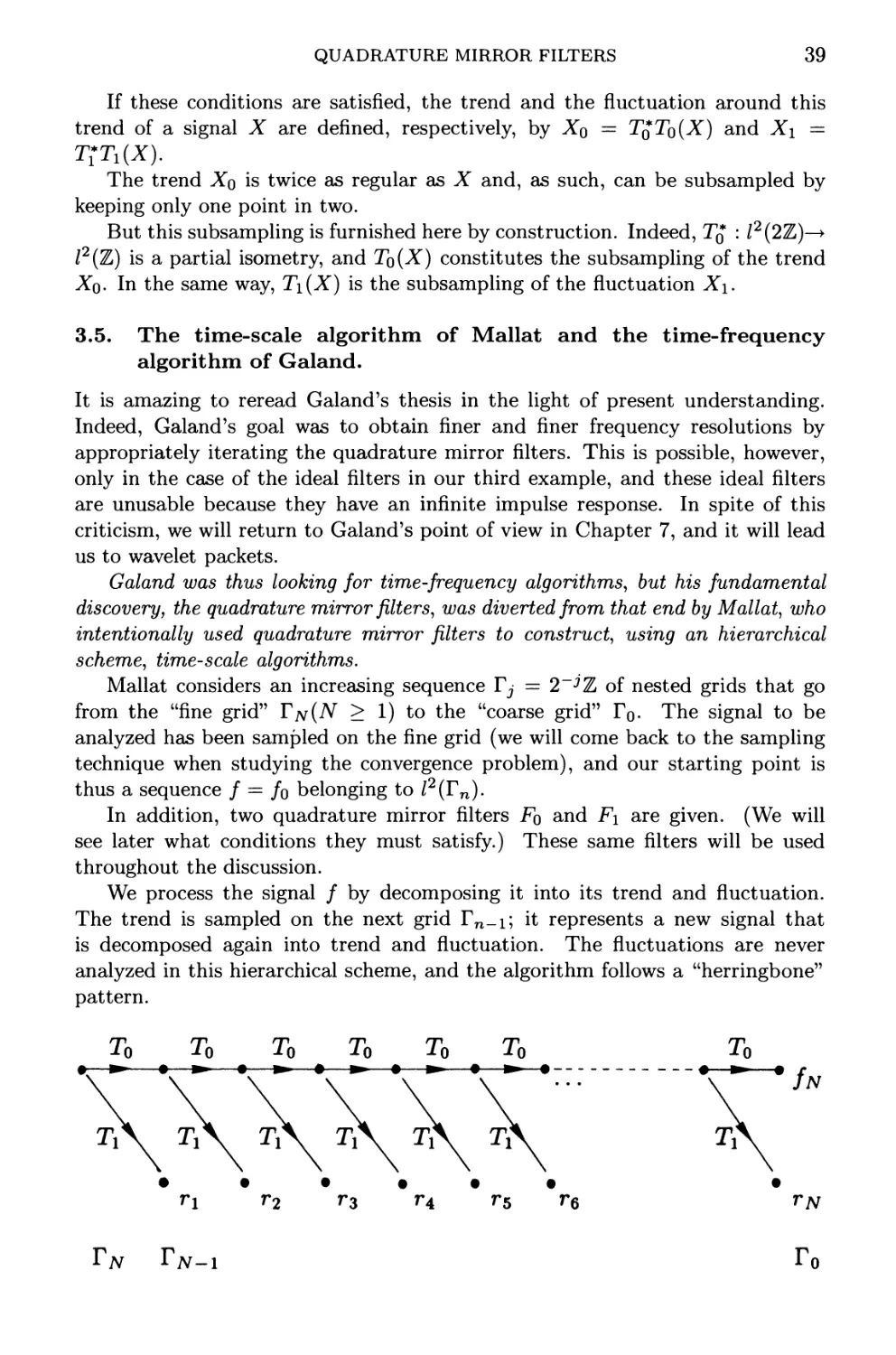
The Trend and Fluctuation 38
The Time-Scale Algorithm of Mallat and the Time-Frequency Algorithm of
Galand 39
Trends and Fluctuations with Orthonormal Wavelet Bases 40
Convergence to Wavelets 42
The Waveleh of Daubechies 43
Conclusions 44
v

VI
CHAPTER 4.
4.1
4.2
4.3
4.4
4.5
4.6
4.7
CHAPTER 5.
5.1
5.2
5.3
5.4
5.5
5.6
5.7
5.8
CHAPTER 6.
6.1
6.2
6.3
6.4
6.5
6.6
6.7
6.8
6.9
CHAPTER 7.
7.1
7.2
7.3
7.4
7.5
CHAPTER 8.
8.1
8.2
8.3
8.4
8.5
8.6
CHAPTER 9.
9.1
9.2
9.3
9.4
9.5
CONTENTS
Pyramid Algorithms for Numerical Image Processing
Introduction 45
The Pyramid Algorithms of Burt and Adelson 46
Examples of Pyramid Algorithms 50
Pyramid Algorithms and Image Compression 51
Pyramid Algorithms and Multiresolution Analysis 53
The Orthogonal Pyramids and Wavelets 55
Bi-orthogonal Wavelets 59
Time-Frequency Analysis for Signal Processing
Introduction 63
The Time-Frequency Plane 66
The Wigner- Vi lIe Transform 66
The Computation of Certain Wigner-Ville Transforms 67
The Wigner- Ville Transform and Pseudodifferential Calculus 69
The Wigner- Vi lIe Transform and Instantaneous Frequency 70
The Wigner- Ville Transform of Asymptotic Signals 72
Return to the Problem of Optimal Decomposition in Time-Frequency Atoms 73
Time-Frequency Algorithms Using Malvar's Wavelets
Introduction 75
Malvar Wavelets: A Historical Perspective 76
Windows with Variable Lengths 77
Malvar Wavelets and Time-Scale Wavelets 80
Adaptive Segmentation and the Split-and-Merge Algorithm 81
The Entropy of a Vector with Respect to an Orthonormal Basis 83
The Algorithm for Finding the Optimal Malvar Basis 83
An Example Where This Algorithm Works 85
The Discrete Case 86
Time-Frequency Analysis and Wavelet Packets
Heuristic Considerations 89
The Definition of Basic Wavelet Packets 92
General Wavelet Packets 95
Splitting Algorithms 97
Concluions 98
Computer Vision and Human Vision
Marr's Program 101
The Theory of Zero-Crossi ngs 104
A Counterexample to Marr's Conjecture 105
Mallat's Conjecture 106
The Two-Dimensional Version of Mallat's Algorithm
Conclusions 110
109
Wavelets and Fractals
Introduction III
The Weierstrass Function 111
The Determination of Regular Points in a Fractal Background
Study of the Riemann Function 115
Conclusions 117
113

CHAPTER 10.
10.1
10.2
10.3
10.4
10.5
CHAPTER II.
II. I
11.2
11.3
11.4
11.5
CONTENTS
Vll
Wavelets and Turbulence
Introduction 119
The Statistical Theory of Turbulence and Fourier Analysis
Verification of the Hypothesis of Parisi and Frisch 120
Farge's Experiments 121
Numerical Approaches to Turbulence 122
119
Wavelets and the Study of Distant Galaxies
Introduction 125
The New Telescopes 125
The Hierarchical Organization of the Galaxies and the Creation of the Universe 126
The Multifractal Approach to the Universe 126
The Advent of Wavelets 126
Index 129

Translator's Foreword
The question most often asked by those who heard I was translating this book was, HHow did you
get the job?" Well, I asked for it. I nlentioned to Professor Meyer in March 1992 that I had heard
that he had written a new book. He said, yes, and that the book was based on notes from lectures he
had given at the Spanish Institute in Madrid. He added that the book was being translated into
Spanish and that SIAM was interested in publishing an English edition, for which they would need a
translator. I volunteered to do the job; what you have is the result.
In addition to translating the text, I have tried to Hwork through" much of the mathematics to
correct typos. I have also added a line of explanation here and there where it seemed appropriate,
and sections of text and references have been updated. These revisions are not highlighted in any
particular way (i.e., there are no translator's notes except at one reference), but rather incorporated
into the text. These changes were made with Professor Meyer's blessing. Of course, there is
always the possibility that in the process of updating the manuscript I have introduced other errors;
for these I take full responsibility.
The great fun of this project has been the chance to work with Yves Meyer and other members
of Hteam wavelet." Professor Meyer improved both my French and my mathematics, and his
enthusiasm and appreciation for my efforts kept things moving. Direct help also came from John
Benedetto, Marie Farge, Patrick Flandrin, Stephane Jaffard, and Hamid Krim. Alex Grossmann
gave moral support by assuring me that it was an important project. My sincere thanks to all of
these people. The work was done while I was a Liaison Scientist for the Office of Naval Research
European Office, where my primary job was to report on mathematics in Europe. It was through
this work that I first made contact with the French wavelet community, and I thank the Office of
Naval Research for that opportunity. This was essentially a weekend and evening project, and
hence a family project. In this context, I thank my son, Michael J. Ryan, who kept house and
produced great dinners while I kept the electrons moving.
Robert D. Ryan
November I 992
London, UK
IX

Preface
The Htheory of wavelets" stands at the intersection of the frontiers of mathematics, scientific
computing, and signal processing. Its goal is to provide a coherent set of concepts, methods, and
algorithms that are adapted to a variety of nonstationary signals and that are also suitable for
numerical signal processing.
This book results from a series of lectures that Mr. Miguel Artola Gallego, Director of the
Spanish Institute, invited me to give on wavelets and their applications. I have tried to fulfill, in the
following pages, the objective the Spanish Institute set for me: to present to a scientific audience
coming from different disciplines, the prospects that wavelets offer for signal and image processing.
A description of the different algorithms used today under the name Hwavelets" (Chapters 2-7)
will be followed by an analysis of several applications of these methods: to numerical image
processing (Chapter 8), to fractals (Chapter 9), to turbulence (Chapter 10), and to astronomy
(Chapter II). This will take me out of my scientific domain; as a result, the last two chapters are
merely resumes of the original articles on which they are based.
I wish to thank the Spanish Institute for its generous hospitality as well as its Director for his
warm welcome. Additionally, I note the excellent organization by Mr. Pedro Corpas.
My thanks go also to my Spanih friends and colleagues who took the time to attend these
lectures.
XI

CHAPTER 1
Signals and Wavelets
The purpose of this first chapter is to give the reader a fairly clear idea about
the scientific content of the following chapters. All of the "themes" that will be
developed in this study, using the inevitable mathematical formalism, already
appear in this "overture." It is written with a concern for simplicity and clarity,
while avoiding as much as possible the use of formulas and symbols.
Signal and image processing always leads to a collection of techniques or
procedures. But like all other scientific disciplines, signal and image process-
ing assumes certain preliminary scientific conventions. We have sought, in this
first chapter, to describe the intellectual architecture underlying the algorithmic
constructions that will be presented in the following chapters.
1.1. What is a signal?
Signal processing has become an essential part of contemporary scientific and
technological activity. Signal processing is used in telecommunications (tele-
phone and television), in the transmission and analysis of satellite images, and
in medical imaging (echography, tomography, and nuclear magnetic resonance),
all of which involve the analysis and interpretation of complex time series. A
record of stock price fluctuations is a signal, as is a record of temperature readings
that permit the analysis of climatic variations and the study of global warming.
This list is by no means exhaustive.
Does there exist a precise definition of a signal that is appropriate for the
field of scientific acti vi ty called "signal processing"? A needlessly broad def-
inition could include the sequence of letters, spaces, and punctuation marks
appearing in Montaigne's Essays, but the tools we present do not apply to such
a signal. However, the structuralist analysis done by Roland Barthes on literary
.texts shares some amusing similarities with the multiresolution analysis that we
describe in Chapter 4.
The signals we study will always be series of numbers and not series of letters,
words, or phrases. These numbers come from measurements, which are typically
made using some recording method. The signals ultimately appear as functions
of time. This is true for one-dimensional signals. The case of two-dimensional
signals will be examined in a moment.
The objectives of signal processing are to analyze accurately, code efficiently,
transmit rapidly, and then to reconstruct carefully at the receiver the delicate
1

2
CHAPTER 1
oscillations or fluctuations of this function of time. This is important because
all of the information contained in the signal is effectively present and hidden in
the complicated arabesques appearing in its graphical representation.
These remarks apply to speech: A speech signal originates as subtle time
variations of air pressure and becomes a curve whose complex graphical charac-
teristics are an "adapted copy" of the voice.
It is equally important to consider two-dimensional signals, which is to say,
images. Here again, image processing is done on the numerical representation of
the image. For a black and white image, the numerical representation is created
by replacing the x and y coordinates of an image point with those of the closest
point on a sufficiently fine grid. The value f (x, y) of the "gray scale" is then
replaced with an average coefficient, which is then assigned to the corresponding
grid point.
The image thus becomes a large, typically square, matrix. Image processing
is done on this matrix.
These matrices are enormous, and as soon as one deals with a sequence of
images, the volume of numerical data that must be processed becomes immense.
Is it possible to reduce this volume by considering the "hidden laws" or correla-
tions that exist among the different pieces of numerical information representing
the image? This question leads us naturally to define the goals of the scientific
discipline called "signal processing."
1.2. The goals of signal and image processing.
Experts in signal processing are called on to describe, for a given class of signals,
algori thms that lead to the construction of microprocessors and that allow certain
operations and tasks to be done automatically. These tasks may be: analysis
and diagnostics, coding, quantization and compression, transmission or storage,
and synthesis and reconstruction.
We will use several examples to illustrate the nature of these operations and
the difficulties they present. It will become clear that no "universal algorithm"
is appropriate for the extreme diversity of the situations encountered. Thus, a
large part of this work is devoted to constructing coding or analysis algorithms
that can be adapted to the signals that one processes.
Our first example is the study of climatic variations and global warming.
This example was discussed by Professor Jacques-Louis Lions at the Spanish
Institute in 1990, and the following thoughts were inspired by his talks [4].
In this example, one has fairly precise temperature measurements from differ-
ent points in the northern hemisphere that were taken over the last two centuries,
and one tries to discover if industrial activity has caused global warming. The
extreme difficulty of the problem arises from the existence of significant natural
temperature fluctuations. Moreover, these fluctuations and the corresponding
climatic changes have always existed, as we learn from paleoclimatology [6].
To specify a diagnostic, it is essential to analyze, and then to erase, these
natural fluctuations (which play the role of noise) in order to have access to the

SIGNALS AND WAVELETS
3
"artificial" heating of the planet resulting from human activity. The diagnos-
tic often depends on extracting a small number of significant parameters from
a signal whose complexity and size are overwhelming. Thus the analysis and
the diagnostic rely naturally on data compression. If this compression is done
inappropriately, it can falsify the diagnostic.
Data compression also occurs in the problem of transmission. Indeed, trans-
mission channels have a limited capacity, and it is therefore important to reduce
as much as possible the abundance of raw information so that it fits within the
channel's "bit allocation."
One thinks, for example, of the digital telephone (Chapter 3) and the 64
Kbit/sec standard, which limits, without appeal, the quantity of information
that can be transmitted in one second.
A more surprising example appears in neurophysiology. The optic nerve's ca-
pacity to transmit visual information is clearly less than the volume of informa-
tion collected by all the retinal cells. Thus, there must be "low-level processing"
of information before it transits the optic nerve. David Marr has developed a the-
ory that allows us to understand the purpose and performance of this low-level
processing. We present this theory in Chapter 8.
We now consider problems posed by coding and quantization. Different cod-
ing algorithms will be presented and studied in this work: subband coding,
transform coding, and coding by zero-crossings. In each case, coding involves
methods to transform the recorded numerical signal into another representation
that is, depending on the nature of the signals studied, more convenient for
some task or further processing. Quantization is associated with coding. The
"exact" numerical values given by coding are replaced with nearby values that
are compatible with the bit allocation dictated by the transmission capacity.
Quantization is an unavoidable step in signal and image processing. U nfor-
tunately, it introduces systematic errors, known as "quantization noise." The
coding algorithms that are used (taking into account the nature of the signals)
ought to reduce the effects of quantization noise when decoding takes place. One
of the advantages of quadrature mirror filters is that they "trap" this quantiza-
tion noise inside well-defined frequency channels. These filters will be studied in
Chapter 3.
The problems encountered in archiving data (as well as problems of transmis-
sion and reconstruction) are illustrated by the FBI's task of storing the American
population's fingerprints. Different image-compression algorithms were tested,
and a variant of the algorithm described in Chapter 6 gave the best results. This
established a standard for fingerprint compression and reconstruction.
The last group of operations consists of decoding, synthesis, and restoration.
Synthesis and decoding are the inverse operations of coding and quantization.
The task is to reconstruct an image or audible signal at the receiver from the
series of a's and l's that have traveled over the transmission channel. One thinks
of decoding an encoded message, as in cryptography, and this analogy is correct
because one cannot reconstruct an image or signal without knowing the coding
algorithm.

4
CHAPTER 1
Signal restoration is similar to the restoration of old paintings. It amounts to
ridding the signal of artifacts and errors (which we call noise), and to enhancing
certain aspects of the signal that have undergone attenuation, deterioration, or
degradation.
1.3. Stationary signals, transient signals, and adaptive coding
algorithms.
We have just defined a set of tasks, or operations, to be performed on signals
or images. These tasks form a coherent collection. The purpose of this book is
to describe certain coding algorithms that have, during the last few years, been
shown to be particularly effective for analyzing signals having a fractal structure
or for compression and storage. We will also describe certain "meta-algorithms"
that allow one to choose the coding algorithm best suited to a given signal.
To better approach this problem of choosing an adaptive algorithm, we briefly
classify signals by distinguishing stationary signals, quasi-stationary signals, and
transient signals.
A signal is stationary if its properties are statistically invariant over time. A
well-known stationary signal is white noise, which, in its sampled form, appears
as a series of independent drawings. A stationary signal can exhibit unexpected
events, but we know in advance the probabilities of these events. These are the
statistically predictable unknowns.
The ideal tool for studying stationary signals is the Fourier transform. In
other words, stationary signals decompose canonically into linear combinations
of waves (sines and cosines). In the same way, signals that are not stationary
decompose into linear combinations of wavelets.
The study of nonstationary signals, where transient events appear that can-
not be predicted (even statistically with knowledge of the past), necessitates tech-
niques different from Fourier analysis. These techniques, which are specific to
the nonstationarity of the signal, include wavelets of the "time-frequency" type
and wavelets of the "time-scale" type. "Time-frequency" wavelets are suited,
most specifically, to the analysis of quasi-stationary signals, while "time-scale"
wavelets are adapted to signals having a fractal structure.
Before defining "time-frequency" wavelets and "time-scale" wavelets, we in-
dicate their common points. They belong to a more general class of algorithms
that are encountered as often in mathematics as in speech processing. Mathe-
maticians speak of "atomic decompositions," while speech specialists speak of
"decompositions in time-frequency atoms"; the scientific reality is the same in
both cases.
An "atomic decomposition" consists in extracting the simple constituents
that make up a complicated mixture. However, contrary to what happens in
chemistry, the "atoms" that are discovered in a signal will depend on the point
of view adopted for the analysis. These "atoms" will be "time-frequency atoms"
when we study quasi-stationary signals, but they could, in other situations, be
replaced by "time-scale wavelets" or "Grossmann-Morlet wavelets."

SIGNALS AND WAVELETS
5
These "atoms" or "wavelets" have no more physical existence than the num-
ber system used to multiply the mass of the earth by that of the moon. Each
number system has an internal logical coherence, but no scientific law asserts
that multiplication must of necessity be done in base 10 rather than base 2. On
the other hand, the number system used by the Romans is certainly excluded
because it is not suitable for multiplication.
Having different algorithms that allow us to code a signal by decomposing it
into "time-frequency atoms" presents us with a similar situation. The decision to
use one or the other of these algorithms will be made by considering their perfor-
mance. How well they perform must be judged in terms of one of the anticipated
goals of signal processing. A n algorithm that is optimal for compression can be
disastrous for analysis: A standard energetic criterion for the compression could
cause details that are important for the analysis to be systematically neglected.
These thoughts will be developed and clarified in 991.6 and 1.7. It is time to
define wavelets, which we do in the next two sections.
1.4. Grossmann-Morlet time-scale wavelets.
"Time-scale" analysis (which should be called "space-scale" in the image case,
but which we prefer to call "multiresolution analysis") involves using a vast
range of scales for signal analysis. This notion of scale, which clearly refers to
cartography, implies that the signal (or image) is replaced, at a given scale, by
the best possible approximation that can be drawn at that scale. By "traveling"
from the large scales toward the fine scales, one "zooms in" and arrives at more
and more exact representations of the given signal.
The analysis is then done by calculating the change from one scale to the
next. These are the details that allow one, by correcting a rather crude ap-
proximation, to move toward a better quality representation. This algorithmic
scheme is called "multiresolution analysis" and is developed in Chapters 3 and
4. Multiresolution analysis is equivalent to an atomic decomposition where the
atoms are Grossmann-Morlet wavelets.
We define these wavelets by starting with a function 1/;( t) of the real variable
t. This function is called a "mother wavelet" provided it is well localized and
oscillating. (By oscillating it resembles a wave, but by being localized it is a
wavelet.) The localization condition is expressed in the usual way as decreasing
rapidly to zero when It I tends to infinity. The second condition suggests that
1/;(t) vibrates like a wave: Here we require that the integral of 1/;(t) be zero and
that the same hold true for the first m movements of 1/;. This is expressed as
(1.1)
o = i: VJ(t) dt = . . . = i: tm-1VJ(t) dt.
The "mother wavelet," 1/;(t), generates the other wavelets, 1/;(a,b) (t), a > 0,
b E IR, of the family by change of scale (the scale of 1/;(t) is conventionally 1,
and that of 1/;(a,b) (t) is a > 0) and translation in time (the function 1/;( t) is
conventionally centered around 0, and 1/;(a,b) (t) is then centered around b).

6
CHAPTER 1
Thus we have
(1.2)
1 ( t - b )
'I/J(a,b)(t) = ya 'I/J ----;;- ,
a > 0,
b E IR.
Alex Grossmann and Jean Morlet have shown that, if'ljJ(t) is real-valued, this
collection can be used as if it were an orthonormal basis. This means that any
signal of finite energy can be represented as a linear combination of wavelets
'ljJ(a,b) (t) and that the coefficients of this combination are, up to a normalizing
factor, the scalar products Joo f(t)'ljJ(a,b)(t) dt.
These scalar products measure, in a certain sense, the fluctuations of the
signal f (t) around the point b, at the scale given by a > O.
It required uncommon scientific intuition to assert, as Grossmann and Morlet
did, that this new method of time-scale analysis was suitable for the analysis and
synthesis of transient signals. Signal processing experts were annoyed by the
intrusion of these two poachers on their preserve and made fun of their claims.
This polemic died out after only a few years. In fact, the argument should
never have arisen because the methods of time-scale or multiresolution analysis
had existed for five or six years under various disguises: in signal analysis (under
the name of quadrature mirror filters) and in image analysis (under the name of
pyramid algorithms).
The first to report on this was Stephane Mallat. He constructed a guide
that allowed the same signal analysis method to be recognized under very dif-
ferent presentations: wavelets, pyramid algorithms, quadrature mirror filters,
Littlewood-Paley analysis, David Marr's zero crossings. . .
Mallat's brilliant synthesis has been the source of many new developments.
One of the most notable of these is Ingrid Daubechies's discovery of orthonor-
mal wavelet bases having preselected regularity and compact support. The
only previously known case was the Haar system (1909), which is not regu-
lar. Thus 80 years separated Alfred Haar's work and its natural extension by
Daubechies [1].
1.5. Time-frequency wavelets from Gabor to Malvar.
Dennis Gabor was the first to introduce time-frequency wavelets or Gabor
wavelets. He had the idea to divide a wave (whose mathematical representa-
tion is cos(wt + <p)) into segments and then to throwaway all but one of these
segments. This left a piece of a wave, or a wavelet, which had a beginning and
an end.
To use a musical analogy, a wave corresponds to a note (a re, for example)
that has been emitted since the origin of time and sounds indefinitely, without
attenuation, until the end of time. A wavelet then corresponds to the same re
that is struck at a certain moment, say, on a piano, and is later muffled by the
pedal. In other words, a Gabor wavelet has (at least) three pieces of information:
a beginning, an end, and a specific frequency in between.

SIGNALS AND WAVELETS
7
Difficulties appeared when it was necessary to decompose a signal using Ga-
bor wavelets. As long as one does only continuous decompositions (using all
frequencies and all time), Gabor wavelets can be used as if they formed an or-
thonormal basis. But the corresponding discrete algorithms do not exist, or they
require so much tinkering that they become too complicated.
It is only very recently, by abandoning Gabor's approach, that two sepa-
rate groups have discovered time-frequency wavelets having good algorithmic
qualities. These special time-frequency wavelets, called Malvar wavelets, are
particularly well suited for coding speech and music. Moreover, they are equally
useful to the FBI for storing fingerprints.
The decomposition of a signal in an orthonormal basis of Malvar wavelets
imitates writing music using a musical score. But this composition is misleading
because a piece of music can be written in only one way, whereas there exists
a nondenumerable infinity of orthonormal bases of Malvar wavelets. Choosing
one among these is equivalent to segmenting the given signal and then doing
a traditional Fourier analysis on the delimited pieces. What is the best way
to choose this segmentation? This question leads us naturally to the following
section.
1.6. Optimal algorithms in signal processing.
Which wavelet to choose? I have often posed this question at meetings on
wavelets and their applications held since 1985. But this question needs to be
sharpened. What freedom of choice is at our disposal? What are the objectives
of the choices we make? Can we make better use of the choices offered to us by
considering the anticipated goals? These are several of the questions we will try
to answer.
The goal we have in mind is aptly illustrated by a remark by Benoit Mandel-
brot made in an interview on "France-Culture": "The world around us is very
complicated. The tools at our disposal to describe it are very weak."
It is notable that Mandelbrot used the word "describe" and not "explain"
or "interpret." We are going to follow him in this, ostensibly, very modest
approach. This is our answer to the problem about the objectives of the choices:
Wavelets, whether they are of the time-scale or time-frequency type, will not help
us to explain scientific facts, but they will serve to describe the reality around us,
whether or not it is scientific.
OUf task is to optimize the description. This means that we must make the
best use of the resources allocated to us (for example, the number of available
bit) to obtain the most precise possible description.
To resolve this problem, we must first indicate how the quality of the de-
scription will be judged. Most often, the criteria used are academic and do not
correspond at all to the user's point of view.
For example, in image processing, all the calculations for judging the quality
of the description use the quadratic mean value of gray levels. It is clear, however,
that our eye has a much more selective sensitivity. Thus, in the last analysis, we

8
CHAPTER 1
should submit the performance of an "optimal algorithm" to the users because
the average approximation criterion that leads to this algorithm will often be
inadequate.
The case of speech (telephonic communication) or music is similar. After
systematic research that optimizes the reception quality (quality calculated with
an aveage), it would be advisable to experiment by taking into account the
judgments of telephone users and musicians.
Thus we see a two-state program developing. Nevertheless, the only stage we
describe in the following pages is the "objective search" for an optimal algorithm,
even though its optimality is defined in terms of a debatable energy criterion.
Rather than formulate ad hoc algorithms for each signal or each class of
signals, we are going to construct, once and for all, a vast collection called a
library of algorithms. We will also construct a "meta-algorithm" whose function
will be to find the particular algorithm in the library that best serves the given
signal in view of the criterion for the quality of the description.
It is hardly an exaggeration to say that we will introduce almost as many
analysis algorithms as there are signals. For example, for a signal recorded on
2 10 == 1024 points, the number of algorithms at our disposal will be of the order
2 1024 . This is the number of all the signals defined on our 1024 points that take
only two values, 0 and 1.
Thus we will use a "very large library" to describe the signals, but we exclude
the "library of Babel." This would contain all the books, or all the signals in
our case. And as everyone knows, the search for a specific book in the library of
Babel is an insurmountable task. The "ideal library" must be sufficiently rich
to suit all transient signals, but the "books" must be easily accessible.
While a single algorithm (Fourier analysis) is appropriate for all station-
ary signals, the transient signals are so rich and complex that a single analysis
method (whether of time-scale or time-frequency) cannot serve them all.
If we stay in the relatively narrow environment of Grossmann-Morlet
wavelets, also called time-scale algorithms, we have only two ways to adapt
the algorithm to the signal being studied: We can choose one or another analyz-
ing wavelet, and we can use either the continuous or the discrete version of the
wavelets.
For example, we can require the analzing wavelet 1jJ to be an analytic signal,
which means that its Fourier transform 1jJ(w) is zero for negative frequencies. In
this case, all the wavelets 1jJ(a,b), a > 0, b E IR, generated by 1jJ will still have
this property, and their linear combinations given by the algorithm will be the
analytic signal F associated with the real signal f.
Likewise, we can follow Daubechies and, for a given r > 1, choose for 1jJ(x) a
real-valued function in the class C r with compact support such that the collection
2 j / 2 1jJ(2 j x - k), j,k E Z, is an orthonormal basis for L 2 (IR). In this discrete
version of the algorithm, a == 2- j and b == k2- j ,j,k E Z.
In spite of this, the choices that can be made from the set of time-scale
wavelets remain limited. The search for optimal algorithms leads us on some

SIGNALS AND WAVELETS
9
remarkable algorithmic adventures, where time-scale wavelets and time-frequency
wavelets are in competition, and where they are also compared to intermediate
algorithms that mix the two extreme forms of analysis.
These considerations are developed in Chapters 6 and 7 and the question I
asked myself six years ago (what wavelet to choose?) seems passe to me today.
The choices that we can and must consider no longer involve only the analyzing
instrument (the wavelet); they also involve the methodology employed (time-
scale, time-frequency, or intermediate algorithms).
Today, the competing algorithms (time-scale and time-frequency) are in-
cluded in a whole universe of intermediate algorithms. An entropy criterion
permits us to choose the algorithm that optimizes the description of the given
signal within the given bit-allocation.
Each algorithm is presented in terms of a particular orthogonal basis. We
can compare searching for the optimal algorithm to searching for the best point
of view, or best perspective, to look at a statue in a museum. Each point of view
reveals certain parts of the statue and obscures others. We change our point
of view to find the best one by going around the statue. In effect, we make a
rotation; we change the orthonormal basis of reference to find the optimal basis.
These reflections lead us quite naturally to the scientific thoughts of David
Marr, which we present in the next section.
1.7. Optimal representation, according to Marr.
David Marr was fascinated and intrigued by the complex relations that exist
between the choice of a representation of a signal and the nature of the operations
or transformations that such a representation permits. He wrote [5, pp. 20-21]:
A representation is a formal system for making explicit certain entities or
types of information, together with a specification of how the system does this.
And I shall call the result of using a representation to describe a given entity a
description of the entity in that representation.
For example, the Arabic, Roman and binary numerical systems are all formal
systems for representing numbers. The Arabic representation consists of a string
of symbols drawn from the set {O, 1, 2, 3, 4, 5, 6, 7, 8, 9} and the rule for
constructing the description of a particular integer n is that one decomposes
n into a sum of multiples of powers of 10. .. A musical score provides a way
of representing a symphony; the alphabet allows the construction of a written
representation of words. . .
A representation, therefore, is not a foreign idea at all-we all use represen-
tations all the time. However, the notion that one can capture some aspect of
reality by making a description of it using a symbol and that to do so can be
useful seems to me a fascinating and powerful idea. But even the simple exam-
ples we have discussed introduce some rather general and important issues that
arise whenever one chooses to use one particular representation.
For example, if one chooses the Arabic numerical representation, it is easy to
discover whether a number is a power of 10 but difficult to discover whether it is
a power of 2. If one chooses the binary representation, the situation is reversed.

10
CHAPTER 1
Thus, there is a trade-off; any particular representation makes certain informa-
tion explicit at the expense of information that is pushed into the background and
may be quite hard to recover. 1
This issue is important, because how information is presented can greatly
affect how easy it is to do different things with it. This is evident even from
our numbers example: it is easy to add, to subtract and even to multiply if the
Arabic or binary representations are used, but it is not at all easy to do these
things---especially multiplication-with Roman numerals. This is a key reason
why the Roman culture failed to develop mathematics in the way the earlier
Arabic cultures had. . .
There is an essential difference between Marr's considerations and the algo-
rithms that we develop in the first six chapters. The difference is that the choice
of the best representation, according to Marr, is tied to an objective goal. For
the problem posed by vision, the goal is to extract the contours, recognize the
edges of objects, delimit them, and understand their three-dimensional organiza-
tion. In the algorithms we develop, the only criterion is internal to the algorithm
and consists in reducing the amount of data. We have not yet studied situations
where one must also take into consideration an external criterion. In spite of
this difference, Marr's point of view is very close to the one we will present.
1.8. Terminology.
The elementary constituents used for signal analysis and synthesis will be called,
depending on the circumstances, wavelets, time-frequency atoms, or wavelet
packets (Chapter 8).
The wavelets used will be either Grossmann-Morlet wavelets of the form
  Ca b),
the wavelets of Daubechies that have the form
a > 0,
b E IR,
2 j 1 2 1/;(2 j t - k),
j, k E Z,
or Gabor-Malvar wavelets of the form
w (t - l) cos [7r (k + 1/2) (t - l)],
kEN,
1 E Z.
In the first two cases, we will speak of time-scale algorithms; in the last case,
we will speak of time-frequency algorithms. Later we will mix the two points of
view and subject the Gabor-Malvar wavelets to dyadic dilations to construct the
Daubechies wavelets. One thus encounters generalized time-frequency atoms.
We will use only two "very large libraries." The first consists of orthonormal
bases whose elements are wavelet packets. In the second, the wavelet packets are
replaced by the generalized time-frequency atoms that we have just described.
1 The italics are ours.

SIGNALS AND WAVELETS
11
1.9. Reader's guide.
In Chapters 2 through 7, we present the time-scale algorithms (Chapters 3 and
4) and time-frequency algorithms (Chapters 5,6, and 7). Chapter 2 has a special
status. We have tried to retrace the path that led from Fourier analysis (Fourier
1807) to wavelet analysis (Calderon 1960 and Stromberg 1981) and to the very
core of contemporary mathematics.
Quadrature mirror filters are studied in Chapter 3 in connection with prob-
lems posed by the digital telephone.
The pyramid algorithms described in Chapter 4 concern numerical image
processing. The orthogonal pyramids use precisely the quadrature mirror filters
of Chapter 3. The pyramid algorithms lead either to orthogonal wavelets or to
bi-orthogonal wavelets.
From Chapter 5 on, we will study time-frequency algorithms. The Wigner-
Ville transform enables "the signal to be displayed in the time-frequency plane."
After indicating the main properties of the Wigner- Ville transform, we must
point out that it does not provide an algorithm that allows us to decompose a
signal into time-frequency atoms that are the analogues of musical notes.
The two algorithms that do provide access to these "atomic decompositions"
are presented in Chapters 6 (Malvar wavelets) and 7 (wavelet packets).
The first six chapters form a coherent unit. This is not the case for the last
four chapters; each of them treats a special application of wavelets and time-
scale methods. Chapter 8 deals with the Marr-Mallat theory. This concerns the
possibility of coding an image using the zero-crossings of its wavelet transform.
Using the Grossmann-Morlet analysis one can determine the fractal expo-
nents, as a function of position, of a multifractal object. This is one of the most
remarkable applications of the Grossmann-Morlet wavelets, and it is presented
in Chapter 6.
The last two chapters cover two very dynamic subjects: turbulence and the
multifractal approach to turbulence (Chapter 10) and the hierarchical organi-
zation of the galaxies and the structure of the Universe (Chapter 11). In both
cases, results are still meager. But these avenues of research are fascinating, and
the researchers involved have such good reputations that one can reasonably
expect important progress before long.
Bibliography
[1] I. DAUBECHIES, Ten Lectures on Wavelets, Society for Industrial and Applied Mathemat-
ics, Philadelphia, P A, 1992.
[2] D. GABOR, Theory of communication, J. lEE, 93 (1946), pp. 429-457.
[3] C. GASQUET AND P. WITOMSKI, Analyse de Fourier et applications, Filtrage, Calcul
numenque, Ondelettes, Masson, Paris, 1990.
[4] J. L. LIONS, La planete terre: role des mathematiques et des super-ordinateurs, cours it
l'lnstitut d'Espagne, 1990.
[5] D. MARR, Vision, W. H. Freeman and Co., New York, 1982.
[6] R. V AUTARD AND M. G HIL, Singular spectrum analysis in nonlinear dynamics, with ap-
plications to paleoclimatic time series, Physica D, 35 (1989), pp. 359-424.

CHAPTER 2
Wavelets From a Historical
Perspective
2.1. Introduction.
The application of wavelets to signal and image processing is only a few years
old. But in looking back over the history of mathematics, we will uncover at least
seven different origins of wavelet analysis. Most of this work was done around
the 1930s, and, at that time, the separate efforts did not appear to be parts of a
coherent theory. In particular, neither the word "wavelet" nor the corresponding
concept appeared in this research done a half-century ago. Only today do we
know that this work prefigured the theory of wavelets.
It is important to describe these seven sources in some detail. Each of them
corresponds to a specific point of view and a particular technique, which, only
now, are we able to view from a common scientific perspective. What's more,
these specific techniques were rediscovered several years ago by physicists and
mathematicians working on wavelets. For example, the Littlewood-Paley anal-
ysis (32.4), which dates from 1930, underlies Mallat's work on image processing.
Matthias Holschneider used, without knowing it, Lusin's technique (1930) to
clarify the fractal structure of Riemann's function (32.6 and 39.4). Grossmann
and Morlet rediscovered Alberto Calderon's identity (1960) 20 years later. And,
to spare no one, the author of these lines was not the first to construct a reg-
ular, well-localized orthonormal wavelet basis having the algorithmic structure
of Haar's system (1909); J. O. Stromberg had done the same thing five years
earlier.
Does this mean that everything had already been written and that "team-
wavelet" researchers appropriated-while making a great show of it-results dis-
covered by others? This judgment must be qualified for two reasons. In the first
place, the physicists from "team wavelet" were not aware of Calderon's work; it
was in completely good faith that they presented as a revolutionary innovation
results that were about 20 years old. "Team wavelet" researchers can be accused
of ignorance but not of plagiarism. But above all, by rediscovering these known
scientific facts, the investigators gave them new life and authority. Our debt to
Grossmann and Morlet is not so much for having rediscovered the identity of
Calderon as it is for having related it to processing nonstationary signals. This
bold synthesis certainly encountered resistance, and Calderon himself found this
use of his work incongruous.
13

14
CHAPTER 2
The role of Morlet and Grossmann in the wavelet saga can be compared to
that of Mandelbrot in the story of fractals. It is true that before Mandelbrot
there were Pierre Fatou and Gaston Julia, and certain of Mandelbrot's discoveries
repeat their work. But Mandelbrot showed us the possibility of interpreting
the world around us with the help of a new concept, that of fractals. None
of the mathematicians working on Hausdorff dimension were ready, from their
training or experience, for such a leap into the unknown. Wavelets have gone
the same way, and one of our objectives is to construct the bridge that relates
signal processing to the different mathematical efforts that developed outside the
"theory of wavelets."
2.2. From Fourier (1807) to Haar (1909), frequency analysis becomes
scale analysis.
Let's go back to the origins, that is to Joseph Fourier. As everyone knows, he as-
serted in 1807 that any 27r-periodic function f(x) is the sum ao + L (ak cos kx+
b k sin kx) of its "Fourier series." The coefficients ao, ak, and bk(k > 1) are cal-
culated by
1 (27r
ao = 211" 10 f(x) dx,
and by
1 1 27r
ak==- f(x)coskxdx,
7r 0
1 1 27r
bk == - f(x) sin kx dx.
7r 0
When Fourier announced his surprising results, neither the notion of function
nor that of integral had yet received a precise definition. We can even say
that Fourier's statement played an essential role in the evolution of the ideas
mathematicians have had about these concepts.
Before Fourier's work, entire series were used to represent and manipulate
functions, and the most general functions that could be constructed were en-
dowed with very special properties indeed. Furthermore, these properties were
unconsciously associated with the notion of function itself. By passing from a
representation of the form
(2.1 )
2 3
ao + alx + a2x + a3 x +...
to one of the form
(2.2) ao + (al cos x + b 1 sin x) + (a2 cos 2x + b 2 sin 2x) + . . .
Fourier discovered, without knowing it, a new functional universe.
However, in 1873, Paul Du Bois-Reymond constructed a continuous, 27r-
periodic function of the real variable x, whose Fourier series diverged at a given
point. If Fourier's assertion were true, it could not be so in the naIve sense
imagined by Fourier.
At that time, three new avenues were opened to mathematicians, and all
three have led to important results:

WAVELETS FROM A HISTORICAL PERSPECTIVE
15
(a) They could modify the notion of function and find one that is adapted,
in a certain sense, to Fourier series;
(b) They could modify the definition of convergence of Fourier series; or
(c) They could find other orthogonal systems for which the phenomenon,
discovered by Du Bois-Reymond in the case of the trigonometric system, cannot
happen.
The functional concept best suited to Fourier series was created by Henri
Lebesgue. It involves the space £2 [0, 27r] of (classes of) functions that are square-
integrable on the interval [0, 27r]. The sequence
1
J21r '
1
 cosx,
1 .
 SIn x,
1
 cos2x,
1 .
 sm2x,...
is an orthonormal basis for this space. Furthermore, the coefficients of the de-
composition in this orthonormal basis form a square-summable series, and this
expresses the conservation of energy: The quadratic mean value of the devel-
oped function f (x) is (up to a normalization factor) the sum of the squares of
the coefficients. Finally, the Fourier series of f converges to f in the sense of the
quadratic mean.
The second way that was followed to avoid the difficulty raised by Du Bois-
Reymond was to modify the notion of convergence. The partial sums Sn (x) are
replaced by the Cesaro sums (J n ==  (So + . . . + Sn -1), and everything falls into
place.
The third route leads to wavelets. This was followed by Haar, who
asked himself this question: "Does there exist another orthonormal system
ko (x), hI (x), . . . , h n (x), . .. offunctions defined on [0,1] such that for any func-
tion f(x), continuous on [0,1], the series
(2.3) (f, ho) ho ( x) + (f, hI) hI ( x) + . . . + (f, h n ) h n ( x) + . . .
converges to 1 (x) uniformly on [0,1]?"
Here we have written (u, v) == fol u(x) v(x) dx, where v is the complex conju-
gate of v, and chosen the interval [0,1] for convenience to fix our ideas.
As we will see, this problem has an infinite number of solutions. In 1909,
Haar discovered the simplest solution and, at the same time, opened one of the
routes leading to wavelets.
Haar begins with the function h(x) that is equal to 1 on [0,1/2), -Ion
[1/2,1), and 0 outside the interval [0,1). For n > 1, he writes n == 2 j + k,
j > 0,0 < k < 2 j , and defines hn(x) == 2 jj2 h(2 j x - k). The support of hn(x)
is the dyadic interval In == [k2- j , (k + 1)2- j ), which is included in [0,1) when
o < k < 2 j . To complete the set, define ho (x) == 1 on [0,1). Then the series
ho (x), hI (x), . . . , h n (x), . . . is an orthonormal basis (also called a Hilbert basis)
for £2[0,1].
The uniform approximation of f(x) by the sequence Sn(/)(x)
(I, ho)ho(x)+" '+(/, hn)hn(x) is nothing more than the classical approximation
of a continuous function by step functions whose values are the mean values of
1 (x) on the appropriate dyadic intervals.

16
CHAPTER 2
We can criticize the Haar construction on a couple of points. On one hand, the
"atoms" h n (x) used to construct the continuous function 1 (x) are not themselves
continuous functions, and thus there is a lack of coherence.
But there is a more serious criticism. Suppose that, instead of being contin-
uous on the interval [0,1], f (x) is a function of the class C 1 , which means 1 (x)
is continuous and has a continuous derivative. Then the approximation of I(x)
by step functions would be completely inappropriate. In this case, a suitable
approximation would be the one created from the graph of I(x) by inscribing
polygonal lines.
The Haar construction is suitable only for continuous functions, functions
square-integrable on [0,1] or, more generally, functions whose index of regularity
is near O. We will see a little later what this means.
These two defects of the Haar system and the idea of approximating the
graph of I(x) with inscribed polygonal lines led Faber and Schauder to replace
the functions hn(x) of the Haar system by their primitives. This research began
in 1910 and continued until 1920.
Define the "triangle function" (x) by (x) == 0 if x f/. [0,1], (x) == 2x if
o < x < 1/2, and (x) == 2(1 - x) if 1/2 < x < 1. Then Faber and Schauder
considered the series n (x), n > 1, defined by
(2.4) n(x) == (2j x - k) for n == 2) + k,
j > 0,
o < k < 2).
The support of n(x) is the dyadic interval In == [k2- j , (k + 1)2- j ], and n(x)
is the primitive of hn(x) multiplied by 2 . 2 j / 2 and zero outside In.
For n == 0, we set o(x) == x, and we add the constant 1 to complete the
set of functions. Then the sequence 1, o (x), . . . , n (x), . . . is a S chauder basis
for the Banach space E of continuous functions on [0,1]. This means that every
continuous function on [0,1] can be written as
(2.5)
ex:>
I(x) == a + bx + L Qnn(x)
1
and that the series has the following properties: the convergence is uniform on
[0,1] and, as a consequence, the coefficients are unique.
We note that the Haar system is not a Schauder basis of E because a Schauder
basis of a Banach space must be made up of vectors of that space, and the
functions h n are not continuous.
The calculation of the coefficients in (2.5) is immediate. We have successively
1(0) == a and 1(1) == a + b, which gives a and b. This allows us to consider a
function I(x) - a - bx, which is zero at 0 and 1. Once this reduction is made, we
have 1(1/2) == Q1, which allows us to consider a function equal to zero at 0, 1/2,
and 1. The calculation continues with 1(1/4) == Q2 and 1(3/4) == Q3, and so on.
If we do not wish to "peel" 1 (x) this way, the coefficients Qn can be computed
directly by the formula
(2.6)
. 1. .
Qn == 1 (( k + 1/2) 2 -)) - - [I (k2 -)) + 1 (( k + 1) 2 -) )].
2

WAVELETS FROM A HISTORICAL PERSPECTIVE
17
We can give a further interpretation to (2.5). If, instead of being continuous,
I(x) was a function in the class C 1 , then we could differentiate (2.5) term by
term and obtain the expansion of I' (x) in the Haar basis. If I (x) is in class
C 1 , the series (2.5) converges uniformly to I(x) and the series differentiated
term by term converges uniformly to I'(X). Does this mean that the functions
n(x), n > 0, with the added function 1, constitute a Schauder basis for the
Banach space C 1 [0, I]? As before, this is not the case because the functions
n(x) do not belong to the space in question.
Following Holder, we define the space cr [0, 1], for 0 < r < 1, by the relation
I/(x) - l(y)1 < Clx - ylr for a certain constant C and for all x, y E [0,1]. Then it
is clear from (2.6) that Ian I < C2-(j+1)r if I belongs to cr. Since 2 j < n < 2 j + 1
we can also write lanl < Cn- r , n > 1. The converse, although much less evident,
is nevertheless true when 0 < r < 1. It is not true if r = 1.
Contemporary physicists are very interested in the Holder spaces cr because
they occur naturally in the study of fractal structures. In fact, the physicists
require more. They wish to calculate a Holder exponent r that varies from one
point to another. Here is the definition of pointwise Holder exponents. We
say that I(x) satisfies a Holder condition of exponent r, 0 < r < 1, at Xo if
If(x) - l(xo)1 < Clx - xol r . Then we look for the largest possible value of r,
which is denoted r( xo) if it exists.
Contemporary science deals with numerous physical phenomena having
multifractal structures. This means that the "fractal exponents" r( xo) vary
from point to point. In this case, the Hausdorff dimension of the set of points
Xo, where r(xo) = a is a function of d(a) whose graph has a distinctive form.
An example from mathematics is the celebrated function attributed to Bern-
hard Riemann L(1/n2)sin(n2x). This example illustrates the point that the
Fourier series of a function provides no directly accessible information about
the function's multifractal structure. By using the wavelets of Lusin (which we
present in 32.6), it is possible to elucidate the multifractal structure of Riemann's
function. This was done by Matthias Holschneider and Philippe Tchamitchian.
We describe their work in Chapter 9.
A second example is the signal coming from fully developed turbulence. The
multifractal structure of this signal has been studied with great care by Alain
Arneodo and his collaborators. We present this example in Chapter 10.
Conceivably, the pointwise Holder exponents could be computed by going
back to the definition. However, the example of the Riemann functions shows
that such an approach is too crude to yield practical results. This approach offers
no way to take into consideration the inevitable noise (assumed to be Gaussian)
that alters a signal. The Schauder basis presents the same difficulties because the
calculation of the coefficients an (according to (2.6)) calls directly upon explicit
values of the signal.
Today, we are fortunate to have much more subtle ways to attack this
problem. Specifically, the pointwise Holder exponents are now determined
using wavelet analysis. The wavelet coefficients replace those given by for-
mula (2.6). They are less sensitive to noise because they measure, at different
scales, the average fluctuations of the signal. These methods will be described
in Chapter 9.

18 CHAPTER 2
2.3. New directions of the 1930s: Levy and Brownian motion.
Brownian motion is a random signal. We will limit our discussion to the one-
dimensional case. We thus write X(t,w) for the Brownian motion: t denotes
time, w belongs to a probability space 0, and X (t, w) is regarded as a real-valued
function of time depending on the parameter w.
To obtain a realization of Brownian motion, we choose a particular orthonor-
mal basis Zi(t), i E I, for the usual Hilbert space L 2 (IR). Then we know that
the derivative (in the sense of distributions) :t X (t, w) is written as
(2.7)
d
dt X(t,w) = L9i(W)Zi(t),
iEI
where the gi (w), i E I, are independent identically distributed Gaussian random
variables with zero mean.
Then the problem is to choose the best possible representation of Brownian
motion. It is certainly advisable, as in all signal processing problems, to have in
mind the desired end result.
If we wish to examine the spectral properties of Brownian motion, we are
led to select the Fourier representation. The real line is cut into intervals [217r,
2(1+1)7r), 1 E Z, and the trigonometric system is used on each of the intervals. In
its real form, this trigonometric system is vk ,  cos kx, and  sin kx, k > 1.
If we wish to highlight the multifractal structure of Brownian motion, Fourier
analysis is inadequate. On the other hand, the analysis using the Schauder basis
immediately reveals the Holder regularity cr, T < 1/2, of the Brownian motion
trajectories.
We start with the Haar basis for L 2 (IR) composed of the functions hn(t -l),
n > 0, I E Z, and expand the white noise :t x( t, w) in this orthonormal basis.
By taking primitives, we obtain the development of Brownian motion in the
Schauder basis.
To fix our ideas, we restrict the discussion to Brownian motion on the interval
[0,1]. For this 1 = 0, and
1 ex:> .
X(t,w) = ao(w) + tbo(w) + "2 L TJ/29n(W)n(t),
1
where the gn(w) are independent Gaussian random variables with mean zero and
the same distribution.
To verify that the function X ( t, w) belongs to the Holder space C r for almost
all w E 0, it is sufficient to show that 2- j / 2 Ign(w)1 < C(w)2- jr . If, for almost
all w E 0, one had sUPnO Ign(w)1 < 00, then the trajectories of the Brownian
motion would almost surely belong to the sp ace C 1 / 2 . But this is not the case,
and instead we have sUPn2(lgn(w)I/ V log n) < 00 for almost all w E O. Then
the criterion for Holder regularity gives
(2.8)
(2.9)
IX(t + h,w) - X(t,w)1 < C(w) y' hlog l/h,
where C(w) < 00 for almost all w E O.

WAVELETS FROM A HISTORICAL PERSPECTIVE
19
We see, from this theorem of Paul Levy, the superiority of the Schauder basis
over the Fourier basis for studying local regularity properties.
The determination of the fractal exponents requires some extensions. These
extensions that allow the study of small, complicated details form part of "mul-
tiresolution analysis," which we define in the following chapters. These ideas are
already incorporated in the definition of the Schauder basis itself, in particular,
within the mapping x  2 j x - k. They are clearly absent in the trigonometric
system.
Patrick Flandrin [5] has extended this work to the case of fractional Brown-
ian motion, as it was proposed by Benoit Mandelbrot and John W. van Ness
to model certain noise. Albert Benassi, Stephane Jaffard, and Daniel Roux
[3] have generalized these ideas to certain Gaussian-Markov fields. All of this
work demonstrates that multiresolution methods are adapted to the analysis and
synthesis of these processes.
2.4. New directions of the 1930s: Littlewood and Paley.
We have shown, with the example of Brownian motion, that the trigonometric
system does not provide direct and easy access to local regularity properties and
that these properties are clearly apparent when examined with other represen-
tations.
Similar difficulties are encountered when we try to localize the energy of a
function. To be more precise, the integral 2 Jo 27r If(x)1 2 dx, which is the mean
value of the energy, is given directly by the sum of the squares of the Fourier
coefficients. However, it is often important to know if the energy is concentrated
around a few points or if it is distributed over the whole interval [0,27r]. This
determination can be made by calculating 2 Jo 27r If(x)1 4 dx, or more generally,
2 J7r If(x)IPdx for 2 < p < 00. When the energy is concentrated around a few
points, this integral will be much larger than the mean value of the energy, while
it will be the same order of magnitude when the energy is evenly distributed. We
write II flip == ( 2 Jo 27r If(x)I P dx)l/ p and, for obvious reasons of homogeneity, we
compare the norms Ilfll p to determine if the energy is concentrated or dispersed.
But if p is different from 2, we can neither calculate nor even estimate these
norms II flip by examining the Fourier coefficients of f.
The information needed for this calculation is hidden in the Fourier series of
f; to reveal it, it is necessary to subject the series to manipulations that were
discovered by Littlewood and Paley as long ago as 1930.
Littlewood and Paley define the "dyadic blocks" jf(x) by
(2.10)
jf(x) ==
L (ak cos kx + bk sin kx),
2.1 :::; k < 2.1 + 1
where ao + L (ak cos kx + b x sin kx) denotes the Fourier series of f. Then
ex:>
f(x) == ao + L jf(x),
o

20
CHAPTER 2
and the fundamental result of Littlewood and Paley is that there exists, for
1 < p < 00, two constants C p > c p > 0 such that
(2.11 )
( 00 ) 1/2
cpllfll p < laol 2 +  ljf(x)12
< Cpll/li p .
p
If p == 2, C p == c p == 1, and there is equality in (2.11).
Up to this point, wavelets have not yet appeared. The path that leads from
the work of Littlewood and Paley to wavelet analysis passes through the research
done by Antoni Zygmund's group at the University of Chicago. Zygmund and
the mathematicians around him sought to extend to n-dimensional Euclidean
space the results obtained in the one-dimensional periodic case by Littlewood
and Paley.
It was at this point that the "mother wavelet" 1/;(x) appeared. It is an
infinitely differentiable, rapidly decreasing function of x, defined on the Euclidean
space }Rn, whose Fourier transform rJ;() satisfies the following four conditions:
(2.12)
rJ;() == 1 if 1 + Q < II < 2 - 2Q,
where Q, is by hypothesis, chosen in the interval (0,1/3],
(2.13)
rJ;() == 0 if II < 1 - Q or II > 2 + 2Q,
(2.14)
rJ;() is infinitely differentiable on
}Rn
,
and
00
(2.15 )
LIrJ;(2-j)12==1 for all #O.
-00
Condition (2.15) does not amount to much. It is sufficient to verify it for 1- Q <
II < 2 - 2Q, and then only two cases arise: if 1 - Q < II < 1 + Q, (2.15) reduces
to 1rJ;()12 + 1rJ;(2)12 == 1, while if 1 + Q < II < 2 - 2Q, (2.15) is automatically
satisfied since one term is equal to 1 and all the others are zero.
Condition (2.15) implies that the analysis of Littlewood-Paley-Stein (whose
definition will be given in a moment) conserves energy. This same condition
(2.15) is satisfied by all the orthonormal wavelet bases of the form 2 j /21/;(2 j x - k),
j, k E Z. It also anticipates similar conditions shared by the quadrature mirror
filters (Chapter 3) and the Malvar wavelets (Chapter 6).
The theory for }Rn proceeds by setting 1/;j(x) == 2 nj 1/;(2 j x) and replacing the
dyadic blocks of Littlewood and Paley with the convolution products j (I) ==
1 * 1/;j. The "Littlewood-Paley-Stein function" is defined by
( 00 ) 1/2
g(x) =  lj(f)(xW .

WAVELETS FROM A HISTORICAL PERSPECTIVE
21
If f(x) belongs to £2(IRn), the same is true for g(x), and IIfl12 IIgl12 (the
conservation of energy).
If 1 < p < 00, there exist two constants C p > c p > 0 such that, for all
functions f belonging to V(IRn),
(2.16)
cpllgll p < Ilfll p < Cpllgll p ,
where
II/lip = (In 1/(X)lPdX) liP.
This double inequality (2.16) does not hold in the limiting case where
Q == 0 [4].
The Littlewood-Paley-Stein function g(x) provides a method for analyzing
f(x) in which a major role is played by the ability to vary arbitrarily the scales
used in the analysis; by the same token, the notion of frequency plays a minor
role. The dilations of size 2 j are present in the definition of the operators  j .
Nevertheless, conditions (2.12) and (2.13) endow these operators with a frequen-
tial content. The sequence of operators j, j E Z, constitutes a bank of band-pass
filters, oriented on frequency intervals covering approximately an octave.
Thanks to the work of Marr and Mallat (which we describe in Chapter 8) the
Littlewood-Paley analysis provides an effective algorithm for numerical image
processIng.
2.5. New directions of the 1930s: The Franklin system.
In 1927, Philip Franklin, who was a professor at the Massachusetts Institute
of Technology (MIT), had the idea to create an orthonormal basis from the
Schauder basis by using the Gram-Schmidt process. This gives a sequence fn(x)
with f -1 (x) == 1, fo(x) == 2J3(x - 1/2),.. . , which is an orthonormal basis for
£2[0,1]. This sequence (fn)n-l is called the Franklin system and satisfies
(2.17)
1 1 /n(x)dx = 1 1 x/n(x)dx = 0 for n > 1.
The Franklin system has advantages of both the Haar basis and the Schauder
basis. It can be used to decompose any function f in £2[0,1], which the Schauder
basis does not allow, and it can be used to characterize the spaces cr, 0 <
r < 1, by l(f,fn)1 < Cn- 1 / 2 - r , which the Haar basis does not allow. Thus
the Franklin system works as well in relatively regular situations as it does in
relatively irregular situations.
The weakness of the Franklin basis is that it no longer has a simple algorith-
mic structure. The functions of the Franklin basis, unlike those of the Haar basis
or those of the Schauder basis, are not derived from a fixed function 1/J by integer
translations and dyadic dilations. This defect caused the Franklin system to be
abandoned and forgotten for almost 40 years.

22
CHAPTER 2
Fortunately, the Franklin system has survived this disgrace. Zbigniew Ciesiel-
ski revived it in 1963 by showing the existence of an exponent 'Y > 0 and a
constant C > 0 such that
(2.18)
Ifn(x)1 < C2 j / 2 exp(-'Y12 j x - kl)
if 0 < x < 1, n == 2 j + k, 0 < k < 2 j , and
(2.19)
d fn(X) < C2 3j / 2 exp(--y12 j x-kl).
Thus, everything works as if !n(x) == 2 j / 2 1/J(2 j x - k) and 1/J(x) were a Lipschitz
function with exponential decay.
Today we have an asymptotic estimate for the functions fn(x). This esti-
mate shows that, in a certain sense, the orthonormal wavelet basis discovered
by Stromberg in 1980 was living hidden inside the Franklin system. We have, in
fact, for n == 2 j + k, 0 < k < 2 j ,
(2.20 )
f n ( x) == 2 j / 21/J (2 j x - k) + Tn ( X)
where, for a certain constant C,
(2.21 )
II T n(x)112 < C(2 - v'3)d(n),
d(n) = inf(k, 2 j - k).
The function 1/J(x), which was discovered in 1980 by Stromberg, is completely
explicit. It has the following three properties:
(2.22)
1/J (x) is continuous on the whole real line,
is linear on the intervals [1,2], [2,3],..., [l, l + 1], . . .
and similarly on the intervals
[ l+l l ]
[1/2,1], [0,1/2], [-1/2,0],..., -2'-2 ,...,
(2.23) 11/J(x) I < C(2 - v'3)lx l , and
(2.24) 2 j / 2 1/J(2 j x - k), j, k E Z, is an orthonormal basis for L 2 (IR).
Note that (2 - v'3) < 1, and hence (2.23) means that 1/J decreases rapidly at
infinity.
2.6. New directions in the 1930s: The wavelets of Lusin.
The interpretation of Lusin's work in terms of the theory of wavelets would
probably astonish its author. But it is certainly the best reading, the one that
gives the greatest beauty to Lusin's work.
We begin by introducing the object of Lusin's study, namely, the Hardy
spaces HP(IR), where 1 < p < 00. Let P denote the open, upper-half plane

WAVELETS FROM A HISTORICAL PERSPECTIVE
23
defined by z = x + iy and y > O. Then a function f(x + iy) belongs to HP(IR) if
it is holomorphic in the half-plane P and if
(2.25)
(J OO ) lip
sup If(x + iy)IPdx < 00.
y>O -00
When this condition is satisfied, the upper bound, taken over y > 0, is also
the limit as y tends to o. Furthermore, f (x + iy) converges to a function denoted
by f(x) when y tends to 0, where convergence is in the sense of the V-norm.
The space HP(IR) can thus be identified with a closed subspace of V(IR), which
explains the notation.
The Hardy spaces play a fundamental role in signal processing. One asso-
ciates with a real signal f(t), -00 < t < 00, of finite energy, the analytic signal
F(t) for which f(t), -00 < t < 00, is the real part. By hypothesis, the energy
of f is Joo If(t)1 2 dt, and we require that F(t) have finite energy as well. This
implies that F belongs to the Hardy space H2(IR). Then F(t) = f(t) + ig(t),
and the function g(t) is the Hilbert transform of f(t). For further information
about analytic signals, the reader may refer to [9, pp. 118-119]. One may also
consult the remarkable exposition by Jean Ville, [10].
Read in the light of the theory of wavelets, Lusin's work concerns the analysis
and synthesis of functions in HP(IR) using "atoms" or "basis elements," which are
the elementary functions of HP (IR). These are, in fact, the functions (z - ( ) - 2 ,
where the parameter ( belongs to P.
Thus one wishes to obtain effective and robust representations of the functions
j(z) in HP(IR) of the form
(2.26) fez) = f l (z - ( )-2 a (()dudv,
where ( = u + iv and where a() plays the role of the coefficients. These
coefficients should be simple to calculate, and their order of magnitude should
provide an estimate of the norm of f in HP(IR).
The synthesis is obtained by the following rule. We start with an arbitrary
measurable function a(), subject only to the following condition introduced by
Lusin: The quadratic functional A(x) must be such that Joo(A(x))Pdx is finite.
This quadratic functional is defined by
(2.27)
( ) 1/2
A(x)= fl(x)la(u+iv W v- 2 dUdV ,
where
r(x) = {(u, v) E IR 2 , V > lu - xl}.
Note that this condition involves only the modulus of the coefficients a().
If the integral Joo (A (x) )P dx is finite, then necessarily
f(z) = fl(z- ( )-2 a (()dUdV belongs to HP(lR),

24
CHAPTER 2
and if 1 < p < 00,
(2.28)
(J CX> ) lip
II flip < C(p) -00 (A(x))Pdx .
The left member of (2.28) is the norm of f in HP(IR), as defined by (2.25). This
estimate, however, is sometimes very crude. If, for example, f(z) == (z + i)-2,
one is led to choose the Dirac measure at the point i for a((), and the second
member of (2.28) is infinite. This paradox arises because the representation
(2.29)
f(z) = J l (z - ( )-2a(()dudv
is not unique.
To obtain a unique decomposition, which we call the natural decomposition,
we restrict the choice to a(() ==  vf'(u + iv). When we do this, the two norms
Ilfll p and IIAllp become equivalent if 1 < p < 00. Today this choice of natural
coefficients has an interesting explanation. This interpretation, which depends on
the contemporary formalism of wavelet theory, is given in the following section.
2.7. Atomic decompositions, from 1960 to 1980.
Guido Weiss, in collaboration with Ronald R. Coifman, was the first to interpret,
as we have just done, Lusin's theory in terms of "atoms" and "atomic decompo-
sitions." The "atoms" are the "simplest elements" of a function space, and the
objective of the theory is to find, for the usual function spaces, (1) the atoms
and (2) the "assembly rules" that allow the reconstruction of all the elements of
the function space using these atoms.
In the case of the holomorphic Hardy spaces of the last section, the atoms
were the functions (z - ( )-2, ( E P, and the assembly rules were given by the
condition on Lusin's area function A(x).
For the spaces LP[0,27r], 1 < p < 00, the "atoms" cannot be the functions
cos kx and sin kx, k > 1, because this choice does not lead to assembly rules that
are sufficiently simple and explicit to be useful in practice. Marcinkiewicz showed
in 1938 that the simplest atomic decomposition for the spaces LP[O, 1], 1 < p <
00, is given by the Haar system. The Franklin basis would have served as well
and, from the scientific perspective given by wavelet theory, the Franklin basis
and Littlewood-Paley analysis are naturally related.
One of the approaches to "atomic decompositions" is given by Calderon's
identity. To explain Calderon's identity, we start with a function 1jJ(x) belonging
to L 2 (IRn). Later in this history, Grossmann and Morlet called this function an
analyzing wavelet. Its Fourier transform rJ;() is subject to the condition that
( 2 . 30 )
[00 I( tW dt = 1 for almost all  E ]Rn.
Jo t

WAVELETS FROM A HISTORICAL PERSPECTIVE
25
If 1/J(x) belongs to L 1 (IRn), condition (2.30) implies
(2.31 )
[ 'I/J(x)dx = O.
JJRn
We write ;j;(x) == 1/J( -x), 1/Jt(x) == t- n 1/J(x/t), and ;j;t(x) == t-n;j;(x/t). Let Qt
denote the operator defined  convolution with 1/Jt; its adjoint Q; is the operator
defined as convolution with 1/Jt.
Calderon's identity is a decomposition of the identity operator, written as
(2.32)
I = ['JO QtQ; dt .
Jo t
Grossmann and Morlet rediscovered this identity in 1980, 20 years after the
work of Calderon. However, with this rediscovery, they gave it a different inter-
pretation by relating it to "the coherent states of quantum mechanics" [6].
They defined wavelets (generated from the analyzing wavelet 1/J) by
(2.33 )
'I/J(a,b) (x) = a -n/2'I/J ( X : b ) ,
a > 0,
b E IR n .
In the analysis and synthesis of an ar bi trary function f (x) belonging to
L 2 (IRn), these wavelets 1/J( a,b) are going to play the role of an orthonormal basis.
The wavelet coefficients W(a, b) are defined by
(2.34 )
W(a,b) == (f,1/J(a,b)),
where (u, v) == J u(x) v(x) dx.
The function f(x) is analyzed by (2.34). The synthesis of f(x) is given by
(2.35 )
l CX> 1 da
f(x) == W( a, b )1/J(a,b) (x )db n+l .
o JRn a
This is a linear combination of the original wavelets using the coefficients given
by the analysis.
We return to the specific case of the Hardy spaces HP(IR) for 1 < p < 00.
The analyzing wavelet 1/J(x) == (x + i)-2 chosen by Lusin is the restriction to
the real axis of the function  (z + i) -2; it is holomorphic in P and belongs to
all of the Hardy spaces. The Fourier transform of 1/J is ;j;() == -2e- for  > 0
and ;j;() == 0 if  < o.
Condition (2.30) is not satisfied but, on the other hand, we have
[OOI(tw dt =l if >O, =0 if  < O.
Jo t
Condition (2.36) implies that the wavelets 1/J(a,b) generate H 2 (IR) instead of
L 2 (IR) when a > 0, b E IR.
(2.36 )

26
CHAPTER 2
The wavelet coefficients of a function f (x) belonging to the Hardy space
H2(lR) are then
(2.37)
1 J OO aya
W(a,b) = (f,1/;(a,b») = - f(x) ( b . )2 dx,
1r _ 00 X - - 'la
which is equal to 2iayaf'(b + ia) since f(z) is holomorphic in P.
Thus the representation (2.35) of a function in the Hardy space H2(lR) coin-
cides with the "natural representation" that we defined in the preceding section.
Note that 1jJ(x) == xi ' although it belongs to all the Hardy spaces, cannot
be used as an analyzing wavelet because
1 00 dt
1(t)12_ == +00 if  > o.
o t
2.8. Stromberg's wavelets.
The real version of the holomorphic Hardy space HI (lR) is denoted by 'HI (lR)
and is composed of real-valued functions u(x) such that u(x) + iv(x) belongs to
HI(lR), where v(x) is also real-valued. In other words, u(x) belongs to 'Hl(lR) if
and only if u and its Hilbert transform it belong to £1 (lR).
Research on "atomic decompositions" for the functions in the Hardy space
'Hl(lR) takes two completely different approaches: one involves the atomic de-
composition of Coifman and Weiss, and the other concerns the search for uncon-
ditional bases for the space 'HI. Here is an outline of these theories.
Coifman and Weiss showed that the most general function f of 'HI can
be written as f(x) == L Akak(X), where the coefficients Ak are such that
L IAkl < 00 and where the ak(x) are atoms of 'HI. This means that for
each ak (x), there exists an interval I k such that ak (x) == 0 outside of I k,
lak(x)1 < l/l l kl (Ilkl is the length of lk), and Ilk ak(x)dx == O. These three
conditions imply that the norms of the ak in 'HI are bounded by a fixed constant
Co. The price to pay for this extraordinary decomposition is that it is not given
by a linear algorithm.
Finding an unconditional basis means constructing, once and for all, a se-
quence of functions bk(x) of 'HI that are linearly independent, in a very strong
sense, and that allow all functions f of 'HI to be decomposed as
00
(2.38 )
f(x) == L,Bkbk(X),
o
where the scalars ,Bk are defined explicitly by the formulas
(2.39)
(3k = J f(X)gk(X)dx.
Here the gk are specific functions in the dual of 'HI, which is to say they are
specific BMO functions.

WAVELETS FROM A HISTORICAL PERSPECTIVE
27
The strong independence property is this: There exists a constant C such
that if two sequences of coefficients f3k and Ak verify lf3k I < IAk I for all k, then
00
00
Lf3k b k(X) < C LAkbk(X) ,
o 0
where II . II is the norm of the function space 'HI.
Wojtasczyk proved that the Franklin system fo(x), 11 (X),..., In (X), ...,
without the function 1, is an unconditional basis for the subspace of 'HI (IR)
composed of functions that vanish outside the interval [0,1].
Stromberg showed that the orthonormal wavelet basis defined by (2.24) is,
in fact, an unconditional basis for the space 'HI (IR).
Does there exist a relation between these two types of atomic decompositions?
To construct the decomposition of Coifman and Weiss using an unconditional
basis, it is necessary, first of all, to use a wavelet with compact support in place
of the one used by Stromberg.
The discovery of orthonormal bases of the form 2 j / 2 1/J(2 j x-k), j, k E Z, where
1/J(x) is in the class C 1 and has compact support, is due to Ingrid Daubechies
and dates from 1987. This will be developed a little later in 32.9.
To obtain the Coifman and Weiss decomposition of a function f in 'HI,
we first decompose it in Daubechies's orthonormal basis, 1/Jj,k. The series ob-
tained is regrouped into blocks. These blocks are a little like the dyadic blocks
of Littlewood and Paley; however, this time, they are defined by considering
the moduli of the coefficients Q-j,k of this series. The interested reader is referred
to [8].
(2.40 )
2.9. A first synthesis: Wavelet analysis.
Thanks to the historical perspective that we have today, we can relate the
Littlewood-Paley decomposition (1930), the version of Franklin's basis given
by Stromberg (1927), and Calderon's identity (1960).
This first synthesis will be followed by a more inclusive synthesis that en-
compasses the techniques of numerical signal and image processing. This second
synthesis will lead to Daubechies's orthonormal bases.
This first synthesis is based on the definition of the word "wavelet" and
on the concept of "wavelet transform." We will see that the success of this
synthesis depends on a certain lack of specificity in the original definition. At
this time, mathematicians had not created a general formalism covering all of
the examples we presented above. A physicist and an engineer, Grossmann and
Morlet, provided a definition and a way of thinking based on physical intuition
that was flexible enough to cover all these cases. Starting with the Grossmann-
Morlet definition, we will present two other definitions and indicate how they
are related.
The first definition of a wavelet, which is due to Grossmann and Morlet, is
quite broad. A wavelet is a function 1/J in L 2 (IR) whose Fourier transform ()
satisfies the condition 10 00 I(t) 1 2 t = 1 almost everywhere.

28
CHAPTER 2
The second definition of a wavelet is adapted to the Littlewood-Paley-Stein
theory. A wavelet is a function 1/; in L 2 (IRn) whose Fourier transform "j;()
satisfies the condition LCX) 1"j;(2-j)12 = 1 almost everywhere. If1/; is a wavelet
in this sense, then y'log 2 1/; satisfies the Grossmann-Morlet condition.
The third definition refers to the work of Franklin and Stromberg. A wavelet
is a function 1/; in L 2 (IR) such that 2 j / 2 1/;(2 j x - k), j, k E Z, is an orthonormal
basis for L 2 (IR). Such a wavelet 1/; necessarily verifies the second condition.
This shows that in going from the first to the third definition we are adding
more conditions and thus narrowing the scope of "wavelet." The same is true
for the wavelet analysis of a function. In the general Grossmann-Morlet the-
ory (which is identical to Calderon's theory) the wavelet analysis of a function
f yields a function W (a, b) of n + 1 variables a > 0 and b E IRn. This func-
tion is defined by (2.34): W(a,b) = (f,1/;(a,b»)' where 1/;(a,b) (x) = a-n/21/;( xb ),
a > 0, b E IRn.
In the Littlewood-Paley theory, a is replaced by 2- j , while b is denoted by x.
In other words, if r is the multiplicative group {2- j , j E Z}, then the Littlewood-
Paley analysis is obtained by restricting the Grossmann-Morlet analysis to
r x IRn.
In the Franklin-Stromberg theory, a is replaced by 2- j and b is replaced
by ka- j , where j, k, E Z. In other words, the analysis of f in the Franklin-
Stromberg basis is obtained by restricting the Littlewood-Paley analysis to the
"hyperbolic lattice" S in (0,00) x IR consisting of the points (2- j , k2- j ), j, k E Z.
The logical relations among these wavelets analyses are easy to verify.
We start with the Grossmann-Morlet analysis, that is, the Calderon identity.
This is written I = JoCX) QtQ; t , where Qt(f) = f * 1/;t. This becomes I =
LCX) j; in the Littlewood-Paley theory, and if t = 2- j , one has Qt(f) =
j(f). Replacing t by 2- j and the integral JoCX) u(t) t by the sum LCX) u(2- j )
is completely classic.
To relate Littlewood-Paley analysis to the analysis that is obtained using the
orthogonal wavelets of Franklin an d Stro mberg, we write 1/;j(x) = 2 j 1/;(2 j x), and
{fj(x) = 2 j {f(2 j x), where {f(x) = 1/;( -x). We let j(f) denote the convolution
product f*1/;j and; : L 2 (IR)  L 2 (IR) the adjoint of the operator j : L 2 (IR) 
L 2 (IR). Then ;(f) = f * {fj. The coefficients a(j, k) of the decomposition of f
in Stromberg's orthonormal basis are then given by
(2.41 )
aU, k) = 2 j / 2 J f(x)'I/J(23x - k) dx
= 2- j / 2 (f * {fj )(k2- j ) = 2-j/2; f(k2- j ).
Thus the coefficients are obtained by restricting ; (f) to the hyperbolic
lattice S.
In all three cases, wavelet analysis is followed by a synthesis that reconstructs
f(x) from its wavelet transform. In the case of Grossmann-Morlet wavelets, this

WAVELETS FROM A HISTORICAL PERSPECTIVE
29
synthesis is given by the identity (2.35), which we rewrite here:
(2.42)
l ex:> 1 da
f(x) = W(a, b)1/J(a,b) (x)db n+l '
o Rn a
In the case of the Littlewood-Paley analysis, the integral Joex:> u( a) daa is replaced,
as we have already mentioned, by the sum Lex:> u(2- j ) and (2.42) becomes
(2.43 )
ex:>
f(x) = L r (f).;f)(b)1j;j(x - b)db.
JRn
-ex:>
Finally, for the one-dimensional case and for Stromberg's orthogonal wavelets,
the last integral becomes a sum, and (2.43) becomes
ex:> ex:>
(2.44 )
f(x) = L L a(j, k)1/Jj,k(X).
- ex:> - ex:>
All of the preceding arguments remain at a fairly superficial level since the
hypothesis on 1/J enables us to analyze only the space £2 of square-summable
functions. This is the setting in which Grossmann and Morlet wrote their the-
oretical work. But this is evidently a sort of regression, for we have just shown
that, across a century of mathematical history, wavelet analysis was created
specifically to analyze function spaces other than £2. Fourier analysis serves
admirably for £2.
If we want wavelets to be useful for the analysis of these other function spaces,
it is necessary to impose conditions on them in addition to those we have already
given. Up until now we have required only that the analysis preserve energy or,
which is the same thing, that the synthesis give an exact reconstruction.
These new conditions are
(2.45 )
(2.46 )
(2.47)
the regularity of the wavelet 1/J,
the decay at infinity of 1/J, and
the number of vanishing moments.
We can, for example, impose the conditions that 1/J belongs to the Schwartz
class and that all of its moments vanish. We can also require (which will be the
case for Daubechies's wavelets) that 1/J(x) have m continuous derivatives, that it
have compact support, and that its first T + 1 moments vanish.
The properties of the Stromberg wavelet are intermediate: It has exponential
decay, as does its first derivative, and
I: 1j;(x)dx = I: x1j;(x)dx = O.

30 CHAPTER 2
2.10. The advent of signal processing.
If history had stopped with this first synthesis, the Daubechies orthonormal
bases, which improve the rudimentary Haar basis, would never have been dis-
covered.
A new start was made in 1985 by Stephane Mallat, a specialist in numerical
image processing. Mallat discovered some close relations among
(a) the quadrature mirror filters, which were invented by Croissier, Esteban,
and Galand for the digital telephone.
(b) the pyramid algorithms of Burt and Adelson, which are used in the con-
text of numerical image processing, and
(c) the orthonormal wavelet bases discovered by Stromberg and his succes-
sors.
These relations will be explained in the next two chapters. Using "Mallat's
program," Daubechies was able to complete Haar's work. For each integer T,
Daubechies constructs an orthonormal basis for L 2 (IR) of the form
(2.48 )
2 j /21/Jr (2 j x - k),
j, k E Z,
having the following properties:
(2.49)
the support of 1/Jr is the interval [0, 2T + 1],
(2.50 )
o = I: 'I/lr(x)dx = .. . = I: xr'l/lr(x)dx, and
(2.51 )
1/Jr(X) has "'IT continuous derivatives,
where the positive constant "'I is about 1/5. When T == 0, this reduces to the
Haar system.
Daubechies's wavelets provide a much more effective analysis and synthesis
than that obtained with the Haar system. If the function being analyzed has
m continuous derivatives, where 0 < m < T + 1, then the coefficients a(j, k)
from its decomposition in the Daubechies basis will be of the order of magni-
tude 2-(m+l/2)j, while it would be of the order 2- 3j / 2 with the Haar system.
This means that as soon as the analyzed function is regular, the coefficients one
keeps (those exceeding the machine precision) will be much less numerous than
in the case of the Haar system. Thus one speaks of signal "compression." Fur-
thermore, this property has a purely local aspect because Daubechies's wavelets
have compact support.
Synthesis using Daubechies's wavelets also gives better results than the Haar
system. In the latter case, a regular function is approximated by functions that
have strong discontinuities. This is very annoying for image processing, as the
reader can verify by referring to the image of Abraham Lincoln on page 74 of
Marr's book [7]. These remarkable qualities of Daubechies's bases explain their
undisputed success.

WAVELETS FROM A HISTORICAL PERSPECTIVE
31
2.11. Conclusions.
The status of "wavelet analysis" within mathematics is rather unique. Indeed,
mathematicians have been working on wavelets, which were called "atomic de-
compositions," for a fairly long time. Their goal was to provide direct and
easy access to the various function spaces. But during all of this period, which
stretches from 1909 to 1980, from Haar to Stromberg, there was very little sci-
entific interchange among mathematicians (of the "Chicago School"), physicists,
and experts in signal processing. Not knowing about the mathematical develop-
ments and faced with the pressure of specific needs within their disciplines, the
last two groups were led to rediscover wavelets.
For example, Marr did not know about Calderon's work on wavelets (dating
from 1960) when he announced the hypothesis that we analyze in detail in Chap-
ter 8. Similarly, G. Battle and P. Federbush [2] were not aware of Stromberg's
basis when they needed it to do renormalization computations in quantum field
theory.
In the numerous fields of science and technology where wavelets appeared
at the end of the 1970s, they were handcrafted by the scientists and engineers
themselves. Their use has never resulted from proselytism by mathematicians.
Today the boundaries between mathematics and signal and image processing
have faded, and mathematics has benefited from the rediscovery of wavelets by
experts from other disciplines. The detour through signal and image processing
was the most direct path leading from the Haar basis to Daubechies's wavelets.
Bibliography
[1] G. BATTLE, A block spin construction of ondelettes, Part II: The QFT connection, Comm.
Math. Phys., 114 (1988), pp. 93-102.
[2] G. BATTLE AND P. FEDERBUSH, Ondelettes and phase cluster expansions, a vindication,
Comm. Math. Phys., 109 (1987), pp. 417-419.
[3] A. BENASSI, S. JAFFARD, AND D. Roux, Analyse multi-echelle des champs gaussiens
markoviens d'ordre p indexes par [0,1], C.R. Acad. ScL Paris, Sere I (1991), pp. 403-
406.
[4] C. FEFFERMAN, The multiplier problem for the ball, Ann. of Math., 94 (1971), pp. 330-336.
[5] P. FLANDRIN, Wavelet analysis and synthesis of fractional Brownian motion, preprint,
Ecole Normale Superieure de Lyon, Lab. de Physique (URA 1325 CNRS), Lyon,
France, 1991.
[6] A. GROSSMANN AND J. MORLET, Decomposition of Hardy functions into square integrable
wavelets of constant shape, SIAM J. Math., 15 (1984), pp. 723-736.
[7] D. MARR, Vision, Freeman and Co., New York, 1982.
[8] Y. MEYER, Ondelettes, Hermann, New York, 1990.
[9] A. PAPOULIS, Signal Analysis, 4th edition, McGraw-Hill, New York, 1988.
[10] J. VILLE, Theone et applications de la notion de signal analytique, C&T, Laboratoire
de Telecommunications de la Societe Alsacienne de Construction Mecanique, 2eme A.
No.1, (1948).

CHAPTER 3
Quadrature Mirror Filters
3.1. Introduction.
It was with keen pleasure that I recently reread Claude Galand's thesis entitled
"Codage en sous-bandes: theorie et applications a la compression numerique du
signal de parole." This thesis was defended on 25 March 1983 at the Signals and
Systems Laboratory of the University of Nice.
In his thesis, Galand carefully describes the quadrature mirror filters (which
he invented in collaboration with Esteban and Croissier) and their antic-
ipated applications. He also posed some very important problems that would
lead to the discovery of "wavelet packets" (Chapter 7) and "Malvar's wavelets"
(Chapter 6).
Galand's work was motivated by the possibility of improving the digital tele-
phone, a technology that involves transmitting speech signals as sequences of O's
and 1 's. However, as Galand remarked, these techniques extend far beyond the
digital telephone; facsimile, video, databases, etc., all travel over telephone lines.
At present, the bit allocation used for telephone transmission is the well-
known 64 kilobits per second. Galand sought, by using coding methods tailored
to speech signals, to transmit speech well below this standard.
To validate the method he proposed, Galand compared it to two other tech-
niques for coding sampled speech: predictive coding and transform coding.
Linear prediction coding amounts to looking for the correlations among suc-
cessive values of the sampled signal. These correlations are likely to occur on
intervals of the order of 20 to 30 milliseconds. This leads one to cut the sampled
signal x(n) into blocks defined by 1 < n < N, N + 1 < n < 2N, etc., and then
to seek, for each block, coefficients ak, 1 < k < p, that minimize the quadratic
mean  L le(n)12 of the prediction errors defined by
p
e(n) == x(n) - L akx(n - k).
k=l
In general, p is much smaller than N. To transmit the block x(n), 1 < n < N, it
suffices to transmit the first p values x(l),..., x(p), the p coefficients aI,..', a p ,
and the prediction errors e (n ). The method is efficient if most of the predic-
tion errors are near O. When they fall below a certain threshold, they are not
transmitted, and significant compression can result.
33

34
CHAPTER 3
Transform coding consists in cutting the sampled signal into successive blocks
of length N, as we have just done, and then using a unitary transformation A to
transform each block (denoted by X) into another block (denoted by Y). The
block Y is then quantized, with the hope that, for a suitable linear transforma-
tion, the Y blocks will have a simpler structure than the X blocks. Subband
coding will be presented in the next section.
For a stationary Gaussian signal, the theoretical limits of the minimal distor-
tion that can be obtained by the three methods are the same. But, as Galand
showed, this assumes, in the case of subband coding, that the width of the fre-
quency channels tends to 0 and that their number tends to 00. We will show that
these conditions cannot be satisfied (rigorously) for subband coding. To provide
an approximate solution, Galand proposed a treelike arrangement of quadrature
mirror filters. This construction leads precisely to the wavelet packets, which we
discuss in detail in Chapter 7.
In the cases of linear prediction coding and transform coding, the theoretical
limits of the minimal distortion are calculated as the lengths of the blocks tend
to infinity, while conserving the stationarity hypothesis.
If the three types of coding yield asymptotically the same quality of compres-
sion, why introduce subband coding? Galand saw two advantages: the simplicity
of the algorithm and the possibility that subband coding would reduce the un-
pleasant effects of quantization noise as perceived at the receiver. By quantizing
inside each subband, the signal would tend to mask the quantization noise, and
it would be less apparent.
The same argument has been repeated by Adelson, Hingorani, and Simoncelli
[1] for numerical image processing. The use of pyramid algorithms and wavelets
allows aspects of the human visual system to be cleverly taken into account so
that the signal masks the noise. The perceptual quality of the reconstructed
image is improved even though the theoretical compression calculations do not
distinguish this method from the others.
3.2. Subband coding: The case of ideal filters.
We follow Galand's example and begin with a deceptively simple case. For a
fixed m > 2, let I denote an interval of length 27r 1m within [O,27r], and let l7
denote the Hilbert space of sequence (Ck)kEZ verifying Elckl2 < 00 and such
that f(O) == ECX)ckeikO is zero outside the interval I. This subspace l7 will be
called a frequency channel.
If (Ck)kEZ is a sequence belonging to l7, the subsequence (Cmk)kEZ provides
an optimal, compact representation of the original because
1 1 ( ( 27r ) ( 27r(m - 1) ) ) ""'" imO
m f(O) == m f(O)+f 0+ m +.'.+f 0+ m == Ckme
if f ( 0) vanishes outside I and if 0 E I.
Thus we have ECX) I C kml 2 ==  ECX) I C kI 2 , and this relation expresses the
redundancy contained in the original sequence (Ck), which is strongly correlated.

QUADRATURE MIRROR FILTERS
35
This means that the original sequence contains m times the numerical data
needed to reconstruct f (0) on I, knowing that f (0) is a outside of I.
The ideal scheme for subband coding consists in first filtering the incom-
ing signal into m frequency channels associated with the intervals [21rl/m,
21r(l + 1)/m], a < l < m - 1, and then subsampling the corresponding out-
puts, retaining only one point in m. This operation, which consists in restricting
a sequence defined on Z to mZ, is called decimation and is denoted by m ! 1.
Thus the ideal subband coding scheme is illustrated as follows:
m! 1
Yl(nm) 

( x( n))
m! 1
Y2(nm) -
m! 1
Ym(nm) .
The scheme for reconstructing the original signal is the dual of the analysis
scheme. We began by extending the sequences Yl (nm), . . . , Ym (nm) by inserting
a's at all integers that are not multiples of m. Next we filter this "absurd
decision" by again using the filters Fl'...' Fm. The output returns (x(n)).

Yl (nm)
1 i m

Y2(nm)
1 T m
(x(n)) 
.
Ym(nm)
1 T m
One can, as Galand did, hope for the best, and try to replace the index
functions of the intervals [21rl/m, 21r(l + 1)/m] with nlore regular functions of
the form w(mx - 21rl), a < 1 < m - 1. If the w(x) = wm(x) were a finite
trigonometric sum, then the filters F 1 , . . . , F m would have finite length, which is
essential for applications.
But the Balian-Low theorem (Chapter 6) tells us that such a function w(x)
cannot be constructed if we demand that it be regular and well localized (uni-
formly in m). Consequently, it is not possible to realize the ideal subband coding
scheme just described if we require that the filters F 1 , . . . , Fm have finite length
and, at the same time, provide good frequency definition.

36 CHAPTER 3
3.3. Quadrature mirror filters.
Faced with the impossibility of realizing subband coding using m bands covering
the frequency space regularly and having finite-length filters (whose length must
be Cm, as required by the Heisenberg uncertainty principle), Galand limited
himself to the case m == 2. He then had the idea to effect a finer frequency tiling
by suitably iterating the two-band process. We will see in Chapter 7 that this
arborescent scheme leads directly to "wavelet packets," but we will also see that
these "wavelet packets" do not have the desired spectral properties.
Subband coding using two frequency channels works perfectly. We are going
to describe it in detail.
The input signals x(n) have already been sampled and are defined on the
integers n E Z; they are arbitrary sequences with finite energy:
CX)
L Ix(n)12 < 00.
-CX)
We denote by D : 12(Z)  [2(2Z) the decimation operator (also denoted by
2 11), which consists in retaining only the terms with even index in the sequence
(x (n ) ) nEZ' The adjoint operator
E == D* : l2(2Z)  l2(Z)
is the crudest possible extension operator. It consists, starting with a sequence
(x(2n) )nEZ, in constructing the sequence defined on Z obtained by inserting O's
at the odd indices. Thus we get the sequence
(... ,x(-2),O,x(O),O,x(2),O,x(4),O,.. .).
To simplify the notation we write X in place of (x(n))nEZ' These input signals
X are first filtered using two filters Fo and Fl'
We will see later that Fo must be a low-pass filter (in a sense that will be
made precise) and that Fl will then be a high-pass filter.
The outputs Xo == Fo(X) and Xl == Fl(X) are two signals (xo(n))nEZ and
(Xl (n) )nEZ with finite energy.
Xo and Xl are subsampled with the decimation operator D == 2 11. Then
we have Yo == D(X o ) == (xo(2n))nEZ and Y l == D(X l ) == (xl(2n))nEZ'
Wri te
( CX) ) 1/2
IlYoll =  I x o(2nW
and
( CX) ) 1/2
IIYIII =  I X I(2nW .
The two filters Fo and Fl are called quadrature mirror filters if, for all signals
X of finite energy, one has
(3.1 )
IIY o l1 2 + IIY l l1 2 == IIXI1 2 .
Denote by To the operator DFo : l2(Z)  [2(2Z) and, similarly, let Tl denote
the operator DF 1 : l2(Z)  [2(2Z).

QUADRATURE MIRROR FILTERS
37
Then (3.1) is clearly equivalent to
(3.2)
I == TTo + T:T I .
In (3.2), I : l2(Z)  l2(Z) is the identity operator. What is much less evident is
that the vectors TaTo(X) and TiTI(X) are always orthogonal, as the following
theorem asserts.
THEOREM 3.1. Let Fo (0) and FI (0) denote the transfer functions of the
filters Fo and Fl. Then the following two properties are equivalent to each other
and to (3.1).
(3.3)
1 ( Fo(O) FI(O) )
The matr'lX -
. J2 Fo(O + 11") Fl (0 + 11")
is unitary for almost all 0 E [0, 27r].
The operator (To, T I ) : l2(Z)  l2(2Z) x [2(2Z)
is an isometric isomorphism.
(3.4)
Recall that the sequence of Fourier coefficients of the 27r-periodic function
Fo (0) is the impulse response of the filter Fo, and the same is true for FI (0)
and Fl,
Here are some comments on these different properties.
Condition (3.2) is called the perfect reconstruction property: The input signal
X is the sum of two orthogonal signals TaTo(X) and TiTl(X), where the signals
To(X) and TI (X) were given by the analysis. The operators Ta == Fa E and
Ti == Fi E are applied to two sequences sampled on the even integers. These are
first extended in the crudest way, which is by replacing the missing values with
O's. Next, this seemingly nonsensical step is corrected by passing the sequences
through the filters Fa and Fi, which are the adjoints of Fo and Fl' The correct
result is read at the output. The complete scheme, analysis and synthesis, is
now classic:
 X
X 
\...
"""
.J
\...
"""
..I
analysis
synthesis
Condition (3.4) means that quadrature mirror filters constitute orthogonal
transformations of a particular type, while (3.3) allows us to construct quadra-
ture mirror filters that have finite impulse response.
To see this, we start with a trigonometric polynomial mo(O) == Qo + Qle iO +
... +QNe iNO such that Imo(0)12 + Imo(0+7r)12 == 1 for all O. (We will see further

38
CHAPTER 3
on how to construct these polynomials.) Next, we write Fo(O) == J2mo(O) and
FI (0) == J2 eiOmo(O + 7r). Then it follows directly that (3.3) is satisfied.
The following five examples illustrate the definition of quadrature mirror
filters.
The first example is essentially a counterexample because it is never used, for
a reason that will become clear later. It consists in bypassing the operators Fo
and Fl' More precisely, To(X) is the restriction of the sequence X == (x(n))nEZ
to the even integers, while TI (X) is the restriction of this sequence to the
odd integers. Condition (3.1) is then trivially satisfied, and the unitary ma-
trix (3.3) is
1 ( 1 e iO )
J2 1 _e iO .
The second example is more interesting. The filter operators are defined by
1
Fo((x(n))) = J2 (x(n) + x(n + 1))
1
Fl((x(n))) = J2 (x(n) - x(n + 1)).
and
The orthonormal wavelet basis associated with this choice will be the Haar
system.
The third example recaptures the ideal filters presented at the beginning of
the chapter. The 27r-periodic function mo(O) is 1 on [O,7r) a nd 0 o n [7r, 27r), and
ml (O) == 1 - mo(O). Next, as above, define Fo(O) == J2mo(O) and FI(O) ==
J2 ml (0).
In the fourth example, mo(O) becomes the characteristic function of
[-7r /2, 7r /2) when it is restricted to [-7r, 7r), and ml (0) == 1 - mo (0).
The last example is a smooth modification of the preceding one. Assume
that 0 < Q < 7r/2. We ask that mo(O) be 27r-periodic, equal to 1 on the interval
[ -  + Q,  - Q], equal to 0 on [ + Q, 3; - Q], even, and infinitely differentiable.
In addition, we impose the condition
(3.5) 1 mo ( 0) 1 2 + 1 mo (0 + 7r) 1 2 == 1.
Then write ml(O) == e-iOmo(O + 7r), Fo(O) == J2mo(O), FI(O) == J2ml(O), and
we obtain two quadrature mirror filters.
3.4. The trend and fluctuation.
Returning to Theorem 3.1, let H denote the Hilbert space of all sequences
(x(n))nEZ satisfying LCX) Ix(n)12 < 00, and recall the operators To and TI' Write
Ho and HI for the two subspaces ToTo(H) and TtTI (H). We know that if Fo
and FI are two quadrature mirror filters, then H will be the direct orthogonal
sum of Ho and HI.
Write mo(O) ==  Fo(O) and assume that mo(O) is 0 at 0 == 7r and that this 0
has order q > 1. Then Imo(0)12 == 1+ O(101 2 q) and ml(O) ==O(lolq) when 0 tends
to O. Under these conditions, we say that Fo is a low-pass filter and that FI is
a high-pass filter, even though this terminology may not always be justified.

QUADRATURE MIRROR FILTERS
39
If these conditions are satisfied, the trend and the fluctuation around this
trend of a signal X are defined, respectively, by Xa == ToTa(X) and Xl ==
TiTI (X).
The trend Xa is twice as regular as X and, as such, can be subsampled by
keeping only one point in two.
But this subsampling is furnished here by construction. Indeed, To : l2(2Z)
[2(Z) is a partial isometry, and Ta(X) constitutes the subsampling of the trend
Xa. In the same way, TI(X) is the subsampling of the fluctuation Xl'
3.5. The time-scale algorithm of Mallat and the time-frequency
algorithm of Galand.
It is amazing to reread Galand's thesis in the light of present understanding.
Indeed, Galand's goal was to obtain finer and finer frequency resolutions by
appropriately iterating the quadrature mirror filters. This is possible, however,
only in the case of the ideal filters in our third example, and these ideal filters
are unusable because they have an infinite impulse response. In spite of this
criticism, we will return to Galand's point of view in Chapter 7, and it will lead
us to wavelet packets.
Galand was thus looking for time-frequency algorithms, but his fundamental
discovery, the quadrature mirror filters, was diverted from that end by M allat, who
intentionally used quadrature mirror filters to construct, using an hierarchical
scheme, time-scale algorithms.
Mallat considers an increasing sequence fj == 2- j Z of nested grids that go
from the "fine grid" f N (N > 1) to the "coarse grid" fa. The signal to be
analyzed has been sampled on the fine grid (we will come back to the sampling
technique when studying the convergence problem), and our starting point is
thus a sequence f == fa belonging to l2 (f n)'
In addition, two quadrature mirror filters Fa and FI are given. (We will
see later what conditions they must satisfy.) These same filters will be used
throughout the discussion.
We process the signal f by decomposing it into its trend and fluctuation.
The trend is sampled on the next grid f n-l; it represents a new signal that
is decomposed again into trend and fluctuation. The fluctuations are never
analyzed in this hierarchical scheme, and the algorithm follows a "herringbone"
pattern.
To
To
To
To
. . ----------- . 
· IN
.
T}
T2
.
T3
.
T4
.
.
TS
.
r6
.
TN
f N
fN-l
fo

40
CHAPTER 3
The input signal f E l2 (r N) is finally represented by the sequence rl, . . . , r N
of fluctuations and by the last trend f N E l2 (r 0)' The transformation that maps f
onto the sequence (rl, . . . , r N , f N) is clearly orthogonal, and the inverse is imme-
diately calculated, based on the perfect reconstruction property of the quadrature
mirror filters.
The significance of Mallat's algorithm stems from the following observation:
For appropriate choice of the filters Fo and F 1 , there are numerous cases where
the fluctuations rl, . . . , r N are, at different steps, extremely small. Coding the
signal thus comes down to coding the last trend f N as well as those coefficients
of the fluctuations that are above the threshold fixed by the quantization. Notice
that the last trend contains 2- N times less data than the input signal and that
the gain is appreciable.
3.6. Trends and fluctuations with orthonormal wavelet bases.
We propose to describe the asymptotic behavior of Mallat's algorithm when the
number of stages N tends to infinity. In order to do this, it is first necessary
to present the continuous version of this algorithm. This involves orthonormal
wavelet bases in the following "complete form," which means that we have a
wavelet plus a multiresolution analysis. This will be explained.
We begin with a function cp(x) belonging to L 2 (IR) that has the following
property
(3.6)
cp(X - k),
k E Z, is an orthonormal sequence in L 2 (IR).
Let V o denote the closed linear subspace of L 2 (IR) generated by this sequence.
More generally, define \tj in terms of V o by simply changing scale, that is to say,
(3.7)
f(x) E V o  f(2 j x) E \tj,
for functions f E L 2 (IR).
The other hypotheses are these: The \tj, j E Z, form a nested sequence; their
intersection nCX) \tj reduces to {O}; and their union UCX) \tj is dense in L 2 (IR).
We then write CPj,k(X) == 2 j / 2 cp(2 j x - k), j, k E Z, and define the trend fj, at
scale 2- j , of a function f E L 2 (IR) by
fj(x) == L(f,cpj,k)CPj,k(X).
k
The fluctuations-or details in the case of an image-are denoted by dj(x)
and defined by dj(x) == fj+l (x) - fj(x).
To analyze these details further, we let W j denote the orthogonal complement
of \tj in Vj + 1, so that \tj + 1 == \tj EB W j . Then there exists at least one function
1jJ belonging to W o such that 1jJ(x - k), k E Z, is an orthonormal basis of W 0 0
This function 1jJ (x), called the mother wavelet, has the following properties:
(3.8)
2) / 21jJ (2 j x - k) == 1jJ j , k ( X ) ,
j, k E Z,

QUADRATURE MIRROR FILTERS
41
is an orthonormal basis for L 2 (IR) and, more precisely, for all j E Z, we have
(3.9)
dj(x) == L{3j,k1/;j,k(X).
k
The details, at a given scale, are thus linear combinations of the "elementary
fluctuations," which are the wavelets related to that scale.
This analysis technique will be discussed again in the next chapter under the
name "multiresolution analysis."
Given two functions cp(x) and 1/;(x), called, respectively, "the father and
mother wavelet," it is possible to define two quadrature mirror filters Fo and Fl
by way of the operators To == DFo and Tl == DFl' This is done by relating the
approximation of the function space L 2 (IR) that is given by the nested sequence
of subspaces vj to the approximation of the real line IR that is given by the nested
sequence of grids fJ == 2- j Z.
To do this, we consider that the function CPj,k(X) == 2 j / 2 cp(2 j x - k) is centered
around the point k2- j , which would be the case if cp(x) was an even function.
We associate the point k2- j with the function CPj,k. This gives a correspondence
between f j and the orthonormal basis {cpj,k, k E Z} of \tj. At the same time,
l2 (f j) is identified isometrically with \tj.
To define the operator To : Z2(fj+l)  l2(fj), it is sufficient to define its
adjoint TO' : l2(fj)  Z2(fj+l). This adjoint TO' is a partial isometry. It is
constructed by starting with the isometric injection \tj c  + 1 and by identifying
\tj with Z2(fj) and \tj+l with Z2(fj+l)' as explained above.
The orthonormal basis 1/;j,k of W j allows us to identify W j with Z2 (f j) in the
same way. The isometric injection of W j C \tj + 1, interpreted with this identifica-
tion, becomes the partial isometry
T: : Z2(fj)  l2(fj+l)'
Finally, the couple (cp, 1/;) is represented by the couple (To, T 1 ) or, which
amounts to the same thing, by the pair (Fo, F 1 ) of the two quadrature mirror
filters. This crucial observation is due to Mallat.
Mallat also posed the converse problem: Given two quadrature mirror filters
Fo and F 1 , is it possible to associate with them two functions cP and 1/; having
properties (3.6), (3.7), and (3.8)?
Although the converse is incorrect in general, it is correct in numerous cases,
and this led to the construction of Daubechies's wavelets.
Our first and third examples of quadrature mirror filters show that the con-
verse is generally false. There are no functions cP and 1/; behind these numerical
algorithms.
The second example is related to the Haar system. The function cp(x) is the
index function of [0,1), and \tj is composed of step functions that are constant
on each interval [k2- j , (k + 1)2- j ), k E Z.
The fourth example leads to "Shannon's wavelets." The function cp( x) is the
cardinal sine defined b y sin 7rX .
7rX

42
CHAPTER 3
Finally, the last example is more interesting, because both of the functions
cp(x) and 1jJ(x) belong to the Schwartz class S(IR), which consists of the infinitely
differentiable functions that decrease rapidly at infinity.
In the next section, we are going to arrive at the functional analysis (that is,
the continuous case) by passing to the limit in the discrete algorithms. To do
this, we will give sufficient conditions on mo (0) to construct a multiresolution
analysis starting with two quadrature mirror filters.
3.7. Convergence to wavelets.
In order to "restrict" a very irregular function f (x) belonging to £2 (IR) to a
grid r == hZ, h > 0, it is necessary to filter the function before sampling. This
filtering ought to be done according to specific rules so that, in the event f(x) is
more regular than anticipated, f can be reconstructed from the sampled version
by interpolation.
Today we know exactly what needs to be done, and the technique of sampling
is a direct consequence of Shannon's work.
We filter f by forming the convolution f*gh, where gh(X) == h- 1 g(h- 1 x) and
where g(x) and its Fourier transform g() are chosen so that
(3.10)
g(x) is in the class C r and g(x), g'(x),. . . , g(r) (x)
all decrease rapidly at infinity,
(3.11 )
1: g(x)dx = 1, and
g(2k7r) == 0 if k E Z, k =1= O.
(3.12)
One can then restrict the filtered signal to the grid hZ.
We assume that these conditions are satisfied throughout the discussion, and
we begin by reconsidering Mallat's "herringbone" algorithm. Start by fixing f
in £2 (IR), and sample f on the grid r N using the preconditioning filter f * 9 N,
where gN(X) == 2 N g(2 N x).
We wish to study the asymptotic behavior of Mallat's algorithm as N tends
to infinity. The limit we are looking for is defined as follows: Fix the index j of
the grid r j. (Starting with r 0, we will look at r 1, r 2, etc. . . .) Then we seek the
(simple) limits of the sequences
fN(k),TN(k),rN-l(2- 1 k),... ,rN_j(2- j k),...
when N tends to +00, j and k being fixed. Refer to the "herringbone" scheme
for the definitions of f N, r N, r N -1, . . . Here are the results [6].
THEOREM 3.2. Assume that the impulse responses of the quadrature mirror
filters Fo and F 1 decrease rapidly at infinity and that the transfer function Fo (0)
of Fo satisfies Fo(O) == yI2, Fo(O) =1= 0 if - < 0 < . Then Mallat's "herring-
bone" algorithm, applied to f * 9 N, as indicated above, converges to the analysis
of f in an orthonormal wavelet basis.

QUADRATURE MIRROR FILTERS
43
More precisely,
lim fN(k) == j oo f(x) t.p(x - k) dx,
N-++oo -00
lim rN(k)== j OO f(x)1/J(x-k)dx,...,
N-++oo -00
lim rN _j (2- j k) == j oo f(x) 1/Jj,k(X - k) dx.
N-++oo -00
The functions cp(x) and 1jJ(x) are, respectively, "the father and mother" of
the orthonormal wavelet basis, as explained in the preceding section.
A very beautiful application of this result (to which we return in Chapter 4)
is the construction of the celebrated bases of Daubechies.
3.8. The wavelets of Daubechies.
These wavelets depend on an integer N > 1 that defines the support of the
functions cp(x) and 1jJ(x), namely, [0,2N - 1], as well as the Holder regular-
ity of these functions: cp(x) and 1jJ(x) belong to cr, where r == r(N) and
limN-++oo N- I r(N) == 'Y > O. The value of'Y is about 1/5; this implies that, if a
wavelet 1jJ( x) is to have 10 continuous derivatives, the length of its support must
be about 50.
The functions cp( x) and 1jJ( x), which ought to be written as cp Nand 1jJ N, are,
respectively, the father and mother of the orthonormal wavelet basis.
To construct this orthornormal basis, Daubechies applies the method of the
last section. One starts with the trigonometric sum
P N (t)=l-cN I t (Sinu)2N- 1 dU= L "Yk eikt
a Ikl2N-I
with the constant CN > 0 chosen so that P N (n') == O. There exists (at least one)
finite trigonometric sum ma(t) ==  LN-I hke-ikt such that Ima(t)12 == PN(t)
and ma(O) == 1. The coefficients hk constitute the impulse response of the filter
Fa and are real.
Under these conditions we know from Theorem 3.2 that the functions cp and 1jJ
exist and that they form a multiresolutional analysis. We now use these results
to construct cp and 1jJ explicitly. The function cp, which we seek to construct,
must be a solution of the functional equation
(3.13)
2N-I
t.p(x) = V2 L h k t.p(2x - k) and i: t.p(x)dx = 1.
a
This functional equation follows from the inclusion Va C VI and the fact that
cp(x - k), k E Z, is an orthonormal basis for Va and V2cp(2x - k), k E Z, is an
orthonormal basis for VI.

44
CHAPTER 3
This functional equation leads to
(3.14 )
<P ( ) = mo (  / 2 ) mo (  /4) . . . mo (  / 2 j ) . . . ,
and the principal difficulty in this construction is to show that one has <p() =
O(II-m) at infinity, where m = m(N) tends to infinity with N.
On the other hand, it is almost obvious that the support of cp( x) is in
[0, 2N - 1].
The fact that cp(x - k), k E Z, is an orthonormal sequence is a direct conse-
quence of Theorem 3.2 and the fact that mo (t) =1= 0 on [-7r /2, 7r /2].
To determine the Fouri er transform rJ;() of the wavelet 1/;(x), we write
ml (t) = e i (1-2N)t mo(t + 7r). Then
(3.15 )
rJ;() = ml (/2)<p(/2) = ml (/2)mo(/ 4)mo (/8) . . . mo(/2j) . . .
and the support of1/;(x) is the interval [0,2N -1].
If N = 1, cp( x) is the index function of [0,1), while 1/;( x) = 1 on [0,1/2), -1
on [1/2,1) and 0 elsewhere. The orthonormal basis 2 j / 2 1/;(2 j x - k), j, k E Z, is
then the Haar system.
3.9. Conclusions.
The functions 1/;N used by Daubechies to construct the orthonormal bases named
for her are new "special functions." These "special functions" never appeared in
previous work, and their only definition is provided by (3.14) and (3.15). This
means that the detour by way of quadrature mirror filters and the corresponding
transfer functions was indispensable. In other words, it never would have been
possible to discover Duabechies's wavelets by trying to solve directly the existence
problem: Is there, for each integer T > 0, a function 1/;( x) of class C r such that
2 j / 2 1/;(2 j x - k), j, k E Z, is an orthonormal basis of L2(IR)?
The quadrature mirror filters will be used again in the algorithms for numer-
ical image processing, which we describe in the next chapter.
Bibliography
[1] E. H. ADELSON, R. HINGORANI, AND E. SIMONCELLI, Orthogonal pyramid transforms
for image coding, SPIE, Visual Communications and Image Processing II, Cambridge,
MA, October 27-29, 1987, Vol. 845, pp. 50-58.
[2] I. DAUBECHIES, Orthonormal bases of compactly supported wavelets, Comm. Pure Appl.
Math., 41 (1988), pp. 909-996.
[3] D. ESTEBAN AND C. G ALAND, Application of quadrature mirror filters to split band voice
coding systems, International Conference on Acoustics, Speech, and Signal Processing,
Washington, DC, May 1977, pp. 191-195.
[4] C. G ALAND, Codage en sous-bandes: theorie et applications a la compression numerique
du signal de parole, Thesis, University of Nice, Nice, France, March 1983.
[5] S. MALLAT, A theory for multi resolution signal decomposition: The wavelet representation,
IEEE Trans. Pattern Anal. Machine Intel!., 11 (1989), pp. 674-693.
[6] Y. MEYER AND F. PAIVA, Convergence de l'algorithme de Mallat, preprint, CERE11ADE,
University of Paris-Dauphine, Paris, France.

CHAPTER 4
Pyra mid Algorith ms for N u merica I
Image Processing
4.1. Introduction.
Experts in image processing agree on the following point: An image contains
important information in a wide range of scales, and this information is often
independent from one scale to another.
Marr wrote in Vision [9, p. 51]: "Although the basic elements in our image are
the intensity changes, the physical world imposes on these raw intensity cha:a.lges
a wide variety of spatial organizations, roughly independently at different scales."
And we read on page 54: "Intensity changes occur at different scales in an image,
and so their optimal detection requires the use of operators of different sizes."
In [2], Adelson, Hingorani, and Simoncelli used the same language: "Images
contain information at all scales."
Cartography illustrates this concept very well. Maps contain different infor-
mation at different scales. For example, it is impossible to plan a trip to visit
the Roman churches at Charente and Poitou using the map of France found on
a globe of the earth. Indeed, the villages where these churches are found do not
appear on the global representation.
Cartographers have developed conventions for dealing with geographic in-
formation by partitioning it into independent categories that correspond to the
different scales of a department, a region, a country, a continent, and the whole
globe. These categories are not entirely independent, and the more important
features existing at a given scale are repeated at the next larger scale. Thus, it
is sufficient to specify the relations between information given at two adjacent
scales in order to define unambiguously the embedding of the different represen-
tations at different scales. Naturally these embedding relations (such as which
department belongs to which province, and which province belongs, in turn, to
which country, and so on. . .) are available to us from our knowledge of geogra-
phy; however, they could be discovered by merely examining the maps.
We can see from this example the fundamental idea of representing an image
by a tree. In the cartographic case, the trunk would be the map of the world.
By traveling toward the branches, the twigs, and the leaves, we reach successive
maps that cover smaller regions and give more details, details that do not appear
at lower levels.
45

46
CHAPTER 4
To interpret this cartographic representation using the pyramid algorithm, it
will be necessary to reverse the roles of top and bottom, since the pyramid algo-
rithm progresses from "fine to coarse." In cartography, usage and certain con-
ventions determine which details are deleted in going from one scale to another
and which "coherent structures" (see Chapter 10) persist across a succession of
scales.
In this chapter, we are going to describe the pyramid algorithms of Burt and
Adelson, as well as two important modifications derived from them. The purpose
of these algorithms is to provide an automatic process, in the context of digital
imagery, to calculate the image at scale 2 j + 1 from the image at scale 2 j . If the
original image corresponds to a fine grid with 1024 x 1024 points, the pyramid
algorithm first yields a 512 x 512 image, then one 256 x 256, next a 128 x 128
image, and so on until reaching the absurd (in practice) 1 x 1 limit. The interest
in pyramid algorithms derives from their iterative structure, which uses results
from a given scale, 2 j , to move to the next scale, 2 j + 1 .
Returning to our cartographic example, suppose that we already have maps
of the French Departments at a scale of 1 to 200,000. Then it is of no value
to refer to the new satellite images in order to construct a map of France at a
scale of 1 to 2,000,000. The information needed to make this new map is already
contained in the maps of the Departments. The point is that one uses judiciously
the work already done without going back to the raw data. We have just outlined
the general philosophy of the pyramid algorithms without, however, describing
the algorithms that are used to change scale. How, starting with a very precise
representation of the Brittany coast at a scale of 1 to 200,000, can we arrive
at a more schematic description at a scale of 1 to 2,000,000 without smoothing
or softening too much the myriad details and roughness that characterize the
Brittany coastline?
The pyramid algorithms of Burt and Adelson and their variants (orthogonal
and bi-orthogonal pyramids) deal with this type of problem. In all cases, this
will involve calculating (at each scale) an approximation fj of a given image by
using an interative algorithm to go from one scale to the next.
4.2. The pyramid algorithms of Burt and Adelson.
For the rest of the discussion, r j = 2 - j Z2 will denote the sequence of nested
grids used for image processing. It often happens that the image is bounded by
the unit square, in which case we will speak of a 512 x 512 image to indicate
that j = 9; similarly, a 1024 x 1024 image will correspond to j = 10.
At this point, we are working with images that are already digitized and
appear as numerical functions. The raw image that provided these digital im-
ages will be, for us, a function f(x, y). This function can be very irregular,
either because of noise or because of discontinuities in the image. For example,
discontinuities can be due to the edges of objects in the image.
The sampled images fj are defined on the corresponding grids r j = 2- j Z2 .
These sampled images are obtained from the original physical image, that is,
f (x, y), by the restriction operators Rj : £2 (]R2)  1 2 (r j ). These operators Rj

PYRAMID ALGORITHMS FOR NUMERICAL IMAGE PROCESSING 47
will be defined in the following pages. They are the same type as those used in
numerical analysis to discretize an irregular function or distribution.
The fundamental discovery of Burt and Adelson is the existence of restriction
operators Rj with the property that, for all initial images I, the sampled images
fj == Rj (I) are related to each other by extremely simple causality relations.
These causality relations, of the type "fine to coarse," allow Ij -1 to be calcu-
lated directly from Ij without having to go back to the original physical image
f(x, y).
In order to define the restriction operators Rj, we first consider the case of a
grid given by x == hk, y == hZ, where h > 0 is the sampling step and (k, l) E Z x Z.
Very irregular functions should not be sampled directly and, therefore, the
image must be smoothed before it is discretized. This leads to the following
classic scheme
>
o
>
o
>
where F is a low-pass filter prior to the sampling E.
To determine the characteristics of the filter F, first consider the special case,
f (x, y) == cos( mx + ny + cp), m, n EN. To sample this function correctly on hZ 2 ,
the Nyquist condition must be satisfied. This means that h must be less than
min { 7r / m, 7r / n} if we wish to be able to reconstruct 1 (x, y). Looked at from
the other side, the Nyquist condition says that sampling on hZ 2 will lose all
information at frequencies higher than 7r / h. For the case at hand, the Nyquist
condition comes down to suppressing, through the action of the filter F, all the
frequencies in 1 (x, y) that are greater than 7r / h. This is done by smoothing the
signal through convolution with bg (, *), where g(x, y) is a sufficiently regular
function concentrated around zero.
The filtering/sampling scheme maps the physical image I(x, y) onto a nu-
merical image defined by
c(k, l) = 2 J J 9 (k -  , l - D f(x, y)dx dy.
(4.1 )
By writing cp(x, y) == g( -x, -y) and cph(X, y) == bcp (, *), we have
(4.2)
c(x, y) == (f, CPh(. - kh,. -lh))
where (u,v) == ffu(x,y)v(x,y)dx dy and where. denotes the (dummy) variable
of integration.
The extension operator enables us to extend a sequence c(k, l) defined on hZ 2
to a regular function on }R2. In this sense, it is inverse to the filtering/sampling
operation. We define the extension operator to be the adjoint of the restriction
operator so it is given by
(4.3)
c(k, l)  L L c(k, l)cp(h- 1 x - k, h- 1 y -l).
This is an interpolation operator.

48
CHAPTER 4
The simplest examples are given by the spline functions. We consider the one-
dimensional case to simplify the notation. If we let T be the "triangle" function
T(x) == sup(1 - lxi, 0), then (4.3) yields the usual piecewise linear interpolation
of a discrete sequence. A second choice is given by cp == T * T, which is the basic
cubic spline.
Returning to the general case, we ask that the operator PhR h , composed of
the restriction operator followed by the extension operator, have the property,
that for all functions f E L 2 (IR 2 ),
(4.4) PhRh(f)  f, in the quadratic mean, when h tends to O.
By assuming, for example, that cp(x) is a continuous function that decreases
rapidly at infinity, it is easy to show that (4.4) is equivalent to the condition
PhRh(l) == 1, where 1 represents the function identically equal to 1. And this is
equivalent to
(4.5 )
Icp(O,O)1 == 1,
cp(2k7r,2l7r) == 0 if (0,0) =1= (k, l) E Z2.
In what follows, we assume that II cp(x, y)dx dy == 1, after possibly multiplying
cp by a constant of modulus 1.
We return to the fundamental problem posed by Burt and Adelson. Thus
we consider the nested sequence r j == 2- j Z2. These grids become finer when j
tends toward +00 and coarser when j tends toward -00.
We begin with a function cp(x, y) that is continuous on IR 2 and decreases
rapidly at infinity. We also assume, as above, that cp(O,O) == 1. Denote by Rj
and Pj the restriction and extension operators associated with this choice of cp
and the grid r j .
Burt and Adelson's basic idea is that, for certain choices of the function cp, the
different "sampled images" Rj (f) == fj derived from the same "physical image"
f are necessarily related by extremely simple "causality relations." The dynamic
of these relations is from "fine to coarse," which means that a function defined on
a fine grid is mapped to one on a coarse grid. To make these causality relations
explicit, we denote by Tj the operators that will eventually be defined by these
relations, that is, by Tj(fj) == fj-l, where fj == Rj(f) and fj-l == Rj-l(f). We
can summarize all this with the two conditions:
(4.6)
Tj : Z2(r j )  Z2(r j _ 1 ),
(4.7)
Rj-l == TjRj.
One might naIvely think that the operator Tj can be defined by inverting the
operator Rj in (4.7). But the operator Rj is a smoothing operator, and its
inverse is not defined. In terms of images, it is not possible to go from a blurred
image back to the original image.
Thus we cannot solve (4.7) by elementary algebra. On the other hand, once
Rj is restricted to an appropriate closed subspace Vj of L 2 (IR 2 ), Rj : Vj  Z2(r j )
becomes, in certain cases, an isomorphism. Then we can solve (4.7) directly.

PYRAMID ALGORITHMS FOR NUMERICAL IMAGE PROCESSING 49
Burt and Adelson asked how to determine the functions cp such that (4.6)
and (4.7) are satisfied. Stated this way, the problem is very difficult, for most
of the usual choices of smoothing functions do not have these properties. To
resolve this difficulty, Burt and Adelson proceeded the other way around; that
is to say, they sought to construct cp from the operators Tj.
For this it is necessary to derive some consequences of (4.7). The first is
that the operator To : 12(Z2)  12(2Z2) can be written as To = DFo, where
Fo : l2(Z2)  Z2(Z2) is a filter operator and where D : l2(Z2)  l2(2Z2) restricts
a function defined on Z2 to 2Z 2 . D is the decimation operator, which we have
already encountered in Chapter 3. The fact that To has this form is a consequence
of the fact that To commutes with all even translations.
Thus, if X = (X(k))kEZ2, we can write
(4.8)
T o (X)(2k) = L w(2k -l)x(l),
lEZ 2
where w(k) is the impulse response of the filter Fo. For convenience, we assume
(as Burt and Adelson did) that w(k) is real.
If w e apply To to x(k) = J f(x)cp(x - k)dx, then from (4.7) we get
 J f(x)cp ( - k)dx. Condition (4.8) is thus equivalent to
cp(x, y) = 4 L L w(k, l)cp(2x + k, 2y + I).
k l
Note that the meaning of k changed in (4.9): We had k E Z2 in the preceding
formulas, while k and l now belong to Z.
For obvious reasons, Burt and Adelson were particularly interested in filters
with finite length. This means that w(k, l) is zero if Ikl > N and III > N for
some N.
By taking Fourier transforms of both sides, (4.9) becomes
(4.9)
( 4.10)
(,7]) = mo (,  )  (,  ) ,
where
(4.11) mo(, TJ) = L L w(k, Z)ei(k+l17).
k l
Recall that cp(O,O) = 1. By iterating (4.10) and passing to the limit, it becomes
(4.12)
" (  TJ ) (  TJ ) (  TJ )
cp ( , TJ) = mo 2' 2 mo 4' 4 . . . mo 2j , 2j . . .
The second consequence that we derive from (4.7) is that all of these con-
ditions (for different j) are in fact equivalent. This can be seen by making the
change of variables x 1---+ 2 j x and y 1---+ 2 j y in (4.9), and integrating both sides
against f(x, y). We then have
(4.13 )
R j _ 1 (f)(2- j + 1 k) = L w(2k -l)Rj(f)(2-jZ).
lEZ 2

50
CHAPTER 4
In other words, under our assumptions, the operators Tj are defined by
(4.14)
Tj(X)(2-j+lk) == L w(2k -l)x(2- j Z)
lEZ 2
when X == (x(2- j Z)) belongs to Z2(r j ). The point is that the sequence w(k), k E
Z2, is the same for all the operators Tj. Working backwards, Burt and Adelson
began with a finite sequence of coefficients w(k, Z) such that Lk Ll w(k, Z) == 1.
They defined mo(, TJ) by (4.11) and then cp by (4.12). Then the first question to
arise is whether the second member of (4.12) defines a square-integrable function.
If this is the case, we call this function cp, we define the restriction operators Rj
in terms of the Fourier transform of this function, and we define the transition
operators Tj by (4.14). Then Rj-l == TjRj for all j E Z.
4.3. Examples of pyramid algorithms.
Before continuing the presentation of the Burt and Adelson algorithms, we give
examples of functions cp that illustrate both the existence and the nonexistence
of the transition operators. Conversely, we give examples of sequences w(k, l)
illustrating the existence and nonexistence of the associated function cp.
We begin with two examJ?les 2 where the transition opert.ors do not exist.
Suppose that cp(x, y) == e-x -Y . Then there are no transItIon operators be-
cause (4.10) implies that mo(,TJ) == exp (_(2 + TJ2)), which is clearly not
27r-periodic in  and TJ. In the same way, the transition operators do not ex-
ist if cp(x, y) ==  exp( -Ixl - Iyl). One senses, justifiably, that the existence of
transition operators is exceptional.
Here, however, is an example where the operators do exist. To simplify the
discussion, this example (the spline functions) is presented in dimension one.
Let m > 0 be an integer, and let cp( x) be the convolution product X * . . . * X.
Here there are m products and m + 1 terms, and X is the characteristic function
of the interval [0,1]. Then cp() == ((e-i - 1)/ - i)m+l, and (4.10) is satisfied
with mo() == ((1 + e-i)/2) m+l, which is indeed 27r-periodic.
We now proceed the other way; we start with a sequence of transition oper-
ators (Tj), which is a sequence w(k, l), k, l E Z, and we propose to reconstruct
cp. All the examples that we consider are constructed with separable sequences
w(k, Z), that is, sequences of the form w(k)w(l). The associated function cp(x, y)
will then necessarily be of the form cp(x)cp(y).
For the first example take w(k) == 0 if k =1= 0 and w(O) == 1. In this case
the function cp defined by (4.12) is the Dirac measure at 0 and the restriction
operators Rj : £2 (IR 2 )  l2 (r j) are no longer defined.
In the second example take w(k) == 0 except for k == :f:l, and w(:f:l) == 1/2.
From this we can deduce that mo() == cos() and cp(x) == 1/2 on the interval
[-1,1] and 0 elsewhere. This choice for cp, which is (for the moment) perfectly
reasonable, will be excluded when we introduce the concept of multiresolution
analysis.
Burt and Adelson proposed a very original function for w, and this will be
our third example. Take w(O) == 0.6; w(:f:l) == 0.25; w(:f:2) == -0.05; and

PYRAMID ALGORITHMS FOR NUMERICAL IMAGE PROCESSING 51
w(k) = 0 for Ikl > 3. The corresponding function <p(x) is continuous, its support
is [-2,2], and it resembles C exp( -clxl), C > 0, c > 0, on this interval. This
is why the corresponding algorithm is called a Laplacian pyramid. We shall see
this example again when we introduce bi-orthogonal wavelets at the end of the
chapter.
The purpose of our last example is to show that the existence of the function
cp, defined by (4.12), is not a stable property, even in the simplest cases. In
fact, we limit our discussion to functions w(k) that are zero except at k = 0 and
k = -1, and here w (0) = p, w ( -1) = q, 0 < P < 1, 0 < q < 1, p + q = 1. Then
the choice p = q = 1/2 leads to a function <p that is the characteristic function of
[0,1]. All other choices imply that the mathematical object on the right side of
(4.12) is the Fourier transform of a probability measure J.L that is singular with
respect to the Lebesque measure. The support of this probability measure J.L is
the interval [0,1]. This measure is defined by the following property: If I is a
dyadic interval in [0, 1] and if I' is that left half of I and I" is the right half of
I, then J.L(I') = pJ.L(I) and J.L(I") = qJ.L(I).
We drop for the moment the problem of choosing an optimal filter w(k),
k E Z2. Indeed, such a choice must take into consideration the overall objective.
Burt and Adelson's objective was image compression. We are going to present
their compression algorithm in the next section. After that we will return to the
problem of choosing w(k).
4.4. Pyramid algorithms and image compression.
Image compression is one of the uses of the pyramid algorithms. Burt and
Adelson's algorithm, which we describe in this section, will later be compared
with other algorithms (orthogonal pyramids and bi-orthogonal wavelets) that
perform better. All of the pyramid algorithms act on images that are already
sampled and never on the original physical image. In other words, the function
cp we have tried to construct using the sequence w(k) is never used. Then why
have we worked to learn its properties? The answer is given at the end of 34.6,
but we can indicate the idea here. We want, on reaching the summit of the
pyramid, to have a moderate, softened image and not one that is chaotic and
noisy; this is precisely where the regularity of the function <p comes into play.
The Burt and Adelson pyramid algorithms use only the transition operators
Tj : [2 (f j)  [2 (f j -1). All of these operators are the same, except for a change
of scale; therefore, we are going to assume that j = O.
The discussion of the algorithm begins with the definition of the trend and
the fluctuations around this trend for a sequence f belonging to [2(fo). This
trend cannot be To (f) because it "lives in a different universe" and cannot be
compared to f. To define the trend, it is necessary to leave the coarse grid 2fo,
where To(f) is defined, and return to the fine grid fo, where f is defined. This
is done by using the adjoint operator TO' : [2(2fo)  [2(fo), and the trend of f
is defined by TO'To(f).
We clearly want the trend of a very regular function to coincide with that
function. This leads to the requirements that TO'To(l) = 1 and, more generally,

52
CHAPTER 4
that ToTo(P) = P for all polynomials P of degree less than or equal to N, for
some fixed integer N. This condition is equivalent to the following: The function
mo (, TJ), defined by (4.11), must vanish, along with all of its derivatives of order
less than or equal to N, at points (c17r, c27r), C1,C2 E {O, I}, with the exception
of the origin. At the origin, one must have
I mo (  , TJ) 1 2 == 1 + 0 ( I  I + I TJ I) N + 1 .
The price to pay is naturally the length of the filter w(k, l) that must be used
to satisfy these conditions. This length is proportional to N. Another interesting
observation is that the conditions we have just imposed on mo(, TJ) imply, by
(4.12), that cj;(2k7r,217r) = 0 if (k, l) E Z2 and (k, l) =1= (0,0). But this last
condition is the same as (4.5), which, as we know, is necessary and sufficient to
have PhRh(/)  f in the norm of L2(JR2) when h tends to zero. Since To is the
discrete analogue of the restriction operator R h , whereas To corresponds to the
extension operator Ph, ToTo is the "discrete approximation" operator analogous
to the continuous approximation operator PhRh.
The fluctuation around the trend is I - ToTo(/) when I belongs to l2(ro).
This fluctuation is zero whenever I is a polynomial of degree no greater than N,
and one can easily deduce from this that the fluctuation will be very weak in all
areas where the image is very regular. As we will see, this last property is the
key to the success of the Burt and Adelson algorithm.
The trend, and the fluctuation around the trend, of a sequence I belonging
to l2(r j) are defined by a simple change of scale. The trend is Tj*T j (I) and the
fluctuation is f - TlTj(/).
If the sequence in question, I, is the restriction to the grid r j of a function
F that is very regular in a some (open) region 0, then
( 4.15)
II - T]Tj(/)1 < C2-(N+1)j
at all the points of this region. Thus the Burt and Adelson algorithm becomes
more effective as N increases.
To define the coding and compression algorithm of Burt and Adelson, we
begin with the "fine grid" r m = 2-mz2 and a numerical image 1m sampled on
this fine grid. This numerical image is, in fact, the restriction to r m = 2-mz2 of
a physical image I E £2 (JR2). This means that f m is the restriction in the usual
sense of the convolution product I * gm, where gm(x, y) = 4 m g(2mx, 2my). The
properties of the function 9 were indicated in 94.2; in addition, we shall assume
that the integral of 9 is equal to 1. However it is not necessary to "return to the
physical image" I to use the algorithm.
Burt and Adelson replace 1m by the couple (trend, fluctuation). But the
trend, which is given by T:nTm(/m), is completely defined by Tm(/m). This
amounts to saying that the trend is sufficiently regular that it can be coded by re-
taining one pixel in four. This coding is given by T m (1m)' In summary, Burt and
Adelson code 1m with the couple [Tm(/m), 1m - T:nTm(/m)J. Then the fluctua-
tion, denoted by r m , is not processed further. They write Im-1  Tm(/m) and it-
erate the procedure. Im-1 is coded by (/m-2,r m -1), where Im-2 == T m - 1 (/m-1)
and r m -1 == Im-1 - T:n-1 T m-1(/m-l)'

PYRAMID ALGORITHMS FOR NUMERICAL IMAGE PROCESSING 53
These substitutions are interesting for two reasons:
( 4.16)
Going from fj to fj -1 reduces the data one must
deal with by a factor of four. Indeed, fj is defined on
fJ and fj-l on f j - 1 , which has one-fourth as many points.
( 4.17)
In many cases, the fluctuations are small enough
that they can be replaced by zero.
Condition (4.17) is satisfied in all the regions where the image exhibits a certain
regulari ty.
If we suppose that the starting image fm is bounded on a square of side 1,
then the algorithm is stopped on reaching the summit of the pyramid, which is
the grid fa.
The image f m is coded by the sequence (fa, rl, . . . , r m), where fa, defined on
fa, is a scalar and where the r j == (1 - T j * Tj ) fj, 1 < j < m, are the different
fluctuations.
The diagram below gives a schematic description of the algorithm. The
columns correspond to the different grids f j.
Tm Tm-l Tl
1m i - ju-uun-------.rl. -fo
I
. - - r} -
r m rm-l r m -2
f,n f m-l fm-2 r 1 fo
Running the algorithm the other way, which is reconstructing fm from the
code, is very easy. Begin with fa and rl, and compute fl == Ti fa + rl. In the
same way, reconstruct f2 by f2 == T'; fl + r2, and continue until fm is recovered.
As we will see a little later, this algorithm is advantageous only if most
of the fluctuations are zero. Otherwise it is clearly disadvantageous because
information is wasted.
4.5. Pyramid algorithms and multiresolution analysis.
Before leaving the first version of Burt and Adelson's algorithms, we are going to
describe a continuous version of it. The interplay between the discrete algorithms
and their continuous versions, which is implicit in the work of Burt and Adelson,
was made explicit by Mallat and the author.
We consider the general case because dimension two plays no particular role
in the following definition.
A multiresolution analysis of L 2 (IRn) is an increasing sequence of closed sub-
spaces (Vj)jEZ of L 2 (IRn) having the following three properties:

54
CHAPTER 4
00
00
U Vj is dense in £2(}Rn),
(4.18 )
n Vj = {O},
-00
-00
(4.19 )
for all functions f E £2 (}Rn) and all integers j E Z
f(x) E Va is equivalent to f(2 j x) E Vj
( 4.20 )
there exists a function cp( x), belonging to Va,
such that the sequence cp(x - k), k E zn,
is a Riesz basis for Va.
Recall that if H is a Hilbert space, a Riesz basis (ej )jEJ of H is, by definition,
an isomorphic image T : H  H of a Hilbert basis (fj )jEJ of H. (Note that T
is not necessarily an isometry.) Then each vector x E H is decomposed uniquely
in a series
x = L ojej where L IOjl2 < 00.
jEJ
Furthermore, aj = (x,ej), where ej = (T*)-l(fj) is the dual basis of ej; this
dual basis is itself a Riesz basis.
We are going to measure the regularity of a multiresolution analysis; this
will, in fact, be the regularity of the functions belonging to Va. To measure this
regularity, we introduce an integer r, which can take the values 0,1,2, . . . , and
even +00.
We say that the multiresolution analysis (Vj )jEZ is r-regular if it is possible
to choose the function cp(x) in (4.20) so that, for all integers m > 0 and all
x E }Rn
,
(4.21 )
( 4.22)
18 a cp(x)1 < C m (l + Ixl)-m,
where a = (a1,..', an) is a multi-index satisfying a1 + ... + an < r and where
aa = (a/ax 1 ) a 1 . . . (a/ax n ) an .
We return to the two-dimensional case. Here, a multiresolution analysis is, in
a certain sense, a particular case of the pyramid algorithm. To see this, suppose
that the function cp, which is defined by (4.12), has the following additional prop-
erty: There exist two constants C 2 > C 1 > 0 such that for all scalar sequences
(ak) kEZ 2 ,
( 4.23)
C 1 (L la k l 2 r/ 2 < IlL akCP(X - k)112 < C 2 (L la k l 2 r/ 2 .
To simplify the notation, we have denoted the vector (k 1 , k 2 ) E Z2 by k and
similarly x = (Xl, X2) E }R2.
If this is the case, let Va denote the closed linear subs pace of £2(}R2) generated
by the functions cp( x - k), k E Z2. Then it is easy to verify that the conditions
in (4.18) hold and that Vj C Vj+1 when the Vj are defined by (4.19).

PYRAMID ALGORITHMS FOR NUMERICAL IMAGE PROCESSING 55
The pyramid algorithms associated with multiresolution analyses are the only
ones that we will study in the following sections. They have some quite remark-
able properties. For example, the restriction operator Rj is then an isomorphism
between \tj and [2 (r J ). In this case, the equation Rj -1 == Tj Rj can be solved
directly; it is sufficient, in fact, to restrict the two sides of the space in \tj in
order to invert Rj.
Not all pyramid algorithms are related to a multiresolution analysis. A coun-
terexample is given by one of the pyramid algorithms that we presented in 4.3.
In this example the function cp(x) is 1/2 on [-1,1] and 0 elsewhere. Thus
(4.24 )
N 1
IIcp(x) - cp(x - 1) + cp(x - 2) +... + (-1) cp(x - N)112 = J2 '
whereas, according to (4.23), it should be of the order of ViV.
4.6. The orthogonal pyramids and wavelets.
Shortly after the discovery of quadrature mirror filters by Esteban and Galand,
Woods and O'Neil [13] had the idea to apply this technique to image processing.
They thus obtained the first example of an orthogonal pyramid. We are going
to set aside, for the moment, the specific construction carried out by Woods and
O'Neil using separable filters. Instead we will present the notion of an orthogonal
pyramid in complete generality. Then we will return to the particular case
where the quadrature mirror filters appear in the construction of an orthogonal
pyramid.
The Burt and Adelson algorithm is flawed because it replaces information
coded on N 2 pixels by new information whose description requires  N 2 pixels.
This criticism, which we will analyze in a moment, is not justified because in
many examples of real images, most of the values of the gray levels on the  N2
pixels are in fact zero, and the unfavorable pixel count, where N 2 becomes
 N 2 , occurs very rarely.
Let us examine, however, why the information has been wasted or, more
precisely, where the inefficient coding occurs. At the start, the image 1 has been
coded on N 2 pixels. Next, we replace this by the couple [To (I), (1 - ToTo) (f)],
which is composed of the coding for the trend and the complete description of
the fluctuations around the trend. The description of To (I) requires i N 2 pixels,
whereas the description of 1 - ToTo(/) continues to require N 2 pixels. In all, we
use N 2 + i N 2 pixels. At the next step, the pixel count becomes N 2 + i N 2 + 1 N2,
and so on. .. At the end, we will have used N 2 + i N 2 + 116 N 2 + . . . + 1, or
approximately N2 pixels. The "wasted" pixels appear because the fluctuations
1 - Tj*Tj(/) have not been coded efficiently.
The orthogonal pyramids are a particular class of pyramid algorithms that
code the fluctuations with  N 2 pixels. With this scheme there is no waste.
When the original image 1 is replaced by coding the trend and the fluctuation,
the required pixels are i N 2 and  N 2 , respectively, and the volume of data
remains constant.

56
CHAPTER 4
We say that a pyramid algorithm is orthogonal if, in the sense of the usual
scalar product of l2(ro), the trend ToTo(f) and the fluctuations f - ToTo(f)
around this trend are orthogonal for each image f defined on the grid r 0 .
Write H == 12(ro), Ho == ToTo(H), and HI == (I - ToTo)H. If the pyramid
algorithm is orthogonal, then H == Ho EB HI. Since the dimension of Ho is a
quarter that of H, the dimension of HI is 3/4 dim H, as announced.
An equivalent definition of "orthogonal pyramids" requires the adjoint To of
the operator To to be a partial isometry. (Recall that To is defined on l2(r -1)
with values in 12(r o ).) This takes us back to one of the characteristic properties,
in dimension one, of the "low-pass filter" To in a pair of quadrature mirror
filters, (To, T 1 ). And this observation prompts us, in dimension two, to look for
the corresponding second filter, T 1 . We will see in a moment that three filters
are necessary in this case.
But before this, we show how to construct some pyramid algorithms. We
return to the "transfer function" mo (, TJ) defined by (4.11). The pyramid algo-
rithm is orthogonal if and only if
(4.25 )
I mo (  , TJ) 1 2 + 1 mo ( + 7r, TJ) 1 2 + 1 mo (  , TJ + 7r) 1 2
+ 1 mo ( + 7r, TJ + 7r) 1 2 == 1.
This condition is completely analogous to the one on the transfer function mo()
in the case of two quadrature mirror filters (Chapter 3, 33.3).
Continuing this comparison, we consider the function c.p(x, y) in £2(JR2) n
£1(JR2) defined by (4.12) and normalized by II c.p(x, y)dx dy == 1. We might
expect that the sequence c.p(x - k, y -1), k,l E Z, is orthonormal, and this is true
in most cases. However, the proof involves a delicate limit process, passing from
the discrete to the continuous, and certain orthogonal pyramids do not lead to
orthogonal sequences.
This difficulty already appeared in dimension one for the quadrature mirror
filters. The condition we assume here on mo (, TJ), which is sufficient to allow
passage from the "discrete to the continuous," is completely analogous to the
condition we used in dimension one.
It is sufficient to assume that mo(, TJ) =1= 0 if - <  <  and - < TJ < .
Then c.p(x - k, y - Z), k, [ E Z, is an orthonormal basis of a closed subspace V o
of £2(JR2). At the same time, 2 j c.p(2 j x - k, 2 j y - 1), k, [ E Z2, is an orthonormal
basis for the su bspace \tj; the extension operator Pj : Z2 (r j)  \tj is an isometric
isomorphism; and the restriction operator Rj : £2(JR2)  [2(r j ) is decomposed
into the orthogonal projection operator from £2(JR2) onto \tj followed by the
inverse isomorphism Pj-l : \tj  Z2 (r j ).
This allows us to define explicitly the transition operators Tj : 1 2 (r j) 
12(r j _ 1 ), which, we recall, were defined implicitly by TjRj == R j - 1 . Use
the operator Pj to identify l2 (r j) with \tj, and similarly use Pj -1 to identify
12(r j _ 1 ) with Vj-l. Having made these identifications, the transition operator
Tj : 1 2 (r j)  [2 (r j -1) corresponds quite simply to the orthogonal projection of
\tj on \tj -1, which is Pj -1 Tj Pj-l in our notation.

PYRAMID ALGORITHMS FOR NUMERICAL IMAGE PROCESSING 57
We next define W j to be the orthogonal complement of \tj in VJ+1. Thus
we have \tj+1 == VJ EB W j . It is easy to verify-using once again the "isometric
interpretations" given by Pj : [2 (r j)  \tj and Pj+1 : 1 2 (r j+1)  VJ+l-that this
orthogonal decomposition corresponds precisely to the orthogonal decomposition
of a function into its trend and fluctuation, and this latter decomposition is the
definition of orthogonal pyramids.
We come now to the two-dimensional generalization of the quadrature mirror
filters. In dimension two, we consider four operators To, R 1 , R 2 , and R3. All four
are defined on 12('L2) with values in 12(2Z2). We ask that these four operators
commute with the even translations T E 2Z 2 and that
( 4.26)
IIfl1 2 == II T o(f)112 + IIR1(f)112 + IIR2(f)112 + IIR3(f)112,
for all f belonging to 12(Z2). The left term is of course computed in 12(Z2),
whereas each term on the right is computed in l2(2Z 2 ).
One of the important results in the theory of orthogonal pyramids is the
existence and constructability of these operators R 1 , R 2 , and R3. Furthermore,
if the impulse response w(k, l) of To decreases rapidly at infinity, the operators
R 1, R 2 , and R3 can be constructed to have this same property.
Once R 1 , R 2 , and R3 are constructed, we can construct the corresponding
wavelets 1/;1,1/;2, and 1/;3. Assuming that mo(,TJ) =1= 0 if II <  and ITJI < ,
these three wavelets are defined by
1/;j (x, y) == 4 L L wj(k, 1)cp(2x + k, 2y + 1),
k l
where Wj (k, 1) denotes the impulse response of Rj.
Thus, under quite general conditions, the orthogonal pyramids lead to or-
thonormal wavelet bases, and this development proceeds by way of the two-
dimensional generalization of quadrature mirror filters.
We move on to the two-dimensional generalization of Mallat's algorithm. The
"exact reconstruction" identity,
( 4.27)
j == 1,2, or3,
(4.28) I == ToTo + RR1 + R;R 2 + R;R 3 ,
is deduced immediately from (4.26). Identity (4.28) provides a particularly ele-
gant solution to the problem of coding the fluctuation f - ToTo(f). This fluc-
tuation is exactly
RR1(f) + R;R2(f) + R;R3(f).
The three operators Ri, R'2, and Rj are partial isometries, and this allows us to
code the fluctuation f - ToTo (f) with the three sequences R 1 (f), R 2 (f), R3(f).
These three sequences belong to [2(2rO) when f E 12(ro), and thus the coding
of each of them uses only one pixel in four. Hence, three-fourths of the pixels
are used to code the fluctuation, whereas one-fourth is used to code the trend.
Consequently there are no longer any wasted pixels.
We can now return to the algorithm and give it a much more precise for-
mulation. This is illustrated by the following scheme. The horizontal arrows
correspond to coding the trends, whereas the oblique arrows represent coding
the three fluctuations.

58
CHAPTER 4
Tm Tm-l Tm-2 T I
1m .  :  :  :  : . fo
. WI
W2
. . . . . W3
[2 (r m ) [2(r m-l) [2 ( r 0 )
The wavelets appear in the asymptotic limit of this scheme. This limit is
taken on the number of steps m, which must tend to infinity. We start with a
fixed function I(x, y) belonging to L 2 (IR 2 ). We "restrict" 1 to the fine grid r m
using the classic scheme. This means we have a fixed regular function g, which de-
creases rapidly at infinity and whose Fourier transform g(, TJ) satisfies g(O, 0) == 1
and g(2k7r,217r) == 0 if (k, l) =1= (0,0). We write gm(x, y) == 4 m g(2mx,2my). Fi-
nally, f m is the restriction to the (fine) grid r m of the (filtered) image f * gm'
If we still assume that ma(, TJ) does not vanish on [-,] x [-,] and
that the pyramid is orthogonal as defined by (4.25), then Mallat's algorithm
converges as the number of steps tends to infinity. The limit of this process is
another algorithm, namely, the decomposition of the original image I(x, y) in
the orthonormal basis composed of the following four sequences: c.p(x - k, y -l),
2 j 1/Jl (2 j x - k, 2 j y -l), 2 j 1/J2 (2 j x - k, 2 j y -I), and 2 j 1/J3(2 j x - k, 2 j y -l), where
k, I E Z and j E N.
This means that if we fix the index j of the grid r j, and if we examine the
"out-puts" of Mallat's algorithm that are defined on this grid, then the limits of
their coefficients are, respectively,
2 j J f(x, y)cp(2 j x - k, 2 j y - l)dx dy,
2 j J f(x, y)Vl1 (2 j x - k, 2 j y - l)dx dy,
2 j J f(x, y)'l/J2(2 j x - k, 2 j y - l)dx dy,
2 j J f(x, y)'l/J3(2 j x - k, 2 j y - l)dx dy.
Albert Cohen established this result under very general hypotheses [4]; of
these, the most convenient is that ma(,TJ) =1= 0 if II <  and ITJI < .
The beauty of this theory leads one to think that it provides the correct
response to the image-processing problem. Indeed, the image is decomposed by
wavelet analysis into information that is independent from one scale to another,
and this agrees with the general philosophy expressed in the introduction. These
independent packets of information are represented by the trend in Va and the
fluctuations fj E W j , whose orthogonal sum is equal to f. The characteristic
scale of W j is 2 j . Furthermore, each Ij E W j is itself decomposed into orthogonal

PYRAMID ALGORITHMS FOR NUMERICAL IMAGE PROCESSING 59
components according to the basis 2 j 1/; (2 j x - k, 2 j y - l), (k, l) E Z2, 1/; = 1/;1, 1/;2,
or 1/;3.
The Haar system is the simplest example of orthogonal wavelets, and it has
been used for image processing for a long time. However, it has the disadvan-
tage that, following quantization, it introduces rather harsh "edge effects," thus
producing unpleasant images.
This prompts us to say a few words about the quantization problem. From
the point of view of the mathematician, all orthonormal bases allow the signal to
be reconstructed exactly. This is not the point of view of the numerical analyst
or image specialist. In practice, the coefficients from the decomposition must
be quantized, whether we like it or not. These approximations arise from the
machine accuracy or are imposed by a desire to compress the data. If it is true
that
f(x,y) = LQjej(x,y),
jEJ
what happens to the first term when the Qj are replaced by coefficients iij satisfy-
ing liij - Qj I < €, where € > 0 is related to the machine precision? Anything can
happen if we are not using a robust orthonormal basis, and we know today that
many orthogonal wavelet bases are infinitely more robust than the trigonometric
basis.
In spite of this, orthogonal wavelets (and the corresponding pyramid algo-
rithms) have not completely satisfied the experts in image processing. The crit-
icized defect is the lack of symmetry. The function c.p(x) ought to be even, while
the function 1/; (x) ought to be symmetric in the sense that 1/; (1 - x) = 1/; (x).
These properties are satisfied by certain orthogonal wavelets, but they do not
hold for wavelets with compact support. The Haar system is the only exception.
This lack of symmetry is reflected in visible defects, again following quantiza-
tion. These visible defects do not appear when one uses symmetric bi-orthogonal
wavelets having compact support. We introduce these wavelets in the next
section.
4.7. Bi-orthogonal wavelets.
Following the pioneering work of Philippe Tchamitchian [11], Albert Cohen,
Ingrid Daubechies, and Jean-Christophe Feauveau studied a remarkable gen-
eralization of the notion of orthonormal wavelet bases, namely, bi-orthogonal
systems of wavelets. We begin with the one-dimensional case.
In place of an orthonormal basis of the form 2 j / 2 1/;(2 j x - k), j, E Z, we use
two Riesz bases, each the dual of the other, denoted by 1/;j,k and 1/;j,k. The first
is used for synthesis, and the second is used for analysis. This means that for all
f(x) belonging to L 2 (IR)
(4.29 )
ex:> ex:>
f(x) = L L Qj,k1/;j,k(X),
- ex:> -ex:>
where IIfl12 and (Lex:> Lex:> IQj,kI 2 )1/2 are equivalent norms on L 2 (IR) and

60
CHAPTER 4
where the coefficients are defined by
( 4.30)
CXj,k = i: f(X)-J;j,k(X)dx.
Here
1jJj,k (X) = 2 j /21jJ(2 j x - k), and ;j;j,k (x) = 2 j /2;j;(2 j x - k).
Up to this point we have only weakened the definition of the orthonormal
wavelet bases. We have gained nothing. But now we are going to make consid-
erably stronger demands by requiring 1jJ(x) to be an essentially explicit function.
For example, we can require that 1jJ( x) be the following function:
Then the general theory of Cohen, Daubechies, and Feauveau tells us that,
for this choice of 1jJ(x), 2 j / 2 1jJ(2 j x - k), j, k E Z, is a Riesz basis for L 2 (IR) and
the dual basis has the same structure, which is given by 2 j / 2 ;j;(2 j x - k), j, k E Z.
However, in this particular case, the dual wavelet is not a continuous function.
To repair this we need to take a more general approach.
We assume that 1jJ belongs to a set of functions that are continuous, have
compact support, are linear on each interval [k/2, (k + 1)/2], k E Z, and are
symmetric with respect to 1/2 (in the sense that 1jJ(1 - x) = 1jJ(x)). Then the
Cohen-Daubechies-Feaueau theory states that we can choose a 1jJ from this set
so that the dual waveleE 1jJ is a function in the class C r and has compact support.
Here is how 1jJ and 1jJ are constructed. Start with the triangle function cp( x) =
sup(I-lxl,O), which was mentioned in 34.2. Write mo() == (coS/2)2; then, by
construction, <p() == mo(/2)<p(/2). Next consider gN() = CN J7r (sin t)2N+ldt,
where CN > 0 is adjusted so that gN(O) = 1.
If mo() is defined by mo()mo() = gN(), then
(4.31 )
mo()mo() + mo( + 1I")mo( + 11") == 1.
(In the construction of the Daubechies wavelets, one imposed the condition
1 mo ( ) 1 2 == 9 N ( ) . )
Define cp E L 2 (IR) by its Fourier transform
( 4.32)
cP() = mo(/2)mo(/4) . . .

PYRAMID ALGORITHMS FOR NUMERICAL IMAGE PROCESSING 61
Identity (4.31) is equivalent to
( 4.33)
J rp(x)cp(x - k)dx = 0 if k # 0, and = 1 if k = O.
The function cp(x) is even, its support is the interval [-2N, 2N], and cp(x) is in
the Holder space C r for all sufficiently large N.
It is clear that
( ex:> ) 1/2
 akrp(x - k) 2 < C  lakl 2
ex:>
but (4.33) implies that the inverse inequality also holds.
Thus one can consider the closed subpace V o C L 2 (IR) for which cp(x - k),
k E Z, is a Riesz basis. If the subspaces Vj are defined by (4.19), this sequence
forms a multiresolution analysis of L 2 (IR).
In the same way, let V o be the closed subspace of L 2 (IR) for which c.p(x - k),
k E Z, is a Riesz basis and construct the .Yi again by (4.19).
The two multiresolutions (Vj) and (Vj) are_ the duals of each other. This
duality is used to define the subs paces W j and W j : f belongs to W j if f belongs
ex:> - -
to Vj+1 and if I-ex:> f(x)u(x)dx == a for all u E Vj.
The wavelets 1/; and 1/; will be constructed so that 1/; (x - k), k E _Z, is a Riesz
basis for W o and, similarly, cp(x - k), k E Z, is a Riesz basis for Woo For this,
we define
ml () == e-imo( + 11") and m1 () == e-imo( + 11")
"-
"- - -
and define the Fourier transforms 1/; and 1/; of 1/; and 1/; by
() == ml (/2)cp(/2),
"-
;j;() == ml (/2)cP(/2).
We write 1/;J,k(X) == 2 j / 2 1/;(2 j x - k) and define ;j;j,k(X) similarly.
The only properties that are not clear are that the family 1/;j,k,j, k E Z, is a
Riesz basis for L 2 (IR) and that the same is true for the ;j;j,k. These Riesz bases
are the duals of each other. Furthermore, the function 1/; (x) is as simple as it
is explicit: it is continuous; it has compact support; it is linear on each interval
[k/2, (k + 1)/2]; and the values 1/;(k/2) are explicit rational numbers. Finally,
we have 1/;(1 - x) == 1/;(x), and the symmetry, which Daubechies's wavelets lack,
is reestablished.
In dimension two, we use the wavelets c.p(x)1/;(y), c.p(y)1/;(), and 1/;(x)1/;(y), as
i!l th orthogonal case. Then the dual wavelets are cp(x)1/;(y), cp(y)cp(x), and
1/;( x )1/;(y).
By using these bi-orthogonal wavelets and an efficient method of vector quan-
tization for coding the wavelet coefficients, Barlaud [1] has achieved a compres-
sion ratio of order 100.

62
CHAPTER 4
Bibliography
[1] M. ANTONINI, M. BARLAUD, I. DAUBECHIES, AND P. MATHIEU, Image coding using
vector quantization in the wavelet transform domain, IEEE International Conference
on Acoustics, Speech, and Signal Processing, Albuquerque, NM, April 1990, pp.
2297-2300.
[2] E. H. ADELSON, R. HINGORANI, AND E. SIMONCELLI, Orthogonal pyramid transforms
for image coding, SPIE, Visual Communications and Image Processing II, Cam-
bridge, MA, October 27-29, Vol. 845, pp. 50-58.
[3] P. J. BURT AND E. H. ADELSON, The Laplacian pyramid as a compact image code,
IEEE Trans. Comm., COM-31 (1983), pp. 532-540.
[4] A. COHEN, Ondelettes, analysis multiresolutions et traitement numerique du signal, The-
sis, CEREMADE, University of Paris-Dauphine, Paris, France, September 1990.
[5] J. C. FEAUVEAU, Analyse multiresolution par ondelettes non orthogonales et bases de
filtres numenque, Thesis, University of Paris-South, Paris, France, January 1990.
[6] J. FROMENT, Traitement d'images et applications de la transformee en ondelettes, The-
sis, CEREMADE, University of Paris-Dauphine, Paris, France, November 1990.
[7] J. FROMENT AND J. M. MOREL, Analyse multiechelle, vision stereo et ondelettes, in
Les ondelettes en 1989, P. G. Lemarie, ed., Lecture Notes in Mathematics 1438,
Springer- Verlag, Berlin, New York, 1990, pp. 51-80.
[8] S. MALLAT, A theory for multiresolution signal decomposition: The wavelet representa-
tion, IEEE Trans. Pattern Anal. Machine Intelligence, 11 (1989), pp. 674-693.
[9] D. MARR, Vision, A computational investigation into the human representation and
processing of visual information, W. H. Freeman and Co., New York, 1982.
[10] Y. MEYER, Ondelettes, Hermann, Paris, 1990.
[11] P. TCHAMITCHIAN, Biorthogonalite et Theorie des Operateurs, Revista Matematica
Iberoamericana, 3 (1987), pp. 163-189.
[12] M. VETTERLI, Wavelets and filter banks: Relationships and new results, IEEE Confer-
ence on Acoustics, Speech and Signal Processing, Albuquerque, NM, April 1990, pp.
1723-1726.
[13] J. W. WOODS AND S. O'NEIL, Subband coding of images, IEEE Trans. Acous. Speech
Signal Process., 34 (1986), pp. 1278-1288.

CHAPTER 5
Time-Frequency Analysis for Signal
Processing
5.1. Introduction.
Dennis Gabor (1946) and Jean Ville (1947) both addressed the problem of devel-
oping a mixed signal representation in terms of a double sequence of elementary
signals, each of which occupies a certain domain in the time-frequency plane. In
the following sections we will define what is meant by "time-frequency plane"
and "mixed representation," and we will suggest several choices for "elementary
signals. "
Roger Balian [1] tackled the same problem and expressed the motivation for
his work in these terms:
One is interested, in communication theory, in representing an oscillating
signal as a superposition of elementary wavelets, each of which has a rather
well defined frequency and position in time. Indeed, useful information is often
conveyed by both the emitted frequencies and the signal's temporal structure
(music is a typical example). The representation of a signal as a function of time
provides a poor indication of the spectrum of frequencies in play, while, on the
other hand, its Fourier analysis masks the point of emission and the duration of
each of the signal's elements. An appropriate representation ought to combine
the advantages of these two complementary descriptions; at the same time, it
should be discrete so that it is better adapted to communication theory.
Similar criticism of the usual Fourier analysis, as applied to acoustic signals,
is found in the celebrated work of Ville:
If we consider a passage [of music] containing several measures (which is the
least that is needed) and if a note, la for example, appears once in the pas-
sage, harmonic analysis will give us the corresponding frequency with a certain
amplitude and a certain phase, without localizing the la in time. But it is obvi-
ous that there are moments during the passage when one does not hear the La.
The [Fourier] representation is nevertheless mathematically correct because the
phases of the notes near the la are arranged so as to destroy this note through
interference when it is not heard and to reinforce it, also through interference,
when it is heard; but if there is in this idea a cleverness that speaks well for
mathematical analysis, one must not ignore the fact that it is also a distortion
of reality: indeed when the la is not heard, the true reason is that the la is not
emitted.
63

64
CHAPTER 5
Thus it is desirable to look for a mixed definition of a signal of the sort ad vo-
cated by Gabor: at each instance, a certain number of frequencies are present,
giving volume and timbre to the sound as it is heard; each frequency is asso-
ciated with a certain partition of time that defines the intervals during which
the corresponding note is emitted. One is thus led to define an instantaneous
spectrum as a function of time, which describes the structure of the signal at a
given instant; the spectrum of the signal (in the usual sense of the term), which
gives the frequency structure of the signal based on its total duration, is then
obtained by putting together all of the instantaneous spectrums in a precise way
by integrating them with respect to time. In a similar way, one is led to a dis-
tribution of frequencies with respect to time; by integrating these distributions,
one reconstructs the signal. . .
Ville thus proposed to unfold the signal in the time-frequency plane in such
a way that this development would lead to a mixed representation in time-
frequency atoms. The choice of these time-frequency atoms would be guided by
an energy distribution of the signal in the time-frequency plane.
The time-frequency atoms proposed by Gabor are constructed from the func-
tion g(t) == 7r- 1 / 4 exp( -t 2 /2) and are defined by
(5.1 )
w(t) == h- 1 / 2 exp(iwt)g((t - to)/h).
The parameters wand to are arbitrary real numbers, whereas h is positive. The
meaning of these three parameters is the following: w is the average frequency
of w( t), h > 0 is the duration of w( t), and to - h, to + h are the start and finish
of the "note" w(t). Naturally, all this depends on the convention used to define
the "pass band" of g(t).
The essential problem is to describe an algorithm that allows a given signal to
be decomposed, in an optimal way, as a linear combination of judiciously chosen
time-frequency atoms.
The set of all time-frequency atoms (with wand to varying arbitrarily in the
time-frequency plane and h > 0 covering the whole scale axis) is a collection of
elementary signals that is much too large to provide a unique representation of
a signal as a linear combination of time-frequency atoms. Each signal admits an
infinite number of representations, and this leads us to choose the best among
them according to some criterion. This criterion might be the one suggested
by Ville: The decomposition of a signal in time-frequency atoms is related to
a synthesis, and this synthesis ought logically to be done in accordance with
an analysis. The analysis proposed by Ville will be described in the following
sections. However, Ville did not explain how the results of the analysis would
lead to an effective synthesis.
A similar program (the definition of time-frequency atoms, analysis, and
synthesis) was proposed by Jean-Sylvan Lienard [3]:
We consider the speech signal to be composed of elementary waveforms, wf,
(windowed sinusoids), each one defined by a small number of parameters. A
waveform model (w fm) is a sinusoidal signal multiplied by a windowing func-
tion. It is not to be confused with the signal segment, w f, that it is supposed to
approximate. Its total duration can be decomposed into attack (before the max-

TIME-FREQUENCY ANALYSIS FOR SIGNAL PROCESSING 65
imum of the envelope), and decay. In order to minimize spectral ripples, the
envelope should present no 1st or 2nd order discontinuity. The initial disconti-
nuity is removed through the use of an attack function (raised sinusoids) such
that the total envelope is null at the origin, and maximum after a short time. Al-
though exponential damping is natural in the physical world, we choose to model
the decaying part of the w f s with another raised sinusoid. Actually we see the
w f as a perceptual unit, and not necessarily as the response of a format filter to
a voicing impulse. . .
I. I
.1
1
1
I
I
.'
I
I
: T = 1/ freq
..
Lienard's "time-frequency atoms" are thus different from those used by Ga-
bor. They are, however, based on analogous principles. We have w(t) ==
A( t) cos( wt + 'P), where w represents the average frequency of the emitted "note"
and where the envelope A(t) incorporates the attack and decay. The principal
difference is that, in the "atoms" of Lienard, the duration of the attack and
that of the decay are independent. Thus Lienard's "atoms" depend on four in-
dependent parameters, and the optimal representation of a speech signal as a
linear combination of time-frequency atoms is more difficult to obtain. Some
empirical methods exist, and they lead to wonderful results for synthesizing the
singing voice. I had the chance to hear the Queen of the Night's grand aria
from Mozart's Magic Flute interpreted by "time-frequency atoms." This was
not a copy of the human voice; it involved the creation of a purely numerical
(superhuman) voice. This was commissioned by Pierre Boulez, the director of
the Institut de Recherches Coordonnees Acoustique-Musique.

0)0
_____ ____.!!Q.,O)O)
I
I
I
I
o
to
t

66 CHAPTER 5
5.2. The time-frequency plane.
The time-frequency plane serves the acoustician the way music paper serves the
musician. To continue this metaphor, the signal analysis that we seek to effect
should be compared to an exercise called a "musical dictation," which consists
in writing down the notes on hearing a passage of music.
r r-.
5.3. The Wigner-Ville transform.
We begin by presenting the point of view of Ville. We will then indicate how
to interpret the results in terms of the theory of pseudodifferential operators as
expressed in Hermann Weyl's formalism. This will bring us back to work done
by the physicist Eugene P. Wigner (1932).
Ville, searching for an "instantaneous spectrum," wanted to display the en-
ergy of a signal in the time-frequency plane and to obtain an energy density
W (t,) having (at least) the following properties:
(5.2) I: W(t,)  = If(tW,
(5.3) I: W(t,)dt = Ij(W,
where j() denotes the Fourier transform of f. These two properties reflect the
program that we presented in the introduction: at each instant t, the function
W(t,) gives an instantaneous Fourier analysis of the signal f(t), and (5.2) is
the Plancherel formula. The same remark holds for (5.3): Ij()12 comes from
the contributions of all instants t, and one hopes that Ij()12 is more precisely
analyzed by using these "individual contributions."
Properties (5.2) and (5.3) are clearly not sufficient to define W(t,)
Wf(t, ). We impose two other conditions, namely, "Moyal's formula"
11 Wf(t,)Wg(t,)dt :; = 1 f(t) g(t) dt 2,
(5.4 )
which plays the role of Parseval's identity, and the requirement that if
(5.5 )
f(t) == h- 1 / 2 exp(iwt)g((t - to)/h)
then
( 5.6)
( (t - to) 2 )
Wf(t,) = 2 exp - h 2 exp( _h2( - w)2).

TIME-FREQUENCY ANALYSIS FOR SIGNAL PROCESSING 67
Let's stop a moment to examine (5.6). The second member is a function of
(t,) that is localized on the rectangle of the time-frequency plane defined by
It - tal < h, I - wi < *. This localization corresponds exactly to the frequency
content of the time- frequency atom f ( t). Up to a normalization factor, the second
member of (5.6) is the solution to the localization problem in the time-frequency
plane that we want for our time-frequency atom.
We now come to the general definition of the Wigner- Ville transform of a
signal f(t). First assume that the energy Joc> If(t)1 2 dt is finite. Then define
(5.7)
W(t,) = f: f (t + ; ) f (t - ; ) e-iT dr.
We notice immediately that W(t,) is real and continuous in both variables. It
is easy to verify that W(t,) has the properties indicated in (5.2) to (5.6).
If f(t) = f(-t), then W(O,O) == 2J0c> If(T)1 2 dT > W(t,) for all other pairs
(t, ).
5.4. The computation of certain Wigner- Ville transforms.
We begin by treating the case of signals with finite energy. If W(t,) is the
Wigner- Ville transform of f ( t), then
W(t, -w) is the transform of eiwtf(t),
W(t - to,) is the transform of f(t - to),
and
W (, a ) is the transform of  f ( : ), a > O.
Knowing that the transform of g(t) == 7r- 1 / 4 exp( -t 2 /2) is 2 exp( -t 2 _ 2),
we deduce immediately that the Wigner- Ville transform of
1 iwt ( t - to )
/h e 9 h
IS
2exp ( _ (t :O)2 _ h2( _ W)2) .
Here are some other useful observations. The Wigner- Ville transformation
of a function characterizes the function up to multiplication by a constant of
modulus 1. We will prove this in the next section when we establish the con-
nection between the Wigner-Ville transform and the pseudodifferential calculus.
The Wigner-Ville transform of f( -t) is W( -t, -) when the transform of f(t)
is W(t, ). Multiplying f(t) by a real or complex constant A results in the trans-
form W(t,) being multiplied by IAI2. Thus we need to consider only the case
where Joc> If(t)1 2 dt == 1 when we are working with signals of finite energy.
Not all functions W(t,) of the two variables t and  are the Wigner-Ville
transform of some signal f (t).

68
CHAPTER 5
We consider a positive-definite quadratic form
Q(t,) == p2 + 2rt + qt 2 (p> O,q > O,pq > r 2 )
and ask when 2exp(-Q(t,)) is the Wigner-Ville transform of a signal f(t). In
view of the preceding remarks, we must have f( -t) == f(t), and we assume that
Joo If(t) 1 2 dt == 1. But then J J W(t, )dt d == 211", which implies that pq-r 2 == 1.
We will show that this necessary condition is also sufficient for 2 exp( -Q( t,))
to be the Wigner- Ville transform of a signal.
For this, we observe that if W(t,) is the Wigner-Ville transform of f(t),
then the transform of f(t)e iat2 /2, where a is a real constant, is W(t,  - at).
Our quadratic form p2 + 2rt + qt 2 can also be written as Q( t,) ==
p(  - (r / p ) t) 2 + (t 2 / p) since pq - r 2 == 1. The Wigner- Ville transform of
p-I/4g(t/ yIP), where g(t) == 1I"-1/4e- t2 /2, is 2 exp( -(t 2 /p) - p2), and thus that
of p-I/4g(t/ yIP) exp( i(r /2p )t 2 ) is 2 exp( -Q(t,)). Our problem is solved.
More generally 2 exp( -Q(t - to,  - w)) is the Wigner-Ville transform of the
signal
(5.8) J(t) = p-l/4g ( t o ) exp (i ;p (t - t o )2) exp(iwt),
which is called a "chirp." The quadratic form Q(t,) == p2+2rt+qt2 is subject
to the condition r 2 - pq == -1.
Here is an important identity involving the Wigner-Ville transform. We have
(5.9)  J oo J(w + f,,/2) J (w - f"/2)e i f, t df,, = J oo J(t + r/2) J (t - r/2)e- iwT dr.
211" -00 -00
In other words, if W(t,w) is the Wigner-Ville transform of f(t), then
W(w, -t) is that of k j(). Here again j denotes the Fourier transform
of f.
Another very useful fact is that the Wigner- Ville transform of an arbitrary
function is always real, but it is not always positive. This second remark is the
source of a great deal of difficulty in the interpretation of W(t, ).
Ville interpreted the Wigner-Ville transform W(t,) of a normalized signal
f(t) as a probability density in the time-frequency plane. If this probability den-
sity were concentrated in several well-delimited rectangles in the time-frequency
plane, this would lead to a decomposition of the signal in terms of the corre-
sponding time-frequency atoms.
This program has not led to an effective algorithm. The reason for this failure
is that if f(t) is the sum of two time-frequency atoms eiwltg(t-tl)+eiw2tg(t-t2),
then
W(t,) == WI (t,) + W2(t,) + W3(t,) + W 4 (t, ),
where the terms WI(t,) and W2(t,) are the "square" terms already calculated
and where W 3 and W 4 are two "cross" terms. But these cross terms do not tend

TIME-FREQUENCY ANALYSIS FOR SIGNAL PROCESSING 69
to zero if W2 - WI or if t2 - t 1 tends to infinity. In fact,
IW3(t,)1 == IW4(t,)1 == 2exp( -(t - t3)2 - (- W3)2)
where t3 == (tl +t 2 ) and W3 == (Wl +W2). These "cross" terms are thus artifacts
that are localized in the time-frequency plane midway between the corresponding
square terms.
The fact that the Wigner-Ville transform is not, in general, positive and the
fact that its localization in the time-frequency plane does not necessarily imply
the presence of time-frequency atoms are two independent properties. This can
be seen by considering the signal f(t) == e- t for t > 0, and f(t) == 0 elsewhere.
Then W(t,) == e- 2t sin2t if t > 0 and W(t,) == 0 otherwise.
There exists, however, a simple way to make the Wigner-Ville transform
positive. It suffices to smooth it appropriately. Indeed, if fl and f2 are two
arbitrary functions (with finite energy), then
(5.10) 11 Wit (t - u,  - v)W h (u, v)du dv = 211" I: II (s) f2(t _ s) e-it;Sds 2 .
If, in particular, f2(t) == Jii g(*), where g(t) is the normalized Gaussian and
where h> 0 is arbitrary, then we have W f2 (u,v) == 2exp(-(u 2 /h2) - h 2 v 2 ) and
the smoothing function is a Gaussian kernel. The mean value one obtains is the
square of the modulus of the scalar product of fl and the time-frequency atom
Jii g( 8 h t ) ei8, centered at t, with width h and average frequency .
But the Wigner-Ville transform W(t,) of a signal f can also be smoothed by
using a kernel of the form  exp( -Q(t, )), where Q(t,) is one of the quadratic
forms previously studied. One obtains a positive contribution that is the square
of the modulus of the scalar product of f with a "chirp."
5.5. The Wigner-Ville transform and pseudodifferential calculus.
The following considerations allow us to relate the Wigner- Ville transform to
quantum mechanics and the work of Wigner. We are going to forget signal-
processing problems for the moment and go directly to dimension n. The ana-
logue of the time-frequency plane is the phase space }Rn X }Rn whose elements
are pairs (x, ), where x is a position and  is a frequency.
We start with a "symbol" a( x,) defined on phase space. Certain technical
hypotheses have to be made about this symbol to ensure convergence of the
following integral when f belongs to a reasonable class of test functions, and we
will deal with this in a moment.
Following the formalism of Weyl, we associate with the symbol a(x,) the
pseudodifferential operator a(x, D) defined by
(5.11 )
(211")na(x,D)[J](x) = 11 a ( x;y ,) ei(x-y)of.f(y)dydf.,
where the integral is over }Rn X }Rn. Define the kernel K (x, y) associated with

70
CHAPTER 5
the symbol a(x,) by
(21!f K(x, y) = J a ( x ; y , ) ei(x-y)o€d
= (27r)n L ( x; y , x - y) 0
( 5.12)
This says that the symbol a(x,) is the partial Fourier transform, in the
variable u, of the function L( x, u) and that the kernel K (x, y) that inter-
ests us is L( XY ,x-y). We can also write, in the inverse sense, L(x,y)
K (x + , x - ), and this allows us to recover the symbol a( x,) by writing
a(x,) = J K (x + ; ,x - ; ) e-iyo€dy.
(5.13)
Thus we are led to hypotheses about the symbols that are the reflections, through
the partial Fourier transform, of hypotheses that we may wish to make about the
kernels. If we admit all the kernel distributions K (x, y) belonging to S' (IRn x IRn),
then there will be no restrictions on a( x,) other than the condition that
a(x,) E S'(IR n x IR n ).
An immediate conse quence of (5.13) is this: If a(x,) is the symbol for the
operator T, then a( x,) is the symbol for the adjoint operator T*.
Finally, we consider a function f belonging to L 2 (IRn) and satisfying IIfl12 == 1.
Let Pj denote the orthogonal projection operator that maps L 2 (IRn) onto the
linear span of f. Then the kernel K(x, y) of Pj is f(x)f(y) and the corresponding
Weyl symbol is
(5.14 )
a(x,) = J f (x + ; ) f (x - ; ) e-iyo€dy.
Returning to dimension one, we have the following result: The Wigner- Ville
transform of the function f is the Weyl symbol of the orthogonal projection oper-
ator onto that function f. From this it is clear that the Wigner- Ville transform
of f characterizes f, up to multiplication by a constant of modulus 1.
5.6. The Wigner-Ville transform and instantaneous frequency.
In Ville's fundamental work (which has essentially been the source for this chap-
ter), he makes a careful distinction between the instantaneous frequency of a
signal (assumed to be real) and the instantaneous spectrum of frequencies given
by the Wigner- Ville transform.
More precisely, let f(t) be a real signal with finite energy. Ville writes f(t) ==
Re F( t), where F( t) is the corresponding analytic signal: F( t) is the restriction
to the real axis of a function F( z) that is holomorphic in the upper half-plane
1m z > 0 and belongs to the Hardy space H 2 (IR).
Ville then writes F(t) == A(t)ei<p(t), where A(t) is the modulus of F(t) and
c.p(t) is its argument. He defines the instantaneous frequency of f(t) by it c.p(t).

TIME-FREQUENCY ANALYSIS FOR SIGNAL PROCESSING 71
This definition requires the function f(t) to have additional regularity prop-
erties. Otherwise cp(t) could be as irregular as an arbitrary bounded, measurable
function, and the instantaneous frequency would then be a very singular object.
This also raises a problem about the continuity of cp(t) so as not to introduce
Dirac measures in :t cp(t).
We will not deal with these difficulties, and we assume that Ville's formal
definitions make sense. This, of course, clearly limits the class of analyzed signals.
Following Ville, we define the instantaneous spectrum of f(t) as the Wigner-
Ville transform W(t,) of the analytic signal F(t).
An easy calculation shows that, for all real or complex-valued functions u(t),
one has
I: I: u(t + T/2) u (t - T/2)e-iTE.d dT = -7ri(u'(t) u (t) - u(t) u '(t)).
Applying this identity to u(t) == F(t), it becomes
 ] 00 W(t,)d = cp'(t)IF(tW = cp'(t) ( 2 1 ] 00 W(t,)d ) .
27r -CX) 7r -CX)
IfW(t,) is positive or zero, then 2 W(t,) will be a probability density (when
JCX) IF(t)1 2 dt == 1) and the instantaneous frequency will be the average of the
frequency  computed with respect to the instantaneous spectrum.
Similarly, we can try to compute the analogue of the variance of the variable
 with respect to the instantaneous spectrum. This is JCX)( - cp'(t))2W(t, )d.
The calculation is completely general and does not rely on the assumption that
F(t) == A(t)ei<p(t) is an analytic function. We obtain
(5.15)
I: ( - cp'(t)fW(t, )d = -7r [ 22 (log A(t))] A 2 (t).
If, in particular, A(t) == 1, the second member is zero, and W(t,) cannot be
positive or zero unless it is concentrated on the curve  == cp' (t), which represents
the graph of the instantaneous frequency. Since 27r A2(t) == JCX) W(t, )d, the
"variance" of  is equal to -  ( d 2 / dt 2 ) (log A (t) ).
Here are two examples of the calculation of the instantaneous frequency.
Suppose first that the original signal f (t) is real, equal to 1 on the interval
[ - T, T], and 0 outside this interval. The corresponding analytic signal is then
i t+T
F ( t) == f ( t) + - log T '
7r t-
The phase cp( t) of F( t) is continuous on the whole real line, odd, equal to
 if t > T (and thus -  if t < - T), and strictly increasing on [- T, T]. The
instantaneous frequency is 0 outside the interval [- T, T], strictly positive on
(-T, T), equal to 7r at 0, and increases from 7r to +00 as t traverses the
interval [0, T).

72
CHAPTER 5
As one could have guessed, the instantaneous Fourier analysis proposed by
Ville is not even a local property. This means that knowing the signal in an arbi-
trary large interval centered at to is not sufficient to calculate the instantaneous
frequency at to. The operation responsible for this anomaly is the calculation of
the analytic signal F(t) associated with f(t); as everyone knows, the kernel of
the Hilbert transform decreases slowly at infinity.
This discussion shows that the signals to which the Ville theory applies are
necessarily academic signals (whose algorithmic structure does not change over
time) or asymptotic signals whose behavior on a short time interval is equivalent
to that of a normal signal over a much longer duration.
The second example of a calculation of the instantaneous frequency is for
the signal f (t) == cos t 2 , which is a chirp of infinite duration. The calculation of
the corresponding analytic signal is interesting because it exhibits two different
asymptotic behaviors depending on whether t tends to +00 or -00. Indeed,
the Fourier transform of this analytic signal F(t) is 0 for  < 0 and is equal to
(J1ri e- i f,,2/ 4 + vi 7ri e i f,,2/4) for  > O. It follows that F(t) is asymptotically
equal to e it2 when t tends to +00 and to e- it2 when t tends to -00. The
instantaneous frequency of cos t 2 is thus equal to 2t + €( t) when t tends to +00
and to -2t + €(t) when t tends to -00. In both cases, €(t) tends to 0 when It I
tends to +00.
5.7. The Wigner-Ville transform of asymptotic signals.
As we have already seen in 35.5, the Wigner-Ville transform can be generalized
to the case where, instead of being a signal of finite energy, f(t) is an arbitrary
tempered distribution. We limit our discussion to three examples where f(t) ==
ei<p(t). We begin with the particular case where cp(t) == wt. (f(t) is an analytic
signal only when w > 0, but the calculations that follow do not depend on this
type of hypothesis.)
The Wigner- Ville transform of f (t) == e iwt is 27r8 0 ( - w), where 8 0 () is the
Dirac measure at the origin. Then the instantaneous frequency given by the
Wigner-Ville transform is simply w.
Next, if f(t) == e i o: t2 /2, for a real, the Wigner-Ville transform of f(t) is
27r80( - at). This is a distribution (in fact, a measure) supported by the line
 == at. The corresponding "instantaneous frequency" is at, and both mem-
bers of (5.15) are 0 in this case. In fact, this statement is not correct because
e i o: t2 / 2 is not an analytic signal. However, as we have already observed, e i o: t2 / 2
is asymptotic to an analytic signal when a is strictly positive and when t tends
to +00.
Finally we come to the case where f(t) == e i o: t3 with a > O. The Wigner-Ville
transform of this function is easily calculated and is
J ( 4 ) 1/3 ( ( 4 ) 1/3 )
exp [i (O:T 3 /4 + 30:Tt 2 - wT)]dT = 27r 30: A 30: (30:t 2 - w) ,

TIME-FREQUENCY ANALYSIS FOR SIGNAL PROCESSING 73
where
A(w) =  J CX) e i «s3/ 3 )+ws)ds
27r -CX)
is the Airy function. Here again the Wigner- Ville transform of the function e i o: t3
is "essentially" concentrated around the curve  == 3Qt 2 , which is the graph of
the instantaneous frequencies. All of this must be put in quotation marks since
e i o: t3 is not an analytic signal. But the signal is asymptotically analytic because
the Airy function decreases exponentially when w tends to +00.
5.8. Return to the problem of optimal decomposition in time-
frequency atoms.
As we indicated in the introduction to this chapter, the analysis of the energy
distribution of a signal in the time-frequency plane was, for Ville, a precondition
for his search for optimal decompositions in time-frequency atoms.
Consider the example of the signal f(t) == e i o: t2 /2. In the time-frequency
plane, its energy is concentrated on the line  == Qt. If we try to decompose this
function in time-frequency atoms of the kind advocated by Gabor, this comes
down to covering the line  == Qt in an optimal way with "Heisenberg boxes" of
area 1. We can think of these squares as leading to Gabor wavelets of the form
eio:ktg(t - k). Finally, all of this leads to approximating f(t) == e i o: t2 / 2 with the
sum of the series LCX) e-iO:k2/2eiO:ktg(t - k), and this is a poor approximation.
The other major shortcoming of the Wigner-Ville transform is that it is
not always positive. One might have thought, in light of the example of the
signal f(t) == eiw1tg(t - t 1 ) + e iw2t g(t - t2), that the places where the Wigner-
Ville transform is positive correspond to the time-frequency atoms and that the
places where it oscillates were simply artifacts. But this is not the case, as we
see from the example of the signal f(t) == e- t for t > 0; f(t) == 0 otherwise.
We are forced to conclude that the Wigner- Ville transform yields only im-
perfect information about the distribution of energy in the time-frequency plane.
There does not exist an algorithm that allows us to find an atomic decomposition
of a signal by using the Wigner- Ville transform.
Bibliography
[1] R. BALIAN, Un pnncipe d'incertitude fort en theone du signal ou en mecanique quantique,
C. R. Acad. ScL Paris, Sere II, 292 (1981), pp. 1357-1361.
[2] P. FLANDRIN, Some aspects of non-stationary signal processing with emphasis on time-
frequency and time-scale methods, in Wavelets, J. M. Combe, A. Grossman, and Ph.
Tchamitchian, eds., Springer-Verlag, Berlin, 1989, pp. 68-98.
[3] J. S. LIENARD, Speech analysis and reconstruction using short-time, elementary wave-
forms, ICASSP 87.
[4] J. VILLE, Theone et applications de la notion de signal analytique, C&T, Laboratoire
de Telecommunications de la Societe Alsacienne de Construction Mecanique, 2eme A.
No.1 (1948).

CHAPTER 6
Time-Frequency Algorithms Using
Malvar Wavelets
6.1. Introduction.
This chapter is the logical sequel of the preceding one. We will introduce algo-
rithms that allow us to decompose a given signal s(t) into a linear combination
of time-frequency atoms. The time-frequency atoms that we use are denoted by
IR(t) and are coded by the Heisenberg rectangles R (with sides parallel to the
axes and with area 1 or 27r depending on the normalization). If R == [a, b] x [a,,8],
we require that the function IR be essentially supported on the interval [a, b] and
that its Fourier transform iR be essentially supported on [a, ,8]. We also ask that
the algorithmic structure of I R (t) be simple and explicit to facilitate numerical
processing in real time. The decomposition
ex:>
s(t) == L aj!R j (t)
o
cannot be unique, and we take advantage of this flexibility by looking for optimal
decompositions, which here means they contain the fewest possible terms.
The point of view of Ville (and of numerous other signal-processing experts)
is that it is first necessary to understand the physics of the process and that "the
algorithms will follow." Unfortunately, algorithms associated with the Wigner-
Ville transform have never followed, they have never existed, and the Wigner-
Ville transform is an analytic technique that does not lead to a synthesis or to
the transmission of information.
Our approach here is to favor synthesis and transmission over analysis. The
"time-frequency atoms" that we use are completely explicit: They are either
Malvar wavelets or wavelet packets, and we will immediately write down the
"atomic decompositions" of the type (6.1). This means that the synthesis will be
direct, whereas the analysis will consist in choosing-with the use of an entropy
criterion-the most effective synthesis, which is the one that leads to optimal
compression. Thus the analysis proceeds according to algorithmic criteria and
not according to physics, and it is not at all clear that this approach leads to
a signal analysis that reveals physical properties having a real meaning. For
example, Marie Farge had the idea to apply the algorithm to images of simu-
lated two-dimensional turbulence. The algorithm extracted, in order, coherent
structures, vorticity filaments, and so on down the scale. This is amazing be-
(6.1 )
75

76
CHAPTER 6
cause the algorithm is not based on an analysis that takes into consideration the
underlying physics of fully developed turbulence.
After these general remarks, it is time to specify the algorithms. There are
two options: Malvar wavelets and wavelet packets. With the first option, the
signal is segmented adaptively and optimally, and then the segments are analyzed
using classical Fourier analysis. The second option, "wavelet packets," reverses
the order of these operations and first filters the signal adaptively; the analysis
in the time variable is then imposed by the algorithm.
Ville (1947) proposed two types of analysis. He wrote: "We can either: first
cut the signal into slices (in time) with a switch; then pass these different slices
through a system of filters to analyze them. Or we can: first filter different
frequency bands; then cut these bands into slices (in time) to study their energy
variations." The first approach leads us to "Malvar wavelets" and the second to
"wavelet packets."
6.2. Malvar wavelets: A historical perspective.
The discovery of Malvar wavelets (Henrique Malvar, 1987) falls within the gen-
eral framework of windowed Fourier analysis. The window is denoted by w(t),
and it allows the signal s(t) to be cut into "slices" that are regularly spaced in
time w(t - bl)s(t), l == 0, :f:1, :f:2,. . . The parameter b > 0 is the average length of
these "slices." Next, following Ville, one does a Fourier analysis on these slices,
which reduces to calculating the coefficients J e-iaktw(t - bl)s(t)dt, where a > 0
must be related to b and where k == 0, :f: 1, :f:2, . . . This is thus the same as taking
the scalar products of the signal s (t) with the "wavelets"
Wk,l (t) == eiaktw( t - bl).
This analysis technique was proposed by Gabor (1946), in which case the w(t)
was the Gaussian. The "Gabor wavelets" lead to serious algorithmic difficulties
and, more generally, Low and Balian showed in the early 1980s that if w(t)
is sufficiently regular and well localized, then the functions Wk,l, k, 1 E Z, can
never be an orthonormal basis for L 2 (IR). More precisely, if the two integrals
JCX) (1 + Itl)2Iw(t)1 2 dt and JCX) (1 + 11)2Iw()12d are both finite, the functions
Wk,l, k, 1 E Z, cannot be an orthonormal basis of L 2 (IR).
The crude window defined by w(t) == 1 on the interval [0,21r) and w(t) == 0
elsewhere escapes this criterion. By choosing a == 1 and b == 21r, the windowed
analysis consists in restraining the signal to each interval [2l7r, 2(l+1)1r) and using
Fourier series to analyze each of the corresponding functions. But the functions
obtained by this crude segmentation are not 21r-periodic, and the Fourier analysis
will highlight this lack of periodicity and interpret it as a discontinuity or an
abrupt variation in the signal.
One way to attenuate these numerical artifacts-without, however, elimi-
nating them-is to use the Discrete Cosine Transform (DCT). We describe the
continuous version of this transform.
On each interval [2l1r, 2(l+1)1r), we analyze the signal s(t) using the orthonor-
mal basis composed of the functions vk and  cos (t), k == 1,2,3, . .. If s(t)

TIME-FREQUENCY ALGORITHMS USING MALVAR WAVELETS 77
is a very regular function, the numerical artifacts produced by the segmentation
are reduced from an order of magnitude 1/ k to order 1/ k 2 .
The physicist Kenneth Wilson was the first to have the idea that one could get
around the problem presented in the Balian-Low theorem by imitating the DCT
and using a segmentation created with very regular windows. Wilson alternated
the DCT with the Discrete Sine Transform (DST) according to whether I is even
or odd; I denotes the position of the interval, and the DST uses the orthonormal
basis of functions  sin (t), k == 1, 2, 3, . . .
Wilson's construction has been the point of departure for numerous efforts,
the most notable of which is due to Ingrid Daubechies, Stephane Jaffard, and
Jean-Lin Journe. They used a window w(t) having the property that both it and
its Fourier transform decay exponentially, and they constructed w(t) so that the
functions Uk,l, k == 1,2,3, . . . , I E Z, and UO,l, I E 2Z, defined by
(6.3)
Uk,l(t) = J2 w(t - 2l1l") COS (  t) ,
uo, l ( t) == w (t - 217r),
I E 2Z,
k == 1,2,...
(6.2)
1 E 2Z,
k == 0,
and
(6.4)
Uk,l(t) = J2 w(t - 2l1l") sin (  t) ,
I E 2Z + 1,
k == 1, 2, . . .
constitute an orthonormal basis for L 2 (IR).
Malvar did not know about this work. He discovered a family of orthonormal
bases Uk,l(t), which have exactly the same algorithmic structure described by
(6.2), (6.3), and (6.4), but where the choice of the window w(t) is simpler and
more explicit. In fact, Malvar had only these hypotheses:
(6.5) w(t) == 0 if t < -7r or t > 37r
(6.6) 0 < w(t) < 1 and w(27r - t) == w(t)
(6.7) w 2 (t) + w 2 ( -t) == 1 if - 7r < t < 7r.
Then the construction is the same, and the sequence Uk,l defined by (6.2), (6.3),
and (6.4) is an orthonormal basis for L 2 (IR). In Malvar's construction, the win-
dow w(t) can be very regular (infinitely differentiable, for example), but the
Fourier transform of w cannot have exponential decay. Condition (6.5) prevents
it, and this condition plays an essential role in the demonstrations.
Although similar, the solutions found by Daubechies, Jaffard, and Journe, on
the one hand, and by Malvar, on the other, are not linked by a logical connection.
6.3. Windows with variable lengths.
Coifman and the author tackled the problem of modifying the preceding con-
structions to obtain windows with variable lengths that could be defined arbi-
trarily. The construction by Daubechies, Jaffard, and Journe does not extend to
this context, while that of Malvar generalizes, without the slightest difficulty, to
the case of arbitrary windows.

78
CHAPTER 6
We begin with an arbitrary partition of the real line into adjacent intervals
[aj, aj+I], where ... < a-I < ao < al < a2 < ..., limj--++oo aj = +00, and
limj--+_oo aj = -00. Write lj = aj+1 - aj and let OJ > 0 be positive numbers
that are small enough so that lj > OJ + OJ+1 for all j E Z.
The windows Wj(t) that we use will essentially be the characteristic functions
of the intervals [aj, aj+I]; the role played by the disjoint intervals (aj -OJ, aj +OJ)
is to allow the windows to overlap, which is necessary if we want the windows to
be regular.
More precisely, we impose the following conditions:
(6.8)
(6.9)
(6.10)
(6.11 )
( 6.12)
o < W j ( t) < 1 for all t E IR,
Wj(t) = 1 if aj + OJ < t < aj+1 - 0j+l,
Wj(t)=O if t < aj-oj or t > aj+I+Oj+l,
w;(aj + i) + w;(aj - i) = 1 if Iii < OJ,
Wj-I(aj + i) = wj(aj - i) if Iii < OJ.
Clearly, these conditions allow the windows Wj (t) to be infinitely differentiable.
Wj- 1 (t)
WJ ( t )
WJ+ 1 (t)
---T"-
"
I '
,
I
,
,
,
,
,
I
I
,
I
I
, "
'\ I I I ,
I' ,
I \ I , /:
I \ I , / I
I' .", I
+ - :- - - - - +  - - - -:- - - --
. I I
aj I I a J ,+l
I I I I
'I I I
I .. I
2 P-J
I
I
."",.---- --T------
I
,
,
I
I
I
I
I
I
,
I
t
I
I
,
' 
.
I
I
I
I
I
f.
J
2 j+ 1
. '
.
It is clear that Loo (Wj (t))2 = 1, identically on the whole real line.
Finally, we come to the Malvar wavelets. They appear in two distinct forms.
The first is given by
(6.13 )
Uj,k(t) = If; Wj(t)COS [  (k+) (t - a j )] ,
with k = 0, 1, 2, . . . and j E Z.
The second form consists in alternating the cosines and sines according to
whether j is even or odd. Thus we have three distinct expressions for the second
form:
(6.14 )
If; k7r
Uj,k(t) = fWj(t) cos T(t - aj)
J J

TIME-FREQUENCY ALGORITHMS USING MALVAR WAVELETS 79
if j E 2Z and k == 1, 2, . . .
(6.15)
Uj,k(t) = {F; Wj(t) if j E 21: and k = 0,
and
(6.16) Uj,k(t) =  Wj(t) sin 7r (t - aj)
yi; J
if j E 2Z + 1 and k == 1, 2, . . .
The functions Uj,k(t), j E Z, k == 0,1,2, . . . given by (6.13) are an orthonor-
mal basis for L 2 (IR), and the same is true for the functions defined by (6.14),
(6.15), and (6.16).
Here are two graphs of Malvar wavelets:
Wj (t)
- Wj (t )
,

I
\
,
..
I
-------------- -...
  T 4 
1 1
Note the extreme similarity between the Malvar wavelets and the time-
frequency atoms proposed by Lienard. In particular, the Malvar wavelets are
constructed with an attack (whose duration is 2Qj), a stationary period (which
lasts lj - Qj - Qj+l), and then a decay (which lasts 2Qj+l)' The ability to
choose, arbitrarily and independently, the duration of the attack, then that of
the stationary section, and finally the duration of the relaxation is precisely what

80
CHAPTER 6
differentiates the Malvar wavelets from the preceding constructions (Gabor or
Dau bechies-J affard-J ourne).
Of course, it is important to make good use of the freedom-of-choice at our
disposal. We will see how to do this in the following sections.
6.4. Malvar wavelets and time-scale wavelets.
In 1985, Pierre-Gilles Lemarie and I constructed a function 1jJ(t) belonging to the
Schwartz class S(IR) such that 2 j / 2 1jJ(2 j t - k), j, k E Z, is an orthonormal basis
for L 2 (IR). In addition, the Fourier transform of 1jJ is zero outside the intervals
[ - 87r _ 27r ] and [ 27r 87r ] We will see that these wavelets 2 j /21)/' ( 2 j t - k ) J . k E Z
3' 3 3'3' Cf/ " ,
constitute a particular case of the general Malvar construction.
This is quite surprising because the Lemarie-Meyer wavelets constitute a
"time-scale" algorithm, whereas the Malvar wavelets are a "time-frequency" al-
gorithm. There is thus an incompatibility.
In fact, it is by analyzing the Fourier transform j of a (arbitrary) function f
in an appropriate Malvar basis that we arrive at the analysis by Lemarie-Meyer
wavelets.
We begin with the following observation: The Malvar wavelets allow us to
analyze functions defined on a half-line, and this is contrary to what can be done
with the Daubechies-Jaffard-Journe wavelets. The segmentation of (0, 00) that
we use is the "natural" division into dyadic intervals [2 j , 2j+l], j E Z. Then
it is natural to choose the windows Wj (x), associated with these intervals, to
be of the form Wj(x) == w(2- j x). Thus the whole construction rests on the
precise choice for the function w( x). For this, we make the following choices
in accordance with conditions (6.8)-(6.12): w(x) is zero outside the interval
[2/3,8/3], w(2x) == w(2 - x) for 2/3 < x < 4/3, and w 2 (x) + w 2 (2 - x) == 1 on
. . 1 . .
the same Interval. Then aj == 2), OJ == 3 2 ), and lj == 2) == OJ + Qj+I.
w (2x) w(x) w (x/2)
.,. -, ,----------.....
I : , ' I ----
I : I '.......
I
I
, I I I
I : I I
I I
0 1/31/2 2/3 2 8/3 4 x
The Malvar wavelets of type (6.13) are then
(6.17) Uj,k (x) == v'2 2- j /2 cos[7r(k + 1/2)2- j x]w(2- j x).
We can just as easily replace all of the cosines in (6.13) by sines and thus
obtain a second orthonormal basis for £2[0,00] of the form
(6.18) Vj,k(X) == v'2 2- j / 2 sin[7r(k + 1/2)2- j x]w(2- j x).
We next extend w(x) to the whole real line by making it an even function:
w( -x) == w(x). This gives a natural even extension for the functions Uj,k and
an odd extension for the Vj,k.

TIME-FREQUENCY ALGORITHMS USING MALVAR WAVELETS 81
Finally, the complete collection of extended functions
(6.19 )
{  Uj'k(X),  Vj'k(X); j E Z, k = 0,1,...}
is an orthonormal basis for L 2 (IR).
It follows that the set of functions  (Uj,k + iVj,k),
orthonormal basis for L 2 (IR).
Next, we observe that
.! ( u . k - i v . k ) is also an
2 J, J,
( 6.20 )
(Uj,k + iVj,k)(X) = 2-(j+1)/2 w (T j x)exp(i7r(k + 1/2)T j x)
and, that by letting k* == -1 - k, we have
(6.21) (Uj,k - iVj,k)(X) = T(j+1)/2 W (T j x) exp(i7r(k* + 1/2)T j x).
The conclusion is that the sequence
( 6.22)
2- U + 1 )/2 W (2- j x) exp( i1f(k + 1/2)2-j x),
j, k E Z,
is an orthonormal basis for L 2 (IR).
Denote the Fourier transform of the function  w(x)ei7rX/2 by 1jJ(t). The
function 1jJ(t) is real and satisfies 1jJ(1f - t) == 1jJ(t). Then the sequence
vk 2j/2'I/J(2jt - k1r),
(6.23)
j, k E Z,
is an orthonormal basis for L 2 (IR). To regain the usual form, 2 j / 2 1jJ(2 j t - k),
j, k E Z, it suffices to replace t by 1ft.
It is clearly possible to require that w(x) be an infinitely differentiable func-
tion, in which case 1jJ(t) will be a function in the Schwartz class S(IR).
We recall the program of Ville. There were two possible approaches: either
segment the signal appropriately and follow this by Fourier analysis, or pass the
signal through a bank of filters and then study the individual outputs of the
filter banks.
Here we have selected the second approach. The filter bank that we use is
defined by the transfer functions w(2- j x), where w(x) is the even window used
above.
6.5. Adaptive segmentation and the split-and-merge algorithm.
We are not going to create a segmentation ex nihilo, but we will modify an
existing segmentation to produce a new one. The modification operation is
described in this section. A segmentation is modified by adjusting the partition
(aj) that defines the segmentation, and this is done by iterating the following
elementary modifications: An elementary modification consists in suppressing
a point aj of the partition, which means that the two intervals [aj-l, aj] and

82
CHAPTER 6
[aj, aj+l] are combined into a single interval, namely, [aj-l, aj+d. The other
intervals remain unchanged. This operation is called "merging." The inverse
operation consists in adding an extra point 0 between the points aj and aj+1,
which results in replacing the interval [aj, aj+l] by the two intervals [aj, 0] and
[0, aj+1]. This inverse operation is called "splitting."
A split-and-merge algorithm provides a criterion to decide when and where
to use one or the other of these elementary operations.
We are going to examine the effect of these operations on a Malvar basis.
We will show that an elementary operation induces an elementary modification
of the basis that is very easy to calculate. The following remark is the point of
departure for this discussion.
For each fixed j, let W j denote the closed subspace of £2(IR) generated by
the functions Uj,k(t), k = 0,1,2,. .. described by (6.13). Then f(t) belongs to
W j if and only if f(t) = Wj(t)q(t), where q(t) belongs to £2[aj - OJ, aj+1 +OJ+d
and satisfies the following two conditions: q(aj + I) = q(aj - I) if III < OJ and
q(aj+l + I) = -q(aj+1 - I) if III < 0j+l. There are no conditions that need to
be satisfied on the interval [aj + OJ, aj+1 - OJ+l].
To use the suggestive language of Ronald Coifman and Guido Weiss, W j is
a "dipole" with a positive polarity at aj and a negative polarity at aj+l. The
intervals (aj - OJ, aj + OJ) where the polarities interact are pairwise disjoint.
From here, the merging algorithm is trivial. Removing the point aj of the
partition amounts to replacing the two subspaces W j - 1 and W j by their direct
orthogonal sum W j -1 EB W j without disturbing any of the other spaces W j "
j' =1= j -1 and j' =1= j. But this, in turn, comes down to replacing the two windows
Wj-1 and Wj by the new window Wj defined by Wj(t) = (WJ-1(t) + w;(t))1/2.
The two lengths lj-1 and lj are replaced by lj = Ij-1 + Ij, which changes the
fundamental frequency in (6.13).
To fix our ideas, we start with a segmentation with intervals of length 1,
aj = j, and choose Wj(t) = w(t - j) with OJ = 1/3. Next, we look at which
windows can appear as a result of the merging algorithm, which consists in
removing intermediate points in the partition. The resulting windows and the
corresponding wavelets will look like centipedes (see the figure of the second
Malvar wavelet). The localization of these centipedes in the time-frequency plane
is not optimal. This is because, in using the merging algorithm, we never change
the values of the numbers OJ. In our example, we always keep OJ = 1/3. This
being the case, the algorithm allows us to replace only the partition consisting
of all the integer intervals of length 1 by a partition that has arbitrary integer
intervals [aj, aj+d. The wavelets that appear are given by (6.13), and they are
approximately localized in the time-frequency plane around the rectangles
. [ k7r (k + 1)7r ]
R(J, k) = [aj, aj+1] x lj ' lj , lj = aj+1 - aj.
We must now provide the criterion that allows us to decide when to use the
dynamic split-and-merge algorithm. This means that we need to establish a
numerical value to measure what is gained or lost by adding or deleting a point
in the subdivision. This is the purpose of the next section.

TIME-FREQUENCY ALGORITHMS USING MALVAR WAVELETS 83
6.6. The entropy of a vector with respect to an orthonormal basis.
Let H denote a Hilbert space and let (ej)jEJ be an orthonormal basis for H. Let
x be a vector of H of length 1. We write x == LjEJ ajej; the entropy of x relative
to the basis ej measures the number of significant terms in this decomposition.
This entropy is defined by exp( - LjEJ laj 1 2 log laj 1 2 ).
If we have a collection (ej)jEJ of orthonormal bases where w ranges over a
set 0, we will choose for the analysis of x the particular basis (indexed by wo)
that yields the minimum entropy.
This point of view poses three problems:
(6.24)
(6.25)
Does an optimal basis exist?
A diagnostic on the transmitted signal can be made
impracticable by a compression algorithm whose
only objective is efficiency.
( 6.26)
The under lying energy criterion (the square
of the norm in the Hilbert space H) can cause
certain information in the signal to be given
low priority, and this information can subsequently
disappear in the compression, even though
it may be crucial for the diagnostic.
In image analysis, all of the algorithms are based on calculations that are
done from an energy function, which is defined as the quadratic mean value of
the gray levels; the algorithm used to search for an optimal basis for compression
does not escape this difficulty. The search for a Hilbert norm that is adapted
exactly to the structure of the image is still an unsolved problem.
A concrete example of where these difficulties arise is a program to transmit
radiographic images within large hospitals over the ordinary telephone lines. The
compression needed for transmission and the quality of the received image that
is required for the doctor to make a diagnosis are clearly antagonistic objectives.
The interested reader can refer to [3], where this problem is discussed.
6.7. The algorithm for finding the optimal Malvar basis.
We will examine in detail the particular case where the Hilbert space H is the
space of ignals f(t) with finite energy, which is defined by Joc> If(t)1 2 dt. The
quality of the compression will be measured only by this criterion.
The algorithm looks for "the best basis," which is the one that optimizes
compression based on the reduction of transmitted data. The search is done by
comparing the scores of a whole family of orthonormal bases of L 2 (JR). These
are Malvar bases, and they are obtained from segmentations of the real line into
dyadic intervals. These intervals are systematically constructed in a scheme that
moves from "fine" to "coarse." This means that we start with a segmentation by
intervals of length 2- Q , where q > 0 is large enough to capture the finest details
appearing in the signal.

84
CHAPTER 6
The process consists in removing, if necessary, certain points in the segmen-
tation and in replacing, at the same time, two contiguous dyadic intervals I' and
I" (appearing in the former segmentation) with the dyadic interval I == I' u I" .
For example, [2,3] and [3,4] can become [2,4] with the disappearance of 3, but
[3,4] and [4,5] will never become [3,5]. For the point 4 to disappear, it would
be necessary to wait for the eventual merging of the intervals [0, 4] and [4, 8].
By an obvious change of scale, we may assume that q == O. The starting point
is thus the segmentation where the "fine grid" is Z. The intervals [aj, aJ+d of
36.5 are now [j, j + 1], and the first orthonormal basis to participate in the
competition will be
( 6.27)
Uj,k(t) = V2cos [7r (k+) (t - j)] w(t - j),
where j E Z, k == 1,2,3,...
The other orthonormal bases that participate in the competition will all be
obtained from this first one by merging. The regrouping algorithm that merges
two orthonormal bases into one was described in detail in 36.5. We will limit its
application to situations where [aj-I, aj] and [aj, aj+d are the left (I') and (I")
right halves of a dyadic interval I.
Each partition of the real line into dyadic intervals of length greater than or
equal to 1 thus defines canonically one of the orthonormal bases that are allowed
to participate in the competition.
One reaches all of these partitions by iterating those elementary operations
that combine the left and right halves of a dyadic interval and by traversing this
tree structure, starting from the "fine grid."
We denote by I the collection of all the dyadic intervals I of length III > 1,
and if I == [aj, aj+d is one of these dyadic intervals, we denote by WI the window
that was denoted by Wj in 36.5. In the same way, we denote by WI the closed
subspace of L 2 (IR) that was denoted by W j and by W}k) the orthonormal sequence
defined by (6.13), which is now an orthonormal basis for WI.
If I' and I" are, respectively, the left and right halves of the dyadic interval
I, then we have WI == WI' EB WI" and this direct sum is orthogonal.
The signal f ( t) that we wish to analyze optimally is normalized by
Joo If(t)1 2 dt == 1. To simplify the following discussion, we assume in addi-
tion that f(t) is zero outside the interval [1, T] for some sufficiently large T.
Then f belongs to W L if L == [0, 2l] and 1 is large enough.
It is easy to show that if m tends to +00, the entropy of f in the orthonormal
basis W}k) of WI, I == [0, 2 m ], also tends to infinity. Thus there exists some value
of m after which W}k) no longer enters into the competition. In other words, the
dyadic partitions that come into play will, in fact, be the partitions of L == [0, 2 m ]
(for sufficiently large m) into dyadic intervals I of length III > 1. The number
of partitions is thus finite, but it can be incredibly large (the order of magnitude
being 2(2 m )). It remains to find a fast algorithm to search for the "best basis."
This is the algorithm that we are now going to describe. If I belongs to I,
then C}k) == J f(t)W}k)(t)dt,

TIME-FREQUENCY ALGORITHMS USING MALVAR WAVELETS 85
( 6.28)
ex:>
€(I) = - L Ic}k) 1 2 log IC}k)1 2 ,
o
and
€*(I) = infL€(Jp),
p
where the lower bound is taken over all the partitions (J p ) of the interval I into
dyadic intervals J p belonging to I. If I = [j,j + 1], then clearly €*(I) = €(I).
The problem that we must solve is thus clearly reduced to finding the optimal
partition (J p ) when I = L = [0, 2 m ], the largest of the dyadic intervals involved in
the competition. The calculation of €* (L) and the determination of the optimal
partition cannot be done directly because the number of cases to be considered
is too large. We will calculate €* (I) for III = 2 n by induction on n. For n = 0,
we must calculate €* (I) = €(I) for all intervals I = [j, j + 1] in [0, 2 m ]. Next we
proceed by induction on n, assuming that we have calculated €*(I) for III = 2 n
and that we have determined the corresponding covering (J p ).
Suppose that III = 2n+l and let I' and I" be the left and right halves of I.
There are two cases:
(6.29)
(6.30)
If €(I) < €* (I') + €* (I"), keep I and forget all the preceding
information about I' and I"; define €*(I) = €(I) and the
partition of I is the trivial partition (consisting of only I).
(6.31 )
If €(I) > €*(I') + €*(I"), set €*(I) = €*(I') + €*(I") and the
partition of I is obtained by combining the partitions of
I' and I" that were used to calculate €* (I') and €* (I").
Arriving at the "summit of the pyramid," that is to say, at L, we have, at
the same time, found the minimal entropy and the optimal partition of L, which
leads to the optimal basis.
6.8. An example where this algorithm works.
Consider a signal of the form get) + ),;, eiwtg((t - to)jh), where get) = e-e /2,
o < h < 1 and where w is a real number, which can be arbitrarily large. We will
be concerned with the limiting situation where h is very small.
If this signal f(t) is analyzed using the Malvar wavelets associated with a
regularly segmented grid (aj = ja), then the entropy of the decomposition is
necessarily greater than Clog 1 j h. Indeed, if the grid mesh is of order 1, the
term ),;, eiwtg((t - to)jh) is very poorly represented, whereas if the mesh is of
order h, the term g(t) is very poorly represented.
We will show that the entropy of a decomposition of f(t) can decrease to C
(a constant) by using the adaptive segmentation of the last section.
We assume, to fix ideas, that h = 2- q and that the initial grid is 2- q Z.
The optimal partition in dyadic intervals is then formed from the sequence of
nested dyadic intervals J q C J q - 1 C ... C J o containing to and having lengths

86
CHAPTER 6
2- q ,2 . 2- Q , . . . , 1. To each I n we associate the two contiguous intervals of the
same length to the left and right of I n . The extremities of the dyadic intervals
thus defined constitute the optimal segmentation for f(t).
It is then easy to show that the entropy of f(t) in the Malvar basis corre-
sponding to this segmentation does not exceed a certain constant C.
The adaptive segmentation has allowed us to "zoom in" on the singularity
of f(t), which is located at to. Thus, in this example, the optimal segmentation
algorithm has provided an interesting analysis of the signal f (t).
6.9. The discrete case.
We replace the real line IR by the grid hZ, where h > 0 is the sampling step.
Thus the signal f is given by a sampling denoted f(hk), k == 0, ::f:l, ::f:2, . . ., but
we will not discuss here the technique used to arrive at this sampling. We will
systematically forget h in all that follows.
A partition of Z will be defined by the intervals [aj, aj+d, where aj - ! is an
integer, in such a way that aj does not belong to Z. This point of view has also
often been adapted in the context of the DCT.
We denote a number of points belonging to [aj, aj+d n Z by lj == aj+l - aj,
and we let the numbers OJ > 0 be small enough so that OJ + OJ+l < lj.
The windows Wj(t) will be subject to exactly the same conditions as in the
continuous case. This means that
(6.32 )
Wj(t) == 0 outside the interval [aj - Qj, aj+l + Qj+d
(6.33)
Wj (t) == 1 on the interval [aj + Qj, aj+l - Qj+d
( 6.34 )
(6.35)
o < Wj(t) < 1 and Wj-l(aj + i) == Wj(aj - i) if Iii < Qj
w;(aj + i) + w;(aj - i) == 1 if Iii < Qj.
Then the double sequence
(6.36) ff Wj(t)COS [  (k+) (t-a j )] ,
o < k < lJ - 1,
j E Z,
is an orthonormal basis for [2 (Z).
Furthermore, nothing prevents us from considering a finite interval of integers
and replacing [2(Z) by l2{1,. . . , N}. Start with ao ==  and end with ajo+l ==
N +. We require that wo(t) be equal to 1 on [1/2, al - Qd, and there is no
other constraint on this interval. Similarly, Wjo(t) == 1 on [ajo+l - Qjo+l, ajo+l]
with no other constraint on the interval.
The Malvar wavelets thus exist in very different algorithmic settings, and it
is this that makes them superior to other analytic techniques (Gabor wavelets,
Grossmann-Morlet wavelets, etc.).

TIME-FREQUENCY ALGORITHMS USING MALVAR WAVELETS 87
Bibliography
[1] R. COIFMAN AND Y. MEYER, Remarques sur l'analyse de Founer d fenetre, C. R. Acad.
ScL Paris Sere I (1991), pp. 259-261.
[2] I. DAUBECHIES, The wavelet transform, time-frequency localization and signal analysis,
IEEE Trans. Inform. Theory, 36 (1990), pp. 961-1005.
[3] S. E. ELNAHAS, Kou-Hu Tzou, J. R. Cox, R. L. HILL, AND R. G. JOST, Progressive
coding and transmission of digital diagnostic pictures, IEEE Trans. Medical Imaging,
MI-5, 2 (1986), pp. 73-83.
[4] H. S. MALVAR, Lapped transforms for efficient transform/subband coding, IEEE Trans.
Acoust., Speech, Signal Process., 38 (1990), pp. 969-978.
[5] , Fast algonthm for modulated lapped transform, Electron. Lett., 27 (1991), pp.
775-776.
[6] , Signal processing with lapped transforms, Artech House, Norwood, MA, 1991.
[7] H. S. MALVAR AND D. H. STAELIN, Reduction of blocking effects in image coding with a
lapped orthogonal transform, Proc. ICASSP 88, New York, Apri11988, pp. 781-784.
[8] , The LOT: Transform coding without blocking effects, IEEE Trans. Acoust., Speech,
Signal Process., 37 (1989), pp. 553-559.

CHAPTER 7
Time-Frequency Analysis and
Wavelet Packets
7.1. Heuristic considerations.
A time-frequency analysis of a signal lets us express the signal as a linear com-
bination of time-frequency atoms. These time-frequency atoms are essentially
characterized by
(a) an arbitrary duration, t2 - tl; t 1 is the instant when the signal is first
heard (if it is a speech signal, for example), and t2 is the instant when it ceases
to be heard, and
(b) an arbitrary frequency, which is the average frequency; this average fre-
quency is the frequency of the emitted note in the case of a musical signal, while
the frequency spectrum given by Fourier analysis takes into consideration the
parasitic frequencies created by the note's attack and decay.
We also think of a time-frequency atom as occupying a symbolic region in
the time-frequency plane. This symbolic region is a rectangle with area 2Jr (the
Heisenberg uncertainty principle).

-I---
I
I
I
27r I
hi
I
R
Wo-- --1
I
I I
I I
I
-'---------- :
I
t 1 to t 2
h

t
The most famous example of time-frequency atoms is that of the Gabor
wavelets. For these we have fR(t) = eiwotgh(t - to), where to = (tl + t 2 ) is the
center of the time-frequency atom and gh(t) = h- 1 / 2 g(tjh), g(t) = Jr-l/4e- t2 / 2 .
To say that the time-frequency atom fR(t) occupies the symbolic region R of
the time-frequency plane means that fR(t) is essentially supported by the interval
89

90
CHAPTER 7
[t l , t2] and that the Fourier transform iR() of IR(t) is essentially supported by
the interval [wo - 7r / h, Wo + 7r / h]. It is well known that there does not exist
a function with compact support whose Fourier transform also has compact
support. This leads one to consider the following, less stringent conditions
(7.1)
I: (t - to)2IfR(tWdt < C 2 h 2 ,
I: (- Wo)2IjR(Wd < 27rC 2 h- 2 .
(7.2)
The time-frequency atom that optimizes this criterion (that is, for which
the constant C is the smallest possible) is precisely the Gabor wavelet, and the
Gabor wavelet owes it success to this optimal localization in the time-frequency
plane.
We will see, on the other hand, that the Gabor wavelets have a very dis-
agreeable property, which makes them unsuitable for the time-frequency signal
analysis.
If the time-frequency atoms fR(t) were actually concentrated on rectangles
R in the time-frequency plane, they would enjoy the following property: If RI
and R 2 are disjoint rectangles in the time-frequency plane, then
(7.3)
I: hi (t) fR 2 (t)dt = O.
We indicate the "proof" of this property. If RI and R 2 are disjoint, then
either the horizontal sides of the rectangles are disjoint or the vertical sides are
disjoint. In the first case, the supports of I Rl (t) and I R 2 (t) (in t) are disjoint,
and the integral (7.3) is zero. In the second case, the supports of the Fourier
transforms iR l () and iR 2 () (in ) are disjoint, and the integral (7.3) is still
zero, as we see by applying Parseval's identity. We know, if fact, that this
cannot happen, and if IR l (t) and IR2 (t) are Gabor wavelets, the integral (7.3)
is never zero. But this integral is small if RI and R 2 are "remote," that is, if the
rectangles mRI and mR 2 are disjoint. Here m > 1 is an integer, and mR is the
rectangle that has the same center as R and whose sides are m times the length
of the sides of R. If m is large, remoteness becomes a very strong condition.
Eric Sere [5] has shown that remoteness of the rectangles Ro, R I, R 2 , . . . does
not imply that the corresponding Gabor wavelets fRo (t), f Rl (t), I R2 (t), . .. are
well separated from each other. More precisely, for every m (no matter how
large), there exist rectangles Ro, R I, . .. in the time-frequency plane such that
the rectangles mR j are pairwise disjoint and coefficients ao, aI, . . . , such that
(7.4)
ex:>
L lajl2 == 1,
o
and
(7.5 )
2
I: ajfRj(t) dt = +00.

TIME-FREQUENCY ANALYSIS AND WAVELET PACKETS 91
Thus remoteness of the rectangles in the time-frequency plane does not even
imply that the corresponding Gabor wavelets are almost orthogonal, and con-
sequently the apparent heuristic simplicity of the time-frequency plane is com-
pletely misleading.
This catastrophic phenomenon results from the arbitrariness of the h > 0
that are used in the definition of the time-frequency atoms. The rectangles
Ro, R 1 , . . . in Sere's result have arbitrarily large eccentricity. When h = 1 all is
well, and the corresponding situation has been studied extensively. This is then
a form of windowed Fourier analysis where the sliding window is a Gaussian [4].
Once we abandon the Gabor wavelets we have two options: Malvar wavelets
and wavelet packets. We will briefly indicate the advantages and disadvantages
of these two options.
If we use Malvar wavelets, then by their nature, the duration of the attack
or of the decay is not related to the duration of the stationary part. We can,
for example, have a Malvar wavelet for which the durations of the attack and
of the decay are of order 1, while the stationary part lasts T > > 1. If Wo is
the frequency corresponding to this stationary part, then the Fourier transform
of the Malvar wavelet will be, at best, of the form s:;;l:oo} ( - wo), and it
cannot satisfy (7.2) since h is of the order of magnitude of T. On the other hand,
the Malvar wavelets are constructed to be exactly orthogonal.
The implication of our observations is that the orthogonality of the Malvar
wavelets has been won at the price of their localization in the time-frequency
plane, a localization that no longer guarantees the "minimal conditions" (7.1)
and (7.2).
One last remark about the Malvar wavelets is obvious but significant: Al-
though they are given by a very simple formula, they are not obtained by trans-
lation, change of scale, and modulation (or modulation by e iwt ) of a fixed func-
tion 9 ( t ) .
The option we propose in the following pages is that of wavelet packets. The
advantages of this option are the following:
(a) Daubechies's orthogonal wavelets (Chapter 3) are a particular case of
wavelet packets.
(b) Wavelet packets are organized naturally into collections, and each collec-
tion is an orthonormal basis for L 2 (IR).
(c) Thus one can compare the advantages and disadvantages of the various
possible decompositions of a given signal in these orthonormal bases and select
the optimal collection of wavelet packets for representing the given signal.
(d) Wavelet packets are described by a very simple algorithm 2jj2wn(2jx-k),
where j, k E Z, n = 0,1,2, . . . , and where the supports of the W n (x) are in the
same fixed interval [O,L].
The integer n plays the role of a frequency, and it can be compared to the
integer k = 0,1,2, . . . that occurs in the definition of the Malvar wavelets.
The price to pay for these advantages is the same one that comes up when we
use Malvar wavelets. Indeed, if, to facilitate intuition, we associate the rectangle
R in the time-frequency plane defined by k2- j < t < (k + 1)2- j and n2 j <  <

92
CHAPTER 7
(n+ 1)2 j with the wavelet packet 2 j / 2 w n (2 j t - k), then this choice does not meet
the conditions (7.1) and (7.2). Furthermore, we cannot do better by assigning a
frequency different from n to wn(x), for although IIw n l12 = 1,
(7.6)
lim { inf / 00 ( _ W)2IWn()12 } = +00.
n-++oo wER -00
The frequency localization of wavelet packets is relatively poor, except for
certain values of n, and hence the "lim sup" in (7.6).
7.2. The definition of basic wavelet packets.
We begin by defining a special sequence of functions W n (x), n = 0, 1, 2, . . . , sup-
ported by the interval [0, 2N - 1], where N > 1 is fixed at the outset. If N = 1,
these functions wn(x) constitute the Walsh system, which, we recall, is a well-
known orthonormal basis for £2[0,1]. If N > 2, the functions wn(x) are no
longer supported by [0,1]; however, the double sequence
(7.7)
Wn(X - k),
n= 0,1,2,...,k E Z
will be an orthonormal basis for L2(lR). This orthonormal basis will allow us
to do an orthogonal windowed Fourier analysis. Thus, for the moment, this
construction is similar to the Malvar wavelets. The difference occurs when the
dilations enter (the changes of variable of the form x  2 j x).
We start with an integer N > 1 and consider two finite trigonometric sums
2N-l
mo() =  L hke-ik
v2 0
(7.8)
2N-l
1 '" 'k
ml () = M L..J 9k e - t
v2 0
satisfying the following conditions:
k+l-
(7.9) gk = (-1) h 2N - 1 -k or
ml () = e i (2N -l)mo( + 7r),
(7.10)
mo(O) = 1,
mo()#O on [- ; , ; ],
and, finally,
(7.11)
Imo()12 + Imo( + 7r)1 2 = 1.
One choice is given by
(7.12)
Imo(W = 1 = CN If.(Sint)2N- 1 dt,

TIME-FREQUENCY ANALYSIS AND WAVELET PACKETS 93
where
CN 1 7r (sint)2N- 1 dt = 1,
but other choices are possible [2].
Asafirstexampletakemo == (e-i+l) andm1() == (e-i-l). Condition
(7.11) reduces to
cos 2  + sin 2  = 1.
A second choice is given by
1
V2 h o = 4(1 + V3),
1
V2hl = 4(3 + V3),
1
V2h2 = 4(3 - V3),
1
V2 h 3 = 4(1 - V3),
The wavelet packets wn(x) are then defined by induction on n == 0,1,2, . . . ,
using the two identities
(7.13 )
2N-1
W2n(X) == V2 L h k w n (2x - k)
o
2N-1
W2n+1(X) == V2 L 9k W n(2x - k)
o
and by the condition wo(x) E £l(JR), Joc> wo(x)dx == 1.
We expla.in the roles of these two identities. Identity (7.13), with n == 0, is
(7.14)
(7.15)
2N-1
wo(x) == V2 L hk W O(2x - k),
o
and the function <p(x) == wo(x) appears as a fixed point of the operator
T : £1 (IR)  £1 (IR) defined by
(7.16)
2N-1
Tf(x) == V2 L h k f(2x - k),
o
which becomes
(7.1 7)
(T f)"() == mo(/2)j(/2)
by taking the Fourier transform.

94
'0
CHAPTER 7
o
I
I
t
h,
1
hO
h 2
2
--------------
0/ I 1 I
"
/
I
/
I
/
II
____D______
o 1/2 1/2
I \ h3
I \ \
 \ \
\ \
 \
1------Ri2---.
\
\
\
"
'2
\
\
,
I
I
I
I
/
/
/
/
,
When f is normalized by Joc> f(x)dx == 1, the fixed point is unique, and it
is given by
(7.18)
<P ( ) == mo (  / 2 ) mo (  /4) . . . mo (  / 2 j ) . . .
This diagram illustrates the iterative scheme for constructing cp using the
characteristic function of [0,1] for the initial value fo. Here, fj+l == T(fj), and
we have drawn the first few functions fo, fl, and f2. The coefficients ho, hI, h 2 ,
and h3 are approximately 4 (1 + J3), . . . , 4 (1 - J3), as in the second ex-
ample mentioned above. Then the sequence fj converges uniformly to the fixed
point cp( x).

TIME-FREQUENCY ANALYSIS AND WAVELET PACKETS 95
Once the function cp is constructed, we use (7.14) with n = 0, which gives
us 1fJ = WI. 1fJ( x) is the "mother" wavelet in the construction of orthonormal
wavelet bases, and cp(x) is the "father" wavelet. Next, we use (7.13) and (7.14)
with n = 1 and obtain W2(X) and W3(X). By repeating this process we generate,
two at a time, all of the wavelet packets.
The support of cp(x) is exactly the interval [0, 2N -1] (see [2]), and it is easy
to show that the supports of wn(x), n E N, are included in [0, 2N - 1].
A very important result from this construction of wavelet packets is that the
double sequence
(7.19)
Wn(x - k),
n=0,1,2,...,
k E Z,
is an orthonormal basis for L 2 (IR).
To be more precise, the subsequence derived from (7.19) by taking 2 j < n <
2 j + 1 is an orthonormal basis for the orthogonal complement W j of \tj in \tj+l.
Recall that, in the language of multiresolution analysis, \tj is the closed subspace
of L 2 (IR) spanned by the orthonormal basis 2 j / 2 cp(2 j x - k), k E Z, and similarly,
2 j /21fJ(2j x - k), k E Z, is an orthonormal basis for W j . Thus, the construction
of wavelet packets appears as a change of orthonormal basis inside each W j .
An interesting observation concerns the case where the filter has length 1
and ho = hI ==  , gl == -go ==  . Let us recall the definition of the Walsh
system. We let r(x) denote the periodic function with period 1 that equals 1 on
the interval [0,1/2) and -Ion the interval [1/2,1). To define the Walsh system
Wn(x), n E N, let X(x) denote the characteristic function of the interval [0,1)
and, for n == co + 2cl + ... + 2 j cj, where Cj = 0 or 1, write
W n ( x) == [r ( x ) ] c o [r (2x ) ] c 1 . . . [r (2 j x ) ] C j X ( x ) .
It is helpful to observe that r O == 1 and that r 1 == r. Then we can immediately
verify that
W 2n (x) = W n (2x) + W n (2x - 1)
and that
W 2n + 1 (X) == W n (2x) - W n (2x - 1).
This shows that, in the case of filters of length 1, the construction of wavelet
packets leads to the Walsh system.
The Walsh system Wn(x), n E N, is an orthonormal basis for £2[0,1], and
it follows immediately that the double sequence Wn(x - k), n E N, k E Z, is an
orthonormal basis for £2 (IR).
In the general case of basic wavelet packets (filters longer than 1), the sup-
ports of wn(x - k) and wn,(x - k') are not necessarily disjoint when k =1= k' so
that the orthogonality of the double sequence wn(x - k), n E N, k E Z, is more
su btle.
7.3. General wavelet packets.
The basic wavelet packets are the functions W n (x), n == 0, 1, 2, . .. (which are
derived from a filter {hk}), and the sequence W n (x - k), n EN, k E Z, is an

96
CHAPTER 7
orthonormal basis for L 2 (IR). This orthonormal basis is analogous to the Walsh
system but, for filters longer than 1, it is more regular. That is, the frequency
localization of the functions W n (x) is better than the frequency localization of
the functions in the Walsh system. Nevertheless, this frequency localization does
not yield an estimate of the type
(7.20 )
inf 1 00 ( - w)2Iwn(Wd < C,
wEIR -00
uniformly in n (see [2]).
The general wavelet packets are the functions
(7.21 )
2 j / 2 w n (2 j x - k),
n E N,
j, k E Z.
These are much too numerous to form an orthonormal basis. In fact, we can
extract several different orthonormal bases from the collection (7.21). The choice
j = 0, n E N, j, k E Z, leads to the orthonormal basis described in the previous
section, while the choice n = 1, j, k E Z, leads to the orthonormal wavelet basis
(Chapter 3).
We associate with each of the wavelet packets (7.21) the "frequency interval"
I, (j, n) defined by 2 j n <  < 2 j (n + 1). The following result describes certain
sets of wavelet packets that make up orthonormal bases for L 2 (IR).
THEOREM 7.1. Let E be a set of pairs (j,n), j E Z, n E N, such that the
corresponding frequency intervals I (j, n) constitute a partition of [0, 00 ), up to a
countable set. Then the subsequence
(7.22) 2 j / 2 w n (2 j x - k), (j, n) E E, k E Z,
is an orthonormal basis for L 2 (IR).
Notice that choosing E is choosing a partition of the frequency axis. This
partitioning is "active," whereas the corresponding sampling with respect to the
variable x (or t) is passive and is dictated by Shannon's theorem.
Going back to Ville, wavelet packets lead to a signal analysis technique where
the process is "first filter different frequency bands; then cut these bands into
slices (in time) to study their energy variations."
Similarly, we refer to the methodology developed by Lienard: "The pro-
posed analysis process contains the following steps: filtering with a zero-phase
filterbank, and modeling the output signals into successive waveforms (channel-
to-channel modeling)."
When we have at our disposal a "library" of orthonormal bases, each of which
can be used to analyze a given signal of finite energy, we are necessarily faced
with the problem of knowing which basis to choose. We settle this problem
with the same approach that we used for the Malvar wavelets: The op-
timal choice is given by the entropy criterion that we have already used in the
preceding chapter. This entropy criterion provides an adaptive filtering of the
gi ven signal.

TIME-FREQUENCY ANALYSIS AND WAVELET PACKETS 97
7.4. Splitting algorithms.
Let (Qk) and (f3k) be two sequences of coefficients, indexed by k E Z, and
satisfying the following conditions: E IQk 1 2 < 00, E lf3k 1 2 < 00 and, by defining
mo(O) = EQke-ikO and ml(O) = Ef3ke-ik8, the matrix
U(O) = ( mo(O)
mo (0 + 11")
mi (0) )
ml(O+1I")
is unitary.
Consider a Hilbert space H with an orthonormal basis (ek)kEz, and define
the sequence fk, k E Z, of vectors in H by
(7.23)
CX)
f2k = hI: Q2k-l e l,
CX)
f2k+1 = hI:f32k-l e l.
-CX)
-CX)
Then the sequence (fk), indexed by k E Z, is also an orthonormal basis for the
Hilbert space H.
Next, let Ho be the closed subspace of H generated by the vectors f2k, which
we denote by ek O ); similarly HI will be generated by f2k+1 = ek l ), k E Z.
Nothing prevents us from repeating on (Ho, ek O )) the operation we have done
on (H, ek) and from iterating these decompositions, while keeping the same co-
efficients (Qk) and (f3k) at each step.
An elementary example helps us to understand the nature of this splitting
algorithm. The initial Hilbert space is £2 [0,211"] with the usual orthonormal basis
ek =  eikO, k E Z. The (211"-periodic) functions mo(O) and ml (0) are (when
restricted to [0, 211")) the characteristic functions of [0,11") and [11", 211"). Then the
vectors f2k, k E Z, are }r ei2kOmo(O) and constitute a Fourier basis for the
interval [0,11"), while the vectors f2k+ I, k E Z, constitute a Fourier basis for
the interval [11",211"). Finally, the subspace Ho of H is composed of the functions
supported on the interval [0,11"), while HI is composed of the functions supported
on [11", 211" ) .
Iterating the splitting algorithm leads to subspaces that are naturally denoted
by H(Cl,...,Cj)' CI = 0 or 1,. .. , Cj = 0 or 1, or even by HI, where I denotes the
dyadic interval of length 2- j and origin cI/2+. . . +Cj /2 j . In fact, in the example
we have just studied, HI is exactly the subspace of £2 [0, 211") consisting of the
functions that vanish outside the interval 211"1.
This example has guided the intuition of scientists working in signal pro-
cessing. Assuming that the signal is sampled on Z, they have considered the
situation where (Qk) and (f3k) are two finite sequences and where mo(O) resem-
bles the transfer function of a low-pass filter while mi (0) resembles that of a
high-pass filter. One requires, at least, that mo(O) = 1 and that mo(O) does not
vanish in the interval [- , ].
By analogy with the preceding example, these scientists were led to believe
that the iterative scheme, which we have called the splitting algorithm, would
provide a finer and finer frequency definition, as one wanders through the maze
of "channels" in the following figure.

98
CHAPTER 7
H(O,O,O,O)
H(O, 0, 0) I
H(O,O) I
H(O, 0,1)
Ho
H(O, 1,0)
H (0, 1)
H(O, 1,1)
H
H(l,O,O)
H(l,O)
H(l,O,l)
HI
H(l, 1,0)
H(l,l)

H(l,l,l)-1
H(l,l,l,l)
The initial Hilbert space H is the direct sum of various combinations of these
subspaces. In particular, H is the direct sum of all the subspaces at the same
"splitting level": at the first level there are 2 subspaces, at the next level there
are 4, then 8, 16, and so on.
To give a better understanding of the construction of wavelet packets and
the exact nature of the splitting algorithm, consider the case where the initial
Hilbert space is the space Vj, j > 1, (in the language of multiresolution analysis)
with the orthonormal basis 2 j / 2 <p(2 j x - k), k E Z. Next, suppose that the
splitting algorithm has operated j times. Then we arrive exactly at the sequence
of functions W n (x - k), k E Z, 0 < n < 2 j . More precisely, the integer n ==
co + 2cl +... + 2 j - 1 cj_l is the index of the "frequency channel" H(CO,Cl,...,Cj_l)'
The frequency localization of wavelet packets does not conform to the intu-
ition of the scientists who introduced these algorithms, and the only case where
there is a precise relation between the integer n and a frequency in the sense of
Fourier analysis is the case where mo(O) and ml (0) are the transfer functions of
"ideal filters."
7.5. Conclusions.
It remains for us to indicate how to use wavelet packets. We begin by selecting,
for use throughout the discussion, two sequences hk, gk, 0 < k < 2N - 1, that
satisfy the conditions for constructing wavelet packets. The choice of these se-
quences results from a compromise between the length (2N - 1) of the filters and
the quality of the frequency resolution. Once the filters are selected, we set in

TIME-FREQUENCY ANALYSIS AND WAVELET PACKETS 99
motion the algorithm for constructing the wavelet packets. From this processs
we obtain a huge collection of orthonormal bases for L 2 (IR).
It is then a question of determining, for a given signal, the optimal basis.
And again, the optimal basis is the one (among all those in the wavelet packet)
that gives the most compact decomposition of the signal.
We determine this optimal basis by using a "fine-to-coarse" type strategy and
the method of merging. Thus we start from the finest frequency channels HI,
which are associated with the dyadic intervals I of length III = 2- m . The integer
m is taken to be as large as possible, consistent with the chosen precision. The
algorithm proceeds by making the following decision: It combines the left and
right halves, I' and I", of a dyadic interval I whenever the orthonormal basis of
HI yields a more compact representation than that obtained by using the two
orthonormal bases of HI' and HI".
The discrete version of wavelet packets can also be used and is immediately
available. This is obtained by starting with the Hilbert space H = [2(Z) of
signal sampled on Z and the canonical orthonormal basis (€k)kEZ: €k is 1 at k
and 0 elsewhere. Here there is perfect resolution in position but no resolution
in the frequency variable. Next, we systematically apply the splitting algorithm
to improve the frequency definition until reaching the spaces HI associated with
the dyadic intervals I of length III = 2- m . Finally, we apply the algorithm to
choose the best basis (36.7).
Wavelet packets offer a technique that is dual to the one given by the Malvar
wavelets. In the case of wavelet packets, we effect an adaptive filtering, whereas
the Malvar wavelets are associated with an adaptive segmentation.
Bibliography
[1] R. COIFMAN, Adapted multiresolution analysis, computation, signal processing and oper-
ator theory, ICM 90, Kyoto, Japan, Springer-Verlag.
[2] R. COIFMAN, Y. M EYER, AND V. WICKERHAUSER, Size properties of wavelet pack-
ets, in Wavelets and Their Applications, M. B. Ruskai, G. Beylkin, R. Coifman, I.
Daubechies, S. Mallat, Y. Meyer, L. Raphael, eds., Jones & Bartlett, Boston, MA,
1992, pp. 453-470.
[3] R. COIFMANN, Y. MEYER, S. QUAKE, AND V. WICKERHAUSER, Signal processing and
compression with wavelet packets, preprint, Yale University, New Haven, CT, 1990.
[4] I. DAUBECHIES, The wavelet transform, time-frequency localization and signal analysis,
IEEE Trans. Inform. Theory, 36 (1990), pp. 961-1005.
[5] E. SERE, Thesis, University of Paris-Dauphine, CEREMADE, Paris, France, 1992.

CHAPTER 8
Computer Vision and Human Vision
We propose, in this chapter, to describe and comment on a small part of David
Marr's work. We limit our discussion to Marr's analysis of the "low-level" pro-
cessing of luminous information by the retinal cells. Marr hypothesized that
the coding of this luminous information was done by using the zero-crossings
of the wavelet transform. This hypothesis leads us to state the famous "Marr
conjecture" and then to state its precise form as conjectured by Mallat. This
precise form yields a remarkably effective algorithm. We will see, however, that
the Mallat conjecture is incorrect, and this poses some fascinating new problems.
8.1. Marr's program.
Vision, A Computational Investigation into the Human Representation and Pro-
cessing of Visual Information appeared in 1982, and it is somewhat analogous to
Descartes's Discours de la methode. Exactly as Descartes did, Marr takes us into
his confidence and speaks to us as if we were one of his friends or colleagues from
his laboratory. Marr confides to us his intellectual progress and tells us about
his doubts, his hopes, and his enthusiasms. He gives a lively description of the
theories he has struggled with and rejected, and he explains his own research
program to the reader with a sense of jubilation.
We recall that the goal of Marvin Minsky's group at the Massachusetts In-
stitute of Technology (MIT) artificial intelligence laboratory was to solve the
problem of artificial vision for robots. The challenge was to construct a robot
endowed with a perception of its environment that enabled it to perform spe-
cific tasks. It turned out that the first attempts to construct a robot capable of
understanding its surroundings were completely unsuccessful.
These surprising setbacks showed that the problem of artificial vision was
much more difficult that it seemed. The idea then occurred to imitate, within
the limits imposed by the technology of robotics, certain solutions found in
nature. Marr, who was an expert on the human visual system, was invited to join
the MIT group and leave Cambridge, England, for Cambridge, Massachusetts.
According to Marr, the disappointments of the robotics scientists were due to
having skipped a step. They had tried to go directly from the statement of the
problem to its solution without having at hand the basic scientific understanding
that is necessary to construct effective algorithms.
101

102
CHAPTER 8
Marr's first premise is that there exists a science of vision, that it must be
developed, and that once there has been sufficient progress, the problems posed
by vision in robots can be solved.
Marr's second premise is that the science of human vision is no different from
the science of robotic (or computer) vision.
Marr's third premise is that it is as vain to imitate nature in the case of vision
as it would have been to construct an airplane by imitating the form of birds
and the structure of their feathers. On the other hand, he notes that the laws of
aerodynamics explain the flight of birds and enable us to build airplanes.
Thus it is important, as much for human vision as for computer vision, to
establish scientific foundations rather than blindly seeking solutions.
To develop this basic science, one must carefully define the scope of inquiry.
In the case of human vision, one must clearly exclude everything that depends on
training, culture, taste, etc., for instance, the ability to distinguish the canvas of a
master from that of an imitator. One retains only the mechanical or involuntary
aspects of vision, that is, those aspects that enable us to move around, to drive
a car, and so on.
We thus limit the following discussion to low-level vision: This is the aspect
of vision than enables us to recreate the three-dimensional organization of the
physical world around us from the luminous excitations that stimulate the retina.
The notion that low-level vision functions according to universal scientific
algorithms seemed, to some, an implausible idea, and it encountered two kinds
of opposition. In the first place, neurophysiologists had discovered certain cells
having specific visual functions. But Marr objected to this reductionist approach
to the problems of vision, and he offered two criticisms on this subject:
(a) After several very stimulating discoveries, neurophysiologists had not
made sufficient progress to enable them to explain the action of the human
visual system based on a collection of ad hoc cells.
(b) It would be absurd to look for the cell that lets you immediately recognize
your grandmother.
On another front, Marr objected to attempts by psychologists to relate the
performance of the human visual system to a learning process: We recognize the
familiar objects of our environment by dint of having seen and touched them
simultaneously. Bela Julesz had made a fundamental discovery that eliminated
this as a working hypothesis.
Julesz made a systematic study of the response of the human visual system
when it was presented with completely artificial images-synthetic images hav-
ing no significance-which were computer-generated, random-dot stereograms.
If these synthetic images presented a certain "formal structure" that stimulated
stereo-vision reflexes, the eye deduced, in several milliseconds and without the
slightest hesitation, a three-dimensional organization of the image. This organi-
zation "in relief" is clearly only a mirage in which the mechanism of stero-vision
finds itself trapped. This mechanism acts with the same speed, the same qual-
ity, and the same precision as if it were a matter of recognizing familiar objects.
Thus familiarity with the objects that one sees plays no role in the primary
mechanisms of vision. Marr set out to understand the algorithmic architecture

COMPUTER VISION AND HUMAN VISION
103
of these mechanisms.
This venture can be compared to that of the 17th century physiologists who
studied the human body by comparing it with a complex and subtle machine-
an assembly of bones, joints, and nerves whose functioning could be explained,
calculated, and predicted by the same laws that applied to winches and pulleys.
A century and a half later, Claude Bernard made a similar connection between
the organic functioning of the human body and progress in the nascent field of
organic chemistry. The synthesis of urea (Wohler, 1828) again reduced the gap
between the chemistry of life and organic chemistry.
In their scientific approach, these researchers relied on solid, well-founded
knowledge, which came either from mechanics or from chemistry. They then
tried to effect a technology transfer and to apply results acquired in the study
of matter to life science.
But what Marr set out to do was much more difficult because the relevant
knowlege base, namely, an understanding of robotics, was too tenuous to serve
as the nucleus for an explanation of the human visual system.
Marr asserts that the problems posed by human vision or by computer vision
are of the same kind and that they are part of a coherent and rigorous theory,
an articulate and logical doctrine.
It is advisable, at the outset, to set aside any consideration of whether the
results will ultimately be implemented with copper wires or nerve cells and to
limit the investigation to the four properties of human vision that we wish to
imitate or reproduce in robots. These are
(a) the recognition of contours of objects, the contours that delimit objects
and structure the environment into distinct objects,
(b) the sense of the third dimension from two-dimensional retinal images and
the ability to arrive at a three-dimensional organization of the physical world,
(c) the extraction of relief from shadows, and
( d) the perception of movement in an animated scene.
The fundamental questions posed by Marr are the following:
. How is it scientifically possible to define the contours of objects from the
variations of their light intensity?
. How is it possible to sense depth?
. How is movement sensed? How do we recognize that an object has moved
by examining a succession of images?
Marr opened a very active area of contemporary scientific research by giving
each of these problems a precise algorithmic formulation and by furnishing parts
of the solution in the form of algorithms.
Marr's working hypothesis is that human vision and computer vision face the
same problems. Thus the algorithmic solutions can and must be tested within
the framework of robotics technology and artificial vision.
In case of success, it is necessary to investigate whether these algorithms are
physiologically realistic. For example, Marr did not believe that neuronal circuits
used iterative loops, which are an essential aspect of the existing algorithms.
This discussion raises the basic problem of knowing the nature of the repre-
sentation (the terminology is due to Marr) on which the algorithms act. Marr

104
CHAPTER 8
uses a simple comparison to help us understand the implications of a represen-
tation. If the problem at hand was adding integers, then the representation of
the integers could be given in the Roman system, in the decimal system, or in
the binary system. These three systems provide three representations of the in-
tegers. But the algorithms used for addition will be different in the three cases,
and they will vary greatly in difficulty. This shows that the choice of this or that
representation involves significant consequences.
Marr was truly fascinated by the essential and subtle role played by a repre-
sentation. He wrote: "A representation, therefore, is not a foreign idea at all-we
use representations all the time. However, the notion that one can capture some
aspect of reality by making a description of it using a symbol and that to do so
can be useful seems to me a fascinating and powerful idea. . . "
8.2. The theory of zero-crossings.
Marr felt that image processing in the human visual system has a complex hier-
archical structure, involving several layers of processing. The "low-level process-
ing" furnishes a representation that is used by later stages of visual information
processing. Based on a very precise analysis of the functioning of the ganglion
cells, Marr was led to this hypothesis: The basic representation ("the raw primal
sketch") furnished by the retinal system is a succession of sketches at different
scales and these scales are in geometric progression. These sketches are made
with lines, and these lines are the famous zero-crossings that Marr uses in the
following argument:
The first of the three stages described above concerns the detection of intensity
changes. The two ideas underlying their detection are (1) that intensity changes
occur at different scales in an image, and so their optimal detection requires the
use of operators of different sizes; and (2) that a sudden intensity change will
give rise to a peak or trough in the first derivative or, equivalently, to a zero-
crossing in the second derivative. These ideas suggest that in order to detect
intensity changes efficiently, one should search for a filter that has two salient
characteristics. First and foremost, it should be a differential operator, taking
either a first or second derivative of the image. Second, it should be capable of
being tuned to act at any desired scale, so that large filters can be used to detect
blurry shadow edges, and small ones to detect sharply focused fine details in the
zmage.
Marr and Hildreth (1980) argued that the most satisfactory operator ful-
filling those conditions is the filter G, where  is the Laplacian operator
{)2 / {)x 2 + {)2 / {)y2 and G stands for the two-dimensional Gaussian distribution
G(x, y) = e-(x 2 + y2 )/2a 2 , which has standard deviation of avfii. G is a circu-
larly symmetric Mexican-hat-shaped operator whose distribution in two dimen-
sions may be expressed in terms of the radial distance r from the origin by the
formula
2 ( r 2 ) -r2 / 2a2
G(r) = -2" 1 -  e ...
a 2a
We observe that G(r) = (1/a 2 )1jJ(;, ;), where 1jJ(x, y) is the wavelet that
everyone today calls the Marr wavelet. If a black and white image is defined by

COMPUTER VISION AND HUMAN VISION
105
the gray levels I(x, y), the zero-crossings of Marr's theory are the lines of the
equation (I * 1/;0- )(x, y) == O. Since the function 1/;(x, y) is even, the convolution
product (I * 1/;0- )(x, y) is (up to a proportionality factor) the wavelet coefficient
of I, analyzed with the wavelet 1/;. Thus the zero-crossings are defined by the
vanishing of the wavelet coefficients.
It remains to specify the values of a. These values, in geometric progression,
were discovered by Campbell, Robson, Wilson, Giese, and Bergen, based on neu-
rophysiological experiments. These experiments led to the values a J == (1. 75)j ao.
Marr's conjecture is that the original image I(x, y) is completely determined
by the sequence of lines where the functions (I * 1/;o-J )(x, y) are zero. Interest
in this representation of an image stems from its invariance under translations,
rotations, and dilations (by powers of 1.75).
We quote Marr: "Zero-crossings provide a natural way of moving from an
analogue or continuous representation like the two-dimensional image intensity
values I(x, y) to a discrete, symbolic representation. A fascinating thing about
this representation is that it probably incurs no loss of information. The argu-
ments supporting this are not yet secure. . . "
In the following pages, we propose to study Marr's conjecture. We will show
first of all that it is incorrect for periodic images covering an unbounded idea.
This does not exclude the possibility that the conjecture is true for bounded
images, that is, images having finite extent.
We will then examine Mallat's conjecture, which is a version of Marr's con-
jecture. Mallat's conjecture provides an explicit algorithm for reconstructing
the image. This algorithm works very well in spite of the fact that Mallat's
conjecture is false. The counterexample that we construct is, in a certain sense,
more realistic than the one we present in the case of Marr's conjecture. This
counterexample raises an exciting problem: Why does Mallat's algorithm work
so well?
8.3. A counterexample to Marr's conjecture.
We begin with a counterexample in one dimension. It will then be easy to
transform it into a two-dimensional counterexample. This counterexample has
the property of being periodic in x (or in x and y in the two-dimensional case).
We do not know how to construct other counterexamples.
Consider all the functions I(x) of the real variable x, having real values, and
given by the series
(8.1 )
ex:>
I(x) == sin x + L Qk sin kx,
2
where
ex:>
(8.2)
L k 3 1 Q kl < 1.
2
We are going to show that all choices of the coefficients Qk lead to the
same zero-crossings. For example sin x and sin x + ! sin 2x have the same zero-

106
CHAPTER 8
crossings. We verify this assertion by systematically applying the following sim-
ple observation: If u(x) and v(x) are two continuous functions of x, and if, for
some constant r E [0,1), Iv(x) I < rlu(x) I for all x, then u(x) + v(x) == 0 is
equivalent to u( x) == O.
Returning to (8.1), we define 96(X) = 6 e-x2/262. Then
ex:>
f * 98(X) == e- 82 / 2 sin x + L Qke-k282 /2 sin kx.
2
It follows from this that
- dd 2 2 U *96)(X) = e- 62 / 2 sinx+ fk2ake-k262/2sinkx
x 2
== u(x) + v(x).
Observe that Isinkxl < klsinxl, which implies that Iv(x)1 < rlu(x)l, where
r == L k 3 1 Q kl < 1. Thus the zero-crossings of all the functions f(x) are
x == m7r, m E Z.
If we wish to have 0 < f (x) < 1, it is sufficient to add a suitable constant to
f(x) (defined by (8.1)) and then to renormalize the result by multiplication with
a suitable positive constant. These two operations do not change the positions
of the zero-crossings.
A nontrivial two-dimensional counterexample is
ex:>
f(x, y) == sin x sin y + L Qk sin kx sin ky,
2
where
ex:>
2 L k 4 1 Q kl < 1.
2
8.4. Mallat's conjecture.
The existence of these counterexamples and several remarks Marr made in his
book led Stephane Mallat to a more precise version of Marr's conjecture. He
gave it a formulation that was compatible with the progress made in the early
1980s on pyramid algorithms for numerical image processing.
Mallat observed that numerical image processing using certain kinds of pyra-
mid algorithms (quadrature mirror filters) and Marr's approach represented two
particular examples of wavelet analysis of an image.
In fact, one has (f * 98) == 8- 2 f * 8, where
1 ( x2 + y2 ) ( x2 + y2 )
 ( x, y) == - 7r 1 - 2 exp - 2
is Marr's wavelet. With this in mind, Mallat took up a promising approach:
to give Marr's conjecture a precise numerical and algorithmic content by taking
advantage of the progress that had been made using quadrature mirror filters.

COMPUTER VISION AND HUMAN VISION
107
We start with the one-dimensional case. Mallat replaced the Gaussian
 e-x2 /2 with the basic cubic spline (}(x), whose support is the interval [-2,2].
v21r
Recall that {} == T*T, where T(x) is the triangle function that is equal to I-Ix I
if Ixl < 1 and 0 if Ixl > 1.
Let I(x) be the function we wish to analyze by the method of zero-crossings
and write {} 8 ( x) == t5 -1 {} ( t5 -1 x). Then the zero-crossings are the values of x where
the second derivative (d 2 jdx 2 )(1 * (}8) is zero and changes sign.
To use the pyramid algorithms, Mallat assumes that t5 == 2- j , j E Z. Mallat
then proposes to code the signal 1 (x) with the double sequence (xq,j, Yq,j ), where
(a) x == Xq,j is (for t5 == 2- j ) a zero, with change of sign, of (d 2 jdx 2 )(!*{}8)(X),
and
(b) Yq,j == d (I * (}fJ)(Xq,j).
In other words, Mallat considers the values of x (denote by Xq,j), where
d (I * (}8) has an extremum, and he keeps the values of these local extrema in
memory.
f. 8
 -----------
x, x2 x3
.
I I I
I I I
I I I
I I
f(x)
lL(f.8 h )
dx
I
I
I
I
I
I
d2 I
-2 (f.8 h ) I
dY I
Certain of these local extrema correspond to points where the signal
f (x) changes rapidly; this is the case for the points x 1 and X3 in the figure.
Other extrema are related to points where the function changes very little.
Mallat had the idea to consider only the first of these and thus to retain only
the local maxima of I d (I * (}8) I. This will not change the critical analysis that
follows.

108
CHAPTER 8
Coding I with the double sequence (xq,j, Yq,j) meets two objectives: It is
invariant under translation, and it corresponds to a precise form of Marr's con-
jecture. One reads on page 68 of his book: "On the other hand, we do have
extra information, namely, the values of the slopes of the curves as they cross
zero, since this corresponds roughly to the contrast of the underlying edge in
the image. An analytic approach to the problem seems to be difficult, but in an
empirical investigation, Nishihara (1981) found encouraging evidence support-
ing the view that a two-dimensional filtered image can be reconstructed from its
zero-crossings and their slopes."
We are going to show that this conjecture is incorrect. However, this assertion
must be tempered because our counterexample depends on a specific choice for
the function O( x). If O( x) is the cubic spline, then we have a counterexample.
If, on the other hand, the cubic spline O( x) is replaced with the function that is
equal to l+cosx if Ix I < 7r and to 0 if Ixl > 7r (which is the Thkey window), then,
for all signals I(x) with compact support, reconstruction is theoretically possible
but unstable. In this case, it comes down to determining a function with compact
support from the knowledge of its Fourier transform in the neighborhood of zero,
which is an unstable problem.
To describe the counterexample, we make a change of scale so that the values
of 8 are 27r2- j rather than 2- j , j E Z.
Then we define lo(x) = 1 + cos x if -7r < x < 7r and lo(x) = 0 if Ixl > x. We
next consider the function 11 (x) defined by
ex:>
11 (x) = lo(x) + L Qk(l + cos(2k + l)x) if - 7r < X < 7r
o
and
11 (x) = 0 if I x I > x.
We choose the coefficients Qk, k > 0, so that
(8.3)
IQklk m  0 as k  +00 for all m > 1,
(8.4 )
ex:> 1
L(2k + 1)31 Q kl < -.
o 8
ex:>
(8.5) L( _1)k(2k + 1)- 3Q k cos [(2k + 1)7] = 0 for all 7 = 27r2- J , j E Z,
o
and finally a finite set of conditions of the form
(8.6)
ex:>
L Qkf3k,l = 0,
o
1 < l < N,
sup lf3k,ll < c.
k
Then if 0 < 8 <  , (d 2 / dx 2 ) (11 * ( 8 ) and (d 2 / dx 2 ) (fo * ( 8 ) have the same zeros,
namely, at x = ::f: or at Ix I > 7f + 28. The fact that the derivatives of 11 * 0 8
and fo * 0 8 are the same at these zero-crossings results from (8.5).

COMPUTER VISION AND HUMAN VISION
109
Determining the zero-crossings is also easy if 8 > 87r; they are given by
x == ::f: 2: or at Ixl > 7r + 28. Finally, in the intermediate cases where -1 < j < 4,
condition (8.6) forces the zero-crossings of (d 2 /dx 2 )(/1 *( 8 ) and (d 2 /dx 2 )(/0 *( 8 )
to be at the same places and the values of the first derivatives to be equal at
these points.
The counterexample that we have just given looks very much like the one
given in connection with Marr's conjecture. Notice that the modifications added
to 10 (x) involve "high frequencies" and that they are small.
If, however, the function I(x) that we wish to analyze by Mallat's algorithm
is a step function (with an arbitrarily large number of discontinuities), then
Mallat's conjecture is correct. In fact, thanks to the symmetry of the function
O(x), the zero-crossings occur (for sufficiently small 8 > 0) at the points of
discontinuity, while the values of the first derivatives of the smoothed signal
furnish the jumps in the signal at these discontinuities. In this case, we have
perfect reconstruction of the signal.
All this explains, without doubt, why Mallat's algorithm works in practice
with such excellent precision, no matter what signals are treated. The signals in
question have more in common with step functions than with the subtle functions
described in the counterexamples.
8.5. The two-dimensional version of Mallat's algorithm.
We start with a two-dimensional image f(x, y). From this we create the in-
creasingly blurred versions at scales 8 == 2- j, j E Z, by taking the various
convolution products 1* 08, where, in two dimensions, 08(X,y) == 08(X)08(Y) ==
8- 2 0(x/8)O(y/8). The function O(x) is the basic cubic spline used in one dimen-
Slon.
Next we consider the local maxima of the modulus of the gradient of I * 0 8 .
We keep in memory the positions of these local maxima as well as the gradi-
ents at these points. The conjecture is that this data, computed for 8 == 2- j ,
characterizes the image whose gray levels are given by I(x, y).
We will show that this conjecture is incorrect in this general form. This does
not exclude the possibility of its being true if (1) more restrictive assumptions are
made about the function I(x, y) or (2) the definition of the smoothing operator
is changed.
The counterexample in two dimensions will be f (x, y) == 11 (x) + 11 (y), where
11 (x) is the counterexample in one dimension. One should observe here that
ex:>
11 (x) == lo(x) + L Qk(l + cos(2k + l)x) for - 7r < X < 7r
o
and
ex:> 1
L(2k + 1)31 Q kl < -
o 8
imply that /o(x) < 11 (x) < /o(x) since
1 + cos(2k + l)x < (2k + 1)2(1 + cosx).

110
CHAPTER 8
The support of the function I(x, y) is thus the cross -7r < X < 7r or -7r < Y < 7r
SInce
7 9
8(/o(x) + lo(y)) < I(x, y) < 8(lo(x) + lo(Y)).
Finally,
I(x,y) * (}8(X)(}8(Y) = 11 (x) * (}8(X) + 11(Y) * (}8(Y)
and the gradient of this function is the vector
( d (fl * (h)(x), :y (h * (h)(Y)) .
Its length is (l d (ll * (}8)1 2 + I d (11 * (}8)12)1/2. It has a maximum if and only
if I d (11 * (}8) I and I d (11 * (}8) I are at a maximum. But the set of functions 11 (x)
has been constructed so that the positions of the maxima of I d (11 * (}8) I are in-
dependent of the choice of 11. and the same is true for the values of d (11 * (}8) at
these points when 8 = 27r2- J , j E Z. Thus we have a counterexample in dimen-
sion two. Finding a counterexample whose support is a square is an important
unsolved problem.
8.6. Conclusions.
All of this shows that Marr's conjecture is doubtful. However, the counterexam-
ple that we have constructed is deficient because it does not have finite support.
Regarding Mallat's conjecture, one must distinguish between the problem
of unique representation and that of stable reconstruction. In our opinion, the
reconstruction is never stable (unless the class of images to which the algorithm
is applied is seriously limited). But it is, in certain cases, a representation that
defines the image uniquely.
Bibliography
[1] S. G. M ALLAT, Multifrequency channel decompositions of images and wavelet models,
IEEE Trans. on Acoustics, Speech Signal Process., 37 (1989), pp. 2091-2110.
[2] S. G. MALLAT AND W.-L. HWANG, Singularity detection and processing with wavelets,
Robotics Report No. 245, Courant Institute of Mathematical Sciences, New York, NY,
March 1990.
[3] S. G. MALLAT AND S. ZHONG, Complete signal representation with multiscale edges,
Robotics Report No. 219, Courant Institute of Mathematical Sciences, New York,
NY, December 1989.

CHAPTER 9
Wavelets and Fractals
9.1. Introduction.
This title, in fact, pertains to the last three chapters of the book. In the next
chapter, wavelets will be used to analyze the multifractal structure of fully de-
veloped turbulence. Similarly, in Chapter 11, the astronomer Albert Bijaoui will
propose wavelets as a tool capable of elucidating the multifractal structure of
the hierarchical organization of the galaxies.
In this chapter, we show that Fourier analysis does not easily reveal the
multifractal structure of a signal and that wavelet analysis provides immediate
access to information that is obscured by time-frequency methods. The two
examples we present have played a significant role in the history of mathematics
and, for this reason, this chapter has been written with extra care, by presenting
all the details of the arguments and demonstrations. We invite the reader to
accept our apologies, if he or she is not a mathematician, and to proceed directly
to Chapter 10. We hope that readers who are mathematicians will enjoy reading
this chapter as much as we have enjoyed writing it.
9.2. The Weierstrass function.
We intend to show that the function a(t) = L 2- j cos(2jt) is nowhere differen-
tiable and that the same is true for the function L 2- j sin(2 j t). These proofs
will use wavelet analysis, which, in this example, appears in general outline as a
form of Littlewood-Paley analysis. The method we follow is due to Geza Freud.
Let 1/;(t) denote a function belonging to the holomorphic Hardy space H 2 (IR).
Assume, in addition, that 11/;(t) I < C /ltl 3 if It I > 1 and that the Fourier trans-
form "j;() of 1fJ( t) satisfies the following conditions:
(9.1) "j;() = 0 if  < 1/2 (and in particular on (-00,0]),
(9.2) "j;() = 0 if  > 2,
(9.3) "j;(1) = 1.
We write 1/;j(t) = 2 j 1fJ(2 j t) and denote the convolution operators f  f * 1/;j
by j, j = 0,1,2,. .. These operators j, j = 0,1,2,. . . constitute a bank of
111

112
CHAPTER 9
fil ters that are arrayed on octave intervals. Thus the analysis of a real function
f using the sequence j, j == 0,1,2, . . . resembles a Littlewood-Paley analysis
that would be carried out on the analytic signal whose real part is f.
Freud's method is based on the following lemma.
LEMMA 9.1. Let f (t) be a bounded, continuous function of the real variable
t. A ssume that f is differentiable at to. Then
jf(to) == 2- j cj where Cj  0 as j  +00.
By definition, jf(to) == 2 j J f(to - t)1/;(2 j t)dt. We write f(to + t) == f(to) +
tf'(t o ) + tc(t), where c(t)  0 with t and Ic(t)1 < C if It I > 1. This gives three
terms for jf(to). The first two are zero because J 1/;(t)dt == J t1/;(t)dt == O. The
third term is 2 j J tc(t)1/;(2 j t)dt == 2- j J c(2- j t)t1/;(t)dt. But we have Ic(2- j t)1 <
C, limj--++cx:> c(2- j t) == 0 (simple convergence), and J Itll1/;(t)ldt < 00. From this
it follows that Cj == J c(2- j t)t1/;(t)dt  0 as j  +00.
Let's return to the two functions a(t) == L 2- j cos(2jt) and a(t) ==
L 2- j sin(2 j t). Then by direct computation, (ja)(t) == 2-j-Iei2jt and
(ja)(t) == _i2-j-Iei2jt. Lemma 9.1 applies, and the conclusion is that a
and a are nowhere differentiable.
We make the following observation about the choice of the analyzing wavelet
1/;(t). If we had chosen an even function 1/;, decreasing as 1/lt1 3 at infinity and
satisfying rJ;() == 0 if II < 1/2 or II > 2, this would have led to (ja)(t) ==
2- j sin(2 j t), and we could not have concluded that a is nondifferentiable when
t == p2- Q 7r. From this example we see the merit of choosing an analyzing wavelet
that is analytic. The information contained in jf(t) is more specific.
However, the choice of the analyzing wavelet loses all importance if we
rephrase Lemma 9.1 in the following, more precise form.
LEMMA 9.2. With the same hypotheses as Lemma 9.1, there exists a function
TJ(x), defined for x > 0, increasing, zero at x == 0, and continuous at 0, such that
(9.4)
ljf(tl)1 < It I - tolTJ(lt l - to I) + 2- j TJ(2- j )
for all j > 0 and all real tl.
The proof is similar to the proof of Lemma 9.1.
We return to the issue of choosing the analyzing wavelet. By making the
"bad choice" of a real, even wavelet, we ended up with (ja)(t) == 2- j sin(2 j t),
and we were not able, using Lemma 9.1, to reach the desired conclusion. The
result follow from Lemma 9.2 however. For example, for to == 0, take tl == 2-j
so that sin 2) tl == 1.
For experimental applications, users prefer a formulation such as Lemma 9.1
because there are considerably fewer values to check (one needs only to vary j),
whereas the use of Lemma 9.2 requires one to consider (in addition to j) all
values of tl. This leads to a much more cumbersome algorithm.
The statement of Lemma 9.2 comes close to being a necessary and sufficient
condition for differentiability at to. In fact, differentiability at to cannot be
characterized in this way, and the sufficient condition that we will present in
39.3 is not exactly the converse of Lemma 9.2

WAVELETS AND FRACTALS
113
9.3. The determination of regular points in a fractal background.
We propose to determine the points to where a function, which is otherwise very
irregular, is differentiable. This is done in terms of a condition on the modulus
of the wavelet coefficients. This condition is a sort of converse to Lemma 9.2.
We first state the result in terms of Daubechies's orthogonal wavelets with
C 2 regularity. Next, we will indicate a "corollary of the proof," which will serve
to analyze the differentiability of Riemann's function.
Let 1/;( t) be a function in class C 2 , whose support is the interval [0, L], and
such that 2 j / 2 1/;(2 j t - k) == 1/;j,k(t), j, k E Z, is an orthonormal basis for L 2 (IR).
The following lemma is the analogue of Lemma 9.2 in the language of
wavelets.
LEMMA 9.3. If f (t) is a bounded, continuous function and if f (t) is differ-
entiable at to, then its wavelet coefficients a(j, k) == J f(t)1/;j,k(t)dt satisfy
(9.5) la(j, k)1 < 2- j / 2 [2- j 1J(2- j ) + Ik2- j - tol1J(lk2- j - to I)],
where 1J(x) is defined for x > 0, is increasing, and is continuous at 0, and
1}(0) == O.
The following theorem is a partial converse of Lemma 9.3. On one hand, we
must make an assumption about the global regularity of the function f(t), and
for this we suppose that I(t) belongs to the Holder space CO(O < a < 1). On
the other hand, we must strengthen the conditions on 1J(t).
Recall that f E Co means that there exists a constant C such that for all t
and all h > 0
(9.6)
If(t + h) - f(t)1 < Cho.
In terms of wavelet coefficients, this translates into the condition
(9.7)
la(j, k) I < C2- j / 2 2- jo ,
where here and elsewhere, the constant C may vary from expression to expres-
SIon.
Note that only the values h < 1 are important in (9.6) since f(t) is assumed
to be bounded; if (9.6) holds for these values, then (9.7) is satisfied for all j > O.
THEOREM 9.1. Let f be a function of the real variable t that is in the class
Co, and let to be a fixed real number. A ssume that the wavelet coefficients a (j, k)
of f satisfy, for j > 0 and all k E Z, the condition
(9.8) la(j,k)1 < 2- j / 2 [2- j 1J(2- j ) + Ik2- j - tol1J(lk2- j - tol)]'
where 1J(x) is defined for x > 0, is increasing, continuous at 0, and satisfies the
Dini condition
1 1 dx
1J(X)- < 00.
o x
Then f is differentiable at to, and I' (to) can be computed by differentiating the
wavelet expansion of f term by term.
(9.9)

114
CHAPTER 9
Theorem 9.1 is not exactly the converse of Lemma 9.3 because we use two
additional conditions: a global regularity hypothesis on f and the Dini condition
(9.9).
The proof of Theorem 9.1 is so nice that we cannot resist the temptation to
present it.
In our notation, both the constant C and the function TJ may vary from place
to place. To be specific, when functions of the form TJ( K x) = TJ K (x), K > 0,
appear in estimates, we replace these (which are finite in number) by the largest
of the TJ K and rename it TJ. Note that all the TJ K satisfy the same conditions
as TJ.
By neglecting the contribution of the "low frequencies," which is a very reg-
ular function, we can write f(t) = Ljo Lk a(j, k)1/Jj,k(t). We then have
f(to + h) - f(to) - h L L a(j, k)1/Jj,k(tO) = 8 1 (h) + 8 2 (h) + 8 3 (h),
">0 k
J_
where these three sums are taken over three intervals of j values.
Define the integer jo by 2- jo < l£l < 2 . 2- jo and then define jl > jo by
2- j1 < IhI 2 / Q < 2 . 2- j1 . Write
(9.10) 8 1 (h) = L L a(j, k) [1/Jj,k( to + h) - 1/Jj,k( to) - h1/Jj,k (to)],
O5:j5:jo k
8 2 (h) is the analogous sum taken over jo < j < jl, and 8 3 (h) involves the values
j > jl.
We use two facts to estimate 18 1 (h)l. On one hand, the functions 1/Jj,k(t) are
sufficiently regular so that
(9.11)
2 5"/2
l1/Jj,k(to + h) -1/Jj,k(tO) - h1/Jj,k(tO) I < Ch 2 J ,
and, on the other hand, the support of 1/Jj,k is the interval [k2- j , (k+L )2- j ]. Once
to and h are fixed, the number of values of k for which 1/Jj,k (to) and 1/Jj,k (to + h)
are not zero is no greater than 3L. For these values of k, (9.8) reduces to
la(j, k)1 < C2- 3j / 2 TJ(2- j ) since Ik2- j - tol < C2- j . Finally,
(9.12)
18 1 (h)1 < Ch 2 L 2 j TJ(2- j ) = o(h),
05:j 5:jo
which means that iI81(h)1  0 when h tends to zero.
The estimates for 18 2 (h)1 and 18 3 (h)1 involve only the localization of the
wavelets. The regularity plays no further role since the wavelets whose support
contain to are zero in a neighborhood of to + h and conversely.
We take absolute values inside the sum and use (9.8) while distinguishing
those values of k for which 1/Jj,k(tO) =1= 0 and those for which 1/Jj,k(to + h) =1= O. In
the second case, Ik2- j - tol is the order of magnitude of h.
The contribution 18 2 (h)1 is thus bounded by a constant times
(9.13)
L 2- j TJ(2- j ) + (jl - jo)hTJ(h) + h L TJ(2- j ).
jO<j5:jl jO<j5:jl

WAVELETS AND FRACTALS
115
We have assumed that fol TJ( t) t < 00 and that TJ( t) is an increasing func-
tion. From this it follows that L TJ(2- j ) < 00. Furthermore, TJ(2- j ) de-
creases to 0, from which we conclude that limj-++CX) jTJ(2- j ) == 0 and, hence,
that (log * )TJ( h)  O. But jl - jo is of the order log * with the result that
limh-+o * 8 2 (h) == O.
To bound 18 3 (h) I, we use only the hypothesis on the global regularity of f
as expressed in terms of the wavelet coefficients (9.3). We again take absolute
values inside the sum. By considering, as in the second case, the limitations
imposed by the compact support of 1/;, we deduce that 18 3 (h)1 < Ch 2 , which
implies that limh-+o *83(h) == O.
This completes the proof of Theorem 9.1; however, this is not the result that
will be used in the next section. We will need a "corollary of the proof" of
Theorem 9.1. The statement of the corollary itself follows.
COROLLARY. Let O(x, y), x E IR, 0 < y < 1, be a measurable function of
(x, y) satisfying, in addition, the following two conditions:
(9.14)
yIO(x, y)1 < cyCt for all x E IR and all y E (0,1]
for some constant C and an exponent Q > 0 and
(9.15)
yIO(x,y)1 < YTJ(Y) + Ix - tolTJ(lx - to I),
where the function TJ satisfies the hypotheses of Theorem 9.1, in particular (9.9).
Suppose that g(t) is a function in the class C 2 with compact support. Define
1 1 f CX) ( t X ) 
f ( t) == 0 ( x, y) g dx - .
o -CX) Y Y
Then f (t) is differentiable at to, and f' (to) can be computed by differentiating
under the integral sign:
(9.16)
1 1 f CX) ( t X ) dy
f I ( to) == 0 ( x, y ) g' 0 - dx 2 '
o -CX) Y Y
and the integral (9.17) is absolutely convergent.
The proof of the corollary is parallel to that of Theorem 9.1. Observe that if
we examine the absolute convergence of the integral (9.17) without considering
(9.14), then we come directly to the Dini condition (9.9).
(9.17)
9.4. Study of the Riemann function.
According to historians, Karl Weierstrass mentioned the function W(t) ==
L  sin(7rn 2 t) in a talk to the Academy of Sciences in Berlin on 18 July 1872
and indicated that Riemann had introduced this function to warn mathemati-
cians that a continuous function need not have a derivative anywhere [5]. This
function has come to be known as "Riemann's function," although there seems
to be no written evidence that connects either Riemann or his students with this
function. (See [4] for a fascinating discussion of the mystery surrounding the
origin of W ( t ) . )

116
CHAPTER 9
Not being able to prove that W(t) was nowhere differentiable, Weierstrass
considered the more lacunary series a(t) == L b n cos(ant), 0 < b < 1, and
he showed that if a is an odd integer and if ab is sufficiently large, then a( t)
is nowhere differentiable. We have seen that the result is true for a == 2 and
b == 1/2; in fact, ab > 1 is sufficient.
In 1916, G. H. Hardy proved that the Riemann function W(t) is not differ-
entiable at to in the following three cases:
(9.18)
(9.19)
( 9.20 )
to is irrational;
to == p/q with p 0 (mod 2) and q 1 (mod 4);
to == p/q with p 1 (mod 2) and q 2 (mod 4).
Serge Lang routinely suggested this "conjecture of Riemann" to his students
and, to the general surprise of the mathematics world, Joseph L. Gerver, one of
Lang's undergraduate students, resolved the problem by proving the following
unexpected result: If to == p / q where p and q are odd, then W (t) is differentiable
at to and W' (to) == -1/2. He then showed that W (t) is differentiable at no
other points, and the problem of the differentiability of the Riemann function
was completely settled.
Following Holschneider and Tchamitchian [8], we restudy the function W(t)
by associating with it the corresponding "analytic signal" defined by
(9.21 )
00
F(t) = L ei1rn2t.
n
1
F(t) can be extended to the upper-half plane z == x + iy, y > 0, as the bounded,
holomorphic function
00
F(z) = L ei1rn2z.
n
1
The most natural wavelet analysis for such holomorphic functions is the anal-
ysis advocated by Lusin (32.5). The wavelet transform of F(z) is, up to a nor-
malization, F'(z) == i7r L exp(i7rn 2 z) == i; (O(z) - 1), where O(z) is the Jacobi
function defined by
( 9.22 )
(9.23)
00
O(z) == L exp(i7rn 2 z),
z == x + iy,
y > O.
-00
It is easy to study the behavior of the function O( z) near the real axis by using
the functional equation satisfied by O(z). And everything would go well in the
best of all possible worlds if the analyzing wavelet, 1/;( t) == (t + i) -2, satisfied
the minimal condition allowing the corollary of Theorem 9.1 to be used, namely,
that Joo(l + Itl)I1/;(t)ldt < 00. But this integral diverges.
Holschneider had the remarkable idea to start with the result of the analysis
obtained with the "bad wavelet," and then to do the synthesis with the "good
wavelet" g(t). Thus he considered a function g(t), in the class C 2 and with

WAVELETS AND FRACTALS
117
compact support, such that
(9.24 )
1 00 g(u)e-Udu = 1,
where 9 denotes the Fourier transform of g. We then have, for all A > 0,
(9.25)
rOO J oo 9 ( t - x ) eiA(X+iy) dx dy == .!.eiAt
Jo -00 y y A
and
1 00 J oo ( t - X ) dy 2 00 ei7rn2t
9 (O(x + iy) - l)dx- == - L 2 '
o -00 Y Y 7r 1 n
We can further simplify the identity (9.26) by requiring that the integral of
g(t) be zero, which is to say that it is a Grossmann-Morlet wavelet. Then (9.26)
becomes
(9.26)
1 00 J oo ( t - X ) dy 2 00 ei7rn2t
9 O(x + iy)dx- == - L 2 .
o -00 Y Y 7r 1 n
Let to == ; . To demonstrate that the second member of (9.27) is differen-
tiable at to, we use the corollary of Theorem 9.1.
First of all, the contribution from y > 1 in (9.27) can be neglected. In fact,
IO(z) - 11 < Ce- Y when y > 1 and z == x + iy so that the integral in y from 1
to infinity yields a function in the class C 2 or, more generally, having the same
regulari ty as 9 ( t ) .
To establish the differentiability at to, observe that
(9.27)
(9.28)
IO(x + iy)1 < Cy-l/2 for all real x and 0 < y < 1
and that
(9.29 )
ylO(to + z)1 < Clz1 3 / 2 if z == x + iy,
o < y < 1.
We can then apply the corollary of Theorem 9.1 and prove Gerver's theorem.
9.5. Conclusions.
In view of the example of the Riemann function, one would be tempted to con-
clude that wavelet analysis is better than Fourier analysis for studying fractal
structures. The Riemann function is given explicitly in terms of a Fourier series
and, yet, this exact spectral information yields no direct access to the point-
wise regularity of the function. This conclusion, however, is incorrect for several
reasons.
First of all, the simplest and most precise method for studying the Riemann
function has been found by Itatsu [9], and it is not a time-scale method. On the
contrary, Itatsu's method is based on the judicious use of the Poisson summation
formula. It is thus a "time-frequency" method, and it gives more precise results
than those obtained by wavelet analysis.

118
CHAPTER 9
In the second place, we know today that wavelet analysis is part of a much
larger discipline, namely, 2-microlocal analysis ([2], [10]). 2-microlocal analysis
saw the light of day at about the same time as wavelet analysis. The dictionary
allowing us to go from one type of analysis to the other has been worked out by
Jaffard [10].
Should one use wavelet analysis or 2-microlocal analysis? We refer the reader
to [11], where this problem is carefully studied. My (subjective) point of view
is that 2-microlocal analysis is a more flexible and more precise instrument but
that its sophistication can discourage some scientists. Wavelet analysis offers an
apparent simplicity, which is one of the explanations of its success.
Bibliography
[1] A. ARNEODO, E. BACRY, AND J. F. Muzy, Wavelets and multifractal formalism for
singular signals: Applications to turbulence data, preprint, Centre de Recherche
Paul Pascal, Pessac, France, 1991.
[2] J. M. BONY, Second microlocalization and propagation of singulanties for semi-linear
hyperbolic equations, Taniguchi Symp. HERT. Katata, (1984), pp. 11-49.
[3] , Interaction des singulantes pour l 'equation de Klein-Gordon non lineaire,
Seminaire Goulaouic 1983-1984, Ecole Poly technique, Centre de Mathematique,
Palaiseau, France.
[4] P. L. BUTZER AND E. L. STARK, "Riemann's example" of a continuous nondifferentiable
function in the light of two letters (1865) of Chnstoffel to Prym, Bull. Soc. Math.
Belg., 38 (1986), pp. 45-73.
[5] J. J. DUISTERMAAT, Selfsimilarity of 'Riemann's nondifferentiable function,' Nieuw
Arch. Wisk., 9 (1991), pp. 303-337.
[6] J. G ERVER, The differentiability of the Riemann function at certain rational multiples
of'Tr, Amer. J. Math., 92 (1970), pp. 33-55.
[7] , More on the differentiability of the Riemann function, Amer. J. Math., 93 (1970),
pp. 33-41.
[8] M. HOLSCHNEIDER AND PH. TCHAMITCHIAN, Pointwise analysis of Riemann's "non
differentiable" function, Inventiones Mathematicae, 105 (1991), pp. 157-176.
[9] S. ITATsu, The differentiability of the Riemann function, Proc. Japan Acad., Sere A,
Math. ScL 57 (1981), pp. 492-495.
[10] S. J AFFARD, Pointwise smoothness, two microlocalization and wavelet coefficients, Pub-
licacions Mathematiques (Publicacions de la Universitat Autonoma de Barcelona),
35 (1991), pp. 155-168.
[11] Y. MEYER, L'analyse par ondelettes d'un objet multifractal: la function L  sinn 2 t
de Riemann, Colloquium Mathematique de l'Universite de Rennes, Rennes, France,
November 1991.
[12] H. QUEFFELEC, Denvabilite de certaines sommes de senes de Founer lacunaire, Thesis,
University of Orsay, Orsay, France, 1971.

CHAPTER 10
Wavelets and Turbulence
10.1. Introduction.
The study of profound problems is often influenced by the available instruments
and techniques. The example of Galileo's lens comes immediately to mind. We
propose, by taking up an argument due to Marie Farge, to show that it is as
natural to study turbulence using wavelets as it is to explore the night sky with
a telescope.
This is not to imply, by any means, that all the problems in turbulence have
been resolved thanks to wavelets. We merely see things a little more clearly. The
objective of this chapter is to describe the new point of view that wavelets have
brought to the study of fully developed turbulence.
The following lines are, in reality, only "lecture notes," and we encourage
those who wish to know more about this subject to look at the original articles
cited at the end of the chapter.
10.2. The statistical theory of turbulence and Fourier analysis.
The statistical theory of turbulence was introduced more or less simultaneously
by Kolmogorov (1941), Obukhov (1941), Onsager (1945), Heisenberg (1948), and
Yon Weizsacker (1948). This work involved applying the statistical tools used
for studying stationary process to understand the partition of energy, at different
scales, in the solutions of the N avier-Stokes equation.
According to Leray [6], this statistical point of view if justified by the loss of
stability and uniqueness of the solutions for very large Reynolds numbers and
for large values of time. One then speaks of fully developed turbulence.
The intermediate scales (the inertial zone) lie between the smallest scales
(where, through viscosity, the dynamic energy is dissipated in heat) and the
largest scales (where exterior forces supply the energy). In this inertial zone,
the theory of Kolmogorov stipulates that energy is neither produced nor dissi-
pated but only transferred, without dissipation, from one scale to another and
according to a constant rate €.
Another hypothesis is that turbulence is statistically homogeneous (invariant
under translation), isotropic (invariant under rotation), and self-similar. The
velocity components are treated as random variables, in the probabilistic sense,
119

120
CHAPTER 10
and the statistical description is derived from the corresponding correlation func-
tions. The mathematical tool adapted to this statistical approach is the Fourier
transform, and, by associating scale and frequency in the usual way, Kolmogorov
and Obukhov arrived at €2/3Ikl- 5 / 3 for the average spectral distribution of en-
ergy, where k is the vector-variable of the Fourier transform, which was taken
over the space variables Xl, X2, and X3.
Various wind-tunnel experiments [Batchelor and Townsend (1940); and
Anselmet, Gagne, Hopfinger, and Antonio (1984)] have shown that the energy
associated with the small scales of a turbulent flow is not distributed uniformly
in space. This observation, that the support of the transfer of energy is spatially
intermittent, has led several authors to hypothesize that this support is fractal
[Mandelbrot (1975); and Frisch, Sulem, and Nelkin (1978)] or multifractal [Parisi
and Frisch (1985)].
Use of the Fourier transform does not elucidate the multifractal structure
of fully developed turbulence, and this observation leads us to an important
application of the wavelet transform.
10.3. Verification of the hypothesis of Parisi and Frisch.
The conjecture of Parisi and Frisch [9] is based on experimental data supplied
by Anselmet, Gagne, Hopfinger, and Antonio. The computation that led to
their conjecture involved evaluating, as a function of the displacement lxl, the
average value of the pth power of the change in the vector velocity in a turbu-
lent fluid, that is the average value of Iv(x + x, t) - v(x, t)IP. The surprising
result from these measurements was that they obtained a power law in terms
of lxl'(p), where the exponent ((p) does not depend linearly on p. The inter-
pretation given by Parisi and Frisch is that turbulent flow develops multifractal
singularities when the Reynolds number becomes very large.
The relation between the multifractal structure and the power law is given
by the following heuristic reasoning. To speak of a multifractal structure means
that, for each h > 0, there is a set of singular points with Hausdorff dimension
D(h) on which the increase in velocity acts like Ixlh. The contribution of these
"singularities of exponent h" to the average value of Iv(x + x, t) - v(x, t)IP is
of the order of magnitude of the product lxlphlxI3-D(h); the second factor
is the probability that a ball of radius Ixl intersects a fractal set of dimension
D(h).
When Ixl tends to 0, the dominant term is the one with the smallest possible
exponent, which leads to
((p) = inf {ph + 3 - D(h)}.
h>O
The exponent ((p) is thus given by the Legendre transform of function D(h),
which is, we recall, the Hausdorff dimension of the set of exceptional point X,
where Iv(x + x, t) - v(x, t)1 is the order of magnitude of Ixlh. The nonlinear
dependence of ((p) on p thus indicates that the very abrupt variations in velocity
correspond to a multifractal structure.

WAVELETS AND TURBULENCE
121
The wavelet transformation is the ideal tool for analyzing multifractal struc-
tures, and Frisch has sought to verify his conjecture by plunging into the very
heart of the turbulent signal and traveling across the scales to calculate the fractal
exponents.
The turbulent signal, which is the object of the analysis, is, in fact, a function
of time obtained by hot-wire measurements. The turbulent flow comes from the
Modane wind tunnel, and the hot-wire technique provides the measurement at
a given point of the velocity as a function of time. Taylor's hypothesis implies
that, for the particular conditions created in this tunnel, the "segment in time"
is equivalent to a "segment in space" (along the axis of the tunnel). Finally,
the turbulent signal is analyzed with the wavelet transform and, thanks to a
two-dimensional color visualization, one displays a multifractal structure.
This phenomenological approach has been criticized by Everson, Sirovich, and
Sreenivasan [3]. These investigators have been able to show that wavelet analysis
of Brownian motion produces very similar two-dimensional visualizations.
It then became a matter of urgency to move from the qualitative to the quan-
titative and to extract the fractal exponents h and the corresponding Hausdorff
dimensions D(h) from the "Gagne signal." This research is being actively pur-
sued by Alain Arneodo and his collaborators with the objective to confirm the
hypothesis of Frisch and Parisi.
10.4. Farge's experiments.
Following Farge, we quote John von Neumann [10]:
The phenomenon of turbulence was discovered physically and is still largely
unexplored by mathematical techniques. At the same time, it is noteworthy
that the physical experimentation which leads to these and similar discoveries is
a quite peculiar form of experimentation; it is very different from what is char-
acteristic in other parts of physics. Indeed, to a great extent, experimentation
in fluid dynamics is carried out under conditions where the underlying physical
principles are not in doubt, where the quantities to be observed are completely
determined by known equations. The purpose of the experiment is not to verify
a proposed theory but to replace a computation from an unquestioned theory
by direct measurements. Thus wind tunnels are, for example, used at present,
at least in large part, as computing devices of the so-called analogy type (or, to
use a less widely used, but more suggestive, expression proposed by Wiener and
Caldwell: of the measurement type) to integrate the nonlinear partial differential
equations of fluid dynamics.
Thus it was to a considerable extent a somewhat recondite form of compu-
tation which provided, and is still providing, the decisive mathematical ideas in
the field of fluid dynamics. It is an analogy (i.e., measurement) method, to be
sure. It seems clear, however, that digital (in the Wiener-Caldwell terminology:
counting) devices have more flexibility and more accuracy, and could be made
much faster under present conditions. We believe, therefore, it is now time to
concentrate on effecting the transition to such devices, and that this will increase
the power of the approach in question to an unprecedented extent.
One of the chief architects of this experimentation has, without doubt, been
Norman Zabusky, who, after having discovered solitons (in collaboration with

122
CHAPTER 10
Kruskal), demonstrated the existence of coherent structures within turbulent
flows in two as well as three dimensions. Zabusky comments on his dis-
covery [11]:
In the last decade we have experienced a conceptual shift in our view of
turbulence. For flows with strong velocity shear. . . or other organizing charac-
teristics, many now feel that the spectral or wavenumber-space description has
inhibited fundamental progress. The next "EI Dorado" lies in the mathematical
understanding of coherent structures in weakly dissipative fluids: the formation,
evolution and interaction of metastable vortex-like solutions of nonlinear partial
differential equations. . .
Farge explains to us how and why she was led to use wavelet analysis in her
study of numerical simulations of two-dimensional fully developed turbulence [4]:
The use of the wavelet transform for the study of turbulence owes absolutely
nothing to chance or fashion but comes from a necessity stemming from the
current development of our ideas about turbulence. If, under the influence of
the statistical approach, we had lost the need to study things in physical space,
the advent of supercomputers and the associated means of visualization have
revealed a zoology specific to turbulent flows, namely, the existence of coherent
structures and their elementary interactions, none of which are accounted for by
the statistical theory. . .
What Farge asks of wavelet analysis (or of any other form of "time-frequency"
analysis) is to decouple the dynamics of the coherent structures from the resid-
ual flow. The residual flow would play only a passive role in an action whose
protagonists would be the coherent structures; these "protagonists" clash or join
forces according to their "sign"...
The difficulty arises because the Navier-Stokes equations are nonlinear;
hence, the interactions between the coherent structures and the residual flow
cannot be eliminated. In other words, the coherent structures differ from soli-
tons in that they are not particular solutions of the Navier-Stokes equations.
Farge, after having tried several methods to extract the coherent structures
from the residual flow, decided to use Victor Wicker hauser's algorithm, which
provides a decomposition in a basis adapted to the signal. It is quite remarkable
that the Wickerhauser algorithm extracted the coherent structures by giving
them priority over the residual flow. These unexpected results are in the process
of being published.
10.5. Numerical approaches to turbulence.
It is not unreasonable to believe that the use of new methods in numerical
analysis will considerably reduce the time needed to compute solutions of the
Navier-Stokes equations.
Gregory Beylkin is developing a systematic program in which wavelet analysis
replaces the more traditional methods of numerical analysis-finite elements,
finite differences, and spectral methods. He intends to apply these methods to
the solution of the Navier-Stokes equation.

WAVELETS AND TURBULENCE
123
Farge poses the following questions in [4]:
1. Is it possible to "project," in the sense of Galerkin's method, the Navier-
Stokes equations onto bases that are adapted to the structure of these equations
and that lead to efficient numerical computation?
2. More generally, can one effectively describe the solutions with a small
number of parameters, as is the objective of the theory of inertial varieties of
FOlas and Temam? These inertial varieties contain the "strange attractors,"
which constitute the asymptotic solutions.
3. Can the best basis method of Wickerhauser furnish an effective parame-
terization for these inertial varieties?
There are many questions that have yet to receive satisfactory answers, but
these issues are stimulating research projects that will perhaps be decisive.
Bibliography
[1] F. ARGOUL, A. ARNEODO, G. GRASSEAU, Y. GAGNE, E. F. HOPFINGER, AND U.
FRISCH, Wavelet analysis of turbulence reveals the multifractal nature of the Richard-
son cascade, Nature 338 (1989), pp. 51-53.
[2] A. ARNEODO, G. GRASSEAU, AND M. HOLSCHNEIDER, Wavelet transform of multifrac-
tals, Phys. Rev., 61 (1988), pp. 2281-2284.
[3] R. EVERSON, L. SIROVICH, AND K. R. SREENIVASAN, Wavelet analysis on the turbulent
jet, Phys. Lett. A, 145 (1990), pp. 314-324.
[4] M. FARGE, Transformee en ondelettes continue et application a la turbulence, Societe
Mathematique Fran<;aise, Paris, France, May 5, 1990.
[5] A. M. KOLMOGOROV, A refinement of previous hypotheses concerning the local structure
of turbulence in viscous incompressible fluid at a high Reynolds number, J. Fluid
Mech., 13 (1961), pp. 1,82-85.
[6] J. LERA Y, Etudes de diverses equations integrales non-lineaires et de quelques problemes
que pose l'hydrodynamique, J. Math. Pures Appl., (1933), pp. 1-82.
[7] B. M ANDELBROT, Intermittent turbulence in self-similar cascades: Divergence of high
moments and dimension of caT'T'ter, J. Fluid Mech., 62 (1975), pp. 331-358.
[8] J. F. Muzy, E. BACRY, AND A. ARNEODO, Wavelets and multifractal formalism for
singular signals: Application to turbulence data, preprint, Centre de Recherche Paul
Pascal, Pessac, France.
[9] G. PARISI AND U. FRISCH, Turbulence and predictability in geophysical fluid dynam-
ics and climate dynamics, M. Ghil, R. Benzi, and G. Parisi, eds., North-Holland,
Amsterdam, 1985, pp. 71-88.
[10] J. YON NEUMANN, Complete works, 1949. [Translator's note: The quotation is from On
the Principles of Large Scale Computing Machines by Herman H. Goldstine and
John von Neumann. This paper was never published. It contains material given by
von Neumann in a number of lectures, in particular one at a meeting on May 15, 1946,
of the Mathematical Computing Advisory Board, Office of Research and Inventions,
Navy Department, which in 1947 became the Office of Naval Research.]
[11] N. ZABUSKY, Computational synergetics, Physics Today, July (1984), pp. 2-11.

CHAPTER 11
Wavelets and the Study of Distant
Galaxies
11.1. Introduction.
Wavelets are being used by Albert Bijaoui and his collaborators to clarify the
hierarchical organization of distant galaxies and, possibly from this, to make
deductions about the formation of these galaxies.
The following lines are again "lecture notes," this time from original articles
by Bijaoui and others, and we encourage the interested reader to consult these
articles. Several are listed in the bibliography.
11.2. The new telescopes.
The difficulties encountered today in the analysis of the distribution of the galax-
ies result, paradoxically, from technological progress in the construction of tele-
scopes.
On the one hand, the quality of telescopes has been considerably improved
during the last 50 years. In 1950, astronomers could capture ten million galaxies.
Today, 100 million galaxies can be examined. .. There is now such a quantity of
information that it is impossible to continue using traditional observations based
on the astronomer's eye and judgment.
On the other hand, the very nature of the images coming from these telescopes
has undergone a revolution. Now, CCDs (Charge Coupled Devices) replace plates
of silver salts, and "chemical" photography is already a thing of the past. The
future will involve electronic reception of photons that come to us from the edge
of the Universe.
CCDs do not provide images in the traditional sense but, rather, data that
are suitable for various methods of processing. Tomorrow's telescopes will be
computers that can be accessed from a distance. These computers will, with
proper software, automatically execute certain image-processing algorithms. The
optimal utilization of the marvelous progress offered by these CCDs necessitates
implementing effective algorithms for processing the received images, and this is
where wavelets enter.
125

126 CHAPTER 11
11.3. The hierarchical organization of the galaxies and the creation
of the Universe.
This considerable technological progress has allowed us to study the three-
dimensional organization of the galaxies. The results that have been obtained
challenge the imagination. Far from being arbitrarily distributed like points
tossed at random, the galaxies are organized according to extremely complex
geometric configurations, and these configurations contain information. In some
cases, galaxies are distributed in filaments; in other cases, they are spread over
huge surfaces that surround only void.
Galaxies aggregate into clusters, which are themselves organized into super-
clusters, although a galaxy can belong to a supercluster without being part of a
cluster.
One of the goals of contemporary astronomy is to analyze, in detail, the ge-
ometry of these hierarchical galactic organizations. This analysis is particularly
important in the case of the most distant galaxies. Indeed, the images that we
receive from these galaxies date from the beginning of the creation of the Uni-
verse. It is possible to imagine that the fascinating geometry of these hierarchical
organizations of distant galaxies preserves traces of the process of "fragmenta-
tion" of the smooth, homogeneous primitive matter that made up the Universe.
11.4. The multifractal approach to the Universe.
A fractal description of the distribution of matter in the Universe has been
proposed by Mandelbrot (1975, 1982) and, more or less explicitly, by many
other scientists. But the nature of the distribution of the galaxies precludes
homogeneous fractal descriptions, whereas a multifractal approach corresponds
wi th reality [7].
Although it gives no indication of the physical processes of creation, this
multifractal approach would, however, be very useful if it led to phenomenological
predictions about certain aspects of the galaxies' distribution-the frequency of
voids, etc. .. But the scientists who were using these "multifractal" approaches
were oriented toward calculating global information and parameters, and they
were neglecting the study of the local fractal structure of the galaxies.
11.5. The advent of wavelets.
We encounter the same situation here as the one that arose in the study of
turbulence. In that case, the passage from global fractal properties to local frac-
tal properties required the use of wavelets. The hope placed in the analysis of
astronomic images using wavelets is, without doubt, reasonable if one consid-
ers the arguments presented by Marr. Wavelet analysis is used to delimit the
boundaries of objects and, by so doing, to arrive at their three-dimensional or-
ganization. But it is precisely this three-dimensional organization that is sought
by the astrophysicists.
On the other hand, at a more imaginative level, it is tempting to compare the
flow of the Universe over time to that of a fluid and to continue this metaphor

WAVELETS AND THE STUDY OF DISTANT GALAXIES
127
by comparing the galaxies to the active zones of fully developed turbulence.
Wavelet analysis of astronomic images is thus as natural as the wavelet analysis
of turbulence.
We hope, by these few lines, to have stimulated the readers' curiosity and,
in this case, we encourage him or her to go to the original scientific articles by
Bijaoui, Slezak, and others.
Bibliography
[1] PH. BENDJOYA, E. SLEZAK, AND CL. FROESCHLE, The wavelet transform, a new tool for
astroid family determination, Astronom. and Astrophys., to appear.
[2] A. BIJAOUI, Algorithmes de la transformation en ondelettes, Application a }'image ag-
tronomique, Proc. du Cours CEA/EDF /INRIA, 1991, pp. 1-26.
[3] , Le ciel lointain est-il un mirage? Ciel et Espace, numero special "Du big-bang a
nos jours," June-July-August 1991.
[4] A. BIJAOUI AND M. GIUDICELLI, Optical image addition with the wavelet transform,
Experiment. Astron., 1 (1991), pp. 347-363.
[5] A. BIJAOUI, E. SLEZAK, AND G. MARS, The wavelet transform: A new way to describe the
Universe, Workshop on the Distribution of Matter in the Universe, Meudon, France,
March 1991.
[6] E. ESCALERA, E. SLEZAK, AND A. MAZURE, New evidence for subclustering in the Coma
clustering using the wavelet analysis, Astronom. and Astrophys., 269 (1992), pp. 379-
384.
[7] B. J. T. JONES, V. J. MARTINEZ, E. SAAR, J. EINASTO, Multifractal description of the
large-scale structure of the universe, Astrophys. J., 332 (1988), pp. 1-5.
[8] E. SLEZAK, A. BIJAOUI, AND G. MARS, Identification of structures from galaxy counts:
Use of the wavelet transform, Astronom. and Astrophys., 227 (1990), pp. 301-316.

I n d ex
adaptive filtering. See wavelet packets
adaptive segmentation. See Malvar wavelets
Adelson. See also pyramid algorithms
image processing, 34, 45
analytic signal, 23. See also Wigner-Ville
transform
instantaneous frequency, 70-71
Arneodo
Frisch and Parisi hypothesis, 17, 121
atomic decompositions
Calderon's identity, 24
Hardy spaces, 23-24, 26
LP[O,l], 24
wavelet analysis, 31
Wigner- Ville transform, 73
atoms, 4-5. See also time-frequency atoms
Balian
time-frequency representation, 63
Balian-Low theorem, 35, 76-77
Battle
renormalization, 31
Benassi
Gaussian-Markov fields, 19
best basis. See also Malvar wavelets
approach to turbulence, 123
Malvar wavelets, 83-84
wavelet packets, dual to Malvar wavelets,
99
Beylkin
wavelets and numerical analysis, 122
bi-orthogonal
pyramids. See pyramid algorithms
wavelets, 59-61
Bijaoui
wavelet analysis In astronomy, 111, 125
Boulez
Mozart 's Magic Flute, 65
Brownian motion, 18-19
Burt and Adelson's algorithm. See pyramid
algorithms.
Calderon, 13
identity
decomposition of the identity, 25
Grossmann- Morlet theory, 28
rediscovered by Grossmann and
Morlet, 13
Charge Coupled Devices
in astronomy, 125
chirp signals, 68-69, 72
Ciesielski, 22
coding. See also signal and image procesing
Burt and Adelson's algorithm, 52, 55
bi-orthogonal wavelets, 61
linear prediction coding, 33
Mallat's "herringbone" algorithm, 39
Mallat's image coding algorithm, 106
orthogonal pyramids, 57
subband coding, 3, 34-36
transform coding, 3, 33-34
trends and fluctuations, 55, 57-58
zero-crossings, 3, 13, 101
Cohen
bi-orthogonal wavelets, 59-60
convergence of Mallat's algorithm, 58
coherent states, 25
Coifman. See also Weiss
Hardy spaces, 26-27
Lusin's theory, 24
time-frequency bases, 77
Coifman-Weiss, 26-27
compression. See also signal and image
processing
asymptotic limits of coding schemes, 34
optimal with Malvar basis, 83
pyramid algorithms, 51
Croissier
quadrature mirror filters, 30, 33
cubic splines, 48, 107-108
Daubechies
bi-orthogonal wavelets, with Cohen and
Feauveau, 59-60
extended Haar's work, 6, 30
time-frequency wavelet, with Jaffard and
Journe, 77
wavelets, 8, 10, 29-30
129

130
Daubechies (continued)
construction, 43-44
discovered 1987, 27
packets, 91
Daubechies-Jaffard-Journe wavelets, 80
decimation operator, 35-36
decoding. See signal and image processing
Descartes, 101
differentiability. See also Riemann's function;
Weierstrass function
criterion in terms of wavelets, 112-113
Dini condition, 113-115
Discrete Cosine Transform, 76, 86
Discrete Sine Transform, 77
Du Bois-Reymond
divergent Fourier series, 14
dual basis. See Riesz basis
dyadic blocks, 19-20
energy criterion, 5, 83
energy density, 66. See also Wigner-Ville
transform
entropy criterion, 83
optimal algorithm, 9
wavelet packets, 96
Esteban
quadrature mirror filters, 30, 33
exact reconstruction, 29
extension operator, 35-36, 47, 52, 56
Faber, 16
Farge
wavelet analysis of turbulence, 75, 119,
121-122
Fatou, 14
Feauveau
bi-orthogonal wavelets, 59-60
Feder bush
renormalization, 31
filter banks, 81
filtering/sampling, 47
filters. See also quadrature mirror filters
convolution, 42
finite impulse response, 37
finite length, Burt and Adelson's, 49
high-pass, 36, 38, 97
ideal, 34-35, 38, 44, 98
low-pass, 36, 38, 47, 56, 97
fingerprint storage, 3, 7
Flandrin
Brownian motion, 19
fluctuation. See trend and fluctuation
Fourier
1807 announcement, 14
analysis
Brownian motion, 18
instantaneous, 66
L 2 [0,1], 29
stationary signals, 9
INDEX
statistical theory of turbulence,
119-120
Ville's critique of, 63
wavelet history, 11
series
information hidden in dyadic blocks, 19
provide no local information, 17
Riemann's function, 117
fractal. See also multifractal
exponents, 11, 1 7
structure of Riemann's function, 13
structure of turbulence, 120
Franklin, 21-22
unconditional basis, 27
frequency channel, 34, 97-98
Freud, 111-112
Frisch and Parisi
hypothesis, 120-121
Gabor 6, 63-64, 76
wavelets
compared with Malvar wavelets, 86
optimal property, 90
Sere's result, 90-91
time-frequency atoms, 89
Gagne signal, 121
Galand
quadratic mirror filters, 33
subband coding, 34
Galerkin's method, 123
Gerver, Riemann's function, 116
global warming, 1-2
Grossmann-Morlet, 13
wavelets (analysis), 5-6
analysis of multifractal objects, 11
choices, 8
compared with Malvar wavelets, 86
multiresolution analysis, 5
related to other wavelets, 28-29
Haar system, 15-16
atomic decomposition of LP [0, 1], 24
Brownian motion, 18
compared with Daubechies's wavelets, 31
compared with Franklin and Schauder
bases, 21
exception to nonsymmetry, 59
extreme point in Daubechies's
construction, 44
Hardy
Riemann's function, 116
spaces, 23
real version, 26
role in signal processing, 23
Hausdorff dimension
fractal exponents, 17
turbulence, 120
Heisenberg
rectangles (boxes), 73, 75
Uncertainty Principle, 36, 89

Hilbert transform, 23, 26, 72
Hildreth
zero-crossings, 104
Hingorani
image processing, 34, 45
Holder exponents (condition), 17
bi-orthogonal wavelets, 71
Brownian motion, 18
Daubechies's wavelets, 43, 113
Holschneider
Riemann's function, 13, 17, 116
image
numerical representation, 2
image processing. See also pyramid
algorithms; signal and image
processing
bi-orthogonal wavelets and symmetry, 59
compression, 51
information at different scales, 58
judging quality, 7
Marr's ideas, 104
instantaneous frequency, 70
examples, 71
not a local property, 72
instantaneous spectrum, 71
Ville's ideas, 64, 66
interpolation operator, 47
I tatsu
Riemann's function, 117
J affard
Daubechies-Jaffard-Journe wavelets,
77, 80
Gaussian-Markov fields, 19
2-microlocal analysis, 118
Journe, Daubechies-Jaffard-Journe wavelets,
77, 80
J ulesz
vision experiments, 102
Julia, 14
Kruskal
solitons, 122
Lang, 116
Laplacian pyramid, 51
Lebesgue, 15
Lemarie-Meyer wavelets, 80-81
Leray
statistical theory of turbulence, 119
Levy, 18, 19
library of bases. See wavelet libraries
Lienard
time-frequency atoms, 64-65
time-frequency methodology, 96
Lions, lectures at the Spanish Institute, 2
Littlewood-Paley analysis, 19-21
INDEX
131
image processing, 21
related to other theories, 27-29
underlies Mallat's image work, 13
Littlewood-Paley-Stein theory, 20-21, 28
L usin
wavelets, 22-24
Mallat
formulation of Marr's conjecture, 107-108
case of perfect reconstruction, 109
counterexample, 108-109
"herringbone" algorithm, 39-40
convergence to wavelets, 42-43
synthesis, 6, 30
two-dimensional algorithm, 57
asymptotic behavior, 58
Malvar
optimal basis, 83-85
wavelets
adaptive segmentation, 81, 99
advantages and disadvantages, 91
discrete case, 86
relation with Lemarie- Meyer wavelets,
80-85
similar to wavelet packets, 92, 96
suited to speech and music, 7
variable length windows, 77-80
Mandelbrot
Brownian motion, 19
remark on "France-Culture," 7
story of fractals, 14
turbulence, 120
Marcinkiewicz
atomic decomposition for LP [0,1], 24
Marr
conjecture, 104-105, 110
counterexample, 105-106
Mallat's formulation, 107-108
ideas
astronomy, 126
optimal representation, 9-10
representation of visual information,
103-104
science of vision, 102-103
Vision, 45, 101
wavelet, 10
merging, 81-82
wavelet packet, 98-99
Minsky, 101
Montaigne's Essays, 1
Morlet. See Grossmann-Morlet
mother wavelet, 5
first appearance in mathematics, 20
joined by father wavelet, 41, 43
Moyal's formula, 66
multifractal. See also fractal
approach to structure of the Universe, 11
hypothesis of Frisch and Parisi about
turbulence, 120
structure of Riemann's function, 17

132
multiresolution analysis, 53-54
Grossmann-Morlet analysis, 5-6
one dimension, 40-42
Navier-Stokes equation, 119, 122
Nishihara
zero-crossing algorithm, 108
numerical image processing. See image
processing
Nyquist condition, 47
O'Neil. See Woods and O'Neil
optimal algorithms, 7-9. See also energy
criterion; entropy criterion
orthogonal pyramids, 56. See also pyramid
algorithms
coding is efficient, 55, 57
exact reconstruction, 57
orthonormal wavelet bases as limits, 57
Parisi. See Frisch
perfect (exact) reconstruction property, 29, 37
physical image
filtering and sampling, 46-48
pseudodifferential calculus, 66-67, 69
pyramid algorithms
bi-orthogonal wavelets, 59-61
Burt and Adelson's algorithms, 46-50,
51-53
cartographic example, 45
examples, 50-51
inefficient coding in Burt and Adelson's
algorithm, 55
orthogonal pyramids, 55-58
quadrature mirror filters, 36. See also filters;
pyramid algorithms
Daubechies's wavelets, 44
examples, 38
Mallat constructed time-scale algorithm,
39
orthonormal wavelets, 40-44
perfect reconstruction, 37, 40
properties, 37
quantization noise, 3
two-dimensional generalization, 57
wavelet packets, 33-34, 36, 39
quantization, 59. See also signal and image
processing
noise and subband coding, 34
quasi-stationary signals, 4
reconstruction. See perfect reconstruction;
quadrature mirror filters
representation
Marr's ideas, 9-10, 101
signals in the time-frequency plane, 63-66
INDEX
unique representation versus stable
reconstruction, 110
zero-crossings, 104-105
restriction operator, 46-50, 55-56
Riemann's function
analyzed, 115-117
fractal structure, 13, 17
mystery, 115
Riesz basis, 54, 59-60
Roux
Gaussian-Markov fields, 19
sampled images, 46-47
Schauder basis, 16-19, 21
segmentation. See Malvar wavelets
Sere
results on Gabor wavelets, 90-91
Shannon
smoothing and sampling, 42
wavelets, 41
signal and image processing
archiving data, 3
coding, 1-4
compression, 2-4, 30
decoding, 3
influence on mathematics, 30-31
objectives, 1-4
quantization, 2-3
reconstruction (restoration), 1-2
transmission, 1-3
Simoncelli
image processing, 34, 45
Slezak, 127
split-and-merge algorithm, 81-82
splitting algorithm, 97-98
stationary signals
Fourier analysis, 4, 8
Stein
extension of Littlewood-Paley theory, 20
Stromberg's wavelets, 13, 22, 26-30
subsampling, 35
trend and fluctuations, 38-39
synthesis
favored over analysis with Malvar
wavelets, 75
opposite of analysis, 25
signal processing task, 2-3
Tchamitchian
bi-orthogonal wavelets, 59
multifractal nature of Riemann's function,
17, 116
time-frequency
algorithms, 10
Galand, 39
Malvar, 75
atoms. See also Wigner- Ville transform;
Malvar wavelets; wavelet packets
atomic decompositions, 4
Gabor, 64, 89-90

time-frequency (continued)
Lienard, 64-65
Lienard's compared to Malvar's
wavelets, 79
Mozart's Magic Flute, 65
methods, 111
plane
ideas of Gabor, Balian, Ville, Lienard,
63-65
wavelets, 6-7
time-scale analysis (wavelets). See also
multiresolution analysis
Grossmann-Morlet, 5-6
Malvar's wavelets versus time-scale
wavelets, 80
transfer function, 56
transient signals, 4, 6, 8
transition operators, 48-50
used for coding, 51-53
trend and fluctuation, 39
Mallat's "herringbone" algorithm, 40
pyramid algorithms, 51-52, 55-57
turbulence
Arneodo's wavelet analysis, 121
hypothesis of Frisch and Parisi, 120-121
Marie Farge's ideas, 75, 121-122
statistical theory, 119
Wicker hauser's analysis, 122
2-microlocal analysis, 118
unconditional basis, 26-27
Ville
analytic signals, 23
comments on Fourier analysis, 63-64
instantaneous frequency, 70-73
thoughts on signal processing, 75-76,
81, 96
vision. See Marr's conjecture; Marr's ideas
von Neumann
computers and turbulence, 121
Walsh system, 92-93
wavelet
analysis
astrophysics, 126-127
compared with Fourier analysis, 112
differentiability, 112-113
INDEX
133
Riemann's function, 115-117
signals with fractal structure, 4
status within mathematics, 31
synthesis of earlier theories, 27-31
turbulence, 120-123
Weierstrass function, 111-112
bases
versus the trigonometric basis, 59
coefficients
differentiability, 112-113
Holder condition, 17
zero-crossings, 105
wavelet libraries, 8, 10, 96
wavelet packets
adaptive filtering, 99
advantages and disadvantages, 91
basic wavelet packets, 92-95
compared with Malvar wavelets, 76
discrete case, 99
finding optimal basis, 98-99
frequency localization, 98
general wavelet packets, 95-96
roots in Galand's ideas, 33-34, 36
Weierstrass
function, 111
Riemann's function, 115-116
Weiss. See also Coifman
decompositions of Hardy spaces, 26-27
interprets Lusin's theory, 24
Weyl symbol, 69-70. See also
pseudodifferential calculus
Wicker hauser's algorithm, 122-123
Wigner- Ville transform, 66-67
asymptotic signals, 72-73
energy density, 77
instantaneous frequency, 70-72
properties, 67-70
synthesis algorithm missing, 75
Wilson's basis, 77
windowed Fourier analysis. See Malvar
wavelets; wavelet packets
Wojtasczyk
Franklin system, 27
Woods and O'Neil, 55
Zabusky
coherent structures in turbulence, 121-122
zero-crossings. See Marr's conjecture
Zygmund, 20