/


Текст
s
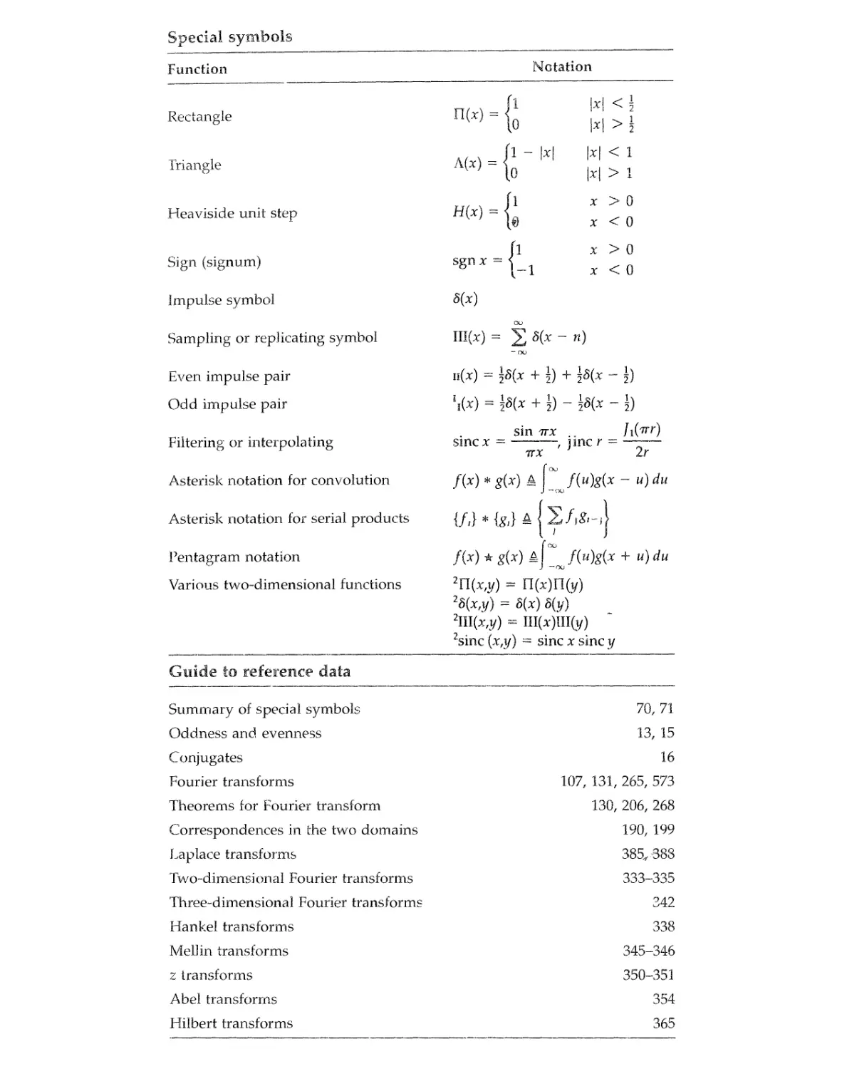
Function
Rectangle
Triangle
Heaviside unit step
Sign (signum)
Impulse symbol
Sampling or replicating symbol
Even impulse pair
Odd impulse pair
Filtering or interpolating
Asterisk notation for convolution
A(x) =
H(x) =
sgnx =
[0
1 - |x
10
\x
^ i
^ 2
< 1
1
—-1
|x| > 1
x > 0
x < 0
x > 0
x < 0
CXJ
<5(x)
III(x) = ^ S(x - n)
n(x) = f
- oo
\S(x - 1
,(x) = iS(x + 1) - |S(x - 1)
sin ttx J\Grr)
sine x = — . i me r = ——
ttx J 2r
fcxj
A f(u)g(x - u)du
— oo
Asterisk notation for serial products {/,} * {g,} A
oo
Pentagram notation
Various two-dimensional functions
Guide to reference data
Summary of special symbols
Oddness and evenness
Conjugates
Fourier transforms
Theorems for Fourier transform
Correspondences in the two domains
Laplace transforms
Two-dimensional Fourier transforms
Three-dimensional Fourier transforms
Hankel transforms
Mel! in transforms
z transforms
Abel transforms
Hilbert transforms
f(x) * g(x) A f(u)g(x 4- u) du
) —no
2n(x,y) = n(x)r%)
28(x,y) = 8{x) %)
2sinc (x,y) ~ sine x sine y
70,71
13, 15
16
107, 131, 265, 573
130, 206, 268
190, 199
385,688
333-335
342
338
345-346
350-351
354
365
U(x)
H(x)
sgn*
8(x)
A. .A.
Ul(x)
u(x)
h(x)
sine x
McGraw-Hill Series in Electrical and Computer Engineering
SENIOR CONSULTING EDITOR
Stephen W. Director, University of Michigan, Ann Arbor
Circuits and Systems
Communications and Signal Processing
Computer Engineering
Control Theory and Robotics
Electromagnetics
Electronics and VLSI Circuits
Introductory
Power
Antennas, Microwaves, and Radar
PREVIOUS CONSULTING EDITORS
Ronald N. Bracewell, Colin Cherry, James F. Gibbons, Willis W. Harman,
Hubert Heffner, Edward W. Herold, John G. Linvill, Simon Ramo, Ronald A.
Rohrer, Anthony E, Siegman, Charles Susskind, Frederick E. Terman, John G.
Truxal, Ernst Weber, and John R. Whinnery
Circuits and Systems
SENIOR CONSULTING EDITOR
Stephen W. Director, University of Michigan, Ann Arbor
Antoniou: Digital Filters: Analysis and Design
Balabanian: Electric Circuits
Bracewell: The Fourier Transform and Its Applications
Chua, Desoer, and Kuh: Linear and Non-Linear Circuits
Conant: Engineering Circuit Analysis with PSPICE and PROBE
Hayt and Kemmerly: Engineering Circuit Analysis
Huelsman: Active and Passive Analog Filter Design: An Introduction
Papoulis: The Fourier Integral and Its Applications
Paul: Analysis of Linear Circuits
Pillage and Rohrer: Electronic Circuit and System Simulation Methods
Reid: Linear System Fundamentals: Continuous and Discrete, Classic and Modern
Siebert: Circuits, Signals and Systems
Temes and LaPatra: Introduction to Circuit Synthesis
Waters: Active Filter Design
Joseph Fourier, 21 March 1768-16
Bibliotheque Municipale de Grenoble
The Fourier Transform and
Its Applications
Third Edition
Ronald N. Bracewell
Lewis M. Terman Professor of Electrical Engineering Emeritus
Stanford University
Boston Burr Ridge, IL Dubuque, IA Madison, WI New York San Francisco St. Louis
Bangkok Bogota Caracas Lisbon London Madrid
Mexico City Milan New Delhi Seoul Singapore Sydney Taipei Toronto
McGraw-Hill Higher Education
A Division of The McGraw-Hill Companies
THE FOURIER TRANSFORMATION AND ITS APPLICATIONS
Copyright © 2000, 1986, 1978, 1965 by The McGraw-Hill Companies, Inc. All rights reserved.
Printed in the United States of America. Except as permitted under the United States Copyright Act
of 1976, no part of this publication may be reproduced or distributed in any form or by any means,
or stored in a data base or retrieval system, without the prior written permission of the publisher.
This book is printed on acid-free paper.
1234567890 FGR/FGR 9098765432109
ISBN 0-07-303938-1
Vice president/Editor-in-Chief: Kevin T. Kane
Publisher: Thomas Casson
Executive editor: Elizabeth A. Jones
Sponsoring editor: Catherine Fields
Editorial assistant: Michelle L. Flomenhoft
Marketing manager: John T Wannemacher
Project manager: Jim Labeots
Senior production supervisor: Heather D. Burbridge
Freelance design coordinator: Mary Christianson
Freelance cover designer: Lynn Knipe
Senior photo research coordinator: Keri Johnson
Supplement coordinator: Marc Mattson
Compositor: York Graphic Services, Inc.
Typeface: 20/22 Palatino
Printer: Quebecor Printing Book Group/Fairfield
Library of Congress Cataloging-in-Publication Data
Bracewell, Ronald Newbold (date)
The Fourier transform and its applications / Ronald N. Bracewell. —
3rd ed.
p. cm.
ISBN 0-07-303938-1
1. Fourier transformations. 2. Transformations (Mathematics).
3. Harmonic analysis. I. Title
QA403.5.B7 2000
515/.723 dc—21 99-21139
http://www.mhhe.com
ABOUT THE AUTHO
RONALD N. BRACEWELL was born in Australia, received his B.Sc, B.E., and
M.E. degrees from the University of Sydney, and earned a Ph.D. in physics from
Cambridge University Currently L. M. Terman Professor of Electrical Engineer-
Engineering Emeritus at Stanford University, Dr. Bracewell has an impressive roster of pro-
professional affiliations, awards, and publications to his credit. He is a Fellow of the
Royal Astronomical Society, the Astronomical Society of Australia, and past Coun-
Councilor of the American Astronomical Society. He is also a life Fellow and Heinrich
Hertz gold medalist of the Institute of Electrical and Electronic Engineers. At Stan-
Stanford Radio Astronomy Institute he designed and built innovative radio telescopes,
including the first antenna with the resolution of the human eye, less than one
minute of arc, and was involved in early discoveries relating to the cosmic back-
background radiation. Fourier analysis played a key role in his novel instrument de-
design and data processing. Fourier's admirable ideas also contributed to Dr.
Bracewell's advances in tomographic imaging which led to his election to the In-
Institute of Medicine of the National Academy of Sciences, to receiving Sydney Uni-
University's inaugural Alumni Award for Achievement, and to being appointed an
Officer of the Order of Australia for service to science in the fields of radio as-
astronomy and image reconstruction.
Fourier's theorem is not only one of the most beautiful results of modern
analysis, but it may be said to furnish an indispensable instrument in the
treatment of nearly every recondite question in modern physics.
Lord Kelvin
To my wife Helen,
whose support made
this edition possible.
Ronald Bracewell
CONTENTS
Preface xvii
1 Introduction 1
2 Groundwork 5
The Fourier Transform and Fourier's Integral Theorem 5
Conditions for the Existence of Fourier Transforms 8
Transforms in the Limit 10
Oddness and Evenness 11
Significance of Oddness and Evenness 13
Complex Conjugates 14
Cosine and Sine Transforms 16
Interpretation of the Formulas 18
3 Convolution 24
Examples of Convolution 27
Serial Products 30
Inversion of serial multiplication / The serial product in matrix notation /
Sequences as vectors
Convolution by Computer 39
The Autocorrelation Function and Pentagram Notation 40
The Triple Correlation 45
The Cross Correlation 46
The Energy Spectrum 47
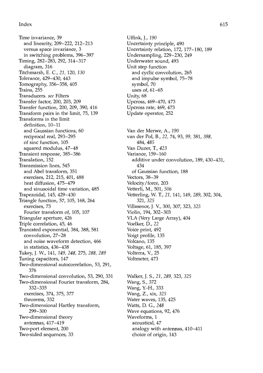
4 Notation for Some Useful Functions 55
Rectangle Function of Unit Height and Base, Il(x) 55
Triangle Function of Unit Height and Area, A(x) 57
Various Exponentials and Gaussian and Rayleigh Curves 57
Heaviside's Unit Step Function, H(x) 61
The Sign Function, sgn x 65
The Filtering or Interpolating Function, sine x 65
Pictorial Representation 68
Summary of Special Symbols 71
ix
x Contents
5 The Impulse Symbol 74
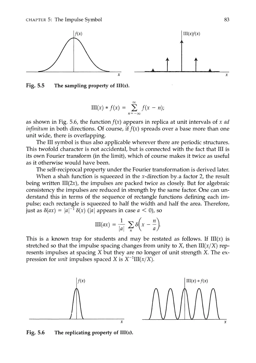
The Sifting Property 78
The Sampling or Replicating Symbol III(x) 81
The Even and Odd Impulse Pairs n(x) and h(x) 84
Derivatives of the Impulse Symbol 85
Null Functions 87
Some Functions in Two or More Dimensions 89
The Concept of Generalized Function 92
Particularly well-behaved functions / Regular sequences / Generalized functions /
Algebra of generalized functions / Differentiation of ordinary functions
6 The Basic Theorems 105
A Few Transforms for Illustration 105
Similarity Theorem 108
Addition Theorem 110
Shift Theorem 111
Modulation Theorem 113
Convolution Theorem 115
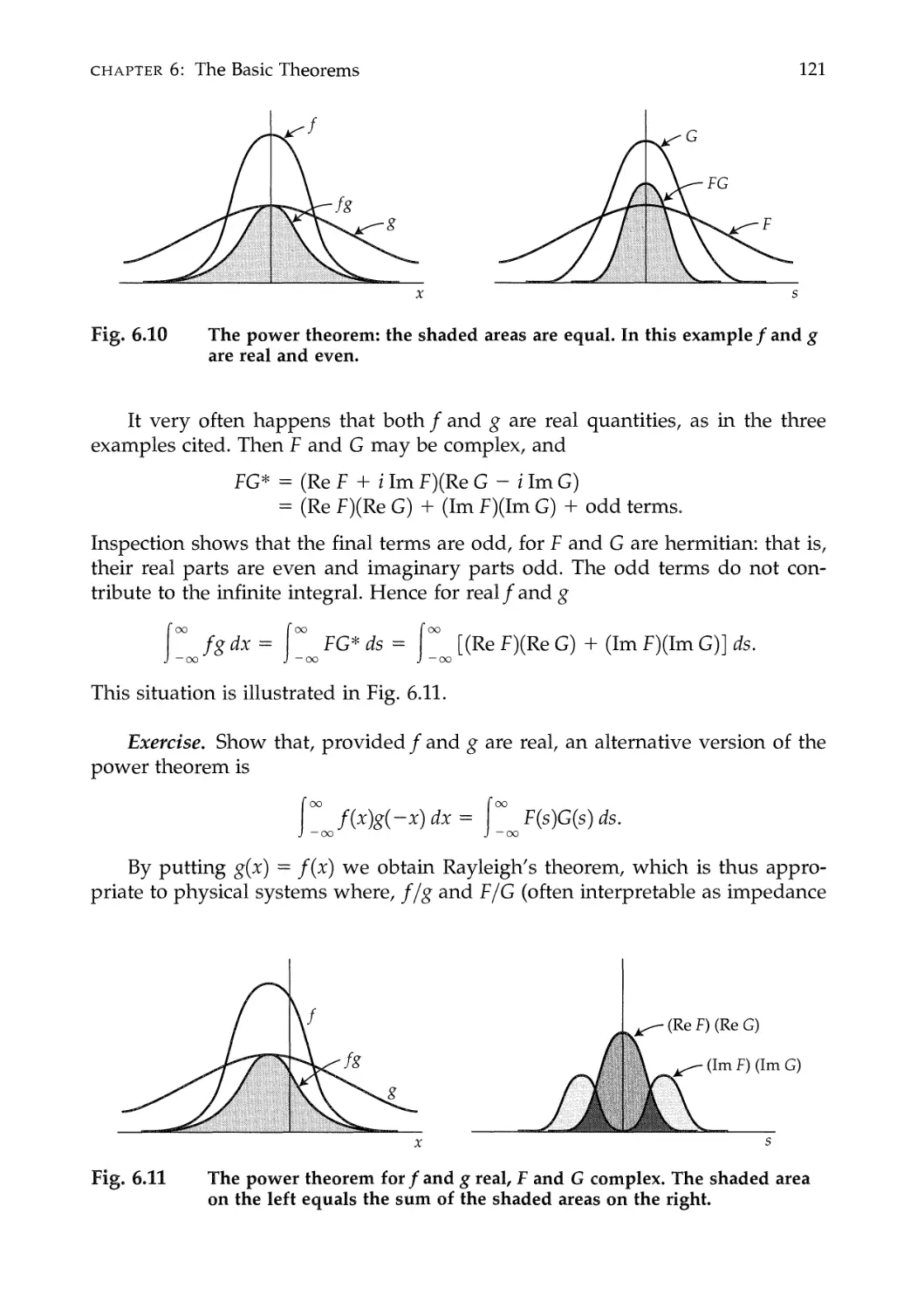
Rayleigh's Theorem 119
Power Theorem 120
Autocorrelation Theorem 122
Derivative Theorem 124
Derivative of a Convolution Integral 126
The Transform of a Generalized Function 127
Proofs of Theorems 128
Similarity and shift theorems / Derivative theorem / Power theorem
Summary of Theorems 129
7 Obtaining Transforms 136
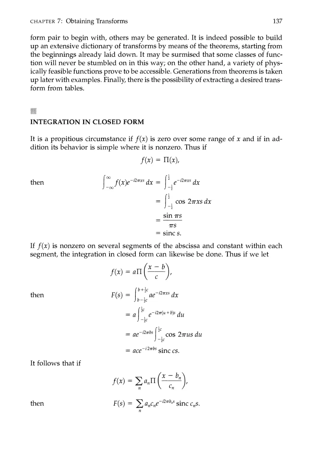
Integration in Closed Form 137
Numerical Fourier Transformation 140
The Slow Fourier Transform Program 142
Generation of Transforms by Theorems 145
Application of the Derivative Theorem to Segmented Functions 145
Measurement of Spectra 147
Radiofrequency spectral analysis / Optical Fourier transform spectroscopy
8 The Two Domains 151
Definite Integral 152
The First Moment 153
Centroid 155
Moment of Inertia (Second Moment) 156
Moments 157
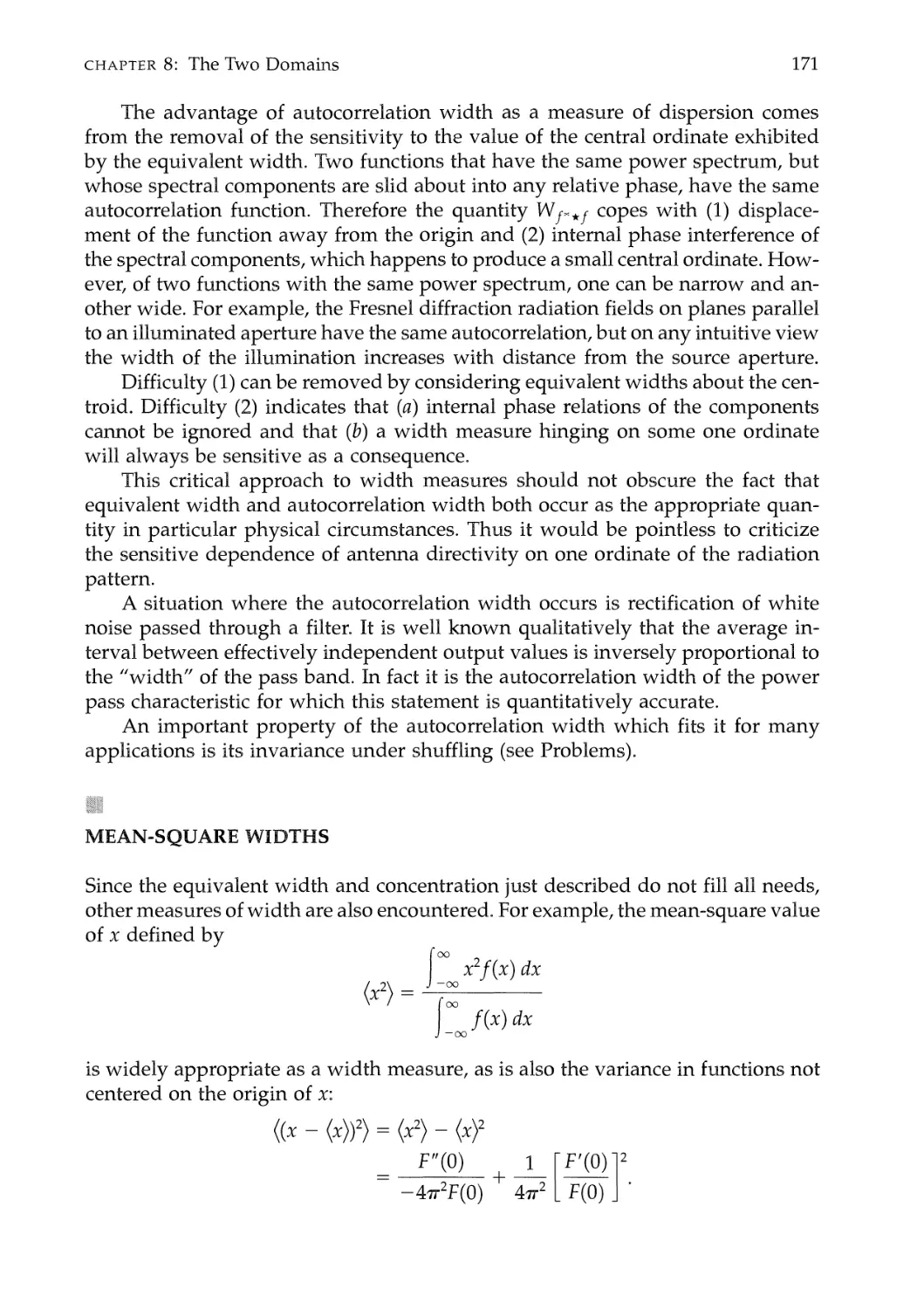
Mean-Square Abscissa 158
Radius of Gyration 159
Contents xi
Variance 159
Smoothness and Compactness 160
Smoothness under Convolution 162
Asymptotic Behavior 163
Equivalent Width 164
Autocorrelation Width 170
Mean Square Widths 171
Sampling and Replication Commute 172
Some Inequalities 174
Upper limits to ordinate and slope / Schwarz's inequality
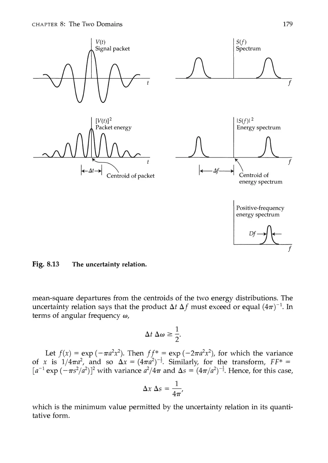
The Uncertainty Relation 177
Proof of uncertainty relation /Example of uncertainty relation
The Finite Difference 180
Running Means 184
Central Limit Theorem 186
Summary of Correspondences in the Two Domains 191
9 Waveforms, Spectra, Filters, and Linearity 198
Electrical Waveforms and Spectra 198
Filters 200
Generality of Linear Filter Theory 203
Digital Filtering 204
Interpretation of Theorems 205
Similarity theorem / Addition theorem / Shift theorem / Modulation theorem /
Converse of modulation theorem
Linearity and Time Invariance 209
Periodicity 211
10 Sampling and Series 219
Sampling Theorem 219
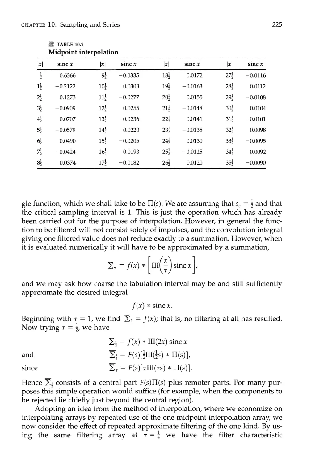
Interpolation 224
Rectangular Filtering in Frequency Domain 224
Smoothing by Running Means 226
Undersampling 229
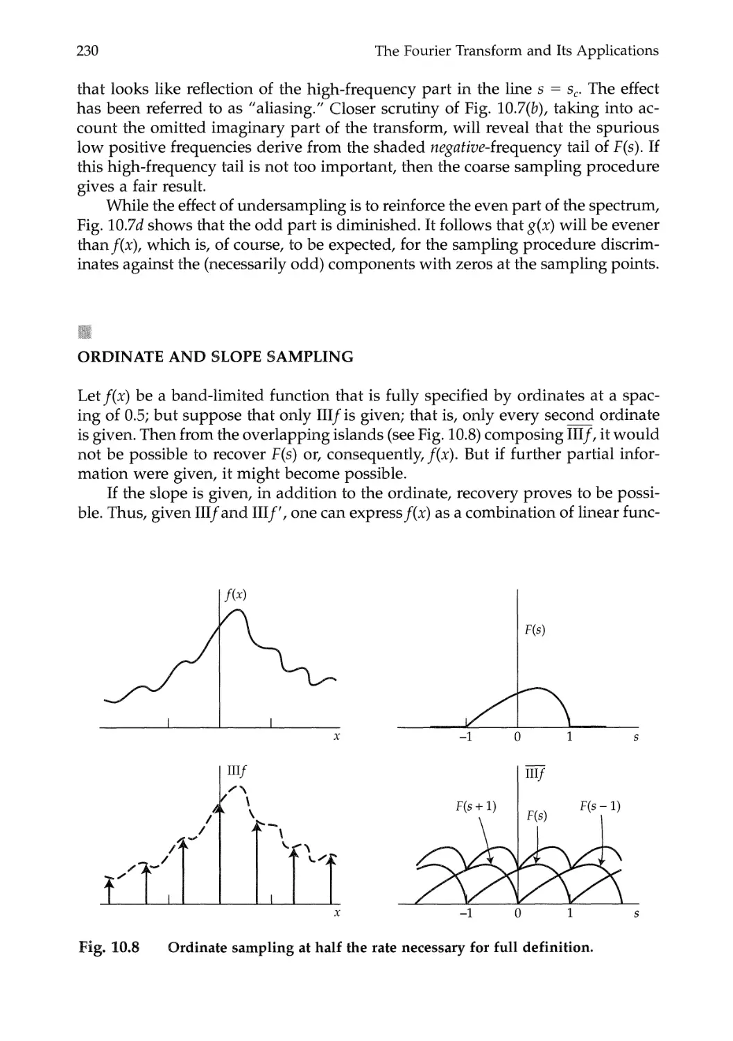
Ordinate and Slope Sampling 230
Interlaced Sampling 232
Sampling in the Presence of Noise 234
Fourier Series 235
Gibbs phenomenon / Finite Fourier transforms / Fourier coefficients
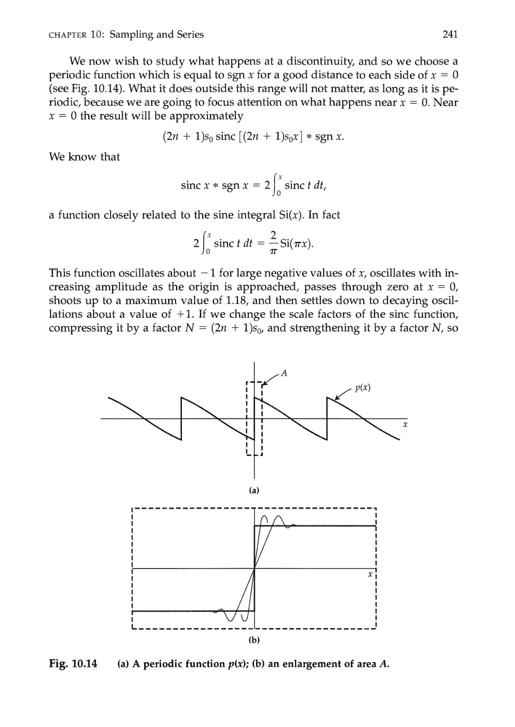
Impulse Trains That Are Periodic 245
The Shah Symbol Is Its Own Fourier Transform 246
11 The Discrete Fourier Transform and the FFT 258
The Discrete Transform Formula 258
Cyclic Convolution 264
Examples of Discrete Fourier Transforms 265
xii Contents
Reciprocal Property 266
Oddness and Evenness 266
Examples with Special Symmetry 267
Complex Conjugates 268
Reversal Property 268
Addition Theorem 268
Shift Theorem 268
Convolution Theorem 269
Product Theorem 269
Cross-Correlation 270
Autocorrelation 270
Sum of Sequence 270
First Value 270
Generalized Parseval-Rayleigh Theorem 271
Packing Theorem 271
Similarity Theorem 272
Examples Using MATLAB 272
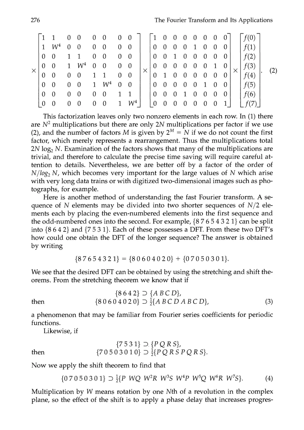
The Fast Fourier Transform 275
Practical Considerations 278
Is the Discrete Fourier Transform Correct? 280
Applications of the FFT 281
Timing Diagrams 282
When N Is Not a Power of 2 283
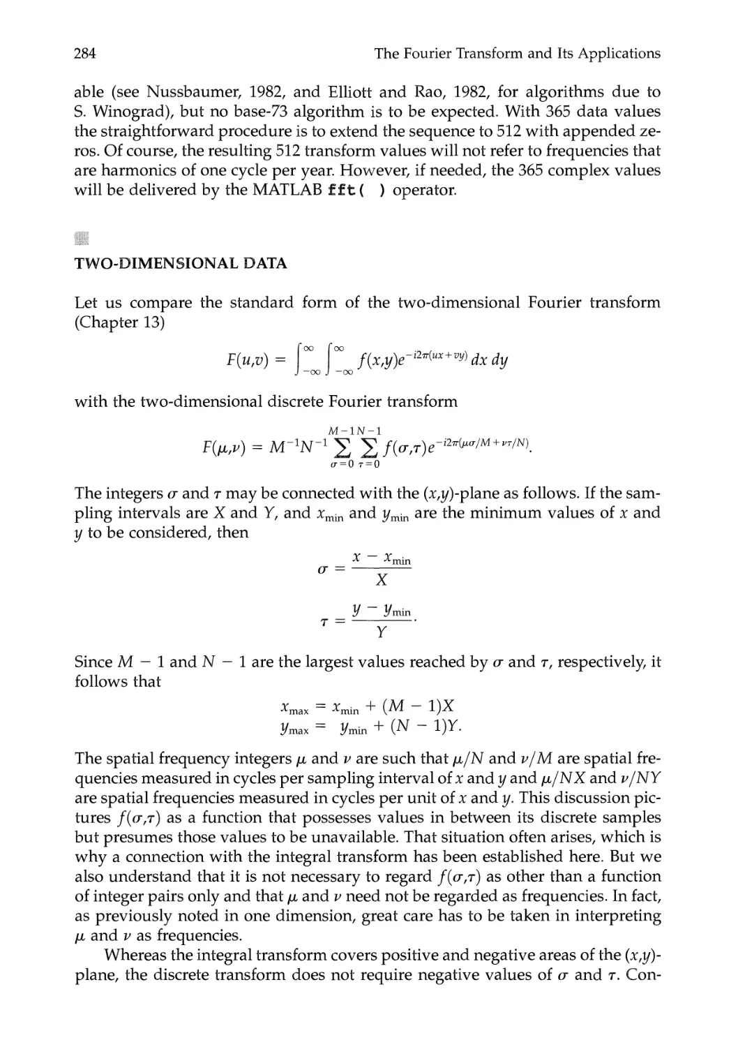
Two-Dimensional Data 284
Power Spectra 285
12 The Discrete Hartley Transform 293
A Strictly Reciprocal Real Transform 293
Notation and Example 294
The Discrete Hartley Transform 295
Examples of DHT 297
Discussion 298
A Convolution of Algorithm in One and Two Dimensions 298
Two Dimensions 299
The Cas-Cas Transform 300
Theorems 300
The Discrete Sine and Cosine transforms 301
Boundary value problems / Data compression application
Computing 305
Getting a Feel for Numerical Transforms 305
The Complex Hartley Transform 306
Physical Aspect of the Hartley Transformation 307
The Fast Hartley Transform 308
The Fast Algorithm 309
Running Time 314
Contents xiii
Timing via the Stripe Diagram 315
Matrix Formulation 317
Convolution 320
Permutation 321
A Fast Hartley Subroutine 322
13 Relatives of the Fourier Transform 329
The Two-Dimensional Fourier Transform 329
Two-Dimensional Convolution 331
The Hankel Transform 335
Fourier Kernels 339
The Three-Dimensional Fourier Transform 340
The Hankel Transform in n Dimensions 343
The Mellin Transform 343
The z Transform 347
The Abel Transform 351
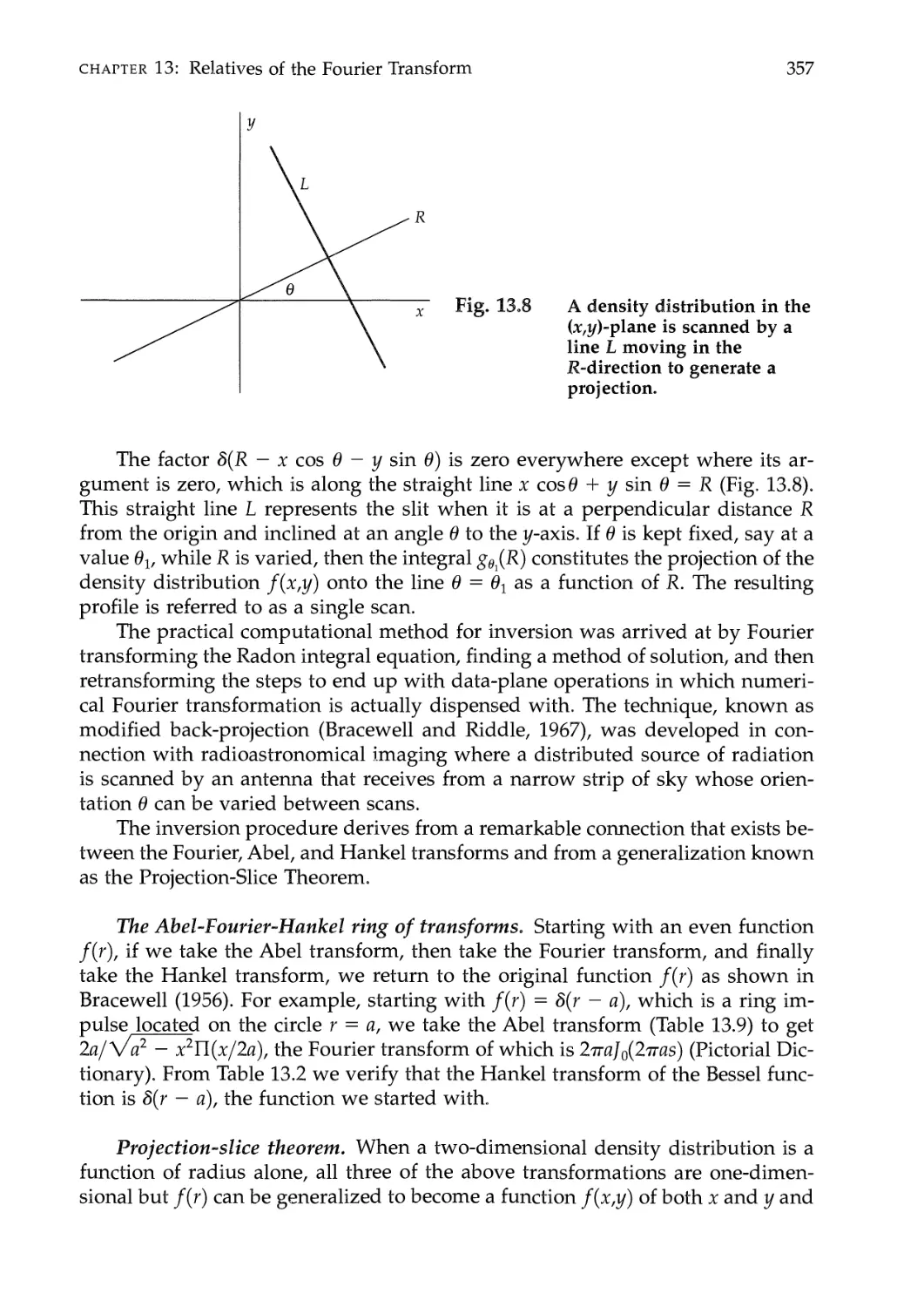
The Radon Transform and Tomography 356
The Abel-Fourier-Hankel ring of transforms / Projection-slice theorem /
Reconstruction by modified back projection
The Hilbert Transform 359
The analytic signal / Instantaneous frequency and envelope / Causality
Computing the Hilbert Transform 364
The Fractional Fourier Transform 367
Shift theorem / Derivative theorems / Fractional convolution theorem /
Examples of transforms
14 The Laplace Transform 380
Convergence of the Laplace Integral 382
Theorems for the Laplace Transform 383
Transient-Response Problems 385
Laplace Transform Pairs 386
Natural Behavior 389
Impulse Response and Transfer Function 390
Initial-Value Problems 392
Setting Out Initial-Value Problems 396
Switching Problems 396
15 Antennas and Optics 406
One-Dimensional Apertures 407
Analogy with Waveforms and Spectra 410
Beam Width and Aperture Width 411
Beam Swinging 412
Arrays of Arrays 413
Interferometers 414
Spectral Sensitivity Function 415
xiv Contents
Modulation Transfer Function 416
Physical Aspects of the Angular Spectrum 417
Two-Dimensional Theory 417
Optical Diffraction 419
Fresnel Diffraction 420
Other Applications of Fourier Analysis 422
16 Applications in Statistics 428
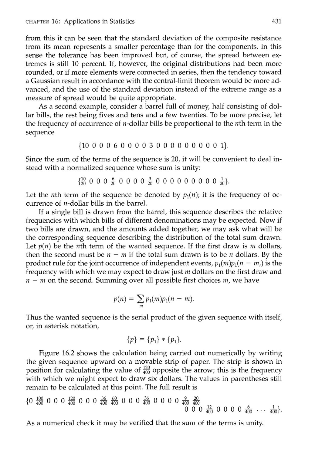
Distribution of a Sum 429
Consequences of the Convolution Relation 434
The Characteristic Function 435
The Truncated Exponential Distribution 436
The Poisson Distribution 438
17 Random Waveforms and Noise 446
Discrete Representation by Random Digits 447
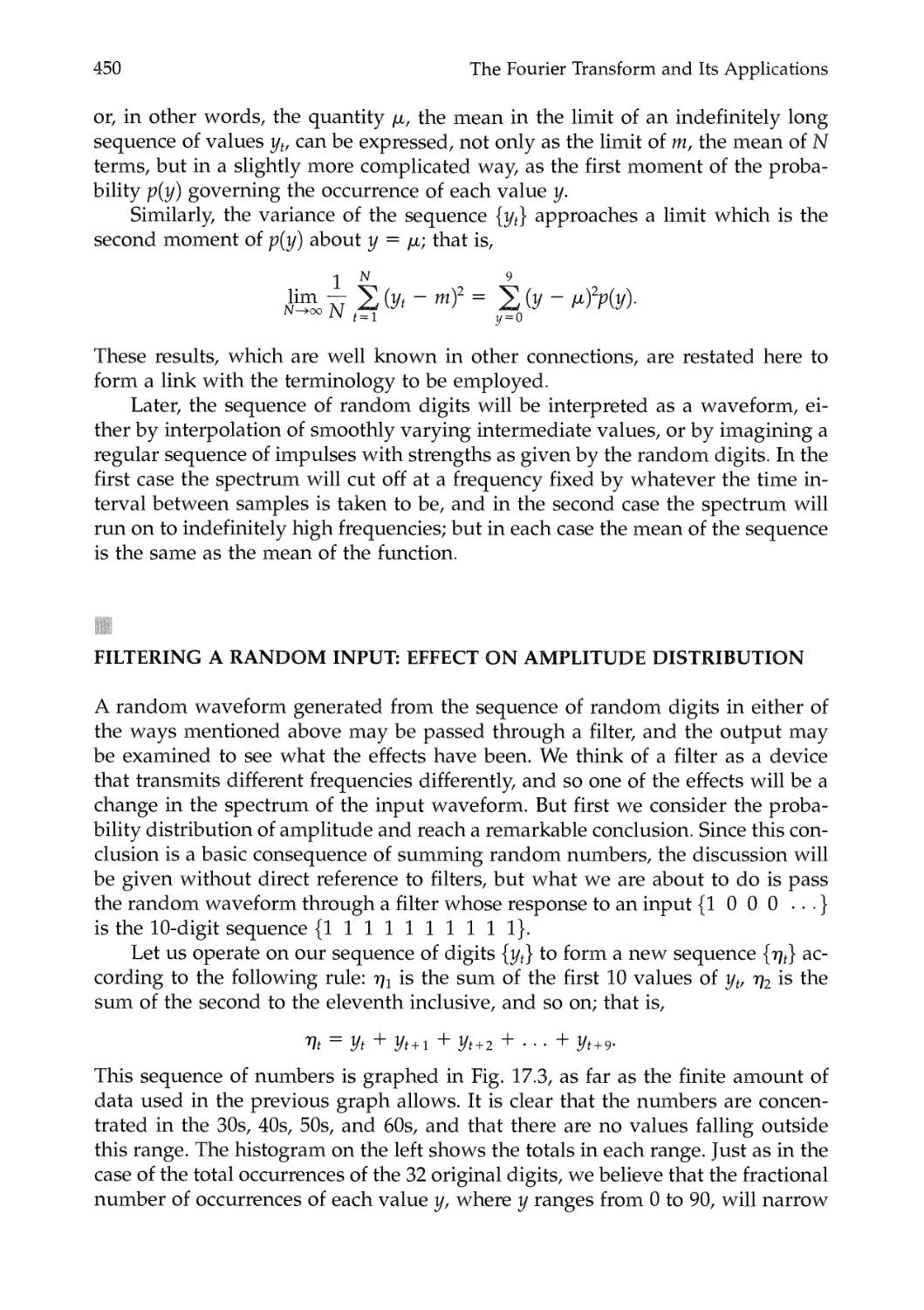
Filtering a Random Input: Effect on Amplitude Distribution 450
Digression on independence / The convolution relation
Effect on Autocorrelation 455
Effect on Spectrum 458
Spectrum of random input / The output spectrum
Some Noise Records 462
Envelope of Bandpass Noise 465
Detection of a Noise Waveform 466
Measurement of Noise Power 466
18 Heat Conduction and Diffusion 475
One-Dimensional Diffusion 475
Gaussian Diffusion from a Point 480
Diffusion of a Spatial Sinusoid 481
Sinusoidal Time Variation 485
19 Dynamic Power Spectra 489
The Concept of Dynamic Spectrum 489
The Dynamic Spectrograph 491
Computing the Dynamic Power Spectrum 494
Frequency division / Time division / Presentation
Equivalence Theorem 497
Envelope and Phase 498
Using log/instead of/ 499
The Wavelet Transform 500
Adaptive Cell Placement 502
Elementary Chirp Signals (Chirplets) 502
The Wigner Distribution 504
Contents xv
20 Tables of sine x, sine2 x, and exp (—ttx2) 508
21 Solutions to Selected Problems 513
Chapter 2 Groundwork 513
Chapter 3 Convolution 514
Chapter 4 Notation for Some Useful Functions 516
Chapter 5 The Impulse Symbol 517
Chapter 6 The Basic Theorems 522
Chapter 7 Obtaining Transforms 524
Chapter 8 The Two Domains 526
Chapter 9 Waveforms, Spectra, Filters, and Linearity 530
Chapter 10 Sampling and Series 532
Chapter 11 The Discrete Fourier Transform and the FFT 534
Chapter 12 The Hartley Transform 537
Chapter 13 Relatives of the Fourier Transform 538
Chapter 14 The Laplace Transform 539
Chapter 15 Antennas and Optics 545
Chapter 16 Applications in Statistics 555
Chapter 17 Random Waveforms and Noise 557
Chapter 18 Heat Conduction and Diffusion 565
Chapter 19 Dynamic Spectra and Wavelets 571
22 Pictorial Dictionary of Fourier Transforms 573
Hartley Transforms of Some Functions without Symmetry 592
23 The Life of Joseph Fourier 594
Index 597
E F A C
I ransform methods provide a unifying mathematical approach to the study of
electrical networks, devices for energy conversion and control, antennas, and other
components of electrical systems, as well as to complete linear systems and to
many other physical systems and devices, whether electrical or not. These same
methods apply equally to the subjects of electrical communication by wire or op-
optical fiber, to wireless radio propagation, and to ionized media—which are all con-
concerned with the interconnection of electrical systems—and to information theory
which, among other things, relates to the acquisition, processing, and presenta-
presentation of data. Other theoretical techniques are used in handling these basic fields
of electrical engineering, but transform methods are virtually indispensable in all
of them. Fourier analysis as applied to electrical engineering is sufficiently im-
important to have earned a permanent place in the curriculum—indeed much of the
mathematical development took place in connection with alternating current the-
theory, signal analysis, and information theory as formulated in connection with elec-
electrical communication.
This is why much of the literature dealing with technical applications has ap-
appeared in electrical and electronic journals. Despite the strong bonds with elec-
electrical engineering, Fourier analysis nevertheless has become indispensable in bio-
medicine and remote sensing (geophysics, oceanography, planetary surfaces, civil
engineering), where practitioners now outnumber those electrical engineers who
regularly use Fourier analysis. But the teaching of Fourier analysis and its appli-
applications still finds its home in electrical engineering.
A course on transforms and their applications has formed part of the electri-
electrical engineering curriculum at Stanford University for many years and has been
given with no prerequisites beyond those that the holder of a bachelor's degree
normally possesses. One objective has been to develop a pivotal course to be taken
at an early stage by all graduates, so that in later, more specialized courses, the
student would be spared encountering the same material over and over again;
later instructors can then proceed more directly to their special subject matter.
It is clearly not feasible to give the whole of linear mathematics in a single
course; the choice of core material must necessarily remain a matter of local judg-
judgment. The choice will, however, be of most help to later instructors if sharply de-
defined.
An early-level course should be simple, but not trivial; the objective of this
book is to simplify the presentation of many key topics that are ordinarily dealt
xvn
XV111
Preface
with in advanced contexts, by making use of suitable notation and an approach
through convolution.
One way of working from the book is to begin by taking the chapters in nu-
numerical order. This sequence is feasible for students who could read the first half
unassisted or who could be taken through it rapidly in a few lectures; but if the
material is approached at a more normal pace, then, as a practical matter, it is a
good idea to interpret each theorem and concept in terms of a physical example.
Waveforms and their spectra and elementary diffraction theory are suitable. Af-
After that, the chapters on applications can then be selected in whatever sequence
is desired. The organization of chapters is as follows:
1. Introduction
i
2. Groundwork
i
3. Convolution
i
4. Notation . . .
I
5. The Impulse Symbol
6. The Basic Theorems
i
7. Obtaining Transforms
i
8. The Two Domains —>-
Choices
Applications
Reference
-H
- 9. Waveforms, Spectra,...
10. Sampling and Series
11. Discrete FT and FFT
12. Hartley Transform
L13. Relatives —» 14. Laplace
15. Antennas and Optics
19. Dynamic Spectra
16. Statistics -> 17. Noise
18. Heat and Diffusion
■20. Tables of sine, . . .
21. Solutions to Problems
22. Pictorial Dictionary
■23. Biography of Fourier
The amount of material is suitable for one semester, or for one quarter, ac-
according to how many of the later chapters on applications are included. A practi-
practical plan is to leave the choice of chapters on applications to the current instructor.
Many fine mathematical texts on the Fourier transform have been published.
This book differs in that it is intended for those who are concerned with apply-
applying Fourier transforms to physical situations rather than with pursuing the math-
mathematical subject as such. The connections of the Fourier transform with other
transforms are also explored, and the text has been purposely enriched with con-
condensed information that will suit it for use as a reference source for transform
pairs and theorems pertaining to transforms.
My interest in the subject was fired while studying analysis from H. S.
Carslaw's "Fourier Series and Integrals'' at the University of Sydney in 1939. I
learned about physical applications as a colleague of J. C. Jaeger at C.S.I.R Ra-
diophysics Laboratory and inherited the physical wisdom of the crystallographers
of the Cavendish Laboratory, Cambridge, as transmitted by J. A. Ratcliffe. Trans-
Transform methods are at the heart of the electrical engineering curriculum. Digital
Preface xix
computing and data processing, which have emerged as large curricular segments,
though rather different in content from the rigorous study of circuits, electronics,
and waves, nevertheless do share a common bond through the Fourier transform.
The diffusion equation, which long ago had a connection with submarine cable
telegraphy, has reemerged as an essential consideration in solid state physics and
devices, both through the practice of doping, by which semiconductor devices are
fabricated, and as a controlling influence in electrical conduction by holes and
electrons. Needless to say, a grasp of Fourier fundamentals is an asset in the solid-
state laboratory.
The explosion of image engineering, much of which can be interpreted via
two-dimensional generalization, has reinforced the value of a core course. Con-
Consequently, the subject matter of this book has easily moved into the pivotal role
foreseen for it, and faculty members from various specialties have found them-
themselves comfortable teaching it. The course is taken by first-year graduate students,
especially students arriving from other universities, and by students from other
departments, notably applied physics and earth sciences. The course is accessible
to students in the last year of their bachelor's degree.
Introduction of the fast Fourier transform (FFT) algorithm has greatly broad-
broadened the scope of application of the Fourier transform to data handling and to
digital formulation in general and has brought prominence to the discrete Fourier
transform (DFT). The technological revolution associated with discrete mathe-
mathematics as treated in Chapter 11 has made an understanding of Fourier notions
(such as aliasing, which only aficionados used to guard against) indispensable to
any professional who handles masses of data, not only engineers but experts in
many subfields of medicine, biology, and remote sensing. Developments based
on Ralph V. L. Hartley's equations (Chapter 12) have made it possible to dispense
with imaginaries in computed Fourier analysis and to proceed elegantly and sim-
simply using the real Hartley formalism.
Hartley's equations, which quietly received honorable mention in the first edi-
edition of this book, gained major relevance to signal processing as computers flour-
flourished. In 1983 I gave them new life in a time-series context with modern notation
under the title of discrete Hartley transform, a name that is now universally rec-
recognized, while Z. Wang (Appl. Math, and Comput., vol. 9, pp. 53-73, 153-163,
245-255, 1983) independently stimulated mathematicians. Hartley's cas (cosine
and sine) function is now widely recognized.
For those who like to do their own computer programming some segments
of pseudocode have been supplied. Translating into your language of choice may
give some insights that complement the algebraic and graphical viewpoints. Fur-
Furthermore, executing numerical examples develops a useful sort of intuition which,
while not as powerful as physical intuition, adds a further dimension to one's ex-
experience. Pseudocode is suited to readers who cannot be expected to know sev-
several popular languages. The aim is to provide the simplest intelligible instructions
that are susceptible to simultaneous transcription into the language of fluency of
the reader, who provides the necessary protocol, array declarations, and other dis-
distinctive features.
xx Preface
The code segments in this book are presented to supplement verbal explana-
explanation, not to be a substitute for a computational toolbox.
However, it is often more important to be able to use a computer algorithm
than to understand in detail how it was constructed, just as when using a table
of integrals or an engineering design handbook. To meet this need and to bring
the power of Fourier transformation into the hands of a much wider constituency,
packages of software tools have been created commercially and have become in-
indispensable. A popular example is MATLAB®, a user-friendly, higher-level,
special-purpose application whose use is illustrated in Chapters 7 and 11.
Caution is needed in circumstances where the user is shielded from the al-
algorithmic details; it is handy to know what to expect before being presented with
computer output. For this and other reasons, transforms presented graphically in
the Pictorial Dictionary have proved to be a useful reference feature. Graphical
presentation is a useful adjunct to the published compilations of integral trans-
transforms, where it is sometimes frustrating to seek commonly needed entries among
the profusion of rare cases and where, in addition, simple functions that are im-
impulsive, discontinuous, or defined piecewise may be hard to recognize or may not
be included at all.
A good problem assigned at the right stage can be extremely valuable for the
student, but a good problem is hard to compose. Many of the problems here go
beyond mathematical exercises by inclusion of technical background or by ask-
asking for opinions. Those wishing to mine the good material in the problems will
appreciate that many of them are now titled, a practice that should be more widely
adopted. Many of the problems are discussed in Chapter 21, but occasionally it
is nice to have a new topic followed by an exercise that is in close proximity rather
than at the end of the chapter; a sprinkling of these is provided.
Notation is a vital adjunct to thinking, and I am happy to report that the sine
function, which we learned from P. M. Woodward, is alive and well, and surviv-
surviving erosion by occasional authors who do not know that "sine x over x" is not the
sine function. The unit rectangle junction (unit height and width) n(x), the trans-
transform of the sine function, has also proved extremely useful, especially for black-
blackboard work. In typescript or other media where the Greek letter is less desirable,
n(x) may be written "rect x," and it is convenient in any case to pronounce it rect.
The jinc function, the circular analogue of the sine function, has the correspond-
corresponding virtues of normalization and the distinction of describing the diffraction field
of a telescope or camera. The shah function III(x) has caught on. It is easy to print
and is twice as useful as you might think because it is its own transform. The as-
asterisk for convolution, which was in use a long time ago by Volterra and perhaps
earlier, is now in wide use and I recommend ** to denote two-dimensional con-
convolution, which has become common as a result of the explosive growth of im-
image processing.
Early emphasis on digital convolution in a text on the Fourier transform
turned out to be exactly the way to start. Convolution has changed in a few years
from being presented as a rather advanced concept to one that can be easily ex-
explained at an early stage, as is fitting for an operation that applies to all those sys-
systems that respond sinusoidally when you shake them sinusoidally.
1
Introduction
Linear transforms, especially those named for Fourier and Laplace, are well
known as providing techniques for solving problems in linear systems. Charac-
Characteristically one uses the transformation as a mathematical or physical tool to al-
alter the problem into one that can be solved. This book is intended as a guide to
the understanding and use of transform methods in dealing with linear systems.
The subject is approached through the Fourier transform. Hence, when the
more general Laplace transform is discussed later, many of its properties will al-
already be familiar and will not distract from the new and essential question of the
strip of convergence on the complex plane. In fact, all the other transforms dis-
discussed here are greatly illuminated by an approach through the Fourier trans-
transform.
Fourier transforms play an important part in the theory of many branches of
science. While they may be regarded as purely mathematical functionals, as is
customary in the treatment of other transforms, they also assume in many fields
just as definite a physical meaning as the functions from which they stem. A wave-
waveform—optical, electrical, or acoustical—and its spectrum are appreciated equally
as physically picturable and measurable entities: an oscilloscope enables us to see
an electrical waveform, and a spectroscope or spectrum analyzer enables us to
see optical or electrical spectra. Our acoustical appreciation is even more direct,
since the ear hears spectra. Waveforms and spectra are Fourier transforms of each
other; the Fourier transformation is thus an eminently physical relationship.
The number of fields in which Fourier transforms appear is surprising. It is a
common experience to encounter a concept familiar from one branch of study in
a slightly different guise in another. For example, the principle of the phase-
contrast microscope is reminiscent of the circuit for detecting frequency modula-
modulation, and the explanation of both is conveniently given in terms of transforms along
the same lines. Or a problem in statistics may yield to an approach which is fa-
familiar from studies of cascaded amplifiers. This is simply a case of the one un-
underlying theorem from Fourier theory assuming different physical embodiments.
2 The Fourier Transform and Its Applications
It is a great advantage to be able to move from one physical field to another
and to carry over the experience already gained, but it is necessary to have the
key which interprets the terminology of the new field. It will be evident, from the
rich variety of topics coming within its scope, what a pervasive and versatile tool
Fourier theory is.
Many scientists know Fourier theory not in terms of mathematics, but as a
set of propositions about physical phenomena. Often the physical counterpart of
a theorem is a physically obvious fact, and this allows the scientist to be abreast
of matters which in the mathematical theory may be quite abstruse. Emphasis on
the physical interpretation enables us to deal in an elementary manner with top-
topics which in the normal course of events would be considered advanced.
Although the Fourier transform is vital in so many fields, it is often encoun-
encountered in formal mathematics courses in the last lecture of a formidable course on
Fourier series. As need arises it is introduced ad hoc in later graduate courses but
may never develop into a usable tool. If this traditional order of presentation is
reversed, the Fourier series then falls into place as an extreme case within the
framework of Fourier transform theory, and the special mathematical difficulties
with the series are seen to be associated with their extreme nature—which is non-
physical; the handicap imposed on the study of Fourier transforms by the cus-
customary approach is thus relieved.
The great generality of Fourier transform methods strongly qualifies the sub-
subject for introduction at an early stage, and experience shows that it is quite pos-
possible to teach, at this stage, the distilled theorems, which in their diverse appli-
applications offer such powerful tools for thinking out physical problems.
The present work began as a pictorial guide to Fourier transforms to com-
complement the standard lists of pairs of transforms expressed mathematically. It
quickly became apparent that the commentary would far outweigh the pictorial
list in value, but the pictorial dictionary of transforms is nevertheless important,
for a study of the entries reinforces the intuition, and many valuable and com-
common types of function are included which, because of their awkwardness when
expressed algebraically, do not occur in other lists.
A contribution has been made to the handling of simple but awkward func-
functions by the introduction of compact notation for a few basic functions which are
usually defined piecewise. For example, the rectangular pulse, which is at least
as simple as a Gaussian pulse, is given the name n(x), which means that it can
be handled as a simple function. The picturesque term "gate function/' which is
in use in electronics, suggests how a gating waveform Yl(t) opens a valve to let
through a segment of a waveform. This is the way we think of the rectangle func-
function mathematically when we use it as a multiplying factor.
Among the special symbols introduced or borrowed are n(x), the even im-
impulse pair, and III(x) (pronounced shah), the infinite impulse train defined by
III(x) = 2 8(x — n). The first of these two gains importance from its status as the
Fourier transform of the cosine function; the second proves indispensable in dis-
discussing both regular sampling or tabulation (operations which are equivalent to
multiplication by shah) and periodic functions (which are expressible as convolu-
chapter 1: Introduction
tions with shah). Since shah proves to be its own Fourier transform, it turns out to
be twice as useful an entity as might have been expected. Much freedom of ex-
expression is gained by the use of these conventions of notation, especially in con-
conjunction with the asterisk notation for convolution. Only a small step is involved
in writing n(x) */(%), or simply n * f, instead of
■*+!
x~-2
1 f(u) du
(for example, for the response to a photographic density distribution f(x) on a
sound track scanned with a slit). But the disappearance of the dummy variable
and the integral sign with limits, and the emergence of the character of the re-
response as a convolution between two profiles n and /, lead to worthwhile con-
convenience in both algebraic and mental manipulation.
Convolution is used a lot here. Experience shows that it is a fairly tricky con-
concept when it is presented bluntly under its integral definition, but it becomes easy
if the concept of a functional is first understood. Numerical practice on serial prod-
products confirms the feeling for convolution and incidentally draws attention to the
practical character of numerical evaluation: for numerical purposes one normally
prefers to have the answer to a problem come out as the convolution of two func-
functions rather than as a Fourier transform.
This is a good place to mention that transform methods do not necessarily in-
involve taking transforms numerically On the contrary, some of the best methods
for handling linear problems do not involve application of the Fourier or Laplace
transform to the data at all; but the basis for such methods is often clarified by
appeal to the transform domain. Thinking in terms of transforms, we may show
how to avoid numerical harmonic analysis or the handling of data on the com-
complex plane.
It is well known that the response of a system to harmonic input is itself har-
harmonic, at the same frequency, under two conditions: linearity and time invariance
of the system properties. These conditions are, of course, often met. This is why
Fourier analysis is important, why one specifies an amplifier by its frequency re-
response, why harmonic variation is ubiquitous. When the conditions for harmonic
response to harmonic stimulus break down, as they do in a nonlinear servo-
mechanism, analysis of a stimulus into harmonic components must be reconsid-
reconsidered. Time invariance can often be counted on even when linearity fails, but space
invariance is by no means as common. Failure of this condition is the reason that
bridge deflections are not studied by analyzing the load distribution into sinu-
sinusoidal components (space harmonics).
The two conditions for harmonic response to harmonic stimulus can be re-
restated as one condition: that the response shall be relatable to the stimulus by con-
convolution. For work in Fourier analysis, convolution is consequently profoundly
important, and such a pervasive phenomenon as convolution does not lack for
familiar examples. Good ones are the relation between the distribution on a film
sound track or recorder tape and the electrical signal read out through the scan-
scanning slit or magnetic head.
4 The Fourier Transform and Its Applications
Many topics normally considered abstruse or advanced are presented here,
and simplification of their presentation is accomplished by minor conveniences
of notation and by the use of graphs.
Special care has been given to the presentation and use of the impulse sym-
symbol 8(x), on which, for example, both n(x) and III(x) depend. The term "impulse
symbol" focuses attention on the status of 8(x) as something which is not a func-
function; equations or expressions containing it then have to have an interpretation,
and this is given in an elementary fashion by recourse to a sequence of pulses
(not impulses). The expression containing the impulse symbol thus acquires mean-
meaning as a limit which, in many instances, "exists." This commonplace mathemati-
mathematical status of the complete expression, in contrast with that of 8(x) itself, directly re-
reflects the physical situation, where Green's functions, impulse responses, and the
like are often accurately producible or observable, within the limits permitted by
the resolving power of the measuring equipment, while impulses themselves are
fictitious. By deeming all expressions containing 8(x) to be subject to special rules,
we can retain both rigor and the direct procedures of manipulating 8(x) which
have been so successful.
Familiar examples of this physical situation are the moment produced by a
point mass resting on a beam and the electric field of a point charge. In the phys-
physical approach to such matters, which have long been imbedded in physics, one
thinks about the effect produced by smaller and smaller but denser and denser
massive objects or charged volumes, and notes whether the effect produced ap-
approaches a definite limit. Ways of representing this mathematically have been ti-
tidied up to the satisfaction of mathematicians only in recent years, and use of 8(x)
is now licensed if accompanied by an appropriate footnote reference to this re-
recent literature, although in some conservative fields such as statistics 8(x) is still
occasionally avoided in favor of distinctly more awkward Stieltjes integral nota-
notation. These developments in mathematical ideas are mentioned in Chapters 5 and
6, the presentation in terms of "generalized functions" following Temple and
Lighthill being preferred. The validity of the original physical ideas remains un-
unaffected, and one ought to be able, for example, to discuss the moment of a point
mass on a beam by considering those rectangular distributions of pressure that
result from restacking the load uniformly on an ever-narrower base to an ever-
increasing height; it should not be necessary to limit attention to pressure distri-
distributions possessing an infinite number of continuous derivatives merely because
in some other problem a derivative of high order is involved. Therefore the sub-
subject of impulses is introduced with the aid of the rather simple mathematics of
rectangle functions, and in the relatively few cases where the first derivative is
wanted, triangle functions are used instead.
IVlost of the material in this chapter is stated without proof. This is done because
the proofs entail discussions that are lengthy (in fact, they form the bulk of con-
conventional studies in Fourier theory) and remote from the subject matter of the pres-
present work.
Omitting the proofs enables us to take the transform formulas and their known
conditions as our point of departure. Since suitable notation is an important part
of the work, it too is set out in this chapter.
THE FOURIER TRANSFORM AND FOURIER'S INTEGRAL THEOREM
The Fourier transform oif(x) is defined as
'oo
f(x)e-'2ms dx.
— oo
This integral, which is a function of s, may be written F(s). Transforming F(s) by
the same formula, we have
00
,-i2ttws
— 00
f(s)e-ll7TWS ds.
When F(x) is an even function of x, that is, when/(x) = /(—%), the repeated trans-
transformation yields f(w), the same function we began with. This is the cyclical prop-
property of the Fourier transformation, and since the cycle is of two steps, the recip-
reciprocal property is implied: if F(s) is the Fourier transform of f(x), then/(x) is the
Fourier transform of F(s).
The cyclical and reciprocal properties are imperfect, however, because when
f(x) is odd—that is, when/(x) = —f(—x)—the repeated transformation yields
6 The Fourier Transform and Its Applications
f(—w). In general, whether/(x) is even or odd or neither, repeated transformation
yields f(-w).
The customary formulas exhibiting the reversibility of the Fourier transfor-
transformation are
.-ilrrxs
F(s) = f{x)e~ams dx
— oo
oo
fix) = F(s)el27rxs ds.
In this form, two successive transformations are made to yield the original func-
function. The second transformation, however, is not exactly the same as the first, and
where it is necessary to distinguish between these two sorts of Fourier transform,
we shall say that F(s) is the minus-f transform of f(x) and that f(x) is the plus-z
transform of F(s).
Writing the two successive transformations as a repeated integral, we obtain
the usual statement of Fourier's integral theorem:
oo
— oo
oo
— oo
f{x)e-l27IXS dx
JllTXS
ell7rxs ds.
The conditions under which this is true are given in the next section, but it must
be stated at once that where/(x) is discontinuous the left-hand side should be re-
replaced by \[f{x + ) + f(x—)], that is, by the mean of the unequal limits of f(x) as
x is approached from above and below.
The factor 2rr appearing in the transform formulas may be lumped with s to
yield the following version (system 2):
f oo
F(s) = f(x)e~ixs dx
— oo
'oo
f{x) = — F(s)elxsds.
2rr j
— oo
And for the sake of symmetry, authors occasionally write (system 3):
°° ~ixs
B7T)
1
2 J-OO
f(x)e
oo
L I CMC- 14-O.
— oo
All three versions are in common use, but here we shall keep the 2tt in the ex-
exponent (system 1). If f(x) and F(s) are a transform pair in system 1, then/(x) and
F(s/2rr) are a transform pair in system 2, and [x/2ttJ] and F(s/2rrf\ are a trans-
transform pair in system 3. An example of a transform pair in each of the three sys-
systems follows.
chapter 2: Groundwork 7
System 1 System 2 System 3
/(*) F(s) f{x) F(s) f(x) F(s)
e~7TX e-TTS e~7TX e~S /47T ^X ^ S2
An excellent notation which may be used as an alternative to F(s) is /(s). Var-
Various advantages and disadvantages are found in both notations. The bar notation
leads to compact expression, including some convenient manuscript or black-
blackboard forms which are not very suitable for typesetting. Consider, for example,
these versions of the convolution theorem,
FG = F *G
F *G = FG
FG = F *G
F * G = FG,
which display shades of distinction not expressible at all in the capital notation.
See Chapter 6 for illustrations of the freedom of expression permitted by the bar
notation. A certain awkwardness sets in, however, when complex conjugates or
primes representing derivatives have to be handled; this awkwardness does not
afflict the capital notation. Therefore we have departed from the usual custom of
adopting a single notation. In the early mathematical sections, where/and g are
nearly the only symbols for functions, the capital notation is mainly used. In the
physical sections, preemption of capitals such as E and H for the representation
of physical quantities leads more naturally to bars.
Neither of the above two notations lends itself to symbolic statements equiv-
equivalent to "the Fourier transform of exp (-ttx2) is exp (-tts2)"; however, we can
write
Te
-7TX2 _
or e""*2 D e'™2.
In the first of these, T can be regarded as a functional operator which converts a
function into its transform. It may be applied wherever the bar and capital nota-
notations are employed, but will be found most appropriate in connection with spe-
specific functions such as those above. It lends itself to the use of affixes, (for exam-
example, Ts and Tc and 2T) and mixes with symbols for other transforms. It can also
distinguish between the minus-i and plus-i transforms through the use of T~x for
the inverse of T) or like the bar notation, but not the capital notation, it can re-
remain discreetly silent. The properties of this notation make it indispensable, and
it is adopted in suitable places in the sequel.
The sign D is not as versatile as T but is simple, and useful for algebraic
work; it is also used to denote the Laplace transform and, for occasional use, C
8 The Fourier Transform and Its Applications
is available to indicate the inverse transform. Nonreversibility is also conveyed
by :f± and its reverse, but it is not obvious which means direct and which means
inverse. The signs —» and => are not recommended because they have established
meanings as "approaches" and "implies" respectively For reversible transforms
such as the cosine, Hilbert and Hartley transforms the signs <-» and <=> do have
the appropriate symmetry
CONDITIONS FOR THE EXISTENCE OF FOURIER TRANSFORMS
A circuit expert finds it obvious that every waveform has a spectrum, and the an-
antenna designer is confident that every antenna has a radiation pattern. It some-
sometimes comes as a surprise to those whose acquaintance with Fourier transforms
is through physical experience rather than mathematics that there are some func-
functions without Fourier transforms. Nevertheless, we may be confident that no one
can generate a waveform without a spectrum or construct an antenna without a
radiation pattern.
The question of the existence of transforms may safely be ignored when the
function to be transformed is an accurately specified description of a physical
quantity Physical possibility is a valid sufficient condition for the existence of a
transform. Sometimes, however, it is convenient to substitute a simple mathe-
mathematical expression for a physical quantity. It is very common, for example, to con-
consider the waveforms
sin t (harmonic wave, pure alternating current)
H(t) (step)
8(t) (impulse).
It turns out that none of these three has, strictly speaking, a Fourier trans-
transform. Of course, none of them is physically possible, for a waveform sin t would
have to have been switched on an infinite time ago, a step H(t) would have to be
maintained steady for an infinite time, and an impulse 8(t) would have to be in-
infinitely large for an infinitely short time. However, in a given situation we can of-
often achieve an approximation so close that any further improvement would be
immaterial, and we use the simple mathematical expressions because they are less
cumbersome than various slightly different but realizable functions. Nevertheless,
the above functions do not have Fourier transforms; that is, the Fourier integral
does not converge for all s. It is therefore of practical importance to consider the
conditions for the existence of transforms.
Transforming and retransforming a single-valued function /(x), we have the
repeated integral
oo
— oo
e
UlTSX
oo
— oo
f(x)e~'2mx dx
ds.
chapter 2: Groundwork 9
This expression is equal to/(x) (or to \[f(x+) + /(*~)] where/(x) is discontinu-
discontinuous), provided that
1. The integral of \f(x) | from — oo to oo exists
2. Any discontinuities in/(x) are finite
A further but less important condition is mentioned below. In physical circum-
circumstances these conditions are violated1 when there is infinite energy, and a kind of
duality between the two conditions is often noted. For instance, absolutely steady
direct current which has always been flowing and always will flow represents in-
infinite energy and violates the first condition. The distribution of energy with fre-
frequency would have to show infinite energy concentrated entirely at zero frequency
and would violate the second condition. The same applies to harmonic waves.
It is sometimes stated that an infinite number of maxima and minima in a
finite interval disqualifies a function from possessing a Fourier transform, the
stock example being sin x~l (see Fig. 2.1), which oscillates with ever-
increasing frequency as x approaches zero. This kind of behavior is not important
in real life, even as an approximation. We therefore record for general interest that
some functions with infinite numbers of maxima and minima in a finite interval
do have transforms. This is allowed for when the further condition is given as
bounded variation} Again, however, there are transformable functions with an in-
infinite number of maxima and with unbounded variation in a finite interval, a cir-
circumstance which may be covered by requiring f(x) to satisfy a Lipschitz condi-
condition.3 Then there is a more relaxed condition used by Dini. This is a fascinating
topic in Fourier theory, but it is not immediately relevant to our branch of it, which
is physical applications. Furthermore, we by no means propose to abandon use-
useful functions which do not possess Fourier transforms in the ordinary sense. On
the contrary, we include them equally, by means of a generalization to Fourier
transforms in the limit. Conditions for the existence of Fourier transforms now
merely distinguish, where distinction is desired, between those transforms which
are ordinary and those which are transforms in the limit.
Exceptions are provided by finite-energy waveforms such as A + I x I) 3/4 and x l sin x, which nev-
nevertheless do not have absolutely convergent infinite integrals.
2 A function f(x) has bounded variation over the interval x = a to x = b if there is a number M such
that
+ ■ ■ • + \f(b) ~ /fe-i)| ^ M
for every method of subdivision a < x1 < x2 < • • • < xn_1 < b. Any function having an absolutely in-
tegrable derivative will have bounded variation.
3A function f(x) satisfies a Lipschitz condition of order a at x = 0 if
\f(h) - /@)| « B\hf
for all \h\ < e, where B and /3 are independent of h, /3 is positive, and a is the upper bound of all /3 for
which finite B exists.
10
The Fourier Transform and Its Applications
Fig. 2.1 A function with an infinite number of maxima.
mm
lit!
TRANSFORMS IN THE LIMIT
Although a periodic function does not have a Fourier transform, as may be ver-
verified by reference to the conditions for existence, it is nevertheless considered in
physics to have a spectrum, a 'Tine spectrum/' The line spectrum may be identi-
identified with the coefficients of the Fourier series for the periodic function, or we may
broaden the mathematical concept of the Fourier transform to bring it into har-
harmony with the physical standpoint. This is what we shall do here, taking the pe-
periodic function as one example among others which we would like Fourier trans-
transform theory to embrace.
Let P(x) be a periodic function of x. Then
oo
— oo
\P(x)\dx
does not exist, but if we modify P(x) slightly by multiplication with a factor such
as exp (—ax2), where a is a small positive number, then the modified version may
have a transform, for
oo
— oo
,-ax
lP(x) | dx
may exist. Of course, any infinite discontinuities in P(x) will still disqualify it, but
let us select P(x) so that exp (—ax2)P(x) possesses a Fourier transform. Then as a
approaches zero, the modifying factor for each value of x approaches unity, and
the modified functions of the sequence generated as a approaches zero thus ap-
approach P(x) in the limit. Since each modified function possesses a transform, a
corresponding sequence of transforms is generated; now, as a approaches zero,
does this sequence of transforms also approach a limit? We already know that it
does not, at least not for all s; we content ourselves with saying that the sequence
of regular transforms defines or constitutes an entity that shall be called a gener-
chapter 2: Groundwork 11
alized function. The periodic function and the generalized function form a Fourier
transform pair in the limit.
The idea of dealing with things that are not functions but are describable in
terms of sequences of functions is well established in physics in connection with
the impulse symbol 8(x). In this case a progression of ever-stronger and ever-
narrower unit-area pulses is an appropriate sequence, and a little later in the
chapter we go into this idea more fully. We use the term "generalized func-
tion" to cover impulses and their like.
Periodic functions fail to have Fourier transforms because their infinite inte-
integral is not absolutely convergent; failure may also be due to the infinite disconti-
discontinuities associated with impulses. In this case we replace any impulse by a se-
sequence of functions that do have transforms; then the sequence of corresponding
transforms may approach a limit, and again we have a Fourier transform pair in
the limit. As before, only one member of the pair is a generalized function in-
involving impulses.
It may also happen that the sequence of transforms does not approach a limit.
This would be so if we began with something that was both impulsive and peri-
periodic; then the members of the transform pair in the limit would both be general-
generalized functions involving impulses.
At this point we might proceed to lay the groundwork leading to the defini-
definition of a generalized function. Instead we defer the rather severe general discus-
discussion to a much later stage, since it can be read with more profit after facility has
been acquired in handling the impulse symbol 8(x).
Symmetry properties play an important role in Fourier theory Arguments from
symmetry to show directly that certain integrals vanish, without the need of eval-
evaluating them, are familiar and perhaps often seem trivial in print. More alertness
is needed, however, to ensure full exploitation in one's own reasoning of sym-
symmetry restrictions and the corresponding restrictive properties generated under
Fourier transformation. Some simple terminology is recalled here.
A function E(x) such that E(—x) = E(x) is a symmetrical, or even, function. A
function O(x) such that O(—x) = —O(x) is an antisymmetrical, or odd, function
(see Fig. 2.2). The sum of even and odd functions is in general neither even nor
odd, as illustrated in Fig. 2.3, which shows the sum of the previously chosen ex-
examples.
Any function/(x) can be split unambiguously into odd and even parts. For if
f(x) = Ex(x) + Ox(x) = E2(x) + O2(x), then El - E2 = O2 - Ox; but Ex - E2 is
even and O2 — O\ odd, hence Ex — E2 must be zero.
The even part of a given function is the mean of the function and its reflec-
reflection in the vertical axis, and the odd part is the mean of the function and its neg-
12
The Fourier Transform and Its Applications
O(x)
Fig. 2.2 An even function E(x) and an odd function O(x).
E(x) + O(x)
Fig. 2.3 The sum of E(x) and O(x).
x
x
ative reflection (see Fig. 2.4). Thus
E(x) = ![/(*) + /(-*)]
and
O(x) = l
The dissociation into odd and even parts changes with changing origin of x,
some functions such as cos x being convertible from fully even to fully odd by a
shift of origin.
chapter 2: Groundwork
13
/(*)
Even
/HO
Odd
f(x)
Fig. 2.4 Constructions for the even and odd parts of a given function f(x).
SIGNIFICANCE OF ODDNESS AND EVENNESS
Let
f{x) = E(x) + O(x),
where E and O are in general complex. Then the Fourier transform of f(x) re-
reduces to
Too Too
2 E(x) cos Bttxs) dx — 2z 0(x) sin (Irrxs) dx.
It follows that if a function is even, its transform is even, and if it is odd, its
transform is odd. Full results are
Real and even
Real and odd
Imaginary and even
Complex and even
Complex and odd
Real and asymmetrical
Imaginary and asymmetrical
Real even plus imaginary odd
Real odd plus imaginary even
Even
Odd
Real and even
Imaginary and odd
Imaginary and even
Complex and even
Complex and odd
Complex and hermitian
Complex and antihermitian
Real
Imaginary
Even
Odd
14
The Fourier Transform and Its Applications
rram:
These properties are summarized in the following diag]
/(x) = o(x) + e(x) = Re o(x) + i Im o(x) + Re e(x) + i Im
F(s) = O(s) + £(s) = Re O(s) + i Im O(s) + Re E(s) + i Im E(s).
Figure 2.5, which records the phenomena in another way, is also valuable for
revealing at a glance the "relative sense of oddness": when/(x) is real and odd
with a positive moment, the odd part of F(s) has i times a negative moment; and
when f(x) is real but not necessarily odd, we also find opposite senses of odd-
ness. However, inverting the procedure—that is, going from F(s) to /(x), or tak-
taking/(x) to be imaginary—produces the same sense of oddness.
Real even functions play a special part in this work because both they and
their transforms may easily be graphed. Imaginary odd, real odd, and imaginary
even functions are also important in this respect.
Another special kind of symmetry is possessed by a function/(x) whose real
part is even and imaginary part odd. Such a function will be described as her-
mitian (see Fig. 2.6); it is often succinctly defined by the property
f(x) = /*(-*),
and as mentioned above its Fourier transform is real. As an example of algebraic
procedure for handling matters of this kind, consider that
Then
and
If we now require that/(x)
E + id.
f(x) = E + O + iE + id.
f(-x) = E-O + iE-i6
/*(-*) = E-O-iE + id.
= /*(—x) we must have O = OandE = 0. Hence/(x)
The Fourier transform of the complex conjugate of a function/(x) is F*(—s), that
is, the reflection of the conjugate of the transform. Special cases of this may be sum-
summarized as follows:
If /(x) is <
real
imaginary u c c ... . .
° J the transform of f*(x) is
even
even
odd
F(s)
-F(s)
F*(s)
-F*(s)
= F*(-s).
chapter 2: Groundwork
15
Imaginary
Real even
Real odd
Imag even
Imag odd
Even
Odd
Real
(Displaced to right)
Real
(Displaced to right)
Real even
Imaginary
Imag odd
Imag even
Real odd
Even
Odd
Hermitian
Antihermitian
Fig. 2.5 Symmetry properties of a function and its Fourier transform.
16
The Fourier Transform and Its Applications
Re/(x)
x
Fig. 2.6 Hermitian functions have their real part even and their imaginary part
odd. Their Fourier transform is pure real.
Related statements are tabulated for reference.
/*(x) D F*(s)
/*(-*) D F*(s)
/(-*) D F(s)
2Re/(x) D F(s) + F*(-s)
2Im/(x) D F(s) - F*(-s)
f(x) +/*(-x) D 2ReF(s)
/(x) -/*(-x) D 2 Im F(s)
COSINE AND SINE TRANSFORMS
The cosine transform of a function/(x) is defined, for positive s, as
oo
2 I /(x) cos 2ttsx dx.
The cosine transform agrees with the Fourier transform if /(x) is an even function.
In general the even part of the Fourier transform of/(x) equals the cosine trans-
transform of the even part of /(x) in the region of definition, s > 0.
chapter 2: Groundwork 17
It will be noted that the cosine transform, as defined, takes no account of f(x)
to the left of the origin and is itself defined only to the right of the origin.
Let Fc(s) represent the cosine transform of /(x). Then the cosine transforma-
transformation and the reverse transformation by which/(x) is obtained from Fc(s) are iden-
identical. Thus
Fc(s) = 2 f(x) cos Irrsx dx, s > 0
oo
0
oo
0
f(x) = 2 FJs) cos Irrsx ds, x > 0.
J Jo
The sine transform of f(x) is defined, for positive s, as
Too
Fs(s) = 2 f(x) sin 2rrsx dx.
This transformation is also identical with its reverse; thus
Too
f(x) = 2 Fs(s) sin 2rrsx dx, x > 0.
o
We may say that / times the odd part of the Fourier transform of f(x) equals the
sine transform of the odd part of /(x), where s > 0.
If f(x) is zero to the left of the origin, then
F(s) =
or, to restate this property for any/(x),
\Fc(s) - \iFs(s) = Tf{x) H(x),
where H(x) is the unit step function (unity when x is positive and zero when x is
negative).
Given/(x) for x > 0, the cosine transform is expressible as the Fourier trans-
transform of the even function/(x) +/(~x); likewise, — / times the sine transform is
the Fourier transform of the odd function/(x) — /(~~x):
Fc(s) = F[f(x) + /(-*)] and -iFs(s) =
By looking for even (odd) functions in the Pictorial Dictionary of Fourier Trans-
Transforms (Chapter 22) one readily obtains cosine (sine) transforms. Tables of cosine
and sine transforms are useful for finding Fourier transforms of functions that are
even or odd; major tables adopt g((o) = /0°°/(x)s^s wx dx as definitions. The ap-
apparently suppressed rr raises its head when this transformation is reversed: re-
remember that the transform of g(x) is 27T/(a))-
18
The Fourier Transform and Its Applications
INTERPRETATION OF THE FORMULAS
Habitues in Fourier analysis undoubtedly are conscious of graphical interpreta-
interpretations of the Fourier integral. Since the integral contains a complex factor, proba-
probably the simpler cosine and sine versions are more often pictured. Thus, given/(x),
we picture/(x) cos 2ttsx as an oscillation (see Fig. 2.7a), lying within the envelope
/(x) and —f(x). Twice the area under /(x) cos 2ttsx is then Fc(s), for Fc(s) =
2 Jo°° /(x) cos 2rrsx dx. In Fig. 2.7b this area is virtually zero, but a rather high value
of s is implied. Figure 2.7c is for a low value of s.
The Fourier integral is thus visualized for discrete values of s. The interpre-
interpretation of s is important: s characterizes the frequency of the cosinusoid and is
equal to the number of cycles per unit of x.
As an exercise in this approach to the matter, contemplate the graphical in-
interpretation of the algebraic statements
f{x) dx
0
s —
s = 0.
The sine transform may be pictured in the same way, and the complex trans-
transform may be pictured as a combination of even and odd parts.
A complementary and equally familiar picture results when the integrand/(x)
cos 2ttxs dx is regarded as a cosinusoid of amplitude/(x) dx and frequency x; that
is, is regarded as a function of s, the integral for a fixed value of x as in Fig. 2.8a.
The same thing is shown in Fig. 2.8b and Fig. 2.8c for other discrete values of x.
The summation of such curves for all values of x gives Fc(s). A feeling for this ap-
approach to the transform formula is engendered in students of Fourier series by
fix) cos Ittxs
X
(a)
X
fix) cos Ittxs
(c)
Fig. 2.7 The product of fix) with cos Ittxs, as a function of x.
chapter 2: Groundwork
19
f(x) dx cos lirxs
(a)
(b)
vwwvwwwwwvwv
z=10
(d)
Fig. 2.8 The product of f(x) dx with cos 2rrxsf as a function of s.
exercises in graphical addition of (co)sinusoids increasing arithmetically in
frequency.
Each of the foregoing points of view has dual aspects, according as one pon-
ponders the analysis of a function into components or its synthesis from components.
The curious fact that whether you analyze or synthesize you do the same thing
20
The Fourier Transform and Its Applications
f(x)
f(x) cos Irrsx
Area = ordinate
Fig. 2.9 The surface f(x) cos Ittsx shown sliced in one of two possible ways.
simply reflects the reciprocal property of the Fourier transform. Figure 2.9 illus-
illustrates the first view of the matter. If we visualize the surface represented by the
slices shown for particular values of s, and then imagine it to be sliced for par-
particular values of x, we perceive the second view.
In a further point of view we think on the complex plane (see Fig. 2.10), tak-
taking s to be fixed. The vector/(x) dx is rotated through an angle Ittsx by the fac-
factor exp (—ilirsx). As x —> ±oo, the integrand/(x) dx exp (—ilirsx) shrinks in am-
amplitude and rotates in angle, causing the integral to spiral into two limiting points,
A and B. The vector AB represents the infinite integral F(s) as in Fig. 2.10a. In Fig.
2.10b the more rapid coiling-up for a larger value of s is shown. The behavior of
F(s) as s —> oo and when s = 0 is readily perceived.
This kind of diagram, to which Cornu's spiral is related, is familiar from op-
optical diffraction. It is known as a useful tool both for qualitative thinking and for
numerical work in optics and antennas. It arises in the propagation of radio waves,
and neatly summarizes the behavior of radio echoes reflected from ionized me-
meteor trails as they form. Probably it would be illuminating in fields where its use
is not customary
imF
ReF
imF
A
ReF
(a)
Fig. 2.10 The Fourier integral on the complex plane of F(s) when s is (a) small,
large.
chapter 2: Groundwork 21
BIBLIOGRAPHY
Fourier integral. The following list includes standard texts on the Fourier integral and
later books oriented towards electrical engineering.
Beurling, A.: "Sur les integrates de Fourier absolument convergentes et leur application a
une transformation fonctionnelle" (Neuvieme congres des mathematiciens scandi-
naves), Helsingfors, Finland, 1939.
Bochner, S.: "Vorlesungen iiber Fouriersche Integrate," Chelsea Publishing Company, New
York, 1948.
Bochner, S., and K. Chandrasekharan: "Fourier Transforms/' Princeton University Press,
Princeton, N.J., 1949.
Bracewell, R. N.: "The Fourier Transform/' Scientific American, vol. 260, pp. 86-95, 1989.
Bracewell, R. N.: "The Hartley Transform/' Oxford University Press, New York, 1986.
Bracewell, R. N.: "Numerical Transforms/' Science, vol. 248, pp. 697-704, 1990.
Bracewell, R. N.: "Two-Dimensional Imaging," Prentice-Hall, Englewood Cliffs, N.J., 1995.
Brigham, E. O.: "The Fast Fourier Transform," Prentice-Hall, Englewood Cliffs, N.J., 1988.
Carleman, T: "L'Integrale de Fourier et questions qui s'y rattachent," Almqvist and
Wiskells, Uppsala, Sweden, 1944.
Cars law, H. S.: "Introduction to the Theory of Fourier's Series and Integrals," Dover Pub-
Publications, New York, 1930.
Champeney, D. C: "Fourier Transforms and Their Physical Applications," Academic Press,
London, 1973.
Gray, R. M., and J. W. Goodman: "Fourier Transforms for Engineers," Kluwer, Boston, 1995.
Korner, T. W.: "Fourier Analysis," Cambridge University Press, Cambridge, England, 1988.
Lighthill, M. J.: "An Introduction to Fourier Analysis and Generalised Functions," Cam-
Cambridge University Press, Cambridge, England, 1958.
Paley, R. E. A. C, and N. Wiener: "Fourier Transforms in the Complex Domain," vol. 19,
American Mathematical Society, Colloquium Publications, New York, 1934.
Papoulis, A.: "The Fourier Integral and Its Applications," McGraw-Hill Book Company,
New York, 1962.
Press, W. H., B. P. Flannery, S. A. Teukolsky, and W. T. Vetterling: "Numerical Recipes: the
Art of Scientific Programming," Cambridge University Press, Cambridge, England,
1990. See also successor volumes devoted to programs and examples in BASIC, C,
FORTRAN 77, FORTAN 90, and PASCAL.
Sneddon, I. N.: "Fourier Transforms," McGraw-Hill Book Company, New York, 1951.
Titchmarsh, E. C: "Introduction to the Theory of Fourier Integrals," Oxford University
Press, Oxford, England, 1937.
Walker, J. S.: "Fourier Analysis," Oxford University Press, New York, 1988.
Wiener, N.: "The Fourier Integral and Certain of Its Applications," Cambridge University
Press, Cambridge, England, 1933.
Tables of Fourier integrals. Since tables of the Laplace transform, properly interpreted,
are sources of Fourier integrals, some are included here. The following are the most lengthy
compilations.
Campbell, G. A., and R. M. Foster: "Fourier Integrals for Practical Applications," Van Nos-
trand Company, Princeton, N.J., 1948.
22 The Fourier Transform and Its Applications
Doetsch, G., H. Kniess, and D. Voelker: "Tabellen zur Laplace Transformation," Springer-
Verlag, Berlin, 1947.
Erdelyi, A.: 'Tables of Integral Transforms/' vol. 1, McGraw-Hill Book Company, New York,
1954.
McCollum, P., and B. F. Brown: "Laplace Transform Tables and Theorems/7 Rinehart and
Wilson, New York, 1965. It has over 500 Laplace transforms of the form that arise in
electric circuits.
McLachlan, N. W., and P. Humbert: "Formulaire pour le calcul symbolique," 2d ed., Gau-
thier-Villars, Paris, 1950.
Tables of the one-sided Laplace transformation (in which the lower limit of integration is
zero) are necessarily sources of Fourier transforms only of functions that are zero for
negative arguments. A table of the double-sided Laplace transform is given in the fol-
following work.
Van der Pol, B., and H. Bremmer: "Operational Calculus Based on the Two-sided Laplace
Integral/' 2d ed., Cambridge University Press, Cambridge, England, 1955.
PROBLEMS
1. What condition must F(s) satisfy in order that/(x) —> 0 as x —> ±oo?
2. Prove that |F(s)|2 is an even function if f(x) is real.
3. The Fourier transform in the limit of sgn x is (ztts). What conditions for the existence
of Fourier transforms are violated by these two functions? (sgn x equals 1 when x is
positive and —1 when x is negative.)
4. Show that all periodic functions violate a condition for the existence of a Fourier trans-
transform.
5. Verify that the function cos x violates one of the conditions for existence of a Fourier
transform. Prove that exp (—ax2) cos x meets this condition for any positive value of a.
6. Give the odd and even parts of H(x), elx, e~xH(x), where H(x) is unity for positive x and
zero for negative x.
7. Graph the odd and even parts of [1 + (x — IJ].
8. Show that the even part of the product of two functions is equal to the product of the
odd parts plus the product of the even parts.
9. Investigate the relationship of TTf to /when /is neither even nor odd.
10. Show that TTTTj = /
11. It is asserted that the odd part of log x is a constant. Could this be correct?
12. Is an odd function of an odd function an odd function? What can be said about odd
functions of even functions and even functions of odd functions?
chapter 2: Groundwork 23
13. Prove that the Fourier transform of a real odd function is imaginary and odd. Does it
matter whether the transform is the plus-f or minus-z type?
14. An antihermitian function is one for which/(x) = —f*(—x). Prove that its real part is
odd and its imaginary part even and thus that its Fourier transform is imaginary. t>
15. Point out the fallacy in the following reasoning. "Let/(x) be an odd function. Then the
value of/(—fl) must be —f(a); but this is not the same as f(a). Therefore an odd function
cannot be even/'
16. Let the odd and even parts of a function/(x) be o(x) and e(x). Show that, irrespective of
shifts of the origin of x,
i f°°
o(x)\ dx + \e(x)\ dx = const
J o
\()\ \e(x)\ dx =
— oo J — oo
17. Note that the odd and even parts into which a function is analyzed depend upon the
choice of the origin of abscissas. Yet the sum of the integrals of the squares of the odd
and even parts is a constant that is independent of the choice of origin. What is the con-
constant?
18. Let axes of symmetry of a real function/(x) be defined by values of a such that if o and
e are the odd and even parts of f(x - a), then
Jo2 dx — J* e2 dx
/ o2 dx + J* e2 dx
has a maximum or minimum with respect to variation of a. Show that all functions
have at least one axis of symmetry If there is more than one axis of symmetry, can there
be arbitrary numbers of each of the two kinds of axis?
19. Note that cos x is fully even and has no odd part, and that shift of origin causes the even
part to diminish and the odd part to grow until in due course the function becomes
fully odd. In fact the even part of any periodic function will wax and wane relative to
the odd part as the origin shifts. Consider means of assigning "abscissas of symmetry"
and quantitative measures of "degree of symmetry" that will be independent of the ori-
origin of x. Test the reasonableness of your conclusions—for example, on the functions of
period 2 which in the range -1 < x < 1 are given by A(x), A(x) - \, A(x) - \. See
Chapter 4 for triangle-function notation A(x). t>
20. The function/(x) is equal to unity when x lies between —\ and \ and is zero outside.
Draw accurate loci on the complex plane of F(s) from which values of F@), F(\), F(l),
F(l\), and FB) can be measured.
21. The function/(x) is equal to 100 when x differs by less than 0.01 from 1,2, 3,4, or 5 and
is zero elsewhere. Draw a locus on the complex plane of F(s) from which F@.05) can be
measured in amplitude and phase.
22. Self-transforming functions. Long-published tables of Fourier transforms have included
two functions that transform into themselves, namely exp(- irx2) and sech x. In 1956, III(x)
joined this select group. When impulses are included, other examples, such as 1 + 8(x),
can be given. Propose a general construction for self-transforming functions. t>
Convolution
I he idea of the convolution of two functions occurs widely, as witnessed by the
multiplicity of its aliases. The word "convolution" is coming into more general use
as awareness of its oneness spreads into various branches of science. The German
term Faltung is occasionally seen, as is the term "composition product/' adapted
from the French. Terms encountered in special fields include superposition
integral, Duhamel integral, Borel's theorem, (weighted) running mean, cross-
correlation function, smoothing, blurring, scanning, and smearing.
As some of these last terms indicate, convolution describes the action of an
observing instrument when it takes a weighted mean of some physical quantity
over a narrow range of some variable. When, as very often happens, the form of
the weighting function does not change appreciably as the central value of the
variable changes, the observed quantity is a value of the convolution of the dis-
distribution of the desired quantity with the weighting function, rather than a value
of the desired quantity itself. All physical observations are limited in this way by
the resolving power of instruments, and for this reason alone convolution is ubiq-
ubiquitous. Later we show that the appearance of convolution is coterminous with
linearity plus time or space invariance, and also with sinusoidal response to si-
sinusoidal stimulus.
Not only is convolution widely significant as a physical concept, but because
of a powerful theorem encountered below, it also offers an advantageous starting
point for theoretical developments. Conversely, because of its adaptability to com-
computing, it is an advantageous terminal point for theory before one starts numeri-
numerical work.
The convolution of two functions f(x) and g(x) is
00
—oo
f(u)g(x - u) du,
or briefly, f(x) * g(x).
The convolution itself is also a function of x, let us say h(x).
24
chapter 3: Convolution
25
Various ways of looking at the convolution integral suggest themselves. For
example, suppose that g(x) is given. Then for every function f{x) for which the
integral exists there will be an h(x). Following Volterra, we may say that h(x) is a
functional of the function f{x). Note that to calculate h(x^) we need to know f(x)
for a whole range of x, whereas to calculate a function of the function f{x) at x = xx,
we need only know /(*i).
In Fig. 3.1 the product f{u)g{x — u) is shown shaded, and the ordinate h(x) is
equal to the shaded area.
A second example with a different f(x) but the same g(x) is shown in Fig. 3.2
to illustrate the general features relating the functional h(x) to f{x). It will be seen
that h(x) is smoother in detail than f{x), is more spread out, and has less total
variation.
In another approach, f(x) is resolved into infinitesimal columns (see Fig. 3.3).
Each column is regarded as melted out into heaps having the form of g(x) but
centered at its original value of x. Just two of these melted-down columns are
shown in the figure, but all are to be so pictured. Then h(x) is equal to the sum
of the contributions at the point x made by all the heaps; that is,
/(*)
X
f(u)
\
\*
■g(x-u)
u
h(x)
Fig. 3.1 The convolution integral h(x) = f(x) * g(x) represented by a shaded area.
26
The Fourier Transform and Its Applications
Fig. 3.2 Illustrating the smoothing effect of convolution (h — f* g).
f(xx) dxx g(x -
= x2
X
1.3 The convolution integral regarded as a superposition of characteristic con-
contributions.
I 00
h(x) = f(x1)g(x - xx) dxv
—oo
A further view is illustrated in Fig. 3.4, where g(u) is shown folded back on itself
about the line u = \x. As before, the area under the product curve f(u)g(x - u) is
the convolution h(x), and its dependence on the position of the line of folding
(German Faltung) may often be visualized from this standpoint.
These suggestions do not exhaust the possible interpretations of the convo-
convolution integral; others will appear later.
It should be noticed that before the operations of multiplication and integra-
integration take place g(x) must be reversed. It is possible to dispense with the reversal,
and in some subjects this is more natural. A consequence of the reversal is, how-
however, that convolution is commutative; that is,
chapter 3: Convolution
27
g(x-u)
u
Fig. 3.4 Convolution from the Faltung standpoint.
or
00
-oo
f(u)g(x — u) du = g(u)f(x ~ u) du°
00
-oo
Convolution is also associative (provided that all the convolution integrals exist),
/ * (g * h) = (/ * g) * h,
and distributive over addition,
The abbreviated notation with asterisks (*) thus proves very convenient in for-
formal manipulation, since the asterisks behave like multiplication signs.
EXAMPLES OF CONVOLUTION
Consider the truncated exponential function
,-x
E(x) =
0
x > 0
x < 0.
We shall calculate the convolution between two such truncated exponentials with
different (positive) decay constants. Thus
I 00
aE(ax) * bE(Cx) = ab E(au) E(Cx -
-oo
du
= abE(Cx) Eiau - Cu) du
o
= abE(px)
E(ax - Cx) - 1
= ab
p — a
E(ax) - E(J3x)
— a
28
The Fourier Transform and Its Applications
Fig. 3.5 Convolution of two truncated
x exponentials.
The result is thus the difference of two truncated exponentials, each with the
same amplitude, as illustrated in Fig. 3.5. This function occurs commonly; for in-
instance, it describes the concentration of a radioactive isotope which decays with
a constant a while simultaneously being replenished as the decay product of a
parent isotope which decays with a constant /3. From the commutative property
of convolution we see that the result is the same if a and /3 are interchanged, and
as t —» oo one of the terms dies out, leaving a simple exponential with constant a
or j8, whichever describes the slower decay As a special case we calculate
E(ax) * E(ax) by taking the limit as /3 - a —» 0. Thus we find
E(ax) * E(ax) = lim
d
E(ax) - E(J3x)
a
= —-E(ax)
da
= xE(ax).
This particular function describes the response of a critically damped resonator,
such as a dead-beat galvanometer, to an impulsive disturbance.
As a further example consider E(-ax) * E(/3x). This gives an entirely differ-
different type of result. Thus
Too
E(-ax) * E(/3x) = \ E(-ax + au)E(fiu) du
= <
—oo
'oo
X
'oo
0
E(-ax) + E(J3x)
a
chapter 3: Convolution
29
Graphical construction for convolution. The movable piece of paper has a
graph of one of the functions plotted backward.
Here we have a function that is peaked at the origin and dies away with a con-
constant a to the left and with a constant /3 to the right.
In calculations of this kind care is required in fixing the limits of the integrals
and checking signs, because the ordinary sort of algebraic error can make a rad-
radical change in the result. The following graphical construction for convolution is
useful as a check. Plot one of the functions entering into the convolution back-
backward on a movable piece of paper as shown in Fig. 3.6, and slide it along in the
direction of the axis of abscissas. When the movable piece is to the left of the po-
position shown, the product of g with / reversed is zero. By marking an arrow in
some convenient position, we can keep track of this. Then suddenly, at the posi-
position shown, the integral of the product begins to assume nonzero values. By mov-
moving the paper a little farther along, as indicated by a broken outline, we find that
the convolution will be positive and increasing from zero approximately linearly
with displacement. Farther along still, we see that a maximum will occur beyond
which the convolution dies away.
In the second example given above, two oppositely directed exponential tails,
the absence of a zero stretch, and the presence of a jump in slope at the origin are
immediately apparent from the construction. In addition to qualitative conclu-
conclusions such as these, certain quantitative results are yielded by this construction in
.A.
it
. 3.7 Examples for practicing graphical convolution. The arrows represent im-
impulses.
30 The Fourier Transform and Its Applications
many cases, particularly where the functions break naturally into parts in suc-
successive ranges of the abscissa.
It is well worth while to carry out this moving construction until it is thor-
thoroughly familiar. There is no doubt that experts do this geometrical construction in
their heads all the time, and a little practice soon enables the beginner also to dis-
dispense with the actual piece of paper. Examples for practice are given in Fig. 3.7.
SERIAL PRODUCTS
Consider two polynomials
and
Their product is
u0v§ ^ \uQul * UiUq)X t-
which we may call
where c0 = aobo
ci = adbi + ^i^o
c2 = a0b2 + a1b2
c3 = aQiK + ah
a0 -
bo-
(a0b2 +
c0 H
+ a2b0
+ a2b1
f «!% ■+
f b^ ■+
h C2X +
- a2x2 +
a2b0)x2
c2x2 +
^3x3 + ...
O3X -h . . . .
+ Oofr3 + «i
c3x3 + ...,
{b2 + 02*?! "
\- a3b0)x3
This elementary observation has an important connection with convolution.
Suppose that two functions / and g are given, and that it is required to calculate
their convolution numerically. We form a sequence of values of/at short regular
intervals of width w,
Jlj2J?> ■" fm}/
and a corresponding sequence of values of g,
{§0 gl gigs • • • gn}-
We then approximate the convolution integral
oo
—oo
f(x')g(x - x') dx'
by summing products of corresponding values of/and g, taking different discrete
values of x one by one. It is convenient to write the g sequence on a movable strip
of paper which can be slid into successive positions relative to the/sequence for
each successive value. The first few stages of this approach are shown in Fig. 3.8.
It will be noticed that the g sequence has been written in reverse as required by
chapter 3: Convolution
31
O ( ( O Cf
On )) ' ' 'OO, 69
8n}}' ' ' g3
yf ) J • * *
f(
8^
j
82£
f{
83l
y
»n
r
k <
2/3
m
h
/o
A
A
A
A
A-
/3-
♦ •
Jm
8n8n_
■>m
on (
Fig. 3.8 Explaining the serial product.
Approximate value of
convolution integral
W
f g w
m'-'n
the formula. Since f * g = g * f, the / sequence could have been written in re-
reverse, in which case it would have been written on the movable strip.
It will be seen that this procedure generates the same expressions that occur
in the multiplication of series, and we therefore introduce the term "serial prod-
uct" to describe the sequence of numbers
fog I + flgo fogl + fig I + f2g0
derived from the two sequences
/l fl /*3 • • •
and
{§0 g\ gi gs • • • }•
We transfer the asterisk notation to represent this relationship between the three
sequences as follows:
{/o /l • • • fm} * {gogl • • • gn} = {fogo fogl + flgo ' ' ' fmgn}-
Alternatively, we may define the (i + l)th term of the serial product of {f{} and
{gi} to be
fiSi-r
In practice the calculation of serial products is an entirely feasible procedure
(for example, on a hand calculator by allowing successive products to accumu-
accumulate in the product register). The two sequences are most conveniently written in
32 The Fourier Transform and Its Applications
2
2
3
3
4
2
1
l->
2
4
! (9)
i (io)
A3)
A0)
(8)
14 4 56 Fig. 3.9 Calculating a serial product by hand.
vertical columns, and the answers are written opposite an arrow marked in a con-
convenient place on the movable strip. Figure 3.9 shows an early stage in the calcu-
calculation of {2 2 3 3 4} * {1 1 2}. The value of 4, shown opposite the arrow, has just
been calculated, and the values still to be calculated as the movable strip is taken
downward are shown in parentheses. Note that the sequence on the moving strip
has been written in reverse (upward).
It will be seen that the serial product is a longer sequence than either of the
component sequences, the number of terms being one less than the sum of the
numbers of terms in the components:
{2 2 3 3 4} * {1 1 2} = {2 4 9 10 13 10 8}.
Furthermore the sum of the terms of the serial product is the product of the
sums of the component sequences, a fact which allows a very valuable check on
numerical work. As a special case, if the sum of one of the component sequences
is unity, then the sum of the serial product will be the same as the sum of the
other component. These properties are analogous to properties of the convolution
integral.
A semi-infinite sequence is one such as
{/o /i fi • •
which has an end member in one direction but runs on without end in the other.
If we take the serial product of such a sequence with a finite sequence, the result
is also semi-infinite; for example,
* {123 4 ...} = {13 5 79 . ..}.
A semi-infinite sequence may or may not have a finite sum, but this does not lead
to problems in defining the serial product because each member is the sum of
only a finite number of terms. Of course, the numerical check, according to which
the sum of the members of the serial product equals the product of the sums,
breaks down if any one of the sums does not exist.
The serial product of two semi-infinite sequences presents no problems when
both run on indefinitely in the same direction; thus
{123 4 ...}*{! 234 . ..} = {1410 20 ...},
chapter 3: Convolution 33
but if they run on in opposite directions then each member of the serial product
is the sum of an infinite number of terms. This sum may very well not exist; thus
... 4321}*{1234 ...
does not lead to convergent series.
Two-sided sequences are often convenient to deal with and call for no spe-
special comment other than that one must specify the origin explicitly, for example,
by an arrow as in
{...0.1 0.2 0.4 0.9 0.8 0.7 0.6 . ..}.
t
The sequence
{... 0001000 ...}
t
plays an important role analogous to that of the impulse symbol S(x). It has the
property that
{/} * {/} = {/}
for all sequences {/}. This property is, of course, also possessed by the one-
member sequence {1} and by other sequences such as {1 0 0}.
Serial multiplication by the sequence
{...0001-1000...} or {1-1}
is equivalent to taking the first finite difference; that is,
-i} * {... /-2/-1/0/1/2 • • •}
= { • • ' /-I ~~ f-2 /o ~~ /-I fl~fo fl~ f\ • •
Where it is important to distinguish between the central difference fn+i — fn-\
and the forward difference fn + \ — fnit is necessary to specify the origins of the
sequences appropriately Apart from a shift in the indexing of the terms, however,
the resulting sequence is the same.
The sequence
1 1 1
. . . in terms) ... —
n n n
generates the running mean over n terms, a familiar process for smoothing se-
sequences of meteorological data. It may be written, as in the case of weekly run
ning means of daily values, as
The sequence {1111111} itself generates running sums, in this case over seven
terms.
34 The Fourier Transform and Its Applications
The semi-infinite sequence
{1111 ...}
enters into a serial product with another sequence to generate a familiar result.
Thus if {/} is a sequence and Sn is the sum of the first n terms, then the sequence
{S} defined by
may be expressed in the form
Since each term of the sequence {/} is the difference between two successive terms
of {S}, a converse relationship can also be written:
Substituting in the previous equation, we have
{1111 ...}*{! -1}*
in other words the two operations neutralize each other. We may express this re-
reciprocal relationship by writing
{1111 ...}*{! -1} = {1000 . ..}
or, in a two-sided version,
{...0001111 ...}*{...0001-100...} = {...0001000...}.
t t
Another example of a reciprocal pair of sequences is
{12 3 4...} and {1-21}.
This is an important relationship because the reciprocal sequence represents the
solution to the problem of finding {g} when {/} and {h} are given and it is known
that
{/} *
The answer is
1
= or1 * w,
where {f}~1 is the reciprocal of {/}, that is, the sequence with the property that
1 = {••• 00100 ...}.
Inversion of serial multiplication. If {/} * {g} = {h}, then {h} is called the se-
serial product of {/} and {g}, because the sequence {h} comprises the coefficients
of the polynomial which is the product of the polynomials represented by {/}
and {g}.
Conversely, the process of finding {g} when {/} and {h} are given may be
called serial division, and in fact one could carry out the solution of such a prob-
problem by actually doing long division of polynomials.
chapter 3: Convolution
35
For example, to solve the problem
= {! 3 31}
one could write
go +
+
3x + 3x2 + x3
1 + x
The long division would then proceed as follows:
1 + 2x + x2
+ 3x + 3x2 + x3
1 + x
?r + 2r2
x2-
x2-
h J3
h J3
Thus
or
go
This, of course, is recognizable immediately as the correct answer.
However, it is not necessary to organize the calculation at such length. A con-
convenient way of doing the job on a hand calculator may be shown by going back
to an example in the previous section, where {2 2 3 3 4} * {1 1 2} was calculated.
The situation at the end of the calculation is as shown in Fig. 3.10a, the serial prod-
product being in the right-hand column. Now, suppose that the left-hand column {/}
if}*ig}=ih]
2
2
3
3
4
2
1
!
2
4
9
10
13
10
8
2
2
3
4
i
i
i
2
4
9
10
13
10
8
2
2
3
3
4
2
4
9
10
13
10
8
(a)
(b)
(c)
Fig. 3.10
(a) Completion of serial multiplication of {2 2 3 3 4} by{l 1 2}, (b) and (c)
first steps in the inversion of the process.
36 The Fourier Transform and Its Applications
and the right-hand column {h} were given. To find {g}, write the sequence up-
upward on the movable strip of paper, and place it in position for beginning the cal-
calculation of the serial product (see Fig. 3.10b). Clearly g0 is immediately deducible,
for it has to be such that when it is multiplied by the 2 on the left the result is 2.
Hence in the space labeled g0 one may write 1 and then move the paper down to
the next position (see Fig. 3.10c). Then, when gx is multiplied by 2 and added to
the product of 2 and 1, the result must be 4. This gives gx, and so on.
With a hand calculator one forms the products of the numbers in the left-hand
column with such numbers on the moving strip as are already known and accu-
accumulates the sum of the products. Subtract this sum from the current value of {h}
opposite the arrow and divide by the first member of {/} at the top of the left col-
column to obtain the next value of {g}. Enter this value on the paper strip, which
may then be moved down one more place. The process is started by entering the
first value of {g}, which is ho/fo. This inversion of serial multiplication is as easy
as the direct process and takes very little longer.
Compared with long division, this method is superior, since it involves writ-
writing down no numbers other than the data and the answer. Furthermore it is as
readily applicable when the coefficients are large numbers or fractions. Long di-
division might, however, be considered for short sequences of small integers.
Table 3.1 lists a few common sequences and their inverses. Most of the en-
entries may be verified by serial multiplication of corresponding entries, whereupon
the result will be found to be {1 0 0 0 . . .}. The table is precisely equivalent to a
list of polynomial pairs beginning as follows:
+ x
- x
1 + x2 1 - x2 + x4 + ...
• • • » • •
In this case the property of corresponding entries would be that their product was
unity
Some of the later entries in Table 3.1 represent exponential and other varia-
variations reminiscent of the natural behavior of circuits, and will prove more difficult,
though not impossible, to verify at this stage. They are readily derivable by trans-
transform methods.
The serial product in matrix notation. Let the sequence {h} be the serial prod-
product of two sequences {/} and {g},
where {/} = {/0 /i /2 • • • fm}
{g} = {gogigi -" gn}
{h} = {/10M2 --
Evidently all three sequences can be expressed as single-row or single-column
matrices, but since the sequences have different numbers of members, matrix no-
notation might not immediately spring to mind. The relationship between {/}, {g},
and {h} can, however, be expressed in terms of matrix multiplication as follows.
chapter 3: Convolution
37
TABLE 3.1
Some sequences and
inverses
Sequence
{11}
{1-1}
{101}
{10-1}
{111}
{12 1}
{n + 1} = {1234 ...}
{(n + IJ} = {14 9 16 ...}
{(n + IK} = {18 27 ...}
{1 -a}
{1 -a}
{e~an} = {le^e'2" ...}
{1 - e-*n + »}
{sin co(n + 1)}
{cos con}
|^-fl(n + l) gjn ^^ + 1)}
{e~an cos wn}
Inverse
{1-11-11-1.. .}
{111111...}
{10-1010...}
{101010 ...}
{1 -10 1 -10...}
{1 -2 3-4 5-6...}
{1 -I} = {1 -2 1}
{1 -I}*3* {II}-1
{1 -I}*4* {14 I}
{la a2 a3 .. .}
{12a 3a2 4a3 ...}
{1 -£Tfl}
{1 -1} * {1 -e~a}/(l - e~a)
{1 —2 cos co l}/sin co
{1 -2 cos co 1} * {1 - cos co}~1
{1 —2e~a cos co e~2a}/e~a sin co
{1 -2e~a cos co e~2a} * {1 -e~a cos w}
First we recall the special case of a matrix product where the first factor has
n rows and n columns, and the second has n rows and one column only The prod-
product is a single-column matrix of n elements. Thus
011
_anl
a2n
» © •
ann_
x2
• • «
Ct\nXn
| e o o
Now we form a column matrix [y] whose elements are equal one by one to the
members of the sequence {h}; we also form a column matrix [x], whose early
members are equal one by one to the members of the sequence {g} as far as they
go, and beyond that are zeros until there are as many elements in [x] as in [y].
Since each member of {h} is a linear combination of members of {g} with a suit-
suitable set of coefficients selected from {/}, we can arrange the successive sets of co-
coefficients, row by row, to form a square matrix such that the rules of matrix mul-
multiplication will generate the desired result. Thus, to illustrate a case where {/} has
five members, {g} has three, and {h} has seven, we can write:
38
The Fourier Transform and Its Applications
/o
fl
fl
h
0
0
0
/o
fi
fi
A
A
0
0
0
A
fi
fi
A
A
0
0
0
A
A
fl
h
0
0
0
0
/o
A
A
0
0
0
0
0
/o
A
0
0
0
0
0
0
/„
Si
gl
0
0
0
0
—
/ogo
/igo
/zgo
fsgo
figo
figl
Jlgl
+
+
+
+
+
fogi
flgl
T 9 ^1
/sgi
A^2
+
+
+
fogi
flgl
flgl
K
h2
h
h
K
The elements in the southeast quadrant of the/matrix could be replaced by
zeros without affecting the result.
By listing parts of the sequence {/} row by row with progressive shift as re-
required, we have succeeded in forcing the serial product into matrix notation. This
may appear to be a labored and awkward exercise, and one that sacrifices the el-
elegant commutative property. In fact, however, matrix representation for serial
products is widely used in control-system engineering and elsewhere because of
the rich possibilities offered by the theory of matrices, especially infinite matri-
matrices. Moreover, in computer packages based on matrix operations, it has been found
convenient to construct the convolution operation as the product of a square ma-
matrix and a column vector and to deem the time lost to computational inefficiency
to be negligible.
Sequences as vectors. Just as the short sequence {xx x2 x3} may be regarded
as the representation of a certain vector in three-dimensional space in terms of
three orthogonal components, so a sequence of n members may be regarded as
representing a vector in n-dimensional space. As a rule we do not expend much
effort trying to visualize the n mutually perpendicular axes along which the vec-
vector is to be resolved, but simply handle the members of the sequence according
to algebraic rules which are natural extensions of those for handling vector com-
components in three-dimensional space. Nevertheless, we borrow a whole vocabu-
vocabulary of terms and expressions from geometry, which lends a certain picturesque-
ness to linear algebra.
If the relationship between two sequences {x} and {y} is
{a} * {x} = {y},
where {a} is some other sequence, then an equivalent statement is
TX = Y,
where X and Y are the vectors whose components are {x} and {y}, and T is an op-
operator representing the transformation that converts X to Y. The transformation
consists of forming linear combinations of the components of X in accordance
with the rules that are so concisely expressed by the serial product.
It will be recalled that the number of members of the sequence {y} exceeds
the number of members of {x} if {x} has a finite number of members. To avoid
chapter 3: Convolution 39
the awkwardness that arises if X and Y are vectors in spaces with different num-
numbers of dimensions, the vector interpretation is usually applied to infinite se-
sequences {x} and {y}. If the sequences arising in a given problem are in actual fact
not infinite, it is often permissible to convert them to infinite sequences by in-
including an infinite number of extra members all of which are zero.
As in the case of representation of sequences by column matrices, the com-
commutative property {a} * {x} = {x} * {a} is abandoned. One of the sequences en-
entering into the serial product is interpreted as a vector, and one in an entirely dif-
different way To reverse the roles of {x} and {a}—for example, to talk of the vector
A—would be unthinkable in physical fields where the vector interpretation is
used. This apparent rigidification of the notation is compensated by greater gen-
generality. To illustrate this we may note first that, to the extent that matrix methods
are used for dealing with vectors, there is no distinction between the representa-
representations of sequences as column matrices and as vectors. Now, examination of the
square matrix in the preceding section that was built up from members of the se-
sequence {/} reveals that in each row the sequence {/} was written backward, the
sequence shifting one step from each row to the next. This reflects the mode of
calculation of the serial product, where the sequence {/} would be written on a
movable strip of paper alongside a sequence {g} and shifted one step after each
cycle of forming products and adding. In the procedure for taking serial products
there is no provision for changing the sequence {/} from step to step. Indeed it
is the essence of convolution, and of serial multiplication, that no such change oc-
occurs. But in the square-matrix formulation, it is just as convenient to express such
changes as not. Thus the matrix notation allows for a general situation of which
the serial product is a special case.
This more general situation is simply the general linear transformation as con-
contrasted with the general shift-invariant linear transformation. If the indexing of a
sequence is with respect to time, then serial multiplication is the most general
time-invariant linear transformation, and would for example be applied in prob-
problems concerned with linear filters whose elements did not change as time went
by. If, on the other hand, one were dealing with the passage of a signal through
a filter containing time-varying linear elements such as motor-driven poten-
potentiometers, then the relationship between output and input could not be expressed
in the form of a serial product. In such circumstances, where convolution is in-
inapplicable, the property referred to loosely as "harmonic response to harmonic
excitation77 also breaks down.
CONVOLUTION BY COMPUTER
Convolution gains extra importance in Fourier analysis because of the convolu-
convolution theorem which is taken up in Chapter 6, and it should be mentioned here
that convolution can be based on fast transform algorithms as discussed in Chap-
40
The Fourier Transform and Its Applications
ter 12. However, it is much more straightforward to code the hand calculation de-
described in connection with Figure 3.9, and in applications to filtering long data
sets this code will usually run faster than a transform method (both being writ-
written in the same language). Let f () and g() have lengths If and lg respec-
respectively; the convolution h() will have length lh equal to lf+lg~l. Here is the
code for direct convolution.
FOR I = 1 to lh
h(I) = 0
FOR J = MAX(l-lg+ 1,1) TO MIN(lffI)
K = I - J + 1
h(I) = h(I) + f(J) * g(K)
NEXT J
NEXT I
THE AUTOCORRELATION FUNCTION AND PENTAGRAM NOTATION
The self-convolution of a function f(x) is given by
* / =
oo
-oo
f(u)f(x ~ u) du.
Suppose, however, that prior to multiplication and integration we do not reverse
one of the two component factors; then we have the integral
00
-oo
f(u)f(u - x) du,
which may be denoted by / * /. A single value of / * / is represented by the
shaded area in Figure 3.11. A moment's thought will show that if the function/
is to be displaced relative to itself by an amount x (without reversal), then the in-
integral of the product will be the same whether x is positive or negative. In other
words, if f(x) is a real function, then / * / is an even function, a fact which is not
N
\
\
f(u-x)
\
\
\
\
f(u)f(u-x)
U
Fig. 3.11 The autocorrelation function represented by an area (shown shaded).
chapter 3: Convolution
41
true in general of the convolution integral. It follows that
Too Too
/ * / = f(u)f(u ~ x) du = f(u)f(u + x) du,
which, of course, is deducible from the previous expression by substitution of
w = u — x.
It is shown in the appendix to this chapter that the value of / * / at its ori-
origin is a maximum; that is, as soon as some shift is introduced, the integral of the
product falls off.
When f(x) is complex it is customary to use the expression
oo
—oo
f(u)f*(u - x) du
or
oo
—oo
f*(u)f(u + x) du.
(Note that it is possible to place the asterisk in the wrong place and thus obtain
the conjugate of the standard version.)
It is often convenient to normalize by dividing by the central value. Then we
may define a quantity y(x) given by
oo
—oo
f(u)f(u + x) du
?(*) =
f(u)f(u) du
J —oo
and it is clear that
r@) = i.
We shall refer to y(x) as the autocorrelation function of f(x). However, it of-
often happens that the question of normalization is unimportant in a particular ap-
application, and the character of the autocorrelation is of more interest than the mag-
magnitude; then the nonnormalized form is referred to as the autocorrelation function.
As an example, take the function f(x) defined by
0 x < 0
f(x) = \\-x 0 < x < 1
0 x > 1.
Then, for 0 < x < 1,
oo
1-x
—oo
f{u)f{u + x) du = A - u)[\ - (u + x)] du
0
X
X
The best way to determine the limits of integration is to make a graph such as
the one in Figure 3.11. Where x > 1, the integral is zero, and since the integral is
known to be an even function of x, we have
42
The Fourier Transform and Its Applications
x
X
oo
—oo
f(u)f(u + x) du = \ 3 2
0
-1 < x < 1
Ix > 1.
The central value, obtained by putting x = 0, is \) hence
y(x) =
1 -
0
3\x
2
-1 < x < 1
> 1.
We note that y@) = 1, and as with the convolution integral, the area under the
autocorrelation function may be checked (it is \) to verify that it is equal to the
square of the area under f{x).
A second example is furnished by
,—ax
/(*) =
x > 0
x < 0.
Then
oo
— oo
f(u)f(u + x)du =
oo
-au e-
0
2a
and
y(x) = e
The autocorrelation function is often used in the study of functions repre-
representing observational data, especially observations exhibiting some degree of ran-
randomness, and ingenious computing machines have been devised to carry out the
integration on data in various forms. In any case, the digital computation is
straightforward in principle. In the theory of such phenomena, however, as dis-
distinct from their observation and analysis, one wishes to treat functions that run
on indefinitely, which often means that the infinite integral does not exist. This
may always be handled by considering a segment of the function of length X and
replacing the values outside the range of this segment by zero; any difficulty as-
associated with the fact that the original function ran on indefinitely is thus re-
removed. The autocorrelation y(x) of the new function fx(x)r which is zero outside
the finite segment, is given, according to the definition, by
oo
y(x) =
— oo
fx*(u)fx(u + x)
oo
—oo
fx(u)fx*(u) du
chapter 3: Convolution
43
el v
5, „ /*(«)/(« + x) du
o A
■lx
r „ fx(u)fx*(u) du
2 A
Thus the infinite integrals are reduced to finite ones, and, of course, this is
precisely what happens in fact when a calculation is made on a finite quantity of
observational data.
Now if we are given a function f(x) to which the definition of y(x) does not
apply because f(x) never dies out, and we have calculated y(x) for finite segments,
we can then make the length X of the segment as long as we wish. It may hap-
happen that as X increases, the values of y(x) settle down to a limit; in fact, the cir-
circumstances under which this happens are of very wide interest. This limit, when
it exists, will be denoted by C(x), and it is given by
'\x
C(x) = lim
x)du
r\
\X
[f(u)fdu
As autocorrelation usually arises with real functions, such as signal waveforms,
allowance has not been made for complex/( ).
Exercise. Show that when this expression is evaluated for a real function for
which y(x) exists, then C(x) = y(x).
Since the limiting autocorrelation C is identical with y in cases where y is ap-
applicable, it would be logical to take C as defining the autocorrelation function,
and this is often done. In the discussion that follows, however, we shall under-
understand the term "autocorrelation function77 to include the operation of passing to
a limit only where that is necessary.
As an example of a function that does not die out and for which the infinite
integral does not exist, consider a time-varying signal which is a combination of
three sinusoids of arbitrary amplitudes and phases, given by
V(t) = Asm (at + </>) + Bsin(pt + x) + Csin(yt +
Then
—2 T
V(t')V(t' + t)dV =
[Asin (at' + <f>) Asm (at' + at + <f>)
+ Bsin (fit1 + x) Ssin (fit1 + fit + x)
+ Csin (yV + e^r) Csin (y? + yt + iji)
+ cross-product terms] dt'
44 The Fourier Transform and Its Applications
{A2[cos at - cos Baf + at + 2x/>)]
2 T
+ B2[cos pt - cos {2pf + pt + 2*)]
+ C2[cos yt - cos Bytf + yt + ^
+ cross-product terms} dt'
= A2T cos af + B2Tcos )8f + C2T cos yt + F(f,r) + G(t,T),
where F stands for oscillatory terms and G for terms arising from cross products.
As T increases, F and G become negligible with respect to the three leading terms,
which increase in proportion to T. Hence
_lTV(t')V(t' + t)dt' A2Tcosat + B2Tcospt + C2T cosyt + F(t,T) +
~i i
and
= lim
•iT
A2 + B2 + C2
cos af + B2 cos )8f + C2 cos yt).
Note that the limiting autocorrelation function C(t) is a superposition of three co-
cosine functions at the same frequencies as contained in the signal V(t), but with dif-
different relative amplitudes, and that C@) = 1.
Since the principal terms in the numerator of y(x) increase in proportion to
X, another way to obtain a nondivergent result is to divide by X before proceed-
proceeding to the limit. The expression
1 fix
lim — f(u)f(u + x) du
is not equal to unity at its origin but is generally referred to simply as the "auto-
"autocorrelation function77 because it becomes the same as C(x) if divided by its cen-
central value (provided the central value is not zero). It may therefore be regarded
as a nonnormalized form of C(x).
When time is the independent variable it is customary to refer to the time av-
average of the product V(t)V(t + t), and write
1
(V(t)V(t + t)> - lim - i ^ V(t)V(t + r) dt,
T-»oo I J
\T
-\T
where the operation of time averaging is denoted by angular brackets according
to the definition
chapter 3: Convolution 45
1 (It
Using this notation for the example worked, we have
(V(t)V(t + r)) = A2 cos ar + B2 cos /3r + C2 cos
which, of course, is a little simpler than the normalized expression. It should be
noticed, however, that we do not get a useful result in cases for which y exists.
A conspicuous feature of C in this example is the absence of any trace of the
original phases. Hence, autocorrelation is not a reversible process; it is not possi-
possible to get back from the autocorrelation function to the original function from
which it was derived. Autocorrelation thus involves a loss of information. In some
branches of physics, such as radio interferometry and X-ray diffraction analysis
of substances, it is easier to observe the autocorrelation of a desired function than
to observe the function itself, and a lot of ingenuity is expended to fill in the lost
information.
The character of the lost information can be seen by considering a cosinu-
soidal function of x. When this function is displaced relative to itself, multiplied
with the unshifted function, and the result integrated, clearly the result will be
the same as for a sinusoidal function of the same period and amplitude. Fur-
Furthermore, the result will be the same for any harmonic function of x, with the
same period and amplitude, and arbitrary origin of x. Thus the autocorrelation
function does not reveal the phase of a harmonic function. Now, if a function is
composed of several harmonic waves present simultaneously, then when it is dis-
displaced, multiplied, and integrated, the result can be calculated simply by consid-
considering the different periods one at a time. This is possible because the product of
harmonic variations of different frequencies integrates to a negligible quantity.
Consequently, each of the periodic waves may be slid along the x axis into any
arbitrary phase, without affecting the autocorrelation. In particular, all the com-
components may be shifted until they become cosine components, thus generating an
even function which, among all possible functions with the same autocorrelation,
possesses a certain uniqueness.
As autocorrelation usually arises with real functions, such as signal wave-
waveforms, allowance has not been made for complex/. The autocorrelation of a com-
complex function f(x) can be treated as a special case of cross correlation.
THE TRIPLE CORRELATION
Ordinary autocorrelation of a waveform abandons information about the direc-
direction of time, which can be important. For example, random noise that is statisti-
statistically the same if the record is reversed can be obtained from a physical source;
the same noise, passed through a simple .RC-filter with impulse response
exp(-t/RC)H(t) can be thought of as a superposition of exponential tails
46
The Fourier Transform and Its Applications
imprinted with the direction of time flow. Therefore the filtered noise may be sta-
statistically different if played backwards. The autocorrelation function does not al-
allow us to investigate this because it tells nothing about the arrow of time. But
there is a higher order property that does and has become important (Weigelt,
1991), namely the triple correlation. It is a function U(xv x2) of two variables de-
defined as
Too
U(x1/ x2) = f(x)f(x
— oo
xi) dx.
For example, the triple correlations of {1 2 3} and {3 2 1} respectively are
0
0
9
6
3
0
6
22
14
6
3
14
36
22
9
6
22
14
6
0
9
6
3
0
0
and
0
0
3
6
9
0
6
14
22
6
9
22
36
14
3
6
14
22
6
0
3
6
9
0
0
and have come out differently, one being the transpose of the other.
THE CROSS CORRELATION
The cross correlation f(x) of two real functions g(x) and h(x) is defined as
Too
f{x) = g * /z = g(u - x)h(u) du.
— oo
It is thus similar to the convolution integral except that the component g{u) is sim-
simply displaced to g(u - x), without reversal. To denote this operation of g on h we
use a five-pointed star, or pentagram, instead of the asterisk that denotes convo-
convolution. While cross correlation is slightly simpler than convolution, its properties
are less simple. Thus, whereas g * h = h * g, the cross-correlation operation of h
on g is not the same as that of g on h. It is a good idea to read g * h as 'g scans
h/ As defined above g scans h to produce /, since h remains stationary while g
moves with changing x. We now show that
g * h ^ h * g.
By change of variables it can be seen that
f(x) = g
oo
— oo
oo
Too
g(u - x)h(u) du = g(u)h(u + x) du
f(—x) = h it g = h(u - x)g(u) du = h(u)g(u + x) du;
— oo
— oo
oo
— oo
g*h =g(-)*h.
chapter 3: Convolution 47
As in the case of the autocorrelation function, the cross correlation is often
normalized so as to be equal to unity at the origin, and when appropriate the av-
average (g(u - x)h(u)) is used instead of the infinite integral. When the functions
are complex it is customary to define the (complex) cross-correlation function as
g* scans h, where g* is the complex conjugate of g\
Too Too
g* * ft = g*(u - x)h(u) du = g*(u)h(u + x) du.
-oo
—oo
As a special case the complex autocorrelation of complex / is /* * /, which
requires care because it is possible to put the asterisk in the wrong place and thus
obtain the conjugate of the standard version.
THE ENERGY SPECTRUM
We shall refer to the squared modulus of a transform as the energy spectrum; that
is, |F(s)|2 is the energy spectrum of f(x). The term is taken directly from the phys-
physical fields where it is used. It will be seen that there is not a one-to-one relation-
relationship between f(x) and its energy spectrum, for although f(x) determines F(s) and
hence also |F(s)|2, it would be necessary to have1 pha F(s) as well as |F(s)| in or-
order to reconstitute f(x). Knowledge of the energy spectrum thus conveys a cer-
certain kind of information about f(x) which says nothing about the phase of its
Fourier components. It is the kind of information about an acoustical wave-
waveform which results from measuring the sound intensity as a function of fre-
frequency.
The information lost when only the energy spectrum can be given is of pre-
precisely the same character as that which is lost when the autocorrelation function
has to do duty for the original function. The autocorrelation theorem, to be given
later, expresses this equivalence.
When f(x) is real, as it would be if it represented a physical waveform, the
energy spectrum is an even function and is therefore fully determined by its val-
values for s ^ 0. To stress this fact, the term "positive-frequency energy spectrum"
may be used to mean the part of |F(s)|2 for which s ^ 0.
Since |F(s)|2 has the character of energy density measured per unit of s, it
would have to become infinite if a nonzero amount of energy were associated
with a discrete value of s. This is the situation with an infinitely narrow spectral
lrThe phase angle of the complex quantity F(s) is written pha F(s) and is defined as follows: if there is
a complex variable z = r exp id, then pha z = 6.
48
The Fourier Transform and Its Applications
Frequency
Frequency
(a)
(b)
Spectra of X radiation from molybdenum: (a) power spectrum; (b) cumu
lative spectrum.
line. Now we can consider a cumulative distribution function which gives the
amount of energy in the range 0 to s:
o
\F(s)\2ds.
Any spectral lines would then appear as finite discontinuities in the cumulative
energy spectrum as suggested by Fig. 3.12, and some mathematical convenience
would be gained by using the cumulative spectrum in conjunction with Stieltjes
integral notation. The convenience is especially marked when it is a question of
using the theory of distributions for some question of rigor. However, the matter
is purely one of notation, and in cases where we have to represent concentrations
of energy within bands much narrower than can be resolved in the given context,
we shall use the delta-symbol notation described later.
We prove that the autocorrelation of the real nonzero function f(x) is a maximum
at the origin, that is,
oo
— oo
f(u)f(u + x) du
oo
— oo
[f(u)fdu.
Let e be a real number. Then, if x =£ 0,
oo
— oo
[f(u) + ef(u + x)fdu > 0
and
oo
— oo
oo oo
[f(u)f du + 2e f(u)f(u + x)du + e2 [f(u + x)]2 du > 0;
— oo
— oo
chapter 3: Convolution 49
?
that is, ae- + be + c > 0,
where a — c —
00
— oo
[/(m)]
00
-oo
= 2 f(u)f(u + x)
Now, if the quadratic expression in e may not be zero, that is, if it has no real root,
then
b2 - Aac ^ 0.
Hence in this case b/2 ^ a, or
00
-oo
f(u)f(u + x) du
oo
-oo
1.
The equality is achieved at x = 0; consequently the autocorrelation function can
nowhere exceed its value at the origin. The argument is the one used to establish
the Schwarz inequality and readily generalizes to give the similar result for the
complex autocorrelation function.
Exercise. Extend the argument with a view to showing that the equality can-
cannot be achieved by any value of x save zero.
BIBLIOGRAPHY
Bracewell, R. N.: 'Two-Dimensional Imaging/' Prentice-Hall, Englewood Cliffs, N.J., 1995.
Bracewell, R. N., and J. A. Roberts: "Aerial Smoothing in Radio Astronomy/' Australian J.
Physics, vol. 7, pp. 615-640, 1954.
Pettit, R. H: "Pulse Sequences with Good Autocorrelation Properties/' Microwave Journal,
vol. 10, pp. 63-67, 1967.
Weigelt, G.: Progress in Optics, vol. 29, p. 293,1991.
PROBLEMS
1. Calculate the following serial products, checking the results by summation. Draw
graphs to illustrate.
(a) {6 9 17 20 101}* {3 8 11}
(b) {11111} * {1 11 1}
(c) {1 4 2 3 5 3 3 4 5 7 6 9} * {1 1}
(d) {14235334576 9} *{H}
50 The Fourier Transform and Its Applications
(e) {142 3 5334 5 76 9}* {121}
(/) {1 4 2 3 5 3 3 4 5 7 6 9} * {\ \ {}
(g) {1 23 7 12 1921 22 18 13 753 2 1} * {1-1}
(h) {1 2 3 7 12 19 21 22 21 18 13 7 5 3 2 1} * {1 1 1 1 . . . }
@ {11}* {11}* {ii}
(/) {1 1 0 0 1 0 1} * {1 1 0 0 1 0 1}
(it) {1 1 0 0 1 0 1} * {1 0 1 0 0 1 1}
(/) {ab cde) * {edcba}
(m) {131}* {10 0 000 ±1}
(n) {131}* {12 2}
(o) Multiply 131 by 122
(p) Multiply 10,301 by 10,202
(q) {181}* {122}
(r) Comment on the smoothness of your results in d and/relative to the longer of the
two given sequences.
(s) Consider the result of i in conjunction with Pascal's pyramid of binomial coeffi-
coefficients.
(t) Seek longer sequences with the same property you discovered in k.
(u) Contemplate j, k, I, m, and n with a view to discerning what leads to serial prod-
products which are even.
(v) Master the implication of n, o, p, and q, and design a mechanical desk computer to
perform serial multiplication.
2. Derive the following results, where H(x) is the Heaviside unit step function (Chap-
(Chapter 4):
* e*H(x) = {2e* - x2 - 2x - 2)H(x)
[sinxH(x)]*2 = |(sinx - x cos x)H(x)
[A - x)H(x)] * [e*H{x)] = xH(x)
H(x) * [e"H(x)] = (ex - l)H(x)
2 = xe*H(x)
■■3 = \x2exH(x)
3. Prove the commutative property of convolution, that is, that / * g = g * /.
4. Prove the associative rule f * (g * h) = (f * g) * h.
5. Prove the distributive rule for addition
6. The function/is the convolution of g and h. Show that the self-convolutions of/ g, and
h are related in the same way as the original functions. D>
7. If / = g * h, show that / * / = (g * g) * (h * h).
8o Show that if a is a constant, a(f * g) = (af) * g = f * (ag).
9. Establish a theorem involving f(g* h). >
. Prove that the autocorrelation function is hermitian, that is, that C( — u) = C*(u), and
hence that when the autocorrelation function is real it is even. Note that if the autocor-
chapter 3: Convolution 51
relation function is imaginary it is also odd; give some thought to devising a function
with an odd autocorrelation function.
11. Prove that the sum and product of two autocorrelation functions are each hermitian. \>
12. Alter the origin of f(x) until / * f\Q is a maximum. Investigate the assertion that the
new origin defines an axis of maximum symmetry, making any necessary modification.
Investigate the merits of the parameter
f*f\o
/*/lo
to be considered a measure of "degree of evenness/'
13. Show that if f(x) is real,
o Too _ Too
f(x)f(-x)dx= [E(x)fdx- [O(x)]2dx,
oo J -oo J -oo
and note that the left-hand side is the central value of the self-convolution of f(x); that
14. Find reciprocal sequences for {1 3 3 1} and {14 6 41}.
15. Find reciprocal sequences for {1 1} and {1 1 1}.
16. Establish a general procedure for finding the reciprocal of finite or semi-infinite
sequences and test it on the following cases:
{643216 84 21 . ..}
{64 64 48 32 2012 7 4 . ..}
17. Find approximate numerical values for a function f(x) such that
/(*) * [e-xH{x)]
is zero when evaluated numerically by serial multiplication of values taken at intervals
of 0.2 in x, except at the origin. Normalize f(x) so that its integral is approximately
unity. \>
18. The cross correlation g • h is to be normalized to unity at its maximum value. It is ar-
argued that
0 ^ [g(u) ~ Ku + x)fdu = \ fdu - 2 g(u)h(u + x)du + h2 du,
and therefore that
g(u)h(u + x) du s£ \\ g2du +\ h2du = M.
52 The Fourier Transform and Its Applications
Consequently (g -k h)/M is the desired quantity. Correct the fallacy in this argument.
19. Barker code. Calculate the autocorrelation sequence of
{11111-1-111-11 -11}.
This sequence is known as the Barker code of length 13 (Pettit, 1967). By coin tossing,
establish a similar 13-element sequence at random and calculate its autocorrelation.
20. Convolution done analytically.
(a) Make a graph of the convolution h(x) of the given functions f(x) and g(x), labeling
both axes with numerical values.
/(*)
0
0
(b) Label any interesting points of h(x) with letters A, B, C,
ues such as the following:
Interesting
point
x
h(x)
A
B
C
. and make a table of val-
21. Self-convolution of sine function. Let f(x) = sine (x + 2) + sine (x — 2). What is the
self-convolution of f(x)l
22. Convolution. In the integral
oo
—oo
f(x - u)g(u) du,
make the substitution
u = x — a,
where a is a constant. Then
oo
—oo
oo oo
f(x - u)g{u) du = f(a)g(x - a)dx = f(a) g{x) dx.
—oo
—oo
chapter 3: Convolution 53
Is this correct? If not, where is the fallacy in the derivation?
23. Optical sound track. The optical sound track on old motion-picture film has a breadth
b, and it is scanned by a slit of width w. With appropriate normalization, we may say
that the scanning introduces convolution by a rectangle function of unit height and
width w. In a certain movie theater the projectionist clumsily dropped the whole pro-
projector on the floor and after that the slit was always inclined at a small angle e to the
striations on the sound track instead of making an angle of zero with them.
(a) What function now describes the convolution that takes place?
(b) Describe qualitatively the effect on the sound reproduction.
24. Numerical convolution compared with analytic. The exponential function e~x may be
represented discretely by the sequence
{a} = {1 0.368 0.135 0.050 ...}
(a) Calculate the serial product or "autocorrelation sum'
and make an accurate graph.
(b) Calculate the "autocorrelation function"
"
oo
/(*)/(* + T) dx
j — oo
when
x > 0
x < 0,
and superimpose a graph of R(t) on the previous graph.
(c) Naturally the continuous graph of R(r) does not pass exactly through the points cal-
calculated from part a. Discuss the discrepancy in terms of round-off error, normaliza-
normalization, or any other effects which you think may account for the disagreement.
25. Two-dimensional convolution. The autocorrelation of two disks of unit diameter
arises in the theory of optical instruments with circular apertures (and describes the
two-dimensional transfer function). It is known as the Chinese hat function. Show that
n(r)** n(r) = chatr = ^[cos^r - r(l - r2f]Tl(-\>
26. Two-dimensional autocorrelation. The two-dimensional autocorrelation function of
n(x)ll(y) is A(x)A(y). The central value is unity.
(a) Verify that the contour A(x)A(y) = e, where e is small compared with unity, is ap-
approximately square.
(b) Verify that the contour A(x)A(y) = 1 — 5, where 8 is small compared with unity, is
also approximately square.
(c) Choosing 8 = e, would you say that the two contours are equally square?
27. Autocorrelation of a convolution. Show that
54 The Fourier Transform and Its Applications
28. Deconvolution. Three sequences are related by convolution as follows:
{a0 ax a2 .. . } * {b0 bx b2 ... } = {c0 cx c2 .. . }.
If the sequences {bk} and {ck} are given, show that the rule for inverting the convolution
to obtain {ak} is
ajh-jh
; = 0 /
Write a computer subprogram for inverting convolution.
29. Transmission line echoes. When a current impulse is injected into a transmission line
that is short-circuited at the far end the voltage appearing at the input terminals is a se-
sequence of equispaced impulses with coefficients {z;} = {1222...}. The current re-
response if an impulse of voltage is applied is {/} = {1 -22-22...}. (a) Show that
{v} * {/} = {1}. (b) Find two functions v[t) and i(t) such that v(t)lll(t) and i{t)lll(t) re-
respectively evoke the impulse trains. D>
30. Deconvolution. Let {bk} be an unknown sequence and let {ak} = {111111}. Let {pk}
be the periodic sequence of which one period is {0 11-1-10}. Verify that
{ak} * {pk} = {0}. As in the previous problem, let {ck} = {ak} * {bk} be given. Is it not
true that convolving {ak} with {bk} + {pk} will also yield {ck}7 If this is so, how can the
deconvolution rule given above recover the unknown {bk}7 What, in fact, will the de-
convolution algorithm produce? >
31. Speed of convolution. Specify a long data sequence / with N elements, smooth it by
convolution with g = {14641}, and obtain the elapsed time. We know that
f * g = g * f, but does elapsed time depend on which sequence comes first? Does the
time become proportional to N2 as N increases? D>
Notation for Some Useful Functions
IVlany useful functions in Fourier analysis have to be defined piecewise because
of abrupt changes. For example, we may consider the function/(x) such that
@ x < 0
A X > 1.
This function, though simple in itself, is awkwardly expressed in comparison with
a function such as, for example, 1 + x2, whose algebraic expression compactly
states, over the infinite range of x, the arithmetical operations by which it is
formed. For many mathematical purposes a function which is piecewise analytic
is not simple to deal with, but for physical purposes, a "sloping step function/'
or "ramp-step function," may be at least as simple as a smoother function.
Fourier himself was concerned with the representation of functions given
graphically, and according to English mathematician and historian E. W. Hobson
"was the first fully to grasp the idea that a single function may consist of detached
portions given arbitrarily by a graph."
To regain compactness and clarity of notation, we introduce a number of sim-
simple functions embodying various kinds of abrupt behavior. Also included here is
a section dealing with sine x, the important interpolating function, which is the
transform of a discontinuous function, and some reference material on notations
for the Gaussian function.
ill
RECTANGLE FUNCTION OF UNIT HEIGHT AND BASE, II (x)
The rectangle function of unit height and base, which is illustrated in Fig. 4.1, is
defined by
55
56
The Fourier Transform and Its Applications
0
x\>
r\
It provides simple notation for segments of functions which have simple expres-
expressions, for example, f{x) = n(x) costtx is compact notation for
/(*)
x < -\
\<x <\
\<x
(see Fig. 4.2). We may note that hYl[(x - c)/b] is a displaced rectangle function of
height h and base b, centered on x = c (see Fig. 4.3). Hence, purely by multipli-
multiplication by a suitably displaced rectangle function, we can select, or gate, any seg-
segment of a given function, with any amplitude, and reduce the rest to zero.
Fig. 4.1 The rectangle function of unit height and base, Yl(x).
Fig. 4.2 A segmented function expressed by II (x) cos ttx.
Fig. 4.3 A displaced rectangle function of arbitrary height and base expressed in
terms of H(x).
chapter 4: Notation for Some Useful Functions
57
The rectangle function also enters through convolution into expressions for
running means, and, of course, in the frequency domain multiplication by the rec-
rectangle function is an expression of ideal low-pass filtering. It is important in the
theory of convergence of Fourier series, where it is generally known as Dirichlet's
discontinuous factor. The notation rect x is in common use as a slightly less com-
compact alternative to n(x) and is useful in conversation. Terms such as gate func-
function, window function, and boxcar function are also in use.
For reasons explained below, it is almost never important to specify the val-
values at x = ± \, that is, at the points of discontinuity, and we shall normally omit
mention of those values. Likewise, it is not necessary or desirable to emphasize
the values FI(±2) = i in graphs; it is preferable to show graphs which are remi-
reminiscent of high-quality oscillograms (which, of course, would never show extra
brightening halfway up the discontinuity).
TRIANGLE FUNCTION OF UNIT HEIGHT AND AREA, A(x)
By definition,
A(x) =
x
1*1 >
\x < 1.
This function, which is illustrated in Fig. 4.4, gains its importance largely from
being the self-convolution of Tl(x), but it has other uses—for example, in giving
compact notations for polygonal functions (continuous functions consisting of lin-
linear segments).
Note that hh(x/\b) is a triangle function of height h, base b, and area \hb.
VARIOUS EXPONENTIALS AND GAUSSIAN AND RAYLEIGH CURVES
Figure 4.5 shows, from left to right, a rising exponential, a falling exponential, a
truncated falling exponential, and a double-sided falling exponential.
Fig. 4.4 The triangle function of unit height and area, A(x).
58
The Fourier Transform and Its Applications
Figure 4.6 shows the Gaussian function exp (—ttx2). Of the various ways of
normalizing this function, we have chosen one in which both the central ordinate
and the area under the curve are unity, and certain advantages follow from this
choice. The Fourier transform of the Gaussian function is also Gaussian, and
proves to be normalized in precisely the same way under our choice. In statistics
the Gaussian distribution is referred to as the "normal (error) distribution with
zero mean" and is normalized so that the area and the standard deviation are
unity. We may use the term "probability ordinate" to distinguish the form
When the standard deviation is a, the probability ordinate is
,—X2.(T
and the area under the curve remains unity. The central ordinate is equal to
0.3989/(j. Prior to the strict standardization now prevailing in statistics, the error
integral erf x was introduced as
erf x =
2
-2 J
X
0
dt.
The complementary error integral erfc x is defined by
erfc x = 1 — erf x.
e~xH{x)
x
Fig. 4.5 Various expo-
exponential func-
functions.
Probability
ordinate
x
Fig. 4.6 The Gaussian function exp (—ttx2) and the probability ordinate
B?r)"^exp(^)
chapter 4: Notation for Some Useful Functions 59
The probability integral a(x), now widely tabulated, is
a(x) =
1
X
e 2dt = erf—.
2
~x 22
2-
In this volume we use exp (-ttx2) extensively because of its symmetry under the
Fourier transformation. Its integral is related to erf x and a(x) as follows:
rrk = \a[{2rrjx]
dt = \ + \ erf rrh = \ + \a[Birfx].
—oo
The customary dispersion parameters of exp (-ttx2) are (see Fig. 4.6) as follows:
(a) Probable error = 0.2691 = 0.6745o-
(b) Mean absolute error (mean of |x|) = tt = 0.3183 = 0.7979o-
(c) Standard deviation (mean of x2) = Btt)~2 = 0.3989 = a
(d) Width to half-peak = 0.9394 = 2.355o-
(e) Equivalent width = 1.0000 = 2.5066o-
The probable error, or semi-interquartile range, characterizes the middle 50
percent of a set of measurements. A statistical report such as "the students have
an average height of 165±10 cm" means that half the students are in the range
155 to 175 cm, unless some other measure of spread is specified. For comparison,
those departing from the mean of a normal distribution by less than one standard
deviation are expected to number 62.27 percent, by less than the mean absolute
error 57.51 percent, by less than the semiwidth to half peak 76.10 percent, and by
less than the semi-equivalent width 78.99 percent.
In two dimensions the Gaussian distribution generalizes to
p-7r(x2+y2)
again with symmetry under the Fourier transformation, with unit central ordi-
nate, and with unit volume. The version used in statistics, for arbitrary standard
deviations ax and ay, is
1
27T(Tx(Ty
Under conditions of circular symmetry, and putting x2 + y2 = r2, the two-
dimensional probability ordinate becomes
The probability R(r) dr of finding the radial distance in the range r to r + dr is
2Trr dr times the above expression; hence
R(r)= r -21"-2
60
The Fourier Transform and Its Applications
This is referred to as Rayleigh's distribution, since it occurred in the famous prob-
problem of the drunkard's walk discussed by Rayleigh. In a simple version of the prob-
problem the drunkard always falls down after taking one step, and the direction of
each step bears no relation to the previous step. After a long time has elapsed, the
probability of finding him at (x,y) is a two-dimensional Gaussian function (ac-
(according to which he is more likely to be at the origin than elsewhere), and the
probability of finding him at a distance r from the origin is given by a Rayleigh
distribution. Since the Rayleigh distribution has a peak that is not at the origin,
the above statements may appear contradictory If they do, the reader will find it
instructive to contemplate the matter further.
Here are some integrals and derivatives often needed for checking:
oo
—oo
,-TTX
dx = 1
OO
—oo
• %2 dx = tt'2
oo
_1Y2
e 2 =
—oo
Btt)
OO
—oo
• A%2 dx =
oo
0
xe %1 dx = \
oo
0
x2e %1 dx =
TT2
T
-—
dx
d:
dx1
2\ ^-
= -2ttA - 2ttx2) e
Sequences of Gaussian functions play a special role in connection with trans-
transforms in the limit. The sequence exp (-ttt2x2) as r approaches zero is useful for
multiplying with functions whose integrals do not converge. The limiting mem-
member of the sequence is unity. The sequence |r| exp {-rrx /t ) is used for recov-
recovering ordinary functions, in cases of impulsive behavior, by convolution. The prop-
properties which make the Gaussian function useful in these contexts are that its
derivatives are all continuous and that it dies away more rapidly than any power
of X) that is,
lim xne~x2 = 0
for all n.
Figure 4.7 shows these two important sequences; later we emphasize that cor-
corresponding members are Fourier transform pairs.
exp (-kt2x2)
exp (-ttx2/t2)
\t\
X
Fig. 4.7 Standard sequences of Gaussian functions.
chapter 4: Notation for Some Useful Functions
61
H(x)
Fig. 4.8 The unit step function.
HEAVISIDE'S UNIT STEP FUNCTION, H(x)
An indispensable aid in the representation of simple discontinuities, the unit step
function is defined by
x < 0
x = 0)
x > 0,
and is illustrated in Fig. 4.8. It represents voltages which are suddenly switched
on or forces which begin to act at a definite time and are constant thereafter. Fur-
Furthermore, any function with a jump can be decomposed into a continuous func-
function plus a step function suitably displaced. As a simple example of additive use,
consider the rectangle function n(x), which has two unit discontinuities, one pos-
positive and one negative. If these are removed, nothing remains. Hence n(x) is ex-
expressible entirely in terms of step functions as follows (see Fig. 4.9):
x
Fig. 4.9 Two functions whose sum is U.(x).
Since multiplication of a given function by H(x) reduces it to zero where x is
negative but leaves it intact where x is positive, the unit step function provides a
convenient way of representing the switching on of simply expressible quantities.
For instance, we can represent a sinusoidal quantity which switches on at t = 0
by sin t H(t) (see Fig. 4.10). A voltage which has been zero until t = t0 and then
jumps to a steady value E is represented by EH(t — t0) (see Fig. 4.11).
The ramp function R(x) = xH(x) furnishes a further example of notation in-
involving H(x) multiplicatively (see Fig. 4.12). (F/m)R(t) represents the velocity of
62
The Fourier Transform and Its Applications
sin t
sin t H(t)
Graphs of sin t and sin t H(t) which exhibit a principal use of the unit
step function.
EH(t-t0)
Fig. 4.11
A voltage E which appears at
t = t0 represented in step-
function notation by
EH(t - t0).
xH(x)
_ Fig. 4.12 The ramp function
* xH(x).
a mass m to which a steady force FH(t) has been applied, or the current in a coil
of inductance m across which the potential difference is FH(t). It will be seen that
R(x) is also the integral of H(x) and, conversely, that H(x) is the derivative of R(x).
Thus
R(x) = H(x') dx'
— oo
and
R'(x) = H(x).
Step-function notation plays a role in simplifying integrals with variable lim-
limits of integration by reducing the integrand to zero in the range beyond the orig-
original limits. Then constant limits such as -oo to oo or 0 to oo can be used. For ex-
example, the function H(x — x') is zero where x' > x, and therefore ^oof(x') dx'
can always be written f^°oof(x')H(x — x') dx'. Thus in the example appearing
above we can write
" X f OO
R{x) = H(x') dx' = H(x')H(x - x') dx'\
—oo
—oo
This last integral reveals the character of R(x) as a convolution integral,
chapter 4: Notation for Some Useful Functions
63
H(x - x)
f(x)
X =X
X
Fig. 4.13 The shaded area is fl^fi*') dx'f or a value of the convolution of f(x)
with H(x).
R(x) = H(x) * H(x),
and in general we may now note that convolution with H(x) means integration
(see Fig. 4.13) provided the integrals exist:
Too f x
H(x) * f(x) = f(x')H(x - xr) dxr = f(x') dx'
J —oo J —oo
or
f(x) = ~[H(x) * /(*)].
Usually, it is not important to define H@), but for the sake of compati-
compatibility with the theory of single-valued functions it is desirable to assign a
value, usually \. Certain internal consistencies are then likely to be observed.
For instance, in the equation R'(x) = H(x) it is clear that .R'@ + ) = H@ + ) = 1
and that R'(O-) = H(O-) = 0, and if we deem R'@) to mean
limA^0 [R(x + 5 Ax) - R(x - \ Ax)]/Ax, we find R'@) = \. Furthermore, the
Fourier integral, when it converges at a point of discontinuity, gives the midvalue.
However, there is no obligation to take H@) = \; it is not uncommonly taken
as zero. This is a natural consequence of a point of view according to which (see
Fig. 4.14)
H{x) = li ^
Then H@) = 0. The circumflex indicates that there is a slight difference from the
definition already decided on.
H(x)
(\-e-x/T)H(x)
x
X
X
(a)
(b)
(c)
Fig. 4.14 (a) The function H(x); (b) an approximation to H(x); (c) the integral of (b).
64 The Fourier Transform and Its Applications
A, x I1 X >
Thus H (x) = < n
w @ x < 0
and H(x) = H(x) + \8°(x)
O x ^ 0
where S (x) =
The function S°(x) is one of a class of null functions referred to below. No dis
crepancy need arise from the relation R'(x) = H(x), since the integral of H(x), re
garded as
lim
—oo
A - e~u/T)H(u) du,
is certainly R(x); and R'@), regarded as the limiting slope at x = 0 of approxima-
approximations such as those shown in Fig. 4.14c, is certainly equal to H@), namely, 0.
It is sometimes useful to have continuous approximations to H(x). The fol-
following examples all approach H(x) as a limit for all x as r —> 0.
a 1 X
o H arctan —
77 T
V T
1
2
c:
Dl
7TX
77 T
"I ■
t sine —
—oo T
—oo
i H(i e) x o.
2 \5(l - e^7) x < 0.
An example which approaches H(x) as r —> 0 for all x except x = 0 is
0 x < -t
J[X/T) 11 e^+T^ x > r.
In this case
lim f(x,r) = H(x) + (\ - e-1) 8P(x),
since /@,r) = 1 — e for all r. A further example which approaches H(x) as r—>0is
\du.
-oo
The difference between H(x) and any version such that H@) ^ 5 is a null func-
function whose integral is always zero. If it were necessary to make physical obser-
observations of a quantity varying as H(x) or H(x), with the finite resolving power to
chapter 4: Notation for Some Useful Functions
65
which physical observations are limited, it would not be possible to distinguish
between the mathematically distinct alternatives, since the weighted means over
nonzero intervals, which are the only quantities measurable, would be unaffected
by the presence or absence of null functions. For physical applications of H(x) it
is therefore perhaps more graceful not to mention H@).
THE SIGN FUNCTION, sgn x
The function sgn x (pronounced signum x) is equal to +1 or
sign of x (see Fig. 4.15). Thus
1, according to the
sgnx
1
x < 0
x > 0.
Clearly it differs little from the step function H(x) and has most of its properties.
It has a positive discontinuity of 2. The relation to H(x) is
sgnx = 2H(x) - 1.
However, lim^^ f*A sgn x dx = 0, whereas /^ H(x) does not exist. Further-
Furthermore, we may note that sgn x, unlike H(x), is an odd function, and this property
distinguishes it sharply from H(x), which has both even and odd parts.
senx
x
Fig. 4.15 The odd function sgn x.
THE FILTERING OR INTERPOLATING FUNCTION, sine x
We define
sincx
TTX
66 The Fourier Transform and Its Applications
a function with the properties that
sine 0 = 1,
sine n = 0 n = nonzero integer
'oo
sincx dx = 1.
— oo
This function will appear so frequently, in many different connections, that it
is convenient to have a special symbol for it, especially in some agreed normal-
normalized form. In the form chosen here, the central ordinate is unity and the total area
under the curve is unity (see Fig. 4.16a); the word "sine" appears in Woodward
A953) and has achieved some currency. A table of the sine function appears on
page 508.
The unique properties of sine x go back to its spectral character: it contains
components of all frequencies up to a certain limit and none beyond. Further-
Furthermore, the spectrum is flat up to the cutoff frequency. By our choice of notation,
sine x and fl(s) are a Fourier transform pair; the cutoff frequency of sine x is thus
0.5 (cycles per unit of x).
When sine x enters into convolution it performs ideal low-pass filtering; that
is, it removes all components above its cutoff and leaves all below unaltered, and
under certain special circumstances discussed later under the sampling theorem,
it performs an important kind of interpolation.
In terms of the widely tabulated sine integral Si x (shown in Fig. 4.16c), where
[x sinu
Si x = du,
Jo u
we have the relations
x Si (ttx)
sine u du =
0 77
d Si (ttx)
sine x = ,
dX TT
and for the integral of sine x (see Fig. 4.16b) we have
H(x) * sine x
X
sine u du =
1 Si (ttx)
—oo
2 77
Another frequently needed function, tabulated on page 508, is the square of
sine x (see Fig. 4.17):
k2
9 , Sin 77%
sine x =
TTX
This function represents the power radiation pattern of a uniformly excited an-
antenna, or the intensity of light in the Fraunhofer diffraction pattern of a slit. Nat-
Naturally, it shares with sine x the property of having a cutoff spectrum, since squar-
chapter 4: Notation for Some Useful Functions
67
sincx
x
(a)
H(x) * sine x
(b)
JL
2
Si x
x
.4.
(c)
(a) The filtering or interpolating function sine x; (b) its integral; (c) the
sine integral Si x.
ing cannot generate frequencies higher than the sum-frequency of any pair of si-
sinusoidal constituents. A little quantitative thought along the lines of this appeal
to physical principles would soon reveal that the Fourier transform of sine2 x is
A(s). The cutoff frequency is one cycle per unit of x.
68
The Fourier Transform and Its Applications
H(x) * sine2 x
Fig. 4.17 The square of sine x and its integral.
x
sine2 n = 0
Among the properties of sine2 x are the following:
sine2 0=1
n = nonzero integer
sinc2xdx = 1.
In two dimensions a function analogous to sine x is
jinc r =
oo
—oo
2r '
which has unit volume, a central value of tt/4, and a two-dimensional Fourier
transform n(s). Another generalization to two dimensions, which has analogous
filtering and interpolating properties, is
sine x sine y.
The two-dimensional Fourier transform of this function is Yl(u)Yl(v).
PICTORIAL REPRESENTATION
Certain conventions in graphical representations will be adopted for the pur-
purpose of clarity. For example, theorems relating to Fourier transforms will be il-
illustrated, where possible, by examples which are real. In these diagrams the
points where the abscissa and ordinate are equal to unity are marked if it is ap-
appropriate to do so.
In representing purely imaginary quantities a dashed line is always used;
hence complex quantities may be shown unambiguously and clearly by their real
and imaginary parts (see Fig. 4.18).
chapter 4: Notation for Some Useful Functions
69
Im F(s)
Fig. 4.18 Representation of a complex function F(s) by its real and imaginary
parts.
^- mod
F(s)
^- pha F{s)
s
Fig. 4.19 Complex function shown in modulus and phase.
Imaginary
Fig. 4.20 Complex function in three dimensions.
Im F(s)
s=l
Fig. 4.21
Values of F(s) on the complex
plane of F(s).
70
The Fourier Transform and Its Applications
H TABLE 4.1
Special symbols
Function
Notation
Rectangle
Triangle
Heaviside unit step
Sign (signum)
Impulse symbol*
Sampling or replicating symbol'
Even impulse pair
Odd impulse pair
Filtering or interpolating
Jinc function
Asterisk notation for convolution
Asterisk notation for serial products
Pentagram notation
Various two-dimensional functions
- |x
H(x) =
sgnx =
1
.0
1
0
0
0
1
-1
<\
> 1
x>0
x<0
x>0
x<0
oo
III(x) = £ S(x - n)
-oo
+ J) + \8{x - 1
h(x) = \8(x + I) - \S(x - I)
smc x =
jinc x =
7TX
2x
M*g(x)£ f(u)g(x-u)du (p. 24)
{/,■}• feM Zfj8i-j
i
-oo
,y) = n(*)n(y)
2S(x,y) = 8{x) 8(y)
sinc (x,y) = sine x sine y
(p. 31)
/(x)*g(xL f(u)g(x + u)du (p. 40)
Chapter 5.
chapter 4: Notation for Some Useful Functions
71
Sometimes a complex function may be shown to advantage by plotting its
modulus and phase, as in Fig. 4.19. Another method is to show a three-dimen-
three-dimensional diagram (see Fig. 4.20), and a third method is to show a locus on the com-
complex plane (see Fig. 4.21).
SUMMARY OF SPECIAL SYMBOLS
A small number of special symbols which are used extensively throughout this
work are summarized in Table 4.1 and in Fig. 4.22 for reference.
n(x)
H(x)
sgnx
8(x)
HIM
t
u(x)
smcx
Fig. 4.22 Summary of special symbols.
BIBLIOGRAPHY
Woodward, P. M.: "Probability and Information Theory with Applications to Radar/
McGraw-Hill Book Company, New York, 1953.
72 The Fourier Transform and Its Applications
PROBLEMS
1. Show that
H(ax
HI x + - 1 a > 0
a < 0,
0 '
and hence that
H(ax + b) = H[x + -)H(a) + H[ -x -
2. Discuss the function ^[1 + x/(x2)'2] used by Cauchy
3. Show that the operation H(x) * is an integrating operation in the sense that
H(x)*[/(x)H(x)] = \j{x)dx.
4. Calculate (d/dx) [Tl(x) * H(x)] and prove that (d/dx)[f(x) * H(x)] = f(x).
5. By evaluating the integral, prove that sine x * sine x = sine x.
6. Prove that sine x * J0Grx) = Jq(ttx).
7. Prove that 4 sine 4x * sinx = sinx. >
8. Show that
n(x) = H(x + \) - H(x - \)
= H(\ + x) + H(\ - x) - 1
= H(J - x2)
= i[sgn (x + $- sgn (x - \)]
and that n(x2) = U(x/2*).
9. Show that
A(x) = n(x) * n(x)
= n(x) * h(x + \)- n(x) * h(x -
10. Experiment with the equation f[f(x)] = f(x) and note that /(x) = sgn x is a solution.
Find other solutions and attempt to write down the general solution compactly with
the aid of step-function notation.
11. Show that erf x = 2<S>BW) - 1, where
—oo
chapter 4: Notation for Some Useful Functions 73
12. Show that the first derivative of A(x) is given by
A'(*)= -n(j
and calculate the second derivative. t>
13. In abbreviated notation the relation of A(x) to Il(x) could be written A = n * n or
A = n*2. Show that
n*2 = n * a = \{x + i^Jn(x + i) + (| - x2)n(x) + \(x - i^Jn(x - i).
Show also that
n*2 = \{x + liJH(x + \\) - \[x + \JH(x + \)+ \{x - \JH(x - \)
- \{x - l\JH(x - lj).
14. Examine the derivatives of n*3 at x = \± and x = l\± and reach some conclusion
about the continuity of slope and curvature.
15. Show that (d/dx)\x\ = sgn x and that (d/dx) sgn x = 28(x). Comment on the fact that
dl\x d
2
dx2 dx2
[2xH(x)] = 28(x).
16. Notation. Prove that
H(x) * H(x + 1) - H(x) * H(x - 1) = A(x),
or, if the RHS is not correct, derive the correct expression.
17. Notation. Prove that
d
dx
or, if the RHS is not correct, derive the correct expression.
18. Derivatives of the sine function. Show that
COS 7TX Sin 7TX
X 7TXZ
sinc'(x) =
sine (x) = j cos ttx -\ sin ttx.
X" TTX*
19. Integrals of the jinc function. When the jinc function was introduced it was mentioned
that Jo°° jinc r 2ttt dr = 1, i.e., regarded as a function of radius in two dimensions,
the volume under the jinc function is unity. Confirm that J^ jinc x dx is also equal to
unity. >
It is convenient to have notation for intense unit-area pulses so brief that mea-
measuring equipment of a given resolving power is unable to distinguish between
them and even briefer pulses. This concept is covered in mechanics by the term
"impulse." The important attribute of an impulse is its integral; the precise de-
details of its form are unimportant. The idea has been current for a century or more
in mathematical circles. For historical examples from the writings of Hermite,
Cauchy, Poisson, Kirchhoff, Helmholtz, Kelvin, and Heaviside, see van der Pol
and Bremmer A955). The notation 8(x), first used by G. Kirchhoff, was subse-
subsequently introduced into quantum mechanics in 1927 by Dirac A947), and is now
in general use. The underlying concept permeates physics. Point masses, point
charges, point sources, concentrated forces, line sources, surface charges, and the
like are familiar and accepted entities in physics. Of course, these things do not
exist. Their conceptual value stems from the fact that the impulse response—the
effect associated with the impulse (point mass, point charge, and the like)—may
be indistinguishable, given measuring equipment of specified resolving power,
from the response due to a physically realizable pulse. It is then a convenience to
have a name for pulses which are so brief and intense that making them any
briefer and more intense does not matter.
We have in mind an infinitely brief or concentrated, infinitely strong unit-area
impulse and therefore wish to write
8(x) = 0 x^
and
oo
— oo
8(x) dx — 1,
However, the impulse symbol1 8{x) does not represent a function in the sense in
which the word is used in analysis (to stress this fact Dirac coined the term "im-
!I use the word "symbol" systematically to signpost the entities that are not functions; one may also
use the term "generalized function," introduced in 1953 by G. Temple. However, the distinction be-
between a function/(x) and the entity h(x) is glossed over in casual writing, where "delta function" is
in common use for the understandable reason that 8(x) handles like a function.
74
chapter 5: The Impulse Symbol 75
proper function"), and the above integral is not a meaningful quantity until some
convention for interpreting it is declared. Here we use it to mean
lim
T->0
oo
—oo
The function r 1YI(x/t) is a rectangle function of height r l and base r and has
unit area; as r tends to zero a sequence of unit-area pulses of ever increasing height
is generated. The limit of the integral is, of course, equal to unity. In other words,
to interpret expressions containing the impulse symbol, we fall back on certain
sequences of finite unit-area pulses of brief but nonzero duration, and of some
particular shape. We perform the operations indicated, such as integration, dif-
differentiation, multiplication, and then discuss limits as the duration approaches
zero. There is some convenience mathematically in taking the pulse shape to be
always Gaussian; obviously, one has to prepare for possible awkwardness in re-
retaining Yl(x) as a choice, where differentiation is involved. However, the essence
of the physics is that the pulse shape should not matter, and we therefore pro-
proceed under the expectation that the choice of pulse shape will remain at our dis-
disposal.
We adapt our approach to each case as it arises. Later we give a systematic
presentation of the theory of generalized functions, a rigorously developed ex-
exposition of the sequence idea in tidied-up mathematical form.
The need to broaden Fourier transform theory was mentioned earlier in con-
connection with functions, such as periodic functions, which do not possess Fourier
transforms. The term "transform pair in the limit" was introduced to describe
cases where one or both members of the transform pair are generalized functions.
All these cases can be expressed with the aid of the impulse symbol and its de-
derivatives, 8(x), S'(x), and so on, which thus furnish the notation for the broadened
theory.
The convenience of the impulse symbol lies in its reserve over detail. As a
specific example of the relevance of this feature to physical systems, consider an
electrical network, say a low-pass filter. An applied pulse of voltage produces a
certain transient response, and it is readily observable, as the applied pulses are
made briefer and briefer, that the response settles down to a definite form. It is
also observable that the form of the response is then independent of the input
pulse shape, be it rectangular, triangular, or even a pair of pulses. This happens
because the high-frequency components, which distinguish the different applied
pulses, produce negligible response. The network is thus characterized by a cer-
certain definite, readily observable form of response, which can be elicited by a mul-
multiplicity of applied waveforms, the details of which are irrelevant; it is necessary
only that they be brief enough. Since the response may be scrutinized with an os-
oscilloscope of the highest precision and time resolution, we must, of course, be pre-
prepared to keep the applied pulse duration shorter than the minimum set by the
quality of the measuring instrument. The impulse symbol enables us to make ab-
abbreviated statements about arbitrarily shaped indefinitely brief pulses.
An intimate relationship between the impulse symbol and the unit step func-
function follows from the property that J*^ 8(x') dx1 is unity if x is positive but zero
76
The Fourier Transform and Its Applications
if x is negative. Hence
X
— oo
8(x') dx' = H(x).
This equation furnishes an opportunity to illustrate the interpretation of an ex-
expression containing the impulse symbol. First we replace 8(x) by the pulse se-
sequence t~1YI(x/t) and contemplate the sequence of integrals
X
— oo
X
dx1
As long as r is not zero or infinite, each such integral is a function of x that may
be described as a ramp-step function, as illustrated in Fig. 5.1. Now fix x, and con-
consider the limit of the sequence of values of the integral generated as r approaches
zero. We see that if we have fixed on a positive (negative) x, then the limit of the
integral will be unity (zero). Therefore, in accordance with the definition of H(x)
we can write
T=l
I
I
I
L
I
T=2
Mt)
X
Fig. 5.1 A rectangular pulse sequence and the sequence of ramp-step functions
obtained by integration.
chapter 5: The Impulse Symbol 77
lim
— oo
dx' = H(x).
The equation
— oo
8(x') dx' =
is shorthand for this.
Since under ordinary circumstances
X
— oo
f{x') dx' = g(x)
implies that
one writes by analogy
and states that "the derivative of the unit step function is the impulse symbol/'
Since the unit step function does not in fact possess a derivative at the origin, this
statement must be interpreted as shorthand for "the derivatives of a sequence of
differentiable functions that approach H(x) as a limit constitute a suitable defin-
defining sequence for 8(x)." The ramp-step functions of Fig. 5.1 are differentiable and
approach H(x). Since the amount of the step is in all cases unity, the area under
each derivative function is unity, thus qualifying the sequence of derivative func-
functions as a suitable sequence to define a unit impulse.
It is not necessary to deal in terms of sequences of rectangle functions to discuss
impulses. Representations of 8(x) in terms of various pulse shapes include the
following sequences, generated as r approaches zero (through positive values).
The sequence
is composed of rectangle functions, all having their left-hand edge at the origin;
it is often considered in the analysis of circuits where transients cannot exist prior
to t — 0, the instant at which some switch is thrown. If one uses this sequence in-
instead of the centered sequence, the results will not necessarily be the same. This
is discussed below in connection with the sifting property. The sequence
of Gaussian profiles, which has been mentioned previously, has the convenient
property that derivatives of all orders exist. On the other hand, these profiles lack
the convenience of being nonzero over only a finite range of x. The sequence
78 The Fourier Transform and Its Applications
of triangle functions is useful for discussing situations where first derivatives are
needed, since the profiles are continuous. In addition, they have an advantage in
being zero outside the interval in which \x\ < r. The sequence
X
t~1 sine —
T
has the curious property of not dying out to zero where x ^ 0; at any value of x
not equal to zero the value oscillates without diminishing as r —» 0. The sequence
serves perfectly well to define S(x) for a reason that is given below in connection
with the sifting property. The resonance profiles
7T(X2 + T2)
decay rather slowly with increasing x. A product with an arbitrary function may
well have infinite area. To eliminate this possibility completely, one is led to con-
contemplate sequences that are zero outside a finite range, thus obtaining freedom
to accept products with functions having any kind of asymptotic behavior. In
addition, one would like to have derivatives of all orders exist. The expression
t exp , , ^
is a specific example of a sequence of profiles, each of which is zero outside the
interval in which \x\ < t, and each of which possesses derivatives of all orders.
To see that it is possible for a function to descend to zero with zero slope, zero
curvature, and all higher derivatives zero, differentiate the function
e~1/xH(x),
and evaluate the derivatives at x — 0. There may seem to be a clash with the
Maclaurin formula, according to which
f(x) = /@) + xf'@) + ^-/"(O) + . . . + ^/(n)@) + remainder.
In the case of many functions familiar from analysis, the remainder term can be
shown to vanish as n —» oo. In the case we have chosen here, however, the first n + 1
terms vanish and the remainder term contains the whole value of the function.
THE SIFTING PROPERTY
Following our rule for interpreting expressions containing the impulse symbol,
we may try to assign a meaning to
chapter 5: The Impulse Symbol
79
oo
— oo
S(x)f(x) dx.
Thus we substitute the sequence r 1Yl(x/r) for 8(x), perform the multiplication
and integration, and finally take the limit of the integral as r —» 0:
lim
oo
►0 I -
oo
In Fig. 5.2 the integrand is indicated in broken outline. Its area is r l times the
shaded area. The shaded area, whose width is r and whose average height is ap-
approximately/@), amounts to approximately r/@). Hence the area under the in-
integrand approaches /@) as r approaches zero. Thus we write
oo
—oo
8(x)f(x) dx = /@)
and refer to this statement as the sifting property of the impulse symbol, since
the operation on/(x) indicated on the left-hand side sifts out a single value of
f(x). It will be seen that it is immaterial what sort of pulse is incorporated in the
integrand, and this fact is the essence of the utility of 8(x). It just stands for a unit
pulse whose duration is much smaller than any interval of interest, and conse-
consequently whose pulse shape means nothing to us; only its integral counts. It will
be represented on graphs (see Fig. 5.3) as a spike of unit height, and impulses in
general will be shown as spikes of height equal to their integral.
It is clear that we can also write
oo
—oo
8(x - a)f(x) dx = f(a)
X
Fig. 5.2 Explaining the sifting property. The shaded area is approximately r/@).
80
The Fourier Transform and Its Applications
8(x)
Fig. 5.3 Graphical representation of the
impulse symbol 8(x) as a spike of
unit height.
and
oo
—oo
8(x)f(x - a) dx =
The resemblance to the convolution integral can be emphasized by writing
oo
—oo
oo
S(x')f(x - x') dx' = 8(x - x')f(xr) dx' = f(x)
—oo
or, in asterisk notation,
8(x) * f(x) = f(x) * 8(x) = f(x).
If f(x) has a jump at x — 0, a little thought devoted to a diagram such as
Fig. 5.2 will show that the sifting integral will have a limiting value of
![/@ + ) + /@—)]. Consequently, it is more general to write
8(x) * f{x) =
/(*+)+ /(*-)
The expression on the right-hand side differs from f(x) only by a null function,
and hence the refinement is ordinarily not important. This does not alter the fact
that \[f(x+) + f(x—)] can be different in value from/(x).
The asymmetrical sequence T~1n[(x — \r)/r] mentioned above will be seen
to have the property of sifting out f(x+). At points of discontinuity of f(x), the
use of this asymmetrical sequence therefore gives a different result. In transient
analysis, where discontinuities at the switching instant t — 0 are particularly com-
common, the choice of sequence can thus appear to give different answers. The dif-
difference, however, can only be instantaneous.
The impulse symbol has many fascinating properties, most of which can be
proved easily. An important one which must be watched carefully in algebraic
manipulation is
8(ax) = -— 8(x);
M
that is, if the scale of x is compressed by a factor a, thus reducing the area of the
pulses which previously had unit area, then the strength of the impulse is reduced
by the factor \a\. The modulus sign allows for the property
8{—x) — 8{x).
chapter 5: The Impulse Symbol
81
From this it would seem that the impulse symbol has the property of evenness;
however, we gave an equation earlier involving a sequence of displaced rectan-
rectangle functions which were not themselves even (Prob. 19, Chapter 5).
It can easily be shown by considering sequences of pulses that we may write,
if f(x) is continuous at x — 0,
f(x) 8(x) = /@) 8(x).
From the sifting property, putting f(x) — x, we have
00
-oo
x 8(x) dx — 0.
One generally writes
x 8(x) = 0,
although if the prelimit graphs are contemplated, it will be seen that this equa-
equation conceals a nonvanishing component reminiscent of the Gibbs phenomenon
in Fourier series. Thus it is true that
lim
X
= 0
for all x;
nevertheless,
lim
X
_ 1
~~ 2/
max
and, moreover, the limit of the minimum value is —\. Consequently, among those
functions which are identically zero, xS(x) is rather curious, and one has the feel-
feeling that if it could be applied to the deflecting electrodes of an oscilloscope, one
would see spikes.
THE SAMPLING OR REPLICATING SYMBOL III(x)
Consider an infinite sequence of unit impulses spaced at unit interval as shown
in Fig. 5.4. Any reservations that apply to the impulse symbol S(x) apply equally
X
Fig. 5.4 The shah symbol
82 The Fourier Transform and Its Applications
in this case; indeed, even more may be needed because we have to deal with an
infinite number of infinite discontinuities and a nonconvergent infinite integral.
For example, all the conditions for existence of a Fourier transform are violated.
The conception of an infinite sequence of impulses proves, however, to be ex-
extremely useful—and easy to manipulate algebraically
To describe this conception we introduce the shah2 symbol III(x) and write
oo
8(x - n).
n— — oo
Various obvious properties may be pointed out:
a
iii(-x) = m[x)
III(x + ri) = III(x) n integral
+ 2)
n + k
1 III(x) dx = 1
III(x) = 0 x^ n.
Evidently, III(x) is periodic with unit period.
A periodic sampling property follows as a generalization of the sifting inte-
integral already discussed in connection with the impulse symbol. Thus multiplica-
multiplication of a function/(x) by III(x) effectively samples it at unit intervals:
oo
III(x)f(x) = V /(«) S(x - n).
= —oo
The information about f(x) in the intervals between integers where III(x) = 0 is
not contained in the product; however, the values of f(x) at integral values of x
are preserved (see Fig. 5.5).
The sampling property makes III(x) a valued tool in the study of a wide va-
variety of subjects (for example, the radiation patterns of antenna arrays, the dif-
diffraction patterns of gratings, raster scanning in television and radar, pulse mod-
modulation, data sampling, Fourier series, and computing at discrete tabular intervals).
Just as important as the sampling property under multiplication is a replicat-
replicating property exhibited when III(x) enters into convolution with a function/(x).
Thus
2The symbol III is pronounced shah after the Cyrillic character III, which is said to have been modeled
on the Hebrew letter j/*y (shin), which in turn may derive from the Egyptian I 6 I 6 I, a hiero-
hieroglyph depicting papyrus plants along the Nile.
chapter 5: The Impulse Symbol
83
/(*)
Fig. 5.5 The sampling property of
oo
III(x) */(*) = V f(x-n);
n= — oo
as shown in Fig. 5.6, the function/(x) appears in replica at unit intervals of x ad
infinitum in both directions. Of course, if f(x) spreads over a base more than one
unit wide, there is overlapping.
The III symbol is thus also applicable wherever there are periodic structures.
This twofold character is not accidental, but is connected with the fact that III is
its own Fourier transform (in the limit), which of course makes it twice as useful
as it otherwise would have been.
The self-reciprocal property under the Fourier transformation is derived later.
When a shah function is squeezed in the x-direction by\a factor 2, the result
being written IIIBx), the impulses are packed twice as closely. But for algebraic
consistency the impulses are reduced in strength by the same factor. One can un-
understand this in terms of the sequence of rectangle functions defining each im-
impulse; each rectangle is squeezed to half the width and half the area. Therefore,
just as S(ax) = \a\ 8(x) (\a\ appears in case a < 0), so
1 v/ n\
>.S\ x .
a
n
a
This is a known trap for students and may be restated as follows. If III(x) is
stretched so that the impulse spacing changes from unity to X, then III(x/X) rep-
represents impulses at spacing X but they are no longer of unit strength X. The ex-
expression for unit impulses spaced X is X~1III(x/X).
Ill(x) */(*)
x
Fig. 5.6 The replicating property of
84
The Fourier Transform and Its Applications
THE EVEN AND ODD IMPULSE PAIRS n(x) and h(x)
Figure 5.7 shows the often-needed impulse-pair symbols defined by
n(x) = \8{x + \) + \S(x - \),
= \8{x + \) - \8{x - \).
The impulse pairs derive importance from their transform relationship to the
cosine and sine functions. Thus
costtx D n(s)
D ih(s).
ii (x) D costts
h(x) D /sinTTS
When convolved with a function/(x), the even impulse pair n(x) has a du-
duplicating property. Thus, as illustrated in Fig. 5.8,
* f(x) = \f(x + 1) + lf(x - 1).
There are occasions when n(x) might better consist of two unit impulses, but
as defined it is normalized to unit area; that is,
00
-oo
ii(x) dx = 1,
which has advantages.
If the finite difference of f(x) is defined by
A/M = f{x + \) - f(x -
then
A/(x) = 2 ii(x) * fix),
n(x)
x
X
Fig. 5.7 The even and odd impulse pairs, n(x) and h(x).
chapter 5: The Impulse Symbol
85
n(x)*f(x)
Fig. 5.8 The convolution of n(x) with f(x).
x
Thus the finite difference operator can be expressed as
A = 2 i! *
DERIVATIVES OF THE IMPULSE SYMBOL
The first derivative of the impulse symbol is defined symbolically by
The mental picture that accompanies this conception is the same as that involved
in the conception of an infinitesimal dipole in electrostatics, and it is well known
that the idea of an infinitesimal dipole is convenient and easy to think with phys-
physically. The S'(x) notation carries this facility over into mathematical form, but, of
course, there are difficulties because we cannot ask a function to go positively in-
infinite just to the left of the origin and negatively infinite just to the right, and to
be zero where \x\ > 0. To cap this we would wish to write S;@) = 0.
For rigorous interpretation of statements involving 8'(x) we may fall back on
sequences of pulses such as were invoked in connection with S(x), and consider
their derivatives (two examples are given in Fig. 5.9). Then statements such as
00
—oo
8'(x)dx = 0
are deemed to be shorthand for statements such as
00
lim
T—»0 J -00
-2tx
dx = 0,
86
The Fourier Transform and Its Applications
k(x2+t2)
X
-2tx
7t(X2+T2J
Fig. 5.9 Pulse sequences (above) and their derivatives (below) which, as r —> 0, are
used for contemplating the meaning of 8(x) and 8'(x).
where the quantity in brackets is the derivative of one of the pulse shapes con-
considered previously in discussing 8(x). The precise form of pulse adopted is unim-
unimportant—even a rectangular one will do—but in later work the possibility that a
differentiable pulse shape may offer an advantage should be considered.
A derivative-sifting property
oo
8' * f = S'(x - x')f{x') dx' = f'{x)
—oo
may be established in this way Further properties are
oo
—oo
"oo
—oo
x S'(x)dx = — 1
\8'(x) \dx
x2 8'(x)
= oo
= 0
f{x) 8'ix) =
x 8\x) = -Six)
8'ix) = /'@) Six).
chapter 5: The Impulse Symbol 87
The following relations apply to derivatives of higher order.
oo
—oo
S"(x) dx = 0
S"(x) * f{x) = f{x)
00
x2 S"(x) dx = 2
—00
*
f(x) = /("
oo
—oo
&n\x)f(x) dx = (-1O("
NULL FUNCTIONS
Null functions are known chiefly for having Fourier transforms which are zero,
while not themselves being identically zero. By def inition,/(x) is a null function if
f(x) dx =
for all a and b. An alternative statement is
oo
— oo
\f[x)\dx = 0.
Null functions arise in connection with the one-to-one relationship between a func-
function and its transform, a relationship defined by Lerch's theorem, which states
that if two functions f(x) and g(x) have the same transform, then f{x) - g(x) is a
null function.
An example of a null function (see Fig. 5.10) is S°(x), an ordinary single-val-
single-valued function defined by
{
which thus has a discontinuity at x = 0 similar in a way to that possessed by H(x)
[defined so that H@) = \]. Under the ordinary rules of integration, the integral
of 8°(x) is certainly zero. However, it aptly describes the current taken by a series
combination of a resistance and a capacitance from a battery, in the limit as the
capacitance approaches zero.
We can now more succinctly state the relation between H(x) and the step func-
function H(x) of Fig. 4.14; thus
H(x) = H(x) +
the difference between the two being a null function.
88
The Fourier Transform and Its Applications
5°(x)
Skx)
< i
< i
< •
a
a
xS(x)
a b c
Fig. 5.10 Sequences (below) defining 8°(x)f 8l(x), and x 8(x) (above).
The symbol 8*(x) has to be considered in terms of sequences of pulses in the
same way as 8(x). Consider the sequence
-
as t
0. Then we can attach meaning to the statements
0 x * 0
*(*) =
oo x = 0,
00
—oo
dx = 0,
and
00
-oo
[8%x)fdx = 1.
We could describe 8*(x) as a null symbol.
Exercise. Would we wish to call 8'(x) a null symbol?
chapter 5: The Impulse Symbol
89
SOME FUNCTIONS IN TWO AND MORE DIMENSIONS
One encounters the two- and three-dimensional impulse symbols 28{x,y), 38{x,y,z),
as natural generalizations of 8(x). For example, 28{x,y) describes the pressure dis-
distribution over the (x,y)-plane when a concentrated unit force is applied at the ori-
origin; 38(x,y,z) describes the charge density in a volume containing a unit charge at
the point @,0,0). In establishing properties of 28(x,y) one considers a sequence, as
t—>0, of functions such as T~2Yl(x/T)Yl(y/T) or Dl/tt)t~2YI[(x2 + y2)VT]/ which
have unit volume (Fig. 5.11). Then we have
lS{x,y) =
0
oo
x2 + y2
0
x2 + y2 = 0/
00
-oo
00
-oo
l8(x,y) dxdy = 1,
1
28{ax,by) = — 28{x,y),
and the very interesting relation
28(X/y) = 8(x) 8(y).
Introducing the radial coordinate r such that r2 = x2 + y2, we can express 28{x,y)
in terms of 8{r):
8{r)
-8(x,y) =
In three dimensions,
0
oo
x2 + y2 + z2 ± 0
x2 + y2 + z2 = 0,
00 00
— oo J —oo
00
— oo
dxdy dz = 1,
28(x,y)
Fig. 5.11 The two-dimensional impulse symbol 28(x,y) and a defining sequence of
functions afbfc.
90
The Fourier Transform and Its Applications
and 3S(x,y,z) = 8(x) 8(y) 8(z) = 28(x,y) 8(z).
In cylindrical coordinates r2 = x2 + y2,
}S(x,y,z) =
5(r) 8(z)
and with p = x + y + z ,
x,y,z) =
For describing arrays in two dimensions we have the bed-of-nails symbol
2III(x,y), illustrated in Fig. 5.12 and defined by
00 00
m=-oo n=-oo
Figure 5.13 shows an approach to the discussion of its properties. It has the prop-
property
2III(x,y) = III(x) III(y)
and various extensions of the integral properties of 2S(x,y) and III(x), for example,
00
— oo J
00
—oo
f(x,y) 2lll(x,y) dxdy=
m n
It is doubly periodic,
2III(x + m, y + n) = 2III(x,y) m,n integral,
and
\XY\
y
x
Fig. 5.12 The bed-of-nails symbol, 2III(x,y).
chapter 5: The Impulse Symbol
91
y
Fig. 5.13 Two functions whose product is suitable for discussing 2lll(x,y).
represents a doubly periodic array of two-dimensional unit impulses with period
X in the x direction and Y in the y direction.
Tabulation at discrete intervals of two independent variables (two-
dimensionally sampled data), and the coefficients of double Fourier series are han-
handled through the relation
f(x,y)
f(m,n) 28(x - m,y - n).
m n
Convolution with 2III(x,y) describes replication in two dimensions, such as
one has in a two-dimensional array of identical antennas, and, as with III in one
dimension, 2III has the distinction of being its own two-dimensional Fourier trans-
transform (in the limit).
The scheme of multidimensional notation introduced here permits various
self-explanatory extensions which are occasionally useful for compactness. Thus
3III(x,y,z) =
2n(x,y) = n(x)n(y)
sin ttx sin Try
sine (x,y) = ^
2n(x,y) = n(x)n(y).
Two other important two-dimensional distributions do not need new sym-
symbols. The row of spikes (see Fig. 5.14) is adequately expressed by III(x) 8(y) and
the grating by III(x). These two distributions form a two-dimensional Fourier
transform pair and are suitable for discussing phenomena such as the diffraction
of light by a row of pinholes or by a diffraction grating.
These two- and three-dimensional examples have further interpretations
when derivatives of impulses are invoked, many of them familiar as line or sheet
distributions of electric charge. For example, S'(x) represents a line distribution
92
The Fourier Transform and Its Applications
III(x) %)
Fig. 5.14 The row of spikes (left) and grating (right).
of electric dipole moment confined to the y-axis on the (x, y)-plane. Interpreted
in three-dimensional space, 8'{x) represents a sheet distribution of electric dipole
moment on the (y, z)-plane. A simple dipole at @, 0, 0) with unit moment in the
x-direction is representable as — 8'{x)8(y)8{z). Quadrupole moment distributions
are similarly expressible in terms of 8"(x). A simple unit quadrupole at @, 0, 0),
formed as the negative derivative with regard to x, is 8"(x)8(y)8(z). The negative
derivative with respect to y produces a second kind of quadrupole. For example,
8'(x)8'(y) represents an electromagnetic radiator with a quatrefoil, or clover-leaf,
radiation pattern in the (x, y)-plane. All these symbolic expressions may confi-
confidently be inserted into Maxwell's equations, the wave equation, Poisson's equa-
equation, and other fundamental differential equations.
THE CONCEPT OF GENERALIZED FUNCTION
As has been seen, a good deal of convenience attends the use of the impulse sym-
symbol 8(x) and other combinations of impulses such as III(x) and n(x). The word
"symbol" has been used to call attention to the fact that these entities are not func-
functions, but despite their apparent lack of status they have many uses, one of which
is to provide derivatives for functions with simple discontinuities. Ordinarily we
would say in such cases that the derivative does not exist, but the impulse sym-
symbol permits simple discontinuities to be accommodated.
The importance of dealing with discontinuous and impulsive behavior, even
though it is nonphysical, was explained earlier in connection with the indispens-
indispensable but nonphysical pure alternating and pure direct current.
Pure alternating current means an eternal harmonic variation, which cannot
be generated. However, the response to a variation that is simple harmonic over
a certain interval and zero outside that range can be made independent of the
time of switching on, to a given precision, by waiting more than a certain length
of time before observing the response. Since the details of time and manner of
chapter 5: The Impulse Symbol 93
switching on are irrelevant, they might as well be relegated to the infinitely re-
remote past, thus making it convenient to refer to the observable response as the
response to pure alternating current.
Impulses are likewise impossible to generate physically, but the responses to
different sufficiently brief but finite pulses can be made indistinguishable to an
instrument of given finite temporal resolving power.
Since precision of measurement is known to be limited by the temporal and
spectral resolution of the measuring instrument, the physical limitations referred
to in the preceding paragraphs can be characterized as "finite resolution/' The
feature of finite resolving power invoked in the explanation contains the key to
the mathematical interpretation of impulse-symbol notation: integrals containing
the impulse symbol are to be interpreted as limits of a sequence of integrals in
which the impulse is replaced by a sequence of unit-area rectangular pulses
t~1YI(x/t). The limit of the sequence of integrals may exist, even though the rec-
rectangular pulses grow without limit.
Thus the statement
oo
—oo
8(x)f(x) dx = /@)
is deemed to mean
lim
In this interpretation of the statement the integrals can exist, and the limit of the
integrals as r —» 0 can exist. The physical situation to which this corresponds is a
sequence of ever more compact stimuli producing responses which become in-
indistinguishable under observation to a given precision, no matter how high that
precision is.
A satisfactory mathematical formulation of the theory of impulses has been
evolved along these lines and is expounded in the books of Lighthill A958) and
Friedman A956). Lighthill credits Temple with simplifying the mathematical
presentation; Temple A953) in turn credits the Polish mathematician Mikusihski
A948) with introducing the presentation in terms of sequences. Schwartz's two
volumes A950, 1951) on the theory of distributions unify "in one systematic the-
theory a number of partial and special techniques proposed for the analytical inter-
interpretation of 'improper' or 'ideal' functions and symbolic methods" (Temple,
1953).
The idea of sequences was current in physical circles before 1948, however,
going back to G.S. Kirchhoff in 1882 (van der Pol, 1937).
The introduction of rectangular pulse sequences was not meant to imply that
other pulse shapes are not equally valid. In fact the essence of the approach is
that the detailed pulse shape is unimportant. The advantage of rectangular pulses
is the purely practical one of facilitating integration. However, rectangular pulses
do not lend themselves to discussing the derivative of an impulse. For that we
need something smoother which does not itself have an impulsive derivative.
94
The Fourier Transform and Its Applications
Now for a general theory in which we wish to discuss derivatives of any order it
is advantageous to have a pulse sequence such that derivatives of all orders ex-
exist. Schwartz and Temple introduce pulse shapes which have all derivatives and
furthermore are zero outside a finite range; an example mentioned earlier in this
chapter is
0
x
x
< T
> T.
In actual fact one never inserts such a function explicitly into an integral; when
it becomes necessary to integrate, a pulse shape with a sufficient number of de-
derivatives is chosen. Often a rectangular pulse suffices.
Particularly well-behaved functions. The term "generalized function" may
be defined as follows. First we consider the class S of functions which possess de-
derivatives of all orders at all points and which, together with all the derivatives,
die off at least as rapidly as |x| as |x| —> oo, no matter how large N may be. We
shall refer to members of the class S as particularly well-behaved functions. We
note that the derivative and the Fourier transform of a particularly well-behaved
function are also particularly well behaved. To prove the second of these state-
statements let
oo
F(s) = F(x)e
- ilrrsx
dx.
— oo
The conditions met by the particularly well-behaved function more than suffice
to ensure that the Fourier integral exists. Differentiating p times, we have
— OO
[(-i2TTxfF(x)]e-'27rsx dx,
and integrating by parts N times, we have
oo
d
■N
N
-oo dx
dN
oo
N
— oo
dx
N
[(-i27TxfF(x)]e-l27rsx dx
dx
= o(\s)-Ny,
hence F(s) belongs to S.
Regular sequences. Among sequences of particularly well-behaved functions
we distinguish sequences pT(x) which lead to limits when multiplied by any other
particularly well-behaved function F(x) and integrated. Thus if
oo
-OO
dx
exists, then we call pT(x) a regular sequence of particularly well-behaved functions.
chapter 5: The Impulse Symbol
95
r~l exp (-x2)
exp (-ttx2/t2)
exp (-x2/r2)
Fig. 5.15 Sequences of particularly well-behaved functions: (a) not regular;
regular; (c) exercise.
A sequence of particularly well-behaved functions which is not regular (see
Fig. 5.15) is
-1 -x2
t Le x.
An example of a regular sequence is
In this example each member of the sequence has unit area, but that is not es-
essential; for instance, consider the regular sequence A + t) exp (—x2/t2).
Generalized functions. A generalized function p(x) is then taken to be defined
by a regular sequence pT(x) of particularly well-behaved functions. In fact the gen-
generalized function is the regular sequence, and since the limit to which a regular
sequence leads can be the same for more than one sequence, a generalized func-
function is finally defined as the class of all regular sequences of particularly well-be-
well-behaved functions equivalent to a given regular sequence. The symbol p(x) thus rep-
represents an entity rather different from an ordinary function. It stands for a class
of functions and is itself not a function. Therefore, when we write it in a context
where ordinary functions are customary, the meaning to be assigned must be
stated. For example, we shall deem that
oo
—oo
p(x)F(x) dx,
where p(x) is a generalized function and F(x) is any particularly well-behaved
function, shall mean
lim
T->0
OO
— oo
pT(x)F(x) dx,
where pT(x) is any regular sequence of particularly well-behaved functions defin-
defining p(x).
Two points may be noticed. First, the sequences t~1YI(x/t) and t~1A(x/t) do
not define a generalized function in the present sense, for the members of these
96 The Fourier Transform and Its Applications
sequences do not possess derivatives of all orders at all points. Second, the func-
function F(x) on which the limiting process is tested has to be particularly well-behaved.
These highly restrictive conditions enable one to make a logical development
at the cost of appearing to exclude the simple sequences and simple functions we
ordinarily handle. We must bear in mind, however, that where differentiability is
not in question we may fall back on rectangular pulses, and that where only first
or second derivatives are required, n*2 and n*3 suffice. The requirement on as-
asymptotic behavior is met by the rectangular pulse. On the other hand, the se-
sequence t sine (x/t), which satisfies the requirement on differentiability, does not
die away quickly enough to be a regular sequence in the strict sense; neverthe-
nevertheless, it is usable when it enters into a product with a function which is zero out-
outside a finite interval.
The advantage of the Gaussian pulse as a special but simple case of a partic-
particularly well-behaved function has been exploited systematically by Lighthill A958),
whose line of development is followed.
The sequence exp (—t2x2) defines a generalized function I(x), for
lim
OO 2 2 I OO
e~T x F(x) dx = F(x) dx,
— oo J —oo
which integral exists. Hence we can make the following statement about I(x):
Too
I(x)F(x)dx= F(x)dx,
— oo J —oo
where F(x) is any particularly well-behaved function.
The sequence r~l exp (—ttx2/t2) defines a generalized function, for
lim
J -OO
exists and is equal to F@), where F(x) is any particularly well-behaved function.
To prove this note that
oo
—oo
dx - F@)|
— OO
- F@)] dx
—oo
« max \F'(x)\
T
= —max |F'(x)|,
which approaches zero as r —» 0. The generalized function defined by this and
equivalent sequences is called 8(x), and we can state immediately that
— oo
8(x)F(x) dx = F@),
where F(x) is any particularly well-behaved function.
Algebra of generalized functions. We have introduced one rule for handling the
symbol standing for a generalized function, namely, a rule giving the meaning of
chapter 5: The Impulse Symbol 97
oo
—oo
p(x)F(x) dx.
Further rules are needed for handling the symbols for generalized functions where
they appear in other algebraic situations.
Let p(x) and q(x) be two generalized functions, defined by the regular se-
sequences pT(x) and qT(x), respectively. Now consider the sequence pT(x) + qT(x).
First, we note that it is a sequence of particularly well-behaved functions. Next,
we see whether the sequence is a regular one, that is, whether
oo
T—»0 J -OO
Too
lim [pT(x) + qT(x)]F(x) dx
T»0 J OO
exists, where F(x) belongs to S. The integral splits into two terms, each of which
has a limit, since pT(x) and qT(x) are by definition regular sequences. The sum of
the two limits is the limit whose existence thus establishes that pT(x) + qT(x) is a
regular sequence that consequently defines a generalized function. This general-
generalized function we would wish to assign as the denotation of
p(x) + q(x);
it remains only to verify that the result is the same irrespective of the choice of
the defining sequences pT(x) and qT{x), and indeed we see that the defining se-
sequences pT(x) + qT(x) are equivalent, since the sum of the two limits is indepen-
independent of the choice of pT(x) and qT(x).
We now have a meaning for the addition of generalized functions.
Let p(x) be a generalized function defined by a sequence pT(x). From the for-
formula for integration by parts,
oo oo
p'T(x)F(x) dx = - \ pT(x)F'(x) dx,
— oo J —oo
where F(x) is any particularly well-behaved function and so therefore is F'(x).
Since F'(x) is a particularly well-behaved function, and since pT(x) is by definition
a regular sequence, it follows that
—lim
OO
—oo
pT(x)F'(x) dx
exists, hence
lim
OO
—oo
p'T(x)F(x) dx
exists. Thus p'T{x) is a regular sequence of particularly well-behaved functions,
and all such sequences are equivalent. To the generalized function so defined we
assign the notation
This gives us a meaning for the derivative of a generalized function. Here is an
example of a statement which can be made about the derivative p'(x) of a gener-
98
The Fourier Transform and Its Applications
alized function p(x):
oo
—oo
oo
p'(x)F(x)dx = - p(x)F'(x)dx.
— oo
Similarly,
oo
—oo
p{n\x)F(x) dx = {-If °° p(x)F^"\x)dx.
— OO
Since by definition F^n\x) exists, however large n may be, it follows that we have
an interpretation for the nth derivative of a generalized function, for any n.
Differentiation of ordinary functions. Generalized functions possess deriva-
derivatives of all orders, and if an ordinary function could be regarded as a generalized
function, then there would be a satisfactory basis for formulas such as
d_
dx
S(x).
If f(x) is an ordinary function and we form a sequence fT(x) such that
Too Too
lim fT(x)F(x) dx = f(x)F(x) dx,
T->0 J -OO
where F(x) is any particularly well-behaved function, then the sequence defines
a generalized function, which we may denote by the same symbol/(x). The sym-
symbol f(x) then has two meanings. We shall limit attention to functions f(x) which
as
x
—» oo behave as
x
-N
for some value of N.
A suitable sequence fT(x) is given by
With this enlargement of the notion of generalized functions we can embrace
the unit step function H(x) as a generalized function and assign meaning to its
derivative H'(x). Thus
oo
—oo
H'(x)F(x) dx
oo
—oo
oo
H(x)F'(x) dx
o
F'(x)dx
0
F'(x)dx
oo
but
hence
oo
— oo
8{x)F(x) dx = F@),
H'[x) = 8(x).
The generalized function 8(x) is thus the derivative of the generalized function
H(x), and this is how we interpret formulas such as H'(x) = 8(x); we take the sym-
symbol for an ordinary function such as H(x) to stand for the corresponding general-
generalized function.
chapter 5: The Impulse Symbol 99
BIBLIOGRAPHY
Friedman B.: "Principles and Techniques of Applied Mathematics/' John Wiley & Sons,
New York, 1956.
Lighthill, M. J.: "An Introduction to Fourier Analysis and Generalised Functions/' Cam-
Cambridge University Press, Cambridge, England, 1958.
Mikusihski, J. G.: Sur la methode de generalisation de Laurent Schwartz et sur la Conver-
Convergence Faible, Fundamenta Mathematicae, vol. 35, p. 235,1948.
Schwartz, L.: "Theorie des distributions," vols. 1 and 2, Herman & Cie, Paris, 1950 and
1951.
Temple, G.: Theories and Applications of Generalised Functions, /. Lond. Math. Soc, vol.
28, p. 181, 1953.
Van der Pol, B.: Discontinuous Phenomena in Radio Communication, /. Inst. Elec. Engrs.,
vol. 81, p. 381,1937.
PROBLEMS
1. What is the even part of
8(x + 3) + 8(x + 2) - 8(x + 1) + \8(x) + 8(x - 1) - 8(x - 2) - 8(x - 3)?
2. Attempting to clarify the meaning of 8(xy), a student gave the following explanation.
"Where u is zero, 8(u) is infinite. Now xy is zero where x = 0 and where y = 0; there-
therefore 8(xy) is infinite along the x and y axes. Hence 8(xy) = 8(x) + 8{y)." Explain the fal-
fallacy in this argument, and show that
8{x) + 8{y)
/ 2 , 2^
(x2 + y2}
3. Show that
n(x) = 8Bx2 - \)
and that 8(x2 - a2) = \\a\~1{8(x - a) + 8(x + a)}. >
4. Show that
oo
-oo
= 8(x)
and that
Too
8(x)el27TSX dx = 1.
j —oo
5. Show that
8(ax + b) = —- 8[ x + -), a =fc 0.
|fl| \ a '
6. If f(x) = 0 has roots xn, show that
100 The Fourier Transform and Its Applications
8[f(x)] = " { "
7 \f'(xn)\
wherever f'(xn) exists and is not zero. Consider the ideas suggested by 8(x3) and
5(sgn x).
7. Show that
7r5(sin77x) = III(x)
and S(sinx) = Tr^IIlf-
8. Show that
III(x) + III(x ~\)=2 IIIBx) = III(x) * 4nBx - \).
9. Show that
8
and also that III(x) D) = HI(x)n (~\ >
V62/ V72/
10. Can the following equation be correct?
x8(x-y)=y 8(x - y).
11. Show that A(x) * 2-oo^n ${x ~ n) is the polygon through the points (n,an).
12. Prove that
x 8'(x) = -
Show also that
f(x) S'(x) = /@) 8'(x) - /'@) 8(x),
for example, by differentiating f(x) 8(x). \>
13. In attempting to show that 8'(x) = —8(x)/x a student presented the following argu-
argument. "A suitable sequence, as r approaches zero, for defining 8(x) is t/7t(x2 + r2).
Therefore a suitable sequence for 8'(x) is the derivative
d t ~2tx
7T(X2 + T2) 7T(X2 + T2J
-2x
2\'
X2 + T2 7r(x2 + T2)
The second factor is the sequence for 5(x), and the first factor goes to -2/x in the limit
as r approaches zero. Therefore 8'(x) = —28(x)/x/' Explain the fallacy in this argument.
chapter 5: The Impulse Symbol 101
14. Show that
^\ = (-l)nnl8(x)
and hence that x2 8"(x) = 28(x)
and x3 8"(x) = 0.
15. The function [x] is here defined as the mean of the greatest integer less than x and the
greatest integer less than or equal to x. Show that
[x]> = III(x)
and also that — {[x]H(x)} = III(x)H(x) - \8{x).
ax
(The common definition of [x] as the greatest integer less than x is not fully suitable for
the needs of this exercise; the two definitions differ by the null function which is equal
to \ for integral values of x and is zero elsewhere.)
16. The sawtooth function Sa(x) is defined by Sa(x) = [x] — x + \. Show that
Sa'(x) = III(x) - 1
and that 4~ [Sa{x)H{x)] = [III(x) - l]H(z).
ax
17. Show that sgn2 x = 1 - 8°(x).
18. The Kronecker delta is defined by
Show that it may be expressed as a null function of i — j as follows:
5,7 = SP(i ~ j).
19. We wish to consider the suitability of a sequence of asymmetrical profiles, such as
r~1{A(x/r) + \A[(x — t)/t]}, for representing the impulse symbol. Discuss the sifting
property that leads to a result of the form
Sa*/ = n8+*f + v8_*f,
where 8a is a symbol based on the asymmetrical sequence, 8+ is based on the sequence
- \t)/t], and 5_ is based on the sequence r~lIl[{x + \t)/t] (t positive). >
20. Prove the relation 28{x,y) = 8(r)/ir\r\.
21. Illustrate on an isometric projection the meaning you would assign to III[(x2 + y
How would you express something which on this diagram would have the appearance
of equally spaced concentric rings of equal height?
102 The Fourier Transform and Its Applications
22. The function fr(x) is formed from/(x) by reversing it; that is, fr(x) = f(-x). Show that
the operation of forming fr from/can be expressed with the aid of the impulse symbol
by
and hence that (/ • 5) • 5 = /.
23. Under what conditions could we say that (/ • 5) • 5 = / • E • 5)?
24. All the sequences f(x/r) given on page 76 have the property that /@,r) increases with-
without limit as r—>0. Show that ^"^[(x/r) - 1] + \r~lh[{x/T) + 1] is an equivalent
sequence which, however, possesses a limit of zero, as r—»0, for all x. Show that
/@,r), far from needing to approach oo as r —» 0, may indeed approach -oo. >
25. Show that
and that in general
26. Impulses and sequences. The delta function possesses a "sifting property"
oo
L = lim
T^O J OO
which arises from physical situations where the function h{x,r) can be thought of as a
sequence of functions of x generated as a parameter r ranges through a series of di-
diminishing constant values.
(a) Give an example of a function h(x/r) for which the sifting property does not hold.
(b) What conditions are sufficient for h{x,r) to meet in order for the sifting property
to be true?
(c) 1. Write down a particular case of h{x,r) that meets your conditions.
2. Using your h{x,r), take
1 *<0.
Does the sifting property hold true for this example?
(d) A particular h{x,r) has the property that, if attention is fixed on a given value of x,
then lim h(x,r) = 0, and the same applies for all values of x. Could such a function
h(x,r) satisfy the sifting property?
(e) Give an h(xj) such that L becomes/B).
(/) Give an h(xj) such that L becomes /'(()).
(g) Give an h(xj) such that L = /0°°/(x) dx.
oo
(h) Give an h(x/r) such that L = 2 /(n) (n integral).
chapter 5: The Impulse Symbol 103
27. Limits. A linear time-invariant system having an impulse response I(t) is excited by an
input voltage V\(t/r), where
and produces a response V2(t,r).
(a) Is it true that lim V1{t/r) = l{t)l
(b) Is it true that lim V-^t/r) = 0?
(c) Is it true that lim V\{t/r) dt = 0?
T^-0 J -OO
Too
(d) Is it true that lim V^t/r) dt = 0?
J OO T^O
-OO
28. Sequence defining 8(x). Construct a sequence of particularly well-behaved functions
/(x,r) that defines 8(x) but has the property that lim f(x/r) = 0 for all x.
29. Generalized functions. Consider the sequence of functions r cos (ttx2/4:t2) generated
as r —> 0. For all values of x, the function value diverges in an oscillatory manner with-
without limit. Could such a sequence exhibit the sifting property of an impulse at x = 0; that
is, could it be true that
f oo / 77 x2 \
lim r cos — FM dx =
r^o J -oo V 42) v }
30. Asymmetrical impulse. Show that 8+(x) introduced in Problem 5.19 differs from 8(x)
by the derivative of a null function (p. 87)
8+(x) = 8(x) -\j
31. Energy of voltage impulse. A voltage V(t) = A8(t) is applied to a resistance R.
(a) How much charge is passed through the resistor?
(b) How much energy is dissipated in the resistor?
32. Delta notation. A voltage V(t) is applied to a resistance R for a finite length of time dur-
during which 2 joules of energy are transferred to the resistor. If the experiment is repeat-
repeated with a stronger voltage for a shorter time, too short a time, in fact, to be of interest,
how could V(t) be written in 8 notation? >
33. Product of delta symbols. No definition is given to a product of impulses in the one-
dimensional theory, but in two dimensions products arise naturally and are readily
interpretable. Consider 8(x) 8(y), each factor being regarded as a function of two vari-
variables and describing straight blades of unit height on the (x,y) plane (p. 335). (Unit
height means unit line density or unit double integral per unit arc length.) Evaluate
Ho Ho 5(J) %) dx dV by W substituting t~1Y\ (x/t) for 8(x) and r^n (y/r) for %) in
accordance with the rule of p. 76, B) performing the integration, and C) proceeding to
the limit as r —> 0. Also show that when two blades intersect at an angle 9, the double
integral is increased by a factor l/sin#. >
104 The Fourier Transform and Its Applications
34. Autocorrelation of ring impulse. A circular ring impulse of total strength 2t70, de-
described by 8(r — a), arises in optics in dealing with annular slits and also comes up in
other fields. Show that
8(r - a) • • 5(r - a) =
r
la
-l
1 -
2a
Graph this function of r and explain the principal features. For example, why does the
autocorrelation become infinite at r = 0 and r = a; why are these singularities unequal;
why is the value exactly 2 at r/2a = 2~~21 Investigate the autocorrelation of
n(r/21) — n(r/19). What are the values at r = 0; r = 20; what is the minimum value;
and at what value of r does it occur? (In this problem k k stands for two-dimensional
autocorrelation.)
35. Delta notation. As an exercise in delta function notation, evaluate the following inte-
integrals.
oo „ oo
5(sin x)U(x - \)dx, f°°_5(cos x)u(^j d*> JT S(sin2x)n(-j dx.
—oo J —oo \ l\ i j —oo
36. Integral of impulse. If J^ 8(x) dx is agreed to be unity, is there any objection to
/» 8(x) dx = 1? >
37. Two variables. Use the method for interpreting expressions containing delta functions
to arrive at the meaning of delta (x, y). >
38. Checking analysis by computer. It has been suggested that III(x) sgn x has Fourier
transform —i cot tt s. The innermost pair of impulses — 8(x + 1) + 8(x — 1) has FT —2z
sin 2tt s; then transforming pair by pair suggests that
oo
2 ~2z sin 2tt ks = —i cot tt s.
jt=i
To check for a sign error, a missing factor of 2, or more serious errors, compute both
sides for a single value of s; for example, does sin 1° + sin 2° + sin 3°. .. add up to
\ cot \°? Graph the sum of N terms versus N and discuss your finding. >
The Basic Theorems
small number of theorems play a basic role in thinking with Fourier trans-
transforms. Most of them are familiar in one form or another, but here we collect them
as simple mathematical properties of the Fourier transformation. Most of their de-
derivations are quite simple, and their applicability to impulsive functions can read-
readily be verified by consideration of sequences of rectangular or other suitable
pulses. As a matter of interest, proofs based on the algebra of generalized func-
functions as given in Chapter 5 are gathered for illustration at the end of this chapter.
The emphasis in this chapter, however, is on illustrating the meaning of the
theorems and gaining familiarity with them. For this purpose a stock-in-trade of
particular transform pairs is first provided so that the meaning of each theorem
may be shown as it is encountered.
A FEW TRANSFORMS FOR ILLUSTRATION
Six transform pairs for reference are listed below. They are all well known, and
the integrals are evaluated in Chapter 7; we content ourselves at this point with
asserting that the following integrals may be verified.
oo
— oo
oo
— oo
oo
— oo
dx = e
-ITS
and
sincxe l2nxs dx = Yl(s) and
sine2 x e ll7TXS dx
= A(s)
and
oo
J —oo
*oo
— oo
f oo
Yl(s)e+i2lTSX
Ms)e+il7TSX
ds
ds
ds
= e'™
= sine
= sine
2
X
2x
— oo
Thus the transform of the Gaussian function is the same Gaussian function,
the transform of the sine function is the unit rectangle function, and the transform
of the sine2 function is the triangle function of unit height and area.
105
106 The Fourier Transform and Its Applications
These formulas are illustrated as the first three transform pairs in Fig. 6.1.
Note that the second row of the figure, which says that ll(s) is the transform of
sine x, could be supplemented by a second figure, with left and right graphs in-
interchanged, which would say that sine s is the transform of Yl(x). A consequence
of the reciprocal property of the Fourier transformation, this extra figure would
appear redundant. However, the statement
n(s) =
oo
sine x e ll7TXS dx
— oo
has quite a different character from
sines = I Yl(x)e-l27TXS dx.
00
,-i2ttxs
—oo
The first statement tells us that the integral of the product of certain rather ordi-
ordinary functions is equal to unity for absolute values of the constant s less than \.
Whether it is equal to say 0.3 or 0.35, the value of the integral is unchanged. How-
However, if \s\ exceeds \, the situation changes abruptly, because the integral now
comes to nothing and continues to do so, regardless of the precise value of s. Thus
■00 SinTTX A |S|<i
-oo 7TX i \j \o\ ^ 2
\
This rather curious behavior is typical of many situations where the Fourier in-
integral connects ordinary, continuous, and differentiable functions, on the one
hand, with awkward, abrupt functions requiring piecewise definition, on the
other. The second statement may be rewritten
sin tts __
Here an elementary definite integral of the exponential function is equal to an
ordinary function of the parameter s. Thus the direct and inverse transforms
express different things. Two separate and distinct physical meanings will later
be seen to be associated with each transform pair.
Three further transforms required for illustrating the basic theorems are trans-
transform pairs in the limiting sense discussed earlier. Taking the result for the Gaus-
Gaussian function, and making a simple substitution of variables, we have1
J —oo
As a —» 0, the right-hand side represents a defining sequence for S(s); the left-hand
side is the Fourier transform of what in the limit is unity It follows that
1 is the Fourier transform in the limit of S(s).
!In this formula the absolute value of a is used in order to counteract the sign reversal associated with
the interchange of the limits of integration when a is negative.
chapter 6: The Basic Theorems
107
(-7TX2)
sine x
x
exp (-its2)
U(s)
smcz x
H(\x\)
- 8(s)
cos irx
sin we
Hs)
t
X
I Sin 7T5
I
\
\
\
\
Fig. 6.1 Some Fourier transform pairs for reference.
108 The Fourier Transform and Its Applications
The remaining two examples come from the verifiable relation
) -oo a
whence
emx is the Fourier transform in the limit of 8(s — \);
or, splitting the left-hand side into real and imaginary parts and the right-hand
side into even and odd parts, cos rrx is the Fourier transform in the limit of
\8[s + \) + \8{s -\) = n(s)
and i sin rrx is the minus-/ Fourier transform in the limit of
1 11 1
— 2^(S + 5) + 2^(S ~ 2) = -Il(S)-
Summarizing the examples,
sine x D FI(s)
sine2 x D A(s)
1 D 8(s)
1 11 1
COS TTX D Il(s) = 2^(S + 2) + 2^(S ~~ 2)
D ih{s) = |iS(s + I) - |iS(s - \
D i sin tts.
All the transform pairs chosen for illustration has physical interpretations,
which will be brought out later. Many properties appear among the transform
pairs chosen for reference, including discontinuity, impulsiveness, limited extent,
nonnegativeness, and oddness. The only examples exhibiting complex or non-
symmetrical properties are
ei7TX D 8[s - \)
and 8(x - \) D e~i7TS.
SIMILARITY THEOREM
If f(x) has the Fourier transform F(s), then f(ax) has the Fourier transform
a\~1F(s/a).
Derivation:
'00 ._ l 1 00
\a\
\a\ \a
chapter 6: The Basic Theorems
109
This theorem is well known in its application to waveforms and spectra, where
compression of the time scale corresponds to expansion of the frequency scale.
However, as one member of the transform pair expands horizontally, the other
not only contracts horizontally but also grows vertically in such a way as to keep
constant the area beneath it, as shown in Fig. 6.2.
A special case of interest arises with periodic functions and impulses. As Fig.
6.3 shows, expansion of a cosinusoid leads simply to shifts of the impulses con-
fl = t
x
The effect of changes in the scale of abscissas as described by the simi-
similarity, or abscissa-scaling, theorem. The shaded area remains constant.
110
The Fourier Transform and Its Applications
Fig. 6.3 Expansion of a cosinusoid and corresponding shifts in its spectrum.
stituting the transform. This is not simply a compression of the scale of s, for that
would entail a reduction in strength of the impulses.
In a more symmetrical version of this theorem,
If fix) has the Fourier transform F(s) then \aff(ax) has the Fourier transform \b\^F(bs),
where b = a'1.
Then, as each function expands or contracts it also shrinks or grows vertically (see
Fig. 6.4) to compensate (in such a way that the integral of its square is maintained
constant, as will be seen later from the power theorem).
ADDITION THEOREM
If f(x) and g(x) have the Fourier transforms F(s) and G(s), respectively, then
f(x) + g(x) has the Fourier transform F(s) + G(s).
chapter 6: The Basic Theorems
111
x
< Width doubled ►
70 percent
height
\<- Width halved -*|
Fig. 6.4 A symmetrical version of the similarity theorem.
Derivation:
oo
— oo
[f(x) + g(x)]e~i2ms dx = \ f{x)e~amsdx
—oo
140 percent
height
— oo
g(x)e~ams dx
= F(s) + G(s).
This theorem, which is illustrated by an example in Fig. 6.5, reflects the suit-
suitability of the Fourier transform for dealing with linear problems. A corollary is
that af{x) has the transform aF(s)f where a is a constant.
SHIFT THEOREM
If f(x) has the Fourier transform F(s), then f{x — a) has the Fourier transform
e-l7TiasF{s).
Derivation:
oo
— oo
oo
f{x - a)e~il7TXS dx = fix - a)e~i2lT{x-a>e-i2lTasd(x - a)
— e
— oo
-iliras
F(s).
If a given function is shifted in the positive direction by an amount a, no
Fourier component changes in amplitude; it is therefore to be expected that the
112
The Fourier Transform and Its Applications
F
x
g
F + G
Fig. 6.5 The addition theorem f + g D F + G.
changes in its Fourier transform will be confined to phase changes. According to
the theorem, each component is delayed in phase by an amount proportional to
s; that is, the higher the frequency, the greater the change in phase angle. This oc-
occurs because the absolute shift a occupies a greater fraction of the period s of a
harmonic component in proportion to its frequency. Hence the phase delay is a/s~l
cycles or Irras radians. The constant of proportionality describing the linear change
of phase with s is Irra, the rate of change of phase with frequency being greater
as the shift a is greater.
The shift theorem is one of those which are self-evident in a chosen physical
embodiment. Consider parallel monochromatic light falling normally on an aper-
aperture. To shift the diffracted beam through a small angle, one changes the angle of
incidence by that amount. But this is simply a way of causing the phase of the il-
illumination to change linearly across the aperture; another way is to insert a thin
prism that injects delays proportional to the prism thickness at each point of the
aperture. These well-understood procedures for shifting the direction of a light
beam are shown in Chapter 13 to exemplify the shift theorem.
In the example of Fig. 6.6, a function f{x) is shown whose transform F{s) is
real. A shifted function f{x — \) has a transform which is derivable by subjecting
F(s) to a uniform twist of tt/2 per unit of s. The figure attempts to show that the
chapter 6: The Basic Theorems
113
Imaginary
Real
Imaginary
Real
mod F(s)
pha F(s)
Imaginary
Imaginary
Slope ir/2
Fig. 6.6 Shifting/(x) by one quarter unit of x subjects F(s) to a uniform twist of
90 deg per unit of s.
plane containing F(s) has been deformed into a helicoid. The practical difficulties
of representing a complex function of s in a three-dimensional plot are overcome
by showing the modulus and phase of F(s) separately; however, the three-
dimensional diagram often gives a better insight.
The second example (see Fig. 6.7) shows familiar results for the cosine and
sine functions and for the intermediate cases which arise as the cosine slides along
the axis of x. In this case the helicoidal surface is not shown. An alternative rep-
representation in terms of real and imaginary parts is given, incorporating the con-
convention introduced earlier of showing the imaginary part by a broken line. A small
shift evidently leaves the real part of the transform almost intact but introduces
an odd imaginary part. With further shift the imaginary part increases until at a
shift of tt/2 there is no real part left. Then the real part reappears with opposite
sign until at a shift of rr both components have undergone a full reversal of phase.
MODULATION THEOREM
If f(x) has the Fourier transform F(s), then f(x) cos cox has the Fourier transform
\F{s - (o/2ir) + \F(s + o)/2tt).
114
The Fourier Transform and Its Applications
f(x) = cos x
X
Imaginary
F(s)
Real
F(s)
COS (X - £ )
(small shift)
X
Imaginary
Real
cos {x-\rr)
(90° shift)
x
Imaginary
Real
8 S
180° shift
x
Imaginary
Real
Fig. 6.7 The effect of shifting a cosinusoid.
Derivation:
oo
— oo
f(x) cos
= \
_ 1
oo
—oo
oo
— oo
-I °°
f(x)ewxe-llms dx + \ j{x)e~lmxe
-mxe-i2irxs
—oo
OO
—oo
- o)/2tt)
chapter 6: The Basic Theorems 115
The new transform will be recognized as the convolution of F(s) with
2^(s + o)/2tt) + 2^(s — co/Itt) — Gr/o))iiGrs/o)). This is a special case of the convo-
convolution theorem, but it is important enough to merit special mention. It is well
known in radio and television, where a harmonic carrier wave is modulated by
an envelope. The spectrum of the envelope is separated into two parts, each of
half the original strength. These two replicas of the original are then shifted along
the s axis by amounts ±w/2tt, as shown in Fig. 6.8.
CONVOLUTION THEOREM
As stated earlier, the convolution of two functions / and g is another function h
defined by the integral
oo
— oo
f(u)s(x ~ u)
A great deal is implied by this expression. For instance, h(x) is a linear functional
of f(x); that is, /z(xa) is a linear sum of values of f(x), duly weighted as described
by g(x). However, it is not the most general linear functional; it is the particular
kind for which any other value h(x2) is given by a linear combination of values
of f(x) weighted in the same way Another way of conveying this special property
of convolution is to say that a shift of f(x) along the x axis results simply in an
equal shift of h(x); that is, if h(x) — f(x) * g(x), then
f(x — a) * g(x) = h(x - a).
Suppose that a train is slowly crossing a bridge. The load at the point x is f(x),
and the deflection at x is h(x). Since the structural members are not being pushed
beyond the regime where stress is proportional to strain, it follows that the de-
deflection at x1 is a duly weighted linear combination of values of the load distri-
distribution f(x). But as the train moves on, the deflection pattern does not move on
with it unchanged; it is not expressible as a convolution integral. All that can be
said in this case is that h(x) is a linear functional of f(x); that is,
oo
— oo
f(u)g(x'u)
It is the property of linearity combined with x-shift invariance which makes
Fourier analysis so useful; as shown in Chapter 9, this is the condition that sim-
simple harmonic inputs produce simple harmonic outputs with frequency unaltered.
If the well-known and widespread advantages of Fourier analysis are con-
concomitant with the incidence of convolution, one may expect in the transform
domain a simple counterpart of convolution in the function domain. This counter-
counterpart is expressed in the following theorem.
116
The Fourier Transform and Its Applications
/(*)
x
f(x) cos 2nx
f(x) cos 4ttx
/(x)cos(^)
Fig. 6.8 An envelope function/(x) multiplied by cosinusoids of various frequen-
frequencies, with the corresponding spectra.
chapter 6: The Basic Theorems 117
Iff(x) has the Fourier transform F(s) and g(x) has the Fourier transform G(s), then
f(x) * g(x) has the Fourier transform F(s)G(s); that is, convolution of two functions
means multiplication of their transforms.
Derivation:
oo
— oo
oo
— oo
f(x')g(x - x') dx'
.—Uttxs
dx
oo
— oo
/(*')
oo
— oo
g(x - x')e-ams dx
dx'
00
— U.TTX Si
— OO
f(x')e-'2msG(s)dx'
Using bars to denote Fourier transforms, we can give compact statements of
the theorem and its converse. Thus
f*g = fg>
Equivalent statements are, using a long bar for the inverse transform,
fs
We have stated earlier that
f * 8 = 8 * f (commutative)
/ * (g * ft) = (/ * g) * ^ (associative)
(distributive).
Further formulas are
f * g*h = fgh,
f * (gh) = f{g * h).
This powerful theorem and its converse play an important role in transform-
transforming a function which can be recognized as the convolution of two others or as the
product of two others.
The following are statements in words of some of the above equations.
1. The transform of a convolution is the product of the transforms.
2. The transform of a product is the convolution of the transforms.
3. The convolution of two functions is the transform of the product of their trans-
transforms.
4. The product of two functions is the transform of the convolution of their trans-
transforms.
118
The Fourier Transform and Its Applications
Three valuable properties often used for checking are the following.
1. The area under a convolution is equal to the product of the areas under the
"factors"; that is,
oo
— oo
*g)dx =
oo
— oo
f(x) dx
oo
— oo
g(x) dx
for
f(u)g(x - u) du
dx = f(u)
g(x - u) dx
du
f(u) du
g(x) dx
The abscissas of the centers of gravity add; that is,
(X)f*g = (X)f + (X)g>
oo
where
— oo
xh(x) dx
oo
— oo
h(x) dx
3. The second moments add if (x)f or (x)g — 0; in general,
(x%g = (x2)
f
2(x)f(x)g/
where
oo
X
— oo
lh(x) dx
oo
— oo
h(x) dx
It follows that the variances must add (p. 158).
We have enunciated the convolution theorem in the form
f(x) * g(x) has the Fourier transform F(s)G(s),
which, written in full, becomes either
oo
— oo
f(u)g(x -u)du= P° F(s)G(s)ei2ms ds
or
F (s)G(s) =
— oo
oo
-oo J
oo
— oo
f(u)g(x — u)e s du dx
There are no fewer than 20 versions in which the convolution theorem is con-
constantly needed, when we allow for complex conjugates and sign reversals of the
variables. The 10 abbreviated forms are
chapter 6: The Basic Theorems
119
/ *p FG
f*g(-)DFG(-)
f * g*(-) D FG*
/ * g* D FG*(-)
/(-)*g*DF(-)G*(-)
/*(-) *#*(-) D F*G*
-) * g* 3 F*G*(-)
/* * g* d F*(-)G*(-)
The self-convolution formulas are
/ * / D F
/*(")• /*(-)=> [F*]2
/* * /* d [F*(-)]2
and for autocorrelation we have
/(-)*/(-) DFF(-)
/*(-)•/*(-) D F*F*(-)
/* •/* D F*F*(-)
RAYLEIGH'S THEOREM
integral of the squared modulus of a function is equal to the integral of the
squared modulus of its spectrum; that is,
oo
— oo
\f(x)\2dx= \F(s)\2ds.
— oo
Derivation:
oo
— oo
f(x)f*(x) dx =
f(x)f*(x)e-i2wxs> dx
= F(s') * F*(-s')
F(s)F*(s - s') ds
— OO
OO
s' = 0
s' = 0
s' = 0
— oo
oo
— oo
F(s)F*(s) ds.
This theorem, which corresponds to ParsevaFs theorem for Fourier series, was
first used by Rayleigh A889) in his study of black-body radiation. In this, as in
many other connections, each integral represents the amount of energy in a sys-
120
The Fourier Transform and Its Applications
fix)
F(s)
X
Fig. 6.9 Rayleigh's theorem: the shaded areas are equal.
tem, one integral being taken over all values of a coordinate, the other over all
spectral components (see Fig. 6.9).
The theorem is sometimes referred to in mathematical circles as Plancherel's
theorem (see Titchmarsh, 1924) after M. Plancherel, who in 1910 established con-
conditions under which the theorem is true. The theorem is true if both the integrals
exist. More recently, it has been shown by Carleman (see Bibliography, Chapter
2) that the theorem is true if one of the integrals exists. Rayleigh simply assumed
in his derivation that the integrals existed.
POWER THEOREM
oo
— oo
f(x)g*(x) dx = F(s)G*(s) ds.
-00
Derivation: The proof is as for Rayleigh's theorem when /* is replaced by g*
and F* by G*. The following version illustrates a compact notation which is use-
useful in its place.
fg* dx = fg*\0 = f * g*|o = F * G*(-)|o = {
ds.
In many physical interpretations, each side of this equation represents energy
or power (see Fig. 6.10), two different approaches being used to evaluate the en-
energy or power. In one approach the instantaneous or local power or energy is eval-
evaluated as the product of a pair of canonically conjugate variables (electric and mag-
magnetic fields, voltage and current, force and velocity) integrated over time or space.
In the second approach the temporal or spatial spectral components are multi-
multiplied and integrated over the whole spectrum.
chapter 6: The Basic Theorems
121
G
F
Fig. 6.10
The power theorem: the shaded areas are equal. In this example / and g
are real and even.
It very often happens that both / and g are real quantities, as in the three
examples cited. Then F and G may be complex, and
FG* = (Re F + i Im F)(Re G - i Im G)
= (Re F)(Re G) + (Im F)(Im G) + odd terms.
Inspection shows that the final terms are odd, for F and G are hermitian: that is,
their real parts are even and imaginary parts odd. The odd terms do not con-
contribute to the infinite integral. Hence for real/and g
oo
— oo
fgdx
oo
FG* ds =
— oo
oo
— oo
[(Re F)(Re G) + (Im F)(Im G)] ds.
This situation is illustrated in Fig. 6.11.
Exercise. Show that, provided / and g are real, an alternative version of the
power theorem is
oo
— oo
I oo
f(x)g(-x)dx= F(s)G(s)ds.
— oo
By putting g{x) = f(x) we obtain Rayleigh's theorem, which is thus appro-
appropriate to physical systems where, f/g and F/G (often interpretable as impedance
(Re F) (Re G)
(Im F) (Im G)
Fig. 6.11
The power theorem for / and g real, F and G complex. The shaded area
on the left equals the sum of the shaded areas on the right.
122 The Fourier Transform and Its Applications
in its general sense) being constant, energy or power may be expressed as the
square of one variable alone. The theorem does not have a distinctive name of its
own; some authors refer to it as Parseval's theorem, which is the well-established
name of a theorem in the theory of Fourier series (Chapter 10).
AUTOCORRELATION THEOREM
If f(x) has the Fourier transform F(s), then its autocorrelation function
™ f*{u) f(u + x) du has the Fourier transform |F(s)|2.
Derivation:
oo
— oo
|F(s) I V2im ds = F(s)F*(s)ea™ ds
J —oo
= f(x) * /*(-*)
f(u)f*(u - x) du
OO
— oo
oo
— oo
f*(u)f(u + x) du.
A special case of the convolution theorem, the autocorrelation theorem is fa-
familiar in communications in the form that the autocorrelation function of a sig-
signal is the Fourier transform of its power spectrum.2 It is illustrated in Fig. 6.12.
The unique feature of this theorem, as contrasted with a theorem that could be
stated for the self-convolution, is that information about the phase of F(s) is en-
entirely missing from |F(s)|2. The autocorrelation function correspondingly contains
no information about the phase of the Fourier components of f(x), being un-
unchanged if phases are allowed to alter, as was shown on p. 45.
Exercise. Show that the normalized autocorrelation function y{x), for which
y@) = 1 (see p. 41), has as its Fourier transform the normalized power spectrum
|$(s)|2 whose infinite integral is unity, and which is defined by
iF(s)p
oo
— oo
\F(s)\2ds
A statement may also be added about the function C(x), which was defined
in Chapter 3 by the sequence of autocorrelation functions yx(x) generated from
2The corresponding theorem for signals that do not tend to zero as time advances is sometimes re-
referred to as Wiener's theorem A949).
chapter 6: The Basic Theorems
123
sine s
n* n
sine2 s
The autocorrelation theorem: autocorrelating a function corresponds
squaring (the modulus of) its transform.
the functions f(x)Yl(x/X) as X—>oo. If yx(x) approached a limit, then the limit
was called C(x). Corresponding to the sequence of normalized autocorrelation
functions, yx(x) ig the sequence of normalized power spectra |$x(s)|2. If yx(x) aP"
proaches a limit as the segment length X increases, then the normalized power
spectrum settles down to a limiting form ^^(s)!2. In these circumstances the
autocorrelation theorem takes the form
C(x) D |<DJS)|2
and one generally says, as before, that the autocorrelation is the Fourier transform
of the power spectrum, suiting the definitions to the needs of the case.
Clearly it may happen that the sequence of transforms of yx(x) does not ap-
approach limits for all s but is of a character describable with impulse symbols S(s).
Therefore situations may be entertained where the transform of C(x) is a gener-
generalized function. For example, an ideal line spectrum such as is possessed by a sig-
signal carrying finite power at a single frequency is such a case. We know that if
f{x) = cos ax, then C(x) = cos ax. The Fourier transform of C(x) is thus a gener-
generalized function |S(s + a/lrr) + \ (s — a/lrr), and if necessary we could work out
the sequence of transforms of yx(x) that define it. The interesting point here, how-
however, is that the power spectrum as a generalized function is not deducible from
the autocorrelation theorem, for no interpretation has been given for products
such as 2
Exercise. Give an interpretation for [S(x)]2 by attempting to apply the auto-
autocorrelation theorem to f(x) = cos ax and test it on some other simple example
such as/(x) = 1.
124
The Fourier Transform and Its Applications
Exercise. Show that the situation cannot arise where the sequence 7x(x) calls
for the use of 8(x) in representing C(x).
Exercise. We wish to discuss the ideal situation of a power spectrum which is
flat and extends to infinite frequency Determine C(x) and its transform. Show that
the nonnormalized autocorrelation function lends itself to this requirement, and
that a good version of the autocorrelation theorem can be devised in which the
power spectrum is normalized so as to be equal to unity at its origin. What does
this form of the theorem say when fix) = cos ax?
DERIVATIVE THEOREM
If fix) has the Fourier transform F(s) then f'(x) has the Fourier transform z2ttsF(s).
Derivation:
oo
' (^\^-i2TTXS J-,
— oo
f(x)e
oo i# f(X+ AX) - f{x) .
lim
Uttxs
— oo
— oo
Ax
dx
oo fix + Ax) . loo
= lim ■ e dx - lim
— oo
Ax
dx
(-77X2)
Function
(-ITS2)
A.
dx
(-77X2)
Derivative
\
Hits exp (-its2)
\
V •
Fig. 6.13 Differentiation of a function incurs multiplication of the transform by
ilrrs.
chapter 6: The Basic Theorems
125
Function
\'
x
sin its
2ilT2S2
sin its
Second derivative
Fig. 6.14 Successive applications of the derivative theorem.
Slir Axs
F(s) - F(s)
= lim
= i2irsF(s).
Since taking the derivative of a function multiplies its transform by ilrrs, we
can say that differentiation enhances the higher frequencies, attenuates the lower
frequencies, and suppresses any zero-frequency component. Examples are given
in Figs. 6.13 and 6.14.
It happens quite frequently that the multiplication of ilrrs causes the integral
of |z2ttsF(s)| to diverge. Correspondingly, the derivative f'(x) will exhibit infinite
discontinuities. Such situations are accommodated by the impulse symbol and its
derivatives.
126 The Fourier Transform and Its Applications
DERIVATIVE OF A CONVOLUTION INTEGRAL
From the derivative theorem taken in conjunction with the convolution theorem,
it follows that if
h=f*g,
then h' = f * g,
and also h' = f * g'.
Derivation:
j- [f(x) * g(x)] D i2irs[F(s)G(s)]
f'(x)*g(x) D [i2irsF(s)]G(s)
f(x)*g'(x)DF(s)[i2irsG(s)].
These conclusions may be stated in a different form as follows:
The derivative of a convolution is the convolution of either of the functions with the
derivative of the other.
Thus
(f*g)' =/'*§ = /*§'>
fx
and again / * g = /' * g dx
/" * gdxdx
Exercise. Investigate the question of what lower limits are appropriate for the
integrals. Investigate the formula /' * g = / * g' by integration by parts.
In terms of the derivative of the impulse symbol we may write
h = 8*h.
Therefore hf = 8f * h = 8' * f * g = (8f * f) * g = f * g
* g = 8 * / * g = (§' * H) * / * g = (S' * /) * (H * g).
The formulas quoted here are applicable to the evaluation of particular con-
convolution integrals analytically or numerically but are principally of theoretical
value (for example, in the deduction of the uncertainty relation and in deriving
the formulas for the response of a filter in terms of its impulse and step responses).
The convenient algebra permitted by the 8 notation in conjunction with the
associative and other properties of convolution enables rapid generation of rela-
chapter 6: The Basic Theorems 127
tions which may be needed for some problem under study. Many interesting pos-
possibilities arise. For example, starting from
d (/ * g) D ilrrsFG
dx
we may factor the right-hand side to get
d " * ^ ^ * '
* P") = r *
4
dx2
THE TRANSFORM OF A GENERALIZED FUNCTION
Let p(x) be a generalized function defined as in Chapter 5 by the sequence pT(x).
Let the Fourier transforms of members of the defining sequence be PT(s), where
oo
' -oo
Perhaps this new sequence PT(s) defines a generalized function. We know that the
members of the sequence are particularly well-behaved; we test the sequence for
regularity by means of an arbitrary particularly well-behaved function F(x) whose
Fourier transform is F(s). From the energy theorem
oo oo
PT(s)F(s) ds = pT(x)F(—x) dx
— oo j —oo
it follows that
OO
— OO
OO
PT(s)F(s) ds = lim pT(x)F(-x) dx,
—oo
and we know the latter limit exists. Hence PT(s) defines a generalized function,
to which we give the symbol P(s) and the meaning "Fourier transform of the gen-
generalized function p(x)."
The following statement can be made about p(x) and P(s),
oo
— oo
OO
P(s)F(s) ds = p(x)F(-x) ds,
— oo
where F{x) is any particularly well-behaved function and F{s) is its Fourier trans-
transform.
Let <fi(x) be a function, such as a polynomial, that has derivatives of all orders
at all points but whose behavior as \x\ —» oo is not so stringently controlled as that
of particularly well-behaved functions. We allow <f>{x) to go infinite as |x|N where
N is finite. Functions such as exp x and log x would be excluded. Then products
of <j)(x) and any particularly well-behaved function will eventually be over-
128 The Fourier Transform and Its Applications
whelmed by the latter as \x\ —» oo, since the particularly well-behaved factor dies
out faster than |x|~N. Furthermore, since the product has all derivatives at all
points, the product itself is particularly well-behaved.
Consider a sequence
It is particularly well-behaved, and
Too Too
Km [(/)(x)pT(x)]F(x) dx = lim pT(x)[<l>(x)F(x)] dx,
T»U J OO T»U J OO
which exists since pT(x) is a regular sequence and [<fi(x)F(x)] is particularly well
behaved. The generalized function so defined we write as
In practice we use this notation with functions <f>(x) that have a sufficient num-
number of derivatives and include exponentially increasing functions when, as is the
case with the pulse sequence t~1YI(x/t)/ the behavior at infinity is inessential.
Nothing is introduced which could be called the product of two generalized
functions; the product of two defining sequences is not necessarily a regular se-
sequence and consequently does not in general define a generalized function.
PROOFS OF THEOREMS
The numerous theorems of Fourier theory, which have proved so fruitful in the
preceding sections, have shown themselves perfectly adaptable to the insertion
of the impulse symbol 8(x), the shah symbol III(x), the duplicating symbol n(x),
and other familiar nonfunctions. Standard proofs of the theorems eliminated these
cases, and accepted conditions for the applicability of the theorems which we have
found in practice need not be observed. This situation was dealt with above by
introducing the idea of a transform in the limit, and special ad hoc interpretations
as limits were placed on expressions containing impulse symbols.
Having established the algebra for generalized functions, we can also give
systematic proofs of the various theorems, free from the awkward conditions that
arise when attention is confined to those functions that meet the conditions for
existence of regular transforms. The difficulties associated with functions that do
not have derivatives disappear, for generalized functions possess derivatives of
all orders. And more intolerable circumstances, such as the lack of a regular spec-
spectrum for direct current, also vanish. The brief "derivations" given above are use-
useful while the theorems are being learned but do not qualify as strict proofs as pre-
presented by Lighthill A958). Some examples of proofs in terms of the sequences
pT(x) used for defining generalized functions are given below as illustrations of
formal proofs.
chapter 6: The Basic Theorems 129
Similarity and shift theorems. We prove these theorems simultaneously. Let
p(x) be a generalized function with Fourier transform P(s). Then
p{ax + b) D
a
i's
a
Proof: Since
Too 1 Too I x b
lim vJax + b)F(x) dx = —- lim PTMF ) dx
r->o J-oorrV J v J \a\ t->o J-oorrV J \ a '
exists, we have a meaning for p(ax + b). Now
pT(ax + b)Z)— T
by substitution of variables. Hence the two theorems follow.
Derivative theorem. The Fourier transform of p'T(x) is z2ttsPt(s). Hence the
Fourier transform of p'(x) is z2ttsP(s).
Power theorem. Since no meaning has been assigned to the product of two
generalized functions, the best theorem that can be proved is
OO I OO
P(s)F(s)ds = p(x)F(-x)dx,
— oo J —oo
where F(x) is a particularly well-behaved function and p(x) is a generalized func-
function. The theorem follows from the fact that
lim
T->0
OO
— oo
T->0
OO OO
PT(s)F(s) ds = lim F(s)p(x)e-'2mx dx ds
— OO J —OO
j OO
= lim vT(x)F(—x)dx.
T->0 J — OO
All the above theorems generalize readily to two dimensions. Rotation and
shear, which do not arise in one dimension, are associated with new basic theo-
theorems, circular symmetry introduces important special cases, and the affine theo-
theorem applying to functions of the form f{ax + by + c,dx + ey + f) has rich im-
implications for graphics (Bracewell et al. 1993, Bracewell 1994).
SUMMARY OF THEOREMS
The theorems discussed in the preceding pages are collected for reference in Table
6.1.
130 The Fourier Transform and Its Applications
TABLE 6.1
Theorems for the Fourier transform
Theorem fix) Fis)
Similarity f(ax)
a \a.
Addition
Shift
Modulation
Convolution
Autocorrelation
Derivative
f(x - a)
f(x) cos (ox
fix) * g(x)
f(x) * f*(-x)
fix)
F(s) + G(s)
e-'2m$F(s)
2FV 2j + 2^
F(s)G(s)
|F(s)|2
i2irsF(s)
'(s+ "
\ 2-n
d
Derivative of convolution ~j~[f(x) * g(x)] — f'(x) * g(x) — f(x) * g'
Joo [ oo
\f{x)\2dx = \F(s)\2ds
-oo J -oo
oo oo
Power f(x)g*(x) dx = F(s)G*(s) ds
J -oo J -oo
Too Too
(/ and g real) f(x)g(-x) dx = F(s)G(s) ds
-oo J -oo
fill
BIBLIOGRAPHY
Bell, R. J.: "Introductory Fourier Transform Spectroscopy" Academic Press, New York, 1972.
Bracewell, R. N.: "Affine Theorem for the Hartley Transform of an Image," Proc. IEEE, vol.
82, pp. 388-390, 1994.
Bracewell, R. N., K. Y Chang, A. K. Jha, and Y H. Wang: "Affine Theorem for Two-
dimensional Fourier Transform," Electronics Letters, vol. 29, p. 304, 1993.
Lighthill, M. J.: "An Introduction to Fourier Analysis and Generalized Functions," Cam-
Cambridge University Press, Cambridge, England, 1958.
Lord Rayleigh: "On the Character of the Complete Radiation at a Given Temperature,"
Phil Mag. ser. 5, vol. 27,1889, Scientific Papers, Cambridge University Press, Cambridge,
England, 1902, and Dover Publications, New York, vol. 3, p. 273, 1964.
Titchmarsh, E. C: "A Contribution to the Theory of Fourier Transforms," Proc. Lond. Math.
Soc, vol. 23, p. 279, 1924.
Wiener, N.: "Extrapolation, Interpolation, and Smoothing of Stationary Time Series," John
Wiley and Sons, New York, 1949.
ill
PROBLEMS
1. Using the transform pairs given for reference, deduce the further pairs listed below by
application of the appropriate theorem. Assume that A and a are positive.
chapter 6: The Basic Theorems 131
sin x „ . . / sin x\2 A . .
D 77nG7S) ( I D 77AG7S)
sin Ax 77 /tts\ ZsinAxV ir firs
~ Ax D ~A \Aj \ Ax ) Dl\ \~A
1
Jl _ 1 2,2
e~x D tt^-778 8(ax) D
a\
)e 8ax + b^)
A) \a
l7TW eix D
2. Show that the following transform pairs follow from the addition theorem, and make
graphs.
1 + COS 7TX D 8(s) + Il(s)
1 + sin 7tx D 8(s) + ih(s)
sincx + \ sine2 \x D U(s) + ABs)
^2 2 2 2
\
ge-ir Ax2 ^ e/ + £
4 cos2 77X + 4 cos2 \ttx - 3 D 5(s + 5) + 5(s - \) + 5(s) + |5(s - 1) + \8(s + 1).
3. Deduce the following transform pairs, using the shift theorem.
C0S
— D -e~l7TSn(s)
7T(X ~
A(x - 1) D £T/27rs sine2 s
U(x-\)D e~i7TS sines
n(x) sgn x D —i sin 577s sine
n( — 1 D |^|e-Z7rflS sinews.
4. Use the convolution theorem to find and graph the transforms of the following func-
functions: sine x sine 2x, (sine x cos 10xJ.
5. Let f(x) be a periodic function with period a, that is, f(x + a) = f(x) for all x. Since the
Fourier transform of f(x + a) is, by the shift theorem, equal to exp (z'2mzs)F(s), which
must be equal to F(s), what can be deduced about the transform of a periodic function?
6. Graph the transform of f(x) sin wx for large and small values of co, and explain graph-
graphically how, for small values of a>, the transform of f(x) sin cox is proportional to the de-
derivative of the transform of f(x). >
7. Graph the transform of exp (—x)H(x) cos cox. Is it an even function of s?
8. Show that a pulse signal described by n(x/X) cos Irrfx has a spectrum
|X{sinc [X(s + /)] + sine [X(s - /)]}
132
The Fourier Transform and Its Applications
9. Show that a modulated pulse described by n(x/X)(l + M cos2ttFx) cos2tt/x has a
spectrum
^Xjsinc [X(s + /)] + sine [X(s -/)]} + |MX{sinc [X(s + / + F)]
+ sine [X(s + / - F)] + sine [X(s - / + F)] + sine [X(s - / - F)]}.
Graph the spectrum to a suitably exaggerated scale for a case where there are 100 mod-
modulation cycles and 100,000 radio-frequency cycles in one pulse and the modulation co-
coefficient M is 0.6. Show by dimensioning how the factors 100,100,000, and 0.6 enter into
the shape of the spectrum.
10. A function f(x) is defined by
f{x)
0
2 - x
1
X
1
X
>
<
<
< 2
show that
f(x) = 2A (| j - A(x) = A(x) * [8{x + 1) + 8(x) + 8(x - 1)]
and hence that
F(s) = 4 sine2 2s — sine2 s = sine2 s(l + 2 cos 2tts).
11. Prove that f *g*hD FGH and hence that /*n D Fn.
12O The notation /*" meaning f(x) convolved with itself n — \ times, where n = 2,3,4,...,
suggests the idea of fractional-order self-convolution. Show that such a generalization
of convolution is readily made and that, for example, one reasonable expression for
f(x) convolved with itself half a time would be
13. Prove that
(/ * g)(h * j) D (FG) * (HJ)
and that
FH + FJ + GH
14. Use the convolution theorem to obtain an expression for
-ax2
15. Prove that
16. Prove that
oo
— oo
f*(u)g*(x - u)duD F*(-s)G*(-s).
oo I oo
— oo J —oo
f*(u)g*(u - x)e~ll7TXS du dx = F*(s)G*(s).
chapter 6: The Basic Theorems
133
17. Show by Rayleigh's theorem that
oo
— oo
oo
-oo
oo
-oo
oo
sine2 x dx = 1
sine4 x dx =
[J0(x)]2dx = oo
_ 77
~ 2~
-oo
A
+ x2J
dx = 1
18. Complete the following schemata for reference, including thumbnail sketches of the
functions.
function
transform
autocorrelation
power spectrum
D
A(x)
sine x
Tl(x)
y(x)
n(x) cos 2t7/x
19. Show the fallacy in the following reasoning. 'The Fourier transform of Jx_oof(x)dx
must be F(s)/i2irs because the derivative of J~ f(x) dx is f(x), and hence by the de-
derivative theorem the transform of f(x) would be F(s), which is true."
20. Establish an integral theorem for the Fourier transform of the indefinite integral of a
function. >
21. Use the derivative theorem to find the Fourier transform of
22. Show that 27rxn(x) D i sine' s.
23. The following brief derivation appears to show that the area under a derivative is zero.
Thus
oo
-oo
/'(*) dx = f\x)
= i2irsF(s)
= 0.
134 The Fourier Transform and Its Applications
Confirm that this is so, or find the error in reasoning.
24. Show that
f(ax-b)
25. Show from the energy theorem that
OO
2
e"™ coslrraxdx
-oo
26. Show from the energy theorem that
sine2 x cos 7tx dx = \. >
oo
-oo
27. Show that the function whose Fourier transform is |sinc s\ has a triangular autocorre-
autocorrelation function.
28. As a rule, the autocorrelation function tends to be more spread out than the function it
comes from. But show that
— * — = 8{x).
TTX TTX
Show that {ttx)~1 must have a flat energy spectrum, and from that deduce and investi-
investigate other functions whose autocorrelation is impulsive. D>
29. The Maclaurin series for F(s) is
s2
+ sF'{0)+-F"{0) + ....
Consider the case of F(s) = exp {—tts2), where the series is known to converge and to
converge to F(s). Thus, in this particular case,
oo
n = 0
If F(s) is the transform of F(x), then transforming this equation we obtain
Too Too Too Y
f{x) = 8(x) f{x) dx- 8'(x)\ xUx) dx + 8"{x) —fix) dx + ..
J -oo J -oo J -oo 2!
How do you explain this result? >
30. Fourier pairs. Derive the following Fourier transform pairs:
(a) ei7Tx2 D elV/VlW
(b) cos (ttx2) D 2"^[cos {tts2) + sin {tts2)]
chapter 6: The Basic Theorems
135
(c) sin (ttx2) D 2~*[cos (tts2) - sin
COS „ j . 9 9. i /
/32 D B + B2)~2 exp
77/3x2 D
sin
+
COS/ //3\ 77
arctan — I —
sin V \ct
a2 +
D (a
31. Frequency analysis. A volcano on the floor of the Pacific Ocean erupted near an in-
inhabited island, causing the sea surface to rise and fall, reaching a maximum height of
about 10 meters. The height was recorded by the captain of a vessel standing offshore,
using a sextant to determine the distance from the water to the top of a cliff. Later ex-
examination showed that the height h(t) could be represented approximately by
h(t) = 11 sin D5° - 72°t) exp (-£2/5),
where h is in meters and t is in minutes. The volcano erupts from time to time, often
causing damage to the docks and shipping in the lagoon, but this is the first time a
waveform has become available and it is to be the basis of a redesign of the port.
(a) Paying particular attention to the correctness of numerical values, but not neces-
necessarily carrying out all the arithmetic, obtain the Fourier transform h(f) of h(t).
(b) At what frequency, in cycles per minute, will the excitation be at a maximum?
32. Chirp signal. A chirp is a signal that sweeps in frequency and is used in radar by bats
and humans to facilitate the sorting out of the emitted signal from the echo under con-
conditions where the first echoes will be returning while the emission is still continuing.
An example is
22
This chirped pulse has an equivalent duration T, a frequency f0 at midpulse, and a fre-
frequency sweep rate 2/3. Show that the power spectrum is centered at f0 and has an
equivalent width A given by A = 2~^T~1A + 4/32T4)l
33. Voigt profiles. Spectral lines often have a profile of the form [1 + 4(/ - foJ/B2]~\
which arises, for example, from absorption by a resonator. This is a shifted Cauchy pro-
profile. Other spectral lines may have a Gaussian profile, as in the case of a gas in a state
of turbulence where Doppler shifts greatly exceed the natural linewidth B. Intermedi-
Intermediate profiles of the form Gaussian-convolved-with-Cauchy are known as Voigt profiles.
They have interesting properties. Show that the convolution of two Voigt profiles is
also a Voigt profile. >
34. Inverse theorems. Show that the inverse derivative and inverse shift theorems are
D F\S)
eil7TSo?cf(x) D F(s - s0).
Are there any other theorems where the direct and inverse forms are not the same?
7
Obtaining Transforms
i\ number of transforms were introduced earlier to illustrate the basic theorems
of the Fourier transformation. Of course, one need not necessarily be aware of
any particular Fourier transform pairs to appreciate the meaning of the theorems.
Many of the chains of argument in which the Fourier transformation is important
are independent of any knowledge of particular examples. Even so, carrying out
a general argument with a special case in mind often serves as insurance against
surprises.
The examples of Fourier transform pairs chosen for illustration were all in-
introduced without derivation and asserted to be verifiable by evaluation of the
Fourier integral. Obviously this does not help when it is necessary to generate
new pairs. We therefore consider various ways of carrying out the Fourier trans-
transformation. Numerical methods based on the discrete Fourier transform and al-
allowing for use of the fast Fourier transform algorithm are discussed in Chapter
11, but this chapter also advocates the slow Fourier transform algorithm that sim-
simply evaluates the integral as a sum. The program is short, completely under the
user's control, and runs in a few seconds for the majority of everyday applica-
applications.
Starting from the given function f(x) whose Fourier transform is to be de-
deduced, one may first contemplate the integral
oo
,-llTTXS
—oo
f(x)e~l2lTXS dx.
If this integral can be evaluated for all s, the problem is solved.
A number of different approaches from the standpoint of integration are dis-
discussed separately in subsequent sections.
In addition to this direct approach we have a powerful resource in the basic
theorems which have now been established. Many of the theorems take the form
"If/and F are a transform pair then g and G are also/' Thus, if one knows a trans-
136
chapter 7: Obtaining Transforms
137
form pair to begin with, others may be generated. It is indeed possible to build
up an extensive dictionary of transforms by means of the theorems, starting from
the beginnings already laid down. It may be surmised that some classes of func-
function will never be stumbled on in this way; on the other hand, a variety of phys-
physically feasible functions prove to be accessible. Generations from theorems is taken
up later with examples. Finally, there is the possibility of extracting a desired trans-
transform from tables.
INTEGRATION IN CLOSED FORM
It is a propitious circumstance if f(x) is zero over some range of x and if in ad-
addition its behavior is simple where it is nonzero. Thus if
f(x) = U(x),
then
oo
— oo
f(x)e
-ilirxs A-v —
dx =
2
,-Httxs
dx
r 1
2
cos Irrxs dx
_ sin rrs
TTS
— sine s.
If f{x) is nonzero on several segments of the abscissa and constant within each
segment, the integration in closed form can likewise be done. Thus if we let
fix) = «n
x — b
then
F(s) =
b-k
ae
-ilirxs
\c
— a
dx
It follows that if
= ae~il7Tbs
r\.
cos Irrus du
= ace ll7Tbs sine cs.
n
then
CnS.
n
138
The Fourier Transform and Its Applications
Functions built up segmentally of rectangle functions include staircase functions
and functions suitable for discussing Morse code, teleprinter signals, and on/off
servomechanisms. They not only occur frequently in engineering but can also sim-
simulate, as closely as may be desired, any kind of variation.
An even simpler case arises if f(x) is zero almost everywhere; for example,
suppose that f(x) is a set of impulses of various strengths at various values of x:
n
Then only the values of an exp (—ilrrxs) at the points x — bn can matter. By the
sifting theorem for the impulse symbol,
F(s) =
oo
— oo
&,+
.-ilirxs
dx
ax 8(x - bi)e
- Uttxs
dx
a2 8(x -
dx
+
If f(x) has some special functional form, it may prove possible to perform the
integration, but no general rules can be given. Some simple examples follow.
1. Let/(x) = sincx. Then
F(s) =
OO
sine x e
- ilirxs
dx
—oo
—oo
oo
—oo
oo
sin ttx cos Irrxs
TTX
dx
sin (ttx + Irrxs) sin (rrx - Irrxs)
2rrx
1 +2s
-oo l 2
1 +2s
sine [A + 2s)x] +
1 - 2s
2rrx
1 - 2s
dx
sine [A - 2s)x] > dx
+ 2s| 2|1 - 2s|
= n(s).
We have used the result that
oo \
sine ax dx —
a\
2. Let f(x) = e~{x[ Then
F(s) =
= 2
oo
— oo
oo
0
e x cos 2ttxs dx
chapter 7: Obtaining Transforms
139
= 2 Re
= 2 Re
= 2 Re-
oo
0
'oo
0
"V2™ dx
-1
ilrrs - 1
4tt2s
2s2
3. Let f[x) = e-™2. Then
F(s) =
oo
—oo
dx
Too . ~ .„ ,
e~<x+llxs)dx
J —oo
= e'773
= e'773
= e'773
oo
— oo
—oo
In this example, we have used the known result that the infinite integral of
exp (—rrx2) is unity. The next case illustrates a contour integral.
4. Let f{x) — x~l. The infinite discontinuity at the origin causes the standard
Fourier integral to diverge; hence we consider instead
_ ^ „ - i2irsx
lim
e->0
dx +
oo
-oo
X
Now consider
e
c z
-Uttsz
dz,
where the contour C is a semicircle of radius R in the complex plane of z, whose
diameter lies along the real axis and has a small indentation of radius e at the
origin. The contour integral is zero since no poles are enclosed. Thus
t-i2iTSX
-R X
dx +
dx +
x
77
0
ie
-i2TTsRe'e Ad —
= 0.
As R —» oo, the fourth integral vanishes and the second equals ± iir according
to the sign of s, so that we have
€ -127TSX
lim
dx +
►0\J-oo X
+ irr sgn s — 0.
Hence the desired transform pair in the limit is
1
x
D — ITT sgn s.
140 The Fourier Transform and Its Applications
5. Let /(x) = sgn x. This is the previous example in reverse, and it is seen that in
this case the Fourier integral fails to exist in the standard sense because the
function does not possess an absolutely convergent integral Therefore consider
a sequence of transformable functions which approach sgn x as a limit, for ex-
example, the sequence exp (—r\x\) sgn xasT->0. The transform will be
e T'*' sgn x e ll7TXS dx =
fO . Too .
-oo J0
1 1
t — ilrrs r + ilrrs
As t —» 0 this expression has a limit 1/iirs. Hence we have the Fourier trans-
transform pair in the limit,
1
sgn x D -
17TS
NUMERICAL FOURIER TRANSFORMATION
If the values of a function have been obtained by physical measurement and it is
necessary to find its Fourier transform, various possibilities exist.
First of all, certain limitations of physical data will influence the result, and
we shall begin with this aspect of numerical transformation.
The data will be given at discrete values of the independent variable x. The
interval Ax may be so fine that there is no concern about interpolating interme-
intermediate values, but in any case we can take the view that the data can hardly con-
contain significant information about Fourier components with periods less than
2 Ax. Therefore it is not necessary to take the computations to frequencies higher
than about B Ax).
In addition, observational data are given for a finite range of x, let us say
for —X < x < X. By a corresponding argument, the Fourier transform need not
be calculated for values of s more closely spaced than As = BX). If there were
any significant fine detail in F(s) that required a finer tabulation interval than
BX) for its description, then measurements of /(x) would have to be extended
beyond x = X to reveal it.
These simple but important facts for the data analyst may be summarized by
saying that the function/(x) tabulated at interval Ax over a range 2X possesses
2X/Ax degrees of freedom, and this should be comparable with the number of
data computed for the transform. In Chapters 10 and 14 the underlying thought
is explored in detail.
A further property of physical data is to contain errors. There is therefore a
limit to the precision that is warranted in calculating values of the Fourier trans-
transform. This limit is expressed concisely by the power spectrum of the error com-
component (or, what is equivalent, the autocorrelation function of the error compo-
chapter 7: Obtaining Transforms 141
nent). Sometimes only the magnitude of the errors is available, and not their spec-
spectrum; and sometimes the magnitude is not known either. Nevertheless, the errors
set a limit to the number of physically significant decimal places in a computed
value of the transform.
Let f(x) be represented by values at x — n, where the integer n ranges from
—X to X. Before the Fourier transform of f(x) can be computed, it is necessary to
have information about f(x) over the whole infinite range of x. Therefore we
call on our physical knowledge and make some assumption about the behavior
outside the range of measurement. In this case suppose that f(x) is zero where
x
> X. Then the sum
x
- ilirsn
f(n)e
-X
will be an approximation to F(s). The real and imaginary parts yield separate sums
x x
C = ^ f(n) cos ^TTsn and S = ^ f(n) s^n 27rsn,
-X -X
and the summations, over 2X + 1 terms, must be done for each chosen value of
s, which can amount to a lot of computing. For this reason it is convenient to pos-
possess tables of cosine and sine prepared for suitable values of s; but instead of be-
being limited to one quadrant they should run on and on, according to the size of
X, showing negative values as they occur. Because of symmetry, summation from
0 to X suffices for computing as discussed in Chapter 14.
In the mid-sixties the signal processing community was profoundly influenced
by Cooley and Tukey A965). If one divides the data set in two, takes the separate
transforms, and combines them, the work can be approximately halved. Further
subdivision into even shorter lengths is even better. C. Lanczos had already pub-
published on this in 1942, and indeed the idea was being used for numerical Fourier
analysis of cometary data by C. F. Gauss in 1805, when he wrote, "Experience will
teach the user that this method will greatly lessen the tedium of mechanical cal-
calculation/' Consequently, after some years the term "Cooley-Tukey Algorithm"
was dropped in favor of Fast Fourier Transform. The usual versions of the FFT
pretabulate cosines and sines. O. Buneman showed that pretabulation of sin 6
and tan \0 was faster (see R. N, Bracewell, 1986), but as processor speeds increase
year by year the intrinsic speed of algorithms assumes less importance.
Libraries of subprograms for Fourier analysis and related signal processing
and graphical presentation are available in books. See for example W. H. Press
et al. A986) and later volumes for subprograms, on various media, in BASIC, C,
FORTRAN, and PASCAL.
High-level software offerings including LINPACK, which is available free
from Argonne National Laboratories, MATHEMATICA, FORTRAN 90, and es-
especially MATLAB®, which is student-friendly and which is discussed in Chapter
11, with exercises, in connection with spectral analysis of data sequences, have
greatly increased the convenience of access to numerical Fourier analysis.
142 The Fourier Transform and Its Applications
The single MATLAB statement F = fft(f)i will operate on a given se-
sequence {/} to generate the complex Fourier transform {F} virtually instanta-
instantaneously, whether the number of elements has factors, is prime, or is a power of
2. The inverse transform is performed by if ft.
In FORTRAN innumerable subprograms for variations on the fast Fourier
algorithm have been published or are available in packages, or "libraries/' of
general-purpose mathematical subprograms such as IMSL A980) and NAG A980)
and are invoked by statements of the form CALL Fourier (f ,N, sign) that re-
replace the N data values of {/} by the complex transform values. The forward
and inverse transforms respond to the same call according as sign is 1 or -1.
FORTRAN 90 provides essentially the same facilities as MATLAB.
All the purposes of numerical Fourier transformation may also be achieved
by use of the Hartley transform (Chapter 12), which performs both Fourier analy-
analysis and synthesis without the need for a separate inverse procedure and does not
generate complex output from real input.
Meanwhile, the speed of computers has increased so much that the "slow
transform/' which directly evaluates sums C and S, may now run fast enough for
some purposes. One use is to enable students of spectral analysis to do numeri-
numerical work before confronting the awkward subtleties of the fast algorithms. An-
Another use in class is to confirm entries in the Pictorial Dictionary and to gain ex-
experience with some of the theorems by applying them to those entries. Work
depending on algebra or calculus may introduce sign errors, factors of 2 or tt, or
other slips of hand work, that can be fixed by checking a numerical case faster
than by careful repetition of a derivation. Finally, the indispensable blackbox, or
canned, routine cannot safely be approached without some understanding of its
inscrutable content; comparison against a transparent program is instructive. A
common experience is to be visited by a student who has tried to run a canned
fast Fourier transform package prematurely and is perplexed when a test run of
rectangle-function data does not produce the expected sine function shape or am-
amplitude.
The code segment following is short, and tolerant of rewriting by the user in
language and symbols of preference.
THE SLOW FOURIER TRANSFORM PROGRAM
Let/(x) be given at integer values of x from -X to X, with values of zero being
assigned where/(x) is undefined. If integer spacing is unsuitable, rescale the in-
independent variable as wanted. Read the data into an array f ( ) « For computer
languages that do not allow the lower array index to be negative, set up a user-
defined function to contain the data values.
Since the real and imaginary parts of the transform do not come at integer
values of frequency s, an integer array index k, proportional to s and running from
0 to K, is introduced. The frequency s is k/2K. Real and imaginary parts R(k) and
chapter 7: Obtaining Transforms 143
I(k) are then computed by summing terms f(x)l™27rsx. Finally, the complex trans-
transform is given by R(k) + ilik) for k > 0, while for negative k the transform is the
complex conjugate R(k) — il(k). The values chosen for K and X must be stated in
advance, the data array f ( ) needs to be filled, and any declarations of variable
type, array dimension statements, and other obligatory protocol of the user's lan-
language also must be supplied. Here is the program for generating R(k) and I(k).
FOR k = 0 TO K Frequency array index has K + 1 values
s = k/B*K) Frequency variable, maximum is 0*5
P=2*PI*s
R(k) = 0 Real part of F(s)
I(k) = 0 Imaginary part of F(s)
FOR x = -X TO X Step in x is unity, limits are +X
R(k) = R(k) + f(x)*C0S(P*x)
I(k) = I(k) + f(x)*SIN(P*x)
NEXT x
NEXT k
With many waveforms the choice of origin is unimportant because the wave
shape does not depend on what instant is chosen as the origin of time. Thus the
real and imaginary parts, which are heavily affected by user choice of origin, are
not explicitly needed all that often. Instead, R and I are merely steps to getting
the power spectrum R2 + I2, which is an intrinsic property of the waveform it-
itself. The phase spectrum arctan(I/R) as a function of frequency is also more of-
often needed than R and I; choice of origin does affect phase but only by a simple
linear phase shift with frequency.
With data at unity spacing, the shortest period representable is 2; consequently
the highest frequency about which information can be obtained from the data is
smax — 0.5. The longest period that counts is 2X, the full span of the data; the cor-
corresponding lowest frequency is smin — \X, which also equals As.
A choice of K — X will yield X + 1 values of R, and X values of I (not count-
counting zero-valued 1@)), adding up to exactly the number of independent constants
justified by the 2X + 1 original data values. The spacing Ascni = \K over the range
0 ^ s ^ 0.5 will then produce the number of R and X values that is necessary and
sufficient to recover the original data. Call Ascni the critical spacing. With a choice
of K = 4X the spacing As is reduced to one-quarter of the critical spacing, and
the additional interleaved values computed for F(s), while containing no extra in-
information, will make quite a difference to the appearance of a graph because of
the closer packing of points. Conversely, letting k run from 0 to X/2 will stretch
As to double the critical spacing, which is good when debugging a program or
when little detail in F(s) is expected.
By letting k run from 5X to 7X with K = 12X one selects a band around
s = 0.25 with As = 1/24X; thus a narrow frequency band containing a feature of
special interest may be examined at 12 times the critical resolution. This flexibil-
flexibility of the user-created program is not offered by the standard fast algorithms.
Finally, to check transform pairs for gross errors, see that R@) equals the sum
of the data values and that 1@) = 0. By not computing R and I for negative
144 The Fourier Transform and Its Applications
frequency one saves roughly half the running time compared with the standard
fast Fourier transform. This time saving also characterizes the Hartley transform.
Example. As input data try
| 11111111111 |},
representing values of f(x) = Yl(x/12), with a known transform 12 sine 12s. The
number of data values is 13, with X = 6. Choose K = 2X = 12, which will yield
transform values at half the critical spacing. The program will give
R(k) = {12 7.596 0 -2.414 0 1.303 0 -.767 0 .414 0 -.132 0}
and, since/(x) is even, all values of I(k) will be zero. As required, R@) equals the
sum of the data values; check the remaining values against the known transform,
noting that R(l) is 0.56% larger than 12 sine 0.5.
Example. Choose K = 24, keeping the data unchanged at X = 6. This will
give
R(k) = {12 10.788 7.596 3.555 0...0 -.141 -.132 -.046 0}.
The bold values occur at the previous values of frequency s; the interleaved fre-
frequencies give a smoother graph. The frequency spacing As is now one-quarter of
the critical spacing.
Example. Change X to 12 and pad the original data to 25 values by inserting
preceding and following zeroes. Keep K at 24. Note that the transform values are
not changed by zero padding.
Example. Keep X at 12 but extend the data to 25 values starting and finish-
finishing with \ and having 23 ones in between. Keep K at 24. The result is
R(k) = 2 X {12 7.629 0 -2.514 0 1.473 0 -1.014 0 .749
0 -.570 0 .439 0 -.334 0}.
Note that representation of Yl(x) by twice as many values reduces the difference
between R(l) and 24 sine 0.5 to 0.14%, a factor of 4 improvement. Verify that the
absolute error does not diminish as k increases.
Example. Return to the first example with K = 12 and X = 6 but change the
first line of code to FOR k = 0 TO 2 * K thereby computing values of R(k) be-
beyond the meaningful limit s = 0.5. When k reaches 2K, s reaches 1.0 and R
climbs to the same value that it had at s = 0. This exercise shows how the
discrepancy between R and 12 sine 12s arises mainly from the overlapping of a
replica 12 sinc[12(s - 1)] and that in general the actual value of R is
2r=-oo 12 sinc[12(s - n)]. Understanding this explains the improvement illus-
illustrated in the previous example and shows how to gain improved accuracy by in-
increasing the density of data values.
chapter 7: Obtaining Transforms
145
GENERATION OF TRANSFORMS BY THEOREMS
A wide variety of functions, especially those occurring in theoretical work, can be
transformed if some property can be found that permits a simplifying application
of a theorem. For example, consider a polygonal function, as in Fig. 7.1. If we per-
perceive that it can be expressed as the convolution of the triangle function and set
of impulses, then we can handle the impulses as described above and multiply
their transform by the transform of the triangle function. Thus
A(x)
M 8(x - an) D sine2 s 2 Ane~i27ranS.
n
n
As an example take the trapezoidal pulse A(x) * n(x). Evidently
A(x) * n(x) D sine2 s cos rrs.
In practice the convolution theorem is frequently applicable for the genera-
generation of derived transforms, and many examples of the use of the convolution the-
theorem and other theorems will be given in the problems for this chapter.
APPLICATION OF THE DERIVATIVE THEOREM TO SEGMENTED
FUNCTIONS
There is a special application of the derivative theorem that has wide use in con-
connection with switching waveforms. Consider a segmentally linear function such
X
is. 7.1
A polygonal function (above) that can be regarded as the convolution of
a set of impulses and a triangle function (below).
146
The Fourier Transform and Its Applications
as that of Fig. 7.2a. The first derivative, shown in 7.2b, contains an impulse. Since
the transform of the impulse is known, we remove the impulse and differentiate
again G.2c). This time there remains only a set of impulses 2Cn S(x - cn). If the
first derivative contained, instead of a single impulse as in the example, a set of
impulses 2Bn S(x - bn), and if the original function f(x) contained impulses
^An S(x — an), then evidently the transform F(s) is given by
(z2ttsJF(s) = (z27tsJX Ane-il7ra«s + ilirs^B^2^ + IC/"/27rc"s.
Clearly this technique extends immediately to functions composed of seg-
segments of polynomials, in which case further continued differentiation is required.
As a simple example let us consider the parabolic pulse A - x2)Yl(x/2). Here
Differentiating twice, we have
-2x11-3 i2irsF(s)
28{x
28{x - 1) D (z2ttsJF(s).
X
(c)
X
Fig. 72. Technique of reduction to impulses by continued differentiation.
chapter 7: Obtaining Transforms 147
Now the left-hand side has a known transform 4 cos Irrs — 4 sine 2s. Hence the
desired transform F(s) is given by
4 cos 2tts - 4 sine 2s T, ^ x
F(s) = ^ + KAs) +
where Ka and K2 are integration constants arising from the fact that a constant Ka
may be added to the original parabolic pulse without changing its first derivative,
and similarly for the second derivative. Integration of the given pulse shows that
no additive constant or linear ramp is present, so in this case Ka = K2 = 0 and
. cos 2tts sin 2tts
F(s) = y-j V ^ o 9 '
V ' 7T2S2 27T3S2
MEASUREMENT OF SPECTRA
While spectra can be determined mathematically either from waveforms ex-
expressed algebraically or from discrete numerical data, the historical sequence of
events begins with Isaac Newton as explained in his Opticks of 1704. Spectra are
still produced by prisms and other optical devices, especially diffraction gratings
and Fabry-Perot interferometers.
The following sections deal with two special cases of the determination of
spectra from signals presented in physical form.
Radiofrequency spectral analysis. Radio communication, radar, television,
and laboratory instruments all make use of spectrum analyzers to display signal
strength as a function of frequency. A radio receiver is being used as a primitive
spectrum analyzer when the tuning knob is being turned; a commercial device
can be imagined that mechanically varies the capacitance of a tuned circuit and
displays the response on a cathode ray tube whose spot is moved horizontally in
synchronism with the variation of the tuning capacitor. Such an instrument, even
when voltage-controlled capacitors have eliminated moving parts, has only a lim-
limited bandwidth. With the passage of time impressive advances have been made
in digitizing oscilloscopes, so that the frequency band from d.c. to millimeter
wavelengths can be covered with virtually level sensitivity. Such an instrument
samples the waveform under study with conventional electric circuitry, performs
fast spectral analysis by computer, and displays or stores the spectrum or any
other desired product of digital signal processing. By 1990 fully programmable
instrumentation based on the Hartley transform was commercially available with
picosecond resolution.
An alternative procedure is to employ a bank of fixed-frequency filters, im-
implemented by computer to be sure, as exemplified by the SETI Institute in search-
searching for radio signals from nonsolar planets over a 20 MHz band with resolution
as fine as 1 Hz.
148 The Fourier Transform and Its Applications
Optical Fourier transform spectroscopy. In the optical wavelength range
spectrum analysis has been carried out by massively parallel analogue devices,
namely prisms and diffraction gratings. But there is another way, not in the line
of evolution from electric circuit practice, and it has become of particular impor-
importance for detecting and identifying molecules by their infrared spectra. If one could
determine the temporal autocorrelation of an electromagnetic signal s(t) then by
Fourier transformation one would have the power spectrum. The technique for
doing this is to split the signal to be analyzed into two beams with a view to form-
forming the product s(t)s(t + t), where r is a variable time delay. Beam splitting can
be accomplished with high efficiency by a mylar film oriented at 45°. One beam
continues straight through with half the incident power; the other beam reflects
at a right angle. Before the two beams are allowed to recombine and pass to a de-
detector, a relative delay r is inserted in one beam. The beam to be delayed is di-
diverted towards a plane mirror and after reflection, returns to its original path. If
now the mirror is moved away then an increasing time delay r is introduced. With
a maximum delay Tmax a spectral resolution bandwidth of \Tmax is achieved. The
total band covered extends to a high frequency \ At, where At is the time for
which the moving mirror dwells at each value r. If the analysis has to be done
fast, as when dynamic chemical reactions are to be studied, the mirror can be
moved continuously, even at explosive speeds and a loud bang. In this case At
is the change in r in one integration time of the final detected output signal. At
the highest mechanical velocities and repetition rates required for transient analy-
analysis, linear motion cannot be counted upon. Instead, the mirror position is followed
by counting optical interference fringes, or alternatively moire fringes, a count
that is used to synchronize digitization at the detector output with the position
of the moving mirror.
It would suffice to work with positive delays only, since the autocorrelation
function is even, and the time-averaged s(t)s(t + r) equals that of s(t - r)s(t).
However, if r is varied from positive to negative then the origin of the autocor-
relogram is apparent in the presence of small maladjustments. This is a practical
point, but also supports a different function of the instrument.
If instead of determining the spectrum of the incident radiation one uses a
known spectrum, for example from a black-body radiator, then a transparent sam-
sample may be placed in one beam and a cross-correlogram will be recorded. This is
not an even function; Fourier transformation will now deliver a complex result
from which properties of the sample, such as permittivity and conductivity, or re-
refractive index and absorption coefficient, can be found over the full spectral range.
This is a richer result than a simple absorption spectrum. Given an opaque spec-
specimen, one can use it as the moving mirror, determine the complex reflection co-
coefficient, and thence electromagnetic properties including conductivity, permit-
permittivity, and penetration depth (Bell, 1972).
Although instruments for spectral analysis have originated and been devel-
developed for use in applications outside the range of electrical engineering, manu-
manufacture has been in the hands of the engineers who have brought us instruments
for medical diagnosis, medical treatment, clocks, and navigational devices, illus-
illustrating what Lord Kelvin said about Fourier's Theorem.
chapter 7: Obtaining Transforms 149
BIBLIOGRAPHY
Bell, R. J.: "Introduction to Fourier Transform Spectroscopy," Academic Press, New York,
1972.
Bracewell, R. N.: "The Hartley Transform," Oxford University Press, New York, 1986.
Cooley, J. W., and J. W. Tukey: "An Algorithm for the Machine Calculation of Complex Se-
Series," Math. ofComput., vol. 19, pp. 297-301,1965.
IMSL: "IMSL Library Reference Manual," IMSL Inc., Houston, Texas, 1980.
NAG: "NAG Fortran Library Manual Mark 8," NAG Central Office, Oxford, England, 1980.
Press, W. H., B. P. Flannery, S. A. Teukolsky, and W. T. Vetterling: "Numerical Recipes, the
Art of Scientific Programming," Cambridge University Press, Cambridge, U.K., 1990.
See also successor volumes devoted to programs and examples in BASIC, C,
FORTRAN 77, FORTRAN 90, and PASCAL.
PROBLEMS
1. Checking the second moment. See whether the exact relation J^ x2f(x) dx =
-F"@)/4tt2 can be made the basis for a numerical check of R(k), the computed real part
of the transform of f(x) (as sampled at unit intervals of x over the range —X to X. The
easily computed second moment 2-x*2/(x) should agree with what property of
R(kO
2. Transform of cos ttx2. Evaluate f°° cos ttx2 cos Ittsx dx to show that the Fourier
J — oo
transform of cos ttx2 is F(s) = 2~/2(costts2 + sin tts2). Before attempting the integra-
integration think how you could apply a numerical check in case a gross error has been made
by omission of a factor such as V2 or Vtt. >
3. Transform of exp iirx2. Show that
4. A more symmetrical transform. Show that
5. Unsymmetrical function. A function of x that is nonzero only for -16 < x < 16, and
is neither even nor odd, is A(x/16) + A(x/8 + 1). (a) Confirm that its exact Fourier
transform is F(s) = 16 sine216s + 8 sine2 8s exp(z'27r8s). (b) Tabulate the 33 values of/(x)
for x = -16,-15, ... 16 and use them in the slow F.T. program to compute the real and
imaginary parts of the transform for 0 ^ s ^ 0.5 with As = 1/64, which is half the crit-
critical spacing that the FFT would generate, (c) Comment on the agreement of the results
with the exact real and imaginary parts of F(s). >
6. Unsymmetrical function. Values of a certain /(/) for i = -4 to 4 are
{1 2 3 4 5 6 7 8 9}. Use the slow Fourier Transform for values of s running
from 0 to 0.5 at intervals As = 1/18 and compare the results with the transform of
g(x) = xU[(x -
150 The Fourier Transform and Its Applications
7. Central limit theorem? Does the product A - s2)(l - s2/4)(l - s2/9)... A - s2/N2)
approach Gaussian form for s « 1 as N becomes large? O
8. Weekly summing. The occurrence of certain events is dependent on, or correlates with,
the day of the week, examples ranging over happenings as diverse as emergency-room
admissions, atmospheric clarity, and noise pollution. Summing the number of events as
a function of the day of the week provides a statistical tool for investigation and possi-
possible mitigation. Given a data set gj for ; = 0 to 6, accumulated in this way over a whole
number of weeks, an investigator considers Fourier analysis. Since there are exactly
seven data values, no more than seven independent numbers Fk (k = 0 to 6) should
be generated by such a change in mode of presentation. In the case of a data set
gj = {5 4 9 8 7 6 10} from Sunday to Saturday, what are the seven numbers
Ft?>
9. Sine transform. Find the sine transform Fs(s) for f(x) = A(x/a — 1).
. Cosine transform. Find the cosine transform Fc(s) for f(x) = A(x/a - 1).
The Two Domains
We may think of functions and their transforms as occupying two domains,
sometimes referred to as the upper and the lower, as if functions circulated at
ground level and their transforms in the underworld (Doetsch, 1943). There is a
certain convenience in picturing a function as accompanied by a counterpart in
another domain, a kind of shadow which is associated uniquely with the func-
function through the Fourier transformation, and which changes as the function
changes. In the illustrations given here the uniform practice is to keep the func-
functions on the left and the transforms on the right.
The theorems given earlier can be regarded as a list of pairs of correspond-
corresponding simultaneous operations, one in the function domain and the other in the
transform domain. For example, compression of the abscissas in the function do-
domain means expansion of the abscissas plus contraction of the ordinates in the
transform domain; translation in the function domain involves a certain kind of
twisting in the transform domain; and convolution in the function domain in-
involves multiplication in the transform domain.
By applying these theorems to everyday problems we are able at will to cross
from one domain to the other and to carry out required operations in whichever
domain is more advantageous. We may find on reaching the conclusion to a line
of argument that we are in the wrong domain; our conclusion is a statement about
the transform of the function we are interested in.
We therefore now consider pairs of corresponding properties; the area under
a function and the central ordinate of its transform are such a pair. Suppose that
we are interested in the area under a function, but we have only its transform;
the desired quantity proves to be equal to the central ordinate of the transform.
It is not necessary for us to invert the Fourier transformation in full and to inte-
integrate the function so determined.
It very often happens that particular features of a function are all we need to
know. The corresponding pairs of properties assembled here then assume an im-
151
152
The Fourier Transform and Its Applications
portant role in enabling us to sidestep details of transformations and go to a di-
direct answer.
DEFINITE INTEGRAL
The definite integral of a function from -oo to oo is equal to the value of its trans-
transform at the origin; that is,
oo
—oo
/(*) dx = F@).
Derivation:
oo
—oo
/(*) dx= f f(x)e
-ilirxs
dx
—oo
= F@).
s = 0
We often refer to this integral as the area under a function; thus in Fig. 8.1 it
is the area shown shaded. The term "central ordinate77 is used for the value at the
origin of abscissas and this value is indicated in the figure by a heavy line.
It follows from the symmetry of the Fourier transform that the area under the
transform is equal to/@). From this simple correspondence of properties many
very interesting conclusions can be drawn. For instance, any operation on f(x)
which leaves its area unchanged—say a translation along the x axis—leaves the
central ordinate of the transform unchanged. In the case of translation, this con-
conclusion is verifiable from the shift theorem, for
f(x -
__ p — iliras
F(s)|0 = F@).
A more abstruse example is furnished by fix — a)H(x — a) + fix + a)H(—x — a),
where a given f(x) is separated at x = 0 into two equal parts, which are then
pushed apart by an amount 2a. Since the area has not been changed, the central
ordinate of the transform is the same. On the other hand, since the central ordi-
ordinate of the function is now zero, we can say that the area of the transform must
now be zero. These two special facts about the transform are a good example of
the powerful reasoning based on corresponding properties.
F(s)
Area = central ordinate
Fig. 8.1 The area under a function is equal to the central ordinate of its transform.
chapter 8: The Two Domains 153
TABLE 8.1
Some functions and
their areas
sine x
AW
sine2 x
!o(x)
7iW
X
n(x)
HO)
1
1
1
1
1
1
1
1
/(*)
COS X
'iW
sin x
III(x)
5(x)
e
H(x)
sgn x
HO)
0
0
0
oo
1
0
oo
0
Exercise. If /(x) were a rectangle function, then the foregoing operation of
splitting and separating the parts would result in a rectangular pulse pair. Obtain
the full transform by use of the modulation theorem, and verify that the infinite
integral of the spectrum of a pulse pair is indeed zero.
Exercise. What distinctive character can you assign to the spectrum of a sig-
signal in Morse code?
In Table 8.1 many special cases are collected, the right-hand column showing
the area under the function to the left.
Exercise. The functions cos x and sin x have infinite integrals which are os-
oscillatory, yet the central ordinates of their transforms have a perfectly definite
value of zero. However, the transforms are transforms in the limit. The definite-
integral/central-ordinate relation, when applied to transforms in the limit, must
thus imply some rule for integrating (co)sinusoids. Investigate this matter. Hint:
Consider transformable functions such as cos x Yl(x/M) and cos ill[(i - Itt)/M],
with the aid of the convolution and shift theorems, in the limit as M —» oo.
Exercise. Consider what would be appropriate entries in the table for H(x)
and sgn x.
THE FIRST MOMENT
By analogy with mass distribution along a line, the first moment of f(x) about the
origin is defined as
154
The Fourier Transform and Its Applications
oo
—oo
xf(x) dx.
The following theorem connects the first moment of a function with the central
slope of its transform.
Iff(x) has the Fourier transform F(s) then the first moment of f(x) is equal to
-Brni)~l times the slope ofF(s) at s = 0; that is,
F'@)
xf(x) dx =
—oo
-2m
Derivation: By the derivative theorem,
oo
— oo
(-2mx)f{x)e
-Uttxs a*, —
dx = F'
Therefore
-2rri
oo
—oo
xf(x) dx = F'@).
In Fig. 8.2 the impulse pair, — Ji(x) is shown with its transform —i sin its. Each
impulse has a positive moment \, hence the total moment is \) thus
oo
— oo
x\\{x) dx = -
oo
—00
j) dx
oo
—00
- 5) dx = 5.
Hence
F'@) = {-2rri)\ = -iir.
In Fig. 8.3 a truncated exponential and its transform are shown. The deriva-
derivative of the real part of the transform is zero at the origin, so the "slope at the ori-
origin" is given by the derivative —i tan 6 of the imaginary part alone. The first mo-
moment of the exponential distribution is thus given by (tan 0)/2tt, a positive real
quantity.
1
2
Positive moment = \
x
I
1
1
1
1
\
\
\
\
\
-i
sin
ITS
1
I
/ S
\
Slope = -iir
Fig. 8.2
The moment of a function is proportional to the central slope of the trans
form.
chapter 8: The Two Domains
155
/(*)
<*>
X
Fig. 8.3 The abscissa of the center of gravity is equal to (tan 0)/27rh.
As a special case consider a function whose first moment is zero. Its trans-
transform has zero slope at its origin. Conversely, if a function has zero slope at the ori-
origin, its transform has zero first moment. Furthermore, if a function has zero slope at
the origin and is not zero there, then its transform has its center of gravity at the
origin.
Exercise. Discuss the first moment and center of gravity of the transform of
n(x - a) as a goes from zero to infinity
Exercise. The function (x — z)Yl(x — z) is zero and has zero slope at the ori-
origin, and it has zero area. What can be said about its transform?
Exercise. Under what condition on f(x) will the derivative of F(s) be purely
imaginary at s = 0?
By the centroid off(x) we mean the point with abscissa (x) such that the area of
the function times (x) is equal to the first moment. Thus
oo
<*> =
—oo
xf(x) dx
oo
—oo
f(x) dx
Roughly speaking, (x) tells us where a function/(x) is mainly concentrated or,
when a signal pulse is described as a function of time, (t) bears on the epoch of
the signal. In statics, (x) is the abscissa of the center of gravity of a rod whose mass
density is/(x). Late we shall find that the centroid of [f(x)]2 is a more suitable
measure of location or epoch in cases where f(x) can go negative. In the worst
case the area off(x) is zero and (x) becomes infinite.
Since (x) is the ratio of the first moment to the area of f(x), its connection with
F(s) follows immediately from the preceding sections:
156
The Fourier Transform and Its Applications
x
■> = -
f'(Q)
2iriF@)
In other words, the abscissa of the centroid of a function is given by the central slope
over the central ordinate of its transform, the constant of proportionality being
-Bm)-\
If the example of Fig. 8.2, chosen to illustrate first moments, the area under
f(x) is zero, and so the idea of center of gravity fails. To give an analogy from me-
mechanics, if i\(x) described a distribution of forces applied to a lever, then no bal-
balance point could be found to which an equilibrating force could be applied.
In Fig. 8.3, however, the center of gravity of f(x) falls at a finite positive value
of x. Since F(s) is hermitian, its derivative at the origin is purely imaginary, say,
i tan 0; the central ordinate h is given by the value of the real part of F(s) alone;
thus
tan 6
Irrh
pip
MOMENT OF INERTIA (SECOND MOMENT)
The moment of inertia or second moment of a function f(x) about the origin is
defined as
oo
— oo
x2f(x) dx.
Low moment of inertia
Low central curvature
x
High moment of inertia
High central curvature
Fig. 8.4 The moment of inertia is proportional to the central curvature of the
transform.
chapter 8: The Two Domains
157
x
Fig. 8.5 A function with an infinite second moment has a transform with a dis-
discontinuity in slope at the origin.
One finds that the higher the second moment of a function the more curved its
transform at the origin (Fig. 8.4). Because of the factor x2, it is clear that the sec-
second moment of a function is sensitive to the behavior of f(x) at large values of x;
thus what happens at large x is reflected in the behavior of the transform at the
origin of s. This remark also applies to the theorem on the first moment.
The moment of inertia off(x) is equal to (Att2)'1 times the downward curvature of its
transform at the origin; that is,
— oo
X J\X) CtX — 2 F @)
Derivation: By the derivative theorem,
oo
-ilirxs A*, —
— oo
{-i2TrxYf{x)e-ll7TXSdx =
Therefore
oo
— oo
x2f(x) dx = -
F"@)
4tt2
A special situation of frequent occurrence is shown in Fig. 8.5, where a func-
function whose second moment is infinite has a transform whose central curvature is
infinite, that is, the slope jumps abruptly at the origin.
MOMENTS
The nth moment of/(x) is equal to {-2rriyn times the nth differential coefficient
of F(s) at the origin; that is,
oo
— oo
*"/(*) dx =
{-2m)n
provided that the moment exists.
158
The Fourier Transform and Its Applications
If f(x) behaves as |x| m for large |x|, where m is positive, then only the first
[m] moments will exist, and only the first [m] differential coefficients of F(s) at
s = 0 will exist; there will be a discontinuity of the [m + l]th order at s = 0. (The
function [m] is the greatest integer less than m.)
For example, if m is a positive integer M, and/(x) dies away as x~M, then the
Mth moment is infinite and the Mth derivative of F(s) is impulsive. Conversely, if
the Mth derivative of f(x) is impulsive, then its transform F(s) dies away as s~M.
MEAN-SQUARE ABSCISSA
The mean-square abscissa, which will be represented by (x2) is the mean value of
x2, the mean being weighted according to the distribution/(x). Thus
(x2) f °° /(x) dx = f °° x2/(x) dx,
—oo
—oo
and hence by previous results
(x2) = -
F"@)
4tt2F@)
In dynamics, the square of the radius of gyration of a rod whose mass den-
density is f(x) is the same as (x2). In statistics, (x2) for a frequency distribution func-
function/(x) is an important concept [the same as the variance of the function/(x)]
and it is useful to know the relationship it bears to the Fourier transform of f(x)
(the "characteristic function"). The mean-square abscissa possesses a very inter-
interesting additive property under convolution.
The mean-square abscissa for f * g is equal to the sum of the mean-square abscissas
for f and g, provided that f {or g) has its centroid at its origin.
We expect the convolution / * g to be wider, in some sense, than either of its
components; this theorem is one quantitative expression of the smoothing-out or
diffusing effect of convolution.
Derivation:
oo
— oo
Af *g)dx = x2(f * g)
0
0
0
= -Dtt2)-1[F"G + 2F'G' + FG"}
o
oo
—oo
(f*g)dx =
0
chapter 8: The Two Domains
159
oo
—oo
x2(f * g) dx
oo
— oo
(/ * g)
= -D7T2)
2\-l
El
F
FG1 G"
o
= (x2)f + (x\
F'@) G'@)
2mF@) 2iriG@)
The final term on the right-hand side, which is twice the product of the abscissas
of the centroids of/and g, will vanish if either/or g has its centroid at its origin.
By taking g{x) = 8(x — a), for which (x2)^ = a2, we have the theorem which is
familiar in relation to the moment of inertia of a mass about an axis not through
its center of gravity. For if f(x) has its origin at its centroid,
{x2)f{x-a) = (*2)f + a2-
Other ways of weighting the means of x2 may be considered. For example, if
f(x) has negative-going parts, they will reduce the variance, but there may be in-
interest in measuring the spread oif(x) irrespective of its sign. Two quantities which
are met in these circumstances are
x
and
RADIUS OF GYRATION
This term stands for the root-mean-square value of x—that is, the square root of
the mean-square abscissa—and its convenience is largely associated with having
the same dimensions as x. Properties such as the relation to the central curvature
of the transform, the additive property, and the radius of gyration about a dis-
displaced axis, are usually simpler when expressed in terms of the mean-square ab-
abscissa rather than in terms of its square root.
VARIANCE
The variance a2 is the mean-square deviation referred to the centroid; that is,
OO
—oo
(x - (x)J f(x) dx
OO
—oo
/(*) dx
F"@)
4tt2[F@)]2
and the statements about (x2) apply also to variance, since a choice of the origin
of abscissas which makes (x) zero will mean that (x2) is the same as the variance.
160 The Fourier Transform and Its Applications
The variance of f * g is equal to the sum of the variances of f and g.
The proof follows from the earlier result for mean-square abscissas.
SMOOTHNESS AND COMPACTNESS
The smoother a function is, as measured by the number of continuous derivatives
it possesses, the more compact is its transform; that is, the faster it dies away with
increasing s.
If a function and its first n — \ derivatives are continuous, its transform dies
away at least as rapidly as |s|~^n + 1^ for large s; that is,
lim \s\nF(s) = 0.
In the customary symbology of Landau, F(s) = O(\s\ "). In the course of the proof
of this theorem the Fourier transforms of the first n — \ derivatives appear, and
it is therefore necessary to mention, in a rigorous statement of the theorem, that
the first n derivatives should possess absolutely convergent integrals.
In Fig. 8.6 several of the common cases are illustrated. The rather familiar fact
that sine2 x dies away much more rapidly than sine x is seen to be associated with
the smoother behavior of its transform. We can say that functions possessing dis-
discontinuities in slope ("corners''), and whose second derivatives are therefore im-
impulsive, will have transforms that die away as \s\~2. In general one can say that
if the fcth derivative becomes impulsive, then the transform behaves as \s\~k at in-
infinity. This simplifies statements, such as the one given above, which contain
n - 1, n, and n + 1 in the same sentence.
It is interesting to note that the function exp (-ttx2) is continuous and has all
continuous derivatives, and is therefore in the present sense as smooth as possi-
possible. Likewise its transform exp (—tts2) is as compact as possible, since it dies away
faster than s~n for all n. This property is not unique to exp (-ttx2), being shared
with many other pairs of transforms (including, for example, the self-reciprocal
pair sech ttx, sech its).
To prove the above statement, let/(x) have an absolutely integrable deriva-
derivative [f(x) is of course itself absolutely integrable and differentiate]. Since f'(x) is
absolutely integrable,
8(*) =
X
— oo
exists, and since g'(x) = f'{x),
f(x) = g(x) + c.
As x —» -oo, g(x) —»0. Now if c were not zero,/(x) could not be absolutely inte-
integrable. Hence g(x) = f(x), and thus as x —» -oo, we also have f(x) —»0.
chapter 8: The Two Domains
161
/(*)
Function itself implusive
x
F(s)
10
First derivative implusive
I I
Second derivative implusive
Third derivative implusive
Fig. 8.6 If the kth derivative of a function becomes impulsive, its transform be-
behaves as \s\~k at infinity.
Now put
oo
—oo
then
/(*) =
—oo
So again cx = 0 and thus f(x) —> 0 for x —> oo. Now
F(s) =
—oo
dx
162 The Fourier Transform and Its Applications
00
—00
ilrrs
on integrating by parts and using the fact that f(x) ->0asx-> ±00.
Then
sF(s)—»0 as s —» ±00
sF(s) = odsp1)
or F(s) = o(\s\~2).
If then, continuing the argument, f(x) possesses n absolutely integrable deriva-
derivatives, we have F(s) = o(\s\~n).
SMOOTHNESS UNDER CONVOLUTION
We know from numerical experience that convolution produces broadening and
smoothing effects. This is also expected on physical grounds in situations such as
scanning the sound track of a film, where convolution describes the physical phe-
phenomenon. One way of giving a precise definition to the general idea of broaden-
broadening has already been established; thus it is known that the standard deviation cry,
which is a measure of spread of a function f(x), is increased under convolution
with g(x) according to the result
There are other ways of measuring spread, and smoothness too could be mea-
measured in different ways. If an automobile were driven along a road whose height
varied as n*2, or A(x), the ride would not be smooth; but it would be smoother
than driving along a road described by Tl(x), which has cliffs. A road surface n*3,
composed of two straight and three parabolic segments, free from abrupt changes
in height or slope, would be smoother. It would not be perfectly smooth, for at
each of the four points of articulation there would be an abrupt change in the cen-
centrifugal force, associated with the abrupt change in curvature. In these cases the
smoothness increases with the number of derivatives possessed by the function.
Let us say that if the fcth derivative of a function is impulsive, then it has
smoothness of order k. Now let/(x) have smoothness of order m, and g(x) smooth-
smoothness of order n. When they are convolved together, is the convolution indeed
smoother, as we would wish, under our quantitative definition?
Since
s~m
and G(s) ~ s n
it follows that F(s)G(s) ~ s~()
chapter 8: The Two Domains 163
But F(s)G(s) is the Fourier transform of / * g, hence the (m + n)th derivative of
/ * g is impulsive, and it therefore has smoothness of order m + n. It is thus
smoother than the functions entering into the convolution; in fact the smoothness
proves to be additive under convolution just as o2 is.
The word "smoothing" is sometimes used as a synonym for convolution. "In-
"Inverse smoothing" and "sharpening" are terms used to mean solving the convo-
convolution integral equation. It is rather interesting from the standpoint of this section
that "sharpening" procedures make use of further smoothing. Consequently the
quantitative measure here given to smoothness does not always coincide with
qualitative conceptions of smoothness. As a particular example, consider
A(x) * t~1 exp (—ttx2/t2), where r is very small. This function is now infinitely
smooth but is a close approximation to the rough A(x). It differs appreciably only
at the corners, which are microscopically rounded off to prevent impulsive de-
derivatives. The new road profile might, however, be just as rough to ride over as
the old.
ASYMPTOTIC BEHAVIOR
It is well known qualitatively that sharp or abrupt features in a waveform beto-
betoken the presence of high-frequency components. Now we can go further and say
quantitatively how the spectrum holds up as frequency increases.
We have seen that if a function is continuous but has a discontinuous deriv-
derivative—that is, it has no jumps but has corners—then its transform dies away as
s~2 and its power spectrum as s~4. To describe such behavior in electric-circuit lan-
language, we would refer to it as attenuation at 12 decibels per octave or 40 decibels
per decade.
On a log-log plot, a function varying as s~2 would become a straight line of
slope -2. Logarithmic units such as the octave or decade, the decibel, the neper,
and the magnitude (in astronomy) permit slope, which is dimensionless in itself,
to be stated in expressive dimensionless units.
Figure 8.7 shows linear and log-log versions of two familiar functions. (Where
the function is negative, the logarithm of the absolute value is shown.) Certain
aspects of the functions, especially the nature of their asymptotic behavior and
their closeness of approach thereto, are more clearly evidenced by the logarith-
logarithmic than by the linear plot. For this and other reasons, logarithmic plots are of-
often used to display electrical-filter characteristics and antenna patterns.
The question arises why only slopes of 0, 3, 6,. .., decibels per octave were
encountered when discontinuities of various kinds were discussed in the pre-
preceding section. We can study this by considering some transform which dies away
at 4.5 decibels per octave, that is, as s~l, and inquiring what sort of discontinuity
the corresponding original function possesses.
Since division by s corresponds to integration, division by s* corresponds to
half-order integration. We ignore powers of 2m.
164
The Fourier Transform and Its Applications
sincx
0
-3
x
-6-
\—i
•I—I
u
Q
-9
-12
Octaves
I
(a)
Fig. 8.7 Asymptotic behavior as expressed on a double logarithmic plot in deci-
decibels per octave: (a) linear plot for comparison; (b) logarithmic plot (nega-
(negative lobes shown broken).
The examples tabulated in Table 8.2 show that for the purposes of asymptotic
behavior there are indeed discontinuities intermediate in severity between jumps
and corners. Thus a corner where a function changes its slope from horizontal to
vertical (A) ranks midway between simple corners and simple jumps. A discon-
discontinuity (£>) midway between a simple jump and an impulsive infinity proves to
be less severe.
There are further subtleties to this matter. Thus 8(x) and x~l prove to have the
same kind of infinity at x = 0, and the infinite discontinuity of log x, which is of
the weakest possible kind, proves to be equivalent to a simple jump.
EQUIVALENT WIDTH
A convenient measure of the width of a function, for certain shapes of function,
is
oo
—oo
f(x) dx
chapter 8: The Two Domains
165
TABLE 8.2
Fractional-order discontinuities
Asymptotic
behavior of
spectrum
H(x)
U(x)
First
derivative
Half-order
derivative
Original
Half-order
integral
Integral
x
x
B
,-1
_3
s ~2
A
-2
X
that is, the area of the function divided by its central ordinate. Expressed differ-
differently, the equivalent width of a function is the width of the rectangle whose height
is equal to the central ordinate and whose area is the same as that of the function.
This is illustrated in Fig. 8.8.
Examples can be drawn from many sources. In spectroscopy the equivalent
width of a spectral line is defined as the width of a rectangular profile which has
the same central intensity and the same area as the line. In antenna theory the
effective beamwidth of an antenna has the character of an equivalent width
(Chapter 15). Other examples occur in radiometry (Chapter 17). Some examples
of functions, with accompanying rectangles illustrating their equivalent width,
are shown in Fig. 8.9; all the examples have the same equivalent width.
If /@) = 0, the equivalent width does not exist. For all cases, however, where
/@) =£ 0 and /^ f(x) dx exists, there exists an "equivalent width/' even though
the character of equivalence in the spectroscopic sense is lost.
166
The Fourier Transform and Its Applications
Equivalent
width
Fig. 8.8 The "equivalent width" of a function.
sincx
i
/
\
\
\
\
sine2
\
\
\
X
1 _«. *"**
4
y
/
/
t
\
\
\
\
exp
\
\
) (-TTX1)
^ + ™
Fig. 8.9 Equivalent widths of some com-
common distributions.
chapter 8: The Two Domains 167
One expects that the wider a function is, the narrower its spectrum will
be, but as functions of various shapes are contemplated, can we express this
inverse relationship quantitatively? It turns out that a very precise relation
exists. Whenever the equivalent width exists, it possesses the following elegant
property
The equivalent width of a function is equal to the reciprocal of the equivalent
width of its transform; that is,
oo
—oo
f(x) dx
oo
—oo
F(s) ds
This theorem is reminiscent of the similarity theorem, according to which the
compression and expansion of a function and its transform behave reciprocally
The similarity theorem, however, is restricted to functions of a given shape. The
present theorem says what quantity it is that behaves reciprocally, and it permits
unlike functions to be ranked in order of that quantity
Equivalent width is not always the best measure of width. For example, in
expressing the bandwidth of a filter or the beamwidth of an antenna, it is com-
common to adopt the "width to half power/' According to this measure the second
example illustrated above is narrower, for some purposes, than the first, which
agrees with experience.
An interesting paradox arises when a localized turbulent motion spreads out-
outward in space while the turbulence spectrum spreads out to higher wave num-
numbers. In this case equivalent width is the wrong measure of spread.
The effective solid angle of an antenna radiation pattern (which is equal to
47r/directivity) is the "equivalent width" of the pattern, generalized to two di-
dimensions.
Exercise. Investigate the behavior of equivalent width under convolution, be-
beginning with some exploratory trials on Gaussian and rectangle functions of var-
various relative widths.
Table 8.3 lists equivalent widths for a number of common functions, together
with autocorrelation widths, which are introduced in the next section. In this table
the following abbreviations are used:
oo
-oo
/ * / = I f(x + u)f(u)
1
W( =
i 11 \ \
-oo
/@)
1
OO
f dx
o J
168
The Fourier Transform and Its Applications
flfl TABLE 8.3
Equivalent widths and autocorrelation widths
/(*)
fdx /(O) Wf
/*/
/*/|
COS 7TXll(x)
e~xH(x)
,-TTX
,-M
1 +
sine
1 1 1
1 1 1
1 1 1
A * A
2/77 1 2/77
cos
277
1 It 1
1 1 1
2 1 2
1>
TM
-77 1 17
277
' '
sine
2 3
3 2
1
2
I
2
14
17/2 2-77
1 1 1
tThe value given is /@+).
chapter 8: The Two Domains
169
TABLE 8.3
Equivalent widths and autocorrelation widths (cont'd)
fix)
fdxfiO) W.
f*f
f)dx /*/|0 WM
sine x
«(*)
2 K0
A(x)H(x)
COS
1 + x2
xU(x - \)
A + X2J
J\
1 1 1
77,
x2
A - sine 2x)
1 3
3 2
1
1 oo 0
8(x)
1 oo 0
1 0 oo
\8(x + 1) + \ 8{x) 1 oo 0
Fourier transform of
A +
1 77 77
1
2
it \
I
3
3
4
77 It 77
1A - 2|x
COS2 77X
sin
\
4/t72
77/2 It 77/2
772/4 77/4 77
\ 0 oo
3
4
77/2 1 77/2
772/4 577/16 477/5
tThe value given is /@ + ).
170
The Fourier Transform and Its Applications
Another interesting "width" is the equivalent width of the autocorrelation func-
function, which we shall call the autocorrelation width:
oo
-oo
(/* + f)dx fdx] f* dx
r*f\
0
ff*dx
Autocorrelation width so defined does not necessarily refer to concentration about
the origin. For example, the two functions shown in Fig. 8.10 would have the same
autocorrelation width because they have the same autocorrelation function, but
they would not have the same equivalent width. If a rectangular pulse were con-
considered, then the idea of equivalent width could completely break down simply
as a result of displacement along the axis of abscissas, because the central ordi-
ordinate could fall to zero. This possibility is eliminated when one uses the equiva-
equivalent width of the autocorrelation function, which is a maximum at the origin,
never zero.
It is clear from the reciprocal property of the equivalent widths of a function
and its transform that the autocorrelation width of a function is the reciprocal of
the equivalent width of its -power spectrum. Thus the idea of autocorrelation width
breaks down if the equivalent width of the power spectrum loses meaning. This
happens when the power spectrum has a zero central ordinate, which in turn
means that the function (and its autocorrelation function) have zero area.
Hence, in relation to functions such as those used to represent wave packets
which have little or no direct-current component, the autocorrelation width is not
an appropriate measure of "extent" or duration.
The reciprocal of the autocorrelation width of the transform of a function is
the equivalent width of the squared modulus of the function:
ff*dx
Fig. 8.10
Functions with different equivalent widths but the same autocorrelation
width.
chapter 8: The Two Domains 171
The advantage of autocorrelation width as a measure of dispersion comes
from the removal of the sensitivity to the value of the central ordinate exhibited
by the equivalent width. Two functions that have the same power spectrum, but
whose spectral components are slid about into any relative phase, have the same
autocorrelation function. Therefore the quantity Wy**y copes with A) displace-
displacement of the function away from the origin and B) internal phase interference of
the spectral components, which happens to produce a small central ordinate. How-
However, of two functions with the same power spectrum, one can be narrow and an-
another wide. For example, the Fresnel diffraction radiation fields on planes parallel
to an illuminated aperture have the same autocorrelation, but on any intuitive view
the width of the illumination increases with distance from the source aperture.
Difficulty A) can be removed by considering equivalent widths about the cen-
troid. Difficulty B) indicates that (a) internal phase relations of the components
cannot be ignored and that (b) a width measure hinging on some one ordinate
will always be sensitive as a consequence.
This critical approach to width measures should not obscure the fact that
equivalent width and autocorrelation width both occur as the appropriate quan-
quantity in particular physical circumstances. Thus it would be pointless to criticize
the sensitive dependence of antenna directivity on one ordinate of the radiation
pattern.
A situation where the autocorrelation width occurs is rectification of white
noise passed through a filter. It is well known qualitatively that the average in-
interval between effectively independent output values is inversely proportional to
the "width" of the pass band. In fact it is the autocorrelation width of the power
pass characteristic for which this statement is quantitatively accurate.
An important property of the autocorrelation width which fits it for many
applications is its invariance under shuffling (see Problems).
MEAN-SQUARE WIDTHS
Since the equivalent width and concentration just described do not fill all needs,
other measures of width are also encountered. For example, the mean-square value
of x defined by
f °°
x f(x) dx
—oo
oo
— oo
f(x) dx
is widely appropriate as a width measure, as is also the variance in functions not
centered on the origin of x:
((x - (x)f) = (x2) - (xf
F'@p
,
-4tt2F@) 4tt-
L F@) J
172 The Fourier Transform and Its Applications
These measures break down when the area of the function is zero and are
therefore inappropriate for measuring the width of an oscillatory signal or wave
packet. To cope with this case we think in terms of the energy density and the
centroid and variance of the energy distribution. We shall refer to the mean-square
departure from the centroid of |/(x)|2 as the variance of the squared modulus, and
it is given by
(Axf = -
oo
—oo
xz\f(x)\2dx
oo
— oo
\f(x)\2dx
oo
— oo
x|/(x)|2 dx
oo
—oo
\f(x)\2dx
This may seem an elaborate expression for the simple physical idea of duration
or bandwidth of a signal packet, but it behaves more reasonably for many pur-
purposes than the simpler measures considered before.
Of course, the square of a given function may not have a finite variance; for
example, sine x and (x2 + I), two concentrated peaked functions having rea-
reasonable "equivalent widths" and "autocorrelation widths/' show up as infinitely
broad on a variance basis. Caution is therefore necessary before assuming that
widths based on variance will have any relation to intuitive ideas of width in par-
particular cases.
In the rigorous expression of the uncertainty relation referred to below, the
squared uncertainties are variances of squared moduli. Suppose an observed
quantity had the form sine x, as would happen if an impulsive wave were sam-
sampled with receiving equipment of limited high-frequency response, or if an infi-
infinite plane wave were sampled through an aperture of limited spatial extent. Then
that spread which is subject to the quantitative uncertainty relation would evi-
evidently be by no means as well in agreement with one's intuitive notion of the
spread as it is in the case of a Gaussian packet exp (-ax2) sin x.
Table 8.4 lists the centroid and the mean-square abscissa for a variety of
functions.
SAMPLING AND REPLICATION COMMUTE
When a function/(x) defined for values of x from — oo to oo is subjected to the
operation of regular sampling at unit interval the result is the sample set
{. . . fix+ 2) fix + 1) fix) fix-\) fix-2) ...}. The result of replica-
replication of f(x) at interval X is the function ... + fix + IX) + fix + X) + fix) +
fix - X) + fix - 2X).... Sometimes, as with /(x) = A + x2), the replication
sum does not exist; the following is not applicable to such functions.
If we replicate a function, and then sample, the result is a doubly infinite
entity
chapter 8: The Two Domains 173
TABLE 8.4
Centroid and mean-square abscissa
fix) (x) (x2) F"@)
ri(x) 0 i -772/3
A(x) 0 I -2t72/3
sine x 0 osc 0
sine2 x 0 oo oo
H(x) oo oo oo
e~~xH(x) 12 -8t72
<TW 0 4 -16772
0 oo oo —2
1 + x2
772 - 8 2
COS 77XE[(X) 0 — G72 - 8) -772
477 77
A - x2)Tl(-) 0 ± -— -2
1 217 .2
e"^" 0 -2t702
lira a
0 ^--(^r-J -^(l-^WJ -(.2 + 277a2) ..
277 V277fl/ a V 2t702/ V }
\ -IT2 0 OO
4 —77 —77
/"@)
0
oo
-772/3
-277 2/3
OO
oo
oo
MxJ
12
1
4
OO
. . .
OO
1
4
1
n(x)
sech 77X
xe~xH(x)
0
0
2
6 -24T72
OO
... + f(x + 2) + ...
... + /(x + 1 + 2X) + f{x + 1 + X) + f(x + 1)
+ f{x + 1 - X) + f{x + 1 - 2X) + ...
... + /(x + 2X) + /(x + X) + /(x) + /(x - X) + fix - 2X) + ...
... + fix - 1 + 2X) + fix - 1 + X) + fix - 1)
+ fix - 1 - X) + fix - 1 - 2X) + ...
... + fix - 2) + ...
shown here in the form of a column matrix, or vector, whose elements are the re-
resulting sample set.
If on the other hand we propose to sample first, and then replicate, it is nec-
necessary first to extend the meaning of replication (introduced above as an opera-
operation on a function) so as to be applicable to a sample set. First restrict the repli-
174 The Fourier Transform and Its Applications
cation interval X to an integer. Let the sample set be ft for — oo < i < oo. Then
the replicated sample set r; will be defined by
r}~ ' • • fj + 2X + fj + X + /; + fj-X + fj-2X + • • •/
(provided the sums exist). Under these definitions, the replicated sample set is
the same as the sampled replication.
An alternative statement of this result uses the equivalence between a sam-
sample set a{ and the generalized function 2/fl/S(x — i). Sampling at unit interval then
consists of multiplication by III(x), while replication at interval X consists of con-
convolution with X~1III(x/X). In terms of the sampling operation III(x) X and the
replication operator X~1III(x/X) * , the commutativity property for sampling and
replication then reads
* [iii(x) x f{x)] = iii(x) x
Referring to Fig. 10.17 may help to illustrate this relation.
SOME INEQUALITIES
The discontinuities, cusps, or other sharp behavior characteristics of a function
reveal the presence of high frequencies in its spectrum; in fact a quantitative mea-
measure of the sharpness of the behavior is linked with the decay of the spectrum in
another section. Now if a function is quite continuous, with all derivatives con-
continuous, there is still a limit to the slope, or curvature, which it can have.
If such a function undergoes a large change in a short interval of abscissa as
in Fig. 8.11 (that is, it has a very large slope in this interval), it may for some prac-
practical purposes be effectively discontinuous. Its spectrum will indeed be found to
behave appropriately Asymptotic behavior appropriate to the continuous func-
function will ultimately set in, but only at high frequencies beyond the range of
interest.
Upper limits to ordinate and slope. Just how steep can the slope of a func-
function be? Consider first the problem of how great a function can become. We can
say that
oo
— oo
as a direct consequence of the relation
f{x) = f°° Fis)ei2msds.
J —oo
On the complex plane of f(x) a Fourier integral for a particular value of x is
illustrated in Fig. 8.12. For other values of x the locus would be different but the
chapter 8: The Two Domains
175
logs
f(x) = n(x) * exp (~
\
log F(s) = log n -7T62s2 + const.
Fig. 8.11 A continuous function with all continuous derivatives, which for certain
purposes is effectively discontinuous, and its transform.
length of the arc, which is equal to
00
-oo
must remain the same. This arc length is the maximum value which \f(x)\ could
assume; and it would do so if there were a value of x for which the arc extended
into a straight line. In other words, the maximum value of a function cannot ex-
exceed the resultant of all its components at that point, if it exists, where they
come into phase together.
Locus for x =
■F(s) exp (i
ds
Complex plane of f(x)
Fig. 8.12 Locus on the complex plane of f(x).
176
The Fourier Transform and Its Applications
The slope of the component F(s)exp(i2irxs)ds is 27risF(s)exp(i27rxs)ds, and by
considering the possibility of all components having their maximum slopes to-
together, we have
oo
—oo
sF(s)\ds.
The two inequalities we have derived both stem from the geometrical phe-
phenomenon that an arc joining two points is equal to or greater than the chord. This
in turn can be further distilled and depends ultimately on the property that two
sides of a triangle are together greater than or equal to the third. In vector notation
+ B
A + B
It appears that inequalities are often reducible to one or the other of a few geo-
geometrical inequalities. This particular one is referred to as Bessel's inequality.
Schwarz's inequality. If two real functions/(x) and g(x) are defined in the in-
interval a < x < b, then
f(x)g(x) dx
\f{x)fdx\\g{x)fdx.
a J a
A related vector inequality states that the scalar product of two vectors cannot ex-
exceed the product of their absolute values; thus
A B < AB.
If F and G are complex functions of x, we have the Schwarz inequality in the
form most suited to the present work:
(F*G + FG*) dx
FF* dx GG* dx.
To prove Schwarz's inequality, let e be a real constant. Then
0 <
(F + eG)(F + eG)* dx,
because the integrand is a positive quantity (unless by accident F happens to be
proportional to G, in which case the value of e that makes F + eG identically equal
to zero must be avoided). By expanding the above inequality we can write
0 < FF*dx + e
(F*G + FG*) dx + e2
GG* dx.
The right-hand side is a quadratic expression in e2; call it c + be + ae2. The con-
condition that it should not reduce to zero for any real value of e is b2 - Aac < 0.
When the Schwarz inequality is applied, definite limits may be assigned to
the integrals. For example, in connection with the uncertainty relation infinite lim-
limits are adopted. The inequality holds, however, for any limits.
chapter 8: The Two Domains 177
THE UNCERTAINTY RELATION
It is well known that the bandwidth-duration product of a signal cannot be less
than a certain minimum value. This is essentially a mathematical phenomenon
bound in with the interdependence of time and frequency, which prevents arbi-
arbitrary specification of signals on the time-frequency plane. One may specify arbi-
arbitrary functions of time or arbitrary spectra, but not both together. Thus a finite
area of the time-frequency plane can contain only a finite number of independent
data. The bandwidth-duration product of a signal cannot be less than the value
for an elementary signal containing only one datum. Such a signal may be brief
and wideband or quasi-monochromatic and persistent.
Since the equivalent widths of a function and its transform are reciprocals, it
follows that
Equivalent duration X equivalent bandwidth = 1.
The product of the autocorrelation widths is deducible from a previous sec-
section as
2
fdx
\f\2dx
and if we deal in mean-square widths,
/"@) J x2f dx /"@)F"@)
4^/@) j / dx 16*Y@)F@)
Neither of these last two width products is a constant, and the second can range
from zero to infinity.
Now consider the energy functions. Let (AxJ be the variance of |/(x)|2 and
(AsJ be the second moment of |F(s)|2, to obtain the usual expression of the un-
uncertainty relation, namely,
1
Ax As >
4tt
Proof of uncertainty relation. In this section all integrals are to be taken be-
between infinite limits. We need the theorem
f'f'*dx = 4tt2 j s2FF*dsf
which may be verified by combining the derivative theorem with Rayleigh's the-
theorem.
178
The Fourier Transform and Its Applications
We also need the Schwarz inequality in the form
4 //* dx gg* dx
(f*g + fg*)
and the formula for integration by parts between infinite limits in the form
xf dx
—
*
fdx
Now, taking/(x), and thus also F(s), to be centered on its centroid,
x2f f* dx
2 _
J J
(AxJ(AsJ =
s2FF* ds
ff*dx
FF*ds
xf.xf*dx ff*dx
ff*dx
(xf*.f'+xf.f*)dx
16tt-:
f d
ff*dx
16tt:
ff*dx
ff*dx
ff*dx
1677-
Therefore Ax As >
4tt
Example of uncertainty relation. Take/(x) to be a voltage V(t) whose Fourier
transform is S(f). We select V(t) so that its spectrum is real for the purpose of il-
illustration but in general S(f) is complex. Voltages or the fields of electromagnetic
waves, on the other hand, can only be real. The signal energy distributions and
the energy spectrum are shown in Fig. 8.13, together with Af and A/ the root-
chapter 8: The Two Domains
179
V(t)
Signal packet
S(f)
Spectrum
[V(t)}2
Packet energy
Centroid of packet
Energy spectrum
■Af-
f
Centroid of
energy spectrum
Fig. 8.13 The uncertainty relation.
Positive-frequency
energy spectrum
f
mean-square departures from the centroids of the two energy distributions. The
uncertainty relation says that the product Af A/ must exceed or equal (Att)'1. In
terms of angular frequency a),
A 1
Aw > -.
Let /(x) — exp (—rra2x2). Then //* = exp (—2tt^2x2), for which the variance
of x is l/Arra2, and so Ax = {Arra2)'^. Similarly, for the transform, FF* =
[a~l exp (—7rs2/a2)]2 with variance 02/4tt and As = {Arr/a2)^. Hence, for this case,
Ax As =
1
Ait'
which is the minimum value permitted by the uncertainty relation in its quanti-
quantitative form.
180 The Fourier Transform and Its Applications
However, we can make a much stronger statement. Suppose that a radar trans-
transmitter emits a 1-microsecond pulse at a frequency of 10,000 megahertz. Then the
uncertainty principle says that
4tt X 1010
Now let the positive-frequency power spectrum defined for / > 0 by 2\S(f) |2 have
a width Df defined by
(Dff = -^
0 \f - (f)\2\S(f)\2 df
\
We know from experience with radio receivers that
since in the case of a 1-microsecond pulse a receiver bandwidth of 1 megahertz
is an optimum choice for detection. The uncertainty relation thus sets a lower limit
to the duration-bandwidth product, which in the case illustrated fails by a factor
of 105 to be practical.
While the positive-frequency energy spectrum is not quite as amenable to
mathematical handling as S(/), the conventional spectrum in terms of which A/
is defined, it is closely connected with what would be observed if the energy spec-
spectrum were explored experimentally with tunable resonators equipped for energy
detection.
The next step is to consider the product
MDf,
which can be shown to agree with experience in cases such as that quoted but
which is not subject to the lower limit of D7T) applicable to Af A/. Whether the
product Af Df has a lower limit has been studied by Uffink and Hilgevoord
A985, 1988). As an example that does not observe the limit consider the
case of s(t) — exp(—rrt1) cos Irrf^t and its Fourier transform S(J) =
\exp[-7r(f + /oJ + \exp[-7r(f - /0J], where f0 = 0.218 as illustrated in
Fig. 8.14. The heavy bars show Af and Df Their product equals 0.400 X A/4tt),
which is well below the quantum limit Af A/.
THE FINITE DIFFERENCE
We define the finite difference of f(x), taken over the interval a, to be
J(x) = fix + \d) - fix - \a\
chapter 8: The Two Domains
181
At
Fig. 8.14
Illustrating the discrepancy between A/, which is
limit set by A/At ^ l/4w, and Df, the width of the
spectrum, which can be smaller.
to a lower
-frequency
The finite difference is often encountered in connection with functions that are
tabulated at discrete intervals and so is defined only at discrete values of x. How-
However, we may also take the finite difference of a function that is defined for all x,
and in that case the finite difference is also a function of the continuous variable x.
Original
function
Fig. 8.15 Finite differences taken over different intervals.
182
The Fourier Transform and Its Applications
When the differencing interval a is small, then Afl/(x) is small but approaches
proportionality to the derivative; when a is large, Afl/(x) may separate out into a
displaced f(x) followed by an inverted f(x). These possibilities are illustrated in
Figs. 8.15 and 8.16.
Since finite differencing in the x domain corresponds to a simple multiplying
operation in the transform domain, it pays to be alert to the possibility of ex-
expressing functions as finite differences.
Exercise. Deduce the original functions of which the examples in Fig. 8.17
are the finite differences (if possible). Can you say whether your solutions are
unique?
Exercise. Discuss the question of whether Afl/(x) is an odd function.
The process of taking the finite difference will be recognized as the equiva-
equivalent of convolution; that is,
Aa/(x) = 2ii(x) * /(*).
y
y
(a)
(b)
Fig. 8.16 Finite differences taken over short and long intervals of (a) rectangle
function, (b) triangle function.
chapter 8: The Two Domains
183
it
Fig. 8.17 Functions to be expressed as finite differences.
The Fourier transform of the odd impulse pair has already been discussed; hence
we know that
1 (x
ill - I D i sin rras.
a
a
Consequently we have, by the convolution theorem, the following precise con-
connection between the two domains.
If Afl/(x) is the finite difference of fix), taken over the interval a, then the Courier
transform of Afl/(x) is 2i sin rras F(s).
Finite differencing thus corresponds, in the transform domain, to multiplication
by 2z sin it as.
Examples given in Fig. 8.18 show how differencing over a wide interval in-
incurs multiplication of the transform by a high-frequency sinusoid, but differenc-
differencing over a small interval incurs multiplication by a low-frequency sinusoid. For
a very small interval—for example, one shorter than the scale of the finest struc-
structure in/(x)—the sinusoid becomes effectively a linear function of s.
The connection with differentiation may be expressed, in the x domain by
d
——
dx
= iim
a
and in the transform domain by
1# 2z sin rras
Iim = ilrrs.
a
184
The Fourier Transform and Its Applications
/(*)
F(s)
X
I
v /
V
\
\
\
\
\
\
<v
-f
I
I /
Fig. 8.18 Finite differencing corresponds to multiplication of the transform by a
sinusoid.
The second difference A2fl/(x) is defined by
Alf(x) = Afl[Afl/(x)] = f(x + a) - 2f(x) + f(x - a).
Since Affl/(x) is obtained by taking the finite difference of the finite difference, it
follows that it corresponds in the transform domain to two successive multipli-
multiplications by 2z sin rras. Hence the Fourier transform of A2/(x) is -4 sin2 rras F(s).
Geometrical interpretations of the finite differences are given in Fig. 8.19. The
first difference is proportional to the average slope and the second difference to
the average curvature over finite intervals.
Exercise. Show that d2/dx2 = a~2 lim A2.
RUNNING MEANS
In the reduction of meteorological data, such as rainfall data, the unimportant
day-to-day fluctuations are customarily smoothed out to reveal the meaningful
chapter 8: The Two Domains
185
Fig. 8.19 Geometrical interpretation of the first difference of f(x) at x = x1 and the
second difference at x = x2.
seasonal trend by taking running means. The running mean of f(x) over the in-
interval a is defined by
1 (x + \a
a )x-\aJ
It is quite general practice, when recording data of any sort automatically, to
smooth out unwanted rapid fluctuations; for example, a signal to be fed to a
recording milliammeter is often passed through a smoothing filter. The running
mean is one kind of smoothed value; it is generated by electronic counters that
integrate an input voltage and print out the result at the end of fixed time inter-
intervals. The usual method of integrating a voltage is to apply the voltage to a
voltage-to-frequency converter and to count the cycles of the voltage controlled
oscillation over a given time interval.
It is evident that the running mean may be expressed in the form of a con-
convolution with a rectangle function of base a and unit area:
£) *
Since the Fourier transform of a lYl{x/a) is sine as, the convolution theorem says
that the transform of the running mean off(x), taken over the interval a, is sine as F(s).
Thus the process of taking running means corresponds, in the transform domain,
to multiplication by sine as.
Exercise. Interpret the properties
lim sine as = 1 and
in terms of running means.
lim sine as = a S(s)
186 The Fourier Transform and Its Applications
Running means of higher order result from successive applications of the same
process; thus the second-order running mean
has a Fourier transform
sine2 as F(s).
Recognizing sine2 as as the transform of a~lK{x/a), we note that the second-order
running mean may be regarded as a weighted running mean generated by convo-
convolution with a~1A(x/a).
A number of successive running means of an original rectangle function,
shown in Fig. 8.20 together with the successive transforms, illustrate the relation
a'1!! I - I * ... ft times ... * a'1!! \ — )d sine" as.
\aj \a
CENTRAL-LIMIT THEOREM
If a large number of functions are convolved together, the resultant may be very
smooth (Fig. 8.20), and as the number increases indefinitely, the resultant may ap-
approach Gaussian form. The rigorous statement of this tendency of protracted con-
convolution is the central-limit theorem. Let us illustrate with an example.
In Fig. 8.20 two sequences of profiles are shown, each approaching Gaussian
form in the central part as n —» oo. Over a small range of s around s = 0 the top
right-hand profile sine s is approximated by the parabolic curve 1 - ms1, and
therefore the nth profile is approximated by A - ms2)n. Now
A - ms2)n =
n{n - X)
1 - nms H —— ms
1 - nms2 +
1.2
2 2 4
nms
1.2
_ e-nms + remainder.
+ remainder
Keeping s fixed and letting n tend to infinity we see that we have a Gaussian term
which continually gets narrower, its width varying as n~~2, plus a remainder of di-
diminishing relative importance. The central curvature of the right-hand profile in-
increases proportionally to n.
The Gaussian term has a Gaussian transform
nm
j
chapter 8: The Two Domains
187
U(x)
sine s
x
n*n
sine3 s
sine4 s
n*4
Fig. 8.20 Successive running means and their transforms.
which continually gets wider, the variance increasing proportionally to n;
this, of course, is a consequence of the property that variances add under con-
convolution.
The interesting phenomenon is the tendency toward Gaussian form under
successive self-convolution and also under successive self-multiplication.
Exercise. Graph cos10s and [/o(s)]10 for small s.
How the remainder term behaves in general is discussed by Khinchin A934),
and obviously not all original profiles lead to the Gaussian result under contin-
continued self-convolution; for example, Yl(x) sin 2rrx does not. However, the functions
which do manage to smooth themselves out into regular Gaussian form are nu-
numerous and include unsymmetrical functions such as e~xH{x) and rather unlikely
looking discontinuous functions, such as IT(x). Even n(x), which has two infinite
discontinuities, comes close. The sometimes surprising rapidity with which the
188 The Fourier Transform and Its Applications
approach to Gaussian form sets in is interesting to investigate numerically by trial.
(For example, form the successive serial products {1 1}*", {111 1}*",
{3 2 1}*", and test by plotting the logarithms of the terms against the square
of the distance from the center.)
The central-limit theorem in its general form states that under applicable con-
conditions the convolution of n functions (not necessarily all the same as in the dis-
discussion above) is equal to a Gaussian function whose variance is the sum of the
variances of the different functions, plus a remainder which diminishes with in-
increasing n in a certain way
Without studying at length the conditions of applicability, we can see that the
essential thing is that the Fourier transform of each of the functions entering into
the convolution should exhibit the humped kind of behavior at the origin, which
is possessed by our example; that is, it should be of the form a — bs2. The quan-
quantity a must not be zero; that is, no one of the n functions may have zero area, or
else the product of the transforms will be zero at s = 0, and the total convolution
will be reduced to zero area. Similarly, it must not be infinite. It does not matter
if b is occasionally zero, but it should in no case be infinite. Clearly, nothing
resembling A(s) at the origin should be included, for one such factor would
leave a permanent corner at the origin, thus preventing approach to the Gauss-
Gaussian form.
It is not necessary that all the transforms have zero slope at the origin, but
this could always be ensured by referring each function to its centroid, provided
that the slope was not infinite.
The conditions may be expressed in the x domain as follows. First consider
the case of identical real functions/(x),
/(*) * /(*) * ... * f(x),
and eliminate the possibility off(x) having negative area. Then the first condition
(a =£ o or oo) becomes
0 <
The condition on F'@) becomes
oo
—oo
f{x) dx < oo.
oo
—oo
xf(x) dx = 0.
The requirement that F(s) have a finite nonpositive second derivative (b finite) be-
becomes
.2
—oo
x2f(x) dx < oo.
The possibility should also be considered that there is a discontinuity in the sec-
second derivative; but if f(x) is real, the real part of F(s), being even, must have the
chapter 8: The Two Domains
189
TABLE 8.5
Table of correspondences
oo
—oo
oo
f(x) dx = F@)
F'@)
-oo
xf(x) dx =
-2m
:*> = -
F'@)
2iriF@)
-oo
F"
r2 - rr1
Vf*8 ~ af
Area equals central ordinate of transform
First moment oc central slope of transform
Abscissa of centroid oc central slope over central
ordinate of transform
Second moment oc central downward curvature of
transform
Mean-square value of x oc central curvature over
central ordinate of transform
Abscissas of centroids add under convolution
Mean-square abscissas add under convolution
Variances add under convolution
If the kth. derivative of f(x) becomes impulsive, F(s) ~ \s
-k
If the mth derivative of/(x) and the nth derivative of g(x) become impulsive, the (m + n)th
derivative of / * g becomes impulsive.
oo
wf =
Wf =
I/Ml
—oo
f(x) dx
/(O)
WF
oo
-oo
\F(s)\ds
sF(s)\ ds
OO
-oo
[ff(x)g(x)dxf ^ f[f(x)fdx f[g(x)fdx
1
(T\ /-per
l/l2OVl2 ^
A/(x) = 2ir(x) * f{x)
Aa/(x) D 2i sin iras F(s)
x
a lIl\ - ) * f(x) D sine as F(s)
14-
* /2 * ••• * fn = e ax2
The equivalent width of/(x) is its area over its central
ordinate
The equivalent width of a function is the reciprocal of
the equivalent width of its transform
Maximum possible magnitude
Maximum possible slope
Schwarz's inequality
Uncertainty relation
Finite differencing is convolution with odd impulse pair
Finite differencing over interval a corresponds, in the
transform domain, to multiplication by 1i sin iras.
(Note: Differentiation corresponds to multiplication by
Hits.)
Taking running means over interval a corresponds to
multiplication by sine as
The convolution of many functions approaches
Gaussian form, provided that their transforms are
humped at the origin (central-limit theorem)
190 The Fourier Transform and Its Applications
same curvature to each side of the origin. Therefore any discontinuity must be
confined to the imaginary part of jF"(s). But the imaginary part of F(s) is zero at
s = 0; therefore any effect of a discontinuity in F"(s) at s = 0 will die out in the
limit. It is therefore sufficient to require/(x) to have finite area, finite mean, and
finite variance.
In the event of nonidentical functions being convolved, a finite absolute third
moment is required plus a more elaborate condition due to Lyapunov to ensure
that the third moments are not too strong.
Exercise. Consider the behavior of (sine x)*n, (sine2 x)*n, [A + x2)]*",
[xFI(x)]*n, [H(x) sin x]*n, [e~ax sin /3xH(x)]*".
If one of the transforms falls to zero for some finite value s = sx the product
of all the transforms will have a zero too, and so their product cannot be Gauss-
Gaussian. Therefore none of the convolving functions of x may be a rectangle function.
This may be a moot point because the transform values of the full convolution
may be so close to Gaussian for s > s1 that a zero value is indistinguishable from
the exact Gaussian value for some intents and purposes. This is the case with
[Yl(x)]*n.
The results of the preceding discussion are tabulated in Table 8.5 for reference.
Abramovitz, M., and I. A. Stegun: "Handbook of Mathematical Functions/7 U.S. Dept. of
Commerce, Washington, D.C., 1964.
Doetsch, G.: "Theory and Application of the Laplace Transformation/7 Dover Publications,
New York, 1943.
Jones, R. C: "Phenomenological Discussion of the Response and Detecting Ability of Ra-
Radiation Detectors," Proc. IRE, vol. 47, p. 1496, 1959.
Khinchin, Ya.: "Korrelationstheorie der stationaren stochastischen Prozesse," Math. Ann.,
vol. 109, pp. 604-614, 1934, reprinted in "Statistical Mechanics," Dover Publications,
New York, 1949.
Uffink, }., and }. Hilgevoord: Foundations of Physics, vol. 15, pp. 925-945, 1985.
Van der Merwe, A., et al, eds.: "Microphysical Reality and Quantum Description,"
pp. 91-114, 1988.
Wiener, N.: "The Fourier Integral and Certain of Its Applications," Cambridge University
Press (reprinted by Dover, New York), 1993.
chapter 8: The Two Domains 191
PROBLEMS
1. Deduce a simple expression for exp (~x2) * exp (~x2). t>
2. Show that the self-convolution of A + x2)~l is identical with itself, except for scale fac-
factors. Show that the self-convolution is twice as wide as the original function, that is,
that the width is additive under convolution in this case, and reconcile this with the
known general fact that variance is additive.
3. Investigate the functional form of A + x2/a2yl * A + x2/b2yl and its width in terms of
the widths of the convolved functions.
4. Show by direct integration that
AxHi
e~l7TS sines
ilrrs
verify the result by applying first the addition and shift theorems to find the Fourier
transform of (d/dx)[A(x)H(x)], and then the derivative theorem in reverse.
5. By separation of the preceding transform into real and imaginary parts, show that
1 — cos its sine s
A(x)H(x) D \ sine2 s +
ilrrs
as checks on the algebra, verify that the central ordinate and slope are connected in the
appropriate way with the area and first moment of A(x)H(x), respectively, and note
whether the transform is indeed hermitian. Break A(x)H(x) into its even and odd parts,
and obtain the transform of each separately.
6. Because of the irregular variation in the number of sunspots, the sequence of daily
sunspot numbers is smoothed by taking five-day running totals; that is, for each day
we add the sunspot number for the preceding and following two days. Here is a se-
sequence of five-day running totals beginning Jan. 1,1900:
45, 35, 25,15, 5, 0, 0, 0, 0,15, 50, 80,100,125,125,100, 80, 70, 45, 30, 30, 30, 35, 60, 80,
90, 95,100, 90, 85, 75. >
From this smoothed sequence, what can be deduced about the actual daily values?
7. Show that
where Wf is the equivalent width of f(x).
8. Show that squares of equivalent widths are additive under convolution of Gaussian
functions.
192
The Fourier Transform and Its Applications
9. Show that the equivalent width of 4 sine2 2s - sine2 s is \, and calculate the equivalent
width of sine s + sine2 2s.
10. Investigate the properties of the Jones bandwidth off(x), which is defined as
oo
FF*ds
F
max
11. Show that the autocorrelation width of f(x)H(x) is twice that of /(x).
12. Verify the following autocorrelation widths.
Function: xTl(x - \)
Width: I
UBx + |) + nBx - |
1
e-x2/2<?2
2ir*cr
13. The abscissa x of a function/(x) is divided into a finite number of finite segments (plus
two semi-infinite end segments). The finite segments are rearranged without overlap-
overlapping, thus defining a new function which we may describe as derivable from /(x) by
shuffling. For example, the string of 11 pulses
n = +5
n(llx - n)
n = —5
and the function |x|n(x/2) are derivable respectively from EI(x) and A(x) by shuffling,
and vice versa. Show that the equivalent width is unaffected by shuffling if the segment
containing x = 0 is not dislodged in the shuffle, and that the autocorrelation width is
not affected in any case. Consider the effect of shuffling on the total energy of a wave-
waveform, and mention several parameters of its power spectrum which are invariant un-
under shuffling. P>
14. An even function g(x) is derived from a function/(x) by the process of symmetrization
illustrated in Fig. 8.21, where AB = CD, EF = GH + I], and so on. This process, known
Fig. 8.21 Steiner symmetrization.
x
chapter 8: The Two Domains 193
as Steiner symmetrization, was used by Jacob Steiner to prove that the circle is the fig-
figure of minimum perimeter for a given area. Show that the autocorrelation functions of
f(x) and g(x) have the same equivalent width.
15. State the relationship between the functions exp (-x)H(x) and exp (— \x\) in the light
of symmetrization, and say how their respective power spectra are related. \>
16. Show that the convolution of two odd functions is even.
17. Establish the following relations between functions and their autocorrelation functions.
Function Autocorrelation
e-'H(x)
e-\*\
A(x)
S(x)
e-l^l +
x\)
18. Show by a simple argument in the Fourier transform domain that the autocorrelation
function of exp (-ttx2) cos cox is 2^2 exp (—\ttx2) cos cox when co is large. D>
19. Some difficulty arises over the autocorrelation of cos x. Show that there is a sense in
which the autocorrelation of a cosine function is also a cosine function.
20. Show that the product of the autocorrelation widths of a function and its transform is
given by
(ffdxf(fFdsJ
(ff2dxJ
and that the product does not have a nonzero lower limit.
21. Show that
— oo
\FG\ds.
22. Self-reciprocal transform. We know that there is at least one function /(.) that is its
own Fourier transform F(.), because
It is reported that
is another function that is its own Fourier transform, that is, that F(s) = f(s). Can you
prove or disprove this claim?
194
The Fourier Transform and Its Applications
23. Wavepacket spectrum. Show that
77
exp (—fix) cos ax D ( — I exp
'a1 + 4ttV
cosh( j
24. Surfing. There is a tradition in surfing communities that every seventh wave is bigger.
What would be the corresponding feature in the wave-spectrum domain?
25. Hermite polynomial pairs. Derive the following Fourier transform pairs
xe
Dttx2 -
Dttx3 -
A6tt2x4 - 24ttx2
D -Dtts2 - )
D iDirs3 - 3s)e~7Tx2
D A6tt2s4 - 24tts2 + 3)e
-7TS"
and, in general,
D (-i)nHn(V2irs)e
,-7TS
where Hn(x) are the Hermite polynomials 1, 2x, 4x2 - 2, 8x3 - 12x,
16x4 - 48x2 + 12, ...,« = 0,1,2, ....
26. Computed music Describe how it might be possible to generate a sound of perpetu-
perpetually rising pitch that never rises beyond the range of audibility. >
27O Acoustic perception. A musician with his back to a violinist is able to tell whether the
player is slowly moving away or is playing diminuendo. On being questioned about
his ability, the musician explained, "The violinist may play a single tone loudly or
softly and maintain steady tone quality, but as he moves away while sustaining a sin-
single note, there is a clear change in the color of the note. It sounds purer—the overtones
less prominent/7 An acoustics engineer said, "When you hear a click it is followed by
reverberant energy that arrives after reflection from the walls. The same click farther
away sounds fainter but the amount of reverberant energy entering the ear is about
the same. Therefore, the subjective impression is not the same as for a faint nearby
click. Since the impulse response is different, naturally the violin note sounds differ-
different/7 Explain how this explanation, if it is correct, is consistent with the musician's
explanation.
28. Central slope of transform phase* Let 4>(s) be the phase of the Fourier transform F(s)
of a given real function/(x). Show that, if 4>(s) passes through the origin, it does so with
a slope
= -2tt
oo
-oo
xf(x) dx f(x)dx.
—oo
Verify the result for the case where f(x) = xe xH(x).
29. Restoration for running means. Suppose that we are given g{x), a function that results
from smoothing f(x) by convolution with a rectangle function Tl(x). Thus
chapter 8: The Two Domains 195
g(x) - Yl(x) * f(x). We wish to find/(x). See whether you can find an inverse operator
n ~l(x) such that n -1(x) * Tl(x) = 8(x) or whether you can find a Fourier transform for
(sine s). D>
30. Restoration for weighted running mean. Attempt to find an inverse operator for run-
running means taken with triangular weighting. Thus if
g(x) = A(x) * f[x)
seek A-1(x) with the property that, if g(x) is given,/(x) may be found by performing the
inverse operation: f(x) = A-1(x) * g(x). If this approach works, it will be necessary that
A-1(x) * A(x) = 8(x). It has been proposed that
f(x) = g"(x - 1) + 2g"(x - 2) + 3g"(x - 3) + ....
Examine this formula for some special case by graphing the first two or three terms and
attempt to derive it.
31. Moments. Determine constants a, b, and c such that f(x) = a + b cos lircx is a good
fit to sine x over the range -1 < x < 1. In what way could F(s) be said to resemble
n(s)?
32. Sine function properties. From p. 75 of Abramovitz and Stegun A964) we discover that
x2'
oo
sine x = TT( 1 - . ..
«=i\ n2j
We may think of each parabolic factor progressively forcing the product through
x = 1,2, ... ,n. Show that the coefficients in the expansion of A - x2)
A - x2/4)(l - x2/9) do not agree with the coefficients of the Taylor series expansion of
sine x. Why is that? Why does the central limit theorem not seem to apply? D>
33. Dual lines of reasoning. Problems that are stated in the time domain and require
answers in the frequency domain can be reasoned out in either of two ways: Translate
the statement into the frequency domain and find the answer to the new question,
or solve in the time domain and translate the answer into the frequency domain. Con-
Consider the following problem. "A short pulse has a more or less flat spectrum up to a
roll-off frequency that is some fraction of (pulse duration), but is it true that the spec-
spectrum of a waveform consisting of two identical pulses in succession, far from being
approximately uniform, is such that there are frequencies where there is no content
at all?"
A line of reasoning leading to this result is as follows: "The pulse pair is express-
expressible as a convolution between the waveform of a single pulse and an impulse pair
\8(i) + \8{t - T), where T is the interval between pulses. Consequently, its spectrum
contains a factor cos irTf, which produces zeros at certain frequencies." The problem
did not require the full spectrum to be calculated and did not ask for the values of fre-
frequency at the zeros, but as with many important questions, was merely concerned with
whether a certain phenomenon existed. Consequently, the reasoning presented can be
brief. Now give the other line of reasoning leading to the same result.
196 The Fourier Transform and Its Applications
34. Variance of wavepacket abscissa. Derive the variance (x2) of the wavepacket
f(x) = exp[-7r(x/WJ]cos277i/x. >
35. A function consisting of an asymmetrical triangular peak, with its reflection, is defined
by
/(*) =
= <
k\x\, 0 «s Jx| < a
1 - x\, a ^ x\ < 1
U \x\ > 1
where k and a lie between 0 and 1. Find its Fourier transform F(s). \>
36. Radar pulse generator. In order to deliver a megawatt of radio frequency power out-
output to an antenna in a pulse of A = 0.1 /jls duration, a generator has to be excited at its
input terminals by a voltage 15,000Tl(t - ^A) volts. A way of doing this would be to
spend a millisecond or so charging one conductor of a transmission line to a steady
voltage of 30 kV. The characteristic impedance Zo of the transmission line would be
made equal to the input resistance of the generator. At t = 0, a switch would connect
the charged transmission line to the generator, applying 15 kV to the generator input.
Electric charge would pour from the transmission line at a constant rate for 0.1 /jls un-
until the total charge was expended, whereupon the generator excitation would drop to
zero and the r.f. pulse going to the transmitting antenna would terminate, (a) What
would the length of the transmission line have to be (in meters)? (b) As seen from the
generator, what would be the input impedance to the transmission line segment and
the voltage transfer function, as a function of frequency? (c) What would the impulse
response of the transmission line segment be? D>
37. Functions to be expressed as finite differences. Do the exercise relating to Fig. 8.17. >
38c Keeping up with periodicals. Scan recent issues of journals in the current field of
study, find a paper that interests you, and submit a synopsis in a form that would equip
your instructor to give a 10-minute talk to the class about the work without having to
refer to the original paper.
39. Composing a homework problem. Compose a homework problem suitable for your
class and hand it in together with a solution suitable in final form for distribution. Bear
in mind the distinction between a problem and an exercise.
40. Schrodinger's equation. A basic principle of quantum mechanics, applied to the har-
harmonic oscillator composed of a mass m constrained by a spring of stiffness k, says that
the spatial wave function i/s(x) (whose squared modulus if/if/^ gives the relative proba-
probability of finding the mass in position x±\dx), obeys the second-order, linear differen-
differential equation
2m
chapter 8: The Two Domains 197
Solutions, for the various allowed energies En = ho)(n + \), n = 0,1, 2,.. . are
= Va/\Ar2nn\Hn(ax)e-ax2/2,
where co2 = k/m and a = (mk/hI^. The Hn are the Hermite polynomials listed above in
Problem 8.25, where the Hermite-Gauss functions Hn(x) exp(-x2/2) can be seen to be
their own Fourier transforms. That seems to imply that if one takes the Fourier trans-
transform of this Schrodinger equation term by term, the resulting differential equation for
the transform ^ must still be a Schrodinger equation. Is that so? >
Waveforms, Spectra, Filters, and Linearity
In this chapter the response of a linear system, such as an electrical filter, is con-
considered from the point of view of resolution of the input into exponential, or har-
harmonic, components, and an equivalent way of looking at filter action in the time
domain is exhibited. The fundamental connections between linearity and convo-
convolution are also derived.
ELECTRICAL WAVEFORMS AND SPECTRA
An electrical waveform V(t) is a single-valued real function of time t subject only
to the general requirement of representing physically possible time dependence.
Yet it is firmly established usage to speak as though steps, impulses, and ab-
absolutely monochromatic signals were electrical waveforms, even though it is
clearly not possible to generate discontinuous, infinite, or eternal currents or volt-
voltages. When we make statements about the behavior of circuits in the presence of
steps or impulses, we imply that a more rigorous statement exists in which that
behavior would appear as the limiting form of behavior under a sequence of stim-
stimuli approaching a discontinuous step or infinite pulse. The same applies to state-
statements about behavior in the presence of alternating or direct current.
The spectrum S(/) of the electrical waveform V(t) is defined as its Fourier
transform (or transform in the limit as necessary):
S(/) = f°° Vifie-*2"*1 dt
—oo
oo
whence V(t) = \ S(f)el27r^df.
—oo
198
chapter 9: Waveforms, Spectra, Filters, and Linearity
199
Since V(t) is by definition restricted to real functions, S(f) is also subject to a
restriction on its generality. The real part of a spectrum function S(f) must always
be even and its imaginary part odd (see Chapter 2); that is, S(f) is hermitian.
Waveforms may also be subject on occasion to special restrictions of which
some of the most common are given in Table 9.1.
The transform formulas for waveforms and spectra have been written in sys-
system 1 of Chapter 2. They are sometimes written in system 2 and then appear as
OO
V(t)
—oo
1 Too
V(t)e-l0)tdt
277-J-
S(co)el(Otd(o.
oo
The substitution of oo for 2tt/ introduces the coefficient 1/277, which, of course,
may be written in front of either integral according as x and s in the system 2 for-
formulas are identified with t and oo, or vice versa. The form given here is widely
used, some users remembering the location of the unsymmetrical coefficient by
the fact that if the factor du>/2iT were replaced by df the formulas would be sym-
symmetrical. The fact that the system 1 formulas are unchanged on generalization to
more than one dimension carries no weight in circuit theory, where t has no higher-
order generalization.
One also encounters the symmetrical system 3, in the form
1
S(o>) =
BttJ j -
1 foo
V(t) = r S(co)ellot dco.
2 J —OO
B77)
The waveform V(t) may be a train of impulses of varying amplitude. In particu-
particular, the impulses may be regularly spaced, occurring at times t = t{ with strengths
Table 9.1
Corresponding restrictions
Restriction on waveform
Restriction on
spectrum
Real
Switches on
Nonnegative
Finite energy
Finite duration
Band-limited
Im V(t) = 0
V(t) = 0 t < 0
V(t) > 0
(°° V2 dt = W
J —oo
V(t) = 0 \t\ > T
V(t) fully determined by lll{Mt)V(t)
Re S(/) even and Im S(/) odd
Im S(/) is Hilbert transform of Re S{f)
Complicated
Too
SS* df = W
J -oo
S(/) fully determined by III(T/)S(/)
S(f) = 0, |/ - /0 > M
200 The Fourier Transform and Its Applications
aif where / and t{ are integers. Normal continuous-time theory will then cover sig-
signals representable by the sequence of coefficients {flz} and directly generate the
subject matter of digital signal processing (DSP).
An interesting pair of formulas with total symmetry was proposed by Hart-
Hartley A942):
i r
if/(co) = -_ V(t)( cos cot + sin cot) dt
— oo
1 foo
V(t) = 1 \fj(co)(cos cot + sin cot) dco.
Btt)< "
\2 J —OO
It is evident that cos oaf + sin oof is a Fourier kernel, as defined in Chapter 13.
The Fourier theorems have counterparts (Chapter 12) and the fast Hartley algo-
algorithm has been explored in hundreds of papers since 1983 (see Proc. IEEE, vol. 82,
March 1994, for a special issue with bibliography).
FILTERS
We shall use the term "filter" here to denote a physical system having an input
and an output. Other equivalent terms are transducer, fourpole, four-terminal net-
network, and two-port element. Although electrical terminology will be used, the
present considerations will usually apply to mechanical and acoustical transduc-
transducers and to equivalent devices in other fields where vibrations or oscillations are
transmitted. Of course, even within the electrical field, filters may assume a wide
variety of physical embodiments, from clusters of wire coils and capacitors to in-
intricate geometrical structures in waveguide.
When a waveform A cos 27r/f is fed into a linear time-invariant electrical fil-
filter, the output is also harmonic, as will be proved later, but has in general a dif-
different amplitude and phase; let it be B cos B7r/f + </>). Then the filter is com-
completely specified by a certain frequency-dependent complex quantity T(/), whose
amplitude is given by B/A and whose phase is </>; thus
We refer to T(/) as the transfer factor, transfer function, system function, or fre-
frequency response of the filter.
When an input V\(t) is applied to the filter and it is desired to calculate the
output V2@/ one analyzes V\(t) into its spectrum, multiplies each spectral com-
component by the corresponding transfer factor to obtain the spectrum of ^(f), and
then synthesizes V2(t) from its spectrum. Thus
S2(/) = T(f)St(f),
chapter 9: Waveforms, Spectra, Filters, and Linearity 201
Too ._ r
and then V2(t) = T(/)Si(/)e'2ir/f df". A)
—oo
Since multiplication of transforms corresponds to convolution of original func-
functions, it follows that V2(t) may be derived directly from V^t) by smoothing with
a certain function which would be characteristic of the filter, that is,
V2(t) = I(t) * Vtf). B)
where I(t) is the Fourier transform of T(/).
These two procedures are shown schematically as follows:
V^t) — transform -> St(f) V^t)
multiply by convolve with
T(f) I(t) <r- transform — T^f)
i i
V2(t) <- transform — Sx(f) V2(t)
Combining all the quantities into one diagram with time functions on the left
and transforms on the right in accordance with the convention, we can summa-
summarize the interrelations concisely as follows:
D St(f)
convolution multiplication
I(t) D T(f)
i i
V2(t) D S2(f)
The characteristic waveform I(t) associated with the filter is seen from A) to
be the output obtained when S^f) = 1, that is, when V\(t) = 8(t). It is known in
communications as the "impulse response" of the filter. For many purposes it is
as useful as the frequency characteristic T(f) as a means of specifying a filter, and
it may be much easier to obtain experimentally Equation B) simply breaks up
V\(t) into a sequence of impulses and expresses V2(t) as a sum of the responses
for each component impulse.
A third means of specifying a filter is by its "step response/' that is, the out-
output corresponding to the switching on of a constant signal V\(t) — H(t). Call this
response A(t). Then, regarding Vi(t) as broken up into a sequence of steps
V[(r)H(t - t), we have
V2(t) = A(t) * V[(t). C)
Transforming this relation and comparing with A), we have the relation of the
step-function response to the transmission characteristic of the filter:
Uf) = A(f)i2"fSi(f); D)
202
The Fourier Transform and Its Applications
therefore T(f) = i2irfA(f),
whence by a further transformation we have the relation between the step-
function response and the impulse response:
Retransforming D) with a different choice of factors, we may obtain
V2(t) = A'{t) * Vt{t),
or formulas involving higher derivatives and integrals, including those of frac-
fractional order.
Figure 9.1 shows the relationships involving the step response A(t).
The procedure with filters is summarized in the following table.
Analyze input into
Sine and cosine waves
Impulses
Steps
Specify filter by
Transmission characteristic T(f)
Impulse response I(t)
Step response A(t)
which has the
Fourier transform
T(f)
T(f)/2mf
The Fourier integral thus arises in filter theory in any of the following forms:
V(t) =
oo
— oo
oo
— oo
df
df
and the convolution integral occurs in
Too
V2(t) = I(t- 7)^G) dr = I(f) * Vt(t) = A'(t) *
— oo
oo
V2(t) = A(t- t)V[(t) dr = A(t) * V[(t).
— oo
Convolution
with
Differentiation
Differentiation
Convolution
with
A(t)
Multiplication
by ilirf
Multiplication
Y Multiplication „, r^7.~ £
T(/) Ji9^ T(f)/t2uf
by ilirf
Multiplication
by
Fig. 9.1 Operations involving the step and impulse responses, and corresponding
operations in the transform domain.
chapter 9: Waveforms, Spectra, Filters, and Linearity 203
iiili
Throughout this section the symbol V has been used for both input and output,
but the discussion is not limited to electrical quantities. Not only are mechanical,
acoustical, and optical interpretations included but the input may be a voltage
and the response may be a current, or vice-versa. When referring to the current
response to voltage excitation, T(f) has the established name transfer admittance,
while transfer impedance applies to voltage response to applied current. The term
transfer factor thus includes transfer admittance and transfer impedance as well
as the dimensionless factor that applies when V2(t) and V^t) are both voltages or
both currents. Although the word "transfer," as in transfer admittance, is intended
to cover cases where excitation at one point produces response at another point,
nevertheless transfer factor does include response measured at the point of exci-
excitation. Transfer admittance thus includes the simple admittance at a point.
Velocity/force, flow/pressure, electromagnetic field ratios and related ratios
in other subjects where linearity prevails are all covered by the foregoing section,
provided time invariance (see below) also applies.
Digital signals consisting of sequences, or arrays of data such as
{1 2.7 7.4 20.1 ... }, are equivalent in information content to impulsive functions
of continuous time, in this example 8(t) + 278(t — 1) + 7A8(t — 2) +
20.18(t - 3) + .... Thus discrete-time signals are included in the theory of this
section. When it comes to numerical work, however, the practical operations are
different, reducing to the convolution sums described in Chapter 3. The situation
is analogous to the computation of an integral by summing discrete values, a pro-
procedure that is different from the evaluation of integrals by analysis.
Filters that are used in digital signal transmission for noise reduction, sharp-
sharpening, ensuring conformity with spectral allocation, synchronizing clock circuits,
and other purposes are apt to be made of electrical conductors, semiconductors,
and dielectric materials configured to perform as resistors, inductances, capaci-
capacitors, and active circuit elements. For the theory of networks of such elements the
circuit diagram is an indispensable tool. The circuit diagram, by origin a me-
mechanical drawing of a schematic kind showing the layout of coiled wires, spaced
condenser plates, terminal posts, and connecting wires, no longer stands for a
physical device at all; it stands for a set of differential equations. This is well il-
illustrated by the migration of the circuit diagram from electrical engineering into
acoustics and mechanical vibrations. The act of abstracting the diagram from the
physical device requires understanding of the physics.
Once the abstraction is made, the resulting mathematical model may be han-
handled without further reference to the physical world. Signal theory is on a further
level of mathematical abstraction where the differential equations are tucked in-
inside black boxes and replaced by overall operators. The interconnections of sig-
signal generators, filters, transmission and feedback systems, detectors, and so on,
may then be represented by a flow diagram. Though clearly descended from the
circuit diagram, the flow diagram suppresses circuit concepts in favor of overall
204 The Fourier Transform and Its Applications
operations, such as the matrix operations that are a staple of digital signal pro-
processing theory, and is thus twice removed from manufacturing reality.
Discrete-time signals, where time t assumes integer values, can arise as regular
samples of a continuous-time signal V(t). The resulting sequence/(ft), where ft is
an integer, is then an approximate representation of an underlying "true" signal
V(t). This does not mean that/(ft) is inferior to V(t); on the contrary, the measured
values such as/(ft) are a basis of our knowledge about V(t).
The sampling device contains a clock that connects V(t) to a capacitance for
a short charging time, and the voltage that builds up by the moment of discon-
disconnect is digitized and recorded. This is the sample-and-hold circuit. An apparently
indirect method that is often preferable is to connect to a voltage controlled os-
oscillator for a short time while passing the signal to a counter that counts the os-
oscillator cycles; the count is then recorded. Whatever the device, a sample is of ne-
necessity a weighted average over a finite time.
Other discrete-time signals, such as daily counts of landings at an airport, or
daily rainfall values, are not samples of any underlying continuous-time function;
the discrete-time signal exists in its own right.
Discrete-time signals /(ft), regarded as input signals, are often subjected to fil-
filtering: low-pass filtering is applied to reduce unwanted random noise or rapid
systematic fluctuations, high-pass filtering reduces unwanted drifts, and preci-
precision filtering is applied to digital signals to meet legal requirements on bandwidth
that apply to telephone lines and wireless transmission.
The filtering operation is one of convolution with a desired discrete-time im-
impulse response //(ft) which, in many cases, is arrived at as the Fourier transform
of an imposed frequency response. Calling the output signal g(n) we have the con-
convolution sum
g(n) = h(n) * /(ft),
which may be compared with the continuous-time convolution integral
V2(t) = I(t) * Vt(t).
Chapter 3 has dealt with the machinery of discrete convolution. Chapter 13
discusses the equivalent z-transform notation that is favored in control system
analysis. In theory, an impulse response h(n) might have an infinite number of
terms; where there is room for misunderstanding, the term "finite impulse re-
response" (FIR) filter is available, but in numerical computing it goes without say-
saying that impulse responses have a finite number of terms.
If a discrete-time signal /(ft) had to be filtered by convolution with a contin-
continuous-time impulse response I(t) such as e~lH(t) one could readily evaluate, or
graph, V2(t) = -K0 * [2/(ftM(£ ~ ft)], but the output V2(t) would no longer be a
chapter 9: Waveforms, Spectra, Filters, and Linearity
205
Fig. 9.2
(a)
(b)
(a) The continuous-time impulse response I(t) = e fH(t) and its samples
h(n) at integer values of t. (b) An input/(n) ={12 1} elicits three re-
responses, e'Hit), le'^'^Hit - 1), e~(t~2)H(t - 2), (light curves) that sum
to V2(t) (heavy curve). The samples of V2(t) are identical with
g(n) = h(n)
discrete-time signal. The normal procedure would be to convert I(t) into a
discrete-time impulse response h(n) given by h@) = 0.5, h(l) = e~l, hB) = e~2, —
The initial value h@) is chosen as the mean of 1@—) and 1@+ ).
Example. Given the foregoing h(n) and taking /(ft) = {1 2 1},
g(n) = {0.5 e~le-2e~3 ...}*{1 2 1}
= {0.5 1.37 1.37 0.69 0.25 ...}.
The equivalence of a data sequence and the corresponding continuous-time im-
impulse train is illustrated by noting that the values of g(n) are the same as the sam-
samples of V2(t) at integer values of t (Fig. 9.2).
All the theorems concerning functions and their Fourier transforms which were
dealt with in Chapter 6 are interpretable in relation to waveforms, spectra, and
filters. For convenience the theorems are gathered in Table 9.2 for reference, in
the symbology appropriate to this chapter. The first four theorems are discussed
below.
Similarity theorem. The reciprocal relationship of period and frequency is ev-
evident in this theorem, for compression of the time scale by a given factor com-
206
The Fourier Transform and Its Applications
Table 9.2
Theorems for waveforms and their spectra
Theorem
Waveform V(t)
Spectrum S(f)
Similarity
Addition
Shift
Modulation
Convolution
Autocorrelation
Differentiation
Inverse
Finite difference
Second difference
Running means
V(at)
a
a
V{t - T)
V(t) cos cot
W * Vm
V1(t) * V
V\t)
V"(t)
tV(t)
+ s2(/)
2
S'(f)/i2TT
AV(t) = V(t + \T) - V(t - \T)
2i sin irTfS(f)
-4 sin2 irTfS(f)
sin tt/T
77-/T
2W
Rayleigh
Energy
Definite integral
Center of gravity
First moment
Moment of inertia
Moment of nth order
Equivalent width
Inequalities
oo
-oo
OO
-OO
OO
-OO
OO
[V{t)fdt= SS*df
—oo
va(ov2(o ^ =
oo
—oo
d/
1/@ dt = S@)
tv(t) dt s,@)
OO
—oo
(oo
-oo
oo
-oo
"oo
-oo
OO
-oo
roo
t2V{t) dt =
tnV{t) dt =
m dt f-
V(t) dt
S'@)
2iriS@)
-liri
S"@)
-4tt-2
oo
—oo
V'@
-oo
chapter 9: Waveforms, Spectra, Filters, and Linearity 207
presses the periods of all harmonic components equally and therefore raises the
frequency of every component by the same factor. Since V@) remains unaffected
by time-scale changes, the area under the spectrum must, by the definite-integral
theorem, remain constant, hence the compensating factor lap1, which appropri-
appropriately weakens the spectrum if it spreads to higher frequencies.
Addition theorem. Even when translated into the language of electrical wave-
waveforms and spectra, this theorem is simply an expression of the linearity of the
Fourier transformation. It has nothing to do with the linearity of the systems in
which the waveforms are found; it must, of course, be true even of waveforms in
nonlinear circuits. The linear property of the transformation makes it suitable,
however, for dealing with linear problems.
Shift theorem. When a waveform V(t) is delayed by a given time interval T,
its harmonic components are affected in different ways; for example, a compo-
component whose frequency is equal to or is an integral multiple of T is not affected
at all. Components whose period is much greater than T are not affected much,
but those with periods short compared with T may be seriously altered in phase.
In general, we can say that the component of period Tt = fi1 will be unchanged
in amplitude but delayed in phase by lirT/T^ Hence each component S(/1) be-
becomes exp (—/2tt/1T)S(/1).
Modulation theorem. In the ordinary method of imposing an audio-frequency
tone of angular frequency wona carrier wave of angular frequency ft, the mod-
modulated waveform is
A + M cos cot) cos ftf,
where M is the depth of modulation. This waveform differs from the unmodu-
unmodulated carrier cos ftf by the addition of M cos ftf cos cot, a quantity in the form to
which the modulation theorem applies.
The modulation theorem states that if a waveform V(t) has a transform S(/),
then the waveform V(t) cos cot is derivable by splitting S(/) into two halves, one
of which is slipped to the right by an amount co/2ir, the other going an equal dis-
distance to the left. Hence if
V(t) = M cos ftf,
for which S(f) = \ M8(f + £) + \ MS (/
then the transform of M cos ftf cos cot is
1 i*J r ft (O\ 1 wc7r ft CO\
-M8[f - — + — +-M8[f - ,
4 V 2tt 2tt7 4 V 2tt IttJ
208
The Fourier Transform and Its Applications
and this latter expression must be added to the spectrum of the unmodulated car-
carrier cos fit (addition theorem) to give the spectrum of the amplitude-modulated
wave A + M cos cot) cos fit. In this way the familiar sidebands of simple mod-
modulation theory are reproduced (see Fig. 9.3).
Converse of modulation theorem. Two identical signals are sent out in suc-
succession; the spectrum of the composite signal is obtained from the spectrum of
one signal alone by multiplication by a cosine function of frequency. Thus
V(t + T) + V(t - T) D 2 cos 2tt Tf S(f).
In this expression of the converse theorem the time origin has been chosen
midway between the origins of the separate signals, but one could also write (see
Fig. 9.4)
V(t) + V(t - IT) D 2e-i2nTf cos lirTf S(f).
Both forms are derivable directly from the shift theorem.
277
-H'V
cos nt
\ A A A
V V V I
A A /
t
1 v V v
t
t
R f
277
Mcosilf cos cot
AA
(O
-flr
A +Mcos cot) cosilf
A
Fig. 9.3 Modulated waveforms and their spectrao
chapter 9: Waveforms, Spectra, Filters, and Linearity
209
V{t + T)
V(t + T) + V{t - T)
V(t-T)
2 cos 2nTf\S(f)\
Fig. 9.4 The converse of the modulation theorem.
LINEARITY AND TIME INVARIANCE
Suppose that V2(t) is the response of a filter to a stimulus Vi(t), and that W2(t) is
the response to W^f). Then the filter is said to be linear if the response to
V^t) + ]Nl(t) is V2(t) + W2(£), irrespective of the choice of V^t) and W^t). Some-
Sometimes a condition is added that aV^t) shall have a response aV2(t) for all a and
V\(t), but one can deduce this relation from the superposition property (proving
it first where a is an integer, then a ratio of integers1).
Time invariance means that the response to V^t — T) is V2(t — T) for all T
and V^t).
As a consequence of linearity and time invariance a stimulus A cos lirft,
where/is any frequency, produces a response
B cos (lirft - 41),
where <p and B/A may vary with frequency. Thus the response is of the same form
but possibly delayed in phase by an amount </> and possibly different in ampli-
amplitude by a factor B/A. The quantities </> and B/A are properties of the filter and
may be compactly expressed in the form of a single complex quantity T(/), the
transfer factor, defined by
T(f) = je>*.
The essential feature of the above assertion, which will be now proved, is that a
stimulus of harmonic form at a given frequency produces a response that is of
the same form and the same frequency, regardless of the choice of frequency. This
property is sometimes loosely referred to as "harmonic response to harmonic in-
input/'
Let the input stimulus be of unit strength and let it be the real part of a com-
complex time-dependent function V\(t) defined by
1 For a guide to the mathematical considerations that arise when the possibility of a voltage being ir-
irrational is not excluded ab initio, see Newcomb A963).
210 The Fourier Transform and Its Applications
Then the response can be shown to be given by
V2(t) =
The circumflex accent reminds us that, contrary to custom, we are using com-
complex instantaneous values instead of real ones. This is done for algebraic sim-
simplicity
To prove the assertion, let the response to Vi(t) = exp (Hitft) be
K(/,f) exp (ilirft), a quite general function of/and f, from which the exponential
factor is extracted for convenience. Now apply a delayed stimulus
exp [ilirfit - T)]; because of time invariance the response will be K(f, t - T) exp
[i2irf(t - T)]. However, the delayed stimulus can be expressed as the product of
the original stimulus with a complex constant exp (-ilirfT); that is,
Hence the response can, because of linearity, be expressed as the product of the
original response with this same complex factor. Thus
K(f, t -
and therefore K(f, t - T) = K(/,f);
that is, K(f,t) is time-invariant and may be represented simply by T(f).
The basic property of harmonic response to harmonic stimulus is thus shown
to be a consequence of linearity plus time invariance.
We now show that the existence of a convolution relation
v2(t) = i(f) * v1(t)
between the stimulus and response is an equivalent condition.
Since the filter is linear, the response may be expressed in the form of the most
general linear functional of the stimulus V\(t); that is, let
f oo
v2(t) = J(tf)v1(t') dv.
— oo
Given also time invariance, under which V^t — T) produces V2(t — T) for all T,
it follows that
oo
V2(t - T) = J(t,t')Vt(t' - T) it'
— oo
oo
or V2(t) = J(t + T, V + T)Vi(f') if
— OO
Hence /(£/) = }(t + T,t' + T), for all T,
is the condition for time invariance. It follows that /(£,£') is a function purely of
t - t'. Thus
/(£,£') = I(t - V)
chapter 9: Waveforms, Spectra, Filters, and Linearity 211
oo
and V2{t) = I(t - t'
— oo
Hence linearity plus time invariance implies the convolution relation.
A nonconstant function/(x) defined for all x is said to be periodic, with period T,
if there is a positive constant T such that f(x + T) = f(x), for all x. The function
does not have to be continuous. A function can have more than one period, for
example, cos x has a period 2tt, but is also periodic with period 4tt, 6tt, .... The
smallest period is the fundamental period. A system of impulses such as III(x)
does not meet the requirement of being defined for all x, but a sequence of func-
functions defining III(x) may be produced, each one of which is periodic with unit pe-
period; one could say that III(x) is periodic-in-the-limit (no one does). The sum of
two periodic functions is not necessarily periodic (cos x + cos ttx) but may be
(cos x + cos 99x), and may have more than one period. The presence of a peri-
periodic component does not guarantee periodicity and conversely a waveform may
be periodic without any trace of a component at the corresponding frequency be-
being detectable in the Fourier analysis (see Problems).
BIBLIOGRAPHY
Hartley, R. V. L.: "A More Symmetrical Fourier Analysis Applied to Transmission Prob-
Problems/' Proc. IRE, vol. 30, pp. 144-150, 1942.
Newcomb, R. W.: "Distributional Impulse Response Theorems/7 Proc. IEEE, vol. 51, p. 1157,
1963.
Olnejniczak, K. }., and G. T. Heydt: "Scanning the Special Section on the Hartley Trans-
Transform/7 Proc. IEEE, vol. 82, pp. 372-380, 1994.
Oppenheim, A. V., and R. W. Schafer: "Discrete-time Signal Processing/' Prentice-Hall, En-
glewood Cliffs, New Jersey, 1989.
Schwartz, M.: "Information Transmission, Modulation and Noise/7 4th ed., McGraw-Hill,
New York, 1990.
1. When a voltage tH(t) is applied to a circuit, the response R(t) is called the ramp
response. Show that the response to a general applied voltage V\(t) is given
by
oo
— oo
R(t - u)V'{(u) du
212 The Fourier Transform and Its Applications
and that this expression is particularly suited to situations where the input voltage
waveform is a polygon.
2. A sound track on film is fed into a high-fidelity reproducing system at twice the correct
speed. It is physically obvious, and the similarity theorem confirms that the frequency
of a sinusoidal input will be doubled. Ponder what the similarity theorem says about
amplitude until this is also obvious physically.
3. A transparent band (at x = 0) in an otherwise opaque sound track is scanned by a rec-
rectangular slit. Show that the equivalent width of the response is equal either to the width
of the band or to the width of the slit.
4. A signal of finite duration is applied to a filter whose impulse response is brief in du-
duration compared with the signal. Show that the output waveform has a longer duration
than the input waveform but that the amount of stretching, as measured by equivalent
width, is short compared with the duration of the impulse response.
5. The (complex) electrical length of a uniform transmission line is 6. Show that the trans-
transfer factor relating the output voltage to the input voltage is given by T(f) = sech 0
when no load impedance is connected.
6. A filter consists of a tee-section whose series impedances are Z1 and Z2 and the shunt
impedance is Z3. Show that the voltage transfer function is given by
T(/) = -^—.
7. In the tee-section of the previous problem, let Z2 = 0 and Z3 = R. The element Z1 is an
open-circuited length of loss-free transmission line of characteristic impedance R, so
that we may write Zl = —iR cot 2ttT/, where T is a constant. Show that the output volt-
voltage response to an input voltage step is a rectangle function of time, and hence that in
general the output voltage is the finite difference of the input voltage.
8. A very large number of identical passive two-port networks are cascaded, and a volt-
voltage impulse is applied to the input, causing a disturbance to propagate down the chain.
The disturbance at a distant point is expressible by repeated self-convolution of the im-
impulse response of a single network. Does the disturbance approach Gaussian form?
9. Show that a linear system can be imagined whose response to a modulated signal
A + M cos o)t) cos fit is proportional to the audio signal M cos o)t.
10. Fourier coefficients. Let the y deflection of the spot on a cathode-ray oscilloscope be
controlled by a periodic voltage waveform p(t) of unit period so that, in some units,
y = p(t) and let the x deflection be controlled by a time-base generator running at a fre-
frequency n so that x = sin Irrnt. Show that the area of the figure traced out in one period
leads to a value of the Fourier coefficient an and that the corresponding value of bn can
be obtained similarly.
11. Time invariance. A two-port system contains nothing but a gate that is initially open
but closes the first time a step in the input voltage occurs. Prior to this event, there is
chapter 9: Waveforms, Spectra, Filters, and Linearity
213
no output, whatever the continuous input; but subsequently the output faithfully fol-
follows the input. Smith says, "It is clear to rne that the response to V^t - T) is V2(t - T)
no matter what value T has and no matter what the input waveform Vx is. Therefore,
the system is time-invariant." But Jones says, "I don't agree. I fed some music into that
box this morning and nothing came out, but this afternoon I fed in the same waveform
and it was transmitted perfectly." Is the system (a) time-invariant; (b) linear? \>
12. Elastic capacitor. A parallel-plate capacitor contains solid dielectric that is squeezed
when the capacitor is charged, the compression being proportional to the attractive
force between the opposite charges. When a sinusoidal voltage is applied, the capaci-
capacitance rises above its base value twice per cycle because the capacitance is increased
when the plates are closer together. When the sinusoidal voltage is at 1000 hertz, the
capacitance varies at 2000 hertz, and it is apparent that the current drawn will not be
strictly sinusoidal. Consider the system whose input is the voltage and whose response
is the current. Is the breakdown of sinusoidal response to sinusoidal input due to a fail-
failure of linearity, time invariance, or both? D>
13. Linearity and space invariance. A glass slide carries a two-dimensional image f{x,y),
where the value of/is the light intensity emerging from the glass when light falls on it.
A second slide g{x,y) (a mask) is placed in contact with it. The quantity g is the trans-
transmission factor (ranging from 0 to 1). The effect of the mask is to multiply the original
image by g{x,y) to transmit a new image h(x,y) = f(x,y)g(x/y).
(a) Show that the operation of multiplication is linear but space variant.
(b) Give an example of a particular mask to show how high spatial frequencies in the
original image may be reduced to low spatial frequencies.
14. Linearity. A certain device, which is suspected to be nonlinear, is subjected to the fol-
following test. A pulse generator is available that can supply voltage pulses ranging in du-
duration from 1 to 100 microseconds and with amplitudes from 1 millivolt to 1 volt, and
also an oscilloscope to monitor the response current. It is observed that when the pulse
duration dial is set, the waveform seen on the oscilloscope is proportional in amplitude
to the voltage of the pulse. Regardless of the pulse duration selected, this proportion-
proportionality is always observed. Does this establish that the device is linear? (We realize that
higher voltages than those used in the test may produce nonlinear results such as
sparks: therefore, we are only asking if the device is linear for amplitudes of excitation
not greater than those in the tests.)
Pulse
generator
AA/V
Oscilloscope
214 The Fourier Transform and Its Applications
If you say the device is linear, state and prove the superposition rule that it obeys (mak-
(making due provision for the allowable limits of excitation.)
If you do not admit that the device is linear, give an example of a nonlinear device
that would pass the pulse generator test.
15. Output proportional to input. A system is such that W^t) is the response to V\(t) and
nWi(t) is the response to nVx(t), where n is integral, for all V\(t). Must the system be lin-
linear? Show that the system specification is equivalent to the definition on p. 209, or pro-
produce a system that meets the specifications and show that it is nonlinear.
16. Associativity failure. Two two-port networks with impulsive responses Ii(t) and I2(t)
are connected in tandem so that the impulse response of the composite network is
I(t) = lx(t) * I2(t). [This can be ensured to high accuracy by making the input imped-
impedance of the second network high, or can be made exact by defining I^t) to be the im-
impulse response at the output terminals of the first network, with the second network in
place.]
Let lx{t) = H(t), I2(t) = 8(t) - 8(t - 1), and I(t) = U(t - \). If the voltage V-Jt) at
the input is given by Vin(t) = e~t, then the output voltage is given by
^out = ^in@ * I(t) = U(t -\)* e~l = $l_xe~u du - (e - l)e~'. In effect, we have said
that
By the associative property of convolution, we expect to be able to say that
VUt) = [Vin(t) * h(t)} * h(t),
where the quantity in brackets is the response at the junction between the two net-
networks. But Vm(t) * Ix(t) = e~t * H(t) = f™ e~uH(t - u) du = flj?" du, which is not a
convergent integral. Discuss this breakdown of associatively
17. Associativity. What can be said about the associativity of convolution in the following
cases?
H(x) * 8'(x) * H(-x)
H(x) * 8'(x) * sgnx
e~x * [8(x) - 8(x - 1)] * H(x).
18, Stability. In mechanics a system is said to be stable if a small perturbation produces
forces tending to return the system to its original configuration. Similar usage is found
in electronics in connection with amplifiers and feedback circuits. However, a different
idea is also in use according to which a linear system is said to be stable if |V2(f)| < kM
for any 1^@1 < M. In other words, if the input V\(t) keeps below a maximum value
M in absolute value, then, for a stable system, the output will also remain below some
maximum kM for any choice of the input waveform. In another form of the definition,
the system is said to be stable if the absolute integral of the impulse response,
/^JJWI dt, has a finite value k. Are the following systems stable? [Let V\{t) be the ap-
applied voltage and V2(t) be the current that flows.]
chapter 9: Waveforms, Spectra, Filters, and Linearity
215
Negative
resistance
(a)
o
c
R
(b)
19. Stability. A short-circuited loss-free transmission line of length I on which the wave ve-
velocity is v has a current impulse response
1@ = Zo1
8(t) + 281 t ) + 281 t - - ) +
Because J^JI(£)| dt is not finite, it seems to be unstable. On second thoughts,
if a bounded input voltage Tl(t) is applied, the current response is Z^[n(f) +
2Tl(t - 21/v) + 2Tl(t - 4l/v) + ... ], which is a bounded output. Since bounded input
seems to produce bounded output, it now seems to be stable. What is the truth?
20. Linearity: continuity of transformation. A mathematical system model has the follow-
following relations between input functions V\{t) and output functions V2(t); namely, V2(t) is
the same as V\(t) except that any discontinuities are removed. To be precise, if V\(t) has
a finite number N of discontinuities of size ]lt J2/..., Jn at t = ax, a2,..., aN, then
N
n = \
Find out whether this system is linear and time-invariant.
21. Continuity of transformation. Let M(x) be a nonzero, real-valued function such as
exp [-A - x2)~1]Tl(x/2) that possesses (nonimpulsive) derivatives of all orders and
is zero for all t outside the interval ( — 1,1). Consider the sequence pT(x) =
t~1M[t~1(x - t)] generated as r —»0. The area under pT(x) remains constant indepen-
independent of t. Given any value of x,
pT(x) = 0 for all x.
The reason is that all the profiles pT(x) are identically zero for x ^ 0; and for any posi-
positive x there is a value r = x/2 such that pT(x) = 0 for all smaller values of t.
Apply pT{x) as an input to a linear system which is represented by a transformation
S that maps the input function pT(x) into an output function qT(x). Represent this by
r = S[pr}.
Let the transformation S be continuous:
«S[limPT]
lim S[pT].
216
The Fourier Transform and Its Applications
Because of linearity the LHS <S[0] = 0; therefore, the RHS
But we would expect to elicit the impulse response on the RHS. Does this mean that or-
ordinary physical systems are not continuous?
22. Impulse response. A linear time-invariant system having an impulse response I(t) is
excited by an input voltage V\(t), where
Vl(t,r) = [1 + tA - 2r)|x|]n
X
and produces a response V2(t,r).
a) Is it true that lim V1(t,r) = !(£)?
(b) Does lim Vi(t,r) exist?
T—»0
23. Sine function properties. Verify that
/4(x) = cos
ttx
ttx
cos
COS
cos
TTX
is a good approximation to sine x by finding out how large x has to be before the error
reaches 1 percent of the peak value. If the expression quoted is a good approximation
to sine x, should not its Fourier transform be a good approximation to Tl(s)? Discuss
this question by first working out the transform. Now show that
oo
sincx=
If the continued product is taken to N factors only, instead of to infinity, show that the
formula can be saved by including a rather broad correction factor sine (x/2N):
N
sine x = YL cos
n = \
X
sinc
24. Rectangular impulse response. A signal entering a certain system with input at A and
output at B is divided into two channels, one of which contains a delay T: and the other
a longer delay T2, and then the two channels are brought together and added to form
the output signal. Let the transfer function be T(f).
A
-*©
chapter 9: Waveforms, Spectra, Filters, and Linearity 217
(a) Show that T1 and T2 may be chosen to make |T(/)| any desired cosine function of
frequency
(b) Show that a chain of three such systems is suitable for practical equipment that is
to generate a rectangular impulse response. Explain how to choose T3 and T4.
25. Prolate spheroidal wavefunctions. Radial-meridional (nonlongitudinal) oscillations of
electric field u around a conducting football obey the differential equation
?n d2u du
-2t
where t (later to be reinterpreted as time) is the meridional coordinate. The parameter
o) is Btt/free-space wavelength) X semi-interfocal distance, and the constant ^ is a sep-
separation constant. For each choice of x and o>, there is a series of resonant modes
n = 0,1,2, .... The corresponding electric charge solutions of the differential equa-
equation, which are known as prolate spheroidal wavefunctions S0n((o,t), turn out to be of
interest where a signal must be squeezed into the shortest time and simultaneously into
the narrowest band. A property of the prolate spheroidal wavefunctions is that
i
-l
sine
,o>') dt' = \S0n((o,t),
where A is an eigenvalue. The subscript 0 refers to the absence of longitude depen-
dependence. Interpreting t as time, we may say that the integral operation consists of gating
or truncating the operand to eliminate portions outside t = ± 1 s, followed by sine
function smoothing that eliminates frequencies co/Itt beyond ± 1 Hz. The consequence
of this squeezing operation is to leave S0n((o,t) unchanged except for a factor A. The pro-
prolate spheroidal wavefunctions are thus eigenfunctions of the integral operator. The
eigenvalue A, which may be looked up in tables (Abramovitz and Stegun, p. 753), is
A = [Ro/W)]2.
Show that the prolate spheroidal wavefunctions are also eigenfunctions of the fi-
finite Fourier transform, that is, that
26. Multiplication by x. Show that xf(x) D (i/2ir)F'(s).>
27. Elusive period, (a) Make a plot of y(x) = 9 cos 5x + 11 cos 4x for 0 ^ x ^ 6, but sup-
suppose that x actually runs from — oo to oo. Examine your sample of the function y(x) and
decide whether y(x) meets the condition for a periodic function. If yes, what is the pe-
period? If no, explain, (b) Plot the Fourier transform of y(x). D>
28. Periodic barcode. A pattern consisting of a set of thin black lines on white is made by
printing 31 lines spaced by 5 mm of white and then overprinting with 37 lines spaced
4 mm. The first black line of the second set falls exactly on the first black line of the first
set. The lines have a width w = 1 mm; thus each line is describable by Tl(x/zv) suitably
shifted. The final printing is describable by y(x), where y(x) = 0 for white and 1 for
black. The printed barcode appears periodic to the eye, but is the corresponding fre-
frequency present in the Fourier transform Y(s)? \>
218 The Fourier Transform and Its Applications
29. Spectral resolution. A spectrograph responds to a spectral line 8(x) as exp(— irx2/W2).
If there are two equal spectral lines spaced X apart, the instrumental response is
exp[-7r(x + \LJ/W2} + exp[-7r(x - \LJ/W2]. If the lines are well spaced, L » W,
then two separate peaks are recorded with a minimum between, (a) As the two lines are
brought closer together there is a value L = Lcnt, where the central minimum rises to
the level of the two peaks. What is the value of Lcnt? (b) If the lines are more closely
spaced, say L = 0.8Lcrit, only one peak will be recorded. Would it then be possible to de-
deduce that two lines had been involved and to determine their line spacing? \>
30. Filtering a digital signal. A discrete-time signal {1 1.6 2 0.6} whose elements are
spaced one microsecond is applied to a resistance-capacitance filter whose impulse re-
response is exp(—t/RC)H(t), where R = 1 ohm and C = 1 microfarad and the time con-
constant RC is 1 microsecond. Represent the signal by the continuous-time impulse train
V^t) = 8(t - 1) + 1.65(f - 2) + 28(t - 3) + 0.68(t - 4) and graph the response V2(t)
as the sum of four exponentials, (a) Mark the values of V2(t) for t = 0,1,2,3,4, 5, 6 and
give algebraic expressions for these values, (b) Compare the coefficients in these ex-
expressions with those obtained from numerical evaluation of the convolution
{0.5 e~l e~2 e~3 <T4...}*{1 1.6 2 0.6}. >
Sampling and Series
Suppose that we are presented with a function whose values were chosen arbi-
arbitrarily, and suppose that no connection exists between the neighboring values cho-
chosen for the dependent variable. Thus if the independent variable were time, we
would have to expect jumps of arbitrary magnitude and sign from one instant to
the next.
In nature such a function would never be observed. Because of limitations of
the measuring instrument, or for other reasons, there is always a limit to the rate
of change. One might thus surmise that there is at least a little interdependence
between waveform values at neighboring instants, and consequently that it might
be possible to predict from past values over a certain brief time interval. This sug-
suggests that it might be possible to dispense with the values of a function for inter-
intervals of the same order and yet preserve essentially all the information by noting
a set of values spaced at fine, but not infinitesimal, intervals. From this set of sam-
samples it would seem reasonable that the intervening values could be recovered if
only to some degree of approximation.
SAMPLING THEOREM
The sampling theorem states that, under a certain condition, it is in fact possible
to recover with full accuracy the values intervening between regularly spaced
samples; in other words, the sample set can be fully equivalent to the complete
set of function values. The condition is that the function should be "bandlimited";
that is, it should have a Fourier transform that is nonzero over a finite range of
the transform variable and zero elsewhere. Digital signal processing can be ap-
applied to the sample set while at the same time the theory of functions of a con-
continuous variable can be advantageously applied to derive and clarify the basics
of DSP.
219
220
The Fourier Transform and Its Applications
Clearly, the interval between samples is crucial in deciding the utility of the
theorem; if the samples had to be very close together, not much would be gained.
As an illustration of the fineness of sampling we take a simple band-limited func-
function, namely sine x, whose spectrum is flat where \s\ < \ and zero beyond. The
sampling interval, deduced as explained below, is 1. Figure 10.1a shows the sam-
sample values that define sine x, and it will be seen that the interval is extremely
coarse in comparison, for example, with the interval that would intuitively be cho-
chosen for numerical integration. The sampling intervals indicated by this theorem
often seem, at first, to be surprisingly wide. Also shown in Fig. 10.1b are a set of
samples for sine2 \x, a function whose spectrum cuts off at the same points (\s \ = \)
as that of sine x. Figure 10.1c and lO.ld provide some samples for experiment.
With any given waveform, there is always a frequency beyond which spec-
spectral contributions are negligible for some purposes. However, on the other hand,
the transform probably never cuts off absolutely; consequently, in applications of
the sampling theorem, the error incurred by taking a given waveform to be band-
limited must always be estimated.
sincx
(a)
(b)
o
(C)
o
o
(d)
1
6
n
X
Fig. 10.1 Two functions and their samples, and two sets of samples for practice.
chapter 10: Sampling and Series
221
/(*)
F(s)
(a)
x
(c)
t
Fig. 10.2
x
(d)
(a) A band-limited function/(x) with a cutoff spectrum (b). The samples
(c) suffice to reconstitute f(x) accurately in full detail and are equivalent
in content to the train of impulses (d).
Consider a function/(x), whose Fourier transform F(s) is zero where \s\ > sc
(see Fig. 10.2). Evidently/(x) is a band-limited function; in this case the band to
which the Fourier components are limited is centered on the origin of s. Such a
function is representative of a wide class of physical distributions which have
been observed with equipment of limited resolving power. We shall refer to such
transforms as "cutoff transforms" and describe them as being cut off beyond the
"cutoff frequency" sc.
In general a cutoff transform is of the form Il(s/2sc)G(s), where G(s) is arbi-
arbitrary, and therefore the general form of functions whose transforms are cut off is
sine 2scx * g(x),
where g(x) is arbitrary
Of course, if the original function is cut off, then it is not a band-limited func-
function; it is the transform which is band-limited.
With the exception noted below, band-limited functions have the peculiar
property that they are fully specified by values spaced at equal intervals not ex-
exceeding Is'1 (see Fig. 10.2c).
In the derivation that follows, the introduction of the shah symbol proves con-
convenient, because multiplication by III(x) is equivalent to sampling, in the sense
that information is retained at the sampling points and abandoned in between.
222
The Fourier Transform and Its Applications
As an additional bonus, the shah symbol, as a result of its replicating prop-
property under convolution, enables us to express compactly the kind of repetitive
spectrum that arises in sampling theory
In the course of the argument we use the relation
III(x) D III(s),
which is discussed at greater length at the end of this chapter.
Consider the function
n
shown in Fig. 10.2c. Information about/(x) is conserved only at the sampling
points where x is an integral multiple of the sampling interval r. The intermedi-
(a)
(b)
F(s)
tIII(ts)
(c)
tIII(ts) * F(s)
In -1
2Sc
h-
(e)
Fig. 10.3 Demonstrating the sampling theorem.
chapter 10: Sampling and Series
223
tIII(ts) * F(s)
(a)
A
tIII(ts) * F(s)
(b)
Fig. 10.4 Critical sampling.
ate values of f(x) are lost. Therefore, if f(x) can be reconstructed from /(x)III(x/t),
the theorem is proved. The transform of III(x/t) is tIII(ts), Fig. 103b, which is a
row of unit impulses at spacing r. Therefore
/(x)III(x/r) = tIII(ts) * F(s),
and we see that multiplication of the original function by III(x/r) has the effect of
replicating the spectrum F(s) at intervals t (see Fig. 10.3c). We can reconstruct
f(x) if we can recover F(s), and this can evidently be done, in the case illustrated
in Fig. 10.3c, by multiplying tIII(ts) * F(s) by Il(s/2sc). Except for cases of singu-
singular behavior at s = sc (to be considered below), this is sufficient to demonstrate
the sampling theorem.
At the same time a condition for sufficiently close sampling becomes appar-
apparent, for recovery will be impossible if the replicated islands overlap as shown in
Fig. 10.3e, and this will happen if the spacing of the islands r becomes less than
the width of an island 2sc. Hence the sampling interval r must not exceed \s^,
the semiperiod of a sinusoid of frequency sc, and for critical sampling we shall
have the islands just touching, as in Fig. 10.3d.
A small refinement must now be considered before the sampling theorem can
be enunciated with strictness. In the illustration F(sc) is shown equal to zero. If
F(sc) is not zero, the islands have cliffs which, under conditions of sampling at
precisely the critical interval, make butt contact. In Fig. 10.4a this is on the point
of happening, but careful examination, taking into account also the imaginary part
of F(s), reveals that multiplication by Yl(s/2sc) permits exact recovery of F(s). How-
However, if F(s) behaves impulsively at s = sc, that is, if /(x) contains a harmonic com-
component of frequency sc, then there is more to be said.
In Fig. 10.4b, which shows such a case, consider first that F(s) is even; that is,
ignore the odd imaginary part shown dotted. Then as the sampling interval ap-
224 The Fourier Transform and Its Applications
proaches the critical value, the impulses A and A' tend to fuse at s = sc into a sin-
single impulse of double strength, and multiplication by Yl(s/2sc) taken equal to \ at
s = sc, restores the impulse to its proper value, thus permitting exact recovery of
F(s). The impulses A represent, of course, an even, or cosinusoidal, harmonic com-
component: 2A cos 2ttscx. Now consider the impulses contained in the odd part of
F(s). Under critical sampling, B and B' fuse and cancel. Any odd harmonic com-
component proportional to sin 2ttscx therefore disappears in the sampling process.
Exercise, The harmonic function cos (cot — <p) is sampled at its critical inter-
interval (the semiperiod tt/co). Split the function into its even and odd parts and note
that the sample values are precisely those of the even part alone. Note that the
odd part is sampled at its zeros.
The sampling theorem can now be enunciated for reference:
A function whose Fourier transform is zero for \s\ > sc is fully specified by values
spaced at equal intervals not exceeding \s~x save for any harmonic term with zeros at
the sampling points.
In this statement of the sampling theorem there is no indication of how the
function is to be reconstituted from its samples, but from the argument given in
support of the theorem it is clear that it is possible to reconstruct the function
from the train of impulses equivalent to the set of samples, using some process
of filtration. This procedure, which is envisaged as filtering in the transform do-
domain, evidently amounts in the function domain to interpolation.
INTERPOLATION
The numerical process of calculating intermediate points from samples does not
of course depend on calculating Fourier transforms. Since the process of recov-
recovery was to multiply a transform by Yl(s/2sc), the equivalent operation in the func-
function domain, namely, convolution with 2sc sine 2scx, will yield f(x) directly from
III(x/t)/(x). Convolution with a function consisting of a row of impulses is an at-
attractive operation numerically because the convolution integral reduces exactly
to a summation (serial product).
For midpoint interpolation we can permanently record a table (see Table 10.1)
of suitably spaced values of sine x, and it proves practical when further interpo-
interpolation is required to repeat the midpoint process, using the same array.
RECTANGULAR FILTERING IN FREQUENCY DOMAIN
Suppose that it is required to remove from a function spectral components whose
frequencies exceed a certain limit, that is, to multiply the transform by a rectan-
chapter 10: Sampling and Series
225
ff TABLE 10.1
Midpoint interpolation
X
1
2
^2
31
4^
si
«i
81
sine x
0.6366
-0.2122
0.1273
-0.0909
0.0707
-0.0579
0.0490
-0.0424
0.0374
X
9;
10;
11;
sine x
\ -0.0335
£ 0.0303
\ -0.0277
12j 0.0255
13;
14;
£ -0.0236
\ 0.0220
15| -0.0205
16j 0.0193
17;
£ -0.0182
sine x
18| 0.0172
19;
20;
\ -0.0163
\ 0.0155
2I5 -0.0148
22;
23;
24;
\ 0.0141
\ -0.0135
^ 0.0130
25^ -0.0125
26^ 0.0120
X
sine x
27\ -0.0116
28;
\ 0.0112
29^ -0.0108
30^ 0.0104
315 -0.0101
32^ 0.0098
33;
I -0.0095
34^ 0.0092
35;
I -0.0090
gle function, which we shall take to be Tl(s). We are assuming that sc = \ and that
the critical sampling interval is 1. This is just the operation which has already
been carried out for the purpose of interpolation. However, in general the func-
function to be filtered will not consist solely of impulses, and the convolution integral
giving one filtered value does not reduce exactly to a summation. However, when
it is evaluated numerically it will have to be approximated by a summation,
2T =
X
III( — ) sine x
and we may ask how coarse the tabulation interval may be and still sufficiently
approximate the desired integral
f(x) * sine x.
Beginning with r = 1, we find 2i — f(x); that is, no filtering at all has resulted.
Now trying r = \, we have
and
since
2j = f(x) * IIIBx) sine x
= F(s)[|m(|s) * n(s)],
= F(s)[tIII(ts) * n(s)].
Hence 2i consists of a central part F(s)n(s) plus remoter parts. For many pur-
purposes this simple operation would suffice (for example, when the components to
be rejected lie chiefly just beyond the central region).
Adopting an idea from the method of interpolation, where we economize on
interpolating arrays by repeated use of the one midpoint interpolation array, we
now consider the effect of repeated approximate filtering of the one kind. By us-
using the same filtering array at r = \ we have the filter characteristic
226
The Fourier Transform and Its Applications
* n(±)
1
T=l
1
Fig. 10.5 Numerical procedure for achieving the desired filter characteristic II (s).
|III(s/4) * n(s/2), which when multiplied by \lll(s/2) * U(s) gives the bottom line
of Fig. 10.5. In other words, repeated application of the process has pushed down
more of the outer islands of response. The same result is obtained by taking r = \
initially.
To summarize, approximate rectangular filtering with a cutoff at sc is carried
out by reading off f(x) at half the critical sampling interval (that is, at intervals of
Is) and taking the convolution (more precisely, the serial product) with 2sc sine
2scx, where 2scx assumes all half-integral values, including 0. This filtering array
for use in the function domain (see Table 10.2) contains precisely the values tab-
tabulated for interpolation plus interleaved zeros and a central value of unity.
SMOOTHING BY RUNNING MEANS
Convolving a function f(x) with a rectangle function of width W results in the
transform F(s) being subjected to a form of low-pass filtering that is far from hav-
having the sharp cutoff discussed above. We understand that the transfer function
chapter 10: Sampling and Series 227
TABLE 10.2
Array for approximate rectangular filtering
-0.0909
0
0.1273
0
-0.2122
0
0.6366
1.0000
0.6366
0
-0.2122
0
0.1273
0
-0.0909
associated with convolution with Wn(x/W), given by F(s) = sine Ws, has a pass
band of equivalent width 1/W, or a 3 dB bandwidth of 0.8859/W, but that the fall-
off in transmission is not at all sharp enough for many purposes. Moreover, the
transmission does not descend gracefully to zero but overshoots and oscillates
rather strongly. How to make a trade-off between sharpness of cutoff and mild-
mildness of the sidelobes, to borrow a convenient term from antenna practice, will
now be discussed, starting with the rectangular convolving function as a basis for
comparison. However, we look at the convolving operation as a numerical one to
be applied to discrete data, in the spirit of Chapter 3 and the exercises there.
Suppose that W = 12, a case that can be thought of as generating 12-month
running means from 12 data samples one month apart. Instead of U(x/W) we deal
with f2 2#(x - ft), for n = ±\, ±l\, ... ±5\. The associated transfer function will
be like sine 12s for small s, but will be replicated at unit intervals in the
s-domain, as follows from the transform of ^III(x - ^)n(x/12), namely
[e~Z7rsIII(s)] * sine 12s. The overlapping sine functions can be simplified by trans-
transforming the impulses 2<>(x — ft) pair by pair to get 2 2 cos lirns,
ft = \, l\, 2\, ... 5^. To condense further, transform impulse by impulse to get the
geometric series
1
228
The Fourier Transform and Its Applications
where the ratio r of each term to the preceding one is e ll7TS and the first term is
a = (^)exp(f27r5|s). The expression a(\ - rn)/(l - r) for the sum of a geometric
series of n terms then gives
12
- r)=
12
1
- <
i27rl2s
)/(l - e~i27TS)
,-z'2tt6s
.-iliiks
e
) =
1 sin 2tt6s
12 •
sin
In general, for N equispaced impulses of strength 1/N this expression becomes
(sin Ntts)/(N sin tts), which is convenient for computing and is shown in Fig.
10.6.
It has been standard practice in meteorology to calculate annual running
means using 13 coefficients one month apart instead of 12 but to reduce the first
and last to half strength, keeping the sum of the strengths at 12; the transition to
zero is smoother. In this case the transfer function becomes sin Ntts/(N tan its).
The upper curve of Fig. 10.6 is recognizable as the antenna field pattern of an
array of 12 well-spaced small antennas, while the square of the same curve is the
optical diffraction pattern of a row of 12 pinholes.
Fig. 10.6
The transfer function for 12 coefficients of strength ^ (top curve). With
13 coefficients, those at the ends being of half strength, the sidelobes are
somewhat reduced (bottom) and the first order "grating lobes" are not
reversed in phase.
chapter 10: Sampling and Series
229
UNDERSAMPLING
Suppose that/(x) (see Fig. 10.7a) is read off at intervals corresponding to a de-
desired cutoff for rectangular filtering. Then this set of values (see Fig. 10.7b) defines
a band-limited function g(x) (see Fig. 10.7c) that has a cutoff spectrum of the de-
desired extent and may at first sight appear to be a product of rectangular filtering.
But the process is not the same as rectangular filtering, since the result depends
on high-frequency components in/(x); for example, one of the sample values may
fall at the peak of a narrow spike; furthermore, the phase of the coarse sampling
points will clearly affect the result. However, the effect may often be a good ap-
approximation to rectangular filtering.
By examining the process in terms of Fourier transforms, we see that the band-
limited function g{x) derived from too-coarse sampling contains contributions
from high-frequency components of/(x), impersonating low frequencies in a way
(a)
x
sd s
(c)
(d)
Fig. 10.7
\
A band-limited function g(x) derived from/fa) by undersampling; high-
frequency components of f(x) shift inside the band limits. Shaded areas
indicate high frequencies masquerading as low.
230
The Fourier Transform and Its Applications
that looks like reflection of the high-frequency part in the line s = sc. The effect
has been referred to as "aliasing." Closer scrutiny of Fig. 10.7(b), taking into ac-
account the omitted imaginary part of the transform, will reveal that the spurious
low positive frequencies derive from the shaded negative-frequency tail of F(s). If
this high-frequency tail is not too important, then the coarse sampling procedure
gives a fair result.
While the effect of undersampling is to reinforce the even part of the spectrum,
Fig. 10.7d shows that the odd part is diminished. It follows that g(x) will be evener
than/(x), which is, of course, to be expected, for the sampling procedure discrim-
discriminates against the (necessarily odd) components with zeros at the sampling points.
ORDINATE AND SLOPE SAMPLING
Let/(x) be a band-limited function that is fully specified by ordinates at a spac-
spacing of 0.5; but suppose that only III/is given; that is, only every second ordinate
is given. Then from the overlapping islands (see Fig. 10.8) composing III/, it would
not be possible to recover F(s) or, consequently,/(x). But if further partial infor-
information were given, it might become possible.
If the slope is given, in addition to the ordinate, recovery proves to be possi-
possible. Thus, given III/and III/', one can express/(x) as a combination of linear func-
Hs)
X
-1
0
I
III/
F(s
F(s -1)
x
-1
0
Fig. 10.8 Ordinate sampling at half the rate necessary for full definition.
chapter 10: Sampling and Series 231
tionalsof III/and III/':
f(x) = a(x) * (III/) + b(x) * (III/'),
where a(x) and b(x) are solving functions that have to be found. Just as the sine
function, which is the solving function for ordinary sampling, must be zero at all
its sample points save the origin, where it must be unity, so must a(x). And b(x)
must be zero at all sample points but have unit slope at the origin.
To find a(x) and b(x), note that in the interval -1 ^ s ^ 1
III/ = F(s + 1) + F(s) + F(s - 1)
and that III/' = /2tt(s + l)F(s + 1) + i2*irsF(s) + i2ir(s - l)F(s - 1).
These two equations can be solved for F(s), for although there appear to be three
unknowns, namely, F(s + 1), F(s), F(s — 1), in fact, for any value of s, one of them
is always known to be zero. Thus for positive s we have F(s + 1) = 0, and on
eliminating F(s — 1) we have
i2irF(s) = HI/' - i2ir(s - 1I11/,
and for negative s we have
-i2irF(s) = III/' - i2ir(s + 1I11/.
For all s, both positive and negative, we have concisely
F(s)= l —
Hence f(x) = sine2 x * (III/) + x sine2 x * (III/').
The solving functions are
a(x) = sine2 x
b(x) = x sine2 x,
and the convolution integrals reduce to a sum of spaced a's and Vs of suitable
amplitudes,
oo oo
—oo —oo
oo oo
/(ft) sine2 (x - ft) + 2/'(nXx ~~ n) smc
— oo —oo
We see that each a(x — ft) is zero at all sampling points (integral values of x) save
where x = ft, and that each has zero slope at all sampling points (see Fig. 10.9a).
Each b[x - n) has zero ordinate at all sampling points and likewise zero slope,
save where x = n (see Fig. 10.9b).
232
The Fourier Transform and Its Applications
(a)
Fig. 10.9
(a) The ordinate-dependent constituents f(n)a(x - n); (b) The slope-
dependent constituents f'(n)b(x - n).
INTERLACED SAMPLING
As in the previous example, let III/ represent every second ordinate of the set that
is necessary to specify /(x), and let a supplementary set III(x - a)f(x), interlaced
with the first as illustrated in Fig. 10.10, also be available. Will it be possible to
reconstitute /(x)? It is known that equispaced samples, separated by just more
than the critical interval, do not suffice, and in the case of interlaced sampling
every second jump exceeds this critical interval. On the other hand, it has been
shown that ordinate-and-slope sampling suffices, and this is clearly equivalent to
extreme interlacing as a approaches zero.
If there is a solution, it should be in the form of a sum of two linear func-
tionals of III/and IIIa/, where IIIa = III(x - a):
f(x) = a(x) * (III/) + b(x) * (III8/).
The solving function a(x) must be equal to unity at x = 0, and zero at all other
sampling points, and b(x) must be the mirror image of a(x); that is, b(x) = a(-x).
In the interval -1 < s < 1,
and
III/ = F(s + 1) + F(s) + F(s - 1)
fflj = ea7TaF(s + 1) + F(s) + e-il7TaF(s - 1).
For positive s we have F(s + 1) = 0, and on eliminating F(s - 1) we have
F(s) =
1 -e
—Una
III/ +
i
1 -e
—Hit a
chapter 10: Sampling and Series
233
a(x)
Fig. 10.10 Interlaced samples.
and for negative s we have
f oo = -
e
ihra
1 - e
ilira
III/ +
1
1 - e
i7/na
For all s we have
F(s) = A(s)lllf + A*(s)mj,
where
= <
- e
J2ira
~i2iTa
1 - e
iltra
0
0 < s < 1
-1 < s < 0
si > 1
Hence
\i cot <MrA'(s).
a(x) = sine 2x - G7 cot a7r)x sine2 x,
as graphed in Fig. 10.10.1
It may seem strange that the equidistant samples may be regrouped in pairs,
even to the extreme of close spacing. However, it is also possible to bunch the
samples in groups of any size separated by such wide intervals as maintain the
original average spacing. The bunching may be indefinitely close; see Linden for
a proof that the ordinates and first n derivatives, at points spaced by n + 1 times
1 For a discussion of sampling theorems see Linden, A959). In this paper the solving function a(x) is
given in the form
cos {Ittx — air) — cos air
lirx sin air
The numerator is a cosine wave so displaced that it has zeros at x = n and x = n + a, but the zero at
x = 0 is counteracted by the vanishing of the denominator in such a way that a@) = 1.
234 The Fourier Transform and Its Applications
the usual spacing, suffice to specify a band-limited function. In the limit, as ft ap-
approaches infinity, the formula for reconstituting the function becomes the Maclau-
rin series. This introduces doubt of the practical applicability of higher-order sam-
sampling theorems, for it is well known that the Maclaurin series
does not usually converge to f{x). (Consider the functions Yl{ax), which, for dif-
different values of a, all have the same Maclaurin series.)
In practice, higher-order sampling breaks down at some point because small
amounts of noise drastically affect the determination of high-order derivatives or
finite differences. In the total absence of noise, trouble would still be expected to
set in at some stage because of the impossibility of ensuring perfectly band-
limited behavior. In applications of sampling theorems, the claim of a given func-
function to be band-limited must always be scrutinized, and any error resulting must
be estimated.
SAMPLING IN THE PRESENCE OF NOISE
Suppose that the samples /(ft) of a certain function f{x) cannot be obtained with-
without some error being made; that is, the observable quantity is
/(ft) + error.
Then when an attempt is made to reconstruct f(x) from the observed samples by
applying the same procedure used for true samples, the reconstructed values will
differ from the true values of f(x).
Consider the case of midpoint interpolation, supposing that samples have
been taken at x = ±\, ±\\, ±l\, . . . . Then
= 0.6366[/(i) + /(-I)] - /) /)
+ 0.1273[/B|) + f(-2\)] - . . . .
The errors affecting f(\) and /(—2) will have the greatest effect on/@); each error
is reduced by 0.6366, and the resulting net error at x = 0, due to the errors at the
nearest two sampling points, could be anywhere from zero, if the two errors hap-
happened to cancel, up to 1.27 times either error. Clearly, the error involved in using
the sampling theorem to interpolate will be of the same order of magnitude as
the errors affecting the data. More than this could not be expected, and so it may
be concluded that the interpolating procedure is tolerant to the presence of noise.
It is not the purpose here to go into statistical matters, but a simple result
should be pointed out that arises when the errors are of such a nature that they
are independent from one sample to the next, and all come from a population
with zero mean value and a certain variance a1. Then the variance of the error
contributed at x = 0 by the error at x = \ is @.6366Jcr2, and the variance of the
chapter 10: Sampling and Series 235
total error at x = 0 due to the errors at all the sampling points is
[ ... + @.1273J + @.2122J + @.6366J + @.6366J + @.2122)
@.1273J+ ..
Now the terms of the series within the brackets are values of sine2 x at unit in-
intervals of x and hence add up to unity Therefore, in this simple error situation,
the interpolated value is subject to precisely the same error as the data.
Now we apply the same reasoning to interlaced sampling, especially to the
extreme situation where the narrow interval is small compared with the wide one,
that is, where fl « l.At the point x = \a + \, which is in the middle of the wide
interval, the four nearest sample values enter with coefficients
The first and last of these are positive and the others negative, and the presence
of the factor cot air in the formula for a(x) shows that the numerical values may
be large. Thus the interpolated value may result from the cancellation of large
terms, and the total error may be large.
In another way of looking at this, a pair of terms
+ f(a)b(x - a)
may be reexpressed in the form
[a(x) + b(x — a)]
7@) + /(«)
b(x - a) - a(x)
+ - 1—— [/(«)-/(O)].
Here the first term represents the mean of a sample pair multiplied by a certain
coefficient, and the second represents the difference between two close-spaced
samples multiplied by a certain other coefficient. In the limit as a —> 0, the solv-
solving functions for the ordinate-and-slope sampling theorem would result. Now the
coefficient of the difference term can be large; for example, when a < 0.2, the
value adopted in the illustration of interlaced sampling, the coefficient exceeds
unity. Thus errors in the difference terms may be amplified.
It thus appears that interlaced sampling, where the sample spacing is alter-
alternately narrow and wide, is not tolerant to errors, and therefore the magnitude of
the errors would have to be estimated carefully in an application. In a full study
it would be essential to take account of any correlation between the errors in suc-
successive samples since it is clear that the error in f(a) - /@) would be reduced if
both f(a) and /@) were subject to about the same error.
«sss
FOURIER SERIES
It is well known that a periodic waveform, such as the acoustical waveform as-
associated with a sustained note of a musical instrument, is composed of a funda-
fundamental and harmonics. Exploration of such an acoustical field by means of tun-
236 The Fourier Transform and Its Applications
able resonators reveals that the energy is concentrated at frequencies which are
integral multiples of the fundamental frequency. There is nothing here that should
exclude this case from treatment by the Fourier transform methods so far used.
However, insistence on strict periodicity, a physically impossible thing, will clearly
lead to an impulsive spectrum and to the refined considerations that are needed
in connection with impulses. We now proceed to do this, using the shah symbol
for convenient handling of the sets of impulses that arise, in connection both with
the replication inherent in periodicity and with the sampling associated with har-
harmonic spectra.
The Fourier series will be exhibited as an extreme situation of the Fourier
transform, even though the opposite procedure, taking the Fourier series as a point
of departure for developing the Fourier transform, is traditional.
For reference let it be stated that the Fourier series associated with the peri-
periodic function g{x), with frequency / and period T, is
oo
ao + 2 (an cos 27rft/x + bn sin lirnfx),
1 [\T
where a0 =-j g(x)dx
2 (It
an = —\ i g{x) cos lirnfx dx
-T
It is necessary for g(x) to have been chosen so that the integrals exist; otherwise
g(x) is arbitrary.
The purpose of a good deal of theory dealing with the Fourier series has been
to show that the series associated with a periodic function g(x) does in fact often
converge, and furthermore, that when it converges, it often converges to
\W + 0) + g(x - 0)].
The rigorous development of this topic was initiated by Dirichlet in 1829, fol-
following a controversial period dating back to D. Bernoulli's success in 1753 in ex-
expressing the form of a vibrating string as a series
y = A1 sin x cos at + A2 sinlx cos 2at +
....
Euler, who had been working on this problem and had just obtained the general
solution in terms of traveling waves, said that if Bernoulli was right, an arbitrary
function could be expanded as a sine series. This, he said, was impossible. In 1807,
when Fourier made this same claim in his paper presented to the Paris Academy,
Lagrange rose and said it was impossible. This exciting subject led to many im-
important developments in pure mathematics, including the invention of the Rie-
mann integral. It must be remembered that the expressions for the Fourier con-
constants a0, an, bn were given long before modern analysis developed.
chapter 10: Sampling and Series
237
For the present purpose let us take T = 1 and note that the complex constant
an — ibn is related to the one-period segment g{x)Yl{x) by the Fourier transform
#„ — iby, — 2
n
n
= 2
oo
—oo
,-iT.Tcnx
dx
dx = 2 F(n).
We now recover this result by considering the Fourier transform of a periodic
function.
Let f(x) be a function that possesses a regular Fourier transform F(s) (see Fig.
10.11). Then its convolution with the replicating symbol III(x) will be the periodic
function p(x), defined by
oo
pipe) = III(x) * f{pc) =
n integral.
—oo
The convergence of the summation is guaranteed by the absolute integrability of
fix), which was requisite for the possession of a Fourier transform. The period of
p{x) is unity; that is,
pipe + 1) = p{x)
for all x.
There will be no regular Fourier transform for p(x) because
oo
—oo
\p(x)\dx
cannot converge, save in the trivial case where p(x) is identically zero. Hence we
multiply p(x) by a factor y(pc) that dies out to zero for large values of x, both pos-
fix)
p(x) = III
il
P(s) = IIIF
Fig. 10.11 The transform in the limit of a periodic function.
238
The Fourier Transform and Its Applications
itive and negative. In effect we are bringing the strictly periodic function p(x) back
to the realm of the physically possible, but only barely so (see Fig. 10.12). Let
y{x) = e-^2*2',
then the Fourier transform F(s) of y(x) will be given by
F(s) = T-le-7TS/T.
The function y{x)p{x) will possess a Fourier transform,
oo
y(x)p(x) = y(x) y f(x - n)
— OO
OO
D T(s) * 2 <Ti2misF(s)
— OO
OO
F(n)T(s - n).
— OO
In ste/z-symbol notation,
OO
JF(n)F(s -n) = F(s) *
—oo
Now let
P(s) =
This entity P(s) is a whole set of equidistant impulses of various strengths, as
given by samples of F(s) at integral values of s, and has the property that
yp D T * P.
By the convolution theorem we see that P is a suitable symbol to assign as the
Fourier transform of p{x), and indeed as r —> 0 and yp runs through a sequence
of functions having p as limit, the sequence T * P defines an entity P of such a
type that, as agreed, we may call p(x) and P(s) a Fourier transform pair in the
limit.
Taking f(x) to be the one-period segment g{x)Yl{x), we see that the spectrum
of a periodic function is a set of impulses whose strengths are given by equidis-
r*p
Fig. 10.12
The convergence factor y applied to a periodic function p(x) renders its
infinite integral convergent while the convolvent F removes infinite
discontinuities from a line spectrum F(s).
chapter 10: Sampling and Series 239
tant samples of F(s), the Fourier transform of the one-period segment. Now
'oo °° fn + 0
lll(s)F(s)e+i27TSX ds = 21 _QF(s)e+l27TSX ds
oo
"\. ^ 7-1 / \ -\-ir)'TTWY
= 2,F(«)e
— OO
OO
= F@) + ^ [F(n)e+a™ + conjugate]
1
00
= F@) + 2 ^ (Re F cos 27rnx - Im F sin lirnx)
1
00
= a0 + 2 (an cos 277HX + bn sin lirnx)
1
if an - fbn = 2F(n). And this is precisely the value that was quoted earlier for the
complex coefficient an - ibn.
The fact that rigorous deliberations on Fourier series generally are more com-
complex than those encountered with the Fourier integral is essentially connected with
the infinite energy of periodic functions (the integrals of which are not absolutely
convergent). It is therefore very natural physically to regard a periodic function as
something to be approached through functions having finite energy, and to con-
consider a line spectrum as something to be approached via continuous spectra with
finite energy density. The strange thing is that the physically possible functions
and spectra are often presented as elaborations of the physically impossible. Some
people cannot see how a line spectrum, no matter how closely the lines are packed,
can ultimately become a continuous spectrum. This order of presentation is in-
inherited from the historical precedence of the theory of trigonometric series, and
runs as follows (in our terminology). The periodic function III * / has a line spec-
spectrum IILF (set of Fourier coefficients). If the repetition period is lengthened to r,
the lines of the spectrum are packed r times more closely and are r times weaker
(note compensating change in ordinate scale in Fig. 10.13). Now let the period be-
become infinite, so that the pulse/does not recur. Then the trigonometric sum which
represented its periodic predecessors passes into an infinite integral, and the fi-
finite integral which specified the series coefficients does likewise. These two inte-
integrals are the plus-/ and minus-/ Fourier integrals.
On the view described here line spectra and periodic functions are regarded
as included in the theory of Fourier transforms, to be handled exactly as other
transforms by means of the III symbology, and with the same caution accorded
to other transforms in the limit.
As assumed in Fig. 10.13 an infinite array of input impulses at spacing r trans-
transforms into impulses at spacing r but not of unit strength. If r > 1, as illustrated,
then the spacing of the impulses of the transform is less than unity and their
strength is greater than unity. Thus
1 IIlf-jD III(ts).
240
The Fourier Transform and Its Applications
IIIF
. . A i t t
t t i A . ■
r\
III (ts)F
r\
r\
/\
Fig. 10.13 Deriving the Fourier integral from the Fourier series.
If we write III(x/t) D |t|III(ts) then the right-hand side consists of unit impulses
(spaced r) while III(x/t) has stronger impulses (taking r > 1). These relations
result from the similarity theorem. One can understand that, when a train of brief
pulses is stretched, each pulse is widened and gains area; the corresponding im-
impulses gain proportionately in strength.
Gibbs phenomenon. One of the classical topics of the theory of Fourier series
may be studied profitably from the point of view that we have developed. In sit-
situations where periodic phenomena are analyzed to determine the coefficients of
a Fourier series, which is then used to predict, it is a matter of practical impor-
importance to know how many terms of the series to retain. Various considerations en-
enter into this, but one of them is the phenomenon of overshoot associated with dis-
discontinuities, or sharp changes, in the periodic function to be represented.
It is quite clear that by omitting terms beyond a certain limiting frequency we
are subjecting the periodic function p(x) to low-pass filtering. Thus, if the funda-
fundamental frequency is s0, and frequencies up to ns0 are retained, it is as though the
spectrum had been multiplied by a rectangle function Tl(s/2sc), where sc is a cut-
cutoff frequency between ns0 and (ft + l)s0. It makes no difference precisely where
sc is taken; for convenience it may be taken at (ft + \)s0. Multiplication of the spec-
spectrum by n [s/Bft + l)s0] corresponds to convolution of the original periodic func-
function p(x) with Bft + l)s0 sine [Bft + l)sox]. Therefore, when the series is summed
for terms up to frequencies ns0 only, the sum will be
p{x) * Bft + l)s0 sine [Bft + l)sox].
The convolving function has unit area, so in places where p(x) is slowly varying,
the result will be in close agreement with p(x).
chapter 10: Sampling and Series
241
We now wish to study what happens at a discontinuity, and so we choose a
periodic function which is equal to sgn x for a good distance to each side of x = 0
(see Fig. 10.14). What it does outside this range will not matter, as long as it is pe-
periodic, because we are going to focus attention on what happens near x = 0. Near
x = 0 the result will be approximately
Bft + l)s0 sine [Bft + l)sox] * sgn x.
We know that
sine x * sen x = 2 sine t dt,
° Jo
a function closely related to the sine integral Si(x). In fact
x
i 2
2 sine t dt = — Si
J0 77
This function oscillates about -1 for large negative values of x, oscillates with in-
increasing amplitude as the origin is approached, passes through zero at x = 0,
shoots up to a maximum value of 1.18, and then settles down to decaying oscil-
oscillations about a value of +1. If we change the scale factors of the sine function,
compressing it by a factor N = Bft + l)s0, and strengthening it by a factor N, so
A
p(x)
(a)
L
(b)
Fig. 10.14 (a) A periodic function p(x); (b) an enlargement of area A.
242 The Fourier Transform and Its Applications
as to retain its unit area, then convolution with sgn x will result in oscillations
about -1 and then about +1 that are faster but have the same amplitude, that is,
2
N sine Nx * sgn x = — Si(Nirx).
77
The overshoot, amounting to 9 percent of the amount of the discontinuity, remains
at 9 percent, but the maximum is reached nearer to the discontinuity The same
applies to the minimum that occurs on the negative side.
Now we see precisely what happens when a Fourier series is truncated. There
is overshoot on both sides of any discontinuity, amounting to about 9 percent, re-
regardless of the inclusion of more and more terms. At any given point to one side
of the discontinuity the oscillations decrease indefinitely in amplitude as N in-
increases, so that in the limit the sum of the series approaches the value of the func-
function of which it is the Fourier series (and at the point of discontinuity, the sum of
the series approaches the midpoint of the jump). In spite of this, the maximum
departure of the sum of the series from the function, i.e., the error, remains dif-
different from zero, and as the maximum moves in close to the step, it approaches
the precise value of 9 percent that was derived for sgn x, because the parts of the
function away from the discontinuity have indeed become irrelevant.
This behavior is reminiscent of that of x 8{x), which is zero for all x, even
though sequences defining it have nonvanishing maxima and minima.
Finite Fourier transforms. In problems where the range of the independent
variable is not from — oo to oo, advantages accrue from the introduction of finite
transforms; for example,
F(s,a,b) = [ f(x)e-i2™ dx.
J a
With such a definition one can work out an inversion formula, a convolution the-
theorem, theorems for the finite transform of derivatives of functions, and so on. As
a particular example of an inversion formula we have
'Q'\) = f(x) sin 2irxsdx/
oo
f{x) = 4^^E,0,1) sin lirxs.
s =
The right-hand side of the last equation will be recognized as the Fourier series
for a periodic function of which the segment in the interval @, \) is identical with
f(x).
It will be evident that the theory of finite transforms will be the same as the
theory of Fourier series and that the principal advantage of their use will lie in
the approach. We have seen the convenience of embracing Fourier series within
the scope of Fourier transforms through the concept of transforms in the limit,
and we shall therefore also include finite transforms. Thus we may write the fore-
chapter 10: Sampling and Series 243
going example in terms of ordinary sine transforms as follows:
oo
f(x) sin Ittxs dx = 2 [\ Yl(x)f(x)] sin Ittxs dx
and in the general case
'b Too
-iIttxs a*, —
f{x)e-i2wxs dx =
e~ll7!XS dx.
a J — oo
In other words, we substitute for integration over a finite range infinite integra-
integration of a function which is zero outside the old integration limits.
All the special properties of finite transforms then drop out. For example, the
derivative of a function will (in general) be impulsive at the points a and b where
it cuts off, and therefore the Fourier transform of the derivative will contain two
special terms proportional to the jumps at a and b. It is not necessary to make ex-
explicit mention of this property of the transformation when stating the theorem
that the Fourier transform of the derivative of a function is Utts times the trans-
transform of the function; for example, the Fourier transform of Yl'{x) is
/277S.sinc s = 2/ sin tts. However, the derivative theorem for finite transforms con-
contains these additive terms explicitly Thus
dx = i27rsF(s,a,b) + f(a)e
~i27Tas
Fourier coefficients. If we consider the usual formula for the series coeffi-
coefficients an and bn for a periodic function p(x) of unit period, namely,
an - ibn = l\2_ip(x)e-i27Tnxdx/
we note that the integral has the form of a finite Fourier transform. Thus in spite
of the fact that p(x) is a function of a continuous variable x, whereas the Fourier
series coefficients depend on a variable n which can assume only integral values,
Fourier transforms as we have been studying them enter directly into the deter-
determination of series coefficients. The finite transform can, we know, be expressed
as a standard transform of a slightly different function Yl(x)p(x) as follows:
'oo
U(x)p(x)e-'2mx dx.
— OO
Our ability to handle transforms can thus be freely applied to the determination
of Fourier series coefficients.
As an example consider a periodic train of narrow triangular pulses shown
in Fig. 10.15a,
oo
~ A[10(x - n)].
n= —oo
244
The Fourier Transform and Its Applications
AA0x) * III(x)
A A_
H~Tn
10
U(x)\AA0x) * III(x)]
(a)
T
(b)
Fig. 10.15 Obtaining Fourier series coefficients.
To sinc2 15III(S)
J_ sinc2 JL
10 10
A 1
1 A
. A A
With the aid of the shah notation this train can also be expressed in the form
AA0x) * III(x),
whose transform is
10 10
We note that the jq sine2 (s/10) part of this expression came from
oo
—oo
dx,
which, in terms of the periodic train AA0x) * III(x), is the same as
oo
—oo
n(x)[AA0x) * III(x)]e-l2iTSX dx.
Thus by taking the Fourier transform of a single pulse of the train we obtain
precisely the expression which arose in connection with the series. It is true that
s is a continuous variable while n is not, but
chapter 10: Sampling and Series 245
s
— sine2 —■ III(s)
10 10 w
is zero everywhere save at discrete values of s, and at these values the strength
of the impulse is equal to the corresponding series coefficient.
In the general case of a function
/to * h in (~
of any period T, the transform
F(s)m(Ts)
shows that the coefficients are obtained by reading off the same F(s) at different
intervals s = T. This is illustrated in Fig. 10.15b.
IMPULSE TRAINS THAT ARE PERIODIC
A periodic function of x has a transform that is a train of evenly spaced impulses,
and vice versa. What if the periodic function is itself composed of evenly spaced
impulses, or if an impulse train is itself periodic?
Starting from an original function/(x), let a periodic function p(x) of unit pe-
period be generated by convolution with III(x). Since p(x) has unit period, its trans-
transform P(s) will consist of impulses at unit spacing. Now sample p(x) by multipli-
multiplication with a train of unit impulses with a spacing X that is less than unity to
produce a periodic impulse train (Fig. 10.16, bottom left)
By inspection,
/(x) D F(s) = [III(s)F(s)] * III(Xs).
Thus, a regularly sampled periodic function of x (bottom left) produces a struc-
structure similar to regular replication of a sampled function (bottom right). It follows
that f(x) can be expressed in two ways, namely
* III(x).
X
Only the first of these ways is illustrated; there therefore exists another diagram
whose top and bottom rows are the same as in Fig. 10.16 but whose central row
is replaced by X~1III(x/X)/(x) on the left and by III(Xs) * F(s) on the right.
When the discrete Fourier transform is implemented, both the data set and
the discrete transform are equivalent to regular impulse trains. Their relationship
246
The Fourier Transform and Its Applications
x
P = IIIF
-H h-
X
Fig. 10.16
s\
x
F
A periodic impulse train (bottom left) generated from f(x) by first repli-
replicating (middle left) at unit interval and then sampling at interval X.
The corresponding transforms on the right show sampling at unit inter-
interval (middle right) followed by replication at interval 1/X. Ticks on all
axes are at ±1.
is the same as exists between the central clusters of the bottom row. Fig. 10.16 will
prove helpful in understanding the phenomena of leakage and aliasing that may
cause the coefficients of F(s) to differ from the values of F(s), as described in
Chapter 11 in the section entitled "Is the Discrete Fourier Transform Correct?"
■ill
THE SHAH SYMBOL IS ITS OWN FOURIER TRANSFORM
The shah symbol III(x) is defined by
oo
III(x) = V 8(x - n)
—oo
chapter 10: Sampling and Series
247
and therefore, in accordance with the approach being adopted here, is to be con-
considered in terms of defining sequences. If, as asserted, its Fourier transform proves
to be III(s), then it too will be considered in terms of sequences.
We proceed therefore to construct a sequence of regular Fourier transform
pairs of ordinary functions such that one sequence is suitable for defining III(x),
and we then see whether the other sequence defines III(s).
Consider the function
oo
f(X) =
—-l^-TTTX
n = —oo
For a given small value of r (which we shall later allow to vary to generate a se-
sequence), the function/(x) represents a row of narrow Gaussian spikes of width r,
the whole multiplied by a broad Gaussian envelope of width r (see Fig. 10.17).
As r —> 0, each spike narrows in on an integral value of x and increases in height.
For any value of x not equal to an integer, we can show that /(x) ->0asr->0
and, in addition, the area under each spike approaches unity The sequence is
therefore a suitable one for defining a set of equal unit impulses situated at inte-
integral values of x.
The function/(x) possesses a regular Fourier transform, since |/(x)| is inte-
grable, and there are no discontinuities. The Fourier transform F(s) is given by
oo
-1
F(S) = T
rnip-TTT (s-m)
m= —oo
One way of establishing this is to note that the factor
oo
T
-1
n = —oo
is periodic, with unit period, and hence may be expressed as a Fourier series. The
theory of Fourier series is a well-established branch of mathematics that we are
entitled to draw upon here, as long as we do not attempt to make the self-
Gaussian envelope
F(s)
Gaussian locus of maxima
Fig. 10.17 A transform pair for discussing the shah symbol.
248 The Fourier Transform and Its Applications
transforming property of the shah symbol a basis for reestablishing the theory of
Fourier series. The Fourier series is
oo
s,-TTT2m2
cos lirmx.
m= -oo
oo
Therefore f(x) = V e "T m e "T ^ cos lirmx
m= —oo
oo
,-iTT2m2 2-2
TT7■ x Jlrrimx
m= -oo
By applying the shift theorem term by term, we obtain F(s) in the form quoted
above.
The function F(s) is a row of Gaussian spikes of width r with maxima lying
on a broad Gaussian curve of width r. As before, it may be verified that as r —> 0
a suitable defining sequence for the shah symbol results.
BIBLIOGRAPHY
Blackman, R. B., and }. W. Tukey: "The Measurement of Power Spectra from the Point of
View of Communications Engineering/' Dover Publications, New York, 1958.
Jenkins, G. M., and D. G. Watts: "Spectral Analysis and Its Applications/' Holden-Day, San
Francisco, 1969.
Linden, D. A.: "A Discussion of Sampling Theorems/' Proc. IRE, vol. 47, p. 1219, 1959.
Shannon, C. E.: "A Mathematical Theory of Communications/' Bell Syst. Tech. /., vol. 27,
pp. 379-423 and 623-656, 1948.
: "Communication in the Presence of Noise," Proc. IRE, vol. 37, pp. 10-21, 1949.
Wiener, N.: "The Extrapolation, Interpolation and Smoothing of Stationary Time Series with
Engineering Applications," Wiley, New York, 1949.
PROBLEMS
1. Show that a periodic function p(x) with unit period can always be expressed in the
form III(x) * f(x) in infinitely many ways, and relate this to the fact that infinitely many
different functions can share the same infinite set of equidistant samples.
2. Express the periodic pulse train
oo
2 n[10(x-n)]
n= -oo
in the form III(x) * f(x) in three distinct ways.
chapter 10: Sampling and Series 249
3. Series coefficients. Determine the Fourier series coefficients for the functions of period
equal to unity which, in the interval —\ < x < \, are defined as follows:
(a) cos 7tx, ABx), UBx) - \,
(b) A(8x - 1), A - 4x)H(x),
(c) e-™2,1 - 2 W
4. Interpolation. The following sample set defines a band-limited function:
... 0,10, 30, 50, 50, -40, -35, -10, -5, 0, ...
All samples omitted are zero. Establish the form of the function by numerical interpo-
interpolation. What is the minimum value assumed by the function?
5. Undersampling. A certain function is approximately band-limited, that is, a small frac-
fraction /A of its power spectrum in fact lies beyond the nominal cutoff frequency It is sam-
sampled at the nominal sampling interval and reconstituted by the usual rules. Use the in-
inequality
Too
f(x) « |F(s)| ds
— oo
to examine how great the discrepancy between the original and reconstituted functions
can become.
6. Undersampling ordinate and slope. The approximately band-limited function men-
mentioned above is subjected to ordinate-and-slope sampling. Use the inequality
oo
-oo
sF(s)\ds
to show that the discrepancy between the original and reconstituted functions can be
serious, even when /a is small. \>
7. Sampling in the presence of noise. A little noise is added to a band-limited function.
Before sampling, one subjects the noisy function to filtering that eliminates the noise
components beyond the original cutoff. However, the function is still contaminated
with a little band-limited noise. Examine the relative susceptibilities of ordinate-and-
slope sampling and of ordinary ordinate sampling to the presence of the noise.
8. Self-convolution. A finite sequence of equispaced impulses of finite strength
a0 8(x) + ax 8(x - 1) + ... + an 8(x - n)
is convolved with itself many times, and the result is another sequence of impulses
* 8(x - i).
Combine the central-limit theorem with the sampling theorem to show that a
graph of a{ against i will approach a normal distribution. State the simple condition that
the coefficients a0, ax,... ,an must satisfy.
9. Self-convolution. In the previous problem, practice with simple cases that violate the
condition, and develop the theory that suggests itself.
250 The Fourier Transform and Its Applications
10. Gibbs overshoot. Show that the overshoot quoted as around 9 percent in the discus-
discussion of the Gibbs phenomenon is given exactly by
oo
- sine x dx.
11. Sampling a bandpass signal. A carrier telephony channel extends from a low-
frequency limit // = 95 kilohertz to a high-frequency limit fh = 105 kilohertz. The sig-
signal is sampled at a rate of 21 kilohertz, and a new waveform is generated consisting of
very brief pulses at the sampling instants with strength proportional to the sample val-
values. Make a graph showing the spectral bands occupied by the new waveform, and
verify that the original waveform could be reconstructed. Show that in general the crit-
critical sampling rate is 2fh divided by the largest integer not exceeding fhlifh ~ //)•
12. Interlaced sampling. In the previous problem, show that 2 (fh - //) is in general too
slow a sampling rate to suffice to reconstitute a carrier signal. Show that by suitably in-
interlacing two trains of equispaced samples the average sampling rate can, however, be
brought down to twice the bandwidth.
13. Analogue filtering of data samples. A band-limited signal X(t) passes through a filter
whose impulse response is I(t). The input and output signals X(t) and Y(t) can be rep-
represented by sample values X2 and Y2. Show that
{Y,.} = {I,} * {X,}
and explain how to derive the sequence {Jz}.
14. Input from output. In the previous problem the input signal samples are {X,-} =
{12 3 4 5 ... }, and the sequence {I,-} describing the filter is {121}. Show that the out-
output sequence {Y2} is {1 4 8 12 ... } and that it is possible to work back from the known
output and determine the input by evaluating
{1 -2 3-4 5 ...}*{14812 ...}.
15. Prediction by recursion. In the previous problem, verify numerically that a particular
output signal sample can be expressed in terms of the history of the output plus a
knowledge of the most recent input signal sample, that is,
Y2 = aiYt.1
Show that the coefficients alf a2, ... and C are given in terms of the reciprocal sequence
{Ko Ki K2.. l
by {<*! a2 a3 ... } = -— {Xj K2 K3...}
and B = —
16. Bandpass filter. The input signal to a filter ceases, but the output continues, with each
new sample deducible from the previous ones by the relation
chapter 10: Sampling and Series 251
Show that
Y(t) = [ax8(t - 1) + a28(t - 2) + ... ] * Y(t).
In a particular case, there are only two nonzero coefficients:
Y{ = 1.65Y2_! - Q.9Y2_2.
The first two output samples immediately after the input ceased were each 100; calcu-
calculate and graph enough subsequent output values to determine the general character of
the behavior. Show that a damped oscillation Y(t) = e~at cos [co(t — a)] satisfies the
convolution relation given above when
ax = 2.e~u cos co
and a2 = -e~2cr
Is this band-limited behavior?
17. General filter. In the previous problem, show that the series for Y2 contains only a fi-
finite number of terms if the filter is constructed of a finite number of inductors, capaci-
capacitors, and resistors. Hence show that the output due to any input signal is deducible, for
a filter whose internal construction is unknown, after a certain number of consecutive
sample measurements have been made at its terminals. How would you know that
enough samples had been taken? \>
18. Unraveling a black box. The input voltage X(t), and output voltage Y(t) of an electri-
electrical system are sampled simultaneously at regular intervals with the following results.
0 0 0 0 0
X(t)
Y(t)
15
15
10
15
6
7.5
2
-2.75
1
-2.5
Calculate the missing values of Y(t), and also calculate what the output would be if, af-
after some time had elapsed, X(t) began to rise linearly.
19. Shah symbol. Show that
oo
n= -oo
20. Sum of samples proportional to integral. A bandlimited signal of long but finite du-
duration is sampled at regular intervals T and the sample values are summed. Show that,
provided a certain condition is met, the sum will be the same if the same total number
of samples are taken, but at intervals that alternate between T - b and T + b (inter-
(interlaced samples).
21. Computer graphics. A computer printout presents a long string of numbers which
have to be graphed. Smith plots the points by hand, and as they seem to lie on a rea-
reasonably smooth curve, he draws a smooth curve through them by hand. Johnson, on
the other hand, has the numbers plotted automatically using a computer program that
joins successive points by a straight line. Smith says, "I can see by the sharp corners in
your mechanical-looking curve that you have introduced spurious high frequencies
that have no basis in fact." Johnson says, "My curve is more reliable because no sub-
subjective judgment enters into it." Robinson says, "I have put the Smith and Johnson
252 The Fourier Transform and Its Applications
curves through my Fourier analyzer, and it is true that Johnson has a small high-
frequency content that is absent from Smith's, but it is practically undetectable. The
main discrepancy is that Smith's spectrum is noticeably stronger than Johnson's except
for the d-c and neighboring low frequencies. If anything, it seems to be Smith who has
added extra components, but in the middle-frequency range." Lee says, "Maybe the
Smith curve is best and the mechanical plotting method has subtracted components."
The time has come to do better than give a qualitative opinion; what do you say?
22. Update operator. Complicated input waveforms are to be applied to a linear time-
invariant system and the response is to be computed step by step from an equation of
the form
where U describes an operation to be carried out on the part of V\(t) that has been ap-
applied up to any particular moment. Then, after a step AHn time, exactly the same op-
operation will be carried out on the updated segment of V\{t) and a new increment in
V2(t) will be computed, and so on. What is this operation U? In what way might this
method of computation be superior to simply convolving V\(t) with the impulse re-
response l{t)l
23. Associativity of multiplication and convolution. Two functions are to be convolved
but first one of them is to be sampled. Investigate whether [/(x)III(x)] *g(x) =
fix) * [m(x)§(x)}.
24. Parseval's theorem. If p(x) is real and periodic with period T, show that
1 [T/2 1
n = l
l + b2n),
where an and bn are the Fourier coefficients of the Fourier series for p(x).
25. Interpolation. Values of a function/(x) are given at all integral values of x.
(a) Show that
oo
f(n)sinc (x -n)
n= -oo
is an interpolation formula that yields f(x) correctly for any value of x, provided
that/(x) contains no frequencies as high as 0.5 cycle per unit of x or higher.
(b) Show that this interpolation formula is expressible as a convolution between sinc x
and ^=-oof(n)8(x - n).
26. Spline interpolation. Let f(n), f(n + a), f(n + 2a), and f(n + 3a) be four consecutive
data values (labeled A, B, C, and D). It is proposed to interpolate as follows. A cubic
curve (shown broken) will be put through A, B, C, and D (a cubic can be put through
six points) and two extra conditions will be imposed. The slope at B will be the same
as the slope of the line AC and the slope at C will be the same as the slope of the line
BD. The arc BC will be accepted as the interpolation; then an arc CD will be determined
in the same way using the points B, C, D, E, and so on. This is a form of spline inter-
interpolation, so called by analogy with the flexible splines used by draftsmen as a guide in
drawing curved lines. Show that the operation described is expressible as convolution
chapter 10: Sampling and Series
253
with
Kx) =
- 5a\x\2 + 2a3)
+ 5a\x\2 - 8a2\x\ + 4a3)
0 < \x
< a
.0
a < x
x > 2a
and work out the corresponding transfer function. Obtain the sequence of coefficients
for midpoint interpolation and explain the value obtained for their sum.
h(x)
A/
/
9 s
s
J 1
B
1
. C
s
i
1
i
E
\ •
s
x = n
27. Lagrange interpolation. Values of a function/(x) are given for all integral values of x
and interpolated values at x = n + p, where 0 < p < 1, are calculated from the La-
grange four-point formula.
f(n + p) « -
-p(p
- 2)
- 2)
- 2)
+
+ 2)
The interpolated value is a linear function of the given values, but can it be expressed
in the form of a convolution, in which case Lagrange interpolation could be character-
characterized as a filtering operation with a distinctive transfer function?
28. Finite number of samples. By measuring the flow in a river at a suitable site on differ-
different dates it is possible to establish a calibration curve relating the flow in cubic meters
per second to the height of the water at a single height gage. After that the height can
be measured automatically and telemetered to a central point where calculations can be
made regarding future water storage in the dam receiving the discharge and future hy-
hydroelectric power production. In a certain network where the measurements from each
site were made once a day, the predicted height of the dam based on the first 6 months
of operation came out all wrong. Computer programmer Lee said, "Summing the daily
flows and multiplying by 24 hours, which is what my program did, can only be an ap-
approximation to the actual volume delivered in 6 months, which is, strictly speaking, an
integral, not a sum." Mathematician Long said, "Even if the height of a river is a
bandlimited function of time, and even though we use 180 samples, there are an infi-
infinite number of functions, all with the same band limit, that pass through the 180 sam-
sample points. The key virtue of the sampling theorem is to permit interpolation, but the
interpolation formula requires an infinite number of samples. We implicitly assumed that
sample values prior to the first were zero. I have a proof that the set of functions, all
passing through the N sample points, do not even have to be approximately the same,
but may differ from each other by more than |M|, for any M no matter how large." Give
your opinion on each sentence of the quoted statements. If you were the hydrologist,
what would you have said?
254 The Fourier Transform and Its Applications
29. Sampling rate versus interpolation quality. A data stream arrives in the form of a volt-
voltage which contains very little at frequencies above 1 Hz but enough to cause concern
over aliasing. A careful investigation reveals that S(/) = exp(-7r/2) is as good a
representation of the voltage spectrum as any. A single pulse of the form
V0(t) = exp (-irt2) has this spectrum, so it is used for test purposes. A sampling device
looks at V0(t) for 1 millisecond every 0.5 second. The samples are subsequently used to
reconstruct a waveform by linear interpolation for display on an oscilloscope. The re-
resulting polygon is only a rough approximation to the waveform V0(t). Over the inter-
interval from t = —1 to t = +1, what is the mean absolute error? Does the phasing of the
samples relative to the time of occurrence of peak signal make a difference? If sine func-
function interpolation was used, more elaborate arrangements would be needed but what
would the error be reduced to? If linear interpolation were retained but the sampling
rate were doubled, what would the error be? What would you recommend?
30. Aliasing. It is necessary to predict the sunspot number 6 months ahead for scheduling
frequencies for overseas radio communication. Each day the sunspot number is deter-
determined, as it has been for the last two centuries; at the end of each month the list is pub-
published, together with the mean value for the month. The monthly means, when
graphed, give a rather jagged curve, not suited to the prediction of trends, so for each
month a 12-month weighted running mean Rq is calculated from the formula
0 24 12 12 12 12 12 12 12
+ ^2+^3+^1 + ^ + ^6
12 12 12 12 24
Naturally, this quantity is only available after a delay. From Fourier analysis of Rq, it is
found that although Rq is reasonably smooth, it nevertheless tends to have wiggles in
it with a period of about 8 months; in fact, the Fourier transform peaks up at a fre-
frequency of 1/8.4 cycle per month.
Natural periodicities connected with the sun include the 11-year cycle and the 27-
day interval between times when the sun presents roughly the same face to the earth,
so it is hard to see how 8-month wiggles would have a solar origin. Can you explain
why the wiggles are there?
31. Theorem for band-limited functions. An article in a current technical journal was be-
being summarized before a discussion group by Smith, who said, "The author refers to a
property of band-limited signals according to which two consecutive maxima cannot
be more closely spaced than aT, where T is the critical sampling interval. Does anyone
know this theorem?" Lee said, "It's more or less obvious. Consecutive maxima of a sine
function range from a greatest separation equal to 2.49 T down to IT in the limit. A su-
superposition of such sine functions, which after all is what a band-limited function is,
cannot possess maxima closer than IT. Therefore, a = 2." Yanko, who had been think-
thinking, then pointed out that sin It - exp [-(f/1000J] would be adequately sampled at
intervals T = 1 and made a sketch to show that the function possessed two rather
closely spaced zeros at A and B. "I am pretty sure," he said, "that the integral of a band-
limited function is also band-limited. Therefore, the maxima occurring at A and B in the
integral of my function are spaced more closely than IT. What's more, I can make them
chapter 10: Sampling and Series 255
as close as I please by adjusting the amplitude of the sine wave." Confirm or disprove
the various statements. What is your value of a?
32. Harmonics. The rails of an electric train system deliver d-c power obtained by 12-phase
rectification of 60-hertz power to the locomotive, and the signals that are depended
upon for safety precautions, such as keeping a maximum of one train in any one block,
are delivered along the same rails but at audio frequency. (Signals are in a binary code
generated by switching between two frequencies in the 5- to 10-kilohertz range, differ-
different pairs of frequencies being used in adjacent blocks.) The heavy currents have the
same direction in the two rails and are nominally equal ("balanced"). The audio cur-
currents, on the other hand, are in opposite directions and are picked off the rails by two
noncontacting ferrite-core coils whose outputs are combined so as to double the signal
pickup and, in theory, cancel the ripple at power frequencies. As a final step, the signal
frequencies are selected out by "maximally flat" quartz filters. In spite of this, the sig-
signaling system is not reliable enough to depend on for automatic train control.
The term "power frequencies" was used advisedly because the d-c motors draw
ripple currents at 720 hertz (and harmonics) from the rails. To explain: let
(A cos a)Qt when cos a)ot > 0
^ ' \0 when cos co0t < 0,
where oj0 = 2tt X 60 Hz and let
1@ = 1,@ + lx{t - ^o) + h(t - zio) + ... + hit - ^).
which is almost pure d-c as a result of the combining of the 12 staggered waveforms
but in fact has a fluctuating component with a fundamental frequency of 720 hertz. If,
as happens when the train starts, the d-c component of I(t) is 10,000 amperes, calculate
the number of amperes flowing in each harmonic that falls in the range 5 to 10 kilo-
hertz.
Consultant A makes wise remarks about the frequency stability of the audio oscil-
oscillators, bit rate, signal bandwidth, filter bandwidth, and out-of-band rejection level but
as an interim measure recommends inspecting and replacing all quartz filters that do
not comply with specifications, and wire-brushing the rails. Consultant B states that the
waveform I(t) exhibits a scalloped form as illustrated and that the waveform picked up
by the ferrite coils has a sawtooth form because a coil responds to the derivative of the
flux through it. To suppress this sawtooth interference component in the desired audio
signal, he proposed to differentiate once again; then the interference component will be
strictly localized in time, in the form of brief pulses which may be clipped at a level that
does not affect the desired sinusoidal signals. Is this right?
IV)
HO t t t t t t
33. Convolution of band-limited functions. The acoustic energy flux incident on an air-
airport bus stop as an aircraft takes off is to be measured with precision. The plan is to
256 The Fourier Transform and Its Applications
digitally record samples of the air pressure p(t) and velocity v(t). Preliminary investi-
investigation reveals that both waveforms are band-limited and adequately sampled when
the sampling interval is one unit of t. Then the energy flux per unit area is given by
/^o p(t)v(t) dt. This procedure was adopted in the hope of avoiding the uncertainty of
basing an energy measurement on pressure alone, especially in the presence of a si-
simultaneous rush of hot fumes. A young systems-theory student on a summer job
pointed out that the theoretically correct integral cannot be obtained from discrete data
and offered to write a program for getting a least-mean-squares estimate of the integral
from the discrete data. The engineer on the job said he always just took the products of
the data values and added them up. "As a matter of fact/' he said, "when I used to do
this by hand I found that if you throw away every second value on both channels you
only have half the work and you still get exactly the right answer." What is the truth of
the matter?
34. Fourier series. Euler published the formula x/2 = sin x — \ sin 2x + \ sin 3x — ...
well before Fourier's work on trigonometric series. Is it correct? What is there about
this formula that causes Euler not to receive the credit for Fourier's series?
35. Binomial coefficients. The rth binomial coefficient B(r, n) for a given n is given by
nl/r\(n - r)\. Write a MATLAB M-file whose first line reads function [y] = binom(n) so
that the string of n + 1 coefficients for a stated n can be generated. For example, typing
binomE) should produce 15101051.
36. Improved notation for stretched shah function. When III(x) is stretched by an integer
factor L to give III(x/L), the impulses that were originally at unit spacing are now
spaced by L units; but they are no longer unit impulses: they have strength L. Moun-
tararat says, "I propose an improved notation IIIL(x) to stand for unit impulses at spac-
spacing L. In the old notation my function would be represented as (l/L)III(x/L)." Would it
be right to suppose that, in the improved notation, the Fourier transform of IIIL(x)
would be (l/L)III1/L(s)? >
37. Inverse sampling theorem. A signal waveform has a duration T; consequently the sig-
signal spectrum is fully determined by equispaced values separated by a frequency inter-
interval T. Is it necessary for one of the frequency values to be zero? For example, can the
area under the signal be determined from spectral samples at frequencies that do not
include / = 0? >
38. A Fourier series. Show that sin x can be expanded as a cosine series as follows:
1 2 2 2
— 77 sin x = 1 - —— cos 2x - -— cos Ax - —— cos 6x - • . ., 0 ^ x ^ tt
and explain how an odd function can be expanded as a sum of even functions. \>
39. Cotangent as a replication. See whether the cotangent function can be represented as
a superposition of 1/x functions suitably displaced along the x-axis so that their poles
coincide with the poles of cot x at x = 0, ±77, 2tt, .... In other words, investigate
00 -1
COt X =
^00 x-krr
chapter 10: Sampling and Series 257
40. Checking analysis by computer. It has been suggested that III(x) sgn x has Fourier
transform —i cot its. The innermost pair of impulses —8(x + 1) + 8(x - 1) has FT
—2i sin 2tts; then transforming pair by pair suggests that
oo
2 2 sin Irrks = cot its.
k = \
To check for a sign error, a missing factor of 2, or more serious errors, compute both
sides for a single value of s; for example, does sin 1° + sin 2° + sin 3° ... add up to
\ cot \°? Graph the sum of N terms versus N and discuss your finding. \>
11
The Discrete Fourier Transform
and the FFT
If one wishes to obtain the Fourier transform of a given function, it may happen
that the function is defined in terms of a continuous independent variable, as is
most often the case in books, especially in lists of transform pairs. But it may also
happen that function values are given only at discrete values uf the independent
variable, as with physical measurements made at regular time intervals. Regard-
Regardless of the form of the given function, if the transform is evaluated by numerical
computing, the values of the transform will be available only at discrete intervals.
We often think of this as though an underlying function of a continuous variable
really exists and we are approximating it. From an operational viewpoint, how-
however, it is irrelevant to talk about the existence of values other than those given
and those computed (the input and output). Therefore, it is desirable to have a
mathematical theory of the actual quantities manipulated.
THE DISCRETE TRANSFORM FORMULA
Questions of discreteness also arise in connection with periodic functions. A pe-
periodic function is describable by a sequence of coefficients at discrete intervals (of
frequency), but this situation may be viewed as a special case of continuous fre-
frequency. The transform is then regarded as a string of equally spaced delta func-
functions (Fig. 11.1) of strengths given by the coefficients. What if this transform were
itself periodic? Then the original function would also reduce to a string of delta
functions. With both function and transform now being periodic, all the infor-
information about both would be limited to two finite sets of coefficients: the strengths
of the delta functions. Periodic impulse trains were discussed earlier, towards the
end of Chapter 10.
Thus the practical situation where a finite set of values is given and a finite
set is computed does actually lie within the continuous theory. However, it pays
258
chapter 11: The Discrete Fourier Transform and the FFT
259
(a)
P(f)
. I I.
Q(f)
. i.
Fig 11.1
(b)
(a) A periodic function p(t) has a transform P(f) which is a string of eq-
equispaced delta functions; (b) a periodic function q(t), which is a string of
equispaced delta functions, has a transform Q(f) which is also a string of
equispaced delta functions and the string is periodic.
to start afresh rather than to force the theory of the discrete Fourier transform into
the continuous framework. The reason is that the discrete notation is concise and
reasonably standardized.
To retain some physical ties, let us think in terms of a signal that is a func-
function of time; but to recognize the discreteness of the independent variable, let us
use the symbol r, which we agree can assume only a finite number N of consec-
consecutive integral values. Furthermore, we agree that r cannot be negative. Thus, be-
before entering into the realm of the discrete Fourier transform, we first make, if
necessary, a change of scale and a change of origin. For example, suppose that a
voltage waveform v(t) is half a period of a cosinusoid of period 1 second (Fig. 11.2):
v(t) =
-0.25 < t < 0.25
otherwise
-0.25
0.25
fir)
-1
0
I I I
8
Fig. 11.2
A function of the continuous variable t and one way of representing it
by eight sample values.
260 The Fourier Transform and Its Applications
TABLE
t
(milliseconds)
-250
-150
-50
50
150
250
11.1
v(t)
0
0.588
0.951
0.951
0.588
0
T
0
1
2
3
4
5
11 TABLE 11.2
/M
0
0.588
0.951
0.951
0.588
0
and that samples are taken at intervals of 100 milliseconds. Table 11.1 shows sig-
signal values as a function of t but Table 11.2 shows how it is to be converted into a
function /(t) of discrete time r before proceeding. In general, if the sampling in-
interval is T and the first sample of interest occurs at t = t0, then
t = 0,1,2, ...,N-1.
In what follows, /(r) forms the point of departure. It will be noticed that no
provision is made for cases where there is no starting point, as with a function
such as exp (~t2). This is in keeping with the practical character of the discrete
transform, which does not contemplate data trains dating back to the indefinitely
remote past. A second feature to note is that the finishing point must occur after
a finite time. However, it need not come at r = 5 as in Table 11.2; one might choose
to let r run on to 15 and assign values of zero to the extra samples. This is a con-
conscious choice that must always be made. It may be important; for example, Table
11.2 does not convey the information given in the equation preceding it—that fol-
following the half-period cosine, the voltage remains zero. The table remains silent
on that point, and if it is important, the necessary number of zeros would need
to be appended.
By definition, /(r) possesses a discrete Fourier transform F(v) given by
N-l
FM = N" 2 f{r)e~i2^v/N)T. A)
7 = 0
Just as the leading coefficient a0 in the Fourier series expansion of a periodic func-
function equals the mean of the function values, so the leading value F@) of the dis-
discrete Fourier transform equals the mean N 2/(t) of the values of /(t). Respect
for prior convention is the reason for the factor N in the definition. In comput-
computing practice, as distinct from formal definition, it is efficient to combine the N
with later normalizing factors or graphical scale factors than to prematurely mul-
multiply every element of F(v) by N.
The quantity v/N is analogous to frequency measured in cycles per sampling
interval. The correspondence of symbols may be summarized as follows:
chapter 11: The Discrete Fourier Transform and the FFT 261
Time Frequency
Continuous case t f
Discrete case r v/N
The symbol v has been chosen in the discrete case, instead of/, to emphasize
that the frequency integer v is related to frequency but is not the same as frequency
/. For example, if the sampling interval is 1 second and there are eight samples
(N = 8), then the component of frequency / will be found at v = 8/; conversely,
the frequency represented by a frequency integer v = 1 will be | hertz.
Given the discrete transform F(v), one may recover the time series /(r) with
the aid of the inverse relationship
N-l
1<'N) B)
To see that this is so, we first verify the fact that
N-1 (N t = t'
Y e-i2ir(v/N)(r-T') = JiN/ T T
JTO [0 otherwise.
One way is to picture the summation as a closed polygon on the complex plane,
except when r = t', in which case the polygon becomes a straight line composed
of N unit vectors end to end. (The variable t' is taken to assume values 0,1, ...,
N — 1; if larger values were allowed, for example if r — t' could become equal
to N, 2N, ..., the summation would equal N for r = t' mod N.) Another way to
think of this is by analogy with the orthogonality relation of sinusoids of differ-
different frequencies, a viewpoint that is aided by rewriting it
v = v'
V V
otherwise.
To establish the inverse discrete transform, introduce a dummy variable t' for
convenience, and substitute A) into the right-hand side of B):
N-l N-l N-l
AT1
7 = 0
T = Tf
The definition of the inverse differs by having a positive sign in the exponent and
in having no preceding factor N.
262 The Fourier Transform and Its Applications
From the inverse transform we see that only N integral values of the frequency
integer v are needed and that they range from 0 to N - 1 just as with the discrete
time r. It certainly sounds reasonable that a function defined by N measurements
should be representable after transformation by just N parameters. Even when
the values of/ are real, the values of F are in general complex and, as will be seen
below, one must be careful how to count complex numbers. The fact that v ranges
over integer values, whereas the frequency v/N is fractional, is the reason for in-
introducing the integer v\ mathematical convenience takes priority over physical
significance.
In order to regain our physical feeling for numerical orders of magnitude, let
us consider a record consisting of 1,024 samples separated by 1-second intervals.
We expect this to be representable by a Fourier series consisting of a constant term
and multiples of a certain fundamental frequency. The fundamental period should
be 1,024 seconds, corresponding to a fundamental frequency 1/1,024 hertz. The
highest frequency needed will be 0.5 hertz, which has two samples per period.
This will be the 512th harmonic. The reason that v assumes 1,024 values, whereas
the number of frequencies is only 512, is as follows. If the values of /(r) are real,
as is usual in records of physical quantities, there are 1,024 real data values. Now
the transform F(v) has 1,024 complex values which would require 2,048 real num-
numbers to specify except that F@) and F(N/2) have no imaginary part [see (Eq. 1)]
and half the remaining values of F(y) are complex conjugates of the other half.
This is because /(r) is real (Chapter 2). If /(r) were complex, there would be 2,048
real data values and F(y) would require 2,048 real numbers for its specification.
Since the highest frequency reached is 0.5 hertz, it is apparent that v/N, which
reaches a maximum value of 1,023/1,024, is not a strict analogue of frequency. For
instance, where v = 724, v/N = 0.707 hertz and, as we have seen, frequencies
above 0.5 hertz are neither required nor can be represented by samples at
1-second intervals. Rather, v = 724 corresponds to a negative frequency
-300/1,024 hertz.
This anomaly is a distinct impediment to the visualization of the connection
between the Fourier transform and the discrete Fourier transform. One way to
bring the two into harmony would be to redefine the discrete transform in terms
of summation over negative and positive values, although it might be objected
that negative subscripts are not permitted in some computer languages. Figure
113b shows how a signal v(t) and its transform S(/) might be made to correspond
with /(t) and its discrete transform F(v). Alternatively, as in Fig. 11.3c, it could be
arranged that r = 0 corresponds to t = t0; this would not prevent the small neg-
negative values of frequency labeled A from corresponding to large positive values
of v labeled B.
Finally, another way of looking at this, which is customary, is to lift the re-
restriction of r and v to values from 0 to N - 1 and to allow all integral values, in-
including negative values. The function values assigned are on the basis that /(t)
and F{v), in their extended sense, are periodic, with period N. Thus
/(t) = /(t ± N) = /(t ± 2N) = • • •
F{v) = F{v ± N) = F(v ± 2N)= ... ■
chapter 11: The Discrete Fourier Transform and the FFT
263
v(t)
t=tn t =
H?)
f(r)
Fig. 11.3
(a)
I
N-l
(b)
N-l
@
Sif)
Phase
77
-77 ■-
•' 1
77
—77
N-l
Phase
(a) A function and its Fourier transform; (b) and (c) two ways of repre-
representing the function by N samples and the corresponding discrete
Fourier transforms, shown by modulus (dots) and phase (small dots).
This plan will be adopted here. Under this plan, the basic transform and its in-
inverse may be written
F 0) =
N/2-1
t=-N/2
N/2-1
C)
D)
v=-N/2
and v/N may be identified with frequency measured in cycles per sampling in-
interval over the range -\N ^ v ^ \N. If the sampling interval is T, the frequency
measured in hertz is v/NT.
In Fig. 11.4, we see a way of visualizing /(r) and F(y) as having cyclic de-
dependence on r and v. The upper type of diagram is helpful in making a connec-
connection with our previous experience [e.g., to take the autocorrelation of a sequence,
264
The Fourier Transform and Its Applications
Function
»MM0MI»HIH8IIM
mei
r=0
/ r
r = N-l
Autocorrelation
12
12
48
Discrete
transform
II
v = 0 1
ir
Fig. 11.4 Cyclic (above) and standard (below) representations of a sampled rectan
gle function, its triangular autocorrelation, and its transform.
we imagine /(r) to be rotated, in the top left-hand diagram, relative to itself]. Mul-
Multiplication of corresponding values followed by summation gives a value of the
autocorrelation, and we can see how the result ties in with our previous knowl-
knowledge that the autocorrelation of a rectangle function is a triangle function. This il-
illuminates the lower diagrams where the original form of indexing, starting from
zero, obscures the simple shapes.
CYCLIC CONVOLUTION
If we convolve two sequences, one having m elements and the other n, then the
convolution sum, or serial product, will have m + n - 1 elements (p. 32). In par-
particular, if we deal with sequences having N elements, then the convolution of two
such sequences will not itself be containable in an N-element sequence. Figure
chapter 11: The Discrete Fourier Transform and the FFT 265
11.4 (top center) coped with the desire to exhibit the triangular autocorrelation of
two rectangles by packing the sequence expressing the rectangle with extra ze-
zeros. Three-fourths of the elements shown at the top left are zeros, and at the top
center there are still plenty of zeros left to witness to the isolated nature of the tri-
triangular island.
Suppose now that N is kept constant while the number of nonzero elements
at the top left is increased. When the rectangle extends more than halfway around
the circle, the outer ends of the triangle overlap. The result will be a flat, nonzero
segment in the region of overlap. Clearly, the result is wrong if we are looking for
the triangular autocorrelation. However, the operation exists in its own right, and
may be defined as cyclic convolution.
The cyclic convolution integral h{6) of two periodic functions /(•) and g( •)
with period 2tt is defined as
W= \J f(e')g(e - e') de1.
The cyclic convolution sum h(r) of two N-element sequences /(r) and g(r) is
defined as
N-l
Kr) = 2 f(T'MT ~ *' + NH(t' - t)],
t' = 0
where H(-) is the Heaviside unit step function. Because t — t' may range from
— (N - 1) to N - 1 as r and r' range from 0 to N - 1, a term N must be added
to t — t' when r' > r to bring r — r' into the range [0, N - 1]. This is the effect
of the term NH(t' — r), which will be explicitly required in computations. How-
However, interpreting g(j) in its extended or cyclic sense allows us to omit the term
NH(t' - t) from the written expressions.
EXAMPLES OF DISCRETE FOURIER TRANSFORMS1
Certain short, discrete transform pairs are often needed. A small stock of trans-
transform pairs can be helpful for checking and is recommended when studying new
algorithms and transforms. Here is a reference list for the DFT.
N = 2: {1 0} D \{1 1}
{1 1} D \{2 0}
1 As there is little risk of confusion, we may use the sign D to stand for "has DFT." Thus Eq. A) could
be written f(j) D F(v) and Eq. B) could be written F(v) C /(t), where C means "has inverse DFT."
266 The Fourier Transform and Its Applications
N = 4: {1 0 0 0} D |{1 1 1 1}
{0 1 0 0} D |{1 -i -1 i}
{0 0 1 0} D \{1 -1 1 -1}
{0 0 0 1} D |{1 i -1 -i}
{1 1 0 0} D |{2 1 - / 0 1 + i}
{0 0 1 1} D 1{2 -1 + / 0 -1 - /}
{1 1 1 1} D |{4 0 0 0}
{1 1 0 -1} D |{1 1-2/ 1 1 + 2/}
{1 0 0 1}D|{2 1 + iO 1- /}.
N = 8: {1 1 1 1 1 1 1 1} D |{8 0 0 0 0 0 0 0}
{1 0 0 0 0 0 0 0} D |{1 1 1 1 1 1 1 1}
{0 1 0 0 0 0 0 0} D |{1 e~i27T/s e
{0 0 1 0 0 0 0 0} D \{1 -i -1 f 1 -/ -1 /}
RECIPROCAL PROPERTY
Just as the Fourier transformation applied twice in succession, with alternating
sign of i, gives back the original function, so there is a corresponding property for
the discrete Fourier transform. But owing to the use of a scaling factor N to make
the index v integral, the discrete transform is not strictly reciprocal, even allow-
allowing for the sign of /. Thus
N-l N-l
-1
AT1 2 /(T')e->Mll/N)T'
N
If the DFT is applied twice in succession without changing the sign of /, we
will get N'1/^^ on the right-hand side. Expressing this differently, if
fij) 3 F(y),
then F(y) D N~1/(-r).
This property and other properties, and several theorems will not be derived,
but are readily verifiable by numerical trial. Instead, emphasis will be placed on in-
interpreting and illustrating them and presenting them in a form suitable for reference.
ODDNESS AND EVENNESS
By definition, /(t) is even if
f(-r) = /(t)
and odd if
f(~r) = -
chapter 11: The Discrete Fourier Transform and the FFT
267
r=15
Even
Odd
Fig. 11.5 Even and odd sequences shown cyclically.
Figure 11.5 illustrates the following odd and even sequences of 16 elements, where
r runs from 0 to 15.
Even: {5 432 1000 0000 123 4}.
Odd: {0 8 76 5 4 32 0-2-3-4 -5-6-7-8}.
In these examples, the elements have been grouped in fours to help display the
nature of the symmetry Even and odd sequences of four elements are as follows:
Even: {a b c b}.
Odd: {ObO-b}.
Clearly the rules for extending the range of r to negative integers are required
here, in particular the special case
/(-r) = f(N - t).
A similar relation holds for F{y),
F(-v) = F(N - v).
EXAMPLES WITH SPECIAL SYMMETRY
Symmetry rules with respect to oddness and evenness assume the same form for
the discrete transform as given in Chapter 2 for the continuous transform.
real D hermitian
imaginary D antihermitian
real and even D real and even
real and odd D imaginary and odd
imaginary and even D imaginary and even
imaginary and odd D real and odd
even D even
odd D odd.
268 The Fourier Transform and Its Applications
The following examples illustrate these results, which are of major importance
in practical computing
{1 2 3 4} D |{10 -2 + 2i -2 -2 - 2i]
i{\ 2 3 4} D |{10/ -2 - 2/ -2 2 - 2/}
{1 0 0 0} D |{1 1 1 1}
{0 1 0 -1} D |{0 -2i 0 2i]
i{4 2 1 2} D \i{9 3 1 3}
i{0 1 0 -1} D |{0 2 0 -2}
{1 + 4/ 2i i 2t} D |{1 +9/ 1 + 3/ 1 + i 1 + 3/}
{0 1 + / 0 -1 - i} D |{0 2 - 2/ 0 -2 - 2/}.
COMPLEX CONJUGATES
The discrete transform of the conjugate is the conjugate of the transform, reversed:
/*(t) D F*(-i/).
By "reversal," we mean changing the sign of the independent variable.
REVERSAL PROPERTY
If the sign of r is changed, that is, if /(r) is reflected in the line 7 = 0, the sign of
v is changed:
/(-t) D F(-y).
It is worth noting that this operation on f(r) is also produced by reflection in the
line 7 = \N.
ADDITION THEOREM
+ /2(t) D F1(v)
If {2 0 0 0} D \{2 2 2 2}
and {0 1 0 0} D |{1 -i -1 /},
then {2 1 0 0} D |{3 2-i 1 2 + /}.
SHIFT THEOREM
/(t - T) D
chapter 11: The Discrete Fourier Transform and the FFT 269
Example:
{1 0 0 0} D \{l 1 1 1}
{010 0}d|{1 ~i (-if {-if}
{ooio}i>i{i (-02 (-04 HN}
{oooi}d|{i (-03 (-06 (-09}-
Sometimes a shift in the frequency domain is required; one version of what could
be called the inverse shift theorem is
CONVOLUTION THEOREM
The cyclic convolution of two sequences {/i(r)} and {/^(t)} was defined by
t'=0
Remember that /2( •) has to be understood in its extended cyclic sense. To em-
emphasize the distinction between this discrete operation and the convolution inte-
integral, we may use the term convolution sum, but where there is no risk of confu-
confusion, it may be called simply the convolution of the sequences {/J and {/2}. The
theorem is
/i(t) * fiir) D NF1{v)F2(p).
Example:
Let {1 1 0 0} D \{2 \-i 0 1 + /}.
Then {1 1 0 0} * {1 1 0 0} = {1 2 1 0} D |{4 -2i 0 2i}.
Also, {1 1 0 0} * {0 0 2 2} = {2 0 2 4} D |{8 4/ 0 -4/}.
PRODUCT THEOREM
The inverse of the convolution theorem, which applies to products in the r do-
domain, or convolution in the v domain, is
N-l
/1(t)/2(t) D 2 F^')^ " V).
A = h = hh = {1 1 0 0} D |{2 1 - i 0 1 + »}.
270 The Fourier Transform and Its Applications
CROSS-CORRELATION
N-l
fi(r') f2(r' + t) D NF1(v)F2(-v).
t' =
AUTOCORRELATION
N-l
•' + t) D
t' =
Example:
{1 1 0 0} • {1 1 0 0} = {2 1 0 1}
D |{4 2 0 2}.
SUM OF SEQUENCE
N-l
/(t) = NF@).
7 = 0
{10 5 0} D {1.5 -1 1.5 -1}.
We see that 2/ = 6, F@) = 1.5, N = 4, and NF@) = 6. If we follow the practice
of writing N as a first factor of F(y), the theorem means that the sum of the se-
sequence is equal to the first term after the opening brace on the right-hand side.
FIRST VALUE
This is the inverse of the preceding:
N-l
/@) = 2 F(v).
Example:
/@) = 1 and 2F = 1.5 - 1 + 1.5 - 1 = 1.
chapter 11: The Discrete Fourier Transform and the FFT 271
We see that the mean of a sequence equals the first value of its DFT, but con-
conversely the first value of the sequence equals the sum of the DFT.
mean equals A
{a... } D {A... }
v-—v-
first value a equals sum *
GENERALIZED PARSEVAL-RAYLEIGH THEOREM
N-l N-l
r = 0 v = 0
Example:
{1 1 0 0} D \{2 1 - i 0 1 + i}.
We see that 2/2 = 2 and that N2F2 = 4 X 0.5 = 2.
PACKING THEOREM
The packing operator PackK packs a given N-member sequence /(r) with trailing
zeros so as to increase the number of elements to KN.
PackK{/(r)} = {g(r)}r
KN - 1.
Thus Pack2 {1 2 3 4} = {1 2 3 4 0 0 0 0}.
This theorem is
PackK {/(r)} D G(v),
where G(y) =^F(^\ v = Q,K,2K, . . . ,KN - K.
The intermediate values of G(v), not given by this relation, can be determined by
sine-function interpolation between the known values [e.g., by midpoint inter-
interpolation (p. 225) when K = 2], but for a better method, see Problem 11.8.
272 The Fourier Transform and Its Applications
SIMILARITY THEOREM
To have an analogy with expansion or contraction of the scale of continuous time,
we must supply sufficient zero elements, either at the end, as with packing, so
that the sequence may expand, or between elements, so that there is room for con-
contraction. The operation of inserting zeros between elements so as to increase the
total number of elements by a factor K will be denoted by the stretch operator
Stretchy.
Stretch* {/(r)} = fe(r)},
jf(r/K) r = 0,K,2K,...,(N-l)K
where #(t) = <„ t
6W |0 otherwise.
Example:
Stretch2 {1 2 3 4} = {1 0 2 0 3 0 4 0}.
The theorem is, if {g} D {G},
G{v) =
j-F(v - N) v = N,...,2N - 1
K
-F(v - K - IN) v = (K- 1)N,..., KN - 1.
K
Thus, stretching by a factor K in the r domain results in K-fold repetition of F(v)
in the v domain; the frequency scale is not compressed by a factor K.
EXAMPLES USING MATLAB
The DFT is readily evaluated using MATLABR, a high-level language that can ex-
execute operations on arrays from the keyboard and therefore is particularly adapted
to displaying numerical results as the sequence of complex values constituting
the DFT of a given sequence. For example, to obtain the DFT of the sequence
{11110 0 0 0} just type
fft([l 11 10 000]),
press the return key, and the following is displayed:
4.0000 1.0000-2.4142i 0 1.0000-0.4142/ 0 1.0000+0.4142* 0 1.0000+2.4142/
chapter 11: The Discrete Fourier Transform and the FFT 273
The MATLAB definition of the operator f f t() does not include division by
N, consequently the first value 4.0000 shows the sum of the input values rather
than their mean. The DFT definition in this chapter includes division by N and
so ensures that first value of the DFT sequence is the mean of the input values,
as has long been established for the first coefficient a0 of a Fourier series. Further
minor differences vis-a-vis the DFT are seen from the definitions. Calling the in-
input sequence x(n), 1 ^ n ^ N, the computed discrete transform values are de-
defined by
while the slightly different inverse summation that yields the original x(n) is
where the suppressed factor2 1/N now raises its head. The inverse summation is
performed by if f t().
The variable n is the serial number of the input samples. For example, the N
elements of a time series are to be indexed so that the first value is at n = 1 and
the last value is at n = N. The connection between the variable k and frequency
can be explained as follows. If the unit of n is one second, then when k ^ N/2 + 1
the frequency in hertz is (k - 1)/N. This is not the standard3 use of k in digital
signal processing, where k is directly proportional to frequency (for k ^ N/2); still,
the leftmost value of k in the display corresponds to zero frequency, just what one
is accustomed to.
From continuous-variable theory it is known that applying the Fourier trans-
transform to a function/(f) twice in succession produces f(—t), the reverse of the orig-
original function. To test MATLAB against expectation, type
fft(fft([l 11 10000]))
and obtain
8.0000 0.0000 + 0.0000/ 0 + 0.0000/ -0.0000 + 0.0000/,
0 8.0000 - 0.0000/ 8.0000 - 0.0000/ 8.0000 - 0.0000/
2 In practical computing as distinct from algebraic definition, where consistency with previous prac-
practice is advised, it is wasteful to include the factor 1/N in the evaluation of either the direct or inverse
summation. The stage following transformation usually calls for an additional multiplier for normal-
normalization to unit area or to unity at the origin or for adjusting the height of graphics output. Combina-
Combinations of numerical factors can be reduced to a single multiplication at the final stage.
3 It is customary to expect that ak cos lirkt represents the A:th harmonic and in particular that k = 0
refers to the d.c. component at zero frequency, while k = 1 refers to the first harmonic (of unit fre-
frequency). With MATLAB, k = 1 refers to the d.c. component and k = 2 refers to the first harmonic.
274 The Fourier Transform and Its Applications
which for ease of inspection may be rewritten
8{1 0 0 0 0 1 1 1}.
Apart from the factor 8 arising from the definitions, this is in fact the correct re-
reverse of the original, under the same rules as for the DFT (see Fig. 11.3b). The left-
leftmost element of n discrete samples of /(£) corresponds to t = 0, the next element
to the right corresponds to t = At, while the rightmost element corresponds to
t = -At.
A symmetrical function of t, say Yl(t/5), sampled at intervals At = 1, would
be represented by {1 1 1 0 0 0 1 1}. The DFT should be purely real since the given
sequence is symmetrical about n = 1. Typing
fft([11100011])
yields
{5 2.4142 -1 -0.4142 -1 2.4142}
which, we see, turns out to be purely real, in agreement with expectation for a
symmetrical real input.
Exercise a. Representation of an even function. An even function of t has
the property that f(—t) = f(t) but a discrete sample set x(ri), where ft runs from
1 to 8, does not allow for negative indices; therefore we cannot say that a sample
set is even when x(—n) = x(n). Satisfy yourself empirically that the sequence
{4 2 1 0 0 0 1 2} is, however, suitable for representing samples of an even function
on the grounds that its discrete Fourier transform is purely real. >
Exercise b. Replacement rule for indices that are zero or negative. Verify
that the sequence {43210123} is suitable for representing the even function
4A(£/3.5) at unit intervals of t if the following replacement is made where n is
nonpositive: x(—ri) => x(8 - ft). Check that this replacement also accounts for the
result of the previous exercise. >
Exercise c« Applying the index replacement rule. Consider a sequence
{12 3 4 4 3 210}, which consists of samples taken at one second intervals of a
function/(f). Note that the values are samples of A[(£ - 4)/4] (which is not an
even function) taken at t = 1, 2, ... 9. First show that applying f ft ( ) to the
given sequence produces imaginary parts that are zero and that the result cannot
therefore be even a rough approximation to the Fourier transform of A[(£ — 4)/4],
which will be complex. What then is an even function of t that the given sequence
could refer to? >
Exercise da Odd functions. Verify that the sequence {03210-1-2 —3} is
suitable for representing an odd function by showing empirically that operating
on it with f f t ( ) produces a purely imaginary discrete transform. Check that
chapter 11: The Discrete Fourier Transform and the FFT
275
the sampled function could be the odd function A(f/4) sgn t. Would another pos-
possibility be A(£/4) sgn t + sin <irt? >
Exercise e. Zero packing. Let x4(n) = {1111}, x8(n) = {11110000}, and
x16(n) = {1 1 1 1 0 0 0 0 0 0 0 0 0 0 0 0}, all generated by sampling U[(t - 2.5)/4] at
intervals At = 1. Apply f ft ( ) to all three, compare the three results, and rec-
reconcile with the Fourier transform F(s) = 4 exp (—/3tts) sine 4s. >
THE FAST FOURIER TRANSFORM
In 1965 a method of computing discrete Fourier transforms suddenly became
widely known (Cooley and Tukey, 1965) and revolutionized many fields where
onerous computing was an impediment to progress. Good sources of historical
information are the IEEE Transactions on Audio and Electroacoustics, vol. AU-2,
June 1967 and Bergland A969). The name Discrete Fourier Transform was intro-
introduced in Good A951).
There are various ways of understanding this fast Fourier transform (FFT).
One way, which will appeal to certain people, is in terms of factorization of the
transform matrix. From the definition, we can write the DFT relation (for N = 8)
in the form of a matrix product,
F@)"
1
1
1
1
1
1
1
I
1
w
w2
w3
w4
w5
w6
w7
1
w2
w4
w6
w8
w10
w12
w14
1
w3
w6
w9
w12
w15
w18
w21
1
w4
w8
w12
w16
w20
w24
w28
1
w5
w10
w15
w20
w25
w30
w35
1
w6
w12
w18
w24
w30
w36
w42
FB)
1 [\J ) _L K V K V K V K V K V K V K V I V^^
T2(A\ ~ 1 TA74 TA7-8 TA7-12 TA76 TA7O TA 74 TA 78 r//I \ ' V ^ /
FE)
FF)
LfG).
where W = exp (—ilir/N). The quantity W is an Nth root of unity, since
WN = exp (—Hit) = 1. It may be thought of as a complex number whose modu-
modulus is unity and whose phase is — A/N) turns.
1
w7
wu
w21
w28
w35
w42
W49_
x
7@)
/(I)
^^ I ^\ \
/ \ \ * I
/D)
/F)
1
0
0
0
1
0
0
0
0
1
0
0
0
1
0
0
0
0
1
0
0
0
1
0
0
0
0
1
0
0
0
1
1
0
0
0
w4
0
0
0
0
w
0
0
0
w5
0
0
0
0
w2
0
0
0
w6
0
0
0
0
w3
0
0
0
w7
x
1
0
1
0
0
0
0
0
0
1
0
1
0
0
0
0
1
0
w4
0
0
0
0
0
0
w2
0
w6
0
0
0
0
0
0
0
0
1
0
1
0
0
0
0
0
0
1
0
1
0
0
0
0
1
0
w4
0
0
0
0
0
0
w2
0
w6
276
The Fourier Transform and Its Applications
X
1
1
0
0
0
0
0
0
1
w4
0
0
0
0
0
0
0
0
1
1
0
0
0
0
0
0
1
w4
0
0
0
0
0
0
0
0
1
1
0
0
0
0
0
0
1
w4
0
0
0
0
0
0
0
0
1
1
0
0
0
0
0
0
1
w4
X
1
0
0
0
0
0
0
0
0
0
0
0
1
0
0
0
0
0
1
0
0
0
0
0
0
0
0
0
0
0
1
0
0
1
0
0
0
0
0
0
0
0
0
0
0
1
0
0
0
0
0
1
0
0
0
0
0
0
0
0
0
0
0
I
X
/(O)
/(I)
/B)
£ { ^^ i
I \ \ ■* J
/D)
/F)
/Y7
B)
This factorization leaves only two nonzero elements in each row. In A) there
are N2 multiplications but there are only 2N multiplications per factor if we use
B), and the number of factors M is given by 2M = N if we do not count the first
factor, which merely represents a rearrangement. Thus the multiplications total
2N log2 N. Examination of the factors shows that many of the multiplications are
trivial, and therefore to calculate the precise time saving will require careful at-
attention to details. Nevertheless, we are better off by a factor of the order of
N/log2 N, which becomes very important for the large values of N which arise
with very long data trains or with digitized two-dimensional images such as pho-
photographs, for example.
Here is another method of understanding the fast Fourier transform. A se-
sequence of N elements may be divided into two shorter sequences of N/2 ele-
elements each by placing the even-numbered elements into the first sequence and
the odd-numbered ones into the second. For example, {8 7654321} can be split
into {8 6 4 2} and {7 5 3 1}. Each of these possesses a DFT. From these two DFT's
how could one obtain the DFT of the longer sequence? The answer is obtained
by writing
{8 7654321} = {8 060402 0}+ {0 7050301}.
We see that the desired DFT can be obtained by using the stretching and shift the-
theorems. From the stretching theorem we know that if
then
{8 6 4 2} D {A B C D},
{8 0 6 0 4 0 2 0} D \{A B C D A B C D},
C)
a phenomenon that may be familiar from Fourier series coefficients for periodic
functions.
Likewise, if
then
{7531} D.{PQRS},
{7 0 5 0 3 0 1 0} D \{P Q R S P Q R S}.
Now we apply the shift theorem to find that
{0 7 0 5 0 3 0 1} D \{P WQ W2R W3S W4P W5Q W6R W7S}. D)
Multiplication by W means rotation by one Nth of a revolution in the complex
plane, so the effect of the shift is to apply a phase delay that increases progres-
chapter 11: The Discrete Fourier Transform and the FFT
277
v
0
1
2
3
4
5
6
7
2F(v)
B +WQ
C+ W2R
D + W3S
A + WAP
B + W5Q
C+W6R
D + W7S
Fig. 11.6 Reduction of eight-element DFT to two four-element DFTs.
sively along the sequence of elements {P QRS P QRS}. Adding C) and D) gives
the DFT of the long sequence. Thus the transformation with N = 8 has been bro-
broken down into two transformations with N = 4, which potentially represents a
50 percent time saving, since the number of multiplications in a DFT performed
according to A) goes as N2. To see how this breaking down can be taken even fur-
further, we refer to Fig. 11.6. Starting with the given sequence on the left, we re-
rearrange it into the two short sequences {8 6 4 2} and {7 5 3 1} that form the inputs
to two transformers with N = 4 whose outputs are {ABC D} and {P Q R S}, re-
respectively. The unbroken flow lines show that A, B, C, and D are transferred to
the output nodes to deliver {ABC D ABC D}. The broken flow lines are tagged
with factors that cause the delivery of P, WQ, W2R, etc., as in D) to the same out-
output nodes, where addition takes place. Figure 11.7 now shows a further reduc-
reduction of each four-element transformer to two two-element transformers, and Fig.
11.8 shows the full reduction to multiplications and additions.
Finally, the steps may be summarized as follows. First, we rearrange the given
sequence into {8 4 6 2 7 3 5 1}, an operation corresponding exactly to multiplica-
Fig. 11.7 Reduction to four two-element DFTs.
278
The Fourier Transform and Its Applications
_* {+>-«*■ (+
ie. 11.1
Reduction of eight-element DFT to 3 x 16 multiplications and 3 x 8 ad-
additions. In the foregoing three figures, multiplication by unity is shown
by a full line and the broken lines are associated with the factors shown.
(Adapted from Cochran et al., 1967.)
tion by the first square matrix of B) and sometimes loosely referred to as bit re-
reversal. Then eight new numbers are calculated as linear combinations of various
pairs of the rearranged data, exactly as indicated by the second square matrix of
B). These numbers are the outputs from the left-hand column of adders in Fig. 11.8.
There are two more similar stages, making a total of three such operations in all
(or M, in general, where 2M = N). Of course, not all the 48 multiplications are sig-
significant. There are 32 multiplications by unity and 7 multiplications by W4, which
is simply a sign reversal. In addition, W2 and W6 are rather simple to handle.
We thus see that Fig. 11.8 is an intimate representation of the four matrix mul-
multiplications of B), and the considerations leading to the construction of Fig. 11.8
could be the basis of a step-by-step discovery of the factors that were presented
in B) without derivation.
If the number of elements cannot be halved indefinitely (i.e., N is not ex-
expressible as 2M), a fast algorithm may still be tailormade to suit. The final reduc-
reduction might then incorporate three-element transformers if, for example, N was di-
divisible by 3. Such algorithms are not quite as fast.
PRACTICAL CONSIDERATIONS
Many practical considerations have been incorporated into the programs avail-
available for performing the fast Fourier transform. For some applications, speed is an
overriding consideration; for others, convenience. If N is not a power of 2, con-
convenience says pack the data with zeros; speed says choose a modified program
taking advantage of such factors as N possesses. Some users never require com-
complex output; others do, but not in the form of real and imaginary parts. Some re-
chapter 11: The Discrete Fourier Transform and the FFT
279
quire two and three dimensions. Some normally have to segment their data be-
because N exceeds the capacity of their computer. Questions of this kind, though
important, can be studied through the literature using the sources given above or
by examination of existing programs. Examination of documentation can be par-
particularly important, because some software packages do not implement the DFT
at all but rather some modification possessing more or less convenience.
Here we shall look into the very common situation where a data string of,
say, 60 elements is to be transformed by a general-purpose program which allows
a choice of 64, 128, or other power of 2 for N. Adding four zeros will fit the data
to the program. Will it make a difference whether the zeros trail, precede, or are
placed in twos at start and finish? From Fig. 11.4 and remembering the shift the-
theorem, we see that \F(v)\ will be unaffected but that the effective shifts of origin
will introduce phase differences. If phase is important, as it might be if the data
string has a natural origin, the shift theorem will supply the appropriate phase
correction factor.
Will it make a difference if 68 trailing zeros are added and the N = 128 pro-
program is used? Surprisingly to some, the answer can be yes. To understand this,
consider the extended sense in which /(r) and F(y) are regarded as periodic with
period N.
Let v(t) be a function of the continuous variable t, which at integral values of
t in the range just embracing 0 to N — 1 agrees with /(r) and is zero outside, as
in Fig. 11.9a. Then, v(t)Ul(t) is a string of impulses (Fig. 11.9b) that contains pre-
precisely the same information as /(r) but does not have the property of repeating
v(t)
\ \
f(r)
-N
N
(a)
v(t)
Fig. 11.9
i U U k
/ v
[v(t)
r-1
* AT1 lll{t/N)
(c)
A function (a) and its discrete r
(c) and (d) show two pulse
that are equivalent to the discrete
(d)
ion (b) on a cyclic basis. Parts
, as functions of continuous time,
280 The Fourier Transform and Its Applications
with period N. Periodic character is, however, exhibited by the expression
which is in strict analogy with /(t). Because of the convention of representing im-
impulses by arrows with length equal to the strength of the impulse, Fig. 11.9c would
become a precise representation of /(r) if the abscissa label were changed to r and
the arrowheads were changed to blobs.
If the Fourier transform of v(t) is S(/), then we may use the convolution the-
theorem and knowledge that the shah function III( •) transforms into itself to obtain
Pif) = [SCO * III(/)]IH(N/).
This expression has the same exact correspondence with the DFT F(y) that p(t)
has with /(r), provided that we use the relation / = v/N to translate between /
and v. The factor N in C) is accounted for. Thus the rather simple algebra de-
developed in Chapter 10 includes as a special case discrete situations that appear at
first to be outside the scope of the integral transform.
If we now replicate the same data string v(t)lll(t) with a period 2N, we have
* BN)III(f/2N) and the transform becomes
[S(f)
*
The only difference is that the same expression S(/) * III(/) is sampled twice as
closely in frequency. How, then, could an apparently improved sampling be per-
perceived as different? The answer is that S(/) may be oscillatory and indeed nor-
normally will be, unless /(r) is free from large jumps such as those that often occur
at the beginning and end of data strings. Of course, because of the cyclic charac-
character of /(t), a large initial value/@) will not count as a large jump if the final value
f(N — 1) is approximately equal. But if such a data string of 64 elements were ex-
extended to 128 elements by the addition of trailing zeros, there would be jumps.
Rough structure would then appear in F(v). Likewise, if four consecutive elements
of the relatively smooth 64-element string were put to zero, oscillations would ap-
appear in F(v). This suggests that adding zeros might not always be the best way
to pack a data string out to 64 elements. A result more in keeping with expecta-
expectation might result from packing with dummy values having more plausibility as
data than zeros would have.
IS THE DISCRETE FOURIER TRANSFORM CORRECT?
While the theory of the DFT is precise and self-consistent and exactly describes
the manipulations performed on actual data samples when a Fourier transform
is to be computed, the question remains to what degree the DFT approximates
the Fourier transform of the function underlying the data samples. Clearly, the
DFT can be only an approximation, since it provides only for a finite set of dis-
discrete frequencies. But will these discrete values themselves be correct? It is easy
chapter 11: The Discrete Fourier Transform and the FFT 281
to show simple cases where they are not. Discussion of the question can be based
on the sampling theorem and the phenomenon of aliasing. If the initial samples
are not sufficiently closely spaced to represent high-frequency components pres-
present in the underlying function, then both the DFT values and a smooth curve
passing through them will be falsified by aliasing. If the underlying function is
known, then the error associated with a given choice of sampling interval is cal-
calculable. If one takes the operational viewpoint that the measured data samples
may be the only knowledge we have, then avoidance of error will depend on ex-
experimental factors such as prior knowledge or experience. For example, a run with
twice the number of samples in the same time could confirm the presence or ab-
absence of higher frequencies.
A further important source of error in the DFT lies in the truncation of data
strings. It is, of course, unavoidable that truncation of a function will result in an
erroneous Fourier transform (the result obtained will be the convolution of the
true Fourier transform with a certain sine function), and so truncation error is not
specific to the DFT. However, the error committed will be different. To see this,
imagine a case where the sampling interval is quite fine enough to cope with the
highest frequencies present in the data, so that there is no aliasing error. Now
truncate the data. The effect on the DFT will be to convolve it with samples of the
sine function corresponding to the width of the rectangle-function factor describ-
describing the truncation. But this time we are convolving with an entity such as Q(f)
in Fig. 11.1. In addition to the smoothing out we now have the prospect of the left
and right islands of Q(f) leaking into the central island. The truncation effect thus
comprises both smoothing error, or reduction of fine detail in the DFT, and leak-
leakage error. Leakage error may be reduced, at the expense of increased smoothing
error, by use of a tapered truncation factor in place of the rectangle-function fac-
factor. The best compromise must depend on the case; leakage error tends to falsify
the "higher" frequencies (v in the neighborhood of N/2), whereas smoothing er-
error is distributed differently
APPLICATIONS OF THE FFT
In some subjects, such as x-ray diffraction and radio interferometry, the observa-
observational data require Fourier transformation in order to be presented in customary
ways, such as a molecular shape, a crystal structure, or a brightness distribution
map of a celestial source. In these fields the introduction of the FFT merely speeds
up what was already practiced.
In other applications, one takes the Fourier transform in order to perform
some operation on it and then retransforms. For example, if we had a photo-
photographic enlargement that was particularly grainy (i.e., finely speckled because of
the grain structure within the photographic emulsion) we might subject the pho-
photograph to two-dimensional low-pass filtering. First we would digitize it into a
two-dimensional array of numbers, although it might already be in digitized form
282 The Fourier Transform and Its Applications
Fig. 11.10 Flow diagram for convolving.
(e.g., if it had been received by radio telemetry from a space probe). Then we
would take the two-dimensional DFT and remove or reduce the higher spatial
frequencies by multiplication with a suitable low-pass transfer function. Finally,
we would invert the DFT. Of course this would be equivalent to convolving the
digitized photograph with the appropriate point-source response (inverse DFT of
the transfer function). For desk calculation one convolution may be more attrac-
attractive than two DFT's and one set of multiplications. But with the large quantities
of data that a photograph normally contains, a larger computer would be required,
and it would then be found that the DFT route is quicker if the FFT is used. The
reason is that, if there are N elements in the array of data, the number of multi-
multiplications required is of the order of N2, whereas as we have seen, the FFT re-
requires far fewer if N is large.
Thus convolution in general, including cross correlation and autocorrelation,
is now best performed by taking the two DFT's, multiplying, and inverting the
DFT. Some special considerations arise. Consider first a case where (Fig. 11.10)
the two inputs / and g to be convolved have the same number of elements, as
happens with autocorrelation. The output function will have twice as many ele-
elements as the input functions. So if one simply multiplies F and G term by term
and retransforms, the output will be only half the correct length. The result of this
procedure can be visualized in terms of cyclic convolution as in the example of
autocorrelation shown in Fig. 11.4. What will happen is that the output sequence
will close around the circle and overlap itself. Clearly this can be avoided, as in
the figure, by packing the given functions with zeros; enough to double the length
of the given sequences will suffice. Figure 11.11 brings out these practical points
in a way that is glossed over in Fig. 11.9.
TIMING DIAGRAMS
Much literature devoted to fast algorithms has relied on numerical evaluation of
computational complexity, usually in the form of counts of multiplications and
additions, counts that are easily obtained by inserting a program line that incre-
increments a counter by one at each point in the program where the operation to be
counted occurs. Such counts, as a function of N in the case of Fourier transforms,
have frequently been published and compared with the results for predecessor
programs. Programs that succeed in reducing the number of operation counts are
chapter 11: The Discrete Fourier Transform and the FFT
283
{abed}
{a b c d 0 0 0 0) <>
\{AaBf5 CyD8}
\{A'a'B' p'C'Y'D'8'}
\ [AX ad ... DD' 88'}
Fig. 11.11
{abed}* {a! V c' d'}
Convolution of two four-element sequences performed by using the
DFT.
then said to be faster. However, timing is the fundamental criterion for speed and
has proved a convenient tool for investigating the time-consuming components
such as permutation, pretabulation of sines and cosines, and other steps, as shown
in Fig. 12.5.
MATLAB facilitates timing of program segments by insertion of tic, which
starts a timer, and toe, which gives elapsed time. Use of this tool allows overall
running time to be broken down into components to reveal steps where time is
wasted. In the past, users of central computers found timing to be interfered with
by time-sharing between users, and later even stand-alone computers found ways
to perform clean-up tasks while ostensibly working on the owner's program. Such
interference with timing, if present, can be revealed by rerunning the program
and noting that the elapsed time is reported differently. Serious programmers can
attempt to work around this unwanted behavior by plotting elapsed time against
some parameter, such as N, where a smooth plot is expected, and superposing
numbers of reruns to help identify spurious contributions to elapsed time.
WHEN N IS NOT A POWER OF 2
A data sequence of N = 365 elements is not directly amenable to successive halv-
halvings, but since 365 = 5 X 73 there is still, in theory, an advantage to be extracted.
In practice, special base-3, base-5, base-7, base-11, and base-13 algorithms are avail-
284 The Fourier Transform and Its Applications
able (see Nussbaumer, 1982, and Elliott and Rao, 1982, for algorithms due to
S. Winograd), but no base-73 algorithm is to be expected. With 365 data values
the straightforward procedure is to extend the sequence to 512 with appended ze-
zeros. Of course, the resulting 512 transform values will not refer to frequencies that
are harmonics of one cycle per year. However, if needed, the 365 complex values
will be delivered by the MATLAB f f t ( ) operator.
TWO-DIMENSIONAL DATA
Let us compare the standard form of the two-dimensional Fourier transform
(Chapter 13)
F(u,v)
oo oo
—oo J —oo
with the two-dimensional discrete Fourier transform
M-1N-1
a=0r=0
The integers a and r may be connected with the (x,y)-plane as follows. If the sam-
sampling intervals are X and Y, and xmin and ymin are the minimum values of x and
y to be considered, then
min
y - ymin
Since M — 1 and N — 1 are the largest values reached by a and r, respectively, it
follows that
V (M -
+ (N -
The spatial frequency integers /jl and v are such that jjl/N and v/M are spatial fre-
frequencies measured in cycles per sampling interval of x and y and /jl/NX and v/NY
are spatial frequencies measured in cycles per unit of x and y. This discussion pic-
pictures /(o",t) as a function that possesses values in between its discrete samples
but presumes those values to be unavailable. That situation often arises, which is
why a connection with the integral transform has been established here. But we
also understand that it is not necessary to regard /(ct,t) as other than a function
of integer pairs only and that /jl and v need not be regarded as frequencies. In fact,
as previously noted in one dimension, great care has to be taken in interpreting
/JL and v as frequencies.
Whereas the integral transform covers positive and negative areas of the (x,y)-
plane, the discrete transform does not require negative values of a and r. Con-
chapter 11: The Discrete Fourier Transform and the FFT
285
N-l
M-l
(a)
y
in-i
x
2M-1
(b)
Fig. 11.12
(a) When f(x,y) is formed into an M x N array with positive subscripts
starting from zero, it appears on the (cF,r)-plane dissected as shown;
(b) a surround of zeros in the (x,i/)-plane (shown shaded) is not entered
as a surround in the (cf,t) plane.
sequently, a simple object in the (x,y)-plane as in Fig. 11.12a becomes carved up
in a strange way on the (cr,r)-plane when the shifts of origin are made. It is very
helpful to have the topology of this figure in mind when handling two-
dimensional data. For example, the idea of surrounding the object with a guard
zone of zeros, shown crosshatched, a trivial move in the (x,y)-plane, not requir-
requiring reassignment of existing data, calls for a rather tricky maneuver on the ((t,t)
matrix as shown in Fig. 11.12b.
If, by oversight or design, the a and r axes are not taken to coincide with the
nominal axes x and y, then the transform obtained will be affected. For example,
an object symmetrical with respect to the x and y axes will have a real-valued
transform, but complex values will result if the a and r axes are shifted. If, not
realizing this, one reads out the real transform values only, they will be wrong.
However, if one reads out the complex values they will differ only in a trivial way
from the nominal transform. The modulus will be correct and the phase will ad-
advance linearly with a and r in the way controlled by the shift theorem.
POWER SPECTRA
In many situations where transform phase is unimportant or unknowable, one
could deal with \F{y)\, but it is customary to deal with |F(V)|2, which is equiva-
286 The Fourier Transform and Its Applications
lent, and to refer to \F(v)\2 as the power spectrum. Values of \F(v)\2 may indeed
represent a number of watts in some applications, but even where the physical
significance is not power or where there is no physical significance at all, the term
"power spectrum" is in common use. The term is also used in connection with
the Fourier transform S(f) of a function of continuous time (pp. 120, 122), but
there is a distinction. A power spectrum |S(/)|2 would be measured in units of
watts per hertz or something more complicated (such as ohm-watts per hertz as
in Rayleigh's theorem on p. 206) but never in plain watts.
At first sight it might seem unnecessary to give special computational atten-
attention to the power spectrum, which is, after all, included within the larger concept
of the (complex) Fourier transform. But, in fact, a great deal has been written un-
under the heading of power spectra, where power spectra per se have not actually
been of the essence. The literature referred to might equally well have been enti-
entitled spectra of random functions of time. The reason for the terminology is that
random functions or noise waveforms present one of the important situations
where phase loses meaning and the power spectrum becomes the natural entity
to work with.
Although the power spectrum has a wider range of application than just to
random processes or to deterministic signals of random origin, these applications
are nevertheless important. The power spectrum of a random process is quite of-
often defined as the Fourier transform of the autocovariance function of the process.
(The autocovariance is what results when any d-c component is subtracted before
autocorrelation is performed. But the distinction in terminology is not universally
observed because it is commonly understood that any nonzero mean level is to
be subtracted before calculating the autocorrelation, since the calculation is im-
impossible otherwise.)
A definition of power spectrum in terms of autocorrelation (or autocovari-
autocovariance) seems indirect to many students but does permit the solution of problems
involving random processes that are specified in the time domain by probabili-
probabilities. When computation is required, however, one is never dealing with a random
process but with an actual data string, possibly of random origin in some sense.
(There may, in addition, be random errors of measurement.)
The curious fact that makes computation of power spectra so interesting is
this. Suppose one takes the DFT of a data string of N elements. To be concrete, let
the N data values be the height of the sea surface at a certain point, taken at 10-
second intervals. Naturally, the values of Fn(y) ought to show in what frequency
bands the wave power resides, but the precision will be limited, as will the reso-
resolution, because N is only finite. The values of pha FN(v) will not be zero, but can
hardly be expected to contain anything of interest, and if they are abandoned,
\FN(v)\2 will constitute our measurement of the power spectrum of the waves. If
the state of the sea were to change, as it is always doing, that measurement would
have to stand as the record of the sea spectrum at that epoch. But because of the
finite value of N, the measurements are imperfect to a degree that is evidenced
by irregular variation from one value of v to the next. To make a better measure-
measurement next time we might take data for four times as long, but how would we
chapter 11: The Discrete Fourier Transform and the FFT 287
know that the sea spectrum had not changed during the period of observation?
The only way to tell from the data would be to divide the string into segments
and make a judgment. Since this discussion has been cast in terms of sea waves,
it is apparent that discussion of limits as N -» oo would be inappropriate, but so
would it be in the case of almost all kinds of data. One can conceive of exceptions
such as determination of the power spectrum of the data string constituted by the
consecutive digits of the decimal expansion of tt, but in the physical world things
change if an observation takes too long. Yet experience might suggest that quad-
quadrupling N, thus staying far short of infinity, would double our precision or nearly
so (i.e., the irregular variation might be halved). The strange thing is that the pre-
precision is not improved at all by increasing N. Thus, even in theory, the idea of
defining the power spectrum as a limit as N —> oo , does not work for data of ran-
random origin.
One might suspect that the paradox disappears if the situation is viewed in
the right way. Here is an explanation. In any frequency band, chosen in advance,
the amount of power will indeed be measured with increased precision as N is
increased. If N is quadrupled the DFT will supply four values in a fixed frequency
band that previously contained only one. Even though these four values are no
more precise than the previous one, the sum of the four, which represents the new
measurement of the power in the band, will have greater precision.
This correct view illuminates the procedure followed for computing power
spectra of real data. The computed values of \FN(v)\2 will fall above and below
some general trend with v, and the scatter may be reduced by averaging several
adjacent values. If high precision is sought by averaging too many consecutive
values, the precision is paid for by loss of resolution in frequency, so a compro-
compromise must be arrived at by judgment based on experience with the character of
the data. No unique advice can be offered by theory alone; that is why a variety
of prescriptions can be found in the literature. In any case, the outcome is to
smooth the sequence \F(v)\2 by taking running means over a certain number of
values, that is, by discrete convolution in the power spectrum domain with some
sequence of weights.
Naturally several smoothing sequences have been proposed, but which is op-
optimum? The answer to this depends on the purpose of the analysis and on the
character of the data. Although it is true that smoothing increases precision, there
are a number of accompanying effects that may be undesirable. For example, if
there is a narrow spectral feature that is of interest, then extra smoothing will give
an erroneous low value for the central strength, an erroneous large value for the
width and may introduce lobe structure on each side. There are cases where ab-
absolute strength measurement is important as in chemical spectral analysis per-
performed by Fourier transform spectroscopy, other cases where it is important to
separate close spectral features, and others where there is a heavy penalty for false
detection of faint features. In the latter case one may suppress lobes that might
be counted as real and accept the accompanying loss of resolution as represented
by widening of the spectral feature. In another case one might accept lobe struc-
structure in order to get a better strength measurement at a frequency peak. Even when
288 The Fourier Transform and Its Applications
such costs and benefits are balanced to the user's satisfaction, the result will not
necessarily be optimum for a new batch of data. It is apparent that selection of
smoothing sequences goes beyond the realm of mathematical analysis to involve
experience and judgment.
In principle, smoothing in the power spectrum domain is achievable by mul-
multiplying the autocorrelation function by a tapering factor. The term lag window for
such a factor applied to the autocorrelation function was introduced by Black-
mann and Tukey A958). (Spectral window is the Fourier transform of the lag win-
window.) However, when large amounts of data are involved, it is convenient to com-
compute the autocorrelation by first performing the FFT, then forming the power
spectrum and inverting the FFT. Once the power spectrum is formed, one might
as well do the smoothing directly, especially as the sequence of weights is only
likely to be short.
In an earlier section it was shown that the DFT of a sampled function is not
necessarily in close agreement with the Fourier transform of the function itself,
especially where discontinuities in the function cause the spectrum to run out to
high frequencies. A finite segment of data from a data stream will possess exactly
the sharp start and finish that give rise to such disagreement. Therefore, some
practitioners apply a tapering factor to the data to remove or reduce the terminal
discontinuities. This is not the same thing as a lag window, but the general effect
will be a "power spectrum" that is smooth. In general, the result will not be ex-
expressible as a convolution between the raw power spectrum and a sequence of
weights and therefore does not strictly represent the power in a frequency band.
Whether this cost is less than the cost of providing for zeros must depend on the
case.
Clearly there is more to using the FFT than a prepackaged software program
can provide. Because circumstances are varied, and users differ according to their
needs, use of the FFT is rather an art. As programs have become very fast and
convenient, experimenting with one's own data and desiderata in order to gain
relevant experience has become a valuable use for commercial programs.
BIBLIOGRAPHY
Bergland, G. D.: "A Guided Tour of the Fast Fourier Transform/' IEEE Spectrum/' vol. 6,
pp. 41-52, 1969.
Blackman, R. B., and }. W. Tukey: 'The Measurement of Power Spectra/' Dover Publica-
Publications, New York, 1958.
Bracewell, R. N.: 'The Hartley Transform/7 Oxford University Press, New York, 1986.
Bracewell, R. N.: 'Two-Dimensional Imaging/' Prentice-Hall, Englewood Cliffs, New Jer-
Jersey, 1995.
Brigham, E. O.: 'The Fast Fourier Transform/' Prentice-Hall, Englewood Cliffs, New Jer-
Jersey, 1988.
Cochran, W. T., et al.: "What Is the Fast Fourier Transform?" IEEE Trans. Audio Electro-
acoustics, vol. AU-15, pp. 45-55, 1967.
chapter 11: The Discrete Fourier Transform and the FFT 289
Cooley, T. W., and J. W. Tukey: "An Algorithm for the Machine Calculation of Complex
Fourier Series/' Math. Computation, vol. 19, pp. 297-301.
Elliott, D. F, and K. R. Rao: "Fast Transforms: Algorithms, Analyses, Applications/7 Aca-
Academic Press, New York, 1982.
Ersoy, O. K.: "Fourier-related Transforms/' Prentice-Hall, Upper Saddle River, New Jersey,
1997.
Evans, D. M.: "An Improved Bit-reversal Algorithm/' IEEE Trans. Acoustics, Speech and Sig-
Signal Processing, vol. ASSP-35, pp. 1120-1125, 1987.
Gertner, L: "A New Efficient Algorithm to Compute the Two-Dimensional Fourier Trans-
Transform/' IEEE Trans. Acoustics, Speech and Signal Processing, vol. ASSP-36, pp. 1036-1050,
1988.
Good, I. J.: "Random Motion on a Finite Abelian Group," Proc. Camb. Phil. Soc, vol. 47, pp.
756-762, 1951.
Nussbaumer, H. J.: "Fast Fourier and Convolution Algorithms," Springer-Verlag, Berlin,
1982.
Oppenheim, A. V., and R. W. Schafer: "Discrete-time Signal Processing," Prentice-Hall, En-
glewood Cliffs, New Jersey, 1989.
Press, W. H., B. P. Flannery, S. A. Teukolsky, and W. T. Vetterling: "Numerical Recipes, the
Art of Scientific Programming," Cambridge University Press, Cambridge, UK, 1990.
See also successor volumes devoted to programs and examples in BASIC, C, FOR-
FORTRAN 77, FORTRAN 90 and PASCAL.
Rabiner, L. R., and B. Gold: "Theory and Application of Digital Signal Processing," Pren-
Prentice-Hall, Englewood Cliffs, New Jersey, 1975.
Rao, K. R., and P. Yip: "Discrete Cosine Transform," Academic Press, New York, 1990.
. Special issue on the fast Fourier transform with an extensive bibliography. IEEE
Trans. Audio and Electroacoustics, vol. AU-17, no. 2, June 1969.
Walker, J. S.: "Fourier Analysis," Oxford University Press, New York, 1988.
Walker, J. S.: "A New Bit-reversal Algorithm," IEEE Trans. Acoustics, Speech and Signal Pro-
Processing, vol. ASSP-38, pp. 1472-1474, 1990.
PROBLEMS
1. Discrete representation. A function A + t2)~lTl{t/VS) is to be represented discretely for
the purpose of computer experiments on the discrete Fourier transform using N = 16
samples. Draw up a suitable table of values.
t 0 1 2 3 4 5 6 7 8 9 10 11 12 13 14 15
2. Cyclic convolution. Obtain the following cyclic convolution sums:
{1 2 0 0} * {2 3 0 0}, {1 1 1 1} * {0 1 1 0}, and {1 0 0 1} * {0 1 0 0}.
3. Discrete transforms. Obtain the DFT of the following sequences, checking the results
by both the "sum of sequence" and "first-value" rules:
{12 3 4} and {12 3 4 0 0 0 0}.
290 The Fourier Transform and Its Applications
4. Convolution theorem. Obtain the cyclic convolutions
{0 1 0 0} * {0 0 1 0} and {1 1 0 0} * {0 0 1 1}
and verify the results by the convolution theorem.
5. Two-dimensional convolution. Obtain the two-dimensional cyclic convolution sums
fo ol Jo ol , fi ol Jo
> * * < > and < > * * <
.1 0j [0 lj [0 2) \0 0,
and verify that the results are correct by mean of the two-dimensional convolution
theorem.
6. Two-dimensional DFT. Verify the following four DFT pairs in two dimensions and
show that the fifth results from adding the four together.
Ol l_
1 0|D4|l II t
t
[0 01 Ifl -1
.0 lj 4\l -l
1 01 1 1-1 -11
0 0fD4l 1 l)
t
0 ll lf-1
[0 Oj D 4 \ 1 - 11
'l ll 1. fO 0'
1 1JD4\4 OJ
Enunciate two-dimensional sum and first-value theorems. Reconcile the pattern of mi-
minuses in the transform with what might be expected from the two-dimensional shift
theorem. Verify the two-dimensional Rayleigh-Parseval theorem on the examples.
7. Midpoint interpolation. A 16-element sequence whose DFT is ¥{v) is extended to 32
elements by the addition of 16 trailing zeros. The new DFT is G(v). By the packing the-
theorem we can obtain half the values of G(v) immediately; for example, G@) =
0.5F@),GB) = 0.5F(l), ... GC0) = 0.5F( 15). Show that the intermediate values of G[y)
can be obtained by cyclic convolution of the known values with the midpoint interpo-
interpolation sequence (p. 225), that is, that
oo / \
G(v) = 0.5 2 Fi — - k — \\ sine (k + \), v = 1, 3, . . ., 31.
8. Supplement to packing theorem. The preceding problem requires summing an infinite
number of terms to obtain intermediate values of G{y). Show that the sum reduces to a
finite number of terms if the interpolating coefficients are modified as follows:
sin [tt(k
sin
v = 1,3, • • -,22V - 1,
chapter 11: The Discrete Fourier Transform and the FFT 291
where N is the number of elements in the original sequence before the N trailing zeros
are added.
9. Two-dimensional autocorrelation.
(a) Calculate the two-dimensional autocorrelation of the following data array (non-
cyclically):
l-i 1 1
T
0
r i
0 1
G
(b) Describe the nature of the symmetry possessed by the result.
(c) Calculate the autocorrelation of the following one-dimensional sequences
{1 1 1 2}, {1 1 0 1 2}, and {110 012}. Can you see a way of performing the two-
dimensional autocorrelation by doing only one-dimensional autocorrelation?
10. Comparison of DFT with FT. A function of the discrete variable r is defined by
f(r) = exp (—t/4) for 1 ^ t ^ 31, and for r = 0 the initial value /@) = 0.5. Compute
the DFT and compare with V(f) the FT of v(t) = exp (-t/4)H(t). >
11. Smoothing due to cosine-bell taper. If a function g(x) is gated by multiplication with
H(x/X) and then tapered by multiplication by a cosine bell 0.5 + 0.5 cos Bttx/X)
its Fourier transform G(s) is smoothed as by convolution with X sine Xs
[\d(s + X) + \d(s) + \d(s - X)]. If an N-element sequence /(t) is similarly tapered
so as to rise from zero at the beginning (t = 0) and fall to zero again at the end (t = N),
show that the discrete transform F(v) will be modified by discrete convolution with the
N-element sequence {[\ —\ 0 . . • 0 —4]}. The effect of this operation is to replace any
value F(v) by -\F(v - 1) + \F{v) - \F(v + 1). From Problem 3.1/(p. 58) we know that
serial products with {\ \ {} lead to smoothing. Would not the sequence {—| \ —£} lead
to sharpening?
12. Index reversal in MATLAB. A row vector {1 2 3 4 5 6 7} is to be reversed to form a
new row vector y(n) = {17 6 5 4 2 2}. Show how to perform the reversal operation in
MATLAB.
13. M-file for the discrete Hartley transform, (a) We would like to have a MATLAB
function named dht that will operate on an 8-element data sequence such as
{1 2 3 4 5 6 7 8}, for instance, and produce the known discrete Hartley transform.
{4.5000 -1.7071 -1.0000 -1.7071 -0.5000 -0.2929 0.0000}.
The desired function program would read as follows
£-[12345678];
N= 8;
dht(f,N)
292 The Fourier Transform and Its Applications
Write the M-file whose first line reads function y = dht (f #N) „
(b) With the command dht available, compare the discrete Hartley transform results
with some of the discrete Fourier transforms given in Chapter 11. Execute
dht (dht (f, N) ) for inspection and then write an M-file idht that delivers the
inverse discrete Hartley transform. \>
14. Discrete FT versus expectation, (a) Verify that the sequence {123454321} consists
of samples at unit spacing of the continuous triangle function 5A(x/5) whose Fourier
transform is 25 sine2 5s. (b) Obtain the DFTs of
{12 34 54 3 2 1},
{0 000123454321000 0},
{5 432100000000000123 4},
using the DFT definition sum or an available built-in routine such as f f t ( ) in
MATLAB. Which, if any, of the DFTs obtained meets the expectation of agreement with
25 sine2 5s? >
15. DFT of binomial coefficients. Take {14 6 41} as an example of the binomial coeffi-
coefficients B(n,x) = nl/(n - x)\x\ for n = 4 and fit a normal distribution A exp(-x2/2a2).
Match a to the root-mean-square departure of x from its mean (namely a = 1), and fix
A by equating the area under the normal curve to the sum of the coefficients. Obtain
the DFT of {6 41000000000001 4} and compare with the FT of A exp( -x2/2o-2). >
16. Cyclic convolution sum. Given two sequences {1 7 21 35 35 21 7 1} and
{1 5 9 5 —5 —9 —5 —1}, what is their cyclic convolution on a 12-element circular
support? D>
17O A timing experiment. Use the definition of T4, the nominal time for four multiplies, to
see whether the time changes when an average is taken over many more or many fewer
than N = 1000 tries. If possible, try two different computers, or different languages.
Find out what can be deduced from such timing experiments.
18o Sine interpolation. Midpoint interpolation by convolution with a sequence of samples
of the sine function was described in Chapter 10. The same result is obtained by trun-
truncating {/} to N elements and taking the DFT of {/} to obtain {F}, which has N complex
values. Now create a sequence {G} that retains these N values but has an additional N
trailing zeros to extend the length to 2N elements, the zeros being used to extend the
transform to higher frequencies. Take the inverse transform, which will now have 2N
values. Half of these agree with {/}, the other half being midpoint interpolates, (a)
Write a short program to illustrate the method, (b) What adjustment is necessary to
compensate for the change in N? (c) What should be done to interpolate three values
between the given values of {/}? (d) Compare with other methods of sine-function in-
interpolation. >
A STRICTLY RECIPROCAL REAL TRANSFORM
Given a real waveform V{t), we can define the integral transform
i f°°
if/(co) = B7rp V(£)(cos cot + sin cot) tit, A)
—oo
where the integral exists. The waveform may be complex, but will be taken as
real in what follows, and may contain generalized functions such as delta func-
functions and their derivatives. Clearly ifj{co) is a sum of double-sided sine and cosine
transforms from whose reciprocal properties one readily deduces the inverse re-
relation
i f
V(t) = B7rp if/(co)(cos vt + sin wf)dco-
—oo
These relations (p. 200) were presented by Hartley A942) and never disap-
disappeared from the technical literature, but have not been well known. The direct
and inverse relations are identical in form and if the given waveform V(t) is real,
so is its waveform ifj{co).
To connect the transform ifj{co) with the Fourier transform S(co) of V{t), it pays
us to adopt the definition
i f °°
S(co) = B77p V(t)e-llotdt
— OO
Reprinted with permission from /. Opt. Soc. Am., vol. 73, no. 12, December 1983, pp. 1832-1835.
293
294 The Fourier Transform and Its Applications
and its inverse
oo
icot
V(t) = (In)'*] S(oj)e"o'doj.
— OO
Let i/j(co) = e(co) + o{co), where e(co) and o(co) are the even and odd parts of
respectively Then
Mco) + il/( — @) j Too
e(co) = J = B7T) V(£)cos cot dt
—oo
oo
M) MCO) ! f
and o((o) = = Btt)^ V(t) sin cot dt.
—oo
Given if/(co) we may form the sum e(co) — io(co) to obtain the Fourier transform
S(co):
i f °°
S(co) = e(co) - io(co) = (lir)^ V(t)(cos cot - i sin cot) dt. C)
—oo
Thus we see that from \fj{co) one readily extracts the Fourier transform of V(t) by
simple reflections and additions.
Conversely, given the Fourier transform S(co), we may obtain i/j(co) by noting
that
if/(co) = Re [S(co)] - Im [S(co)]. D)
Thus from S(co) one finds \fj{co) as the sum of the real part and sign-reversed imag-
imaginary part of the Fourier transform.
NOTATION AND EXAMPLE
As an example take
|exp(-f/2) t>
W 'n t < 0.
Then
S(a>) =
and i/j(co) =
1 + co2
B77^A + CO)
co2
Figure 12.1 shows V(t) on the left and the Fourier transform S(co) on the right;
the real part of the transform is a broken line and the imaginary part is dotted.
The imaginary part has been reversed in sign. Hartley's transform, shown by the
full line, is simply the sum of the real part and the sign-reversed imaginary part
chapter 12: The Discrete Hartley Transform
295
V(t)
1 On the left a waveform V(t) and on the right the real part of the spec-
spectrum S(o)) (broken), the sign-reserved imaginary part of S(co>) (dotted)
and Hartley's transform of V(t) (full line).
of S(co). It is real and clearly unsymmetrical. From its even and odd parts we could
readily reverse the construction to recover the real and imaginary parts of the
complex-valued Fourier transform S(co).
For historical continuity we have retained the elegant factors (IttJ- used by
Hartley. But in what follows we drop these factors and move to the more famil-
familiar notation where the 2tt appears only in the combination 2tt X frequency.
THE DISCRETE HARTLEY TRANSFORM
Now consider a discrete variable r that is like time but can assume only the N in-
integral values from 0 to N — 1. Given a function /(r), which one could think of as
the representation of a waveform, we define its DHT to be
E)
where cas 6 = cos 6 + sin 6, an abbreviation adopted from Hartley. For com-
comparison, the discrete Fourier transform ¥(y) is
¥{y) = N l ^ /(T) exP
7 = 0
The inverse DHT relation is
N-l
F)
To derive this result we use the orthogonality relation
N~l Bttvt\
cas I —7z— I cas
N
0
T = T
T
T'.
296 The Fourier Transform and Its Applications
Substituting E) into the right-hand side of F),
2 H(v) cas (—j = SN E/(.') cas {—) cas
which verifies F).
We see that the DHT is symmetrical, apart from the factor N which is fa-
familiar from the DFT, and it is real.
The DHT could be made strictly symmetrical by changing the factor N in
the definition of the DHT to N~1/2. Then changing the definition of the inverse
DHT to include a factor N~1/2 we would have a strictly symmetrical transforma-
transformation. Hartley ensured the symmetry of his original integral relations by such
means. However, it is often convenient when computing to stop short of multi-
multiplication throughout by the constant factor and simply allow it to be absorbed
into a normalization factor or graphics scale factor that will be introduced later.
To indicate this relatively benign asymmetry we may say that the DHT is quasi-
symmetrical.
To get the DFT from the DHT, split the latter into its "even" and "odd" parts.
H(y) = E(y) + O{v),
H(v) + H(N - v)
where E(v) =
H{v) - H(N - y)
and O(v) = .
Then the DFT is given by
F(v) = E(v) - iO{v).
Conversely, H{v) = 2£[/even] - ^[/odd].
As the real, strictly invertible, integral transform which forms the basis for
the present discrete formulation was originally presented in 1942 by Ralph V. L.
Hartley, it is appropriate to name the DHT, derived from his idea, in his honor.
Hartley was a Rhodes scholar, a Fellow of the Institute of Radio Engineers, and
rose to be in charge of telephone line research at the Bell Telephone Laboratories
A918-1929). To generations of electrical engineers his name was well known
through the Hartley oscillator, which was once the standard textbook example of
an electronic sine-wave source. A simple system to analyze, it comprised a single
triode amplifier with feedback derived from a tapped inductance. For a bibliog-
chapter 12: The Discrete Hartley Transform
297
raphy of hundreds of papers see the special issue of Proc. IEEE, March 1994, with
a special section devoted to Hartley transform (edited by K. J. Olejniczak and
G. T. Herdt). For subsequent papers use the Science Citation Index.
EXAMPLES OF DHT
For comparison with Fig. 12.1, consider
f(r) =
0.5
exp (—r/2)
r = 0
T 1, Z, ,. . ., ID,
which represents the earlier function of continuous t by N = 16 equispaced sam-
samples. The value at r = 0, since it falls on the discontinuity of V(t), is assigned as
[V@ + ) + V@-)]/2 = 0.5. The result for H(v), which is shown in Fig. 12.2, closely
resembles samples of the transform of Fig. 12.1 taken at intervals Aco/Itt = 1/16.
The discrepancies, which are small in this example, are due partly to the trun-
truncation of the exponential waveform and partly to aliasing, exactly as with the DFT.
As a final example, take the binomial sequence 1, 6, 15, 20, 15, 6, 1 representing
samples of a smooth pulse. To obtain the simplest result assign the peak value at
r = 0. Thus
t,v = 0 1 2 3 4 5 6 7 8 9 10 11 12 13 14 15,
/(t) =20 15 6 100 000000 0 1 6 15,
H{v) = 4 3.56 2.49 1.32 0 0.12 0.01 0 0 0 0 0.12 0.5 1.32 2.49 3.56.
-rl.o
o
f(r)
l.o
H(v)
15
0
f t y—r
15
v
Fig. 12.2
A 16-point representation of the truncated exponential waveform as used
in Fig. 12.1 (left) and its DHT (right).
298
The Fourier Transform and Its Applications
20
f(r)
f—y-
H(v)
l
f
0
15
0
15
v
Fig. 123
Samples representing a smooth binomial hump (left) and its DHT
(right).
The result shown in Fig. 12.3 is the expected smooth pulse peaking at v = 0.
For numerical checking it is useful to know that, as for the discrete Fourier
transform, the sum of the DHT values XH(V) is equal to/@). Conversely, the sum
of the data values 2/(r) is equal to NF@).
till
DISCUSSION
At first sight it may seem strange that N real values of the DHT can substitute for
the N complex values of the DFT, a total of 2N real numbers. We can understand
this, however, by remembering that the Hermitian property of the DFT means re-
redundancy by a factor of 2. The N/2 real numbers that suffice to specify the co-
cosine transform combine with the N/2 needed for the sine transform to form a to-
total of N DHT coefficients containing no degeneracy due to symmetry.
The function cas 0, which may be thought of as a sine wave shifted 45°, au-
automatically responds to cosine and sine components equally. If, as a kernel, we
use 2} sin @ + a), where a is an arbitrary shift, the responses will be unequal but
no information will be lost unless a = 0, tt/2, .... Consequently one would ex-
expect to be able to invert; the inversion kernel is cot1 a sin 0 + tan5 a cos 0.
A CONVOLUTION ALGORITHM IN ONE AND TWO DIMENSIONS
The convolution theorem obeyed by the DHT is as follows. If /(r) is the convo-
convolution of /i(r) with /2(t), i.e.,
N-l
fir) - Mr) * /2(t) =
-t'),
t' =
chapter 12: The Discrete Hartley Transform 299
then H(y) = H^H^v) +
where H(y), H^v), and H2(y) are the DHTs of /(r), /i(r), and /2(t), respectively,
and H2(y) = H2e(y) + H2o(y), the sum of its even and odd parts.
A customary way of performing convolution numerically is to take the dis-
discrete Fourier transform of each of the two given sequences and then to do com-
complex multiplication element by element in the Fourier domain, which will require
four real multiplications per element. Then one inverts the Fourier transform, re-
remembering to change the sign of i. Analogous use of the Hartley transform for
convolution will require only two real multiplications per element.
However, it very often happens, especially in image processing but also in
digital filtering in general, that one of the convolving functions, say /2(r), is even.
In that case H2o(y) is zero, and the convolution theorem therefore simplifies to
H(y) = H1(y)H1(y). In view of this simplified form of the theorem one need only
take the DHTs of the two data sequences, multiply together term by term the two
real sequences resulting, and take one more DHT. Thus the proposed procedure is
* hi?) = DHT of [(DHT of/0 X (DHT of/2)].
Before taking the DHT, one extends the given sequences to twice the original length
with zeros in order to have space for the convolution. The zeros may lead, trail, or
bracket the data. When the sequences to be convolved are of unequal but compa-
comparable length, the method of extending with zeros and multiplying transforms may
be used; but if one sequence is much shorter than the other, as is usual in digital
filtering, then direct convolution is recommended (see Chapter 3 for simple code).
For image processing in two dimensions exactly the same procedure is avail-
available and the advantages of avoiding complex arithmetic and nonreciprocal sub-
subprograms are increased.
TWO DIMENSIONS
Manipulation of two-dimensional images may also benefit from the existence of
a real transform. An image f(r1/r2} represented by an M X N matrix does indeed
possess a two-dimensional discrete Hartley transform BDHT) which is itself an
M X N matrix H(vlrv2) of real numbers. The transformation and its inverse are
M N
H(vlfv2) = M 2N 2 ^ 2 /(Ti'T2) cas [2tt(i/1t1 + v2r2)]f
M N
+ V2T2)\
The two-dimensional Hartley transform can be broken down into N one-
dimensional transforms as explained by Bracewell et al. A986) or can be done
more efficiently (Meher, 1992; Yang, 1989).
300 The Fourier Transform and Its Applications
A convenience of the Hartley transform in two dimensions is that it may be
presented as a single diagram representing the full spectral analysis of an image,
whereas the Fourier transform of an image, which is hardly ever published, re-
requires two diagrams, either for the real and imaginary parts, or for the amplitude
and phase. Use of this presentation in optics is exemplified in Bracewell and Vil-
Villasenor A990). A striking example of the Hartley transform of a spiral slit, pre-
prepared by J. Villasenor, appears on the cover of the Proceedings of the Institute of
Electrical and Electronic Engineers, March 1994, while on pp. 587 and 588 of
Bracewell A995b) a complex Fourier transform of a 2D object can be contrasted
with the single real Hartley diagram that contains the full phase and amplitude
information about the object. Computer storage of a two-dimensional transform
as a single real array has the same convenience as the graphical representation.
Where phase is not included in the presentation, the two-dimensional power spec-
spectrum is the same for both transforms.
For three dimensions, see Hao and Bracewell A987), and for four dimensions
see Buneman A987).
THE Cas~Cas TRANSFORM
In two dimensions, instead of the kernel cas[27r(^1r1 + ^2t2)] one mav use
cas 2ttv1t1 cas 2ttt2t2, tne distinguishing feature of which is to be separable
(Perkins, 1987). The cas-cas transform is reciprocal (Bracewell, 1983) and is related
to the standard two-dimensional Hartley transform in the same way that arises
when choosing between Fourier components of the form cos 2tt[(v1t1 + ^2t2)],
representing corrugations on the (v1/v2)-pl^ne with parallel null loci, and those of
the form cos 2ttv1t1 cos 2t7^2t2, whose null loci intersect at right angles. The choice
of kernel has also been discussed by Millane A994) who gives additional refer-
references. Separability has not proved to be a basis for preference; consequently the
kernel cas[2tt(v1t1 + ^2t2)] nas become the standard.
THEOREMS
There is a Hartley transform theorem for every theorem that applies to the Fourier
transform, some of the theorems corresponding exactly, as with 2H(i>) = /@) and
2/(r) = NH@). Likewise, the Hartley transform of most convolutions is the
product of the separate Hartley transforms, as mentioned above. In other cases
there are differences. For example, the shift theorem, needed in implementation
of the fast Hartley algorithm, is
DHT of/(t + a) = H(v) cos (^j - H(-p) sin
chapter 12: The Discrete Hartley Transform 301
There is a quadratic content theorem
N-l N-l
7 = 0 l> = 0
which resembles the analogous theorem for the discrete Fourier transform except
that no complex conjugates enter, only real numbers.
According to the reversal theorem, /( —r) has DHT H(—v), where the nega-
negative arguments are interpreted modulo N; that is, where the argument falls out-
outside the range 0 to N - 1, add or subtract multiples of N as needed.
The first difference theorem states that /(r + 1) - /(r) has DHT
[cosBttv/N) - l]H(v) - sinB7Tv/N)H(N - v).
THE DISCRETE Sine AND Cosine TRANSFORMS
Many examples of the integral cosine transform of f(x), defined earlier as
2 /0°°/(x) cos lirsxdx, are obtainable directly from the Pictorial Dictionary of
Fourier Transforms by looking for purely even graphs, in either column. In ad-
addition, cosine transforms can be arrived at algebraically by extending a function,
given for x > 0, to the left so as to generate an even function and then applying
any of the various techniques for obtaining Fourier transforms. Were it not for ex-
extensive tables (notably Erdelyi's Tables of Integral Transforms) that exist for
Fourier sine and cosine transforms of functions from advanced mathematics, these
transforms might be regarded as merely special cases of the Fourier transform.
The cosine transform has a discrete version So f{j) cosBttvt/N) (and like-
likewise for the sine transform), but this discrete transform cannot be inverted to re-
recover /(t) because components of /(r) of the form sin (ttvt/N) are integrated out
and leave no trace. The sine and cosine transforms themselves are invertible, but
only when attention is restricted to functions/(x) that are zero for negative x. One
could say that the discrete form of the cosine transform is invertible, but only
when attention is restricted to functions /(t) that are even [in the sense that
/(t) = f(N - t) for r = 1 to N - 1].
Boundary value problems. Useful invertible discrete sine and cosine trans-
transforms are generated if in place of frequencies 0,1/N, 2/N, 3/N ... , as above, we
change to 0, \/N, 1/N, l\/N, .... The fundamental frequency is now 1/2N and the
fundamental period is 2 N. Consider the discrete sum
N-l
/(t) sin
7 =
For this operation, attention is restricted to values of r from 1 to N - 1; if a
value is assigned to/@), the value will leave no trace, even if the sum
N-l
302 The Fourier Transform and Its Applications
evaluated, because the basis functions sin (tt^t/N) all have a null at r = 0. This
operation, if applied twice in succession, returns \N f(j). Thus we can define a
discrete sine transform
o N-l
NTt1
with an inverse
/to = %FMsin(m>T/N).
The corresponding discrete cosine transform Fc(y) is
o N-l
COS
However, to recover /(t), given Fc(i>), is algebraically complicated. A fast algo-
algorithm COSFT, that depends on the FFT, appears in Press et al. A986). A revised
definition introduced in the second edition A992) based on N + 1 data values is
strictly symmetrical:
fW = Jdi[/@) + (-iO(N)] +
A related DCT (Rao and Yip, 1990) departs from the smooth cosinusoidal ba-
basis functions used above, for example by substituting 1/V2 for unity where the
argument of cosine is zero. Thus
NK (?0 W)cos(WN), v = 0 to N.
The factors kv and A:T are unity, except when the subscript is zero or N, in which
case the value is 1/V2.
Whereas hitherto N was the number of elements comprising /(t), here it is
the number of elements minus 1 (there are N + 1 elements). This transform is
strictly symmetrical:
/~2~ N
M^ 2 fc/Fc(^COSG7^T/N), 1/ = 0 to N,
and is known as DCT1.
A body of lore for the solution of differential equations without involving
complex Fourier analysis is responsible for the importance of the discrete sine and
cosine transforms. As a simple example, if a violin string of length L is drawn
aside at a noncentral point and one wishes to study the consequences, it is not
necessary to apply full Fourier analysis of the string shape y(x). Components re-
restricted to the series sinGrx/L), sinB7rx/L), sinC7rx/L), and so on, suffice to syn-
chapter 12: The Discrete Hartley Transform 303
thesize the string shape because the boundary conditions y@) = 0 and y(L) = 0
render cosine terms unnecessary. In another problem where, instead of y@) = 0
the boundary condition is that [dy/dx]x=0/L equals zero, cosine components alone
may suffice. While it is certainly possible to do these boundary value problems
with the full Fourier transform, it is not customary. Normal Fourier analysis would
yield both sine and cosine components instead of just one kind alone. Thus, tak-
taking L = 1 and
2x 0 < x < a
f{x) = \1 - x a < x < 1
0 elsewhere
then the complex Fourier transform is
. . 1 9 1 9 . sin 2tts - 3 sin liras
tis) = - sine s — —a sine as + i
Inverting,/(x) may be expressed as J(^oooF(s)el27TSXds/ where the integrand is com-
complex.
But for the range 0 ^ x ^ oo, we can also write the simpler relation
., N f°° sin 2tts — 3sin27ras
fix) = 2 Yi sin277sxas.
o
where the integrand is purely real, consisting only of sine waves of different am-
amplitudes and frequencies.
No matter how complicated the initial shape of the string may be at the mo-
moment of release, and whether or not any symmetry or antisymmetry is present, it
is striking that the string shape can be analyzed into sine components alone. Waves
in a canal with closed ends can be analyzed into cosine components alone.
Fields of physics involving the wave equation, Laplace's equation, the diffu-
diffusion equation, and other fundamental differential equations in two, three, and
four dimensions, provide a wide range of application for numerical analysis us-
using the discrete sine and cosine transforms.
Data compression application. When images have to be transmitted digitally
computers are generally not fast enough to preserve photographic quality, but much
successful effort has gone into reducing the number of bits transmitted while si-
simultaneously minimizing deterioration of the received image. If an image repre-
represented by a million samples, each sample quantized to 256 levels, has too many bits
for some purpose, then a fourfold reduction in the number of bits will result if sets
of 2 X 2 pixels are replaced by one pixel, to which is assigned the mean value of the
pixels replaced. The deterioration will consist of blurring describable as convolu-
convolution followed by coarser sampling. If the image is printed with typical newspaper
quality, spread over an area about the size of a sheet of letter paper, the blurring
will be distinctly noticeable to the eye. There will be an additional 32-fold reduc-
reduction in the number of bits because newsprint offers only about eight grey levels,
304 The Fourier Transform and Its Applications
but for many purposes, such as recognizing a face, this would be acceptable dete-
deterioration. It is clear that the criteria of acceptability will involve the psychophysics
of vision and the character of the image in addition to the digitizing procedure.
Empirical study shows that many images when subjected to spatial harmonic
analysis have little content at high spatial frequencies. This suggests transmitting
the Fourier transform of the image, but with the higher frequencies suppressed
or deemphasized (for example by quantizing to fewer levels). At the receiving
end, inverting the transform will yield an image whose deterioration may be ac-
acceptable. This procedure is known as transform encoding. Whether such data com-
compression is implemented in the image domain or in the transform domain, all
parts of the image are treated equally; still, it is apparent that blurring is less ac-
acceptable in some areas of an image than in others: on a page of text for example.
Therefore, further gain can be achieved by one-dimensional data manipulation
such as run-length encoding, TIFF encoding, and delta-row encoding. Segmenta-
Segmentation of an image into parts characterized by more or less uniform spatial statis-
statistics offers further opportunities.
When statistical properties of images are taken into account, data-compres-
data-compression advantages may be claimed on behalf of one transform over another. Such a
preferred transform, and its inverse, are defined by
a(v)
N-l
77
_2N
77
_2N
[It + 1)v
Br + 1)i>
N-l
/(r) = ^ a(^)nF(^)cos
where a:(i>) = 1 except that a@) = 1/ V2. The transform F(i>) was introduced as
"a DCT" by Ahmed, Natarajan, and Rao A974). This influential letter ultimately
led to mention of this DCT in an international standard described in Pennebaker
and Mitchell A993). It is known as DCT2 (Rao and Yip, 1990).
The DCT2 analyzes into frequencies 0, \/N, 1/N, \\/N, .. . just as the DCT1
does, but the samples are time shifted by half a unit and the basis functions are
not exactly cosinusoidal. Thus the cosine factor is no longer unity at r = 0 but
has a variable value cos(t7^/2N). Nevertheless, the basis vectors are orthogonal.
The transformation is not strictly invertible; that is, if applied twice in succession,
it does not return the original object. Familiar theorems for the DFT and the Hart-
Hartley transform, the shift and convolution theorems, for example, become opaque.
For computation it is found convenient, as exemplified by Press et al. and MAT-
LAB (which offers an operation dct(f)), to rearrange the data so that the FFT
can be applied. Alternatively see code that has been published by several authors
to apply the Hartley transform to arrive at DCT2 (p. 65 of Rao and Yip, 1990). The
main distinguishing advantage claimed for the DCT2 is favorable performance as
judged empirically on images whose statistics approximate spatially uniform first
order Markov statistics. Transmission of text images may not benefit much from
data compression nor will time signals such as ASCII or cellular telephone trans-
transmissions, or digitized speech or music.
chapter 12: The Discrete Hartley Transform 305
COMPUTING
The properties of the discrete Hartley transform commend themselves for appli-
application to numerical analysis. Where speed is of the essence one may use the "fast
Hartley transform" (FHT) described next. Many users' programs will run signif-
significantly faster with a fast Hartley transform than with the FFT; and on personal
computers the simplicity of the Hartley transform is an advantage. The practice
of making up pseudo-complex data from real data to suit the character of the
Fourier transform has been obsoleted by the introduction of means for operating
directly on real data (Buneman, 1986).
A theoretical convenience of the Fourier transform is that its complex kernel
is an eigenfunction of a linear time-invariant operator. This algebraic property is
valueless in the computing environment, neither the sine, cosine, nor cas function
being an eigenfunction.
GETTING A FEEL FOR NUMERICAL TRANSFORMS
Experience with Fourier integral transform pairs presented graphically, as in the
Pictorial Dictionary, develops a feeling for the interpretation of frequency analy-
analysis that transfers readily to the corresponding numerical transforms. Of course,
the practice of avoiding negative indices, which is inherited from early program-
programmers, clashes with the idea of negative frequency that is imbedded in mathe-
mathematical analysis as exemplified by
1 • 1 .
cos cot = -e~mt + -e+l0)t.
2 2
The analysis of a cosine function into two frequencies, one negative and one posi-
positive, each with amplitude \, is reinforced by that familiar diagram where there is a
cosine on the left and two half-strength impulses on the right (Fig. 6.1). If cos B7r£/4),
which has period 4, is discretized at unit interval of f, one would connect that di-
diagram with the discretized version if the pair were presented numerically as
t = 0 i/ = -2 v = +2
...0 -1010 -10 0-^0 0 +£ 0 0 ...
waveform spectrum
For sin (lirt/A) we would also recognize
t = 0 v = 0
...10 -1010 -1 00 +1 0 0 0 -£ 0 0 ...
waveform spectrum
306 The Fourier Transform and Its Applications
and if some d.c. were added, say of strength 2, the graphical form of the state-
statement
cosBtt£/4) D \8(t + \) + 28A) + \8(t - \)
would connect with
7 = 0 V = 0
...2123212 00+^020+^00....
waveform spectrum
The origins of time (r = 0) and of frequency (y = 0) have been emphasized
by bold type.
However, the indexing convention presents us with the following for the three
examples above.
r = 0 v = 2 v = 6
{10-1 0 10-1 0} D {0 0 \ 0 0 0 \ 0}
{0 1 0-101 0 -1} D {0 0 -\ 0 0 0 \ 0}
{3 2 1 2 3 2 1 2} D {2 0 ^000^0}
The frequencies 1/8, 2/8, 3/8, and 4/8 are represented by ^-values of 1,2, 3,
and 4, while frequencies -1/8, -2/8, -3/8 are represented by ^-values of 7, 6, 5
respectively
We recall that v/N gives the frequency, for nonnegative frequencies
@ ^ v ^ N), while a negative frequency such as —0.25, which could have fallen
at v = -2 if negative indices were allowed, is placed at -2 mod 8, i.e., at v = 6.
When we look at a numerical spectrum, the first element gives the d.c. value (just
as the leading Fourier series coefficient a0 does), while a frequency/is represented
at the two locations v = (±Nf) mod N. Cosine components have equal values at
these locations; sine components are equal with opposite signs.
All of the above examples apply to the discrete Fourier transform and to the
discrete Hartley transform. For the other real valued transforms there is more to
be said. For comparison, here are the three transforms presented above for both
the DCT1 (middle) and the DCT2 (right).
/(t) DCT1 DCT2
{10-1 0 10-1 0}{.ll .47 .32 1.31 1.31 -.32 .41 -.11) {0 .530 1.09 1.41 -.73 0-.11)
{0 1 0 -10 1 0 -l){0 10-10 10 -1) {5.66.53 0 1.09 1.41 -.73 0-.11)
{3 2 1 2 32 1 2) {5.49 .41 .12 1.31 1.75 -.32 .85 -.11) {0 .53 0 1.09 -1.41 0 -.73-.11)
THE COMPLEX HARTLEY TRANSFORM
Since the radiation pattern of an antenna is expressible as the Fourier transform
of an aperture distribution of an electromagnetic field, and since a lens can con-
chapter 12: The Discrete Hartley Transform 307
vert an optical aperture distribution to another distribution that is similarly ex-
expressible, it might appear that the Hartley transform is a mathematical construct
without physical interpretation. However, an intimate relationship exists between
the two transforms such that, whatever property one of the transforms may pos-
possess, a corresponding property is possessed by the other. This relationship can be
explained with the aid of a diagram introduced in Fig. 2.10, where the real and
imaginary parts of a Fourier transform F(s) are plotted as a locus on the complex
plane of R = Im F versus S = Re F, each point on the locus parameterized by a
value of s. If a second coordinate system R',Sf is constructed by rotating the R-
and S-axes through -45° and the component in the R' direction is read off as a
function of s, the result will be the Hartley transform. If on the other hand the
component in the S' direction is examined it will be found to add no information,
in the case of the transform of a real function/(x). The transformation
R'(s) + H'(s) = [R(s) + il(s)] x e'v/4
describes the intimate relationship between the two transforms. The complex-
plane locus can be reconstructed from R(s) and I(s) together; but the absence of
the redundancy associated with the symmetries of R(s) and I(s) permits the real
f(x) to be recovered from the component in the Rr-direction alone, or indeed from
any direction save only the R- and S-directions.
For an original function/(x) representing complex data, the S'-direction han-
handles the additional information; the Hartley transform, as conventionally defined,
then becomes complex. Millane A994) gives an extended treatment of the com-
complex Hartley transform.
PHYSICAL ASPECTS OF THE HARTLEY TRANSFORMATION
From this complex-plane view the construction of the Hartley transform in phys-
physical space can be derived (Bracewell, 1989). The first apparatus to demonstrate
the possibility of phase recovery from a real electromagnetic field distribution uti-
utilized an optical beamsplitter (Bracewell et al., 1985; Bracewell, 1986; Villasenor
and Bracewell, 1987; Villasenor, 1989) and Michelson interferometer technique.
Later, appropriate substitution of microwave elements enabled the wavelength
range of feasibility to be extended (Villasenor and Bracewell, 1988).
In the Hartley plane, phase is encoded by amplitude alone; in fact when
the apparatus is in proper adjustment the plane is in isophase, except for the
phase reversal where the mathematical Hartley transform would be negative.
The possibility of obtaining electromagnetic phase by amplitude or intensity
measurement alone is of technical interest because at ultraviolet and x-ray
wavelengths phase is important but difficult to measure. Implementation with
x-rays has been discussed but will be technically difficult and needs further con-
consideration.
308 The Fourier Transform and Its Applications
THE FAST HARTLEY TRANSFORM
A sequence of N real numbers possesses a discrete Hartley transform (DHT) that
is a sequence of the same length and is also real valued. From the DHT one can
return to the original sequence by applying the same transformation formula a
second time. The convenience of not having to manage the real and imaginary
parts either in separate arrays, or interleaved in one array of double length, or in
other ingenious ways that have been adopted in various embodiments of the
Fourier transform commends the DHT for consideration in applications to nu-
numerical spectral analysis and convolution. Not having to allow for an inverse
transformation that is different and differs among authors is also helpful.
The DHT is a suitable substitute for the discrete Fourier transform (DFT) for
some purposes; however, if the real and imaginary parts of the DFT are expressly
required, then they are directly obtainable as the even and odd parts of the DHT.
When the power spectrum is the desired goal, it may be obtained directly from
the DHT without first calculating the real and imaginary parts of the DFT as in
the usual way of calculating power spectra.
A fast algorithm has been developed for computing the DHT and, by anal-
analogy, with the fast Fourier transform will be referred to as the fast Hartley trans-
transform (FHT). A subprogram appears in an explanatory context in Bracewell A986)
under the name FHTSUB. At the end of this chapter a condensed radix-4 version
appears. In order to make the material as accessible as possible to personal-
computer users the program is presented in pseudocode that is as free from idio-
idiosyncrasies as possible and ready to be transcribed into any current computer lan-
language.
In addition to the convenient features mentioned, the FHT is faster than the
complex FFT by a factor that depends on circumstances discussed below. There
are one-way programs related to the FFT that are available for operating only on
real data and save time by omitting the computation of those coefficients that are
complex conjugates of other coefficients. Nevertheless, the real input leads to com-
complex output; to invert the complex output requires storage of an additional one-
oneway program which is suitably modified to accept complex data and which saves
time by not computing imaginary parts. By comparison the FHT, which is bidi-
bidirectional and real-valued, is simpler and more elegant. Neither of the fast one-
oneway programs can accept its own output. For later developments see Guo et al.
A998).
When the fast Hartley algorithm appeared in 1984 some incredulity was ex-
expressed about the merits of speed, reality, and reversibility claimed for it by com-
comparison with the familiar FFT, but hundreds of papers appeared (Olejniczak and
Heydt, 1994), chips were manufactured for incorporation into commercial in-
instruments, and the physical significance of the Hartley transform was demon-
demonstrated in the laboratory with microwaves and visible light. Engineering applica-
applications answered a criticism that the Fourier transform was a property of nature
whereas the Hartley was not, a difficult claim to defend, seeing that complex num-
chapter 12: The Discrete Hartley Transform 309
bers are a mental construct. It soon became clear that the relationship is very in-
intimate, amounting to full equivalency.
We recall that for a real function /(r), for r = 0,1,.. ., N - 1, one defines the
discrete Hartley transform H(y) by
v = 0,1,. . ., N - 1.
The inverse relation is
S
i, r = 0,1,.. ., N - 1.
The integer r can be thought of as a mnemonic for time, while v/N, where
v ^ N/2, is like frequency measured in cycles per unit of time.
THE FAST ALGORITHM
If the DHT is evaluated numerically from its defining expression, the time taken
for long data sequences of length N is proportional to N2 as with the DFT, be-
because for each value of v there are N evaluations of the product /(r) cas (Ittvt/N)
and there are N values of v. Let N be expressible as 2 raised to some power P, i.e.,
N = 2P. Just as with the FFT, the number of arithmetic operations can be reduced
to the order of N log2 N or NP.
One way of proceeding is shown in the flow diagram of Fig. 12.1 for the case
of N = 8, P = 3. The operation labeled PERMUTE, discussed further in a later
section, rearranges the sequence of data. The /th member is placed into the ;th po-
position where j may be calculated from i as follows.
J =
FOR K = 1 TO P
J^j + J + R-S-S
R = S
NEXT K
The purpose of permutation is the same as with the FFT, namely, to bisect the
data sequence progressively until data pairs are reached. By definition when
N = 2,
{a b} has DHT \{a + b a - b}
which is very simple. To superimpose all the two-element transforms requires a
decomposition formula that expresses the DFT of a given sequence in terms of
the DHTs of subsequences of half length. This formula permits, for example, the
DHT of a four-element sequence {ax a2 b1 b2} to be expressed in terms of the DHTs
310
The Fourier Transform and Its Applications
of the two interleaved two-element sequences {a2 by} and {a2 b2}. To derive the de-
decomposition formula, we require two theorems, the shift theorem and the simi-
similarity theorem. The shift theorem states that if /(r) has DHT H(y), then
/(t + a) has DHT H(y) cos
" H(N - v) sin
The similarity theorem, which is the same as for the DFT, states that if a sequence
/(r) is stretched to double its length by inserting a zero element after each given
element, then the elements of the original DHT are repeated. As examples,
{12 3 4} has DHT {2.5 -1 -0.5 0},
{10 2 0 3 0 4 0} has DHT {2.5 -1 -0.5 0 2.5 -1 -0.5 0}.
Both these theorems are derivable in one line from the DHT definition. Sup-
Suppose that
{a-y a2 by b2 CyC2...} has DHT H(y)
where there are N elements. Then the ax sequence of \N elements {ay b1 cx. ..} has
DHT {ax /32 yx. ..} and the a2 sequence {a2 b2c2.. .} has DHT {a2 f32 y2...}. We see
that
HO) =
DHT of {ay 0 by 0 cx 0 ...} + DHT of {0 a2 0 b2 0 c2 0 . . .}
7!... ax [3y y1...} + DHT of {0 1} * {a2 b2 c2...}
2tt\ /2tt.2
COS
y2 cos
a2
cos
2tt(N/2
+ \ 0 .. . y2 sin
N
2tt(N/2 - 2)
y2 cos
N
sin
N
2tt(N/2 + 2)
N
2tt(N/2 -
N
N
0. ..
y2 sin
2tt(N/2 + 2)
N
sin
2tt(N/2 + 3)
N
The general decomposition formula is thus
H(p) = Hai(p) + Hai(p) cos
+ Hfl2(N - v) sin
where Hai(v) and Ha2(v) are \{ax /32 yx .. . «2 /32 y2 . . .} and ^
«2 /32 72 • • •}/ respectively. In this derivation we have put a = -1 in the shift the-
theorem. In the first two operations following permutation on the left of Fig. 12.4,
the sine and cosine factors assume only values of 0, 1, or -1. For this reason the
diagram can make use of two flow line types: unbroken lines that transmit val-
values unchanged and broken lines that transmit with a sign reversal. In later stages
sine and cosine factors are associated with two-thirds of the flow lines; of course,
chapter 12: The Discrete Hartley Transform
Fig. 12.4
Flow diagram for the discrete Hartley transform with N = 8 and P = 3.
Broken lines represent transfer factors —1 while full lines represent
unity transfer factors. The crossover boxes perform the sign reversal
called for by the shift theorem which also requires the sine and cosine
factors SnfCna
many of these factors are still 0, 1, or — 1. For the case of N = 16, Table 12.1
summarizes the equations represented by the flow diagram using the level-de-
level-dependent abbreviations Cn and Sn to stand for ^(Itth/I1), respectively, where L is
the level number of the stage. Table 12.2 shows how the equations in fact simplify
when the special values 0, 1, — 1, and r = 2~1/2 are substituted. The small boxes
containing crossover connections that appear in one-third of the connections in
the later stages (Fig. 12.4) are to implement the sign reversal demanded by the
factor H(N - v) in the shift theorem. [When v = 0, H(N) is assigned the value
An example (Table 12.3) will clarify the steps involved. As will be seen, the
computations for N = 8 can easily be carried out by hand. For illustration let the
given data sequence be f(r) = {12 3 4 5 6 7 8}. Permutation proceeds in P - 1
steps. The first step is to separate out the data into two four-element sequences
{13 5 7} and {2 4 6 8}, as in the column headed tt. The second step separates each
four-element sequence into two two-element sequences: {1 5}, {3 7}, {2 6}, and
{4 8}. As P = 3, the second step is the last step of permutation.
The sequence {15 3 7 2 6 4 8} is the permuted sequence /o(t). Each two-
element sequence {a b} is now transformed; thus {1 5} gives \{6 -4}, but we sup-
suppress the factors \ until the end. When concatenated, these elementary transforms
TABLE 12.1
Equations relating successive stages of the FHT as indexed by level number L
Data
F@,0)
F@,l)
F@,2)
F@,3)
F@,4)
F@,5)
F@,6)
F@,7)
F@,8)
F@,9)
F@,10)
F@,ll)
Permute
F@,0) = F@,0) F(l
F@,l) = F@,8) F(:
F@,2) = F@,4) F(l
F@,3) = F@,12) F(l
F@,4) = F@,2) F(:
F@,5) = F@,10) F(l
F@,6) = F@,6) F(l
F@,7) = F@,14) F(l
F@,8) = F@,l) FA
F@,9) = F@,9) F(:
F@,10) = F@,5) F(l,
F@,ll) = F@,13) F(l,
F@,12) F@,12) = F@,3) F(l,
F@,13)
F@,13) = F@,ll) FA,
F@,14) F@,14) = F@,7) F(l,
F@,15)
F@,15) = F@,15) F(l,
Level 1
L,0) = F@,0) + F@,l) FB,0) = FA
L,l) - F@,0) - F@,l) FB,l) = FA
L,2) = F@,2) + F@,3) FB,2) = FA
L,3) = F@,2) - F@,3) FB,3) = F(l
1,4) = F@,4) + F@,5) FB,4) = F(
L,5) = F@,4) - F@,5) FB,5) = F(
L,6) = F@,6) + F@,7) FB,6) = F(
L,7) =- F@,6) - F@,7) FB,7) = F(
L,8) = F@,8) + F@,9) FB,8) = F(
1,9) = F@,8) - F@,9) FB,9) = F(
10) = F@,10) + F@,ll) FB,10) = F(
11) = F@,10) - F@,ll) FB,11) = F(
12) = F@,12) + F@,13) FB,12) = F(
13) = F@,12) - F@,13) FB,13) = F(
14) = F@,14) + F@,15) FB,14) = F(
15) = F@,14) - F@,15) FB,15) = F(
Level 2
L,0) + F(l,2)C0 +
1,1) + F(l,3)d +
1,0) + FA,2)C2 +
1,1) + FA,3)C3 +
1,4) + F(l,6)C0 -
1,5) + FA,7)C! -
1,4) + FA,6)C2 -
1,5) + FA,7)C3 -
1,8) + F(l,10)C0
1,9) + FA,11)C1
1,8) + F(l,10)C2
1,9) + FA,11)C3
1,12) + FA,14)C
1,13) + FA,15)C
1,12) + FA,14)C
F(l,2)S0
FA,3)S!
FA,2)S2
FA,3)S3
f F(l,6)S0
f FA,7)S!
*■ FA,6)S2
f FA,7)S3
+ F(l,10)S0
+ FilA^S,
+ F(l,10)S2
+ FA,11)S3
:0 + F(l,14)S0
\ + FA,15)S1
:2 - FA,14)S2
1,13) + FA,15)C3 + FA,15)S3
FC,0) = FB,0) -
FC,l) = FB,l) -
FC,2) = FB,2) -
FC,3) = FB,3) -
FC,4) = FB,0) +
FC,5) = FB,l) +
FC,6) = FB,2) +
FC,7) = FB,3) +
FC,8) = FB,8) -
FC,9) = FB,9) -
FC,10) = FB,10)
FC,ll) = FB,ll)
FC,12) = FB,8) -
FC,13) = FB,9) -
FC,14) = FB,10)
FC,15) = FB,ll)
Level 3
f FB,4)C0 + FB,4)S0
f FB,5)Ca + FB,7)Sa
h FB,6)C2 + FB,6)S2
F FB,7)C3 + FB,5)S3
FB,4)C4 + FB,4)S4
FB,5)C5 + FB,7)S5
FB,6)Q + FB,6)S6
FB,7)C7 + FB,5)S7
h FB,12)C0 + FB,12)S0
f FB,13)C! + FB,15)S!
+ FB,14)C2 + FB,14)S2
+ FB,15)C3 + FB,13)S3
f FB,12)C4 + FB,12)S4
f FB,13)C5 + FB,15)S5
+ FB,14)C6 + FB,14)S6
+ FB,15)C7 + FB,13)S7
FD,0) = FC,0)
FD,l) = FC,l)
FD,2) = FC,2)
FD,3) = FC,3)
FD,4) = FC,4)
FD,5) = FC,5)
FD,6) = FC,6)
FD,7) = FC,7)
FD,8) = FC,0)
FD,9) = FC,l)
FD,10) = FC,2)
FD,ll) = FC,3)
FD,12) = FC,4)
FD,13) = FC,5)
FD,14) = FC,6)
FD,15) = FC,7)
16 x DHT
+ FC,8)C0 + FC,8)S0
+ FC,9)Ca + FC,15)S!
+ FC,10)C2 +
+ FC,11)C3 +
+ FC,12)C4
+ FC,13)C5 ■
+ FC,14)C6 ■
+ FC,15)C7
+ FC,8)C8 +
+ FC,9)C9 +
+ FC,10)C]0
+ FC,ll)Cn
+ FC,12)C12
+ FC,13)C13
+ FC,14)C]4
+ FC,15)C15
FC,14)S2
FC,13)S3
+■ FC,12)S4
+■ FC,11)S5
+■ FC,10)S6
+■ FC,9)S7
FC,8)S8
FC,15)S9
+ FC,14)S10
+ FC,13)Sn
+ FC,12)S12
+ FC,11)S13
+ FC,10)S]4
+ FC,9)S15
n
'-d
H
TABLE 12.2
Simplification permitted by explicit substitution for the sine and cosine factors of Table 12.1, many
of which are 0,1, or —1
Data
Permute
Level 2
Level 3
a*
a
h->•
n
HH
F@,0)
F@,2)
F@,3)
F@,4)
F@,5)
F@,6)
F@,7)
F@,8)
F@,9)
F@,10)
F@,ll)
F@,12)
F@,13)
F@,14)
F@,15)
F@,0) = F@,0) Fl
F@,l) = F@,8) F|
F@,2) = F@,4) Fl
F@,3) = F@,12) Fl
F@,4) = F@,2) Fl
F@,5) = F@,10) Fl
F@,6) = F@,6) Fl
F@,7) = F@,14) F|
F@,8) = F@,l) F|
F@,9) = F@,9) Fl
F@,10) = F@,5) F(l
F@,ll) = F@,13) FA
F@,12) = F@,3) F(l
F@,13) = F@,ll) FA
F@,14) = F@,7) F(l
F@,15) = F@,15) F(l
[1,0) = F@,0) + F@,l)
[1,1) = F@,0) - F@,l)
[1,2) = F@,2) + F@,3)
[1,3) = F@,2) - F@,3)
[1,4) = F@,4) + F@,5)
[1,5) = F@,4) - F@,5)
[1,6) = F@,6) + F@,7)
[1,7) = F@,6) - F@,7)
[1,8) = F@,8) + F@,9)
[1,9) = F@,8) - F@,9)
1,10) = F@,10) + F@,ll)
1,11) = F@,10) - F@,ll)
.,12) = F@,12) + F@,13)
1,13) = F@,12) - F@,13)
1,14) = F@,14) + F@,15)
.,15) = F@,14) - F@,15)
FB,0) =
FB,2) =
FB,3) =
F B,4) =
F B,5) =
F B,6) =
FB,7) =
FB,8) =
FB,9) =
FB,10) =
FB,12) =
FB,13) =
FB,14) =
FB,15) =
FC,0) = FB,0) + FB,4)
FC,l) = FB,l) + rFB,5) + rFB,7)
FC,2) = FB,2) + FB,6)
FC,3) = FB,3) - rFB,7) + rFB,5)
FC,4) = FB,0) - FB,4)
FC,5) = FB,l) - rFB,5) - rFB,7)
FC,6) = FB,2) - FB,6)
FC,7) = FB,3) + rFB,7) - rFB,5)
FC,8) = FB,8) + FB,12)
FC,9) = FB,9) + rFB,13) + rFB,15)
FC,10) = FB,10) + FB,14)
FC,H) = FB,ll) - rFB,15) + rFB,13)
FC,12) = FB,8) - FB,12)
FC,13) = FB,9) - rFB,13) + rFB,15)
FC,14) = FB,10) - FB,14)
FC,15) = FB,ll) + rFB,15) - rFB,13)
I 1
o
3
314
The Fourier Transform and Its Applications
TABLE 12.3
Numerical example of a short FHT with N = 8, P = 3
f(r)
fo(r)
/2(t)
/3(t)
0
1
2
3
4
5
6
7
1
2
3
4
5
6
7
8
1
3
5
7
2
4
6
8
1
5
3
7
2
6
4
8
6—7
-4 —A
10//
-4/
8
-4
12
-4
16
-8
-4
0
20
-8
-4
0
36
-13.6
-8
-5.6
-4
-2.4
0
5.6
4.5
-1.7
-1
-0.7
-0.5
-0.3
0
0.7
0
1
2
3
4
5
6
7
constitute the first stage f^r) = {6 -4 10 -4 8 -4 12 -4}. Owing to the
degeneracy exhibited in Table 12.1, the steps for obtaining /2(t) are also very sim-
simple. Thus 16 = 6 + 10, -8 = -4 - 4, -4 = 6- 10, 0 = -4 + 4, etc. Some
of the flow lines from Fig. 12.4 are included in Table 12.3 to facilitate cross-refer-
cross-reference. In the final stage, computation of /3(r) involves sines and cosines of eighths
of a turn. In the operation labeled COMBINE there are three sets of eight inputs
each and one set of eight outputs. The first of the eight outputs is the sum of the
first elements of the three input sets and similarly for the next outputs.
We remember that a factor \ was suppressed P times so the result f3(r) must
be divided by 8 to conclude that
{12345 6 78} has DHT {4.5 -1.7 -1 -0.7 -0.5 -0.30 0.7}.
As a check we note that the sum of the data equals 8 times the first element of
the DHT. A study by Hou A987) led to a different flow diagram with features fa-
favorable for VLSI implementation.
If we wished to go on and get the DFT R(v) + jX(y), we would proceed as
follows. The real part R{y) is equal to the even part of the DHT H(y), and the
imaginary part X{y) equals the negative odd part. If we want the "power spec-
spectrum" Z2 = R2 + X2, we do not have to go via the complex quantity R + ;X; the
power spectrum can be calculated directly from
2 =
Z2 =
RUNNING TIME
It is of interest to know how the FHT compares with the FFT in speed. The ratio
depends on several factors including the language and the machine; this paper
reports on experience with the HP-85 personal computer which provided repeat-
able run times. In order to normalize the numerical results, one may introduce a
figure of merit Y as follows. In the FFT the innermost arithmetic operation is a
chapter 12: The Discrete Hartley Transform 315
complex multiplication which can be carried out by four real multiples, although
a very clever method with three multiplies was invented by O. Buneman A973).
One may determine the time T4 for four real multiples by the following arbitrary
but definite prescription:
FOR I~l TO 1000; R=A*C»B*D; X~B*C+A*D; NEXT I
T4~(TIME-TO)/1000; PRINT T4; END
Then the running time required to take the FHT of a sequence of length N = 2P
may be expressed as
TFHT = YNPT4.
For a standardized comparison I translated a well-known fast Fourier trans-
transform program so as to run on my computer (see later section). In the range
1 < P < 11, Y ranged from 3.1 to 5.8. Using the fast Hartley transform to get the
Fourier transform yielded Y = 1.3 approximately. Comparison with other pro-
programs will require tests in a common language or languages, including assembly
language, on a common machine. Programming style, which is important and ac-
accounts for some of the discrepancy in the test reported, also needs to be balanced.
The fact that Y turns out to depend on N is an interesting reality that is not brought
out simply by counting operations in the inner loop and will now be examined.
TIMING VIA THE STRIPE DIAGRAM
Running time dependence on N has been studied using a program given below.
For this purpose, and to keep the program as clear as possible, some simplifica-
simplifications have been adopted. For example, each successive stage is allocated to a sep-
separate array F(L, I), where L is the "level" or stage number and I ranges from 0 to
N - 1. In the notation used so far, F(L, I) = fL(I). However F@,1) is used first for
the data /(r) and then reused for the permuted data /0(t). Stages 1 and 2 are then
computed directly from the short equations of Table 12.2, without recourse to sines
or cosines. After that an iterative loop is entered; as each stage is completed, ex-
execution returns to the beginning of the loop.
By varying N we see how the components of Y behave in the "stripe dia-
diagram" of Fig. 12.5. There are three kinds of component to be prepared for. First
there are some "overhead" operations that do not depend much, if at all, on N
and can be expected to die out rapidly when the ordinate is normalized with re-
respect to NP. Second, there are operations such as the precalculation of the needed
sines and cosines of multiples of one Nth of a turn that are carried out a number
of times proportional to N. (It is desirable to precalculate these factors; otherwise
many of them must be redone many times.) Therefore, the contribution of the pre-
precalculation to the running time after division by NP dies out as P as exhibited
316
The Fourier Transform and Its Applications
- TIME /NP
sec
- 0.05
(N
[(
(N
O
w
X
00
(N
X
00
(N
LO
(N
X
VO
IT)
(N
(N
LO
X
(N
T—(
CN
O
X
(N
O
Overhead
i i
8
10
P = log2N
Y
Fig. 12.5
Stripe diagram showing the figure of merit Y versus P (upper heavy
curve) for the FHT program printed below and contributions made by
overhead, data insertion, precalculation of powers of 2 and sines and
cosines, permutation, and the various numbered stages. The additional
time involved in going on to the real and imaginary parts of the discrete
Fourier transform is shown by the top stripe. The ordinate scale on the
left, which is specific to the author's personal computer, shows running
time divided by NP.
by the declining vertical thickness of the stripe labeled "C & S." A second exam-
example is the contribution of, let us say, stage 3. As N becomes larger, stage 3 requires
more time in proportion to N. Therefore the thickness of the stripe labeled "
also decays as P. But, the number of such stripes increases as P; the zone
bounded by heavy lines remains of approximately constant vertical thickness.
The third kind of behavior is exhibited by the contribution from permutation.
Permutation involves N reassignments of variables, repeated P times; so the time
required is proportional to NP and the permutation stripe therefore does not die
out. Any effort made to streamline permutation is consequently most valuable.
Merely replacing J/2 by 0.5 * / or 2 * / by / + / may make a significant im-
improvement in the end.
Stages 1 and 2 have been lumped together for the purposes of the stripe di-
diagram. It is apparent that the stripe labeled & 2" is of much the same width
as the stripe for stage 3. When stages 1 and 2 were computed by the same gen-
general equations as for later stages there was a loss of speed that was quantified by
timing and found to be significant. This is the justification for using the short
equations of Table 12.2. Further, but diminishing, gains would also be realized
from further postponement of iteration.
chapter 12: The Discrete Hartley Transform
317
If the final step to the DFT is taken, a thin decaying band of the second kind
is added on top, ultimately becoming negligible.
The nondecaying zone, which is indicated by heavy lines in the stripe dia-
diagram, has a thickness of 0.038 s. This means that the running time, in the limit as
P approaches infinity, will be 0.038NP. In the neighborhood of P = 10 the run-
running time is about one-third more than this. By special tricks one might hope to
erode this one-third. The widest component comes from pretabulation using built-
in sine and cosine functions and can be substantially reduced by an algorithm
due to O. Buneman A986) or, as he explains, eliminated entirely when runs are
repeated or dedicated hardware is introduced. Overhead and precalculation of
powers of 2 are both negligible. Fetching and loading data are shown by this
analysis to be also negligible in the current implementation. Permutation is pos-
possibly near the ideal limit.
MATRIX FORMULATION
A different and condensed view of the fast Hartley operator may be gained by
formulating the equations of Table 12.1 in matrix form. We may write
where f and H are, respectively, the N-element column matrices representing the
data/(r) and the discrete Hartley transform H(y), P is the permutation matrix and
the Lf are matrix operators which convert the column matrix operand to the col-
column matrix of level i. In this example with N = 16 and P = 4, i runs from 1 to 4.
A subsequent step of conversion to the discrete Fourier transform F(y) may also
be represented by the (complex) matrix multiplication
F = $H.
Combining the above equations, we obtain a new expression of the discrete
Fourier transform:
F = N*LPLp_1...L1Pf.
The matrix operator N~2<I>Lp .. . LaP thus represents a new factorization of the
DFT matrix operator W, where F = Wf, W = exp (—Utt/N) and
1 1 1
1 W W2
1 W2 W4
W(N-3J W(N-3)(N-2) w(N-l)(N-3)
W(N-2)(N-3) W(N-2J W(N-2)(N-1)
W(N-l)(N-3) w(N-l)(N-2) 2
318
The Fourier Transform and Its Applications
The factors, which are directly verifiable from Table 12.1 are as follows:
1
1
1
1
1
1
1
1
1
1
1
1
1
1
1
1
1 1
1 -1
1
1
1
-1
1
1
1
-1
1 1
1 -1
1 1
1 -1
1
1
1
-1
1 1
1 -1
1
1
1
-1
1 1
1 1
1 -1
1 -1
1 1
1 1
1 -1
1 -1
1 1
1 1
1 -1
1 -1
1 1
1 1
1 -1
1 -1
chapter 12: The Discrete Hartley Transform
319
1
1
1
1
1
1
1
1
Q
Q Si
s3 c3
Q
s7 c7
1
1
1
1
1
1
1
1
Q
Q Si
K2
s3 c3
c5 s5
s7 c7
1
1
1
1
1
1
1
1
1
1
1
1
1
1
1
1
Co
Ci
c2
c3
8c9
1Ocn
Sl3
s14
Sis
Si
s2
s3
4c5
c6
c7
s9
Sio
Su
12Ci3
c14
2
1-i
1-i
1-
:
i
i
i-i
1-i
1-i
1-i
1 + i
1 + i
1 + i
i + i
]
1 +
1 + i
1 + i
I
1-i
1-i
1-
1
1 + i
1 + i
1 + i
[ + i
!
!
i-i
1-z
320 The Fourier Transform and Its Applications
In the above equations Cn and Sn are the level-dependent abbreviations for
^SB7rft/2L), respectively, and Kn = Cn + Sn.
The matrix representation offers a different way of viewing the fast Hartley
procedure. For example, L4 shows the retrograde indexing of the sine factors as
elements on lines of slope 45°. L2 and L2 do not have such elements at all. One
might also notice that L2 and L2 have only 2N nonzero elements compared with
3N in the limit for factors of higher level. Allowing for the time taken to access
the trigonometric values, one may gain an intimate understanding of the empir-
empirical timing results of Fig. 12.2.
CONVOLUTION
In the vast majority of image processing applications, convolution is carried out
between two functions of which one is symmetrical. Since two-dimensional con-
convolution performed on an image can be reduced to one dimension by spreading
the image out serially as in a television waveform, it will suffice here to speak in
terms of one dimension. Under conditions where /i(t) has no particular symme-
symmetry and is to be convolved with /2(t), which is an even function, the convolution
theorem for the DHT is:
/i(t)*/2(t) has DHT
In other words, the DHT of a convolution of this type is the product of the two
separate Hartley transforms. Therefore, to perform convolution, we take the two
DHTs, multiply them together term by term, and take the DHT again. This pro-
procedure represents an improvement over taking the two DFTs, multiplying the
complex values together and inverting, since one complex multiplication
(a + jb)(c + jd) = ac - bd + ]{ad + be) stands for four real multiplications.
In the general case where f2(j) is not symmetrical, the convolution theorem
has a second term. Let H2(y) = H2e(v) + H2o{y), where H2e and H2o are the even
and odd parts of H2{y). [If f2{r) were symmetrical then the odd part of H2o{y)
would be zero.] The general convolution theorem then reads
/i(t) * /2(t) = Ht(v)H2e(v) + HiL-vWdy).
This theorem is immediately deducible from the convolution theorem for the DFT.
If convolution by the transform method uses up significant time the stage of
permutation may be omitted, since the resulting misordering in the transform do-
domain affects both factors identically. If fast permutation as described in the next
section is used instead of explicit bit reversal, the speedup is lessened. This re-
refinement becomes moot for users of built-in routines for transforms or transform-
based convolution who value convenience over efficiency.
When fi{) and /2() are of comparable but not equal length, the shorter se-
sequence may be extended with zeros in order to convolve by transform. However,
with digital filtering of lengthy data /2(), the sequence /2() that performs the fil-
filtering is much shorter; in that case direct convolution by computer is recom-
recommended (see Chapter 3).
chapter 12: The Discrete Hartley Transform
321
PERMUTATION
Given a sequence of eight elements/(/), where the index / = 0, . . . 7, permutation
rearranges the elements into the order/@),/D),/B),/F),/(l),/E),/C),/G). Writ-
Writing the original index / in binary form ib we see that reversing ib (third row) and
reconverting to decimal form produces the permuted index j.
h
0
000
000
1
001
100
2
010
010
3
011
110
4
100
001
5
101
101
6
110
011
7
111
111
0
4
2
How this step arises is well described by Press et al. A990). Permutation, also
called bit reversal, scrambling, or shuffling, may be implemented by repeated in-
integer division by 2 and commonly is; but implementation by reversing binary dig-
digits turns out in retrospect to have been naive. Permutation takes a noticeable frac-
fraction of the execution time for a fast Fourier transform as shown in the classical
timing diagram of Fig. 12.6. In the example given above, half of the indices, namely
0, 2, 5, and 7, remain unchanged because their binary representations are sym-
symmetrical, an observation showing that substantial time can be saved by skipping
them. Looking for further simplification I plotted scatter diagrams of / versus /
and found that all the diagrams break down into two basic cells (Fig. 12.6).
The first of these calls for 4-element permutation by swapping the pair of in-
indices, 1^2, while the second involves the 8-element example tabulated above,
Fig. 12.6
Scatter diagrams of the permuted, or bit-reversed, index / versus the in-
index i for N = 4, 8,16, ... showing that each diagram is like a crystal
formed by replicating cells that contain a kite (N = 4) or a frog (N =
TABLE 12.4
Pseudocode for a fast Hartley subprogram in which N is a power of 4.
FAST HARTLEY TRANSFORM TO RADIX 4
SUB "FHTradix4" (F()#P)
N=4AP
N4=N/4
Permute to radix 4
J=l
1=0
as 1=1+1
IF I>=J THEN GOTO b
T=F(J-1)
F(I-1)=T
bs K=N4
cs IF 3*K>=J THEN GOTO d
J=J-3*K
K=K/4
GOTO c
ds J=J+K
IF KN-1 THEN GOTO a
Get DHT
Stage 1
FOR 1=0 TO N-l STEP 4
T2=F(I)-F(I+1)
T3=F(I+2)+F(I+3)
T4=F(I+2)-F(I+3)
F(I)=T1+T3
F(I+1)=T1-T3
F(I+2)=T2+T4
F(I+3)=T2-T4
NEXT I
FOR L=2 TO P
El=2A(L+L-3)
E2=E1+E1
E3=E2+E1
E4=E3+E1
E5=E4+E1
E6=E5+E1
E7=E6+E1
E8=E7+E1
FOR J=0 TO N-l STEP E8
T1=F(J)+F(J+E2)
T2=F(J)-F(J+E2)
T3=F(J+E4)+F(J+E6)
T4=F(J+E4)-F(J+E6)
F(J)=T1+T3
F(J+E2)=T1-T3
F(J+E4)=T2+T4
F(J+E6)=T2-T4
T1=F(J+E1)
2 to P
T2=F(J+E3)*R
T3=F(J+E5)
T4=F(J+E7)*R
F(J+E1)=T1+T2+T3
F(J+E3)=T1-T3+T4
F(J+E5)=T1-T2+T3
F(J-E7)=T1-T3-T4
FOR K=l TO El-1
L2=L1+E2
L3=L1+E4
L4=L1+E6
L5=J+E2-K
L6=L5+E2
L7=L5+E4
L8=L5+E6
A1=PI*K/E4
A2=A1+A1
A3=A1+A2
C1=COS(A1)
S1=SIN(A1)
C2=COS(A2)
S2=SIN(A2)
C3=COS(A3)
S3=SIN(A3)
T6=F(L3)*C2+F(L7)*S2
T7=F(L4)*C3+F(L8)*S3
T9=F(L7)*C2-F(L3)*S2
T0=F(L8)*C3»F(L4)*S3
T1=F(L5)-T9
T2=F(L5)+T9
T3=»T8»T0
T4=T5-T7
F(L5)=T1+T4
F(L6)=T2+T3
F(L7)=T1»T4
F(L8)=T2-T3
T1=F(L1)+T6
T2=F(L1)-T6
T3=T8-T0
T4=T5+T7
F(L1)=T1+T4
F(L2)=T2+T3
F(L3)=T1-T4
F(L4)=T2-T3
NEXT K
NEXT J
NEXT L
SUBEND
chapter 12: The Discrete Hartley Transform 323
which calls for swapping two pairs 1^4 and 3^± 6. These trivial swaps are then
simply replicated over all the cells with no further operations than shifts. For a
program see Bracewell A986) and for other papers developing the approach see
Evans A987) and Walker A990).
A FAST HARTLEY SUBROUTINE
As the speed of central processing units has increased year by year the benefit of
small improvements in the speed of programs has diminished. However, a
radix-4 algorithm that saves around 25 percent of the running time can be rec-
recommended when efficiency is important. Restrict data lengths to powers of 4 A6,
64, 256, 1024, 4096, . . .) and append zeros to data sets as needed. The following
pseudocode appeared in Bracewell A995) and is published with the permission
of the American Institute of Physics.
Methods of combining radix-2 with radix-4 algorithms to gain a speed ad-
advantage are available (Pei and Wu, 1986; Bracewell, 1987). For very long data sets,
parallel processing using a vector Hartley transform has been considered (Vil-
lasenor and Bracewell, 1989) and found attractive as compared with correspond-
corresponding procedures for getting the FFT on a multiprocessor machine.
Short code segments elsewhere in this book are intended to be explanatory,
but this subroutine is presented as a tool for spectral analysis. The pseudocode
chooses expressions on the left rather than the examples on the right on the ba-
basis of which is intelligible to more readers.
FOR K = 0
NEXT K
K < N
TO N-1
STEP
4
NEXT
FOR K =
or ENDFOR
(K
ls4sN
or END
.LT, N)
When time is of the essence it seems wasteful to work around GOTO statements
knowing that the compiler will convert the resulting indirect code back to in-
instructions to transfer execution in just the way that the high-level GOTO specified.
GOTO forms part of C, FORTRAN, and PASCAL, but not MATLAB. However the
permutation segment in the pseudocode subroutine can be purged of GOTOs as fol-
follows, for a sequence F ( ) indexed from 1 to N (kindly supplied by John E. Baron).
J = 1;
I = 0;
while A < N - 1),
1 = 1 + 1;
if (I < J),
T = F(J);
= P(
= T;
324 The Fourier Transform and Its Applications
while C * K < J)f
J = J - 3 * K;
;
J s J
For fast operation, the pseudocode can be rewritten in C or in an assembler
language. For easy immediate access to Hartley transforms, use an available FFT
package and subtract the imaginary parts from the real parts using only half of
the complex values generated.
Ilti
BIBLIOGRAPHY
Ahmed, N., T. Natarajan, and K. Rao: IEEE Trans. Comp., vol. C-23, pp. 90-93, 1974.
Bracewell, R. N.: 'The Discrete Hartley Transform/' /. Optical Soc. Amen, vol. 73, pp. 1832-
1835, 1983.
Bracewell, R. N.: "The Fast Hartley Transform," Proc. IEEE., vol. 72, pp. 1010-1018, 1984.
Bracewell, R. N.: 'The Hartley Transform/' Oxford University Press, New York, 1986.
Bracewell, R. N.: "Alternative to Split-Radix Hartley Transform/' Electronics Letters, vol. 23,
pp. 1148-1149, 1987.
Bracewell, R. N.: "Physical Aspects of the Hartley Transform," /. Atmospheric Terestrial
Physics, vol. 51, pp. 791-795, 1989.
Bracewell, R. N.: "Assessing the Hartley Transform," IEEE Trans. Acoustics, Speech and
Signal Processing, vol. ASSP-38, pp. 2174-2176, 1990.
Bracewell, R. N.: "Affine Theorem for the Hartley Transform," Proc. IEEE, vol. 82,
pp. 388-390, 1994.
Bracewell, R. N.: "Computing with the Hartley Transform," Computers in Physics, vol. 9,
pp. 373-379, 1995a.
Bracewell, R. N.: "Two-Dimensional Imaging," Prentice-Hall, Englewood Cliffs, New
Jersey, 1995b.
Bracewell, R. N., H. Bartelt, A. W. Lohmann, and N. Streibl: Applied Optics, "Optical Syn-
Synthesis of Hartley Transform," vol. 24, pp. 1401-1402, 1985.
Bracewell, R. N., O. Buneman, H. Hao, and }. Villasenor: "Fast Two-dimensional Hartley
Transform," Proc. IEEE, vol. 74, pp. 1282-1283, 1986.
Buneman, O.: "Inversion of the Helmholtz (or Laplace-Poisson) Operator for Slab Geom-
Geometry," /. Comp. Phys., vol. 12, pp. 124-130,1973.
Buneman, O.: "Conversion of FFT's to Fast Hartley Transforms," SI AM J. Sci. Statist. Comp.,
vol. 7, pp. 624-638, 1986.
Buneman, O.: "Multidimensional Hartley Transform," Proc. IEEE, vol. 75, p. 267, 1987.
Buneman, O.: "In-situ Bit-reversed Ordering for the Hartley Transform," IEEE Trans.
Acoustics, Speech and Signal Processing, vol. ASSP-35, pp. 1120-1125, 1989.
Ersoy, O. K.: "A Comparative Review of Real and Complex Fourier-Related Transforms,"
Proc. IEEE, vol. 82, pp. 429-447, 1994.
chapter 12: The Discrete Hartley Transform 325
Evans, D. M.: "An Improved Bit-reversal Algorithm/' IEEE Trans. Acoustics, Speech and Sig-
Signal Processing, vol. ASSP-35, pp. 1120-1125, 1987.
Guo, H., G. A. Sutton, and C. S. Burrus: "The Quick Fourier Transform/' IEEE Trans. SP,
vol. 46, pp. 338-341, 1998.
Hao, H., and R. N. Bracewell: "A Three-dimensional DFT Using the Fast Hartley Trans-
Transform," Proc. IEEE. vol. 75, pp. 264-266, 1987.
Hartley, R. V. L.: "A More Symmetrical Fourier Analysis Applied to Transmission Prob-
Problems," Proc. Inst. Radio Engrs., vol. 30, pp. 144-150, 1942. Introduced the cas function
kernel, emphasizing the property of real spectral representation of real data and not-
noting the failure of reciprocity of the complex Fourier transform kernel.
Hou, H. S.: "The Fast Hartley Transform Algorithm," IEEE Trans. Comp., vol. C-36,
pp. 147-156, 1987.
Meher, P. K., J. K. Satapathy, and G. Panda: Electronics Letters, vol. 28, pp. 1077-1078,1992.
Millane, R. P.: "Analytic Properties of the Hartley Transform and Their Implications," Proc.
IEEE, vol. 82, pp. 413-428, 1994.
Olnejniczak, K. }.: "The Hartley Transform," in E. Poularikas ed. "The Handbook of Trans-
Transforms," Chemical Rubber Company, Boca Raton, Florida, 1998.
Olnejniczak, K. }., and G. T. Heydt: "Scanning the Special Section on the Hartley Trans-
Transform," Proc. IEEE, vol. 82, pp. 372-380, 1994. Contains extensive bibliography
Pei, S-C, and J-L Wu: "Split-Radix Fast Hartley Transform," Electronics Letters, vol. 22,
pp. 26-27, 1986.
Pennebaker, W., and }. L. Mitchell: "JPEG: Still Image Data Compression Standard," Van
Nostrand Reinhold, New York, 1993.
Perkins, M. G.: "A Separable Hartley-like Transform in Two or More Dimensions," Proc.
IEEE, vol. 75, pp. 1127-1129, 1987.
Press, W. H., B. P. Flannery, S. A. Teukolsky, and W. T. Vetterling: "Numerical Recipes, the
Art of Scientific Programming," Cambridge University Press, Cambridge, UK, 1990.
See also successor volumes devoted to programs and examples in BASIC, C, FOR-
FORTRAN 77, FORTRAN 90, and PASCAL.
Rao, K. R., and P. Yip: "Discrete Cosine Transform: Algorithms, Advantages, Applications,"
Academic Press, Boston, 1990.
Trans. IEEE. Special issue on the fast Fourier transform with an extensive bibliography.
IEEE Trans. Audio and Electroacoustics, vol. AU-17, no. 2, June 1969.
Villasenor, J. D.: "Two-dimensional Optical Hartley Transforms in the Presence of Errors,"
Applied Optics, vol. 28, pp. 2671-2676, 1989.
Villasenor, J. D.: "Optical Hartley Transform," Proc. IEEE, vol. 82, pp. 391-399, 1994.
Villasenor, J. D., and R. N. Bracewell: "Optical Phase Obtained by Analogue Hartley Trans-
Transformation," Nature, vol. 330, pp. 735-737, 1987.
Villasenor, J. D., and R. N. Bracewell: "Lensless Microwave Imaging Using the Hartley
Transform," Nature, vol. 335, pp. 617-619, 1988.
Villasenor, J. D., and R. N. Bracewell: "Vector Hartley Transform," Electronics Letters,
vol. 25, pp. 1110-1111, 1989.
Walker, J. S.: "A New Bit-reversal Algorithm," IEEE Trans. Acoustics, Speech and Signal Pro-
Processing, vol. ASSP-38, pp. 1472-1474, 1990.
Wang, Z.: "Fast Algorithms for the Discrete W Transform and for the Discrete Fourier Trans-
Transform," IEEE Trans. Acoustics, Speech and Signal Processing, vol. ASSP-32, pp. 803-816,
1984.
Yang, D.: "New Fast Algorithm to Compute the Two-dimensional Discrete Hartley Trans-
Transform," Electronics Letters, vol. 25, pp. 1705-1706, 1989.
326 The Fourier Transform and Its Applications
PROBLEMS
1. Obtain the DHTs of the following sequences: {1 2}, {1 2 3 4}, {1 2 3 4 5 6 7 8}.
2. (a) From the previous results guess a rule about the occurrence of a zero element in the
DHT of {1 2 3 ... 2P}.
(b) Is your rule true for P = 4?
(c) Prove algebraically that the DHT of {1 2 3 ... 2P} always has one term that is zero.
3. Obtain the DHTs of the following sequences: {2 1}, {4 3 2 1}, {8 7 6 5 4 3 2 1}.
4. (a) Obtain the DFT of {8 7654321} from the DHT. (b) Deduce the power spectrum of
{87654321} directly from the DHT.
5. Obtain the DHTs of {2 3 4 5 6 7 8 1} and {3 4 5 6 7 8 1 2}.
6. (a) Deduce the DFT of {3 4 5 6 7 8 1 2} from the DHT.
(b) Deduce the power spectrum of {3 4 5 6 7 8 1 2} directly from the DHT.
7. Obtain the DHTs of {7 6 5 4 3 2 1 8} and {6 5 4 3 2 1 8 7}.
8. Obtain the DHT of {1 2 3 4 1 2 3 4 1 2 3 4 1 2 3 4}.
9. (a) Obtain the DHTs of {1 2 1 2 1 2 1 2} and {1 1 2 1 1 2 1 1}.
(b) Explain why the peaks fall where they do.
10. {a) Obtain the DHT of {-2 2-22-22-2 2} and explain the structure of
the DHT.
(b) Obtain the power spectrum and explain the structure. >
11. New use for cas function. Make a polar coordinate plot of r = [cas@ mod \tt)]~l, for
o ^ e «
12. Cyclic transforms. Show that application of the Fourier transform four times in suc-
succession recovers the original function, i.e., that $F$F$F$Ff(x) = f(x), and that for the Hart-
Hartley transform W2tf(x) = f(x). >
13. Discrete cosine transform. Taking N = 8, graph the basis functions versus t, for
v = 0,1,2, 3 and for v = 7, for each of the discrete transforms DCT1 and DCT2. Select
a pair of basis functions and check whether the sum of the products is zero. >
14. Inserted zeros. Obtain the DFTs for the following sequences and point out any notice-
noticeable interrelationships.
{2 718 2818 0000 000 0}, {0 000 2718 2818 000 0}, {2 000 0000
0818 2817}.
15. Integer data. Under what condition will a sequence of eight integers have a DHT con-
consisting of integers only?
chapter 12: The Discrete Hartley Transform 327
16. Binomial sequences. Comment on the DHTs of the following sequences.
{1 7 21 35 35 21 7 1}, {35 35 21 7 117 21}, {1 8 28 56 70 56 28 8 1}, {70 56 28 8
1 1 8 28 56}.
17. Random binary data. A sequence consists of N randomly chosen values 1 or — 1. (a)
What are the expected values of H@) and H(N/2O (b) What would you expect for the
standard deviation of H@) if values were computed for a substantial number of such
sequences?
18. Accuracy of discrete transform. Gain some numerical intuition by comparing the DHT
of {8 765 4321 0000 0000 0123 456 7} with 24 equispaced values of
(8/3)sinc>/3).
19. Sum of two angles. Show that
cas(A + B) = cas A cas B + cas' A sin B.
20. Derivative theorem. If V(t) has Hartley transform H(f), what is the Hartley transform
of V'(t)l >
21. Hartley intensity. The Hartley intensity [H(u,v)]2 of a shifted impulse 8(x - a, y — b) is
seen to consist of parallel fringes running from WNW to SSE. The fringe crest that
passes nearest to the origin does so in the first quadrant and the fringe period is d. What
is the exact location {a, b) of the original impulse? \>
22. Complex Hartley plane. Show that the complex plane whose real axis is H(v) and
imaginary axis H( — v) is related to the complex Fourier phase by a -45° rotation and
magnification by V2. In other words
H(v) + iH(-v) = (Freal + iFimag) X Vle^\ >
23. Fourier phase. Show that the Fourier phase <j> = arctan(F2mfl^/Frra/) is deducible directly
from the Hartley transform without reference to the complex Fourier transform at all
by <f> = arctan[H(-i/)/H(i/)] - tt/4. >
24. Affine theorem. The affine transformation in two dimensions (Bracewell, 1993) states
that if f(x,y) 2D H(u,v) then
. H(a,j6)cos 9 - H(-a,-j3)sin 9
f(ax + by + c, dx + ey + f) ZD ; — ,
\ae - bd\
where
eu - dv -bu + av lTr[(ec - bf)/u + (af - cd)/v]
a = —■, j8 = tt~, and 6 = — •
ae — bd ae - bd ae — bd
Many of the Hartley transform theorems are special cases. Show that the rotation
theorem is a special case of the affine theorem. \>
25. Convolution by DCT. Hubert Smith, MD, and Dy Jones, MS, work as programmers
in a small medical instrumentation company. Smith says, "I want to convolve using
the DCT, but I am too busy to do the algebra. I know that the DCT of a convolution is
328 The Fourier Transform and Its Applications
K times the product of the DCTs and I know that {4 3 2 1} has DCT
{5.0000 2.2304 0 0.1585} and that {2 3 5 7} has DCT {8.5000 -3.8076 0.5000 -0.0464}.
Do you think this will give me K?"
Jones says, " Shouldn't you avoid cyclic overlap by starting with {123400 0} and
{2357000}?" What value of K did these workers arrive at, and what advice do you
have for them?
26. Checking the DCT numerically. Discrete Hartley transforms can be checked numeri-
numerically by seeing that the initial element H@) is the mean, or d.c, value of the data. Con-
Conversely, the inverse transformation can be checked by comparing/@) with the sum of
the DHT values. The same is true of the DFT, taking into account that the values are
complex. When it comes to checking the discrete transform we note that the DCT2 of
{12 3 4} is {1.77 -0.79 0 -0.06} and that nF@) is neither the sum nor the mean of the
values of /(t). What is the expression that checks nF@)? Conversely, what property of
llF(v) can be used to check/@)?
Now noting that the DCT1 of /(t) = {1 2 3 4} is lFc(v) = {4.03 2.14 0.85 -0.65},
what are the expressions for checking the leading elements of /(t) and llFc(v)l \>
://M?'7,i?/,
Relatives of the Fourier Transform
IVlany of the linear transforms in common use have a direct connection with ei-
either the Fourier or the Laplace transform. The closest relationship is with the gen-
generalizations of the Fourier transform to two or more dimensions, and with the
Hankel transforms of the zero and higher orders, into which the multidimensional
Fourier transforms degenerate under circumstances of symmetry The Mellin
transform is illuminated by previous study of the Laplace transform and is the
tool by which the fundamental theory of Fourier kernels is constructed. Particu-
Particularly impressive is the simplification of the Hilbert transform when it is studied
by the Fourier transform, and finally there is the intimate relationship whereby
the Abel, Fourier, and Hankel transformations, applied in succession, regenerate
the original function.
All these transforms are tabulated in two volumes by Erdelyi et al. A954). The
Radon transform (Deans, 1983) may be viewed as a generalization of the Abel
transform where circular symmetry is dropped. The Abel-Fourier-Hankel cycle
then generalizes to the projection-slice theorem, an important thinking tool for re-
reconstruction from projections, or inversion of the Radon transform.
THE TWO-DIMENSIONAL FOURIER TRANSFORM
The variable x may stand for some physical quantity such as time or frequency,
which is essentially one-dimensional, or it may be the coordinate in a one-
dimensional physical system such as a stretched string or an electrical transmis-
transmission line. However, in cases which are two dimensional—stretched membranes,
antennas and arrays of antennas, lenses and diffraction gratings, pictures on tele-
television screens, and so on—more general formulas apply.
A two-dimensional function f(x,y) has a two-dimensional transform F(u,v),
and between the two the following relations exist:
329
330
The Fourier Transform and Its Applications
F(u,v) =
f(x,y) =
oo oo
—oo J —oo
oo Too
—oo J —oo
f{x,y)e-i2^ux+vy)dxdy
These equations describe an analysis of the two-dimensional function f{x,y)
into components of the form exp [i2ir(ux + vy)]. Since any such component can
be split into cosine and sine parts, we may begin by considering a cosine com-
component cos [2tt(ux + vy)].
As an example of a two-dimensional function consider the height of the
ground at the geographical point (x,y), for example, over the area occupied by the
mountain which is conventionally represented in Fig. 13.1 by contours of constant
height. The function cos [2tt(ux + vy)] represents a cosinusoidally corrugated
land surface whose contours of constant height coincide with lines whose equa-
equation is
ux + vy = const.
The corrugations face in a direction that makes an angle arctan (v/u) with the x
axis and their wavelength is (u2 + v2)~*. If a section is made through the corru-
corrugations, in the x direction, it will undulate with a frequency of u cycles per unit
of x. Similarly, v may be interpreted as the number of cycles per unit of y, in the
y direction.
In Fig. 13.1, a prominent Fourier component of the mountain is shown. In the
transform domain the complex component is characterized in wavelength and
orientation by the point (u,v) in the uv plane and its amplitude by F(u,v). The in-
interpretation of u and v as spatial frequencies is emphasized by dimensioning u~l
and v~l, the wavelengths of sections taken in the x and y directions, respectively
(see Fig. 13.1). The second of the Fourier relations quoted above asserts that a
summation of corrugations of appropriate wavelengths and orientations, taken
with suitable amplitudes, can reproduce the original mountain. The sinusoidal
components, which must also be included, allow for the possibility that the cor-
corrugations may have to be slid into appropriate spatial phases.
Fig. 13.1 A mountain (left) and a prominent Fourier component thereof (right).
chapter 13: Relatives of the Fourier Transform
331
U(x)
U(y)
y
m(x,y)
y
U(x)S(y)
U(y)S(x)
y
m{x,y)
y
Fig. 13.2 Expressing a two-dimensional function as a product and as a convolu-
convolution.
TWO-DIMENSIONAL CONVOLUTION
The convolution integral of two two-dimensional functions f(x,y) and g(x,y) is de-
defined by
f**g =
oo oo
— oo J —oo
f(x'>y')g(x - x'> y - y')dx' */'•
Thus one of the functions is rotated half a turn about the origin by reversing the
sign of both x and y, displaced, and multiplied with the other function, and the
product is then integrated to obtain the value of the convolution integral for that
particular displacement.
The two-dimensional autocorrelation function is formed in the same way save
that the sign reversal is omitted; thus
/**£ =
oo oo
— oo J —oo
It is often convenient to be able to perceive ways in which a given function
can be expressed as a convolution. For example, the two-dimensional function
[U(x,y) =
X
and \y\ < \
0 elsewhere
may be expressed as a product or as a convolution:
2U(x,y) = n(x)n(y) = [Yl(x) 8(y)] *
These two possibilities are illustrated in Fig. 13.2.
332 The Fourier Transform and Its Applications
TABLE 13.1
Theorems for the two-dimensional Fourier transform
Theorem f(x,y) F(u,v)
Similarity f(ax,by) —— F —,—
\ab\ \a Y
Addition f{x,y) + &(*/]/) F(u,v) + G(u,v)
Shift f(x - a,y -b) e-2^au+bv^F{ufv)
Modulation f{x,y) cos o)X \l
Convolution f{x,y) * &(*/]/) F(u,v)G(u,v)
Autocorrelation /fay) * f*(~x'~y) \F(u,v)\2
oo | oo _ / oo / oo
|2 j,, m. — \ \r(*. r,,\\2
Rayleigh \f(x,y)\dxdy = \F(u,v)\ dudv
J -oo J -oo J -oo J -oo
Too Too Too Too
Power I I f{x,y)g*{x,y) dxdy = \ | F(u,v)G*(u,v) du dv
Parseval
where F(u,v) = V V amn[28(u — m,v — n)]
-oo J -oo J -oo J -oo
•1 r\
2 ■> 2
d \mf d V
Differentiation I — — f(x,y) BTriu)mBmv)nF(u,v)
dx) \dyj
2TriuF(u,v)
dy
dx2
f(x,y) = f'y(x,y) 2TrivF(u,v)
dy2
d2
f&y) = fxy(X>y) -±TT2UVF(U,V)
dx dy
dx2 ' d 2 i f(x>y) -4tt2(u2 + v2)F(U/v)
The theorems pertaining to the one-dimensional transform generalize read-
readily, as shown briefly in Table 13.1.
Some theorems that come into existence in two dimensions are as follows.
Rotation theorem. If f(x,y) is rotated on the (x,y)-plane then its transform is ro-
rotated on the (t/,t?)-plane through the same angle and in the same sense:
f(x cos 0 — y sin6,x sin 6 + y cos 6)has2-DFTF(w cos 6— v sin 6,u sin 6 + vcos 6).
chapter 13: Relatives of the Fourier Transform
333
TABLE 13.1
Theorems for the two-dimensional Fourier transform (cont.)
Theorem
f(x,y)
F(u,v)
Definite integral
First moments
Second moments
Equivalent width
oo / oo
—oo
'oo
—oo
'oo
-oo
oo
-oo
oo
f(x,y) dx dy = F@,0)
xf{x,y) dx dy = -^ F'u@,0)
-oo J —oo
(x cos 6 + y sin 6)f(x,y) dx dy
- [cos 0 FH@,0) + sin 6 F'v@,0)]
Center of gravity (x) =
F'JjOfi)
-2iriF@,0)
-277/
f;(o,o)
-2t7/T@,0)
oo / oo
-oo
'oo
— oo
'oo
-oo
'oo
-oo
'oo
-oo
oo
-oo
'oo
x2f(x,y) dx dy =
xyf(x,y) dx dy =
F',
-4tt
-4tt
(x2 + y2)/(x,y) dxdy = -— [F»m(p,O) + ^@,
4tt
-oo J -oo
f(x,y) dx dy
oo / oo
-oo J -oo
F{u,v) du dv
Finite differencest
Running means
Separable product
f(x)g(y)
il sin ttu F(u,v)
-4 sin ttu sin ttv F(u,v)
-4(sin TTufF(u,v)
ab sine au sine bv F(u,v)
F(u)G(v)
tThe finite differences in the table are defined as follows:
+ i y) - /(* - i y)
+ \,y + l)-f(x-iy + \)- f(x + iy
f(x + l,y) - 2f(x,y) + f{x - l,
- \,y - \)
Simple shear theorem. If f{x,y) is subjected to shear then its transform is sheared
to the same degree in the perpendicular direction:
f(x + by, y) has 2-D FT F(u, v - bu).
Ajfine theorem. A function f{x,y) subjected to an affine transformation of its coor-
coordinate plane, becomes (Bracewell et al., 1993; Bracewell, 1994) f(ax + by + c,
dx + ey + f) and then has 2-D FT \ae - bd\~l exp{i2ir(ae - bdy^ec -
bf)u + (af - cd)v]}F[(eu - dv)/(ae - bd), (-bu + av)/(ae - bd)].
Figure 13.3 illustrates a number of two-dimensional Fourier transforms.
334
The Fourier Transform and Its Applications
228(U - 2,V)+ 223(U + 2
cos [2k(x cos 0 + y sin 0)]
y
cos 2kx cos lity
\\\{v)
u
sine2 x sine2 y
v
A(u)A(v)
u
chapter 13: Relatives of the Fourier Transform
335
exp [-7r{u2 + v2)]
u
A(u)U(v)
cos Try 8{x)
Aa exp [-tt(A2u2 + a2v2)]
u
U(v)
Fig. 13.3 Some two-dimensional Fourier transforms.
THE HANKEL TRANSFORM
Two-dimensional systems may often show circular symmetry; for example, opti-
optical systems are often constructed from components that, in themselves, are cir-
circularly symmetrical. Then again, waves spreading out in two dimensions from a
source of energy exhibit symmetry for natural reasons. It may be expected that in
these cases a simplification will result, for one radial variable will suffice in place
336
The Fourier Transform and Its Applications
of the two independent variables x and y. The appropriate expression of such
problems is in terms of the Hankel transform, a one-dimensional transform with
Bessel function kernel.
When circular symmetry exists, that is, when
where r2 = x2 + y2,
then F(u,v) proves also to be circularly symmetrical; that is,
F(u,v) = F(<j),
where q2 = u2 + v2.
To show this, change the transform formula to polar coordinates and integrate
over the angular variable.1 Then the relations between the two one-dimensional
functions f(r) and F(^) are
oo
o i(r)J0Birqr)rdr
and
oo
f (r) = 2tt F(q)J0B7rqr)q dq.
We refer to F(^) as the Hankel transform (of zero order) of f(r) and note that
the transformation is strictly reciprocal, as was the case when the kernels were
cos and sin. The kernel /0, together with cos, sin, and others, is referred to as
a Fourier kernel in the broad sense of a kernel associated with a reciprocal
transform.
The factors 2tt in the above formulas may be canceled by suitable redefini-
redefinition of the variables, but their retention follows logically from the form adopted
for Fourier transforms. In physical situations the 2tt in parentheses will be found
to result from the measurement of q in whole cycles per unit of r. The 2tt before
the integral sign comes from the element of area 2ttt dr.
1 That is,
oo oo
-oo J -oo
foo Cltr
'o Jo
foo
O
f(T)
e-a*qr cos 6
oo
= re10
where x + iy = re10, u + iv =
= 2tt jo i(r)J0B7rqr)r dr
and we have used the relation
drdO
r dr
chapter 13: Relatives of the Fourier Transform
337
A number of zero-order Hankel transforms are shown as two-dimensional
Fourier transforms in Fig. 13.4. Table 13.2 lists various Hankel transforms for ref-
reference.
Many of the theorems for the two-dimensional Fourier transform can be re-
restated in terms of the Hankel transform. The names of the corresponding Fourier
theorems are listed in Table 13.3 to allow comparison.
Numerical evaluation of the Hankel transform is straightforward if the Jo
Bessel function is available. An alternative method is to obtain the Abel transform
/a(x) f°r nonnegative x, turn it into an even function of double length by sup-
supplying values for negative x, and call a fast Fourier transform.
For aspects of the Hankel and two-dimensional Fourier transforms related to
imaging see Bracewell A995).
hilirar)
sin Iwar
M(ar)
Fig. 13.4
Some zero-order Hankel transforms shown as two-dimensional Fourier
transforms.
338
The Fourier Transform and Its Applications
TABLE 13.2
Some Hankel transforms
2a.
sin 2ttoy
r
\ 8(r - a)
M(arY
(a2 + r2f
1
(«=
2a1
{a2 + r2J
{a2 + r2K
a2 - r2) n(
1
aj^lvaq)
/
(a2 ~
7raJ0B7raq)
a
2irK0Biraq)
4ir2aqK1B7raq)
47T2aqK1B7raq) + 4ir3a2q2K0Biraq)
a2j2B7raq)
ttq2
,-ar
,-ar
r
5(r)
\2a
2a
)
cos
)
r
2a
1 -
il
l —i
n
-4772r2/(r)
jinc
jinc2 ar
sine2
2rra
2f
a2
277
2f
a2
[hjliraq)]'
2q2
dq2 q dq
1
77
a~2U(q/a)
1 q - q{\ - q2I/2U(q/2)]
(ira2) 1 cosh 1(a/q)
277A - 22l\
lire
- nr2q2
-1)!
tin this table M(x) = 2ir
X
Jo(x)dx- x-2]0(x)
chapter 13: Relatives of the Fourier Transform
339
m TABLE 13.3
Theorems for the Hankel transform
Theorem
f(r)
Similarity
Addition
Shift
Convolution
i(ar)
f(r) + g(r)
Shift of origin destroys circular symmetry
"oo [2tt
I i(r')g(R)r' dr' dS
(R2 = r2 + r'2 - 2rr' cos 6)
a
Ffa) + Gfa)
Rayleigh
Power
Differentiation
Second moment
0
oo
r
f(r)g*(r)r ^r =
oo
Exercise for student
/ oo
Definite integral 2tt f(r)r ^r = F@)
o
F"@)
2tt r i(r)r dr =
277
o
oo
Equivalent width
-2tt2
F@)
1@)
2tt
oo
FOURIER KERNELS
Let two functions/and g be related through the following integral equation whose
kernel is k:
= Jo f(x)k(s,x)dx,
and let the kernel be such that a reciprocal relationship also holds; that is,
oo
/(*) = Jo g(s)k(s,x) ds.
We know that 2 cos lirax, 2 sin 2irax, and cas 27rax are such kernels, and a
whole further set is furnished by a theorem established by Hankel, namely2
oo i
o ds(xs)*Jv(xs)
oo
' Where/(x) is discontinuous, the left-hand side should be replaced by \[f(x + 0) + f(x - 0)].
340 The Fourier Transform and Its Applications
Too x
whence G(s) = g(x)(xsyjv(xs) dx,
Too x
and conversely, g{x) = G(s)(xsyjv(xs) ds.
By splitting off a factor s* from G(s) and x2 from g(x), that is, by putting
G(s) = s*F(s) and g(x) = xlf(x), we obtain the following alternative expressions of
the above formulas:
oo
F(s)= jo xf(x)]v(xs)dx
Too
/(*) = Jo sF(s)Jv(xs)ds.
The case in which v = 0 was derived earlier from the two-dimensional Fourier
transform under conditions of circular symmetry
It is interesting that by taking v = ± \ and using the relations
sin 2' 7-B) = (^)cos
we recover the known kernels 2 cos lirax and 2 sin lirax, which shows that the
cosine and sine transform formulas are included in Hankel's theorem.
THE THREE-DIMENSIONAL FOURIER TRANSFORM
Undoubtedly physical systems have three dimensions, but for reasons of theo-
theoretical tractability, one seeks simplifications. The classical example in which
Fourier analysis in three dimensions has nevertheless had to be faced is the dif-
diffraction of X-rays by crystals. The formulas are
oo oo oo
F(u,v,w)=\ f{x,y,z)e-ilv{xu+yv+zw)dxdydz
—oo J —oo J —oo
oo oo oo
f{x,y,z)=\ F(u/v/w)eil7r{ux+vv+wz)dudvdw.
— oo J —oo J —oo
Multidimensional transforms, should they be encountered, will be recog-
recognized without difficulty. By taking x and s to be vectors whose components are
(xlrx2, • • •) and (s^, • • •), we have the following convenient vector notation for
n-dimensional transforms:
F(s) = . . . f(x)e~l27rxs dxx dx2 • • • dxn.
In cylindrical coordinates r, 6, z where
chapter 13: Relatives of the Fourier Transform 341
x + vy = rew,
the three-dimensional transform may be expressed in terms of the transform vari-
variables s, </>, w, where
u + iv = sel(j),
by the formulas
f \ f g{ff)dz
0 J0 J -oo
foo [Itt foo
g(r,e,z) =\
JO JO J -oo
These results are derivable directly from the basic formulas by substituting
g{r,d,z) = f{x,y,z)
and G(s,<f>,w) = F(u,v,w).
Under circular symmetry, that is, when/is independent of 6 (and hence F in-
independent of </>), we find by writing
h(r,z) = f(x,y,z)
and H(s,w) = F(u,v,w)
oo oo
that H(s,w) = 2tt\ h{r,z)]Q{2>Trsr)e-il7TWZr dr dz
JO J -oo
foo foo
h(r,z) = 27t\ H(s,w)J0B7Tsr)el27rwzs ds dw.
JO J -oo
To obtain this result we use the formula derived earlier for the Hankel transform
of zero order.
Under cylindrical symmetry, that is, when / is independent of both 6 and z,
being a function of r only, say j{x,y,z) = k(r) and F(u,v,w) = K{s,w), then
K(s,w) = K(s) S(w),
Too
where K(s) = 2tt k(r)J0B7rsr)r dr.
In spherical coordinates r,0,</>, with transform variables s,0,<E>, we have
x = r sin 6 cos </> y — ^ sin 0 sin </> z = r cos 0
m = s sin 0 cos <E> i? = s sin 0 sin <E> k; = s cos 0.
Writing f(x,y,z) = g(r,d,4>) and F(u,v,w) = G(s,0,<E>), we find
e cos^+szne smd COS (*"
G(s,0,d>) = f[ fe(r,^,</>)^z27rsr[cos e cos^+szne smd COS (*"*¥ sin 6 dr dd dcf>.
Jo Jo Jo °
X(r,0,<l>) = ff fG(s/e/*)^^c^ecos6>+sinesin6>CO8(*-*¥ sin
° Jo Jo Jo
342 r The Fourier Transform and Its Applications
With circular symmetry, that is, when j{x,y,z) is independent of <p, we have, writ-
writing /(x,y,z) = h(r,d) and F(u,v,w) = H(s,6),
TOO f 7T
H(s,6) = 2tt\ I h(r,6)]QB<Trsr sin 6 sin 0)<T'27rsr cos e cos er2 sin 0drd0.
With spherical symmetry, we have, writing j{x,y,z) = k(r) and
F(u,v,w) = K(s),
Too
K(s) = 4tt I Jfc(r) sine Bsr) r2 dr,
k(r) = 4tt K(s) sine Bsr) s2 ds.
A few examples of three-dimensional Fourier transforms are given in Table 13.4.
Many more can be generated by noting that
f(x)g(y)h(z) D F(u)G(v)H(w),
where f(x), F(u), and the like are one-dimensional Fourier transform pairs. This
result is proved by expressing f(x)g(y)h(z) in the form
f(x) S(y) 8B) * 8(x)g(y) S(z) * S(x) S(y)h(z)
TABLE 13.4
Some three-dimensional Fourier transformst
f(x,y,z) F(u,v,w)
38(x - a,y -b,z- c) point ^(au+bv+cw)
e-Tr{x2/a2+y2/b2+z2/c2) GaUSSian ahce-<a2u2+b2v2+c2w2)
3Tl(x,y,z) cube sine u sine v sine w
2Yl(x,y) bar sine u sine v 8{w)
U(x) slab sine u 8(v) 8(w)
1i\tt(v2 + w2^
n(x)U[(y2 + z2J] disk sine i
2(v2 + w2J
_. r\ , „ sin 2tts - 2tts cos 2tts
n| 2) bal1 ^3
77 12 2A - cos 2tts) - 2tts sin 2tts
3 /O_\4 ^4
r\ 8tt [3 - BttsJ] sin 2tts - 3Btts) cos 2tts
2/ Bt7M s
5
2R2s2J
A + 4tt2R2s2)
fIn this table r2 = x2 + y2 + z2 and s2 = w2 + z;2 + w2.
chapter 13: Relatives of the Fourier Transform 343
and then applying the convolution theorem in three dimensions. As various cases
of this kind we have
D F(u)G(v)H(w)
f(x)g(y) D F(u)G(v) S(w)
fix) D F(u) Sip) 8(w)
k(r)/z(z) D K(s)Hiw)
k(r) D K(s)
THE HANKEL TRANSFORM IN n DIMENSIONS
When symmetry in n dimensions exists, the resulting one-dimensional transform
is
£(?) = j^X° fMh.&irqr)*'dr.
By putting n = 1,2, 3, we recover the Fourier and Hankel transforms and the
case of spherical symmetry previously stated (bearing in mind that
/i(x) = B/ttxJ sin x and /-i(x) = il/irxI cos x).
THE MELLIN TRANSFORM
The transform defined for complex s by
= \™f(xY-*dx
proves to be equivalent to the Laplace transform (Chapter 14) when a simple
change of variable is made. Putting
x = e
we have dx = -e~l dt
xs-i = e-Ks-i\
oo _ _
)e s
T _ _
whence FM(s) = f(e )e s dt.
— oo
The Laplace transform of the t functions, and the Mellin transform of the
x function, shown in Fig. 13.5, are the same. When we replot a function of time
as a function of e~[\ we compress all positive time into the range from 1 to 0.
Several Mellin transforms are listed in Table 13.5.
The inversion formula for the Mellin transform is
1 Cc + ioo
fix) = —.\ . FM(s)x~sds.
2777 Jcioo
c-ioo
344
The Fourier Transform and Its Applications
G(x)
X
X=l
f=oo
Fig. 13.5 Relation between Mellin and Laplace transforms.
t —»-oo
Just as the Laplace transform approaches the Fourier series as a special case when
the nonzero parts of FL(s) concentrate around imaginary integral values of s, so
is the Mellin transform related to power series.
We may regard FM(s) as the (s - l)th moment of f(x). For example, if
f(x) = Il(x - |), then FM(s) = s (provided Re s is positive). This Mellin trans-
transform pair is illustrated in Fig. 13.6. In general,
Area of /(x) =
First moment of /(x) =
Second moment of /(x) =
Abscissa of centroid, (x) =
Radius of gyration
FmC)
L FM(i) J
Second moment about centroid = FMC) -
f(x)
■<x>
Area First
moment
Second
moment
Re s Fig. 13.6 Mellin transform pair.
chapter 13: Relatives of the Fourier Transform
345
■ TABLE 13.5
Some Mellin transforms
fix)
Convergence
condition
8(x - a)
H(x - a)
H(a - x)
xnH(x - a)
xnH(a - x)
e-ax
-x2
e x
sin x
cos x
1
1
1
A
+
1
—
1
+
1
X
X
x)a
1 + X7
A - x)a-lH{\ - x)
(x - l)aH(x - 1)
In A + x)
\rr - tan x
A(x - 1)
erfcx
Six
ar
a
s+n
a
s+n
a~T(s)
Ms)
T(s) sin \tts
T(s) cos \tts
it cosec its
77 COt 7TS
T(s)T(a - s)
\tt cosec \tts
T(s + a)
T(a - s)r(l - a)
cosec tts
s(s +
,2 In 2
s = 0
772S
F(s) sin ^
Re a > 0, Re s > 0
-1 < Res < 1
0 < Re s < 1
Re a > 0
> 0
0 < Re a < 1
-1 < Res < 0
Res > -1
Res > 0
-1 < Res < 0
346 The Fourier Transform and Its Applications
TABLE 1
L3.6
Theorems for the Mellin transform
fix)
f(ax)
/1 + /2
xf(x)
xaf(x)
a SFM
Fm(s ■
Fm(s ■
FM(s)
(s) a > 0
■Fim
■f 1)
■f fl)
f(x') a"lpM© a
/'M "(s - 1)Fm(s " 1)
xf'(x) sFM(s)
x"f'(x) -(s + a- l)FM(s + a)
/"(x) (s - l)(s - 2)FM(s - 2)
2 + l)FM(s)
(-l)VFM(S)
Theorems for the Mellin transform are listed in Table 13.6. These theorems
are closely related to those discussed earlier in respect to Fourier transforms.
By taking Mellin transforms of each of the equations
Too
<*) = j0 f{x)k(ax)dx
and f(x) = g(a)h(ax) da,
oo
0
the relation between the Mellin transforms KM(s) and HM(s) is found to be
KM(s)HM(l - s) = 1.
chapter 13: Relatives of the Fourier Transform 347
This relation leads to the solving kernel h(ax) for integral equations with kernel
k(ax) and also, when h(ax) = k(ax), leads to the condition for Fourier kernels of
the form k(ax), namely,
KM(s)KM(l - s) = 1.
THE z TRANSFORM
A good deal of interest attaches to signals whose sample values at equispaced in-
intervals of time constitute the full available information about the signal. Such sig-
signals arise in communications systems using pulse modulation, where several dif-
different messages are interlaced on a time-sharing basis, and another important
sphere of interest includes control systems in which feedback is applied on a ba-
basis of samples, taken at regular intervals, of some quantity which is to be con-
controlled. Many other examples come to mind, including topics involving proba-
probability theory and periodic structures in space, but pulse modulation and
sampled-data control systems are the main fields where the z transform is cus-
customarily introduced.
It is usual to suppose that the time interval between samples is T, but here
the interval will be taken to be unity. If it is necessary to deal with some other in-
interval, one can always introduce a new independent variable differing by a suit-
suitable factor.
Let the function /(£) be known to us only through its sample values at
t = 0,1, 2, .. ., ft, namely,
/@) /(I) /B).../(n).
Then the polynomial
m = /@) + /(l)z + fB)z~2 + ■■■+ f(n)z-"
is referred to as the z transform of /(£). The function /(£) is real and is taken to
be zero for t < 0; the variable z is taken to be complex.
The impulse string
4>(t) = /@) 8{t) + /(I) 8{t - 1) + /B) 8{t - 2) + .. . + /(ft) 8{t - ft),
though quite different in character from the original function /(£), is fully equiv-
equivalent to the set of samples, as has been pointed out in connection with the sam-
sampling theorem. In fact it is often convenient to deal directly with the sequence
{/@) /(I) /B) .. . /(«)}
without specifying the kind of signal.
If such signals are applied to the input of a system whose impulse response
is
348 The Fourier Transform and Its Applications
then the output of the system is represented by the serial product
{/@) /(I) /B) • • • f(n)} * {h@) h{\) hB) • • • h(n)}.
But we have seen in Chapter 3 that the serial-product rule for convolving se-
sequences is the same as that for multiplying polynomials. Hence the z transform
of the output is the product
F(z)H(z),
where H(z) is the z transform of the impulse response.
For example, if a signal {2 1} is applied to a system whose impulse response
is {8 4 2 1}, then
F(z) = 2 + z~l
H(z) = 8 + 42 + 2z + z
and the z transform of the output is given by
F(z)H(z) = B + 2~1)(8 + 42 + 2z~2 + z~3)
= 16 + I62 + 8z + 4z + z.
Hence the output sequence is
{16 16 8 4 1}.
Conversely, if the input and output are given and it is desired to find what
impulse response the system must have, one simply divides the z transform of
the output by the z transform of the input and expands the result as a polyno-
polynomial in z~l. The coefficients then give the answer.
Serial multiplication and its inversion, as introduced in Chapter 3, constitute
an alternative and quite direct approach to the theory of such numerical prob-
problems, and present the essential arithmetic of multiplying and dividing z trans-
transforms which remains when the numerous z's are omitted.
The possibility of factoring polynomials entering into products or quotients
makes for theoretical convenience of the z transform and allows one's familiarity
with algebraic manipulation to be brought into play For this reason, a table of z
transforms of some common impulse signals is useful for reference. If the signal
is specified by a sequence of numerical data, it is a trivial matter to write down
the z transform. We consider here cases in which the strengths of the successive
impulses are given by some simple formula instead of by actual data. Let
<£(£) = /@) 8(t) + /(I) S(t - 1) + /B) 8(t-2)+ ... + f(n) 8(t - n).
Taking the Laplace transform of </>(£) and calling it FL(p), we have
oo
FL(p)= cf>(t)e-pt dt =
J-°° n=0
This is a simple polynomial in exp (—p). Putting
2 = <*
chapter 13: Relatives of the Fourier Transform 349
oo
-ft
we find FL(p)= 2,/(n)z
ft =
but this polynomial is by definition the z transform of /(£).
As an example, consider the sequence of pulses 8{t) + 8(t - 1) + 8(t - 2) ....
Its Laplace theorem is given by 1 + e~p + e~2p + . . ., and its z transform is
1 + z~l + z~2 + . . .. Thus the z transform is directly deducible from the Laplace
transform. In this case of a function specifiable by a simple formula rather than
by data, the polynomial can be expressed in finite form,
— p~V 1 — y~^'
c 1 L
and makes a compact entry in Table 13.7 where z transforms are listed.
Operations carried out on /(ft) will correspond with operations on the z trans-
transform; pairs of such operations are listed in Table 13.8.
A comparison of this table with the theorems quoted for the Mellin transform
will reveal that the two are virtually identical This is because the Mellin trans-
transform and the inverse z transform are related to the Laplace transform in much
the same way Thus in the Laplace integral
oo
f(f.\p-pt Aj.
J I t- it- HI
—oo
we put x = exp (-£) to derive the Mellin transform, while we put z = exp (—p)
to derive the z transform. The three transforms and their inversion integrals are
listed below for reference and comparison.
HP) = f °° f(t)e-pt dt f(t) = ^- \C+KX FL(pKf dp
J — oo Z77/JC —zoo
oo . 1 fc + ioo
l f{x) = \
f{y f{) \
O LlTl J c-ioo
f(n) = ^t |r F(z)z" ~l dz F(z) = {^ 4tt)z-' dt
OO
0
It is clear that the z transform is like the inverse Mellin transform except that
t must assume real values whereas s may be complex, and conversely, x is real
whereas z may be complex. The contour F on the z plane may be understood as
follows. It must enclose the poles of the integrand. If the contour c — zoo to c + /oo
for inverting the Laplace transformation is chosen to the right of all poles, then
the circle into which it is transformed by the transformation z = exp (— p) will en-
enclose all poles. In the common case where c = 0 is suitable (all poles of FL(p) in
the left half-plane), the contour F becomes the circle |x| = 1.
350
The Fourier Transform and Its Applications
TABLE 13.7
Some z transforms for algebraically specifiable signals
{fin)}
fin)
Fiz)
{#0 ax a2
{1111 ...}
{0111 ...}
{0 1 2 3 ...
{0149...
{0 1 8 27 . . .
— a ~ — 2a
{le~ae
{0 1 - <Ta 1 - e
~2a
~a 2e~2a
{0 e~a 2e
{0 e~a
a
n
n
n
,-an
~an
ne
n2e~an
e-an _
sin an
cos an
sinh
cosh an
e an cos con
e an sin
f(n +
f(n + 2)
naf(n)
a0 + axz~l + a2z~2
1
1 -
z~
1 -
z
A-
A
3z
A
z"i
-l
■ z~lY
- z~lf
A + z-1)
- z-1L
1
l) z~\l
A - zK
A -
e-az~l
(e~a -
A-e-
1 -z
1 -
1 - z"]
1 -z"]
1 -
1 -z"]
1
1 -z"]
"z'^fl - e~^z~l)
Ami l\ J- W >W /
-1 sin a
2 cos a + z
z cos a
2 cos a + z~2
-1 sinha
2 cosh a + z
z cosh a
2 cosh a + z
- z^"" cos o)
2e~a cos a> + e~ az~
z~le~a sin a>
" cos a
zF(z) - /@)z
z2F(z) - /@)z2 -
-z(d/dz)aF(z)
chapter 13: Relatives of the Fourier Transform 351
; TABLE 13.8
Theorems for the z transform
/l(«)
/(»-
/(«-
»/(«)
—[n -
cCnf(r
fin)
+ Mn)
1)
a)
- l)/(« - 1)
»)
* /2(«)
F(z)
F,(z) + F2(z)
z-'F(z)
z-"F(z) a
-zF'(z)
F'W
F(az) a
F1(z)F2(z)
>0t
> 0
tThis restriction is a consequence of assuming
f{n) to be zero for n < 0.
THE ABEL TRANSFORM
As soon as one goes beyond the one-dimensional applications of Fourier trans-
transforms and into optical-image formation, television-raster display, mapping by
radar or passive detection, and so on, one encounters phenomena which invite
the use of the Abel transform for their neatest treatment. These phenomena arise
when circularly symmetrical distributions in two dimensions are projected in one
dimension. A typical example is the electrical response of a television camera as
it scans across a narrow line; another is the electrical response of a microdensito-
meter whose slit scans over a circularly symmetrical density distribution on a pho-
photographic plate.
Fractional-order derivatives are also closely connected with the Abel trans-
transform, which therefore also arises in fields, such as conduction of heat in solids or
transmission of electrical signals through cables, where fractional-order deriva-
derivatives are encountered.
The Abel transform fA(x) of the function f(r) is commonly defined as
o f(r)rdr
(r2 - x2J
The choice of the symbols x and r is suggested by the many applications in which
they represent an abscissa and a radius, respectively, in the same plane.
The above formula may be written
oo
o k(r,x)f(r)dr,
, u , Br(rXy> r>x
where k(r,x) = \
10 r < x.
352 ' The Fourier Transform and Its Applications
The kernel fc(r,x), regarded as a function of r in which x is a parameter, shifts to
the right as x increases, and it also changes its form. A slight change of variable
leads to a kernel which simply shifts without change of form. Thus putting £ = x2
and p = r2, and letting fA(x) = FA(x2) and f(f) = F(r2), we have
oo
o m - p)F{P) dp,
where K(fl = {^ f <
Vb; lO £ > 0;
T F(p)
alternatively, FA{g) =
or again, FA = K * F.
When necessary, F^ will be referred to as the "modified Abel transform of F.
Having reduced the formula to a convolution integral, we may take Fourier trans
forms and write
FA = KF.
1
Since K(s) =
i—
{-2is}
it follows that F = (-2isfFA
1 1
r llTTSt
A
whence F = K * Fi;
77
that is,
77 Jp (t - p\i
The solution of the modified Abel integral equation enables F to be expressed
in terms of the derivative of FA. Integrating the solution by parts, or choosing dif-
different factors for the transform of F, we obtain a solution in terms of the second
derivative of FA:
where
0 £ SO.
chapter 13: Relatives of the Fourier Transform 353
Since K is nowhere zero, the solution is unique (except for additive null func-
functions).
Reverting to / and fA, we may write the solutions as
£f x 1 [oof'A{x)dx 1 Too , d
f(r) = — tt = (x - rJ —
"AW ,
dx,
X
or, if the integral is zero beyond x = r0, and allowing for the possibility that the
integrand may behave impulsively at r0, we have
f/i^dx , />o)
o - i2}
(x2-
Useful relations for checking Abel transforms are
oo Too
fA(x)dx = 2tt\ f(r)rdr
-oo J 0
.'oo
and
Another property is that
* K * Ff = -ttF;
that is, the operation K * applied twice in succession annuls differentiation; then
FA is the half-order integral of F, and conversely, F is the half-order differential
coefficient of FA. To prove this, note that if FA = K * F implies that
F = —tt~1K * FA/ then it follows further that F'A = K * P; whence
K*K*F' = K*F'A= -ttF.
In Table 13.9 the first eight examples are to be taken as zero for r and x greater
than a.
Numerical evaluation of Abel transforms is comparatively simple in view
of the possibility of conversion to a convolution integral. One first makes the
change of variable, then evaluates sums of products of K(p) and /(£ — p) at dis-
discrete intervals of p. The values of K turn out to be the same, however fine an
interval is chosen, save for a normalizing factor; consequently, a universal table
of values (see Table 13.10) can be set up for permanent reference. The table
shows coefficients for immediate use with values of F read off at p = \, l\, . .., 9\,
the scale of p being such that F becomes zero or negligible at p = 10. The table
gives mean values of K over the intervals 0 — 1,1 — 2, .... Thus at p = n + \
the value is
K(-p) dp = 2(ft + 1M - 2ft2".
354
The Fourier Transform and Its Applications
TABLE 13.9
Some Abel transforms
fir)
U(r/2a)
(a2 - r2fU(r/2a)
(a2 - r2)U(r/2a)
(a2 - fZfTHr/la)
aA(r/a)
it'1 cosh (a/r)U(r/2a)
8(r - a)
exp (-r2/2o-2)
r2exp(-r2/2o-2)
(r2 - a2) exp (-r2/2o-2)
(a2 + r2yl
J0B7rar)
2ir
r Jov)ar r Jo
8(t)/tt r\
2a sine 2ar
Disk
Hemisphere
Paraboloid
Cone
Ring impulse
Gaussian
ij)
= M(r)
fAix)
2(a2 - x2fU(x/2a)
7rU(x/2a)
\ir{a2 - x2)U(x/2a)
\{a2 - x2fU(x/2a)
C7r/S)(a2 - x2JU(x/2a)
[a(a - xLy — xzcosh \a/x)\Yl(x/z
aA(x/a)
2a(a2 - x2y'U(x/2a)
B7r)Wexp(-x2/2o-2)
Birfa(x2 + a2) exp (-x2/2o-2)
B7r)W2exp(-x2/2o-2)
ir(a2 + x2y1^
(iray1 cos 2irax
sine2 x
8(x)
J0B7rax)
sine 2ax
Semiellipse
Rectangle
Parabola
\a)
Triangle
Gaussian
■ TABLE 13.10
Coefficients for performing or inverting
the Abel transformation
P
i
2
12-
2j
K
2.000
0.828
0.636
0.536
0.472
P
S1
6\
K
0.427
0.393
0.364
0.343
0.325
P
10|
11|
12J
13j
K
0.309
0.295
0.283
0.272
0.263
P
15\
16J
17|
18i
K
0.254
0.246
0.239
0.233
0.226
chapter 13: Relatives of the Fourier Transform
355
When N points of subdivision are used, the scale of p is arranged so that F
becomes zero at p = N. The coefficients may then all be multiplied by A0/Nf, or
the coefficients may be left unchanged and the answers multiplied by A0/NM.
As an example consider F(p) = A0 — pf, for which the modified Abel trans-
transform is known to be FA{£) = |ttA — £). We work at unit intervals and, visualiz-
visualizing the algorithm as a manual procedure, copy the coefficients on a movable strip.
The calculation in progress is shown in Fig. 13.7. The movable strip is in position
for calculating FA(Jj) as the sum of products of corresponding values of F and K:
7.78 = 2.12 X 2.000 + 1.87 X 0.828 +
+ 0.71 X 0.472.
The inverse problem, that of calculating F from FA/ can be handled by means
of the relation F = — tt~1K * F'A if FA is first differentiated. However, it will be
perceived that the calculation just described can be done in reverse, using the val-
values of FA, and working the movable strip upward from the bottom. The strip is
shown in position for calculating FE — \), let us say by means of a pocket calcu-
calculator. Form the products 0.71 X 0.472, .. .,1.87 X 0.828, allowing them to accu-
accumulate in the memory. Subtract this sum of products from 7.78 and divide by
2.000 to obtain the next wanted value, FE — \) = 2.12.
These convolution procedures are readily programmable; an alternative ap-
approach, sharing the virtue of avoiding the singularity as r approaches x, is as fol-
follows. Set up a user-defined function FNf (r) using an algebraic expression or, if the
radial function is available as data samples, make values of f(f) between samples
F
K
F
A
1
2
3
4
5
6
7
8
9
10
3.08
2.91
2.74
2.55
2.35
2.12
1.87
1.58
1.22
0.71
2.000
0.828
0.636
0.536
0.472
0.427
15.65
14.08
12.52
10.94
9.37
7.78
6.20
4.62
3.03
1.42
0
Fig. 13.7 Calculating modified Abel transforms.
356 The Fourier Transform and Its Applications
available by interpolation. Here is the program, based on N equispaced integer
values of f(r) from 0 to N — 1. For higher precision, increase M.
(I/N)
XNT(M*SQR(NA2-IA2))
A
s~s+FN£(r)
NEXT j
PRINT l/N?FNrB*s/N/M)
An example starting from f(f) = 1 — r gave these results. The mean absolute
error is less than 10~5.
r 0.1 2 .3 .4 .5 .6 .7 .8 .9
f(r) 1 .9 .8 .7 .6 .5 .4 .3 .2 .1
1 .9651 .8881 .7853 .6658 .5368 .4045 .2753 .1564 .0575
THE RADON TRANSFORM AND TOMOGRAPHY
When a slit scans over a circularly symmetrical two-dimensional density distrib-
distribution on a photographic plate, generating a profile /a(x) from a radial density
function /(r), we have one example of a way in which the one-dimensional Abel
transform arises. If the density distribution is f(x,y), which is not symmetrical but
depends on two coordinates, the scans may still be taken but they will depend
on the direction of scanning 6. Calling the abscissa for each scan R, we define the
Radon transform ge(R) of the function f{x,y) by
oo oo
go(R) = f(x,y)8(R - x cos 6 — sin 6)dxdy.
—oo J —oo
How to invert this transformation, that is, given the scans ge(R), usually for con-
continuous R and a discrete set of scanning directions 6, to arrive at the unknown
function f{x,y), became very important with the advent of computer-assisted to-
tomography Chest x-rays of the lungs are degraded by unwanted images of ribs
superposed both in front of and behind the features of interest. The possibility of
obtaining the density distribution within a slice of tissue inside the body by
x-rays without shadowing by ribs or other contiguous tissue has revolutionized
diagnosis, first by computer-assisted tomography (CAT scans) and then by NMR
(nuclear magnetic resonance) imaging. Tomography, before computing, was a
technique of defocusing the foreground and background by translating the x-ray
source during the exposure and simultaneously moving the x-ray plate in the op-
opposite direction at the appropriate speed.
chapter 13: Relatives of the Fourier Transform
357
Fig. 13,8
A density distribution in the
(x,i/)-plane is scanned by a
line L moving in the
jR-direction to generate a
projection.
The factor 8(R — x cos 6 — y sin 6) is zero everywhere except where its ar-
argument is zero, which is along the straight line x cos 6 + y sin 6 = R (Fig. 13.8).
This straight line L represents the slit when it is at a perpendicular distance R
from the origin and inclined at an angle 6 to the y-axis. If 6 is kept fixed, say at a
value By while R is varied, then the integral ge^R) constitutes the projection of the
density distribution f(x,y) onto the line 6 = 61 as a function of R. The resulting
profile is referred to as a single scan.
The practical computational method for inversion was arrived at by Fourier
transforming the Radon integral equation, finding a method of solution, and then
retransforming the steps to end up with data-plane operations in which numeri-
numerical Fourier transformation is actually dispensed with. The technique, known as
modified back-projection (Bracewell and Riddle, 1967), was developed in con-
connection with radioastronomical imaging where a distributed source of radiation
is scanned by an antenna that receives from a narrow strip of sky whose orien-
orientation 6 can be varied between scans.
The inversion procedure derives from a remarkable connection that exists be-
between the Fourier, Abel, and Hankel transforms and from a generalization known
as the Projection-Slice Theorem.
The Ahel-Fourier-Hankel ring of transforms. Starting with an even function
/(r), if we take the Abel transform, then take the Fourier transform, and finally
take the Hankel transform, we return to the original function f(f) as shown in
Bracewell A956). For example, starting with f(r) = 8(r - a), which is a ring im-
impulse located on the circle r = a, we take the Abel transform (Table 13.9) to get
2a/v a2 - x2Yl{x/2a), the Fourier transform of which is lira]0B7ras) (Pictorial Dic-
Dictionary). From Table 13.2 we verify that the Hankel transform of the Bessel func-
function is 8(r — a), the function we started with.
Projection-slice theorem. When a two-dimensional density distribution is a
function of radius alone, all three of the above transformations are one-dimen-
one-dimensional but f(r) can be generalized to become a function f(x,y) of both x and y and
358 The Fourier Transform and Its Applications
what was the Hankel transform above generalizes to a function F(u,v) of u and
v. These two two-dimensional functions constitute a two-dimensional Fourier
transform pair, as explained earlier in the chapter in connection with the Hankel
transformation. One way of thinking about Fourier transformation in two di-
dimensions is to note that F{u,0), the slice through F(u,v) along the t/-axis, is given
by putting v = 0 in the two-dimensional Fourier transform definition to get
F(u,0) =
oo
—oo
oo
— oo
f{x,y)dy
e~lZiTUXdx.
The item in square brackets is the projection of /(x,y) on the x-axis. The remain-
remaining integral with respect to x simply transforms the projection. In consequence,
when f{x, y) is given, one slice through F(u,v), namely the one along the w-axis,
is obtainable by first projecting /(x,y) onto its x-axis and then taking a one-
dimensional Fourier transform. The Projection-Slice Theorem says that the slice
through F(u,v) at any angle 01 in the (t/,t?)-plane, i.e., along a line parallel to the
axis R in the (x,y)-plane, is obtainable as the Fourier transform of the projection
of /(x,y) onto the axis R in the (x,y)-plane (Bracewell, 1956).
Reconstruction by modified hack projection. Now the process of tomogra-
tomography is to project a certain /(x,y) at various angles 6, preferably numerous and eq-
uispaced; consequently those parts of the transform F(u,v) can be deduced that
lie on slices at corresponding angles. From knowledge of F{u,v) one can recover
/(x,y) by two-dimensional Fourier transformation; but to do this one must first
interpolate onto a square grid in the (t/,t?)-plane in order to be able to utilize avail-
available algorithms. Such numerical interpolation proves to take more time than the
transformation. To avoid interpolation we note that in the (t/,t?)-plane, the data
points resulting from the various one-dimensional transformations lie on diverg-
diverging spokes 6 = const. The density of points is thus inversely proportional to ra-
radius, a nonuniformity that can be corrected for by multiplication by the absolute
value of radius in the (w,t/)-plane. Let M be a spatial frequency in the (w,t?)-plane
beyond which no content is expected, and let q = vu2 + v2. Then the correction
factor is Yl(q/2M) — A(q/M). After such correction a two-dimensional Fourier
transform would deliver the desired /(x,y).
But the multiplicative correction to values along the slice in the (t/,t?)-plane
corresponds to a rather simple convolution operation on the original projections
ge(R) in the data domain, an operation that produces a modified scan
ge(R) = ge(R) * BM sinc 2MR- M sine2 M R).
Thus the inversion procedure for the Radon transform is (a) to modify each mea-
measured scan by simple convolution to get ge(R), (b) to back-project, and (c) to ac-
accumulate the separate back projections over the (x,y)-plane. Back projection is to
distribute the modified scan gdl(R) uniformly over the (x,y)-plane in the direction
perpendicular to the K-axis. For more details see Bracewell A995) and Deans
A983).
chapter 13: Relatives of the Fourier Transform
359
THE HILBERT TRANSFORM
The Hilbert transform has a variety of applications; the ones to be mentioned here
concern causality and the generalization of the phasor idea beyond pure alter-
alternating current.
We define the Hilbert transform of f{x) by
_ 1 foo f(x')dx'
77 J-oo x' — X
The divergence at x = x' is allowed for by taking the Cauchy principal value
of the integral. It will be seen that FHi(x) is a linear functional of /(x); in fact it is
obtainable from f{x) by convolution with (—ttx). To emphasize this relation-
relationship, we may write
Fw; —
Hi
-1
7TX
/(*)•
From the convolution theorem we can now say how the spectrum of FHi(x) is re-
related to that of /(*).
The Fourier transform of (—ttx)~1 is i sgn s (Fig. 13.9), which is equal to + i
for positive s and —i for negative s; hence Hilbert transformation is equivalent to
a curious kind of filtering, in which the amplitudes of the spectral components
are left unchanged, but their phases are altered by tt/2, positively or negatively
according to the sign of s (Fig. 13.9).
Since the application of two Hilbert transformations in succession reverses
the phases of all components, it follows that the result will be the negative of the
original function. Hence
-1
*fHi
Hi
Imaginary
Real
Imaginary
Fige 13.9 The kernel (— ttx) and its Fourier transform i sgn s.
360
The Fourier Transform and Its Applications
Real
Real
Imaginary
Imaginary
Convolution with
7TX
Multiplication by i sgn s
Convolution with
TTX
Multiplication by i sgn s
*
Fig. 13.10
The left-hand column shows a function and the result of two successive
Hilbert transformations, while the right-hand column shows the corre-
corresponding Fourier transforms.
or
/(*) = "
o FHi(x') dx'
77 J-oo x' — X
Had the kernel been chosen as [/tt(x' — x)] l instead of [ir(x' — x)] l, the
transformation would have been strictly reciprocal, for then the effect would have
been to multiply the spectrum by sgn s, and two such multiplications produce no
net change. The custom is to sacrifice the symmetry which would be gained by
this procedure in favor of the property that the Hilbert transform of a real func-
function should also be a real function.
It will be noticed that all cosine components transform into negative sine com-
components and that all sine components transform into cosines (Fig. 13.11). A con-
consequence of this is that the Hilbert transforms of even functions are odd and those
of odd functions even.
chapter 13: Relatives of the Fourier Transform
361
Real
Imaginary
Real
Imaginary
x i sgn s
xi sgn s
Fig. 13.11
Explaining the Hilbert transform of cosine and sine functions (left) in
terms of their spectra (right).
The analytic signal. Consider a real function /(£). With it we may associate
a complex function
whose real part is /(£). In signal analysis and optics, where the independent vari-
variable is time, this associated complex function is known as the analytic signal, and
the Hilbert transform is referred to as the quadrature function of /(£). As an ex-
example, the quadrature function of cos t is - sin t and the analytic signal corre-
corresponding to cos t is exp it. One might say that the analytic signal bears the same
relationship to /(£) as exp it does to cos t.
Just as phasors simplify manipulations in a-c theory, so the analytic signal is
useful in some situations in which departure from absolutely monochromatic be-
behavior prevents use of phasors. Modulated carriers and laser signals furnish ex-
examples. Figure 13.12 shows a function /(£) that could be regarded as a modulated
carrier; that is, it is a quasi-monochromatic pulse that slowly builds up and dies
362
The Fourier Transform and Its Applications
Analytic signal
./^Imaginary
Quadrature
function
Fig. 13.12
An amplitude modulated carrier fit), its quadrature function FHi(£), and
the associated complex analytic signal.
away Its Hilbert transform is also shown, and together the two constitute the
complex function of time represented by a helix that slowly dilates and contracts.
The original signal /(£) is the projection of this twisted curve on the plane defined
by the time axis and the axis of reals (the vertical plane shown), and the quadra-
quadrature function FHi(t) is the projection on the horizontal plane.
If a mean angular frequency w can be assigned, the analytic signal can be
written
where the complex coefficient V(t), since it is a generalization of the phasor, can
be described as a "time-varying phasor/' In the case illustrated in Fig. 13.12, V(t)
is real and slowly rises and falls in value. If there were some frequency modula-
modulation, V(t) would also rock backward and forward in phase.
From the explanation it is clear that the analytic signal contains no negative-
frequency components; in fact it is obtainable from /(£) by suppressing the neg-
negative frequencies. For example, noting that
Jcot
COS (Ot =
+ e
— ioot
we obtain the analytic signal by suppressing the negative-frequency term exp
(- icot). It is also necessary to double the result. To show this directly, let /(£) D F(f)
and let/(£) be derived by suppressing the negative frequencies and doubling:
f(t) D 2H(f)F(f).
since
H(f) C ±
2irt'
chapter 13: Relatives of the Fourier Transform 363
it follows that /(£) = 2
i
>m + 2,t
= /W-M-7 */@
= f(t) - iFm(t).
Thus /(£) is indeed the analytic signal, as originally defined.
Instantaneous frequency and envelope. There is some question how one
might define the envelope of a signal, since it only touches the signal waveform
from time to time and might do anything in between. Similarly, the frequency of
a quasi-monochromatic signal is not obviously defined from moment to moment.
However, one does not hesitate to say what the amplitude of a sine wave is be-
between peaks; furthermore, there is equal confidence about the moment-to-
moment frequency as long as the maxima and minima, and the zero-crossing in-
intervals remain steady Since the analytic signal V(t) exp icot is defined for contin-
continuous t we may say that, in the not strictly sinusoidal, or monochromatic, case
\V(t)\ is the instantaneous amplitude, or envelope, and that the time rate of change
of the phase of the analytic signal is the instantaneous frequency
To compute instantaneous amplitude from a given /(£) requires adoption of a
mean angular frequency w, a parameter that may be assigned with confidence to
some waveforms. For example, with an AM radio signal you would take a> to be
the carrier frequency. But in general, co and V{t) are not uniquely defined; conse-
consequently, when you see the term envelope used for V(t) be prepared for surprises.
Causality. It is well known that effects never precede their causes, and so /(£),
the response of a physical system to an impulse applied at t = 0, must be zero
for negative values of t:
/(£) = 0 t < 0.
Impulse responses satisfying this condition are said to be "causal/' This condi-
condition is sometimes called the condition of "physical realizability," which is a bad
term because it ignores the fact that a system may be impossible to construct for
quite other reasons.3
Consider some real function /(£). The most general causal impulse response
has the form
i(t) = H@/@-
The spectrum of 1@, namely the transfer function T(f), where
T(f) = fI(t)e~i2vft dt,
~oo
3 In the literature the term "physical realizability" may include a second condition having nothing to
do with causality, namely, that /(£) should die away with time in such a way as to eliminate circuits,
such as transmission-line segments, that do not have a finite number of degrees of freedom.
364 The Fourier Transform and Its Applications
must have a special property corresponding to the causal character of /(£), and
from the previous discussion of the analytic signal this property must be that the
real and imaginary parts of T(f) are a Hilbert transform pair. Split /(£) into its
even and odd parts:
/(£) = E(£) + O(t)
= \[l{t) + /(-£)] + \[l(t) - I(-t)].
Now since O(£) = sgn £E(£), and sgn t D —i/irf,
1@ = A + sgn 0E@
Hence all causal transfer functions T(f) are of the form
T(f) = G(f) + iB(f),
where B(f) is the Hilbert transform of G(/); that is,
1
B(f) = -
77 J -oo f — f
and
Several Hilbert transforms are listed in Table 13.11.
COMPUTING THE HILBERT TRANSFORM
It would appear that the Hilbert transform of f(x) could be computed as follows.
First discretize at unit interval in x. Take the discrete Fourier transform, multiply
by i sgn s (which is the Fourier transform of — i/irx), and invert the transform. It
is simpler, however, to discretize f(x) and convolve with a set of coefficients rep-
representing -1/ttx. For example, if a semispan of N = 5 sample spacings was
deemed sufficient the 2N + 1 coefficients would be
{.064 .080 .106 .159 318 0 -.318 -.159 -.106 -.080 -.064}.
It might seem more satisfactory to restrict the dependence of each Hilbert trans-
transform value to the immediate vicinity than to involve the behavior of f(x) far away
The reason for concern about distant places has to do with the coefficients that
are discarded when a span of only 10 is adopted (or any other finite span), be-
because the sum of the discarded coefficients is infinite (on the left) or minus infin-
infinity (on the right). By convolving with the finite set of coefficients we trust that the
two infinities will cancel, but how can they after data samples have been multi-
multiplied in? A second concern is the discrete sampling interval, which must be kept
chapter 13: Relatives of the Fourier Transform
365
■ TABLE 13.11
Some Hilbert transforms
fix)
const.
cos x
sin x
cos2 x
sin2x
cas x
x ] sin x
n(x)
A(x)
A(x) sgn x
1/A + X2)
sine' x
5(x)
S'(x)
5"(x)
X
-1/2
x| * sgn x >
A-
A-
A +
n(x)
X2)
III(X)
0
— sin x
cos x
—\ sin 2x
\ sin 2x
cas(-x)
ieix
x - 1)
^{ln |(x - l)/(x + 1)| + In |x7(x2 - 1)|}
-tt-^! - x) In |x/(x 4
—it sine x
-1/ttx
1/ttx2
-2/ttx3
\tt sine2 \x
sgnx
-2x}
-x + (x2 -
A - x)/(l + x2)
X/1T& - X2)
- n(x/2)] sgnx
77-(x - h)]
small enough to work against aliasing of signal content where \s\ > 0.5. This con-
concern might seem to be alleviated by the Fourier transform approach, but in fact
it is not.
First note that the convolving function h{x), represented as a string of
impulses
N
h(x) =
1 1
—8(x + ft) 8(x - ft)
77ft 77ft
366
has a Fourier transform
The Fourier Transform and Its Applications
n
H(s) =
sin 277ns
that can be compared with the desired transfer function i sgn s (Fig. 13.13). The
phase is correct, tt/2 for positive s and — tt/2 for negative s, but the amplitude in-
instead of having magnitude unity as desired (see the fine line), discriminates against
both high and low frequencies, treating only a relatively narrow band peaking
near 0.45N with approximately unity transfer function. Samples of 1/ttx taken at
x = ±\,l\, ... instead of at eleven integer values of x lead to the same outcome.
Now the transfer function achieved by the Fourier method fails similarly, hug-
hugging the line from @,1) to @.5, 0) more or less tightly according to the length of
the data set, despite the fact that the multiplying factor i sgn s has unit amplitude
for all s. The saw-tooth behavior can be traced to unavoidable aliasing due to un-
under sampling.
One can obtain a satisfactory envelope for a narrow-band oscillatory function
such as the sunspot number series (Bracewell, 1985) but in general it is recom-
recommended that the N = 5 convolution method be tried on a few sinusoidal signals
in the frequency band occupied by the data. Drooping of the transfer function be-
below unity can then be corrected empirically. Pulsations that appear on the enve-
envelope between the expected points of tangency to the data can be reduced by ad-
adjusting the discretizing interval. Further improvement can be sought by changing
to the Fourier method and adjusting the Fourier transform by division by \H(s)\
over the band of interest.
Hilbert transformation can be performed numerically on any finite-duration
signal but has some unpleasant attributes that are not obvious when the Hilbert
transform is invoked in an analytic context.
Hilbert transformation may be implemented using the discrete Hartley trans-
transform as follows. Let the data f(r) be specified for values of r running from 0 to
N - 1. Take the Hartley transform H(v) and swap N/2 — 1 pairs of values to form
Fig. 13.13
The transfer function with amplitude sgn s required for Hilbert trans-
transformation (fine line) compared with the transfer function actually
achieved (curve) with the 11-element convolving sequence. The Fourier
method applied using the same discretizing interval fails in a similar
way, hugging the broken line.
chapter 13: Relatives of the Fourier Transform
367
H2(y). In each swap, one of the elements changes sign as indicated. Thus
replace H = {H@) H(l)
HF) HG)}
byH2 = {H@) -HG) -HF) -HE) HD) HC) HB)
Take the inverse Hartley transform of /(£) to get the Hilbert transform (Pei and
Jaw, 1989).
THE FRACTIONAL FOURIER TRANSFORM
As noted in Chapter 2, the repeated Fourier transformation 2F2F/(x) yields f(—x)
while four applications 2FgFgF2F/(x) comes full circle and yields the original /(x).
In two dimensions, 2F2F/(x,y) yields f(—x,—y), which can be regarded as a rota-
rotation of /(x,y) through an angle it, while 2FgFgFgF/(x,y), or 2F4 for short, introduces
a further rotation 77 that returns to the original /(x,y).
Letting the notation 2Fa represent a applications of the Fourier transform we
now have interpretations 2Fa for a = 1,2, and 4, and can readily generalize to any
integer value of a such as 0 and 3; the case 2F would be the inverse Fourier trans-
transformation, whose kernel is exp ilirsx. The Fourier transform of order a, where a
is an integer, exhibits
consistency
additivity
commutativity
and linearity
Is there an algebraic generalization that retains these group-theoretical prop-
properties when a is not restricted to being an integer? For example, can meaning be
given to a half-order Fourier transform 3^? jf would be required to possess the
above properties; in particular, half-order transformation applied twice in suc-
succession should exhibit additivity and thus yield the ordinary Fourier transform.
= & when a = 1,
_ ra + b
368
The Fourier Transform and Its Applications
(a)
(b)
@
Fig. 13.14 Three focusing arrangements that produce Fourier transforms in the
planes marked by •. (a) A lens of focal length/, (b) A spaced set of
thin lenses, (c) An optical fiber with radially graded refractive index.
When the FFT is computed as described in Chapter 11, the data set of N val-
values is replaced in successive stages until a final set is reached that is the desired
transform. The intermediate stages can be viewed as partial transformations, and
the middle one might be a half-order candidate. To follow up this idea one would
have to deal with the fact that there is a middle stage only for N = 8, 32, ... and
with similar restrictions for values of a other than one-half. Permutation would
have to be distributed over the stages too, instead of being concentrated at the
beginning or end, and the resulting flow diagrams for each stage would have to
be the same.
This discussion nevertheless offers a concept for developing a fast algorithm
for computing purposes. A physical approach is offered by a two-dimensional ex-
example from diffraction theory, where a field distribution f(x,y) in one plane can
excite in a parallel plane, by Fraunhofer diffraction, a field distribution that is the
two-dimensional transform of /(x,y). Therefore the field distribution in an inter-
intermediate plane is a candidate for a fractional transform with 0 < a < 1. Radiation
diffracted by an aperture in the first plane spreads out in space, ultimately ap-
approaching the Fourier transform on the plane at infinity, a configuration that can
be compacted by insertion of a simple lens of focal length/behind the (x,y)-plane,
whereupon the transform will appear nearby in the focal plane of the lens at z = /.
A difficulty arises that is reminiscent of permutation which, in the computing case,
is normally concentrated at a single stage. In the lens case, it is the focusing that
is concentrated at one place.
However, focusing in practice can be distributed (Fig. 13.14); one way is to
replace the lens by several thin lenses distributed between the function plane and
the transform plane. In addition continuous focusing is already available in cer-
certain types of existing optical fiber, any slice of which is a disc that acts just like a
thin lens. A lens achieves focusing by being thicker on axis and thus delaying the
axial ray relative to the outer rays as required for all to arrive at the focus in the
same phase; a disc sliced from a fiber or rod can delay the axial ray by having a
greater refractive index on axis.
Let the refractive index n fall off quadratically from a central value n0 on the
axis (just as lens thickness varies quadratically) according to the formula
n = no(l — r2/h2). Such a dielectric is known as a graded refractive index medium.
chapter 13: Relatives of the Fourier Transform
369
A field distribution /(x,y,0) on the entry plane z = 0 gives rise to the Fourier trans-
transform (corresponding to a = 1) in the plane z = L, where L = irh/2 V 2n0. The half-
order transform (a = |) appears half way and other fractional orders appear
at distances ah from the aperture. The detailed theory of wave propagation in
a graded medium is the background for the definition adopted below for the
fractional-order Fourier transform.
Reverting to a one-dimensional independent variable, as exemplified by time
t, let f{t) have a Fourier transform F(J), and define its fractional Fourier trans-
transform of order a, where a is a fraction between 0 and 1, by
oo
= f«(/) =
7=7
V si
sin
exp
-/2tt
ft - i(tz + 4tt72) cos cf>
sin
tit,
where </> = \na. This definition is derived from Namias A980) by elimination
of a factor Vztt to conform with system 1 of Chapter 2. Testing for consistency
by putting a = 1 we find F\(J) = J^ f(t)exp(—i27rft)dt, which is the same as F().
For fl->0a painstaking limiting process (McBride and Kerr, 1987) confirms that
the defining expression approaches /(), the original function. Use of frequency/,
whose unit is one cycle per unit of t, as the independent variable for the transform
lends some familiarity to the expressions. An unfamiliar feature is that the frac-
fractional transform glides continuously from the time domain to the frequency do-
domain; this peculiarity is glossed over if the independent variable is taken to be di-
mensionless. Some theorems and examples of fractional transforms are as follows.
Shift theorem. If fit) has fractional Fourier transform Fa(f) then
Derivative theorems.
= [ilTTf + COS <t>Jj
mf{t) = -{lirf cos <(> + i sin <f>
^at\t) = ( 2tt/ cos cf) + i sin </>
Fractional convolution theorem.
where b = 2 cot (jTrfl).
Examples of transforms.
00
-00
V si
sin
370
The Fourier Transform and Its Applications
,-l
V sin cf>
T) + 8(t - T)] =
Vsin cf>
sin
Vsm</>y
where the Hn(x) are Hermite polynomials (see Problem 8.25 for listing), and the
orthogonal functions Hn('\/l7Tx)e~7Tt are eigenfunctions of the fractional Fourier
transform.
Applications. Applications to solving Schrbdinger's and other second order
differential equations in one or more dimensions are illustrated by Namias A980).
Applications in optics, especially to optical fibers (Mendelovic and Ozaktas, 1993;
Ozaktas and Mendelovic, 1993a) and to optical information processing systems
(Ozaktas and Mendelovic, 1993b) have been reported and followed up. Lohmann
A995) has related the fractional Fourier transform to rotation of the Wigner dis-
distribution with implications for time-frequency analysis of signals (Mendlovic et
aL, 1996). Sheppard A998) has derived a relationship between free-space diffrac-
diffraction and the fractional Fourier transform, while Kutay and Ozaktas A998) have
demonstrated restoration of optical images.
Noting varying disadvantages of working with complex integrals Mendlovic
et al. A995) have demonstrated a fractional optical transform that is real, starting
from a technique of Bracewell et aL A985), for the two-dimensional optical Hartley
transform. If V{t) has one-dimensional Hartley transform H(/) = /^cas 2tt ft dt
then for the fractional Hartley transform of order a one has
Ha{f) =
oo
v si
sin
—oo
/(f)cas
- \<t>) + 277
ft-\(t2 + 4t72/2)cos
sin
dt.
Future applications may be expected in the area of lens system design. Other
branches of physics where situations analogous to optical guiding occur include
ion beams, where magnetic focusing is utilized (Pierce, 1954), and magnetospheric
physics, where 5 to 15 kHz radio waves from lightning escape into ducts that
guide the radiation to the opposite hemisphere (Helliwell, 1965). It is striking that
the quantum mechanical harmonic oscillator wave functions are the same as the
natural modes of a graded-index optical fiber and of a laser cavity and at the same
time are the eigenfunctions of the fractional Fourier transform operator. The frac-
fractional Fourier transform offers a new window on old topics.
For an unrelated confusingly-named discrete transform based on fractional
roots of unity rather than the conventional Nth roots of unity exp( — ilir/N), see
Bailey and Swartztrauber A990).
chapter 13: Relatives of the Fourier Transform 371
BIBLIOGRAPHY
Ahmed, A., T. Natarajan and K. Rao: "Discrete Cosine Transform/' IEEE Trans. Comp.,
vol. C-23, pp. 90-03, 1974.
Bailey, D. H., and P. N. Swartztrauber: "The Fractional Fourier Transform and Applica-
Applications/' SIAM Review, vol. 33, 389-404, 1990.
Bracewell, R. N.: "Sunspot Series Envelope and Phase/' Austral J. Physics, vol. 38,
pp. 1009-1025, 1985.
Bracewell, R. N.: "Affine Theorem for the Hartley Transform of an Image," Proc. IEEE,
vol. 82, pp. 381-387, 1994.
Bracewell, R. N.: "Two-dimensional Imaging," Prentice-Hall, Englewood Cliffs, New
Jersey, 1995.
Bracewell, R. Nv and A. C. Riddle: "Inversion of Fan Beam Scans in Radio Astronomy,"
Astrophys. J., vol. 150, pp. 427-434, 1967.
Bracewell, R. N., K.-Y Chang, A. K. Jha, and Y.-H. Wang: Electronics Letters, vol. 29, p. 304,
1993.
Bracewell, R. N., H. Bartelt, A. W. Lohmann, and N. Streibl: "Optical Synthesis of the Hart-
Hartley Transform," Appl Opt., vol. 24, pp. 1401-1402,1985.
Deans, S. R.: "The Radon Transform and Some of Its Applications," Wiley, New York,
1983.
Erdelyi, A. ed.: "Tables of Integral Transforms," McGraw-Hill, New York, 1954.
Helliwell, R. A.: "Whistlers and Related Ionospheric Phenomena," Stanford University
Press, Stanford, Calif., 1965.
Lohmann, A. W.: "Image Rotation, Wigner Rotation, and the Fractional Fourier Transform,"
/. Opt. Soc. Am. A, vol. 10, pp. 2181-2186, 1993.
Lohmann, A. W.: "A Fake Zoom Lens for Fractional Fourier Experiment," Opt. Comm.,
vol. 115, pp. 437-443, 1996.
Lohmann, A. W., D. Mendlovic, and Z. Zalevsky: "Fractional Transformations in Optics,"
Prog, in Optics, vol. 38, pp. 263-342,1998.
McBride, A. C, and F. H. Kerr: "On Namias's Fractional Fourier Transform," IMA J. Appl.
Math., vol. 39, pp. 159-175, 1987.
Mendlovic, D., and H. M. Ozaktas: "Fractional Fourier Transformations and Their Optical
Implementation, I," /. Opt. Soc. Am. A, vol. 10, pp. 1875-1881,1993.
Mendlovic, D., Z. Zalevsky, N. Konforti, R. G. Dorsch, and A. W. Lohmann: "Incoherent
Fractional Fourier Transform and Its Optical Implementation," Appl. Opt., vol. 34,
pp. 7615-7620, 1995.
Mendlovic, D., H. D. Ozaktas, and A. W. Lohmann: "Graded-index Fibers, Wigner-distri-
bution Functions and the Fractional Fourier Transform," Appl. Opt., vol. 33, pp. 6188-
6193, 1994.
Mendlovic, D., H. D. Ozaktas, and A. W. Lohmann: "Graded-index Fibers, Wigner-
distribution Functions, and the Fractional Fourier Transform," Appl. Comm., vol. 33,
pp. 6188-6193, 1996.
Namias, V.: "The Fractional Order Fourier Transform and Its Application to Quantum
Mechanics," /. Inst. Maths Apllics., vol. 25, pp. 241-265, 1980.
Ozaktas, H. M., and D. Mendlovic: "Fractional Fourier Transformations and Their Optical
Implementation, II," /. Opt. Soc. Am. A, vol. 10, pp. 2522-2531, 1993a.
372 The Fourier Transform and Its Applications
Ozaktas, H. M., and D. Mendlovic: "Fourier Transforms of Fractional Order and Their
Optical Interpretation/' Opt. Comm., vol. 101, pp. 163-169, 1993b.
Ozaktas, H. M., B. Barshan, D. Mendlovic, and L. Onural: "Convolution, Filtering, and
Multiplexing in Fractional Fourier Domains and Their Relation to Chirp and Wavelet
Transforms/' /. Opt. Soc. Am. A, vol. 11, pp. 547-559, 1994.
Pei, S-C, and S-B Jaw: "Discrete Hilbert Transform by FHT," IEEE Trans. Circuits Systems,
vol. 36, pp. 1251-1252, 1989.
Pierce, J. R.: "Theory and Design of Electron Beams/' Van Nostrand, New York, 1954.
Sheppard, C. J.: "Free-space Diffraction and the Fractional Fourier Transform," /. Mod. Opt.,
vol. 45, pp. 2097-2103, 1998.
Wang, S., and N. George: "Fresnel Zone Transforms in Spatially Incoherent Illumination,"
Appl. Opt, vol. 24, pp. 842-850, 1985.
PROBLEMS
1. Demonstrate the following theorems relating to a function f(x) and its Hilbert
transform Fm(x).
(a) f{ax) D FHi(ax) (similarity)
(b) f(x) + g(x) D Fm(x) + GHi(x) (addition)
(c) f(x - a) D FHi(x - a) (shift)
oo oo
(d) f(x)f*(x)dx= Fm(x)FUx)dx (power)
—oo J —oo
oo Too
(e) f*(x)f(x-u)dx= F%(x)Fm(x - u) dx
J -oo J -oo
(autocorrelation)
(/) / * g D ~FHi * GHi (convolution)
2. Hilbert transform of convolution. Let Wf represent the Hilbert transform of f(x).
Show that the Hilbert transform of a convolution can be expressed as follows:
3. Autocorrelation. Explain why a function and its Hilbert transform have the same au-
autocorrelation function.
4. Uniqueness. It is said that the Hilbert transformation is not unique because the trans-
transform of unity is zero. Consequently, the inverse transform of zero would be any con-
constant, and therefore the Hilbert transform of any function would be uncertain to the
extent of an additive constant. Examine this argument critically and make an authori-
authoritative report on the question of uniqueness.
5. What are the analytic signals corresponding to the following waveforms: sine t,
exp [~(t - tQJ] cos cot, A + M cos fit) cos cot? Make three-dimensional sketches
showing the analytic signal and its two projections.
6. Creating Hilbert pairs. Generate Hilbert transform pairs by separating the real and
imaginary parts of the Fourier transforms of the following physically realizable im-
impulse-response functions: exp ( — t)H(t), t exp ( — t)H(t), A(t - 1), exp (-t) cos cot H(t).
chapter 13: Relatives of the Fourier Transform 373
7. Generate Hilbert transform pairs by taking the Fourier transform of the odd and even
parts of the following physically realizable impulse-response functions:
8. A real function of t is zero for t < 1. Prove that the real and imaginary parts of its
Fourier transform form a Hilbert transform pair.
9. Precocious causality. What can be said about the Fourier transform of a real function
of t that is zero for t < -1?
10. Let the transfer function T(f) of a filter be expressed as
T(f) = eW\
where O(/) is the complex electrical length. Show that O(/) is hermitian.
11. In the preceding problem, let
6(/) = a(f) + Wf),
where a(f) is the gain and f3(f) the phase change of the filter. Thus if
T(f) = G(f) + iB(f),
then a(f) = log (G2 + B2)| = log \T\
D
and /3(/) = tan -1 — = pha T.
G
It has been shown that 0(/) is hermitian, that is, that 6(-/) = ©*(/)/ or that a(f) is
even and /3(/) is odd. To prove this, was it only necessary to assume that T(f) was her-
hermitian [I(t) real]? If so, what further property must a(f) and /3(/) exhibit if T(f) is, in
addition, causal?
12. Causal filter. If G(/) + iB(f) is the transfer function of a causal filter, show that
2/
oo
TT JO f2 - u
2 foo uB(u)
and G(f) = — —^ ~du.
J TTJOf2- u2
13. What can be said about the Hilbert transform of a function that is hermitian?
14. Band-limited functions. Show that the Hilbert transform of a band-limited function is
band-limited.
15. A function f(t) is band-limited. It is said that from a knowledge of f(t)H(-t) only, the
whole of f(t) can be deduced. Examine this statement.
16. Show that the Hankel transformation is equivalent to an Abel transformation followed
by a one-dimensional Fourier transformation, or that
277
oo
OO . / OO i
drjoB7r£r)r ds el27Trs dx 2xf(x)(x2 - s2) =
-oo
374 The Fourier Transform and Its Applications
17. 2 transform. Let the impulse train
oo
2 - n)
possess a Laplace transform where a < Re p < /3. Show that the z transform F(z) of the
sequence f(n) exists in an annulus of the z plane where e~^ < |z| < e~a,
18. Establish the following Hankel transform pairs.
JoBirar)
J20B7rar)
jinc r = Br)-1/i
;inc2 r
r-"Jn(r)
exp (ir2)
sine2 ar
B77a) 8(q -
77"VV -
(irr) U(q)
^[cos q -
2ttA - 47T2q
itt exp (—/V
G7a2) cosh
- a)
- qYm{7rq/2)
q{\ - q2j]U{q/2)
<2)n-xY\(Trq)/2n-\n
V)
-1(a/q)
-1)!
19. Shear theorem. If f(x,y) has F.T. F(u,v), show that f(x,y - ax) has RT F(u + av, v).
20* Instantaneous musical pitch. A sound wave producing an air-pressure variation at the
ear of 0.01 cos [2t7E00£ + 50t2)] newtons/meter2 could be described as a moderately
loud pure tone E4 decibels above reference level of 0.1 newton/meter2) with a rising
pitch. At t = 0 the frequency would be 500 hertz and rising at a rate of 100 hertz per
second and after 2 or 3 minutes the sound would fade out as it rose through the limit
of audibility
(a) How long would it take for the pitch to rise 1 octave A) starting from 500 hertz;
and B) starting from 6000 hertz?
(b) Calculate the rate of change of frequency in semitones per second.
(c) Construct a waveform that would be perceived by the ear as a pure tone having a
uniformly rising pitch. Arrange that the tone rises through 500 hertz at a rate of 100
hertz per second.
21. Two-dimensional diffraction* A plowed field of 300 hectares is three times longer than
it is wide and the furrows are three to the meter. The long axis of the field is oriented
20° east of north. On a (u,v) plane, with the u axis running east, sketch and dimension
the principal features of the two-dimensional Fourier transform of h(x,y), the height of
the surface of the field. Conceive of a situation where the Fourier transform of a plowed
field might arise.
22. Two-dimensional transform. An antenna in the form of a diamond-shaped or rhombic
aperture has a long diagonal N wavelengths long and a short diagonal of n wave-
wavelengths. If N and n were equal, the aperture would be square and we know that the an-
angular spectrum would be sine u sine v, and there would be null lines in directions
u = ±1, v = ±1, etc. The following argument was presented. 'The null lines are con-
connected with the four directions of symmetry of a square aperture, two parallel to the
sides and two parallel to the diagonals. But the rhombic aperture is symmetrical about
its diagonals only This leaves a lattice of discrete directions on which the angular spec-
chapter 13: Relatives of the Fourier Transform 375
trum is zero, but the null lines are destroyed no matter how little the corner angles de-
depart from 90 degrees." Is that right?
23. X-ray diffraction. The atoms in a certain plane of a crystal lie on a square lattice of spac-
spacing 0.54 nanometer and give rise to a square pattern of diffraction spots when illumi-
illuminated by an x-ray beam, as would be expected since the two-dimensional Fourier trans-
transform of 2III(x,y) is 2lll(u,v). The crystal is now traversed by a microwave acoustic wave
that places the plane mentioned in periodic shear. Opinions given by colleagues in-
include the following.
(a) The diffraction spots will be displaced and the direction of displacement will de-
depend on the wave direction in the plane.
(b) The spots will be widened in one direction only
(c) The spots will be enlarged.
(d) The spot structure may be destroyed because the crystal strain could be large
enough to prevent the constructive interference of the extremely short x-ray wave-
wavelengths on which the spots depend.
(e) Any effect would be so small compared with the spot size as to be undetectable.
Comment on these opinions.
24. Three-dimensional diffraction. X-rays incident on a crystal are scattered by the orbital
electrons. Therefore, it is in principle possible by observing the scattered intensity in all
directions to deduce the electron density in the crystal and then possibly to reason out
the locations of the various atomic nuclei, even though the nuclei themselves are not
probed. Let the electron density in a spherically symmetrical case be p(r). Show that the
intensity of scattering K(s) is a function of one variable only and that p(r) may be cal-
calculated from
Too
p(r) = 4tt K(s) sine 2rs ds.
What is the physical meaning of s and how could a crystalline substance in any way be
regarded as spherically symmetrical?
25. Three-dimensional convolution. Consider a ball function n(£), that is, a function of x,
y, and z that is equal to unity inside a sphere of unit radius and zero outside. Show that
its three-dimensional autocorrelation function (or self-convolution) is
-!+iWj)
26. Two-dimensional impulse. State the nature of the following impulse symbols in two
dimensions by giving (a) the locus where the impulse is located and (b) the linear den-
density at each point of the locus: 8(x + y), 8(xy), 5(sin 0), 8(x2 + y2 - 1), 8(x2 + y2).
27. Derivative theorems for Hankel transform. Show that
(rf)' D -(qF)'
and that/' D -
28. Derivative theorem for Hankel transform. Show that
376 The Fourier Transform and Its Applications
29. Hankel transform theorem. Show that
30. Henkel transform example. Establish that the Hankel transform of r2 exp (—ttt2) is
tt - q2) exp (-irq2).
31. Hankel transform. Show that
X)
h(x)J0(ax) dx = H(l - a2).
oo
o
32. Hankel transform example. Verify that (Attt2) 1 J2(tj"t) has Hankel transform
A - f
33. Cauchy principal value. We often use the phrase "area under the curve f(x)" to mean
the integral from — oo to oo. Intuitively, from experience with areas, one might expect
that the area under f(x) is the same as the area under f(x + 1). Can you prove that
oo I oo
sgn x dx = sgn (x + 1) dx?
—oo j —oo
34. Radial sampling under circular symmetry. The light from a star is received at two
points spaced a certain distance q apart and the complex correlation between the two
optical waveforms is determined. It can be shown that this complex number is a value
of the Hankel transform B(q) of the brightness distribution b(r) over the stellar disk (as-
(assuming that the brightness distribution has circular symmetry). (If r is measured in ra-
radians, q will be measured in wavelengths.) Since the star is of finite extent, it suffices to
sample the transform at regularly spaced distances. Show how to determine b(r) from
values of B(q) determined at q = 0, a, la, . . . .
35. Abel transform. Let /(•) be subjected to two Abel transformations in succession. Show
that the resulting function /aa(x) is equal to the volume under /(•) outside radius x,
that is, /aa(x) = 2tt Jx°° rf(r) dr. (This problem was supplied by S. J. Wernecke.)
36. Two-dimensional autocorrelation. Let f(r) have Abel transform fA(x). If we take the
two-dimensional autocorrelation of f(r), we get another circularly symmetrical func-
function. Show that the Abel transform of the two-dimensional autocorrelation is the one-
dimensional autocorrelation of the Abel transform /^(x); that is, f(r) * * f(r) has Abel
transform FA(x) * fA(x).
37. Abel-Fourier-Hankel cycle of transforms. Functions can be spatially arranged in
groups of four to exhibit the Abel-Fourier-Hankel cycle of transforms (R. N. Bracewell,
Austral J. Phys., vol. 9, p. 198,1956, and Problem 13.16). Thus the relationships
jinc r has Abel transform sine x
sine x has Fourier transform Il(^)
ll(^) has Hankel transform jinc r
U(q) has Abel transform A - 4u2fU(u)
A - 2u2)lYl(u) has Fourier transform jinc r,
chapter 13: Relatives of the Fourier Transform
377
where jinc r = Br) 1/iG7r)/ are all compactly summarized by grouping the four func-
functions as in the box.
sine x
jinc r A - 4uyU(u)
Fourier ——>#
t
Abel Hankel Abel
Fourier
The diagram on the right is the key to the transforms implied by the spatial relation-
relationship. Verify the following important groups.
M(r)
sine2 x
A - u2I - u2 cosh 1 u
-1
38. Verify the composite similarity theorem for the Fourier-Abel-Hankel cycle of trans-
transforms, for a > 0:
If
then
39. Noncircularly symmetrical Fourier transforms. Establish the following two-
dimensional Fourier transform pairs.
f(*,y)
8{r - a)einB
8(r - a) cos n6
8(r - a) sin nd
8(r - a) cos 6
8(r — a) sin 6
F(u,v)
{-i)n27raemejnB7raq)
(-iflira cos m/>/nBiraq)
(-i)n2ira sin m/>]n{2iraq)
-i2ira cos
-i2ira sin <j> J^
n( — ) cos
,2a.
cos
SJ0B7raq) + Biraq -
378 The Fourier Transform and Its Applications
40. Three-dimensional Fourier transforms. Establish the following three-dimensional
Fourier transform pairs.
k(r)
exp (—ar)
r exp (-ar)
r~2 exp (-ar)
r-\
r1
r-3/2
r2
exp (-7rr2)
sine2 r
yncr - QrVUm)
8ira[a2 + BttsJ]
47r[fl + Btts) J
2s tan!^^)
V a )
Dtt-)-1s-5/2
TT-^-2
s-3/2
77-S-1
exp (-7TS2)
B1rS)-1nDS7r)
2ir(l - 4s2)/2n(s)
41. Fourier transform in ft dimensions. A function f(r) in n-dimensional space is a func-
function only of distance r from the origin, and its n-dimensional Fourier transform F(q) is
a function of only one variable q. For n = 1,2, and 3 verify that the general formula
oo
F(q) = 2Trf-n»2 jo r"/2/(K_2)/2B77(?r)/(r) dr
can claim to represent the n-dimensional Fourier transform.
42. Cosine transform. A function/(x) is defined from 0 to oo by
1 - 2x2, 0 < x < \
.0, x > \
Find its cosine transform Fc(s) = 2/0°° cos2ttsx^x. D>
43. A business transform. A stock market analyst is accustomed to take daily stock prices
f(r) and to compute a transform
1 0
/(t)cosB77^t/N), 0^
with a view to discerning seasonal trends that are combined with other information to
advise clients. Usually N is taken as 365 and the transformation is repeated monthly. A
new idea requires modification of Fc(v), followed by a reverse transformation, and you
have been interviewed as a prospective consultant to supply the formula for the inver-
inversion. The nature of the processing of Fc(v) and its purpose constitute proprietary infor-
information that has not been divulged to you. Take this assignment seriously; the financial
compensation is very much higher than you are used to. Compose a competent pro-
professional report. >
chapter 13: Relatives of the Fourier Transform 379
44. A transparent fiber made of silica is lightly doped with germanium dioxide so that the
refractive index n has a value n0 on the longitudinal z-axis but drops off with radius r
according to n = no(l - r2/h2), where h is a distance large compared with the radius of
the fiber. The value of n0 is only one or two percent larger than the value (around 1.55)
for silica. A light ray having entered the fiber at r = 0, z = 0, makes an angle i with the
z-axis. Show that the ray follows the sinusoidal curve
2L tan i . ttz
r = sin—-
77 2L
where L = irh/l'Vln^ is the distance from z = 0 to the first turning point of the ray. \>
45. Inverse function. Show that the function 1/ttx has -1/ttx as its convolutional inverse
in the sense that A/ttx) * (-1/ttx) = 8(x).
14
The Laplace Transform
.Hitherto we have taken the variables x and s to be real variables. Now, how-
however, let t be a real variable and p a complex one, and consider the integral
oo
f(t\p~Pl dt
—oo
This is known as the (two-sided) Laplace transform of /(£) and will be seen to
differ from the Fourier transform merely in notation. When the real part of p is
zero, the identity with the Fourier transform (as interpreted with noncomplex
variables) is complete. In spite of this, however, there is a profound difference in
application between the two transforms.
Alternative definitions of the Laplace transform include
oo
0 +
which may be referred to as the one-sided Laplace transform, and
p { f(t)e-r> dt,
which may be referred to as the p-multiplied form.
The one-sided transform arises in the analysis of transients, where /(£) comes
into existence following the throwing of a switch at t = 0. However, if we deem
that /(£) = 0 for t < 0, such cases are seen to be included in the two-sided defi-
definition. It is not always stressed that the lower limit of the integral defining the
one-sided Laplace transform is 0 + ; indeed in practice it is normally written as 0.
One must remember that
oo Too
fity^dt usually means lim f(t)e~pt dt.
0 J W J h^O )\h\ J W
380
chapter 14: The Laplace Transform 381
Many writers have adopted the p-multiplied form for the sake of continuity
with the operational notation of Heaviside, whose early success with the differ-
differential equations of electrical transients stimulated long-continuing development
in transform theory The admittance operator Y(p), where p is interpreted as the
time-derivative operator, turns out to be the p-multiplied Laplace transform of the
response to a unit voltage step.
The p-multiplied transform is now dying out, and so the connection with a
good deal of electrotechnical and applied-mathematical literature has been dis-
disturbed. On the other hand, by omitting the p, one can have exact correspondence
with the Fourier transform. Furthermore, one can preserve the compactness of
routine operational solutions (which save a line or two), by dealing in terms of
the impulse response instead of, as formerly, the step response. Thus in the opera-
operational relation
i{t) = Y(p)v(t)
between an applied voltage waveform v(t) and a response current i(t), where p is
interpreted as the time-derivative operator, Y(p) proves to be the not-p-multiplied
two-sided Laplace transform of the response to a unit voltage impulse. This op-
operational formula is often also true for the one-sided transform.
The inversion formula for regaining /(£) from its Laplace transform has the
sort of symmetry possessed by the inverse Fourier transformation. However, the
variable p, unlike co, is normally complex, so that a contour of integration in the
complex plane of p must be specified. Thus
Too
where FL(p) = /(*>'"'* dt,
— OO
and c is a suitably chosen positive constant.
Advantages of the Laplace transform over the Fourier transform for handling
electrical transient and other problems are often quoted in books. The essential
advantage of the Fourier transform is its physical interpretability—as a spectrum,
a diffraction pattern, and so on. Laplace transforms are not so interpretable, and
once we take Laplace transforms of an equation we retain only a mathematical,
not a physical, grasp of its meaning.
In general, however, the Laplace transform is used for initial-value problems,
such as transients in dynamical systems, and is not used at all in a broad class of
problems included in the present work.
For basic texts see Doetsch A943) and van der Pol and Bremmer A955), and
for extensive lists of Laplace transforms see Erdelyi et al. A954) and Roberts and
Kaufman A966). McCollum and Brown A965) have provided an exhaustive com-
compilation of transforms arising in electric circuit applications.
382
The Fourier Transform and Its Applications
The definition integral tells us that we are to multiply a given function /(£) by
e~vt, where p is any complex number, and integrate from — oo to +00. If we con-
consider for a moment only values of p which are real, we can graph the product
f(t)e~pt for a sequence of values of p (see Fig. 14.1). When p = 0, the product is
equal to /(£) itself; hence the Laplace transform at p = 0 is equal to the infinite
integral of /(£); that is,
Too
FL@) = f(t) dt.
—00
The areas under the successive curves labeled p = —0.1, —0.2 give
FL(-0.1), FL(-0.2). Clearly, as p goes more and more negative, e~pt represents an
ever-larger factor by which the values of /(£) for positive values of t have to be
multiplied. There may be a limit, as suggested by the figure, which p must ex-
exceed if the integral is to remain finite. Let this limiting value of p be a. When p
has an imaginary part, it can be shown that the integral will not be finite if the
real part of p falls below this same real number a. Similarly, if positive real val-
values of p are considered, it is possible that the area under the product may become
infinite to the left of the origin. Of course, if /(£) = 0 for t < 0 this cannot hap-
happen, nor can it happen if the definition integral is one-sided. But in general there
will be a real number /3 which p may not exceed, and as before it can be shown
in the complex case that the real part of p is what counts.
Laplace transforms therefore may not exist for all values of p, and in the typ-
typical case there is a range specified by
a < Rep < /3
Fig. 14.1 The broken curves show e pt, and the full curves e ptf(t), for certain real
values of p.
chapter 14: The Laplace Transform
383
Imp
Rep=p
Rep
Fig. 14.2 Complex plane of p showing the strip of convergence.
in which the definition integral converges. This means that in the complex plane
of p, convergence occurs in a strip (see Fig. 14.2). It is not necessary that conver-
convergence occur on the imaginary axis of p, as happens in the figure, or that it should
occur at all.
Consider, for example, /(£) = eK This elementary function, widely used in cir-
circuit analysis and other subjects studied by means of the Laplace transform, does
not possess a convergent Laplace integral if Re p > 1, or if Re p < 1. In this case
the strip of convergence has contracted to a line: the integral converges only where
Re p = 1, and even then not exactly at p = 1.
The function exp [tH(t)] would require Re p < 0 for the left-hand part of the
integral to converge; but convergence of the right-hand side requires Re p > 0;
hence there can be convergence for no value of p. On the other hand, exp [ -£H(£)]
can converge on the right-hand side if Re p > — 1, hence there is a strip of con-
convergence such that -1 < Rep < 0.
To summarize the convergence situation let us note that the left-hand limit a
is determined by the behavior of the right-hand part of /(£). The more rapidly
/(£) dies away with increasing t, the further to the left a may be, and if /(£) falls
to zero and remains zero, or diminishes as exp (~£2) then a recedes to -oo.
Similarly, the right-hand limit /3 depends on the left-hand half of /(£), reced-
receding to + ex) if, for example, /(£) is zero to the left of some point. Examples illus-
illustrating the various possibilities are given in Fig. 14.3.
THEOREMS FOR THE LAPLACE TRANSFORM
Most of the theorems given for the Fourier transform are restated in Table 14.1
for the Laplace transform. To a large extent the theorems are similar, the main ad-
additional item concerning the strip of convergence.
384
The Fourier Transform and Its Applications
H'l
etB-sgnt)
,-t
-3t
etH(t)
e-M(t)
<*H(t)
e*H(-t)
a
Imp
Rep
a
a
a-*.
a
a
a
■p
a
Fig. 14.3 Some simple functions and their strips of convergence.
chapter 14: The Laplace Transform
385
S; TABLE 14.1
Theorems for the Laplace transform
Theorem
Hp)
Strip of convergence
Similarity
Addition
Shift
Modulation
Convolution
Product
fiat)
flit) 4
fit ~ r)
f(t) COS (Ot
a \a
-'
f(t)
F2(p)
\F{p - ico) + \F(p + ia>)
F{p + a)
flit) * flit) F,(p)F2(p)
/1W/2W
Autocorrelation /(£) * f(—t)
Differentiation /'@
Finite difference f(t + |
1 f c + zoo
2iri Jc -ico
F(p)F(-p)
pF{p)
2 sinh \rp F(p)
Integration
~t
-00
Coo
t
f(u) du
f(u) du
p-'Hp)
Reversal
a < a ^ Rep < ft
max @:2,0:2) < Rep < min
o < Re p < ft
a < Rep < ft
a-Rea<Rep<ft-Rea
max
— s) ds ax
< Rep
Rep < (:
\Rep\ <
a < Re p < /3 (often)
a < Re p < ft
max (a,0) < Re p < ft
a < Rep < min (ft,0)
—ft < Rep < —a
TRANSIENT-RESPONSE PROBLEMS
Let a time-vary ing stimulus Vi(£) elicit a response V2@ from a linear time-
invariant system. For example, V\(t) might be the voltage applied to the input of
a linear time-invariant electrical network, and V2(t) might be the output voltage
caused by V\(t). Then the relation between the two will often be conveniently ex-
expressible in the form of a linear differential equation with constant coefficients:
V1{t)
= bQV2{t)
d_
dt
V2{t)
V2(t)
Such a differential equation is suitable for solution by the Laplace transformation.
Multiply each term by exp (—pt) and integrate each term from -oo to oo. Then
a
0
—00
dt
00
— OO
= h
OO
0
— OO
V2(f)e"pf dt +
00
— OO
dt
386 The Fourier Transform and Its Applications
Using bar notation for Laplace transforms, that is,
— oo
and recalling that the Laplace transform of the derivative V[(t) is pV^p), we have
aoVi(p) + aipVi(p) + a2P2Vi(p) + . . . = b0V2(p) + bxpV2{jp) + b2p2V2(p) + . ...
This equation relating the Laplace transforms of V\(t) and V2(t) is known as the
subsidiary equation. It is not a differential equation; it is merely an algebraic equa-
equation and may readily be solved for V2(p). Thus, where the denominator is not
zero,
a0 + axp + a2p2 + ...
This simple step typifies the essence of transform methods. By translating a
problem to the transform domain one gets a simpler problem.
It will be found that partial differential equations in which there are two in-
independent variables, such as x and t on a transmission line, are reduced to ordi-
ordinary differential equations. Simultaneous differential equations are reduced to si-
simultaneous algebraic equations, and so on.
In the present case, by the act of solving the trivial algebraic problem, we have
solved the differential equation. It only remains to retranslate the result into the
original domain.
If V\{t) is a simple conventional stimulus, and we shall refer later to cases in
which it is not, then its Laplace transform V\(p) may be recalled from the mem-
memory or from a small stock of transform pairs kept for reference. The reference list
is eked out by theorems and one or two established procedures, for example, the
expansion of ratios of polynomials in partial fractions. After calculating V2(p) from
V\(p) by multiplication with the ratio of polynomials as indicated, one retrans-
forms, by the same procedures, to find V2(t).
LAPLACE TRANSFORM PAIRS
It is rarely necessary to evaluate a Laplace transform by integration. Most fre-
frequently, the method is used on systems with a finite number of degrees of free-
freedom, for which a quite small stock of transform pairs suffices. The key pair is
1
e~atH(t) D -Re a < Re p.
p + a
Taking a to be zero, we have
H(t) D - 0 < Re p.
p
chapter 14: The Laplace Transform 387
Taking a — ico, we have
e-i(otH(t) D —— 0 < Rep
p + ico
1
and el0)tH(t) D — 0 < Rep.
p ~ ico
Adding the last two pairs, we have
1 1 11
cos cotH(t) D
2 p — i(o 2 p + ico
2 0<Rep,
or
and subtracting, we have
11 1
sin cot H(t) D —
2i p - ico 2i p + ico
CO
= —7 -, 0 < Re p.
p2 + co2 r
By applying the integration theorem to H(£) D p we find
tH(t) D \ 0 < Re p,
P
and the derivative theorem gives
8(t) D 1 -co < Rep < co.
By the addition theorem, we have
A - e~at)H(t) D -—^—- max @, -Re a) < Re p.
By differentiating exp (—at)H(t) 3 (p + a)'1 with respect to a, we have
te-atH(t) D -r -Re a < Re p.
(P + aC
Splitting « into real and imaginary parts, a = a + /w, we have
e-{a±i(o)tH(t) D -a < Rep,
p + a
whence e at cos wf H(f) D ^—;—^ — cr < Rep,
CO
i Hi)
CO
and ^ sin wf Hit) D -^ -a < Re p.
w (p + o-J + co2 v
(p + o-J + co
388 The Fourier Transform and Its Applications
TABLE 14.2
Some Laplace transforms
00
Strip of
fit)e~pt dt convergence
e~atHit) 1 1 f-Rea<Rep
—e afH(—1)\ p + a [Rep < —Re a:
Hit) - 0 < Re p
tH(t) —0 0 < Re p
V
hit) 1 all p
8'(t) p all p
a
- e~at)Hit) — max @, -Re a) < Re p
' w pip + a) v y v
V
cos wf HU) — 0 < Re p
p2 + co2 r
sin cot Hit) , ^ , 0 < Re p
p2 + w2
te~atHit) —- -Re a < Re p
(p + a)
p + a
e~at cos cot Hit) r -a < Re p
ip + aJ + co2
e~at sin cot Hit) %. -a < Re p
ip + aJ + co2 r
2a
e~a]t] — -Re a < Rep < Re a
az - jr
n(f) S11 lV all p
AW —r^" a11
I) T^^ 0<ReF
ii(f) sinh ^p all p
n(f) cosh \p all p
-H(-f) - Rep<0
p
2
sen t - Re p = 0
V
coth |p 0 < Re p
chapter 14: The Laplace Transform 389
From the representative variety of familiar transient waveforms that are so
readily derivable from
e-atH(t) D ——,
w p + a
it is clear that the exponential waveform plays a fundamental role. As shown else-
elsewhere, exponential response to exponential stimulus is synonymous with linear-
linearity plus time invariance. All the time functions listed are thus inherent in linear
time-invariant systems and may be elicited by simple stimuli.
For reference, the examples are tabulated in Table 14.2, together with a few
other examples that are characteristic of simple stimuli. These further examples
may all be readily obtained by integration, or converted directly from the known
Fourier transforms, by replacing ilirf by p. The strip of convergence has to be
considered separately
NATURAL BEHAVIOR
In the transient-response problem described above, the answer V2(t) is the re-
response elicited by the stimulus V\(t). The system may also, however, be capable
of natural behavior that requires no stimulus for its maintenance. Usually, some
prior stimulus has been applied to the network to excite the natural behavior (but
not necessarily; the system may have been assembled from elements containing
stored energy).
Evidently any natural behavior associated with the circulation of energy not
injected by the stimulus V\(t) has to be added to V2(t) to give the total behavior.
The well-known procedure for finding the natural behavior amounts to solv-
solving for a response V2(t) when the stimulus V\(t) = 0. Thus putting V^p) = 0 in
the subsidiary equation, we have
b0 + btp + b2p2 + ... =0.
This is known as the characteristic equation, and it furnishes the set of complex
roots klf A2,..., that define the natural modes of the system.
A variation V2(t) = exp (Xkt) will be seen on substitution in the differential
equation to be a solution when Vi(t) = 0. A simultaneous combination of all the
modes, with arbitrary strengths, expresses the natural behavior in its most gen-
general form: 2* ak exp \kt, provided the roots \lf A2, .. . are all different.
If there is a repeated root, say for example that A3 equals A4, then nonexpo-
nential behavior t exp A3£ can occur. In a sense this is conceivable as a combina-
combination of exponential modes as follows. Consider a system in which A3 and A4 are
almost equal, and then consider a sequence of systems in which A3 and A4 ap-
approach equality as attention progresses from one system to the next. The expres-
expression
390 The Fourier Transform and Its Applications
denotes possible forms of behavior, where a3 and a4 are arbitrary strengths. Let a3
be equal to a4 in magnitude, but opposite in sign. Let A4 = A3 + 8X. Then the ex-
expression above becomes
3 _ J3 )
t j,
which describes a humped waveform, rising from zero and than falling back; but
as 8A approaches zero the expression also goes to zero. Since, however, the coef-
coefficients ak are arbitrary, and the modes may be evoked in any strength, we are
quite entitled to amplify the faint behavior as 8X diminishes. Suppose that as we
move from system to system we make the coefficients a3 and a4 increase in inverse
proportion to 8X. Then a sequence of possible behaviors is
e(X3+8X)t _ eX3t
8X '
an expression which in the limit is the derivative of exp X3t with respect to A3.
Therefore, in the limiting system, where A4 is equal to A3,
is a possible time variation and any multiple thereof. It might seem that the merg-
merging modes would have to be hit extremely hard in order to produce this result,
but in fact only a finite amount of energy is required. Hence, if repeated roots oc-
occur, derivatives of exp Xkt with respect to Xk must be included in the expression
for the most general natural behavior.
IMPULSE RESPONSE AND TRANSFER FUNCTION
Let V2{t) = I(t) when V\{t) = 8(t), irrespective of the choice of the origin of t. Then
/(£) may be called the impulse response, and by the superposition property,
oo
V2(t) = Huy/^t - u) du.
— oo
Now if V\{i) is an exponential function,
Vt(t) = 0*.
where p is some complex constant, it follows that
—oo
'oo
—oo
The result shows that the response to exponential stimulus is also exponential,
with the same constant p, but with an amplitude given by the quantity in brack-
brackets. We call this quantity the transfer function, and it is seen to be the Laplace trans-
chapter 14: The Laplace Transform
391
form of the impulse response. From the subsidiary equation given earlier we see
that the transfer function is
a0
a2p
b
0
b2p
For lumped electrical networks, one can write the transfer function readily
from experience with calculating a-c impedance. Hence, through the Laplace
transformation, the impulse response also becomes readily accessible. Thus in the
circuit of Fig. 14.4, the ratio of V2(t) to V\(t) when V^t) varies as exp pt is, by
inspection,
1
R + L2p
R
R + L2p
+ Cp
= R
(R + L2p)
R
Cp
L2)p + LtRCp
R + L2p
Cp
By the method of partial fractions, this ratio of polynomials can be expressed in
the form
A
C
p + a
and thus the impulse response is
(Ae~at +
p + b p + c
Be~bt + Ce~ct)H(t).
In problems where V2(t) must be found when V\(t) is given, two distinct
courses must always be borne in mind: one is to proceed by multiplication with
the transfer function in the transform domain; the other method is to proceed, by
use of the impulse response, directly through the superposition integral.
A strange difference between the two procedures may be noted. The super-
superposition integral
V2(h) =
oo
— oo
— u) du
L
o +
V2(t)
Fig. 14.4 Find V2(t) when V2(t) is given.
392 The Fourier Transform and Its Applications
does not make use of values of V^t) for t > tx during the course of calculating
y2(^i)- (This is clear because of the fact that the integrand vanishes for negative
values of u.) In other words, to calculate what is happening now, we need only
know the history of excitation up to the present moment.
But the procedure in the transform domain normally makes use of informa-
information about the future excitation. Indeed, to calculate the Laplace transform of the
excitation Vi(t) we have to know its behavior indefinitely into the future.
As a rule, one obtains the same result for the response at t = tx irrespective
of what Vi(t) does after tx passes, but occasional trouble can be expected. For ex-
example, it is perfectly reasonable to ask what is the response of a system to
V\{t) = exp £2[H(£)], and the superposition integral gives it readily, but the Laplace
integral diverges because of troubles connected with the infinitely remote future.
One way out of this dilemma is to assume that the excitation is perpetually on
the point of ceasing; in other words, assume an excitation exp t2[H(t) - H(t - t
INITIAL-VALUE PROBLEMS
Various types of initial-value problems may be distinguished. One type represents
the classical problem of a differential equation plus boundary conditions. Thus
the driving function is given for all1 t > 0, but no information is provided about
the prior excitation of the system. Consequently, some continuing response to
prior excitation may still be present, and therefore extra facts must be furnished.
The number of extra facts is the same as, or closely connected with, the number
of modes of natural behavior, for the continuing response may be regarded as a
mixture of natural modes excited by a stimulus that ceased at t = 0. Thus suffi-
sufficient facts must be supplied to allow the strength of each natural mode to be
found. These data often consist of the "initial" response and a sufficient number
of "initial" derivatives. The word "initial" refers to t = 0 + ; the value at t = 0,
which may seem to have more claim to the title, is frequently different. To deal
with this problem, calculate the response due to a stimulus V\{t) that is equal to
zero for — oo < t < 0,2 and equal to the given driving function for t > 0.3 Of the
many possible particular solutions of the differential equation, this one corre-
corresponds to the condition of no stored energy prior to t = 0. At t = 0 + , this re-
response function and its derivatives possess values that may be compared with the
initial data. If they are the same, then there was no stored energy prior to t = 0,
and the solution is complete. But if there are discrepancies, the differences must
1 The exciting function V\{t) is given sometimes for t > 0 and sometimes for t > 0, but the statement
of the problem, as in the example that follows, often does not say which.
2 In this statement — oo means a past epoch subsequent to the assembly of a physical system which
has since remained in the same linear, time-invariant condition.
3 At t = 0, take a value equal to \ V@ + ); or take any other finite value, since, as previously seen, there
is no response to a null function.
chapter 14: The Laplace Transform 393
be used to fix the strengths ak of the natural modes by solving a small number of
simultaneous equations of the form
V2@+) = 2 ake>
k
A much better method, which injects the boundary conditions in advance, de-
depends on assuming that the response, not the stimulus, is zero for t < 0. Let it be
required to solve the differential equation
b0V2(t) + b$'2(t) + b2V'2'(t)
for V2(£), given Vt(t) for £ > 0, and the initial values V2@ + ), 1^@ + ), .... The cir-
circumflex accents indicate that the functions are undefined save for positive t. We
replace the differential equation by a new one for V2(t) where
v2(t) = p
1K) \0 £<0.
The function V2@ is tnus defined for all f, and agrees with V2{t), where the latter
is defined. Since
o '^ \ < o,
the new differential equation is
b0V2(t) + b2V'2(t) + b2V'2'(t) + ... = Vtf),
where Vx(t) = [b1V2@+M(t)] + [b2V'2@+)8(t) + b2V2@+)8'(t)]
t > 0
0 t < 0.
This differential equation differs from the original one by the inclusion in the dri-
driving function of impulses necessary to produce the initial discontinuities of V2(t)
and its derivatives. Taking Laplace transforms throughout, we have the subsidiary
equation
b0V2(p) + blPV2(p) + b2p2V2(p)
Thus V2(p) =
b0 + bip + b2p2 + .. .
+ 2^2@+)p] + • • • + I V^ty'dt
b0 + bxp
394 The Fourier Transform and Its Applications
Inversion of this transform to the time domain gives V2{t); and the part of it
referring to t > 0 gives the desired solution V2(t), with built-in satisfaction of the
initial conditions.
Consider the following example: Given the differential equation
d2y 3 dy
dt1 dt y
solve for y(£) (t > 0), subject to the initial conditions y@) = l,y'@) = 0. (Although
this is customary notation, y@) really stands for y@+), as we have noted.) It may
be observed that the driving function is 2, independent of time. However, it is not
explicitly stated whether the driving function is equal to 2 for t > 0, or for £ > 0.
Let
Y(t) = l
[> [0 t<0,
as shown in Fig. 14.5. Then
no-*o+> «>♦{»■">
and Y"(t) = y'@+) 8(t) + y@+) S'(t) +
and the new differential equation for Y(£) is
Y"(t) + 3Y'(f) + 2Y = 8'(f) + 3S(f) + 2H(f).
The subsidiary equation is
p2Y(p) + 3pY(p) + 2Y(p) = p + 3 + B/p),
p + 3 + B/p)
whence Y(p) = —z
KF) f + 3p + 2
_ 1.
P
and hence Y(t) = H(t) for all t.
Thus finally, for the limited region t > 0, the desired solution is
y@ = i-
It is now instructive to study this example from the standpoint of investigat-
investigating the prior excitation, which was not divulged in the statement of the problem,
and in lieu of which the initial conditions were given. For the sake of concrete-
ness, let it be observed that
. Q
f
dt C
chapter 14: The Laplace Transform
395
Response function
y(t)
Driving function
New
response function
Y(t)
t
New
driving function
8'(t) + 3<5(£) + 2H(t)
Fig. 14.5 An initial-value problem (left) and its equivalent (right).
is the differential equation for the charge Q on the capacitor of a series LRC cir-
circuit across which there is a voltage V(t). If L = 1, R = 3, C = 2, we deduce from
the previous work that a Q of one coulomb, constant for t > 0, is compatible with
an applied voltage of 2 volts (t > 0), and with the conditions Q@ + ) = 1 and
Q'@ + ) = 0.
Unless the circuit was assembled from elements with energy stored in them,
the capacitor charge must have been drawn from the voltage source. We can eas-
easily find what the voltage source must have done by making some simple suppo-
supposition. Suppose, for example, that the charge was placed instantaneously at t = 0;
that is, take
Q(t) = H(t).
Then, from the differential equation,
V(t) = 8'(t) + 38(t) + 2H(t).
The impulsive parts force a current impulse through the inductance and resis-
resistance, placing the charge on the capacitor, and the voltage step holds it there.
We have just solved a problem in which a complete history of excitation is
given and no supplementary initial conditions enter. By now suppressing the in-
information about the drastically impulsive behavior of V{t) at t = 0 and introduc-
introducing in its stead the fact that at t = 0+ the capacitor was seen to be already charged,
with zero rate of change, we return to the original problem.
There are many other ways in which the capacitor could have been given its
initial charge. In particular, in this problem, the charging could have been done
in the same way but earlier, as described by
Q(t) = H(t + 1)
V(t) = S'(t + 1) + 3S(t + 1) + 2H(t + 1).
396 The Fourier Transform and Its Applications
The positive-f part of these quantities would also satisfy the initial-condition prob-
problem, but Q@) and V@) would not be the same as before.
The peculiarity of the systematic method given for incorporating initial con-
conditions is that impulsive terms are added to the driving function so as to inject
all requisite initial energy instantaneously at t = 0.
SETTING OUT INITIAL-VALUE PROBLEMS
When the principle of the Laplace transform solution is understood, fewer steps
in setting out are required. From the differential equation and initial conditions
the subsidiary equation is written directly by inspection. Thus, given
d2y 3 dy
2+ +
we write
f oy(p) + 3p oy(p) + 2 oy(p) = [y'@ + ) + y@+)p] + [3y@ + )] + Qlp(p),
where oy(P) C
and MP) <= | t<Q
Since these transforms refer to functions that are zero for t < 0, they are equal
to the one-sided transforms of the functions y(£), cp(£). Early emphasis on this type
of problem accounts for the prevalence of the one-sided transform.
Two types of problems have been described which are suited for handling by
Laplace transforms:
1. Transient response of a linear, time-invariant system to a driving function given
for all t (includes problem of natural behavior on taking driving function to be
zero).
2. Initial-value problems where information on the driving function for t > 0 is
supplemented by initial data regarding the response.
In a third type of problem the time invariance is violated in a simple way by
switching. It is important to realize that throwing a switch changes an electric cir-
circuit to a different circuit, as regards application of the linear, time-invariant the-
theory. For example, when switching places a battery voltage across a resistor, a new
chapter 14: The Laplace Transform 397
circuit comes into existence. This simple switching problem is quite different in
kind from the transient-response problem in which a voltage source in series with
a resistor develops a voltage H(£). It is true that in each case a step function of
current flows in the resistor, but the second case involves a time-invariant circuit
whose resistance is the same before t = 0 and after t = 0. There is an equivalence
between the two problems, but only the second is amenable to the treatment al-
already given for linear, time-invariant systems.
Of course, after the switch is thrown, both systems are identical. Consequently,
if initial values of response are furnished ("initial" means after the switch has
closed), together with details of the subsequent excitation, if any, the problem can
be handled as an initial-value problem; for in those problems one does not in-
inquire into t < 0.
More commonly, however, preinitial conditions (at t = 0—) are furnished, or
the previous history of excitation is given. The technique for handling switching
problems is to convert to an equivalent problem concerning a time-invariant cir-
circuit, as in the simple case of the battery and resistor.
A voltage V\{t), given for all f, is applied to a circuit; at t = 0 an open switch
somewhere in the circuit closes. To find the response V2(t), at some place, we can
proceed as before for times preceding the throwing of the switch. We could also
easily calculate what the response to V\(t) would have been if the switch had al-
always been closed. In fact we expect that this response will become apparent af-
after the switch has been closed long enough, and the circuit has "forgotten" the
effects of the preswitching excitation. To find the response during the transition
following t = 0 is the present problem.
Across the terminals of the open switch a certain voltage exists, and it could
be calculated as a transient response to the given driving function V\(t). Let it be
Vs(t). If a voltage source having zero internal impedance were connected across
the switch, and if its voltage varied in exact agreement with Vs(t), no current
would flow in it. Since no current was flowing through the open switch, the volt-
voltage source could thus be connected without disturbing the behavior of the cir-
circuit. An important change has, however, been effected, for the zero-impedance
connection now introduced across the switch has brought the circuit, for negative
values of time, into identity with the circuit which was to be created at t = 0 by
throwing the switch. The throwing of the switch can be fully simulated by the in-
introduction of a voltage source Vs(t)H( — t). This can be split into two terms
Vs(t) - Vs(t)H(t). The response associated with the first term is already known; it
is the response, for all t, of the open-switch system to V\(t). (The superposition of
the responses of the closed-switch system to V\{t) and Vs(t) would give the same
result.) The response associated with the second term, — Vs(t)H(t), gives the de-
desired transition term that has to be added to the response of the open-switch sys-
system to get the answer to the problem.
In problems where a switch is opened and any current through it thereby in-
interrupted, one applies the principle of duality and introduces a suitable current
generator.
398 The Fourier Transform and Its Applications
Doetsch, G.: "Theory and Application of the Laplace Transformation/' Dover Publications,
New York, 1943.
Erdelyi, A., ed.: "Tables of Integral Transforms," McGraw-Hill, New York, 1954.
McCollum, P. A., and B. F. Brown: "Laplace Transforms, Tables and Theorems," Holt, Rine-
hart and Wilson, New York, 1965. Provides a well-organized list of ratios of polyno-
polynomials with denominators up to degree 5 and their transforms.
Roberts, G. E., and H. Kaufman: "Table of Laplace Transforms," W.B. Saunders, Philadel-
Philadelphia, 1966.
van der Pol, B., and H. Bremmer: "Operational Calculus Based on the Two-sided Laplace
Integral," Cambridge University Press, Cambridge, UK, 1955.
1. State the strip of convergence for the following functions:
H(t) U(t) exp(-F)H(t) A + f2)
(I + t3ylH(t) (logOH(f) sgnf t~lYl(t)
r1 8(t) A + e'Y1 A + t
2. Find the Laplace transforms of the following functions, stating the strip of convergence:
3. Derive the Laplace transforms of Tl(t), Yl(t — \), and A(t), stating the strip of conver-
convergence. D>
4. Find the current that flows in a series-LR circuit in response to a voltage exp (— \t|).
5. From one coil, one capacitor, and one resistor, 17 different two-terminal networks can
be made. Tabulate the step and impulse responses of all these. D>
6. Find the current in a series-LR circuit in response to a voltage exp (t) sin t H(t).
7. A current impulse passes through a series-LR circuit. What is the voltage across the cir-
circuit?
8. The input impedance to a short-circuited length of cable is 75 tan ACT8/). A voltage
generator of zero internal impedance applies an impulse. What current flows in re-
response? D>
9. A voltage sin cot H(t) is applied to a series-LR circuit. Show that the response current is
Lo)e~Rt/L — Leo cos cot + R sin cot
chapter 14: The Laplace Transform
399
10. A voltage cos cot H(t) is applied to a series-RC circuit. Show that the response current
is
Rco2C2 cos cot - ojC sin cot + IT
co
H{t). >
11. A voltage exp (-at)H(t) is applied to a series-LR circuit. Show that the response current
is
,-at _ e~Rt/L
R- aL
H(t).
12. A series-LR circuit is shunted by a capacitor C, and a ramp voltage tH(t) is applied.
Show that the response current is
R R2
R:
,-Rt/L
13. Alternating voltage drives d.c. An alternating voltage sin cot H(t) is applied to a cir-
circuit, and direct current is observed. What is the circuit? >
14. Battery delivers alternating current. A steady voltage is applied to a circuit, and a cur-
current sin cot H(t) results. What is the circuit? >
15. A capacitor C carries a charge Q. At t = —la switch is closed, allowing the capacitor to
discharge through a resistor R. At t = 0 the switch is opened. Make a graph showing
the current flow during the interval —2<t<l.
16. A resistor and an uncharged capacitor are connected in parallel to form a two-terminal
network. At t = —la battery is switched across the network, and at t = 0 the switch is
opened. Find the current in the resistor and capacitor for all t.
17. The voltage source applies a voltage exp (t)H(t) (see Fig. 14.6). At t
closes. Find the current through the voltage source during the interval
assuming the capacitor to have been initially uncharged.
1 the switch
00 < t < 00,
18. At t = -1 capacitors Q and C2 of Fig. 14.7 were seen to be discharging through the cir-
circuit containing the resistor R. At t = 0 the switch closed. Find the current through Q
for all t.
WvV
c
Fig. 14.6
400
The Fourier Transform and Its Applications
AAA/V
R
C,
Fig. 14.7
19. Solve the following differential equations for y(t){t > 0), subject to initial values 1/@
y'@ + ), ....
(a) y'W + y« - l
Answer: y
'(f) + 6y(f) - 6
- 3]e~2t + [2 -
~f + [1 +
1 + [y@ + ) — l
(b) y"(f) + 5y'(f) + 6y(f) - 6
A^er: 1 + [3y@+) + y'@
(c) y"« + 2y'(t) + y(t) = 2 sin
Answer: y = [1 + y@+) +
cos t
20. For each of the above problems derive an electric circuit obeying the same equation.
Deduce driving functions for all t that would produce the responses quoted for t > 0.
21. Strip of convergence. Find four different time functions all having
[(p - 2)(p - l)(p + I)] as their Laplace transform. For each time function state the
strip of convergence. \>
22. Show that the Laplace transform of the staircase function H(t) + H(t - T) +
H(t - IT) + ... is given by
0 < Re p.
p{\ -
23. A voltage v(t)H(t) is applied to a circuit that already contained energy before t = 0. As
no information about the stimulus has been suppressed, no compensating postinitial
data are needed. However, in order to get the total behavior f(t) it will be necessary to
know about the natural behavior that is going on independently. It may be that the full
history of earlier energy injection is unavailable, but it will suffice to know the situation
immediately prior to the application of the voltage at t = 0. For example, the energy
stored in each inductor and capacitor at t = 0— might be given; but suppose here that
a sufficient number of preinitial values of the behavior are given: /@—), f'@—),
/"@-), .... Show that the total behavior can be conveniently calculated by means of
a special form of the Laplace transform defined by
oo
f(t)e-^dt.
Work out the theorem for this transform, deducing, for example, that the derivative
theorem is f'(t) D pF_(p) - /@-). >
chapter 14: The Laplace Transform 401
24. Convergence of Laplace integral. Find the region of convergence of the Laplace trans-
transform of t~lH{i - 1).
25. Applying two-sided LT to initial value problem. Show how to solve y + y = 0 subject
to initial condition y = y@ +) by the two-sided Laplace theorem. >
26. One-sided Laplace transform. A series LR circuit obeys the differential equation
+ RI(t) = V(t).
Find out what current flows when the voltage is turned on at t = 1. Assume that no
stored magnetic energy was previously present. \>
27. Decaying echo train. The impulse response of a certain system is a regular train of im-
impulses of exponentially decaying strength. Calculate the transfer function. >
28. Short-circuited transmission line. The input impedance to a two-terminal network is
iR tan 2irTf. Show that the current that flows in response to an applied voltage impulse
is
1@ = R-1
oo
S(t) + 2 ^ S(t - 2nT)
and that the step response is
_ d-i
A(t) = R
oo
H(t) + 2 ^ H(t - 2nT)
29. Triggered clock-pulse generator. The network of the previous problem is placed in
parallel with a resistance R. Show that the current that flows in response to a voltage
impulse is given by
oo
— OD-1
= 2R'1 ^ S(t - 2nT)
30. A suspicious transform. Authors listing Laplace transform pairs often indicate that
lU(t)H(t) has Laplace transform coth \p, @ < Re p). The corresponding Fourier trans-
transform is coth \ico or —i cos irf, which is an odd function of/. Now lll(t)H(t) is not an odd
function, having an even part as well as an odd part. Therefore the implied Fourier pair
cannot be correct, (a) Show that when the missing even part of the Fourier transform is
included, the correct Fourier transform pair is lll(t)H(t) D \lll(f) - i cot irf. \>
,ntenna theory is sufficiently analogous to the theory of waveforms and spec-
spectra that familiarity with one field can be carried over to the other, once one has
the key. The first step is to establish a Fourier transform relation in this subject
and then to see what the physical quantities are that enter into it. Since our pur-
purpose is to improve the versatility of the Fourier transform as a tool, only one as-
aspect of antenna theory is touched on, but it is of fundamental and far-reaching
We approach the subject by considering one-dimensional apertures. This may
seem inappropriate, because the essence of antenna theory is that a higher di-
dimensionality is required than suffices for the study of waveforms, which are func-
quate, however, for discussing a great many antennas whose directivity is
separable into a product of directivities of one-dimensional apertures, and it is
sufficient for setting up the analogy. Features of the two-dimensional theory are
introduced later.
Much of the material of this chapter is directly applicable, with changes in
terminology, at optical as well as at radio wavelengths; thus the parallel light in-
incident on an aperture is diffracted into space in much the same way as radio emis-
emission from an aperture which is of the same shape (but larger, in proportion to its
wavelength). In one class of problem an irradiating field, optical or radio, is given,
but the aperture illumination is not specified explicitly. It is often sufficient to as-
sume that the illumination that an incident wave produces in an aperture in a
screen is the same as would have been produced if the screen had not been there,
but since these more subtle questions of diffraction theory are not to be consid-
excitation of an aperture, both in amplitude and in phase, may be directly im-
imposed by separate transmission lines leading to an array of closely spaced dipoles,
a possibility that does not exist at optical wavelengths. For this reason it seems
chapter 15: Antennas and Optics
appropriate for a discussion of diffraction from given aperture distributions to be
couched in terms of antennas.
An electromagnetic horn feeding energy into semi-infinite space, as shown in Fig,
15.1, is an example of a type of antenna which can conveniently be replaced by a
plane-aperture model. As far as the flow of energy into the right-hand half-plane
is concerned, we may say that the source is equivalent to a certain distribution of
electric field over an aperture plane AA'. The field is zero over the part of the
plane occupied by conductor, but some definite distribution is maintained over
the horn opening by the source of electromagnetic energy.
Suppose that all conditions are independent of y, the coordinate perpendicu-
perpendicular to the plane of the paper. Then the antenna will be called a one-dimensional
aperture. It is also supposed in most of what follows that the opening is at least
several wavelengths across. This proves to be equivalent to assuming antennas of
high directivity
Since any antenna may be replaced, as far as its distant effects are concerned,
by a plane distribution of field, restriction to plane apertures is not in principle
destructive of generality But some antennas (particularly end-fire arrays such as
the Yagi antenna) are so nonplanar
Two-dimensional apertures are readily handled as a generalization of the one-
dimensional case.
Let the aperture distribution of electric field at the point x at time t be
F(x) cos [a)t - <f>(x)], where & is
.X
Solid copper
Energy source
Wave guide
Energy ^
flow z
Horn
An antenna which can be regarded a§ a plane aperture.
408
The Fourier Transform and Its Applications
oscillation and F{x) and 4>(x) are the amplitude and phase, respectively. The pha-
sor E(x), that is, the complex quantity given by
E(x) =
will be understood wherever electric fields are dealt with below. We note that the
instantaneous field is given by the real part of E(x) exp icot; that is,
F{x) cos [<ot - 4>(x)] = Re [E(x)ei(Ot].
By Huyghens' principle, the electric field produced at a distant point will be
the sum of the effects of the elements of the aperture. Each element produces an
effect proportional in amplitude to the field at the element and retarded in phase
by the number of cycles contained in the path to the distant point. Thus at a dis-
distance r the field due to the element between x and x + dx is proportional to
E(x) dxe~il7rr/\
where A is the wavelength.
Consider the field at a distant point P in a direction making an angle 0 with
the z axis (Fig. 15.2). Let the point P be at a distance R from the origin x = 0, z = 0.
Then to an approximation,
r = R + x sin 0
where
Then
becomes
= R + xs
s = sin 0.
E(x)e-i27rR/xe~i27rxs/xdx.
Let the factor exp (—ilirR/X), which expresses the average phase retardation of
the effects of the aperture elements at a distance R, be lumped with the complex
constant of proportionality. Then, integrating all the separate effects, we find that
the distant field, in the direction s, is given by
oo
—oo
E(x)e'i2vx$/Xdx.
dx
T
X
e
Fig. 15.2 Construction for applying Huyghens' principle.
chapter 15: Antennas and Optics
409
The distant field, as a function of direction, is thus seen to be related to the
aperture field distribution through the Fourier transformation. To throw the ba-
basic relation into the standard form, we henceforth measure distances in the aper-
aperture plane in terms of the wavelength; that is, we deal in xjX instead of x. We then
define E(x/\) to be equal to the old E(x) and introduce P(s) such that
The quantity Pis); which is proportional to the distant field produced in the di-
direction s, is known as the field radiation pattern or angular spectrum. Usually it
is normalized in some way, but as we have introduced it, it depends not only on
the character of the aperture excitation E(x) but also on the level of excitation.
When normalized, it is characteristic of the antenna alone, irrespective of the
strength of the energy source.
By the reciprocal property of the Fourier transformation, it then follows that
oo
-oo
Since s is the sine of an angle, the meaning of an integral taken between infinite
limits of s may be obscure. However, the restriction to high directivity ensures
that the integrand falls to zero while s is still well within the range -1 to +1. The
precise limits then do not matter, provided only that they are large enough.
As an example consider an aperture for which
e (xA) = m
where xx 4 x/A;
that is, a uniform field is maintained over a distance of wx wavelengths, outside
which the field is zero. Then
P(s) = wx sine wxs
as shown in Fig. 15.3.
Fig. 15.3 An aperture distribution and its angular spectrum.
410 The Fourier Transform and Its Applications
In the one-dimensional theory that follows, we shall restrict the discussion to
highly directive antennas. In the more general case the following phenomena en-
enter the discussion. First, the polarization of the field must be taken into account;
in directions around the normal to the aperture, the radiated energy is approxi-
approximately the same whether the aperture field is in the x or the y direction, but at
wide angles a cosine factor enters in one case and not in the other. Another fac-
factor allows for the difference which sets in between the radian and the unit of s.
Then sharp edges in the aperture distribution must be allowed for; they set up
evanescent fields which die away with increasing z and do not contribute to the
radiated energy. In a highly directive antenna the energy of the evanescent fields
is negligible in comparison with the radiation.
ANALOGY WITH WAVEFORMS AND SPECTRA
Having established a Fourier transform relation between a pair of physical quan-
quantities in the subject of antenna theory, we are in a position to translate statements
about antennas into statements about waveforms and spectra, and vice versa. It
only remains to set up a table of corresponding terms as follows:
Waveforms and
spectra Antennas
Time t Aperture distance in wavelengths xk
Frequency / Direction sine s
Waveform V(t) Aperture field distribution E(xx)
Spectrum S(f) Field radiation pattern or angular spectrum P(s)
In view of the reciprocity of the Fourier transformation, it is possible to set
up the correspondence in two different ways. The one given here is customary,
as evidenced by terminology such as "angular spectrum/' However, there are two
separate and distinct antenna analogues to any one waveform-spectrum pair, and
we draw on both as needed.
It will be noticed that P(s) is the minus-/ transform of £(xA), just as S(f) is the
minus-z transform of V(t). Clearly this is a convenience in the present context, but
the opposite choice might just as well have been made. For the present it is de-
desirable to bear in mind that x and 0 are measured in opposite directions.
If we know that a rectangular pulse has a spectrum which is a sine function
of frequency, it follows that a uniformly excited finite aperture produces an an-
angular spectrum of radiation which is a sine function of direction.
Knowing that an impulse has a flat spectrum tells us that a very small aper-
aperture radiates isotropically, and the fact that an impulse pair has a cosinusoidal
spectrum means that two infinitesimal antennas produce a cosinusoidal variation
of field on a distant plane. These cases are illustrated in Fig. 15.4, and any of the
Fourier transform pairs which have been encountered may be so interpreted.
chapter 15: Antennas and Optics
411
Fig. 15.4
Some aperture distributions and the field that they produce on a distant
plane.
In addition to this possibility of reinterpreting particular transform pairs, there
are other classes of information which may be transferred from our body of knowl-
knowledge about waveforms and their spectra. For example, all the theorems given ear-
earlier may be endowed with new meaning in the new physical field. Furthermore,
all the corresponding properties investigated previously may be translated into
corresponding properties of aperture distributions and their angular spectra. As
a first example, consider the similarity theorem.
BEAM WIDTH AND APERTURE WIDTH
The similarity theorem tells us that if the dimensions of an aperture are scaled
up, the form of the aperture distribution being kept the same, then the field ra-
radiation pattern retains its form and is compressed by the scaling factor, for if
£(xA) gives rise to P(s),
then
E(axx) gives rise to
Thus the wider the aperture, the narrower the beam.
412
The Fourier Transform and Its Applications
P(s)
Aperture distribution
Angular spectrum
ACF of aperture
distribution
Beam width
to half power
Effective
beam width
W,
!# V
|PF
Angular
power spectrum
Fige 15.5 Relations between some antenna quantities.
The quantity |P(s)|2 will be referred to as the angular power spectrum. Its
Fourier transform is the autocorrelation function of the aperture distribution. From
the reciprocal relation between the equivalent widths of a function and its trans-
transform it follows that, given an aperture distribution, we can calculate the effective
beam width of its radiation by taking the reciprocal of the equivalent width of
the autocorrelation function of the aperture distribution. For example, if we have
a uniform aperture 10 wavelengths wide, the equivalent width of the (triangular)
autocorrelation function will be 10 wavelengths; hence the equivalent width of
the angular power spectrum will be one-tenth of a radian, or 57 degrees. This ex-
example is illustrated in Fig. 15.5.
According to the shift theorem, if a waveform is shifted with respect to t — 0, the
result is a progressive phase delay increasing with increasing frequency /. One
must therefore be able to shift the beam of an antenna (with respect to s — 0) by
introducing a linear gradient of phase along the aperture coordinate x. In fact the
shift theorem states that
E(xx)e
D P(S + S).
Hence, to shift the beam by an amount S it is necessary to introduce a phase gra-
gradient of S cycles per wavelength along the aperture.
Various methods of beam swinging are in use which depend on this princi-
principle. A direct approach is to insert phase shifters or to introduce extra lengths of
chapter 15: Antennas and Optics 413
transmission line. Extra air paths may be introduced, as in the method of swing-
swinging the beam of a parabolic reflector by displacing the feed point from the focus.
Small shifts in frequency can also be used to introduce a suitable phase gradient.
If a thin dielectric prism were placed on the aperture, it would introduce a pro-
progressive phase delay depending linearly on x, and the beam would consequently
be shifted. The amount of shift would be precisely that which we would calcu-
calculate on the basis of the prismatic refraction.
ARRAYS OF ARRAYS
In its application to antennas, the convolution theorem parades as the array-of-
arrays rule. According to this well-known rule, the field pattern of a set of iden-
identical antennas is the product of the pattern of a single antenna and an "array fac-
factor/' This factor is the pattern which would be obtained if the set of antennas were
replaced by a set of point sources.
Let the aperture distribution of a certain antenna be E(x/\). Then the distrib-
distribution
n = l
is a set of N such antennas centered at the points x — xlf x2,.. ., %. Such a dis-
distribution may be expressed as a convolution
where q(x/\) is a set of impulses,
T — T
n
A
Let Q(s) be the Fourier transform of q{x/K). It follows from the convolution theo
rem that if a single antenna has a pattern P(s), then the set of antennas has a pat
tern
Here Q(s) is the array factor.
We may also apply the convolution theorem in reverse. If we begin with an
aperture distribution E(x/\) and then multiply it by some factor depending on x,
then the effect on the beam may be deduced by convolving the original beam with
the transform of the factor. For example, many aperture distributions are ap-
approximately uniform, departing from uniformity only in that the excitation falls
off toward the edges. This broad tapering factor has a narrow transform whose
convolution with the pattern of the uniform distribution makes the necessary
The Fourier Transform and Its Applications
modification. The multiplying factor need not be real; suppose that it is exp ikx,
that is, a factor whose modulus is unity and whose phase is proportional to x. Its
transform is a displaced impulse. Convolution with a displaced impulse simply
displaces the beam.
INTERFEROMETERS
The modulation theorem, a special case of the convolution theorem, has particu-
particular significance for antennas. Consider a pair of identical antennas spaced well
apart. Such an arrangement is called a two-element interferometer. Since the full
distribution can be expressed as a convolution between a single element and a
pulse pair of the appropriate spacing, the pattern may be obtained from that of a
single antenna simply by multiplying it by a suitable cosine function of s.
Thus Fig. 15.6 shows an aperture distribution
P(s)
Power radiation pattern f
An aperture distribution,
angular spectrum P(s), and its
g a two-element interferometer, its
radiation pattern.
chapter 15: Antennas and Optics 415
which could be set up by means of two antennas spaced 2WA connected to a cen-
central pair of terminals by equal lengths of cable. It follows that
P(s) = 2wk sine wxs cos 2ttWas,
and that the power radiation pattern is approximately the square of this, as shown
in the figure.
SPECTRAL SENSITIVITY FUNCTION
When the first sky maps of radio emission were made it was apparent that the
observed distribution of radio intensity as a function of direction could not be ex-
exactly the same as the true distribution because of averaging of the power received
from different directions within the antenna beam. But because of the spherical
curvature of the sky and the wide beams of 10° or more that were then at the limit
of antenna practice, the connection with two-dimensional convolution was not
immediately apparent. The notion that a celestial brightness distribution could be
analyzed into spatially sinusoidal components and that the response of a scan-
scanning antenna would be sinusoidal was not obvious, and indeed is only an ap-
approximation. However, when a small patch of sky is scanned by a narrow beam
the situation is analogous to signal theory The true distribution of brightness is
the input signal; the power radiation pattern of the antenna is the impulse re-
response of a linear system; and the output record is the convolution between the
true distribution and the antenna pattern. Therefore, by the convolution theorem,
there is a transfer function describing the sensitivity of the system to different
spectral components. Spatially uniform sky brightness can now be spoken of as
spatial d.c. The response to sinusoidal components of brightness weakens as the
spatial frequency u, measured in cycles per radian, increases; the spatial minima,
straddled by the beam, are partly filled in by contributions from brighter areas
that are adjacent to the minima but still within the beam, while spatial maxima
are eroded by inclusion within the beam of regions that are less bright. Conse-
Consequently, the amplitude of a sinusoidal component, when scanned by an antenna,
is reduced. As a function of spatial frequency u, the reduction factor, relative to
spatial d.c, is the spectral sensitivity function. From the convolution theorem it
follows that the autocorrelation function of the antenna aperture distribution (see
Fig. 15.5) expresses the dependence of sensitivity on spatial frequency For ex-
example, for an aperture distribution E(x/\) = Yl(x/w) as in Fig. 15.3, the spectral
sensitivity function T(u) equals A(wu/\), normalized to T@) = 1. We learn from
this that a simple antenna of width w responds to different spatial frequencies in
a calculable way, that there is a critical spatial frequency sc = Xjw above which
the antenna does not respond at all, and that this cutoff is the same for all an-
antennas representable by an aperture distribution of width w.
416 The Fourier Transform and Its Applications
Thus the analogy with signal filters has a curious twist; a filter with impulse
response of finite duration has a frequency response that runs on, while the anal-
analogous frequency response of an antenna cuts off. The ability to translate antenna
mapping terminology into terms of filter theory is discussed by Bracewell and
Roberts A954) and Bracewell A958,1962,1995).
MODULATION TRANSFER FUNCTION
An image created by a camera lens depends on the scene in a way that is related
to antenna mapping as follows. First the three-dimensional scene is imagined to
be projected onto an object plane parallel to the film plane in the camera. Then
the light from each point of the object will be smeared into a spot of light on the
film described as the point response function of the lens. Despite the effort of lens
design, the point response function varies over the image plane, but is taken to
be invariant for practical purposes over limited regions referred to as isoplanatic
patches. Within such a patch a simple convolution relation holds between object
and image. If the object brightness is a spatial sinusoid then the image will be si-
sinusoidal too, but of reduced amplitude as given by a visibility function that is
normalized to be unity for spatial d.c. or uniform brightness. There may in gen-
general be a spatial phase shift although for the central isoplanatic patch the circular
symmetry of a lens makes phase shift unimportant.
The visibility function played a basic role in the measurement of stellar di-
diameters by A. A. Michelson A902) in observations made visually of the ampli-
amplitude of sinusoidal diffraction fringes seen in a telescope when the aperture was
blocked except for two parallel slits. By noting how the visibility of the fringes
fell off with increased slit spacing. Michelson obtained part of the Fourier trans-
transform of the brightness distribution over Betelgeuse and deduced an angular size
parameter. Atmospheric variation causes the diffraction fringes to be in motion
in the eyepiece; consequently spatial phase was ignored. The descriptive term
fringe visibility in optics came to be replaced by modulation transfer function
(MTF); it corresponds to the absolute value of the spectral sensitivity function.
When Fourier methods were introduced into lens design the modulation transfer
function became an important tool for characterizing the performance of a lens
in more detail than the customary resolution expressed in lines per cm, a single
parameter easily obtainable by photographing ruled grids.
When spatial phase came to be taken into account the term optical transfer func-
function (OTF) was adopted for the complex Fourier transform of the point response
function; its absolute value is the old modulation transfer function. From the point
of view of radio interferometry, fringe visibility generalizes into complex fringe vis-
visibility, which takes into account not only the observed fringe amplitude but also
any spatial displacement expressed in terms of the fringe spacing (Bracewell, 1958).
In electronics, the complex factor T(f) (Chapter 9) relating the output sinusoid
to the input sinusoid, as well as |T(/)|, may both be called the transfer function.
chapter 15: Antennas and Optics 417
PHYSICAL ASPECTS OF THE ANGULAR SPECTRUM
Fourier analysis of an aperture distribution E(x/K) is in terms of components of
the form
P(s)^'277^.
Such a component is one whose amplitude is the same at all points x of the aper-
aperture but whose phase advances progressively along the aperture. It is the field
that would be set up by a plane wave incident on the aperture from behind at a
suitable angle to account for the phase gradient. (The angle of incidence is one
whose sine is s.) Naturally the aperture field set up by a certain incident plane
wave is the aperture field which will launch a plane wave in the same direction
as the incident one. Thus each component of the aperture distribution launches a
plane wave in a certain direction, and the total radiation from the aperture in all
directions is expressible as a combination of infinite plane waves in all directions,
each with suitable amplitude and phase.
When \s\ > 1, the phase 2rrxxs at the point x has a rate of change exceeding
one full cycle in a distance A. It is apparent that no incident traveling wave can
set up such a field because the crest-to-crest distance measured along any oblique
section of the wave can exceed or equal the wavelength A, but cannot be less. If
such an aperture field is imposed, no traveling wave will be launched; the field
will simply die away in the z direction.
Instead of analyzing into exponentials, we can break the aperture distribu-
distribution down into cosine and sine distributions of the form
cos
sin
Bttxas).
The spatial period of such a component, measured in units of x, is A/s, or the
"spatial frequency" is s/k cycles per unit of x. Since each such component is
composed of a pair of exponentials, it launches a pair of equal plane waves in di-
directions equally inclined to the x direction. The lower the spatial frequency, the
closer these two waves are to the z direction, and conversely, as the spatial fre-
frequency approaches one cycle per freespace wavelength A, we have the standing
wave set up by two waves traveling in opposite directions in the plane of the
aperture.
This often-helpful approach to the angular distribution of the radiation from
an aperture is an alternative to the treatment by Huyghens' principle, where the
aperture is analyzed into elements.
TWO-DIMENSIONAL THEORY
Since the radiation from an aperture distribution essentially involves two-
dimensional transform theory, the one-dimensional presentation should be re-
418 The Fourier Transform and Its Applications
garded as an introduction to the subject. The following discussion sets up the
Fourier transform relation in the two-dimensional case and without the restric-
restriction referred to above as the high-directivity approximation.
Let the distribution of electric field over an aperture plane (x,y) have a com-
component Ey(xx,yx) in the y direction, and let the x component be zero. If it is not, it
may be handled separately in the same way as the y component. There will be a
z component normal to the aperture plane, but since it can be deduced from the
y component by applying the condition that the divergence of the electric field
vector should be zero, it is not needed in a specification of the aperture distribu-
distribution.
The field set up by the aperture can be expressed as a sum of plane waves of
the form
where l,m,n are direction cosines and 2P(/,m) dl dm is the complex amplitude of the
waves in the cone / to / + dl, m to m + dm.
A wave traveling in the direction (l,m,ri) produces on the z - 0 plane a field
whose spatial period A' is given by
/V=
(I2 + m2f
If I2 + m2 exceeds unity, the spatial period A' is less than A and thus repre-
represents fine detail in the aperture distribution. In this case n is imaginary, because
of the property of direction cosines that
I2 + m2 + n2 = 1,
and a component plane wave takes the form
) dl
which represents a wave traveling in the (x,y)-plane, but decaying exponentially
with z. Such a field does not contribute to the radiation field at any great distance
from the aperture.
If I2 + m2 is less than unity, A' ranges from infinity (propagation normal to
aperture plane) to A (propagation parallel to plane). The power radiated per unit
solid angle in the direction (l,m) is proportional to the squared modulus of the
complex amplitude of the waves proceeding, per unit solid angle, in a small cone
of directions centered on (l,m). Since the solid angle subtended by an element
dl dm is n~l dl dm, the radiation pattern is
m,m)dldm 2
V ; = n2\<3>(l,m)\2.
n dl dm
chapter 15: Antennas and Optics 419
To find the aperture distribution £y(xA,yA) associated with a given 2P(Z,m), we
sum the component plane waves on z - 0 for all Z and m. The cosine of the an-
angle /3 between the field of the ray (Z,m) and the y axis is n(l - Z2)". Hence, re-
resolving the field of each ray into the y direction we have
'oo foo n .,_ ,.,„
dl dm.
-oo
This is not quite the classical Fourier transformation. Let the Fourier trans-
transform of Ey(xA,yA) be P(l,m); it will be referred to as the angular spectrum produced
by the aperture distribution. Thus
P(/,m)=
OO I OO
-oo J -oo
and conversely,
OO J OO
-oo J -oo
It follows that the relation between P{l,m) and the complex amplitude
is
Here the radiation pattern is given by
where (ft is the angle between the direction (Z,m) and the yz plane. In the case of
highly directional antennas radiating in directions close to the z direction, cos 4>
is approximately equal to unity, and |P|2 is essentially the same as the radiation
pattern.
OPTICAL DIFFRACTION
Since the electromagnetic theory governing optical radiation is the same as for
antennas, there is a fundamental analogy between optics and antenna theory. In-
Indeed there is no clear boundary between radio waves and optics, as witnessed by
the field of microwave optics. However, most optical devices are very much
smaller than antennas, which leads to conspicuous differences in fabrication and
use, even if there is a certain range of overlap. With the passage of time optical
420 The Fourier Transform and Its Applications
excitation by optical fibers, or by microcircuits that are recognizably derived from
microwave circuitry, have blurred the distinction between antennas and optics in
practice, and it has become common to combine the fundamentals of both for
some teaching purposes.
Quantum effects are not significant for antennas except at the very highest
frequencies or at very low temperatures. A more striking difference between a
telescope and a receiving antenna is that the telescope captures an image in its
focal plane while an antenna usually does not. There is indeed an image in the
focal plane of a paraboloidal reflector, but only one pixel is normally captured,
for example by a single electromagnetic horn centered on the focal point. It is as
though the film or CCD array in the focal plane of a telescope was replaced by a
single photodetector. So when point response function is mentioned, in optics that
is an entity that is recorded in its entirety by an exposure on a photographic plate
or film, whereas for an antenna a two-dimensional raster scan has to be performed.
A closer analogy between an antenna and a telescope is provided in the practice
of precision photometry of stars, where telescopes are in use that are provided
with a single photodetector in the focal plane.
Ill
FRESNEL DIFFRACTION
In the discussion of antennas the objective was to relate a plane aperture distri-
distribution of field to the radiation pattern as a function of direction in the distant
field. Appropriately for this book the development was based on the Fourier trans-
transform of the aperture distribution, or angular spectrum. Because of the uniqueness
relationship between a function and its Fourier transform, the angular spectrum
contains all the information that is contained in the specification of the aperture
distribution, and thus provides a rigorous basis. However, with antennas, the dis-
distant radiation pattern is of more importance to communication links and received
the emphasis.
Where does the distant field set in? If the aperture is N wavelengths across,
the distant field, far field, or Fraunhofer region, sets in at a distance of N aper-
aperture widths. Communication ordinarily takes place over distances much greater
than this. There are exceptional cases at very low frequencies, for example with
radars studying the ionosphere, where the near field extends to several tens of
kilometers; also, the elements of many antenna arrays are close enough together
to be in each other's near fields, which becomes a factor in the antenna design.
In optics on the other hand the near field, or Fresnel field, is of everyday impor-
importance. Conveniently, the Fresnel field may also be discussed by considering the
Fourier components of the aperture distribution.
As before, let the aperture plane, or function domain, be the (x,y)-plane, while
the z-axis is normal to the aperture plane, A Fourier component of the aperture
distribution is a spatially stationary sinusoid such as cos kxx, where kx is the an-
angular spatial frequency in radians per unit of x (radians per meter for example).
chapter 15: Antennas and Optics 421
The crest lines of this particular wave are parallel to the y-axis, while the z-axis
passes through a crest line. The general component is of the form
a cos (kxx + kyy) + b sin(kxx + kyy),
which allows for any orientation on the (x,y)-plane and any position of the z-axis
with respect to a crest line. But, by rotating and shifting the (x,y)-axes we can re-
return to cos kxx with whatever amplitude we please, and this expression will suf-
suffice for the following discussion.
As we have seen, such a standing wave may be created by shining onto the
(x,y)-plane, two equal plane waves of wavelength A described by rays equally in-
inclined at angle i to the z-axis and coplanar with it. It follows that the standing
wave cos kxx, however created, will radiate a pair of equally inclined rays. The
angle of incidence will be related to kx by sin i — kxk/2ir. An alternative parame-
parameter \x, the wavelength in the x-direction, is related to kx by kx — 2tt/Xx. When the
two traveling waves are added together at z — 0 the result is the standing wave
cos kxx, or cosBttx/Ax). But away from the (x,y)-plane, where z > 0, the constituent
traveling waves will combine, with delayed phase, to produce a reduced copy
given by cos kxx cos kzz, where fc2. + fc2 — Btt/AJ. At a distance z - 2Tr/kz - A2from
the aperture plane, the field will have returned to cos kxx. The field thus propa-
propagates in the z-direction through a distance A2 in one cycle. Since A2 must be greater
than A (provided i =£ 0), the speed in the z-direction is A2/A times the speed of the
incident waves. This is exactly the situation in a waveguide that extends in the
z-direction and is enclosed by conducting walls at x — ± Ax/4.
To understand this configuration better, consider two extreme cases. When
i — 0, both incident waves coincide, kx is infinite, cos kxx becomes unity inde-
independent of x, and there is uniform illumination over the aperture plane. Natu-
Naturally this aperture distribution launches a single ray in the z-direction. If i is just
a little less than tt/2, and increasing, then the incident waves pass through each
other in almost exactly opposite directions and produce a resultant wave in which
kx ~ A, while A2 —> oo. This might seem to exhaust the possible cases but it is per-
perfectly possible to create an aperture distribution where Kx < A. This can be done
by inserting an iris diaphragm in a waveguide or by oblique illumination as with
total internal reflection inside glass. As z increases the field then decays expo-
exponentially, or evanesces, as cos kxx exp(- I kz I z).
From this physical picture one can construct the Fresnel field at any distance
z from a given aperture distribution as follows. Fourier analyze the aperture dis-
distribution into sinusoids, of various spatial frequencies kx/ multiply each by the
corresponding propagation factor cos kzz, where kz — VB7r/AJ - fc2 and recom-
bine to synthesize the Fresnel field by addition. The presence of evanescent waves,
which are not common in everyday applications, will be revealed by imaginary
values of kz, for such components use the corresponding decay factor exp(— |fcz|).
This procedure is rigorous and is similar to calculating the response of a fil-
filter to an input waveform by analyzing into components, altering each separately
by a transfer factor, and recombining. It is well adapted to numerical computa-
computation of fields in the Fresnel region.
422 The Fourier Transform and Its Applications
OTHER APPLICATIONS OF FOURIER ANALYSIS
Antennas and optical devices are common parts of measuring instruments, com-
communication links, recording equipment, machines, and elastic structures and as
such play a role in a variety of fields. Microwave sensing of the environment and
photography are examples where convolution relations exist between what is
there and what is recorded. Thus a background in Fourier analysis is useful not
only for understanding and designing radio and optical sensors themselves but
also for their information-gathering functions. As far as the information aspect is
concerned the sensor might be regarded as a black box specified by external prop-
properties such as beamwidth. Not only is Fourier analysis a tool for electromagnetic
design of the box contents but it is also a tool for the user who is not concerned
with such details but is engaged in information gathering and processing. The no-
notion that scanning or mapping with a beam in space is analogous to electrical fil-
filtering in time, once a novel and unformulated concept, illustrates the remarkable
versatility of the Fourier approach.
To further explore the field of antennas requires a sound background in elec-
electromagnetic theory, followed by study of a text such as Kraus A988), written by
one of our outstanding teachers. Further detailed references can be found in other
texts listed below and in the lists of references in articles in issues of the IEEE
Transactions on Antennas and Propagation. To pursue the study of optical applica-
applications refer to Goodman A996), to the various publications of the Optical Society
of America and SPIE (The International Society for Optical Engineering), and to
other texts mentioned in the bibliography.
BIBLIOGRAPHY
Annual Reports of the Lehrstuhl fur Optik, Physikalisches Institut, Universitat Erlangen-
Nurnberg, Germany.
Born, M., and E. Wolf: "Principles of Optics/' 6th ed., Pergamon, New York, 1986.
Bracewell, R. N.: "Radio Interferometry of Discrete Sources/' Proc. Inst. Radio Engrs., vol.
46, pp. 97-105, 1958.
Bracewell, R. N.: "Radio Astronomy Techniques," Encyc. of Physics, vol. 54. S. Fliigge, ed.,
Springer-Verlag, Berlin, 1962.
Bracewell, R. N.: "Two-Dimensional Imaging," Prentice-Hall, Englewood Cliffs, New Jer-
Jersey, 1995.
Bracewell, R. N., and J. A. Roberts: "Aerial Smoothing in Radio Astronomy," Aust. ]. Phys.,
vol. 7, pp. 615-640, 1954.
Clarke, R. H., and J. Brown: "Diffraction Theory and Antennas," Ellis Horwood, Chichester;
Wiley, New York, 1980.
Collin, R. E.: "Antennas and Radiowave Propagation," McGraw-Hill, New York, 1985.
Gaskill, J. D.: "Linear Systems, Transforms, and Optics," Wiley, New York, 1978.
Goodman, J. W.: "Introduction to Fourier Optics," 2d ed., McGraw-Hill, New York, 1996.
chapter 15: Antennas and Optics 423
Griffiths, J.: "Radio Wave Propagation and Antennas: An Introduction/' Prentice-Hall, En-
glewood Cliffs, New Jersey, 1987.
Haus, H. A.: "Waves and Fields in Optoelectronics/' Prentice-Hall, Englewood Cliffs, New
Jersey, 1984.
Kraus, J. D.: "Antennas," 2d ed., McGraw-Hill, New York, 1988.
Marathay, A. S.: "Elements of Optical Coherence Theory," Wiley, New York, 1982.
Michelson, A. A.: "Light Waves and Their Uses," University of Chicago Press, 1902.
O'Neill, O.: "Introduction to Statistical Optics," Addison-Wesley, Reading, Massachusetts,
1963.
Papoulis, A.: "Systems and Transforms with Applications in Optics," McGraw-Hill, New
York, 1968.
Ramo, S., J. R. Whinnery, and T. Van Duzer: "Fields and Waves in Communication Elec-
Electronics," 3d ed., Wiley, New York, 1994.
Schelkunoff, S. A., and H. Friis: "Antennas, Theory and Practice," Wiley, New York,
1952.
Silver, S.: "Microwave Antenna Theory and Design," McGraw-Hill, New York, 1949.
Stutzman, W L., and G. A. Thiele: "Antenna Theory and Design," Wiley, New York, 1981.
Thompson, A. R., J. M. Moran, and G. W Swenson, Jr.: "Interferometry and Synthesis in
Radio Astronomy," 2d ed., Wiley, New York, 1999.
Yariv, A.: "Optical Electronics," Holt, Rinehart and Winston, New York, 1985.
PROBLEMS
1. Explain why the equivalent width of the angular spectrum P(s) might be unsatisfactory
as a general-purpose beamwidth parameter. >
2. Draw diagrams on the complex plane of E(x) to illustrate the integral
Take E(x/\) equal to unity over a certain range and zero beyond. Take values of s such
that the path differences between extreme rays is 0, A/2, A, 3A/2. >
3, Explain with aid of a phasor diagram why the nulls in the pattern of a uniformly ex-
excited aperture occur in directions such that the distant fields of the end elements of the
aperture are in the same phase.
4. Monopulse antenna. An aperture is uniformly excited in amplitude, but one half is in
antiphase with the other. Draw phasor diagrams to show that the angular spectrum has
a null in the direction normal to the aperture and that the maximum halfway out to the
next null is 2/tt of what it would be in the absence of the phase reversal.
5c Investigate by phasor diagrams the location of the first nulls, and the strength and lo-
location of the principal maximum in the pattern of a uniform aperture of which one half
is in quadrature with the other. >
424 The Fourier Transform and Its Applications
6. Tolerance to decay. An antenna is fed from an energy source at one end by a transmis-
transmission line which excites each element with the same amplitude and phase. Because of
deterioration of dielectric components, the transmission line becomes lossy, which
causes the amplitude of excitation to diminish with distance from the source end. In-
Investigate the effects on (a) the direction in which the beam points, and (b) the nulls. \>
7. Consider the aperture distributions
COS* TTX U(x).
What is the effective beam width in each case? >
8. By taking an aperture distribution f(x)Tl(x) such that the amplitude is greater at the
edges than at the center, can the effective beam width be made narrower than in the
uniform case f(x) = 1?
9. Give physical interpretations of the following theorems and relations in terms of an-
antennas: Rayleigh's theorem, definite-integral relation, uncertainty relation.
10. Focal-plane image. A radio image of a celestial object that emits radio waves is formed
on a surface containing the focus of a paraboloidal reflector; show that it suffices
to sample the image at certain discrete intervals. The collector normally found at
the focus of a paraboloid has a finite size; is this size connected with the sampling
interval? >
11. It is desired to form an x-ray image of an extended celestial object suspected of emit-
emitting x-rays, but it is difficult to focus the rays because they are not much refracted or re-
reflected. How would you tackle this problem? >
12. Given an example of a highly directive antenna for which the power level of the near
side lobes of the radiation pattern goes down as |0|~3 where the angle 6 is measured
from the center of the beam. Explain why this law cannot persist out to 6 = tt/2, and
work out the actual behavior for your example.
13. Sidelobe leveL The amplitude of excitation of a circular aperture of radius a is propor-
proportional to a2 — r2. Show that the first side lobe is 26 decibels below the main beam. Men-
Mention some reasons that this figure might not be attainable in practice; investigate the
magnitude of the perturbation to be expected from a feed-supporting tripod that ob-
obstructs 5 percent of the aperture.
14. Visual acuity. Calculate the beam width of the eye in milliradians, taking the diameter
of the pupil to be 4 millimeters.
15. Radiation from slot. The y component of tangential electric field in the aperture of a
slot antenna is given by
where the width w is small compared with the length /. What is the equivalent width
of the beam in the principal directions? In what direction is the radiation zero?
chapter 15: Antennas and Optics 425
16. Slot array. An array of eight parallel slots is cut in the metal undersurface of an aircraft.
The width and length of the slots are fixed by structural considerations, and the slot
spacing is to be chosen so that the gain is a maximum. The structural expert claims that
the slots can be tightly packed because the field intensity on the ground vertically be-
below the aircraft is independent of the spacing, by Huyghens' principle. The antenna ex-
expert says the field intensity may be the same, but that extra power will be radiated in
unwanted directions; he proposes to install them four-fifths of a wavelength apart. His
assistant argues by Rayleigh's theorem that the power radiated is the sum of the pow-
powers passing through each slot and concludes that tighter packing is warranted, pro-
provided the beam width is unimportant. Identify and correct the wrong statements. >
17. Lunar occultation. A remote point source of meter-wave radiation emerges from be-
behind the moon's limb. Show that the power received by an antenna varies as
oo
-x
where D is the distance to the moon and x is the distance of the observer from the graz-
grazing ray Let q(x) be the derivative of this expression with respect to x. Show that the
Fourier transform of q(x) is given by
Q(s) = ADezVADs2sgns.
Let the derivative of the power received from an extended source be g(x); show that it
has the same autocorrelation function as the true source distribution. Since convolving
a function with q{x) merely scrambles its Fourier components by dephasing them in
proportion to the square of their frequency, convolution with q(—x) should unscramble
them. Examine the merits of
q(~x)*g(x)
as a restoration of the true source distribution.
18. Wild's array. A well-known antenna consists of 96 steerable 42-foot paraboloids equally
spaced on a circle 1.5 kilometers in radius, and operates at a wavelength of 3.5 meters.
Show that the angular spectrum as a function of the direction cosines / and m is
96
COS
2irp 2irp\
2tt X 430 ( / cos —- - m sin —-
96 96 )\
where r = (I2 + m2f and P(r) is the angular spectrum of a single element. Note that the
superposition of the 96 cosinusoidal corrugations equally spaced in orientation peaks
up at the origin and on certain concentric rings at points where the crests and troughs
of the corrugations tend to converge. Show directly that the central peak is to a close
approximation described by JoBt7 X 430r)P(r). Show that the precise result is
[J0Bt7 X 430r) + 2J96Btt X 430r) cos 960 + 2/192Bt7 X 430r) cos 1920 + .. .]P(r)
where 0 = arctan (m/l).\>
19. Ocean wave direction finder. Show how an array of pressure gauges could be con-
constructed on the sea bottom for directional reception of wave energy, and how by suit-
suitable processing of the pressure record from each instrument, various directions could
be examined. Why is it that the beam of an antenna array, on the contrary, points in only
one direction at a time; and why does there not appear to be any problem analogous to
426 The Fourier Transform and Its Applications
that of correctly phasing antenna elements? The ocean swell off the coast of California
in the frequency range 50 to 100 cycles per kilosecond (wavelengths up to about 1 kilo-
kilometer) comes principally from storms in the Southern Ocean. Could this be confirmed
by a coastal array? \>
20. Calculate the diffraction pattern of an aperture in the form of an equilateral triangle.
21. High-resolution interferometer. Eighteen identical antennas are located at x =
1, 2, 3,..., 15,16,16.5, 32.5, where the unit of x is large compared with the wavelength.
The signals from all the antennas are brought to a common point through identical
transmission lines and there the voltages from the first 16 are added, those from the re-
remaining two (at x = 16.5 and 32.5) are added, and the two resulting voltages are mul-
multiplied together. A point source of radiation passes through the beam of this system.
Show that the width of the response is approximately equal to the half-power
beamwidth of a single long antenna stretching from x = 1 to x = 48. >
22. Celestial raster scanning. The response of a radiometer to a celestial radiation source,
under conditions often met in practice, is given by the two-dimensional convolution
A ** T, where T is the temperature of the source as a function of direction and A is the
response to a point source. A source is scanned in a raster pattern with a spacing of X
milliradians between successive scans. Show that the data so obtained suffice to fill in
the missing scans, provided X < 500 X/w, where A is the wavelength and w is defined
as follows. Make an orthogonal projection of the antenna aperture onto a plane per-
perpendicular to the direction of the source; then w is the width of the projected aperture
in the direction perpendicular to a raster line.
23. Spoke diffraction pattern. Consider a function f(x,y) which consists of a line impulse
8(y) plus N - 1 copies rotated respectively 180° i/N where i = 1, 2,..., N - 1. Thus
there are N line impulses in all (or 2N "spokes")- Let f(x,y) = f(r,6). Write an expres-
expression for /(r,0). Find P(q,6), the two-dimensional Fourier transform of f{x,y).
24. Triangular aperture. An equilateral triangular aperture many wavelengths in extent
lies in a plane and has a uniform excitation of unity Outside the triangle the excitation
is zero. The angular spectrum is P{l,m). Consider the contour P(l,m) = 0.707P@,0)
(i.e., the half-power contour), (a) Does it remind you of a circle, a triangle, or some
other shape? (b) Can you explain simply (other than by blind calculation) how it
comes to possess the character that you have discovered? (c) Can you give a reason
for thinking that there does or does not exist a null contour of P(l,m) surrounding the
main beam? >
25. Apodization. The aperture field distribution on a telescope of diameter 2a is character-
characterized by E0(r) = Tl(r/2a) and, associated with the discontinuous reduction to zero at
r = a, there are strong diffraction rings, or optical sidelobes, that do not die away very
rapidly. In fact, since
U(r/2a) has Hankel transform Ba) jinc 2aq,
where jincq = Bq)~1J1Grq)/ and if q ^> 1,/1(^)~B irq)~l cos (q — 37r/4), the sidelobe
amplitude dies away as q~3/2 and the power as q~3. If we wish to make the sidelobes fall
chapter 15: Antennas and Optics 427
to lower levels, we may remove the discontinuity and go even further, to remove the
discontinuity in slope, and so on. Apertures treated by shading in this way are said to
be apodized. For example, an aperture field distribution A — r2/a2)Tl(r/2a) is continu-
continuous but has discontinuous slope at r = a; A — r2/a2JTl(r/2a) has continuous slope but
discontinuous second derivative, and so on. In general, we can say that the kth deriva-
derivative of A — r2/az)kTl(r/2a) is discontinuous. As k increases, the aperture functions
A — r2/a2)kTl(r/2a) thus generated exhibit progressively improved sidelobe reduc-
reduction. They are called Sonine functions. Show that A - r2/a2)kU(r/2a) has HT
k
26. Nulling interf erometry. A nearby star with an angular diameter of 0.001" is to be in-
inspected for the possible presence of a planet at an angular distance 0.5" by use of a two-
element interferometer. The star's radiation is 5000 times greater than the planet's. The
two interferometer elements will be connected together in antiphase so that a null in
the directional response can be pointed at the star. How many wavelengths should sep-
separate the interferometer elements in order that the presumed planet will lie in a direc-
direction of maximum reception of the interferometer? D>
27. Parabolic aperture distribution. An aperture distribution is given by E(£) =
A - 4£2/#2)n(£/#), where £ = x/A and a = 10. (a) What is the overall width of the aper-
aperture in wavelengths? (b) Find the angular spectrum P(s), normalized so that P@) = 1.
(c) Show that the first sidelobe occurs at s = 0.01835, or ±1.05°, from the beam axis
and is 21 dB down relative to the main beam. >
ications in
Pourier transform theory arises in statistics and in physical subjects involving
random phenomena in several ways, many of them traceable to a certain convo-
convolution relation that plays a basic role. Application of the convolution theorem to
this basic relation then introduces Fourier transforms and enables us to bring to
bear the theory dealt with in this book.
The range of topics involved is extremely wide, embracing all those branches
of physics and engineering in which random phenomena are considered. Our ex-
examples, however, can of necessity illustrate only a negligible fraction of the many
possible applications. Suitable texts for related reading include Gardner A986),
Gray A987), Leon-Garcia A989), Papoulis A965), and Parzen A962).
We begin with a resume of the terminology to be used. Examples of frequency
distributions are the normal distribution (of errors), the Rayleigh distribution, the
Poisson distribution, and other well-known functions describing the relative fre-
frequency with which some quantity assumes various possible values. In general we
shall use the notation P(x) for a frequency distribution; then the relative frequency,
or probability, with which some quantity assumes values between x and x + dx
is P(x) dx, a dimensionless quantity. (In cases where dx has physical dimensions,
P(x) also has dimensions, which are the reciprocal of those of dx.)
Because of the variety of applications of statistical theory, we encounter many
terms more or less synonymous with frequency distribution, such as probability
distribution, probability law, probability density function, and distribution func-
function.1
In the following section two problems are worked out which exhibit the con-
convolution relation referred to above.
1 The term "distribution function" is also used to denote cumulative frequency distribution, the inte-
integral of P(x) from -oo.
428
chapter 16: Applications in Statistics
429
Ifitt
DISTRIBUTION OF A SUM
If we purchase a large number of 100-ohm resistors quoted as subject to a 10 per-
percent tolerance, we shall find that the resistances range from 90 to 110 ohms, and
that there are roughly as many in one 1-ohm interval as in any other. The varia-
variations are compatible with those to be expected if the resistors were drawn from
an infinite supply containing equal numbers of resistors in any 1-ohm interval be-
between 90 and 110 and none outside that range. This is a consequence of the method
of manufacture and sorting by which the resistors are produced. (There is an in-
insidious possibility that there will be no resistances between 99 and 101 ohms,
those resistors having been sorted out and sold at a premium as precision resis-
resistors.) Let us suppose, therefore, that our stock of resistors has been drawn from
a supply in which the frequency of occurrence of resistances between R and
+ dR is Pa(JR) dR, where
20
20
In this formula Il(JR) is the unit rectangle function, and the factor ^ allows
for the requirement that
Too
o P1(R)dR = l.
Jo
The frequency distribution P\(R) is shown in Fig. 16.1.
If we also have a stock of 50-ohm resistors, also with a 10 percent tolerance,
we have a second frequency distribution P2{R) given by
0.1
J 1
J I
I
P2(R)
-0.1
50
100
150 R
P(R)
0.1
50
100
150 R
III!
50
100
150 R
Fig. 16.1 Frequency distribution of a resistance R formed by a series combination
of two stock resistors, each having a tolerance of 10 percent.
430 The Fourier Transform and Its Applications
We propose to build an electronic circuit, in which the design calls for a 150-ohm
resistance, by combining two of the stock resistors in series, and we require to
know what tolerance should be ascribed to the composite element. In other words,
we wish to know the distribution describing the frequency of occurrence of re-
resistances lying between the minimum possible value of 135 ohms and the maxi-
maximum of 165. Call this frequency distribution P(R).
It is seen that both Pi(JR) and P2(R) enter into the determination of P(R). The
problem is solved as follows. Let the resistor picked from the 100-ohm stock have
a resistance R'; then if the series combination is to have a total resistance R, the
resistor from the 50-ohm stock will have to have resistance R — Rr. The frequency
of occurrence of a total resistance R will be the product of the frequencies of oc-
occurrence of R' in the first component and R — Rr in the second, integrated over
the range of possibilities of Rr; that is,
oo
P(R) = PX(JR')P2(JR - R') dR'.
J —OO
In this integral the limits of integration could be put at 90 and 110, since that is
the range of possible values of Rf in the particular circumstances under consid-
consideration. Since, however, Pa(JR) has been defined to be zero outside the range of 90
to 110, the value of the integral is not affected by the use of infinite limits, and
there is a gain in generality of the formula.
Inspection of the result now reveals that Pi(R) and P2W enter into the con-
constitution of P(R) through the standard convolution integral; in fact, in asterisk
notation,
P = P^ P2.
This is an instance of the basic convolution relation between the frequency
distribution describing the sum of two quantities and the frequency distributions
of the given quantities. In this particular case the convolution can readily be
performed, and it is found that the composite resistance has a mean value of
150 ohms and is distributed trapezoidally as shown in Fig. 16.1.
This trapezoidal response is, of course, what would result from scanning a
uniform stripe 20 units wide on a sound track with a slit 10 units wide; as the slit
moved onto the stripe, there would be a linear change in response, then an in-
interval of unchanged response while the slit was entirely contained within the lim-
limits of the stripe, and then a linear return to the initial state. The duration of each
of the three phases would be 10 units. A similar analogy exists with any other sit-
situation involving convolution. For example, a rectangular pulse lasting 20 units
of time, if put into a filter whose impulse response was a rectangular pulse last-
lasting 10 units of time, would produce the trapezoidal output illustrated.
Among the properties of convolution is the additive property of the abscis-
abscissas of the centroids, and it is seen that the mean value of the composite resistance
is indeed the sum of the means of the components. Also, the area under the con-
convolution is the product of the areas under the convolved functions; since both
P\(R) and P2(R) had unit area to begin with, the same should be true of P(R), and
inspection confirms that this is so. Variances are also additive under convolution;
chapter 16: Applications in Statistics 431
from this it can be seen that the standard deviation of the composite resistance
from its mean represents a smaller percentage than for the components. In this
sense the tolerance has been improved but, of course, the spread between ex-
extremes is still 10 percent. If, however, the original distributions had been more
rounded, or if more elements were connected in series, then the tendency toward
a Gaussian result in accordance with the central-limit theorem would be more ad-
advanced, and the use of the standard deviation instead of the extreme range as a
measure of spread would be quite appropriate.
As a second example, consider a barrel full of money, half consisting of dol-
dollar bills, the rest being fives and tens and a few twenties. To be more precise, let
the frequency of occurrence of n-dollar bills be proportional to the nth term in the
sequence
{10 000600003000000000 1}.
Since the sum of the terms of the sequence is 20, it will be convenient to deal in-
instead with a normalized sequence whose sum is unity:
{1 0 0 0 | 0 0 0 0 | 0 0 0 0 0 0 0 0 0 ^
Let the nth term of the sequence be denoted by pi(n); it is the frequency of oc-
occurrence of n-dollar bills in the barrel.
If a single bill is drawn from the barrel, this sequence describes the relative
frequencies with which bills of different denominations may be expected. Now if
two bills are drawn, and the amounts added together, we may ask what will be
the corresponding sequence describing the distribution of the total sum drawn.
Let p(n) be the nth term of the wanted sequence. If the first draw is m dollars,
then the second must be n — m if the total sum drawn is to be n dollars. By the
product rule for the joint occurrence of independent events, P\(jn)pi{n — m,) is the
frequency with which we may expect to draw just m dollars on the first draw and
n — m on the second. Summing over all possible first choices m, we have
P(n) =
m
Thus the wanted sequence is the serial product of the given sequence with itself,
or, in asterisk notation,
{p} = ivi) * {pi}-
Figure 16.2 shows the calculation being carried out numerically by writing
the given sequence upward on a movable strip of paper. The strip is shown in
position for calculating the value of |§| opposite the arrow; this is the frequency
with which we might expect to draw six dollars. The values in parentheses still
remain to be calculated at this point. The full result is
As a numerical check it may be verified that the sum of the terms is unity.
432
The Fourier Transform and Its Applications
n Vl(n)
+20
1 10
2 0
3 0
4 0
5 6
6 0
7 n
/ u
8 0
9 0
10 3
11 0
12 0
13 0
14 0
15 0
16 0
17 0
18 0
19 0
20 1
21
22
23
24
25
26
27
28
29
30
31
32
33
34
35
36
37
38
39
40
3
U
0
0
0
0
n
u
n
u
n
u
10
p(n)
-400
0
100
0
0
0
120
n
u
0
0
C6)
F0)
0
0
0
C6)
0
0
0
0
(9)
B0)
0
0
0
A2)
0
0
0
0
F)
0
0
0
0
0
0
0
0
0
A)
Fig. 16.2 Calculating the serial product of p^ri) with itself.
The very close similarity between this example and the earlier one dealing
with resistors will be apparent. In one case a wanted frequency distribution de-
depends on two given distributions through convolution, and in the other through
a serial product. However, if in the resistor problem numerical computation were
resorted to in a case where the given distributions consisted of data not amenable
to integration by analytic methods, we would compute a serial product based on
sufficiently close-spaced data. Thus the numerical approach to both problems is
the same.
Conversely, there is nothing gained by making a distinction between the two
problems in algebraic treatment; in this case, however, we treat both in terms of
chapter 16: Applications in Statistics
433
convolution. Thus the contents of the barrel may be described by a frequency dis-
distribution over a continuous variable x by writing
= iS{x - 1) + &8(x - 5) + ±8(x - 10) + io8(x - 20).
Figure 16.3 illustrates this by means of the convention that an impulse symbol is
represented by an arrow of height equal to the strength of the impulse. The fig-
figure also shows the distribution for the sum of two draws, namely P(x), which
may be written
P(x) =
*
+ 368(x
+ 128(x
- 2) + 1205(x - 6) + 368(x - 10) + 608(x
15) + 98(x - 20) + 208(x - 21)
25) + 68(x - 30) + 8(x - 40)].
- 11)
It may be verified that the integral of both Pi(x) and P(x) is unity.
We have now seen the basic convolution relation, which may be restated
briefly as follows. If two quantities can assume values of x describable by fre-
frequency distributions P\(x) and Pi{x), respectively, then their sum is described by
a frequency distribution P{x) given by
P(x) =
*
P2(x).
We have assumed that neither of the two quantities is influenced by the choice of
the other. But if the barrel of money had been filled by throwing in great wads of
each denomination and the contents had not been thoroughly stirred, then the re-
results could be different; again, if there were only one twenty-dollar bill in the bar-
barrel, then drawing it would radically influence the second draw. Before the con-
convolution relation is applied, it is always necessary to consider whether the two
draws are independent, or whether the product rule is applicable.
1Q
20
6_
20
P(x)
100
J3_
20
10
120
_
20
20
x
400 4°° 60
36 400 -^ j_ zy_ j^
400 400 400 400
20
400
4
400
30
T
5
10
20
40
x
Fig. 16.3 Frequency distributions expressed in terms of impulse symbols.
434 The Fourier Transform and Its Applications
CONSEQUENCES OF THE CONVOLUTION RELATION
Let P(x) be the convolution of Pi(x) and P2(x); that is,
Too
P(x) = P^x - u)P2(u) du,
—oo
and let m, mlf and m2 be the abscissas of the centroids of the three distributions
P, Plf and P2; that is,
m =
oo
xP(x) dx
—oo
oo
—oo
P(x) dx
Since it has been shown that the abscissas of the centroids are additive under con-
convolution, it follows that
m = m1 + m2.
If P, Pv and P2 are frequency distributions, then m, mlr and tn2 are the mean val-
values for the three distributions. Therefore the theorem quoted above corresponds,
in statistics, to the result that the mean of the sum of two random variables is the
sum of the two respective means.
According to a second theorem, variances are also additive under convolu-
convolution. Let
oo
2
G =
(x - mJP(x) dx
oo
P(x) dx
—oo
.2 2
Then cr = cr\ +
The interpretation of this result in terms of statistics is well known.
If three random quantities are added together, and their respective frequency
distributions are Pi(x), P2(x), and P3(x), then the frequency distribution of the sum
of the first two is Pa * P2, and the frequency distribution of the sum of all three
must be (Pa * P2) * P3. But by the associative property of convolution it is not nec-
necessary to retain the parentheses, and therefore the distribution of the sum of the
three quantities P(x) is given by
P = Pi*P2* P3.
It also follows that
m = mi + mi + m3
and cr2 = o\ + o\ + cr2.
This result clearly extends to the sum of any number of random quantities.
chapter 16: Applications in Statistics 435
From the central-limit theorem we know that if several functions are con-
convolved together, the result approaches a Gaussian distribution, provided that
certain conditions are fulfilled. Therefore it follows that if several random quan-
quantities are added, then the frequency distribution of the sum will approach a
Gaussian distribution. The mean of the distribution will be the sum of the com-
component means, and the variance will be the sum of the component variances. If
sufficient quantities are involved to ensure that the Gaussian result is approached
within an accuracy that is sufficient for some purpose, then the additive proper-
properties of the mean and variance suffice to fix the parameters of the Gaussian dis-
distribution.
A final consequence of the convolution relation is that known properties of
Fourier transforms may be brought to bear on statistics through the convolution
theorem. This will now be considered.
THE CHARACTERISTIC FUNCTION
The characteristic function <fi(t) associated with a frequency distribution P(x) is
defined by the relation
oo
eltxP(x) dx
-oo
and is thus the plus-z Fourier transform of the frequency distribution.
By transforming the relation
P = Pr* P2
we find <f>{t) = <f>i{t)<f>2{t).
In other words, by the convolution theorem, simple multiplication of the charac-
characteristic functions gives the characteristic function of the frequency distribution of
a sum.
Characteristic functions possess the following properties:
Too
a. 0@) = 1 [since P(x) dx =
J —oo
b. <fi(t) is hermitian [since P(x) is real]; that is, the real part of <fi(t) is even,
and the imaginary part odd;
c.
In addition, the real and imaginary parts of the characteristic function may
not be independent. If, for example, P(x) is zero for x < 0, the real and imaginary
parts of <p(t) will form a Hilbert transform pair. If P(x) is zero over some other
semi-infinite range then an appropriate application of the shift theorem will pro-
produce a similar interconnection.
436 The Fourier Transform and Its Applications
THE TRUNCATED EXPONENTIAL DISTRIBUTION
As an illustration of the convolution relation, and to lay a basis for later consid-
considerations of noise waveforms, we consider the following frequency distribution:
P(x) = X~le~x'xH{x)f
where H(x) is the Heaviside unit step function (Fig. 16.4). This will be referred to
as the truncated exponential distribution. The mean m and variance a2 are given,
respectively, by
m = X
a2 = X2.
This frequency distribution arises in a fundamental way. Consider a com-
completely random event, the best example of which is the spontaneous radioactive
disintegration of an atomic nucleus. The occurrence of telephone calls, or the emis-
emission of electrons from a cathode might furnish other examples under certain con-
conditions. Figure 16.5 shows a record of such individual events. It has been shown
by observation that an unstable atom is as likely to disintegrate at any one mo-
moment as it is at any other moment; thus the number of disintegrations occurring
per second in a radioactive mass is proportional, on the average, to the number
of unstable atoms present. We shall assume that this number is so large that it is
not noticeably depleted by the occurrence of the disintegrations.
Examination of Fig. 16.5 shows that the interval between one event and the
next has a certain average value corresponding to the average rate of occurrence,
but also shows that intervals shorter than average are more frequent than longer
ones. In fact, the shorter the interval, the more frequent, right down to zero in-
interval. This fact is connected with a folk saying that misfortunes occur in pairs.
We now show that the frequency of occurrence of an interval between x and
x + dx is P(x) dx, where
P[x) = X~le~x/xH{x)f
and X is the mean interval between events.
X x
Fig. 16.4 The truncated exponential distribution with mean X.
chapter 16: Applications in Statistics 437
i u in i
I » I 1 I H II I 1
I 111 ' i I" I
J 11 I 111
Fig. 16.5 A record of events occurring at random but at a constant average rate.
The average interval is AB.
Because the average interval between events is X, the average rate of occur-
occurrence is X per unit of x. Therefore the frequency of occurrence in a brief space
Ax will be X Ax; and the frequency of nonoccurrence will be 1 - X Ax. Sup-
Suppose that, following one event, an interval x elapses before the occurrence of the
next. Let x be N times Ax. The frequency with which the random event will fail
to occur in each of N successive spaces Ax, to be followed by an occurrence in the
succeeding space Ax, is by definition approximately P(x) Ax, and it is given by
P(x) Ax = A - X Ax)N X Ax x > 0.
In the limit as Ax —> 0,
P(x) = lim A - X Ax)*/A* X
= X~le~xlx x > 0.
The frequency of an event with respect to its predecessor declines exponentially
with delay (which cannot be negative). Hence
P(x) - X~le~x/xH{x).
The truncated exponential distribution arises wherever events occur ab-
absolutely randomly in time or in one-dimensional space, and then it describes the
frequency distribution of the interval between one event and the next.
It also arises commonly in another connection. The events shown in Fig. 16.5
were identical events, but it often happens that events not only occur at random
but have various sizes. Size distributions resembling the exponential are common,
for example, among geophysical phenomena where small earthquakes, small
showers of rain, and the like tend to be frequent and the larger events rare. Such
438 The Fourier Transform and Its Applications
size distributions often occur because the phenomena are triggered at random and
then release a quantity of something (such as elastic energy, or water) that has
been accumulating steadily since the preceding event. If the size of the event is
proportional to the elapsed interval, and the event is as likely to occur at one mo-
moment as at any other, then the frequency distribution of sizes will follow the trun-
truncated exponential law exactly
Other quite distinct ways exist that give rise to the same distribution. One im-
important case comes up later in connection with the detection of noise waveforms.
THE POISSON DISTRIBUTION
This discussion takes as its point of departure the truncated exponential distrib-
distribution, denoted by E(x), where
E(x) = e~xH(x).
By applying the convolution relation to describe the frequency distribution of
a sum of quantities taken successively from distributions E(x), we obtain an un-
understanding of the Poisson distribution. This is important in itself, but in addi-
addition it furnishes excellent examples of standard procedures with frequency dis-
distributions. In particular, we gain a detailed view of a transition into a Gaussian
distribution as envisaged by the central-limit theorem.
To lend an air of reality to the development, we shall express it in terms of a
physical situation. Thus let us assume that in a certain locality the frequency
P(x) dx with which one day's rain is between x and x + dx, is given by
P(x) = E(x).
The average daily rainfall is thus one unit.
How much rain falls on two days? Since it is the sum of two quantities drawn
from a known frequency distribution, use of the convolution relation is indicated.
First, it is necessary to verify that the rainfall on any day is independent of that
on the previous day. In many localities this is not so, each day tending to be like
the previous day; but we are going to deal here with an unpredictable climate.
Then the frequency distribution of two-day totals is
P *P.
Performing the indicated convolution, we find
P*P = E(x) * E(x)
e~x'H{x')e-(x-xl)H{x - x') dx'
= \ e~x>e~{x~x>) dx'
Jo
- xE(x).
oo
—oo
chapter 16: Applications in Statistics
439
The frequency distribution £ * £ of two-day totals is thus like the impulse re-
response of a critically damped instrument (see Fig. 16.6 for E and E * £). This is
different from the truncated exponential in that the most frequent two-day total
is no longer zero; in fact there is a marked alteration in character in the direction
of a normal or Gaussian distribution. The mean two-day total is two units; the
mode is at one unit.
The distribution of n-day totals is the n-fold self-convolution of E(x),
We can easily evaluate this distribution for n — 3 by using the result for n
obtaining
2
— 2,
[£(*)]
X
2!
~x
H(x).
This suggests that the n-day totals have a distribution
~
if this is so, then the (n + l)-day total would be
X
n-\
E(x)
X
0
u
n-\
Mean = n
Variance = n
Standard deviation = n2
Area = 1
n
Fig. 16.6 The Pearson Type III distribution exhibited as successive self-convolutions
of the truncated exponential E{x).
440
The Fourier Transform and Its Applications
Mean = 1
Variance =
1
n
Standard deviation = —j-
Area = -
n
Height ~
Fig. 16.7 E*M normalized to (x) = 1 to show the approach to Gaussian form.
Thus if the conjecture is correct for n-day totals, it is also correct for (n + l)-day
totals, and so on. But it is known to be correct for n — 3; hence it is correct for
n — 4, and so on ad infinitum.
The distribution
x
n
n\
E(x) =
shown in Fig. 16.6 may be referred to as a Pearson Type III distribution. It repre-
represents the frequency with which the sum of n + 1 exponentially distributed quan-
quantities with unit mean value has a value x.
chapter 16: Applications in Statistics
441
By the central-limit theorem we know that for large values of n we shall have
approximately Gaussian distributions.
The mean value of x is equal to n + 1, and the variance is equal to n + 1, as
a consequence of the theorems that variance and the abscissa of the center of grav-
gravity are additive under convolution. (The mode can be shown to fall at x — n by
differentiation.)
For large n, the standard deviation about the mean is n~~2 times the mean. Thus
if we express the distribution in terms of £ - x/n, so as to refer all the distribu-
distributions to the same mean, we have
x
n-\
(n - 1)!
n
n-\
(n - 1)!
n-le-n
We expect this formula to exhibit the contraction to an ever-narrower Gaussian
form, as in Fig. 16.7; that is, we expect that
n
n—l^—n
r~le
Putting e =
numbers
(n - 1)!- - pirn)*
1, and making use of the Stirling formula for factorials of large
nl - Brrnfnne~n,
xn
nl
X
0
1
2
3
4
5
n
0
1.000
.368
.135
.050
.018
.007
1
.368
.271
.149
.073
.034
2
.184
.271
.224
.146
.084
3
.061
.180
.224
.195
.140
4
.015
.090
.168
.195
.175
5
.003
.036
.101
.156
.175
Mean = x
Variance = x
n
Fig. 16.8 The Poisson distribution regarded as a continuous set of histograms.
442 The Fourier Transform and Its Applications
the left-hand side reduces to
(Irrn
which, for small values of e, expands to
BirnJ
and thus matches, as far as these first terms go, a Gaussian distribution centered
on £ = 1 — 1/n.
If events occur at random as in Fig. 16.5 with an average interval of unity, the
probability that precisely n events will occur in the interval x depends first on
[E(x')]*n dx' (the probability that the nth event from now will occur in the inter-
interval x' ± \dx', x' < x) and then on the probability that the one following those
will occur after a further interval x — xf. This second probability is the integral of
E(x) from x - x' to infinity and is thus equal to E(x — x'). Multiplying these two
probabilities and integrating over the range of possibilities of x'', we have
\XE(x - x')[E(x')]*" dx' = [E(x)]*("+1) = ^
This is precisely the function we have been studying as a probability density per
unit of X) as a discrete probability depending on n, however, we know it as the
Poisson distribution (Fig. 16.8).
BIBLIOGRAPHY
Gardner, W. A.: "Statistical Spectral Analysis/' Prentice-Hall, Englewood Cliffs, New Jer-
Jersey, 1988.
Gray, R. M.: "Probability, Random Processes, and Ergodic Properties/' Springer, New York,
1987.
Leon-Garcia, A.: "Probability and Random Processes for Electrical Engineering," Addison-
Wesley, Reading, Massachusetts, 1989.
Papoulis, A.: "Systems and Transforms with Applications in Optics," McGraw-Hill, New
York, 1968.
Parzen, E.: "Modern Probability Theory and Its Applications," Wiley, New York, 1960.
PROBLEMS
1. Sum of reciprocals. The distribution of resistance in a batch of nominally identical re-
resistors is P(x). Calculate the distribution of resistance of parallel combinations of two
resistors from the batch.
chapter 16: Applications in Statistics 443
2. Show that the frequency distribution of the complex impedance Z = X + iY obtained
by connecting in series a resistance R and inductance L, each equally likely to be any-
anywhere within one percent of the nominal value, is given by
P(X,Y)
R
0.02R
\S(Y)/R
where the double asterisk represents two-dimensional convolution, and sketch this dis-
distribution on the complex plane of Z.
3. Beating the odds. It is proposed to set up an absolute standard 1-megohm resistor of
unusual precision, for delicate measurements on insulators, by taking 10,000 ordinary
1 percent 100-ohm resistors and connecting them in series by means of mercury cups
of negligible resistance. The argument given is as follows. If n resistors from a batch of
mean resistance R and variance a2 are connected in series, the combined resistance will
be, on the average over many trials, nR, and the variance will be na2. The standard de-
deviation about the mean will be rta. Consequently, if a/R was originally of the order of
10 ~2, it will be of the order of
for 10,000 resistors in series. Explain the fallacy in thinking that a resistance equal to
1 megohm within one part in 104 could be achieved in this way. >
4. Bernoulli distribution. The probability of emission of n electrons in 1 microsecond
from a microscopic area of a cathode is
0.95(w) + 0.15(w - 1).
Calculate the probability of emission of n electrons in one second from a cathode that
is more extensive by a large factor M.
5. Poisson distribution. If a random event occurs 0.1 times per microsecond on the aver-
average, what is the frequency of occurrence of just two events in 1 microsecond?
6. Distribution of a sum. Calculate the frequency distributions of the totals thrown with
(a) a pair of dice, (b) three dice.
7. Distribution of a sum. A flip-flop circuit has two stable states, A and B. It changes from
one state to the other whenever it is pulsed. If the pulses arrive at an average rate of 10
per second, but at completely random times (as in Fig. 16.5), calculate the frequency
distribution for the time interval between successive transitions from state A to state B.
What is the most frequent value?
8. Characteristic function. Show that if <p(t) is a characteristic function, then it must be ex-
expressible as the autocorrelation function of some other function. Show that It cosech irt
can be a characteristic function, and determine two or more functions of which it is the
autocorrelation function. \>
9. Spatial probability. A target whose location is better known in latitude than in longi-
longitude is fired upon by a weapon which is more accurate in azimuth than in range.
444 The Fourier Transform and Its Applications
Calculate the two-dimensional probability distribution of the miss distance. Is it more
favorable (for the one firing) to fire from the north or from the east?
10. Moments. It is known that the mean and variance are additive under conditions where
the probability distribution of a sum is given by a convolution relation. Is this true of
the third moment? \>
11. Meteor-trail communication. A point-to-point communication system utilizes signal
bursts due to specular reflection from the transient ionized trails left by meteors. If the
transmitter is left on, the signal amplitude at the receiver consists of bursts of the form
A = Aoe~(f~fi)/TH(£ - tt) occurring at random epochs tr The number of bursts with am-
amplitude greater than Ax is given by N = cA\a during a certain period when c and a are
constant. If communication is possible when the signal exceeds the threshold Alr show
that the channel is open for a time T given by
T = -cA\a
a
and that the fraction of usable bursts with durations exceeding tx is e
-atjr
12. A Bernoulli trial is one whose outcome x is described by the probability distribution
q 8(x) + p 8(x — 1), where q = 1 — p. In terms of discrete probabilities this may be writ-
written {q p}. The sum of the outcomes after n independent trials has a distribution {q p}*n,
(n\
called the binomial distribution [because its terms ]qn x px are the same as in the ex-
W
pansion of the nth. power of the binomial expression q + p\ Show that the characteris-
characteristic function of the binomial distribution is [q + p exp it]n and deduce that if two inde-
independent quantities have binomial distributions then their sum has a binomial distribu-
distribution provided that p is the same for each.
13. Show that the characteristic function of the Poisson distribution (xn/n\)e~x is
exp {x[exp it — 1]} and deduce that if two independent quantities have Poisson distri-
distributions with means X\ and x2, then their sum has a Poisson distribution with mean
x1 + \>
14. Verify that the terms of the Poisson distribution (xn/nl) exp (—x), when summed for
n = 0,1, 2 . .., add up to unity. Show that, when x is a positive integer, there are always
two equal terms.
15. Probability distribution of sum. The chances of hitching a ride from the campus to the
freeway on Sunday night are such that the probability is P\(t) dt that it will take a time
between t and t + dt to get a lift, counting from the time the thumb is extended. Reports
indicate that P\{t) is approximated by P\{t) = 0.025 exp (—f/40), where t is in minutes.
The travel time to the freeway averages 10 minutes but itself varies over a narrow range
with a standard deviation of 2 minutes. Waiting time at the freeway is described by
P3(t) = 0.1 exp (—t/10) and the travel time to the airport is 25 minutes ±5 (standard de-
deviation). What is the mean travel time from the campus to the airport by this mode of
transportation and what is the standard deviation?
chapter 16: Applications in Statistics 445
16. Distribution of reciprocal. The frequency of occurrence of resistances between R and
R + dR is 0.0511 @.05.R - 5), but when they are tested on an instrument which mea-
measures conductance it is found that the distribution does not appear to be flat-topped.
What is the probable explanation? >
17. Bernoulli's theorem, central limit theorem. The impulse pair p8(x) + q8(x — X),
where p and q are both positive and p + q = 1, may be convolved with itself several
times to produce a string of impulses [p8(x) + q8(x — X)]*n whose strengths, as n —> oo,
delineate a certain Gaussian function. Show that the multiple self-convolution with n
factors approaches
18. Central limit theorem, Bernoulli's theorem. The quantities p and q in Bernoulli's the-
theorem are necessarily positive because they represent probabilities. But if p and q were
of opposite sign, what could be said about the n-fold self-convolution of
p8(x) + q8(x - X)?
1 he whole of physics is permeated by naturally occurring random phenomena,
and we may draw some examples from an account of a straightforward physical
observation. Figure 17.1 shows a record obtained by allowing the extragalactic ra-
radio source Cygnus A to pass through the beam of a radiotelescope. Clearly this
radio source consists of at least two parts, but it is important to know whether
there is also a halo associated with the two obvious components. The existence
of a third source, broader and weaker than the first two, cannot, however, be re-
revealed by studying this record, because of the presence of unwanted wiggles in
the record.
This is a typical example of detection of a signal against a noise background.
The sources of the fluctuations in this example are well understood; microwave
radiation emitted thermally from the earth and from the walls of the antenna
transmission line enters the receiver, and the receiver itself generates radiation;
the background emission of the galaxy contributes a tiny amount, but the source
under study itself contributes significantly even when it is out of the main beam
of the antenna. All this unwanted radiation adds up, and the total is not constant.
The fluctuations, as the illustration shows, are smaller than the wanted signal, al-
although the total unwanted power is actually very much greater. Such fluctuations
often reveal characteristic behavior that is quite independent of their precise phys-
physical cause, and this chapter will be concerned with these universal phenomena.
However, it should certainly be recorded here that actual observations also often
reveal behavior that is inexplicable from the standpoint of prior theory and can
only be interpreted after observational experience; these peculiar phenomena,
which may become the dominant ones as the more understandable fluctuations
are gradually reduced by appropriate measures, are too diverse to be studied from
the literature.
In our example, the wanted radiation itself also reveals random aspects; in
fact the signal that we are extracting from the noise background is itself random
noise. It is almost completely randomly polarized, which means that the electric
446
chapter 17: Random Waveforms and Noise
447
East
I I I
10
I I I I
I I I l
I I I I
Minutes of arc
0
I I I 1 I I I
10
I I I 1 I I I 1
West
I I 1 I
Fig. 17.1
Record of power received from the extragalactic radio source Cygnus A
passing through the beam of a radio telescope, the first instrument to
generate a radio beam E2 arcseconds, one dimensional) as good as that
of the human eye (Swarup, Thompson and Bracewell, 1963).
field in the wavefront is about as likely to point in one direction as any other. Fur-
Furthermore, the amplitude of the electric field of the signal fluctuates in a charac-
characteristic way as time elapses. The fluctuations of the horizontal and vertical com-
components of the field are identical in character but almost completely different in
detail.
For reading related to this chapter see Gardner A988), Goodman A996), Pa-
poulis A968), and Ripley A981).
DISCRETE REPRESENTATION BY RANDOM DIGITS
To study the characteristics of noise in the various forms discussed above, we first
construct a particular noise waveform by a purely numerical procedure and be-
become familiar with its properties. In this example we work with sequences
of numbers which may be deemed to represent successive samples of a band-
limited waveform; therefore we need not hesitate at any time to graph the se-
sequence and draw a smooth curve through the points. To draw such a curve we
may interpolate in accordance with the rules given in connection with the sam-
sampling theorem in Chapter 10.
Suppose that digits from 0 to 9 can be drawn from a supply, any one digit be-
being as likely to be drawn as any other. For instance, we could take the random
448
The Fourier Transform and Its Applications
numbers distributed uniformly between 0 and 1 that are provided by a computer
language, multiply by 10, and take the integer part. But for the sake of a concrete
example, we shall use here the successive digits in the decimal representation of
77. We know that
77 - 3.14159265358979323846264338327950288419716939937510. . . .
These first 32 digits are graphed in Fig. 17.2. It has been shown that in almost all
decimals the various digits occur with uniform frequency; that is, each occurs in
about one-tenth of the possible places; and in the case of 77 this question has been
the subject of investigation out to extreme numbers of decimals. Certainly in the
finite run illustrated the number of occurrences is not the same for each digit
(the histogram on the left gives the totals), but there is no way of proving that
this finite sequence is incompatible with having been drawn from a uniform
supply.
Let yt be the value of the fth digit; that is, y1 - 3, y2 = 1/ 3/3 - 4,. ... We may
also refer to the sequence {yt} and write
{yt} = {314159...}.
The quantity t may be regarded as time, and it may be supposed that digits are
drawn at instants regularly spaced at one unit of time. The mean m of the first N
digits is given by
m
1/1 + Vi +
+ • • • +
N
N
N &
for instance, when N - 32, the mean is 4.84. If we are correct in thinking that the
digits are drawn from a uniform supply, then we would wish, in another way of
y
y
9 9
Run of 5
o o
— 66
0 0
0 0
10
20
30
Fig. 17.2 A finite sequence of digits yt from the decimal representation of is, their
occurrence histogram a(y), and the probability p(y) we choose to associ-
associate with the infinite sequence.
chapter 17: Random Waveforms and Noise 449
expressing a consequence of this property, that the mean m would approach a
limit /x equal to 4.5 as the number of digits N increased indefinitely, that is, that
ix = lim m = 4.5.
^ N-»oo
This expectation could be made the basis of a (partial) test of the assumption of
uniformity.
An alternative way of calculating the mean m is to count the number of nines
and multiply by 9, multiply the number of eights by 8, and so on, and divide by
N. Let a(y) be the number of times the value y occurs; a histogram standing on
end at the left of the sequence of digits in Fig. 17.2 represents a(y), and it is tab-
tabulated below. So
a(l) + 2aB) + .. . + 8a(8) + 9a(9) 1 *
m = — = - V ya(y).
N N ^0 y w
Considering the situation as the number of terms N increases without limit, we
have for the value [x which m approaches,
= lim m
N—>oo
1 9
= lim — V ya(y)
There is no reason why we should not replace the limit of the sum by the sum of
the separate limits. Now the quantity a(y)/N, which is here
y
a(y)/N
tabulated for our particular case, is the fractional number of times the value y oc-
occurs, and we believe that this is the same in the limit for all values of y from 0 to
9, namely 0.1. Calling this the probability p(y) that a value y will occur, we write
0
0
0
1
2
.06
2
4
.12
3
7
.22
4
3
.09
5
4
.12
6
3
.09
7
2
.06
8
3
.09
9
4
.12
a{y)
In Fig. 17.2 p(y) is represented as a histogram standing on end. Since 2fl(y) — N,
it is clear that p(y) possesses the property 2p(y) — 1 that is required of a proba-
probability distribution.
Finally, then, we can write
450 The Fourier Transform and Its Applications
or, in other words, the quantity \x, the mean in the limit of an indefinitely long
sequence of values yt, can be expressed, not only as the limit of m, the mean of N
terms, but in a slightly more complicated way, as the first moment of the proba-
probability p(y) governing the occurrence of each value y.
Similarly, the variance of the sequence {yt} approaches a limit which is the
second moment of p(y) about y = /x; that is,
1 N 9
^ • ■ - mf =
These results, which are well known in other connections, are restated here to
form a link with the terminology to be employed.
Later, the sequence of random digits will be interpreted as a waveform, ei-
either by interpolation of smoothly varying intermediate values, or by imagining a
regular sequence of impulses with strengths as given by the random digits. In the
first case the spectrum will cut off at a frequency fixed by whatever the time in-
interval between samples is taken to be, and in the second case the spectrum will
run on to indefinitely high frequencies; but in each case the mean of the sequence
is the same as the mean of the function.
FILTERING A RANDOM INPUT: EFFECT ON AMPLITUDE DISTRIBUTION
A random waveform generated from the sequence of random digits in either of
the ways mentioned above may be passed through a filter, and the output may
be examined to see what the effects have been. We think of a filter as a device
that transmits different frequencies differently, and so one of the effects will be a
change in the spectrum of the input waveform. But first we consider the proba-
probability distribution of amplitude and reach a remarkable conclusion. Since this con-
conclusion is a basic consequence of summing random numbers, the discussion will
be given without direct reference to filters, but what we are about to do is pass
the random waveform through a filter whose response to an input {1 0 0 0 . . .}
is the 10-digit sequence {1111111111}.
Let us operate on our sequence of digits {yt} to form a new sequence {r]t} ac-
according to the following rule: r\i is the sum of the first 10 values of yt, r\2 is the
sum of the second to the eleventh inclusive, and so on; that is,
This sequence of numbers is graphed in Fig. 17.3, as far as the finite amount of
data used in the previous graph allows. It is clear that the numbers are concen-
concentrated in the 30s, 40s, 50s, and 60s, and that there are no values falling outside
this range. The histogram on the left shows the totals in each range. Just as in the
case of the total occurrences of the 32 original digits, we believe that the fractional
number of occurrences of each value y, where y ranges from 0 to 90, will narrow
chapter 17: Random Waveforms and Noise
451
I I I I I i I I I I I i
90
80
70
60
50
40
30
20
10
0
o o o o o o
o o o
O r. _Q O_ O
o o o
o
10
15
20
Fig. 17.3 A sequence of digits into which correlation has been introduced be-
between successive values, with corresponding spectral modification.
in on some limit as the length of the sequence increases. We call this limit for each
y the probability pio(y) that a sum of ten digits shall make a total y.
Since it was shown in Chapter 16 that the sum of two independent quanti-
quantities having given probability distributions is distributed according to the convo-
convolution of the given distributions, we can immediately deduce Pio(y)/ provided that
successive digits in the decimal representation of it are independent. This raises
a new and grave question.
Digression on independence. We could have avoided this question by postu-
postulating a sequence {yt} with the desired properties, without disclosing the actual
values. However, since we have chosen to illustrate the subject by an actual ex-
example, a digression on independence is necessary; it is also appropriate, since the
applicability of simple theory to actual data is an important matter.
It is quite possible that the digits may have equal relative frequencies of
occurrence in the long run, yet at the same time each need not be indepen-
independent of its predecessor. For example, the infinite decimal fraction
3.01234567890123456789..., which repeats in the way suggested, exhibits uni-
uniform frequency of occurrence of each digit, but successive digits are not inde-
independent.
A casual look at Fig. 17.2 does not reveal any obvious connections between
one digit and the next; indeed, it has been established that in almost all decimals
there is no connection, but it will certainly be in order here to apply some quan-
quantitative test such as the following. If yt+1 is truly independent of yt, then it is as
likely to be on the same side of 4.5 as it is to be on the opposite. Counting reveals
that yt + 1 crossed to the other side of 4.5 from yt 15 times and remained on the
same side 16 times. This is satisfactory; a stronger test is to examine the length of
the runs above and below 4.5. Thus the first four digits 3, 1, 4, 1 are below, the
next two are above, then we have one above, two below, and so on. A little far-
farther there is a run of length 5 that is identified in Fig. 17.2. The lengths of the 16
runs are 4, 2, 1, 2, 1, 5, 3, 1, 1, 1, 1, 1, 3, 1, 2, 3. It is clear that the probability of a
452
The Fourier Transform and Its Applications
0.5 -
,-fc
0.25 -
12 3 4 5 6
Fig. 17.4 The probability of a run of length k.
run of length 1 is the probability that a crossing that has just occurred will be im-
immediately followed by a return, namely \. The probability of a run of length 2 is
I, and in general the probability pk of a run of length k is 2~k.
A graph of pk = 2~k is shown in Fig. 17.4, with points representing the actual
total numbers of runs of different lengths in the example. One cannot fail to be
struck by the agreement between theory and fact; but if we wished to pause and
examine the significance of the agreement, it would be necessary to establish first
the probability with which a run of length k occurs just n times out of 16. As an
exercise the student might carry out a similar analysis of the length of runs of
even digits and runs of odd digits.
As a more detailed check, construct a correlation diagram by plotting yt+1
against yt as in Fig. 17.5. If this diagram revealed an elongation along the diago-
Fig. 17.5 Correlation diagram relating each digit yt+1 to its predecessor yt.
chapter 17: Random Waveforms and Noise
453
nal through the first and third quadrants, it would mean a tendency of high val-
values to be followed by high, and low values by low. This tendency could be eval-
evaluated numerically by calculating the covariance, or product moment about the
centroid, 2(j/f+i ~ (i/t+i))(yt ~ (yf))-If desired, the product-moment correlation co-
coefficient could then be derived by dividing by the maximum possible value, but
this entails much numerical work. Usually some other measure of correlation
meets the demands of speed better; for example, we divide the diagram into quad-
quadrants meeting at the median point, and count the number of points in each quad-
quadrant. The excess in the first and third over those in the second and fourth, divided
by the maximum possible value of that excess (the total number of points), pro-
provides an excellent correlation coefficient, which in the present case comes to 0.03.
Here again we do not pause to look more closely into the significance of this re-
result, but go on to note additional requirements imposed by independence.
Either of the correlation coefficients mentioned could have small values, while
at the same time there could be some degree of dependence of yt+1 upon yt. Fig-
Figure 17.6 presents an artificial example. Therefore it should be noticed that corre-
correlation coefficients alone are not sufficient to guarantee independence. To demon-
demonstrate independence, it would be necessary to show that the correlation diagram
occupied the square lattice with the expected degree of uniformity and, in addi-
addition, that the sequence of tracing out the diagram was free from order.
In these tests we have been concentrating on the possible dependence of one
digit on its immediate predecessor; but since we propose to add together 10 con-
consecutive digits, we should also look for such connections as could be revealed by
constructing the eight further correlation diagrams of yt+1r})t+?>r etc-/ UP to Vt+9r
against yt.
9
8
7
6
5
4
3
2
0*-
0
4
8 9
Vt
Fig. 17.6 A correlation diagram showing dependence of yt+1 on ytf which would
not be revealed by correlation coefficients.
454 The Fourier Transform and Its Applications
At this point the writer will take the responsibility for asserting that succes-
successive digits are indeed independent.
This is an important step in the discussion of actual data, and the experi-
experimenter or observer must remember that it was taken, in case of later conflict, be-
because one can never be absolutely sure that there is no underlying dependence.
In effect, we have postulated a certain stochastic model, and we have found, from
the partial tests so far made, no reason to doubt that it is a suitable choice as a
basis for discussing the data in hand. We have also indicated the directions in
which the theory of such tests, if elaborated, would lead. The responsibility for
the degree of testing rests on the experimenter, who generally notes the absence
of phenomena which, experience indicates, are most likely to complicate the sit-
situation.
The convolution relation. If the successive digits are independent, then the
convolution relation holds, and {pio(y)} is the tenfold serial product of {p(y)} with
itself; that is,
/_ (..\\ — f±±±±±J_J_J_J_ J_\*10
IPIOWJ ~~ 110 10 10 10 10 10 10 10 10 10/
= 10~10{l 10 54 212 679 ... (91 terms) ... 54 10 1}.
The numerical values may be established directly by carrying out the successive
convolutions. By the central-limit theorem we know that these values will be ac-
accurately given by a normal distribution with mean and variance each 10 times
the mean 4.5 and variance 8.25, respectively, of the infinite sequence {yt}. Hence
the probability of occurrence of a value y in the infinite sequence {r]t} is given ap-
approximately by
1-^-45OBX82.5)^
Btt X 82.5)^
Of course, this approximate expression assigns nonzero probabilities to val-
values of y that are less than 0 and greater than 90, whereas we know from the method
of construction of {y]t} that such values are impossible. Therefore it would be pos-
possible to reveal that pio(y) was not in fact normal by examining a long-enough se-
sequence. However, an extremely long sequence would be needed. Certainly the
short sequence illustrated in Fig. 17.3 can be taken as indistinguishable from one
derived from a strictly normal probability distribution.
The considerations that we have discussed reveal an important phenomenon.
Because of the central-limit theorem, a sequence described by a probability dis-
distribution, when subjected to summing of successive terms, leads to a new se-
sequence whose probability distribution is more nearly normal. Now, when a wave-
waveform is passed through a filter the output is a sum of successive input values,
duly weighted, and so we may expect that normal probability distributions will
be a common property of the amplitude of random signals emerging from filters.
The numerical process presented above as a running sum over ten
terms is equivalent to passage through a filter with impulse response
chapter 17: Random Waveforms and Noise
455
{1111111111}. What would be the result of passing the sequence {yt}
through a filter with impulse response {g0 g1 g2 • • •}? As a concrete example, let
{g} = {531 1}.
Then the probability distribution of values of the output sequence is
{100001000010000100001000010000
100001000010000 1}
* {100100100100100100100100100 1}
* {1111111111}
* {1 11111111 1} x 10~4.
= 10~4{l 2 3 5 7 10 14 18 23 29 ... (91 terms) ... 3 2 1}.
In general, the probability distribution of the filter output is
This result shows in detail how multiple convolution enters into the amplitude
distribution for only a single convolution connecting the input and output se-
sequences. There is reason to think, therefore, that our sequence {r\t} illustrates a
widespread phenomenon, as regards its approximately normal amplitude distri-
distribution. However, this is not its only characteristic. We now have to consider the
correlation that has been introduced between one term and the next. Successive
terms are now clearly correlated, for each is the sum of ten numbers, nine of them
common.
EFFECT ON AUTOCORRELATION
To examine the correlation between successive values of the sequence {qt} of Fig.
17.3, a plot of iqt+1 versus r]t may be constructed as in Fig. 17.7. The points, which
are numbered serially, reveal the strong correlation; evaluating the correlation as
before by counting the points in the quadrants defined by the medians, we find
a value of A8 — 2)/20 = 0.8. A similar calculation of the correlation of 7]t+2 gives
0.6, and so on, with decreasing values. These graphical calculations, which are
quite speedy and visually informative, form a useful tool for practical data analy-
analysis. However, we now wish to calculate the correlation theoretically.
Consider the product-moment correlation coefficient. Let the sequence {r]t}
have N terms, let M1 be the mean of the first N — r terms, where r = 0,1, 2, ...,
and let M2 be the mean of the last N — r terms. Then the correlation coefficient
is defined by
+T - M2)(t,, - Mx)
456
The Fourier Transform and Its Applications
Fig. 17.7
60
50
40
40
50
60 r]t
Correlation diagram relating successive pairs of terms of the sequence rjt.
The correlation coefficient is [9 + 9 - A + 1)] / 20 = 0.8.
where the summations run from t = l to t = N — t. There is a certain awkward-
awkwardness in this expression because the means M1 and M2 are unequal and, further-
furthermore, change with t; it is nevertheless the precise expression for the product-
moment correlation coefficient of a scatter of points (as in Fig. 17.7) about their
centroid.
A simple and important result comes out if it is assumed at once that the cor-
correlation between one term and the next approaches a limit as the length of the se-
sequence increases indefinitely, and if this limit is calculated.
For convenience in notation, we restate the problem in terms of sequences re-
referred to their means in the limit. Thus
where
and
where
Then
lim
N->oo
N
yt
= Vt
-t N
lim — "V 7it.
N->oo N
lim
N->oo
N
yt
-i N
lim — "V nt
N->oo N
= 0.
If the relation between these new centroid quantities is
{nt} = {1111111111}*
chapter 17: Random Waveforms and Noise 457
then the relationship is the same as in the original problem where ten consecu-
consecutive values of yt were added, except for end effects that will be insignificant for
long sequences. For greater generality, write
W = {/*} * {y,},
where {It} is a finite but more general sequence than the one previously consid-
considered. Without loss of generality we may, however, restrict {It} so that
21, = 1.
Then the problem to be discussed is this: From a sequence of N uncorrelated ran-
random digits {yt} form a new sequence {yt} by subtracting the mean, and form lin-
linear combinations {nt} by taking the serial product with a sequence {It}. Find the
correlation between members of {nt}, in the limit as N tends to infinity
The product-moment correlation coefficient between {nt} and itself dis-
displaced is
where the summations are suitably carried out. For convenience, we shall write
this expression in the form
nt * nt
normalizing factor'
using the pentagram notation introduced in Chapter 3; it serves here to simplify
the algebra. In the following argument we use the result that
(f*g)*(J*g) = (J*f)*(g* g)-
To derive this result, put fr for the reverse of/; then by definition,
/ * g = fr * g,
and
(/ * g) * (/ * g) = (/ * g)r * (/ * g) = fr * gr * / * g = fr * / * gr * g
= (/*/)* (g * g)-
Now let C(t) be the limiting value of
nf * nf
normalizing factor
for each displacement t as N —> oo. We shall refer to C(t) as the autocorrelation
function of the sequence {nf}, or of functions for which the sequence stands. Then
{nt} * {nt}
C(t) = lim " .
n-»oo normalizing factor
458 The Fourier Transform and Its Applications
,. m * {yt}] * [{h} * {yt}]
= lim
normalizing factor
* {!,}] * [{yj * {y,}]
normalizing factor
• {!,}] * |m [{yt} * {y,}]
normalizing factor
But the members of {yt} are uncorrelated; hence
lim {yt} * {yt} oc {... 0 0 1 0 0 ...}
and C(t) =
normalizing factor
Since the normalizing factor was so chosen that C@) = 1, it follows that the right-
hand side is a normalized autocorrelation function itself.
Hence, finally, the autocorrelation of an initially uncorrelated sequence, after
passage through a filter, is given by the autocorrelation of the impulse response
of the filter.
EFFECT ON SPECTRUM
To consider the spectral effects of passing a noise waveform through a filter, it is
well to reconsider the ways in which the sequence {xt} may be used to represent
a waveform. Thus the string of numbers {xt} is fully equivalent to
2*;8('-7')/
i
a succession of uniformly spaced impulses of strengths given by the numbers of
the sequence, and also to the smooth curve
-a
which passes through values given by the sequence. These two expressions have
quite different spectra; the first has spectral components out to indefinitely high
frequencies, whereas the spectrum of the second cuts off to zero. The following
discussion will refer to the second case to avoid reference to two different kinds
of spectrum, but the results will always be restatable in terms of an impulsive
signal.
Spectrum of random input. Consider the waveform
chapter 17: Random Waveforms and Noise 459
corresponding to the sequence {yf}, which has zero mean and equal probability
of occurrence for the ten possible values that it can assume. What is the spectrum
of this waveform?
Taking the Fourier transform directly,
V(t) D
Looking at this result, we see that the transform is zero where |/| > \, and that
for smaller values of/it can be regarded as the vector sum of a set of vectors of
length Yj, oriented at progressively advancing angles —lirjf. The length of the
resultant is the first thing to be calculated; its square will be given by multiply-
multiplying the Fourier transform above by its complex conjugate. This is what we have
previously called the power spectrum. It is given by
+ • • • + 2(yxy2 + y2y3 + y3y4 + ...) cos 2irf
y2y4 + y3y5 + ...) cos Avf + ... ]U(f)
cos
The product moments 2y;y;+T are not in themselves zero, but the sequence
is such that its autocorrelation function is zero for t =£ 0. By the definition, this
means that 2y;y;+T becomes negligible relative to Ey2, for all t except r — 0, as
the number of terms in the sequence increases indefinitely, and hence the first
term on the right-hand side becomes the dominant contribution. The important
thing to notice is that this term does not contain the frequency /; in other words
the power spectrum SS* tends to become flat; it then cuts off at / - \.
Had we carried out the discussion in terms of the impulsive waveform
Ex; S(t - j), we would have found a power spectrum that was flat to indefinitely
high frequencies.
A difficulty arises over assigning a numerical value to the power spectrum,
for as is obvious the leading term Ey2 itself increases without limit as the length
of the sequence increases. If a waveform is supposed to contain infinite energy
(to convey power at a nonzero level for an infinite time), then there is no way of
avoiding indefinitely large energy per unit bandwidth if all the energy is to be
packed into a finite band.
It may be clear already that 2y2 is the total energy of the waveform, for
—oo
and similarly,
460
The Fourier Transform and Its Applications
Of course, it follows from Rayleigh's theorem that these two integrals must be
equal. One good way of avoiding the difficulty over infinite energy is to deal
with waveforms of finite duration and to consider whether some quantity un-
under discussion approaches a limit as the duration approaches infinity. The
strength of the power spectrum happens not to, but the shape of the spectrum
does.
From the autocorrelation theorem it follows that if the power spectrum is pro-
proportional to n(/), then the autocorrelation function will be sine t, and since this
is equal to unity for t — 0, it is the normalized form; thus
C(t)
To verify this result directly, we have
V(t) * V(t)
sine t.
C(t) = lim
normalizing factor
- lim
2 30 sine (f- ;)
2 30 sine (f- ;)
= lim-
normalizing factor
* sine w *
* sine t
normalizing factor
— lim
_2y,*-;)_
*
_2y,*-7)_
*
sine £ * sine t
normalizing factor
— lim
sine t
normalizing factor
sine t
normalizing factor
y2j sine t
normalizing factor
sine t.
Speaking in terms of the impulsive waveform 2y; S(t - j) we would have
found C(t) — 6°(f), where 5°(t) is the null function that is equal to unity at r - 0
and is equal to zero elsewhere, but some awkwardness would have arisen. For
one thing, we wish C(t) to be the Fourier transform of the power spectrum, but
the transform of a null function is zero; therefore, as a consequence of introduc-
introducing infinite-energy pulses in infinite numbers we would have to put up with a
power spectrum that was flat out to infinite frequency, but equal to zero. It may
chapter 17: Random Waveforms and Noise 461
be noted, however, that the impulsive waveform proved convenient to introduce
in the derivation given above.
Finally, the phase of the Fourier transform should be referred to, but it is suf-
sufficient to state here that the phase is equally likely to assume any value between
0 and 2tt and to suggest as a problem the dependence of the phase on frequency,
for a waveform of finite duration.
The output spectrum. When the waveform V(t) is passed.through a filter, the
output waveform W(t) is given by
W(t) = V(t) * I(t),
where I(t) is the impulse response of the filter and is related to the sequence {It},
which was previously used to specify the filter, in the usual way, namely,
, sine (*-;).
j
It follows that the spectrum of W(t) is given by the product of S(/), the Fourier
transform of V(t), and T(/), the transfer function of the filter. Thus
W(t) D S(f)T(f),
and the power spectrum of the output is given by
SS*TT*.
Since the power spectrum of the input waveform becomes flat out to its cutoff at
|/| = \ as the duration of the waveform increases, we put SS* oc H(f), and hence
the power spectrum of the output is proportional to
TT*Tl(f).
This is the Fourier transform of
[/(*) * I(t)] * sine t,
a band-limited function whose representation as a sequence is
This is exactly in accord with the result found previously for the autocorrelation
function C(t) of the output, namely,
r( , {It} *
C{t) =
normalizing factor
Evidently a key role is played by {It} * {It} and by its Fourier transform TT*,
which may be referred to as the power-transfer function of the filter.
If two filters {It} and {Jt} are cascaded, the key quantities become
* {«) * m *
462
The Fourier Transform and Its Applicationss
and the over-all power-transfer function, which is the product of the separate
functions. This observation permits handling the problem of random noise with
any given power spectrum which is passed through a filter. We simply say that
the given waveform is like noise with a flat spectrum that has already passed
through one filter.
SOME NOISE RECORDS
Figure 17.8 shows a long sample of a noise waveform which was prepared by
convolving the random digits published by Kendall and Smith A940) with the se-
sequence of binomial coefficients {1 5 10 10 5 1} and putting a smooth curve
through the points so obtained. Since the mean value of digits distributed ran-
randomly from 0 to 9 is 4.5, the derived sequence has a mean of 144; the horizontal
axis has been shown at this mean value. Let us consider the spectrum of the wave-
waveform.
It has already been shown that the autocorrelation coefficients in this situa-
situation will have values proportional to {It} * {IJ, where {It} represents the impulse
response of the filter; in the present case the numerical operation of convolution
with {1 5 10 10 5 1} is equivalent to passage through a physical filter. Indeed
the analogy is so close that one ordinarily speaks of numerical filtering. Hence
the autocorrelation sequence for the series prepared as above, after subtraction of
the mean, is
{1 5 10 10 5 1} * {1 5 10 10 5 1} - {1 10 45 120 210 252 210 120 45 10 1}.
Scale of seconds
Fig. 17.8 A sample of low-pass noise with a duration of 860 values.
chapter 17: Random Waveforms and Noise 463
Now this binomial sequence may also be expressed as
{1 I}*10,
and hence it is to be expected from the central-limit theorem that the result will
be approximately Gaussian. In fact, if values of the Gaussian expression
252 exp [-7r@.24ftJ] are calculated for integral values of n and compared with
the binomial coefficients, we obtain:
n
Gaussian
Binomial
0
252
252
1
210
210
2
122
120
3
49
45
4
14
10
5
3
1
For compactness in the expressions that follow, the Gaussian expression will be
substituted, but it is clear that the more precise results can be calculated just as
easily.
Assume that the interpolation between points was carried out by convolution
with a sine function as in connection with the sampling theorem. Then the auto-
autocorrelation function of the smooth curve is proportional to
* sine r
and its power spectrum is proportional to the Fourier transform
This last expression is approximately equal to
1
,-77(//0.24J
0.24
The degree of approximation is high, for the expression is already down to 10 5
at / — 0.5, where it must cut off abruptly to zero.
It follows that the noise record illustrated has an approximately Gaussian
spectrum centered on zero frequency. The amplitude distribution may also be ex-
examined and will be found to be Gaussian to a good approximation. One need not
hesitate, therefore, to accept the graph as an example of how Gaussian low-pass
noise may be expected to behave. Many interesting features may be studied on
the record, such as the general way in which the strength, rapidity, and character
of the oscillations change as time elapses, and many quantitative questions are
suggested, such as the rate and distribution of zero crossings, the distribution of
maxima and minima, and so on.
Fig. 17.9 shows cases where the spectrum is now centered on a nonzero fre-
frequency, and the bandwidth is a fraction of the midfrequency. The top sample was
constructed by drawing a smooth curve through a set of points {yt}, each of which
was calculated from the equation
yt = ayt-1 + byt_2 + et,
where a — 1.84, b = -0.9, and et was assigned values uniformly distributed at ran-
random between -0.5 and 0.5. The basis of this simple procedure is as follows. First,
The Fourier Transform and Its Applications
Fig. 17.9 Samples of bandpass noise.
consider the case in which the term et is not included and where t is not restricted
to integral values; thus let y(t) be a function of t whose values at integral values
of t are yt. Then
y(t) = [a 8(t - 1) + b 8(t - 2)] * y(f).
This equation is obeyed by a damped oscillation
Ae~8t cos (cot + a),
where A and a are an arbitrary amplitude and phase, respectively, and the an-
angular frequency a) and the damping constant 8 are related to the constants a and
b by
a — 2 - (xI - 8
fe = -A - 8).
By inclusion of the random term we obtain the response of the damped resonator
to random excitation which has a flat spectrum up to the cutoff frequency asso-
associated with the discrete spacing of successive terms.
The general character of bandpass noise is seen to consist of an oscillation
centered on the midfrequency of the band and having an envelope amplitude that
varies considerably Close inspection would show that the phase of the oscillation
drifts at a rate connected with the rate at which the amplitude of the envelope
varies.
If the noise were passed through several damped resonators in tandem, each
like the single one under discussion, the spectrum would approach a Gaussian
distribution about its midfrequency. As it is, this example does not have a Gauss-
chapter 17: Random Waveforms and Noise 465
ian spectrum, but it does have a Gaussian amplitude distribution to a good de-
degree of approximation. A question arises now that did not arise in connection with
the low-pass noise sample: what is the distribution of the envelope amplitude?
ENVELOPE OF BANDPASS NOISE
To study the envelope of a noise waveform y(t) we need to know its Hilbert trans-
transform z(t). Then the amplitude of the envelope is defined, as explained in Chap-
Chapter 13, by
{[y(t)f + [z(t)f}K
Let the probability of finding y(t) between y and y + dy be py(y) dy, and let the
probability of finding z(i) between z and z + dz be pz(z) dz. In the case we are con-
considering py{y) is Gaussian; let
Vy{y) = ae'^l
If, as will be shown in a moment, z{t) has the same distribution, then
pz(z) - ae~^az)\
and if in addition z is independent of y, then the probability of finding y{t)
between y and y + dy, and simultaneously z{t) between z and z + dz, is
py(y)pz(z) dy dz, where
Py{y)Pz{z) = a2e-™W+*X
Then on the (y, z)-plane the two-dimensional probability distribution can be writ-
written in terms of polar coordinates r and 0:
py(y)pz(z) dy dz = a2e~77fl2rV dO dr.
Thus the probability p(r) dr of finding the envelope amplitude {[y(£)]2 + [ZW]2}
between r and r + dr is given by
p(r) dr - a2e~™2i22'iTr dr,
or p(r) - 22\
This is the Rayleigh distribution, some of whose numerical parameters were
recorded in Chapter 4. It is generally written, with reference to its mean-square
abscissa (r2), in the form
v(r) = e
vv) / 2\ *
Now the probability distribution of the Hilbert transform z(t) has to be ex-
examined. The basic idea here is that z(t) has statistics identical to those of y(t); first,
it has the same power spectrum and autocorrelation function. Regarding y{t) as
466 The Fourier Transform and Its Applications
the superposition of harmonic components in unrelated phases, we see that the
process of Hilbert transformation, which shifts every Fourier component by a dif-
different amount, gives another but independent superposition of the same kind. On
these assumptions it is thus found that the envelope is distributed according to a
Rayleigh distribution.
DETECTION OF A NOISE WAVEFORM
If a noise waveform y(t) is passed through a linear detector whose output is \y(t)\,
then it is clear that the output waveform has the same Gaussian probability dis-
distribution as the input waveform, as regards positive outputs. Furthermore, the
envelope of \y(t) | is the same as the envelope of y(t) and therefore has the same
Rayleigh distribution.
If we use a square-law detector whose output is [j/(£)]2/ the envelope V is the
square of the envelope r of y(t). Thus
V = r2
and dV — 2rdr.
Hence, since pv dV — p(r) dr,
This is a truncated exponential distribution.
MEASUREMENT OF NOISE POWER
Consider a noise waveform with power spectrum R(f), and suppose that we are
required to measure its strength. The signal might be one emerging from a band-
bandpass amplifier connected to an antenna pointing at a wideband source of elec-
electromagnetic radiation; if the spectrum of the source is flat over the pass band of
the amplifier, then R(f) may be described as the power-transfer function of the
reception filter.
Since the mean value of the signal is zero, it is passed through a detector to
produce a unidirectional flow of current whose mean will be a measure of the
strength. A square-law detector will be considered here, and we need to know
that the output-power spectrum is given by
2R(f) * R(f) +
oo
—oo
R(f) df
chapter 17: Random Waveforms and Noise
467
In this expression the first term enumerates the number of ways a difference fre-
frequency/ (or sum frequency) can be found within the spectrum R(f), and the sec-
second term represents the unidirectional component. The sum and difference fre-
frequencies arise from squaring a combination of harmonic components, as in the
simple theory of detection of oscillatory signals.
To measure the mean value it is necessary to reduce the fluctuating part. Let
this be done by passing the detected waveform through a linear smoothing filter
whose power-transfer function is S(/). Then its output has a spectrum
S(f) {2R(f) * R(f)
° R(f)
OO
The fluctuations are now reduced relative to the mean; the mean-square fluctua-
fluctuation is
—00
S(f)[R(f) * R(f)] df = 2R(f) * R(f)
0
00
—00
S(f) df,
and the mean value is
—00
R(f) df.
The ratio of the root-mean-square fluctuation to the mean determines the limit
to the precision that will be attainable in measuring the mean value, a limitation
that is universally encountered in the theory of measurement. In this formulation
rms fluctuation
mean
2R(f) + R(f)\
0
00
—00
S(f)dfl
00
—00
R(f) * R(f) df
S@)
where Ws is the equivalent width (Chapter 8) of the power-transfer spectrum of
the smoothing filter, given by
W.=
S(f) df
-OO
~SEj '
and WR+R is a quantity that has been described in Chapter 8 as the autocorrela-
autocorrelation width of R(f). It is the equivalent width of R * R, the function that results
when R(f), including its negative frequency part, is substituted in the autocorre-
autocorrelation integral:
OO
R(f')R(f+f')df.
—oo
468
The Fourier Transform and Its Applications
■ TABLE 17.1
Data for reception and smoothing filterst
Reception filter^
R(f)
Rectangular pass band, f0 > |
Two separate rectangular pass bands
Triangular pass band, /0 >
n
l/l-Zc
A
I/I-Zc
Single tuned circuit, f0 ^> A
Two isolated tandem tuned circuits, f0 ^> A
Gaussian pass band§
1 +
1 +
I/I-Zc
-1
-2
exp
1 /1/1-M2
|A
Smoothing filter
S(f)
Takes running means over time T
Single RC circuit
Two isolated tandem RC circuits
Critically damped RLC circuit
Rectangular pass band
Gaussian pass band
sine2 Tf
[1 +
[1 +
*Y +
l\2Lj
f
-2
n
,2/c
exp
I
2fl
T
2RC
ARC
8L
R
1
1
tBracewell A962).
JFor bandwidths such that R@) is zero or negligible.
§The half-power bandwidth is (8 In 2I A.
Thus
00
—00
* R(f) df
R(f) *
It is convenient to write r - — and A/ - \WRirR. Then
rms fluctuation
1
mean
(T A/)'
In the simple situation where the reception filter receives uniformly in a band of
width A and receives nothing outside this band, and the smoothing filter consists
of a device that takes an average over a time interval T, then r — T and A/ — A.
For other shapes of reception filter and other kinds of smoothing filter, the val-
values of r and A/ are presented in Table 17.1.
chapter 17: Random Waveforms and Noise 469
Bracewell, R. N.: "Radio Astronomy Techniques/7 Handbuch der Astrophysik, vol. 54, pp.
50-129, Springer, Berlin, 1962.
Gardner, W. A.: "Statistical Spectral Analysis/7 Prentice-Hall, Englewood Cliffs, New Jer-
Jersey, 1988.
Goodman, J. W.: "Introduction to Fourier Optics/7 2nd ed., McGraw-Hill, New York, 1996.
Goodman, J. W.: "Statistical Optics/7 Wiley, New York, 1966.
Gray, R. M: "Probability, Random Processes, and Ergodic Properties/7 Springer, New York,
1987.
Leon-Garcia, A.: "Probability and Random Processes for Electrical Engineering/7 Addison-
Wesley, Reading, MA, 1989.
Papoulis, A.: "Systems and Transforms with Applications in Optics/7 McGraw-Hill, New
York, 1968.
Parzen, E.: "Modern Probability Theory and Its Applications/7 Wiley, New York, 1960.
Ripley, B. D.: "Spatial Statistics/7 Wiley, New York, 1981.
Steward, E. G.: "Fourier Optics/7 Ellis Horwood, Chichester, U.K., 1987.
Swarup, G., A. R. Thompson, and R. N. Bracewell: "The Structure of Cygnus A/7 Astro-
phys. /., vol. 238, pp. 305-309, 1963.
PROBLEMS
1. Rule of thumb. Before one can measure a signal-to-noise ratio, as, for example, from a
record such as that of Fig. 17.1, it is first necessary to measure the strength of the noise.
One way would be to read off values at closely spaced intervals and to calculate the
root-mean-square value. However, according to a widely quoted rule of thumb, the
root-mean-square value is one-fifth of the peak-to-peak value. Investigate this
rule. >
2. Accuracy of peak width. From a record like that shown in Fig. 17.1, but in which the
signal is of Gaussian form rather than double-peaked, the width of the signal at half-
peak level is measured. Assuming that the signal-to-noise ratio is large, calculate the
standard deviation of the measured width. How many times larger than the root-mean-
square noise must the peak signal be if the width is to be measured with a standard
deviation of 5 percent? >
3. A noise waveform has a Gaussian amplitude distribution and a certain power spec-
spectrum. What can be said about the amplitude distribution and power spectrum of its de-
derivative?
4. Dependence of upcross rate and peak rate on power spectrum, (a) A sequence of ran-
random numbers with a Gaussian distribution is convolved with a sequence {It}. Let us
say that successive members of the sequences are spaced 1 second apart. When one
470 The Fourier Transform and Its Applications
member of the output sequence is negative and the following one is positive we say
that a positive zero crossing, or upcross, has occurred. Show that the expected number
of upcrosses per second v is given by
1
v = — arccos ylf
2ir
where
*
normalizing factor
and the normalizing factor is chosen in the usual way so that y0 = 1.
(b) Show that knowledge of y1 is equivalent to knowing the central second difference
of {yt}, or the central curvature of the autocorrelation function (ACF) of the smooth
curve defined by {It} when {It} is a long sequence. Hence or otherwise show that
the number of upcrosses per second v is equal to the radius of gyration of the
power spectrum S(/)S*(/), or
'°°
2 = /f2\ = j-J S^S*(^df = central curvature of ACF
\f /ss* roo central value of ACF
S(f)S*(f)df
-oo
How would you interpret physically a situation where the integral in the numerator
did not exist?
(c) Show that the number of maxima per second in a noise waveform whose power
spectrum is S(f)S*(f) is equal to the number of upcrosses per second in a different
waveform whose power spectrum is /2S(/)£*(/)• \>
5. (a) The waveform shown in Fig. 17.8 has a Gaussian power spectrum exp (-/2/2/o).
From the information given in the text regarding the construction of the figure, and
assuming successive calculated values to be 1 second apart, determine /0. >
(b) It is required to find f0 for an observed waveform possessing a Gaussian power
spectrum by counting the number of upcrosses per second. By actual count, esti-
estimate the value of the coefficient K in the relation f0 = Kv, where v is the expected
number of upcrosses per second. What is the precision of this estimate? \>
6. Plot r)t+T against r\t as in Fig. 17.7 for integral t values up to 10, and graph the correla-
correlation against t.
7. Let p be the product-moment correlation coefficient, and let \\j be the simple coefficient
based on counting the dots in the quadrants of a scatter diagram as in Fig. 17.5. Under
what circumstances will there be a one-to-one relationship between p and i/j? Show
that
is a useful conversion formula.
chapter 17: Random Waveforms and Noise 471
8. Clipping noise peaks. The wideband voltage induced in an antenna by radiofrequency
radiation from outer space is expected to contain narrow-band signals caused by vari-
various interstellar molecules. Owing to severe technical difficulties associated with the
faintness of the signal, computer processing is envisaged in which the received voltage
is first clipped so as to assume a value of +1 whenever the voltage is positive and -1
when it is negative. It might seem that information would thereby be lost, but show
that the autocorrelation function of the original signal is given by
sin
where C(r) is the autocorrelation function of the clipped signal, and hence that the pres-
presence of a spectral line in the radiation may be deduced by Fourier transformation. >
9. Artificial random noise. A signal V(t) containing three closely spaced but incommen-
incommensurable frequencies is given by
V(t) = cos t + cos et + cos irt
Graph the signal, beginning at unit intervals of t, to gain an impression of the behavior
for the first few cycles, and then quickly graph the envelope of the signal out to about
t = 150. The envelope rises and falls in a way reminiscent of narrow-band noise, but
the amplitude distribution cannot, of course, be Gaussian. Show that in fact the proba-
probability of finding the signal level between V and V + dV is proportional to
Show that the resemblance to Gaussian noise is so great that the amplitude distribution
of a sample running on for hundreds of cycles would be difficult to distinguish from
the real thing. >
10. Mapping a radio source by coherence measurement. The radio waves originating in
our galaxy and other galaxies arrive at the earth with a strength which, for each direc-
direction of arrival, is specified by a temperature T (a convenient quantity which, in the fre-
frequency range concerned, is directly proportional to power per unit frequency interval).
Two identical antennas immersed in the field are equipped with identical narrow-band
amplifiers. The amplifier output voltages, which are given by the (complex) time-
dependent phasors V\(t) and V2(t) are transmitted by identical transmission lines
to a nonlinear circuit which measures the complex quantity T defined by
r =
?@>
The quantity T is known as the complex degree of coherence of the field as a function
of spacing between points occupied by the two antennas. If attention is confined to a
small solid angle, for example, by the use of directional antennas, show that the sky
source can be mapped using
472 The Fourier Transform and Its Applications
where T is the Fourier transform of the wanted temperature map T. State the nature of
the independent variables on which T and T depend. Hint: One approach to this prob-
problem is to deal in terms of a transverse field component F(t) on a remote plane perpen-
perpendicular to the line of sight (the plane being supposed to be less remote than the sources
of energy). The quantity T may be introduced as a statistic of this field expressible by
T oc (F{t)F*{t)). >
11. The power-transfer function of an amplifier, as a function of frequency /, is
exp (-/2/2B2). The amplifier is followed by a square-law detector, a low-pass filter
whose power-transfer function is exp (-f2/2b2), and a recording ammeter. As an over-
overall-gain calibration procedure, a signal from a well-designed noise generator is applied
to the amplifier and the resulting deflection is read from the record. The noise power
from the diode has a spectrum that is uniform from a low frequency that is negligible
compared with B to a high frequency much greater than B and its level is well
standardized. Show that the rms fluctuation on the record is K times the deflection,
where
Suppose that B = 104 and b ~ 102 and that the precision requirements are such that
gain changes of 1 percent should be detectable. Would it take more or less than 1 sec-
second to establish that the gain had changed by 1 percent? How would you investigate
gain fluctuations taking place with characteristic times of the order of \ second? >
12. A voltage V\(t) is applied to a band-pass amplifier whose impulse response is I(t),
squared by a detector, and smoothed by a low-pass filter whose impulse response is
J(t). Show that the output voltage V2(t) is given by
'oo foo
- t2) drl dr:
2/
-oo J -oo
where
K(tut2) = I I(Tl - t)/(t)I(t2 - t) dr.
OO
-oo
13. The spectrum of a noise waveform with Gaussian amplitude distribution extends up to
but not beyond a frequency fc. The critical rate of sampling given by the sampling the-
theorem is thus 2/c. Show that the samples are not in general independent, and deduce un-
under what circumstances the samples are uncorrelated. The precision with which noise
power may be measured is expressible in terms of the square root of the number of in-
independent measures. Show that the rate of occurrence of effectively independent val-
values is connected with the autocorrelation width of the power spectrum rather than with
14. Surface tolerance of a reflector antenna. Spherical wavefronts diverging from a point
source at the focus of a perfect paraboloidal reflector become plane after reflection, but
because of irregularities in construction permitted by the design, the wavefront emerg-
emerging from a certain antenna is corrugated in a way resembling Fig. 17.8. Let y be the de-
chapter 17: Random Waveforms and Noise 473
parture of the wavefront from the plane of best fit, and let A be the operating wave-
wavelength. Show that, at a distant receiving point on the normal to the plane, the received
power falls below what could be received from a perfect reflector by a factor
1
where 8 = liry/X. The angular brackets signify averaging over the antenna aperture,
and 2) is a design parameter which is equal to unity if the intended field intensity is the
same at all points of the emerging wavefront. >
15. Random antenna array. A number N of identical antennas, all pointing at the zenith,
are arranged at random on an area of ground G that is so large that the possibility of
antennas overlapping does not have to be considered. The antennas are connected to a
single pair of terminals through equal lengths of transmission line in such a way that
signals from a distant point source in the direction of the zenith arrive at the terminal
pair in the same phase. To explore the field-radiation pattern of such a "random array/7
we move the point source about on the surface of a sphere that is large compared with
G and is centered on the centroid of G, and measure the terminal voltage in amplitude
and phase. The voltage at the terminals falls off as the point source moves away from
the zenith, and for each source direction we consider the ensemble-average voltage,
that is, the average of the voltage phasors produced by all possible arrangements of the
N antennas within G. Show that the ensemble-average voltage is proportional to the
voltage that would be received if G were completely filled with antennas, and that the
field-radiation pattern of the random array is therefore the same, on the average, as that
of one huge antenna occupying the whole area G. \>
16. A peak voltmeter contains a diode in series with a resistor and capacitor in parallel. An
alternating voltage applied across this circuit forces charge into the capacitor during
brief intervals at the voltage peaks at an average rate that just balances the leakage of
charge from the capacitor through its shunt resistor. A meter across the capacitor indi-
indicates the peak voltage of the applied waveform. Investigate the suitability of such an
instrument for measuring the rms voltage of a noise waveform.
17. Turbulent trail. The trail left in the atmosphere by a meteor soon develops many wig-
wiggles, and the effects of the twisting of the trail are observable by radar, and also by pho-
photography when the persistence of visibility is sufficient. One of the physical causes orig-
originally proposed to explain the distortion was random turbulent motion of the
atmosphere, the theory of which automatically generates mean-square quantities. To
test this theory, the trail is supposed to be projected onto a plane, and its slope with re-
respect to, and its departure from, a straight line of best fit are considered. It is deduced
that the number of upcrosses per unit length v is given by
root-mean-square slope
2ttv =
root-mean-square departure
Investigate this result.
18. Random noise and linear detector. A zero-mean random noise voltage waveform v(t)
with standard deviation a is passed through a linear detector so that the output is zero
474 The Fourier Transform and Its Applications
when v(t) is negative but is unchanged when v(t) is positive. The output then passes
through a low-pass filter. Let us say that the pass band of the filter is so related to the
spectrum of v(t) that the filter output is the average of five effectively independent val-
values of the detector output. The filter output fluctuates about a mean voltage m with a
standard deviation o-j.
(a) Show that
m = (l/irfa
(b) If the waveform v(t) has a resonance spectrum with a 3-decibel bandwidth of 1000
hertz centered on 6000 hertz, and if the filter is a digital counter whose output ac-
accurately averages the detector output for 5 milliseconds, show that
1 - 2/tt' '
(Tf = l —i | cr.
1 he subject of heat conduction holds a special place in Fourier theory, because
it was Fourier's work on problems connected with heat that led him to expound
his ideas in his "Theorie Analytique de la Chaleur," published in 1822. In this
chapter it is shown how Fourier analysis enters into the study of heat flow, so
that the background of ideas acquired thus far may be directly applied to this
field. For simplicity only one-dimensional flow of heat is discussed, but this is
sufficient for our purposes. Furthermore, it will be clear how the Fourier trans-
transforms in two and three dimensions would be required in the more general geo-
geometrical situation. For general background see Jakob A957).
It should not be thought that the ideas of this chapter are confined to heat
conduction; they refer basically to diffusion and to behavior in general that is de-
described by the diffusion equation. Thus the kind of physics involved is the same
as that governing the diffusion of electrons and holes in semiconductors, the dif-
diffusion of electrons in a plasma, or ionized meteor trails in the ionosphere. But for
convenience the text is written in terms of heat conduction, with some reference
to electric phenomena in cables.
ONE-DIMENSIONAL DIFFUSION
The diffusion equation
1 dV
2
y
K dt
or, in its one-dimensional form,
dx2 ~ K dt'
475
476 The Fourier Transform and Its Applications
is well known as describing the phenomena of heat conduction and diffusion. We
shall confine attention to the one-dimensional equation, which suffices for the pres-
present discussion of diffusion, and only differs from the more general equation in
being less complex geometrically
If V(x) is the temperature in a bar in which the heat can flow only in the ±x
directions, then there will be flow of heat only where there is a gradient of tem-
temperature dV/dx. The amount of heat per second, I, which can be urged along the
bar, is proportional to the temperature gradient and is inversely proportional to
the thermal resistance r of the material of the bar per unit length. Thus
-
r dx
The conducted heat, having flowed down the temperature gradient to places
where temperature is lower, produces a temperature rise, which is proportional
to the amount of heat accumulating per unit length. The property of the material
which describes the amount by which the temperature will rise is the thermal ca-
capacitance1 per unit length, c; the temperature rise is inversely proportional to c.
The amount of heat accumulated in unit length per second is the difference be-
between what flows in and what flows out, namely, 31/dx. Thus
3V
3t c dx
This equation allows for a falling temperature where the received heat is insuffi-
insufficient to supply what must flow out, that is, where 31/3x is positive, or the rate of
change of temperature gradient 32V/3x2 is negative. It will be seen that this tends
to make V(x) smoother as time progresses, and as we possess quantitative mea-
measures of smoothness we can give a definite meaning to this statement.
A basic difference between diffusion and wave propagation shows up at this
point. The smoothness of a stretched string or a water surface in the presence of
waves described by the (nondissipative) one-dimensional wave equation
1 32V
dx2 v2 3t2'
where v is the wave velocity, cannot increase as time elapses, as a general prop-
property, for the waves described by substituting —t for t are also solutions of the wave
equation. Under any reasonable definition, therefore, the smoothness of a string
must remain the same as time elapses. In diffusion, on the other hand, the phe-
phenomena are not reversible; a sequence of distributions V would not be compati-
compatible with nature if considered in reverse order.
!For bars of unit cross section, r and c may be translated into conventional quantities by replacing r l
by thermal conductivity and c by volumetric specific heat ps, where p is density and s specific heat.
The units of r and c are the thermal ohm, or thohm, per meter and the thermal farad, or tharad, per
meter. The author is indebted to W. Shockley for this information. Obviously, V and I are to be mea-
measured in tholts and thamps.
chapter 18: Heat Conduction and Diffusion
477
From the two equations describing one-dimensional heat flow we obtain, by
elimination of 31/dx,
d2V
dx2
= re
dV_
dt
By appropriate redefinition of symbols one can establish the same partial dif-
differential equation wherever the gradient of a physical quantity V is the driving
agent causing, in linear proportion, transfer of the same stuff whose accumula-
accumulation linearly raises V. Examples of such quantities V are the concentration of a
chemical in solution, the partial pressure of a gaseous constituent of an atmos-
atmosphere, the temperature in a medium, the potential difference between the con-
conductors of a submarine cable, and the concentration of holes or electrons in a semi-
semiconductor. We choose the cable as our second example because it permits
representation by a circuit diagram. The conductors have a combined resistance
r and an electrical capacitance c per unit length. The potential difference is V(x),
and the current is I(x) in one conductor and —I(x) in the other. The electric charge
stored per unit length is cV. Any inductive reactance is negligible compared to
the resistance of the conductors, and conduction currents in the medium sepa-
separating the conductors are negligible in comparison with the displacement current.
Then the equations
ldV
I —
r dx
dV_
dt
c dx
will apply to the cable, and a length dx of the cable may be represented by circuit
(a) of Fig. 18.1. A finite length of cable may be regarded as a chain (b) of infini-
infinitesimal elements (a). The diffusion of heat along a poker whose end has been
thrust in the fire is analogous to the penetration of charge from a battery into a
cable (Fig. 18.2). The quantity q — cV is the linear charge density, or, in the ther-
thermal case, the quantity of heat per unit length.
I
v
cdx
rdx
A/WV
I + dl
Charge = cdxV
V + dV
dl = cdx
dV
dt
(a)
(b)
Fige 18.1 Circuit representation of an electrical cable that has only resistance and
capacitance.
478
The Fourier Transform and Its Applications
Temperature of poker
Charge density on cable
Inches
Miles
T
• J*\J o
The irreversibility of time in heat-conduction phenomena can be associated
with the change of entropy, which increases at the rate
c(dV/dt)
V
dx.
In the electrical case the irreversibility is associated with the dissipation of energy
at a rate
\ rl2 dx.
In the conduction case entropy increases until an isothermal state is reached and
the flow of heat ceases; in the electrical case the final state of zero energy dissi-
dissipation occurs when each conductor reaches constant potential and the flow of
current ceases.
Does this mean that increase of entropy during heat flow corresponds to con-
conversion of electrical to thermal energy? No, for the requirement on electrical dis-
dissipation holds point by point whereas entropy may decrease at some points while
increasing at others, only the integral over all points being subject to the require-
requirement of monotonic increase.
It is well known that resistance-capacitance networks are nonoscillatory, a rea-
reason being that in the absence of inductance we do not have the two different kinds
of energy storage element upon which ordinary network oscillations depend. One
or more pulsations are not excluded from the natural behavior, but if in the be-
beginning (or at any time) there are no negative potentials, then none can subse-
subsequently develop, as they would in an ordinary oscillatory circuit. Of course, a
nonisothermal system of heat conductors left to itself never develops tempera-
temperatures lower than the original minimum.
The simple diffusion equation arises in a variety of fields of physics, chem-
chemistry, and engineering and the same transform approach can be applied to all; dif-
diffusion of electrons and holes in semiconductors is one example. Transference of
a basic theory to a different field is impeded by the nonuniformity of symbols
and the choice of parameters to which the symbols are assigned. Such relation-
relationships are illustrated in Table 18.1.
chapter 18: Heat Conduction and Diffusion
479
TABLE 18.1
Analogies between diffusion of heat in thermal conductors, diffusion of electric
current carriers in semiconductors, and propagation of electric signals in a cable
without inductance or leakage conductance.
Equation A) gives the voltage, temperature, and particle density gradients. Equation B)
gives the current, heat flow, and particle flow gradients. Eliminating the current / (or /
or/) leads to the familiar diffusion equations C). Equation A) in its three versions states
that flow is proportional to gradient. Equation B), which expresses the Kirchhoff law
: = 0 at the input node, corresponds to the continuity equation of fluid dynamics.
Electric
Thermal
Semiconductor
V(x)
■>•-
TT
X
Voltage V (volts)
Current / (amps)
Vol'a§e dV/Sx (volt nr1
gradient
Resistance/m r (ft m)
Capacitance/m cfFm)
rdx
column of earth
|
"i i
i | \
1 i '
x
area A
Temperature T (kelvins)
Heat flow / (watts)
Temperature , t _l
J\ L dT/dx(Km
gradient v
Thermal res./m re (thohm m)
Thermal capacitance cB
J
TndX J + dJ
T
V
1
dl
T TJ
cdx
V + dV
T
cedx
T
T + dT
rl = -dV/dx
cdV/dt = -dl/dx
d2V dV
—- = rc-
dxz
dt
rej = -dT/dx
cedT/dt = -dj/dx
d2T _ dT
dxz
Carrier density n (particles cm 3)
Flow density / (particles cm s)
Density , _4N
,. J dn/dx (cm )
gradient v '
(Diffusion const.) D (s
Unity and dimensionless
; D~ldx 1
n -
1 1
HWWW-
a^/af = -ay/ax
d2n 1 aV
a2x d dt
cm)
" T
n + dn
1
(i)
B)
C)
When an electric cable is modeled by equations containing only resistance
and capacitance per unit length, modification is required if dielectric loss becomes
significant; in that case conductivity g per unit length may be taken into account
by inserting in the equivalent circuit a conductance in parallel with the capaci-
capacitance. When thermal diffusion along a conductor is affected by lateral heat loss,
the same circuit modification applies. When plasma devices are excited electrically
at such high frequencies that the kinetic energy of the electrons begins to influence
behavior, an inductance is to be placed in parallel with the capacitance. If plasma
density becomes so high that collisions between electrons and plasma particles
cannot be ignored then that inductance acquires a resistance in series with it.
480
The Fourier Transform and Its Applications
The electric circuit analogy, which is purely mathematical, standing as it does
for a set of equations based on Kirchhoff's laws, illuminates abstruse equations
in unfamiliar fields and confers the power of applying physical intuition that one
may possess from experience in one field to a new discipline.
GAUSSIAN DIFFUSION FROM A POINT
Two special cases will now be considered. Let the initial distribution of V at t — 0
be given by
A 8(x),
where A is a constant. Then it may be verified by substitution that for subsequent
values of t,
Vt(x)
\lirt
.1-:
and
It(x) = A
rex
,-x2rc/4t
2t \4TTt
In other words the distribution V is a Gaussian one which broadens as tl and di-
diminishes in amplitude as t~l so that the area under it remains constant. The flow
I is representable by two Rayleigh distributions which broaden as tl and diminish
as t~l. The distributions of V and I are shown in Fig. 18.3. At any nonzero value
of x the values of both V and I pass through maxima before subsiding to zero.
At any instant after t — 0 the total stored energy in the electrical case is given
by
oo
\cV2dx
_ 1 A2rc
—oo
oo
—oo
re3 V
\32irrtJ'
V(x,t)
Early
Late
x
Fig. 18.3 The consequences of a local injection of heat
chapter 18: Heat Conduction and Diffusion
481
Gaussian 1
(widthoc t'2)
Gaussian 1
(widths T2)
Exponential
rt(s)
Fig. 18.4 The Green's function for the diffusion equation, rt(x), and its Fourier
transform.
Knowing that a concentrated deposit of heat diffuses away in a Gaussian man-
manner as described by
re
and bearing in mind the linearity of the diffusion equation, which permits the su-
superposition of different solutions, we may express the diffusion of an arbitrary
initial distribution V0(x) in the form of a convolution integral over x:
Vt(x) = Tt(x) * V0(x).
At any positive value of t we can say that the distribution V is the convolution of
the initial distribution with the Gaussian distribution to which a point concen-
concentration would have died away in the time t. The function Tt(x) would ordinarily
be referred to as the Green's function for the diffusion equation. It is illustrated
in Fig. 18.4.
DIFFUSION OF A SPATIAL SINUSOID
Special interest now attaches to the Fourier transforms Tt(s) of the Gaussian dif-
diffusion functions Tt(x), for Fourier theory can now be introduced via the convo-
convolution theorem. We know that
and note that Ff@) - 1 for all t just as Tt(x) has the same area for all t. It follows
from the convolution theorem that
Vt(s) -
482 The Fourier Transform and Its Applications
which can be interpreted as follows. Suppose Vt(x) to be resolved into spatial
Fourier components having the form ^2ttsx. Then each such component decays
exponentially with time with a time constant
re
2'
that is, the higher the spatial frequency s, the more rapid the decay, as would be
expected from the higher temperature gradients associated with the shorter spa-
spatial wavelength. For s — 0, that is, for a uniform distribution, the time constant is
infinite, as, of course, it must be since there is no gradient to cause any heat flow.
We can now picture the diffusion of any initial distribution as follows. Sub-
Subject the distribution to a low-pass filtering operation in which the filter charac-
characteristic is Gaussian and gives no phase change. According to the time which is to
elapse, adjust the filter so that its width shrinks in proportion to t". In effect we
are saying that
represents natural behavior, that (co)sinusoidal distributions remain (co)sinu-
soidal, simply dying away without changes of spatial frequency and without
x shift, and that, therefore, Fourier analysis leads to a simple description of the
diffusion phenomenon. The behavior of distributions depending (co)sinusoidally
on x can be derived directly from
d2V dV
dx2 dt
by noting that partial differentiation with respect to x will be equivalent to mul-
multiplication by Hits. Then
dV
(ilrrsfV = re —,
where V is the phasor such that the real part of V exp ilrrsx is the actual distri-
distribution. Thus
V - ,
where A exp i<$> is an arbitrary complex constant and
V = Re [Ae^e~
= Ae~^h2tlrc cos (lirsx + <&).
The solution to the one-dimensional diffusion problem has now been pre-
presented in two forms. In the first we follow the evolution of a point concentration
of heat and express the diffusion of an arbitrary distribution by linear superpo-
superposition of the Gaussian humps resulting from each element of the distribution. In
the second we make a Fourier analysis of the arbitrary distribution and follow
the fortunes of each harmonic component as it decays exponentially at its own
rate (Fig. 18.5), then resynthesizing to obtain the result.
chapter 18: Heat Conduction and Diffusion
483
x
x
Fig. 18.5
Exponential decay of sinusoidal distribution, without change of form, at
rates proportional to the square of the spatial frequency.
From what has gone earlier we know that the procedure in terms of convo-
convolution is one which is conceptually attractive. Both ways of looking at the matter
are, however, illuminating, and we have shown that they are intimately related
through the convolution theorem.
The equivalent electrical circuit suggests a number of further points. Both I
and V, the two quantities necessary to specify the state of an electric circuit, are
naturally regarded as equally important. However, on eliminating V from the ba-
basic equations we find that I satisfies the same differential equation as V; that is,
dx
- re
dt
Thus the distribution of I behaves with the lapse of time exactly in the manner
already described for V. For instance, the equation
it{x) = r,(X)
describes the solution to a problem in which the flow is distributed in a Gauss-
Gaussian manner and was initially concentrated at one point only; in other words, the
problem is what happens when V is a step function having nonzero gradient at
only one point. The solution for V must be
rTt(x) dx.
By the principle of duality the inductive-conductive transmission line
(Fig. 18.6) obeys the same equations we have been discussing, but with V and I
interchanged. Thus V is proportional to the gradient of I and not vice versa.
Another possible transmission-line circuit suggests itself, namely the
capacitive-conductive one shown in Fig. 18.7. Its equations will be
484
The Fourier Transform and Its Applications
Fig. 18.6 The inductive-conduc-
inductive-conductive line.
Fig. 18.7 The capacitive-conduc-
tive line.
and
whence
0L
dx
d3v
dx2dt
= SgV,
and I obeys the same third-order partial differential equation. Since one might ex-
expect the simple combination of elements to behave rather simply, it is perhaps
surprising to see a third-order equation appear where second-order sufficed pre-
previously. Going immediately to the initial sinusoidal distribution for a clue to the
general character of the phenomena, we have
dV
(ilrrsf — = SgV,
V -
whence
Thus a uniform distribution of V would decay instantaneously, and harmonic spa-
spatial distributions would decay with time constants proportional to the square of
the spatial frequency, extremely fine spatial variations being persistent. By the
principle of duality we can say that the resistive-inductive line of Fig. 18.8 obeys
the same differential equation, the roles of V and I being interchanged.
Solutions to the diffusion equation subject to more general initial and bound-
boundary conditions have traditionally been obtained by application of Laplace trans-
transform formalism (see Carslaw and Jaeger, 1947; van der Pol and Bremmer, 1955).
The resistive-inductive
line.
chapter 18: Heat Conduction and Diffusion 485
SINUSOIDAL TIME VARIATION
In the a-c theory of transmission lines it is known from experience that the im-
impedance, that is, the ratio of V to I, and the propagation constant provide very
convenient secondary parameters which for many purposes are more useful than
the primary ones, in our case r and c. We could expect this superior utility to carry
over into problems in which alternating excitation arises in heat-diffusion prob-
problems. The characteristic impedance Zo is given by
)
i
l(x)Cj
where go is the angular frequency of excitation and the propagation constant y is
given by
y = {i(x)crf.
Both Zo and y are complex, but since each has its real and imaginary parts equal
in absolute value, only two real constants are involved (corresponding to the two
real data r and c).
BIBLIOGRAPHY
Carslaw, H. S., and J. C. Jaeger: "Conduction of Heat in Solids/' Oxford University Press,
London, 1947.
Jakob, M.: "Heat Transfer/' Wiley, New York, 1957.
van der Pol, B., and H. Bremmer: "Operational Calculus Based on the Two-Sided Laplace
Integral," Cambridge University Press, Cambridge, UK, 1955.
PROBLEMS
1. Retrodiction. The temperature distribution in a rod is given. It is required to retrace its
history and to discover the initial (or some earlier) temperature distribution. We know
that the diffusion equation does not govern the flow of events in reverse. Derive the rel-
relevant differential equation. Consider the possibility of inverting the convolution process
used for proceeding forward in time, and apply the concept of filtering spatial compo-
components to the problem. \>
2. The temperature distribution on an infinite bar for which re - 2500 seconds/square meter
is given by
V(x) = 300 + lOe00*2 + 5e~75x\
Deduce the probable past history of V(x).
486 The Fourier Transform and Its Applications
3. Compare and contrast the reverse diffusion problem with the problem of equalization
by means of filters. \>
4. Fluctuation of thermal radiation. The surface temperature at the nearest point of the
moon is approximately 350 degrees Kelvin for half the month and 150 degrees Kelvin
for the remainder. (Infrared measurements at times of lunar eclipse show that the sur-
surface temperature can fall at a rate of hundreds of degrees Kelvin per hour when the
sunlight is turned off.) The average temperature of the moon's disk at a wavelength of
one centimeter is observed to be 240 + 40 cos (o)t — \tt) in degrees Kelvin, where
o) = 2.46 X 10 ~6 radians/second. Explain qualitatively (a) why the variation is cos-
inusoidal; (b) why the amplitude is only 40 degrees Kelvin; (c) why full moon at
microwavelengths comes an eighth of a month later than full moon as optically de-
defined. >
5. Electric-thermal analogy. The ohmic dissipation term \rl2 is a moment-by-moment
and point-by-point expression of the irreversibility of diffusion of charge in an electric
cable. Interpret \rl2 in the language of heat conduction, identifying it with some ther-
modynamically irreversible process. \>
6. The increase in entropy dS when a quantity of heat dq is absorbed by unit length of a
bar, where the temperature is V, is defined by
dq
dS =
V
Satisfy yourself that the entropy of the whole bar must increase steadily with the
progress of diffusion, and prove that the increase in entropy as the temperature distri-
distribution changes from V0(x) to Vt(x) is given by
Vt(x)
Vt(x) f
log dx = c log Vt(x) dx + const.
Now interpret the expression / log Vt(x) dx in terms of voltage distributions over elec-
electric cables, and identify it with some concept from the field of electrical communica-
communications which would be expected to increase with the passage of time. \>
7. Cylindrical diffusion. A meteorite shooting through the earth's atmosphere leaves a
trail of a electrons and positive ions per meter, which diffuse away with a diffusion co-
coefficient K. Show that the electron density N per cubic meter at a distance r from a point
on the meteor trail at a time t after the meteorite passes the point is given by
N =
4irKt
Kt
If the refractive index of air containing N electrons per cubic meter is given, for radio
waves of frequency/, by
show that the surface of zero refractive index is a cylinder whose radius expands to a
maximum radius of
T
chapter 18: Heat Conduction and Diffusion 487
and shrinks to zero after a total time
A weakly ionized column contains a electrons per unit length distributed so that the
number per unit area distant r from the axis is N(r). Radio waves of length A incident
normally on the column are partially reflected. Show that as the column diffuses, in-
interference reduces the echo power by a factor
-f
where k is the propagation constant 2tt/A, x is measured from the axis in the incident
direction, and dS is an element of area in the transverse plane. \>
9. Thermal-electrical analogy. Seek a one-dimensional continuous physical system anal-
analogous to the electrical transmission line whose equation was d3V/dx2 dt = V.\>
10. Half-order derivative. Show that the flow of heat into a bar is proportional to the half-
order derivative of the temperature difference applied at one end.
11. Spherical diffusion. You mix some puddings from an old recipe and hang them in a
cloth to drain until they are stiff, spherical, homogeneous balls weighing one kilogram
each. Day after day you pop one into a preheated oven and increase the cooking time
until one day inspection reveals no soggy uncooked core. You now prepare a ten kilo-
kilogram pudding. Explain why you think the proper cooking time, after the oven is pre-
preheated exactly as before, will be five times as long.
12. Diffusion. At each of a number of places equally spaced by a distance d on a long ditch
of length L, I simultaneously (at t = 0) drop a quantity Q of liquid fertilizer which
rapidly diffuses through the stagnant water in the ditch. Let Vt(x) be the concentration
of fertilizer in kilograms/meter as a function of distance x along the ditch at time t.
(a) Write an expression for the initial distribution Vo(x).
(b) In time, the concentration will be nearly uniform. What constant value will it ap-
approach?
(c) If It(x) is the number of kilograms per second flowing in the positive x direction
at a cross section x at time t, is it true that dVt(x)/dt — —dlt(x)/dx?
(d) If we Fourier-analyze the initial distribution VQ(x), what do we get for the initial
amplitude of the Fourier component whose wavelength is d (spatial frequency
1/d)? Check your units to make sure that the amplitude you obtain is in kilograms/
meter. (You may find it advantageous to solve this problem for an infinitely long
ditch, which should give the same answer.)
(e) We allow a long time to elapse, so that the concentration is not quite uniform, but
we would like to consider just how irregular it is. Write an approximate expres-
expression for Vt(x), defining any additional symbols you have to introduce.
13. Sinusoidal temperature variation. The temperature 6(t) in the soil in degrees Fahren-
Fahrenheit, a few feet below the surface, is given by 0(t) = 60° + 10° cos (cot - tt/4), where
2tt/oo = 1 year, and t = 0 corresponds to midsummer.
The Fourier Transform and Its Applications
(a) Give reasons to believe that the vertical heat flow I(t) at the same depth in response
to the applied temperature variation would also depend sinusoidally on time.
(b) Assume that I(t) does vary sinusoidally, say I(t) = Io cos (cot + a). Deduce the
phase angle a.
(c) In view of the fact that the soil temperature 60(t) at the surface shows pronounced
diurnal variations, and thus is not of the simple form A + B cos (oot + 0), where a)
has the same value as above, can you explain why the subsurface temperature pro-
produced by the irregular surface input excitation would tend to simple annual sinu-
sinusoidal form? >
14. Transmission-line analogue. Describe a mechanical one-dimensional continuous sys-
system that obeys the one-dimensional diffusion equation. Find an example where such a
system might arise. O
15. Subsurface temperature. On a sunny day the temperature at the surface of the soil rises
rapidly, reaches a maximum in the early afternoon, and falls sharply around sunset. Ex-
Explain why the soil temperature at a depth of 1 m varies essentially sinusoidally with a
period of 24 h and has a peak-to-peak variation much less than the maximum-to-min-
maximum-to-minimum temperature change at the surface. As representative values, take the soil density
p as 2000 kg m~3, the specific heat s as 50 J kg K, and the thermal conductivity k as
m^s^K. >
*",", vv%
Dynamic Power Spectra
e can represent an elaborate waveform, such as might be generated by a mi-
microphone responding to a passage of music, by its Fourier series, or spectrum,
and it can be claimed that any subtlety in the original passage, even the briefest
pizzicato, is captured in the spectrum, the spectrum being fully equivalent to the
waveform. But we would have trouble pointing out a feature in the transform
that corresponds to plucking the string; and if we could find such a feature, it
would be hard to say, just by looking at the spectrum, at what moment the vio-
violin string was plucked. That is because the Fourier series coefficients are constants,
independent of time. If we had only the power spectrum it would be impossible
to say when the string was plucked because the power spectrum is independent
of choice of the origin of time and does not change if some harmonics are trans-
translated in time with respect to others. It follows that the epoch information must
be encoded in the phase of the complex coefficients distributed around the nat-
natural frequency of the string A96 Hz if the G-string was plucked). The phase of
the 196 Hz coefficient alone would not suffice, because that phase would be com-
compatible with a time shift of any number of natural periods.
THE CONCEPT OF DYNAMIC SPECTRUM
The ear is equipped for effectively analyzing sound into a bank of frequency bins
by the use of several thousand flexible hair cells of graded sizes excited by a ta-
tapered fluid-dynamic waveguide, the cochlea. But the ear does not merely perform
a Fourier analysis; the function of the operations performed behind the ear is to
extract information while the music is in progress. So the ear's frequency-analysis
filter bank continually furnishes changing individual outputs from which we con-
construct an impression of the actions that originally created the sound. The ear effec-
489
The Fourier Transform and Its Applications
tively attends to the signal in short successive time intervals. When high-frequency
resolution is needed, as when a violinist plays a drawn out note to match the
oboist's standard 440 Hz, long time segments are automatically attended to. When
high time resolution is needed, as for recognition of plosive consonants, attention
shifts to shorter time segments. These changes are made adaptively as the signal
flows in.
Musical notation suggests very aptly the sensation of pitch and duration ex-
experienced by the listener. The notes of high pitch are high on the staff, while time
flows from left to right. A dynamic spectrogram inherits these two features of mu-
musical notation.
To describe a spectrum that develops with time involves a compromise be-
between spectral and temporal resolution that is connected with the uncertainty
principle of quantum mechanics, a relationship originally emphasized by Dennis
Gabor A900-1979) (see Gabor, 1946), the father of holography. Fine spectral res-
resolution requires segmentation into longer time slices; fine time resolution results
from short segments, and thereby accepts lower frequency resolution.
Computed presentations of recordings of birdsong, speech (Rabiner and
Schafer, 1978), and various geophysical phenomena have usually been based on
division of the time signal into short equal segments, each segment then being
Fourier analyzed into complex coefficients. On each segment of the f-axis, cells
are stacked vertically to contain the coefficients (Fig. 19.1). The cell height (or
bandwidth), is inversely proportional to cell width (or duration) in accordance
with the uncertainty relation; thus the cell shape, or aspect ratio, is the same all
over the computed presentation. However, the aspect ratio would be different if
shorter segments were chosen so as not to blur brief transients or if, conversely,
longer segments were chosen in order to gain better discrimination in frequency.
Other ways of partitioning the (i, /)-plane will be dealt with after techniques of
measurement and computation have been explained and some dynamic spectra
have been illustrated.
(a) Time
(c)
(d)
Partition of the (£,/)-plane into cells of width At and height A/ that can-
cannot have an area less than a certain limit. Each cell is associated with a
complex number that in (a) is a time sample of the signal and in (d) is a
transform value. Cases (b) and (c) illustrate frameworks for dynamic
spectra with different choices of cell height-to-width ratio.
chapter 19: Dynamic Power Spectra
493
s(t)
Fig. 19.4
cu
cr
cu
!
.TV
Time
Time
A signal source s(£), amplifier, power divider, and the outputs r}(t) from
a bank of bandpass filters centered on /J. The filter transfer functions
Hj{f) shown on the left frequency axis all have the same shape; the filter
impulse responses are hjit). On the right, the dynamic spectrum is pre-
presented by profiles generated by rectifying and low-pass filtering the
bandpass filter outputs. Square-law rectification will yield values of the
dynamic power spectrum at points (t, fj).
by computer. Resolution is similar to that of the original analogue instruments.
Dynamic power spectra have long been important tools in ionospheric and mag-
netospheric studies (Helliwell, 1965), speech analysis (Flanagan and Cherry, 1969),
music (Pierce, 1983), birdsong, bat chirps, the calls of marine mammals, and other
underwater sound.
Some quantitative aspects of dynamic spectral analysis are illustrated by the
artificial example of Fig. 19.5. A signal waveform shown at the bottom rises and
falls in strength and has a duration of 0.1 s. During the course of the signal the
frequency, in some intuitive sense, falls noticeably as witnessed by the increasing
peak-to-peak spacing exhibited by the waveform as time elapses. The signal was
constructed from the expression E(t) cos[2rr(at + \f3t2 + \yt3)], where E(t) is the
rising and falling envelope and a — 2200 Hz is the initial frequency at t - 0. By
differentiating the phase at + \fSt2 + \yt3 (measured in cycles) with respect to t,
we get the instantaneous frequency finst — a + f3t + yt2. The figure uses
fS = -27,500 Hz s for the drift rate. The term containing y = 95,000 Hz s in-
introduces some curvature into the drift as witnessed by the descending curve of
finst versus time.
The power spectrum of the signal, shown against the frequency axis, ranges
from 500 Hz to 2200 Hz approximately, is somewhat skew, and as previously
noted, fails to convey the drifting character of the signal. If spectral phase is avail-
available, or the Hartley transform H(f) as shown on the left, inversion is possible.
Each filter has an equivalent bandwidth of 100 Hz; consequently the envelopes
of the filter outputs all have the same equivalent width @.01 s). The carrier fre-
frequencies can be seen to agree with the center frequencies read from the frequency
axis. For purposes of the illustration the center frequencies are spaced 200 Hz,
which is twice the bandwidth, but it would be more practical to use a spacing of
one bandwidth. To use a spacing narrower than the bandwidth would be redun-
redundant, but could improve a grey-scale presentation such as Fig. 19.2.
The Fourier Transform and Its Applications
s
/
(
\
,iin11«AMlMMnnfllUll\ftMiVJ\AAru!
- -LnAAAAftflAMftmiiliflflflflhAA/ij
■/>Mwvvvvyyyuu|Hiuyy^yvvvv
0.02
I
IMAIMIlAAAftA/Vuv t
——*/\A/\rt/\AAA]lfHlMAAAAAA/
0.04
I
0.06
I
0.08
I
2 -
X
0)
§• -
Fre
1
1 1 1 1 1 1
0.1 (sec)
1
FiQ" 19
A signal waveform (below) and the responses of a bank of filters illus-
illustrating the frequency-division approach. The smooth curve on the left
shows the power spectrum of the signal as a whole. The computed in-
instantaneous frequency is shown by the curve threading the several filter
responses.
COMPUTING THE DYNAMIC POWER SPECTRUM
There are two ways of computing values such as those plotted on the right of
Fig. 19.4: frequency division and time division. We deal with frequency division
first, as exemplified by the figure.
frequency division. Frequency division means that the incoming signal is si-
simultaneously (or sequentially) passed to a series of bandpass filters shown as
boxes in Fig. 19.4. The center frequencies cover a range from fmin to fmax and may
be spaced uniformly as illustrated, or uniformly in log /, which makes sense bi-
biologically
Let the ;th filter be centered on frequency /;. The filter bandwidths would
normally be equal to the frequency spacing or greater or less according to cir-
circumstances. With uniformly spaced frequencies the filter bandwidth is thus in-
independent of frequency; each such constant-bandwidth filter will respond to an
chapter 19: Dynamic Power Spectra 495
incoming impulse by oscillating in the vicinity of the mid-frequency of its band
and be modulated by an envelope which is of the same duration for all. With fre-
frequencies uniformly spaced in log/rather than/, the bandwidths, as measured in
hertz, would increase in proportion to /;; the impulse response of each corre-
corresponding constant-Q filter would oscillate near the mid-frequency /; but with a
shorter duration for higher frequencies. The number of oscillation periods under
the envelope would be the same for each filter, in fact the impulse responses would
be identical, but compressed in time by a factor proportional to the mid-frequency.
In Fig. 19.4, if the input signal was an impulse instead of a gliding tone, the var-
various responses would be lined up below one another because all filters would be
stimulated at the same time. Evidently the input signal illustrated is a whistle of
descending pitch.
An analogue filter, characterized by its impulse response h(t), will provide a
response r(t) — s(t) * h{t). To compute the response we work with signal samples
Si taken at a sampling rate fsamp from the physical input signal s(t). Then
Si = s(i/fsamp), where i = 1, 2, 3,... . Represent the filter by discrete values h{ of
h(t) spaced at the same sampling interval l/fsamp. Then the discrete values of the
output response {rj of that filter are given by {rt} — ^kst_khk — {sz} * {hi}. The
summation extends over the number of coefficients, possibly 20 or 30, deemed
necessary to describe the filter.
This seems straightforward but some practical concerns will be recognized.
Suppose that fsamp = 15 kHz. Then frequencies as high as 7.5 kHz will be ade-
adequately sampled in theory, but in the presence of a little noise, two samples per
period is not satisfactory. Consequently, perhaps 4 kHz is as high as one might
expect reliable results and one would prudently test the performance on actual
physical signals. But now suppose that s(t) contained components at frequencies
in the range 8 to 10 kHz, as might arise from those harmonics, equally spaced in
frequency, that are essential to voice recognition and musical appreciation, or from
unwanted noise or interference. Samples taken at 15 kHz would be indistin-
indistinguishable from samples of signal components in the range 7 to 5 kHz (aliasing).
Consequently, assurance would be needed that the analogue sensor with which
the digital data were acquired rejected inputs with components whose frequen-
frequencies exceeded half the sampling frequency.
Convolution by summing is fast computationally when one of the factors, in
this case {/zz}, has relatively few terms, say not greater than about 30. But a prac-
practical concern arises from the choice of sampling interval. If the impulse response
{hf} varies from filter to filter, then for the lower values of /; the number of coef-
coefficients spaced at l/fsamp is more than is needed for adequate specification of the
impulse response of those filters, by one or two orders of magnitude. The cost of
storing unneeded data needs to be avoided. Constant-Q filters do not present this
concern.
An alternative method for convolution is to take the Fourier or Hartley trans-
transform of the signal, adequately padded by zeros, multiply by the transfer function
of each filter in turn, and invert the transform. Exactly the same result will be ar-
496
The Fourier Transform and Its Applications
rived at as for time domain convolution; the choice of method will depend on cir-
circumstances, perhaps on speed of computation or perhaps on computer capacity
With signals sampled at 15 kHz, which as we have seen may be good only for
low-fidelity situations where only frequencies up to about 6 kHz are present, a
5-second recording means 75,000 samples, which makes convolution by trans-
transforms impractical in some contexts. Time division is thus introduced.
Time division. Instead of dividing the signal into numerous frequency bands
we can begin by gating out a segment of the time signal; two such segments are
shown in Fig. 19.6 at mid-time epochs t{ — 0.03 s and 0.07 s. Each has a duration
of 0.01 s, as measured by the equivalent width of the profile, or time window, h(t).
One could gate out a sharp-edged slice, just as one would have taken a sharp-
edged filter pass band in Fig. 19.4, but Gaussian shading is better. Thus the ear-
earlier of the two segments is given by
fit) =
2000
1000-
0
0.02
0.04
I
0.06
I
0.08
I
0.1
_J
S.
Time (sec)
Fig. 19.6
To illustrate time division, two segments taken from the earlier signal
(broken outline) by multiplication with Gaussian functions
exp[-7r{t - rf/W2] with equivalent width W = 0.01 s and t = 0.03
0.07 s. Power spectra of six segments are plotted against frequency
(heavy curves).
chapter 19: Dynamic Power Spectra 497
where W = 0.01 s. The transform of this segment can be computed, then the seg-
segment can be advanced through W/2 and a new transform taken, and so on until
the complete signal has been covered. This is computationally convenient because
all the transforms have the same length.
As an example, if fsamp = 15 kHz, then 350 samples will suffice to specify/(f)
over a span 2W. At the edges of this bounded segment, the Gaussian factor is
27 dB below its peak value, which should be enough to do justice to the signal-
to-noise ratio in many situations. In the figure a span of 0.02 s is illustrated, and
the truncation involved can just be seen by eye. If one extended the span to 2.4W,
the envelope would be 40 dB down and there would be 420 samples. This is clearly
practical, leaving leeway for broader segments and larger transforms where finer
resolution in frequency is appropriate.
To show the Fourier transform of a time segment in Fig. 19.6 by the power
spectrum alone means that phase has been abandoned. A dynamic phase spec-
spectrum also exists and in some applications is valuable.
Presentation. After the dynamic power spectrum values have been computed
and stored there is a choice of presentations, including grey-scale renderings us-
using pixels with different visual densities, diagrams with contours of equal value,
and numerical matrix printouts. With grey-scale spectra one can enhance desired
features by choosing a suitable functional relationship between the density and
the computed value, set thresholds, expand the dynamic range, add false color,
and so on.
EQUIVALENCE THEOREM
Let the Fourier transform in amplitude and phase be calculated at some frequency
fj for some epoch t{ by time division, and call it G(tt, f)). Will the amplitude and
phase be the same as obtained at that time tt by frequency division with a filter
centered at fj? Clearly the answer depends on the filter bandwidth. The filter
bandwidth should be such that the envelope of the impulse response corresponds
to the multiplying factor used for gating out the segment centered at tt. Narrow-
Narrowing the bandwidth would spread the response over a longer time and reduce the
power at t — t{.
In terms of frequency division let the response to the signal s(t) from the fil-
filter at f j be Tj(t) = /^ s(t')hj(t - t')dt', where hj(t) is the impulse response of the
;th filter; the transfer function Hj(f) of that filter is the Fourier transform of the
impulse response as expressed by H;(/) = J^h^t) exp(-i2rrft)dt. In the time
division approach, one multiples the signal s(t) by a translated time function
w(i — tt) centered on t = tu takes the Fourier transform, and then asks whether
the transform value at / = fj, for the same index pair (i, j), relates to the ampli-
amplitude and phase of Tj{t). The indicated value of the Fourier transform is
~~ ti) exp(-/27r/y£)d£, so the two representations are equivalent if
The Fourier Transform and Its Applications
hj(tl - t) = w(i - t) exp( — i2irfJt). Thus
CO f CO
2^7
f f
r(t) = e-12^ S(/')H,(/' - /y2^7 d/' = s{t')w(t' -
J -co J -co
Since H//) is of the form Ho(/) * 8(f - fj), / > 0, it follows that hj(t), the in-
inverse Fourier transform of H;(/), is indeed of the form u?(£) exp(—f27r/;i), and that
equality results when the multiplying factor u?(£) is chosen to agree with the en-
envelope of the filter impulse response.
If the pass band H;{/) is Gaussian as described by exp[7r(/ — fjJ/Wj], then
the values for the dynamic power spectrum will be the same as results from time
division when w(t) is also Gaussian and has an equivalent width W that is the
reciprocal of Wf. With W - 0.01 s the corresponding filter bandwidth Wf would
be 100 Hz, as in fact was used in Fig. 19.5.
ENVELOPE AND PHASE
After the filter responses r}(t) have been determined the envelope (and the phase
if wanted) must be found as described in connection with Fig. 19.4. Rectifying
with a diode and smoothing with a low-pass filter can readily be simulated in the
computer. A rough procedure for the power spectrum is to square the response,
shift half a period, and add; this estimate is [r;(£)]2 + [rj(t + l/4/;)]2.
More sophisticated is to determine the instantaneous envelope and phase by
taking the Hilbert transform of the response (Chapter 13). Although Fig. 19.4
shows a bank of; discrete filters, and the description of Fig. 19.6 also assumes
that; is discrete, one is in fact free to think of; as a continuous variable and in-
indeed the original Sonograph scanned continuously in frequency Thus rj(t) can be
defined in terms of the impulse response hj(t) of the ;th filter as
r/0 - hj{t) * s(t) = [e-^l^2 cos 2irfjt] * s(t),
where t and /; are regarded as continuously varying and the impulse sequence
{hj} is replaced by the impulse response hj(t). For any t and /;, r;(£) has an in-
instantaneous envelope G(t, f}) and phase <t>(t,fj) such that r;(£) =
Re{G(f//;>/w'^)+6)f]}. We could call Gei(f> the Gabor dynamic spectrum because,
evaluated at discrete values of t and /;, it is the same as the complex coefficient
associated with a cell. In this notation the dynamic power spectrum would be
[G{t,f,)f.
Though much information may be encoded in the phase, phase is not as easy
to present or interpret as the power spectrum. One way is to construct a half-tone
display directly from [r;(£)]2 without smoothing. The diagram will then acquire
hologram-like fringes in the form of thin, quasiparallel isophase lines passing
through the zero crossings of r}{t).
Let Tj be evaluated only for discrete values of t equal to mAf, where A Ms the
width of a Gabor cell, let the values of; be related to frequency by / - n j A/,
where A/ is the critical cell height corresponding to Af, and let the complex Ga-
chapter 19: Dynamic Power Spectra 499
bor coefficients for the cells be written amn. Gabor had in mind that the signal s(t)
would be expressible in terms of these coefficients by
m n
for a rigorous result, m and n need to be fractions less than unity (Bastiaans, 1994).
Much literature has descended from the paper of Gabor A946); refer to
Boashash A988) and Cohen A989) for bibliographies and to the Science Citation
Index under Gabor and later authors.
USING log/INSTEAD OF/
We now return to nonuniform partitioning of the (£,/)-plane, first considering the
example of log/instead of/on the vertical axis, exactly the same coordinate sys-
system as is used on a player-piano roll and, before that, on the cylinder of a music
box. To generate a dynamic power spectrum of this kind, on a frequency-division
basis, calls for a bank of filters of constant Q with impulse responses such as
hj(t) = e-^1^ cos
where the equivalent width T is inversely proportional to the channel center fre-
frequency fj. Thus T = k/fj. Choose k — 2; then there are exactly two cycles at the
frequency /; in a time T. A set of such impulse responses at frequencies
fj = 500, 707,1000,1414, 2000 Hz is shown on the left of Fig. 19.7. Since the du-
duration of each impulse response is now inversely proportional to frequency /;,
the time resolution has improved as the frequency resolution has deteriorated.
When the same signal as that of Fig. 19.5 is presented to these filters the responses
Tj(t) are as shown.
On the 500 Hz channel the impulse response h500(t) is of relatively long du-
duration, perhaps 10 ms, while the response r500(t) runs on for about 30 ms. On the
2000 Hz channel the impulse response is 4 times briefer, corresponding to the en-
enhanced time resolution; however, the response r2ooo(O *s no briefer than at 500 Hz,
running on for about 40 ms because of the degraded frequency resolution that ac-
accompanies the enhanced time resolution. Thus, response is spread over the time
it takes for the signal tone to slide through the relatively broad frequency response
H2Ooo(/) of the highest frequency filter.
It is noticeable that the peak response of r2Ooo(O occurs later than the moment
when the instantaneous frequency of the signal passes through the 2000 Hz cen-
center frequency of the filter. Conversely, if one focuses on a time, the frequency that
reaches maximum response at that time is less than the instantaneous frequency
for that time. These significant effects are a direct consequence of the uncertainty
inherent in the bandwidth-duration inequality. To understand this in terms of an
analogy, imagine a skewnormal bivariate probability distribution. There is a ridge
line coinciding with the major axes of the concentric elliptical loci of constant
probability density p(x, y), which is analogous to our locus of instantaneous fre-
500
The Fourier Transform and Its Applications
Fig. 19.7
Time, t (sec)
The responses of a bank of constant-Q filters whose center frequencies
ft, and associated bandwidths, increase in geometric progression with a
frequency ratio V2. Left: Impulse responses hj(t) of the filters and their
transfer functions H;(/). Main plot: The responses r;(f) to a gliding tone
whose frequency descends as indicated by curve C.
quency. The regression lines of y on x and of x on y are analogous to peak time
versus frequency and peak frequency versus time.
In some applications, such as chirp radar, an attempt is made to determine
instantaneous frequency and frequency drift rate to better precision than the
bandwidth-duration inequality would seem to allow, for example by detecting
zero crossings. This can be done successfully with electronically generated chirps,
but if the character of the signal were not known in advance, as in observational
geophysical research, then the inherent uncertainty would reveal itself when the
zero-crossing technique was attempted in the presence of signals more compli-
complicated than one chirp.
THE WAVELET TRANSFORM
A substantial literature (Grossman and Morlet, 1984; Kronland-Martinet, 1987;
Mallat, 1989; Strang, 1989; Daubechies, 1991; Sheng, 1996) that deals with dynamic
spectrum analysis depending on constant-Q filters is characterized by the use of
the term wavelet, which has been given a sharp meaning as follows. Instead of
the set of responses
oo
r/f) = hj(t - V)s{t')dV = hj{t) * s/f)
—oo
chapter 19: Dynamic Power Spectra 501
that we generate by convolving various impulse responses with the signal
consider the different set generated by
In this reformulation, the impulse responses change with /; but simply by time
dilation of a chosen basic wavelet h(t), which might be a Gaussian wavepacket
but need not. The basic wavelet is chosen to be compact in time and in frequency,
two conditions that are met by arranging that h(t) is a square-integrable function
(thus dying out in both directions) and has zero mean (frequency content not
reaching to d.c). The impulse responses generated by dilation are called wavelets.
Using filter banks for the purpose of separately encoding signal bands natu-
naturally suggested sampling rates that varied according to the band center and gave
rise to "subband coding" (see Vetterli, 1984), a technique with evolutionary roots
in work of Kretzmer A946). "Wavelet" terminology has now supplanted earlier
expressions of the same concepts.
In the customary notation, the wavelet transform is written
The quantity b having the dimensions of time represents translation in time, while
the scale factor a, defined as —loginfj, also having dimensions of time, repre-
represents dilation, or stretching, in time. The normalization factor \a\~^2 compensates
for the stretching to give the wavelets all the same quadratic content. As frequency
increases, a becomes more and more negative, so the corresponding frequency
axis points downward instead of upward. The definition of <!>(#, V) contains a
cross-correlation rather than a convolution integral, a distinction that would not
matter if h( ) was an even function. Nevertheless, the wavelet transform can be
introduced as a convolution, as was done above, by dealing directly in terms of
fj instead of a.
The wavelet transform is thus a highly oscillatory entity and if rectified and
directly displayed as a half-tone image would present the striations discussed
above in connection with phase display. Of course, the wavelet transform may be
smoothed after rectification and presented in the same manner as in Fig. 19.2. The
main difference would lie in the broadening of the filter bandwidths as \a\ in-
increased. If h(t) was chosen as a Gaussian wavepacket, as in Fig. 19.7, that would
be the only difference. As explained above, if one chose to plot on the (a, b)-plane,
the diagram would be inverted and would also be compressed nonlinearly in the
vertical direction so that a linear frequency drift would appear curved.
Although the wavelet terminology in its origins simply connoted constant-Q
filters as distinct from the constant-bandwidth filters discussed by Gabor, several
mathematical advances of wide-reaching significance quickly occurred. For one
thing, as Gabor had pointed out, Gaussian elementary signals are not orthogonal.
This deficiency has been overcome by making use of the freedom of choice of the
basic wavelet.
502 The Fourier Transform and Its Applications
Ability to invert the wavelet transform has become of importance in data com-
compression, especially of images. When a waveform is represented by cells on the
(£,/)-plane, the omission, before transmission, of cells with little content, or thresh-
threshold coding, can clearly compress the data to some extent. The practice in subband
coding was to omit components beyond a certain level of decomposition, a prac-
practice that has been refined under wavelet theory and competes with the DCT en-
encoding of 8 X 8 blocks associated with the now superseded JPEG4 image trans-
transmission protocol. Thus the subject of dynamic spectra has broadened beyond the
simple representation of complicated waveforms by visually interpretable pat-
patterns on the (£,/)-plane. Nevertheless, simple representation based on Gaussian
elementary signals will continue to be widely practiced, especially as extended
by the use of spatially variable cell shapes, chirplets, and algorithms that can adapt
locally to the signal encountered and bring into focus fine structure that has hith-
hitherto been blurred.
ADAPTIVE CELL PLACEMENT
Constant-Q filters have been advocated for the purpose of obtaining an increase
in time resolution at high frequencies, and in the case of whistlers of descending
pitch and diminishing frequency drift a better representation would result from
improved frequency resolution at low frequencies combined with improved time
resolution at higher frequencies. In the two schemes described so far the cell shape
and placement did not take the character of the signal into account, the cell shape
not allowing for local structure on the (£,/)-plane. But there is no reason why the
cell shape should not be allowed to depend both on time and frequency One
might base a specification of cell shape versus cell location on a provisional dy-
dynamic spectrogram. Of course, tiling the plane with cells of changing shape is not
necessarily possible without overlap or gaps; however, there is no harm in al-
allowing cells to overlap, as when more filters than necessary are used in order to
improve presentation, although no information is added.
ELEMENTARY CHIRP SIGNALS (CHIRPLETS)
We have seen that the elementary cells on the (t, /)-plane may have any width
and height consistent with a lower limit to area, and that the aspect ratio may be
allowed to vary with frequency. When the lower limit is achieved or approxi-
approximated, an elementary signal, as defined by Gabor, exists. It is just the impulse re-
response of the analyzing filter. The cell aspect ratio may vary with time if the sig-
signal to be analyzed so suggests. That introduces filters that do not observe time
invariance, and may adapt to the arriving signal as the ear does.
To take advantage of this flexibility in computing one would first analyze with
a suitable choice of fixed time and frequency resolution. Where vertically striated
chapter 19: Dynamic Power Spectra
503
structure was found, analysis could be repeated with better time resolution, at a
sacrifice of frequency resolution in the direction where little frequency depen-
dependence was found. Conversely, areas of horizontal striation could be redone with
better frequency resolution, while oblique structure would call for chirplets.
Figure 19.2 showed the dynamic spectrum of a natural phenomenon with a
multiplicity of descending tones of different strengths but of almost identical
shape separated by short time delays, new components being received before ear-
earlier ones died away. At the low frequencies neighboring components appear to
merge; how does one know that at higher frequencies the structures presented
are not already composite but unresolved? Fig. 19.8 considers two simple gliding
tones with a time separation of one second. A square cell straddling the pair of
instantaneous frequency loci shows a choice of A/ and Af that would not resolve
the components. Two other rectangular cells representing other choices of ele-
elementary signals, but of the same area, show that making the filter bandwidth nei-
neither narrower (lower right rectangle) nor broader (upper left) can resolve the dual
structure. However, if the (i, /)-plane could be partitioned into oblique cells as
shown centered on the earlier of the two components then the structure would
be resolved. To do this requires filters with impulse responses of the form
where the frequency drift rate fS (negative in the example) could be chosen in ac-
accordance with the degree of obliquity desired. This new elementary signal, not
known to Gabor, is called a chirplet and was reported independently at about the
same time by Mihovilovic and Bracewell A991, 1992) and Mann and Haykin
A992); a chirplet occupies a minimum area on the (£,/)-plane. Computed dynamic
spectra for the gliding-tone pair confirm that the fine structure is resolvable using
chirplets. The results also show that in any given time segment when signals of
two frequencies are both present in a rectangular cell, there will be beats modu-
Fig. 19.8
Time, t
Two gliding tones in quick succession that would not be resolved by
square cells nor by cells elongated vertically (left) or horizontally (right),
as evidenced by the fact that the cells straddle both frequency loci
Oblique cells of the same area could give resolution in the direction nor-
normal to the loci.
504 The Fourier Transform and Its Applications
la ting the strength of the time response of the filter. In Fig. 19.2 such beats are seen
in several places, indicating that several of the apparently simple components are
in fact composite. Adaptive chirplet analysis can thus be expected to be of impor-
importance in physical investigations, wherever complicated waveforms are recorded.
THE WIGNER DISTRIBUTION
Among the various ways of operating on a one-dimensional time function/(f) so
as to set up a two-dimensional representation on the time-frequency plane,
Wigner's procedure is one of the oldest. Let the real-valued Wigner distribution
W(t,f) corresponding to f(t) be
, f) = f °° fit + §r)/*(t - \r)e-i2^dr.
J -co
Some examples can be easily established. Thus S(t - T), a unit impulse at t - T
has a Wigner distribution that is a vertical line crossing the (£,/)-plane at t — T.
This can itself be written as S(t - T), a distribution now to be regarded as a func-
function of two variables, t and/, but independent of/. The Gabor diagram for a click
would look much the same on a grey-scale rendering, except that the Wigner dis-
distribution is completely free of the fuzziness, associated with the uncertainty prin-
principle, that is characteristic of Gabor diagrams and the various wavelet transforms.
As a second example take a chirp signal of constant amplitude whose fre-
frequency is /0 at t — 0 and increases with time at a rate /3Hzs~\ so that the
instantaneous frequency is /0 + (St. The Wigner distribution for f(t) —
exp[i2TT(\f3t2 + fot - c)] is 5(/3£ + /0 - /), a distribution concentrated on the
straight line / — /0 + (St. This is in striking agreement with the mental picture of
what might happen when one steadily turns the frequency knob of a signal gen-
generator. The physical reality of the limits to resolution set by the uncertainty prin-
principle, however, would not permit an equally clear Wigner distribution for a pair
of gliding tones f(t) + f(t -At) nor for a single gliding tone with a Gaussian am-
amplitude envelope.
As a third example, f(t) — cos lirf^t, a cosine wave of frequency /0, which
would appear as a horizontal band at / - /0 on a Gabor diagram, has a Wigner
distribution \S(J + /0) + \S(J - /0) + \8(j) cos 47r/0£. In addition to the hori-
horizontal lines at / — ±/0, an interaction term has appeared, in the form of a straight
line at / — 0, varying in strength with a period \f0 as time elapses. This interac-
interaction term is a mathematical consequence of the definition and does not have the
intuitive appeal of the steady lines at / - ±/0.
Finally consider f(t) — 8(t - 1) + S(t - 5). The Wigner distribution is
S(t - 1) + S(t - 5) + 28(t - 3) cos 8tt/. The horizontal lines that each impulse,
taken alone, would give rise to, are there, but in addition another has appeared
at the mean time of occurrence t - 3 and it is modulated in the/-direction.
The Wigner distribution for a complicated signal made up of many parts, such
as a speech waveform, would be quite unsuitable for the visual interpretation that
chapter 19: Dynamic Power Spectra 505
the Gabor diagram is useful for.
The Wigner distribution can readily be inverted; thus, given W(t,f), one ob-
obtains the original signal as
Furthermore, projecting downward onto the time axis yields
oo
—oo
W(t, f)df
while projecting horizontally onto the frequency axis yields the power spectrum
oo
— oo
W(t, f)dt.
The total quadratic content off(t) equals the volume under the Wigner distribution:
oo I oo I oo
\m\-
— oo J —oo J —oo
The Wigner distribution proves to have applications to optics that have dis-
distinguished it as a tool for thinking about existing systems. Consider that the
Wigner distribution of the Fourier transform F( ) of the signal/(f) is W(—/, t),
which is the same as the distribution W(t, f) rotated through 90°. In a graded in-
index fiber (Chapter 13), the spatial field distribution in the input aperture converts
itself to its Fourier transform in a distance L that is calculable from the refractive
index distribution in the transverse plane. At intermediate locations one ath of the
distance L from the input, the field is expressible as a fractional Fourier transform
of order a of the aperture distribution. Lohmann A993) has described a direct con-
connection with rotation of a Wigner distribution by one ath of 90°, while further con-
connections with wavelets, chirp transforms, and optical diffraction are dealt with by
Ozaktas et al. A993).
BIBLIOGRAPHY
Bastiaans, M. J.: "Oversampling in Gabor's Expansion by an Integer Factor/' Proc.
IEEE-SP International Symposium on Time-Frequency and Time-Scale Analysis,
Philadelphia, Pennsylvania, USA, October 25-28, 1994.
Boashash, B.: "Time-Frequency Signal Analysis and Synthesis/' SPIE vol. 975, pp. 164-185,
1989.
Cohen, L.: "Time-frequency Distributions—A Review/' Proc. IEEE, vol. 77, pp. 941-981,
1989.
Daubechies, I.: "The Wavelet Transform: A Method for Time-Frequency Localization/'
pp. 366-417 in "Advances in Spectrum Analysis and Array Processing," vol. 1,
S. Haykin, ed., 1991.
506 The Fourier Transform and Its Applications
Flanagan, J. L., and L. Cherry: "Excitation of Vocal-Tract Synthesizers/' /. Acoust. Soc. Amer.,
vol. 45, pp. 764-769, 1969.
Gabor, D.: "Theory of Communication," J.I.E.E., vol. 93, Part III, pp. 429-444, 1946.
Grossman, A., and J. Morlet: "Decomposition of Hardy Functions into Square-Integrable
Wavelets of Constant Shape," SIAM J. Math. Anal, vol. 15, pp. 723-736, 1984.
Helliwell, R. A.: "Whistlers and Related Ionospheric Phenomena," Stanford University
Press, 1965.
Kretzmer, E. R.: "Reduced-alphabet Representation of Television Signals," IRE Conv. Rec,
vol. 4, pp. 140-147, 1956.
Kronland-Martinet, R., J. Morlet, and A. Grossman: "Analysis of Sound Patterns Through
Wavelet Transforms," Intl. J. Pattern Recognition and Artificial Intelligence, vol. 1, pp. 97-
126, 1987.
Lohmann, A. W: "Image Rotation, Wigner Rotation, and the Fractional Fourier Transform,"
/. Opt. Soc. Am. A, vol. 10, pp. 2181-2186, 1993.
Mallat, S.: "A Theory for Multi-resolution Signal Decomposition: The Wavelet Represen-
Representation," IEEE Trans. Patt. Anal. Machine Intell, vol. 7, pp. 674-693, 1989.
Mann, S., and S. Haykin: "'Chirplets' and 'Warblets': Novel Time-frequency Methods,"
Electronics Letters, vol. 28, no. 2, pp. 114-116, 1992.
Mihovilovic, D., and R. N. Bracewell: "Chirplet Analysis of Dynamic Spectra," Electronics
Letters, vol. 27, pp. 1159-1161, 1991.
Mihovilovic, D., and R. N. Bracewell: "Whistler Analysis in the Time-Frequency Plane
Using Chirplets," Journal of Geophysical Research, vol. 97, pp. 17199-17204, 1992.
Ozaktas, H. M., B. Barshan, D. Mendlovic, and L. Onural: "Convolution, Filtering, and
Multiplexing in Fractional Fourier Domains and Their Relation to Chirp and Wavelet
Transforms," /. Opt. Soc. Am. A, vol. 11, pp. 547-559, 1994.
Pierce, J. R.: "The Science of Musical Sound," Scientific American Library, New York, 1983.
Qian, S., and D. Chen: "Joint Time-frequency Analysis: Methods and Applications," Pren-
Prentice-Hall, Upper Saddle River, New Jersey, 1996.
Rabiner, L. R., and R. W Schafer: "Digital Processing of Speech Signals," Prentice-Hall,
Upper Saddle River, NJ, 1978.
Sheng, Y: "Wavelet Transform," pp. 747-827 in "The Transforms and Applications Hand-
Handbook," A. D. Poularikas, ed., CRC Press/IEEE Press, Boca Raton, Florida, 1996.
Strang, G.: "Wavelets and Dilation Equations: A Brief Introduction," SIAM Review, vol. 31,
pp. 614-627, 1989.
Vetterli, M.: "Multi-dimensional Subband Coding," Signal Processing, vol. 6, pp. 97-112,
1984.
PROBLEMS
1. Wavelet definition. A basic wavelet h(t) has a Fourier transform H(/). (a) Show that the
Fourier transform of \a\~1/2h[(t - b)/a] has the same quadratic content as H(/). (b) Al-
Alternatively, if wavelets were constructed from the basic wavelet as ^("^[(f — b)/a],
show that the Fourier transforms would all have the same value at / = 0.
2. Scaling function. A function <£(x) is to satisfy a dilation equation 4>(x) =
cQ(j)Bx) + c^ilx - 1) + c2(j){2x - 2) + c3(j){2x - 3) + . . ., k = 0,1, 2, 3, . . . , which says
that 4>(x) can be broken into a finite sequence of shifted copies of the compressed func-
chapter 19: Dynamic Power Spectra 507
tion 4>Bx). The allowed shifts are \k, i.e., 0, \, \\, . . . , and arbitrary coefficients ck are al-
allowed, (a) Show that A(x — 1) satisfies the dilation equation and give the coefficients ck.
(b) If A(x — 1) is represented by samples spaced Ax = \, i.e., by {0 1 2 1 0}, is the dilation
equation satisfied? (c) Is the dilation equation satisfied by the Haar wavelet defined by
= U(x) sgn(-x)?
3. Slide whistle. A sound lasts for one second during which the amplitude rises and then
falls, while the pitch rises from 200 to 400 Hz and then falls. Write an expression that is
consistent with the sound pressure signal during this occurrence. \>
4. Screeching halt A train approaching a road crossing is braking to a halt with an accel-
acceleration —g and blowing its whistle. The fundamental frequency of the whistle, at rest, is
550 Hz. (a) Write an expression for the acoustic air pressure signal s(t) at the crossing. >
5. Mean frequency. A signal s(t) has a Fourier transform S(f) and a power spectrum |S(/)|2,
which does not go negative, and in that respect resembles a mass distribution along a
line. Define the mean frequency of a signal s(t) as the centroid of the mass distribution
that corresponds to the power spectrum, i.e., by
oo
-oo
f\S(f)\2df
oo
-oo
\S(f)\2df
(a) Under this definition, what is the mean frequency for a signal
s(t) = exp[— 7rA0~5tJ] cos 2ir60t? (b) What is the root-mean-square deviation of
the power spectrum of this highly monochromatic signal from its mean frequency?
(c) The waveform s(t) is to be subjected to time-frequency analysis. What would be
a suitable choice of cell size and shape? \>
6. A simple waveform. A signal s(t) = J0B7rt), which approaches a frequency of 1 Hz as
\t\ —> oo, would appear to have a lower frequency in the vicinity of t = 0, perhaps reach-
reaching about 2/3 Hz. How could this departure from monochromaticity be displayed on the
, £)-diagram? >
7. Fourier transform of Haar wavelet. Derive the transform
F(s) = (tts)^ — cos 77s)(sin its + i cos its)
for the Haar wavelet defined by f(x) = 1 where @ < x < \), f(x) = — 1 where
y f
{\ < x < 1), and f(x) = 0 where x < 0 or x > 1. >
8. Wigner distribution theorems. If/(£) has Wigner distribution W(t,f), show that
f(-t) hasW.D. W(-t,-f) (tt rotation)
af(t) hasW.D. \a\2]N{t, f) (nonlinearity)
f(at) hasW.D. — W(at,f/a) (similarity).
14-
9. Wigner distribution for Gaussian pulse, (a) Show that f(t) = exp(—irt2/W2) has Wigner
distribution W{t,f) = VlW exp[-2ir(t2/W2 - W2/2)]. (b) For a given equivalent width
W, what is the shape of the loci W(t, f) = const?
x, sine x
In this table, the well-normalized functions sine x, sine2 x, and exp (- rrx2) are tab-
tabulated to six decimal places from 0 to 3.99. The definition of sine x is
sine x
Sin 77X
TTX
Table of sine x? sine2 x? and exp (—wx2)
X
.00
.01
.02
.03
.04
.05
.06
.07
.08
.09
.10
.11
.12
.13
.14
.15
.16
.17
.18
.19
.20
.21
.22
.23
.24
sine x
1.000 000
.999 836
.999 342
.998 520
.997 370
.995 893
.994 089
.991 959
.989 506
.986 729
.983 632
.980 215
.976 481
.972 432
.968 070
.963 398
.958 418
.953 135
.947 550
.941 667
.935 489
.929 021
.922 265
.915 227
.907 909
sine2
1.000
.999
.998
.997
.994
.991
.988
.983
.979
.973
.967
.960
.953
.945
.937
.928
.918
.908
.897
.886
.875
.863
.850
.837
.824
X
000
671
685
043
747
802
212
983
121
634
531
821
515
623
159
135
566
466
851
736
140
080
573
640
298
exp (—wx2)
1.000 000
.999 686
.998 744
.997 177
.994 986
.992 177
.988 754
.984 724
.980 095
.974 874
.969 072
.962 700
.955 769
.948 292
.940 282
.931 755
.922 724
.913 208
.903 221
.892 788
.881 911
.870 625
.858 943
.846 885
.834 472
X
e25
»26
.27
.28
.29
.30
.31
,32
.33
.34
.35
.36
.37
.38
.39
.40
.41
e42
.43
44
.45
.46
.47
O48
.49
sine
.900
.892
.884
.875
.867
.858
.849
.839
.830
.820
.810
.800
.789
.778
.767
.756
.745
.734
.722
.710
.698
.686
.674
.661
.649
X
316
454
325
936
290
394
251
869
251
403
332
043
542
834
927
827
539
070
428
618
647
522
249
837
291
sine2
.810
.796
.782
.767
.752
.736
.721
.705
.689
.673
.656
.640
.623
.606
.589
.572
.555
.538
.521
.504
.488
.471
.454
.438
.421
at/ '
569
473
031
263
192
840
228
379
316
061
638
068
376
583
712
787
828
859
902
977
107
312
612
028
579
pvrn f —
.821
.808
.795
.781
.767
.753
.739
.724
.710
.695
.680
.665
.650
.635
.620
.604
.589
.574
.559
.544
.529
.514
.499
.484
.470
7TX2)
725
664
311
687
814
713
407
916
263
470
556
544
454
308
124
923
723
545
406
323
315
396
585
895
341
508
Table of sine x? sine2 x9 and exp ( — tx2) (cont'd)
X
2.50
2.51
2.52
2.53
2.54
2.55
2.56
2.57
2.58
2.59
2.60
2.61
2.62
2.63
2.64
2.65
2.66
2.67
2.68
2.69
2.70
2.71
2.72
2.73
2.74
2.75
2.76
2.77
2.78
2.79
2.80
2.81
2.82
2.83
2.84
2.85
2.*86
2.87
2.88
2.89
2.90
2.91
2.92
2.93
2.94
2.95
2.96
2.97
2.98
2.99
sine
.127
.126
.126
.125
.124
.123
.122
.120
.119
.118
.116
.114
.112
.111
.109
.107
.104
.102
.100
.097
.095
.092
.090
.087
.084
.081
.078
.075
.072
.069
.066
.063
.060
.057
.053
.050
.047
.044
.040
.037
.033
.030
.027
.023
.020
.016
.013
.010
.006
.003
X
324
754
064
256
331
291
137
873
500
020
435
748
961
076
097
025
864
615
283
869
377
810
170
461
685
847
949
994
985
926
821
671
482
255
995
705
388
047
687
309
918
517
110
699
288
880
478
086
707
344
sine2
.016
.016
.015
.015
.015
.015
.014
.014
.014
.013
.013
.013
.012
.012
.011
.011
.010
.010
.010
.009
.009
.008
.008
.007
.007
.006
.006
.005
.005
.004
.004
.004
.003
.003
.002
.002
.002
.001
.001
.001
.001
.000
.000
.000
.000
.000
.000
.000
.000
.000
X
211
067
892
689
458
201
918
610
280
929
557
167
760
338
902
454
996
530
057
578
097
614
131
649
172
699
233
775
327
890
465
054
658
278
916
571
246
940
655
392
150
931
735
562
412
285
182
102
045
Oil
exp (—ttx2)
.082
.082
.082
.O81
.O81
.O81
.08l
.099
.098
.097
.095
.095
.094
.093
.093
.092
,092
.O91
.O91
.O91
.O91
.0io9
.O108
.O106
.0io5
.0io4
.0io4
.0i03
.0io2
.0i02
.0i02
.Oiol
.Oiol
.Oiol
.0n9
.0n8
.0n6
.0n5
.0n4
.0n4
.0n3
.0n2
.0n2
.Onl
.Onl
.Onl
.Onl
.0i29
.Oi27
.O126
969
537
166
848
576
343
144
737
283
041
982
078
309
654
096
622
219
877
587
340
132
547
050
783
712
807
043
398
855
396
010
686
412
183
897
277
917
778
823
023
354
795
327
936
610
338
111
225
652
344
X
3.00
3.01
3.02
3.03
3.04
3.05
3.06
3.07
3.08
3.09
3.10
3.11
3.12
3.13
3.14
3.15
3.16
3.17
3.18
3.19
3.20
3.21
3.22
3.23
3.24
3.25
3.26
3.27
3.28
3.29
3.30
3.31
3.32
3.33
3.34
3.35
3.36
3.37
3.38
3.39
3.40
3.41
3.42
3.43
«5e'll!\ff
3.45
3.46
3.47
3.48
3.49
sine x
.000 000
-.003 322
-.006 618
— .009 886
-.013 123
-.016 326
-.019 492
-.022 618
-.025 701
-.028 740
-.031 730
— .034 670
-.037 557
-.040 389
-.043 162
-.045 876
-.048 528
-.051 114
-.053 635
-.056 087
-.058 468
-.060 777
-.063 012
-.065 171
-.067 253
-.069 255
-.071 177
-.073 018
-.074 775
-.076 448
-.078 036
-.079 537
-.080 951
-.082 277
-.083 514
-.084 662
-.085 719
-.086 686
-.087 561
-.088 346
-.089 038
-.089 640
-.090 149
-.090 567
-.090 893
-.091 128
-.091 272
-.091 325
-.091 288
-.091 161
sine2
.000
.000
.000
.000
.000
.000
.000
.000
.000
.000
.001
.001
.001
.001
.001
.002
.002
.002
.002
.003
.003
.003
.003
.004
.004
.004
.005
.005
.005
.005
.006
.006
.006
.006
.006
.007
.007
.007
.007
.007
.007
.008
.008
.008
.008
.008
.008
.008
.008
.008
X
000
Oil
044
098
172
267
380
512
661
826
007
202
411
631
863
105
355
613
877
146
419
694
971
247
523
796
066
332
591
844
090
326
553
770
975
168
348
514
667
805
928
035
127
202
262
304
331
340
333
310
exp (-
.0125
.0i24
,Qio3
.0i22
.0io2
.Oiol
.Oiol
.O12.1
.0i39
.0i37
.0u6
.0i34
.0i33
.0i32
.0i32
.Oi3l
•Oi3l
.Oi3l
.Oi3l
.0H8
.0i47
.0H5
.0u4
.0i43
.0i43
.0i42
.0H2
.0Hl
.Oul
.0i4I
.0i59
.0iB7
.0iB6
.0i54
.0i53
.0i53
.0i52
.0i52
.Oi5l
.O15I
.O15I
.0i68
•0i67
.0i65
.0i64
?0i63
1 I 4 £<Z
.0i62
7TX2)
255
351
600
977
460
032
677
383
140
393
733
362
231
299
530
897
376
948
595
306
069
736
138
829
757
879
162
575
096
706
387
127
147
423
020
879
951
198
587
091
690
364
101
877
153
761
637
730
998
409
512
The Fourier Transform and Its Applications
Table of sine x3 sine2 x, and exp ( — ttx2) (cont^d)
X
3.50
3.51
3.52
3.53
3.54
3.55
3.56
3.57
3.58
3.59
3.60
3.61
3.62
3.63
3.64
3.65
3.66
3.67
3.68
3.69
3.70
3.71
3.72
3.73
3.74
sine
-.090
-.090
-.090
-.089
-.089
-.088
-.087
-.087
-.086
-.085
-.084
-.082
-.081
-.080
-.079
-.077
-.076
-.074
-.073
-.071
-.069
-.067
-.065
-.064
-.062
X
946
642
251
773
209
561
829
015
120
145
092
962
756
477
125
703
212
655
032
346
599
794
931
013
042
sine2
.008
.008
.008
.008
.007
.007
.007
.007
.007
.007
.007
.006
.006
.006
.006
.006
.005
.005
.005
.005
.004
.004
.004
.004
.003
X
271
216
145
059
958
843
714
572
417
250
071
883
684
476
261
038
808
573
334
090
844
596
347
098
849
exp ( —
.0i6l
.0i8l
.Oi6l
.0i79
.0n7
.0n6
.0i75
.0i74
.0n3
.0i72
.0n2
.Oi7l
.Onl
.Onl
.0i88
.0i86
.0i85
.0ig4
.0i83
.0i82
.0i82
.Oisl
.Oisl
.Oisl
.0i98
934
551
244
969
983
389
110
085
263
605
078
657
320
051
367
654
289
201
335
646
097
662
316
041
235
X
3.75
3.76
3.77
3.78
3.79
3.80
3.81
3.82
3.83
3.84
3.85
3.86
3.87
3.88
3.89
3.90
3.91
3.92
3.93
3.94
3.95
3.96
3.97
3.98
3.99
sine
-.060
-.057
-.055
-.053
-.051
-.049
-.046
-.044
-.042
-.039
-.037
-.035
-.032
-.030
-.027
-.025
-.022
-.020
-.017
-.015
-.012
-.010
-.007
-.005
-.002
X
021
952
836
677
476
236
960
649
306
984
535
111
666
200
718
221
712
194
668
138
606
074
545
022
506
sine2
.003
.003
.003
.002
.002
.002
.002
.001
.001
.001
.001
.001
.001
.000
.000
.000
.000
.000
.000
.000
.000
.000
.000
.000
.000
X
603
358
118
881
650
424
205
994
790
595
409
233
067
912
768
636
516
408
312
229
159
101
057
025
006
exp ( —
.O196
.0i95
.0i94
.0i93
.0i92
.Oi9l
.Oi9l
.Oi9l
.0209
.0207
.0205
.0204
.0203
.0202
.0202
.O20I
.O20I
.O20I
.O218
.02i6
.02i5
.02i4
.02i3
.02i2
.O11I
•irx})
508
140
057
201
523
988
565
232
685
611
978
692
680
885
260
769
384
083
459
606
156
022
135
442
901
Half-peak abscissas
sine 0.603355 = 0.5
sine2 0.442946 = 0.5
exp[-7r@.469719J] = 0.5
sine 0.442946 = 1/V2~
exp [-7r@.332141J] =
sine' x = (cos ttx — sine x)/x
21
Solutions to Selected Problems
CHAPTER 2: GROUNDWORK
14. Since the real part of a complex quantity f(x) = R(x) + il(x) can be obtained by adding
the quantity to its complex conjugate and dividing by 2,
It is given that f*(x) = ~f(~x). Hence
We see that R(x) is odd because R(x) + R(—x) is zero. For the imaginary part I(x) we
find
which we see is even because I(x) - I(—x) = 0.
The Fourier transform of f(x) = R(x) + il(x) has two parts. The transform of R(x)
(which is real and odd) is imaginary by the previous problem. The transform of I(x)
(which is real and even) is real; therefore the transform of il(x) is imaginary and the
whole of the transform is therefore imaginary
19. The expression of 2.18 will be satisfactory as a measure of degree of symmetry, pro-
provided the integrals are evaluated over one period. For the first function mentioned, the
even axes are at x = 0, ±1, ±2, . . . , and the degree of symmetry is 100 percent. The
degree of odd symmetry would be 100 percent for A(x) — \ because that function be-
becomes odd if shifted half a unit of x. The function A(x) — \ retains 100 percent even
513
514
The Fourier Transform and Its Applications
symmetry but the odd symmetry is essentially destroyed, amounting only to 12.5 per-
percent by the index.
- \][A(x - 1) - \}dx/W
dx
= 1/8.
22. If f(x) is even, then f(x) + F(x) transforms into itself. For example, where f(x) = 1 and
F(s) = 8(s) then 1 + 8(x) transforms into itself; another example is II (x) + sine x, which
transforms into sincx + Yl(s). More generally (/. Phys. A: Math. Gen., vol. 24, pp.
L1143-1144,1991),/(x) + F(x) + f(-x) + F(-x) is self-transforming. This follows from
the above because f(x) + f(—x) is an even function whose transform is F(s) + F(—s).
The eigenfunctions of the Fourier transformation which are by definition self-trans-
self-transforming, are listed in Problem 8.25.
CHAPTER 3: CONVOLUTION
6. Let f = g *h. Then
f*f = (g*h)*(g*h)
= g * [h * (g * h)]
= g * [h * (h * g)]
= g*[(h*h)*g]
= g*[g*(h*h)]
= (g * g) * (h * h), Q.E.D.
oo
oo
9. Theorem: I f(g * h) dx = I g(h * /) dx
-oo J -oo
I oo I oo
Derivation: f(g * h) dx = f(x)
-oo
-oo
'oo
-oo
'oo
-oo
'oo
-oo'
-oo
'oo
-oo
g(u) h(x
f{x) h(x
g(u)[f * h(-)] du
g(h * /) du.
u) du
u) dx
dx
du
A more symmetrical theorem, not involving f(g * h), but deducible from the foregoing
by interchanging g and h, is
oo
-oo
{ oo
g(h*f)dx= h(g*f)dx.
-oo
Comment: A relation involving the Fourier transforms is
chapter 21: Solutions to Selected Problems, Chapter 3 515
oo oo
f(g*h)dx= F{-)GHds.
-oo J -oo
11. Let Ki(u) and K2(u) be two hermitian functions and let S(u) = Ki(u) + K2(u) and
P(u) = Ki(u)K2(u). The sum S(u) is hermitian by definition if S(—u) = S*(w). We see that
S{-u) = K^-u) + K2{-u) = Kt (u) + K% (m) - [JC^m) + K2(m)]*
= S*{u),
so the sum is hermitian. Now
P(-u) = K^-u^-u) = Kt {u)K$ (u) =
= P*(u)
and the product is also hermitian.
17. Let x = 0.2 n where n is integral. Then the problem is first to find approximate values
for fi(x) where
* {1.0 0.8187 0.6703 0.5488 0.4493 0.3679 . . .} = {1}.
By the method of Fig. 3.10 we find {fi(n)} = {1 —0.8187}. The normalized sequence
asked for is {1 -0.8187}/0.1812 = {5.518 -4.518}.
25. The desired function is given by the area of overlap of two unit-diameter circles whose
centers are separated by r. If the centers are at C and C, Q is the midpoint of CC, P
is a point of intersection of the two circles and R is the point nearest to C on the cir-
circle with center at C, the area is four times the segment PQR.
chat r = 4(sector CPR - triangle CPQ) = 4
~l
\
cos~lr-\cQ'PQ
2
1
= —[cos 1 r — r(l — r2I/2l.
29. (a) Each sequence is the reciprocal of the other as verified by taking the convolution
sum. (b) Two functions whose samples agree with the two sequences are v{t) = 2H(t)
and i(t) = 2 cos irt H(t).
30. Any sequence having period 2, 3, or 6 elements is invisible to convolution with the 6-
element {ak}; consequently no periodic components of period 2, 3, or 6 will be present
in the given {ck}. The deconvolution algorithm cannot recreate them; it will produce
that part of the unknown {bk} from which the components of period 2, 3, and 6 have
been removed—known as the principal solution (Austral J. Phys., vol. 7, pp. 615-640,
1954). In some circumstances the unknown {bk} may nevertheless be recoverable, for
example where {bk} has finite extent. This important subject comes under the heading
of restoration.
31. Time to convolve should not depend on which sequence is shorter. Asymptomatic vari-
variation with N will depend on whether the convolution is computed by direct multipli-
multiplication and adding, by the matrix multiplication method of Chapter 3, by multiplica-
multiplication of transforms, or by a built-in routine. The interesting thing about timing is that
the asymptotic variation for your chosen method can be determined empirically.
516
The Fourier Transform and Its Applications
CHAPTER 4: NOTATION FOR SOME USEFUL FUNCTIONS
7. 4 sine 4x * sin x
sin(x - u) sin 4t7X
-oo
ITU
du
sin x I oo cos u sin
-oo
cos x f°° sin w sin 4itu
77
477
-oo
u
du
2 sin x f°° cos u sin
77
o
du — (null term due to odd integrand).
We need the standard integral (e.g., see Gradshteyn and Ryzhik No. 3.741.2).
o sin ax cos bx
o
X
dx = tt/2, a > b > 0.
Thus
sin 4ttw cos u
u
du = it/2
and 4 sine 4x * sin x = sin x.
12. We find that
' ~ \x
-Kx<0
0<x<l
and we see that this is equal to —U(x/2) sgn x. The second derivative, away from the
points of discontinuity at x = —1, 0,1, is zero. In classical analysis we say that A'(x) is
not differentiable at those points, or that the second derivative of A(x) does not exist
at those points. However, in the next chapter such a situation will be handled by delta-
symbol notation, as follows.
A"(x) = 8{x + l)- 28{x) + 8{x - 1).
A'{x)
x
t
A"{x)
t
x
15. By definition
x
x x > 0
■x x < 0
and, because x is continuous,
chapter 21: Solutions to Selected Problems, Chapter 5 517
d f 1 x > 0
x
dx [-1 x < 0
= sgnx.
Now, sgn x is not continuous; therefore we cannot simply differentiate the expressions
1 and —1 in the two ranges of x and conclude that (d/dx) sgn x is zero everywhere. The
discontinuity of amount +2 at x = 0 will produce a result sgn' x = 26(x) in the nota-
notation of the next chapter. The fact that \x\ and 2xH(x) have the same second derivative
is due to the fact that their first derivatives differ by a constant as may be seen by dif-
differentiating \x\ — x = 2xH(x).
19. The result can be confirmed with a lengthy table of integrals or, equivalently, from a
table of cosine transforms, both of which are available as software packages. Also the
Pictorial Dictionary shows that jincx D A — s2)Yl(s/2). The desired infinite integral
equals the value of the transform at s = 0, which is unity
CHAPTER 5: THE IMPULSE SYMBOL
3. The expression 8Bx2 — I) is zero except where 2x2 — \ = 0, i.e., at x = ±^ where there
will be impulses. The strength of each impulse will be the reciprocal of the absolute
slope of 2x2 - \, which is 2 at both x = \ and x — \, Hence 8Bx2 — \) =
^8(x — 2) + 2$(x + 2)- IR the case °f ^(j2 ~~ al) the absolute slope is 2a at x = a and
x = -a. Hence 8(x2 - a2) = S(x - a)/2a + 8(x + a)/2a.
7. (a) The roots of sin ttx are at x = 0, ±1, ±2, . . . and the absolute slope at the zero
crossings is 77. Therefore 8(sin ttx) consists of impulses of strength ir~l at integral
values of x. Consequently 7r6(sin ttx) is the same as III(x).
(b) In the case of 6(sin x) the impulses are of unit strength situated at x = 0, ±77,
±2tt, . . . and the ensemble is represented by ir~l III(x/tt). The 77 in parentheses
stretches the abscissa to make the impulse separation 77 instead of unity as for III(x).
But the stretching strengthens the impulses; hence the compensating factor tt~1.
9. A graph will show that
III(x) U(x/S) = -8(x + 4) + III(x) U(x/7)^8(x - 4)
provided we take n(zt^) to be \. This feature was not provided for in the definition of
n(x). It arises here, not out of the definition of Tl(x), but out of the sifting integral when
the sifting impulse falls at a discontinuity of the function being sampled. The result is
(p. 76)
(°° S(x-a)f(x) = [/(« + ) +/(«-)]/2.
J -oo
In our example we could write, for the right-hand edge of n(x/8),
518 The Fourier Transform and Its Applications
Consequently 8(x — 4) Yl(x/8) is equivalent to \8(x - 4) and similarly for the left-hand
edge where 8(x + 4) U(x/8) = {8(x + 4).
12. (a) A satisfactory proof that 8'(—x) = —8'(x) is as follows. The sequence pT(x) =
t~1 exp(—ttx2/t2) defines 8(x) and
"oo f°°
8{x) F(x) dx 4 lim I pT(x) F(x) dx = F@) A)
() {) j _
in the notation of p. 92. The sequence pT(x) defines 8'(x). Let us now establish that
oo
8'(x)F(x)dx = -F@). B)
j -oo
By definition
Too Too
8'{x) F(x) dx = lim p'T(x) F{x) dx
J -oo t—>0 J -oo
Too
= -lim pT(x) F'(x) dx (p. 93)
T—>U J -OO
= -F@) from(l).
Now for 8'(-x):
'oo Too
8'{-x) F(x) dx = lim v'T{-x) Fix) dx
-oo t—>0 J -oo
Too
= -lim p'T(x) F(x) dx (p'T being odd)
T—>0 J -OO
= no)-
This discussion has provided an opportunity to exhibit the derivation of the basic
relations A) and B) using generalized functions. But the argument can be summed
up as follows. The generalized function 8'(—x) is the negative of 8r(x) because the
sequence defining 8'(—x) is the negative of the one defining 8'(x).
An interesting feature of the result is that there are sequences equivalent to
pT(x) that are not even and sequences equivalent to p'T(x) that are not odd. Never-
Nevertheless 8(x) and 8'(x) possess the properties of evenness and oddness respectively,
in generalized function theory. For more on this see 5.19.
In another approach we may regard
£ C)
as a basic property of 8'(x). It follows by reversing both sides that
Let g(x) = f(~x). Then
d
D)
chapter 21: Solutions to Selected Problems, Chapter 5 519
Comparison of C) and D) shows that 8'(—x) behaves like —8'(x).
(b) To investigate x8'(x), multiply it by a test function F(x) and integrate. From B)
00 xS'(x) F(x) dx = -~ [xF(x)]x=0
oo ax
Too
But [~8{x)]F{x)dx = -F@). Hence x8f = -8(x).
-oo
= - [/(O) S(x)] = /(O)
Also
dx
= f{x)8'{x) + f'@)8{x).
Hence /(*) S'(x) - /(O) S'(x) - /'(O) S(x).
All the foregoing discussions can be redone in terms of the sequence t~1Y\(x/t)
and its derivative r~1[8(x + r/2) — 8(x — t/2)] with a view to reinforcing intuitive feel-
feeling for the results.
19. The "causal" sequence t!!^* — \t)/t] (t > 0) is sometimes adopted in books deal-
dealing with the response of systems whose inputs switch on at t = 0. The impulse re-
response is then the limit of the response to rectangular pulses as t —► 0. The sequence
of rectangular functions defines an entity 8+(x) with the property
Too „ 1 Too
G@ + ) - lim r^UKx - \t)/t]G{x) dx = 8+(x) G(x) dx
T—>0 J -OO J -OO
where G@ + ) = limG(x + |e|).
A similar property holds for S_(x). Since (p. 76)
S(x) G(x) ^ = -
J -oo 2
Z
it follows that 8(x) = \8.(x) + \8+(x).
The asymmetrical profile t~1{A(x/t) + ^A[(x - t)/t]} contains two parts, the first
behaving as 8(x), the second as \8+(x). It defines an entity 8a(x) = 8(x) + \8 + (x) =
8+{x) + \8_(x) (i.e., fl = l,v = \).
In the theory of generalized functions many problems are circumvented by limit-
limiting attention to sequences and test functions that have derivatives of all orders. Since
we are always applying impulse symbol notation to test functions G(x) that do not meet
the requirements, subsidiary arguments are often required to establish that a standard
result will remain true even though G(x) is defective. In addition, however, there are
phenomena that arise in practice that are not in the theory of generalized functions at
all. The notion of 8+(x), which sifts out the value at the right-hand side of a disconti-
discontinuity is one of these.
520 The Fourier Transform and Its Applications
24. (a) When we take the limit of \t~1K[(x/t) - 1] as r —> 0 we must first fix x. If we fix x
at 0, the function value is zero for all t and so the limit is zero. If x =£ 0, the func-
function value rises to a peak and declines as t —>■ 0; for t < x/2 it remains zero and
thus has a limit of zero. The function /(x,t) quoted has unit area but approaches
zero for all x, in the limit as t —>■ 0. (One might note that max[/(x,T)] increases with-
without limit as t —> 0.) Regular sequences (p. 90) also exist with the same properties.
Nevertheless such sequences are equivalent to other sequences for 8(x).
(b) An example where /@,t) —» — oo as t—»0 is furnished by t~1[A(t~1x — 2) —
A(t~1x) + A(t~1x + 2)], representing a negative central triangle function flanked
by two equal positive ones, the whole having unit area.
25. (a) From Problem 5.12, f(x)8'(x) = f{0)8'{x) - f'{0)8{x).
Differentiate to obtain f(x)8"(x) + f'{x)8'{x) = f{0)8"{x) - f'{0)8'{x).
Thusf(x)8"(x) = f@)8"(x) - /'@)S'(x) - f'(x)8'(x). Using 5.12 again to expand the
third term we have
f(x)S"(x) = f@)S"(x) - 2f'@)S'(x) + f"@)S(x).
(b) Prove this part by mathematical induction. If f(x)8fri\x) =
a0f@)8^\x) - aj'^-'Xx) + ... + anfn\0)8(x) A)
then
f(xpn + 1\x) + f'(x)8f>nXx) = a0f@)8(n + l\x) - arf'iO^Xx) + ... + anfn)@)8'(x)
and, transposing and using A),
- a0f'@)8{n\x) + ... + flM-
+ ... + bnfn\0)8'(x) - bn + lfn + l\0)8(x). B)
We see that the sequence {b0 bx ... bn} = {1 1} * {a0 ax ... an}. Now A) is true for
n — 2, with binomial coefficients {12 1}. Therefore B) is true for n = 3, with bino-
binomial coefficients {13 31} and so for n = 4 and for all integral n.
32. As the waveform should not matter let us select a rectangular pulse. We can also
study the current I(t). Thus V(t) = KU(t/r) and since V(t) = R I(t) it follows that
I(t) = (K/R)n(t/r). It is given that
'v{t)I(t)dt = 2.
Now V(t)I(t) = (Kz/R)U(t/r). Therefore
(K2/R)U(t/r)dt - 2
from which we find K2 = 2R/r. Thus for the instantaneous power
V(t)I(t) = 2r-1U(t/r)
which tells us that the power is describable by an impulse 28(t) as t becomes too brief
to worry about. However, if the voltage itself were a regular impulse, infinite energy
chapter 21: Solutions to Selected Problems, Chapter 5
521
would be transferred to the resistor, contrary to what is given. Noting that
v(t)i(t) = [V(t)f/R = 11
we obtain
V(t) = l1'1^1'1 U(t/T).
The desired 6-notation for V(t) is therefore 21/2 81/2(t/r). Even though the voltage wave-
waveform is a null function, it can deliver finite energy to a resistor.
33. (a)
oo I oo
-oo J -oo
oo I oo
8{x)8(y) dx dy = lim I I T~lI\{x/T)T~lU[y/T) dx dy
t—>0 J -oo J -oo
fr/2 Tt/2
= lim t dx dy = 1.
t->0 J -t/2 J -t/2 ^
Because of this property we write 5(x)S(y) = 28{x,y) as on p. 85.
(b) A unit blade making an angle 6 with the x-axis is described by 8{y — x tan 6) and
8(y) is a unit blade along the x-axis. Thus the problem asks us to consider an inte-
integral such as
I =
oo I oo
-oo J -oo
8(y - x tan 6)8(y) dx dy.
Following the rule,
/y-xtan
t—>0 J -oo J -oo
lim
T->0 J
.-2
ABCD
dxdy.
X
T
sin
T
35.
The integrand is t 2 over the parallelogram ABCD whose height is t, base t/ sin ^
and area t2/ sin ^. Hence the value of the integral is 1/ sin 0 and approaches infin-
infinity as the intersection becomes more and more skew.
oo
-oo
oo
-oo
'oo
-oo
6(sin x)U[ x
6(cos
1\ 1
— I dx = —
= 2
_ 3
~ 2
522 The Fourier Transform and Its Applications
36, There is a strong objection from practitioners of the single-sided Laplace transform,
which they can avoid by changing their notation to 8+(x) for explanatory purposes (see
Problem 5.19).
37. Because \x\ is continuous its derivative, away from the origin of x, simply equals sgn(x).
So the asserted equality is subject to the condition x =£ 0. At x = 0 the derivative will
be an undetermined constant but it disappears on further differentiation. As \x\ + x is
identically equal to 2xH(x), both these functions have the same second derivative 28(x),
even though both are undefined at the origin.
38. Examine the normalized sum N S^2 sin lirks over the range 0 < s < 0.25 for larger
and larger values of N, such as N = 200, 400, and 800. The graph will show, if it was
not otherwise obvious, that 2fc2 sin lirks does not converge, but will also show that
the partial sums oscillate evenly about the value \ cos \° when s is chosen so that
2tts = 1°. In problems where III(x) sgn x occurs as a factor in an expression that is phys-
physically more realistic, adoption of the suggested transform can lead to a rigorously cor-
correct result.
111!
CHAPTER 6: THE BASIC THEOREMS
12. Let the notation /*3/2 mean/convolved with itself half a time. From the previous prob-
problem it would be reasonable to require that
r*3/2 D
or
1*3/2 =
"*3/2 == | AIttsx
-oo
,-ilrrsu
f(u) du
3/2
ds.
This integral expression provides an operational definition for fractional-order self-con-
self-convolution. For a different view see Chapter 13.
14. From Problem 6.
e~a%1 D
Hence
X OO
20. Let g(x) = f(u) du. Then G(s) ds = g@). Consequently
-oo
OO
-oo
f(u) du
'0
dx = f(u) du.
chapter 21: Solutions to Selected Problems, Chapter 6 523
oo I oo
26. sine2 x cos ttx dx = A(s)
-oo J -oo
1.
2
28* First verify that (ttx) 1 D —i sgn s, which is easily done by evaluating the Fourier in
tegral of the R.H.S. Then
(ttx) * (-ttx) D (—z sgns)(i sgns) = sgn s = 1.
The function whose transform is 1 is 8(x). It follows that any function whose transform
jumps between 1 and -1 will have an impulsive autocorrelation. Examples of such
functions are 2 sine x - 8(x), 8(x) — 4 sine x cos cox (oo > 2tt), and (ttx)'1 elx.
29. The surprising result seems to say that
e-™2 = 8(x) + D77) 8"(x) + ... , A)
which cannot possibly be true. The flaw appears if we write the reasoning out in full
as follows:
N sn
c/ \ err i* "%. ^ ^ T~[(n)/n\ /r%\
f(x) = $F lim 2j ~t" j@) B)
= lim X $r\s F{ \0)/nl I C)
N—>oo "^°°^
lim
N—>oo
I:
/() () f
oo J -oo
t/x
We know that the Fourier transform of a sum of a finite number of functions is the sum
of the separate transforms, but is the transform of a limit of a sum B) equal to the limit
of the sum of the transforms C)? Evidently not. The situation is analogous to a dou-
doubly infinite series that has to be summed over rows and columns. If we plan to obtain
the row sums first, then sum those, the row sums themselves must exist. In the pre-
present case we move from B), where the sum for each s does exist in the limit, to a re-
rearrangement C), where Fourier integrals over s do not in the strict sense exist. Even
so, the peculiar relation A) may have some application. For example, if we had to find
the transform of e""s Y\(s/a), which is not analytically convenient, would a correct se-
series result be furnished by
a sine ax * [6(x) + D77) 8"(x) + ...]?
33. Let (Exp) mean any function of the form #exp(-|x|). Then (Voigt) = (Gaussian)
(Cauchy) D (Gaussian) X (Exp).
So (Voigt) * (Voigt) D (Gaussian) X (Gaussian) X (Exp) X (Exp)
= (Gaussian) X (Exp).
Hence (Voigt) * (Voigt) = (Voigt).
524 The Fourier Transform and Its Applications
CHAPTER 7: OBTAINING TRANSFORMS
1. The second derivative F"(s) is approximated by the second finite difference
F(s + As) - 2F(s) + F(s - As) divided by (AsJ. So F"@) is approximated by
[F(As) - 2F@) + F(-As)]/(AsJ. The imaginary part of F(s), being odd, has no curva-
curvature at s = 0 while the real part, being even, allows F( —As) to be replaced by F(As).
Consequently, the expression -F"@)/4tt2 is approximated by 2[R@) - RA)]/4tt2(AsJ,
a quantity that should be a little less than the second moment of the data (the agree-
agreement improving as As is smaller). After R@) has been verified as being equal to 2/(x),
the moment test checks that R(l) has no gross error.
2. See tables of integrals under trigonometrical functions of complicated arguments, or
tables of cosine transforms. A simple numerical check is to sum cos ttx2 at intervals
Ax, multiply by Ax, and compare with F@) = 2~1/2. The summand becomes so highly
oscillatory as x increases that numerical summing might seem unreliable. However,
most of the contribution to the integral comes in the first few cycles around x = 0, the
rapid oscillations at larger |x| tending to cancel. Thus the sum from x = 0 to 10 with
Ax = 0.1 agrees with expectation within a few percent, immediately eliminating gross
errors. Repeating for x = 0 to 100 with Ax = 0.001 gives agreement to 0.2 percent. While
numerical approximation of this kind does not constitute a proof, it gives fast reas-
reassurance against the factors of 2, ir, and so on, that tend to creep into algebra and cal-
calculus.
3o It is already known that cos ttx2 D 2~1/2(cos tts2 + sin tts2). The additional integral
irx2e~l2iTSXdx equals 2//0°°sin ttx2cos 2ttsx dx (after omitting the infinite integral
of sin 77X2 sin 2ttsx on the grounds that this integrand is an odd function of x). From
tables of integrals or of cosine transforms we conclude that
emx2 D 2-1/2[cos 77S2 + sin tts2 + /(cos tts2 - sin tts2)]
= \/ie'irrs
While tables are convenient, transforms can also be worked out by hand. Take this
case as an example. Since neither cos x2 nor sin x2 dies out as x increases, introduce
damping that will later be allowed to approach zero. Thus consider exp(—o~x2)exp zx2,
where a will later approach zero. Then
<D(S) =
—oo
Q
—oo
0 |
J —oo
77
-oo v a — i
Finally
eix2 D
<7->0
chapter 21: Solutions to Selected Problems, Chapter 7 525
From this it follows that
and, separating the real and imaginary parts, that
cos ttx2 D 2~1/2(cos its2 + sin its2)
sin 7TX2 D 2~1/2(cos tts2 - sin tts2).
5. (a) Apply the similarity and shift theorems, (b) {/} = {0 l\ 3 4^ ... 10J 12
I2 1 2 0}. (c) Agreement is better than 0.25 percent of F@) at the worst.
6. The agreement with G(s) = Se~l9iTS sine Ss + 4.5S(s) is not very good. Suppose that in a
similar case you were unable to obtain the theoretical transform so easily but that you
could compute it. In preparation for such a day, experiment with ways of recomput-
recomputing the present case so that the computed values are closer to the theoretical transform.
7. The product has a limiting value of zero for all integer values of s up to N since there
is one null factor for each such integer. For s « 1, the product approximates
1 - s2 - s2/4 - s2/9 - ... = 1 - s2(l + 1/4 + 1/9 + ...) = 1 - (^2/6)s2, which is also
approximated by the Gaussian exp(—tt2s2/6). Consequently computation will show
agreement with Gaussian only for s values so small that the quadratic expansion for
the exponential function is good enough. Such poor agreement is to be expected from
the standard expansion
sin 7TS = 7TS JJA — s2/}?■),
k = l
which shows that the limit of the original continued product is sine s, as mentioned in
problem 8.32.
8. Assign the weekly mean A/7) 2j to Fo. The fundamental component, with a frequency
of one cycle per week, will have both an amplitude and phase; assign these to Fl and
F2. Assign F3 and F4 to the component with a frequency of two cycles per week, and
the two numbers for the third harmonic, at three cycles per week, will complete the
set of seven.
This raises an interesting question. The highest frequency discernible from daily
values is 0.5 cycles per day, or 3.5 cycles per week, and the amplitude and phase of
this two-day periodicity would have been ascertainable from the long data set that was
used to compile gy However, the frequencies associated with the seven sufficient num-
numbers Fk were at 0, 1/7, 2/7, and 3/7; the highest of these does not reach 0.5 cycles per
day. Thus information on a conceivably significant characteristic (day-to-day alterna-
alternation) has been lost. The loss mechanism is that data for alternate Mondays would be
in antiphase, and so daily alternation is canceled out by the weekly summation. Such
a variation would be discernible by summing over a fortnight to obtain a data set of
14 values. Now, posing the original question in terms of the new Fk, k = 0 to 13, and
assigning Fo to the mean (l/14JFfc/ what would be the remaining 13 values of Fk
needed to fully represent the 14 data values?
526 The Fourier Transform and Its Applications
CHAPTER 8: THE TWO DOMAINS
1. We may convolve the two Gaussians as in Problem 6.14 or use the following reason-
reasoning. Each of the Gaussians has area tt1/2; therefore their convolution will have area it
because of the property
oo
— oo
oo oo
(f * g)dx = f dx\ g dx. A)
—oo j —oo
(This is the property used for checking on convolution performed numerically (p. 32)
and is derivable from the definite integral relation (p. 136), according to which both
the left and right hand sides of A) are equal to F@) G@).) Now since variance is addi-
additive under convolution (p. 143) the variance of the desired convolution is double that
of exp(—x2); therefore it is 21/2 times wider; multiplication by tt1/2/21/2 will bring the
area to tt as required. Hence
exp(-x2) * exp(-x2) D Gr/2I/2exp(-x2/2).
This type of reasoning is valuable (a) for cross-checking results because it is rather un-
unlike integration and therefore not likely to be subject to the same kind of mistakes and
(b) for obtaining partial results, such as widths alone, when peak values or areas may
be fixed by other considerations. In the above discussion we are shooting for parame-
parameters; we already know that Gaussians convolve into Gaussians.
6. The actual daily values are deducible and must be as follows, beginning January 1,
1900:
10,10,5,0, 0,0,0,0,0,0, 0,15,35,30,20,25,15,10,10,10,0,0,10,10,15,25,20,20,15,20,15.
In general, inversion of running totals is subject to an uncertain term consisting
of a strictly periodic variation with a period equal to the length of the totalling period,
and with zero mean value. Very often there are external facts helping to determine the
amplitude and form of such an additive term. In the present problem the key fact is
that the numbers represent sunspots and therefore cannot be negative. Consequently,
on any occasion when the five-day running total is zero, the five adjacent daily values
must be zero, and in January 1900 this enabled a unique solution to be found. On other
occasions, our prior knowledge that there is no five-day periodicity in sunspots could
be used. For example, by guessing a few consecutive values we could arrive at a so-
solution, then numerically filter out frequencies around integral multiples of one-fifth of
a cycle per day This would lead to a fine optimization problem, since the limited quan-
quantity of data prevents the achievement of indefinitely narrow filter bands.
10. The definition proposed attempts to extend the applicability of the equivalent width
in two ways. First, the integral of the spectrum F(s) is replaced by the integral of the
power spectrum F(s)F*(s) which will eliminate the cancellation that otherwise occurs
if F(s) is in antiphase with F@) at some values of s. Then, to allow for the possibility
that the spectrum may peak up about a value other than s = 0, normalization is made
to depend upon Fmax. However, the definition does not have the dimensions of band-
bandwidth which should have the same units as s, and this will cause trouble. For exam-
chapter 21: Solutions to Selected Problems, Chapter 8 527
pie, if a given F(s) is amplified by a factor 2 at each value of s, which would not
ordinarily be considered a band-width change, the quantity proposed increases by a
factor 2.
13. (a) Let g(x) be a shuffled form of f(x). Then Jg(x)dx = J f(x) dx and / gg*dx = Jff*dx.
Hence, referring to the definition,
:^= \fdxl f*dx/[ ff*dx =
(b) The equivalent width Wg of g(x) is, however, sensitive to g@). So
= \gdx/g(p)=\fdx/g(p)
which is equal to Wf only if /@) = g@).
(c) The total energy of a waveform is / / ff*dx, which is unchanged by shuffling. Hence
|F(s)|2 at s = 0 is an invariant. Also W|fp is constant because W|f2| = [Wf+f]. Like-
Likewise J\F\2 ds is constant.
15. If f(x) = e~xH(x) then the symmetrized function is g(x) = e~2'*'. Hence e~|x| is the same
as the symmetrized function but with abscissas expanded by a factor 2. From this re-
relationship we find that the power spectrum of e~w has twice the area (twice the wave-
waveform energy), half the equivalent width, and four times the central value.
18. By the modulation theorem
1 1
COSWX D -e-7r(S + 0)/2rr? + -
2 2
This transform consists of two humps of unit equivalent width and if co » 1, the
humps will be widely separated. The transform of the desired autocorrelation function
will be the square of the transform above and will also consist of two humps:
I -27r(s + a>/27rJ , I -2rr(s-w/27rf
4 4
plus a cross-product term which is small. Inverting the transform we find the auto-
autocorrelation function to be
2-3/2e-rrx2/2 cog ^%
26. Consider a pressure variation
0.01 e'^W2 cosB500 et/5) Nm~2,
where T is say 10 s. It represents a tone that waxes and wanes in intensity and rises
through one octave each 3.5 s. If this tone is repeated indefinitely at intervals of 3.5 s
then at any given moment there will be several frequencies present going up by fac-
factors of 2. The impression will be of a complex note with harmonics, and as time elapses
the pitch of the note will appear to rise. As each harmonic in turn rises out of audibil-
audibility a subharmonic enters quietly from below, to gain in strength and to carry for a time
the continuing impression of rising pitch.
528
The Fourier Transform and Its Applications
29. Since g(x) = f(x) * U{x)
_l\. J _3
2 \X 2
/«*
n u
-)+n[x--)+n[x
Differentiating,
Hence
We can verify directly that
fix) * H(x).
+ 8'[x
+ 8'\x-
+ ... = f(x)
+ ...
* g(x) = f{x).
8'{x
A)
Since (sine s) ^(s) = F(s) where sine s i= 0, it might seem that n \x) D (sine s) \
However, we cannot divide by sine s where sine s = 0, so we cannot know F(s) at
s = ± 1, ± 2,... and for a good reason. Any Fourier component of f(x) having an in-
integral number of periods fitting into the width of the rectangle function is suppressed,
is absent from the given function g(x), and therefore cannot be restored. When
H^) * g(x) has been calculated it is subject to a periodic additive term of unit period
and arbitrary shape and magnitude signaling irreversibility, in much the same way as
an arbitrary integration constant does.
This characteristic irreversibility shows up in the s-domain derivation at the point
where division by zero alerts us. The x-domain argument conceals a subtle point.
Rewriting A) for a finite number of terms we get
U(x)
+ 8'
Six)-
n
~1
As n —>■ oo it would seem that the negative impulse would move out to the right beyond
our ken, for all x. But, if we convolve both sides with some operand before letting n-^oo
we may not get the same answer as convolving directly with 8(x). The exceptions will
be sinusoids of period 1, 1/2,1/3,.. . which will be wiped out by the negative impulse.
In many cases the parameters of any periodic component can be determined from
a priori information. For example, if a function f(x) has stretches where it is zero, as at
the beginning and end of finite-duration signals, any periodic component, which by de-
definition never dies out, must have zero amplitude. The above discussion does not deal
with restoration of deterministic signals in the presence of errors (Proc. I.R.E., vol. 46,
pp. 106-111, 1958), which in practice dominate what may be done.
32. We see that A - x2)(l - x2/4)(l - x2/9) = 1 - A + 1/4 + l/9)x2 +
A/4 + 1/9 + l/36)x4 - x6/36 - 1 - 1.3611 x2 + 0.0274 x4 - 0.027 x6,
whereas
sine x = 1 - 1.6449 x2 + 0.8117 x4 - 0.1908 x6 + . .. .
A)
The coefficient of x2 determines the central curvature (and the second moment of
the Fourier transform), and the correct value is — tt2/6. In the infinite-product formula,
chapter 21: Solutions to Selected Problems, Chapter 8 529
each successive factor increases the central curvature; consequently, no finite number
of factors gives the correct coefficient. We may however note that the series 2n / which
appears as the coefficient of x2 in A), has a sum to infinity of tt2/6. In connection with
the central limit theorem (p. 168) it was found that the product of many parabolic curves
of the form 1 — ms2, not necessarily all with the same value of m, would approach a
Gaussian function under certain conditions. Here we find a sine function instead.
34. The desired variance is given by
oo
■? J -oo
a =
OO _ 2
e [1TX/VV cos 2irvx dx
-oo
To avoid the integrations, work in terms of the Fourier transform F(s) of the wavepacket
fix). Then
4t72F@)'
From the modulation theorem
i-^s; — 2v\e i-
and F@) = We~7rW2v\ Note from a sketch of F(s), which takes the form of two Gaussian
humps of width 1/W centered at s = ± v (see Pictorial Dictionary), that the second de-
derivative at the origin, F"@), is twice the second derivative of exp(—itW2s2) at s = v. So
F"@) - WDtt2W2s2 - 2ir>TirWV|s =
Hence,
V-277>-
1 - WV.
277
If Wz^ > 1/ VSr is o-2 negative? Yes. When W = i> = 1; then o-2 = -0.
35. Begin by looking for a simple way to construct the function.
(a) Note that g'(x) is expressible as a sum of four rectangle functions
U[(x + fc)/c] - U[(x - fc)/c] - (a - l)n[(x + iflj/fl],
where b = A + «)/2 and c = 1 — fl. The transform of this, equal to i2irsF(s)/ gives
F(s) = (c sine cs sin 2tt^s — A —a) sine 0s sin 7ras)/7rs.
(b) The second derivative g"(x) = 8(x + 4) + 8(x - 4) - (fl - l)[8{x + 1) +
8{x - 1)] + 4(fl-1 - l)8{x). Therefore
F(s) = [2 cos 2tt4s - 2(a~l - l)cos 2tts + 4(^ - 1)]/(-4tt2s2).
(c) Subtracting A - a)A(x/a) from the trapezoid A - a)U[(x/(l + fl)] * n[x/(l - a)]/
A — a) offers another construction, from which
F(s) = A — a)(l + a) sinc[(l + a)s] X sinc[(l - a)s] - a{\ — a) sine2 as.
(d) Noting that fix) is the difference of two triangle functions, f(x) = A(x) — A(x/a),
gives
530 The Fourier Transform and Its Applications
F(s) = sine s — a sine as.
This last is obviously the preferred answer. It is striking how different the various ver-
versions look, even though they are all equal. But they are not equal as regards the amount
of work required to derive and verify. The moral is to begin by spending time imag-
imagining different approaches.
36. (a) The length would be such that the round-trip travel time on the line is A =
i.e., 15 m. (b) The input impedance Z to a transmission line of length L, open-circuited
at the far end, is
V (r + iwl)(g + icoc)L
Z = Zo coth
and the usual approximation for a loss-free line (r = g = 0) in terms of the inductance
/ and capacitance c per unit length is
Z = — iZ0 cot 2o)T,
where T = 2vL and v = 1/V/c is the wave velocity on the line (close to the speed of
light). The corresponding voltage transfer function is —i cot loiT. (c) The impulse re-
response is I(t) = 8(t) + 28(t - A) + 28(t - 2A) +
The transfer function of an open-circuited length of transmission line is the Fourier
transform of I(t). Since I(t) is not an odd function of t, the transfer function cannot be
pure imaginary but must have a real part. This seems to imply that a loss-free circuit
can dissipate power, but in reality an electric circuit always dissipates some power. (See
Electronics Letters, vol. 34, pp. 1927-1928, 1998.)
37. In Fig. 8.16 the second curve can be written in terms of E(x) = exp(—x)H(x) as
— [E(x + 5) — E(x — 5)], which is a finite difference.
The first curve cannot be expressed in this way as a finite difference of a single
hump taken over a long interval. However, the curve possesses a finite sum in terms
of which it is therefore expressible as a finite difference. A finite sum s(x) of a function
/(*) is f(x) * {11 1 1 ...} = f(x) + f(x - a) + f(x - la) + f(x - 3a) + .. . . The finite
difference of s(x) over the same interval a, yields the original f(x). Finite summing and
finite differencing are thus reciprocal operations, analogous to integration and differ-
differentiation. Sequential application of the two operators {1111...} and {1 1} * yields
the identity operator. Thus {1 1 1 1 .. .} * {1 —1} = {1}.
The third example can be expressed as the derivative of the function with four
steps that is the integral of the given set of four impulses, but cannot be expressed as
a finite difference.
CHAPTER 9: WAVEFORMS, SPECTRA, FILTERS, AND LINEARITY
11. (a) Consider the history of the input for the whole day, and the corresponding output.
If we began again tomorrow with an identical box and the same day's worth of in-
input the whole output would be the same, delayed by one day. Therefore the sys-
system is time-invariant. Jones did not take account of the fact that the state of the sys-
system was different in the afternoon, possibly because someone else used it at
lunchtime and applied a step voltage.
chapter 21: Solutions to Selected Problems, Chapter 9 531
(b) The system is nonlinear. Understand that the gate switch has to be open before the
second input V2(t) is applied, so that all tests are performed on the same initial state
of the system, and opened again, if necessary, before applying the sum V\(t) + V2(t)
of the two separate inputs whose superposition is to be tested.
12. The system is time-invariant, by the definition of time-invariance. We can see that su-
superposition breaks down because the compressive force is proportional to the charge
on each plate and therefore to the square of the voltage. Doubling the voltage will not
therefore merely double the response, but will produce something different. Therefore
the system is nonlinear.
26. The relation follows from the derivative theorem in reverse, namely —i2irxf{x) D F'(s).
27. (a) The function y(x) is strictly periodic, with period 2t7, or frequency \tt, as can be
seen by eye from the plot, (b) The Fourier transform Y(s) has four spikes, at s = ±\ir
and ± 177. This follows from addition of the transforms 4.56(s if77) aRd 5.58(s ± |tt).
The transform Y(s) does not contain a component at the frequency \tt. We conclude
that periodicities may be apparent to the eye that are not detectable by Fourier analy-
analysis. This phenomenon is particularly striking in two- and three-dimensional crystal
structures.
28. The transform of the sum of two functions equals the sum of the transforms, and there-
therefore no linear combination of the two functions can contain any frequency that is not
present in either of the original functions. The present problem, however, is nonlinear
because the two component functions yx(x) and y2(x) do not simply add; the final print-
printing is given by y(x) = Hly^x) + yi{x)\ Where one black line overprints another the
result is black; the resulting value of y(x) is 1, not 2. In this case, Fourier analysis will
reveal the visible periodicity.
29. (a) Lcrit = W/V277 = 0.79788W. The minimum disappears where the second derivative
of exp(-irx2/W2) is zero.
Fig* 9.29 Pairs of equal Gaussians, of equivalent width W and symmetri-
symmetrically placed at ±\L as indicated by ticks, are summed. The cen-
central curvature of the composite profile changes sign when
L = Lcrit = 0.8W (heavy ticks and curve). The spectrograph record
for lines spaced by Lcrit shows a flat top with no central mini-
minimum. The adjacent curves, above and below the flat topped
curve, are for 0.8Lcrit and 1.2Lcrit respectively, while the outlying
curve is for 2Lcrit.
(b) The single peak resulting when two "unresolved" lines coalesce is not Gaussian in
shape; the separation and amplitudes of the two components can be extracted in
532 The Fourier Transform and Its Applications
principle. But in practice, where the observed profile is the sole source of informa-
information, who would assure the observer that the "true" distribution consisted of just
two equal-strength lines? To know that is to have foreknowledge of the unknown.
As an alternative, the observer might postulate the existence of a small number of
lines with arbitrary positions and strengths and show that an unequal line pair was
compatible with observation within the errors, and use the conclusion in the de-
design of a further observation. In the presence of instrumental or external errors, one
could establish the resolvable separation of an equal line pair as a function of er-
error level, assuming plausible error statistics. No doubt it would be hard to improve
much over Lcrit.
Finally, another given of the original problem as worded was the assertion that
the instrumental profile was known. That is sometimes effectively the case in prac-
practice where an instrument can be tested with a single strong narrow line, but even
then the instrumental response is fundamentally a measured profile subject to its
own errors; could one ever assume that an instrumental response was Gaussian
out to more than two or three equivalent widths from line center?
30. (a) V@) = 0
V{1) = 0.5
V{2) = e~l + 0.8
V{3) = e~2 + l.fc? + 1
VD) = e~3 + 1.6*T2 + 2e~l + 0.3
VE) = e~4 + l.fc? + 2e~2 + 1
V{6) = e~5 + l.fcT4 + 2e~3 +
(b) The coefficients are exactly the same as the values of V2(t) at integer values of time,
as expected from the fact that digital signal theory is included within continuous-
time theory as supplemented by delta notation.
CHAPTER 10: SAMPLING AND SERIES
6. The integral of \sF(s)\ over a limited band may differ seriously from the infinite inte-
integral, because of the factor s, even though the fraction of power fi beyond the band lim-
limits is small. The corresponding view in the x-domain is that a small amplitude sinu-
sinusoid, added to a band-limited function, can seriously affect the net slope if the frequency
of the sinusoid is high.
17. (a) A filter containing only a finite number of inductors, capacitors and resistors has a
finite number of natural modes and its natural behavior is therefore specified by a
finite number of constants.
(b) It will be evident when sufficient coefficients for use in Yt = «iV/-i + <x2Yi-2 + • • •
+ pXi have been determined because the right hand side will then correctly pre-
predict the output Y,-.
35. £unct£on[y]=b£nom(n)
b=([l 1]); y=l; count»1;
while count < n+1
y=conv(y#b); count=count+1;
end
chapter 21: Solutions to Selected Problems, Chapter 10 533
36. Yes. So we see that Mountararat's lofty desire for simplification has suppressed the fac-
factor 1/L in one place only to have it rebound in two places in the transform domain.
The transform of the string of unit impulses spaced L is III(Ls), as obtainable directly
from the similarity theorem. It seems a retrograde step to adopt notation that makes a
fundamental theorem inapplicable, while at the same time not saving any ink.
37. The sample values of the spectrum S(f) suffice to obtain other values by interpolation.
For example, if the samples straddle / = 0 symmetrically, one can get S@) from
S@) =
The coefficients applied to the samples in this case are those for midpoint interpola-
interpolation.
38. The sum of the series must be even and also periodic with period 2tt. Outside the range
0 < x < 77, the sum of the series must be ^7r|sin x\. The fundamental period is thus it.
The coefficients are found by integrating \ir sin x cos lirnx from 0 to 2tt.
39. The summation has its poles coinciding with those of cot x, and, if the proposed iden-
identity is correct, the zeros would fall at ± tt/2, ± 3tt/2, ± 5ir/2,.... Examine
~ ~~ kir)~l to see if it is zero at x = it/2. The series to be checked is
+ ... + O.63S(—T j - O.2isf-l^
tt/2 - far 77 ^ 1 - 2fc
111 1
77
If the terms are selectively paired the sum can be made zero, but can be made to have
other values too; for this reason the series cannot be claimed to converge.
The selective pairing of (x — kir)~l with (x + kir)~l can be made explicit by sum-
summing each pair to obtain 2x/(x2 — tfir2). The resulting formula
1 „
cot x = - + 2x 2, 2
X j~[ X2
is then correct for all x except those values where cot x has a pole. The impeccability
of this expansion results from forcing the sequence of summing.
One expects problems arising from the fact that cot x has an infinite number of
infinite discontinuities. If these are removed by convolution with e exp(-7rx2/e2)/
where e is a very small positive number, the resulting smoothed function can be made
as indistinguishable from cot x as we please. Consequently the proposed identity has
some virtue; thus, it can be used with the convolution theorem to produce such cor-
correct results as
X ^) e^III^Sgn S.
The trouble is this. Convolving x~l with a string of unit impulses spaced by it en-
entails adding samples of a function x~l that has area ±oo under its tails. If equal and
opposite samples are neutralized by preaddition then a finite sum for the convolution
results; but the teaching of our mathematical forbears is that, with infinite sums,
bundling the terms can lead to discordant results. There is no unique sum.
534 The Fourier Transform and Its Applications
40. The graph will show, if it was not otherwise obvious, that 2fc sin k does not converge,
but will also show that the partial sums oscillate evenly about the value \ cot \°.
Replication of 1/x at intervals ir, the operation supposed to add up to cot x, may
be expressed by x~l * Tr~lYSl{x/Tr), whose FT is (—iir sgn s)III(t7s), which back trans-
transforms into SJ°2 sin 2kx. Thus a consequence of the supposed representation of cot x
by superposed 1/x functions would be that cot x = SJ°2 sin kx.
As in the preceding problem, incorporation of the suggested transform as a
factor in an expression that is physically more realistic can lead to a rigorously correct
result.
CHAPTER 11: THE DISCRETE FOURIER TRANSFORM AND THE FFT
Solutions to Exercises a to e appearing in the body of Chapter 11 are presented first and
are followed by solutions to the numbered problems.
(a) We find that f f t ([42100012]) yields
{10 6.8284 2 1.1716 2 1.1716 2 6.8284},
which is purely real, as stated.
(b) The eight samples of A(*/4) for t = -3, -2, . . ., 3,4 are
{12 3 4 3 2 1}
-2-10 1 2 3 4
6 7 8
where the small numbers immediately below the samples are indices n that are allowed
to go negative, just as t does. Apply the rule for replacing —n by 8 — n to obtain the
positive indices 6, 7, 8 in the second row of small numbers. The representation of the
even function A(t/3.5) using positive indices is then seen to be {4 3 2 1 0 1 2 3}. In
general, for an N-element sequence, the replacement rule is
x(N — n),
for those values of n such that 1 «s N — n «s N.
(c) Consider an even function /(*) for which /@) = 0//(±l) = l,/(±2) = 2,/(±3) = 3
and /(± 4) = 4. By the replacement rule, the corresponding 9-element sequence,
indexed starting with « = 1, is {/(I) /B) /C) /D) /(-2) /(-I) /@)} =
{123443210}. More than one function of a continuous variable possesses this
set of samples. The simplest example in this case is f(t) = 4.5{U(t - \)/9] — A(//4.5)}
whose Fourier transform is 40.5 sine 9s — 20.25 sine2 4.5s. As a further exercise one
could plot the real and imaginary parts of this Fourier transform and compare with
what f f t ( ) gives for the sample sequence.
(d) The given sequence represents a sample set of A(t/4) sgn t at unit intervals of t. Ap-
Applying fft( ) produces {0 -9.6569f -4f -1.6569* 0 1.6569/ 4 9.6569*},
which is purely imaginary as expected. The presence of the additional term sin irt
would not change the sample values at the integer locations.
(e) The three discrete transforms are
chapter 21: Solutions to Selected Problems, Chapter 11
535
= {4 0 0 0}.
X8(fc) - {4 1 - 2.4142f 0 1 - 0.4142f 0 1 + 0.4142/ 0 1 + 2.4142/}.
X16(fc) - {4 3.0137 - 2.0137/ 1 - 2.4142/ -0.2483 - 1.2483/ 0 0.8341 + 0.1659/
1 - 0.4142/ 0.4005 - 0.5995/ 0 0.4005 + 0.5995/ 1 + 0.4142/
0.8341 - 0.1659/ 0 -0.2483 + 1.2483/ 1 + 2.4142/ 3.0137 + 2.0137/}.
For comparison, ReF(s) = 4 cos 5tt sine 4s and ImF(s) = — 4 sin 5tts sine 4s.
10. The transform V(f) = 4A + iSirfy1 is illustrated by its real and imaginary parts. It
will be noticed that the imaginary part dies out much less rapidly than the real part.
(That is because the odd part of v(i) is discontinuous.) The real and imaginary parts of
F(v) and the DFT are also shown. The two real parts agree very well in the range
0 =ss / ss 0.5 corresponding to 0 ^ r ^ 16. However, in the vicinity of / = 0.5 the agree-
agreement is not good as regards the imaginary parts.
0
30
t (sec)
Im V(f- 1)
1.0
/(Hz)
1.0
s
c
c
c
c
0.5-
/(t)
c
c
• c
0
31
4/32-
—
2/32-
—
n
u
F(v)
c
©
C
c
c
c
c
c
©
c
a
V
c
c
^- Real part
^^ Imaginary part
c
c
o C
1
i/ 31
This can be understood in terms of aliasing that would arise in the imaginary part of
V(f) if one were to take samples at one-second intervals. Because Im V(f) has not died
out by / = 0.5 Hz, one-second sampling would be inadequate. Inclusion of the repli-
replicated island Im V(f — 1), shown dotted, accounts for the main discrepancy between
FT and DFT around / = 0.5, in this case. In general, more distant islands V(f — n) may
contribute noticeably also.
536 The Fourier Transform and Its Applications
13. (a) The discrete Hartley M-file is
function y=dht (£#N)
% Discrete Hartley transform of N»element real vector £
F=fft(f);
y=(real(F)»imag(F))/N;
(b) Applying the command dht twice in succession produces the original vector as
expected except that it is eight times too small. To remedy this, omit the division
by N. For the inverse operation idht the M-file is
function y=idht(f,N)
% Inverse discrete Hartley transform of N»element real vector f
F=fft(f);
y=(real(F)-imag(F)
14. (a) Taking the central element 5 to correspond to x = 0, we see that the given elements
are values of 5A — |x|/5)forx = 0, ±1, ±2, . . .. But the nine elements do not con-
constitute the full infinite range of samples, (b) The index v corresponds to frequency
v/N in cycles per unit of x, where in this example N = 20 elements. Thus the first
null at v = 4 corresponds to frequency 4/20, in agreement with that expected from
s = 1/5. Agreement between DFT and FT is perhaps reasonable; but at
v = 6, s = 0.03, where the maximum of the first sidelobe of sine2 occurs with a value
25 X 0.045032 = 1.1258, the DFT gives 1.5279. This is because of the overlap of re-
repeats such as the one seen peaking at v = 20. These overlaps can be pushed fur-
further away by insertion of more zero samples.
V
20 X DFT
s
25 sine2 5s
0
25
0
25
1
20.43
1/20
20.26
2
10.47
2/20
10.13
3
2.43
3/20
2.25
4
0
4/20
0
5
1.00
5/20
0.81
6
1.53
6/20
1.13
20
20.43
1
20.43
15. The sequence {14 641} matches f(x) = A6/V27r)exp(-^x2) as to both r.m.s. width
and area. The transform F(s) = 16exp(—2tts2) gives values in rough agreement with
the DFT as follows:
v 0 1 2 3
16 X DFT 16 14.80 11.66 7.65
s 0 1/16 2/16 3/16 . . .
16exp(-2772s2) 16 14.81 11.75 7.99
One sees that if the FT is to be obtained by taking the DFT of samples then accu-
accuracy is a major concern. Values of the DFT can be compared graphically with
6 + 8 cos 2tts + 2 cos 27r2s, the transform of 8(x + 2) + 46(x + 1) + 6S(x) +
1 - 1) + 8(x - 2), to see the effects of replication.
8
0
8/16
0.115
... 15
. . . 14.80
... 15/16
... 5/107
16
16
1
4/108
16. The ordinary convolution sum is
{1 12 65 208 429 572 429 0 -429 -572 -429 -208 -65 -12-1}
with the cyclic convolution sum is
{-64 0 64 208 429 572 429 0 -429 -572 -429 -208}.
chapter 21: Solutions to Selected Problems, Chapter 12 537
18. (a) A MATLAB program is
Jn ■""""
G =
G(9
h =
[14 6 4 1];
fft(f);
£ai£jL\J& \ ± 1 ±\J 1 i
slO) = FDs5);
Ifft(G)*2
(b) Multiply the result by 2 to compensate for the change from 10 values to 5.
(c) Change line 3 to G = zeros (It 30) and change line 5 to G B 9 s 30) = FD:5)
(d) The MATLAB interpolates, for comparison, are
{.1273 0 .2970 0 .5516 1 2.4190 4 5.4323 6 5.4323 4 2.4190 1 .5516 0 .2970 0 .1273}
CHAPTER 12: THE HARTLEY TRANSFORM
10. (a) {0 0 0 0 -2 0 0 0}
There is no d.c. value; the only frequency present is 0.5; consequently the only con-
content of the DHT is at v/N = 0.5, or v = 4.
(b) The power spectrum is {00004000}. Since there is no content at v — 1 and 7, 2
and 6, 3 and 5, all the power spectrum values are zero except at v = 4.
11. The Fourier series r = r0 + Lan cos n6 can represent a square as closely as wished if
enough terms are used. The cas function formula is not only a simple exact equation
for a square but it is in a directly computable form. Using 6 mod ± \ir is also inter-
interesting.
12. In the case of the Fourier transform, $F$Ff(x) = f(~x) and the function is reversed, so
four transformations are required to return to the original f(x). The cyclicity of the
Hartley transform is already known from the reciprocal property of this transform.
20. Although the infinite integral of 8'(t) is zero, the integral from zero to infinity is not,
nor is the integral from minus infinity to infinity of the absolute value. Consequently
the derivative of a delta function is not a null function. Nor would we want it to be.
If you hit a golf ball of mass m with a force A8'(t) you would give a velocity (A/m)8(t)
and produce a displacement (A/m) for t > 0, whereas if you hit something massive
with a null function it does nothing.
21. The impulse is located to the ENE. The period of the cas function transform is
(a2 + b2r> = Id. Thus a = cos 22.5°/2d and b = sin 225°/2d.
22. Let Freal = x and Fimag = y. In the coordinate system (x',y') which is rotated through 6
relative to (x,y),
x' = x cos 6 + y sin 6
y' = y cos 6 — x sin 6.
When 6 = -tt/4,
538 The Fourier Transform and Its Applications
' =x-y = Freal - Fimag = H(y)
\/ly' =y + x = Fima, + Freal = H(-v).
Thus H(v) + iH(—v) is derivable from Freal + z'Fimag by rotating through -tt/4 and mag
nification by V5.
23. From the formula for the tangent of a sum we have
tan@ + ir/A) = [tan(?r/4) + tan <f>]/[\ - tan(w/4) tan <f>]
= A + tan 0)/(l - tan <f>)
V^real "■" Mmagj/V/real Mmag/
= H(-v)/H(v).
24. Put fl = cos 0, b = - sin 0, c = 0, d = sin 0, e = cos 0,f = 0.
26. The value of nF@) should equal the mean of the data values divided by V5. For the
inverse DCT2 there is nothing comparable in simplicity. The relation is
/@) - 2-1/2IIF@) + nF(l)cosGr/2N) + nFB)cosB7r/2N) + llFC)cosCir/2N) + . . . .
For DCT1 the leading value is AT1/2[/@)/V5 + /(I) + /B) +
. .. + f(N - 1) + f{N)/V2], and, since DCT1 is symmetrical, the value of /@) can be
checked similarly.
CHAPTER 13: RELATIVES OF THE FOURIER TRANSFORM
42. Convert to the Fourier transform of the even function f(\x\) and evaluate
/^o/(M)c°s 27rsxdx. Since f(\x\) = lU(x) + \(\ - 4x2)ll(x) we can use the known
transform of a rectangular function plus a parabolic pulse to find
Fc(s) = — sine s H—^-(sinc s - cos its).
Check by noting that Fc@) = 5/6, which equals the area under f(\x\).
43. Since you do not know the purpose of the processing it might be effective, in getting
the job, to list questions that reveal your capabilities. For example, is computing speed
desired? Something done once a month does not sound urgent, but there may be a
publishing deadline shortly after close of business at the end of the month. So, if speed
is of the essence, you will develop a fast algorithm based on factorization of 365 as
5 X 73. Are daily fluctuations in /(r) to be deemphasized? You note that the monthly
mean has been suppressed; explain what you would do about the 7-day component
that is caused by weekends. Is the choice of the cosine function intended to suppress
the odd part of /(r)? If there is a monthly cycle (such as accounting practice intro-
introduces), the end-of-month trend will be suppressed. You will investigate the effect of
varying the origin of t. Finally say how you would invert the transformation, which
was the ostensible assignment, trying to say something that will give you an advan-
advantage over other prospective consultants whose reports will be compared with yours.
chapter 21: Solutions to Selected Problems, Chapter 14 539
44. A ray traversing an inhomogeneous medium with a slowly varying refractive index n
suffers curvature equal to the gradient of n in the direction transverse to the ray. For
rays only lightly inclined to the z-axis, d2r/dz2 ~ dn/dr = —Bno/h2)r. Recalling that
d2r/dx2 = —oo2r has solution A cos oox + B sin oox, applying the boundary conditions
r = 0 and dr/dz = tan i at z = 0 gives
r = oo~l tan i sin oox,
where oo = V2n~0/h and is related to the quarter period L by oo = tt/ZL. Hence
L = \
CHAPTER 14: THE LAPLACE TRANSFORM
3. (a) F(v)= f Tl(t)e-Ptdt= \V e~pt dt
J -oo J -1/2
1 sinh(p/2), all p.
(b) F{p) = He-fit = -p-\e~v - l),allp.
. oo (i
(c) F(p) = I A(t)e~ptdt = j ^1 - \t\)e-ptdt
-1 x ' JO
These simple integrals may be evaluated in several more lines but application of the
convolution theorem (p. 385) to (a) yields F(p) = 4p~2 sinh2(/?/2), all p.
5. See p. 540.
8. Using the relation tan ix = i tanh x and remembering that the given impedance
is reactive we may write the cable impedance as Z(p) = 75 tanh (lO~8p/2ir) =
Zo tanh rp = Z0(l - e~2rp)/(l + e~2rp) where t = lCT8/^ seconds =0.6 nanoseconds is
the time taken for an electromagnetic wave to travel the length of the cable. Evidently
the cable is a convenient piece about 12 cm long.
8(t)
The first term comes from Table 14.2. The second term, which is an identical train of
impulses delayed by a time 2s, the round-trip echo time, comes from the shift theorem.
The net result is as shown:
Circuit
Admittance
Impulse Response
Step Response
i W 1
_J L_
L—nnnr»—*
rWr^WT^
Cp
+
R~lp{p
R + L~lp~l
R + Cp
+
R
1/LC)
-l
Cp + irfy + R/L)
k-i
+
+ 1/RC)
-l
1 - R-2C~lp{p2
or (equal roots), 4R = L/C
L~\p
p/RC
or (equal roots), 4R2 = L/C
R'1 + {R2C - L){R2LCyl[p - R{R2C
or (equal roots), 4R = L/C
L~lp(pl +
+ 1/LC)
C8'{t)
R~l8{t) - L-le-
L'1 cos[{LCy1/2t]H{t)
R~l8{t) + L~lH{t)
R~l8{t) + C8'{t)
L~lH(t) + C8'(t)
C8\t)
Lcos[(LCI/2f]H(f)
- L-le~Rt/LH{t)
- R-2C~\a - by\ae~at - be~bt)H{t)
a,b = {2RC)-1 + [BRC) - (LC)]1/2
-^l - ct)e-ctH{t),c = BRC)
- a)e~at - (c - b)e-ht]H(t),
a, b as above, c = 1/RC
L-a[l + (c - d)tYdtH{t),c = l/RC,d = BRC)
2 + p/RC + 1/LC)-1
^it) + (R2C - L)(R2LC)-a(fe - ayl[(c - a)e~at
- (c - byht}H{t), a,b as above, c = R{L - R
+ {R2C - L)(R2LC)-a[l + (c - d)t]e-dtH{t),
c = -R{R2C - L)~\d = {IRC)'1
BL)-\a2 - b2yll2{[a + [a2 - b2I'2}
exp[-a -{a2 - b2f/2t] - [a -{a2 - b2I'2}
exp[-a +{a2- b2)ll2t]}H(t)
2a = R/L, b2 = 1/LC
L-ltH{t)
C8[t)
L~\l - e
R~lH{t) - R~\\ - e-Rt/L)H{t)
{C/Lf/2sin[{LCy1/2t}H{t)
R^Hit) + irHH[t)
R~lH(t) + C8[t)
C8{t)
en
o
O
3
3
L~HH{t)
(C/LI/2sin[(LC)-]/2f]H@
- R-T(l - e-Rt'L)H{t)
a(fl - b)-\e~bt -
C8(t)
L-ltH{t)
R~lH{t)
R~lH{t) - R-2C-He~ctH{t)
lT\b - ayl[-a-\c - a){\ - e~at)
+ b~\c - b)(l - e~bt)]H(t)
a2 - e~dt) - (c - d)d-He-dt]H(t)
R~lH{t) + (R2C - L)(R2LC)-\b - a)~'
[-a-\c-a)(l - e~at)
+ b~\c - b)(l - e~bt)]H{t)
R-'Hit) + {R2C - L)(R2LCyl[cd-2{l - e~dt)
- (c - d)d-He-dt]H{t)
BL)-\a2 - &2)-1/2{-exp[-a - [a2 - b2f/2t]
+ exp[-a + {a2- b2f'2t}}H{t)
chapter 21: Solutions to Selected Problems, Chapter 14
541
-l
1@
2t
The doubling that occurs after the first current pulse is due to momentary superposi-
superposition of a reflected wave on the echo.
Only the operational layout for this problem is given as the conventional presen-
presentation is too bulky.
10. By inspection lip)
1
V
R + 1/Cp p2 +
co:
— D-l
- R
ip + a)ip2 + a2)
A B
where a = 1/RC
C
_p + a p + ia p — ia_
where A = a2/{a2 + oJ), B = (o/2i(a — icoi) and C = —a)/2i(a + i(o). Hence
I(t) = R'l[a\a2 + oJYle-at + Be~i(t)t + Ceio)t]H(t)
= R-^a2 + oJ)~l [a2e~at + oJ cos wt - o)a sin wt] H(f)
- A + oJC2R2Yl [R-le~at + Rw2C2 cos at - ojC sin at] H(t).
13. Suppose that steady direct current I(t) = H(t) appears at t = 0 in a parallel combina-
combination of L and C for which Z(p) = Lp{LCp2 + I) and calculate the voltage V(t) from
the operational expression
V(t) = Z{p) H(t)
= C~1(p2 +
From the table of transforms we see that
V{t) = C~lo)~l sin at H{t).
14. Consider a series L, C circuit for which Zip) = Lp + (Cp)'1 through which a current
sin at H(t) flows. The voltage V(t) will be expressible in operational notation as
V(t) = [Lp + iCp)~l] sin atH(t).
Now from Table 14.2
sin at H(t) = o)(p2 + a2)'1 8(t).
Hence
542
The Fourier Transform and Its Applications
LCp2 + 1
Cp(p2 + aJ)
= Loop'1 8(t) if
= L(oH(t).
co2 = 1/LC
Thus, the flow of a.c. in this circuit is associated with the appearance of a d.c. voltage
across it. The direct voltage exists entirely across the capacitance. Alternating voltages
appear across the L and C but there is no net alternating voltage across the combina-
combination.
21. The standard explanation of existence of several time functions with the same Laplace
transform refers to the inversion integral (p. 381) and points out that the path of inte-
integration defined by the constant c may have several significantly different relationships
to the poles of the transform. Thus in the problem at hand where poles occur at p = 2,
1 and —1 we may choose 2 < c, 1 < c < 2, — 1 < c < 1 or c < —1 and obtain differ-
different results on carrying out the integration.
An alternative explanation starts with the theorem, that if for real a
then
Now fit) =
1 it
-e2t -
e~atH(t) D F(p)
-e-atH(-t) D F(p)
H(t)D
-a < Rep
Rep < —a.
2 < Re p.
(p - 2)(p - l)(p + 1)
The region of convergence is set by the term in e2t as we may note from the diagram
showing the regions of convergence of all three terms
-l
0
1
Rep
Now consider the following functions derived from fx{t) by altering one or more terms
as shown:
flit) = -
+
f3(t) = ~e2tH(-t) + \e'H(-t) + ^
fS) = -
-t) + -e'Hi-t)
1 < Re p < 2
1 < Rep < 1
Re p < -1
The following diagrams show the existence of strips of convergence common to all
three terms.
chapter 21: Solutions to Selected Problems, Chapter 14
543
H-/2W-H
-1
0
Rep
23. If there was no stored energy before the voltage v(t)H(t) was applied, all integrals from
0— to 00 would be the same as integrals from —00 to 00 because all integrands from
-00 to 0- would be zero. Then the situation would be the same as for the two-sided
Laplace transform and the theorems for the special transform would be the same as in
Table 14.1 for the two-sided transform. There would be no occasion, as in the example
set out on p. 396, to include terms representing initial behavior /@ + ), /'@ + ), etc.
But if energy is present prior to the application of v(t)H(t) an adjustment will be
needed. The values of /@—), /'@—), • • • will suffice to define the prior state. The spe-
special transform of f'(t) may be evaluated by integration by parts as follows.
00
„ e-"f'(t)dt =
oo
0-
-*
SL+Pl <T*/(t>fc
= -/@-) + pF.(p).
Likewise
0-
e P'f"(t)dt =
/
= -f\0~) - PRO-) + P2F-(P)-
Example. A voltage source in series with a resistance R and capacitance C gener-
generates a voltage V0H(t) but just before the voltage jumps from zero to Vo a current Io is
flowing. Find the subsequent current.
The differential equation is
V08(t).
The subsidiary equation is
C~rI(p) + R[pl(p) -
The bars refer to the special transform, and we have used the derivative theorem. Solv-
Solving for I(p) we have
544 The Fourier Transform and Its Applications
Vo + RI0
Rp + C
1
= (V0/R + I0)-k.l.
Inverting the transform we have
I(t) = (Vo/R + I0)e-t/RC t > 0.
(Verify that the transform of e~t/RC is the same whether the lower limit of integration
isO- or 0 + .)
Comment. Note that post-initial values such as 1@ + ) were not needed. It seems
more natural to be given the prior state and the excitation and to be asked to find what
happens than to be given the excitation and part of what then happens, with the task
of finding out the rest of what happens.
25. Transforming the differential equation term by term
sY(s) + Y(s) = 0
(s + l)Y(s) - 0
Y(s) = 0 + k8(s + 1)
because Y(s) can contain a delta function of any strength k at s + 1 = 0. Inverting the
transform,
and the initial conduction fixes the value of k at y@ + ).
26. This interesting problem illustrates two philosophical points. First let us approach it
by forming the subsidiary equation
0I(p)Lp + 0I(p)R = 0V(p).
The zero subscript indicates one-sided Laplace transform. No term in 1@ +) is required
because at t = 0 the circuit was as yet quiescent. Thus the first comment is that the ap-
appearance of initial values on the RHS in the traditional layout of initial value problems
(p. 396) is restricted to situations where the switching on takes place at t = 0. In a vir-
virtually identical problem where switching on occurs later, these terms are dispensed
with. And yet we expect to get the solution nonetheless. Continuing, we solve for 0I(p)
to find
Lp + R
Let us take a particular case where V(t) = H(t — 1) and we know the solution must
turn out to be
= R~\l - e-^-^/L)H{t - 1).
Since
H(t - 1) D p^e-f
chapter 21: Solutions to Selected Problems, Chapter 15 545
Ap)
Lp + R
R/L
R~le~P '
p(p +
From p. 388 this gives
— p-l/i 0~(R/L){t~1L)\IJD- 1\
1\ I -L t- j±±\l //
which is the correct response.
Had the voltage been applied at t = 0, it would have been necessary to give 1@ +)
in order to get a solution; but in the present problem it was not necessary to be given
the analogous 1A +).
The second comment is, why should it be necessary to be given partial informa-
information about the response current, such as initial values, when the response is what we
are charged with discovering. Does it ever happen in practice when we need to find
out what current will flow that a circuit (or equivalently its differential equation) is
given, that the exciting voltage is given, and that in addition some intelligent agent is
able to furnish 1@+ ), l'@ + ), l"@ + ), . . . ? In other words, in some way, someone knew
what was about to happen next. Possibly the reason for the appearance of such unreal
problems in books is that traditional boundary value exercises in standard texts on dif-
differential equations (such as finding the trajectory of a ball when height and tilt of the
cannon are given) have been unthinkingly translated from the space to the time
domain.
27. Let l(t) = 8(t) + aS(t - 1) + a28(t - 2) + ....
Then l(p) - 1 + ae~P + a2e~2p + ...
In terms of frequency, the transfer function T(f) is given by
T(f) =
This result could be produced by a resistance in parallel with a lossy, nondispersive,
short-circuited transmission line.
30. (a) Express lll(t)H(t) as the sum of its even and odd parts: lll(t)H(t) = \lll(t) + \ sgn t.
The transform of \lLl(t) is 5III/, which supplies the missing even part of the trans-
transform.
CHAPTER 15: ANTENNAS AND OPTICS
1. Two antennas with beamwidths that are equal by some customary measure such as
the angle between half-power directions may have quite different equivalent widths
of their angular spectra. For example, since P(s) can in some directions be opposite in
sign to P@), the value of JP(s) ds can be sensitive to the sign of sidelobes which have
little to do with the concept of beamwidth. As an extreme example, the two aperture
546
The Fourier Transform and Its Applications
distributions ll(x/1000A) and ll(x/1000A) - ll(x/10A) are quite similar and have sim-
similar beams, but the equivalent width of the angular spectrum of the second is zero.
As a different kind of objection, an antenna, whose beam was shifted (by phas-
phasing) with no change of beamwidth at all (as measured in units of s between half-peak
points), would exhibit a change in the equivalent width of P(s) because P@) changed.
2. The diagrams are of the kind shown in Fig. 2.10 (p. 20) and in the answers to Prob-
Problems 2.20 and 2.21. The Cornu spiral arising in optical diffraction is a diagram of this
kind. Although the function domain and transform domain are normally regarded as
distinct, it is interesting to note that the plane of these diagrams may be regarded
equally as the complex plane of the aperture field E or of the angular spectrum P. The
phasor AB is the resultant of the elementary phasors E(x/\) d(x/\) exp(-z27rsx/A) and
gives the angular spectrum in amplitude and phase for particular values of direction
s. In each diagram the arc length is the same,
A
Im E(x)
Path difference = 0
B
ReE(x)
A
B
A B
p.d. =
3A/2
2A
5. The first null on one side is in the direction where the path difference to the end ele-
elements of the aperture is -A/2, and the second null is where the path difference is -2A.
The third null is at -2.5A. In the direction normal to the aperture (path difference to
ends = 0) the resultant AB has a magnitude 2~1/2 times the arclength AB. Moving away
from the normal we can see graphically that the resultant decreases toward the side
considered above (see p.d. = -A/4) but increases toward the other side. Representing
the aperture distribution by E(f) = —illBj; — \) + nBf + \), where f = x/w and w is
the full aperture width, we obtain for the angular spectrum
P(s) =
_. 1 -1
—ie mcr- sine a + el7rcr~ sine a
2 2
A)
where a = ws/2X. To find the location of the principal maximum we can solve
dP/ds = 0, which is rather tedious. Alternatively, we can establish by rough sketches
that there is a maximum in the vicinity of p.d. = 3A/8. The magnitude may then be
calculated to be 1.85 P@), and of course the phase is -45° by symmetry.
chapter 21: Solutions to Selected Problems, Chapter 15
547
A
P@)
B
A = 0 direction
p.d. = 0
e
Principal
maximum
3A/8
O
First
null
3A/2
Second
null
2X
B
A
-A/2
First null
-A
-3A/2
-2A
Second null
7. By direct integration we obtain values for n = 0 to 7. The crude approximation
described under central-limit theorem (p. 169) leads to an approximation (nir/2I/2 for
large n
n
Effective
beamwidth
(imt/2)
1/2
n
Effective
beamwidth
0
1
2
3
1
77/2 =
2
3t7/4 =
1.57
2.36
1.25
1.77
2.17
4
5
6
7
8/3 = 2.67
1577/16 = 2.95
16/5 = 3.20
3577/32 = 3.44
2.51
2.80
3.06
3.32
10. Because an antenna aperture has finite extent (say N wavelengths), its angular spec-
spectrum is deficient in spatial frequencies (measured in cycles per unit of s) exceeding \N,
and its power radiation pattern contains no spatial frequencies higher than N. Conse-
Consequently the radio image formed in the focal plane of a paraboloidal reflector of focal
length/is correspondingly devoid of fine detail. The critical spatial sinusoid has a pe-
period N~l radians on the sky and a period on the focal plane of fN~l meters. The crit-
critical sampling interval is \fN~l meters. The collector normally found at the focus of a
paraboloid is designed so that its beam fills the solid angle subtended at the focus by
the rim of the paraboloid. The angle of the cone is 2 arctan(^NA//), or roughly N\/f
radians, a beamwidth obtainable with a focal collector about fN~l meters across. These
calculations verify that the size of a focal collector could in fact be thought of as a de-
device that is correctly sized to fit one image cell in the focal plane.
548
The Fourier Transform and Its Applications
11. One way is to construct a pinhole camera, i.e., an opaque sheet of material containing
a pinhole behind which is a photographic plate or other array of detectors.
If the intensity is so low as to require an unreasonably low exposure time the hole
size may be increased. If the blurring due to increased hole size becomes the limiting
consideration, increased sensitivity can be gained by the use of several small holes dis-
distributed somewhat at random. This will produce a superposition of faint images that
can be combined, for example by autocorrelating the total image. As with all autocor-
autocorrelation functions, there will be a sacrifice of phase information.
Another approach is to make use of the fact that x-rays do reflect at highly graz-
grazing incidence, which in effect lengthens the wavelength. A paraboloidal annulus re-
remote from both the vertex and the focus will act as a lens.
16. It is true that the field intensity on the ground vertically below the aircraft is inde-
independent of the spacing of the slots (assuming that the slot fields are kept the same).
However, it is wrong to deduce from this that it is permissible to pack the slots tightly,
because the gain, which is to be a maximum, depends not only on the field intensity
vertically below, but also on the input power required to maintain it. The structural
expert, although possessing a wide background, does not take this into account and
therefore his statement should be accorded only the respect due to an expert speaking
outside his field.
Tight spacing
0
sin 6
-z- A spacing
sin 6
Open spacing
sin 6
evanescent regime
sin 6 > 1
The antenna expert's assistant, a mathematically inclined fellow, is right in saying
that the power radiated is the sum of the powers passing through each slot, but of
chapter 21: Solutions to Selected Problems, Chapter 15 549
course means time-averaged powers. Rayleigh's theorem, however, applies instant by
instant, and the power flowing through the slots at one instant may flow back in a
quarter cycle later. This would be the case with an aperture excited by a field that pro-
produces evanescent waves but does not radiate at all. The actual antenna problem in-
involves some power flow of this kind.
To maximize the gain while keeping the field vertically below the same, we have
to minimize
J J 2irPn{B^)d£i.
In the illustration, all cases show the same radiation on axis. The tight-spacing
case shows a fat beam which means power is wasted in unwanted directions. The open-
spacing case shows power being wasted in a grating lobe. The optimum occurs just as
the first grating lobe is sliding over from the evanescent regime (sin 6 > 1) to the ra-
radiating regime. This optimum is a flat one which in practice is of the order of four-
fifths wavelength spacing.
18. Consider a ring of 96 equispaced two-dimensional unit delta functions on a radius a.
The diametrically opposite pair at (a, 2irp/96) and (a, it + 2irp/96), where p =
1,2, . . ., 48, possess an angular spectrum in the form of a cosinusoidal corrugation
with isolines perpendicular to the line joining the two delta functions, or 2 cos BiraQ/k)
where Q is measured perpendicular to the isolines. For any point in the (/,m)-plane, Q
is given by Q = I cos Birp/96) + m sin Birp/96). Adding the contributions from the 48
pairs of deltas, we see that the angular spectrum of the 96 deltas is
47
22 cos {B7n*/A)[/cos Birp/96) + m sin B7rp/96)]}. A)
The summation, if carried top = 95, would give double the result. Note that a/k = 214
(not 430).
Now use q for radial variable in the (l,m) or angular spectrum plane, instead of r
as in the problem wording, and reserve r for radial variable in the antenna plane, or
(x,y)-plane.
The ensemble of point deltas, when the points are extremely numerous, is like a
ring delta of strength 96 given by 96 Bira/k)~l 8(r — a/k) where r is the dimensionless
radial coordinate, measured in wavelengths, in the antenna plane; in fact this ring delta
can be thought of as deriving from the leading constant in a Fourier series
96 B7ra/k)~1 8(r — a/k)(l + 2 2 cos nd) for the periodic function of angle constituted
by the 96 deltas. This leading term transforms into a Jo function as we know from the
transform pair
8(r - a/kJ D Bira/k) J0Biraq/k) (p. 338).
Later we establish the more general transform pair
8(r - a/k) cos 96n62 D Bira/k) J96n Biraq/k) cos 96^0,
where r = k~l(x2 + y2I/2 if x and y are rectangular coordinates in the antenna plane.
Thus the angular spectrum is proportional to
96
J0Biraq/k) + ^2 J96nBiraq/k) cos 96 n6.
550 The Fourier Transform and Its Applications
If we are not dealing with delta functions, but elements whose angular spectrum is
P(q), then the foregoing "array factor" would be multiplied by P(q) (p. 413).
The Bessel function 2/96 (liraq/X) has a maximum of 0.29 near liraq/X = 99.72 and
is extremely small for smaller arguments, varying roughly as Biraq/\)96. Its first zero
is at 2iraq/\ = 104.72. In this vicinity the second term J198 is absolutely negligible. In
the vicinity of the origin both are negligible and so the diffraction pattern is propor-
proportional to Jo to high precision. In the vicinity of liraq/X = 100, the envelope of Jo(z), cal-
calculated from the asymptotic expression B/7rzI/2, is about 0.08 and therefore interacts
with 2/96(z) to produce important intensity variations.
The figure shows positive crest lines of the cosinusoidal corrugations corre-
corresponding to p = 0,1,2. Clearly the sum of such corrugations, near the origin, should
approximate a Jo function because Jo can be defined as the limit of such a sum as the
number of elements approaches infinity (see footnote p. 336). The next point of inter-
interest is at A where many of the positive crests reinforce. Exactly the same happens at B,
C, etc. Similar reinforcement occurs again at 96 further points A', B', etc., points which
are about twice the distance from the origin and so on to higher orders.
Midway between A and B troughs of the corrugations reinforce, but this does not
lead to an intensity maximum in this case because corrugations at other values of p
tend to have compensating crests there. Even so, A) is a perfectly good formula for
computing the intensity distribution. To see analytically what is happening in the first
order grating response it is more direct to consider [Jo(z) + 2/96(z) cos 96 6]2. It is help-
helpful to know that J0(z)~B/7rzI/2 cos (z - tt/4)96, that the first maximum of ]n(z) is near
z = n + 0.81nl/3 and the adjacent zero near z = n + l.S6n1/3 (Abramovitz and Stegun,
p. 371).
Appendix to 15.18
To show that
8(r - a/A) cos n6 2D (lira/X) cos n())(-i)nJnBiraq/A)
we need to draw on the basic integral
T /~\ —
L{Z)~2J
cos nB iz cos"
(Abramovitz and Stegun, p. 360, no. 9.1.21.)
oo oo
—oo J —oo
OO [ TT
_ f(xfy)e~i2^r cos (° "*V dr dd (p. 247)
- a/\) cos ^^
nde
= d-(l); then
Film) = (a/\)^ cos[n(C + </>)]
chapter 21: Solutions to Selected Problems, Chapter 15 551
= (a/X) cos n<j> | cos n/3 e~l2rr^A) cosPdp + null term
= (lira/X) cos w<^ in Jn(-2iraq/A).
As a special case
8(r - a/X) cos 6 2D -iBira/\) cos^/i (liraq/X).
Rotating f(x,y) in its own plane rotates the two-dimensional Fourier transform through the
same angle. Therefore cos may be replaced on both sides by sin. By the addition theorem
cos# may be replaced by exp id and cos<£ by exp i<j).
19. An antenna array may be correctly phased to point in a particular direction by the in-
insertion of extra lengths of transmission line arranged as shown. If the transmission
lines are air-filled, so that the wave velocity in the line is the same as in free space,
then the extra lengths (shown heavy) are such that the transmission line layout has the
direction A A' parallel to the wavefronts coming from the direction of maximum re-
reception. Such an array can point in only one direction at a time because the phase gra-
gradient along the array is fixed by the transmission line lengths.
An array of pressure gauges on the sea bed could be connected together in a sim-
similar way by tubing; but if independent pressure records are made, they may be com-
combined additively with artificial insertion of time delays equal to what would have been
inserted by extra lengths of tubing. Thus an array of recording systems permits retro-
retrospective processing for several directions (eight?). With one receiver one looks in only
one direction at a time.
The radiofrequency analogy using multiple receivers would require local-oscilla-
local-oscillator frequency stability to a faction of one radiofrequency period over the observing pe-
period, which is available at some expense. A more practical procedure is to divide the
antenna outputs several ways and to apply the numerous receivers to the numerous
two-antenna combinations that can be formed by direct interconnection (Proc. IEEE,
vol. 61, no. 9, pp. 1249-1257, September 1973).
Direction finding on traveling ocean waves is feasible in principle in the open
ocean but near the coast is subject to complications introduced by reflection and
refraction. Wave velocity c depends on water depth h as given by v2 =
(gX/2ir) tan (lirh/X). On the deep ocean, 1 km waves travel with a velocity of 39 ms-1
552 The Fourier Transform and Its Applications
(frequency of 0.39 Hz); but over the continental shelf (h = 200 m) the velocity drops
and the wave direction is changed by refraction. In shallower coastal waters the wave
direction will be nearly perpendicular to the coastline, independent of the original di-
direction. Coastal scattering and reflection confuse the situation further.
direction of
maximum reception \ wavefront_ ___---
A
21. Let ej be the instantaneous voltage that the element labeled ; delivers to the common
point. The product of two radiofrequency voltages contains a steady or slowly-vary-
slowly-varying component of interest and a component at twice the radio frequency whose rejec-
rejection will be indicated by time-averaging brackets ( ). The interferometer response is
proportional to the time average of the product of the voltages delivered from the two
sides, or
((£>! + e2 + ... + f?16)(f?16.5 + f?32.5))
= ((^16.5 + ^16.5 + ' ' ' + ^16*16.5) + (^32.5 + ^32.5 + • • • + el6e3Z5)).
Each of the 32 terms is the response of a two-element interferometer; thus the term
(e,-,e;-) is the response of a two-element interferometer of spacing (j - i) a/A, where A is
the wavelength and a is the unit of x expressed in the same units as for A. Let ip = iras/\
where s = sin# as on p. 277. Then
(f?ff?;) oc cos[(; - i)V],
as may be deduced directly from the angular spectrum of two narrow antennas spaced
(j - i)a apart. The total response is thus
(cos i/j + cos 3ip + ... + cos 31i/j) + (cos 33i/> + ... + cos 63i/>).
We recognize this expression as a Fourier series; the usual formula is
„ ^ T sin
2 2 cos ^
71 = 1,3, 5-
Sm
For N = 64 the width to half response is given by AW = 0.059 or As = 0.019A/fl.
A single antenna of length 47#/A has a power response sine2 D8#s/A); since
sine2 0.44 = 0.5, the width of half response is As = 0.018X/a. Thus it is interesting to
note that the interferometer has a beamwidth similar to that of a conventional array
about half as long again. This fact can be associated with the level transfer function of
the interferometer contrasted with redundant emphasis on low spatial frequencies by
conventional antennas.
chapter 21: Solutions to Selected Problems, Chapter 15
553
sin 64^
64~ si
64x
64 , ,1 1
277
Fig. 21.15.21. The field pattern of the 18-element array.
The antenna array described was demonstrated with a spacing of 83.68 wavelengths
at a wavelength of 9.107 cm, and achieved a beamwidth of 52 arcseconds (Astrophys.
/., vol. 138, pp. 305-309, 1963). This was the first time that an antenna reached the an-
angular resolution of the human eye. The breakthrough was based on a novel technique
of equalizing transmission line lengths to geodetic accuracy, about 1 in 105 (IRE Trans.
Ant. Prop., vol. AP-9, pp. 22-30; 75-81, 1961).
The approach to Fourier series of p. 208 (and Fig. 10.12) may be applied to the
present periodic function as follows.
N-\ N-l
2 2 cosniD ^ [S(s + n/lir) + 8(s -
71 = 1,3, 5- n = l,3-
= Trill
1
77l S — — 77
U(tts/N).
Noting that, by the inverse shift theorem,
^III(x/t7) D 77III
and that elx = (—\)m at x = mir, which is where III(x/t7) has its impulses, we see that
1
77l S — — 77
oo
[(N/tt) sine (Nx/tt)] = (-l)mN Y sinc[(N/7r)(x - mir)]
m- -oo
transforms into B), by the convolution theorem. The form B), a set of narrow sine func-
functions of alternating sign, is an alternative to the compact form A). The latter may be
derived by substituting 2 cos n x = etx + e~lx in A) and summing the N terms of the re-
resulting geometric series.
24. (a) Let E(x/A, y/A) represent the aperture distribution, whose FT is P(l,m), and let (R,S)
be a coordinate system in the same plane rotated counter clockwise through an an-
554
The Fourier Transform and Its Applications
P(l,0) = ,3 sine2 /
P@,ra) = —-[sinc2cr + (zVcr) :A - costtct sine a)]
gle a with respect to (x/A, y/A). Let ga(R) = J^°ooE(x/\/ y/X)dS. The one-dimensional
FT of ga(R) gives a cross-section through P(l,m) in the a-direction. Let us compare
the principal cross-sections obtained as FTs of go(R) and g^R)'-
A)
B)
where a = (v3/2)m. LetP(/0,0) = |P(O,mo)| = 0.707. Then we find that/0 = 0.502 and
m0 = 0.492. Thus the half-power contour is highly circular (circular within one per-
percent). The contours within the half-power contour will be even more closely circu-
circular in spite of the triangular shape of the aperture. Clearly the central curvature of
P(l,m) does not depend strongly on direction.
(b) According to the second moment theorem (p. 339), the central curvature of the two-
dimensional transform is proportional to the second moment of the original func-
function. So we can study the nature of P(l,m) near its origin by examining the second
moment of the triangular aperture. If we translate the problem into mechanics it
becomes the question of the moment of inertia Ia of a triangular lamina about an
axis lying in the plane of the triangle and passing through its centroid in a general
direction a. The moment of inertia Ia of a flat plate depends on position angle a of
the axis in such a way that if Ia is plotted against a in polar coordinates the result
is a central ellipse. [If a is measured from a principal axis of inertia the relation is
I a = hxcos2 a + JyySin2 a.] The only ellipse with three axes of symmetry, which is
what an equilateral triangle demands, is a circle. Hence the moment of inertia, or
second moment, of the triangle is independent of direction. Consequently the cen-
central curvature of P(l,m) is strictly independent of direction. This is one way of un-
understanding why the contours surrounding the origin are approximately circular.
m
y/A
x/X
R
go(R)
R
■
||
CdB contour)
0.2
0.4
Fig. 21.15.24 The 3dB contour of the radiation pattern of a triangular
is almost circular.
e
chapter 21: Solutions to Selected Problems, Chapter 16 555
Well away from the origin the pattern \P(l,m)\2 must be periodic in angle with
a period of 60°, i.e., it possesses six-foid symmetry The reason for this is that the
power radiation pattern, in any plane through the beam axis, is an even function.
We can see from Fig. 1 that the minor departures from circularity are in the form
of six bumps spaced 60°. Numbers show radial distances.
(c) From A) we see that P(/,0) has nulls at / = ±1, ±2, etc. But from B) we see that
there are no nulls on the m-axis, because at the points where the real part is zero
the imaginary part is non-zero and at the point (m = 0) where the imaginary part
is zero the real part is non-zero. Hence |P@,m)|2, which is the sum of the squares
of the real and imaginary parts, has no zeros at all. We can therefore say that there
is no null contour surrounding the main beam. (This does not say that there is no
null contour. However at the moment we cannot say whether the nulls on the l-
axis are isolated points, or lie on closed loops or lie on loci that run out to infinity.)
26. With a spacing LA between elements the aperture distribution will be
[8(xk + \hk) + 8(xk - \Lk] * E0(xk). So the field radiation pattern will be proportional
to simrLks multiplied by the broad angular spectrum of a single element. The inner-
innermost maxima of the power pattern will be at s = ±\Lk. For s to be 0.5" = 2.4 X 10~6
radians, means Lk = 2.1 X 10⁵. At a wavelength A = 20 ^m the baseline length L of the
interferometer would be approximately 4 m. This scheme was proposed (Nature, vol.
274, pp. 780-781,1978) and used to observe the bright star Betelgeuse's immediate sur-
surroundings, which are too faint to be seen by normal astrophotography (Nature, vol.
395, pp. 251-253,1998).
27. (a) The overall width is 10 wavelengths, (b) The Fourier transform of E(f) is
B0/772s2)(sinc 10s - cos IOtts). (c) Tabulating P(s) shows a minimum of -0.0865 at
s = 0.01835, with a corresponding dB level of 20 log 0.0865 = 21 dB.
CHAPTER 16: APPLICATIONS IN STATISTICS
3. If you purchased 10,000 ordinary 1 percent 100-ohm resistors, you could reasonably
expect that their mean resistance would be between 99 and 101 ohms. You could hardly
expect the manufacturer, in testing his 1 percent product, to control meteorological fac-
factors (temperature, humidity, cleanliness of contacts, supervision of technicians, absolute
calibration of meters, etc.) so that his resistance measurements would be in agreement
with the National Institute of Science and Technology to much better than 1 percent.
It would be unreasonable if the mean resistance of your 10,000 1 percent resistors was
100.1 ohms and the total resistance of the series combination 1,001,000 ohms. If you re-
repeated the purchase many times, buying from the same original batch, the spread could
indeed possibly be as little as one part in 104; but about a mean that could disagree
with an absolute standard by much more than one in 104.
8. A probability distribution P(x) being positive is expressible as \f(x)\2. Let f(x) have a
Fourier transform F(t). Then if <j>{t) is the Fourier transform of P(x),
P(x) d
556 The Fourier Transform and Its Applications
it follows from the autocorrelation theorem (p. 122) that
4>(t) = F(t) • F(t).
The following summarizes the relationships.
f(x) D F(t)
\f(x)\2 or P(x) D F* For<£(*).
A particular example is
sech itx D sech irt
sech2 itx D It cosech irt (p. 266).
Thus It cosech irt is the autocorrelation function of sech irt. It is also the autocorrela-
autocorrelation function of sech [ir(t - 1)], of ^{sechxsgnx} and in general of ^{sechx el6^},
where 0(x) is any arbitrary phase, because of the fact that f(x) is not uniquely defined.
10. Under convolution variances add, but second moments about the origin do not in gen-
general add. However, when probability distributions are convolved, then the second mo-
moment about the mean is the same as the variance (because the integral of the proba-
probability distribution is unity). Therefore we shall consider the third moment about the
mean since there is no reason to think that third moments in general will add.
Let the probability distributions f(x) and g(x) have their means at x = 0. Then
F@) = G@) = 1 and F'@) = G'@) = 0, where F and G are the Fourier transforms of/
and g. The third moment of f(s) is
and
^
3F"G' + 3F'G" + FG"']0
Further problem: Do the fourth central moments add? (No).
We can show that
(x%g = % ft A
The fourth cumulant (x4) - 3(x2J is additive; in fact this is the defining property of
cumulants.
13. Write the Poisson distribution in delta function notation as if n were a continuous vari-
variable. It is
x2
S(x) + x8(x - 1) + — S(x - 2) + ..
Take the Fourier transform to get the characteristic function,
e~\
chapter 21: Solutions to Selected Problems, Chapter 17
557
xe
lt
£>2
lt
= exp (xelt)e x
= exp (xelt — x).
16. Let Pl(R)dR be the number of resistances in R ±\dR and let P2(G)dG be the number of
conductances in G ± \dG. When R = 1/G, these numbers must be equal. In this case,
\dR\ = G~2\dG\. Hence from
Px{R)dR = P2{G)dG
we deduce
P2(G) =
dR
dG
= 0.05G-2n(— G-5
As the graph shows P2(G) is by no means flat-topped.
0.05
Pi(R)
605
405
P2(G)
N
90 110 R
G
110 90
CHAPTER 17: RANDOM WAVEFORMS AND NOISE
1. Let x{t) have a Gaussian amplitude distribution and zero mean and a power spectrum
W(/). The peak-to-peak value of a long segment x(t)Tl(t/T) = g(t) is
and the standard deviation cr is
T J -t/2
As T —>■ oo, the first of these expressions increases without limit while the second does
not. Therefore, one thing to investigate is how a factor of 5 could be found to relate
two such unlike expressions.
One approach is to calculate the peak-to-peak value as a function of the segment
duration T. The probability that g{t) exceeds 2.5 a is 1 part in 161. Thus, starting from
a trough where g{t) < -2.5a, we might expect the order of 200 "cycles" to elapse be-
before a peak occurred with g{t) > 2.5a. By "cycle" is meant a time period (A/) where
558 The Fourier Transform and Its Applications
A/, the rate of occurrence of effectively independent values, is calculable (p. 468) from
the autocorrelation width of the power spectrum.
By reference to a table of probabilities for deviations from the mean of a normal
distribution and rounding off heavily we find the following.
(Peak-to-peak)/a 4 5 6 7
Number of "cycles" 50 200 1000 6000
It appears that on segments several hundred "cycles" long an accuracy better than ±20
percent will be achieved by use of the 5 a rule. Records for inspection by eye (and ap-
application of rules of thumb) are not likely to be much longer. Records longer than 50
cycles would yield accuracy better than 20 percent. Short records based on fewer than
50 independent values would have less accuracy, but in such cases estimates of a are
not defined to much better than 20 percent. So it seems that the 5a rule makes sense.
Further problems suggested by this discussion are:
(a) Find the precise value of the factor (peak-to-peak)/a as a function of the number
of "cycles" N.
(b) Find a fast procedure for estimating N which does not require determination of the
whole power spectrum of the sample but works instead from countable things like
peaks and zero crossings.
(c) Is the peak-to-peak value as stable a statistic as say the difference between the sec-
second highest maximum and the second lowest minimum?
2. Consider a signal waveform H exp(—irt2) whose width at half peak is 0.94, and whose
slope at half peak is 1.47H. Let an be the root-mean-square noise. The procedure for
measuring the width is first to find the half-peak points on the given record and then
to measure the time interval between them. Because of the slope, a vertical error crn
will become a horizontal, or timing error <xn/1.47H. The error in width, obtained by
subtracting two times, each with its own independent error, will make a width error
25<xn/1.47H. Equating this to 5 percent of 0.94 gives H/an = 20. This seems equitable.
A more refined measuring procedure is to reduce an by first convolving the record with
another Gaussian waveform and then correcting for the increased width. In the theory
of this procedure it is necessary to increase the factor 25 because the half-peak timing
errors come to be correlated.
4. (a) The expected number of upcrosses per second v is equal to the probability that a
value xt will be negative and that xt + l will be positive. Let p(x,y)dx dy be the prob-
probability that xt will be found at x + \dx and xt + i will be found at y ± \dy. Put
a2 = (xf) = (x?+i). The correlation yl between successive values is given by
ji = (xtxt + i)/<t2. From texts on statistics we know that p(x,y) is given by the two-
dimensional normal distribution
exP H*2 - 2xy + f)/2<T2(l - y\)]
a function which is represented by a few contours in the left figure.
chapter 21: Solutions to Selected Problems, Chapter 17
559
y
X
So v is equal to the shaded fraction of the volume of p(x,y) in the left-hand figure or
dy p(x,y)dx.
v =
0
-oo
Since the contours of p(x,y) are similar and similarly situated concentric ellipses,
this integral may be simplified by noting that it is equal to the shaded fraction of
the area of the ellipse in the right-hand figure. The equation of the ellipse is
x2 y2
— - yixy + — = const.
Its axes lie at ±45°; substituting y = ±x gives the major and minor semiaxes:
1 .„ 1
a2 =
7i
1+7/
a2/b2 =
Expand the ellipse NW-SE by a factor ajb, converting it into a circle; this leaves area
ratios unchanged. So v is equal to the hatched fraction of the circle:
v = 2VOQ/27T
cos 2irv = cos 2VOQ
= cos2 VOQ - sin2 VOQ
a2 - b2
= =■ (since cot VOQ = RQ/OR = RQ/RP = a/b)
a + b
-l
.-. v = Bir)
When there is no correlation between successive terms (yi = 0), the expected
number of upcrosses per second is 0.25; i.e., the average period between upcrosses
is 4 seconds.
(b) The central value of the second difference of {yt} is (yi — y0) — (y0 - 7i) or 2{yi — 1)
since y0 = 1 by normalization. Hence knowledge of ji fixes the central second dif-
difference of {yt} and vice versa. The second difference approximates to the curvature
F"@) of the smooth curve when 1 is approximately equal to unity, provided {It} is
of such a character as to define a smooth curve. Now
560 The Fourier Transform and Its Applications
= cos lirv = 1 - 2ir2v2 + . . ..
Hence when y: = 1,
BirvJ = 2A -
Let SS* be the Fourier transform of the smooth curve defined by unnormalized
[{It} * {It}], whose central curvature is F"@)|SS* df. Then
fSS*df = -Btt)-2F"@)
oo
fS(f)S*(f)df
oo
-oo
S(f)S*(f)df
The integral in the numerator would not exist if, for example,
SS* = sine2 /.
This power spectrum corresponds to taking running sums over a finite time inter-
interval. One might be tempted to say "white noise passed through a running integra-
integrator has an infinite number of zero crossings per second." This paradox will not in
fact arise if we stick to running sums on discrete sequences. So we might content
ourselves with observing that the integral in the numerator does exist if the range
of/is limited to the spectral range occupied by the input signal. (It is reasonable
to restrict the range of integration in this way since the output is unaffected by the
filter transfer function in bands where there is no input.) Now if we apply input
noise which has a flat spectrum up to a very high frequency indeed then the out-
output will be considerably smoothed, but zero crossings will survive the smoothing
in the sense that if we double the upper frequency limit the output zeros will re-
remain in the same proportion to the input zeros. If we claim to put in an infinite
number of zeros ("real white noise") we get out an infinite number.
This is not unreasonable behavior on the part of the filter. However, with a fil-
filter whose transfer falls off more rapidly at high frequencies (or with the filter pos-
postulated if we allow a non-zero rise time) zero crossings will be lost in the smooth-
smoothing to the extent that they approach a finite limit per unit of time as the upper
frequency of the flat input spectrum increases without limit.
(c) Maxima occur at the upcrosses of the derivative. The power spectrum of the de-
derivative is Btt/J times the power spectrum of the waveform. So the number of
maxima per second is
df
f2SS* df
The integral in the numerator shows that maxima will be more numerous than
upcrosses, and may indeed be infinite while the number of upcrosses is finite. This
may be handled along lines indicated in the previous part. But even if we choose
a filter whose power spectrum falls off as /~20, there will still be infinite numbers
of some high-order derivative, which is just as paradoxical as an infinite number
of maxima. Presumably we can always get rid of these difficulties (a) by not ask-
chapter 21: Solutions to Selected Problems, Chapter 17
561
ing more of the output than we specify at the input, and (b) by not specifying im-
impulse responses outside the realm of the physically possible.
5. (a) The sequence {15 10 10 5 1}, in which the successive values are taken
to be one second apart, has a variance a2 of 1.25 seconds. Convolution with this
sequence acts like a Gaussian transfer function 32BttI/2 cr exp(-2772<x2/2) since
exp(-t2/2a2) D B77I/2o-exp(-2772o2) (Prob. l(i), p. 130). The power transfer
function is proportional to exp(-4772cr2/2) = exp(-/2/2/o) where j\ = Dir2cr2)~l.
Hence f0 = 0.142 Hz.
(b) The record of Fig. 21.17.5 has a total duration of 860 seconds and counting gives
the total number of upcrosses as 82. The measured upcross frequency v is there-
therefore 0.095 upcrosses per second. The precision of this result is of some interest be-
because measuring v on a noise sample is a practical thing to do either by hand or
by computer. First we compare against the theory of Prob. 16.4. The expected cor-
correlation ji is determined from the autocorrelation of {1 5 10 10 5 1} at
unit shift: yx = E X 1 + 10 X 5 + 10 X 10 + 5 X 10 + 1 X 5) + A + 25 + 100 +
.100 + 25 + 1) = 0.833. Then
v = (Itt)'1 arccos 0.833 = 0.93 s
-l
This agreement to within 2 percent is quite impressive. The precision may be in-
investigated empirically to gain a feel for the length of record that might be required
by plotting the serial number n of each upcross against its time of occurrence tn.
Using the method of Prob. 17.1 we read off Af, the r.m.s. fluctuation of tn from the
trend value v~ln as 12 seconds. Then &v = (&t/tmax)v is the r.m.s. error in v and
tkvlv = 12/860 = 1.4 percent. This calculation, which is very rough, shows how the
general order of precision can be arrived at empirically in the absence of prior
knowledge (such as the spectrum, in this example).
- 90
—
- 60
—
—
- 30
—
~ y/''
.. y
y
Serial number
of upcross, n
y "''I''
y.' ' y
>' 200
1
—^*f. •* y*
y' y'
y' y
'.' y'
.' y
400
1
y
y
y
.y.
y •
y . y
y'.'y"
y .'y
y . •>
y ,'y
4— 5At = 60 seconds
600
1
i (seconds)
800
1
8. Here we take a waveform x(t) and explicitly replace it by sgn[x(£)]. Hence the auto-
autocorrelation of the clipped signal is the same as the \\j coefficient of x(t) and x(t + r) as
in Prob. 17.7.
9. The following graph shows V(t) = cos t + cos et + cos irt from t = 0 to t = 150, plot-
plotted at intervals oit = 0.25. The general character is certainly reminiscent of low-pass noise.
562
The Fourier Transform and Its Applications
G(V)
150
The amplitude distribution of cos kt is P(V) = tt^I - V2)~1/2n(V/2), regardless of k,
and since the three terms are uncorrelated, we expect the sum of three such variables
to have an amplitude distribution [P{V)]*3. The variance of P(V), given by
V2 = $lj?2P(V)dV is 0.5. Hence, the variance of [P{V)]*3 is 1.5. From the central
limit theorem we might expect that [P(^)]*3 is approximated by
B77)-1/2A.5)-1/2exp(-V2/3) = G(V), a curve which is shown above in lieu of [P(V)]*3,
which is harder to calculate. The actual fraction of values of V(t) in each amplitude
range is also shown. The agreement is reasonable, but clearly a longer sample of V(t)
would be required before a distribution smooth enough to discriminate between G(V)
and some different smooth curve would result. There are 59 upcrosses. From the vari-
variance Btt)~2[A + e2 + 772)/3] = 0.154 we expect @.154I/2 = 0.392 upcrosses per unit of
t, or a total of 59 in [0,150]. Thus in certain ways the waveform simulates random noise.
The peculiar spectrum could easily be revealed even in the short sample shown, but
of course random noise may have any spectrum. The waveform would fail any test of
randomness that brought out the coherence in narrow bands around angular frequen-
frequencies of 1, e or 77.
10c The real part of (ViV^*) is given by time-averaging the product of the two instantaneous
voltages, and the imaginary part is obtained by introducing a quarter-cycle phase shift
between the two voltages before applying them to a second multiplier and integrator.
Let F(l,m) be the field phasor in the direction (l,m) on a remote transverse plane. T(l,m),
the temperature in the direction (l,m), is proportional to (FF*). Let E(x/k, y/k) be the as-
associated electric field distribution over the receiving plane, which is also transverse to
the direction of the antenna beam. E and F would be a two-dimensional Fourier trans-
transform pair if the fields were steady alternating fields, and they are in this case too, where
F fluctuates with time, if allowance is made for propagation time by defining E to be
measured with a delay equal to the propagation time between the two planes. Thus
E(x/A,y/A) oc
The spatial autocorrelation of E transforms into FF*;
E*(x'/ k,y'/ k)E(x'/ k - x/Ky'/k - y/k)d(x'/k)d(y'/k)
oc
The expression on the left may be written (EiE*)spatiai/ where El is the field with refer-
reference to an origin which is movable with respect to E2, whose origin is fixed. (Think of
an instantaneously frozen field pattern, displace it by an amount (x/k,y/k) with respect
to itself, multiply and integrate.) Time averaging both sides,
chapter 21: Solutions to Selected Problems, Chapter 17 563
<X ^{T} = T.
Under circumstances where the fields at different points in the receiving plane differ
in detail but have the same statistics, which will be the case for a remote constant source,
spatial averaging at an instant will give the same result as time averaging at one pair
of points only. Hence the time averaging on the left-hand side is sufficient. Thus
<x f
and if both sides are normalized to be zero at their origin
r = ' ■ '2
(E.Ef) T(l,m)
r(x/A, y/A) = ~-^ = =^-1.
K ' '*' ' (E.Ef) 7@,0)
11. The bandwidth A/ of the reception filter whose power-transfer function is exp( -f2/2B2)
is given by A/ = \WRirR (p. 468). The equivalent width WR of exp(-/2/2B2) is BttI/2B
(p. 59). Since variances add under convolution (p. 190) WRirR = 21/2WR and A/ = 1.77B.
The integrating time of the smoothing filter is Bir)~1/2b~l (Table 17.1). Hence
= r.m.s. fluctuation = =
mean deflection v J} v ' }
With B = 104 Hz and b = 102 Hz, K = 0.14. The sensitivity would have to be 14
times better to permit working to 1 percent. The integrating time Btt)~1/2^~1 is 4 milli-
milliseconds. Since sensitivity improves as the square root of t it would be necessary to in-
integrate for 142 X 4 milliseconds = 0.8 seconds. To establish that a change had occurred,
the change would have to amount to two or three times the r.m.s. error. This would
take several seconds.
Gain fluctuations of the order of 1 percent taking place in times shorter than a sec-
second could not be detected with the setup described (unless the fluctuations were sys-
systematic over considerable times), and it might not be important to know about a phe-
phenomenon simulating the generated noise. However, such gain fluctuations might be
deleterious for some purposes and could be revealed by comparison of three ampli-
amplifiers fed from the same noise source or by use of a single-frequency signal generator.
13. We are given that the spectrum is of the form S(f)Yl(f/2fc), but S(f) is not specified.
The autocorrelation function (x(t)x(t + t)) is the Fourier transform of the power spec-
spectrum SS* n(//2/c) and is therefore
SS* * B/c sine 2fct).
The question is whether this is zero at the sample interval 0.5 fc. Now the function
B/c sine 2/ct) is itself zero at t = 0.5 fc, but if we convolve this function with some
other function, the zero will in general shift. Therefore, in general, critical samples are
correlated.
The correlation will be zero if SS* = 8(t), i.e., if SS*(f) is a flat spectrum.
The average spacing of effectively independent samples must be the reciprocal of
the equivalent width of the autocorrelation of SS*Yl(f/2fc) since the theory of pp.
466-468 shows that this is the quantity whose square root controls the increase of pre-
precision of noise power measurement.
564 The Fourier Transform and Its Applications
14. Let the average field strength over an antenna aperture be Em, but let the field depart
slightly from uniform by a fraction e which is a function of position in the (x,y)-plane.
Then the field is A + e)Em. The power per unit solid angle launched in the forward di-
direction is //(I + e)Em(l + e*)E%dxdy which falls below what would be launched on
axis in the absence of errors by a factor
aperture area
A + e)(l + <?)dxdy
It is understood that the total radiated power is the same in both cases. If the errors e
are entirely due to small wavefront corrugations of amount 8, there are no amplitude
variations and e = i8 and
aperture area 1
( =
ef
)dxdy
where (82) = JJ82dxdy/(aperture area).
If the aperture distribution is not uniform, even in the absence of errors, as is the
case for a paraboloidal reflector (because the rim is further from the focus and in ad-
addition is away from the beam maximum of the feedhorn at the focus), we introduce
the concept of directivity factor 2). For a paraboloid 2) has a value of about 0.6 and for
a rectangular feedhorn about 0.8. It represents the power reduction relative to an aper-
aperture area si of the same size that is excited uniformly. In this case the fractional de-
departure from the mean is real and not particularly small and
i *\ j j 1 + var e
+ e*)dxdy
If now we perturb the excitation by introducing small corrugations that bring the to-
total errors to e', we have
1 + var e
1 + var e''
Putting e' = e + i8 we get
1 + var e
1 + var e + var 8
1 1
1 + var 8 1 + 8r
provided 8{x,y) does not correlate with e(x,y), i.e., var(e6) = 0.
15. Let the N antennas be located at (xn,yn) where n ranges from 1 to N. Then the angular
spectrum as a function of direction cosines (/, m) is (p. 418)
N
P(l,m) = AT1 ^ f^+my.)
n=\
where the factor N~l has the effect of normalizing so that P@,0) = 1. We could now
regard xn and yn as random variables and treat P(l,m) as a sum of random variables
chapter 21: Solutions to Selected Problems, Chapter 18 565
and use the central limit theorem. Alternatively, impose a fine square grid of M2 lat-
lattice points on the area G. At any lattice point (x,-,i/,-) there is a probability N/M2 of find-
finding an antenna and a probability 1 — N/M2 that there is none. If there were antennas
excited with amplitude a{ at each point we would have
-1 M2
i=l
The present problem is one where a{ has a probability distribution
Pr(flf) = A - N/M2)8(ai) + (N/M2)8(ai - 1).
Using angular brackets to represent ensemble averages
-1 M2
The factor 2fl,- will fluctuate somewhat from arrangement to arrangement within the
ensemble but will be equal to N on the average. Taking it outside the brackets and not-
noting that {a) = N/M2 we get
M2
(P(l,m)) « AT1 ^
i=\
M2
= M~2 "V
i=\
This is precisely the pattern that would result if the area G were filled with antennas.
In return for the advantage of achieving with N antennas the resolution associated with
M2 antennas the price paid is a reduction of sensitivity by a factor N/M2.
CHAPTER 18: HEAT CONDUCTION AND DIFFUSION
1. The differential equation governing the pouring together or confusion rather than the
melting away or diffusion is obtained by changing the sign of t; thus
d2V/dx2 = -re dV/dt.
Whether one can obtain an earlier temperature distribution by convolution is rather
an interesting question because convolution tends generally to broaden and smooth a
distribution whereas here narrowing and sharpening would be required. In ordinary
diffusion a transfer function exp(-4ir2ts2/rc) corresponding to low-pass filtering was
applicable. Here it would be appropriate to use expDir2ts2/rc) which would have the
effect of increasing high-pass filtering as we advance into the past. Any spatially Gauss-
Gaussian component of the temperature distribution will then revert to a point deposit of
heat a finite time before. Normally one would convert a transfer function to a corre-
corresponding function of x by taking the Fourier transform. There is a serious problem of
conversion of the Fourier integral in this case, but it may be tackled, with practical re-
results, in the following way. Note that
expD772fc2/rc) = 1 + 4ir2ts2/rc + D>n-2ts2/rcJ/2 +
566 The Fourier Transform and Its Applications
Transforming term by term yields
8{x) - {t/rc) 8"(x) + {t/rcJ8""{x)
which would be the desired inverse convolving function. As a special case, if we wish
to turn back the clock by only a small fraction of the time to the last deposit, only the
first two terms count. Then we see that the present temperature distribution V(x) is to
be corrected by subtracting a small distribution that is proportional to the second de-
derivative, since
[8(x) - (t/rc)8"(x)] * V{x) = V(x) - (t/rc) V"(x).
A few trials will soon reveal that we do indeed have here a convolution process that
narrows and sharpens as desired.
3. Equalization is the correction of transmission system distortion due to disturbance of
the relative amplitudes and phases in the Fourier components of a signal waveform.
The correction is made by an equalizing filter which might, for example, compensate
for reduction of low frequencies in transmission by boosting them relative to higher
frequencies. Reverse diffusion could be thought of as correction for distortion of a spa-
spatial temperature pattern due to lapse of time. The analogy is rather close in that the
distortion of the pattern may be compensated by a simple operation on the spatial fre-
frequencies although in this case it is the high frequencies that are to be boosted. A fur-
further resemblance is that full restoration is limited in both cases by noise. Thus, a high
spatial frequency component of a temperature distribution would rapidly become small
in amplitude and would then require a large restoring factor; but it would be unwise
to apply the large theoretical factor if the amplitude had fallen to the level of spatial
noise, or measurement error, at that spatial frequency. Reverse diffusion differs from
equalization in general in not requiring phase correction and in requiring only correc-
correction factors of the form exp ks2.
4. If one-centimeter radiation fell on the moon it would be partly reflected or scattered
back and partly transmitted into the interior, where it would be absorbed in the first
few centimeters or so depending on the local electrical conductivity and permittivity.
Conversely, radiation escaping from the moon originates in a subsurface layer, suffer-
suffering attenuation appropriate to the depth of origin as it emerges. The intensity at the
depth of origin is proportional to the temperature there. From p. 485, the depth of pen-
penetration d of a sinusoidal temperature variation at angular frequency co is given by
exp(-ad) = 1/e where a — Re y = (oocr/2)~1/2; the lower frequencies penetrate more
deeply. Consequently, below a certain depth into the moon, the temperature variation
will be sinusoidal at the fundamental frequency because the harmonics will have died
away. The emitted microwave radiation will be a weighted sum of contributions at fre-
frequency co from a range of depths. The surface amplitude of the fundamental is in the
neighborhood of 100 K but is modified at depth x by a factor exp(-yx). This not only
produces a reduction factor exp(-o;x) but a phase factor exp(- y'jSx). Since a = f3 in
this case, there is a phase delay of one radian associated with each neper of reduction
in amplitude. That is why the microwave full moon comes an eighth of a month late.
5. In an electric circuit rI2/2 is always positive and its time integral, which represents the
energy dissipated ohmically, is of necessity monotonic increasing. In heat conduction
entropy is always monotonic increasing in a closed system. However, no analogy with
chapter 21: Solutions to Selected Problems, Chapter 18 567
entropy can be found; for example, entropy may decrease at some places, but dissi-
dissipated energy in a circuit cannot. Therefore, rl2 interpreted as the product of thermal
resistance per unit length and the square of heat flow has to possess some other sig-
significance. It certainly has the mathematical significance that applies to the time inte-
integral of the square of any time varying quantity, but that does not possess any specifi-
specifically thermal significance. Likewise, the stored energy CV2/2 in a capacitor plays an
important role in circuit theory, but thermal capacity times the square of temperature
is not a working concept in the theory of heat conduction. (Example: When an un-
uncharged capacitor C is connected across an identical capacitor charged to voltage V ini-
initially containing energy CV2/2 the voltage drops to V/2 and the energy now stored in
the two capacitors is C(V/2J/2 + C(V/2J/2 which is only half the initial energy. This
alerts us that no matter how heavy the connecting wire, half the energy is dissipated
in it ohmically, even in the limit as its resistance approaches zero. This can be presented as
a curious puzzle. However, in the thermal analogy, where a cold thin copper plate is
applied face on to an identical hot plate, we understand that the temperature drops to
the midvalue, and it is hard to present this behavior as puzzling even though the equa-
equations are the same as in the electrical case.)
6. The thermal capacitance of a segment dx of the bar is cdx, and if a quantity of heat dq
enters the segment the temperature rise dV will be dq/cdx. Then by definition the in-
increase in entropy of the segment will be cdx dV/V, and the increase in entropy if the
temperature rises from V from an initial value To to a value Vt at time t will be
Vtcdx dV/V = cdx h\(Vt/V0).
0
The increase in entropy of the whole bar will be
c \n{Vt/V0)dx = c (In Vt(x) dx - c (In V0(x) dx.
Xmax
The final integral depends on the initial situation but is constant with time.
The integral J\nVt(x) dx is familiar in electrical transmission of images. In that in-
interpretation x would be a two-component vector and Vt, representing intensity, would
be a scalar function of the vector variable. By analogy with thermodynamics this inte-
integral is called the entropy of the image, but the resemblance is only superficial. A less
misleading term would be "decibel integral." The term image entropy is also applied
to JV In V dx (the reason is the resemblance to an expression Jp In p dp that occurs in
statistical mechanics). Needless to say, neither form of image "entropy" possesses pro-
profound properties such as increasing as time elapses.
7. Since meteors move with velocities around 40 kilometers per second, the whole of a me-
meteor trail, which may be 10 kilometers long at a height of 80 kilometers, is formed very
rapidly. We may imagine the trail of ionization created as diffusing cylindrically as time
elapses. If the electron density N is to be a Gaussian function of r at each value of t, with
width proportional to tl/1, then the peak density must diminish as t~l if the number of
electrons is to be preserved. (In one-dimensional diffusion this factor was t~l/1)
The general diffusion equation (p. 475) is
d2N d2N d2N 1 dN
_i_ _i_ —
dx2 dy2 dz2 K dt
568 The Fourier Transform and Its Applications
and under cylindrical symmetry this becomes
1 d2N d2N _ 1 dV
r2 dd2 dz2 ~ K dt'
Substituting N = (a/AirKt) exp(-r2/4K£) into this differential equation we verify that
we have a solution.
The refractive index is zero at frequency/in MHz when the electron density N per
cubic meter is given by N = f2/Sl. To find the maximum value of r we could differ-
differentiate AirKN/a = t~l exp(-r2/4K/;) with respect to t and set dr/dt = 0, but it saves
a line or two to differentiate AirKN/a = uexp(—r2u/4iK) with respect to u and set
dr/du = 0; thus
0 = u(d/du)(-r2u/4K) exp() + exp(
= -(u/4K)[r2 + 2r(dr/du)u] exp() + exp().
Setting dr/du = 0 we get 0 = - ur2/4K + 1 or
r2/4Kt = 1.
The maximum radius thus occurs at t = a/AireKN and the maximum radius is
(a/7reNI/2 in general or
{Sla/iref2I'2 = 3.07a1/2//
when N = f/Sl.
The cylinder of zero refractive index shrinks to zero radius when the central elec-
electron density a/AirKt falls to /2/81, i.e., when t = Sla/AirKf2 = 6Aa/Kf2.
After that, the column of electrons ceases to act as a sharply bounded reflector but
may continue to reflect by the mechanism of Prob. 18.8.
8. All the electrons lying within a range R + x to R + x + dx from the radio transmit-
transmitter, in number §N{r)dy, combine to produce an echo field strength proportional to
exp[(i2fc(.R + x)]dx dy where the phase factor exp[(i2fc(.R + x)] allows for the total path
length 2(R + x) and an amplitude factor depending on range has been absorbed into
the constant of proportionality. Integrating over the values of x embracing the trail and
taking the opportunity to absorb a phase factor exp(vkR) also we get the total echo
field as proportional to JJN(r)exp(i2kx)dx dy. We recognize JN(r)dy = NA(x) as an Abel
transform and the expression for the total field JNA(x)exp(i2kx)dx = T(k) as a one-
dimensional Fourier transform. With k fixed we recognize this integral as one whose
maximum value (p. 174) could reach JNA(x)dx = JJN(r)dx dy = a if all the electrons
were confined to the axis. Consequently the power reduction factor, as the column ex-
expands, is \a~l JJN(r)exp(i2kx)dx dy\2. The absorbed factors do not affect this conclusion.
Now, since the wavenumber k is proportional to frequency we see that the Fourier
transform T(k) is a transfer function describing the frequency response of the ionized
column. Thus the quantity NA(x) may be regarded as the impulse response resulting
from an incident impulse of electrical field. It gives the spatial waveform of the re-
reflected field.
9. No strictly continuous system has been proposed but an analogue to the discrete cir-
circuit of Fig. 18.8 can be set up. Imagine a drive shaft turning in a viscous medium that
exerts a torsional resistance r per unit length. (The unit of r Ax is unit torque per unit
angular velocity.) Let the moment of inertia per unit length be / and the torsional com-
chapter 21: Solutions to Selected Problems, Chapter 18
569
Angular velocity
>
rAx
lAx
Torque
cAx
pliance per unit length be c. Then the equivalent circuit of length Ax would be as shown.
Now connect an additional inertia to each segment by means of a differential gear
Differential
Friction
Additional inertia L
cAx
rAx
MA/Y
Negligible
shaft inertia
rAx
AAAAr
L
inserted in the shaft as illustrated. Then the equivalent circuit would acquire an extra
inductance L, where L equals the extra moment of inertia (referred to the shaft). The
property of the differential is that 63 = 6l — 62. Now suppose that the shaft inertia is
negligible (/Ax co « rAx), a condition that is met when the angular velocity is steady
(a) = 0) or only slowly varying.
In addition, let
La) <SC 1/cocAx
which means that much more current flows through L than through cAx. In such cir-
circumstances the combination of the two shunt elements is effectively an inductance.
This new condition is similar to the first as both will be met for small enough o). Or,
of course, we can suppose that torsional compliance is negligible. A series resistance
shunt-inductance circuit then results, as in Fig. 18.8. There is a dual to the mechani-
mechanical scheme (imagine a massive shaft of viscous nonelastic pitch suspended by spiral
clocksprings). The impossibility of converting these systems to a continuous one is
apparent, and it may be possible to prove that no such continuous torsional system
can exist.
570 The Fourier Transform and Its Applications
However, a continuous electrical system can be conceived in the form of a coaxial
transmission line whose inductive reactance per unit length is negligible compared
with the series resistance of the inner conductor. The shunt inductance is introduced
by filling the line with plasma and operating at frequencies (well below the plasma fre-
frequency) so that the convection current carried between the conductors by free electrons
dominates the displacement current associated with the capacitance between the con-
conductors.
13. (a) Sinusoidal response to sinusoidal excitation occurs in the presence of linearity plus
time invariance. A few feet below the surface, only conductance can take place, so
we need not take into account that heat transfer from surfaces by radiation is non-
nonlinear, and that heat removal by convection is complicated. Because the thermal re-
resistivity and specific heat can be treated as constants (independent of temperature)
over small ranges of temperature, nonlinearity should not be important. (One may
note that the range of temperature variation is only moderate and that the tem-
temperature does not go down to the freezing point of water where significant changes
in soil constants might be expected.) Time invariance is a separate question since
it may very well happen that the soil is wet in winter and dry in summer, but in
practice distortion of the annual sinusoid is hardly noticeable at depths of a few
feet.
(b) The characteristic thermal impedance Zo = (r/jcocI/2 has a phase angle of 45°. There-
Therefore the heat flow lags the temperature variation by one-eight of a year. The
temperature maximum comes one-eighth of a year after t = 0, so the heat flow
maximum comes one-quarter of a year after t = 0, and is expressible by
I(t) - I0cos(cot - tt/2). Thus a = -it/2.
(c) The diffusion equation
d2d 86
= ye
dx2 dt
becomes, for sinusoidal time variation,
dx
2 = j cored
where 6 is the temperature phasor (i.e., 0(t) = Re de^1). The solution
6 = 0O exp[-(yct>rcI/2x] shows that the amplitude dies out with depth in propor-
proportion to w1/2. So the diurnal variation does not penetrate very deeply and below that
the simple annual variation predominates.
14. Consider a drive shaft that transmits torque and angular motion. It is a continuous
physical system and is one-dimensional in the sense that its state is adequately repre-
represented by functions of x only, where x is distance along the shaft. A suitable pair of
functions might be torque T(x) and angular velocity Cl(x). Let the torsional compliance
per unit length be c; this means that if a length dx is clamped at one end, then c dx is
the ratio of angular displacement to applied torque. Let the torsional resistance per
unit length be r(x); this means that if a steady torque exists on a free section of length
dx then r dx is the ratio of that torque to the accompanying steady angular velocity.
The drive shaft requires no further parameters to specify it (for example, it has no in-
inertia). The equations are:
dT/dx = -rVL and dVt/dx = -c dT/dt.
chapter 21: Solutions to Selected Problems, Chapter 19 571
Therefore, by eliminating fl and T respectively,
d2T/dx2 = rcdT/dt and d2Cl/dx2 = rcdVt/dt.
Since inertia is zero, it might seem improbable that practical examples of inertia-
less driveshafts could arise in practice, but in fact we do not require absence of mass,
only that inertial impedance should be negligible compared with torsional resistance.
Thus, if the moment of inertia per unit length is /, we should be looking for situations
where ico <SC r. This condition is more than adequately met by steady rotation and may
be complied with very well where angular velocity is only slowly varying. (Remem-
(Remember that o) = 0 for Cl = const, with time.) An example would be a drill turning in con-
contact with the wall of its hole. The dual of this case would arise with a rotating shaft
where inertia was important, but there was no external friction and negligible torsional
stiffness. The second parameter would be viscous torsional conductance. (Picture a
glassblower spinning a vase on the end of an overheated white-hot glass tube, so hot
that viscous angular flow dominates torsional elastic deflection.)
15. Consider a vertical column of cross-section area A. Then the thermal resistance per me-
meter to vertical flow of heat is given by r = 1/kA thohms per meter, and the thermal ca-
capacitance per meter is given by c = psA tharads per meter (p. 476). If x is measured
downward from the surface and the surface temperature phasor is V@) then the sub-
subsurface temperature V(x) is given by V(x) = V@) exp(-yx), where the propagation con-
constant y = (icocrI/2 and co is the angular frequency to which the phasor refers (p. 485).
Splitting the propagation constant into an attenuation constant a and a phase constant
jS we have y = a + ifi = (o)cr/2)l/2 + i(o)cr/2)l/2 and V(x) = exp(—ax) V@) expz/3.
The attenuation factor in this case where x = 1 m, o) = 27r/86,400 rad s and
re = ps/k = 2.1 X 10⁶ s m~2 is given by exp(-o;x) = exp [-(cocr/2I/2] =exp (-8.5) =
2 X 10~4. Thus the 24-hour component of the surface temperature variation is reduced
by 8.5 nepers, a factor of 2 X 10~4 (and since a = /3, its phase is retarded by 8.5 radi-
radians or nearly 33 hours). The surface temperature does not vary sinusoidally but pos-
possesses harmonics. They will be attenuated even more, so that the temperature one me-
meter down will be very much more sinusoidal. It would seem that one meter is much
deeper than necessary for many practical purposes. For the annual temperature vari-
variation the attenuation factor is exp(-8.5/3651/2) = exp(-0.45) = 0.64, so the seasonal
variation is not much reduced and the lag is 0.64 radians or approximately one month.
CHAPTER 19: DYNAMIC SPECTRA AND WAVELETS
3. An expression meeting the description is
(t - £2) cos B00* + 400£2 - 267t3).
4. (a) The velocity of approach is v = —gt, taking t = 0 to be the moment when the train
halts. The doppler shifted frequency is 550 + 550(z?/c) = 550A — gt/c), where c is the
speed of sound. Integrate to get the corresponding phase 550(t — gt2/2c). Hence
s(t) = cos[550(f - gt2/2c)].
5. (a) The mean frequency is zero, as for all real signals, (b) The standard deviation is
analogous to the radius of gyration of the line mass corresponding to
572
The Fourier Transform and Its Applications
- 0.5 X iq-V^105^60)]2 + 0.5 X io-5e-<w%f-6o)? and/ for such a narrow_band
signal, is close to 60 Hz. The exact value is [602 + A0~5/Z5066J]1/2. The factor 2.5066
is the ratio of equivalent width to standard deviation.
6. Since the first zero crossing is at t = 2.405/277, the lowest frequency to be dealt with
might be judged to correspond to a period 4 times 2.405/277 or 0.65 Hz. A choice of
A/ = 0.08 Hz and At = 1 s might be a good combination to start with. However, the
lengthening of period that is apparent to the eye from a graph of /0Bt7/:), and could be
supported by a table of intervals between zero crossings, is not demonstrable on a (t,f)
diagram. The figure, due to David Choi, does show a reduction of amplitude as time
elapses, as expected.
N
E
J-i
2.5
2
1.5
0.5
0
—
—
t f i:
1 j_
+
1 !
+
ill
+ s 0 * *
""\ ""'
+
0 10 20 30 40 50 60
Time (seconds)
70
80 90
7. The Haar wavelet may be expressed in terms of two rectangle functions, but may also
be expressed as — rect x sgn x shifted half a unit right. The transform of — rect x sgn x
is — sines * (—i/TTs), a convolution representing the Hilbert transform of —/sines,
which is known to be iGrs)~\l - cos tts). Allow for the right shift by multiplication
with exp(-/77s) to get F(s) = (t7s)~1A - cos 77s)(sin 77s + fcos its).
22
Pictorial Dictionary of Fourier
Transforms
I hroughout the following table of Fourier transform pairs a function of x is on
the left, and on the right is the minus-/ Fourier transform, a function of s given by
f{) dx.
■CO
Small ticks show where the variables have a value of unity, imaginary quan-
quantities are shown by broken or thin lines, and impulses are shown by arrows of a
length equal to the strength of the impulse.
Most of the functions f(t) presented have either even or odd symmetry, partly
because of the inconvenience of representing a spectrum that is complex by two
curves, one for the real part and one for the imaginary Consequently, most of the
Fourier transforms are also Hartley transforms. Some Hartley transforms H(s) of
unsymmetrical functions are given at the end; additional examples can easily be
generated from a given Fourier transform F(s) - 9l(s) + iX(s) using H(s) -
9l(s) - X(s). In these cases, all of the information about the spectrum is contained
in just the one curve.
This pictorial dictionary, which contains the most frequently encountered
transform pairs, is useful for finding the transform of a function, whether it is
given graphically or analytically. There are, of course, many transforms that are
uncommon, and it is necessary to search for these in tables.1
There are a number of other uses for this pictorial dictionary, such as check-
checking numerical values in calculations and browsing through it for inspiration. One
can also practice transforms by verifying that F@) equals the area under f(x) and/
lG. A. Campbell and R. M. Foster, Fourier Integrals for Practical Application, John Wiley & Sons, New
York, 1948; A. Erdelyi (ed.), Tables of Integral Transforms, McGraw-Hill Book Company, New York, 1954.
573
574 The Fourier Transform and Its Applications
or that /@) equals the area under F(s), at least approximately If this quick test is
passed, there may still be a sign error; check this by comparing the sign of the
first moment of f(x) with the slope of F(s) at the origin; the signs should be op-
opposite. Corresponding checks may also be applied to transform pairs generated
from discrete samples; when a packaged program is first used such checks are es-
essential to make sure that the sampling intervals Ax and As are compatible, to as-
ascertain whether it is the direct or inverse transform, if either, that has a multiplier
N, to see what convention has been followed regarding 2tt, and to check that
it is the direct transform that uses —i.
chapter 22: Pictorial Dictionary of Fourier Transforms
575
0.25
s
s
s
c
^s0.25
s
\
\
\
\
V
\
\
\
\
\
-ise-™2
1
s
s
s
s
s
1
8(s)
COS 77X
576
The Fourier Transform and Its Applications
n(x)
COS 77S
sin ttx
4
i 1 i
Ms)
J
\ /
I Sin 7TS
\ I
_ \[8(x + 1) + 8(x + 2)
+ 8(x-2) +
2 COS 77S COS 377S
chapter 22: Pictorial Dictionary of Fourier Transforms
577
III(x)
A A A A A A
III(S)
m(f)
2IIIBs)
> k > k
<rf7rslll(s)
-f;sin
a
-i) sin 7ts
578
The Fourier Transform and Its Applications
sine x
n(s)
inc2
sine x
A(s)
sine x sgn x
»= — — — f
A
i±±
s
\
\
— \
II
sine x H(x)
I1.
-T'
II
chapter 22: Pictorial Dictionary of Fourier Transforms
579
A
2 sine 4(s +1) + 2 sine 4(s - 1)
COS TTX
\sine (s + \) + ± sine (s - ■*■
^ sine (s + 1) - ^ sine (s - 1)
0.5
\
I— S
-i sine s sin27rs
\/
I i
I i
I i
I I
I i
I I
I I
i I
\ I
V
580
The Fourier Transform and Its Applications
-1 sine s sin its
-0.5
xXl(x)
/ 1
-0.2
-0.1
cos its - sine s
277S
<■"■*
\
\
-/2SiB77s)
COS 77X
chapter 22: Pictorial Dictionary of Fourier Transforms
581
■-1*1
1 +
\
— J4:7TS
+ Birs):
1 - Hits
+ BttsJ
\-'
x
arctan
277V
582
The Fourier Transform and Its Applications
\X\ 2
S 2
\x\ 2 sgnx
-i\s\ 2 sgnx
e 'X'
cOS 7TX
* II(s)
U(x) * Yl(x) * U(x)
sine3 s
chapter 22: Pictorial Dictionary of Fourier Transforms
583
sech2 ttx
2s cosech tts
sech ttx
sech tts
H(x)
I
sgnx
i
ITS
584
The Fourier Transform and Its Applications
A(x) * sgn x
—i
. sine s
ITS
■J—„-
Yl(x) * sgn x
sine s
ITS
tanh itx
-i cosech tts
J0Bttx)
n(s/2)
77 A - S2) 2
chapter 22: Pictorial Dictionary of Fourier Transforms
585
JqBttx) sgn x
iif-\s2 - 1) ^ [n(s/2) - 1] sgn s
2x
sinc(s-|)]
4-
fflBs)[sinc(s+|)
+ sinc(s - \
1
4-
586
The Fourier Transform and Its Applications
cos 2ttx
1 -7T(S + IJ , I -1T(S - IJ
2 c -r 2 t:
cos 2tts sine s
2 sine 2s - sine2 s
A(x) sgn x
sin 2tts \
277S /
chapter 22: Pictorial Dictionary of Fourier Transforms
587
xe~x H(x)
- e~x) H(x)
8(x - \)
III(x) H(x)
> f
III(x) sgnx
1 + B77SJ 277S J
i COt 7TS
1 I
i
1
I
I
I
J-
5SS
The Fourier Transform and Its Applications
- 4x2) Yl(x)
8
(sine s - cos tts)
COS 7TXll(\x)
cos 2ttxTI(\x)
sinc[2(s + 1)] + sinc[2(s - 1)]
cos 3ttxTI(\x)
sinc[2(s + li)] + sinc[2(s -1^
chapter 22; Pictorial Dictionary of Fourier Transforms
589
COS2 7TXTl(x)
I-
jsinc(s + 1) +|-sines + jsinc(s - 1)
icos 7txYI(x)+jYI(x)
\ sinc(s + \) + \sine s + \sine(s-\)
\ sine s + sine 2s
- A(x)-\ABx)
sine2 s- \ sinc2(is)
590
The Fourier Transform and Its Applications
0.1
x2e~
■TTX*
(V277 - s2)e
r-0.5
U27TX)
(l-2s2)/(l-s2Jn(s/2)
1-0.5
Re = (its sin 2tts - sin2 tts)/2tts
Im = (its cos 2tts -| sin 2tts)/2tts2
8(x + 3) + S(x + 2) + S(x - 1) + S(x - 3)
Re = 2 cos 6tts + cos 4tts + cos 2tts
Im = sin 4tts - sin 2tts
chapter 22: Pictorial Dictionary of Fourier Transforms
591
Circular
envelope
t
l
hB7TS)/2s
\r\ ^ ^
\ '
A - cos its)/(its sin its)
+ i(l- COS 77S)/G7S COS ITS)
\ '
592
The Fourier Transform and Its Applications
mil
HARTLEY TRANSFORMS OF SOME FUNCTIONS WITHOUT SYMMETRY
xii{x-\)
A + \ its) sine 2s
- \ sine2 s
-(cos 2tts)/2tts
8(x + 3) + 8(x + 2) + 8(x - 1) + 8(x - 3)
2cos 6tts + cas (-4tts) + cas 2irs
where cas s = cos s + sin s
Correlated impulse sequence
chapter 22: Pictorial Dictionary of Fourier Transforms
593
Circular
envelope
1
\ cas(-477S) + casB77s)
t
\8{x + 2) - 8(x + 1) + 8(x - 1) - iS(x - 2)
-sin477S
t
>
f
>
The Life of Joseph Fourier
aron Jean-Baptiste-Joseph Fourier (March 21,1768-May 16,1830), born in poor
circumstances in Auxerre, introduced the idea that an arbitrary function, even one
defined by different analytic expressions in adjacent segments of its range (such
as a staircase waveform), could nevertheless be represented by a single analytic
expression. This idea encountered resistance at the time but has proved to be cen-
central to many later developments in mathematics, science, and engineering. It is at
the heart of the electrical engineering curriculum today Fourier came upon his
idea in connection with the problem of the flow of heat in solid bodies, includ-
including the earth.
The formula
\x — sin x — \ sin 2x + \ sin 3x + ...
was published by Leonhard Euler A707-1783) before Fourier's work began, so
you might like to ponder the question why Euler did not receive the credit for
Fourier's series.
Fourier was obsessed with heat, keeping his rooms uncomfortably hot for vis-
visitors, while also wearing a heavy coat himself. Some traced this eccentricity back
to his 3 years in Egypt, where he went in 1798 with the 165 savants on Napoleon's
expedition to civilize the country
Prior to the expedition Fourier was a simple professor of mathematics, but he
now assumed administrative duties as secretary of the Institut d'Egypte, a scien-
scientific body that met in the harem of the palace of the Beys. Fourier worked on the
theory of equations at this time but his competence at administration led to po-
political and diplomatic assignments that he also discharged with success. It should
be recalled that the ambitious studies in geography, archaeology, medicine, agri-
agriculture, natural history, and so on, were being carried out at a time when Napoleon
was fighting Syrians in Palestine, repelling Turkish invasions, hunting Murad Bey,
the elusive Mameluke chief, and all this without support of his fleet, which had
594
chapter 23: The Life of Joseph Fourier 595
been obliterated by Nelson at the Battle of the Nile immediately after the disem-
disembarkation.
Shortly before the military capitulation in 1801, the French scientists put to
sea but were promptly captured with all their records by Sidney Smith, com-
commander of the British fleet. However, in accordance with the gentlemanly spirit
of those days, Smith put the men ashore, retained the documents and collections
for safekeeping, and ultimately delivered the material to Paris in person, except
for the Rosetta stone, key to Egyptian hieroglyphics, which stands today in the
British Museum memorializing both Napoleon's launching of Egyptology and his
military failure.
The English physicist Thomas Young A773-1829), father of linearity, is well
known for establishing the transverse wave nature of light, explaining polariza-
polarization, and also for introducing the double pinhole interferometer, which exhibits
the Fourier analysis of an optical object. Less well known is that he shared an in-
interest in Egyptology with Fourier: he worked on the Rosetta stone, explained the
demotic and hieratic scripts as descended from hieroglyphic writing, and isolated
and identified consonantal signs.
Fourier was appointed as Prefect of Isere by Napoleon in 1802 after a brief
return to his former position as Professor of Analysis at the Ecole Polytechnique
in Paris. His duties in Grenoble included taxation, military recruiting, enforcing
laws, and carrying out instructions from Paris and writing reports. He soothed
the wounds remaining from the Revolution of 1789, drained 80,000 km2 of malar-
malarial swamps, and built the French section of the road to Torino.
By 1807, despite official duties, Fourier had written down his theory of heat
conduction, which depended on the essential idea of analyzing the temperature
distribution into spatially sinusoidal components; but doubts expressed by
Laplace and Lagrange hindered publication. Criticisms were also made by Biot
and Poisson. Even so, the Institut set the propagation of heat in solid bodies as
the topic for the prize in mathematics for 1811, and the prize was granted to
Fourier but with a citation mentioning lack of generality and rigor. The fact that
publication was then further delayed until 1815 can be seen as an indication of
the deep uneasiness about Fourier analysis that was felt by the great mathemati-
mathematicians of the day.
It is true that the one-dimensional distribution of heat in a straight bar would
require a Fourier integral for its correct expression. Fourier avoided this compli-
complication by considering heat flow in a ring, that is, a bar that has been bent into a
circle. In this way, the temperature distribution is forced to be spatially periodic.
There is essentially no loss of generality because the circumference of the ring can
be supposed larger than the greatest distance that could be of physical interest on
a straight bar conducting heat. This idea of Fourier remains familiar as one of the
textbook methods of approaching the Fourier integral as a limit, starting from a
Fourier series representation.
Fourier was placed in a tricky position in 1814, when Napoleon abdicated and
set out for Elba with every likelihood of passing southward through Grenoble, on
what has come to be known today as the Route Napoleon. To greet his old mas-
596 The Fourier Transform and Its Applications
ter would jeopardize his standing with the new king, Louis XVIII, who in any
case might not look favorably on old associates and appointees of the departing
emperor. Fourier influenced the choice of a changed route and kept his job. But
the next year Napoleon reappeared in France, this time marching north through
Grenoble where he fired Fourier, who had made himself scarce. Nevertheless,
three days later Fourier was appointed Prefect of the Rhone at Lyons, thus sur-
surviving two changes of regime. Of course, only 100 days elapsed before the king
was back in control and Napoleon was on his way to the south Atlantic, never to
return. Fourier's days in provincial government then ended and he moved to Paris
to enter a life of science and scientific administration, being elected to the
Academie des Sciences in 1817, to the position of permanent secretary in 1823,
and to the Academie Fran<;aise in 1826. He never married.
At the beginning mention was made of Euler's formula. The formula is cor-
correct for — 77 < x < 77 but not for other ranges of x. The RHS is the Fourier series
for the sawtooth periodic function (x/2)YI(x/2tt) * B77)"~1III(x/2t7). Fourier wrote,
around 1808-1809, "The equation is no longer true when the value of x is between
77 and 2t7. However, the second side of the equation is still a convergent series
but the sum is not equal to x/2. Euler, who knew this equation, gave it without
comment/' (Quotation from J. Herivel, Joseph Fourier, the Man and the Physicist,
Clarendon Press, Oxford, 1975, p. 319.)
Index
Pages in italics refer to end-of-chapter bibliographies.
Abel transform, 351-356
cycle of transforms, 329, 357
exercise, 376
modified, 352
programs, 356
tables, 354, 377
Abel-Fourier-Hankel ring, 329, 357
exercises, 376, 377
Abramovitz, M, 290, 195
Abscissa
of center of gravity, 118
of centroid, 155-156,173, 430
and integration in closed form, 137-140
mean-square, 158-159,173
and ordinate equal unity, 68
of symmetry, 23
value at origin, 152
Abscissa-scaling theorem. See Similarity theo-
theorem
Absolute strength, 287
Absorption coefficient, 148
Acoustic perception, 194
Addition theorem
and discrete Fourier transform, 268
for Fourier transform, 110-111, 112, 130,
207, 268
for Hankel transform, 339
for Hilbert transform, 372
for Laplace transform, 385, 387
problems, 130
proof, 129
in two dimensions, 329
for two-dimensional Fourier transform, 332
waveform, spectrum and filter applicabil-
applicability, 205-207, 207
Additivity, 367
Admittance operator, 381
Affine theorem, 129, 327, 333
Ahmed, N., 304, 324, 371
Aliasing
and DFT, 281
and Hilbert transform, 366
and periodic impulse trains, 246
sunspot exercise, 254
and undersampling, 229-230
Alternating current, 92,198, 359
AM radio signal, 363
Amplitude distribution, 450-455, 463
Analogue, thermal, 479, 541
Analogy, antennas and waveforms, 410-411
Analytic signal, 361-363
Angular spectrum, 409-417, 417-419
Animal sounds, 493
Annual running means, 228-229
Annular slot, 104, 338
Antenna theory, 165,167, 419
Antennas
analogy with waveforms, 410-411
angular spectrum, 409-417
aperture distribution, 407-412, 415, 417-419
array factor, 413
beam swinging, 412-413
beam width, 411-412
and convolution theorem, 413-414
evanescent field, 410, 418, 548
Huyghens' principle, 408, 416
interferometers, 414-415
in microwave spectroheliograph, 402
and modulation theorem, 414-415
monopulse, 423
597
598
The Fourier Transform and Its Applications
Antennas (Cont):
parabolic, 427
paraboloidal, 420, 472
radiation pattern, 418
in radio telescope, 403
random array, 473
related applications, 422
sidelobes, 424
and sine function, 66
slot, 424, 425
spatial frequency, 415, 417
spectral sensitivity, 415-416
surface tolerance, 472-473
triangular, 426
two-dimensional theory, 417-419
Very Large Array (VLA), 404
Antihermitian, 23
Apertures distribution, 407-412
fine detail, 418
in two dimensions, 417
Apodization, 426
Area under a function, 152-153
Array factor, 413
Array-of-arrays rule, 413-414
Arrays, 90-91, 225. See also End-fire arrays
Associate law, 27, 214, 252
Asterisk notation, xx, 3. See also Pentagram
notation
algebra, 26-27
defined, 70
for serial product, 31
in statistics, 432-434
Asymptotic behavior, 163-164, 174
Autocorrelation function
and amplitude distribution, 455-458
common form / * /, 40-42
complex form/* */, 41
and DFT, 263-264, 270, 282
of digital signal, 471
of disk, 53
of error component, 140
Hermitian, 50, 51
of Hilbert transform, 372
irreversibility, 45
maximum at origin, 48-49
and noise, 471
nonnormalized form of C(x), 43
normalized form y(x), 41, 122
normalized form of C(x), 43, 122
pentagram notation, 40, 46, 70
and power spectra, 286, 288
problems, 133-134,192-193
of ring impulse, 104
of sequence, 270, 455
Autocorrelation theorem, 122-124, 130, 270
and energy spectrum, 47
for Fourier transform, 130
for Laplace transform, 385
and random input, 460
in two dimensions, 332
versions, 119
for waveforms and spectra, 206
Autocorrelation width, 168-171, 467, 472
Autocovariance, 286
Axis of symmetry, 23
Back projection, 358
modified, 357
Bailey, D. H., 370, 371
Band-limited function, 219-221, 229, 254-255
Hilbert transform of, 373
Bandpass filters, 250-251, 494
Bandpass noise, 464-466
Bandpass signal, 250
Bandwidth duration product, 177
Bandwith, 167
Bar notation, for transforms, 7, 117
Barcode, periodic, 217
Barker code, 52
Baron, John, 323
Barrel of money example, 431
Barshan, B., 372, 505, 506
Bartelt, H., 370
BASIC, 141, 149
Bastiaans, M. J., 499, 505
Bat chirps, 493
Beam splitting, 148
Beam swinging, 412-413
Beam width, 165, 167, 411-412
Bed-of-nails symbol, 90
Bell, R. J., 130, 148, 149
Bergland, G. D., 275, 288
Bernoulli, D., 236, 443-445
Bessel function, 336, 337
Abel transform of, 354
Fourier transform of, 377, 584
Hankel transform of, 338, 377
as kernel, 336, 343
Bessel's inequality, 176
Beurling, A., 21
Binomial coefficients, 50, 292, 327, 462
Biomedicine, xvii
Biot, J. B., 595
Birdsong, 490, 493
Bit reversal, 278, 321
Black-body radiation, 119
Black box, 251
Index
599
Blackman, R. B., 248, 288
Blurring, 24
Boashash, B., 499, 505
Bochner, S., 21
Borel's theorem, 24
Born, M., 422
Bounded variation, 9
Boxcar function, 57
Bracewell, R. N., 21, 49, 130, 149, 288, 324,
371, 422, 469
on affine theorem, 129, 333
on chirplets, 503, 506
on complex integrals, 370
on fringe visibility, 416
on Hartley transform, 141, 299, 300, 307,
323
on modified back projection, 357
on radio telescope, 403
on Radon transform, 358
on sunspots, 366, 402
Bremmer, H., 22, 74, 381, 398, 484, 485
Bridge deflections, 3,115
Brigham, E. O., 21, 288
Broadening, 162-163
Brown, B. R, 22, 381, 398
Brown, ]., 422
Buneman, O., 141, 300, 305, 315, 317, 324
Burrus, C. S., 308, 325
C programming language, 141, 323
Cables, 351, 475-479
problems, 212, 215, 401, 488
Calculator, 31, 35, 39
Campbell, G. A., 21, 573
Capacitors
elastic, 213
initial charge, 395-396
Carleman, T., 21, 120
Carrier telephony, 250
Carslaw, H. S., xviii, 21, 484, 485
Cas function, 295-296, 326
cas-cas transform, 300
Cassiopeia A, 404
CAT scan, 356
Cauchy, A. L., v, 72, 74, 376
Cauchy distribution, 168, 581
Cauchy function, 581
Cauchy principal value, 359, 376
Causality, 359, 363-364, 373, 519
Center of gravity, 155, 173, 206, 333
Central curvature, 156, 189
Central difference, 33
Central ordinate, 152-153, 189
Central slope, 154, 189
Central-limit theorem, 186-191
and convolution, 435, 454
examples, 431, 441
exercises, 150, 249, 445
and sampling theorem, 249
Centroid, 155-156, 173, 206, 333
abscissas of, 430
Champeney, D. C, 21
Chandrasekharan, K., 21
Chang, K.-Y., 333
Characteristic equation, 389
Characteristic function, 435
Characteristic impedance, 485
Chemistry, 287
Chen, D., 506
Cherry, L., 493, 506
Chinese hat function, 53
Chirp radar, 500
Chirp signals, 135, 502-504
Chirplets. See Elementary chirp signals
Circuit diagram, 203
Circuit theory, 199
Circuits, switching, 396-397
Circular distributions, in one dimension, 351
Circumflex notation, 63
Clarke, R. H., 422
Clocks, 148
Closed form, integration in, 136-140
Cochran, W. T., 278, 288
Cohen, L., 499, 505
Coherence, 471-472
Collin, R. E., 422
Colvin, R. S., 403
Commutative law, 26-27, 172
Commutativity, 367
Compactness, 160-162
Complementary error integral (erfc), 58-59
Complex conjugate, 14-16, 119, 268
Complex reflection coefficient, 148
Complex transform, 18
Composition product, 24
Computer code, for slow Fourier transform,
142-143
Computer graphics, 251-252
Computer-assisted tomography (CAT), 356
Computing Fourier transforms, 136-137,
140-144
Conduction, of heat. See Heat conduction
Conductivity
and spectral measurement, 148
thermal, 476
Consistency, 367
Continuity, of transformation, 215-216
600
The Fourier Transform and Its Applications
Continuous-time impulse response, 205
Continuous-variable theory, 273
Contour integral, 139
Control systems, and sampled data, 347
Convergence
and Laplace integral, 382-384
of periodic functions, 236-238
Convolution, 118. See also Deconvolution
and Abel transform, 351-356
algorithm, 298-299
and amplitude distribution, 454-455
in antenna theory, 413-414
associative nature, 27,117, 214
autocorrelation, 40-45, 53-54
of band-limited functions, 255-256
commutative nature, 26,117
computing, 39-40
and cross correlation, 46-47
cyclic, 264-265, 289
definition, 24
derivative of, 126, 130
DHT of, 320
and digital filtering, 204-205
by discrete cosine transform, 327-328
distributive nature, 27, 117
and energy spectrum, 47-48
equivalent width under, 167
examples, 27-30
graphical construction, 29
and harmonic response, 3
in heat conduction, 480
and Hilbert transform, 359
Hilbert transform of, 372
in image processing, 320
integral of, 118
and interpolation, 224
inversion, 269, 413
and linearity and time invariance, 209
in matrix notation, 36, 515
and mean-square abscissa, 158
moments of, 118
and noise, 454-455
numerical evaluation, 32
optimal method, 282, 283
self-convolution, 40, 52, 119
and shah replication, 82-83
significance, 25-27
smoothing effect, 162-163
in spectral analysis, 495-496
speed of, 54
in statistics, 430, 433-435, 454
sum, 30, 264-265, 269
and time invariance and linearity, 209-211
between truncated exponentials, 27-28
Convolution (Cont.):
in two dimensions, 53, 290, 291, 331
variance of, 191
Convolution theorem
for DFT, 269, 290
and diffusion, 481-482
and Fourier series, 238
for Fourier transform, 115-119, 129-130, 332
for Hankel transform, 339
for Hartley transform, 298-299, 320
in heat conduction, 481-482
for Hilbert transform, 359, 372
for Laplace transform, 385
and spectroheliograph, 402
in statistics, 434-435
for waveforms and spectra, 206
for z transform, 351
Cooley, J. W., 141, U9, 275, 289
Cooley-Tukey Algorithm, 141, 275
Cornu spiral, 20, 546
Correlation coefficient, 45, 46, 455, 470
Correlation diagrams, 452-456
Correspondences
between functions and transforms,
151-152, 189
summary, 189
waveforms and spectra, 198-200, 206
COSFT algorithm, 302
Cosine bell, 291, 416, 579
Cosine on pedestal, 589
Cosine transform
discrete, 301-304, 306, 327-328
and evenness, 16-17
exercise, 150
and Hankel's theorem, 340
widths, 168
Cosinusoid, 18-19, 45, 116
Cotangent, 401, 533, 587
hyperbolic, 530
Covariance, 453. See also Au toco variance
Critical damping, 28, 468
Critical sampling, 223-224
Critical spacing, 143, 144, 149
Cross correlation, 46-47, 270, 282
exercise, 51
in two dimensions, 331
Cumulant, 556
Cumulative frequency distribution, 428
Cumulative spectrum, 47-48
Cusp, at the origin, 157,188
Cutoff frequency, 66-67, 221
Cutoff transform, 220-221, 329, 357
Cycle of transforms, 329, 357, 376, 377
Cycles per unit, 18, 19
Index
601
Cyclic convolution, 264-265, 289-290, 292
Cygnus A, 446, 447
D'Addario, L. R., 403
Dashed line notation, 68
Data
compression, 303-304
density, 143, 144
digital filtering, 299, 320
sampling, 82, 347
Daubechies, L, 500, 505
Days of the week, 150
DCT, 328, 502
DCT1 and DCT2, 301-304
Deans, S. R., 329, 358, 371
Decay product, 28
Deconvolution, 34, 54
exercises, 51, 250
Definite integral theorem
derivation, 152-153
for Hankel transform, 339
for two-dimensional Fourier transform, 333
for waveforms and spectra, 206
Degree of evenness, 51
Degrees of freedom, 140
Delta function, 70, 74. See also Impulse symbol
notation, 103, 104, 126-127
sifting property, 102
Depth, of modulation, 207
Derivative
of a convolution, 126, 130
Fourier transform, 124-125, 126, 333
of fractional Fourier transform, 369
of Gaussian function, 60
half-order, 127, 351, 487
of impulse, 85-87, 126
Laplace transform of, 386
for Mellin transform, 346
of segmented function, 145
of unit step function, 72
Derivative theorem
of convolution integral, 126-127, 130
for Fourier transform, 124-125, 130, 145
and Laplace transform, 385
for Mellin transform, 346
Detection, of noise waveform, 466, 473
DFT, 258
definition, 260, 264
examples, 265
inverse, 261, 264
leakage, 280
packing theorem, 271, 290
truncation error, 253, 280
DFT (Cont):
two-dimensional, 284, 290
DHT. See Discrete Hartley transform
dht (f,N), 291-292
Dielectric loss, 479
Differential equations
with constant coefficients, 385, 393, 396
in intial value problems, 392, 396
Schrodinger's, 370
Differentiation theorem
for Fourier transform, 332
for Hankel transform, 339
for Laplace transform, 385
for waveforms and spectra, 206
Diffraction
antenna analogy, 419-420
Fraunhofer, 66, 368
Fresnel, 171, 420-421
optical and radio, 406
problem solutions, 545
three dimensional, 375
in two dimensions, 92, 374, 377, 417-419
X-ray, 340, 375
Diffraction gratings, 82, 147, 148
Diffusion
cylindrical, 486-487
exercise, 487
Gaussian, 480-481
notation, 479
of a spatial sinusoid, 481-485
spherical, 487
in two dimensions, 426
versus wave propagation, 476
Diffusion equation, 475-480, 481
Digital data compression, 303-304
Digital filtering, 299, 320
Digital signals
autocorrelation, 471
and linear filter theory, 203, 218
and sampling theorem, 219
and spectrograms, 492-493
Dilation equation, 506
Dipoles, 85, 92
Dirac, P. A. M., 74-75
Direct current, 170, 198
Direction cosines, 417-418
Dirichlet, P. G. L., 236
Dirichlet's discontinuous factor, 57
Discontinuity. See also Gibbs phenomenon;
Impulse symbol
and central-limit theorem, 190
fractional-order, 165
infinite, at the origin, 139
and large slope in short interval, 174
602
The Fourier Transform and Its Applications
Discontinuity (Cont.):
of sign function (sgn x), 65
and smoothness, 160
unit step function, 61
Discrete cosine transforms (DCT), 301-304,
306, 327-328
Discrete Fourier transform (DFT). see also DFT
accuracy, 280-281
applications, 281
autocorrelation, 263-264, 270
checking numerically, 328
and convolution, 269, 282
cross-correlation, 270
from DHT, 295-296
error causes, 280-281
examples, 265-266, 272
factorization, 317
FFT, 275
first value, 270-271
formula, 258-264
and Fourier transform, 262-263, 288, 291
Hermitian property, 298
inverse, 261-262, 263
MATLAB examples, 272-275
reversal property, 268
sum of sequence, 270
theorems, 266-272
timing, 282
two-dimensional, 284-285, 290
Discrete frequency, 260-261
Discrete Hartley transform (DHT)
checking numerically, 328
computing, 305
of a convolution, 320
convolution using, 298-299, 320
examples, 297-298
fast algorithm, 309, 322
and Hilbert transform, 366-367
matrix formulation, 317
notation, 294
theorems, 300-301
timing, 314
in two dimensions, 299-300
Discrete samples, 219-220, 258
Discrete-time signals, 203, 204-205, 218
Distribution function, 428
of a sum, 429
Distributions, see also Generalized function
of amplitude, 450-455
multidimensional, 89-92
normal error, with zero mean, 58
of size, 437-438
of a sum, 429-433
truncated exponential, 436-438
Distributive law, 27
Doetsch, G., 22, 151, 190, 381, 398
Dorsch, R. G., 370, 371
Drift reduction, 204
Driving function, 392
Drunkard's walk, 60
Duhamel integral, 24
Duplicating property, 84
Duplicating symbol, 128
Duration, 170-173
Dynamic power spectra, 492
computing, 494
E(x), 27
Ear, 489-490
Echoes, 20, 54
Elastic capacitor, 213
Electric charge distributions, 91-92
Electric circuits, 396-397
Electrical current
alternating, 92, 198, 359
direct, 170, 198
Electrocardiograms, 491
Electromagnetic radiator, 92
Electromagnetics, 148, 203
Electrostatics, 85
Elementary chirp signals (chirplets)
frequency division, 494
interactive presentation, 502
spectrograph, 491
time division, 496
Elliot, D. F., 283-284, 289
End-fire arrays, 407
Energy
infinite, 9
and Laplace transform, 389, 392-396
and power theorem, 120-122
stored, 392
Energy spectrum, 47-48
Energy theorem, 127, 206. See also Power the-
theorem
Entropy, 478, 486
of image, 567
Envelope
of bandpass noise, 465-466
and dynamic power spectra, 408-409
Gaussian, 247
of a signal, 363
Envelope function, 116
Epoch, 155
Equalization, 486, 566
Equivalence theorem, 497-498
Equivalent width, 164, 189
Index
603
Equivalent width (Cont.):
and beamwidth, 167
of distributions, 166
of function, 166, 167
of functions, 166
of Gaussian function, 59
for Hankel transform, 339
reciprocal property, 167
in spectroscopy, 165
for two-dimensional Fourier transform, 333
of various functions, 168-169
of waveforms and spectra, 206
Erdelyi A., 22, 329, 371, 381, 398, 573
Erdelyi's tables, 301
Erf, 58-59
Error integral, 58
Errors
in convolution examples, 29
in discrete Fourier transform, 280-281
and precision, 140-141
in sampling, 234-235
sign, 142
Ersoy, O. K., 289, 324
Euler, L., 236, 256, 594, 596
Evanescent fields, 410, 418, 421
Evans, D. M., 289, 323, 325
Even function, 13, 266
transform of, 13, 15, 266-267
Even impulse pair, 2-3, 70, 84
Eye, 424, 447, 553
Fabry-Perot interferometers, 147
T, 7, 8, 367
Faltung, 24, 26, 27
Fast Fourier transform (FFT). See also Cooley-
Tukey algorithm; FFT
applications, 281-282
and critical spacing, 149
factorization of transform matrix, 275-276
versus FHT, 305, 315
and permutation, 321
power spectra, 285-288
practical considerations, 278-280
and shift theorem, 276
and stretching theorem, 276
and 365 data values, 283-284
timing, 283, 292
Fast Hartley transform (FHT)
algorithm, 309-314
versus FFT, 308-309, 315
matrix formulation, 317-320
subroutine, 322-324
timing, 308, 314-317
FFT, 141, 275, 281. see also Fast Fourier trans-
transform
fft( ), 272-273, 284
FHT. See Fast Hartley transform
Filtering, numerical, 224, 225
Filters, 198
analogue, 250, 495
analogy with antennas, 416
bandpass, 250-251, 494
characteristic waveform, 201-202
constant-Q, 501-502
definition, 200
digital, 299
fixed-frequency, 147
general, 251
and Hilbert transform, 359
low-pass, 66, 75
measuring, 167
of noise, 45-46, 171
and random input, 450-455, 462, 466, 473
reception, 468
rectangular, 224-226, 227
smoothing, 468
time-invariant, 39
Finite difference, 84,180-184, 189, 206
as convolution, 33, 84-85
Fourier transform of, 182
for Laplace transform, 385
in two dimensions, 333
Finite Fourier transform, 217, 242-243
Finite impulse response (FIR), 204
Finite resolution, 93
Finite transforms, 242-243
First difference theorem, 301
First moment, 153-156,189
and Mellin transform, 344
in two dimensions, 333
of waveform, 206
Fixed-frequency filters, 147
Flanagan, J. L., 493, 506
Flannery, B. P., 21, 141, 149, 289, 302, 304,
321, 325
Flow diagram, 278, 311
Flow/pressure, 203
Focus, 369
Formula interpretation, 18-20
FORTRAN, 142,149, 323
FORTRAN 90,141,142
Forward difference, 33
Foster, R. M., 21, 573
Fourier, J. B. ]., 55, 236
biography, 594-596
Fourier kernels, 329, 339-340, 346-347
Fourier series
604
The Fourier Transform and Its Applications
Fourier series (Cont):
convergence, 57
double, 91
as extreme case of transform, 237
and Gibbs phonomenon, 240, 250
and sampling, 235, 237, 256
and shah, 82, 83, 247-248
Fourier transform, see also Abel-Fourier-Han-
kel ring; Discrete Fourier transform; Fast
Fourier transform; Fractional Fourier
transform; Slow Fourier transform
of Abel transform, 373
applications, 370, 405
of autocorrelation function, 122
conditions for existence, 8-10
and convolution theorem, 115-119
definition, 5-6
of derivative, 124
eigenfunctions, 194, 196, 514
examples, 134, 369
finite, 217, 242-243
of Gaussian function, 58, 105
of generalized function, 127
half-order, 367
and Hartley transform, 293-295, 306-307
of Hilbert transform, 360
and Laplace transform, 22, 381
notation, 7
of null functions, 87-88
numerical, 140-142
of point response function, 416
of product, 117
reciprocal properties, 18-20, 194, 266
recovery of original function, 326
and sampling, 82, 230
and Schrodinger's equation, 197
of sine2, 67-68
slow, 136, 142
software packages, 141-142
spectroscopy, 148
symmetry properties, 15
tables, 107, 130
theorems, 130, 332-333
in three dimensions, 340-343, 375, 378
in two dimensions, 284, 329-331, 332-335
exercises, 374, 375, 377
Fourier's integral theorem, 6, 21-22
Fourpole. see Filters
Four-terminal network, 200
Fractional convolution, 369
Fractional Fourier transform, 367-370, 505
Fractional order derivatives, 127, 351, 353
Fraunhofer diffraction, 66, 420
Frequency analysis, 135, 305, 489
Frequency division, 494-495
Frequency response, 3, 200
Fresnel diffraction, 171, 420-421
Friedman, B., 93, 99
Friis, H., 423
Fringe visibility, 416
Functional, 3, 25
Gabor, Dennis, 490, 499, 501, 502, 505
Galvanometers, 28
Gardner, W. A., 428, 442, 447, 469
Gaskill, J. D., 422
Gate function, 2, 57
Fourier transform of, 105, 137
Hilbert transform of, 365
Laplace transform of, 388
Gauss, C. F., 141
Gaussian amplitude distribution, 463
Gaussian diffusion, 480
Gaussian envelope, 247
Gaussian function, 58, 575
and central-limit theorem, 186-188
derivatives, 60
double humped, 218, 531
Fourier transform of, 139
and frequency, 435
and heat, 480-481
and noise, 463, 464-465
and pulse shape, 75, 77-78
table of, 508
transform of, 105
in two dimensions, 59
Gaussian functions, 412
Generalized function, 4, 75
concept, 92-94
derivative, 97
exercise, 103
Fourier transform, 127-128
as ordinary function, 98
product, 128
transform, 98
Geophysics, xvii
George, N., 372
Gertner, I., 289
Gibbs phenomenon, 81, 240-242, 250
Gold, B., 289
Good, I. J., 275, 289
Goodman, J. W., 21, 422, 422, 447, 469
Graded refractive index, 368, 379
Graphical representation
of functions, 55
of imaginary quantities, 68
of impulse symbol, 80
Index
605
Graphics, 129, 251-252
Gratings, 82, 147, 148
Gravity, center of
and centroid, 155
and convolution theorem, 118
for two-dimensional Fourier transform, 333
for waveforms and spectra, 206
Gray, R. M., 21, 428, 442, 469
Grebenkemper, C. J., 403
Green's function, 4, 481. See also Impulse re-
response
Griffiths, J., 422
Grossman, A., 500, 506
Group theory, 367
G-string, 489
Guo, H., 308, 325
Gyration, radius of, 159, 344
Half-order derivative, 127, 351, 487
Half-power, width to, 167
Hankel transform, 335-339, 343, 357. See also
Abel-Fourier-Hankel ring
exercise, 376
in n dimensions, 343
Hao, H., 300, 325
Harmonic response, 3, 39, 209
Harmonics, 255
Hartley, R. V. L., xix, 200, 211, 293, 296-297,
325
Hartley oscillator, 296-297
Hartley transform, 142, 147, 293, 573. See also
Discrete Hartley transform; Fast Hartley
transform
complex, 306-307, 327
convolution theorem, 298-300, 320
decomposition formula, 310
discrete (DHT), 293
factorization, 317
fast (FHT), 308, 322
and Fourier transform, 144, 306-307
instrumentation, 147
intensity, 337
matrix formulation, 317
microwave, 307
numerical example, 314
optical, 307
physical aspect, 307
power spectrum, 314
and spectral analysis, 493
theorems, 298, 300-301, 310, 375-376
in two dimensions, 299-300
Haus, H. A., 423
Haykin, S., 503, 506
Heat conduction
diffusion along a poker, 477
Fourier's theory, 475, 595
Green's function, 481
irreversibility, 476
one-dimensional diffusion, 475-480
point concentration, 480
problems, 485
spatial sinusoid diffusion, 481-485
thermal-electric analogy, 487
Heaviside, O., 74, 381
Heaviside step function, 61-65, 70, 265
Fourier transform. See Pictorial
Dictionary
Fourier transform of, 583
Laplace transform of, 388
Helicoid, 113
Helix, 362
Helliwell, R. A., 370, 371, 493, 506
Helmholtz, H. von, 74
Herivel, J., 596
Hermite-Gauss functions, 194, 575
Hermite polynomial pairs, 194, 197
Hermitian, 14, 191, 298
autocorrelation, 50, 51
characteristic, 435-436
exercises, 373
transfer, 373
Hermitian spectrum, 199
Heydt, G. T., 211, 297, 308
Hilbert transform, 329
analytic signal, 361
causality, 363
computing, 364-367
definition, 359
envelope, 363
Fourier transform of, 359
instantaneous frequency, 363, 493
instantaneous phase, 498
of noise, 465-466
phasor generalization, 361
tables, 365
theorems, 372
Hilgevoord, J., 190
Histograms
distribution of sum, 429
noise amplitude, 448
Poisson distribution, 441
Hobson, E. W., 55
Hou, H. S., 314, 325
Humbert, P., 22
Huygens, C, 408
Huyghens' principle, 408, 416, 417
Hydrology, 253
606
The Fourier Transform and Its Applications
Impedance, 485
Improper function, 74-75. see also Impulse
symbol
Impulse response
continuous-time, 205
convenience, 74
in digital filtering, 204
exercises, 216-217
for fictitious impulse, 4
of filter, 200-204
Fourier transform, 200-201
Laplace transform, 381, 390-392
rectangular, 216
transfer function, 390-392
Impulse symbol, S(x), 4, 74
causal, 519
derivatives, 85-87, 97, 126
duplication, 84
in electrical networks, 74-75
and finite resolution, 93
Fourier transform of, 106
as generalized function, 92, 95
graphical representation, 80
Laplace transform of, 388
notation, 4, 85
and null functions, 87-88
pairs, 84, 154, 414
problems, 99, 517
product, 103, 431
in proofs of theorems, 128
properties, 80-81
and pulse shape, 75, 79
replicating property, 83-84
ring impulse, 104, 338
sampling property, 81-83
sifting property, 78-81, 86
two-dimensional, 334, 375, 377
and unit step function, 75-78
utility, 80, 92
Impulse train, 365, 401
periodic, 245-246
IMSL, 142, 149
Independence, 451-454
Index replacement rule, 274
Index reversal, 291
Inequalities, 174-176, 206
Bessel's, 176
limits
to autocorrelation, 49
to ordinate and slope, 174-176
Schwarz's, 49, 176, 178, 189
for waveforms and spectra, 206
Inertia, 156-157
Infinite impulse train, 2
Infinitesimal dipole, 85
Information loss, 45, 47
Infrared, 486
Initial-value problems, 392-396
Instantaneous frequency, 363, 374
Integral
as convolution, 63
Laplace transform of, 385
Integration in closed form, 137-140
Integration theorem
for Laplace transform, 385, 387
Interferometer, 471
and autocorrelation, 45
and Hartley transform, 307
and modulation theorem, 414-415
nulling, 427
problems, 425, 426, 427
radio, 416
and spectra measurement, 147
Interlaced sampling, 232-234, 235
exercises, 250, 251
Interpolation, 65-68
exercises, 249, 252-253
Lagrange, 253
midpoint, 224, 225, 290
and sampling, 252-254
sine function, 292
symbol, 70
Inverse sampling theorem, 256
Inverse sequence, 34, 37
problems, 51, 250
Inverse smoothing, 163
Inverse transform notation, 7-8
Inversion
Abel transform, 355
of convolution, 34, 269, 413, 485
problems, 51, 54, 250
of DHT, 295-296, 298
finite Fourier transform, 242
Fourier transform, 6
three-dimensional, 340
two-dimensional, 329-330
Hankel transform, 336
Hilbert transform, 359
Laplace transform, 349, 381
Mellin transform, 343, 349
Radon transform, 358
serial multiplication, 34-36
z transform, 348
Ion beams, 370
Ionosphere, 493
Irreversibility See also Retrodiction
autocorrelation function, 45
heat conduction, 476
Index
607
Jaeger, J. C, xviii, 484, 485
Jakob, M., 475, 485
Jaw, S-B, 367, 372
Jenkins, G. M., 248
Jha, A. K., 333
Jinc function, ]1{ttx)/2x, 422
exercises, 73, 374, 376, 377, 378
Hankel transform, 337, 338
integrals, 73
notation, xx
pictorial, 585
Jones, R. C, 190, 192
Kaufman, H., 381, 398
Kelvin, Lord, viii, 74,148
Kerr, F. H., 369, 371
Khinchin, A., 187, 190
Kirchoff, G. R., 74, 93
Kirchoff 's laws, 479, 480
Kniess, H., 22
Konforti, N., 370, 371
Korner, T. W., 21
Kraus, J. D., 422, 423
Kretzmer, E. R., 501, 506
Kronecker delta, 101
Kronland-Martinet, R., 500, 506
Lag window, 288
Lagrange, J. L., 236, 595
Lagrange interpolation, 253
Lanczos, C, 141
Landau, L., 160
Laplace, P. S., 595
Laplace integral, convergence, 382-383
Laplace transform
advantages, 381-382
applications
initial value, 392-396
switching problems, 396-397
transient response, 385-392
convergence, 382
and diffusion equation, 484
examples, 388
impulse response, 381, 390-392
inversion, 349, 381
and Mellin transform, 343-344
natural behavior, 389-390
notation, 7
one-sided, 22, 380, 401, 522
pairs, 386-389
p-multiplied, 381
switching problems, 396
Laplace transform (Cont.):
table, 388
theorems, 385
and transient problems, 385-386, 392-396
and z transform, 348-349
Leakage, 246, 281
Lenses, 368, 370
Leon-Garcia, A., 428, 442, 469
Lerch's theorem, 87
Light, 66, 112, 308. See also Diffraction
Lighthill, M. J., 21, 93, 96, 99, 128, 130
Lightning, 370, 491
Limit. See Transforms in the limit
Linden, D. A., 233-234, 248
Linear algebra, 38-39
Linear filters, 39, 203-204
time-invariant, 200, 209
Linear transformation, 39, 213, 215
Linearity, 367
exercises, 212-213, 215, 530-532
and space invariance, 213
and stability, 214
and time invariance, 209-211, 212-213
LINPACK, 141
Lipschitz condition, 9
Location measurement, 155
Lohmann, A. W., 370, 371, 505, 506
Low-pass filter, 54, 65-68, 75, 224-226
Lunar eclipse, 486
McBride, A. C, 369, 371
McCollum, P. A., 22, 381, 398
McLachlan, N. W., 22
Maclaurin series, 78, 134, 234, 528
Magnetic focusing, 370
Magnetosphere, 370, 493
Mallat, S., 500, 506
Mann, S., 503, 506
Mapping, radio source, 471
Marathay, A. S., 423
Marine mammals, 493
MATHEMATICA, 141
MATLAB, xx, 141-142, 272-275
and DCT, 304
and DFT, 272-275
and DHT, 291-292, 323
exercises, 536, 537
reversal in, 291, 326
and 365 data values, 284
timing program segments, 283
Matrix notation, 36-38, 275, 317
Maxima, infinite number, 9, 10
Maxwell distribution, 590
608
The Fourier Transform and Its Applications
Maxwell's equations, 92
Mean frequency, 507
Mean-square abscissa, 158-159,173
square root of, 159
Mean-square width, 171-172
Measure
location, 155
of uration, 170-172
Medical instruments, 148
Meher, P. K., 299, 325
Mellin transform, 343-347, 349
table, 345
theorems, 346
Mendlovic, D., 370, 371, 505, 506
Meteorology, 33,184-185, 228
Meteors
communication system, 444
diffusion of trail, 475, 486
trail distortion, 473
Michelson, A. A., 416, 423
Michelson interferometry, 307
Microdensitometer, 351
Microscopes, 1
Microwave spectroheliograph, 402
Microwaves, 308, 419, 486
Midpoint interpolation, 225, 290
Mihovilovic, D., 503, 506
Mikusmski, J. G., 93, 99
Millane, R. P., 300, 307, 325
Minus-/ transform, 6, 410
Misfortunes, 436
Mitchell, J. L., 304, 325
Modified Abel transform, 352
Modulation theorem
and antennas, 414-415
converse, 208, 209
for Fourier transform, 113-115, 130
for Laplace transform, 385
and rectangular pulse pair, 153
for two-dimensional Fourier transform, 332
for waveforms and spectra, 206, 207-208
Moment
addition property, 434
and central-limit theorem, 190
first, 153-155, 155-156
given by Mellin transform, 344
nth, 157-158, 206
second, 157,189
third, 444
in two dimensions, 333
Moon
occultation, 425
radiation from, 486
Moran, J. M., 423
Morlet, J., 500, 506
Morse code, 138,153
Mountain example, 330
MRI image, 405
MTF (Modulation transfer function), 416
Multidimensional transforms, 340
Multiplication, and convolution, 252
Music, 194, 195, 374
G-string, 489
Musical pitch, 374
NAG, 142, 149
Namias, V., 370, 371
Natarajan, R., 304, 324, 371
Natural behavior, 389-390
Navigational devices, 148
Near field, 420
Networks
electrical networks, 74-75, 391
four-terminal, 200
resistance-capacitance, 478-479
Newcomb, R. W., 209n, 211
Newton, Isaac, 147
Noise, 446
amplitude distribution, 450-451, 454, 463
apectral component
autocorrelation, 455-458, 470, 471
bandpass, 464-466, 465
coherence, 471-472
detection, 466, 473
envelope, 465-466
filtering, 450-451, 462
fluctuations, 446-447, 472
Hilbert transform, 465-466
low-pass, 561
measurement, 466-468, 469
random, 446, 471, 473-474
Rayleigh distribution, 465-466
records, 447, 462-465
spectra, 458-461
white, 171, 560
zero crossing, 469-470, 473
Nonreversibiity, 8, 45
Normal distribution, 58
in two dimensions, 59. See also Gaussian
function
Normalization, 41
Notation, see also Asterisk; Pictorial represen-
representation; Shah; Symbols
circumflex, 63
for complex functions, 68-70
for diffusion, 479
for Fourier transform, 7
Index
609
Notation (Cont):
for Fractional Fourier transform, 367
frequency distribution, 428
for Laplace transform, 7
matrix, 36-38
multidimensional, 89-92
musical, 490
pentagram, 40-45
for rectangle function of unit height and
base, 55-57
for rectangle pulse, 2
reversibility notation, 7-8
for sequences in serial products, 39
for serial product in matrix, 36-38
special symbol summary, 70-71
step-function, 62-65
Stieltjes integral, 48
systems 1, 2 and 3, 6-7,199
for triangle function of unit height and
area, 57-60
Nuclear magnetic resonance (NMR), 356
Null functions, 64-65, 87-88,101
Numerical convolution, 32, 53
Numerical filtering, 224-225, 462
Numerical transformation, 305
Abel, 353
Fourier, 140-144, 272-275, 275-278
Nussbaumer, H. J., 283-284, 289
Occupation, lunar, 425
Ocean, 194, 286-287
Oceanography, xvii, 425
Odd function, 11-14, 266
Odd impulse pair, 70
Olnejniczak, K. J., 211, 297, 308, 325
O'Neill, O., 423
On/off servomechanisms, 138
Onural, L., 372, 505, 506
Oppenheim, A. V., 211, 289
Optical Fourier transform spectroscopy, 148
Optical-image formation, 351
Optics, 20, 368
and antenna theory, 419
and Wigner distribution, 505
Ordinates
and abscissa equal unity, 68
sampling, 230-232, 249
Oscillator, Hartley, 296-297
Oscilloscopes, 75,147
OTF (optical transfer function), 416
Overshoot, 240-242, 250
Ozaktas, H. M, 370, 371, 505, 506
Packing theorem, 271, 290. See also Zero
packing
Paley, R. E. A. C, 21
Panda, G., 325
Papoulis, A., 21, 423, 428, 442, 447, 469
Papyrus, 82
Parabolic pulse, 146-147, 588
Paraboloid reflector, 403, 424, 472
Parseval's theorem, 252
related theorems, 119-120, 271, 290
in two dimensions, 332
Particularly well-behaved functions, 94-96,
127-128
Parzen, E., 428, 442, 469
PASCAL, 141,149, 323
Pascal's pyramid, 50
Pauly, John, 405
Peak voltometer, 473
Pearson Type III, 439, 440
Pei, S-C, 323, 325, 367, 372
Pennebaker, W., 304, 325
Pentagram notation, 40, 46, 70
Periodic barcode, 217
Periodic functions
convergence, 236-238
and discreteness, 258-259
exercise, 217
as impulse trains, 245-246
overshoot, 240-242, 250
in pairs in the limit, 10-11, 75
and similarity theorem, 109
sum of, 211
Periodic structures, 82-83
Periodicity, 211, 236
of impulse trains, 245-246
Perkins, M. G., 300, 325
Permittivity, 148
Permutation, 276-278, 309, 321-323
PERMUTE, 309
Pettit, R. H., 49, 52
Phase angle (pha), 47
Phasor generalization, by Hilbert transform,
361
Phasor representation, of Fourier integral, 20,
423
Photography, 281-282, 422
Physical readability, 363, 363n
Pictorial Dictionary, xx, 2, 142, 573
Fourier integral transform pairs, 305
integral cosine transform examples, 301
Pictorial representation, 68-70
Pierce, J. R., 370, 372, 493, 506
Plancherel, M., 120
610
The Fourier Transform and Its Applications
Plancherel's theorem. See Rayleigh's theorem
Plasma devices, 479
Plus-/ Fourier transform, 6, 435
Point charge, mass, 4, 74
Point response function, 416
Poisson, S. D., 74, 595
Poisson distribution, 428, 434, 438, 441, 444
Poisson's equation, 92
Poker, heated, 478
Polygonal functions, 57,145-147, 211-212
Polynomials, 30, 348. See also Hermite poly-
polynomial pairs
Power spectrum
angular, 412
and autocorrelation, 122, 170
definition, 285-286
and DHT, 314
and electromagnetic signal, 148
of error component, 140
of noise, 459, 466-468
positive frequency, 180
in slow Fourier transform program, 142
smoothing, 287-288
and spectrograph, 493
and upcross and peak rates, 469-70
of waveform, 143
Power theorem, 120-122
for generalized functions, 129
for Hankel transform, 339
for Hilbert transform, 363-364
in two dimensions, 332
Precision resistor, 443
Prediction, 250
Press, W. H., 21, 141, 149, 289, 302, 304, 321,
325
Pressure distribution, 89
Pressure gauges, 425
Price, K. M., 403
Principal solution, 515
Prisms, 112, 147-148, 413
Probability distribution, 428
convolution of, 430, 433
Fourier transform of, 435, 450-455
of reciprocal, 444
of sum, 329, 444
Probability integral, 59
Probability ordinate, 58-59
Probable error, 59
Product
Fourier transform of, 117, 269
of impulses, 103
for Laplace transform, 385
for Mellin transform, 346
Product moment, 453, 455, 470
Projection, 357-358
Prolate spheroidal wavefunctions, 217
Proofs, of theorems, 128-129
Pseudocode, xix
Pulse modulation, 82, 347
Pulse sequence, 75-78, 590-593
Pulse train, 248
Quadratic content theorem, 301
Quadrature function, 361
Quadrupoles, 92
Quasi-monochromatic pulse, 361
Quatrefoil pattern, 92
Quian, S., 506
Rabiner, L. R., 289, 490, 506
Radar
and Abel transform, 351
echoes from planets, 491
frequency determination, 500
pulse generator, 196
raster scanning, 82
spectral analysis, 147
and uncertainty relation, 180
Radar mapping, 351
Radial sampling, 376
Radiator, electromagnetic, 92
Radio image, 404
Radio interferometry, 45, 281
Radio signal, 363
Radio source, 403, 471
Radio telescope, 403, 446, 447
exercises, 424, 471
Radio waves, 20
Radioactive atom, 436
Radioactive decay, 28
Radioactive isotope decay, 28
Radiofrequency spectral analysis, 147
Radiometry and equivalent width, 165
Radius of gyration, 159, 344
Radon transform, 329, 356-358
Railroads, 255
Rainfall, 184-185, 438
Ramo, S., 423
Ramp function, 61-62, 211
Ramp-step function, 55, 76-77, 584
Random array, 473
Random digits, 447-450
Random input, 450
Random noise, 45-46, 444, 446
artificial, 447, 471
and linear detector, 473-474
Index
611
Random numbers, sum of, 450
Random phenomena, 428, 437, 443-444
Random polarization, 446-447
Random process, 286
Random walk, 60
Rao, K. R., 283-284, 289, 302, 304, 324, 325,
371
Raster scanning, 426
Ratcliffe, J. A., xviii
Rayleigh, Lord, 119, 130
Rayleigh distribution, 428, 575
definition, 59-60
of detector output, 466
exercise, 133
of heat flow, 480
of noise envelope, 465
Rayleigh's theorem
for Fourier transform, 119-120, 130
for Hankel transform, 339
Parseval-Rayleigh theorem, 271
and power theorem, 121-122
in two dimensions, 332
for waveform, 206
Real transforms, 293-295, 301, 305-306
Reciprocal sequences, 34, 348
calculation, 35-36
exercises, 51, 250
Reciprocal transform, 5, 16, 266, 293, 301, 329
rect x, U(x), xx, 55, 57
Rectangle function, 4
defined, 55-57
evenness, 80-81, 101
exercises, 53, 212, 216
Fourier transform of, 105-107, 137
generator for, 212, 216
Hilbert transform of, 365
and impulse symbol, 75, 77, 83
inverse operator, 528
Laplace transform of, 388
notation, 2
and running means, 57
and sampling, 224-226
and segmentally built functions, 138
sequences of, 77, 81, 83, 93
and sine function, 105
widths, 168, 468
Rectified sinusoid, 585
Reflection coefficient, 148
Refractive index, 148, 368
Regular sequence, 94-95
Repeated root, 389
Replacement rule, 274
Replication, 81, 83-84, 91
and sampling, 172-174, 221, 237
Replication (Cont.):
of sine function, 552
Resistance, negative, 215
Resistance-capacitance networks, 478-479
Resistor tolerances, 429-430, 443
Resolution, finite, 93
Resolving power, 4, 24, 74, 531
Resonance, 78
Resonators, 28
Response, to point source, 4, 74
Restoration, running mean, 194-195
Retrodiction, 485
Reversal property, 17, 268
Reversal theorem, for Laplace transform, 385
Reversibility
of autocorrelation, 45
and diffusion versus wave propagation,
476-480
notation, 6, 8
Riddle, A. C, 357, 371
Riemann integral, 236
Ring impulse, 104, 338
Ripley, B. D., 447, 469
River current, 253
Road example, 162-163
Roberts, G. E., 381, 398, 416
Root-mean-square value, 469
Rotation theorem, 129, 332
Row of spikes, 91-92
Rule of thumb, 469
Running mean
exercises, 194-195
and filtering, 226-229
and rectangle function, 57
of sunspot number, 191
in transform domain, 184, 189
in two dimensions, 333
of waveform, 206
for weekly data, 33
Runs, 452
Sampling. See also Undersampling
critical, 223
for data control, 82, 347
interlaced, 232-234, 235, 250, 251
intervals in, 219
ordinate and slope, 230-232, 249
in presence of noise, 234-235
radial, 376
and replication, 172-174
shah, 81-82, 221-223, 236, 251
slopes, 230-232, 249
Sampling rate, 254
612
The Fourier Transform and Its Applications
Sampling symbol, 70, 81-83
Sampling theorem, 219, 222, 224
inverse, 256
Satapathy, J. K., 325
Scanning, see Convolution
Schafer, R. W., 211, 289, 490, 506
Schelkunoff, S. A., 423
Schrodinger's equation, 196-197, 370
Schwartz, L., 93-94, 99
Schwartz, M., 211
Schwarz's inequality, 49, 176, 178, 189
and uncertainty relation, 178
Scrambling, 321
Sea spectra, 286-287
Sech pulse, 583
Second difference, 184, 206
Second moment, 156-157,189
for Hankel transform, 339
infinite, 157
from Mellin transform, 344
Second moment theorem
in two dimensions, 333
Segmented functions, 57, 145-147
Seismograms, 491
Self-convolution, 189, 438-439
and autocorrelation, 40-41
exercises, 51,191
formulas, 119
and Gaussian form, 187
Gaussian tendency, 187
and sampling, 249
of sine function, 52
Self-multiplication, 187
Self-transforming functions, 23, 193
Semicircular envelope, 591
Semicircular pulse, 585
Semiconductors, 475, 479
Semi-infinite sequence, 32, 34
Separable product theorem, 333
Sequence
of Gaussian functions, 60
inverses of, 36, 37
mean of, 271
of particularly well-behaved functions,
95-96
of pulses, 75-78, 88, 93
reciprocal, 34
of rectangle functions, 77-78, 81, 83
regular, 94-95
representable by polynomial, 30-34, 347
semi-infinite, 32, 34
in serial products, 38-39
sum of, 34, 270
two-sided, 33
Sequence (Cont.):
as vectors, 38-39
Serial division, 32, 348. See also Convolution
asterisk notation, 32
inversion of, 34-36
in matrix notation, 36-38
numerical calculation, 32
problems, 49, 250
sequences in, 38-39
of signal samples, 250
in statistics, 431-432
SETI Institute, 147
Seventh wave, 194
Sgn, 22, 65, 71, 72
Fourier transform of, 140, 420
Shah function, xx, 577
Shah symbol, xx, 3, 74-78, 414
in Fourier series, 237
Fourier transform, 246-248
notation, 82n, 256
replicating property, 82-84
in sampling, 81-82, 221-222, 251
sifting property, 82
Shannon, C. E., 248
Sharpening, 162-163, 174, 194-195
Shear theorem, 129, 333, 374
Sheng, Y, 500, 506
Sheppard, C. J., 370, 372
Shift theorem, 207
and antennas, 412-413
and discrete Fourier transform, 268-269
for Fourier transform, 111-112, 111-113,
114, 129, 130, 131, 207, 268-269, 332
for fractional Fourier transform, 369
for Hankel transform, 339
for Hilbert transform, 365
for Laplace transform, 385
proof, 129
in two dimensions, 332
and waveforms, 207
Shockley, W., 476n
Shuffling, 171, 192, 321
Si, 66-67, 241
Sifting, 78-81, 86, 102
shah symbol, 82
Sign function (sgn), 22, 65, 71, 72
Fourier transform of, 140, 583
Signal theory, 203
Signal-to-noise ratio, 469
Silver, S., 423
Similarity theorem, 108-110
for antennas, 411-412
and DFT, 272
and equivalent width, 167
Index
613
Similarity theorem (Cont.):
and FHT algorithm, 310
for Fourier transform, 129-130
for Hankel transform, 339
for Laplace transform, 385
proof, 129
symmetrical version, 111
in two dimensions, 332, 335
for waveforms, 205-207
Simple shear theorem, 333
Sine function, 168
and antennas, 415
and central-limit theorem, 195
as continued product, 195, 525
derivatives, 73
exercise, 216
Fourier transform of, 105, 107, 138
interpolation, 292
Maclaurin series, 528
notation, xx
pictorial, 578
and power spectrum, 460
replicated, 552
and running mean, 185
and sampling, 220, 224
self-convolution, 52
sine2, 66-68, 105
in slow Fourier transform example, 144
and smoothness, 160
spectral nature, 65-66
table, 508-512
Sine function
central ordinate of transform, 153
Hilbert transform, 360-361
and impulse pairs, 84
Sine integral, 65
Sine transform, 17, 150
discrete, 301-304
graphic representation, 18
and Hankers theorem, 340
Sinusoid, 61, 183-184, 416
Sinusoidal response, xx, 3, 39
Sinusoidal time variation, 485
Size distributions, 437-438
Slopes
sampling, 230-232, 249
upper limits, 174-176
Sloping step function, 55
Slow Fourier transform, 136, 142-144
Smearing, 24
Smith, Babington, 462
Smoothness, 160-163, 476
Sneddon, I. N., 21
Software, for Fourier analysis, 141-142
Soil temperature, 487, 488
Sonine functions, 427
Sound, underwater, 493
Sound tracks, 3, 53, 162
exercise, 212
Space invariance, 3, 115, 213
Spacing, of impulses, 83
Spatial frequency, 417
Spatial sinusoid diffusion, 481-484
Special symbols, 70, 71
Specific heat, 476
Spectral analysis, 142, 147-148
Spectral lines, 48, 164, 239, 287
Spectral window, 288
Spectrograph, dynamic, 491-494
Spectroheliograph, 402
Spectroscopy
and equivalent width, 165
Fourier transform, 287
Spectrum. See also Angular spectrum;
Dynamic power spectra
angular, 409-417, 417-419
cutoff, 66-67
energy, 47-48
frequency increase effect, 163-164, 174
and function width, 167
Hermitian, 199
line to continuous, 239
measurement of, 147-148
of noise waveform, 458, 461
random input effect, 458-462
resolution exercise, 218
and sharpness, 174
and waveforms, 1, 198-200, 206
of X radiation, 48
Speech, 490, 491, 492-493
Spline interpolation, 252-253
Square, equation of, 537
Stability, 214, 215
Staircase function, 138, 400
Standard deviations, 43, 59
Statics, 155, 428-445
mean-square abscissa, 158
Statistics. See also Random numbers
for frequency distribution
and convolution, 430-435
distribution of a sum, 429-433
notation, 429
probability density, 438-442
truncated exponential distribution,
436-438
Gaussian distribution in, 59
Stegun, I. A., 190, 195
Steiner, Jacob, 192-193
614
The Fourier Transform and Its Applications
Steiner symmetrization, 192-193
Step function, 61-65, 70
Step response, 201-202
Steward, E. G., 469
Stieltjes integral, 4, 5, 48
Stirling formula, 441
Stock market problem, 378
Stored energy, 392
Strang, G., 500, 506
Streibl, N., 370
Strength, absolute, 287
Stress deflection, 115
Stretching, 272, 276
Strip of convergence, 382-383, 384, 385
exercises, 398, 400
Stripe diagram, 315
Stutzman, W. L., 423
Subband coding, 502
Subsidiary equation, 386
Sum
distribution of, 429-433
of series, 34
Summary
of symbols, 70, 71
of theorems, 130
Sunspots, 191, 254, 366
Superposition, 24, 209, 391-392
Surfing, 194
Sutton, G. A., 308, 325
Swartztrauber, P. N., 370, 371
Swamp, G., 402, 469
Swenson, G. W., Jr., 423
Switching problems, 396-397
Switching waveforms, 145-146
Symbols, 2-3. See also Notation
bed-of-nails, 90
definition, 74n
for generalized functions, 96-98
impulse, 4
sampling (replicating), 70, 81-83
summary of special, 70, 71
for transformation, 7-8
Symmetrization, 193
Symmetry, 11-14, 267
exercises, 22-23, 51
System function, 200
Systems, 1, 6-7, 199
Tables
Abel transform, 354
Fourier transform, 21-22, 105
Gaussian function, 508
Hankel transform, 338
Tables (Cont.):
Hilbert transform, 365
Laplace transform, 388
Mellin transform, 345
of sequences and inverses, 37
sine x, sine2*, exp (—ttx2), 508-512
special symbols, 70-71
three-dimensional Fourier transform, 342
two-dimensional Fourier transform,
334-335
z transform, 350, 351
Tabular intervals, 82, 91, 140
Tabulation, 2
Tangent, hyperbolic, 539, 584
Tanh, Fourier transform of, 584
Tape recorders, 3
Tapering factor, 288, 291
Telescopes. See also Radio telescope
antenna analogy, 419-420
Television camera, 351
Temperature
sinusoidal, 481, 485, 486, 487
subsurface, 488
Temperature, sinusoidal, 487-488
Temple, G., 74n, 93-94, 99
Teukolsky, S. A., 21, 141, 149, 289, 302, 304,
321, 325
Theorems
Fourier transform, 130
Hankel transform, 339
Hartley transform, 298, 300-301, 310,
375-376
for Hilbert transform, 372
Laplace transform, 385
Mellin transform, 346
transform generation by, 145-147
for two-dimensional Fourier transform,
332-335
for waveforms spectra, 206
for z transform, 351
Thermal radiation, 486
Thermal units, 476
Thermo-electric analogy, 487, 541
Thompson, A. R., 403, 423
Three dimensional Fourier transform,
340-343, 375, 378
Tic and toe, 283
Time
and autocorrelation, 45-46
in heat conduction, 476-480
and similarity theorem, 109
and spectral resolution, 489-490, 502
Time domain, and frequency domain,
195
Index
615
Time invariance, 39
and linearity, 209-222, 212-213
versus space invariance, 3
in switching problems, 396-397
Timing, 282-283, 292, 314-317
diagram, 316
Titchmarsh, E. G, 21, 120, 130
Tolerance, 429-430, 443
Tomography, 356-358, 405
Trains, 255
Transducers, see Filters
Transfer factor, 200, 203, 209
Transfer function, 200, 209, 390, 416
Transform pairs in the limit, 75, 139
Transforms in the limit
definition, 10-11
and Gaussian functions, 60
reciprocal real, 293-295
of sine function, 105
squared modulus, 47-48
Transient response, 385-386
Translation, 152
Transmission lines, 545
and Abel transform, 351
exercises, 212, 215, 401, 488
heat diffusion, 475-479
and sinusoidal time variation, 485
Trapezoidal, 145, 429-430
Triangle function, 57, 105, 168, 264
exercises, 73
Fourier transform of, 105, 107
Triangular aperture, 426
Triple correlation, 45, 46
Truncated exponential, 384, 388, 581
convolution, 27-28
and noise waveform detection, 466
in statistics, 436-438
Tukey, J. W., 141, 149, 248, 275, 288, 289
Tuning capacitors, 147
Two-dimensional autocorrelation, 53, 291,
376
Two-dimensional convolution, 53, 290, 331
Two-dimensional Fourier transform, 284,
332-335
exercises, 374, 375, 377
theorems, 332
Two-dimensional Hartley transform,
299-300
Two-dimensional theory
antennas, 417-419
Two-port element, 200
Two-sided sequences, 33
Uffink, J., 190
Uncertainty principle, 490
Uncertainty relation, 172, 177-180, 189
Undersampling, 229-230, 249
Underwater sound, 493
Unit step function
and cyclic convolution, 265
and impulse symbol, 75-78
symbol, 70
uses of, 61-65
Unity, 68
Upcross, 469-470, 473
Upcross rate, 469, 473
Update operator, 252
Van der Merwe, A., 190
van der Pol, B., 22, 74, 93, 99, 381, 398,
484, 485
Van Duzer, T, 423
Variance, 159-160
additive under convolution, 189, 430-431,
434
of Gaussian function, 188
Vectors, 38-39
Velocity/force, 203
Vetterli, M., 501, 506
Vetterling, W. T, 21, 141, 149, 289, 302, 304,
321, 325
Villasenor, J. V, 300, 307, 323, 325
Violin, 194, 302-303
VLA (Very Large Array), 404
Voelker, D., 22
Voice print, 492
Voigt profile, 135
Volcano, 135
Voltage, 61, 185, 397
Volterra, V, 25
Voltmeter, 473
Walker, J. S., 21, 289, 323, 325
Wang, S., 372
Wang, Y.-H., 333
Wang, Z., xix, 325
Water waves, 135, 425
Watts, D. G., 248
Wave equations, 92, 476
Waveforms, 1
acoustical, 47
analogy with antennas, 410-411
choice of origin, 143
616
The Fourier Transform and Its Applications
Waveforms (Cont.):
detection of noise, 466
and Laplace transform, 389
ocean, 194. See also Sea spectra
periodicity of, 211
random, 447-450
and sampling theorem, 220
and shift theorem, 412
and spectra, 1, 198-200, 206
switching, 145-147
Wavelet, 501, 506, 507
Wavepacket, 172, 194, 502, 586
Weather data, 184-185
Weekly summing, 150
Weigelt, G., 46, 49
Whinnery, J. R., 423
Whistlers, 491
Whistles, 502, 507
White noise, 171
Width. See also Autocorrelation width;
Equivalent width
to half power, 167
Wiener, N., 21, 130, 190, 248
Wiener's theorem, 122n
Wigner distribution, 370, 504-505, 507
Wild, J. W, 425
Wild's array, 425
Window, spectral, 288
Window function, 57
Winograd, S., 284
Wolf, E., 422
Woodward, P. M., xx, 66, 71
Wu, J-L, 323, 325
X-rays
and autocorrelation, 45
diffraction, 340, 375
exercises, 374, 424
and FFT, 281
spectra from molybdenum, 48
Yagi antenna, 407
Yang, D., 299, 325
Yang, K. S., 402
Yarbrough, J., 491, 492
Yariv, A., 423
Yip, P., 289, 302, 304, 325
Young, Thomas, 595
z transform, 347, 350, 374
Zalevsky, Z., 370, 371
Zero
area of function, 172
and central-limit theorem, 191
replacement rule for indices, 274
Zero crossing, 469-470, 473
Zero packing, 275
Zero slope at the origin, 155