Wavelets
An Introduction
Paul Abbott
Department of Physics
University of Western Australia
Nedlands WA 6907
1. Introduction
This module will only be a brief introduction to wavelets and it will not be overly mathematical. Note that the basic
mathematical tools required are quite simple: basic calculus, eigenvalues and eigenvectors, and recursive equations.
Familiarity with the Discrete and Fast Fourier Transform (DFT and FFT) and their algorithms will make things easier
(but these are not necessary prerequisites). It is not essential to use a computer to truly understand wavelets---but I
strongly recommend it!
Broadly speaking, wavelets and Fourier methods have similar areas of application. One motivation for the
development of wavelets was to overcome deficiencies with Fourier methods. Basically, because Fourier methods
analyse signals using a periodic basis, they are not well adapted to signals that have finite (spatial or temporal)
duration.
Nevertheless, one path for understanding wavelets comes from analysis of the Fourier transform. There are interesting
connections between wavelets and the Fourier transform---but this will only be touched upon in this module.
Here is a brief list of some assorted applications:
Seismic analysis • turbulence • fractals • adaptive numerical methods for partial differential equations • dynamical
systems • asteroid family determination • climate-induced patterns • signal processing • signal and image compression
1.1. References
This course is available at http://www.pd.uwa.edu.au/Physics/Courses/Honours/Modules/wavelets.html.
Newland D E 1994 An Introduction to Random Vibrations, Spectral and Wavelet Analysis, Third
Edition, (Wiley)
Written using engineering maths and includes MatLab programs
Koornwinder, T H 1993 Wavelets: An Elementary Treatment in Theory and Applications (World
Scientific, Singapore)

Strang G 1989 Wavelets and Dilation Equations: A Brief Introduction in SIAM Review 31(4)
614-627
Press W H, et al. 1991 Numerical Recipes: The Art of Scientific Computing (Cambridge
University Press)
§13.10 is on Wavelet Transforms. The latest edition of Numerical Recipes is available at the URL:
http://nr.harvard.edu/nr/nrnogifs.html
Daubechies I 1992 Ten Lectures on Wavelets CBMS-NSF Series in Applied Mathematics (SIAM
Publications, Philadelphia)
Rioul O and Vetterli M 1991 Wavelets and Signal Processing in IEEE Signal Processing
Magazine pp14-38
This article includes lots of pictures and examples and explains the major difference between traditional Fourier
techniques and wavelet analysis.
Chui C K 1992 An Introduction to Wavelets (Academic Press)
1.2. Web Resources
There are many wavelet resources on the web. Here are three:
The Wavelet Digest at http://www.wavelet.org/ is a fundamental wavelets resource.
Amara's Wavelet Page, http://www.amara.com/current/wavelet.html, has a good list of wavelet references plus a
number of on-line tutorials.
MacWavelets available at http://www.intergalact.com/ is a Macintosh program for demonstrating basic features of
wavelets.
1.3. Organisation
This module is organised as follows:
Introduction
Brief historical introduction
Continuous wavelets
Discrete wavelets
Applications
The principal focus will be on discrete wavelets. There are orthonormal basis sets for square integrable functions on
the real line. They share the property that the full, infinite basis set is constructed by translating and scaling copies of
a single wavelet function. Beyond that you will find that every author has at least one, and more likely many,
idiosyncratic ways of constructing wavelets of differing properties. Also a number of different sign conventions and
notations exist, so beware.
2

2. Brief History
2.1. Comparison with Fourier
To appreciate the fundamentals of wavelets, we firstly consider Fourier theory. Fourier demonstrated that any periodic
function, f  x!, is decomposible into its Fourier components:
(2.1)
ak 1
!∀0
2!f x!cos kx!∀x,
bk 1
!∀0
2!f x!sin kx!∀x,
and expressible as a Fourier series,
(2.2)
f x! a0
2##
k 1
∃  ak cos kx! # bk sin kx!!.
The functions ∃cos kx%k%0and ∃sin kx%k%1form an orthonormal basis for the decomposition of f  x!. Here we are using
the inner-product
(2.3)
&f,g∋ 1
!∀0
2!f x!g x!∀x ∋ ak  &f,cosk (∋,
where the g x! denotes complex conjugation.
Note that cos k ( denotes a pure or anonymous function (in computer science terminology). The position of · indicates
the location of the function argument. It does not make sense to write & f ,cos kx∋ because x is the dummy integration
variable. Mathematica makes the same distinction: Cos is a pure function, as is Cos k  ! &. The denotes the
location of the function argument and the & delimits the end of the function (this can also be written as
Function x,Cos kx!!). For example
Cos k  ! & y!
cos ky!
2.2. Haar Basis
Can we form an orthonormal basis set using a simple set of transformations on a single function other than a sinusoid?
It was this very question that lead Haar (1910), to discover the simplest of all wavelet bases. The basis ∃h)1 x!, h0 x!,
h1,0 x!, h1,1 x!,...% is built up from a simple square pulse, h)1 x!, defined on the interval (0,1!, i.e.,
h!1 x_ ∀;0∀ x#1! :∃ 1
h!1 x_! :∃ 0
SetOptions Plot,PlotRange % #! 2.1,2.1∃,Ticks % #Range 0,1,0.25!,Range ! 2,2,1!∃!;
3

Plot h 1 x!, ∀x,0,1#!
0.25
0.5
0.75
1
)2
)1
1
2
In a wavelet basis, a function of this type is called the scaling function or father wavelet.
For any continuous function, f(x), within the domain, the series:
(2.4)
f x! &f,h)1∋h)1 x!#&f,h0∋h0 x!#&f,h1,0∋h1,0 x!#&f,h1,1∋h1,1 x!#...
converges uniformly on (0,1). Here we have used the inner product
(2.5)
&f, g∋ ∀0
1f x!g x!∀x.
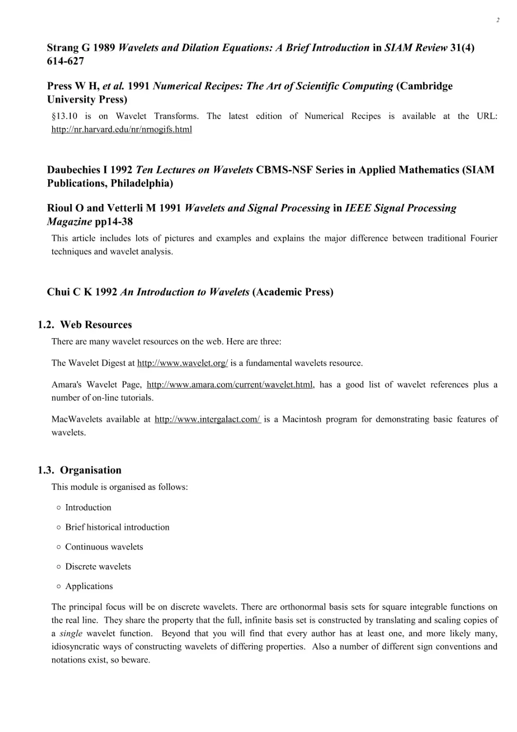
The Haar mother wavelet, h0 x!, is defined in terms of the father wavelet:
h0 x_! :∃ h!1 2 x! ! h!1 2 x ! 1!
Plot h0 x!, ∀x,  0.1`,1.1`#!
0.25 0.5 0.75
1
)2
)1
1
2
The remaining functions of the Haar basis are built up of both translations, ∗ x! +∗ x # 1!, and dyadic dilations,
∗ x! +∗ 2 x!, of the mother wavelet until we reach the required resolution. In analytical form, the general
expression is:
(2.6)
hj,k x! 2j∗2h0+2j x )k,.
In Mathematica this can be implemented directly:
hj_,k_ x_! :∃ 2 j∀2 h0%2 j x ! k&
Applying a dyadic dilation to h0 x! (corresponding to a change of scale by a factor of two) then there are two possible
translations which complete the basis at this scale (scale 1):
pj_,k_ :∃ Plot%h j,k x!, #x, ! 0.1,1.1∃,DisplayFunction % Identity&
4

Show GraphicsRow  Table p1,k, ∀k,0,1#!!!
0.25 0.5 0.75 1
)2
)1
1
2
0.25 0.5 0.75 1
)2
)1
1
2
It is clear that these functions are orthogonal to one another and to both h)1 x! and h0 x!. At the next finest scale
(scale 2) we have four basis functions:
Show GraphicsRow  Table p2,k, ∀k,0,3#!!!
0.25 0.5 0.75 1
)2
)1
12
0.25 0.5 0.75 1
)2
)1
12
0.25 0.5 0.75 1
)2
)1
12
0.25 0.5 0.75 1
)2
)1
12
It should be apparent that the Haar basis forms an orthonormal basis:
(2.7)
-hj,k, hl,m. ∀0
1h j,k x! hl,m x! ∀ x  -j,l-k,
m.
Note that this basis is not differentiable. Hence it is not an ideal basis for differentiable functions.
2.2.1. Example
Here is a sine wave sampled 64 times over one period:
10
20
30
40
50
60
-1
-0.5
0.5
1
Here is the sequence of partial sums of the expansion of this function into a Haar wavelet basis:
10
20
30
40
50
60
-1
-0.5
0.5
1
10
20
30
40
50
60
-1
-0.5
0.5
1
10
20
30
40
50
60
-1
-0.5
0.5
1
5

10
20
30
40
50
60
-1
-0.5
0.5
1
10
20
30
40
50
60
-1
-0.5
0.5
1
10
20
30
40
50
60
-1
-0.5
0.5
1
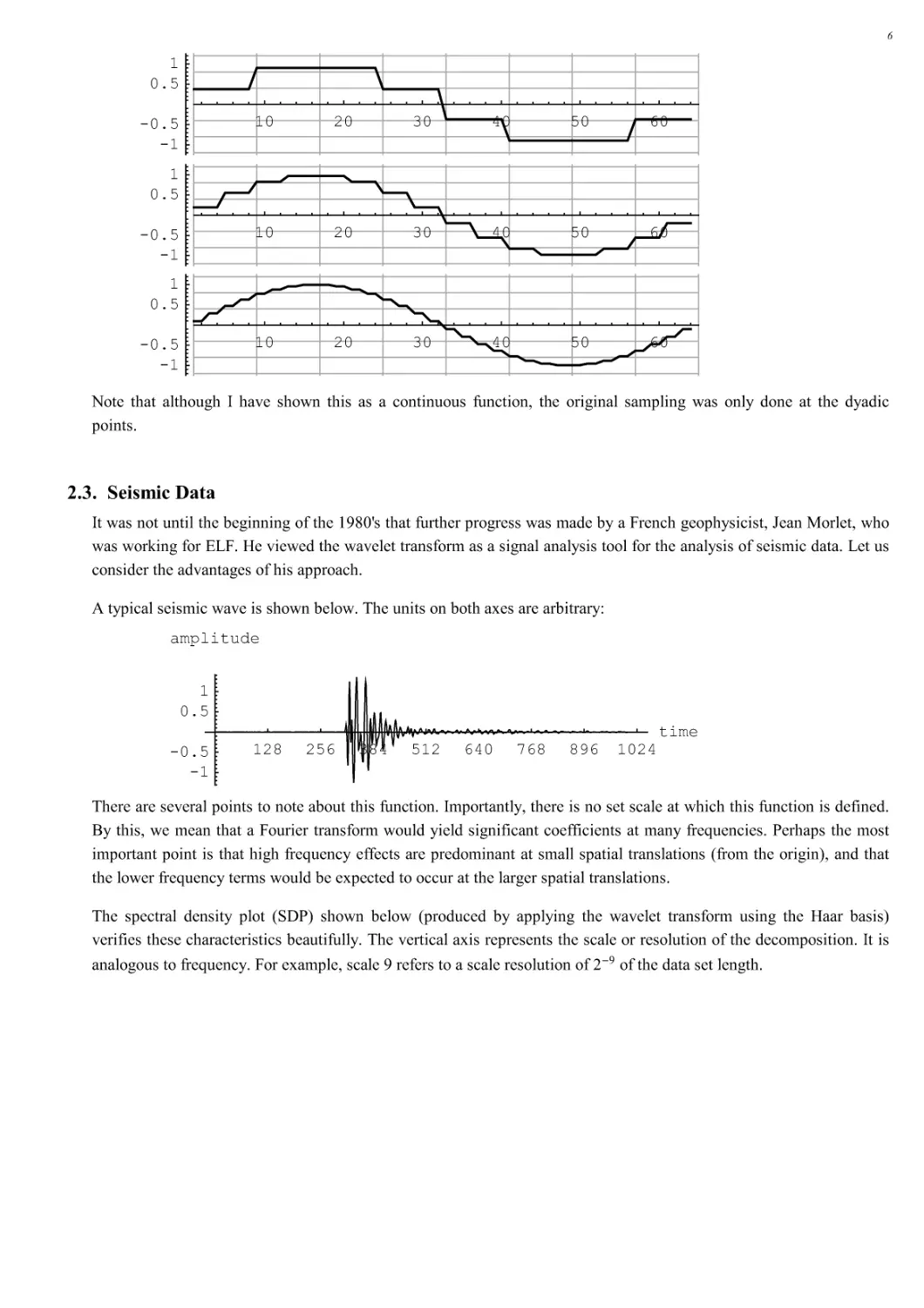
Note that although I have shown this as a continuous function, the original sampling was only done at the dyadic
points.
2.3. Seismic Data
It was not until the beginning of the 1980's that further progress was made by a French geophysicist, Jean Morlet, who
was working for ELF. He viewed the wavelet transform as a signal analysis tool for the analysis of seismic data. Let us
consider the advantages of his approach.
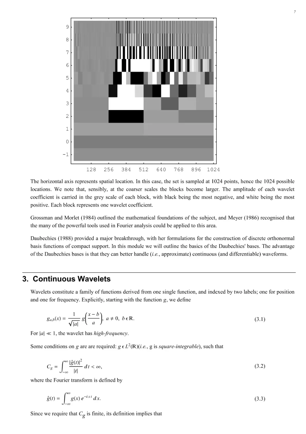
A typical seismic wave is shown below. The units on both axes are arbitrary:
128 256 384 512 640 768 896 1024 time
-1
-0.5
0.5
1
amplitude
There are several points to note about this function. Importantly, there is no set scale at which this function is defined.
By this, we mean that a Fourier transform would yield significant coefficients at many frequencies. Perhaps the most
important point is that high frequency effects are predominant at small spatial translations (from the origin), and that
the lower frequency terms would be expected to occur at the larger spatial translations.
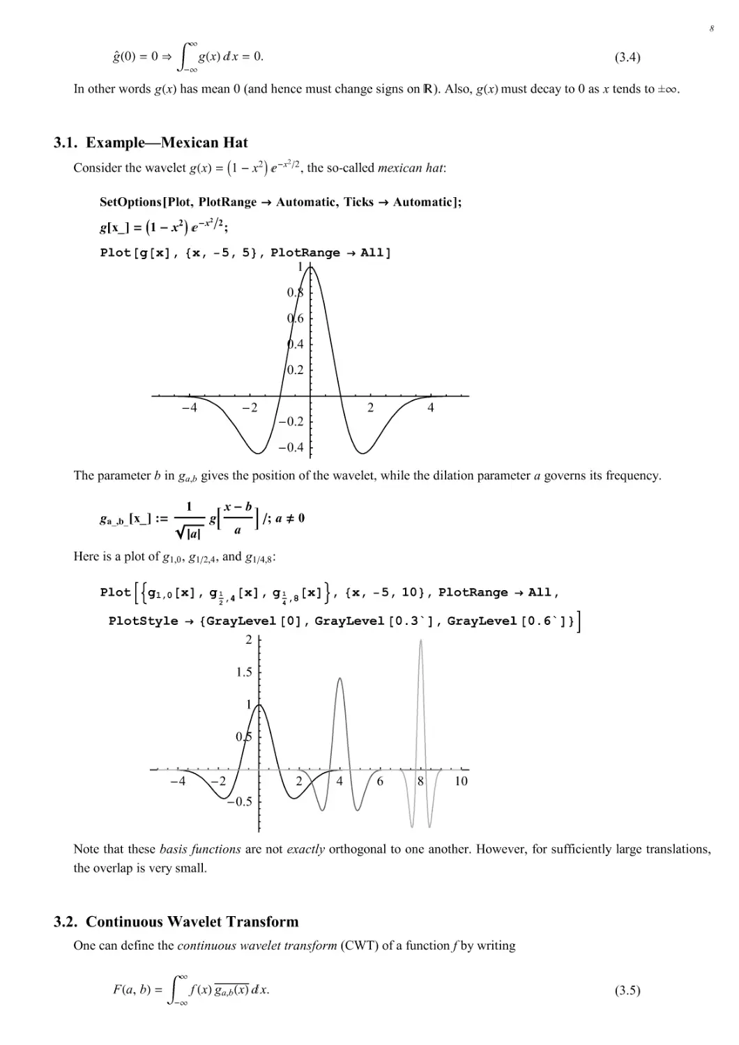
The spectral density plot (SDP) shown below (produced by applying the wavelet transform using the Haar basis)
verifies these characteristics beautifully. The vertical axis represents the scale or resolution of the decomposition. It is
analogous to frequency. For example, scale 9 refers to a scale resolution of 2)9 of the data set length.
6

128 256 384 512 640 768 896 1024
-1
0
1
2
3
4
5
6
7
8
9
The horizontal axis represents spatial location. In this case, the set is sampled at 1024 points, hence the 1024 possible
locations. We note that, sensibly, at the coarser scales the blocks become larger. The amplitude of each wavelet
coefficient is carried in the grey scale of each block, with black being the most negative, and white being the most
positive. Each block represents one wavelet coefficient.
Grossman and Morlet (1984) outlined the mathematical foundations of the subject, and Meyer (1986) recognised that
the many of the powerful tools used in Fourier analysis could be applied to this area.
Daubechies (1988) provided a major breakthrough, with her formulations for the construction of discrete orthonormal
basis functions of compact support. In this module we will outline the basics of the Daubechies' bases. The advantage
of the Daubechies bases is that they can better handle (i.e., approximate) continuous (and differentiable) waveforms.
3. Continuous Wavelets
Wavelets constitute a family of functions derived from one single function, and indexed by two labels; one for position
and one for frequency. Explicitly, starting with the function g, we define
(3.1)
ga,b x! 1
/a0g x)b
a , a.0,b/R.
For /a0 1, the wavelet has high-frequency.
Some conditions on g are are required: g / L2 R!(i.e., g is square-integrable), such that
(3.2)
Cg  ∀)∃
∃ /g0  t!02
/t0 ∀t 1∃,
where the Fourier transform is defined by
(3.3)
g0 t!  ∀)∃
∃ g x! 2)3 xt ∀x.
Since we require that Cg is finite, its definition implies that
7

(3.4)
g0 0! 0 ∋∀)∃
∃g x!∀x 0.
In other words g x! has mean 0 (and hence must change signs on R). Also, g x! must decay to 0 as x tends to ±∃.
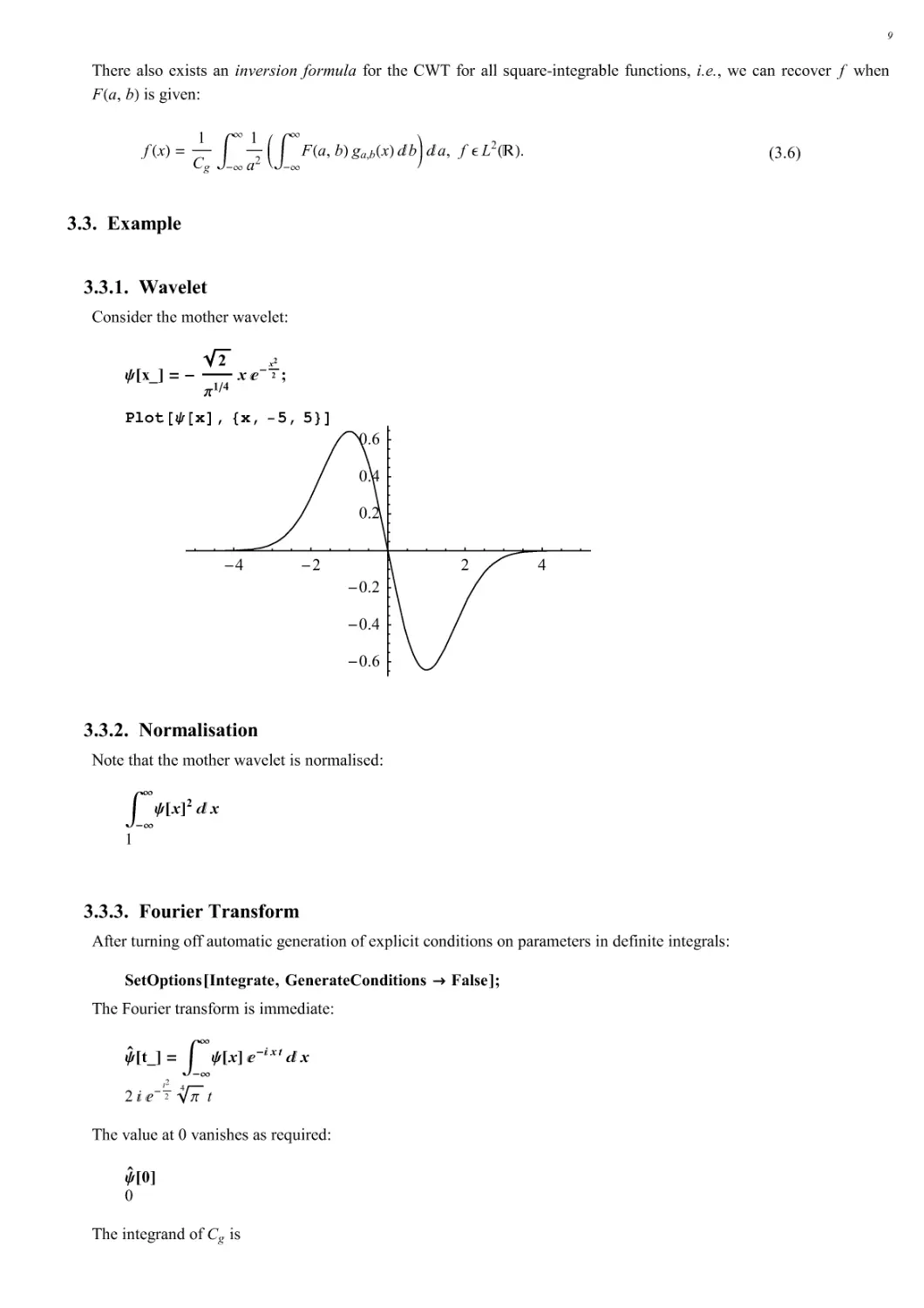
3.1. Example---Mexican Hat
Consider the wavelet g x! +1 ) x2, 2)x2∗2 , the so-called mexican hat:
SetOptions Plot,PlotRange % Automatic,Ticks % Automatic!;
g x_! ∃ ∋1 ! x2(&!x2)2;
Plot g x!, ∀x,  5,5#,PlotRange ! All!
)4
)2
2
4
)0.4
)0.2
0.2
0.4
0.6
0.8
1
The parameter b in ga,b gives the position of the wavelet, while the dilation parameter a governs its frequency.
ga_,b_ x_! :∃ 1
∗a+ g,x!b
a-∀;a∋0
Here is a plot of g1,0, g1∗2,4, and g1∗4,8:
Plot∃%g1,0 x!,g1
2,4 x!,g1
4,8 x!&, ∀x,  5,10#,PlotRange ! All,
PlotStyle ! ∀GrayLevel  0!,GrayLevel  0.3`!,GrayLevel  0.6`!#∋
)4 )2
246810
)0.5
0.5
1
1.5
2
Note that these basis functions are not exactly orthogonal to one another. However, for sufficiently large translations,
the overlap is very small.
3.2. Continuous Wavelet Transform
One can define the continuous wavelet transform (CWT) of a function f by writing
(3.5)
F a, b!  ∀)∃
∃f x!ga,b x!∀x.
8

There also exists an inversion formula for the CWT for all square-integrable functions, i.e., we can recover f when
F a, b! is given:
(3.6)
f x! 1
Cg ∀)∃
∃1
a2 1∀)∃
∃F a, b! ga,b x! ∀b2∀ a, f / L2 R!.
3.3. Example
3.3.1. Wavelet
Consider the mother wavelet:
( x_! ∃! 2
)1∀4 x&!x2
2;
Plot # x!, ∀x,  5,5#!
)4
)2
2
4
)0.6
)0.4
)0.2
0.2
0.4
0.6
3.3.2. Normalisation
Note that the mother wavelet is normalised:
.!∗
∗( x!2 + x
1
3.3.3. Fourier Transform
After turning off automatic generation of explicit conditions on parameters in definite integrals:
SetOptions Integrate,GenerateConditions % False!;
The Fourier transform is immediate:
(,  t_! ∃ .!∗
∗( x!&!-xt+x
2 32)t2
2!
4t
The value at 0 vanishes as required:
(,  0!
0
The integrand of Cg is
9

/(, 0t122
∗t+ ∀∀ ComplexExpand
42)t2 ! t2
so we obtain
 g ∃.!∗
∗4E!t2 ) t2 +t
4!
3.3.4. Moments
The moments, &m∋, of monomials xmare easily computed:
3m_4 :∃ .!∗
∗
xm( x!+x
The mean has to vanish:
304
0
3.3.5. Continuous Wavelet Basis
Here is the wavelet basis (formed by translations and dilations of the mother wavelet):
(a_,b_ x_! ∃ 1
∗a+ (,x!b
a-;
The general overlap integral, 3)∃
∃ ∗a,b(x) ∗c,d (x) ∀ x, can be computed directly but the integral is most easily obtained
parametrically. Consider:
ga_,b_ x_! ∃&!0x!b12
2a2 ;
The derivative of ga,b(x) with respect to b is proportional to ∗a,b(x):
.b ga,b x!
(a,b x!
)!
4 /a0
2a
Hence, from the integral:
.!∗
∗ ga,b x! gc,d x! + x ∀∀ Simplify
2)  b)d!2
2+a2#c2, 2!
1
c2#1
a2
the general overlap integral is given by the derivative with respect to b and d :
10

3#a_,b_∃, #c_,d_∃4 ∃ 2 a c .b,d /
) ∗a+ ∗c+ ∀∀ Simplify
2 2 ac+a2)b2#c2)d2#2bd,2)  b)d!2
2+a2#c2,
1
c2#1
a2 +a2 # c2,2 /a0 /c0
As a check, we confirm that this result again yields the normalisation integral:
3#a, b∃, #a, b∃4 ∀. ∗a_+ % a ∀∀ PowerExpand
1
Note that individual basis elements are not orthgonal. For example,
3#1,0∃, #1,1∃4
1
22
4
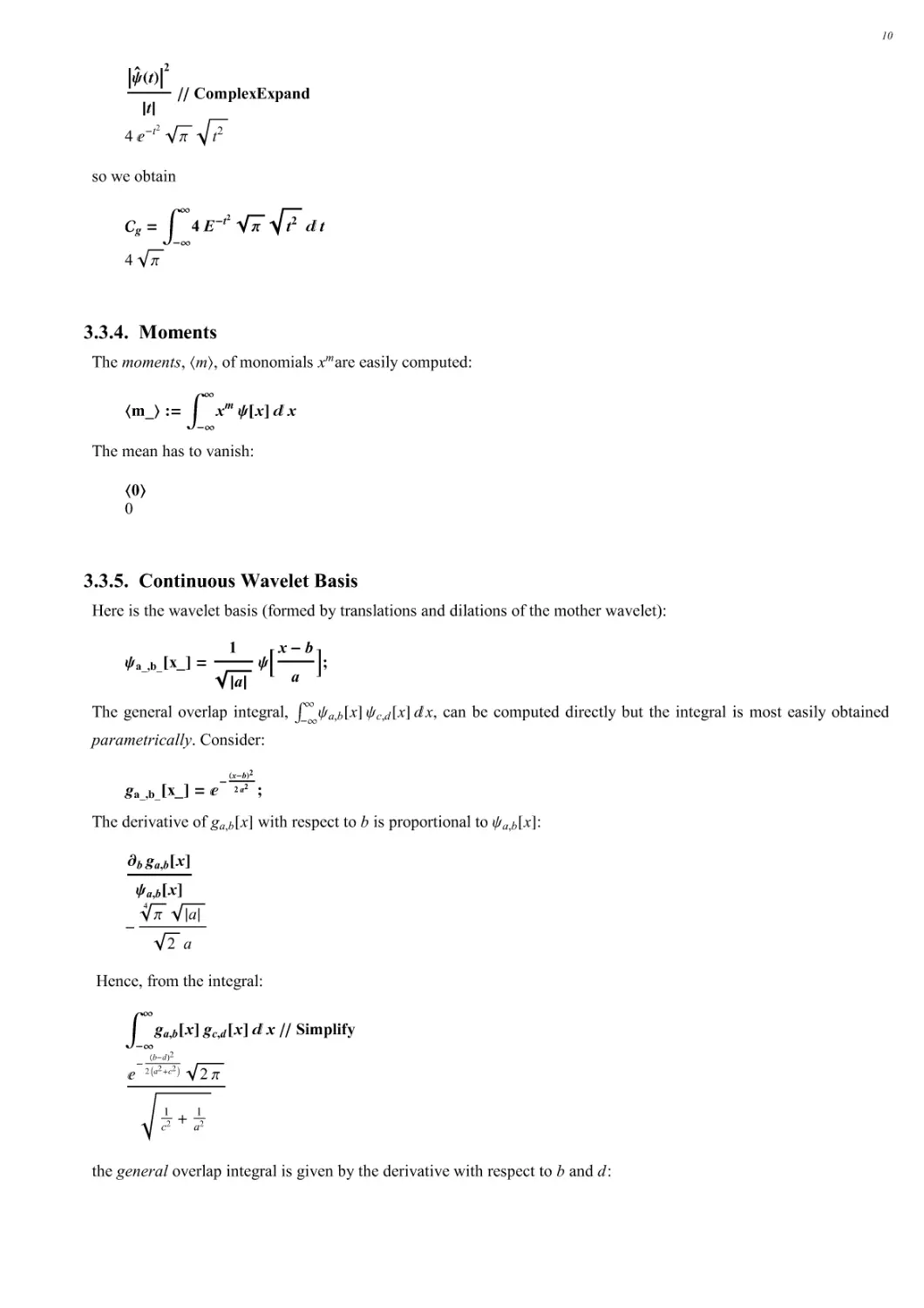
However, though states with different scale parameter, a, are not orthogonal, the maximum value of the overlap
integral occurs when the difference is 0. For example, here is a plot of &∃a, b%, ∃1, b%∋ as a function of a:
Plot Evaluate  (∀a,b#, ∀1,b#)!, ∀a,  5,5#!
)4
)2
2
4
)1
)0.5
0.5
1
Similarly, states with different translation parameter are not orthogonal. Here is a plot of &∃1,1%, ∃1, d%∋ as a function
of d:
Plot Evaluate  (∀1,1#, ∀1,d#)!, ∀d,  5,7#!
)4 )2
2
4
6
)0.4
)0.2
0.2
0.4
0.6
0.8
1
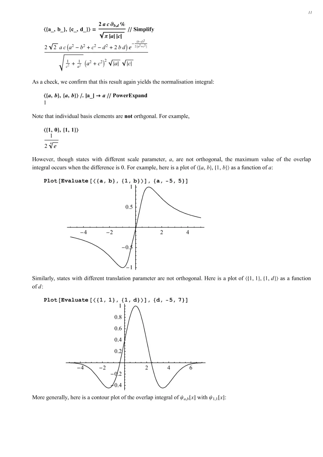
More generally, here is a contour plot of the overlap integral of ∗a,b(x) with ∗1,1(x):
11

ContourPlot  Evaluate  (∀a,b#, ∀1,1#)!,
∀a,0.1`,4#, ∀b,  2,3#,Axes ! True,AxesLabel ! ∀a,b#!
1
2
3
4
)2
)1
0
1
2
3
a
b
This plot suggests that there exists a contour (which could be expressed as a parametric equation in a and b) on which
the overlap integral vanishes. However, the set of wavelets, ∗a,b(x), even though orthogonal to ∗1,1(x) are not
orthogonal to one another, nor do they form a basis for the expansion of arbitrary functions in L2 R!.
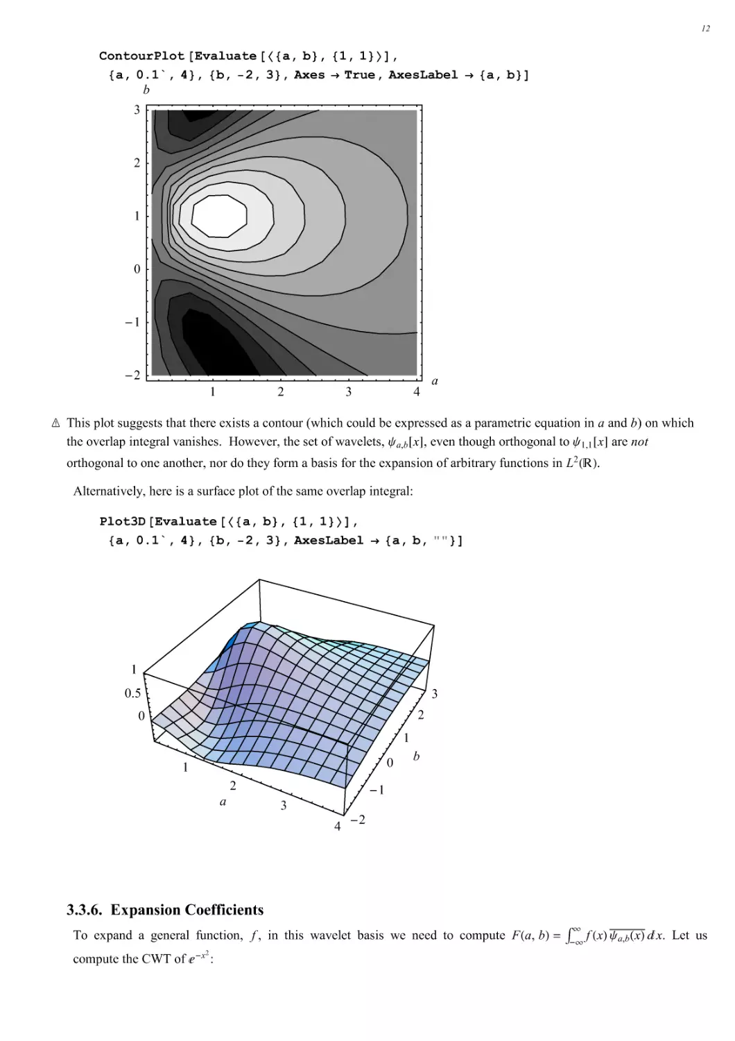
Alternatively, here is a surface plot of the same overlap integral:
Plot3D  Evaluate  (∀a,b#, ∀1,1#)!,
∀a,0.1`,4#, ∀b,  2,3#,AxesLabel ! ∀a,b, ""#!
)2
)1
0
1
2
3
b
0
0.5
1
1
2
3
4
a
3.3.6. Expansion Coefficients
To expand a general function, f, in this wavelet basis we need to compute F a, b! 3)∃
∃ f x!∗a,b x!∀x. Let us
compute the CWT of 2)x2 :
12

!  a_,b_! ∃ .!∗
∗
&!x2 (a,b x! + x ∀∀ ComplexExpand ∀∀ PowerExpand ∀∀ Simplify
4a2b2
b2
)2a2)1 !
4
+2 a2 # 1,3∗2 /a0
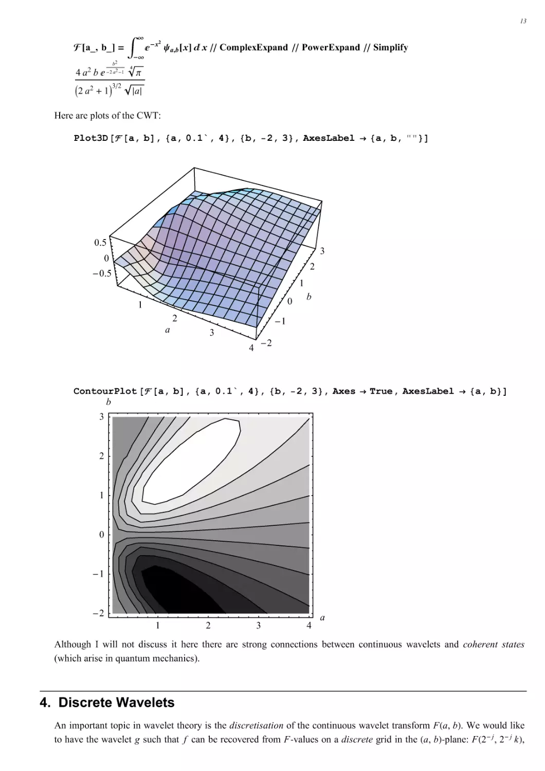
Here are plots of the CWT:
Plot3D  a,b!, ∀a,0.1`,4#, ∀b,  2,3#,AxesLabel ! ∀a,b, ""#!
)2
)1
0
1
2
3
b
)0.5
0
0.5
1
2
3
4
a
ContourPlot  a,b!, ∀a,0.1`,4#, ∀b,  2,3#,Axes ! True,AxesLabel ! ∀a,b#!
1
2
3
4
)2
)1
0
1
2
3
a
b
Although I will not discuss it here there are strong connections between continuous wavelets and coherent states
(which arise in quantum mechanics).
4. Discrete Wavelets
An important topic in wavelet theory is the discretisation of the continuous wavelet transform F a, b!. We would like
to have the wavelet g such that f can be recovered from F-values on a discrete grid in the  a, b!-plane: F 2) j,2) j k!,
13

j, k 4 Z. In particular it would be nice if g equals a function ∗ such that the wavelets 2j∗2 ∗ 2j x ) k!, j, k 4 Z, form
an orthonormal basis for square-integrable functions on R (i.e., L2 R!). Note that the mexican hat does not have this
property. A wavelet ∗ that does have this property is called the mother wavelet.
4.1. Motivation
To localise (as far as possible) in both time and frequency using efficient algorithms
To produce an orthogonal (orthonormal) basis set that is compact in both "space" and "time"
To provide frequency information coupled with spatial (temporal) location of the signals
To overcome problems with Fourier methods due to periodicity and infinite duration of basis sets
4.2. Multiresolution Analysis
Discrete wavelets are based on
Translation ∗ x! +∗ x # 1!
and
Dilation ∗ x! +∗ 2 x!.
We have already seen the Haar basis which is built from these transformations. An important point is that it is possible
to construct an infinite family of orthonormal wavelet bases.
Before we discuss the construction of an orthonormal wavelet basis we introduce multiresolution analysis. The basic
idea is that we want to look at data (a signal or a function) at varying (dyadic, i.e., powers of 2) levels of resolution.
Note that I will not give proofs of the results in this section.
Definition: A multiresolution analysis of L2 R! is a sequence of closed subspaces, ..., V)1, V0 , V1, V2,...such that
1. Vn5Vn)1,n4Z
2. 4n )∃
∃ Vn is dense in L2 R! and 5n )∃
∃ Vn  ∃0%.
3. f x!4Vn 7f 2x!4Vn)1.
4. f x!4V07f x)k!4V0,8k4Z.
Roughly speaking, when f is an oscillating function in V0, the function that oscillates "twice as fast" is an element of
V)1. Intuitively, V)1 is "twice as large" as V0.
4.3. Scaling Relation---Father Wavelet
Consider constructing a scaling function, 9, such that the translates, 9 x ) k!, are orthonormal, i.e., ∃9 x ) k! k 4 Z%
is an orthonormal family. Assume that V0 is generated by the integer translates 9 x ) k!. Then Vn , n 4 Z, defines a
multiresolution analysis of L2 R! generated by the scaling function 9. The function 9+ x2 , lies in V1 and hence in V0, so
we have
(4.1)
96x
27 #k
ck9 x)k!,
where only a finite number (N) of the ck are non-zero. Equivalently, the fact that ∃9 x ) k! k 4 Z% is an orthonormal
family yields:
14

(4.2)
ck  ∀96x
279 x )k!∀x.
When limits are omitted, summations are over all Z, and integrations over all R. However, since only a finite number
(N) of the ck are non-zero, the sums involving ck are from k 0,1,..., N ) 1, and the scaling relation can be written
(4.3)
9 x! #
k 0
N)1
ck9 2x)k!,
This is the form found in the majority of texts. This type of equation is known as a two-scale dilation equation. Before
we try to solve this equation we need to apply suitable conditions to 9.
In the literature, instead of the ck one often deals with the filter coefficients, hk , defined by hk 1
2 ck.The 1
2is
introduced for normalisation. In this text, where there is no possible confusion, I will generically refer to both ck and hk
as filter coefficients.
4.4. Conditions on the Filter Coefficients
Using the above definitions it easy to obtain a number of conditions on the filter coefficients.
4.4.1. Normalisation
It is apparent that the scaling relation only determines 9 x! up to a multiplicative constant. To normalise 9 x! we
require:
(4.4)
∀9 x!∀x  1,
4.4.2. Discrete Normalisation
Let us see some of the consequences of the scaling relation. Using the definition of the scaling function and its
normalisation, one finds that:
(4.5)
1  ∀9 x!∀x
 #kck∀9 2x)k!∀x
 1
2#kck∀9 y!∀y
 1
2#kck
∋#kck 2.
Alternatively, this can be written 8k hk 2 .
4.4.3. Orthonormality
We require that ∃9 x ) k! k 4 Z% forms an orthonormal family, i.e., 9 x! is orthogonal to its translates. This is
equivalent to requiring that
∀9 x!9 x )k!∀x  -k,0
15

 #lcl#mcm∀9 2x)l!9 2x)2k)m!∀x
 1
2#lcl#mcm∀9 y!9 y#l)2k)m!∀y
 1
2#l cl#m cm -l,2k#m
∋#mcm cm#2k  2-k,0.
Note that, when k 0, one has:
(4.7)
∀92 x!∀x  1∋#mcm
2  2.
4.4.4.N∃2
For N 2, i.e., just 2 non-zero filter coefficients, these conditions become
(4.8)
c02#c12 2,andc0#c1 2∋c0 1andc1 1.
The solution of the dilation equation is the box function:
(4.9)
9 x! 91,0&x11,
0,otherwise
which is just the Haar (father) wavelet.
4.4.5. Approximation
The accuracy of piecewise polynomial approximation depends on the answer to this question (Strang 1989): To what
degree p can the monomials, 1, x, x2 ,..., x p)1, be reproduced exactly using a basis of scaling functions?, i.e., to what
degree p is the following possible:
(4.10)
xp)1  #k dkp9 x #k!.
In the Haar basis it is easily seen that p 1. To answer this question in general it is useful to introduce a basis of
wavelets (which are defined to be orthogonal to the scaling functions).
Note that the orthonormality of the scaling functions implies that
(4.11)
dkp  ∀xp)19 x#k!∀x.
4.4.6. Orthonormal Wavelet Basis
Assume, as above, that the spaces Vn , n 4 Z, form a multiresolution analysis of L2 R! with 9 the scaling function. In
other words, 9 is the generator of a multiresolution wavelet basis. We define:
(4.12)
9j,k  2j∗29+2jx)k,.
The spaces Vj span :9) j,k k 4 Z; correspond with the different resolution levels of our decomposition. Let Wn be
the orthogonal complement of Vn in Vn)1, i.e.,
(4.13)
Vn:Wn  Vn)1.
Then there is a function ∗ (the mother wavelet), such that the space W j span :∗) j,k k 4 Z; with
16

(4.14)
∗j,k  2j∗2∗+2jx)k,,
satisfies (4.13).
4.4.7. Wavelet
Roughly speaking, if we decompose a function into the V and W subspaces the lowest resolution part is in V and the
difference is in W . (This is the basis of the discrete wavelet transform which will be introduced later.)
It can be shown that a suitable wavelet can be obtained by taking simple linear combination of scaling functions:
(4.15)
∗ x! #k  )1!kck9 2x#k)N#1!;#k  )1!N)k)1cN)k)19 2x)k!.
There are many slightly different but formally equivalent definitions in the literature
It is straightforward to show that the wavelet is orthogonal to the scaling function:
(4.16)
∀9 x!∗ x!∀x  #k
ck#l  )1!lcl∀9 2x)k!9 2x#l)N#1!∀x
 1
2#k
ck#l  )1!lcl∀9 y!9 y#k#l)N#1!∀y
 1
2#k
ck#l  )1!l cl -k,N)l)1
 1
2#
l 0
N)1 )1!l cl cN)l)1
For N even, reversing the order of the summation leads to:
(4.17)
1
2#
l 0
N)1 )1!l cl cN)l)1 l+N)l)1 1
2#
l 0
N)1 )1!N)l)1 cl cN)l)1  )1
2#
l 0
N)1 )1!l cl cN)l)1
These summations can only be equal if they both vanish. Hence:
(4.18)
∀9 x!∗ x!∀x  0.
More generally, it can be shown that
(4.19)
∀9 x#k!∗ x!∀x 0,8k4Z
Hence the approximation condition, x p)1 8k dkp 9 x # k!, can be expressed as the (moment) requirement:
(4.20)
∀xp)1∗ x!∀x  0.
4.4.8. p∃1
Putting p 1 into the moment condition, provides another condition on the ck :
(4 21)
∀∗ x!∀x 0 #k  )1!kck∀9 2x#k)N#1!∀x 1
2#k  )1!k ck∀9 y!∀y
17

∋#k  )1!k ck 0.
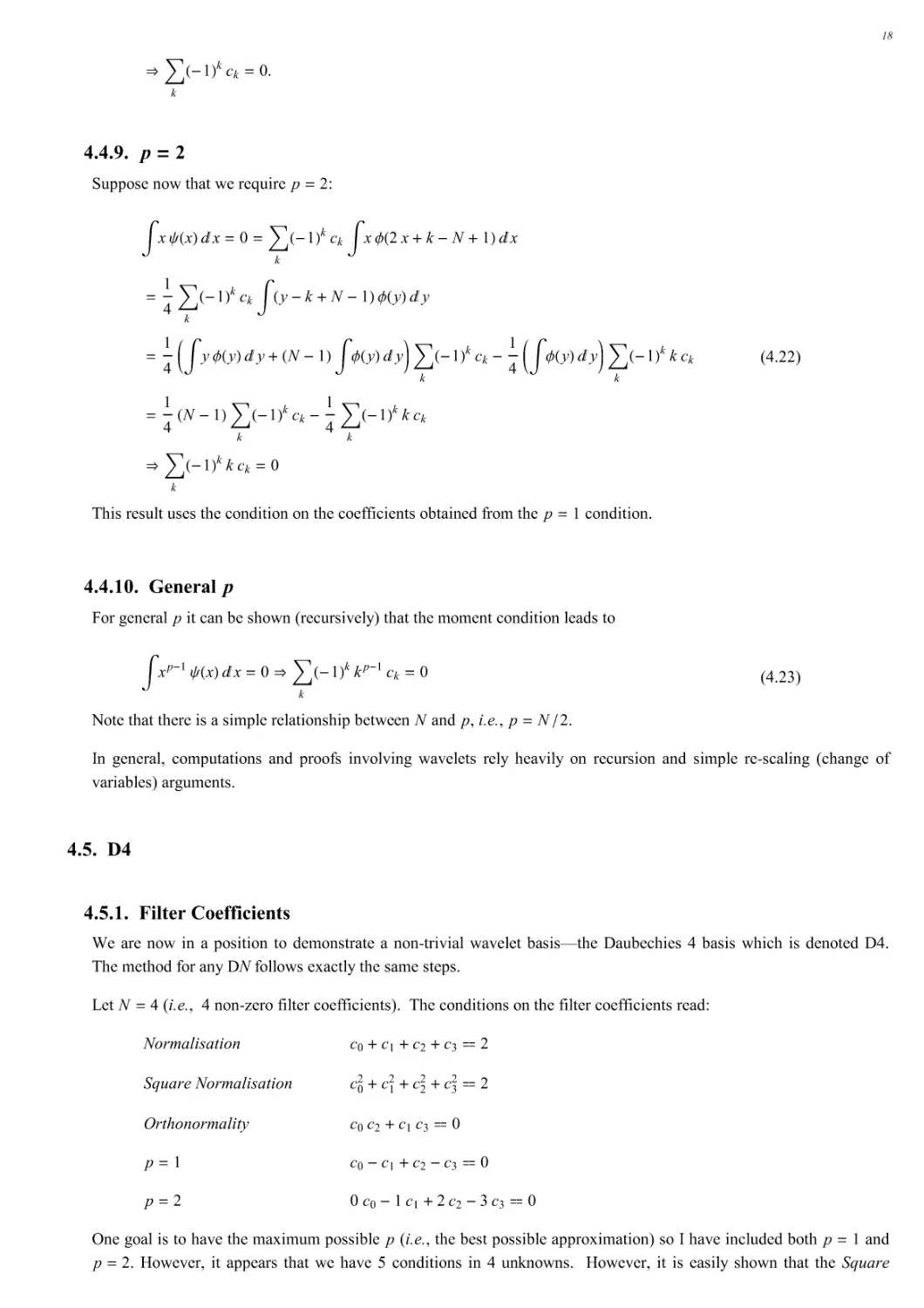
4.4.9. p∃2
Suppose now that we require p 2:
(4.22)
∀x∗ x!∀x 0 #k  )1!kck∀x9 2x#k)N#1!∀x
 1
4#k  )1!kck∀ y)k#N)1!9 y!∀y
 1
41∀y9 y!∀y# N)1!∀9 y!∀y2#k  )1!k ck ) 1
41∀9 y! ∀ y2#k  )1!k kck
 1
4  N)1!#k  )1!kck) 1
4#k  )1!kkck
∋#k  )1!k kck  0
This result uses the condition on the coefficients obtained from the p 1 condition.
4.4.10. General p
For general p it can be shown (recursively) that the moment condition leads to
(4.23)
∀xp)1∗ x!∀x  0∋#k  )1!kkp)1 ck  0
Note that there is a simple relationship between N and p, i.e., p N ∗ 2.
In general, computations and proofs involving wavelets rely heavily on recursion and simple re-scaling (change of
variables) arguments.
4.5. D4
4.5.1. Filter Coefficients
We are now in a position to demonstrate a non-trivial wavelet basis---the Daubechies 4 basis which is denoted D4.
The method for any DN follows exactly the same steps.
Let N 4 (i.e., 4 non-zero filter coefficients). The conditions on the filter coefficients read:
Normalisation
c0#c1#c2#c3<2
Square Normalisation
c02#c12#c22#c32<2
Orthonormality
c0c2#c1c3<0
p 1
c0)c1#c2)c3<0
p 2
0c0)1c1#2c2)3c3<0
One goal is to have the maximum possible p (i.e., the best possible approximation) so I have included both p 1 and
p 2. However, it appears that we have 5 conditions in 4 unknowns. However, it is easily shown that the Square
18

Normalisation condition can be obtained from the Normalisation, Orthonormality, and p 1 conditions.
In general we are lead to an equation of degree N ) 2 for the coefficients. For N 4 we get a quadratic equation.
4.5.2. Mathematica Implementation
Entering the equations, the Mathematica solution reads:
Solve #c00c10c20c312,c0c20c1c310,
c0!c10c2!c310,0c0!1c102c2!3c310∃,#c0,c1,c2,c3∃!
99c0+1
4)3
4,c1+1
2
3
2)3
2 ,c3+1
4+1# 3,,c2+1
4+3# 3,<,
9c0+1
4+1# 3,,c1+1
4+3# 3,,c3+1
2
1
2)3
2 ,c2+1
4+3) 3,<<
Solve returns two equivalent (reversed) solutions. The usual choice for the D4 filter coefficients (ck) is the last of these:
∀ ∃ Last /!;
0#c0, c1, c2, c3∃ ∃ #c0, c1, c2, c3∃ ∀. ∀1 ∀∀ TableForm
14+1# 3,
14+3# 3,
14+3) 3,
12612 ) 3
27
There are 4 coefficients:
# :∃ Length ∀!
We check that the ck satisfy the filter coefficient conditions:
56
k∃0
#!1
ck, 6
k∃0
#!1
ck2, 6
k∃0
#!10!11k ck c#!k!1, 6
k∃0
#!10!11k ck, 6
k∃0
# !1 0! 11k kck7 ∀∀ Simplify
∃2,2,0,0,0%
4.5.3. Iterative Approach to the Scaling Function
Once the filter coefficients have been determined, one method of approximately computing the scaling function is to
use recursion. Let us start with a square pulse as the zeroth-order approximation:
200x_ ∀;0∀ x#11 ∃ 1;
200x_1 ∃ 0;
and the iterative scaling relation
(4.24)
9m x! #
k 0
N)1
ck9m)1 2x)k!
implemented via
2m_0x_1 :∃2m0x1 ∃ 6
k∃0
#!1
ck2m!102x!k1
19

The syntax 9m_ (x_) : 9m(x) ...is called dynamic programming. It defines and saves function values as they are
computed.
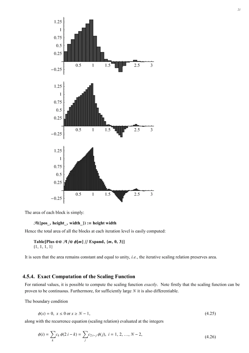
We now visualise the iterates of the scaling relation. Creating (and saving) a table of {position, height, width} triples
one can then visualise the iterates of the scaling relation:
20m_1 :∃20m1 ∃ Table,5z 0 1
2m01,2m z0 1
2m01,1
2m7,5z,0, #!1, 1
2m 7-
∃∃ "BarCharts`"; ∃∃ "Histograms`"; ∃∃ "PieCharts`"
bar m_,opts___ ! :% BarChart  & m!,ChartStyle ! ∀GrayLevel  0.2`!#,opts!
Table,bar i,PlotRange % ! 0.075 3.075
! 0.4 1.4 , #i,0,5∃-;
0.511.522.53
)0.25
0.25
0.5
0.75
1
1.25
0.511.
22.53
)0.25
0.25
0.5
0.75
1
1.25
0.511.522.53
)0.25
0.25
0.5
0.75
1
1.25
20

0.511.522.53
)0.25
0.25
0.5
0.75
1
1.25
0.5 1 1.5
2.5 3
)0.25
0.25
0.5
0.75
1
1.25
0.5 1 1.5
2.5 3
)0.25
0.25
0.5
0.75
1
1.25
The area of each block is simply:
∃0#pos_,height_,width_∃1 :∃ heightwidth
Hence the total area of all the blocks at each iteration level is easily computed:
Table Plus 33 ∃ ∀32 m! ∀∀ Expand, #m,0,3∃!
∃1,1,1,1%
It is seen that the area remains constant and equal to unity, i.e., the iterative scaling relation preserves area.
4.5.4. Exact Computation of the Scaling Function
For rational values, it is possible to compute the scaling function exactly. Note firstly that the scaling function can be
proven to be continuous. Furthermore, for sufficiently large N it is also differentiable.
The boundary condition
(4.25)
9 x! 0, x&0orx%N)1,
along with the recurrence equation (scaling relation) evaluated at the integers
(4.26)
9 i! #k
ck9 2i)k! #j
c2i)j9 j!, i 1,2,...,N)2,
21

leads to the eigenvalue equation C ( 2 2, where the  N )2!= N)2! matrix C has elements  C!i,j  c2i)j and
2  9 1!,9 2!,..., 9 N )2!!T. In matrix form,
(4.27)
c1c000(
(
(
c3c2c1c00(
(
c5c4c3c2c1 (
(
(
(
(!!(
(
(
(
(
(!!(
(
(
(
(
( cN)1 cN)2
9 1!
9 2!
9 3!
∀∀
9 N)2!
9 1!
9 2!
9 3!
∀∀
9 N )2!
,
For N  4, the eigenvalue equation reads
(4.28)
1c1 c0
c3 c22 9 1!
9 2! 9 1!
9 2! ,
Note that this equation only determines the values of 9 1! and 9 2! up to a multiplicative constant. However, even
with coarsest sampling of the scaling function, the area under the curve must be equal to unity (since area is preserved
in the recursive process). Hence, if we sample the function at the integer values only, then we can replace the
normalisation integral by a (Riemann) summation:
(4.29)
∀9 x!∀x 1∋#
k 0
N)19 k! 1 N 4 9 1!#9 2! 1.
Computing the eigenvector of 1c1 c0
c3 c22corresponding to unit eigenvalue, and imposing the condition, 9(1)+9(2)=1,
one finds that
(4.30)
9 1! 1# 3
2 ,9 2! 1) 3
2(
Later we will see that, for general N, some of the other eigenvalues are related to the dilational derivatives of the
scaling function. Briefly, this can be seen because, formally, taking the derivative of the scaling function and
evaluating the derivatives at integral values leads to:
(4.31)
9> x! 2#
k 0
N)1
ck9> 2x)k!∋1c1 c0
c3 c22 9> 1!
9> 2! 1
2 9> 1!
9> 2! .
4.5.5. Explicit Values
With 9 x!implemented as
Remove 2!
20x_ ∀; x∀08x4#!11:∃0
2011∃ 1
2910 3:;2021∃ 1
291! 3:;
20x_1:∃20x1∃Simplify,6
k∃0
#!1
ck202x!k1-
here are a few explicit values
22

523
2,21
2,21
4,23
4,25
87
90, 1
4+2# 3,, 1
16+5#3 3,, 1
16+9#5 3,, 1
2#9 3
32<
In general, every point in this dyadic (x k 2) j) set is of the form a # 3 b where a and b are rational.
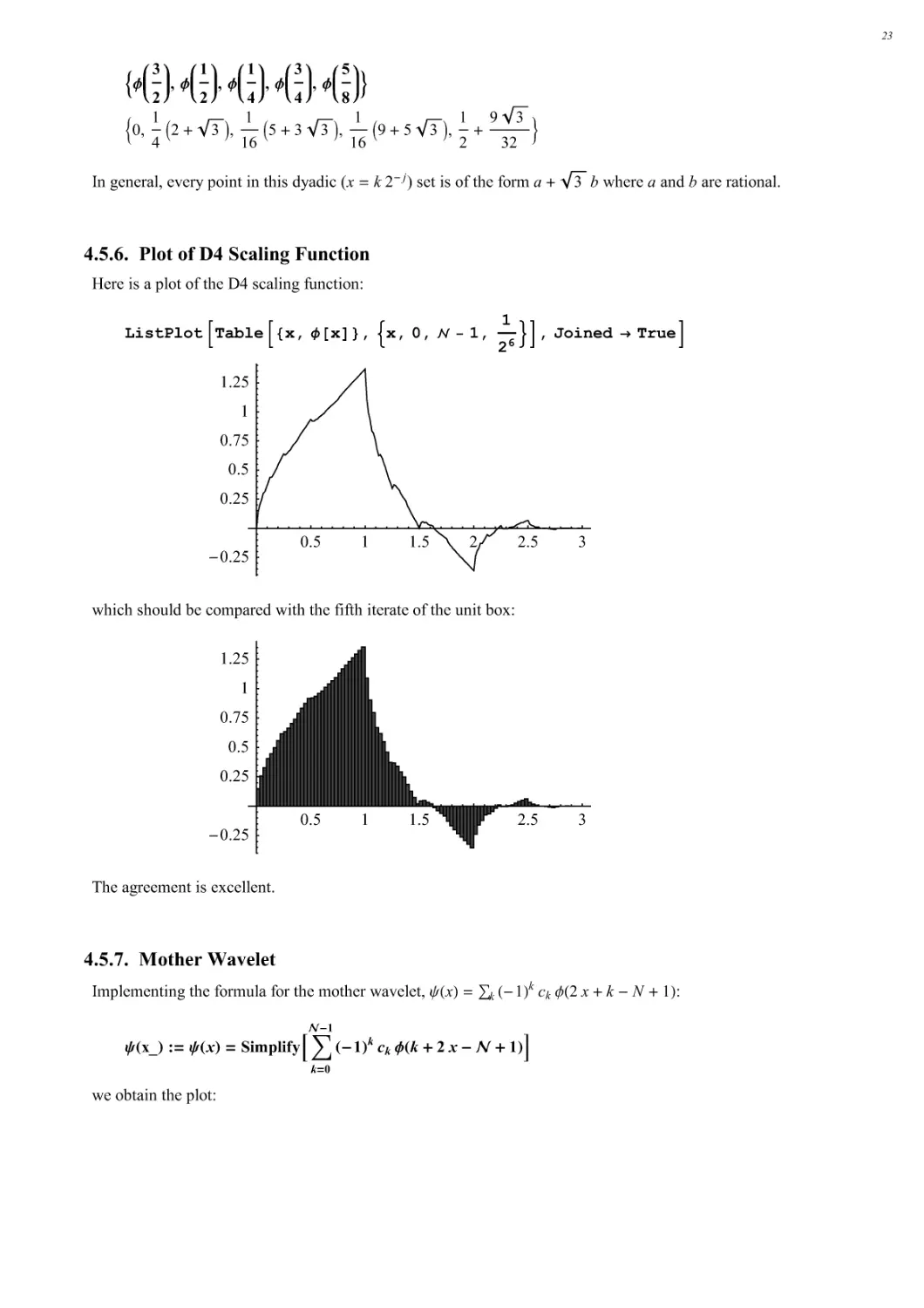
4.5.6. Plot of D4 Scaling Function
Here is a plot of the D4 scaling function:
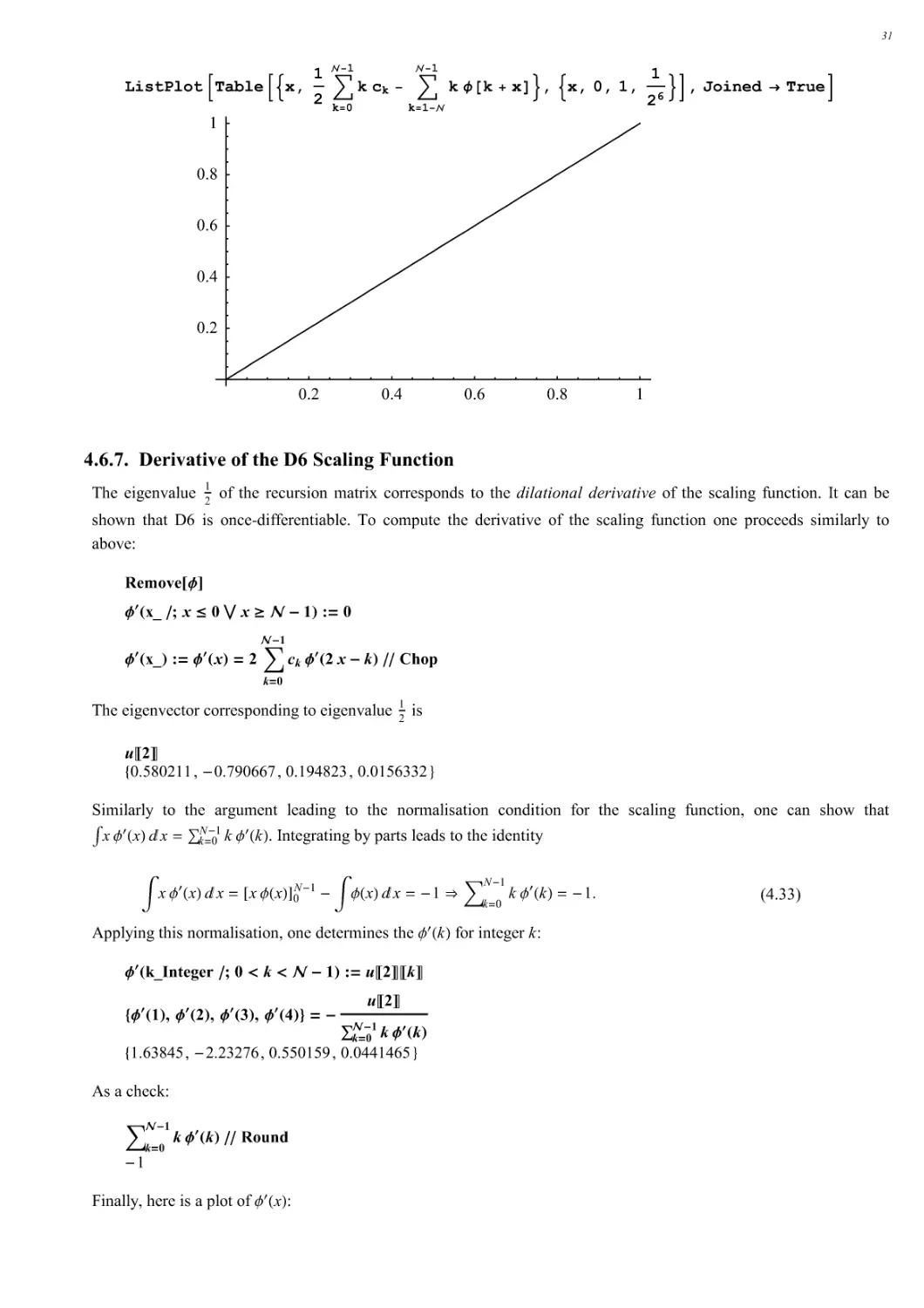
ListPlot∃Table∃∀x, & x!#, %x,0, ! 1, 1
26 &∋,Joined ! True∋
0.511.522.53
)0.25
0.25
0.5
0.75
1
1.25
which should be compared with the fifth iterate of the unit box:
0.5 1 1.5
2.5 3
)0.25
0.25
0.5
0.75
1
1.25
The agreement is excellent.
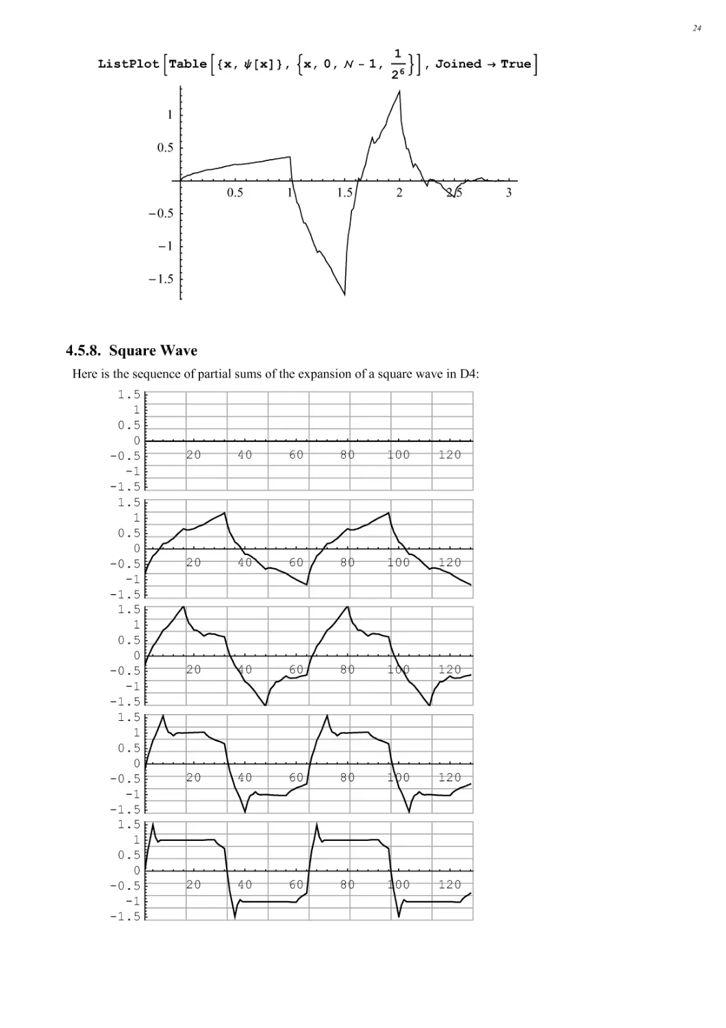
4.5.7. Mother Wavelet
Implementing the formula for the mother wavelet, ∗ x! 8k  ) 1!k ck 9 2 x # k ) N # 1!:
(0x_1 :∃(0x1 ∃ Simplify,6
k∃0
#!10!11kck20k02x!#011-
we obtain the plot:
23

ListPlot∃Table∃∀x, # x!#, %x,0, ! 1, 1
26 &∋,Joined ! True∋
0.5
1
1.5
2
2.5
3
)1.5
)1
)0.5
0.5
1
4.5.8. Square Wave
Here is the sequence of partial sums of the expansion of a square wave in D4:
20
40
60
80 100 120
-1.5
-1
-0.5
0
0.5
1
1.5
20
40
60
80 100 120
-1.5
-1
-0.5
0
0.5
1
1.5
20
40
60
80 100 120
-1.5
-1
-0.5
0
0.5
1
1.5
20
40
60
80 100 120
-1.5
-1
-0.5
0
0.5
1
1.5
20
40
60
80 100 120
-1.5
-1
-0.5
0
0.5
1
1.5
24

20
40
60
80 100 120
-1.5
-1
-0.5
0
0.5
1
1.5
20
40
60
80 100 120
-1.5
-1
-0.5
0
0.5
1
1.5
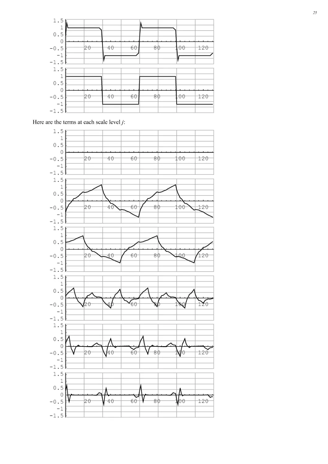
Here are the terms at each scale level j:
20
40
60
80 100 120
-1.5
-1
-0.5
0
0.5
1
1.5
20
40
60
80 100 120
-1.5
-1
-0.5
0
0.5
1
1.5
20
40
60
80 100 120
-1.5
-1
-0.5
0
0.5
1
1.5
20
40
60
80 100 120
-1.5
-1
-0.5
0
0.5
1
1.5
20
40
60
80 100 120
-1.5
-1
-0.5
0
0.5
1
1.5
20
40
60
80 100 120
-1.5
-1
-0.5
0
0.5
1
1.5
25

20
40
60
80 100 120
-1.5
-1
-0.5
0
0.5
1
1.5
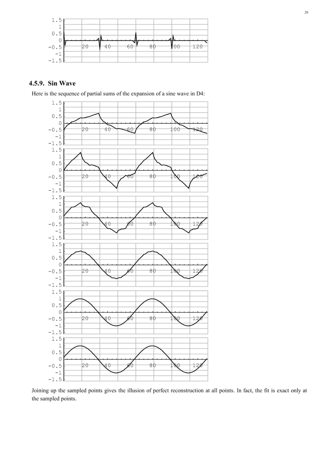
4.5.9. Sin Wave
Here is the sequence of partial sums of the expansion of a sine wave in D4:
20
40
60
80 100 120
-1.5
-1
-0.5
0
0.5
1
1.5
20
40
60
80 100 120
-1.5
-1
-0.5
0
0.5
1
1.5
20
40
60
80 100 120
-1.5
-1
-0.5
0
0.5
1
1.5
20
40
60
80 100 120
-1.5
-1
-0.5
0
0.5
1
1.5
20
40
60
80 100 120
-1.5
-1
-0.5
0
0.5
1
1.5
20
40
60
80 100 120
-1.5
-1
-0.5
0
0.5
1
1.5
Joining up the sampled points gives the illusion of perfect reconstruction at all points. In fact, the fit is exact only at
the sampled points.
26

4.6. D6
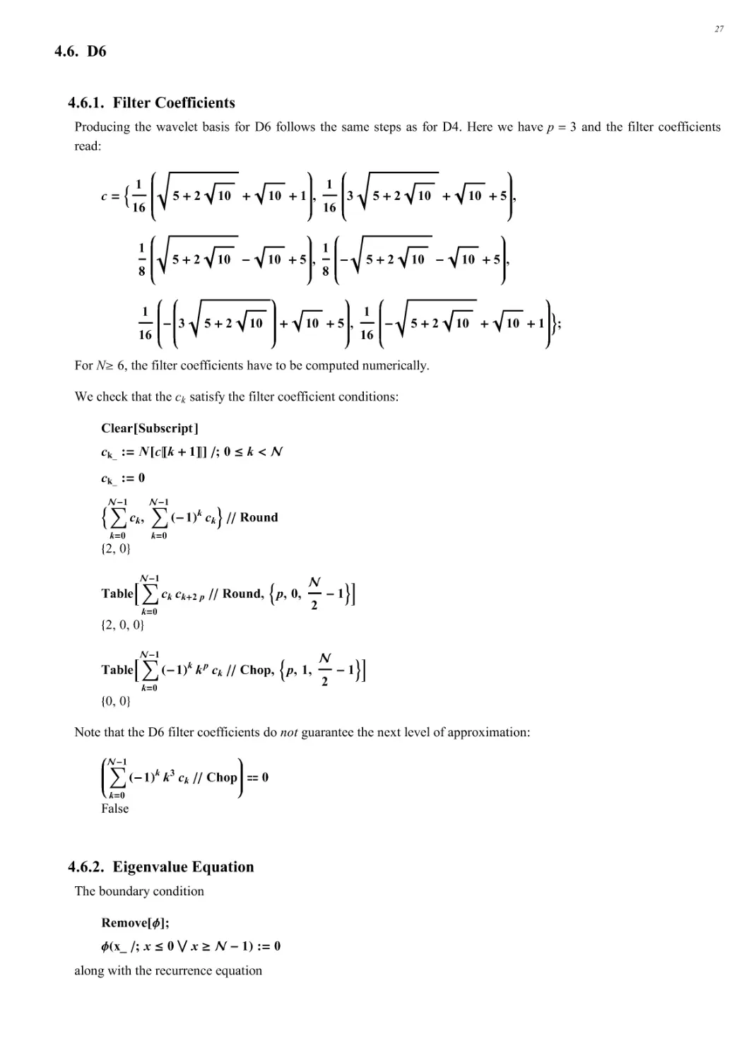
4.6.1. Filter Coefficients
Producing the wavelet basis for D6 follows the same steps as for D4. Here we have p 3 and the filter coefficients
read:
∀ ∃51
16 5021001001,1
1635021001005,
1
8 502 10! 1005,1
8!50210!1005,
1
16!35021001005,1
16!50210010017;
For N% 6, the filter coefficients have to be computed numerically.
We check that the ck satisfy the filter coefficient conditions:
Clear Subscript !
ck_ :∃ N  ∀;k 0 1<! ∀;0∀k##
ck_:∃0
56
k∃0
#!1
ck, 6
k∃0
#!10!11k ck7∀∀ Round
∃2,0%
Table,6
k∃0
#!1
ck ck02 p ∀∀ Round, 5p,0, #
2 !17-
∃2,0,0%
Table,6
k∃0
#!10!11k kp ck ∀∀ Chop,5p,1, #
2 !17-
∃0,0%
Note that the D6 filter coefficients do not guarantee the next level of approximation:
6
k∃0
#!10!11k k3 ck ∀∀ Chop 1 0
False
4.6.2. Eigenvalue Equation
The boundary condition
Remove 2!;
20x_∀;x∀08x4#!11:∃0
along with the recurrence equation
27

20x_1 :∃20x1 ∃ Chop,6
k∃0
#!1
ck202x!k1-
leads to the recursion matrix of size  N ) 2! =  N ) 2!:
%∃Table%c2i!j,#i,#!2∃,#j,#!2∃&
1.14112 0.470467 0
0
) 0.190934 0.650365 1.14112 0.470467
0.0498175 ) 0.120832 ) 0.190934 0.650365
0
0
0.0498175 ) 0.120832
Again, this matrix only determines the values of 9 k! up to a multiplicative constant. The normalisation integral
implies that 8k 0
N)19 k! < 1.
The eigensystem of the recursion matrix:
#5, u∃ ∃ Eigensystem  %!;
has eigenvalues:
Rationalize 5!
91, 1
2, ) 76606213
283427848 , 1
4<
The unit eigenvalue leads to the scaling function. Projecting out the eigenvector associated with unit eigenvalue:
u;1<
∃0.955434, ) 0.286583,0.0707606,0.00314509 %
we normalise it so that its components sum to unity:
#2011, 2021, 2031, 2041∃ ∃ /
Plus 33 /
∃1.28634, )0.385837,0.0952675,0.00423435 %
As a check:
6
k∃0
# !1 20k1 ∀∀ Round
1
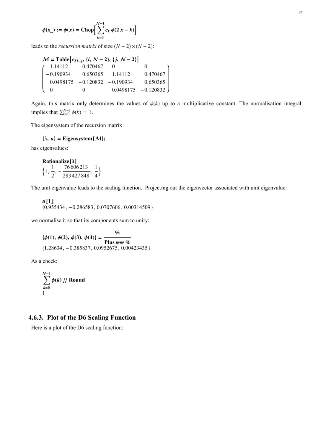
4.6.3. Plot of the D6 Scaling Function
Here is a plot of the D6 scaling function:
28

ListPlot∃Table∃∀x, & x!#, %x,0, ! 1, 1
26 &∋,Joined ! True∋
1
2
3
4
5
)0.25
0.25
0.5
0.75
1
1.25
Although this function may not look differentiable, zooming in near x 1 shows that the scaling function is smooth in
that vicinity:
ListPlot∃Table∃∀x, & x!#, %x,1 1
212 ,1∋ 1
212, 1
216 &∋,Joined ! True∋
0.9998 0.9999
1.0001
1.0002
1.2861
1.2862
1.2863
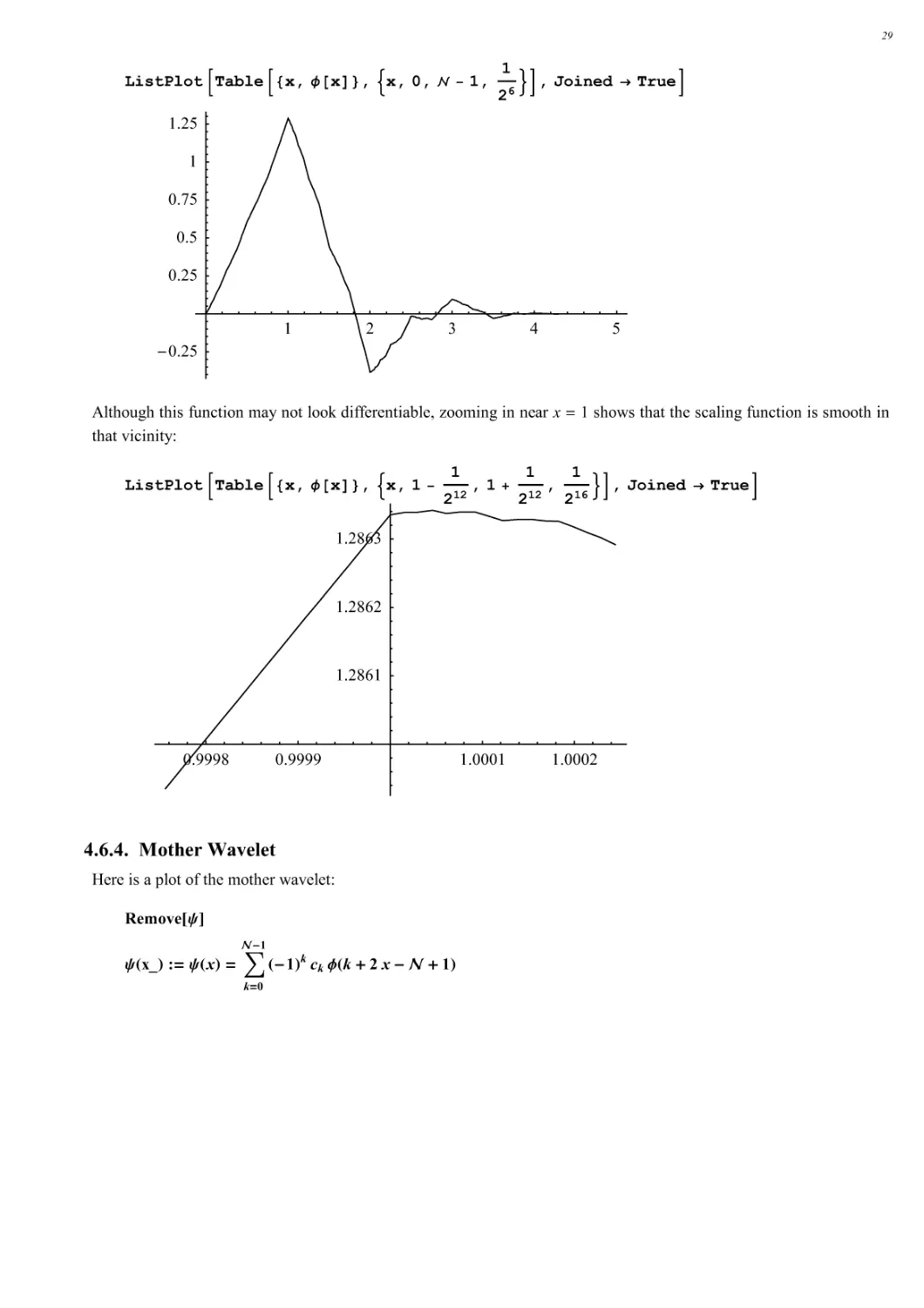
4.6.4. Mother Wavelet
Here is a plot of the mother wavelet:
Remove (!
(0x_1 :∃(0x1 ∃ 6
k∃0
#!10!11kck20k02x!#011
29

ListPlot∃Table∃∀x, # x!#, %x,0, ! 1, 1
26 &∋,Joined ! True,PlotRange ! All∋
1
2
3
4
5
)1.5
)1
)0.5
0.5
1
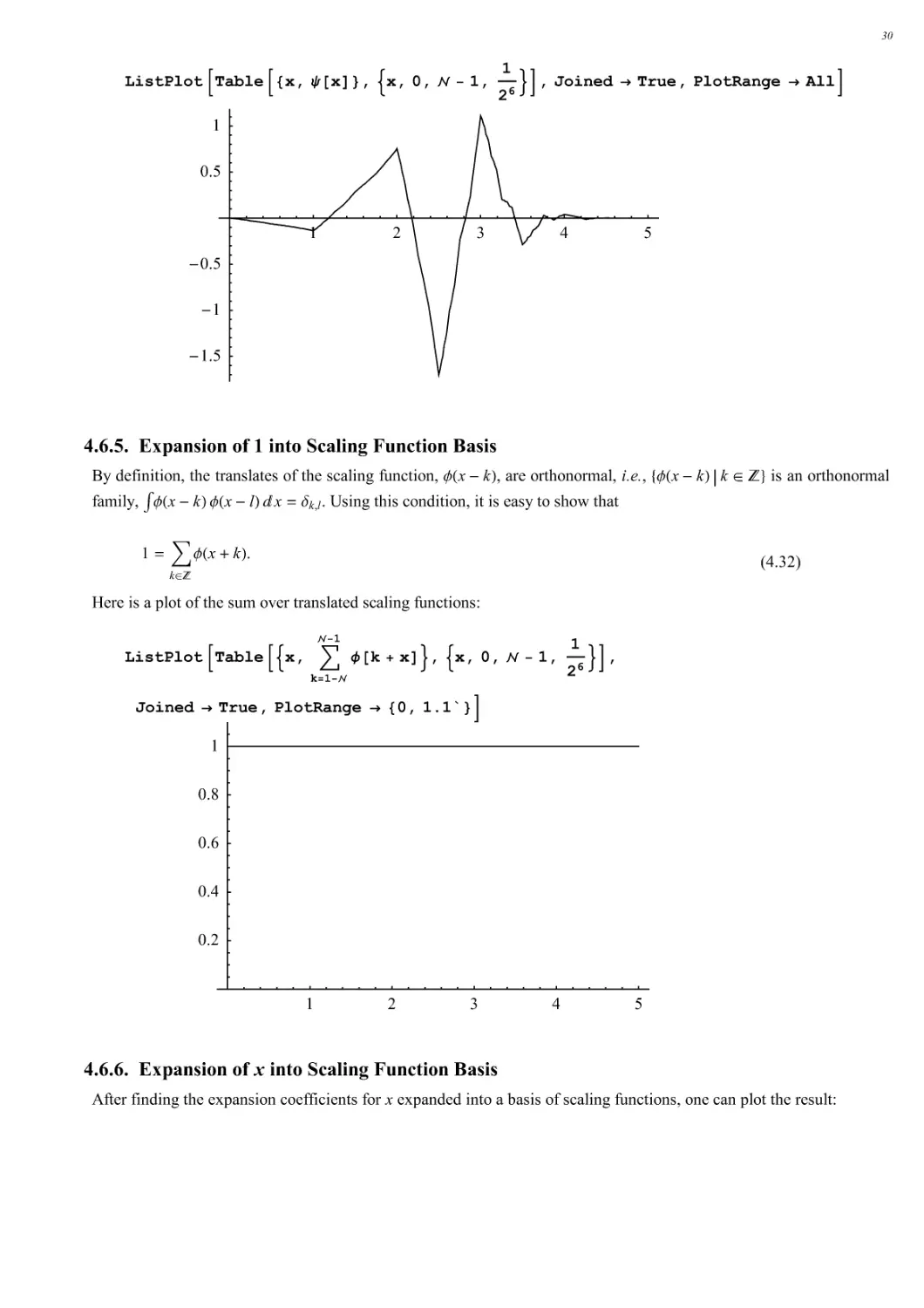
4.6.5. Expansion of 1 into Scaling Function Basis
By definition, the translates of the scaling function, 9 x ) k!, are orthonormal, i.e., ∃9 x ) k! k 4 Z% is an orthonormal
family, 3 9 x ) k! 9 x ) l! ∀ x  -k,l. Using this condition, it is easy to show that
(4.32)
1 #
k4Z 9 x # k!.
Here is a plot of the sum over translated scaling functions:
ListPlot∃Table∃%x, ∗
k%1 !
! 1& k∋x!&,%x,0,! 1, 1
26 &∋,
Joined ! True,PlotRange ! ∀0,1.1`#∋
1
2
3
4
5
0.2
0.4
0.6
0.8
1
4.6.6. Expansion of x into Scaling Function Basis
After finding the expansion coefficients for x expanded into a basis of scaling functions, one can plot the result:
30

ListPlot∃Table∃%x, 1
2∗
k%0
! 1 kck ∗
k%1 !
! 1 k & k ∋ x!&, %x,0,1, 1
26 &∋,Joined ! True∋
0.2
0.4
0.6
0.8
1
0.2
0.4
0.6
0.8
1
4.6.7. Derivative of the D6 Scaling Function
The eigenvalue 1
2 of the recursion matrix corresponds to the dilational derivative of the scaling function. It can be
shown that D6 is once-differentiable. To compute the derivative of the scaling function one proceeds similarly to
above:
Remove 2!
260x_∀;x∀08x4#!11:∃0
260x_1 :∃260x1 ∃ 2 6
k∃0
#!1
ck2602x!k1∀∀Chop
The eigenvector corresponding to eigenvalue 12 is
u;2<
∃0.580211, )0.790667,0.194823,0.0156332 %
Similarly to the argument leading to the normalisation condition for the scaling function, one can show that
3x9> x!∀x  8k 0
N )1 k 9> k!. Integrating by parts leads to the identity
(4.33)
∀x9> x!∀x (x9 x!)0N)1 )∀9 x!∀x  )1∋#k 0
N)1 k 9> k!  )1.
Applying this normalisation, one determines the 9> k! for integer k:
260k_Integer ∀;0#k## ! 11 :∃ u;2<;k<
#26011, 26021, 26031, 26041∃ ∃! u;2<
=k∃0
#!1k260k1
∃1.63845, )2.23276,0.550159,0.0441465 %
As a check:
6k∃0
# !1 k 260k1 ∀∀ Round
)1
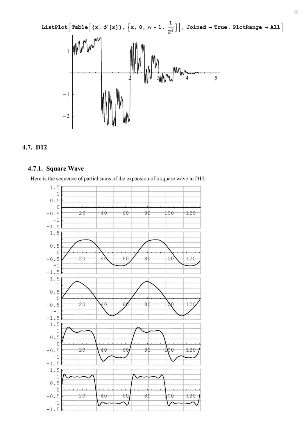
Finally, here is a plot of 9> x!:
31

ListPlot∃Table∃∀x, &( x!#, %x,0, ! 1, 1
26 &∋,Joined ! True,PlotRange ! All∋
1
2
3
4
5
)2
)1
1
4.7. D12
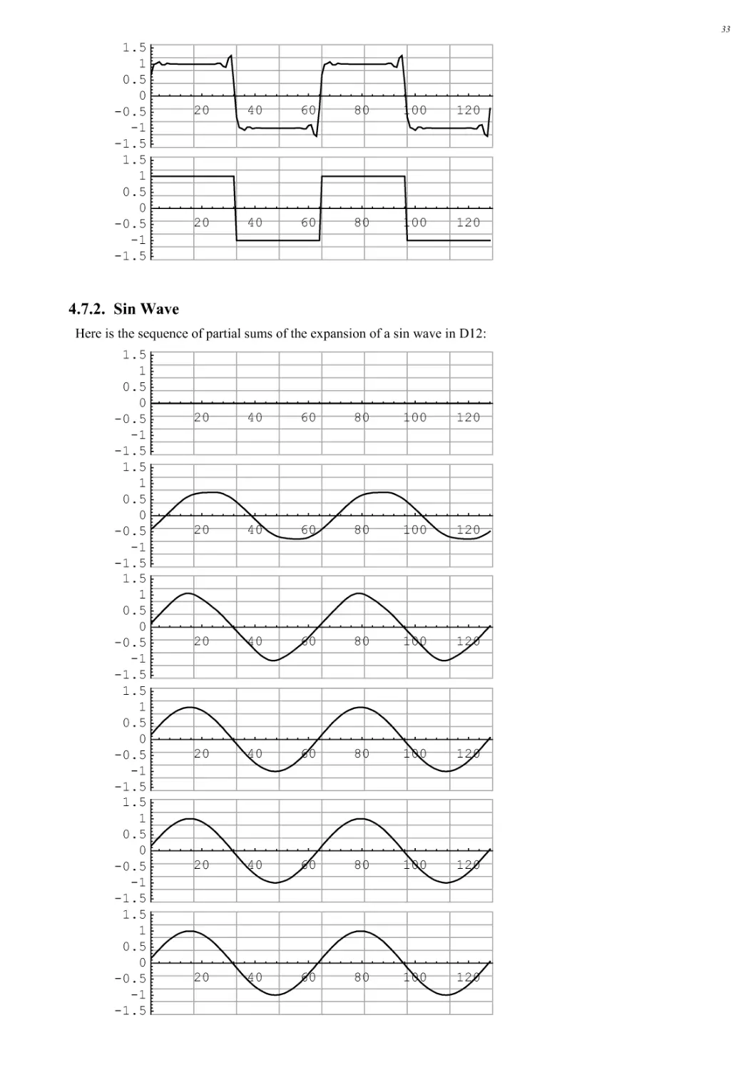
4.7.1. Square Wave
Here is the sequence of partial sums of the expansion of a square wave in D12:
20
40
60
80 100 120
-1.5
-1
-0.5
0
0.5
1
1.5
20
40
60
80 100 120
-1.5
-1
-0.5
0
0.5
1
1.5
20
40
60
80 100 120
-1.5
-1
-0.5
0
0.5
1
1.5
20
40
60
80 100 120
-1.5
-1
-0.5
0
0.5
1
1.5
20
40
60
80 100 120
-1.5
-1
-0.5
0
0.5
1
1.5
32

20
40
60
80 100 120
-1.5
-1
-0.5
0
0.5
1
1.5
20
40
60
80 100 120
-1.5
-1
-0.5
0
0.5
1
1.5
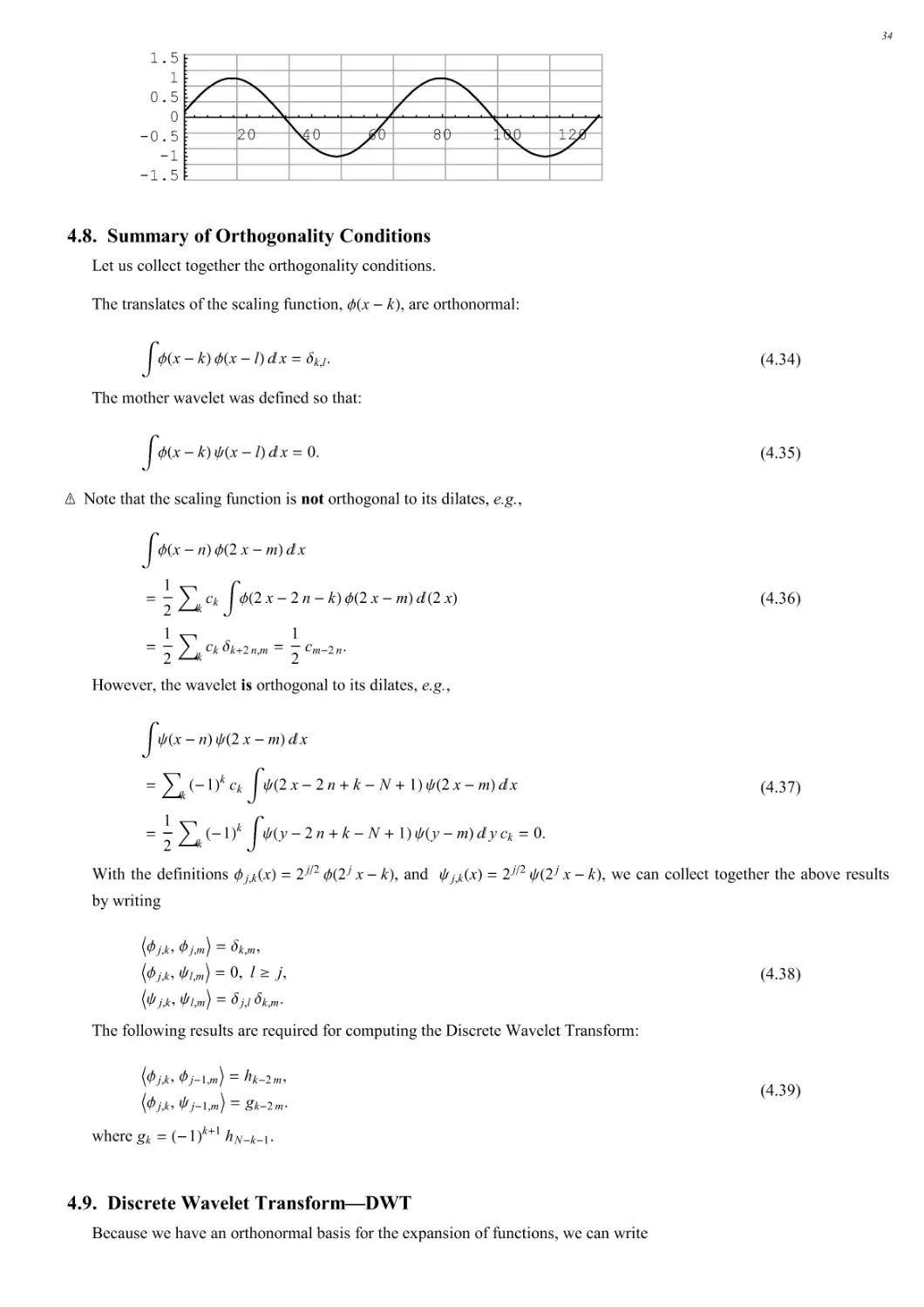
4.7.2. Sin Wave
Here is the sequence of partial sums of the expansion of a sin wave in D12:
20
40
60
80 100 120
-1.5
-1
-0.5
0
0.5
1
1.5
20
40
60
80 100 120
-1.5
-1
-0.5
0
0.5
1
1.5
20
40
60
80 100 120
-1.5
-1
-0.5
0
0.5
1
1.5
20
40
60
80 100 120
-1.5
-1
-0.5
0
0.5
1
1.5
20
40
60
80 100 120
-1.5
-1
-0.5
0
0.5
1
1.5
20
40
60
80 100 120
-1.5
-1
-0.5
0
0.5
1
1.5
33

20
40
60
80 100 120
-1.5
-1
-0.5
0
0.5
1
1.5
4.8. Summary of Orthogonality Conditions
Let us collect together the orthogonality conditions.
The translates of the scaling function, 9 x ) k!, are orthonormal:
(4.34)
∀9 x )k!9 x )l!∀x  -k,l.
The mother wavelet was defined so that:
(4.35)
∀9 x)k!∗ x)l!∀x 0.
Note that the scaling function is not orthogonal to its dilates, e.g.,
(4.36)
∀9 x)n!9 2x)m!∀x
 1
2#kck∀9 2x)2n)k!9 2x)m!∀ 2x!
 1
2#kck-k#2n,m 1
2 cm)2n.
However, the wavelet is orthogonal to its dilates, e.g.,
(4.37)
∀∗ x)n!∗ 2x)m!∀x
 #k )1!kck∀∗ 2x)2n#k)N#1!∗ 2x)m!∀x
 1
2#k )1!k∀∗ y)2n#k)N#1!∗ y)m!∀yck 0.
With the definitions 9j,k x! 2 j∗2 9 2 j x ) k!, and ∗j,k x! 2 j∗2 ∗ 2 j x ) k!, we can collect together the above results
by writing
(4.38)
-9j,k, 9j,m. -k,
m,
-9j,k,∗l,m. 0, l% j,
-∗ j,k , ∗l,m.  -j,l-k,
m.
The following results are required for computing the Discrete Wavelet Transform:
(4.39)
-9j,k, 9j)1,m. hk)2m,
-9j,k, ∗j)1,m. gk)2m.
where gk  )1!k#1 hN)k)1.
4.9. Discrete Wavelet Transform---DWT
Because we have an orthonormal basis for the expansion of functions, we can write
34

(4.40)
f x! #
k/Z
ck0 90,k x! # #j 0
∃#
k /Zdkj∗j,k x!,
where the coefficients can be computed using
(4.41)
ck0 f! &f,90,k∋, dkj f! -f,∗j,k..
It can be shown that the wavelet series converges for a wide class of functions and wavelet bases.
A most striking point about discrete wavelets is that, although the expansion coefficients are defined in terms of
integrals, because of the recursive nature of the equations defining the scaling function (and hence the wavelets), we
do not actually ever need to compute any integrals! Before we look at this in more detail, here is the computation of a
DWT for a particular case: Suppose that we have a set of 8 23 values corresponding to the sampled values of a
particular function. Call these c3 :c03, c13,..., c73;. The steps required to compute the DWT in, say, a D4 basis are
h0h1h2h30000
00h0h1h2h300
0000h0h1h2h3
h2h30000h0h1
g2g30000g0g1
g0g1g2g30000
00g0g1g2g300
0000g0g1g2g3
.
c03
c13
c23
c33
c43
c53
c63
c73
?
c02
c12
c22
c32
d02
d12
d32
d42
.
Now we leave the d coefficients alone and apply the same operation to the new c coefficients:
h0h1h2h3
h2h3h0h1
g2g3g0g1
g0g1g2g3
.
c02
c12
c22
c32
?
c01
c11
d01
d11
,
And one last time:
h0#h2 h1#h3
g0#g2 g1#g3 . c01
c11 ? c00
d00 .
The filter coefficients---or the expansion coefficients---are wrapped so as to make the transformation periodic. Also, it
is apparent that a matrix implementation of the DWT is not optimal because the intermediate matrices are sparse can
have a few elements repeated a number of times.
In other words, the steps in the transform produce intermediate vectors as follows:
c03
c13
c23
c33
c43
c53
c63
c73
?
c02
c12
c22
c32
d02
d12
d32
d42
?
c01
c11
d01
d11
d02
d12
d32
d42
?
c00
d00
d01
d11
d02
d12
d32
d42
.
The final vector is the DWT of the initial set of values. The original sequence c3 is decomposed into a lowest
resolution signal (DC term) c0, and difference signals d0, d1, d2, of finer and finer resolution.
35

To show how this comes about, from (4.39), we see that
(4.42)
9 j,k x! #l hk)2 l 9 j)1,l x! ##l gk)2 l ∗j)1,l x!,
which implies that
(4.43)
ckj  #l hk)2lclj)1##l gk)2ldlj)1 ; cj  H≅ (cj)1#G≅ (dj)1,
where this equation defines the adjoint quadrature mirror filters (QMF≅) H ≅ and G≅:
(4.44)
 H≅ (a!k  #l hk)2lal,  G≅ (a!k  #l gk)2l al.
It turns out that H is a low-pass filter and G is a high pass filter. These filters are perfect in the sense that they permit
exact reconstruction of the signal.
Because of the orthogonality of the filter coefficients, it is straightforward to show that
(4.45)
H(H≅  I G(G≅,H(G≅  0 G(H≅,
where the QMF are defined by
(4.46)
 H(a!k  #l hl)2k al,  G(a!k  #l gl)2k al.
Note the difference between the QMF and QMF≅ .
The orthogonality of the QMF is best seen by an example:
(4.47)
 H(H≅ (a!k  #l hl)2k H≅ (a!l  #l hl)2k#m hl)2m am
 #m #l hl)2khl)2m am  #m -k,m am ak,
where the orthonormality of the filter coefficients, (4.6), has been used.
Applying the quadrature mirror filters H and G to the expression for c j we obtain:
(4.48)
cj)1  H(cj, dj)1  G(cj.
Suppose that we have a set of J 2M numbers (corresponding to the sampled values of a particular function),
cM f! :c0M, c1M,..., cj)1
M ;. We have associated the sampled values with the integrals at the finest scale. Starting with
(4.49)
f x! #k
ckM f!9M,k x!,
the coefficients c j and d j can be computed recursively using (4.49), i.e.,
(4.50)
f x! #k
ckM f ! 9M,k x!?#k
ckM)1 f!9M)1,k x!##k dkM)1 f!∗M)1,k x!
#k
ckM)2 f!9M)2,k x!##k dkM)2 f!∗M)2,k x!
36

#k
ckM)3 f!9M)3,k x!##k dkM)3 f!∗M)3,k x!,
and so on, leading to
(4.51)
f x! #k
ck0 f!90,k x!##k dk0 f!∗0,k x!##k dk1 f!∗1,k x!# ... ##k dkM)1 f!∗M)1,k x!.
The essential point is that the coefficients c j and d j in this expansion are computed recursively by simple operations
on the sampled function values and no integrals need to be computed. This is (essentially) Mallat's pyramid algorithm
for computing the DWT by computing the expansion of a (discretely sampled) function in a discrete wavelet basis.
4.10. Wrapping
We have neglected to discuss the required wrapping of the basis functions so that the wavelet basis is confined to
(0,1). In the DWT (and FFT) algorithm, it is usual to limit the domain to x 4 (0,1). Functions may need to be re-
scaled or wrapped so that they fit into this domain. It is convenient to assume that f  x!, x 4 (0,1), is one period of a
periodic signal, where f  x! itself is identically 0 outside (0,1). This is the same assumption as for the discrete Fourier
transform.
It can be shown that, with this periodicity assumption, the wavelet decomposition can be written as
(4.52)
f x! c09 x!
# ##j 0
∃#
k 0
2j)1d2j#k ∗j,k x!,
where 9 x!
# indicates that the function has been wrapped to fit into the unit interval (0,1). The coefficients are
defined by
(4.53)
c0  -f, 9∃. ∀0
1f x!9 x!
#∀x ;∀)∃
∃f x!9 x!∀x  -f%
, 9.,
d2j#k ;dj,k  -f, ∗j,k
#. -f%
, ∗ j,k.,
where f  x! indicates that the function f  x! has been periodically extended outside (0,1).
Importantly, the wrapped scaling functions and wavelets are still orthonormal. Hence it is easy to show that the mean-
square is given by
(4.54)
&f, f∋ ∀0
1f2 x!∀x c02 ##j 0
∃#
k 0
2j)1d2j#k
2.
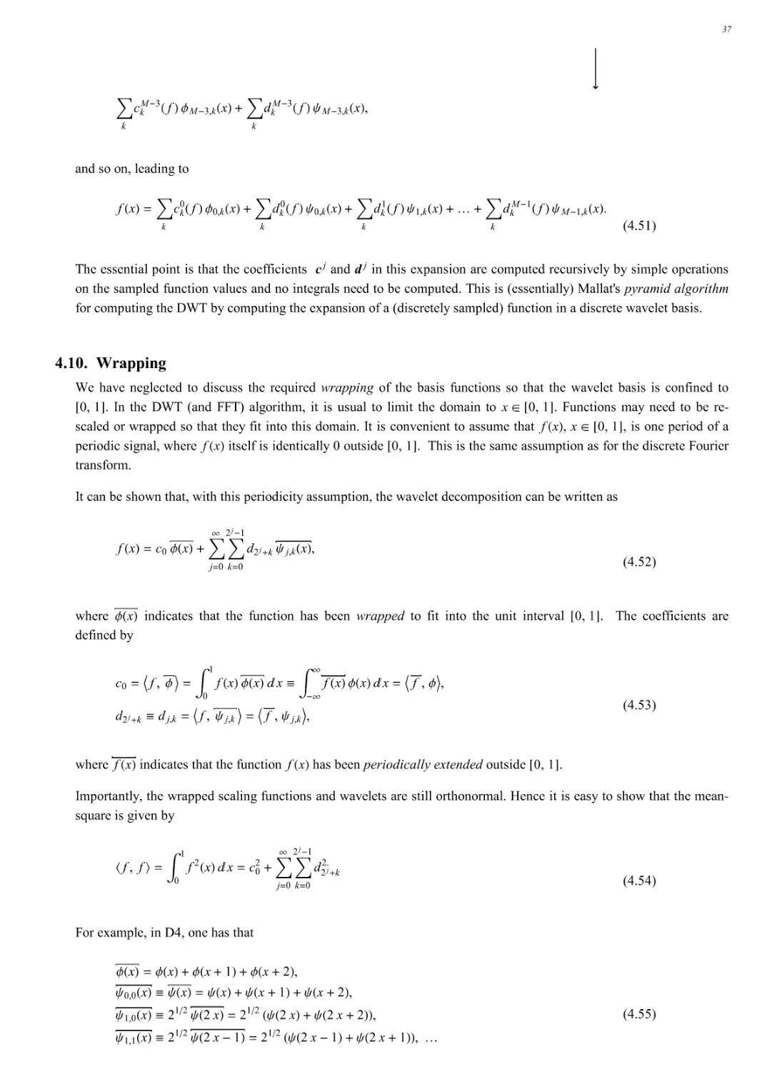
For example, in D4, one has that
(4.55)
9 x!
#
 9 x! #9 x # 1! #9 x # 2!,
∗0,0 x! ;∗ x!
#
 ∗ x! #∗ x # 1! #∗ x # 2!,
∗1,0 x! ; 21∗2 ∗ 2 x! 21∗2  ∗ 2 x! #∗ 2 x # 2!!,
∗1,1 x!;21∗2∗ 2x)1! 21∗2 ∗ 2x)1!#∗ 2x#1!!,...
37

Here are the wrapped D4 basis elements:
0.5
1
-4
-2
2
4
0.5
1
-4
-2
2
4
0.5
1
-4
-2
2
4
0.5
-4
-2
2
4
0.5
1
-4
-2
2
4
0.5
1
-4
-2
2
4
0.5
1
-4
-2
2
4
0.5
1
-4
-2
2
4
Note that these basis elements can be obtained by applying the inverse wavelet transform (IWT) to an appropriate unit
vector (ei). For example, here are the IWT of length 64 unit vectors e1, e2,..., e8.
102030405060
-4
-2
2
4
102030405060
-4
-2
2
4
102030405060
-4
-2
2
4
38

102030405060
-4
-2
2
4
102030405060
-4
-2
2
4
102030405060
-4
-2
2
4
102030405060
-4
-2
2
4
102030405060
-4
-2
2
4
By way of comparison, here is the inverse discrete Fourier transform (IDFT) of e1:
10
20
30
40
50
60
-1
-0.5
0.5
1
Here are the real and imaginary parts of the IDFT of e2:
10
20
30
40
50
60
-1
-0.5
0.5
1
10
20
30
40
50
60
-1
-0.5
0.5
1
Here are the real and imaginary parts of the IDFT of a e10:
39

10
20
30
40
50
60
-1
-0.5
0.5
1
10
20
30
40
50
60
-1
-0.5
0.5
1
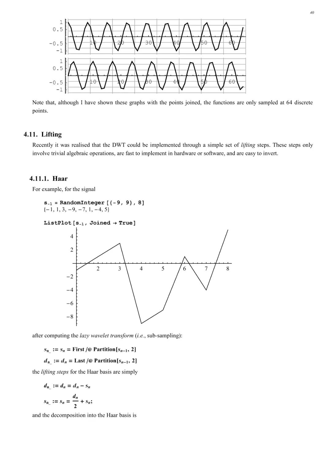
Note that, although I have shown these graphs with the points joined, the functions are only sampled at 64 discrete
points.
4.11. Lifting
Recently it was realised that the DWT could be implemented through a simple set of lifting steps. These steps only
involve trivial algebraic operations, are fast to implement in hardware or software, and are easy to invert.
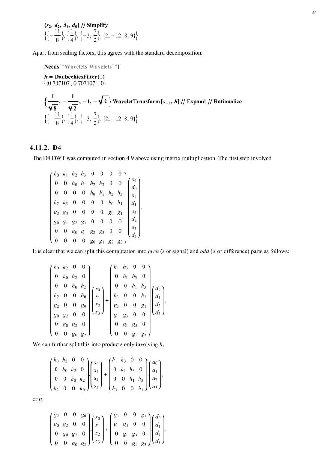
4.11.1. Haar
For example, for the signal
s 1 % RandomInteger  ∀ 9,9#,8!
∃)1,1,3, )9, )7,1, )4,5%
ListPlot  s 1,Joined ! True!
2
3
4
5
6
7
8
)8
)6
)4
)2
2
4
after computing the lazy wavelet transform (i.e., sub-sampling):
&n_ :∃ &n ∃ First ∀3 Partition sn!1,2!
∋n_ :∃ ∋n ∃ Last ∀3 Partition sn!1,2!
the lifting steps for the Haar basis are simply
dn_:∃dn ∃∋n!&n
sn_:∃sn∃dn
20&n;
and the decomposition into the Haar basis is
40

#s2, d2, d1, d0∃ ∀∀ Simplify
99) 11
8<,91
4<,9)3, 7
2<, ∃2, )12,8,9%<
Apart from scaling factors, this agrees with the standard decomposition:
Needs "Wavelets`Wavelets`"!
( ∃ DaubechiesFilter 011
∃∃0.707107,0.707107 %,0%
51
8,!1
2 , ! 1, ! 2 7 WaveletTransform  s!1, (! ∀∀ Expand ∀∀ Rationalize
99) 11
8<,91
4<,9)3, 7
2<, ∃2, )12,8,9%<
4.11.2. D4
The D4 DWT was computed in section 4.9 above using matrix multiplication. The first step involved
h0h1h2h30000
00h0h1h2h300
0000h0h1h2h3
h2h30000h0h1
g2g30000g0g1
g0g1g2g30000
00g0g1g2g300
0000g0g1g2g3
.
s0
d0
s1
d1
s2
d2
s3
d3
.
It is clear that we can split this computation into even (s or signal) and odd (d or difference) parts as follows:
h0h200
0h0h20
00h0h2
h200h0
g200g0
g0g200
0g0g20
00g0g2
.
s0
s1
s2
s3
#
h1h300
0h1h30
00h1h3
h300h1
g300g1
g1g300
0g1g30
00g1g3
.
d0
d1
d2
d3
,
We can further split this into products only involving h,
h0h200
0h0h20
00h0h2
h200h0
.
s0
s1
s2
s3
#
h1h300
0h1h30
00h1h3
h300h1
.
d0
d1
d2
d3
,
or g,
g200g0
g0g200
0g0g20
00g0g2
.
s0
s1
s2
s3
#
g300g1
g1g300
0g1g30
00g1g3
.
d0
d1
d2
d3
.
41

Writing the vector of even terms, s ∃s0, s1, s2, s3%, and odd terms d ∃d0, d1, d2, d3%, and using the z-transform (shift
operator), these computations can be collected together and written as a single (parallel) matrix computation,
 0# 2
z  1# 3
z
zg0#g2 zg1#g3
.1sd2,
which is true for datasets of arbitrary (even) size.
The 2=2 matrix here is known as the polyphase matrix. It turns out that it is possible to factorise the polyphase
matrix to obtain a simple lifting implementation of the DWT. In this case, one possible factorisation is
 0# 2
z  1# 3
z
zg0#g2 zg1#g3
;2#3
0
0
2)3
(10
z1(1 3
4#3
)
2
4
z
01(10
)31.
This factorisation corresponds to the following lifting implementation:
d!,d!) 3s!
s!, 3d!
4 #6)12# 3
47d!#1#s!
d!,d!#s!)1
s!,2#3s!
d!,2)3d!
The lifting implementation is very attractive because:
1. It consists of trivial arithmetic operations;
2. It allows "in-place" operations, i.e., each memory location is overwritten;
3. It works in parallel on the entire s and d vectors simultaneously;
4.Since1a
01
)1
 1)a
0 1 , the inverse DWT is trivially implemented.
5. Applications
5.0.1. Prerequisites
$FormatType ∃ TraditionalForm;
$TextStyle ∃ #FontSize % 10∃;
Needs "Wavelets`Wavelets`"!
Needs "Audio`"!
SetOptions ListDensityPlot,Mesh % False,Frame % None!;
SetOptions ListPlay,SampleRate % 8012,PlayRange % All!;
5.1. Signal Processing
Here is a digitised sound played using ListPlay :
SetDirectory ToFileName #$TopDirectory, "AddOns", "Applications", "Wavelets", "Data"∃!!;
42

ListPlay  & ∃## m.dat!;
After selecting a basis (filter):
( ∃ DaubechiesFilter 031;
here are two ways of visualizing the DWT coefficients:
)& ∃ WaveletTransform 0&, (1;
PlotCoefficients0)&,PlotRange % All,Frame % True1;
0 500 1000 1500 2000 2500 3000 3500
PhaseSpacePlot 0)&,LogarithmicScale % True,Frame % True,FrameTicks % None1;
Generating normally distributed (gaussian) noise:
## Statistics`
∗ ∃ Table Random NormalDistribution 00,20001!, #Length &!∃!;
43

here is the "noise spectrum":
)∗ ∃ WaveletTransform 0∗, (1;
PlotCoefficients0)∗,PlotRange % All,Frame % True1;
0 500 1000 1500 2000 2500 3000 3500
Adding the noise to the signal we obtain:
ListPlay ∗& ∃ ∗ 0 &!;
)∗& ∃ WaveletTransform 0∗&, (1;
Filtering using a threshold
∀ ∃ Compress0)∗&,1500,Threshold % True1;
The resulting sound is still clearly recognisable:
ListPlay  InverseWaveletTransform 0∀, (1,PlayRange % All!;
44

5.2. Image Processing
Efficient Signal and image compression uses a coding scheme that takes into account the spatial correlations that
occur in natural images (and sounds). Good image compression requires a good image decomposition scheme. One
method of image decomposition is to split the image into a low resolution part, and a difference signal (see Nacken in
Koornwinder 1993). The low resolution image will still contain spatial correlations. Iterating the decomposition
several times achieves a hierarchical decomposition. This decomposition can be seen to be related to multiresolution
analysis and can be naturally implemented using wavelets.
5.2.1. Wavelets in Two Dimensions
Two-dimensional scaling functions and wavelets are usualy formed by taking a direct product of two one-dimensional
functions, i.e., :9 x!, ∗ j,k x!;Α ∃9 y!, ∗l,m y!%:
(5.1)
9 x, y!  9 x! 9 y!,
∗ I! x, y!  9 x! ∗ y!,
∗ II! x, y!  ∗ x! 9 y!,
∗ III! x, y!  ∗ x! ∗ y!.
If we have a discretely sampled two-dimensional signal such as an image, the data takes the form of a matrix. The
two-dimensional wavelet transform of a matrix is defined in terms of the one-dimensional transforms of its rows and
columns. The first step is to take the one-dimensional transform of all of the rows (columns), and then take the one-
dimensional transform the resulting columns (rows). Since the one-dimensional signal component at the next level is
contained in the first half of a transformed vector, the signal component of the transformed matrix is contained in its
top-left quarter. Therefore the next step of the algorithm is executed on this part of the matrix. This process
continues until we reach a 2=2 matrix, and cannot transform any further.
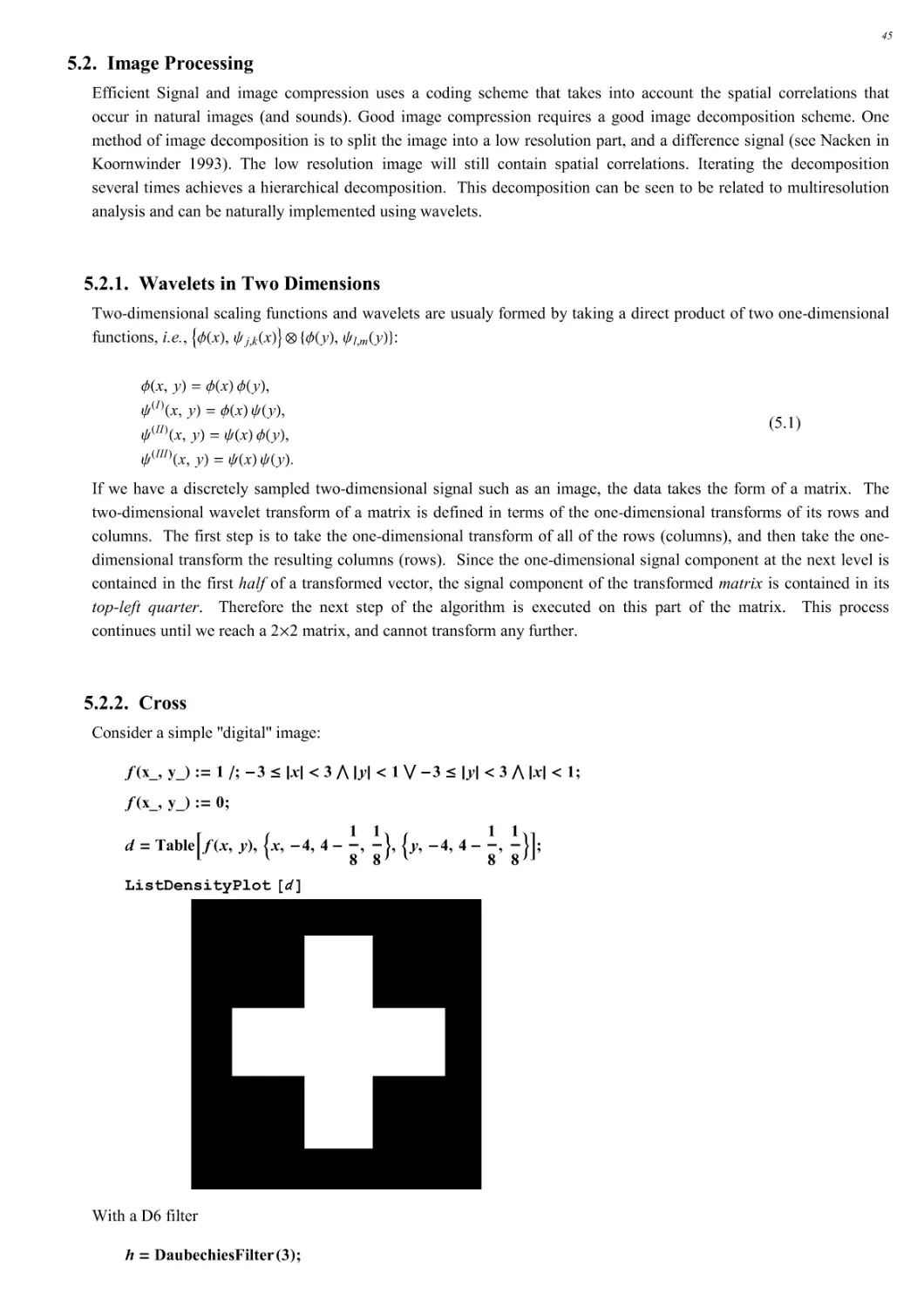
5.2.2. Cross
Consider a simple "digital" image:
f0x_,y_1:∃1∀;!3∀∗x+#3>∗y+#18!3∀∗y+#3>∗x+#1;
f 0x_,y_1 :∃ 0;
∋ ∃ Table,f 0x, y1, 5x, !4,4!1
8,1
87,5y, !4,4!1
8,1
87-;
ListDensityPlot  ∀!
With a D6 filter
( ∃ DaubechiesFilter 031;
45

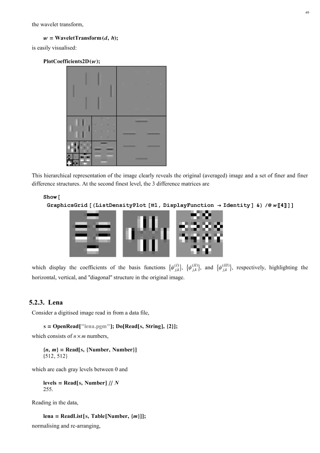
the wavelet transform,
) ∃ WaveletTransform 0∋, (1;
is easily visualised:
PlotCoefficients2D0)1;
This hierarchical representation of the image clearly reveals the original (averaged) image and a set of finer and finer
difference structures. At the second finest level, the 3 difference matrices are
Show
GraphicsGrid  +ListDensityPlot  )1,DisplayFunction ! Identity ! &, -∗ #.4/!!
which display the coefficients of the basis functions :∗ j,k
 I!;, :∗j,k
 II!;, and :∗ j,k
 III!;, respectively, highlighting the
horizontal, vertical, and "diagonal" structure in the original image.
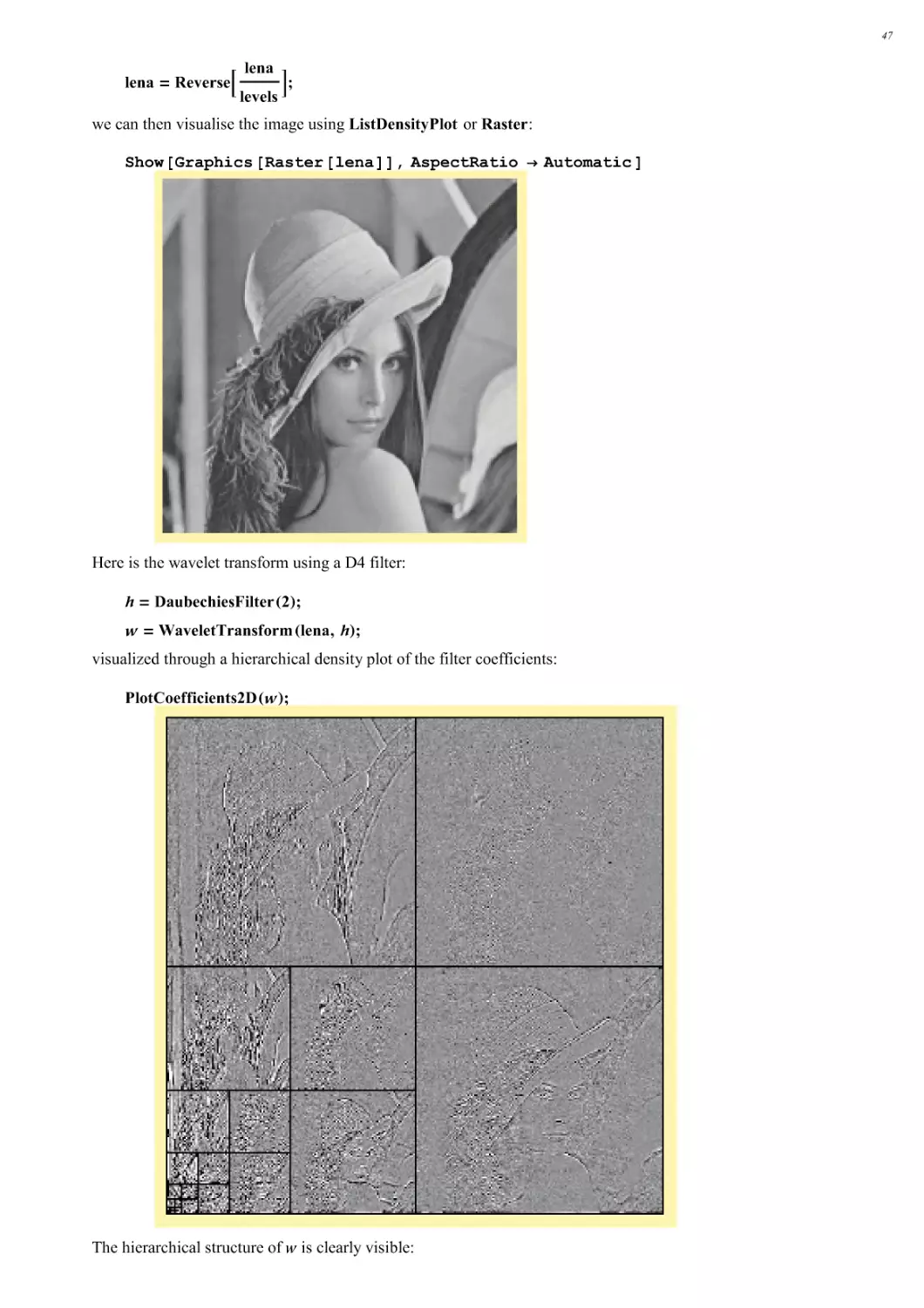
5.2.3. Lena
Consider a digitised image read in from a data file,
& ∃ OpenRead "lena.pgm"!;Do Read &,String!, #2∃!;
which consists of n = m numbers,
#n, m∃ ∃ Read &, #Number,Number∃!
∃512,512%
which are each gray levels between 0 and
levels ∃ Read &,Number! ∀∀ N
255.
Reading in the data,
lena ∃ ReadList &,Table Number, #m∃!!;
normalising and re-arranging,
46

lena ∃ Reverse, lena
levels -;
we can then visualise the image using ListDensityPlot or Raster:
Show Graphics  Raster  lena!!,AspectRatio ! Automatic !
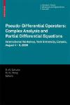
Here is the wavelet transform using a D4 filter:
( ∃ DaubechiesFilter 021;
) ∃ WaveletTransform 0lena, (1;
visualized through a hierarchical density plot of the filter coefficients:
PlotCoefficients2D0)1;
The hierarchical structure of ∀ is clearly visible:
47

Dimensions ∀3 )
∃∃2,2%, ∃3,2,2%, ∃3,4,4%, ∃3,8,8%, ∃3,16,16%, ∃3,32,32%, ∃3,64,64%, ∃3,128,128%, ∃3,256,256%%
Compressing this image by only keeping the 2048 coefficients with largest absolute value and setting the rest to 0
(which corresponds to a compression ratio of 128:1):
∀ ∃ Compress0),20481;
Taking the inverse transform leads to the following reconstructed image:
Show Graphics  Raster  InverseWaveletTransform  ∃, %!!!,AspectRatio ! Automatic !
The reconstructed image is clearly recognisable.
48