/


Автор: Griffiths D. J.
Теги: mathematics physics mathematical physics prentice hall publisher electrodynamics
Год: 1999


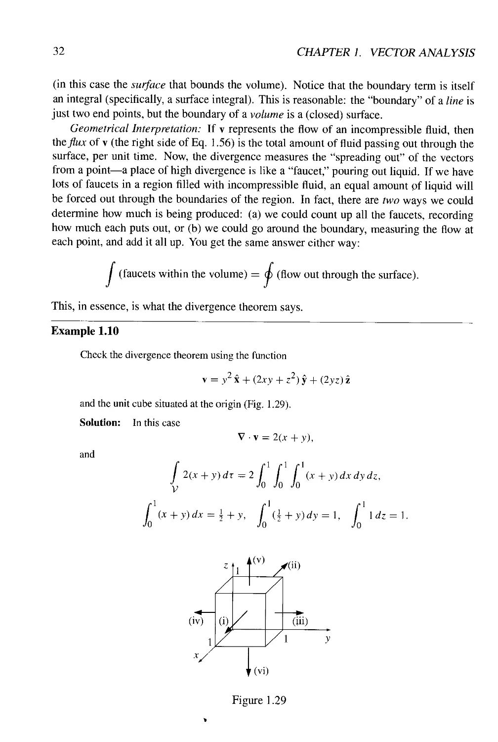
Текст
Introduction to Electrodynamics
David J. Griffiths
Reed College
Prentice
Hall
Prentice Hall
Upper Saddle River, New Jersey 07458
Library of Congress Cataloging-in-Publication Data
Griffiths, David J. (David Jeffrey)
Introduction to electrodynamics / David J. Griffiths - 3rd ed.
p. cm.
Includes bibliographical references and index.
ISBN0-13-805326-X
1. Electrodynamics. I. Title.
OC680.G74 1999
537.6—dc21 98-50525
C1P
Executive Editor: Alison Reeves
Production Editor: Kim Delias
Manufacturing Manager: Trudy Pisciotti
Art Director: Jayne Conte
Cover Designer: Bruce Kenselaar
Editorial Assistant: Gillian Keiff
Composition: PreTjrX, Inc.
1999, 1989, 1981 by Prentice-Hall, Inc.
Upper Saddle River, New Jersey 07458
All rights reserved. No part of this book may be
reproduced, in any form or by any means,
without permission in writing from the publisher.
Reprinted with corrections September, 1999
Printed in the United States of America
10 9 8 7 6 5
ISBN D-13-flDS32t>-X
Prentice-Hall International (UK) Limited, London
Prentice-Hall of Australia Pty. Limited, Sydney
Prentice-Hall Canada Inc., Toronto
Prentice-Hall Hispanoamericana, S.A., Mexico City
Prentice-Hall of India Private Limited, New Delhi
Prentice-Hall of Japan, Inc., Tokyo
Prentice-Hall Asia Pte. Ltd., Singapore
Editora Prentice-Hall do Brasil, Ltda., Rio de Janeiro
Contents
Preface ix
Advertisement xi
1 Vector Analysis 1
1.1 Vector Algebra 1
1.1.1 Vector Operations 1
1.1.2 Vector Algebra: Component Form 4
1.1.3 Triple Products 7
1.1.4 Position, Displacement, and Separation Vectors 8
1.1.5 How Vectors Transform 10
1.2 Differential Calculus 13
1.2.1 "Ordinary" Derivatives 13
1.2.2 Gradient 13
1.2.3 The Operator V 16
1.2.4 The Divergence 17
1.2.5 The Curl 19
1.2.6 Product Rules 20
1.2.7 Second Derivatives 22
1.3 Integral Calculus 24
1.3.1 Line, Surface, and Volume Integrals 24
1.3.2 The Fundamental Theorem of Calculus 28
1.3.3 The Fundamental Theorem for Gradients 29
1.3.4 The Fundamental Theorem for Divergences 31
1.3.5 The Fundamental Theorem for Curls 34
1.3.6 Integration by Parts 37
1.4 Curvilinear Coordinates 38
1.4.1 Spherical Polar Coordinates 38
1.4.2 Cylindrical Coordinates 43
1.5 The Dirac Delta Function 45
1.5.1 The Divergence of f/r2 45
1.5.2 The One-Dimensional Dirac Delta Function 46
in
iv CONTENTS
1.5.3 The Three-Dimensional Delta Function 50
1.6 The Theory of Vector Fields 52
1.6.1 The Helmholtz Theorem 52
1.6.2 Potentials 53
2 Electrostatics 58
2.1 The Electric Field 58
2.1.1 Introduction 58
2.1.2 Coulomb's Law 59
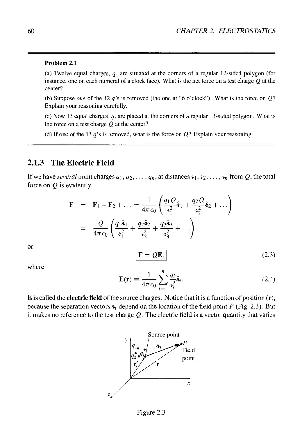
2.1.3 The Electric Field 60
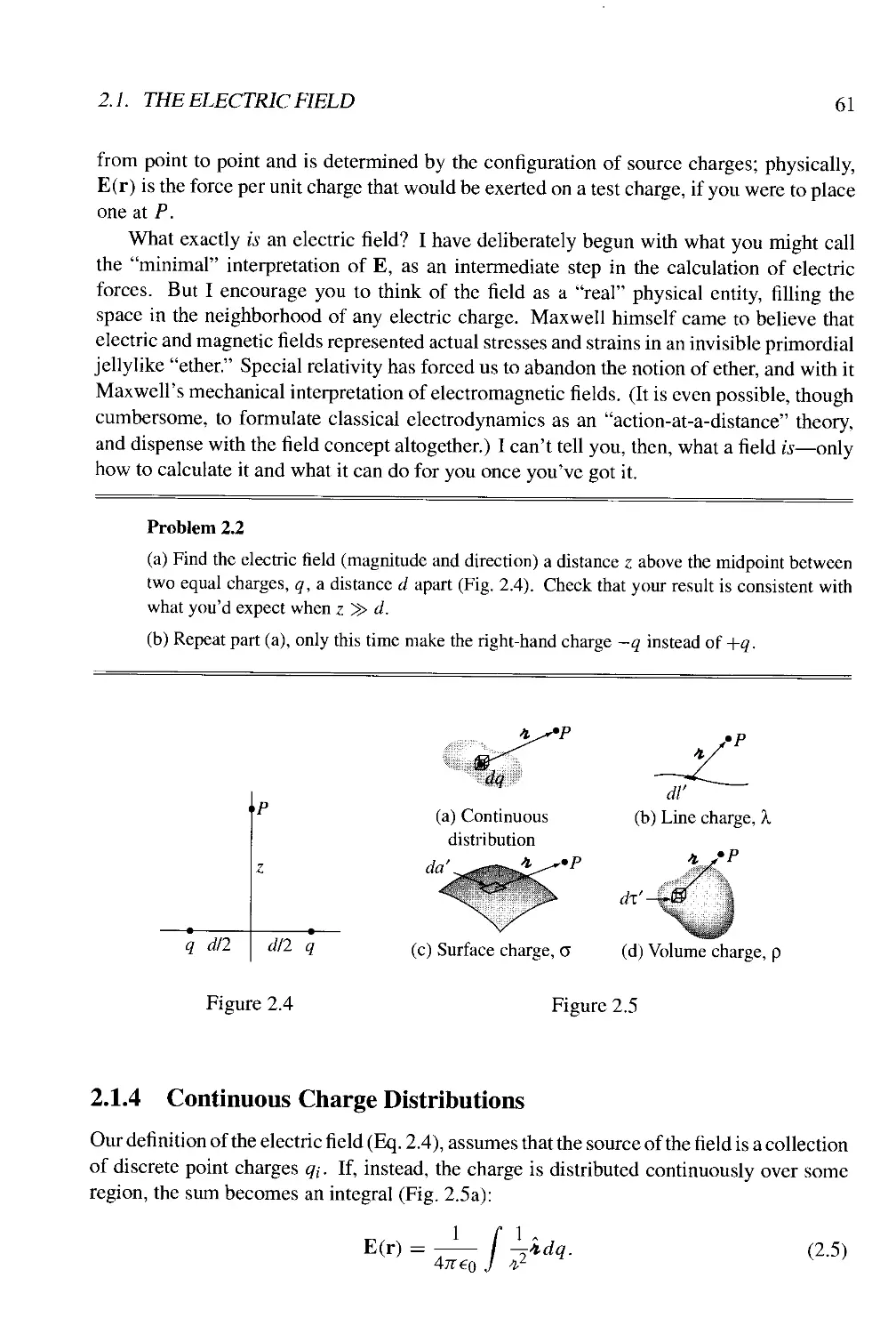
2.1.4 Continuous Charge Distributions 61
2.2 Divergence and Curl of Electrostatic Fields 65
2.2.1 Field Lines, Flux, and Gauss's Law 65
2.2.2 The Divergence of E 69
2.2.3 Applications of Gauss's Law 70
2.2.4 The Curl of E 76
2.3 Electric Potential 77
2.3.1 Introduction to Potential 77
2.3.2 Comments on Potential 79
2.3.3 Poisson's Equation and Laplace's Equation 83
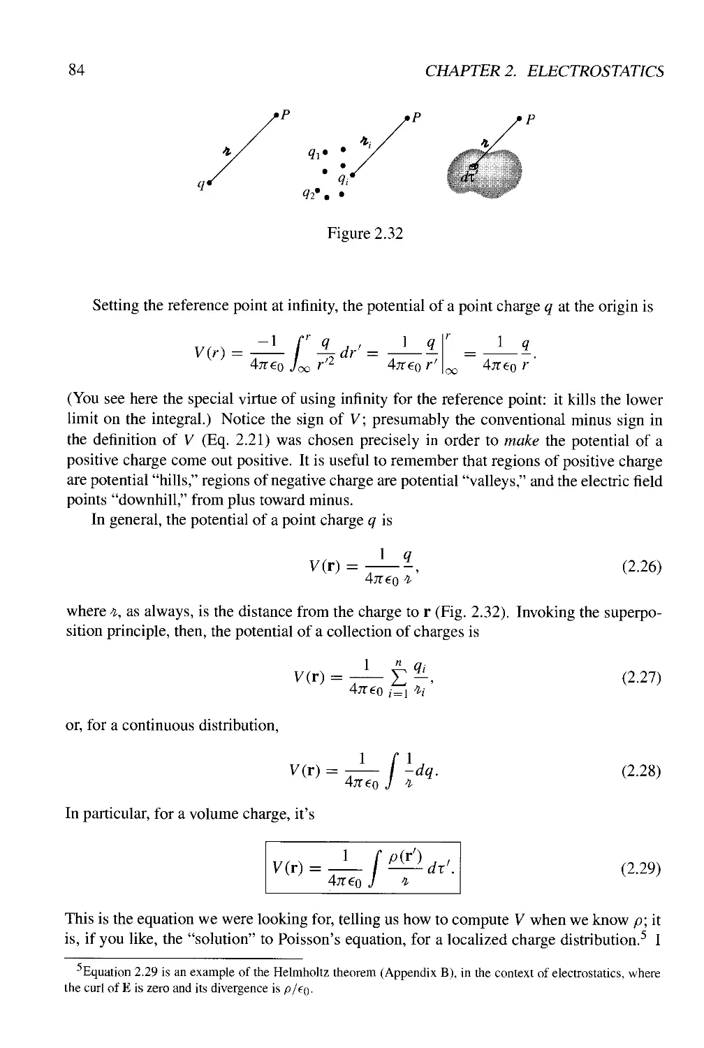
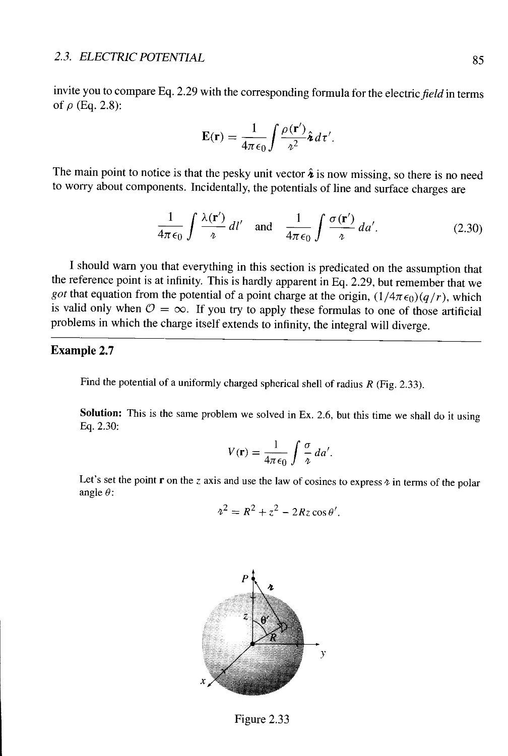
2.3.4 The Potential of a Localized Charge Distribution 83
2.3.5 Summary; Electrostatic Boundary Conditions 87
2.4 Work and Energy in Electrostatics 90
2.4.1 The Work Done to Move a Charge 90
2.4.2 The Energy of a Point Charge Distribution 91
2.4.3 The Energy of a Continuous Charge Distribution 93
2.4.4 Comments on Electrostatic Energy 95
2.5 Conductors 96
2.5.1 Basic Properties 96
2.5.2 Induced Charges 98
2.5.3 Surface Charge and the Force on a Conductor 102
2.5.4 Capacitors 103
3 Special Techniques 110
3.1 Laplace's Equation 110
3.1.1 Introduction 110
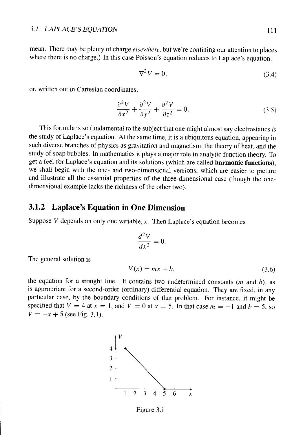
3.1.2 Laplace's Equation in One Dimension Ill
3.1.3 Laplace's Equation in Two Dimensions 112
3.1.4 Laplace's Equation in Three Dimensions 114
3.1.5 Boundary Conditions and Uniqueness Theorems 116
3.1.6 Conductors and the Second Uniqueness Theorem 118
3.2 The Method of Images 121
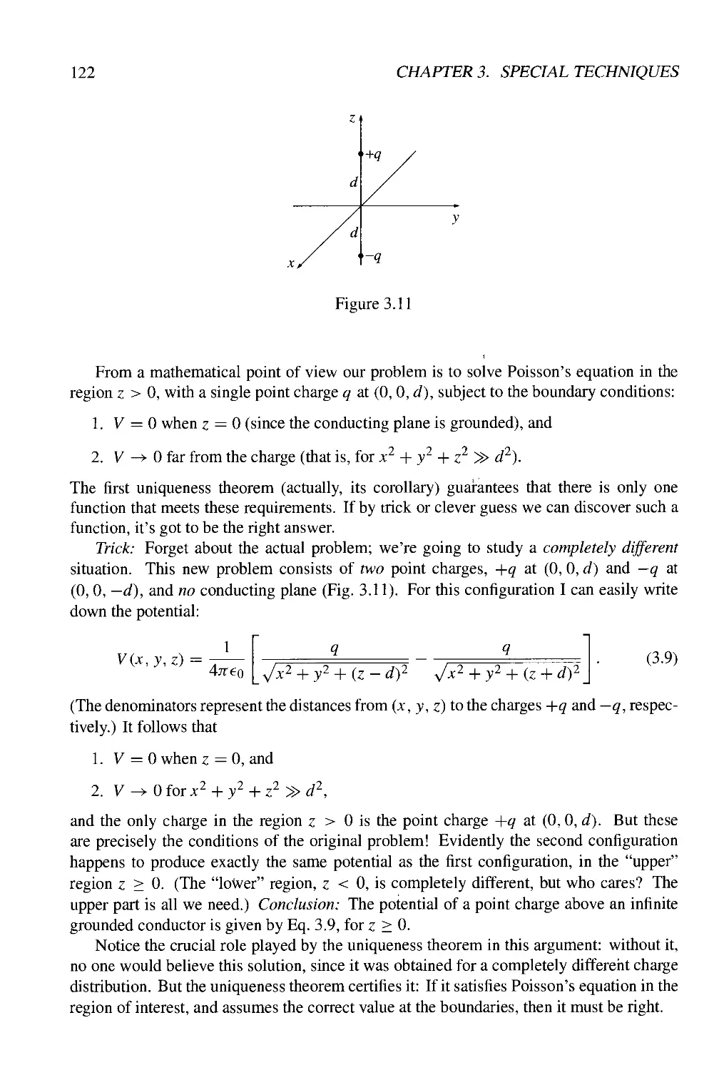
3.2.1 The Classic Image Problem 121
3.2.2 Induced Surface Charge 123
CONTENTS v
3.2.3 Force and Energy 123
3.2.4 Other Image Problems 124
3.3 Separation of Variables 127
3.3.1 Cartesian Coordinates 127
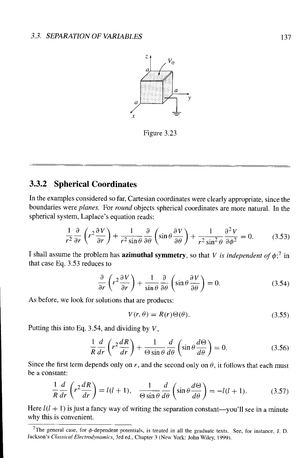
3.3.2 Spherical Coordinates 137
3.4 Multipole Expansion 146
3.4.1 Approximate Potentials at Large Distances 146
3.4.2 The Monopole and Dipole Terms 149
3.4.3 Origin of Coordinates in Multipole Expansions 151
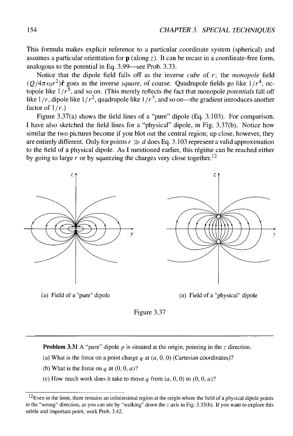
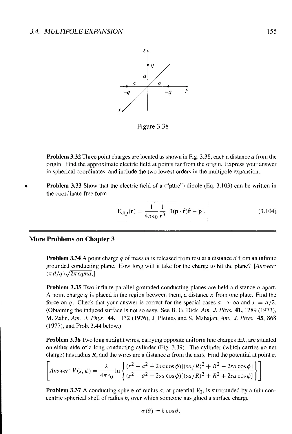
3.4.4 The Electric Field of a Dipole 153
4 Electric Fields in Matter 160
4.1 Polarization 160
4.1.1 Dielectrics 160
4.1.2 Induced Dipoles 160
4.1.3 Alignment of Polar Molecules 163
4.1.4 Polarization 166
4.2 The Field of a Polarized Object 166
4.2.1 Bound Charges 166
4.2.2 Physical Interpretation of Bound Charges 170
4.2.3 The Field Inside a Dielectric 173
4.3 The Electric Displacement 175
4.3.1 Gauss's Law in the Presence of Dielectrics 175
4.3.2 A Deceptive Parallel 178
4.3.3 Boundary Conditions 178
4.4 Linear Dielectrics 179
4.4.1 Susceptibility, Permittivity, Dielectric Constant 179
4.4.2 Boundary Value Problems with Linear Dielectrics 186
4.4.3 Energy in Dielectric Systems 191
4.4.4 Forces on Dielectrics 193
5 Magnetostatics 202
5.1 The Lorentz Force Law 202
5.1.1 Magnetic Fields 202
5.1.2 Magnetic Forces 204
5.1.3 Currents 208
5.2 The Biot-Savart Law 215
5.2.1 Steady Currents 215
5.2.2 The Magnetic Field of a Steady Current 215
5.3 The Divergence and Curl of B 221
5.3.1 Straight-Line Currents 221
5.3.2 The Divergence and Curl of B 222
5.3.3 Applications of Ampere's Law 225
5.3.4 Comparison of Magnetostatics and Electrostatics 232
vi CONTENTS
5.4 Magnetic Vector Potential 234
5.4.1 The Vector Potential 234
5.4.2 Summary; Magnetostatic Boundary Conditions 240
5.4.3 Multipole Expansion of the Vector Potential 242
6 Magnetic Fields in Matter 255
6.1 Magnetization 255
6.1.1 Diamagnets, Paramagnets, Ferromagnets 255
6.1.2 Torques and Forces on Magnetic Dipoles 255
6.1.3 Effect of a Magnetic Field on Atomic Orbits 260
6.1.4 Magnetization 262
6.2 The Field of a Magnetized Object 263
6.2.1 Bound Currents 263
6.2.2 Physical Interpretation of Bound Currents 266
6.2.3 The Magnetic Field Inside Matter 268
6.3 The Auxiliary Field H 269
6.3.1 Ampere's law in Magnetized Materials 269
6.3.2 A Deceptive Parallel 273
6.3.3 Boundary Conditions 273
6.4 Linear and Nonlinear Media 274
6.4.1 Magnetic Susceptibility and Permeability 274
6.4.2 Ferromagnetism 278
7 Electrodynamics 285
7.1 Electromotive Force 285
7.1.1 Ohm's Law 285
7.1.2 Electromotive Force 292
7.1.3 Motional emf 294
7.2 Electromagnetic Induction 301
7.2.1 Faraday's Law 301
7.2.2 The Induced Electric Field 305
7.2.3 Inductance 310
7.2.4 Energy in Magnetic Fields 317
7.3 Maxwell's Equations 321
7.3.1 Electrodynamics Before Maxwell 321
7.3.2 How Maxwell Fixed Ampere's Law 323
7.3.3 Maxwell's Equations 326
7.3.4 Magnetic Charge 327
7.3.5 Maxwell's Equations in Matter 328
7.3.6 Boundary Conditions 331
CONTENTS vii
8 Conservation Laws 34$
8.1 Charge and Energy 345
8.1.1 The Continuity Equation 345
8.1.2 Poynting's Theorem 346
8.2 Momentum 349
8.2.1 Newton's Third Law in Electrodynamics 349
8.2.2 Maxwell's Stress Tensor 351
8.2.3 Conservation of Momentum 355
8.2.4 Angular Momentum 358
9 Electromagnetic Waves 364
9.1 Waves in One Dimension 364
9.1.1 The Wave Equation 364
9.1.2 Sinusoidal Waves 367
9.1.3 Boundary Conditions: Reflection and Transmission 370
9.1.4 Polarization 373
9.2 Electromagnetic Waves in Vacuum 375
9.2.1 The Wave Equation for E and B 375
9.2.2 Monochromatic Plane Waves 376
9.2.3 Energy and Momentum in Electromagnetic Waves 380
9.3 Electromagnetic Waves in Matter 382
9.3.1 Propagation in Linear Media 382
9.3.2 Reflection and Transmission at Normal Incidence 384
9.3.3 Reflection and Transmission at Oblique Incidence 386
9.4 Absorption and Dispersion 392
9.4.1 Electromagnetic Waves in Conductors 392
9.4.2 Reflection at a Conducting Surface 396
9.4.3 The Frequency Dependence of Permittivity 398
9.5 Guided Waves 405
9.5.1 Wave Guides 405
9.5.2 TE Waves in a Rectangular Wave Guide 408
9.5.3 The Coaxial Transmission Line 411
10 Potentials and Fields 416
10.1 The Potential Formulation 416
10.1.1 Scalar and Vector Potentials 416
10.1.2 Gauge Transformations 419
10.1.3 Coulomb Gauge and Lorentz* Gauge 421
10.2 Continuous Distributions 422
10.2.1 Retarded Potentials 422
10.2.2 Jefimenko's Equations 427
10.3 Point Charges 429
10.3.1 Lienard-Wiechert Potentials 429
10.3.2 The Fields of a Moving Point Charge 435
viii CONTENTS
11 Radiation 443
11.1 Dipole Radiation 443
11.1.1 What is Radiation? 443
11.1.2 Electric Dipole Radiation 444
11.1.3 Magnetic Dipole Radiation 451
11.1.4 Radiation from an Arbitrary Source 454
11.2 Point Charges 460
11.2.1 Power Radiated by a Point Charge 460
11.2.2 Radiation Reaction 465
11.2.3 The Physical Basis of the Radiation Reaction 469
12 Electrodynamics and Relativity 477
12.1 The Special Theory of Relativity 477
12.1.1 Einstein's Postulates 477
12.1.2 The Geometry of Relativity 483
12.1.3 The Lorentz Transformations 493
12.1.4 The Structure of Spacetime 500
12.2 Relativistic Mechanics 507
12.2.1 Proper Time and Proper Velocity 507
12.2.2 Relativistic Energy and Momentum 509
12.2.3 Relativistic Kinematics 511
12.2.4 Relativistic Dynamics 516
12.3 Relativistic Electrodynamics 522
12.3.1 Magnetism as a Relativistic Phenomenon 522
12.3.2 How the Fields Transform 525
12.3.3 The Field Tensor 535
12.3.4 Electrodynamics in Tensor Notation 537
12.3.5 Relativistic Potentials 541
A Vector Calculus in Curvilinear Coordinates 547
A.I Introduction 547
A.2 Notation 547
A.3 Gradient 548
A.4 Divergence 549
A.5 Curl 552
A.6 Laplacian 554
B The Helmholtz Theorem 555
C Units 558
Index 562
Preface
This is a textbook on electricity and magnetism, designed for an undergraduate course at
the junior or senior level. It can be covered comfortably in two semesters, maybe even
with room to spare for special topics (AC circuits, numerical methods, plasma physics,
transmission lines, antenna theory, etc.) A one-semester course could reasonably stop
after Chapter 7. Unlike quantum mechanics or thermal physics (for example), there is a
fairly general consensus with respect to the teaching of electrodynamics; the subjects to
be included, and even their order of presentation, are not particularly controversial, and
textbooks differ mainly in style and tone. My approach is perhaps less formal than most; I
think this makes difficult ideas more interesting and accessible.
For the third edition I have made a large number of small changes, in the interests of
clarity and grace. I have also modified some notation to avoid inconsistencies or ambiguities.
Thus the Cartesian unit vectors i, j, and k have been replaced with x, y, and z, so that all
vectors are bold, and all unit vectors inherit the letter of the corresponding coordinate.
(This also frees up k to be the propagation vector for electromagnetic waves.) It has always
bothered me to use the same letter r for the spherical coordinate (distance from the origin)
and the cylindrical coordinate (distance from the z axis). A common alternative for the
latter is p, but that has more important business in electrodynamics, and after an exhaustive
search I settled on the underemployed letter s; I hope this unorthodox usage will not be
confusing.
Some readers have urged me to abandon the script letter* (the vector from a source point
r' to the field point r) in favor of the more explicit r - r'. But this makes many equations
distractingly cumbersome, especially when the unit vector •? is involved. I know from my
own teaching experience that unwary students are tempted to read * as r—it certainly makes
the integrals easier! I have inserted a section in Chapter 1 explaining this notation, and I
hope that will help. If you are a student, please take note: * = r — r', which is not the same
as r. If you're a teacher, please warn your students to pay close attention to the meaning of
*. I think it's good notation, but it does have to be handled with care.
The rnain structural change is that I have removed the conservation laws and potentials
from Chapter 7, creating two new short chapters (8 and 10). This should more smoothly
accommodate one-semester courses, and it gives a tighter focus to Chapter 7.
I have added some problems and examples (and removed a few that were not effective).
And I have included more references to the accessible literature (particularly the American
Journal of Physics). I realize, of course, that most readers will not have the time or incli-
IX
x PREFACE
nation to consult these resources, but I think it is worthwhile anyway, if only to emphasize
that electrodynamics, notwithstanding its venerable age, is very much alive, and intriguing
new discoveries are being made all the time. I hope that occasionally a problem will pique
your curiosity, and you will be inspired to look up the reference—some of them are real
gems.
As in the previous editions, I distinguish two kinds of problems. Some have a specific
pedagogical purpose, and should be worked immediately after reading the section to which
they pertain; these I have placed at the pertinent point within the chapter. (In a few cases
the solution to a problem is used later in the text; these are indicated by a bullet (•) in the
left margin.) Longer problems, or those of a more general nature, will be found at the end
of each chapter. When I teach the subject I assign some of these, and work a few of them
in class. Unusually challenging problems are flagged by an exclamation point (!) in the
margin. Many readers have asked that the answers to problems be provided at the back
of the book; unfortunately, just as many are strenuously opposed. I have compromised,
supplying answers when this seems particularly appropriate. A complete solution manual
is available (to instructors) from the publisher.
I have benefitted from the comments of many colleagues—I cannot list them all here.
But I would like to thank the following people for suggestions that contributed specifically
to the third edition: Burton Brody (Bard), Steven Grimes (Ohio), Mark Heald (Swarth-
more), Jim McTavish (Liverpool), Matthew Moelter (Puget Sound), Paul Nachman (New
Mexico State), Gigi Quartapelle (Milan), Carl A. Rotter (West Virginia), Daniel Schroeder
(Weber State), Juri Silmberg (Ryerson Polytechnic), Walther N. Spjeldvik (Weber State),
Larry fankersley (Naval Academy), and Dudley Towne (Amherst). Practically everything I
know about electrodynamics—certainly about teaching electrodynamics—I owe to Edward
Purcell.
David J. Griffiths
Advertisement
What is electrodynamics, and how does it fit into the
general scheme of physics?
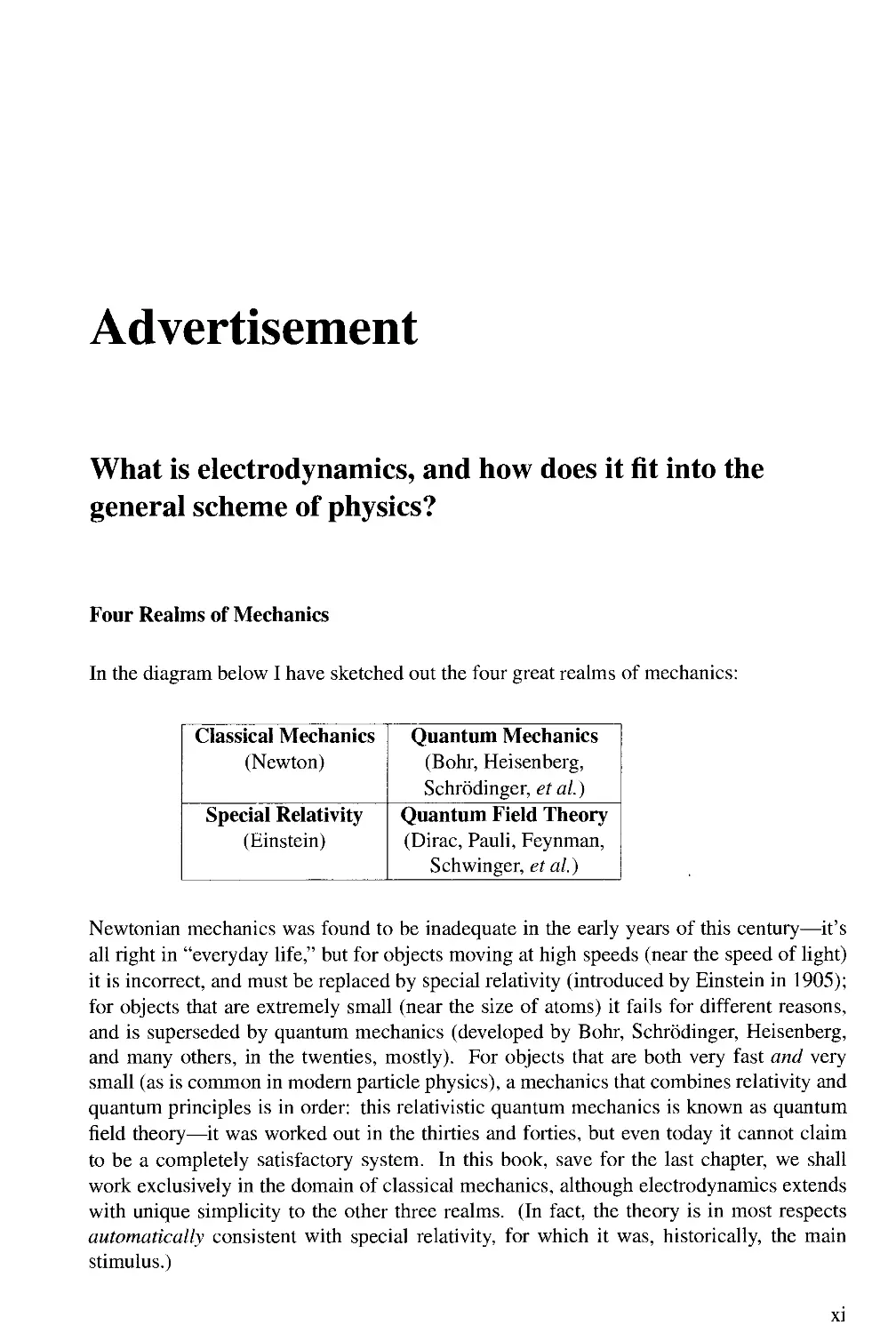
Four Realms of Mechanics
In the diagram below I have sketched out the four great realms of mechanics:
Classical Mechanics
(Newton)
Special Relativity
(Einstein)
Quantum Mechanics
(Bohr, Heisenberg,
Schrodinger, et al.)
Quantum Field Theory
(Dirac, Pauli, Feynman,
Schwinger, et al.)
Newtonian mechanics was found to be inadequate in the early years of this century—it's
all right in "everyday life," but for objects moving at high speeds (near the speed of light)
it is incorrect, and must be replaced by special relativity (introduced by Einstein in 1905);
for objects that are extremely small (near the size of atoms) it fails for different reasons,
and is superseded by quantum mechanics (developed by Bohr, Schrodinger, Heisenberg,
and many others, in the twenties, mostly). For objects that are both very fast and very
small (as is common in modern particle physics), a mechanics that combines relativity and
quantum principles is in order: this relativistic quantum mechanics is known as quantum
field theory—it was worked out in the thirties and forties, but even today it cannot claim
to be a completely satisfactory system. In this book, save for the last chapter, we shall
work exclusively in the domain of classical mechanics, although electrodynamics extends
with unique simplicity to the other three realms. (In fact, the theory is in most respects
automatically consistent with special relativity, for which it was, historically, the main
stimulus.)
XI
xii ADVERTISEMENT
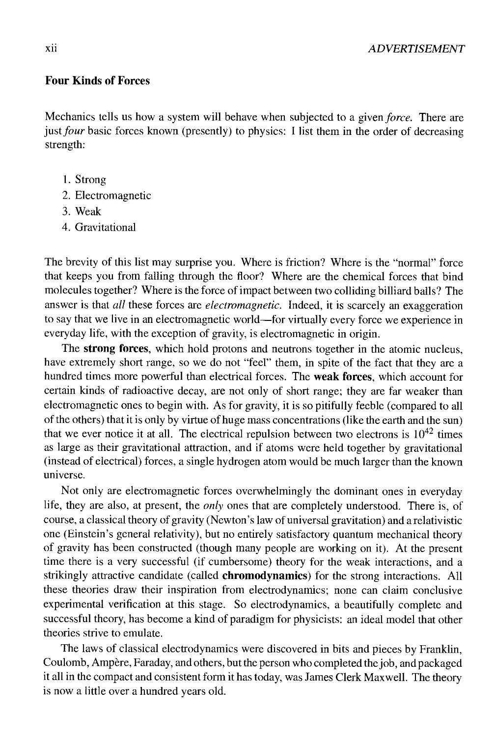
Four Kinds of Forces
Mechanics tells us how a system will behave when subjected to a given force. There are
just four basic forces known (presently) to physics: I list them in the order of decreasing
strength:
1. Strong
2. Electromagnetic
3. Weak
4. Gravitational
The brevity of this list may surprise you. Where is friction? Where is the "normal" force
that keeps you from falling through the floor? Where are the chemical forces that bind
molecules together? Where is the force of impact between two colliding billiard balls? The
answer is that all these forces are electromagnetic. Indeed, it is scarcely an exaggeration
to say that we live in an electromagnetic world—for virtually every force we experience in
everyday life, with the exception of gravity, is electromagnetic in origin.
The strong forces, which hold protons and neutrons together in the atomic nucleus,
have extremely short range, so we do not "feel" them, in spite of the fact that they are a
hundred times more powerful than electrical forces. The weak forces, which account for
certain kinds of radioactive decay, are not only of short range; they are far weaker than
electromagnetic ones to begin with. As for gravity, it is so pitifully feeble (compared to all
of the others) that it is only by virtue of huge mass concentrations (like the earth and the sun)
that we ever notice it at all. The electrical repulsion between two electrons is 1042 times
as large as their gravitational attraction, and if atoms were held together by gravitational
(instead of electrical) forces, a single hydrogen atom would be much larger than the known
universe.
Not only are electromagnetic forces overwhelmingly the dominant ones in everyday
life, they are also, at present, the only ones that are completely understood. There is, of
course, a classical theory of gravity (Newton's law of universal gravitation) and arelativistic
one (Einstein's general relativity), but no entirely satisfactory quantum mechanical theory
of gravity has been constructed (though many people are working on it). At the present
time there is a very successful (if cumbersome) theory for the weak interactions, and a
strikingly attractive candidate (called chromodynamics) for the strong interactions. All
these theories draw their inspiration from electrodynamics; none can claim conclusive
experimental verification at this stage. So electrodynamics, a beautifully complete and
successful theory, has become a kind of paradigm for physicists: an ideal model that other
theories strive to emulate.
The laws of classical electrodynamics were discovered in bits and pieces by Franklin,
Coulomb, Ampere, Faraday, and others, but the person who completed the job, and packaged
it all in the compact and consistent form it has today, was James Clerk Maxwell. The theory
is now a little over a hundred years old.
Xlll
The Unification of Physical Theories
In the beginning, electricity and magnetism were entirely separate subjects. The one dealt
with glass rods and cat's fur, pith balls, batteries, currents, electrolysis, and lightning; the
other with bar magnets, iron filings, compass needles, and the North Pole. But in 1820
Oersted noticed that an electric current could deflect a magnetic compass needle. Soon
afterward, Ampere correctly postulated that all magnetic phenomena are due to electric
charges in motion. Then, in 1831, Faraday discovered that a moving magnet generates an
electric current. By the time Maxwell and Lorentz put the finishing touches on the theory,
electricity and magnetism were inextricably intertwined. They could no longer be regarded
as separate subjects, but rather as two aspects of a single subject: electromagnetism.
Faraday had speculated that light, too, is electrical in nature. Maxwell's theory provided
spectacular justification for this hypothesis, and soon optics—the study of lenses, mirrors,
prisms, interference, and diffraction—was incorporated into electromagnetism. Hertz, who
presented the decisive experimental confirmation for Maxwell's theory in 1888, put it this
way: "The connection between light and electricity is now established ... In every flame,
in every luminous particle, we see an electrical process ... Thus, the domain of electricity
extends over the whole of nature. It even affects ourselves intimately: we perceive that we
possess ... an electrical organ—the eye." By 1900, then, three great branches of physics,
electricity, magnetism, and optics, had merged into a single unified theory. (And it was
soon apparent that visible light represents only a tiny "window" in the vast spectrum of
electromagnetic radiation, from radio though microwaves, infrared and ultraviolet, to x-
rays and gamma rays.)
Einstein dreamed of a further unification, which would combine gravity and electrody-
namics, in much the same way as electricity and magnetism had been combined a century
earlier. His unified field theory was not particularly successful, but in recent years the same
impulse has spawned a hierarchy of increasingly ambitious (and speculative) unification
schemes, beginning in the 1960s with the electroweak theory of Glashow, Weinberg, and
Salam (which joins the weak and electromagnetic forces), and culminating in the 1980s with
the superstring theory (which, according to its proponents, incorporates all four forces in a
single "theory of everything"). At each step in this hierarchy the mathematical difficulties
mount, and the gap between inspired conjecture and experimental test widens; nevertheless,
it is clear that the unification of forces initiated by electrodynamics has become a major
theme in the progress of physics.
The Field Formulation of Electrodynamics
The fundamental problem a theory of electromagnetism hopes to solve is this: I hold up
a bunch of electric charges here (and maybe shake them around)—what happens to some
other charge, over there? The classical solution takes the form of a field theory: We say
that the space around an electric charge is permeated by electric and magnetic fields (the
electromagnetic "odor," as it were, of the charge). A second charge, in the presence of these
fields, experiences a force; the fields, then, transmit the influence from one charge to the
other—they mediate the interaction.
xiv ADVERTISEMENT
When a charge undergoes acceleration, a portion of the field "detaches" itself, in a
sense, and travels off at the speed of light, carrying with it energy, momentum, and angular
momentum. We call this electromagnetic radiation. Its existence invites (if not compels)
us to regard the fields as independent dynamical entities in their own right, every bit as
"real" as atoms or baseballs. Our interest accordingly shifts from the study of forces
between charges to the theory of the fields themselves. But it takes a charge to produce an
electromagnetic field, and it takes another charge to detect one, so we had best begin by
reviewing the essential properties of electric charge.
Electric Charge
1. Charge comes in two varieties, which we call "plus" and "minus," because their effects
tend to cancel (if you have +q and — q at the same point, electrically it is the same as having
no charge there at all). This may seem too obvious to warrant comment, but I encourage you
to contemplate other possibilities: what if there were 8 or 10 different species of charge?
(In chromodynamics there are, in fact, three quantities analogous to electric charge, each
of which may be positive or negative.) Or what if the two kinds did not tend to cancel?
The extraordinary fact is that plus and minus charges occur in exactly equal amounts, to
fantastic precision, in bulk matter, so that their effects are almost completely neutralized.
Were it not for this, we would be subjected to enormous forces: a potato would explode
violently if the cancellation were imperfect by as little as one part in 1010.
2. Charge is conserved: it cannot be created or destroyed—what there is now has always
been. (A plus charge can "annihilate" an equal minus charge, but aplus charge cannot simply
disappear by itself—something must account for that electric charge.) So the total charge of
the universe is fixed for all time. This is called global conservation of charge. Actually, I can
say something much stronger: Global conservation would allow for a charge to disappear
in New York and instantly reappear in San Francisco (that wouldn't affect the total), and yet
we know this doesn't happen. If the charge was in New York and it went to San Francisco,
then it must have passed along some continuous path from one to the other. This is called
local conservation of charge. Later on we'll see how to formulate a precise mathematical
law expressing local conservation of charge—it's called the continuity equation.
3. Charge is quantized. Although nothing in classical electrodynamics requires that it be
so, the fact is that electric charge comes only in discrete lumps—integer multiples of the
basic unit of charge. If we call the charge on the proton +e, then the electron carries charge
—e, the neutron charge zero, the pi mesons +e, 0, and —e, the carbon nucleus +6e, and
so on (never 7.392e, or even l/2e).' This fundamental unit of charge is extremely small,
so for practical purposes it is usually appropriate to ignore quantization altogether. Water,
too, "really" consists of discrete lumps (molecules); yet, if we are dealing with reasonably
large large quantities of it we can treat it as a continuous fluid. This is in fact much closer
to Maxwell's own view; he knew nothing of electrons and protons—he must have pictured
' Actually, protons and neutrons are composed of three quarks, which carry fractional charges (± | e and ± A e).
However, free quarks do not appear to exist in nature, and in any event this does not alter the fact that charge is
quantized; it merely reduces the size of the basic unit.
XV
charge as a kind of "jelly" that could be divided up into portions of any size and smeared
out at will.
These, then, are the basic properties of charge. Before we discuss the forces between
charges, some mathematical tools are necessary; their introduction will occupy us in Chap-
ter 1.
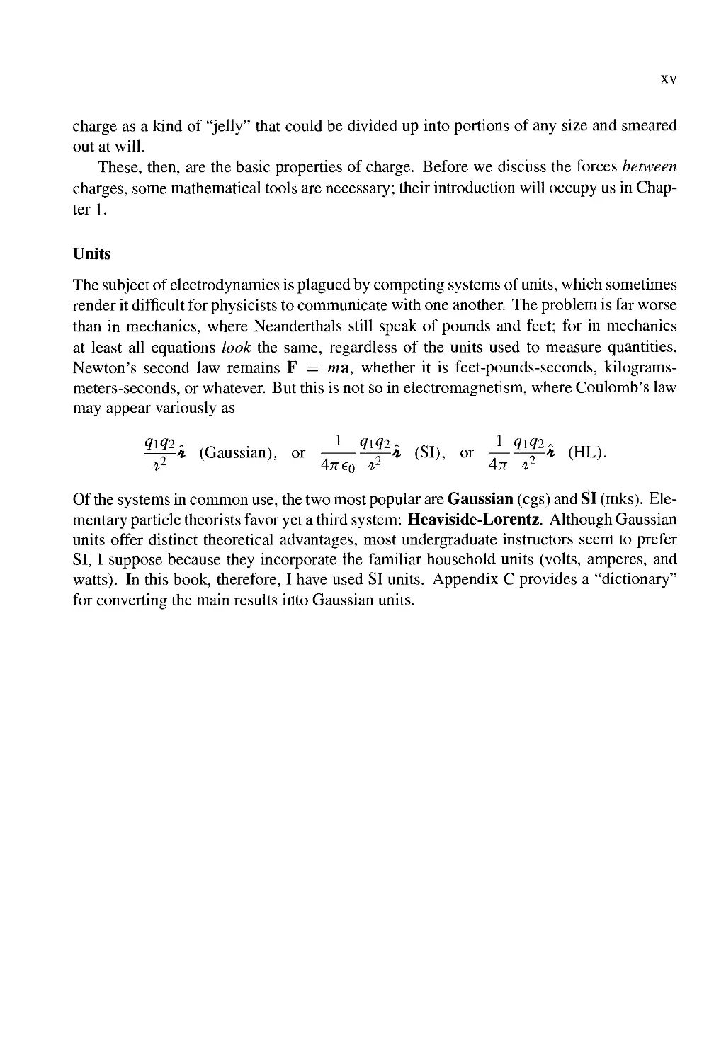
Units
The subject of electrodynamics is plagued by competing systems of units, which sometimes
render it difficult for physicists to communicate with one another. The problem is far worse
than in mechanics, where Neanderthals still speak of pounds and feet; for in mechanics
at least all equations look the same, regardless of the units used to measure quantities.
Newton's second law remains F — ma, whether it is feet-pounds-seconds, kilograms-
meters-seconds, or whatever. But this is not so in electromagnetism, where Coulomb's law
may appear variously as
(Gaussian), or -±-^i (SI), or J-*«i (HL).
4t€ il Ait n,L
Of the systems in common use, the two most popular are Gaussian (cgs) and Sil (mks). Ele-
mentary particle theorists favor yet a third system: Heaviside-Lorentz. Although Gaussian
units offer distinct theoretical advantages, most undergraduate instructors seerrl to prefer
SI, I suppose because they incorporate the familiar household units (volts, amperes, and
watts). In this book, therefore, I have used SI units. Appendix C provides a "dictionary"
for converting the main results irito Gaussian units.
Chapter 1
Vector Analysis
1.1 Vector Algebra
1.1.1 Vector Operations
If you walk 4 miles due north and then 3 miles due east (Fig. 1.1), you will have gone a
total of 7 miles, but you're not 7 miles from where you set out—you're only 5. We need an
arithmetic to describe quantities like this, which evidently do not add in the ordinary way.
The reason they don't, of course, is that displacements (straight line segments going from
one point to another) have direction as well as magnitude (length), and it is essential to
take both into account when you combine them. Such objects are called vectors: velocity,
acceleration, force and momentum are other examples. By contrast, quantities that have
magnitude but no direction are called scalars: examples include mass, charge, density,
and temperature. I shall use boldface (A, B, and so on) for vectors and ordinary type
for scalars. The magnitude of a vector A is written |A| or, more simply, A. In diagrams,
vectors are denoted by arrows: the length of the arrow is proportional to the magnitude of
the vector, and the arrowhead indicates its direction. Minus A (—A) is a vector with the
3 mi
5 mi
Figure 1.1
Figure 1.2
2 CHAPTER 1. VECTOR ANALYSIS
same magnitude as A but of opposite direction (Fig. 1.2). Note that vectors have magnitude
and direction but not location: a displacement of 4 miles due north from Washington is
represented by the same vector as a displacement 4 miles north from Baltimore (neglecting,
of course, the curvature of the earth). On a diagram, therefore, you can slide the arrow
around at will, as long as you don't change" its length or direction.
We define four vector operations: addition and three kinds of multiplication.
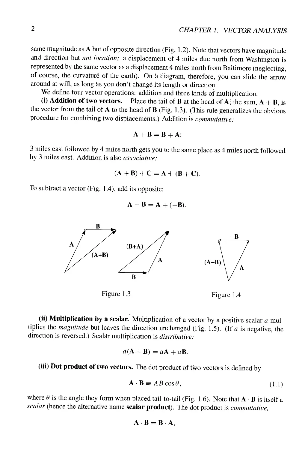
(i) Addition of two vectors. Place the tail of B at the head of A; the sum, A + B, is
the vector from the tail of A to the head of B (Fig. 1.3). (This rule generalizes the obvious
procedure for combining two displacements.) Addition is commutative:
A + B = B + A;
3 miles east followed By 4 miles north gets you to the same place as 4 miles north followed
by 3 miles east. Addition is also associative:
To subtract a vector (Fig. 1.4), add its opposite:
A-B = A +
Figure 1.4
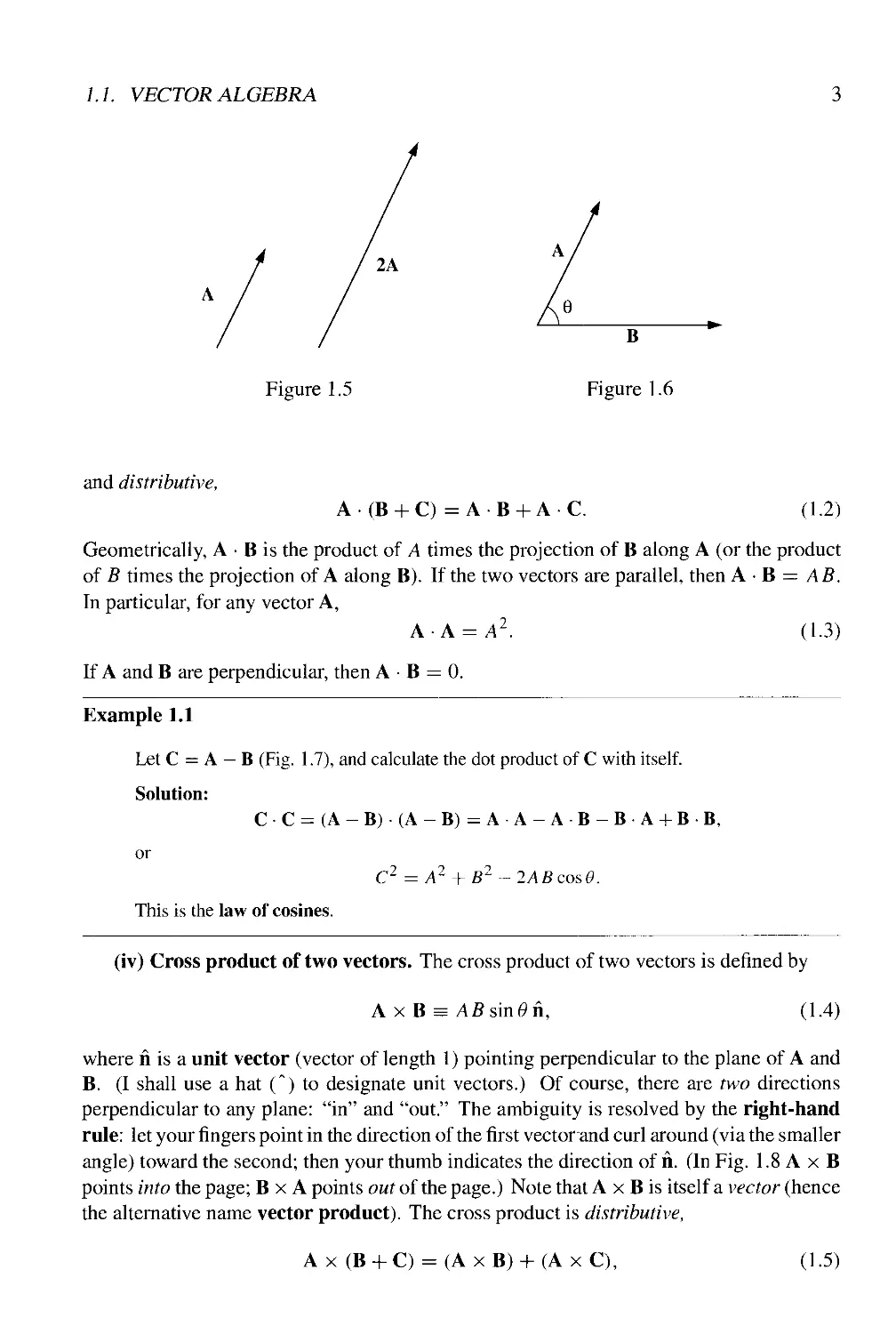
(ii) Multiplication by a scalar. Multiplication of a vector by a positive scalar a mul-
tiplies the magnitude but leaves the direction unchanged (Fig. 1.5). (If a is negative, the
direction is reversed.) Scalar multiplication is distributive:
a(A + B) = aA + aB.
(iii) Dot product of two vectors. The dot product of two vectors is defined by
A-B = AB cos6, A.1)
where 6 is the angle they form when placed tail-to-tail (Fig. 1.6). Note that A ¦ B is itself a
scalar (hence the alternative name scalar product). The dot product is commutative,
A • B = B • A,
/./. VECTOR ALGEBRA
2A
B
Figure 1.5 Figure 1.6
and distributive,
A-(B + C) = A-B + A-C. A.2)
Geometrically, A • B is the product of A times the projection of B along A (or the product
of B times the projection of A along B). If the two vectors are parallel, then A • B = A B.
In particular, for any vector A,
X-X = A2. A.3)
If A and B are perpendicular, then A ¦ B = 0.
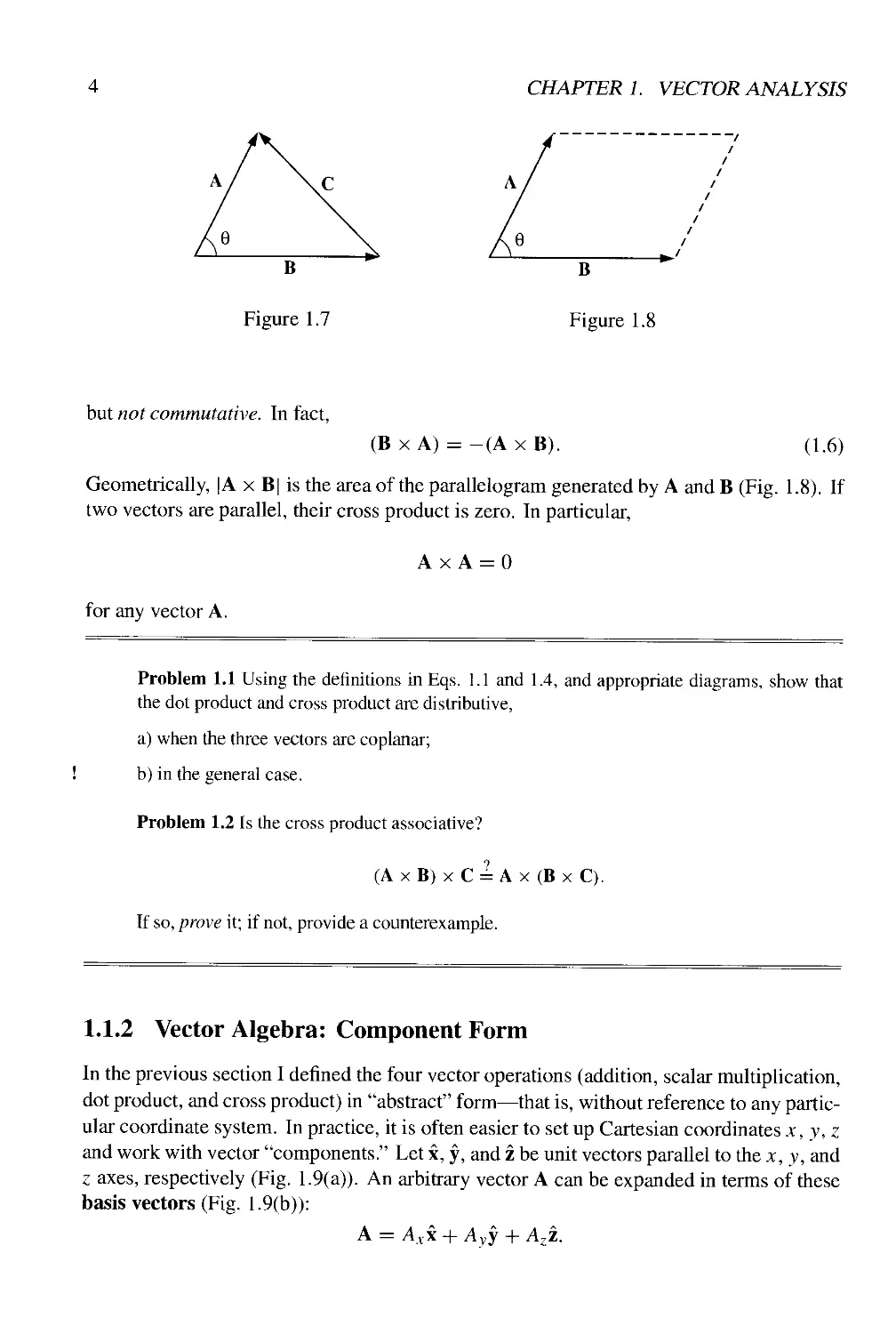
Example 1.1
Let C = A - B (Fig. 1.7), and calculate the dot product of C with itself.
Solution:
CC = (A-B)(A-B)=AA-AB-BA + BB,
or
C2 = A2 + B2 -2ABcos0.
This is the law of cosines.
(iv) Cross product of two vectors. The cross product of two vectors is defined by
A x B =-4fisin6»n, A.4)
where n is a unit vector (vector of length 1) pointing perpendicular to the plane of A and
B. (I shall use a hat (") to designate unit vectors.) Of course, there are two directions
perpendicular to any plane: "in" and "out." The ambiguity is resolved by the right-hand
rule: let your fingers point in the direction of the first vector and curl around (via the smaller
angle) toward the second; then your thumb indicates the direction of n. (In Fig. 1.8 A x B
points into the page; B x A points out of the page.) Note that A x B is itself a vector (hence
the alternative name vector product). The cross product is distributive,
A x (B + C) = (A xB) + (A x C), A.5)
CHAPTER 1. VECTOR ANALYSIS
B
Figure 1.8
but not commutative. In fact,
(B x A) = -(A x B).
A.6)
Geometrically, | A x B is the area of the parallelogram generated by A and B (Fig. 1.8). If
two vectors are parallel, their cross product is zero. In particular,
Ax A = 0
for any vector A.
Problem 1.1 Using the definitions in Eqs. 1.1 and 1.4, and appropriate diagrams, show that
the dot product and cross product are distributive,
a) when the three vectors are coplanar;
b) in the general case.
Problem 1.2 Is the cross product associative?
(A x B) x C = A x (B x C).
If so, prove it; if not, provide a counterexample.
1.1.2 Vector Algebra: Component Form
In the previous section I defined the four vector operations (addition, scalar multiplication,
dot product, and cross product) in "abstract" form—that is, without reference to any partic-
ular coordinate system. In practice, it is often easier to set up Cartesian coordinates x, y, z
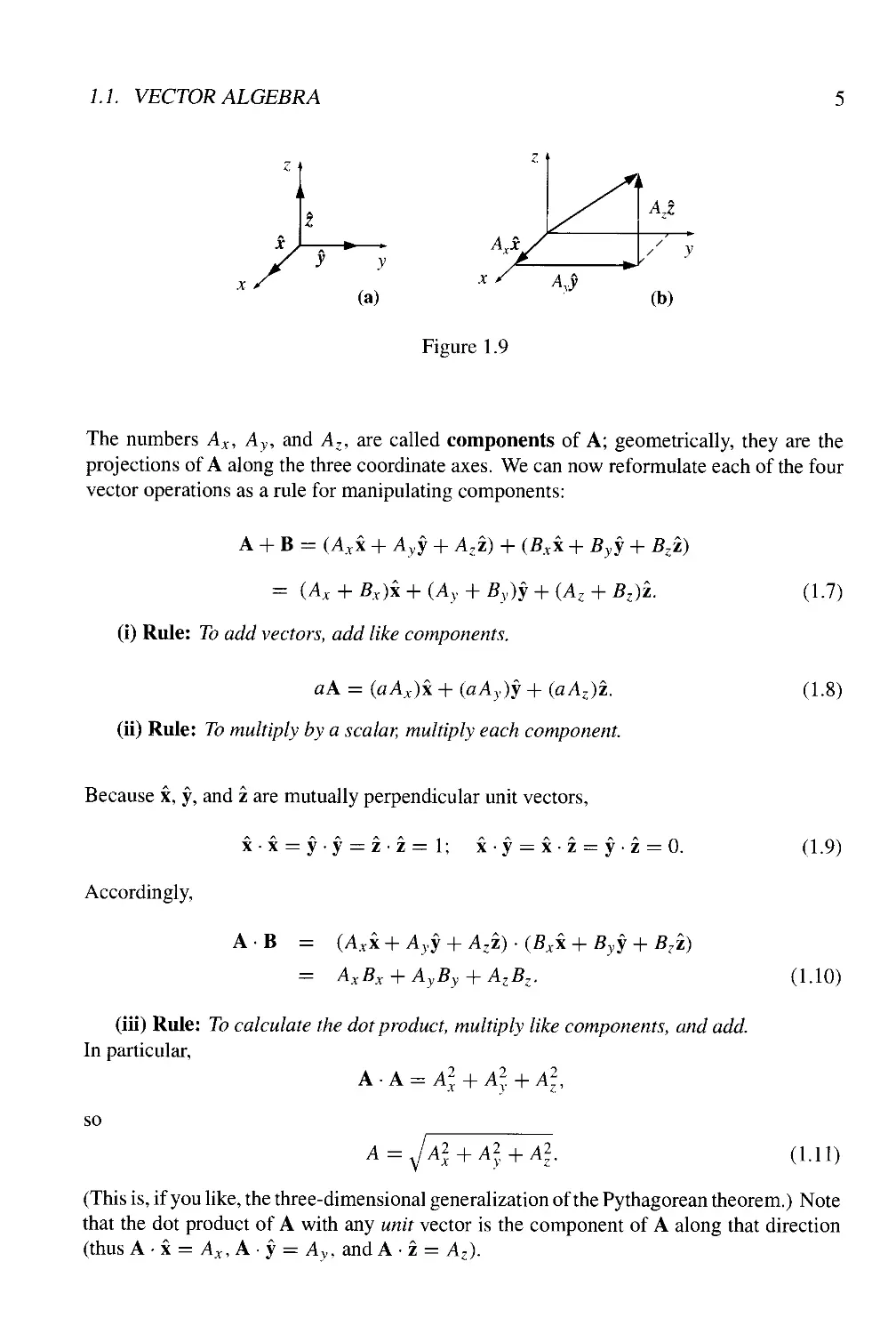
and work with vector "components." Let x, y, and z be unit vectors parallel to the x, y, and
Z axes, respectively (Fig. 1.9(a)). An arbitrary vector A can be expanded in terms of these
basis vectors (Fig. 1.9(b)):
A = Axx + Ayf + Azz.
1.1. VECTOR ALGEBRA
z
y
y
(a)
A
X A
z
V
/
Aj
(b)
Figure 1.9
The numbers Ax, Ay, and Az, are called components of A; geometrically, they are the
projections of A along the three coordinate axes. We can now reformulate each of the four
vector operations as a rule for manipulating components:
A + B = (Axx + Ayy + Azi) + (Bxx + Byy + Bzi)
= (Ax + Bx)x + (Ay + By)y + (Az + Bz)z.
(i) Rule: To add vectors, add like components.
aA = (aAx)x + (aAy)y + (aAz)z.
(ii) Rule: To multiply by a scalar, multiply each component.
A.7)
A.8)
Because x, y, and z are mutually perpendicular unit vectors,
Accordingly,
A • B = (Axx + Ayy + Azz) ¦ (Bxx + Byy + Bzz)
= AXBX + AyBy + AZBZ.
(iii) Rule: To calculate the dot product, multiply like components, and add.
In particular,
A • A = A\ + A\. + A\,
so
A.9)
A.10)
A.11)
(This is, if you like, the three-dimensional generalization of the Pythagorean theorem.) Note
that the dot product of A with any unit vector is the component of A along that direction
(thus A • x = Ax, A • y = Av, and A • z = Az).
CHAPTER 1. VECTOR ANALYSIS
Similarly,1
x x x = yxy = z x z = 0,
x x y = —y x x = z,
y x z = — z x y = x,
z x x = —x x z = y. A-12)
Therefore,
Aw K — (A v I A v I A rw\ y (R v I R v I R 7^ /I 1 ^
= (AyBz - AzBy)x + (AZBX - AxBz)f + (AxBy - AyBx)z.
This cumbersome expression can be written more neatly as a determinant:
A xB =
Ax Ay Az
Bx By Bz
A.14)
(iv)Rule: To calculate the cross product, form the determinantwhose first row is x, y, z,
whose second row is A (in component form), and whose third row is B.
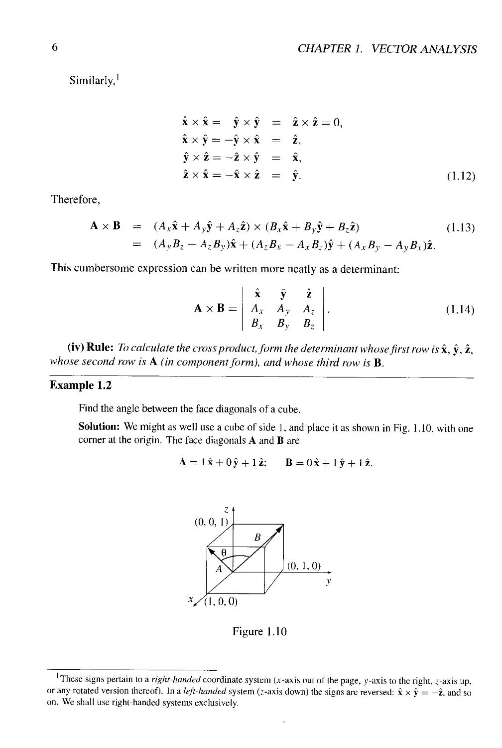
Example 1.2
Find the angle between the face diagonals of a cube.
Solution: We might as well use a cube of side 1, and place it as shown in Fig. 1.10, with one
corner at the origin. The face diagonals A and B are
A = lx + 0y+lz; B=0x+ly+lz.
0,
/
\
/
Z
1L
k
/
y
/
@,1
,0)
y
,0,0)
Figure 1.10
1 These signs pertain to a right-handed coordinate system (jc-axis out of the page, y-axis to the right, z-axis up,
or any rotated version thereof). In a left-handed system (z-axis down) the signs are reversed: x x y = —z, and so
on. We shall use right-handed systems exclusively.
1.1. VECTOR ALGEBRA
So, in component form,
A B= 1 -0 + 0- 1 + 1-1 = 1.
On the other hand, in "abstract" form,
A-B = ABcos9 =
= 2cos#.
Therefore,
cose = 1/2, or 6»=60°.
Of course, you can get the answer more easily by drawing in a diagonal across the top of the
cube, completing the equilateral triangle. But in cases where the geometry is not so simple,
this device of comparing the abstract and component forms of the dot product can be a very
efficient means of finding angles.
Problem 1.3 Find the angle between the body diagonals of a cube.
Problem 1.4 Use the cross product to find the cdmponents of the unit vector ii perpendicular
to the plane shown in Fig. 1.11.
1.1.3 Triple Products
Since the cross product of two vectors is itself a vector, it can be dotted or crossed with a
third vector to form a triple product.
(i) Scalar triple product: A • (B x C). Geometrically, |A ¦ (B x C)| is the volume
of the parallelepiped generated by A, B, and C, since |B x C| is the area of the base, and
|Acos6»| is the altitude (Fig. 1.12). Evidently,
A • (B x C) = B • (C x A) = C • (A x B),
A.15)
for they all correspond to the same figure. Note that "alphabetical" order is preserved—in
view of Eq. 1.6, the "nohalphabetical" triple products,
A • (C x B) = B • (A x C) = C • (B x A),
Figure 1.11
CHAPTER 1. VECTOR ANALYSIS
have
Note
the opposite sign.
In component form,
A (B
that the dot and cross can be
A-
xC) =
Ax
Bx
cx
interchanged:
(BxC)
= (A
Ay
By
Cy
xB)
Az
Bz
cz
C
A.16)
(this follows immediately from Eq. 1.15); however, the placement of the parentheses is
critical: (A • B) x C is a meaningless expression—you can't make a cross product from a
scalar and a vector.
(ii) Vector triple product: A x (B x C). The vector triple product can be simplified
by the so-called BAC-CAB rule:
Ax(BxC) = B(A-C)-C(A-B). A.17)
Notice that
(A x B) x C = -C x (A x B) = -A(B • C) + B(A • C)
is an entirely different vector. Incidentally, all higher vector products can be similarly
reduced, often by repeated application of Eq. 1.17, so it is never necessary for an expression
to contain more than one cross product in any term. For instance,
(AxB).(CxD) = (A-C)(B-D)-(A-D)(B-C);
Ax(Bx(CxD)) = B(A • (C x D)) - (A • B)(C x D). A.18)
Problem 1.5 Prove the BAC-CAB rule by writing out both sides in component form.
Problem 1.6 Prove that
[A x (B x Q] + [B x (C x A)] + [C x (A x B)] = 0.
Under what conditions does A x (B x C) = (A x B) x C?
1.1.4 Position, Displacement, and Separation Vectors
The location of a point in three dimensions can be described by listing its Cartesian coor-
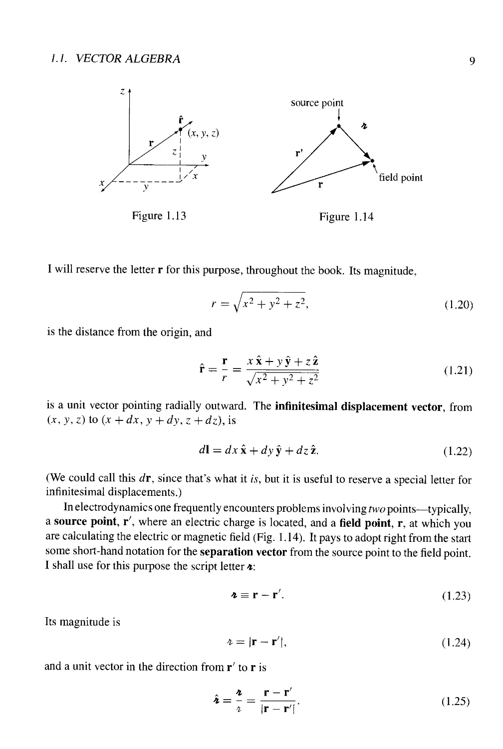
dinates (x, y, z). The vector to that point from the origin (Fig. 1.13) is called the position
vector:
r=xx + yy + zz. A.19)
1.1. VECTOR ALGEBRA
Figure 1.13
source point
field point
Figure 1.14
I will reserve the letter r for this purpose, throughout the book. Its magnitude,
r =
is the distance from the origin, and
r xx + yy + zz
A.20)
A.21)
is a unit vector pointing radially outward. The infinitesimal displacement vector, from
(x, y,z) to (x + dx, y + dy,z +dz), is
d\ = dxx + dyy + dzi.
A.22)
(We could call this dr, since that's what it is, but it is useful to reserve a special letter for
infinitesimal displacements.)
In electrodynamics one frequently encounters problems involving two points—typically,
a source point, r', where an electric charge is located, and a field point, r, at which you
are calculating the electric or magnetic field (Fig. 1.14). It pays to adopt right from the start
some short-hand notation for the separation vector from the source point to the field point.
I shall use for this purpose the script letter t:
Its magnitude is
*=|r-r'|,
and a unit vector in the direction from r' to r is
* ~ i ~ |r - r'
A.23)
A.24)
A.25)
10 CHAPTER 1. VECTOR ANALYSIS
In Cartesian coordinates,
* = (* - x')x + (y- y')y + (z - z')i, A.26)
-x'J + (y-y'J + (z-z'J, A.27)
i = v; ~x )x+(y ~y )y + (z ~z )z (i.28)
V(x - *'J + (y - y'J + (z - z'J
(from which you can begjn to appreciate the advantage of the scripts notation).
Problem 1.7 Find the separatiop vector* from fhe source point B,8,7) to the field point D,6,8).
Determine its magnitude D), and construct the unit vector •&.
1.1.5 How Vectors Transform
The definition of a vector as "a quantity with a magnitude and direction" is not altogether
satisfactory: What precisely does "direction" mean? This may seem a pedantic question,
but we shall shortly encounter a species of derivative that looks rather like a vector, and
we'll want to know for sure whether it is one. You might be inclined to say that a vector
is anything that has three components that combine properly under addition. Well, how
about this: We have a barrel of fruit that contains Nx pears, Ny apples, and Nz bananas.
Is N = Nxx + Nyy + Nzz a vector? It has three components, and when you add another
barrel with Mx pears, My apples, and Mz bananas the result is (Nx + Mx) pears, (Ny + My)
apples, (Nz + Mz) bananas. So it does add like a vector. Yet it's obviously not a vector, in
the physicist's sense of the word, because it doesn't really have a direction. What exactly
is wrong with it?
The answer is that N does not transform properly when you change coordinates. The
coordinate frame we use to describe positions in space is of course entirely arbitrary, but
there is a specific geometrical transformation law for converting vector components from
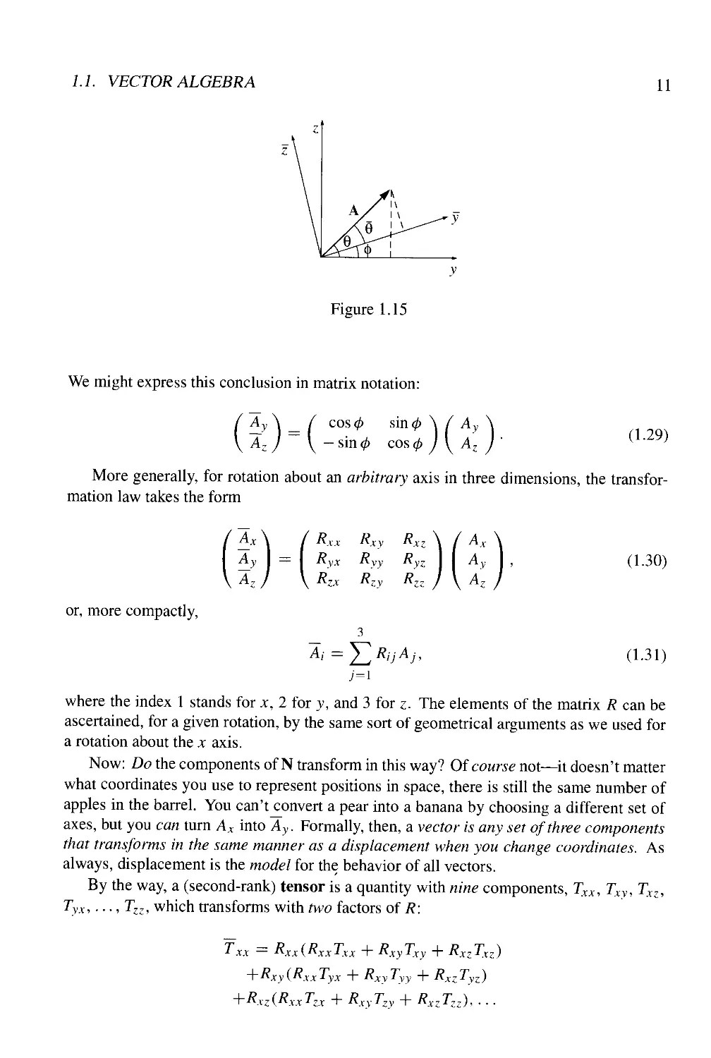
one frame to another. Suppose, for instance, the x, ~y, ~z system is rotated by angle <j>, relative
to x, y, z, about the common x = ~x axes. From Fig. 1.15,
Ay = Acos8, Az = Asin9,
while
Ay — A cos 6* = AcosF* — (p) = A(cos9coscp + sin 6* sin0)
= cos (pAy + sin (pAz,
Az = A sin 0 = A sinF* — (p) = A (sin 6 cos (p — cos 9 sin <j>)
= — sin (p Ay + cos 4>AZ.
This section can be skipped without loss of continuity.
1.1. VECTOR ALGEBRA
11
Figure 1.15
We might express this conclusion in matrix notation:
Ay
A,
cos 4> sin 4>
— sin 4> cos (/>
Ay
A7
A.29)
More generally, for rotation about an arbitrary axis in three dimensions, the transfor-
mation law takes the form
or, more compactly,
Rxx
Ryx
Rxy
Ryy
Rzy
Rxz \
Ryz
Rzz
Ax
\ Az
A.30)
A.31)
where the index 1 stands for x, 2 for y, and 3 for z. The elements of the matrix R can be
ascertained, for a given rotation, by the same sort of geometrical arguments as we used for
a rotation about the x axis.
Now: Do the components of N transform in this way? Of course not—it doesn't matter
what coordinates you use to represent positions in space, there is still the same number of
apples in the barrel. You can't convert a pear into a banana by choosing a different set of
axes, but you can turn Ax into Ay. Formally, then, a vector is any set of three components
that transforms in the same manner as a displacement when you change coordinates. As
always, displacement is the model for the behavior of all vectors.
By the way, a (second-rank) tensor is a quantity with nine components, Txx, Txy, Txz,
Tyx, ...,TZZ, which transforms with two factors of R:
+ Rxy(RxxTyx
+Rxz(RXxTZx +
+ RxyTxy + RXZTXZ)
RxyTyy + RxzTyz)
xyTzy + RXZTZZ),...
12
CHAPTER 1. VECTOR ANALYSIS
or, more compactly,
A.32)
k=l /=!
In general, an «th-rank tensor has n indices and 3" components, and transforms with n
factors of R. In this hierarchy, a vector is a tensor of rank 1, and a scalar is a tensor of rank
zero.
Problem 1.8
(a) Prove that the two-dimensional rotation matrix A.29) preserves dot products. (That is,
show that ~Ay~By + ~AZ~BZ = AyBy + AZBZ.)
(b) What constraints must the elements (/J/y) of the three-dimensional rotation matrix A.30)
satisfy in order to preserve the length of A (for all vectors A)?
Problem 1.9 Find the transformation matrix R that describes a rotation by 120° about an axis
from the origin through the point A,1,1). The rotation is clockwise as you look down the
axis toward the origin.
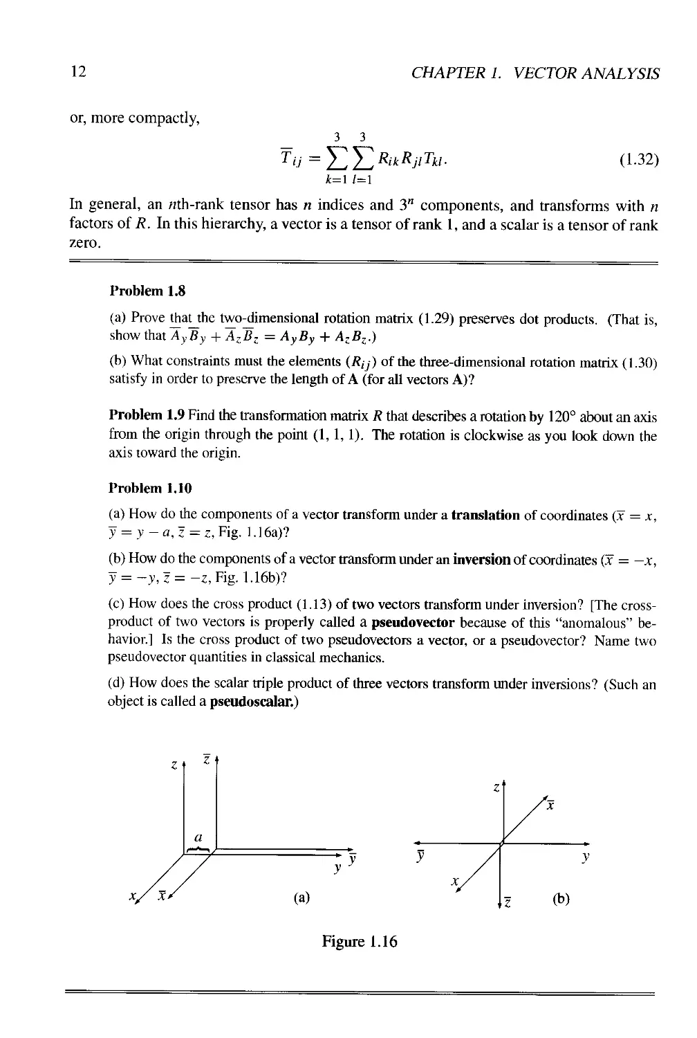
Problem 1.10
(a) How do the components of a vector transform under a translation of coordinates (x = x,
y = y — a, z = z, Fig. 1.16a)?
(b) How do the components of a vector transform under an inversion of coordinates (x = —x,
y = -y,Z= -Z, Fig. 1.16b)?
(c) How does the cross product A.13) of two vectors transform under inversion? [The cross-
product of two vectors is properly called a pseudovector because of this "anomalous" be-
havior.] Is the cross product of two pseudovectors a vector, or a pseudovector? Name two
pseudovector quantities in classical mechanics.
(d) How does the scalar triple product of three vectors transform under inversions? (Such an
object is called a pseudoscalar.)
(a)
(b)
Figure 1.16
1.2. DIFFERENTIAL CALCULUS 13
1.2 Differential Calculus
1.2.1 "Ordinary" Derivatives
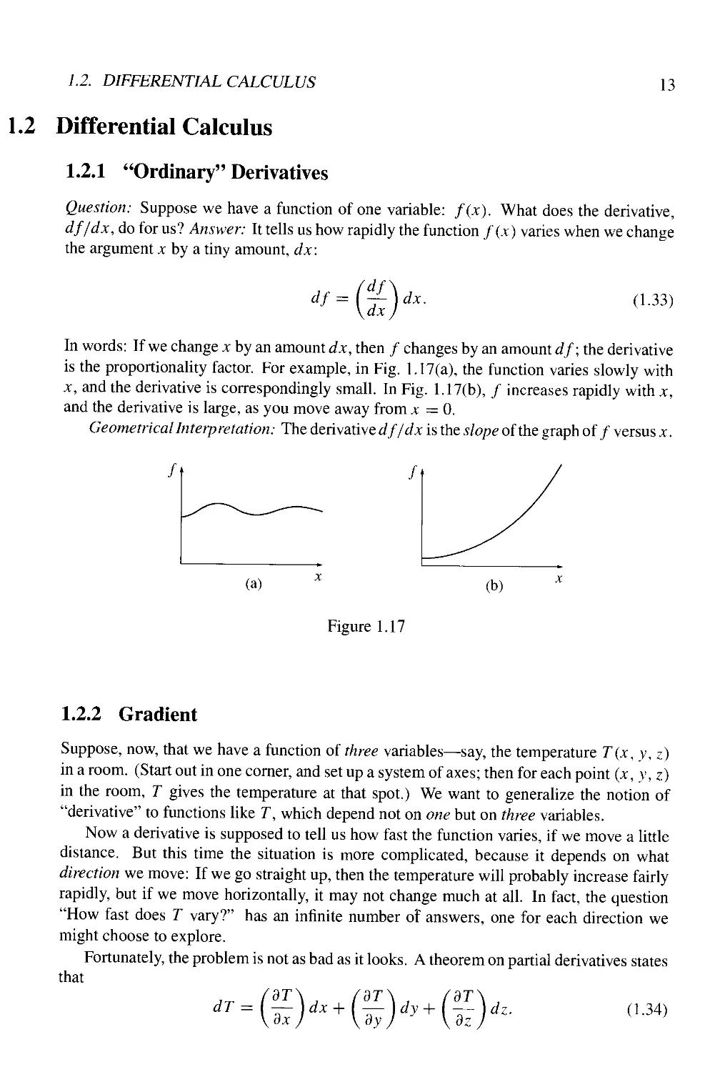
Question: Suppose we have a function of one variable: f(x). What does the derivative,
df/dx, do for us? Answer: It tells us how rapidly the function f(x) varies when we change
the argument x by a tiny amount, dx:
df =
dx
dx.
A.33)
In words: If we change x by an amount dx, then / changes by an amount df; the derivative
is the proportionality factor. For example, in Fig. 1.17(a), the function varies slowly with
x, and the derivative is correspondingly small. In Fig. 1.17(b), / increases rapidly with x,
and the derivative is large, as you move away from x = 0.
Geometrical Interpretation: The derivative df/dx is the slope of the graph of / versus x.
f
f
(a)
(b)
Figure 1.17
1.2.2 Gradient
Suppose, now, that we have a function of three variables—say, the temperature T(x, y, z)
in a room. (Start out in one corner, and set up a system of axes; then for each point (x, y, z)
in the room, T gives the temperature at that spot.) We want to generalize the notion of
"derivative" to functions like T, which depend not on one but on three variables.
Now a derivative is supposed to tell us how fast the function varies, if we move a little
distance. But this time the situation is more complicated, because it depends on what
direction we move: If we go straight up, then the temperature will probably increase fairly
rapidly, but if we move horizontally, it may not change much at all. In fact, the question
"How fast does T vary?" has an infinite number of answers, one for each direction we
might choose to explore.
Fortunately, the problem is not as bad as it looks. A theorem on partial derivatives states
that
CT\, (dT
dy+
?)*•
A.34)
14 CHAPTER 1. VECTOR ANALYSIS
This tells us how T changes when we alter all three variables by the infinitesimal amounts
dx,dy, dz. Notice that we do not require an infinite number of derivatives—three will
suffice: the partial derivatives along each of the three coordinate directions.
Equation 1.34 is reminiscent of a dot product:
dT = l—x+--y+—z)-(dxx + dyy + dzz)
\ ox dy dz /
= (VT)-(dl), A.35)
where
97\ dT dT
Vr = —x+—y+—z A.36)
dx dy dz
is the gradient of T. VT is a vector quantity, with three components; it is the generalized
derivative we have been looking for. Equation 1.35 is the three-dimensional version of
Eq. 1.33.
Geometrical Interpretation of the Gradient: Like any vector, the gradient has magnitude
and direction. To determine its geometrical meaning, let's rewrite the dot product A.35) in
abstract form:
dT = VT-dl= |VT||dl|cos6>, A.37)
where 0 is the angle between VT and d\. Now, if we fix the magnitude \dl\ and search
around in various directions (that is, vary 6), the maximum change in T evidentally occurs
when 0=0 (for then cos 6 = 1). That is, for a fixed distance \dl\, dT is greatest when I
move in the same direction as V7\ Thus:
The gradient VT points in the direction of maximum increase of the function
T.
Moreover:
The magnitude \ V T \ gives the slope (rate of increase) along this maximal
direction.
Imagine you are standing on a hillside. Look all around you, and find the direction
of steepest ascent. That is the direction of the gradient. Now measure the slope in that
direction (rise over run). That is the magnitude of the gradient. (Here the function we're
talking about is the height of the hill, and the coordinates it depends on are positions—
latitude and longitude, say. This function depends on only two variables, not three, but the
geometrical meaning of the gradient is easier to grasp in two dimensions.) Notice from
Eq. 1.37 that the direction of maximum descent is opposite to the direction of maximum
ascent, while at right angles F = 90°) the slope is zero (the gradient is perpendicular to
the contour lines). You can conceive of surfaces that do not have these properties, but they
always have "kinks" in them and correspond to nondifferentiable functions.
What would it mean for the gradient to vanish? If VT = 0 at (x, y, z), then dT = 0
for small displacements about the point (x,y,z). This is, then, a stationary point of the
function T(x, y, z). It could be a maximum (a summit), a minimum (a valley), a saddle
1.2. DIFFERENTIAL CALCULUS 15
point (a pass), or a "shoulder." This is analogous to the situation for functions of one
variable, where a vanishing derivative signals a maximum, a minimum, or an inflection. In
particular, if you want to locate the extrema of a function of three variables, set its gradient
equal to zero.
Example 1.3
Find the gradient of r = y/x2 + y2 + z2 (the magnitude of the position vector).
Solution;
or „ dr „ dr „
Vr = —x+—y+—z
ox dy dz
1 Ix „ 1 2y „ \ 2z
y2 + z2 r
Does this make sense? Well, it says that the distance from the origin increases most rapidly in
the radial direction, and that its rate of increase in that direction is 1.. .just what you'd expect.
Problem 1.11 Find the gradients of the following functions:
(a) f{x, y, Z)=x2 + y3+ z4.
(b) fix, y, z) = x2y3z4.
(c) fix, y, z) =exsmiy)\niz).
Problem 1.12 The height of a certain hill (in feet) is given by
Hx, y) = 10Bjry - 3x2 ~ Ay2 - 18* + 28y + 12),
where y is the distance (in miles) north, x the distance east of South Hadley.
(a) Where is the top of the hill located?
(b) How high is the hill?
(c) How steep is the slope (in feet per mile) at a point 1 mile north and one mile east of South
Hadley? In what direction is the slope steepest, at that point?
Problem 1.13 Let-4be the separation vector from a fixed point ix', y', z!) to the point ix, y, z),
and let 1 be its length. Show that
(a)yD2) =2*.
(b) V(l/4) = -i/i2.
(c) What is the general formula for V(V)?
16 CHAPTER 1. VECTOR ANALYSIS
Problem 1.14 Suppose that / is a function of two variables (y and z) only. Show that the
gradient V/ = (df/dy)y + C//3z)z transforms as a vector under rotations, Eq. 1.29. [Hint:
(df/dy) = (df/dy)(dy/dy) + (df/dz)(dz/dy), and the analogous formula for df/dz. We
know that y = y cos <p + z sin <p and z = —y sin <p + z cos 0; "solve" these equations for y and
z (as functions of y and z), and compute the needed derivatives 'dy/'dy, 'dz/'dy, etc.]
1.2.3 The Operator V
The gradient has the formal appearance of a vector, V, "multiplying" a scalar T:
V
= X
9
_
dx
hy
a
av
„ a
f 2—.
dz
dx dy
(For once 1 write the unit vectors to the left, just so no one will think this means dxjdx, and
so on—which would be zero, since x is constant.) The term in parentheses is called "del":
A.39)
Of course, del is not a vector, in the usual sense. Indeed, it is without specific meaning until
we provide it with a function to act upon. Furthermore, it does not "multiply" T; rather, it
is an instruction to differentiate what follows. To be precise, then, we should say that V is
a vector operator that acts upon T, not a vector that multiplies T.
With this qualification, though, V mimics the behavior of an ordinary vector in virtually
every way; almost anything that can be done with other vectors can also be done with V, if
we merely translate "multiply" by "act upon." So by all means take the vector appearance
of V seriously: it is a marvelous piece of notational simplification, as you will appreciate if
you ever consult Maxwell's original work on electromagnetism, written without the benefit
ofV.
Now an ordinary vector A can multiply in three ways:
1. Multiply a scalar a : Aa;
2. Multiply another vector B, via the dot product: A • B;
3. Multiply another vector via the cross product: A x B.
Correspondingly, there are three ways the operator V can act:
1. On a scalar function T : VT (the gradient);
2. On a vector function v, via the dot product: V • v (the divergence);
3. On a vector function v, via the cross product: V x v (the curl).
We have already discussed the gradient. In the following sections we examine the other
two vector derivatives: divergence and curl.
1.2. DIFFERENTIAL CALCULUS
17
1.2.4 The Divergence
From the definition of V we construct the divergence:
V-v =
, 3
'3x
3 . 3
+ v Hz—
3y dz
(VXX
VZZ)
A.40)
Observe that the divergence of a vector function v is itself a scalar V • v. (You can't have
the divergence of a scalar: that's meaningless.)
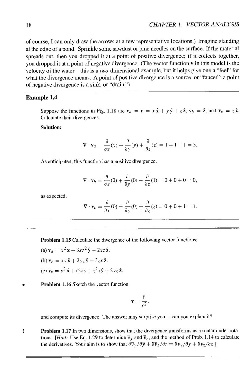
Geometrical Interpretation: The name divergence is well chosen, for V • v is a measure
of how much the vector v spreads out (diverges) from the point in question. For example,
the vector function in Fig. 1.18a has a large (positive) divergence (if the arrows pointed in,
it would be a large negative divergence), the function in Fig. 1.18b has zero divergence, and
the function in Fig. 1.18c again has a positive divergence. (Please understand that v here is
a function—there's a different vector associated with every point in space. In the diagrams,
(a)
(b)
t t t t t t t
(c)
Figure 1.18
18 CHAPTER 1. VECTOR ANALYSIS
of course, I can only draw the arrows at a few representative locations.) Imagine standing
at the edge of a pond. Sprinkle some sawdust or pine needles on the surface. If the material
spreads out, then you dropped it at a point of positive divergence; if it collects together,
you dropped it at a point of negative divergence. (The vector function v in this model is the
velocity of the water—this is a fwo-dimensional example, but it helps give one a "feel" for
what the divergence means. A point of positive divergence is a source, or "faucet"; a point
of negative divergence is a sink, or "drain.")
Example 1.4
Suppose the functions in Fig. 1.18 are ya = r = xx + yy + zz, v;, = z, and vc = zz.
Calculate their divergences.
Solution:
V • ya = — (x) + —00 + — (z) = 1 + 1 + 1=3.
dx dy dz
As anticipated, this function has a positive divergence.
V ¦ yh = ^-@) + |-@) + |-A) = 0 + 0 + 0 = 0,
ox dy dz
as expected.
V • vc = — @) + — @) + — (z) =0 + 0+1 = 1.
dx dy dz
Problem 1.15 Calculate the divergence of the following vector functions:
(a) vfl = x2 x + 3xz2 y - 2xz z.
(b) yh = xy x + 2yz y + 3zx z.
(c) vc = y2 x + Bxy + z2) y + 2yz z.
Problem 1.16 Sketch the vector function
and compute its divergence. The answer may surprise you... can you explain it?
! Problem 1.17 In two dimensions, show that the divergence transforms as a scalar under rota-
tions. [Hint: Use Eq. 1.29 to determine vy and vz, and the method of Prob. 1.14 to calculate
the derivatives. Your aim is to show that diiy/dy + dvz/dz = dvv/dy + dvz/dz.]
1.2. DIFFERENTIAL CALCULUS
19
1.2.5 The Curl
From the definition of V we construct the curl:
V x v =
x y z
3/3x d/dy d/dz
VX Vy VZ
dvz dv
3y dz
dz
dvz
~dx
dVy
~dx~
dvx
^7
Notice that the curl of a vector function v is, like any cross product, a vector. (You cannot
have the curl of a scalar; that's meaningless.)
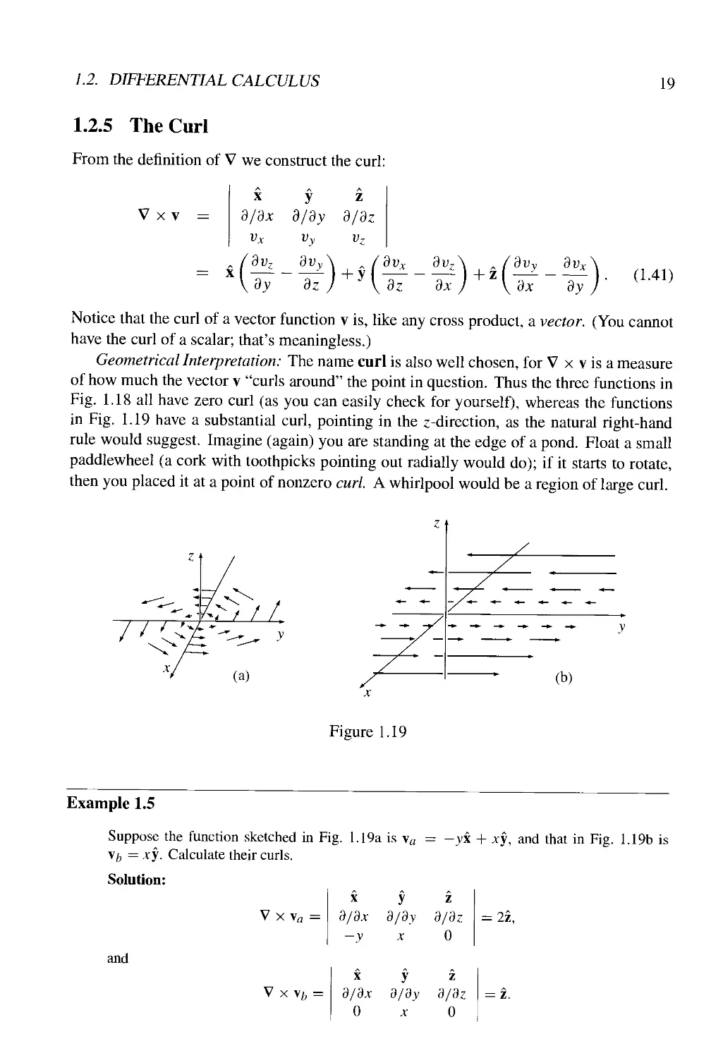
Geometrical Interpretation: The name curl is also well chosen, for V x v is a measure
of how much the vector v "curls around" the point in question. Thus the three functions in
Fig. 1.18 all have zero curl (as you can easily check for yourself), whereas the functions
in Fig. 1.19 have a substantial curl, pointing in the z-direction, as the natural right-hand
rule would suggest. Imagine (again) you are standing at the edge of a pond. Float a small
paddlewheel (a cork with toothpicks pointing out radially would do); if it starts to rotate,
then you placed it at a point of nonzero curl. A whirlpool would be a region of large curl.
.%-V/ /
(a)
(b)
Figure 1.19
Example 1.5
Suppose the function sketched in Fig. 1.19a is ya = —yx + xy, and that in Fig. 1.19b is
\h = xy. Calculate their curls.
Solution:
Vxvfl =
and
d/dx d/dy d/dz
-y x 0
x y z
d/dx d/dy d/dz
0 x 0
= 2z,
= z.
20 CHAPTER 1. VECTOR ANALYSIS
As expected, these curls point in the +z direction. (Incidentally, they both have zero divergence,
as you might guess from the pictures: nothing is "spreading out"... it just "curls around.")
Problem 1.18 Calculate the curls of the vector functions in Prob. 1.15.
Problem 1.19 Construct a vector function that has zero divergence and zero curl everywhere..
(A constant will do the job, of course, but make it something a little more interesting than
that!)
1.2.6 Product Rules
The calculation of ordinary derivatives is facilitated by a number of general rules, such as
the sum rule:
the
the
and
rule for multiplying
product rule:
the quotient rule:
d
d~xif + 8
by a constant:
(hi
d~xW
dx
d /f\
dx\g)
)-df4
]-Tx*
. df
'~ dx
dg
1 dx '
df__
81
dg
' dx'
df
?Tx'
A
3 dx
Similar relations hold for the vector derivatives. Thus,
V(/ + g) = V/ + Vg, V • (A + B) = (V ¦ A) + (V • B),
V x (A + B) = (V x A) + (V x B),
and
V(kf)=kVf V • (A:A) = k(V -A), V x (ifcA) = &(V x A),
as you can check for yourself. The product rules are not quite so simple. There are two
ways to construct a scalar as the product of two functions:
fg (product of two scalar functions),
A • B (dot product of two vector functions),
and two ways to make a vector:
/A (scalar times vector),
A x B (cross product of two vectors).
1.2. DIFFERENTIAL CALCULUS 21
Accordingly, there are six product rules, two for gradients:
(i) V(/#) = /Vg+sV/,
(ii) V(A • B) = A x (V x B) + B x (V x A) + (A • V)B + (B • V)A,
two for divergences:
(iii) V-(/A) = /(V-A)+A-(V/),
(iv) V • (A x B) = B • (V x A) - A • (V x B),
and two for curls:
(v) V x (/A) = /(V x A) - A x (V/),
(vi) V x (A x B) = (B • V)A - (A • V)B + A(V • B) - B(V • A).
You will be using these product rules so frequently that I have put them on the inside front
cover for easy reference. The proofs come straight from the product rule for ordinary
derivatives. For instance,
f\ o O
= —(fAx) + —(fAy) + —
ox ay dz
It is also possible to formulate three quotient rules:
g(V • A) - A • (Vg)
V x l-^ =
However, since these can be obtained quickly from the corresponding product rules, I
haven't bothered to put them on the inside front cover.
22 CHAPTER 1. VECTOR ANALYSIS
Problem 1.20 Prove product rules (i), (iv), and (v).
Problem 1.21
(a) If A and B are two vector functions, what does the expression (A • V)B mean? (That is,
what are its x, y, and z components in terms of the Cartesian components of A, B, and V?)
(b) Compute (r ¦ V)f, where f is the unit vector defined in Eq. 1.21.
(c) For the functions in Prob. 1.15, evaluate (va •
Problem 1.22 (For masochists only.) Prove product rules (ii) and (vi). Refer to Prob. 1.21 for
the definition of (A • V)B.
Problem 1.23 Derive the three quotient rules.
Problem 1.24
(a) Check product rule (iv) (by calculating each term separately) for the functions
A = xx + 2yy + 3zz; B = 3>> x - 2* y.
(b) Do the same for product rule (ii).
(c) The same for rule (vi).
1.2.7 Second Derivatives
The gradient, the divergence, and the curl are the only first derivatives we can make with
V; by applying V twice we can construct five species of second derivatives. The gradient
V T is a vector, so we can take the divergence and curl of it:
A) Divergence of gradient: V • (VT).
B) Curl of gradient: V x (VT).
The divergence V ¦ v is a scalar—all we can do is take its gradient:
C) Gradient of divergence: V(V • v).
The curl V x v is a vector, so we can take its divergence and curl:
D) Divergence of curl: V • (V x v).
E) Curl of curl: V x (V x v).
This exhausts the possibilities, and in fact not all of them give anything new. Let's
consider them one at a time:
x hy Hz—| • (—xh yH z
dx dy dz) \dx dyy dz
g2T 92r q2t
= ITT + ITT + ITT-
dxz 3vz dz
1.2. DIFFERENTIAL CALCULUS 23
This object, which we write V2r for short, is called the Laplacian of T; we shall be
studying it in great detail later on. Notice that the Laplacian of a scalar T is a scalar.
Occasionally, we shall speak of the Laplacian of a vector, V2v. By this we mean a vector
quantity whose x-component is the Laplacian of vx, and so on:3
V2v s (V2vx)x + (V2vy)y + (V2vz)z. A.43)
This is nothing more than a convenient extension of trje meaning of V2.
B) The curl of a gradient is always zero:
Vx(VT)=0. A.44)
This is an important fact, which we shall use repeatedly; you can easily prove it from the
definition of V, Eq. 1.39. Beware: You might think Eq. 1.44 is "obviously" true—isn't it
just (V x V)T, and isn't the cross product of any vector (in this case, V) with itself always
zero? This reasoning is suggestive but not quite conclusive, since V is an operator and does
not "multiply" in the usual way. The proof of Eq. 1.44, in fact, hinges on the equality of
cross derivatives:
9
If you think I'm being fussy, test your intuition on this one:
(VT) x (V5).
Is that always zero? (It would be, of course, if you replaced the V 's by an ordinary vector.)
C) V(V ¦ v) for some reason seldom occurs in physical applications, and it has not been
given any special name of its own—it's just the gradient of the divergence. Notice that
V(V ¦ v) is not the same as the Laplacian of a vecfor: V2v = (V ¦ V)v ^ V(V ¦ v).
D) The divergence of a curl, like the curl of a gradient, is always zero:
V • (V x v) = 0. A.46)
You can prove this for yourself. (Again, there is a fraudulent short-cut proof, using the
vector identity A • (B x C) = (A x B) ¦ C.)
E) As you can check from the definition of V:
V x (V x v) = V(V • v) - V2v. A.47)
So curl-of-curl gives nothing new; the first term is just number C) and the second is the
Laplacian (of a vector). (In fact, Eq. 1.47 is often used to define the Laplacian of a vector,
in preference to Eq. 1.43, which makes specific reference to Cartesian coordinates.)
Really, then, there are just two kinds of second derivatives: the Laplacian (which is
of fundamental importance) and the gradient-of-divergence (which we seldom encounter).
3In curvilinear coordinates, where the unit vectors themselves depend on position, they too must be differentiated
(see Sect. 1.4.1).
24 CHAPTER 1. VECTOR ANALYSIS
We could go through a similar ritual to work out third derivatives, but fortunately second
derivatives suffice for practically all physical applications.
A final word on vector differential calculus: It all flows from the operator V, and from
taking seriously its vector character. Even if you remembered only the definition of V, you
should be able, in principle, to reconstruct all the rest.
Problem 1.25 Calculate the Laplacian of the following functions:
(a)Tfl =x2 + 2xy + 3z+4.
(b) Tj, = sin* sin>> sinz.
(c) Tc = e~5x sin4ycos3z.
(d) v = x2 x + 3xz2 y - 2xz z.
Problem 1.26 Prove that the divergence of a curl is always zero. Check it for function \a in
Prob. 1.15.
Problem 1.27 Prove that the curl of a gradient is always zero. Check it for function (b) in
Prob. 1.11.
L.3 Integral Calculus
1.3.1 Line, Surface, and Volume Integrals
In electrodynamics we encounter several different kinds of integrals, among which the most
important are line (or path) integrals, surface integrals (or flux), and volume integrals.
(a) Line Integrals. A line integral is an expression of the form
f
/
b
v-dl, A.48)
where v is a vector function, d\ is the infinitesimal displacement vector (Eq. 1.22), and the
integral is to be carried out along a prescribed path V from point a to point b (Fig. 1.20). If
the path in question forms a closed loop (that is, if b = a), I shall put a circle on the integral
sign:
r v • d\. A.49)
At each point on the path we take the dot product of v (evaluated at that point) with the
displacement d\ to the next point on the path. To a physicist, the most familiar example of
a line integral is the work done by a force F: W = f F • d\.
Ordinarily, the value of a line integral depends critically on the particular path taken
from a to b, but there is an important special class of vector functions for which the line
integral is independent of the path, and is determined entirely by the end points. It will be
our business in due course to characterize this special class of vectors. (A force that has
this property is called conservative.)
1.3. INTEGRAL CALCULUS
25
a<n
d\
M
*
\
w
\
1
1
1
1
Figure 1.20
V)/
(ii)
1 2
Figure 1.21
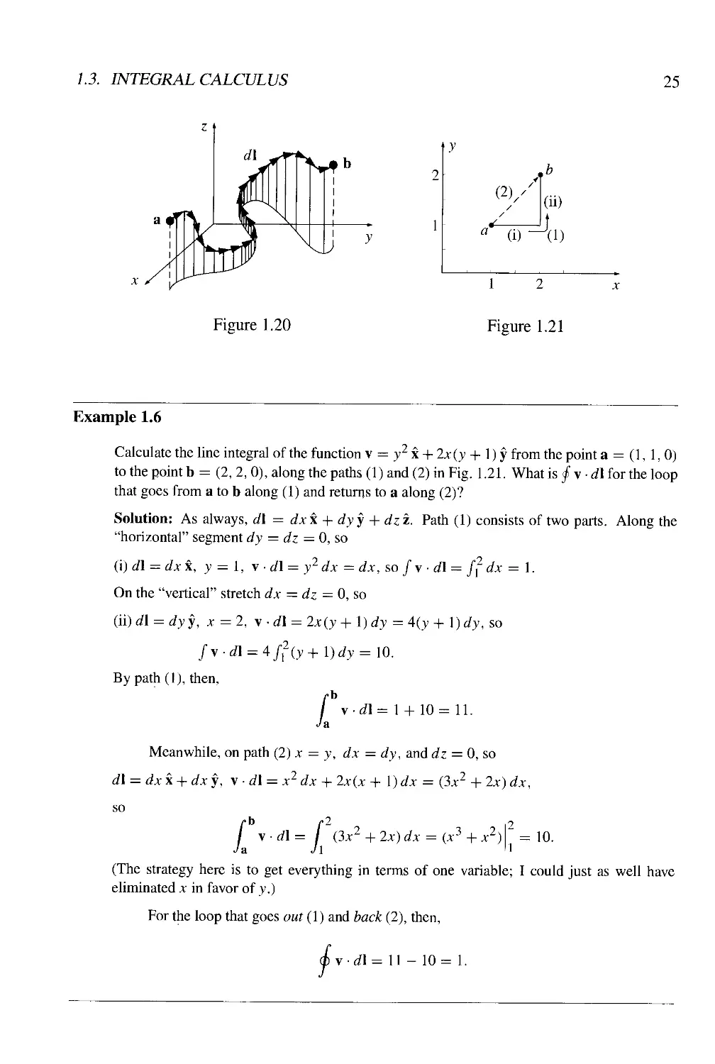
Example 1.6
Calculate the line integral of the function v = y x + 2x(y + 1) y from the point a = A, 1, 0)
tothepointb = B, 2, 0), along the paths A) and B) in Fig. 1.21. What is § v • d\ for the loop
that goes from a to b along A) and returns to a along B)?
Solution: As always, d\ = dxx + dyy + dzi. Path A) consists of two parts. Along the
"horizontal" segment dy = dz = 0, so
(\)d\ = dxx, y = 1, v -d\ = y2 dx =dx, so /v- d\ = f? dx = 1.
On the "vertical" stretch dx = dz = 0, so
(ii)dl = rf>-y, * =2, \ d\ = 2x(y+ I) dy = 4(y + V)dy, so
fy.dl = 4f?(y+l)dy= 10.
By path A), then,
/
vd\= 1 + 10 = 11.
Meanwhile, on path B) a: = y, dx = dy, and dz = 0, so
= dx x + dx y, v • d\ = x2 dx + 2x(x + 1) dx = Cx2 + 2x) dx,
-r
2x) dx =
xL)
= 10.
(The strategy here is to get everything in terms of one variable; I could just as well have
eliminated x in favor of y.)
For the loop that goes out A) and back B), then,
\-d\= 11 - 10= 1.
26
CHAPTER 1. VECTOR ANALYSIS
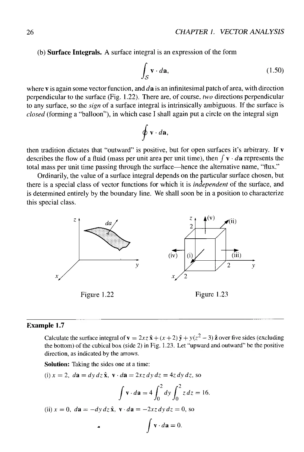
(b) Surface Integrals. A surface integral is an expression of the form
L
v • da,
A.50)
where v is again some vector function, and da is an infinitesimal patch of area, with direction
perpendicular to the surface (Fig. 1.22). There are, of course, two directions perpendicular
to any surface, so the sign of a surface integral is intrinsically ambiguous. If the surface is
closed (forming a "balloon*'), in which case I shall again put a circle on the integral sign
v • da,
then tradition dictates that "outward" is positive, but for open surfaces it's arbitrary. If v
describes the flow of a fluid (mass per unit area per unit time), then f v ¦ da represents the
total mass per unit time passing through the surface—hence the alternative name, "flux."
Ordinarily, the value of a surface integral depends on the particular surface chosen, but
there is a special class of vector functions for which it is independent of the surface, and
is determined entirely by the boundary line. We shall soon be in a position to characterize
this special class.
da,
(iv)
(i)
f(v)
(iii)
x/2
Figure 1.22
Figure 1.23
Example 1.7
Calculate the surface integral of v = 2xz x + (x + 2) y + y(z2 — 3) z over five sides (excluding
the bottom) of the cubical box (side 2) in Fig. 1.23. Let "upward and outward" be the positive
direction, as indicated by the arrows.
Solution: Taking the sides one at a time:
(i) x = 2, da = dydzx, v ¦ da = 2xz dy dz = 4z dy dz, so
f vda = 4 I dy f zdz = 16.
J Jo Jo
(ii) x = 0, d a = — dy dzx, v ¦ d a = — 2xz dy dz = 0, so
/¦
1.3. INTEGRAL CALCULUS 27
(iii) y = 2, da = dxdzy, v ¦ da = (x + 2) dx dz, so
[\-da= [ (x +2) dx f dz = 12.
J Jo Jo
(iv) y = 0, da = —d* dz y, v ¦ da = —(x + 2) dx dz, so
f2
f v da = - f (x + 2)dx f dz = -12.
(v) z = 2, da = dx dy z, v • da = y(z — 3) dx dy = v dx dy, so
/v ¦ da = I dx I ydy = A.
Jo Jo
Evidently the total flux is
f v da = 16 + 0+12-12 + 4 = 20.
./surface
(c) Volume Integrals. A volume integral is an expression of the form
f T dx, A.51)
Jv
where T is a scalar function and dx is an infinitesimal volume element. In Cartesian
coordinates,
dx=dxdydz. A.52)
For example, if T is the density of a substance (which might vary from point to point), then
the volume integral would give the total mass. Occasionally we shall encounter volume
integrals of vector functions:
/ \dx = / (vx x + vy y + vzi)dx = x / vxdx +f vydx +z / vzdx; A.53)
because the unit vectors are constants, they come outside the integral.
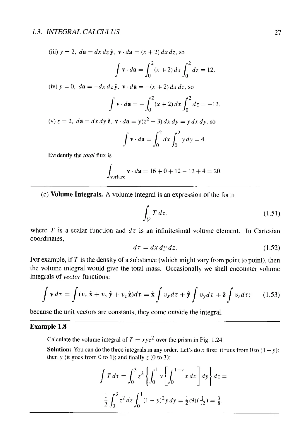
Example 1.8
Calculate the volume integral of T = xyz^ over the prism in Fig. 1.24.
Solution: You can do the three integrals in any order. Let's do x first: it runs from 0 to A — v);
then y (it goes from 0 to 1); and finally z @ to 3):
28
CHAPTER 1. VECTOR ANALYSIS
Figure 1.24
Problem 1.28 Calculate the line integral of the function v = x2 x + 2yz y + y2 z from the
origin to the point A,1,1) by three different routes:
(a) @,0,0)^ A,0,0) -> A,1,0) -> A, 1,1);
(b) @,0,0) -> @,0, 1) -> @,1,1) -> A, 1, 1);
(c) The direct straight line.
(d) What is the line integral around the closed loop that goes out along path (a) and back along
path (b)?
Problem 1.29 Calculate the surface integral of the function in Ex. 1.7, over the bottom of the
box. For consistency, let "upward" be the positive direction. Does the surface integral depend
only on the boundary line for this function? What is the total flux over the closed surface of the
box {including the bottom)? [Note: For the closed surface the positive direction is "outward,"
and hence "down," for the bottom face.]
Problem 1.30 Calculate the volume integral of the function T = z2 over the tetrahedron with
corners at @,0,0), A,0,0), @,1,0), and @,0,1).
1.3.2 The Fundamental Theorem of Calculus
Suppose f(x) is a function of one variable. The fundamental theorem of calculus states:
I
bdf
-j-dx =
ax
- /(a).
In case this doesn't look familiar, let's write it another way:
= /(*) - f(a),
A.54)
I
Ja
where df/dx = F(x). The fundamental theorem tells you how to integrate F(x): you
think up a function f(x) whose derivative is equal to F.
1.3. INTEGRAL CALCULUS
29
Geometrical Interpretation: According to Eq. 1.33, df = (df/dx)dx is the infinitesi-
mal change in / when you go from (x) to (x + dx). The fundamental theorem A.54) says
that if you chop the interval from a to b (Fig. 1.25) into many tiny pieces, dx, and add up
the increments df from each little piece, the result is (not surprisingly) equal to the total
change in /: f(b) - f(a). In other words, there are two ways to determine the total change
in the function: either subtract the values at the ends or go step-by-step, adding up all the
tiny increments as you go. You'll get the same answer either way.
Notice the basic format of the fundamental theorem: the integral of a derivative over
an interval is given by the value of the function at the end points (boundaries). In vector
calculus there are three species of derivative (gradient, divergence, and curl), and each has
its own "fundamental theorem," with essentially the same format. I don't plan to prove
these theorems here; rather, I shall explain what they mean, and try to make them plausible.
Proofs are given in Appendix A.
Kb)
a dx x x
Figure 1.25
Figure 1.26
1.3.3 The Fundamental Theorem for Gradients
Suppose we have a scalar function of three variables T(x, y, z). Starting at point a, we
move a small distance dl\ (Fig. 1.26). According to Eq. 1.37, the function T will change
by an amount
dT =
Now we move a little further, by an additional small displacement d\i; the incremental
change in T will be (VT) • dh- In this manner, proceeding by infinitesimal steps, we make
the journey to point b. At each step we compute the gradient of T (at that point) and dot it
into the displacement d\... this gives us the change in T. Evidently the total change in T
in going from a to b along the path selected is
A.55)
(VT) -d\ = T(b)-T(a).
30
CHAPTER 1. VECTOR ANALYSIS
This is called the fundamental theorem for gradients; like the "ordinary" fundamental
theorem, it says that the integral (here a line integral) of a derivative (here the gradient) is
given by the value of the function at the boundaries (a and b).
Geometrical Interpretation: Suppose you wanted to determine the height of the Eiffel
Tower. You could climb the stairs, using a ruler to measure the rise at each step, and adding
them all up (that's the left side of Eq. 1.55), or you could place altimeters at the top and
the bottom, and subtract the two readings (that's the right side); you should get the same
answer either way (that's the fundamental theorem).
Incidentally, as we found in Ex. 1.6, line integrals ordinarily depend on the path taken
from a to b. But the right side of Eq. 1.55 makes no reference to the path—only to the
end points. Evidently, gradients have the special property that their line integrals are path
independent:
Corollary 1: /ab (V T) ¦ d\ is independent of path taken from a to b.
Corollary 2: <f(VT)-d\ — 0, since the beginning and end points
are identical, and hence T(b) — T(a) — 0.
Example 1.9
Let T = xy2, and take point a to be the origin @, 0. 0) and b the point B, 1,0). Check the
fundamental theorem for gradients.
Solution: Although the integral is independent of path, we must pick a specific path in order
to evaluate it. Let's go out along the x axis (step i) and then up (step ii) (Fig. 1.27). As always,
d\ = dx x + dy y + dz z; VT = y2 x + 2xy y.
(i) y = 0; d\ = dxx, VT ¦ d\ = y2 dx = 0, so
= 0.
(ii) x = 2; d\ = dy y, \T ¦ d\ = 2xy dy = Ay dy, so
J\\ Jo
= 2.
(i)
b
(ii)
1 2
Figure 1.27
1.3. INTEGRAL CALCULUS
31
Evidently the total line integral is 2. Is this consistent with the fundamental theorem? Yes:
r(b) - 7" (a) =2-0 = 2.
Now, just to convince you that the answer is independent of path, let me calculate the same
integral along path iii (the straight line from a to b):
(iii) y = \x, dy = \dx, VT • d\ = v2dx + 2xydy = \x2dx, so
VT d\= I \x2 dx = \x3
= 2.
Problem 1.31 Check the fundamental theorem for gradients, using T = x2 + 4xy + 2yz3, the
points a = @,0,0), b = A, 1, 1), and the three paths in Fig. 1.28:
(a) @,0,0) -> A,0,0) -> A. 1,0) -> A, 1. 1);
(b) @,0.0) -> @,0, 1) -^ @, 1, 1) -> A, 1, 1);
(c) the parabolic path z = x2; y = x.
I
i
y
(a)
/
X/
•
y
(b)
/
x/
\; y
si
(c)
Figure 1.28
1.3.4 The Fundamental Theorem for Divergences
The fundamental theorem for divergences states that:
A.56)
In honor, I suppose of its great importance, this theorem has at least three special names:
Gauss's theorem, Green's theorem, or, simply, the divergence theorem. Like the other
"fundamental theorems," it says that the integral of a derivative (in this case the divergence)
over a region (in this case a volume) is equal to the value of the function at the boundary
32
CHAPTER 1. VECTOR ANALYSIS
(in this case the surface that bounds the volume). Notice that the boundary term is itself
an integral (specifically, a surface integral). This is reasonable: the "boundary" of a line is
just two end points, but the boundary of a volume is a (closed) surface.
Geometrical Interpretation: If v represents the flow of an incompressible fluid, then
the flux of v (the right side of Eq. 1.56) is the total amount of fluid passing out through the
surface, per unit time. Now, the divergence measures the "spreading out" of the vectors
from a point—a place of high divergence is like a "faucet," pouring out liquid. If we have
lots of faucets in a region filled with incompressible fluid, an equal amount of liquid will
be forced out through the boundaries of the region. In fact, there are two ways we could
determine how much is being produced: (a) we could count up all the faucets, recording
how much each puts out, or (b) we could go around the boundary, measuring the flow at
each point, and add it all up. You get the same answer either way:
/
(faucets within the volume) = (b (flow out through the surface).
This, in essence, is what the divergence theorem says.
Example 1.10
Check the divergence theorem using the function
v = y2 x + Bxy + z2) y + Byz) i
and the unit cube situated at the origin (Fig. 1.29).
Solution: In this case
V • v = 2(x + y),
and
2(x + y)dr = 2 / / (x + y)dxdydz,
Jv JO JO Jo
,1 ,1 ,1
/ (x + y) dx = \ + y, / Cj+y)dy = \, / \dz = \.
Jo Jo Jo
(iv)
(i)
(v)
(pi)
l y
Figure 1.29
1.3. INTEGRAL CALCULUS 33
Evidently,
V -ydx = 2.
V
So much for the left side of the divergence theorem. To evaluate the surface integral we must
consider separately the six sides of the cube:
(i)
\da= / y2dydz = ±
Jo Jo
'l t\
(ii)
/v ¦ da = — / / y2dydz = — i.
Jo Jo
(iii) / v da = / / Bx + z2) dx dz =
J Jo Jo
(iv) /v da = -\ I zzdxdz = -\.
1 /"' 2
!ozt
(v) / v • da = I I lydxdy = 1.
7 7o Jo
•1 ,-1
(vi)
So the total flux is:
[ y da = - / / 0dxdy = 0.
J Jo Jo
S
as expected.
Problem 1.32 Test the divergence theorem for the function v = (xy) x + Byz) y + (izx) i.
Take as your volume the cube shown in Fig. 1.30, with sides of length 2.
34
CHAPTER 1. VECTOR ANALYSIS
/
Z
/
2
/ >
Figure 1.30
1.3.5 The Fundamental Theorem for Curls
The fundamental theorem for curls, which goes by the special name of Stokes' theorem,
states that
A.57)
As always, the integral of a derivative (here, the curl) over a region (here, a rJatch of surface)
is equal to the value of the function at the boundary (here, the perimeter of the patch). As
in the case of the divergence theorem, the boundary term is itself an integral—specifically,
a closed line integral.
Geometrical Interpretation: Recall that the curl measures the "twist" of the vectors v; a
region of high curl is a whirlpool—if you put a tiny paddle wheel there, it will rotate. Now,
the integral of the curl over some surface (or, more precisely, the flux of the curl through
that surface) represents the "total amount of swirl," and we can determine that swirl just as
well by going around the edge and finding how much the flow is following the boundary
(Fig. 1.31). You may find this a rather forced interpretation of Stokes' theorem, but it's a
helpful mnemonic, if nothing else.
You might have noticed an apparent ambiguity in Stokes' theorem: concerning the
boundary line integral, which way are we supposed to go around (clockwise or counter-
clockwise)? If we go the "wrong" way we'll pick up an overall sign error. The answer is
that it doesn't matter which way you go as long as you are consistent, for there is a com-
pensating sign ambiguity in the surface integral: Which way does da point? For a closed
surface (as in the divergence theorem) da points in the direction of the outward normal; but
for an open surface, which way is "out?" Consistency in Stokes' theorem (as in all such
matters) is given by the right-hand rule: If your fingers point in the direction of the line
integral, then your thumb fixes the direction of da (Fig. 1.32).
Now, there are plenty of surfaces (infinitely many) that share any given boundary line.
Twist a paper clip into a loop and dip it in soapy water. The soap film constitutes a surface,
with the wire loop as its boundary. If you blow on it, the soap film will expand, making
a larger surface, with the same boundary. Ordinarily, a flux integral depends critically on
what surface you integrate over, but evidently this is not the case with curls. For Stokes'
1.3. INTEGRAL CALCULUS
35
Figure 1.31
Figure 1.32
theorem says that /(V x v) • da is equal to the line integral of v around the boundary, and
the latter makes no reference to the specific surface you choose.
Corollary 1: /(V x v) ¦ da depends only on the boundary line, not
on the particular surface used.
Corollary 2: (f(Vx\)-da — 0 for any closed surface, since the
boundary line, like the mouth of a balloon, shrinks
down to a point, and hence the right side of Eq. 1.57
vanishes.
These corollaries are analogous to those for the gradient theorem. We shall develop the
parallel further in due course.
Example 1.11
Suppose v = Bxz + 3y2)y + Dyz2)i. Check Stokes' theorem for the square surface shown
in Fig. 1.33.
Solution: Here
V x v = Dz - 2x
and
= dydzx.
(iii)
Figure 1.33
36
CHAPTER 1. VECTOR ANALYSIS
(In saying that da points in the x direction, we are committing ourselves to a counterclockwise
line integral. We could as well write da = —dy dz x, but then we would be obliged to go
clockwise.) Since x = 0 for this surface,
f(Vxv)-da=f f \z2dydz=\.
Now, what about the line integral? We must break this up into four segments:
(i) x = 0, z = 0, \-d\ = 3y2 dy, f v ¦ d\ = /Q] 3y2 dy = 1,
(ii) x=0, v = 1, v-d\ = 4z2dz, f v ¦ d\ = f(j Az2 dz = j,
(iii) x=0, z = l, v ¦ d\ = 3y2dy, f v • d\ = /j° 3y2 dy = -1,
(iv) x=0. y = 0, v-rfl = 0, f\-dl = J?0dz = 0.
So
v • d\ = 1
-1 + 0= I
It checks.
A point of strategy: notice how I handled step (iii). There is a temptation to write d\ = —dyy
here, since the path goes to the left. You can get away with this, if you insist, by running the
integral from 0 —>• 1. Personally, I prefer to say d\ = dx x + dy y + dz z always (never any
minus signs) and let the limits of the integral take care of the direction.
Problem 1.33 Test Stokes' theorem for the function v = (xy) x + Byz) y + Czx) z, using the
triangular shaded area of Fig. 1.34.
Problem 1.34 Check Corollary I by using the same function and boundary line as in Ex. 1.11,
but integrating over the five sides of the cube in Fig. 1.35. The back of the cube is open.
l(v)
(iv)
(iii)
Figure 1.34
Figure 1.35
1.3. INTEGRAL CALCULUS 37
1.3.6 Integration by Parts
The technique known (awkwardly) as integration by parts exploits the product rule for
derivatives:
d (f . f(dg\ (df\
dx \ d x) \ d x )
Integrating both sides, and invoking the fundamental theorem:
or
/ f\~J~)dx = —l S\-j-]dx + fg . A.58)
That's integration by parts. It pertains to the situation in which you are called upon to
integrate the product of one function (/) and the derivative of another (g)\ it says you can
transfer the derivative from g to /, at the cost of a minus sign and a boundary term.
Example 1.12
Evaluate the integral
f
Solution: The exponential can be expressed as a derivative:
-x d -x\
in this case, then, f(x) = x, g(x) = — e~x, and df/dx = 1, so
/•oo
xe x dx.
/ xe~x dx = <
JO JO
e~x dx - xe~x
= 1.
0
We can exploit the product rules of vector calculus, together with the appropriate fun-
damental theorems, in exactly the same way. For example, integrating
over a volume, and invoking the divergence theorem, yields
/ V ¦ (/A) dx = /(V • A) dx + A (V/) dx = <b /A • da,
or
/ /(V ¦ A) dx = - / A ¦ (V/) dx + (i) /A • da. A.59)
Jv Jv Js
38 CHAPTER 1. VECTOR ANALYSIS
Here again the integrand is the product of one function (/) and the derivative (in this case
the divergence) of another (A), and integration by parts licenses us to transfer the derivative
from A to / (where it becomes a gradient), at the cost of a minus sign and a boundary term
(in this case a surface integral).
You might wonder how often one is likely to encounter an integral involving the product
of one function and the derivative of another; the answer is surprisingly often, and integration
by parts turns out to be one of the most powerful tools in vector calculus.
Problem
(a) Show
(b) Show
1.35
that
that
Is
//
/(V
•(V
x A) • da
x A)dt =
= f [A x (V/)]
is
= / A-(V xB)d
./V
/
¦ da+ (b
JV
'r + (f> (A
Is
/A ¦ d\.
x B) • da.
A
A
.60)
.61)
1.4 Curvilinear Coordinates
1.4.1 Spherical Polar Coordinates
The spherical polar coordinates (r, 6, </>) of a point P are defined in Fig. 1.36; r is the
distance from the origin (the magnitude of the position vector), 6 (the angle down from the
z axis) is called the polar angle, and </> (the angle around from the x axis) is the azimuthal
angle. Their relation to Cartesian coordinates (x, y, z) can be read from the figure:
x = r sin#cos</>, y = r sin# sin</>, z = rcos#. A-62)
Figure 1.36
1.4. CURVILINEAR COORDINATES 39
A a a
Figure 1.36 also shows three unit vectors, r, 9, <j>, pointing in the direction of increase
of the corresponding coordinates. They constitute an orthogonal (mutually perpendicular)
basis set (just like x, y, z), and any vector A can be expressed in terms of them in the usual
way:
A = Arr + Ade + A,p$. A.63)
Ar, Ae, and A^ are the radial, polar, and azimuthal components of A. In terms of the
Cartesian unit vectors,
f = sin 6 cos cp x + sin 6 sin </> y + cos 6 z, "I
6 = cos#cos</>x + co&9 sin</>y - sin#z, \ A-64)
A I
0 = - sin</>x+ cos</>y, J
as you can easily check for yourself (Prob. 1.37). I have put these formulas inside the back
cover, for easy reference.
But there is a poisonous snake lurking here that I'd be*tter warn you about: f, 9, and $
are associated with a particular point P, and they change direction as P moves around. For
example, f always points radially outward, but "radially outward" can be the x direction,
the y direction, or any other direction, depending on where you are. In Fig. 1.37, A = y and
B — —y, and yet both of them would be written as r in spherical coordinates. One could
take account of this by explicitly indicating the point of reference: r(9, <j>), 0(9, </>), $(9, <j>),
but this would be cumbersome, and as long as you are alert to the problem I don't think it
will cause difficulties.4 In particular, do not naively combihe the spherical components of
vectors associated with different points (in Fig. 1.37, A + B = 0, not 2?, and A • B = — 1,
not +1). Beware of differentiating a vector that is expressed in spherical coordinates, since
the unit vectors themselves are functions of position (dr/d0 = 9, for example). And do
not take f, 0, and 0 outside an integral, as we did with x, y, and z in Eq. 1.53. In general,
if you're uncertain about the validity of an operation, reexpress the problem in Cartesian
coordinates, where this difficulty does not arise.
Figure 1.37
I claimed on the very first page that vectors have no location, and I'll stand by that. The vectors themselves
live "out there," completely independent of our choice of coordinates. But the notation we use to represent them
does depend on the point in question, in curvilinear coordinates.
40
CHAPTER 1. VECTOR ANALYSIS
An infinitesimal displacement in the f direction is simply dr (Fig. 1.38a), just as an
infinitesimal element of length in the x direction is dx:
dlr = dr.
A.65)
On the other hand, an infinitesimal element of length in the 6 direction (Fig. 1.38b) is not
just dO (that's an angle—it doesn't even have the right units for a length), but rather r d9:
dl0=rd9. A.66)
Similarly, an infinitesimal element of length in the <j> direction (Fig. 1.38c) is r sin 0 d<f>:
dl4>=r sin0 dt/>. A.67)
Thus, the general infinitesimal displacement d\ is
j A.68)
This plays the role (in line integrals, for example) that d\ = dx x + dy y + dz z played in
Cartesian coordinates.
dr
r dQ
rsin9
(c)
The infinitesimal volume element dx, in spherical coordinates, is the product of the
three infinitesimal displacements:
dx = dlr die dU = r2 sin 9 dr d9 d<j>.
A.69)
I cannot give you a general expression for surface elements da, since these depend on the
orientation of the surface. You simply have to analyze the geometry for any given case (this
goes for Cartesian and curvilinear coordinates alike). If you are integrating over the surface
of a sphere, for instance, then r is constant, whereas 9 and </> change (Fig. 1.39), so
da\ = die dl^ r = r2 sin 9 d9 d<j> r.
On the other hand, if the surface lies in the xy plane, say, so that 9 is constant (to wit: n/2)
while r and </> vary, then
da2 - dlr dU6 -r dr dcj) S.
1.4. CURVILINEAR COORDINATES
41
*"¦¦
da-,
Figure 1.39
Notice, finally, that r ranges from 0 to oo, <p from 0 to 2n, and 9 from 0 to n {not
2n—that would count every point twice).5
Example 1.13
Find the volume of a sphere of radius R.
Solution:
V =
/rK rjt rZJt
dx = / / / r1 sin<9 dr d6 dcj>
Jr=O J0=O J<t>=0
r2dr
2?r
(Not a big surprise.)
So far we have talked only about the geometry of spherical coordinates. Now I would
like to "translate" the vector derivatives (gradient, divergence, curl, and Laplacian) into r,
9, cp notation. In principle this is entirely straightforward: in the case of the gradient,
z,
dT
—y+
ay dz
for instance, we would first use the chain rule to reexpress the partials:
dT
—
dx
97
8T dT /dr
Jx ~ ~dr \dx
dT /d0\ dT /d<f>\
~d9 \dx) + 'dip \dx) '
Alternatively, you could run cj> from 0 to n (the "eastern hemisphere") and cover the "western hemisphere" by
extending 6 from jr up to 2jt . But this is very bad notation, since, among other things, sin 9 will then run negative,
and you'll have to put absolute value signs around that term in volume and surface elements (area and volume
being intrinsically positive quantities).
42
CHAPTER 1. VECTOR ANALYSIS
The terms in parentheses could be worked out from Eq. 1.62—or rather, the inverse of
those equations (Prob. 1.36). Then we'd do the same for dT/dy and dT/dz. Finally, we'd
substitute in the formulas for x, y, and z in terms of f, 8, and $ (Prob. 1.37). It would take
an hour to figure out ttje gradient in spherical coordinates by this brute-force method. I
suppose this is how it was first done, but there is a much more efficient indirect approach,
explained in Appendix A, which has the extra advantage of treating all coordinate systems
at once. I described the "straightforward" method only to show you that there is nothing
subtle or mysterious about transforming to spherical coordinates: you're expressing the
same quantity (gradient, divergence, or whatever) in different notation, that's all.
Here, then, are the vector derivatives in spherical coordinates:
Gradient:
Divergence:
9T 19T _^9T
dr r d9 r sin 9 dcp
19,
V • v = -j — (r2vr) +
r2 dr
13
1
r sin0 89
1
(sin0wfl) + —
s
rsm9
d-71)
Curl:
V x v —
1 T 3
rsin9
-f \r+- —--f
30 J r \_sm9 dcp
3
—
dr
39
A.72)
Laplacian:
1 3
dT
dT
1 d2T
For reference, these formulas are listed inside the front cover.
Prpbl^m 1.36 Find formulas for r, 6, <p in terms of x, y, z (the inverse, in other words, of
Eq. 1.62).
Problem 1.37 Express the unit vectors f, 6, (j> in terms of x, y, z (that is, derive Eq. 1.64).
Check your answers several ways (r ¦ r = 1, 6, ¦ <j> = 0, r x 6 = </>,...). Also work out the
inverse formulas, giving x, y, z in terms of f, 6, 0 (and 9, <p).
Problem 1.38
(a) Check the divergence theorem for the function V] = r i, using as your volume the sphere
of radius R, centered at the origin.
b) Do the same for V2 = (l/r )r. (If the answer surprises you, look back at Prob. 1.16.)
1.4. CURVILINEAR COORDINATES
43
Figure 1.40
Figure 1.41
Problem 1.39 Compute the divergence of the function
v = (r cos 6) f + (r sin 6) 9 + (r sin 9 cos <j>) <j>.
Check the divergence theorem for this function, using as your volume the inverted hemispher-
ical bowl of radius R, resting on the xy plane and centered at the origin (Fig. 1.40).
Problem 1.40 Compute the gradient and Laplacian of the function T = r(cos6 + sm6 cos</>).
Check the Laplacian by converting T to Cartesian coordinates and using Eq. 1.42. Test the
gradient theorem for this function, using the path shown in Fig. 1.41, from@, 0, 0) to @, 0, 2).
1.4.2 Cylindrical Coordinates
The cylindrical coordinates (s,<j>,z) of a point P are defined in Fig. 1.42. Notice that </>
has the same meaning as in spherical coordinates, and z is the same as Cartesian; 5 is the
distance to P from the z axis, whereas the spherical coordinate r is the distance from the
origin. The relation to Cartesian coordinates is
The unit vectors (Prob. 1.41) are
s
The infinitesimal displacements are
dls =ds,
A.74)
cos cp x + sin (j> f,
— sin </> x + cos <j) y,
A.75)
z = z.
dlz = dz
A.76)
44
CHAPTER 1. VECTOR ANALYSIS
p
I
JL.
Figure 1.42
so
dl = ds s + s d<f> (j> + dz z,
A.77)
and the volume element is
dx = sdsd<f>dz.
The range of 5 is 0 ->¦ oo, </> goes from 0 ->• 27r, and z from -oo to oo.
The vector derivatives in cylindrical coordinates are:
A.78)
Gradient-
Divergence:
dT A 1 97
3T
13
V-v=
s ds
9uz
H -¦
dz
A.79)
A.80)
Curl:
,\dv7
V x v= --
ocp dz J \
fdvs
s + I
z os J s ids 30 J
Laplacian:
2 13/ dT\ i 32r 32r
s ds V 3^ / s2 d(j>2 + dz2 '
These formulas are also listed inside the front cover.
A.82)
Problem 1.41 Express the cylindrical unit vectors s, 0, z in terms of x, y, z (that is, derive
Eq. 1.75). "Invert" your formulas to get x, y, i in terms of s, 0, z (and (f>).
7.5. THE DIRAC DELTA FUNCTION
45
\ A /
•*— ¦< .•'.
Figure 1.43
Figure 1.44
Problem 1.42
(a) Find the divergence of the function
v = s(Z + sin </>) s + s sin <p cos <p 4> + 3z z.
(b) Test the divergence theorem for this function, using the quarter-cylinder (radius 2, height
5) shown in Fig. 1.43.
(c) Find the curl of v.
1.5 The Dirac Delta Function
1.5.1 The Divergence of r/r2
Consider the vector function
1
A.83)
At every location, v is directed radially outward (Fig. 1.44); if ever there was a function that
ought to have a large positive divergence, this is it. And yet, when you actually calculate
the divergence (using Eq. 1.71), you get precisely zero:
_L 9
r2 dr
1
1 9
A.84)
(You will have encountered this paradox already, if you worked Prob. 1.16.) The plot
thickens if you apply the divergence theorem to this function. Suppose we integrate over a
sphere of radius R, centered at the origin (Prob. 1.38b); the surface integral is
-^r) ¦ (R2 sin6» dddcpr)
sin G d6 / fi?0 = 47r.
o / \Jo
A.85)
46
CHAPTER 1. VECTOR ANALYSIS
But the volume integral, / V • \dr, is zero, if we are really to believe Eq. 1.84. Does this
mean that the divergence theorem is false? What's going on here?
The source of the problem is the point r = 0, where v blows up (and where, in Eq. 1.84,
we have unwittingly divided by zero). It is quite true that V • v = 0 everywhere except
the origin, but right at the origin the situation is more complicated. Notice that the surface
integral A.85) is independent of R; if the divergence theorem is right (and it is), we should
get /(V • v) dx = An for any sphere centered at the origin, no matter how small. Evidently
the entire contribution must be coming from the point r = 0! Thus, V • v has the bizarre
property that it vanishes everywhere except at one point, and yet its integral (over any
volume containing that point) is An. No ordinary function behaves like that. (On the other
hand, a physical example does come to mind: the density (mass per unit volume) of a point
particle. It's zero except at the exact location of the particle, and yet its integral is finite—
namely, the mass of the particle.) What we have stumbled on is a mathematical object
known to physicists as the Dirac delta function. It arises in many branches of theoretical
physics. Moreover, the specific problem at hand (the divergence of the function r/r2) is not
just some arcane curiosity—it is, in fact, central to the whole theory of electrodynamics.
So it is worthwhile to pause here and study the Dirac delta function with some care.
1.5.2 The One-Dimensional Dirac Delta Function
The one dimensional Dirac delta function, 8(x), can be pictured as an infinitely high,
infinitesimally narrow "spike," with area 1 (Fig. 1.45). That is to say:
S(x) =
0,
oo,
if jc ^0
if jc =0
and
f
8(x)dx = 1.
A.86)
A.87)
Technically, 8{x) is not a function at all, since its value is not finite at x =0. In the
mathematical literature it is known as a generalized function, or distribution. It is, if you
8(x)
-Area 1
Figure 1.45
1.5. THE DIRAC DELTA FUNCTION
47
~R2(x)
-1/2-1/4 1/4 1/2 x
(a)
-1 -1/2 1/2 1 x
(b)
Figure 1.46
like, the limit of a sequence of functions, such as rectangles Rn(x), of height n and width
\/n, or isosceles triangles Tn (x), of height n and base 2/n (Fig. 1.46).
If f(x) is some "ordinary" function (that is, not another delta function—in fact, just
to be on the safe side let's say that f(x) is continuous), then the product f{x)8(x) is zero
everywhere except at x =0. It follows that
f{x)S(x) = /(O)S(jc). A.88)
(This is the most important fact about the delta function, so make sure you understand why
it is true: since the product is zero anyway except at x — 0, we may as well replace f(x)
by the value it assumes at the origin.) In particular
/•o
/
J — o
f(x)S(x)dx =
po
S(x)dx = f@).
A.89)
Under an integral, then, the delta function "picks out" the value of f{x) at x = 0. (Here
and below, the integral need not run from — oo to +oo; it is sufficient that the domain extend
across the delta function, and —e to +e would do as well.)
Of course, we can shift the spike from x = 0 to some other point, x = a (Fig. 1.47):
S(x — a) —
Equation 1.88 becomes
and Eq. 1.89 generalizes to
0,
oo,
ifjc ^a
xix=a
with
S(x — a) dx = 1.
f(x)S(x-a) = f(a)S(x-a),
f
J — (
f(x)8(x ~a)dx = f(a).
A.90)
A.91)
A.92)
Example 1.14
Evaluate the integral
Jo
x3S(x-2)dx.
48 CHAPTER 1. VECTOR ANALYSIS
SQc-a)
* Area 1
Figure 1.47
Solution: The delta function picks out the value of Jt3 at the point x = 2, so the integral is
23 = 8. Notice, however, that if the upper limit had been 1 (instead of 3) the answer would be
0, because the spike would then be outside the domain of integration.
Although 8 itself is not a legitimate function, integrals over 8 are perfectly acceptable.
In fact, it's best to think of the delta function as something that is always intended for use
under an integral sign. In particular, two expressions involving delta functions (say, D\ (x)
and D2(x)) are considered equal if6
/.OO POO
I f(x)Dl(x)dx= f(x)D2(x)dx, A.93)
J—oo J—oo
for all ("ordinary") functions f(x).
Example 1.15
Show that
S(kx) = -r&(x), A.94)
where k is any (nonzero) constant. (In particular, S(—x) = S(x).)
Solution: For an arbitrary test function f(x), consider the integral
f(x)S(kx)dx.
poo
J-oo'
Changing variables, we let y = kx, so that x = y/k, and dx = l/kdy. If k is positive, the
integration still runs from —oo to +oo, but if & is negative, then x = oo implies y = — oo, and
6This is not as arbitrary as it may sound. The crucial point is that the integrals must be equal for any f(x).
Suppose D\ (x) and Djix) actually differed, say, in the neighborhood of the point x = 17. Then we could pick a
function f(x) that was sharply peaked about x = 17, and the integrals would not be equal.
1.5. THE DIRAC DELTA FUNCTION 49
vice versa, so the order of the limits is reversed. Restoring the "proper" order costs a minus
sign. Thus
f°° f°° dy 1 1
/ f(x)S(kx)dx = ± / f(y/k)8(y)-± = ±-/@) = — /@).
(The lower signs apply when k is negative, and we account for this neatly by putting absolute
value bars around the final k, as indicated.) Under the integral sign, then, 8 (kx) serves the
same purpose as (l/\k\)8(x):
r°° f°° f 1 1
/ f(x)8(kx)dx = / f(x) —S(x) dx.
According to criterion 1.93, therefore, 8(kx) and (\/\k\)8(x) are equal.
Problem 1.43 Evaluate the following integrals:
(a) /26Cx2 -2x - l)S(x - 3)dx.
(b) /05 cosx8(x -n)dx.
Problem 1.44 Evaluate the following integrals:
(b) /02(x3 + 3x + 2) 5A - x)dx.
Problem 1.45
(a) Show that
x~-
ax
[Hint: Use integration by parts.]
(b) Let 0(x) be the step function:
II, if* >0 1
A.95)
0, if x < 0
Show that de/dx = S(x).
50 CHAPTER 1. VECTOR ANALYSIS
1.5.3 The Three-Dimensional Delta Function
It is an easy matter to generalize the delta function to three dimensions:
S3(r)=S(x)S(y)S(z). A.96)
(As always, r=xx + yy + zzisthe position vector, extending from the origin to the point
(x, y, z)). This three-dimensional delta function is zero everywhere except at @, 0, 0),
where it blows up. Its volume integral is 1:
r /»oo /»oo /»oo
/ 83(r)dr= / / S(x)8(y)8(z)dxdydz = 1. A.97)
./all space J—oo J—oo J —oo
And, generalizing Eq. 1.92,
/ /(r)«53(r-a)^T = /(a). A.98)
./all space
As in the one-dimensional case, integration with 8 picks out the value of the function / at
the location of the spike.
We are now in a position to resolve the paradox introduced in Sect. 1.5.1. As you will
recall, we found that the divergence of r/r2 is zero everywhere except at the origin, and
yet its integral over any volume containing the origin is a constant (to wit: 4jt). These are
precisely the defining conditions for the Dirac delta function; evidently
V ¦ (jA = An8\r). A.99)
More generally,
A.100)
where, as always, <* is the separation vector: <* = r — r'. Note that differentiation here is
with respect to r, while r' is held constant. Incidentally, since
(Prob. 1.13), it follows that
V - =-- A.101)
,4
V2- = -47r<S3D). A.102)
1.5. THE DIRAC DELTA FUNCTION 51
Example 1.16
Evaluate the integral
' = /v<'2 + 2> *¦(?)*¦
where V is a sphere of radius R centered at the origin.
Solution 1: Use Eq. 1.99 to rewrite the divergence, and Eq. 1.98 to do the integral:
/ = (r2 + 2LjTS3(r)dr = 4n@ + 2) = Sn.
JV
This one-line solution demonstrates something of the power and beauty of the delta function,
but I would like to show you a second method, which is much more cumbersome but serves to
illustrate the method of integration by parts, Sect. 1.3.6.
Solution 2: Using Eq. 1.59, we transfer the derivative from i/r2 to (r2 + 2):
/ = - f ^ ¦ [W(r2 + 2)]dr + (f(r2 +2)^ ¦ da.
J r2 J r2
The gradient is
V(r2 + 2) = 2rr,
so the volume integral becomes
f -dr = f -r2 sin6 drddd<p = 8n J rdr =4nR2.
Meanwhile, on the boundary of the sphere (where r — R),
da = R2 sin 6 d9 d<p f,
so the surface integral becomes
f(R2 + 2) sin 6ddd<p = 4n(R2 + 2).
Putting it all together, then,
/ = -AnR2 + 4n(R2 + 2) = 8tt,
as before.
52 CHAPTER 1. VECTOR ANALYSIS
Problem 1.46
(a) Write an expression for the electric charge density p(r) of a point charge q at r'. Make
sure that the volume integral of p equals q.
(b) What is the charge density of an electric dipole, consisting of a point charge —q at the
origin and a point charge +q at a?
(c) What is the charge density of a uniform, infinitesimally thin spherical shell of radius R and
total charge Q, centered at the origin? [Beware: the integral over all space must equal Q.]
Problem 1.47 Evaluate the following integrals:
all spac
(b) /y |r — b| <53 Er) dx, where V is a cube of side 2, centered on the origin, and b = 4 y + 3 z.
a) /all space (/2 + r • a + a2)S (r — a) dx, where a is a fixed vector and a is its magnitude.
(c) /y(r4 + r2(r ¦ c) + c4)<53(r - c) dx, where V is a sphere of radius 6 about the origin,
c = 5x + 3y + 2z, and c is its magnitude.
(d)/yr ¦ (d - rM3(e -r)dx, where d = A, 2, 3),e = C, 2, 1), and Vis a sphere of radius
1.5 centered at B, 2, 2).
Problem 1.48 Evaluate the integral
(where Visa sphere of radius R, centered at the origin) by two different methods, as in Ex. 1.16.
1.6 The Theory of Vector Fields
1.6.1 The Helmholtz Theorem
Ever since Faraday, the laws of electricity and magnetism have been expressed in terms of
electric and magnetic fields, E and B. Like many physical laws, these are most compactly
expressed as differential equations. Since E and B are vectors, the differential equations
naturally involve vector derivatives: divergence and curl. Indeed, Maxwell reduced the
entire theory to four equations, specifying respectively the divergence and the curl of E and
B.7
Strictly speaking, this is only true in the static case; in general, the divergence and curl are given in terms of
time derivatives of the fields themselves.
1.6. THE THEORY OF VECTOR FIELDS 53
Maxwell's formulation raises an important mathematical question: To what extent is a
vector function determined by its divergence and curl? In other words, if I tell you that the
divergence of F (which stands for E or B, as the case may be) is a specified (scalar) function
A
V -F= D,
and the curl of F is a specified (vector) function C,
V xF = C,
(for consistency, C must be divergenceless,
V • C = 0,
because the divergence of a curl is always zero), can you then determine the function F?
Well... not quite. For example, as you may have discovered in Prob. 1.19, there are
many functions whose divergence and curl are both zero everywhere—the trivial case F — 0,
of course, but also F = yzx + zxy+xyz, F = sin a; cosh y x — cos x sinhjy, etc. To solve
a differential equation you must also be supplied with appropriate boundary conditions.
In electrodynamics we typically require that the fields go to zero "at infinity" (far away
from all charges).8 With that extra information the Helmholtz theorem guarantees that the
field is uniquely determined by its divergence and curl. (A proof of the Helmholtz theorem
is given in Appendix B.)
1.6.2 Potentials
If the curl of a vector field (F) vanishes (everywhere), then F can be written as the gradient
of a scalar potential (V):
V xF = 0<^>F = -VV. A.103)
(The minus sign is purely conventional.) That's the essential burden of the following
theorem:
Theorem 1: Curl-less (or "irrotational") fields. The following con-
ditions are equivalent (that is, F satisfies one if and only
if it satisfies all the others):
(a) V xF = 0 everywhere.
(b) fa F • d\ is independent of path, for any given end
points.
(c) § F • d\ = 0 for any closed loop.
(d) F is the gradient of some scalar, F = — V V.
In some textbook problems the charge itself extends to infinity (we speak, for instance, of the electric field of
an infinite plane, or the magnetic field of an infinite wire). In such cases the normal boundary conditions do not
apply, and one must invoke symmetry arguments to determine the fields uniquely.
54 CHAPTER 1. VECTOR ANALYSIS
The scalar potential is not unique—any constant can be added to V with impunity, since
this will not affect its gradient.
If the divergence of a vector field (F) vanishes (everywhere), then F can be expressed
as the curl of a vector potential (A):
V-F = O^F=VxA. A.104)
That's the main conclusion of the following theorem:
Theorem 2: Divergence-less (or "solenoidal") fields. The following
conditions are equivalent:
(a) V • F = 0 everywhere.
(b) / F-da is independent of surface, for any given bound-
ary line.
(c) § F • da = 0 for any closed surface.
(d) F is the curl of some vector, F = V x A.
The vector potential is not unique—the gradient of any scalar function can be added to A
without affecting the curl, since the curl of a gradient is zero.
You should by now be able to prove all the connections in these theorems, save for
the ones that say (a), (b), or (c) implies (d). Those are more subtle, and will come later.
Incidentally, in all cases {whatever its curl and divergence may be) a vector field F can be
written as the gradient of a scalar plus the curl of a vector:
F = -VV + VxA (always). A.105)
Problem 1.49
(a) Let Fi = x2 z and F2 = xx + yy + zi- Calculate the divergence and curl of Fj and F2.
Which one can be written as the gradient of a scalar? Find a scalar potential that does the job.
Which one can be written as the curl of a vector? Find a suitable vector potential.
(b) Show that F3 = yz x + zx y + xy z can be written both as the gradient of a scalar and as
the curl of a vector. Find scalar and vector potentials for this function.
Problem 1.50 For Theorem 1 show that (d) => (a), (a) => (c), (c) => (b), (b) => (c), and
(c) => (a).
Problem 1.51 For Theorem 2 show that (d) => (a), (a) => (c), (c) => (b), (b) => (c), and
(c) => (a).
1.6. THE THEORY OF VECTOR FIELDS
55
Problem 1.52
(a) Which of the vectors in Problem 1.15 can be expressed as the gradient of a scalar? Find a
scalar function that does the job.
(b) Which can be expressed as the curl of a vector? Find such a vector.
More Problems on Chapter 1
Problem 1.53 Check the divergence theorem for the function
v = r2 cos 6 f + r2 cos 4> 6 — r2 cos 0 sin 4> #,
using as your volume one octant of the sphere of radius R (Fig. 1.48). Make sure you include
the entire surface. [Answer: tiR^/A]
Problem 1.54 Check Stokes' theorem using the function v = ay x+bx y (a and b are constants)
and the circular path of radius R, centered at the origin in the xy plane. [Answer: nR2(b — a)]
Problem 1.55 Compute the line integral of
along the triangular path shown in Fig. 1.49. Check your answer using Stokes' theorem.
[Answer: 8/3]
Problem 1.56 Compute the line integral of
v= (r cos,2 9) r - (r cos 9 sin 6H + 3r j>
around the path shown in Fig. 1.50 (the points are labeled by their Cartesian coordinates). Do
it either in cylindrical or in spherical coordinates. Check your answer, using Stokes' theorem.
[Answer: 3;r/2]
@,1,2)
@,1,0) ,
A,0,0) ' - y
Figure 1.48
Figure 1.49
Figure 1.50
56
CHAPTER 1. VECTOR ANALYSIS
Figure 1.52
Problem 1.57 Check Stokes' theorem for the function v = y z, using the triangular surface
shown in Fig. 1.51. [Answer: a2]
Problem 1.58 Check the divergence theorem for the function
v = r2 sin 9 r + 4r2 cos 9 6 + r2 tan 9 <f>,
using the volume of the "ice-cream cone" shown in Fig. 1.52 (the top surface is spherical, with
radius R and centered at the origin). [Answer: (ttR4/12)Bjt ^
Problem 1.59 Here are two cute checks of the fundamental theorems:
(a) Combine Corollary 2 to the gradient theorem with Stokes' theorem (v = V7\ in this case).
Show that the result is consistent with what you already knew about second derivatives.
(b) Combine Corollary 2 to Stokes' theorem with the divergence theorem. Show that the result
is consistent with what you already knew.
Problem 1.60 Although the gradient, divergence, and curl theorems are the fundamental in-
tegral theorems of vector calculus, it is possible to derive a number of corollaries from them.
Show that:
(a)fy(VT)dr = <fig T da. [Hint: Let v = c7\ where c is a constant, in the divergence
theorem; use the product rules.]
(b) /y(V x v) dx = — §s v x da. [Hint: Replace v by (v x c) in the divergence theorem.]
(c)/v[7"V2[/ + (VT).(V[/)]dr = <fs(TVU)- da. [Hint: Letv = TVU in the divergence
theorem.]
(d)/vG"V2[/-[/V27")dr = §S(TVU-UVT)-da. [Comment: This is known as Green's
theorem; it follows from (c), which is sometimes called Green's identity.]
(e) JSVT xda = -fpT d\. [Hint: Let v = cT in Stokes' theorem.]
1.6. THE THEORY OF VECTOR FIELDS 57
Problem 1.61 The integral
a= da A.106)
JS
is sometimes called the vector area of the surface iS. If iS happens to be flat, then a is the
ordinary (scalar) area, obviously.
(a) Find the vector area of a hemispherical bowl of radius R.
(b) Show that a = 0 for any closed surface. [Hint: Use Prob. 1.60a.]
(c) Show that a is the same for all surfaces sharing the same boundary.
(d) Show that
a = A <p r x d\, A.107)
where the integral is around the boundary line. [Hint: One way to do it is to draw the cone
subtended by the loop at the origin. Divide the conical surface up into infinitesimal triangu-
lar wedges, each with vertex at the origin and opposite side d\, and exploit the geometrical
interpretation of the cross product (Fig. 1.8).]
(e) Show that
r
)(c -r)d\ = a x c, A.108)
for any constant vector c. [Hint: let T = c • r in Prob. 1.60e.]
Problem 1.62
(a) Find the divergence of the function
r
v = -.
r
First compute it directly, as in Eq. 1.84. Test your result using the divergence theorem, as in
Eq. 1.85. Is there a delta function at the origin, as there was for r/r2? What is the general
formula for the divergence of r"r? [Answer: V • (r"f) = (n + 2)rn~i, unless n = —2, in
which case it is 3
(b) Find the curl of rnr. Test your conclusion using Prob. 1.60b. [Answer: V x (r"r) = 0]
Chapter 2
Electrostatics
2.1 The Electric Field
2.1.1 Introduction
The fundamental problem electromagnetic theory hopes to solve is this (Fig. 2.1): We have
some electric charges, q\, q2, q?,, ¦ ¦ ¦ (call them source charges); what force do they exert
on another charge, Q (call it the test charge)? The positions of the source charges are given
(as functions of time); the trajectory of the test particle is to be calculated. In general, both
the source charges and the test charge are in motion.
The solution to this problem is facilitated by the principle of superposition, which states
that the interaction between any two charges is completely unaffected by the presence of
others. This means that to determine the force on Q, we can first compute the force F], due
to q\ alone (ignoring all the others); then we compute the force F2, due to ^2 alone; and so
on. Finally, we take the vector sum of all these individual forces: F = Fi + F2 + F3 + ...
Thus, if we can find the force on Q due to a single source charge q, we are, in principle,
done (the rest is just a question of repeating the same operation over and over, and adding
it all up).1
Well, at first sight this sounds very easy: Why don't I just write down the formula for
the force on Q due to q, and be done with it? I could, and in Chapter 10 I shall, but you
would be shocked to see it at this stage, for not only does the force on Q depend on the
separation distance*between the charges (Fig. 2.2), it also depends on both their velocities
and on the acceleration of q. Moreover, it is not the position, velocity, and acceleration
of q right now that matter: Electromagnetic "news" travels at the speed of light, so what
concerns Q is the position, velocity, and acceleration q had at some earlier time, when the
message left.
' The principle of superposition may seem "obvious" to you, but it did not have to be so simple: if the electromag-
netic force were proportional to the square of the total source charge, for instance, the principle of superposition
would not hold, since {q\ + ^2) 7^ [ + ?| (mere would be "cross terms" to consider). Superposition is not a
logical necessity, but an experimental fact.
58
2.1. THE ELECTRIC FIELD 59
•e
9lm * .
"Source" charges "Test" charge
Figure 2.1 Figure 2.2
Therefore, in spite of the fact that the basic question ("What is the force on Q due to
qV) is easy to state, it does not pay to confront it head on; rather, we shall go at it by
stages. In the meantime, the theory we develop will permit the solution of more subtle
electromagnetic problems that do not present themselves in quite this simple format. To
begin with, we shall consider the special case of electrostatics in which all the source
charges are stationary (though the test charge may be moving).
2.1.2 Coulomb's Law
What is the force on a test charge Q due to a single point charge q which is at rest a distance
i away? The answer (based on experiments) is given by Coulomb's law:
7
47T60
B.1)
The constant eo is called the permitivity of free space. In SI units, where force is in
Newtons (N), distance in meters (m), and charge in coulombs (C),
e0 = 8.85 x 1CT12
N-m2'
In words, the force is proportional to the product of the charges and inversely proportional
to the square of the separation distance. As always (Sect. 1.1.4), >i is the separation vector
from r' (the location of q) to r (the location of Q):
i = r - r'; B.2)
i is its magnitude, and i is its direction. The force points along the line from q to Q; it is
repulsive if q and Q have the same sign, and attractive if their signs are opposite.
Coulomb's law and the principle of superposition constitute the physical input for
electrostatics—the rest, except for some special properties of matter, is mathematical elab-
oration of these fundamental rules.
60
CHAPTER 2. ELECTROSTATICS
Problem 2.1
(a) Twelve equal charges, q, are situated at the corners of a regular 12-sided polygon (for
instance, one on each numeral of a clock face). What is the net force on a test charge Q at the
center?
(b) Suppose one of the 12 g's is removed (the one at o'clock"). What is the force on Q1
Explain your reasoning carefully.
(c) Now 13 equal charges, q, are placed at the corners of a regular 13-sided polygon. What is
the force on a test charge Q at the center?
(d) If one of the 13 q's is removed, what is the force on Ql Explain your reasoning.
2.1.3 The Electric Field
If we have several point charges </i, q2,... ,qn, at distances i\, 12, ¦ ¦ ¦ ,^n from Q, the total
force on Q is evidently
F = F, + F2 + ... =
_ Q / <?!-*! <72*2 <73*3
4ite0 \
or
where
F= QE,
4ne0 f
B.3)
B.4)
E is called the electric field of the source charges. Notice that it is a function of position (r),
because the separation vectors *, depend on the location of the field point P (Fig. 2.3). But
it makes no reference to the test charge Q. The electric field is a vector quantity that varies
y
Source point
Figure 2.3
2.1. THE ELECTRIC FIELD 61
from point to point and is determined by the configuration of source charges; physically,
E(r) is the force per unit charge that would be exerted on a test charge, if you were to place
one at P.
What exactly is an electric field? I have deliberately begun with what you might call
the "minimal" interpretation of E, as an intermediate step in the calculation of electric
forces. But I encourage you to think of the field as a "real" physical entity, filling the
space in the neighborhood of any electric charge. Maxwell himself came to believe that
electric and magnetic fields represented actual stresses and strains in an invisible primordial
jellylike "ether." Special relativity has forced us to abandon the notion of ether, and with it
Maxwell's mechanical interpretation of electromagnetic fields. (It is even possible, though
cumbersome, to formulate classical electrodynamics as an "action-at-a-distance" theory,
and dispense with the field concept altogether.) I can't tell you, then, what a field is—only
how to calculate it and what it can do for you once you've got it.
Problem 2.2
(a) Find the electric field (magnitude and direction) a distance z above the midpoint between
two equal charges, q, a distance d apart (Fig. 2.4). Check that your result is consistent with
what you'd expect when z > d.
(b) Repeat part (a), only this time make the right-hand charge —q instead of +q.
' " (a) Continuous (b) Line charge, A.
distribution
q d/2
j
j
d!2 q (c) Surface charge, a (d) Volume charge, p
Figure 2.4 Figure 2.5
2.1.4 Continuous Charge Distributions
Our definition of the electric field (Eq. 2.4), assumes that the source of the field is a collection
of discrete point charges qi. If, instead, the charge is distributed continuously over some
region, the sum becomes an integral (Fig. 2.5a):
E(r) = / -ridq. B.5)
62 CHAPTER 2. ELECTROSTATICS
If the charge is spread out along a line (Fig. 2.5b), with charge-per-unit-length X, then
dq = X dl' (where dl' is an element of length along the line); if the charge is smeared
out over a surface (Fig. 2.5c), with charge-per-unit-area a, then dq = a da' (where da!
is an element of area on the surface); and if the charge fills a volume (Fig. 2.5d), with
charge-per-unit-volume p, then dq = pdx' (where dx' is an element of volume):
dq —> X dl1 ~ a da' ~ p dx'.
Thus the electric field of a line charge is
E(r) = -*- / ^idl'; B.6)
V
for a surface charge,
E(r) = / a—^-kda'\ B.7)
S
and for a volume charge,
1 r nCr'1
B.8)
Equation 2.8 itself is often referred to as "Coulomb's law," because it is such a short
step from the original B.1), and because a volume charge is in a sense the most general
and realistic case. Please note carefully the meaning of* in these formulas. Originally, in
Eq.2.4,4,- stood for the vector from the source charge </, to the field point r. Correspondingly,
in Eqs. 2.5-2.8, * is the vector from dq (therefore from dl', da', or dx') to the field point
r.2
Example 2.1
Find the electric field a distance z above the midpoint of a straight line segment of length 2L,
which carries a uniform line charge A (Fig. 2.6).
Solution: It is advantageous to chop the line up into symmetrically placed pairs (at ±jc), for
then the horizontal components of the two fields cancel, and the net field of the pair is
dE = 2 ( -^- )cos#z.
4 V *
Warning: The unit vector-i is not constant; its direction depends on the source point r', and hence it cannot be
taken outside the integrals 2.5-2.8. In practice, you must work with Cartesian components (x, y, z are constant,
and do come out), even if you use curvilinear coordinates to perform the integration.
2.1. THE ELECTRIC FIELD
63
dx
-L
+L x
Figure 2.6
Here cos9 = z/1,1 = Vz2 + x2, and x runs from 0 to L:
1 2XZ
E =
47T60/0 (Z2+*2K/2
X
dx
4^60 zjz2 + L2 '
and it aims in the z-direction.
For points far from the line (z > L), this result simplifies:
^ 1 2AL
4;re0 z2
which makes sense: From far away the line "looks" like a point charge q = 2XL, so the field
reduces to that of point charge q/D7ieoz ). In the limit L —> oo, on the other hand, we obtain
the field of an infinite straight wire:
or, more generally,
where s is the distance from the wire.
B.9)
Problem 2.3 Find the electric field a distance z above one end of a straight line segment of
length L (Fig. 2.7), which carries a uniform line charge k. Check that your formula is consistent
with what you would expect for the case z»L.
64
CHAPTER 2. ELECTROSTATICS
i
i
i z
i
Figure 2.7
Figure 2.8
Figure 2.9
Problem 2.4 Find the electric field a distance z above the center of a square loop (side a)
carrying uniform line charge k (Fig. 2.8). [Hint: Use the result of Ex. 2.1.]
Problem 2.5 Find the electric field a distance z. above the center of a circular loop of radius r
(Fig. 2.9), which carries a uniform line charge k.
Problem 2.6 Find the electric field a distance z above the center of a flat circular disk of radius
R (Fig. 2.10), which carries a uniform surface charge a. What does your formula give in the
limit R —*¦ oo? Also check the case z^> R.
Problem 2.7 Find the electric field a distance z from the center of a spherical surface of radius
R (Fig. 2.11), which carries a uniform charge density a. Treat the case z < R (inside) as well
as z > R (outside). Express your answers in terms of the total charge q on the sphere. [Hint:
Use the law of cosines to writer in terms of R and 9. Be sure to take the positive square root:
y/R2 + z2 - 2Rz = (R - z) if R > z, but it's (z - R) if R < z.]
Problem 2.8 Use your result in Prob. 2.7 to find the field inside and outside a sphere of radius
R, which carries a uniform volume charge density p. Express your answers in terms of the
total charge of the sphere, q. Draw a graph of |E| as a function of the distance from the center.
P,
Figure 2.10
Figure 2.11
2.2. DIVERGENCE AND CURL OF ELECTROSTATIC FIELDS
65
2.2 Divergence and Curl of Electrostatic Fields
2.2.1 Field Lines, Flux, and Gauss's Law
In principle, we are done with the subject of electrostatics. Equation 2.8 tells us how to
compute the field of a charge distribution, and Eq. 2.3 tells us what the force on a charge Q
placed in this field will be. Unfortunately, as you may have discovered in working Prob. 2.7,
the integrals involved in computing E can be formidable, even for reasonably simple charge
distributions. Much of the rest of electrostatics is devoted to assembling a bag of tools and
tricks for avoiding these integrals. It all begins with the divergence and curl of E. I shall
calculate the divergence of E directly from Eq. 2.8, in Sect. 2.2.2, but first I want to show
you a more qualitative, and perhaps more illuminating, intuitive approach.
Let's begin with the simplest possible case: a single point charge q, situated at the
origin:
-i
E(r) = - Y*. B.10)
47T60 rL
To get a "feel" for this field, I might sketch a few representative vectors, as in Fig. 2.12a.
Because the field falls off like 1/r2, the vectors get shorter as you go farther away from the
origin; they always point radially outward. But there is a nicer way to represent this field,
and that's to connect up the arrows, to form field lines (Fig. 2.12b). You might think that I
have thereby thrown away information about the strength of the field, which was contained
in the length of the arrows. But actually I have not. The magnitude of the field is indicated
by the density of the field lines: it's strong near the center where the field lines are close
together, and weak farther out, where they are relatively far apart.
In truth, th,e field-line diagram is deceptive, when I draw it on a two-dimensional surface,
for the density of lines passing through a circle of radius r is the total number divided by the
circumference {n/2nr), which goes like A/r), not A/r2). But if you imagine the model in
three dimensions (a pincushion with needles sticking out in all directions), then the density
of lines is the total number divided by the area of the sphere (n/Anr2), which does go like
A/r2).
Figure 2.12
66
CHAPTER 2. ELECTROSTATICS
Equal but opposite charges
Figure 2.13
Such diagrams are also convenient for representing more complicated fields. Of course,
the number of lines you draw depends on how energetic you are (and how sharp your pencil
is), though you ought to include enough to get an accurate sense of the field, and you must
be consistent: If charge q gets 8 lines, then 2q deserves 16. And you must space them
fairly—they emanate from a point charge symmetrically in all directions. Field lines begin
on positive charges and end on negative ones; they cannot simply terminate in midair, though
they may extend out to infinity. Moreover, field lines can never cross—at the intersection,
the field would have two different directions at once! With all this in mind, it is easy to
sketch the field of any simple configuration of point charges: Begin by drawing the lines
in the neighborhood of each charge, and then connect them up or extend them to infinity
(Figs. 2.13 and 2.14).
Equal charges
Figure 2.14
2.2. DIVERGENCE AND CURL OF ELECTROSTATIC FIELDS
67
Figure 2.15
In this model the flux of E through a surface <S,
<t>? = E da,
B.11)
is a measure of the "number of field lines" passing through S. I put this in quotes because of
course we can only draw a representative sample of the field lines—the total number would
be infinite. But for a given sampling rate the flux is proportional to the number of lines
drawn, because the field strength, remember, is proportional to the density of field lines
(the number per unit area), and hence E • da is proportional to the number of lines passing
through the infinitesimal area da. (The dot product picks out the component of da along
the direction of E, as indicated in Fig. 2.15. It is only the area in the plane perpendicular
to E that we have in mind when we say that the density of field lines is the number per unit
area.)
This suggests that the flux through any closed surface is a measure of the total charge
inside. For the field lines that originate on a positive charge must either pass out through
the surface or else terminate on a negative charge inside (Fig. 2.16a). On the other hand, a
charge outside the surface will contribute nothing to the total flux, since its field lines pass
in one side and out the other (Fig. 2.16b). This is the essence of Gauss's law. Now let's
make it quantitative.
V
,E
(a)
(b)
Figure 2.16
68 CHAPTER 2. ELECTROSTATICS
In the case of a point charge q at the origin, the flux of E through a sphere of radius r is
d>Eda = I —^— (%r\-{r2 sin 0 dO d<t> r) = —q. B.12)
/ J 4tt€0 \r2 / eo
Notice that the radius of the sphere cancels out, for while the surface area goes up as r2, the
field goes down as 1 / r2, and so the product is constant. In terms of the field-line picture, this
makes good sense, since the same number of field lines passes through any sphere centered
at the origin, regardless of its size. In fact, it didn't have to be a sphere—any closed surface,
whatever its shape, would trap the same number of field lines. Evidently the flux through
any surface enclosing the charge is q/eo-
Now suppose that instead of a single charge at the origin, we have a bunch of charges
scattered about. According to the principle of superposition, the total field is the (vector)
sum of all the individual fields:
The flux through a surface that encloses them all, then, is
...=|;(/e,.,,,) = ?(!„).
For any closed surface, then,
(
B.13)
where Qem is the total charge enclosed within the surface. This is the quantitative state-
ment of Gauss's law. Although it contains no information that was not already present in
Coulomb's law and the principle of superposition, it is of almost magical power, as you will
see in Sect. 2.2.3. Notice that it all hinges on the 1/r2 character of Coulomb's law; without
that the crucial cancellation of the r's in Eq. 2.12 would not take place, and the total flux
of E would depend on the surface chosen, not merely on the total charge enclosed. Other
1/r2 forces (I am thinking particularly of Newton's law of universal gravitation) will obey
"Gauss's laws" of their own, and the applications we develop here carry over directly.
As it stands, Gauss's law is an integral equation, but we can readily turn it into a
differential one, by applying the divergence theorem:
(j)E-da = J(V-E)dr.
V
Rewriting Qenc in terms of the charge density p, we have
Gene = / pdX.
V
2.2. DIVERGENCE AND CURL OF ELECTROSTATIC FIELDS
69
So Gauss's law becomes
V V
And since this holds for any volume, the integrands must be equal:
V-E= —p.
B.14)
Equation 2.14 carries the same message as Eq. 2.13; it is Gauss's law in differential
form. The differential version is tidier, but the integral form has the advantage in that it
accommodates point, line, and surface charges more naturally.
Problem 2.9 Suppose the electric field in some region is found to be E = kr^i, in spherical
coordinates (k is some constant).
(a) Find the charge density p.
(b) Find the total charge contained in a sphere of radius R, centered at the origin. (Do it two
different ways.)
Problem 2.10 A charge q sits at the back corner of a cube, as shown in Fig. 2.17. What is the
flux of E through the shaded side?
Figure 2.17
2.2.2 The Divergence of E
Let's go back, now, and calculate the divergence of E directly from Eq. 2.8:
1
4tt€0
B.15)
all space
(Originally the integration was over the volume occupied by the charge, but I may as
well extend it to all space, since p = 0 in the exterior region anyway.) Noting that the
70 CHAPTER 2. ELECTROSTATICS
r-dependence is contained in n. = r — r', we have
1
V E =
This is precisely the divergence we calculated in Eq. 1.100:
V • ( -^ ) =
Thus
1 f 1
V . E = / 47r,53(r - r')p(r') dx' = —p(r), B.16)
which is Gauss's law in differential form B.14). To recover the integral form B.13), we
run the previous argument in reverse—integrate over a volume and apply the divergence
theorem:
f f 1 f 1
/ V -Edx = (f)E-da= — / pdt = — Qenc.
J J e0 J eo
V 5 V
2.2.3 Applications of Gauss's Law
I must interrupt the theoretical development at this point to show you the extraordinary
power of Gauss's law, in integral form. When symmetry permits, it affords by far the
quickest and easiest way of computing electric fields. I'll illustrate the method with a series
of examples.
Example 2.2
Find the field outside a uniformly charged solid sphere of radius R and total charge q.
Solution: Draw a spherical surface at radius r > R (Fig. 2.18); this is called a "Gaussian
surface" in the trade. Gauss's law says that for this surface (as for any other)
I
and gene = q. At first glance this doesn't seem to get us very far, because the quantity we
want (E) is buried inside the surface integral. Luckily, symmetry allows us to extract E from
under the integral sign: E certainly points radially outward,3 as does da, so we can drop the
dot product,
E-da= / \E\dci,
S S
3 If you doubt that E is radial, consider the alternative, Suppose, say, that it points due east, at the ''equator." But
the orientation of the equator is perfectly arbitrary—nothing is spinning here, so there is no natural "north-south"
axis—any argument purporting to show that E points east could just as well be used to show it points west, or
north, or any other direction. The only unique direction on a sphere is radial.
2.2. DIVERGENCE A/Vt) CURL OF ELECTROSTATIC FIELDS 71
Gaussian
surface
Figure 2.18
and the magnitude of E is constant over the Gaussian surface, so it comes outside the integral:
f \E\da = \E\ f da = \E\4nr2.
Thus
\E\4nr2 = —q,
r2
Notice a remarkable feature of this result: The field outside the sphere is exactly the same as
it would have been if all the charge had been concentrated at the center.
Gauss's law is always true, but it is not always useful. If p had not been uniform (or, at
any rate, not spherically symmetrical), or if I had chosen some other shape for my Gaussian
surface, it would still have been tfue that the flux of E is (l/en)<7, but I would not have
been certain that E was in the same direction as da and constant in magnitude over the
surface, and without thdt I could not pull |E| out of the integral. Symmetry is crucial to this
application of Gauss's law. As far as I know, there are only three kinds of symmetry that
work:
1. Spherical symmetry. Make your Gaussian surface a concentric sphere.
2. Cylindrical symmetry. Make your Gaussian surface a coaxial cylinder
(Fig. 2.19).
3. Plane symmetry. Use a Gaussian "pillbox," which straddles the surface
(Fig. 2.20).
Although B) and C) technically require infinitely long cylinders, and planes extending to
infinity in all directions, we shall often use them to get approximate answers for "long"
cylinders or "large" plane surfaces, at points far from the edges.
72
Gaussian surface
Figure 2.19
CHAPTER 2. ELECTROSTATICS
Gaussian
pillbox'
Figure 2.20
Example 2.3
A long cylinder (Fig. 2.21) carries a charge density that is proportional to the distance from
the axis: p = ks, for some constant k. Find the electric field inside this cylinder.
Solution: Draw a Gaussian cylinder of length / and radius s. For this surface, Gauss's law
states:
1
The enclosed charge is
2enc = f pdx = I\ks')(s'ds'd<t>dz) = 2nkl V s'2 ds' =
(I used the volume element appropriate to cylindrical coordinates, Eq. 1.78, and integrated cp
from 0 to 2n, dz from 0 to /. I put a prime on the integration variable s\ to distinguish it from
the radius s of the Gaussian surface.)
Gaussian
surface
Figure 2.21
2.2. DIVERGENCE AND CURL OF ELECTROSTATIC FIELDS
73
Now, symmetry dictates that E must point radially outward, so for the curved portion of the
Gaussian cylinder we have:
/ E • da = f\E\da = |E| / da = |E| In si,
while the two ends contribute nothing (here E is perpendicular to da). Thus,
\E\2n si = nkls3.
eo3
or, finally,
E= — ksls.
3
Example 2.4
An infinite plane carries a uniform surface charge a. Find its electric field.
Solution: Draw a "Gaussian pillbox," extending equal distances above and below the plane
(Fig. 2.22). Apply Gauss's law to this surface:
I
E-rfa = — gene-
eo
In this case, gene = <r A, where A is the area of the lid of the pillbox. By symmetry, E points
away from the plane (upward for points above, downward for points below). Thus, the top and
bottom surfaces yield
Figure 2.22
74
CHAPTER 2. ELECTROSTATICS
whereas the sides contribute nothing. Thus
2A|E| = —a A,
€0
2e0
B.17)
where n is a unit vector pointing away from the surface. In Prob. 2.6, you obtained this same
result by a much more laborious method.
It seems surprising, at first, thaf the field of an infinite plane is independent of how far away
you are. What about the \/r in Coulomb's law? Well, the point is that as you move farther
and farther away from the plane, more and more charge comes into your "field of view" (a
cone shape extending out from your eye), and this compensates for the diminishing influence
of any particular piece. The electric field of a sphere falls off like 1 / r ; the electric field of an
infinite line falls off like 1/r; and the electric field of an infinite plane does not fall off at all.
Although the direct us,e of Gauss's law to compute electric fields is limited to cases of
spherical, cylindrical, and planar symmetry, we can put together combinations of objects
possessing such symmetry, even though the arrangement as a whole is not symmetrical.
For example, invoking the principle of superposition, we could find the field in the vicinity
of two uniformly charged parallel cylinders, or a sphere near an infinite charged plane.
Example 2.5
Two infinite parallel planes carry equal but opposite uniform charge densities ±a (Fig. 2.23).
Find the field in each of the three regions: (i} to the left of both, (ii) between them, (iii) to the
right of both.
Solution: The left plate produces a field (l/2eo)a which points away from it (Fig. 2.24)—to
the left in region (i) and to the right in regions (ii) and (iii). The right plate, being negatively
charged, produces a field (l/2eo)f, which points toward it—to the right in regions (i) and
(ii) and to the left in region (iii). The two fields cancel in regions (i) and (iii); they conspire
in region (ii). Conclusion: The field is (l/eo)a, and points to the right, between the planes;
elsewhere it is zero.
(i)
(iii)
-a
Figure 2.23
Figure 2.24
2.2. DIVERGENCE AND CURL OF ELECTROSTATIC FIELDS 75
Problem 2.11 Use Gauss's law to find the electric field inside and outside a spherical shell of
radius R, which carries a uniform surface charge density a. Compare your answer to Prob. 2.7.
Problem 2.12 Use Gauss's law to find the electric field inside a uniformly charged sphere
(charge density p). Compare your answer to Prob. 2.8.
Problem 2.13 Find the electric field a distance s from an infinitely long straight wire, which
carries a uniform line charge X. Compare Eq. 2.9.
Problem 2.14 Find the electric field inside a sphere which carries a charge density proportional
to the distance from the origin, p = kr, for some constant k. [Hint: This charge density is not
uniform, and you must integrate to get the enclosed charge.]
Problem 2.15 A hollow spherical shell carries charge density
k
in the region a < r < b (Fig. 2.25). Find the electric field in the three regions: (i) r < a, (ii)
a < r < b, (iii) r > b. Plot |E| as a function of r.
Problem 2.16 A long coaxial cable (Fig. 2.26) carries a uniform volume charge density p on
the inner cylinder (radius a), and a uniform surface charge density on the outer cylindrical
shell (radius b). This surface charge is negative and of just the right magnitude so that the
cable as a whole is electrically neutral. Find the electric field in each of the three regions: (i)
inside the inner cylinder (s < a), (ii) between the cylinders (a < s < b), (iii) outside the cable
(s > b). Plot |E| as a function of s.
Problem 2.17 An infinite plane slab, of thickness Id, carries a uniform volume charge density
p (Fig. 2.27). Find the electric field, as a function of y, where y = 0 at the center. Plot E
versus y, calling E positive when it points in the +v direction and negative when it points in
the —v direction.
Problem 2.18 Two spheres, each of radius R and carrying uniform charge densities +p and
—p, respectively, are placed so that they partially overlap (Fig. 2.28). Call the vector from the
positive center to the negative center d. Show that the field in the region of overlap is constant,
and find its value. [Hint: Use the answer to Prob. 2.12.]
a
<
Figure 2.25 Figure 2.26
76
CHAPTER 2. ELECTROSTATICS
Figure 2.27
Figure 2.28
2.2.4 The Curl of E
I'll calculate the curl of E, as I did the divergence in Sect. 2.2.1, by studying first the simplest
possible configuration: a point charge at the origin. In this case
E= %r.
4neo rl
Now, a glance at Fig. 2.12 should convince you that the curl of this field has to be zero, but
I suppose we ought to come up with something a little more rigorous than that. What if we
calculate the line integral of this field from some point a to some other point b (Fig. 2.29):
f
Ja
E-dl.
In spherical coordinates, d\ = dr f + r d6 8 + r sin 0 d(p <j>, so
1
>
Therefore,
r
B.18)
where ra is the distance from the origin to the point a and
integral around a closed path is evidently zero (for then ra =
1 (q q
47te0 \ra rb/
is the distance to b. The
E • d\ = 0,
B.19)
2.3. ELECTRIC POTENTIAL
77
Figure 2.29
and hence, applying Stokes' theorem,
VxE = 0.
B.20)
Now, I proved Eqs. 2.19 and 2.20 only for the field of a single point charge at the origin,
but these results make no reference to what is, after all, a perfectly arbitrary choice of
coordinates; they also hold no matter where the charge is located. Moreover, if we have
many charges, the principle of superposition states that the total field is a vector sum of
their individual fields:
E = E] + E2 + ...,
so
V x E = V x (E] + E2 + ...) = (V x Ei) + (V x E2) + ... = 0.
Thus, Eqs. 2.19 and 2.20 hold for any static charge distribution whatever.
Problem 2.19 Calculate V x E directly from Eq. 2.8, by the method of Sect. 2.2.2. Refer to
Prob. 1.62 if you get stuck.
2J Electric Potential
2.3.1 Introduction to Potential
The electric field E is not just any old vector function; it is a very special kind of vector
function, one whose curl is always zero. E = yx, for example, could not possibly be
an electrostatic field; no set of charges, regardless of their sizes and positions, could ever
produce such a field. In this section we're going to exploit this special property of electric
fields to reduce a vector problem (finding E) down to a much simpler scalar problem. The
first theorem in Sect. 1.6.2 asserts that any vector whose curl is zero is equal to the gradient
of some scalar. What I'm going to do now amounts to a proof of that claim, in the context
of electrostatics.
78
CHAPTER 2. ELECTROSTATICS
o
a^~ f.
(n)
Figure 2.30
Because V x E = 0, the line integral of E around any closed loop is zero (that follows
from Stokes' theorem). Because § E • d\ = 0, the line integral of E from point a to point
b is the same for all paths (otherwise you could go out along path (i) and return along path
(ii)—Fig. 2.30—and obtain § E • d\ ^ 0). Because the line integral is independent of path,
we can define a function4
V(r) = - I E-dl.
o
B.21)
Here O is some standard reference point on which we have agreed beforehand; V then
depends only on the point r. It is called the electric potential.
Evidently, the potential difference between two points a and b is
V(b) - V(a)
E-dl
= - f E-di+ r
Jo Jo
/*b /*O /*b
= - / E dl - / E dl = - E-dl.
Jo Ja Ja
B.22)
Now, the fundamental theorem for gradients states that
rb
V(b) - V(a)
Ja
(VV) d\,
so
f (VV)-dl = - f
E-dl.
Since, finally, this is true for any points a and b, the integrands must be equal:
E = -VV.
B.23)
Equation 2.23 is the differential version of Eq. 2.21; it says that the electric field is the
gradient of a scalar potential, which is what we set out to prove.
4To avoid any possible ambiguity I should perhaps put a prime on the integration variable:
V(r) = - f E(r') ¦ d\.
JO
But this makes for cumbersome notation, and I prefer whenever possible to reserve the primes for source points.
However, when (as in Ex. 2.6) we calculate such integrals explicitly, I shall put in the primes.
2.3. ELECTRIC POTENTIAL 79
Notice the subtle but crucial role played by path independence (or, equivalently, the fact
that V x E = 0) in this argument. If the line integral of E depended on the path taken, then
the "definition" of V, Eq. 2.21, would be nonsense. It simply would not define a function,
since changing the path would alter the value of V(r). By the way, don't let the minus sign
in Eq. 2.23 distract you; it carries over from 2.21 and is largely a matter of convention.
Problem 2.20 One of these is an impossible electrostatic field. Which one?
(b) E = k[y2x + Bxy + Z2)y + 2yzz].
Here k is a constant with the appropriate units. For the possible one, find the potential, using
the origin as your reference point. Check your answer by computing W. [Hint: You must
select a specific path to integrate along. It doesn't matter what path you choose, since the
answer is path-independent, but you simply cannot integrate unless you have a particular path
in mind.]
2.3.2 Comments on Potential
(i) The name. The word "potential" is a hideous misnomer because it inevitably
reminds you of potential energy. This is particularly confusing, because there is a connection
between "potential" and "potential energy," as you will see in Sect. 2.4. I'm sorry that it
is impossible to escape this word. The best I can do is to insist once and for all that
"potential" and "potential energy" are completely different terms and should, by all rights,
have different names. Incidentally, a surface over which the potential is constant is called
an equipotential.
(ii) Advantage of the potential formulation. If you know V, you can easily get
E—just take the gradient: E = — V V. This is quite extraordinary when you stop to think
about it, for E is a vector quantity (three components), but V is a scalar (one component).
How can one function possibly contain all the information that three independent functions
carry? The answer is that the three components of E are not really as independent as
they look; in fact, they are explicitly interrelated by the very condition we started with,
V x E = 0. In terms of components,
dEX dEy dEZ _ dEy dEx dE,
dy dx ' dy dz dz dx
This brings us back to my observation at the beginning of Sect. 2.3.1: E is a very special
kind of vector. What the potential formulation does is to exploit this feature to maximum
advantage, reducing a vector problem down to a scalar one, in which there is no need to
fuss with components.
80 CHAPTER 2. ELECTROSTATICS
(Hi) The reference point O. There is an essential ambiguity in the definition of
potential, since the choice of reference point O was arbitrary. Changing reference points
amounts to adding a constant K to the potential:
/¦f rO pi
V'(r) = - Ed\ = - Edl- E ¦ d\ = K + V(r),
JO1 JO' JO
where K is the line integral of E from the old reference point O to the new one O'. Of
course, adding a constant to V will not affect the potential difference between two points:
V'(b) - V'(a) = V(b) - V(a),
since the K 's cancel out. (Actually, it was already clear from Eq. 2.22 that the potential
difference is independent of O, because it can be written as the line integral of E from a to
b, with no reference to O.) Nor does the ambiguity affect the gradient of V:
vv' = vv,
since the derivative of a constant is zero. That's why all such V's, differing only in their
choice of reference point, correspond to the same field E.
Evidently potential as such carries no real physical significance, for at any given point
we can adjust its value at will by a suitable relocation of O. In this sense it is rather like
altitude: If I ask you how high Denver is, you will probably tell me its height above sea level,
because that is a convenient and traditional reference point. But we could as well agree
to measure altitude above Washington D.C., or Greenwich, or wherever. That would add
(or, rather, subtract) a fixed amount from all our sea-level readings, but it wouldn't change
anything about the real world. The only quantity of intrinsic interest is the difference in
altitude between two points, and that is the same whatever your reference level.
Having said this, however, there is a "natural" spot to use for O in electrostatics—
analogous to sea level for altitude—and that is a point infinitely far from the charge. Or-
dinarily, then, we "set the zero of potential at infinity." (Since V(O) = 0, choosing a
reference point is equivalent to selecting a place where V is to be zero.) But I must warn
you that there is one special circumstance in which this convention fails: when the charge
distribution itself extends to infinity. The symptom of trouble, in such cases, is that the
potential blows up. For instance, the field of a uniformly charged plane is (a/2eo)n, as we
found in Ex. 2.4; if we naively put O = oo, then the potential at height z above the plane
becomes
V(z) = - [ ~adz = -^-a{z - oo).
Joe let) Isq
The remedy is simply to choose some other reference point (in this problem you might use
the origin). Notice that the difficulty occurs only in textbook problems; in "real life" there
is no such thing as a charge distribution that goes on forever, and we can always use infinity
as our reference point.
2.3. ELECTRIC POTENTIAL 81
(iv) Potential obeys the superposition principle. The original superposition princi-
ple of electrodynamics pertains to the force on a test charge Q. It says that the total force
on Q is the vector sum of the forces attributable to the source charges individually:
F = Fi + F2 + ...
Dividing through by Q, we find that the electric field, too, obeys the superposition principle:
E = Ei + E2 + ...
Integrating from the common reference point to r, it follows that the potential also satisfies
such a principle:
V = V\ + V2 + ¦. .
That is, the potential at any given point is the sum of the potentials due to all the source
charges separately. Only this time it is an ordinary sum, not a vector sum, which makes it
a lot easier to work with.
(v) Units of Potential. In our units, force is measured in newtons and charge in
coulombs, so electric fields are in newtons per coulomb. Accordingly, potential is measured
in newton-meters per coulomb or joules per coulomb. A joule per coulomb is called a volt.
Example 2.6
Find the potential inside and outside a spherical shell of radius R (Fig. 2.31), which carries a
uniform surface charge. Set the reference point at infinity.
Figure 2.31
82 CHAPTER 2. ELECTROSTATICS
Solution: From Gauss's law, the field outside is
where q is the total charge on the sphere. The field inside is zero. For points outside the sphere
(r > R),
V(r) = -
1 q
O 47re0 Joo r"- 43T€o r
1 q
r
To find the potential inside the sphere (r < R), we must break the integral into two sections,
using in each region the field that prevails there:
4ne0 r'
— 1 rR a fr
V(r) = - / \dr'- / @)dr' =
4Jte0 Joo r'2 Jr
R
+ 0= ' <
oo
R'
Notice that the potential is not zero inside the shell, even though the field is. V is a constant
in this region, to be sure, so that V K = 0—that's what matters. In problems of this type you
must always work your way in from the reference point; that's where the potential is "nailed
down." It is tempting to suppose that you could figure out the potential inside the sphere on
the basis of the field there alone, but this is false: The potential inside the sphere is sensitive to
what's going on outside the sphere as well. If I placed a second uniformly charged shell out at
radius R' > R, the potential inside R would change, even though the field would still be zero.
Gauss's law guarantees that charge exterior to a given point (that is, at larger r) produces no
netfield at that point, provided it is spherically or'cylindrically symmetric; but there is no such
rule for potential, when infinity is used as the reference point.
Problem 2.21 Find the potential inside and outside a uniformly charged solid sphere whose
radius is R and whose total charge is q. Use infinity as your reference point. Compute the
gradient of V in each region, and check that it yields the correct field. Sketch V(r).
Problem 2.22 Find the potential a distance s from an infinitely long straight wire that carries
a uniform line charge A. Compute the gradient of your potential, and check that it yields the
correct field.
Problem 2.23 For the charge configuration of Prob. 2.15, find the potential at the center, using
infinity as your reference point.
Problem 2.24 For the configuration of Prob. 2.16, find the potential difference between a point
on the axis and a point on the outer cylinder. Note that it is not necessary to commit yourself
to a particular reference point if you use Eq. 2.22.
2.3. ELECTRIC POTENTIAL 83
2.3.3 Poisson's Equation and Laplace's Equation
We found in Sect. 2.3.1 that the electric field can be written as the gradient of a scalar
potential.
The question arises: What do the fundamental equations for E,
V • E = — and V x E = 0,
look like, in terms of V? Well, V • E = V • (- V V) = - V2 V, so, apart from that persisting
minus sign, the divergence of E is the Laplacian of V. Gauss's law then says that
B.24)
This is known as Poisson's equation. In regions where there is no charge, so that p = 0,
Poisson's equation reduces to Laplace's equation,
V2V = 0. B.25)
We'll explore these equations more fully in Chapter 3.
So much for Gauss's law. What about the curl law? This says that
V x E = V x (-VV)
must equal zero. But that's no condition on V—curl of gradient is always zero. Of course,
we used the curl law to show that E could be expressed as the gradient of a scalar, so it's not
really surprising that this works out: V x E = 0permits E = — V V; in return, E = — V V
guarantees V x E = 0. It takes only one differential equation (Poisson's) to determine V,
because V is a scalar; for E we needed two, the divergence and the curl.
2.3.4 The Potential of a Localized Charge Distribution
I defined V in terms of E (Eq. 2.21). Ordinarily, though, it's E that we're looking for (if we
already knew E there wouldn't be much point in calculating V). The idea is that it might be
easier to get V first, and then calculate E by taking the gradient. Typically, then, we know
where the charge is (that is, we know p), and we want to find V. Now, Poisson's equation
relates V and p, but unfortunately it's "the wrong way around": it would give us p, if we
knew V, whereas we want V, knowing p. What we must do, then, is "invert" Poisson's
equation. That's the program for this section, although I shall do it by roundabout means,
beginning, as always, with a point charge at the origin.
84
CHAPTER 2. ELECTROSTATICS
Figure 2.32
Setting the reference point at infinity, the potential of a point charge q at the origin is
V(r) =
-1
?-dr'= -?—?-
¦'2 4-rceo r'
1
An €q r
(You see here the special virtue of using infinity for the reference point: it kills the lower
limit on the integral.) Notice the sign of V; presumably the conventional minus sign in
the definition of V (Eq. 2.21) was chosen precisely in order to make the potential of a
positive charge come out positive. It is useful to remember that regions of positive charge
are potential "hills," regions of negative charge are potential "valleys," and the electric field
points "downhill," from plus toward minus.
In general, the potential of a point charge q is
V(r) =
1 q
B.26)
where i, as always, is the distance from the charge to r (Fig. 2.32). Invoking the superpo-
sition principle, then, the potential of a collection of charges is
V(r) =
1
n.
or, for a continuous distribution,
1 f 1
V(r) = / -dq.
In particular, for a volume charge, it's
V(r)
1 f P(r') . ,
= / dr.
47T€0 J 1
B.27)
B.28)
B.29)
This is the equation we were looking for, telling us how to compute V when we know p; it
is, if you like, the "solution" to Poisson's equation, for a localized charge distribution.5 I
Equation 2.29 is an example of the Helmholtz theorem (Appendix B), in the context of electrostatics, where
the curl of E is zero and its divergence is
2.3. ELECTRIC POTENTIAL 85
invite you to compare Eq. 2.29 with the corresponding formula for the electric field in terms
ofp(Eq. 2.8):
4n€o J n-1
The main point to notice is that the pesky unit vector * is now missing, so there is no need
to worry about components. Incidentally, the potentials of line and surface charges are
1 /"Mr'),,, . 1 /"* (r'),,
/ di and / da .
7T60 J t A7T€Q J 1
/ di and / da . B.30)
47T60 J t A J 1
I should warn you that everything in this section is predicated on the assumption that
the reference point is at infinity. This is hardly apparent in Eq. 2.29, but remember that we
got that equation from the potential of a point charge at the origin, (l/4jreo)(#/r), which
is valid only when O = oo. If you try to apply these formulas to one of those artificial
problems in which the charge itself extends to infinity, the integral will diverge.
Example 2.7
Find the potential of a uniformly charged spherical shell of radius R (Fig. 2.33).
Solution: This is the same problem we solved in Ex. 2.6, but this time we shall do it using
Eq. 2.30:
1
V(r) =
\°-da'.
J *
Let's set the point r on the z axis and use the law of cosines to express t in terms of the polar
angle 6:
I2 = R2 + z2 -2Rz cos 6'.
Figure 2.33
86
CHAPTER 2. ELECTROSTATICS
An element of surface area on this sphere is R2 sin 9' d9' d<f>', so
f R2 sin 9'd9'd(p'
J VR2+z2 -2Rzcos9'
2 r* sine'
Jo s/rZ + z2^2
:d9'
2Rzcos9f
Rz
z2
-2Rzcos9>
2nRo
2nRo
At this stage we must be very careful to take the positive root. For points outside the sphere, z is
greaterthan R, and hence *J(R — zJ = z — /?; for points insKfe the sphere, v(/? — zJ = R—z.
Thus,
V(z) =
V(z) =
2e0z
2e0z
z)-(z-R)] =
eoz "
Ro
outside;
inside.
In terms of the total charge on the shell, q = AnR a, V(z) = (]/4neo)(q/z) (or, in general,
V(r) = (l/A7Z€Q)(q/r)) for points outside the sphere, and {\/An€Q){q/R) for points inside.
Of course, in this particular case, it was easier to get V by using 2.21 than 2.30, because
Gauss's law gave us E with so little effort. But if you compare Ex. 2.7 with Prob. 2.7, you will
appreciate the power of the potential formulation.
Problem 2.25 Using Eqs. 2.27 and 2.30, find the potential at a distance z above the center of
the charge distributions in Fig. 2.34. In each case, compute E = — VV, and compare your
answers with Prob. 2.2a, Ex. 2.1, and Prob. 2.6, respectively. Suppose that we changed the
right-hand charge in Fig. 2.34a to — q; what then is the potential at PI What field does that
suggest? Compare your answer to Prob. 2.2b, and explain carefully any discrepancy.
+q d +q
(a) Two point charges
2L
(b) Uniform line charge (c) Uniform surface charge
Figure 2.34
2.3. ELECTRIC POTENTIAL
87
Problem 2.26 A conical surface (an empty ice-cream cone) carries a uniform surface charge
a. The height of the cone is h, as is the radius of the top. Find the potential difference between
points a (the vertex) and b (the center of the top).
Problem 2.27 Find the potential on the axis of a uniformly charged solid cylinder, a distance
z from the center. The length of the cylinder is L, its radius is R, and the charge density is p.
Use your result to calculate the electric field at this point. (Assume that z > L/2.)
Problem 2.28 Use Eq. 2.29 to calculate the potential inside a uniformly charged solid sphere
of radius R and total charge q. Compare your answer to Prob. 2.21.
Problem 2.29 Check that Eq. 2.29 satisfies Poisson's equation, by applying the Laplacian and
using Eq. 1.102.
2.3.5 Summary; Electrostatic Boundary Conditions
In the typical electrostatic problem you are given a source charge distribution p, and you
want to find the electric field E it produces. Unless the symmetry of the problem admits a
solution by Gauss's law, it is generally to your advantage to calculate the potential first, as
an intermediate step. These, then, are the three fundamental quantities of electrostatics: p,
E, and V. We have, in the course of our discussion, derived all six formulas interrelating
them. These equations are neatly summarized in Fig. 2.35. We began with just two exper-
imental observations: A) the principle of superposition—a broad general rule applying to
all electromagnetic forces, and B) Coulomb's law—the fundamental law of electrostatics.
From these, all else followed.
s
Figure 2.35
CHAPTER 2. ELECTROSTATICS
above
Figure 2.36
below
You may have noticed, in studying Exs. 2.4 and 2.5, or working problems such as 2.7,
2.11, and 2.16, that the electric field always undergoes a discontinuity when you cross a
surface charge a. In fact, it is a simple matter to find the amount by which E changes at
such a boundary. Suppose we draw a wafer-thin Gaussian pillbox, extending just barely
over the edge in each direction (Fig. 2.36). Gauss's law states that
E • da = — Qenc = —aA,
where A is the area of the pillbox lid. (If a varies from point to point or the surface is
curved, we must pick A to be extremely small.) Now, the sides of the pillbox contribute
nothing to the flux, in the limit as the thickness e goes to zero, so we are left with
Jabove
--L -1
ibelow — _ CT'
B.31)
where ?^ove denotes the component of E that is perpendicular to the surface immediately
above, and ?low 's tne same> only just below the surface. For consistency, we let "upward"
be the positive direction for both. Conclusion: The normal component of E is discontinuous
by an amount cr/eo at any boundary. In particular, where there is no surface charge, E1- is
continuous, as for instance at the surface of a uniformly charged solid sphere.
The tangential component of E, by contrast, is always continuous. For if we apply
Eq. 2.19,
E ¦ d\ = 0,
to the thin rectangular loop of Fig. 2.37, the ends give nothing (as e ->¦ 0), and the sides
f" — ¦
above ~
below'
B.32)
2.3. ELECTRIC POTENTIAL
89
E\
below
Figure 2.37
where E11 stands for the components of YL parallel to the surface. The boundary conditions
on E (Eqs. 2.31 and 2.32) can be combined into a single formula:
Eabove ~
B.33)
where n is a unit vector perpendicular to the surface, pointing from "below" to "above.
The potential, meanwhile, is continuous across any boundary (Fig. 2.38), since
,b
Vabove — ^below = — I E • dl;
Ja
as the path length shrinks to zero, so too does the integral:
^above = Hielow- B.34)
Figure 2.38
6Notice that it doesn't matter which side you call "above" and which "below," since reversal would switch the
direction of n. Incidentally, if you're only interested in the field due to the (essentially flat) local patch of surface
charge itself the answer is (<r/2eo)n immediately above the surface, and — (<r/2eo)n immediately below. This
follows from Ex. 2.4, for if you are close enough to the patch it "looks" like an infinite plane. Evidently the entire
discontinuity in E is attributable to this local patch of charge.
90 CHAPTER 2. ELECTROSTATICS
However, the gradient of V inherits the discontinuity in E; since E = — W, Eq. 2.33
implies that
V Vabove - V Vbelow = an, B.35)
or, more conveniently,
B.36)
3 ^above
dn
dV
~dn
3 Vbelow
dn
= VV-n
1
where
dV
B.37)
denotes the normal derivative of V (that is, the rate of change in the direction perpendicular
to the surface).
Please note that these boundary conditions relate the fields and potentials just above and
just below the surface. For example, the derivatives in Eq. 2.36 are the limiting values as
we approach the surface from either side.
Problem 2.30
(a) Check that the results of Exs. 2.4 and 2.5, and Prob. 2.11, are consistent with Eq. 2.33.
(b) Use Gauss's law to find the field inside and outside a long hollow cylindrical tube, which
carries a uniform surface charge a. Check that your result is consistent with Eq. 2.33.
(c) Check that the result of Ex. 2.7 is consistent with boundary conditions 2.34 and 2.36.
2.4 Work and Energy in Electrostatics
2.4.1 The Work Done to Move a Charge
Suppose you have a stationary configuration of source charges, and you want to move a test
charge Q from point a to point b (Fig. 2.39). Question: How much work will you have to
do? At any point along the path, the electric force on Q is F = QE; the force you must
exert, in opposition to this electrical force, is — QE. (If the sign bothers you, think about
lifting a brick: Gravity exerts a force mg downward, but you exert a force mg upward. Of
course, you could apply an even greater force—then the brick would accelerate, and part
2.4. WORK AND ENERGY IN ELECTROSTATICS
91
of your effort would be "wasted" generating kinetic energy. What we're interested in here
is the minimum force you must exert to do the job.) The work is therefore
W
Fdl = -Q E-dl = Q[V(b)-V(a)].
Ja
Notice that the answer is independent of the path you take from a to b; in mechanics, then,
we would call the electrostatic force "conservative." Dividing through by Q, we have
W
V(b) - V(a) = —.
B.38)
In words, the potential difference between points a and b is equal to the work per unit charge
required to carry a particle from a to b. In particular, if you want to bring the charge Q in
from far away and stick it at point r, the work you must do is
W = Q[V(r) - V(oo)],
so, if you have set the reference point at infinity,
W=QV(r). B.39)
In this sense potential is potential energy (the work it takes to create the system) per unit
charge (just as the field is the force per unit charge).
2.4.2 The Energy of a Point Charge Distribution
How much work would it take to assemble an entire collection of point charges? Imagine
bringing in the charges, one by one, from far away (Fig. 2.40). The first charge, q\, takes
no work, since there is no field yet to fight against. Now bring in qi- According to Eq. 2.39,
this will cost you <72Vi(r2), where V\ is the potential due to q\, and r2 is the place we're
putting^:
W2= ' -(*
Figure 2.40
92 CHAPTER 2. ELECTROSTATICS
(«12 is the distance between q\ and q2 once they are in position). Now bring in qy, this
requires work #3^,2^3), where V\^ is the potential due to charges q\ and qi, namely,
(l/4ieo)(?iAi3 +q2/t-23)- Thus
l ( 11 , ^\
1 •
Similarly, the extra work to bring in q$ will be
fil , 12 . 1
qA — + — H .
\4 » ^/
The total work necessary to assemble the first four charges, then, is
_ * /glg2 fflff3 glg4 g2g3 g2g4
4 V
4^60 V t\2 413 -8-14 4-23 4-24 ^34 /
You see the general rule: Take the product of each pair of charges, divide by their separation
distance, and add it all up:
*YYq^ B.40)
The stipulation j > i is just to remind you not to count the same pair twice. A nicer way
to accomplish the same purpose is intentionally to count each pair twice, and then divide
by 2:
-. n n
"^ B.41)
(we must still avoid i = j, of course). Notice that in this form the answer plainly does not
depend on the order in which you assemble the charges, since every pair occurs in the sum.
Let me next pull out the factor q;:
The term in parentheses is the potential at point r, (the position of g,) due to all the other
charges—all of them, now, not just the ones that were present at some stage in the building-
up process. Thus,
1 "
J2V() B.42)
That's how much work it takes to assemble a configuration of point charges; it's also the
amount of work you'd get back out if you dismantled the system. In the meantime, it
2.4. WORK AND ENERGY IN ELECTROSTATICS
93
represents energy stored in the configuration ("potential" energy, if you like, though for
obvious reasons I prefer to avoid that word in this context).
Problem 2.31
(a) Three charges are situated at the corners of a square (side a), as shown in Fig. 2.41. How
much work does it take to bring in another charge, +q, from far away and place it in the fourth
corner?
(b) How much work does it take to assemble the whole configuration of four charges?
Figure 2.41
2.4.3 The Energy of a Continuous Charge Distribution
For a volume charge density p, Eq. 2.42 becomes
W
-u
pV dr.
B.43)
(The corresponding integrals for line and surface charges would be f XV dl and f aV da,
respectively.) There is a lovely way to rewrite this result, in which p and V are eliminated
in favor of E. First use Gauss's law to express p in terms of E:
/0 = 60V-E, SO W= y MV -E)VdT.
Now use integration by parts (Eq. 1.59) to transfer the derivative from E to V:
- \ E-(VV)dr + (hVEdal.
J J J
ButVV = -E, so
c~ I r r \
B.44)
W = -M / EAdx + <f> VE ¦ da .
94 CHAPTER 2. ELECTROSTATICS
But what volume is this we're integrating over? Let's go back to the formula we started
with, Eq. 2.43. From its derivation, it is clear that we should integrate over the region
where the charge is located. But actually, any larger volume would do just as well: The
"extra" territory we throw in will contribute nothing to the integral anyway, since p — 0
out there. With this in mind, let's return to Eq. 2.44. What happens here, as we enlarge the
volume beyond the minimum necessary to trap all the charge? Well, the integral of E2 can
only increase (the integrand being positive); evidently the surface integral must decrease
correspondingly to leave the sum intact. In fact, at large distances from the charge, E goes
like 1/r2 and V like 1/r, while the surface area grows like r2. Roughly speaking, then,
the surface integral goes down like 1/r. Please understand that Eq. 2.44 gives you the
correct energy W, whatever volume you use (as long as it encloses all the charge), but the
contribution from the volume integral goes up, and that of the surface integral goes down,
as you take larger and larger volumes. In particular, why not integrate over all space? Then
the surface integral goes to zero, and we are left with
B.45)
Example 2.8
Find the energy of a uniformly charged spherical shell of total charge q and radius R.
Solution 1: Use Eq. 2.43, in the version appropriate to surface charges:
W= - faV da.
Now, the potential at the surface of this sphere is (\/4jT€Q)q/R (a constant), so
\ a f „
W=- 1 oda = - V-
8JT60 R J
8JT6Q
Solution 2: Use Eq. 2.45. Inside the sphere E = 0; outside,
Therefore,
(r2 sine drd6d<P)
go f (I)
outside
32jr2e0 Jr r2 8jr60 R
2.4. WORK AND ENERGY IN ELECTROSTATICS 95
Problem 2.32 Find the energy stored in a uniformly charged solid sphere of radius R and
charge q. Do it three different ways:
(a) Use Eq. 2.43. You found the potential in Prob. 2.21.
(b) Use Eq. 2.45. Don't forget to integrate over all space.
(c) Use Eq. 2.44. Take a spherical volume of radius a. Notice what happens as a —>¦ oo.
Problem 2.33 Here is a fourth way of computing the energy of a uniformly charged sphere:
Assemble the sphere layer by layer, each time bringing in an infinitesimal charge dq from far
away and smearing it uniformly over the surface, thereby increasing the radius. How much
work dW does it take to build up the radius by an amount dr? Integrate this to find the work
necessary to create the entire sphere of radius R and total charge q.
2.4.4 Comments on Electrostatic Energy
(i) A perplexing "inconsistency." Equation 2.45 clearly implies that the energy of a
stationary charge distribution is always positive. On the other hand, Eq. 2.42 (from which
2.45 was in fact derived), can be positive or negative. For instance, according to 2.42, the
energy of two equal but opposite charges a distance t, apart would be —(l/4ji€o)(q2/^).
What's gone wrong? Which equation is correct?
The answer is that both equations are correct, but they pertain to slightly different
situations. Equation 2.42 does not take into account the work necessary to make the point
charges in the first place; we started with point charges and simply found the work required
to bring them together. This is wise policy, since Eq. 2.45 indicates that the energy of a
point charge is in fact infinite:
/ ( q-j )(r2 siri 6 dr d9 d(/>) = ^— f
J \r4) 87re0 Jo
W = /
2D7re0J
Equation 2.45 is more complete, in the sense that it tells you the total energy stored in
a charge configuration, but Eq. 2.42 is more appropriate when you're dealing with point
charges, because we prefer (for good reason!) to leave out that portion of the total energy
that is attributable to the fabrication of the point charges themselves. In practice, after
all, the point charges (electrons, say) are given to us ready-made; all we do is move them
around. Since we did not put them together, and we cannot take them apart, it is immaterial
how much work the process would involve. (Still, the infinite energy of a point charge
is a recurring source of embarrassment for electromagnetic theory, afflicting the quantum
version as well as the classical. We shall return to the problem in Chapter 11.)
Now, you may wonder where the inconsistency crept into an apparently water-tight
derivation. The "flaw" lies between Eqs. 2.42 and 2.43: In the former, V(r,) represents
the potential due to all the other charges but not <?,, whereas in the latter, V(r) is the full
potential. For a continuous distribution there is no distinction, since the amount of charge
right at the point r is vanishingly small, and its contribution to the potential is zero.
96 CHAPTER 2. ELECTROSTATICS
(ii) Where is the energy stored? Equations 2.43 and 2.45 offer two different ways of
calculating the same thing. The first is an integral over the charge distribution; the second
is an integral over the field. These can involve completely different regions. For instance,
in the case of the spherical shell (Ex. 2.8) the charge is confined to the surface, whereas the
electric field is present everywhere outside this surface. Where is the energy, then? Is it
stored in the field, as Eq. 2.45 seems to suggest, or is it stored in the charge, as Eq. 2.43
implies? At the present level, this is simply an unanswerable question: I can tell you what
the total energy is, and I can provide you with several different ways to compute it, but it is
unnecessary to worry about where the energy is located. In the context of radiation theory
(Chapter 11) it is useful (and in General Relativity it is essential) to regard the energy as
being stored in the field, with a density
— E2 — energy per unit volume. B.46)
But in electrostatics one could just as well say it is stored in the charge, with a density \pV ¦
The difference is purely a matter of bookkeeping.
(iii) The superposition principle. Because electrostatic energy is quadratic in the
fields, it does not obey a superposition principle. The energy of a compound system is not
the sum of the energies of its parts considered separately—there are also "cross terms":
= Wi + W2 + e0 / E] ¦ E2 dr. B.47)
For example, if you double the charge everywhere, you quadruple the total energy.
Problem 2.34 Consider two concentric spherical shells, of radii a and b. Suppose the inner
one carries a charge q, and the outer one a charge —q (both of them uniformly distributed
over the surface). Calculate the energy of this configuration, (a) using Eq. 2.45, and (b) using
Eq. 2.47 and the results of Ex. 2.8.
2.5 Conductors
2.5.1 Basic Properties
In an insulator, such as glass or rubber, each electron is attached to a particular atom. In a
metallic conductor, by contrast, one or more electrons per atom are free to roam about at will
through the material. (In liquid conductors such as salt water it is ions that do the moving.)
A perfect conductor would be a material containing an unlimited supply of completely free
2.5. CONDUCTORS
97
charges. In real life there are no perfect conductors, but many substances come amazingly
close. From this definition the basic electrostatic properties of ideal conductors immediately
follow:
(i) E = 0 inside a conductor. Why? Because if there were any field, those free charges
would move, and it wouldn't be electrostatics any more. Well... that's hardly a satisfactory
explanation; maybe all it proves is that you can't have electrostatics when conductors are
present. We had better examine what happens when you put a conductor into an external
electric field Eo (Fig. 2.42). Initially, this will drive any free positive charges to the right,
and negative ones to the left. (In practice it's only the negative charges—electrons—that
do the moving, but when they depart the right side is left with a net positive charge—the
stationary nuclei—so it doesn't really matter which charges move; the effect is the same.)
When they come to the edge of the material, the charges pile up: plus on the right side,
minus on the left. Now, these induced charges produce a field of their own, E i, which, as
you can see from the figure, is in the opposite direction to Eo. That's the crucial point, for
it means that the field of the induced charges tends to cancel off the original field. Charge
will continue to flow until this cancellation is complete, and the resultant field inside the
conductor is precisely zero.7 The whole process is practically instantaneous.
Figure 2.42
(ii) p = 0 inside a conductor. This follows from Gauss's law: V E = p/eo- If E = 0,
so also is p. There is still charge around, but exactly as much plus charge as minus, so the
net charge density in the interior is zero.
(iii) Any net charge resides on the surface. That's the only other place it can be.
(iv) A conductor is an equipotential. For if a and b are any two points within (or at the
surface of) a given conductor, V (b) - V (a) = - /a E • d\ = 0, and hence V(a) — V(b).
7 Outside the conductor the field is not zero, for here Eq and Ej do not cancel.
98 CHAPTER 2. ELECTROSTATICS
/E
Figure 2.43
(v) E is perpendicular to the surface, just outside a conductor. Otherwise, as in (i),
charge will immediately flow around the surface urltil it kills off the tangential component
(Fig. 2.43). (Perpendicular to the surface, charge cannot flow, of course, since it is confined
to the conducting object.)
I think it is strange that the charge on a conductor flows to the surface. Because of their
mutual repulsion, the charges naturally spread out as much as possible, but for all of them
to go to the surface seems like a waste of the interior space. Surely we could do better, from
the point of view of making each charge as far as possible from its neighbors, to sprinkle
some of them throughout the volume... Well, it simply is not so. You do best to put all the
charge on the surface, and this is true regardless of the size or shape of the conductor.8
The problem can also be phrased in terms of energy. Like any other free dynamical
system, the charge on a conductor will seek the configuration that minimizes its potential
energy. What property (iii) asserts is that the electrostatic energy of a solid object (with
specified shape and total charge) is a minimum when that charge is spread over the surface.
For instance, the energy of a sphere is A/87T eo) (<?2/^) if the charge is uniformly distributed
over the surface, as we found in Ex. 2.8, but it is greater, C/20jteo)(q2/R), if the charge is
uniformly distributed throughout the volume (Prob. 2.32).
2.5.2 Induced Charges
If you hold a charge +q near an uncharged conductor (Fig. 2.44), the two will attract one
another. The reason for this is that q will pull minus charges over to the near side and repel
plus charges to the far side. (Another way to think of it is that the charge moves around in
such a way as to cancel off the field of q for points inside the conductor, where the total
field must be zero.) Since the negative induced charge is closer to q, there is a net force of
attraction. (In Chapter 3 we shall calculate this force explicitly, for the case of a spherical
conductor.)
8By the way, the one- and two-dimensional analogs are quite different: The charge on a conducting disk does
not all go to the perimeter (R. Friedberg, Am. J. ofPhys. 61, 1084 A993)), nor does the charge on a conducting
needle go to the ends (D. J. Griffiths and Y. Li, Am. J. ofPhys. 64, 706 A996)). See Prob. 2.52.
2.5. CONDUCTORS
99
f \
- Coiuliii'lnr -H
J
+q
Figure 2.44
Gaussian
surface
Conductor
Figure 2.45
By the way, when I speak of the field, charge, or potential "inside" a conductor, I
mean in the "meat" of the conductor; if there is some cavity in the conductor, and within
that cavity there is some charge, then the field in the cavity will not be zero. But in a
remarkable way the cavity and its contents are electrically isolated from the outside world
by the surrounding conductor (Fig. 2.45). No external fields penetrate the conductor; they
are canceled at the outer surface by the induced charge there. Similarly, the field due to
charges within the cavity is killed off, for all exterior points, by the induced charge on the
inner surface. (However, the compensating charge left over on the outer surface of the
conductor effectively "communicates" the presence of q to the outside world, as we shall
see in Ex. 2.9.) Incidentally, the total charge induced on the cavity wall is equal and opposite
to the charge inside, for if we surround the cavity with a Gaussian surface, all points of
which are in the conductor (Fig. 2.45), § E • da = 0, and hence (by Gauss's law) the net
enclosed charge must be zero. But Qeac = q + ginduced, so qinduced — -<?•
Example 2.9
An uncharged spherical conductor centered at the origin has a cavity of some weird shape
carved out of it (Fig. 2.46). Somewhere within the cavity is a charge q. Question: What is the
field outside the sphere?
Cavity
Figure 2.46
100 CHAPTER 2. ELECTROSTATICS
Solution: At first glance it would appear that the answer depends on the shape of the cavity
and on the placement of the charge. But that's wrong: The answer is
regardless. The conductor conceals from us all information concerning the nature of the cavity,
revealing only the total charge it contains. How can this be? Well, the charge +q induces
an opposite charge —q on the wall of the cavity, which distributes itself in such a way that
its field cancels that of q, for all points exterior to the cavity. Since the conductor carries no
net charge, this leaves +q to distribute itself uniformly over the surface of the sphere. (It's
uniform because the asymmetrical influence of the point charge +q is negated by that of the
induced charge —q on the inner surface.) For points outside the sphere, then, the only thing
that survives is the field of the leftover +q, uniformly distributed over the outer surface.
It may occur to you that in one respect this argument is open to challenge: There are actually
three fields at work here, E?, E intiuced > and E leftover • All we know for certain is that the sum
of the three is zero inside the conductor, yet I claimed that the first two alone cancel, while
the third is separately zero there. Moreover, even if the first two cancel within the conductor,
who is to say they still cancel for points outside? They do not, after all, cancel for points
inside the cavity. I cannot give you a completely satisfactory answer at the moment, but this
much at least is true: There exists a way of distributing — q over the inner surface so as to
cancel the field of q at all exterior points. For that same cavity could have been carved out of
a huge spherical conductor with a radius of 27 miles or light years or whatever. In that case
the leftover +q on the outer surface is simply too far away to produce a significant field, and
the other two fields would have to accomplish the cancellation by themselves. So we know
they can do it ... but are we sure they choose to? Perhaps for small spheres nature prefers
some complicated three-way cancellation. Nope: As we'll see in the uniqueness theorems of
Chapter 3, electrostatics is very stingy with its options; there is always precisely one way—no
more—of distributing the charge on a conductor so as to make the field inside zero. Having
found a possible way, we are guaranteed that no alternative exists even in principle.
If a cavity surrounded by conducting material is itself empty of charge, then the field
within the cavity is zero. For any field line would have to begin and end on the cavity wall,
going from a plus charge to a minus charge (Fig. 2.47). Letting that field line be part of a
closed loop, the rest of which is entirely inside the conductor (where E = 0), the integral
Figure 2.47
2.5. CONDUCTORS 101
(flL-dl is distinctly positive, in violation of Eq. 2.19. It follows that E = 0 within an empty
cavity, and there is in fact no charge on the surface of the cavity. (This is why you are
relatively safe inside a metal car during a thunderstorm—you may get cooked, if lightning
strikes, but you will not be electrocuted. The same principle applies to the placement of
sensitive apparatus inside a grounded Faraday cage, to shield out stray electric fields. In
practice, the enclosure doesn't even have to be solid conductor—chicken wire will often
suffice.)
Problem 2.35 A metal sphere of radius R, carrying charge q, is surrounded by a thick concentric
metal shell (inner radius a, outer radius b, as in Fig. 2.48). The shell carries no net charge.
(a) Find the surface charge density a at R, at a, and at b.
(b) Find the potential at the center, using infinity as the reference point.
(c) Now the outer surface is touched to a grounding wire, which lowers its potential to zero
(same as at infinity). How do your answers to (a) and (b) change?
Problem 2.36 Two spherical cavities, of radii a and b, are hollowed out from the interior of a
(neutral) conducting sphere of radius R (Fig. 2.49). At the center of each cavity a point charge
is placed—call these charges qa and q\,.
(a) Find the surface charges aa,o\,, and or.
(b) What is the field outside the conductor?
(c) What is the field within each cavity?
(d) What is the force on qa and <#,?
(e) Which of these answers would change if a third charge, qc, were brought near the conductor?
3
Figure 2.48 Figure 2.49
102
CHAPTER 2. ELECTROSTATICS
2.5.3 Surface Charge and the Force on a Conductor
Because the field inside a conductor is zero, boundary condition 2.33 requires that the field
immediately outside is
E = ~n, B.48)
consistent with our earlier conclusion that the field is normal to the surface. In terms of
potential, Eq. 2.36 yields
dn
B.49)
These equations enable you to calculate the surface charge on a conductor, if you can
determine E or V; we shall use them frequently in the next chapter.
In the presence of an electric field, a surface charge will, naturally, experience a force; the
force per unit area, f, is <rE. But there's a problem here, for the electric field is discontinuous
at a surface charge, so which value are we supposed to use: ER\,ove, Ebeiow, or something in
between? The answer is that we should use the average of the two:
f =
— ra(E above
+ E below)-
B.50)
Why the average? The reason is very simple, though the telling makes it sound complicated:
Let's focus our attention on a small patch of surface surrounding the point in question
(Fig. 2.50). Make it tiny enough so it is essentially flat and the surface charge on it is
essentially constant. The total field consists of two parts—that attributable to the patch
itself, and that due to everything else (other regions of the surface, as well as any external
sources that may be present):
E = E patch + E oiher •
Now, the patch cannot exert a force on itself, any more than you can lift yourself by standing
in a basket and pulling up on the handles. The force on the patch, then, is due exclusively
to E other, and this suffers no discontinuity (if we removed the patch, the field in the "hole"
would be perfectly smooth). The discontinuity is due entirely to the charge on the patch,
2.5. CONDUCTORS 103
which puts out a field (cr/2eo) on either side, pointing away from the surface (Fig. 2.50).
Thus,
a A
E above = Eother + -—n,
2e0
a „
E below = E other — -—n,
2e0
and hence
Mother = ~(E above ~r E below) = Eaverage-
Averaging is really just a device for removing the contribution of the patch itself.
That argument applies to any surface charge; in the particular case of a conductor, the
field is zero inside and (a/eo)n outside (Eq. 2.48), so the average is (cr/2eo)n, and the force
per unit area is
f=—cr2n. B.51)
2e0
This amounts to an outward electrostatic pressure on the surface, tending to draw the
conductor into the field, regardless of the sign of a. Expressing the pressure in terms of the
field just outside the surface,
P = jE2. B.52)
Problem 2.37 Two large metal plates (each of area A) are held a distance d apart. Suppose
we put a charge Q on each plate; what is the electrostatic pressure on the plates?
Problem 2.38 A metal sphere of radius R carries a total charge Q. What is the force of
repulsion between the "northern" hemisphere and the "southern" hemisphere?
2.5.4 Capacitors
Suppose we have two conductors, and we put charge +Q on one and —Q on the other
(Fig. 2.51). Since V is constant over a conductor, we can speak unambiguously of the
potential difference between them:
,D
= V+-V- = -
J(-)
V = V+ - V- = - I E • d\.
'(-)
We don't know how the charge distributes itself over the two conductors, and calculating
the field would be a mess, if their shapes are complicated, but this much we do know: E is
proportional to Q. For E is given by Coulomb's law:
J
/
104 CHAPTER 2. ELECTROSTATICS
¦ O -Q
Figure 2.51
so if you double p, you double E. (Wait a minute! How do we know that doubling Q (and
also —Q) simply doubles pi Maybe the charge moves around into a completely different
configuration, quadrupling p in some places and halving it in others, just so the total charge
on each conductor is doubled. The fact is that this concern is unwarranted—doubling Q
does double p everywhere; it doesn 't shift the charge around. The proof of this will come
in Chapter 3; for now you'll just have to believe me.)
Since E is proportional to Q, so also is V. The constant of proportionality is called the
capacitance of the arrangement:
Q
C = ^. B.53)
Capacitance is a purely geometrical quantity, determined by the sizes, shapes, and separation
of the two conductors. In SI units, C is measured in farads (F); a farad is a coulomb-per-volt.
Actually, this turns out to be inconveniently large;9 more practical units are the microfarad
A0~6 F) and the picofarad A0~12 F).
Notice that V is, by definition, the potential of the positive conductor less that of the
negative one; likewise, Q is the charge of the positive conductor. Accordingly, capacitance
is an intrinsically positive quantity. (By the way, you will occasionally hear someone
speak of the capacitance of a single conductor. In this case the "second conductor," with
the negative charge, is an imaginary spherical shell of infinite radius surrounding the one
conductor. It contributes nothing to the field, so the capacitance is given by Eq. 2.53, where
V is the potential with infinity as the reference point.)
Example 2.10
Find the capacitance of a "parallel-plate capacitor" consisting of two metal surfaces of area A
held a distance d apart (Fig. 2.52).
Figure 2.52
9In the second edition I claimed you would need a forklift to carry a 1 F capacitor. This is no longer the
case—you can now buy a 1 F capacitor that fits comfortably in a soup spoon.
2.5. CONDUCTORS 105
Solution: If we put + Q on the top and - Q on the bottom, they will spread out uniformly over
the two surfaces, provided the area is reasonably large and the separation distance small.10
The surface charge density, then, is a = Q/A on the top plate, and so the field, according to
Ex. 2.5, is A/€q)Q/A. The potential difference between the plates is therefore
Ae0
and hence
C = ^°-. B.54)
If, for instance, the plates are square with sides 1 cm long, and they are held 1 mm apart, then
the capacitance is 9 x 10 F.
Example 2.11
Find the capacitance of two concentric spherical metal shells, with radii a and b.
Solution: Place charge +Q on the inner sphere, and — Q on the outer one. The field between
the spheres is
1 Q
E=- -5|f,
4 l
so the potential difference between them is
fa Q fa 1
V = - Edl= — / — dr =
Jb 47T€0 Jb rl
v« b
As promised, V is proportional to Q; the capacitance is
r Q ... ab
c-v~'
To "charge up" a capacitor, you have to remove electrons from the positive plate and
carry them to the negative plate. In doing so you fight against the electric field, which is
pulling them back toward the positive conductor and pushing them away from the negative
one. How much work does it take, then, to charge the capacitor up to a final amount Q?
Suppose that at some intermediate stage in the process the charge on the positive plate is
q, so that the potential difference is q/C. According to Eq. 2.38, the work you must do to
transport the next piece of charge, dq, is
dW = (|) dq.
The exact solution is not easy—evert for the simpler case of circular plates. SeeG. T. Carlson and B.L. Illman,
Am. J. Phys. 62, 1099 A994).
106 CHAPTER 2. ELECTROSTATICS
The total work necessary, then, to go from q = 0 to q = Q, is
q=,
Jo * 2 C
or, since Q — CV,
W = -CV2, B.55)
where V is the final potential of the capacitor.
Problem 2.39 Find the capacitance per unit length of two coaxial metal cylindrical tubes, of
radii a and b (Fig. 2.53).
Figure 2.53
Problem 2.40 Suppose the plates of a parallel-plate capacitor move closer together by an
infinitesimal distance e, as a result of their mutual attraction.
(a) Use Eq. 2.52 to express the amount of work done by electrostatic forces, in terms of the
field E, and the area of the plates, A.
(b) Use Eq. 2.46 to express the energy lost by the field in this process.
(This problem is supposed to be easy, but it contains the embryo of an alternative derivation
of Eq. 2.52, using conservation of energy.)
More Problems on Chapter 2
Problem 2.41 Find the electric field at a height z above the center of a square sheet (side a)
carrying a uniform surface charge a. Check your result for the limiting cases a —*¦ oo and
[Answer: (o-/2?0){D/7r)tan-1 ^1 + (a2/2z2) - 1)]
Problem 2.42 If the electric field in some region is given (in spherical coordinates) by the
expression
A f + B sin 9 cos </> 4>
E(r) = ,
r
where A and B are constants, what is the charge density? [Answer: eo(A — B sin</>)/r2]
2.5. CONDUCTORS
107
Problem 2.43 Find the net force that the southern hemisphere of a uniformly charged sphere
exerts on the northern hemisphere. Express your answer in terms of the radius R and the total
charge Q. [Answer: (l/4neo)CQ2/l6R2)]
Problem 2.44 An inverted hemispherical bowl of radius R carries a uniform surface charge
density a. Find the potential difference between the "north pole" and the center. [Answer:
(Ro/2e0)(V2-\)]
Problem 2.45 A sphere of radius R carries a charge density p(r) = kr (where A: is a constant).
Find the energy of the configuration. Check your answer by calculating it in at least two
different ways. [Answer: nk^R1/Tsq]
Problem 2.46 The electric potential of some configuration is given by the expression
e-lr
V(r) = A ,
where A and k are constants. Find the electric field E(r), the charge density p(r), and the total
charge Q. [Answer: p = eoADnS^(r) — k2e~Xr /r)]
Problem 2.47 Two infinitely long wires running parallel to the x axis carry uniform charge
densities +k and -k (Fig. 2.54).
(a) Find the potential at any point (x, y, z), using the origin as your reference.
(b) Show that the equipotential surfaces are circular cylinders, and locate the axis and radius
of the cylinder corresponding to a given potential Vq.
Problem 2.48 In a vacuum diode, electrons are "boiled" off a hot cathode, at potential zero,
and accelerated across a gap to the anode, which is held at positive potential Vb- The cloud of
moving electrons within the gap (called space charge) quickly builds up to the point where it
reduces the field at the surface of the cathode to zero. From then on a steady current / flows
between the plates.
Suppose the plates are large relative to the separation (A » d2 in Fig. 2.55), so that edge
effects can be neglected. Then V, p, and v (the speed of the electrons) are all functions of x
alone.
A
Electron
Cathode
(V = 0)
/Anode
(Vo)
Figure 2.54
Figure 2.55
108 CHAPTER 2. ELECTROSTATICS
(a) Write Poisson's equation for the region between the plates.
(b) Assuming the electrons start from rest at the cathode, what is their speed at point x, where
the potential is V(xI
(c) In the steady state, / is independent of x. What, then, is the relation between p and u?
(d) Use these three results to obtain a differential equation for V, by eliminating p and v.
(e) Solve this equation for V as a function of x, Vq, and d. Plot V(x), and compare it to the
potential without space-charge. Also, find p and v as functions of x.
(f) Show that
/ = KVq/2, B.56)
and find the constant K. (Equation 2.56 is called the Child-Langmuir law. It holds for other
geometries as well, whenever space-charge limits the current. Notice that the space-charge
limited diode is nonlinear—it does not obey Ohm's law.)
Problem 2.49 Imagine that new and extraordinarily precise measurements have revealed an
error in Coulomb's law. The actual force of interaction between two point charges is found to
where k is a new constant of nature (it has dimensions of length, obviously, and is a huge
number—say half the radius of the known universe—so that the correction is small, which is
why no one ever noticed the discrepancy before). You are charged with the task of reformulating
electrostatics to accommodate the new discovery. Assume the principle of superposition still
holds.
(a) What is the electric field of a charge distribution p (replacing Eq. 2.8)?
(b) Does this electric field admit a scalar potential? Explain briefly how you reached your
conclusion. (No formal proof necessary—-just a persuasive argument.)
(c) Find the potential of a point charge q—the analog to Eq. 2.26. (If your answer to (b) was
"no," better go back and change it!) Use oo as your reference point.
(d) For a point charge q at the origin, show that
/ 1 /• 1
<t> E • da H—=¦ / Vdt = —q,
Is x2 Jv
JV
where S is the surface, V the volume, of any sphere centered at q.
(e) Show that this result generalizes:
1
Jv «o
(f E-da + ^r f
Is ^ Jv
for any charge distribution. (This is the next best thing to Gauss's Law, in the new "electro-
statics.")
(f) Draw the triangle diagram (like Fig. 2.35) for this world, putting in all the appropriate
formulas. (Think of Poisson's equation as the formula for p in terms of V, and Gauss's law
(differential form) as an equation for p in terms of E.)
2.5. CONDUCTORS 109
Problem 2.50 Suppose an electric field E(jc, y, z) has the form
Ex = ax, Ey = 0, Ez = 0
where a is a constant. What is the charge density? How do you account for the fact that the
field points in a particular direction, when the charge density is uniform? [This is a more subtle
problem than it looks, and worthy of careful thought.]
Problem 2.51 All of electrostatics follows from the 1 /r2 character of Coulomb's law, together
with the principle of superposition. An analogous theory can therefore be constructed for
Newton's law of universal gravitation. What is the gravitational energy of a sphere, of mass M
and radius R, assuming the density is uniform? Use your result to estimate the gravitational
energy of the sun (look up the relevant numbers). The sun radiates at a rate of 3.86 x 1026 W;
if all this came from stored gravitational energy, how long would the sun last? [The sun is in
fact much older than that, so evidently this is not the source of its power.]
Problem 2.52 We know that the charge on a conductor goes to the surface, but just how it
distributes itself there is not easy to determine. One famous example in which the surface
charge density can be calculated explicitly is the ellipsoid:
2 2 2
x y z
^ + 72 +-2=1-
a1 bz cl
In this case11
2\~ll2
M , B.57)
Anabc \a4 b4 c4
where Q is the total charge. By choosing appropriate values for a, b, and c, obtain (from
Eq. 2.57): (a) the net (both sides) surface charge density o(r) on a circular disk of radius R;
(b) the net surface charge density a(x) on an infinite conducting "ribbon" in the x y plane,
which straddles the y axis from x = — a to x = a (let A be the total charge per unit length
of ribbon); (c) the net charge per unit length X(x) on a conducting "needle", running from
x = —a to x = a. In each case, sketch the graph of your result.
'' For the derivation (which is a real tour deforce) see W. R. Smythe, Static and Dynamic Electricity, 3rd ed.
(New York: Hemisphere, 1989), Sect. 5.02.
Chapter 3
Special Techniques
Laplace's Equation
3.1.1 Introduction
The primary task of electrostatics is to find the electric field of a given stationary charge
distribution. In principle, this purpose is accomplished by Coulomb's law, in the form of
Eq. 2.8:
! \\ C.1)
Unfortunately, integrals of this type can be difficult to calculate for any but the simplest
charge configurations. Occasionally we can get around this by exploiting symmetry and
using Gauss's law, but ordinarily the best strategy is first to calculate Mae,potential, V, which
is given by the somewhat more tractable Eq. 2.29:
V(r) = -!- / -p(r')dx'. C.2)
4lT€o J 1
Still, even this integral is often too tough to handle analytically. Moreover, in problems
involving conductors p itself may not be known in advance: since charge is free to move
around, the only thing we control directly is the total charge (or perhaps the potential) of
each conductor.
In such cases it is fruitful to recast the problem in differential form, using Poisson's
equation B.24),
V2V = --p, C.3)
which, together with appropriate boundary conditions, is equivalent to Eq. 3.2. Very often,
in fact, we are interested in finding the potential in a region where p = 0. (If p = 0
everywhere, of course, then V = 0, and there is nothing further to say—that's not what I
110
3.1. LAPLACE'S EQUATION
111
mean. There may be plenty of charge elsewhere, but we're confining our attention to places
where there is no charge.) In this case Poisson's equation reduces to Laplace's equation:
VZV = 0,
or, written out in Cartesian coordinates,
d2V B2V d2V
_
C.4)
C.5)
This formula is so fundamental to the subject that one might almost say electrostatics is
the study of Laplace's equation. At the same time, it is a ubiquitous equation, appearing in
such diverse branches of physics as gravitation and magnetism, the theory of heat, and the
study of soap bubbles. In mathematics it plays a major role in analytic function theory. To
get a feel for Laplace's equation and its solutions (which are called harmonic functions),
we shall begin with the one- and two-dimensional versions, which are easier to picture
and illustrate all the essential properties of the three-dimensional case (though the one-
dimensional example lacks the richness of the other two).
3.1.2 Laplace's Equation in One Dimension
Suppose V depends on only one variable, x. Then Laplace's equation becomes
d2V
T = o.
The general solution is
dx2
V(x) = mx
C.6)
the equation for a straight line. It contains two undetermined constants (m and b), as
is appropriate for a second-order (ordinary) differential equation. They are fixed, in any
particular case, by the boundary conditions of that problem. For instance, it might be
specified that V = 4 at x = 1, and V = 0 at x = 5. In that case m = — 1 and b = 5, so
V = -x + 5 (see Fig. 3.1).
112 CHAPTER 3. SPECIAL TECHNIQUES
I want to call your attention to two features of this result; they may seem silly and
obvious in one dimension, where I can write down the general solution explicitly, but the
analogs in two and three dimensions are powerful and by no means obvious:
1. V(x) is the average of V(x + a) and V(x — a), for any a:
V(x) = \[V(
Laplace's equation is a kind of averaging instruction; it tells you to assign to the point
x the average of the values to the left and to the right of x. Solutions to Laplace's
equation are, in this sense, as boring as they could possibly be, and yet fit the end
points properly.
2. Laplace's equation tolerates no local maxima or minima; extreme values of V must
occur at the end points. Actually, this is a consequence of A), for if there were a local
maximum, V at that point would be greater than on either side, and therefore could
not be the average. (Ordinarily, you expect the second derivative to be negative at
a maximum and positive at a minimum. Since Laplace's equation requires, on the
contrary, that the second derivative be zero, it seems reasonable that solutions should
exhibit no extrema. However, this is not a proof, since there exist functions that have
maxima and minima at points where the second derivative vanishes: x4, for example,
has such a minimum at the point x — 0.)
3.1.3 Laplace's Equation in Two Dimensions
If V depends on two variables, Laplace's equation becomes
d2V d2V
This is no longer an ordinary differential equation (that is, one involving ordinary derivatives
only); it is & partial differential equation. As a consequence, some of the simple rules you
may be familiar with do not apply. For instance, the general solution to this equation doesn't
contain just two arbitrary constants—or, for that matter, any finite number—despite the fact
that it's a second-order equation. Indeed, one cannot write down a "general solution" (at
least, not in a closed form like Eq. 3.6). Nevertheless, it is possible to deduce certain
properties common to all solutions.
It may help to have a physical example in mind. Picture a thin rubber sheet (or a soap
film) stretched over some support. For definiteness, suppose you take a cardboard box, cut
a wavy line all the way around, and remove the top part (Fig. 3.2). Now glue a tightly
stretched rubber membrane over the box, so that it fits like a drum head (it won't be aflat
drumhead, of course, unless you chose to cut the edges off straight). Now, if you lay out
coordinates (x, y) on the bottom of the box, the height V (x, y) of the sheet above the point
3.1. LAPLACE'S EQUATION
113
Figure 3.2
O, y) will satisfy Laplace's equation.1 (The one-dimensional analog would be a rubber
band stretched between two points. Of course, it would form a straight line.)
Harmonic functions in two dimensions have the same properties we noted in one di-
mension:
1. The value of V at a point (x, y) is the average of those around the point. More
precisely, if you draw a circle of any radius R about the point (x, y), the average
value of V on the circle is equal to the value at the center:
V(x,y) =
1
2nR
Vdl.
circle
(This, incidentally, suggests the method of relaxation on which computer solutions
to Laplace's equation are based: Starting with specified values for V at the boundary,
and reasonable guesses for V on a grid of interior points, the first pass reassigns to
each point the average of its nearest neighbors. The second pass repeats the process,
using the corrected values, and so on. After a few iterations, the numbers begin to
settle down, so that subsequent passes produce negligible changes, and a numerical
solution to Laplace's equation, with the given boundary values, has been achieved.J
V has no local maxima or minima; all extrema occur at the boundaries. (As before,
this follows from A).) Again, Laplace's equation picks the most featureless func-
tion possible, consistent with the boundary conditions: no hills, no valleys, just the
smoothest surface available. For instance, if you put a ping-pong ball on the stretched
rubber sheet of Fig. 3.2, it will roll over to one side and fall off—it will not find a
Actually, the equation satisfied by a rubber sheet is
dV
dV
= 0, where g = | 1 + | -j + {-)
21-1/2
it reduces (approximately) to Laplace's equation as long as the surface does not deviate too radically from a plane.
See, for example, E. M. Purcell, Electricity and Magnetism, 2nd ed., problem 3.30 (p. 119) (New York:
McGraw-Hill, 1985).
114 CHAPTER 3. SPECIAL TECHNIQUES
"pocket" somewhere to settle into, for Laplace's equation allows no such dents in
the surface. From a geometrical point of view, just as a straight line is the shortest
distance between two points, so a harmonic function in two dimensions minimizes
the surface area spanning the given boundary line.
3.1.4 Laplace's Equation in Three Dimensions
In three dimensions I can neither provide you with an explicit solution (as in one dimension)
nor offer a suggestive physical example to guide your intuition (as I did in two dimensions).
Nevertheless, the same two properties remain true, and this time I will sketch a proof.
1. The value of V at point r is the average value of V over a spherical surface of radius
R centered at r:
sphere
2. As a consequence, V can have no local maxima or minima; the extreme values of V
must occur at the boundaries. (For if V had a local maximum at r, then by the very
nature of maximum I could draw a sphere around r over which all values of V—and
a fortiori the average—would be less than at r.)
Proof: Let's begin by calculating the average potential over a spherical surface
of radius R due to a single point charge q located outside the sphere. We may
as well center the sphere at the origin and choose coordinates so that q lies on
the z-axis (Fig. 3.3). The potential at a point on the surface is
1 a
V -
where
n2 = z2 + R2 -2zRcos6,
so
1 q
Vave =
f[Z2 + R2 -2ZR cos6rl/2R2 sin6 d6d(j)
R2 - 2zR cos 9
0
But this is precisely the potential due to q at the center of the sphere! By the
superposition principle, the same goes for any collection of charges outside the
sphere: their average potential over the sphere is equal to the net potential they
produce at the center, qed
3.1. LAPLACE'S EQUATION
115
V
Figure 3.3
Problem 3.1 Find the average potential over a spherical surface of radius R due to a point
charge q located inside (same as above, in other words, only with z < R). (In this case, of
course, Laplace's equation does not hold within the sphere.) Show that, in general,
^ave = Vcenter +
where Vcenter is the potential at the center due to all the external charges, and gene is the total
enclosed charge.
Problem 3.2 In one sentence, justify Earnshaw's Theorem: A charged particle cannot be
held in a stable equilibrium by electrostatic forces alone. As an example, consider the cubical
arrangement of fixed charges in Fig. 3.4. It looks, off hand, as though a positive charge at
the center would be suspended in midair, since it is repelled away from each corner. Where
is the leak in this "electrostatic bottle"? [To harness nuclear fusion as a practical energy
source it is necessary to heat a plasma (soup of charges particles) to fantastic temperatures—so
hot that contact would vaporize any ordinary pot. Earnshaw's theorem says that electrostatic
containment is also out of the question. Fortunately, it is possible to confine a hot plasma
magnetically.]
>
I
h
Figure 3.4
116 CHAPTER 3. SPECIAL TECHNIQUES
Problem 3.3 Find the general solution to Laplace's equation in spherical coordinates, for the
case where V depends only on r. Do the same for cylindrical coordinates, assuming V depends
only on s.
3.1.5 Boundary Conditions and Uniqueness Theorems
Laplace's equation does not by itself determine V; in addition, a suitable set of boundary
conditions must be supplied. This raises a delicate question: What are appropriate boundary
conditions, sufficient to determine the answer and yet not so strong as to generate incon-
sistencies? The one-dimensional case is easy, for here the general solution V = mx + b
contains two arbitrary constants, and we therefore require two boundary conditions. We
might, for instance, specify the value of the function at the two ends, or we might give the
value of the function and its derivative at one end, or the value at one end and the derivative
at the other, and so on. But we cannot get away with just the value or just the derivative at
one end—this is insufficient information. Nor would it do to specify the derivatives at both
ends—this would either be redundant (if the two are equal) or inconsistent (if they are not).
In two or three dimensions we are confronted by a partial differential equation, and it
is not so easy to see what would constitute acceptable boundary conditions. Is the shape
of a taut rubber membrane, for instance, uniquely determined by the frame over which it
is stretched, or, like a canning jar lid, can it snap from one stable configuration to another?
The answer, as I think your intuition would suggest, is that V is uniquely determined by
its value at the boundary (canning jars evidently don't obey Laplace's equation). However,
other boundary conditions can also be used (see Prob. 3.4). The proof that a proposed set of
boundary conditions will suffice is usually presented in the form of a uniqueness theorem.
There are many such theorems for electrostatics, all sharing the same basic format—I'll
show you the two most useful ones.3
First uniqueness theorem: The solution to Laplace's equation in some volume
V is uniquely determined if V is specified on the boundary surface S.
Proof: In Fig. 3.5 I have drawn such a region and its boundary. (There could
also be "islands" inside, so long as V is given on all their surfaces; also, the
outer boundary could be at infinity, where V is ordinarily taken to be zero.)
Suppose there were two solutions to Laplace's equation:
V2Vi =0 and V2V2 = 0,
both of which assume the specified value on the surface. I want to prove that
they must be equal. The trick is look at their difference:
V3 = Vi- V2.
3I do not intend to prove the existence of solutions here—that's a much more difficult job. In context, the
existence is generally clear on physical grounds.
3.1. LAPLACE'S EQUATION 117
V wanted in
this volume
V specified ¦ V)
on this
surface (S)^
Figure 3.5
This obeys Laplace's equation,
v2v3 = v2Vi - v2y2 = o,
and it takes the value zero on all boundaries (since V\ and V2 are equal there).
But Laplace's equation allows no local maxima or minima—all extrema oc-
cur on the boundaries. So the maximum and minimum of V3 are both zero.
Therefore V3 must be zero everywhere, and hence
Vi = V2. qed
Example 3.1
Show that the potential is constant inside an enclosure completely surrounded by conducting
material, provided there is no charge within the enclosure.
Solution: The potential on the cavity wall is some constant, Vo (that's item (iv), in Sect. 2.5.1),
so the potential inside is a function that satisfies Laplace's equation and has the constant value
Vo at the boundary. It doesn't take a genius to think of one solution to this problem: V = Vq
everywhere. The uniqueness theorem guarantees that this is the only solution. (It follows that
the field inside an empty cavity is zero—the same result we found in Sect. 2.5.2 on rather
different grounds.)
The uniqueness theorem is a license to your imagination. It doesn't matter how you
come by your solution; if (a) it satisfies Laplace's equation and (b) it has the correct value
on the boundaries, then it's right. You'll see the power of this argument when we come to
the method of images.
Incidentally, it is easy to improve on the first uniqueness theorem: I assumed there was
no charge inside the region in question, so the potential obeyed Laplace's equation, but
118 CHAPTER 3. SPECIAL TECHNIQUES
we may as well throw in some charge (in which case V obeys Poisson's equation). The
argument is the same, only this time
,1,1
v2Vi = —p, v2y2 = —p,
eo eo
so
v2y3 = v2V] - v2v2 = ~—p + l-p = o.
Once again the difference (V3 = V\ — V2) satisfies Laplace's equation and has the value
zero on all boundaries, so V3 = 0 and hence V\ = V2.
Corollary: The potential in a volume V is uniquely determined if (a) the charge
density throughout the region, and (b) the value of V on all boundaries, are
specified.
3.1.6 Conductors and the Second Uniqueness Theorem
The simplest way to set the boundary conditions for an electrostatic problem is to specify the
value of V on all surfaces surrounding the region of interest. And this situation often occurs
in practice: In the laboratory, we have conductors connected to batteries, which maintain
a given potential, or to ground, which is the experimentalist's word for V — 0. However,
there are other circumstances in which we do not know the potential at the boundary, but
rather the charges on various conducting surfaces. Suppose I put charge Q\ on the first
conductor, g2 on the second, and so on—I'm not telling you how the charge distributes
itself over each conducting surface, because as soon as 1 put it on, it moves around in a way
I do not control. And for good measure, let's say there is some specified charge density p
in the region between the conductors. Is the electric field now uniquely determined? Or
are there perhaps a number of different ways the charges could arrange themselves on their
respective conductors, each leading to a different field?
Second uniqueness theorem: In a volume V surrounded by conductors and
containing a specified charge density p, the electric field is uniquely determined
if the total charge on each conductor is given (Fig. 3.6). (The region as a whole
can be bounded by another conductor, or else unbounded.)
Proof: Suppose there are two fields satisfying the conditions of the problem.
Both obey Gauss's law in differential form in the space between the conductors:
VE VE
And both obey Gauss's law in integral form for a Gaussian surface enclosing
each conductor:
E2-d* = —Qi.
I
I
/th conducting
surface
Ei-rft
1
eo
Qt,
f
I
/th conducting
surface
3.1. LAPLACE'S EQUATION
119
Integration surfaces
Outer boundary-
could be at infinity
Figure 3.6
Likewise, for the outer boundary (whether this is just inside an enclosing con-
ductor or at infinity),
/
1
|
eo
E2-da= -Qtot.
outer
boundary
outer
boundary
As before, we examine the difference
E3 = Ei - E2,
which obeys
V • E3 = 0
in the region between the conductors, and
E3•da = 0
C.7)
C.8)
over each boundary surface.
Now there is one final piece of information we must exploit: Although
we do not know how the charge Qi distributes itself over the /th conducting
surface, we do know that each conductor is an eguipotential, and hence V3 is
a constant (not necessarily the same constant) over each conducting surface.
(It need not be zero, for the potentials V\ and V2 may not be equal—all we
know for sure is that both are constant over any given conductor.) Next comes
a trick. Invoking product rule number E), we find that
V • (V3E3) =
-E3) +E3 • (VV3) = -
120 CHAPTER 3. SPECIAL TECHNIQUES
Here I have used Eq. 3.7, and E3 — — VV3. Integrating this over the entire
region between the conductors, and applying the divergence theorem to the left
side:
f V • (V3E3) dx = j> V3E3 • da = - f(E3J dx.
The surface integral covers all boundaries of the region in question—the con-
ductors and outer boundary. Now V3 is a constant over each surface (if the
outer boundary is infinity, V3 — 0 there), so it comes outside each integral, and
what remains is zero, according to Eq. 3.8. Therefore,
(Eifdx = 0.
But this integrand is never negative; the only way the integral can vanish is if
?3 = 0 everywhere. Consequently, Ei = E2, and the theorem is proved.
This proof was not easy, and there is a real danger that the theorem itself will seem
more plausible to you than the proof. In case you think the second uniqueness theorem is
"obvious," consider this example of PurcelPs: Figure 3.7 shows a comfortable electrostatic
configuration, consisting of four conductors with charges ±Q, situated so that the plusses
are near the minuses. It looks very stable. Now, what happens if we join them in pairs,
by tiny wires, as indicated in Fig. 3.8? Since the positive charges are very near negative
charges (which is where they like to be) you might well guess that nothing will happen—the
configuration still looks stable.
Well, that sounds reasonable, but it's wrong. The configuration in Fig. 3.8 is impossible.
For there are now effectively two conductors, and the total charge on each is zero. One
possible way to distribute zero charge over these conductors is to have no accumulation of
charge anywhere, and hence zero field everywhere (Fig. 3.9). By the second uniqueness
theorem, this must be the solution: The charge will flow down the tiny wires, canceling
itself off.
©0
0©
Figure 3.7 Figure 3.8
3.2. THE METHOD OF IMAGES
121
Figure 3.9
Problem 3.4 Prove that the field is uniquely determined when the charge density p is given
and either V or the normal derivative 3 V/dn is specified on each boundary surface. Do not
assume the boundaries are conductors, or that V is constant over any given surface.
Problem 3.5 A more elegant proof of the second uniqueness theorem uses Green's identity
(Prob. 1.60c), with T = U = V3. Supply the details.
3.2 The Method of Images
3.2.1 The Classic Image Problem
Suppose a point charge q is held a distance d above an infinite grounded conducting plane
(Fig. 3.10). Question: What is the potential in the region above the plane? It's not just
(l/4jr€o)q/^, for q will induce a certain amount of negative charge on the nearby surface
of the conductor; the total potential is due in part to q directly, and in part to this induced
charge. But how can we possibly calculate the potential, when we don't know how much
charge is induced or how it is distributed?
,' d
Figure 3.10
122
CHAPTER 3. SPECIAL TECHNIQUES
Figure 3.11
From a mathematical point of view our problem is to solve Poisson's equation in the
region z > 0, with a single point charge q at @, 0, d), subject to the boundary conditions:
1. V = 0 when z — 0 (since the conducting plane is grounded), and
2. V
0 far from the charge (that is, for x2 + y2 + z2 > d2).
The first uniqueness theorem (actually, its corollary) guarantees that there is only one
function that meets these requirements. If by trick or clever guess we can discover such a
function, it's got to be the right answer.
Trick: Forget about the actual problem; we're going to study a completely different
situation. This new problem consists of two point charges, +q at @, 0, d) and — q at
@, 0, —d), and no conducting plane (Fig. 3.11). For this configuration I can easily write
down the potential:
V(x,y,z) =
1
+ y2 + (z - dJ
+ y2 + (z + dJ
C.9)
(The denominators represent the distances from (x, y, z) to the charges +q and — q, respec-
tively.) It follows that
1. V = 0when^ = 0, and
2. V -> 0 for x2 + y2 + z2 » d2,
and the only charge in the region z > 0 is the point charge +q at @, 0, d). But these
are precisely the conditions of the original problem! Evidently the second configuration
happens to produce exactly the same potential as the first configuration, in the "upper"
region z > 0. (The "lower" region, z < 0, is completely different, but who cares? The
upper part is all we need.) Conclusion: The potential of a point charge above an infinite
grounded conductor is given by Eq. 3.9, for z > 0.
Notice the crucial role played by the uniqueness theorem in this argument: without it,
no one would believe this solution, since it was obtained for a completely different charge
distribution. But the uniqueness theorem certifies it: If it satisfies Poisson's equation in the
region of interest, and assumes the correct value at the boundaries, then it must be right.
3.2. THE METHOD OF IMAGES 123
3.2.2 Induced Surface Charge
Now that we know the potential, it is a straightforward matter to compute the surface charge
a induced on the conductor. According to Eq. 2.49,
3V
where dV/dn is the normal derivative of V at the surface. In this case the normal direction
is the z-direction, so
dV
a - -<?o —
°Z z=0
From Eq. 3.9,
dV 1 f -q(z-d) , q(z+d)
dz 4-jreo \ [x2 + y2 + (z — <
so
X'y) = 2*tf + y>+W C-10)
As expected, the induced charge is negative (assuming q is positive) and greatest at x =
y = 0.
While we're at it, let's compute the total induced charge
Q = a da.
This integral, over the xy plane, could be done in Cartesian coordinates, with da = dx dy,
but it's a little easier to use polar coordinates (r, 0), with r2 = x2 + y2 and da =r dr d(j).
Then
-qd
a{r) =
and
r.27T ,00
'r2 + d2
Evidently the total charge induced on the plane is —q, as (with benefit of hindsight) you
can perhaps convince yourself it had to be.
3.2.3 Force and Energy
The charge q is attracted toward the plane, because of the negative induced charge. Let's
calculate the force of attraction. Since the potential in the vicinity of q is the same as in
the analog problem (the one with +q and —q but no conductor), so also is the field and,
therefore, the force:
F = -^D* C'12)
124 CHAPTER 3. SPECIAL TECHNIQUES
Beware: It is easy to get carried away, and assume that everything is the same in the two
problems. Energy, however, is not the same. With the two point charges and no conductor,
Eq. 2.42 gives
i|-. C.13)
But for a single charge and conducting plane the energy is half of this:
W = —. C.14)
4jz€ Ad
Why half? Think of the energy stored in the fields (Eq. 2.45):
In the first case both the upper region (z > 0) and the lower region (z < 0) contribute—and
by symmetry they contribute equally. But in the second case only the upper region contains
a nonzero field, and hence the energy is half as great.
Of course, one could also determine the energy by calculating the work required to
bring q in from infinity. The force required (to oppose the electrical force in Eq. 3.12) is
(l/Aneo)(q2/Az2)i, so
W ¦ - -
= /
Joo
1
Az
d
1
Ad'
As I move q toward the conductor, I do work only on q. It is true that induced charge
is moving in over the conductor, but this costs me nothing, since the whole conductor is
at potential zero. By contrast, if I simultaneously bring in two point charges (with no
conductor), I do work on both of them, and the total is twice as great.
3.2.4 Other Image Problems
The method just described is not limited to a single point charge; any stationary charge
distribution near a grounded conducting plane can be treated in the same way, by introducing
its mirror image—hence the name method of images. (Remember that the image charges
have the opposite sign; this is what guarantees that the xy plane will be at potential zero.)
There are also some exotic problems that can be handled in similar fashion; the nicest of
these is the following.
Example 3.2
A point charge q is situated a distance a from the center of a grounded conducting sphere of
radius R (Fig. 3.12). Find the potential outside the sphere.
3.2. THE METHOD OF IMAGES 125
Figure 3.12 Figure 3.13
Solution: Examine the completely different configuration, consisting of the point charge q
together with another point charge
?' = -*?. C-15)
placed a distance
b = — C.16)
a
to the right of the center of the sphere (Fig. 3.13). No conductor, now—just the two point
charges. The potential of this configuration is
(? ?) C.17)
where 1 and n! are the distances from q and q', respectively. Now, it happens (see Prob. 3.7)
that this potential vanishes at all points on the sphere, and therefore fits the boundary conditions
for our original problem, in the exterior region.
Conclusion: Eq. 3.17 is the potential of a point charge near a grounded conducting
sphere. (Notice that b is less than R, so the "image" charge q' is safely inside the sphere—you
cannot put image charges in the region where you are calculating V; that would change p,
and you'd be solving Poisson's equation with the wrong source.) In particular, the force of
attraction between the charge and the sphere is
f l qq> l qlRa m*
r ==C1)
r = = t~T'
(a — bI 4jreo {a1 — R1I
This solution is delightfully simple, but extraordinarily lucky. There's as much art as
science in the method of images, for you must somehow think up the right "auxiliary problem"
to look at. The first person who solved the problem this way cannot have known in advance
what image charge q to use or where to put it. Presumably, he (she?) started with an arbitrary
charge at an arbitrary point inside the sphere, calculated the potential on the sphere, and then
discovered that with q' and b just right the potential on the sphere vanishes. But it is really a
miracle that any choice does the job—with a cube instead of a sphere, for example, no single
charge anywhere inside would make the potential zero on the surface.
126 CHAPTER 3. SPECIAL TECHNIQUES
d«-2q
Figure 3.14
Problem 3.6 Find the force on the charge +q in Fig. 3.14. (The xy plane is a grounded
conductor.)
Problem 3.7
(a) Using the law of cosines, show that Eq. 3.17 can be written as follows:
r, 9) = -±- [ , q - q 1 , C.19)
4ne | Vr2 + a2 - 2ra cos 9 *J R2 + (ra/RJ - 2ra cos 6 \
where r and 6 are the usual spherical polar coordinates, with the z axis along the line through
q. In this form it is obvious that V = 0 on the sphere, r — R.
(b) Find the induced surface charge on the sphere, as a function of 0. Integrate this to get the
total induced charge. (What should it be?)
(c) Calculate the energy of this configuration.
Problem 3.8 In Ex. 3.2 we assumed that the conducting sphere was grounded (V = 0). But
with the addition of a second image charge, the same basic model will handle the case of a
sphere at any potential Vq (relative, of course, to infinity). What charge should you use, and
where should you put it? Find the force of attraction between a point charge q and a neutral
conducting sphere.
Problem 3.9 A uniform line charge X is placed on an infinite straight wire, a distance d above
a grounded conducting plane. (Let's say the wire runs parallel to the x-axis and directly above
it, and the conducting plane is the xy plane.)
(a) Find the potential in the region above the plane.
(b) Find the charge density a induced on the conducting plane.
Problem 3.10 Two semi-infinite grounded conducting planes meet at right angles. In the
region between them, there is a point charge q, situated as shown in Fig. 3.15. Set up the
image configuration, and calculate the potential in this region. What charges do you need, and
where should they be located? What is the force on ql How much work did it take to bring
q in from infinity? Suppose the planes met at some angle other than 90°; would you still be
able to solve the problem by the method of images? If not, for what particular angles does the
method work?
3.3. SEPARATION OF VARIABLES
127
V=0
Figure 3.15
Figure 3.16
Problem 3.11 Two long, straight copper pipes, each of radius R, are held a distance 2d apart.
One is at potential Vq, the other at — Vo (Fig. 3.16). Find the potential everywhere. [Suggestion:
Exploit the result of Prob. 2.47.]
33 Separation of Variables
In this section we shall attack Laplace's equation directly, using the method of separation
of variables, which is the physicist's favorite tool for solving partial differential equations.
The method is applicable in circumstances where the potential (V) or the charge dehsity
(a) is specified on the boundaries of some region, and we are asked to find the potential
in the interior. The basic strategy is very simple: We look for solutions that are products
of functions, each of which depends on only one of the coordinates. The algebraic details,
however, can be formidable, so I'm going to develop the method through a sequence of
examples. We'll start with Cartesian coordinates and then do spherical coordinates (I'll
leave the cylindrical case for you to tackle on your own, in Prob. 3.23).
3.3.1 Cartesian Coordinates
Example 3.3
Two infinite grounded metal plates lie parallel to the xz plane, one at y = 0, the other at y = a
(Fig. 3.17). The left end, at x = 0, is closed off with an infinite strip insulated from the two
plates and maintained at a specific potential V^iy). Find the potential inside this "slot."
Solution: The configuration is independent of z, so this is really a fwo-dimensional problem.
In mathematical terms, we must solve Laplace's equation,
dlV
=
C.20)
128
CHAPTER 3. SPECIAL TECHNIQUES
Figure 3.17
subject to the boundary conditions
(i)
(ii)
(iii)
(iv)
V - 0 when y = 0,
V = 0 when y = a,
V = V0(y) when* = 0,
V —*¦ 0 as x —>¦ oo.
C.21)
(The latter, although not explicitly stated in the problem, is necessary on physical grounds: as
you get farther and farther away from the "hot" strip at x =0, the potential should drop to
zero.) Since the potential is specified on all boundaries, the answer is uniquely determined.
The first step is to look for solutions in the form of products:
V(x,y) = X(x)Y(y).
C.22)
On the face of it, this is an absurd restriction—the overwhelming majority of solutions to
Laplace's equation do not have such a form. For example, V(x, y) = Ex + 6y) satisfies
Eq. 3.20, but you can't express it as the product of a function x times a function y. Obviously,
we're only going to get a tiny subset of all possible solutions by this means, and it would be a
miracleif one of them happened to fit the boundary conditions of our problem ... But hang on.
because the solutions we do get are very special, and it turns out that by pasting them together
we can construct the general solution.
Anyway, putting Eq. 3.22 into Eq. 3.20, we obtain
dxz dy1
The next step is to "separate the variables" (that is, collect all the x-dependence into one term
and all the y-dependence into another). Typically, this is accomplished by dividing through
by V:
d2X
d2Y
Here the first term depends only on x and the second only on y; in other words, we have an
equation of the form
fix) + g(y) = 0. C.24)
3.3. SEPARATION OF VARIABLES 129
Now, there's only one way this could possibly be true: / and g must both be constant. For
what if fix) changed, as you vary x—then if we held y fixed and fiddled with x, the sum
f(x) + g(x) would change, in violation of Eq. 3.24, which says it's always zero. (That's a
simple but somehow rather elusive argument; don't accept it without due thought, because the
whole method rides on it.) It follows from Eq. 3.23, then, that
1 dzX 1 dzY
T = C\ and T = C2, with C\ + C2 = 0. C.25)
X dxz Y dyz
One of these constants is positive, the other negative (or perhaps both are zero). In general, one
must investigate all the possibilities; however, in our particular problem we need C\ positive
and C2 negative, for reasons that will appear in a moment. Thus
^ ^ -^y. C.26)
dxL dyz
Notice what has happened: A partial differential equation C.20) has been converted into two
ordinary differential equations C.26). The advantage of this is obvious—ordinary differential
equations are a lot easier to solve. Indeed:
so that
X(x) = Aekx + Be~~kx, Yiy) = Csinfcy + Dco&ky,
V(x, y) = (Aekx + Be~kx)(Csmky + Dcosky). C.27)
This is the appropriate separable solution to Laplace's equation; it remains to impose the
boundary conditions, and see what they tell us about the constants. To begin at the end,
condition (iv) requires that A equal zero.4 Absorbing B into C and D, we are left with
V ix, y) = e~kx (C sin ky + D cos ky).
Condition (i) now demands that D equal zero, so
V(x, y) = Ce~kx sin ky. C.28)
Meanwhile (ii) yields sin ka = 0, from which it follows that
k=—, in = 1,2,3,...). C.29)
a
(At this point you can see why I chose C\ positive and C2 negative: If X were sinusoidal, we
could never arrange for it to go to zero at infinity, and if Y were exponential we could not make
it vanish at both 0 and a. Incidentally, n = 0 is no good, for in that case the potential vanishes
everywhere. And we have already excluded negative n's.)
That's as far as we can go, using separable solutions, and unless VqOO Just happens to have the
form sininny/a) for some integer n we simply can 'tfit the final boundary condition at x = 0.
But now comes the crucial step that redeems the method: Separation of variables has given
us an infinite set of solutions (one for each n), and whereas none of them by itself satisfies
I'm assuming k is positive, but this involves no loss of generality—negative k gives the same solution C.27),
only with the constants shuffled (A <-* B, C —> —C). Occasionally (but not in this example) k = 0 must also be
included (see Prob. 3.47).
130 CHAPTER 3. SPECIAL TECHNIQUES
the final boundary condition, it is possible to combine them in a way that does. Laplace's
equation is linear, in the sense that if V\, V2, V3, ... satisfy it, so does any linear combination,
V = a\ V\ + a*i V2 + 013 V3 + ... , where a\, <X2,... are arbitrary constants. For
V2V = a1V2V1 +a2V2V2 + ¦ • ¦ = Oal + 0tt2 + • • • = 0.
Exploiting this fact, we can patch together the separable solutions C.28) to construct a much
more general solution:
oo
V(x, y) = J2 Cne~n7Ix/a sm(nnyfa). C.30)
n=\
This still satisfies the first three boundary conditions; the question is, can we (by astute choice
of the coefficients Cn) fit the last boundary condition?
oo
V@, y) = ^2cn sin(wjry/aj = V0(y). C.31)
n — 1
Well, you may recognize this sum—it's a Fourier sine series. And Dirichlet's theorem guaran-
tees that virtually any function Vb(}>)—it can even have a finite number of discontinuities—can
be expanded in such a series.
But how do we actually deternline the coefficients Cn, buried as they are in that infinite sum?
The device for accomplishing this is so lovely it deserves a name—I call it Fourier's trick,
though it seems Euler had used essentially the same idea somewhat earlier. Here's how it goes:
Multiply Eq. 3.31 by sin(n'ny/a) (where n' is a positive integer), and integrate from 0 to a:
00 pa pa
Y^ Cn I s'm(nny/a) sm(n'ny/a)dy = I Vo(y)sin(n'ny/a)dy. C.32)
nt~i ^° ^°
You can work out the integral on the left for yourself; the answer is
0,
sin(nny/a) sm(n'ny/a)dy =
f
JO
-, if n' = n.
Thus all the terms in the series drop out, save only the one where n' — n, and the left side of
Eq. 3.32, reduces to (a/2)Cn<. Conclusion:6
1 fa
Cn = - V0(y)sm(n7ty/a)dy. C.34)
a Jo
That does it: Eq. 3.30 is the solution, with coefficients given by Eq. 3.34. As a concrete
example, suppose the strip at x = 0 is a metal plate with constant potential Vq (remember, it's
insulated from the grounded plates at y = 0 and y = a). Then
-¦ 2V0
Cn = / sin(nny/a)dy = A — cos«jt) =
-n = / sir
a Jo
nn
0, if n is even,
, ifrcisodd.
nn
5Boas, M., Mathematical Methods in the Physical Sciences, 2nd ed. (New York: John Wiley, 1983).
6For aesthetic reasons I've dropped the prime; Eq. 3.34 holds for n = 1, 2, 3,... , and it doesn't matter
(obviously) what letter you use for the "dummy" index.
3.3. SEPARATION OF VARIABLES
131
V/Vo
Figure 3.18
Evidently,
V{x, v) =
fr1 n
C.36)
n=l,3,5...
Figure 3.18 is a plot of this potential; Fig. 3.19 shows how the first few terms in the Fourier
series combine to make a better and better approximation to the constant Vq: (a) is n = 1 only,
(b) includes n up to 5, (c) is the sum of the first 10 terms, and (d) is the sum of the first 100
terms.
V/Vo
0.2 0.4 0.6 0
Figure 3.19
132
CHAPTER 3. SPECIAL TECHNIQUES
Incidentally, the infinite series in Eq. 3.36 can be summed explicitly (try your hand at it, if
you like); the result is
2v0 , / sinGT}>/a) \
V(x, y) = — tan . v yi ' . C.37)
n \sinh(jrx/a)/
In this form it is easy to check that Laplace's equation is obeyed and the four boundary
conditions C.21) are satisfied.
The success of this method hinged on two extraordinary properties of the separable
solutions C.28): completeness and orthogonality. A set of functions fn(y) is said to be
complete if any other function f(y) can be expressed as a linear combination of them:
C.38)
n=\
The functions sin(njr;y/a) are complete on the interval 0 < y < a. It was this fact,
guaranteed by Dirichlet's theorem, that assured us Eq. 3.31 could be satisfied, given the
proper choice of the coefficients Cn. (The proof of completeness, for a particular set of
functions, is an extremely difficult business, and I'm afraid physicists tend to assume it's
true and leave the checking to others.) A set of functions is orthogonal if the integral of
the product of any two different members of the set is zero:
f
Jo
fn(y)fn(y)dy = O lorn'
C.39)
The sine functions are orthogonal (Eq. 3.33); this is the property on which Fourier's trick
is based, allowing us to kill off all terms but one in the infinite series and thereby solve
for the coefficients Cn. (Proof of orthogonality is generally quite simple, either by direct
integration or by analysis of the differential equation from which the functions came.)
Example 3.4
Two infinitely long grounded metal plates, again at y = 0 and y = a, are connected at x — ±b
by metal strips maintained at a constant potential Vo, as shown in Fig. 3.20 (a thin layer
of insulation at each corner prevents them from shorting out). Find the potential inside the
resulting rectangular pipe.
Solution: Once again, the configuration is independent of z. Our problem is to solve Laplace's
equation
d2v d2v _
3*2 ^ 3,2
subject to the boundary conditions
(i) V = 0 when y = 0,
(ii) V = 0 when y = a,
(iii) V = Vq when x = b,
(iv) V = Vq when x = —b.
C.40)
3.3. SEPARATION OF VARIABLES 133
Figure 3.20
The argument runs as before, up to Eq. 3.27:
V(x,y) = (Aekx + Be~kx)(C sin ky + Dcosky).
This time, however, we cannot set A = 0; the region in question does not extend to x = oo,
so e is perfectly acceptable. On the other hand, the situation is symmetric with respect to x,
so V(-x, y) = V(x, y), and it follows that A = B. Using
ekx + e~kx = 2coshfcc,
and absorbing 2A into C and D, we have
V (x, y) = cosh kx (C sin ky + D cos ky).
Boundary conditions (i) and (ii) require, as before, that D = 0 and k = nn/a, so
V(x,y) = Ccosh(nnx/a) sm(nny/a). C.41)
Because V (x, y) is even in x, it will automatically meet condition (iv) if it fits (iii). It remains,
therefore, to construct the general linear combination,
oo
V(x, y) = ^ Cn cosh(«jrx/a) sin(nny/a),
n=l
and pick the coefficients Cn in such a way as to satisfy condition (iii):
oo
V(b, y) = ^ Cn cosh(nnb/a) sin(n7iy/a) = Vq.
n=\
This is the same problem in Fourier analysis that we faced before; I quote the result from
Eq. 3.35:
0, if n is even
Cn cosh(rmb/a) = \
, if n is odd
nit
134
CHAPTER 3. SPECIAL TECHNIQUES
V/Vo
Conclusion: The potential in this case is given by
V(x, y) =
4Vn
cosh(n7r.v/fl)
/ sin(«jrv/fl).
C.42)
This function is shown in Fig. 3.21.
Example 3.5
An infinitely long rectangular metal pipe (sides a and b) is grounded, but one end, at x = 0, is
maintained at a specified potential Vo(v, z), as indicated in Fig. 3.22. Find the potential inside
the pipe.
Solution: This is a genuinely three-dimensional problem,
d2v d2v d2v _
3xz 9>'z 3z-
C.43)
V0(.v, z)
y
*
T
V
0
/
\
\
X
Figure 3.22
3.3. SEPARATION OF VARIABLES 135
subject to the boundary conditions
(i) V = 0 when y = 0,
(ii) V = 0 when y = a,
(iii) y = 0 when z = 0,
(iv) V = 0 when z = b,
(v) V -*¦ 0 as x ->• oo,
(vi) V = Vo(>>, z) when x = 0.
C.44)
As always, we look for solutions that are products:
V(x,y,z) = X(x)Y(y)Z{z). C.45)
Putting this into Eq. 3.43, and dividing by V, we find
1 d2X 1 d2Y 1 d2Z
_
It follows that
1 d2X 1 d2Y
c
Our previous experience (Ex. 3.3) suggests that C\ must be positive, C^ and C3 negative.
Setting C2 = —fc2 and C3 = —/2, we have C\ = k2 + I2, and hence
^ ? ff -/2Z. C.46)
dxl dyl dzl
Once again, separation of variables has turned a partial differential equation into ordinary
differential equations. The solutions are
X(x) =
Y(y) = Csmky + Dcosky,
Z(z) = E sin lz + Fcoslz.
Boundary condition (v) implies A = 0, (i) gives D = 0, and (iii) yields F = 0, whereas (ii)
and (iv) require that k = nn/a and / = rrni/b, where n and m are positive integers. Combining
the remaining constants, we are left with
V(x, y, z) = Ce-7l^(nlaI+{mlb)lx sin(rt7r;y/a) sin(mnz/b). C.47)
This solution meets all the boundary conditions except (vi). It contains two unspecified
integers (n and m), and the most general linear combination is a double sum:
V(x, y,z)=J^J2 Cn,me-jr^/(n/flJ+(m/feJ* sin(n7r;y/a) sm(mnz/b). C.48)
«=1m=1
We hope to fit the remaining boundary condition,
00 00
V@, y, z) = ? J2 C"'m ^n(n^yta) ^Hmnz/b) = V0(y, z), C.49)
«=1m=\
136 CHAPTER 3. SPECIAL TECHNIQUES
by appropriate choice of the coefficients Cn^m. To determine these constants, we multiply by
sin(n'ny/a) sm(mr7iz/b), where n' and m' are arbitrary positive integers, and integrate:
ra rb
Cn m I sin(nny/a) s'm(n'ny/a) dy I sin(m7Tz/b) sin(m'nz/b) dz
' Jo Jo
n=lm=
ra rb
C.50)
ra rb
= / / Vo(y, z)sin(n'ny/a) sin(m'jrz/b)dy dz.
Jo Jo
Quoting Eq. 3.33, the left side is (ab/4)Cni m>, so
4 ra rb
Cn m = — / / Vo(>>, z) sm(n7iy/a) sm(mnz/b)dy dz.
ab Jo Jo
Equation 3.48, with the coefficients given by Eq. 3.50, is the solution to our problem.
For instance, if the end of the tube is a conductor at constant potential Vo,
4V0 fa fh
Cn m = / sin(rt7Ty/a) dy I sin(mnz/b)dz
ab Jo Jo
0, if n or m is even,
16V0 C-51)
—z , if n and m are odd.
In this case
V{x,y, z) = ^^ >' — e-JT^(n/ar+<-m!°rx sin(nny/a) sin(mnz/b). C.52)
nl ^—' nm
n,m=l,3,5...
Notice that the successive terms decrease rapidly; a reasonable approximation would be ob-
tained by keeping only the first few.
Problem 3.12 Find the potential in the infinite slot of Ex. 3.3 if the boundary at x = 0 consists
of two metal strips: one, from y = 0 to y = a/2, is held at a constant potential Vo> ar|d the
other, from y = a/2 to y = a, is at potential — Vo.
Problem 3.13 For the infinite slot (Ex. 3.3) determine the charge density a(y) on the strip at
x = 0, assuming it is a conductor at constant potential Vq-
Problem 3.14 A rectangular pipe, running parallel to the z-axis (from —00 to +00), has three
grounded metal sides, at y = 0, y = a, and x = 0. The fourth side, at x = b, is maintained at
a specified potential Vo(y).
(a) Develop a general formula for the potential within the pipe.
(b) Find the potential explicitly, for the case VoC)) = ^0 (a constant).
Problem 3.15 A cubical box (sides of }ength a) consists of five metal plates, which are welded
together and grounded (Fig. 3.23). The top is made of a separate sheet of metal, insulated from
the others, and held at a constant potential Vq. Find the potential inside the box.
3.3. SEPARATION OF VARIABLES
137
Figure 3.23
3.3.2 Spherical Coordinates
In the examples considered so far, Cartesian coordinates were clearly appropriate, since the
boundaries were planes. For round objects spherical coordinates are more natural. In the
spherical system, Laplace's equation reads:
1 9
8V
~dr
1
9
90
8V
He
1
sin
t\ 1/
C.53)
I shall assume the problem has azimuthal symmetry, so that V is independent offi;1 in
that case Eq. 3.53 reduces to
9
9r
1 9
dr ) sin^ 9i
As before, we look for solutions that are products:
V(r, 0) — R(r)@(e).
Putting this into Eq. 3.54, and dividing by V,
1 d
I r
RTr1"
1 d ( d&\
sine— =0.
0 sin 0 de \ de
C.54)
C.55)
C.56)
Since the first term depends only on r, and the second only on 0, it follows that each must
be a constant:
1 d
R dr
2dR\
r2— =
d
dr /
1 d . d&\ , , ,
sine— = -/(/ + 1).
8 sine d6 \ d6 I
C.57)
Here/(/ + 1) is just a fancy way of writing the separation constant—you'll see in a minute
why this is convenient.
7The general case, for ^-dependent potentials, is treated in all the graduate texts. See, for instance, J. D.
Jackson's Classical Electrodynamics, 3rd ed., Chapter 3 (New York: John Wiley, 1999).
138
CHAPTER 3. SPECIAL TECHNIQUES
As always, separation of variables has converted a partial differential equation C.54)
into ordinary differential equations C.57). The radial equation,
has the general solution
dr \ dr
R(r) = Arl
B
C.58)
C.59)
as you can easily check; A and B are the two arbitrary constants to be expected in the
solution of a second-order differential equatiqn. But the angular equation,
C.60)
C.61)
C.62)
is not so simple. The solutions are Legendre polynomials in the variable cos 6:
P{(x) is most conveniently denned by the Rodrigues formula:
The first few Legendre polynomials are listed in Table 3.1.
Po(x)
Pi(x)
Pl(x)
P3(x)
P4(x)
Ps(x)
= 1
= X
= Cx2 -
= Ex3 -
= C5x4
= F3x5
l)/2
3x)/2
- 30x2 H
- 70x3 H
h3)/8
h15x)/8
Table 3.1 Legendre Polynomials
Notice that Pi(x) is (as the name suggests) an /th-order polynomial in x; it contains only
even powers, if / is even, and odd powers, if / is odd. The factor in front A /2l I!) was chosen
in order that
P{A) = 1. C.63)
The Rodrigues formula obviously works only for nonnegative integer values of/. More-
over, it provides us with only one solution. But Eq. 3.60 is second-order, and it should pos-
sess two independent solutions, for every value of/. It turns out that these "other solutions"
3.3. SEPARATION OF VARIABLES 139
blow up at 6 = 0 and/or 6 = n, and are therefore unacceptable on physical grounds.8 For
instance, the second solution for / = 0 is
6F") = In I tan-I. C.64)
You might want to check for yourself that this satisfies Eq. 3.60.
In the case of azimuthal symmetry, then, the most general separable solution to Laplace's
equation, consistent with minimal physical requirements, is
V(r,0) =
(There was no need to include an overall constant in Eq. 3.61 because it can be absorbed into
A and B at this stage.) As before, separation of variables yields an infinite set of solutions,
one for each /. The general solution is the linear combination of separable solutions:
C.65)
V(r,O) =
00 /
y ( ai
1=0 ^
\
Y i
The following examples illustrate the power of this important result.
Example 3.6
The potential Vo@) is specified on the surface of a hollow sphere, of radius R. Find the
potential inside the sphere.
Solution: In this case B/ = 0 for all /—otherwise the potential would blow up at the origin.
Thus,
oo
V(r, 6) = ^ Air1 Pi (cos 6). C.66)
/=0
At r = R this must match the specified function Vq(O):
oo
V(R,0) = J2AlRlpl(-C0s9'> = Vo(°)- C-67)
/=0
Can this equation be satisfied, for an appropriate choice of coefficients Af! Yes: The Legendre
polynomials (like the sines) constitute a complete set of functions, on the interval — 1 < x < 1
sIn rare cases where the z axis is for some reason inaccessible, these "other solutions" may have to be considered.
140 CHAPTER 3. SPECIAL TECHNIQUES
@ < 6 < ji). How do we determine the constants? Again, by Fourier's trick, for the Legendre
polynomials (like the sines) are orthogonal functions:9
/ Pi(x)Pv{x)dx = / P{ (cos 8)Pt,(cos 8) sin 8 d8
J-l Jo
0, ifZ'^Z,
2 C.68)
Thus, multiplying Eq. 3.67 by Py (cos 8) sin 8 and integrating, we have
AVRl'^T—{= f V0(8)Pl,(cosd)sm8dd,
2/' + 1 Jo
or
2/ + 1 f*
At = j- V0(8) Pi (cos 8) sin 8 d8. C.69)
2/f' JO
Equation 3.66 is the solution to our problem, with the coefficients given by Eq. 3.69.
In can be difficult to evaluate integrals of the form 3.69 analytically, and in practice it is often
easier to solve Eq. 3.67 "by eyeball.0 For instance, suppose we are told that the potential on
the sphere is
yoF>)=fcsin2(<9/2), C.70)
where k is a constant. Using the half-angle formula, we rewrite this as
V0F>) = -A -cos 6>) = -[P0(cos6>) - Pi (cos 61)].
Putting this into Eq. 3.67, we read off immediately that Aq = k/2, A\ = —k/BR), and all
other Ai's vanish. Evidently,
V(r,6) = ^ r°P0(cos8) - -P^cosd) = ^ (l - ^cos6>) . C.71)
Example 3.7
The potential Vb (8) is again specified on the surface of a sphere of radius R, but this time we
are asked to find the potential outside, assuming there is no charge there.
Solution: In this case it's the A['s that must be zero (or else V would not go to zero at oo), so
oo „
V(r,6) = ]P -—-P/(cos6>). C.72)
i=0r
M. Boas, Mathematical Methods in the Physical Sciences, 2nd ed., Section 12.7 (New York: John Wiley.
1983).
10This is certainly true whenever VqF) can be expressed as a polynomial in cos 6. The degree of the polynomial
tells us the highest / we require, and the leading coefficient determines the corresponding A;. Subtracting off
AiR1 Pi(cos9) and repeating the process, we systematically work our way down to Aq. Notice that if Vo is an
even function of cos 0, then only even terms will occur in the sum (and likewise for odd functions).
3.3. SEPARATION OF VARIABLES
141
At the surface of the sphere we require that
1=0
Multiplying by P[t (cos 0) sinO and integrating—exploiting, again, the orthogonality relation
3.68—we have
B" = / Vo@)Pv{cosO)sm6dO.
Jo
Rl'+\ 2V + 1
„ 2Z+1
/•jr
Rl+1
Jo
Vo@)Pi(cos 6) sin 6 dO.
C.73)
Equation 3.72, with the coefficients given by Eq. 3.73, is the solution to our problem.
Example 3.8
An uncharged metal sphere of radius R is placed in an otherwise uniform electric field E = Eqz.
[The field will push positive charge to the "northern" surface of the sphere, leaving a negative
charge on the "southern" surface (Fig. 3.24). This induced charge, in turn, distorts the field in
the neighborhood of the sphere.] Find the potential in the region outside the sphere.
Solution: The sphere is an equipotential—we may as well set it to zero. Then by symmetry
the entire xy plane is at potential zero. This time, however, V does not go to zero at large z.
In fact, far from the sphere the field is Eqz, and hence
V
-Eoz + C.
Figure 3.24
142 CHAPTER 3. SPECIAL TECHNIQUES
Since V = 0 in the equatorial plane, the constant C must be zero. Accordingly, the boundary
conditions for this problem are
(i) V = 0 whenr = fl, 1
(ii) V -+ -Eor cos 6 for r » R. J V
We must fit these boundary conditions with a function of the form 3.65.
The first condition yields
0
C.75)
so
1=0 \ I
For r » R, the second term in parentheses is negligible, and therefore condition (ii) requires
that
oo
YJ A/r P{(cos6) = —En_rcos6.
1=0
Evidently, only one term is present: / = 1. In fact, since Pi(cos6) = cos6*, we can read off
immediately
A\ = —Eq_, all other Aj's zero.
Conclusion:
rz
cos6. C.76)
The first term ( — E$r cos 6) is due to the external field: the contribution attributable to the
induced charge is evidently
Rl
En^r COSfe*.
If you want to know the induced charge density, it can be calculated in the usual way:
= 3eoEo cos 0. C.77)
BV
'"97
r=R
r=R
As expected, it is positive in the "northern" hemisphere @ < 0 < n/2) and negative in the
"southern" (n/2 <6<n).
Example 3.9
A specified charge density &$ @) is glued over the surface of a spherical shell of radius R. Find
the resulting potential inside and outside the sphere.
Solution: You could, of course, do this by direct integration:
3.3. SEPARATION OF VARIABLES 143
but separation of variables is often easier. For the interior region we have
00
V(r, 9) = J2 AtrlP/(cos6) (r < R) C.78)
1=0
(no B[ terms—they blow up at the origin); in the exterior region
J2[
1=0 r
(r>R) C.79)
(no A/ terms—they don't go to zero at infinity). These two functions must be joined together
by the appropriate boundary conditions at the surface itself. First, the potential is continuous
at r = R (Eq. 2.34):
oo °° B
J2 A//?'/>/(cos0) = J^ -~^Pi(cos9). C.80)
/=0 1=0
It follows that the coefficients of like Legendre polynomials are equal:
Bi = AlR2l+l. C.81)
(To prove that formally, multiply both sides of Eq. 3.80 by Py (cos 9) sin 9 and integrate from
0 to n, using the orthogonality relation 3.68.) Second, the radial derivative of V suffers a
discontinuity at the surface (Eq. 2.36):
= ao(O). C.82)
r=R 60
'dr dr
Thus
^ Rl+2
1=0 1=0
1
= ao(O),
or, using Eq. 3.81:
oo .
E B1 + i) A i Rl~] Pi (cos 9) = —ao(9). C.83)
From here, the coefficients can be determined using Fourier's trick:
1 f71
Ai = j—r / ct0 (9) Pi (cos 0) sin 6d9. C.84)
2e0^' ^0
Equations 3.78 and 3.79 constitute the solution to our problem, with the coefficients given by
Eqs. 3.81 and 3.84.
For instance, if
<70 @) = kcos9 = kPl(cos9), C.85)
for some constant k, then all the Ai 's are zero except for / = 1, and
= r— /" [Pi (cos 9)]2 sin 9 d9 =
3e0
144 CHAPTER 3. SPECIAL TECHNIQUES
The potential inside the sphere is therefore
k
V(r,0) = rcos6> (r < R), C.86)
3e0
whereas outside the sphere
kR^ 1
V(r6)= 3-cos6» (r>R). C.87)
3e0 rl
In particular, if oq{6) is the induced charge on a metal sphere in an external field Eqz, so
that k = 3eo?o (Eq. 3.77), then the potential inside is E$r cos 6 = Eqz, and the field is
— Eqz—exactly right to cancel off the external field, as of course it should be. Outside the
sphere the potential due to this surface charge is
consistent with our conclusion in Ex. 3.8.
Problem 3.16 Derive Pj (x) from the Rodrigues formula, and check that P$ (cos 6) satisfies the
angular equation C.60) for 1 = 3. Check that Pt, and P\ are orthogonal by explicit integration.
Problem 3.17
(a) Suppose the potential is a constant Vq over the surface of the sphere. Use the results of
Ex. 3.6 and Ex. 3.7 to find the potential inside and outside the sphere. (Of course, you know
the answers in advance—this is just a consistency check on the method.)
(b) Find the potential inside and outside a spherical shell that carries a uniform surface charge
cro, using the results of Ex. 3.9.
Problem 3.18 The potential at the surface of a sphere (radius R) is given by
Vo = kcos36,
where k is a constant. Find the potential inside and outside the sphere, as well as the surface
charge density cr(8) on the sphere. (Assume there's no charge inside or outside the sphere.)
Problem 3.19 Suppose the potential Vq@) at tne surface of a sphere is specified, and there is
no charge inside or outside the sphere. Show that the charge density on the sphere is given by
|^ J^ C.88)
1=0
where
C{= V0@)Pi(cose)smede. C.89)
/
3.3. SEPARATION OF VARIABLES 145
Problem 3.20 Find the potential outside a charged metal sphere (charge Q, radius R) placed
in an otherwise uniform electric field E[j. Explain clearly where you are setting the zero of
potential.
Problem 3.21 In Prob. 2.25 you found the potential on the axis of a uniformly charged disk:
V(r,0) = ^~(
2e0
(a) Use this, together with the fact that f/(l) = 1, to evaluate the first three terms in the
expansion C.72) for the potential of the disk at points off the axis, assuming r > R.
(b) Find the potential for r < R by the same method, using C.66). [Note: You must break
the interior region up into two hemispheres, above and below the disk. Do not assume the
coefficients A; are the same in both hemispheres.]
Problem 3.22 A spherical shell of radius R carries a uniform surface charge oq on the "north-
em" hemisphere and a uniform surface charge — ctq on the "southern" hemisphere. Find the
potential inside and outside the sphere, calculating the coefficients explicitly up to Ag and Bg.
Problem 3.23 Solve Laplace's equation by separation of variables in cylindrical coordinates,
assuming there is no dependence on z (cylindrical symmetry). [Make sure you find all solutions
to the radial equation; in particular, your result must accommodate the case of an infinite line
charge, for which (of course) we already know the answer.]
Problem 3.24 Find the potential outside an infinitely long metal pipe, of radius R, placed at
right angles to an otherwise uniform electric field Eo- Find the surface charge induced on the
pipe. [Use your result from Prob. 3.23.]
Problem 3.25 Charge density
a D>) = a sin 5(f>
(where a is a constant) is glued over the surface of an infinite cylinder of radius R (Fig. 3.25).
Find the potential inside and outside the cylinder. [Use your result from Prob. 3.23.]
Figure 3.25
146
CHAPTER 3. SPECIAL TECHNIQUES
3.4 Multipole Expansion
3.4.1 Approximate Potentials at Large Distances
If you are very far away from a localized charge distribution, it "looks" like a point charge,
and the potential is—to good approximation—(l/4jzeo)Q/r, where Q is the total charge.
We have often used this as a check on formulas for V. But what if Q is zero? You might
reply that the potential is then approximately zero, and of course, you're right, in a sense
(indeed, the potential at large r is pretty small even if Q is not zero). But we're looking for
something a bit more informative than that.
Example 3.10
A (physical) electric dipole consists of two equal and opposite charges (±q) separated by a
distance d. Find the approximate potential at points far from the dipole.
Solution: Let 1- be the distance from — q and 1+ the distance from +q (Fig. 3.26). Then
1 ( q
V(r) =
and (from the law of cosines)
nL = r2 + (d/2J^rdcos8 = r2 I 1 =p-cos6H ~ I.
\ r 4r2'
We're interested in the regime r 3> d, so the third term is negligible, and the binomial expansion
yields
1/2
Thus
and hence
d
r
1 1 ^ d
1+ 1— r
± — cos e \.
r V 2r
V(r) =
1 qd cos 6
C.90)
Figure 3.26
3.4. MULTIPOLE EXPANSION
147
Monopole
Dipole
(V~Ur2)
Figure 3.27
+
+ .
- + -
Quadrupole
(V~l/r3)
/
/f
/
/
Octopole
(V~l/r4)
Evidently the potential of a dipole goes like l/r2 at large /¦; as we might have anticipated,
it falls off more rapidly than the potential of a point charge. Incidentally, if we put together
a pair of equal and opposite dipoles to make a quadrupole, the potential goes like l/r3; for
back-to-back quadrupoles (an octopole) it goes like l/r4; and so on. Figure 3.27 summarizes
this hierarchy; for completeness I have included the electric monopole (point charge), whose
potential, of course, goes like l/r.
Example 3.10 pertained to a very special charge configuration. I propose now to develop
a systematic expansion for the potential of an arbitrary localized charge distribution, in
powers of l/r. Figure 3.28 defines the appropriate variables; the potential at r is given by
V(r)
4jzeo
Using the law of cosines,
n2 = r2 + (r'f - 2rr' cos<9' = r2
-p(r')dr'.
C.91)
or
where
n, =
C.92)
r / \ r
For points well outside the charge distribution, e is much less than 1, and this invites a
binomial expansion:
11 1/2 1 / 1 3 2 5 3 »
- = -A + er1/2 = - 1 - -e + -e2 - —e3 + ... ,
n. r r V 2 8 16
C.93)
Figure 3.28
148
CHAPTER 3. SPECIAL TECHNIQUES
or, in terms of r, r', and 8':
2\r
1 r \ i r
8 \7
y) Ccos2(9'-l)/2
/\ 3
-) Ecosi0'-3cos0')/2 + ...
In the last step I have collected together like powers of (r'/r); surprisingly, their coefficients
(the terms in parentheses) are Legendre polynomials! The remarkable result11 is that
1
C.94)
where 8' is the angle between r and r'. Substituting this back into Eq. 3.91, and noting that
r is a constant, as far as the integration is concerned, I conclude that
or, more explicitly,
C.95)
V(r) =
1 n
"I"
V- f p(r')dz' + ^ f r'cos8'p(r')dTr
f , i /3 , , 1\ , , 1
/ (r'y I - cosz 8' - - I p(r') dx + ... \.
J V / J
C.96)
This is the desired result—the multipole expansion of V in powers of 1/r. The
first term in = 0) is the monopole contribution (it goes like 1/r); the second (n = 1)
is the dipole (it goes like 1/r ); the third is quadrupole; the fourth octopole; and so on.
As it stands, Eq. 3.95 is exact, but it is useful primarily as an approximation scheme: the
lowest nonzero term in the expansion provides the approximate potential at large r, and the
successive terms tell us how to improve the approximation if greater precision is required.
"incidentally, this affords a second way of obtaining the Legendre polynomials (the first being Rodrigues'
formula); \/1 is called the generating function for Legendre polynomials.
3.4. MULTIPOLE EXPANSION
149
Problem 3.26 A sphere of radius R, centered at the origin, carries charge density
p(r,d) =k^r(R -2r)sind,
rl
where k is a constant, and r, 8 are the usual spherical coordinates. Find the approximate
potential for points on the z axis, far from the sphere.
3.4.2 The Monopole and Dipole Terms
Ordinarily, the multipole expansion is dominated (at large r) by the monopole term:
C.97)
where Q = J p dx is the total charge of the configuration. This is just what we expected
for the approximate potential at large distances from the charge. Incidentally, for a point
charge at the origin, Vmon represents the exact potential everywhere, not merely a first
approximation at large r; in this case all the higher multipoles vanish.
If the total charge is zero, the dominant term in the potential will be the dipole (unless,
of course, it also vanishes):
\ f r'cos6'p(r')dr'.
2 J
f
J
Since 6' is the angle between r' and r (Fig. 3.28),
and the dipole potential can be written more succinctly:
Vdip(r) = j^-ir- f r'p(r')dz'.
This integral, which does not depend on r at all, is called dipole moment of the distribution:
' = jr'p{r')dr',
C.98)
and the dipole contribution to the potential simplifies to
1 P
4tt€q r
2 '
C.99)
150
CHAPTER 3. SPECIAL TECHNIQUES
The dipole moment is determined by the geometry (size, shape, and density) of the
charge distribution. Equation 3.98 translates in the usual way (Sect. 2.1.4) for point, line,
and surface charges. Thus, the dipole moment of a collection of point charges is
P=
C.100)
For the "physical" dipole (equal and opposite charges, ±q)
p = qr'+- qr'_ = q(r'+ - r'_) = qd,
C.101)
where d is the vector from the negative charge to the positive one (Fig. 3.29).
Is this consistent with what we got for a physical dipole, in Ex. 3.10? Yes: If you
put Eq. 3.100 into Eq. 3.99, you recover Eq. 3.90. Notice, however, that this is only
the approximate potential of the physical dipole—evidently there are higher multipole
contributions. Of course, as you go farther and farther away, Vdip becomes a better and
better approximation, since the higher terms die off more rapidly with increasing r. By the
same token, at a fixed r the dipole approximation improves as you shrink the separation d.
To construct a "pure" dipole whose potential is given exactly by Eq. 3.99, you'd have to let d
approach zero. Unfortunately, you then lose the dipole term too, unless you simultaneously
arrange for q to go to infinity! A physical dipole becomes a. pure dipole, then, in the rather
artificial limit d —» 0, q —>• oo, with the product qd = p held fixed. (When someone uses
the word "dipole," you can't always tell whether they mean a physical dipole (with finite
separation between the charges) or a pure (point) dipole. If in doubt, assume that d is small
enough (compared to r) that you can safely apply Eq. 3.99.)
Dipole moments are vectors, and they add accordingly: if you have two dipoles, pi and
P2, the total dipole moment is pi + P2. For instance, with four charges at the corners of a
square, as shown in Fig. 3.30, the net dipole moment is zero. You can see this by combining
the charges in pairs (vertically, \. + f = 0, or horizontally, -» + <- = 0) or by adding up
the four contributions individually, using Eq. 3.100. This is a quadrupole, as I indicated
earlier, and its potential is dominated by the quadrupole term in the multipole expansion.)
Figure 3.29
Figure 3.30
3.4. MULTIPOLE EXPANSION
151
Figure 3.31
Problem 3.27 Four particles (one of charge q, one of charge 3q, and two of charge —1q) are
placed as shown in Fig. 3.31, each a distance a from the origin. Find a simple approximate
formula for the potential, valid at points far from the origin. (Express your answer in spherical
coordinates.)
Problem 3.28 In Ex. 3.9 we derived the exact potential for a spherical shell of radius R, which
carries a surface charge a = k cos 8.
(a) Calculate the dipole moment of this charge distribution.
(b) Find the approximate potential, at points far from the sphere, and compare the exact answer
C.87). What can you conclude about the higher multipples?
Problem 3.29 For the dipole in Ex. 3.10, expand 1 /1± to order (d/ rK, and use this to determine
the quadrupole and octopole terms in the potential.
3.4.3 Origin of Coordinates in Multipole Expansions
I mentioned earlier that a point charge at the origin constitutes a "pure" monopole. If it is
not at the origin, it's no longer a pure monopole. For instance, the charge in Fig. 3.32 has a
dipole moment p = qdy, and a corresponding dipole term in its potential. The monopole
potential (I/An€o)q/r is not quite correct for this configuration; rather, the exact potential
is (\/4iz€Q)q/i.. The multipole expansion is, remember, a series in inverse powers of r (the
distance to the origin), and when we expand \fi we get all powers, not just the first.
So moving the origin (or, what amounts to the same thing, moving the charge) can
radically alter a multipole expansion. The monopole moment Q does not change, since the
total charge is obviously independent of the coordinate system. (In Fig. 3.32 the monopole
term was unaffected when we moved q away from the origin—it's just that it was no
longer the whole story: a dipole term—and for that matter all higher poles—appeared as
well.) Ordinarily, the dipole moment does change when you shift the origin, but there is an
important exception: If the total charge is zero, then the dipole moment is independent of
152
CHAPTER 3. SPECIAL TECHNIQUES
y\
Figure 3.32
Figure 3.33
the choice of origin. For suppose we displace the origin by an amount a (Fig. 3.33). The
new dipole moment is then
p = Jr'p(r')dT' = j(r'-a)p(r')dT'
= f r'p(r')dr'-a f p(r')dr'= p-Qa.
In particular, if Q =0, then p = p. So if someone asks for the dipole moment in
Fig. 3.34(a), you can answer with confidence "gd," but if you're asked for the dipole
moment in Fig. 3.34(b) the appropriate response would be: "With respect to what origin?'
d
-<? q
(a)
Figure 3.34
(b)
Problem 3.30 Two point charges, 3q and — q, are separated by a distance a. For each of the
arrangements in Fig. 3.35, find (i) the monopole moment, (ii) the dipole moment, and (iii)
the approximate potential (in spherical coordinates) at large r (include both the monopole and
dipole contributions).
3.4. MULTIPOLE EXPANSION
153
(a)
3q
(b)
Figure 3.35
(c)
3.4.4 The Electric Field of a Dipole
So far we have worked only with potentials. Now I would like to calculate the electric^zeW
of a (pure) dipole. If we choose coordinates so that p lies at the origin and points in the z
direction (Fig. 3.36), then the potential at r, 6 is (Eq. 3.99):
r p
pcos8
To get the field, we take the negative gradient of V:
dV 2pcos6
Er = ~ =
dr
Thus
1 8V psinO
r 86 4neor3
1 dV
r sin 8 dd>
Edip(r,6i) =
-Bcos6>f + sin80).
C.102)
C.103)
Figure 3.36
154
CHAPTER 3. SPECIAL TECHNIQUES
This formula makes explicit reference to a particular coordinate system (spherical) and
assumes a particular orientation for p (along z). It can be recast in a coordinate-free form,
analogous to the potential in Eq. 3.99—see Prob. 3.33.
Notice that the dipole field falls off as the inverse cube of r; the monopole field
(Q/47ieor2)r goes as the inverse square, of course. Quadrupole fields go like 1/r4, oc-
topole like 1/r5, and so on. (This merely reflects the fact that monopole potentials fall off
like 1/r, dipole like 1/r , quadrupole like 1/r3, and so on—the gradient introduces another
factor of 1/r.)
Figure 3.37(a) shows the field lines of a "pure" dipole (Eq. 3.103). For comparison.
I have also sketched the field lines for a "physical" dipole, in Fig. 3.37(b). Notice how
similar the two pictures become if you blot out the central region; up close, however, they
are entirely different. Only for points r ^> d does Eq. 3.103 represent a valid approximation
to the field of a physical dipole. As I mentioned earlier, this regime can be reached either
by going to large r or by squeezing the charges very close together.12
(a) Field of a "pure" dipole
(a) Field of a "physical" dipole
Figure 3.37
Problem 3.31 A "pure" dipole p is situated at the origin, pointing in the z direction.
(a) What is the force on a point charge q at (a, 0, 0) (Cartesian coordinates)?
(b) What is the force on q at @, 0, a)?
(c) How much work does it take to move q from (a, 0, 0) to @, 0, a)?
12Even in the limit, there remains an infinitesimal region at the origin where the field of aphysical dipole points
in the "wrong" direction, as you can see by "walking" down the z axis in Fig. 3.35(b). If you want to explore this
subtle and important point, work Prob. 3.42.
3.4. MULTIPOLE EXPANSION
155
Figure 3.38
Problem 3.32 Three point charges are located as shown in Fig. 3.38, each a distance a from the
origin. Find the approximate electric field at points far from the origin. Express your answer
in spherical coordinates, and include the two lowest orders in the multipole expansion.
Problem 3.33 Show that the electric field of a ("pure") dipole (Eq. 3.103) can be written in
the coordinate-free form
Edip(r) =
3 [3(p-f)f-p].
i
C.104)
More Problems on Chapter 3
Problem 3.34 A point charge q of mass m is released from rest at a distance d from an infinite
grounded conducting plane. How long will it take for the charge to hit the plane? [Answer:
{n d/q) *J2n €Qmd.]
Problem 3.35 Two infinite parallel grounded conducting planes are held a distance a apart.
A point charge q is placed in the region between them, a distance x from one plate. Find the
force on q. Check that your answer is correct for the special cases a —>• oo and x = a/2.
(Obtaining the induced surface is not so easy. See B. G. Dick, Am. J. Phys. 41, 1289 A973),
M. Zahn, Am. J. Phys. 44, 1132 A976), J. Pleines and S. Mahajan, Am. J. Phys. 45, 868
A977), and Prob. 3.44 below.)
Problem 3.36 Two long straight wires, carrying opposite uniform line charges ±A., are situated
on either side of a long conducting cylinder (Fig. 3.39). The cylinder (which carries no net
charge) has radius R, and the wires are a distance a from the axis. Find the potential at point r.
Answer: V(s, cp) =
X
In
(s2
a2 + 2sacos(p)[(sa/RJ
R2 -
4tz€0 I (s2 +a2 - 2sacos(j))[(sa/RJ + R2 + 2sacos<p] jj
Problem 3.37 A conducting sphere of radius a, at potential Vq, is surrounded by a thin con-
centric spherical shell of radius b, over which someone has glued a surface charge
a F) =