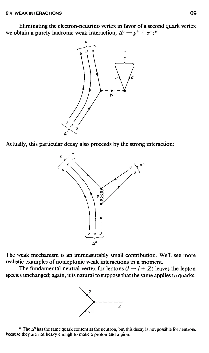
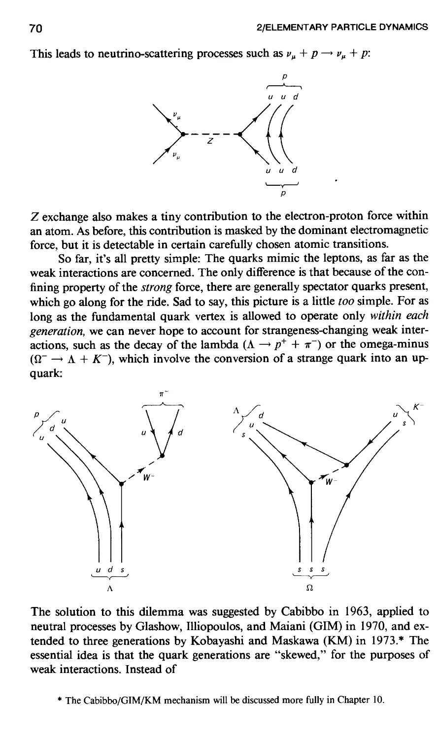
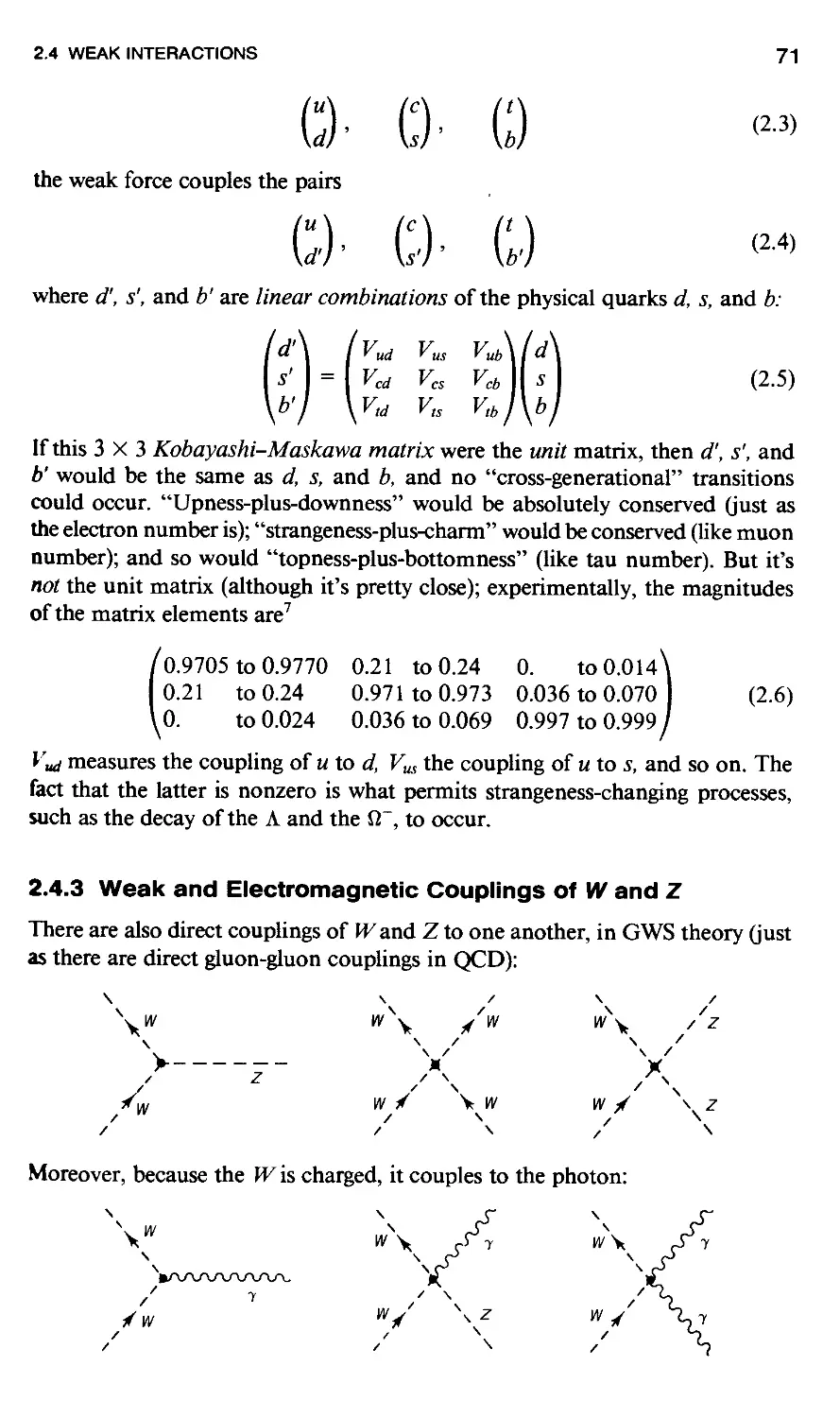
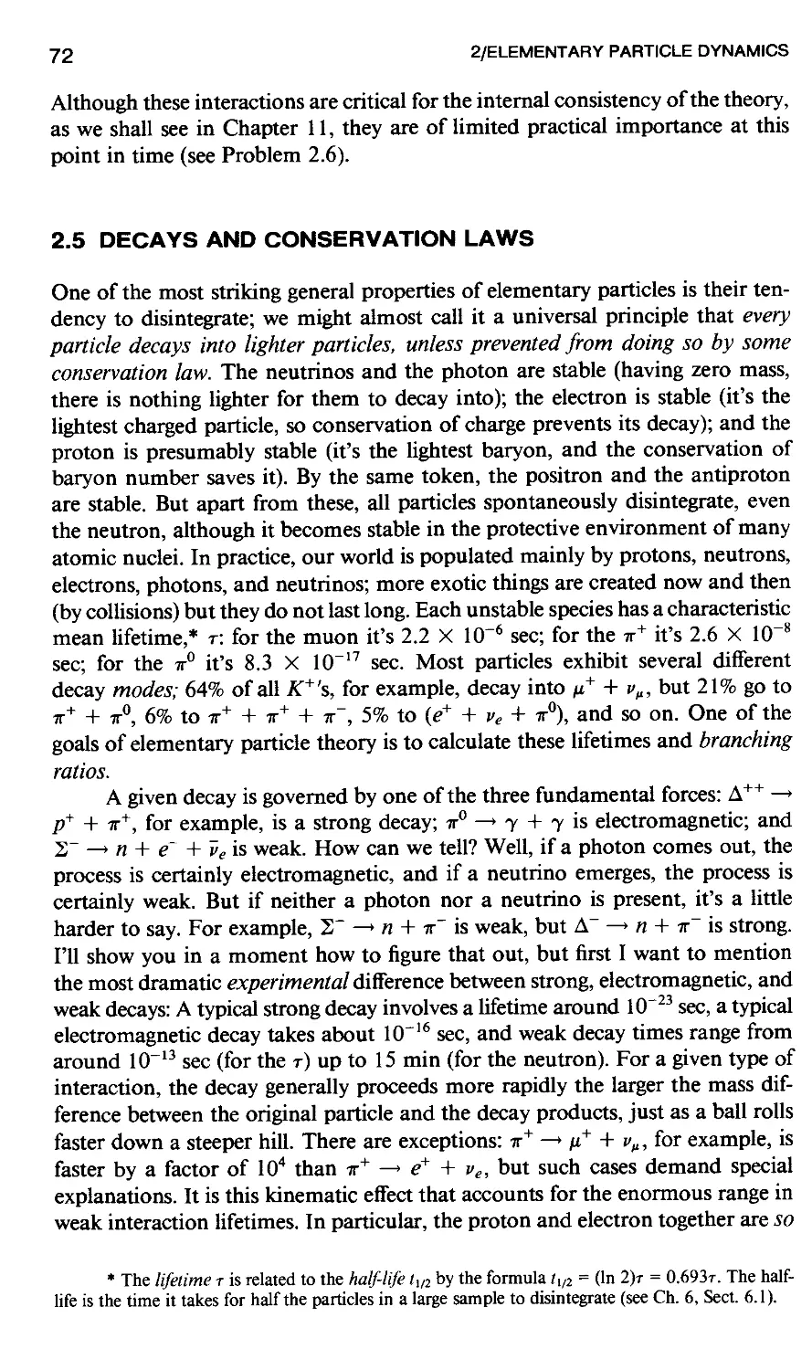
/


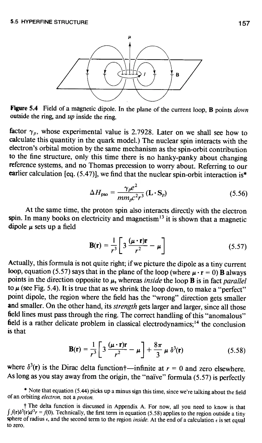


Автор: Griffiths D.
Теги: mathematics mathematical physics quantum mechanics higher mathematics john wiley & sons inc
ISBN: 0-471-60386-4
Год: 1987


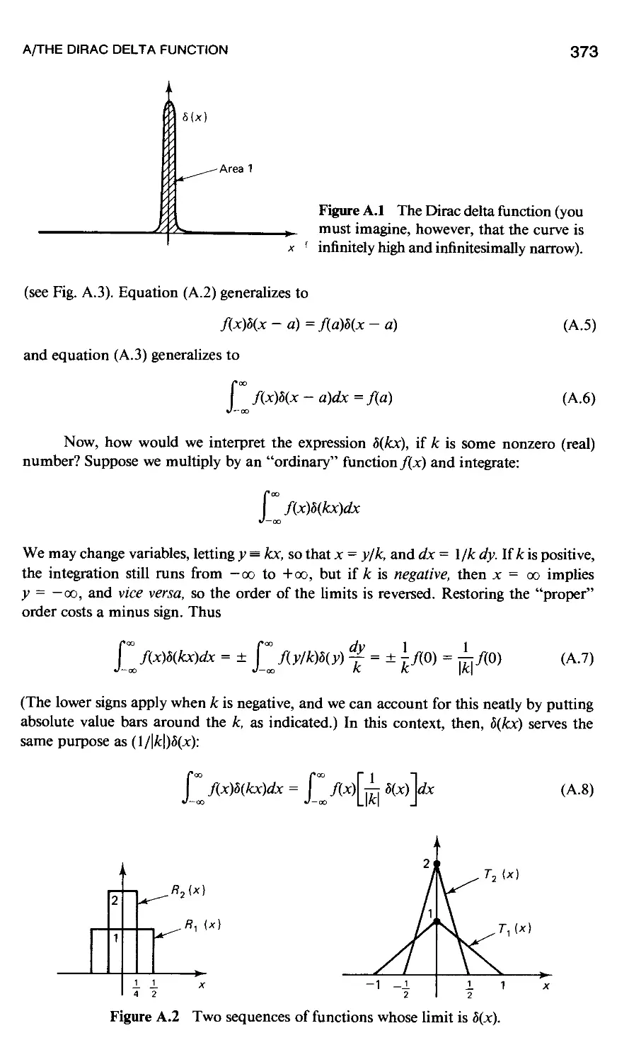
Текст
INTRODUCTION TO
ELEMENTARY
PARTICLES
David Griffiths
Reed College
JOHN WILEY & SONS, INC.
WI LEY New York • Chichester • Brisbane • Toronto • Singapore
INTRODUCTION TO ELEMENTARY PARTICLES
Copyright © 1987 John Wiley & Sons, Inc.
AH rights reserved. Published simultaneously in Canada.
Reproduction or translation of any part of this work beyond that permit-
permitted by Section 107 or 108 of the 1976 United States Copyright Act without
the permission of the copyright owner is unlawful. Requests for permis-
permission or further information should be addressed to the Permissions De-
Department, John Wiley & Sons, Inc.
Library of Congress Cataloging-in-Publication Data
Griffiths, David J. (David Jeffrey), 1942-
Introduction to elementary particles.
Includes bibliographies and index.
1. Particles (Nuclear physics) I. Title.
QC793.2.G75 1987 539.7'2l 86-25709
ISBN 0-471-60386-4
Printed and bound in the United States of America
20 19 18 17 16 15 14
CONTENTS
Preface vii
Introduction
Elementary Particle Physics 1
How Do You Produce Elementary Particles? 4
How Do You Detect Elementary Particles? 7
Units 8
References and Notes 10
1 Historical Introduction to the Elementary Particles 11
1.1 The Classical Era A897-1932) 11
1.2 The Photon A900-1924) 14
1.3 Mesons A934-1947) 17
1.4 Antiparticles A930-1956) 18
1.5 Neutrinos A930-1962) 22
1.6 Strange Particles A947-1960) 28
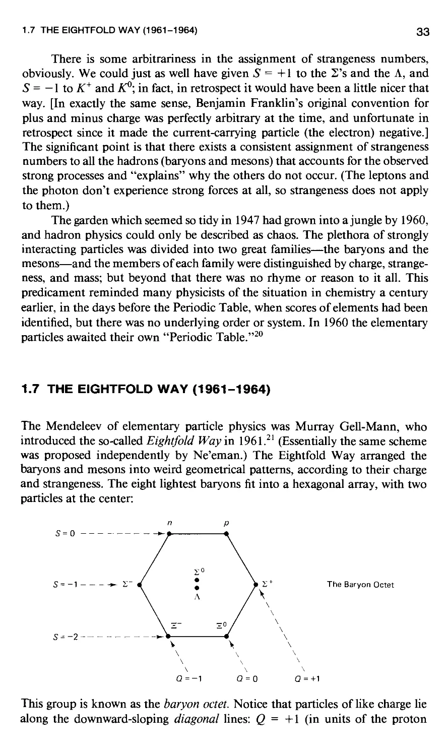
1.7 The Eightfold Way A961 -1964) 33
1.8 The Quark Model A964) 37
1.9 The November Revolution and Its Aftermath A974-1983) 41
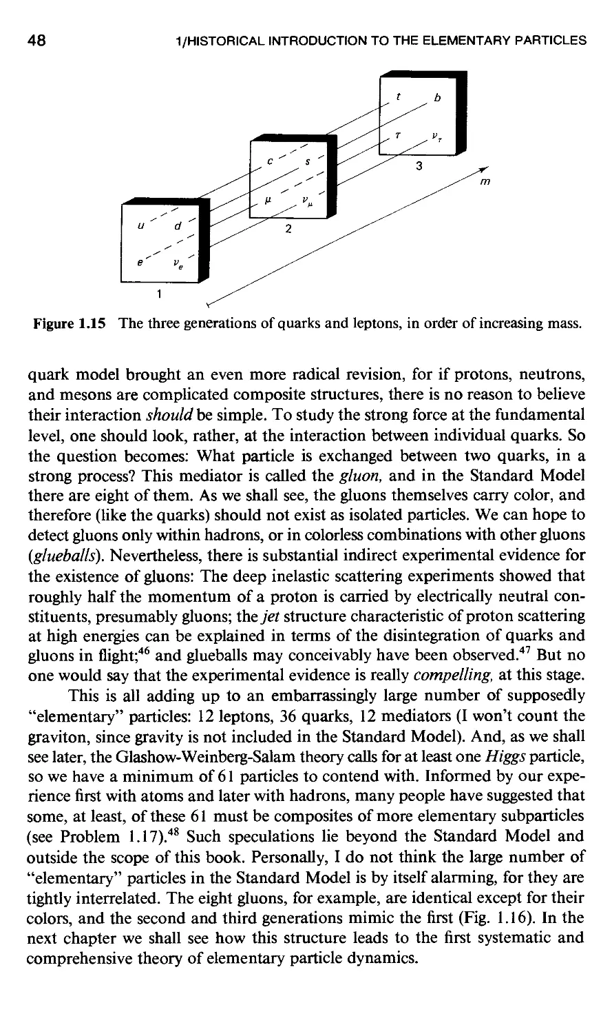
1.10 Intermediate Vector Bosons A983) 44
1.11 The Standard Model A978-?) 46
References and Notes 49
Problems 51
2 Elementary Particle Dynamics 55
2.1 The Four Forces 55
2.2 Quantum Electrodynamics (QED) 56
2.3 Quantum Chromodynamics (QCD) 60
2.4 Weak Interactions 65
2.5 Decays and Conservation Laws 72
2.6 Unification Schemes 76
References and Notes 78
Problems 78
iv CONTENTS
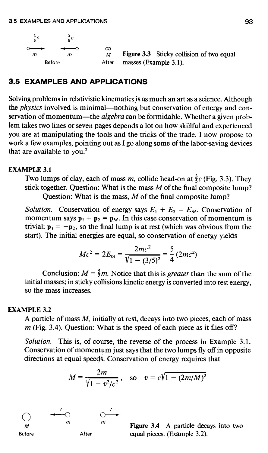
3 Relativistic Kinematics 81
3.1 Lorentz Transformations 81
3.2 Four-Vectors 84
3.3 Energy and Momentum 87
3.4 Collisions 91
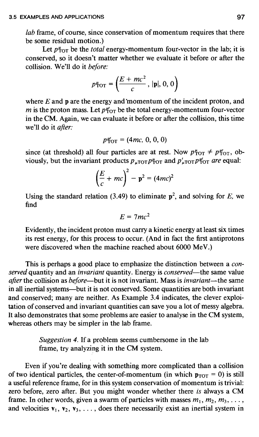
3.5 Examples and Applications 93
References and Notes 99
Problems 99
4 Symmetries 103
4.1 Symmetries, Groups, and Conservation Laws 103
4.2 Spin and Orbital Angular Momentum 107
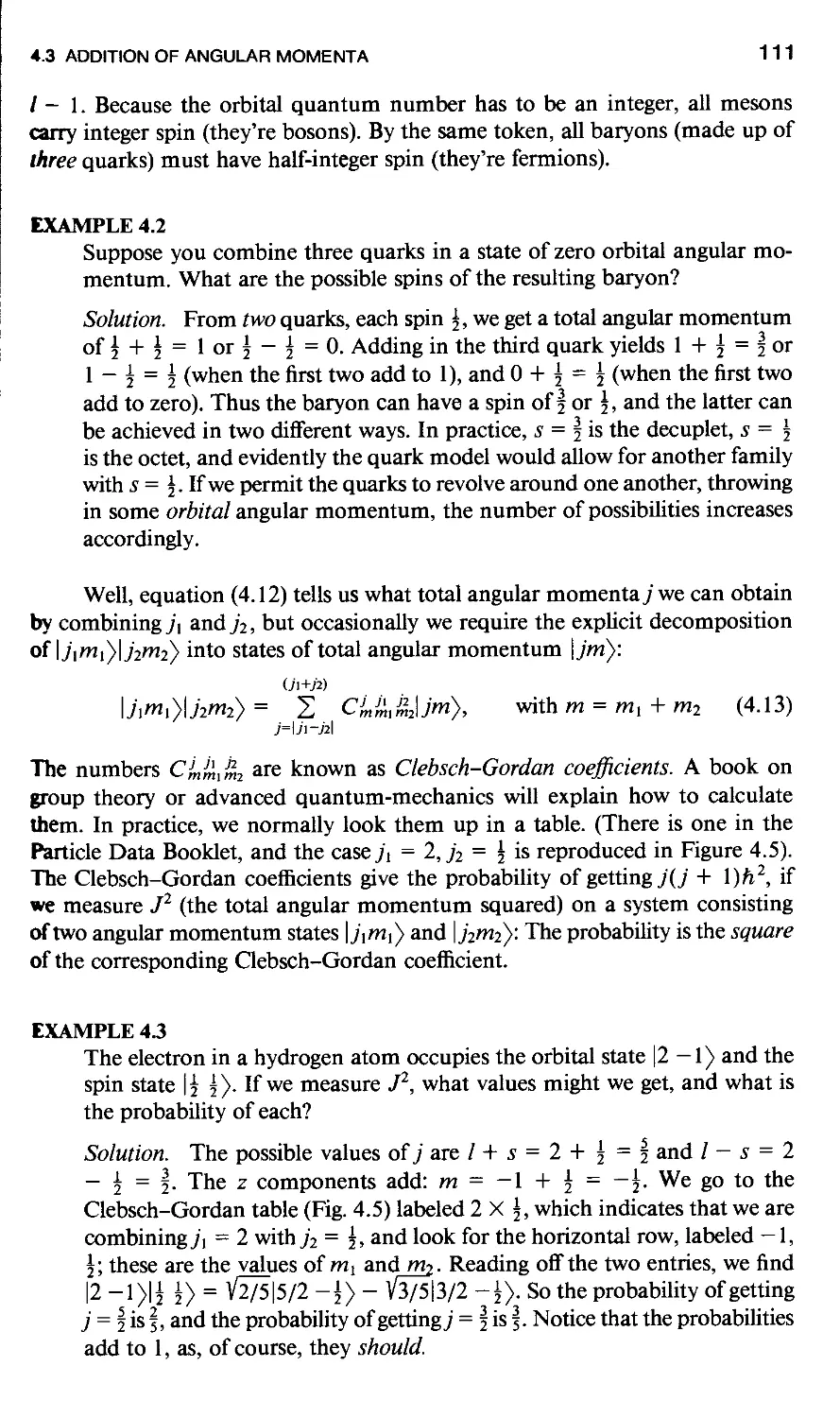
4.3 Addition of Angular Momenta 109
4.4 Spin ? 113
4.5 Flavor Symmetries 116
4.6 Parity 122
4.7 Charge Conjugation 128
4.8 CP Violation 130
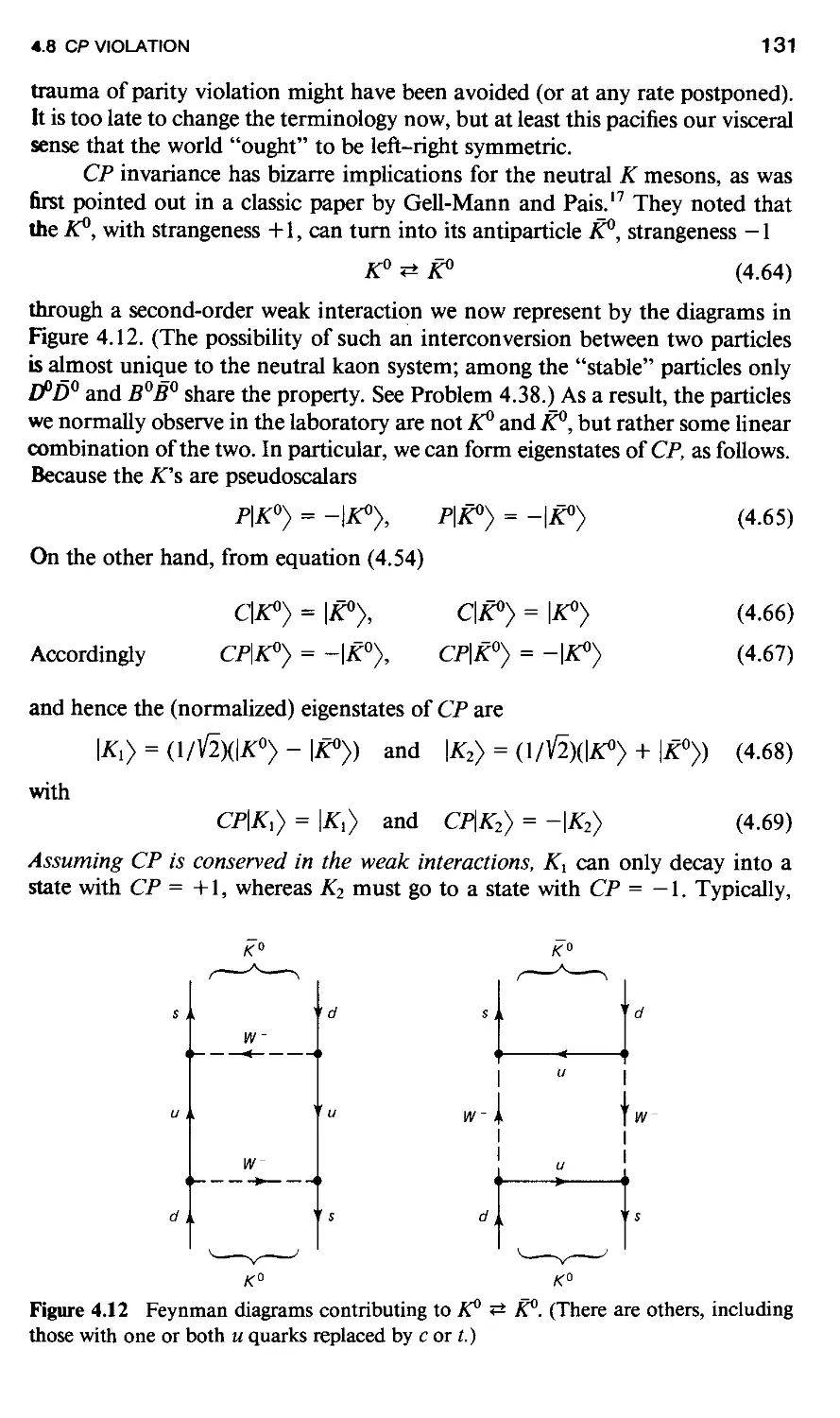
4.9 Time Reversal and the TCP Theorem 134
References and Notes 135
Problems 137
5 Bound States 143
5.1 The Schrodinger Equation for a Central Potential 143
5.2 The Hydrogen Atom 148
5.3 Fine Structure 151
5.4 The Lamb Shift 154
5.5 Hyperfine Structure 156
5.6 Positronium 159
5.7 Quarkonium 164
5.8 Light Quark Mesons 168
5.9 Baryons 172
5.10 Baryon Masses and Magnetic Moments 180
References and Notes 184
Problems 186
6 The Feynman Calculus 189
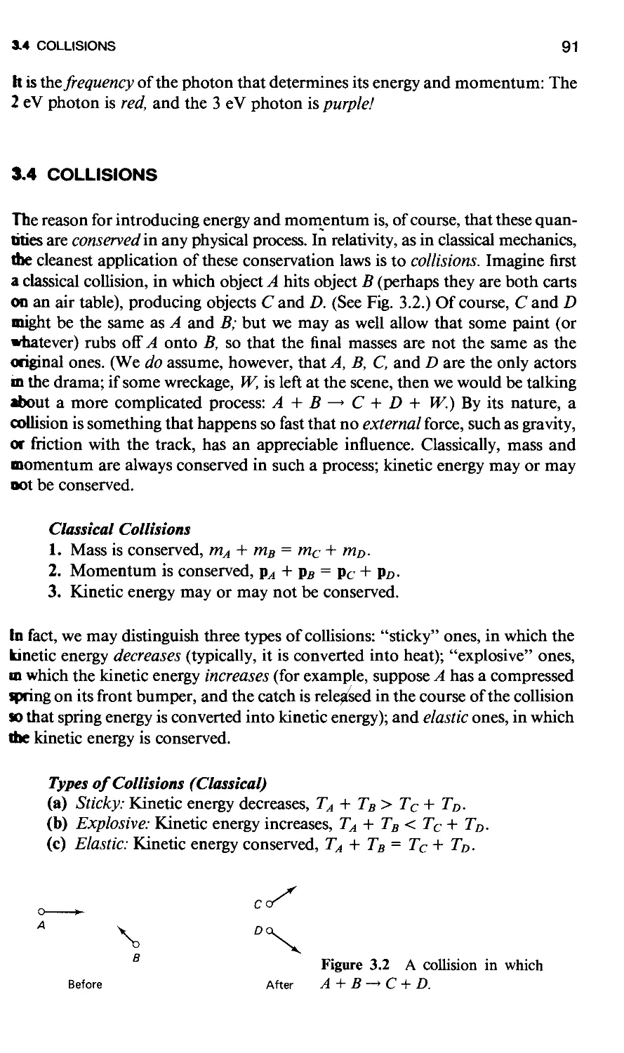
6.1 Lifetimes and Cross Sections 189
6.2 The Golden Rule 194
6.3 The Feynman Rules for a Toy Theory 201
6.4 Lifetime of the A 204
6.5 Scattering 204
CONTENTS
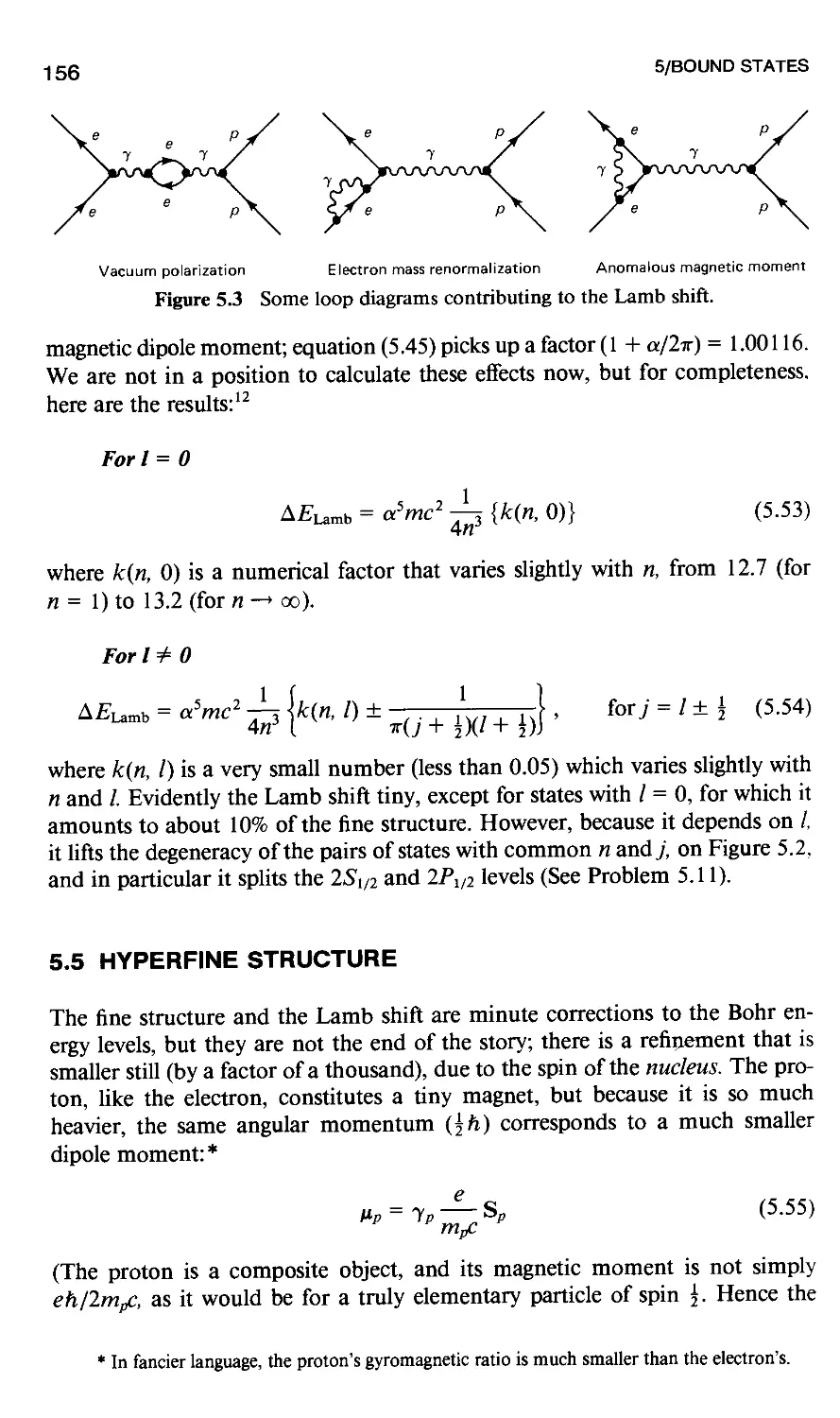
6.6 Higher-Order Diagrams 206
References and Notes 210
Problems 211
7 Quantum Electrodynamics 213
7.1 The Dirac Equation 213
7.2 Solutions to the Dirac Equation 216
7.3 Bilinear Covariants 222
7.4 The Photon 225
7.5 The Feynman Rules for Quantum Electrodynamics 228
7.6 Examples 231
7.7 Casimir's Trick and the Trace Theorems 236
7.8 Cross Sections and Lifetimes 240
7.9 Renormalization 246
References and Notes 250
Problems 251
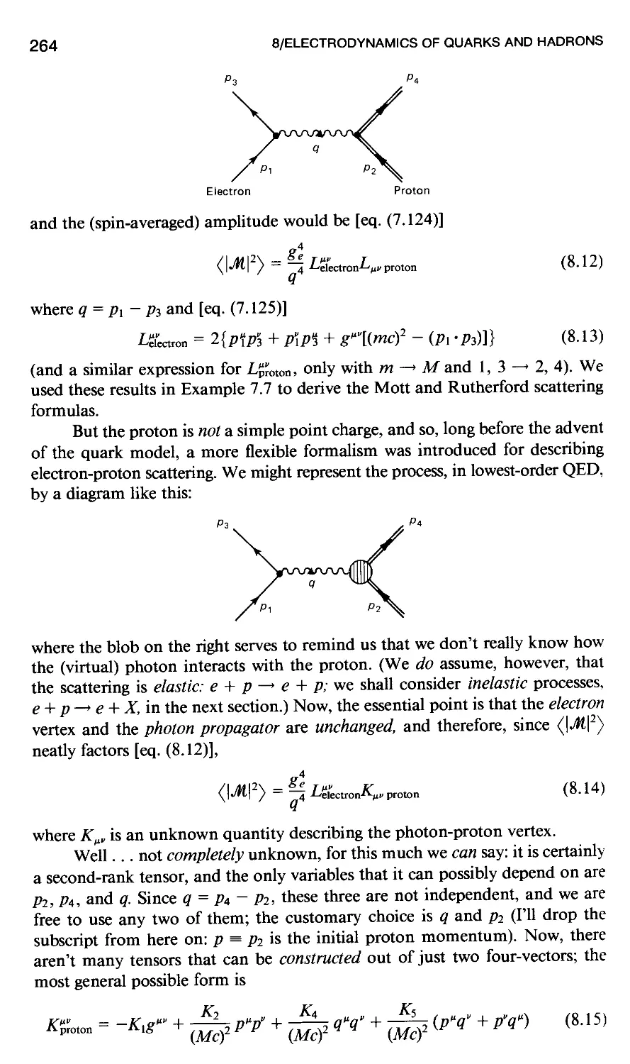
8 Electrodynamics of Quarks and Hadrons 257
8.1 Electron-Quark Interactions 257
8.2 Hadron Production in e+e~ Scattering 258
8.3 Elastic Electron-Proton Scattering 262
8.4 Inelastic Electron-Proton Scattering 266
8.5 The Parton Model and Bjorken Scaling 269
8.6 Quark Distribution Functions 273
References and Notes 277
Problems 277
9 Quantum Chromodynamics 279
9.1 Feynman Rules for Chromodynamics 279
9.2 The Quark-Quark Interaction 284
9.3 Pair Annihilation in QCD 289
9.4 Asymptotic Freedom 292
9.5 Applications of QCD 295
References and Notes 296
Problems 296
10 Weak Interactions 301
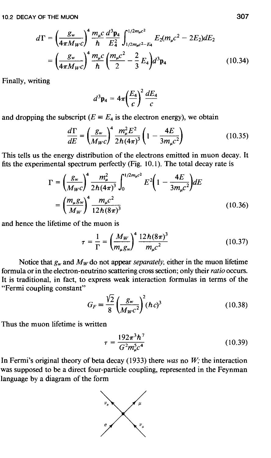
10.1 Charged Leptonic Weak Interactions 301
10.2 Decay of the Muon 304
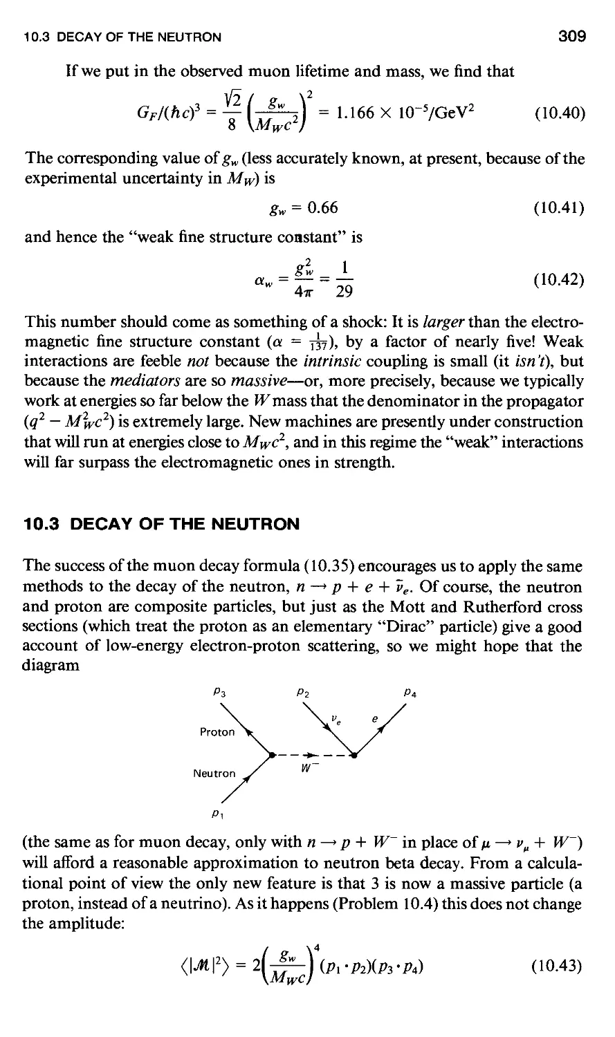
10.3 Decay of the Neutron 309
10.4 Decay of the Pion 314
Vi CONTENTS
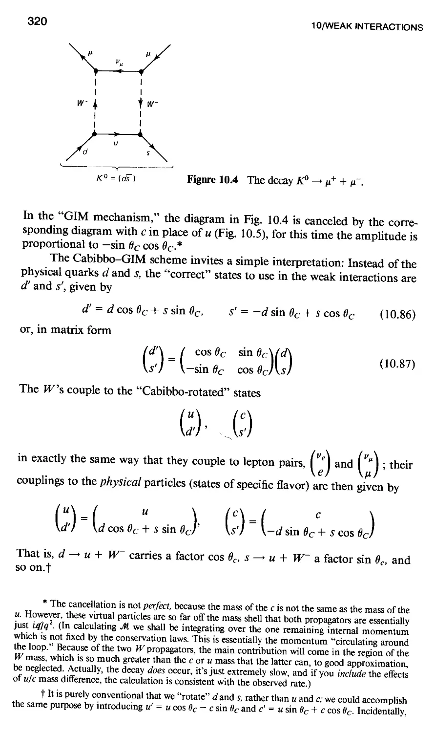
10.5 Charged Weak Interactions of Quarks 317
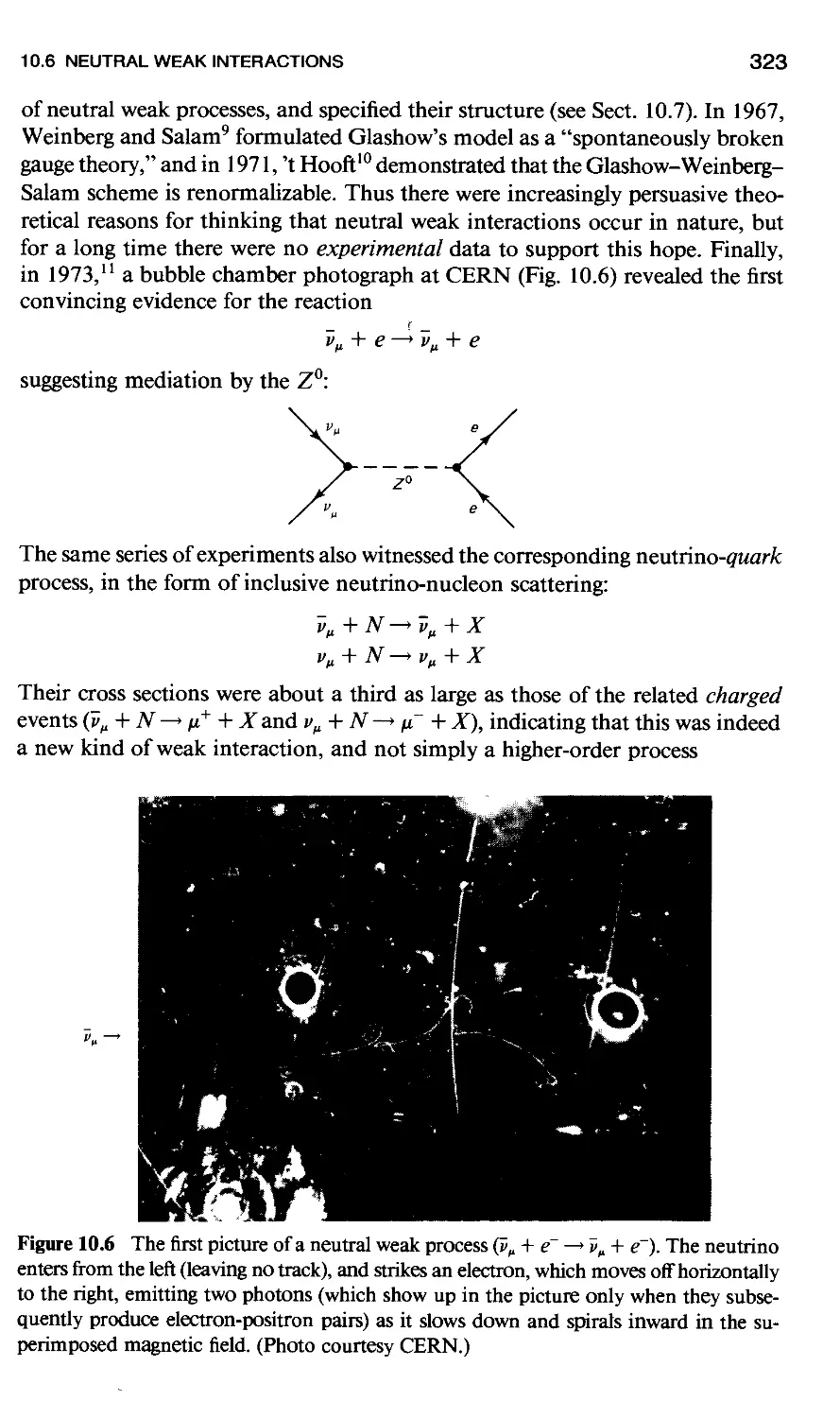
10.6 Neutral Weak Interactions 322
10.7 Electroweak Unification 330
References and Notes 338
Problems 339
11 Gauge Theories 343
11.1 Lagrangian Formulation of Classical Particle Mechanics 343
11.2 Lagrangians in Relativistic Field Theory 344
11.3 Local Gauge Invariance 348
11.4 Yang-Mills Theory 350
11.5 Chromodynamics 355
11.6 Feynman Rules 357
11.7 The Mass Term 360
11.8 Spontaneous Symmetry-Breaking 362
11.9 The Higgs Mechanism 365
References and Notes 368
Problems 368
APPENDIX A. The Dirac Delta Function 372
APPENDIX B. Decay Rates and Cross Sections 376
APPENDIX C. Paul! and Dirac Matrices 378
APPENDIX D. Feynman Rules 380
Index 384
PREFACE
This introduction to the theory of elementary particles is intended primarily for
advanced undergraduates who are majoring in physics. Most of my colleagues
consider this subject inappropriate for such an audience—mathematically too
sophisticated, phenomelogically too cluttered, insecure in its foundations, and
uncertain in its future. Ten years ago I would have agreed. But in the last decade
the dust has settled to an astonishing degree, and it is fair to say that elementary
particle physics has come of age. Although we obviously have much more to
learn, there now exists a coherent and unified theoretical structure that is simply
too exciting and important to save for graduate school or to serve up in diluted
qualitative form as a subunit of modern physics. I believe the time has come to
integrate elementary particle physics into the standard undergraduate curriculum.
Unfortunately, the research literature in this field is clearly inaccessible to
undergraduates, and although there are now several excellent graduate texts,
these call for a strong preparation in advanced quantum mechanics, if not quan-
quantum field theory. At the other extreme, there are many fine popular books and
a number of outstanding Scientific American articles. But very little has been
written specifically for the undergraduate. This book is an effort to fill that need.
It grew out of a one-semester elementary particles course I have taught from
time to time at Reed College. The students typically had under their belts a
semester of electromagnetism (at the level of Lorrain and Corson), a semester
of quantum mechanics (at the level of Park), and a fairly strong background in
special relativity.
In addition to its principal audience, I hope this book will be of use to
beginning graduate students, either as a primary text, or as preparation for a
more sophisticated treatment. With this in mind, and in the interest of greater
completeness and flexibility, I have included more material here than one can
comfortably cover in a single semester. (In my own courses I ask the students
to read Chapters 1 and 2 on their own, and begin the lectures with Chapter 3.1
skip Chapter 5 altogether, concentrate on Chapters 6 and 7, discuss the first two
sections of Chapter 8, and then jump to Chapter 10). To assist the reader (and
the teacher) I begin each chapter with a brief indication of its purpose and content,
its prerequisites, and its role in what follows.
This book was written while I was on sabbatical at the Stanford Linear
Accelerator Center, and I would like to thank Professor Sidney Drell and the
other members of the Theory Group for their hospitality.
David Griffiths
VII
Introduction
ELEMENTARY PARTICLE PHYSICS
Elementary particle physics addresses the question, "What is matter made of?"
on the most fundamental level—which is to say, on the smallest scale of size.
It's a remarkable fact that matter at the subatomic level consists of tiny chunks,
with vast empty spaces in between. Even more remarkable, these tiny chunks
come in a small number of different types (electrons, protons, neutrons, pi me-
mesons, neutrinos, and so on), which are then replicated in astronomical quantities
to make all the "stuff" around us. And these replicas are absolutely perfect
copies—not just "pretty similar," like two Fords coming off the same assembly
line, but utterly indistinguishable. You can't stamp an identification number on
an electron, or paint a spot on it—if you've seen one, you've seen them all. This
quality of absolute identicalness has no analog in the macroscopic world. (In
quantum mechanics it is reflected in the Pauli exclusion principle.) It enormously
simplifies the task of elementary particle physics: we don't have to worry about
big electrons and little ones, or new electrons and old ones—an electron is an
electron is an electron. It didn't have to be so easy.
My first job, then, is to introduce you to the various kinds of elementary
particles, the actors, if you will, in the drama. I could simply list them, and tell
you their properties (mass, electric charge, spin, etc.), but I think it is better in
this case to adopt a historical perspective, and explain how each particle first
came on the scene. This will serve to endow them with character and personality,
making them easier to remember and more interesting to watch. Moreover,
some of the stories are delightful in their own right.
Once the particles have been introduced, in Chapter 1, the issue becomes,
"How do they interact with one another?" This question, directly or indirectly,
will occupy us for the rest of the book. If you were dealing with two macroscopic
1
2 INTRODUCTION
objects, and you wanted to know how they interact, you would probably begin
by suspending them at various separation distances and measuring the force
between them. That's how Coulomb determined the law of electrical repulsion
between two charged pith balls, and how Cavendish measured the gravitational
attraction of two lead weights. But you can't pick up a proton with tweezers or
tie an electron onto the end of a piece of string; they're just too small. For
practical reasons, therefore, we have to resort to less direct means to probe the
interactions of elementary particles. As it turns out, almost all our experimental
information comes from three sources: A) scattering events, in which we fire
one particle at another and record (for instance) the angle of deflection; B)
decays, in which a particle spontaneously disintegrates and we examine the debris;
and C) bound states, in which two or more particles stick together, and we study
the properties of the composite object. Needless to say, determining the inter-
interaction law from such indirect evidence is not a trivial task. Ordinarily, the pro-
procedure is to guess a form for the interaction and compare the resulting theoretical
calculations with the experimental data.
The formulation of such a guess ("model" is a more respectable term for
it) is guided by certain general principles, in particular, special relativity and
quantum mechanics. In the diagram below I have indicated the four realms of
mechanics:
Small—>
Fast
The world of everyday life, of course, is governed by classical mechanics. But
for objects that travel very fast (at speeds comparable to c), the classical rules
are modified by special relativity, and for objects that are very small (comparable
to the size of atoms, roughly speaking), classical mechanics is superseded by
quantum mechanics. Finally, for things that are both fast and small, we require
a theory that incorporates relativity and quantum principles: quantum field the-
theory. Now, elementary particles are extremely small, of course, and typically they
are also very fast. So elementary particle physics naturally falls under the do-
dominion of quantum field theory.
Please observe the distinction here between a type of mechanics and a
particular force law. Newton's law of universal gravitation, for example, describes
a specific interaction (gravity), whereas Newton's three laws of motion define
a mechanical system (classical mechanics), which (within its jurisdiction) governs
all interactions. The force law tells you what F is, in the case at hand; the me-
mechanics tells you how to use F to determine the motion. The goal of elementary
particle dynamics, then, is to guess a set of force laws which, within the context
of quantum field theory, correctly describe particle behavior.
However, some general features of this behavior have nothing to do with
the detailed form of the interactions. Instead they follow directly from relativity,
Classical
mechanics
Relativistic
mechanics
Quantum
mechanics
Quantum
field theory
ELEMENTARY PARTICLE PHYSICS 3
from quantum mechanics, or from the combination of the two. For example,
in relativity, energy and momentum are always conserved, but (rest) mass is not.
Thus the decay A —< p + ¦k is perfectly acceptable, even though the A weighs
more than the sum of p plus ¦k. Such a process would not be possible in classical
mechanics, where mass is strictly conserved. Moreover, relativity allows for par-
particles of zero (rest) mass—the very idea of a massless particle is nonsense in
classical mechanics—and as we shall see, photons, neutrinos, and gluons are all
(apparently) massless.
In quantum mechanics a physical system is described by its state, s (rep-
(represented by the wave function \ps in Schrodinger's formulation, or by the ket \s)
in Dirac's). A physical process, such as scattering or decay, consists of a transition
from one state to another. But in quantum mechanics the outcome is not uniquely
determined by the initial conditions; all we can hope to calculate, in general, is
the probability for a given transition to occur. This indeterminacy is reflected in
the observed behavior of particles. For example, the charged pi meson ordinarily
disintegrates into a muon plus a neutrino, but occasionally one will decay
into an electron plus a neutrino. There's no difference in the original pi
mesons; they're all identical. It is simply a fact of nature that a given particle can
go either way.
Finally, the union of relativity and quantum mechanics brings certain extra
dividends that neither one by itself can offer: the existence of antiparticles, a
proof of the Pauli exclusion principle (which in nonrelativistic quantum me-
mechanics is simply an ad hoc hypothesis), and the so-called TCP theorem. I'll tell
you more about these later on; my purpose in mentioning them4iere is to em-
emphasize that these are features of the mechanical system itself, not of the particular
model. Short of a catastrophic revolution, they are untouchable. By the way,
quantum field theory in all its glory is difficult and deep, but don't be alarmed:
Feynman invented a beautiful and intuitively satisfying formulation that is not
hard to learn; we'll come to that in Chapter 6. (The derivation of Feynman's
rules from the underlying quantum field theory is a different matter, which can
easily consume the better part of an advanced graduate course, but this need
not concern us here.)
In the last few years a theory has emerged that describes all of the known
elementary particle interactions except gravity. (As far as we can tell, gravity is
much too weak to play any significant role in ordinary particle processes.) This
theory—or, more accurately, this collection of related theories, incorporating
quantum electrodynamics, the Glashow-Weinberg-Salam theory of electroweak
processes, and quantum chromodynamics—has come to be called the Standard
Model. No one pretends that the Standard Model is the final word on the subject,
but at least we now have (for the first time) a full deck of cards to play with.
Since 1978, when the Standard Model achieved the status of "orthodoxy," it
has met every experimental test. It has, moreover, an attractive aesthetic feature:
in the Standard Model all of the fundamental interactions derive from a single
general principle, the requirement of local gauge invariance. It seems likely that
future developments will involve extensions of the Standard Model, not its re-
repudiation. This book might be called an "Introduction to the Standard Model."
4 INTRODUCTION
As that alternative title suggests, this is a book about elementary particle
theory, with very little on experimental methods or instrumentation. These are
important matters, and an argument can be made for integrating them into a
text such as this, but they can also be distracting and interfere with the clarity
and elegance of the theory itself. (I encourage you to read about experimental
aspects of the subject, and from time to time I will refer you to particularly
accessible accounts.) For now, I'll confine myself to scandalously brief answers
to the two most obvious experimental questions.
HOW DO YOU PRODUCE ELEMENTARY PARTICLES?
Electrons and protons are no problem; these are the stable constituents of ordinary
matter. To produce electrons one simply heats up a piece of metal, and they
come boiling off. If one wants a beam of electrons, one then sets up a positively
charged plate nearby, to attract them over, and cuts a small hole in it; the electrons
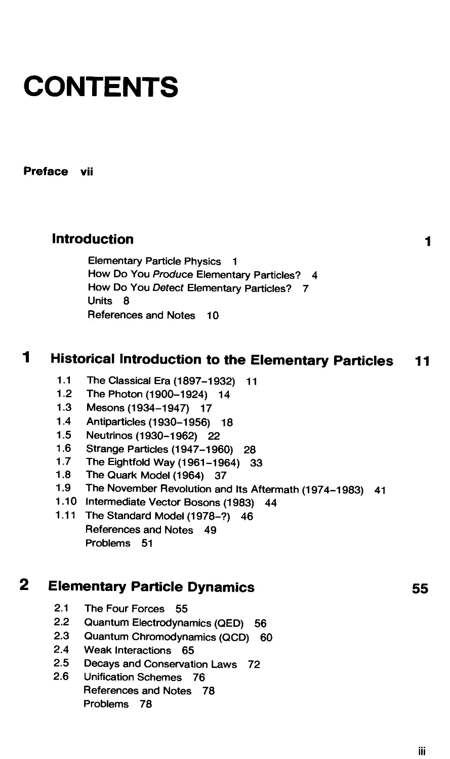
that make it through the hole constitute the beam. Such an electron gun is the
starting element in a television tube or an oscilloscope or an electron accelerator
(Fig. I.I).
To obtain protons you ionize hydrogen (in other words, strip off the elec-
electron). In fact, if you're using the protons as a target, you don't even need to
bother about the electrons; they're so light that an energetic particle coming in
will knock them out of the way. Thus, a tank of hydrogen is essentially a tank
of protons. For more exotic particles there are three main sources: cosmic rays,
nuclear reactors, and particle accelerators.
Cosmic Rays The earth is constantly bombarded with high-energy particles
(principally protons) coming from outer space. What the source of these particles
might be remains something of a mystery; at any rate, when they hit atoms in
the upper atmosphere they produce showers of secondary particles (mostly
muons, by the time they reach ground level), which rain down on us all the
time. As a source of elementary particles, cosmic rays have two virtues: they are
free, and their energies can be enormous—far greater than we could possibly
produce in the laboratory. But they have two major disadvantages: The rate at
which they strike any detector of reasonable size is very low, and they are com-
completely uncontrollable. So cosmic ray experiments call for patience and luck.
Nuclear Reactors When a radioactive nucleus disintegrates, it may emit a variety
of particles—neutrons, neutrinos, and what used to be called alpha rays (actually,
alpha particles, which are bound states of two neutrons plus two protons), beta
rays (actually, electrons or positrons), and gamma rays (actually, photons).
Particle Accelerators You start with electrons or protons, accelerate them to
high energy, and smash them into a target. By skillful arrangements of absorbers
and magnets, you can separate out of the resulting debris the particle species
you wish to study. Nowadays it is possible in this way to generate intense sec-
HOW DO YOU PRODUCE ELEMENTARY PARTICLES?
Figure I.I The Stanford Linear Accelerator Center (SLAC). Electrons and positrons are
accelerated down a straight tube 2 miles long, reaching energies as high as 45 GeV. (Photo
courtesy of SLAC.)
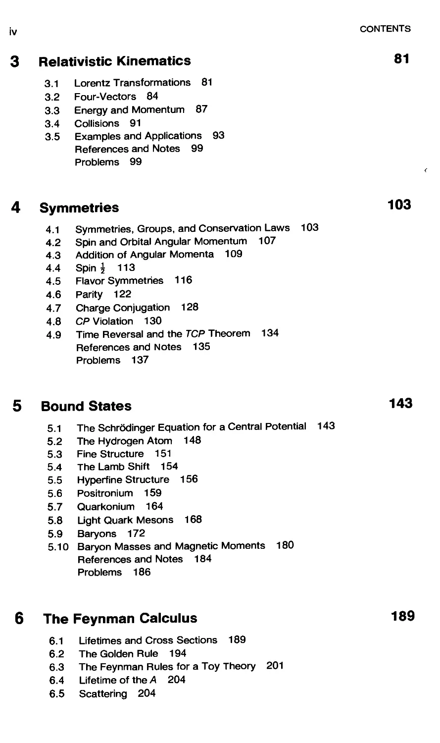
ondary beams of positrons, muons, pions, kaons, and antiprotons, which in turn
can be fired at another target. The stable particles—electrons, protons, positrons,
and antiprotons—can even by fed into giant storage rings in which, guided by
powerful magnets, they circulate at high speed for hours at a time, to be extracted
and used at the required moment (Fig. 1.2).
In general, the heavier the particle you want to produce, the higher must
INTRODUCTION
Figure 1.2 CERN, outside Geneva, Switzerland. SPS is the 450 GeV Super Proton Syn-
Synchrotron, later modified to make a proton-antiproton collider; LEP is a 50 GeV electron-
positron storage ring now under construction. (Photo courtesy of CERN.)
be the energy of the collision. That's why, historically, lightweight particles tend
to be discovered first, and as time goes on, and accelerators become more pow-
powerful, heavier and heavier particles are found. At present, the heaviest known
particle is the Z°, with nearly 100 times the mass of the proton. It turns out that
the particle gains enormously in energy if you collide two high-speed particles
head-on, as opposed to firing one particle at a stationary target. (Of course, this
calls for much better aim!) Therefore, most contemporary experiments involve
colliding beams from intersecting storage rings; if the particles miss on the first
pass, they can try again the next time around. Indeed, with electrons and positrons
(or protons and antiprotons) the same ring can be used, with the plus charges
circulating in one direction and the minus charges in the other.
There is another reason why particle physicists are always pushing for
higher energies: In general, the higher the energy of the collision, the closer the
two particles come to one another. So if you want to study the interaction at
very short range, you need very energetic particles. In quantum-mechanical terms,
a particle of momentum p has an associated wavelength X given by the de Broglie
formula X = h/p, where h is Planck's constant. At large wavelengths (low mo-
momenta) you can only hope to resolve relatively large structures; in order to ex-
examine something extremely small, you need comparably short wavelengths, and
hence high momenta. If you like, consider this a manifestation of the uncertainty
principle (Ax Ap > h/Air)—to make Ax small, Ap must be large. However you
HOW DO YOU DETECT ELEMENTARY PARTICLES? 7
look at it, the conclusion is the same: to probe small distances you need high
energies.
HOW DO YOU DETECT ELEMENTARY PARTICLES?
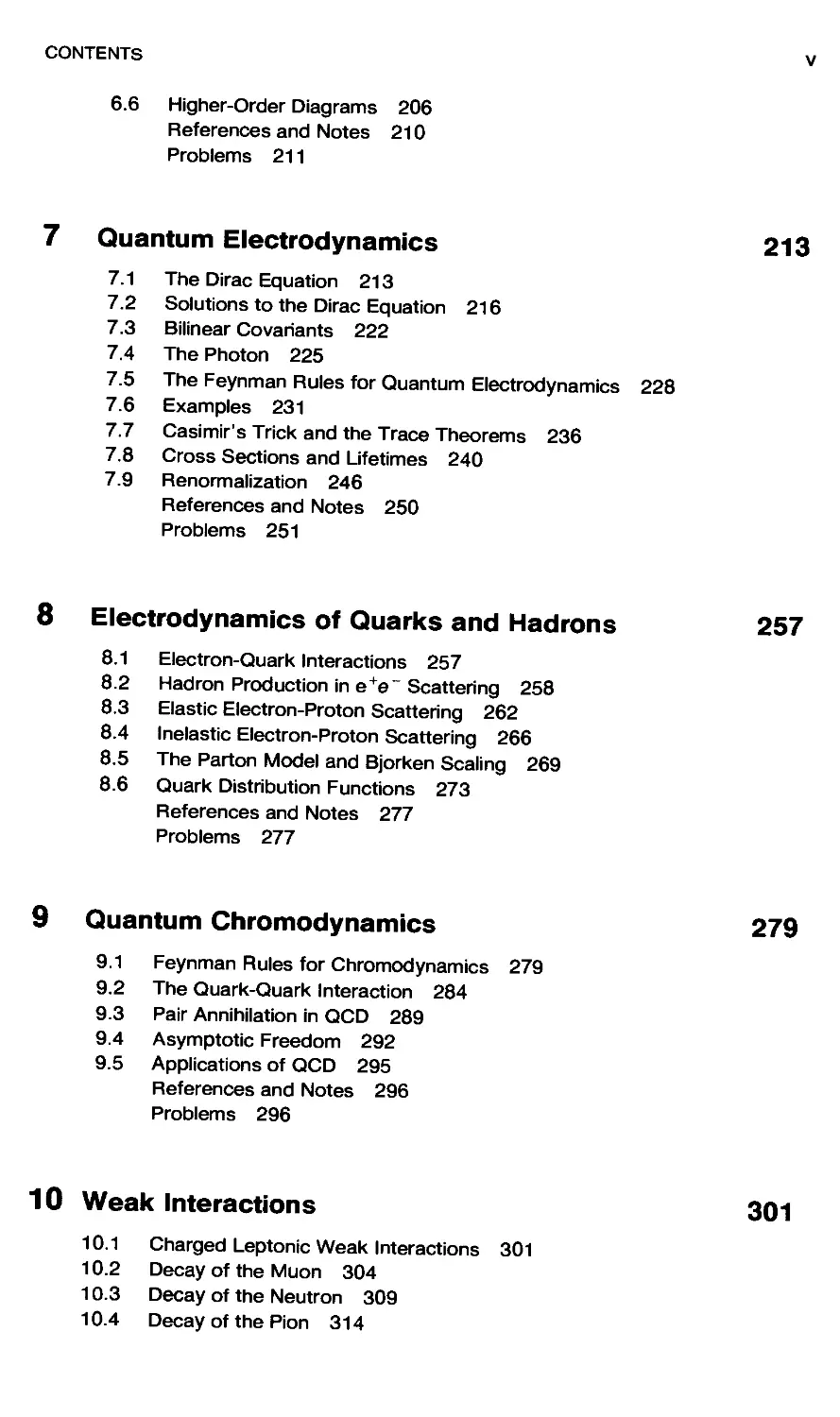
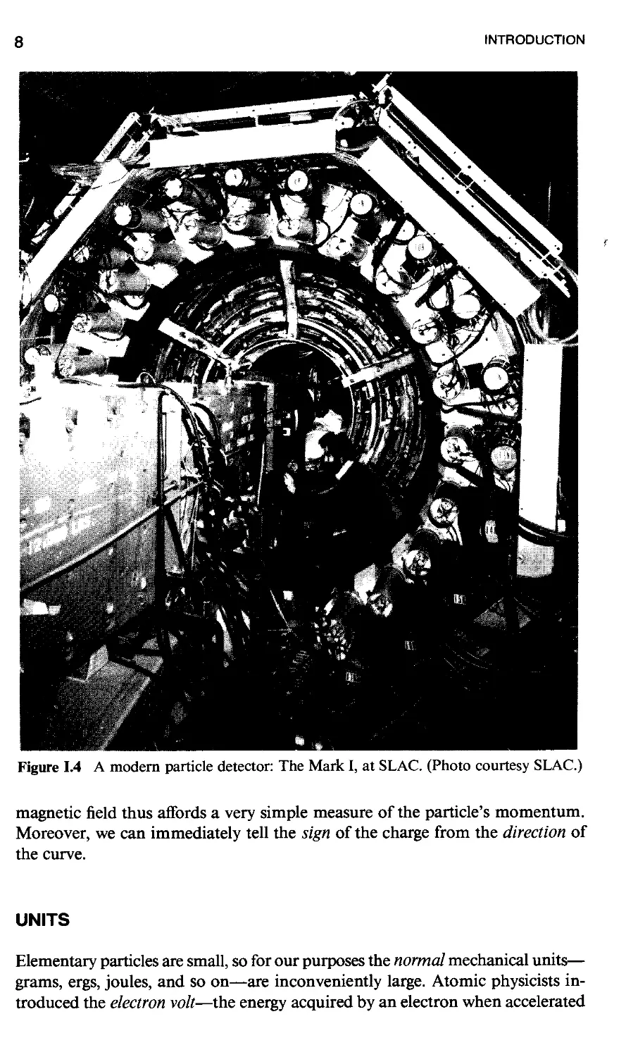
There are many kinds of particle detectors—Geiger counters, cloud chambers,
bubble chambers, spark chambers, photographic emulsions, Cerenkov counters,
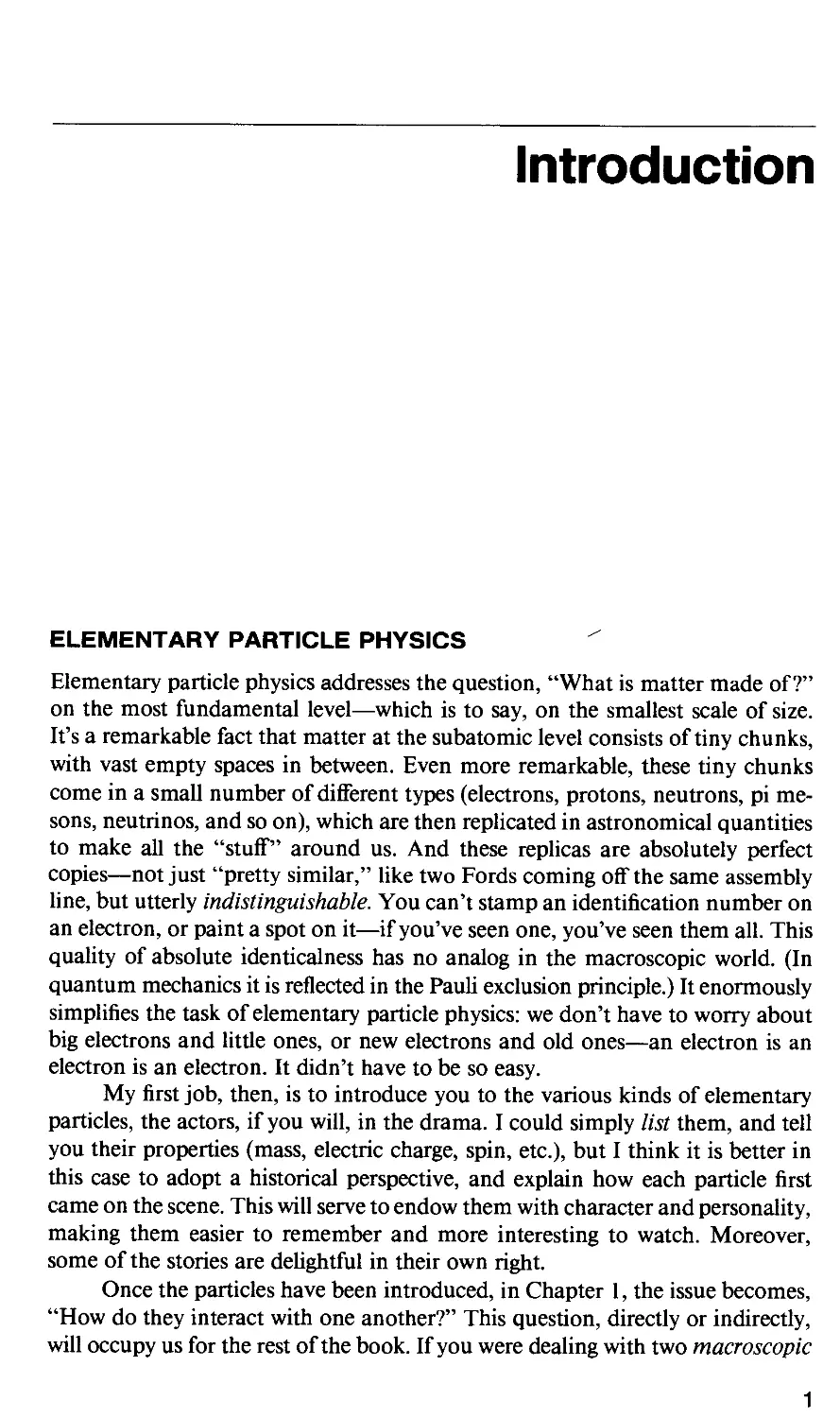
scintillators, photomultipliers, and so on (Fig. 1.3). Actually, a typical modern
detector has whole arrays of these devices, wired up to a computer that tracks
the particles and displays their trajectories on a television screen (Fig. 1.4). The
details do not concern us, but there is one thing to be aware of: Most detection
mechanisms rely on the fact that when high-energy charged particles pass through
matter they ionize atoms along their path. The ions then act as "seeds" in the
formation of droplets (cloud chamber) or bubbles (bubble chamber) or sparks
(spark chamber), as the case may be. But electrically neutral particles do not
cause ionization, and they leave no tracks. If you look at the bubble chamber
photograph in Fig. 1.11, for instance, you will see that the five neutral particles
are "invisible"; their paths have been reconstructed by analyzing the tracks of
the charged particles in the picture and invoking conservation of energy and
momentum at each vertex. Notice also that most of the tracks in the picture are
curved (actually, all of them are, to some extent; try holding a ruler up to one
you think is straight). Evidently the bubble chamber was placed between the
poles of a giant magnet. In a magnetic field B, a particle of charge q and mo-
momentum p will move in a circle of radius R given by the famous cyclotron formula:
R = pc/qB, where c is the speed of light. The curvature of the track in a known
¦¦ I
Figure 1.3 An early particle detector: Wilson's cloud chamber (ca. 1900). (Photo courtesy-
Science Museum, London.)
INTRODUCTION
Figure 1.4 A modern particle detector: The Mark I, at SLAC. (Photo courtesy SLAC.)
magnetic field thus affords a very simple measure of the particle's momentum.
Moreover, we can immediately tell the sign of the charge from the direction of
the curve.
UNITS
Elementary particles are small, so for our purposes the normal mechanical units—
grams, ergs, joules, and so on—are inconveniently large. Atomic physicists in-
introduced the electron volt—the energy acquired by an electron when accelerated
UNITS 9
through a potential difference of 1 volt: 1 eV = 1.6 X 10~19 joules. For us the
eV is inconveniently small, but we're stuck with it. Nuclear physicists use keV
A03 eV); typical energies in particle physics are MeV A06 eV), GeV A09 eV),
or even TeV A012 eV). Momenta are measured in MeV/c (or GeV/c, or whatever),
and masses in MeV/c2. Thus the proton weighs 938 MeV/c2 = 1.67 X 10~24 g.
Actually, particle theorists are lazy (or clever, depending on your point of
view)—they seldom include the c's and ft's (h = h/2ir) in their formulas. You're
just supposed to fit them in for yourself at the end, to make the dimensions
come out right. As they say in the business, "set c = h = 1." This amounts to
working in units such that time is measured in centimeters and mass and energy
in inverse centimeters; the unit of time is the time it takes light to travel 1
centimeter, and the unit of energy is the energy of a photon whose wavelength
is 2ir centimeters. Only at the end of the problem do we revert to conventional
units. This makes everything look very elegant, but I thought it would be wiser
in this book to keep all the c's and ft's where they belong, so that you can check
for dimensional consistency as you go along. (If this offends you, remember that
it is easier for you to ignore an h you don't like than for someone else to conjure
one up in just the right place.)
Finally, there is the question of what units to use for electric charge. In
introductory physics courses most instructors favor the 57 system, in which charge
is measured in coulombs, and Coulomb's law reads
^T (SI)
Most advanced work is done in the Gaussian system, in which charge is measured
in electrostatic units (esu), and Coulomb's law is written
F=q-f (G)
But elementary particle physicists prefer the Heaviside-Lorentz system, in which
Coulomb's law takes the form
F~^~rT (HL)
The three units of charge are related as shown:
In this book I shall use Gaussian units exclusively, in order to avoid unnecessary
confusion in an already difficult subject. Whenever possible I will express results
in terms of the fine structure constant
a he 137
where e is the charge of the electron in Gaussian units. Most elementary particle
10 INTRODUCTION
texts write this as e2/4ir, because they are measuring charge in Heaviside-Lorentz
units and setting c = h = 1; but everyone agrees that the number is 757.
REFERENCES AND NOTES
This book is a brief survey of an enormous and rapidly changing subject. My
aim is to introduce you to some important ideas and methods, to give you a
sense of what's out there to be learned, and perhaps to stimulate your appetite
for more. If you want to read further in quantum field theory, I particularly
recommend:
Bjorken, J. D., and S. D. Drell. Relativistic Quantum Mechanics and Relativistic Quantum
Fields. New York: McGraw-Hill, 1964.
Sakurai, J. J. Advanced Quantum Mechanics. Reading, MA: Addison-Wesley, 1967.
Itzykson, C, and J.-B. Zuber. Quantum Field Theory. New York: McGraw-Hill, 1980.
I warn you, however, that these are all difficult and advanced books. For ele-
elementary particle physics itself, the following books (listed in order of increasing
difficulty) are especially useful:
Gottfried, K., and V. F. Weisskopf. Concepts of Particle Physics. Oxford: Oxford University
Press, 1984.
Frauenfelder, H., and E. M. Henley. Subatomic Physics. Englewood Cliffs, NJ: Prentice-
Hall, 1974.
Perkins, D. H. Introduction to High-Energy Physics, 2d Ed. Reading, MA: Addison-
Wesley, 1982.
Halzen, F., and A. D. Martin. Quarks and Leptons. New York: Wiley, 1984.
Aitchison, I. J. R., and A. J. G. Hey. Gauge Theories in Particle Physics. Bristol: Adam
Hilger Ltd., 1982.
Close, F. E. An Introduction to Quarks and Partons. London: Academic, 1979.
Quigg, C. Gauge Theories of the Strong, Weak, and Electromagnetic Interactions. Reading,
MA: Benjamin/Cummings, 1983.
Cheng, T.-P., and L.-F. Li. Gauge Theories of Elementary Particle Physics. New York:
Oxford University Press, 1984.
Chapter 1
Historical Introduction to the
Elementary Particles
This chapter is a kind of "folk history" of elementary particle physics. Its
purpose is to provide a sense of how the various particles were first discovered,
and how they fit into the overall scheme of things. Along the way some of the
fundamental ideas that dominate elementary particle theory are explained.
This material should be read quickly, as background to the rest of the book.
(As history, the picture presented here is certainly misleading, for it sticks
closely to the main track, ignoring the false starts and blind alleys that ac-
accompany the development of any science. That's why I call it "folk" history—
// 's the way particle physicists like to remember the subject—a succession of
brilliant insights and heroic triumphs unmarred by foolish mistakes, confusion,
and frustration. It wasn't really quite so easy.)
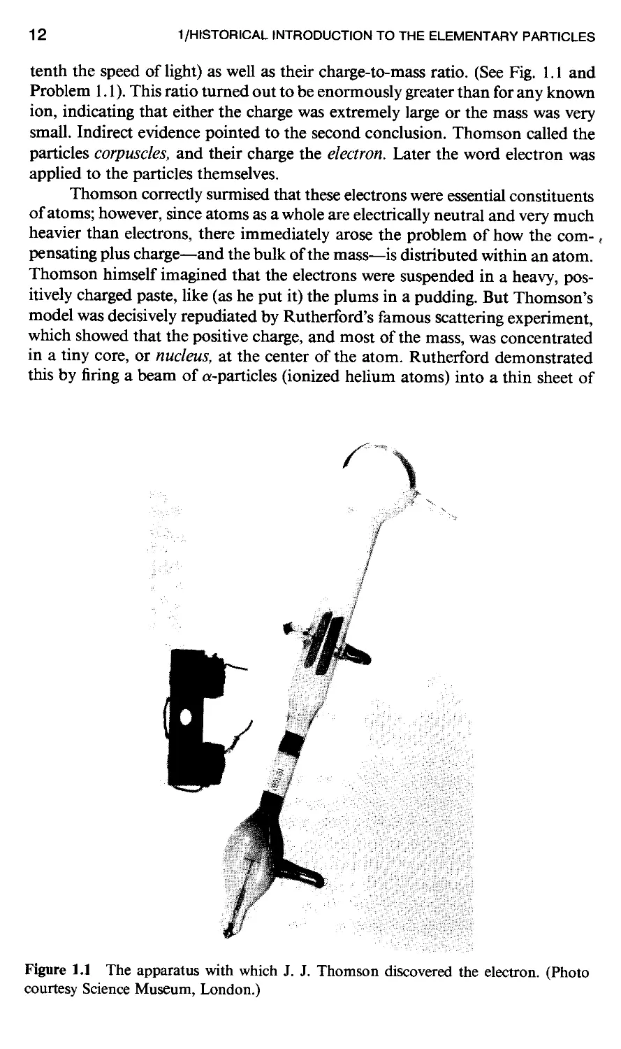
1.1 THE CLASSICAL ERA A897-1932)
It is always a little artificial to pinpoint such things, but I'd say that elementary
particle physics was born in 1897, with J. J. Thomson's discovery of the electron.1
(It is fashionable to carry the story all the way back to Democritus and the Greek
atomists, but apart from a few suggestive words their metaphysical speculations
have nothing in common with modern science, and although they may be of
modest antiquarian interest, their relevance is infinitesimal.) Thomson knew
that cathode rays emitted by a hot filament could be deflected by a magnet. This
suggested that they carried electric charge; in fact, the direction of the curvature
required that the charge be negative. It seemed, therefore, that these were not
rays at all, but rather streams of particles. By passing the beam through crossed
electric and magnetic fields, and adjusting the field strength until the net deflection
was zero, Thomson was able to determine the velocity of the particles (about a
11
12 1/HISTORICAL INTRODUCTION TO THE ELEMENTARY PARTICLES
tenth the speed of light) as well as their charge-to-mass ratio. (See Fig. 1.1 and
Problem 1.1). This ratio turned out to be enormously greater than for any known
ion, indicating that either the charge was extremely large or the mass was very
small. Indirect evidence pointed to the second conclusion. Thomson called the
particles corpuscles, and their charge the electron. Later the word electron was
applied to the particles themselves.
Thomson correctly surmised that these electrons were essential constituents
of atoms; however, since atoms as a whole are electrically neutral and very much
heavier than electrons, there immediately arose the problem of how the com-,
pensating plus charge—and the bulk of the mass—is distributed within an atom.
Thomson himself imagined that the electrons were suspended in a heavy, pos-
positively charged paste, like (as he put it) the plums in a pudding. But Thomson's
model was decisively repudiated by Rutherford's famous scattering experiment,
which showed that the positive charge, and most of the mass, was concentrated
in a tiny core, or nucleus, at the center of the atom. Rutherford demonstrated
this by firing a beam of a-particles (ionized helium atoms) into a thin sheet of
\
Figure 1.1 The apparatus with which J. J. Thomson discovered the electron. (Photo
courtesy Science Museum, London.)
1.1 THE CLASSICAL ERA A897-1932)
13
gold foil (see Fig. 1.2). Had the gold atoms consisted of rather diffuse spheres,
as Thomson supposed, then all of the a-particles should have been deflected a
bit, but none would have been deflected much—any more than a bullet is de-
deflected much when it passes, say, through a bag of sawdust. What in fact occurred
was that most of the a-particles passed through the gold completely undisturbed,
but a few of them bounced off at wild angles. Rutherford's conclusion was that
the a-particles had encountered something very small, very hard, and very heavy.
Evidently the positive charge, and virtually all of the mass, was concentrated at
the center, occupying only a tiny fraction of the volume of the atom (the electrons
are too light to play any role in the sattering; they are knocked right out of the
way by the much heavier a-particles).
The nucleus of the lightest atom (hydrogen) was given the name proton by
Rutherford. In 1914 Niels Bohr proposed a model for hydrogen consisting of a
single electron circling the proton, rather like a planet going around the sun,
held in orbit by the mutual attraction of opposite charges. Using a primitive
version of the quantum theory, Bohr was able to calculate the spectrum of hy-
hydrogen, and the agreement with experiment was nothing short of spectacular. It
was natural then to suppose that the nuclei of heavier atoms were composed of
two or more protons bound together, supporting a like number of orbiting elec-
electrons. Unfortunately, the next heavier atom (helium), although it does indeed
carry two electrons, weighs four times as much as hydrogen, and lithium (three
electrons) is seven times the weight of hydrogen, and so it goes. This dilemma
Zinc sulfide screen Gold foil
Collimated beam
of a-particles
Microscope \
Source of
a-particles
v v
Figure 1.2 Schematic diagram of the apparatus used in the Rutherford scattering ex-
experiment. Alpha particles scattered by the gold foil strike a fluorescent screen, giving off
a flash of light, which is observed visually through a microscope.
14 1 /HISTORICAL INTRODUCTION TO THE ELEMENTARY PARTICLES
was finally resolved in 1932 with Chadwick's discovery of the neutron—an elec-
electrically neutral twin to the proton. The helium nucleus, it turns out, contains
two neutrons in addition to the two protons; lithium evidently includes four;
and in general the heavier nuclei carry very roughly the same number of neutrons
as protons. (The number of.neutrons is in fact somewhat flexible: the same atom,
chemically speaking, may come in several different isotopes, all with the same
number of protons, but with varying numbers of neutrons.)
The discovery of the neutron put the final touch on what we might call
the classical period in elementary particle physics. Never before (and I'm sorry
to say never since) has physics offered so simple and satisfying an answer to the
question, "What is matter made of?" In 1932 it was all just protons, neutrons,
and electrons. But already the seeds were planted for the three great ideas that
were to dominate the middle period A930-1960) in particle physics: Yukawa's
meson, Dirac's positron, and Pauli's neutrino. Before we come to that, however,
I must back up for a moment to introduce the photon.
1.2 THE PHOTON A900-1924)
In some respects the photon is a very "modern" particle, having more in common
with the PFand Z (which were not discovered until 1983) than with the classical
trio. Moreover, it's hard to say exactly when or by whom the photon was really
"discovered," although the essential stages in the process are clear enough. The
first contribution was made by Planck in 1900. Planck was attempting to explain
the so-called blackbody spectrum for the electromagnetic radiation emitted by
a hot object. Statistical mechanics, which had proved brilliantly successful in
explaining other thermal processes, yielded nonsensical results when applied to
electromagnetic fields. In particular, it led to the famous "ultraviolet catastrophe,"
predicting that the total power radiated should be infinite. Planck found that he
could escape the ultraviolet catastrophe—and fit the experimental curve—if he
assumed that electromagnetic radiation is quantized, coming in little "packages"
of energy
E = hv (l.l)
where v is the frequency of the radiation and h is a constant, which Planck
adjusted to fit the data. The modern value of Planck's constant is
h = 6.626 X 10⁷ergs A.2)
Planck did not profess to know why the radiation was quantized; he assumed
that it was due to a peculiarity in the emission process: For some reason a hot
surface only gives off light* in little squirts.
Einstein, in 1905, put forward a far more radical view. He argued that
quantization was a feature of the electromagnetic field itself, having nothing to
* In this book the word light stands for electromagnetic radiation, whether or not it happens
to fall in the visible region.
1.2 THE PHOTON A900-1924) 15
do with the emission mechanism. With this new twist, Einstein adapted Planck's
idea, and his formula, to explain the photoelectric effect: When electromagnetic
radiation strikes a metal surface, electrons come popping out. Einstein suggested
that an incoming light quantum hits an electron in the metal, giving up its energy
(hv)\ the excited electron then breaks through the metal surface, losing in the
process an energy w (the so-called work function of the material—an empirical
constant that depends on the particular metal involved). The electron thus
emerges with an energy
E<hv-w A.3)
(It may lose some energy before reaching the surface. That's the reason for using
<:, instead of =.) Einstein's formula A.3) is pretty trivial to derive, but it carries
an extraordinary implication: The maximum electron energy is independent of
the intensity of the light and depends only on its color (frequency). To be sure,
a more intense beam will knock out more electrons, but their energies will be
the same.
Unlike Planck's theory, Einstein's theory met a hostile reception, and over
the next 20 years he was to wage a lonely battle for the light quantum.2 In saying
that electromagnetic radiation is by its nature quantized, regardless of the emission
mechanism, Einstein came dangerously close to resurrecting the discredited par-
particle theory of light. Newton, of course, had introduced such a corpuscular model,
but a major achievement of nineteenth-century physics was the decisive repu-
repudiation of Newton's idea in favor of the rival wave theory. No one was prepared
to see that accomplishment called into question, even when the experiments
came down on Einstein's side. In 1916 Millikan completed an exhaustive study
of the photoelectric effect and was obliged to report that "Einstein's photoelectric
equation ... appears in every case to predict exactly the observed results. . ..
Yet the semicorpuscular theory by which Einstein arrived at his equation seems
at present wholly untenable.
What finally settled the issue was an experiment conducted by A. H.
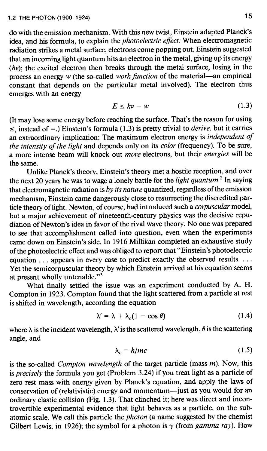
Compton in 1923. Compton found that the light scattered from a particle at rest
is shifted in wavelength, according the equation
X' = X + Xc(l -cos0) A.4)
where X is the incident wavelength, X' is the scattered wavelength, 6 is the scattering
angle, and
\c = hi me A.5)
is the so-called Compton wavelength of the target particle (mass m). Now, this
is precisely the formula you get (Problem 3.24) if you treat light as a particle of
zero rest mass with energy given by Planck's equation, and apply the laws of
conservation of (relativistic) energy and momentum—just as you would for an
ordinary elastic collision (Fig. 1.3). That clinched it; here was direct and incon-
incontrovertible experimental evidence that light behaves as a particle, on the sub-
subatomic scale. We call this particle the photon (a name suggested by the chemist
Gilbert Lewis, in 1926); the symbol for a photon is y (from gamma ray). How
16 1 /HISTORICAL INTRODUCTION TO THE ELEMENTARY PARTICLES
7<V>
' 6
Before After /
Figure 1.3 Compton scattering. A photon of wavelength X scatters off a particle, initially
at rest, of mass m. The scattered photon carries wavelength X' given by equation A.4).
the particle nature of light on this level is to be reconciled with its well-established
wave behavior on the macroscopic scale (exhibited in the phenomena of inter-
interference and diffraction) is a story I'll leave to the quantum texts.
Although the photon initially ./orm/ itself on an unreceptive community
of physicists, it eventually found a natural place in quantum field theory, and
was to offer a whole new perspective on electromagnetic interactions. In classical
electrodynamics, we attribute the electrical repulsion of two electrons, say, to
the electric field surrounding them; each electron contributes to the field, and
each one responds to the field. But in quantum field theory, the electric field is
quantized (in the form of photons), and we may picture the interaction as con-
consisting of a stream of photons passing back and forth between the two charges,
each electron continually emitting them and continually absorbing them. And
the same goes for any noncontact force: where classically we interpret "action
at a distance" as "mediated" by a field, we now say that it is mediated by an
exchange of particles (the quanta of the field). In the case of electrodynamics,
the mediator is the photon; for gravity, it is called the graviton (though a fully
successful quantum theory of gravity has yet to be developed and it may well
be centuries before anyone detects a graviton experimentally).
You will see later on how these ideas are implemented in practice, but for
now I want to dispel one common misapprehension. When I say that every force
is mediated by the exchange of particles, I am not speaking of a merely kinematic
phenomenon. Two ice skaters throwing snowballs back and forth will of course
move apart with the succession of recoils; they "repel one another by exchange
of snowballs," if you like. But that's not what is involved here. For one thing,
this mechanism would have a hard time accounting for an attractive force. You
might think of the mediating particles, rather, as "messengers," and the message
can just as well be "come a little closer" as "go away."
I said earlier that in the "classical" picture ordinary matter is made of
atoms, in which electrons are held in orbit around a nucleus of protons and
neutrons by the electrical attraction of opposite charges. We can now give this
model a more sophisticated formulation by attributing the binding force to the
exchange of photons between the electrons and the protons in the nucleus. How-
However, for the purposes of atomic physics this is overkill, for in this context quan-
quantization of the electromagnetic field produces only minute effects (notably the
1.3 MESONS A934-1947) 17
Lamb shift and the anomalous magnetic moment of the electron). To excellent
approximation we can pretend that the forces are given by Coulomb's law (to-
(together with various magnetic dipole couplings). The point is that in a bound
state enormous numbers of photons are continually streaming back and forth,
so that the "lumpiness" of the field is effectively smoothed out, and classical
electrodynamics is a suitable approximation to the truth. But in most elementary
particle processes, such as the photoelectric effect or Compton scattering, indi-
individual photons are involved, and quantization can no longer be ignored.
1.3 MESONS A934-1947)
Now there is one conspicuous problem to which the "classical" model does not
address itself at all: What holds the nucleus together? After all, the positively
charged protons should repel one another violently, packed together as they are
in such close proximity. Evidently there must be some other force, more powerful
than the fcrce of electrical repulsion, that binds the protons (and neutrons) to-
together; physicists of that less imaginative age called it, simply, the strong force.
But if there exists such a potent force in nature, why don't we notice it in everyday
life? The fact is that virtually every force we experience directly, from the con-
contraction of a muscle to the explosion of dynamite is electromagnetic in origin;
the only exception, outside a nuclear reactor or an atomic bomb, is gravity. The
answer must be that, powerful though it is, the strong force is of very short range.
(The range of a force is like the arm's reach of a boxer—beyond that distance
its influence falls off rapidly to zero. Gravitational and electromagnetic forces
have infinite range, but the range of the strong force is about the size of the
nucleus itself.)*
The first significant theory of the strong force was proposed by Yukawa in
1934. Yukawa assumed that the proton and neutron are attracted to one another
by some sort offield, just as the electron is attracted to the nucleus by an electric
field and the moon to the earth by a gravitational field. This field should properly
be quantized, and Yukawa asked the question: What must be the properties of
its quantum—the particle (analogous to the photon) whose exchange would ac-
account for the known features of the strong force? For example, the short range
of the force indicated that the mediator would be rather heavy; Yukawa calculated
that its mass should be nearly 300 times that of the electron, or about a sixth
the mass of a proton. (See Problem 1.2.) Because it fell between the electron and
the proton, Yukawa's particle came to be known as the meson (meaning "middle-
"middleweight"). [In the same spirit the electron is called a lepton ("light-weight"), whereas
the proton and neutron are baryons ("heavy-weight").] Now, Yukawa knew that
no such particle had ever been observed in the laboratory, and he therefore
assumed his theory was wrong. But at the time a number of systematic studies
* This is a bit of an oversimplification. Typically, the forces go like e'ir/a)/r2, where a is the
"range." For Coulomb's law and Newton's law of universal gravitation, a = oo; for the strong force
a is about 10~13 cm (one fermi).
18 1 /HISTORICAL INTRODUCTION TO THE ELEMENTARY PARTICLES
of cosmic rays were in progress, and by 1937 two separate groups (Anderson
and Neddermeyer on the West Coast, and Street and Stevenson on the East)
had identified particles matching Yukawa's description. Indeed, the cosmic rays
with which you are being bombarded every few seconds as you read this consist
primarily of just such middle-weight particles.
For a while everything seemed to be in order. But as more detailed studies
of the cosmic ray particles were undertaken, disturbing discrepancies began to
appear. They had the wrong lifetime and they seemed to be significantly lighter
than Yukawa had predicted; worse still, different mass measurements were not
consistent with one another. In 1946 (after a period in which physicists were
engaged in a less savory business) decisive experiments were carried out in Rome
demonstrating that the cosmic ray particles interacted very weakly with atomic
nuclei.4 If this was really Yukawa's meson, the transmitter of the strong force,
the interaction should have been dramatic. The puzzle was finally resolved in
1947, when Powell and his co-workers at Bristol5 discovered that there are actually
two middle-weight particles in cosmic rays, which they called tt (or "pion") and
ti (or "muon"). (Marshak reached the same conclusion simultaneously, on theo-
theoretical grounds.6) The true Yukawa meson is the tt; it is produced copiously in
the upper atmosphere, but ordinarily disintegrates long before reaching the
ground. (See Problem 3.4.) Powell's group exposed their photographic emulsions
on mountain tops (see Fig. 1.4). One of the decay products is the lighter (and
longer-lived) fi, and it is primarily muons that one observes at sea level. In the
search for Yukawa's meson, then, the muon was simply an imposter, having
nothing whatever to do with the strong interactions. In fact, it behaves in every
way like a heavier version of the electron and properly belongs in the lepton
family (though some people to this day call it the "mu-meson" by force of habit).
1.4 ANTIPARTICLES A930-1956)
Nonrelativistic quantum mechanics was completed in the astonishingly brief
period 1923-1926, but the relativistic version proved to be a much thornier
problem. The first major achievement was Dirac's discovery, in 1927, of the
equation that bears his name. The Dirac equation was supposed to describe free
electrons with energy given by the relativistic formula E2 — p2c2 = m2c4. But
it had a very troubling feature: For every positive-energy solution (E =
+Vp2c2 + m2c4) it admitted a corresponding solution with negative energy (E =
—Vp2c2 + m2c4). This meant, given the natural tendency of every system to
evolve in the direction of lower energy, that the electron should "runaway" to
increasingly negative states, radiating off an infinite amount of energy in the
process. To rescue his equation, Dirac proposed a resolution that made up in
brilliance for what it lacked in plausibility: He postulated that the negative energy
states are all filled by an infinite "sea" of electrons. Because this sea is always
there, and perfectly uniform, it exerts no net force on anything, and we are not
normally aware of it. Dirac then invoked the Pauli exclusion principle (which
says that no two electrons can occupy the same state), to "explain" why the
1.4 ANTIPARTICLES A930-1956)
By
19
Figure 1.4 One of Powell's earliest pic-
pictures showing the track of a pion in a pho-
photographic emulsion exposed to cosmic
rays at high altitude. The pion (entering
from the left) decays into a muon and a
neutrino (the latter is electrically neutral,
and leaves no track). Reprinted by per-
permission from C. F. Powell, P. H. Fowler,
and D. H. Perkins, The Study of Elemen-
Elementary Particles by the Photographic Method
(New York: Pergamon, 1959). First pub-
published in Nature 159, 694 A947).
electrons we do observe are confined to the positive energy states. But if this is
true, then what happens when we impart to one of the electrons in the "sea" an
energy sufficient to knock it into a positive energy state? The absence of the
20
1/HISTORICAL INTRODUCTION TO THE ELEMENTARY PARTICLES
"expected" electron in the sea would be interpreted as a net positive charge in
that location, and the absence of its expected negative energy would be seen as
a net positive energy. Thus a "hole in the sea" would function as an ordinary
particle with positive energy and positive charge. Dirac at first hoped that these
holes might be protons, but it was soon apparent that they had to carry the same
mass as the electron itself—2000 times too light to be a proton. No such particle
was known at the time, and Dirac's theory appeared to be in trouble. What may
have seemed a fatal defect in 1930, however, turned into a spectacular triumph
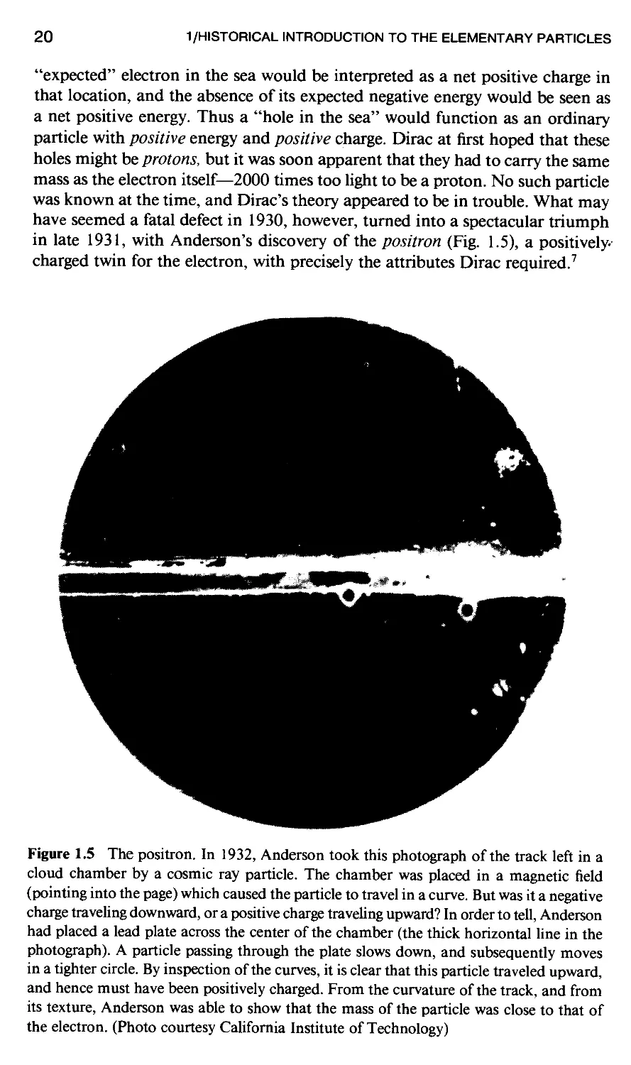
in late 1931, with Anderson's discovery of the positron (Fig. 1.5), a positively-
charged twin for the electron, with precisely the attributes Dirac required.7
Figure 1.5 The positron. In 1932, Anderson took this photograph of the track left in a
cloud chamber by a cosmic ray particle. The chamber was placed in a magnetic field
(pointing into the page) which caused the particle to travel in a curve. But was it a negative
charge traveling downward, or a positive charge traveling upward? In order to tell, Anderson
had placed a lead plate across the center of the chamber (the thick horizontal line in the
photograph). A particle passing through the plate slows down, and subsequently moves
in a tighter circle. By inspection of the curves, it is clear that this particle traveled upward,
and hence must have been positively charged. From the curvature of the track, and from
its texture, Anderson was able to show that the mass of the particle was close to that of
the electron. (Photo courtesy California Institute of Technology)
1.4 ANTIPARTICLES A930-1956) 21
Still, many physicists were uncomfortable with the notion that we are awash
in an infinite sea of invisible electrons, and in the forties Stuckelberg and Feynman
provided a much simpler and more compelling interpretation of the negative-
energy states. In the Feynman-Stuckelberg formulation the negative-energy so-
solutions are reexpressed as positive-energy states of a different particle (the posi-
positron); the electron and positron appear on an equal footing, and there is no need
for Dirac's "electron sea" or for its mysterious "holes." We'll see in Chapter 7
how this—the modern interpretation—works. Meantime, it turned out that the
dualism in Dirac's equation is a profound and universal feature of quantum
field theory: For every kind of particle there must exist a corresponding anti-
particle, with the same mass but opposite electric charge. The positron, then, is
the antielectron. (Actually, it is in principle completely arbitrary which one you
call the "particle" and which the "antiparticle"—I could just as well have said
that the electron is the antipositron. But since there are a lot of electrons around,
and not so many positrons, we tend to think of electrons as "matter" and positrons
as "antimatter"). The (negatively charged) antiproton was first observed exper-
experimentally at the Berkeley Bevatron in 1955, and the (neutral) antineutron was
discovered at the same facility the following year.8
The standard notation for antiparticles is an overbar. For example, p denotes
the proton and p the antiproton; n the neutron and n the antineutron. However,
in some cases it is more customary simply to specify the charge. Thus most
people write e+ for the positron (not e) and n+ for the antimuon (not jit). [But
you must not mix conventions: e+ is ambiguous, like a double negative—the
reader doesn't know if you mean the positron or the a«?/positron, (which is to
say, the electron).] Some neutral particles are their own antiparticles. For example,
the photon: y = y. In fact, you may have been wondering how the antineutron
differs physically from the neutron, since both are uncharged. The answer is that
neutrons carry other "quantum numbers" besides charge (in particular, baryon
number), which change sign for the antiparticle. Moreover, although its net charge
is zero, the neutron does have a charge structure (positive at the center and at
the edges, negative in between) and a magnetic dipole moment. These, too, have
the opposite sign for n.
There is a general principle in particle physics that goes under the name
of crossing symmetry. Suppose that a reaction of the form
A + B-+ C + D
is known to occur. Any of these particles can be "crossed" over to the other side
of the equation, provided it is turned into its antiparticle, and the resulting
interaction will also be allowed. For example,
A -> B + C + D
A + C-> B + D
C + D^A+ B
In addition, the reverse reaction occurs C + D —> A + B, but technically this
derives from the principle of detailed balance, rather than from crossing sym-
symmetry. Indeed, as we shall see, the calculations involved in these various reactions
22 1 /HISTORICAL INTRODUCTION TO THE ELEMENTARY PARTICLES
are practically identical. We might almost regard them as different manifestations
of the same fundamental process. Now, there is one important caveat in this:
Conservation of energy may veto a reaction that is otherwise permissible.
For example, if A weighs less than the sum of B, C, and D, then the decay
A —> B + C + D cannot occur; similarly, if A and C are light, whereas B and D
are heavy, then the reaction A + C—> B + D will not take place unless the initial
kinetic energy exceeds a certain "threshold" value. So perhaps I should say that
the crossed (or reversed) reaction is dynamically permissible, but it may or may
not be kinematically allowed. The power and beauty of crossing symmetry can ,
scarcely be exaggerated. It tells us, for instance, that Compton scattering
y + e~ —> y + e~
is "really" the same process as pair annihilation
e~ + e+ —> y + y
although in the laboratory they are completely different phenomena.
The union of special relativity and quantum mechanics, then, leads to a
pleasing matter/antimatter symmetry. But this raises a disturbing question: How
come our world is populated with protons, neutrons, and electrons, instead of
antiprotons, antineutrons, and positrons? Matter and antimatter cannot coexist
for long—if a particle meets its antiparticle, they annihilate. So maybe it's just
a historical accident that in our corner of the universe there happened to be
more matter than antimatter, and pair annihilation has eliminated all but a
leftover residue of matter. If this is so, then presumably there are other regions
of space in which antimatter predominates. Unfortunately, the astronomical
evidence is pretty compelling that all of the observable universe is made of or-
ordinary matter. Recently, Wilczek and others have put forward a possible expla-
explanation for this cosmic asymmetry. I shall not go into it here, but if you are
interested, I recommend Wilczek's article in Scientific American (December
1980).
1.5 NEUTRINOS A930-1962)
For the third strand in the story we return again to the year 1930.9 A problem
had arisen in the study of nuclear beta decay. In beta decay a radioactive nucleus
A is transformed into a slightly lighter nucleus B, with the emission of an electron:
A->B + e~ A.6)
Conservation of charge requires that B carry one more unit of positive charge
than A. [We now realize that the underlying process here is the conversion of a
neutron (in A) into a proton (in B), but remember that in 1930 the neutron had
not yet been discovered.] Thus the "daughter" nucleus (B) lies one position
farther along on the Periodic Table. There are many examples of beta decay:
Potassium goes to calcium (fpK —> 2oCa), copper goes to zinc B9CU —> foZn),
tritium goes to helium (?H —> ^He), and so on. [The upper number is the atomic
1.5 NEUTRINOS A930-1962)
23
1000
500
8
¦s
10
15
20
Electron kinetic energy in KeV
Figure 1.6 The beta decay spectrum of tritium (?H —» iHe). (Source: G. M. Lewis,
Neutrinos (London: Wykeham, 1970), p. 30.)
weight (the number of neutrons plus protons) and the lower number is the atomic
number (the number of protons).]
Now, it is a characteristic of two-body decays such as expression A.6) that
the outgoing energies are kinematically determined, in the center-of-mass frame.
Specifically, if the "parent" nucleus (A) is at rest, so that B and e come out back-
to-back with equal and opposite momenta, then conservation of energy dictates
that the electron energy is
,= l
m\ -m2B
m2e
2mA
A.7)
The derivation of this result will be explained in Chapter 3; for now, the point
to notice is that E is fixed, once the three masses are specified. But when the
experiments are done it is found that the emitted electrons vary considerably in
energy. Equation A.7) only determines the maximum electron energy, for a
particular beta-decay process (see Fig. 1.6).
This was a most disturbing result. Niels Bohr (not for the first time) was
ready to abandon the law of conservation of energy.* Fortunately, Pauli took a
more sober view, suggesting that another particle was emitted along with the
electron, a silent accomplice that carries off the "missing" energy. It had to be
electrically neutral, to conserve charge (and also, of course, to explain why it left
no track); Pauli proposed to call it the neutron. The whole idea was greeted with
some skepticism, and in 1932 Chadwick preempted the name. But in the fol-
following year Fermi presented a theory of beta decay that incorporated Pauli's
* It is interesting to note that Bohr was an outspoken critic of Einstein's light quantum (prior
to 1924), that he discouraged Dirac's work on the relativistic electron theory (telling him, incorrectly,
that Klein and Gordon had already succeeded), that he opposed Pauli's introduction of the neutrino,
that he ridiculed Yukawa's theory of the meson, and that he disparaged Feynman's approach to
quantum electrodynamics.
24 1/HISTORICAL INTRODUCTION TO THE ELEMENTARY PARTICLES
particle and proved so brilliantly successful that Pauli's suggestion had to be
taken seriously. From the fact that the observed electron energies range up to
the value given in equation A.7) it follows that the new particle is extremely
light; as far as we know, its mass is in fact zero. Fermi called it the neutrino. (For
reasons you'll see in a moment, we now call it the antineutrino.) In modern
terminology, then, the fundamental beta-decay process is
n^p+ + e~ + v A.8)
(neutron goes to proton plus electron plus antineutrino). ,
Now, you may have noticed something peculiar about Powell's picture of
the disintegrating pion (Fig. 1.4): The muon emerges at about 90° with respect
to the original pion direction. (That's not the result of a collision, by the way;
collisions with atoms in the emulsion account for the dither in the tracks, but
they cannot produce an abrupt left turn.) What that kink indicates is that some
other particle was produced in the decay of the pion, a particle that left no
footprints in the emulsion, and hence must have been electrically neutral. It was
natural (or at any rate economical) to suppose that this was again Pauli's neutrino:
ir^H + v A.9)
A few months after their first paper, Powell's group published an even more
striking picture, in which the subsequent decay of the muon is also visible
(Fig. 1.7). Now, muon decays had been studied for many years, and it was
well established that the charged secondary is an electron. From the figure
there is clearly a neutral product as well, and you might guess that it is again a
neutrino. However, this time it is two neutrinos:
fi^e + 2v A.10)
How do we know there are two of them? Same way as before: We repeat the
experiment over and over, each time measuring the energy of the electron. If it
always comes out the same, we know there are just two particles in the final
state. But if it varies, then there must be (at least) three. By 1949* it was clear
that the electron energy in muon decay is not fixed, and the emission of two
neutrinos was the accepted explanation. By contrast, the muon energy in pion
decay is perfectly constant, within experimental uncertainties, confirming that
this is a genuine two-body decay.
By 1950, then, there was compelling theoretical evidence for the existence
of neutrinos, but there was still no direct experimental verification. A skeptic
might have argued that the neutrino was nothing but a bookkeeping device—a
purely hypothetical particle whose only function was to rescue the conservation
laws. It left no tracks, it didn't decay; in fact, no one had ever seen a neutrino
do anything. The reason for this is that neutrinos interact extraordinarily weakly
* Here, and in the original beta-decay problem, conservation of angular momentum
also requires a third outgoing particle, quite independently of energy conservation. But the spin assign-
assignments were not so clear in the early days, and for most people energy conservation was the
compelling argument. In the interests of simplicity, I will keep angular momentum out of the story
until Chapter 4.
Figure 1.7 Here, a pion decays into a
muon (plus a neutrino); the muon sub-
subsequently decays into an electron (and two
neutrinos). Reprinted by permission from
C. F. Powell, P. H. Fowler, and D. H. Per-
Perkins, The Study of Elementary Particles
by the Photographic Method (New York:
Pergamon, 1959). First published in Na-
Nature 163, 82 A949).
25
26 1/HISTORICAL INTRODUCTION TO THE ELEMENTARY PARTICLES
with matter; a neutrino of moderate energy could easily penetrate a thousand
light-years(I) of lead.* To have a chance of detecting one you need an extremely
intense source. The decisive experiments were conducted at the Savannah River
nuclear reactor in South Carolina, in the mid-fifties. Here Cowan and Reines
set up a large tank of water and watched for the "inverse" beta-decay reaction
^n + e+ A.11)
At their detector the antineutrino flux was calculated to be 5 X 10'3 particles
per square centimeter per second, but even at this fantastic intensity they could
only hope for two or three events every hour. On the other hand, they developed
an ingenious method for identifying the outgoing positron. Their results provided
unambiguous confirmation of the neutrino's existence.10
As I mentioned earlier, the particle produced in ordinary beta decay is
actually an antineutrino, not a neutrino. Of course, since they're electrically
neutral, you might ask—and many people did—whether there is any distinction
between a neutrino and an antineutrino. The neutral pion, as we shall see, is its
own antiparticle; so too is the photon. On the hand, the antineutron is definitely
not the same as a neutron. So we're left in a bit of a quandary: Is the neutrino
the same as the antineutrino, and if not, what property distinguishes them? In
the late fifties, Davis and Harmer put this question to an experimental test."
From the positive results of Cowan and Reines, we know that the crossed reaction
v + n^p+ + e~ A.12)
must also occur, and at about the same rate. Davis looked for the analogous
reaction using awr/neutrinos:
v + n^p+ + e~ A.13)
He found that this reaction does not occur, and thus established that the neutrino
and antineutrino are distinct particles.
Davis's result was not unexpected. In fact, back in 1953 Konopinski and
Mahmoud12 had introduced a beautifully simple rule for determining which
reactions [such as A.12)] will work, and which [like A.13)] will not. In effect,f
they assigned a lepton number L = +1 to the electron, the muon, and the neutrino,
and L = — 1 to the positron, the positive muon, and the antineutrino (all other
particles are given a lepton number of zero). They then proposed the law of
conservation of lepton number (analogous to the law of conservation of charge):
In any physical process, the sum of the lepton numbers before must equal the
sum of the lepton numbers after. Thus the Cowan-Reines reaction A.11) is
allowed (L = -1 before and after), but the Davis reaction A.13) is forbidden
(on the left L = -1, on the right L = +1). [It was in anticipation of this rule
that I called the beta-decay particle, in expression A.8), an antineutrino.] In
* That's a comforting realization when you learn that hundreds of billions of neutrinos pass
through every square inch of your body per second, night and day, coming from the sun (they hit
you from below, at night, having passed right through the earth).
t Konopinski and Mahmoud (ref. 12) did not use this terminology, and they got the muon
assignments wrong. But never mind, the essential idea was there.
1.5 NEUTRINOS A930-1962) 27
view of the conservation of lepton number, the charged pion decays A.9) should
actually be written
\-\l* A.14)
and the muon decays A.10) are really
p.+ —> e+ + v + v
What property distinguishes the neutrino from the antineutrino, then? The
cleanest answer is: lepton number—it's +1 for the neutrino and -1 for the an-
antineutrino. These numbers are experimentally determinable, just as electric charge
is, by watching how the particle in question interacts with others. (As we shall
see, they also differ in their helicity: the neutrino is "left-handed" whereas
the antineutrino is "right-handed." But this is a technical matter best saved
for later.)
There is a final twist to the neutrino story. Experimentally, the decay of a
muon into an electron plus a photon is never observed:
fi'^e' + y A.16)
and yet this process is consistent with conservation of charge and conservation
of the lepton number. Now, there's a very reliable rule of thumb in particle
physics (generally attributed to Richard Feynman) which says that whatever is
not expressly forbidden is mandatory. The absence of fi —> e + y suggests a law
of conservation of "mu-ness"; but then how are we to explain the observed
decays \i —> e + v + v7 The answer occurred to a number of people in the late
fifties and early sixties:13 Suppose there are two different kinds of neutrino—one
associated with the electron (ve) and one with the muon (i>J. If we assign a muon
number L^ = +1 to n~ and !»„, and L^ = -1 to ji+ and !>„, and at the same time
an electron number Le = +1 to e~~ and ve, and Le = — 1 to e+ and ve, and refine
the conservation of lepton number into two separate laws—conservation of elec-
electron number and conservation of muon number—we can then account for all
the allowed and forbidden processes. Neutron beta decay becomes
n^p+ + e~ + ve A.17)
the pion decays are
and the muon decays take the form
i+Zl+VvlVvl (L19)
I said earlier that when pion decay was first analyzed it was "natural" and "eco-
"economical" to assume that the outgoing neutral particle was the same as in beta
28 1 /HISTORICAL INTRODUCTION TO THE ELEMENTARY PARTICLES
decay, and that's quite true: It was natural, and it was economical, but it was
wrong.
The first experimental test of the two-neutrino hypothesis (and the separate
conservation of electron and muon number) was conducted at Brookhaven in
1962.14 Using about 10'4 antineutrinos from ir" decay, Lederman, Schwartz,
Steinberger, and their collaborators identified 29 instances of the expected reaction
vll + p+^fi+ + n A.20)
and no cases of the forbidden process
vll + p+-^e+ + n A.21)
With only one kind of neutrino the second reaction would be just as common
as the first. (Incidentally, this experiment presented truly monumental shielding
problems. Steel from a dismantled warship was stacked up 44 feet thick, to make
sure that nothing except neutrinos got through to the target.)
By 1962, then, the lepton family had grown to eight: the electron, the
muon, their respective neutrinos, and the corresponding antiparticles (Table
1.1). The leptons are characterized by the fact that they do not participate in
strong interactions. For the next 14 years things were pretty quiet, as far as the
leptons go, so this is a good place to pause and let the strongly interacting par-
particles—the mesons and baryons, known collectively as the hadrons—catch up.
1.6 STRANGE PARTICLES A947-1960)
For a brief period in 1947 it was possible to believe that the major problems of
elementary particle physics were solved. After a lengthy detour in pursuit of the
muon, Yukawa's meson (the ir) had finally been apprehended. Dirac's positron
had been found, and Pauli's neutrino, although still at large (and, as we have
TABLE 1.1 THE LEPTON FAMILY, 1962-1976
Leptons
e~
"e
M~
Antileptons
e+
Ve
Lepton
number
1
1
1
1
-1
-1
-1
-1
Electron
number
1
1
0
0
-1
-1
0
0
Muon
number
0
0
1
1
0
0
-1
-1
1.6 STRANGE PARTICLES A947-1960) 29
seen, still capable of making mischief), was basically under control. The role of
the muon was something of a puzzle ("Who ordered that?" Rabi asked); it
seemed quite unnecessary in the overall scheme of things. On the whole, however,
it looked in 1947 as though the job of elementary particle physics was essentially
done.
But this comfortable state did not last long. In December of that year
Rochester and Butler15 published the cloud chamber photograph shown in Figure
1.8. Cosmic ray particles enter from the upper left and strike a lead plate, pro-
producing a neutral particle, whose presence is revealed when it decays into two
charged secondaries, forming the upside-down "V" in the lower right. Detailed
analysis shows that these charged particles are in fact a ir+ and a ir". Here, then,
was a new neutral particle with at least twice the mass of the pion; we call it the
K° ("kaon"):
K°^ir+ + ir- A.22)
In 1949, Powell published the photograph reproduced in Figure 1.9, showing
the decay of a charged kaon:
K+ -»ir+ + ir+ + T~ A.23)
(The K° was first known as the V° and later as the 0°; the K+ was originally
called the t+. Their identification as neutral and charged versions of the same
basic particle was not completely settled until 1956—but that's another story,
to which we shall return in Chapter 4.) The kaons behave in some respects like
heavy pions, and so the meson family was extended to include them. In due
course, many more mesons were discovered—the 77, the </>, the u>, the p's, and
so on.
Meanwhile, in 1950 another neutral "F" particle was found, this time by
Anderson's group at Cal Tech. The photographs were similar to Rochester's (Fig.
1.8), but this time the products were a p+ and a tt~. Evidently this particle is
substantially heavier than the proton; we call it the A:
A^p+ + ir~ A.24)
The lambda belongs with the proton and the neutron in the baryon family. To
appreciate this, we must go back for a moment to 1938. The question had arisen,
"Why is the proton stable?" Why, for example, doesn't it decay into a positron
and a photon:
p+^e+ + y A.25)
Needless to say, it would be unpleasant for us if this reaction were common (all
atoms would disintegrate), and yet it does not violate any law known in 1938.
(Actually, this particular process does violate conservation of lepton number,
but that law was not recognized, remember, until 1953.) Stiickelberg16 proposed
to account for the stability of the proton by asserting a law of conservation of
baryon number: Assign to all baryons (which in 1938 meant the proton and the
neutron) a "baryon number" A = +1, and to the antibaryons (p and n)
30
1/HISTORICAL INTRODUCTION TO THE ELEMENTARY PARTICLES
Incident cosmic ray
shower
3 cm
of'lead
"Unusual
fork"
Debris
Figure 1.8 The first strange particle. Cosmic rays strike a lead plate, producing a K°,
which subsequently decays into a pair of charged pions. (Photo courtesy of Prof. G. D.
Rochester. Reprinted by permission from Nature 160, 855. Copyright © 1947, Macmillan
Journals Limited.)
A = -1; then the total baryon number is conserved in any physical process.
Thus, neutron beta decay (n -> p+ + e~ + ve) is allowed (A = 1 before and after),
and so also is the reaction in which the antiproton was first observed:
1.6 STRANGE PARTICLES A947-1960)
31
Figure 1.9 K+, entering from above, decays at A: K+ —> ir+ + ir+ + w . (The w subse-
subsequently causes a nuclear disintegration at B). [Reprinted by permission from C. F. Powell,
P. H. Fowler, and D. H. Perkins, The Study of Elementary Panicles by the Photographic
Method (New York: Pergamon, 1959). First published in Rep. Prog. Phys. 13, 384 A950).]
p-*P+P+P
A.26)
(A = 2 on both sides). But the proton, as the lightest baryon, has nowhere to
go; conservation of the baryon number guarantees its absolute stability.* If we
are to retain the conservation of baryon number in the light of reaction A.24),
the lambda must be assigned to the baryon family. Over the next few years
many more heavy baryons were discovered—the S's, the S's, and the A's, and
so on. [By the way: unlike leptons and baryons, there is no conservation of
mesons. In pion decay (?r~ —> \f + i»J a meson disappears, and in lambda
decay (A —> p+ + ir") a meson is created.]
* Recent "grand unified" theories allow for a minute violation of baryon number conservation,
and in these theories the proton is not absolutely stable. See the article by S. Weinberg in Scienlific
American, June 1981. The experimental situation is discussed by J. M. LoSecco et ai, Scientific
American, June 1985.
32 1/HISTORICAL INTRODUCTION TO THE ELEMENTARY PARTICLES
It is some measure of the surprise with which these new heavy baryons
and mesons were greeted that they came to be known collectively as "strange"
particles. In 1952 the first of the modern particle accelerators (the Brookhaven
Cosmotron) began operating, and soon it was possible to produce strange particles
in the laboratory (before this the only source had been cosmic rays).. . and with
this, the rate of proliferation increased. Willis Lamb began his Nobel Prize ac-
acceptance speech in 1955 with the words
When the Nobel Prizes were first awarded in 1901, physicists knew something of
just two objects which are now called "elementary particles": the electron and the
proton. A deluge of other "elementary" particles appeared after 1930; neutron,
neutrino, \x. meson, ir meson, heavier mesons, and various hyperons. I have heard
it said that "the finder of a new elementary particle used to be rewarded by a Nobel
Prize, but such a discovery now ought to be punished by a $10,000 fine". [Source:
Les Prix Nobel 1955, The Nobel Foundation, Stockholm.]
Not only were the new particles unexpected; there is a more technical sense
in which they seemed "strange": They are produced copiously (on a time scale
of about 10~23 sec), but they decay relatively slowly (typically about 10~10 sec).
This suggested to Pais17 and others that the mechanism involved in their pro-
production is entirely different from that which governs their disintegration. In
modern language, the strange particles are produced'by the strong force (the same
one that holds the nucleus together), but they decay by the weak force (the one
that accounts for beta decay and all other neutrino processes). The details of
Pais's scheme required that the strange particles be produced in pairs. The ex-
experimental evidence for this was far from clear at that time, but in 1953 Gell-
Mann18 and Nishijima19 found a beautifully simple, and, as it developed stun-
stunningly successful, way to implement and improve Pais's idea. They assigned to
each particle a new property (Gell-Mann called it "strangeness") that (like charge,
lepton number, and baryon number) is conserved in any strong interaction, but
(««like those others) is not conserved in a weak interaction. In a pion-proton
collision, for example, we might produce two strange particles:
ir" + p+ -» K+ + 2"
-»K° + 2°
-^K° + A A.27)
Here the K's carry strangeness S = +1, the 2's and the A have S = — 1, and the
"ordinary" particles—ir, p, and n—have 5 = 0. But we never produce just one
strange particle:
r~ + p+ -A tt+ + 2~
y*K° + n A.28)
On the other hand, when these particles decay, strangeness is not conserved:
A -» p+ + ir"
-^n + w+ A.29)
for these are weak processes, which do not respect conservation of strangeness.
1.7 THE EIGHTFOLD WAY A961-1964)
33
There is some arbitrariness in the assignment of strangeness numbers,
obviously. We could just as well have given S = +1 to the S's and the A, and
S = — 1 to K+ and K°; in fact, in retrospect it would have been a little nicer that
way. [In exactly the same sense, Benjamin Franklin's original convention for
plus and minus charge was perfectly arbitrary at the time, and unfortunate in
retrospect since it made the current-carrying particle (the electron) negative.]
The significant point is that there exists a consistent assignment of strangeness
numbers to all the hadrons (baryons and mesons) that accounts for the observed
strong processes and "explains" why the others do not occur. (The leptons and
the photon don't experience strong forces at all, so strangeness does not apply
to them.)
The garden which seemed so tidy in 1947 had grown into a jungle by 1960,
and hadron physics could only be described as chaos. The plethora of strongly
interacting particles was divided into two great families—the baryons and the
mesons—and the members of each family were distinguished by charge, strange-
strangeness, and mass; but beyond that there was no rhyme or reason to it all. This
predicament reminded many physicists of the situation in chemistry a century
earlier, in the days before the Periodic Table, when scores of elements had been
identified, but there was no underlying order or system. In 1960 the elementary
particles awaited their own "Periodic Table.0
1.7 THE EIGHTFOLD WAY A961-1964)
The Mendeleev of elementary particle physics was Murray Gell-Mann, who
introduced the so-called Eightfold Way in 1961.21 (Essentially the same scheme
was proposed independently by Ne'eman.) The Eightfold Way arranged the
baryons and mesons into weird geometrical patterns, according to their charge
and strangeness. The eight lightest baryons fit into a hexagonal array, with two
particles at the center:
The Baryon Octet
This group is known as the baryon octet. Notice that particles of like charge lie
along the downward-sloping diagonal lines: Q = +1 (in units of the proton
34
1/HISTORICAL INTRODUCTION TO THE ELEMENTARY PARTICLES
charge) for the proton and the S+; Q = 0 for the neutron, the lambda, the 2°,
and the H°; Q = -1 for the 2" and the H". Horizontal lines associate particles
of like strangeness: S = 0 for the proton and neutron, S = — 1 for the middle
line and S = — 2 for the two H's.
The eight lightest mesons fill a similar hexagonal pattern, forming the
(pseudo-scalar) meson octet:
K° K*
The Meson Octet
Once again, diagonal lines determine charge, and horizontals determine strange-
strangeness; but this time the top line has 5=1, the middle line 5 = 0, and the bottom
line S = — 1. (This discrepancy is a historical accident; Gell-Mann could just as
well have assigned S = 1 to the proton and neutron, S = 0 to the S's and the
A, and 5 = -1 to the H's. In 1953 he had no reason to prefer that choice, and
it seemed most natural to give the familiar particles—proton, neutron, and pion—
a strangeness of zero. After 1961 a new term—hypercharge—was introduced,
which was equal to S for the mesons and to S + 1 for the baryons. But later
developments showed that strangeness was the better quantity after all, and the
word "hypercharge" has now been taken over for a quite different purpose.)
Hexagons were not the only figures allowed by the Eightfold Way; there
was also, for example, a triangular array, incorporating 10 heavier baryons—
the baryon decuplet:
C — 1 _
The Baryon Decuplet
\
\
Q = -1
co
01
Figure 1.10 The discovery of the fl . The actual bubble chamber photograph is shown
on the left; a line diagram of the relevant tracks on the right. (Photo courtesy Brookhaven
National Laboratory.)
36
1/HISTORICAL INTRODUCTION TO THE ELEMENTARY PARTICLES
Sn) K* K°
K~ K°
K— K*
Figure 1.11 Established meson nonets. Obviously, we are running out of letters. It is
customary to distinguish different particles represented by the same letter by indicating
the mass parenthetically (in MeV/c2), thus K*{%92), AT*A430), AT*A650), and so on. In
this figure the supermultiplets are labeled in spectroscopic notation (see Chap. 5). At
present, there are no complete baryon supermultiplets beyond the octet and decuplet,
although there are many partially filled diagrams.
Now, as Gell-Mann was fitting these particles into the decuplet, an absolutely
lovely thing happened. Nine of the particles were known experimentally, but at
that time the tenth particle—the one at the very bottom, with a charge of -1
and strangeness —3—was missing: No particle with these properties had ever
been detected in the laboratory.22 Gell-Mann boldly predicted that such a particle
would be found, and told the experimentalists exactly how to produce it. More-
Moreover, he calculated its mass—as you can for yourself, in Problem 1.6—and its
lifetime, Problem 1.8—and sure enough, in 1964 the famous omega-minus par-
particle was discovered,23 precisely as Gell-Mann had predicted (see Fig. 1.10).
Since the discovery of the omega-minus (Q~), no one has seriously doubted
that the Eightfold Way is correct.* Over the next 10 years, every new hadron
found a place in one of the Eightfold Way supermultiplets. Some of these are
shown in Figure 1.11. (This is not to say there were no false alarms; particles
have a way of appearing and then ^appearing. Of the 26 mesons listed on a
standard table in 1963, 19 were later found to be spurious!) In addition to the
baryon octet, decuplet, and so on, there exist of course an antibaryon octet,
decuplet, etc., with opposite charge and opposite strangeness. However, in the
case of the mesons, the antiparticles lie in the same supermultiplet as the cor-
corresponding particles, in the diametrically opposite positions. Thus the antiparticle
* A similar thing happened in the case of the Periodic Table. There were three famous "holes"
(missing elements) on Mendeleev's chart, and he predicted that new elements would be discovered
to fill in the gaps. Like Gell-Mann, he confidently described their properties, and within 20 years all
three—gallium, scandium, and germanium—were found.
1.8 THE QUARK MODEL A964) 37
of the pi-plus is the pi-minus, the anti-A^-minus is the A^-plus, and so on (the pi-
zero and the eta are their own antiparticles).
Classification is the first stage in the development of any science. The
Eightfold Way did more than merely classify the hadrons, but its real importance
lies in the organizational structure it provided. I think it's fair to say that the
Eightfold Way initiated the modern era in particle physics.
1.8 THE QUARK MODEL A964)
But the very success of the Eightfold Way begs the question: Why do the hadrons
fit into these curious patterns? The Periodic Table had to wait many years for
quantum mechanics and the Pauli exclusion principle to provide its explanation.
An understanding of the Eightfold Way, however, came already in 1964, when
Gell-Mann and Zweig independently proposed that all hadrons are in fact com-
composed of even more elementary constituents, which Gell-Mann called quarks.24
The quarks come in three types (or "flavors"), forming a triangular "Eightfold-
Way" pattern:
d--
2 The Quarks
1
The u (for "up") quark carries a charge of § and a strangeness of zero; the d
("down") quark carries a charge of — 5 and 5 = 0; the s (originally "sideways",
but now more commonly "strange") quark has Q = — 5 and S = — 1. To each
quark (q) there corresponds an antiquark (q), with the opposite charge and
strangeness:
The Antiquarks
s-0-
38 1/HISTORICAL INTRODUCTION TO THE ELEMENTARY PARTICLES
The quark model asserts that
1. Every baryon is composed of three quarks (and every antibaryon is
composed of three antiquarks).
2. Every meson is composed of a quark and an antiquark.
With these two rules it is a matter of elementary arithmetic to construct
the baryon decuplet and the meson octet. All we need to do is list the combi-
combinations of three quarks (or quark-antiquark pairs), and add up their charge and
strangeness:
THE BARYON DECUPLET
999
uuu
uud
udd
ddd
uus
uds
dds
uss
dss
sss
0
2
1
0
-1
1
0
-1
0
-1
-1
s
0
0
0
0
-1
-1
-1
-y
-2
-3
Baryon
A++
A+
A0
A"
2*+
2*°
2*~
3*°
3*~
Notice that there are 10 combinations of three quarks. Three m's, for instance,
at Q = § each, yield a total charge of +2, and a strangeness of zero. This is the
A++ particle. Continuing down the table, we find all the members of the decuplet
ending with the Or, which is evidently made of three s quarks.
A similar enumeration of the quark-antiquark combinations yields the
meson table:
THE
99
uu
ud
du
dd
us
ds
su
sd
ss
MESON NONET
0
0
1
-1
0
1
0
-1
0
0
s
0
0
0
0
1
1
-1
-1
0
Meson
x°
7T+
7T~
V
K+
K°
K~
K°
V.
But wait! There are nine combinations here, and only eight particles in the
meson octet. The quark model requires that there be a third meson (in addition
1.8 THE QUARK MODEL A964) 39
to the tt° and the v) with Q = 0 and S = 0. As it turns out, just such a particle
had already been found experimentally—the ri'. In the Eightfold Way the rl had
been classified as a singlet, all by itself. According to the quark model it properly
belongs with the other eight mesons to form a meson nonet. (Actually, since uu,
dd, and ss all have Q = 0 and S = 0, it is not possible to say, on the basis of
anything we have done so far, which is the tt°, which the rj, and which the r\.
But never mind, the point is that there are three mesons with Q = S = 0.) By
the way, the a«?zmesons automatically fall in the same supermultiplet as the
mesons: ud is the antiparticle of du, and vice versa.
You may have noticed that I avoided talking about the baryon octet—and
it is far from obvious how we are going to get eight baryons by putting together
three quarks. In truth, the procedure is perfectly straightforward, but it does call
for some facility in handling spins, and I would rather save it until Chapter 5.
For now, I'll just tantalize you with the mysterious observation that if you take
the decuplet and knock off the three corners (where the quarks are identical—
uuu, ddd, and sss), and double the center (where all three are different—uds),
you obtain precisely the eight states in the baryon octet. So the same set of quarks
can account for the octet; it's just that some combinations do not appear at all,
and one appears twice.
Indeed, all the Eightfold Way supermultiplets emerge in a natural way
from the quark model. Of course, the same combination of quarks can go to
make a number of different particles: The delta-plus and the proton are both
composed of two «'s and a d; the pi-plus and the rho-plus are both ud; and so
on. Just as the hydrogen atom (electron plus proton) has many different energy
levels, so a given collection of quarks can bind together in many different ways.
But whereas the various energy levels in the electron/proton system are relatively
close together (the spacings are typically several electron volts, in an atom whose
rest energy is nearly 109 electron volts), so that we naturally think of them all
as "hydrogen," the energy spacings for different states of a bound quark system
are very large, and we normally regard them as distinct particles. Thus we can,
in principle, construct an infinite number of hadrons out of only three quarks.
Notice, however, that some things are absolutely excluded in the quark model:
For example, a baryon with 5 = 0 and Q = -2; no combination of the three
quarks can produce these numbers. Nor can there be a meson with a charge of
+2 (like the A++ baryon) or a strangeness of —3 (like the Q~). For a long time
there were major experimental searches for these so-called "exotic" particles;
their discovery would be devastating for the quark model, but none has ever
been found (see Problem 1.11).
The quark model does, however, suffer from one profound embarrassment:
In spite of the most diligent search over a period of 20 years, no one has ever
seen an individual quark. Now, if a proton is really made out of three quarks,
you'd think that if you hit one hard enough, the quarks ought to come popping
out. Nor would they be hard to recognize, carrying as they do the conspicuous
label of fractional charge; an ordinary Millikan oil drop experiment would clinch
the identification. Moreover, at least one of the quarks should be absolutely
40
1/HISTORICAL INTRODUCTION TO THE ELEMENTARY PARTICLES
stable; what could it decay into, since there is no lighter particle with fractional
charge? So quarks ought to be easy to produce, easy to identify, and easy to
store, and yet, no one has ever found one.
The failure of experiments to produce isolated quarks occasioned wide-
widespread skepticism about the quark model in the late sixties and early seventies.
Those who clung to the model tried to conceal their disappointment by intro-
introducing the notion of quark confinement: perhaps, for reasons not yet understood,
quarks are absolutely confined within baryons and mesons, so that no matter
how hard you try, you cannot get them out. Of course, this doesn't explain
anything, it just gives a name to our frustration. But at least it poses sharply
what has become a crucial theoretical problem for the eighties: to discover the
mechanism responsible for quark confinement. There are some indications that
the solution may be at hand.25
Even if all quarks are stuck inside hadrons, this does not mean they are
inaccessible to experimental study. One can probe the inside of a proton in much
the same way as Rutherford probed the inside of an atom—by firing something
into it. Such experiments were carried out in the late sixties using high-energy
electrons at the Stanford Linear Accelerator Center (SLAC). They were repeated
in the early seventies using neutrino beams at CERN, and later still using protons.
The results of these so-called "deep inelastic scattering" experiments were strik-
strikingly reminiscent of Rutherford's (Fig. 1.12): Most of the incident particles pass
right through, whereas a small number bounce back sharply. This means that
the charge of the proton is concentrated in small lumps, just as Rutherford's
results indicated that the positive charge in an atom is concentrated at the nu-
nucleus.26 However, in the case of the proton the evidence suggests three lumps,
*\ (a)
• Atom has
substructure
\
\ # •
\
I l\ I
^
- ^
- \
>
—
1
(b)
Proton has
substructure
\ ^
It
\ *
i V I I
Scattering angle
Figure 1.12 (a) In Rutherford scattering the number of particles deflected through large
angles indicates that the atom has internal structure (a nucleus), (b) In deep inelastic
scattering the number of particles deflected through large angles indicates that the proton
has internal structure (quarks). The dashed lines show what you would expect if the
positive charge were uniformly distributed over the volume of (a) the atom, (b) the proton.
[Source: F. Halzen and A. D. Martin, Quarks and Leptons (New York: Wiley, 1984), p.
17. Copyright © John Wiley & Sons, Inc. Reprinted by permission.]
1.9 THE NOVEMBER REVOLUTION AND ITS AFTERMATH A974-1983) 41
instead of one. This is strong support for the quark model, obviously, but still
not conclusive.
Finally, there was a theoretical objection to the quark model: It appears
to violate the Pauli exclusion principle. In Pauli's original formulation the ex-
exclusion principle stated that no two electrons can occupy the same state. However,
it was later realized that the same rule applies to all particles of half-integer spin
(the proof of this is one of the most important achievements of quantum field
theory). In particular, the exclusion principle should apply to quarks, which, as
we shall see, must carry spin \. Now the A++, for instance, is supposed to consist
of three identical u quarks in the same state; it (and also the A~ and the Q~)
appear to be inconsistent with the Pauli principle. In 1964, O. W. Greenberg
proposed a way out of this dilemma:27 He suggested that quarks not only come
in three flavors (u, d, and s) but each of these also comes in three colors ("red,"
"green," and "blue," say). To make a baryon, we simply take one quark of each
color, then the three «'s in A++ are no longer identical (one's red, one's green,
and one's blue). Since the exclusion principle only applies to identical particles,
the problem evaporates.
The color hypothesis sounds like sleight of hand, and many people initially
considered it the last gasp of the quark model. As it turned out, the introduction
of color was one of the most fruitful ideas of our time. I need hardly say that
the term "color" here has absolutely no connection with the ordinary meaning
of the word. Redness, blueness, and greenness are simply labels used to denote
three new properties that, in addition to charge and strangeness, the quarks
possess. A red quark carries one unit of redness, zero blueness, and zero greenness;
its antiparticle carries minus one unit of redness, and so on. We could just as
well call these quantities X-ness, Y-ness, and Z-ness, for instance. However, the
color terminology has one especially nice feature: It suggests a delightfully simple
characterization of the particular quark combinations that are found in nature.
All naturally occurring particles are colorless.
By "colorless" I mean that either the total amount of each color is zero or all
three colors are present in equal amounts. (The latter case mimics the optical
fact that light beams of three primary colors combine to make white.) This clever
rule "explains" (if that's the word for it) why you can't make a particle out of
two quarks, or four quarks, and for that matter why individual quarks do not
occur in nature. The only colorless combinations you can make are qq (the
mesons), qqq (the baryons), and qqq (the antibaryons). (You could have six
quarks, of course, but we would interpret that as a bound state of two baryons.)
1.9 THE NOVEMBER REVOLUTION AND ITS
AFTERMATH A974-1983)
The decade from 1964 to 1974 was a barren time for elementary particle physics.
The quark model, which had seemed so promising at the beginning, was in an
42 1/HISTORICAL INTRODUCTION TO THE ELEMENTARY PARTICLES
uncomfortable state of limbo by the end. It had had some striking successes: It
neatly explained the Eightfold Way, and correctly predicted the lumpy structure
of the proton. But it had two conspicuous defects: the experimental absence of
free quarks and inconsistency with the Pauli principle. Those who liked the
model papered over these failures with what seemed at the time to be rather
transparent rationalizations: the idea of quark confinement and the color hy-
hypothesis. But I think it is safe to say that by 1974 most elementary particle
physicists felt queasy, at best, about the quark model. The lumps inside the
proton were called partons, and it was unfashionable to identify them explicitly
with quarks.
Curiously enough, what rescued the quark model was not the discovery of
free quarks, or an explanation of quark confinement, or confirmation of the
color hypothesis, but something entirely different and (almostJ8 completely un-
unexpected: the discovery of the psi meson. The \p was first observed at Brookhaven
by a group under C. C. Ting, in the summer of 1974. But Ting wanted to check
his results before announcing them publicly, and the discovery remained an
astonishingly well-kept secret until the weekend of November 10-11, when the
new particle was discovered independently by Burton Richter's group at SLAC.
The two teams then published simultaneously,29 Ting naming the particle J, and
Richter calling it \p. The J/\p was an electrically neutral, extremely heavy meson—
more than three times the weight of a proton (the original notion that mesons
are "middle-weight" and baryons "heavy-weight" had long since gone by the
boards). But what made this particle so unusual was its extraordinarily long
lifetime. For the \p lasted fully 10~20 seconds before disintegrating. Now, 10~20
seconds may not impress you as a particularly long time, but you must understand
that the typical lifetimes for hadrons in this mass range are on the order of 10~23
seconds. So the \p has a lifetime about a thousand times longer than any com-
comparable particle. It's as though someone came upon an isolated village in Peru
or the Caucasus where people live to be 70,000 years old. That wouldn't just be
some actuarial anomaly; it would be a sign of fundamentally new biology at
work. And so it was with the \p: its long lifetime, to those who understood, spoke
of fundamentally new physics. For good reason, the events precipitated by the
discovery of the \p came to be known as the November Revolution.20
In the months that followed, the true nature of the \p meson was the subject
of lively debate, but the explanation that won was provided by the quark model.
It is now universally accepted that the \p represents a bound state of a new
(fourth) quark, the c (for charm) and its antiquark: \p = (cc). Actually, the idea
of a fourth flavor, and even the whimsical name, had been introduced many
years earlier, by Bjorken and Glashow.31 Indeed, there was an intriguing parallel
between the leptons and the quarks:
Leptons: e, ve, n, i>M
Quarks: d, u, s
If all mesons and baryons are made out of quarks, these two families are left as
Charm = + 1
dd
o
Mesons
cuu Charm = + 2
cuu
Charm = +1
uds
Baryons
(c)
Id)
Charm = + 3
cdd
ecu Charm = + 2
ddd(A')
cdd
Baryons spin = -|
(e)
Figure 1.13 Supermultiplets constructed with four quarks. (From "Quarks with Color
and Flavor," by S. Glashow. Copyright © Oct. 1975 by Scientific American, Inc. All
rights reserved.)
43
44 1/HISTORICAL INTRODUCTION TO THE ELEMENTARY PARTICLES
the truly fundamental particles. But why four leptons and only three quarks?
Wouldn't it be nicer if there were four of each? Later, Glashow, Iliopoulos, and
Maiani32 offered more compelling technical reasons for wanting a fourth quark,
but the simple idea of a parallel between quarks and leptons is another of those
farfetched speculations that turned out to have more substance than their authors
could have imagined.
So when the \p was discovered, the quark model was ready and waiting
with an explanation. Moreover, it was an explanation pregnant with implications.
For if a fourth quark exists, there should be all kinds of new baryons and mesons,
carrying various amounts of charm. Some of these are shown in Figure 1.13;
you can work out the possibilities for yourself (Problems 1.14 and 1.15). Notice
that the \p itself carries no net charm, for if the c is assigned a charm of +1, then
c will have a charm of —1; the charm of the \p is, if you will, "hidden." To
confirm the charm hypothesis it was important to produce a particle with "naked"
(or "bare") charm.33 The first evidence for charmed baryons (A+ = udc and
possibly 2c+ = uuc) appeared already in 1975 (Fig. 1.14);34 the first charmed
mesons (D° = cu and D+ = cd) were found in 1976,35 and the charmed strange
meson (F+ = cs) in 1977.36 (The F meson was recently renamed Ds. There is
also some evidence for use and ssc.) With these discoveries the interpretation of
the \p as ccwas established beyond reasonable doubt. More important, the quark
model itself was put back on its feet.
However, the story does not end there, for in 1975 a new lepton was dis-
discovered,37 spoiling Glashow's symmetry. This new particle (the tau) presumably
has its own neutrino, so we are up to six leptons, and only four quarks. But
don't dispair, because two years later a new heavy meson (the upsilon) was
discovered,38 and quickly recognized as the carrier of a fifth quark, b (for beauty,
or bottom, depending on your taste): T = bb. Immediately the search began for
mesons and hadrons exhibiting "naked beauty" (or "bare bottom"). (I'm sorry.
/ didn't invent this terminology. In a way, its silliness is a reminder of how wary
people were of taking the quark model seriously, in the early days.) The first
beautiful baryon, Ab = udb, may have been observed in 198139 (the claim is
hotly contested40); the first beautiful mesons (B° = bd a.nd B~ = bu) were found
in 1983.41 At this point it doesn't take much imagination to predict that a sixth
quark will eventually be found; it already has a name: / (for truth, of course, or
top). If and when the t quark is discovered (there were some indications in the
summer of 1984 that it may have been seen at CERN), Glashow's symmetry
will be restored, with six leptons and six quarks. And there (knock on wood) the
proliferation stops.
1.10 INTERMEDIATE VECTOR BOSONS A983)
In his original theory of beta decay A933) Fermi treated the process as a contact
interaction, occurring at a single point, and therefore requiring no mediating
\
Ol
Figure 1.14 The charmed baryon. The probable interpretation of this event is v,,
+ p —> A.c + fT + tt" + 7r~. The charmed baryon decays (A^" —> A 4- tt+) too soon to
leave a track, but the subsequent decay of the A is clearly visible. (Photo courtesy of N.
P. Samios, Brookhaven National Laboratory.)
46 1/HISTORICAL INTRODUCTION TO THE ELEMENTARY PARTICLES
particle. As it happens, the weak force (which is responsible for beta decay) is
of extremely short range, so that Fermi's model was not far from the truth, and
yields excellent approximate results at low energies. However, it was widely
recognized that this approach was bound to fail at high energies, and would
eventually have to be supplanted with a theory in which the interaction was
mediated by the exchange of some particle. The mediator came to be known by
the prosaic name intermediate vector boson. The challenge for theorists was to
predict the properties of the intermediate vector boson, and for experimentalists,
to produce one in the laboratory. You may recall that Yukawa, faced with the
analogous problem for the strong force, was able to estimate the mass of the
pion in terms of the range of the force, which he took to be roughly the same
as the size of a nucleus. But we have no corresponding way to measure the range
of the weak force; there are no "weak bound states" whose size would inform
us—the weak force is simply too feeble to bind particles together. For many
years predictions of the intermediate vector boson mass were little more than
educated guesses (the "education" coming largely from the failure of experiments
at progressively higher energies to detect the particle). By 1962 it was known
that the mass had to be at least half the proton mass; 10 years later the experi-
experimental lower limit had grown to 2.5 proton masses.
But it was not until the emergence of the electroweak theory of Glashow,
Weinberg, and Salam that a really firm prediction of the mass was possible. In
this theory there are in fact three intermediate vector bosons, two of them charged
(W*) and one neutral (Z). Their masses were calculated to be42
Mw = 82 ± 2 GeV/c2, Mz = 92 ± 2 GeV/c2 A.30)
In the late seventies, CERN began construction of a proton-antiproton collider
designed specifically to produce these extremely heavy particles (bear in mind
that the mass of the proton is 0.94 GeV/c2, so we're talking about something
nearly 100 times as heavy). In January 1983 the discovery of the W(zt 81 ±5
GeV/c2) was reported by Carlo Rubbia's group,43 and five months later the same
team announced discovery of the Z (at 95 ± 3 GeV/c2).44 These experiments
represent an extraordinary technical triumph,45 and they were of fundamental
importance in confirming a crucial aspect of the Standard Model, to which the
physics community was by that time heavily committed (and for which a Nobel
Prize had already been awarded). Unlike the strange particles or the \p, however,
the intermediate vector bosons were long awaited and universally expected, so
the general reaction was a sigh of relief, not shock or surprise.
1.11 THE STANDARD MODEL A978-?)
In the current view, then, all matter is made out of three kinds of elementary
particles: leptons, quarks, and mediators. There are six leptons, classified ac-
1.11 THE STANDARD MODEL A978-?)
47
cording to their charge ((?), electron number (Le), muon number (?„), and tau
number (LT). They fall naturally into three families (or generations):
LEPTON CLASSIFICATION
First generation
Second generation
Third generation
/
e
"e
V-
<v
T
"r
Q
-1
0
-1
0
-1
0
L.
1
1
0
0
0
0
L,
0
0
1
1
0
0
L,
0
0
0
0
1
1
There are also six antileptons, with all the signs reversed. The positron, for ex-
example, carries a charge of +1 and an electron number — 1. So there are really
121eptons, all told.
Similarly, there are six "flavors" of quarks, which are classified according
to charge, strangeness (S), charm (C), beauty (B), and truth (T). [For consistency,
I suppose we should include "upness" (?/) and "downness" (D), although these
terms are seldom used. They are redundant, inasmuch as the only qnark with
S=C = B=T=0 and Q= f, for instance, is the up quark, so it is not necessary
to specify U = 1 and D = 0 as well.] The quarks, too, fall into three generations:
QUARK CLASSIFICATION
First generation
Second generation
Third generation
Q
rl
U
S
C
b
t
0
i
~3
2
3
1
3
2
_i
2
3
D
-1
0
0
0
0
0
u
0
1
0
0
0
0
s
0
0
-1
0
0
0
c
0
0
0
1
0
0
B
0
0
0
0
-1
0
T
0
0
0
0
0
1
Again, all signs would be reversed on the table of antiquarks. Meanwhile, each
quark and antiquark comes in three colors, so there are 36 of them in all.
Finally, every interaction has its mediators: the photon for the electro-
electromagnetic force, two Ws and a Z for the weak force, the graviton (presumably)
for gravity, . .. but what about the strong force? In Yukawa's original theory
A934) the mediator of strong forces was the pion, but with the discovery of
heavy mesons this simple picture could not stand; protons and neutrons could
now exchange rho's and eta's and K's and phi's and all the rest of them. The
48
1/HISTORICAL INTRODUCTION TO THE ELEMENTARY PARTICLES
Figure 1.15 The three generations of quarks and leptons, in order of increasing mass.
quark model brought an even more radical revision, for if protons, neutrons,
and mesons are complicated composite structures, there is no reason to believe
their interaction should be simple. To study the strong force at the fundamental
level, one should look, rather, at the interaction between individual quarks. So
the question becomes: What particle is exchanged between two quarks, in a
strong process? This mediator is called the gluon, and in the Standard Model
there are eight of them. As we shall see, the gluons themselves carry color, and
therefore (like the quarks) should not exist as isolated particles. We can hope to
detect gluons only within hadrons, or in colorless combinations with other gluons
(glueballs). Nevertheless, there is substantial indirect experimental evidence for
the existence of gluons: The deep inelastic scattering experiments showed that
roughly half the momentum of a proton is carried by electrically neutral con-
constituents, presumably gluons; the jet structure characteristic of proton scattering
at high energies can be explained in terms of the disintegration of quarks and
gluons in flight;46 and glueballs may conceivably have been observed.47 But no
one would say that the experimental evidence is really compelling, at this stage.
This is all adding up to an embarrassingly large number of supposedly
"elementary" particles: 12 leptons, 36 quarks, 12 mediators (I won't count the
graviton, since gravity is not included in the Standard Model). And, as we shall
see later, the Glashow-Weinberg-Salam theory calls for at least one Higgs particle,
so we have a minimum of 61 particles to contend with. Informed by our expe-
experience first with atoms and later with hadrons, many people have suggested that
some, at least, of these 61 must be composites of more elementary subparticles
(see Problem 1.17).48 Such speculations lie beyond the Standard Model and
outside the scope of this book. Personally, I do not think the large number of
"elementary" particles in the Standard Model is by itself alarming, for they are
tightly interrelated. The eight gluons, for example, are identical except for their
colors, and the second and third generations mimic the first (Fig. 1.16). In the
next chapter we shall see how this structure leads to the first systematic and
comprehensive theory of elementary particle dynamics.
REFERENCES AND NOTES 49
REFERENCES AND NOTES
1. There are many good discussions of the history of elementary particle physics. My
own favorite is a delightful little book by C. N. Yang, Elementary Particles (Princeton,
N.J.: Princeton University Press, 1961). More up-to-date accounts are J. S.
Trefil's From Atoms to Quarks (New York: Scribners, 1980) and F. E. Close's The
Cosmic Onion (London: Heinemann Educational Books, 1983). The early days are
treated well in A. Keller's The Infancy of Atomic Physics (Oxford: Oxford University
Press, 1983) and S. Weinberg's Subatomic Particles (New York: Scientific American
Library, 1983). For a fascinating and comprehensive account, see A. Pais, Inward
Bound (Oxford: Clarendon Press, 1986).
2. The story is beautifully told by A. Pais in his biography of Einstein, Subtle is the
Lord (Oxford: Clarendon Press, 1982).
3. R. A. Millikan, Phys. Rev. 7, 18 A916). Quoted in reference [2].
4. M. Conversi, E. Pancini, and O. Piccioni, Phys. Rev. 71, 209 A947).
5. C. M. G. Lattes et al, Nature 159, 694 A947); 160, 453, 486 A947).
6. R. E. Marshak and H. A. Bethe, Phys. Rev. 72, 506 A947).
7. For an informal history of this discovery, see C. D. Anderson, Am. J. Phys. 29, 825
A961).
8. O. Chamberlain et al., Phys. Rev. 100, 947 A955); B. Cork et al., Phys. Rev. 104,
1193 A956). See also the Scientific American articles by E. Segre and C. E. Wiegand
(June 1956) and by G. Burbridge and F. Hoyle (April 1958).
9. The history of the neutrino is a fascinating story in its own right. See, for instance,
J. Bernstein's The Elusive Neutrino (AEC Publications), L. M. Brown, Physics Today
(Sept. 1978), or P. Morrison, Scientific American (January 1956). An extensive and
useful bibliography on the neutrino is provided by L. M. Lederman, Am. J. Phys.
38, 129A970).
10. F. Reines and C. L. Cowan, Jr., Phys. Rev. 92, 8301 A953); C. L. Cowan et al.,
Science 124, 103A956).
11. R. Davis and D. S. Harmer, Bull. Am. Phys. Soc. 4,217 A959). See also C. L. Cowan,
Jr., and F. Raines, Phys. Rev. 106, 825 A957).
12. E. J. Konopinski and H. M. Mahmoud, Phys. Rev. 92, 1045 A953).
13. B. Pontecorvo, Soviet Physics JETP 37,1236 A960) [translated from 37, 1751 A959)];
T. D. Lee, Rochester Conference 1960, p. 567.
14. G. Danby et al., Phys. Rev. Lett. 9, 36 A962). See also L. Lederman, Scientific
American (March 1963). ~-
15. G. D. Rochester and C. C. Butler, Nature 160,855 A947). See also G. D. Rochester's
memoir in Y. Sekido and H. Elliot (eds.), Early History of Cosmic Ray Studies
(Dordrecht: Reidel, 1985), p. 299.
16. Stuckelberg himself did not use the term baryon, which was introduced by A. Pais
in 1953, Prog. Theor. Phys. 10, 457 A953).
17. A. Pais, Phys. Rev. 86, 663 A952). The same (copious production, slow decay) could
be said for the pion (and for that matter the neutron). But their decays produce
neutrinos, and people were used to the idea that neutrino interactions are weak. What
was new was a purely hadronic decay whose rate was characteristic of neutrino-type
processes.
18. M. Gell-Mann, Phys. Rev. 92, 883 A953), Nuovo Cimento 4, Suppl. 2, 848 A956).
19. T. Nakano and K. Nishijima, Prog. Theor. Phys. 10, 581 A953).
20. Since the early sixties, the Particle Data Group at Berkeley has periodically issued a
listing of the established particles and their properties. These are published in Reviews
50 1/HISTORICAL INTRODUCTION TO THE ELEMENTARY PARTICLES
of Modern Physics and summarized in a booklet that can be obtained by writing to
Technical Information Department, Lawrence Berkeley Laboratory, Berkeley, CA
94720. In the early days this summary took the form of "wallet cards," but by 1984
it had grown to a densely packed 163 pages. I shall refer to it as the Particle Data
Booklet. No student of elementary particle physics should be without it.
21. The original papers are collected in M. Gell-Mann and Y. Ne'eman, The Eightfold
Way (New York: Benjamin, 1964).
22. Actually, there is a possibility that it was seen in a cosmic ray experiment in 1954
[Y. Eisenberg, Phys. Rev. 96, 541 A954)], but the identification was ambiguous.
23. V. E. Barnes et al, Phys. Rev. Lett. 12, 204 A964) (reprinted in ref. 21). See also
W. B. Fowler and N. P. Samios, Sci. Am. (October 1964).
24. An extensive bibliography on the quark model, and useful commentary, is given by
O. W. Greenberg, Am. J. Phys. 50,1074 A982). Many of the classic papers (including
the original unpublished one by G. Zweig) are reprinted in D. B. Lichtenberg and
S. P. Rosen, eds., Developments in the Quark Theory ofHadrons (Nonantum: Had-
ronic Press, 1980).
25. Y. Nambu, Scientific American (November 1976); K. Johnson, Sci. Am. (July 1979);
C. Rebbi, Sci. Am. (February 1983).
26. M. Jacob and P. Landshoff, Sci. Am. (March 1980).
27. O. W. Greenberg, Phys. Rev. Lett. 13, 598 A964). Greenberg did not use this language;
the terminology was introduced by D. B. Lichtenberg, in Unitary Symmetry and
Elementary Particles (New York: Academic Press, 1970).
28. An exception was J. Iliopoulos. At an international conference of particle physicists
held in London in the summer of 1974, he remarked, "I am ready to bet now a whole
case [of wine] that the entire next Conference will be dominated by the discovery of
charmed particles."
29. J. J. Aubert et al., Phys. Rev. Lett. 33, 1404 A974); J.-E. Augustin et al., Phys. Rev.
Lett. 33, 1406A974).
30. A useful bibliography on this material, and reprints of the major articles, is given in
New Physics, J. Rosner, ed., published by the American Association of Physics
Teachers, New York A981). The excitement of the November Revolution is captured
in the SLAC publication Beam Line, Volume 7, No. 11, November 1976. See also
the Scientific American articles by S. D. Drell (June 1975) and S. L. Glashow (October
1975).
31. B. J. Bjorken and S. L. Glashow, Phys. Lett. 11, 255 A964).
32. S. L. Glashow, J. Iliopoulos, and L. Maiani, Phys. Rev. D2, 1285 A970).
33. R. F. Schwitters, Sci. Am. (October 1977).
34. E. G. Cazzoli et al., Phys. Rev. Lett. 34, 1125 A975).
35. G. Goldhaber et al., Phys. Rev. Lett. 37, 255 A976); I. Peruzzi, Phys. Rev. Lett. 37,
569A976).
36. R. Brandelik et al., Phys. Lett. B70, 132 A977).
37. M. Perl et al., Phys. Rev. Lett. 35, 1489 A975). See also M. Perl and W. Kirk, Sci.
Am. (March 1978).
38. S. W. Herb et al., Phys. Rev. Lett. 39,252 A977). See also L. M. Lederman, Sci. Am.
(October 1978). It is an indication of how anxious people were to find the fifth quark
that the discoverers of the upsilon jumped the gun [D. C. Horn et al., Phys. Rev.
Lett. 36, 1236 A976)], announcing a spurious particle now known fondly as the
"oops-Leon" (after Leon Lederman, head of the group).
39. M. Basile et al., Nuovo Cimento Lett. 31, 97 A981).
PROBLEMS 51
40. D. Drijard et al., Phys. Lett. 108B, 361 A982).
41. S. Behrends et al., Phys. Rev. Lett. 50, 881 A983).
42. The formula for the Wand Z masses was first obtained by S. Weinberg, Phys. Rev.
Lett. 19, 1264, A967). It involved a parameter 6W whose value was unknown at that
time, and all Weinberg could say for sure was that Mw > 37 GeV/c2 and Mz > 75
GeV/c2. In the next 15 years 6W was measured in a variety of experiments, and by
1982 the predictions had been refined, as indicated in equation A.30).
43. G. Arnison et al., Phys. Lett. 122B, 103 A983).
44. G. Arnison et al., Phys. Lett. 126B, 398 A983).
45. See D. B. Cline and C. Rubbia, Phys. Today (August 1980) page 44, and D. B. Cline,
C. Rubbia, and S. van der Meer, Sci. Am. (March 1982). Already two books have
been written about the discovery of the Wand the Z: Christine Sutton, The Particle
Connection (New York: Simon & Schuster, 1984), and Peter Watkins, Story of the
Wand Z (Cambridge: Cambridge University Press, 1986).
46. See M. Jacob and P. Landshoff, ref. 26.
47. K. Ishikawa, Sci. Am. (November 1982).
48. See, for instance, the review article by H. Terezawa in XXII International Conference
on High-Energy Physics, Leipzig, Vol. I, A984), p. 63.
PROBLEMS
1.1. If a charged particle is undeflected in passing through uniform crossed electric and
magnetic fields E and B (mutually perpendicular, and both perpendicular to the
direction of motion), what is its velocity? If we now turn off the electric field, and
the particle moves in an arc of radius R, what is its charge-to-mass ratio?
1.2. The mass of Yukawa's meson can be estimated as follows. When two protons in a
nucleus exchange a meson (mass m) they must temporarily violate the conservation
of energy by an amount me2 (the rest energy of the meson). The Heisenberg un-
uncertainty principle says that you may "borrow" an energy AE, provided you "pay
it back" in a time At given by AE At = h (where h = h/2ir). In this case we need
to borrow AE = me2 long enough for the meson to make it from one proton to
the other. It has to cross the nucleus (size r0), and it travels, presumably, at some
substantial fraction of the speed of light, so, roughly speaking, At = ro/c. Putting
this all together, we have
h
m = — ^
roc
Using r0 = 10~13 cm (the size of a typical nucleus), calculate the mass of Yukawa's
meson. Express your answer as a multiple of the electron's mass, and compare the
observed mass of the pion. [If you find that argument compelling, I can only say
that you're pretty gullible. Try it for an atom, and you'll conclude that the mass of
the photon is about 7 X 100 g, which is nonsense. Nevertheless, it is a useful
device for "back-of-the-envelope" calculations, and it does very well for the pi
meson. Unfortunately, many books present it as though it were a rigorous derivation,
which it certainly is not. The uncertainty principle does not license violation of
conservation of energy (nor does any such violation occur in this process; we shall
see later on how this comes about). Moreover, it's an inequality, AE At > h, which
52 1/HISTORICAL INTRODUCTION TO THE ELEMENTARY PARTICLES
at most could give you a lower bound on m. It is typically true that the range of a
force is inversely proportional to the mass of the mediator, but the size of a bound
state is not always a good measure of the range (that's why the argument fails for
the photon: The range of the electromagnetic force is infinite, but the size of an
atom is not). In general, when you hear a physicist invoke the uncertainty principle,
keep a hand on your wallet.]
1.3. In the period before the discovery of the neutron many people thought the nucleus
consisted of protons and electrons, with the atomic number equal to the excess
number of protons. Beta decay seemed to support this idea—after all, electrons
come popping out; doesn't that imply that there were electrons inside? Use the
position-momentum uncertainty relation, Ax Ap> ft, to estimate the minimum
momentum of an electron confined to a nucleus (radius 1CT13 cm). From the
relativistic energy-momentum relation, E2 — p2c2 = m2c4, determine the corre-
corresponding energy, and compare it with that of an electron emitted in, say, the beta
decay of tritium (Fig. 1.6). (This result convinced some people that the beta-decay
electron could not have been rattling around inside the nucleus, but must be pro-
produced in the disintegration itself.)
1.4. The Gell-Mann/Okubo mass formula relates the masses of members of the baryon
octet (ignoring small differences between p and n; 2+, 2°, and 2"; and E° and S~):
2(mN + wH) = 3wA + m-z
Using this formula, together with the known masses of the nucleon N (use the
average of p and n), 2 (again, use the average), and H (ditto), "predict" the mass
of the A. How close do you come to the observed value?
1.5. The same formula applies to the mesons (with 2 —> vr, A —> -q, etc.); only, for reasons
that remain something of a mystery, in this case you must use the squares of the
masses. Use this to "predict" the mass of the ?;. How close do you come?
1.6. The mass formula for decuplets is much simpler—equal spacing between the rows:
MA — My = M-z* — Ms» — M%- — Ma
Use this formula (as Gell-Mann did) to predict the mass of the ti~. (Use the average
of the first two spacings to estimate the third.) How close is your prediction to the
observed value?
1.7. (a) Members of the baryon decuplet typically decay after 1CT23 sec into a lighter
baryon (from the baryon octet) and a meson (from the pseudo-scalar meson
octet). Thus, for example, A++ —»p+ + tr+. List all decay modes of this form
for the A", 2*+, and E*~. Remember that these decays must conserve charge
and strangeness (they are strong interactions).
(b) In any decay, there must be sufficient mass in the original particle to cover the
masses of the decay products. (There may be more than enough; the extra will
be "soaked up" in the form of kinetic energy in the final state.) Check each of
the decays you proposed in part (a) to see which ones meet this criterion. The
others are kinematically forbidden.
1.8. (a) Analyze the possible decay modes of the Sl~, just as you did in Problem 1.7 for
the A, 2*, and E*. See the problem? Gell-Mann predicted that the Q~ would
be "metastable" (i.e., much longer lived than the other members of the decuplet),
for precisely this reason. (The Q~ does in fact decay, but by the much slower
weak interaction, which does not conserve strangeness.)
PROBLEMS 53
(b) From the bubble chamber photograph (Fig. 1.11, measure the length of the Q~
track, and use this to estimate the lifetime of the il~. (Of course, you don't
know how fast it was going, but it's a safe bet that the speed was less than the
velocity of light; let's say it was going about 0.1c. Also, you don't know if the
reproduction has enlarged or shrunk the scale, but never mind: this is quibbling
over factors of 2, or 5, or maybe even 10. The important point is that the
lifetime is many orders of magnitude longer than the 1O~23 sec characteristic
of all other members of the decuplet).
1.9. Check the Coleman-Glashow relation [Phys. Rev. B134, 671 A964)]:
2+ - 2" = p - n + E° - E"
(the particle names stand for their masses).
1.10. Look up the table of "known" mesons compiled by M. Roos in Rev. Mod. Phys.
35, 314 A963), and compare the current Particle Data Booklet20 to determine
which of the 1963 mesons have stood the test of time. (Some of the names have
been changed, so you will have to work from other properties, such as mass, charge,
strangeness, etc.)
1.11. Of the spurious particles you identified in Problem 1.10, which are "exotic" (i.e.,
inconsistent with the quark model)? How many of the surviving mesons are exotic?
1.12. How many different meson combinations can you make with 1, 2, 3, 4, 5, or 6
different quark flavors? What's the general formula for n flavors?
1.13. How many different baryon combinations can you make with 1, 2, 3, 4, 5,. <x 6
different quark flavors? What's the general formula for n flavors?
1.14. Using four quarks (u, d, s, and c), construct a table of all the possible baryon species.
How many combinations carry a charm of +1? How many carry charm +2,
and +3?
1.15. Same as Problem 1.14, but this time for mesons.
1.16. De Rujula, Georgi, and Glashow [Phys. Rev. D12, 147 A975)] estimated the quark
masses to be: mu = md= 336 MeV/c2, ms = 540 MeV/c2, and mc= 1500 MeV/
c2 (the bottom quark is about 4500 MeV/c2). V iaey are right, the average binding
energy for members of the baryon octet is —62 MeV. If they all had exactly this
binding energy, what would their masses be? Compare the actual values, and give
the percent error. (Don't try this on the other supermultiplets, however. There
really is no reason to suppose the binding energy is the same for all members of
the group. The problem of hadron masses is a thorny issue, to which we shall return
in Chapter 5.)
1.17. M. Shupe [Phys. Lett. 86B, 87 A979)] has proposed that all quarks and leptons
are composed of two even more elementary constituents: c (with charge —1/3)
and n (with charge zero)—and their respective antiparticles, c and n. You're allowed
to combine them in groups of three particles or three antiparticles (ccn, for example,
or nnn). Construct all of the eight quarks and leptons in the first generation in this
manner. (The other generations are supposed to be excited states.) Notice that each
of the quark states admits three possible permutations (ccn, cnc, ncc, for example)—
these correspond to the three colors. Mediators can be constructed from three par-
particles plus three antiparticles. W*, Z°, and y involve three like particles and three
like antiparticles (W~ = cccnnn, for instance). Construct W+, Z°, and y in this
way. Gluons involve mixed combinations (ccncnn, for instance). How many pos-
possibilities are there in all? Can you think of a way to reduce this down to eight?
Chapter 2
Elementary Particle Dynamics
This chapter introduces the fundamental forces by which elementary particles
interact, and the Feynman diagrams we use to represent these interactions.
The treatment is entirely qualitative and can be read quickly to get a sense
of the "lay of the land." The quantitative details will come in Chapters 6
through 10.
2.1 THE FOUR FORCES
As far as we know, there are just four fundamental forces in nature: strong,
electromagnetic, weak, and gravitational. They are listed in the following table
in order of decreasing strength:*
Force Strength Theory Mediator
Strong
Electromagnetic
Weak
Gravitational
10
l(T2
103
102
Chromodynamics
Electrodynamics
Flavordynamics
Geometrodynamics
Gluon
Photon
WandZ
Graviton
To each of these forces there belongs a physical theory. The classical theory of
gravity is, of course, Newton's law of universal gravitation. Its relativistic gen-
generalization is Einstein's general theory of relativity ("geometrodynamics" would
be a better term). A completely satisfactory quantum theory of gravity has yet
to be worked out; for the moment, most people assume that gravity is simply
* The "strength" of a force is an intrinsically ambiguous notion—after all, it depends on the
nature of the source and on how far away you are. So the numbers in this table should not be taken
too literally, and (especially in the case of the weak force) you will see quite different figures quoted
elsewhere.
55
56 2/ELEMENTARY PARTICLE DYNAMICS
too weak to play a significant role in elementary particle physics. The physical
theory that describes electromagnetic forces is called electrodynamics. It was
given its classical formulation by Maxwell over one hundred years ago. Maxwell's
theory was already consistent with special relativity (for which it was, in fact,
the main inspiration). The quantum theory of electrodynamics was perfected
by Tomonaga, Feynman, and Schwinger in the 1940s. The weak forces, which
account for nuclear beta decay (and also, as we have seen, the decay of the pion,
the muon, and many of the strange particles) were unknown to classical physics;
their theoretical description was given a relativistic quantum formulation right
from the start. The first theory of the weak forces was presented by Fermi in
1933; it was refined by Lee and Yang, Feynman and Gell-Mann, and many
others, in the fifties, and put into its present form by Glashow, Weinberg, and
Salam, in the sixties. For reasons that will appear in due course, the theory of
weak interactions is sometimes called flavordynamics;1 in this book I refer to it
simply as the Glashow-Weinberg-Salam (GWS) theory. (The GWS model treats
weak and electromagnetic interactions as different manifestations of a single
electroweak force, and in this sense the four forces reduce to three.) As for the
strong forces, beyond the pioneering work of Yukawa in 1934 there really was
no theory until the emergence of chromodynamics in the mid-seventies.
Each of these forces is mediated by the exchange of a particle. The gravi-
gravitational mediator is called the graviton, electromagnetic forces are mediated by
the photon, strong forces by the gluon, and weak forces by the intermediate vector
bosons, W and Z. These mediators transmit the force between one quark or
lepton and another. In principle, the force of impact between a bat and a baseball
is nothing but the combined interaction of the quarks and leptons in one with
the quarks and leptons in the other. More to the point, the strong force between
two protons, say, which Yukawa took to be a fundamental and irreducible pro-
process, must be regarded as a complicated interaction of six quarks. This is clearly
not the place to look for simplicity. Rather, we must begin by analyzing the
force between one truly elementary particle and another. In this chapter I will
show you qualitatively how each of the relevant forces acts on individual quarks
and leptons. Subsequent chapters develop the machinery needed to make the
theory quantitative.
2.2 QUANTUM ELECTRODYNAMICS (QED)
Quantum electrodynamics is the oldest, the simplest, and the most successful
of the dynamical theories; the others are self-consciously modeled on it. So I'll
begin with a description of QED. All electromagnetic phenomena are ultimately
reducible to the following elementary process:
2.2 QUANTUM ELECTRODYNAMICS (QED) 57
This diagram reads: Charged particle e enters, emits (or absorbs) a photon, y,
and exits.* For the sake of argument, I'll assume the charged particle is an
electron; it could just as well be a quark, or any lepton except a neutrino (the
latter is neutral, of course, and does not experience an electromagnetic force).
To describe more complicated processes, we simply patch together two or
more replicas of this primitive vertex. Consider, for example, the following:
Here, two electrons enter, a photon passes between them (I need not say which
one emits the photon and which one absorbs it; the diagram represents both
orderings), and the two then exit. This diagram, then, describes the interaction
between two electrons; in the classical theory we would call it the Coulomb
repulsion of like charges (if the two are at rest). In QED this process is called
Meller scattering; we say that the interaction is "mediated by the exchange of a
photon," for reasons that should now be apparent.
Now, you're allowed to twist these "Feynman diagrams" around into any
topological configuration you like—for example, we could stand the previous
picture on its side:
The rule of the game is that a particle line running "backward in time" (as
indicated by the arrow) is to be interpreted as the corresponding antiparticle
going forward (the photon is its own antiparticle, that's why I didn't need an
arrow on the photon line). So in this process an electron and a positron annihilate
to form a photon, which in turn produces a new electron-positron pair. An
electron and a positron went in, an electron and a positron came out (not the
same ones, but then, since all electrons are identical, it hardly matters). This
represents the interaction of two opposite charges: their Coulomb attraction. In
QED this process is called Bhabha scattering. There is a quite different diagram
which also contributes:
* In this book time always flows upward; the traditional convention. Particle physicists tend
increasingly to let t run horizontally (to the right), but there is no established consensus on the matter.
58
2/ELEMENTARY PARTICLE DYNAMICS
Both diagrams must be included in the analysis of Bhabha scattering.
Using just two vertices we can also construct the following diagrams,
describing, respectively, pair annihilation, e~ + e+ —> y + y; pair production,
y + y —> e~ + e+; and Compton scattering, e~ + y —> e~ + y:
[Notice that Bhabha and Moiler scattering are related by crossing symmetry (see
Section 1.4); as are the three processes shown here. In terms of Feynman diagrams,
crossing symmetry corresponds to twisting or rotating the figure.] If we allow
more vertices, the possibilities rapidly proliferate; for example, with four vertices
we obtain, among others, the following diagrams:
In each of these figures two electrons went in and two electrons came out. They
too describe the repulsion of like charges (Moiler scattering). The "innards" of
the diagram are irrelevant as far as the observed process is concerned. Internal
lines (those which begin and end within the diagram) represent particles that are
not observed—indeed, that cannot be observed without entirely changing the
process. We call them "virtual" particles. Only the external lines (those which
2.2 QUANTUM ELECTRODYNAMICS (QED) 59
enter or leave the diagram) represent "real" (observable) particles. The external
lines, then, tell you what physical process is occurring; the internal lines describe
the mechanism involved.
Please understand: these Feynman diagrams are purely symbolic; they do
not represent particle trajectories (as you might see them in, say, a bubble chamber
photograph). The vertical dimension is time, and horizontal spacings do not
correspond to physical separations. For instance, in Bhabha scattering the electron
and positron are attracted, not repelled (as the diverging lines might seem to
suggest). All the diagram says is: "Once there was an electron and a positron;
they exchanged a photon; then there was an electron and a positron again."
Each Feynman diagram actually stands for a particular number, which can be
calculated using the so-called Feynman rules (you'll learn how to do this in
Chapter 6). Suppose you want to analyze a certain physical process (say, Moller
scattering). First you draw all the diagrams that have the appropriate external
lines (the one with two vertices, all the ones with four vertices, and so on), then
you evaluate the contribution of each diagram, using the Feynman rules, and
add it all up. The sum total of all Feynman diagrams with the given external
hnes represents the actual physical process. Of course, there's a problem here:
there are infinitely many Feynman diagrams for any particular reaction! For-
Fortunately, each vertex within a diagram introduces a factor of a = (e2/hc) = 757,
the fine structure constant. Because this is such a small number, diagrams with
more and more vertices contribute less and less to the final result, and, depending
on the accuracy you need, may be ignored. In fact, in QED it is rare ts^see a
calculation that includes diagrams with more than four vertices. The answers
are only approximate, to be sure, but when the approximation is valid to six
significant digits, only the most fastidious are likely to complain.
The Feynman rules enforce conservation of energy and momentum at
each vertex, and hence for the diagram as a whole. It follows that the primitive
QED vertex by itself does not represent a possible physical process. We can draw
the diagram, but calculation would assign to it the number zero. The reason is
purely kinematical: e~ —* e~ + y would violate conservation of energy. (In the
center-of-mass frame the electron is initially at rest, so its energy is me2. It cannot
decay into a photon plus a recoiling electron because the latter alone would
require an energy greater than me2.) Nor, for instance, is e" + e+ —* y kine-
matically possible, although it is easy enough to draw the diagram:
In the center-of-mass system the electron and positron enter symmetrically
with equal and opposite velocities, so the total momentum before the collision
is obviously zero. But the final momentum cannot be zero, since photons always
60 2/ELEMENTARY PARTICLE DYNAMICS
travel at the speed of light; an electron-positron pair can annihilate to make two
photons, but not one. Within a larger diagram, however, these figures are perfectly
acceptable, because, although energy and momentum must be conserved at each
vertex, a virtual particle does not carry the same mass as the corresponding free
particle. In fact, a virtual particle can have any mass—whatever the conservation
laws require.* In the business, we say that virtual particles do not lie on their
mass shell. External lines, by contrast, represent real particles, and these do carry
the "correct" mass.
[Actually, the physical distinction between real and virtual particles is not
quite as sharp as I have implied. If a photon is emitted on Alpha Centauri, and
absorbed in your eye, it is technically a virtual photon, I suppose. However, in
general, the farther a virtual particle is from its mass shell the shorter it lives, so
a photon from a distant star would have to be extremely close to its "correct"
mass; it would have to be very close to "real." As a calculational matter, you
would get essentially the same answer if you treated the process as two separate
events (emission of a real photon by star, followed by absorption of a real photon
by eye). You might say that a real particle is a virtual particle which lasts long
enough that we don't care to inquire how it was produced, or how it is eventually
absorbed.]
2.3 QUANTUM CHROMODYNAMICS (QCD)
In chromodynamics color plays the role of charge, and the fundamental process
(analogous to e~ —* e~ + y) is quark —> quark-plus-gluon (since leptons do not
carry color, they do not participate in the strong interactions):
As before, we combine two or more such "primitive vertices" to represent more
complicated processes. For example, the force between two quarks (which is
responsible in the first instance for binding quarks together to make baryons,
and indirectly for holding the neutrons and protons together to form a nucleus)
is described in lowest order by the diagram:
* In special relativity, the energy E, momentum, p, and mass m of a free particle are related
by the equation E2 - pV = m2c4. But for a virtual particle E2 — p2c2 can take on any value. Many
authors interpret this to mean that virtual processes violate conservation of energy (see Problem 1.2).
Personally, I consider this misleading, at best. Energy is always conserved.
2.3 QUANTUM CHROMODYNAMICS (QCD) 61
We say that the force between two quarks is "mediated" by the exchange of
gluons.
At this level chromodynamics is very similar to electrodynamics. However,
there are also important differences, most conspicuously, the fact that whereas
there is only one kind of electric charge (it can be positive or negative, to be
sure, but a single number suffices to characterize the charge of a particle), there
are three kinds of color (red, green, and blue). In the process q —> q + g, the
color of the quark (but not its flavor) may change. For example, a blue up-quark
may convert into a red up-quark. Since color (like charge) is always conserved,
this means that the gluon must carry aw&v the difference—in this instance, one
unit of blueness and minus one unit of redness:
WOOOOOOO"
u{b)
Gluons, then, are "bicolored," carrying one positive unit of color and one negative
unit. There are evidently 3X3 = 9 possibilities here, and you might expect there
to be 9 kinds of gluons. For technical reasons, which we'll come to in Chapter
9, there are actually only 8. "
Since the gluons themselves carry color (unlike the photon, which is elec-
electrically neutral), they couple directly to other gluons, and hence in addition to
the fundamental quark-gluon vertex, we also have primitive gluon-gluon vertices,
in fact, two kinds: three gluon vertices and four gluon vertices:
This direct gluon-gluon coupling makes chromodynamics a lot more complicated
than electrodynamics, but also far richer, allowing, for instance, the possibility
of glueballs (bound states of interacting gluons, with no quarks on the scene
at all).
Another difference between chromodynamics and electrodynamics is the
size of the coupling constant. Remember that each vertex in QED introduces a
factor of a = iff, and the smallness of this number means that we need only
consider Feynman diagrams with a small number of vertices. Experimentally,
the corresponding coupling constant for the strong forces, as, as determined,
say, from the force between two protons, is greater than 1, and the bigness of
this number plagued particle physics for decades. For instead of contributing
less and less, the more complex diagrams contribute more and more, and Feyn-
man's procedure, which worked so well in QED, is apparently worthless. One
62
2/ELEMENTARY PARTICLE DYNAMICS
Figure 2.1 Screening of a charge q by a dielectric medium.
of the great triumphs of quantum chromodynamics (QCD) was the discovery
that in this theory the number that plays the role of coupling "constant" is in
fact not constant at all, but depends on the separation distance between the
interacting particles (we call it a "running" coupling constant). Although at the
relatively large distances characteristic of nuclear physics it is big at very short
distances (less than the size of a proton) it becomes quite small. This phenomenon
is known as asymptotic freedom; it means that within a proton or a pion, say,
the quarks rattle around without interacting much. Just such behavior was found
experimentally in the deep inelastic scattering experiments. From a theoretical
point of view, the discovery of asymptotic freedom rescued the Feynman calculus
as a legitimate tool for QCD, in the high-energy regime.
Even in electrodynamics, the effective coupling depends somewhat on how
far you are from the source. This can be understood qualitatively as follows.
Picture first a positive point charge q embedded in a dielectric medium (i.e., a
substance whose molecules become polarized in the presence of an electric field).
The negative end of each molecular dipole will be attracted toward q, and the
positive end repelled away, as shown in Figure 2.1. As a result, the particle
acquires a "halo" of negative charge, which partially cancels its field. In the
Intermolecular
separation
~*~ Figure 2.2 Effective charge as a function
of distance.
2.3 QUANTUM CHROMODYNAMICS (QCD) 63
presence of the dielectric, then, the effective charge of any particle is somewhat
reduced:
Qts=Q/t B.1)
(The factor t by which the field is reduced is called the dielectric constant of the
material; it is a measure of the ease with which the substance can be polarized.2)
Of course, if you are in closer than the nearest molecule, then there is no such
screening, and you "see" the full charge q. Thus if you were to make a graph of
the effective charge, as a function of distance, it would look something like
Figure 2.2. The effective charge increases at very small distances.
Now, it so happensTlv^t in quantum electrodynamics the vacuum itself
behaves like a dielectric; it sprouts positron-electron pairs, as shown in Feynman
diagrams such as these:
The virtual electron in each "bubble" is attracted toward q, and the virtual
positron is repelled away; the resulting vacuum polarization partially screens the
charge and reduces its field. Once again, however, if you get too close to q, the
screening disappears. What plays the role of the "intermolecular spacing" in this
case is the Compton wavelength of the electron, Xc = h/mc = 2.43 X 10~10 cm.
For distances smaller than this the effective charge increases, just as it did in
Figure 2.2. Notice that the unscreened ("close-up") charge, which you might
regard as the "true" charge of the particle, is not what we measure in any ordinary
experiment, since we are seldom working at such minute separation distances.
[An exception is the Lamb shift—a tiny perturbation in the spectrum of hydro-
hydrogen—in which the influence of vacuum polarization (or rather, its absence at
short distances) is clearly discernible.] What we have always called "the charge
of the electron" is actually the fully screened effective charge.
So much for electrodynamics. The same thing happens in QCD, but with
an important added ingredient. Not only do we have the quark-quark-gluon
vertex (which, by itself, would again lead to an increasing coupling strength at
short distances), but now there are also the direct gluon-gluon vertices. So in
addition to the diagrams analogous to vacuum polarization in QED, we must
now also include gluon loops, such as these:
64
2/ELEMENTARY PARTICLE DYNAMICS
It is not clear a priori what influence these diagrams will have on the story;3 as
it turns out, their effect is the opposite: There occurs a kind of competition
between the quark polarization diagrams (which drive as up at short distances)
and gluon polarization (which drives it down). Since the former depends on the
number of quarks in the theory (hence on the number of flavors, /), whereas
the latter depends on the number of gluons (hence on the number of colors, n),
the winner in the competition depends on the relative number of flavors and
colors. The critical parameter turns out to be
a = 2f- \\n
B.2)
If this number is positive, then, as in QED, the effective coupling increases at
short distances; if it is negative, the coupling decreases. In the Standard Model,
/= 6 and n = 3, so a = — 21, and the QCD coupling decreases at short distances.
Qualitatively, this is the origin of asymptotic freedom.
The final distinction between QED and QCD is that whereas many particles
carry electric charge, no naturally occurring particles carry color. Experimentally,
it seems that quarks are confined in colorless packages of two (mesons) and three
(baryons). As a consequence, the processes we actually observe in the laboratory
are necessarily indirect and complicated manifestations of chromodynamics. It
is as though our only access to electrodynamics came from the van der Waals
forces between neutral molecules. For example, the (strong) force between two
protons involves (among many others) the following diagram:
d u u
u u d
2.4 WEAK INTERACTIONS 65
000
Figure 2.3 A possible scenario for quark confinement: As we pull a u quark out of the
proton a pair of quarks is created, and instead of a free quark, we are left with a pion and
a neutron.
You will recognize here the remnants of Yukawa's pion-exchange model, but
the entire process is enormously more complex that Yukawa ever imagined. If
QCD is correct, it must contain the explanation for quark confinement; that is,
it must be possible to prove, as a consequence of this theory, that quarks can
only exist in the form of colorless combinations. Presumably this proof will take
the form of a demonstration that the potential energy increases without limit as
the quarks are pulled farther and farther apart, so that it would take an infinite
energy (or at any rate, enough to create new quark-antiquark pairs) to separate
them completely (see Fig. 2.3). So far, no one has provided a conclusive proof
that QCD implies confinement (see, however, ref. 25 in Chapter 1). The difficulty
is that confinement involves the long-range behavior of the quark-quark inter-
interaction, but this is precisely the regime in which the Feynman calculus fails.
2.4 WEAK INTERACTIONS4
There is no particular name for the "stuff" that produces weak forces, in the
sense that electric charge produces electromagnetic forces and color produces
strong forces. Some people call it "weak charge." Whatever word you use, all
quarks and all leptons carry it. (Leptons have no color, so they do not participate
in the strong interactions; neutrinos have no charge, so they experience no elec-
electromagnetic forces; but all of them join in the weak interactions.) There are two
kinds of weak interactions: charged (mediated by the PF's) and neutral (mediated
by the Z). The theory is cleaner for leptons than it is for quarks, so let us begin
with the leptons.
2.4.1 Leptons
The fundamental charged vertex looks like this:
66 2/ELEMENTARY PARTICLE DYNAMICS
A negative lepton (it could be e~, n~, or t~) converts into the corresponding
neutrino, with emission of a W~ (or absorption of a W+): l~ —> vt + W~* As
always, we combine the primitive vertices together to generate more complicated
reactions. For example, the process n~ + ve —* e~ + v^ would be represented by
the diagram:
Such a neutrino-muon scattering event would be hard to set up in the laboratory,
but with a slight twist essentially the same diagram describes the decay of the
muon, n~ —> e~ + v^ + ve, which happens all the time:
(Technically, this is only the lowest-order contribution to muon decay, but in
weak interaction theory one almost never needs to consider higher-order cor-
corrections.)
The fundamental neutral vertex is:
In this case / can be any lepton (including neutrinos). The Z mediates such
processes as neutrino-electron scattering (i/,, + e~ —* p^ + e~):
Although charged weak processes were recognized from the start (beta decay
itself is a charged process), the theoretical possibility of neutral weak processes
was not appreciated until 1958. The Glashow-Weinberg-Salam (GWS) model
* This implies, of course that /+ —> 5; + W* is also an allowed vertex.
2.4 WEAK INTERACTIONS 67
includes neutral weak processes as essential ingredients, and their existence was
confirmed experimentally at CERN in 1973.5 The reason it took so long for
neutral weak processes to be discovered is twofold: A) nobody was looking for
them and B) they tend to be masked by much stronger electromagnetic effects.
For example, the Z can be exchanged between two electrons, but so can the
photon:
Presumably there is a minute correction to Coulomb's law that's attributable to
the first diagram, but the photon-mediated process overwhelmingly dominates.
Experiments at DESY (in Hamburg) studied the reaction e~ + e+ —»fi~ + fi+ at
very high energy and found unmistakable evidence of a contribution from the
Z.6 But to observe a pure neutral weak interaction one has to go to neutrino
scattering, in which there is no competing electromagnetic mechanism, and neu-
neutrino experiments are notoriously difficult.
2.4.2 Quarks
Notice that the leptonic weak vertices connect members of the same generation:
e~ converts to ve (with emission of W~\ or yT —> n~ (emitting a Z), but e~ never
goes to n~ nor n~ to ve. In this way the theory enforces the conservation of
electron number, muon number, and tau number. It is tempting to suppose that
the same rule applies to the quarks, so that the fundamental charged ver-
vertex is:
A quark with charge — 5 (which is to say: d, s, or b) converts into the corresponding
quark with charge +§ (u, c, or t, respectively), with the emission of a W~. The
outgoing quark carries the same color as the ingoing one, but a different flavor.
It's not that the W carries off the "missing" flavor—after all, the W must be
capable of coupling to leptons, which have no flavor; rather, flavor is simply not
conserved in weak interactions. (Because quark flavor typically changes at a weak
vertex, as quark color changes at a strong vertex, weak interaction theory is
sometimes called "flavordynamics.")
The far end of the PFline can couple to leptons (a "semileptonic" process),
or to other quarks (a purely hadronic process). The most important semileptonic
process is undoubtedly d + ve —> u + e:
68
2/ELEMENTARY PARTICLE DYNAMICS
Because of quark confinement, this process would never occur in nature
as it stands. However, turned on its side, and with the u and d bound to-
together (by the strong force), this diagram represents a possible decay of the
pion, tt~ —> e~ + pe:
(For reasons to be discussed later, the more common decay is actually ir —>
H~ + Vp, but the diagram is the same, with e replaced by p.) Moreover, essen-
essentially the same diagram accounts for the beta decay of the neutron (« —> p+
+ e~ + ve):
Thus, apart from strong interaction contamination (in the form of the "spectator"
u and d quarks), the decay of the neutron is identical in structure to the decay
of the muon, and closely related to the decay of the pion. In the days before the
quark model, these appeared to be three very different processes.
2.4 WEAK INTERACTIONS
69
Eliminating the electron-neutrino vertex in favor of a second quark vertex
we obtain a purely hadronic weak interaction, A0 —> p+ + tt~:*
Actually, this particular decay also proceeds by the strong interaction:
The weak mechanism is an immeasurably small contribution. We'll see more
realistic examples of nonleptonic weak interactions in a moment.
The fundamental neutral vertex for leptons (/—>/+ Z) leaves the lepton
species unchanged; again, it is natural to suppose that the same applies to quarks:
* The A0 has the same quark content as the neutron, but this decay is not possible for neutrons
because they are not heavy enough to make a proton and a pion.
70 2/ELEMENTARY PARTICLE DYNAMICS
This leads to neutrino-scattering processes such as v,, + p —<¦ v^ + p:
Z exchange also makes a tiny contribution to the electron-proton force within
an atom. As before, this contribution is masked by the dominant electromagnetic
force, but it is detectable in certain carefully chosen atomic transitions.
So far, it's all pretty simple: The quarks mimic the leptons, as far as the
weak interactions are concerned. The only difference is that because of the con-
confining property of the strong force, there are generally spectator quarks present,
which go along for the ride. Sad to say, this picture is a little too simple. For as
long as the fundamental quark vertex is allowed to operate only within each
generation, we can never hope to account for strangeness-changing weak inter-
interactions, such as the decay of the lambda (A —> p+ + v~) or the omega-minus
(fl~ —> A + K~), which involve the conversion of a strange quark into an up-
quark:
The solution to this dilemma was suggested by Cabibbo in 1963, applied to
neutral processes by Glashow, Illiopoulos, and Maiani (GIM) in 1970, and ex-
extended to three generations by Kobayashi and Maskawa (KM) in 1973.* The
essential idea is that the quark generations are "skewed," for the purposes of
weak interactions. Instead of
' The Cabibbo/GIM/KM mechanism will be discussed more fully in Chapter 10.
2.4 WEAK INTERACTIONS 71
the weak force couples the pairs
o- (;¦)¦ a
where d', s', and b' are linear combinations of the physical quarks d, s, and b:
fd'\ (v* Vus Vub\(d\
s'\ = \ Vcd Vcs Vcb\\s\ B.5)
/ \vtd vts vtb)\b)
If this 3X3 Kobayashi-Maskawa matrix were the unit matrix, then d', s', and
b' would be the same as d, s, and b, and no "cross-generational" transitions
could occur. "Upness-plus-downness" would be absolutely conserved (just as
the electron number is); "strangeness-plus-charm" would be conserved (like muon
number); and so would "topness-plus-bottomness" (like tau number). But it's
not the unit matrix (although it's pretty close); experimentally, the magnitudes
of the matrix elements are7
^0.9705 to 0.9770 0.21 to 0.24 0. to0.014\
0.21 to 0.24 0.971 to 0.973 0.036 to 0.070 B.6)
to 0.024 0.036 to 0.069 0.997 to 0.999}
Vud measures the coupling of u to d, Vus the coupling of u to s, and so on. The
fact that the latter is nonzero is what permits strangeness-changing processes,
such as the decay of the A and the W, to occur.
2.4.3 Weak and Electromagnetic Couplings of W and Z
There are also direct couplings of PFand Z to one another, in GWS theory (just
as there are direct gluon-gluon couplings in QCD):
\ \ / \ /
\w w\ /w w\ /z
\ \ / \ /
> * w
z / \ / \
1(m W / V W W / \ Z
/ / ^ / \
Moreover, because the W is charged, it couples to the photon:
\
V
/ y * n
/w w/ \z
72 2/ELEMENTARY PARTICLE DYNAMICS
Although these interactions are critical for the internal consistency of the theory,
as we shall see in Chapter 11, they are of limited practical importance at this
point in time (see Problem 2.6).
2.5 DECAYS AND CONSERVATION LAWS
One of the most striking general properties of elementary particles is their ten-
tendency to disintegrate; we might almost call it a universal principle that every
particle decays into lighter particles, unless prevented from doing so by some
conservation law. The neutrinos and the photon are stable (having zero mass,
there is nothing lighter for them to decay into); the electron is stable (it's the
lightest charged particle, so conservation of charge prevents its decay); and the
proton is presumably stable (it's the lightest baryon, and the conservation of
baryon number saves it). By the same token, the positron and the antiproton
are stable. But apart from these, all particles spontaneously disintegrate, even
the neutron, although it becomes stable in the protective environment of many
atomic nuclei. In practice, our world is populated mainly by protons, neutrons,
electrons, photons, and neutrinos; more exotic things are created now and then
(by collisions) but they do not last long. Each unstable species has a characteristic
mean lifetime,* t: for the muon it's 2.2 X 1(T6 sec; for the w+ it's 2.6 X 10~8
sec; for the w° it's 8.3 X 10~17 sec. Most particles exhibit several different
decay modes; 64% of all K+'s, for example, decay into n+ + v^, but 21% go to
ir+ + ir°, 6% to ir+ + ir+ + ir~, 5% to (e+ + ve + ir°), and so on. One of the
goals of elementary particle theory is to calculate these lifetimes and branching
ratios.
A given decay is governed by one of the three fundamental forces: A++ —>
p+ + ir+, for example, is a strong decay; w° —> y + y is electromagnetic; and
2~ —> n + e~ + ve is weak. How can we tell? Well, if a photon comes out, the
process is certainly electromagnetic, and if a neutrino emerges, the process is
certainly weak. But if neither a photon nor a neutrino is present, it's a little
harder to say. For example, 2" —> n + ir~ is weak, but A" —> n + ir~ is strong.
I'll show you in a moment how to figure that out, but first I want to mention
the most dramatic experimental difference between strong, electromagnetic, and
weak decays: A typical strong decay involves a lifetime around 1O~23 sec, a typical
electromagnetic decay takes about 10~16 sec, and weak decay times range from
around 10~13 sec (for the t) up to 15 min (for the neutron). For a given type of
interaction, the decay generally proceeds more rapidly the larger the mass dif-
difference between the original particle and the decay products, just as a ball rolls
faster down a steeper hill. There are exceptions: ir+ —> n+ + v^, for example, is
faster by a factor of 104 than ir+ —> e+ + ve, but such cases demand special
explanations. It is this kinematic effect that accounts for the enormous range in
weak interaction lifetimes. In particular, the proton and electron together are so
* The lifetime t is related to the half-life tl/2 by the formula /,/2 = (In 2)t = 0.693t. The half-
life is the time it takes for half the particles in a large sample to disintegrate (see Ch. 6, Sect. 6.1).
2.5 DECAYS AND CONSERVATION LAWS 73
close to the neutron's mass that the decay n —»p+ + e~ + ve barely makes it at
all, and the lifetime of the neutron is greater by far than that of any other unstable
particle. Experimentally, then, there is a vast separation in lifetime between
strong and electromagnetic decays (a factor of about 10 million), and again
between electromagnetic and weak decays (a factor of at least a thousand). Indeed,
particle physicists are so used to thinking in terms of 103 sec as the "normal"
unit of time that the handbooks generally classify anything with a lifetime greater
than 10~17 sec or so as a "stable" particle!* 8
Now, what about the conservation laws which, as I say, permit certain
reactions and forbid others? To begin with there are the purely kinematic con-
conservation laws—conservation of energy and momentum (which we shall study
in Chapter 3) and conservation of angular momentum (which comes in Chapter
4). The fact that a particle cannot spontaneously decay into particles heavier
than itself is actually a consequence of conservation of energy (although it may
seem so "obvious" as to require no explanation at all). The kinematic conser-
conservation laws apply to all interactions—strong, electromagnetic, weak, and for
that matter anything else that may come along in the future—since they derive
from special relativity itself. However, our concern right now is with the dynam-
dynamical conservation laws that govern the three relevant interactions. Ten years ago
I would simply have stated them as empirical rules coming from experiment,
which you just have to memorize. It is in that spirit that we encountered them
in Chapter 1. But now that we have a workable model for each of the basic
forces, it becomes a question of examining the fundamental vertices:
V
w.z / w.z
Strong Electromagnetic Weak
Since all physical processes are obtained by sticking these together in elaborate
combinations, anything that is conserved at each vertex must be conserved for
the reactions as a whole. So, what do we have?
1. Conservation of charge: All three interactions, of course, conserve electric
charge. In the case of the weak interactions the lepton (or quark) that comes out
may not have the same charge as the one that went in, but if so, the difference
is carried away by the W.
* Incidentally, 10~23 sec is about the time it takes a light signal to cross a hadron (diameter
—10"'5 m). You obviously cannot determine the lifetime of such a particle by measuring the length
of its track [as we did for the Q~ in Problem 1.8(b)]. Instead, you make a histogram of mass mea-
measurements, and invoke the uncertainty principle: AE At = h. Here AE = (Am)c2, and At = t, so
we get
(Am)c2
Thus the spread in mass is a measure of the particle's lifetime.
74 2/ELEMENTARY PARTICLE DYNAMICS
2. Conservation of color: The electromagnetic and weak interactions do
not affect color. At a strong vertex the quark color does change, but the difference
is carried off by the gluon. (The direct gluon-gluon couplings also conserve color.)
However, since naturally occurring particles are always colorless, the observable
manifestation of color conservation is pretty trivial: zero in, zero out.
3. Conservation ofbaryon number: In all the primitive vertices, if a quark
goes in, a quark comes out, so the total number of quarks present is a constant.
In this arithmetic we count antiquarks as negative, so that, for example, at the
vertex q + q — g the quark number is zero before and zero after. Of course, we
never see individual quarks, only baryons (with quark number 3), antibaryons
(quark number —3), and mesons (quark number zero). So, in practice, it is more
convenient to speak of the conservation ofbaryon number (A = 1 for baryons,
A = — 1 for antibaryons, and A = 0 for everything else). The baryon number is
just I the quark number. Notice that there is no analogous conservation of
meson number; since mesons carry zero quark number, a given collision or
decay can produce as many mesons as it likes, consistent with conservation of
energy.
4. Electron number, muon number, and tau number: The strong forces do
not touch leptons at all; in an electromagnetic interaction the same particle
comes out (accompanied by a photon) as went in; and the weak interactions
only mix together leptons from the same generation. So, the electron number,
muon number, and tau number are all conserved. If it weren't for Cabibbo
mixing, there would be a similar conservation of generation type for quarks
(upness-plus-downness, strangeness-plus-charm, and beauty-plus-truth), but the
fact that the generations are skewed in the weak interactions spoils things, and
there is no hadronic analog to conservation of the individual lepton numbers.
5. Approximate conservation of flavor: So far, all the conservation laws we
have considered are absolute, in the sense that they hold for all three interactions,
as presently understood. An observed violation of any of them would be big
news, calling for a major overhaul in our view of the subatomic world. But what
about quark flavor? Flavor is conserved at a strong or electromagnetic vertex,
but not at a weak vertex, where an up quark may turn into a down quark or a
strange quark, with nothing at all picking up the lost upness or supplying the
"gained" downness or strangeness. Because the weak forces are so weak, we say
that the various flavors are approximately conserved. In fact, as you may re-
remember, it was precisely this approximate conservation that led Gell-Mann to
introduce the notion of strangeness in the first place. He "explained" the fact
that strange particles are always produced in pairs:
¦K~(du) + p+(uud) — K+(us) + 2~(dds) B.7)
for instance, but
*-(du) + p+(uud) -/> *\ud) + 2T{dds) B.8)
by arguing that the latter violates conservation of strangeness. (Actually, this is
a possible weak interaction, but it will never be seen in the laboratory, because
it must compete against enormously more probable strong processes that do
2.5 DECAYS AND CONSERVATION LAWS
75
conserve strangeness.) In decays, however, the nonconservation of strangeness
is very conspicuous, because for many particles this is the only way they can
decay; there is no competition from strong or electromagnetic processes. The
A, for instance, is the lightest strange baryon; if it is to decay, it must go to n
(or p) plus something. But the lightest strange meson is the K, and n (or p)
plus K weighs substantially more than the A. If the A decays at all (and it
does, as we know: A —»p+ 4- tt~ 64% of the time,- and A —» n + w° 36% of the
time), then strangeness cannot be conserved, and the reaction must proceed
by the weak interaction. By contrast, the A0 (with a strangeness of zero) can
go to p+ + ir~ or n + 7r by the strong interaction, and its lifetime is accordingly
much shorter.
6. The OZI Rule: Finally, I must tell you about one very peculiar case
that has been on my conscience since Chapter 1. I have in mind the decay of
the psi, which, you will recall, is a bound state of the charmed quark and its
antiquark: ^ = cc. The ^ has an anomalously long lifetime (~1(T20 sec); the
question is, why? It has nothing to do with conservation of charm; the net charm
of the psi is zero. The \p lifetime is short enough so that the decay is clearly due
to the strong interactions. But why is it a thousand times slower than a strong
decay "ought" to be? The explanation (if you call it that) goes back to an old
observation by Okubo, Zweig, and Iizuka, known as the "OZI rule." These
authors were puzzled by the fact that the (j> meson (whose quark content, ss,
makes it the strange analog to the \p) decays much more often into two K's than
into three it's (the two pion decay is forbidden for other reasons, which we will
come to in Chapter 4), in spite of the fact that the three pion decay is energetically
favored (the mass of two K's is 990 MeV/c2; three tt's weigh only 415 MeV/c2).
In Figure 2.4, we see that the three-pion diagram can be cut in two by snipping
u d
d d
d u
Figure 2.4 The OZI rule: If the diagram can be cut in two by slicing only gluon lines
(and not cutting open any external particles), the process is suppressed.
76 2/ELEMENTARY PARTICLE DYNAMICS
only gluon lines. The OZI rule states that such processes are "suppressed." Not
absolutely forbidden, mind you, for the decay $ —» 3tt does in fact occur, but
far less likely than one would otherwise have supposed. The OZI rule is related
to asymptotic freedom, in the following sense: In an OZI-suppressed diagram
the gluons must be "hard" (high energy), since they carry the energy necessary
to make the hadrons into which they fragment. But asymptotic freedom says
that gluons couple weakly at high energies (short ranges). By contrast, in OZI-
allowed processes the gluons are typically "soft" (low energy), and in this regime
the coupling is strong. Qualitatively, at least, this accounts for the OZI rule. (The
quantitative details will have to await a more complete understanding of QCD.)
But what does all this have to do with the \p7 Well, presumably the same
rule applies, suppressing \p —> 3tt, and leaving the decay into two charmed D
mesons (analogs to the K, but with the charmed quarks in place of the strange
quarks) as the favored route. Only there's a new twist in the \p system, for the
jD's turn out to be too heavy: A pair of jD's weighs more than the \p. So the decay
\p -* D+ + D~ (or Z>° + J5°) is kinematically forbidden, while \p -* 3tt is OZI
suppressed, and it is to this happy combination that the \p owes its unusual
longevity.
2.6 UNIFICATION SCHEMES
At one time electricity and magnetism were two distinct subjects, the one dealing
with pith balls, batteries, and lightning; the other with lodestones, bar magnets,
and the North Pole. But in 1820 Oersted noticed that an electric current could
deflect a magnetic compass needle, and 10 years later Faraday discovered that
a moving magnet could generate an electric current in a loop of wire. By the
time Maxwell put the whole theory together in its final form, electricity and
magnetism were properly regarded as two aspects of a single subject: electro-
magnetism.
Einstein dreamed of going a step further, combining gravity with electro-
electrodynamics in a single unified field theory. Although this program was not suc-
successful, a similar vision inspired Glashow, Weinberg, and Salam to join the weak
and electromagnetic forces. Their theory starts out with four massless mediators,
but, as it develops, three of them acquire mass (by the so-called Higgs mechanism),
becoming the W's and the Z, while one remains massless: the photon. Although
experimentally a reaction mediated by W or Z is quite different from one me-
mediated by the y, if the GWS theory is right they are all manifestations of a single
electroweak interaction. The relative weakness of the weak force is attributable
to the enormous mass of the intermediate vector bosons; its intrinsic strength is
in fact somewhat greater than that of the electromagnetic force, as we shall see
in Chapter 10.
Beginning in the early seventies, many people have been working on the
obvious next step: combining the strong force (in the form of chromodynamics)
with the electroweak force (a la GWS). Several different schemes for implementing
this grand unification are now on the table, and although it is too soon to draw
2.6 UNIFICATION SCHEMES 77
any definitive conclusions, some of the early results are promising. You will
recall that the strong coupling constant as decreases at short distances (which is
to say, for very high-energy collisions). So too does the weak coupling aw, but
at a slower rate. Meanwhile, the electromagnetic coupling constant, ae, which
is the smallest of the three, increases. Could it be that they all converge to a
common limiting value, at extremely high energy? (See Fig. 2.5.) Such is
the promise of the grand unified theories (GUTs). Indeed, from the functional
form of the running coupling constants it is possible to estimate the energy at
which this unification occurs: around 10l5GeV. This is, of course, astronomically
higher than any currently accessible energy (remember, the mass of the Z is
90 GeV/c2). Nevertheless, it is an exciting idea, for it means that the observed
difference in strength among the three interactions is an "accident" resulting
from the fact that we are obliged to work at low energies, where the unity of
the forces is obscured. If we could just get in close enough to see the "true"
strong, electric, and weak charges, without any of the screening effects of vac-
vacuum polarization, we would find that they are all equal. How nice!
Another suggestion of the GUTs is that the proton may be unstable, al-
although its half-life is fantastically long (at least 1020 times the age of the universe).
It has often been remarked that conservation of charge and color are in a sense
more "fundamental" than the conservation of baryon number and lepton num-
number, because charge is the "source" for electrodynamics, and color for chro-
modynamics. If these quantities were not conserved, QED and QCD would have
to be completely reformulated. But baryon number and lepton number do not
function as sources for any interaction, and their conservation has no deep dy-
dynamical significance. In the grand unified theories new interactions are contem-
contemplated, permitting decays such as
p+^e+ + ir° or p+ — SM + tt+ B.9)
in which baryon number and lepton number change. Several major experiments
are now under way to search for these proton decays. So far, the results are
negative.9
If grand unification works, all of elementary particle physics will be reduced
to the action of a single force. The final step, then, will be to bring in gravity,
vindicating at last Einstein's dream. Indeed, many theorists are already working
Figure 2.5 Evolution of the three fun-
1015 GeV E damental coupling constants.
78 2/ELEMENTARY PARTICLE DYNAMICS
on this, the ultimate unification. But it is probably safe to say that a detailed
theory is still years off—after all, we hardly know how to carry out the most
rudimentary calculations in chromodynamics, and here we are speculating about
a theory two generations more sophisticated!
REFERENCES AND NOTES
1. Consistent etymology would call for geusidynamics, from the Greek word for "flavor";
see Phys. Today (April 1981), p. 74. M. Gaillard suggests asthenodynamics, from the
Greek word for weak.
2. See, for example, E. M. Purcell, Electricity and Magnetism, 2d Ed. (New York:
McGraw-Hill, 1985), Sec. 10.1.
3. C. Quigg, in Sci. Am. (April 1985) gives a qualitative interpretation of the effect of
gluon polarization, but I do not find it entirely persuasive. Quigg's article is an out-
outstanding and accessible introduction to the current state of elementary particle physics.
4. The classic papers on weak interaction theory up to 1960 are collected in P. K. Kabir,
ed., The Development of Weak Interaction Theory (New York: Gordon & Breach,
1963). A Similar collection covering the modern era is contained in C. H. Lai, ed.,
Gauge Theory of Weak and Electromagnetic Interactions (Singapore: World Scientific,
1981).
5. F. J. Hasert et al., Phys. Lett. 46B, 138 A973), and Nucl. Phys. B73, 1 A974). See
also D. B. Cline, A. K. Mann, and C. Rubbia, Sci. Am. (December 1974).
6. S. L. Wu, Phys. Rep. 107, 59 A984), Section 5.6. See also M.-A. Bouchiat and L.
Pottier, Sci. Am. (June 1984).
7. F. J. Gilman, Rev. Mod. Phys. 56, S296 A984).
8. See D. T. Gillespie, A Quantum Mechanics Primer (London: International Textbook
Co.), p. 78, for a careful justification of the procedure discussed in this footnote.
9. J. M. LoSecco, F. Reines, and D. Sinclair, Sci. Am. (June 1985).
PROBLEMS
2.1. Calculate the ratio of the gravitational attraction to the electrical repulsion between
two stationary electrons. (Do I need to tell you how far apart they are?)
2.2. Sketch the lowest-order Feynman diagram representing Delbruck scattering:
y + y —»y + y. (This process, the scattering of light by light, has no analog in classi-
classical electrodynamics.)
2.3. Draw all the fourth-order (four vertex) diagrams for Compton scattering. (There
are 17 of them; disconnected diagrams don't count.)
2.4. Determine the mass of the virtual photon in each of the lowest-order diagrams for
Bhabha scattering (assume the electron and positron are at rest). What is its velocity?
(Note that these answers would be impossible for real photons.)
2.5. (a) Which decay do you think would be more likely,
S~ —» A + 7r~ or H~ —» n + v"
Explain your answer, and confirm it by looking up the experimental data.
PROBLEMS 79
(b) Which decay of the Lfi(cii) meson is more likely,
?>° -> K- + tt+, rf^w- + w+, or Lf^K+ + w-
Which is least likely? Draw the Feynman diagrams, explain your answer and
check the experimental data. (One of the successful predictions of the Cabibbo/
GIM/KM model was that charmed mesons should decay preferentially into
strange mesons, even though energetically the 2v mode is favored.)
(c) How about the "beautiful" (B) mesons? Should they go to the Z>'s, K's, or tt's?
How about "truthful" mesons?
2.6. Draw all the lowest-order diagrams contributing to the process e+ + e~ —> W+
+ W. [One of them involves the direct coupling of Z to Ws and another the
coupling of 7 to Ws, so if a positron-electron collider is ever built with sufficient
energy to make two Ws, these interactions will be directly observable.]
2.7. Examine the following processes, and state for each one whether it is possible or
impossible, according to the Standard Model (which does not include GUTs, with
their potential violation of the conservation of lepton number and baryon number).
In the former case, state which interaction is responsible—strong, electromagnetic,
or weak; in the latter case cite a conservation law that prevents it from occurring.
(Following the usual custom, I will not indicate the charge when it is unambiguous,
thus 7, A, and n are neutral; p is positive, e is negative; etc.)
(a) p + p^ir+ + ir0
(c) 2°-A + 7r°
(e) e+ + e —»n+ + n
(g) A+^p + ir°
(i) e + P - ve + tt° (j) p + p - 2+ + n + K°
(k) p -> e+ + 7
(m) n + n —> ir+ + tt" + tt°
(o) K~ -» tt" + tt°
(q) 2° -. A + 7
(s) E°^p + 7r-
(u) tt° -» 7 + 7
2.8. Some decays involve two (or even all three) different forces. Draw possible Feynman
diagrams for the following processes:
(a) K+ -. n+ + »<„ + 7
(b) 2 —> p + 7
What interactions are involved? (Both these decays have been observed, by the
way.)
2.9. The upsilon meson, bb, is the bottom-quark analog to the \p, cc. Its mass is 9460
MeV/c2, and its lifetime is 1.5 X 100 sec. From this information, what can you
say about the mass of the B meson, uW. (The observed mass is 5270 MeV/c2.)
2.10. The \p' meson, at 3685 MeV/c2, has the same quark content as the \p (i.e., cc). Its
principal decay mode is \p' —> \p + ir+ + t~. Is this a strong interaction? Is it OZI-
suppressed? What lifetime would you expect for the \p"! (The observed value is
3 X 101 sec.)
(b)
(d)
(f)
(h)
(j)
A)
(n)
(P)
(r)
(t)
(v)
V
2
li
P
P
IT
2
2
— 74
~ —> n
" —»e~
+ P-
+ P^
+ p-<
* + n-
+ + n-
"-» A
-+p-
~ —> n
- 7
+ 7T~
+ ve
*n + e+
¦ 2+ + n H
¦P+P + ,
-> ir~ + p
-» 2" + p
+ 7T~
->A + K°
+ e + ve
Chapter 3
Relativistic Kinematics
In this chapter I summarize the basic principles, notation, and terminology
of relativistic kinematics. This is material you must know cold in order to
understand Chapters 6 through 11 (it is not needed for Chapters 4 and 5,
however, and if you prefer you can read them first). Although the treatment
is reasonably self-contained, I do assume that you have encountered special
relativity before—if not, you should pause here and read the appropriate
chapter in any introductory physics text before proceeding. If you are already
quite familiar with relativity, this chapter will be an easy review—but read
through it anyway because some of the notation may be new to you.
3.1 LORENTZ TRANSFORMATIONS
According to the special theory of relativity,1 the laws of physics apply just as
well in a reference system moving at constant velocity as they do in one at rest.
An embarrassing implication of this is that there's no way of telling which system
(if any) is at rest, and hence there is no way of knowing what "the" velocity of
any other system might be. So perhaps I had better start over. Ahem.
According to the special theory of relativity,1 the laws of physics are equally
valid in all inertial reference systems. An inertial system is one in which Newton's
first law (the law of inertia) is obeyed: objects keep moving in straight lines at
constant speeds unless acted upon by some force.* It's easy to see that any two
inertial systems must be moving at constant velocity with respect to one another,
and conversely, that any system moving at constant velocity with respect to an
inertial system is itself inertial.
* If you are wondering whether a freely falling system in a uniform gravitational field is
"inertial," you know more than is good for you. Let's just keep gravity out of it.
81
82
3/RELATIVISTIC KINEMATICS
Imagine, then, that we have two inertial frames, S and 5", with 5" moving
at uniform velocity v (magnitude v) with respect to S (S, then, is moving at
velocity — v with respect to 5"). We may as well lay out our coordinates in such
a way that the motion is along the common x/x' axis (Fig. 3.1), and set the
master clocks at the origin in each system so that both read zero at the instant
the two coincide (that is, / = t' = 0 when x = x' = 0). Suppose, now, that some
event occurs at position (x, y, z) and time / in S. Question: What are the spacetime
coordinates (x't y', z') and /' of this same event in S"? The answer is provided by
the Lorentz transformations:
i. x' = y(x - vt)
u.
iii.
iv.
= y
C.1)
where
y=.
C.2)
The inverse transformations, which take us back from 5" to 5", are obtained by
simply changing the sign of v (see Problem 3.1):
i'. x = y(x' + vt')
ii'. y = y
iii'. z = z'
W. t =
C.3)
The Lorentz transformations have a number of immediate consequences,
of which I mention briefly the most important:
1. The relativity of simultaneity: If two events occur at the same time in
S, but at different locations, then they do not occur at the same time in 5".
Specifically, if tA - tB, then
~~T (XB ~
C
C.4)
s
y
s'
Figure 3.1 The inertial systems S and 5".
3.1 LORENTZ TRANSFORMATIONS 83
(see Problem 3.2). Events that are simultaneous in one inertial system, then, are
not simultaneous in others.
2. Lorentz contraction: Suppose a stick lies on the x' axis, at rest in S'. Say
one end is at the origin (x' = 0) and the other is at L' (so its length in 5" is L').
What is its length as measured in S? Since the stick is moving with respect to S,
we must be careful to record the positions of its two ends at the same instant,
say t = 0. At that moment the left end is at x = 0 and the right end, according
to equation (i), is at x = L'/y. Thus the length of the stick is L = L'/y, in S.
Notice that y is always greater than or equal to 1. It follows that a moving object
is shortened by a factor of 7, as compared with its length in the system in which
it is at rest. Notice that Lorentz contraction only applies to lengths along the
direction of motion; perpendicular dimensions are not affected.
3. Time dilation: Suppose the clock at the origin in 5" ticks off an interval
T; for simplicity, say it runs from t' = 0 to t' = T. How long is this period as
measured in S? Well, it begins at t = 0, and it ends when t' = T at x' = 0, so
(according to eq. (iV)] t = y T. Evidently the clocks in S tick off a longer interval,
T = yT, by that same factor of 7; or, put it the other way around: moving clocks
run slow. Unlike Lorentz contraction, which is only indirectly relevant to ele-
elementary particle physics, time dilation is a commonplace in the laboratory. For
in a sense every unstable particle has a built-in clock: whatever it is that tells the
particle when its time is up. And these internal clocks do indeed run slow when
the particle is moving. That is to say, a moving particle lasts longer (by a factor
of 7) than it would at rest.* (The tabulated lifetimes are, of course, for particles
at rest.) In fact, the cosmic ray muons produced in the upper atmos-
atmosphere would never make it to ground level were it not for time dilation (see
Problem 3.4).
4. Velocity addition. Suppose a particle is moving in the x direction at
speed u', with respect to S'. What is its speed, u, with respect to S? Well, it travels
a distance Ax = y(Ax' + v At') in a time At = y[At' + (v/c2)Ax'], so
Ax Ax' + v At' (Ax'/At1) + v
At At' + (v/c2) Ax' 1 + (v/c2)(Ax'/At')
But Ax/At = u, and Ax'/At' = u', so
The numerator represents the classical answer to the same question, u = u' + v;
the denominator introduces a relativistic correction that is small unless u' and
v are close to c. Notice that if u' = c, then u = c also: the speed of light is the
same in all inertial systems.
* Actually, the disintegration of an individual particle is a random process; when we speak of
a "lifetime" we really mean the average lifetime of that particle type. When I say that a moving
particle lasts longer, I really mean that the average lifetime of a group of moving particles is longer.
84 3/RELATIVISTIC KINEMATICS
3.2 FOUR-VECTORS
It is convenient at this point to introduce some simplifying notation. We define
the position-time four-vector x", n = 0, 1, 2, 3, as follows:
x° = ct, x1 = x, x2 = y, x3 = z C.6)
In terms of x", the Lorentz transformations take on a more symmetrical ap-
appearance:
x0' = y(x° - pxl)
xu = y(xl- fix0) C 7)
x2' = x2
X3' = X3
where 0 = - C.8)
More compactly:
3
JC*' = 2 Hx" (m = 0, 1, 2, 3) C.9)
The coefficients Ml may be regarded as the elements of a matrix A:
7 -7(8 0 0~
A= ~lP Z ° ? C.10)
7
7(8
0
0
-7/3
7
0
0
0
0
1
0
0
0
0
1
(i.e., Ao = A, = 7; Ao = A? = -7/?; k\ = k\= 1; and all the rest are zero). To
avoid writing lots of S's, we shall follow Einstein's "summation convention,"
which says that repeated Greek indices (one as subscript, one as superscript) are
to be summed from 0 to 3. Thus equation C.9) becomes, finally,*
x>'= Mix" C.11)
A special virtue of this tidy notation is that the same form describes Lorentz
transformations which are not along the x direction; in fact, the S and S' axes
need not even be parallel; the A matrix is more complicated, naturally, but
equation C.11) still holds. [On the other hand, there is no real loss of generality
in using expression C.10), since we are always free to choose parallel axes, and
to align the x axis along the direction of v.]
* In an expression such as this the Greek letter used for the summation index, v, is of course
completely arbitrary. The same goes for the index \i, although it must match on the two sides of the
equation. Thus equation C.11) could just as well be written xJ = AJxx. Either expression stands for
the set of four equations:
x" = Afc0 + A?x' + A°2x2 + AW
x1' = Aix° + AU1 + A'2x2 + A'jx*
x* = Alx° + A]x' + A22x2 + A\x3
Xs = Afc0 + AW + Mx2 + A^x3
3.2 FOUR-VECTORS 85
Although the individual coordinates of an event change, in accordance
with equation C.11), when we go from S to 5", there is a particular combination
of them that remains the same (Problem 3.7):
/ - (x0J - (jc1J - (x2J - (x3J = (x0'J - (jc"J - (x2'J - (x3'J C.12)
Such a quantity, which has the same value in any inertial system, is called an
invariant. (In the same sense, the quantity r2 = x2 + y2 + z2 is invariant under
rotations.) Now, I would like to write this invariant in the form of a sum:
I3=o x"x", but unfortunately there are those three irritating minus signs. To
keep track of them, we introduce the metric, g^, whose components can be
displayed as a matrix g:
10 0 0
0 -1 0 0
g 0 0-10
0 0 0-1
C.13)
(i.e., goo= l;gn = g22 = ?33 = -1; all the rest are zero).* With the help of g^,
the invariant / can be written as a double sum:
3 3
/= 2 2 grXW = g^x'x' C.14)
,1=0 »=o
Carrying things a step further, we define the covariant four-vector x^ (index
down) as follows:
/ x^g^x" C.15)
(i.e., Xo = x°, Xi = —xl, X2 = —x2, x3 = — x3). To emphasize the distinction we
call the "original" four-vector x" (index up) a contravariant four-vector. The
invariant / can then be written in its cleanest form:
I = xl±x11 C.16)
All this will no doubt seem like monstrous notational overkill, just to keep track
of three minus signs, but it's actually very simple, once you get used to it. (What's
more, it generalizes nicely to non-Cartesian coordinate systems and to the curved
spaces encountered in general relativity, though neither of these is relevant to
us here.)
The position-time four-vector jc" is the archetype for all four-vectors. We
define a four-vector, a", as a four-component object that transforms in the same
way JC" does when we go from one inertial system to another, to wit:
a1" = A$a" C.17)
with the same coefficients Alt. To each such (contravariant) four-vector we as-
* I should warn you that some physicists define the metric with the opposite signs (—1, 1, 1,
1). It doesn't matter much—if / is invariant, so too is —/. But it does mean you must be on the
lookout for unfamiliar signs. Fortunately, most particle physicists nowadays use the convention in
equation C.13).
86 3/RELATIVISTIC KINEMATICS
sociate a covariant four-vector «„, obtained by simply changing the signs of the
spatial components, or, more formally
a^g.ja' C.18)
Of course, we can go back from co variant to contravariant by reversing the signs
again:
a" = g'l"av C.19)
where g"" are technically the elements in the matrix g (however, since our
metric is its own inverse, g"" is the same as #¦„„). Given any two four-vectors, a"
and If, the quantity
a% = ajf = a°b° - albl - a2b2 - a3b3 C.20)
is invariant (the same number in any inertial system). We shall refer to it as the
scalar product of a and b; it is the four-dimensional analog to the dot product
of two three-vectors (there is no four-vector analog to the cross product).* If you
get tired of writing indices, feel free to use the dot notation:
a-b-ajf C.21)
However, you will then need a way to distinguish this four-dimensional scalar
product from the ordinary dot product of two three-vectors. The best way is to
be scrupulously careful to put an arrow over all three-vectors (except perhaps
the velocity, v, which, since it is not part of a four-vector, is not subject to
ambiguity). In this book, I use boldface for three-vectors. Thus
a-b = a°b°-a-b C.22)
We also use the notation a2 for the scalar product of a" with itself:
a2 = a-a = (a°J-a2 C.23)
Notice, however, that a2 need not be positive. Indeed, we can classify all four-
vectors according to the sign of a2:
Ifa2>0, a" is called timelike
Ifa2<0, a" is called spacelike C.24)
If a2 = 0, a" is called light like
From vectors it is a short step to tensors: a second-rank tensor, s1", carries
two indices, has 42 = 16 components, and transforms with two factors of A:
s>"' = KKsKC C.25)
a third-rank tensor, t""x, has three indices, 43 = 64 components, and transforms
with three factors of A:
r"X/ = A!A"aA*tK°T C.26)
* The closest thing is (a"hf - a"If), but this is a second-rank tensor, not a four-vector (see
below).
13 ENERGY AND MOMENTUM 87
I so on. In this hierarchy a vector is a tensor of rank 1, and a scalar (invariant)
a a tensor of rank zero. We construct covariant and "mixed" tensors by lowering
¦dices (at cost of a minus sign for each spatial index), for example
s*w = g,xs"x; V = g^g^s* C.27)
and so on. Notice that the product of two tensors is itself a tensor [(Wb") is a
tensor of second rank; (aTx<r) is a tensor of fourth rank; and so on.] Finally, we
can obtain from any tensor of rank « + 2 a "contracted" tensor of rank n, by
lamming like upper and lower indices. Thus 5% is a scalar; t\ is a vector; ajT^
a a second-rank tensor.
3-3 ENERGY AND MOMENTUM
Suppose you're driving down the highway, and pretend for the sake of argument
that you're going at close to the speed of light. You might want to keep an eye
on two different "times": if you're worried about making an appointment in
San Francisco, you should check the stationary clocks posted now and then
along the side of the road. But if you're wondering when would be an appropriate
lune to stop for a bite to eat, it would be more sensible to look at the watch on
your wrist. For according to relativity, the moving clock (in this case, your watch)
a running slow (relative to the "stationary" clocks on the ground), and so too
a your heart rate, your metabolism, your speech and thought, everything. Spe-
Specifically, while the "ground" time advances by an infinitesimal amount dt, your
own (or proper) time advances by the smaller amount dr.
dr =p- C.28)
/y
At normal driving speeds, of course, y is so close to 1 that dt and dr are essentially
¦Jcntical, but in elementary particle physics the distinction between laboratory
lune (read off the clock on the wall) and particle time (as it would appear on
the particle's watch) is crucial. Although we can always get from one to the other,
using equation C.28), in practice it is usually most convenient to work with
proper time, because t is invariant. All observers can read the particle's watch,
and at any given moment they must all agree on what it says, even though their
on?! clocks may differ from it and from one another.
When we speak of the "velocity" of a particle (with respect to the labo-
laboratory), we mean, of course, the distance it travels (measured in the lab frame)
divided by the time it takes (measured on the lab clock):
"I
But in view of what has just been said, it is also useful to introduce the "proper"
88 3/RELATIVISTIC KINEMATICS
velocity, ij, which is the distance traveled (again, measured in the lab frame)
divided by the proper time:*
V = ~ C.30)
According to equation C.28), the two velocities are related by a factor of 7:
i? = 7v C.31)
However, ij is much easier to work with, for if we want to go from the lab system,
S, to a moving system, S', both the numerator and the denominator in C.29)
must be transformed [leading to the cumbersome velocity addition rule C.5)],
whereas in equation C.30) only the numerator transforms; dr, as we have seen,
is invariant. In fact, proper velocity is part of a four-vector:
rf = y~ C-32)
whose zeroth component is
0 dx° d(ct)
V = — = 7TTTT = TC C.33)
dr
Thus v" = y(c, vx, vy, vz) C.34)
Incidentally, ri^if should be invariant, and it is:
ntf = tV - v2x - v2 - vl) = 72c2(l - v2/c2) = c2 C.35)
They don't make 'em more invariant than that!
Classically, momentum is mass times velocity. We would like to carry this
over in relativity, but the question arises: Which velocity should we use—ordinary
velocity or proper velocity? Classical considerations offer no clue, for the two
are equal in the nonrelativistic limit. In a sense, it's just a matter of definition,
but there is a subtle and compelling reason why ordinary velocity would be a
bad choice, whereas proper velocity is a good choice. The point is this: If we
defined momentum as my, then the law of conservation of momentum would
be inconsistent with the principle of relativity (if it held in one inertial system,
it would not hold in other inertial systems). But if we define momentum as mr\,
then conservation of momentum is consistent with the principle of relativity (if
it holds in one inertial system, it automatically holds in all inertial systems). I'll
let you prove this for yourself in Problem 3.10. Mind you, this doesn't guarantee
* Proper velocity is a hybrid quantity, in the sense that distance is measured in the lab frame,
whereas time is measured in the particle frame. Some people object to the adjective "proper" in this
context, holding that this should be reserved for quantities measured entirely in the particle frame.
Of course, in its own frame the particle never moves at all—its velocity is zero. If my terminology
disturbs you, call r) the "four-velocity." I should add that although proper velocity is the more con-
convenient quantity to calculate with, ordinary velocity is still the more natural quantity from the point
of view of an observer watching a particle fly past.
3.3 ENERGY AND MOMENTUM 89
that momentum is conserved; that's a matter for experiments to decide. But it
does say that if we're hoping to extend momentum conservation to the relativistic
domain, we had better not define momentum as m\, whereas mi\ is perfectly
acceptable.
That's a tricky argument, and if you didn't follow it, try reading that last
paragraph again. The upshot is that in relativity, momentum is defined as mass
times proper velocity:
p = mi\ C.36)
Since proper velocity is part of a four-vector, the same goes for momentum:
p" = mv" C.37)
The spatial components of p" constitute the (relativistic) momentum three-vector:
C.38)
V1 - V/C-
Meanwhile, the "time" component is
/ = ymc C.39)
For reasons that will appear in a moment, we define the "relativistic energy,"
E. as
me2
E = ymc2 = 2 2 C.40)
The zeroth component of p", then, is E/c. Thus energy and momentum together
make up a four-vector—the energy-momentum four-vector:
P" = (f. Px. Py> PzJ C.41)
Incidentally, from equations C.35) and C.37) we have
P,P" = ff ~ P2 = m2c2 C.42)
which, again, is manifestly invariant.
The relativistic momentum C.38) reduces to the classical expression in
the nonrelativistic regime (v <? c), but the same cannot be said for relativistic
energy C.40). To see how this quantity comes to be called "energy," we expand
the radical in a Taylor series:
/ 1 v2 3 v4 \ 1 3 v4
E = mc2\ l+r^ + --7+-'') = mc2 + ~ mv2 + « m ~5 + ' ' ' C-43)
V 2 c2 8 c4 ) 2 8 c2
Notice that the second term here corresponds to the classical kinetic energy,
while the leading term (me2) is a constant. Now you may recall that in classical
mechanics only changes in energy are physically significant—you can add a
90 3/RELATIVISTIC KINEMATICS
constant with impunity. In this sense the relativistic formula is consistent with
the classical one, in the limit v -4 c where the higher terms in the expansion are
negligible. The constant term, which survives even when v = 0, is called the rest
energy;
R - me2 C.44)
the remainder, which is energy attributable to the motion of the particle, is the
relativistic kinetic energy:
1 3 v4
T=mc2(y-l) = -mv2 + -m — + • • • C.45)
2 8 c
(Notice that I have never mentioned relativistic mass in all this. It is a superfluous
quantity that serves no useful function. In case you encounter it, the definition
is mKi = ym; it has died out because it differs from E only by a factor of c2.
Whatever can be said about mTei could just as well be said about E, for instance,
the "conservation of relativistic mass" is nothing but conservation of energy,
with a factor of c2 divided out.)
In classical mechanics there is no such thing as a massless particle; its
momentum (my) would be zero, its kinetic energy (\mv2) would be zero, it
could sustain no force, since F = ma—it would be a dynamical cipher. At first
glance you might suppose that the same would be true in relativity, but a careful
inspection of the formulas
m\ me2
A46)
reveals a loophole: When m = 0 the numerators are zero, but if v = c, the
denominators also vanish, and these equations are indeterminate @/0). So it is
just possible that we could allow m = 0, provided the particle always travels at
the speed of light. In this case equations C.46) will not serve to define E and p;
nevertheless, equation C.42) presumably still applies, so that
E = |p|c C.47)
for massless particles. Personally, I would regard this "argument" as a joke, were
it not for the fact that at least two types of massless particles (the photon and
the neutrinos) are known to exist in nature. They do indeed travel at the speed
of light, and their energy and momentum are related by equation C.47). So
evidently we must take the loophole seriously. You may well ask: If equations
C.46) do not define p and E, what does determine the momentum and energy
of a massless particle? Not the mass (that's zero by assumption); not the speed
(that's always c). How, then, does a photon with an energy of 2 eV differ from
a photon with an energy of 3 eV? Relativity offers no answer to this question,
but curiously enough quantum mechanics does, in the form of Planck's formula:
E=hv C.48)
3.4 COLLISIONS 91
h is the frequency of the photon that determines its energy and momentum: The
2 eV photon is red, and the 3 eV photon is purple!
3.4 COLLISIONS
The reason for introducing energy and momentum is, of course, that these quan-
quantities are conserved in any physical process. In relativity, as in classical mechanics,
the cleanest application of these conservation laws is to collisions. Imagine first
a classical collision, in which object A hits object B (perhaps they are both carts
on an air table), producing objects C and D. (See Fig. 3.2.) Of course, C and D
might be the same as A and B; but we may as well allow that some paint (or
whatever) rubs off A onto B, so that the final masses are not the same as the
original ones. (We do assume, however, that A, B, C, and D are the only actors
m the drama; if some wreckage, W, is left at the scene, then we would be talking
about a more complicated process: A+B^>C + D+ W.) By its nature, a
collision is something that happens so fast that no external force, such as gravity,
or friction with the track, has an appreciable influence. Classically, mass and
momentum are always conserved in such a process; kinetic energy may or may
not be conserved.
Classical Collisions
1. Mass is conserved, mA + mB = mc + mD.
2. Momentum is conserved, Pa + Vb = Vc + Vd-
3. Kinetic energy may or may not be conserved.
In fact, we may distinguish three types of collisions: "sticky" ones, in which the
kinetic energy decreases (typically, it is converted into heat); "explosive" ones,
tn which the kinetic energy increases (for example, suppose A has a compressed
spring on its front bumper, and the catch is released in the course of the collision
»that spring energy is converted into kinetic energy); and elastic ones, in which
the kinetic energy is conserved.
Types of Collisions (Classical)
(a) Sticky: Kinetic energy decreases, TA + TB> Tc + TD.
(b) Explosive: Kinetic energy increases, TA + TB < Tc + TD.
(c) Elastic: Kinetic energy conserved, TA + TB = Tc + TD.
\
Figure 3.2 A collision in which
Before After A + B —¦ C + D.
92 3/RELATIVISTIC KINEMATICS
In the extreme case of type (a), the two particles stick together, and there is really
only one final object: A + B —> C. In the extreme case of type (b), a single object
breaks in two: A —» C + D (in the language of particle physics, A decays into
C + D).
In a relativistic collision, energy and momentum are always conserved. In
other words all four components of the energy-momentum four-vector are con-
conserved. As in the classical case, kinetic energy may or may not be conserved.
Relativistic Collisions
1. Energy is conserved, EA + EB = Ec + ED. 1 ^ „ = „
2. Momentum is conserved pa + Vb = Vc + Pb-J
3. Kinetic energy may or may not be conserved.
Again, we may classify collisions as sticky, explosive, or elastic, depending on
whether the kinetic energy decreases, increases, or remains the same. Since the
total energy (rest plus kinetic) is always conserved, it follows that rest energy
(and hence also mass) increases in a sticky collision, decreases in an explosive
collision, and is unchanged in an elastic collision.
Types of Collisions (Relativistic)
(a) Sticky: Kinetic energy decreases, rest energy and mass increase.
(b) Explosive: Kinetic energy increases, rest energy and mass decrease.
(c) Elastic: Kinetic energy, rest energy, and mass are conserved.
Please note: Except in elastic collisions, mass is not conserved;* conversely, if
mass is conserved, the collision is elastic. In an explosive collision (or a particle
decay), rest energy is converted into kinetic energy (or, in the absurd language
of the popular press, infuriating to anyone with the slightest respect for dimen-
dimensional consistency, "mass is converted into energy").
In spite of a certain structural parallel between the classical and relativistic
analyses, there is a striking difference in the interpretation of inelastic collisions.
In the classical case we say that energy is converted from kinetic form to some
"internal" form (heat energy, spring energy, etc.), or vice versa. In the relativistic
analysis we say that it goes from kinetic energy to rest energy, or vice versa. How
can these possibly be consistent? After all, relativistic mechanics is supposed to
reduce to classical mechanics in the limit v <?c. The answer is that all "internal"
forms of energy are reflected in the rest energy of an object. A hot potato weighs
more than a cold potato; a compressed spring weighs more than a relaxed spring.
On the macroscopic scale, rest energies are enormously greater than internal
energies, so these mass differences are utterly negligible in everyday life, and
very small even at the atomic level. Only in nuclear and particle physics are
typical internal energies comparable to typical rest energies. Nevertheless, in
principle, whenever you weigh an object, you are measuring not only the masses
of its constituent parts, but all of their interaction energies as well.
* In the old terminology we would say that relativistic mass is conserved, but rest mass is not.
3.5 EXAMPLES AND APPLICATIONS 93
m m m Figure 3.3 Sticky collision of two equal
Before After masses (Example 3.1).
3.5 EXAMPLES AND APPLICATIONS
Solving problems in relativistic kinematics is as much an art as a science. Although
the physics involved is minimal—nothing but conservation of energy and con-
conservation of momentum—the algebra can be formidable. Whether a given prob-
problem takes two lines or seven pages depends a lot on how skillful and experienced
you are at manipulating the tools and the tricks of the trade. I now propose to
work a few examples, pointing out as I go along some of the labor-saving devices
that are available to you.2
EXAMPLE 3.1
Two lumps of clay, each of mass m, collide head-on at \c (Fig. 3.3). They
stick together. Question: What is the mass M of the final composite lump?
Question: What is the mass, M of the final composite lump?
Solution. Conservation of energy says Ex + E2 = EM. Conservation of
momentum says pi + p2 = Vm- In this case conservation of momentum is
trivial: p! = —p2, so the final lump is at rest (which was obvious from the
start). The initial energies are equal, so conservation of energy yields
Conclusion: M = f m. Notice that this is greater than the sum of the
initial masses; in sticky collisions kinetic energy is converted into rest energy,
so the mass increases.
EXAMPLE 3.2
A particle of mass M, initially at rest, decays into two pieces, each of mass
m (Fig. 3.4). Question: What is the speed of each piece as it flies off?
Solution. This is, of course, the reverse of the process in Example 3.1.
Conservation of momentum just says that the two lumps fly off in opposite
directions at equal speed^. Conservation of energy requires that
M = , lm , so v = cVl - {1mlMf
VI 2/2
I - v2/c2
M mm Figure 3.4 A particle decays into two
Before After equal pieces. (Example 3.2).
94 3/RELATIVISTIC KINEMATICS
This answer makes no sense unless M exceeds 2m; there has to be at least
enough rest energy available to cover the rest energies in the final state
(any extra is fine; it can be soaked up in the form of kinetic energy). We
say that M = 2m is the threshold for the process M —> 2m to occur. The
deuteron, for example, is below the threshold for decay into proton plus
neutron (md = 1875.6 Mev/c2; mp + mn= 1877.9 MeV/c2), and therefore
is stable. A deuteron can be pulled apart, but only by pumping enough
energy into the system to make up the difference. (If it puzzles you that a
bound state of p and n should weigh less than the sum of its parts, the
point is that the binding energy of the deuteron, which, like all internal
energy, is reflected in its rest mass, is negative. Indeed, for any stable bound
state the binding energy must be negative; if the composite particle weighs
more than the sum of its constituents, it will spontaneously disintegrate.)
EXAMPLE 3.3
A pion at rest decays into a muon plus a neutrino (Fig. 3.5). Question:
What is the speed of the muon?
Solution. Conservation of energy requires Ew = ?„ + Ev. Conservation
of momentum gives pT = p^ + p/, but pT = 0, so p^ = —p,,. Thus the muon
and the neutrino fly off back-to-back, with equal and opposite momenta.
To proceed, we need a formula relating the energy of a particle to its
momentum; equation C.42) does the job. [You might have been inclined
to solve equation C.38) for the velocity, and plug the result into equation
C.40). But that would be very poor strategy. In general, velocity is a bad
parameter to work with, in relativity. Better to use equation C.42), which
takes you directly back and forth between E and p.]
Suggestion 1. To get the energy of a particle, when you know
its momentum (or vice versa), use the invariant
E2 - p2c2 = m2c4 C.49)
In the present case, then:
F = m c2
2 + vl
ev = |p,k = IpJc
Putting these into the equation for conservation of energy, we have
mTc2 = cHmlc2 + p2 + |pjc
or (mTc - |pjJ = mlc2 + p2
^, yP Figure 3.5 Decay of the charged pion
Before After (Example 3.3).
3.5 EXAMPLES AND APPLICATIONS 95
Solving for |pj, we find
ml- ml
Meanwhile, the energy of the muon [from eq. C.49)] is
ml + mj 2
2
2mT
Once we know the energy and momentum of a particle, it is easy to
find its velocity. If E = ymc2 and p = ym\, dividing gives
p/? = \/c2
Suggestion 2. If you know the energy and momentum of a
particle, and you want to determine its velocity, use
v = pc2/? C.50)
So the answer to our problem is
ml - ml
ml + ml
Putting in the actual masses, I get «„ = 0.271c.
There is nothing wrong with that calculation; it was a straightforward
and systematic exploitation of the conservation laws. But I want to show
you now a faster way to get the energy and momentum of the muon, by
using four-vector notation. [I should put a superscript jt on all the four-
vectors, but I don't want you to confuse the spacetime index n with the
particle identifier jt, so here, and often in the future, I will suppress the
spacetime indices, and use a dot to indicate the scalar product.] Conser-
Conservation of energy and momentum requires
Pt = P,l + Pv, or pr = pT~ /?„
Taking the scalar product of each side with itself, we obtain
But
pl = 0; pl = mfc2, pj, = mlc2; and pr-pll = —— =
ll
Therefore 0 = mlc2 + mlc2 - im^Ep
from which E^ follows immediately. By the same token
Pn= Ar - P,
Squaring yields
mlc2 = mlc2 — 2mwEp
96 3/RELATIVISTIC KINEMATICS
But E, = |p,|c = \pj\c, so
2/n,|pJ = (ml - ml)c
which gives us |pj. In this case the problem was simple enough that the
savings afforded by four-vector notation are meager, but in more compli-
complicated problems the benefits can be enormous.
Suggestion 3. Use four-vector notation, and exploit the
invariant dot product.
One reason the use of invariants is so powerful in this business is that we
are free to evaluate them in any inertial system we like. Frequently the laboratory
frame is not the simplest one to work with. In a typical scattering experiment,
for instance, a beam of particles is fired at a stationary target. The reaction under
study might be, say, p + p —* whatever, but in the laboratory the situation is
asymmetrical, since one proton is moving and the other is at rest. Kinematically,
the process is much simpler when viewed from a system in which the two protons
approach one another with equal speeds. We call this the center-of-momentum
(CM) frame, because in this system the total (three-vector) momentum is zero.
EXAMPLE 3.4
The Bevatron at Berkeley was built with the idea of producing antiprotons,
by the reaction p + p—>p + p + p + p. That is, a high-energy proton
strikes a proton at rest, creating (in addition to the original particles) a
proton-antiproton pair. Question: What is the threshold energy for this
reaction (i.e., the minimum energy of the incident proton)?
Solution. In the laboratory the process looks like Figure 3.6a; in the CM
frame, it looks like Figure 3.6b. Now, what is the condition for threshold?
Answer: just barely enough incident energy to create the extra two particles.
In the lab frame it is hard to see how we would formulate this condition,
but in the CM it is easy: All four final particles must be at rest, with no
energy "wasted" in the form of kinetic energy. (We can't have that in the
p p
Before
(b)
Before After
Figure 3.6 p + p —> p + p + p + p. (a) In the lab frame; (b) in the CM frame.
3.5 EXAMPLES AND APPLICATIONS 97
lab frame, of course, since conservation of momentum requires that there
be some residual motion.)
Let p'roi be the total energy-momentum four-vector in the lab; it is
conserved, so it doesn't matter whether we evaluate it before or after the
collision. We'll do it before:
E + me2
, |p|, 0, Oj
where E and p are the energy and "momentum of the incident proton, and
m is the proton mass. Let pfoT be the total energy-momentum four-vector
in the CM. Again, we can evaluate it before or after the collision, this time
we'll do it after:
Pfm = Wmc, 0, 0, 0)
since (at threshold) all four particles are at rest. Now p^oi + P'tot, ob-
obviously, but the invariant products p^totP'tot and p'^totP'tot we equal:
,2
I — + mc\ - p2 = (Amcf
Using the standard relation C.49) to eliminate p2, and solving for E, we
find
E = Imc1
Evidently, the incident proton must carry a kinetic energy at least six times
its rest energy, for this process to occur. (And in fact the first antiprotons
were discovered when the machine reached about 6000 MeV.)
This is perhaps a good place to emphasize the distinction between a con-
conserved quantity and an invariant quantity. Energy is conserved—the same value
after the collision as before—but it is not invariant. Mass is invariant—the same
in all inertial systems—but it is not conserved. Some quantities are both invariant
and conserved; many are neither. As Example 3.4 indicates, the clever exploi-
exploitation of conserved and invariant quantities can save you a lot of messy algebra.
It also demonstrates that some problems are easier to analyse in the CM system,
whereas others may be simpler in the lab frame.
Suggestion 4. If a problem seems cumbersome in the lab
frame, try analyzing it in the CM system.
Even if you're dealing with something more complicated than a collision
of two identical particles, the center-of-momentum (in which pTOT = 0) is still
a useful reference frame, for in this system conservation of momentum is trivial:
zero before, zero after. But you might wonder whether there is always a CM
frame. In other words, given a swarm of particles with masses mx, m2, w3,.. .,
and velocities v1; v2, v3, .. ., does there necessarily exist an inertial system in
98 3/RELATIVISTIC KINEMATICS
which the total (three-vector) momentum is zero? The answer is yes; I will prove
it by finding the velocity of that frame and demonstrating that this velocity is
less than c. The total energy and momentum in the lab frame (S) are
?tot = 2 imfi1; Ptot = 2 7/W,v,- C.51)
i i
Since p\ot is a four-vector, we can use the Lorentz transformations to get the
momentum in system S', moving in the direction of Ptot with speed v
In particular, this momentum is zero if v is chosen such that
V = 1ptot|c_ 12 7/W,v,l
TOT
Now, the length of the sum of three-vectors cannot exceed the sum of their
lengths (this geometrically evident fact is known as the triangle inequality), so
and since u, < c, we can be sure that v < c* Thus, the CM system always exists,
and its velocity relative to the lab frame is given by
Vcm = ^ C.52)
It seems odd, looking back at the answer to Example 3.4, that it takes an
incident kinetic energy six times the proton rest energy to produce a p-p pair.
After all, we're only creating 2mc2 of new rest energy. This example illustrates
the inefficiency of scattering off a stationary target; conservation of momentum
forces you to waste a lot of energy as kinetic energy in the final state. Suppose
we could have fired the two protons at one another, making the laboratory itself
the CM system. Then it would suffice to give each proton a kinetic energy of
only me2, one-sixth of what the stationary-target experiment requires. This re-
realization led, in the early 1970s, to the development of so-called colliding-beam
machines (see Fig. 3.7). Today, virtually every new machine in high-energy phys-
physics is a collider.
EXAMPLE 3.5
Suppose two identical particles, each with mass m and kinetic energy T,
collide head-on. Question: What is their relative kinetic energy, V (i.e.,
the kinetic energy of one in the rest system of the other)?
* I am tacitly assuming that at least one of the particles is massive. If all of them are massless,
we may obtain v = c, in which case there is no CM system. For example, there is no CM frame for
a single photon.
PROBLEMS 99
(a) (b)
Figure 3.7 Two experimental arrangements: (a) Colliding beams; (b) fixed target.
Solution. There are many ways to do this one. A quick method is to write
down the total four-momentum in the CM and in the lab
(IE \ „, IE + me2 A
= [—, 0J , pfoT = [ , P'j
set (/?totJ = (PtotJ-
use equation C.49) to eliminate p'
IE1 = mc\E' + me2)
and express the answer in terms of T = E — me2 and T = E' — me2
The classical answer would have been T' = 4T, to which this reduces when
T< me2. (In the rest system of B, A has, classically, twice the velocity, and
hence four times as much kinetic energy as in the CM.) Now, a factor of
4 is some benefit, to be sure, but the relativistic gain can be greater by far.
Colliding electrons with a laboratory kinetic energy of 1 GeV, for example,
would have a relative kinetic energy of 4000 GeV!
REFERENCES AND NOTES
1. There are many excellent textbooks on Special Relativity. I recommend J. H. Smith,
Introduction to Special Relativity (New York: Benjamin, 1967). For a fascinating
(but unorthodox) approach, see E. F. Taylor and J. A. Wheeler, Spacetime Physics
(San Francisco: Freeman, 1966).
2. If you want to go into this more deeply, I recommend R. Hagedorn, Relativistic
Kinematics (New York: Benjamin, 1964).
PROBLEMS
/
/
3.1. Solve equation C.1) for x, y, z, t in terms of x', y', z', t', and check that you recover
equation C.3).
3.2. (a) Derive equation C.4).
(b) According to clocks on the ground (system S), streetlights A and B (situated 4
km apart) were both turned on at precisely 8:00 P.M. Which one went on first
according to an observer on a train (system 5"), which moves from A toward
100 3/RELATIVISTIC KINEMATICS
B at f the speed of light? How much later (in seconds) did the other light go
on? [Note: As always in relativity, we are talking here about what S' observed,
after correcting for the time it took the light to reach her, not what she actually
saw (which would depend on where she was located on the train).]
3.3. (a) How do volumes transform? Specifically, if a container has volume V in its
own rest frame, S', what is its volume as measured by an observer in S, with
respect to which it is moving at speed v?
(b) How do densities transform? (If a container holds p' molecules per unit volume
in its own rest frame, S', how many molecules per unit volume does it carry
in 5?)
3.4. Cosmic ray muons are produced high in the atmosphere (at 8000 m, say) and travel
toward the earth at very nearly the speed of light @.998 c, say).
(a) Given the lifetime of the muon B.2 X 10 sec), how far would it go before
disintegrating, according to prerelativistic physics? Would the muons make it
to ground level?
(b) Now answer the same question using relativistic physics. (Because of time di-
dilation, the muons last longer, so they travel farther.)
(c) Now analyze the same process from the perspective of the muon. (In its reference
frame it only lasts 2.2 X 10 sec; how, then, does it make it to ground?)
(d) Pions are also produced in the upper atmosphere. [In fact, the sequence is
proton (from outer space) hits proton (in atmosphere) —> p + p + pions. The
pions then decay into muons: ir~ —> n~ + iv; tt+ —* jt+ + km.] But the lifetime
of the pion is much shorter, a hundredth that of the muon. Should the pions
reach ground level? (Assume that the pions also have a speed of 0.998 c.)
3.5. As the outlaws escape in their getaway car, which goes |c, the cop fires a bullet
from the pursuit car, which only goes {c. The muzzle velocity (speed relative to
gun) of the bullet is \c. Does the bullet reach its target
(a) According to prerelativistic physics?
(b) According to relativity?
3.6. Find the matrix M that inverts equation C.11): x" = Mtx"' [use eq. C.3)]. Show
that M is the matrix inverse of A: AM = 1.
3.7. Show that the quantity / [in eq. C.12)] is invariant under the Lorentz transformation
C.7).
3.8. A second-rank tensor is called symmetric if it is unchanged when you switch the
indices (s"" = s""); it is called antisymmetric if it changes sign (a'" = —a"").
(a) How many independent elements are there in a symmetric tensor? (Since
s12 = s2x, these would count as only one independent element.)
(b) How many independent elements are there in an antisymmetric tensor?
(c) If s"" is symmetric, show that s^ is also symmetric. If a"" is antisymmetric,
show that a^ is antisymmetric.
(d) If s1 is symmetric and a1" is antisymmetric, show that s^a^ = 0.
(e) Show that any second-rank tensor (/"") can be written as the sum of an anti-
antisymmetric part (a1") and a symmetric part (s""): V" = a1" + s"\ Construct s""
and a"" explicitly, given /"'.
3.9. A particle is traveling at §c in the x direction. Determine its proper velocity, if (all
four components).
PROBLEMS 101
3.10. Consider a collision in which particle A (with mass mA and proper velocity nA) hits
particle B (mass mB, proper velocity t]B), producing particle C(mc, Vc) and particle
D(mo, Vd)- Suppose that (relativistic) energy and momentum are conserved in
system ^(i.e., pA+ pB = Pc + Pb)- Using the Lorentz transformations C.7), show
that (relativistic) energy and momentum are also conserved in 5". (Do not assume
that mass is conserved—in general, it is not: mA + mB?= mc + mD.)
3.11. Is/?" timelike, spacelike, or lightlike, for a (real) particle of mass w?How about a
massless particle? How about a virtual particle?
3.12. How much more does a hot potato weigh than a cold one (in kg)?
3.13. A pion traveling at speed t; decays into a muon and a neutrino, it~ —»p~ + <V • H"
the neutrino emerges at 90° to the original pion direction, at what angle does the
ti come off? [Answer: tan 6 = A - ml/ml)/(Wy2)]
3.14. Particle A (energy E) hits particle B (at rest), producing particles C,, C2, ...:
A + B—>Ct + C2+ • • • + Cn. Calculate the threshold (i.e., minimum E) for this
reaction, in terms of the various particle masses.
Answer: E = c2, where M = m, + m2 + ¦ • • + m,\
L 2mB J
3.15. Use the result of Problem 3.14 to find the threshold energies for the following
reactions, assuming the target proton is stationary:
(a) p ~r p —* p + p + it
(b) p ~\~ p —* p 4" p 4" tt+ "H tt~
(c) ir" + p —»p + p + n
(d) «•" + p -» ^° + 2°
(e) p + p -»p + 2+ + K°
3.16. Particle A, at rest, decays into particles B and C (A —> B + C).
(a) Find the energy of the outgoing particles, in terms of the various masses.
f . „ mA + ml ~ m2c 2~\
Answer: EB =
l 2mA
(b) Find the magnitudes of the outgoing momenta.
1 , 1 1 VX(w^, mB,
Answer: pB = pc =
rc,
2mA
where X is the so-called triangle function:
\(x, y, z) = x2 + y2 + z2- 2xy - 2xz - 2yz. _
(c) Note that X factors: X(a2, b2, c2) = (a + b + c\a + b - c)(a - b + c)(a - b
— c). Thus |pb| goes to zero when mA = mB + mc, and runs imaginary if
mA < imB + mc). Explain.
3.17. Use the result of Problem 3.16 to find the CM energy of each decay product in the
following reactions:
(a) iT -> yT + ?„—-^
(b) 7r° - 7 + 7
(c)
(d)
(e)
K+
A-
- 7T+ + 7T°
—> A + AT"
102 3/RELATIVISTIC KINEMATICS
3.18. (a) A pion at rest decays into a muon and a neutrino (v~ —> ixT + vj. On the
average, how far will the muon travel (in vacuum) before disintegrating? [Answer:
d = [(ml - m])lBmTm^]cT = 186 m.]
(b) The length of the muon track in Figure 1.7 is about 0.6 mm (the photograph
has been enlarged). How do you explain this?
3.19. Particle A, at rest, decays into three or more particles: A^B+C+D+ • • •.
(a) Determine the maximum and minimum energies that B can have in such a
decay, in terms of the various masses.
(b) Find the maximum and minimum electron energies in muon decay, n~ —> e~
+ Ve+ V
3.20. (a) A particle traveling at speed t; approaches an identical particle at rest. What is
the speed of each particle in the CM frame? (Classically, of course, it would
just be v/2. Why isn't this true relativistically?)
(b) Use your result in part (a) to compute the kinetic energy of each particle in the
CM frame, and thus rederive equation C.53).
3.21. In reactions of the type .4 + B —> A + C{ + C2 + • • • (in which particle A scatters
off particle B, producing C1; C2, ...), there is another inertial frame [besides the
lab (B at rest) and the CM (ptot = 0)] which is sometimes useful. It is called the
Breit, or "brick wall," frame, and it is the system in which A recoils with its mo-
momentum reversed (pafter = -Pbefore), as though it had bounced off a brick wall. Take
the case of elastic scattering (A + B —» A + B); if particle A carries energy E, and
scatters at an angle 6, in the CM, what is its energy in the Breit frame? Find the
velocity of the Breit frame (magnitude and direction) relative to the CM.
3.22. In a two-body scattering event, A + B —> C + D, it is convenient to introduce the
Mandelstam variables
S = (Pa+ PbJ/C2
t = (PA~ PcflC2
u = (pA- PdY/c2
(a) Show that s + t + u = m2A-\- m2B + m2c + m2D.
The theoretical virtue of the Mandelstam variables is that they are Lorentz invariants,
with the same value in any inertial system. Experimentally, though, the more ac-
accessible parameters are energies and scattering angles.
(b) Find the CM energy of A, in terms of s, t, u and the masses. [Answer: EaM =
(s + mA - m2B)c2/2\s]
(c) Find the Lab (B at rest) energy of A. [Answer: ?jf = (s - m\ - m2B)c2/2mB]
(d) Find the total CM energy (?T0T = EA + EB = Ec + ED). [Answer: E^T =
fsc2]
3.23. For elastic scattering of identical particles, A + A —> A + A, show that the Mandelstam
variables (Problem 3.22) become
5 = 4(p2 + m2c2)/c2
t= -2p2(l -cos0)/c2
u = -2p2(l +cos0)/c2
where p is the CM momentum of the incident particle, and 0 is the scattering angle.
3.24. (Compton scattering.) A photon of wavelength X collides elastically with a charged
particle of mass m. If the photon scatters at angle 6, find its outgoing wavelength,
X'. [Answer: X' = X + (h/mc)(l - cos $)]
Chapter 4
Symmetries
This chapter is a grab bag of special topics having to do with symmetry. The
first section contains some general remarks about the mathematical description
of symmetry ("group theory") and the relation between symmetry and con-
conservation laws (Noether's theorem). We then take up the case of rotational
symmetry and its relation to angular momentum and spin. This leads in turn
to the "internal" symmetries—isospin, SUC), and flavor SUF). Finally, we
consider "discrete" symmetries—parity, charge conjugation, and time reversal.
Except for the theory of spin (Sections 4.2, 4.3, and 4.4)—which will be used
extensively in subsequent chapters—and the material on parity (Section 4.6)—
which is useful background for Chapter 10—this chapter can be studied as
superficially (or as deeply) as the reader desires. I recommend a quick pass
at this stage and a return to specific sections later, as warranted. Some knowl-
knowledge of matrix theory is presupposed here; readers familiar with quantum
mechanics will find the sections on angular momentum an easy review (those
unacquainted with quantum mechanics may find them obscure, in which case
they should study the relevant chapter of an introductory quantum text). Group
theory is touched on here in a scandalously cursory fashion (my main purpose
is to introduce some standard terminology), but a serious student of elementary
particle physics should plan eventually to study this subject in far greater
detail.
4.1 SYMMETRIES, GROUPS, AND
CONSERVATION LAWS
Examine the graph in Figure 4.1.1 have no idea what the functional form of
f(x) might be, but this muchrT can say: it's an odd function,/(-x) = -f(x).
103
104
4/SYMMETRIES
Hx)k
Figure 4.1 An odd function.
(If you don't believe me, trace the curve, rotate the tracing by 180°, and check
that it perfectly fits the original graph.) It follows, for instance, that
(-x)]6 = [f(x)]6,
dx
+2
dx
-2
r3
f(x)dx = 0,
f [f(x)]2dx = 2 f [f(x)]2dx D.1)
J-7 JO
I know that no cosines appear in the Fourier expansion of f(x), and that its
Taylor series contains only odd powers. In fact, I know quite a lot about f(x),
even though I don't know its functional form, just from my observation that it
has a particular symmetry—oddness, in this case. In physics, intuition or a general
principle often suggests symmetries in a problem, and their systematic exploi-
exploitation can be an extremely powerful tool. [In some respects the appeal to sym-
symmetry is characteristic of an incomplete theory. For example, if we somehow
discovered the explicit form off(x), say, f(x) = e~xl sin(x3), then the theorems
in equation D.1) would lose their luster. Why bother with partial information
when we can have it all? But even in a mature theory, symmetry considerations
often lead to deeper understanding and calculational simplification; for instance,
if you're integrating/^) from —3 to +3, it pays to notice thaxf(x) is odd, even
if you do know its functional form!]
The most obvious examples of symmetry in physics are, I suppose, crystals.
But we're not so much interested here in static symmetries of shape as in dy-
dynamical symmetries of motion. The Greeks apparently believed that the sym-
symmetries of nature should be directly reflected in the motion of objects: Stars
must move in circles because those are the most symmetrical trajectories. Of
course, planets don't, and that was embarrassing (it was not the last time that
naive intuitions about symmetry ran into trouble with experiment). Newton
recognized that fundamental symmetries are revealed not in the motions of
individual objects, but in the set of all possible motions—symmetries are manifest
in the equations of motion rather than in particular solutions to those equations.
Newton's law of universal gravitation, for instance, exhibits spherical symmetry—
the force is the same in all directions—yet planetary orbits are elliptical. Thus
the underlying symmetry of the system is only indirectly revealed to us; indeed,
4.1 SYMMETRIES, GROUPS, AND CONSERVATION LAWS
105
TABLE 4.1 SOME SYMMETRIES AND THE ASSOCIATED
CONSERVATION LAWS
Symmetry
Conservation law
Translation in time
Translation in space
Rotation
Gauge transformation
Energy
Momentum
Angular momentum
Charge
you might wonder how we would ever have discovered it from the observed
planetary trajectories if we didn't have a pretty strong hunch that the gravitational
field of the sun "ought" to be spherically symmetrical.
It was not until 1917 that the dynamical implications of symmetry were
completely understood. In that year Emmy Noether published her famous theo-
theorem relating symmetries and conservation laws:
NOETHER'S THEOREM: SYMMETRIES *-> CONSERVATION LAWS
Every symmetry of nature yields a conservation law; conversely, every conser-
conservation law reveals an underlying symmetry. For example, the laws of physics
are symmetrical with respect to translations in time; they work the same today
as they did yesterday. Noether's theorem relates this in variance to conservation
of energy. If a system is invariant under translations in space, then momentum
is conserved; if it is symmetrical under rotations about a point, then angular
momentum is conserved. Similarly, the invariance of electrodynamics under
gauge transformations leads to conservation of charge (we call this an internal
symmetry, in contrast to the space-time symmetries). I'm not going to prove
Noether's theorem; the details are not terribly enlightening.1 The important thing
is the profound and beautiful idea that symmetries are associated with conser-
conservation laws (see Table 4.1).
I have been speaking rather casually about symmetries and I cited some
examples, but what precisely is a symmetry? It is an operation you can perform
(at least conceptually) on a system that leaves it invariant—that carries it into a
configuration indistinguishable from the original one. In the case of the function
in Figure 4.1, changing the sign of the argument, x —¦ —x, and multiplying the
whole thing by —1 [f(x) —> —f(—x)] is a symmetry operation. For a meatier
example, consider the equilateral triangle (Fig. 4.2). It is carried into itself by a
clockwise rotation through 120° (R+), and by a counterclockwise rotation through
Figure 4.2 Symmetries of the equilateral
triangle.
106 4/SYMMETRIES
120° (R-), by flipping it about the axis Aa (Ra), or around the corresponding
axis through B (Rb), or through C (Rc). Is that all? Well, doing nothing at all (I)
obviously leaves it invariant, so this too is a symmetry operation, albeit a pretty
trivial one. And then we could combine operations, for example, rotate clockwise
through 240°. But that's the same as rotating counterclockwise by 120° (i.e.,
R\ = R-). As it turns out, we have already identified all the distinct symmetry
operations on the equilateral triangle (see Problem 4.1).
The set of symmetry operations on any system must have the following
properties:
1. Closure. If Rj and Rj are in the set, then the product, RjRj—meaning:
first perform Rj, then perform Rt —is also in the set; that is, there exists
some Rk such that RtRj = Rk.
2. Identity. There is an element / such that IRt = RtI = Rt for all elements
Rt.
3. Inverse. For every element Rt there is an inverse, RJl, such that
RjRi = R[ Rj = I.
4. Associativity. Ri(RjRk) = (RiRj)Rk.
These are precisely the defining properties of a group. Indeed, the mathematical
theory of groups may be regarded as the systematic study of symmetries. Notice
that group elements need not commute: RjRj + RjRj, in general; if all the elements
do commute, the group is called Abelian. Translations in space and time form
an Abelian group; rotations do not.1 Groups can be finite (like the triangle group,
which has just six elements) or infinite (for example, the set of integers, with
addition playing the role of group "multiplication"). We shall encounter contin-
continuous groups (such as the group of all rotations in a plane) in which the elements
depend on one or more continuous parameters (the angle of rotation, in this
case) and discrete groups, in which the element may be labeled by an index that
takes on only integer values (all finite groups are, of course, discrete).
As it turns out, most of the groups of interest in physics are groups of
matrices. The Lorentz group, for instance, consists of the set of 4 X 4 A matrices
introduced in Chapter 3. In elementary particle physics the most common groups
are of the type mathematicians call U(n): the collection of all unitary n X n
matrices (see Table 4.2). (A unitary matrix is one whose inverse is equal to its
transpose conjugate: U~l = U*.) If we restrict further to unitary matrices with
determinant 1, the group is called SU(n). (The 5 stands for "special," which just
TABLE 4.2 THE MOST IMPORTANT GROUPS IN
ELEMENTARY PARTICLE PHYSICS
Group name Matrices in group
U(n) nXn unitary (U*U = 1)
SU(n) nX n unitary with determinant 1
O(n) nXn orthogonal @0 = 1)
SO(n) nXn orthogonal with determinant 1
4.2 SPIN AND ORBITAL ANGULAR MOMENTUM 1 07
means "determinant 1".) If we restrict ourselves to real unitary matrices, the
group is O(n). (O stands for "orthogonal"; an orthogonal matrix is one whose
inverse is equal to its transpose: O~l = O.) Finally, the group of real, orthogonal,
n X n matrices of determinant 1 is SO(n). SO(n) may be thought of as the group
of all rotations in a space of n dimensions. Thus SO(i) describes the rotational
symmetry of our world, a symmetry that is related by Noether's theorem to the
conservation of angular momentum. Indeed, the entire quantum theory of an-
angular momentum is really closet group theory. It so happens that SOC) is almost
identical in mathematical structure to SUB), which is the most important internal
symmetry in elementary particle physics. So the theory of angular momentum,
to which we turn next, will actually serve us twice.
One final thing. Every group G can be represented by a group of matrices:
For every group element a there is a corresponding matrix Ma, and the cor-
correspondence respects group multiplication, in the sense that if ab = c, then
MaMb = Mc. A representation need not be "faithful": there may be many distinct
group elements represented by the same matrix. (Mathematically, the group of
matrices is homoraovphxc, but not necessarily womorphic, to G.) Indeed, there
is a trivial case, in which we represent every element by the 1 X 1 unit matrix
(which is to say, the number 1). If G is a group of matrices, such as SUF) or
0A8), then it is a (faithful) representation of itself—we call it the fundamental
representation. But there will in general be many other representations, by ma-
matrices of various dimensions. For example, SUB) has representations of dimen-
dimension 1 (the trivial one), 2 (the fundamental one), 3,4, 5, and in fact every positive
integer. A major problem in group theory is the enumeration of all the repre-
representations of a given group. Of course, you can always construct a new repre-
representation by combining two old ones, thus
Ma =
(zeros)
(zeros)
But we don't count this separately; when we list the representations of a group,
we are talking about the so-called irreducible representations, which cannot be
decomposed into block-diagonal form. Actually, you have already encountered
several examples of group representations, probably without realizing it: An
ordinary scalar belongs to the one-dimensional representation of the rotation
group, SOC), and a vector belongs to the three-dimensional representation; four-
vectors belong to the four-dimensional representation of the Lorentz group; and
the curious geometrical arrangements of Gell-Mann's Eightfold Way correspond
to irreducible representations of the group SUC).
4.2 SPIN AND ORBITAL ANGULAR MOMENTUM
The earth, in its motion, carries two kinds of angular momentum: orbital angular
momentum, rmv, associated with its annual revolution around the sun, and
108 4/SYMMETRIES
spin angular momentum, Iw, associated with its daily rotation about the north-
south axis. The same goes for the electron in a hydrogen atom: It too carries
both orbital and spin angular momentum. In the macroscopic case the distinction
is not terribly profound; after all, the spin angular momentum of the earth is
nothing but the sum total of the "orbital" angular momenta of all the rocks and
dirt clods that make it up, in their daily "orbit" around the axis. In the case of
the electron this interpretation is not open to us: The electron, as far as we know,
is a true point particle; its spin angular momentum is not attributable to con-
constituent parts revolving about an axis, but is simply an intrinsic property of the
particle itself (see Problem 4.8).
Classically, we are free to measure all three components of the orbital
angular momentum vector, L = r X m\, to any desired accuracy, and these
components can assume any values whatever. In quantum-mechanics, however,
it is impossible in principle to measure all three components simultaneously; a
measurement of Lx, say, inevitably alters the value of Ly, by an unpredictable
amount. The best we can do is to measure the magnitude of L, (or rather, its
square: L2 = L • L) together with one component (which we customarily take to
be the z component, Lz). Furthermore, these measurements can only return
certain "allowed" values.* Specifically, a measurement of L2 always yields a
number of the form
l(l+\)h2 D.2)
where / is a nonnegative integer:
7 = 0,1,2,3,... D.3)
For a given value of/, a measurement of Lz always gives a result of the form
m,h D.4)
where mi is an integer in the range [—/, +/]:
m, = -/,-/+ 1, ..., -1, 0, +1, ...,/- 1, / D.5)
[B/ + 1) possibilities in all]. Figure 4.3 may help you to visualize the situation.
Here / = 2, so the magnitude of L is \6h = 2.45ft; Lz can assume the values
2h, h, 0, -h, or -2h. Notice that the angular momentum vector cannot be
oriented purely in the z direction.
The same goes for spin angular momentum: A measurement of S2 = S • S
can only return values of the form
s(s+ \)h2 D.6)
In the case of spin, however, the quantum number s can be a /^//-integer as
well as an integer:
s = 0,i, 1,1,2, L... D.7)
* I am not going to prove the quantization rules for angular momentum, and if this material
is new to you, I suggest that you consult a textbook on quantum mechanics. All I propose to do here
is summarize the essential results we will need in what follows.
4.3 ADDITION OF ANGULAR MOMENTA
109
Figure 4.3 Possible orientations of the
angular momentum vector for / = 2.
For a given value of s, a measurement of Sz must yield an answer of the form
msh D.8)
where ms is an integer or half-integer (whichever 5 is) in the range [s, s]:
ms = —s, —s + I, ..., s — I, s
D.9)
lBs + 1) possibilities].
Now, a given particle can be put into any orbital angular momentum state
you wish, but for each type of particle the value of s is fixed. Every pion or kaon,
for example, has s = 0; every electron, proton, neutron, and quark carries s =
I: for the p, the \p, the photon, and the gluon, s = \; for the A's and the W, s =
;-. and so on. We call 5 the "spin" of the particle. Particles with half-integer spin
are known asfermions—all baryons, leptons, and quarks are fermions; particles
with integer spin are known as bosons—all mesons and mediators are bosons
(see Table 4.3).
4.3 ADDITION OF ANGULAR MOMENTA
Angular momentum states are labeled with a "ket": \lmj) or Isms}. Thus if I say
the electron in a hydrogen atom occupies the orbital state |3 — 1) and the spin
state |? ?), I mean that / = 3, mi= —\,s= \ (which is unnecessary, of course;
if it's an electron, s must be 5), and ms= \. Now, it may happen that we are
not interested in the spin and orbital angular momenta separately, but rather in
TABLE 4.3 CLASSIFICATION OF PARTICLES BY SPIN
Bosons (integer spin)
SpinO
Pseudo-scalar mesons
Spin 1
Mediators
Vector mesons
Fermions (^-integer spin)
Spin \
Quarks, leptons
Baryon octet
Spin f
Baryon decuplet
•—Elementary
•—Composite
110 4/SYMMETRIES
the total angular momentum, J = L + S. (In the presence of coupling between
L and S—tidal, if it's the earth-sun system; magnetic, for the electron-proton
system—it is J, and not L and S individually, that will be conserved.) Or per-
perhaps we are studying the two quarks that go to make a \p meson; in this case,
as we shall see, the orbital angular momentum is zero, but we are confronted
with the problem of combining the two quark spins to get the total spin of the
\p: S = Si + S2. In either case the question arises: How do we add two angular
momenta
J = J,+J2 D.10)
Classically, of course, we just add the components. But in quantum me-
mechanics we do not have access to all three components; we are obliged to work
with one component and the magnitude. So the question becomes: If we combine
states \jimty and \hmi)-, what total angular momentum state(s) \jm) do we get?
The z components still add, naturally, so
m = mt + m2 D.11)
but the magnitudes do not; it all depends on the relative orientation of Jt and
J2 (Fig. 4.4). If they are parallel the magnitudes add, but if they are antiparallel
the magnitudes subtract; in general, the magnitude of the vector sum is some-
somewhere between these extremes. As it turns out, we get every j from (j{ +j2) down
to \ji -j2\, in integer steps:3
j = \ji -h\, \h -h\ + 1, • • •, (ji +h) ~ 1, O"i +h) D-12)
For instance, a particle of spin 1 in an orbital state / = 3 could have total angular
momentum; = 4 (i.e., J2 = 20ft2), or; = 3 (J2 = 12ft2), or; = 2 (J2 = 6ft2).
EXAMPLE 4.1
A quark and an antiquark are bound together, in a state of zero orbital
angular momentum, to form a meson. What are the possible values of the
meson's spin?
Solution. Quarks carry spin |, so we can get { + \ = 1 or \ — \ = 0. The
spin-0 combination gives us the "pseudo-scalar" mesons, it's, K's, jj, jj';
"scalar" means spin 0; "pseudo-" will be explained shortly. The spin-1
combination gives the "vector" mesons, p's, K^s, 0, w, "vector" means
spin 1.
To add three angular momenta, we combine two of them first, using equa-
equation D.12), and then add on the third. Thus if we allow the quarks in Example
4.1 an orbital angular momentum / > 0, we get mesons with spin / + 1, /, and
Figure 4.4 Addition of angular mo-
momenta.
4.3 ADDITION OF ANGULAR MOMENTA 111
/ - 1. Because the orbital quantum number has to be an integer, all mesons
carry integer spin (they're bosons). By the same token, all baryons (made up of
three quarks) must have half-integer spin (they're fermions).
EXAMPLE 4.2
Suppose you combine three quarks in a state of zero orbital angular mo-
momentum. What are the possible spins of the resulting baryon?
Solution. From two quarks, each spin j, we get a total angular momentum
°f 2 + 2 = 1 or 2 ~ 2 = 0. Adding in the third quark yields 1 + \ = § or
1 ~~ 2 = 2 (when the first two add to 1), and 0 + 5 = 5 (when the first two
add to zero). Thus the baryon can have a spin of 3 or 5, and the latter can
be achieved in two different ways. In practice, s = § is the decuplet, s = \
is the octet, and evidently the quark model would allow for another family
with s= \. If we permit the quarks to revolve around one another, throwing
in some orbital angular momentum, the number of possibilities increases
accordingly.
Well, equation D.12) tells us what total angular momenta j we can obtain
by combining 71 and 72, but occasionally we require the explicit decomposition
of \j\mly\j2m2s) into states of total angular momentum \jm):
O1+/2)
\ji™l)\j2m2) = 2 CJmJX&2\jm), with m = m, + m2 D.13)
j=\h-h\
The numbers CJmJmim2 are known as Clebsch-Gordan coefficients. A book on
group theory or advanced quantum-mechanics will explain how to calculate
them. In practice, we normally look them up in a table. (There is one in the
Particle Data Booklet, and the case^! = 2, j2 = \ is reproduced in Figure 4.5).
The Clebsch-Gordan coefficients give the probability of getting j(j + \)h2, if
we measure J2 (the total angular momentum squared) on a system consisting
of two angular momentum states \j\m{y and \j2m2): The probability is the square
of the corresponding Clebsch-Gordan coefficient.
EXAMPLE 4.3
The electron in a hydrogen atom occupies the orbital state |2 — 1) and the
spin state |j 5). If we measure J2, what values might we get, and what is
the probability of each?
Solution. The possible values of j are / + s = 2 + \ = f and I — s = 2
— 2 = i- The z components add: m = — 1 + 3 = ~2- We go to the
Clebsch-Gordan table (Fig. 4.5) labeled 2 X \, which indicates that we are
combining j{ = 2 with 72 = 1, and look for the horizontal row, labeled — 1,
j; these are the values of mx and m2. Reading off the two entries, we find
I2 —l>li 5> = V2/5|5/2 -5> - V3/5J3/2 -5>. So the probability of getting
j = f is 3, and the probability of getting^' = | is |. Notice that the probabilities
add to 1, as, of course, they should.
112
4/SYMMETRIES
2x
1/2
+2 1/2
+2
+1
5/2
+5/2
1
-1/2
+1/2
5/2
3/2
1/5
4/5
1
0
3/2
+3/2
4/5
-1/5
J1/2
+1/2
5/2
+1/2
2/5
3/5
0
-1
3/2
+1/2
3/5
-2/5
-1/2
+1/2
5/2
-1/2
3/5
2/5
-1
-2
3/2
-1/2
2/5
-3/5
-1/2
+1/2
5/2
-3/2
4/5
1/5
-2
3/2
-3/2
1/5
-4/5
-1/2
5/2
-5/2
1
Figure 4.5 Clebsch-Gordan coefficients for j, = 2J2= \. (A square root sign over each
number is implied.)
EXAMPLE 4.4
We know from Example 4.1 that two spin-j states combine to give spin 1
and spin 0. Find the explicit Clebsch-Gordan decomposition for these
states.
Solution. Consulting the ^ X \ table, we find
D.14)
= 0/V2)|io>-(i/V2)|oo>
Thus the three spin 1 states are
D.15)
whereas the spin 0 state is
D.16)
[By the way, equations D.15) and D.16) can be read directly off the Clebsch-
Gordan table; the coefficients work both directions:
\jm) = 2
D.17)
J1.J2
This time we read down the columns, instead of along the rows.] The
spin-1 combination is called the "triplet," for obvious reasons, and spin 0
is called the "singlet." For future reference, notice that the triplet is sym-
symmetric under interchange of the particles, 1 <-» 2, whereas the singlet is
antisymmetric (that is, it changes sign). Incidentally, in a singlet state the
spins are oppositely aligned (antiparallel); however, it is not the case that
4.4 SPIN \ 113
in a triplet state the spins are necessarily parallel; they are for m = 1 and
m = -1, but not for m = 0.
4.4 SPIN \
The most important spin system is s = 5; the proton, neutron, electron, all
quarks, and all leptons carry spin \. Furthermore, once you understand the
formalism for s = \, any other case is a relatively simple matter to work out. So
I'll pause here to develop the theory of spin 5 in some detail. A particle with
spin j can have ms = \ ("spin up") or ms = — \ ("spin down"). Informally, we
represent these two states by arrows: f and \. But a better notation is afforded
by two-component column vectors, or spinors:
It is often said that a particle of spin 5 can only exist in one or the other of these
two states, but that is quite false. The most general state of a spin-5 particle is
the linear combination
/™\ /1\ /n\
D.19)
where a and /3 are two complex numbers. It is true that a measurement of Sz
can only return the value +jh or —\h, but the first outcome, say, does not
prove that the particle was in the state I I prior to the measurement. In the
general case I I, \a\2 is the probability that a measurement of Sz would yield
the value +\h, and |/3|2 is the probability of getting —\h. Since these are the
only allowed results, it follows that
l«|2 + W = 1 D.20)
Apart from this "normalization" condition, there is no a priori constraint on
the numbers a and /3.
Suppose now that we are to measure Sx or Sy on a particle in the state
. What results might we get, and what is the probability of each? Symmetry
dictates that the allowed values be ±\h; after all, it's perfectly arbitrary which
direction we choose to call z in the first place. But determining the probabilities
is not so simple. To each component of S we associate a 2 X 2 matrix:*
* Again, the derivation of these matrices will be found in any quantum-mechanics text. My
purpose here is to show you how angular momentum is handled in particle physics, not to explain
it is done this way.
114 4/SYMMETRIES
The eigenvalues of Sx are ±h/2, and corresponding normalized eigenvectors
*
are*
1/V2
/ 1/V2 \
(see Problem 4.15). An arbitrary spinor I I can be written as a linear combination
of these eigenvectors:
D.23)
where a = A/V2)(a + 0); b = A/V2)(a - 0) D.24)
The probability that a measurement of Sx will yield the value 5 h is \a\2; the
probability of getting -?ft is \b\2. Evidently, \a\2 + \b\2 = 1 (see Problem 4.16).
The general procedure, of which this was a particular instance, is as follows:
1. Construct the matrix, A, representing the observable A in question.
2. The allowed values of A are the eigenvalues of A.
3. Write the state of the system as a linear combination of eigenvectors of
A; the absolute square of the coefficient of the jth eigenvector is the
probability that a measurement of A would yield the z'th eigenvalue.
EXAMPLE 4.5
Suppose we measure S2X on a particle in the state I I. What values might
we get, and what is the probability of each?
Solution. The matrix representing Sx would be the square of the matrix
representing Sx:
*-t(J D
* A nonzero column matrix
is called an eigenvector of a given n X n matrix M if
M% = Xx
for some number X (the eigenvalue). Notice that any multiple of x is still an eigenvector, with the
same eigenvalue.
4.4 SPIN I 115
Since *1{1 0\/«\ *V«\
W 4 \p)
4 VO l/W 4 \p
every spinor is an eigenvector of Si, with eigenvalue h2/4. Thus we would
be certain to get h2/4 (probability 1). The same goes for S2 and Si,
so every spinor is an eigenstate of S2 = Si + S2 + Si, with eigenvalue
3fe2/4. This should come as no surprise—in general, for spin s we must
have S2 = s(s + \)h2.
For mathematical purposes the factor of h/2 in equation D.21) is ugly,
and it is customary to introduce the Pauli spin matrices:
1\ /0 -A /I 0\
o)' " = (/ o)' *z = (o -i) D26)
so that S = (h/2)a. The Pauli matrices have many interesting properties, some
of which are explored in Problems 4.19 and 4.20. We shall encounter them
repeatedly in the course of this book.
In a sense, spinors (two-component objects) occupy an intermediate po-
position between scalars (one component) and vectors (three components). Now,
when you rotate your coordinate axes, the components of a vector change, in a
prescribed manner (see Problem 4.6), and we might inquire how the components
of a spinor transform, under the same circumstances. The answer4 is provided
by the following rule:
0 -
0 0 D27)
where U(B) is the 2 X 2 matrix
U@) = e'w-'/2 D.28)
The vector B points along the axis of rotation, and its magnitude is the angle of
rotation, in the right-hand sense, about that axis. Notice that the exponent here
is itself a matrix (!). An expression of this form is to be interpreted as shorthand
for the power series:
eA = 1 + A + \A2 + jiA3 + • • • D.29)
(see Problem 4.21).* As you can check for yourself (Problem 4.22), U@) is a
unitary matrix of determinant 1; in fact, the set of all such rotation matrices
constitutes the group SUB). Thus spin-5 particles transform under rotations
according to the fundamental, two-dimensional representation of SUB). Simi-
Similarly, particles of spin 1, described by vectors, belong to the three-dimensional
representation of SUB); spin- \ particles, described by a four-component object,
* Beware: For matrices it is not the case that eAeB = eA+B, in general. You might want to
check this by using the matrices in Problem 4.21. However, the usual rule does apply if A and B
commute (i.e., if AB = BA).
116 4/SYMMETRIES
transform under the four-dimensional representation of SUB); and so on. (The
construction of these higher-dimensional representations is explored in Problem
4.23.) You're probably wondering what SUB) has to do with rotations; well, as
I mentioned earlier, SUB) is essentially* the same group as SOC), the group of
rotations in three dimensions. Particles of different spin, then, belong to different
representations of the rotation group.
4.5 FLAVOR SYMMETRIES
There's an extraordinary thing about the neutron, which Heisenberg observed
shortly after its discovery in 1932: apart from the obvious fact that it carries no
charge, it is almost identical to the proton. In particular, their masses are aston-
astonishingly close, mp = 938.28 MeV/c2, mn = 939.57 MeV/c2). Heisenberg5 proposed
that we regard them as two "states" of a single particle, the nucleon. Even the
small difference in mass might be attributed to the fact that the proton is charged,
since the energy stored in its electric field contributes, according to Einstein's
formula (E = me2) to its inertia. Unfortunately, this argument suggests that the
proton should be the heavier of the two, which is not only untrue, but would be
disastrous for the stability of matter. More on this in a moment. If we could
somehow "turn off" all electric charge, the proton and neutron would, according
to Heisenberg, be indistinguishable. Or, to put it more prosaically, the strong
forces experienced by protons and neutrons are identical.
To implement Heisenberg's idea, we write the nucleon as a two-component
column matrix
D.30)
with P = [~) and « = (") D.31)
This is nothing but notation, of course, but it is notation seductively reminiscent
of the spinors we encountered in the theory of angular momentum. By direct
analogy with spin, S, we are led to introduce isospin, I.f However, I is not
a vector in ordinary space, with components along the coordinate directions x.
y, and z, but rather in an abstract "isospin space," with components we'll call
/i, I2, and 73. On this understanding, we may borrow the entire apparatus of
* There is actually a subtle distinction between 5GB) and SOC). According to Problem 4.21.
the matrix U for rotation through an angle of 2ir is -1; a spinor changes sign under such a rotation.
And yet, geometrically, a rotation through 2ir is equivalent to no rotation at all. 5GB) is a kind of
"doubled" version of SOC), in which you don't come back to the beginning until you've turned
through 720°. In this sense spinor representations of SU{2) are not true representations of the rotation
group, and that's why they do not appear in classical physics. In quantum mechanics only the square
of the wave function carries physical significance, and in the squaring the minus sign goes away.
t The word derives from the older term isotopic spin, which was misleading, since two isotopes
of a given nucleus have different numbers of nucleons, whereas isospin rotations preserve the number
of nucleons. Nuclear physicists use the (better) term isobaric spin.
4.5 FLAVOR SYMMETRIES 117
angular momentum, as developed earlier in the chapter. The nucleon carries
isospin j, and the third component, 73, has the eigenvalues* +\ (the proton)
and — j (the neutron):
P=IH>. « = l*-0 D-32)
The proton is "isospin up"; the neutron is "isospin down." This is still just
notation; the physics comes in Heisenberg's proposition that the strong inter-
interactions are invariant under rotations in isospin space, just as, for example, elec-
electrical forces are invariant under rotations in ordinary configuration space. We
call this an "internal" symmetry, because it has nothing to do with space and
time, but rather with the relations between different particles. A rotation through
180° about axis number 1 in isospin space converts protons into neutrons, and
vice versa. If the strong force is invariant under rotations in isospin space, it
follows, by Noether's theorem, that isospin is conserved in all strong interactions,
just as angular momentum is conserved in processes with rotational invariance
in ordinary space.f
In the language of group theory, Heisenberg asserted that the strong inter-
interactions are invariant under an internal symmetry group SUB), and the nucleons
belong to the two-dimensional representation (isospin 5). In 1932 this was a
bold suggestion; today the evidence is all around us, most conspicuously in the
"multiplet" structure of the hadrons. Recall the Eightfold Way diagrams in
Chapter 1: The horizontal rows all display exactly the feature that caught Hei-
Heisenberg's eye in the case of the nucleons; they have very similar masses but
different charges. To each of these multiplets we assign a particular isospin /,
and to each member of the multiplet we assign a particular 73. For the pions,
/= 1:
1T+=|11>, 7T° = |1O>, 7T- = |1 -1> D.33)
for the A, I = 0:
A = |00> D.34)
for the A's, 7 = §:
A++ - |22\ A+ - |2I\ A0 - |2 — ±\ A" - |2 _2\ (A "ISI
a - l22/> a ~ 12 2/» a ~ \2 2/> a - |2 2/ V^-JJ)
and so on. To determine the isospin of a multiplet, just count the number of
particles it contains; since 73 ranges from —7 to +7, in integer steps, the number
of particles in the multiplet is 27 + 1:
multiplicity = 27+1 D.36)
* There is no factor of h in this case; isospin is dimensionless, by convention.
t By the way, it is tempting to overstate the so-called "charge independence" of the strong
forces (the fact that they are the same for protons as for neutrons). It does not say that you'll get the
same result if you substitute an individual proton for a neutron, only if you interchange all protons
and neutrons. [For example, there exists a bound state of the proton and the neutron (to wit, the
deuteron), but there is no bound state of two protons or two neutrons.] Indeed, any such assertion
would be incompatible with the Pauli exclusion principle, since a proton and a neutron can be in
the same quantum state, but two neutrons (or two protons) cannot.
118 4/SYMMETRIES
The third component of isospin, 73, is determined by the charge, Q, of the particle.
We assign the maximum value, 73 = I, to the member of the multiplet with the
highest charge, and fill in the rest in order of decreasing Q. For the "pre-1974"
hadrons—those composed of u, d, and s quarks only—the explicit relation be-
between Q and 73 is the Gell-Mann-Nishijima formula:
Q = 73 + \(A + S) D.37)
where A is the baryon number and S is the strangeness.* Originally, this equation
was a purely empirical observation, but in the context of the quark model it
follows simply from the isospin assignments for quarks: u and d form a "doublet"
(like the proton and the neutron):
«=IH>. d=\{-l1) D.38)
and all the other flavors carry isospin zerof (see Problems 4.25 and 4.26).
But classification is not all that isospin does for us. It also has important
dynamical implications. For example, suppose we have two nucleons. From the
rules for addition of angular momenta we know that the combination gives a
total isospin of 1 or 0. Specifically (using Example 4.4), we obtain a symmetric
isotriplet:
(a) \U)=pp
(b) 110) ¦¦
(c) |1 -1) = nn D.39)
and an antisymmetric isosinglet:
|00> = (l/V2Xpn - np) D.40)
Experimentally, the neutron and proton form a single bound state, the deuteron
(d); there is no bound state of two protons or of two neutrons. Thus the deuteron
must be an isosinglet. If it were a triplet, all three states would have to occur
since they differ only by a rotation in isospin space. Evidently there is a strong
attraction in the 7 = 0 channel, but not in the 7 = 1 channel. Presumably the
potential describing the interaction between two nucleons contains a term of
the form IA) • I<2), which takes the value \ in the triplet configuration and -\ in
the singlet (see Problem 4.27).
Isospin invariance has implications, too, for nucleon-nucleon scattering.
Consider the processes
(a) p + p -» d + 7T+
(b) p + n —> d + 7T°
(c) n + n —rf + iT D.41)
* Since Q, A, and S are all conserved by the electromagnetic forces, it follows that 73 is also
conserved. However, the other two components, and hence also / itself, are not conserved in elec-
electromagnetic interactions. For example, in the decay ir° —> y + y, I goes from 1 to 0. As for the
weak interactions, they don't even conserve S, so 73 is not conserved in weak processes (for exam-
example, A —> p + ir").
f Since isospin pertains only to the strong forces, it is not a relevant quantity for leptons. If
you insist, all leptons and mediators carry isospin zero.
4.5 FLAVOR SYMMETRIES 119
Since the deuteron carries 7 = 0, the isospin states on the right are |11), |10),
and 11 -1 >, respectively, whereas those on the left are 111 >, A /V2)( 110> + |00>),
and 11 — 1). Only the / = 1 combination contributes (since the final state in each
case is pure / = 1, and isospin is conserved), so the scattering amplitudes are in
the ratio
Ma: Mb: Mc= 1 : A/V2): 1 D.42)
As we shall see,* the cross section, a, goes like the absolute square of the amplitude;
thus
aa : ab : ac = 2 : 1 : 2 D.43)
Process (c) would be hard to set up in the laboratory, but (a) and (b) have been
measured, and (when corrections are made for electromagnetic effects) they are
found to be in the predicted ratio.6
As a final example, let's consider pion-nucleon scattering, irN—¦* irN. There
are six elastic processes:
D.44)
D.45)
Since the pion carries 1=1, and the nucleon / = \, the total isospin can be \
or \. So there are just two distinct amplitudes here: M3, for / = 5, and Mu for
/ = 5. From the Clebsch-Gordan tables we find the following decompositions:
<•)
(c)
(e)
and
<?)
(¦)
l-lppZl-tpP
four charge-exchange
7T+ + n — 7T0 + p
ir° + n^ir~ +p
(b)
(d)
(f)
processes:
(h)
(j)
tt+ + n —>
iz~ + n —»
;!;;;
tt+ + n
iz~ + n
ir+ + n
*0 + n
P'
= (l/V3)|§-i>- V2/3|J-i> I D.46)
7T" H- «.• |lU>|i -i> = V273II -
Reactions (a) and (f) are pure I = \:
Ma = Mf= M3 D.47)
The others are all matures; for example
Mc = \M3 + \MX, Mj = (V2/3)Jl3 - (V2/3)Jti D.48)
(I'll let you work out the rest, see Problem 4.28). The cross sections, then, stand
in the ratio
* The theory of scattering amplitudes and cross sections will be developed in Chapter 6. In
this and the following paragraph I anticipate later results, but I hope it is clear from the context how
the calculation proceeds. If you wish, skip these two paragraphs for now.
120
aa:ac
: \Jl3
4/SYMMETRIES
: 2\M3 - Mx\2 D.49)
At a CM energy of 1232 MeV there occurs a famous and dramatic bump in
pion-nucleon scattering, first discovered by Fermi in 1951;7 here the pion and
nucleon join to form a short-lived "resonance" state—the A. We know the A
carries / = §, so we expect that at this energy M3 p JHU and hence
aa : ac: a}• = 9 : 1 : 2
D.50)
Experimentally, it is easier to measure the total cross sections, so (c) and (j) are
combined:
p)
¦p)
„ o
D.51)
As you can see in Figure 4.6, this prediction is well satisfied by the data.
200
190
180
170
160
150
140
130
120
_ 110
_o
900
1100
2500
1300 1500 1700 1900 2100 2300
Mass of n p system (MeV)/c2
Figure 4.6 Total cross sections for iz*p (solid line) and r~p (dashed line) scattering.
(Source: S. Gasiorowicz, Elementary Particle Physics (New York: Wiley, copyright ©
1966, page 294. Reprinted by permission of John Wiley and Sons, Inc.)
4.5 FLAVOR SYMMETRIES 121
In the late fifties history repeated itself. Just as in 1932 the proton and
neutron were seen to form a pair, it was now increasingly clear that the nucleons,
the A, the S's, and the H's together, constituted a natural grouping within the
baryon family. They all carry spin \, and their masses are similar. It is true that
the latter range from 940 MeV/c2, for the nucleons, up to 1320 MeV/c2, for the
JTs, so it would be stretching things a bit to argue that they are all different states
of one particle, as Heisenberg had implied for the proton and neutron. Nev-
Nevertheless, it was tempting to regard these eight baryons as a supermultiplet, and
this presumably meant that they belonged in the same representation of some
enlarged symmetry group, in which the SUB) of isospin would be incorporated
as a subgroup. The critical question became: What is the larger group? (The
"Eight Baryon Problem," as it was called, was not always phrased this way; at
the time most physicists were surprisingly ignorant of group theory. Gell-Mann
worked out most of the formalism he needed from scratch, and only later learned
that it was well known to mathematicians.) The Eightfold Way was Gell-Mann's
solution to the Eight Baryon Problem. The symmetry group is SUC); the octets
constitute eight-dimensional representations of SUC), the decuplet a ten-di-
ten-dimensional representation, and so on. One thing that made this case more difficult
than Heisenberg's was that no naturally occurring particles fall into the funda-
fundamental (three-dimensional) representation of SUC), as the nucleons, and later
the AT's, the H's, and so on, do for SUB). This role was reserved for the quarks:
u, d, and s together form a three-dimensional representation of SUC), which
breaks down into an isodoublet (u, d) and an isosinglet (s) under SUB).
Of course, when the charmed quark came along, the flavor symmetry group
of the strong interactions expanded once again—this time to SUD) (some SUD)
supermultiplets are shown in Fig. 1.13). But things barely paused there before
the arrival of the bottom quark, taking us to SUE), and the putative top quark,
5GF). However, there is an important caveat in this neat hierarchy: Isospin,
SUB), is a very "good" symmetry; the members of an isospin multiplet differ
in mass by at most 2 or 3%, which is about the level at which electromagnetic
corrections would be expected.* But the Eightfold Way, SUC), is a badly "bro-
"broken" symmetry; mass splittings within the baryon octet are around 40%. The
symmetry breaking is even worse when we include charm; the A<t (udc) weighs
more than twice the A (uds), although they are in the same SUD) supermultiplet.
It is worse still with bottom, and absolutely terrible with top.
Why is isospin such a good symmetry, the Eightfold Way fair, and flavor
SUF) so poor? The Standard Model blames it all on the quark masses. Now,
the theory of quark masses is a slippery business, given the fact that they are not
accessible to direct experimental measurement. Various arguments8 suggest that
the u and d quarks are intrinsically very light, about ten times the mass of the
electron. However, within the confines of a hadron their effective mass is much
greater. The precise value, in fact, depends on the context; it tends to be a little
* Indeed, it used to be thought that isospin was an exact symmetry of the strong interactions,
and the whole of the symmetry breaking was attributable to electromagnetic contamination. The fact
that the n-p mass splitting is in the wrong direction to be purely electromagnetic was troubling,
however, and we now believe that 5GB) is only an approximate symmetry of the strong interactions.
122
4/SYMMETRIES
higher in baryons than in mesons (more on this in Chapter 5). In somewhat the
same way, the effective inertia of a teaspoon is greater when you're stirring honey
than when you're stirring tea, and in either case it exceeds the true mass of the
spoon. Generally speaking, the effective mass of a quark in a hadron is about
350 MeV/c2 greater than its bare mass (see Table 4.4). Compared to this, the
quite different bare masses of up and down quarks are practically irrelevant;
they function as though they had identical masses. But the s quark is distinctly
heavier, and the c, b, and t quarks are widely separated. Apart from the differences
in quark masses, the strong interactions treat all flavors equally. Thus isospin is
a good symmetry because the effective u and Amasses are so nearly equal (which
is to say, on a more fundamental level, because their bare masses are so small):
the Eightfold Way is a. fair symmetry because the effective mass of the strange
quark is not too far from that of the u and d. But the heavy quarks are so far
apart that their flavor symmetry is severely broken. Of course, this "explanation"
raises two further questions: A) Why does the binding of quarks into hadrons
increase their effective mass by about 350 MeV/c2? The answer presumably lies
within QCD, although the details are not yet understood.9 B) Why do the bare
quarks have the particular masses they do? Is there some pattern here? To this
question the Standard Model offers no answer; the six bare quark masses, and
also the six lepton masses, are simply input parameters, for now, and it is the
business of theories beyond the Standard Model to say where they come from.
4.6 PARITY
Prior to 1956 it was taken for granted that the laws of physics are ambidextrous:
that is, the mirror image of any physical process also represents a perfectly possible
physical process. To be sure, we drive on the right (at least, Americans do) and
our hearts are on the left, but these are obviously historical or evolutionary
accidents; it could just as well have been the other way around. Indeed, most
physicists regarded the mirror symmetry (or "parity invariance") of the laws of
nature as self-evident. But in 1956 Lee and Yang10 were led to wonder (for
reasons we will come back to at the end of this section) whether there had been
any experimental test of this assumption. Searching the literature, they were
TABLE 4.4 QUARK MASSES (MeV/c2)
Light quarks i
I
r
Heavy quarks \
I
Quark flavor
u
d
s
c
b
t
Bare mass
4.2
7.5
150
1,100
4,200
Effective mass
in mesons
310
483
in baryons
363
538
1,500
4,700
>23,000
The second column lists the bare (or "current") mass; the third column lists the effective (or "constituent")
mass. Warning: These numbers are somewhat speculative and model-dependent.
4.6 PARITY
123
\< J Figure 4.7 In the beta decay of cobalt 60,
most electrons are emitted in the direction
of the nuclear spin.
surprised to discover that although there was ample evidence for parity invariance
in strong and electromagnetic processes, there was no confirmation in the case
ofweak interactions. They proposed a test, which was carried out later that year
by C. S. Wu,11 to settle the issue. In this famous experiment, radioactive cobalt
60 nuclei were carefully aligned, so that their spins pointed in, say, the z direction
(Fig. 4.7). Cobalt 60 undergoes beta decay, and Wu recorded the direction of
the emitted electrons. What she found was that most of them came out in the
"northerly" direction, that is, in the direction of the nuclear spin.
That's all there was to it. But that simple observation had astonishing
implications. For suppose we examine the mirror image of that same process
(Fig. 4.8). The image nucleus rotates in the opposite direction; its spin points
downward. And yet the electrons (in the mirror) still came off upward. In the
mirror, then, the electrons are emitted preferentially in the direction opposite to
the nuclear spin. Here, then, is a physical process whose mirror image does not
occur in nature; evidently parity is not an invariance of the weak interactions.
If it were, the electrons in Wu's experiment would have to come out in equal
distribution ("north" and "south"), but they don't.
The overthrow of parity had a profound effect on physicists—devastating
to some, exhilarating to others.12 The violation is not a small effect; as we shall
see in Chapter 10, it is in fact "maximal." Nor is it limited to beta decay in
cobalt; once you look for it, parity violation is practically the signature of the
weak force. It is most dramatically revealed in the behavior of the neutrino. Let
me explain. In the theory of angular momentum the axis of quantization is, by
Figure 4.8 Mirror image of Figure 4.7:
Most electrons are emitted opposite to
nuclear spin.
124 4/SYMMETRIES
(a) Right-handed (b) Left-handed
Figure 4.9 Helicity. In (a) the spin and velocity are parallel (helicity +1); in (b) they are
antiparallel (helicity -1).
convention, the z axis. Of course, the orientation of the z axis is completely up
to us, but if we are dealing with a particle traveling through the laboratory at
velocity v, a natural choice suggests itself: Why not pick the direction of motion
as the z axis? The value of(ms/s) for this axis is called the helicity of the particle.
Thus a particle of spin { can have a helicity of+ 1 {ms = 5) or — 1 (ms = — 5):
we call the former "right-handed" and the latter "left-handed."* The difference
is not terribly profound, however, because it is not Lorentz-invariant. Suppose
I have a right-handed electron going to the right (Fig. 4.9a), and someone else
looks at it from an inertial system traveling to the right at a speed greater than
v. From his perspective the electron is going to the left (Fig. 4.9b); but it is still
spinning the same way, so this observer will say it's a left-handed electron. In
other words, you can convert a right-handed electron into a left-handed one
simply by changing your frame of reference. That's what I mean when I say the
distinction is not Lorentz-invariant.
But what if we applied that same reasoning to a neutrino, instead of an
electron? The neutrino is massless, so it travels at the speed of light, and hence
there is no observer traveling faster. It is impossible to "reverse the direction of
motion" of a neutrino by getting into a faster-moving reference system, and
therefore the helicity of a neutrino (or any other massless particlef) is Lorentz-
invariant—a fixed and fundamental property, which is not an artifact of the
observer's reference frame. It becomes an important experimental matter to
determine the helicity of a given neutrino. Until the mid-fifties everyone assumed
that half of all neutrinos would be left-handed, and half right-handed, just like
photons. What they, in fact, discovered was that
ALL NEUTRINOS ARE LEFT-HANDED,
AND ALL ANTINEUTRINOS ARE RIGHT-HANDED.
Of course, it's tough to measure the helicity of a neutrino directly; they're hard
enough to detect at all. There is, however, a relatively easy indirect method,
using the decay of the pion: w~ —> fT + v^. If the pion is at rest, the muon and
the antineutrino come out back to back (Fig. 4.10). Moreover, since the pion
* In Chapter 10 I shall introduce a technical distinction between "handedness" and heliciiy
but for the moment we shall use the terms interchangeably.
t For massless particles only the maximal value of \ms\ occurs. For example, the photon can
have ms = +1 or ms = — 1, but not ms = 0. So the helicity of a massless particle is always ±1. In
the case of the photon these represent states of left- and right-circular polarization. The absence of
ms = 0 corresponds to the absence of longitudinal polarization in classical optics.
4.6 PARITY 125
"„•-
s s
Figure 4.10 Decay of ir~ at rest.
has spin 0, the muon and the antineutrino spins must be oppositely aligned.*
Therefore if the antineutrino is right-handed, the muon must be right-handed
too (in the pion rest frame)—and this is precisely what is found experimentally.13
Measurement of the muon helicity, then, enables us to determine the antineutrino
belicity. By the same token, in ir+ decay the antimuon is always left-handed,
and this indicates that the neutrino is left-handed. For contrast, consider the
decay of the neutral pion, ir° —> y + y. Once again, in any given decay the two
photons must have the same helicity. But this is an electromagnetic process,
which respects parity, and thus, on the average, we get just as many right-handed
photon pairs as left-handed pairs. Not so for neutrinos; they only interact weakly,
and every one is left-handed; the mirror image of a neutrino does not exist.f
That is about the starkest violation of mirror symmetry you could ask for4
In spite of its violation in weak processes, parity in variance remains a valid
symmetry of the strong and electromagnetic interactions. It is useful, therefore,
to develop some formalism and terminology. First a minor technical point: in-
instead of reflections, which oblige us to choose arbitrarily the plane of the "mirror",
we'll talk about inversions, in which every point is carried through the origin to
the diametrically opposite location (Fig. 4.11). Both transformations have the
property of turning a right hand into a left hand; in fact, an inversion is nothing
but a reflection followed by a rotation A80° about the y axis, in the figure). Thus
in the cases of interest (which also possess rotational symmetry) it is a matter of
indifference which one is used. Let P denote inversion; we call it the "parity
operator." If the system in question is a right hand, P turns it into an upside-
* The orbital angular momentum (if there is any) points perpendicular to the outgoing velocities,
» it does not affect this argument.
t This is perhaps too strong a statement. There could, I suppose, be right-handed neutrinos
•round, but they do not interact with ordinary matter by any mechanism presently known. If it turns
out that neutrinos have a small but nonzero mass, then, of course, right-handed neutrinos must exist.
None of this, however, can alter the fact that when a w~ decays, the emerging p~ is right-handed in
ibe CM frame and that by itself destroys mirror symmetry.
By the way, back in 1929, shortly after the publication of Dirac's equation, Weyl presented a
beautifully simple theory of massless particles of spin \, which had the feature that they carried a
fixed "handedness." At the time Weyl's theory aroused limited interest, since there were no massless
particles known, except for the photon, which carries spin 1. When Pauli introduced the neutrino,
in 1931, you might suppose that he would dust offWeyl's theory and put it to use. He did not. Pauli
rejected Weyl's theory out of hand, on the ground that it violated mirror symmetry. He lived to
regret this mistake, and in 1957 Weyl's theory was triumphantly vindicated.
% It may occur to you, as it did to many physicists at the time, that if we simultaneously
convert all particles into their antiparticles, then a kind of mirror symmetry is restored; the image of
t~ — m~ + ?„ (with a right-handed antineutrino) becomes x+ —»n+ + vf (with a left-handed neutrino),
which is perfectly okay. This realization was some comfort, until 1964, when it, too, was shown to
fail. More on this in the following sections.
126
4/SYMMETRIES
(a) Reflection (in the x-z plane)
(x, y, z) -> (x,-y,z)
(b) Inversion (x, y,z) -> (-x, —y, —*
Figure 4.11 Reflections and inversions.
down and backward left hand (Fig. 4.1 lb). When applied to a vector, a, P produces
a vector pointing in the opposite direction: P(a) = —a. How about the cross
product of two vectors: c = a X b? Well, if P changes the sign of a and of b, then
evidently c itself does not change sign: P(c) = c. Very strange! Apparently there
are two kinds of vectors—"ordinary" ones, which change sign under the parity
transformation, and this other type, of which the cross product is the classic
example, which do not. We call the former "polar" vectors, when the distinction
must be drawn, and the latter "pseudo" (or "axial") vectors. Notice that the
cross product of a polar vector with a pseudo\ector would be a polar vector.
You will have encountered pseudovectors before, perhaps without using
this language; angular momentum is one, and so is the magnetic field. In a theory
with parity invariance, you must never add a vector to a pseudovector, just as
in a theory with rotational symmetry, you cannot add a vector to a scalar. For
example, in the Lorentz force law, F = g(E + v/c X B), it is the cross product
(a polar vector) that enters; B itself could never be added to E. As we shall see,
it is precisely the addition of a vector to a pseudovector in the theory of weak
interactions that leads to the breakdown of parity. Finally, the dot product of
two polar vectors does not change sign under P, but the dot product of a polar
vector and a pseudovector [or the triple product of three vectors: a • (b X c)] does
change sign. So there are two kinds of scalars, too: the "ordinary" kind, which
don't change sign, and "pseudoscalars," which do. All this is summarized in
Table 4.5.*
* The terminology extends very simply to special relativity: a' = (a0, a) is called a pseudo-
vector if its spatial components constitute a pseudovector P{*) = a; p is a pseudoscalar if it goes into
minus itself under spatial inversions P(p) - —p.
4.6 PARITY 127
TABLE 4.5 BEHAVIOR OF SCALARS AND VECTORS
UNDER THE PARITY TRANSFORMATION, P
Scalar
Pseudoscalar
Vector (or polar vector)
Pseudovector (or axial vector)
: P(s)
: P(p)
¦ P(y)
: P(a)
= s
= ~P
= —v
= a
If you apply the parity operator twice, of course, you're right back where
you started:
P2 = I D.52)
(The parity group, then, consists of just two elements: / and P.) It follows that
the eigenvalues of P are ± 1 (see Problem 4.34). For example, scalars and pseudo-
vectors have eigenvalue +1, whereas vectors and pseudoscalars have eigenvalue
-1. The hadrons are eigenstates of P and can be classified according to their
eigenvalue, just as they are classified by spin, charge, isospin, strangeness, and
so on. According to Quantum Field Theory the parity of a fermion (half-integer
spin) must be opposite to that of the corresponding antiparticle, while the parity
of a boson (integer spin) is the same as its antiparticle. We take the quarks to
have positive intrinsic parity, so the antiquarks are negative.* The parity of a
composite system in its ground state is the product of the parities of its constituents
(we say that parity is a "multiplicative" quantum number, in contrast to charge,
strangeness, and so on, which are "additive".! Thus the baryon octet and decuplet
have positive parity, [(+1K], whereas the pseudoscalar and vector meson nonets
have negative parity [(-1)(+1)]. (The prefix "pseudo" tells you the parity of the
particles.) For excited states there is an extra factor of (— 1)', where / is the orbital
angular momentum.14 Thus, in general, the mesons carry a parity of (-1)/+1 (see
Table 4.6). Meanwhile, the photon is a vector particle (it is represented by the
vector potential A*1). Its spin is 1 and its intrinsic parity is —14
The mirror symmetry of strong and electromagnetic interactions means
that parity is conserved in all such processes. Originally, everyone took it for
* This choice is completely arbitrary; we could just as well do it the other way around. Indeed,
in principle we could assign positive parity to some quark flavors and negative to others. This would
lead to a different set of hadronic parities, but the conservation of parity would still hold. The rule
stated in the text is obviously the simplest, and it leads to the conventional assignments.
t There is less to this distinction than meets the eye; in a sense, it results from a notational
anomaly. Scrupulous consistency would require that we write the parity operator in exponential
form, P = e"K, with the operator K playing a role analogous to, say, spin [see eq. D.28)]. The
eigenvalues of AT would be 0 and 1, corresponding to +1 and -1 for P, and multiplication of parities
would correspond to addition, mod 2, of K.
% Incidentally, you will notice here a certain parallel between parity and angular momentum.
Just as angular momentum comes in two varieties—orbital (associated with the particle's motion)
and spin (an intrinsic property of the particle itself), so too does parity. There is the factor (-1)'
(associated with the spatial configuration) and the intrinsic parities of the constituents. But whereas
the net angular momentum of a composite system is the sum of the individual terms, the net parity
is the product.
128
TABLE 4.6
Orbital
ang. mom.
/ = 0
/= 1
QUANTUM NUMBERS OF
OF u, d, AND s QUARKS
Net
spin JK
s = 0 0-+
s= I l~
s = 0 1+"
r o++
,= i i-
[2-
MESONS 1
COMPOSED
Observed
/= 1
7T
P
B
&
A,
A2
1=1
K
K*
Qi
K
G.
K*
Nonet
1 = 0
v, v'
W, <j)
H,?
t,S*
D,E
f,f
4/SYMMETRIES
Typical mass
MeV/c2
500
800
1250
1150
1300
1400
granted that the same goes for the weak interactions as well. But a disturbing
paradox arose in the early fifties, known as the "tau-theta puzzle." Two strange
mesons, called at the time t and 6, appeared to be identical in every respect—
same mass, same spin, same charge, and so on—except that one of them decayed
into two pions and the other into three pions, states of opposite parity:
V
+ ir+ + iT
D.53)
It seemed most peculiar that two otherwise identical particles should carry dif-
different parity. The alternative, suggested by Lee and Yang in 1956 was that
r and d are really the same particle (now known as the K+), and parity is simply
not conserved in one of the decays. This idea prompted their search for evidence
of parity invariance in the weak interactions and, when they found none, to
their proposal for an experimental test.
4.7 CHARGE CONJUGATION
Classical electrodynamics is invariant under a change in the sign of all electric
charges; the potentials and fields reverse their signs, but there is a compensating
charge factor in the Lorentz law, so the forces still come out the same. In ele-
elementary particle physics we introduce an operation that generalizes this notion
of "changing the sign of the charge"—it's called charge conjugation, C, and it
converts each particle into its antiparticle:
C\p) = \p) D.54)
"Charge conjugation" is something of a misnomer, for C can be applied to a
neutral particle, such as the neutron (yielding an antineutron), and it changes
the sign of all the "internal" quantum numbers—charge, baryon number, lepton
number, strangeness, charm, beauty, truth—while leaving mass, energy, mo-
momentum, and spin untouched.
4.7 CHARGE CONJUGATION 129
As with P, application of C twice brings us back to the original state:
C2 = I D.55)
and hence the eigenvalues of C are ± 1. Unlike P, however, most of the particles
in nature are clearly not eigenstates of C. For if \p) is an eigenstate of C, it
follows from equation D.54) that
C\p) = ±\p) = \p) D.56)
so |p) and \p} differ at most by a sign, which means that they represent the same
physical state. Thus only those particles that are their own antiparticles can be
eigenstates ofC. This leaves us the photon, as well as all those mesons which lie
at the center of their Eightfold Way diagrams: ir°, tj, tj', p°, 0, to, ^, and so on.
Because the photon is the quantum of the electromagnetic field, which changes
sign under C, it makes sense that the photon's "charge conjugation number" is
-1. It can be shown15 that a system consisting of a spin-^ particle and its anti-
particle in a configuration with orbital angular momentum / and total spin s
constitutes an eigenstate of C, with eigenvalue (— 1 )/+s. According to the quark
model, the mesons in question are of precisely this form: For the pseudo-scalars,
/ = 0 and s = 0, so C = +1; for the vectors, / = 0 and s = 1, so C = -1. (Often,
as in Table 4.6, C is listed as though it were a valid quantum number for the
entire supermultiplet; in fact it pertains only to the central members.)
C is a multiplicative quantum number, and, like parity, it is conserved in
the strong and electromagnetic interactions. Thus, for example, the ir° decays
into two photons:
ir° — y + y D.57)
(C = +1 before and after), but it cannot decay into three photons. (For a system
of n photons, C = (—1)".) Similarly, the to goes to tt° + y, but never to V + 27.
In the strong interactions, charge conjugation invariance requires, for example,
that the energy distribution of the charged pions in the reaction
p + p-^ir+ + 7T- + ir° D.58)
should (on the average) be identical.16 On the other hand, charge conjugation is
not a symmetry of the weak interactions: when applied to a neutrino (left-handed,
remember), C gives a left-handed a/rt/neutrino, which does not exist. So the
charge-conjugated version of any process involving neutrinos is certainly not a
possible physical process. And purely hadronic weak interactions also show vi-
violations of C as well as P.
Because so few particles are eigenstates of C, its direct application in ele-
elementary particle physics is rather limited. Its power can be somewhat extended,
if we confine our attention to the strong interactions, by combining it with an
appropriate isospin transformation. Rotation by 180° about the number 2 axis
in isospin space* will carry 73 into —I3, converting, for instance, a ir+ into a w~.
* Some authors use the number 1 axis. Obviously, any axis in the 1-2 plane will do the job.
130 4/SYMMETRIES
If we then apply the charge conjugation operator, we come back to ir+. Thus
the charged pions are eigenstates of this combined operator, even though they
are not eigenstates of C alone. For some reason the product transformation is
called "G-parity":
G = CR2, where R2 = ehh D.59)
All mesons that carry no strangeness (or charm, beauty, or truth) are eigenstates
of G;* for a multiplet of isospin /the eigenvalue is given (see Problem 4.36) by
G = (-1)'C D.60)
where Cis the charge conjugation number of the neutral member. For a single
pion, G = — 1, and for a state with n pions
G = (-1)" D.61)
This is a very handy result, for it tells you how many pions can be emitted in a
particular decay. For example, the p mesons, with / = 1, C = -1, and hence
G = +1, can go to two pions, but not to three, whereas the 0, the to, and the \f>
can go to three, but not to two.
4.8 CP VIOLATION
As we have seen, the weak interactions are not invariant under the parity trans-
transformation P; the cleanest evidence for this is the fact that the antimuon emitted
in pion decay
ir+ - M+ + IV D.62)
always comes out left-handed. Nor are the weak interactions invariant under C,
for the charge-conjugated version of reaction D.62) would be
tT -»/T + iv D.63)
with a left-handed muon, whereas in fact the muon always comes out right-
handed. However, if we combine the two operations we're back in business: CP
turns the left-handed antimuon into a right-handed muon, which is exactly what
we observe in nature. Many people who had been shocked by the fall of parity
were consoled by this realization; perhaps it was the combined operation that
our intuition had been talking about all along—maybe what we should have
meant by the "mirror image" of a right-handed electron was a left-handed pos-
positron.^ If we had denned parity from the start to be what we now call CP, the
* K+, for example, is not an eigenstate of G, for R2 takes it to K°, and C takes that to ^°. The
idea could be extended to the A^'s, by using an appropriate 5GC) transformation in place of
R2, but since 5GC) is not a very good symmetry of the strong forces, there is little advantage in
doing so.
t Incidentally, we could perfectly well take electric charge to be a pseudoscalar in classical
electrodynamics; E becomes a pseudovector and B a vector, but the results are all the same. It is
really a matter of taste whether you say the mirror image of a plus charge is positive or negative.
4.8 CP VIOLATION
131
trauma of parity violation might have been avoided (or at any rate postponed).
It is too late to change the terminology now, but at least this pacifies our visceral
sense that the world "ought" to be left-right symmetric.
CP invariance has bizarre implications for the neutral K mesons, as was
first pointed out in a classic paper by Gell-Mann and Pais.17 They noted that
the K°, with strangeness +1, can turn into its antiparticle K°, strangeness -1
K°+±K° D.64)
through a second-order weak interaction we now represent by the diagrams in
Figure 4.12. (The possibility of such an interconversion between two particles
is almost unique to the neutral kaon system; among the "stable" particles only
?PD° and B°B° share the property. See Problem 4.38.) As a result, the particles
we normally observe in the laboratory are not K° and K°, but rather some linear
combination of the two. In particular, we can form eigenstates of CP, as follows.
Because the A"'s are pseudoscalars
P\K°) = -\K°)
D.65)
On the other hand, from equation D.54)
C\K°) = \K°), C\K°) = \K°) D.66)
Accordingly CP\K°) = -\K°), CP\K°) =-\K°) D.67)
and hence the (normalized) eigenstates of CP are
|*i> = A/V2)(|is:o> - \K°)) and |is:2> = A/V2)(|^°> + \K0)) D.68)
with
CPlKi) = \Ki) and CP\K2) = -\K2) D.69)
Assuming CP is conserved in the weak interactions, Kx can only decay into a
state with CP = +1, whereas K2 must go to a state with CP = -1. Typically,
K°
s i,
Figure 4.12 Feynman diagrams contributing to K°
those with one or both uquarks replaced by cor t.)
K°
K°
K°. (There are others, including
132 4/SYMMETRIES
neutral kaons decay into two or three pions. But we have already seen that the
two-pion configuration carries a parity of +1, and the three-pion system has
P = — 1 [eq. D.53)]; both have C = +1. Conclusion: K\ decays into two pions
(never three); K2 decays into three pions (never two):
AT, -» 2tt, K2 -» 3tt D.70)
Now, the 2tt decay is much faster, because the energy released is greater. So if
we start with a beam of AT°'s
|AT°> = (l/V2Xl*i> + I**)) D.71)
the Kt component will quickly decay away, and down the line we shall have a
beam of pure AT2's. Near the source we should see a lot of 2tt events, but farther
along we expect only 3tt decays.
Well ... that's a lot to swallow. As Cronin put it, in a delightful
memoir:18
So these gentlemen, Gell-Mann and Pais, predicted that in addition to the short-
shortlived K mesons, there should be long-lived K mesons. They did it beautifully,
elegantly and simply. I think theirs is a paper one should read sometime just for
its pure beauty of reasoning. It was published in the Physical Review in 1955. A
very lovely thing! You get shivers up and down your spine, especially when you
find you understand it. At the time, many of the most distinguished theoreticians
thought this prediction was really baloney.
But it wasn't baloney, and in 1956 Lederman and his collaborators discovered
the K2 meson at Brookhaven.19 Experimentally, the two lifetimes are
t, = 0.89 X 100 sec
t2 = 5.2 X 10~8 sec D.72)
so the Ki's are mostly gone after a few centimeters, whereas the AT2's can travel
many meters. Notice that K\ and K2 are not antiparticles of one another, like
K° and K°; rather, each is its own antiparticle (C = — 1 for Ki and C = +1 for
K2). They differ ever-so-slightly in mass; experiments give20
m2-mx = 3.5 X 10 eV D.73)
The neutral kaon system adds a subtle twist to the old question, "What is
a particle?" Kaons are typically produced by the strong interactions, in eigenstates
of strangeness (K° and K°), but they decay by the weak interactions, as eigenstates
of CP(KX and K2). Which, then, is the "real" particle? If we hold that a "particle"
must have a unique lifetime, then the "true" particles are Ki and K2 .* But we
need not be so dogmatic. In practice, it is sometimes more convenient to use
one set, and sometimes the other. The situation is in many ways analogous to
polarized light. Linear polarization can be regarded as a superposition of left-
circular polarization and right-circular polarization. If you imagine a medium
that preferentially absorbs right-circularly polarized light, and shine on it a linearly
polarized beam, it will become progressively more left-circularly polarized as it
* This, incidentally, was the position advocated by Gell-Mann and Pais.
*B CP VIOLATION 133
passes through the material, just as a AT0 beam turns into a K2 beam. But whether
you choose to analyze the process in terms of states of linear or circular polar-
polarization is largely a matter of taste.
The neutral kaons provide a perfect experimental system for testing CP
mvariance. By using a long enough beam, we can produce an arbitrarily pure
ample of the long-lived species. If at this point we observe a 2ir decay, we shall
know that CP has been violated. Such an experiment was reported by Cronin
and Fitch in 1964.21 At the end of a beam 57 feet long, they found 45 two-pion
events in a total of 22,700 decays. That's a tiny fraction (roughly one in 500),
but unmistakable evidence of CP violation. Evidently the long-lived neutral
kaon is not a perfect eigenstate of CP after all, but contains a small admixture
of/:,:
The coefficient e is a measure of nature's departure from perfect CP invariance;
experimentally its magnitude is about 2.3 X 10~3.
Although the effect is small, and has never been observed outside the neutral
kaon system, CP violation poses a far deeper problem than parity ever did. The
•onconservation of parity was quickly incorporated into the theory of weak
interactions (in fact, part of the "new" theory—Weyl's equation for the neu-
neutrino—had been "waiting in the wings" for many years). Parity violation was
easier to handle precisely because it was such a large effect: all neutrinos are left-
handed, not just 50.01% of them. Parity is, in this sense, maximally violated, in
the weak interactions. By contrast, CP violation is a small effect on any scale,
and no one has yet found a "natural" way to accommodate it.*
The Fitch-Cronin experiment destroyed the last hope for any form of
exact mirror symmetry in nature. And subsequent study of the semileptonic
decays of KL has revealed even more dramatic evidence for CP violation. Al-
Although 34% of all A"L's decay by the 3ir mode we have discussed, some 39%
goto
(a) ir+ + e~ + ve
or (b) iT + e+ + ve D.75)
Notice that CP takes (a) into (b), so if CP were conserved, and KL were a pure
eigenstate, (a) and (b) would be equally probable. But experiments show22 that
A'/, decays more often into a positron than into an electron, by a fractional
amount 3.3 X 10. Here for the first time is a process that makes an absolute
distinction between matter and antimatter, and provides an unambiguous, con-
convention-free definition of positive charge: it is the charge carried by the lepton
preferentially produced in the decay of the long-lived neutral K meson. The fact
that CP violation permits unequal treatment of particles and antiparticles suggests
* A complex phase factor S in the Kobayashi-Maskawa matrix is a convenient vehicle for
•troducing CP violation into the Standard Model. Indeed, it was this that led Kobayashi and Maskawa
» propose a third generation of quarks, before even charm was discovered. At present, however, S
o an arbitrary input parameter, which (like the other elements in the KM matrix) nobody knows
how to calculate.
134 4/SYMMETRIES
that it may be responsible for the dominance of matter over antimatter in the
universe.23
4.9 TIME REVERSAL AND THE TCP THEOREM
Suppose we made a movie of some physical process, say, an elastic collision of
two billiard balls. If we ran the movie backward, would it depict a possible
physical process, or would the viewer be able to say with certainty "No, no.
that's impossible; the film must be running in reverse"? In the case of classical
elastic collisions the "time-reversed" process is perfectly possible. (To be sure,
if we put a lot of billiard balls in the picture the backward version may be highly
improbable; we would be surprised to see the balls gather themselves together
into a perfect triangle, with a single cue ball rolling away, and we would strongly
suspect that the film had been reversed. But that's just because we know it would
be extraordinarily difficult to set up the necessary starting conditions, such that
all the balls would roll together at just the right speeds and in just the right
directions. Thus the initial conditions may give us a clue to the "arrow of time,"
but the laws governing the collisions themselves work just as well forward as
backward.) Until fairly recently it was taken for granted that all elementary
particle interactions share this time-reversal invariance. But with the downfall
of parity it was natural to wonder whether time reversal was really so sacred.24
As it turns out, time reversal is a lot harder to test than P or C. In the first
place, whereas all particles are eigenstates of P, and many are eigenstates of C,
none is an eigenstate of T (the "time-reversal operator," which runs the movie
backward).* So we cannot check the "conservation of T" simply by multiplying
numbers, the way we can for P and C. The most direct test would be to take a
particular reaction (say, n + p —» d + y), and run it in reverse (d + y —» n + p).
For corresponding conditions of momentum, energy, and spin, the reaction rate
should be the same in either direction. (This is called the "principle of detailed
balance," and it follows directly from time-reversal invariance.) Such tests work
fine for the strong and electromagnetic interactions, and a variety of processes
have been checked. The results have always been negative (no evidence of T
violation), but this is hardly surprising. On the basis of our experience with P
and C we expect to see a failure of time reversal in the weak interactions, if
anywhere. Unfortunately, inverse-reaction experiments are tough to do in the
weak interactions. Take, for instance, the typical weak decay A —> p+ + ir~. The
inverse reaction would be p+ + ir~ —» A, but we are never going to see such a
process, because the strong interaction of the proton and the pion will totally
swamp the feeble weak interaction. To avoid strong and electromagnetic con-
contamination, we might go to a neutrino process. But it is notoriously difficult to
do accurate measurements on neutrinos, and here we are presumably looking
for a very small effect. In practice, therefore, the critical tests of T invariance
involve careful measurements of quantities that should be precisely zero if T is
a perfect symmetry. The classic example is a static electric dipole moment on
* A particle can be identical to its mirror image, and, if it's neutral, to its own antiparticle.
but it can't very well be identical to itself-going-backward-in-time (at least, not if anything ever
happens to it).
REFERENCES AND NOTES 135
an elementary particle.* Probably the most sensitive experiment to date is Ram-
Ramsey's upper limit on the electric dipole moment of the neutron:25
|d| <<?-FX l(T25cm) D.76)
where e is the charge of the proton. As of 1985, no experiment has shown direct
evidence of T violation.
Nevertheless, there is a compelling reason to believe that time reversal
cannot be a perfect symmetry of nature. It comes from the so-called TCP theorem,
one of the deepest results of quantum field theory.26 Based only on the most
general assumptions—Lorentz invariance, quantum mechanics, and the idea
that interactions are carried by fields—the TCP theorem states that the combined
operation of time reversal, charge conjugation, and parity (in any order) is an
exact symmetry of any interaction. It is simply impossible to construct a quantum
field theory in which the product TCP is violated. If, as the Fitch-Cronin ex-
experiment demonstrated, CP is violated, there must be a compensating violation
of T. Of course, like any assertion of impossibility, the TCP theorem may just
be a measure of our lack of imagination; it must be tested in the laboratory, and
that is one reason it is so important to look for independent evidence of T
violation. But the TCP theorem has other implications that are also subject to
experimental verification: If the theorem is correct, every particle must have
precisely the same mass and lifetime as its antiparticle.f Measurements have
been made on a number of particle-antiparticle pairs; the most sensitive test to
date is the K° — K° mass difference, which, as a fraction of the K° mass, is
known to be less than 6 X 10~19. So the TCP theorem is on extremely firm
ground theoretically, and it is relatively secure experimentally. Indeed, as one
prominent theorist has put it, if a departure is ever found, "all hell breaks loose."
REFERENCES AND NOTES
1. See, for example, F. Halzen and A. D. Martin, Quarks and Leptons (New York:
Wiley, 1984) Section 14.2. For a more complete (if somewhat dated) discussion, see
E. L. Hill, Rev. Mod. Phys. 23, 253 A951).
2. If this fact is not familiar, you might want to look at D. Halliday and R. Resnick,
Physics, 3d Ed. Part I, (New York: Wiley, 1977), p. 221.
3. See, for example, E. Merzbacher, Quantum Mechanics, 2d Ed. (New York: Wiley,
1970), Chapter 16, Sections 6 and 7.
4. See ref. 3, Chapter 12, Sections 5 and 6.
5. W. Heisenberg, Z. Phys. 11, 1 A932). An English translation of this classic paper
appears in D. M. Brink, Nuclear Forces (Elmsford, NY: Pergamon, 1965).
6. V. B. Fliagin et al, Sov. Phys. JETP35(&), 592 A959).
* For an elementary particle, the dipole moment d, would have to point along the axis of the
spin, s; there is no other direction available. But d is a vector, whereas s is a pseudovector, so a
nonzero dipole moment would imply violation of P. Similarly, s changes sign under time reversal,
but d does not, so a nonzero d would also (and more interestingly) mean violation of T. For further
details see ref. 25.
t This would also follow from C invariance. However, since we know that the latter is violated,
a is significant that the equality of masses and lifetimes (also magnetic moments, incidentally, although
they have opposite signs) follows from the far weaker assumption of TCP symmetry.
136 4/SYMMETRIES
7. H. L. Anderson, E. Fermi, E. A. Long, and D. E. Nagle, Phys. Rev. 85, 936 A952).
8. A. De Rujula, M. Georgi, and S. L. Glashow, Phys. Rev. D12,147 A975); S. Weinberg,
Trans. N. Y. Acad. Sci., Series II, 38, 185 A977); S. Gasiorowicz and J. L. Rosner.
Am. J. Phys. 49, 962 A981); J. Gasser and H. Leutwyler, Phys. Rep. 87, 78 A982).
9. A qualitatively plausible mechanism is suggested by the "MIT Bag Model". Free
quarks of mass m, confined within a spherical shell of radius R, are found to have
an effective mass mefr = Vw2 + (hx/RcJ, where x is a dimensionless number around
2.5. Using the radius of the proton (say, 1.5 X 103 cm) for R, we obtain me!f = 330
MeV/c2 for the up and down quarks. See F. E. Close, An Introduction to Quarks and
Partons (London: Academic, 1979), Section 18.1.
10. T. D. Lee and C. N. Yang, Phys. Rev. 104, 254 A956).
11. C. S. Wu et al., Phys. Rev. 105, 1413 A957). In the interest of clarity I am ignoring
the formidable technical difficulties involved in this experiment. To keep the cobalt
nuclei aligned, the sample had to be maintained at a temperature of less than 1 ° K
for 10 minutes. Small wonder that no earlier experiments had stumbled on evidence
of parity violation.
12. See, for example, Pauli's letter to Weisskopf in W. Pauli, Collected Scientific Papers,
Vol. I, R. Kronig and V. F. Weisskopf, eds. (New York: Wiley-Interscience, 1964).
p. xii; Scientific American (March 1957), p. 154; P. Morrison, Scientific American
(April 1957).
13. G. Backenstoss et al., Phys. Rev. Lett. 6, 415 A961); M. Bardon et al., Phys. Rev.
Lett. 7,23 A961).
14. This comes from the angular part of the spatial wave function, Yf(B, <t>). See, for
example, ref. 3, p. 186 (or Problem 5.3 below).
15. D. H. Perkins, Introduction to High-Energy Physics, 2d Ed. (Reading, MA: Addison-
Wesley, 1982), p. 99.
16. C. Baltay et al., Phys. Rev. Lett. 15, 591 A965).
17. M. Gell-Mann and A. Pais, Phys. Rev. 97,1387 A955). This paper was written before
the overthrow of parity, but the essential idea remains unchanged if we substitute
CP for their C. Of course, they didn't draw a quark diagram like Figure 4.12; they
based their argument for equation D.64)_on the fact that both ^° and K° can decay
into ir+ + t~, so that K° <-» ir+ + iT <-» K°.
18. J. W. Cronin and M. S. Greenwood, Phys. Today (July 1982), p. 38. Cronin uses an
unorthodox sign convention, putting a — 1 into our equation D.66), but the physics
is still the same.
19. K. Lande et al., Phys. Rev. 103, 1901 A956).
20. The detection of so minute a mass difference is itself a fascinating story. See, for
example, ref. 15, Sect. 16.13.1.
21. J. H. Christenson et al., Phys. Rev. Lett. 13, 138 A964).
22. S. Gjesdal et al., Phys. Lett. 52B, 113 A974); S. Bennett et al., Phys. Rev. Lett. 19,
993 A967); D. Dorfan et al., Phys. Rev. Lett. 19, 987 A967).
23. F. Wilczek, Scientific American (December 1980).
24. Excellent informal treatments of time reversal are O. E. Overseth, Scientific American
(October 1969) and R. G. Sachs, Science, 176, 587 A972).
25. N. F. Ramsey, Rep. Prog. Phys. 45, 95 A982).
26. The TCP Theorem was discovered by J. Schwinger and G. Liiders, and perfected by
W. Pauli, Niels Bohr and the Development of Physics, W. Pauli, ed., (New York:
McGraw-Hill, 1955). At first no one paid much attention to the TCP theorem, because
at that time everyone thought T, C, and P were all perfect symmetries individually.
It was only with the fall of parity, and especially with the failure of CP, that the
importance of this theorem was fully appreciated.
PROBLEMS
PROBLEMS
137
4.1. Prove that /, R+, R-, Ra, Rb, and Rc are all the symmetries of the equilateral
triangle. [Hint: One way to do this is to label the three corners, as in Figure 4.2. A
given symmetry operation carries A into the position formerly occupied by A, B,
or C. If A —> A, then either B —> B and C —> C, or else B —> C and C —> B. Take
it from there.]
4.2. Construct a "multiplication table" for the triangle group, filling in the blanks on
the following diagram:
/
R-
Ra
Rt
Rc
1
R+
R-
Ra
Rb
Rc
[In row i, column/ put the product RjRj] Is this an Abelian group? How can you
tell, just by looking at the multiplication table?
43. The triangle group, like any other group, has a trivial one-dimensional represen-
representation. It also has a norctrivial, one-dimensional representation, in which the elements
are not all represented by 1. Work out this second one-dimensional representation.
That is, figure out what number A X 1 matrix) each group element is represented
by. Is this representation faithful?
4.4. Work out the symmetry group of a square. How many elements does it have?
Construct the multiplication table, and determine whether or not the group is
Abelian.
4.5. (a) Show that the set of all unitary n X n matrices constitutes a group. (To prove
closure, for instance, you must show that the product of two unitary matrices
is itself unitary.)
(b) Show that the set of all n X n unitary matrices with determinant 1 constitutes
a group.
(c) Show that O(n) is a group.
(d) Show that SCXn) is a group.
4.6. Consider a vector A in two dimensions. Suppose its components with respect to
Cartesian axes x, y, are (ax, ay). What are its components (a'x, a'y) in a system x',
y' which is rotated, counterclockwise, by an angle 8, with respect to x, y? Express
your answer in the form of a 2 X 2 matrix RF):
{"'¦)-A"
\aJ \a
Show that R is an orthogonal matrix. What is its determinant? The set of all such
rotations constitutes a group; what is the name of this group? By multiplying the
matrices, show that RF1)R(d2) = RFt + 82); is this an Abelian group?
138 4/SYMMETRIES
(\ 0\
4.7. Consider the matrix I I. Is it in the group 0B)? How about 5OB)? What
is its effect on the vector A of Problem 4.6? Does it describe a possible rotation of
the plane?
4.8. Suppose we interpret the electron literally as a classical solid sphere of radius r.
mass m, spinning with angular momentum j h. What is the speed, v, of a point on
its "equator"? Experimentally, it is known that r is less than 106 cm. What is the
corresponding equatorial speed? What do you conclude from this?
4.9. When you're adding angular momenta, using equation D.12), it is useful to check
your results by counting the number of states before and after the addition.
For instance, in Example 4.1 we had two quarks to begin with, each could have
m, = +j or ms = — \, so there were four possibilities in all. After adding the
spins, we had one combination with spin 1 (hence ms = 1, 0, or —1) and one with
spin 0 (ms = 0)—again, four states in all.
(a) Apply this check to Example 4.2.
(b) Add angular momenta 2, 1, and \: list the possible values of the total angular
momentum, and check your answer by counting states.
4.10. Show that the "original" beta-decay reaction n —> p + e would violate conservation
of angular momentum (all three particles have spin j). If you were Pauli, proposing
that the reaction is really n —> p + e + ve, what spin would you assign to the
neutrino?
4.11. In the decay A++ —» p + ir+, what are the possible values of the orbital angular
momentum quantum number, /, in the final state?
4.12. An electron in a hydrogen atom is in a state with orbital angular momentum quan-
quantum number 1=1. If the total angular momentum quantum number j is \, and
the z component of total angular momentum is \h, what is the probability of
finding the electron with ms= + j?
4.13. Suppose you had two particles of spin 2, each in a state with Sz = 0. If you measured
the total angular momentum of this system, given that the orbital angular mo-
momentum is zero, what values might you get, and what is the probability of each1?
Check that they add up to 1.
4.14. Suppose you had a particle of spin \, and another of spin 2. If you knew that their
orbital angular momentum was zero, and that the total spin of the composite system
was §, and its z component was —\, what values might you get for a measurement
of S2 on the spin-2 particle? What is the probability of each? Check that they add
up to 1.
4.15. Check that x±. equation D.22), are normalized eigenvectors of Sx, [equation D.21)].
and find the associated eigenvalues.
4.16. Show that \a\2 + \b\2 = 1, [equation D.24)], provided the spinor in question is
normalized [equation D.20)].
4.17. (a) Find the eigenvalues and normalized eigenspinors of Sy, [equation D.21)].
(b) If you measured Sy on an electron in the state I J, what values might you
get, and what is the probability of each?
fl/)f5\
4.18. Suppose an electron is in the state I ,-1.
(a) If you measured Sx, what values might you get, and what is the probability of
each?
PROBLEMS 139
(b) If you measured Sy, what values might you get, and what is the probability of
each?
(c) If you measured Sz, what values might you get, and what is the probability of
each?
4.19. (a) Show that o2x= oy= a\ = 1. (" here really means the 2 X 2 unit matrix; if
no matrix is specified, the unit matrix is understood.)
(b) Show that axay = iaz, ayaz = iax, azax = iay.
These results are neatly summarized in the formula
(fjffj = Ojj T" lCykffk
(summation over k implied), where Sy is the Kronecker delta:
. if/-; i
otherwise)
and tyu is the Levi-Civita symbol:
f 1, if ijk= 123, 231, or 312
tljk = -1, if //7c = 132, 213, or 321
[ 0, otherwise
4.20. Use the results of Problem 4.19 to show that
(a) The commutator, [A, B] = AB — BA, of two Pauli matrices is [cr,, crj = 2kijkak.
(b) The anticommutator, {A, B) = AB + BA, is {o-,, oj} = 2Sy.
(c) For any two vectors a and b, (<r • a)(c • b) = a • b + ia • (a X b).
4.21. (a) Show that e'"*'2 = iaz.
(b) Find the matrix U representing a rotation by 180° about the y axis, and show
that it converts "spin up" into "spin down", as we would expect.
(c) More generally, show that
8 ~ 8
U(8) = cos - - i(8 • a) sin -
' 2 v ' 2
where U(8) is given by equation D.28), 6 is the magnitude of 0, and 8 = 8/8.
[Hint: Use Problem 4.20, part (c).]
4.22. (a) Show that U, in equation D.28), is unitary.
(b) Show that det U = 1.
[Hint: You can either do this directly (however, see footnote on page 115), or
else use the results of Problem 4.21.]
4.23. The extension of everything in Section 4.4 to higher spin is relatively straightforward.
For spin 1 we have three states (ms = +1, 0, —1), which we may represent by
column vectors:
i). (!), (I
oy Voy Vi
respectively. The only problem is to construct the 3X3 matrices Sx, Sy and Sz
The latter is easy:
(a) Construct Sz for spin 1.
140 4/SYMMETRIES
To obtain Sx and Sy it is easiest to start with the "raising" and "lowering"
operators, S± = Sx± iSy, which have the property
S±\sm) = hVs(s+ Y)-m(m ± \)\s(m ± 1)>
(b) Construct the matrices 5+ and S-, for spin 1.
(c) Using (b), determine the spin-1 matrices Sx and Sy.
(d) Carry out the same construction for spin \.
4.24. Determine the isospin assignments \l 73) for each of the following particles (refer
to the Eightfold Way diagrams in Chapter 1): $T, 2+, S°, p+, v, K°-
4.25. (a) Check that the Gell-Mann-Nishijima formula works for the quarks u, d.
ands.
(b) What are the appropriate isospin assignments, \I 73), for the antiquarks, u, d.
and s? Check that your assignment is consistent with the Gell-Mann-Nishijima
formula.
[Since Q, 73, A, and S all add, when we combine quarks together, it follows
that the Gell-Mann-Nishijima formula holds for all hadrons made out of u, d.
s, u, 3, and s.]
4.26. (a) The Gell-Mann-Nishijima formula, equation D.37), was proposed in the early
fifties, which is to say long before the discovery of charm, beauty, or truth.
Using the table of quark properties (on page 47), and the quark isospin
assignments, equation D.38), deduce the general formula expressing Q in terms
of A, 73, S, C, B, and T.
(b) Because u and d are the only quarks with nonzero isospin, it should be possible
to express 73 in terms of U ("upness") and D ("downness"). What's the formula?
Likewise, express A in terms of the flavor numbers U, D, S, C, B, and T.
(c) Putting it all together, obtain the formula for Q in terms of the flavor numbers
(that is, eliminate A and 73 from your formula in part (a)). This final version
represents the cleanest statement of the Gell-Mann-Nishijima formula, in the
three-generation quark model.
4.27. For two isospin-j particles, show that IA) • IB) = \ in the triplet state and — | in the
singlet. [Hint: Itot = IA) + IB); square both sides.]
4.28. (a) Referring to equations D.47) and D.48), work out all the tN scattering am-
amplitudes, Ma through Mjt in terms of Mx and Mi.
(b) Generalize equation D.49) to include all 10 cross sections.
(c) In the same way, generalize equation D.50).
4.29. Find the ratio of the cross sections for the following reactions, when the total
CM energy is 1232 MeV: (a) iT + p -> K° + 2°; (b) *¦" + p — K+ + 2"; (c) w~
+ p — K+ + 2+.
4.30. What are the possible total isospins for the following reactions: (a) K+ + p —> 2+
+ ir+; (b) K~ + p —» 2+ + ir~. Find the ratio of the two cross sections, assuming
one or the other isospin channel dominates.
4.31. On the graph in Figure 4.6 we see "resonances" as 1525, 1688, 1920, and 2190 (as
well as the one at 1232). By comparing the two curves, determine the isospin of
each resonance. The nomenclature is ,/V (followed by the mass) for any state with
/ = j, and A for any state with I = \. Thus the nucleon is ./V(939), and the "original"
A is AA232). Name the other resonances, and confirm your answers by looking in
the Particle Data Booklet.
4.32. The 2*° can decay into 2+ + ir~, 2° + ir°, or 2" + ir+ (also A + w°, but we're not
WOBLEMS 141
concerned with that here). Suppose you observed 100 such disintegrations, how
many would you expect to see of each type?
433. (a) The a particle is a bound state of two protons and two neutrons, that is, a 4He
nucleus. There is no isotope of hydrogen with an atomic weight of four D//),
nor of lithium 4Li. What do you conclude about the isospin of an a particle?
(b) The reaction d + d—> a + ir° has never been observed. Explain why not.
(c) Would you expect 4Be to exist? How about a bound state of four neutrons?
434. (a) Using equation D.52), prove that the eigenvalues of/"are ±1.
(b) Show that any function f(x, y, z) can be expressed as the sum of an eigenfunction
f+(x, y, z) with eigenvalue +1 and an eigenfunction /_(*, y, z) with eigenvalue
-1. Construct the functions/,- and/_, in terms of/
435. (a) Is the neutrino an eigenstate of P? If so, what is its intrinsic parity?
(b) Now that we know t+ and 6+ are actually both the K+, which of the decays in
equation D.53) actually violates parity conservation?
436. (a) Using the information in Table 4.6, determine the G parity of the following
mesons: irA40), pG70), a>G83), jjE49), V(958), <K 1020), /A270).
(b) Show that R2\I0) = (-1O|/0>, and use this result to justify equation D.60).
437. The dominant decays of the r\ meson are
V — 2t C9%), jj -> 3t E6%), r> -> ttj E%)
and it's classified as a "stable" particle, so evidently none of these is a purely strong
interaction. Offhand, this seems odd, since at 549 MeV/c2 the r\ has plenty of mass
to decay strongly into 2ir or 3ir.
(a) Explain why the 2ir mode is forbidden, for both strong and electromagnetic
interactions.
(b) Explain why the 3ir mode is forbidden as a strong interaction, but allowed as
an electromagnetic decay.
438. For two particles to interconvert, A <=* B, it is necessary that they have the same
mass (which in practice means that they must be antiparticles of one another), the
same charge, the same baryon and lepton numbers. In the Standard Model, with
the usual three generations, show that A and B would have to be neutral mesons,
and identify their possible quark contents. Which of these particles have been found,
so far? Why doesn't the neutron mix with the antineutron, in the same way as the
K° and K° mix to produce Kt and K21 Why don't we see mixing of the neutral
strange vector mesons K°* and K°*1
439. Suppose you wanted to inform someone on a distant galaxy that humans have their
hearts on the left side. How could you communicate this unambiguously, without
sending an actual "handed" object (such as a corkscrew, a circularly polarized light
beam, or a neutrino). For all you know their galaxy may be made of antimatter.
You cannot afford to wait for any replies, but you are allowed to use English.
Chapter 5
Bound States
Most of this chapter is devoted to the nonrelativistic theory of two-particle
bound states, with emphasis on hydrogen (e~p+), positronium (e~e+), char-
monium (cc), and bottomonium (bb). This material is not used in subsequent
chapters and may be skimmed, saved for later, or skipped entirely. Two tools
from elementary quantum mechanics are essential: the Schrodinger equation
and perturbation theory; readers unacquainted with these subjects should refer
to the appropriate sections of an introductory quantum text (though the es-
essential points are reviewed here, as they arise). The final two sections E.8
and 5.9) concern relativistic light quark systems—the familiar mesons and
baryons—about which far less can be said with confidence. I concentrate on
the spin/flavor/color structure of the wave functions and develop a model for
estimating masses and magnetic moments. This material does not involve
the Schrodinger equation or perturbation theory and can be read independently
of Sections 5.1 through 5.7. It will be used briefly later on, in the latter part
of Chapter 9.
5.1 THE SCHRODINGER EQUATION FOR A
CENTRAL POTENTIAL
Until recently, the theory of bound states played a rather minor role in particle
physics. There was, of course, hydrogen (proton plus electron)—but this (the
simplest atom) fell in the domain of atomic physics. And there was the deuteron
(proton plus neutron)—but this (the simplest nontrivial nucleus) belonged more
properly to nuclear physics. The quark model, though, changed everything. Sud-
Suddenly the hadrons themselves were bound states—all mesons were two-quark
systems, and all baryons were three-quark systems. With this discovery the theory
of bound states became an important component of elementary particle physics.
143
144 5/BOUND STATES
The analysis of a bound state is simplest when the constituents travel a:
speeds substantially less than c, for then the apparatus of nonrelativistic quantum
mechanics can be brought to bear. Such is the case for hydrogen and for hadrons
made out of heavy quarks (c, b, and t). The more familiar light-quark states
(made out of u, d, and s) are much more difficult to handle, because they are
intrinsically relativistic, and quantum field theory (as currently practiced) is no:
well suited to bound-state problems. (Most of the techniques available start from
the premise that the particles are initially free, and free again after some brie:
interaction (a collision, typically), whereas in a bound state, by its nature, the
particles interact continuously over a long period.) At present, therefore, there
exists a very rich theory of "charmonium" (cc, the 4> meson system) and "bot-
tomonium" (bb, the T system), but comparatively little can be said about the
excited states of uu (say) or dd. How can we tell whether a given bound state is
relativistic or not? The simplest criterion is the following: If the binding energ>
is small compared to the rest energies of the constituents, then the system is
nonrelativistic* For example, the binding energy of hydrogen is 13.6 eV, whereas
the rest energy of an electron is 511,000 eV—this is clearly a nonrelativistic
system. On the other hand, quark-quark binding energies are on the order of a
few hundred MeV, which is about the same as the effective rest energy of u, a
or s quarks, but substantially less than c, b, and t (see Table 4.4). So the ligh:
quark hadrons are relativistic, but the heavy quark systems are not.
For most of this chapter we shall restrict our attention to nonrelativistic
bound states of two particles. To establish the framework for this discussion I
must first review some basic quantum mechanics.1 The principal foundation
for nonrelativistic quantum theory is Schrodinger's equation. I cannot pretend
to derive the Schrodinger equation—any more than one can derive Newton's
laws of motion—it is, after all, an axiom of the theory. But I can perhaps
make it plausible, as follows. In classical mechanics the sum of the kinetic en-
energy (jmv2 = p2/2m) and the potential energy (V(x, y, z)) is a constant—the
total energy (E)-.-f
1
p2 + V= E E.1
h d h d\
—— ,/>*-> —— I E.21
i dy i dz)
2m
In quantum mechanics the momentum p is replaced by the momentum operator
h „ ( h d
i V i dx
* In general, the total energy of a composite system is the sum of three terms: (i) the res:
energy of the constituents, (ii) the kinetic energy of the constituents, and (iii) the potential energy o:
the configuration. The latter two are typically comparable in size (the precise relation is given by the
virial theorem, which you can look up on any mechanics or quantum text). If the binding energy is
much less than the constituent rest energies, so too is their Jdnetic energy, and hence (he system is
nonrelativistic. On the other hand, if the mass of the composite structure is substantially different
from the sum of the rest masses of the constituents, then the kinetic energy is large and the system
is relativistic.
t In a dissipative system (say, one with friction), the mechanical energy is not conserved. But
on the microscopic level there is no such thing as a dissipative force, and what may have looked like
nonconservation of energy on the macroscopic scale is simply a conversion of energy into an unseen
form (typically heat).
11 THE SCHRODINGER EQUATION FOR A CENTRAL POTENTIAL 145
and energy by the operator
E^ih^- E.3)
at
Equation E.1) becomes a collection of derivatives, which we take to act on the
"wave function," ^(x, y, z, t):
[- — V2 + fW = ih--9 E.4)
V 2m ) dt
This is the (time-dependent) Schrodinger equation. The solution (ty) describes
a particle of mass m in the presence of a specified potential energy function V.
Specifically, \ty(x, y, z, t)\2 dx dy dz is the probability of finding the particle in
the volume element d3x = dx dy dz, at time t. Since the particle must be some-
somewhere, the integral of |^|2 over all space has to be 1:
J
d3x = 1 E.5)
We say that the wave function is "normalized."*
The Schrodinger equation can be solved by "separation of variables." To
begin with, we look for solutions that are simple products of a function of position,
iix, y, z), and a function of time,/(i):f
*(x, y, z, t) = iix, y, z)f{t) E.6)
With this ansatz, equation E.4) can be written
^f E-7)
f dt
The left side depends only on position, the right side depends only on time; the
only way this equation can hold for all x, y, z, and t is if both sides are in fact
constant. Physically, this "separation constant" represents the total energy of the
particle, so we call it E:
i2 \
-=- V2+FM =
2m )
E.8)
ih @= Ef E.9)
The second of these is easy to solve: %
* Notice that a solution to the Schrodinger equation E.4) can be multiplied by any constant
and still remain a solution. In practice, we fix this constant by demanding that equation E.5) be
satisfied; this process is called "normalizing" the wave function.
t Of course, most solutions to the Schrodinger equation do not have this form. For a justification
of the method of separation of variables, see, for example, reference 2, Section 3.3.
% The general solution to equation E.9) includes an overall multiplicative constant. However,
since we're going to multiply/by \p [eq. E.6)], we may as well absorb the constant into \p and keep
/as simple as possible.
146 5/BOUND STATES
f(t) = e~iEt/h E.10)
The first [eq. E.8)] is called the time-independent Schrodinger equation. The
operator on the left is known as the "Hamiltonian":
H^-^-W2+ V E.11)
2m
and the (time-independent) Schrodinger equation has the form of an eigenvalue
equation:
H\p = ?V E.12)
\p is an eigenfunction of H, and E is the eigenvalue. Evidently, the complete
wave function for a particle of mass m and energy E, under the influence of a
potential energy V(x, y, z), is
*(x, y, z, t) = tfx, y, z)e-'Et/h E.13)
where ^ satisfies equation E.8).*
In the case of a spherically symmetrical (or "central") potential, V is a
function only of the distance from the origin, and we adopt the usual spherical
coordinates (r, 6, 0), in which the Laplacian, V2 s tf/dx2 + d2/dy2 + d2/dz2
takes the form2
The time independent Schrodinger equation can now be solved by further sep-
separation of variables. Writing
flr, 0, 0) = i?(r)ew#@) E.15)
equation E.8) reduces to three (ordinary) differential equations for the functions
R. G, and #:
sin 9 je (sin 9 *) = [m2 - /(/ + l)sin2 fl]e E.17)
^-J=-m2# E.18)
The separation constants, / and mh have been aptly chosen, for they correspond
precisely to the orbital angular momentum quantum numbers introduced in
Chapter 4. The solution to equation E.18) is easy:f
* Notice that |?|2 = \\p\2. For most purposes it is only the absolute square of the wave function
that matters, and we shall work almost exclusively with ip- Casually, we often refer to ^ as "the wave
function," but remember that the complete wave function carries the exponential time dependence.
f The second (linearly independent) solution, e~""'*, is covered by letting m/ run to negative
values. We could use sin(wj;0) and cos(wj;0) instead, and in electrostatics (where the same problem
5.1 THE SCHRODINGER EQUATION FOR A CENTRAL POTENTIAL 147
#(</>) = eimi* E.19)
Solutions to equation E.17) are less familiar; they are the so-called associated
Legendre functions:3
6@) = iT'(cos 6) E.20)
where (in case you're interested)*
1 / d \(!+mi>
(l 2n/2(JJ (z2 - l)' E.21)
Actually, it is customary to combine 0 and #, with a conventional normalization
factor, to form spherical harmonics:-\
17*0, 0) = W^^ Gt3 (-l)m'^r'(cos d)eim>* E.22)
Spherical harmonics are tabulated in many places (including the Particle Data
Booklet); a few of the more useful ones are given in Table 5.1.
Please don't let the complicated-looking formulas distract you. I include
them mainly for completeness, but also to demonstrate that there is nothing
mysterious about the angular part of the wave function; it's just that it involves
functions that are not terribly familiar. Notice, however, that in spite of the fancy
names, they're only combinations of sines, cosines, and exponentials. Our real
concern is not with the angular dependence at all, but rather with equation
E.16), which carries the sole reference to the specific potential. We can simplify
the situation slightly by introducing a new function:
u{r) - rR{r) E.23)
in terms of which equation E.16) becomes
?±i>U?u E.24)
We call this the "radial Schrodinger equation"; curiously enough, it has exactly
the same form as equation E.8) for one dimension, except that the potential is
augmented by the so-called "centrifugal barrier," (h2/2m)l(l + l)/r2.
Equation E.24) is about as far as we can pursue the matter in general
terms; at this point we have to put in the particular potential V(r) for the problem
at hand. The strategy then will be to solve the radial equation for u(r) and combine
•rises in solving Laplace's equation) we would, since the potential must be real. But there is no
such constraint on \p, and in quantum mechanics the exponential form E.19) is preferable, because,
unlike the sine and cosine, it is an eigenstate of Lz. Notice that wj; must be an integer, in order that
•@ + 2ir) will equal $@); after all, 0 and <t> + 2ir describe the same geometrical point.
* Notice that equation E.21) makes sense only if/, like m/, is an integer, and gives zero if
"t, > I. There exist solutions to equation E.17) for other values of / and rri/, but they do not yield
oormalizable wave functions.
t This assumes m, i 0; for m, < 0, we use Yf" = (- XfiYj"')*.
148 5/BOUND STATES
TABLE 5.1 SPHERICAL HARMONICS FOR / = 0, 1, 2, AND 3
11= \ /-J- E cos3 9 - 3 cos 9),
V loir
-^- sin 9 E cos2 9-1) e'*
645T
^- sin2 9 e2i*, Y\= \ / — sin2 9 cos 9 e'*
32 V 32
the result with the appropriate spherical harmonic to get the full wave function
\p. In the course of solving the radial equation, however, we shall discover that
only certain special values of is lead to acceptable results. For most values of ?
the solution to equation E.24) blows up at large r, and yields a nonnormalizable
wave function. Such a solution does not represent a possible physical state. This
rather technical detail is the source of the most striking and important feature
of quantum mechanics: a bound system cannot have just any old energy (as it
could classically); instead, the energy can take on only certain specific values,
the so-called "allowed energies" of the system. Indeed, our real concern is not
with the wave function itself, but with the spectrum of allowed energies.
5.2 THE HYDROGEN ATOM
The hydrogen atom consists, of course, of an electron and a proton. The proton,
however, is so heavy (relatively) that it essentially just sits at the origin; the wave
function in question is that of the electron. Its potential energy, due to the electrical
attraction of the nucleus, is (in Gaussian units)
V(r) = -e- E.25)
When this potential is put into the radial equation, it is found (see Problem 5.5)
that normalizable solutions occur only when E assumes one of the special values
where « - ? = -^ E.27)
5.2 THE HYDROGEN ATOM 149
is the fine structure constant. The corresponding (normalized) wave function is4
h2
where a = —5 = 0.529 X 10"8 cm E.29)
me2
b the "Bohr radius" (roughly speaking, the radius of a hydrogen atom) and
E.30)
b an associated Laguerre polynomial. Obviously, the wave function itself is a
bit of a mess, but that's not really what concerns us. The crucial thing is the
formula of the allowed energies, equation E.26). [This result was first obtained
by Bohr in 1913 (more than a decade before the Schrodinger equation was
introduced) by a brilliant (although, in retrospect, extraordinarily lucky) amalgam
of classical ideas and primitive quantum theory, a blend, as Rabi put it, of
"artistry and effrontery."] Observe that the wave function is labeled by three
numbers: n, (the "principal quantum number"), which can be any positive in-
integer—it determines the energy of the state [eq. E.26)]; /, an integer which ranges
from 0 up to n — 1 and specifies the total orbital angular momentum [eq. D.2)];
and mi, an integer which can assume any value between —/ and +/, giving the
z component of the angular momentum [eq. D.4)]. Evidently, there are 2/ + 1
different m/s, for each /, and n different /'s, for each n. The total number of
distinct states that share the same principal quantum number n, and hence the
same energy, is, therefore
2B/+l) = «2 E.31)
This is called the degeneracy of the «th energy level. Hydrogen is a surprisingly
degenerate system; spherical symmetry alone dictates that the 2/ + 1 states with
a given value of the total angular momentum should be degenerate, since they
differ only in the orientation of L, but this suggests a sequence 1, 3, 5, 7, . . .,
whereas the energy levels of hydrogen have much higher degeneracies: 1, 4, 9,
16,.... So far, however, we have neglected the electron's spin, as well as a small
relativistic effect. Their inclusion, as we shall see in the next section, leads to
corrections that "lift" the "extra" degeneracy, splitting the Bohr energies into
groups of closely spaced levels.
Before coming to that, however, I should describe how the quantized energy
levels of hydrogen reveal themselves in the laboratory, for in practice we do not
measure the energies themselves, but rather the wavelength of the light emitted
when the electron makes a transition from a higher level to a lower one (or the
light absorbed when it goes the other way).5 The photon carries the difference
Bohr energy levels
cn
o
¦ 1,215 ¦
. 1,026 i
¦ 973-
¦ 950-
¦ 938-
Balmer
series
~* Emission
Absorption —»
¦ 6,563 -
• 4,861 ¦
¦4,340-
•4,102-
•3,970-
•3,889-
¦ 3,835 -
• 3,798 -
Paschen
series
18,751
12,818
10,938
10,050
9,546
Brackett f40,500
series "^26,300
Pfund series - 74,000
I I
8
3
Energy (eV)
Figure 5.1 The spectrum of hydrogen. When an atom changes from one state to another, the difference in energy appears as a quantum
of radiation. The energy of the photon is directly proportional to the frequency of the radiation and inversely proportional to the wavelength.
Absorption of radiation stimulates a transition to a state of higher energy; an atom falling to a state of lower energy emits radiation. The
spectrum is organized into series of lines that share a common lower level. Wavelengths are given in angstroms; the relative intensity of the
lines is indicated by thickness. (From "The Spectrum of Atomic Hydrogen," by T. W. Hansch, A. L. Schawlow, and G. W. Series. Copyright
© March 1979 by Scientific American, Inc. All rights reserved.)
13 FINE STRUCTURE 151
¦i energy between the initial and final states. According to the Planck formula
(eq. A.1)], then
c- _ u - zr zr - meA I l l\ am
•fcphoton — nV — ^initial "" ^final ~ "" TTT I ~~2 ~~2 I p.JZ;
in \«i «//
The emitted wavelength, therefore, is given by
)
where R - ^^ E.34)
4nJ
This is the famous Rydberg formula for the spectrum of hydrogen. It was dis-
discovered experimentally by nineteenth-century spectroscopists, for whom R was
amply an empirical constant. The greatest triumph of Bohr's theory was its
derivation of the Rydberg formula, and its calculation of R in terms of the
fundamental constants m, e, c, and h (see Fig. 5.1).
5.3 FINE STRUCTURE
As the precision of experimental spectroscopy improved, small departures from
the Rydberg formula were detected. Spectral lines were resolved into doublets,
triplets, and even larger families of closely spaced peaks. This ./me structure is
actually attributable to two distinct mechanisms: one a small relativistic correc-
correction, and the other a magnetic coupling between the electron's spin and its
orbital motion. We shall analyze the two effects separately, and then com-
combine them.
But first a word about perturbation theory. Suppose we have solved the
Schrodinger equation for some Hamiltonian H, in the sense that we know the
allowed energies Ej and the corresponding wave functions \pj (j being whatever
collection of indices is used to label the states; in the case of hydrogen, it stands
for n, I, and mi). Now suppose we change the Hamiltonian slightly, adding a
small perturbation AH, so that the new Hamiltonian is H + AH. This will
presumably displace the energy levels a bit, and we may ask the question: By
bow much, AEjt is the/th energy level shifted? The answer, to good approxi-
approximation, is that AEj is the average value of AH, as computed in the state fy (see
Problem 5.8):*
AEj = (AH)j = Jtf (AHWj d3x E.35)
* I think this is a reasonably plausible result, but if you want to see it derived, look in any
introductory quantum text (such as those in ref. 1) under "perturbation theory."
152 5/BOUND STATES
5.3.1 The Relativistic Correction
In developing the Schrodinger equation, I used the classical formula for kinetic
energy: T = p2/2m. The relativistic formula C.45), expressed in terms of p, is
rrel = VpVTmV - me2 = mc2[Vl + (p/mcJ - 1]
= mc2[l + i(p/mcJ - i(p/mc)* + • • • -1]
= -p! ?L+--- E-36)
2m 8/nV
The lowest-order relativistic correction to the Hamiltonian is therefore
E-37)
Now, to apply equation E.35), we need the expectation value of p4 (using the
quantum replacement E.2) for p) in the state ipn,i,m, ¦ ¦ ¦, and that does not look
easy. Fortunately, we can get around it by using the fact that in such a state
— = En- V E.38)
Thus
;(E2n-2En(V) + (V2)) E.39)
Since V = -e2/r, we now require only the expectation values of 1/r and 1/r2.
These are worked out in the more advanced quantum texts:6
E.40)
r/
^) = * 3 2 <5-41)
r I A+ k)n a2
where a, again, is the Bohr radius E.29). Using these expressions in equation
E.39), we find that
E.42)
The Bohr energy levels go like a2mc2 [eq. E.26)]; the relativistic correction
carries two more powers of a, and hence is smaller by a factor of about 10~4.
So we're talking about a very small perturbation indeed. The fine structure con-
constant, a, owes its name to the fact that it (or rather, a2) sets the relative scale of
the fine structure in hydrogen.*
* However, one might say equally well that a2 sets the scale of the Bohr levels themselves, in
the sense that a2 = — 2E, /me2.
5.3 FINE STRUCTURE 153
5.3.2 Spin-Orbit Coupling
From the electron's point of view it is the proton that circles around, and this
orbital motion creates a magnetic field at the center given by*
B = ^ E.43)
cr
or, in terms of the electron's orbital angular momentum, L = rmv:
B = —^ L E.44)
mcr
The spinning electron constitutes a tiny magnetic dipole, with dipole momentf
ft = - — S E.45)
me
From classical electrodynamics we know that the energy of a magnetic dipole n
in the presence of a magnetic field B is7
W=-ti-'R E.46)
But the electron is not in an inertial frame'4 to make all this rigorous we should
really speak of the "instantaneously comoving frame" of the electron, the inertial
system whose velocity coincides with that of the electron at a given moment.
Following the motion of the electron, then, involves a continuous succession of
infinitesimal Lorentz transformations, as we step from one comoving frame to
the next. This procedure leads to the so-called Thomas precession? which in the
present context simply introduces a factor of \. The Hamiltonian for spin-orbit
coupling is thus
S) E.47)
2c2r3
* You can get this most simply by looking up the formula for the magnetic field at the center
of a circular ring, B = 2nl/rc, and using / = e/t for the "proton current," where t = 2nr/v is the time
it takes to complete one revolution. Alternatively, exploit the fact that if B = 0 in one inertial system
(the proton's), then B = -v/c X E in a system moving with velocity v; in this case E is the field of
the proton: e/r2.
t The proportionality factor between ti and S is known as the gyromagnetic ratio. Classically,
it should have the value -e/2mc, and this is correct for orbital angular momentum. But for relativistic
reasons spin is "twice as effective as it ought to be" in producing a magnetic dipole. One of the major
successes of Dirac's original theory of the electron was its explanation of this extra 2. As it happens,
however, even this is not quite right; there are minute corrections introduced by quantum electro-
electrodynamics that were first calculated by Schwinger in the late forties. By now both experimental and
theoretical determinations of the anomalous magnetic moment of the electron have been carried out
to fantastic precision, and stunning agreement. The Particle Data Booklet lists 13 significant digits!
For our present purpose, though, the magnetic moment of the electron is eh/2mc, the Bohr magneton.
t One can, of course, analyze the whole problem in the rest frame of the proton. From this
perspective there is no magnetic field, and spin-orbit coupling is attributable to the torque t on a
magnetic dipole m that moves with velocity v through an electric field E: t = -(l/c)m X (v X E).
154 5/BOUND STATES
In the presence of spin-orbit coupling neither L nor S is separately con-
conserved; the conserved quantity is the total angular momentum, J = L + S.9
Squaring, we have
J2 = L2 + S2 + 2L-S E.48)
and hence, using expressions D.2) and D.6), we have
L-S = \h2[j(j + 1) - /(/ + 1) - s(s + 1)] E.49)
where j, I, and s are the quantum numbers describing total, orbital, and spin
angular momenta, respectively (for the electron, s = \, of course). This time we
need the expectation value of r~3: *
\r I 1A+ \)(l+ l)n5a3
Putting this into equation E.35), we find
Notice that this is of the same order as the relativistic correction, a4me2, even
though the physical agencies involved are (in this treatment) entirely different.
The combination of the two effects, equations E.42) and E.51), yields the total
fine structure for hydrogen. Using the fact that; can only be / + \ or / - \ [eq.
D.12)], we obtain (Problem 5.9)
<5-52)
Curiously, this formula is identical to that for the relativistic correction alone,
equation E.42), except that / is replaced by / The energies are all depressed
(AE{s is negative). Since / can take on any integer value from 0 to n - \,j can
be any half-integer from j to n - j, so the «th energy level, En, splits into n
sublevels (see Fig. 5.2).
5.4 THE LAMB SHIFT
A striking feature of the fine structure formula E.52) is that it depends only on
j, not on /; in general, two different values of / share the same energy. For example,
the 25i/2 (n = 2,1 = 0,j = j) and 2Pi/2 (n = 2, / = \,j= j) states should remain
perfectly degenerate. In 1947 Lamb and Retherford performed a classic exper-
experiment10 which demonstrated that this is not, in fact, the case; the S state is slightly
* See reference 6. When / = 0, <V~3) blows up. Really, this case should be handled separately.
Fortunately, the / cancels out, and our final result, equation E.52), is correct even when / = 0. The
spin-orbit coupling by itself is zero, of course, when the orbital angular momentum vanishes, but
there is a compensating correction to the relativistic part of the fine structure, having to do with the
non-Hermiticity of p4 when / = 0.
5.4 THE LAMB SHIFT 155
' 2
;= 3
(S) (/>) (D) (F)
Figure 5.2 Fine structure in hydrogen. The nth Bohr level (fine line) splits into n sublevels
(dashed lines), characterized by 7 = |, §,...,(« — |). Except for the last of these, two
different values of / contribute to each level: / = j — j and / = j + 5. Spectroscopists'
nomenclature—S for / = 0, P for / = },Dfotl = 2,F for / = 3—is indicated. All levels
are shifted downward, as shown (the diagram is not to scale, however).
higher in energy than the P state. The explanation of this Lamb shift was provided
by Bethe, Feynman, Schwinger, Tomonaga, and others: it is due to the quanti-
quantization of the electromagnetic field itself. Everywhere else in this discussion—in
the calculation of the Bohr levels, in the derivation of the fine structure formula,
and even in the analysis of hyperfine structure in the next section—the electro-
electromagnetic field is treated entirely classically. Coulomb's law is the basis for equa-
equation E.25); the Biot-Savart Law yields equation E.43); the Lorentz force law is
responsible for equation E.46). The Lamb shift, by contrast, is an example of a
radiative correction in quantum electrodynamics, to which the semiclassical*
theory is insensitive. In the Feynman formalism, it results from loop diagrams,
such as those in Figure 5.3, which we shall discuss quantitatively later on.
Qualitatively, the first diagram in Fig. 5.3 describes spontaneous production
of electron-positron pairs in the neighborhood of the nucleus, leading to a partial
screening of the proton's charge (Fig. 2.1). The second diagram reflects the fact
that the ground state of the electromagnetic field is not zero;11 as the electron
moves through the "vacuum fluctuations" in the field, it jiggles slightly, and this
alters its energy. The third diagram leads to a tiny modification of the electron's
* I call it sew/classical because the electron is treated quantum mechanically, whereas the
electrodynamic field is treated classically.
156
5/BOUND STATES
Vacuum polarization
Electron mass renormalization
Anomalous magnetic moment
Figure 5.3 Some loop diagrams contributing to the Lamb shift.
magnetic dipole moment; equation E.45) picks up a factor A + a/2ir) = 1.00116.
We are not in a position to calculate these effects now, but for completeness,
here are the results:12
Forl= 0
= a5mc2 —r {k(n, 0)}
4«3 l J
E.53)
where k(n, 0) is a numerical factor that varies slightly with n, from 12.7 (for
n= l)to 13.2 (for «-> oo).
For 1
E.54)
where k(n, I) is a very small number (less than 0.05) which varies slightly with
n and /. Evidently the Lamb shift tiny, except for states with / = 0, for which it
amounts to about 10% of the fine structure. However, because it depends on /,
it lifts the degeneracy of the pairs of states with common n and;, on Figure 5.2,
and in particular it splits the 2Si/2 and 2P1/2 levels (See Problem 5.11).
5.5 HYPERFINE STRUCTURE
The fine structure and the Lamb shift are minute corrections to the Bohr en-
energy levels, but they are not the end of the story; there is a refinement that is
smaller still (by a factor of a thousand), due to the spin of the nucleus. The pro-
proton, like the electron, constitutes a tiny magnet, but because it is so much
heavier, the same angular momentum (%h) corresponds to a much smaller
dipole moment: *
P E.55)
(The proton is a composite object, and its magnetic moment is not simply
eh lint;/:, as it would be for a truly elementary particle of spin \. Hence the
* In fancier language, the proton's gyromagnetic ratio is much smaller than the electron's.
5.5 HYPERFINE STRUCTURE
157
Figure 5.4 Field of a magnetic dipole. In the plane of the current loop, B points down
outside the ring, and up inside the ring.
factor yp, whose experimental value is 2.7928. Later on we shall see how to
calculate this quantity in the quark model.) The nuclear spin interacts with the
electron's orbital motion by the same mechanism as the spin-orbit contribution
to the fine structure, only this time there is no hanky-panky about changing
reference systems, and no Thomas precession to worry about. Referring to our
earlier calculation [eq. E.47)], we find that the nuclear spin-orbit interaction is*
E.56)
At the same time, the proton spin also interacts directly with the electron
spin. In many books on electricity and magnetism13 it is shown that a magnetic
dipole n sets up a field
E.57)
Actually, this formula is not quite right; if we picture the dipole as a tiny current
loop, equation E.57) says that in the plane of the loop (where m • r = 0) B always
points in the direction opposite to fi, whereas inside the loop B is in fact parallel
to ix (see Fig. 5.4). It is true that as we shrink the loop down, to make a "perfect"
point dipole, the region where the field has the "wrong" direction gets smaller
and smaller. On the other hand, its strength gets larger and larger, since all those
field lines must pass through the ring. The correct handling of this "anomalous"
field is a rather delicate problem in classical electrodynamics;14 the conclusion
is that
E-58)
where 53(r) is the Dirac delta functionf—infinite at r = 0 and zero elsewhere.
As long as you stay away from the origin, the "naive" formula E.57) is perfectly
* Note that equation E.44) picks up a minus sign this time, since we're talking about the field
of an orbiting electron, not a proton.
t The delta function is discussed in Appendix A. For now, all you need to know is that
//(rN3(r)dV =J\0). Technically, the first term in equation E.58) applies to the region outside a tiny
sphere of radius e, and the second term to the region inside. At the end of a calculation e is set equal
to zero.
158 5/BOUND STATES
correct. However, as we shall soon see, the delta function term makes a crucial
contribution to hyperfine structure. In the present case the proton sets up the
field B, and the energy of the electron in its presence is given by equation E.46).
Thus the spin-spin Hamiltonian is
AHm = -&—2 - [3(Sp • f)(Se • f) - (S, • S,)] + — (Sp ¦ S,M3(r) E.59)
YYlYYlpC \Jf j )
where Sp and S,, are the spin angular momenta of the proton and electron,
respectively.
Together, the nuclear spin-orbit interaction E.56) and the proton-electron
spin-spin coupling E.59) are responsible for the hyperfine structure of hydrogen.
To calculate the resulting energy shifts, we again use the standard formula from
perturbation theory E.35). At this point the treatment is quite different for states
with / = 0, so we'll consider them first. Since the orbital angular momentum is
zero, there is no spin-orbit coupling. Moreover, because the wave function is
spherically symmetrical (Yo@, <j>) = l/Vix) the expectation value of the first
term in equation E.59) vanishes (see Problem 5.12). This leaves only the delta
function contribution
A?hf = j^-i (SP ¦ S,)l^oo@)|2 E.60)
From equation E.28) we find (Problem 5.13) that
wn a
Let F = L + S«. + Sp = J + Sp E.62)
be the total angular momentum of the atom, with quantum numbers /and mf;
in the present case L = 0, so F2 = Si + Si + 2Se • Sp, and hence
- Se = y [/(/+ 1) - Sp(sp + 1) - sJise + 1)] = y [/(/+ 1) - |
E.63)
Thus A^hf=(^)«wgf[/(/+lL] E.64)
Comparing the fine structure formula E.52), we see that the difference in scale
is due to the mass ratio (m/mp) in front; it follows that hyperfine effects in
hydrogen are about one thousand times smaller. Notice that/can take on two
values: zero, in the singlet state (when the spins are oppositely aligned) and one,
in the triplet state (when the spins are parallel). Thus each / = 0 level divides
into two, with the singlet pushed down and the triplet pushed up (Fig. 5.5). For
n = 1 the energy gap is
~ -^triplet — ^singlet ~ ~Z T (J.03)
corresponding to a photon of wavelength
5.6 POSITRONIUM
159
Triplet
?„ (modified by fine
structure and lamb shift) /
V Singlet
Figure 5.5 Hyperfine splitting for / = 0.
2irhc
A = = 21.1 cm
E.66)
This is the transition that gives rise to the famous 1-centimeter line" in mi-
microwave astronomy.15
For / = 0, as we have seen, the hyperfine structure comes entirely from
the "contact" term in the spin-spin coupling; for / ?= 0 it is exactly the reverse.
This time the delta function contributes nothing; the wave function E.28) goes
bke r' at small r, so \p@) = 0 when / > 0. Physically, the centrifugal (pseudo-)
force keeps the electron away from the nucleus. Accordingly, we now have
2 (\ [(L • S,)
rrTrrlpC \f
f) - (Sp • Se)]
E.67)
This expectation value is calculated, for instance, by Bethe and Salpeter;16 the
result is
lm\ 4 2
= I — la me
\mj
2«3
E.68)
As it turns out, this formula works for / = 0 as well, since in that case j = \,
and we recover equation E.64). Because the proton carries spin {,/can only
be; + j or; - \; with this in mind, equation E.68) simplifies slightly:
for/=;±| E.69)
+ i)'
Each of the levels in Figure 5.2, characterized by particular values of n, I, and;',
is split into two—one moving up, and the other down.
5.6 POSITRONIUM
The theory we have developed here for ordinary hydrogen carries over, with
some modifications, to the so-called "exotic" atoms, in which either the proton
160 5/BOUND STATES
or the electron is replaced by some other particle. For instance, one can make
muonic hydrogen (p+n~), pionic hydrogen (p+t~), positronium (e+e~), muonium
(n+e~), and so on. Of course, these exotic states are unstable, but many of them
last long enough to exhibit a well-defined spectrum. In particular, positronium
provides a rich testing ground for quantum electrodynamics. It was analyzed
theoretically by Pirenne in 1944, and first produced in the laboratory by Deutsch
in 1951.17 In recent years positronium has assumed a special importance as the
model for quarkonium.
The most conspicuous difference between positronium and hydrogen is
that we are no longer dealing with a heavy, essentially stationary nucleus, around
which the electron orbits, but rather with two particles of equal mass, both orbiting
around the common center. As in classical mechanics, this two-body problem
can be converted into an equivalent one-body problem with the reduced mass
E.70)
For if the two-body Hamiltonian has the form
+V(rr2) E.71)
and if the potential depends only on the separation distance, r = |r2 — rj, and
if we work in the CM system, where Pi = —P2 = p, then
H = -*— + V(r) E.72)
2mTed
which is the Hamiltonian for a single particle of momentum p and mass mted,
whose "radial" coordinate, r, is the distance between 1 and 2. The unperturbed
Hamiltonian for positronium is of the form E.71), with m, = m2 = m, so that
^red = m/2 and V = -e2/r, the same as hydrogen. So we get the unperturbed
energy levels for positronium by the simple substitution m —> m/2 in the Bohr
formula E.26):*
?5" = \En = -a2mc2 ^ (« = 1, 2, 3, . . .) E.73)
For example, the ground-state binding energy is 13.6 eV/2 = 6.8 eV. The un-
unperturbed wave functions are the same as before E.28), except that the Bohr
radius, which goes like \/m [see eq. E.29)], is doubled:
apos = 2a = 1.06 X 10"8 cm E.74)
The perturbations run much as before, apart from pesky numerical factors.
For example, the relativistic correction picks up a factor of 2:
* In the case of ordinary hydrogen, the reduced mass differs from the electron mass by only
a very small amount, about 0.05%. Nevertheless, technically the m in the Bohr formula is the reduced
mass, and this does lead to observable differences between the spectra of hydrogen and deuterium.
5.6 POSITRONIUM
161
A//rel = -
Smjc
,3,2 Pi
4m c
3,2
E.75)
On the other hand, the expectation value of p4 in the hydrogenic state \pnim goes
like (meL, so for positronium it is reduced by (jL. All told, then, the relativistic
correction for positronium is one eighth that of hydrogen [eq. E.42)]. More
significant is the fact that in positronium the hyperfine splitting is of the same
order as the fine structure (a4mc2), since the mass ratio (m/mp) which suppresses
proton spin effects in hydrogen is one in positronium.* Meanwhile, since the
"nucleus" (e+) is not stationary, we are no longer working with a truly static
potential, and there is a new correction due to the finite propagation time for
the electromagnetic field. This can be calculated using classical electrodynamics;
it has the form
E.76)
and its contribution is also of order (a4me2). When all this is put together, the
fine structure formula for positronium is found to be18
where e = 0 for the singlet spin combination, whereas for the triplet
-C/ + 4) . /
, for; = 1+1
+ l)B/ + 3)
« = 1 , for; = /
for; = / - 1
C/-1)
I 1B1 - 1)'
E.78)
[In hydrogen, where the proton spin (Sp) contributes only at the hyperfine level,
we used J for the sum of the electron's spin and orbital angular momentum
(J = L + Se); for the total angular momentum we needed a new letter: F = J
+ Sp = L + S? + Sp. In positronium the two spins contribute on an equal footing,
and it is customary to combine them first (S = Si + S2) and use J for the total:
J = L + S = L + S, + S2.]
The Lamb shift, of order a5me2, makes a smallish correction to this; how-
however, since the "accidental" degeneracy is already broken at the fine structure
level in positronium, the Lamb shift loses much of its interest, and I shall not
consider it here. There is, however, an entirely new perturbation, with no analog
* This leads to some terminological confusion in the literature. I'll use the words "fine structure"
for all perturbations of order a*mc2, except the pair annihilation term (see below) including the spin-
spin and positron spin-orbit couplings, whose analogs in hydrogen would be called "hyperfine."
162 5/BOUND STATES
Figure 5.6 Pair annihilation diagram,
which affects the spectrum of positronium
but does not occur in hydrogen.
in hydrogen, resulting from the fact that e+ and e can annihilate temporarily
to produce a virtual photon. In the Feynman picture this process is represented
by the diagram in Figure 5.6. Because it requires that the electron and positron
coincide, this perturbation is proportional to ^(O)!2, and hence occurs only when
/ = 0. [See remarks before eq. E.67).] Moreover, since the photon carries spin
1, it takes place only in the triplet configuration. We are not in a position yet to
calculate this correction, but it raises the energy of the triplet S states by an
amount
A?annih. = a4mc2 ^3 (/ = 0, s = 1) E.79)
Note that it is of the same order as the fine structure. The complete splitting of
the n = 1 and n = 2 Bohr levels in positronium is indicated on Figure 5.7.
[Positronium states are conventionally labeled «BlS+1V,-, with / given in spectros-
copist's notation (S for / = 0, P for / = \,D for / = 2, etc.), and s the total spin
@ for the singlet, 1 for the triplet).]
As in the case of hydrogen, positronium can make transitions from one
state to another with the emission or absorption of a photon, whose wavelength
is determined by the difference in energy between the two levels. Unlike hydrogen,
positronium can disintegrate completely, the positron annihilating the electron
to produce two or more real photons. (Why can't they go to a single real photon?)
The charge conjugation number for positronium is (— 1)'+I, while for n photons
C = (-1)" (see page 129). Thus charge conjugation invariance prescribes the
selection rule
(-l)/+* = (-l)" E.80)
for the decay of positronium in state /, s into n photons. Since the positron and
electron overlap only when / = 0, such decays occur only from S states.* Evi-
Evidently, the singlet (s = 0) must go to an even number of photons (typically two),
whereas the triplet (s = 1) must go to an odd number (typically three). As we
* Actually, positronium can in principle decay directly from a state with / > 0 by a higher-
order process, but it is much more likely to cascade down to an S state first, and decay from there.
1,000
900
800
> 700
CD
5
a 60°
g 500
jo
I 400
300
200
100
0
-100
-
-
_
-
_ 1 'Vr)c
'S States
33S,
23S, W)
i3s, w
3S States
CHARMONIUM
23A>2(x2)
23^, (X,)
23A>o(Xo)
^States ^States
I
7
6
5
4
3
2
1
0
Dissociation
_ energy
* = 2 /^
\
V
-
-
-
n= 1
000
10,
X
X 1,000
POSITRONIUM
2'Sn
13S,
'S States
3S States
23A>2
2 V, V
23/>, ^
23/'n/
1P States
3A> States
O5
CO
Figure 5.7 Spectrum of energy levels in positronium and charmonium. Note that the scale is greater by a factor of 100 million for charmonium.
In positronium the various combinations of angular momentum cause only minuscule shifts in energy (shown by expanding the vertical scale),
but in charmonium the shifts are much larger. All energies are given with reference to the I35*i state. At 6.8 electron volts positronium dissociates.
At 633 MeV above the energy of the \p charmonium becomes quasi-bound, because it can decay into If and D° mesons. (From "Quarkonium,"
by E. Bloom and G. Feldman. Copyright © May 1982 by Scientific American, Inc. All rights reserved.)
164 5/BOUND STATES
shall see in Chapter 7, the two-photon annihilation cross section* for low relative
velocity v in the singlet configuration is
(^ E.81)
\nrcvj
In terms of this cross section, the decay rate is
T = <ri#@)|2 E.82)
Using equation E.61) with the Bohr radius appropriate to positronium [eq.
E.74)], we obtain
^ E.83)
In particular, the lifetime, t = T~l, of the ground state is
2h
a5mc2
= 1.25 X 10-'°sec E.84)
5.7 QUARKONIUM
In the quark model all mesons are two-particle bound states, qxqi, and it is
natural to ask if the methods we have developed for hydrogen and positronium
can be applied to mesons as well. There are two immediate difficulties with this
program:
1. Unlike hydrogen and positronium, in which the forces at work are en-
entirely electromagnetic and well understood, quarks are bound by the strong force.
We don't know what potential to use, in place of Coulomb's law, or what the
strong analog to magnetism might be, to obtain the spin couplings. In principle,
these are derivable from chromodynamics, but no one at present knows how to
do the calculation. Still, we can make some educated guesses, for chromodynam-
chromodynamics is very similar in structure to electrodynamics, except for some nonlinear
terms which, in the light of asymptotic freedom, probably don't contribute much
at short distances. In the language of QCD (quantum chromodynamics), the
short-distance behavior is dominated by one-gluon exchange, just as in QED
(quantum electrodynamics) it is dominated by one-photon exchange. Since the
gluon and the photon are both massless spin-1 particles, the interactions are, in
this approximation, identical, apart from the overall coupling constant (as in
place of a) and various so-called "color factors," which result from counting the
number of different colors of gluons that contribute to a given process. All of
this will be discussed in Chapter 9; for now, the essential point is that at short
range we expect a Coulombic potential, V ~ \/r, and a fine-hyperfine structure
that is qualitatively similar to that of hydrogen and positronium. On the other
* This paragraph anticipates some material on cross sections, decay rates, and lifetimes that
will be discussed in Chapter 6. It is included here for completeness.
5.7 QUARKONIUM 165
hand, at large distances we have to account for quark confinement: the potential
must increase without limit. The precise functional form of V(r) at large r is
rather speculative; some authors favor a harmonic oscillator potential, V ~ r2,
others a logarithmic dependence, V ~ ln(r). Perhaps the simplest is a linear
potential, V ~ r, corresponding to a constant force. The fact is, any of these can
match the data presently available reasonably well, because they do not differ
substantially over the rather narrow range of distances for which we have sensitive
probes. For our purposes, then, we may as well choose
3^ E.85)
where as is the chromodynamic analog to the fine structure constant, and f is
the appropriate color factor, which we'll calculate in Chapter 9. Experimentally,
Fo is about 16 tons (!), which is to say that a quark and an antiquark attract one
another with a force of at least 16 tons, regardless of how far apart they are.*
This perhaps makes it easier to understand why no one has ever managed to
pull a quark out of a hadron.
2. The light quark (u, d, s) mesons are intrinsically relativistic, since the
binding energies (typically a few hundred MeV) are not small compared to the
constituent masses. Everything we have done was based on nonrelativistic quan-
quantum mechanics, in particular, the Schrodinger equation. It is true that we included
a relativistic correction, but it was only a lowest-order approximation to begin
with, and the use of perturbation theory for this and the other contributions to
fine and hypernne structure was predicated on the assumption that they make
very small modifications in the energy levels (the splitting is grossly exaggerated
in Figures 5.2 and 5.7). Unfortunately, an exact solution of the relativistic bound-
state problem is not available at this stage. For the heavy quarks (c, b, t), though,
the nonrelativistic theory should work reasonably well.f Even here, however,
the binding energy (E) is such a substantial fraction of the total that we are
disposed to regard the various energy levels as representing different mesons,
with masses given by
M= m, + ra2 + E/c2 E.86)
Shortly before the discovery of the \p, Politzer and Appelquist19 suggested
that if a heavy "charm" quark existed (as Glashow and others had proposed) it
should form a nonrelativistic bound state cc, with a spectrum of energy levels
* At extremely short distances Fo and as themselves decrease, leading to asymptotic freedom,
but for now we shall treat them as constants.
t In the case of a purely Coulombic potential, E/mc2 ~ a2 [eq. E.26)], so the binding energy
is a fixed fraction of the rest energy of the constituents, regardless of their mass. If this were true in
chromodynamics, the heavy quark mesons would be no less relativistic than the light ones. However,
two things work in our favor here, both attributable to the fact that a bound state of two heavy
particles is typically smaller than one of two light particles [the Bohr radius, for example, goes like
Mm (eq. E.29)]: (i) the light quark mesons are more sensitive to the confining term in the potential,
and the binding energies of a linear potential go like m", not m, and (ii) because of asymptotic
freedom, as itself is smaller for the heavy quark states; experimentally, it's about 0.5 for the 4> meson,
but closer to 0.2 for the tp.
166 5/BOUND STATES
similar to positronium. They called the system "charmonium" (which does more
to emphasize the parallel than to beautify the language). When the \p was found,
in 1974, it was quickly identified as the I35i state of charmonium. (In the SLAC
experiments the \p was produced from e+e~ annihilation through a virtual photon:
e+e~ —-> y —* # so it has to carry the same quantum numbers as y—in particular,
spin 1. Thus it could not be the ground state of charmonium, but presumably
it was the lowest-lying state with total angular momentum 1.) Consulting the
positronium level diagram (Fig. 5.7), we immediately anticipate a spin-0 state
at lower mass (the 11SO) and six n = 2 configurations. Within two weeks the #
B3<Si) was found. This was easy, because it again carries the same spin—and
parity—as the photon; it was produced in the same way as the \p, simply by
cranking up the beam energy. In due course all the n = 1 and n = 2 states were
discovered,20 save for the 2lPt at a predicted mass of about 3500 MeV/c2, which
presents special experimental problems. The following nomenclature has been
adopted: singlet S states (spin 0) are called 77c's; triplet S states (spin 1) are i^'s;
and triplet P states (spin 0, 1, or 2) are designated xo> Xi> Xi- For a while the
value of n was indicated by primes, but this quickly got out of hand, and the
current practice is simply to list the mass parenthetically; thus for n = 1 we have
\p = #3100); for « = 2, # = #3685); for n = 3, #' = #4030); for n = 4, #" =
#4160); and so on.* The correlation between states of charmonium and those
of positronium is almost perfect (Fig. 5.7). Bear in mind that the gap between
the two n = 1 levels, which would be called hyperfine splitting in the case of
hydrogen, is a factor of 10" greater in charmonium than in positronium. Yet
even over so huge a change of scale, the ordering of the energy levels and, for a
given value of n, their relative spacing, are strikingly similar, f Unfortunately,
the exact solutions to the Schrodinger equation with linear-plus-Coulomb po-
potential are not known, and I cannot give you a simple formula for the "Bohr"
energies. However, it can, of course, be done numerically (see Table 5.2), and
Fo can then be chosen so as to fit the data (that's how the value of 16 tons—or,
in more sensible units, 900 MeV/fm—was obtained).21 (See Problem 5.21.)
All the charmonium states with n - 1 and n = 2 are relatively long-lived,
because the OZI rule (Chap. 2, Sect. 2.5) suppresses their strong decays. For
n ^ 3 the charmonium masses lie above the threshold for (OZI-allowed) pro-
production of two charmed D mesons (D°, D° at a mass of 1865 MeV/c2, or Z)*,
at 1869 MeV/c2). Their lifetimes are therefore much shorter, and we call them
"quasi-bound states" (see Fig. 5.8). Quasi-bound states of charmonium have
been observed going up at least as high as n = 4.
In the aftermath of the November Revolution there was widespread spec-
speculation about the possible existence of a third quark generation (b and t), and
* Some authors, including those of the Particle Data Booklet, number states consecutively,
starting with 1 for each combination of s, I, and j, so that what I call a IP state (in Fig. 5.7) is listed
as IP. Sorry about that. Incidentally, the ^C770) is a displaced 33Z), state, and does not really belong
in this hierarchy.
t In the early days there was some consternation when the rjc and rj'c appeared to be about 150
MeV/c2 too light, but the experiments were wrong, and the corrected values are in accord with theory.
See reference 20.
5.7 QUARKONIUM
167
TABLE 5.2 "BOHR" ENERGY LEVELS FOR LINEAR-PLUS-
COULOMB POTENTIAL (EQ. 5.85) WITH VARIOUS
VALUES OF Fo. THEY ARE FOR S-STATES (/ = 0
AND ASSUME as = 0.2, m = 1500 MeV/C2
(REDUCED MASS, 750 MeV/c2).
(MeV/fm)
500
1000
1500
(MeV)
307
533
727
?>
(MeV)
677
1100
1480
E3
(MeV)
961
1550
2040
E.
(MeV)
1210
1940
2550
Numerical results from unpublished tables prepared by Richard E. Crandall.
in 1976 Eichten and Gottfried22 predicted that "bottomonium" (bt>) would exhibit
a hierarchy of bound states even richer than charmonium (Fig. 5.9). The bottom
analog to the D meson (to wit, the B) had an estimated mass large enough that
not only the n = 1 and n = 2, but also the n = 3 levels should be bound. In
1977 the upsilon meson was discovered, and immediately interpreted as the 135'1
state of bottomonium. At present, the 3Si states have been found for n up to 4,
as well as the six 3i3 states for n = 2 and n = 3. It happens that the level spacings
in the \p and X systems are remarkably similar (Fig. 5.10), in spite of the fact
that the bottom quark is more than three times as heavy as the charm quark.
For a purely Coulombic potential the spacing is directly proportional to mass,
[eq. E.26)], whereas for a purely linear potential it goes like m~1/3 (Problem
5.20). If we take the interquark potential E.85) seriously, the equal spacing must
be due to a conspiracy of the two terms and an accidental feature of the particular
value of Fo (which we adjusted, remember, to fit the \p data). The much heavier
"toponium" (ft) system should be more sensitive to the short-distance (Coulom-
u d
d d
d u
(a) (b)
Figure 5.8 (a) OZI-suppressed decay for charmonium below the DD threshold, (b) OZI-
allovjed decay for cVvaimotvium abo\e the DD \hiesho\d.
168
1,200
1,100
1,000
900
800
i 700
nergy (M
o
1 500
rr
400
300
200
100
0
43S,(T'"A0575))
-
?]<, 33S, (T"A0355))
-
23S, (T'A0025»
= 2'/>,
_____ -
-
>-
-
1 3S, (T(9460»
5/BOUND STATES
Quasi-bound states
Bound states
/33/>2(X(,A0270))
X 33/>0(X(,A0235))
33D,
/23/>2(x6<9915))
2 J/>, (x6(9895))
~x23/>0(X(,(9875))
1S States 3S States 1/> States 3P States 'D States 3D States
Figure 5.9 Bottomonium. Note that there are far more bound states than for charmo-
nium—compare Fig. 5.7. (From "Quarkonium," by E. Bloom and G. Feldman. Copyright
© May 1982 by Scientific American, Inc. All rights reserved.)
bic) part of the potential, and presumably will not share the equal spacing of ip
and X.*
Incidentally, charmonium and bottomonium are only the first two of six
possible "quarkonium" systems; in addition to toponium, we can look forward
eventually to the mixed combinations cb, ct, and bi. The model for these, how-
however, will be muonium (n+e~), rather than positronium.
5.8 LIGHT QUARK MESONS
Consider now the mesons made entirely out of light quarks (w, d, s). These are
relativistic systems, remember, so we cannot use the Schrodinger equation, and
* However, a logarithmic potential gives level separations that are independent of mass,
so if the toponium system does match the i/< and T splittings, it will be an argument for using
V(r) ~ \a(r).
5.8 LIGHT QUARK MESONS
169
1.0
0.5
0 L
23S,
^D160)
i//D030)
¦ V'C685)
T'"A0570)
T"A0350)
T'( 10020)
i//C097)
T(9460)
Figure 5.10 Level spacings in the 4> and T systems. {Source: D. H. Perkins, Introduction
to High-Energy Physics, 2d Ed. (Reading, MA: Addison-Wesley, 1982), p. 214.)
the theory is rather limited.23 In particular, we shall not concern ourselves with
the spectrum of excited states (Table 4.6), as we did in the case of the heavy
quarks, but will confine our attention to the ground state, with / = 0. The quark
spins can be antiparallel (singlet state, 5 = 0) or parallel (triplet state, s = 1); the
former configuration yields the pseudoscalar nonet, the latter gives the vector
nonet (Fig. 5.11).
To begin with I want to clear up a problem that was not resolved in Chapter
1. We obtained nine mesons simply by combining a quark and an antiquark in
all possible combinations (Chap. 1, Sect. 1.8), but this left three neutral states
with strangeness 0 (uu, dd, and ss), and it was not clear which of these was the
t°, which the 77, and which the 7/ (or, in the vector case, the p°, ui, and $). We
are now in a position to resolve the ambiguity. The up and down quarks constitute
an isospin doublet:
So too do the antiquarks:
il = U — J-N
M 12 2/
E.87)
E.88)
(Notice that dcarries 73 = +5, and u has 73 = -\; within a multiplet, the particle
with the higher charge is assigned the greater 73. The minus sign is a technical
detail,24 which does not affect the argument here in any essential way.) When
we combine two particles with / = 5, we obtain an isotriplet (eq. 4.15)
170
5/BOUND STATES
rj rj
Pseudoscalar nonet Vector nonet
Figure 5.11 Light-quark mesons with 1 = 0.
) ud
0> = (uu - dd)lfi
E.89)
and an isosinglet D.16)
|00> = (uu + dd)jfl
E.90)
In the case of the pseudoscalar mesons the triplet is the pion; for the vector
mesons it is the p. Evidently the ir° (or the p°) is neither uu nor dd, but rather
the linear combination
p° = (uu -
E.91)
If you could pull a ir° apart, half the time you'd get a u in one hand and a u in
the other, and half the time you'd get a d and a J.
This leaves two 7 = 0 states (the isosinglet combination, equation E.90),
and ss) which must represent 77 and 77' (or to and 4>). Here the situation is not so
clean, for these particles carry identical quantum numbers, and they tend in
practice to "mix." In the case of the pseudoscalars the physical states appear
to be
E.92)
E.93)
rj = (uu + dd-
ri' = (uu + dd + ss)lH
whereas for the vector mesons we find
to = (uu + dd)lfl
(j) = SS
E.94)
E.95)
To the extent that the Eightfold Way is a good symmetry, the pseudoscalar
combinations are more "natural", since the rf, which treats u, d, and s sym-
symmetrically, is unaffected by SUC) transformations; it is a "singlet" under SUC),
in exactly the same sense that the ir° is a singlet under SUB) (isospin). The 77,
meanwhile, transforms as part of an SUC) "octet", whose other members are
the three pions and the four K's. (This is, in fact, the original pseudoscalar octet.)
5.8 LIGHT QUARK MESONS 171
d
Figure 5.12 Quarks and antiquarks.
By contrast, neither the <f> nor the co is an SUC) singlet. They are, you might
say, "maximally" mixed, since the strange quark is isolated from the other two.
[Incidentally, the other meson nonets seem to follow the (p-u mixing pattern,
with the possible exception of the D and E (Table 4.6).]
Meanwhile, the strange mesons are constructed by combining an s quark
with u or d
K+ = us, K° = ds, K° = -set, K~ = su E.96)
In the language of group theory, the three light quarks belong to the fundamental
representation (denoted 3) of SUC), whereas the antiquarks belong to the con-
conjugate representation C) (See Fig. 5.12). What we have done is to combine these
representations, obtaining an octet and a singlet:
3 0 3 = 801 E.97)
just as in Chapter 4 we combined two two-dimensional (spin-3) representations
of SUB) to obtain a triplet and a singlet:*
2 0 2 = 301 E.98)
If 51/C) were a perfect symmetry, all the particles in a given supermultiplet
would have the same mass. But they obviously do not; the K weighs more than
three times the ir, for example. As I indicated in Chapter 4, the breaking of
flavor symmetry is due to the fact that the quarks themselves have unequal
masses; the u and d quarks weigh about the same (which is why isospin is such
a good symmetry) but the s quark is substantially heavier. Roughly speaking,
the A^'s weigh more than the it's because they contain an s in place of a u or d.
But that cannot be the whole story, for if it were, the p's would weigh the same
as the it's; after all, they have the same quark content and are both in the spatial
ground state (w = 1, / = 0). Since the pseudoscalar and vector mesons differ only
in the relative orientation of the quark spins, the difference in their masses must
be attributed to a spin-spin interaction, the QCD analog to hyperfine splitting
in the ground state of hydrogen. The QED formula, remember, is
* Unfortunately (from the point of view of notational consistency) representations of 51/C)
are customarily labeled by their dimensionality, whereas representations of 51/B) are more often
identified by their spin, so that equation E.98) would usually be written { ® { = 1 © 0. By the way,
it happens that the fundamental representation of 51/B) is equivalent to its conjugate^ there's only
one kind of spin \. That's why we were able in equation E.88), to represent u and d in terms of
ordinary isospin-j states. For 51/C) this is no longer the case.
172 5/BOUND STATES
TABLE 5.3 PSEUDOSCALAR AND VECTOR
MESON MASSES (MeV/c2)
Meson Calculated Observed
7T 140 138
K 484 496
7i 559 549
p 780 776
a 780 783
AT* 896 892
d> 1032 1020
, (Se-Sn)|^100@)|2 E.60)
imrripC
It seems reasonable to suppose that the spin-spin coupling in QCD has a similar
structure; that is, it should be proportional to the dot product of the spins and
inversely proportional to the product of the constituent masses. On this as-
assumption we are led to the following meson mass formula:
M(meson) = m, + m2 + A ——- E.99)
171x1712
The coefficient A is related to |^@)|2, which we are not in a position to calculate.
One assumes it is the same for all the vector and pseudoscalar mesons, since
they occupy the same quantum state.* By the usual trick of squaring S =
Si + S2 [see eq. E.63)], we find that
co 1 4ft2' for s = 1 (vector mesons)} ,cinn>
[—in, for s = 0 (pseudoscalars) J
For constituent masses mu = md = 310 MeV/c2, ms = 483 MeV/c2, the "best-
fit" value of A is Bmu/hJl60 MeV/c2, and we obtain the results in Table 5.3.
Considering its somewhat shaky theoretical foundation, equation E.99) works
surprisingly well, matching seven independent meson masses to an accuracy of
about 1%, with three adjustable input parameters. (Notice, however, that the 77'
is not included in the table. See Problem 5.22.)
5.9 BARYONS
Some day, presumably, we shall be able to make nonrelativistic heavy-quark
baryons—ccc, perhaps, or even, cbt. These are the baryonic relatives of quar-
* In ray view this is a questionable assumption: (i) For a Coulombic potential we know [eqs.
E.61 and 5.29)] that |\M0)|2 goes like the cube of the reduced mass (for a linear potential it is proportional
to m). Why preserve the explicit mass dependence in the denominator of equation E.99), if we are
prepared to ignore it in the numerator? (ii) The central (/3 = 0) members of each nonet combine a
quark with its own antiquark, and hence admit annihilation diagrams, just as positronium does, that
are not possible for the other mesons. However, nothing succeeds like success, and equation E.99)
works remarkably well.
S.9 BARYONS
173
TABLE 5.4 LIGHT-QUARK BARYONS (J = SPIN, P = PARITY, S = STRANGENESS, / =
ISOSPIN. THIS IS NOT A COMPLETE LIST; BARYONS WITH SPINS AS HIGH
AS t HAVE BEEN OBSERVED.)
SUC)
Representation
g
10
1
g
10
g
g
10
g
10
Jp
i+
3 +
2
i-
2
3-
l-
tt
3-
"
2
i-
2
3-
2
J +
2
5 +
| +
3 +
2
| +
7 +
2
i +
2
3 +
s = o
M939)
AA232)
#A535)
Ml 700)
#A520)
Ml 700)
Ml 670)
AA650)
AA670)
M1810)
M168g)
AA910)
A(lg90)
AA950)
Ml 470)
AA690)
S =
/ = 0
AA116)
AA405)
AA520)
AA670)
A(lg70)
AA690)
A(lg30)
A(lg60)
A(lgl5)
-1
/ = 1
2A193)
2A385)
2A750)
2A670)
2A940)?
2A765)
2A915)
2B030)
2A660)
S = -2
HA31g)
2A533)
2A820)?
EB030)?
S = -3
?2A672)
Source: S. Gasiorowicz and J. L. Rosner. Am. J. Phys. 49, 954 A981).
konium—"quarkelium," you might call it, since the nearest atomic analog would
be helium. At present, though, it is hard enough to make a baryon with one
heavy quark, never mind three, and I won't speculate here about the heavy quark
baryon spectrum. On the other hand, the array of observed light quark baryons
is immense (see Table 5.4). Baryons are harder to analyze than mesons, for
several reasons. In the first place, a baryon is a three-body system. There's not
just one orbital angular momentum to consider, but two (see Fig. 5.13). We'll
concentrate on the ground state, for which / = /' = 0. In that case the angular
momentum of the baryon comes entirely from the combined spins of the three
quarks. Now, the quarks carry spin \, so each can occupy either of two states:
"spin up" (T), or "spin down" (I). Thus we have eight possible states for the
three quarks: (TTT), (TTI), (TIT), (Til), (ITT), (ITI), (UT), and (III). But these are not
Figure 5.13 Orbital angular momenta for
a three-body system. L is the angular mo-
momentum of 1 and 2 about their center of
mass (A); L' is the angular momentum of
this combination and 3 about the center
of mass of all three (B).
L'
174 5/BOUND STATES
the most convenient configurations to work with, because they are not eigenstates
of the total angular momentum. As we found in Example 4.2, the quark spins
can combine to give a total of | or \, and the latter can be achieved in two
distinct ways. Specifically
-fUt + niyiS ,
(ill + 111 -I- \U)/\i
-§> = (ui)
-O12 = (U-1TI/V2 f P 2KWW
|i _i>23 = i(U iT)/l/2 j P 2W2i>
The spin-1 combinations are completely symmetric, in the sense that interchang-
interchanging any two particles leaves the state untouched. The spin-j combinations are
partially ann'symmetric: interchange of two particles switches the sign. The first
set is antisymmetric in particles 1 and 2 (hence the subscript); the second is
antisymmetric in 2 and 3. We could also, of course, construct a pair of states
antisymmetric in 1 and 3:
However, these are not independent of the other two; as you can check for
yourself,
I >13=l >12 + l >23 E.105)
In the language of group theory, the direct product of three fundamental (two-
dimensional) representations of SUB) decomposes into the direct sum of a four-
dimensional representation and two two-dimensional representations:*
2©2©2 = 4©2©2 E.106)
A second respect in which baryons are more complicated than mesons has
to do with the Pauli exclusion principle. In its original formulation the Pauli
principle stated that no two electrons can occupy the same quantum state. It
was designed to explain why all the electrons in an atom don't simply cascade
down to the ground state (lAioo) (there wouldn't be much left of chemistry if they
did): they cannot, because the ground state can only accommodate two of them—
one spin up, one spin down. Once those positions are occupied, the next electrons
are stuck in the first excited state, n = 2, .. ., and so on. In this form the Pauli
* If the representations are labeled by spin, instead of dimensionality, equation E.106) reads
$®$®|=f©j©j. Incidentally, it is also possible to construct a spin-j combination that is
symmetric in particles 1 and 2: | ) = | ),3 + | J3. Some authors prefer to use | I2 and | ), instead
of | >12and| >23.
5.9 BARYONS 175
principle seems a little ad hoc, but it is actually based on something far deeper:
If two particles are absolutely identical, then the wave function should treat them
on an equal footing. If someone secretly interchanges them, the physical state
should not be altered. You might conclude from this that ^A,2) = \f/B, 1), but
that's a little too strong. Physical quantities are determined by the square of the
wave function, so all we can say for sure is that ^A,2) = ±iAB, 1): the wave
function must either be even—symmetric—or odd—antisymmetric—under the
interchange of two identical particles.* But which is it, even or odd? Nonrela-
tivistic quantum-mechanics offers no answer; there are simply two classes of
particles—bosons, for which the wave function is even, and fermions, for which
it is odd. It is an empirical fact that all particles of integer spin are bosons,
whereas those of ^-integer spin are fermions. One of the major achievements of
quantum field theory was the rigorous proof of this connection between "spin
and statistics."
Bosons (integer spin) =» symmetric wave function: ^A,2) = ^B, 1)
Fermions (j-integer spin) =» antisymmetric wave function: ^A, 2) = —$B, 1)
Suppose that we have two particles, one in state \l/a and the other in state
tp- If the particles are distinct (one a muon and one an electron, say) then it
makes sense to ask which is in state i/a and which in state \[/p. The wave function
for the system is
if particle 1 is in \f/a and 2 is in ^j, or
Ml, 2) = M
if it's the other way around. But if the two particles are indistinguishable, we
cannot say which is in which state. If the particles are identical bosons, the wave
function is the symmetric combination
iKl, 2) = A/^X^A)^2) + Wl?«B)) E.107)
and if they are identical fermions, the wave function is the antisymmetric com-
combination
iKl, 2) = A/V2)(^A)W2) - MVM2)) E.108)
In particular, if you try to put two fermions (electrons, say) into the same state
(&> = fa) you get zero; it can't be done. That's the original Pauli exclusion
principle; but we see now that it is not an ad hoc assumption, but rather a
consequence of a structural requirement on the wave functions of identical par-
particles. Notice, by the way, that the Pauli principle does not apply to bosons; you
can put as many pions into the same state as you like. Nor is there any symmetry
requirement for distinguishable particles; that's why we didn't have to worry
about it when we were constructing meson wave functions (since one constituent
* From \\p(l, 2)|2 = \\pB, 1)|2 it follows only that ^A, 2) = e'*4>B, 1). However, applying the
interchange twice brings us back to where we started, so e1'* = 1, and hence e'* = ±1.
176
5/BOUND STATES
is a quark and the other an antiquark, they're always distinguishable). But in
the case of the baryons we're putting three quarks together, and this time we
must take the antisymmetrization requirement into account.
Now, the wave function of a baryon consists of several pieces; there is the
spatial part, describing the locations of the three quarks; there is the spin part,
representing their spins; there is a flavor component, indicating what combination
of u, d, and s is involved; and there is a color term, specifying the colors of the
quarks:
= ^(space) ^(spin) ^(flavor) ^(color)
E.109)
It is the whole works that must be antisymmetric under the interchange of any
two quarks.* We do not know the functional form of the spatial ground-state
wave function, but it is surely symmetric; since / = /' = 0, there is no angular
dependence at all. The spin state can either be completely symmetric (j = §) or
of mixed symmetry (j = 5). As for flavor, there are 33 = 27 possibilities: uuu,
uud, udu, udd, . . . , sss, which we reshuffle into symmetric, antisymmetric, and
mixed combinations; they form irreducible representations of SUC), just as the
analogous spin combinations form representations of SUB). These are conve-
conveniently displayed in eightfold-way patterns:
ddd
(ddu + dud + udd)/y/3 (uud + udu + duu)ly/2
(uds 4 usd + dus + dsu + sud + sdu )/y/6
(dds + dsd + sdd)ls/2 '
- usu +suu)l</3
(dss +sds +ssd)lsf5
(uss + sus +ssu)/v/3~
i//s: Completely symmetric states
* Notice that a subtle extension of the notion of "identical particle" has implicitly been made
here, for we are treating all quarks, regardless of color or even flavor, as different states of a single
particle.
5.9 BARYONS
177
(uds - usd + dsu — dus + sud - sdu
: Completely antisymmetric state
(ud-du)dls/2
(ud-du)ul\/2
(ds-sd)dls/2
[2{ud-du}s + (us -su)d- (ds -sd)u
[(us-su)d + (ds-sd)u}/2
i,us-su)ul\/2
{.us-su)sl\/2
>i 2- Antisymmetric in 1 and 2
d{ud-du)l\/2
u{ud-du)l\/2
[2s(ud-du) +d(us-su)-u(ds-sd)]ly/Y2
Idius-su) +ulds-sd}]/2
s(us-su)l\/2
i//23- Antisymmetric in 2 and 3
Thus the combination of three light quark flavors yields a decuplet, a singlet,
and two octets; in the language of group theory, the direct product of three
fundamental representations of SUC) decomposes according to the rule
178 5/BOUND STATES
30303 = 10 080801 E.110)
Incidentally, we can also construct an octet which is antisymmetric in 1 and 3,
but this is not independent (^3 = \[/n + ^23); we have already used up the 27
states available in making the four representations 10, 8, 8, and 1.
(udd-ddu)ls/2 (uud -duu)/y/2
{2(usd-dsu) + uds-sdu-dus + sud) A/T2
(dds -sdd)ls/2 ^ y (uus-suu
luds- sdu + dus - sud ] 12
(dss -ssd)ls/2
: Antisymmetric in 1 and 3
Finally, there is the question of color. In Chapter 1,1 stated a general rule
that all naturally occurring particles are colorless; if a meson contains a red
quark, it must also contain an antired quark, and every baryon must harbor one
quark of each color. Actually, this is a naive formulation of a deeper law:
EVERY NATURALLY OCCURRING
PARTICLE IS A COLOR SINGLET
The three colors generate a color SUC) symmetry, just as the three light quark
flavors generate flavor SUC). (The former is, however, an exact symmetry—
quarks of different colors all weigh the same—whereas the latter is only approx-
approximate—quarks of different flavor carry different mass.) By putting together three
colors, we obtain a color decuplet, two color octets, and a color singlet (simply
make the flavor —> color transcription u —> red, d —> green, s —> blue, in the
diagrams above). But nature chooses the singlet, and so for baryons the color
state is always
iKcolor) = (rgb - rbg + gbr - grb + brg - bgr)/^6 E.111)
Because the color wave function is the same for all baryons, we generally
do not bother to include it explicitly. However, it is absolutely crucial to remember
that ^(color) is antisymmetric, for this means the rest of the wave function must
be symmetric. In particular, in the ground state [with ^(space) symmetric] the
product of lA(spin) and ^(flavor) has to be completely symmetric. Suppose we
5.9 BARYONS 179
start with the symmetric spin configuration; this must go with the symmetric
flavor state, and we obtain the spin-3 baryon decuplet:
^(baryon decuplet) = ^s(spin) ^(flavor) E.112)
EXAMPLE 5.1
Write down the wave function for the A+, in the spin state m}¦¦ = — \ (never
mind the space and color parts).
Solution.
|A+: \ -5) = [{uud + udu + duu)/V3][(UT + ITI + Tll)/V3]
For instance, if you could pull such a particle apart, the probability is 5
that the first quark would be a d with spin up, and 5 that it would be a u
with spin down.
The baryon octet is a little trickier, for here we must put together states of
mixed symmetry to make a completely symmetric combination. Notice first that
the product of two antisymmetric functions is itself symmetric. Thus ^12(spin)
X ^12(flavor) is symmetric in 1 and 2, for we pick up two minus signs when
1 <-» 2. Likewise, ^(spin) • ^(flavor) is symmetric in 2 and 3, and
^(spin)'^(flavor) is symmetric in 1 and 3. If we now add these, the result
will clearly be symmetric in all three (for the normalization factor, see Prob-
Problem 5.26):
l^baryon octet) = (V2/3Mi2(spin) iMflavor)
+ ^l3(spin) ^13(flavor)] E.113)
EXAMPLE 5.2
Write down the spin/flavor wave function for a proton with spin up.
Solution.
du - duu) + i(TTi - U1)(uud - udu)
- duu)} — = {uud(im - TIT - ITT)
+ uduiim - ITT - TTI) + duuiim - TIT - TTI)} —j=
1= (m(I)m(T)(/(T)) + permutations.
180 5/BOUND STATES
If nothing else, I hope you will have gathered from this exercise that the
construction of baryon wave functions is a nontrivial business, in the quark
model. Apart altogether from the spatial wave function, there are three spins to
juggle, as well as three flavors and three colors, and it all has to be put together
in a way that is consistent with the Pauli principle. Perhaps also you will forgive
me for deferring the explanation of how three quarks can generate the baryon
octet (the decuplet, remember, we got by naive quark counting back in Chapter
1). The essential point is that the corners of the decuplet contain three identical
quarks (uuu, ddd, and sss); they necessarily form a symmetric flavor state, and
hence must go with the symmetric spin state (j = §). With two identical quarks
(uud, say) there are three arrangements (uud, udu, diiii); you can make a sym-
symmetric linear combination, which goes into the decuplet, and two of mixed
symmetry, which belong to SUC) octets. Finally, with all three different, uds,
there are six possibilities—the completely symmetric linear combination com-
completes the decuplet, the completely antisymmetric combination makes an SUC)
singlet, and the remaining four go into the two octets. Notice again the essential
(if hidden) role of color in all this. Without it we would be looking for antisym-
antisymmetric spin/flavor wave functions; spin § (symmetric) would have to go with the
flavor singlet (antisymmetric). It is possible to make a spin-j octet without color
(see Problem 5.28), but in place of the decuplet we would have just one spin-|
baryon. It was to avoid that disaster, without sacrificing the Pauli principle, that
color was introduced in the first place.25
5.10 BARYON MASSES AND MAGNETIC MOMENTS
As an application of the baryon spin/flavor wave functions, we now calculate
the magnetic dipole moments of the particles in the octet.* In the absence of
orbital motion, the net magnetic moment of a baryon is simply the vector sum
of the moments of the three constituent quarks:
H = M1 + M2 + M3 E.114)
It depends on the quark flavors (because the three flavors carry different magnetic
moments) and on the spin configuration (because that determines the relative
orientations of the three dipoles). As I mentioned earlier (eq. E.45)), the magnetic
dipole moment of a spin- \ point particle of charge q and mass m isf
(i = — S E.45)
me
* No decuplet moments have been measured, so I won't bother with them. As for the mesons,
the pseudoscalars have no spin, and hence have zero magnetic moment. The vector mesons do have
magnetic moments, but as far as I know they have not been measured.
t This ignores radiative corrections, which should be larger for quarks than for electrons, but
still small relative to the total magnetic moment.
5.10 BARYON MASSES AND MAGNETIC MOMENTS 181
Its magnitude, then, is
^ E.H5)
More precisely, this is the value of \iz in the spin-up state, for which Sz = h/2;
if the charge is negative, so too is n—this reminds us that the magnetic moment
points opposite to the spin. It is customary to refer to \l, rather than n itself, as
"the magnetic moment" of the particle. For the quarks, we have
2 eh I eh I eh
E.116)
3 2w«c 3 imjc 3 2mfi
The magnetic moment of baryon B, then, is
2 3
+H2 + M3)zl5T> = t- 2 (B\\(toSu)\B\) E.117)
EXAMPLE 5.3
Calculate the magnetic moment of the proton.
Solution. The wave function was found in Example 5.2. The first term is
Now 0»i Su + H2S2, +
so this term contributes an amount
Similarly, the second term (»(T)«(l)d(T)) gives jsnd, as does the third.* We
could continue in this way to evaluate all nine terms, but the rest are
simply permutations, in which d occupies position 2 or position 1. The
result, then, is
In this way we can calculate all the octet magnetic moments in terms of
Hu, Hd, and ns (Problem 5.29). The results are listed in the second column of
Table 5.5. To get numbers, we need to know the quark magnetic moments
E.116). Using the baryon constituent quark masses in Table 4.4, we obtain the
* Note that everything is normalized, so that for instance <u(f)|u(t)> = 1, and the states are
orthogonal <u(t)|«(|)> = 0.
182 5/BOUND STATES
TABLE 5.5 MAGNETIC DIPOLE MOMENTS OF OCTET BARYONS
Baryon
P
n
A
2 +
2°
2"
wo
H"
Moment
(Ik - (Ik
(Iw ~ (Ik
Us
(Ik - (Ik
(f )(>*„ + fid) - (|K
(Ik ~ (l)>*s
(Ik - (Ik
(Ik - (Ik
Prediction
2.79
-1.86
-0.58
2.68
0.82
-1.05
-1.40
-0.47
Experiment
2.793
-1.913
-0.61
2.33 ±0.13
-1.41 ±0.25
-1.253 ±0.014
-0.69 ±0.04
The numerical values are given as multiples of the nuclear magneton, eh/2mpc = 3.152
X 10"" MeV/gauss.
Source: S. Gasiorowicz and J. L. Rosner, Am. J. Phys. 49, 954 A981).
figures in the third column of Table 5.5. The comparison with experiment is
reasonably good, considering the uncertainties in the quark masses and anom-
anomalous magnetic moments. Somewhat better predictions are obtained if we take
ratios. In particular, to the extent that mu = md, we have
- = -\ E.118)
MP 3
which compares well with the experimental value, 0.68497945 ± 0.00000058.
Finally, we come to the problem of baryon masses. The situation is the
same as for the mesons: If flavor SUC) were a perfect symmetry, all the octet
baryons would weigh the same. But they don't. We attribute this in the first
instance to the fact that the s quark is more massive than u and d. But that can't
be the whole story, or the A would carry the same mass as the 2's and the A's
would match the proton. Evidently there is a significant spin-spin ("hyperfine")
contribution, which, as before, we take to be proportional to the dot product of
the spins and inversely proportional to the product of the masses. The only
difference is that this time there are three pairs of spins to contend with:
Mbaryon) = m, + m2 + m3 \^ ^ §^1
\
[_mlm2
Here A' [like A in equation E.99)] is a constant, which we adjust to obtain the
optimal fit to the data.
The spin products are easiest when the three quark masses are equal, for
J2 = (S, + S2 + S3J = S\ + Si + S2 + 2(S, • S2 + S, • S3 + S2 • S3) E.120)
and hence
S1-S2 + S1-S3 + S2-S3 = -y[7O+l)-!]
\h2, {or j = f(decuplet)]
-\h2, for; = ?(octet) J
5.10 BARYON MASSES AND MAGNETIC MOMENTS 183
Thus the nucleon (neutron or proton) mass is
», i 3 h2 j> t< i-m
MN=5mu ,A E.122)
4 m2u
the A is
MA = 3mu + -—zA' E.123)
Ami
and the fi" is
Ma = 3ms-\ 1A E.124)
Indeed, in the case of the decuplet the spins are all "parallel" (every pair combines
to make spin 1) so
(Si + S2J = Si + S22 + 2Si -S2 = 2ft2 E.125)
(and the same for 1 and 3, or 2 and 3). Hence for the decuplet
[which is consistent, notice, with eq. E.121)], and therefore
M2. = 2mu + ms + ^- A'(—2 + -^—) E.127)
4 \ml mums)
while
MP = mu + 2ms + — A'\ + —=) E.128)
4 \mums m2s)
The S and A can be done by noting that the up and down quarks combine to
make isospin 1 and 0, respectively, and in order for the spin/flavor wave function
to be symmetric, under the interchange of u and d, the spins must therefore
combine to a total of 1 and 0, respectively. For the S's, then
ft2
(SB + SdJ = S2U + S2d + 2S«• Sd = 2ft2, so that Su • Sd = — E.129)
whereas for the A
(Su + SdJ = 0, so that Su • Sd = -|ft2 E.130)
Using these results together with equation E.121), we find
= 2mu + ms
J
mumd mums
^-A'l—2--^—) E.131)
4 \m2u mums)
184 5/BOUND STATES
TABLE 5.6 BARYON OCTET AND
DECUPLET MASSES (MeV/c2)
Baryon
N
A
2
A
A
2*
H*
Q
Calculated
939
1116
1179
1327
1239
1381
1529
1682
Observed
939
1114
1193
1318
1232
1384
1533
1672
ft2
Ami
I'll let you figure out the mass of the E's (Problem 5.32):
and MA = 2mu + ms--—2A' E.132)
E.133)
Ai2
4 \mt mum
Using the constituent quark masses in Table 4.4, and picking A' = Bmu/hJ •
50 MeV/c2, we obtain an excellent fit to the experimental data (Table 5.6).
REFERENCES AND NOTES
1. The material that follows may be very familiar to some readers, and much too brief
for others. Those in the first category are encouraged to skim through it quickly:
those in the second should refer to any of the standard quantum texts, such as D.
Park, Introduction to the Quantum Theory, 2d Ed. (New York: McGraw-Hill, 1974).
or E. Merzbacher, Quantum Mechanics, 2d Ed. (New York: Wiley, 1970).
2. A derivation will be found in any intermediate-level electromagnetism text, for ex-
example, D. Griffiths, Introduction to Electrodynamics (Englewood Cliffs, NJ: Prentice-
Hall, 1981), App. A.
3. Merzbacher (ref. 1), p. 184.
4. Merzbacher (ref. 1), p. 209.
5. For a fascinating account of the experimental study of the hydrogen spectrum, from
its beginnings in the mid-nineteenth century up to the present day, see the article by
T. W. Hansch, A. L. Schawlow, and G. W. Series in Scientific American (March
1979).
6. See, for example, H. Margenau and G. M. Murphy, The Mathematics of Physics and
Chemistry, 2d Ed. (Princeton, NJ: Van Nostrand, 1956), p. 388, or M. Mizushima,
Quantum Mechanics of Atomic Spectra and Atomic Structure (New York: Benjamin,
1970), Sect. 5.2. Equation E.40) can be obtained very simply from the Virial Theo-
Theorem—see Merzbacher (ref. 1) p. 168. Expectation values of powers of rare connected
by a beautiful formula due to Kramers—see A. Messiah, Quantum Mechanics, Vol.
I (New York: Wiley, 1958), p. 431.
REFERENCES AND NOTES 185
7. If the electrodynamics involved in equations E.43), E.45), and E.46) is not familiar
to you, refer to any electricity and magnetism text, for instance, E. M. Purcell, Elec-
Electricity and Magnetism, 2d Ed. (New York: McGraw-Hill, 1985), or J. D. Jackson,
Classical Electrodynamics, 2d Ed. (New York: Wiley, 1975).
8. See, for example, R. B. Leighton, Principles of Modern Physics (New York: McGraw-
Hill, 1959).
9. In quantum-mechanics this is confirmed by showing that J, and also L2 and S2,
commute with Ai/*,. See Park (ref. 1), p. 469. My treatment of fine structure closely
follows Park's.
10. W. E. Lamb, Jr., and R. C. Retherford, Phys. Rev. 72, 241 A947).
11. Each normal mode of the electromagnetic field functions as an oscillator, in quantum-
mechanics the ground-state energy of a harmonic oscillator is not zero, but rather,
\ ho>. See J. D. Bjorken and S. D. Drell, Relativistic Quantum Mechanics (New York:
McGraw-Hill, 1964), p. 58.
12. See H. A. Bethe and E. E. Salpeter, Quantum Mechanics of One- and Two-Electron
Atoms (Berlin: Springer-Verlag, 1957), Sect. 21, for details.
13. See, for instance, reference 2, p. 213.
14. See, for example, D. J. Griffiths, Am. J. Phys. 50, 698 A982).
15. H. I. Ewen and E. M. Purcell, Nature 168, 356 A951).
16. See reference 12, p. 109.
17. The spectrum of positronium is discussed in Bethe and Salpeter (ref. 12), Sect. 23.
Recent work is reviewed by S. Berko and H. N. Pendleton, Ann. Rev. Nucl. Part. Sci.
30, 543 A980) and A. Rich, Rev. Mod. Phys. 53, 127 A981).
18. See reference 17.
19. T. Appelquist and H. D. Politzer, Phys. Rev. Lett. 34, 43 A975); Phys. Rev. D12,
1404 A975).
20. For an interesting account of these discoveries, see the article "Quarkonium" by
E. D. Bloom and G. J. Feldman in Scientific American (May 1982). The details of
the fine structure are not quite the same in quarkonium as in positronium; see
E. Eichten and F. Feinberg, Phys. Rev. Lett. 43, 1205 A979) and Phys. Rev. D23,
2724A981).
21. There are other ways to estimate Fo, which give roughly the same answer. See D. H.
Perkins, Introduction to High Energy Physics, 2d Ed. (Reading, MA: Addison-Wesley,
1982), p. 209.
22. E. Eichten and K. Gottfried, Phys. Lett. 66B, 286 A977).
23. The "MIT Bag Model" offers a possible approach to relativistic light-quark systems,
but at the cost of vastly oversimplified dynamics. The quarks are treated as free
particles confined within a spherical "bag", which is stabilized by an ad hoc external
pressure. Many interesting calculations have been carried out using the bag model,
but no one would pretend that it is a realistic picture of hadron structure. See F. E.
Close, An Introduction to Quarks and Partons (London: Academic, 1979),
Chapter 18.
24. See, for example, F. Halzen and A. D. Martin, Quarks and Leptons (New York:
Wiley, 1984), p. 42.
25. The construction of mesonic and baryonic wave functions is accomplished by some-
somewhat different means in S. Gasiorowicz and J. L. Rosner, Am. J. Phys. 49,954 A981),
an article that contains a wealth of useful and accessible information about the quark
model.
186 5/BOUND STATES
PROBLEMS
5.1. (a) The deuteron's mass is 1875.6 MeV/c2. What is its binding energy? Is this a
relativistic system?
(b) If you take the up- and down-quark masses to be those given in Table 4.4,
("eifective mass in mesons"), what is the binding energy of a pion? Is this a
relativistic system?
5.2. Derive equations E.16), E.17), and E.18) from equation E.8), using equations
E.14) and E.15).
5.3. Show that the spherical harmonics are either even or odd under the parity trans-
transformation, depending on whether / is even or odd. That is
5.4. Using equations E.21) and E.22), find To, Y%, and Y\. Check your results against
Table 5.1.
5.5. Show that putting equation E.25) into equation E.24) leads to the Bohr energies,
equation E.26). [Hint: The basic idea is to solve equation E.24) by a power series,
and demand that the result be normalizable. But if you have never been through
this derivation before, you had better refer to a quantum text before proceeding.
See, for example, Merzbacher (ref. 1), Chap. 10, Sects. 5 and 6.]
5.6. Use equation E.28) to obtain the ground-state wave function ^ioo- Check that it
satisfies the Schrodinger equation E.8), with the appropriate energy, and that it is
properly normalized. [Answer: ^ioo = (l/rJra^)e~r/a]
5.7. Work out all of the hydrogen wave functions for n = 2, using equation E.28). (How
many are there?)
5.8. Suppose you are interested in some dynamical quantity, Q(t, p)—for instance,
kinetic energy (p2/2w), potential energy (V(r)), or angular momentum (r X p). If
you measure Q on an ensemble of particles all in the same state \p, you will not in
general get reproducible results; quantum mechanics can only tell you the probability
of obtaining a given answer. In particular, the average (or "expectation") value of
Q is given by the formula
d3x
(a) Compute (r), (r2), (r), (r~2) in the ground state of hydrogen. [Use the wave
function from Problem 5.6.]
(b) Find the expectation values of the kinetic and potential energies in the ground
state of hydrogen. Is their sum what you would expect?
5.9. Derive the fine structure formula E.52), starting with the relativistic correction
E.42) and the spin-orbit coupling E.51).
5.10. Find the energy splitting between the; = § and; = \ levels for n = 2 (see Fig. 5.2),
in electron volts. How does this compare with the spacing between the n = 2 and
n = 1 Bohr energies?
5.11. Estimate the Lamb shift energy gap between the 2S1/2 and 2P1/2 levels in hydrogen,
using equations E.53) and E.54). What is the frequency of the photon emitted in
such a transition? [The experimental value is 1057 MHz.]
PROBLEMS 187
5.12. Suppose A and B are two fixed vectors. Show that the expectation value of
G = [3(A-f)(B-f)-(A-B)]
is zero in any spherically symmetrical state. [Hint: First convince yourself that (Q)
must be proportional to (A • B):
= a(A-B)
where a, the proportionality constant, is independent of A and B. To evaluate a,
take the case where A and B are parallel, and choose the z axis to lie along this
direction. Then
a = <C cos2 6 - 1)>
Now perform the 8 integral. [Notice that the argument is not affected if an arbitrary
function of r is thrown into the expectation value. In particular, the expectation
value of the first term in equation E.59) must vanish for an electron in the S state.]
5.13. Derive equation E.61). [Hint: First show, using E.30), that Z-J-i(O) = n(nl).]
5.14. If you include the fine structure, Lamb shift, and hyperfine splitting, how many
different n = 2 energy levels are there altogether in hydrogen? Find the hyperfine
splitting between the 2(Sr1/2 and 2P\a levels, and compare the Lamb shift (Prob-
(Problem 5.11).
5.15. Analyze the splitting of the n = 3 Bohr level in positronium. How many different
levels are there, and what are their relative energies? Construct the level diagram,
analogous to Figure 5.7.
5.16. The cross section for e+ + e~ —> 37, in the triplet spin configuration, is
Find the lifetime of positronium in the I35i state. [The experimental answer is 1.45
X 10 sec]
5.17. Suppose particle A has charge ea, and particle B has charge eb. Assume A is much
heavier than B. As we shall see in Chapter 7, the cross section for the electromagnetic
process A + A —> B + Bis
>2
Calculate the decay rate for "muonic muonium" n+n in its ground state (a) to y
+ 7 and (b) to e+ + e~.
5.18. Just as positronium, in the triplet configuration, decays to three photons (Problem
5.16), the \{/ meson (charmonium in the triplet configuration) decays to three gluons.
(The gluons subsequently turn into various combinations of hadrons.) Indeed, the
cross section for c + c —> 3g is the same as for e+ + e~ —> 3y, only with a3 —>
Ttal (the ^ is a so-called "color factor," which you'll learn how to calculate in
Chapter 9). Use this, together with the formulas in Problems 5.16 and 5.17, and
equation E.82), to determine the "branching ratios"
T(^ —> hadrons):r(^ -» e+e'):T(ip -> ii+n~)
Compare the experimental results.
5.19. Would you consider the <t>(ss) meson bound or ^«a^;'-
188 5/BOUND STATES
5.20. On dimensional grounds, show that the energy levels of a purely linear potential.
V(r) = For, must be of the form
\ m I
where an is a dimensionless numerical factor.
5.21. Use the numerical results on Table 5.2 to "predict" the masses of the four lightest
^'s and T's; compare the experimental results (Fig. 5.10). What value of Fo gives
the best fit to the level spacings? Why aren't the calculated masses in better agreement
with the experiments?
5.22. On the basis of equation E.99), using the values ofmu, md, ms, and A given in the
text, calculate all the meson masses in Table 5.3. [Hint: For the r\, </>, and a>, first
find the mass for pure uu, pure dd, and pure ss. Think of the r\, for instance, as
being \uu, \dd, and \ss\ Also apply the formula to the rf, and note the disastrous
result. [For commentary on the jj' mass problem, see C. Quigg, Gauge Theories of
the Strong, Weak, and Electromagnetic Interactions (New York: Benjamin, 1983),
p. 252.]
5.23. In the text we used equation E.99) to calculate the masses of light quark pseudo-
scalar and vector mesons. But the same formula can be applied to heavy quark
systems involving charm and beauty quarks.
(a) Calculate the masses of the pseudoscalar mesons vAcc), D(cu), F{cs), and the
corresponding vector mesons \f/(cc), D*(cu), and F*(cs~). Compare the experi-
experimental values, from the Particle Data Booklet.
(b) Do the same for the "beautiful" mesons bu, bs, be, and bb. [At present only
the pseudoscalar B(bu) and the vector t(bb) have been detected experi-
experimentally.]
5.24. Construct the eight states ^12 in Section 5.9. [Hint: The six outer ones are easy—
the quark content is determined by Q and S, and all you have to do is antisymmetrize
in 1 and 2. To get the two states in the center, remember that the one in the °"
position forms an isotriplet with the +" and ""; the "A" may then be con-
constructed by orthogonalizing with respect to °" and \f/A.]
5.25. Find the color wave function for mesons, analogous to equation E. 111).
5.26. Check that the baryon octet spin/flavor wave function E.113) is correctly nor-
normalized. Remember that ^13 is not independent of ^12 and fe.
5.27. Construct the spin-flavor wave functions, as in Example 5.2, for 2+ with spin up
and A with spin down.
5.28. Construct a totally ann'symmetric spin/flavor baryon octet. [In this configuration
we do not need color to antisymmetrize the wave function. However, an antisym-
antisymmetric decuplet cannot be constructed.] (See Halzen and Martin, ref. 24, Exercise
2.18.)
5.29. (a) Derive the expressions in the second column of Table 5.5.
(b) From these results, calculate the numbers in the third column of Table 5.5.
5.30. Calculate the ratio pn/nP in the configuration you found for Problem 5.28. Notice
that Up is negative in this case (!). Is your result consistent with experiment? (Here,
then, is a second strike against the quark model without color, the first strike being
its failure to account for the decuplet.)
5.31. Show that fip+ = —fip- = fip. (See Halzen and Martin, ref. 24, Exercise 2.19).
5.32. Use equation E.119) to determine the mass of the S.
Chapter 6
The Feynman Calculus
In this chapter we begin the quantitative formulation of elementary particle
dynamics, which amounts, in practice, to the calculation of decay rates (T)
and scattering cross sections (a). The procedure involves two distinct parts:
A) evaluation of the relevant Feynman diagrams to determine the "amplitude"
(M) for the process in question, and B) insertion ofM into Fermi's "Golden
Rule" to compute T or a, as the case may be. To avoid distracting algebraic
complications, I introduce here a simplified model. Realistic theories—QED,
QCD, and GWS—are developed in succeeding chapters. If you like. Chapter
6 can be read immediately after Chapter 3. Study it with scrupulous care, or
what follows will be unintelligible.
6.1 LIFETIMES AND CROSS SECTIONS
As I mentioned in the Introduction, we have three experimental probes of ele-
elementary particle interactions: bound states, decays, and scattering. Nonrelativistic
quantum mechanics (in Schrodinger's formulation) is particularly well adapted
to handle bound states, which is why we used it, as far as possible, in Chapter
5. By contrast, the relativistic theory (in Feynman's formulation) is especially
well suited to describe decays and scattering. In this chapter I'll introduce the
basic ideas and strategies of the Feynman "calculus"; in subsequent chapters we
will use it to develop the theories of strong, electromagnetic, and weak inter-
interactions.
To begin with, we must decide what physical quantities we would like to
calculate. In the case of decays, the item of greatest interest is the lifetime of the
particle in question. What precisely do we mean by the lifetime of, say, the
muon? We have in mind, of course, a muon at rest; a moving muon lasts longer
189
1 90 6/THE FEYNMAN CALCULUS
(from our perspective) because of time dilation. But even stationary muons don't
all last the same amount of time, for there is an intrinsically random element
in the decay process. We cannot hope to calculate the lifetime of any particular
muon; rather, what we are after is the average (or "mean") lifetime, r, of the
muons in any large sample. Now, elementary particles have no memories, so
the probability of a given muon decaying in the next microsecond is independent
of how long ago that muon was created. (It's quite different in biological systems:
An 80-year-old man is much more likely to die in the next year than is a 20-
year-old, and his body shows the signs of eight decades of wear and tear. But all
muons are identical, regardless of when they were produced; from an actuarial
point of view they're all on an equal footing.) The critical parameter, then, is
the decay rate, T, the probability per unit time that any given muon will disin-
disintegrate. If we had a large collection of muons, say, N(t), at time t, then AT dt of
them would decay in the next instant dt. This would, of course, decrease the
number remaining:
dN=-TNdt F.1)
It follows that
N(t) = N@)e~rt F.2)
Evidently, the number of particles left decreases exponentially with time. As you
can check for yourself (Problem 6.1), the mean lifetime is simply the reciprocal
of the decay rate:
r = ? F.3)
Actually, most particles can decay by several different routes. The x+, for
instance, usually decays to n+ + v^, but sometimes one goes to e+ + ve; occa-
occasionally, a x+ decays to y? + v^ + y, and they have even been known to go to
e+ + ve + tt°. In such circumstances the total decay rate is the sum of the individual
decay rates:
n
Ttot = 2 r, F.4)
1=1
and the lifetime of the particle is the reciprocal of rtot:
r = l/rtot F.5)
In addition to r, we want to calculate the various branching ratios, that is, the
fraction of all particles of the given type that decay by each mode. Branching
ratios are determined by the decay rates:
Branching ratio for z'th decay mode = r,/rtot F.6)
For decays, then, the essential problem is to calculate the decay rate F, for each
mode; from there it is an easy matter to obtain the lifetime and branching ratios.
How about scattering? What quantity should the experimentalist measure
and the theorist calculate? If we were talking about an archer aiming at a "bull's-
eye," the parameter of interest would be the size of the target, or more precisely
6.1 LIFETIMES AND CROSS SECTIONS 191
the cross-sectional area it presents to a stream of incoming arrows. In a crude
sense, the same goes for elementary particle scattering: If you fire a stream of
electrons into a tank of hydrogen (which is essentially a collection of protons)
the parameter of interest is the size of the proton—the cross-sectional area a it
presents to the incident beam. The situation is more complicated than in archery,
however, for several reasons. First of all the target is "soft"; it's not a simple case
of "hit-or-miss," but rather "the closer you come the greater the deflection."
Nevertheless, it is still possible to define an "effective" cross section; I'll show
you how in the next paragraph. Second, the cross section depends on the nature
of the "arrow" as well as the structure of the "target." Electrons scatter off hy-
hydrogen more sharply than neutrinos and less so than pions, because different
interactions are involved. It depends, too, on the outgoing particles; if the energy
is high enough we can have not only elastic scattering (e + p —> e + p), but a
variety of inelastic processes, such as e + p —> e + p + y, or e + p + tt°, or even,
in principle, ve + A. Each one of these has its own ("exclusive") scattering cross
section, at (for process i). In some experiments, however, the final products are
not examined, and we are interested only in the total ("inclusive") cross section.
n
fftot = 2 "i F.7)
Finally, each cross section typically depends on the velocity of the incident particle.
At the most naive level we might expect the cross section to be proportional to
the amount of time the incident particle spends in the vicinity of the target,
which is to say that a should be inversely proportional to v. But this behavior is
dramatically altered in the neighborhood of a "resonance"—a special energy at
which the particles involved "like" to interact, forming a short-lived semibound
state before breaking apart. Such "bumps" in the graph of a versus v (or, as it
is more commonly plotted, a versus E) are in fact the principal means by which
short-lived particles are discovered (see Fig. 4.6). So, unlike the archer's target,
there's a lot of physics in an elementary particle cross section.
Let's go back, now, to the question of what we mean by a "cross section"
when the target is "soft." Suppose a particle (maybe an electron) comes along,
encounters some kind of potential (perhaps the Coulomb potential of a stationary
proton), and scatters off at an angle 8. This scattering angle is a function of the
impact parameter b, the distance by which the incident particle would have
missed the scattering center, had it continued on its original trajectory (Fig. 6.1).
Ordinarily, the smaller the impact parameter, the larger the deflection, but the
actual functional form of 8{b) depends on the particular potential involved.
EXAMPLE 6.1 Hard-Sphere Scattering
Suppose the particle bounces elastically off a sphere of radius R. From
Figure 6.2, we have
b = R sin a, 2a + 8 = ¦*
Thus sin a = sin(x/2 - 8/2) = cos@/2)
and hence b = R cos@/2) or 8 = 2 cos (b/R)
This is the relation between 8 and b for classical hard-sphere scattering.
192
6/THE FEYNMAN CALCULUS
Scattering center
Figure 6.1 Scattering from a fixed po-
potential: 0 is the scattering angle, b is the
impact parameter.
If the particle comes in with an impact parameter between b and b + db,
it will emerge with a scattering angle between 8 and 8 + d8. More generally, if
it passes through an infinitesimal area da, it will scatter into a corresponding
solid angle dQ (Fig. 6.3). Naturally, the larger we make da, the larger dQ will be.
The proportionality factor is called the differential scattering cross section, D:
do = D(8)dQ
F.8)
In principle, D might depend on the azimuthal angle <t>; however, most potentials
of interest are spherically symmetrical, in which case the differential cross section
depends only on 0 (or, if you prefer, on b). By the way, the notation, D, is my
own; most people call it simply da/dQ, and in the rest of the book I'll revert to
the standard terminology. The name "differential cross section" is poorly chosen;
it's not a differential at all, in the mathematical sense (the words would apply
more naturally to da than to da/dQ).
Now, from Figure 6.3 we see that
da = \b db d(j)\, dQ = |sin 8 d.8 d<j)\ F.9)
(Areas and solid angles are intrinsically positive, hence the absolute value signs.)
Accordingly,
«•>-?-
sin 6>
F.10)
Figure 6.2 Hard-sphere scattering.
6.1 LIFETIMES AND CROSS SECTIONS
193
Figure 6.3 Particle incident in area da scatters into solid angle dil.
EXAMPLE 6.2
In the case of hard-sphere scattering, Example 6.1, we find
db = _R . F)
dd 2 '
and hence
= Rb sin@/2) = Rl cos@/2) sin@/2) = R^
2 sin 0 2 sin 0 4
Finally, the total cross section is the integral of da over all solid angles:
a = J da = J D@)dQ F.11)
EXAMPLE 63
For hard-sphere scattering
a = I — dil = irR2
J 4
which is, of course, the total cross section the sphere presents to an incoming
beam: Any particles within this area will scatter, any outside will pass by
unaffected.
As Example 6.3 indicates, the formalism developed here is consistent with our
naive sense of the term "cross section," in the case of a "hard" target; its virtue
is that it applies as well to "soft" targets, which do not have sharp edges.
EXAMPLE 6.4 Rutherford Scattering
A particle of charge q\ scatters off a stationary particle of charge qi ¦ In
classical mechanics the formula relating the impact parameter to the scat-
scattering angle is1
194 6/THE FEYNMAN CALCULUS
where E is the initial kinetic energy of the incident charge. The differential
cross section is therefore
In this case the total cross section is actually infinite.-*
o = 2J^J r~1±—smede = oo
\4E) Jo sin4 @/2)
Suppose now, that we have a beam of incoming particles, with uniform
luminosity JL {JL is the number of particles passing down the line per unit time,
per unit area). Then dN = JL dais the number of particles per unit time passing
through area da, and hence also the number per unit time scattered into solid
angle d?l:
dN= ?da =
It follows that
This is frequently a more convenient way to think of the differential cross section:
It is the number of particles per unit time scattered into solid angle dQ., divided
by dQ and by the luminosity. (Or, as accelerator physicists like to put it, "the
event rate is the cross section times the luminosity".)!
6.2 THE GOLDEN RULE
In Section 6.1 I introduced the basic physical quantities we need to calculate:
decay rates and scattering cross sections. In either case there are two ingredients
in the recipe: A) the amplitude (M) for the process and B) the phase space
available.^ The amplitude contains all the dynamical information; we calculate
it by evaluating the relevant Feynman diagrams, using the "Feynman rules"
appropriate to the interaction in question. The phase space factor contains only
kinematical information; it depends on the masses, energies, and momenta of
the participants, and reflects the fact that a given process is more likely to occur
* This is related to the fact that the Coulomb potential has infinite range (see footnote on
p. 17).
t In this discussion I have assumed that the target itself is stationary, and that the incident
particle is simply deflected as it passes through the scattering potential. My purpose was to introduce
the essential ideas in the simplest possible context. But in Section 6.2 the formalism is completely
general; it includes the recoil of the target, and allows for a change in the identity of the participants
during the scattering process (in the reaction *¦" + p+ —¦ K+ + S~, for example, dil might represent
the solid angle into which the K+ scatters).
t The amplitude is also called the matrix element; the phase space is sometimes called the
density of final stales.
6.2 THE GOLDEN RULE 195
the more "room to maneuver" there is in the final state. For example, the decay
of a heavy particle into many light secondaries involves a large phase space
factor, for there are many different ways to apportion the available energy. By
contrast, the decay of the neutron (« —> p + e + ve), in which there is almost no
extra mass to spare, is tightly constrained, and the phase space factor is
very small.*
The transition rate for a given process is determined by the amplitude and
the phase space according to Fermi's "Golden Rule":
transition rate = — |M |2 X (phase space) F.13)
n
A derivation of the Golden Rule in the nonrelativistic context will be found in
any quantum mechanics text2; for the relativistic version one must consult a
book on quantum field theory.3 We shall not go into that here; for our purposes
it will suffice to quote the quantitative formulation of the Golden Rule in the
two cases of interest:
Golden Rule for Decays. Suppose particle 1 decays into several other
particles 2, 3, 4, ..., n:
1^2 + 3 + 4+---+« F.14)
The decay rate is given by the formulaf
,r =
2hmx
X BttL 54(a - p2 - Pi pn) F.15)
where p, = (Ei/c, p,) is the four-momentum of the /th particle (which carries
mass mit so that Ej — jtfc2 = mfc4).i The delta function§ enforces conservation
of energy and momentum; it is zero unless P\ = p2 + Pi + • • • + pn- The
decaying particle is presumed to be at rest: px = (m\C, 0). S is a product of
statistical factors: 1//! for each group of j identical particles in the final state.
Equation F.15) determines the differential rate for a decay in which the three-
momentum of particle 2 lies in the range d*p2 about the value p2, that of particle
3 lies in the range d3v3 about p3, and so on. Ordinarily, we are not interested in
the individual momenta of the decay products, and so we integrate over all
* For a more extreme case, consider the (kinematically forbidden) decay ST —> H" + K°. Since
the final products weigh more than the fl, there is no phase space available at all, and the decay rate
is zero.
t The formula looks simpler if you collect together the various factors of c, 2t, and so on,
but its structure is clearer when they are grouped as shown.
J Notice that this makes Et a function of ps. Ei = cHmic1 + pf; in fact, as far as equation
F.15) is concerned, Et should be regarded as shorthand for this expression.
§ Those unfamiliar with the Dirac delta function should study Appendix A before proceeding.
196 6/THE FEYNMAN CALCULUS
outgoing momenta to get the total decay rate F for mode in question F.14). In
particular, if there are only two particles in the final state
In general, the amplitude M is a function of p2 and P3, and it cannot be taken
outside the integral. Nevertheless, for a two-body decay we can carry out the
integration explicitly, without knowing the functional form of M, as the following
two examples show. Because the general case (Example 6.6) involves some cum-
cumbersome algebra, we shall first consider the special case in which the decay prod-
products are both massless (Example 6.5).
EXAMPLE 6.5
A particle of mass m decays into two massless secondaries (for instance,
7T° —» 7 + 7). If the amplitude for the process is M(p2, P3), find the de-
decay rate.
Solution. First, rewrite the delta function, using the fact that E{ = me2
and p! = 0:
54(Pi -Pi- p3) = b(mc - y - y)«3(~P2 - P3) F.17)
Since m2 = m3 = 0, we have E2 = |p2|c, ?3 = \fi\c. Thus
r= -.-."-. W
hmW) 2J |p2||p3|
X 8{mc - |p2| - |p3|M3(-p2 - P3^3P2 ^3P3 F.18)
Next, use 53(-p2 - P3) to do the p3 integral. This simply replaces every p3
by — J>2, reflecting the conservation of momentum:
T = S.2. f f% 8(mc - 2|p2|)rf3p2 F.19)
2Dit) hm J |p2|
At this stage \M \2 is a function of p2 alone; indeed, since it has to be a
scalar, it can only depend on |p2|.* Going to spherical coordinates,
d^2 = IP2I2 ^|p2|sin e de d<j> F.20)
and performing the angular integration, J sin 6 dd d<j> = 4ir, we have
S Cx
F = —:— \M\ 8(mc — 2|p2|)<i|p2| F.21)
Sirnm Jo
* If the particles carry spin, then |Jt|2 might depend also on (p,-S;) and (S,-S;). However,
since experiments rarely measure the spin orientation, we almost always work with the spin-averaged
amplitude. In that case, as in the case of spin 0, the only vector in sight is p2, and the only scalar
variable is p|.
6.2 THE GOLDEN RULE 197
Now [see eq. (A.9)]
5(mc-2|p2|) = ^(|p2|-y) F.22)
and we conclude that
r = 77^—\M I2 F.23)
where M is evaluated at the momenta dictated by the conservation laws,
to wit: P3 = —p2 and |p2| = mc/2*
EXAMPLE 6.6 Two-Body Decay
Consider now the general case of a two-body decay, in which the outgoing
particles carry masses m2 and m3. Find the decay rate, assuming M is
given.
Solution. Again, we begin by rewriting the delta function, as in equation
F.17), and performing the p3 integral; but this time E2 = cVmic2 + pi
Ei = cSm\c2 + pi so in place of equation F.19) we have
2{4rfhmi J
\M\2 b(mxc — ^mlc2 + p2 — Vw2c2 + p2) .,
a 3p2
+ p2 Mmjc2 + pi
F.24)
As before, |./H |2 is now a function only of jp2U so we can introduce spherical
coordinates and do the angular integration:
i Jo
S fx \M |2 h(mxc - Mm22c2 + p2 - ^m\c2 + p2)
+ p2 ymjc2 + p2
F-25>
where p is shorthand for |p2|. We could use the general formula (A. 13) to
reduce the remaining delta function, but it is simpler, and more illumi-
illuminating, to make a change of variables: Let
E ¦= c(Vw2c2 + p2 + ^m\c2 + p2) F.26)
(Physically, E represents the total energy of the outgoing particles—hence
the choice of letter.) It follows that
dE = , Ep^== dp F.27)
Vwic2 + p2 \m\c2 + p2
and therefore
* In the specific case x0 —> 7 + 7 there are two identical particles in the final state, so 5 = \.
For ir0 ^ v + D, S = 1.
r = f f° Mt|2^5(m1c--W F.28)
198 6/THE FEYNMAN CALCULUS
But [eq. (A.9)]
«(/w,c - E/c) = c5(E - mxc2) F.29)
and we conclude that
r = rf^ F.30,
provided Wi > (m2 + ra3); otherwise the delta function spike is outside the
domain of integration and we get T = 0, recording the fact that a particle
cannot decay into heavier secondaries. Here p0 is the value of p for which
E = m.\C2. Solving equation F.26), we find (Problem 6.5) that
c
Po = -z— Vm4 + mt + mi- 2m\m\ - 2m\m\ - 2m\m\ F.31)
Remember that p was short for the variable |p2|; Po is the particular value
of |p2| that is consistent with conservation of energy, and equation F.31)
simply reproduces the result we obtained back in Chapter 3 (see Problem
3.16). In more comprehensible notation, then,
M|2 F.32)
where |p| is the magnitude of either outgoing momentum, given in terms
of the three masses by equation F.31), and M is evaluated at the momenta
required by the conservation laws. Notice that if m2 = ra3 = 0, then |p| =
WiC/2 and we recover equation F.23).
The final two-body decay formula F.32) is surprisingly simple and general.
We shall use it frequently in later chapters. Unfortunately, when there are three
or more particles in the final state the integrals cannot be done until we know
the specific functional form of M for the process in question. In such cases (of
which we shall encounter mercifully few) you have to go back to the Golden
Rule, and work it out from scratch.
Golden Rule for Scattering Suppose particles 1 and 2 collide, producing
particles 3, 4, . .., n:
1+2^3 + 4+ ••• +« F.33)
The cross section is given by the formula
, i M ,2 h*S I"/ cd^Pi V cd3p4 \ ( cd3pn \~]
da = \M \ , I ; II 5 I • • • I ; I
*r\(Pl Pi) — \fYl\TYl2C ) L\\^<>) ?*-'$/W.*'") ^¦r'4/ \\^") ¦iJ-'n/ J
X BttL b\px +p2- p3-p4 • • • ~ pn) F.34)
where, as before, Pi = (Ej/c, p,) is the four-momentum of particle / (mass m,),
Et = cim2c2 + p2, and S is a statistical factor A/y! for each group of/ identical
6.2 THE GOLDEN RULE 199
04
Before After
Figure 6.4 Two-body scattering in the CM frame.
particles in the final state). Note that the delta function enforces conservation
of energy and momentum.
Equation F.34) determines the cross section for a process in which the three-
momentum of particle 3 lies in the range <i3p3 about the value p3, that of particle
4 falls in the range <i3p4 about p4, and so on. In a typical situation we study only
the angle at which particle 3 emerges. In that case we integrate over all the other
momenta (p4, p5, .. ., p«), and over the magnitude of p3; what's left gives us
dff/dQ, the differential cross section for the scattering of particle 3 into solid
angle d?l.
EXAMPLE 6.7 Two-Body Scattering in the CM Frame
Consider the process
1+2-^3 + 4 F.35)
in the CM frame (Fig. 6.4). If the amplitude is M, calculate the differential
cross section.
Solution. In the CM frame, p2 = —Pi, and hence Pi'P2 = ExE2lc2
+ p2. It follows, after some simple algebra (see Problem 6.7), that
F.36)
hc\2 S\M\2c
Thus da = 1^1 ' ' ~ "* 5>, + p2 - p3 - p4) F.37)
As usual, we begin by rewriting the delta function:*
54(Pi +P2-P3- Pa) = 5(^' + ^ ~ ^ ~ ?4M3(-P3 - P4) F-38)
Next we express the outgoing energies in terms of p3 and p4 (is, =
2 + p2, and carry out the p4 integral (which sends p4 —* -p3):f
* Observe that p, and p2 art fixed vectors (related by our choice of reference frame: p2 = -p,),
but at this stage p3 and p4 are integration variables. It is only after the p4 integration that they are
restricted (p4 = -p3), and after the Ip3| integration that they are determined by the scattering
angle S.
11 follow the standard (sloppy) notation, in which we use the same symbol, da, before and
after integration over p4 (and indeed over |p3| as well, as you'll see in a moment).
200 6/THE FEYNMAN CALCULUS
\2 S\M\2c
da = I —
*c.+ .VBrc.+ - — ^ F-39)
This time, however, \M \2 depends on the direction of p3 as well as its
magnitude,* so we cannot carry out the angular integration. Writing
d3j>3 = p2 dp dQ F.40)
(where p is shorthand for |p3| and dQ = sin 0 dd d(j>), we obtain
da (h\2 Sc C«> . M ..
= I I j T I |^rt|
Ci\l \O7T/ \i^\ "T" xS2/|Pll vO
+ p2 Vw2c2 + p2
The integral over p is the same as in equation F.25), with m2 —> m4 and
m{ ~~> ((Ei + E2)/c2). Quoting our previous result F.32), I conclude that
da (hc\2 S\M\2 |P/|
where |p/| is the magnitude of either outgoing momentum and |p,| is the
magnitude of either incoming momentum.
As in the case of decays, the two-body final state is peculiarly simple,
in the sense that we are able to carry the calculation through to the end
without knowing the explicit functional form ofM. We will be using equation
F.42) frequently in later chapters.
By the way, lifetimes obviously carry the dimensions of time (seconds);
decay rates (F = 1/t), therefore, are measured in inverse seconds. Cross sections,
have dimensions of area—cm2, or, more conveniently, "barns":
1 barn = 104 cm2 F.43)
Differential cross sections, da/dQ, are given in barns per steradian, or simply
barns (steradians, like radians, being dimensionless). The amplitude, M, has
units which depend on the number of particles involved: If there are n external
lines (incoming plus outgoing), the dimensions of M are those of momentum
raised to the power 4 - n:
Dimensions of M = (me)*'" F.44)
* In general, \M |2 depends on all four momenta. However, in this case p2 = -pi and p4 =
-p3, so it remains a function only of p, and p3, (assuming again that spin does not come into
it). From these vectors we can construct three scalars: pi-pi = IpJ2, P3-P3 = |p3|2, and pi-p3 =
|pil|p3| cos 8. But pi is fixed, so the only integration variables on which \M\2 can depend are |p3
and S.
6.3 THE FEYNMAN RULES FOR A TOY THEORY 201
For example, in a three-body process (A —» B + C), M has dimensions of mo-
momentum; in a four-body process {A —> B + C + D, or A + B —»C + D), M is
dimensionless. You can check for yourself that the two Golden Rules then yield
the correct units for T and a.
6.3 THE FEYNMAN RULES FOR A TOY THEORY
In Section 6.2 we learned how to calculate decay rates and scattering cross sec-
sections, in terms of the amplitude M for the process in question. Now I'll show
you how to determine M itself, using the "Feynman rules" to evaluate the relevant
diagrams. We could go straight to a "real-life" system, such as quantum elec-
electrodynamics, with electrons and photons interacting via the primitive vertex:
This is the original, the most important, and the best understood application of
Feynman's technique. Unfortunately, it involves diverting complications (due
to the fact that the electron carries spin \ and the photon carries spin 1) which
have nothing to do with the Feynman calculus as such. In Chapter 7 I'll show
you how to handle particles with spin, but for the moment I don't want to
confuse the issue, so I'm going to introduce a "toy" theory, which does not
pretend to represent the real world, but will serve to illustrate the method, with
a minimum of extraneous baggage.4
Imagine a world in which there are just three kinds of particles—call them
A, B, and C—with masses mA, mB, and mc- They all have spin 0, and each is
its own antiparticle. There is one primitive vertex, by which the three particles
interact:
I shall assume that A is the heaviest of the three, and in fact weighs more than
B and C combined, so that it can decay into B + C. The lowest-order diagram
describing this disintegration is:
202
6/THE FEYNMAN CALCULUS
to which there are (small) third-order corrections:
b c/ \s c
A
C\ /B
A
and even smaller ones of higher order. Our first project will be to calculate the
lifetime of the A, to lowest order. After that, we'll look at various scattering
processes, such as A + A —> B + B:
A + B -> A + B:
and so on. We shall determine the cross sections for such events. Our problem
is to find the amplitude M associated with a given Feynman diagram. The ritual
is as follows:5
1. Notation. Label the incoming and outgoing four-momentapu p2,...
pn (Fig. 6.5). Label the internal momenta qu q2, ... . Put an arrow on
each line, to keep track of the "positive" direction (arbitrarily assigned,
for the internal lines).*
2. Coupling Constant. For each vertex, write down a factor of
-ig
g is called the coupling constant; it specifies the strength of the interaction
between A, B, and C. In this toy theory g has the dimensions of mo-
momentum; in the "real-world" theories we shall encounter later on the
coupling constant is always dimensionless.
* Since these particles are their own antiparticles, we do not need the arrows here to keep
track of that distinction. In later chapters we shall have to be more careful.
6.3 THE FEYNMAN RULES FOR A TOY THEORY 203
p.
/ \
/ \
I I
\ Figure 6.5 A typical Feynman diagram,
P3 with external lines labeled (internal lines
not shown).
3. Propagator. For each internal line, write a factor
qj - mjc2
where qj is the four-momentum of the line (qj = qfqjj and m, is the
mass of the particle the line describes. (Note that qj + mjc2, because a
virtual particle does not lie on its mass shell.)
4. Conservation of Energy and Momentum. For each vertex, write a delta
function of the form
BttL b\k, + k2 + k3)
where the A;'s are the three four-momenta coming into the vertex (if the
arrow leads outward, then k is minus the four-momentum of that line).
This factor imposes conservation of energy and momentum at each
vertex, since the delta function is zero unless the sum of the incoming
momenta equals the sum of the outgoing momenta.
5. Integration over Internal Momenta. For each internal line, write down
a factor
and integrate over all internal momenta.
6. Cancel the Delta Function. The result will include a delta function
BttL54(a+p2+ pn)
enforcing overall conservation of energy and momentum. Erase this
factor, and what remains is —iM*
* Once you get used to it, steps 4, 5, and 6 can be collapsed into a single rule: "Integrate over
all undetermined internal momenta." This is how most books do it, right from the start, but I think
the method presented here is clearer, even if it does take a little extra time. By the way, you'll notice
that every delta function carries a factor of B*)*, and every four-dimensional volume element carries
a factor of Bir)~*. Most of these factors eventually cancel out, and you might wonder if they are
really necessary (similar remarks apply to the ;'s in the propagators and coupling constants). They
are necessary, and the prescription given here is the most systematic way to keep track of them.
Feynman is supposed to have shouted once in exasperation (at a graduate student who "couldn't be
bothered with such trivial matters"), "If you can't get the 4ir's in the right place, you don't know
nothing!"
204 6/THE FEYNMAN CALCULUS
Pi
Figure 6.6 Lowest-order contribution to
In the following sections we'll see how these rules are used to evaluate some
elementary Feynman diagrams in the "ABC theory."
6.4 LIFETIME OF THE A
The simplest possible diagram, representing the lowest-order contribution to
A —> B + C, has no internal lines at all (Fig. 6.6). There is one vertex, at which
we pick up a factor of —ig (rule 2) and a delta function
B,rL 8\Pi - p2 - p3)
(rule 4), which we promptly discard (rule 6), obtaining — iM = —ig, or
M=g F.45)
This is the amplitude (to lowest order); the decay rate is found by plugging M
into equation F.32):
F.46)
where |p| (the magnitude of either outgoing momentum) is
._, ...iA + mB + m% — 2mAm2B — 2mAmc - 2mimc F.47)
2mA
The lifetime of the A, then, is
T = I = ^? F.48)
You should check for yourself that t comes out with the correct units.
6.5 SCATTERING
The lowest-order contribution to the process A + A—> B + Bis shown in Figure
6.7. In this case there are two vertices (hence two factors of —ig), one internal
line, with the propagator
6.5 SCATTERING
205
P3
Figure 6.7 Lowest-order contribution to
A + A —> B + B.
q2 - mhc2
two delta functions:
BttL 5\
and one integration:
p3 - q) and BttL 8\p2 + q - p4)
1 4
Rules 1 through 5, then, yield
-WY f 2 l
j q *
The second delta function serves to pick out the value of everything else at the
point q = P4 - P2, so we have
1
(P* ~ Pif ~ m2cc2
p2 - p3 -
As promised, there is one remaining delta function, reflecting overall conservation
of energy and momentum. Erasing it (rule 6), we are left with
M =
,2 ,,2
(At - P2) ~ mzcc
F.49)
But that's not the whole story, for there is another diagram of order g2,
obtained by "twisting" the B lines (Fig. 6.8). (You don't get yet another new
diagram by twisting the A lines; the only choice here is whether p3 connects to
Pi or to p2). Since this differs from Figure 6.7 only by the interchange p3<-> p4,
there is no need to compute it from scratch; quoting equation F.49), we
Figure 6.8 Second diagram contributing
in lowest order to A + A —> B + B.
206 6/THE FEYNMAN CALCULUS
B
Pi
Before
Figure 6.9 A
p2
V A
— A
—> B -
/
B
f Bin
the
» j
/
After
CM frame.
can write down immediately the total amplitude (to order g2) for the process
A + A -> B + B:
g2 g2
M = 7 Vi 2-2 + 7 Ti i—i F-5°)
(P* ~ Pi) ~ mlc2 (Pi - p2J - m2cc2
Notice, incidentally, that M is a Lorentz-invariant quantity. This is always the
case; it is built into the Feynman rules.
Suppose we are interested in the differential cross section (da/dQ) for this
process, in the CM system (Fig. 6.9). Say, for simplicity, that mA = mB = m and
mc = 0. Then
(P4 ~ PiJ ~ mlc2 = pl + P2-2p2-p4 = -2p2( 1 - cos 6) F.51)
(Pi ~ PiJ ~ mlc2 = p2i+p22-2p3-p2 = -2p2(l + cos 6) F.52)
(where p is the incident momentum of particle 1), and hence
g2
5 F.53)
p sin 6
According to equation F.42), then,
^ = U hf J F.54)
dQ. 2 U67r?p2sin20/
In this case, as for Rutherford scattering (Example 6.4), the total cross section
is infinite.
6.6 HIGHER-ORDER DIAGRAMS
So far we have looked only at lowest-order ("tree level") Feynman diagrams; in
the case of A + A —¦ B + B, for instance, we considered the graph:
This diagram has two vertices, so that M is proportional to g2. But there are a
number of diagrams with four vertices which contribute to this process. If the
added line starts on line A), it could terminate also on line A):
6.6 HIGHER-ORDER DIAGRAMS
207
or it could terminate on line B):
B
or on line C):
or on line D) or line E). So there are five diagrams in which the added line
attaches to line A). There are five also, of course, in which it attaches to line B),
but we have already counted one of these (the one joining lines A) and B)), so
there are four new diagrams. Likewise, three for line C), two for line D), and
one for line E). All told, then, there are
5+4 + 3 + 2+1 = 15
fourth-order diagrams for this process, and another 15 for the "twisted" version.
(Disconnected diagrams, such as
don't count.)
I am certainly not going to evaluate all these "one-loop" diagrams (or even
think about two-loop diagrams), but I would like to take a closer look at one of
them—the one in which line E) joins onto itself:
P-3.
B
A
208 6/THE FEYNMAN CALCULUS
Applying Feynman Rules 1 through 5, we obtain
~ Q\~ P^\Q\ -<h~ g3>d4(g2 + g3 ~ g4)^4(g4 +Pi- Pa)
(q\ - m2cc2){q22 - m2Ac2)(q23 - mWtql - m2cc2)
X d4qx d4q2 d% d4q4 F.55)
Integration over qx, using the first delta function, replaces qx by (pi - p3); in-
integration over q4, using the last delta function, replaces q4 by (p4 — p2):
[(Pi ~ Pif ~ m2cc2][(p4 - p2f - m2cc2]
\Q2 + Q3-P4 + Pi)
J
F6)
Here the first delta function replaces q2 by pi - p3 — q3, so the second delta
function becomes
84(Pi +P2-P3~ Pa)
which, by rule 6, we erase, leaving
2) [(px-pi-qJ-m2Ac2](q2-m2Bc2)dAq
F.57)
(I drop the subscript on q3 at this point.)
You can try calculating this integral, if you've got the energy, but I'll tell
you right now you're going to hit a snag. For the four-dimensional volume
element could be written d4q = q3 dqdSt (where dSX stands for the angular part)
(just as in two-dimensional polar coordinates the element of area is r dr dd and
in three-dimensional spherical coordinates the volume element is r2 dr sin 8 dd
d<p). At large q the integrand is essentially just l/q4, so the q integral has the
form
f
-4q3dq = In q\°° = oo F.58)
The integral is logarithmically divergent at large q. This disaster, in one form or
another, held up the development of quantum electrodynamics for nearly two
decades, until, through the combined efforts of many great physicists—from
Dirac, Pauli, Kramers, Weisskopf, and Bethe through Tomonaga, Schwinger,
and Feynman—systematic methods were developed for "sweeping the infinities
under the rug." The first step is to regularize the integral, using a suitable cutoff
procedure that renders it finite without spoiling other desirable features (such as
Lorentz invariance). In the case of equation F.57) this can be accomplished by
introducing a factor
-M2c2
(q2 - M2c2)
F.59)
6.6 HIGHER-ORDER DIAGRAMS 209
under the integral sign. The cutoff'mass M is assumed to be very large, and will
be taken to infinity at the end of the calculation (note that the "fudge factor"
F.59) goes to 1 as M—> oo).* The integral can now be calculated6 and separated
into two parts: a finite term, independent of M, and a term involving (in this
case) the logarithm of M, which blows up as M —> oo.
At this point a miraculous thing happens: all the divergent, Af-dependent
terms appear in the final answer in the form of additions to the masses and the
coupling constant. If we take this seriously, it means that the physical masses
and couplings are not the m's and g's that appeared in the original Feynman
rules, but rather the "renormalized" ones, containing these extra factors:
^physical = m + 5m; physical = g + &g F.60)
The fact that 8m and 5g are infinite (in the limit M —> oo) is disturbing, but not
catastrophic, for we never measure them anyway; all we ever see in the laboratory
are the physical values, and these are (obviously) finite (evidently the unmea-
surable "bare" masses and couplings, m and g, contain compensating infinities).!
As a practical matter, we take account of the infinities by using the physical
values of m and g in the Feynman rules, and then systematically ignoring the
divergent contributions from higher-order diagrams.
Meanwhile, there remain the finite (Af-/«dependent) contributions from
the loop diagrams. They, too, lead to modifications in m and g (perfectly cal-
calculable ones, in this case)—which, however, are functions of the four-momentum
of the line in which the loop is inserted (pt — p3 in the example). This means
that the effective masses and coupling constants actually depend on the energies
of the particles involved; we call them "running" masses and "running" coupling
constants. The dependence is typically rather slight, at low energies, and can
ordinarily be ignored, but it does have observable consequences, in the form of
the Lamb shift (in QED) and asymptotic freedom (in QCDL
The procedure I have sketched in the last three paragraphs is called renor-
* No one would deny that this procedure is artificial. Still, it can be argued that expression
F.59) merely reflects our ignorance of the high-energy (short distance) behavior of quantum field
theory. Perhaps the Feynman propagators are not quite right in this regime, and M is simply a crude
iray of accounting for the unknown modification. (This would be the case, for example, if the "particles"
have substructure that becomes relevant at extremely close range.) Dirac once remarked:
It's just a stop-gap procedure. There must be some fundamental change in our ideas, probably
a change just as fundamental as the passage from Bohr's orbit theory to quantum mechanics.
When you get a number turning out to be infinite which ought to be finite, you should admit
that there is something wrong with your equations, and not hope that you can get a good
theory just by doctoring up that number. [From P. Buckley and F. D. Peat, A Question of
Physics (Toronto: University of Toronto Press, 1979), page 39.]
t In case it is some comfort, I should point out that essentially the same thing occurs in
classical electrodynamics: the electrostatic energy of a point charge is infinite, and makes an infinite
contribution (via E = me1) to the particle's mass. Perhaps this means that there are no true point
charges, in classical electrodynamics; perhaps that's what it means in quantum field theory, too. In
neither case, however, do we know how to avoid the point particle as a theoretical construct.
% A physical interpretation of the running coupling constant in QED and QCD was suggested
in Chapter 2, Section 2.3. A nice explanation of mass renormalization is given by P. Nelson in
American Scientist, 73, 66 A985): (footnote continues on p. 210)
210 6/THE FEYNMAN CALCULUS
malization. If all the infinities arising from higher-order diagrams can be accom-
accommodated in this way, we say that the theory is renormalizable. ABC theory and
quantum electrodynamics are renormalizable. In the early seventies 't Hooft
showed that all gauge theories, including chromodynamics and the electroweak
theory of Glashow, Weinberg, and Salam, are renormalizable. This was a pro-
profoundly important discovery, because, beyond lowest-order calculations, a non-
renormalizable theory yields answers that are cutoff-dependent and, therefore,
really, quite meaningless.
REFERENCES AND NOTES
1. See, for example, H. Goldstein, Classical Mechanics, 2d Ed. (Reading, MA: Addison-
Wesley, 1980), Sects. 3-10.
2. See, for example, D. Park, Introduction to the Quantum Theory, 2d Ed. (New York:
McGraw-Hill, 1974), Sect. 8.7.
3. Convincing and accessible accounts are in fact difficult to find. R. P. Feynman, Theory
of Fundamental Processes (Reading, MA: Benjamin, 1961), Chapters 15 and 16, is
a good place to start. See also J. M. Jauch and F. Rohrlich, Theory of Photons and
Electrons, 2d Ed. (Berlin: Springer, 1976), Sect. 8.6, or R. Hagedorn, Relativistic
Kinematics (New York: Benjamin, 1963), Chap. 7.
4. This model was shown to me by Max Dresden.
5. You may well ask where these rules come from, and I am not sure Feynman himself
could have given you a completely satisfactory answer in 1949, when he first published
the rules for QED (R. P. Feynman, Phys. Rev. 76, 749 and 769 A949)). It remained
for Freeman Dyson to show how the Feynman Rules could be obtained from quantum
field theory (F. J. Dyson, Phys. Rev. 75, 486 and 1376 A949) and 82, 428 A951)).
For a fascinating personal history of these events, see Chapters 5 and 6 of Dyson's
book Disturbing The Universe (New York: Harper & Row, 1979). We shall return
to the question of how Feynman's Rules are derived in Chapter 11; for now I will
simply treat them as axioms.
6. The method is explained in J. J. Sakurai, Advanced Quantum Mechanics (Reading,
MA: Addison-Wesley, 1967); see particularly the useful collection of formulas in
Appendix E.
According to renormalization theory, not only the strengths of the various interactions but
the masses of the participating particles appear to vary on differing length scales. To get a feel
for this seemingly paradoxical statement, imagine firing a cannon underwater. Even neglecting
friction, the trajectory will be very different from the corresponding one on land, since the
cannonball must now drag with it a considerable amount of water, modifying its apparent,
or "effective," mass. We can experimentally measure the cannonball's effective mass by shaking
it to and fro at a rate u>, computing the mass from F = ma. (This is how astronauts "weigh"
themselves in space.) Having found the effective mass, we can now replace the difficult problem
of underwater ballistics by a simplified approximation: we ignore the water altogether, but in
Newton's equations we simply replace the true cannonball mass by the effective mass. The
complicated details of the interaction with the medium are thus reduced to determining one
effective parameter.
A key feature of this approach is that the effective mass so computed depends on w.
since as w approaches zero, for example, the water has no effect whatever. In other words, the
presence of a medium can introduce a scale-dependent effective mass. We say that the effective
mass is "renormalized" by the medium. In quantum physics, every particle moves through a
"medium" consisting of the quantum fluctuations of all particles present in the theory. We
again take into account this medium by ignoring it but changing the values of our parameters
to scale-dependent "effective" values.
PROBLEMS 211
PROBLEMS
6.1. Derive equation F.3). [Hint: What fraction of the original sample decays between
t and / + dt? What, then, is the probability of any given particle decaying between
t and t + dt? Take it from there.]
6.2. Nuclear physicists traditionally work with "half-life" (ti/2) instead of mean life (t);
tl/2 is the time it takes for half the members of a large sample to decay. Show that
for exponential decay [eq. F.2)]
ti/2 = t In 2
63. (a) Suppose you started out with a million muons (at rest); how many would still
be around 2.2 X 10~5 sec later? (b) What is the probability of a ir~ lasting more
than 1 sec?
6.4. A nonrelativistic particle of mass m scatters from a fixed repulsive potential,
V(r) = k/r2, where k is a constant.
(a) Find the scattering angle, 6, as a function of the impact parameter, b.
(b) Determine the differential cross section d<r/dQ.
(c) Find the total cross section.
[References: Goldstein (ref. 1), p. 108, eq. C-97), and Becker, Introduction to Theo-
Theoretical Mechanics (New York: McGraw-Hill, 1954), p. 231, Example 10-3.]
6.5. Derive equation F.31), using definition F.26).
6.6. As an application of Example 6.5, consider the decay of ir° —> y + y. Of course,
the ir° is a composite object (mm and dd), and so equation F.23) does not really
apply. But let's pretend that the ir° is a true elementary particle, and see how close
we come. Unfortunately, we don't know the amplitude M; however, it must have
the dimensions of mass times velocity [eq. F.44)], and there is only one mass and
one velocity available. Moreover, the emission of each photon introduces a factor
of \a (the fine structure constant) into M, as we shall see in Chapter 7, so the
amplitude must be proportional to a. On this basis, estimate the lifetime of the ir°.
Compare the experimental value. [Evidently, the decay of the ir° is a much more
complicated process than this crude model suggests. See C. Quigg, Gauge Theories
of the Strong, Weak, and Electromagnetic Interactions, Reading, MA: Benjamin/
Cummings, 1983, eq. A.2.25).]
6.7. (a) Derive equation F.36) for scattering of particles 1 and 2 in the CM.
(b) Obtain the corresponding formula for the lab frame (particle 2 at rest).
[Answer: V(prp2J - (wiw2c2J = w2|pi|c]
6.8. Consider the case of elastic scattering, A + B —> A + B, in the lab frame (B initially
at rest) assuming the target is so heavy (mgc2 > EA) that its recoil is negligible. Use
equation F.34) to determine the differential scattering cross section.
[Answer: (da/dQ) = (ft/8irmacJ|./tt|2]
6.9. Consider the collision 1 + 2 —> 3 + 4 in the lab frame B at rest), with particles 3
and 4 massless. Obtain the formula for the differential cross section.
r a d° (h\2
\Answer:-={-)
S\M\2\p3\
m2c2 - |p,|c cos
6.10. (a) Analyze the problem of elastic scattering (w3 = mx, m4 = m2) in the lab frame
(particle 2 at rest). Derive the formula for the differential cross section.
212 6/THE FEYNMAN CALCULUS
r do (h\2
Answer: —- = —
dQ V8ir/ w2|pi|||P3|(?'i + m2c2) — \v\\Ei cos #|
(b) If the incident particle is massless (w, = 0), show that the result in part (a)
simplifies to
6.11. (a) Is A —> B + B a possible process in the ABC theory?
(b) Suppose a diagram has nA external A lines, nB external B lines, and nc external
C lines. Develop a simple criterion for determining whether it is an allowed
reaction.
(c) Assuming A is heavy enough, what are the next most likely decay modes, after
A —> B + C? Draw a Feynman diagram for each decay.
6.12. (a) Draw all the lowest-order diagrams for A + A —> A + A. (There are six of them.)
(b) Find the amplitude for this process, in lowest order, assuming mB = me = 0.
Leave your answer in the form of an integral over one remaining four-
momentum, q.
6.13. Calculate do/dO, for A + A —> B + B, in the CM frame, assuming mB = mc = 0.
Find the total cross section, a.
6.14. Find do/dQ and a for A + A —> B + B in the lab frame. (Let E be the energy, and
p the momentum, of the incident A. Assume mB = mc = 0.) Determine the non-
relativistic and ultrarelativistic limits of your formula.
6.15. (a) Determine the lowest-order amplitude for A + B —> A + B. [Note: There are
two diagrams.]
(b) Find the differential cross section for this process in the CM frame, assuming
mA = mB = m, mc = 0. Express your answer in terms of the incident energy.
E, and the scattering angle, 8.
(c) Find da/dQ for this process in the lab frame, assuming B is much heavier than
A, and remains stationary. A is incident with energy E. [Hint: See Problem
F.8). Assume mB > mA, mc, and E/c2.]
(d) In case (c), find the total cross section, a.
Chapter 7
Quantum Electrodynamics
In this chapter I introduce the Dirac equation, state the Feynman rules for
quantum electrodynamics, develop some useful calculational tools, and derive
some of the classic QED results. The treatment leans heavily on material
from Chapters 2, 3, and 6, as well as on the spin-j formalism in Chapter 4.
In turn, Chapter 7 is the indispensable foundation for everything that follows
(however, you may want to skip Example 7.8 and Section 7.9, together with
the related passages in Chapters 8 and 9).
7.1 THE DIRAC EQUATION
Although the "ABC" model in Chapter 6 is a perfectly legitimate quantum field
theory, it does not describe the real world, because the particles A, B, and C
have spin 0, whereas quarks and leptons carry spin \, and mediators carry spin
I. The inclusion of spin can be algebraically cumbersome; that's why I decided
to introduce the Feynman calculus in the context of a "toy" theory free of such
distractions. In nonrelativistic quantum mechanics particles are described by the
Schrbdinger equation; in relativistic quantum mechanics particles of spin 0 are
described by the Klein-Gordon equation, particles of spin \ by the Dirac equation,
and particles of spin I by the Proca equation. Once the Feynman rules have
been established, however, the underlying field equation fades into the back-
background—that's how we got through Chapter 6 without ever mentioning the
Klein-Gordon equation. But for spin \ the very notation of the Feynman rules
presupposes some familiarity with the Dirac equation. So for the next three
sections we shall study the Dirac theory in its own right.
In Chapter 5 I "derived" the Schrodinger equation by starting with the
classical energy-momentum relation:
213
214 7/QUANTUM ELECTRODYNAMICS
— +V=E G.1)
2m
applying the quantum prescription
p —» — V, E— ih— G.2)
i dt
and letting the resulting operator act on the "wave function," \p:
h2 dty
V2* + F* = ih — (Schrodinger equation) G.3)
2m dt
The Klein-Gordon equation can be obtained in exactly the same way, beginning
with the relativistic energy-momentum relation, E2 — p2c2 = m2c4, or (better)
p"Pli - m2c2 = 0 G.4)
(I'll leave out the potential energy, from now on; we'll stick to free particles).
Surprisingly, the quantum prescription G.2) requires no relativistic modification;
in four-vector notation, it reads
p^ —> ih dp
Here* d» = T~»
which is to say
- l <L - —
c dt' ' dx'
Putting G.5) into G.4), and letting the derivatives act on a wave function \p, we
obtain
-h2 drd$ - m2c2\P = 0 G.8)
1 rfi-1 /'mr\2
or ~ —% + V2\p = I — I \p (Klein-Gordon equation) G.9)
c2 dt1 \h }
Schrodinger apparently discovered this equation even before the nonrel-
ativistic one that bears his name; it was eventually rejected on the ground that
(for reasons we need not go into) it was incompatible with the statistical inter-
interpretation of \p [which says that |i/-|2 is the probability of finding the particle at
the point (jc, y, z)]. The source of the difficulty was traced to the fact that the
Klein-Gordon equation is second order in /.f So Dirac set out to find an equation
consistent with the relativistic energy-momentum formula, and yet first order
in time. Ironically, in 1934 Pauli and Weisskopf showed that the statistical in-
* The gradient with respect to a contravariant position-time four-vector x" is itself a covariant
four-vector, hence the placement of the index. Written out in full, equation G.5) says (E/c, —p) —•
ih(- - , vV Of course, 3" = d/dx, (See Problem 7.1.)
\cdt }
t Notice that the Schrodinger equation G.3) is first order in t.
d
d
3 ~ dz
G.5)
G.6)
G.7)
7.1 THE DIRAC EQUATION 215
terpretation itself is flawed in relativistic quantum theory,* and restored the
Klein-Gordon equation to its rightful place, while keeping the Dirac equation
for particles of spin \.
Dirac's basic strategy was to "factor" the energy-momentum relation G.4).
This would be easy if we had only p° (that is, if p were zero):
(p0J - m2c2 = (p° + mc)(p° - me) = 0 G.10)
We then obtain two first-order equations:
(p° -mc) = 0 or (/ + me) = 0 G.11)
either one of which guarantees that p^p^ — m2c2 = 0. But it's a different matter
when the other three components of p" are included; in that case we are looking
for something of the form
(p"P, - m2c2) = @*pK + bicXyVx - me) G.12)
where 0" and yx are eight coefficients to be determined.f Multiplying out the
right-hand side, we have
2c2
' - yK)pK - m2c
We don't want any terms linear in pK, so we must choose ft" = y"; to finish the
job, we need to find coefficients y" such that
which is to say
(P0J ~ (P1J ~ (P2J - (p3J = (y°)VJ + (yWJ + (Y2)VJ
+ (T3)VJ + (W + yl
+ (y V + yV)ap2 + (y'y3 + y
+ (yV + y3y2)P2P3 G.13)
You see the problem: we could pick y° = 1 and y1 = y2 = y3 = i, but there
doesn't seem to be any way to get rid of the "cross-terms". At this point Dirac
had a brilliant inspiration: what if the y's are matrices, instead of numbers? Since
matrices don't commute, we just might be able to find a set such that
(Y°J=l, (Y'J = (Y2J = (Y3J=-1,
yy + yV = o, for n * v G.14)
Or, more succinctly,
{y*, Y"} = 2g"- G.15)
* The essential point is that a relativistic theory must account for pair production and anni-
annihilation, and hence the number of particles is not a conserved quantity.
t In case the notation confuses you, I'll write equation G.12) out "long-hand":
(P°J-(p'J-(/J-(P3J-^2
= @V - /8 V - PY - /8 V + mc\yV - 7V " tV " 73P3 " me)
216 7/QUANTUM ELECTRODYNAMICS
where g1" is the Minkowski metric [eq. C.13)], and curly brackets denote the
anticommutator:
{A,B}=AB + BA G.16)
You might try fiddling with this problem for yourself. It turns out that it can be
done, although the smallest matrices that work are 4 X 4. There are a number
of essentially equivalent sets of "gamma matrices"; we'll use the standard "Bjor-
ken and Drell" convention:1
where a' (i = 1, 2, 3) is the indicated Pauli matrix [eq. D.26)], 1 denotes the
2X2 unit matrix, and 0 is the 2X2 matrix of zeroes.*
As a 4 X 4 matrix equation, then, the relativistic energy-momentum relation
does factor:
(p'p, ~ m2c2) = (y'pK + mc)(yxpx - me) = 0 G.18)
We obtain the Dirac equation, now, by peeling off one term (it doesn't really
matter which one, but this is the conventional choice—see Problem 7.10):
ypM - me = 0 G.19)
Now we make the usual substitution^ —> ih d^ [eq. G.5)] and let the result act
on the wave function \p:
ihy*dj/ - mcty = 0 (Dirac equation) G.20)
Note that \p is now a four-element column matrix:
G.21)
We call it a "bi-spinor," or "Dirac spinor." (Although it carries four components,
this object is not a four-vector. In Section 7.3 I'll show you how it does transform
when you change inertial systems; it's not going to be an ordinary Lorentz trans-
transformation.)
7.2 SOLUTIONS TO THE DIRAC EQUATION
Let's now look for simple solutions to the Dirac equation. Suppose first that \p
is independent of position:
* When the context allows no room for ambiguity, I'll use 1 and 0 this way for 2 X 2 or
4X4 matrices; also, a unit matrix of the appropriate dimension is implied, when necessary, as on
the right-hand side of equation G.15). Incidentally, since a is not the spatial part of a four-vector,
we do not distinguish upper and lower indices: a' = a,.
7.2 SOLUTIONS TO THE DIRAC EQUATION 217
? = ? = ?-<> G.22)
dx By dz
In view of equation G.5), this describes a state with zero momentum (p = 0).
The Dirac equation G.20) reduces to
G.23)
A O\(d\l/Aldt\ me2 I^aX
where $A = ( J G.25)
carries the upper two components, and
^B=( ) G.26)
carries the lower two. Thus
s G.27)
ir xirr- ir
and the solutions are
Ut) = e-Kmc2/h)'U0), Ut) = e+i(mc2/h)'M0) G.28)
Referring to equation E.10) we recognize the factor
e-iEt/h G29)
as the characteristic time dependence of a quantum state with energy E. For a
particle at rest, E = me2, so \(/A is exactly what we should have expected, in the
case p = 0. But what about \pB? It ostensibly represents a state with negative
energy (E = -me2). This is the famous disaster I mentioned back in Chapter 1,
which Dirac at first tried to avoid by postulating an unseen infinite "sea" of
negative energy particles, which fill up all those unwanted states.* Instead, we
now interpret the "negative energy" solutions as representing a«;/particles with
positive energy. Thus \pA describes electrons (for example), whereas \pB describes
positrons. Each is a two-component spinor, just right for a system of spin \. In
conclusion then, the Dirac equation with p = 0 admits four independent solutions
(ignoring normalization factors, for the moment):
* You might ask why we don't simply assume that \I/B is always zero; call the negative energy
solutions "physically unacceptable" and forget about them. Unfortunately, this can't be done. In a
quantum system we need a complete set of states, and the positive energy states by themselves are
not complete. In the Schrodinger equation the sign of; is purely conventional. Had we made the
other choice, then e'Elth would replace G.29) as the characteristic time dependence for a stationary
state of energy E. In relativistic quantum theory both signs are forced on us, and this, when properly
interpreted, implies the existence of antiparticles.
218 7/QUANTUM ELECTRODYNAMICS
T
.A) _ -;(mc2/A)r| 0 I .B) _ -KmcVh)t\
G.30)
describing, respectively, an electron with spin up, an electron with spin down,
a positron with spin up, and a positron with spin down.
We look next for plane-wave solutions, of the form
#r, t) = ae-'/h(E'-v• r)u(E, p) G.31)
or, in tidier notation
= ae~m)x-pu(p) G.32)
(Here a is a normalization constant, irrelevant to our present purpose, but nec-
necessary later to keep the units consistent.) We're hoping to find a bispinor u(p)
such that i^(jc) satisfies the Dirac equation. (At this stage p = (E/c, p) is simply
a set of four arbitrary parameters, but since they turn out to represent energy
and momentum it seems simplest to assign them the appropriate letters right
from the start.) Because the jc dependence is confined to the exponent
W = - T />,ae-w^^u G.33)
n
Putting this into the Dirac equation G.20), we get
YPvae-(ilh*'pu - mcae~m)x'pu = 0
or (YV» ~ mc)u = 0 G.34)
This is known as the "momentum space Dirac equation". Notice that it is purely
algebraic, with no derivatives. If u satisfies equation G.34), then \p G.32) satisfies
the Dirac equation G.20).
Now
E (\ 0\ / 0 a\ (E/c -p-<7\
= -( ,)-P- J= «•/ ) G35)
c \0 -1/ \-a 0/ \p-a -E/c/
Thus (YPn ~ mc)u =
7.2 SOLUTIONS TO THE DIRAC EQUATION 219
where, as before, the subscript A denotes the upper two components, and B
stands for the lower two. In order to satisfy equation G.34), then, we must have
Ua — ~ 7 (p • o)Ub, Ub — 7r~ ? (P * <*)UA G.36)
E - me E + me2
Substituting the second of these into the first gives
c2 '¦
UA = e2 _ ^4 (p • afuA G.37)
But
/0 1\ @ -A /I 0\
P" = /Hi o) + p'(i o)+Ho -ij
G.38)
= 2 n ^
\(Px + IPy)
SO
/ . a\2 = I P2* + (P* ~ lPy)(Px + fry) P^Px ~ lPy) ~ P^Px ~ ipy)\ =
\PAPx + iPy) ~ PziPx + iPy) (Px + lPy)(Px ~ iPy) + Pz I
where 1 is the 2X2 unit matrix (written in explicitly, just this once).
Thus
Pv
ua = -^T- 2 "^ G.40)
Ez - mzc4
and hence*
E2 - m2c4 = p2c2 G.41)
That is, in order to satisfy the Dirac equation, is and p [in eq. G.31)] must obey
the usual relativistic energy-momentum relation. That's hardly surprising, but
it is interesting to see how the Dirac equation enforces this requirement. As an
equation for E, G.41) admits two solutions:
E = ±VmV + py G.42)
The positive root is associated with particle states, and the negative root with
antiparticle states.
Returning to equation G.36), and using G.38), it is a simple matter to
construct four independent solutions to the Dirac equation (ignoring normal-
normalization factors for a moment):
* Equation G.40) would also allow uA = 0 as a solution; however, the same argument, starting
with equation G.36) but inserting the first into the second, yields equation G.40) with us in place of
uA. Thus unless uA and Ub are both zero (in which case we have no solution at all) equation G.41)
must hold.
220
A)
B)
C)
D)
then ue^
7/QUANTUM ELECTRODYNAMICS
C
me
(P' °\o)
then uB =
then uA =
then uA =
E - me2
E - me1
px - ipy
_Pz
G.43)
For A) and B) we must use the plus sign in equation G.42), otherwise uB blows
up as p —> 0; these are evidently particle solutions. For C) and D) we are obliged
to use the minus sign; these are an/iparticle states. It is convenient to normalize
these spinors in such a way that*
u'u = 2\E\/c G.44)
where the dagger signifies the transpose conjugate (or "Hermitian conjugate"):
so that
= \a\2
Thus the four solutions are:
1
0
c(pz)
E + mc2
c(px + ipy)
, E + me2 .
(with E = VrnV
t =
\y\2 + \6\2
C(PX - JPy)
E + mc2
c{~pz)
\e + me2
G.45)
* Actually, there are at least three different conventions in the literature: xtu = 2\E\/c (Halzen
and Martin), tfu = \E\lmc2 (Bjorken and Drell), tfu = 1 (Bogoliubov and Shirkov). In this
one instance I depart from Bjorken and Drell, whose choice introduces spurious difficulties when
m—>0.
7.2 SOLUTIONS TO THE
MC> = JV
. DIRAC EQUATION
/
E
c(l
E
\
\
c(pz) \
-mc2\
~>x + iPy)
— me2
1 /
0 /
221
- JPy)
D) =
E — me2
c(~pz)
E — me2
0
1
(with E = -ym2c4 + p2c2)
and the normalization constant is (see Problem 7.3)
N= V(|?| + mc2)/c
G.46)
G.47)
You might guess that uA) describes an electron with spin up, uB) an electron
with spin down, and so on, but this is not quite the case. For Dirac particles the
spin matrices [generalizing D.21)] are
with 2
0
G.48)
and it's easy to check that u°\ for instance, is not an eigenstate of Sz. However,
if we orient the z axis so that it points along the direction of motion (in which
casepx = py = 0) then mA), mB), mC), and uw are eigenspinors of Sz; um and MC)
are spin up, and uB) and uD) are spin down* (Problem 7.6).
I said earlier that E and p [in eq. G.31)] are mathematical parameters
which correspond physically to energy and momentum, and this is quite true
for the electron states, MA) and MB). However, the E in mC) and MD) cannot represent
positron energy; all free particles, positrons and electrons alike, carry positive
energy. The "negative-energy" solutions must be reinterpreted as positive energy
anftparticle states. To express these solutions in terms of the physical energy and
momentum of the positron, we flip the signs of E and p:
i/<r, t) = aei/h(Et~v'T)u(-E, -p) [for solutions C) and D)] G.49)
Mind you, these are the same old solutions to the Dirac equation; I have simply
adopted a different sign convention for the parameters—one that better conforms
to their physical interpretation, f It is customary to use the letter v for positron
states, expressed in terms of the physical energy and momentum::):
* As a matter of fact, it is impossible to construct spinors that satisfy equation G.34) and are,
at the same time, eigenstates of Sz (except in the special case p = pzz). The reason is that S by itself
is not a conserved quantity; only the total angular momentum, L + S, is conserved here (see Problem
7.8). It is possible to construct eigenstates of helicity, S-p (there's no orbital angular momentum
about the direction of motion), but these are rather cumbersome (see Problem 7.7), and in practice
it is easier to work with the spinors G.46), even though their physical interpretation is not so clean.
All that really matters is that we have a complete set of solutions.
t If it bothers you to change notation in "midstream" like this, go back to equation G.32)
and don't call it p" at all—call it k" (or something). Then, at the end, identify k° = E/c, k = p for
solutions A) and B), k° = -E/c, k = -p for solutions C) and D).
J It is conventional to associate uA) with mD), and uB) with —mC). In the special case px =
py = 0, then, t)A) is spin down and uB) is spin up. This seems silly at first, but there is a reason for it:
222
7/QUANTUM ELECTRODYNAMICS
vm(E, p) = um(-E, -p) = N
vB\E, p) = -u°\-E, -p) =
c(-pz)
E + mc2
0
, 1 /
/ c(pz) \
E + me2
C(Px + JPy)
E+mc2
\:
(with E =
G.50)
From now on I will never mention mC) and MD); the solutions we shall use
are u(l), uB) (representing the two spin states of an electron with energy E and
momentum p), and v(l\ vB) (representing the two spin states of a positron with
energy E and momentum p). Notice that whereas the m's satisfy the momentum
space Dirac equation G.34) in the form
(y"P» ~ mc)u = 0
the u's obey the equation with the sign of /?„ reversed:
(rfp^ + mc)v = 0
G.34)
G.51)
Incidentally, plane waves are, of course, rather special solutions to the Dirac
equation. They are the ones of interest to us, however, because they describe
particles with specified energies and momenta, and in a typical experiment these
are the parameters we control and measure.
7.3 BILINEAR COVARIANTS
I mentioned in Section 7.1 that the components of a Dirac spinor do not trans-
transform as a four-vector, when you go from one inertial system to another. How,
then, do they transform? I shall not work it out here, but merely quote the re-
result:2 If we go to a system moving with speed v in the x direction, the transfor-
transformation rule is
Y —* y = iSy G.jZ)
The charge conjugation operator takes an electron with spin up into a positron with spin down, so
this way uw, uA) are "particle-antiparticle pairs," as are mB), t>B) (see Problem 7.9).
7.3 BILINEAR COVARIANTS 223
where S is the following 4X4 matrix:
G.53)
\a-a\ a+
with
a± = ±V^(t ± 1) G.54)
and y = 1/Vl - v2/c2, as usual.
Suppose we want to construct a scalar quantity out of a spinor \p. It would
be reasonable to try the expression
G.55)
Unfortunately, this is not a scalar, as you can check by applying the preceding
transformation rule:*
(t^V) G.56)
In fact (see Problem 7.11):
G.57)
Of course, the sum of the squares of the elements of a four-vector is not invariant
either; we need minus signs for the spatial components [eq. C.12)]. With a little
trial-and-error you will discover that in the case of spinors we need minus signs
for the third and fourth components. Just as we introduced covariant four-vectors
to keep track of the signs in Chapter 3, we now introduce the adjoint spinor:
* - *V = (*T *f -# -m G.58)
I claim that the quantity
W = tfyOf = |^|2 + |^2|2 - |^3|2 - l^l2 G.59)
is a relativistic invariant. For S^y°S = y° (Problem 7.11), and hence
f = tfyof = W G.60)
In Chapter 4 we learned to distinguish scalars and/wettdoscalars, according
to their behavior under the parity transformation, P: (x, y, z) —> (~x, —y, -z).
Pseudoscalars change sign; scalars do not. It is natural to ask whether ^ is the
* Note that the transpose of a product is the product of the transposes in reverse order:
(ABlj = (AB)j, = AjkBkt = BlkAkj = (BA)tj
The same goes for the Hermitian conjugate:
224 7/QUANTUM ELECTRODYNAMICS
former type, or the latter. First, we need to know how Dirac spinors transform
under P. Again, I won't derive it, but simply quote the result:3
*^*' = y°* G.61)
It follows that
(**)' = (*')W = iAWyW = *V* = ** G.62)
so {**) is invariant under P; it's a "true" scalar. But we can also make a pseudo-
scalar out of *:
fa5* G.63)
where
J G.64)
I'll let you check that it is Lorentz-invariant (Problem 7.12). As for its behavior
under parity
(fa5*)' = GnVW = ^VtVtV = ^VyV G.65)
(I used the fact that G0J = 1 in the last step.) Now, the 70 is on the "wrong
side" of the 7s, but we can "pull it through" by noting that it awncommutes
with 71, y2, and y3 [eq. G.15)] and commutes (of course) with itself G37° =
-TV, Y2Y° = -yV, yV = -yV, Y°Y° = Y°Y°), so
y5y° = «yVy2y3y0 = (-iKy°(*yVyV) = -y°y5
By the same token, 7s anticommutes with all the other y matrices:
{7", y5} = 0 G.66)
At any rate
(fa5*)' = -*W* = -(^tV) G.67)
so it's a ^5??M<afoscalar.
All told, there are 16 products of the form *f*j (taking one component
from ** and one from *), since i and j run from 1 to 4. These 16 products can
be added together in various linear combinations to construct quantities with
distinct transformation behavior, as follows:
f A) ** = scalar (one component)
B) fa5* = pseudoscalar (one component)
< C) fa»* = vector (four components)
D) *Yy5* = pseudovector (four components)
L E) *&"* = antisymmetric tensor (six components)
G.68)
where &" = - (y^" - 7V) G-69)
This gives 16 terms, so it's all we can hope to make, in this way. You cannot,
for example, construct a symmetric tensor bilinear in ** and *, and if you're
7.4 THE PHOTON 225
looking for a vector, ^7"^ is the only candidate.* (Another way to think of it is
this: 1, y5, y", Vy5, and a1"" constitute a "basis" for the space of all 4 X 4
matrices; any 4X4 matrix can be written as a linear combination of these 16.
In particular, if you ever encounter a product of five y matrices, say, you may
be sure that it can be reduced down to a product of no more than two.) Pause
a moment to admire the notation in G.68). The tensorial character of the bilinear
covariants, and even their behavior under parity, is indicated at a glance: \py*ip
looks like a four-vector, and it is a four-vector. But y" by itself is certainly not
a four-vector; it's a collection of four fixed matrices G.17); they don't change
when you go to a different inertial system—it's yp that changes.
7.4 THE PHOTON
In classical electrodynamics the electric and magnetic fields (E and B) set
up by a charge density p and a current density J are determined by Maxwell's
equations:!
(i) V • E = 4irp (iii) V • B = 0
(ii) VXE + = 0 (iv) VXB = — J
c at c at c
In relativistic notation, E and B together form an antisymmetric second-rank
tensor, the "field strength tensor," F"":
0 —p —p —p
u iLx Cy iLz
hjy 0 B7 Bv
E, B, 0 -4'
Ez -By Bx 0 /
(that is, F01 = Ex, F12 = —Bz, etc.), while p and J constitute a four-vector:
J" = (cp, J) G.72)
The inhomogeneous Maxwell equations [(i) and (iv)] can now be written more
neatly (Problem 7.18)
d^ = — 7" G.73)
c
* Notice that \J"yV = ^VtV = ^V>so ^V 's actually the zeroth component of a four-vector.
That's why the normalization convention G.44), which no doubt looked peculiar at the time, is
actually very sensible. By normalizing tfu to the zeroth component of the four-vector p", we obtain
a relativistically "natural" convention (see Problem 7.14). By the way, as in nonrelativistic quantum
mechanics, \p*\p has the dimensions of (volume), so the constant a in equation G.31) carries the
units mc{ h ~m).
t This section presupposes some familiarity with classical electrodynamics; it is designed to
make the description of photons in quantum electrodynamics more plausible, but if you don't un-
understand it, skip directly to Section 7.5. As always, I use Gaussian cgs units.
226 7/QUANTUM ELECTRODYNAMICS
From the antisymmetry of F"" (that is: F"" = -F"") it follows (Problem 7.18)
that J" is divergenceless:
<V" = 0 G.74)
Or, in three-vector notation, V • J = —dp/dt; this is the "continuity equation,"
expressing local conservation of charge (Problem 7.19).
As for the homogeneous Maxwell equations, (iii) is equivalent to the state-
statement that B can be written as the curl of a vector potential, A:
B = V X A G.75)
With this, (ii) becomes
which is equivalent to the statement that E + (l/c)(dA/dt) can be written as the
gradient of a scalar potential, V:
E = -VF--^ G.77)
c at
In relativistic notation, equations G.75) and G.77) become
F>" = &A" - d"A» G.78)
where A" = (V, A) G.79)
In terms of this four-vector potential, the inhomogeneous Maxwell equations
G.73) read:
dJFA" - ff'id^A") = —J" G.80)
c
In classical electrodynamics the fields are the physical entities; the potentials
are simply useful mathematical constructs. The virtue of the potential formulation
is that it automatically takes care of the homogeneous Maxwell equations: given
equations G.75) and G.77), (ii) and (iii) follow immediately, no matter what V
and A may be. This leaves us only the inhomogeneous equation G.80) to worry
about. The defect of the potential formulation is that V and A are not uniquely
determined. Indeed, it is clear from equation G.78) that new potentials
A',, = A,. + d^k G.81)
(where A is any function of position and time) would do just as well, since
PA" - dTA"' = d"A" - dTA". Such a change of potentials, which has no effect on
the fields, is called a gauge transformation. We can exploit this gauge freedom
to impose an extra constraint on the potential:4
d^A" = 0 G.82)
This is called the Lorentz condition; with it Maxwell's equations G.80) simplify
still further:
7.4 THE PHOTON 227
DA" = — 7" G.83)
c
1 d2
— —j
1 d2
Here ? = d^d^ = — —j - V2; it is called the d'Alembertian operator.
Even the Lorentz condition, however, does not uniquely specify A". Further
gauge transformations are possible, without disturbing equation G.82), provided
that the gauge function X satisfies the wave equation:
?X = 0 G.84)
Unfortunately, there is no clean way to eliminate the residual ambiguity in A11,
and one can either A) live with the indeterminacy, which means carrying along
spurious degrees of freedom, or B) impose an additional constraint, which spoils
the manifest Lorentz covariance of the theory. Both approaches have been used
in formulating quantum electrodynamics; we shall follow the latter course. In
empty space, where J" = 0, we pick (see Problem 7.20)
A0 = 0 G.85)
The Lorentz condition then reads
V-A = 0 G.86)
This choice (the Coulomb gauge) is attractively simple, but by selecting one
component (A0) for special treatment, it ties us down to a particular inertial
system (either that, or it obliges us to perform a gauge transformation in con-
conjunction with every Lorentz transformation, in order to restore the Coulomb
gauge condition). In practice, this is very seldom a problem, but it is aesthetically
displeasing.
In quantum electrodynamics A" becomes the wave function of the photon.
The free photon satisfies equation G.83) with J" = 0
DA" = 0 G.87)
which we recognize in this context as the Klein-Gordon equation G.9) for a
massless particle. As in the case of the Dirac equation, we look for plane-wave
solutions with momentum p = (E/c, p):
A"(x) = ae-(ilh)p-xt\p) G.88)
Here e" is the polarization vector—it characterizes the spin of the photon—and
a is a normalization factor. Substituting equation G.88) into equation G.87),
we obtain a constraint on p":
/>"/>„ = 0, so that E = |p|c G.89)
which is as it should be for a massless particle.
Meanwhile, e" has four components, but they are not all independent. The
Lorentz condition G.82) requires that
P\ = 0 G.90)
228 7/QUANTUM ELECTRODYNAMICS
Moreover, in the Coulomb gauge we have
e° = 0, ?-p = 0 G.91)
which is to say that the polarization three-vector (e) is perpendicular to the di-
direction of propagation; we say that a free photon is transversely polarized. For
this reason the Coulomb gauge is also known as the transverse gauge. Now, there
are two linearly independent three-vectors that are perpendicular to p; for ex-
example, if p points in the z direction, we might choose
6A) = A,0,0), eB) = @,1,0) G.92)
Thus instead of four independent solutions for a given momentum (too many,
for a particle of spin 1), we are left with only two. That looks like too few:
shouldn't the photon have three spin states? The answer is no: a massive particle
of spin 5 admits 25 + 1 different spin orientations, but a massless particle has
only two, regardless of its spin (except for s = 0, which has only one). Along its
direction of motion it can only have ms = +s or ms = —5/ its helicity, in other
words, can only be +1 or — 1 .*
7.5 THE FEYNMAN RULES FOR QUANTUM
ELECTRODYNAMICS
In Section 7.2 we found that free electrons and positrons of momentum
p = (E/c, p), with E = Sm2c* + p2c2, are represented by the wave functionsf
Electrons Positrons
iAW = ae-m)p-xu(s\p) 4<{x) = aeWh)p-xv(s\p) G.93)
where 5=1,2 for the two spin states. The spinors w(s) and v(s) satisfy the mo-
momentum space Dirac equations:
(y*Pn ~ mc)u = 0 (YPn + mc)v = 0 G.94)
and their adjoints, u = u^y°, v = v^y°, satisfy
u{y*Pn — me) = 0 viy^Pn + me) = 0
They are orthogonal,
uA)uB) = 0 v(l)vB) = 0 G.95)
* Photon states with ms = ±1 correspond to right- and left-circular polarization; the respective
polarization vectors are t± = +(c, + k-filH- Notice that it is by specifying a particular gauge that we
eliminate the nonphysical (ms = 0) solution. If we were to follow a "covariant" approach, in which
we avoid imposing the Coulomb gauge condition, longitudinal free photons would be present in the
theory. But these "ghosts" decouple from everything else, and they do not affect the final results.
t To make this section as self-contained as possible for easier reference, and also to emphasize
the similarities and differences in the theories of electrons, positrons, and photons, I begin with a
summary of the essential results from earlier sections. For the sake of argument I speak of "electrons"
and "positrons," but they could as well be \xT and p+, or t" and t+, or (with the appropriate electric
charges) quarks and antiquarks—in short, any point charges of spin \.
7.5 THE FEYNMAN RULES FOR QUANTUM ELECTRODYNAMICS 229
normalized,
uu = 2mc vv = -2mc G.96)
and complete, in the sense that
2 u(s)ils) = G"/v + me) 2 tW = (V/V ~ me)
.=1,2 .= i,2 G.97)
(see Problem 7.22). A convenient explicit set (wA), uB\ vA), vB)) is given in
equations G.46) and G.50). Ordinarily, we shall be averaging over electron and
positron spins, and in that case it doesn't matter that these are not pure spin up
and spin down; all we really need is completeness. For the occasional problem
in which the spins are specified, we must, of course, use the spinors appropriate
to the case at hand.
Meanwhile, a free photon of momentum p = (E/c, p), with E = |p|c, is
represented by the wave function
Photons
A»{x) = ae-Wh)p-Xets) G.98)
where s = 1, 2 for the two spin states (or "polarizations") of the photon. The
polarization vectors ef^ satisfy the momentum space Lorentz condition:
e"/v = 0 G.99)
They are orthogonal, in the sense that
efaw = 0 G.100)
and normalized
?"*?„= 1 G.101)
In the Coulomb gauge
e° = 0, ?-p = 0 G.102)
and the polarization three-vectors obey the completeness relation (Problem 7.23)
2 U(S)Wt))j = h ~ Mj G.103)
s=l,2
A convenient explicit pair (eA), ?B)) is given in equation G.92).
To calculate the amplitude, M, associated with a particular Feynman dia-
diagram, proceed as follows:
1. Notation. Label the incoming and outgoing four-momentap\, p2,.. .,
pn, and the corresponding spins su s2, . .., sn; label the internal four-
momenta q\, q2, . ... Assign arrows to the lines as follows: the arrows
on external fermion lines indicate whether it is an electron or a positron;
arrows on internal fermion lines are assigned so that the "direction of
the flow" through the diagram is preserved (i.e., every vertex must have
one arrow entering and one arrow leaving). The arrows on external
230 7/QUANTUM ELECTRODYNAMICS
°^S p6,S6
Figure 7.1 A typical QED diagram, with
? external lines labeled. (Internal lines not
Pl'Si p2,s2 p3.*3 shown.)
photon lines point "forward"; for internal photon lines the choice is
arbitrary. (See Fig. 7.1.)
2. External Lines. External lines contribute factors as follows:
(Incoming ( f ): u
Electrons: < . y _
(Outgoing ( S ): u
(Incoming ( X ): v
Positrons: i . *
(Outgoing ( s ): v
(Incoming ( V* ): e"
Photons: i . "_,
(Outgoing (y ): e"*
3. Vertex Factors. Each vertex contributes a factor
The dimensionless_couplingconstant ge is related to the charge of the
positron: ge = e^Air/hc = V4ira.*
4. Propagators. Each internal line contributes a factor as follows:
Ky^Qu + me)
Electrons and positrons: —j TT~
Photons: —^
5. Conservation of Energy and Momentum. For each vertex, write a delta
function of the form
BirL b\ki + k2 + k3)
* In Heaviside-Lorentz units, with h and c set equal to I, ge is the charge of the positron,
and hence is written "e" in most texts. In this book I use Gaussian units, and keep all factors of h
and c. The easiest way to avoid trouble over units is to express all results in terms of the universal
dimensionless quantity a. In writing the Feynman rules for QED I assume we are dealing with
electrons and positrons. In general, the QED coupling constant is —^V4ir/ftc, where q is the charge
of the particle (as opposed to the anft'particle). For electrons, q = —e, but for "up" quarks, say,
q= \e.
7.6 EXAMPLES 231
where the k's are the three four-momenta coming into the vertex (if an
arrow leads outward, then k is minus the four-momentum of that line,
except for external positrons*). This factor enforces conservation of
energy and momentum at the vertex.
6. Integrate Over Internal Momenta. For each internal momentum q, write
a factor
,BirL
and integrate.
7. Cancel the Delta Function. The result will include a factor
BttL5V. +P2+ Pn)
corresponding to overall energy-momentum conservation. Cancel this
factor, and what remains is — iM.
As before, the procedure is to write down all diagrams contributing to the process
in question (up to the desired order), calculate the amplitude (M) for each one,
and add them up to get the total amplitude, which is then inserted into the
appropriate formula for the cross section or the lifetime, as the case may be.
There's just one new twist, here: the antisymmetrization of fermion wave func-
functions requires that we insert a minus sign in combining amplitudes that differ
only in the interchange of two identical external fermions. It doesn't matter
which diagram you associate the minus sign with, since the total will be squared
eventually anyway; but there must be a relative minus sign between them.
8. Antisymmetrization. Include a minus sign between diagrams that differ
only in the interchange of two incoming (or outgoing) electrons (or
positrons), or of an incoming electron with an outgoing positron (or
vice versa).
The handling of fermion loops will be discussed in the final section of this chapter.
7.6 EXAMPLES
We are now in a position to reproduce many of the classic calculations in quan-
quantum electrodynamics. Just so you don't get lost in the details, let me begin by
giving you a catalog of the most important processes (see Table 7.1). The simplest
* The problem here is that the arrows are being asked to do double duty: they establish the
convention for the sign of momentum, and in the case of external fermion lines, they tell you whether
it is a particle or an antiparticle (for internal lines we need not distinguish). The latter role takes
precedence, so for external positrons the "positive" direction for momentum is opposite to the direction
of the arrow.
TABLE 7.1 CATALOG OF BASIC QUANTUM ELECTRODYNAMIC PROCESSES
Second-order processes
Elastic
^yw-u-^^
Inelastic
Electron-muon scattering (e + ix -* e + jli)
(Mott scattering {M >m) => Rutherford scattering (v<c))
X^^-.-y^ Z^-**^! J Electron-electron scattering (e +e -+e +e
Jr >-"""« aaaaA, S
y< \ V V I (Miller scattering)
Electron-positron scattering {e~+ e+ ->e~
(Bhabha scattering)
Pair annihilation (e~ + e+ ^7 + 7)
V
i I
A
Most important third-order process
Pair production G + 7 ->e +e + )
Compton scattering G + e -» 7 + e )
> Anomalous magnetic moment of electron
232
7.6 EXAMPLES 233
Figure 7.2 Electron-muon scattering.
case is electron-muon scattering, for here only one diagram contributes in sec-
second order.*
EXAMPLE 7.1 Electron-Muon Scattering
In applying the Feynman rules, we proceed "backward" along each fermion
line (Fig. 7.2):
BttL J [«<*3>(,
X 54(ft - ft - q)d\p2 + q ~
Notice that the space-time indices on the photon propagator contract with
those of the vertex factors at either end of the photon line. Carrying out
the (trivial) q integration, and dropping the overall delta function, we find
e2
(ft-ftJ1
In spite of its complicated appearance, with four spinors and eight y ma-
matrices, this is just a number, which you can work out once the spins are
specified (see Problem 7.24).
EXAMPLE 7.2 Electron-Electron Scattering
In this case there is a second diagram, in which the electron that emerges
with momentum p$ and spin 53 comes from the p2, s2 electron, instead of
the px, Si electron (Fig. 7.3). We can obtain this amplitude from equation
G.104) simply by the replacement ft, ^^ft, s4. According to rule 8, the
two diagrams are to be subtracted, so the total amplitude is
(Pi ~ ft)
, 8e ,2 [t7DO"M(l)][t7CO^B)] G.105)
(ft - ft)
* It doesn't have to be an e and a n, of course. Any spin- \ point charges would do (e and t,
for instance, or n and t, or electron and quark, etc.), as long as you put in the correct masses and
charges. As a matter of fact, most books use electron-proton scattering as the canonical example, but
that is actually a rather inappropriate choice, since the proton is a composite structure, not a point
particle. Still, to the extent that the internal structure of the proton can be ignored, it is not a bad
approximation (it is rather like treating the sun as a point mass in the theory of the solar system). In
the regime where the "muon" is much heavier than the "electron," we have Mott scattering; if,
moreover, the "electron" is nonrelativistic, it reduces to Rutherford scattering, and actually reproduces
exactly the same formula for the cross section as Rutherford obtained using classical mechanics.
234
7/QUANTUM ELECTRODYNAMICS
e Figure 7.3 "Twisted" diagram for elec-
electron-electron scattering.
EXAMPLE 7.3 Electron-Positron Scattering
Again, there are two diagrams.* The first is similar to the electron-muon
diagram (Fig. 7.4):
BttL
X [VB)(igey-)V D)]8\Pi -p3- q)b\p2 + q- p4)d4q
Notice that "proceeding backwards" along an aw//particle line means
worldngforward in time; the order is always adjoint spinor/gamma matrix/
spinor. The amplitude for this diagram is thus
Jit, = —
g2e
(Pi - PiJ
G.106)
The other diagram represents virtual annihilation of the electron and pos-
positron, followed by pair production (Fig. 7.5):
BttL f [uC)(igey»)vD)] ^
J q
X [H2)(igey")u(l)]8\q - p3 - p4)8\Pi + p2 - q)d4q
The amplitude for this diagram is therefore
Mo = —
(Pi +
[t7CO*t>D)PBO,,K(l)] G.107)
P4,S4
Figure 7.4 Electron-positron scattering.
* The fact that there are two diagrams for electron-electron and electron-positron scattering,
but only one for electron-muon scattering, would appear offhand to be inconsistent with the classical
limit. After all, Coulomb's Law says that the force of attraction or repulsion between two particles
depends only on their charges, not on whether they happen to be identical (or antiparticles of one
another). In the nonrelativistic limit, then, we should get the same answer whether we use the electron-
muon formula or the electron-electron formula. The amplitudes, to be sure, are not the same, but
the cross-section formula F.34) carries a factor of S, which is \ for electron-electron scattering and
1 for electron-muon scattering. [For electron-positron scattering, 5" = 1, but the second amplitude
G.107) is smaller than the first G.106) by a factor (v/cf, so that in the nonrelativistic limit only M1
contributes.]
7.6 EXAMPLES
235
Figure 7.5 Second diagram contributing
to electron-positron scattering.
Now, do we add these diagrams, or subtract them? Interchanging the in-
incoming positron and the outgoing electron in the second diagram (Fig.
7.5), and then redrawing it in a more customary configuration
we recover the first diagram (Fig. 7.4). According to rule 8, then, we need
a minus sign:
[t7CO*«(l)PBO>M4)]
8e
2
(Pi ~ Pv
(Pi + Pi)
G.108)
EXAMPLE 7.4 Compton Scattering
For an example involving the electron propagator and photon polarization,
consider the case of Compton scattering, 7 + e —» 7 + e. Again there are
two diagrams, but they do not differ by the interchange of fermions, and
the amplitudes add. The first diagram (Fig. 7.6) yields
B7T)
¦'/<¦<
X
8\Pi -ft- q)b\p2 + q-
Notice that the space-time index on each photon polarization vector is
contracted with the index of the 7 matrix at the vertex where the photon
was created or absorbed. Notice also how the electron propagator fits in
as we work our way backward along the fermion line. I have introduced
here the convenient shorthand "a-slash":
236
7/QUANTUM ELECTRODYNAMICS
P3'S3
P2,S2
Figure 7.6 Compton scattering.
Evidently, the amplitude associated with this diagram is*
(Pi - PiJ - m2c2
Meanwhile, the second diagram (Fig. 7.7) yields
Mo =
ge
2 (Pi + PiJ ~ m2c2
and the total amplitude is M = Mt + M2.
+ ^2 +
G.109)
G.110)
G.111)
7.7 CASIMIR'S TRICK AND THE TRACE THEOREMS
In some experiments the incoming and outgoing electron (or positron) spins are
specified, and the photon polarizations are given. If so, the next thing to do is
insert the appropriate spinors and polarization vectors into the expression for
M, and compute |M\2, the quantity we actually need to determine cross sections
and lifetimes. More often, however, we are not interested in the spins. A typical
experiment starts out with a beam of particles whose spin orientations are random,
and simply counts the number of particles scattered in a given direction. In this
case the relevant cross section is the average over all initial spin configurations,
i, and the sum over all final spin configurations, / In principle, we could compute
\M(i —>/)|2 for every possible combination, and then do the summing and av-
averaging:
(|M\2S) = average over initial spins, sum over final spins,
||2
G.112)
Pa.S.
! ¦ H Figure 7.7 Second diagram for Compton
scattering.
* Here and below, /* means y"(t*); the y matrix is not conjugated.
7.7 CASIMIFVS TRICK AND THE TRACE THEOREMS 237
In practice, it is much easier to compute {|./M|2) directly, without ever evaluating
the individual amplitudes.
Consider, for instance, the electron-muon scattering amplitude G.104).
Squaring, we have
\M\2 = , 8e ,4 [«CO""(l)][t7DO>,MB)][t7CO"M(l)]*["DO,"B)]* G.113)
(Pi ~ Pi)
(I use v for the second space-time index, to avoid confusion.) A glance at the
first and third terms (or the second and fourth) reveals that we must handle
quantities of the general form
G - [u{a)Y{u{b)][u{a)T2u(b)]* (V.I 14)
where (a) and (b) stand for the appropriate spins and momenta, and r\, and F2
are two 4X4 matrices. All the other processes described in Section 7.6—Moller,
Bhabha, and Compton scattering, as well as pair production and annihilation—
lead to expressions with similar structure. To begin with, we evaluate the complex
conjugate (which is the same as the Hermitian conjugate, since the quantity in
brackets is a 1 X 1 "matrix"):
[u(a)T2u(b)]* = [M(fl)t70r2i/(Zj)]t = i0fTW*t4a) G.115)
Now, 7Ot = 7°, and G0J = 1, so
[u(a)T2u(b)]* = M(ft)t7°7°rJ7°M(fl) = u(b)T 2u(a) G.116)
where* f 2 ~ y°Th° G.117)
Thus G = [u(a)Tlu(b)][u(b)T2u(a)] G.118)
We are ready now to sum over the spin orientations of particle (b). Using
the completeness relation G.97), we have
2 g = M(fl)r,{ 2 u
spins ^sb=^'
b spin
= «(a)r,(^ + myc)t 2u(a) = iKa)Qu(a) G.119)
where Q is a temporary shorthand for the 4X4 matrix
Q ¦= T,(^ + mbc)t2 G.120)
Next, we do the same for particle (a):
2 2 G= 2 u^(pa)Qu^\pa)
a spins b spins sa= 1,2
Or, writing out the matrix multiplication explicitly (/' and j are summed from 1
to 4):
2 uHPaWijuHPal = Qij
G.121)
* Observe that the overbar now serves two different functions. On a spinor it denotes the
adjoint: \p = <p^y° [eq. G.58)]; on a 4 X 4 matrix it defines a new matrix: f = 7°rt7°.
238 7/QUANTUM ELECTRODYNAMICS
where Tr denotes the trace of the matrix (the sum of its diagonal elements):
Tr(A)--Z.As G.122)
Conclusion:
2 [u(a)TiU(b)]lu(aW2u(b))* = Tr[T^b + mbc)t2^a + m^)] G.123)
all spins
This may not look like much of a simplification, but notice that there are no
spinors left; once we do the summation over spins, it all reduces to matrix mul-
multiplication and taking the trace. For want of a better name, I call equation G.123)
"Casimir's trick," since Casimir was apparently the first one to use it.5 If either
u (in 7.123) is replaced by a v, the corresponding mass on the right-hand side
switches sign (see Problem 7.26).
EXAMPLE 7.5
In the case of electron-muon scattering G.113), F2 = 7", and hence
f 2 = 7<Vt7° = 7" (Problem 7.27). Applying Casimir's trick twice, we find
4
^ pi + me)]
~~ Pv
X Tr[y.(p2 + McYiMi + Me)] G.124)
where m is the mass of the electron and M is the mass of the muon. The
factor of 3 is included because we want the average over the initial spins;
since there are two particles, each with two allowed spin orientations, the
average is a quarter of the sum.
Casimir's trick reduces everything down to a problem of calculating the
trace of some complicated product of 7 matrices. This algebra is facilitated by
a number of theorems, which I collect together below (I'll leave the proofs to
you—see Problems 7.29 through 7.32). First of all, I should mention three facts
about traces in general: if A and B are any two matrices, and a is any number
1. Tr(A + B) = Tr(A) + Tr(B)
2. Tr(aA) = aTr(A)
3. Tr(AB) = Tr(BA)
It follows from number 3 that Tr(ABC) = Tr(CAB) = Tr(BCA), but this
is not equal, in general, to the trace of the matrices taken in the other order:
Tr(ACB) = Tr(BAC) = Tr(CBA). In this way you can "peel" matrices off the
back end of a product and move them around to the front, but you must
preserve the ordering. It is useful to note that
4. &^" = 4
and to recall the fundamental anticommutation relation for the 7 matrices (to-
(together with an associated rule for "slash" products):
5. 7" + 7V = 2g"v 5'. ?(%+ M=2a-b
7.7 CASIMIR'S TRICK AND THE TRACE THEOREMS 239
From these there follows a sequence of "contraction theorems":
6. 7^7" = 4
7. 7,7V=-27" 7'.
8- T.M^V" 8'.
9. 7/yV7* = -27V7" 9'.
And finally, there is a set of "trace theorems":
10. The trace of the product of an odd number of gamma matrices is zero
11. 7>A) = 4
12. 7>GV) = 4?'" 12'. Tried?) = 4a-b
13. 7VGV7V) 13'. Tr{e(%eZ?) = 4(a-bc-d
= 4fe'V<7 - ?*y° + g^g*) -a-cb-d+a-db-c)
Since 75 = /7°7'7273 is the product of an even number of 7 matrices, it follows
from rule 10 that Tr(y5y») = 7>GV7V) = 0. When 75 is multiplied by an
even number of 7 's, we find
14. Tr(y5) = 0
15. Tr(y5y"yv) = 0 15'. Tr(y5^b) = 0
16. rrG57X7°) = 4/e""Xir 16'.
where
f — 1, if >ivXa is an even permutation of 0123,
e""x<r = \ +1, if iiv\o is an odd permutation,
[ 0, if any two indices are the same.*
EXAMPLE 7.6
Evaluate the traces in electron-muon scattering [eq. G.124)].
me)]
{mcJTr{y*yv)
Solution. According to rule 10, the terms in square brackets are zero. The
last term can be evaluated using rule 12, and the first by rule 13:
g"\Pl- Pi)
Thus 7>G*(^ + mc)y\& + me)]
+ pWx + g^mcJ - (Pl >p3))] G.125)
* By "even permutation" I mean an even number of interchanges of two indices. Thus
e»»x« = _{wi. = e»v» = _e-i"'<'j and s0 on putting it differently, «*'*' is antisymmetric in every pair of
superscripts. It might seem strange that e0123 is minus 1; why not make it plus 1? It's purely conventional,
of course. Evidently, whoever established the definition wanted €0123 to be plus 1, and from that it
follows that €0123 = — 1, since three spatial indices are raised. By the way, if you are used to working
with the three-dimensional Levi-Civita symbol tijk (see Problem 4.19), be warned that although an
even permutation on three indices corresponds to preservation of cyclic order (ttjk = tjki = tkij), this
is not the case for four indices: t'"" = -t'x°" = tu" = -c"*.
240 7/QUANTUM ELECTRODYNAMICS
The second trace (in 7.124) is the same, with m —> M, 1 —» 2, 3 —» 4, and
the Greek indices lowered. So
, 4ge ,4 IPW + PM + g"X(mcJ - (Pl
{P\ - Pi)
X [P2>P4, + P4.Pi, + g»X(.Mcf - (Pi-Pa))]
Ra4
U [(P\ -P2)(P3 -Pa) + (P\
- PiT
Pi • Pi)(McJ - (p2 • p4)(mcJ + 2(mMc2J] G.126)
7.8 CROSS SECTIONS AND LIFETIMES
We are now back on familiar "turf." Having calculated \M\2 (or, where appro-
appropriate, (|^W|2)), we simply plug it into the relevant cross-section formula from
Chapter 6: equation F.34), in the general case; equation F.42), for two-body
scattering in the CM; or one of the equations from Problems F.8), F.9), or
F.10), in the lab frame.
EXAMPLE 7.7 Mott and Rutherford Scattering
An electron (mass m) scatters off a much heavier "muon" (mass M > m).
Assuming that the recoil of M can be neglected, find the differential scat-
scattering cross section in the lab frame {M at rest).
Solution. According to Problem F.8), the cross section is given by
Because the target is stationary, we have (see Fig. 7.8):
Pi = [~> Pi) ' P2 = (Mc' °)' Pi = G ' P3) ' p*
where E is the incident (and scattered) electron energy, pi is the incident
momentum, and p3 is the scattered momentum (their magnitudes are equal,
IPil = IP3I = IpIj a^d the angle between them is 6: Pi • p3 = p2 cos 6). So
(Pi ~ Pif = -(Pi - P3J = -Pi ~ Pa + 2p, • p3
= -2p2(l - cos 6>) = -4p2 sin2 -
Figure 7.8 Electron scattering from a
After heavy target.
7.8 CROSS SECTIONS AND LIFETIMES 241
F2 0
2 + 22 2 ^ 22 + ^2 2
(Pi -PiXPi'P*) = (P\ -PdiPi-Pi) = (MEJ
F
(P\ 'Pi) = ~2 ~ Pi' P3 = P2 + m2<-2 ~ P2 cos ^ = m<- + ^P sm t
Putting this into equation G.126), we have
1) <7'127)
and therefore (recalling that ge = \4ira)
This is the Mott formula. It gives, to good approximation, the differential
cross section for electron-proton scattering. If the incident electron is non-
relativistic, so that p2 < (meJ, equation G.128) reduces to the Rutherford
formula (compare Example 6.4):
rffi = \2mv2 sin2 F/2)) G" *29)
What about decays? Actually, there is no such thing, in pure QED, for if
a single fermion goes in, that same fermion must eventually come out; a fermion
line cannot simply terminate within a diagram, nor is there any mechanism in
QED for converting one fermion (say, a muon) into another (such as an electron).
To be sure, there exist electromagnetic decays of composite particles, for example,
7T° —» 7 + y; but the electromagnetic component in this process is nothing but
quark-antiquark pair annihilation, q + q—> y + y.ltis really a scattering event,
in which the two colliding particles happen to be in a bound state. The cleanest
example of such a process is the decay of positronium: e+ + e~ —» y + y, which
we consider in the following example. We'll do the analysis in the positronium
rest frame (which is to say, in the CM frame of the electron-positron pair). They
are typically moving rather slowly; indeed, for purposes of calculating the am-
amplitude we shall assume they are at rest. On the other hand, this is one of those
cases in which we cannot average over initial spins, because the composite system
is either in the singlet configuration—spins antiparallel—or in the triplet con-
configuration—spins parallel—and the formula for the cross section (and hence the
lifetime) is quite different in the two cases.*
EXAMPLE 7.8 Pair Annihilation
Compute the amplitude, M, for e+ + e~ —» y + y, assuming the electron
and positron are at rest, and in the singlet spin configuration.
* As a matter of fact, you can do this particular problem by Casimir's trick, because of a rather
special circumstance: the singlet state can only decay to an even number of photons (predominantly
two) and the triplet to an odd number (usually three). So in calculating the matrix element for
e* + e~ —> 7 + 7, we are automatically selecting out the singlet configuration even if the triplet was
included in the sum over spins.
242 7/QUANTUM ELECTRODYNAMICS
Solution. Two diagrams contribute, as shown in Figure 7.9. The amplitudes
are (for simplicity I'll suppress the complex conjugate signs on the e's):
G.130)
fl
(Px-p3f-mlc
e2
G.131)
(Px — Pi) — me
and they add
Jn, — jn,\ + Jn,2 \IA32.)
With the initial particles at rest, the photons come out "back to back,"
and we may as well choose the z axis to coincide with the photon line;
then
Pi = mc(l,0, 0, 0), p2 = mc(l, 0,0,0),
p3 = mc(l,0, 0, 1), p4 = mc(l,0,0,-l) G.133)
and hence
(Pi ~ PiJ ~ m2c2 = (pi - p4J - m2c2 = -2(mcJ G.134)
The amplitudes simplify somewhat if we exploit rule 5' from Section 7.7:
But 63 has only spatial components (in the Coulomb gauge), whereas px is
purely temporal, so p\ • e3 = 0, and hence
G.135)
Similarly p3Jt3 = -jt3p3 + 2(p3 • e3)
but (pi • t3) = 0 by virtue of the Lorentz condition G.90), so
p3S3 = -f3p3 G.136)
Therefore (px - p3 + mc)f3u( 1) = X3(-^, + #3 + mc)u{ 1)
But (p\ — mc)u{\) = 0, because «A) satisfies the Dirac equation G.34), so
(Pi ~J>3 + mc)f3u( 1) = jtrf3u{ 1) G.137)
1 2
Figure 7.9 Two contributions to pair annihilation.
7.8 CROSS SECTIONS AND LIFETIMES 243
By the same token
G.138)
Putting all this together, we find
^ G.139)
Now p3 = mc(y° - y3), , pA = mc(y° + y3)
so the expression in square brackets can be written as
3 G-140)
But x=-e.y = -( ° *<) G.141)
and therefore
= U.,3 0 JU-,4 O
0 (a • e3)(<r • «
In Chapter 4 (Problem 4.20) we encountered the useful theorem
(<7-a)(<7-b) = a-b + /<7-(aXb) G.143)
It follows that
(^3 + hh) = -2«3-«4 G.144)
(which we could have obtained directly from rule 5'), and
= 2/(«3X«4)-2 G.145)
where 2 = 1 I , as before. Accordingly
\U a)
2
M = -^?- uB)[«3-«47° + /(«3 X «4)-273]mA) G.146)
(me)
So far, I have said nothing about the spins of the electron and positron.
Remember that we are interested in the singlet state:
Symbolically
Aing.e, = (Mn ~ M^/il G.147)
Mn is obtained from equation G.146) with "spin up" for the electron
T
0
G.148)
244 7/QUANTUM ELECTRODYNAMICS
and "spin down" for the positron
vB) = V2wc@010) G.149)
Using these spinors, we find
vB)y°u(l) = 0 G.150)
SBJ73hA) = -2mcz G.151)
So Mn = -2/^(<3 X 64J G.152)
Meanwhile, for Mu we have
'0N
\ .
G.153)
from which it follows that
Mtt = 2ig2e(e3 X <4)z = -jHn G.154)
Thus the amplitude for annihilation of a stationary e+e~ pair into two
photons, which emerge in the directions ± z, is
Single, = -2V2 ig2e(e3 X <4)z G.155)
(I note in passing that since Mn = —Mlu the triplet configuration
(U + IT)/V2 gives z^ro, confirming our earlier observation that the two-
photon decay is forbidden in that case.)
Finally, we must put in the appropriate photon polarization vectors.
Recall that for "spin up" (ms = +1) we have
er A/V2K1, i. 0) G.156)
whereas for "spin down" {ms = — 1)
«i = A/V2X1,-/, 0) G.157)
If the photon is traveling in the +z direction, these correspond to right-
and left-circular polarization, respectively. Since the z component of the
total angular momentum must be zero, the photon spins must be oppositely
aligned: Tl or IT. In the first case we have
(U): 63 = - A/V2X1, I, 0), 64 = A/V2X1, "I, 0),
so that 63X64 = * G.158)
In the second case 3 and 4 are interchanged, so that
(IT): e3 X e4 = -ik G.159)
Evidently, we need the antisymmetric combination, (Tl — IT)/V2, which
should come as no surprise: this corresponds to a total spin of zero, just
as it did when we combined two particles of spin \. Again, the amplitude
is (Jtn - Jtn)/V2, only this time the arrows refer to photon polarization.
Finally, then:
7.8 CROSS SECTIONS AND LIFETIMES 245
Aing.et=-4^ G.160)
(I have restored the complex conjugation of the polarization vectors, sup-
suppressed until now; this simply reverses the signs in G.158) and G.159).)
That was a lot of work, for a rather modest looking answer. What can we
do with it? In the first place, we can calculate the total cross section for electron-
positron annihilation. In the CM frame, the differential cross section is [see eq.
F.42)]
- = ( M^W G-161)
dQ. \8ir(El+E2)) |p,-|
Here
EX=E2 = me2, |p/| = me G.162)
and, since the collision is nonrelativistic
|p,| = mo G.163)
where v is the incident electron (or positron) speed. (We used v = 0 in calculating
M, but obviously we cannot do so here. Is there an inconsistency in this? Not
really. Think of it this way: M (and also EUE2, |p/|, and |p,|) could be expanded
in powers of v/c. What we have done is to calculate the leading term in each
expansion.) Putting all this together, we find
M cv\m) G-164)
Since there is no angular dependence, the total cross section is 4ir times this:6
1
a = — (—) G.165)
Finally, we would like to determine the lifetime of positronium, in the
singlet state. This is clearly related to the cross section for pair annihilation
G.165), but what is the precise connection? Well, going back to equation F.12)
ail jl ail
we see that the total number of scattering events per unit time is equal to the
luminosity times the total cross section:
N=?a G.166)
If p is the number of incident particles per unit volume, and if they are traveling
at speed v, then the luminosity (Fig. 7.10) is
L = pv G.167)
For a single "atom," the electron density is |iA@)|2, and N represents the probability
of a disintegration, per unit time—which is to say, the decay rate. Thus
T = va\\P@)\2 G.168)
246
7/QUANTUM ELECTRODYNAMICS
¦• • •
• ".••••
«*« «
• • •
vdt
Figure 7.10 The number of particles in
the cylinder is pAv dt, so the luminosity
(number per unit area per unit time)
is pv.
Equations G.165) and G.168) are the formulas we used in Chapter 5 to determine
the lifetime of positronium, t = 1/T [see eq. E.84)]:
G.169)
7.9 RENORMALIZATION
In Section 7.6 we considered "electron-muon" scattering, described in lowest
order by the diagram
and by the corresponding amplitude
with
^ [u(P4)yu(p2)]
G.170)
G.171)
Q = Pi- Pi
There are a number of fourth-order corrections, of which perhaps the most
interesting is the "vacuum polarization" diagram
Here the virtual photon momentarily splits into an electron-positron pair, leading
(as we saw qualitatively in Chapter 2) to a modification in the effective charge
of the electron. My purpose now is to indicate how this works out quantitatively.
The amplitude for this diagram is (Problem 7.38)
:2)((q-kf-mW[a(P4)Yu{P2)]
G.172)
7.9 RENORMALIZATION 247
Its inclusion amounts to a modification of the photon propagator:
q2 q2 ^V G.173)
where [comparing G.170) and G.172)]:
I - e2 f d*k Tr[yjfc + mc)yvD-* + me)]
" Se J BttL (k2 - m2c2)((q - kJ - m2c2) ( '
Unfortunately, this integral is divergent. Naively, it should go like
J \k? d\k\ ^ = J \k\dk = \k\\ as \k\ - oo G.175)
(That is, it should be "quadratically divergent.") In actual fact, because of can-
cancellations in the algebra, it only goes like ln|fc| (it is "logarithmically divergent").
But never mind—either way, it blows up. We encountered a similar problem in
Chapter 6; it seems to be characteristic of closed-loop diagrams in the Feynman
calculus. Once again, the strategy will be to absorb the infinities into "renor-
malized" masses and coupling constants.
The integral G.174) carries two space-time indices; once we have integrated
over k, the only four-vector left is q", so /„„ must have the general form &,„( )
+ QnQX ), where the parentheses contain some functions of q2. We write it
thus:7
I,* = -ig^2I{Q2) + Q,qJ(q2) G.176)
The second term contributes nothing to M, since the <?„ contracts with y" in
equation G.172), giving
while, from equation G.94)
^iu(pi) = me, u(p3)p3 = i({pi)mc
and hence
[H(p3Wu(Pl)] = 0 G.177)
So we'll forget about the second term in equation G.176). As for the first term,
appropriate massaging of the integral G.174) reduces it to the form (Prob-
(Problem 7.39)
I(q2) = -^1 \ I"" — - 6 f' z(l - z) ln(l - -^ z(l - z))dz\ G.178)
12ir [Jm2 x Jo \ me ) J
The first integral clearly isolates the logarithmic divergence. To handle it, we
temporarily impose a cutoff M (not to be confused with the mass of the muon),
which we shall send to infinity at the end of the calculation:
Jnfl X
^=ln«! G.179)
nfl X m-
248
The second integral
7/QUANTUM ELECTRODYNAMICS
Ax) - 6 f'
Jo
z(\ -
+xz(l - z))dz
G.180)
is perfectly finite. It's irritating that it has to be left in this form; the integral just
can't be reduced to elementary functions. It is easy enough, however, to evaluate
numerically (Fig. 7.11), and the limiting expressions for large and small x are
simple:
[x/S (x<l))
'\\nx (x>\)\
At any rate
G.181)
G.182)
Notice that q2 is negative, here. If the incident electron's three-momentum in
the CM is p, and the scattering angle is 6, then (Problem 7.40)
q1 = -4p2 sin2 -
G.183)
Thus -q2/m2c2 ~ v2/c2, and the limiting cases in equation G.181) correspond
to nonrelativistic and ultrarelativistic scattering, respectively.
The amplitude for electron-muon scattering, including vacuum polariza-
polarization, is therefore
A
q- I 12tt2
X [u(p,)Yu(p2)] G.184)
Now comes the critical step, in which we "sop up" the infinity (contained for
the moment in the cutoff M) by introducing the "renormalized" coupling con-
constant
, ge . .—
1 - r^~^ lnl —T
12ir
G.185)
Rewriting G.184) in terms of gR, we have
[l
[u(p4)y"u(p2)] G.186)
Figure 7.11 Graph of/(x) [eq. G.180)].
Solid line is the numerical result; dashed
line below is In x [which approximates
f(x) at large x]; straight line above is x/5
[which approximates f(x) at small x].
7.9 RENORMALIZATION 249
[Equation G.184) is only valid to order g4e anyway, so it doesn't matter whether
we use ge or gR within the curly brackets.] There are two important things to
notice about this result:
1. The infinities are gone: there is no M in equation G.186). All reference
to the cutoff has been absorbed into the coupling constant. To be sure, everything
is now written in terms of gR, instead of ge. But that's all to the good: gR, not
ge, is what we actually measure in the laboratory (in Heaviside-Lorentz units it
is the charge of the electron—or muon—and we determine it experimentally as
the coefficient of attraction or repulsion "between two such particles). If, in our
theoretical analysis, we look only at "tree level" (lowest-order) diagrams, we are
led to suppose that the physical charge is the same as the "bare" coupling constant,
ge. But as soon as we include higher-order effects we find that it is really gR, not
ge, that corresponds to the measured electric charge. Does this mean that our
earlier results are all wrong? No. What it means is that by naively interpreting
ge as the physical electric charge we were unwittingly taking into account the
divergent part of the higher-order diagrams.
2. There remains the finite correction term, and here the important thing
to notice is that it depends on q1. We can absorb this, too, into the coupling
constant, but the "constant" is now a function of q2; we call it a "running"
coupling constant:
) G-"*
or, in terms of the fine structure "constant" (ge = V4ira):
ai88)
The effective charge of the electron (and the muon), then, depends on the mo-
momentum transferred in the collision. Higher momentum transfer means closer
approach, so another way of saying it is that the effective charge of each particle
depends on how far apart they are. This is a consequence of vacuum polarization,
which "sc/eens" each charge. We now have an explicit formula for what was,
in Chapter 2, a purely qualitative description. How come Millikan and Ruth-
Rutherford, or even Coulomb, never noticed this effect? If the electron's charge is not
a constant, why doesn't this foul up everything from electronics to chemistry?
The answer is that the variation is extremely slight, in nonrelativistic situations.
Even in a head-on collision at jqC, the correction term in equation G.188) is
only about 6 X 10~6 (Problem 7.41). For most purposes, therefore, a@) = ^
will do just fine. Nevertheless, the second term in G.188) makes a detectable
contribution to the Lamb shift, for example.8 Moreover, we shall encounter the
same problem in quantum chromodynamics, where (because of quark confine-
confinement) the short-distance, relativistic regime is the case of interest.
We have concentrated on one particular fourth-order process (vacuum
polarization), but there are, of course, several others. There are the "ladder-
diagrams":
250
7/QUANTUM ELECTRODYNAMICS
These are finite and present no particular problems. But there are also three
divergent graphs:
(and of course three more in which the extra virtual photon couples to the
muon). The first two renormalize the electron's mass; the third modifies its
magnetic moment. In addition, all three, considered separately, contribute to
the renormalization of the electron's charge. Luckily, the latter contributions
cancel one another, so that equation G.185) remains valid. (I say "luckily," for
these corrections depend on the mass of the particle to which the virtual photon
line attaches, and if they did not cancel we would have a different renormalization
for the muon than for the electron. The Ward identity (the official name for this
cancellation) guarantees that renormalization preserves the equality of electric
charges, irrespective of the mass of the carrier).* And then, there are even higher-
order diagrams, such as
These introduce further terms in equation G.188), of order a2, a3, and so on,
but we shall not pursue the matter here, for the essential ideas are now on
the table.
REFERENCES AND NOTES
1. J. D. Bjorken and S. D. Drell, Relativistic Quantum Mechanics and Relativistic
Quantum Fields (New York: McGraw-Hill, 1964).
2. See for instance, Bjorken and Drell (ref. 1) chapter 2.
* Of course, we can put a muon bubble onto a photon line, just as we did with the electron
in equation G.172). But this will modify the electron and muon charge (and for that matter the tau
and the quarks) by the same amount. The electron insertion is the dominant correction, simply
because it is the lightest charged particle.
PROBLEMS 251
3. Bjorken and Drell (ref. 1), Sect. 2.3. Actually, the sign in equation G.61) is pure
convention; that is, \p' = —y°\p would do just as well.
4. See J. D. Jackson, Classical Electrodynamics, 2d Ed. (New York: Wiley, 1975),
Sect. 6.5.
5. A. Pais, Inward Bound (New York: Oxford, 1986) p. 375.
6. For more elegant derivations of G.165), see J. M. Jauch and F. Rohrlich, The Theory
of Photons and Electrons, 2d Ed. (New York: Springer- Verlag, 1975), Sect. 12-6, or
J. J. Sakurai, Advanced Quantum Mechanics (Reading, MA: Addison-Wesley, 1967),
pp. 216 ff.
7. My notation follows that of F. Halzen and A. D. Martin, Quarks and Leptons, (New
York: Wiley, 1984), Chap. 7, and Bjorken and Drell (ref. 1), Chap. 8. I refer the
reader to these texts, or to Sakurai (ref. 6), for further discussion.
8. See, for example, Halzen and Martin (ref. 7) Sect. 7.3.
PROBLEMS
7.1. Show that dcfr/dx11 is a covariant four-vector (<t> is a scalar function of x, y, z,
and /). [Hint: First determine [from C.7)] how covariant four-vectors transform;
then use d^/dx"' = (d^/dx-^dx'/dx") to find out how d(j>/dx" transforms.]
7.2. Show that equation G.17) satisfies equation G.15).
13. Derive equation G.47), using equations G.44) and G.46).
7.4. Show that uw and uB) [eq. G.46)] are orthogonal, in the sense that u(wuB) = 0.
Likewise, show that «C) and uw are orthogonal. Are uw and «C) orthogonal?
7.5. Show that for uw and «B) [eq. G.46)] the lower components (uB) are smaller than
the upper ones (uA), in the nonrelativistic limit, by a factor v/c. [This observation
simplifies matters, when we are doing nonrelativistic approximations; we think of
uA as the "big" components and uB as the "little" components. (For u0) and uw
the roles are reversed.) In the relativistic limit, by contrast, uA and uB are comparable
in size.]
7.6. If the z axis points along the direction of motion, show that equation G.46) reduces
to
mc2)/c
0
- mc2)/c
0
, and so on
Confirm that these are eigenspinors of Sz, and find the eigenvalues.
7.7. Construct the normalized spinors «(+) and m("} representing an electron of mo-
momentum p with helicity ± 1. [That is, find the «'s that satisfy equation G.34),
with positive E, and are eigenspinors of the helicity Operator (p • 2) with eigen-
eigenvalues ± 1.]
Solution: u{±) = N |
\(E + me2) UaJ
(E+ me2)
where uA = I and TV =
2|p|c(|p|±pz)
252 7/QUANTUM ELECTRODYNAMICS
7.8. [The purpose of this problem is to demonstrate that particles described by the Dirac
equation carry "intrinsic" angular momentum (S) in addition to their orbital angular
momentum (L), neither of which is separately conserved, although their sum is. It
should be attempted only if you are reasonably familiar with quantum mechanics.]
(a) Construct the Hamiltonian, H, for the Dirac equation. [Hint: Solve equation
G.19) for p°/c. Solution: H = cy°(y-p + me), where p = (h/i)V is the mo-
momentum operator.]
(b) Find the commutator of H with the orbital angular momentum L = r X p.
[Solution: [H, L] = -ihcy°(y X p)]
Since [H, L] is not zero, L by itself is not conserved. Evidently there is some
other form of angular momentum lurking here. Introduce the "spin angular
momentum," S, defined by equation G.48).
(c) Find the commutator of H with the spin angular momentum, S = (ft/2J.
[Solution: [H, S] = ihcy°(y X p)]
It follows that the total angular momentum, J = L + S, is conserved.
(d) Show that every bispinor is an eigenstate of S2, with eigenvalue h2s(s + 1).
and find s. What, then, is the spin of a particle described by the Dirac equation?
7.9. The charge conjugation operator (C) takes a Dirac spinor \p into the "charge-con-
"charge-conjugate" spinor \pc, given by
[See Halzen and Martin, ref. 7, Sect. 5.4.] Find the charge-conjugates of «A) and
ui2), and compare them with vw and vi2).
7.10. In going from equation G.18) to G.19), we (arbitrarily) chose to work with the
factor containing the minus sign. How would Section 7.2 be changed if we were to
replace G.19) by y^ + me = 0?
7.11. (a) Starting from equation G.53), calculate S^S, and confirm equation G.57).
(b) Show that S*y°S = y°.
7.12. Show that \pys$ [eq. G.63)] is invariant under equation G.52).
7.13. Show that the adjoint spinors «°'2) and v(U2) satisfy the equations
u{y"pu - me) = 0, v(y"p^ + me) = 0
[Hint: Take the transpose conjugate of equations G.34) and G.51); multiply from
the right by 70, and show that (t'OV = tV.]
7.14. Show that the normalization condition G.44), expressed in terms of the adjoint
spinors, becomes
uu = —vv = 2mc
7.15. Show that ^t'V' is a four-vector, by confirming that its components transform
according to the Lorentz transformation rule C.7). Check that it transforms as a
(polar) vector under parity (that is, the "time" component is invariant, whereas the
"spatial" components change sign).
7.16. Show that the spinor representing an electron at rest [eq. G.30)] is an eigenstate of
the parity operator, P. What is its intrinsic parity? How about the positron? What
if you changed the sign convention in equation G.61) (see ref. 3)? [Notice that
whereas the absolute parity of a spin-5 particle is in a sense arbitrary, the fact that
particles and antiparticles carry opposite parity is not arbitrary.]
PROBLEMS 253
7.17. (a) Express 7*7" as a linear combination of 1, 7s, 7*, 7I'75, and a1".
(b) Construct the matrices <r12, (r13, and a23 [eq. G.69)], and relate them to 2', 22,
and 23 [eq. G.48)].
7.18. (a) Derive equations G.70, i and iv) from equation G.73).
(b) Prove equation G.74), from equation G.73).
7.19. Show that the continuity equation G.74) enforces conservation of charge. [If you
don't see how to do this, look in any electrodynamics textbook.]
7.20. Show that we are always free to pick A0 = 0, in free space [eq. G.85)]. [That is,
given a potential A" which does not satisfy this constraint, find a gauge function X,
consistent with equation G.84), such that^o, in equation G.81), is zero.]
7.21. Suppose we apply a gauge transformation G.81) to the plane-wave potential G.88),
using as the gauge function
X = ihKae-(ilh)I"x
where k is an arbitrary constant and p is the photon four-momentum.
(a) Show that this X satisfies equation G.84).
(b) Show that this gauge transformation has the effect of modifying-1": (" —>
t" + up*. [In particular, if we choose k = -e°/p° we obtain the Coulomb gauge
polarization vector G.91).]
This observation leads to a beautifully simple test for the gauge invariance of
QED results: the answer must be unchanged if you replace t" by t" + kp*.
1.22. Using u°\ uB) G.46) and v°\ vB) G.50), prove the completeness relations G.97).
[Note that the matrix multiplication is "backwards": uu is a 4 X 4 matrix, defined
by (uu)ij= UjUj.]
7.23. Using eA) and eB) G.92), confirm the completeness relation G.103).
7.24. Evaluate the amplitude for electron-muon scattering G.104) in the CM system,
assuming the e and \i approach one another along the z axis, repel, and return back
along the z axis. Assume the initial and final particles all have helicity +1. [Answer:
M = -2s2]
7.25. Determine the total amplitude [the analog to equation G.104), or G.105), or G.108),
or G.110) plus G.111)] for pair annihilation, e+ + e~ —> 7 + 7.
7.26. Work out the analog to Casimir's trick G.123) for antipartides
2
all spins
and for the "mixed" cases
2 [a
all spins alt spins
7.27. (a) Show that 7W = 7", for v = 0, 1, 2, or 3.
(b) If r is any product of 7 matrices (r = ^a^b • • • yc) show that T [eq. G.117)] is
the same product in reverse order, t = yc- • • 7*7,,.
7.28. Apply Casimir's trick to obtain an expression analogous to equation G.124) for
Compton scattering. Note that there are four terms here:
\M\2 = [Mil2 + \M2\2 + MiMf + M1M2
254 7/QUANTUM ELECTRODYNAMICS
7.29. (a) Prove trace theorems 1, 2, and 3, in Section 7.7.
(b) Prove equation 4.
(c) Using the anticommutation relation 5, prove 5'.
7.30. (a) Use the anticommutation relation 5 to prove the contraction theorems 6, 7, 8,
and 9.
(b) From 7, prove 7'; from 8, prove 8'; from 9, prove 9'.
7.31. (a) Confirm the trace theorems 10, 11, 12, and 13.
(b) From 12, prove 12'; from 13, prove 13'.
7.32. (a) Prove theorems 14, 15, and 16.
(b) From 15, prove 15'; from 16, prove 16'.
7.33. (a) Show that &"*"(„,*, = —65°. (Summation over/i, v, \ implied.)
(b) Show that t^°t^T = -2{h\ K ~ ti hi).
(c) Find the analogous formula for (^"t^r.
(d) Find the analogous formula for t""x°tu^,r.
[Here 5% is the Kronecker delta: 1 if n = v, 0 otherwise. It could be written in
terms of the mixed (co/contravariant) metric tensor: &t = g", = g,".]
7.34. Starting with equation G.105), determine the spin-averaged amplitude, [analogous
to equation G.126)] for electron-electron scattering. Assume we're working at high
energies, so that the mass of the electron can be ignored (i.e., set m = 0). [Hint:
You can read <Mt,|2> and (\M2\2) from equation G.126). For (M{Mf) use the
same strategy as Casimir's trick to get
4(p, -
Then exploit the contraction theorems to evaluate the trace. Notice that for massless
particles the conservation of momentum (/?, + p2 = /?3 + p4) implies that prP2 =
Pi-Pa,P\-Pt, = Pi-Pa, andprPa = Pi'Pi-]
^Answer: (\M?) = ^.J^.^y K*i '^L + (/>. 'PiT + iPx -PaL]]
7.35. (a) Starting with equation G.126), find the spin-averaged amplitude for electron-
muon scattering in the CM frame, in the high-energy regime (m, M —» 0).
(b) Find the CM differential cross section for electron-muon scattering at high
energy. Let E be the electron energy and 6 the scattering angle.
r da (hc\2 g\ (\ + cos4 0/2 Vj
[Answer:- = (-)W2[ ^ ^ )]
7.36. (a) Using the result of Problem G.34), determine the spin-averaged amplitude for
electron-electron scattering in the CM in the high-energy regime (m —> 0).
(b) Find the CM differential cross section for electron-electron scattering at high
energy.
da
Compare the answers to Problems 7.35 and 7.36. (See footnote page 234).
7.37. Starting with equation G.155), calculate \M\2, and use equation G.103) to sum
over photon polarizations. Check that the answer is consistent with equation G.160),
PROBLEMS 255
and explain why this method gives the correct answer. [Note that we are now
summing over all photon polarizations, whereas in fact the photons must be in the
singlet configuration.]
7.38. Derive equation G.172). For this we need one last Feynman rule: For a closed
fermion loop include a factor — 1 and take the trace.
7.39. Derive equation G.178). [Hint: Use the integral theorems in Appendix E of Sakurai
(ref. 6).]
7.40. Derive equation G.183).
7.41. Evaluate the correction term in eq. G.188) for the case of a head-on collision in
the CM; assume the electron is traveling at j^c.
Problems 42-44 pertain to the following model:
What if the photon, instead of being a massless vector (spin 1) particle, were a
massive scalar (spin 0) particle? Specifically, suppose the QED vertex factor were
(where 1 is the 4X4 unit matrix), and the "photon"propagator were
q2 - (mycJ '
There is no photon polarization vector now, and hence no factor for external photon
lines. Apart from this, the Feynman rules for QED are unchanged.
7.42. Assuming it is heavy enough, this "photon" can decay.
(a) Calculate the decay rate for y —> e+ + e~.
(b) If my = 300 MeV/c2, find the lifetime of the "photon," in seconds.
7.43. (a) Find the amplitude, M, for electron-muon scattering, in this theory.
(b) Calculate the spin-averaged quantity, (\M\2).
(c) Determine the differential cross section for electron-muon scattering in the CM
frame. Assume the energy is high enough so that the electron and muon masses
can be neglected: me, mM —> 0. Express your answer in terms of the incident
electron energy, E and the scattering angle, 8.
(d) From your result in (c), calculate the total cross section, assuming the "photon"
is extremely heavy, myc2 > E.
(e) Going back to (b), consider now the case of /ow-energy scattering from an
extremely heavy "muon": |pj/c < me < my < mM. Find the differential cross
section in the lab frame (muon at rest), assuming the muon does not recoil
appreciably. Compare the Rutherford formula (Example 7.7), and calculate
the total cross section.
7.44. (a) Find the amplitude, M, for pair annihilation, e+ + e~ —> y + y), in this theory.
(b) Determine (jM |2), assuming the energy is high enough that we can ignore both
the electron and the "photon" mass (me, my —» 0).
(c) Evaluate your result, in (b), in the CM system. Express your answer in terms
of the incident electron energy, E, and the scattering angle, 8.
(d) Find the differential cross section for pair annihilation, in the CM system, still
assuming me = my = 0. Is the total cross section finite?
Chapter 8
Electrodynamics of Quarks
and Hadrons
Because the electromagnetic interactions of electrons are well understood,
they serve as useful probes of the structure of mesons and baryons. In this
chapter we investigate the two most important examples: production of hadrons
in e+e~ scattering, and "deep inelastic scattering" of electrons and protons.
Both were crucial in establishing the color/flavor model of quarks. This ma-
material will not be used in subsequent chapters, but the first two sections, at
least, should be studied with care.
8.1 ELECTRON-QUARK INTERACTIONS
Everything I said in Chapter 7 about the electrodynamics of electrons and muons
applies just as well to quarks (using, of course, the appropriate charge: § e or
-\e). However, the experimental situation is complicated by the fact that the
quarks themselves never see the light of day, and we are obliged to infer from
the observed behavior of mesons and baryons what their constituents are up to.
In this chapter we shall consider two important examples: the production of
hadrons in electron-positron scattering, for which the underlying electromagnetic
process is
257
258 8/ELECTRODYNAMICS OF QUARKS AND HADRONS
and high-energy electron-proton scattering ("deep inelastic scattering"), for which
the basic diagram is
In the former case the quark-antiquark pair subsequently "hadronizes," pro-
producing the mesons and baryons we actually observe; in the latter case the quark
is accompanied by "spectator" quarks to make up the proton. However, that
part of the problem is c/iromodynamics, not electrodynamics; for the moment,
we are concerned only with the electrodynamic part of the process.
8.2 HADRON PRODUCTION IN e e SCATTERING
Electrons and positrons do not participate in the strong interactions; at present
energies, the only way an e*e~ collision can produce strongly interacting particles
is through a virtual photon: e+ + e~—>y—>q + q—> hadrons. (By 1987 the
Linear Collider at SLAC should be operating at energies high enough to produce
virtual Z°'s copiously; the dominant mechanism will then be the weak interaction:
e+ + e~ —* Z° —» q + q —> hadrons.) For a brief moment the quarks fly apart as
free particles, but when they reach a separation distance of around 10~15 m (the
diameter of a hadron), their (strong) interaction is so great that new quark-
antiquark pairs are produced—this time mainly from gluons:
These quarks and antiquarks, literally dozens of them, in a typical modern ex-
experiment, join together in myriad combinations to make the mesons and baryons
that are actually recorded at the detector. In all the debris there is one unmis-
unmistakable footprint left behind by the original quark-antiquark pair: the hadrons
emerge in two back-to-back "jets," one along the direction of the primordial
quark, the other marking the direction of the antiquark (Fig. 8.1). [Occasionally
one sees a three-jet event (Fig. 8.2), indicating that a gluon carrying a substantial
fraction of the total energy was emitted in conjuntion with the original qq pro-
production:
Figure 8.1 A typical two-jet event. (Courtesy J. Dorian, SLAC.)
Figure 8.2 A three-jet event. (Courtesy J. Dorfan, SLAC.)
259
260
8/ELECTRODYNAMICS OF QUARKS AND HADRONS
Indeed, the observation of three-jet events is generally regarded as our most
direct evidence for the existence of gluons.]
Now, the first stage in this process (e+ + e~ —> y —> q + q) is ordinary
QED; the calculation is exactly the same as for e+ + e
¦ M + m~:
The amplitude is
M =
Qgl
P2)'
[v(p2)y"u(pl)][u(p3)yfiv(PA)]
(8.1)
where Q is the quark charge, in units of e E, for u, c, and t; — \ for d, s, and b).
Exploiting Casimir's trick, we obtain
X Tr[y"{^ -
- me)]
+ Me)]
(8.2)
where m is the mass of the electron and M is that of the quark. (See Problem
8.1.) Invoking the trace theorems of Chapter 7, we can reduce this to
f 1
(Pi + Pi) J
(mcJ(Pi -p4)
- p2) + 2(mc)\McJ]
(8.3)
8.2 HADRON PRODUCTION IN e+e" SCATTERING 261
Or, in terms of the incident (CM) electron energy E and the angle 6 between
the incoming electron and the outgoing quark:
<m-*4i+ffi+ffi
The differential scattering cross section is given by equation F.42); integrating
over 6 and 0, we obtain the total cross section (Problem 8.2):
¦kQ2 (hcaV , /I - {Me2IEJ
'-—IJ V
1 (Mc2YJ 1 (mc2\2l o x
1(t) I1+2 It) J (8-5)
Notice the threshold at E = Me2; for energies less than this the square root
is imaginary, reflecting the fact that the process is kinematically forbidden when
there is not enough energy to create the qq pair. If we are substantially above
threshold (E > Me2 ^> me2), equation (8.5) simplifies considerably:*
¦k
As we crank up the beam energy, we encounter a succession of such thresholds—
first the muon and the light quarks, later (at about 1500 MeV) the charm quark,
the tau (at 1784 MeV), the bottom quark D700 MeV) and eventually (one hopes)
the top quark. There is a beautiful way to display this structure: suppose we
examine the ratio of the rate of hadron production to that for muon pairs:
_ G(gV -> hadrons)
* = ,(,V - mV) (8J)
Since the numerator includes all the quark-antiquark events,! equation (8.6)
gives
R(E) = 3 2 Q2 (8.8)
in which the sum is over all quark flavors with thresholds below E. Notice the
3 in front—it records the fact that there are three colors for each flavor. We
anticipate a "staircase" graph for R(E), then, ascending one step at each new
• This approximation is actually better than it looks, because of a lucky algebraic cancellation:
expanding the radical, Vl - (Me2 IEJ [1 + \{Mc2IEf\ = 1 - J (Mc2/Ef..., so the error is of order
(Mc2/EL, not (Mc2/EJ. As for the electron mass terms, these are smaller to begin with, though there
is a second-order correction; however, these terms cancel exactly in the calculation of R
[eq. (8.7)].
t The t lepton decays predominantly into hadrons, and this should add something (less than
1) to R, above 1784 MeV. This presumably explains why the experimental numbers are somewhat
higher than the "w + d + s + c" line in Figure 8.3. The fact that the (unanticipated) t threshold
comes so soon after the c led to some confusion at first, and the theory seemed to be in trouble, but
the discovery of the t, and the flatness of the graph above the T restored confidence in this simple
picture.
262 8/ELECTRODYNAMICS OF QUARKS AND HADRONS
quark threshold, with the height of the rise determined by the quark's charge.
At low energy where only the u, d, and 5 quarks contribute, we expect
R = 3[(§J + HJ + HJ] = 2 (8.9)
Between the c threshold and the b threshold we should have
R = 2 + 3(lJ = f (8.10)
and above the b
* = T+3HJ = ^ (8.11)
The experimental results are shown in Figure 8.3. (The top quark should
produce a jump to R = 5; evidently its mass exceeds 18 GeV/c2, since no such
rise is apparent in these data.) The agreement between theory and experiment
is pretty good, especially at high energy. But you may well ask why it is not
perfect. Apart from the approximation in going from equation (8.5) to equation
(8.6) (which artificially sharpens the corners at each threshold), and the neglect
of the tau (which leads to an underestimate in the region above 1784 GeV), we
have made a fundamental oversimplification in assuming that we could treat
the process as a sequence of two independent operations: e+e~ —> qq (QED)
followed by qq —» hadrons (QCD). In point of fact, the quarks produced in the
first step are not free particles, obeying the Dirac equation; rather, they are virtual
particles, on their way to a second interaction. This is particularly critical when
the energy is right for formation of a bound state @ = ss, \p = cc, T = bh); in
the vicinity of such a "resonance" the interaction of the two quarks can scarcely
be ignored. Hence the sharp spikes in the graph, which typically occur just below
each threshold. In the broad plateau regions, however, the flatness of the graph
is an indication that our naive picture is not too bad. Like the jet structure, this
is a manifestation of asymptotic freedom, and not surprisingly it works better
at high energies.
But, really, all this is quibbling anyway, for the importance of Figure 8.3
lies not in what the small discrepancies whisper, but in what the overall agreement
shouts: the factor of 3 in equation (8.8) clearly belongs there. Without it the
theory would be wildly off (look at the dashed line in Figure 8.3)—and not just
as isolated resonances, but across-the-board. That 3, remember, counts the num-
number of colors. Here, then, is compelling experimental evidence for the color
hypothesis—a hypothesis that was introduced originally for esoteric theoretical
reasons but is now, of course, an indispensable ingredient in the whole story of
strong interactions.
8.3 ELASTIC ELECTRON-PROTON SCATTERING
We now turn to electron-proton scattering, our best probe of the internal structure
of the proton. If the proton were a simple point charge, obeying the Dirac equa-
equation, we could just copy our analysis of electron-muon scattering, with M now
the mass of the proton. The lowest-order Feynman diagram would be
I'.
TT'T"
u+d+s+c
u +
i 1
No color
I
I
I
5 10 15
Figure 8.3 R is plotted against electron energy (in GeV). (Source: F. Halzen and A. D.
Martin, Quarks and Leptons (New York: Wiley, copyright © 1984, p. 229. Reprinted by
permission of John Wiley & Sons, Inc.)
20
264 8/ELECTRODYNAMICS OF QUARKS AND HADRONS
P3
and the (spin-averaged) amplitude would be [eq. G.124)]
^ (8.12)
where q = p{ - p3 and [eq. G.125)]
- (Pl ¦ p3)]} (8.13)
(and a similar expression for -L?rOton, only with m —> M and 1, 3 —» 2, 4). We
used these results in Example 7.7 to derive the Mott and Rutherford scattering
formulas.
But the proton is not a simple point charge, and so, long before the advent
of the quark model, a more flexible formalism was introduced for describing
electron-proton scattering. We might represent the process, in lowest-order QED,
by a diagram like this:
where the blob on the right serves to remind us that we don't really know how
the (virtual) photon interacts with the proton. (We do assume, however, that
the scattering is elastic: e + p —» e + p; we shall consider inelastic processes,
e + p —> e + X, in the next section.) Now, the essential point is that the electron
vertex and the photon propagator are unchanged, and therefore, since (|«M|2)
neatly factors [eq. (8.12)],
(\M\2) = ^ UUonK^ proton (8.14)
where K^ is an unknown quantity describing the photon-proton vertex.
Well... not completely unknown, for this much we can say: it is certainly
a second-rank tensor, and the only variables that it can possibly depend on are
P2, Pa, and q. Since q = Pa, — Pi, these three are not independent, and we are
free to use any two of them; the customary choice is q and p2 (I'll drop the
subscript from here on: p = p2 is the initial proton momentum). Now, there
aren't many tensors that can be constructed out of just two four-vectors; the
most general possible form is
pTq") (8.15)
8.3 ELASTIC ELECTRON-PROTON SCATTERING 265
where the AT, are (unknown) functions of the only scalar variable in the problem:
q2. [Notice that/?2 = (MeJ is a constant, and q-p = — q2/2]. The factors (Mc)~2
have been pulled out, in defining AT2, AT4, and AT5, just so all the AT's will have
the same dimensions.* In principle, we could add an antisymmetric combination
(P"Qr ~ P'q"), but since L"" is symmetric (8.13), such a term would contribute
nothing to (|«M|2). Now, these four functions are not independent; it can be
shown (Problem 8.4) that
=\ (8.16)
from which it follows (Problem 8.5) that
Ki, = —5— ATi + — AT2 and AT5 = — AT2 (8.17)
q 4 2
Thus AT"" can be expressed in terms of just two (unknown) functions, K\(q2) and
K2(q2):
-g"" + ^r) + —^1 \P" + - Q")\P" + - Q" I (8.18)
q ) (Me) \ 2 )\ 2 )
A fundamental problem for any theory of proton structure is to determine
these two functions. They are easy enough to measure experimentally, for they
are directly related to the electron-proton elastic scattering cross section. Ac-
According to equations (8.13) and (8.18), (Problem 8.7)
We shall work in the laboratory frame, with the target proton at rest, p = (Me,
0,0, 0). An electron with incident energy E scatters at an angle 6, emerging with
energy ?". Let us assume it's a moderately energetic collision (E, E') P- me2,
so that we can safely ignore the mass of the electron (set m = 0);f then p\ =
E E'
— A, Pi) and/?3 = — A, p/), with p,-p/= cos 0, and we find (Problem 8.8)
(8-20)
The outgoing electron energy, ?", is not an independent variable; it is kinemat-
ically determined by E and 6 (Problem 8.9):
E> = 1 + (IE/Me2) sin2 F/2) (8'21)
* The subscript 3 is traditionally reserved for a term that enters in the corresponding analysis
of neutrino-proton scattering, but does not occur here.
t The Mott formula G.127) neglects proton structure and proton recoil; it applies to the
regime E 4, Me2, but it does not assume E > me2. We now work in the regime E t> me2, but do not
ignore proton structure and recoil (i.e., we do not assume E 4, Me2). In the intermediate range,
me2 4.E 4. Me2, the two results agree. (See Problem 8.10.)
266 8/ELECTRODYNAMICS OF QUARKS AND HADRONS
For a massless incident particle we have (Problem 6.10)
(83)
where E' is given by equation (8.21). This is known as the Rosenbluth formula;
it was first derived in 1950.1 By counting the number of electrons scattered in a
given direction, for a range of incident energies, we can determine the "form
factors" K\{q2) and K2{q2), and compare the results with theoretical predictions2
(see Fig. 8.4).
and so, for elastic electron-proton scattering
J f
8.4 INELASTIC ELECTRON-PROTON SCATTERING
At modest energies, electron-proton scattering is necessarily elastic (e + p —»
e + p); the proton recoils, but it's still just a proton. But if the incident electron
carries enough energy, all sorts of other stuff may come out—pions, kaons,
deltas, you name it. We describe such an inelastic process (e + p —» e + X) by
a diagram of the form
Electron
Proton
Again, the blob veils our ignorance about the photon-proton vertex; the extra
outgoing lines represent the hadronic "shrapnel" from the exploded proton. As
before, the electron vertex is unaffected by all the excitement at the proton end,
and so the (spin-averaged) amplitude, for a given final state X, takes the form
(8.24)
where K^ is some (unknown) quantity describing the subprocess y + p —> X; it
depends on q = (pi - p3), p = p2, and the various outgoing momenta p4, p5,
.. ., pn. The scattering cross section is determined by the "Golden Rule" [eq.
F.34)]:
a
h\\M\2)
3y3 \f cd'y, \
2?3;VB1rK2?4;'
BirK2E
X BxL 8\Pl +P2-P3-P4 Pn)
(8.25)
8.4 INELASTIC ELECTRON-PROTON SCATTERING
10° I
267
TO r
10-3 r
0 10 20
-q7 (GeV/cJ
Figure 8.4 Proton elastic form factors. Apart from an overall constant A + AT), the
electric and magnetic form factors GE and GM (ref. 2) are practically identical, and [at
least, up to about 10 (GeV/cJ] are well fit by the phenomenological "dipole" function
Gd (solid line). Circles are experimental values of GMI(\ + AT)( «»(??). [Source: H. Frauen-
felder and E. M. Henley, Subatomic Physics (Englewood Cliffs, NJ: Prentice-Hall, copyright
© 1974), p. 127. Based on data of P. N. Kirk et al., Phys. Rev. D8, 63 A973).]
However, in a typical experiment only the momentum of the scattered
electron (p3) is recorded. What we measure is the so-called "inclusive" cross
section, in which all accessible final states X, and all possible outgoing momenta,
are included. To obtain the inclusive cross section from equation (8.25), we sum
over X and integrate over p4, p5, . . ., pn:
irMWu,
(8.26)
where
W =
X
p - p4
(8.27)
For a massless electron of energy E striking a stationary proton of mass M,
the square root is just ME. Meanwhile, d3p3 = |p3|2 d|p3|dQ, and (again setting
m = 0) |p3| = E'/c, where E'(=E3) is the outgoing electron energy. Thus
268 8/ELECTRODYNAMICS OF QUARKS AND HADRONS
da
dE' d?l
Notice that E' is not kinematically determined by E and 6, in the inelastic case,
for the outgoing hadrons can soak up a range of energies. [More precisely, the
total hadronic momentum, ptot = p4 + p5 + • • • + pn, is no longer constrained
by the condition p\oX = M2c2, as it would be for a single proton. Therefore p^ =
P\ + Pi ~ Ptot is also unconstrained, and equation (8.21) no longer follows.]
Accordingly, what we are interested in is the differential cross section for scattering
in a particular energy range dE', and this is what equation (8.28) gives us.
From here on the story is familiar: W^ is a second-rank tensor, which can
only depend on q and p, all other momenta having been integrated out. As
before, it can be written in the form
W W W
W + W) (8.29)
However, this time the Wt are functions of two independent scalars, q2 and q • p
(because p20t is no longer constrained, q • p is no longer related to q2). Once again,
we have (Problem 8.4)
q^W" = 0 (8.30)
from which it follows that (Problem 8.11)
and therefore W" can be expressed in terms of just two "structure functions":
m
Putting equations (8.13) and (8.32) into equation (8.28) (and again setting m =
0) we conclude
{^)[2Wsin2m)+Wicos2m] (8-33)
Equation (8.33) is the fundamental result for inclusive inelastic electron-
proton scattering; it is the analog to the Rosenbluth formula (8.23)
Jfl2Kisin2m)+Kicos2{m)] (8-23)
which describes elastic scattering. Remember that the structure functions (Wi
and W2) depend on two independent variables, for a given incident energy (?).
The experimentalist would use E' and 6, whereas the theorist would generally
prefer the Lorentz-invariant quantities q2 and q-p—or better (for reasons you'll
see in the next section)—q2 and
q2
x = - ^— (8.34)
2q-p
8.5 THE PARTON MODEL AND BJORKEN SCALING
269
By contrast, the elastic form factors (Ki and K2) depend on only one variable @,
for the experimentalist, q2 for the theorist)—in this case E' is determined by
equation (8.21) and x is fixed (x = 1). In a formal sense, elastic scattering is a
special case of inelastic scattering, in which we impose an extra constraint
(Ptot = M2c2) on the outgoing hadron momenta. It should be possible, therefore,
to obtain the Rosenbluth formula from equation (8.33), by appropriate choice
of the Ws. You can check for yourself that
Kia(q2) „
(8.35)
does the job (see Problem 8.12).
I should point out that there is precious little physics in all of this; what
we have done is to set the agenda for a theory of proton structure. A successful
theory must enable us to calculate the structure functions and form factors,
which at this stage are completely arbitrary. The most naive model treats the
proton as a simple point charge; in this case (Problem 8.6)
Kt = -q2 and K2 = {2Mcf
(8.36)
It's not a bad model at low energies, where only elastic scattering occurs, and
the electron never gets close enough to "see" the structure of the proton. But it
is grossly inadequate at high energies (see Fig. 8.5). In the next two sections we
shall see what the quark model has to say about the high-energy regime.
8.5 THE PARTON MODEL AND BJORKEN SCALING
In the late sixties, Bjorken predicted that at very high energy the dependence of
the inelastic structure functions on q2 fades away, and they become functions
of x alone. More precisely, he suggested that3
1.51—
1.0 -
0.5 -
1
-
-
*
4
4
1
?
e
= 10GeV
= 6°
* ¦ *
I i
W (GeV/c2)
Figure 8.5 Cross section for inclusive inelastic electron-proton scattering, as a function
of "missing mass" (W = VpL/c). The elastic peak at W = M has been reduced by factor
8.5, to fit it on the graph. (Source: J. I. Friedman and H. W. Kendall; reproduced, with
permission, from the Annual Review of Nuclear and Particle Science, Volume 22, ©
1972 by Annual Reviews Inc.; page 210.)
270
8/ELECTRODYNAMICS OF QUARKS AND HADRONS
0.5
0.4
0.3
0.2
0.1
¦ r
-
r
I
i , i , i i
Figure 8.6 Scaling behavior of the structure function W2 in deep inelastic scattering.
Here the quantity -(q2/2Mc2x)W2(q2, x) is plotted against -q2 (in GeV/cJ, forx = 0.25.
(Source: J. I. Friedman and H. W. Kendall; reproduced, with permission, from the Annual
Review of Nuclear and Particle Science, Volume 22, © 1972 by Annual Reviews Inc.;
page 227.)
MWx{q\
Fi(x)
-Q
2Mc2x
- W2(q\ x) -> F2(x)
(8.37)
(8.38)
in the so-called "deep inelastic scattering" regime, where — q2[=DEE'/c2)
X sin2 @/2)] and q-p[=M(E - ?")] are both large, but their ratio Bx =
~Q2lQ'P) is not* This behavior is known as "scaling," and it was dramatically
confirmed by experiments at SLAC in the early seventies (Fig. 8.6). As we shall
see in a moment, scaling is a consequence of the fact that the proton is made of
pointlike constituents ("partons"—hideous term—they were called in those days,
when it was unfashionable to take quarks and gluons too seriously). In 1969,
Callan and Gross4 suggested that Bjorken's scaling functions are related:
2xFl(x) = F2(x)
(8.39)
This, too, has been confirmed experimentally (Fig. 8.7). The Callan-Gross re-
relation reflects the fact that the charged constituents of the proton carry spin \
(for spin 0 one predicts 2xFjF2 = 0, instead of 1, and this is clearly inconsistent
with the data). The experimental verification of Bjorken scaling and the Callan-
Gross relation in deep inelastic scattering provided the first compelling evidence
for the existence of quarks.
There are several ways to derive equations (8.37), (8.38), and (8.39), but
the crucial point is that at high energies the virtual photon interacts with a single
essentially free quark.f We can treat this scattering, therefore, using the old
* Experimentally, Bjorken scaling sets in for -q2 ? 1 (GeV/cJ and (q-p) > 3.5 (GeV/cJ.
Notice that x is restricted to the range 0 ? x < 1 (see Problem 8.13).
t At low energies (long wavelengths) the photon "sees" the whole proton as a simple point
charge—that gives Mott scattering. At high energies (short wavelengths) the photon "sees" a single
quark—this gives Bjorken scaling and the Callan-Gross relation. At intermediate energies the photon
"sees" the proton in all its complex structure—this will clearly be the hardest case to analyse.
8.5 THE PARTON MODEL AND BJORKEN SCALING
2.0 ri 0.4
0.3
uT 0.2
, 0.1
271
0.5
(b)
I
1.0
1.2
^ 0.8
x
CM
0.4
0.2
0.4
(c)
0.6
0.8
- spin 0
Figure 8.7 Scaling functions and the Callan-Gross relation. In (a) and (b) I plot the
experimental measurements of F^x) and F2(x). In (c) the ratio 2xFi /F2 is plotted against
x, as a test of the Callan-Gross relation, which evidently holds well for x 5 0.2. [Data
from A. Bodek etal., Phys. Rev. D20, 1471 A979).]
electron-muon results. According to equations (8.35) and (8.36), the structure
functions for scattering off a quark of flavor i are
2m,-
Here m,- is the mass of the quark and
(8.40)
Xi= -
2<7 -Pi
(8.41)
272 8/ELECTRODYNAMICS OF QUARKS AND HADRONS
where pt is the quark's momentum. As before, Q, is the quark charge, in units
of e (f for the u, -\ for d and s); we include a factor of Q2 in W' so that we
don't have to touch the rest of the cross-section formula (8.33). The trouble is,
although the proton momentum is p, we do not know the momenta of the in-
individual quarks. Let us suppose that z, is the fraction of the total momentum
carried by quark i, so that
Pi = ziP (8.42)
[This may sound reasonable, but it is actually a pretty slippery proposition, for
it assumes that each component pf gets the same fraction of p*. There is no
room here for the quarks to move around within the proton; if the proton is at
rest, so too are all the quarks. In particular, it follows (since pf = mjc2 and
p2 = M2c2) that
w, = ztM (8.43)
which implies that if z, is variable, so too is the quark mass!*] Equation (8.42)
implies that
Xi = - (8.44)
and hence
O2 2x2Mc2
Wx = lM Kx ~ zd' Wl = 'g^ Qj 8{x ~ Zi) (8'45)
Finally, let^(z,) be the probability that the zth quark carries momentum fraction
z,. Integrating over z,, and summing over all the quarks in the proton, we conclude
that
= 2 f ^7 S{x - z,)f,(z,)dzt = -J-
(- Jo 2M 2.M
(8.46)
Thus
W, = \ 2 QUiix) = Fy[x) (8.48)
; W2 = x 2 Qlftix) - F2(x) (8.49)
confirming the Bjorken scaling law. Comparing the two expressions, we obtain
F2(x) = 2xFl(x) (8.50)
which is the Callan-Gross relation.
The importance of Bjorken scaling and the Callan-Gross formula lies in
the fact that they provide for a clear experimental test of the quark-parton model,
* More rigorous derivations of the scaling equations avoid this problem by working in the
"infinite momentum frame," in which the proton energy is so much greater than its mass that the
proton and the quarks can be treated as massless particles, and (8.43) is trivially satisfied.
8.6 QUARK DISTRIBUTION FUNCTIONS 273
a test that was passed with flying colors in SLAC's deep inelastic scattering ex-
experiments. Protons really do have charged constituents, and those constituents
really do behave as pointlike Dirac particles, carrying spin \. One modest dividend
is a radical simplification in the analysis of high-energy electron-proton scattering,
for in place of two unknown functions of two variables [Wx{q2, x) and
W2{q2, x)] we now have only one unknown function of one variable to contend
with [Fi(x)]. If we put equations (8.37), (8.38), and (8.39) back into (8.33), we
find
_^_ = FM I ah \2V _1EE_ 81
dE' da 2M \E sin@/2)/ |_ (E - E'J l\
Moreover, equation (8.48) shows that to finish the job we need to know the
probability functions ft(x), for then
Fi(x) = i 2 Qtiix) (8.52)
i
We consider this problem in the following section.
8.6 QUARK DISTRIBUTION FUNCTIONS
If we take equation (8.43) at face value, the momentum fraction carried by the
rth quark is proportional to its mass, and the probability density^ must therefore
be a delta function:*
If, moreover, the proton consists simply of two up quarks and a down quark,
then equation (848) says
If, moreover, the proton
then equation (8.48) says
and if mu = md, we obtain the simple resultf
{^) (8-55)
In this model the cross section reduces to the electron-muon form, with the
quark mass in place of the muon mass. The proton as such has disappeared
from the problem; we simply have elastic scattering of electrons from free quarks.
What's wrong with this naive picture (which, as you can see from Figure
8.7, is totally incompatible with the experimental data)? Basically, we have taken
too literally the idea that the quarks inside a proton are free. It is true that they
* I assume that ^ fAx)dx = 1, since this is the total probability of finding quark ; with some
fraction of the proton momentum.
t Consistency requires that mu = \M, for if these are the only constituents of the proton, we
must have Z, ^ xfj(x)dx = 1. However, this naive picture ignores the contribution of gluons and
"sea" quarks, as we shall see momentarily.
8/ELECTRODYNAMICS OF QUARKS AND HADRONS
0.8
1.0
Figure 8.8 Quark structure functions.
[Source: F. Halzen and A. D. Martin,
Quarks and Leptons (New York: Wiley,
copyright © 1984), p. 203. Reprinted by
permission of John Wiley & Sons, Inc.]
behave as free particles in their interaction with the virtual photon, but on a
longer time scale they are obviously not free; after all, they are bound together
by the confining force of QCD. In particular, the "mass" of a quark within a
hadron is not a very well-defined notion (as we have discovered on several pre-
previous occasions—see Chap. 4, Sect. 4.5 and Chap. 5, Sects. 5.8 and 5.10). Since
they are continually interacting with one another, the quarks are really virtual
particles, and do not lie on their mass shells. In this sense it is appropriate after
all to regard m, as a continuous variable, in equation (8.43), and the delta function
in (8.53) is smeared out accordingly. Exactly what shape it assumes is a problem
for quantum chromodynamics, which we are not presently in a position to address.
Moreover, it is an oversimplification to say that the proton consists only
of quarks. Let's say that u(x) is the probability (density) that momentum fraction
x is carried by a u quark, and d{x) is the corresponding probability for a d quark,*
so that
Fi{x) = x{{\fu{x) + {\f d(x)}
(8.56)
[In the naive model u(x) = 28(mJM - x) and d(x) = 5(md/M - x).] One is
tempted to guess that u(x) = 2d(x), but this assumption is not sustained by the
data (see Fig. 8.8), at least, not near x = 0 and x = 1. (A quark carrying 90% of
the proton's momentum is almost certain to be a u, whereas at the 10% level it
is only slightly more likely to be a u.) Nevertheless, the average momentum
carried by up quarks (Jo pxu{x)dx) is surely twice the average carried by the
down quark, since there are twice as many o/them, and they all weigh about
the same:
xu(x)dx = 2 \ x d(x)dx (8.57)
Jo Jo
* More precisely, if you had a large sample of protons, u(x)dx is the average number of up
quarks (per proton) carrying a momentum fraction between x and (x + dx).
8.6 QUARK DISTRIBUTION FUNCTIONS
275
[And this is confirmed by data on electron-neutron scattering (see Problem 8.15).]
Combining equations (8.56) and (8.57), we find
I xd(x)dx= I F2(x)dx
Jo Jo
(8.58)
If you measure the area under the experimental curve (Fig. 8.7b), you'll find
that this integral is about 0.18, and hence
I x d(x)dx = 0.18, I xu(x)dx = 0.36 (8.59)
Jo Jo
These numbers have a remarkable implication: the average total momentum
carried by the quarks is
xpu(x)dx + I xpd(x)dx = p(OAS + 0.36) = 0.54/7 (8.
Jo Jo
.60)
On the average, then, only 54% of the proton's momentum is accounted for by
the quarks. Who's got the rest of it? Answer: the gluons. They're uncharged, so
they don't contribute to electron-proton scattering, but they do carry a share of
the proton's momentum. The structure functions allow us to determine the
momentum carried by charged partons; whatever is left over must be ascribed
to uncharged partons. Thus, in an indirect way, the deep inelastic scattering
experiments provide substantial evidence for the existence of gluons, as well as
quarks.
Finally, even the quark content of the proton is more complicated than I
have suggested. For the gluons can produce quark-antiquark pairs:
Proton
At any given moment the proton might actually contain an extra uu pair, or
dd, or ss, or even several such pairs. (In principle, it could even have a heavy
quark pair—cc, bb, tt—but this is far less likely, because of the large mass term
in the denominator of the quark propagator.) We call the "original" quarks
(u, u, d, for the proton) "valence" quarks, and the "extra" ones "sea" quarks.
It is possible for the virtual photon, in dectron-proton scattering, to couple to
276 8/ELECTRODYNAMICS OF QUARKS AND HADRONS
one of the sea quarks, so they should really be included in our formulas for
Fi and Fi.
Fxix) = \W\u(x) + Q(x)] + (tf[d(x) + d{x) + s(x) + s(x)]} (8.61)
Not much progress here: we seem to have traded one unknown function
for six unknown functions! Fortunately, the same "quark structure functions"*
occur (with different coefficients) in electron-neutron scattering, and in neutrino-
proton scattering, so we have a certain amount of independent experimental
information about them. In addition, they are constrained by several "sum rules"
(see Problem 8.16). Because the sea quarks are all produced by the same mech-
mechanism, and carry roughly the same mass, it is reasonable to assume that
u(x) ss d(x) s s(x) s s(x) (8.62)
while the up and down quark distributions can be separated into a valence part
and a sea part [the latter presumably again equal to s(x)]
u{x) = uv(x) + s(x), d(x) = dv(x) + s(x) (8.63)
This reduces the problem down to three unknown functions:
Fi(x) = ts{4uv(x) + dv(x) + I2s(x)} (8.64)
The shape of these functions, as inferred from experiments, is indicated in Figure
8.8. Notice that the sea contributes only at relatively low x (that is, sea quarks
typically carry only a small fraction of the proton's momentum—that's why I
could safely ignore them in calculating the gluon contribution). Now, the number
of valence u quarks is certainly 2, and for d quarks, 1, so
I uv(x)dx =2, I dv(x)dx = 1 (8.65)
Jo Jo
J s{x)dx= \{l J Fx{x)dx- M (8.66)
It follows that
and therefore, in principle, we can determine the average number of sea quarks
of each species, by measuring the area under the F\(x) graph (Fig. 8.7a). Un-
Unfortunately, the area is extremely sensitive to the behavior of the function as
x —¦ 0, and depending on how you extrapolate the experimental curve, it is
possible to produce any number between 0.5 and infinity. (As a matter of
fact, some theories predict that the proton contains enormous numbers of very
low-energy sea quarks; hence, I suppose, the name "sea").
* In this business everything is called a "structure function": Wx, W2,F,, and F2 are "proton
structure functions"; them's and u(x), u(x), d(x), d(x), s(x), six), uv(x), and dv(x) are "quark structure
functions." I prefer the term "distribution functions" for the latter.
PROBLEMS 277
REFERENCES AND NOTES
1. M. N. Rosenbluth, Phys. Rev. 79, 615 A950).
2. See, for example, H. Frauenfelder and E. M. Henley, Subatomic Physics, (Englewood
Cliffs, N.J.: Prentice-Hall, 1974), Chapter 6.1 should warn you that this subject is a
notational nightmare in the literature. There are only two variables in the problem—
the incident electron energy (E) and the scattering angle @)—but it is common to
encounter a more or less random mixture of E, E', 6, q2, Q2 = — q2, t = —q2/4M2c2,
v = p-q/Mc, w = -2p-q/q2, W = V(#t+ pf, x = -q2/2p-q, and y = p-q/p-p,.
Moreover, although there are only two independent form factors involved, there are
many different ways to express them. Some authors favor F\ and F2, with K\ =
-q2{Fx + KF2f and K2 = BMcJF\ - K2q2F\ (K = 1.7928 is the "anomalous"
contribution to the proton's magnetic moment); others prefer GE = F\ — KtF2,
Gm = Ft + KF2. (The latter are related to the Fourier transforms of the charge and
magnetic moment distributions, respectively; see F. Halzen and A. D. Martin, Quarks
and Leptons (New York: Wiley, 1984), Sect. 8.2.) Anyone can play this game; Kx,
and Ki are my own contributions.
3. J. D. Bjorken, Phys. Rev. 179, 1547 A969); Phys. Rev. 163, 1767 A967). (Bjorken's
functions Fi and F2 have no relation to the elastic form factors Fi and F2 of ref. 2.
Sorry about that.)
4. C. G. Callan and D. Gross, Phys. Rev. Lett. 22, 156 A969).
PROBLEMS
8.1. (a) Derive equation (8.1), from the Feynman rules for QED.
(b) Obtain equation (8.2) from equation (8.1).
(c) Derive equation (8.3) from equation (8.2).
(d) Derive equation (8.4) from equation (8.3).
8.2. Derive equation (8.5), starting with equation (8.4).
8.3. Why don't we use a(e+e~ —* e+e~) in the denominator, to define R [eq. (8.7)]?
[Answer: For one thing, we would have to include the crossed diagram
and the kinematic factors would no longer cancel.]
8.4. Prove equation (8.16). [Hint: First show that qjj" = 0. Then argue that we may
as well take K"" such that qJC"" = 0, in the sense that any term in K"" that does
not obey qJC1 = 0 will contribute nothing to If'K^.] Comment: Equation (8.16)
actually follows more simply and generally from charge conservation at the proton
vertex, but I have not developed the formalism here to make this argument (see
Halzen and Martin, ref. 2, Sects. 8.2 and 8.3).
One way to proceed is as follows. Take q" = @, 0, 0, q); then qJ-T = 0 =» If" =
\ So L-K,, = OYQxY a*l x ™* ** w&\* zero.l
OOCK \0 0 0 0' \X xx x/ XX XX -I
278 8/ELECTRODYNAMICS OF QUARKS AND HADRONS
8.5. Prove equation (8.17), from equation (8.16). [Hint: First contract with q,, then
with;v]
8.6. Find K\ and K2 for a "Dirac" proton. [Answer: compare (8.13) and (8.18): Ki =
-q\ K2 = BMcJ.]
8.7. Derive equation (8.19).
8.8. Derive equation (8.20).
8.9. Derive equation (8.21).
8.10. Check that the Rosenbluth formula (8.23) agrees with the Mott formula G.128) in
the intermediate-energy regime (me2 < E <| Me2). Use the expressions for K^ and
K2 appropriate to a "Dirac" proton (Problem 8.6).
8.11. Derive equation (8.31). [Note the reduction to equation (8.17) in the elastic case,
where p-q = —q2/2.)
8.12. Put equation (8.35) into equation (8.33), and carry out the E' integration (holding
6 constant) to recover equation (8.23).
8.13. Show that x [eq. (8.34)] is restricted to the range 0 <. x < 1. What sort of collision
would have x = 1? What sort of collision has x = 0? [Answers: Elastic; E > E'.]
8.14. Suppose the proton were a "Dirac" charge; would the structure functions scale? If
so, what are F\(x) and F2(x) in this case? Is the Callan-Gross relation satisfied?
[Answer: F,(x) = \h(x - 1); F2(x) = 8(x - 1); yes.]
8.15. Electron-neutron scattering experiments are harder to do than electron-proton ex-
experiments, because you cannot make a target of free neutrons. Nevertheless, the
essential data can be inferred from electmn-deuteron scattering, and it is found that
r
'dx = 0A2
Use this, together with the proton result
to confirm equation (8.57). [Hint: How do you suppose u"(x) and d"{x) are related
to the corresponding functions for the proton?]
8.16. From the known flavor content of the proton, find the value of ? [u(x) - u(x)]dx.
State corresponding "sum rules" for d and s.
8.17 Are the data in Figures 8.7b and 8.8 compatible with equation (8.56)?
Chapter 9
Quantum Chromodynamics
In this chapter I develop the Feynman rules for quantum chromodynamics,
the theory of strong interactions. Some suggestive results in perturbative QCD
are derived (in particular, the effective interquark potential in various meson
and baryon configurations), and the essential ideas underlying asymptotic
freedom are sketched. This material relies heavily on Chapter 7, and also on
the last three sections of Chapter 5. It is not necessary as background for
Chapters 10 and 11.
9.1 FEYNMAN RULES FOR CHROMODYNAMICS
In the last two chapters we have seen how quantum electrodynamics (QED)
describes the interactions of charged particles; in the present chapter we look at
how quantum c/zromodynamics (QCD) describes the interactions of colored^ par-
particles. Electromagnetic interactions are mediated by photons, chromodynamic
interactions by gluons. The strength of the electromagnetic force is set by the
coupling constant
ge=i4^x (9.1)
In appropriate units ge is the fundamental charge (the charge of the positron).
The strength of the chromodynamic force is set by the "strong" coupling constant
gs = V4^ (9.2)
which may be thought of as the fundamental unit of color. Quarks come in three
colors,* "red" (r), "blue" (b), and "green" (g). Thus the specification of a quark
* Quarks also come in different flavors, of course, but this is irrelevant in QCD, except insofar
as the different quark flavors carry different masses. Just as QED only looks at the charge of a particle,
QCD cares only about its color.
279
280 9/QUANTUM CHROMODYNAMICS
state in QCD requires not only the Dirac spinor u(s)(p), giving its momentum
and spin, but also a three-element column vector c, giving its color:
c = 0 for red, 1 for blue, 0 for green (9.3)
(I'll label the elements of c by a Roman subscript near the middle of the
alphabet—c,, for example—so that /, j, k, ... run from 1 to 3 over quark colors.)*
Typically, the quark color changes at a quark-gluon vertex, and the differ-
difference is carried off by the gluon. For example:
00000000'
rb
(In this diagram a red quark turned into a blue quark, emitting a red-antiblue
gluon.) Each gluon carries one unit of color and one of anticolor. It would
appear, then, that there should be nine species of gluons—rr, rb, rg, br, bb, bg,
gr, gb, gg. Such a nine-gluon theory is perfectly possible in principle, but it would
describe a world very different from our own. In terms of color SUC) symmetry
(on which, as we shall see, QCD is based), these nine states constitute a "color
octet":
11 > = (rb + br)lil |5> = -i(rg - gr)lil
2) = -i(rb - br)lil |6> = (bg + gb)lfi ,
|3> = (rr- bb)lf2 |7> = -i(bg - gb"^ '
|4> = (rg + gf)lfl |8> = (rr+ bb -
and a "color singlet":
(See Section 5.8; there we were concerned with flavor, not color, but the math-
mathematics is identical—just let u, d, s —> r, b, g. We're not concerned with isotopic
spin, here, and I have used different linear combinations of states within the
octet. This simplifies the notation later on.) If the singlet gluon existed, it would
be as common and conspicuous as the photon.f Confinement requires that all
naturally occurring particles be color singlets, and this "explains" why the octet
gluons never appear as free particles.^ But |9) is a color singlet, and if it exists
* I should perhaps warn you that most books do not specify quark color states explicitly; they
are "implied," or "understood to be contained in u(p)." I think it is wiser at this stage to write them
out explicitly, even at the cost of some extra notational complexity.
t Maybe the "ninth gluon" is the photon! That would make for a beautiful unification of the
strong and electromagnetic interactions. Of course, the coupling strength isn't quite right, but that's
a problem with all unification schemes, and could presumably be handled. There's a much more
serious difficulty with this idea, which I'll let you figure out (see Problem 9.1).
i Notice the distinction between "colorless" and "color singlet." Gluons |3) and |8) are colorless,
in the sense that the net amount of each color is zero, but they are not color singlets. The situation
9.1 FEYNMAN RULES FOR CHROMODYNAMICS
281
as a mediator it should also occur as a free particle. Moreover, it could be ex-
exchanged between two color singlets (a proton and a neutron, say), giving rise to
a long-range force with strong coupling,* whereas in fact we know that the strong
force is of very short range. In our world, then, there are evidently only eight
kinds of gluons.f
Like the photon, gluons are massless particles of spin 1; they are represented
by a polarization vector, e", which is orthogonal to the gluon momentum, p:
t"P» = 0 (Lorentz condition) (9.6)
As before, we adopt the Coulomb gauge::):
e° = 0, so that € • p = 0 (9.7)
This spoils manifest Lorentz covariance, but it cannot be helped (see Sect. 7.4).
To describe the color state of the gluon, we need in addition an eight-element
column vector, a:
a =
0
0
0
0
\0/
for|l>,
0
0
0
0
for |7>,
and so on
(9.8)
[Elements of a will be labeled by a Greek superscript near the front of the alphabet
(aa); a, /3, 7,. .. run from 1 to 8 over gluon color states.] Because the gluons
themselves carry color (in contrast to the photon, which is electrically neutral),
they couple directly to one another. In fact, there is a three-gluon vertex and a
four-gluon vertex:
is analogous to spin: We can have a state with S2 = 0, but this does not prove it has spin 0 (although
spin 0 certainly implies S2 = 0, and by the same token a color singlet is necessarily colorless). Many
authors use the word "colorless" to mean "color singlet," but this can lead to misunderstanding. (I
was sloppy myself, back in Chapters 1 and 2, because at that stage it was not possible to explain the
idea of a color singlet.) You might prefer the word "color-invariant" (instead of "color singlet"), or
even "color scalar"; the essential point is that such a state is unaffected by the transformations of
color SU(S) (see Problem 9.2).
* Because gluons are massless, they mediate a force of infinite range (the same as electrody-
electrodynamics). In this sense the force between two quarks is actually long range. However, confinement,
and the absence of a singlet gluon, conceals this from us. A singlet state (such as the proton) can only
emit and absorb a singlet (such as the pion), so individual gluons cannot be exchanged between a
proton and a neutron. That's why the force we observe is of short range. If the singlet gluon existed,
it could be exchanged between singlets, and the strong force would have a component of infinite
range.
t In group theoretical terms, the issue here is whether the symmetry of QCD is t/C) (which
would require all nine gluons) or SU(i) (which calls for only eight). The experimental situation
resolves the question decisively in favor of the latter.
% There is a subtle problem here, because gauge transformations in chromodynamics are more
complicated than equation G.81), and in fact the Coulomb gauge cannot be consistently imposed.
However, the correction to equation G.81) contains a factor of gs, and hence, in the Feynman calculus,
the "error" introduced by using the Coulomb gauge can be compensated for by appropriate modi-
modification of the rules for computing higher-order (loop) diagrams.
282 9/QUANTUM CHROMODYNAMICS
Before I can state the Feynman rules for QCD, I need to introduce two
items of notation. First, the Gell-Mann "X-matrices," which are to SUC) what
the Pauli spin matrices are to SUB):
/0 1 0 [
A1 = 1 0 0 X2 = i 0 0 X3 =
Vo oo V
0 0 0\
0 0 1 (9.9)
o 1 0/
Second, the commutators of the X matrices define the "structure constants"
(faf)y) of the group ST/C):
[Xa, A"] = 2ifaffy\y (9.10)
(summation over 7—from 1 to 8—implied by the repeated index). The structure
constants are completely antisymmetric, fffay = fayff = —faffy. You can work
them out for yourself (Problem 9.5). Since each index runs from 1 to 8, there
are 8X8X8 = 512 structure constants in all, but most of them are zero, and
the rest can be obtained by antisymmetry from the following set:
/¦123_ j /¦147_/-246_/-2 57_/-3 45_^5 16_/-637_ I
/458=/678 = V3/2 2' (9.11)
I can now state the Feynman rules for evaluating tree-level diagrams*
in QCD:
1. External Lines. For an external quark with momentum p, spin s, and
color c:
fincoming ( f ): uis\p)c \
Quark \ . \ (9.12)
(outgoing ( jf ): u(s)(p)J)
(note that c1' = c* will be a row matrix). For an external anf/quark:
* Loop diagrams in QCD require special rules, including the introduction of so-called "Faddeev-
Popov ghosts." These are deep waters, into which we shall not venture here.'
9.1 FEYNMAN RULES FOR CHROMODYNAMICS
283
(9.13)
where c represents the color of the corresponding quark. For an external
gluon of momentum p, polarization e, and color a, include a factor
(incoming ( jS ): v(s\p)c*}
Antiquark« . . .. \
(outgoing ( >^ ): v(s\p)c J
Gluon
incoming ( a'li
):
outgoing ( "¦'VC* ):
> (9-14)
To avoid confusion it is helpful to indicate on the diagram the indices
(space-time and color) you are using for each gluon.
2. Propagators. Each internal line contributes a factor
Quark-antiquark (
me)
q2 - m2c2
Gluon i
3. Vertices. Each vertex introduces a factor
(9.15)
(9.16)
Quark-gluon (
Three gluon (
7.x ):
(9.17)
-gsf^lgjki - k2)x + gAk2 ~ ^3)M + Sx,(fc3 - ki%] (9.18)
Here the gluon momenta (ku k2, k3) are assumed to point into the
vertex; if any point outward in your diagram, change their signs.
Four gluon (
284 9/QUANTUM CHROMODYNAMICS
(9.19)
(summation over 17 implied.
Everything else is the same as for QED: Impose conservation of energy and
momentum at each vertex to determine the internal four momenta; follow each
fermion line "backward" along the arrow, erase the overall delta function, and
set the result equal to —iM. In the next two sections I'll work out some examples,
to show you how it goes.
9.2 THE QUARK-QUARK INTERACTION
In this section we consider the interaction between two quarks (also a quark and
an antiquark) in lowest-order QCD. Of course, we cannot observe quark-quark
scattering directly in the laboratory (although hadron-hadron scattering is an
indirect manifestation), so we won't be looking for cross sections here. Instead,
we concentrate on the effective potentials between quarks—the QCD analog of
the Coulomb potential in electrodynamics. We used such potentials, with a
promise to derive them later, back in Chapter 5, in the analysis of quarkonium.
Bear in mind that this is a perturbation theory calculation, valid only insofar as
the coupling as is small. We cannot hope to get the confining term in the potential
by this route—we are implicitly relying on asymptotic freedom, and all we're
going to find is the short-range behavior. Nevertheless, we will obtain a very
suggestive result: Quarks attract one another most strongly when they are in the
color singlet configuration (indeed, in other arrangements they generally repel).
At very short range, then, the color singlet is the "maximally attractive channel"—
an indication that binding is more likely, at least, for singlet states.*
Case 1: Quark and Antiquark Consider first the interaction of a quark
and an antiquark, in QCD. We shall assume that they have different flavors, so
the only diagram (in lowest order) is the one in Figure 9.1,f representing, for
instance, u + J —> u + d. The amplitude is given by
* This is a very pleasing conclusion, but it does not prove that binding must occur in the color
singlet, or that it cannot occur in other configurations. For this we would have to know the long-
range behavior of the potential, about which, at present, we can only speculate.
t In principle, for the same flavor (e.g., « + «—>« + «) we should include a second diagram:
9.2 THE QUARK-QUARK INTERACTION
285
p4,ct
Figure 9.1 The quark-antiquark inter-
interaction.
-iM =
(9.20)
Thus
(9.21)
(summation over a implied). This is exactly what we had for electron-positron
scattering G.106), except that ge is replaced by gs (of course), and we have in
addition the "color factor"
/=
(9.22)
The potential describing the qq interaction is, therefore, the same as that acting
in electrodynamics between two opposite charges (to wit: the Coulomb potential),
only with a replaced by fas:
Vqi(r) = -f
(ashc)
(9.23)
Now, the color factor itself depends on the color state of the interacting quarks.
From a quark and an antiquark we can make a color singlet (9.5) and a color
octet (9.4) (all members of which yield the same/). I'll calculate the octet color
factor first, because it's a little easier.2
EXAMPLE 9.1 Color Factor for Octet Configuration
A typical octet state (9.4) is rb (any of the others would do just as
well; see Problem 9.6). Here the incoming quark is red, and the incoming
antiquark is antiblue. Because color is conserved, the outgoing quark must
also be red and the antiquark antiblue. Thus
= c4 =
and hence
@ 1 0)X
However, in the nonrelativistic limit of interest here this second diagram does not contribute anyway
(see footnote, page 234), so in practice what we're doing applies just as well whatever the quark
flavors. (See also Problem 9.7.)
286
9/QUANTUM CHROMODYNAMICS
A glance at the X matrices reveals that the only ones with entries in the 11
and 22 positions are X3 and X8. So
/= }(X?iM2 + Xf.XL) = HUX-D + A/V3X1/V3)] = -| (9.24)
EXAMPLE 9.2 Color Factor for Singlet Configuration
The color singlet state is (9.5)
If the incoming quarks are in the singlet state (as they would be for a
meson, say) the color factor is a sum of three terms:
f 4'V3
\" 0
0)Xac4]
[@ 1 0)X%]
°
i
K001)X%]
The outgoing quarks are necessarily also in the singlet state, and we get
nine terms in all, which can be written compactly as follows:
(9.25)
(summation over / and j, from 1 to 3, implied in the second expres-
expression). Now
7>(XaX*) = 2bafl (9.26)
(Problem 9.3), so, with the summation over a,
Tr(\a\") = 16 (9.27)
Evidently, then, for the color singlet
/= 5 (9-28)
Putting equations (9.24) and (9.28) into equation (9.23), we conclude that
the quark-antiquark potentials are
4 (a,hc)
3 r
1 («5^c)
6 r
(color singlet)
(color octet)
(9.29)
(9.30)
From the signs we see that the force is attractive in the color singlet but repulsive
for the octet. This helps to explain why quark-antiquark binding (to form mesons)
occurs in the singlet configuration but not in the octet (which would have pro-
produced colored mesons).
9.2 THE QUARK-QUARK INTERACTION 287
p2,c2 Figure 9.2 The quark-quark interaction.
Case 2: Quark and Quark We turn now to the interaction of two quarks.
Again, we shall assume that they have different flavors, so the only diagram (in
lowest order) is the one indicated in Figure 9.2,* representing, say, u + d —> u
+ d. The amplitude is
-s2 1
M = -~ — [t7C)T"M(l)]["D)TMwB)](cIXac1X4Xac2) (9.31)
This is the same as for electron-muon scattering G.104), except that ge is replaced
by gs, and there is a color factor
/= i(cJX-c,x4X-C2) (9-32)
The potential, therefore, takes the same form as that for like charges in electro-
electrodynamics:
Fw(r)=/^ (9.33)
Again, the color factor depends on the configuration of the quarks. From two
quarks, however, you can't make a singlet and an octet (as for qq)—rather, we
obtain a triplet (the antisymmetric combinations):
(rb - br)/il I
bg-gb)lil (triplet) (9.34)
(gr - rg)/il J
and a sextet (the symmetric combinations): f
{
{ (gr + rg)lfl
* For identical quarks there is also the "crossed" diagram:
However, inclusion of this diagram, together with the statistical factor S in the cross-section formula,
leads to the same nonrelativistic limit (see footnote page 234), so in fact our potentials are correct
even for same-flavor quarks.
t In group theoretical language, 3 0 3= 1 © 8, but 3 © 3 = 3 © 6.
288
9/QUANTUM CHROMODYNAMICS
EXAMPLE 9.3 Color Factor for Sextet Configuration
A typical sextet state is rr (use any of the others if you prefer—you'll get
the same result for/). In this case
c{ = c2 = c3 = c4 = 0
Vo/
and hence /= -
lO)Xa 0
Vo,
A0 0)Xa 0
Vo
= - (Xf,Xf,)
= 4 [X?,X?, + X!,X!,] = 7KIXO +
(m\
(9.36)
EXAMPLE 9.4 Color Factor for Triplet Configuration
A typical triplet state is (rb - br)lil, so
/=i._L._L
flv\ r f°
A 0 0)X" 0 @ 10)Xa 1
¦ iiw r f°
@ 10)Xa 0 A0 0)Xa 1
Vo/J L Vo/j
r (°^
- A0 0)Xa 1
@ 10)Xa 1
Vo,
@ 1 0)X" f 0
A 0 0)Xa( 0
Vo/J
= j(XilX22 + X11X22 — X12X21 — X12X21)
(9.37)
Putting equations (9.36) and (9.37) into equation (9.33), we conclude that
the quark-quark potentials are
(color triplet)
(9.38)
(color sextet)
(9.39)
In particular, the signs indicate that the force is attractive for the triplet and
repulsive for the sextet. Of course, that's not too helpful as it stands, because
9.3 PAIR ANNIHILATION IN QCD
289
neither combination occurs in nature.* However, it does have interesting im-
implications for the binding of three quarks. This time we can make a singlet
(completely antisymmetric), a decuplet (completely symmetric), and two octets
(of mixed symmetry), as we found in Section 5.9 of Chapter 5.f Since the singlet
is completely antisymmetric, every pair of quarks is in the (antisymmetric) triplet
state—the attractive channel. In the decuplet, every pair is in the (symmetric)
sextet state—they repel. As for the two octets, some pairs are triplet and some
are sextet; we expect some attraction, then, and some repulsion. Only in
the singlet configuration, though, do we get complete mutual attraction of the
three quarks. Again, this is a comforting result: as in the case of mesons, the po-
potential is most favorable for binding when the quarks are in the color singlet
configuration.
9.3 PAIR ANNIHILATION IN QCD
In this section we consider the process quark plus antiquark —»two gluons—
the QCD analog of pair annihilation. The calculation is quite similar to Example
7.8; however, in QCD there are three contributing diagrams, in lowest order:
).S3.C:
P4.S4.C4
1 2
The amplitude for diagram 1 is given by
X
(D
[-11 A<
q2 - m2c2 = p\ ~ 2pi -p3 + p\ - m2c2 = -2px
B)
(9.40)
(To simplify the already overburdened notation I'll leave the * off the gluon
polarization vectors and color states until the end.) Here q = p{ — p3, so
(9.41)
* If you don't heed the warning in footnote (*) on p. 284, you may be alarmed to find that
two quarks in the triplet state attract one another. There is some comfort in the observation that the
singlet ## coupling is twice as strong; but still, if this were the whole story we might very well expect
triplet qq binding to occur, leading to free "diquark" states. There has, in fact, been some speculation
about the possible existence of diquarks within nuclei.3
t In Chapter 5 we were dealing withyZavor, not color, but the mathematics is the same. Group
theoretically, 3©3©3 = 1©8©8©1O.
290 9/QUANTUM CHROMODYNAMICS
S2 1
and hence M{ = -^- vB)[^4(^{ -fC3 + mc)x3]u(\)
PP
X flfflKcJX^c,) (9.42)
Similarly, for diagram 2
-s2 1
M2 = -fi DB)[e3(/>i -^4 + wc)«4]w(l) a?aS(cSX«X'c,) (9.43)
8 P'P
Notice that the X's appear this time in the opposite order. Finally, for diagram
3:
-iM3 =
+ gA-P* - q\ + gUi + ft).]} [«Saf][«JflS] (9.44)
In this case ^r = p3 + p4, so q2 = 2p3-p4; simplifying (and using €3'p3 =
U-p4 = 0), we find (Problem 9.10):
M3 = ij —7- »B)[(«3 • €4)(^4 - id) + 2(p3 • «4)«3 - 2(/74 • «3)«4]«A)
X/'^fls'flKclX'c,) (9.45)
So far, this is all completely general (and rather messy). To make things
more manageable, let's assume (as we did in our study of e+e~ annihilation) that
the initial particles are at rest:
Pi = Pi = (me, 0), p3 = (me, p), p4 = (me, -p) (9.46)
Then p{ -p3 = p{ -p4 = (meJ and p3 -p4 = 2(mcf (9.47)
Meanwhile, in the Coulomb gauge, equation (9.7)
P3 • «4 = -P • €4 = ~P4 • «4 = 0 (9.48)
(likewise p4 • e3 = 0), so two terms in M3 drop out. Using equations G.137) and
G.138) to simplify Mi and M2, we find that the total amplitude (M = M{ + M2
+ M3) can be written
M = - g^-5 afai D
- i(e3¦ l4\ff4 - ff3)fa^K\cxu(\) (9.49)
We may as well orient our coordinates so that the z axis lies along p; then
tf3 = mc(y° - y\ tf4 = mc(y° + y3), ff4 - fc = 2mcy3 (9.50)
From equations G.142) and G.143) we have
«3 «4 = ~(«3 • «4) - fa X €4) • 2, fifH = -(€3 • e4) + i(«3 X €4) • 2 (9.51)
Putting this into equation (9.49), and exploiting the commutation relation (9.10)
for the X's, we obtain
9.3 PAIR ANNIHILATION IN QCD 291
+ /F3 X 64)• 2([A", AV + {\a, X3}T3))clW(l) (9.52)
where curly brackets denote the anticommutator: {A, B) = AB + BA. (You
might compare this result with the corresponding expression in QED G.146),
to which it reduces if you set all the X's equal to 1, drop the color states a and
c, and let gJ2 -»ge.)
Suppose now we put the quarks into a spin-0 (singlet) state (the triplet state
cannot go to two gluons anyway; it needs at least three):
M = (Mn - Jtlt)/V2 (9.53)
For Mn we have [see eqs. G.150) and G.151)]
DB)t°mA) = DBJt°mA) = 0, DBJy3wA) = -Imcz (9.54)
As before, Ma = —Mn, and we are left with*
1- s2
M = -in ^ (€3 X «4)z ata%c\{\", A^c,) (spin singlet) (9.55)
Once again, we have obtained a result that is identical to the one in QED (eq.
7.155), except that ge —»gs, and there is a color factor
/= \a%at(c\{\a, A'}c,) (9.56)
In particular, if the quarks occupy the color singlet state, (l/v3)(rr + bb + gg),
@ 1 0){Aa, y{ 1 ]+ @0 1){A", A3/o )
\oj \\J\
(9.57)
But Tr{\", \ff} = 2Tr{\"^) = 45a3 (9.58)
(Problem 9.3), so
/=—pflfa? (color singlet) (9.59)
Now, the singlet state for two gluons (see Problem 9.12) is
1 8
|singlet> = -j= 2 l«>il«>2 (9.60)
V8
* At this stage all terms in e3 • e4 drop out. The fact that M3 is proportional to e3 • e4 [eq. (9.49)]
means that the diagram containing a three-gluon vertex makes no contribution, when the quarks are
at rest in the spin singlet configuration. Most books simply ignore it from the start, but in principle
it should be included (see also Problem 9.11).
292 9/QUANTUM CHROMODYNAMICS
Evidently a%a% = -^= (8) = 2V2 (9.61)
V8
and hence /= V5/3 (9.62)
Conclusion: for q + q —-> g + g in the spin singlet, color singlet configuration,
with the quarks at rest, the amplitude is
M = -Afljlg] (9.63)
[see eq. G.160)], and the cross section is
() (9.64,
3 cv\ m )
[see eq. G.165)]. Just as the cross section for e+ + e~ —> y + y indicated, the
positronium decay rate
T = <rv\\l/@)\2 (9.65)
[eq. G.168)], so we can now give a formula for the decay of a spin-0 quarkonium
state (such as r\c—note that \p and T themselves carry spin 1, and go to three
gluons):
^(^f (9.66)
As it stands, this is not terribly useful, since we don't know ^@). However, the
electromagnetic decay r\c —> 1y involves the same factor, and we can derive a
clean expression for the branching ratio (see Problem 9.13).
9.4 ASYMPTOTIC FREEDOM
In the last section of Chapter 7 we found that the loop diagram
in quantum electrodynamics makes the effective charge of the electron a function
of the momentum transfer q*
a(\q2\) = «@){l + ^ In(\q2\/(mcJ)} (\q2\ = -q2 > (meJ) (9.67)
* It also introduces a divergent term, which we soak up in the "renormalized" charge
[eq. G.185)]. But that's an entirely different problem, one which (however troublesome you may
find it) has no observable consequences, and once the appropriate words have been said is of no
further importance. The perfectly finite dependence of a on q2 is the significant matter, for it car-
carries direct and measurable implications.
9.4 ASYMPTOTIC FREEDOM
293
The coupling strength increases as the charges get closer together (larger \q2\), a
fact that we interpret physically as a consequence of "vacuum polarization": the
vacuum functions as a kind of dielectric medium, partially screening the charge.
The closer we approach, the less complete is the screening, and the greater is the
effective charge. Of course, equation (9.67) is valid only to order a@J. There
are higher-order corrections, of which the dominant ones come from chains of
bubbles:
As it happens, these can be summed explicitly, and the result is*
- («(O)/3tt) ln(|<72|/(mcJ)
(|<72I > (meJ) (9.68)
Ostensibly, the coupling blows up at ln(|<72|/(mcJ) = 37r/a(O). However, this is
not to be taken too seriously, since it occurs at an energy of about 10280 MeV,
which (to put it mildly) is not an accessible region (see Problem 9.15).
Much the same thing happens in QCD: quark-antiquark bubbles
lead to a screening of the quark color which (modulo appropriate color factors)
is the same as equation (9.67). However, there is a new twist to the story, for in
QCD we also have virtual gluon bubbles
* This is perhaps not so surprising. What we have, in effect, is the geometric series
1
1 + x + x2 + x3
1 -x
where x is for one bubble, x2 is for two, and so on. Although equation (9.68) is correct to all orders
in <*@), it is not exact, since we are ignoring diagrams such as
These can be shown to make a much smaller contribution in the limit |<72| > (meJ. Equation (9.68)
is called the "leading log" approximation.
294
9/QUANTUM CHROMODYNAMICS
as well as diagrams of the form
It turns out4 that the gluon contribution works in the other direction, producing
"antiscreening," or "camouflage." I do not know of a persuasive qualitative
explanation of this effect5—suffice it to say that the formula for the running
coupling constant in QCD [analogous to eq. (9.68)] is
<*A\<12\) =
1 + Mm2)/12tt)A In - If) ln(|<72|//i2)
(|<72| >
(9.69)
where n is the number of colors C, in the Standard Model), and/is the number
of flavors F, in the Standard Model). In any theory for which 1 In > If anti-
screening will dominate, and the coupling constant will decrease with increasing
\q\ at short distances the "strong" force becomes relatively weak. This, of course,
is the basis of asymptotic freedom, on which so much of what we can say quan-
quantitatively about the hadrons is predicated. Asymptotic freedom is what allows
us to treat partons as essentially free particles, leading to Bjorken scaling; it is
what licenses the use of the Feynman calculus in QCD to calculate interquark
potentials; it is a basic ingredient in the theory of quarkonium; and it is presum-
presumably responsible for the OZI rule. Chromodynamics would have gone out of
business if it had not been for the timely discovery of asymptotic freedom.6
You may have noticed the appearance of a new parameter, n, in equation
(9.69). In electrodynamics it is natural to define "the charge" of a particle as the
long-range (fully screened) value—that's what Coulomb and Millikan measured,
and it's what an engineer or a chemist or even an atomic physicist (unless he's
measuring the Lamb shift) is concerned with. Thus a@) is the "good old" fine
structure constant, jjf, and it is the sensible parameter in terms of which to do
perturbation expansions. But we don't have to do it this way; we could work
from any other value of a2 [provided only that we stay well below the singularity
in (9.68), where «(k2|) runs larger than 1, and perturbation theory breaks down].
In QCD, however, we cannot work from a2 = 0, because that's where as is large.
We must use as a reference some place where as is small enough to justify a
perturbation expansion. That's why equation (9.69) is expressed in terms of
as(fi2), instead of a^O). Provided that it's large enough so that «X/t2) < 1, it
9.5 APPLICATIONS OF QCD 295
doesn't matter what value of n we use (see Problem 9.16). Indeed, if we introduce
a new variable A, defined by
In A2 = In fi2 - 12tt/[A In - 2/K(M2)] (9.70)
the running coupling constant can be expressed in terms of a single parameter:
^2|) = (lln-2/Hn(|gW), (I^A2) (9J1)
(see Problem 9.17). This compact result'tells us explicitly the value of the strong
coupling at any \q2\, in terms of the constant A. Unfortunately, it is hard to
determine A precisely from experimental data, but Ac appears to lie somewhere
in the range
100 MeV < Ac < 500 MeV. (9.72)
Notice that whereas the QED coupling varies only minutely over the accessible
energy range (Problem 9.15), variation in the QCD coupling is substantial (Prob-
(Problem 9.18).
9.5 APPLICATIONS OF QCD
It must be admitted that the number of things one can actually calculate in QCD
is, at this stage, embarrassingly meager. I have not, of course, shown you every-
everything that has been done: violations of scaling, due to gluon emission processes
such as
have been analyzed in detail, and the agreement with experiment is impressive;
QCD corrections to the R formula [eq. (8.8)] can be computed; you can work
out the distribution of jets in e+e~ and e~p scattering; and the "Drell-Yan"
process, p + p —»fi+ + n~ + x, can be studied for scaling violations.7 All this is
perturbative, based on asymptotic freedom, and limited to the short-distance
region. At the other extreme, much work has been devoted to an understanding
of confinement in QCD, but this, involving as it must the long-range behavior
of the interquark force, cannot be done perturbatively. The most promising
technique is "lattice gauge theory," in which the space-time continuum is re-
replaced by a finite lattice of discrete points, and the equations of QCD are solved
numerically. One hopes to achieve realistic results in the limit as the lattice
spacing shrinks to zero.8 The trouble is that any theory, even QED, exhibits
confinement on a finite lattice. The delicate question is whether this behavior
persists in the continuum limit. In QED we find a kind of "phase transition" at
which the system flips over to a nonconfining mode; computer studies indicate
296 9/QUANTUM CHROMODYNAMICS
that no such phase transition occurs in QCD, and so the theory remains confining.
This is tantalizingly close to a confirmation of confinement in QCD, although
a rigorous proof would, of course, be preferable.
But even confinement, important though it is, has more to do with the
internal consistency of the model than with experimental data. If QCD is the
correct theory of strong interactions, where is its solution to the classic problems
in hadron physics? Why don't we now calculate the neutron-proton mass dif-
difference, or the force between two protons, or the cross section for pion-nucleon
scattering, or the binding energy of the deuteron? The trouble is that all these
simple-sounding questions involve complicated many-body problems. I sup-
suppose that in the course of time we will find ways of handling such matters using
QCD, just as physical chemists have learned to apply quantum mechanics
to large molecules. But for the moment we must make do with more modest
achievements.9
REFERENCES AND NOTES
1. The interested reader should consult the classic treatise by E. S. Abers and B. W.
Lee, Phys. Rep. 9C, A973), 1.
2. People in the know seem to be able to calculate color factors on their fingers; everyone
has his or her own tricks. See D. H. Perkins, Introduction to High-Energy Physics,
2d Ed. (Reading, MA: Addison-Wesley, 1982), App. G; F. Halzen and A. D. Martin,
Quarks and Leptons, (New York: Wiley, 1984), Sect. 2.15 and p. 211; C. Quigg,
Gauge Theories of the Strong, Weak, and Electromagnetic Interactions (Reading,
MA: Benjamin/Cummings, 1983), pp. 198-199. Iprefertodo it by the more pedestrian
method shown here, which is close in spirit to the approach of G. L. Kane in Color
Symmetry and Quark Confinement, Proceedings of the 12th Rencontre de Mariond,
Vol. Ill, J. Tran Thanh Van, ed. A977), p. 9.
3. See F. Close, "Demon Nuclei," in Nature 296, 305 A982).
4. C. Quigg, ref. 2, Sect. 8.3.
5. See, however, C. Quigg, ref. 2, p. 223 and Sci. Am. (April 1985).
6. H. D. Politzer, Phys. Rev. Lett. 30, 1346 A973); Phys. Rep. 14C, 130 A974); D. J.
Gross and F. Wilczek, Phys. Rev. Lett. 30, 1343 A973).
7. Halzen and Martin, ref. 2, Chaps. 10 and 11; Quigg, ref. 2, Sects. 8.4 and 8.5.
8. C. Rebbi, Sci. Am. (February 1983).
9. A summary of the experimental evidence in support of QCD is given by P. Soding
and G. Wolf, Ann. Rev. Nucl. Part. Sci. 31, 231 A981).
PROBLEMS
9.1. Why can't the "ninth gluon" be the photon? [Answer: The gluon would couple to
all baryons with the same strength, not (as the photon does) in proportion to their
charge. Since the mass and baryon numbers are approximately proportional in bulk
matter, such a force would, in fact, look very much like an extra contribution to
gravity. There was a flurry of interest in this possibility in early 1986. (E. Fischbach
et al., Phys. Rev. Lett. 56, 3 A986). See, however, the comments in Phys. Rev. Lett.
56,2423A986).]
PROBLEMS 297
9.2. Color SUC) transformations relabel "red," "blue," and "green" according to the
transformation rule
c—>c'= Uc
where I/is any unitary (?/?/+ = 1KX3 matrix of determinant 1, and c is a three-
element column vector. For example
U
would take r—>b,b^g,g—>r. The ninth gluon (|9)) is obviously invariant under
U, but the octet gluons are not. Show that |7) and |8) go into linear combinations
of one another:
|8'> = 7|7>
Find the numbers a, /?, y, and 8.
9.3. Show that
7>(XOX") = 2ba(>
(Notice that all the X matrices are traceless.)
9.4. What are the structure constants for SUBI That is, what are the numbers/"* in
9.5. (a) Given that/'1' is completely antisymmetric (so that/1'2 = 0 automatically,
. and having calculated/'2 3, we don't need to bother with/2'3,/2 3', etc.) how
many distinct nontrivial structure constants remain?
Mrcwr: 3-2>1 = 56 I
(Of these, it turns out that only nine are nonzero—those listed in equation
(9.11)—and among these there are only three different numbers.)
(b) Work out [X1, X2], and confirm that/127 = 0 for all y except 3, while
/'23=1.
(c) Similarly, compute [X1, X3] and [X4, X5], and determine the resulting structure
constants.
9.6. Calculate the octet qq color factor using the state
(a) bg
(b) (rr-bh)i2
(c) (rr+ bb- 2gg)H
9.7. Find the amplitude M for the diagram
298 9/QUANTUM CHROMODYNAMICS
What is the color factor [analogous to eq. (9.22)] in this case? Evaluate /in the
color singlet configuration. Can you explain this answer? [Answer: it's zero; a singlet
cannot couple to an octet (gluon).]
9.8. Calculate the sextet qq color factor using the state (rb + br)il.
9.9. Color factors always involve expressions of the form XgX& (summed over a). There
is a simple formula for this quantity, which shortens the arithmetic:
XgXifc/ = 25,/ Sjk ~ l$ij Ski
[See Kane, ref. 2]. Check this theorem for
(a) / = j = k = I = 1 [see eq. (9.36)]
(b) / = ; = 1, k=l=2 [see eq. (9.24)]
(c)/=/=l, j=k = 2 [seeeq. (9.37)]
and
(d) Use it to confirm equation (9.27).
9.10. Derive equation (9.45), starting from equation (9.44).
9.11. There is a simple test for the gauge invariance of an amplitude (M) in QCD
(or QED): Replace any gluon (or photon) polarization vector by its momentum
(ti —* Pi, say), and you must get zero (see Problem 7.21). Show using this criterion
that M = M{ + M2 + Mi is gauge-invariant, but Mi + M2 alone is not. [Thus the
three-gluon vertex is essential in QCD to preserve gauge invariance. Notice, by
contrast, that M{ + M2 alone is gauge-invariant in QED (Example 7.8). The fact
that X matrices do not commute makes the difference.]
9.12. Construct the color singlet combination of two gluons (9.60). [One method is as
follows:
Let c= i-b
\g
Under SUC), c—>c'= Uc, where I/is a unitary {UlP = 1) matrix of determinant
1. Similarly, let d1 = (r, b, g), transforming by the rule rf+ —> dA = rf+tA Form the
matrix
(rr rb rg
br bb bg
gr gb gg
Note that M' = c'd'1 = UMU\
Remove the trace:
N = M- \[Tr(M)], so that Tr(N) = 0
[Note that 7>(Af) = Tr(M) = (rr+ bb_ + gg), so this combination is St/C)-invariant;
it is the singlet combination in 3 © 3 = 1 © 8, N is the octet.]
N' = M'- $(Tr(AT)] = UMU* - $[Tr(M)]UU* = UNlP
The question is how to put together two 8's to make a 1; that is, how to make
something bilinear in iV, and N2 which is invariant under U. The solution is
5 - 7>(iV,JV2)
PROBLEMS 299
For
s' = Tr(N\N'2) = Tr(UNilPUN2U*) = Tr(U^UNtN2) = Tr(NtN2) = 5
It remains to figure out what 5 is in terms of the elements of M, and M2:
Tr{N,N2) = 7>{(M, - H7>(M,)](M2 - \[Tr(M2)]}
= T-r(MlM2) - i[Tr(M1)][Tr(M2)]
= l[(rr)i(rrh + (bbUbb)i
rJ + (gg)i(bbJ] + [{rb\{brJ + (rg)i(grJ
+ (bf)i(rb\ + {bg\(gbJ + (g7),{rgJ + (gt>UbgJ]
= |1),|1J+|2I|2J+|3I|3J + |4),|4J
+ |5>,|5J + |6),|6J + |7),|7>2 + |8),|8J = 2 l»>il»>2
This—the invariant product of two octets—is the SUC) analog to the dot product
of two 3-vectors in SUB).]
9.13. Determine the branching ratio r(rjc —> 2g)/T(rjc —> 27). [Hint: Use equation (9.66)
for the numerator, and a suitable modification of equations G.165) and G.168) for
the denominator. There are two modifications: (i) the quark change is Qe, and (ii)
there is a color factor of 3, for quarks in the singlet state (9.5). Answer: i(ajaJ.]
9.14. (Gluon-gluon scattering)
(a) Draw the lowest-order diagrams (there are four of them) representing the in-
interaction of two gluons.
(b) Write down the corresponding amplitudes.
(c) Put the incoming gluons into the color singlet state; do the same for the outgoing
gluons. Compute the resulting amplitudes.
(d) Go to the CM frame, in which each gluon has energy E; express all the kinematic
factors in terms of E and the scattering angle 6. Add the amplitudes to get the
total, M.
(e) Find the differential scattering cross section.
(f) Determine whether the force is attractive or repulsive (if it is the former, this
may be a likely glueball configuration).
9.15. (a) Calculate the energy (i\q2\c2) at which the QED coupling constant (9.68) blows
up. (Remember, a@) = 757, the fine structure constant.)
(b) At what energy do we get a 1 % departure from a@)? Is this an accessible energy?
9.16. Prove that the value of n in equation (9.69) is arbitrary. [That is, suppose physicist
A uses the value na, and physicist B uses a different value, fib. Assume A's version
of equation (9.69) is correct, and prove that B's is also correct.]
9.17. Derive equation (9.71) from equations (9.69) and (9.70).
9.18. Calculate as at 10 and 100 GeV. Assume Ac = 0.3 GeV. What if Ac = 1 GeV?
How about Ac = 0.1 GeV?
Chapter 10
Weak Interactions
This chapter surveys the theory of weak interactions. It relies heavily on
Chapter 7, but not on Chapters 8 and 9; Section 4.6 of Chapter 4 would be
useful background. I begin by stating the Feynman Rules for the coupling of
leptons to W±, and treat three classic problems in some detail: the beta decays
of the muon, the neutron, and the charged pion. Next, we consider the coupling
of quarks to W*, which brings in the Cabibbo angle, the GIM mechanism,
and the Kobayashi-Maskawa matrix. In Section 10.6 I state the Feynman
rules for coupling quarks and leptons to the Z°, and the final section (probably
the most difficult in this book) shows how all electromagnetic and weak vertex
factors can be derived, in the Glashow- Weinberg-Salam electroweak theory.
10.1 CHARGED LEPTONIC WEAK INTERACTIONS
The mediators of weak interactions (analogous to photons in QED and gluons
in QCD) are the Ws {W+ and W) and the Z°. Unlike the photon and gluons,
which are massless, these "intermediate vector bosons" are extremely heavy—
by far the heaviest elementary particles yet detected. Experimentally,
Mw = 82 ± 2 GeV/c2, Mz = 92 ± 2 GeV/c2 A0.1)
Now, a massive particle of spin 1 has three allowed polarization states (m, = 1,
0, — 1), whereas a free massless particle has only two (if z is the direction of
motion, the "longitudinal" polarization ms = 0 does not occur). Thus for photons
and gluons, we imposed both the Lorentz condition
^P, = 0 A0.2)
(reducing the number of independent components in e" from 4 to 3) and also
301
302 10/WEAK INTERACTIONS
the Coulomb gauge (e° = 0, so that * • p = 0, which reduces it further from 3 to
2). However, for the Ws and the Z the Lorentz condition alone exhausts the
gauge freedom, and we do not invoke the Coulomb gauge. Moreover, the prop-
propagator for massive spin-1 particles is no longer simply —ig^/q2, but rather,*
-i(g ~ g^JM2c2)
(propagator for W and Z) A0.3)
27755
q — Me
where M is Mw or Mz, as the case may be. In practice, q2 is ordinarily so much
smaller than (MeJ that we may safely use
^ (propagator for q2 < (MeJ) A0.4)
7^5
(McY
However, when a process involves energies that are comparable to Me2 we must,
of course, revert to the exact expression.
The theory of "charged" weak interactions (mediated by the Ws) is simpler
than that for "neutral" ones (mediated by the Z), so for the moment I shall
concentrate on the former. In this section we consider the coupling of Ws to
leptons; in the next section we'll discuss their coupling to quarks and hadrons.
The fundamental leptonic vertex is
Here an electron, muon, or tau is converted into the associated neutrino, with
emission of a W~ (or absorption of W+). The reverse process (e/ —¦ /" + W+) is
also possible, of course, as well as the "crossed" reactions involving antileptons.
The Feynman rules are the same as for QED (apart from the modifications
already mentioned to accommodate the massive mediator), except for the vertex
factor
-— y(l - y5) (weak vertex factor) A0.5)
The various 2's are purely conventional, and gw = ^Airaw is the "weak coupling
constant" (analogous to ge in QED and gs in QCD). The factor A - y5), however,
is of profound importance, for 7" alone would yield a vector coupling (like QED
or QCD), whereas Vy5 gives an axial vector [see eq. G.68)]. A theory that adds
* It might bother you that this does not reduce to the photon propagator as M —> 0. For
particles of spin 1 (or higher) the massless limit is notoriously treacherous, because in one critical
respect it is not a continuous procedure. The number of degrees of freedom (that is, the number of
allowed spin orientations) drops abruptly from 2s + 1 (for M # 0) to 2 (for M = 0). There are ways
of formulating the theory that allow a smooth transition to M = 0, but only at the cost of introducing
spurious nonphysical states.
10.1 CHARGED LEPTONIC WEAK INTERACTIONS 303
a vector to an axial vector is bound to violate the conservation of parity, and
this is precisely what happens in the weak interactions (Chap. 4, Sect. 4.6).*
EXAMPLE 10.1 Inverse Muon Decay
Consider the process
p,, + e~ —> (i~ + ve
represented (in lowest order) by the diagram
Pi
Here q = P\ — P3, and for any experiment likely in the near future q2 ^
M2wc2, so we can safely use the simplified propagator A0.4), and the am-
amplitude is
M = *w x2 [MC)T"A - 75)«0)][«Dfr,(l - 7>B)] A0.6)
Applying Casimir's trick G.123), we find
2 \M\2 = (^y Tr[Yi\ - y5M + mec)Y(l - 7V3]
X 7r[7M(l - 7V2TXI - T5)(^4 + nyO] A0.7)
The trace theorems of Chapter 7, Section 7.7, yield
8[/T/>3 + p[fi - g"\Px ¦ A) - iV^iJ*.] A0-8)
for the first trace, and
8 [P2.P4, + P2.P4, - gJ.Pi' Pa) ~ ie^rPiPl] A0.9)
for the second. It follows thatf
2 \M\2 = 4-^-) (Pl -p2)(P3-P4) A0.10)
Actually, we want the sum over final spins but the average over initial
* In fact, the violation is "maximal," in the sense that the two terms are equally large. When
parity violation was first considered, a factor of the form A + ey5) was used, but experiments soon
dictated that t = -1. (See Problem 10.1.) We call it a " V-A" ("vector minus axial vector") coupling.
Fermi's original theory of beta decay was a pure vector theory (like QED), and although others
proposed scalar, pseudoscalar, tensor, or pure axial couplings, it was not until 1956 that anyone
seriously contemplated mixing terms of different parity.
t Note that e""x'(^»T = -2(«J# - «J«9. (See Problem 7.33.)
304
10/WEAK INTERACTIONS
spins. The electron has two spin states, but the neutrino (as we learned in
Chapter 4, Section 4.6) has only one (if you like, the incident neutrinos
are always polarized, since they only come "left-handed"). So
A0.11)
If we now go to the CM frame, and neglect the mass of the electron
where E is the incident electron (or neutrino) energy. The differential scat-
scattering cross section [eq. F.42)] is isotropic (all scattering angles equally
likely)
hcgjE
da
and the total cross section is
[2E)\
10.2 DECAY OF THE MUON
Electron-neutrino scattering is not the easiest thing in the world to study exper-
experimentally, but the closely related process, muon decay (ji—*e+vll + ve), is the
cleanest of all weak interaction phenomena, theoretically and experimentally.
The Feynman diagram
leads to the amplitude
from which we obtain, as before,
<W = 2
A0.15)
A0.16)
In the muon rest frame, px = (m^c, o), we have
10.2 DECAY OF THE MUON 305
px-p2 = mliE2 A0.17)
and since p\ = p2+ p-} + p4
(P3 + PaJ = P\ + Pa + 2p3 -p4 = m2ec2 + 2p3 -p4
= (Pi ~ Pi? =P2+P22-2pi -p2 = my - 2p, -p2 A0.18)
from which it follows that
A0-19)
The algebra will be simpler later on, at no significant cost in accuracy, if we set
me = 0, so that
(\M\2) = (^) mlE2(m,c2 - 2E2) A0.20)
Now, the decay rate is given by the Golden Rule F.15):*
A0.21)
where E2 = |p2|c, E3 = |p3|c, and E4 = |p4|c. To begin with, we peel apart the
delta function:
54(/>, - p2 ~ p3 ~ Pa) = 4m*c ~ — ~ — ~ —)§3(P2 + P3 + P4) A0.22)
V c c c)
and perform the p3 integral:
c c c
where E3 now stands for |p2 + p4|c. Next we'll do the p2 integral. Setting the
polar axis along p4 (which is fixed, for the purposes of the p2 integration), we
have
— | = |P2 + P4I2 = P2 + P4 + 2p2 • p4
\(l E$ + 2E2E4 cos 6) A0.24)
= (—) — si
V c I c
and d3p2 = (—) — sin 0 d6 dcj> A0.25)
V c I c
The 4> integral is trivial (J d<t> = 2tt); to carry out the 6 integration, let
I
I 7
x = - V?2 + E\ + 2E2E4 cos 0 = — A0.26)
c c
Note that this is a three body decay, so we have to go all the way back to the Golden Rule.
306
so that
Then
where
r
sin 6 de 1
E3 v"""
c r+
E2E4 Jx-
\ c
= \ E2E4 '
{ o,
1
c
fly-
E2 Et,
c c
51 m^c - x
if x- <
\E4 sin 1
cE3
E4\
c)
E2
c
otherwise
U\ + El i
: 2E2E4
9 de
4 1
c)
E
c
i
c
dx
2
\E2
10/WEAK INTERACTIONS
?4 \ 1
J
±?4|
A0
A0
A0.
.27)
.28)
.29)
The inequality in equation A0.28) can be expressed more neatly:
\E2 - EA\ < (m^c2 -E2- E4) < E2 + E4 A0.30)
or, adding (E2 + E4) and dividing through by 2:
\{\E2 - E4\ +E2 + E4} < imBc2 < (E2 + E4) A0.31)
The term on the left is simply the larger of E2 and E4; the other one is necessarily
even smaller, so expression A0.31) is equivalent to three inequalities:
A0.32)
[These constraints make good sense kinematically: Particle 2, for example, gets
the maximum possible energy when 3 and 4 emerge diametrically opposite to
it:
In this case 2 picks up half the available energy ({my), while 3 and 4 share the
other half. If there is a nonzero angle between 3 and 4, 2 gets less, and 3 plus 4
get correspondingly more. Thus {m^c2 is the maximum energy for any individual
outgoing particle, and the minimum total for any pair.]
The inequalities A0.32) specify the limits on the E2 and E4 integrals: E2
runs from {-m^c2 — E4 up to {m^c2, and E4 will go from 0 to {-my. The 6 and
4> integrals leave us with
JM?<!? (,0.33,
Putting in equation A0.20) and carrying out the E2 integral, we have
10.2 DECAY OF THE MUON 307
4
r&-) ^r *w
4-irMwC/ n E%
H3
Finally, writing
EA2dE4
J
and dropping the subscript (E = ?4 is the electron energy), we obtain
_4E\
dE \Mwc) IH^f V Imj
This tells us the energy distribution of the electrons emitted in muon decay. It
fits the experimental spectrum perfectly (Fig. 10.1). The total decay rate is
= (-
\Mwc) 2hDirf Jo \ 7>m,fi2
A0.36)
r
Mw) 12ft(87rK
and hence the lifetime of the muon is
T = I = (_*?=_ I -——> A0 37)
r Xm^gJ - -2
Notice that gw and Mwdo not appear separately, either in the muon lifetime
formula or in the electron-neutrino scattering cross section; only their ratio occurs.
It is traditional, in fact, to express weak interaction formulas in terms of the
"Fermi coupling constant"
A0.38)
Thus the muon lifetime is written
1927r3ft7
t = ^2 5 4 A0.39)
G2mlc4
In Fermi's original theory of beta decay A933) there was no W; the interaction
was supposed to be a direct four-particle coupling, represented in the Feynman
language by a diagram of the form
308
10/WEAK INTERACTIONS
15 X 103 —
d
10 X 103 -
5 X 10³ -
10
20 30
Positron momentum MeV/c
40
Figure 10.1 Experimental spectrum of positrons in n+ —» e+ + ve + v^. The solid line is
the theoretically predicted spectrum based on equation A0.35), corrected for electro-
electromagnetic effects. {Source: M. Bardon et^al., Phys. Rev. Lett. 14, 449 A965).)
From the modern perspective, Fermi's theory combined the W propagator
with the two vertex factors, in the diagram
to make an effective four-particle coupling constant GF. It worked, but only
because the Wis so heavy that expression A0.4) is a good approximation to the
true propagator A0.3),* and in fact it was recognized already in the fifties that
Fermi's theory could not be valid at high energies. The idea of a weak mediator
(analogous to the photon) was suggested by O. Klein as far back as 1938.
* Fermi also thought the coupling was pure vector, as I mentioned in the footnote (*) on
p. 303. Despite these defects (for which Fermi could scarcely be blamed; after all, he invented the
theory at a time when the neutrino was a wild speculation and the Dirac equation itself was quite
new) Fermi's theory was astonishingly prescient, and all subsequent developments have been relatively
small adjustments to it.
10.3 DECAY OF THE NEUTRON 309
If we put in the observed muon lifetime and mass, we find that
GFKhcf = 4- G7^) = 1-166 X 10-5/GeV2 A0.40)
8 \Mwc )
The corresponding value of gw (less accurately known, at present, because of the
experimental uncertainty in Mw) is
^ = 0.66 A0.41)
and hence the "weak fine structure constant" is
-=i-| A0-42>
This number should come as something of a shock: It is larger than the electro-
electromagnetic fine structure constant (a = 737), by a factor of nearly five! Weak
interactions are feeble not because the intrinsic coupling is small (it isn't), but
because the mediators are so massive—or, more precisely, because we typically
work at energies so far below the Wmass that the denominator in the propagator
(q2 — M2wc2) is extremely large. New machines are presently under construction
that will run at energies close to Mwc2, and in this regime the "weak" interactions
will far surpass the electromagnetic ones in strength.
10.3 DECAY OF THE NEUTRON
The success of the muon decay formula A0.35) encourages us to apply the same
methods to the decay of the neutron, n —> p + e + ve. Of course, the neutron
and proton are composite particles, but just as the Mott and Rutherford cross
sections (which treat the proton as an elementary "Dirac" particle) give a good
account of low-energy electron-proton scattering, so we might hope that the
diagram
Proton
Neutron
(the same as for muon decay, only with n—>p+W in place of n —» v^ + W )
will afford a reasonable approximation to neutron beta decay. From a calcula-
tional point of view the only new feature is that 3 is now a massive particle (a
proton, instead of a neutrino). As it happens (Problem 10.4) this does not change
the amplitude:
(^\ 4) A0.43)
310 10/WEAK INTERACTIONS
which is the same as A0.16). In the rest frame of the neutron, we find
(\M |2> = {]^-JrnnE2[(m2n - m2p - ml)c2 - 2mnE2] A0.44)
In this case the electron rest energy is a substantial fraction of the total energy
released, (mn — mp — me)c2, so we cannot afford to ignore the electron mass.
The decay rate calculation proceeds as before:
dT =
2hmn
A0.45)
where E2 = c|p2|, E3 = cVp2, + mpx2, E4 = cVp^ + m2ec2 A0.46)
The p3 integral yields
sges^^ *?*) A0.47)
n E2E3E4 \ c c c
which is the same as equation A0.23), except that this time
E3 = cV(p2 + p4J + mpc2 A0.48)
To carry out the p2 integral, we set
d*V2 = |p2|2 d\Pi\ sin B dB d<t> = — E\ dE2 sin 0 rf0 rf0 A0.49)
and orient the coordinates so that the z axis lies along p4 (which is fixed, for
purposes of the p2 integral); then
E3 = cV|p2|2 + |p4|2 + 2]p2||p4| cos 6 + m2c2 - ex A0.50)
E2 sin 9 d6 dx
and = --j—: A0.51)
E3 |p4|
The 4> and 6 (or rather, x) integrals yield
„__&&_&*!., A052)
DirLhmn E4\j,4\
b\ m,fi — x \dx
x- \ C C)
l, n) }
V c c) AO-53)
0, otherwise J
and the limits [from A0.50)] are
x± = V(|p2| ± |p4|J + m2pc2 A0.54)
As before, equation A0.53) defines the range of the E2 integral; I'll let you work
out the algebra (Problem 10.5):
10.3 DECAY OF THE NEUTRON 311
_ {(ml - mj + m2)c2 - mnE4
mn - E4/c2 + |p4|/c
The E2 integral is thus
2-r I- I/- A0.55)
r
2 - m2 - m2)c2 - 2mnE2]dE2 - 7(?4) A0.56)
4tt
and since d3p4 = 4tt|p4|2 c?|p4j = — |p4|?4 dE4 A0.57)
we conclude that
(since there is no further occasion for ambiguity, I'm eliminating the subscript
on E4; from now on E is the electron energy).
Equation A0.58) is exact (use it, if you like, to rederive equation A0.35),
setting mn —> m^ and mp, me —¦ 0), but J(E) is a rather cumbersome function.
From the definition A0.56):
J(E) = \{m2n-m2p- ml)c\E2+ -E2.)-^ (E\ - El) A0.59)
where E± are given by equation A0.55). It pays to approximate, at this stage,
recognizing that there are four small numbers here:
=^ = 0.0005,
m
@<<t><v) A0.60)
mn mn
= E* (8< <e) <b = —
m,fi2 ' mnc
(The last of these is not independent, of course: <f>2 = rj2 — 82.) Expanding to
lowest order (Problem 10.5), we obtain
4
J s 4m4nc6v<t>(e - vJ = —2 E\E2 - m2ec\(mn - mp)c2 - E]2 A0.61)
So the distribution of electron energies is given by
The experimental results are shown in Figure 10.2. The electron energies
range from mec2 up to about (mn - mp)c2 (Problem 10.6). Integrating over E,
we get the total decay rate (Problem 10.7):
X 1^ Ba4 - 9a2 - 8)Va2 - 1 + a ln(a + Ma2 - 1I
A0.63)
312
10/WEAK INTERACTIONS
dE
'I
\
V
i i I LJ IZStm
0.511
1.29
f(MeV)
Figure 10.2 Electron energy distribution from neutron beta decay. (Solid line is the
theoretical curve; dots are experimental data.) [Source: C. J. Christensen et al., Phys. Rev.
D5, 1628A972), Figured]
where
_mn- mp
me
Putting in the numbers, we find (Problem 10.8)
r = — = 1316 sec
A0.64)
A0.65)
This is in the right ball park, as they say: The experimental neutron lifetime* is
898 ± 16 sec, and given that weak decays range from 15 min down to 1O~13 sec,
perhaps we should be pleased to get the right order of magnitude. But why isn't
the agreement perfect?
The main problem is that we have treated the proton and neutron as though
they were simple point particles, interacting with the Win exactly the same way
as leptons do. To be honest about it, we should go back to the beginning, admit
that we do not really know how the W couples to composite structures, draw in
a blob on the Feynman diagram (to symbolize our ignorance)
and express the amplitude in terms of various unknown "form factors," whose
* The number is taken from the Particle Data Booklet. Free neutrons are hard to work with,
and the "official" neutron lifetime has changed substantially over time, dropping by more than 10%
in the last 15 years. Note also that nuclear physicists tend to list the half-life (t,/2 = x In 2), and beta-
decay specialists often quote the "comparative half-life"—the so-called "ft" value—which has certain
kinematic and Coulombic factors removed. (For the neutron the correction factor/is about 1.7.)
All this is just to warn you that the numbers quoted in the literature for the neutron "lifetime" are
scattered all over the map, and it pays to read the fine print and check the date.
10.3 DECAY OF THE NEUTRON 313
structure is limited only by Lorentz covariance—just as we did in Chapter 8 for
the proton-photon vertex. Only when a mature QCD can provide us with the
detailed structure of the nucleons will we be in a position to perfect the neutron
lifetime calculation.
And yet, the Mott formula works well for low-energy electron-proton scat-
scattering: Why does essentially the same procedure give us the right answer in
electrodynamics, but not in the weak interactions? In both cases the wavelength
of the "probe" G or W, as the case may be) is much larger than the diameter
of the "target" (p or ri) (see Problem 10.9); the nucleon's internal structure is
not "resolved," and it behaves as a point particle. The crucial question, though,
is: What is the net coupling strength of this object? Of course, the net charge of
the proton is simply e (the same as for the n+, say.) It doesn't matter what
complicated processes are going on inside—valence quarks emitting virtual
gluons, gluons producing quark-antiquark pairs, these "sea" quarks recombining,
and so on—because all this frenzied activity conserves charge. From the per-
perspective of a long wavelength photon it just looks like a point, and the net charge
of the composite nucleon is just the sum of the charges of the valence quarks.
But there is no a priori reason to suppose that the same applies to the weak
coupling; when a gluon splits into a quark-antiquark pair, the net contribution
of this pair to the weak coupling may not be zero—who knows? To account for
this, we make the following replacement in the n—>p+W vertex factor:
55 A0.66)
where cv is the correction to the vector "weak charge," and cA is the correction
to the axial vector "weak charge."* Now, the same basic process, n —> p + e
+ ve, occurs not only for the free neutron, but also within radioactive nuclei, so
we have in principle many independent opportunities to measure cv and cA-t
The experimental results are as follows:
cv = 1.000 ± 0.003, cA = 1.26 ± 0.02 A0.67)
Surprisingly, the vector weak charge is not modified by the strong interactions
within the nucleon. Presumably, like electric charge, it is "protected" by a con-
conservation law; we call this the "Conserved Vector Current" (CVC) hypothesis.
Even the axial term is not altered much; evidently, it is "almost" conserved. We
call this the "Partially Conserved Axial Current" (PCAC) hypothesis.
The effect of the substitution A0.66) on the neutron lifetime is something
you can calculate for yourself, if you have the stamina; to good approximation,
the decay rate is increased by a factor of
\(c2v+3c2A)= 1.44 A0.68)
and the lifetime is decreased in the same ratio:
* cY and cA are related to the q2 = 0 limits of the corresponding weak form factors.
t A particular favorite is I4O —> 14N, which is known (from the observed spin and parity of
the initial and final states) to involve only vector coupling. It affords a direct and relatively precise
measure of cv.
314
1316 sec
1.44
= 914 sec
10/WEAK INTERACTIONS
A0.69)
This is now within the error bars of the experimental value. Unfortunately, the
agreement is deceptive, for there is yet another correction to be made. The un-
underlying quark process here is d —> u + W (with two spectators):
and this quark vertex carries a factor of cos Bc, where
0r= 13.1°
A0.70)
is the Cabibbo angle. I'll have more to say about this in the next section, but the
essential point for now is that our theoretical value for the neutron lifetime,
corrected for nonconservation of the axial charge and modified by the Cabibbo
angle, is
914 sec
t = =— = 963 sec
cos2 6C
A0.71)
Two steps forward, one step back!*
10.4 DECAY OF THE PION
According to the quark model, the decay of a charged pion (tt~ —> l~ + vi, where
/ is a muon or an electron) is really a scattering event in which the incident
quarks happen to be bound together:
* This isn't the end of the story; there is a small Coulomb correction, (due to the attraction
of the electron and proton in the final state); there is presumably some q2 dependence in the form
factors even near q2 = 0; and there may yet be inaccuracies in the experimental data. In particular,
10.4 DECAY OF THE PION 315
In this sense it is a weak-interaction analog to positronium decay (e+ + e~ —> y
+ 7) or 7jc decay (c + c —> g + g)—electromagnetic and strong processes, re-
respectively. We could analyze it this way, following the methods of Example 7.8
and Chapter 9, Section 9.3 (see Problem 10.10.), but in the end we would be
stuck with a factor of |^@)|2, and at this stage we have no idea what the wave
function (\p) of the quarks within a pion looks like. Given that such a calculation
will carry this undetermined multiplicative factor anyway, it is simpler to proceed
as follows.
Redraw the Feynman diagram, with a blob to represent the coupling of
ir~ to W~:
Pion
We may not know how the W couples to the pion, but we do know how it
couples to the leptons, so the amplitude must have the general form
M = ^r\2 ["CW1 - 7>B)]F" A0.72)
(M C)
where F" is a "form factor" describing the v —> W blob. It has to be a four-
vector, to contract with the y^ in the lepton factor. But the pion has spin zero;
the only vector associated with it, out of which we might construct F", is its
momentum, p"* (I won't bother with a subscript on the pion's momentum:
p = P\.) So F" must be some scalar quantity timesp":
F"=fTp" A0.73)
(In principle, X is a function of p2—the only available scalar—but since the pion
is on its mass shell, p2 = mlc2 and hence X is simply a fixed number. We call it
the "pion decay constant".)f
the neutron lifetime is very sensitive to uncertainties in cA. But we are within 6% of the experimental
result, and it is time to move on.
* Notice that we introduce the (weak) pion form factor at the level of M, whereas for the
(electromagnetic) proton form factors and structure functions we waited until the (l-^l2) stage. The
reason is that the proton has a spin, and we would have to include that in the roster of available
vectors; it is only after we have averaged over the spins that the list reduces to two, and the problem
becomes manageable. The pion, however, has no spin, so we can afford to introduce the form factor
directly in M, where it is only a vector quantity, instead of a tensor.
t The pion decay constant evidently contains the factor of |^@)|2 alluded to earlier; we have
simply wrapped our ignorance in a more convenient package. (See Problem 10.10.)
316 10/WEAK INTERACTIONS
Summing over the outgoing spins, we have
] V 75M + mlC)\
i-a
2(p • pi)(p • pi) — p2(p2'Pi)] A0.74)
[the trace was already calculated in equation A0.9)]. But p = p2 + p^, so
P-Pi = Pi'Pi, P-P3 = rn}c2 + p2-p3 A0.75)
and p2 = pi + p\ + 2p2-pi, so that 2p2-p3 = (ml - mj)c2 A0.76)
Thus (\M|2> = (-f^-) flmf(ml - mj) A0.77)
(a constant).
The decay rate is given by the standard formula F.32):
and the outgoing momentum is [see eq. F.31) or Problem 3.16]
\P2\ = ^-(ml - mj) A0.79)
Thus T = -^ (-g-) mhml - mjf A0.80)
Of course, without knowing the decay constant, f*, we cannot calculate the pion
lifetime.* Nevertheless, we are able to determine the branching ratio
"ti"
The experimental number is 1.23 ± 0.02 X 10. At first glance this is a very
surprising result, for it predicts (correctly) that the pion prefers the muon mode,
in spite of the fact that the electron is much lighter. Phase space considerations
favor decays for which the mass decrease is as large as possible, and unless some
conservation law intervenes, we ordinarily find that the lightest final state is the
most common one. Pion decay is the notorious exception, and it calls for some
special dynamical explanation. A clue is suggested by equation A0.80): Notice
that if the electron were massless, the ir~ —> e~ + ve mode would be forbidden
completely. Can we understand this limiting case? Yes. The pion has spin 0, so
the electron and the antineutrino must emerge with opposite spins, and hence
equal helicities:
* It is a rather striking fact that if you put in/, = m,c (or, better yet, m,c cos Bc) you come
out very close to the ir~ —> n~ + vr lifetime, but I know of no persuasive theoretical justification for
this ansatz.
10.5 CHARGED WEAK INTERACTIONS OF QUARKS 317
The antineutrino is always right-handed, so the electron must be right-handed
as well. But if the electron were truly massless, then (like the neutrino) it would
only exist as a left-handed particle. More precisely, the 1 — 75 in the weak vertex
factor would couple only to left-handed electrons, just as it couples only to left-
handed neutrinos (see Problem 10.11). That's why if the electron were massless,
the decay it~ —> e~~ + pe could not occur at all, and why (the physical electron
being very close to massless) the decay ifc so heavily suppressed.
10.5 CHARGED WEAK INTERACTIONS OF QUARKS
In the case of leptons, the coupling to W± takes place strictly within a particular
generation:
\\, [)' ( ) (lepton generations)
That is, e~ —> ve + W~, n~ —> v^ + W~, r~ —> vT + W~, but there is no cross-
generational coupling, of the form e~ —> v^ + W~, for example. This observation,
in fact, is enshrined in the laws of conservation of electron number, muon num-
number, and tau number. The coupling of W to quarks is not quite so simple, for
although the generation structure is similar
\d)' \s)' \b) ^QUark generations)
the weak interactions do not strictly respect their separate identities. There are,
to be sure, interactions of the form d —> u + W~ (the process that underlies
neutron decay, n —> p + e + ve), but there exist as well cross-generational cou-
couplings, such as s —> u + W~ (seen, for example, in the decay A —> p + e + ve).
Indeed, if this were not the case, we would have three absolute "flavor-conser-
"flavor-conservation" laws: conservation of "upness-plus-downness," "charm-plus-strange-
"charm-plus-strangeness," and "truth-plus-beauty"—analogous to the three lepton number conser-
conservation laws. As a result, the lightest strange particle (K~) would be absolutely
stable, and so would the B meson (the lightest beautiful particle); our world
would be a quite different place.
In 1963 (when u, d, and s were the only quarks known) Cabibbo1 suggested
that the d —> u + W~ vertex carries a factor of cos 6C, whereas s —» u + W~
carries a factor of sin dc; apart from that they are identical to the leptonic cou-
couplings [eq.{ 10.5)]:
- 75) cos 6C -^ 7*0 - 75) sin 6C A0.82)
318 10/WEAK INTERACTIONS
The strangeness-changing process (s —> u + W~) is conspicuously weaker than
the strangeness-conserving one (d —> m + W~), so evidently the "Cabibbo angle"
0C is rather small. Experimentally
0C =13.1° A0.83)
The weak interactions almost respect quark generations .. . but not quite.
EXAMPLE 10.2 Leptonic Decays
Consider the decay K~ —> /~ + vh where / is an electron or a muon. This
is the analog to ir~ decay (Sect. 10.4), but now the quark vertex is s
+ u —> W~, instead of d + u —> W~. From equation A0.80) we have
The coupling strength is presumably the same as before, except that where
X contained a factor of cos 0C, /k carries a factor of sin 0C. Accordingly,
rvf- 7— i_ -. \ /*vi \3/»v,2 ™2\2
—-— —— = tatrOc\ — I I —2 j I A0.84)
T(ir —> / + pj) \mKJ \mi — mfj
Putting in the appropriate numbers, we get 0.96 for the muon mode
(/ = n) and 0.19 for the electron mode (/ = e). [The experimental ratios
are 1.34 and 0.26, respectively, corresponding to a Cabibbo angle of 15.4°.
These decays are pure axial-vector, and as we discovered earlier—see eq.
A0.67)—perfect agreement is not to be expected.]
For obvious reasons, processes of the kind considered in Example 10.2 are
called leptonic decays. There also exist semileptonic decays, such as ir~ —> ir°
+ e~ + ve, K° —> tt+ + n~ + v^ (Fig. 10.3a), or for that matter the beta decay of
the neutron: n —> p+ + e~ + ve. Finally, there are nonleptonic weak interactions,
such as K~ —* w° + ir~ or A —> p+ + ir~ (Fig. 10.3b). Generally speaking, the
latter are the hardest to analyze, because there is strong interaction contamination
at both ends of the W line. We shall not consider nonleptonic weak processes
in this book.B)
EXAMPLE 10.3 Semileptonic Decays
In the case of neutron decay (n —> p + e + J>e) the basic quark process is
d —> u + W~ (with two spectators). However, there are two d quarks in
the neutron, and either one could couple to the W; the net amplitude for
the process is the sum. The simplest way to keep track of the numbers
is to use the quark wave functions of Chapter 5, Section 5.9; the flavor
states ^12, for instance, give n = (ud — du)d/\2, from which (with d—>u)
we get [(uu - uu)d + (ud - du)u]lil = (ud - du)u/il = p. The overall
coefficient is then simply cos 0C (as I claimed at the end of Section 10.3).
10.5 CHARGED WEAK INTERACTIONS OF QUARKS 319
(a) (b)
Figure 103 (a) A typical semileptonic decay (A" —> v+ + fT + i>u). (b) A typical nonleptonic
weak decay (A —> p+ + 7r~).
By contrast, in the decay 2° —> S+ + e + ve, the quark process is still
d —* u, but here 2° = [(us - su)d + (ds - sd)u]/2 —> [(us - su)u + (us
— su)u]/2 = (us — su)u = V2S+, and hence the amplitude carries a factor
of V2 cos 8C* The decay rate is given by equation A0.63), which reduces
(in the case a P 1) to the form
l^) 2MX2
(Amc2MX
\2Mwc2
where Am is the baryon mass decrease and X is the Cabibbo factor
(cos dc, for neutron decay; V2 cos 6C, for 2° —> S+ + e + ve; etc.). I'll let
you work out the numbers for yourself (Problem 10.l3).f
Cabibbo's theory was very successful in correlating dozens of decay rates,
but there remained a disturbing problem: this picture allowed the K° to decay
into a n+n~ pair (see Fig. 10.4). The amplitude should be proportional to
sin 8C cos Bc, but the calculated rate is far greater than the experimental lim-
limits allow. A solution to this paradox was proposed in 1970 by Glashow, Iliop-
oulos, and Maiani (GIM).3 They introduced a fourth quark (c)—remember,
this was four years before the "November Revolution" produced the first direct
experimental evidence for charm—whose couplings to s and d carry factors of
cos 8C and —sin 6C, respectively:
w~
~lgw 7*0 75)
7*0 - 75)(-sin 6C) -^ 7 - T5) cos 6C A0.85)
2V2
* Actually, there is a technical difference here: The active quark is bound to the spectator in
a spin singlet state. Fortunately, this does not affect the lifetime.
t This procedure includes only the valence quarks, and hence is insensitive to the noncon-
servation of the axial coupling. As we found in equation A0.68), PCAC can lead to a correction of
nearly 50%, so one does not expect fine precision in the lifetimes. Cabibbo's theory included a way
of calculating the axial couplings, but I shall not go into that here.
320 10/WEAK INTERACTIONS
I I
I I
! !
k° = (ds) Fignre 10.4 The decay K° —> p+ + n .
In the "GIM mechanism," the diagram in Fig. 10.4 is canceled by the corre-
corresponding diagram with c in place of u (Fig. 10.5), for this time the amplitude is
proportional to —sin Bc cos Be*
The Cabibbo-GIM scheme invites a simple interpretation: Instead of the
physical quarks d and s, the "correct" states to use in the weak interactions are
d' and s', given by
d' = d cos 6C + s sin 6C, s' = -d sin 6C + s cos 0C A0.86)
or, in matrix form
) ( ) A0.87)
s'J V-sin0c cos0c/W
The W's couple to the "Cabibbo-rotated" states
(ve\ (pA
in exactly the same way that they couple to lepton pairs, I I and I I ; their
couplings to the physical particles (states of specific flavor) are then given by
() ( U ) (C)-( C )
\d') \d cos ec + s sin 6CJ \s'J \-d sin 6C + s cos 6C)
That is, d —> u + W carries a factor cos 8C, s —> u + W~ a factor sin 8C, and
so on.f
* The cancellation is not perfect, because the mass of the c is not the same as the mass of the
u. However, these virtual particles are so far off the mass shell that both propagators are essentially
just i4Jq2. (In calculating M we shall be integrating over the one remaining internal momentum
which is not fixed by the conservation laws. This is essentially the momentum "circulating around
the loop." Because of the two W propagators, the main contribution will come in the region of the
W mass, which is so much greater than the c or u mass that the latter can, to good approximation,
be neglected. Actually, the decay does occur, it's just extremely slow, and if you include the effects
of u/c mass difference, the calculation is consistent with the observed rate.)
t It is purely conventional that we "rotate" rfand s, rather than u and c; we could accomplish
the same purpose by introducing u' = u cos 0C — c sin Bc and c' = u sin Bc+ c cos Bc. Incidentally,
10.5 CHARGED WEAK INTERACTIONS OF QUARKS 321
Figure J0.5 The GIM mechanism. [This
diagram cancels A0.4). Note the virtual c
= (ds) quark replacing the u.\
88)
At the time, the GIM mechanism seemed a little extravagant—introducing
a new quark just to fix a rather esoteric technical defect in a largely untested
theory. But the skeptics were silenced by the discovery of the f(cc) in 1974.
Meanwhile, Kobayashi and Maskawa4 had generalized the Cabibbo-GIM scheme
to handle three generations of quarks.* The "weak interaction generations,"
I, ( I, II (weak interaction quark generations) A0.
are related to the physical quark states by the Kobayashi-Maskawa matrix:
'd'\ (Uud Uus Uub\fd\
s' = Ucd Ucs U* \\ s } A0.89)
7 \Uld Uls UtbJ\bJ
where Uud, for example, specifies the coupling of u to d(d —> u + W~). There
are nine entries in the KM matrix, but they are not all independent (see Problem
10.14). [/can be reduced to a kind of "canonical form," in which there remain
just three "generalized Cabibbo angles," (fix, 82, 83) and one phase factor E):5
U= [ — S\C2 C1C2C3 — S2S3 e16 C1C2S3 + S2C3 e'6 I A0.90)
C1S2C3 + C2S3 *
Here c, stands for cos 0,, and 5, for sin 0,. If 82 = 83 = 0, the third generation
does not mix with the other two, and we recover the original Cabibbo-GIM
picture, with 8\ = 8C. However, there is compelling evidence (namely, the ob-
you might ask why a similar rotation does not occur in the lepton sector. The answer is, it already
has—or rather, we'd never notice it if it did. The point is that all neutrinos are massless, and any
linear combination of them is still massless. So there is no "tag" to identify the "unrotated" states,
and what we call ve, for example, is "the neutrino paired with the e in weak interactions," just as d'
is "the quark paired with u in weak interactions."
* It is interesting to note that Kobayashi and Maskawa proposed a third quark generation
before the second was complete, and long before there was any experimental evidence for a third
generation ofleptons or quarks. They were motivated by a desire to explain CP violation within the
Cabibbo-GIM scheme. It turned out that for this purpose they needed a complex number in the
"rotation" matrix A0.87), but such a term could always be eliminated, by suitable redefinition of
the quark phases, unless they went to a 3 X 3 matrix, and hence to three generations. It remains to
be seen whether the & term in the KM matrix is the actual source of CP violation in nature, but the
precocious prediction of three generations has, of course, been richly confirmed.
322 10/WEAK INTERACTIONS
served decay of the B~(bu) meson) for some third-generation mixing, although
it must be fairly small in order to account for the success of the original Cabibbo-
GIM scheme. The Standard Model oifers no insight into the KM matrix (indeed,
this is one of the most conspicuous weaknesses of the Standard Model); for the
moment, we simply take the values of the matrix elements from experiment.
There is a small industry devoted to the accurate measurement of these param-
parameters. So far, only their magnitudes are known with any precision:6
/ 0.9705 to 0.9770 0.21 to 0.24 0. to 0.014 \
\Uij\ = 0.21 to 0.24 0.971 to 0.973 0.036 to 0.070 A0.91)
\0. to 0.024 0.036 to 0.069 0.997 to 0.999 /
The third generation mixing (the off-diagonal elements in the third row and
column) turns out to be very small indeed, as we learned from the surprisingly
long lifetime of the B meson A0~12 sec).
10.6 NEUTRAL WEAK INTERACTIONS
In 1958, Bludman7 suggested that there might exist neutral weak interactions,
mediated by an uncharged partner of the Ws—the Z°:
z°
Here/stands for any lepton or any quark. Notice, however, that the same Fermion
comes out as went in (just as in QED and QCD). We do not allow couplings of
the form n~ —» e~ + Z°, for example (this would violate conservation of muon
and electron number), nor of the form s —* d + Z° (such a strangeness-changing
neutral process would lead to K° —> n+ + n~, which, as I have already remarked,
is strongly suppressed).* In 1961, Glashow8 published the first paper on unifi-
unification of weak and electromagnetic interactions; his theory required the existence
* In the case of neutral processes, it doesn't matter whether you use the physical states (d, s.
b) or the "Cabibbo-rotated" states (d\ s', b'). Schematically, the argument runs as follows:
gives M ~ d'd' = dd cos2 Bc + ss sin2 8C + (ds + sd) sin Bc cos 0C
Z°
gives M ~ s's' = dd sin2 8C + ss cos2 Bc — (ds + sd) sin 0C cos 8C
So the sum of the two is Mtot ~ d'd' + s's' = dd + ss. Thus the net amplitude, once both diagrams
are combined, is the same whichever states we use. (The same argument generalizes to three generations,
as long as the KM matrix is unitary.)
10.6 NEUTRAL WEAK INTERACTIONS
323
of neutral weak processes, and specified their structure (see Sect. 10.7). In 1967,
Weinberg and Salam9 formulated Glashow's model as a "spontaneously broken
gauge theory," and in 1971, 't Hooft10 demonstrated that the Glashow-Weinberg-
Salam scheme is renormalizable. Thus there were increasingly persuasive theo-
theoretical reasons for thinking that neutral weak interactions occur in nature, but
for a long time there were no experimental data to support this hope. Finally,
in 1973,11 a bubble chamber photograph at CERN (Fig. 10.6) revealed the first
convincing evidence for the reaction
suggesting mediation by the Z
o.
z°
The same series of experiments also witnessed the corresponding neutrino-quark
process, in the form of inclusive neutrino-nucleon scattering:
Their cross sections were about a third as large as those of the related charged
events (?„ + N —> /*+ + Xand vll + N—*p~+ X), indicating that this was indeed
a new kind of weak interaction, and not simply a higher-order process
Figure 10.6 The first picture of a neutral weak process (»„ + e —> »„ + e ). The neutrino
enters from the left (leaving no track), and strikes an electron, which moves off horizontally
to the right, emitting two photons (which show up in the picture only when they subse-
subsequently produce electron-positron pairs) as it slows down and spirals inward in the su-
superimposed magnetic field. (Photo courtesy CERN.)
324 10/WEAK INTERACTIONS
(which would yield a far smaller cross section). The CERN results came as wel-
welcome encouragement to electroweak theorists, who had been out on a limb now
for several years. Meanwhile a series of deep inelastic neutrino scattering exper-
experiments was conducted (also at CERN) that confirmed not only the basic structure
of charged and neutral weak interactions, but also the quark-parton model itself—
which carries over directly from electron-nucleon scattering, (an electromagnetic
process) to neutrino-nucleon scattering (a weak process).12
As we have seen, the coupling of quarks and leptons to W± is a universal
" V-A" form; the vertex factor is always
lgw y"( 1 - y5) (JV± vertex factor) A0.92)
2V2
(It is true that the axial coupling to composite structures, such as the proton, is
modified, but that is a result of strong interaction contamination—the underlying
quark process is pure V-A). The coupling of the Z° is not so simple:
— y"(cfv - cfAy5) (Z° vertex factor) A0.93)
where gz is the neutral coupling constant, and the coefficients cv and cA depend
on the particular quark or lepton (/) involved. In the GWS model, all these
numbers are determined by a single fundamental parameter 6W, called the "weak
mixing angle" (or "Weinberg angle"). See Table 10.1. Moreover, the weak cou-
coupling constants are related to the basic unit of electric charge:
^ = ^V> fe= ¦ /' . A0.94)
sin ow sin dw cos dw
where ge is the electromagnetic coupling constant (in appropriate units, the charge
TABLE 10.1 NEUTRAL VECTOR AND
AXIAL VECTOR
COUPLINGS
IN THE GWS MODEL
cv cA
I
iV, v^, v, 2
e~. m". r- -5 + 2 sin 6
u.c.t 5-5 sin2
d.s.b ~i + § sin2 6»
10.6 NEUTRAL WEAK INTERACTIONS 325
of the positron). You'll see where these predictions come from in the following
section. The Standard Model provides no way to calculate Bw itself; like the KM
matrix, its value is taken from experiment:
6W = 28.7° (sin2 6W = 0.23) A0.95)
Derivation of 0w stands as a major challenge for any theory going beyond the
Standard Model. Meanwhile, the Z° propagator is [eq. A0.3)]
A0.96)
q2 - M\c2
In the typical case q2 -4 M\c2, it reduces to
Finally, the W± and Z° masses are related by
MW = MZ cos 6W A0.98)
Equations A0.93)-( 10.98) are the basic predictions of the GWS model. Given
the weak mixing angle, we can now calculate the Wand Z masses (see Problem
10.17). Their discovery by Rubbia at CERN in 1983, at Mw = 82 GeV/c2 and
Mz = 92 GeV/c2 (as predicted) was persuasive evidence for the GWS model.13
EXAMPLE 10.4 Elastic Neutrino-Electron Scattering
In Example 10.1 we calculated the cross section for the fF-mediated process
!>„ + e —» ve + (i. We now consider the related Z°-mediated reaction
!/„ + e —> iv + e:
The amplitude is
and hence
M = Z* [mC)t"A - 75)wA)][wDO,(ck - cAy5)uB)] A0.99)
X Triy^cy - cAy5)(&> + mc)yXcv ~ cAy5)(ti + me)}
\ \j^j {(Cv + CAJ(Pl
(cv - cAJ(Pl -PaKPi-Pi) ~ (mc)\c2v - d)(p, -p3)} A0.100)
326 10/WEAK INTERACTIONS
P3
¦Pi
Before
Pa
Figure 10.7 Elastic neutrino-electron scattering in the CM.
where m is the mass of the electron, and cv and cA are the neutral weak
couplings for the electron. If we now go to the CM frame, and ignore the
electron mass (i.e., set m —> 0), we find
v4r
|2\ _ t| Sz^ \ /„__ _|_ „ ,\2 i /- _ - \2 __C4 .
(\M\2) = 2(^5) [(cK + cAf + (cv - cAf cos4 |] A0.101)
where E is the electron (or neutrino) energy, and 6 is the scattering angle
(Fig. 10.7). The differential scattering cross section [eq. F.42)] is
cos4- A0.102)
and the total cross section (integrating over all angles) is
\ 4
a = —(he? (rr^M ?2(d- + d + cvcA) A0.103)
3ir \2MzC /
Putting in the GWS values for cy and cA (from Table 10.1), and comparing
the result of Example 10.1 [eq. A0.14)], we find that for energies substan-
substantially above the muon mass
a(v" + e^p" + g> = 1 _ sin2 g + 1 sin4 K = 0 09 A0104)
ff(^ + e^c<? + M) 4 3
The current experimental value14 is 0.08, which, given the 10% uncertainties
in the measurements, as well as the (somewhat smaller) uncertainty in 6W,
is excellent agreement.
You might well ask why it took so long for neutral weak interactions to
be detected in the laboratory; after all, 15 years separate Bludman's original
speculations from the definitive experiments at CERN. The reason is that most
neutral processes are "masked" by competing electromagnetic ones. For example,
e+ + e~ —> n+ + p can occur either by a virtual Z° or by a virtual 7 (Fig. 10.8);
at low energies the photon mechanism overwhelmingly dominates.* That's why
* It is interesting to note, however, that there is a weak contamination in every electromagnetic
process, since the Z° couples to everything the 7 does (and then some). For example, the Coulomb
potential binding the electrons to the nucleus in an atom is slightly modified by Z° exchange, and
this is observable in atomic spectra. Similarly, there is a weak contribution to electron-proton scattering.
Although these effects are minute, they carry a tell-tale signature: parity violation. (See ref. 15.)
10.6 NEUTRAL WEAK INTERACTIONS 327
Figure 10.8 Weak and electromagnetic
? contributions to e+ + e~ —> /*+ + n~.
neutrino scattering was originally used to confirm the existence of neutral weak
interactions; neutrinos have no electromagnetic coupling, so the weak effects are
not obscured. But neutrino experiments are notoriously difficult; hence the long
delay. An alternative would be to work at extremely high energies—specifically,
in the neighborhood of the Z° mass, where the denominator of the Z° propagator
is small, and the "weak" interaction is correspondingly large. In the early days
it was hard to estimate 0W, and hence the Z° mass was quite uncertain. But by
the late seventies a variety of experimental data pointed to Bw s» 29°, and hence
to Mz = 90 GeV/c2 (see Problem 10.17). This prediction was stunningly con-
confirmed in 1983,13 and inspired a major effort to build electron-positron colliders
that would operate at the Z° peak. [Two such facilities, the Stanford Linear
Collider (SLC) at SLAC, and LEP at CERN, are presently under construction,
and scheduled to begin operation in 1987 and 1989, respectively.]
EXAMPLE 10.5 Electron-Positron Scattering Near the Z° Pole
Consider the process e+ + e~ —>/+/(Fig. 10.9), where/is any quark or
lepton.* This time we shall not use the approximate form of the Z° prop-
propagator [eq. A0.97)], for we are interested precisely in the regime q2 «
'. The amplitude is
X (&, - (]^)t»B)<y"(c'K - cW)u(\j\ A0.105)
where q = px + p2 = p-$ + Pa ¦ Since we are working in the vicinity of 90
GeV, we can afford to ignore the lepton and quark masses.f In this case
the second term in the propagator contributes nothing, for #„ contracts
with y to give
* Not an electron, however, for then we would have to include the diagram
11 assume mf< Mz, which is safe unless perhaps/is a top quark. All we know at present is
, > 23 GeV.
11 assue
that m, > 23 GeV.
328 10/WEAK INTERACTIONS
'Y'
i
q ¦
i
e
Figure 10.9 Electron-positron scattering
p2 near the Z° pole.
but4~= tfi + P4, and mD)^ = 0 (the Dirac equation G.94) for a massless
particle), and
~ cAy5)vC) = (cv + cutV3vC) = 0
for the same reason. Thus
X [vB)y,(cev - cAy5)u(l)] A0.106)
and it follows that
X Tr{ylcev - ceAy5)^yXcev ~ ceAy5)^2} A0.107)
Now, the first trace is
(c2v + cA)\p\p\ + p\p% - g»\pi -p4)] - 2icvcAe»"x°p3xp4. A0.108)
and there is the corresponding expression for the second trace, so we obtain
= \ [q2
[q2
X [(Pi 'P3)(P2 -Pa) + (Pi -P4)(P2-P3)]
+ A&C&cWAiPx -P3KP2-P4) ~ (Pi 'P4)(P2-P3)]} A0.109)
In the CM frame this reduces to
/2 ^22 2 2 6)
cos 9} A0.110)
where E is the energy of each particle and 6 is the scattering angle. The
differential scattering cross section F.42) is therefore
COS 6} A0.111)
10.6 NEUTRAL WEAK INTERACTIONS 329
and the total cross section is
As it stands, a blows up at the Z° pole—that is, when the total energy
(IE) hits the value Mzc2 (just right to put the Z° on its mass shell). The
problem is that we have treated the Z° as a stable particle, which it is not.
It has a finite lifetime rz(not yet accurately measured), which has the effect
of "smearing out" its mass. We can account for this by modifying the
propagator16
~* 2 (McJ + ihMT A0.113)
q ~ (Mzcf q2 - (MzcJ + ihMzTz
where Tz is the decay rate (Tz = l/rz). With this adjustment, the cross
section becomes
(hcg2zEJ [{4J + (c?J][(^J + (ceAJ]
48tt [(IEJ - (Mzc2J]2 +
Because hTz < Mzc2, the correction for finite Z° lifetime is negligible
except in the immediate vicinity of the Z° pole, where it has the effect of
softening the infinite spike.
In Chapter 8 we calculated the cross section for the same process
when mediated by a photon [eq. (8.6)]:
(where Q/is the charge off, in units of e). Thus the ratio of weak to
electromagnetic rates in (for example) muon production, is
a(e+e- — Z° — mV) f<i — 2 sin2 0w + 4 sin4 dw)
o(e+e —> y —> n+fi ) [ (sin Bw cos 6WL
E4
The factor in curly brackets is approximately 2, if we use the current value
of the weak mixing angle A0.95). Substantially below the Z° pole (IE <^
Mzc2), then, ,
I F \4
I A0.117)
and the electromagnetic route dominates (at 2E = \Mzc2, for instance,
the weak contribution is less than 1%). But right on the Z° pole (IE =
Mzc2)
A0.118)
330
10/WEAK INTERACTIONS
2 20 200
ECM <GeV>
Figure 10.10 Electron-positron scattering in the neighborhood of the Z° pole.
The lifetime of the Z° is easily estimated (Problem 10.20); using hTz =
2.5 GeV, we obtain az/oy = 200. At the Z° pole, therefore, the weak
mechanism is favored, by a factor of well over 100, and possibly by as
much as 1000.* (See Fig. 10.10.)
10.7 ELECTROWEAK UNIFICATION
10.7.1 Chiral Fermion States
All the cards are now on the table;f it remains only to explain where the GWS
parameters in Table 10.1 and equations A0.94) and A0.98) come from. Glashow's
original aim was to unify the weak and electromagnetic interactions, to combine
* Equally interesting is the electromagnetic-weak "interference" that occurs when the two
amplitudes are combined: \My + Mz\2 = \My\2 + \MZ\2 + 2 Re(MyMz). We have calculated \MZ\2
and (in Chap. 8) \My\2, but the cross term provides a sensitive test of the GWS theory, even at energies
substantially below the Z° pole. (See Halzen and Martin, ref. 12, Sect. 13.6, and ref. 15.) Indeed, it
was the success of the electroweak interference experiments in 1978 that convinced most theorists
that the GWS model is correct. For a contemporary account, see Physics Today, September 1978,
p. 17.
11 have not discussed the couplings of Ws and Z°'s to one another (or of Ws to the photon).
The rules are similar to those for gluon-gluon coupling in QCD, and are listed in Appendix D.
10.7 ELECTROWEAK UNIFICATION 331
them into a single theoretical system, in which they would appear not as unrelated
phenomena, but rather as different manifestations of one fundamental "elec-
troweak" interaction. This was a bold proposition, in 1961.17 In the first place,
there was the enormous disparity in strength between weak and electromagnetic
forces. However, as Glashow and others recognized, this could be accounted for
if the weak interactions were mediated by extremely massive particles. Of course,
this immediately begs the second question: If it's really all one basic interaction,
how come the electromagnetic mediator G) is massless, when the weak mediators
(W± and Z°) are so heavy? Glashow had no particularly good answer ("It is a
stumbling block we must overlook," he said coyly). The solution was provided
by Weinberg and Salam, in 1967 (see refs. 8 and 9) in the form of the "Higgs
mechanism" (Chapter 11). Finally, there is a structural difference between the
electromagnetic and weak vertex factors, which at first glance would seem to
preclude any possibility of unification: The former are purely vectorial (y),
whereas the latter contain vector and axial vector parts. In particular, the W±
coupling is "maximally" mixed V-A in character (y( 1 — 75)).
This last difficulty is overcome by the ingenious device of absorbing the
matrix A — 7s) into the particle spinor itself. Specifically, we define
(l~y) A0.119)
The subscript (L) stands for "left-handed," and is supposed to make you think
"helicity — 1." However, this is somewhat misleading, since uL is not, in general,
a helicity eigenstate. In fact, as you can easily show (see Problem 10.23)
c(p • a)
0
' u(p) A0.120)
0
E — me2 ¦
If the particle in question is massless, then E = |p|c, and
5 A0.121)
A* °
V0 a
where 2 = A0.122)
\0 a)
as before. Recall [eq. G.48)] that ft/22 is the spin matrix for a Dirac particle,
and hence (p- 2) is the helicity, with eigenvalues ±1. Accordingly
0, if u(p) carries helicity + 1 ]
\ (form = 0only)
u(p), if u(p) carries helicity — 1J
/ A0.123)
1
More generally, j(l - 75) functions as a "projection operator," picking out the
helicity — 1 component of u(p). On the other hand, if the particle is not massless,
it is only in the ultrarelativistic regime (E > me2) that equation A0.121) holds
(approximately), and hence only in this limit that uL (as defined by equation
A0.119) carries helicity -1. Nevertheless, everybody calls uL a "left-handed"
332 10/WEAK INTERACTIONS
TABLE 10.2 CHIRAL SPINORS
Particles Antiparticles
uL =
Ur =
«? =
Ur =
5A "
5A "
«Jd
«2A
>
|-7>
+ 75)
-75)
vL = i(l
Uj! = 5C
Ui = Ujl
Vr = V$.
I + 75)t)
I - 75)t)
A - 75)
A + 75)
/{and L correspond to helicity +1 and — 1 if m =
0, and approximately so if ? > me2.
state, and I shall stick to the customary language.* Meanwhile, for an anf/particle
equation A0.121) reads
y5v(p) = -(p-'S)v(p) (ifm = 0) A0.124)
(see Problem 10.23), and for this reason we define
A + y5)
vL(p) = K 2 Y'v(p) A0.125)
The corresponding "right-handed" spinors are
A + 75) A - 75)
As for the adjoint spinors, we have
V = ut<!^T. = uV<l±2!) = u-(!±i2 A0.127)
[Recall that y5 is Hermitian (y5^ = y5), and it anticommutes with y G**75 =
-757").] Similarly
A0.,28,
We call these various spinors (summarized in Table 10.2) "chiral" fermion states
(from the Greek word for "hand"—same root as "chiropractor").
I emphasize that all this is only notation and terminology; it is useful because
it allows us to recast the weak and electromagnetic interactions in a form that
facilitates their unification. Consider, to begin with, the coupling of an electron
and a neutrino to the W (as it occurs, say, in inverse beta decay, Example 10.1):
* Please understand that equation A0.119) is a definition of uL—nobody's arguing about that.
I'm only worrying about the potentially misleading name. "Left-handed" does not mean "helicity
— 1," except in cases where the particle's mass is negligible.
10.7 ELECTROWEAK UNIFICATION 333
The contribution to M from this vertex is given by
A0.129)
(here e and v stand for the particle spinors; for a while we need to keep careful
track of the different particle species, and ue, uVe, etc. just gets too cumbersome).
This quantity is called the (negatively charged) weak "current"; as we shall see,
it plays a role somewhat analogous to the electric current in QED. Now
and
so y"\2j = I 2 M 2 ) A0.132)
This may not look like much of an improvement, but it enables us to rewrite
equation A0.129) more neatly, in terms of the chiral spinors:
U = hy^L A0.133)
The weak vertex factor is now purely vectorial—but it couples only left-
handed electrons to left-handed neutrinos. In the latter sense it is still structurally
different from the fundamental vertex in QED; however, we can play a similar
game there, too. Notice that
A0.134)
(similarly u = uL + uR), so the electromagnetic "current" can itself be written
in terms of chiral spinors:
j'lm = -ey>e = -{eL + ex)y^eL + eR) = -eLy^eL - eRy^eR A0.135)
(For future purposes it is best to build in a factor of —1, to account for the
negative charge of the electron). Observe that the "cross terms" vanish:
A0-136)
but A-75)A +75)= 1 -G5J = 0 A0.137)
Equations A0.13^) and A0.135) are beginning to look like the stuff of which
one might build a unified theory. It is true that the weak current only couples
left-handed states, whereas the electromagnetic current couples both types, but
apart from that they are strikingly similar. So attractive is this formulation that
physicists have come to regard left- and right-handed fermions almost as different
334 10/WEAK INTERACTIONS
particles.* In this view, the factor A — 75)/2 in the charged weak coupling char-
characterizes the participating particles, rather than the interaction itself; the latter
is vectorial in all cases—strong, electromagnetic, and weak alike.
10.7.2 Weak Isospin and Hypercharge
In addition to the negatively charged weak current
describing the process e —»ve + W , there is also, of course, a positively charged
current
= eLy,j>L
representing the process ve —» e + W+. We can express them both in a more
compact notation by introducing the left-handed doublet
\e)L
A0.138)
\e/L
and the 2X2 matrices
/n i\ /n n\
A0.139)
-(::)¦
so that Jt = XlI^Xl A0.140)
The matrices t* are linear combinations of the first two Pauli spin matrices [eq.
D.26)]:
t* = i(r'± it2) A0.141)
* There is a danger in carrying this too far. You may find yourself wondering, for example,
whether the left-handed electron necessarily has the same mass as the right-handed electron; or,
noting that no vector interaction can couple a left-handed particle to a right-handed one [see eqs.
A0.136) and A0.137)], you may ask how the two "worlds" communicate at all. Both questions are
based on a misunderstanding of uL and ug- The problem is that, useful as it is in describing particle
interactions, handedness is not conserved in the propagation of a free particle (unless its mass is zero).
(Formally, y5 does not commute with the free particle Hamiltonian.) In fact, uL and uR do not satisfy
the Dirac equation (see Problem 10.24). A particle that starts out left-handed will soon evolve a right-
handed component. (By contrast, helicity is conserved in free-particle propagation.) Only for massless
fermions can left- and right-handed species be considered distinct particles in the full sense of the
word; and, of course, left- and right-handed neutrinos are distinct: as far as we know right-handed
neutrinos do not exist at all.
10.7 ELECTROWEAK UNIFICATION 335
(I use the letter r here, instead of a, to avoid possible confusion with ordinary
spin.) This is all very reminiscent of isospin; in Chapter 4, Section 4.5, we put
the proton and neutron into a doublet similar to A0.138). Indeed, we could
contemplate a full "weak isospin" symmetry, if only there were a third weak
current, corresponding to
= jl I:
L A0.142)
"Perfect!" (I hear you exclaim.) "There's the neutral weak current!" Not so fast.
This current only couples left-handed particles; in the older language it is pure
V-A, whereas the neutral weak interaction involves right-handed components
as well. But hang on—we're almost there.
Building on the parallel with isospin, we are led to consider a weak analog
of hypercharge (Y)* which is related to electric charge (Q, in units of e) and the
third component of isospin G3), by the Gell-Mann-Nishijima formula [eq. D.37)]:
Q = P+\Y A0.143)
We introduce, then, the "weak hypercharge" current
Jl = 2/T - 2Jl = -le-R-i^R - eLy»eL - vLi#L A0.144)
This is an invariant construct, as far as weak isospin is concerned, for the latter
does not touch right-handed components at all, and the combination
is itself invariantf The underlying symmetry group is called SUB)L ® U(l);
SUB)L refers to the weak isospin (with a subscript to remind us that it involves
left-handed states only), and U(l) refers to weak hypercharge (involving both
chiralities).
I have developed all this in terms of the electron and its neutrino, but it is
a trivial matter to extend it to the other leptons and quarks. From the left-handed
doublets (Cabibbo-rotated, in the case of the quarks)
a ci a a a a
we construct three weak isospin currents
h =hXLl,rXL A0.146)
and a weak hypercharge current
il=2)T-V\ A0.147)
* You have probably forgotten this word, but hypercharge is essentially the same as strangeness,
only shitted, in the case of baryons, so that the center row of Eightfold Way diagrams will always
carry Y = 0. Specifically, Y = S + A, where A is the baryon number.
t If you care to think of it this way, what we have done is to combine two weak-isospin
doublets to make an isotriplet, vueL, tyiML ~ eLeL), eLvL [analogous to E.89)], and an isosinglet
(yLvL + eLeL) [analogous to E.90)]. The first three go to make the weak isospin currents7* and y;
the last, together with a right-handed piece, makes the weak hypercharge current,^.
336 10/WEAK INTERACTIONS
where jej" is the electric current:
2
O = 2 QtiuiLy^iL + ««7m««) A0.148)
/=i
(summed over the particles in the doublet, with Q, the electric charge).*
10.7.3 Electro-Weak Mixing
Now, the GWS model asserts that the three weak isospin currents couple, with
strength gw,toa weak isotriplet of intermediate vector bosons, W, whereas the
weak hypercharge current couples with strength g'/2 to an isosinglet intermediate
vector boson, B:
A0.149)
Within this fundamental structure is contained all of electrodynamics and all of
the weak interactions. The arrow denotes a three-vector in weak isospin space;
the dot product can be written out explicitly:
jM • W = jl Wl + jl W + jl W1^ A0.150)
or, in terms of the charged currents,^* = j\. ± ij\:
jM-W = (l/V2);+^"+ + A/V2);;^"" +jlJV A0.151)
where W% = A / V2)( W\ + iW^) A0.152)
are the wave functions representing the W*1 particles.
The couplings to W* can now be read off, from the coefficients of W^ in
expression A0.149). For example, in the process e~ —> ve + W~ we have j~ =
^>l1,?l - ^[(l ~ 75)/2]e [see eq. A0.129)], giving a term
-igJLI/V2I7- W»- = - ^ [vy,( 1 - y5)e] W~ A0.153)
The vertex factor is
A0.154)
which is exactly what we started with [eq. A0.5)].
* You might ask what the difference is between weak isospin (and hypercharge) and their
ordinary ("strong") counterparts. The question is particularly pertinent when you come to the light
quarks: The weak isospin doublet is I I , whereas the strong isospin doublet is I , I . Pretty similar
\d'/L \d)
... is there anything to this? Nope. After all, (i) weak isospin applies to leptons as well as quarks
(and to all three quark generations); (ii) weak isospin involves only the left-handed chiralities, (all
right-handed states are singlets—i.e., invariant—as far as weak isospin is concerned); (iii) weak iso-
doublets are Cabibbo-rotated. To put it plainly, strong isospin and weak isospin have nothing to do
with one another, save for a common mathematical structure (which, for that matter, they share with
many other systems, such as ordinary spin \) and the (perhaps unfortunate) similarity in their names.
10.7 ELECTROWEAK UNIFICATION 337
But the underlying SUB)L ® U(l) symmetry is "broken," in GWS theory:
The two neutral states, W3 and B, "mix," producing one massless linear com-
combination (the photon), and an orthogonal massive combination (the Z°):
A,. = ?„ cos ew + W\ sin 0W
Z» = -?„ sin 6W + W\ cos 6W A0.155)
(You see now why 6W is called the "weak mixing angle.") In terms of the physical
states {A* and Z*1), then, the neutral portion of the electro-weak interaction
A0.149) reads: <
. sin 6Jl + | cos ej
cos 8wjl - | sin 6wjj]z"J A0.156)
Of course, we know the electromagnetic coupling; in the present language it is
A" A0.157)
Meanwhile, from equation A0.147), j%" = j\ + jjj. Evidently consistency of
the unified electro-weak theory with ordinary QED requires
gw sin dw = g' cos 6W = ge A0.158)
The weak and electromagnetic coupling constants are not independent.
There remains the weak coupling to the Z°. Using equations A0.147),
A0.156), and A0.158), we obtain
-igMl - sin2 ewj^T)Z" A0.159)
where gz = -^-—^—- A0.160)
sin 6W cos 6W
From expression A0.159) we can pick out the neutral weak couplings. For ex-
example, the process i>e—>ve + Z° comes exclusively from the j\ term; referring
back to equation A0.142), we have
z" = - — \
and hence the vector and axial vector couplings [eq. A0.93)] are c"v = c"A = j.
I'll leave it for you to work out the other entries in Table 10.1* (Problem 10.26).
Finally, there is the obvious question: why is the underlying SUBJ © t/(l)
symmetry of the electroweak interactions "broken"—why do the B and W3
states "mix"? [eq. A0.155)]—to form the Z° and the photon? If weak and elec-
electromagnetic interactions are, deep down, both manifestations of a single elec-
electroweak force, how come the weak mediators {Wt and Z°) are so heavy, while
the electromagnetic mediator G) is massless? We shall address these matters in
the next chapter.
* Since the weak mixing angle is undetermined, in the GWS model, there remain in effect
two independent coupling constants (ge and gw, say, or ge and gz); in this sense it is not a completely
unified theory, but rath6r_an integrated theory of weak and electromagnetic interactions.
338 10/WEAK INTERACTIONS
REFERENCES AND NOTES
1. N. Cabibbo, Phys. Rev. Lett. 10, 531 A963).
2. For more detailed calculations in weak interaction theory consult the classic treatise
by R. E. Marshak, Riazuddin, and C. P. Ryan: Theory of Weak Interactions in Particle
Physics (New York: Wiley, 1969), or the briefer account by E. D. Commins: Weak
Interactions (New York: McGraw-Hill, 1973). For an up-to-date review of weak in-
interactions in the quark model, see J. F. Donoghue, E. Golowich, and B. Holstein,
Phys. Rep. 131, 319 A986) or E. D. Commins and P. H. Bucksbaum: Weak Inter-
Interactions ofLeptons and Quarks (Cambridge: Cambridge Univ. Press, 1983).
3. S. L. Glashow, J. Iliopoulos, and L. Maiani, Phys. Rev. D2, 1585 A970). This and
the other fundamental papers in modern weak interaction theory are reprinted in
Gauge Theory of Weak and Electromagnetic Interactions, C. H. Lai, ed. (Singapore:
World Scientific, 1981).
4. M. Kobayashi and K. Maskawa, Prog. Theor. Phys. 49, 652 A973).
5. Different authors use different conventions in writing the KM matrix; I follow the
notation of L.-L. Chau, Phys. Rep. 95, 2 A983).
6. F. J. Gilman, Rev. Mod. Phys. 56, S297 A984). For a useful discussion of the KM
matrix, see T.-P. Cheng and L.-F. Li, Gauge Theory of Elementary Particle Physics
(New York: Oxford, 1984), Sect. 12.2.
7. S. A. Bludman, Nuovo Cimento 9,443 A958). In a sense the process shown in Figure
A0.4) is already a neutral weak interaction, since d and s have the same charge.
However, I shall reserve the word "neutral" for weak interactions mediated by
the Z°.
8. S. L. Glashow, Nucl. Phys. 22, 579 A961). Reprinted in Lai, ref. 3.
9. S. Weinberg, Phys. Rev. Lett. 19, 1264 A967); A. Salam, in Elementary Particle
Theory, N. Svartholm, ed. (Stockholm: Almquist and Wiksell, 1968). Reprinted in
Lai, ref. 3.
10. G. 't Hooft, Nucl. Phys. B33, 173 A971) and B35, 167 A971). Reprinted in Lai,
ref. 3.
11. F. J. Hasert et al., Phys. Lett. 46B, 138 A973); Nucl. Phys. B73, 1 A974).
12. See, for example, D. H. Perkins, Introduction to High-Energy Physics, 2d Ed. (Reading,
MA: Addison-Wesley, 1982), Sect. 8.8.2; I. J. R. Aitchison and A. J. G. Hey, Gauge
Theories in Particle Physics (Bristol: Adam Hilger, 1982) Sect. 6.2; F. Halzen and
A. D. Martin, Quarks andLeptons (New York: Wiley, 1984), Sects. 12.7 and 12.10;
F. E. Close, An Introduction to Quarks and Partons (London: Academic, 1979), Sect.
11.3.
13. G. Arnison, et al., Phys. Lett. 122B, 103 A983) and 126B, 398 A983). For a review
of these discoveries, see E. Radermacher, Prog. Part. Nucl. Phys. 14, 231 A985).
14. Data on v^ + e" -> ve + \x~ is from F. Bergsma et al., Phys. Lett. 122B, 465 A983);
data on v^ + e~ —< v^ + e~ is from R. H. Heisterberg et al., Phys. Rev. Lett. 44, 635
A980) (earlier data by P. Alibran et al., Phys. Lett. 74B, 422 A978), which was
inconsistent with the GWS model, turned out to be wrong, although it caused some
consternation at the time; it was corrected by N. Armenise et al., Phys. Lett. 86B,
225 A979).
15. E. N. Fortson and L. Wilets, Advances in Atomic and Molecular Physics, 16, 319
A980); C. Y. Prescott et al., Phys. Lett. 77B, 347 A978) and 84B, 524 A979); S. L.
Wu, Phys. Rep. 107, 229 A984).
16. See, for example, H. Frauenfelder and E. M. Henley, Subatomic Physics, (Englewood
Cliffs, NJ: Prentice-Hall, 1974), Sect. 5.7.
PROBLEMS 339
17. Even bolder in 1957, when Schwinger laid the essential groundwork for such a theory:
J. Schwinger, Ann. Phys. (NY) 2, 407 A957). Reprinted in Lai, Ref. 3.
PROBLEMS
10.1. (a) Calculate (|jM|2) for v,, + e~ —< n~ + ve using the more general coupling
Y(\ + «T5)- Check that your answer reduces to equation A0.11) in the case
e = -1. <
\Answer: 2 \M\2 = \ (¦?-) [A - *2J(/7,
L spins 2 W/
(b) Let me = m^ = 0, and calculate the CM differential scattering cross section.
Also, find the total cross section.
(c) If you had accurate experimental data on this reaction, how could you deter-
determine e?
10.2. Calculate the lifetime of the r lepton. Compare the experimental result. (Assume
that the muon mass can be neglected, in comparison with mr. Do the experimental
data support this approximation?)
10.3. Suppose the weak interaction were pure vector (as Fermi supposed). Would you
still get the graph shown in Figure 10.1?
10.4. Using the coupling V(l + ty5) for n —»p + W, but y"(\ - y5) for the leptons,
calculate the spin-averaged amplitude for neutron beta decay. Show that your
result reduces to equation A0.43) when e = -1.
Answer: (\M\2) = X- {^--^ [(p, • p2)(p3• P4)( 1 - O2
[
+ (Pi -P4)(P2-P3)A + eJ - A - «2)«VM,,c2(p2-p4)]J
10.5. (a) Derive equation A0.55). (b) Derive equation A0.61).
10.6. In the text I said that electron energies in neutron decay range up to about
{mn — mp)c2. This is not exact, since it ignores the kinetic energy of the proton
and the neutrino. What kinematic configuration gives the maximum electron
energy? Apply conservation of energy and momentum to determine the exact
maximum electron energy.
[Answer: (m2n - m2p + ml)c2/2mn.]
How far off is the approximate answer (give the percent error)?
10.7. (a) Integrate equation A0.62) to get equation A0.63).
(b) Approximate as suitable for me <t Am = (mn — mp). Note that me now drops
out.
10.8. Obtain equation A0.65).
10.9. Find the minimum de Broglie wavelength (X = h/p) of the W in neutron decay,
and compare it with the diameter of the neutron (~ 103 cm). [Answer: maximum
340 10/WEAK INTERACTIONS
|p| = 1.18 MeV/c, occurring when p and e emerge back to back, so the minimum
X = lO0 cm]
10.10. Analyze ir~ decay as a scattering process, using the methods of Example 7.8 and
Section 9.3. Calculate the decay rate, and, by comparing your answer with the
one in the text, obtain the formula for /, in terms of |^@)|2. Assume mu =
md = m.
\Answer: f I = ^^ cos2 0<#(O)|21
10.11. Show that if we2 < E
-Y5M - I \U
\ 0 a-p)
where u is a particle spinor satisfying the Dirac equation:
uA
"=l c(p-(T)
E + me
with E > 0 [eq. G.36)]. Show therefore that the projection matrix
P± = \(\ ± y5)
picks out the helicity ± 1 component of u:
10.12. Calculate the ratio of the decay rates K~ —> e~ + ve and K~ —> \f + v^. The
observed K~ lifetime is 1.2 X 10"8 sec, and 64% of all K~ particles decay by the
\x~ + Vf, route. Estimate the kaon decay constant^.
10.13. Calculate decay rates for the following processes: (a) 2° —» S+ + e + ve, (b) S" —>
A + e + ve, (c) H" —> H° + e + ve, (d) A —» p + e + ve, (e) S~ —> n + e + ve;
@ S° —> S+ + e + ve. Assume the coupling is always y(l — 75)—that is, ignore
the strong interaction corrections to the axial coupling—but do not forget the
Cabibbo factor. Compare the experimental data, where available.
10.14. (a) Show that as long as the KM matrix is unitary {TJ~X = lP\ the GIM mechanism
for eliminating K° —> n+n~ works for three (or any number of) generations.
(b) How many independent real parameters are there in the general 3X3 unitary
matrix? How about n X n?
We are free to change the phase of each quark wave function (normalization
of u really only determines |iV|2; see Problem 7.3), so In of these parameters
are arbitrary—or rather, Bn - 1), since changing the phase of all quark wave
functions by the same amount has no effect on U. Question: Can we thus
reduce the KM matrix to a real matrix (if it is real and unitary, then it is
orthogonal: U~l = U).
(c) How many independent real parameters are there in the general 3X3 (real)
orthogonal matrix? How about n X n?
(d) So, what is the answer? Can you reduce the KM matrix to real form? How
about for only two generations {n = 2)?
10.15. Show that the KM matrix A0.90) is unitary for any (real) numbers 0,, 82, 83,
and 8.
PROBLEMS 341
10.16. Suppose you started with a T+ meson (td). Given equation A0.91), what is the
most likely sequence of decays? [Answer: Leaving out pions or leptons, we expect
T+^B°^D+^K°^ tt+.]
10.17. Using the value of the Fermi constant GF [eq. A0.40)] and of 6W [eq. A0.95)],
"predict" the mass of the W* and the Z°, in GWS theory. Compare the experi-
experimental values.
10.18. In Example 10.4 I used muon neutrinos, rather than electron neutrinos. As a
matter of fact, v^ and v,, beams are easier to produce then ve and ve, but there is
also a theoretical reason why v^ + e~ -i» v^ + e~ is simpler than ve + e~ —> ve + e~
or ve + e~ —> ve + e~. Explain.
10.19. (a) Calculate the differential and total cross section for ?„ + e~ —> v^ + e~ in the
GWS model.
[Answer: Same as equation A0.103), only with the sign of cAcv reversed; see
Halzen and Martin, ref. 12, eq. 13.49.]
(b) Find the ratio oly,, + e~ —> v^ + e~)/a(v^ + e~ —> v^ + e~). Assume the energy
is high enough that you can set me = 0.
10.20. (a) Calculate the decay rate for Z° —>/ + / where/is any quark or any lepton.
Assume/is so light (compared to the Z) that its mass can be neglected.
\Answer: T(Z° -/+/) = ^? (\ctf + \cfA\2)]
(b) Assuming these are the dominant decay modes, find the branching ratio for
each species of quark and lepton (remember that the quarks come in three
colors). Assume that 2m, < Mz, and that the approximation in (a) is valid
even for t.
[Answer: 3% each for e, n, t; 6% each for ve, v^, vr; 10% each for u, c, t; 14%
each for d, s, b.]
(c) Calculate the lifetime of the Z°. How would it change if there exists a fourth
generation? (Notice that an accurate measurement of the Z° lifetime will
tell us how many quarks and leptons there can be with masses less than
45 GeV/c2.)
10.21. Estimate R (the total ratio of quark pair production to muon pair production in
e+e~ scattering), when the process is mediated by Z°. For the sake of argument
assume the top quark is light enough so that equation A0.112) can be used. Don't
forget color.
10.22. Graph the ratio, equation A0.116) as a function of total energy (IE), using 2 for
the expression in brackets, Mzc2 = 90 GeV, and hTz = 2.5 GeV.
10.23. Derive equation A0.120), using equation G.36). Also derive equation A0.124).
10.24. (a) If u(p) satisfies the Dirac equation G.34), show that uL and uR (Table 10.2)
do not (unless m - 0).
(b) Find the eigenvalues and eigenspinors of the matrices P±= \(\ ± 75).
(c) Can there exist spinors that are simultaneously eigenstates of P+ (say) and of
the Dirac operator (tf- mcI
[Answer: No; these operators do not commute.]
10.25. Work out the weak isospin currents j* and j\ for the light quark doublet u and
d'. Also, construct the electromagnetic current G™) and the weak hypercharge
current GJ). (Leave your answers in terms of d'.)
10.26. From expression A0.159), determine the vector and axial vector couplings in
Table 10.1. N
Chapter 11
Gauge Theories
This chapter introduces the "gauge theories" that are now believed to underlie
all elementary particle interactions. I begin with the Lagrangian formulation
of classical mechanics, and proceed to Lagrangian field theory, the principle
of local gauge invariance, the notion of spontaneous symmetry breaking, and
the Higgs mechanism (which accounts for the mass of the W's and the Z).
This material is quite abstract (in contrast to previous chapters); it concerns
the fundamental quantum field theories from which the Feynman rules derive.
It will not help you to calculate any cross sections or lifetimes. On the other
hand, the ideas discussed here constitute the foundation on which virtually
all modern theories are predicated. To understand this chapter it will help to
have studied some Lagrangian mechanics, but more essential is the relativistic
notation in Chapter 3, the taste of group theory in Chapter 4, the Feynman
calculus from Chapter 6, and the Dirac equation from Chapter 7.
11.1 LAGRANGIAN FORMULATION OF CLASSICAL
PARTICLE MECHANICS
According to Newton's second law of motion, a particle of mass m, subjected
to a force F, undergoes an acceleration a given by
F = ma A1.1)
If the force is conservative, it can be expressed as the gradient of a scalar potential
energy function U:
F = -VC7 A1.2)
and Newton's law reads
343
344 11 /GAUGE THEORIES
dv
m — = -VU A1.3)
at
where v is the velocity.1
An alternative formulation of classical mechanics begins with the "La-
"Lagrangian"
L=T-U A1.4)
where T is the kinetic energy of the particle:
T=\mv2 A1.5)
The Lagrangian is a function of the coordinates <?, (say, qx = x, <fe = y, Q3 = z)
and their time derivatives #,(#1 = vx, q\ = vy, #3 = vz). In the Lagrangian for-
formulation the fundamental law of motion is the Euler-Lagrange equation:2
dt \dqj dqt
Thus in Cartesian coordinates we have
^ = ^=rnvx A1.7)
dqx dvx
d±=-d-V A1.8)
dqx dx K
and the Euler-Lagrange equation (for / = 1) reproduces the x component of
Newton's law, in the form of equation A1.3). The Lagrangian formulation is
thus equivalent to Newton's (at least, for conservative systems), but it has certain
theoretical advantages, as we shall see in the following sections. (See also
Problem 11.1.)
11.2 LAGRANGIANS IN RELATIVISTIC FIELD THEORY
A particle, by its nature, is a localized entity; in classical particle mechanics we
are typically interested in calculating its position as a function of time: x(t), y(t),
z(t). A field, on the other hand, occupies some region of space; in field theory
our concern is to calculate one or more functions opposition and time: 4>i(x, y,
z, t). The field variables 0, might be, for example, the temperature at each point
in a room, or the electric potential V, or the three components of the magnetic
field B. In particle mechanics we introduced a Lagrangian L that was a function
of the coordinates qt and their time derivatives, qt; in field theory we start with
a Lagrangian (technically, a Lagrangian density) ?, which is a function of the
fields 0, and their x, y, z and / derivatives:
11.2 LAGRANGIANS IN RELATIVISTIC FIELD THEORY 345
In the former case, the left side of the Euler-Lagrange equation A1.6) involves
only time derivatives; a relativistic theory must treat space and time coordinates
on an equal footing, and the Euler-Lagrange equations generalize as you might
expect:
(li.io)
EXAMPLE 11.1 The Klein-Gordon Lagrangian for a Scalar (Spin-0) Field
Suppose we have a single, scalar field variable 0, and the Lagrangian is
In this case
A1.12)
(If this confuses you, write out the Lagrangian "longhand":
.2
1
2 o o
- - I — 1
In this form it is clear that
d
and so on.) Meanwhile
V2
0
d?_ = JmcY
d(j>~ \h)
and hence the Euler-Lagrange formula requires
= 0 A1.13)
which is the Klein-Gordon equation [eq G.9)], describing (in quantum
field theory) a particle of spin 0 and mass m.
EXAMPLE 11.2 The Dirac Lagrangian for a Spinor (Spin-§) Field
Consider now a spinor field \p, and the Lagrangian
jC = i{hc)iY drf - (mc2)M A1.14)
We treat \p and the adjoint spinor \p as independent field variables.* Ap-
Applying the Euler-Lagrange equation to \p, we find
* Since \p is a complex spinor, there are actually eight independent fields here (j runs from 1
to 8): the real and imaginary parts of each of the four components of \j/. But in applying the Euler-
Lagrange equations any linear combinations of these eight will do just as well, and we choose to use
the four components of \p plus the four components of \p.
346 11 /gauge theories
tttt. =0, -=- = 2
- (y V =
so that iy" djk - (y V = 0 A1.15)
This is the Dirac equation [eq. G.20)], describing (in quantum field theory)
a particle of spin \ and mass m. Meanwhile, if we apply the Euler-Lagrange
equation to \p, we obtain
—— = ihch", tt = -mc24<
dtfrf) dip
and hence / djj/y" + [^rU = 0
which is the adjoint of the Dirac equation (see Problem 7.13).
EXAMPLE 11.3 The Proca Lagrangian for a Vector (Spin-1) Field
Finally, suppose we take a vector field, A", with the Lagrangian
L~ dA^ + ^ (x) A'A' (nA6)
Here = — (d*A' - PA") A1.17)
(see Problem 11.2), and
A4~ = 4vT)^ A1-18)
so the Euler-Lagrange equation yields
' - PA") + [ — 1 A'= 0 A1.19)
This is called the Proca equation; it describes a particle of spin 1 and mass
m. Incidentally, since the combination (d*A" — ff'A") occurs repeatedly in
this theory, it is useful to introduce the shorthand
F"" = d»A" - d"A" A1.20)
Then the Lagrangian reads
and the field equation becomes
t) a" = ° AL22)
11.2 LAGRANGIANS IN RELATIVISTIC FIELD THEORY 347
If the notation is beginning to remind you of electrodynamics, it's no ac-
accident, for the electromagnetic field is precisely a massless vector field; if
you set m = 0 in equation A1.22) you're left with Maxwell's equations for
empty space.
The Lagrangians in these examples came out of thin air (or rather, they
were concocted in such a way as to reproduce the desired field equations). In
classical particle mechanics L is derived (L = T — U), but in relativistic field
theory X. is usually taken as axiomatic^-we have to start somewhere. The La-
Lagrangian for a particular system is by no means unique; you can always multiply
X by a constant, or add a divergence, (dMMM, where M" is any function of fa
and d^fa)—such terms cancel out when you apply the Euler-Lagrange equations,
so they do not affect the field equations. In this sense the factors of j in the
Klein-Gordon Lagrangian, for example, are purely conventional.* Apart from
that, however, what we have here are the Lagrangians for spin 0, spin \, and
spin 1. So far, however, we are talking only of free fields, with no sources or
interactions.
EXAMPLE 11.4 The Maxwell Lagrangian for a Massless Vector Field with
Source J"
Suppose
?=TT- F^Fu, ~ ~ J*A* (!! -23)
loir c
where F"* (again) stands for 3M" - ff'A", and •/" is some specified function.
The Euler-Lagrange equations yield
df^j- (n.24)
c
which (as we found in Chapter 7, Section 7.4) is the tensor form of Maxwell's
equations, describing the electromagnetic fields produced by a current •/".
Incidentally, it follows from equation A1.24) that
d,J' = 0 A1.25)
That is, the internal consistency of the Maxwell Lagrangian A1.23) requires
that the current satisfy the continuity equation G.74); you can't just put
in any old function for •/"—it's got to respect conservation of charge.
* The Lagrangian (L) carries units of energy [eq. A1.4)], and the Lagrangian density (X) has
the units of energy per unit volume. The fields carry dimensions as follows:
d> (scalar field):
4> (spinor field): L'3'2
A' (vector field):
These are chosen so that ^ will go over to the Schrodinger wave function (in the nonrelativistic limit)
and A' to the Maxwell vector potential (in the nonquantum limit). By the way, in Heaviside-Lorentz
units the Proca and Maxwell Lagrangians would be multiplied by 4ir.
348 11 /GAUGE THEORIES
11.3 LOCAL GAUGE INVARIANCE
Notice that the Dirac Lagrangian
? = ihc\py" drf - mc2W (H.14)
is invariant under the transformation
\p —> e'"\p (global gauge transformation) A1.26)
(where 8 is any real number), for then ^ —> e~"ip, and in the combination \p\p
the exponential factors cancel out. For historical reasons, we call A1.26) a (global)
gauge transformation ("phase" transformation would be a more sensible term).
But what if the phase factor is different at different space-time points; that is,
what if 8 is a function ofx":
\p —> e'm\p (local gauge transformation) A1.27)
Is the Lagrangian invariant under such a "local" gauge transformation? The
answer is no, for now we pick up an extra term from the derivative of 8:
BJLe*f) = KWf + e"d^ A1.28)
so that ?^?- hcidJWy^ A1.29)
Actually, for what follows it is convenient to pull a factor of —(q/hc) out of 8,
letting
he
A(jc)- 0(x) A1.30)
Q
where q is the charge of the particle involved. In terms of X, then,
X — Z + (#7"VRA A1.31)
under the local gauge transformation
xp -» e~iqHxVhc\P A1.32)
So far, there is nothing particularly new or deep in all this. The crucial
point comes when we demand that the complete Lagrangian be invariant under
local gauge transformations.* Since the free Dirac Lagrangian A1.14) is not
locally gauge invariant, we are obliged to add something, in order to soak up
the extra term in equation A1.31). Suppose
? = [ihc^Y drf - mc2W] - teifo'V'K, A1.33)
where A,, is some new field (called a "gauge" field) which transforms under local
gauge transformations according to the rule
* I know of no compelling physical argument for why a global invariance should necessarily
hold locally. If you believe that gauge transformations are in some sense "fundamental," then I
suppose one should be able to carry them out independently at spacelike-separated points (which
are, after all, out of communication with one another). But I think this begs the question. Better, for
the moment at least, to take the requirement of local gauge invariance as a new principle of physics
in its own right.
11.3 LOCAL GAUGE INVARIANCE 349
A,^A, + d,X A1.34)
This "new, improved" Lagrangian is now invariant under local gauge transfor-
transformations; the price we had to pay was the introduction of a new vector field that
couples to \p through the last term in equation A1.33) (see Problem 11.6). But
equation A1.33) isn't the whole story; the full Lagrangian must include a "free"
term for the gauge field. Since it is a vector field, we look to the Proca Lagrangian
X^FTr+^teplA-A. A1.21)
loir 8ir V n I
But there is a problem here, for whereas F"p = dM" - d"A" is invariant under
A1.34), as you should check for yourself, A'AV is not. Evidently, the gauge field
must be massless (mA = 0), otherwise local gauge invariance will be lost.
Conclusion: if we start with the Dirac Lagrangian, and impose local gauge
invariance, we are forced to introduce a massless vector field (A*), and the com-
complete Lagrangian becomes
? = [ihch" dj - mc2n\ + [^ F""iv] - [(#y*KJ A1 -35)
As you will have guessed, A" is precisely the electromagnetic potential; the gauge
transformation rule for A" A1.34) is just what we found back in Chapter 7 [eq.
G.81)], and the last two terms in equation A1.35) reproduce the Maxwell La-
Lagrangian A1.23), with the current density
J1' = CQ(\py^\p) A1.36)
Thus the requirement of local gauge invariance, applied to the free Dirac La-
Lagrangian, generates all of electrodynamics, and specifies the current produced
by Dirac particles.
In case the procedure for invoking local gauge invariance seems mysterious,
let's review it, and see what was actually involved. The difference between global
and local gauge transformations arises when we calculate derivatives of the fields
[eq. A1.28)]:
-/ — (d^XnP A1.37)
Instead of a simple phase factor, we pick up an extra term involving d^X. If in
the original (free) Lagrangian we replace every derivative (dj by the so-called
"covariant derivative"
? =d, + i-f-A, A1.38)
nc
the transformation of A,, [eq. A1.34)] will cancel the offending term in equation
A1.37)
A1.39)
350 11 /GAUGE THEORIES
and the invanance of JL is restored. The substitution of $„ for #„, then, is a
simple device for converting a globally invariant Lagrangian into a locally in-
invariant one; we call this the "minimal coupling rule" [it's what I used, in fact,
to generate the extra term in eq. A1.33)].* But the covariant derivative introduces
a new vector field (AJ, which requires its own free Lagrangian; if the latter is
not to spoil local gauge invariance, we must take the gauge fields to be massless.
This leads to the final expression A1.35), which people in the know would im-
immediately recognize as the Lagrangian for quantum electrodynamics—Dirac
fields (electrons and positrons) interacting wth Maxwell fields (photons).
The idea of local gauge invariance goes back to the work of Hermann Weyl
in 1919.3 However, its power and generality were not fully appreciated until the
early seventies. Our starting point—the global phase transformation A1.26)—
may be thought of as multiplication of ^ by a unitary 1 X 1 matrix:
f — U$, where WU = 1 A1.40)
(Here U = e'6). The group of all such matrices is f/(l) (see Table 4.2), and hence
the symmetry involved is called "i/(l) gauge invariance." This terminology is
extravagant for the case at hand (a 1 X 1 matrix is a number, so why not leave
it at that?), but in 1954 Yang and Mills4 applied the same strategy (insisting that
a global invariance hold locally) to the group SUB), and later on the idea was
extended to color SUC), producing chromodynamics. In the Standard Model
all of the fundamental interactions are generated in this way.
11.4 YANG-MILLS THEORY
Suppose now that we have two spin-^ fields, \p\ and \p2- The Lagrangian, in the
absence of any interactions, is
? = [ihchy" d^i - mic^iti) + [ihchy'd^ - m1c1^1i>1\ A1.41)
It's just the sum of the two Dirac Lagrangians. (Apply the Euler-Lagrange equa-
equations to this X, and you'll find that \p\ and \p2 both obey the Dirac equation,
with the appropriate mass.) But we can write equation A1.41) more compactly
by combining \pt and \p2 into a two-component column vector:
*-(, A1-42)
(Of course, \pi and \p2 are themselves four-component Dirac spinors, and you
might prefer a double-index notation: i/^,, where a = 1, 2 identifies the particle
* The minimal coupling rule is much older than the principle of local gauge invariance. In
terms of momentum [pr <-» ihd,,, see eq. G.5)] it reads pr —¦ pr — i^q/c^^, and is a well-known
trick in classical electrodynamics for obtaining the equation of motion for a charged particle in the
presence of electrodynamic fields. See J. D. Jackson, Classical Electrodynamics, 2d Ed. (New York:
Wiley, 1975), eq. A2.29). It amounts, in this sense, to a sophisticated formulation of the Lorentz
force law. In modern particle theory we prefer to regard local gauge invariance as fundamental, and
minimal coupling as a device for achieving it.
11.4 YANG-MILLS THEORY 351
and / = 1,2,3,4 labels the spinor component. However, in the present context
we are only concerned with the particle index, although the Dirac matrices, of
course, act on the spinor indices.) The adjoint spinor is
* = $i h) A1-43)
and the Lagrangian becomes
jC = ihc\py" drf - c2iM^ A1.44)
'= /m, 0 \
VO m2)
where M=[ A1.45)
V 0 ra2/
is the "mass matrix." In particular, if the two masses happen to be equal equation
A1.44) reduces to
JL = ihcty drf - mc2M A1.46)
This looks just like the one-particle Dirac Lagrangian. However, \p is now
a two-element column vector, and X admits a more general global invariance
than before:
\l/->U\lt A1.47)
where U is any 2X2 unitary matrix
UW=l A1.48)
For under the transformation A1.47),
jj A1.49)
and hence the combination \fy is invariant. Now, just as any complex number
of modulus 1 can be written in the form e'e, with real 0, so any unitary matrix
can be written in the form5
U = eiH A1.50)
where H is Hermitian (W = H).* Moreover, the most general Hermitian
2X2 matrix can be expressed in terms of four real numbers, a\,a2, a^, and 0
(Problem 11.10):
H=0\+r-a A1.51)
where 1 is the 2X2 unit matrix, rj, T2, r3 are the Pauli matrices D.26), and the
dot product is a convenient shorthand for nfli + ridi + T^a^. Thus any unitary
2X2 matrix can be expressed as a product:
U=e"eh" A1.52)
* In matrix theory the natural generalization of complex conjugation (*) is Hermitian con-
conjugation (f)—transpose conjugation. Of course, there's no distinction in the case of 1 X 1 matrices
(complex numbers), but for higher dimensions it is the Hermitian conjugate that shares the most
useful properties of ordinary complex conjugation. In this sense the closest analog to a real number
(a = a*) is a Hermitian matrix (A = A^), and the analog to a number of modulus 1 (a*a - 1) is a
unitary matrix (A*A = 1).
352 11 /GAUGE THEORIES
We have already explored the implications of phase transformations (e'e); in this
section we shall concentrate on transformations of the form
\p -» e"' V [global SUB) transformation] A1.53)
The matrix e'T'a has determinant 1 [see Problem 4.22], and therefore belongs
to the group SUB). Generalizing the terminology of Section 11.3, we say that
Lagrangian A1.46) is invariant under global SUB) gauge transformations.* What
Yang and Mills did was to promote this global in variance to the status of a local
in variance.
The inspiration and the strategy were similar to Weyl's, but the imple-
implementation is more subtle, in Tact, it's quite remarkable that it works at all. The
first step is to let the parameters (a) be functions of x" [as before, equation
A1.30), I'll let \(x) = -(hc/q)a(x), where q is a coupling constant analogous to
electric charge]:
4>^S4>, where S=e-iqr-Hxyhc [local SUB) transformation] A1.54)
As it stands, jC is not invariant under such a transformation, for the derivative
picks up an extra term:
dj, ^Sdrf + (d^Sty A1.55)
The remedy, again, is to replace the derivative in X by a "covariant derivative,"
modeled on equation A1.38), but taking into account the structure of equation
A1.55):
®, = d, + i-^r-A^ A1.56)
he
and assign to the gauge fields A,, (it takes three of them this time) a transformation
rule such that
') A1.57)
For then the Lagrangian A1.46) will clearly be invariant.
It is not a trivial matter to deduce the transformation rule for A,, from
A1.57).6 I'll leave it for you to show (Problem 11.11) that A,, -» A;, where AJ,
is given by
t-A; = SX-r-AJS-1 + /(—WsjS-1 A1.58)
This much is relatively straightforward. But 51 and S~x in the first term cannot
be brought together, because they do not commute with t • A,,. Nor is the gradient
of 51 simply — i(qr • d)i\/hc)S, because 51 does not commute with t • d^\. You can
work out the exact result (using Problems 4.20 and 4.21), if you have the energy,
* It is also invariant under the larger group GB). But A1.52) shows that any element of GB)
can be expressed as an element of 5GB) times an appropriate phase factor (in group-theoretical
language, GB) = G( 1) © 5GB)), and since we have already studied G( 1) invariance, the only thing
new here is the 5GB) symmetry.
11.4 YANG-MILLS THEORY 353
but the answer is not particularly illuminating. For our purposes it will suffice
to know the approximate transformation rule, in the limiting case of very small
X, for which we may expand S and keep only the first-order terms:
Ssl-fr-X, 5-Sl+fr.X, ^-fr.(^X) A1.59)
he he he
In this approximation equation A1.58) yields
t• A' ^ t• AM + t~ [rr AB, t• X] +r-dll\ A1.60)
he
and hence (using Problem 4.20, to evaluate the commutator)
a; ^AM + a,x + -^(Xx a,,) (i i.6i)
The resulting Lagrangian
is invariant under local gauge transformations A1.54) and A1.58), but we have
been obliged to introduce three new vector fields A" = (At, A$, A1?), and they
will require their own free Lagrangian:
1 1 _...._ L TPU.VT? — T?UV 17 (\ 1 (Tii
, ,, ± 3 ± api , r * * ilp V1 I.VJJ)
16tt 16tt 16tt 16tt
(Again, the three-vector notation pertains to the particle indices.) The Proca
mass term
*"'" l'-A, A1.64)
is excluded by local gauge invariance; as before, the gauge fields must be massless.
But this time the old association F1"" = cTA" — d"A" must itself be modified, for
with this definition the gauge field Lagrangian A1.63) is not invariant either (see
Problem 11.12). Rather, we take*
F"' = d*A" - <TA* - — (A" X A") A1.65)
he
Under infinitesimal local gauge transformations A1.61)
2a
FUV . T?HP I ^ /\ W T?UV\ t 1 1 ??\
>r -I" (A AT') (ll.OOj
he
(Problem 11.13), and hence ?.A is invariant. (See Problem 11.14 for a proof that
the invariance extends to finite gauge transformations.)
* Definition A1.65) is not as arbitrary as it may seem; the point is that with three vector fields
there is a second antisymmetric tensor form available, (A" X A"), and the coefficient, —2q/hc, is
chosen precisely to make LA invariant. Notice that when the coupling constant q goes to zero we
are left with the free Dirac Lagrangian for each spinor field and the free (massless) Proca Lagrangian
for each of the three gauge fields.
354 11 /GAUGE THEORIES
Conclusion: The complete Yang-Mills Lagrangian is
? = [ihcW W ~ mc2^] - — F*" • F^ - (qfa*n(,) • AM A1.67)
with F"" defined by equation A1.65); it is invariant under local SUB) gauge
transformations, A1.54) and A1.58), and describes two equal-mass Dirac fields
in interaction with three massless vector gauge fields. It all results from insisting
that the global SUB) invariance of the original free Lagrangian A1.46) shall
hold locally. Borrowing the language of electrodynamics, we say that the Dirac
fields generate three currents
J" = cq(\py*T\p) A1.68)
which act as sources for the gauge fields; the Lagrangian for the gauge fields
alone
? = - — F"r-F^--J"-A^ A1.69)
16tt c
is reminiscent of the Maxwell Lagrangian A1.23), and gives rise to a rich and
interesting classical field theory.7 (See Problem 11.15.)
Although Yang-Mills theory is inspired by the same idea as Weyl's (namely:
a global invariance should hold locally), the implementation was more subtle at
two points: A) the local transformation rule for gauge fields, and B) the expression
for F"" in terms of A". Both complications derive from the fact that the symmetry
group in question is non-Abelian Bx2 matrices do not commute, whereas
1 X 1 matrices—obviously—do). To emphasize the distinction, we refer to the
Weyl case as an Abelian gauge theory, and Yang-Mills as a non-Abelian gauge
theory. In contemporary elementary particle physics many symmetry groups
have been explored; we shall encounter a few in the remaining sections of this
book. However, the hard work is over: Extending non-Abelian gauge theory to
higher symmetry groups is a straightforward procedure, once the Yang-Mills
model is on the table.
Curiously, though, Yang-Mills theory in its original form turned out to
be of little use. After all, it starts from the premise that there exist two elementary
spin- \ particles of equal mass, and as far as we know there are no such pairs in
nature. Yang and Mills themselves had the nucleon system (proton and neutron)
in mind, and thought of their model as a way of implementing Heisenberg's
isospin invariance in the strong interactions. The small mass difference between
proton and neutron, 1.29 MeV/c2, would be attributed to electromagnetic
symmetry-breaking. For the theory to succeed there had to exist a massless
isotriplet of vector (spin-1) particles. The only candidates in sight are the p mesons;
but they are hardly massless (Mp = 770 MeV/c2), and this is not a minor dis-
discrepancy that can be plausibly blamed on electromagnetic contamination. A
number of attempts were made to doctor up Yang-Mills theory to accommodate
massive gauge bosons, but by the time they finally bore fruit (through the Higgs
mechanism) it was pretty clear that p, n, and p are composite particles anyway,
and that isospin is just one component of a larger flavor symmetry that is too
11.5 CHROMODYNAMICS 355
drastically broken to play any fundamental role in the strong interactions. When
non-Abelian gauge theory finally came into its own, it was in the context of color
(SUC)) symmetry in the strong interactions and weak isospin-hypercharge (SUB)
® U(\)) symmetry in the weak interactions. Meanwhile, for more than a decade
after 1954 the Yang-Mills model languished—a lovely idea that nature had
evidently chosen not to exploit.
11.5 CHROMODYNAMICS
According to the colored quark model, each flavor of quark comes in three
colors—red, blue, and green. Although the \arious flavors carry different masses
(Table 4.4), the three colors of a given flavor are all supposed to weigh the same.
Thus the free Lagrangian for a particular flavor reads
? = [ihdpry" d^r ~ mc2\pr\pr] + [ihc\pby" d^t - mc2ipb\pb]
+ lihcttf d^g - mc2^g) A1.70)
As before, we can simplify the notation by introducing
so that L = ihc^Y drf - mc2\pip A1.72)
This looks just like the original Dirac Lagrangian, only \p now stands for a three-
component column vector (each element of which is itself a four-component
Dirac spinor). Just as the one-particle Dirac Lagrangian A1.14) has (global) U( 1)
phase in variance, and the (equal mass) two-particle Lagrangian A1.41) admits
UB) invariance, so this (equal mass) three-particle Lagrangian exhibits ?/C)
symmetry. That is to say, it is invariant under transformations of the form
A1.73)
where U is any unitary 3x3 matrix:
UW=l A1.74)
But remember [eq. A1.50)], any unitary matrix can be written as an ex-
exponentiated Hermitian matrix:
U=eiH, with If = H A1.75)
Moreover, any 3x3 Hermitian matrix can be expressed in terms of nine real
numbers, au a2, . .., a%, and 6 (Problem 11.16):
H=d\ + \-& A1.76)
where 1 is the 3X3 unit matrix, \i, X2,..., \« are the Gell-Mann matrices [eq.
(9.9)], and the dot product now denotes a sum from 1 to 8:
X-a = Xifli + \2a2 + • • • + \8fl8 A1.77)
356 11/GAUGE THEORIES
Thus u=ei$eiX-' A1.78)
We have already explored phase transformations (e'$); what is new is the second
term. The matrix e'v" has determinant 1 (see Problem 11.17); it belongs to the
group SUC).* So what we are interested in is the invariance of the Lagrangian
A1.72) under SU{3) gauge transformations, a global symmetry that we now
propose to make local.
That is: we modify X in such a way as to render it invariant under local
SUC) gauge transformations:
i -» Sf, where S - <r'«x'm/hc A1.79)
(again, I let <t> = -(hc/q)&, with the coupling constant q playing a role analogous
to electric charge in QED). As always, the trick is to replace the ordinary deriv-
derivative, d,,, by the "covariant derivative" #„:
S^^ + '-r-X-A,, A1.80)
and assign to the gauge fields A,, (there are eight of them, notice) a transformation
rule such that
) A1.81)
Again [see eq. A1.58)], this entails
X • A; = S(\ • AJS + il — Kd^yS'1 A1.82)
which, for the infinitesimal case, yields a formula identical to expression A1.61)
1q
A',, = A,, + d^rf) + ~r— (</> X A^) A1.83)
However, this time the cross-product notation is shorthand for
(BXC),= ZfaBjCk .84)
where/# are the structure constants of 51/C) [eq. (9.10)], analogous to eiJk for
SUB). (See Problem 11.18.)
The modified Lagrangian
? = ihctyDrf - mc2j/\p = [ihcW d^ - mc2^] - (#-y"X^) • A^ A1.85)
is invariant under local SUC) gauge transformations [A1.79) and A1.82)] but
as usual the cost is the introduction of gauge fields A" (eight of them, this time).
In particle language, these correspond to the eight gluons, just as the U( 1) gauge
field in Weyl's theory represents the photon.f To finish the job we must adjoin
the free gluon Lagrangian
* In the language of group theory, we have shown that t/C) = [/(I) © SUQ).
t Remember that a "ninth gluon," coupling universally to all quarks, is apparently excluded
by experiment (see Problem 9.1).
11.6 FEYNMAN RULES 357
Xgluons=--^-F""-F^ A1.86)
where, as in the Yang-Mills case
2q
F"" = d*A" - d"A" -(A'XA") A1.87)
he
[with the SUC) "cross-product" defined by equation A1.84)].
Conclusion: The complete Lagrangian for chromodynamics is
? = [ihc^Y drf - mc2M] - 77- F"" • F^ - (qfa»ty) • AM A1.88)
Of course, we need six replicas of equation A1.88), each with the appropriate
mass, to handle the six quark flavors. JL is invariant under local SUC) gauge
transformations, and describes three equal mass Dirac fields (the three colors of
a given quark flavor) in interaction with eight massless vector fields (the gluons).
It derives from the requirement that the global 51/C) symmetry of the original
Lagrangian A1.70) should hold locally. The Dirac fields constitute eight color
currents
j" = Cq$y"\\p) A1.89)
which act as sources for the color fields (AJ, in the same way that electric currents
act as sources for the electromagnetic field. The theory described here is very
close in structure to that of Yang and Mills. In this case, however, we believe it
to be the correct description of a phenomenon realized in nature: the strong
interaction.
11.6 FEYNMAN RULES
Up to this point the Lagrangians we have considered might just as well describe
classical fields as quantum ones; indeed, the Maxwell Lagrangian will be found
in any textbook on classical electrodynamics. The passage from a classical field
theory to the corresponding quantum field theory does not involve modification
of the Lagrangian or the field equations, but rather a reinterpretation of the field
variables; the fields are "quantized," and particles emerge as quanta of the as-
associated fields. Thus the photon is the quantum of the electrodynamic field, A";
leptons and quarks are quanta of Dirac fields; gluons are quanta of the eight
SUC) gauge fields; and W± and Z° are quanta of the appropriate Proca fields.
The quantization procedure itself is recondite, and this is not the place to go
into it;8 for our purposes the essential point is that each Lagrangian determines
a particular set of Feynman rules. What we need, then, is a prescription for
working out the Feynman rules dictated by a given Lagrangian.
To begin with, notice that JL consists of two kinds of terms: the free La-
Lagrangian for each participating field, plus various interaction terms (Xint). The
former—Klein-Gordon, for spin 0; Dirac, for spin \; Proca, for spin 1; or some-
something more exotic, for a theory with higher spin—determines the propagator,
358 11 /GAUGE THEORIES
the latter—obtained by invoking local gauge invariance, or by some other
means—determine the vertex factors:
Free Lagrangian => propagator
Interaction terms => vertex factors
Let us consider the propagators first.
Application of the Euler-Lagrange equation to the free Lagrangian yields
the free field equations:
r d" + (t) r ° (Klein-Gordon, for spin 0) A1.13)
[V d, - I™Xl(, = 0 (Dirac, for spin J) A1.15)
' - d"A") + ^) A°~\ = ° (Proca' for sPin 0 A1 -22)
The corresponding "momentum-space" equations are obtained by the standard
prescription [eq. G.5)] p^ «-»ih d^.
[p2 - (mcJ]<t> = 0 A1.90)
[jf-(mc)]\p = 0 A1.91)
[(-p2 + (mcJ)gft, + p.pM" = 0 A1.92)
The propagator is simply (/ times) the inverse of the factor in square brackets:
Spin-0 propagator: -=—-—-= A1.93)
pr — (me)
me)
— me p2 — (meJ
Spin-i propagator: -j^ = i KJ > A1.94)
p2 - (meJ I * (meI]
Spin-1 propagator: ——-—3 g^ - -^ A1.95)
p2 (meJ I * (meI]
Note that in the second case this factor is a 4 X 4 matrix, and we want the matrix
inverse; in the third case the factor is a second-rank tensor (T^), and we want
the tensor inverse (T'\v, such that T^(T~lf" = 5;. (See Problem 11.19.) These
are precisely the propagators we used in Chapters 6, 7, and 10.* Since we ob-
obviously cannot set m —> 0 in the Proca propagator A1.95), we must go back to
the free field equation A1.22) to work out the photon propagator:
dJ^A" - d"A") = 0 (Maxwell, for massless spin 1) A1.96)
* Actually, this procedure only determines the propagator up to a multiplicative constant,
since the field equations, A1.90), A1.91), and A1.92), can always be multiplied by such a factor. In
the "canonical" form of these equations the coefficient of me or (mcf is taken to be ±1, with the
sign matching that of the mass term in X. Other conventions lead to a slightly different set of
Feynman rules, but do not, of course, change the calculated reaction amplitudes.
11.6 FEYNMAN RULES
359
As I have remarked before, this equation does not uniquely determine A"; if we
impose the Lorentz condition
<V4* = 0 G.82)
then A1.96) reduces to
&AV = 0
which, in momentum space, can be written
{-p2g»»)A* = 0
A1.97)
A1.98)
So the photon propagator is
a
Massless spin-1 propagator: — /-j
A1.99)
To get the vertex factors, first write down /Xint in momentum space
(ih dp —> Pv), and examine the fields involved; these determine the qualitative
structure of the interaction. For example, in the case of the QED Lagrangian
A1.35)
Uint = -ifafy'V'M,
A1.100)
there are three fields involved {ip, \p, and AJ, and this defines a vertex in which
three lines are joined—an incoming fermion, an outgoing fermion, and a photon.
To obtain the vertex factor itself, simply rub out the field variables:
—i
(QED vertex factor for negatively charged particle) A1.101)
(In the case of the photon, what we actually rub out is She/'4ttA"; the extra factor
is due to our use of cgs units which are, for this purpose, a little cumbersome.)
The same goes for chromodynamics A1.88): The quark-gluon coupling
-tint = -
A1.102)
yields a vertex of the form
with the vertex factor
l — y"\
A1.103)
(The strong coupling constant is traditionally defined with a factor of 2: gs =
iSAir/hcq, where q is the "strong charge" appearing in the Lagrangian). However,
there are also direct gluon-gluon couplings, coming from the F"" • FM1, term in X,
360 11/GAUGE THEORIES
since F"" contains not only the "free" part, d*A" — d"A", but also an interaction
term -2q/hc(A» X A") [eq. A1.87)]. Squaring it out, we find:
• (A, X A,) + (A" X A") • CMA, -
Q2
- —T-T? (A" X A") • (AM X A,) A1.104)
The first term carries three factors of A", and leads to the three-gluon vertex
(9.18); the second term carries four factors of A", and gives the four-gluon vertex
(9.19). (For some practice in extracting Feynman rules from Lagrangians, see
Problems 11.20 and 11.21.)
11.7 THE MASS TERM
The principle of local gauge in variance works beautifully for the strong and
electromagnetic interactions. In the first place, it gives us a machine for deter-
determining the couplings (in the "old days" the construction of -?int was a purely
ad hoc guess). Moreover, as 't Hooft and others proved in the early seventies,9
gauge theories are automatically renormalizable. But the application to weak
interactions was stymied by the fact that gauge fields have to be massless. Re-
Remember, the mass term in the Proca Lagrangian is not locally gauge invariant,
and whereas the photon and the gluons are massless, the W% and the Z° certainly
are not. So the question arises, Can we doctor up gauge theory in such a way as
to accommodate massive gauge fields? The answer is yes, but the procedure—
exploiting spontaneous symmetry-breaking and the Higgs mechanism—is dia-
diabolically subtle, and it pays to begin by thinking very carefully about how one
identifies the mass term in a Lagrangian.
Suppose, for instance, you were given the following Lagrangian for a scalar
field 0:
? = WM&& + e~ia*J A1.105)
where a is some (real) constant. Where is the mass term here? At first glance
there's no sign of one, and you might conclude that this is a massless field. But
that is incorrect, for if you expand the exponential, JL takes the form
1 - «V + i«V - 5«V + • • • A1-106)
The 1 is irrelevant (a constant term in ?. has no affect on the field equations),
but the second term looks just like the mass term in the Klein-Gordon Lagrangian
A1.11), with a2 = \{mc/hJ. Evidently this Lagrangian describes a particle of
mass
m=ilahlc A1.107)
The higher-order terms represent couplings, of the form
11.7 THE MASS TERM
361
and so on. This is not supposed to be a realistic theory, of course—I offer it only
as an example of how the mass term in a Lagrangian may be "disguised." To
identify it, we expand L in powers of 0 and pick out the term proportional to
02 (in general, it's the term of second order in the fields—0, \p, A", or whatever).
But there is a deeper subtlety lurking here, which I illustrate with the fol-
following Lagrangian:
? = ^0)(<9*0) + i/*V " iXV A1.108)
Here n and X are (real) constants. The second term looks like a mass, and the
third like an interaction. But wait! The sign is wrong [compare equation
A1.11)]—if that's a mass term, then m is imaginary, which is nonsense. How,
then, should we interpret this Lagrangian? To answer this question, we must
understand that the Feynman calculus is really a perturbation procedure, in
which we start from the ground state (the "vacuum"), and treat the fields as
fluctuations about that state. For the Lagrangians we have considered so far, the
ground state—the field configuration of minimum energy—has always been the
trivial one: 0 = 0. But for the Lagrangian A1.108), 0 = 0 is not the ground state.
To determine the true ground state, we write X as a "kinetic" term {\ d,,0 d*0)
minus a "potential" term [inspired by the classical Lagrangian A1.4)]:
L = T -U
and look for the minimum of 11. In the present case
/@) = -\n2<j>2 + i\204
and the minimum occurs at
0 = ±M/X
A1.109)
A1.110)
A1.111)
(see Fig. 11.1). For this Lagrangian, the Feynman calculus must be formulated
in terms of deviations from one or the other of these ground states. This suggests
that we introduce a new field variable, n, defined by
In terms of ?j, the Lagrangian reads
±
A1.112)
A1.113)
The second quantity is now a mass term with the correct sign, and we discover
[comparing eq. A1.11)] that the mass of the particle is
m =
A1.114)
362
11/GAUGE THEORIES
01@)
+ /J/A
Figure 11.1 Graph of *U(<t>), equation
A1.110).
Meanwhile, the third and fourth terms represent couplings of the form
(the last term is a constant, signifying nothing).
I emphasize that Lagrangians A1.108) and A1.113) represent exactly the
same physical system; all we have done is to change the notation A1.112). But
the first version is not suited to the Feynman calculus (technically, a perturbation
series in <j> would not converge, because it is an expansion about an unstable
point); only in the second formulation can we read off the mass and the vertex
factors.
Conclusion: To identify the mass term in a Lagrangian, we first locate the
ground state [the field configuration for which /@) is a minimum] and reexpress
? as a function of the deviation, rj, from this minimum. Expanding in powers
of 7j, we obtain the mass from the coefficient of the n2 term.
11.8 SPONTANEOUS SYMMETRY-BREAKING
The example we have just considered illustrates another phenomenon of im-
importance: spontaneous symmetry-breaking. The original Lagrangian A1.108) is
even in <j>: It is invariant as 0 —> —0. But the reformulated Lagrangian A1.113)
is not even in tj; the symmetry has been "broken." How did this happen? It
happened because the "vacuum" (whichever of the two ground states we care
to work with) does not share the symmetry of the Lagrangian. (The collection
of all ground states, of course, does, but to set up the Feynman formalism we
are obliged to work with one or the other of them, and that spoils the symmetry.)
We call this "spontaneous" symmetry-breaking because no external agency is
responsible (as, for example, gravity breaks the three-dimensional symmetry in
this room, making "up" and "down" quite different from "left" and "right").
To put it the other way around, the true symmetry of the system is "hidden"
by the arbitrary selection of a particular (asymmetrical) ground state. There are
examples of spontaneous symmetry-breaking in many branches of physics. Take,
11.8 SPONTANEOUS SYMMETRY-BREAKING
363
Figure 11.2 Spontaneous symmetry-
breaking in a plastic strip.
for instance, a thin plastic strip (say, a short ruler): If you squeeze the ends
together, it will snap into a curved configuration, but it can just as well buckle
to the left as to the right—both are ground states for the system, and either one
breaks the left-right symmetry (see Fig. 11.2).
But the spontaneously broken symmetry we have just considered was a
discrete symmetry, with just two ground states. More interesting things happen
when we consider continuous symmetries. (Replace the plastic strip in Figure
11.2 with a plastic rod—say, a knitting needle. Then it can buckle in any direction,
not just left or right.*) It is easy to construct a Lagrangian with spontaneously
broken continuous symmetry. For example
? =
02) -
A1.115)
This is identical to equation A1.108), except that now there are two fields, 0t
and 02, and because jC involves only the sum of the squares, it is invariant
under rotations in 0t, 02 space.t
This time the "potential energy" function is
and the minima lie on a circle of radius n/\:
0lmin + 02min = I" A
A1.116)
A1.117)
(see Fig. 11.3). To apply the Feynman calculus, we have to expand about a
particular ground state ("the vacuum")—we may as well pick
02min = 0
A1.118)
As before, we introduce new fields, rj and ?, which are the fluctuations about
this vacuum state:
02
A1.119)
* A more sophisticated example is the ferromagnet: In the ground state all the electron spins
are aligned, but the direction of alignment is an accident of history. The theory is symmetrical, but
a given piece of iron has to pick a particular orientation, and that breaks the symmetry.
t Group theoretically, it is invariant under SOB): <(>,
+ <f>2 cos 8, for any "rotation angle" 8. (See Problem 4.6.)
cos 8 + <t>2 sin 8; <tn —> —<t>i sin 8
364
11/GAUGE THEORIES
Circle of minima
Figure 11.3 The potential function
A1.116).
Rewriting the Lagrangian in terms of these new field variables, we find (Problem
11.22):
- mY ] + [^
//DX2) A1.120)
The first term is a free Klein-Gordon Lagrangian A1.11) for the field r\, which
evidently carries a mass
mn=iltihlc A1.121)
[the same as before, see eq. A1.114)]; the second term is a free Lagrangian for
the field ?, which is massless:
me = 0
and the third term defines five couplings:
\s
A1.122)
v v
(the final constant, of course, is irrelevant). In this form the Lagrangian doesn't
look symmetrical at all; the symmetry of A1.115) has been broken (or rather,
"hidden") by the selection of a particular vacuum state.
The important thing to notice here is that one of the fields (?) is automat-
automatically massless. This is no accident. It can be shown (Goldstone's theorem10)
that spontaneous breaking of a continuous global symmetry is always accom-
accompanied by the appearance of one or more massless scalar (spin-0) particles (we
call them "Goldstone bosons").* Well, this is a disaster; we were hoping to use
* Intuitively, this is related to the fact that there is no resistance to excitations in the f direction.
Flick the bent knitting needle and it will spin freely about the axis, whereas radial excitations encounter
a restoring force, and the system oscillates.
11.9 THE HIGGS MECHANISM 365
the mechanism of spontaneous symmetry-breaking to account for the mass of
the weak interaction gauge fields, but now we find that this introduces a massless
scalar boson, and there is no such thing on the roster of known elementary
particles.* But hold on, for there is one final incredible twist in the story. It
comes when we apply the idea of spontaneous symmetry-breaking to the case
of local gauge invariance.
11.9 THE HIGGS MECHANISM <
The Lagrangian we studied in Section 11.8 can be written more neatly if we
combine the two real fields, 0t and 02, into a single complex field:
0 = 0,-1-/02 A1.123)
so that 0*0 = 0? + 02 A1.124)
In this notation (and it is nothing but notation) the Lagrangian A1.115) reads
L = i(^0)*(a) + in2(<t>*<t>) - iX2@*0J A1.125)
and the rotational (SOB)) symmetry that was spontaneously broken becomes
invariance under (f/(l)) phase transformations:
0^e'*0 A1.126)
This is precisely the kind of symmetry we considered back in Section 11.3,
except that now we are working with scalar fields instead of with spinors. We
can make the system invariant under local gauge transformations
0^e'«<*>0 A1.127)
by the usual device of introducing a massless gauge field A", and replacing the
derivatives in equation A1.125) with covariant derivatives A1.38):
®" = d" + i~h~cA>l A1.128)
+ \ M2@*0) - j X2@*0J - t^- F% A1.129)
2 4 1D7T
Now we simply retrace our steps in Section 11.8, applying them to the
locally invariant Lagrangian A1.129). Defining the new fields
?^02 A1.130)
* It is hard to imagine that such a particle could have escaped detection. With heavy particles
this is always a possibility—maybe you just didn't have enough energy to produce it—but a massless
particle would surely have shown up somewhere, if only in the form of "missing" energy and mo-
momentum.
366 11 /GAUGE THEORIES
[compare eq. A1.119)], the Lagrangian becomes (see Problem 11.25):
— I A1.131)
The first line is the same as before, equation A1.120); it describes a scalar particle
(?j) of mass Ylfih/c and a massless Goldstone boson (?). The second line describes
the free gauge field A", but—mirabile dictul—it has acquired a mass:
A1.132)
[compare the Proca Lagrangian A1.21)]. The term in curly brackets specifies
various couplings of ?, t\, and A" (see Problem 11.26). It is easy to see where the
mass of A11 came from: The original Lagrangian A1.129) contains a term of the
form 4>*(j>Al,A'', which—absent spontaneous symmetry-breaking—would rep-
represent a coupling:
But when the ground state moves "off center," and the field fi/\ picks up a
constant [(eq. A1.130)], this piece of the Lagrangian takes the form of the Proca
mass term.
However, we still have that unwanted Goldstone boson (?). Moreover,
there is a suspicious-looking quantity in ?\
fi q
What are we to make of this? If we read it as an interaction, it leads to a vertex
of the form
in which the ? turns into an A. Any such term, bilinear in two different fields,
indicates that we have incorrectly identified the fundamental particles in the
theory (see Problem 11.23). Both difficulties involve the field ? = 02, and both
11.9 THE HIGGS MECHANISM 367
can be resolved exploiting the local gauge invariance of jC [in the original form
A1.129)] to transform this field away entirely! Writing equation A1.126) in
terms of its real and imaginary parts:
0^0' = (cos 8 + i sin 0)@, + /02)
= @i cos (9-02 sin 8) + /@, sin 8 + 02 cos 8) A1.134)
we see that picking
8 = -tan7'@2/01) A1.135)
will render 0' real, which is to say that 02 = 0. The gauge field A" will transform
accordingly A1.34), but the Lagrangian will take the same form in terms of the
new field variables as it did in terms of the old ones (that's what it means to say
that jC is invariant). The only difference is that ? is now zero. In this particular
gauge, then, the Lagrangian A1.131) reduces to
\ (X ?
By an astute choice of gauge, we have eliminated the Goldstone boson and the
offending term in jC; we are left with a single massive scalar ?j (the "Higgs"
particle) and a massive gauge field ^4".
Please understand that Lagrangians A1.129) and A1.136) describe exactly
the same physical system; all we have done is to select a convenient gauge A1.135)
and rewrite the fields in terms of fluctuations about a particular ground state
A1.130). We have sacrificed the manifest symmetry of A1.129) in favor of a
notation that makes the physical content more transparent, and allows us to
extract the Feynman rules more directly. There is an illuminating way to think
of this: A massless vector field carries two degrees of freedom (transverse polar-
polarizations); when A" acquires mass, it picks up a third degree of freedom (longi-
(longitudinal polarization). Where did this extra degree of freedom come from? Answer:
it came from the Goldstone boson, which meanwhile disappeared from the theory.
The gauge field "ate" the Goldstone boson, thereby acquiring both a mass and
a third polarization state.* This is the famous Higgs mechanism, built on the
union of gauge invariance and spontaneous symmetry-breaking.
According to the Standard Model, the Higgs mechanism is responsible for
the masses of the weak interaction gauge bosons (W± and Z°). The details are
still matters of speculation—the Higgs particle has never been seen in the lab-
laboratory (presumably it is just too heavy to make with any existing accelerator),f
* We don't have to adopt any particular gauge. However, if we do not, the theory will contain
a nonphysical "ghost" particle, and it is simplest to eliminate it explicitly from the start.
t Many particle physicists are presently campaigning for the construction of a Superconducting
Supercollider (SSC), whose main purpose would be to search for the Higgs particle.
368 11 /GAUGE THEORIES
and the Higgs "potential" [It ((/>)] is completely unknown (I used It = — ^2@*0)
+ ?^2@*0J just for the sake of argument). There may in fact be many Higgs
particles, or it may be a composite structure, but never mind: The important
thing is that we have found a way in principle of imparting mass to the gauge
fields,* and that is our license to believe that all the fundamental interactions—
weak as well as strong and electromagnetic—can be described by local gauge
theories.11
REFERENCES AND NOTES
1. See, for example, R. Resnick and D. Halliday, Physics, 3d Ed., (New York: Wiley,
1977), Part I, Chap. 8.
2. The Euler-Lagrange equation can be obtained, in turn, from the Principle of Least
Action. For further discussion of the Lagrangian method in classical particle me-
mechanics, see J. B. Marion, Classical Dynamics of Particles and Systems, 2d Ed. (New
York: Academic Press, 1970) or H. Goldstein, Classical Mechanics, 2d Ed. (Reading,
MA: Addison-Wesley, 1980).
3. H. Weyl, Ann. Phys. 59, 101 A919). See also K. Moriyasu, An Elementary Primer
for Gauge Theory (Singapore: World Scientific, 1983).
4. C. N. Yang and R. L. Mills, Phys. Rev. 96, 191 A954).
5. See, for example, C. Chevalley, Theory of Lie Groups (Princeton, NJ: Princeton
University Press, 1946).
6. This, and many other aspects of local gauge theories, are treated with extraordinary
clarity and beauty in the unpublished research notes "Classical Chromodynamics"
and "Bare Bones of the Classical Theory of Gauge Fields," by N. A. Wheeler (Portland,
OR: Reed College, 1981).
7. A. Actor, Rev. Mod. Phys. 51, 461 A979).
8. The details will be found in any treatise on quantum field theory, such as those cited
in the Introduction.
9. G. 't Hooft, Nucl. Phys. B33, 173 A971), B35, 167 A971). Reprinted in C. H. Lai,
ed. (Singapore: World Scientific, 1981).
10. J. Goldstone, Nuovo Cimento 19,154 A961); J. Goldstone, A. Salam, and S. Weinberg,
Phys. Rev. 127,965A962).
11. For detailed application of the Higgs mechanism in the electroweak theory of Glashow,
Weinberg, and Salam, see, for instance, Chapter 15 of F. Halzen and A. D. Martin,
Quarks and Leptons (New York: Wiley, 1984).
PROBLEMS
11.1. One advantage of the Lagrangian formulation is that it does not commit us to
any particular coordinate system—the q's in equation A1.6) could be Cartesian
* In the Standard Model the Higgs particle is also responsible for the masses of quarks and
leptons; they are initially taken to be massless, but are assumed to have Yukawa couplings (see
Problem 11.21) to the Higgs particle. When the latter is "shifted," by spontaneous symmetry-breaking
A1.130), the Yukawa coupling splits into two parts, one of which is a true interaction, and the other
a mass term for the field <p. This is a nice idea, but it does not help us to calculate the fermion masses,
since the Yukawa coupling constants themselves are unknown. Only when (and if) the Higgs particle
is actually found will it be possible to confirm all this empirically.
PROBLEMS
369
coordinates or polar coordinates or any other variables we might use to designate
the particle's position. Suppose, for example, we want to analyze the motion of a
particle that slides frictionlessly on the inside surface of a cone mounted with its
axis pointing upward, as shown.
(a) Express T and U in terms of the variables z and <j> and the constants a (the
opening angle of the cone), m (the mass of the particle), and g (the acceleration
of gravity).
(b) Construct the Lagrangian, and apply the Euler-Lagrange equations to obtain
differential equations for z(t) and 4>(i).
(c) Show that L = (m tan2 a)z24> is a constant of the motion. What is this quantity,
physically?
(d) Use the result in (c) to eliminate 4> from the z equation. (You are left with a
second-order differential equation for z(i); if you want to pursue the problem
further, it is easiest to invoke conservation of energy, which yields a^rsz-order
equation for z.)
11.2. Derive equation A1.17).
11.3. Starting with equation A1.19), show that d^A" = 0, and hence that each component
of A" satisfies the Klein-Gordon equation: Q4" + (mc/hJA" = 0.
11.4. As it stands, the Dirac Lagrangian A1.14) treats $ and $ asymmetrically. Some
people prefer to deal with them on an equal footing, using the modified Lagrangian
Apply the Euler-Lagrange equations to this -C, and show that you get the Dirac
equation A1.15) and its adjoint.
11.5. The Klein-Gordon Lagrangian for a complex field would be
-C = i(a»V«) - h{mclhJ4>*4>
Treating <j> and <j>* as independent field variables, deduce the field equations for
each, and show that these field equations are consistent (i.e., one is the complex
conjugate of the other).
11.6. Apply the Euler-Lagrange equations to A1.33) to find the Dirac equation with
electromagnetic coupling.
11.7. Show that the Dirac current A1.36) satisfies the continuity equation A1.25).
370 11 /GAUGE THEORIES
11.8. The complex Klein-Gordon Lagrangian (Problem 11.5) is invariant under the
global gauge transformation 4> —»e'e4>. Impose local gauge invariance to construct
the complete gauge-invariant Lagrangian, and determine the current density J".
Check that this current obeys the continuity equation A1.25).
11.9. (a) Suppose the field variables @,) are subjected to an infinitesimal global trans-
transformation 8<t>j. Show that the Lagrangian -C@,, d/fri) changes by an amount
In particular, if the Lagrangian is invariant under the transformation in ques-
question, then S? = 0, and the term in curly brackets constitutes a conserved
current (that is, it obeys the continuity equation). This is the essence of Noeth-
er's theorem, relating symmetries of the Lagrangian to conservation laws.
(b) Apply Noether's theorem to the Dirac Lagrangian A1.14), to construct the
conserved current associated with global phase invariance [equation A1.26)].
Compare the electric current A1.36).
(c) Do the same for the complex Klein-Gordon Lagrangian in Problem 11.8.
11.10. Derive equation A1.51).
11.11. Deduce equation A1.58) from equation A1.57), using(l 1.54), A1.55), and A1.56).
11.12. Suppose we were to define
F"» = d»A" - d"A"
in Yang-Mills theory.
(a) Find the transformation rule for this F"", under infinitesimal gauge transfor-
transformations A1.61).
(b) Determine the infinitesimal transformation rule for ?A A1.63), in this case.
Is the Lagrangian invariant?
\ Answers: (a) F"" -> F"" + — [X X F"" + A" X d"X - A' X d"\
I he
(b) P" • F^ — F" • FB, + -^ (A, X P") • 3^X
TtC
11.13. Derive equation A1.66), starting with A1.61) and A1.65).
11.14. Prove that gauge field Lagrangian A1.63) is invariant under finite local gauge
transformations, as follows:
(a) Using expressions A1.58) and A1.65), show that
T-F"" = S(t-F"p)S-'
[Note that d^S'^S) = 0 =» (^5"'M = -S'^S).]
(b) Show, therefore, that
is invariant,
(c) Using Problem 4.20(c), show that the trace in (b) is equal to 2F"" • Fw_.
11.15. Apply the Euler-Lagrange equations to Lagrangian A1.69). Using the standard
associations G.71), G.72), and G.79), obtain "Maxwell's equations" for classical
Yang-Mills theory. [Note that there are three charge densities, three current den-
PROBLEMS 371
sities, three scalar potentials, three vector potentials, three "electric" fields, and
three "magnetic" fields, in this theory.] (Unlike electrodynamics, your expressions
for the divergence and curl of the E's and B's will inevitably involve the potentials.)
11.16. Show that any Hermitian 3X3 matrix can be written as a linear combination of
the unit matrix and the eight Gell-Mann matrices [eq. A1.76)].
11.17. (a) Show that det(^) = ew\ for any matrix A. [Hint: Check it first for a diagonal
matrix. Then extend the proof to any diagonalizable matrix (S~'AS = D,
where D is diagonal, for some matrix S)—show that Tr (A) = Tr (?>) and
5" VS = eD, so that det(^) = <det(eD). Of course, not all matrices are di-
diagonalizable; however, every matrix can be brought into Jordan canonical
form (S~lAS = J, where J is diagonal except for some l's immediately below
the main diagonal). Take it from there.]
(b) Show that e0"* [in equation A1.78)] has determinant 1.
11.18. Starting with equation A1.81), derive A1.82) and A1.83).
11.19. Confirm that the Proca propagator A1.95) is the inverse of the tensor in equation
A1.92), in the sense explained in the text.
11.20. Construct the Lagrangian for ABC theory (Chap. 6).
11.21. Give a physical interpretation of the Yukawa Lagrangian:
? = [i
What are the spins and masses of the particles? What are their propagators? Draw
the Feynman diagram for their interaction, and determine the vertex factor.
11.22. Derive equation A1.120).
11.23. Suppose we took
as the fundamental fields, instead of definition A1.119). Express the Lagrangian
A1.120) in terms of i^i and 1^2- [Comment: Offhand, it looks as though we have
two massive fields here, and thus escape Goldstone's theorem. Unfortunately,
there is also a term of the form -/i2^,^2. If you interpret this as an interaction, it
converts 1^1 into i^2, and vice versa, but that means neither one exists as an in-
independent free particle. Rather, such an expression should be interpreted as an
off-diagonal term in the mass matrix A1.45), indicating that we have incorrectly
identified the fundamental fields in the theory. The physical fields are those for
which M is diagonal, and for which no direct transitions from one to the other
can occur. We have encountered this situation once before, in Section 4.8 of
Chapter 4: We found that K° «-> K°, and hence that these are not the physical
particle states; instead, the linear combinations Kx and K2, in terms of which the
mass matrix is diagonal, are the "true" particles.]
11.24. Generalize the argument following equation A1.115) to three fields D>\, 4>2, fa)-
What are the masses of the three particles? How many Goldstone bosons are there
in this case?
11.25. Starting from expressions A1.129) and A1.130), derive equation A1.131).
11.26. Draw the primitive vertices for all the interactions in curly brackets in equation
A1.131). Circle the ones that survive in equation A1.136).
Appendix A
The Dirac Delta Function
The Dirac delta function, 8(x), is an infinitely high, infinitesimally narrow spike at the
origin, with area 1 (Fig. A.I). Specifically
fO, ifx?=0) f°°
5(x) = \ \ and 5{x)dx = 1 (A.I)
loo, ifx = OJ J-oo
Technically, it's not a function at all, since its value is not finite at x = 0. In the mathematical
literature it is known as a generalized function, or distribution. It is, if you like, the limit
of a sequence of functions, such as rectangles of height n and width \/n, or isosceles
triangles of height n and base 2/n (Fig. A.2), or any other shape you might wish to use.
If/(x) is some "ordinary" function (that is, not another delta function—in fact,
just to be on the safe side let's say that /(x) is continuous—then the product f(x)S(x) is
zero everywhere except at x = 0. It follows that
f(x)8(x)=f(OM(x) (A.2)
(This is the most important fact about the delta function, so make sure you understand
why it is true. The point is that since the product is zero anyway except at x = 0, we may
as well replace/(x) by the value it assumes at the origin.) In particular
f(x)8(x)dx = /@) ( 8(x)dx = /@) (A.3)
J—CO
Under an integral, the delta function "picks out" the value of/(x) at x = 0. (Here and
below, the integral need not run from — oo to +oo; it is sufficient that the domain extend
across the delta function, and —t to +t would do just as well.)
Of course, we can move the spike from x = 0 to some other point, x = a:
5(x - a) = \ \ and 5(x - a)dx = 1 (A.4)
(oo, if x = a) J-<x>
372
A/THE DIRAC DELTA FUNCTION
373
-Area 1
Figure A.I The Dirac delta function (you
^_ must imagine, however, that the curve is
x ' infinitely high and infinitesimally narrow).
(see Fig. A.3). Equation (A.2) generalizes to
f(x)S(x - a) = f(a)S(x - a)
and equation (A.3) generalizes to
f(x)S(x-a)dx=f(a)
(A.5)
(A.6)
Now, how would we interpret the expression b(kx), if k is some nonzero (real)
number? Suppose we multiply by an "ordinary" function/(x) and integrate:
f
J-c
f(x)b(kx)dx
We may change variables, letting y = kx, so that x = y/k, and dx = l/k dy. If A: is positive,
the integration still runs from — oo to +00, but if k is negative, then x = 00 implies
y = —00, and vice versa, so the order of the limits is reversed. Restoring the "proper"
order costs a minus sign. Thus
JT f(x)8(kx)dx = ± J_^ Aylk)b(y) & = ± iflo) = ^
(A.7)
(The lower signs apply when k is negative, and we can account for this neatly by putting
absolute value bars around the k, as indicated.) In this context, then, 5(kx) serves the
same purpose as (l/\k\)8(x):
^
(x)b(kx)dx =
(A.8)
4 2
Figure A.2 Two sequences of functions whose limit is 5(x).
374
A/THE DIRAC DELTA FUNCTION
J i V
Figure A.3 "Graph" of 8{x — a).
Because this holds for anyf(x), it follows that the delta function expressions are equal:*
8(kx) = ij 5(x) (A.9)
What we have just analyzed is really a special case of the general form 8(g(x)),
where g(x) is some function of x. 5(g(;t)) has spikes at the zeros, xx, x2, x3,..., of g(x):
g(x,) = O (/= 1,2, 3,...,«) (A. 10)
In the neighborhood of the rth zero, we may expand g(x) as a Taylor series:
g{x) = g(xt) + (x - x,Mx,) + j(x - x,)V(x,) + • • • S (x - x,Mx,) (A.I 1)
In view of equation (A.9), the spike at x, has the form
1
(x s x,)
(A. 12)
The factor |?'(x,)|~' tells us the "strength" of the delta function at x,. Putting this together
with the spikes at the other zeros, we conclude
1
(A. 13)
Thus any expression of the form 8{g(x)) can be reduced to a sum of simple delta functions, t
EXAMPLE A.I
Simplify the expression 8(x2 + x — 2).
Solution. Here g(x) = x2 + x - 2 = (x - 1 Xx + 2); there are two zeros, at x, =
1 and x2 = -2. Differentiating, g\x) = 2x + 1, so g'(xx) = 3 and g'(x2) = -3. Thus
5(x2 + x - 2) = \8(x - 1) + \8(x + 2)
* You ought to ponder that last step for a moment. Ordinarily, the equality of two integrals
certainly does not imply equality of the integrands. The crucial point here is that the integrals are
equal for anyf(x). Suppose the delta function expressions &(kx) and (\/\k\)&(x) actually differed, say,
in the neighborhood of the point x = 17. Then I would pick a function/(x) that was sharply peaked
about x = 17, and the integrals would not be equal. Since, on the contrary, the integrals must be
equal, it follows that the delta function expressions are themselves equal. [Well, technically they
might still differ at isolated points, provided these contribute nothing to the integral. But we can
silence this objection by noting that both sides of equation (A.9) are clearly zero except at x = 0.]
t Equation (A. 13) is exact, notwithstanding the truncated Taylor series (A.I 1) I used in its
derivation. At xt, the "extra" terms are zero, since they contain powers of (x - x,).
A/THE DIRAC DELTA FUNCTION 375
It is an easy matter to generalize to three (or more) dimensions:
53(r) = &(.x)S(yM(z) (A. 14)
This three-dimensional delta function is zero everywhere except at the origin, where it
blows up. The triple integral over 53(r) is 1:
J 8\r)d3r = J b(x)b(y)b(z)dx dy dz = 1 (A. 15)
and J /(rM3(r - ro^3r = /(r0) (A. 16)
For example, the charge density (charge per unit volume) of a point charge q located at
the point r0 can be written
p(r) = q i\x - r0)
PROBLEMS
A.I. (a) ? Bx2 + Ix + 3M(x - \)dx = ?
(b) Jo3 In A + xM(tt - x)dx = ?
A.2. Use equation (A. 13) to simplify the expression 5(Vx2 + 1 — x — 1).
A.3. Use equation (A. 13) to simplify the expression 5(sin x). Sketch this function.
A.4. Letyi;^) = X2 Ky - x{2 - x))dx. Find/(y), and plot it from y = -2 to y = +2.
A.5. J_5, x4 —-j 8(x - 3) \dx = ? [Hint: Integrate by parts.]
A.6. Evaluate / r-(a - rM3(r - b)d3r, if a = A, 2, 3), b = C, 2, 1), and the integration
is over a sphere of radius 1.5 centered at B, 2, 2).
Appendix B
Decay Rates and
Cross Sections
B.1 Decays
Suppose particle 1 decays into particles 2, 3, 4,..., n:
1-^2 + 3 + 4+ ••¦ +n
The decay rate is given by the formula
2E3J \_(
1 ' 2hmt lLBirK2?'JLBirK2?'3J lBwK2Ej)
X BttL d\p, -P2-P3- ¦•¦ ~Pn) (B. I)
where pt = (Ej/c, p,) is the 4-momentum of the fth particle (which carries mass m-,, so
that E2 — pfc2 = rrifc4). The decaying particle is presumed to be at rest: /?, = (mtc, 0).
5 is a product of statistical factors: 1/7! for each group of j identical particles in the
final state.
Two-Body Decays If there are just two particles in the final state, the integrals can be
performed explicitly. The total decay rate is
\M\2 (B.2)
Where |p| is the magnitude of either outgoing momentum:
|p| = Sm\ + m\ + m\- 2m\mz2 - 2m\m\ - irr^rrA, (B.3)
2m i
In particular, if the outgoing particles are massless, then |p| = mxcl2, and
r = ——^— 1-^t-l2 (B.4)
376
B/DECAY RATES AND CROSS SECTIONS 377
B.2 Cross Sections
Suppose particles 1 and 2 collide, producing particles 3, 4, ...,«:
1+2 — 3 + 4+ ••• + n
The cross section is given by the formula
4V(p, -ftJ
X BxL 54(/?t + p2 - Pa - P4 - •, • • - P») (B.5)
where (as before) p, = (ii,7c, p,) is the 4-momentum of particle i (mass mi), Et =
cHm2c2 + pj, and S is a statistical factor A/j! for each group ofj identical particles in the
final state).
Two-Body Scattering If there are just two particles in the final state, the integrals can
be performed explicitly.
(a) In the center-of-momentum frame. Here
= (f, + ?i)|p,|/c (B.6)
da (hc\2 S\M\2 \pf\
and s-y^T^is (B-7)
where ]p,| is the magnitude of either incoming momentum, and |p/| is the magnitude of
either outgoing momentum. In particular, for elastic scattering (A + B —» A + B), |p,| =
|p/|, so [letting E = (E, + E2)/2]:
da_ _ ihcV
dQ. ~ \\6ir)
(B8)
E2
(b) In the lab frame (particle 2 at rest). Here
= m2c\pt\ (B.9)
In the case of elastic scattering (A + B —> A + B), the differential cross section is
(B.10)
da /J^2
dQ \8W w2|pi|||p3|(?i + m2c2) — \pi\E} cos d\
If, in particular, the incident particle is massless (mx = 0), this reduces to
dQ
If the target recoil is negligible (m2c21> E{), then (B.10) reduces to
If the outgoing particles are massless (m3 = m4 = 0), (B.5) yields
^l^l2IP3l (B j 3)
m2\pi\(El + m2c2 — |p,|ccos 6)
h\2
Appendix C
Pauli and Dirac Matrices
C-1 Pauli Matrices
These are three Hermitian, unitary, traceless 2X2 matrices:
/O 1\ /0 -/\ /I O\
H o)' "-(/ o)' <H -i)
(C1)
(Often we use numerical indices: <r, = ax, a2 = ay, <t3 = az; a is not part of a 4-vector,
and we do not distinguish upper and lower indices: <r, = <r\ o2 ~ o2, ~ c3-)
(a) Product Rules.
oft = Sv + Uijkak (C.2)
(A 2 X 2 unit matrix is implied in the first term, and summation over k in the second).
Thus, in particular:
ai= 4= al=\ (C.3)
axoy = iaz, oyoz = iax, azax = iay (C.4)
[ot, Oj\ = 2kiJkak (commutator) (C.5)
{oj, Oj) = 26,j (anticommutator) (C.6)
and for any two vectors a and b,
(a-<r)(b-<r) = a-b + /<r-(aX b) (C.7)
(b) Exponentials.
e"° = cos 6 + id • <t sin 5 (C.8)
378
C/PAULI AND DIRAC MATRICES 379
C.2 Dirac Matrices
These are four unitary traceless 4X4 matrices:
o ,/- ¦=(-!- o) (C9)
(Here 1 is the 2X2 unit matrix, and 0 is the 2X2 matrix of zeros; a" are the Pauli
matrices. Lowering indices changes the sign of the "spatial" components: 70 = 70, 7, =
—7'.) We introduce as well the auxiliary matrices
T5 = /TyTV (CIO)
Ho!) (cn)
Y"-7'r) (C.I 2)
For any 4-vector a", we define the 4X4 matrix ?t~as follows:
Jf^a.y" (C.I 3)
(a) Product Rules. In terms of the metric
1
0
0
0
-1
0
0
0
-1
0
0
0
(C.I 4)
0 0-1
(note that g^g^ = 4), we have:
7*7" + 7-7" = Ig11", 4b + b/{=2a-b (C. 15)
7M7" = 4 (C.I 6)
7M7/' = —27", 7M^V = — 2if (C.17)
7*7 Vt" = 4g'\ y^by" = 4a-b (C.I 8)
(C.I 9)
(b) Trace Theorems. The trace of the product of an odd number of gamma matrices
is zero.
4 (C.20)
Tr G") = 4g<", Tr @) = 4a-b (C.21)
Tr G<'7X7<7) = 4(gl'"g>'° — g^g"" + g^g"*),
= 4(a-bc-d-a-cb-d+ a-db-c) (C22)
Since 7s is the product of an even number of 7 matrices, it follows that Tr G57/') = 0
and Tr G57/'7''7x) = 0. When 7s is multiplied by an even number of 7's, we find
7VG5) = 0 (C.23)
Tr GV7") = 0, Tr (y$db) = 0 (C.24)
Tr GV7V7") = 4/e""x'', Tr (y5?Cb^er) = 4ii<"x° afi^d, (C.25)
where e*"*" = — 1, if fiuXa is an even permutation of 0123, +1 for an odd permutation,
and 0 if any two indices are the same. Note that
t thmr ¦?@kOt — otOk) (L,.Zo)
Appendix D
Feynman Rules (Tree Level)
D.1 External Lines
Spin 0:
Spin
Spin 1:
(nothing)
Incoming particle: u
I Incoming antiparticle: t;
1 Outgoing particle: u
I Outgoing antiparticle: v
(incoming: e"
(outgoing: e"'
D.2 Propagators
Spin 0:
Spin \:
Spin 1:
q1 - (meJ
me)
q2 - (meJ
Massless:
Massive: -
q2 - (meJ
D.3 Vertex Factors
QED:
380
(ge =
D/FEYNMAN RULES (TREE LEVEL)
381
qcd: y^nrmnnr^-^
fyhlo a — a a )
a,n
GWS:
r
2V2
(Here / is any lepton, and vi the corresponding
neutrino.)
(Here j = u, c, or J, and j = d, s, or b;
t/ is the Kobayashi-Maskawa matrix.)
(Here /is any quark or lepton.)
Ve,
u,
d
f
V V
C, t
s.b
— i
1
-i
1
2
+ 2 sin2 e,,,
- f sin2 6W
+ \ sin2 6,,,
i
i
2
1
"I
382
Ml
I
\\
D/FEYNMAN RULES (TREE LEVEL)
igw cos
\ .0 ,o /
X
-lgw<
- g,..g.x)
/ s
-
The weak coupling constants are related to the electromagnetic coupling constant:
si
sin 8W ' sin »„, cos 8W
There are also "mixed" couplings of the photon to the fiKand Z:
D/FEYNMAN RULES (TREE LEVEL)
383
~ g,«,g,\)
Index
A: see Conservation laws; Baryon number
ABC theory, 201-213
Abelian, 106, 354
See also Gauge invariance; Groups
Accelerator, 4
Adjoint, 223, 228
Allowed energies, 148
a: see Fine structure constant
a,, 61, 77, 165,279,294
aw, 76, 302, 309
a particle: see Particles
Amplitude, 119, 189, 194-195, 200-201,
229,231
Anderson, C. D., 18, 20, 29
Angular momentum, 103
addition, 109-113
eigenfunctions: see Spherical harmonics
eigenvalues, 146
matrices: see Spin matrices
orbital, 107-109, 153, 252
spin, 103, 107-109, 116,252
Annihilation: see Pair annihilation
Anomalous magnetic moment
electron, 17, 153, 156, 232
proton, 156-157
Anticommutator, 139,216
Antielectron: see Positron
Antineutrino, 24, 26-28, 124-125
Antineutron, 21
Antiparticle, 3, 18-22, 36-37, 135, 217, 220-
221
Antiproton, 21, 30-31, 96-97
Antisymmetric state, 112, 118, 174-180
Antisymmetric tensor, 100, 224
Antisymmetrization, 231
Associated Laguerre polynomial, 149
Associated Legendre function, 147
Associated production, 32-33
Asymptotic freedom 62-64, 164-165, 209,
279, 292-295
Axial vector, 126-127, 224, 302-303, 324
B: see Beauty
B meson, 44,79, 167
b quark, 44, 122
Bare: see Charge; Coupling constant; Mass
Barn, 200
Baryon, 17, 29, 34, 36
decuplet, 34-36, 38, 111, 179
magnetic moment, 180-182
mass, 182-184
number: see Conservation laws
octet, 33, 39, 111, 179-180
Beautiful baryon, 44
Beautiful meson, 44
Beauty, 44, 47
Beta decay, 22-24, 27, 46, 52, 56, 301, 309-
314
/3 particle: see Electron
Bethe, H. A., 155, 159,208
Bevatron, 21,96
Bhabha scattering, 57-59, 78, 232, 234
Bilinear covariants, 222-225
Bispinor: see Dirac spinor
Bjorken, J. D., 42, 269
Bjorken scaling, 269-273, 294-295
Bohr, N., 13,23, 149, 151
Bohr energies, 148, 186
Bohr magneton, 153
384
INDEX
385
Bohr model, 13
Bohr radius, 149
Bohr theory, 149-151
Boson, 109, 175
Bottom: see Beauty
Bottomonium, 143-144, 167-168
See also X meson
Bound state, 2, 39, 42, 52, 143-188
Branching ratio, 72, 190, 316
Brookhaven, 32,42, 132
Breit frame, 102
Brick wall frame: see Breit frame
Broken symmetry, 336
See also Gauge invariance
Bubble chamber, 35
C: see Charm; Charge, conjugation
c quark, 42-44, 122
Cabibbo, N., 70, 317
Cabibbo angle, 301, 314, 317-321
Cabibbo theory, 317-322
Callan-Gross relation, 270-273
Casimir's trick, 236-238, 253
Center of momentum, 96-98
Central potential, 146
Centrifugal barrier, 147, 159
CERN, 6, 40, 44, 46, 67, 323-325, 327
Chadwick, J., 14
Charge
bare, 63, 249
conjugation, 103, 128-130, 134-135, 162,
222, 252
conservation: see Conservation laws
effective, 63, 249
electric, 47, 60, 118
independence, 117
renormalization, 246-250
weak, 65
See also Coupling constant
Charged weak interactions, 301-304
Charm, 42-44, 47, 165
Charmed baryons, 43-45
Charmed mesons, 43-44
Charmonium, 44, 143-144, 162-169
See also ^ meson
Chiral states, 330-333
Chromodynamics, 55-56, 355-357
See also Quantum chromodynamics
Clebsch-Gordan coefficients, 111-112
Cloud chamber, 7, 20
CM: see Center of momentum
Coleman-Glashow formula, 53
Colliding beams, 6, 46, 98-99
Collisions, 91-93
Color, 41-42, 60-61, 64, 74, 261-262, 279
factor, 164,285-289,291
octet, 280, 285-286
sextet, 288
singlet, 178, 188, 280-281, 284-286, 289,
291,298
SUC), 178,281, 355-356
triplet, 287-288
Colorless particle, 41, 64-65, 280-281
See also Color, singlet
Commutator, 139
Completeness, 217, 221, 229, 237
Compton, A. H., 15
Compton
scattering, 15-16, 58, 78, 102, 232, 235-
236
wavelength, 15, 63
Confinement, 40, 42, 64-65, 286, 289, 295-
296
Conservation laws, 72-76, 79, 103, 105
angular momentum, 105
baryon number, 29-31, 72-74, 77, 118
charge, 32, 72-73, 105, 128, 226, 313
color, 74
electron number, 27, 47, 74, 317
energy, 51-52, 60, 91-92, 105, 203, 230
flavor, 67, 74-75
isospin, 117-120
lepton number, 26-27, 31
mass, 91-92
momentum, 91-92, 105, 203, 230
muon number, 27, 74, 317
parity, 125-128
quark number, 74
strangeness, 32-34, 74-75, 118
tau number, 47, 74, 317
Conserved current, 313
Continuity equation, 226, 347
Contraction of indices, 87
Contraction theorems, 239
Contravariant four-vector, 85, 214
Cosmic rays, 4, 18-20, 29, 100
Coulomb force, 57
Coulomb gauge, 227-229, 281, 302
Coulomb potential, 148, 164, 194, 285, 287
Coupling constant, 61, 202
bare, 249
dimensions, 230
effective, 63, 209-210
electromagnetic, 62-63, 230, 336, 359
renormalized, 247-248, 292
running, 62, 77, 209-210, 249, 292, 294-
295
strong, 61,77, 279, 359
weak, 77, 302, 309, 324, 335-337
See also Charge
Covariant derivative, 349, 352, 356, 365
Covariant four-vector, 85-86, 214, 251
Cowan, C. L, 26
CP violation, 130-134, 321
Cronin, J. W., 132-133, 135
Crossing symmetry, 21-22, 58
Cross section, 119, 189-194, 378
See also Golden rule, for scattering
A + A -+ B + B, 204-206
hard sphere, 193
Mott, 241
nucleon-nucleon, 119
386
INDEX
Cross section (Continued)
pair annihilation (QCD), 292
pair annihilation (QED), 164, 187, 245,
261
pion-nucleon, 119-120, 140
Rutherford, 194, 241
two-body, 199-201
Current
charged weak, 332
color, 357
conserved, 226, 313
electromagnetic, 225-227, 333, 335-336,
349
weak hypercharge, 334-335
weak isospin, 334-335
Yang-Mills, 354
Cutoff, 208, 247
CVC hypothesis, 313
Cyclotron formula, 7
D meson, 44, 76, 79, 166
Ds meson: see F meson
d quark, 37, 122
D'Alembertian, 227
Davis, R., 26
De Broglie wavelength, 6
Decay rate, 189-190, 195-198, 377
kaon, 318
muon, 304-309
neutron, 311-312
pion, 316
positronium, 164, 245-246
quarkonium, 292
two-body, 197-198
Decays, 2, 3, 72-76, 93-94, 241
Decuplet: see Baryon, decuplet
Deep inelastic scattering, 40, 48, 257-258,
266-273
Degeneracy, 149
Delbruck scattering, 78
A, 31,34, 69, 120
Delta function: see Dirac delta function
Density of states, 194
See also Phase space
DESY, 67
Detailed balance, 21-22, 134
Detectors, 7
Deuteron, 118, 143
Differential cross section, 192, 200, 245
Differential decay rate, 195
Dimensions
amplitudes, 200-201
coupling constants, 202, 230
fields, 347
Dipole function, 267
Dipole moments: see Electric dipole moment;
Magnetic moment
Diquarks, 289
Dirac, P. A. M., 18, 208-209, 214-215
Dirac delta function, 157, 195-196, 203,
230-231,373-376
Dirac equation, 18, 213-222
momentum space, 218, 228
Dirac matrices, 215, 380
See also Gamma matrices
Dirac sea, 18-21,217
Dirac spinor, 216, 226
Disconnected diagram, 207
Discrete symmetry, 103
Dot product, 86
Down quark: see d quark
Downness, 47
Drell-Yan process, 295
Dresden, M., 201
Effective charge: see Charge
Effective mass: see Mass
Eigenfunction, 146
Eigenvalue, 114, 146
Eigenvector, 114
Eight-baryon problem, 121
Eightfold Way, 33-39, 107, 121-122
Einstein, A., 14-15, 76
Einstein summation convention, 64
Elastic collision, 91-92
Electric dipole moment, 135
Electric form factor, 267
Electrodynamics, 55-56, 225-228
See also Quantum electrodynamics
Electromagnetic current: see Current
Electromagnetic decay, 241
Electromagnetic field, 225
Electromagnetic force, 55-56
Electromagnetic potential, 226
Electron, 4, 11-12,230
Electron number: see Conservation laws
Electron-deuteron scattering, 278
Electron-electron scattering: see Moller scat-
scattering
Electron-muon scattering, 232-233, 238-240
Electron-neutron scattering, 276, 278
Electron-positron scattering
elastic: see Bhabha scattering
inelastic, 257-262, 327-330
Electron-positron annihilation: see Pair anni-
annihilation
Electron-proton scattering
elastic, 262-267, 269
inelastic, 266-269
Electroweak force, 3, 46, 56, 322, 330-337
See also GWS theory
Electroweak interference, 326, 330
Elementary particles, 1
See also Particles
Energy
conservation: see Conservation laws
kinetic, 90-92, 152
operator, 145; see also Hamiltonian
relativistic, 87-91, 152
rest, 90
Energy-momentum four-vector, 89
ij meson, 38-39, 170
INDEX
387
ij' meson, 38-39, 170, 172, 188
Euler-Lagrange equation, 344-345
Exchange of particles, 16, 57, 61
See also Mediator
Exclusion principle: see Pauli
Exotic atom, 159
Exotic particle, 53
Expectation value, 151-152, 186
External line, 58-60, 229-231, 282-283
F meson, 44 (now called Ds)
Faddeev-Popov ghost, 282
Family: see Generation
Fermi, E., 23, 56, 120
Fermi constant (GF), 307-309
Fermi's Golden Rule: see Golden Rule
Fermi theory of beta decay, 23-24, 44, 46,
56, 307-308
Fermion, 109, 175
Feynman, R. P., 3, 21, 27, 56, 155, 203, 208
Feynman calculus, 59, 189-212, 361-362
Feynman diagram, 55, 57, 59, 189, 194, 201,
203
Feynman rules, 3, 59, 194, 213, 357-360,
381-384
ABC theory, 201-204
GWS, 336-337
QCD, 279-284
QED, 213, 228-231,255
weak interactions, 302, 317-318, 322
Feynman-Stiickelberg interpretation, 21
Field strength tensor, 225
Fifth force, 296
Fine structure, 151-155
Fine structure constant, 9, 59, 148, 152, 230,
249, 294, 309
Flavor, 41-44, 47, 53, 64, 116-122, 279, 280
Flavordynamics, 55-56, 67
Form factor, 266-269, 312, 315
Four-momentum, 89
Four-vector, 84-87
Four-velocity: see Proper velocity
/(-value, 312
Fundamental representation, 121, 171
G: see G-parity
GF: see Fermi constant
Gamma matrices, 216, 224, 238-239, 380
Gamma rays: see Photon
Gauge fields, 348-349, 352, 356
Gauge invariance, 253, 298
abelian, 354
broken, 362-365
global, 348, 350, 352, 354
local 348-350, 352, 354, 365-367
nonabelian, 354-355
Gauge theory, 210, 343-371
Gauge transformation, 105, 226-227, 348-
349
Gell-Mann, M., 32-34, 36-37, 56, 131-132
Gell-Mann matrices, 282, 355
Gell-Mann-Nishijima formula, 118, 140, 334
Gell-Mann-Okubo mass formula, 52
Generation, 47-48, 317, 321-322
Ghost particle, 228, 282, 367
GIM mechanism, 44, 70-71, 301, 319-320,
322
Glashow, S. L., 42-44, 56, 70, 322-323, 330
Global gauge transformation, 348, 352, 354
Glueball, 48, 61
Gluon, 48, 55-56, 60-61, 260, 275, 279-281
octet, 280
Gluon-gluon coupling, 61, 282-284, 291,
299,359-360
Golden Rule, 189, 194-201, 305
for decays, 195, 305
for scattering, 198-199
Goldstone boson, 364, 366-367
Goldstone's theorem, 364, 371
G-parity, 129-30
Grand Unification, 31, 76-77
Gravitational force, 55
Graviton, 16, 48, 55-56
Greenberg, O. W., 41
Ground state
baryon, 176
hydrogen, 186
See also Vacuum
Group theory, 103, 106
Groups, 106
abelian, 106
continuous, 106
finite, 106
infinite, 106
O(n), 106, 137
SOC), 107
SO(n), 106-107, 137
SUB), 107, 121, 352
See also Isospin
SUB)XU(l), 334-337, 355
SUQ), 103, 107, 121
See also Eightfold Way; Color, 5C/C)
SUF), 103, 121
SU(n), 106, 137
U(n), 106
GUTs; see Grand Unification
GWS (Glashow/Weinberg/Salam) theory, 3,
46, 48, 56, 66, 76, 210, 301, 322-325,
330-337
Gyromagnetic ratio, 153, 156
Hadron, 28, 33, 143
See also Baryon; Meson
Hadron production, 257-262
Half-life, 72, 211, 312
Hamiltonian, 146, 151-153, 158, 160,252
Hard-sphere scattering, 191-193
Heaviside-Lorentz units, 9, 230, 249, 347
Heavy lepton, 44
Heavy quark, 165, 172
Helicity, 27, 124, 221, 330-333, 339
388
INDEX
Heisenberg, W., 116
See also Uncertainty principle
Hermitian conjugate, 220, 223
Hermitian matrix, 351, 355
Hidden symmetry, 364
Higgs mechanism, 76, 330, 343, 354, 360,
365-368
Higgs particle, 48, 367
Higher-order processes, 58, 63, 202, 206-210,
246-250,281,292-294
Hole theory, 20-21
t'Hooft, G., 210, 323, 360
Hydrogen, 143, 148-159
Hypercharge, 34, 334-335
See also Weak hypercharge
Hyperfine splitting
in baryons, 182-184
in hydrogen, 156-159
in mesons, 172
in positronium, 161
Identical particles, 1,41, 175-176
Impact parameter, 191
Inclusive cross section, 267-269
Indistinguishable particles, 1
Inertial frame, 81
Infinite momentum frame, 272
Intermediate vector boson, 46, 56, 335
See also W; Z
Internal line, 58-60, 202, 229
Internal momenta, 203, 231
Internal quantum number, 128
Internal symmetries, 103, 105, 116-120
Intrinsic angular momentum: see Angular
momentum, spin
Intrinsic parity: see Parity
Intrinsic strength of weak force, 76, 309
Intersecting storage rings, 6
In variance, 105
See also Symmetry
Invariant, 85, 88-89, 94, 97, 281
Inverse beta decay, 26, 303
Inversion, 125-126
Ionization, 7
Irreducible representation, 107
Isospin, 103, 116-120, 335
See also Weak isospin
J/ip: see ^ meson
Jets, 48, 258-260
K meson, 29-38, 128, 131-133, 318
Kaon: see K meson
Ket, 3, 109
Klein-Gordon equation, 213-215, 227
KM matrix: see Kobayashi-Maskawa matrix
Kobayashi-Maskawa matrix, 70-71, 133,
301, 321-322, 325
Kronecker delta, 139
Lagrangian, 343-347
classical, 343-344
Dirac, 345-346
Higgs, 367
Klein-Gordon, 345
Maxwell, 347
Proca, 346-347
QCD, 357
QED, 350
Yang-Mills, 354
Yukawa, 371
Lagrangian density, 344, 347
See also Lagrangian
Lamb, W. E., 32, 154
Lamb shift, 17, 154-156, 161, 209, 249, 294
A (scale parameter in QCD), 295
A baryon, 29, 32-35, 70
A matrices: see Gell-Mann matrices
Laplacian, 146
Lederman, L. M., 28, 132
Lee, T. D., 56, 122, 128
Left-handed doublet, 334-335
Left-handed state, 27, 124, 330-334
Lepton number, 26-27
See also Conservation laws
Leptonic decay, 318
Leptons, 17-18, 28, 65-67
families, 47
table, 28, 47
weak interactions, 301-304, 317
See also Electron; Muon; Neutrino; Tau
Levi-Civita symbol, 139, 239, 254, 303
Lifetime, 42, 52, 72-73, 75-76, 132, 189-190
A particle, 204
muon, 307
neutron, 312-314
pion, 316
positronium, 164, 187, 246
See also Decay rate
Light quark baryons, 172-184
Light quark mesons, 143, 168-172
Lightlike four-vector, 86
Linear-plus-coulomb potential, 165-167
Local gauge invariance, 3, 343, 348-350, 352,
360
Local gauge transformations, 348, 365
Logarithmic divergence, 208, 247
Longitudinal polarization, 301
Loop diagram, 207-210, 231, 246, 255, 281-
282, 292-294
Lorentz condition, 226-229, 281, 301-302
Lorentz contraction, 83
Lorentz invariance, 85-86, 97
Lorentz transformations, 81-84
Lowering operator, 140
Luminosity, 194, 245-246
Magnetic form factor, 267
Magnetic moment, 153
anomalous: see Anomalous magnetic mo-
moment
INDEX
389
baryons, 180-182
electron, 17, 153, 156
proton, 156-157
Mandelstam variables, 102
Marshak, R. E., 18
Mass formulas
baryons, 182-184
Coleman-Glashow, 53
Gell-Mann-Okubo, 52
mesons, 172
pion, 51
quarkonium, 165
Wand Z, 325
Mass
bare, 122
constituent, 122
current, 122
effective, 121-122, 209-210
matrix, 351, 371
neutral kaon, 132, 135
origin, 368
physical, 209
relativistic, 90, 92
renormalized, 209, 247
running, 209
shell, 60
term, 360-362
Massless particle, 90
Matrix element, 194
See also Amplitude
Matter-antimatter asymmetry, 22, 134
Maximal parity violation, 123, 133, 303
Maxwell, J. C, 56, 76
Maxwell Lagrangian, 347
Maxwell's equations, 225-228
Mechanics, 2
Mediator, 16, 47-48, 55-57, 61, 301, 308-
309
See also Gluon; Graviton; Intermediate
vector boson; Photon; Pion; W; Z
Meson, 17-18, 29, 31, 33-34, 36, 38-39, 128,
168-72
mass, 171-172
nonet, 36, 38-39, 128, 169
octet, 34
Metric, 85, 216
Millikan, R. A., 15, 39
Minkowski metric: see Metric
Minimal coupling, 350
Mixing
Cabibbo, 70-71, 74, 317-322
Kobayashi-Maskawa, 70-71, 321-322, 325
neutral kaons, 130-134
neutral mesons, 170-171
Moller scattering, 57-58, 232-233
Momentum
conservation: see Conservation laws
four-vector, 89
operator, 144, 214
relativistic, 87-91
space, 218, 228-229, 358
Mott scattering, 232-233, 240-241, 265, 270,
309, 313
Multiplets, 117-118
Multiplicative quantum number, 127, 129
Muon, 4, 18-19, 24-25, 27, 66, 100, 304-
309
Muon number, 27, 47
See also Conservation laws
Muonium, 159-160, 168
A': see Nucleon
n: see Neutron
Neddermeyer, S., 18
Ne'eman, Y., 33
Negative energy states, 18, 217-218, 221
Neutral weak interactions, 65-67, 322-324,
326
Neutrino, 14, 19, 22-28, 124-125
Neutrino-electron scattering, 303, 323-327
Neutrino-nucleon scattering, 323-324
Neutron, 14, 24, 27, 68, 116, 135, 309-315
Ninth gluon, 280-281, 296, 356
Noether's theorem, 103, 105, 117, 370
Nonabelian gauge, 354-355
Nonet: see Meson, nonet
Nonleptonic decay, 318-319
Normalization
Dirac spinor, 218, 220-221, 225, 229
Pauli spinor, 113
polarization vector, 229
wave function, 145
November Revolution, 41-45, 166
Nucleon, 116
See also Neutron; Proton
Nucleon-nucleon scattering, 118-119
Nucleus, 12-14
O(ri): see Groups
Octet, 35
See also Baryon, octet; Color, octet; Gluon,
octet; Meson, octet
ST, 34-36, 52-53, 70
w, 170, 172
Orthogonal matrix, 107
Orthogonal polarization vectors, 229
Orthogonal spinors, 228, 251
OZI rule, 75-76, 79, 166-167, 294
P: see Parity, operator
Pair annihilation, 58, 161-162, 215, 232,
241-245, 257-262, 289-292
Pair production, 58, 215, 232
Pais, A., 32, 131-132
Parity, 103, 122-128, 130-131, 134,223-224
baryon, 127
conservation, 125, 127-128
intrinsic, 127
invariance, 122-123
meson, 127-128
operator, 125-127,224
particle and antiparticle, 127, 252
photon, 127
390
INDEX
Parity (Continued)
quarks, 127
violation, 123, 131
Particle Data Booklet, 50, 111
Particles
a, 12-13, 141
antineutrino, 24, 26-28, 124-125
antineutron, 21
antiproton, 21, 30-31, 96-97
B meson, 44,79, 167
b (beauty or bottom) quark, 44, 122
0: see Electron
c (charm) quark, 42-44, 122
D meson, 44, 76, 79, 166
d (down) quark, 37, 122
A, 31,34, 69, 120
deuteron, 118, 143
electron, 4, 11-12,230
ij, 38-39, 170
ij\ 38-39, 170, 172, 188
F meson, 44 (now called Ds)
y: see Photon
gluon, 48, 55-56, 60-61, 260, 275, 279-
281
graviton, 16, 48, 55-56
J or J/ip meson: see ^ meson
K meson
charged, 29, 31-38, 128, 318
neutral, 29-30, 32-38, 131-133
kaon: see K meson
A, 29, 32-35, 70
Ac, 44-45
muon, 4, 18-19, 24-25, 27, 66, 100, 304-
309
neutrino, 14, 19, 22-28, 124-125
neutron, 14, 24, 27, 68, 116, 135, 309-314
nucleon, 116
ST, 34-36, 52-53, 70
o) meson, 170, 172
4> meson, 75, 170, 172, 262-263
photon, 14-17, 47, 55-57, 225-230
t meson: see Pion
pion, 18-19, 24-25, 27, 51, 68, 124-125,
211,314-317
positron, 14, 20-21, 217, 230
proton, 4, 13, 29-34, 39-40, 77, 116, 262-
275
i meson, 42, 44, 75, 144, 262-263; see
also Charmonium
p meson, 170, 172
s (strange) quark, 37, 122
2, 31-33, 182-184
((top or truth) quark, 44, 47, 122
r lepton, 44,47,261
u (up) quark, 37, 122
X meson, 44, 79, 144, 167-169, 262-263
W, 44-47, 55-56, 301
2,31,33,35,78, 182-184
Z, 6, 46-47, 55-56, 301, 340
Parton model, 269-273
Partons, 42, 270
See also Gluon; Quark
Pauli, W., 23, 125,208,215
Pauli matrices, 115, 139, 216, 334, 351, 379
Pauli principle, 1, 3, 18, 41, 174-176
PCAC hypothesis, 313, 319
Perturbation theory, 59
nonrelativistic, 143, 151
relativistic: see Feynman calculus
Perturbative QCD, 279, 295
Phase transformation: see Gauge transforma-
transformation
Phase space, 194-195
<t> meson, 75, 170, 172, 262-263
Photoelectric effect, 15
Photon, 14-17, 47, 55-57, 225-230
Pion, 18-19, 24-25, 27, 51, 68, 124-125,
211,314-317
Pion decay constant, 315-316
Planck, M, 14
Planck formula, 14, 90, 149
Planck's constant, 14, 108
Plane waves, 218, 227
Polar vector, 126-127
Polarization, 62-63, 227-229
Polarization vector, 227-229
Positron, 14, 20-21, 217, 230
Positronium, 143, 159-64, 245-246
Potential
Coulomb, 148, 164, 194, 285, 287
four-vector, 226-228
interquark, 165-167, 279, 284-289
linear-plus-coulomb, 165-167
scalar, 226
vector, 226-228
Potential energy term, 361, 363
Powell, C. F., 18-19, 24-25, 29, 31
Primitive vertex: see Vertex
Proca equation, 213, 346
Projection matrix, 339
Propagator, 203, 357
electron, 230
gluon, 283
modified, 247
photon, 230
quark, 283
spin zero, 203, 358
spin one-half, 203, 358
spin one, massive, 302, 358
spin one, massless, 230, 359
unstable particle, 329
WandZ, 302, 325, 329
Proper time, 87
Proper velocity, 88
Proton, 4, 13, 29-34, 39-40, 77, 116, 262-
275
Pseudoscalar, 126-127, 223-224
Pseudoscalar mesons, 34, 110, 169-172
Pseudovector: see Axial vector
^ meson, 42, 44, 75, 144, 262, 263
See also Charmonium
Q: see Charge, electric
Quantum chromodynamics (QCD), 3, 55-56,
60-65, 164, 279-299, 355-357
INDEX
391
Quantum electrodynamics (QED), 3, 18, 55-
60,63, 153, 155,213-255
Quantum field theory, 2, 3, 10, 16, 21, 135,
175, 189,213,343,357
Quantum mechanics, 2, 3, 143-148, 189
Quark
confinement: see Confinement
distribution functions, 273-276
masses, 53, 122
model, 37-44
number, 74
search, 39-40
table, 47, 122
weak interactions, 317-322
See also particles
Quark-quark interaction, 284-289
Quarkonium, 160, 162-169
See also Bottomonium; Charmonium
Quasi-bound state, 162-163, 166
R, 261-263
Rabi, 1.1., 29, 149
Radial equation, 147
Radiative corrections, 155
Raising operator, 140
Range, 17,51-52
Reactor, 4, 26
Real particle, 59-60
Reduced mass, 160
Reflection, 125-126
Regularization, 208
Relativistic correction, 151-152
Relativistic mechanics, 2, 87-99
Relativity, 3, 81-82
Reines, F., 26
Renormalization, 156, 209-210, 246-250,
360
Representation, 107, 116
Resonance, 120, 140, 191, 262-263
p meson, 170, 172
Richter, B., 42
Right-handed state, 27, 124, 331-333
Rochester, G. D., 29-30
Rosenbluth formula, 266, 268-269
Rotation, 105-106
Rotation group, 107
See also Groups
Rotation matrix, 115, 137, 139
Rubbia, C, 46, 327
Running coupling constant: see Coupling
constant
Rutherford, E., 12-13,249
Rutherford scattering, 12-13, 40, 193-194,
232-233,240-241,309,313
Rydberg formula, 151
S: see Strangeness
s (strange) quark, 37, 122
Salam, A., 56, 323, 330
Scalar, 87, 224
See also Invariant
Scalar product, 86
Scaling: see Bjorken scaling
Scattering, 2
See also Bhabha scattering; Collisions:
Compton; Cross sections; Electron-
muon scattering; Electron-positron scat-
scattering; Electron-proton scattering;
Golden Rule; Moller scattering; Mott
scattering; Neutrino-electron scattering;
Rutherford scattering
Scattering amplitude, 119
See also Amplitude
Scattering angle, 191-192
Schrodinger equation, 143-148, 213-214,
217
Schwinger, J. S., 56, 153, 155, 208
Screening, 62-64, 249, 294
Sea: see Dirac sea
Sea quarks, 275-276
Semileptonic decay, 67, 318-319
Separation of variables, 145-146
Sextet, 288
2,31-33, 182-184
Simultaneity, 82
Singlet, 112, 118, 158-159
See also Color, singlet
SLAC, 5, 8, 40, 258, 273, 327
Slash notation, 235-236, 238
SO(n): see Groups
Solar neutrinos, 26
Spacelike four-vector, 86
Spectator quark, 68, 70
Spectrum, 148, 150-151, 155, 162-163, 167
Spherical harmonics, 147-148, 186
Spin: see Angular momentum
Spin {, 113-116
Spin matrices, 113-115, 139, 221
Spin and statistics, 175
Spin-averaged amplitude, 236
Spin-orbit coupling, 151, 153-154, 157
Spin-spin coupling: see Hyperfine structure
Spinor, 113-115
See also Dirac spinor
Spontaneous symmetry-breaking, 323, 343,
360, 362-365
Stable particle, 72-73
Standard Model, 3, 46-48, 121-122, 322,
325, 350, 367-368
State, 3
Statistical factor, 195
Stevenson, E. C, 18
Storage rings, 5
Strange particles, 28-33
Strangeness, 32-34, 37-39, 47, 118
Street, J. C, 18 ^-
Strength, 55, 76, 78
Strong force, 17, 32-33, 55-56, 279
Structure constants, 282, 297
Structure functions, 264-276
See also Quark, distribution functions;
Form factor
Stuckelberg, E. C. G., 21, 29
Subparticles, 48, 53
392
INDEX
Sum rules, 276, 278
Supermultiplet, 36, 43, 121, 171-80
See also Baryon, decuplet; Baryon, octet;
Meson, nonet
Su(n): see Groups
Symmetric state, 112, 118, 174
Symmetric tensor, 100
Symmetry, 103-141
See also Gauge invariance; Groups; Invari-
ance
T: see Time reversal
(quark, 44, 47, 122
t lepton, 44, 47, 261
t number, 47
See also Conservation laws
t-# puzzle, 128
TCP theorem, 3, 135
Tensor, 86-87
9C: see Cabibbo angle
Bw: see Weak mixing angle
Thomas precession, 153
Thomson, J. J., 11-12
Three-jet event, 258-260
Threshold, 22, 96-97, 101, 261-263
Time dilation, 83
Time reversal, 103, 134-135
Timelike four-vector, 86
Ting, C. C, 42
Top, 44, 47
Top quark: see t quark
Toporiium, 167
Total cross section, 193
Trace, 237-239
Trace theorems, 238-239, 380
Transformation
Dirac spinor, 222-223
four-vector: see Lorentz transformations
tensor, 86-87
See also Charge, conjugation; Parity; Time
reversal
Transition probability, 3
Translation, 105
Transverse gauge: see Coulomb gauge
Transverse polarization, 228
Tree-level diagram, 206, 249, 282
Triangle function, 101
Triplet, 112, 118, 158-159
Truth, 44, 47
Two-jet event, 258-259
Two-neutrino hypothesis, 27-28
u quark, 37, 122
U(n): see Groups
Uncertainty principle, 51-52, 73
Unification, 31, 76-78, 330-337
See also: Electroweak force; Grand Unifi-
Unification; GWS theory
Unitary matrix, 106, 351
Units, 8, 9, 200-201, 230, 347
Up quark: see u quark
Upness, 47
X meson, 44, 79, 144, 167-169, 262-263
V-A interaction, 303, 324, 330
K-events, 29
Vacuum, 362-364
Vacuum polarization, 63, 156, 246, 293
Valence quarks, 275-276
Vector, 224
Vector interaction, 302-303, 309, 313, 324,
330, 332
Vector meson, 110, 169-172
Vector potential, 226-228
Velocity addition rule, 83, 88
Vertex, 73
ABC, 201
QCD, 60-61, 280, 282-283, 359
QED, 56-57, 230, 359
weak, 65-67, 69-71, 302, 317, 322, 336-
337
Vertex factor: see Feynman rules; Vertex
Virial theorem, 144
Virtual particle, 58-60, 78, 257-258
H^boson, 46-47, 48, 55-56, 301
Ward identity, 250
Wave function, 3, 145, 176, 214, 347
Weak force, 32, 55-56, 123, 301-341
Weak hypercharge, 333-335
Weak interaction, 65-72
charged, 65, 67, 301-304, 317-322
neutral, 66, 69, 322-330
Weak isospin, 333-335
Weak mixing angle, 324, 336
Weinberg, S., 56, 323, 330
Weinberg angle: see Weak mixing angle
Weyl, H., 125, 350, 354, 356
Work function, 15
Wu, C. S., 123
E, 31, 33, 35,78, 182-184
Yang, C. N., 56, 122, 128, 350
Yang-Mills theory, 350-355
Yukawa, H., 17-18,47,56
Yukawa coupling, 368
Yukawa meson, 14, 17-18, 47, 51, 65
See also Pion
Z boson, 6, 46-47, 55-56, 301, 340
Zweig, G., 37
PAULI MATRICES
0 1>
1\ /O -i\ (I O\
<f/Oj- = &ij + llijkOk; [Oi, Oj] ~ 2/tyjfcff/fc; {<T,, oy} = 25y
(a-<7)(b-<7) = a-b + /*•(¦ X b); e"" = cos 9 + iB-a sin 9
DIRAC MATRICES
1 0 0 0N
,0 0 0 -1
Product rules and trace theorems: see Appendix C.
DIRAC EQUATION
ihy drf - mcty = 0
(if- mc)u = 0; (ff+ mc)v = 0
u(ff- me) = 0; v(ff+ me) = 0
^ = ^t^o. p = ^OrV; 7°7° = 7»t
FEYNMAN RULES
EXTERNAL LINES
Spin 0: (Nothing)
(Incomingparticle: u
Incoming antiparticle: v
Outgoing particle: u
Outgoing antiparticle: v
(Incoming: i*
Spln 1: {Outgoing: €»*
PROPAGATORS
g2 - (mcf
me)
Spin 0:
Spin i: 2 2
q2 - (meJ
r
Massless: -
Spin 1: \
-
Massive: -
q
Vertex factors: see Appendix D.
PHYSICAL CONSTANTS AND CONVERSION FACTORS
Speed of light
Planck's constant
Electron charge (magnitude)
Electron mass
Proton mass
Fine structure constant
Classical electron radius
Electron compton wavelength
Bohr radius
Bohr energies
1 A = 100 m
1 fin = 105 m
1 barn = 108 m2
leV= 1.60219 X 10⁹J
1 MeV/c2 = 1.782676 X 100 kg
1 C = 2.997925 X 10⁹ esu
c = 2.9979 X 10⁸ m/s
h = hp.it = 1.0546 X 10⁴ J s = 6.5822 X 10~22 MeV s
e = 1.6022 X 10~19 C = 4.8032 X 100 esu
mr = 0.511003 MeV/c2 = 9.10953 X 101 kg
mp = 938.280 MeV/c2 = 1.67265 X 10⁷ kg
a = e2/hc = 1/137.036
re = e2/mec2 = 2.8179 X 10⁵ m
X,, = h/mec = 2.4263 X 10² m
a = h2/e2me = 5.29177 X 10^" m
En = -me^lBh,2n2) = -a2mec2/2n2 = -13.6 eV/n2
PARTICLE DATA
(Mas* in MeV/c2; Lifetime in Seconds; Charge in Units of Proton Charge.)
QUARKS (Spin
First generation
Second generation
Third generation
Flavor
d
u
s
c
b
t
Charge
-i
+ 1
+ §
Mass (speculative)
Bare
7.5
4.2
150
1100
4200
Effective
In baryons
] 363
538
In mesons
310
483
1500
4700
>23,0OO
LEPTONS (Spin \)
First generation
Second generation
Third generation
Lepton
e
Ve
V-
»/.
T
V,
Charge
-1
0
-1
0
-1
0
Mass
0.511003
0
105.659
0
1784
0
Lifetime
00
00
2.197 X10~6
00
3.3 X10~13
00
Principal decays
—
—
HV-rV,., evrve, pvr
—
MEDIATORS (Spin 1)
Mediator
gluon
photon (y)
W*
Z°
Charge
0
0
±1
0
Mass
0
0
81,800
92,600
Lifetime
00
00
unknown
unknown
Force
strong
electromagnetic ~i
(charged) weak \ electroweak
(neutral) weak J
BARYONS (Spin \)
Baryon
I"
A
2+
2°
2"
S°
•g-
"k
Quark content
uud
udd
uds
uus
uds
dds
uss
dss
udc
Charge
+ 1
0
0
+ 1
0
-1
0
-1
+1
Mass
938.280
939.573
1115.6
1189.4
1192.5
1197.3
1314.9
1321.3
2281
Lifetime
00
900
2.63 X 10"'°
0.80X10"'°
6XlO-2°
1.48X10"'°
2.90X10"'°
1.64X10"'°
2X10"'3
Principal decays
peie
P*~, MC°
pir°, mr+
a7
m~
k*°
Air-
not established
Baryon
A
2*
ir
Quark content
uuu, uud, udd, ddd
uus, uds, dds
uss, dss
sss
BARYONS
Charge
+2,+1,0, -1
+ 1,0, -1
o,-i
-1
(Spin 1)
Mass
1232
1385
1533
1672
Lifetime
0.6 X 10³
2 X 10³
7 X 10³
0.82 X 10"'°
Principal decays
Mr
kir, 2?r
AJT, HV, EV
PSEUDOSCALAR MESONS (Spin O)
Meson
AT*
k°,k°
V
v'
D*
D°,D°
F* (now Df)
B*
B°, B°
Vc
Quark content
ud, du
(uu - dd)lfl
- —
US, ill
ds.sd
(uu + da - 2ss)/i6
(uu + dd + ss)lfi
cd, dc
cu, uc
cs, sc
ub, bu
dh,bd
cc
Charge
+ 1,-1
0
+ l 1
0,0
0
0
+1, -1
0,0
+1,-1
+ 1, -1
0,0
0
Mass
139.569
134.964
493.67
497.72
548.8
957.6
1869
1865
1971
5271
5275
2981
Lifetime
2.60 X 10"8
8.7X10""
1.24 X 10"8
( K°s 0.892X10-'°
[ K°L 5.18 X10"8
7X10"'9
3 X lO1
9 X 10"'3
4X10"'3
3X1O"'3
f 14X10"'3
6 X 10³
Principal decays
if.
77
ireve, ¦KiMili, iririr
77, 5r°7r°5r°, x+*-x°
titt, p°y
K"K"K
Kttx
not established
D + l
KKir, i)irir, rjirir
VECTOR MESONS (Spin 1)
Meson
P
K*
w
<t>
w
D*
T
Quark content
ud, du, (uu - dd)/H
us, su, ds, sd
(uu + dd)/i2
ss
cc
cd, dc, cu, uc
bb
Charge
+ l,-l,0
+ 1, -1,0,0
0
0
0
+ 1,-1,0,0
0
Mass
770
892
783
1020
3097
2010
9460
Lifetime
0.4 X 10³
1 X 10³
7 X 10~23
20X103
1 X lO0
>1X1O2
2 X 10°
Principal decays
Kt
K+K~, K°K°
e+e~, n+ii~, 5t, lit
Dir,Dy
t+t", h*iiT, e*e~