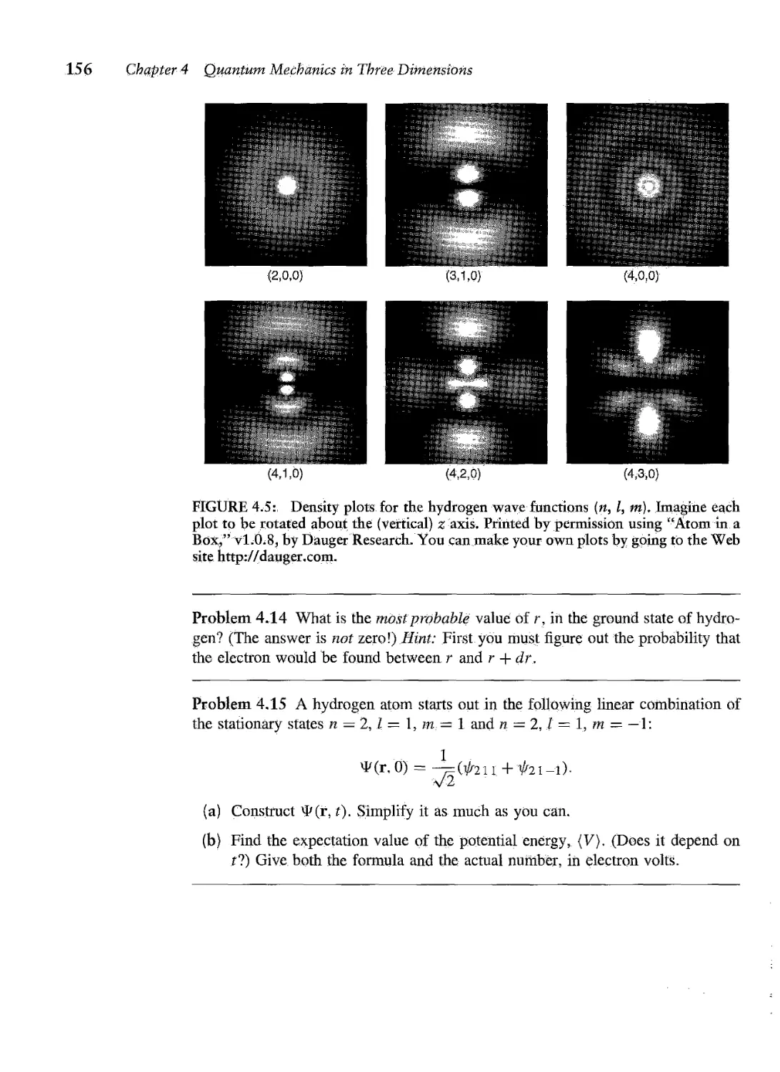
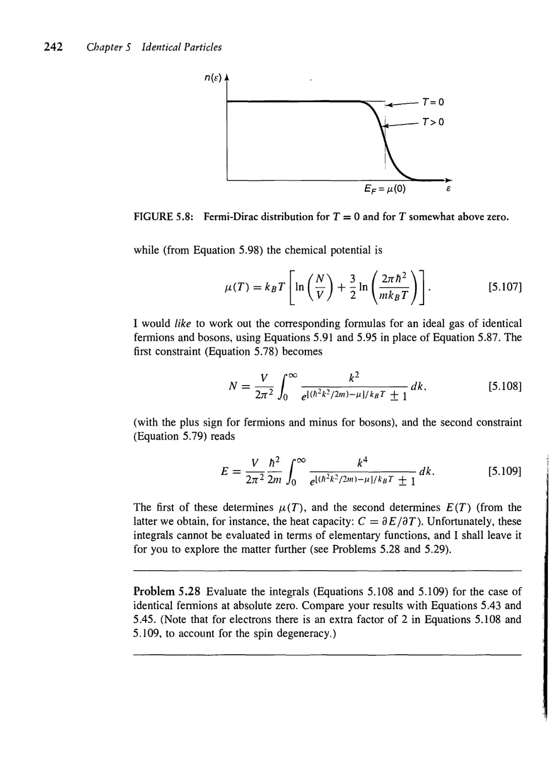
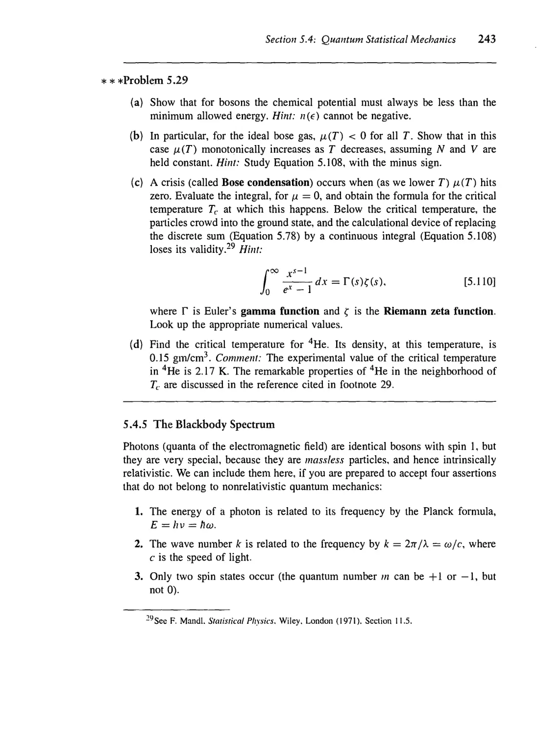
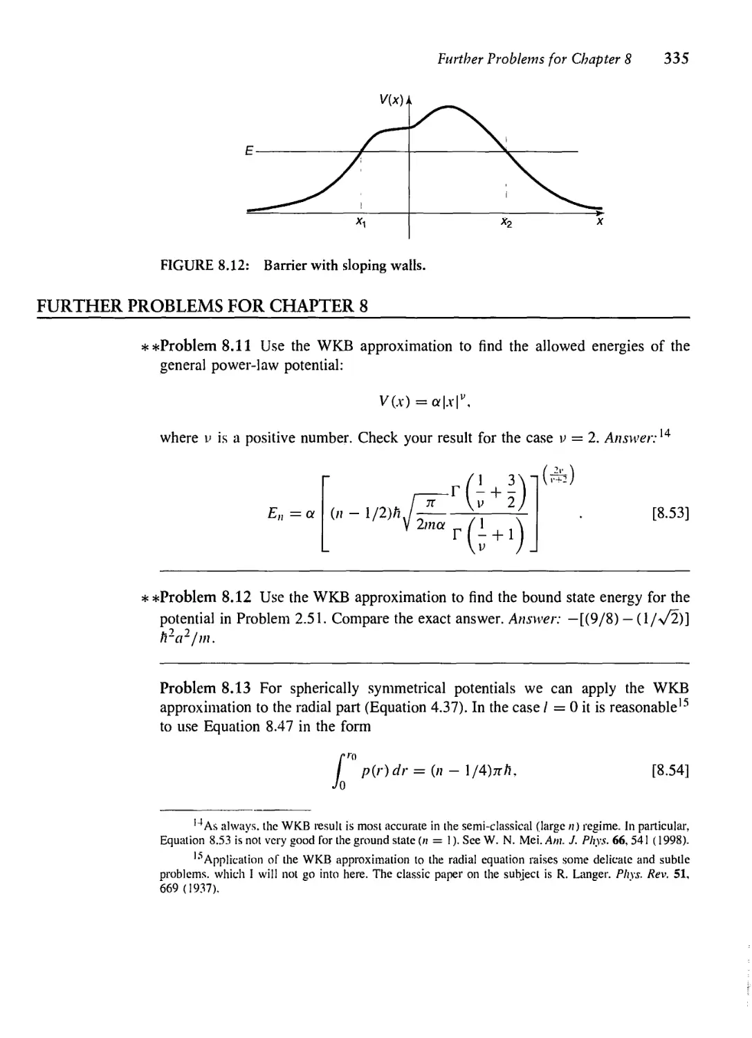
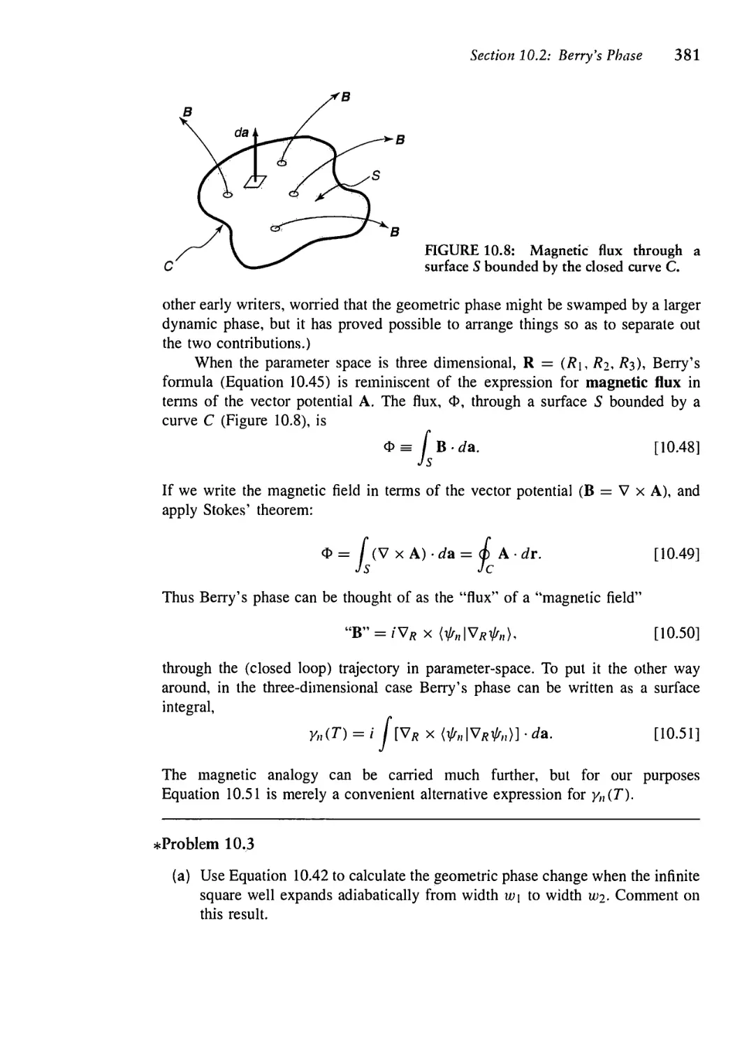
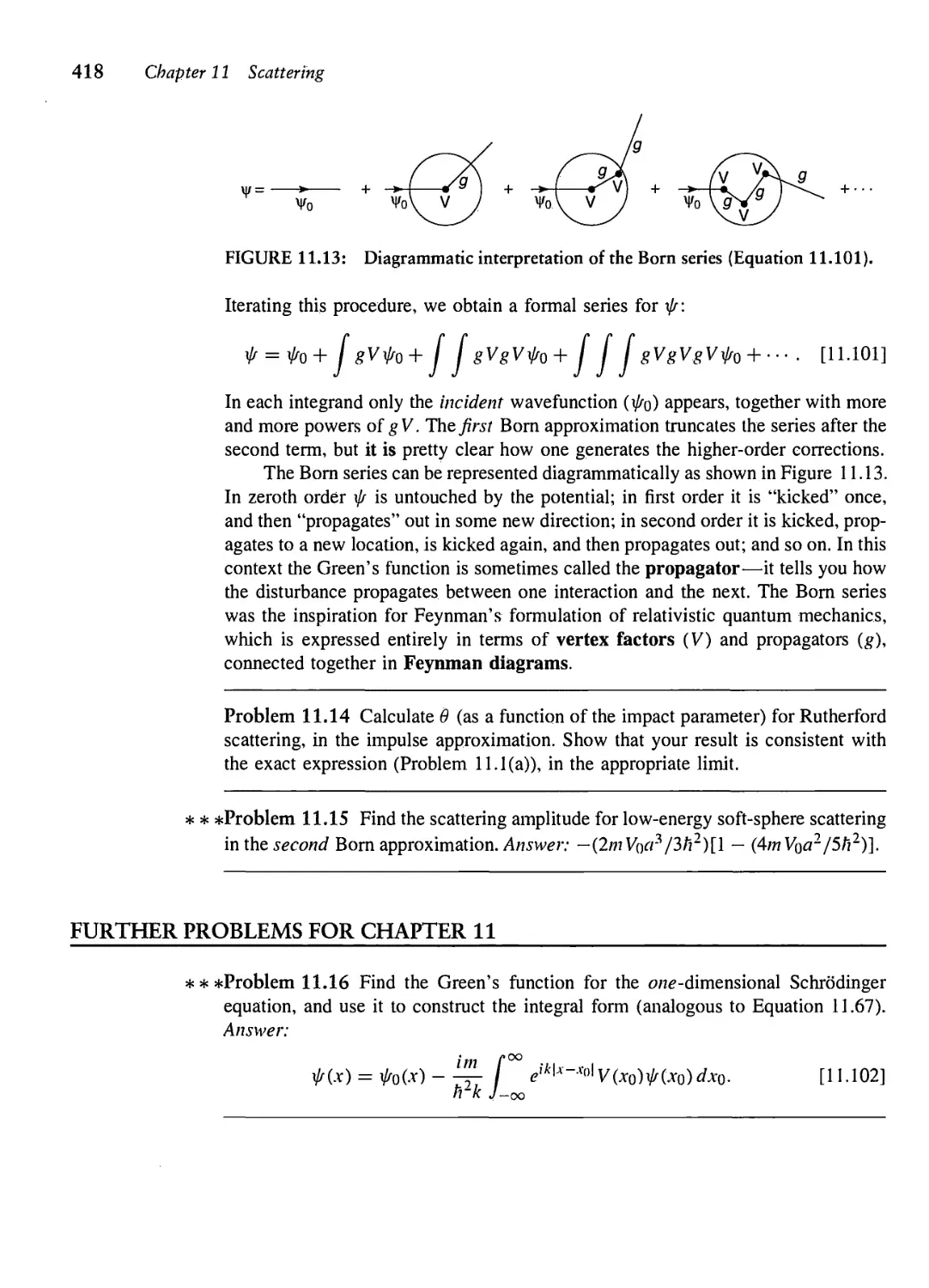
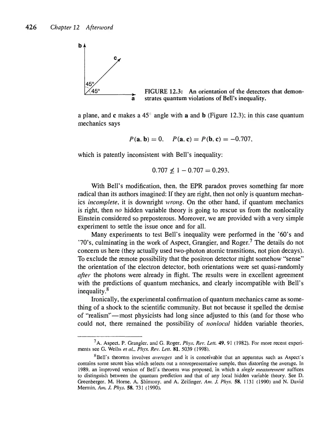
/


Текст
INTRODUCTION TO
Quantum
Mechanics
SECOND EDITION
DAVID J. GRIFFITHS
Fundamental Equations
Schrodinger equation:
9*
ih— = //*
dt
Time-independent Schrodinger equation:
Hamiltonian operator:
Hty = Ef, * = fe~iEt/h
2m
Momentum operator:
Time dependence of an expectation value:
p = -ihV
^->•«>-(¥:
Generalized uncertainty principle:
gaob >
\: U, B])
LI
Heisenberg uncertainty principle:
Canonical commutator:
oxOp > h/2
[x, p] = ih
Angular momentum:
[L,, Lv] = ihLz, [Lv, Lz) = ihLx, [L-, Lx]
Pauli matrices:
a, =
'0 P
A 0
'0 -i'
^=/ 0 I
a~ =
0
Fundamental Constants
h = 1.05457 x 1(T34 J s
c = 2.99792 x 10⁸ m/s
me = 9.10938 x 10⁻³¹ kg
mp = 1.67262 x 10"27 kg
e = 1.60218 x 10"I9C
Charge of electron: -e = -1.60218 x 10⁻¹⁹ C
Planck's constant:
Speed of light:
Mass of electron:
Mass of proton:
Charge of proton:
Permittivity of space: eo =
Boltzmann constant: kg =
8.85419 x 10-'2 C2/Jm
1.38065 x 10~23 J/K
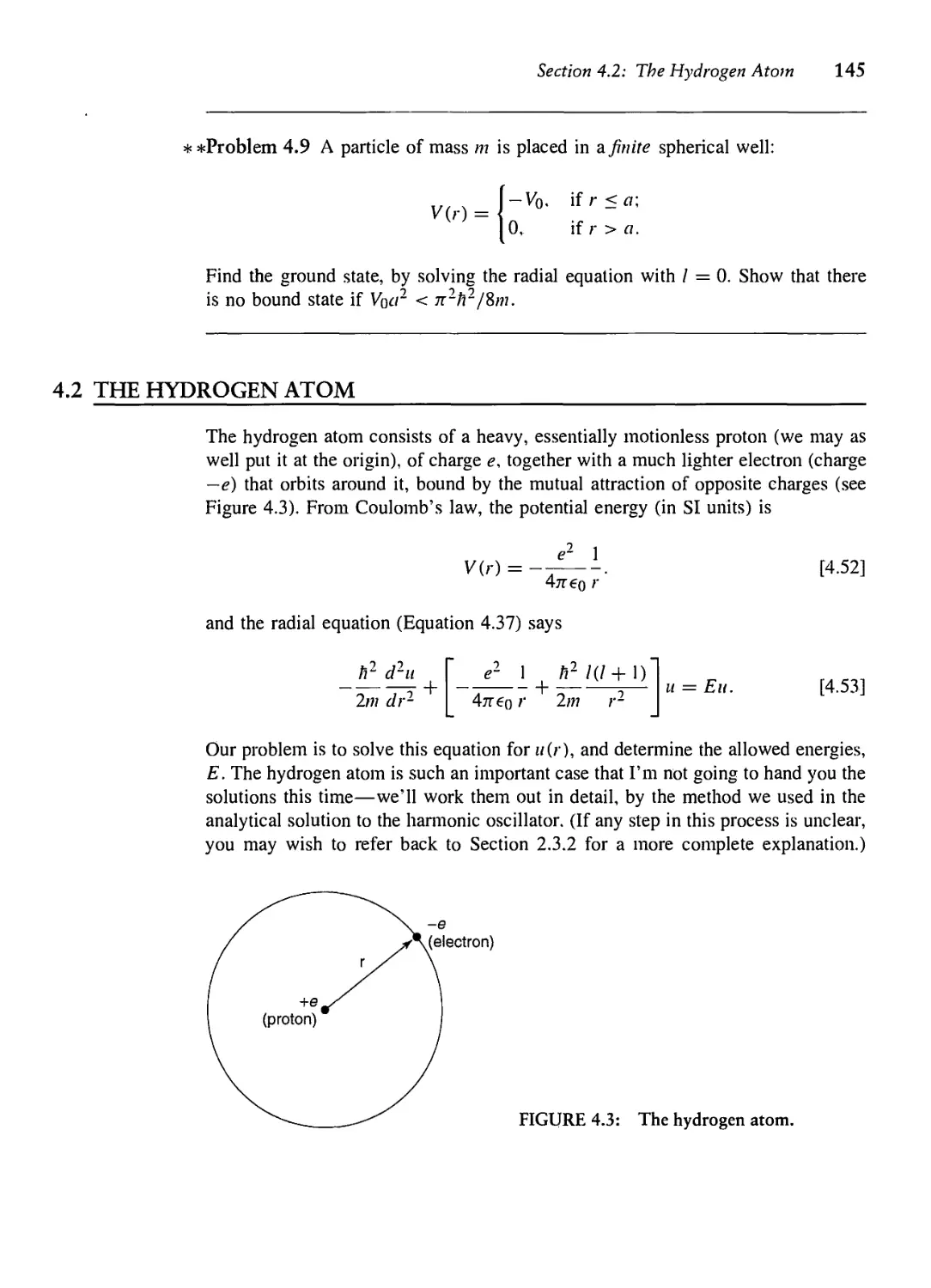
Hydrogen Atom
Fine structure constant: or =
Bohr radius:
Bohr energies:
Binding energy:
Ground state:
Rydberg formula:
a =
En =
-EX =
l
X ~
47t£ohc
4jT€o fl2
mee2
m
2(47te
h2
2m ea2
1
e
h
amec
ee4
0)¾2
9 9
a~mec~
2
-rja
y/jta^
ny nj
1/137.036
5.29177 x 10⁻¹¹ m
-4 (n= 1,2,3,...)
= 13.6057 eV
Rydberg constant:
R =
2nhc
= 1.09737 x 10⁷ /m
Introduction to
Quantum Mechanics
Second Edition
David J. Griffiths
Reed College
^^^KiiH Pearson Education International
Editor-in-Chief. Science: John Challice
Senior Editor: Erik Fahlgren
Associate Editor: Christian Bolting
Editorial Assistant: Andrew Sobel
Vice President and Director of Production and Manufacturing, ESM: David W. Riccardi
Production Editor: Beth Lew
Director of Creative Services: Paul Belfanli
Art Director: Jayne Conte
Cover Designer: Bruce Kenselaar
Managing Editor, AV Management and Production: Patricia Burns
Art Editor: Abigail Bass
Manufacturing Manager: Trudy Pisciolti
Manufacturing Buyer: Lynda Castillo
Executive Marketing Manager: Mark Pfallzgraff
Prentice
Hall
__ © 2005, 1995 Pearson Education, Inc.
Pearson Prentice Hall
Pearson Education, Inc.
Upper Saddle River, NJ 07458
All rights reserved, No part of this book may be reproduced in any form or by any means, without
permission in writing from the publisher.
Pearson Prentice Hall® is a trademark of Pearson Education, Inc.
Printed in the United Stales of America
10 9 8 7
ISBN D-13-nil7S-T
If you purchased this book wilhin the United States or Canada you should be aware that il has been
wrongfully imported without the approval of the Publisher or the Author.
Pearson Education LTD.. London
Pearson Education Australia Ply. Ltd., Sydney
Pearson Education Singapore, Pie. Ltd.
Pearson Education North Asia Ltd., Hong Kong
Pearson Education Canada, Inc., Toronto
Pearson Educacion de Mexico, S.A. de C.V.
Pearson Education—Japan, Tokyo
Pearson Education Malaysia, Pie. Ltd.
Pearson Education, Upper Saddle River, New Jersey
CONTENTS
PREFACE vii
PARTI THEORY
1 THE WAVE FUNCTION 1
1.1 The Schrbdinger Equation 1
1.2 The Statistical Interpretation 2
1.3 Probability 5
1.4 Normalization 12
1.5 Momentum 15
1.6 The Uncertainty Principle 18
2 TIME-INDEPENDENT SCHRODINGER EQUATION 24
2.1 Stationary States 24
2.2 The Infinite Square Well 30
2.3 The Harmonic Oscillator 40
2.4 The Free Particle 59
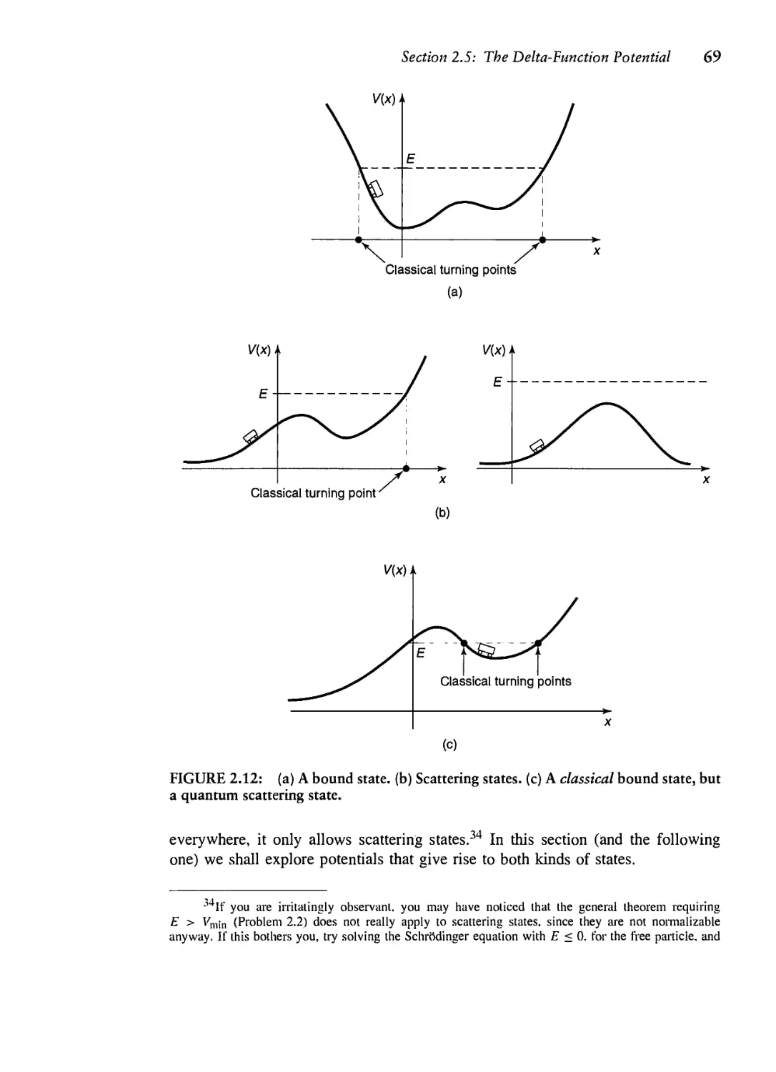
2.5 The Delta-Function Potential 68
2.6 The Finite Square Well 78
3 FORMALISM 93
3.1 Hilbert Space 93
3.2 Observables 96
3.3 Eigenfunctions of a Hermiiian Operator 100
iii
3.4 Generalized Statistical Interpretation 106
3.5 The Uncertainty Principle 110
3.6 Dirac Notation 118
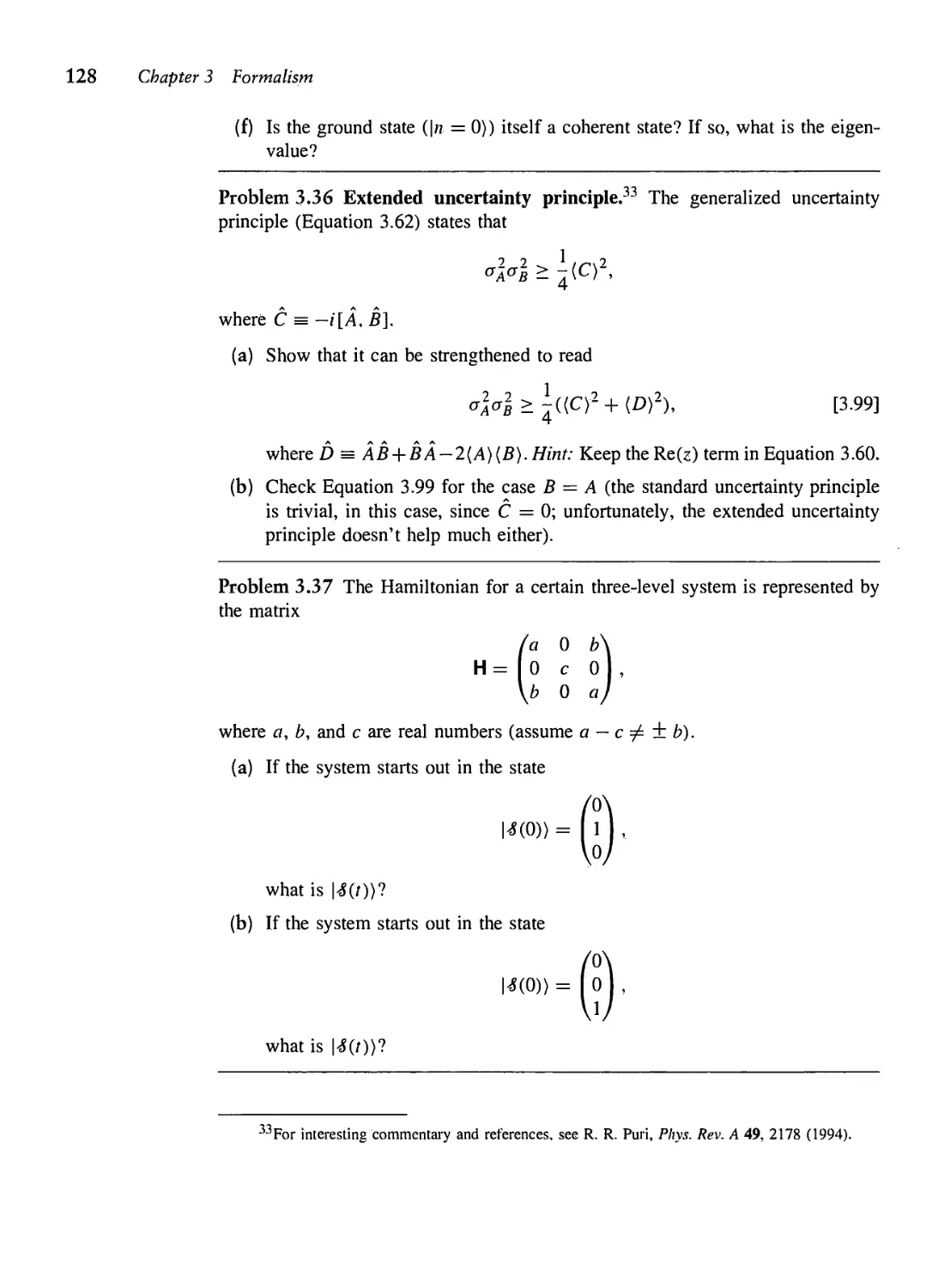
4 QUANTUM MECHANICS IN THREE DIMENSIONS 131
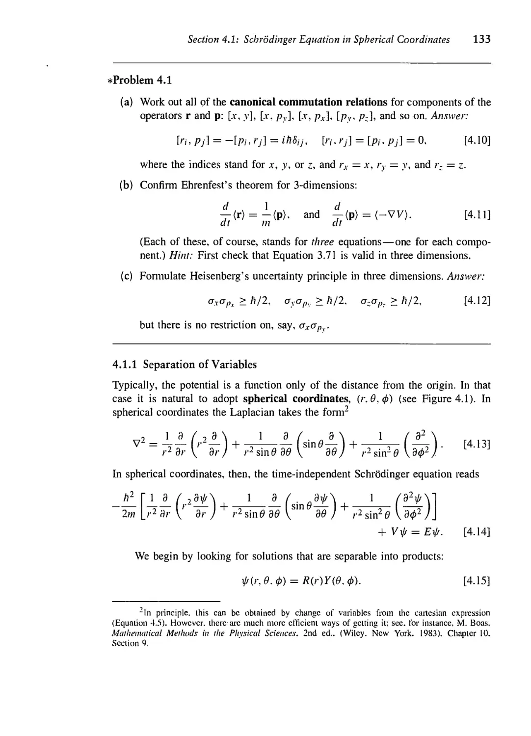
4.1 Schrodinger Equation in Spherical Coordinates 131
4.2 The Hydrogen Atom 145
4.3 Angular Momentum 160
4.4 Spin 171
5 IDENTICAL PARTICLES 201
5.1 Two-Particle Systems 201
5.2 Atoms 210
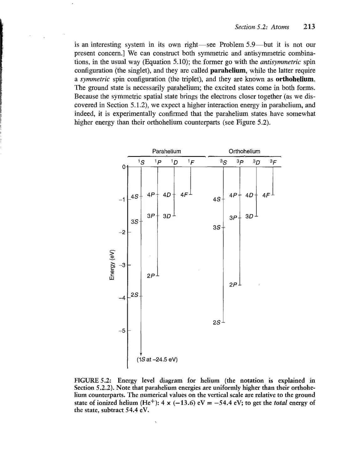
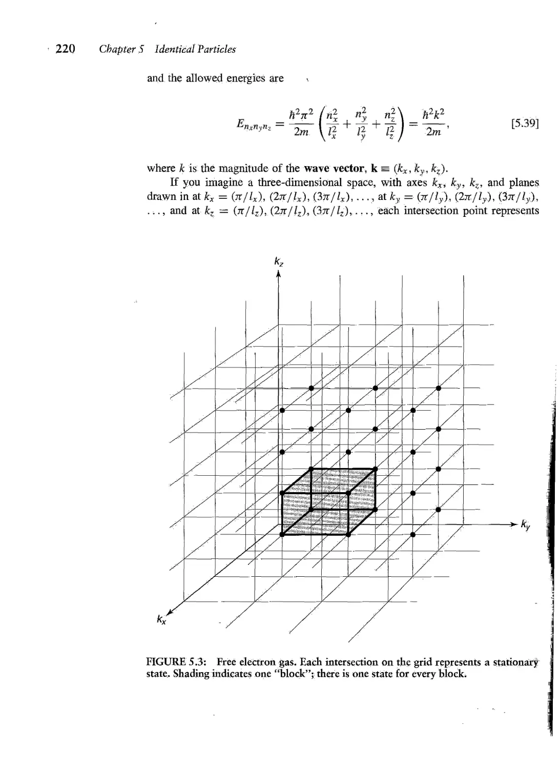
5.3 Solids 218
5.4 Quantum Statistical Mechanics 230
PART II APPLICATIONS
6 TIME-INDEPENDENT PERTURBATION THEORY 249
6.1 Nondegenerate Perturbation Theory 249
6.2 Degenerate Perturbation Theory 257
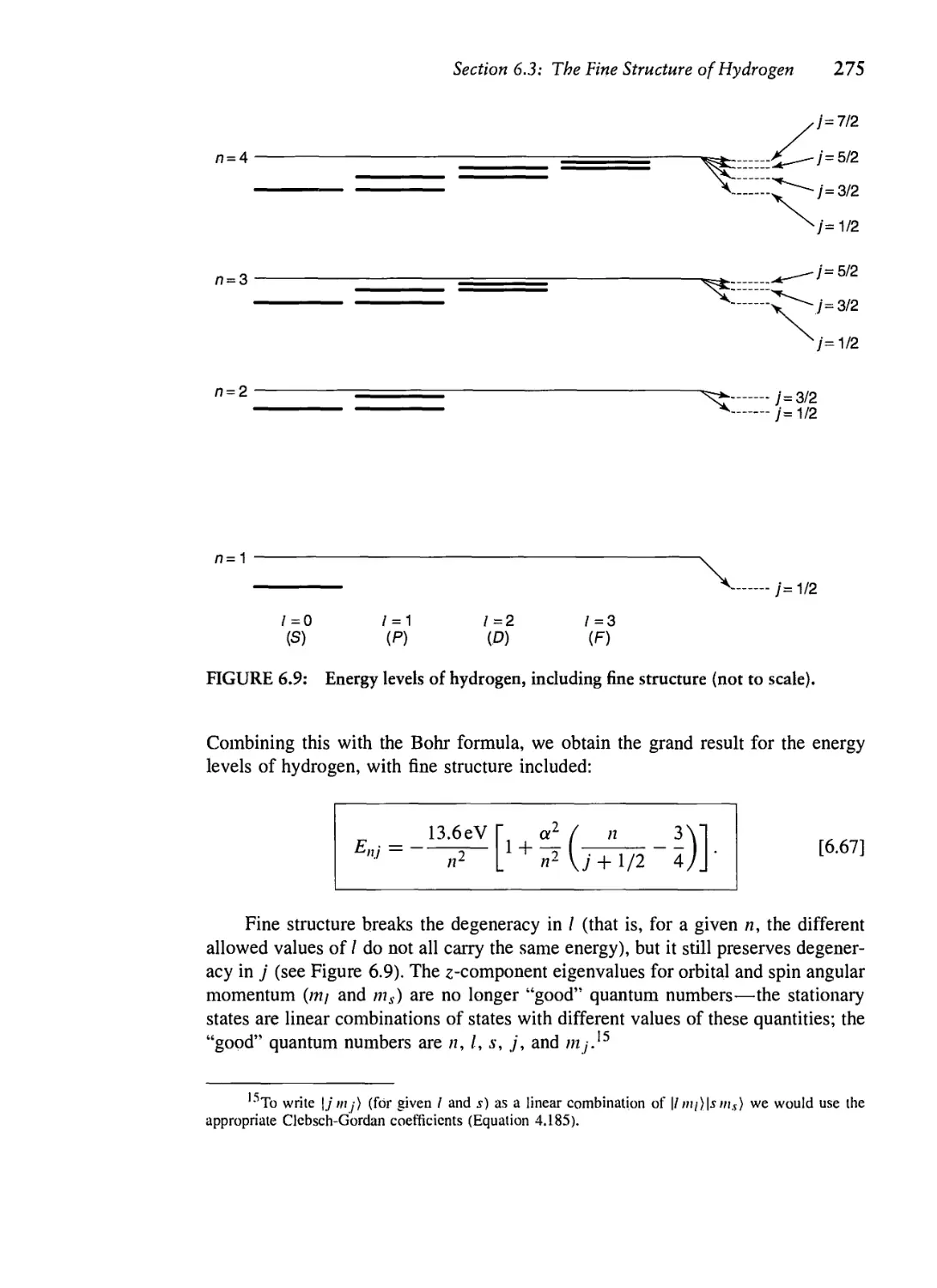
6.3 The Fine Structure of Hydrogen 266
6.4 The Zeeman Effect 277
6.5 Hyperfine Splitting 283
7 THE VARIATIONAL PRINCIPLE 293
7.1 Theory 293
7.2 The Ground State of Helium 299
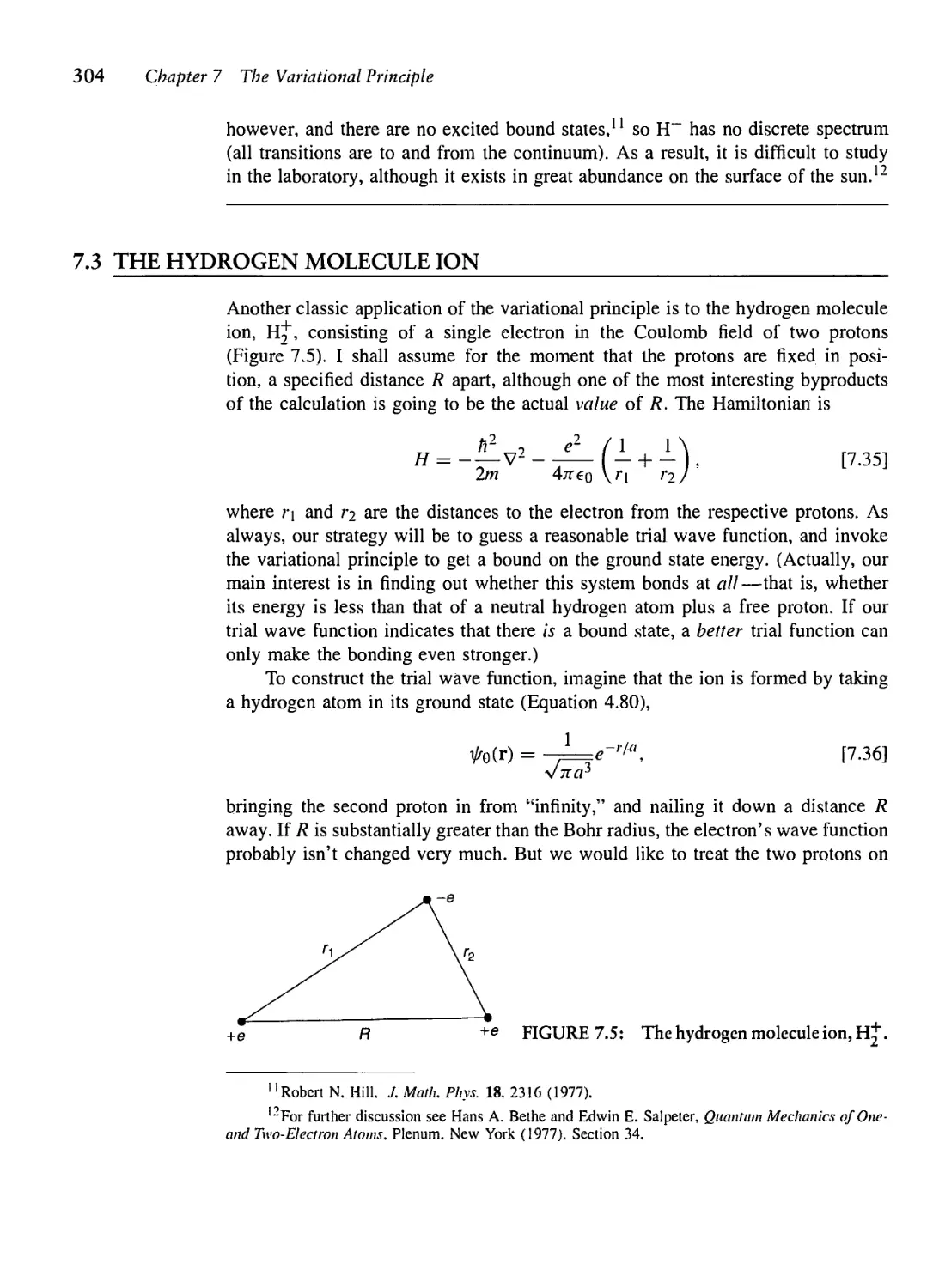
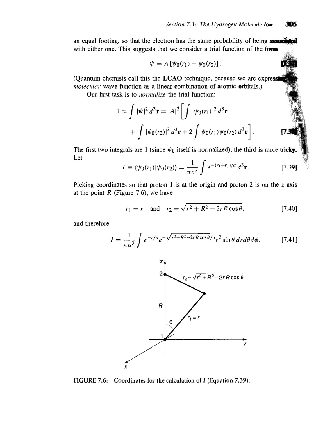
7.3 The Hydrogen Molecule Ion 304
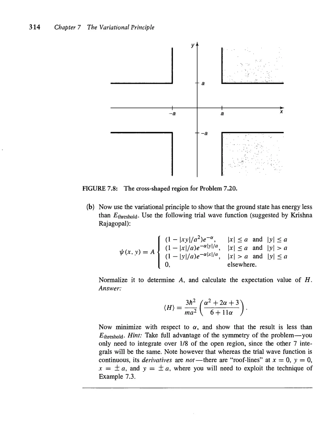
8 THE WKB APPROXIMATION 315
8.1 The "Classical" Region 316
8.2 Tunneling 320
8.3 The Connection Formulas 325
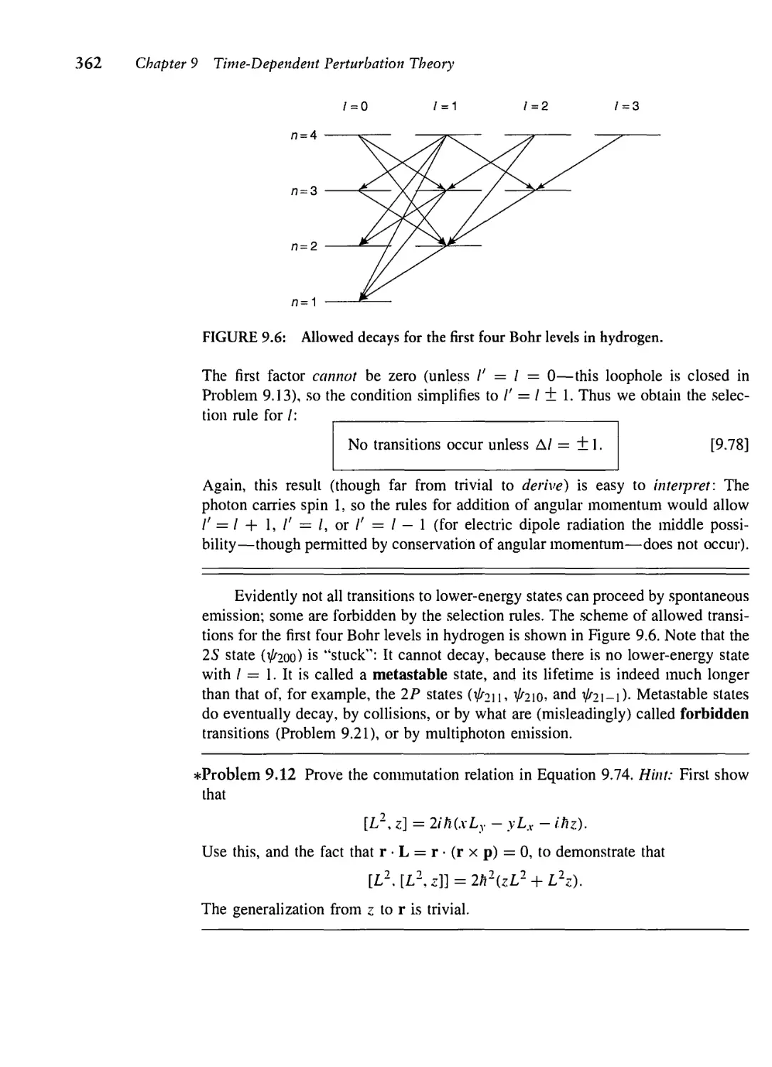
9 TIME-DEPENDENT PERTURBATION THEORY 340
9.1 Two-Level Systems 341
9.2 Emission and Absorption of Radiation 348
9.3 Spontaneous Emission 355
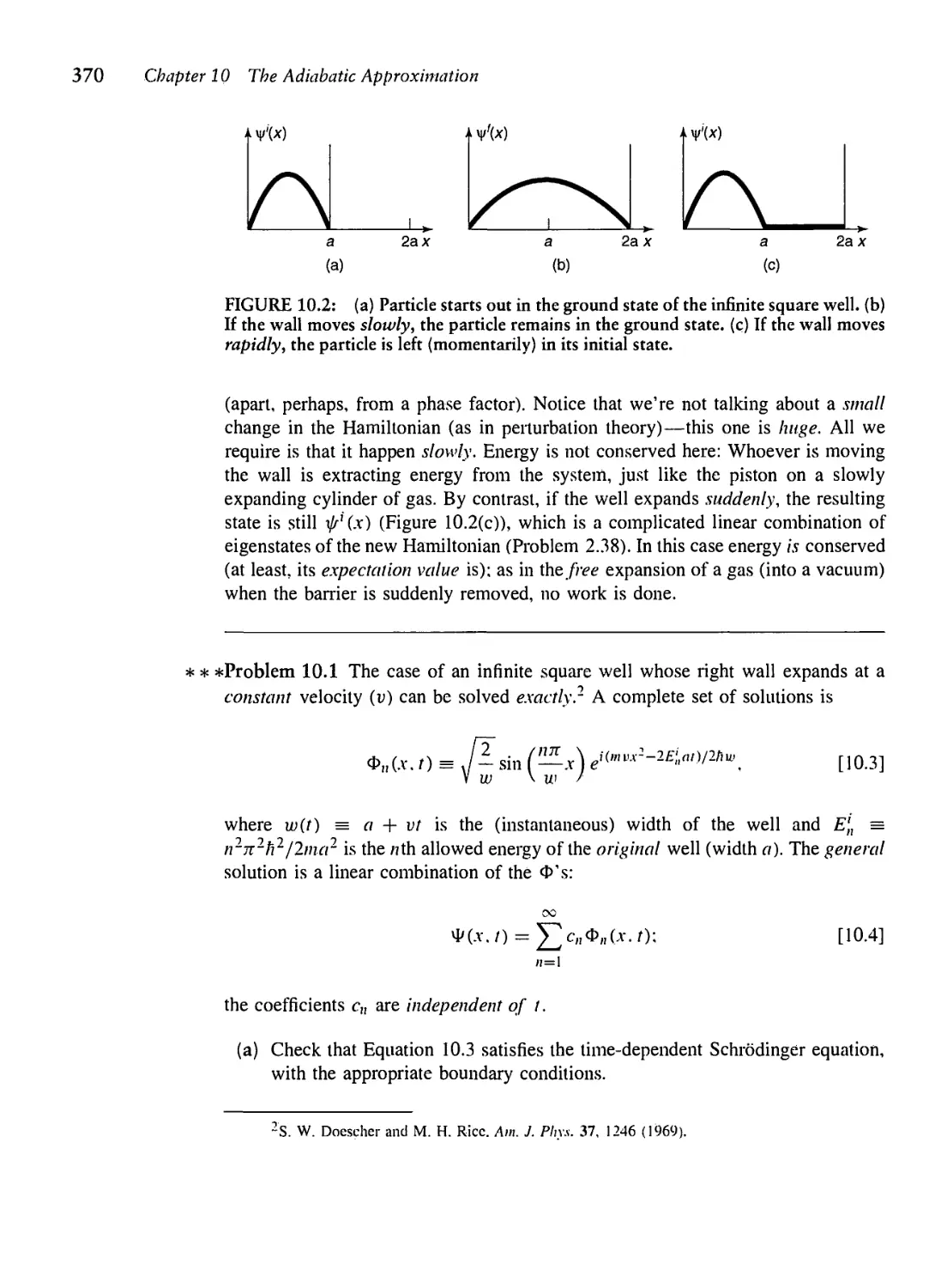
10 THE ADIABATIC APPROXIMATION 368
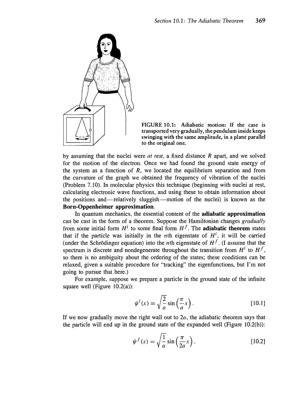
10.1 The Adiabatic Theorem 368
10.2 Berry's Phase 376
Contents v
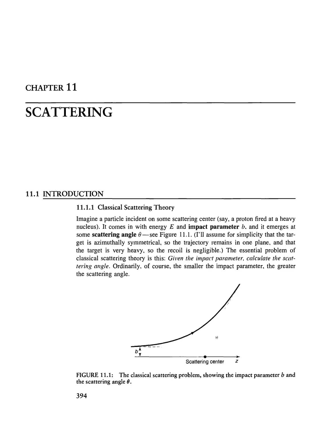
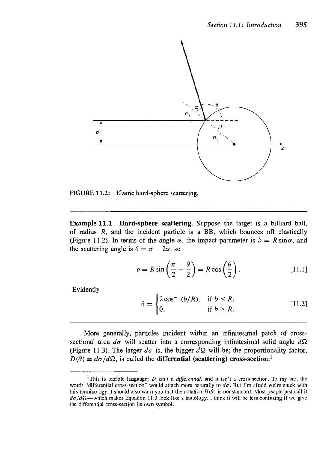
11 SCATTERING 394
11.1 Introduction 394
11.2 Partial Wave Analysis 399
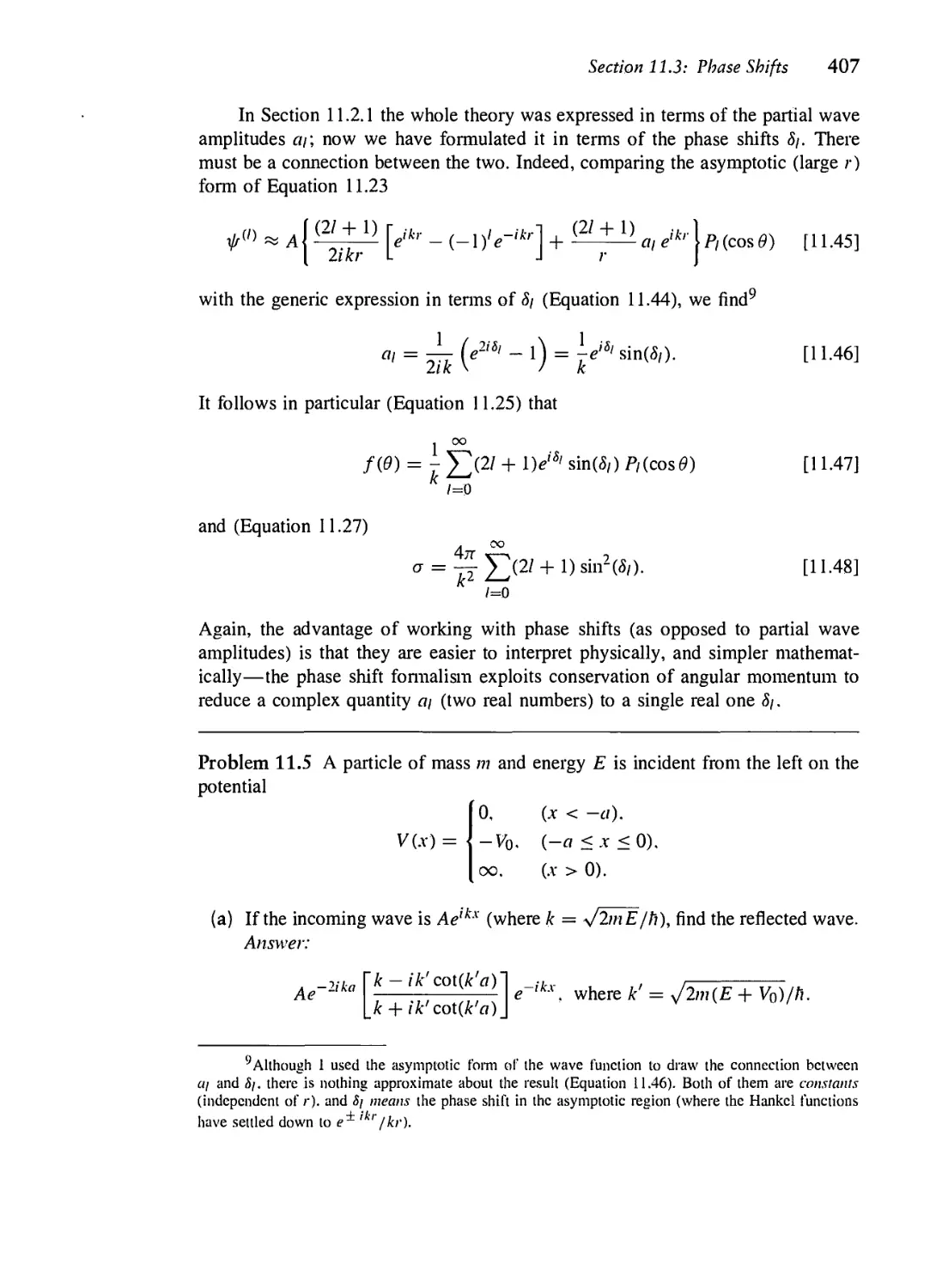
11.3 Phase Shifts 405
11.4 The Born Approximation 408
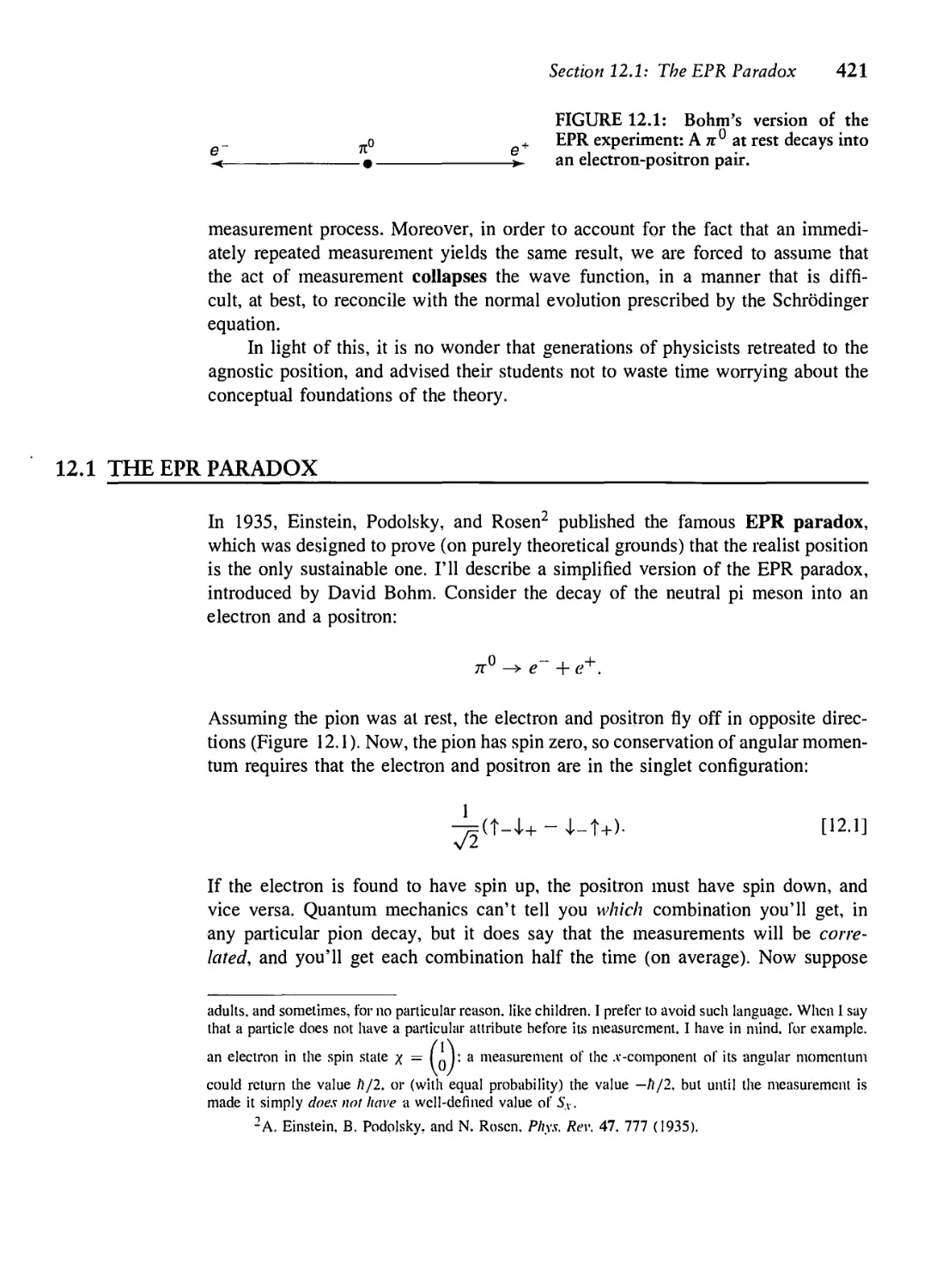
12 AFTERWORD 420
12.1 The EPR Paradox 421
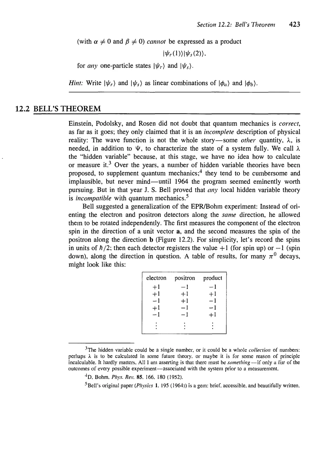
12.2 Bell's Theorem 423
12.3 The No-Clone Theorem 428
12.4 Schrodinger's Cat 430
12.5 The Quantum Zeno Paradox 431
APPENDIX LINEAR ALGEBRA 435
A.l Vectors 435
A.2 Inner Products 438
A.3 Matrices 441
A.4 Changing Bases 446
A.5 Eigenvectors and Eigenvalues 449
A. 6 Hermitian Transformations 455
INDEX 459
PREFACE
Unlike Newton's mechanics, or Maxwell's electrodynamics, or Einstein's relativity,
quantum theory was not created—or even definitively packaged—by one
individual, and it retains to this day some of the scars of its exhilarating but traumatic
youth. There is no general consensus as to what its fundamental principles are, how
it should be taught, or what it really "means." Every competent physicist can "do"
quantum mechanics, but the stories we tell ourselves about what we are doing are
as various as the tales of Scheherazade, and almost as implausible. Niels Bohr said,
"If you are not confused by quantum physics then you haven't really understood
it"; Richard Feynman remarked, "I think I can safely say that nobody understands
quantum mechanics."
The purpose of this book is to teach you how to do quantum mechanics. Apart
from some essential background in Chapter 1, the deeper quasi-philosophical
questions are saved for the end. I do not believe one can intelligently discuss what
quantum mechanics means until one has a firm sense of what quantum
mechanics does. But if you absolutely cannot wait, by all means read the Afterword
immediately following Chapter 1.
Not only is quantum theory conceptually rich, it is also technically difficult,
and exact solutions to all but the most artificial textbook examples are few and far
between. It is therefore essential to develop special techniques for attacking more
realistic problems. Accordingly, this book is divided into two parts;' Part I covers
the basic theory, and Part II assembles an arsenal of approximation schemes, with
illustrative applications. Although it is important to keep the two parts logically
separate, it is not necessary to study the material in the order presented here. Some
'This structure was inspired by David Park's classic text, Introduction to the Quantum Theory,
3rd ed.. McGraw-Hill, New York (1992).
vii
instructors, for example, may wish to treat time-independent perturbation theory
immediately after Chapter 2.
This book is intended for a one-semester or one-year course at the junior or
senior level. A one-semester course will have to concentrate mainly on Part I;
a full-year course should have room for supplementary material beyond Part II.
The reader must be familiar with the rudiments of linear algebra (as summarized
in the Appendix), complex numbers, and calculus up through partial derivatives;
some acquaintance with Fourier analysis and the Dirac delta function would help.
Elementary classical mechanics is essential, of course, and a little electrodynamics
would be useful in places. As always, the more physics and math you know the
easier it will be, and the more you will get out of your study. But I would like
to emphasize that quantum mechanics is not, in my view, something that flows
smoothly and naturally from earlier theories. On the contrary, it represents an
abrupt and revolutionary departure from classical ideas, calling forth a wholly new
and radically counterintuitive way of thinking about the world. That, indeed, is
what makes it such a fascinating subject.
At first glance, this book may strike you as forbiddingly mathematical. We
encounter Legendre, Hermite, and Laguerre polynomials, spherical harmonics,
Bessel, Neumann, and Hankel functions, Airy functions, and even the Riemann
zeta function—not to mention Fourier transforms, Hilbert spaces, hermitian
operators, Clebsch-Gordan coefficients, and Lagrange multipliers. Is all this baggage
really necessary? Perhaps not, but physics is like carpentry: Using the right tool
makes the job easier, not more difficult, and teaching quantum mechanics without
the appropriate mathematical equipment is like asking the student to dig a
foundation with a screwdriver. (On the other hand, it can be tedious and diverting if
the instructor feels obliged to give elaborate lessons on the proper use of each
tool. My own instinct is to hand the students shovels and tell them to start
digging. They may develop blisters at first, but I still think this is the most efficient
and exciting way to learn.) At any rate, I can assure you that there is no deep
mathematics in this book, and if you run into something unfamiliar, and you don't
find my explanation adequate, by all means ask someone about it, or look it up.
There are many good books on mathematical methods—I particularly recommend
Mary Boas, Mathematical Methods in the Physical Sciences, 2nd ed., Wiley, New
York (1983), or George Arfken and Hans-Jurgen Weber, Mathematical Methods for
Physicists, 5th ed., Academic Press, Orlando (2000). But whatever you do, don't
let the mathematics—which, for us, is only a tool—interfere with the physics.
Several readers have noted that there are fewer worked examples in this book
than is customary, and that some important material is relegated to the problems.
This is no accident. I don't believe you can learn quantum mechanics without doing
many exercises for yourself. Instructors should of course go over as many problems
in class as time allows, but students should be warned that this is not a subject
about which anyone has natural intuitions—you're developing a whole new set
of muscles here, and there is simply no substitute for calisthenics. Mark Semon
Preface ix
suggested that I offer a "Michelin Guide" to the problems, with varying numbers
of stars to indicate the level of difficulty and importance. This seemed like a good
idea (though, like the quality of a restaurant, the significance of a problem is partly
a matter of taste); I have adopted the following rating scheme:
* an essential problem that every reader should study;
* * a somewhat more difficult or more peripheral problem;
* * * an unusually challenging problem, that may take over an hour.
(No stars at all means fast food: OK if you're hungry, but not very nourishing.)
Most of the one-star problems appear at the end of the relevant section; most of
the three-star problems are at the end of the chapter. A solution manual is available
(to instructors only) from the publisher.
In preparing the second edition I have tried to retain as much as possible the
spirit of the first. The only wholesale change is Chapter 3, which was much too
long and diverting; it has been completely rewritten, with the background material
on finite-dimensional vector spaces (a subject with which most students at this level
are already comfortable) relegated to the Appendix. I have added some examples
in Chapter 2 (and fixed the awkward definition of raising and lowering operators
for the harmonic oscillator). In later chapters I have made as few changes as I
could, even preserving the numbering of problems and equations, where possible.
The treatment is streamlined in places (a better introduction to angular momentum
in Chapter 4, for instance, a simpler proof of the adiabatic theorem in Chapter
10, and a new section on partial wave phase shifts in Chapter 11). Inevitably, the
second edition is a bit longer than the first, which I regret, but I hope it is cleaner
and more accessible.
I have benefited from the comments and advice of many colleagues, who
read the original manuscript, pointed out weaknesses (or errors) in the first edition,
suggested improvements in the presentation, and supplied interesting problems. I
would like to thank in particular P. K. Aravind (Worcester Polytech), Greg Benesh
(Baylor), David Boness (Seattle), Burt Brody (Bard), Ash Carter (Drew), Edward
Chang (Massachusetts), Peter Collings (Swarthmore), Richard Crandall (Reed),
Jeff Dunham (Middlebury), Greg Elliott (Puget Sound), John Essick (Reed), Gregg
Franklin (Carnegie Mellon), Henry Greenside (Duke), Paul Haines (Dartmouth),
J. R. Huddle (Navy), Larry Hunter (Amherst), David Kaplan (Washington), Alex
Kuzmich (Georgia Tech), Peter Leung (Portland State), Tony Liss (Illinois), Jeffry
Mallow (Chicago Loyola), James McTavish (Liverpool), James Nearing (Miami),
Johnny Powell (Reed), Krishna Rajagopal (MIT), Brian Raue (Florida
International), Robert Reynolds (Reed), Keith Riles (Michigan), Mark Semon (Bates),
Herschel Snodgrass (Lewis and Clark), John Taylor (Colorado), Stavros Theodor-
akis (Cyprus), A. S. Tremsin (Berkeley), Dan Velleman (Amherst), Nicholas
Wheeler (Reed), Scott Willenbrock (Illinois), William Wootters (Williams), Sam
Wurzel (Brown), and Jens Zorn (Michigan).
Introduction to
Quantum Mechanics
PARTI THEORY
CHAPTER 1
THE WAVE FUNCTION
1.1 THE SCHRODINGER EQUATION
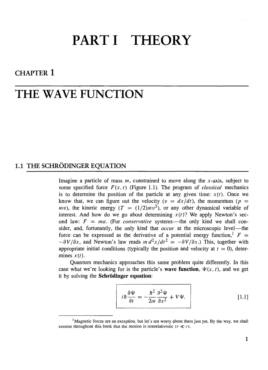
Imagine a particle of mass w, constrained to move along the x-axis, subject to
some specified force F(x.t) (Figure 1.1). The program of classical mechanics
is to determine the position of the particle at any given time: x(t). Once we
know that, we can figure out the velocity (v = dx/dt), the momentum (p =
mv), the kinetic energy (T = (l/2)mv2), or any other dynamical variable of
interest. And how do we go about determining x(/)? We apply Newton's
second law: F = ma. (For conservative systems—the only kind we shall
consider, and, fortunately, the only kind that occur at the microscopic level—the
force can be expressed as the derivative of a potential energy function,1 F =
—3V/3.V, and Newton's law reads mdrxjdt1 = —dV/dx.) This, together with
appropriate initial conditions (typically the position and velocity at t = 0),
determines x{t).
Quantum mechanics approaches this same problem quite differently. In this
case what we're looking for is the particle's wave function, W(x, f), and we get
it by solving the Schrodinger equation:
9vj/ fi1 dH ,, ,
at 2m
axil A]
1 Magnetic forces are an exception, but let's not worry about ihem just yet. By the way. we shall
assume throughout this book that the motion is nonrelalivislic (,i» <SC c).
1
2 Chapter 1 The Wave Function
x(t)
m
o n
* r{X,t)
X
FIGURE 1.1: A "particle" constrained to move in one dimension under the influence
of a specified force.
Here i is the square root of —1, and h is Planck's constant—or rather, his original
constant (/?) divided by 2tt:
h = — = 1.054572 x 10~34J s.
2tt
[1.2]
The Schrodinger equation plays a role logically analogous to Newton's second
law: Given suitable initial conditions (typically, ty{x, 0)), the Schrodinger equation
determines ty(x,t) for all future time, just as, in classical mechanics, Newton's
law determines x(t) for all future time.2
1.2 THE STATISTICAL INTERPRETATION
But what exactly is this "wave function," and what does it do for you once you've
got it? After all, a particle, by its nature, is localized at a point, whereas the wave
function (as its name suggests) is spread out in space (it's a function of x, for any
given time /). How can such an object represent the state of a particle'? The answer
is provided by Bom's statistical interpretation of the wave function, which says
that \^(x, t)\2 gives the probability of finding the particle at point x, at time t—or,
more precisely,3
/
J.a
\V(x\t)\2dx =
probability of finding the particle
between a and /?, at time t.
[1.3]
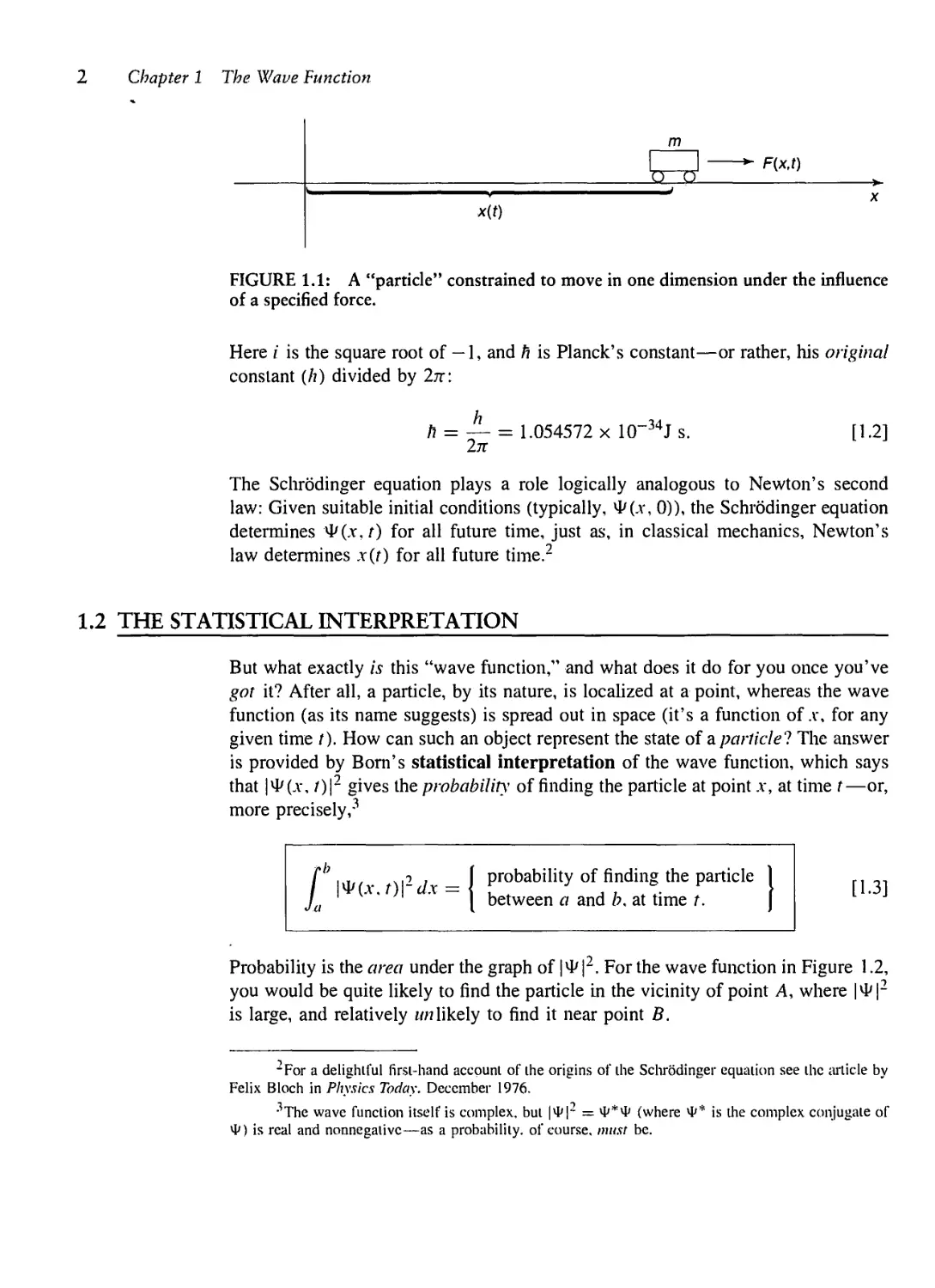
Probability is the area under the graph of \ty |2. For the wave function in Figure 1.2,
you would be quite likely to find the particle in the vicinity of point A, where |4>|2
is large, and relatively mh likely to find it near point B.
^For a delightful first-hand account of the origins of the Schrodinger equation see the article by
Felix Bloch in Physics Today. December 1976.
•'The wave function itself is complex, but |*|2 = *** (where ** is the complex conjugate of
*) is real and nonnegalivc—as a probability, of course, must be.
Section 1.2: The Statistical Interpretation 3
*M2
B C x
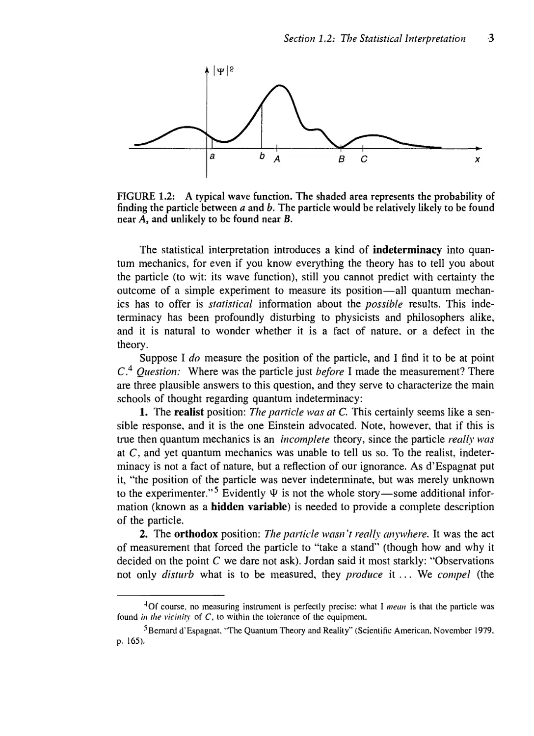
FIGURE 1.2: A typical wave function. The shaded area represents the probability of
rinding the particle between a and b. The particle would be relatively likely to be found
near A, and unlikely to be found near B.
The statistical interpretation introduces a kind of indeterminacy into
quantum mechanics, for even if you know everything the theory has to tell you about
the particle (to wit: its wave function), still you cannot predict with certainty the
outcome of a simple experiment to measure its position—all quantum
mechanics has to offer is statistical information about the possible results. This
indeterminacy has been profoundly disturbing to physicists and philosophers alike,
and it is natural to wonder whether it is a fact of nature, or a defect in the
theory.
Suppose I do measure the position of the particle, and I find it to be at point
C.4 Question: Where was the particle just before I made the measurement? There
are three plausible answers to this question, and they serve to characterize the main
schools of thought regarding quantum indeterminacy:
1. The realist position: The particle was at C. This certainly seems like a
sensible response, and it is the one Einstein advocated. Note, however, that if this is
true then quantum mechanics is an incomplete theory, since the particle really was
at C, and yet quantum mechanics was unable to tell us so. To the realist,
indeterminacy is not a fact of nature, but a reflection of our ignorance. As d'Espagnat put
it, "the position of the particle was never indeterminate, but was merely unknown
to the experimenter."5 Evidently 4> is not the whole story—some additional
information (known as a hidden variable) is needed to provide a complete description
of the particle.
2. The orthodox position: The particle wasn 7 really anywhere. It was the act
of measurement that forced the particle to "take a stand" (though how and why it
decided on the point C we dare not ask). Jordan said it most starkly: "Observations
not only disturb what is to be measured, they produce it ... We compel (the
4Of course, no measuring instrument is perfectly precise: what I mean is that the particle was
found in the vicinity of C. to within the tolerance of the equipment.
•'Bernard d'Espagnat, "The Quantum Theory and Reality" (Scientific American. November 1979.
p. 165).
4 Chapter 1 The Wave Function
particle) to assume a definite position."6 This view (the so-called Copenhagen
interpretation), is associated with Bohr and his followers. Among physicists it
has always been the most widely accepted position. Note, however, that if it is
correct there is something very peculiar about the act of measurement—something
that over half a century of debate has done precious little to illuminate.
3. The agnostic position: Refuse to answer. This is not quite as silly as it
sounds—after all, what sense can there be in making assertions about the status
of a particle before a measurement, when the only way of knowing whether you
were right is precisely to conduct a measurement, in which case what you get is no
longer "before the measurement?" It is metaphysics (in the pejorative sense of the
word) to worry about something that cannot, by its nature, be tested. Pauli said:
"One should no more rack one's brain about the problem of whether something one
cannot know anything about exists all the same, than about the ancient question of
how many angels are able to sit on the point of a needle."7 For decades this was the
"fall-back" position of most physicists: They'd try to sell you the orthodox answer,
but if you were persistent they'd retreat to the agnostic response, and terminate the
conversation.
Until fairly recently, all three positions (realist, orthodox, and agnostic) had
their partisans. But in 1964 John Bell astonished the physics community by showing
that it makes an observable difference whether the particle had a precise (though
unknown) position prior to the measurement, or not. Bell's discovery effectively
eliminated agnosticism as a viable option, and made it an experimental question
whether 1 or 2 is the correct choice. I'll return to this story at the end of the book,
when you will be in a better position to appreciate Bell's argument; for now, suffice
it to say that the experiments have decisively confirmed the orthodox
interpretation:8 A particle simply does not have a precise position prior to measurement, any
more than the ripples on a pond do; it is the measurement process that insists on
one particular number, and thereby in a sense creates the specific result, limited
only by the statistical weighting imposed by the wave function.
What if I made a second measurement, immediately after the first? Would I
get C again, or does the act of measurement cough up some completely new
number each time? On this question everyone is in agreement: A repeated measurement
(on the same particle) must return the same value. Indeed, it would be tough to
prove that the particle was really found at C in the first instance, if this could not
be confirmed by immediate repetition of the measurement. How does the orthodox
"Quoted in a lovely article by N. David Mennin. "Is the moon there when nobody looks?"
(Physics Today. April 1985. p. 38).
7Quolcd by Mermin (footnote 6). p. 40.
8This statement is a little loo strong: There remain a lew theoretical and experimental loopholes,
some of which I shall discuss in the Afterword. There exist viable nonlocal hidden variable theories
(notably David Bohm's). and other formulations (such as the many worlds interpretation) that do not
fit cleanly into any of my three categories. But 1 think it is wise, at least from a pedagogical point of
view, to adopt a clear and coherent platform at this stage, and worry about the alternatives later.
Section 1.3: Probability
tM2
C x
FIGURE 1.3: Collapse of the wave function: graph of |>P|2 immediately after a
measurement has found the particle at point C.
interpretation account for the fact that the second measurement is bound to yield
the value C? Evidently the first measurement radically alters the wave function,
so that it is now sharply peaked about C (Figure 1.3). We say that the wave
function collapses, upon measurement, to a spike at the point C (it soon spreads out
again, in accordance with the Schrodinger equation, so the second measurement
must be made quickly). There are, then, two entirely distinct kinds of physical
processes: "ordinary" ones, in which the wave function evolves in a leisurely fashion
under the Schrodinger equation, and "measurements," in which ^ suddenly and
discontinuously collapses.9
1.3 PROBABILITY
1.3.1 Discrete Variables
Because of the statistical interpretation, probability plays a central role in quantum
mechanics, so I digress now for a brief discussion of probability theory. It is mainly
a question of introducing some notation and terminology, and I shall do it in the
context of a simple example.
Imagine a room containing fourteen people, whose ages are as follows:
one person aged 14,
one person aged 15,
three people aged 16,
JThe role of measurement in quantum mechanics is so critical and so bizarre that you may
well be wondering what precisely constitutes a measurement. Does it have to do with the interaction
between a microscopic (quanlum) system and a macroscopic (classical) measuring apparatus (as Bohr
insisted), or is it characterized by the leaving of a permanent "record" (as Heisenberg claimed), or does
it involve the intervention of a conscious "observer" (as Wigner proposed)? I'll return to this thorny
issue in the Afterword: for the moment let's lake the naive view: A measurement is the kind of thing
that a scientist does in the laboratory, with rulers, stopwatches, Geiger counters, and so on.
6 Chapter 1 The Wave Function
two people aged 22,
two people aged 24.
five people aged 25.
If we let N(j) represent the number of people of age j, then
N(U) = 1,
N(15) = 1,
N(16) = 3,
N(22) = 2,
N(24) = 2,
N(25) = 5,
while N(17), for instance, is zero. The total number of people in the room is
00
tf = X>c/).
[1.4]
7=0
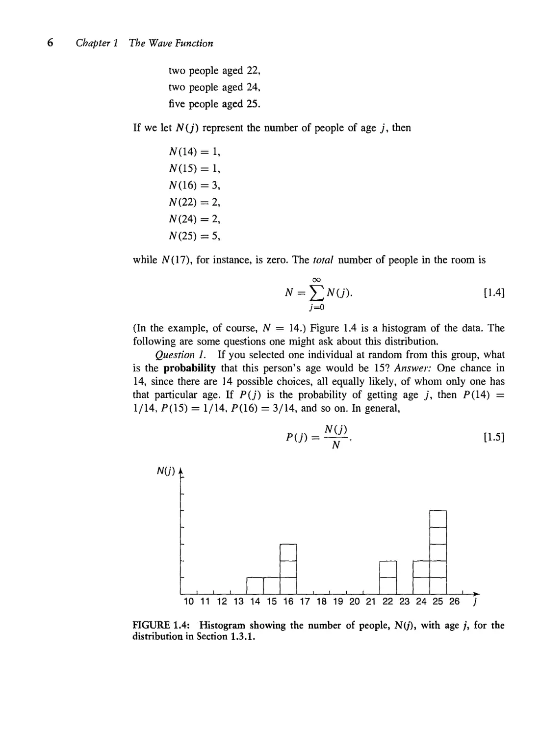
(In the example, of course, N = 14.) Figure 1.4 is a histogram of the data. The
following are some questions one might ask about this distribution.
Question 1. If you selected one individual at random from this group, what
is the probability that this person's age would be 15? Answer: One chance in
14, since there are 14 possible choices, all equally likely, of whom only one has
that particular age. If P(j) is the probability of getting age j, then P(14) =
1/14, P(15) = 1/14, P(16) = 3/14, and so on. In general,
P(j) =
N(j)
N
[1.5]
N(J) I
j i i
J I L
10 11 12 13 14 15 16 17 18 19 20 21 22 23 24 25 26 j
FIGURE 1.4: Histogram showing the number of people, NO), with age ;, for the
distribution in Section 1.3.1.
Section 1.3: Probability 7
Notice that the probability of getting either 14 or 15 is the sum of the individual
probabilities (in this case, 1/7). In particular, the sum of all the probabilities is
1—you're certain to get some age:
oo
En/) = i.
[1.6]
7=0
Question 2. What is the most probable age? Answer: 25, obviously; five
people share this age, whereas at most three have any other age. In general, the
most probable j is the j for which P(j) is a maximum.
Question 3. What is the median age? Answer: 23, for 7 people are younger
than 23, and 7 are older. (In general, the median is that value of j such that the
probability of getting a larger result is the same as the probability of getting a
smaller result.)
Question 4. What is the average (or mean) age? Answer:
(14) + (15) + 3(16) + 2(22) + 2(24) + 5(25) 294
= 21.
14 14
In general, the average value of j (which we shall write thus: (/')) is
0")
= —jv— = 1^, j nj).
[1.7]
7=0
Notice that there need not be anyone with the average age or the median age—in
this example nobody happens to be 21 or 23. In quantum mechanics the average
is usually the quantity of interest; in that context it has come to be called the
expectation value. It's a misleading term, since it suggests that this is the outcome
you would be most likely to get if you made a single measurement {that would
be the most probable value, not the average value)—but I'm afraid we're stuck
with it.
Question 5. What is the average of the squares of the ages? Answer: You
could get 142 = 196, with probability 1/14, or 152 = 225, with probability 1/14,
or 16~ = 256, with probability 3/14, and so on. The average, then, is
00
U2) = ^J2PU)-
7=0
In general, the average value of some function of j is given by
[1.8]
[1.9]
8 Chapter 1 The Wave Function
N(j) A
i i i i i i i i i i > i i i i i i i i i i i >
123456789 10/ 123456789 10/
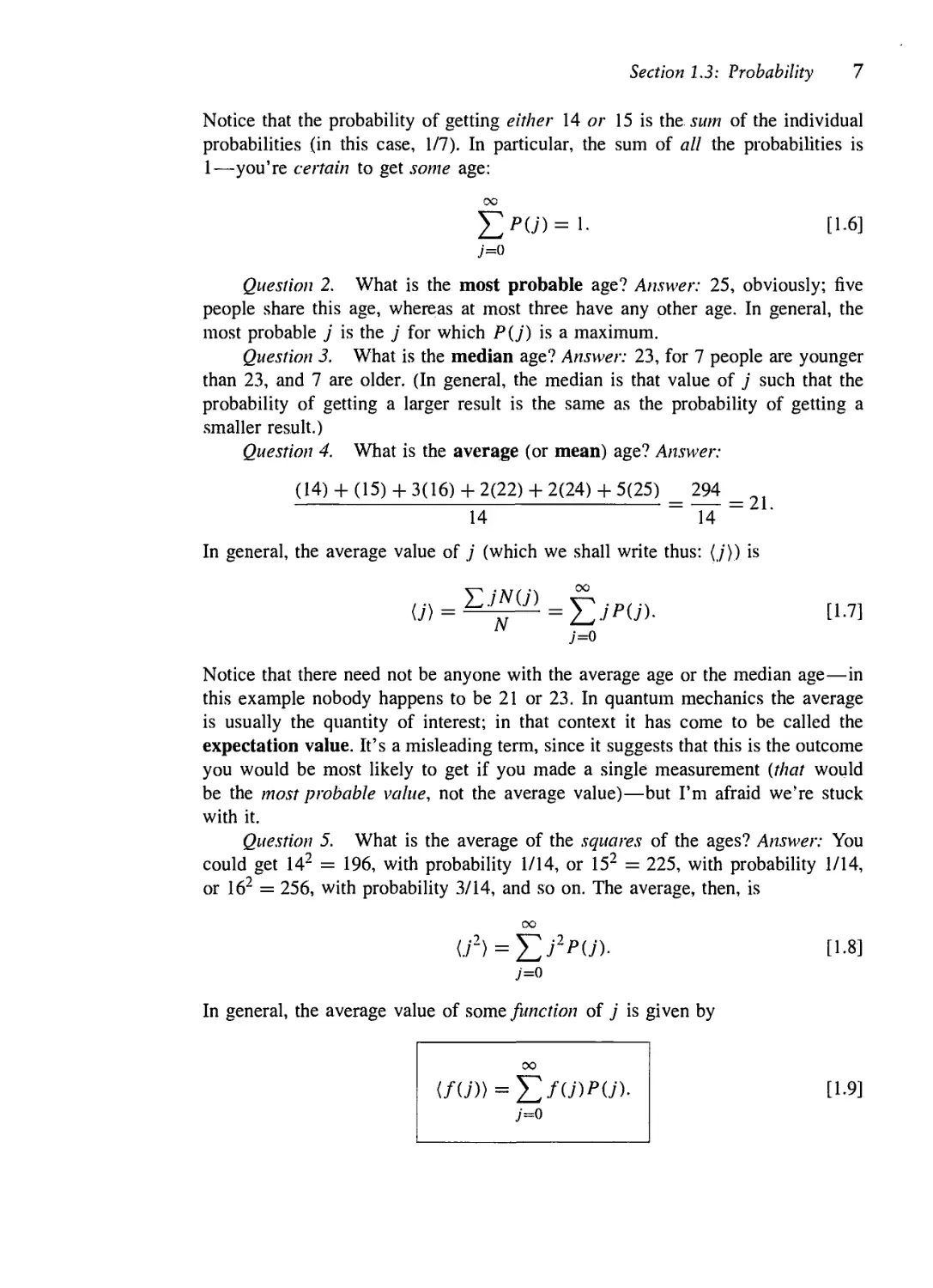
FIGURE 1.5: Two histograms with the same median, same average, and same most
probable value, but different standard deviations.
(Equations 1.6, 1.7, and 1.8 are, if you like, special cases of this formula.) Beware:
The average of the squares, (j2), is not equal, in general, to the square of the
average, (./)2. For instance, if the room contains just two babies, aged 1 and 3,
then (x1) = 5, but (x)2 = 4.
Now, there is a conspicuous difference between the two histograms in Figure 1.5,
even though they have the same median, the same average, the same most probable
value, and the same number of elements: The first is sharply peaked about the average
value, whereas the second is broad and flat. (The first might represent the age profile
for students in a big-city classroom, the second, perhaps, a rural one-room school-
house.) We need a numerical measure of the amount of "spread" in a distribution,
with respect to the average. The most obvious way to do this would be to find out
how far each individual deviates from the average,
Aj = j-{j), [l.io]
and compute the average of Aj. Trouble is, of course, that you get zero, since, by
the nature of the average, Aj is as often negative as positive:
(aj) = J2u - u))pu) = J2 Jpw - u) £ p(j)
= U) - (j) = o.
(Note that (j) is constant—it does not change as you go from one member of
the sample to another—so it can be taken outside the summation.) To avoid this
irritating problem you might decide to average the absolute value of Aj. But
absolute values are nasty to work with; instead, we get around the sign problem
by squaring before averaging:
Nil) i
a2 = ((Aj)2).
[1.11]
Section 1.3: Probability 9
This quantity is known as the variance of the distribution; a itself (the square
root of the average of the square of the deviation from the average—gulp!) is
called the standard deviation. The latter is the customary measure of the spread
about (j).
There is a useful little theorem on variances:
a2 = ((Aj)2) = £(A/)2P(./) = £(./ - (j))2P(j)
= £ j2P(j) - 2U)^jP(j) + U)2 J2 P{j)
= U2)-2U)(j) + U)2 = U2)-U)2.
Taking the square root, the standard deviation itself can be written as
° = y/(J2) ~ U)2- [1.12]
In practice, this is a much faster way to get a: Simply calculate (/2) and (j)2,
subtract, and take the square root. Incidentally, I warned you a moment ago that
{j~) is not, in general, equal to (j)~. Since a~ is plainly nonnegative (from its
definition in Equation 1.11), Equation 1.12 implies that
(r)>0*)2, [i.i3]
and the two are equal only when a = 0, which is to say, for distributions with no
spread at all (every member having the same value).
1.3.2 Continuous Variables
So far, I have assumed that we are dealing with a discrete variable—that is, one
that can take on only certain isolated values (in the example, j had to be an
integer, since I gave ages only in years). But it is simple enough to generalize to
continuous distributions. If I select a random person off the street, the probability
that her age is precisely 16 years, 4 hours, 27 minutes, and 3.333 ... seconds is
zero. The only sensible thing to speak about is the probability that her age lies in
some interyal—say, between 16 and 17. If the interval is sufficiently short, this
probability is proportional to the length of the interyal. For example, the chance that
her age is between 16 and 16 plus two days is presumably twice the probability
that it is between 16 and 16 plus one day. (Unless, I suppose, there was some
extraordinary baby boom 16 years ago, on exactly that day—in which case we
have simply chosen an interval too long for the rule to apply. If the baby boom
The Wave Function
lasted six hours, we'll take intervals of a second or less, to be on the safe side.
Technically, we're talking about infinitesimal intervals.) Thus
I probability that an individual (chosen 1 ,., r, , ...
.. \ ,• L j/ , j x \=p{x)dx. [1.14]
at random) lies between x and (a* + ax) J
The proportionality factor, p(x), is often loosely called "the probability of getting
A'," but this is sloppy language; a better term is probability density. The probability
that x lies between a and b (a. finite interval) is given by the integral of p(x):
Pah= I P(x)dx, [1.15]
= / P(x
Ja
and the rules we deduced for discrete distributions translate in the obvious way:
/+oo
p(x)dx, [1.16]
-oc
/+oo
xp(x)dx, [1.17]
-oo
/+0C
f(x)p(x)dx, [1.18]
-oo
a2 ee <(Aa-)2) = (x2) - (a)2. [1.19]
Example 1.1 Suppose I drop a rock off a cliff of height h. As it falls. I snap a
million photographs, at random intervals. On each picture I measure the dssUince
the rock has fallen. Question: What is the average of all these distances' That rs
to say, what is the time average of the distance traveled?10
Solution: The rock starts out at rest, and picks up speed as it falls; it spends more
time near the top, so the average distance must be less than h/2. Ignoring air
resistance, the distance x at time t is
1 9
*(') = J*' •
The velocity is dx/dt = gt, and the total flight time is T = y/2h/g. The probability
that the camera flashes in the interval dt is dt/T, so the probability that a given
l0A statistician will complain that I am confusing the average of a finite sample (a million, in
this case) with the "true" average (over the whole continuum). This can be an awkward problem for
the experimentalist, especially when the sample size is small, but here I am only concerned, of course,
with the true average, lo which the sample average is presumably a good approximation.
Section 1.3: Probability 11
P(x)"
FIGURE 1.6: The probability density in Example 1.1: p(x) = l/(2</hx).
photograph shows a distance in the corresponding range dx is
dt _ dx jg _ 1
T~~giy2h~27n=x
dx.
Evidently the probability density (Equation 1.14) is
p(x) =
1
2Vhx
, (0 < x < h)
(outside this range, of course, the probability density is zero).
We can check this result, using Equation 1.16:
I
1
0 ly/hx
dx =
1
2Vh
M
= l.
The average distance (Equation 1.17) is
1 /2
Jo iVte 2Vh \
r3/2
h
3'
which is somewhat less than /?/2, as anticipated.
Figure 1.6 shows the graph of p(x). Notice that a probability density can
be infinite, though probability itself (the integral of p) must of course be finite
(indeed, less than or equal to 1).
12 Chapter 1 The Wave Function
*Problem 1.1 For the distribution of ages in Section 1.3.1:
(a) Compute (./2) and (j)2.
(b) Determine Ay for each j, and use Equation 1.11 to compute the standard
deviation.
(c) Use your results in (a) and (b) to check Equation 1.12.
Problem 1.2
(a) Find the standard deviation of the distribution in Example 1.1.
(b) What is the probability that a photograph, selected at random, would show a
distance x more than one standard deviation away from the average?
*Problem 1.3 Consider the gaussian distribution
p(x) = Ae-k{x~a)\
where A, a, and k are positive real constants. (Look up any integrals you need.)
(a) Use Equation 1.16 to determine A.
(b) Find (x), {x2), and er.
(c) Sketch the graph of p(x).
1.4 NORMALIZATION
We return now to the statistical interpretation of the wave function (Equation 1.3),
which says that \ty(x, t)\2 is the probability density for finding the particle at point
x, at time t. It follows (Equation 1.16) that the integral of |^|2 must be 1 (the
particle's got to be somewhere):
/+oo
\V(x,t)\2dx = l.
-co
[1.20]
Without this, the statistical interpretation would be nonsense.
However, this requirement should disturb you: After all, the wave function is
supposed to be determined by the Schrodinger equation—we can't go imposing
an extraneous condition on ^ without checking that the two are consistent. Well, a
Section 1.4: Normalization 13
glance at Equation 1.1 reveals that if ^(jc, f) is a solution, so too is A^U, /), where
A is any (complex) constant. What we must do, then, is pick this undetermined
multiplicative factor so as to ensure that Equation 1.20 is satisfied. This process
is called normalizing the wave function. For some solutions to the Schrodinger
equation the integral is infinite; in that case no multiplicative factor is going to
make it 1. The same goes for the trivial solution vj/ = 0. Such non-normalizable
solutions cannot represent particles, and must be rejected. Physically realizable
states correspond to the square-integrable solutions to Schrodinger's equation.11
But wait a minute! Suppose I have normalized the wave function at time t = 0.
How do I know that it will stay normalized, as time goes on, and ^ evolves? (You
can't keep ^normalizing the wave function, for then A becomes a function of t,
and you no longer have a solution to the Schrodinger equation.) Fortunately, the
Schrodinger equation has the remarkable property that it automatically preserves the
normalization of the wave function—without this crucial feature the Schrodinger
equation would be incompatible with the statistical interpretation, and the whole
theory would crumble.
This is important, so we'd better pause for a careful proof. To begin with,
dt;_
+0O
oo
l*(*, t)\2d
-oo
+oc a
dt
\V(x,t)\2dx.
[1.21]
(Note that the integral is a function only of t, so I use a total derivative (d/dt)
in the first expression, but the integrand is a function of x as well as r, so it's a
partial derivative (d/dt) in the second one.) By the product rule,
9
9
— |vl/|2 = — (vi/*vi/) = ijr
dt dt
Now the Schrodinger equation says that
9^ iti d2V
9* 8V*
+
dt
i
dt
vl/.
[1.22]
dt
2m dx- n
[1.23]
and hence also (taking the complex conjugate of Equation 1.23)
9** ih d2V* / *
dt 2m dx1 ft
[1-24]
so
9,-, i
—1*1 = „
dt 2m.
Im \ dx2
92vl>* \ 9
9x2 1 dx
2m \
9* 8V*
dx
dx
*
[1.25]
1 'Evidently *(.v. t) must go to zero faster than \/y/[x], as |.v| —*■ oo. Incidentally, normalization
only fixes the modulus of A: the phase remains undetermined. However, as we shall see, the latter
carries no physical significance anyway.
The Wave Function
The integral in Equation 1.21 can now be evaluated explicitly:
+00
d f+00 ■ w m"> J ^ /"t*9^ 9Vr /
— / |vl/(.r,r)|~</.r = — (**- — *
af J.qo 2m \ 3jc 3x
—00
[1.26]
But *!>(*. f) must go to zero as x goes to (i) infinity—otherwise the wave function
would not be normalizable.12 It follows that
d f+°°
— \V(x,t)\2dx = 0, [1.27]
dt J_oo
and hence that the integral is constant (independent of time); if ^ is normalized
at t = 0, it stays normalized for all future time. QED
Problem 1.4 At time t = 0 a particle is represented by the wave function
V(x, 0) = •
A-, if 0 < x < a,
a
(b - x)
if a < x < b,
(b-a)
0. otherwise,
where A, a, and b are constants.
(a) Normalize vj> (that is, find A, in terms of a and /?).
(b) Sketch W(x, 0), as a function of x.
(c) Where is the particle most likely to be found, at t = 0?
(d) What is the probability of finding the particle to the left of al Check your
result in the limiting cases b = a and b = 2a.
(e) What is the expectation value of x?
^Problem 1.5 Consider the wave function
where A, k, and co are positive real constants. (We'll see in Chapter 2 what potential
(V) actually produces such a wave function.)
(a) Normalize vj>.
(b) Determine the expectation values of x and x2.
,2A good mathematician can supply you with pathological counterexamples, but they do not arise
in physics; for us the wave function always goes to zero at infinity.
Section 1.5: Momentum 15
(c) Find the standard deviation of x. Sketch the graph of \W\2, as a function
of a", and mark the points ((x) -f- er) and {(x) — er), to illustrate the sense in
which er represents the "spread" in x. What is the probability that the particle
would be found outside this range?
1.5 MOMENTUM
For a particle in state vj>, the expectation value of x is
/+oo
x\V(x,t)\2dx
-00
[1.28]
What exactly does this mean? It emphatically does not mean that if you measure
the position of one particle over and over again, j x\^\2dx is the average of the
results you'll get. On the contrary: The first measurement (whose outcome is
indeterminate) will collapse the wave function to a spike at the value actually obtained,
and the subsequent measurements (if they're performed quickly) will simply repeat
that same result. Rather, (x) is the average of measurements performed on particles
all in the state ^, which means that either you must find some way of returning the
particle to its original state after each measurement, or else you have to prepare a
whole ensemble of particles, each in the same state ^, and measure the positions of
all of them: (x) is the average of these results. (I like to picture a row of bottles on
a shelf, each containing a particle in the state ^ (relative to the center of the bottle).
A graduate student with a ruler is assigned to each bottle, and at a signal they all
measure the positions of their respective particles. We then construct a histogram
of the results, which should match |vl>|2, and compute the average, which should
agree with (x). (Of course, since we're only using a finite sample, we can't expect
perfect agreement, but the more bottles we use, the closer we ought to come.)) In
short, the expectation value is the average of repeated measurements on an
ensemble of identically prepared systems, not the average of repeated measurements on
one and the same system.
Now, as time goes on, (x) will change (because of the time dependence
of ^), and we might be interested in knowing how fast it moves. Referring to
Equations 1.25 and 1.28, we see that13
d{X) •-" --- - '--" '--- - -dx. [1.29]
dt
J dt 2m J dx \ dx dx ,
To keep things from gelling too cluttered. I'll suppress the limits of integration.
The Wave Function
This expression can be simplified using integration-by-parts:14
d(x) ih C /.,3^ 9^*
dt
2m
/(*•?
dx
■* dx.
[1.30]
(I used the fact that dx/dx = 1, and threw away the boundary term, on the ground
that vj> goes to zero at ( + ) infinity.) Performing another integration by parts, on
the second term, we conclude:
d(x)
dt
= / V* — dx
m J cix
[1.31]
What are we to make of this result? Note that we're talking about the
"velocity" of the expectation value of A', which is not the same thing as the velocity of
the particle. Nothing we have seen so far would enable us to calculate the velocity
of a particle. It's not even clear what velocity means in quantum mechanics: If the
particle doesn't have a determinate position (prior to measurement), neither does it
have a well-defined velocity. All we could reasonably ask for is the probability of
getting a particular value. We'll see in Chapter 3 how to construct the probability
density for velocity, given ^; for our present purposes it will suffice to
postulate that the expectation value of the velocity is equal to the time derivative of the
expectation value of position:
, \ d{x)
(v) =
dt
[1-32]
Equation 1.31 tells us, then, how to calculate (v) directly from ^.
Actually, it is customary to work with momentum (p = mv), rather than
velocity:
[1.33]
14
The product rule says that
from which it follows that
d.f, ,.dg df
ax ax dx
Under the integral sign. then, you can peel a derivative off one factor in a product, and slap it onto the
other one—it'll cost you a minus sign, and you'll pick up a boundary term.
Section 1.5: Momentum 17
Let me write the expressions for (.v) and (p) in a more suggestive way:
(a-) = J ty*(x)Vd.x, [1.34]
(p)= Jv*(j^)vdx. [1.35]
We say that the operator15 x "represents" position, and the operator (/?//)(3/3.v)
"represents" momentum, in quantum mechanics; to calculate expectation values we
"sandwich" the appropriate operator between ^* and ^, and integrate.
That's cute, but what about other quantities? The fact is, all classical
dynamical variables can be expressed in terms of position and momentum. Kinetic energy,
for example, is
r l 2 P2
T = -mv = —,
2 2m
and angular momentum is
L = r x m\ = r x p
(the latter, of course, does not occur for motion in one dimension). To calculate
the expectation value of any such quantity, Q{x, p), we simply replace every p
by (fi/i)(d/dx), insert the resulting operator between ^* and ^, and integrate:
(Qix.p)) = J**Q(x,~^Vdx.
[1.36]
For example, the expectation value of the kinetic energy is
a2*
(T)
= W*a^ I1371
Equation 1.36 is a recipe for computing the expectation value of any dynamical
quantity, for a particle in state ^; it subsumes Equations 1.34 and 1.35 as special
cases. I have tried in this section to make Equation 1.36 seem plausible, given
Bom's statistical interpretation, but the truth is that this represents such a radically
new way of doing business (as compared with classical mechanics) that it's a good
idea to get some practice using it before we come back (in Chapter 3) and put it
on a firmer theoretical foundation. In the meantime, if you prefer to think of it as
an axiom, that's fine with me.
'-''An "operator" is an instruction lo do something lo the function that follows it. The position
operator lells you lo multiply by .v: Ihe momentum operator tells you to differentiate with respect lo
.v (and multiply the result by — ih). In this book all operators will be derivatives (d/clt, ch/clt~.
a-/i)xciy. etc.) or multipliers (2. i. x~. etc.). or combinations of these.
18 Chapter 1 The Wave Function
Problem 1.6 Why can't you do integration-by-parts directly on the middle
expression in Equation 1.29—pull the time derivative over onto x, note that dx/dt = 0,
and conclude that d(x)/dt = 0?
^Problem 1.7 Calculate d{p)/dt. Answer:
Equations 1.32 (or the first part of 1.33) and 1.38 are instances of Ehrenfest's
theorem, which tells us that expectation values obey classical laws.
Problem 1.8 Suppose you add a constant Vo to the potential energy (by "constant"
I mean independent of x as well as /). In classical mechanics this doesn't change
anything, but what about quantum mechanics? Show that the wave function picks
up a time-dependent phase factor: exp(—iV^t/h). What effect does this have on
the expectation value of a dynamical variable?
1.6 THE UNCERTAINTY PRINCIPLE
Imagine that you're holding one end of a very long rope, and you generate a
wave by shaking it up and down rhythmically (Figure 1.7). If someone asked you
"Precisely where is that wave?" you'd probably think he was a little bit nutty: The
wave isn't precisely any where—it's spread out over 50 feet or so. On the other
hand, if he asked you what its wavelength is, you could give him a reasonable
answer: It looks like about 6 feet. By contrast, if you gave the rope a sudden jerk
(Figure 1.8), you'd get a relatively narrow bump traveling down the line. This time
the first question (Where precisely is the wave?) is a sensible one, and the second
(What is its wavelength?) seems nutty—it isn't even vaguely periodic, so how
can you assign a wavelength to it? Of course, you can draw intermediate cases, in
which the wave is fairly well localized and the wavelength is fairly well defined,
but there is an inescapable trade-off here: The more precise a wave's position is,
the less precise is its wavelength, and vice versa.16 A theorem in Fourier analysis
makes all this rigorous, but for the moment I am only concerned with the qualitative
argument.
That's why a piccolo player must be right on pitch, whereas a double-bass player can afford to
wear garden gloves. For the piccolo, a sixty-fourth note contains many full cycles, and the frequency
(we're working in the time domain now, instead of space) is well defined, whereas for the bass, at a
much lower register, the sixty-fourth note contains only a few cycles, and all you hear is a general sort
of "oomph," with no very clear pitch.
Section 1.6: The Uncertainty Principle 19
50 x (feet)
FIGURE 1.7: A wave with a (fairly) well-defined wavelength, but an ill-defined
position.
*
AH
10
20
30
40
50 x (feet)
FIGURE 1.8: A wave with a (fairly) well-defined position, but an ill-defined
wavelength.
This applies, of course, to any wave phenomenon, and hence in particular to
the quantum mechanical wave function. Now the wavelength of ^ is related to the
momentum of the particle by the de Broglie formula:17
h lit ft
P = l =
[1.39]
Thus a spread in wavelength corresponds to a spread in momentum, and our general
observation now says that the more precisely determined a particle's position is,
the less precisely is its momentum. Quantitatively,
[1-40]
where ax is the standard deviation in x, and ap is the standard deviation in /?.
This is Heisenberg's famous uncertainty principle. (We'll prove it in Chapter 3,
but I wanted to mention it right away, so you can test it out on the examples in
Chapter 2.)
Please understand what the uncertainty principle means: Like position
measurements, momentum measurements yield precise answers—the "spread" here
refers to the fact that measurements on identically prepared systems do not yield
identical results. You can, if you want, construct a state such that repeated
position measurements will be very close together (by making ^ a localized "spike"),
but you will pay a price: Momentum measurements on this state will be widely
scattered. Or you can prepare a slate with a reproducible momentum (by making
l7I"ll prove this in due course. Many authors lake the de Broglie formula as an axiom, from
which they then deduce the association of momentum with the operator (h/i)(B/dx). Although this is
a conceplually cleaner approach, il involves diverting mathematical complications lhal I would rather
save for later.
20 Chapter 1 The Wave Function
^ a long sinusoidal wave), but in that case, position measurements will be widely
scattered. And, of course, if you're in a really bad mood you can create a state for
which neither position nor momentum is well defined: Equation 1.40 is an
inequality, and there's no limit on how big ax and ap can be—just make ^ some long
wiggly line with lots of bumps and potholes and no periodic structure.
* Problem 1.9 A particle of mass m is in the state
V(x,t) = Ae-al(mx2/ti)+i'\
where A and a are positive real constants.
(a) Find A.
(b) For what potential energy function V(x) does ^ satisfy the Schrodinger
equation?
(c) Calculate the expectation values of x, x~, p, and p .
(d) Find ax and ap. Is their product consistent with the uncertainty principle?
FURTHER PROBLEMS FOR CHAPTER 1
Problem 1.10 Consider the first 25 digits in the decimal expansion of tt (3, 1, 4,
1,5,9,...).
(a) If you selected one number at random, from this set, what are the probabilities
of getting each of the 10 digits?
(b) What is the most probable digit? What is the median digit? What is the
average value?
(c) Find the standard deviation for this distribution.
Problem 1.11 The needle on a broken car speedometer is free to swing, and
bounces perfectly off the pins at either end, so that if you give it a flick it is
equally likely to come to rest at any angle between 0 and tt.
(a) What is the probability density, p(0)? Hint: p(6)d6 is the probability that
the needle will come to rest between 9 and (0+d0). Graph p(0) as a function
of 6, from —tt/2 to 3tt/2. (Of course, part of this interval is excluded, so p
is zero there.) Make sure that the total probability is 1.
Further Problems for Chapter 1 21
(b) Compute (6), (0-), and a, for this distribution.
(c) Compute (sin#), (cos#), and (cos20).
Problem 1.12 We consider the same device as the previous problem, but this time
we are interested in the .*-coordinate of the needle point—that is, the "shadow,"
or "projection," of the needle on the horizontal line.
(a) What is the probability density p(.r)? Graph p(x) as a function of ,v, from
—2r to +2/-, where r is the length of the needle. Make sure the total
probability is 1. Hint: p(x)dx is the probability that the projection lies between
x and (x + dx). You know (from Problem 1.11) the probability that 9 is in
a given range; the question is, what interval dx corresponds to the
interval dOl
(b) Compute (x), (x2), and a, for this distribution. Explain how you could have
obtained these results from part (c) of Problem 1.11.
* * Problem 1.13 Buffon's needle. A needle of length / is dropped at random onto a
sheet of paper ruled with parallel lines a distance I apart. What is the probability
that the needle will cross a line? Hint: Refer to Problem 1.12.
Problem 1.14 Let Pab(t) be the probability of finding a particle in the range
(a < x < h), at time t.
(a) Show that
**J°± = j(a.t)-J(b.t),
dt
where
ift ( dV
— 4/
2»r \ 3,v
J(x.t) = — [V^^-V* —
2/7/ V dx dx
What are the units of J(x. t)l Comment: J is called the probability current,
because it tells you the rate at which probability is "flowing" past the point
x. If Pc,b(t) is increasing, then more probability is flowing into the region at
one end than flows out at the other.
(b) Find the probability current for the wave function in Problem 1.9. (This is
not a very pithy example, I'm afraid; we'll encounter more substantial ones
in due course.)
The Wave Function
* Problem 1.15 Suppose you wanted to describe an unstable particle, that
spontaneously disintegrates with a "lifetime" t. In that case the total probability of
finding the particle somewhere should not be constant, but should decrease at
(say) an exponential rate:
'+00
Pit)
/-t-oo
\V(x,t)\2dx = e-'tT.
-00
A crude way of achieving this result is as follows. In Equation 1.24 we tacitly
assumed that V" (the potential energy) is real. That is certainly reasonable, but it
leads to the "conservation of probability" enshrined in Equation 1.27. What if we
assign to V an imaginary part:
V = Vo-iT,
where Vq is the true potential energy and r is a positive real constant?
(a) Show that (in place of Equation 1.27) we now get
dt n
(b) Solve for P(t), and find the lifetime of the particle in terms of F.
Problem 1.16 Show that
d f°°
— / ** vj/, dx = 0
dt y_oo
for any two (normalizable) solutions to the Schrodinger equation, ty\ and vi/2.
Problem 1.17 A particle is represented (at time t = 0) by the wave function
f A(a2-x2]
I o.
otherwise.
(a) Determine the normalization constant A.
(b) What is the expectation value of .v (at time t = 0)?
(c) What is the expectation value of p (at time t = 0)? (Note that you cannot
get it from p = md{x)/dt. Why not?)
(d) Find the expectation value of x2.
(e) Find the expectation value of p2.
(f) Find the uncertainty in .v (ax).
Further Problems for Chapter 1 23
(g) Find the uncertainty in p (crp).
(h) Check that your results are consistent with the uncertainty principle.
Problem 1.18 In general, quantum mechanics is relevant when the de Broglie
wavelength of the particle in question (h/p) is greater than the characteristic size
of the system (d). In thermal equilibrium at (Kelvin) temperature 7\ the average
kinetic energy of a particle is
p- 3
— = -kBT
2/77 2
(where ks is Bol'tzmann's constant), so the typical de Broglie wavelength is
_ h
v/3/77/V/jr
The purpose of this problem is to anticipate which systems will have to be treated
quantum mechanically, and which can safely be described classically.
(a) Solids. The lattice spacing in a typical solid is around d = 0.3 nm. Find the
temperature below which the free18 electrons in a solid are quantum
mechanical. Below what temperature are the nuclei in a solid quantum mechanical?
(Use sodium as a typical case.) Moral: The free electrons in a solid are
always quantum mechanical; the nuclei are almost never quantum
mechanical. The same goes for liquids (for which the interatomic spacing is roughly
the same), with the exception of helium below 4 K.
(b) Gases. For what temperatures are the atoms in an ideal gas at pressure P
quantum mechanical? Hint: Use the ideal gas law {PV = NkgT) to deduce
the interatomic spacing. Answer: T < (I/ ks)(h2 /3m)*/5 P2^5. Obviously
(for the gas to show quantum behavior) we want m to be as small as possible,
and P as large as possible. Put in the numbers for helium at atmospheric
pressure. Is hydrogen in outer space (where the interatomic spacing is about
1 cm and the temperature is 3 K) quantum mechanical?
l8In a solid Ihe inner electrons are attached to a particular nucleus, and for them the relevant
size would be the radius of the atom. But the outermost electrons are not attached, and for them the
relevant distance is the lattice spacing. This problem pertains to the outer electrons.
CHAPTER 2
TIME-INDEPENDENT
SCHRODINGER EQUATION
2.1 STATIONARY STATES
In Chapter 1 we talked a lot about the wave function, and how you use it to
calculate various quantities of interest. The time has come to stop procrastinating,
and confront what is, logically, the prior question: How do you get ^(x, t) in the
first place? We need to solve the Schrodinger equation,
9vl/ h1 92*
/ft—= - ——+ V¥. [2.1]
dt 2m dx-
for a specified potential1 V(x, t). In this chapter (and most of this book) I shall
assume that V is independent of t. In that case the Schrodinger equation can be
solved by the method of separation of variables (the physicist's first line of attack
on any partial differential equation): We look for solutions that are simple products,
V(x.t) = f{x)<p(t). [2.2]
where xj/ (lower-case) is a function of .v alone, and <p is a function of t alone. On
its face, this is an absurd restriction, and we cannot hope to get more than a tiny
'It is tiresome to keep saying "potential energy function." so most people just call V the
"potential." even though this invites occasional confusion with electric potential, which is actually
potential energy per unit charge.
24
Section 2.1: Stationary States 25
subset of all solutions in this way. But hang on, because the solutions we do obtain
turn out to be of great interest. Moreover (as is typically the case with separation
of variables) we will be able at the end to patch together the separable solutions
in such a way as to construct the most general solution.
For separable solutions we have
9* dtp
dt v dt
d2V d2yfr
dx
2 =^
(ordinary derivatives, now), and the Schrodinger equation reads
h2 d2f
2m dx-
Or, dividing through by yfr<p:
h2 1 d2ir
<p dt 2m \f/ dx2
in —
+ V.
[2.3]
Now, the left side is a function of t alone, and the right side is a function of
x alone.2 The only way this can possibly be true is if both sides are in fact
constant—otherwise, by varying t, I could change the left side without touching
the right side, and the two would no longer be equal. (That's a subtle but crucial
argument, so if it's new to you, be sure to pause and think it through.) For reasons
that will appear in a moment, we shall call the separation constant E. Then
or
and
or
.„ld<p
//2--7-
<p dt
d<p
~dt=~
h2 1 d2xj/
2m \j/ dx2
h2 d2i/
= £.
iE
h
+ v --
2m dx1
= E.
Ef.
[2.4]
[2-5]
Separation of variables has turned a partial differential equation into two
ordinary differential equations (Equations 2.4 and 2.5). The first of these (Equation 2.4)
-Note that this would not be true if V were a function of t as well as .v.
Time-Independent Schrodinger Equation
is easy to solve (just multiply through by dt and integrate); the general solution is
C exp(—i.Et/Ii), but we might as well absorb the constant C into \j/ (since the quantity
of interest is the product yjr<p). Then
(p(t) = e-[Et^. [2.6]
The second (Equation 2.5) is called the time-independent Schrodinger equation;
we can go no further with it until the potential V(x) is specified.
The rest of this chapter will be devoted to solving the time-independent
Schrodinger equation, for a variety of simple potentials. But before I get to
that you have every right to ask: What's so great about separable solutions?
After all, most solutions to the (time dependent) Schrodinger equation do not
take the form \Jf(x)<p(t). I offer three answers—two of them physical, and one
mathematical:
1. They are stationary states. Although the wave function itself,
y(x,t) = xl/(x)e-iE'/n, [2.7]
does (obviously) depend on t, the probability density,
|vi/(X; t)\2 = *** = ^e+iEt'hi;e-iE,'h = |i/r(x)|2, [2.8]
does not—the time-dependence cancels out.3 The same thing happens in
calculating the expectation value of any dynamical variable; Equation 1.36 reduces to
(Q(X, p)) = j ^*Q L l±\^djCt [2.9]
Evety expectation value is constant in time; we might as well drop the factor <p(t)
altogether, and simply use \j/ in place of ^. (Indeed, it is common to refer to \Jf as
"the wave function," but this is sloppy language that can be dangerous, and it is
important to remember that the true wave function always carries that exponential
time-dependent factor.) In particular, {x) is constant, and hence (Equation 1.33)
(p) = 0. Nothing ever happens in a stationary state.
2. They are states of definite total energy. In classical mechanics, the total
energy (kinetic plus potential) is called the Hamiltonian:
P2
H(x,p) = ^- + V(x). [2.10]
2m
3 For normalizable solutions, E must be real (see Problem 2.1(a)).
Section 2.1: Stationary States 2.7
The corresponding Hamiltonian operator, obtained by the canonical substitution
p -> (h/i)(d/dx), is therefore4
h2 92
H = ---^+ V(x). [2.11]
2m ox-
Thus the time-independent Schrodinger equation (Equation 2.5) can be written
Hf = Ejfr, [2.12]
and the expectation value of the total energy is
(H)= f f*Hirdx = E ( \yj/\2 dx = E f \V\2dx = E. [2.13]
(Notice that the normalization of *I/ entails the normalization of \j/.) Moreover,
H2ir = H(Hir) = H{Ef) = E(Hf) = E2i/,
and hence
(H2) = f yj/*H2yj/dx = E2 j \^\2dx = E2.
So the variance of H is
ajd = (H2)-(H)2 = E2-E2=0. [2.14]
But remember, if a = 0, then every member of the sample must share the same
value (the distribution has zero spread). Conclusion: A separable solution has the
property that every measurement of the total energy is certain to return the value
E. (That's why I chose that letter for the separation constant.)
3. The general solution is a linear combination of separable solutions. As
we're about to discover, the time-independent Schrodinger equation (Equation 2.5)
yields an infinite collection of solutions (ijfi(x), xj/jix), foix),...), each with
its associated value of the separation constant (E\, Ei, £3,...); thus there is a
different wave function for each allowed energy:
*i (x, t) = xl/{(x)e-iEi'/h, vi/2(A% t) = if2(x)e-iE2^h, ....
Now (as you can easily check for yourself) the (time-dependent) Schrodinger
equation (Equation 2.1) has the property that any linear combination5 of solutions
4Whenever confusion might arise. I'll put a "hat" C) on the operator, to distinguish it from the
dynamical variable it represents.
5A linear combination of the functions f\ (z). /2(2) is an expression of the form
/U) = n/iU) + Q/2(<-) + --- •
where q. ct. ... are any (complex) constants.
Time-Independent Schrodinger Equation
is itself a solution. Once we have found the separable solutions, then, we can
immediately construct a much more general solution, of the form
CO
¥(*. t) = J^cMx)e-',E"'/h- [2.15]
11=1
It so happens that every solution to the (time-dependent) Schrodinger equation
can be written in this form—it is simply a matter of finding the right constants
(cj, ci, ...) so as to fit the initial conditions for the problem at hand. You'll see
in the following sections how all this works out in practice, and in Chapter 3 we'll
put it into more elegant language, but the main point is this: Once you've solved
the ti me- in dependent Schrodinger equation, you're essentially done; getting from
there to the general solution of the time-dependent Schrodinger equation is, in
principle, simple and straightforward.
A lot has happened in the last four pages, so let me recapitulate, from a
somewhat different perspective. Here's the generic problem: You're given a (time-
independent) potential V(x), and the starting wave function ^(.v,0); your job is
to find the wave function, ^(x, t), for any subsequent time t. To do this you must
solve the (time-dependent) Schrodinger equation (Equation 2.1). The strategy6 is
first to solve the time-in dependent Schrodinger equation (Equation 2.5); this yields,
in general, an infinite set of solutions (\j/\ (x), \j/2(x), 1^3CO,.. ■), each with its own
associated energy (£1, Ei, £3,...). To fit ^(a-,0) you write down the general
linear combination of these solutions:
00
vI/(x,0) = ]Tc,,iMa-): [2-16]
the miracle is that you can always match the specified initial state by appropriate
choice of the constants c\, ci, C3, ... . To construct W(x, t) you simply tack onto
each term its characteristic time dependence, exp(—/£,,///2):
V(x.
0--
00
»=1
,if„(x)e
-iE„t/tt
CO
»=1
r%(-V
0.
The separable solutions themselves,
%(x,t) = ifn(x)e-iE"'/r\ [2.18]
"Occasionally you can solve the time-dependent Schrodinger equation without recourse to
separation of variables—-see. for instance. Problems 2.49 and 2.50. But such cases are extremely rare.
Section 2.1: Stationary States 29
are stationary states, in the sense that all probabilities and expectation values are
independent of time, but this property is emphatically not shared by the general
solution (Equation 2.17); the energies are different, for different stationary states,
and the exponentials do not cancel, when you calculate |^|2.
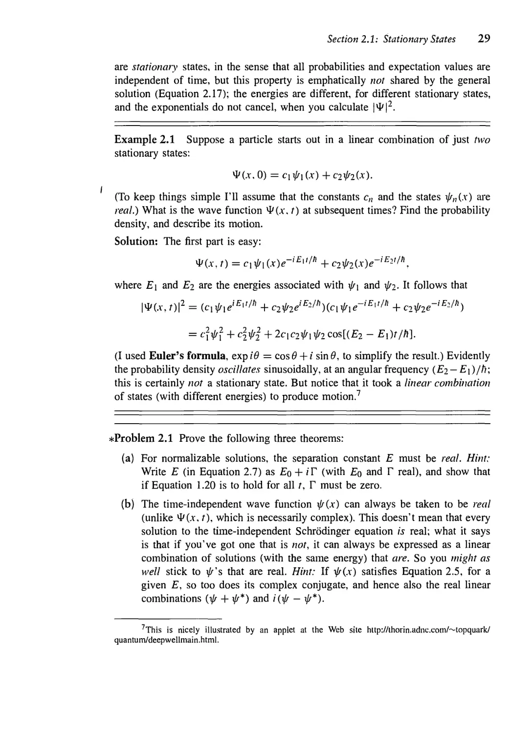
Example 2.1 Suppose a particle starts out in a linear combination of just two
stationary states:
*(*. 0) = ci fi (x) + cifiix).
(To keep things simple I'll assume that the constants cn and the states \j/n(x) are
real.) What is the wave function *I>(a\ t) at subsequent times? Find the probability
density, and describe its motion.
Solution: The first part is easy:
vl/(A% t) = c\f\{x)e-iE^fh + c2 i/o (*)<?"'" £2'//!,
where E\ and Ei are the energies associated with \f/[ and xj/j. It follows that
|y(.v,Ol2 = (cifieiE^^ +c2f2eiE2/h)(ciirie-iEi,/'1 +C2f2e~iE2/l1)
= c\fl + c\\lrl H-2cic2^i^2Cos[(£:2 - E\)t/fi].
(I used Euler's formula, exp IB — cos B -f- i sin B, to simplify the result.) Evidently
the probability density oscillates sinusoidally, at an angular frequency (E2 — Ei)/h;
this is certainly not a stationary state. But notice that it took a linear combination
of states (with different energies) to produce motion.7
^Problem 2.1 Prove the following three theorems:
(a) For normalizable solutions, the separation constant E must be real. Hint:
Write E (in Equation 2.7) as £o + 'T (with Eq and F real), and show that
if Equation 1.20 is to hold for all t, T must be zero.
(b) The time-independent wave function \j/(x) can always be taken to be real
(unlike ty(x. t), which is necessarily complex). This doesn't mean that every
solution to the time-independent Schrodinger equation is real; what it says
is that if you've got one that is not, it can always be expressed as a linear
combination of solutions (with the same energy) that are. So you might as
well stick to i/r's that are real. Hint: If i/(x) satisfies Equation 2.5, for a
given E, so too does its complex conjugate, and hence also the real linear
combinations (i/r + \f/*) and i(if/ — if/*).
'This is nicely illustrated by an applet at the Web site http://lhorin.adnc.com/~topquarky
quantum/deepwellmain.html.
30 Chapter! Time-Independent Schrodinger Equation
(c) If V(x) is an even function (that is, V(—x) = V(x)) then \j/(x) can always
be taken to be either even or odd. Hint: If yfr(x) satisfies Equation 2.5, for
a given E, so too does \f/(—x), and hence also the even and odd linear
combinations yfr(x) + \fr(—x).
*Problem 2.2 Show that E must exceed the minimum value of V(x), for every
normalizable solution to the time-independent Schrodinger equation. What is the
classical analog to this statement? Hint: Rewrite Equation 2.5 in the form
d2i/ 2m
dxl tr
if E < Vmin, then \j/ and its second derivative always have the same sign—argue
that such a function cannot be normalized.
2.2 THE INFINITE SQUARE WELL
Suppose
V(x)
0. ifO<A'<«,
oo. otherwise
[2.19]
(Figure 2.1). A particle in this potential is completely free, except at the two ends
(x = 0 and x = a), where an infinite force prevents it from escaping. A classical
model would be a cart on a frictionless horizontal air track, with perfectly elastic
bumpers—it just keeps bouncing back and forth forever. (This potential is
artificial, of course, but I urge you to treat it with respect. Despite its simplicity—or
rather, precisely because of its simplicity—it serves as a wonderfully
accessible test case for all the fancy machinery that comes later. We'll refer back to it
frequently.)
V(x)i
->- FIGURE 2.1: The infinite square well poten-
x tial (Equation 2.19).
Section 2.2: The Infinite Square Well 31
Outside the well, ij/(x) = 0 (the probability of finding the particle there is
zero). Inside the well, where V = 0, the time-independent Schrodinger equation
(Equation 2.5) reads
h2 d2ir
y = Ex//, [2.20]
2m dx
or
d2^ 1^ , u r ^2m£ mil
—=- = —k-d/, where /: = —-—. [2.21]
dx1 h
(By writing it in this way, I have tacitly assumed that E > 0; we know from
Problem 2.2 that E < 0 won't work.) Equation 2.21 is the classical simple
harmonic oscillator equation; the general solution is
\//(x) = A s'mkx + B cos kx, [2.22]
where A and B are arbitrary constants. Typically, these constants are fixed by the
boundary conditions of the problem. What are the appropriate boundary
conditions for i/f(x)? Ordinarily, both yj/ and d\J//dx are continuous, but where the
potential goes to infinity only the first of these applies. (I'll prove these boundary
conditions, and account for the exception when V = oo, in Section 2.5; for now I
hope you will trust me.)
Continuity of \//(x) requires that
^(0) = \/r(a) = 0, [2.23]
so as to join onto the solution outside the well. What does this tell us about A and
5? Well,
t/K0) = Asin0 + ficos0 = fi,
so B = 0, and hence
i/r(x) = Asmkx. [2.24]
Then \j/(a) = Asinka, so either A = 0 (in which case we're left with the
trivial—non-normalizable—solution }Jr(x) = 0), or else sin ka = 0, which means
that
ka = 0, ±tt, ±2tt, ±3tt, ... [2.25]
But k = 0 is no good (again, that would imply yj/(x) = 0), and the negative
solutions give nothing new, since sin(—0) = — sin(0) and we can absorb the
minus sign into A. So the distinct solutions are
mt
k„ = —. with n = 1, 2, 3. ... [2.26]
a
Time-Independent Schrodinger Equation
Vi(*)|
V|/2(X) A
¥3W-
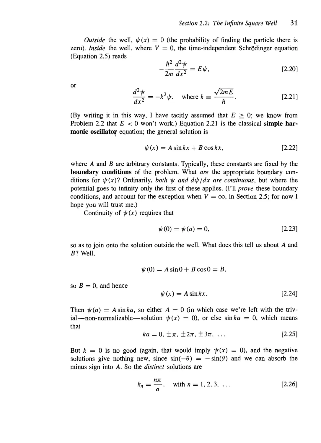
FIGURE 2.2: The first three stationary states of the infinite square well (Equation 2.28).
Curiously, the boundary condition at x = a does not determine the constant
A, but rather the constant k, and hence the possible values of E:
[2.27]
In radical contrast to the classical case, a quantum particle in the infinite square
well cannot have just any old energy—it has to be one of these special allowed
values.8 To find A, we normalize \}/:
f
Jo
|A|2 sm2(kx) dx = | A\2- = 1, so \A\2 = -.
2 a
This only determines the magnitude of A, but it is simplest to pick the positive real
root: A = *J2/a (the phase of A carries no physical significance anyway). Inside
the well, then, the solutions are
tyn (X) = J~
v!sin(T*)-
[2.28]
As promised, the time-independent Schrodinger equation has delivered an
infinite set of solutions (one for each positive integer n). The first few of these are
plotted in Figure 2.2. They look just like the standing waves on a string of length a;
\J/\, which carries the lowest energy, is called the ground state, the others, whose
energies increase in proportion to n2, are called excited states. As a collection, the
functions ^„(x) have some interesting and important properties:
1. They are alternately even and odd, with respect to the center of the well:
t/^i is even, \j/2 is odd, 1//3 is even, and so on.9
8Nolice lhal the quantization of energy emerged as a rather technical consequence of the
boundary conditions on solutions to the time-independent Schrodinger equation.
9To make this symmetry more apparent, some authors center the well at the origin (running it
from — a to +«)• The even functions are then cosines, and the odd ones are sines. See Problem 2.36.
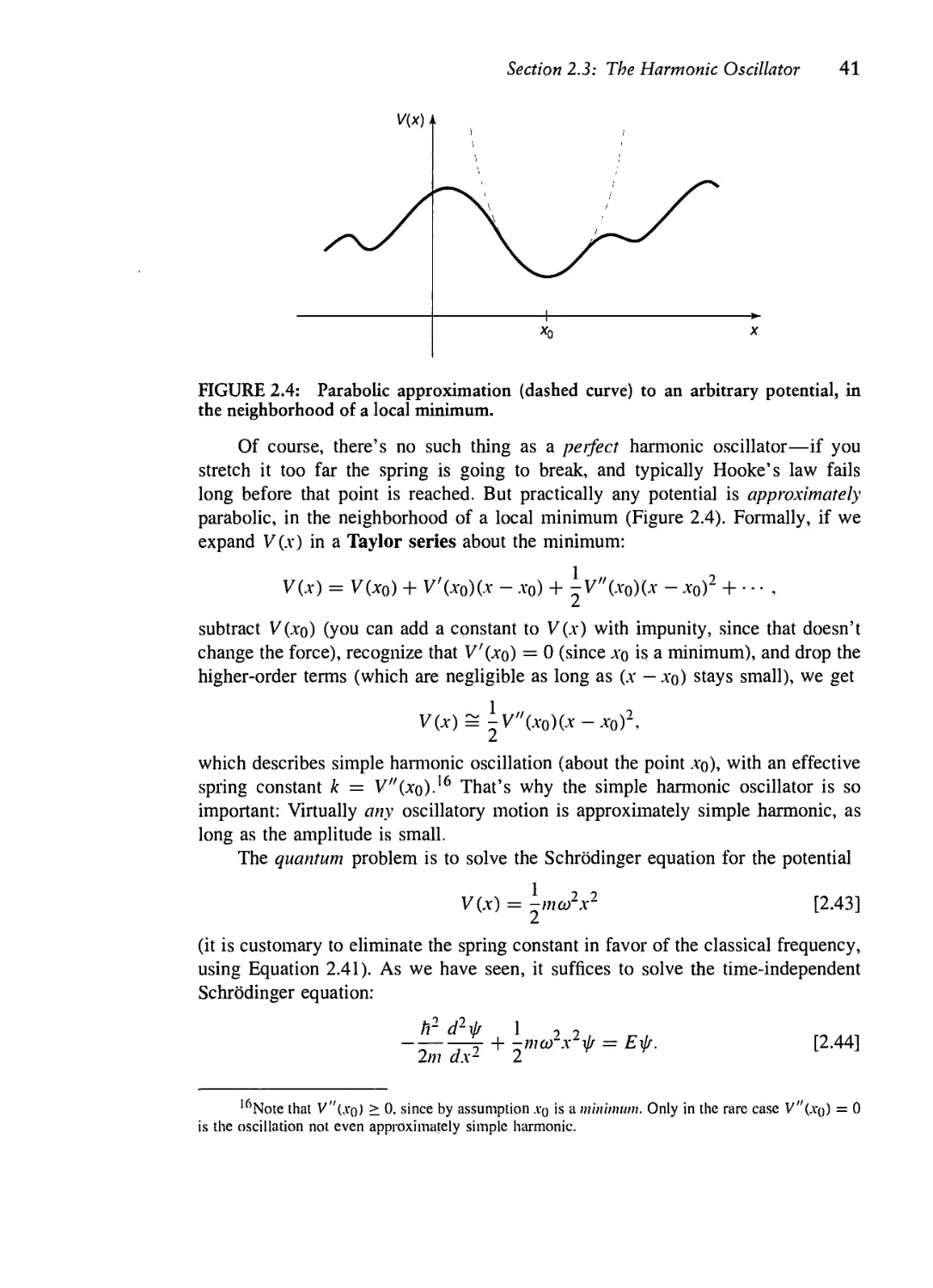
\
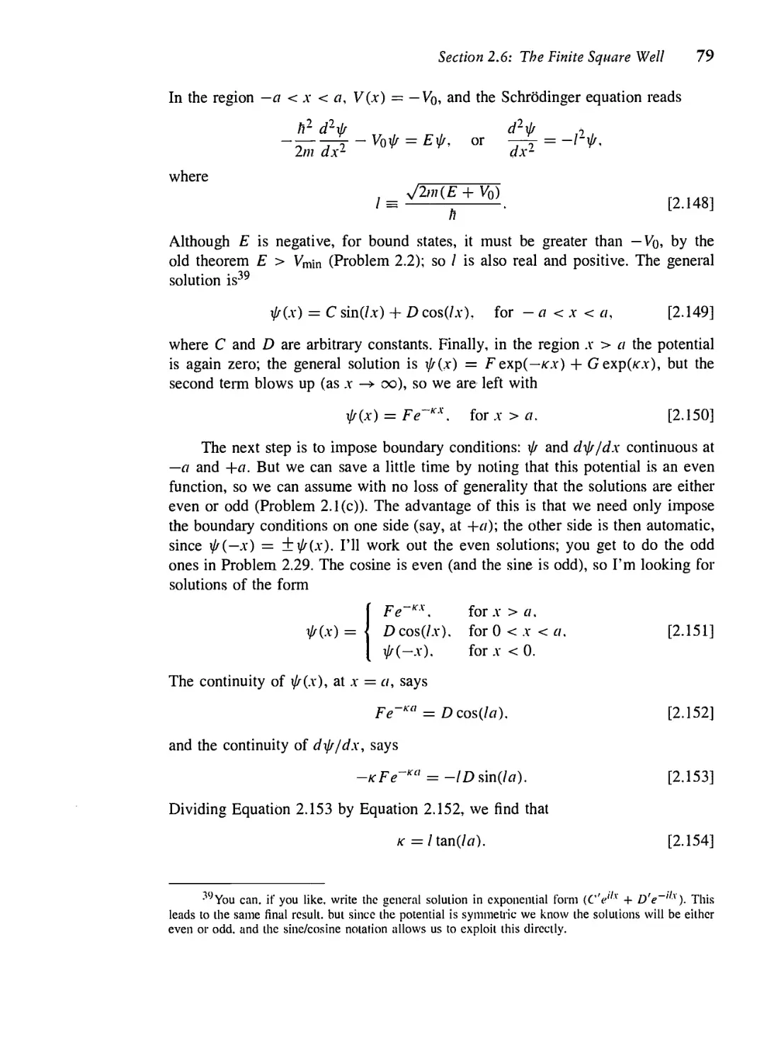
Section 2.2: The Infinite Square Well 33
2. As you go up in energy, each successive state has one more node (zero-
crossing): \f/i has none (the end points don't count), fa has one, fa has two, and
so on.
3. They are mutually orthogonal, in the sense that
[jfm(xrfa(x)dx = 0,
whenever m ^ n. Proof:
I fat(x)*fa(x) dx = - / sin (—■*) sin (—x) dx
1 rr (m-n \ fm+n \~| ,
= -1 cos Ttx — cos Ttx dx
a Jo I V a J \ a /J
. (m — n \ 1 . (m + n \\
—— sin Ttx — sin Ttx \
n)Tt \ a / (in + n)Tt \ a ) \
[2.29]
(m — n)it \ a ) (in +
sin[(w — n)rt] sin[(w + n)7t]
il
(m — n)
(m + n)
= 0.
Note that this argument does not work if m = n. (Can you spot the point at which
it fails?) In that case nonnalization tells us that the integral is 1. In fact, we can
combine orthogonality and normalization into a single statement:10
/ fa,(x)*fa
(x)dx = 5,,,,,,
[2.30]
where 5,,,,, (the so-called Kronecker delta) is defined in the usual way,
_ J 0, if iw #«;
5""'-j 1. \fm=n. [231]
We say that the \J/'s are orthonormal.
4. They are complete, in the sense that any other function, ./(.*), can be
expressed as a linear combination of them:
oo nr oo
fix) = ]T c„fa(x) = J- ]T c„ sin (—.vj
n=\ /7=1
[2.32]
In this case the Vr's-are real, so the * on rjrm is unnecessary, but for future purposes it's a good
idea to get in the habit of putting it there.
Time-Independent Schrodinger Equation
I'm not about to prove the completeness of the functions sin (tmx/a), but if you've
studied advanced calculus you will recognize that Equation 2.32 is nothing but the
Fourier series for f(x), and the fact that "any" function can be expanded in this
way is sometimes called Dirichlet's theorem.11
The coefficients c„ can be evaluated—for a given f(x)—by a method I call
Fourier's trick, which beautifully exploits the orthonormality of {\//n}: Multiply
both sides of Equation 2.32 by \//m(x)*, and integrate.
oo . oo
/ ,„«./(*)* = E,/«-v»V,W* = £>,„„ = cm. [2.33]
/1=1 /1 = 1
(Notice how the Kronecker delta kills every term in the sum except the one for
which n = m.) Thus the nth coefficient in the expansion of f(x) is12
■n = / fnO
x)*f(x)dx.
[2.34]
These four properties are extremely powerful, and they are not peculiar to the
infinite square well. The first is true whenever the potential itself is a symmetric
function; the second is universal, regardless of the shape of the potential.13
Orthogonality is also quite general—I'll show you the proof in Chapter 3. Completeness
holds for all the potentials you are likely to encounter, but the proofs tend to be
nasty and laborious; I'm afraid most physicists simply assume completeness, and
hope for the best.
The stationary states (Equation 2.18) of the infinite square well are evidently
*,,(.,.,) = y| sin (™x) e-'V-*/2'-2)'. [2.35]
I claimed (Equation 2.17) that the most general solution to the (time-dependent)
Schrodinger equation is a linear combination of stationary states:
¥(*. t) = Y,c»yJ- sin (—A") e-''("~V/?/W)'. [2.36]
/7 = 1
'' See, for example, Mary Boas, Mathematical Methods in the Physical Sciences, 2d cd. (New
York: John Wiley, 1983), p. 313; ,/'(.v) can even have a finite number of finite discontinuities.
'-It doesn't matter whether you use m or n as the "dummy index" here (as long as you are
consistent on the two sides of the equation, of course): whatever letter you use. it just stands for "any
positive integer."
1 * See. for example, John L. Powell and Bemd Crasemann, Quantum Mechanics (Addison-
Wesley, Reading. MA, 1961), p. 126.
Section 2.2: The Infinite Square Well 35
(If you doubt that this is a solution, by all means check it!) It remains only for
me to demonstrate that I can fit any prescribed initial wave function, ^(.v. 0), by
appropriate choice of the coefficients c„:
CO
^-,0) = ^,,^).
/1=1
The completeness of the \j/'s (confirmed in this case by Dirichlet's theorem)
guarantees that I can always express ^(.v,0) in this way, and their orthonormality
licenses the use of Fourier's trick to determine the actual coefficients:
c„ = J- sin (—Jc) *(-v. 0) dx.
[2.37]
That does it: Given the initial wave function, ^(.v.0), we first compute the
expansion coefficients c„, using Equation 2.37, and then plug these into Equation 2.36
to obtain vl>(.\\ t). Armed with the wave function, we are in a position to compute any
dynamical quantities of interest, using the procedures in Chapter 1. And this same
ritual applies to any potential—the only things that change are the functional form
of the 1^'s and the equation for the allowed energies.
Example 2.2 A particle in the infinite square well has the initial wave function
V(x. 0) = Ax (a - x). (0 < -v < a).
for some constant A (see Figure 2.3). Outside the well, of course, ^ = 0. Find
V(x.t).
A ^(x, 0)
FIGURE 2.3: The starting wave function in Example 2.2.
Time-Independent Schrodinger Equation
Solution: First we need to determine A, by normalizing vl>(.v, 0):
1= r|¥(jr,0)|2</jc = |A|2 fax2(a-x)2dx = \A\2^
Jo JO M
SO
A= /?°.
V a5
The /7th coefficient is (Equation 2.37)
„=^r,n(-v)/lo,(a_.v)rf,
V a Jo \ a / y a3
2v/l5 T fa . nm v f 2 . //77T \ ■
= —=— <:/ / .v sin I —x dx — I x sin I —x dx
a* L Jo v a I Jo \ a J _
2\/l5( \/ a \2 //77T \ ax /nn \\
= —— \a f—) sin f—x) cos!—a)
ai [ 1_V/77T/ \ a / /J7T V a /J 0
„/ a \2 . (nit \ (nitx/a)- — 2 /tut \
2 — I .v sin —a* J =— cos —x J
V/77r/ \ a / {nit ay \ a /
2v^l5
a-
o
3
3(/77T)2 -2
C0S(/77T) + a1 : = COS(/77T) + CT =- COS(0)
/77T (nity (nity
4</l5 r
-=; [COS(0) - COS(/77T)]
(mty
10, if /7 is even.
8vT5/(/7tt)3. if /7 is odd.
Thus (Equation 2.36):
V a \izJ *-? 773 V fl /
x 7 //=1.3.5...
Loosely speaking, c„ tells you the "amount of yjf„ that is contained in vl/."
Some people like to say that |c„|2 is the "probability of finding the particle in the
/7th stationary state," but this is bad language; the particle is in the state 4>, not
ty,,, and, anyhow, in the laboratory you don't "find a particle to be in a particular
state"—you measure some obseivable, and what you get is a number. As we'll
see in Chapter 3, what |c„|2 tells you is the probability that a measurement of the
Section 2.2: The Infinite Square Well 37
energy would yield the value E„ (a competent measurement will always return one
of the "allowed" values—hence the name—and \c„\2 is the probability of getting
the particular value E„).
Of course, the sum of these probabilities should be 1,
[2.38]
Indeed, this follows from the normalization of vj/ (the c„'s are independent of time,
so I'm going to do the proof for t = 0; if this bothers you, you can easily generalize
the argument to arbitrary t).
1
(CO \ ^ / CO \
oc oc
= E EC'»C» / fm(x)*fn(x)dx
m=\ n=\
CO CO
CO
= J21lc»>c"8»"' = J2\c"\2-
lt=l 111=1
»=1
(Again, the Kronecker delta picks out the term m = n in the summation over m.)
Moreover, the expectation value of the energy must be
CO
n=\
[2.39]
and this too can be checked directly: The time-independent Schrodinger equation
(Equation 2.12) says
Hfn = E„Vo,. [2.40]
so
(H) = J V*HVdx = J (]Tc„,Vo„)* H (][>"V0,) dx
= E Ec'»c»£» / *£*»dx = E ic»i2£»-
Notice that the probability of getting a particular energy is independent of time, and
so, a fortiori, is the expectation value of H. This is a manifestation of conservation
of energy in quantum mechanics.
Time-Independent Schrodinger Equation
Example 2.3 In Example 2.2 the starting wave function (Figure 2.3) closely
resembles the ground state yfr\ (Figure 2.2). This suggests that \c\ \2 should dominate,
and in fact
The rest of the coefficients make up the difference:14
,,= 1 \ * J n=TT.5....n
The expectation value of the energy, in this example, is
480/?2 y^ J_ _ 5/32
7T4ma2 fr1^ n4 ma2
,,=1.3.5....
As one might expect, it is very close to E\ = 7T2h~/2ma2—slightly larger, because
of the admixture of excited states.
Problem 2.3 Show that there is no acceptable solution to the (time-independent)
Schrodinger equation for the infinite square well with E = 0 or E < 0. (This is a
special case of the general theorem in Problem 2.2, but this time do it by explicitly
solving the Schrodinger equation, and showing that you cannot meet the boundary
conditions.)
^Problem 2.4 Calculate (x), (x~), {p), (p2), ax, and ap, for the /ith stationary state
of the infinite square well. Check that the uncertainty principle is satisfied. Which
state comes closest to the uncertainty limit?
*Problem 2.5 A particle in the infinite square well has as its initial wave function
an even mixture of the first two stationary states:
*U.0) = A[ylr\(x) + f2(x)l
1 You can look up the series
and
J_ 1 j_ _ 7T6
lfl + 3^ + 56 +""~ %()
111 jr4
1 1 h ■ ■ ■ = —
H 34 54 96
in math tables, under "Sums of Reciprocal Powers" or "Riemann Zela Function."
Section 2.2: The Infinite Square Well 39
(a) Normalize ^(x,0). (That is, find A. This is very easy, if you exploit the
orthonormality of %f/\ and yfri. Recall that, having normalized ^ at t = 0,
you can rest assured that it stays normalized—if you doubt this, check it
explicitly after doing part (b).)
(b) Find ty(x,t) and \ty(x,t)\2. Express the latter as a sinusoidal function of
time, as in Example 2.1. To simplify the result, let a> = jr-ft/2ma-.
(c) Compute (x). Notice that it oscillates in time. What is the angular frequency
of the oscillation? What is the amplitude of the oscillation? (If your amplitude
is greater than a/2, go directly to jail.)
(d) Compute (p). (As Peter Lorre would say, "Do it ze kveek vay, Johnny!")
(e) If you measured the energy of this particle, what values might you get, and
what is the probability of getting each of them? Find the expectation value
of H. How does it compare with E\ and £2?
Problem 2.6 Although the overall phase constant of the wave function is of no
physical significance (it cancels out whenever you calculate a measurable quantity),
the relative phase of the coefficients in Equation 2.17 does matter. For example,
suppose we change the relative phase of \f/\ and \j/2 in Problem 2.5:
W{x,0) = A[\lrax) + ei*\lr2{x)],
where (p is some constant. Find ^(x, t), \ty(x,t)\-, and (,r), and compare your
results with what you got before. Study the special cases <p = tt/2 and $> = tt.
(For a graphical exploration of this problem see the applet in footnote 7.)
*Problem 2.7 A particle in the infinite square well has the initial wave function15
nx o) = f Ax< ° -x - a/2<
v ; J A(a-x). a/2<x <a.
(a) Sketch W(x, 0), and determine the constant A.
(b) Find V(x.t).
1 •'There is no restriction in principle on the shape of the starting wave function, as long
as il is normalizable. In parlicular, ty(.v.O) need nol have a conlinuous derivative—in facl, il
doesn't even have to be a conlinuous function. However, if you iry 10 calculate (H) using
f ty(.v. 0)*//ty(.v-. 0)dx in such a case, you may encounter technical difficulties, because the second
derivative of #(x. 0) is ill-defined. Il works in Problem 2.9 because the discontinuities occur at Ihe end
points, where ihe wave function is zero anyway. In Problem 2.48 you'll see how to manage cases like
Problem 2.7.
40 Chapter 2 Time-Independent Schrodinger Equation
(c) What is the probability that a measurement of the energy would yield the
value E\ ?
(d) Find the expectation value of the energy.
Problem 2.8 A particle of mass m in the infinite square well (of width a) starts
out in the left half of the well, and is (at t = 0) equally likely to be found at any
point in that region.
(a) What is its initial wave function, vJ/(a',0)? (Assume it is real. Don't forget
to normalize it.)
(b) What is the probability that a measurement of the energy would yield the
value 7T2/72/2ma2l
Problem 2.9 For the wave function in Example 2.2, find the expectation value of
H, at time t = 0, the "old fashioned" way:
(H) = I V(x. 0)*HV(x, 0) dx.
Compare the result obtained in Example 2.3. Note: Because (H) is independent of
time, there is no loss of generality in using t = 0.
2.3 THE HARMONIC OSCILLATOR
The paradigm for a classical harmonic oscillator is a mass m attached to a spring
of force constant k. The motion is governed by Hooke's law,
v i d2x
F = —kx = m --^
dt-
(ignoring friction), and the solution is
x(t) = A sin(atf) + B cos(atf),
where
co = J- [2.41]
V m
is the (angular) frequency of oscillation. The potential energy is
V(x) = ^kx2; [2.42]
its graph is a parabola.
Section 2.3: The Harmonic Oscillator 41
V(X)A
FIGURE 2.4: Parabolic approximation (dashed curve) to an arbitrary potential, in
the neighborhood of a local minimum.
Of course, there's no such thing as a perfect harmonic oscillator—if you
stretch it too far the spring is going to break, and typically Hooke's law fails
long before that point is reached. But practically any potential is approximately
parabolic, in the neighborhood of a local minimum (Figure 2.4). Formally, if we
expand V(.v) in a Taylor series about the minimum:
V(x) = V(x0) + V'(xo)(x - a-o) + iV"(jto)(* - *o)2 + ■ • • ,
subtract V(xo) (you can add a constant to V(a") with impunity, since that doesn't
change the force), recognize that V'(xo) = 0 (since a'o is a minimum), and drop the
higher-order terms (which are negligible as long as (x — .vo) stays small), we get
V(x) = ^V"(x0)(x-x0)2,
which describes simple harmonic oscillation (about the point xo), with an effective
spring constant k = ^"(a-o).16 That's why the simple harmonic oscillator is so
important: Virtually any oscillatory motion is approximately simple harmonic, as
long as the amplitude is small.
The quantum problem is to solve the Schrodinger equation for the potential
t// \ * 2 2
V(x) = -mco x
[2.43]
(it is customary to eliminate the spring constant in favor of the classical frequency,
using Equation 2.41). As we have seen, it suffices to solve the time-independent
Schrodinger equation:
tr d2xj/ 1 2 2
■- pj- + -mco x f = Ef.
2m ax1 2
[2.44]
l6Note that V"(.vo) > 0. since by assumption xq is a minimum. Only in the rare case V"(.vo) = 0
is the oscillation not even approximately simple harmonic.
Time-Independent Schrodinger Equation
In the literature you will find two entirely different approaches to this problem.
The first is a straightforward "brute force" solution to the differential equation,
using the power series method; it has the virtue that the same strategy can be
applied to many other potentials (in fact, we'll use it in Chapter 4 to treat the
Coulomb potential). The second is a diabolically clever algebraic technique, using
so-called ladder operators. I'll show you the algebraic method first, because it is
quicker and simpler (and a lot more fun);17 if you want to skip the power series
method for now, that's fine, but you should certainly plan to study it at some
stage.
2.3.1 Algebraic Method
To begin with, let's rewrite Equation 2.44 in a more suggestive form:
— [p2 + {mcox)2]^ = Ef. [2.45]
2/7/
where p = {h/ i)d/dx is, of course, the momentum operator. The basic idea is to
factor the Hamiltonian,
H = —[p2 + {mcox)2]. [2.46]
2m
If these were numbers, it would be easy:
it + v~ = {in + v){—iu + v).
Here, however, it's not quite so simple, because p and x are operators, and
operators do not, in general, commute {xp is not the same as px). Still, this does
motivate us to examine the quantities
^=^(^+^)
[2.47]
(the factor in front is just there to make the final results look nicer).
Well, what is the product a-ci+7
1
a~a+ = {ip + mcox){—ip + mcox)
2ft mco
= — [p2 + {mcox)2 - imco{xp - px)].
Inmco
17We'll encounter some of the same strategies in the theory of angular momentum (Chapter 4).
and the technique generalizes to a broad class of potentials in super-symmetric quantum mechanics
(see. for example. Richard W. Robinett. Quantum Mechanics. (Oxford U.P., New York. 1997). Section
14.4).
Section 2.3: The Harmonic Oscillator 43
As anticipated, there's an extra term, involving (xp — px). We call this the
commutator of X and p; it is a measure of how badly they fail to commute. In general,
the commutator of operators A and B (written with square brackets) is
In this notation,
[A, B] = AB - BA.
1
CI-CI+ =
-) -> '
ol. IP' + (ma>x)~] - — [a\ p].
2ft m co 2ft
[2.48]
[2.49]
We need to figure out the commutator of a- and p. Warning: Operators are
notoriously slippery to work with in the abstract, and you are bound to make
mistakes unless you give them a "test function," f(x), to act on. At the end you
can throw away the test function, and you'll be left with an equation involving the
operators alone. In the present case we have:
[Jr, p]f(x) =
ft d „ ft d
i dx i dx
n ( df df \
= T X— -X—-f)= Iftf (A").
i V dx dx J
[2.50]
Dropping the test function, which has served its purpose,
[x, p] = ih.
[2.51]
This lovely and ubiquitous result is known as the canonical commutation
relation.18
With this, Equation 2.49 becomes
or
1 1
a-a+ = -—// + -.
ftCD 2
H = ftcD I a-a+ —
[2.52]
[2.53]
Evidently the Hamiltonian does not factor perfectly—there's that extra —1/2 on the
right. Notice that the ordering of a+ and a- is important here; the same argument,
with a+ on the left, yields
In particular,
1 „ 1
a+a- = —H .
ftCD 2
[a-,a+] = 1.
[2.54]
[2.55]
18In a deep sense all of the mysteries of quantum mechanics can be traced to the fact that position
and momentum do not commute. Indeed, some authors take the canonical commutation relation as an
axiom of the theory, and use it to derive p = (h/i)d/dx.
Time-Independent Schrodinger Equation
So the Hamiltonian can equally well be written
H = hco I a+a- +
1
[2.56]
In terms of a±, then, the Schrodinger equation19 for the harmonic oscillator takes
the form
hco
(«±*F±i)
±-)f = Ef
[2.57]
(in equations like this you read the upper signs all the way across, or else the lower
signs).
Now, here comes the crucial step: I claim that if \j/ satisfies the Schrodinger
equation with energy E, (that is: H\j/ = E\j/), then a+\j/ satisfies the Schrodinger
equation with energy (E + hco): H(a+\f/) = (E + hco){a+\}/). Proof:
H(a+\j/) = hco I a+ci- + - 1 (a+xf/) = hco I a+a-a+ + -a+ J if/
= hcoa+ lci-d+ + -) \f/ = a+
hco I a+a- + 1 + -1^
= a+(H + hco)\j/ = a+(E + ftco)\j/ = (E + hco)(a+\j/).
(I used Equation 2.55 to replace a~a+ by a+a- + 1, in the second line. Notice
that whereas the ordering of a+ and a- does matter, the ordering of a± and
any constants—such as h, co, and E—does not; an operator commutes with any
constant.)
By the same token, a-\f/ is a solution with energy (E — hco):
H(ci-\j/) = hco I a-a+ — - ] (fl-VO = hcoci- I a+ci- — - I \f/
= a-
hco I a-a+ - 1 - - j \j/
= a-(H — hco)\j/ = a-(E — hco)\j/
= (E - hoj)(a-i/).
Here, then, is a wonderful machine for generating new solutions, with higher and
lower energies—if we could just find one solution, to get started! We call a±
ladder operators, because they allow us to climb up and down in energy; a+ is
the raising operator, and a- the lowering operator. The "ladder" of states is
illustrated in Fisure 2.5.
19I'm getting tired of writing ''time-independent Schrodinger equation," so when it's clear from
the context which one I mean. I'll just call it the "Schrodinger equation."
Section 2.3: The Harmonic Oscillator 45
FIGURE 2.5: The "ladder" of states for the harmonic oscillator.
But wait! What if I apply the lowering operator repeatedly? Eventually I'm
going to reach a state with energy less than zero, which (according to the general
theorem in Problem 2.2) does not exist! At some point the machine must fail.
How can that happen? We know that ci-\j/ is a new solution to the Schrodinger
equation, but there is no guarantee that it will be normalizable—it might be zero,
or its square-integral might be infinite. In practice it is the former: There occurs a
"lowest rung" (call it \j/o) such that
a-i,0 = 0. [2.58]
We can use this to determine \j/q(x):
ltd \
, [h-r + m(0X )fo = 0.
s/lhmco \ ax J
Time-Independent Schrodinger Equation
or
dxf/Q mco
dx h
This differential equation is easy to solve:
d\[/o mco
to
so
/
h
/.V„.V
Xf0-
, , mco -,
In y/Q = —x" + constant.
2/J
_ into 2
xj/0(x) = Ae 2ft A .
We might as well normalize it right away:
\ = \A\2 (°° e-'"»x2/hdx = \A\\[^-
J-oo V m cc
so A1 = y/mco/jrh, and hence
[2.59]
To determine the energy of this state we plug it into the Schrodinger equation (in
the form of Equation 2.57), hco(a+ci- + 1/2)^0 = Eofa, and exploit the fact that
a-xj/o = 0:
£o = \hco. [2.60]
With our foot now securely planted on the bottom rung (the ground state of the
quantum oscillator), we simply apply the raising operator (repeatedly) to generate
the excited states,20 increasing the energy by hco with each step:
[2.61]
where A„ is the normalization constant. By applying the raising operator
(repeatedly) to t/tq, then, we can (in principle) construct all21 the stationary states of
20In the case of the harmonic oscillator it is customary, for some reason, to depart from the usual
practice, and number the states starting with n — 0, instead of n = 1. Obviously, the lower limit on the
sum in a formula such as Equation 2.17 should be altered accordingly.
-lNote that we obtain all the (normalizable) solutions by this procedure. For it" there were some
other solution, we could generate from it a second ladder, by repeated application of the raising and
lowering operators. But the bottom rung of this new ladder would have to satisfy Equation 2.58, and
since that leads inexorably to Equation 2.59, the bottom rungs would be the same, and hence the two
ladders would in fact be identical.
Section 2.3: The Harmonic Oscillator 47
the hamionic oscillator. Meanwhile, without ever doing that explicitly, we have
determined the allowed energies.
Example 2.4 Find the first excited state of the harmonic oscillator.
Solution: Using Equation 2.61,
1/4
A\ ( d \ (mo)\ ' _>mo i
i/i (x) = A\a+\j/0 = -^3-+m(i)X )\—T e u'
/ma>\' lima) _w<jdl.2
=AiU v—~
[2.62]
We can normalize it "by hand":
so, as it happens, A\ = 1.
I wouldn't want to calculate xf/so this way (applying the raising operator fifty
times!), but never mind: In principle Equation 2.61 does the job—except for the
normalization.
You can even get the normalization algebraically, but it takes some fancy
footwork, so watch closely. We know that a±\f/n is proportional to \j/n±\,
a+\lfn = c„ fn+\, a- fn = dn VOi—i [2-63]
but what are the proportionality factors, c„ and d„'l First note that for "any"22
functions f(x) and g(x),
/00 /»0O
f*(a±g)dx = (aTf)*gdx. [2.64]
-co «/—CO
(In the language of linear algebra, a^ is the hermitian conjugate of a ±.)
Proof:
/ f*(ct±g)dx = / f*(Th—+ max )gdx..
J-cc y/lhmo) J-oo V dx J
±oo.
-~0f course, the integrals must exist, and this means that /(.v) and g(x) must go to zero at
Time-Independent Scbrodinger Equation
and integration by parts takes f f*(dg/dx)dx to — J(df/dx)*gdx (the boundary
terms vanish, for the reason indicated in footnote 22), so
/00
-co
±g)dx =
1
y/2hm(D
J-oQ l_\ dx
-I*
+ mcox) f
/OO
<
-oc
gdx = (a^fTgdx,
QED
In particular,
/OO /»CO
(fl ± ^/i) * (A ± ^/i) ^A" = / (flTfl ± VOi) * VOi ^A' •
-co J-oc
But (invoking Equations 2.57 and 2.61)
a+a-fn = mjr„, a-a+f„ = (n+l)f„.
[2.65]
so
J-oc
»oo
/OO /»0C
|T/r„+I|2c/A" = (/1 + 1)/ l^nl2^-
-co ./-co
/OO /»CO /»CO
(«_^,)*(«-^)^ = K|2 / |^,-i|2«/jr = n / llM2*/*.
-OO «/—oo «/—OO
But since \j/„ and ^r„ +_ \ are normalized, it follows that \c„ \~ = n +1 and |J„ |2 = »,
and hence
a+f„ = Jn + 11/0,+1, fl-^n = Vnfn-i-
[2.66]
Thus
1 1 ,
1
1
* = 71°^1 = VJT2
and so on. Clearly
1
1
V4 V4•3 • 2
(fl+)Vo*
^/1 = -j== (0+^^0-
[2.67]
which is to say that the normalization factor in Equation 2.61 is An = 1/VhT (in
particular, A\ = 1, confirming our result in Example 2.4).
Section 2.3: The Harmonic Oscillator 49
As in the case of the infinite square well, the stationary states of the harmonic
oscillator are orthogonal:
/co
-oc
f*fndx = 5,
inn-
[2.68]
This can be proved using Equation 2.65, and Equation 2.64 twice—first moving
a+ and then moving a_:
/oo /»oo
ir*„ (a+fl-) ir„ dx =n I tfr * f„ dx
-oo J -oo
/OO /»0O
{a-\jrm)*{a-ifn)dx= / (a+a-f,„)*$„ dx
-oo J—oc
='"/
CO
fmfndx.
oo
Unless w = /7, then, f\l/*\f/„dx must be zero. Orthonomiality means that we
can again use Fourier's trick (Equation 2.34) to evaluate the coefficients, when we
expand ty(x, 0) as a linear combination of stationary states (Equation 2.16), and
|c„|2 is again the probability that a measurement of the energy would yield the
value En.
Example 2.5 Find the expectation value of the potential energy in the /7 th state
of the harmonic oscillator.
Solution:
1
2"
tt\ 1 o/ 1
(V) = { -mco~x~) = -ma>~ I \js*x-\j/n d:
x.
There's a beautiful device for evaluating integrals of this kind (involving powers
of .,v or p): Use the definition (Equation 2.47) to express .v and p in terms of the
raising and lowering operators:
h lima)
(C1++CI-): p = /./ —-—(«+—fl_).
2m (o
[2.69]
In this example we are interested in .v2:
A'" =
n r
2ni(o
So
(V)
ft® f I*
-T *:
(a+)2 + (a+a-) + (fl_fl+) + (a-)2
(a+)~ + (a+a-) + (fl-fl+) + (ci-Y
\j/n dx.
Time-Independent Schrodinger Equation
But (a+)2Voi is (apart from normalization) 1^,,+2, which is orthogonal to \j/n, and
the same goes for (a-)2\f/n, which is proportional to i/n-2- So those terms drop
out, and we can use Equation 2.65 to evaluate the remaining two:
ha) 1 ( \\
(V) = — (n + n + 1) = -ha> In + - J .
As it happens, the expectation value of the potential energy is exactly half the
total (the other half, of course, is kinetic). This is a peculiarity of the harmonic
oscillator, as we'll see later on.
♦Problem 2.10
(a) Construct 1/^2 (-0-
(b) Sketch \J/o, \j/\, and 1/0.
(c) Check the orthogonality of t/tq, \j/\, and 1/0, by explicit integration. Hint: If
you exploit the even-ness and odd-ness of the functions, there is really only
one integral left to do.
♦Problem 2.11
(a) Compute (x), (/?). (.v2), and (p2), for the states \f/o (Equation 2.59) and \f/\
(Equation 2.62), by explicit integration. Comment: In this and other problems
involving the harmonic oscillator it simplifies matters if you introduce the
variable £ = s/mco/h x and the constant a = (mco/nh)x^.
(b) Check the uncertainty principle for these states.
(c) Compute (T) (the average kinetic energy) and {V) (the average potential
energy) for these stales. (No new integration allowed!) Is their sum what you
would expect?
*Problem 2.12 Find (a*), (p), (x2), (p2), and (T), for the /7th stationary state of the
harmonic oscillator, using the method of Example 2.5. Check that the uncertainty
principle is satisfied.
Problem 2.13 A particle in the harmonic oscillator potential starts out in the state
*(.r.O) = A[3^o(*)+4TM.v)].
(a) Find A.
(b) Construct *(.v.r) and |vI/(a\ f)|2.
Section 2.3: The Harmonic Oscillator 51
(c) Find (x) and (p). Don't get too excited if they oscillate at the classical
frequency; what would it have been had I specified faix), instead of \j/\ (x)?
Check that Ehrenfest's theorem (Equation 1.38) holds for this wave function.
(d) If you measured the energy of this particle, what values might you get, and
with what probabilities?
Problem 2.14 A particle is in the ground state of the harmonic oscillator with
classical frequency a>, when suddenly the spring constant quadruples, so to' = 2a>,
without initially changing the wave function (of course, vj/ will now evolve
differently, because the Hamillonian has changed). What is the probability that a
measurement of the energy would still return the value ftco/21 What is the probability
of getting ftcol [Answer: 0.943.]
2.3.2 Analytic Method
We return now to the Schrodinger equation for the harmonic oscillator,
ft1 d2xj/ 1 , ,
V + -m(D2x2xj/ = Ef. [2.70]
2m dx2 2
and solve it directly, by the series method. Things look a little cleaner if we
introduce the dimensionless variable
I mm
[2.71]
in terms
where K
of £ the Schrodinger
III
equation
d2yj/
Imco
Vfiv;
reads
i^-K
is the energy, in units of (l/2)/?a>:
K
_ 2E
ftco
[2.72]
[2.73]
Our problem is to solve Equation 2.72, and in the process obtain the "allowed"
values of K (and hence of E).
To begin with, note that at very large £ (which is to say, at very large x), £2
completely dominates over the constant K, so in this regime
-Jr * *V< [2.74]
d$~
which has the approximate solution (check it!)
1r(%) % Ae~t2/2 + Be+*1/2. [2.75]
Time-Independent Schrodinger Equation
The B term is clearly not normalizable (it blows up as |jc| -> oo); the physically
acceptable solutions, then, have the asymptotic form
^(S) -► ( )^2/2< at large £. [2.76]
This suggests that we "peel off" the exponential part,
W$) = /i($)«~|2/2, [2.77]
in hopes that what remains, /?(£), has a simpler functional form than i/r(£) itself.23
Differentiating Equation 2.77,
df (dh \ _ti/2
and
dH /^_2^ + (f._1)/V-,V2!
df- \df- "s^
so the Schrodinger equation (Equation 2.72) becomes
d2h dh
— -2l;— + (K-\)h=0. [2.78]
#f- d%
I propose to look for solutions to Equation 2.78 in the form of power series
in £.
h<&) = fl0 + fl|? +02^2 + • ■- = J2ajtJ- [2J9]
/=0
Differentiating the series term by term,
-=0,+ 2a2£ + 3a^2 + • • • = V JaiSJ~
j=Q
and
d2h °°
—j = 2c,2 + 2 • 3fl3£ + 3 • 4«4£2 + --- = T]U + 1)0' + 2)aj+2^.
-•'Note that although we invoked some approximations to motivate Equation 2.77. what
follows is exact. The device of stripping off the asymptotic behavior is the standard first step in
the power series method for solving differential equations-—see, for example. Boas (footnote 11).
Chapter 12.
-4This is known as the Frobenius method for solving a differential equation. According to
Taylor's iheorem. any reasonably well-behaved function can be expressed as a power scries, so
Equation 2.79 ordinarily involves no loss of generality. For conditions on the applicability of the
method, see Boas (footnote 11) or George B. Arfken and Hans-Jurgen Weber, Mathematical Methods
for Physicists. 5th cd.. Academic Press. Orlando (2000). Section 8.5.
Section 2.3: The Harmonic Oscillator 53
Putting these into Equation 2.78, we find
oo
J2 [U + DC/ + 2)0./+2 - 2jaj + (K- \)aj] £•'' = 0. [2.80]
7=0
It follows (from the uniqueness of power series expansions25) that the coefficient
of each power of £ must vanish,
(j + 1)(7 + 2)aj+2 - 2jaj + (K - l)aj = 0,
and hence that
(2j + 1-K)
a;+-> = a;. [2.81]
J (./ + 1)0+2) J
This recursion formula is entirely equivalent to the Schrodinger equation.
Starting with ao, it generates all the even-numbered coefficients:
(1-/0 (5-K) (5-/0(1-/0
—^-«>. a4 = —[j-a2 =
and starting with a\, it generates the odd coefficients
a2 = —^-a{), a4 = —[j-a2 = a0t
(3-K) (7-/0 (7-/0(3-/0
«3 = —g—-.. ^ = -^-^ = 120 fl,< "•••
We write the complete solution as
/*(£)=/*even(S) + /*odd(£). [2.82]
where
hcvcn(Z) = «0 + aii1 + «4?4 H
is an even function of £, built on ao, and
/*odd(£) = fli£+fl3£3+tf5£5 + ---
is an odd function, built on a\. Thus Equation 2.81 determines /z(£) in terms of
two arbitrary constants (ao and a\)—which is just what we would expect, for a
second-order differential equation.
However, not all the solutions so obtained are normalizable. For at very large
j, the recursion formula becomes (approximately)
2
c'j+2 « -aj,
^Sce. for example. Arfkcn (footnote 24). Section 5.7.
Time-Independent Schrodinger Equation
with the (approximate) solution
C
a,- % .
7 072)!
for some constant C, and this yields (at large £, where the higher powers dominate)
'?; ^ 072)! ^j\q
Now, if /7 goes like exp(£2), then \(/ (remember \f/l—that's what we're trying to
calculate) goes like exp(£2/2) (Equation 2.77), which is precisely the asymptotic
behavior we didn't want.26 There is only one way to wiggle out of this: For
normalizable solutions the power series must terminate. There must occur some
"highest" j (call it /?), such that the recursion formula spits out an+2 = 0 (this will
truncate either the series /zCvcn or the series /7 odd; the other one must be zero from
the start: ci\ = 0 if n is even, and ciq = 0 if n is odd). For physically acceptable
solutions, then, Equation 2.81 requires that
K = 2h + 1.
for some non-negative integer /7, which is to say (referring to Equation 2.73) that
the energy must be
E„ = (n + -)h(o. for n =0.1,2 [2.83]
Thus we recover, by a completely different method, the fundamental quantization
condition we found algebraically in Equation 2.61.
It seems at first rather surprising that the quantization of energy should
emerge from a technical detail in the power series solution to the Schrodinger
equation, but let's look at it from a different perspective. Equation 2.70 has
solutions, of course, for any value of E (in fact, it has two linearly independent
solutions for every E). But almost all of these solutions blow up exponentially at
large x, and hence are not normalizable. Imagine, for example, using an E that
is slightly less than one of the allowed values (say, 0.49/?a>), and plotting the
solution (Figure 2.6(a)); the "tails" fly off to infinity. Now try an E slightly larger
(say, 0.51/"7a>); the "tails" now blow up in the other direction (Figure 2.6(b)). As
you tweak the parameter in tiny increments from 0.49 to 0.51, the tails flip over
when you pass through 0.5—only at precisely 0.5 do the tails go to zero, leaving
a normalizable solution.27
-"It's no surprise lhal the ill-behaved solutions are still contained in Equation 2.81: this recursion
relation is equivalent to the Schrodinger equation, so it's got to include both the asymptotic forms we
found in Equation 2.75.
27 It is possible to set this up on a computer, and discover the allowed energies "experimentally."
You might call it the wag the dog method: When the tail wags, you know you've just passed over an
allowed value. See Problems 2.54-2.56.
Section 2.3: The Harmonic Oscillator 55
1
-4
i
-2
A
2
1.5
X 0.5
-0.5
-1
-1.5
-2
:
'-
>v
\
1
2
4$
(a)
1
-4 .
/^1 -2
j
2
1.5
/o.5
-0.5
-1
-1.5
-2
i
"
':
2 ^
1 >
\ n
(b)
FIGURE 2.6: Solutions to the Schrodinger equation for (a) E = 0.49 fico, and
(b)E = 0.51/1«.
For the allowed values of K, the recursion formula reads
«y+2
-20? - j)
(7 + 1)(7+2)
fly-
If n = 0, there is only one term in the series (we must pick a \
and 7=0 in Equation 2.84 yields «2 = 0):
[2.84]
0 to kill /20Cid,
/?()(£) =flo.
and hence
V'o(£) = a0e $~12
Time-Independent Schrodmger Equation
(which, apart from the normalization, reproduces Equation 2.59). For n = 1 we
take «o = 0,28 and Equation 2.84 with j = 1 yields «3 = 0, so
and hence
M$) = <M$.
tfr,($) = a^e-^~'2
(confirming Equation 2.62). For n = 2, 7 — 0 yields «2 = — 2«o> and 7=2 gives
«4 = 0, so
and
h2(t)=a0(\-2$2).
M$) = «od -2$2)«"*2/2.
and so on. (Compare Problem 2.10, where this last result was obtained by algebraic
means.)
In general, //„(£) will be a polynomial of degree 11 in £, involving even powers
only, if n is an even integer, and odd powers only, if n is an odd integer. Apart
from the overall factor («o or a\) they are the so-called Hermite polynomials,
#„(£).29 The first few of them are listed in Table 2.1. By tradition, the arbitrary
multiplicative factor is chosen so that the coefficient of the highest power of £
is 2". With this convention, the normalized30 stationary states for the harmonic
oscillator are
fn(x) =
mco
1/4
1
:#„($)<?
-f-/2
[2.85]
They are identical (of course) to the ones we obtained algebraically in Equation 2.67.
TABLE 2.1: The first few Hermite
polynomials, H„(%).
H0-
Hy-
H2 =
#3 =
HA--
H5-
= 1,
= ¾.
= 4^2_
= 8¾3 -
= 16¾4
= 32¾5
2,
1¾
- 48¾2 +
-160^-
12,
f120¾.
28Note lhal there is a completely different set of coefficients aj for each value of n.
29The Hermite polynomials have been studied extensively in the mathematical literature, and
there are many tools and tricks for working with them. A few of these are explored in Problem 2.17.
30I shall not work out the normalization constant here: if you are interested in knowing how it is
done, see for example Leonard Schiff, Quantum Mechanics, 3rd ed., McGraw-Hill, New York (1968).
Section 13.
Section 2.3: The Harmonic Oscillator 57
In Figure 2.7(a) I have plotted \j/n(x) for the first few /?'s. The quantum
oscillator is strikingly different from its classical counterpart—not only are the
energies quantized, but the position distributions have some bizarre features. For
instance, the probability of finding the particle outside the classically allowed range
(that is, with x greater than the classical amplitude for the energy in question) is
not zero (see Problem 2.15), and in all odd states the probability of finding the
particle at the center is zero. Only at large n do we begin to see some resemblance
to the classical case. In Figure 2.7(b) I have superimposed the classical position
distribution on the quantum one (for n = 100); if you smoothed out the bumps,
the two would fit pretty well (however, in the classical case we are talking about
the distribution of positions over time for one oscillator, whereas in the quantum
case we are talking about the distribution over an ensemble of identically prepared
systems).31
Problem 2.15 In the ground state of the harmonic oscillator, what is the probability
(correct to three significant digits) of finding the particle outside the classically
allowed region? Hint: Classically, the energy of an oscillator is E = (l/2)ka2 =
{\/2)marar, where a is the amplitude. So the "classically allowed region" for an
oscillator of energy E extends from —y/2E/mco2 to +y/2E/mco2. Look in a math
table under "Normal Distribution" or "Error Function" for the numerical value of
the integral.
Problem 2.16 Use the recursion formula (Equation 2.84) to work out //5(^) and
//g(£). Invoke the convention that the coefficient of the highest power of £ is 2"
to fix the overall constant.
* * Problem 2.17 In this problem we explore some of the more useful theorems (stated
without proof) involving Hermite polynomials.
(a) The Rodrigues formula says that
Hn^) = (-\)"e^(J^j e-*\ [2.86]
Use it to derive H$ and //4.
(b) The following recursion relation gives you Hn+\ in terms of the two
preceding Hermite polynomials:
//„+,(£) = 2£//„(£) - 2/7#„_,(£). [2.87]
Use it, together with your answer in (a), to obtain //5 and H^.
- 'The parallel is perhaps more direct if you interpret the classical distribution as an ensemble of
oscillators all with the same energy, but with random starting times.
2 Time-Independent Schrodinger Equation
|Vl00(x)i2 0.24 r
0.20 -
0.16 -
0.12
0.06 -
0.04 -
(a)
/7 = 3
/7 = 2
/7=1
/7 = 0
(b)
FIGURE 2.7: (a) The first four stationary states of the harmonic oscillator. This
material is used by permission of John Wiley 8c Sons, Inc.; Stephen Gasiorowicz,
Quantum Physics, John Wiley 8c Sons, Inc., 1974. (b) Graph of |^iool2> w^h l^e
classical distribution (dashed curve) superimposed.
Section 2.4: The Free Particle 59
(c) If you differentiate an nth-order polynomial, you get a polynomial of order
(n — 1). For the Hermite polynomials, in fact,
^=2,7//,,,^). [2.88]
Check this, by differentiating H$ and H(>.
(d) Hn (£) is the »th z-derivative, at z = 0, of the generating function exp(—z2 +
2z%)\ or, to put it another way, it is the coefficient of z"/n\ in the Taylor
series expansion for this function:
«-=2+2* = 5^/^). [2.89]
Use this to rederive Hq, H\, and Hi.
/7=0
2.4 THE FREE PARTICLE
We turn next to what should have been the simplest case of all: the free particle
(V(x) = 0 everywhere). Classically this would just mean motion at constant
velocity, but in quantum mechanics the problem is surprisingly subtle and tricky. The
time-independent Schrodinger equation reads
h2 d2i/
\ = Ef. [2.90]
2m dx
or
d~\l/ i y/2mE
—L = -k2f, vj\ierek=- . [2.91]
dx- h
So far, it's the same as inside the infinite square well (Equation 2.21), where the
potential is also zero; this time, however, I prefer to write the general solution in
exponential form (instead of sines and cosines), for reasons that will appear in due
course:
yjr (x) = Aeikx + Be-ikx. [2.92]
Unlike the infinite square well, there are no boundary conditions to restrict the
possible values of k (and hence of E); the free particle can carry any (positive)
energy. Tacking on the standard time dependence, exp{—iEt/h),
vl/(x, t) = Aeik{x-^n + Be-iHx+^n. [2.93]
Now, any function of x and t that depends on these variables in the special
combination (x + vt) (for some constant v) represents a wave of fixed profile,
traveling in the :pf-direction, at speed v. A fixed point on the waveform (for
Time-Independent Schrodinger Equation
example, a maximum or a minimum) corresponds to a fixed value of the argument,
and hence to x and t such that
x + vt = constant, or x = =fvt + constant.
Since every point on the waveform is moving along with the same velocity, its
shape doesn't change as it propagates. Thus the first term in Equation 2.93
represents a wave traveling to the right, and the second represents a wave (of the same
energy) going to the left. By the way, since they only differ by the sign in front of
k, we might as well write
Vk{.\\t) = Aei{kx-!^t\ [2.94]
and let k run negative to cover the case of waves traveling to the left:
, y/lmE f k > 0 => traveling to the right, „ __.,
k = ± . with { , .. , , r«. [2.951
/j [ k < 0 => traveling to the left. J
Evidently the "stationary states" of the free particle are propagating waves; their
wavelength is k = 2n/\k\, and, according to the de Broglie formula (Equation 1.39),
they carry momentum
p = hk. [2.96]
The speed of these waves (the coefficient of t over the coefficient of x) is
-*'*' _ E nan
^quantum — ~ — w « ■ l~-"'J
On the other hand, the classical speed of a free particle with energy E is given by
E = (l/2)mir (pure kinetic, since V = 0), so
_ 2E _
^classical = \/ = ^'quantum- [2.98J
m
Apparently the quantum mechanical wave function travels at half the speed of the
particle it is supposed to represent! We'll return to this paradox in a moment—there
is an even more serious problem we need to confront first: This wave function is
not normalizable. For
/-t-oo r+oo
V];Vkdx = \A\2 / dx = |A|2(oo). [2.99]
-co J—oo
In the case of the free particle, then, the separable solutions do not represent
physically realizable states. A free particle cannot exist in a stationary state; or,
to put it another way, there is no such thing as a free particle with a definite
energy.
Section 2.4: The Free Particle 61
But that doesn't mean the separable solutions are of no use to us, for they
play a mathematical role that is entirely independent of their physical
interpretation. The general solution to the time-dependent Schrodinger equation is still a
linear combination of separable solutions (only this time it's an integral over the
continuous variable k, instead of a sum over the discrete index n):
[2.100]
(The quantity l/y/ln is factored out for convenience; what plays the role of the
coefficient c„ in Equation 2.17 is the combination (\/y/2n)<p(k)dk.) Now this
wave function can be normalized (for appropriate 0(fc)). But it necessarily carries
a range of fc's, and hence a range of energies and speeds. We call it a wave
packet.32
In the generic quantum problem, we are given ty(x, 0), and we are asked to
find y(x,t). For a free particle the solution takes the form of Equation 2.100;
the only question is how to determine 0(fc) so as to match the initial wave
function:
* (jr. 0) =
-co
ikx
0 (*)<?'" dk.
[2.101]
This is a classic problem in Fourier analysis; the answer is provided by Plancherel's
theorem (see Problem 2.20):
[2.102]
F(k) is called the Fourier transform of f(x)\ f(x) is the inverse Fourier
transform of F(k) (the only difference is in the sign of the exponent). There is, of
course, some restriction on the allowable functions: The integrals have to exist}*
For our purposes this is guaranteed by the physical requirement that ^(.v. 0) itself
-^Sinusoidal waves extend out to infinity, and they are not normalizable. But superpositions of
such waves lead to interference, which allows for localization and normalizability.
■,3The necessary and sufficient condition on f(x) is that /^, \f(x)\2dx be finite. (In that
case f^ \F(k)\-dk is also finite, and in fact the two integrals are equal.) Sec Arfken (footnote 24).
-3C
Section 15.5.
Time-Independent Scbrodinger Equation
be normalized. So the solution to the generic quantum problem, for the free particle,
is Equation 2.100, with
[2.103]
Example 2.6 A free particle, which is initially localized in the range —a < x < a,
is released at time t = 0:
_ _ f A, if — a < x < a,
[ 0, otherwise,
where A and a are positive real constants. Find ty (x, t).
Solution: First we need to normalize 4>(a\ 0):
/oo pa
|vI/(a\0)|2c/a- = \A\2 / dx = 2a\A\2 => A =
-oo J—a
Next we calculate ¢(1(), using Equation 2.103:
1 1
1 1 Ca 1
V27T V2fl J-a IJllCl
,-ikx
Jka _ p—ika
kJWa
2i
-ik
1 sin (ka)
■s/tFci k
Finally, we plug this back into Equation 2.100:
If00 sin(fctf) ;a... m2m „
*(jc.r) = —= / —^-—e'^-^0 dk.
Tty/la J-oo k
[2.104]
Unfortunately, this integral cannot be solved in tenns of elementary functions,
though it can of course be evaluated numerically (Figure 2.8). (There are, in fact,
precious few cases in which the integral for vJ/(a\ t) (Equation 2.100) can be
calculated explicitly; see Problem 2.22 for a particularly beautiful example.)
It is illuminating to explore the limiting cases. If a is very small, the starting
wave function is a nicely localized spike (Figure 2.9(a)). In this case we can use
the small angle approximation to write sm(ka) % ka, and hence
<t>{k)
Section 2.4: The Free Particle 63
u|¥(x,0l2
FIGURE 2.8: Graph of |*(x, t)\2 (Equation 2.104) at t = 0 (the rectangle) and at
t = ma2/h (the curve).
V2a
V(X, 0)
m
/a/n
(a) (b)
FIGURE 2.9: Example 2.6, for small a. (a) Graph of W(x, 0). (b) Graph of 4>{k).
it's yfotf, since the fc's cancelled out (Figure 2.9(b)). This is an example of the
uncertainty principle: If the spread in position is small, the spread in momentum
(and hence in k—see Equation 2.96) must be large. At the other extreme {large
a) the spread in position is broad (Figure 2.10(a)) and
*(*) =
'TTsinffcfl)
ka
Now, sinz/z has its maximum at z = 0, and drops to zero at z = i tt (which, in
this context, means k = + n/a). So for large a, 0(/:) is a sharp spike about k = 0
(Figure 2.10(b)). This time it's got a well-defined momentum but an ill-defined
position.
Time-Independent Scbrodinger Equation
V(x. 0)
V2a
(a) (b)
FIGURE 2.10: Example 2.6, for large a. (a) Graph of *(x, 0). (b) Graph of $(&).
I return now to the paradox noted earlier: the fact that the separable solution
*I>it(..Y, f) in Equation 2.94 travels at the "wrong" speed for the particle it
ostensibly represents. Strictly speaking, the problem evaporated when we discovered
that Wk is not a physically realizable state. Nevertheless, it is of interest to
discover how information about velocity is contained in the free particle wave function
(Equation 2.100). The essential idea is this: A wave packet is a superposition of
sinusoidal functions whose amplitude is modulated by 0 (Figure 2.11); it consists of
"ripples" contained within an "envelope." What corresponds to the particle velocity
is not the speed of the individual ripples (the so-called phase velocity), but rather
the speed of the envelope (the group velocity)—which, depending on the nature
of the waves, can be greater than, less than, or equal to, the velocity of the ripples
that go to make it up. For waves on a string, the group velocity is the same as the
phase velocity. For water waves it is one-half the phase velocity, as you may have
noticed when you toss a rock into a pond (if you concentrate on a particular ripple,
you will see it build up from the rear, move forward through the group, and fade
away at the front, while the group as a whole propagates out at half the speed). What
I need to show is that for the wave function of a free particle in quantum mechanics
FIGURE2.il: A wave packet. The
"envelope" travels at the group velocity; the
"ripples" travel at the phase velocity.
Section 2.4: The Free Particle 65
the group velocity is twice the phase velocity—just right to represent the classical
particle speed.
The problem, then, is to determine the group velocity of a wave packet with
the general form
1 P+OO
*(*, t) = -== / 0(Jt)e'(*jr_fttf) dk.
s/2tt J-oo
(In our case co = (hk2/2m), but what I have to say now applies to any kind
of wave packet, regardless of its dispersion relation—the formula for a> as a
function of k.) Let us assume that 0(fc) is narrowly peaked about some particular
value ko. (There is nothing illegal about a broad spread in k, but such wave packets
change shape rapidly—since different components travel at different speeds—so
the whole notion of a "group," with a well-defined velocity, loses its meaning.)
Since the integrand is negligible except in the vicinity of ko, we may as well
Taylor-expand the function co(k) about that point, and keep only the leading terms:
coik) = coo + co'Q(k -ko),
where co'0 is the derivative of co with respect to k, at the point ko.
Changing variables from k to s = k — ko (to center the integral at ko), we
have
vl>(.v, t) = -== / <j)(ko + 5)<?'K*o+J)*-("o+4,J>r] ds.
V 2TX J-oo
At t = 0,
1 f+oa
*(x, 0) = -= / 0(£o + s)e'(kQ+s)x ds,
\I2ti J—oo
-co
and at later times
1 r+oo
vl/(.v. t) = -—e'"<-a>n'+M»'> / 0(^o + synko+sKx-^n ds
\j2ti J—oo
Except for the shift from x to (a- — co0t), the integral is the same as the one in
vi>(x,0). Thus
vJ/(a\ t) = g-'^-^o)^^ - co'0t. 0). [2.105]
Apart from the phase factor in front (which won't affect |vj/|2 in any event) the
wave packet evidently moves along at a speed (o'Q:
dco
"group = -77- [2.106]
(evaluated at k = ko). This is to be contrasted with the ordinary phase velocity
co
"phase — , •
[2.1071
Time-Independent Scbrodinger Equation
In our case, a> = (hk2/2m), so co/k = (hk/2m), whereas dco/dk = (ftk/m), which
is twice as great. This confirms that it is the group velocity of the wave packet,
not the phase velocity of the stationary states, that matches the classical particle
Velocity:
^classical — ugroup = 2l)phase- [2.10oJ
Problem 2.18 Show that [Aelkx + Be~lkx] and [C cos kx + D sin kx] are equivalent
ways of writing the same function of x, and determine the constants C and D in
terms of A and B, and vice versa. Comment: In quantum mechanics, when V = 0,
the exponentials represent traveling waves, and are most convenient in discussing
the free particle, whereas sines and cosines correspond to standing waves, which
arise naturally in the case of the infinite square well.
Problem 2.19 Find the probability current, J (Problem 1.14) for the free particle
wave function Equation 2.94. Which direction does the probability current flow?
*Problem 2.20 This problem is designed to guide you through a "proof" of Plan-
cherel's theorem, by starting with the theory of ordinary Fourier series on a finite
interval, and allowing that interval to expand to infinity.
(a) Dirichlet's theorem says that "any" function f{x) on the interval [—a, +a]
can be expanded as a Fourier series:
CO
f(x) = 2^[«/i sin(n-7rx/a) + bn cosijmx/a)}.
Show that this can be written equivalently as
00
n=—OG
What is c„, in terms of a„ and bnl
(b) Show (by appropriate modification of Fourier's trick) that
f{x)e-'mnx'a dx.
a
(c) Eliminate n and c„ in favor of the new variables k = (nn/a) and F(k) =
•v/2/tt ac„. Show that (a) and (b) now become
1 °° 1 f+a
f(x) = -== V F(k)eikxAk: F{k) =-= f(x)e-''kxdx,
V^,,^ V2^J-„-
where Afc is the increment in k from one n to the next.
C" = TaL
Section 2.4: The Free Particle 67
(d) Take the limit a —> oo to obtain Plancherel's theorem. Comment: In view
of their quite different origins, it is surprising (and delightful) that the two
formulas—one for F(k) in terms of f(x), the other for f(x) in terms of
F(k)—have such a similar structure in the limit a -*• oo.
Problem 2.21 A free particle has the initial wave function
vl>(.T.0) = Ae~alxl,
where A and a are positive real constants.
(a) Normalize ^(jt, 0).
(b) Find <f)(k).
(c) Construct ty(x,t), in the form of an integral.
(d) Discuss the limiting cases {a very large, and a very small).
*Problem 2.22 The gaussian wave packet. A free particle has the initial wave
function
vl>(.v,0) = Ae-"x\
where A and a are constants (a is real and positive).
(a) Normalize V(x,0).
(b) Find W(x,t). Hint: Integrals of the form
/+OC
e-«,x-+bx) dx
-oo
can be handled by "completing the square": Let y = s/a[x + (b/2a)], and
note that (ax2 + hx) = y2 — (b2/4a). Answer:
/2a\i/4 e-ax2/[l+ainal/m)\
vl>(.v.D= — =■
\7r / y/\ +(2ihat/m)
(c) Find 1^(.1-, t)\^. Express your answer in terms of the quantity
I a
w =
Y 1 +(2hat/m)2'
Sketch |^|2 (as a function of x) at t = 0, and again for some very large t.
Qualitatively, what happens to |^|2, as time goes on?
(d) Find (.v), (/?), (.v2), (p2), ax, and ap. Partial answer: (p2) = ah2, but it
may take some algebra to reduce it to this simple form.
(e) Does the uncertainty principle hold? At what time t does the system come
closest to the uncertainty limit?
68 Chapter 2 Time-Independent Schrodinger Equation
2.5 THE DELTA-FUNCTION POTENTIAL
2.5.1 Bound States and Scattering States
We have encountered two very different kinds of solutions to the time-independent
Schrodinger equation: For the infinite square well and the harmonic oscillator they
are normalizahle, and labeled by a discrete index n; for the free particle they are
non-normalizable, and labeled by a continuous variable k. The former represent
physically realizable states in their own right, the latter do not; but in both cases the
general solution to the time-dependent Schrodinger equation is a linear combination
of stationary states—for the first type this combination takes the form of a sum
(over «.), whereas for the second it is an integral (over k). What is the physical
significance of this distinction?
In classical mechanics a one-dimensional time-independent potential can give
rise to two rather different kinds of motion. If V{x) rises higher than the particle's
total energy (E) on either side (Figure 2.12(a)), then the particle is "stuck" in the
potential well—it rocks back and forth between the turning points, but it cannot
escape (unless, of course, you provide it with a source of extra energy, such as
a motor, but we're not talking about that). We call this a bound state. If, on the
other hand, E exceeds V(x) on one side (or both), then the particle comes in from
"infinity," slows down or speeds up under the influence of the potential, and returns
to infinity (Figure 2.12(b)). (It can't get trapped in the potential unless there is some
mechanism, such as friction, to dissipate energy, but again, we're not talking about
that.) We call this a scattering state. Some potentials admit only bound states (for
instance, the harmonic oscillator); some allow only scattering states (a potential
hill with no dips in it, for example); some permit both kinds, depending on the
energy of the particle.
The two kinds of solutions to the Schrodinger equation correspond precisely to
bound and scattering states. The distinction is even cleaner in the quantum domain,
because the phenomenon of tunneling (which we'll come to shortly) allows the
particle to "leak" through any finite potential barrier, so the only thing that matters
is the potential at infinity (Figure 2.12(c)):
IE < [V(-oo) and V(+oo)] =$> bound state, ,,. „Q1
E > [V(-oo) or V(+oo)]=> scattering state.
In "real life" most potentials go to zero at infinity, in which case the criterion
simplifies even further:
IE < 0 => bound state, ._ . „,
E > 0 => scattering state.
Because the infinite square well and harmonic oscillator potentials go to infinity as
x —> +oo, they admit bound states only; because the free particle potential is zero
Section 2.5: The Delta-Function Potential 69
Classical turning points
(a)
Classical turning point
V(x)k
(c)
FIGURE 2.12: (a) A bound state, (b) Scattering states, (c) A classical bound state, but
a quantum scattering state.
everywhere, it only allows scattering states.34 In this section (and the following
one) we shall explore potentials that give rise to both kinds of states.
34
If you are irritatingly observant, you may have noticed that the general theorem requiring
E > Vmjn (Problem 2.2) does not really apply to scattering states, since they are not normalizable
anyway. If this bothers you, try solving the Schrodinger equation with E < 0. for the free particle, and
Time-Independent Schrodinger Equation
8(x)
_^ FIGURE 2.13: The Dirac delta function
x (Equation 2.111).
2.5.2 The Delta-Function Well
The Dirac delta function is an infinitely high, infinitesimally narrow spike at the
origin, whose area is 1 (Figure 2.13):
^H°oo. lltl]- with £%*)«** = 1. [2.111]
Technically, it isn't a function at all, since it is not finite at x = 0 (mathematicians
call it a generalized function, or distribution).35 Nevertheless, it is an extremely
useful construct in theoretical physics. (For example, in electrodynamics the charge
density of a point charge is a delta function.) Notice that 8(x — a) would be a spike
of area 1 at the point a. If you multiply 8(x — a) by an ordinary function f(x),
it's the same as multiplying by f(a),
f(x)8(x -a) = f{a)8{x - a), [2.112]
because the product is zero anyway except at the point a. In particular,
/+0O r+oo
f(x)8(x - a) dx = f(a) / 8(x - a) dx = f(a). [2.113]
-oo J—oo
That's the most important property of the delta function: Under the integral sign it
serves to "pick out" the value of /(.*) at the point a. (Of course, the integral need
not go from —oo to -f-oo: all that matters is that the domain of integration include
the point a, so a — e to a + e would do, for any e > 0.)
Let's consider a potential of the form
V(x) = -a8(x),
[2.114]
note thai even linear combinations of these solutions cannot be normalized. The positive energy solutions
by themselves constitute a complete set.
-^The delta function can be thought of as the limit of a .sequence of functions, such as rectangles
(or triangles) of ever-increasing height and ever-decreasing width.
Section 2.5: The Delta-Function Potential 71
where a is some positive constant.36 This is an artificial potential, to be sure (so was
the infinite square well), but it's delightfully simple to work with, and illuminates
the basic theory with a minimum of analytical clutter. The Schrodinger equation
for the delta-function well reads
h2 d2i/
Y - a8(x)1r = Ejr; [2.115]
2m dx2
it yields both bound states (E < 0) and scattering states (E > 0).
We'll look first at the bound states. In the region x < 0, V(x) = 0, so
d2f 2m E 2 ron*!
—T = zt$=k$, [2.116]
dx1 ft1
where
K = ^—r • [2.117]
n
{E is negative, by assumption, so k is real and positive.) The general solution to
Equation 2.116 is
i/(x) = Ae-KX+BeK\ [2.118]
but the first term blows up as x -» —oo, so we must choose A = 0:
\l/{x) = BeK\ (x<0). [2.119]
In the region x > 0, V(x) is again zero, and the general solution is of the form
F exp(-Kx) + Gexp(/c.r); this time it's the second term that blows up (as x ->
+00), so
yj/{x) = Fe-KX. (x > 0). [2.120]
It remains only to stitch these two functions together, using the appropriate
boundary conditions at jc = 0. I quoted earlier the standard boundary conditions
for \j/:
\. if/ is always continuous;
2. dty/dx is continuous except at points where the potential is infinite.
[2.121]
In this case the first boundary condition tells us that F = B, so
f BeKX. (x < 0).
:%The delta function itself carries units of Mkngth (see Equation 2.111). so a has the dimensions
energy x length.
Time-Independent Schrodinger Equation
FIGURE 2.14: Bound state wave function for the delta-function potential
(Equation 2.122).
\}/{x) is plotted in Figure 2.14. The second boundary condition tells us nothing;
this is (like the infinite square well) the exceptional case where V is infinite at the
join, and it's clear from the graph that this function has a kink at x = 0. Moreover,
up to this point the delta function has not come into the story at all. Evidently the
delta function must determine the discontinuity in the derivative of \j/, at x = 0.
I'll show you now how this works, and as a by-product we'll see why d\f//dx is
ordinarily continuous.
The idea is to integrate the Schrodinger equation, from — e to +e, and then
take the limit as e —> 0:
-— I -^jdx+l V(x)xj,(x)dx = E I f{x)dx. [2.123]
The first integral is nothing but d\[//dx, evaluated at the two end points; the last
integral is zero, in the limit e -» 0, since it's the area of a sliver with vanishing
width and finite height. Thus
A
'djj_
dx
= lim
~dx
dir
+€
dx
) = -^- lim / V(x)xj/(x)dx. [2.124]
-J /r 6->o J-€
Typically, the limit on the right is again zero, and that's why dif/fdx is ordinarily
continuous. But when V(.\') is infinite at the boundary, this argument fails. In
particular, if V(.v) = — a8(x), Equation 2.113 yields
A
d\J/
2ma
.dx J h2
For the case at hand (Equation 2.122),
■^(0).
df/dx = -BKe~K\
df/dx = +BKe+K-\
for („y > 0). so d\j//dx\, = — Bk,
for (jc < 0), so d\j//dx\_ = +Bk.
[2.125]
and hence A(d\f//dx) = —2Bk. And i/r(0) = B. So Equation 2.125 says
ma
k =
h2
[2.126]
Section 2.5: The Delta-Function Potential 73
and the allowed energy (Equation 2.117) is
E =
h-K-
2m
ma~
[2.127]
Finally, we normalize \f/:
>+00
/+oo /»oo \E\-
\i/(x)\2 dx = 2\B\2 / e~lKX clx = — = 1,
-oo ./0 «
so (choosing, for convenience, the positive real root):
B = Jk =
y/ma
[2.128]
Evidently the delta-function well, regardless of its "strength" a, has exactly one
bound state:
nx)="/mae-'na^t'2;
h
E =
ma~
2/72 "
[2.129]
What about scattering states, with E > 0? For .v < 0 the Schrodinger equation
reads
d2f
~dx~5
where
k =
2mE , /2 ,
n-
\j2mE
h
is real and positive. The general solution is
if(x) = Aeikx + Be~ikx.
[2.130]
[2.131]
and this time we cannot rule out either term, since neither of them blows up.
Similarly, for .v > 0,
yj/ (x) = Feikx + Ge~ikx. [2.132]
The continuity of \j/(x) at x = 0 requires that
F + G = A + B. [2.133]
The derivatives are
dxjf/dx = ik [Feikx - Ge-'kx). for (.v > 0), so dxj//dx\+ = i.k(F - G),
dif/dx = ik (Aeikx - Be-''kx), for (x < 0), so dxj//dx\_ = ik(A - B).
Time-Independent Scbrodinger Equation
and hence A{df/dx) = ik(F -G-A + B). Meanwhile, xf/(0) = (A + B), so the
second boundary condition (Equation 2.125) says
ik(F -G- A + B) =
2ma
(A + fl),
[2.134]
or, more compactly,
F - G = A(l + 2ij8) - 5(1 - 2/£). where 0 =
met
[2.135]
Having imposed both boundary conditions, we are left with two equations
(Equations 2.133 and 2.135) in four unknowns (A, B, F, and G)—five, if you
count k. Normalization won't help—this isn't a normalizable state. Perhaps we'd
better pause, then, and examine the physical significance of these various
constants. Recall that exp(ikx) gives rise (when coupled with the time-dependent
factor exp(—i.Et/ft)) to a wave function propagating to the right, and exp(—ikx)
leads to a wave propagating to the left. It follows that A (in Equation 2.131) is the
amplitude of a wave coming in from the left, B is the amplitude of a wave
returning to the left, F (Equation 2.132) is the amplitude of a wave traveling off to the
right, and G is the amplitude of a wave coming in from the right (see Figure 2.15).
In a typical scattering experiment particles are fired in from one direction—let's
say, from the left. In that case the amplitude of the wave coming in from the right
will be zero:
G = 0, (for scattering from the left);
[2.136]
A is the amplitude of the incident wave, B is the amplitude of the reflected wave,
and F is the amplitude of the transmitted wave. Solving Equations 2.133 and
2.135 for B and F, we find
B =
ifi
l-ifi
A, F =
1
\-ifi
[2.137]
(If you want to study scattering from the right, set A = 0; then G is the incident
amplitude, F is the reflected amplitude, and B is the transmitted amplitude.)
Ae
ikx
B&
■ikx
!
Fe
ikx
Ge
-ikx
FIGURE 2.15: Scattering from a delta
function well.
Section 2.5: The Delta-Function Potential 75
Now, the probability of finding the particle at a specified location is given by
|vl> |2, so the relative27 probability that an incident particle will be reflected back is
\B\2 = P2
\A\2 1+^2
& = 7TTT = T-T-^T- t2-138]
R is called the reflection coefficient. (If you have a beam of particles, it tells
you the fraction of the incoming number that will bounce back.) Meanwhile, the
probability of transmission is given by the transmission coefficient
IFI2 1
T = W = TW [2'1391
Of course, the sum of these probabilities should be 1—and it is:
R + T=\. [2.140]
Notice that R and T are functions of /3, and hence (Equations 2.130 and 2.135)
of E:
1 1
R = = -. T =
1 + (2h2E/ma2)' 1 + (ma2/2h2E)
[2.141]
The higher the energy, the greater the probability of transmission (which certainly
seems reasonable).
This is all very tidy, but there is a sticky matter of principle that we cannot
altogether ignore: These scattering wave functions are not normalizable, so they
don't actually represent possible particle states. But we know what the resolution to
this problem is: We must form normalizable linear combinations of the stationary
states, just as we did for the free particle—true physical particles are represented
by the resulting wave packets. Though straightforward in principle, this is a messy
business in practice, and at this point it is best to turn the problem over to a
computer.38 Meanwhile, since it is impossible to create a normalizable free-particle
wave function without involving a range of energies, R and T should be interpreted
as the approximate reflection and transmission probabilities for particles in the
vicinity of E.
Incidentally, it might strike you as peculiar that we were able to analyze a
quintessentially time-dependent problem (particle comes in, scatters off a potential,
-7This is not a normalizable wave function, so the absolute probability of finding the particle
al a particular location is not well defined: nevertheless, the ratio of probabilities for the incident and
reflected waves is meaningful. More on this in the next paragraph.
38Numerical studies of wave packets scattering off wells and barriers reveal extraordinarily rich
su'ucture. The classic analysis is A. Goldberg, H. M. Schey. and J. L. Schwartz, Am. J. Pliys. 35, 177
(1967); more recent work can be found on the Web.
Time-Independent Schrodinger Equation
iV(x) = a5(x)
_._
x FIGURE 2.16: The delta-function barrier.
and flies off to infinity) using stationcuy states. After all, \j/ (in Equations 2.131
and 2.132) is simply a complex, time-independent, sinusoidal function, extending
(with constant amplitude) to infinity in both directions. And yet, by imposing
appropriate boundary conditions on this function we were able to determine the
probability that a particle (represented by a localized wave packet) would bounce
off, or pass through, the potential. The mathematical miracle behind this is, I
suppose, the fact that by taking linear combinations of states spread over all space,
and with essentially trivial time dependence, we can construct wave functions that
are concentrated about a (moving) point, with quite elaborate behavior in time (see
Problem 2.43).
As long as we've got the relevant equations on the table, let's look briefly at
the case of a delta-function barrier (Figure 2.16). Formally, all we have to do is
change the sign of a. This kills the bound state, of course (Problem 2.2). On the
other hand, the reflection and transmission coefficients, which depend only on a",
are unchanged. Strange to say, the particle is just as likely to pass through the barrier
as to cross over the well! Classically, of course, a particle cannot make it over an
infinitely high barrier, regardless of its energy. In fact, classical scattering problems
are pretty dull: If E > Vmax> then T = 1 and R = 0—the particle certainly
makes it over; if E < V^ax then T = 0 and R = 1—it rides up the hill until
it runs out of steam, and then returns the same way it came. Quantum scattering
problems are much richer: The particle has some nonzero probability of passing
through the potential even if E < Vmilx. We call this phenomenon tunneling; it is
the mechanism that makes possible much of modern electronics—not to mention
spectacular advances in microscopy. Conversely, even if E > Vmax there is a
possibility that the particle will bounce back—though I wouldn't advise driving
off a cliff in the hope that quantum mechanics will save you (see Problem 2.35).
*Problem 2.23 Evaluate the following integrals:
(a) /+' (x3 - 3a-2 + 2x - 1)5(x + 2) dx.
(b) /0°°[cos(3x) + 2]8(x - tt) dx.
(c) /+1exp(|.t|+3)5(A--2)dT.
Section 2.5: The Delta-Function Potential 77
Problem 2.24 Delta functions live under integral signs, and two expressions (D\ (x)
and Di{x)) involving delta functions are said to be equal if
• + 00 C+OQ
/(.t)D, (x) dx = / f(x)D2(x) dx,
-CO J—OQ
for every (ordinary) function f(x).
(a) Show that
8(cx) = ^-8(x). [2.142]
where c is a real constant. (Be sure to check the case where c is negative.)
(b) Let 6(x) be the step function:
•Hi £<£ ^
(In the rare case where it actually matters, we define 0(0) to be 1/2.) Show
that d9/dx = 8(x).
* ^Problem 2.25 Check the uncertainty principle for the wave function in
Equation 2.129. Hint: Calculating (p1) is tricky, because the derivative of \(/ has
a step discontinuity at x = 0. Use the result in Problem 2.24(b). Partial answer:
(P1) = Ona/h)2.
^Problem 2.26 What is the Fourier transform of 8(x)l Using Plancherel's theorem,
show that
1 f+oc
8(x) = — / eikx dk. [2.144]
lit ./-oc
Comment: This formula gives any respectable mathematician apoplexy. Although
the integral is clearly infinite when x = 0, it doesn't converge (to zero or
anything else) when x ^ 0, since the integrand oscillates forever. There are ways
to patch it up (for instance, you can integrate from —L to +L, and interpret
Equation 2.144 to mean the average value of the finite integral, as L —>• oo).
The source of the problem is that the delta function doesn't meet the requirement
(square-integrability) for Plancherel's theorem (see footnote 33). In spite of this,
Equation 2.144 can be extremely useful, if handled with care.
^Problem 2.27 Consider the double delta-function potential
V(x) = -<x[8(x + a) + 8(x - a)],
where a and a are positive constants.
78 Chapter 2 Time-Independent Scbrodinger Equation
(a) Sketch this potential.
(b) How many bound states does it possess? Find the allowed energies, for a =
h~/ma and for a = n-/4ma, and sketch the wave functions.
* ^Problem 2.28 Find the transmission coefficient for the potential in Problem 2.27.
2.6 THE FINITE SQUARE WELL
As a last example, consider the finite square well potential
V(x) =
— Vq, for — a<x<a,
0.
for |.v| > a,
[2.145]
where Vo is a (positive) constant (Figure 2.17). Like the delta-function well, this
potential admits both bound states (with E < 0) and scattering states (with E > 0).
We'll look first at the bound states.
In the region x < —a the potential is zero, so the Schrodinger equation reads
h1 d1* d2ir 9
———T = E$. or -—=K-1r,
2m ax- dx-
where
k =
y/—2mE
[2.146]
is real and positive. The general solution is \j/(x) = A exp(—kx) + B exp(/CA'), but
the first term blows up (as a" —> —oo), so the physically admissible solution (as
before—see Equation 2.119) is
f(x) = BeKX, for a" < -a.
[2.147]
FIGURE 2.17: The finite square well
(Equation 2.145).
Section 2.6: The Finite Square Well 79
In the region — a < x < a, V(x) = —Vo, and the Schrodinger equation reads
- - Vof = E\j/, or —3- = -1-f,
2m dx1 dx
where
I . MH. [2..48]
li
Although E is negative, for bound states, it must be greater than — Vq, by the
old theorem E > Vm\n (Problem 2.2); so / is also real and positive. The general
solution is39
\f/(x) = C sin(/.r) -f D cos(/x), for — a < x < a, [2.149]
where C and D are arbitrary constants. Finally, in the region .v > a the potential
is again zero; the general solution is \jr{x) = Fexp(-Kx) + Gexp(/c.t), but the
second term blows up (as x —> 00), so we are left with
ir(x) = Fe~K\ for x > a. [2.150]
The next step is to impose boundary conditions: \J/ and difr/dx continuous at
—a and +a. But we can save a little time by noting that this potential is an even
function, so we can assume with no loss of generality that the solutions are either
even or odd (Problem 2.1(c)). The advantage of this is that we need only impose
the boundary conditions on one side (say, at +a); the other side is then automatic,
since \j/(—x) = +\j/(x). I'll work out the even solutions; you get to do the odd
ones in Problem 2.29. The cosine is even (and the sine is odd), so I'm looking for
solutions of the form
Mx) =
Fe KX. for .Y > a.
D cos(/.v). for 0 < x < a. [2.151]
\j/(—x). for a < 0.
The continuity of \Js(x), at x = a, says
Fe~Ka = Dcos(/tf). [2.152]
and the continuity of d\j//dx, says
-KFe~Ka = -ID sin(/fl). [2.153]
Dividing Equation 2.153 by Equation 2.152, we find that
/r=/tan(/fl). [2.154]
•^You can. if you like, write the general solution in exponential form (C'e'lx + D'e~'x). This
leads to the same final result, but since the potential is symmetric we know the solutions will be either
even or odd. and the sine/cosine notation allows us to exploit this directly.
Time-Independent Schrodinger Equation
FIGURE 2.18: Graphical solution to Equation 2.156, for Zo = 8 (even states).
This is a formula for the allowed energies, since k and I are both functions
of E. To solve for E, we first adopt some nicer notation: Let
z = la. and zo = — yJlmVo.
n
[2.155]
According to Equations 2.146 and 2.148, (k2 +12) = 2m Vo/li2, so xa = Jzq — z1,
and Equation 2.154 reads
tan z = yjizu/z)2 - 1.
[2.156]
This is a transcendental equation for z (and hence for E) as a function of zo
(which is a measure of the "size" of the well). It can be solved numerically, using
a computer, or graphically, by plotting tanz and yJ(zo/z)2 — 1 on the same grid,
and looking for points of intersection (see Figure 2.18). Two limiting cases are of
special interest:
1. Wide, deep well. If zo is very large, the intersections occur just slightly
below zn = hjt/2, with n odd; it follows that
En + V0 =
rrn-n-
2m(2a)
9 •
[2.157]
But E + Vb is the energy above the bottom of the well, and on the right side
we have precisely the infinite square well energies, for a well of width 2a (see
Equation 2.27)—or rather, half of them, since this n is odd. (The other ones, of
course, come from the odd wave functions, as you'll discover in Problem 2.29.) So
the finite square well goes over to the infinite square well, as Vq —> oo; however,
for any finite Vq there are only a finite number of bound states.
2. Shallow, narrow well. As zo decreases, there are fewer and fewer bound
states, until finally (for zo < tt/2, where the lowest odd state disappears) only one
remains. It is interesting to note, however, that there is always one bound state, no
matter how "weak" the well becomes.
Section 2.6: The Finite Square Well 81
You're welcome to normalize f (Equation 2.151), if you're interested
(Problem 2.30), but I'm going to move on now to the scattering states (E > 0).
To the left, where V(x) = 0, we have
f(x) = Aeik* + Be~ikx, for (x < -a). [2.158]
where (as usual)
k=?-—. [2.159]
n
Inside the well, where V(x) = — Vo>
f(x) = C sin(Zx) + D cos(/a), for (-a < x < a), [2.160]
where, as before,
, = 2^±W. [2.m
n
To the right, assuming there is no incoming wave in this region, we have
f{x) = Feikx. [2.162]
Here A is the incident amplitude, B is the reflected amplitude, and F is the
transmitted amplitude.40
There are four boundary conditions: Continuity of f(x) at — a says
Ae~ika + Beika = -C sin(/«) + D cos(/a), [2.163]
continuity of dfjdx at — a gives
ik[Ae~ika - Beika] = l[C cos(/a) + D sin(/a)] [2.164]
continuity of f(x) at +a yields
C sin(/«) + D cos(/«) = Feika. [2.165]
and continuity of dfjdx at +a requires
/[Ccos(/fl) - Dsin(/fl)] = ikFeika. [2.166]
40We could look for even and odd functions, as we did in the case of bound states, but the
scaltering problem is inherenlly asymmetric, since the waves come in from one side only, and ihc
exponential notation (representing traveling waves) is more natural in this context.
Time-Independent Schrodinger Equation
FIGURE 2.19: Transmission coefficient as a function of energy (Equation 2.169).
We can use two of these to eliminate C and D, and solve the remaining two for
B and F (see Problem 2.32):
.sin(2/a) 2 2
B = i —tt-.— (/ — k )F.
2kl
-2ika
F =
[2.167]
[2.168]
cos(2/a)-/^psin(2/fl)
The transmission coefficient (T = |F|2/|A|2), expressed in terms of the
original variables, is given by
T~x = 1 +
V2
4^^0)^(1^^^)-
[2.169]
Notice that T = 1 (the well becomes "transparent'") whenever the sine is zero,
which is to say, when
-H-y/2m(En + V0)=njr, [2.170]
n
where n is any integer. The energies for perfect transmission, then, are given by
E» + Vo =
n~7T~n~
[2.171]
2m(2fl)2'
which happen to be precisely the allowed energies for the infinite square well. T
is plotted in Figure 2.19, as a function of energy.41
*Problem 2.29 Analyze the odd bound state wave functions for the finite square
well. Derive the transcendental equation for the allowed energies, and solve it
graphically. Examine the two limiting cases. Is there always an odd bound state?
41 This remarkable phenomenon has been observed in the laboratory, in the form of the Ramsauer-
Townsend effect. For an illuminating discussion see Richard W. Robineii, Quantum Mechanics. Oxford
U.P.. 1997. Section 12.4.1.
Section 2.6: The Finite Square Well 83
Problem 2.30 Normalize \f/(x) in Equation 2.151, to determine the constants D
and F.
Problem 2.31 The Dirac delta function can be thought of as the limiting case of a
rectangle of area 1, as the height goes to infinity and the width goes to zero. Show
that the delta-function well (Equation 2.114) is a "weak" potential (even though it
is infinitely deep), in the sense that zq —> 0. Determine the bound state energy for
the delta-function potential, by treating it as the limit of a finite square well. Check
that your answer is consistent with Equation 2.129. Also show that Equation 2.169
reduces to Equation 2.141 in the appropriate limit.
Problem 2.32 Derive Equations 2.167 and 2.168. Hint: Use Equations 2.165 and
2.166 to solve for C and D in terms of F:
C =
k
sin(la) + i- cos(la)
eikaF\ D =
cos(la) — i- sin(/tf)
eikaF.
Plug these back into Equations 2.163 and 2.164. Obtain the transmission coefficient,
and confirm Equation 2.169.
* ^Problem 2.33 Determine the transmission coefficient for a rectangular barrier
(same as Equation 2.145, only with V(x) = +Vb > 0 in the region — a < x < a).
Treat separately the three cases E < Vq, E = Vq, and E > Vq (note that the
wave function inside the barrier is different in the three cases). Partial answer: For
E < V0,42
^Problem 2.34 Consider the "step" potential:
... . ( 0, if jc <0.
V(X)=\ V0. ifx>0.
(a) Calculate the reflection coefficient, for the case E < Vq, and comment on
the answer.
(b) Calculate the reflection coefficient for the case E > Vq.
(c) For a potential such as this, which does not go back to zero to the right of
the barrier, the transmission coefficient is not simply |F|2/|A|2 (with A the
4-This is a good example of tunneling—classically the particle would bounce back.
Chapter 2 Time-Independent Schrodinger Equation
nV(X)
-V0
X
FIGURE 2.20: Scattering from a "cliff" (Problem 2.35).
incident amplitude and F the transmitted amplitude), because the transmitted
wave travels at a different speed. Show that
for E > Vq. Hint: You can figure it out using Equation 2.98, or—more
elegantly, but less informatively—from the probability current (Problem 2.19).
What is T, for E < V01
(d) For E > Vb, calculate the transmission coefficient for the step potential, and
check that T + R = 1.
Problem 2.35 A particle of mass m and kinetic energy E > 0 approaches an
abrupt potential drop Vo (Figure 2.20).
(a) What is the probability that it will "reflect" back, if E = V0/3? Hint: This
is just like Problem 2.34, except that the step now goes down, instead of up.
(b) I drew the figure so as to make you think of a car approaching a cliff, but
obviously the probability of "bouncing back" from the edge of a cliff is far
smaller than what you got in (a)—unless you're Bugs Bunny. Explain why
this potential does not correctly represent a cliff. Hint: In Figure 2.20 the
potential energy of the car drops discontinuously to — Vo, as it passes .t = 0;
would this be true for a falling car?
(c) When a free neutron enters a nucleus, it experiences a sudden drop in
potential energy, from V = 0 outside to around — 12 MeV (million electron volts)
inside. Suppose a neutron, emitted with kinetic energy 4 MeV by a fission
event, strikes such a nucleus. What is the probability it will be absorbed,
thereby initiating another fission? Hint: You calculated the probability of
reflection in part (a); use T = 1 — R to get the probability of transmission
through the surface.
Further Problems for Chapter 2 85
FURTHER PROBLEMS FOR CHAPTER 2
Problem 2.36 Solve the time-independent Schrodinger equation with
appropriate boundary conditions for the "centered" infinite square well: V(x) = 0 (for
—a < x < +a), V(x) = oo (otherwise). Check that your allowed energies are
consistent with mine (Equation 2.27), and confirm that your \f/'$ can be obtained
from mine (Equation 2.28) by the substitution x —>■ (x + a)/2 (and appropriate
renormalization). Sketch your first three solutions, and compare Figure 2.2. Note
that the width of the well is now 2a.
Problem 2.37 A particle in the infinite square well (Equation 2.19) has the initial
wave function
*(.*. 0) = A sin3(7TA/fl) (0 < .v < a).
Determine A, find W(x. t), and calculate (x), as a function of time. What is the
expectation value of the energy? Hint: sin" 6 and cos" 6 can be reduced, by repeated
application of the trigonometric sum formulas, to linear combinations of sin(w#)
and cos(w0), with m = 0. 1. 2, ... . /?.
* Problem 2.38 A particle of mass m is in the ground state of the infinite square well
(Equation 2.19). Suddenly the well expands to twice its original size—the right
wall moving from a to 2a—leaving the wave function (momentarily) undisturbed.
The energy of the particle is now measured.
(a) What is the most probable result? What is the probability of getting that
result?
(b) What is the next most probable result, and what is its probability?
(c) What is the expectation value of the energy? Hint: If you find yourself
confronted with an infinite series, try another method.
Problem 2.39
(a) Show that the wave function of a particle in the infinite square well returns
to its original form after a quantum revival time T = Anur/nti. That is:
vl/(jr. T) = W(x. 0) for any state (not just a stationary state).
(b) What is the classical revival time, for a particle of energy E bouncing back
and forth between the walls?
(c) For what energy are the two revival times equal'?43
4- The fact that the classical and quantum revival times bear no obvious relation to one another
(and the quantum one doesn't even depend on the energy) is a curious paradox: see Daniel Slyer.
Am.J.Phys. 69, 56(2001).
86 Chapter 2 Time-Independent Schrodinger Equation
Problem 2.40 A particle of mass m is in the potential
V(x) = ■
oo (a- < 0),
-32/r /ma2 (0<x<a).
0 (a- > a).
(a) How many bound states are there?
(b) In the highest-energy bound state, what is the probability that the particle
would be found outside the well (x > a)? Answer: 0.542, so even though it
is "bound" by the well, it is more likely to be found outside than inside!
Problem 2.41 A particle of mass m in the harmonic oscillator potential
(Equation 2.43) starts out in the state
unco \ _wm1.2
vI/(a,0) = AI I -2 /— a-I <T^A ,
for some constant A.
(a) What is the expectation value of the energy?
(b) At some later time T the wave function is
(unco \ "no ,.2
1 +2 / a) e~^x ,
for some constant B. What is the smallest possible value of Tl
Problem 2.42 Find the allowed energies of the half harmonic oscillator
vr — I (1/2)w.<w2a-2, for x > 0,
U)~ J oo. for a <0.
(This represents, for example, a spring that can be stretched, but not compressed.)
Hint: This requires some careful thought, but very little actual computation.
* ^Problem 2.43 In Problem 2.22 you analyzed the stationary gaussian free particle
wave packet. Now solve the same problem for the traveling gaussian wave packet,
starting with the initial wave function
vl/(A-,Q) = A<rflA'V/v
where / is a real constant.
Further Problems for Chapter 2 87
* *Problem 2.44 Solve the time-independent Schrodinger equation for a centered
infinite square well with a delta-function barrier in the middle:
... , f a8(x), for — a < x < +«,
[ oo, for |jc| > a.
Treat the even and odd wave functions separately. Don't bother to normalize them.
Find the allowed energies (graphically, if necessary). How do they compare with
the corresponding energies in the absence of the delta function? Explain why the
odd solutions are not affected by the delta function. Comment on the limiting cases
a —> 0 and a —> oo.
Problem 2.45 If two (or more) distinct44 solutions to the (time-independent)
Schrodinger equation have the same energy E, these states are said to be
degenerate. For example, the free particle states are doubly degenerate—one solution
representing motion to the right, and the other motion to the left. But we have never
encountered normalizable degenerate solutions, and this is no accident. Prove the
following theorem: In one dimension45 there are no degenerate hound states. Hint:
Suppose there are two solutions, \j/\ and \j/2, with the same energy E. Multiply the
Schrodinger equation for \f/\ by i/^, and the Schrodinger equation for \f/2 by \f/\,
and subtract, to show that {^/id^\/dx — \f/\d\//2/dx) is a constant. Use the fact
that for normalizable solutions \j/ —> 0 at + oo to demonstrate that this constant is
in fact zero. Conclude that xj/i is a multiple of \j/\, and hence that the two solutions
are not distinct.
Problem 2.46 Imagine a bead of mass m that slides frictionlessly around a circular
wire ring of circumference L. (This is just like a free particle, except that \j/(x +
L) = t^(a')-) Find the stationary states (with appropriate normalization) and the
corresponding allowed energies. Note that there are two independent solutions for
each energy En—corresponding to clockwise and counter-clockwise circulation;
call them tJ/*(x) and \J/~(x). How do you account for this degeneracy, in view of
the theorem in Problem 2.45 (why does the theorem fail, in this case)?
**Problem 2.47 Attention: This is a strictly qualitative problem—no calculations
allowed! Consider the "double square well" potential (Figure 2.21). Suppose the
44If two solutions differ only by a multiplicative constant (so that, once normalized, they differ
only by a phase factor e"^). they represent the same physical slate, and in this sense they are not distinct
solutions. Technically, by "distinct" I mean "linearly independent."
45In higher dimensions such degeneracy is very common, as we shall see in Chapter 4. Assume
that the potential does not consist of isolated pieces separated by regions where V = co—two isolated
infinite square wells, for instance, would give rise to degenerate bound stales, for which the particle is
either in the one or in the other.
88 Chapter 2 Time-Independent Schrodinger Equation
kV(x)
b
-vn
FIGURE 2.21: The double square well (Problem 2.47).
depth Vq and the width a are fixed, and large enough so that several bound states
occur.
(a) Sketch the ground state wave function \j/i and the first excited state t/t2,
(i) for the case b = 0, (ii) for b % a, and (iii) for b ^> a.
(b) Qualitatively, how do the corresponding energies (E\ and Ei) vary, as b goes
from 0 to oo? Sketch E\(b) and Ejib) on the same graph.
(c) The double well is a very primitive one-dimensional model for the potential
experienced by an electron in a diatomic molecule (the two wells represent
the attractive force of the nuclei). If the nuclei are free to move, they will
adopt the configuration of minimum energy. In view of your conclusions in
(b), does the electron tend to draw the nuclei together, or push them apart?
(Of course, there is also the internuclear repulsion to consider, but that's a
separate problem.)
Problem 2.48 In Problem 2.7(d) you got the expectation value of the energy by
summing the series in Equation 2.39, but 1 warned you (in footnote 15) not to try it
the "old fashioned way," (H) = f V(x.0)*HV(x.0)dx, because the
discontinuous first derivative of ty(x. 0) renders the second derivative problematic. Actually,
you could have done it using integration by parts, but the Dirac delta function
affords a much cleaner way to handle such anomalies.
(a) Calculate the first derivative of ^(.v.O) (in Problem 2.7), and express the
answer in terms of the step function, 9(x — a/2), defined in Equation 2.143.
(Don't worry about the end points—just the interior region 0 < .v < a.)
(b) Exploit the result of Problem 2.24(b) to write the second derivative of W (x, 0)
in terms of the delta function.
(c) Evaluate the integral f W(x.0)*HV(x,0)dx, and check that you get the
same answer as before.
Further Problems for Chapter 2 89
* * ^Problem 2.49
(a) Show that
/ mco\
1/4
exp
mco
in
fa+£(,+,-*-) + £*
\ 2 m
- 2axe-il0t}
satisfies the time-dependent Schrodinger equation for the harmonic oscillator
potential (Equation 2.43). Here a is any real constant with the dimensions of
length.46
(b) Find \^(x, t)\2, and describe the motion of the wave packet.
(c) Compute (x) and (p), and check that Ehrenfest's theorem (Equation 1.38) is
satisfied.
**Problem 2.50 Consider the moving delta-function well:
V(x,t) = -aS(x-vt),
where v is the (constant) velocity of the well.
(a) Show that the time-dependent Schrodinger equation admits the exact solution
vl/(x< t) = "^""c-'«o\x-vr\/H2c-i\(E+(\/2)mv2)t-mvx\/h
h
where E = —ma~/2tr is the bound-state energy of the stationary delta
function. Hint: Plug it in and check it! Use the result of Problem 2.24(b).
(b) Find the expectation value of the Hamiltonian in this state, and comment on
the result.
* * ^Problem 2.51 Consider the potential
V(x) = secrr(fl.Y),
m
where a is a positive constant, and "sech" stands for the hyperbolic secant.
(a) Graph this potential.
(b) Check that this potential has the ground state
\j/q(x) = A sech(rtA').
and find its energy. Normalize \J/-q, and sketch its graph.
46This rare example of an exact closed-form solution to the time-dependent Schrodinger equation
was discovered by Schrodinger himself, in 1926.
Time-Independent Schrodinger Equation
(c) Show that the function
/ik — atenh(ax)\
V ik+a J
fkti) = A I ,-;•" I eikx,
(where k = y/2niE/ti, as usual) solves the Schrodinger equation for any
(positive) energy E. Since tanhz -» —1 as z -» —oo,
fk(x) % Ae,kx. for large negative x.
This represents, then, a wave coming in from the left with no
accompanying reflected wave (i.e., no term exp(—/Aw)). What is the asymptotic form
of fkix) at large positive x? What are R and T, for this potential?
Comment: This is a famous example of a reflectionless potential—every incident
particle, regardless of its energy, passes right through.47 <
Problem 2.52 The scattering matrix. The theory of scattering generalizes in
a pretty obvious way to arbitrary localized potentials (Figure 2.22). To the left
(Region I), V(x) = 0, so
/2mF
fix) = Ae,kx + Be~iL\ where k = -—-. [2.173]
n
To the right (Region III), V(x) is again zero, so
f (a) = Feikx + Ge~ikx. [2.174]
In between (Region II), of course, I can't tell you what f is until you specify the
potential, but because the Schrodinger equation is a linear, second-order differential
equation, the general solution has got to be of the form
f(x) = Cfix) + Dgix).
where /*(a') and g(x) are two linearly independent particular solutions.48 There
will be four boundary conditions (two joining Regions I and II, and two joining
Aeikx Vix) A peikx
Be-'kx ^/ \ Ge~ikx
x
^
Region I Region II Region III
FIGURE 2.22: Scattering from an arbitrary localized potential (Vix) = 0 except in
Region II); Problem 2.52.
47R. E, Crandall and B. R. Lill. Annals of Physics. 146. 458 (1983).
48Sce any book on differential equations—for example, J. L. Van Iwaarden. Ordinary Differential
Equations with Numerical Techniques. Harcourl Brace Jovanovich, San Diego, 1985, Chapter 3.
Further Problems for Chapter 2 91
Regions II and III). Two of these can be used to eliminate C and D, and the other
two can be "solved" for B and F in terms of A and G:
B =SUA + S\2G. F = S2\A + S22G.
The four coefficients S{j, which depend on k (and hence on E), constitute a 2 x 2
matrix S, called the scattering matrix (or S-matrix, for short). The S-matrix tells
you the outgoing amplitudes (B and F) in terms of the incoming amplitudes (A
and G):
B\ fSu Sl2\(A\ [2A75]
C
So
In the typical case of scattering from the left, G = 0, so the reflection and
transmission coefficients are
2 |F|2
[2.176]
\B\2
I/"!2
= |52i I2
G=0
For scattering from the right, A =0, and
\F\2
Rr ~ lap
-> \B\2
4=0 Id'
= \Sn\2
A=0
[2.177]
(a) Construct the S-matrix for scattering from a delta-function well
(Equation 2.114)'.
(b) Construct the S-matrix for the finite square well (Equation 2.145). Hint: This
requires no new work, if you carefully exploit the symmetry of the problem.
* * ^Problem 2.53 The transfer matrix. The S-matrix (Problem 2.52) tells you the
outgoing amplitudes (B and F) in terms of the incoming amplitudes (A and
G)—Equation 2.175. For some purposes it is more convenient to work with the
transfer matrix, M, which gives you the amplitudes to the right of the potential
(F and G) in terms of those to the left (A and B):
\Gj \M2l
(a) Find the four elements of the Af-matrix, in terms of the elements of the
S-matrix, and vice versa. Express /?/, 7/, /?,-, and 7)- (Equations 2.176 and
2.177) in terms of elements of the M-matrix.
(b) Suppose you have a potential consisting of two isolated pieces (Figure 2.23).
Show that the M-matrix for the combination is the product of the two
M-matrices for each section separately:
M = M2Mi. [2.179]
(This obviously generalizes to any number of pieces, and accounts for the
usefulness of the M-matrix.)
92 Chapter 2 Time-Independent Schrodinger Equation
Mh ^ /W.
1/=0 1/=0 1/=0
FIGURE 2.23: A potential consisting of two isolated pieces (Problem 2.53).
(c) Construct the M-matrix for scattering from a single delta-function potential
at point a:
V (.t) = -a8(x-a).
(d) By the method of part (b), find the M-matrix for scattering from the double
delta function
V(x) = -a[8(x + a) + 8(x - a)].
What is the transmission coefficient for this potential?
Problem 2.54 Find the ground state energy of the harmonic oscillator, to five
significant digits, by the "wag-the-dog" method. That is, solve Equation 2.72
numerically, varying K until you get a wave function that goes to zero at large £. In
Mathematica, appropriate input code would be
PIot[EvaIuate[u[x]/.NDSoIve[{u"[x] -(x2 - K)*u[x] == 0, u[0] == 1,
u'[0] == 0), u[x], {x, 10"8, 10), MaxSteps -> 10000]], {x, a, b),
PlotRange -> {c, d}];
(Here (a, b) is the horizontal range of the graph, and (c, d) is the vertical range—
start with a = 0, b = 10, c = —10, d = 10.) We know that the correct solution is
K = 1, so you might start with a "guess" of K = 0.9. Notice what the "tail" of the
wave function does. Now try K = 1.1, and note that the tail flips over. Somewhere
in between those values lies the correct solution. Zero in on it by bracketing K
tighter and tighter. As you do so, you may want to adjust a, b, c, and d, to zero
in on the cross-over point.
Problem 2.55 Find the first three excited state energies (to five significant digits)
for the harmonic oscillator, by wagging the dog (Problem 2.54). For the first (and
third) excited state you will need to set u[0] == 0. «'[0] == 1.
Problem 2.56 Find the first four allowed energies (to five significant digits) for
the infinite square well, by wagging the dog. Hint: Refer to Problem 2.54, making
appropriate changes to the differential equation. This time the condition you are
looking for is u{\) = 0.
CHAPTER 3
FORMALISM
3.1 HILBERT SPACE
In the last two chapters we have stumbled on a number of interesting properties of
simple quantum systems. Some of these are "accidental" features of specific
potentials (the even spacing of energy levels for the harmonic oscillator, for example),
but others seem to be more general, and it would be nice to prove them once and
for all (the uncertainty principle, for instance, and the orthogonality of stationary
states). The purpose of this chapter is to recast the theory in a more powerful form,
with that in mind. There is not much here that is genuinely new; the idea, rather,
is to make coherent sense of what we have already discovered in particular cases.
Quantum theory is based on two constructs: wave functions and operators. The
state of a system is represented by its wave function, observables are represented
by operators. Mathematically, wave functions satisfy the defining conditions for
abstract vectors, and operators act on them as linear transformations. So the
natural language of quantum mechanics is linear algebra.1
But it is not, I suspect, a form of linear algebra with which you are immediately
familiar. In an N-dimensional space it is simplest to represent a vector, \a), by the
AMuple of its components, {a,,}, with respect to a specified orthonormal basis:
|or> -»• a =
ai
W/
[3.1]
If you have never studied linear algebra, you should read the Appendix before continuing.
93
Formalism
The inner product, (a\f$), of two vectors (generalizing the dot product in three
dimensions) is the complex number,
(ct\P) = a\b\ + a$b2 4- • ■ - + a*NbN. [3.2]
Linear transformations, T, are represented by matrices (with respect to the specified
basis), which act on vectors (to produce new vectors) by the ordinary rules of matrix
multiplication:
(t\\ t\2 •■■ t\N\ /fli\
ljB> = T\a)
b = Ta =
ti i /22
hN
cn
[3.3]
But the "vectors" we encounter in quantum mechanics are (for the most part)
functions, and they live in infinite -dimensional spaces. For them the //-tuple/matrix
notation is awkward, at best, and manipulations that are well-behaved in the finite-
dimensional case can be problematic. (The underlying reason is that whereas the
finite sum in Equation 3.2 always exists, an infinite sum—or an integral—may not
converge, in which case the inner product does not exist, and any argument involving
inner products is immediately suspect.) So even though most of the terminology and
notation should be familiar, it pays to approach this subject with caution.
The collection of all functions of .v constitutes a vector space, but for our
purposes it is much too large. To represent a possible physical state, the wave
function ^ must be normalized:
I
\V\2dx = 1.
The set of all square-integrable functions, on a specified interval,2
f(x) such that
f
\f(x)\~dx < oo.
[3.4]
constitutes a (much smaller) vector space (see Problem 3.1(a)). Mathematicians
call it Li(a. b)\ physicists call it Hilbert space.3 In quantum mechanics, then,
Wave functions live in Hilbert space.
[3.5]
2For us. the limits (a and b) will almost always be ±oo. but we might as well keep things more
general for the moment.
-^Technically, a Hilberl space is a complete inner product space, and the collection of square-
integrable functions is only one example of a Hilberl space—indeed, every finite-dimensional vector
space is trivially a Hilberl space. But since Lj is Ihe arena of quantum mechanics, it's what physicists
generally mean when they say "Hilbert space." By Ihe way. ihe word complete here means lhal any
Cauchy sequence of functions in Hilberl space converges lo a function that is also in the space: it has no
"holes" in il. jusl as the set of all real numbers has no holes (by contrast, ihe space of all polynomials,
for example, like ihe set of all rational numbers, certainly does have holes in it). The completeness
of a space has nothing lo do wilh ihe completeness (same word, unfortunately) of a set of functions,
which is the properly lhal any oilier function can be expressed as a linear combination of them.
Section 3.1: Hilbert Space 95
We define the inner product of two functions, f(x) and g(x), as follows:
(f\g)= / f(x)*g(x)dx. [3.6]
If / and g are both square-integrable (that is, if they are both in Hilbert space),
their inner product is guaranteed to exist (the integral in Equation 3.6 converges to
a finite number).4 This follows from the integral Schwarz inequality:5
\j f{xTg{x)dx\<JJ,\f{x)\2dxj \g{x)\2dx. [3.7]
You can check for yourself that Equation 3.6 satisfies all the conditions for an inner
product (Problem 3.1(b)). Notice in particular that
<*l/> = (f\8)*- [3-8]
Moreover, the inner product of f(x) with itself,
(/1/)= / \ftx)\2dx. [3.9]
is real and non-negative; it's zero only6 when f(x) = 0.
A function is said to be normalized if its inner product with itself is 1; two
functions are orthogonal if their inner product is 0; and a set of functions, {/„},
is orthonormal if they are normalized and mutually orthogonal:
(fm\f,,)=Sm„. [3.10]
Finally, a set of functions is complete if any other function (in Hilbert space) can
be expressed as a linear combination of them:
CO
f(x) = ^2cnf„{x). [3.11]
/7=1
4ln Chapter 2 we were obliged on occasion to work with functions that were not nqrmalizable.
Such functions lie outside Hilbert space, and wc are going to have to handle them with special care, as
you will see shorlly. For the moment. 1 shall assume that all Ihe functions we encounter are in Hilbert
space.
•'For a proof, see F. Riesz and B. Sz.-Nagy. Functional Analysis (Unger, New York, 1955),
Section 21. In -a finite dimensional vector space the Schwarz inequality, |(a|y3)|- < (a|a)(/0|/3), is
easy to prove (see Problem A.5). But that proof assumes the existence of the inner products, which is
precisely what we are trying to estabiisli here.
6What about a function that is zero everywhere except at a few isolated points? The integral
(Equation 3.9) would still vanish, even though the function itself does not. If this bothers you, you
should have been a math major. In physics such pathological functions do not occur, but in any case, in
Hilbert space two functions that have the same square integral are considered equivalent. Technically,
vectors in Hilbert space represent equivalence classes of functions.
96 Chapter 3 Formalism
If the functions {f„ (.v)} are orthonormal, the coefficients are given by Fourier's trick:
ctt = (f„\f). [3.12]
as you can check for yourself. I anticipated this terminology, of course, back
in Chapter 2. (The stationary states for the infinite square well (Equation 2.28)
constitute a complete orthonormal set on the interval (0. a); the stationary states
for the harmonic oscillator (Equation 2.67 or 2.85) are a complete orthonormal set
on the interval (—oo. oo).)
Problem 3.1
(a) Show that the set of all square-integrable functions is a vector space (refer
to Section A.l for the definition). Hint: The main problem is to show that
the sum of two square-integrable functions is itself square-integrable. Use
Equation 3.7. Is the set of all nonnalized functions a vector space?
(b) Show that the integral in Equation 3.6 satisfies the conditions for an inner
product (Section A.2).
* Problem 3.2
(a) For what range of v is the function f(x) = xv in Hilbert space, on the
interval (0. 1)? Assume v is real, but not necessarily positive.
(b) For the specific case v = 1/2, is f(x) in this Hilbert space? What about
x/(.v)? How about (d/dx)f(x)1
3.2 OBSERVABLES
3.2.1 Hermitian Operators
The expectation value of an observable <2(.\\ p) can be expressed very neatly in
inner-product notation:7
((2)= fv*QVdx = mQV). [3.13]
Remember ihal Q is the operator constructed from Q by the replacement p -»■ /3 s (ft/i)d/dx.
These operators arc linear, in the sense that
Q\af{x) + bg{x)] = aQf(x) + bQg(x).
for any functions f and g and any complex numbers a and b. They constitute linear transformations
(Scclion A.3) on the space of all functions. However, they sometimes carry a function inside Hilbert
Section 3.2: Observables 97
Now, the outcome of a measurement has got to be real, and so, a fortiori, is the
average of many measurements:
(Q) = {Q)*. [3.14]
But the complex conjugate of an inner product reverses the order (Equation 3.8), so
<*|6*> = <G*I*>. [3-15]
and this must hold true for any wave function vj/. Thus operators representing
obsetvables have the very special property that
(f\Qf) = (Qf\f) for all/(.v). [3.16]
We call such operators hermitian.
Actually, most books require an ostensibly stronger condition:
(f\Qg) = (Qf\z) for all fix) and all g(x). [3.17]
But it turns out, in spite of appearances, that this is perfectly equivalent to my
definition (Equation 3.16), as you will prove in Problem 3.3. So use whichever
you like. The essential point is that a hermitian operator can be applied either to
the first member of an inner product or to the second, with the same result, and
hermitian operators naturally arise in quantum mechanics because their expectation
values are real:
Observables are represented by hermitian operators.
[3.18]
Well, let's check this. Is the momentum operator, for example, hermitian?
f°° tide h oo C°° /hdf\*
if\pg)= r~dX = -f*g + ["-f) gdx = (pf\g). [3.19]
J_oo i dx i -do J_00 \ i dx)
1 used integration by parts, of course, and threw away the boundary term for the
usual reason: If f(x) and g(x) are square integrable, they must go to zero at ioo.8
space into a function outside it (see Problem 3.2(b)). and in this case the domain of the operator may
have to be restricted.
,s Actually, this is not quite true. A.s 1 mention in Chapter 1. there exist pathological functions
that are square-integrablc but do not go to zero at infinity. However, such functions do not arise in
physics, and if you are worried about it we will simply restrict the domain of our operators to exclude
them. On finite intervals, though, you really do have to be more careful with the boundary terms,
and an operator that is hermitian on (—oo. oo) may not be hermitian on (0. co) or (—n, n). If you're
wondering about the infinite square well, it's safest to think of those wave functions as residing on the
infinite line—they just happen to be zero outside (0. a).
Formalism
Notice how the complex conjugation of i compensates for the minus sign picked
up from integration by parts—the operator d/dx (without the i) is not hermitian,
and it does not represent a possible observable.
*Problem 3.3 Show that if {h\Qh) = (Qh\h) for all functions h (in Hilbert space),
men (f\Qg) = (Qf\g) f°r all / and g (i-e-> tne two definitions of
"hermitian"—Equations 3.16 and 3.17—are equivalent). Hint: First let h = f + g, and
then let h = f + ig.
Problem 3.4
(a) Show that the sum of two hermitian operators is hermitian.
(b) Suppose Q is hermitian, and or is a complex number. Under what condition
(on a) is a Q hermitian?
(c) When is the product of two hermitian operators hermitian?
At
(d) Show that the position operator (.v = x) and the hamiltonian operator (H =
are hermitian.
Problem 3.5 The hermitian conjugate (or adjoint) of an operator Q is the
operator Qf such that
(f\Qg) = (Q\f\g) (for all / and g). [3.20]
(A hermitian operator, then, is equal to its hermitian conjugate: Q = Q'.)
(a) Find the hermitian conjugates of ,v, i, and d/dx.
(b) Construct the hermitian conjugate of the harmonic oscillator raising operator,
«+ (Equation 2.47).
(c) Show that (<2^)f = R*Qf-
3.2.2 Determinate States
Ordinarily, when you measure an observable Q on an ensemble of identically
prepared systems, all in the same state ^, you do not get the same result each
time—this is the indeterminacy of quantum mechanics.9 Question: Would it be
possible to prepare a state such that eveiy measurement of Q is certain to return
the same value (call it q)l This would be, if you like, a determinate state, for
the observable Q. (Actually, we already know one example: Stationary states are
determinate states of the Hamiltonian; a measurement of the total energy, on a
I'm talking about competent measurements, of course—it's always possible to make a mistake.
and simply get the wrong answer, but that's not the fault of quantum mechanics.
Section 3.2: Observahles 99
particle in the stationary state %, is certain to yield the corresponding "allowed"
energy £„.)
Well, the standard deviation of Q, in a determinate state, would be zero, which
is to say,
o1 = («2 - (<2»2> = (*|(G - <?)2*> = («2 ~ q)V\{Q ~ <?)*> = 0. [3.21]
(Of course, if every measurement gives q, their average is also q: (Q) = q. I also
used the fact that Q, and hence also Q — q, is a hermitian operator, to move one
factor over to the first term in the inner product.) But the only function whose inner
product with itself vanishes is 0, so
QV=qV. [3.22]
This is the eigenvalue equation for the operator Q; ^ is an eigenfunction of Q,
and q is the corresponding eigenvalue. Thus
Determinate states are eigenfunctions of Q.
[3.23]
Measurement of Q on such a state is certain to yield the eigenvalue, q.
Note that the eigenvalue is a number (not an operator or a function). You can
multiply any eigenfunction by a constant, and it is still an eigenfunction, with the
same eigenvalue. Zero does not count as an eigenfunction (we exclude it by defi-
nition—otherwise every number would be an eigenvalue, since Q 0 = q 0 = 0 for
At
any operator Q and all q). But there's nothing wrong with zero as an eigenvalue.
The collection of all the eigenvalues of an operator is called its spectrum.
Sometimes two (or more) linearly independent eigenfunctions share the same eigenvalue;
in that case the spectrum is said to be degenerate.
For example, determinate states of the total energy are eigenfunctions of the
Hamiltonian:
Hf = Eir. [3.24]
which is precisely the time-independent Schrodinger equation. In this context we
use the letter E for the eigenvalue, and the lower case \j/ for the eigenfunction (tack
on the factor exp(—iEt/h) to make it 4>, if you like; it's still an eigenfunction
of//).
Example 3.1 Consider the operator
d
Q = i — < [3.25]
dq>
where 0 is the usual polar coordinate in two dimensions. (This operator might arise
in a physical context if we were studying the bead-on-a-ring; see Problem 2.46.)
Is Q hermitian? Find its eigenfunctions and eigenvalues.
100 Chapter 3 Formalism
Solution: Here we are working with functions /(0.) on the finite interval 0 < 0 <
2tt, and stipulate that
/(0 + 2tt) = /(0). [3.26]
since 0 and 0 + 2tt describe the same physical point. Using integration by parts,
so Q is hermitian (this time the boundary term disappears by virtue of Equation 3.26).
The eigenvalue equation,
i-^-fW)= ¢/(0)- [3-27]
d<$>
has the general solution
/(0) = Ac-'**. [3.28]
Equation 3.26 restricts the possible values of the q:
e-ic,2n = , ^ 9 = 0, +1. ±2,... [3.29]
The spectrum of this operator is the set of all integers, and it is nondegenerate.
Problem 3.6 Consider the operator Q = d2/d02, where (as in Example 3.1)
0 is the azimuthal angle in polar coordinates, and the functions are subject to
Equation 3.26. Is Q hermitian? Find its eigenfunctions and eigenvalues. What is
the spectrum of <2? Is the spectrum degenerate?
3.3 EIGENFUNCTIONS OF A HERMITIAN OPERATOR
Our attention is thus directed to the eigenfunctions of hermitian operators
(physically: determinate states of observables). These fall into two categories: If the
spectrum is discrete (i.e., the eigenvalues are separated from one another) then the
eigenfunctions lie in Hilbert space and they constitute physically realizable states.
If the spectrum is continuous (i.e., the eigenvalues fill out an entire range) then
the eigenfunctions are not normalizable, and they do not represent possible wave
functions (though linear combinations of them—involving necessarily a spread
in eigenvalues—may be normalizable). Some operators have a discrete spectrum
only (for example, the Hamiltonian for the harmonic oscillator), some have only a
continuous spectrum (for example, the free particle Hamiltonian), and some have
both a discrete part and a continuous part (for example, the Hamiltonian for a
Section 3.3: Eigenfunctions of a Hermitian Operator 101
finite square well). The discrete case is easier to handle, because the relevant inner
products are guaranteed to exist—in fact, it is very similar to the finite-dimensional
theory (the eigenvectors of a hermitian matrix). I'll treat the discrete case first, and
then the continuous one.
3.3.1 Discrete Spectra
Mathematically, the normalizable eigenfunctions of a hermitian operator have two
important properties:
Theorem 1: Their eigenvalues are real.
Proof: Suppose
Qf = qf*
(i.e., fix) is an eigenfunction of Q, with eigenvalue q), and10
(/1(2/) = ((2/1/)
(<2 is hermitian). Then
ci(f\f)=cj*(f\f)
iq is a number, so it comes outside the integral, and because the first function
in the inner product is complex conjugated (Equation 3.6), so too is the q on
the right). But (/1/) cannot be zero (/(.y) = 0 is not a legal eigenfunction),
so q = q*, and hence q is real. QED
This is comforting: If you measure an observable on a particle in a determinate
state, you will at least get a real number.
Theorem 2: Eigenfunctions belonging to distinct eigenvalues are
orthogonal.
Proof: Suppose
Qf = clf and Qg = q'g,
and Q is hermitian. Then (f\Qg) = (Qf\g), so
q'{f\g)=q*{f\g)
(again, the inner products exist because the eigenfunctions are in Hilbert
space by assumption). But q is real (from Theorem 1), so if q' ^ q it must
be that (f\g) = 0. QED
,()U is here ihai we assume ihe eigenfunctions arc in Hilbert space—otherwise the inner product
might not exist at all.
102 Chapter 3 Formalism
That's why the stationary states of the infinite square well, for example, or the
harmonic oscillator, are orthogonal—they are eigenfunctions of the Hamiltonian
with distinct eigenvalues. But this property is not peculiar to them, or even to the
Hamiltonian—the same holds for determinate states of any observable.
Unfortunately, Theorem 2 tells us nothing about degenerate states (q' = q).
However, if two (or more) eigenfunctions share the same eigenvalue, any
linear combination of them is itself an eigenfunction, with the same eigenvalue
(Problem 3.7(a)), and we can use the Gram-Schmidt orthogonalization
procedure (Problem A.4) to construct orthogonal eigenfunctions witliin each degenerate
subspace. It is almost never necessary to do this explicitly (thank God!), but it can
always be done in principle. So even in the presence of degeneracy the
eigenfunctions can be chosen to be orthogonal, and in setting up the formalism of quantum
mechanics we shall assume that this has already been done. That licenses the use
of Fourier's trick, which depends on the orthonormality of the basis functions.
In a yjm'te-dimensional vector space the eigenvectors of a hermitian matrix
have a third fundamental property: They span the space (every vector can be
expressed as a linear combination of them). Unfortunately, the proof does not
generalize to infinite-dimensional spaces. But the property itself is essential to the
internal consistency of quantum mechanics, so (following Dirac11) we will take it
as an axiom (or, more precisely, as a restriction on the class of hermitian operators
that can represent observables):
Axiom: The eigenfunctions of an observable operator are complete: Any
function (in Hilbert space) can be expressed as a linear combination of
them.12
Problem 3.7
At
(a) Suppose that f{x) and g(x) are two eigenfunctions of an operator Q, with
the same eigenvalue q. Show that any linear combination of / and g is itself
an eigenfunction of Q, with eigenvalue q.
(b) Check that f(x) = exp(.v) and g(x) = exp(—a) are eigenfunctions of the
operator d2/dx2, with the same eigenvalue. Construct two linear
combinations of / and g that are orthogonal eigenfunctions on the interval (—1. 1).
P. A. M. Dirac. 77k' Principle!; of Quantum Mechanics. Oxford University Press, New York
(1958).
'-In some specific cases completeness is provable (wc know that the stationary states of the
infinite square well, for example, arc complete, because of Dirichlef s theorem). It is a little
awkward lo call something an "axiom" that is provable in some cases, but 1 don't know a better way to
handle it.
Section 3.3: Eigenfunctions of a Hermitian Operator 103
Problem 3.8
(a) Check that the eigenvalues of the hermitian operator in Example 3.1 are real.
Show that the eigenfunctions (for distinct eigenvalues) are orthogonal.
(b) Do the same for the operator in Problem 3.6.
3.3.2 Continuous Spectra
If the spectrum of a hermitian operator is continuous, the eigenfunctions are not
normalizable, and the proofs of Theorems 1 and 2 fail, because the inner products
may not exist. Nevertheless, there is a sense in which the three essential properties
(reality, orthogonality, and completeness) still hold. I think it's best to approach
this subtle case through specific examples.
Example 3.2 Find the eigenfunctions and eigenvalues of the momentum operator.
Solution: Let fp{x) be the eigenfunction and p the eigenvalue:
T-^-fP(.x) = pfP(x). [3.30]
i ax
The general solution is
fp{x) = Ae*x>h.
This is not square-integrable, for any (complex) value of p—the momentum
operator has no eigenfunctions in Hilbert space. And yet, if we restrict ourselves to
real eigenvalues, we do recover a kind of ersatz "oithononnality." Referring to
Problems 2.24(a) and 2.26,
/OO /»0O
fp(x)fp(x)dx = \A\2 / eHP-W dx = \A\227rh8(p - p'). [3.31]
-OO J — OO
If we pick A = X/^/lnh, so that
fp(x) = -jL=eipxlK [3.32]
then
(fp'\fP)=&(p-p'). [3-33]
which is strikingly reminiscent of true orthonormality (Equation 3.10)—the indices
are now continuous variables, and the Kronecker delta has become a Dirac delta,
but otherwise it looks just the same. I'll call Equation 3.33 Dirac orthonormality.
Formalism
Most important, the eigenfunctions are complete, with the sum (in Equation 3.11)
replaced by an integral: Any (square-integrable) function f{x) can be written in
the form
/OC 1 poo
c{p) fp{x) dp = -== / c{p)eiPx'h dp. [3.34]
-oo \JlMn J-oo
The expansion coefficient (now a function, c(p)) is obtained, as always, by Fourier's
trick:
/OC /»0O
c(p)(fP'\fp)dp = / c(p)8(p - p')dp = c(p'). [3.35]
-oo J-oc
Alternatively, you can get them from Plancherel's theorem (Equation 2.102), for
the expansion (Equation 3.34) is nothing but a Fourier transform.
The eigenfunctions of momentum (Equation 3.32) are sinusoidal, with
wavelength
X = ^. [3.36]
P
This is the old de Broglie formula (Equation 1.39), which I promised to prove at
the appropriate time. It turns out to be a little more subtle than de Broglie imagined,
because we now know that there is actually no such thing as a particle with
determinate momentum. But we could make a normalizable wave packet with a narrow
range of momenta, and it is to such an object that the de Broglie relation applies.
What are we to make of Example 3.2? Although none of the eigenfunctions
of p lives in Hilbert space, a certain family of them (those with real eigenvalues)
reside in the nearby "suburbs," with a kind of quasi-normalizability. They do not
represent possible physical states, but they are still very useful (as we have already
seen, in our study of one-dimensional scattering).13
Example 3.3 Find the eigenfunctions and eigenvalues of the position operator.
Solution: Let gy{x) be the eigenfunction and y the eigenvalue:
xgy(x) = ygy(x). [3.37]
13What about the eigenfunctions with notire&l eigenvalues? These are not merely non-
normalizable—they actually blow up at ±oo. Functions in what 1 called the "suburbs" of Hilbert space
(the entire metropolitan area is sometimes called a "rigged Hilbert space": see. for example, Leslie
Ballentine's Quantum Mechanics: A Modern Development, World Scientific, 1998) have the property
that although they have no (finite) inner product with themselves, they do admit inner products with all
members of Hilbert space. This is not true for eigenfunctions of p with nonreal eigenvalues. In
particular. I showed that the momentum operator is hermitian for functions in Hilbert space, but the argument
depended on dropping the boundary term (in Equation 3.19). That term is still zero if g is an
eigenfunction of p with a real eigenvalue (as long as f is in Hilbert space), but not if the eigenvalue has an
imaginary part. In this sense any complex number is an eigenvalue of the operator p, but only real numbers
are eigenvalues of the hermitian operator /3—the others lie outside the space over which p is hermitian.
Section 33: Eigenfunctions of a Hermitian Operator 105
Here y is a fixed number (for any given eigenfunction), but x is a continuous
variable. What function of ,v has the property that multiplying it by x is the same
as multiplying it by the constant y? Obviously it's got to be zero, except at the one
point x = y; in fact, it is nothing but the Dirac delta function:
gy(x) = A8(x -y).
This time the eigenvalue has to be real; the eigenfunctions are not square-integrable,
but again they admit Dirac orthonormality:
/00 /»00
gp(x)gy(x)dx = \A\2 / 8{x - y')8(x - y)dx = \A\28(y - y'). [3.38]
-co " J—oo
If we pick A = 1, so
gy(x) = 8(x-y). [3.39]
then
{gy>\gy) = &(y-y')- [3-40]
These eigenfunctions are also complete:
/■no /»oo
/(
with
/no /»oo
c(y)g,(x)dy= / c{y)8(x-y)dy, [3.41]
-co «/—oo
c{y) = /(>') [3.42]
(trivial, in this case, but you can get it from Fourier's trick if you insist).
If the spectrum of a hermitian operator is continuous (so the eigenvalues are
labeled by a continuous variable—p or y. in the examples; z, generically, in what
follows), the eigenfunctions are not normalizable, they are not in Hilbert space and
they do not represent possible physical states; nevertheless, the eigenfunctions with
real eigenvalues are Dirac orthonormalizable and complete (with the sum now an
integral). Luckily, this is all we really require.
Problem 3.9
(a) Cite a Hamiltonian from Chapter 2 (other than the harmonic oscillator) that
has only a discrete spectrum.
(b) Cite a Hamiltonian from Chapter 2 {other than the free particle) that has only
a continuous spectrum.
106 Chapter 3 Formalism
(c) Cite a Hamiltonian from Chapter 2 (other than the finite square well) that
has both a discrete and a continuous part to its spectrum.
Problem 3.10 Is the ground state of the infinite square well an eigenfunction of
momentum? If so, what is its momentum? If not, why not?
3.4 GENERALIZED STATISTICAL INTERPRETATION
In Chapter 1 I showed you how to calculate the probability that a particle would be
found in a particular location, and how to determine the expectation value of any
observable quantity. In Chapter 2 you learned how to find the possible outcomes
of an energy measurement and their probabilities. I am now in a position to state
the generalized statistical interpretation, which subsumes all of this and enables
you to figure out the possible results of any measurement, and their probabilities.
Together with the Schrodinger equation (which tells you how the wave function
evolves in time) it is the foundation of quantum mechanics.
Generalized statistical interpretation: If you measure an observable Q(x, p)
on a particle in the state W(x, f), you are certain to get one of the eigenvalues of
the hermitian operator Q{x. —ihcl/dx). If the spectrum of Q is discrete, the
probability of getting the particular eigenvalue qn associated with the orthonormalized
eigenfunction f„(x) is
|c„|2. where c„ = (f„\V). [3.43]
If the spectrum is continuous, with real eigenvalues q{z) and associated Dirac-
orthonormalized eigenfunctions fz(x), the probability of getting a result in the
range dz is
\c(z)\2dz where c(z) = (/s|*). [3.44]
Upon measurement, the wave function "collapses" to the corresponding eigen-
state.14
The statistical interpretation is radically different from anything we encounter
in classical physics. A somewhat different perspective helps to make it plausible:
The eigenfunctions of an observable operator are complete, so the wave function
can be written as a linear combination of them:
V{x,t) = J2c'iMx)- [3-45]
n
In the case of continuous specira ihe collapse is lo a narrow range aboul the measured value,
depending on the precision of the measuring device.
Section 3.4: Generalized Statistical Interpretation 107
(For simplicity, I'll assume that the spectrum is discrete; it's easy to generalize this
argument to the continuous case.) Because the eigenfunctions are orthonormal, the
coefficients are given by Fourier's trick:15
-» = (/i.l*>= j f„0c)*nx,t)dx.
[3.46]
Qualitatively, c„ tells you "how much /„ is contained in vj>," and given that a
measurement has to retum one of the eigenvalues of Q, it seems reasonable that
the probability of getting the particular eigenvalue q„ would be determined by the
"amount of /„" in ^. But because probabilities are determined by the absolute
square of the wave function, the precise measure is actually |c„|2. That's the
essential burden of the generalized statistical interpretation.16
Of course, the total probability (summed over all possible outcomes) has got
to be one:
[3.47]
£k„l2 = l.
and sure enough, this follows from the normalization of the wave function:
= Jl J2 c*,,c"8"'" = J2 c'*c«= Jl ic»|2-
[3.48]
n' "
Similarly, the expectation value of Q should be the sum over all possible outcomes
of the eigenvalue times the probability of getting that eigenvalue:
<<2) = E>"U2-
[3.49]
Indeed,
(Q) = mQ^) = l\Tcn'f,A
Qj2c"f"
[3.50]
l5Notice thai the lime dependence—which is not al issue here—is carried by ihe coefficients;
to make this explicit, we should really wrile c„(.t).
l6Again, I am scrupulously avoiding the all-loo-common assertion "\cn\2 is ihe probabilily lhal
the particle is in the stale f„." This is nonsense. The particle is in the stale *, period. Rather, \cn |2 is
the probabilily that a measurement of Q would yield the value qn. It is true that such a measurement
will collapse ihe stale lo the eigenfunclion /„, so one could corrcclly say "|c-;;l** is ihe probabilily that
a particle which is now in the stale * u'/7/ be in the stale J'„ subsequent lo a measurement of Q" ...
but that's a completely different assertion.
108 Chapter 3 Formalism
but Qf„ =q„f„, so
(Q) = ^2^2c*,cHq„(fn'\f„) = ^2^2c*,cHq„8„'„ = J^<?/i|cw|2. [3.51]
So far, at least, everything looks consistent.
Can we reproduce, in this language, the original statistical interpretation for
position measurements? Sure—it's real overkill, but worth checking. A
measurement of x on a particle in state ^ must return one of the eigenvalues of the
position operator. Well, in Example 3.3 we found that every (real) number y is an
eigenvalue of a\ and the corresponding (Dirac-orthonormalized) eigenfunction is
gy(x) = 5 (a- — y). Evidently
/oo
*(jr-y)*(jr.r)djr = ¥(y.O, [3.52]
-oo
so the probability of getting a result in the range dy is \W(y, t)\2dy, which is
precisely the original statistical interpretation.
What about momentum? In Example 3.2 we found that the eigenfunctions of
the momentum operator are fp(x) = (l/*l/27rh~)exp{ipx/fi), so
1 f°°
c(p) = (fpm = -== / e-"}X/h*(x.t)dx. [3.53]
This is such an important quantity that we give it a special name and symbol: the
momentum space wave function, <£(/?, r). It is essentially the Fourier transform
of the (position space) wave function *(x,f)—which, by Plancherel's theorem,
is its inverse Fourier transform:
*(p,0 = -i=/ e-^WVix.Odx; [3.54]
v!/(a\ t) = —== / e'px/n<$>{p, t)dp. [3.55]
V2tt/7 7-00
According to the generalized statistical interpretation, the probability that a
measurement of momentum would yield a result in the range dp is
Mp,t)\2dp. [3.56]
Example 3.4 A particle of mass m is bound in the delta function well V(x) =
—cc8(x). What is the probability that a measurement of its momentum would yield
a value greater than po = ma,/hi
Section 3.4: Generalized Statistical Interpretation 109
Solution: The (position space) wave function is (Equation 2.129)
n
(where E = —ma2/2fi2). The momentum space wave function is therefore
4>0>,r) =
= 1 Vma^-iEt/h f°° e-iPx/ne-ma\x\/n2 dx = y- H ~e 'E"
J-z
-co
(I looked up the integral). The probability, then, is
PPO
* P2 + Pq
2 3 I*00
(pl + ps>
i . i
—i^dp = -
p2 + pI
+ tan
-l
\P0/
oo
A»0
1 _ 1
4 " 2Jr
= 0.0908
(again, I looked up the integral).
Problem 3.11 Find the momentum-space wave function, <£(/?, f), for a particle in
the ground state of the harmonic oscillator. What is the probability (to 2 significant
digits) that a measurement of p on a particle in this state would yield a value
outside the classical range (for the same energy)? Hint: Look in a math table
under "Normal Distribution" or "Error Function" for the numerical part—or use
Mathematica.
Problem 3.12 Show that
(x) =
I<S>*(-^iz\<S>dp.
n a
^P,
[3.57]
Hint: Notice that x exp(ipx/h) = —ifr(d/dp)exp(ipx/Ii).
In momentum space, then, the position operator is i lid/dp. More generally,
(Q(x.p))= •
/**fiRs)*'x'
in position space;
I/
h 9
[3.58]
0(2 —-r-, pl^dp, in momentum space.
V i dp )
In principle you can do all calculations in momentum space just as well (though
not always as easily) as in position space.
110 Chapter 3 Formalism
3.5 THE UNCERTAINTY PRINCIPLE
I stated the uncertainty principle (in the form oxop > h/2), back in Section 1.6,
and you have checked it several times, in the problems. But we have never actually
proved it. In this section I will prove a more general version of the uncertainty
principle, and explore some of its implications. The argument is beautiful, but
rather abstract, so watch closely.
3.5.1 Proof of the Generalized Uncertainty Principle
For any observable A, we have (Equation 3.21):
a\ = ((A - (A))*\(A - (A)m = (/|/>,
where / = (A — (A))^. Likewise, for any other observable, B,
<7B = (g\g)' where 8 = & - WW-
Therefore (invoking the Schwarz inequality, Equation 3.7),
°14 = (f\f)(g\g) > \(f\g)\2- [3-59]
Now, for any complex number z,
\z\2 = [Re(z)]2 + [Im(z)]2 > [Im(z)]2 =
Therefore, letting z = (f\g),
2i
n2
[3.60]
o\a\ > (J;[(f\g) - (g\f)]j . [3.61]
But
(f\g) = ((A - (A))V\(B - (B)m = (vl/|(A - (A))(B - <*))¥)
= {V\(AB - A(B) - B(A) + (A)(B)m
= (V\ABV) - (B)(V\AV) - (A)(V\BV) + {A){B)-(V\V)
= (AB)-(B)(A)-(A)(B) + (A)(B)
= (AB)-(A)(B).
Similarly,
(g\f) = (BA)-(A)(B),
Section 3.5: The Uncertainty Principle 111
so
a a a a
a a
</!*) " (g\f) = (AB) - (BA) = {[A, B])t
where
[A. fl] = Afl - SA
is the commutator of the two operators (Equation 2.48). Conclusion:
(:
1
<rlcri>[-([lB])J
[3.62]
This is the (generalized) uncertainty principle. You might think the i makes it
trivial—isn't the right side negative'? No, for the commutator of two hermitian
operators carries its own factor of i, and the two cancel out.17
As an example, suppose the first observable is position (A = x), and the
second is momentum (B = (h/i)d/dx). We worked out their commutator back in
Chapter 2 (Equation 2.51):
[x. p] = ih.
So
°l*\ > (±itl) = g) ,
or, since standard deviations are by their nature positive,
VxOp > -.
[3.63]
That's the original Heisenberg uncertainty principle, but we now see that it is just
one application of a much more general theorem.
There is, in fact, an "uncertainty principle" for every pair ofobservables whose
operators do not commute—we call them incompatible observables. Incompatible
observables do not have shared eigenfunctions—at least, they cannot have a
complete set of common eigenfunctions (see Problem 3.15). By contrast, compatible
(commuting) observables do admit complete sets of simultaneous eigenfunctions.18
l7More precisely, the commutator of two hermitian operators is itself anti-hermitian (Q* = —Q),
and its expectation value is imaginary (Problem 3.26).
l8This corresponds to the fact that noncommuting matrices cannot be simultaneously diagonalized
(that is, they cannot both be brought to diagonal form by the same similarity transformation), whereas
commuting hermitian matrices can be simultaneously diagonalized. See Section A.5.
Chapter 3 Formalism
For example, in the hydrogen atom (as we shall see in Chapter 4) the Hamilto-
nian, the magnitude of the angular momentum, and the z component of angular
momentum are mutually compatible observables, and we will construct
simultaneous eigenfunctions of all three, labeled by their respective eigenvalues. But there is
no eigenfunction of position that is also an eigcnfunction of momentum, because
these operators are in compatible.
Note that the uncertainty principle is not an extra assumption in quantum
theory, but rather a consequence of the statistical interpretation. You might wonder
how it is enforced in the laboratory—why can't you determine (say) both the
position and the momentum of a particle? You can certainly measure the position
of the particle, but the act of measurement collapses the wave function to a narrow
spike, which necessarily carries a broad range of wavelengths (hence momenta)
in its Fourier decomposition. If you now measure the momentum, the state will
collapse to a long sinusoidal wave, with (now) a well-defined wavelength—but
the particle no longer has the position you got in the first measurement.19 The
problem, then, is that the second measurement renders the outcome of the first
measurement obsolete. Only if the wave function were simultaneously an eigenstate
of both observables would it be possible to make the second measurement without
disturbing the state of the particle (the second collapse wouldn't change anything,
in that case). But this is only possible, in general, if the two observables are
compatible.
*Problem 3.13
(a) Prove the following commutator identity:
[AB, C] = A[B. C] + [A. C]B. [3.64]
(b) Show that
[x".p] = ihtvcn-1.
(c) Show more generally that
[f(x),p] =01^-, [3.65]
ax
for any function f(x).
IJNiels Bohr was at pains to track down the mechanism by which the measurement of .v (for
instance) destroys the previously existing value of p. The crux of the mailer is lhal in order to determine
the position of a particle you have to poke it with something—shine light on it. say. Bui these photons
imparl to the particle a momentum you cannot control. You now know the position, but you no longer
know ihe momentum. His famous debates with Einstein include many delightful examples, showing
in detail how experimental constraints enforce the uncertainly principle. For an inspired account see
Bohr's article in Albert Einstein: Philosopher-Scientist, edited by P. A. Schilpp, Tudor, New York
(1949).
Section 3.5: The Uncertainty Principle 113
*Problem 3.14 Prove the famous "(your name) uncertainty principle," relating the
uncertainty in position (A = x) to the uncertainty in energy (B = p2/2m + V):
h
oxoh >—\(p)l
2/77
For stationary states this doesn't tell you much—why not?
Problem 3.15 Show that two noncommuting operators cannot have a complete set
At At
of common eigenfunctions. Hint: Show that if P and Q have a complete set of
At At
common eigenfunctions, then [P. Q]f = 0 for any function in Hilbert space.
3.5.2 The Minimum-Uncertainty Wave Packet
We have twice encountered wave functions that hit the position-momentum
uncertainty limit {axap = Ii/2): the ground state of the harmonic oscillator
(Problem 2.11) and the Gaussian wave packet for the free particle (Problem 2.22).
This raises an interesting question: What is the most general minimum-uncertainty
wave packet? Looking back at the proof of the uncertainty principle, we note that
there were two points at which in equalities came into the argument: Equation 3.59
and Equation 3.60. Suppose we require that each of these be an equality, and see
what this tells us about *I>.
The Schwarz inequality becomes an equality when one function is a
multiple of the other: g(x) = c/(.v), for some complex number c (see Problem A.5).
Meanwhile, in Equation 3.60 I threw away the real part of z\ equality results if
Re(s) = 0, which is to say, if Re(/|g) = Re(c(/|/)) = 0. Now, (/|/) is certainly
real, so this means the constant c must be purely imaginary—let's call it ia. The
necessary and sufficient condition for minimum uncertainty, then, is
g(x) = iaf(x), where a is real. [3.66]
For the position-momentum uncertainty principle this criterion becomes:
(7 Tx ~{p)) * = ia{x ~ <jr))** [3-67]
which is a differential equation for * as a function of .v. Its general solution
(Problem 3.16) is
V(x) = Ae-°{x-{x))2/2liei{p)x/h. [3.68]
Evidently the minimum-uncertainty wave packet is a gaussian—and the two
examples we encountered earlier were gaussians.20
-^Note thai it is only the dependence of * on .v that is at issue here—the "constants" -4. a. (x).
and (p) may all be functions of lime, and for thai mailer * may evolve away from ihe minimal form.
All I'm asserting is lhat if, at some instant, the wave function is gaussian in .v. then (al thai instant) the
uncertainly product is minimal.
114 Chapter 3 Formalism
Problem 3.16 Solve Equation 3.67 for W(x). Note that (x) and (p) are constants.
3.5.3 The Energy-Time Uncertainty Principle
The position-momentum uncertainty principle is often written in the form
h
AxAp>-\ [3.69]
Ajv (the "uncertainty" in ,v) is loose notation (and sloppy language) for the standard
O 1
deviation of the results of repeated measurements on identically prepared systems.-1
Equation 3.69 is often paired with the energy-time uncertainty principle,
AtAE>-. [3.70]
Indeed, in the context of special relativity the energy-time form might be thought
of as a consequence of the position-momentum version, because .v and t (or
rather, ct) go together in the position-time four-vector, while p and E (or rather,
E/c) go together in the energy-momentum four-vector. So in a relativistic theory
Equation 3.70 would be a necessary concomitant to Equation 3.69. But we're not
doing relativistic quantum mechanics. The Schrodinger equation is explicitly non-
relativistic: It treats t and .v on a very unequal footing (as a differential equation
it is first -order in t, but second-order in x), and Equation 3.70 is emphatically not
implied by Equation 3.69. My purpose now is to derive the energy-time uncertainty
principle, and in the course of that derivation to persuade you that it is really an
altogether different beast, whose superficial resemblance to the position-momentum
uncertainty principle is actually quite misleading.
After all, position, momentum, and energy are all dynamical variables—
measurable characteristics of the system, at any given time. But time itself is
not a dynamical variable (not, at any rate, in a nonrelativistic theory): You don't
go out and measure the "time" of a particle, as you might its position or its energy.
Time is the independent variable, of which the dynamical quantities are
functions. In particular, the At in the energy-time uncertainty principle is not the
standard deviation of a collection of time measurements; roughly speaking (I'll
make this more precise in a moment) it is the time it takes the system to change
substantially.
"'Many casual applications of the uncertainly principle are actually based (often inadvertently) on
a completely different—and sometimes quite unjustified—measure of "uncertainty." Conversely, some
perfectly rigorous arguments use other definitions of "uncertainly.'' See Jan Hilgevoord. Am. J. Phxs.
70, 983 (2002).
Section 3.5: The Uncertainty Principle 115
As a measure of how fast the system is changing, let us compute the time
derivative of the expectation value of some observable, Q(.x, p, t):
d d * /9*
*<G> = *<*'«*>= IT
QV)+[V
dQ
dt
V + *
Now, the Schrodinger equation says
9*
ih — = HV
dt
(where H = p2/2m + V is the Hamiltonian). So
d 1-* 1 * „ I dQ
-r(Q) = -tt{HV\QV) + -mQHV) + -f-
dt in in \ at
a a
But H is hermitian, so (HV\QV) = {y\HQV), and hence
[3.71]
This is an interesting and useful result in its own right (see Problems 3.17 and
3.31). In the typical case where the operator does not depend explicitly on time,22
it tells us that the rate of change of the expectation value is determined by the
commutator of the operator with the Hamiltonian. In particular, if Q commutes
with H, then (Q) is constant, and in this sense Q is a consented quantity.
Now, suppose we pick A = H and B = Q, in the generalized uncertainty
principle (Equation 3.62), and assume that Q does not depend explicitly on t:
aHaQ n
(W-tef^HfH™)2-
> —
Or, more simply,
Let's define AE = 07/, and
OhOq
d(Q)
dt
aQ
At = --
\d(Q)/dt\
[3.72]
[3.73]
—Operators that depend explicitly on t are quite rare, so almost always 'dQ/'dt = 0. As an
example of explicit lime dependence, consider the potcnlial energy of a harmonic oscillator whose
spring constant is changing (perhaps the temperature is rising, so the spring becomes more flexible):
Q = (l/2)w[ft>(/)]V.
Formalism
Then
AEAt>~, [3.74]
~ 2
and that's the energy-time uncertainty principle. But notice what is meant by Af,
here: Since
d(Q)
OQ =
dt
Ar,
Af represents the amount of time it takes the expectation value of Q to change by
one standard deviation.23 In particular, Ar depends entirely on what observable
(<2) you care to look at—the change might be rapid for one observable and slow
for another. But if Af is small, then the rate of change of all observables must be
very gradual; or, to put it the other way around, if any observable changes rapidly,
the "uncertainty" in the energy must be large.
Example 3.5 In the extreme case of a stationary state, for which the energy is
uniquely determined, all expectation values are constant in time (AE = 0 =>■
Ar = oo)—as in fact we noticed some time ago (see Equation 2.9). To make
something happen you must take a linear combination of at least two stationary
states—say:
If a, b, \fr\, and fa are real,
E2 - E\
|*(*, t)\2 = a2d/r, (.0)2 + b2tyi(x))2 + 2ah^ {x)in{x) cos (-
t
The period of oscillation is r = 2ttH/(E2 — E\). Roughly speaking, AE = Ei — E\
and At = t (for the exact calculation see Problem 3.18), so
AE At = 27ih,
which is indeed >h/2.
Example 3.6 How long does it take a free-particle wave packet to pass by a
particular point (Figure 3.1)? Qualitatively (an exact version is explored in Problem 3.19),
Ar = Ax/v = mAx/p, but E = p2/2m, so AE = pAp/m. Therefore,
pAp mAx
AE At = -— = AxAp,
m p
which is >ft/2 by the position-momentum uncertainty principle.
•^This is sometimes called the "Mandelstam-Tamm" formulation of the energy-time uncertainty
principle. For a review of alternative approaches see Paul Busch, Found. Phys. 20, 1 (1990).
Section 3.5: The Uncertainty Principle 117
Ax-
FIGURE 3.1: A free particle wave packet approaches the point A (Example 3.6).
Example 3.7 The A particle lasts about 10~23 seconds, before spontaneously
disintegrating. If you make a histogram of all measurements of its mass, you get
a kind of bell-shaped curve centered at 1232 MeV/c2, with a width of about 120
MeV/c2 (Figure 3.2). Why does the rest energy (mc2) sometimes come out higher
than 1232, and sometimes lower? Is this experimental error? No, for
AE At = (— MeV ] (10-23 sec) = 6 x 10~22 MeV sec,
whereas h/2 = 3 x 10-22 MeV sec. So the spread in m is about as small as the
uncertainty principle allows—a particle with so short a lifetime just doesn't have
a very well-defined mass.24
1100
1200 1300
MASS (MeV/c2)
1400
FIGURE 3.2: Histogram of measurements of the A mass (Example 3.7).
24 Actually, Example 3.7 is a bit of a fraud. You can't measure 10-23 sec on a stop-watch, and in
practice the lifetime of such a short-lived particle is inferred from the width of the mass plot, using the
uncertainty principle as input. However, the point is valid, even if the logic is backwards. Moreover,
if you assume the A is about the same size as a proton (~10-'*5 m), then 10--3 sec is roughly the
time it takes light to cross the particle, and it's hard to imagine that the lifetime could be much less
than that.
118 Chapter 3 Formalism
Notice the variety of specific meanings attaching to the term At in these
examples: In Example 3.5 it's a period of oscillation; in Example 3.6 it's the time
it takes a particle to pass a point; in Example 3.7 it's the lifetime of an unstable
particle. In every case, however, At is the time it takes for the system to undergo
"substantial" change.
It is often said that the uncertainty principle means energy is not strictly
conserved in quantum mechanics—that you're allowed to "borrow" energy AE,
as long as you "pay it back" in a time At % h/(2AE); the greater the violation,
the briefer the period over which it can occur. Now, there are many legitimate
readings of the energy-time uncertainty principle, but this is not one of them.
Nowhere does quantum mechanics license violation of energy conservation, and
certainly no such authorization entered into the derivation of Equation 3.74. But the
uncertainty principle is extraordinarily robust: It can be misused without leading
to seriously incorrect results, and as a consequence physicists are in the habit of
applying it rather carelessly.
*Problem3.17 Apply Equation 3.71 to the following special cases: (a) Q = 1;
(b) Q = H; (c) Q = x; (d) Q = p. In each case, comment on the result,
with particular reference to Equations 1.27, 1.33, 1.38, and conservation of energy
(comments following Equation 2.39).
Problem 3.18 Test the energy-time uncertainty principle for the wave function in
Problem 2.5 and the observable x, by calculating 07/, ax, and d{x)/dt exactly.
Problem 3.19 Test the energy-time uncertainty principle for the free particle wave
packet in Problem 2.43 and the observable „v, by calculating an, ax, and d(x)/dt
exactly.
Problem 3.20 Show that the energy-time uncertainty principle reduces to the "your
name" uncertainty principle (Problem 3.14), when the observable in question is x.
3.6 DIRAC NOTATION
Imagine an ordinary vector A in two dimensions (Figure 3.3(a)). How would you
describe this vector to someone? The most convenient way is to set up
cartesian axes, x and >\ and specify the components of A: Ax = f • A, Ay = ./ • A
(Figure 3.3(b)). Of course, your sister might have drawn a different set of axes,
x' and y\ and she would report different components: Ax = V ■ A. A'y = j' ■ A
(Figure 3.3(c)). But it's all the same vector—we're simply expressing it with
respect to two different bases ({/\ j} and {?',./'}). The vector itself lives "out there
in space," independent of anybody's (arbitrary) choice of coordinates.
Section 3.6: Dime Notation 119
(a)
(b)
(c)
FIGURE 3.3: (a) Vector A. (b) Components of A with respect to xy axes.
(c) Components of A with respect to x'y axes.
The same is true for the state of a system in quantum mechanics. It is
represented by a vector, \£{t)), that lives "out there in Hilbert space," but we can
express it with respect to any number of different bases. The wave function W(.v. t)
is actually the coefficient in the expansion of \S) in the basis of position
eigenfunctions:
V(x,t) = (x\S(t)). [3.75]
(with \x) standing for the eigenfunction of .v with eigenvalue .v),25 whereas the
momentum space wavefunction <t>(p.r) is the expansion of \S) in the basis of
momentum eigenfunctions:
<5>{p,t) = (p\S{t))
[3.76]
(with \p) standing for the eigenfunction of /5 with eigenvalue /?).26 Or we could
expand \S) in the basis of energy eigenfunctions (supposing for simplicity that the
spectrum is discrete):
c„(t) = (n\4(t)) [3.77]
(with \n) standing for the /7th eigenfunction of H)—Equation 3.46. But it's all the
same state; the functions W and ¢, and the collection of coefficients {c,,}, contain
exactly the same information—they are simply three different ways of describing
the same vector:
¥(*./>
= /#(>'.
t)S(x-y)dy
-I
$>(p.t)
I
Jhih
9ipx/h
dp
= J2^e-iE"r/h^n(x).
[3.78]
-5I don't want to call it gx (Equation 3.39). because that is its form in the position basis, and
the whole point here is to free ourselves from any particular basis. Indeed, when I first defined Hilbert
space as the set of squarc-intcgrable functions—over x—that was already too restrictive, committing
us to a specific representation (the position basis). 1 want now to think of it as an abstract vector space,
whose members can be expressed with respect to any basis you like.
26
In position space it would be /;>(.v) (Equation 3.32).
Chapter 3 Formalism
Operators (representing observables) are linear transformations—they
"transform" one vector into another:
\fi) = Q\a). [3.79]
Just as vectors are represented, with respect to a particular basis {\e„)},21 by their
components,
|a> = ][>„k„). with an = (e„\a): \0) = ][>„k„), with b„ = (e„\fi), [3.80]
operators are represented (with respect to a particular basis) by their matrix
elements28
{em\Q\en)=Q,m. [3.81]
In this notation Equation 3.79 takes the form
J>.ki.) = J>«fik,i). [3.82]
n n
or, taking the inner product with \em),
£M*»»k«) = £fl«<*i«lfiki.). [3.83]
n n
and hence
»
Thus the matrix elements tell you how the components transform.
Later on we will encounter systems that admit only a finite number (N) of
linearly independent states. In that case \S(t)) lives in an A7-dimensional vector
space; it can be represented as a column of (N) components (with respect to a
given basis), and operators take the form of ordinary (N x N) matrices. These
are the simplest quantum systems—none of the subtleties associated with infinite-
dimensional vector spaces arise. Easiest of all is the two-state system, which we
explore in the following example.
Example 3.8 Imagine a system in which there are just two linearly independent
states:29
|1> = Q and |2) = (°).
Til assume llic basis is discrete: otherwise n becomes a continuous index and the sums arc
replaced by integrals.
-sThis terminology is inspired, obviously, by the linile-dimcnsional case, but the "matrix" will
now typically have an infinite (maybe even uncountable) number of elements.
2 Technically, the "equals" signs here mean "is represented by." but I don't think any confusion
will arise if we adopt the customary informal notation.
Section 3.6: Dirac Notation 121
The most general state is a normalized linear combination:
\4) =a\l)+ b\2) = (ab\ , with \a\2 + \b\2 = 1.
The Hamiltonian can be expressed as a (hermitian) matrix; suppose it has the
specific form
-c o-
where g and h are real constants. If the system starts out (at t = 0) in state |1),
what is its state at time tl
Solution: The (time-dependent) Schrodinger equation says
ih — \S) = H\S). [3.85]
dt
As always, we begin by solving the time-w dependent Schrodinger equation:
H\t) = £|<t); [3.86]
that is, we look for the eigenvectors and eigenvalues of H. The characteristic
equation determines the eigenvalues:
a (h-E
det .
\ 8 h
£ E\ = (/7 - E)2 - g2 = 0 =» h - E = T8 => E± = h ± g.
Evidently the allowed energies are (h + g) and (h — g). To determine the
eigenvectors, we write
C 0 CO = {h±8) CO =* ha +sP = {h±g)a^f} = ± a.
so the normalized eigenvectors are
1 ( 1 \
l*±> =
J2\±K
Next we expand the initial state as a linear combination of eigenvectors of the
Hamiltonian:
K(0)) = Q = -^(k+) + k-)).
Finally, we tack on the standard time-dependence exp(—iE„t/h):
\4(t)) = -l=[e-i{h+8)t'n\4.+)+e-i(h-g)t/n\4-)]
V2
122 Chapter 3 Formalism
2
= le-iht/h
c-Whl^+c®/*
-igt/h
fe-.s.,.>+e>-8'/n\_ h
e-igt/H - eigtltt J ~ e
cos(gtfh)
-i sin(gf//J)
If you doubt this result, by all means check it: Does it satisfy the time-dependent
Schrodinger equation? Does it match the initial state when t = 0?
This is a crude model for (among other things) neutrino oscillations. In
that case |1) represents the electron neutrino, and |2) the muon neutrino; if the
Hamiltonian has a nonvanishing off-diagonal term (g) then in the course of time
the electron neutrino will turn into a muon neutrino (and back again).
Dirac proposed to chop the bracket notation for the inner product, (a|/3), into
two pieces, which he called bra, (a|, and ket, \/3) (I don't know what happened to
the c). The latter is a vector, but what exactly is the former? It's a linear function
of vectors, in the sense that when it hits a vector (to its right) it yields a (complex)
number—the inner product. (When an operator hits a vector, it delivers another
vector; when a bra hits a vector, it delivers a number.) In a function space, the bra
can be thought of as an instruction to integrate:
(/1
-/'
[•••]dx,
with the ellipsis [• • • ] waiting to be filled by whatever function the bra encounters in
the ket to its right. In a finite-dimensional vector space, with the vectors expressed
as columns,
\a) =
Cll
w
[3.87]
the corresponding bra is a row vector:
(a\ = {a*a*_ ... a*)
[3.88]
The collection of all bras constitutes another vector space—the so-called dual
space.
The license to treat bras as separate entities in their own right allows for
some powerful and pretty notation (though I shall not exploit it in this book). For
example, if |ck) is a normalized vector, the operator
P = \a)(ct\
[3.89]
Section 3.6: Dirac Notation 123
picks out the portion of any other vector that "lies along" |a):
P\fi) = (ct\P)\a);
we call it the projection operator onto the one-dimensional subspace spanned by
|a). If {\e„)} is a discrete orthonormal basis,
(««k»)-=8»». [3.90]
then
£h,)<e„l = l [3.91]
n
(the identity operator). For if we let this operator act on any vector |a), we recover
the expansion of \a) in the {\en)} basis:
J2\en)(e„\a) = \a). [3.92]
n
Similarly, if (|e;)} is a Dirac orthonormalized continuous basis,
(e-\ez>)=8(z-z'), [3.93]
then
J \ez)(ez\dz=\. [3.94]
Equations 3.91 and 3.94 are the tidiest ways to express completeness.
Problem 3.21 Show that projection operators are idempotent: P2 = P. Determine
the eigenvalues of P, and characterize its eigenvectors.
Problem 3.22 Consider a three-dimensional vector space spanned by an
orthonormal basis |1), |2), |3). Kets |a) and \fi) are given by
|a)=i|l)-2|2)-/|3), |/J)=/|1)+2|3).
(a) Construct {a\ and (/31 (in terms of the dual basis (1|, (2|, (3|).
(b) Find (a\P) and (0\a), and confirm that (0\a) = (a\0)*.
(c) Find all nine matrix elements of the operator A = \a)(fi\, in this basis, and
construct the matrix A. Is it hermitian?
124 Chapter 3 Formalism
Problem 3.23 The Hamiltonian for a certain two-level system is
# = 6(|1)<1|-|2)(2| + |1)<2| + |2)(1|),
where |1>, |2> is an orthonormal basis and e is a number with the dimensions of
energy. Find its eigenvalues and eigenvectors (as linear combinations of 11) and
|2)). What is the matrix H representing H with respect to this basis?
Problem 3.24 Let Q be an operator with a complete set of orthonormal
eigenvectors:
Q\e„)=q„\e„) (ii = 1,2.3,...).
Show that Q can be written in terms of its spectral decomposition:
n
Hint: An operator is characterized by its action on all possible vectors, so what
you must show is that
Q\a) =
for any vector \a).
]T//Hk„ )(<?„!
I«>,
FURTHER PROBLEMS FOR CHAPTER 3
Problem 3.25 Legendre polynomials. Use the Gram-Schmidt procedure
(Problem A.4) to orthonormalize the functions 1, .v, x2, and x3, on the interval —1 <
x < 1. You may recognize the results—they are (apart from the normalization)30
Legendre polynomials (Table 4.1).
Problem 3.26 An anti-hermitian (or skew-hermitian) operator is equal to minus
its hermitian conjugate:
Qf = -Q. [3.95]
(a) Show that the expectation value of an anti-hermitian operator is imaginary.
(b) Show that the commutator of two hermitian operators is anti-hermitian. How
about the commutator of two fl/m-hermitian operators?
?'Legendre didn'l know what the best convention would be: he picked the overall factor so that
all his functions would ao to 1 at x = 1. and we're stuck with his unfortunate choice.
Further Problems for Chapter 3 125
Problem 3.27 Sequential measurements. An operator A, representing
observable A, has two normalized eigenstates \j/\ and i/o, with eigenvalues ci\ and ct2,
respectively. Operator B, representing observable B, has two normalized
eigenstates 0| and 02, with eigenvalues h\ and bi. The eigenstates are related by
f\ = (30, +407)/5, fo = (401 - 302)/5.
(a) Observable A is measured, and the value a\ is obtained. What is the state of
the system (immediately) after this measurement?
(b) If B is now measured, what are the possible results, and what are their
probabilities?
(c) Right after the measurement of B, A is measured again. What is the
probability of getting oi? (Note that the answer would be quite different if I had
told you the outcome of the B measurement.)
**Problem 3.28 Find the momentum-space wave function ¢,,(p. t) for the nth
stationary state of the infinite square well. Graph \<&\(p,t)\2 and \<&2(p< t)\2, as
functions of p (pay particular attention to the points p = -tnnh/a). Use ¢,,(/7. t)
to calculate the expectation value of p2. Compare your answer to Problem 2.4.
Problem 3.29 Consider the wave function
1
q/(A\0)= _
■.e
il7txl'\ -nX < x < nX.
\/2n~A.
0, otherwise,
where n is some positive integer. This function is purely sinusoidal (with wavelength
X) on the interval —nX < x < nX, but it still carries a range of momenta, because
the oscillations do not continue out to infinity. Find the momentum space wave
function ¢(/7,0). Sketch the graphs of |^(a-,0)|2 and |«J>(/?, 0)|2, and determine
their widths, wx and wp (the distance between zeros on either side of the main
peak). Note what happens to each width as n ->• oo. Using wx and wp as estimates
of A.t and A/?, check that the uncertainty principle is satisfied. Warning: If you try
calculating ap, you're in for a rude suiprise. Can you diagnose the problem?
Problem 3.30 Suppose
vl>(.\\ 0) = —^ y. (-oo < x < oo)
.v- + a-
for constants A and a.
126 Chapter 3 Formalism
(a) Determine A, by normalizing ty(.\\0).
(b) Find (x), (x2), and ax (at time t = 0).
(c) Find the momentum space wave function <£>(/?, 0), and check that it is
normalized.
(d) Use <£(/?, 0) to calculate (/?), {p2), and ap (at time t = 0).
(e) Check the Heisenberg uncertainty principle for this state.
* Problem 3.31 Virial theorem. Use Equation 3.71 to show that
i<">=2<r>-(*9' [3-%i
where T is the kinetic energy (H = T + V). In a stationary state the left side is
zero (why?) so
2(T) = Lx^-\. [3.97]
This is called the virial theorem. Use it to prove that (T) = (V) for stationary
states of the harmonic oscillator, and check that this is consistent with the results
you got in Problems 2.11 and 2.12.
Problem 3.32 In an interesting version of the energy-time uncertainty principle31
Ar = t/jt, where r is the time it takes \j/(.v, r) to evolve into a state
orthogonal to vl/(x,0). Test this out, using a wave function that is an equal admixture
of two (orthonormal) stationary states of some (arbitrary) potential: vj/(jt, 0) =
(lA/2)Wri(jr) + fo(*)].
**Problem 3.33 Find the matrix elements {n\x\n') and {n\p\n') in the (orthonormal)
basis of stationary states for the harmonic oscillator (Equation 2.67). You already
calculated the "diagonal" elements (» = ri) in Problem 2.12; use the same
technique for the general case. Construct the corresponding (infinite) matrices, X and P.
Show that (l/2/n)P2 + (mar/2)X2 = H is diagonal, in this basis. Are its diagonal
elements what you would expect? Partial answer:
(»1*1»') = yj^ (Vn7*,,.,,'-! + V»~5„',„-i) • [3-98]
See Lev Vaidman, Am. J. Phys. 60. 182 (1992) I'or a proof.
Further Problems for Chapter 3 127
Problem 3.34 A harmonic oscillator is in a state such that a measurement of the
energy would yield either (l/2)/?a> or (3/2)/?a>, with equal probability. What is the
largest possible value of (p) in such a state? If it assumes this maximal value at
time t = 0, what is W(x, r)?
* * ^Problem 3.35 Coherent states of the harmonic oscillator. Among the stationary
states of the harmonic oscillator (|/j) = \j/„(x), Equation 2.67) only n = 0 hits the
uncertainty limit (axap = h/2); in general, axap = (2h- + l)/i/2, as you found
in Problem 2.12. But certain linear combinations (known as coherent states) also
minimize the uncertainty product. They are (as it turns out) eigenfunctions of the
lowering operator}2
a-\a) = a\a)
(the eigenvalue a can be any complex number).
(a) Calculate (x), {x2), (/?), (p2) in the state \a). Hint: Use the technique in
Example 2.5, and remember that a+ is the hermitian conjugate of «_. Do not
assume a is real.
(b) Find ax and ap; show that axap = ///2.
(c) Like any other wave function, a coherent state can be expanded in terms of
energy eigenstates:
CO
|Qf) = ]Pc„|/?).
//=0
Show that the expansion coefficients are
a"
Cn = —f=c0-
(d) Determine cq by normalizing |a). Answer: exp(—|a|2/2).
(e) Now put in the time dependence:
\n)^e-iE"'/h\n),
and show that \a(t)) remains an eigenstate of a-, but the eigenvalue evolves
in time:
a(t) = e~itota.
So a coherent state stays coherent, and continues to minimize the uncertainty
product.
-There are no normalizable eigenfunctions of the raising operator.
128 Chapter 3 Formalism
(f) Is the ground state (|« = 0)) itself a coherent state? If so, what is the
eigenvalue?
Problem 3.36 Extended uncertainty principle.33 The generalized uncertainty
principle (Equation 3.62) states that
aAaB ^^C) '
At At
where C = -i[A. B],
(a) Show that it can be strengthened to read
^I>~((02+(£>)2), [3-99]
yy At At Al
where D = AB + BA-2(A)(B).Hint: Keep the Re(z) term in Equation 3.60.
(b) Check Equation 3.99 for the case B = A (the standard uncertainty principle
At
is trivial, in this case, since C = 0; unfortunately, the extended uncertainty
principle doesn't help much either).
Problem 3.37 The Hamiltonian for a certain three-level system is represented by
the matrix
where a, b, and c are real numbers (assume a — c ^ + b).
(a) If the system starts out in the state
what is |4(/))?
(b) If the system starts out in the state
what is \S{t))l
For interesting commentary and references, see R. R. Puri, Phys. Rev. A 49, 2178 (1994).
Further Problems for Chapter 3 129
Problem 3.38 The Hamiltonian for a certain three-level system is represented by
the matrix
/1 0 0N
H = Ao> 0 2 0
\0 0 2,
Two other observables, A and B, are represented by the matrices
/0 1 0\ /2 0 0N
A = X 1 0 0] , B = /x 0 0 1
\0 0 2/ V0 1 0,
where a>, A., and /x are positive real numbers.
(a) Find the eigenvalues and (normalized) eigenvectors of H, A, and B.
(b) Suppose the system starts out in the generic state
with |cj|2 + |C2|2 + |C312 = 1. Find the expectation values (at t = 0) of H,
A, and B.
(c) What is \<8(t))1 If you measured the energy of this state (at time t), what
values might you get, and what is the probability of each? Answer the same
questions for A and for B.
* ^Problem 3.39
(a) For a function f(x) that can be expanded in a Taylor series, show that
fix+x0) = ^^/11 f(x)
(where xq is any constant distance). For this reason, p/h is called the
generator of translations in space. Note: The exponential of an operator is defined
by the power series expansion: e& = 1 + Q + (1/2)(22 + d/3!)fi3 + ....
(b) If vj/(.v, r) satisfies the (time-dependent) Schrodinger equation, show that
Vix,t + to) = e-i"H)/hVix,t)
(where to is any constant time); —H/h is called the generator of translations
in time.
130 Chapter 3 Formalism
(c) Show that the expectation value of a dynamical variable Q(x, p, t), at time
t + to, can be written34
((2),+,,, = {^{x.t)\eifl^hQ{x.p,t + tQ)e-ifl'ttln\^(x,t)).
Use this to recover Equation 3.71. Hint: Let to = dt, and expand to first
order in dt.
* ^Problem 3.40
(a) Write down the time-dependent "Schrodinger equation" in momentum space,
for a free particle, and solve it. Answer: exp(—ip2t/2mh) 0(p, 0).
(b) Find ¢(/7,0) for the traveling gaussian wave packet (Problem 2.43), and
construct <£>(/?, t) for this case. Also construct |0(/?, t)\2, and note that it is
independent of time.
(c) Calculate (p) and {p2) by evaluating the appropriate integrals involving 0,
and compare your answers to Problem 2.43.
(d) Show that {H) = (p)2/2m + {H)q (where the subscript 0 denotes the
stationary gaussian), and comment on this result.
34In particular, if we set, — 0. and drop the subscript on Iq.
{Q(t)) = (*(A-.r>|j2l*(.v.0> = <*(.*. 0)11/-1 QUmx.0)).
where U = exp{—iHr/ti). This says that you can calculate expectation values of Q either by
sandwiching Q between ^(.v, t)* and *(.v.f), as we have always done (letting the wave functions carry
the time dependence), or else by sandwiching U~]QU between *(.v.0)* and *(.v.0). letting the
operator carry the lime dependence. The former is called the Schrodinger picture, and the lallcr ihe
Heisenberg picture.
CHAPTER 4
QUANTUM MECHANICS IN
THREE DIMENSIONS
4.1 SCHRODINGER EQUATION IN SPHERICAL COORDINATES
The generalization to three dimensions is straightforward. Schrodinger's equation
says
ili— = HV; [4.1]
at
the Hamiltonian operator1 H is obtained from the classical energy
{-mv2 + V = ±-{p2.+p1x + p1) + V
2 2m
by the standard prescription (applied now to y and z, as well as .v):
h B fl B Ad
Px -^77-- Pv -^77-. Pc "* 7 7-. [4.2]
i 3.v i 3v / az
'Where confusion might otherwise occur I have been putting "hats" on operators, to distinguish
them from the corresponding classical obscrvables. I don't think there will be much occasion for
ambiguily in this chapter, and the hats gel lo be cumbersome, so I am going lo leave them off from
now on.
131
132 Chapter 4 Quantum Mechanics in Three Dimensions
or
[4.3]
for short. Thus
9*
ih— =
dt
n2 ,
2m
[4.4]
where
V2 =
a2 a2 92
9^+9v^+9?
[4.5]
is the Laplacian, in cartesian coordinates.
The potential energy V and the wave function ^ are now functions of r =
(.v. v, z) and t. The probability of finding the particle in the infinitesimal volume
d3r = dxdyclz is 1^(1% t)\2d3r, and the normalization condition reads
/
|2 j3
\V\-d*r= 1
[4.6]
with the integral taken over all space. If the potential is independent of time, there
will be a complete set of stationary states.
^„(r. t) = ^,,(^-1 E"'/fi,
[4.7]
where the spatial wave function \fr„ satisfies the lime-independent Schrodinger
equation:
h1 ,
— V^ + Vf = Eyjt.
2m
[4.8]
The general solution to the (lime-dependent) Schrodinger equation is
^{T,t) = J2c"^n(T)e-iE"'/r\
[4.9]
with the constants c„ determined by the initial wave function, 4>(r, 0), in the
usual way. (If the potential admits continuum states, then the sum in Equation 4.9
becomes an integral.)
Section 4.1: Schrodinger Equation in Spherical Coordinates 133
*Problem 4.1
(a) Work out all of the canonical commutation relations for components of the
operators r and p: [a-, v], [x, py], [x, px], [pY. pz], and so on. Answer:
in, Pj] = -lPh rj] = ihSij, [/7./7] = [ph pj] = 0, [4.10]
where the indices stand for x, y, or z, and rx = x, ry = v, and rz = z.
(b) Confirm Ehrenfest's theorem for 3-dimensions:
^-(r) = -(p). and -^-<p) = <-VV>. [4.11]
at in at
(Each of these, of course, stands for three equations—one for each
component.) Hint: First check that Equation 3.71 is valid in three dimensions.
(c) Formulate Heisenberg's uncertainty principle in three dimensions. Answer:
oxaPx > h/2, a,alh. > h/2. aza,h > h/2, [4.12]
but there is no restriction on, say, axaPv.
4.1.1 Separation of Variables
Typically, the potential is a function only of the distance from the origin. In that
case it is natural to adopt spherical coordinates, (r. 9, ¢) (see Figure 4.1). In
spherical coordinates the Laplacian takes the form"
, 1 a /?3\ 1 3 / 9 \ 1 ( 92 \
/■- 9r \ 9/-/ r*sm9d9\ 99 J r2sin-9 \30^/
In spherical coordinates, then, the time-independent Schrodinger equation reads
h2 r
2m
1 3 / 23^\ 1 3 / . <hfr\ 1 /32^
7-lu- V " ~dr~) + ~r~l^9d9 \*m0~dO ) + ~rh*n1~9 \WJ]
+ V$ = E\lf. [4.14]
We begin by looking for solutions that are separable into products:
i/(r,0.fr = R(r)Y(O^). [4.15]
-In principle, this can be obtained by change of variables from the cartesian expression
(Equation 4.5). However, there-arc much more efficient ways of getting it; see. for instance, M. Boas,
Mathematical Methods in the Physical Sciences. 2nd ed.. (Wiley. New York. 1983), Chapter 10.
Section 9.
134 Chapter 4 Quantum Mechanics in Three Dimensions
FIGURE 4.1: Spherical coordinates: radius r, polar angle 9, and azimuthal angle ¢.
Putting this into Equation 4.14, we have
//2
2/77
Y d
R 9
P-dr [! dr ) r2 sin 0 90
R
92y
sin0— +
M J ,-2 sin2 0 902 J
+VRY=ERY.
-> it-T.
Dividing by RY and multiplying by -2////-//7
[1 d ( -ydR\ 2m/-2 )
+ ^1^(,^ + -^1=0.
Y sin 0 90
39 J sin2 0 902
The term in the first curly bracket depends only on /\ whereas the remainder
depends only on 0 and 0; accordingly, each must be a constant. For reasons that
will appear in due course,3 I will write this "separation constant" in the form /(/+1):
1 d / -,dR\ 2m r2
1 f 1 9 / . JY\ 1 92y)
sir»0 — ) + -^-- =-/(/ + 1).
Y sin 0 90
90/ sin20 90:
[4.16]
[4.17]
• Note that there is no loss of generality here—at this stage I could be any complex number.
Later on we'll discover that / must in fact be an inieger. and il is in anticipation of that result that I
express the separation constant in a way that looks peculiar now.
Section 4.1: Scbrodinger Equation in Spherical Coordinates 135
*Problem 4.2 Use separation of variables in cartesian coordinates to solve the
infinite cubical well (or "particle in a box"):
[0. if .v, v. z are all between 0 and a:
V(x. v. z) = { ' tU ' ■
[ oo, otherwise.
(a) Find the stationary states, and the corresponding energies.
(b) Call the distinct energies £j. £2. £3. ••• • in order of increasing energy.
Find E\. £2. £3, £4. £5, and E&. Determine their degeneracies (that is, the
number of different states that share the same energy). Comment: In one
dimension degenerate bound states do not occur (see Problem 2,45), but in
three dimensions they are very common.
(c) What is the degeneracy of £14, and why is this case interesting?
4.1.2 The Angular Equation
Equation 4.17 determines the dependence of yp on 9 and 0; multiplying by Y sin2 0,
it becomes:
9 ( dY\ d2Y 9
sin^r^)+^=-'('+i)sin^ [418]
You might recognize this equation—it occurs in the solution to Laplace's equation
in classical electrodynamics. As always, we try separation of variables:
Y(0, 0) = 0(0)0(0). [4.19]
Plugging this in, and dividing by 0<£>, we find:
f 1
0
sin0— sin0—
dO \ d9
o ) 1 dr$
+ /(/+1)51112 0+--^=0.
J <$> d<$>-
The first term is a function only of 9, and the second is a function only of 0, so
each must be a constant. This time4 I'll call the separation constant m2:
1
0
' • «d ( ■ J®'
sin 9— sin0——
d9 \ d9
+ /(/ + 1) sin2 9 = m2: [4.20]
,£/2*=-m'. [4.21]
O dfr
"'Again, there is no loss of generality here, since at this stage in could be any complex number:
in a moment, though, we will discover that m must in fact be an integer. Beware: The letter 111 is
now doing double duty, as mass and as a separation constant. There is no graceful way to avoid this
confusion, since both uses are standard. Some authors now switch to M or /i for mass, but I hate to
change notation in mid-stream, and I don*t think confusion will arise, as long as you are aware of the
problem.
136 Chapter 4 Quantum Mechanics in Three Dimensions
The 0 equation is easy:
* = -m-$ =*. ¢(0) = e,m<p. [4.22]
d2® ...2* . ^,,, _Jm*
[Actually, there are /wo solutions: exp(zw0) and exp(—?'m0), but we'll cover the
latter by allowing m to run negative. There could also be a constant factor in
front, but we might as well absorb that into 0. Incidentally, in electrodynamics we
would write the azimuthal function (¢) in terms of sines and cosines, instead of
exponentials, because electric potentials must be real. In quantum mechanics there
is no such constraint, and the exponentials are a lot easier to work with.] Now,
when 0 advances by 2rt, we return to the same point in space (see Figure 4.1), so
it is natural to require that5
¢(0 + 271-) = 0(0). [4.23]
In other words, exp[/m(0 + 2n)] = exp(/w0), or exp(27n'//z) = 1. From this it
follows that m must be an integer:
m =0,+1, ±2 [4.24]
The 9 equation,
sin9^ (sin 0^) + [1(1 + 1) sin2 9 - m2]0 = 0. [4.25]
is not so simple. The solution is
0(0) = A Pj" (cos 9), [4.26]
where P"' is the associated Legendre function, defined by6
/ d \ I"1'
P/"(jr) = (1 - a-2)I'"I/2 f — J P,(x). [4.27]
and Pi(x) is the /th Legendre polynomial, defined by the Rodrigues formula:
M-Mil1*2-1*- [4-28]
■"'This is more slippery than it looks. After all. the probability density (|4>|2) is single-valued
regardless of m. In Section 4.3 we'll obtain the condition on in by an entirely different—and more
compelling—argument.
^Notice that Pj~'" — Pj". Some authors adopt a different sign convention for negative values
of in: see Boas (footnote 2), p. 505.
Section 4.1: Schrodinger Equation in Spherical Coordinates 137
TABLE 4.1: The first few Legendre polynomials, P/(.v): (a) functional form,
(b) graphs.
^0 =
^1 =
P2 =
P3 =
P* =
P5 =
1
X
j(3.v2 -
M5x> -
1(35,-
1(6^
1)
3x)
- 30.v
- 70.v
- + 3)
*+15.v)
i
1
1 /\j )
-l / N. y^
"^ -l
Py//'/I
N. / / 1 x
(a)
(b)
For example,
Po(-v) = 1. P\(x) = - — {x1 - 1) =.r.
lax
1 ( d \ ~, , 1 -,
and so on. The first few Legendre polynomials are listed in Table 4.1. As the name
suggests, P/(.v) is a polynomial (of degree /) in .v, and is even or odd according to
the parity of /. But P"'(x) is not, in general, a polynomial—if m is odd it carries
a factor of Vl — x1:
P,°(A-) = i(3A-2-l). pUx) = (1-x^/2^-
2 ~ dx
I(3a-2-1) =3.*V7
x-
^(.v) = (l-.v2)(£)
9 r-
]f1 2
-(3a*
2
1)
= 3(1-a-2).
etc. (On the other hand, what we need is Pj" (cos 9), and Vl - cos2 9 = sin 9, so
Pj" (cos 9) is always a polynomial in cos 0, multiplied—if m is odd—by sin0.
Some associated Legendre functions of cos# are listed in Table 4.2.)
Notice that / must be a nonnegative integer, for the Rodrigues formula to
make any sense; moreover, if \m\ > 1, then Equation 4.27 says Pj" = 0. For any
given /, then, there are (2/ + 1) possible values of m:
/ = 0, 1. 2.
m = -l. -/+1
■1. 0. 1, ... , /- 1. /. [4.29]
But wait! Equation 4.25 is a second-order differential equation: It should have two
linearly independent solutions, for any old values of / and m. Where are all the
138 Chapter 4 Quantum Mechanics in Three Dimensions
TABLE 4.2: Some associated Le'gendre functions, P"'(cos9): (a) functional form,
(b) graphs of/* = P"'(cos9) (in these plots r tells you the magnitude of the function in
the direction 0; each figure should be rotated about the z-axis).
p°- 1
r0 - i
P\ = sin 9
P\] = cos 9
Pl = 3s\rr9
P\ = 3 sin B
cos
e
pV =
p! =
p} =
rh
P{h
^(3 cos2 9-1)
15 sin 9(1- cos2 9)
15 sin2 $ cos0
\sin 9(5 cos2 0-1)
| (5 cos3 0 - 3 cos 0)
(a)
'i.:
pV(W)
(b)
a"
-e&
p,'(^
8-** -^
^(^
->Z
CO ^>
other solutions? A/z.yiv<?/*: They e.mf, of course, as mathematical solutions to the
equation, but they are physically unacceptable, because they blow up at 0 = 0
and/or 9 = n (see Problem 4.4).
Now, the volume element in spherical coordinates7 is
dyT = r1^medrdOd(f),
[4.30]
so the normalization condition (Equation 4.6) becomes
/\\lf\2r2^\-\Bdrd6d(j)= j \R\2r2 dr j \Y\2 sin 0 d$ d<j) =
It is convenient to normalize R and Y separately:
poo nlTt nrt
I \R\2r2dr=[ and / / |r|2 sin0</0 d<t> = 1. [4.31]
Jo Jo Jo
7Sce. lor instance. Boas (footnote 2). Chapter 5. Section 4.
Section 4.1: Schrodinger Equation in Spherical Coordinates 139
TABLE 4.3: The first few spherical harmonics, Yju(6. ¢).
y?-(i)"2
COS0
^-(4)^(3^-1)
Yfl = + (§|) '/2 sin & cos Be**
^ " = (ifc) '/2 (5 C°S3 9 ~ 3 C°S ^
y^1 = + (^) '/2 sin 0 (5 cos2 0- 1)*±'*
Yf- = I ~— I sin- 6> cos Qe x-"''
The normalized angular wave functions8 are called spherical harmonics:
/(2/+l)(/-|m |)! ,-mfl4 ,„
1^(0, 0) = g/ V""* P/"(cos0).
A/ 47T (/ + |w|)!
[4.321
where e = (—1)'" for m > 0 and e = 1 for /// < 0. As we shall prove later on,
they are automatically orthogonal, so
pin pir
/ / '
JO JO
[Yi"{0, &]*[YI? (0, 0)] sin0</0<ty = 5//'5mm', [4.33]
In Table 4.3 I have listed the first few spherical harmonics. For historical reasons, /
is called the azimuthal quantum number, and /// the magnetic quantum number.
^Problem 4.3 Use Equations 4.27, 4.28, and 4.32, to construct Fj and 7-,1. Check
that they are normalized and orthogonal.
Problem 4.4 Show that
0(0) = Aln[tan(0/2)]
8Thc normalization factor is derived in Problem 4.54: e (which is always 1 or -1) is chosen
for consistency with the notation we will be using in the theory of angular momentum: it is reasonably
standard, though some older books use other conventions. Notice that
i" lv»'\*
y,-'" = (-\)"'{y;")
140 Chapter 4 Quantum Mechanics in Three Dimensions
satisfies the 6 equation (Equation 4.25), for / = m = 0. This is the unacceptable
"second solution"—what's wrong with it?
^Problem 4.5 Use Equation 4.32 to construct YJ(6, 0) and Y$(6. ¢). (You can take
P-2 from Table 4.2, but you'll have to work out PJ from Equations 4.27 and 4.28.)
Check that they satisfy the angular equation (Equation 4.18), for the appropriate
values of I and m.
* ^Problem 4.6 Starting from the Rodrigues formula, derive the orthonormality
condition for Legendre polynomials:
£™w*=(tt
»//'■
[4.34]
Hint: Use integration by parts.
4.1.3 The Radial Equation
Notice that the angular part of the wave function, Y(9, ¢), is the same for all
spherically symmetric potentials; the actual shape of the potential, V{r), affects only
the radial part of the wave function, R(r), which is determined by Equation 4.16:
d_
dt
' ( odR'
-^[V(r)-E]R = l(l + l)R.
n~
This equation simplifies if we change variables: Let
u{r) = rR(r),
[4.35]
[4.36]
so that R = u/r, dR/dr = [r(du/dr) - u]/r2, (d/dr)[r2(dR/dr)] = rd2u/dr2\
and hence
h2 d2u
2ni dr
7 +
V +
/?2 /(/ + 1)
2m r-
u = Eu.
[4.37]
This is called the radial equation;9 it is identical inform to the one-dimensional
Schrodinger equation (Equation 2.5), except that the effective potential,
Veff = V +
h2 1(1 + 1)
2/7/
r2
[4.38]
equation.
Those w's are masses, of course—ihc separation consiant m does not appear in the radial
Section 4.1: Schrodinger Equation in Spherical Coordinates 141
contains an extra piece, the so-called centrifugal term, (ti2/2m)[l(l + l)/r2]. It
tends to throw the particle outward (away from the origin), just like the
centrifugal (pseudo-)force in classical mechanics. Meanwhile, the normalization condition
(Equation 4.31) becomes
\u\2dr=\. [4.39]
L
That's as far as we can go until a specific potential V{r) is provided.
Example 4.1 Consider the infinite spherical well,
V(r) =
0, if r < a:
oo, if r > a.
[4.40]
Find the wave functions and the allowed energies.
Solution: Outside the well, the wave function is zero; inside the well, the radial
equation says
/-/2,, rid _i_ n 1
[4.41]
where
d-u
dr2 ~
k
r/(/ + D ,,i
L >-2 J
_ s/lmE
[4.42]
as usual. Our problem is to solve this equation, subject to the boundary condition
u(a) = 0. The case / = 0 is easy:
d2u
dr
y = — k^u =$> u(r) = A sin(A-r) + B cos(kr).
But remember, the actual radial wave function is R(r) = w('*)/'". and [cos(kr)]/r
blows up as r -> 0. So10 we must choose B = 0. The boundary condition then
requires sin(/rfl) = 0, and hence ka = rm, for some integer n. The allowed energies
are evidently
E„0 =
n-n-n-
2m a2
(n = 1.2.3, ...),
[4.43]
'^Actually, all wc require is that the wave function be nornuilizable. not that it he finite: /?(;•) ~
I//- at the origin is normalizable (because of the r2 in Equation 4.31). For a more compelling proof
that B = 0. sec R. Shankar. Principles of Quantum Mechanics (Plenum. New York. 1980). p. 351.
142 Chapter 4 Quantum Mechanics in Three Dimensions
the same as for the one-dimensional infinite square well (Equation 2.27).
Normalizing u(r) yields A = -J2ja\ tacking on the angular part (trivial, in this instance,
since Yq{0, ¢) = 1/V4~7r), we conclude that
1 sin(fljrr/fl)
Vr„oo = -j= • [4.44]
V27Ttf r
[Notice that the stationary states are labeled by three quantum numbers, /7,/, and
tn: tynimO'i #> 0). The energy, however, depends only on n and /: £„/.]
The general solution to Equation 4.41 (for an arbitrary integer /) is not so
familiar:
u(r) = Arji(kr) + Brni(kr). [4.45]
where ji(x) is the spherical Bessel function of order /, and /?/(a) is the spherical
Neumann function of order /. They are defined as follows:
/ /1 d V sin.y , /'1 d V cos a r_ ,,,
;,(*) = (-*)'(—_) ; ,7/(A-) = _(_.v)/ _ . [4.46]
\x ax / x \xax/ x
For example,
sin.Y cos A'
./0(-0 = : «oCO = ;
A* X
1 d /sinx\ sin a cos.y
Mx) = (-a)- — = — :
a ax \ X / A" A
-,/1 */ \~ sin a 9/l ^/ \ a cos a — sin a
\a-<1y/ a \xdxj a3
3 sin a — 3a cos x — x2 sin x
and so on. The first few spherical Bessel and Neumann functions are listed in
Table 4.4. For small a (where sinA = x — a3/3! + a5/5! — ••• and cosa =
1-a2/2 + a4/4! ),
1 A A2
7o(.v)%l; /10(.0¾—: ./iCO%-: /2(.v) * -;
a 3 15
etc. Notice that Bessel functions are finite at the origin, but Neumann functions
blow up at the origin. Accordingly, we must have Bi = 0, and hence
R(r) = Aji(kr).
[4-47]
Section 4.1: Schrodinger Equation in Spherical Coordinates 143
TABLE 4.4: The first few spherical Bessel and Neumann functions,
7/z (-v) and /i/(.v); asymptotic forms for small .v.
./0 =
sin x
x
./1
sin .v cos -V
.v
x
»0 =
COS .V
cos .v sin x
x-
x
./3 1 \ . 3 (3 1 \
ji = —r sin.v ~ cos,v >h=-\ —$
J~ V.v3 W x2 ~ Vx3 x)
cos .v y sin .v
A-
- 2'n I
Jl (2/+ 1)!A '
,^.(2^ 1, for.v«i.
i 2'/! x/+1
There remains the boundary condition, R(a) = 0. Evidently /: must be chosen
such that
j,(ka) = 0: [4.48]
that is, (ka) is a zero of the /th-order spherical Bessel function. Now, the Bessel
functions are oscillatory (see Figure 4.2); each one has an infinite number of zeros.
V8 / v10 \ 12 V .14 X
-.31-
FIGURE 4.2: Graphs of the first four spherical Bessel functions.
144 Chapter 4 Quantum Mechanics in Three Dimensions
But (unfortunately for us) they are not located at nice sensible points (such as n.
or mj, or something): they have to be computed numerically.11 At any rate, the
boundary condition requires that
k = -/3,,/. [4.49]
a
where /3,,/ is the «th zero of the /th spherical Bessel function. The allowed energies,
then, are given by
E,„ = /^Ai [4.50]
2m ci-
and the wave functions are
fnlmir. 9. ¢) = A„,M[}„ir/a)Y;"{0. ¢). [4.51]
with the constant A„i to be determined by normalization. Each energy level is
(2/ 4- l)-fold degenerate, since there are (21 + 1) different values of m for each
value of / (see Equation 4.29).
Problem 4.7
(a) From the definition (Equation 4.46), construct n\(.x) and /n(-v).
(b) Expand the sines and cosines to obtain approximate formulas for /ii(.v) and
ni(x), valid when .v <$C 1. Confirm that they blow up at the origin.
Problem 4.8
(a) Check that Arj\(kr) satisfies the radial equation with V(r) = 0 and /=1.
(b) Determine graphically the allowed energies for the infinite spherical well,
when 1=1. Show that for large /;., E„\ =¾ (tl27i2/2mcr)(n + 1/2)2. Hint:
First show that ./i(.v) = 0 => .v = tan .v. Plot .v and tan.v on the same graph,
and locate the points of intersection.
Abramowiiz and Siegun. eds.. Handbook of Mathematical Functions. (Dover. New York. 1965).
Chapter 10. provides an extensive listing.
Section 4.2: The Hydrogen Atom 145
* *Problem 4.9 A particle of mass m is placed in a. finite spherical well:
V(r) = ■
-Vb. if r < a;
0, ifr>a.
Find the ground state, by solving the radial equation with / = 0. Show that there
is no bound state if Vocr <iz~
4.2 THE HYDROGEN ATOM
The hydrogen atom consists of a heavy, essentially motionless proton (we may as
well put it at the origin), of charge e, together with a much lighter electron (charge
—e) that orbits around it, bound by the mutual attraction of opposite charges (see
Figure 4.3). From Coulomb's law, the potential energy (in SI units) is
V(r) =
e2 1
and the radial equation (Equation 4.37) says
[4.52]
!~r cl^u
7 +
2m dr2
e1 1 //2 /(/+1)~
1 5
4tz€q r 2m r-
u = En.
[4.53]
Our problem is to solve this equation for u (/■), and determine the allowed energies,
E. The hydrogen atom is such an important case that I'm not going to hand you the
solutions this time—we'll work them out in detail, by the method we used in the
analytical solution to the harmonic oscillator. (If any step in this process is unclear,
you may wish to refer back to Section 2.3.2 for a more complete explanation.)
-e
(electron)
FIGURE 4.3: The hydrogen atom.
146 Chapter 4 Quantum Mechanics in Three Dimensions
Incidentally, the Coulomb potential (Equation 4.52) admits continuum states (with
E > 0), describing electron-proton scattering, as well as discrete bound states,
representing the hydrogen atom, but we shall confine our attention to the latter.
4.2.1 The Radial Wave Function
Our first task is to tidy up the notation. Let
sJ-lmE
K =
h
[4.54]
(For bound states, E is negative, so k is real.) Dividing Equation 4.53 by E, we
have
we2 1 /(/ + !)'
1 d2u
k2 dr2
1
+
2n€ofi2K b<r) (Kr)2
u.
This suggests that we introduce
p = Kr, and po —
me-
27T€qITK
so that
d2u
dp*
po /(/+1)
1 T t
[4.55]
[4.56]
Next we examine the asymptotic form of the solutions. As p —> oo, the
constant term in the brackets dominates, so (approximately)
d2u
dp7
= u.
The general solution is
u(p) = Ae~p + Bep.
but ep blows up (as p —> oo), so B — 0. Evidently,
u(p) ~ Ae~p.
[4.57]
[4.58]
for large p. On the other hand, as p -» 0 the centrifugal term dominates;12
approximately, then:
d2u /(/+1)
dp- p-
'-This argument does nol apply when I = 0 (although the conclusion. Equation 4.59, is in fact
valid for that case loo). But never mind: All I am Irving lo do is provide some motivation lor a change
of variables (Equation 4.60).
Section 4.2: The Hydrogen Atom 147
The general solution (check it!) is
u(p) = Cpl+* +Dp~!.
,-/
but p ' blows up (as p —> 0), so D = 0. Thus
«(p) ~ Cp
/+1
[4.59]
for small p.
The next step is to peel off the asymptotic behavior, introducing the new
function v(p):
u(p) = pl+le-pv(p), [4.60]
in the hope that v(p) will turn out to be simpler than u(p). The first indications
are not auspicious:
and
d2u
dp2
= p'«~' {
du l -p
— = p'e p
dp
-2/ - 2 + p +
(/ + 1-
/(/+1)1
P .
dv~
p)v + p —
dp.
v + 2(/ + 1
dv d2v
dp dp2
In terms of v(p), then, the radial equation (Equation 4.56) reads
d~v dv
p—7 + 2(/ + 1 - p)— + [p0 - 2(/ + 1 )]v = 0.
dp- ap
[4.61]
Finally, we assume the solution, v(p), can be expressed as a power series
in p:
oo
v(p) = Ylc.iPi ■
7=0
[4.62]
Our problem is to determine the coefficients (co. c\. co....). Differentiating term
by term:
oc
00
dv x—v .. , -c-^ .
dp u u
[In the second summation I have renamed the "dummy index": j —> j + 1. If this
troubles you, write out tlie first few terms explicitly, and check it. You may object
148 Chapter 4 Quantum Mechanics in Three Dimensions
that the sum should now begin at j = — 1, but the factor (./ + 1) kills that term
anyway, so we might as well start at zero.] Differentiating again,
d~V t—v ; I
^ = E^./ + ikv+ip'-1.
Inserting these into Equation 4.61, we have
OO oc
Y,j(j + DoW+2(/ +1) j^u + u<--j+\pj
./=0 j=0
-2 J2 jcjpi + [p0 - 2(/ + 1)] £cjpj = 0.
i=0 7=0
Equating the coefficients of like powers yields
./(./' + l)c;+i + 2(/ + 1)(7 + l)c7+, - 2jcj + [po - 2(/ + l)]c/ = 0.
or:
[ 2(,/+/+1)-/00 ]
W = {(; +1)0- +*+ 2)}^ [4.63]
This recursion formula determines the coefficients, and hence the function u(p):
We start with co (this becomes an overall constant, to be fixed eventually by
normalization), and Equation 4.63 gives us c\\ putting this back in, we obtain ci,
and so on.13
Now let's see what the coefficients look like for large j (this corresponds to
large p, where the higher powers dominate). In this regime the recursion formula
says14
~ 2' - 2
Cj+[ ~ JuTT)Cj ~ JTiCj-
'-'You might wonder why ] didn't use the series method directly on u(p)—why factor out the
asymptotic behavior before applying this procedure? Well, the reason for peeling off p'+l is largely
aeslhelic: Wilhoul ihis. the sequence would begin wilh a long siring of zeros (the firsl nonzero coefficient
being r/+|): by factoring out p/+l we obtain a scries thai starts out wilh p°. The e~p factor is more
critical—if you don't pull lhal out. you gel a three-term recursion formula, involving fy+2* <*/+i> and
Cj (try ii!) and lhal is enormously more difficult to work wilh.
14You might ask why 1 don't drop ihe 1 in j + 1—-after all, I am ignoring 2(/+ 1)- po in ihe
numerator, and 2/ + 2 in the denominator. In ihis approximation il would be fine to drop ihe 1 as well,
but keeping il makes the argument a lillle cleaner. Try doing il without the 1. and you'll see what I
mean.
Section 4.2: The Hydrogen Atom 149
Suppose for a moment that this were exact. Then
so
and hence
V
Cj = —cq. [4.64]
00 2J
V(p) =C0y —pi = CQ(TP,
7=0 7
u(p) = cQpl+[ep, [4.65]
which blows up at large p. The positive exponential is precisely the asymptotic
behavior we didn't want, in Equation 4.57. (It's no accident that it reappears here;
after all, it does represent the asymptotic form of some solutions to the radial
equation—they just don't happen to be the ones we're interested in, because they
aren't normalizable.) There is only one way out of this dilemma: The series must
terminate. There must occur some maximal integer, ./max, such that
cOm,v+D=0. [4.66]
(and beyond which all coefficients vanish automatically). Evidently (Equation 4.63)
20"max+/+0-/00 = 0.
Defining
n = ymax +/ + 1 [4.67]
(the so-called principal quantum number), we have
P0 = In. [4.68]
But po determines E (Equations 4.54 and 4.55):
^ ? 4
n k me
E = -^- = ,,,-,- [4.69
2m S7t2€^h2pl
so the allowed energies are
150 Chapter 4 Quantum Mechanics in Three Dimensions
This is the famous Bohr formula—by any measure the most important result in
all of quantum mechanics. Bohr obtained it in 1913 by a serendipitous mixture
of inapplicable classical physics and premature quantum theory (the Sehrodinger
equation did not come until 1924).
Combining Equations 4.55 and 4.68, we find that
K=(
me'
1
1
\47teo^'2 / n an'
[4.71]
where
a =
47re0^
= 0.529 x 10"10 m
me"
[4.72]
is the so-called Bohr radius.15 It follows (again, from Equation 4.55) that
r
P =
an
[4.73]
The spatial wave functions for hydrogen are labeled by three quantum numbers (n,
I, and m):
fnlm(r, 0, ¢) = Rnl(r) lf(0, 0), [4.74]
where (referring back to Equations 4.36 and 4.60)
Rnl(r) = -pJ+le-pv{p),
[4.75]
and v(p) is a polynomial of degree 7max = n — I — 1 in p, whose coefficients are
determined (up to an overall normalization factor) by the recursion formula
2(j+l + l-n)
Cj+1 (./ + 1)04-2/ + 2)6
,7'
[4.76]
The ground state (that is, the state of lowest energy) is the case n = 1; putting
in the accepted values for the physical constants, we get:
E\ =-
2~l
m
2ft2 \47T€0i
= -13.6 eV.
[4.77]
■5It is traditional to write the Bohr radius with a subscript: oq. But this: is cumbersome and
unnecessary, so 1 prefer to leave the subscript off.
Section 4.2: The Hydrogen Atom 151
Evidently the binding energy of hydrogen (the amount of energy you would have
to impart to the electron in the ground state in order to ionize the atom) is 13.6 eV.
Equation 4.67 forces I =-0, whence also m. — 0 (see Equation 4.29), so
^ioo(n#,</O = #io(r)^(0,<a
[4.78]
The recursion formula truncates after the first term (Equation 4.76 with j = 0
yields C{ = 0), so v(p) is a constant (cq), and
a
Normalizing it, in accordance with Equation 4.31:
i2
[4.79]
f id i2 2 j lC0l f —Irla 2 7 11^ 1
/ \Rw\~rdr = -^=- I e ~r/a r~dr = c0 - - 1,
k a2 Jo 4
so co — %1-sfa. Meanwhile, Y® = ljy/4n, and hence the ground state of hydrogen
is
^1()0 (r, 0, ¢) =
1
VjTtf,3
-r/a
[4.80]
If n = 2 the energy is
-13.6 eV
E2 = —— = -3.4 eV;
[4.81]
this is the first excited state—or rather, states, since we can have either I — 0 (in
which case m = 0) or I = 1 (with m = —1, 0, or +1); evidently four different
states share this same energy. If I = 0> the recursion relation (Equation 4.76) gives
ci — —Co (using j = 0),.. and ¢2 = 0 (using ;' = 1).,
so v(p) — cq(1 — p), and therefore
[Notice that the expansion coefficients {cj} are completely different for different
quantum numbers n and /.] If I = 1 the recursion formula terminates the series
after a single term; v(p) is a constant, and we find
4a2
[4.83]
(In each case the constant cq is to be determined by normalization—see
Problem 4.11.)
152 Chapter 4 Quantum Mechanics in Three Dimensions
For arbitrary n, the possible, values of I (consistent with Equation 4.67) are
/ = 0,1,2,...,^-1, [4.84]
and for each I there are (21 + 1) possible values of m (Equation 4.29), so the total
degeneracy of the energy level E]t is
/j-i
d(n) = J] (21 + 1) = a2; [4.85]
The polynomial v.(p) (defined by the recursion formula, Equation 4.76) is a function
well known to applied mathematicians; apart from normalization, it can be written
as
v(p) - ^SLi(2a)> [4-86]
where
tf-p (*> = ("i)p (JA 'H<*> [4.87]
is an associated Laguerre polynomial, and
Lq(x) = e*(J^\ (*"***) [4.88]
is the #m Laguerre polynomial,16 (The first few Laguerre polynomials are listed
in Table 4.5; some associated Laguerre polynomials are given in Table 4.6. The
first few radial wave functions are listed in Table 4.7, and plotted in Figure 4.4.)
The normalized hydrogen wave functions are17
*■* = IWi^§^'m O' [*->(2rH *™ «■
[4.89]
They are not pretty, but don't complain—this is one of the very few realistic
systems that can be solved at all, in exact closed form. Notice that whereas the
wave functions depend on all three quantum numbers, the energies (Equation 4.70)
are determined by n alone. This is a peculiarity of the Coulomb potential; in the
16As usual, there, are rival normalization conventions in the literature; 1 have adopted the most
nearly standard one.
17If you want to see how the normalization factor is calculated, study (for example), L. Schiff,
Quantum Mechanics, 2nd ed., (McGraw-Hill, New York, 1968), page 93.
Section 4.2: The Hydrogen Atom 153
TABLE 4.5: The first few Laguerre polynomials, Lq (x).
Lp-
Lr-
L2 =
h=
L4 =
h~-
L6 =
= 1
= -x-
--x2-
=-.¾3
--xA-
--x5
--X«-
+- 1
- Ax + 2
+ 9x2-
18*+ 6
-16^ + 72^-96^ + 24
+ 25X4-
-36^ +
- 200X3 + 600x2-
- 600x +
450x4 - 2400x3 + 5400.¾2
120
-4320x +
720
TABLE 4.6: Some associated Laguerre
polynomials, Lp (x).
j 0 _ 1
L,0- 1
Lf=-jc+l
£.0 = .^-4^+2
L]-l
Z.J = -2x + 4
1^ = 3x2 - 18x + 18
L2 = 2
L2 = -6x+18
L|=12x2-96x+144
L3 = 6
Lj= -24x + 96
L|=60x2-600x+1200
case of the spherical well, you may recall, the energies depend also on I
(Equation 4.50). The wave functions are mutually orthogonal:
/ ^nim ifti'i'm* >'2 sin # dr d$ # = 8ntI>8n>&mri ■ [4,90]
This follows from the orthogonality of the spherical harmonics (Equation 4.33)
and (for n, ^ nr) from the fact that they are eigenfunctions of H with distinct
eigenvalues.
Visualizing the hydrogen wave functions is not easy. Chemists like to draw
"density plots," in which the brightness of the cloud is proportional to \ty\2 (Figure 4.5).
More quantitative (but perhaps harder to read) are surfaces of constant probability
density (Figure 4.6).
^Problem 4.10 Work out the radial wave functions ./½> ^31, and R32, using the
recursion formula (Equation 4.76). Don't bother to normalize them.
154 Chapter 4 Quantum Mechanics in Three Dimensions
TABLE 4.7: The first few radial wave functions for hydrogen,
RiQ=2a~3/2 exp{-r/d)
#2i =-f=a-312 — exp (-r/2a)
V24 a
n _ 2 ,,-3/2
/tan —■ -r—■ a
V27
^30
R3i
i'-h^i&h^-^
3 a 27 \a
-»_a-M(l -li)(^) exp (-r/3a)
81V30 ^a'
i?32= 4_a-3/2
^4^0474(^1¾¾^^
- * -3/204f4&)2)i-p^)
^4] -
ltiV3
^--ih^i^uw^^
W= —l—crm(—) exp (-r/4a)
768^35
^Problem 4.11
(a) Normalize R20 (Equation 4,82), and construct the function ^200.
(b) Normalize R21 (Equation 4.83), and construct .^2-11, i'DO, and yfrji-i-
^Problem 4.12
(a) Using Equation 4.88, work out the first four Laguerre polynomials.
(b) Using Equations 4.86, 4.87, and 4.88, find v(p), for the case n = 5, I = 2,
(c) Find v{p) again (for the case n — 5,. I = 2), but this time get it from the
recursion formula (Equation 4.76).
Section 4.2: The Hydrogen Atom 155
FIGURE 4.4: Graphs of the first few hydrogen radial wave functions, HM/(r).
*Problem4.13
(a) Find (r) and (r2) for an electron in the ground state of hydrogen. Express
your answers in terms of the Bohr radius.
(b) Find (x) and (x2J for an electron in the ground state of hydrogen. Hint: This
requires no new integration—note that r2 — x2 + y2 + z2, and exploit the
symmetry of the ground state,
(c) Fmd (x2) in the state n — 2, /■ = i, m = 1. Warning: This state is not
symmetrical in jc, y, z. Use x — r sitiO cos0.
156 Chapter 4 Quantum Mechanics in Three Dimensions
(2,0,0)
(4,1,0)
(3,1,0)
(4,2,0)
(4,0,0)
(4,3,0)
FIGURE 4.5: Density plots for the hydrogen wave functions («, I, m). Imagine each
plot to be rotated about the (vertical) z axis. Printed by permission using '"Atom in a
Box," vl.OiS, by Danger Research. Yon can make your own plots by going to the Web
site http://danger.com.
Problem 4.14 What is the most probable value of r, in the ground state of
hydrogen? (The answer is not zero!) Hint: First you must figure out the probability that
the electron would be found between r and r + dr.
Problem 4.15 A hydrogen atom starts out in the following linear combination of
the stationary states n — 2,1 — 1, m..= 1 and n — 2, / = 1, m — —1:
1
W(r,0) = —Ofon+^21-1).
:x/2
(a) Construct ty(r, t). Simplify it as much as you can.
(b) Find the expectation value of the potential energy, (V), (Does it depend on
t?) Give both the formula and the actual number, in electron volts.
Section 4.2: The;Hydrogen Atom 157
FIGURE 4.6: Surfaces of constant |^|2 for the first few hydrogen wave functions.
Reprinted by permissipn from Siegmund Brandt and Hans Dieter Dahmen, The Picture
Book of Quantum Mechanics, 3rd ed.. Springer, New York (2001).
4.2.2 The Spectrum of Hydrogen
In principle, if you put a hydrogen atom into some stationary state ^nim, it should
stay there forever. However, if you tickle it slightly (by collision with another atom,
say, or by shining light on it), the electron may undergo a transition to some other
stationary state—either by absorbing energy, and moving up to a higher-energy
state, or by giving off energy (typically in the form of electromagnetic radiation),
158 Chapter 4 Quantum Mechanics in Three Dimensions
and moving down.18 In practice such perturbations are always present; transitions
(or, as they are sometimes called, "quantum jumps") are constantly occurring, and
the result is that a container of hydrogen gives off light (photons), whose energy
corresponds to the difference in energy between the initial and final states:
Ey = Ei -Ef = -13.6 eV [ \ - ~ ) . [4.91]
n. n;f
Now, according to the Planck formula,19 the energy of a photon is
proportional to its frequency:
EY = hv. [4.92]
Meanwhile, the wavelength is given by K = c/v, so
[4.93]
where
2
R = -^- ( -^ ] = 1.097 x 10⁷ m"1 [4.94]
is known as the Rydberg constant. Equation 4.93 is the Rydberg formula for the
spectrum of hydrogen; it was discovered empirically in the nineteenth century, and
the greatest triumph of Bohr's theory was its ability to account for this result—and
to calculate R in terms of the fundamental constants of nature. Transitions to the
ground state (rif = 1") he in the ultraviolet; they are known to spectroseopists as
the Lyman series. Transitions to the first excited state («/ = 2) fall in the visible
region; they constitute the Balmer series. Transitions to rif = 3 (the Paschen
series) are in the infrared; atid so on (see. Figure 4.7), (At room temperature, most
hydrogen atoms are in the ground state; to obtain the emission spectrum you must
first populate the various excited states; typically this is done by passing an electric
spark through the gas.)
^Problem 4.16 A hydrogenic atom consists of a single electron orbiting a nucleus
with Z protons (Z = 1 would be hydrogen itself, Z — 2 is ionized helium, Z = 3..
By its nature, this involves a unie-ife pendent interaction, and the details will have to wait for
Chapter 9; for our present purposes the actual mechanism involved is immaterial.
19The photon is- a quantum of electromagnetic radiation; it's a relativistic object if there ever was
one, and therefore outside the scope of rionrelalivistic quantum mechanics. It will be useful in a lew
places to speak of photons, and to invoke the Planck formula for their energy, but please bear in mind
that this is external to the theory we are developing..
Section 4.2: The Hydrogen Atom 159
>
S3
CD
C
LU
0
-1.0
-2.0
-3.0
-4.0
-5.0
-6.0
-7.0h
-8.0
-9.0 h
-10.0
-11.0
-12.0
-13.0
v u u u ,r u
u u u u u
Y I Y 'v
Paschen
series
Balmer
series
n
■ OQ
6
5
4
3
1
—14.0 •— Lyman series
FIGURE 4.7: Energy levels and transitions in the spectrum of hydrogen.
is doubly ionized lithium, and so on). Determine the Bohr energies En(Z), the
binding energy E\(Z), the Bohr radius a(Z), and the Rydberg constant R(Z) for a
hydrogenic atom. (Express your answers as appropriate multiples of the hydrogen
values.) Where in the electromagnetic spectrum would the Lyman series fall, for
Z = 2 and Z = 3? Hint: There's nothing much to calculate here—in the potential
(Equation 4.52) e2 —* Ze2, so all you have to do is make the same substitution in
all the final results.
Problem 4.17 Consider the earth-sun system as a gravitational analog to the
hydrogen atom.
(a) What is the potential energy function (replacing Equation 4.52)? (Let m be
the mass of the earth, and M the mass of the sun.)
(b) What is the "Bohr radius," ag, for this system? Work out the actual number.
(c) Write down the gravitational "Bohr formula," and, by equating En to the
classical energy of a planet in a circular orbit of radius r(j, show that n =
■yJ'Toja^. From this, estimate the quantum number n of the earth.
160 Chapter 4 Quantum Mechanics in Three Dimensions
(d) Suppose the earth made a transition to the next lowfer level (n — .1.). How
much energy (in Joules) would be released? What would the wavelength of
the emitted photon (or, more likely, graviton) be? (Express your answer in
light years—is the remarkable answer20 a coincidence?)
4.3 ANGULAR MOMENTUM
As we have seen, the stationary states of the hydrogen atom are labeled by three
quantum numbers: n, I, and m. The principal quantum number («.) determines the
energy of the state (Equation 4.70); as it turns out, I and m are related to the orbital
angular momentum. In the classical theory of central forces, energy and angular
momentum are the fundamental conserved quantities, and it is not surprising that
angular momentum plays a significant (in fact, even more important) role in the
quantum theory.
Classically, the angular momentum of a particle (with respect to the origin) is
given by the formula
L = r x p, [4.95]
which is to say,
Lx = ypz-zpy, Ly = zpx— xpz, Lz=xj?y-ypx. [4.96]
The corresponding quantum operators are obtained by the standard prescription
Px —> —ihd/dx, py —> —ihd/Byi pt -> —ihd/dz- In the following section we'll
obtain the eigenvalues of the angular momentum operators by a purely algebraic
technique reminiscent of the one we used in Chapter 2 to get the allowed energies
of the harmonic oscillator; it is all based on the clever exploitation of commutation
relations. After that we will turn to the more difficult problem of determining the
eigerifunctions.
4.3.1 Eigenvalues
The operators L.x and Ly do not commute; in fact2-
[Lx, Ly] = [ypz - zpy, zpx - xpj
= [yPz, ZPx] ~ [yPz> *Pz\ - kpy, zpx\ +[ZPy, *Pzl [4.-97]
20Thariks Lo John Meyer for pqinling this out.
2'Note thai <ili the operators we encounter in quantum mechanics (footnote 15, Chapter 1) are
distributive with respect to addition: A(B + C) ~ AB + AC. In particular, [A, B + C] = [A, B~\ +
[A, C].
Section 4,3: Angular Momentum 161
From the eanonieal commutation relations (Equation 4.10) we know that the only
operators here that fail to commute are x with px, y with py, and z with pz. So
the two middle terms drop Out, leaving
[LXi Ly] = ypxipz, z] + xpylzi pz] = ih{xpy - ypx) = ihL-z. [4.98]
Of course, we could have started out with [Ly, Lz] or [Lz, Lx], but there is no need
to calculate these separately—-we can get them immediately by cyclic permutation
of the indices (x -> v, y -> z, z-> x):
[LXr Ly] = ihLz; [Ly, Lz] = ihLx; [Lz, Lx] = ihLy.
[4,99]
These are the fundamental commutation relations for angular momentum;
everything else follows from them.
Notice that LXi Ly, and Lz are incompatible observables. According to the
generalized uncertainty principle (Equation 3.62),
~ vLsOLy >~\(LZ)\. ' [4.100]
It would therefore be futile to look for states that are simultaneously eigenfunctions
of Lx and Ly. On the other hand, the square of the total angular momentum,
L2 = Lxl + L2 + L2, [4.101]
does commute with Lx:
[L2, LA = [L2X, Lx] + [L2, Lx] + [L% Lx]
= Ly[Ly,Lx] + [Ly, Lx}Ly+Lz[Lz, LJ+ [LZJ LX]LZ
= Ly(-ihLz) + {-ihLz)Ly + Lz{ihLy) + {ihLy)Lz
= .0.
(I used Equation 3.64 to simplify the commutators; note also that any operator
commutes with itself) It follows, of course, that L2 also commutes with Ly and
Lz-
[L2,Z^] = 0, [L2,Ly]=0, [L^LJ^O, [4.102]
162 Chapter 4 Quantum Mechanics in Three Dimensions
or, more compactly,
[L2,L] = 0.
[4.103]
So L2 is Compatible with each component of L, and we can hope to find
simultaneous eigeristates of L2 and (say) Lz;
.L2f=kf and LJ = iif.
[4.104]
We'll use a "ladder operator" technique, very similar to the one we applied to
the harmonic oscillator back in Section 2.3.1. Let
L + = Lr ±iL.y
[4.105]
The commutator with L7 is
[Lz, L + ] = [Lz, Lx] ± i[Lz, Lyl = ihLy ± ?■(-»£*) = ± h{Lx ± iLy)
yj,
SO
[LZ,L±] = ±HL + .
[4.1Q6]
And, of course,
[LM±] = o.
[4.107]
I claim that if f is an eigenfunction of L2 and Lz, so also is L± /': Equation 4.107
says
L2(L±/) = L±(L2/) = L±(Xf) = HL±f), [4.108]
so L + / is an eigenfunction of L2, with the same eigenvalue X, and Equation 4.106
says:
Lz{L±f) = {LzL±-L±Lz)f + L±LJ = ±hL + f + L^{iif)
= ({j,±K](L+f% [4.109]
so L + f is an eigenfunction of Lz with the new eigenvalue fi ■+ /z. We call L+
the "raising" operator, because it increases the eigenvalue of Lz by h, and L_ the
"lowering*' operator, because it lowers the eigenvalue by h.
For a given value of -A., then, we obtain a "ladder" of states, with each
"rung" separated from its neighbors by one unit of h in the eigenvalue of Lz (see
Figure 4.8). To ascend the ladder we apply the raising operator, and to descend, the
lowering operator. But this process cannot go on forever: Eventually we're going
Section 4.3: Angular Momentum 163
FIGURE 4.8: The "ladder" of angular momentum states.
to reach a state for which the z-eorriporient exceeds the total, and that cannot be.22
There must exist a "top rang," ft, such that23
L+ft = 0.
[4.110]
22Formally, (I1) = (L2) + <L2) +<Lj), but (*%) = iffclf) = {Lxf\Lxf)>$ (and likewise
for L,,)„ so. A - (L2) + {i£) + ^2 > ft.
^Actually, all we can conclude is Ihat L+ft- is not normalizable—its norm could be infinite,
instead of zero. Problem 4.18 explores this alternative.
164 Chapter 4 Quantum Mechanics in Three Dimensions
Let hi be the eigenvalue of Lz at this top rung (the appropriateness of the letter
"/'" will appear in a moment):
Lzft=hlft; L2ft=kft. [4.111]
Now,
L+LT = (Lx + iLy)(Lx ^iLy) = L2 + L2^ i(LxLy - LyLx)
— I? - l}z^i(ihLz),
or, putting it the other way around,
L2 = L±LT + L2Z^ hLz. [4.112]
It follows that
L2ft = (L-.L+ + ut+hLjfi - (0 + h2i2 + nH)fi- = n2w +1)/„
and henee
X=h2l(l + 1). [4.113]
This tells us the eigenvalue of L2 in terms of the maximum eigenvalue of Lz.
Meanwhile, there is also (for the same reason) a bottom rung, j%, such that
L-fh = 0. [4.114]
Let hi be the eigenvalue of Lz at this bottom rung:
Lzfb = Hlfbi L2fh = kfh. [4.115]
Using Equation 4.112, we have
I>fp •= (L+L- + L2- hLz)fb = (0 + h2t - h2l)fb = h2J(l -\)h,
and therefore
X = /z27(7-l). [4.116]
Comparing Equations 4.113 and 4.1-16, we see that 1(1 -f 1) = 7(7 — 1), so either
7 = / + 1 (which is absurd—the bottom rang would be higher than the top rung!)
of else
7--/. [4.117]
Section 4.3: Angular Momentum 165
Evidently the eigenvalues of Lz are mh, where m (the appropriateness of this
letter will also be clear iri a moment) goes from —/ to +1 in N integer steps. In
particular, it fpllows that I' = —l + N, and hence I = N/2, so I must be an integer
or a half-integer. The eigenfunctions are characterized by the numbers I and m;
iS-f? = HH(l + 1) jf; LJ™ = hmfi
rin
[4.118]
where
1 = 0, 1/2, 1,-3/2, .
m = — I, —1 + 1,
I - 1, /,
[4.119]
For a given value of /, there are 2/ -f 1 different values of m (i.e., 11 + 1 "rungs"
on the "ladder").
Some people like to illustrate this result with the diagram in Figure 4.9
(drawn for the case I = 2). The arrows are supposed to represent possible angular
momenta—in units of h they all have the same length *Jl(l + 1) (in this case
Vfr — 2.45), and their z components are the allowed values of m (—2, — 1, 0, 1,
2). Notice that the magnitude of the vectors (the raditis of the sphere) is greater
than the maximum z component! (In general, -^/1(1 + 1) >■ I, except for the
"trivial" case I — 0.) Evidently you can't get the angular momentum to point perfectly
along the z direction. At first, this sounds absurd. "Why can't Ijust pick my axes
so that z. points along the direction of the angular momentum vector?" Well, to
do this you would have to know all three components simultaneously, and the
FIGURE 43: Aiigular momentum states (for 1 = 2).
Chapter 4 Quantum Mechanics in Three Dimensions
uncertainty principle (Equation 4.100) says that's impossible. "Well, all right, but
surely once in a while, by good fortune, I will just happen to aim my £-axis along
the direction of L." No, no I You have missed the point. It's not merely that you
don't know all three components of L; there simply aren't three components—a
particle just cannot have a determinate angular momentum vector, any more than it
can simultaneously have a determinate position and momentum. If Lz has a well-
defined value, then Lx and Ly do not. It is misleading even to draw the vectors
in Figure 4.9—-at best they should be smeared out around the latitude lines, to
indicate that Lx and Ly are indeterminate.
I hope you're impressed: By purely algebraic means, starting with the
fundamental commutation relations for angular momentum (Equation 4.99), we have
determined the eigenvalues of L2 and Lz—without ever seeing the eigenfunctions
themselves! We turn now to the problem of constructing the eigenfunctions, but
I should warn you that this is a much messier business. lust so you know where
we're headed, I'll begin with the punch line: f™ = Yf1—-the eigenfunctions of
L2 and Lz are nothing but the old spherical harmonics, which we came upon by
a quite different route in Section 4.1.2 (that's why I chose the letters I and m,
of course). And I can now tell you why the spherical harmonics are orthogonal:
They are eigenfunctions of hermitian operators (L2 and Lz) belonging to distinct
eigenvalues (Theorem 2, Section 3.3.1),
*Problem 4.1¾ The raising and lowering operators change the value of m by one
unit:
L±f{n={Af)f^±\ [4.120]
where Af is some constant. Question: What is Af, if the eigenfunctions are to
be normalized1? Hint: First show that LT is the hermitian conjugate of L± (since
Lx and Ly are observahles, you may assume they are herimtian . ■.. but prove it
if you like); then use Equation 4.112. Answer:
Af = hy/lQ + l)-m(m±\) = h^(l Tm)(I ±m + 1). [4,121]
Note what happens at the top and bottom of the ladder (i.e., when you apply L_|_
to fj or L_ to /"').
^Problem 4.19
(a) Starting with the canonical commutation relations for position and momentum
(Equation 4.10), work out the following commutators:
[Lz, x] = ihy, [Lz, v] = -ihx, [Lz, z) = 0, 4 ,
[Lz, px] = ihpy, [Lz, py] = -ihpx, [Lz, pz] = 0,
Section 4.3; Angular Momentum 167
(b) Use these results to obtain [Lz, L*] — iHLy directly from Equation 4.96,
(c) Evaluate the commutators [Lz, r2] and {LA, p2] (where, of course, r2 —
x2 + y°- + z2 and p2 = p2x+ p$ + /¾).
(d) Show that the Hamiltonian H = (p2/2m) + V commutes with all three
components of L, provided that V" depends only on r. (Thus H, L2, and Lz
are mutually compatible observables.)
* ^Problem 4.20
(a) Prove that for a particle in a potential V(r) the rate of change of the
expectation value of the orbital angular momentum L is equal to the expectation
value of the torque:
|(L) = (N),
where
N = rx(-VV).
(This is the rotational analog to Ehrenfesfs theorem.)
(b) Show that d(L)/dt — 0 for any spherically symmetric potential. (This is one
form of the quantum statement of conservation of angular momentum.)
4.3.2 Eigenfunctions
First of all we need to rewrite Lx, Ly, and Lz in spherical coordinates, Now,
L — (h/i)(r x V), and the gradient, in spherical coordinates, is;24
V = r— +0 + 0— ;
dr r dO r sin0 90
[4.123]
meanwhile, r = rr, so
L =
h
~ 9 ■ „ * ■ -9 ~ * 1 9
r(r x r) f- (r x 61)— + (r x 0)
_ JBr y ;W K v sine 90.
"^George Arfken and Hans-Jurgen Weber, Mathematical Methods for Physicists, 5th ed.,
Academic Press, Orlando (2000), Section 2,5.
168
Chapter 4 Quantum Mechanics in Three Dimensions
But (f x r) = 0, (r x 9) = 0, and (r X 0) = —0 (see Figure 4.1), and hence
[4.124]
» / --a -: i a
L=- 0--0-
i \ ' 3<9 sin 0 30 /
The unit vectors 9 and 0 can be resolved into their cartesian components:
9 = (cos 9 cos ¢)1 + (cos 9 sin 0)j — (sin#)£;
0 — —(sin0)f-f- (cos0)J,
[4.125]
[4.126]
Thus
. 3
(.-sin 0i +cos0;) —
-(eos# cos 0i + cos9 sin0 J — sin 9k) —
1 3
sin# 30 _
Evidently
-¾ / 3 3 \
Lx = - I - sin0-— - cos0eot# —- ,
z \ 69 ¢¢/
h
3
Ly — — I +CDS0- sin0:eot0
z' V 3n
30,
[4.127]
[4.128]
and
[4-129]
We shall also need the raising and lowering operators:
L+ — Lx + iLi, =
h
i
+ i.
3 , 3
(—sin0 ± i eos0)—- — (cos0 ± i sm0)cot#—
d$ 30 _
But eos 0 ± i sin0 = e* '*,, so
L+ = ±he±ix>
' 3 , 3 A
—: + J: COt£ —
.36» 30 ,
[4.130]
111 particular (Problem 4.21(a))
/ 32
X+L_ - -^
3 , 32
-^- + cot 9 -—h cor 0—
d$2 36»
3
^¢2+l^¢),
[4.131]
Section 4,3: Angular Momentum 169
and hence (Problem 4.21(b)):
L2 = -h'
1 3/.9
— sin (9 —
sin e de \ m
+
_L 3*_'
sin2 0 d(j>2
[4.132]
We are now in a position to determine //"(#, ¢). It's an eigenfunction of L2,
with eigenvalue h2l(l + 1):
2 i-KfJ.
Z//f = -A"
1 3/..3
sin.0 —
sin 6» 9(9 V 96
+
_1 3^
sin2 6» 302 _
jf = fc2/(/ + l)//!
But this is precisely the "angular equation" (Equation 4.18). And it's also an
eigenfunction of Lz, with the eigenvalue mh:
*<zf? = j^fr=*mfr,
but this is equivalent to the azimuthal equation (Equation 4.21). We have already
solved this system of equations: The result (appropriately normalized) is the
spherical harmonic, Fjm(#> ¢)- Conclusion: Spherical harmonics ait eigenfunctions of
L2 and Lz. When we solved the SchrOdinger equation by separation of variables,
in Seetion 4.1, we were inadvertently constructing simultaneous eigenfunctions of
the three commuting operators H, L2, and L?:
Hlfr = Ef, L2iff =h2l{l + 1)^, Lzf = hmifr: [4.133]
Incidentally, we can use Equation 4.132 to rewrite the Sehrodinger equation
(Equation 4,14) more compactly:
1
2mr2
-2 9
dr
+ V
\j/ -f Vifr = Exfr.
There is a curious final twist to this story, for the algebraic theory of
angular momentum permits I (and hence also m) to take on ^//-integer values
(Equation 4.119), whereas separation of variables yielded eigenfunctions only for
integer values (Equation 4.29). You might suppose that the half-integer solutions
are spurious, but it turns out that they are of profound importance, as we shall see
in the following sections.
170 Chapter 4 Quantum Mechanics in Three Dimensions
^Problem 4.21
(a) Derive Equation 4.131 from Equation 4A30,Hint: Use a test function;
otherwise you're likely to drop some terms.
(b) Derive Equation 4.132 from Equations 4.129 and 4.131. Hint: Use
Equation4.112.
^Problem 4.22
(a) What is £+7/? (No calculation allowed!)
(b) Use the result of (a), together with Equation 4.130 and the fact that LzYf =
MYJ, to determine 7/(0,0), up to a normalization constant.
(e) Determine the normalization constant by direct integration. Compare your
final answer to what you got in Problem 4.5.
Problem 4.23 In Problem 4.3 you showed that
Y}@, 0) = -V15/87T sine cos ■$<?*.
Apply the raising operator to find Y%.(8, 0). Use Equation 4.121 to get the
normalization.
Problem 4.24 Two particles of mass m are attached to the ends of a massless rigid
rod of length a. The system is free to rotate in three dimensions about the center
(but the center point itself is fixed).
(a) Show that the allowed energies of this rigid rotor are
En = —-—Y—, for « = 0, 1, 2,.,.
Hint: First express the (classical) energy in terms of the total angular
momentum.
(b) What are the normalized eigenfunctions for this system? What is the
degeneracy of the nth, energy level?
Section 4.4: Spin 171
4*4 SPIN
In classical mechanics, a rigid object admits two kinds of angular momentum:
orbital (L = r x p), associated with the motion of the center of mass, and spin
(S = 1(d),. associated with motion about the center of mass. For example, the earth
has orbital angular momentum attributable to its annual revolution around the sun,
and spin angular momentum coming from its daily rotation about the north-south
axis. In the classical context this distinction is largely a matter of convenience, for
when you come right down to it, S is nothing but the sum total of the "orbitaT'
angular momenta of all the rocks and dirt clods that go to make up the earth, as
they circle around the axis. But an analogous thing happens in quantum mechanics,
and here the distinction is absolutely fundamental. In addition to orbital angular
momentum, associated (in the case of hydrogen) with the motion of the electron
around the nucleus (and described by the spherical harmonics), the electron also
carries another form of angular momentum, which has nothing to do with motion
in space (and which is not, therefore, described by any function, of the position
variables r, 6, ¢) but which is somewhat analogous to classical spin (and for which,
therefore, we use the same word). It doesn't pay to press this analogy too far: The
electron (as far as we know) is a structureless point particle, and its spin angular
momentum cannot be decomposed into orbital angular momenta of constituent
parts (see Problem 4.25).25 Suffice it to say that elementary particles carry intrinsic
angular momentum (S) in addition to their ''extrinsic" angular momentum (L),
The algebraic theory of spin is a carbon copy of the theory of orbital angular
momentum, beginning with the fundamental commutation relations:26
[5x, Syl = ihSz, [Sy, Sz] = ihSx, [Sz:, Sx] = ihSy. [4.134]
It follows (as before) that the eigenvectors of 52 and 51¾ satisfy27
S2\sm) = h2s(s + l)\sm); Sz\sm} = hm\s m); [4.135]
■For a contrary interpretation, see Hans C. Ohanian, "What is Spin?", Am. J. Phys. 54, 500
(1986).
26 We shall take these as postulates for the theory of spin; the analogous formulas for orbital
angular momentum (Equation 4.99) were derived from the known form of the operators (Equation 4.96). In
a more sophisticated treatment they can both be obtained from rotational invariance in three dimensions
(see, for example, Leslie E. Ballentihe, Quantum Mechanics: A Modern Development, World Scientific,
Singapore (1998), Section 3.3). Indeed, these fundamental commutation relations apply \a all forms of
angular mpmentum, whether spin, orbital, or the combined angular momentum of a composite system.
Which Could include some spin and some orbital.
Because the eigenstates of spin are uqL functwnst I will use the "ket" notation for them. (I
could have done the same in Section 4.3, writing \lm) in place of Yfl, but in that context the function
notation seems more natural.) By the way, I'm running out of letters, so I'll use m for the eigenvalue
of SV, just as I did for Lv: (some authors write M\ and ms at this stage, just to be absolutely clear).
172 Chapter 4 Quantum Mechanics in Three Dimensions
and *
S± \sm) = hy/sis + V-miml 1) \s (m ± 1)), [4.136]
where S+ = Sx i iSy. But this time the eigenvectors are not spherical harmonics
(they're not functions of $ and <p at all), and there is no a priori reason to exclude
the half-integer values of 5 and m:
1 3
.*■ = 05 -, lr -,-..; m = -s, -5+1, ... , s - 1, s. [4.137]
It so happens that every elementary particle has a specific arid immutable
value of s, which we call the spin of that particular species: pi mesons have spin
0; electrons have spih 1/2; photons have spin 1; deltas.have spin 3/2; gravitons have
spin 2; and so oh. By contrast, the orbital angular momentum quantum number
I (for an electron in a hydrogen atom, say) Can take on any (integer) value you
please, and will change from one to another when the system is perturbed. But s
is fixed, for any given particle, and this makes the theory of spin comparatively
simple.28
Problem 4.25 If the electron were a classical solid sphere, with radius
e2
re = — y [4.138]
4jr6o7wcz
(the so-called classical electron radius, obtained by assuming the electron's mass is
attributable to energy stored in its electric field, via the Einstein formula E = mc2),
and its angular momentum i$ (l/2)h, then how fast (in m/s) would a point on the
"equator" be moving? Does this model make sense? (Actually, the radius of the
electron is known experimentally to be much less than rc, but this only makes
matters worse.)
28Indeed, in a mathematical sense, spin 1/2 is the simplest possible nontrivial quantum system, for
it admits just two basis states. In place of an infinite-dimensional Hilbcrt space, with all its subtleties
and complications, we find ourselves working in an ordinary 2-dimensional vector space; in place
of unfamiliar differential equations and fancy functions, we are confronted with 2x2 matrices and
2-component vectors. For this reason, some authors begin-quantum mechanics with the study of spin.
(An outstanding example is John S. Townsend, A Modern Approach to Quantum Mechanics, University
Books, Sausalito, C.A, 2000.) But the price of mathematical simplicity is conceptual absti'action, and I
prefer not to do it that way.
Section 4,4: Spin 173
4.4.1 Spin 1/2
By far the most important case is 5 — 1/2, for this is the spin of the particles that
make up ordinary matter (protons, neutrons, and electrons), as well as all quarks
and all leptons. Moreover, once you understand spin 1/2, it is a simple matter to
work out the formalism for any higher spin. There are just two eigenstates; |^ |},
1 1
which we call spin up (informally, |), and |j (—5)), which we call spin down
(4,). Using these as basis vectors, the general state of a spin-1/2 particle can be
expressed as a two-element column matrix (or spinor):
X = (b) = aX+ + bx- [4-139]
with
representing spin up, and
X+=L [4-140]
X-= V [4-141]
for spin down.
Meanwhile, the spin operators become 2x2 matrices, which we can work out
by noting their effect on x+ and X-. Equation A. 135 says
S2x+ = ^2X+ and SV-^V. [4-142]
If we write S as a matrix with (as yet) undetermined elements,
S2 =
then the first equation says
:: flffl-H). -
so c = (3/4)/¾2 and a — 0. The second equation says
'c d\ /0\ 3„2/0\ /<T ' °
so d = 0 and / — (3/4)¾ . Conclusion:
* = l*Co ?)■ ^14¾
174 Chapter 4 Quantum Mechanics in Three Dimensions
Similarly,
h o *
PzX+ = ^x+, s?x- - --x-
h /l o
from which it follows that
Sz = 2V° -V
Meanwhile, Equation 4.. 136 says
s+x- = frx+, S-X+ = hx-y S+x+ = S-x^
-o,
[4.144]
[4.145]
so
S-U=fi
'0 1"
,0 0,
S_ = A..
'0 0^
1 o,
[4.146]
Now S± = Sx ± iSy, so Sx = (1/2)(5+ + S_) and Sy = (1/2/)(5+ - 5_), and
hence
^ - 2 11 or bar"2U. o
[4.147]
Since Sjt,. Sy.,, and Sz all carry a factor of hj'1, it is tidier to write S = (hj2)a,
where
'^s(l o)> °>
'Q -f
1 0
j 0 7' ^^ 10 -1
[4.148]
These are the famous Pauli spin matrices. Notice that Sx, Sy, S2, and S are all
hermitian (as they should be, since they represent observables). On the other hand,
S+ and S- are not hermitian—evidently they are not observable.
The eigenspinors of Sz are (of course):
X+ =
eigenvalue +
H'
X-
eigenvalue J. [4.149]
If you measure Sz on a particle in the general state x (Equation 4.139), you could
get +/1/2, with probability |a|2, or —ft/2, with probability \b\2. Since these are the
only possibilities,
\af + \b\2 = l [4.150]
(i.e., the spinor must be normalized)P
29People often say that |a.|2 is the "probability that the particle is in the spin-up state," but this
is sloppy language; what they mean is that if you measured Sz, la]2 is the probability you'd get h/2.
See footnote 16 in Chapter "3.
Section 4,4: Spin 175
But what if, instead, you chose to measure Sx1 What are the possible results,
and what are their respective probabilities? According to the generalized
statistical interpretation, we heed to know the eigenvalues and eigenspinors of Sx. The
characteristic equation is
-k /J/2
ft/2 -X
= o =>■ r =
'W
=*3t=±
ft
Not surprisingly, the possible values for Sx are the same as those for Sz. The
eigenspiriors are obtained in thte usual way:
;(?.oca-* tew.'
= +
'a'
so ^ — + a. Evidently the (normalized) eigenspinors of Sx are
yW
/J_\
1
1
eigenvalue +
ft"
*«
72
■ 72'
eigenvalue
ft'
[4.151]
As the eigenvectors of a hermitian matrix, they span the space; the generic spinor
X (Equation 4.139) can be expressed as a linear combination of them:
x = (^)tf + (<L^)xn
72
72
[4.152]
If you measure Sx, the probability of getting +ft/2 is .(1/2.)[a + h]1, and the
probability of getting —ft/2 is (1/2)\a, — b\2. (You should cheek for yourself that
these probabilities add up to 1:)
Example 4.2 Suppose a spin-1/2 particle is in the state
X =
Wl+T
76 V '2 ,
What are the probabilities of getting +ft/2 and —ft/2, if you measure Sz and SA?
Solution: Here a = (1 + 0/76 and b — 2/76, so for .S-z the probability of getting
+ft/2 is |(1 +0/76|2 = 1/3, and the probability of getting -ft/2 is |2/76|2 =
2/3. For Sx the probability of getting +ft/2 is (1/2)1(3 + 0/76|2 - 5/6, and
176 Chapter 4 Quantum Mechanics in Three Dimensions
the probability of getting -h/2 is1 (1/2)1(-1 + 0/V6|2 = 1/6. Incidentally, the
expectation value of Sx is
5( h\ l{ h\ ft
6 (+2J + 6 N = ?
which we could also have obtained more directly:
I'd like now to walk you through an imaginary measurement scenario
involving spin 1/2, because it serves to illustrate in very concrete terms some of the
abstract ideas we discussed back in Chapter 1. Let's say we start out with a
particle in the state x+- If someone asks, "What is the z-component of that particle's
spin angular momentum?", we could answer unambiguously: +H/2. For a
measurement of SV is certain to return that value. But if our interrogator asks instead, "What
is the x-componerit of that particle's spin angular momentum?" we are obliged to
equivocate: If you measure Sx, the chances are fifty-fifty of getting either h/2 or
—h/2. If the questioner is a classical physicist, or a ''realist" (in the sense of Section
1.2), he will regard this as an inadequate—-hot to say impertinent—-response: "Are
you telling me that you don't know the true state of that particle?'' On the contrary;
I know precisely what the state of the particle is: x+. "Well, then, how come you
can't tell me what the ^-component of its spin is?" Because it simply does not
have a particular x -component of spin. Indeed, it cannot, for if both Sx and Sz
were well-defined, the uncertainty principle would be violated.
At this point our challenger grabs the test-tube and measures the x-component
of its spin; let's say he gets the value +/I/2. "Aha!" (he shouts in triumph), "You
lied! This particle has a perfectly well-defined value of Sx: h/2," Well, sure—it
does now, but that doesn't prove it had that value, prior to your measurement. "You
have obviously been reduced to splitting hairs. And anyway, what happened to your
uncertainty principle? I now know both Sx and Sz." I'm sorry, but you do not: In
the course of your measurement, you altered the particle's state; it is now in the
state x+ > and whereas you know the value of Sx, you no longer know the value pf
5¾.. "But I was extremely careful not to disturb the particle when I measured Sx"
Very well, if you don't believe me, check it out: Measure Sz, and see what you
get. (Of course, he may get +/i/2, which will be embarfassihg to my ease—but if
we repeat this whole scenario over and over, half the time he will get —h/2.)
To the layman, the philosopher, or the classical physicist, a statement of the
form "this particle doesn't have a well-defined position" (or momentum, or x-
component of spin angular momentum, or whatever) sounds vague, incompetent,
or (worst of all) profound. It is none of these. But its precise meaning is, I think,
Section 4.4; Spin 177
almost impossible to convey to anyone who has not studied quantum mechanics
in some depth. If you find your own comprehension slipping, from time to time
(if you don't, you probably haven't understood the problem), cqme back to the
spin-1/2 system: It is the simplest and cleanest context for thinking through the
conceptual paradoxes of quantum mechanics.
Problem 4.26
(a) Check that the spin matrices (Equations 4.145 and 4.147) obey the
fundamental commutation relations for angular momentum, Equation 4.134.
(b) Show that the Pauli spin matrices (Equation 4.148) satisfy the product rule
ffj<rk = 8jk + i 2^ ejkim* [4-!53]
l
where the indices stand for x, y, or z, and €jm is the Levi-Civita symbol:
+ 1 if jkl = 123, 231,. or 312; -1 if jkl = 132, 213, or 321; 0 otherwise.
*Problem 4.27 An electron is in the spin state
-"CO-
(a) Determine the normalization constant A.
(b) Find the expectation values of Sx., Sy, and Sz,
(c) Find the "uncertainties" crsr, a$v, and 0¾. (Note: These sigmas are standard
deviations, not Pauli matrices!)
(d) Confirm that your results are consistent with all three uncertainty principles
(Equation 4.100 and its cyclic permutations-—only with S in place of L, of
course).
^Problem 4.28 For the most general normalized spinor x (Equation 4.139),
compute (Sx), (Sy), (Sz), (Sj), (S2), and (S2). Check that (S2) + (S2) + (S2Z)
= (S2).
*Problem 4.29
(a) Find the eigenvalues and eigerispinors of S
Chapter 4 Quantum Mechanics in Three Dimensions
(b) If you measured Sy on a particle in the general state-, jjf (Equation 4.139),
what values might you get, arid what is the probability of each? Check that
the probabilities add up to 1. Note: a and b need not be real!
(c) If you measured Sy,. what values might you get, arid with what probabilities?
* ^Problem 4.30 Construct the matrix Sr representing the component of spin angular
momentum along an arbitrary direction f. Use spherical coordinates, for which
r = sin 6 cos (f>.i + sin 6 sin <p j + cos B k. [4.154]
Find the eigenvalues and (normalized) eigenspinors of Sr, Answer:
(,) _ / cos(^/2) \. (/.) _ fe-vmem} r415S1
X+ - [j* m(0/2)j ' X~ ^{- cos(6/2) ) ' L J
Note: You're always free to multiply by an arbitrary phase factor—say, el^~so
your answer may not look exactly the same as mine.
Problem 4,31 Construct the spin matrices (S*, Sy, and Sz) for a particle of
spin 1. Hint: How many eigenstates of Sz are there? Determine the action of Sz:,.
5+,. and SL on each of these states. Follow the procedure used in the text for
spin 1/2.
4.4.2 Electron in a Magnetic Field
A spinning charged particle constitutes a magnetic dipole. Its magnetic dipole
moment, ji, is proportional to its spin angular momentum, S:
\i = yS; [4.156]
the proportionality constant, y, is called the gyromagnetic ratio.30 When a
magnetic dipole is placed in a magnetic field B, it experiences a torque, u, x B, which
"See. for example, D. Griffiths, Introduction to Electrodynamics, 3rd ed. (Prentice Hall, Upper
Saddle River, NJ, 1999), page 252. Classically, the gyromagnetic ratio of an object whose charge--and
mass are identically distributed is q/1m, where q is the charge and m is the mass. For reasons thai are
fully explained only in relatiyistic quantum theory, the gyromagnetic ratio of the electron is (almost)
exactly twice "the classical value: y — — e/m.
Section 4.4: Spin 179
tends to line it up parallel to the field (just like a compass needle). The energy
associated with this torque is31
H = -\lB, [4.157]
so the Hamlltonian of a spinning charged particle, at rest32 in a magnetic field B,
is
# = -yB-S. [4.158]
Example 4.3 Larmor precession: Imagine a particle of spin 1/2 at rest in a
uniform magnetic field, which points in the z-direction:
B = Bok. [4.159]
The Hamiltonian (Equation 4.158), in matrix form, is
H =-yfcS, =-*§£ £ _0,). [4.1601
The eigenstates of H are the same as those of Sz:
X+, with energy E+ = -(yBQk)/2,
X-, with energy E- = +(yBq<ft)/2.
[4.161]
Evidently the energy is lowest when the dipole moment is parallel to the field—just
as it would be classically.
Since the Hamiltonian is time-independent, the general solution to the time-
dependent Schrodiriger equation,
ih%£-=Hx, [4T62]
at
can be expressed in terms of the stationary states:
iyBot/2 n
iyB{)t/2
31 Griffiths (footnote 30), page 281.
32If the particle is allowed to move, there will also be kinetic energy to consider; moreover, it
will be subject to the Lorentz force (q\ x B), which is not derivable from a potential energy function,
arid hence does, not fit the Schrodinger equation as: we have formulated it so far. I'll show you later
on how to handle this (Problem 4.59), but for the moment let's just assume that the particle is free to
rotate, but otherwise stationary.
180 Chapter 4 Quantum Mechanics in Three Dimensions
The constants a and b are determined by the initial conditions:
X-(0) = (f) ,
(of course, \a\2 + |&|2 = 1). With no essential loss of generality33 I'll write a —
:Cos'(a/2) and b = sin (a/2), where a is a fixed angle whose physical significance
will appear in a moment. Thus
,, /cos(ar/2)ez>B°'/2\ rA..„,
To get a feel for what is happening here* let's calculate the expectation value of S,
as a function of time:
(¾) = X (OfS^X (?) = (cos(a/2)^*<"/2 sin^)^^/2)
ft /0 l\ /cos(a/2)e'>B^/2\
X 2 (l oj ^/2),-^^/2) [4.164]
— -sina cos[yB[)t).
Similarly,
and
(Sy) = X(.()%X(!) = --sinasin()/5oO, [4.165]
($z) = Xlrf&rt (t) = ^ cos a. [4.166]
Evidently (S) is tilted at a constant angle ql to the z-axis, and precesses about the
field at the Larmor frequency
co = yB0, [4.167]
just as it would classically34 (see Figure 4.10). No surprise here—Ehrenfest's
theorem (in the form derived in Problem 4.20) guarantees that (S) evolves
according to the classical laws. But it's nice to see how this works out in a specific
context.
■^This does assume that a and b are refill you Can work out 'the general case if you like, but all
it does is add a constant to t.
34See, for instance, Tfve Feynman Lectures on Physics (Addison-Wesley, Reading, 1964), Volume
II, Section 34-3; Of course, in the classical case it is the; angular momentum vector itself, not just its
expectation value, that precesses around the magnetic field.
Section 4.4: Spin 181
z»
y
FIGURE 4.10: Precession of {3} in a
uniform magnetic field.
Example 4.4 The Stern-Gerlach experiment: In an inhomogeneous magnetic
field, there is not only a torque, but also & force, on a magnetic dipole:35
F = VQi-.B). [4.168]
This force can be used to separate out particles with a particular spin
orientation, as follows. Imagine a beam of relatively heavy neutral atoms,36 traveling in
the y direction, which passes through a region of inhomogeneous magnetic field
(Figure 4,11)—say,
h(x, y,z) = -axi + (Bo + az)k, [4.169]
where Bo is a strong uniform field and the constant a describes a small deviation
from homogeneity. (Actually, what we'd like is just the z component^ but
unfortunately that's impossible—it would violate the electromagnetic law V B = 0; like
it or not, an x component comes along for the ride.) The force on these atoms is
^Griffiths, (footnote 30), page 258. Note that F is the negative gradient, of the energy
(Equation 4.157).
36We make them neutral so as to avoid the large-scale deflection that would otherwise result
from the Lorentz force, and heavy so we can construct localized wave packets and treat the motion
in terms of classical particle ti'ajeclofies. In practice, the Stern-Gerlach experiment doesn't work, for
example, with a beam of free electrons.
\
182 Chapter 4 Quantum Mechanics in Three Dimensions
Zn
Spin up
Magnet
FIGURE 4.11: The Stern-Gerlach apparatus.
Spin down
But because of the Larmor precession about Bq, & oscillates rapidly, and
averages to zero; the net force is in the z direction:
Fz = y<xSz,
[4.170]
and the beam is deflected up or down, in proportion to the z component of the
spin angular momentum. Classically we'd expect a smear (because Sz would not
be quantized), but in fact the beam splits into 2s + 1 separate streams,
beautifully demonstrating the quantization of angular momentum. (If you use silver
atoms, for example, all the inner electrons: are paired, in such a. way that their
spin and orbital angular momenta cancel. The net spin is simply that of the
outermost—unpaired—electron, so in this case s = 1/2, and the beam splits
in two.)
Now, that argument was purely classical, up to the very final step; "force"
has no place in a proper quantum calculatiori, and you might therefore prefer
the following approach to the same problem.37 We exarriirie the process from the
perspective of a reference frame that moves along with the beam. In this frame the
Hamiltohian starts out zero, turns on for a time T (as the particle passes through
the magnet), arid then turns off again:
■H (*) =
0, for t < 0,
-y(Bo + aZ)Sz, forO<f <T,
0, for t > T.
[4.171]
(I ignore the pesky x cornporient of B, which—-lot reasons indicated above—is
irrelevant to the problem,) Suppose the atom has spin 1/2, and starts out in the
state
X ft) = ax+ + H-, for t < 0.
This argument follows L. Ballentine.-(footnote'26) Section 9.1,
Section-4.4: Spin 183
While the Hamiltonian acts, x(0 evolves in the usual way:
X(t) = ax+e~iE+!/n + bX-e~iE-t/h, for 0 < t < T,
where (from Equation 4.158)
E± ==py(B0 + az)-i [4.172]
and hence it emerges in the state
(for i > T), The two terms now carry momentum in the z direction (see
Equation 3.32); the spin-up component has momentum
ayTh
Pz = -^-s [4.174]
and it moves in the plus-z direction; the spin-down component has the
opposite momentum, and it moves in the minus-z direction. Thus the beam splits
in two, as before. (Note that Equation 4.174 is consistent with the earlier result
(Equation 4.170), for in this ease Sz = ft/2, and pZ/ — FZT.)
The Stern-Gerlach experiment has played an important role in the philosophy
of quantum mechanics, where it serves both as the prototype: for the preparation
of a quantum state arid as an illuminating model for a certain kind of quantum
measurement. We tend casually to assume that the initial state of a system is known
(the Schrodinger equation tells us how it subsequently evolves)—but it is natural
to wonder how you get a system into a particular state in the first place. Well, if
you Want to prepare a beam of atoms in a given spin configuration, you pass an
unpolarized beam through a Stern-Gerlach magnet, and select the outgoing stream
you are interested in (closing off the others with suitable baffles and shutters).
Conversely, if you want to measure the z component of an atom's spin* you send
it through a Stern-Gerlach apparatus, and record which bin it lands in, I do not
claim that this is always the most practical way to do the job, but it is conceptually
very clean, and hence a useful context in which to explore the problems of state
preparation arid measurement.
Problem 4.32 In Example 4.3:
(a) If you measured the component of spin angular momentum along the x
direction, at time t, what is the probability that you would get +ft/2?
184 Chapter 4 Quantum Mechanics in Three Dimensions
(b) Same question, but for the _y»comp6nent.
(c) Same, for the z component.
* ^Problem 4.33 An electron is at rest in an oscillating magnetic field
B — BQCOs(a)t)k,
where Bq and xo are constants.
(a) Construct the Hamiltonian matrix for this system.
(b) The electron starts out (at t — 0) in the spin-up state with respect to the
x-axis (that is: % (0) — x+ )• Determine x (?) at any subsequent time. Beware:
This is a time-dependent Hamiltonian, so you cannot get /(f) in the usual
way from stationary states. Fortunately, in this case you can solve the time-
dependent Schrodinger equation (Equation 4.162) directly.
(c) Find the probability of getting —h(2, if you measure Sx. Answer:
sur srn(a)f) .
\2cd J
(d) What is the minimum field (Bq) required to force a complete flip in Sx?
4.4.3 Addition of Angular Momenta
Suppose now that we have two spin-1/2 particles—for example, the electron and
the proton in the ground state38 of hydrogen. Each can have spin lip or spin down,
so there are four possibilities in all:39
tt. U, It, 44, [4.175]
where the first arrow refers to the electron arid the second to the proton. Question:
What is the total angular momentum of the atom? Let
S = S<?) + S(2), [4.176]
3^l put them in the ground stale so there won't be any orbital angular momentum to worry about.
39More precisely, each particle is in a linear combination of spin up; and spin down, and the
composite system is in a linear combinixtion of the four states listed.
Section 4.4: Spin 185
Each of these four composite states is an eigenstate of Sz—the z components
simply add:
szxiX2 = (si{) + sf )xiX2 = (sPxi)xi + xiisfhi)
= (hmiXx)X2 + X] (AOT2X2) = ft(m.i + wii)xtxa,
(note that S^ acts only on xi? and S(2^ acts only on xi\ this notation may not be
elegant, but it. does the job). So m (the quantum number for the composite system)
is just mi + mi;
ff: m
f|: m
If: m
44,^ m
l;
0;
0;
-1.
At first glance, this doesn't look right: m is supposed to advance in integer
steps, from — $ to +s, so it appears that s — 1 —but there is an "extra" state
with m = 0. One way to untangle this problem is to apply the lowering operator,
S_ = s!P + 5l2) to the state ft,- usin§ Equation 4.146:
s_(tt) = (S- t) t +1 (s® t)
=.(* ^) t + r (¾ i) - mt + u>.
Evidently the three states with s — 1 are (in the notation \sm)):
<
r in) -tt 1
110) =±tu + m.
..11-1) = 44
5 = 1 (triplet).
[4-177]
(As a check, try applying the lowering operator to |1 0); what should you get? See
Problem 4.34(a).) This is called the triplet combination, for the obvious reason.
Meanwhile, the orthogonal state with m = 0 carries s — 0:
{|00) = i(U - W} 5 = 0 (singlet).
[4.178]
(If you apply the raising or lowering operator to this state, you'll get zero. See
Problem 4.34(b).)
186 Chapter 4 Quantum Mechanics in Three Dimensions
I claim, then, that the combination of two spin-1/2 particles- can carry a total
spin of 1 or 0, depending on whether they occupy the triplet or the singlet
configuration. To confirm this, I need to prove that the triplet states are eigenvectors of
S2 with eigenvalue 2h2, and the singlet is an eigenvector of S2 with eigenvalue
0. Now,
S2- = (S(1) + S(2)) . (S(1) + SC2>) _ (S(l)f + (vS(2))2 + 2S(1) . s(2)_ [4>179fj
Using Equations 4,145 and 4.147, we have
s(1) • smm) = (sp t)(sf $.+ ism txsf ^) + $n t)(^2) i).
h2
= -(24t-H)-
Similarly,
It follows that
sP .s^(w = ^-(2 n- it)-
,2 i fc2
S<" .S(#|i o) = ^--^,(2 If " t4- +2 f4- - W = ^-IJ 0), [4.180]
4 V2 4
and
fe2 i 3^2
S^ . S^IOO) = -j jj=C2 4rt - t4- -2 n + ;t) - -^100). [4.181]
Returning to Equation 4.179 (and using Equation 4.142), we conclude that
0 /sn2 3h2 H2\ 9
S2\\ 0} - ( — + — +2— ] |10) = 2/72|10), [4.182]
so 110) is indeed an eigenstate of S~ with eigenvalue 2k, and
, ,3k1 3h2 3h: , ...
S2\Q0) =[ + -r - z-r- |0.Q> - 0, [4.183]
so |00) is an eigenstate of S2 with eigenvalue 0. (I will leave it for you to confirm
that |1 1) and |.l— 1) are eigenstates of S2, with the appropriate eigenvalue—see
Problem 4,34(6)*)
Section 4.4: Spin, 187
What we have just done (combining spin 1/2 with spin 1/2 to get spin 1 and
spin 0) is the simplest example of a larger problem: If you combine spin s\ with
spin s.2.,. what total spins s can you get?4" The answer41 is that you get every spin
from (s-i + 52) down to (s\ — .¾)—of (¾ — i'l), if «2 > £1—in integer steps:
[4.184]
(Roughly speaking, the highest total spin occurs when the individual spins are
aligned parallel to one another, and the lowest occurs when they are antiparallel.)
For example, if you package together a particle of spin 3/2 with a particle of spin
2, you could get a total spin of 7/2, 5/2, 3/2, or 1/2, depending on the configuration.
Another example: If a hydrogen atom is in the state ijfnim, the net angular
momentum of the electron (spin plus orbital) is I + 1/2 or I — 1/2; if you now throw in
spin of the proton, the atom's total angular momentum quantum number is / + 1,
I, or I — 1 (and I can be achieved in two distinct ways, depending on whether the
electron alone is in the / + 1/2 configuration or the I — 1/2 configuration).
The combined state \s m) with total spin s arid z-Component m will be some
linear combination of the composite states |^i mi) 1¾ «22):
\s m) = £ C%%n 1*1 »1 > 1¾ «a> [4.185]
m.\ -\-m2=m
(because the z components add, the only composite states that contribute are those
for which mi + m.2 — in): Equations 4.177 and 4,178 are special cases of this
general form, with si = s% = 1/2 (I used the informal notation t = It \)-> ^ —
1¾ (-5)).)- The constants Cs,n^m2m ar? called Clebsch-Gotdan coefficients. A few
of the simplest cases are listed in Table 4.8.42 For example, the shaded column of
the 2x1 table tells us that
|30} = -L|2 1)|1 -1) + y§ |20)|10} + -^|2- 1)|11).
In particular, if two particles (of spin 2 and spin 1) are at rest in a box, and the total
spin is 3, and its z component is 0, then a measurement of S% could return the
value h (with probability 1/5), or 0 (with probability 3/5), or —h (with probability
I say spins, for simplicity, but either one (or both) could just as Well be orbital angular
momentum (for which, however, we would use the letter I).
41 For a proof you must look in a more advanced text; see, for instance, Claude Cohen-Tannoudji,
Bernard Diu, and Franck Laloe,: Quantum Mechanics, (Wiley, New York, 1977), Vol. 2, Chapter X.
The general formula is derived in Arno Bohm, Quantum Mechanics: Foundations and
Applications, 2nd ed., (Springer, 1986), p. 172.
18:8 Chapter 4 Quantum Mechanics, in Three Dimensions
TABLE 4.8: Clebsch-Gordan coefficients. (A square root sign is understood for
every entry; the minus sign, if present, goes outside the radical.)
1/5). Notice that the probabilities add up to 1 (the sum of the squares of any column
on "the Clebsch-Gordan table is 1).
These tables also work the other way around:
\si Ml)\s2m1) = V C%$ \sm)^
[4.186]
For example, the shaded row in the 3/2 x I table tells us that
itlUirv,- ft\il\+ /X|3I\ /I|1I\
If you put particles of spin 3/2 and spin 1 in the box, and you know that the
first has mi = 1/2 and the second has mi — Q (so m is necessarily 1/2), and
you measure the total spin, 5, you could get 5/2 (with probability 3/5), or 3/2
(with probability 1/15), or 1/2 (with probability 1/3). Again, the sum of the
probabilities is 1 (the sum of the squares of each row on the Clebsch-Gordan table
is 1).
If you think this is starting to sound like mystical numerology, I don't blame
you. We will not be Using the Clebsch-Gordan tables much in the rest of the
book, but I wanted you to know where they fit into the scheme of things, in case
you encounter them later oil. In a mathematical sense this is all applied group
theory—what we are talking about is the decomposition of the direct product of
Section 4.4: Spin 189
two irreducible representations of the rotation group into a direct sum of irreducible
representations (you can quote that, to impress your friends).
^Problem 4.34
(a) Apply S_ to 110) (Equation 4-177), and confirm that you get V2h\l -1).
(b) Apply S± to )00} (Equation 4.178), and confirm that you get zero,
(c) Show that |11) and 11 -1) (Equation 4.177) are eigenstates of S2,. with the
appropriate eigenvalue.
Problem 4.35 Quarks carry spin 1/2. Three quarks bind together to make a baryon
(such as the proton or neutron); two quarks (or more precisely a quark and an
antiquark) bind together to make a meson (such as the pion or the kaoh). Assume
the quarks are in the ground state (so the orbital angular momentum is zero).
(a) What spins are possible for baryons?
(b) What spins are possible for mesons?
Problem 4.36
(a) A particle of spin 1 and a particle of spin 2 are at rest in a configuration
such that the total spin is 3, and its z component is h. If you measured the
z component of the angular momentum of the spin-2 particle, what values
might you get, and what is the probability of each one?
(b) An electron with spin down is in the state ^510 of the hydrogen atom. If you
could measure the total angular momentum squared of the electron alone
{not including the proton spin), what values might you get, and what is: the
probability of each?
Problem 4.37 Determine the commutator of S2 with s|1} (where S = S<1} + S(2)).
Generalize your result to show that
[S2, S{1)] = 2ifc(S(1) x S(2)). [4.187]
Comment; Because S% does not commute with S2,, we cannot hope to find states
that are simultaneous eigenvectors of both. In order to form eigenstates of 52 we
190 Chapter 4 Quantum Mechanics in Three Dimensions
need linear combinations of eigenstates of 5¾ . This is precisely what the Clebsch-
Gordan coefficients (in Equation 4..185) do for us. On the other hand, it follows by
obvious inference from Equation 4.187 that the sum S^ +SC9- does commute with
S2, which is a special case of something we already knew (see Equation 4.103).
FURTHER PROBLEMS FOR CHAPTER 4
*Problem 4.38 Consider the three-dimensional harmonic oscillator, for which
the potential is
Vir) = -mco2r2. [4.188]
(a) Show that separation of variables in cartesian coordinates turns this into
three one-dimensional Oscillators, and exploit your knowledge of the latter
to determine the allowed energies. Answer:
EA = (n+3/2)h(D. [4.189]
(b) Determine the degeneracy d(n) of En-
* * ^Problem 4.39 Because the three-dimensional harmonic oscillator potential
(Equation 4.188) is spherically symmetric, the Schrodinger equation can be handled by
separation of variables in spherical coordinates, as well as cartesian coordinates.
Use the power series method to solve the radial equation. Find the recursion formula
for the coefficients, and determine the allowed energies. Check your answer against
Equation 4.189.
**Problem 4.40
(a) Prove the three-dimensional vi'rial theorem:
2{T) = (t*VV) [4.190]
(for stationary states). Hint: Refer to Problem 3.31,
(b) Apply the virial theorem to the case of hydrogen, and show that
(T) = -En; (F)=2EW. [4.191]
Further Problems for Chapter 4 191
(e) Apply the virial theorem to the three-dimensional harmonic oscillator
(Problem 4.38), and show that in this ease
(T) = (V) = En/2. [4.192]
■*■■ * ^Problem 4.41 [Attempt this problem only if you are familiar with vector
calculus.] Define the (three-dimensional) probability current by generalization of
Problem 1.14:
J = ~ (vl/ vm* - W* W) . [4.193]
2m
(a) Show that J satisfies the continuity equation
V-J = -|-|*|2, [4.194]
at
which expresses local conservation of probability. It follows (from the
divergence theorem) that
f J~d* = ~ [ |*f d3r, [4.1.95]
Js (it Jy
where V is a (fixed) volume and S is its boundary surface. In words: The flow
of probability out through the surface is equal to the decrease in probability
of finding the particle in the volume.
(b) Find J for hydrogen in the state n-:= 2, I — 1, m — 1..Answer:
h
:re-r/asm0$.
(c) If we interpret mj as the flow of mass, the angular momentum is
L = m / (r x J) d?r.
Use this to calculate Lz for the state #2.11, and comment on the result.
* *. ^Problem 4.42 The (time independent) momentum space wave function in three
dimensions is defined by the natural generalization of Equation 3.54:
^(P) " Tldm Ie"i<Pf)/S*W<?*■ [4.196]
192 Chapter 4 Quantum Mechanics in Three Dimensions
(a) Find the momentum space wave function for the ground state of hydrogen
(Equation 4.80). Hint: Use spherical coordinates, setting the polar axis along
the direction of p. Do the 0 integral first. Answer:
1 / o \ 3/2 1
**) = ;f(t) [i + iaP,nn- [4197]
(b) Check that 0(p) is normalized.
(c) Use 0(p) to calculate (p2), in the ground state of hydrogen.
(d) What is the expectation value of the kinetic energy in this state? Express
your answer as a multiple of Ei, and check that it is consistent with the
virial theorem (Equation 4.191).
Problem 4.43
(a) Construct the spatial wave function (VO for hydrogen in the state n — 3,
I = 2, m — 1. Express your answer as a function of r, 0, </>, and a (the
Bohr radius) only—no other variables (p, z, etc.) or functions (Y, v, etc.), or
constants (A, cq, etc.), or derivatives, allowed {n is okay, and e, and 2, etc.).
(b) Check that this wave function is properly normalized, by carrying out the
appropriate integrals over r, 0, and ¢.
(c) Find the expectation value of rs in this state. For what range of s (positive
and negative) is the result finite?
Problem 4.44
(a) Construct the wave function for hydrogen in the state n — 4,-. / = 3, m = 3.
Express your answer as a function of the spherical coordinates r, 6.., and <fi.
(b) Find the expectation value of r in this state. (As always, look up any nontrivial
integrals.)
(c) If you could somehow measure the observable L2 + L2, on an atom in this
state, what value (or values) could you get, and what is the probability of
each?
Problem 4.45 What is the probability that an electron in the ground state of
hydrogen will be found inside the nucleus?
(a) First calculate the exact answer, assuming the wave function (Equation 4,80)
is correct all the way down to r = 0. Let b be the radius of the nucleus.
Further Problems for Chapter 4 193
(b) Expand your result as a power series in the small number e = 2b/d, and
show that the lowest-order term is the cubic: P «* (4/3)(fr/a)3. This should
be a suitable approximation, provided that h <^a (which it is).
(c) Alternatively, we might assume that ^.(r) is essentially constant over the
(tiny) volume of the nucleus, so that P -¾ (4/3)nb3\f(0)\^. Check that you
get the same answer this way.
(d) Use b ^ 10-15 m and a ~ 0.5 x 10_10m to get a numerical estimate for P.
Roughly speaking, this represents the "fraction of its time that the electron
spends inside the nucleus."
Problem 4.46
(a) Use the recursion formula (Equation 4.76) to confirm that when I — n — 1
the radial wave function takes the form
p , , _ a! vn—^0—rjna
^n(f?-i) — Nnr e ,
and determine the normalization constant Nn by direct integration.
'(b) Calculate (r) and (r2) for states of the form ifn{n-\)m-
(c) Show that the "uncertainty" in r (oy) is (r)l\/2n + 1 for such states. Note
that the fractional spread in r decreases, with increasing n (in this sense the
system "begins to; look classical," with identifiable circular "orbits," for large
n). Sketch the radial wave functions for several values of n, to illustrate this
point.
Problem 4.47 Coincident spectral lines.43 According to the Rydberg formula
(Equation 4.93) the wavelength of a line in the hydrogen spectrum is determined
by the principal quantum numbers of the initial and final states. Find two distinct
pairs {n,,n/} that yield the same X. For example, {6851, 6409} and {15283, 11687}
will do it, but you're not allowed to use those!
Problem 4.48 Consider the observables A = x2 and B = Lz.
(a) Construct the uncertainty principle for <jaGb-
'(b) Evaluate <jb in the hydrogen state \//nim.
(c) What can you conclude about (xy) in this state?
4^ISfichplas Wheeler, "Coincident Spectral Lines" (unpublished Reed College report, 20Q1).
Chapter 4 Quantum Mechanics in Three Dimensions
Problem 4.49 An electron is in the spin state
(a) Determine the constant A by normalizing x-
(b) If you measured Sz on this electron, what values could you get, and what is
the probability of each? What is the expectation value of S^?
(c) If you measured S'x: on this; electron, what values could you get, and what is
the probability of each? What is the expectation value of Sx-?
(d) If you measured Sy on this electron, what values could you get, and what is
the probability of each? What is the expectation value of Sy?
* * ^Problem 4.50 Suppose two spin-1/2 particles are known to be in the singlet
configuration (Equation 4.178). Let .¾ be the component of the spin angular momentum
of particle number 1 in the direction defined by the unit vector a. Similarly, let
$1 ■ be the component of 2's angular momentum in the direction b. Show that
(S^sf) = -jcosB, [4.198]
where 8 is the angle between a and b.
* * ^Problem 4.51
(a) Work out the Clebsch-Gofdari coefficients for the case s\ = 1/2, .¾ —
anything. Hint; You're looking for the coefficients A and B in
Is m) - A\\ 1)1¾ (m - i)> + B\± (-^))1¾ (m + |)),
such that \sm) is an eigenstate of S2. Use the method; of Equations 4.179
(2)
through 4.182. If you can't figure out what 5£ (for instance) does to 1¾ ma),
refer back to Equation 4.136 and the line before Equation 4.147. Answer:
2*2 + l V 2^2+1
where the signs are determined by s■ = S2 i 1/2.
(b) Check this general result against three or four entries in Table 4.8.
Further Problems for Chapter 4 195
Problem 4.52 Find the matrix representing Sx for a particle of spin 3/2 (using, as
always, the basis of eigenstates of S^), Solve the characteristic equation to determine
the eigenvalues of S*.
* * ^Problem 4.53 Work out the spin matrices for arbitrary spin s, generalizing spin 1/2
(Equations 4.145 and 4.147), spin 1 (Problem 4,31), and spin 3/2 (Problem 4.52).
Answer:
S,=
,or — —
S, =
where
h
*s
0 s
0
^
/0
h
2
h
0
0
;
■I
0
\o
/0
H
2
ibs
0
0
•
0
W
0
--1
0
0
hs
0
bS-\
0
fc
T
0
0
-ihs
0
ibs~]
0
;■
0
0
0
0
s-2
0
0
^-1
0
^-2
'.
0
0
0
-ih
0
ibs~
;
0
0
0
0
bs-2
0
'.
0
0
-1
2
0\
0
0
~s)
0
0
-th
0
■
0
0
0
0
o
0
.
I
0
b-s+i
w . .
-2 •••
. . .
0 \
0
0
0
I
b~s+i
o )
0
0
0
0
•
0
i-fe-j+1
0
0
0
0
•■
-ik-s+i
0
\
bj = V^ + ,/)Cy+l-7)
*. * ^Problem 4.54 Work out the normalization factor for the spherical harmonics, as
follows. From Section 4.1.2 we know that
Yff = B?t?m*PFiGQs6y,
the problem is to determine the factor B\n (which I quoted^ but did not derive,
in Equation 4.32). Use Equations 4.120, 4.121, and 4.130 to obtain a recursion
196 Chapter 4 Quantum Mechanics in Three Dimensions
relation giving B^ in terms of *Z?zm. Solve it by induction on m to get B™ up to
an overall constant, CQ). Finally, use the result of Problem 4.22 to fix the constant.
You may find the following formula for the derivative of an associated Legendre
function useful:
dPm
(1 - x1) —l- = Vl-x2^1 - mxP'r. [4.199]
dx l
Problem 4.55 The electron in a hydrogen atom occupies the combined spin and
position state
R2l (7i/3 3fx+ + VV3YU-) ■
(a) If you measured the orbital angular momentum squared (L2), what values
might you get, and what is the probability of each?
(b) Same for the z component of orbital angular momentum (Lz).
(c) Same for the spin angular momentum squared (S2).
(d) Same for the z component of spin angular momentum (¾).
Let J ■= L + S be the total angular momentum.
(e) If you measured J2, what values might you get, and what is the probability
of each?
(f) Same for Jz.
(g) If you measured the position of the particle, what is the probability density
for finding it at r, &, (p?
(h) If you measured both the z component of the spin and the distance from the
origin (note that these are compatible observables), what is the probability
density for finding the particle with spin up and at radius r?
*■ * ^Problem 4.56
(a) For a function /■(#') that can be expanded in a Taylor series, show that
(where tp is an arbitrary angle). For this reason, Lz/h is called the
generator of rotations about the 2-axis, Hint: Use Equation 4.129, and refer to
Problem 3.39.
Further Problems for Chapter 4 197
More generally, L ■ h/h is the generator of rotations about the direction n, in
the sense that exp(zL • n<p/h) effects a rotation through angle <p (in the right-
hand sense) about the axis ft. In the case of spin, the generator of rotations
is S • h/h. In particular, for spin 1/2
X, = ei«x^2x [4-200]
tells us how spinors rotate.
(b) Construct the (2 x 2) matrix representing rotation by 180° about the jc-axis,
and show that it converts "spin up" (x+) into "spin down" (x—)» ^s y°u
would expect.
(c) Construct the matrix representing rotation by 90Q about the y-axis, and check
what it does to x+.
(d) Construct the matrix representing rotation by ,360° about the z-axis. If the
answer is not quite what you expected, discuss its implications.
(e) Show that
ei(a-h)<p/2 =. Gos^/2) + i(b • ff) sin(<p/2). [4.201]
**Problem4.57 The fundamental commutation relations for angular momentum
(Equation 4.99) allow for half-integer (as well as integer) eigenvalues. But for
orbital angular momentum only the integer values occur. There must he some
extra constraint in the specific form L - f x p that excludes half-integer values.44
Let a be some convenient constant with the dimensions of length (the Bohr radius,
say, if we're talking about hydrogen), and define the operators
q\
12
=■ -L [* + (a2/H)py] ; Pi = -¾ [px - (fi/a^y] ;
s 7! [x ~ (a2(hyPy\ r P2 = 7i [px. + (hia2)y\ ■
(a) Verify that [qi,qz\ = [pi, Pi\ = 0; [q\}p\\ = [qo, P2~] = ih. Thus the
q's and the p's satisfy the canonical commutation relations for position and
momentum, and those of index 1 are compatible with those of index 2.
(b) Show that
h ■ 2 -2., fl2
L* = ^t-€) + ^(/>i-H)-
This problem is based on an argument in Ballenline (footnote 26), page 127.
198 Chapter 4 Quantum Mechanics in Three Dimensions
(c) Check that Lz = Hi — H2, where each H is the Hamiltonian for a harmonic
oscillator with mass m — h/a2 and frequency ,co — 1.
(d) We know that the eigenvalues of the harmonic oscillator Hamiltonian are
(n + \/2)hcd, where n — 0, 1, 2,... (In the algebraic theory of Section 2.3.1
this follows from the. form of the Hamiltonian anci the canonical commutation
relations). Use this to conclude that the eigenvalues of Lz must be integers.
Problem 4.58 Deduce the condition for minimum uncertainty in Sx and Sy (that
is, equality in the expression osr(7sy ~> (h/2)\{Sz)\), for a particle of spin 1/2 in
the generic state (Equation 4.139). Answer: With nO loss of generality we can pick
a to be real; then the condition for minimum uncertainty is that b is either pure
real or else pure imaginary.
* * ^Problem 4.59 In elassical electrodynamics the force on a particle of charge q
moving with velocity v through electric and magnetic fields E and B is given by
the Lorentz force law:
F = <7(E + vxBj. [4.202]
This force cannot be expressed as the gradient of a scalar potential energy function,
and therefore the Schrodinger equation in its original form (Equation 1.1) cannot
accommodate it. But in the more sophisticated form
dt
[4.203]
there is no problem; the classical Hamiltonian45 is
1 9
H = --(p - qAY + q<pt
2m
[4.204]
where A is the vector potential (B — V x A.) and <p is the scalar potential (E =
—V<p — dA/ftt), so the Schrodinger equation (making the canonical substitution
p -> (h/i) V) becomes
[4.205]
45.
See, for example, H. Goldstein, C. P. Poole, and J. L. Safko, Classical Mechanics, 3rd ed.,
(Prentice Hall, Upper Saddle River, Nj, 2002), page 342.
Further Problems for Chapter 4 199
(a) Show that
~^ = -<(p-?A)}. [4,206]
at m
(b) As always (see Equation 1.32) we identify d(r)fdt with (v). Show that
m^P- = q(E) + ^- {(p xB-Bxp))-%x B)). [4.207]
at 2m- m
(c) In particular, if the fields E and B are uniform over the volume of the wave
packet, show that
m—p- = q (E + (v) x B), [4.208]
at
so the expectation value of (v) moves according to the Lorentz force law, as
we would expect from Ehrenfesf s theorem.
* * ^Problem 4.60 [Refer to Problem 4.59 for background.] Suppose
A: = -y(xJ - A and cp = Kz2,
where Bq and K are constants.
(a) Find the fields E and B.
(b) Find the allowed energies^ for a particle of mass m and charge q, in these
fields. Answer:
E(nu n2) = («i + j)hm + (/¾ + j)hm, (m, n2 = 0, 1, 2, ...), [4.209]
where ca\ = qBo/m and <»2 = ■s/lgKjm.. Comment: If K' — 0 this is the
quantum analog to cyclotron motion; xd\ is the classical cyclotron frequency,
and it's a free particle in the z direction. The allowed energies, («1 + \)hco\,
are called Landau Levels.46
.■* ^Problem 4.61 [Refer to Problem 4.59 for background.] In classical
electrodynamics the potentials A and p are hot uniquely determined;47 the physical quantities
are the fields, E and B.
46For further discussion see Ballentine (footnote 26) Section 11.3.
47See, for example, Griffiths (footnole 30) Section 10.1.2,
200 Chapter 4 Quantum Mechanics in Three Dimensions
(a) Show that the potentials
9A
¢/ = 0-.-, A' = A + VA [4.210]
at
(where A is an arbitrary real function of position and time) yield the same
fields as tp and A. Equation 4.210 is called a. gauge transformation, and the
theory is said to be gauge invariant..
(b) In quantum mechanics the potentials play a more direct role, and it is of
interest to know whether the theory remains gauge invariant Show that
W'=e'>A/% [4.211]
satisfies the Schrodinger equation (4.205) with the gauge-transformed
potentials cp' and A'. Since M*' differs from ^ only by a phase factor, it represents
the same physical state,48 and the theory is gauge invariant (see Section
10.2.3 for further discussion).
48That is to say, (r)* d(r)/dt, etc. are unchanged. Because A depends on position, (p) (with p
represented by the operator (ft/i)V) does change, but as we found in Equation 4.206, p does not
represent the mechanical momentum (mv) in this context (in lagrangian mechanics it is so-called
canonical momentum).
CHAPTER 5
IDENTICAL PARTICLES
5.1 TWO-PARTICLE SYSTEMS
For a single particle, ^(r, i) is a function of the spatial coordinates, r, and the
time, t (we'll ignore spin, for the moment). The state of a two-particle system is
a function of the coordinates of particle one (n), the coordinates of particle two
(ra), and the time:
*(ri,r2,^. [5.1]
Its time evolution is determined (as always) by the Schrodinger equation:
9*
tf— = H% [5.2]
where H is the Hamiltonian for the whole system:
H = -^-V? - ^-V22 + V(ri, r2, t) [5.3]
(the subscript on V indicates differentiation with respect to the coordinates of
particle 1 or particle 2, as the case may he). The statistical interpretation carries
over in the obvious way:
I^Cn.ta.oi^riAs [5.4]
is the probability of finding particle 1 in the volume ($y\ and particle 2 in the
volume d3i2\ evidently *!> must be normalized in such a way that
/
\^(rur2,t)\1d3r}d3T2 = l. [5.5]
201
202 Chapter 5 Identical Particles
For time-independent potentials, we obtain a complete set of solutions by
separation of variables:
*(ri, r2f 0 = f(r\, Y2)e'iEt/h, [5,6]
where the spatial wave function Oft) satisfies the time-independent Schrodinger
equation:
-7T-Vh ~ ~-^if + Vj, = Ef, [5.7]
2m i Imi
and E is the total energy of the system.
* *Problem 5.1 Typically^ the interaction potential depends only on the vector r =■
ri — r2 between the two particles. In that case the SchrQdinger equation separates*
if we change variables from r\, r2 to r and R = (mir\ + m.2T^/{jn\_ + m.2) (the
center of mass).
(a) Show that rj — R + (/z/mi)f, r2 = R — (/x/miir, and Vi — (/x/m2)VR +
Vn, V2 = (li/mi)VR - V,-, where
mim2
/tt = ■ [5,8]
mi +m2
is the reduced mass of the system.
(b) Show that the (time-independent) Schrodinger equation becomes
h2 h2
-v\f - ^-vff +. V(r)f = Ef.
2(mi+m2) 2fjt
(c) Separate the variables, letting i/f(R, r) = ^jtr (R)-^,- (r). Note that ^r satisfies
the one-particle Schrodinger equation, with the total mass (mj + »22) in
place of ra, potential zero, and energy Er, while \frr satisfies the one-particle
Schrodinger equation with the reduced mass in place of m, potential V(r),
and energy Er. The total energy is the sum: E = Er + Er. What this tells: us
is that the center of mass moves like a free particle, and the relative motion
(that is, the motion of particle 2 with respect to particle 1) is the same as if
we had a single particle with the reduced mass, subject to the potential V.
Exactly the same decomposition occurs in classical mechanics;1 it reduces
the two-body problem to an equivalent one-body problem.
See, for example, Jerry B. Marion and Stephen T. Thornton, Classical Dynamics of Particles
and Systems, 4th ed,, Saunders, Fort Worth, TX (1995), Section 8.2.
Section 5.1: Two-B'article Systems 203
Problem 5.2 In view of Problem 5.1, we can correct for the motion of the nucleus
in hydrogen by simply replacing the electron mass with the reduced mass.
(a) Find (to two significant digits) the percent error in the binding energy of
hydrogen (Equation 4.77) introduced by our use of m instead of \x.
(b) Find the separation in wavelength between the red Balmer lines (n — 3 -»
n = 2) for hydrogen and deuterium.
(c) Find the binding energy of positronium (in which the proton is replaced by
a positron—-positrons have the same mass as electrons, but opposite charge).
(d) Suppose you wanted to confirm the existence of muonic hydrogen* in which
the electron is replaced by a muon (same charge, hut 206.77 times heavier).
Where (i.e., at what wavelength) would you look for the 'Xyman-o:" line
(n = 2 -> n = 1)?
Problem 53 Chlorine has two naturally occurring isotopes, CI35 and CI3'7. Show
that the vibrational spectrum of HC1 should consist of closely spaced doublets, with
a splitting given by Av — 7.51 x 10_4u, where v is the frequency of the emitted
photon. Hint: Think of it as a harmonic oscillator, with co —. s/k/jji, where jjl is
the reduced mass (Equation 5,8) and k is presumably the same for both isotopes.
5.1.1 Bosons and Fefmions
Suppose particle 1 is in the (one-particle) state ifa(x), and particle 2 is in the state
ifb(r). (Remember: I'm ignoring spin, for the moment.) In that ease VKrl> ri) is a
simple product'?
fin, r?) - %(n)^b(^2)- [5.9]
Of course, this; assumes that we can tell the particles apart—otherwise it wouldn't
make any sense to claim that number 1 is in state \jjra and number 2 is in state yj/y,
all we could say is that one of them is in the state \j/a and the other is in state ^/,,
but we wouldn't know which is which. If we were talking classical mechanics this
would be a silly objection: You can always tell the particles apart, in principle—just
2It is emphatically not truelhat every two-partiele wave function is a product of two one-particle
wave functions. There exist so-called entangled states that cannot be decomposed this way. However:
If particle 1 is in state a and particle 2 is in state b, then the two-partiele state is a product. I know
what you're thinking: "How could particle 1 not be in some staxe, and particle 2 in some other state?''
The classic example is the singlet spin configuration (Equation 4.178)—I can't tell you the state of
partiele 1 by itself, because it is "entangled" (Sehrodinger's lovely word) with the state of particle 2.
If 2 is measured, and found to be spin up, then 1 is spin down, but if 2 is spin down, then 1 is spin up.
204 Chapters Identical Particles
paint one of them red and the other one blue, or stamp identification numbers on
them, or hire private detectives to follow them around. But in quantum mechanics
the situation is fundamentally different: You can't paint ah electron red, or pin a
label on it, and a detective's observations will inevitably and unpredictably alter
its state, raising doubts as to whether the two had perhaps switched places. The
fact is, all electrons are utterly identical, in a way that no two classical objects can
ever be. It's not just that we don't happen to know which electron is which; God
doesn't know which is which, because there is no such thing as "this" electron, or
"that" electron; all we can legitimately speak about is "art" electron.
Quantum mechanics neatly accommodates the existence of particles that are
indistinguishable in principle: We simply construct a wave function that is non-
committed as to which particle is in which state. There are actually two ways to
do it:
f+ (ri,r2) = A\^a{Yx)ifb{t2) ± #6(1-,)^0¾)]. [5.10]
Thus the theory admits two kinds of identical particles: bosons, for which we use
the plus sign, and fermions, for which we use the minus sigh. Photons arid mesons
are bosons; protons and electrons are fermions. It so happens that
all particles with integer spin are bosons* and ,,
all particles with half integer spin are fermions.
This connection between spin and statistics (as we shall see, bosons and fermions
have quite different statistical properties) can be proved in relativistic quantum
mechanics; in the nonrelativistic theory it is taken as an axiom.3
It follows, in particular, that two identical fermions (for example, two
electrons) cannot occupy the same state, For if ^ — ^, then
iMri, r2) = A[faft\)fa(Y2) - fa(n)fa(ri)] = 0,
and we are left with no wave function at all.4 This is the famous Pauli exclusion
principle. It is not (as you may have been led to believe) a weird ad hoc assumption
applying only to electrons, but rather a consequence of the rules for constructing
two-particle wave functions, applying to all identical fermions.
I assumed, for the sake of argument, that one particle was in the state i/a
and the other in state \f/-y, but there is a more general (and more sophisticated)
■^It seems bizarre that relativity should have anything to do with it, and there has been a lot
of discussion recently as to whether it might be possible to prove the spin-statistics connection in
other (simpler) ways. See, for example, Robert C. Hilborn, Am. J, Phys. 63, 298 (1995); Ian Duck and
E. C. G. Sudarshan, Pauli and the Spin-Statistics Theorem, World Scientific, Singapore (1997).
4I'm still leaving out the spin, don't forget—if this bothers you (after all, a spmless ferrnion
is a contradiction in terms), assume they're in the same spin state. I'll incorporate spin explicitly in a
moment.
Section 5.i: Two-Particle Systems 205
way to formulate the problem. Let us define the exchange operator, P, which
interchanges the two particles:
Pf(*UT2) = f{T2,T\). [5-12]
Clearly, P2 = 1, and it follows (prove it for yourself) that the eigenvalues of P are
+ 1. Now, if the two particles are identical, the Hamiltonian must treat them the
same: mi — mi and V(r\, t-z) — V(r%, f i). It follows that P and H are compatible
observables,
[P, H] = 0, [5.13]
and hence we can find a complete set of functions that are simultaneous eigenstates
of both. That is to say, we can find solutions to the Schrbdinger equation that
are either symmetric (eigenvalue +1) of antisymmetric (eigenvalue —1) under
exchange;
TA(ri,r2) = ±tA(r2,ri).
[54.4]
Moreover, if a system starts out in such a state, it will remain in such a state. The
new law (Hi call it the symmetrization requirement) is that for identical particles
the wave function is not merely allowed, but required to satisfy Equation 5.14,
with the plus sign for bosons, arid the minus sign for fermions.5 This is the general
statement, of which Equation 5.10 is a special case.
Example 5;1 Suppose we have two noninteracting—they pass right through one
another ,.. never mind how you would set this up in practice!—particles, both of
mass m, in the infinite square well (Section 2.2). The one-particle states are
/2 . /nn \ 7
fn(x) =-1/7 $in(—*)> En=irK
(where K = jr2h2/2ma2, for convenience), If the particles are distinguishable, with
#1 in state n\ and #2 in state ni,: the composite wave function is a simple product:
-"'It is sometimes suggested, that the symmetrization requirement (Equation 5.14) is-forced by
the fact that P and H commute. This is false: It is perfectly possible to imagine a system of two
distinguishable particles (say, an electron and a positron) for which the Hamiltonian is symmetric, and
yet there is no requirement that the: wave function be symmetric (or antisymmetric). But identical
particles have to occupy symmetric or antisymmetric states, and this is a completely new fundamental
law—on a .par, logically, with Schrodinger?s equation and the statistical interpretation. Of course, there
didn't have to be any such things as identical particles; it could have been thai every single particle
in nature was distinguishable from every other One. QuanlUm mechanics allows for the possibility of
identical particles, and nature (being lazy) seized the opportunity^ (But I'm not complaining—this
makes matters enormously simpler!)
206 Chapter 5 Identical Particles
For example, the ground state is
2
\jt\\ — — sin(KXi/a) smty-xz/a), E\\ — 2a;
a
the first excited state is doubly degenerate:
2..
4r\2 — - sin(7r:xi /a) sin (271x2/0), En- — 5K,
2,.
#21 ='—Sin(2jrxi7a)sin(7rx2/d0-, ^21 = 5£;
a
and so on. If the two particles are identical bosons, the ground state is unchanged,
but the first excited state is nondegenerate:
a/2 r -,
-— sm(jtx\/a) sin(27rx?/a) + sin(27rxi/tf) sm(7Txz/.a)
a
(still with energy 5K). And if the particles are identical fermions, there is no state
with energy 2K\ the ground state is
V2r -,
— sin(jrjci/d) sm(2jrx2/fl) —■■sin(2^jci/a) sin(7rx2/a) ,
a
and its energy is 5 K.
^Problem 5.4
(a) If tya and 1/¾ are orthogonal, and both normalized, what is the constant A in
Equation 5.10?
(b) If %ffa — i//t> (and it is normalized), what Is A? (This ease, of course, occurs
only for bosons.)
Problem 5.5
(a) Write down the Harniltonian for two noninteraeting identical particles in the
infinite square well. Verify that the fermion ground state given in Example 5.1
is an eigenfunction of H, with the appropriate eigenvalue.
(b) Find the next two excited states (beyond the ones in Example 5.1)—wave
functions and energies—for each of the three eases (distinguishable, identical
bosons, identical fermions).
Section 5.1: Two-Particle Systems 207
5.1.2 Exchange Forces
To give you some sense of what the symmetrization requirement actually does, Fm
going to work out a simple bhe-dimensional example. Suppose one particle is in
state:yjra(x), and the other is in state fh(x), and these two states are orthogonal
and normalized. If the two particles are distinguishable, and number 1 is the one
in state -^, then the combined wave function is
ir(xi, x2) = fa to) in? to); [5> 15]
if they are identical bosons, the composite wave function is (see Problem 5.4 for
the normalization)
1
f+to,x2) = —~[irato)ih,to) + fhto)fato)\\ [5.1.6]
V2
and if they are identical fermions, it is
1
ir-to, x2) = —^[fato)fbto) - itbtowato)]- [5-17]
Let's calculate the expectation value of the square of the separation distance
between the two particles,
(to - x2)2) = <xf} + (xf) - 2(xix2), [5.18]
Case 1: Distinguishable particles. For the wavefunction in Equation 5.15,
(Xi) = / x\\faix\)\2 dx\ / \ifbto)\2dx2 = (x2}a
(the expectation value of x2 in the one-particle state fa),
(xf) = / \if-a(xi)\2 dxi / xl\fb{X2)\2 4X2 = (X2)b,
and
(xiX2) = / xi\fato)\2dxi / X2\fhto)\2dx2, = {x)a{x)b.
In this case, then,
{(xi - x2)2)d = (x% + (x2)b - 2(x)a{x)h. [5.19]
(Incidentally, the answer would, of course, be the same if particle 1 had been in
state fb, and particle 2 in state x(ra.}
208 Chapter 5 Identical Particles
Case 2: Identical particles- For the wave functions inEquations 5.16 and 5.17,
.(*?) = - / xi\fa(xi)\2dxi / \\ftb(xz)\2dxi
+ / *i2|W*T)|2^'l / \ta(x2)\2dx2
± / xfira(Xi)*fb(X\)dXi / fb(X2)*fa(X2)dx2
± / X2\Jtb(x\)*ifa(xi)dxi / Vkto)V&(*2)'#>B.
= 2 [<*2 >« + (^2}i ± 0 ± 0] = - ((x2)» + <x2)fi) .
Similarly,
(*i) = \ {&2)b + <*2)«) •
(Naturally, (xj) = (x2), since you can't tell them apart.) But
(x1x2) = -\ x\\x(ra(xi)\2 dxi x2\fb(x2)\2 dx2
+ / xi\irb(xi)\2dx\ x2\%(x2)\2dx2
± / ^#ir^(^i)^i / ^2^(^2)^^(^2)^2
+ xifb(xi)*ita(xi)dxi / xifa(x2)*fb(x2)dx2
= -({X)a(x)b + <xMx)« ±(x)afc<x)ta ±(*>&a(*)fl&)
= (x)a{x)b ±\{x)ab\2,
where
Evidently
(x)ab
= / Xljfa
{x)*-fb(x)dx.
[5.20]
((A - x2)2)± = {x2}* + {x2)b - 2{x)a{x)b T 2|{*W|2. [5.21]
Comparing Equations 5.19 and 5.21, we see that the difference resides in the
final term:
{(Ax)2) + = ((Ax)2)d ^ 2\ (x)ab I2. [5.22]
Section 5.1: Two-Particle Systems 209
0^4 •—^0
(b)
FIGURE 5.1: Schematic picture of the covalent bond: (a) Symmetric configuration
produces attractive force, (b) Antisymmetric configuration produces repulsive force.
Identical bosons (the upper signs) tend to be somewhat closer together, and identical
fermions (the lower signs) somewhat farther apart, than distinguishable particles
in the same two states. Notice that (x)ab vanishes unless the two wave
functions actually overlap [if ira(x) is zero wherever ^(#) is nonzero, the integral
in Equation 5.20 is zero]. So if \(ra represents an electron in an atom in Chicago,
and ifb represents an electron in an atom in Seattle, it's not going to make any
difference whether you antisymmetrize the wave function or not. As a practical
matter, therefore, it's okay to pretend that electrons with nohoveflapping wave
functions are distinguishable. (Indeed, this is the only thing that allows physicists
and chemists to proceed at all, for in principle every electron in the universe is
linked to every other one, via the antisymmetrization of their wave functions, and
if this really muttered, you wouldn't be able to talk about any one unless you were
prepared to deal with them allVj
The interesting case is when there is some overlap of the wave functions:
The system behaves as though there were a "force of attraction" between identical
bosons, pulling them closer together, and a "force of repulsion" between
identical fermions, pushing them apart (remember that we are for the moment ignoring
spin). We call it an exchange force, although it's not really a force at all—no
physical agency is pushing on the particles; rather, it is a purely geometrical
consequence of the symmetrization requirement. It is also a strictly quantum mechanical
phenomenon, with no classical counterpart. Nevertheless, it has profound
consequences. Consider, for example, the hydrogen molecule (¾). Roughly speaking,
the ground state consists of one electron in the atomic ground state (Equation 4:80)
centered on nucleus 1, and one electron in the atomic ground state centered at
nucleus 2. If electrons were bosons, the symmetrization requirement (or, if you
like, the "exchange force") would tend to concentrate the electrons toward the
middle, between the two protons (Figure 5.1(a)), and the resulting accumulation
of negative charge would attract the protons inward, accounting for the covalent
bond,6 Unfortunately, electrons aren't bosons, they're fermions, and this means
that the concentration of negative charge should actually be shifted to the wings
(Figure 5.1(b)), tearing the molecule apart!
6 A covalent bond occurs when shared electrons congregate between the nuclei, pulling the atoms
together. It need not involve two electrons—in Section 7.3 we'll encounter a. covalent bond with just
one electron.
210 Chapter 5 Identical Particles
But wait! We have been ignoring spin. The complete state of the electron
includes not only its position wave function, but also a spinor, describing the
orientation of its spin:7
1r(r).xl*)> [5-23]
When we put together the two-electron state, it is the whole works, not just the
spatial part, that has to be antisymmetric with respect to exchange. Now, a glance
hack at the composite spin states (Equations 4.177 and 4.178) reveals that the singlet
combination is antisymmetric (and hence would have to be joined with a symmetric
spatial function) j whereas the three triplet states are all symmetric (and would require
an antisymmetric spatial function). Evidently, then, the singlet state should lead to
bonding, and the triplet to anti bonding. Sure enough, the chemists tell us that covalent
bonding requires the two electrons to occupy the singlet state, with total spin zero.8
^Problem 5.6 Imagine two npninteraeting particles, each of mass m, in the infinite
square well. If one is in the state -tyn (Equation 2.28), and the other in state ^
{I 7^ n), calculate {(x{ — -xi)2), assuming (a) they are distinguishable particles,
(b) they are identical bosons, and (c) they are identical fermions.
Problem 5,7 Suppose you had three particles, one in state ^(i), one in state
■fibix), and one in state t/tc(x). Assuming ^, ^, and ^¾ are orthonomnal, construct
the three-particle states (analogous to Equations 5.15, 5.16, and 5.17) representing
(a) distinguishable particles, (b) identical bosons, and (c) identical fermions. Keep
in mind that (b) must be completely symmetric, under interchange of any pair of
particles, and (e) must be completely antisymmetric, in the same sense. Comment:
There's a cute trick for constructing completely antisymmetric wave functions:
Form the Slater determinant, whose first row is ^(x\),. ^bixi), tycCxi), etc.,
whose second row is. ira{x2)i ^/¾ (#2), i^i-ixi), etc., and so on (this device works
for any number of particles).
5-2 ATOMS
A neutral atom, of atomic number Z, consists of a heavy nucleus, with electric
charge Ze, surrounded by Z electrons (mass m and charge — e). The Hamiltonian
'In the absence of coupling between spin and position, we are free to assume that the state is
separable in its spin and spatial coordinates. This just says that the probability of getting spin up is
independent of the location of the particle. In the presence of coupling, the general state would take
the form of a linear combination: ^+ (r)x+ + #-(r)x-» as in Problem 4.55.
"In casual language; it is often said that the electrons are "oppositely aligned" (one with spin
up, and the other with spin down). This is something of an oversimplification, since the, same could be
said of the m — 0 triplet state. The precise statement is that they are in the singlet configuration.
Section 5.2: Atoms 211
for this system is9
z
/-1
[5.24]
The term in curly brackets represents the kinetic plus potential energy of the ,/th
electron, in the electric field of the nucleus; the second sum (which runs over
all values of / and k except j = k) is the potential energy associated with the
mutual repulsion of the electrons (the factor of 1/2 in front corrects for the fact
that the summation counts each pair twice). The problem is to solve Schrodinger's
equation,
Ha// =■ Ef, [5,25]
for the wave function \Ki*i, i"2>,.. , tz). Because electrons are identical fermions,
however, not all solutions are acceptable: only those for which the complete state
(position and spin),
f(ti, r2,... , rz)x(si, s2,..., sz), [5.26]
is antisymmetric with respect to interchange of any two electrons. In particular, no
two electrons can occupy the same state.
Unfortunately, the Schrodinger equation with Hamiltonian in Equation 5.24
cannot be solved exactly (at any rate, it hasn't been)* except for the very simplest
case, Z = 1 (hydrogen). In practice, one must resort to elaborate approximation
methods. Some of these we shall explore in Part II; for now I plan only to sketch
some qualitative features of the solutions, obtained by neglecting the electron
repulsion term altogether. In Section 5.2.1 we'll study the ground state and excited states
of helium, and in Section 5.2.2 we'll examine the ground states of higher atoms.
Problem 5.8 Suppose you could find a solution (t/r(ri, ti,...., tz)) to the
Schrodinger equation (Equation 5.25), for the Hamiltonian in Equation 5.24. Describe
how you would construct from it a completely symmetric function and a completely
antisymmetric function, which also satisfy the Schrodinger equation, with the same
energy.
■"■I'm assuming the nucleus is stationary. The trick of accounting for nuclear motion by using the
reduced mass (Problem 5.1) works only for the ftw-body problem; fortunately, the nucleus is so much
more massive than the electrons that the correction is extremely small even in the ease pi" hydrogen
(see Problem 5.2(a)), and it is smaller still for the heavier atoms. There are more interesting effects,
due to magnetic interactions associated with electron spin, relativistic corrections, and the finite size of
the nucleus. We'll look into these in later chapters, but all of them are minute corrections to the "purely
coulombie" atom described by Equation 5.24.
212 Chapter 5 Identical Particles
5,2.1 Helium
After hydrogen, the simplest atom is helium (Z — 2)- The Hamiltonian,
, h2 9 1 2e2
1 2m Arteo r\
+
h2 - 1 le1
V2
'i~ "—'—
2m 47reo ri
1 e2
[5.27]
47T60 [n - t2\
consists of two hydrOgenic Hamiltonians (with nuclear charge 2e), one for electron
1 and one for electron 2, together with a final term describing the repulsion of the
two electrons. It is this last term that causes all the trouble. If we simply ignore it,
the Schrodinger equation separates, and the solutions can be written as products of
hydrogen wave functions:
■f (ri, r2) = fnim (ri)Vv/'m' (ri), [5.28]
only with half the Bohr radius (Equation 4:72), and four times the Bohr energies
(Equation 4.70)—if you don't see why, refer back to Problem 4...16. The total
energy would be
E = 4(En + En>), [5.29]
where En — —13.6/n2 eV'.'In particular, the ground state would be
Mri,r2) =^ii«.(ri)^iDD(ra) = -^e~1{r{+n)la, [5.30]
Trar
(see Equation 4.80), and its energy would be
EQ = 8(-13.6 eV) = -109 eV. [5.31]
Because t/^q is a symmetric function, the spin state has to be antisymmetric, so the
ground state of helium should be a singlet configuration, with the spins
"oppositely aligned." The actual ground state of helium is indeed a singlet, but the
experimentally determined energy is —78.975 eV, so the agreement is not very
good. But this is hardly surprising: We ignored electron repulsion, which is
certainly not a small contribution. It is clearly positive (see Equation 5.27), which is
comforting—evidently it brings the total energy up from —109 to —79 eV (see
Problem 5.11).
The excited states of helium consist of one electron in the hydrogenic ground
state, and the other in an excited state:
fnlmfWQ- [5:32]
[If you try to put both electrons in excited states, one irnmediately drops to the
ground state, releasing enough energy to knock the other one into the
continuum (E > 0), leaving you with a helium ion (He+) and a free electron. This
Section 5.2: Atoms 213
is an interesting system in its own right—see Problem 5.9—but it is not our
present concern.] We can construct both symmetric and antisymmetric
combinations, in the usual way (Equation 5.10); the former go with the antisymmetric spin
configuration (the singlet), and they are called parahelium, while the latter require
a symmetric spin configuration (the triplet), and they are known as orthohelium.
The ground state is necessarily parahelium; the excited states come in both forms.
Because the symmetric spatial state brings the electrons closer together (as we
discovered in Section 5.1.2), we expect a tagher interaction energy in parahelium* and
indeed, it is experimentally confirmed that the parahelium states have somewhat
higher energy than their orthohelium counterparts (see Figure 5.2).
Parahelium
Orthohelium
1j
1]
>
3-
o) ~J r
^.
m
c
UJ
-4
3p
3D
4S.T 4P-- AD- 4F
3S
2S
(
3P
2p±
3D1-
4S
3S
2S1-
4P-- 40- 4F
3P
.. 3D1-
2P-L
S at -24.5 eV)
FIGURE 5.2: Energy level diagram for helium (the notation is explained in
Section 5,2.2). Note that parahelium energies are uniformly higher than their
orthohelium counterparts. The numerical values on the vertical scale are relative to the ground
state of ionized helium (He+): 4 x (--13.6} eV = -54.4 eV; to get the total energy of
the state, subtract 54.4 eV.
214 Chapter 5 Identical Particles
Problem 5.9
(a) Suppose you put both electrons in a helium atom into the n — 2 state; what
would the energy of the emitted electron be?
(b) Describe (quantitatively) the spectrum of the helium ion, He+.
Prpblem 5.10 Discuss (qualitatively) the energy level scheme for hehum if
(a) electrons were identical bosons, and (b) if electrons were distinguishable
particles (but with the same mass and charge). Pretend these "electrons" still have spin
1/2, so the spin configurations are the singlet and the triplet.
* *Prpblem 5..11
(a) Calculate {{\f\t\ — rjjl)} for the state -0¾ (Equation 530), Hint: Do the ^3¾
integral first, using spherical coordinates, and setting the polar axis along rj,
so that ^—
|ri - r2] = y r\ + r\- Inn cos B2.
The $2 integral is easy, but be careful to take the positive root. You'll have
to break the ti integral into two pieces, one ranging from 0 to r\, the other
from r\ to co. Answer: 5/4a.
(b) Use your result in (a) to estimate the electron interaction energy in the
ground state of helium. Express your answer in electron volts, and add it
to Eq (Equation 5.31) to get a corrected estimate of the ground state energy.
Compare the experimental value, (Of course, we're still working with an
approximate wave function, so don't expect perfect agreement.)
5.2.2 The Periodic Table
The ground state electron configurations for heavier atoms can be pieced together in
much the same way. To first approximation (ignoring their mutual repulsion
altogether), the individual electrons occupy one-particle hydrogenic states (n, I, m),
called orbitals, in the Coulomb potential of a nucleus with charge Ze. If
electrons were bosons (or distinguishable particles) they would all shake down to the
ground state (.1, 0, 0),. and chemistry would be very dull indeed. But electrons are
in fact identical fermions, subject to the Pauli exclusion principle, so only two
can occupy any given orbital (one with spin up, and one with spin down—or,
more precisely, in the singlet configuration). There are n2 hydrogenic wave
functions (all with the same energy En) for a given value of n, so the n = 1 shell
has room for 2 electrons, the n — 2 shell holds 8, n = 3 takes 18, and in
general the nth shell can accommodate 2n2 electrons. Qualitatively, the horizontal
rows on the Periodic Table correspond to filling out each shell (if this were the.
Section 5.2; Atoms 215
whole story, they would have lengths 2, 8, 18, 32, 50, etc., instead of 2, 8, 8,
18, 18, etc.; we'll see in a moment how the electron-electron repulsion throws the
counting off).
With helium, the n.= \ shell is filled, so the next atom, lithium (Z — 3), has
to put one electron into the n — 2 shell. Now, for n — 2 we can have / = 0 of
/ = 1; which of these will the third electron choose? In the absence of electron-
electron interactions, they both have the same energy (the Bohr energies depend
on h, remember, but not on /). But the effect of electron repulsion is to favor the
lowest value of /, for the following reason. Angular momentum tends to throw
the electron outward, and the farther out it gets, the more effectively the inner
electrons screen the nucleus (roughly speaking, the innermost electron "sees" the
full nuclear charge Ze, but the outermost electron sees an effective charge hardly
greater than e). Within a given shell, therefore, the state with lowest energy (which
is to say, the most tightly bound electron) is I = 0,. and the energy increases with
increasing /. Thus the third electron in lithium occupies the orbital (2, 0, 0). The
next atom (beiyllium, with Z — 4) also fits into this state (only with "Opposite
spin"), but boron (Z — 5) has to make use of /— 1.
Continuing in this way, we reach neon (Z = 10), at which point the n = 2
shell is filled, and we advance to the next row of the periodic table and begin to
populate the n — 3 shell. First there are two atoms (sodium and magnesium) with
( — 0, and then there are six with /-1 (aluminum through argon). Following
argon there "should" be 10 atoms with n = 3 and I = 2; however, by this time the
screening effect is so strong that it overlaps the next shell, so potassium (Z — 19)
and calcium (Z = 20) choose n = 4, I — 0, in preference to n = 3, I — 2. After
that we drop back to pick up the n.— 3, I = 2 stragglers (scandium through zinc),
followed by n — 4,1 = 1 (gallium through krypton), at which point we again make
a premature jump to the next row (n = 5), and wait until later to slip in the 1 — 2
and I = 3 orbitals from the n— A shell. For details of this intricate counterpoint I
refer you to any book on atomic physics.10
I would be delinquent if I failed to mention the archaic nomenclature for
atomic states, because all chemists and most physicists use it (and the people who
make up the Graduate Record Exam love this kind of thing). For reasons known
best to nineteenth century spectroscopists, I = 0 is called s (for "sharp"), I = 1 is p
(for "principal"), I =2hd ("diffuse"), and I = 3 is f ("fundamental"); after that I
guess they ran out of imagination, because it now continues alphabetically (g, h, /,
but skip /—just to be utterly perverse, k, /, etc.).ll The state of a particular electron
is represented by the pair nl, with n (the number) giving the shell, and / (the letter)
10 See* for example, U. Fano arid L. Fario, Basic -Physics of Atoms and Molecules, Wiley, New
York (1959), Chapter 18, or the classic by G'f Herzberg, Atomic Spectra arid Atomic Structure, Dover,
New York (1944).
The shells themselves are assigned equally arbitrary nicknames, stalling (dori'l ask hie why)
wilh K: The K. shell is n = 1, the L shell is n — 2, M is n = 3, and so on (at least they're in
alphabetical order).
216 Chapters Identical Particles
specifying the orbital angular momentum; the magnetic quantum number m is not
listed, but an exponent is used to indicate the number of electrons that occupy the
state in question. Thus the configuration
(lsf.Qs?Q.p)2 [5,33]
tells us that there are two electrons in the orbital (1, 0, Q), two in the orbital (2, 0, 0),
and two in some 'combination .of the orbitals (2, 1., 1),. (2, 1, 0),. and (2, 1, —1). This
happens to be the ground state of carbon.
In that example there are two electrons with orbital angular momentum
quantum number 1,. so the total orbital angular momentum quantum number, L (capital
L, instead of /^ to indicate that this pertains to the total, not to any one particle)
could be 2, 1, or 0. Meanwhile, the two (Is) electrons are locked together in the
singlet state, with total spin zero, and so are the two (2s) electrons, but the two
(2p) electrons could be in the singlet configuration or the triplet configuration. So
the total spin quantum number 5 (capital, again, because it's the total) could be 1
or 0. Evidently the grand total (orbital plus spin), J, could be 3, 2, 1, or 0. There
exist rituals, known as Hund's Rules (see Problem 5.13) for figuring out what
these totals will be, for a particular atom. The result is recorded as the following
hieroglyphic:
2S+iLj, [5.34]
(where S and J are the numbers, and L the letter—capitalized, this time, because
we're talking about the totals). The ground state of carbon happens to be 3Pq:
the total spin is 1 (hence the 3), the total orbital angular momentum is 1 (hence
the P), and the grand total angular momentum is zero (hence the 0). In Table 5.1
the individual configurations and the total angular momenta (in the notation of
Equation 5,34). are listed, for the first four rows of the Periodic Table.12
^Problem 5.12
(a) Figure out the electron configurations (in the notation of Equation 5.33) for
the first two rows of the Periodic Table (up to neon), and check your results
against Table 5.1.
'(b) Figure out the corresponding total angular momenta, in the notation of
Equation 5-34, for the first four elements. List all the possibilities for boron,
carbon, and nitrogen.
-After krypton—element 36—the: situation gets more complicated (fine structure starts to play
a significant role in the ordering of the states) so it is not for want of space that the table terminates
there.
Section $.2: Atoms 217
TABLE 5.1:.- Ground state electron
configurations for the first four rows of the Periodic
Table,
z
1
2
3
4
5
6
7
8
9
10
11
12
13
14
15
16
17
18
19
20
21
22
23
24
25
26
27
28
29
30
31
32
33
34
35
36
Element
H
He
Li
Be
B
c
N
O
F
Ne
Na
Mg
Al
Si
P
S
CI
Ar
K
Ca
Sc
Ti
V
Cf
Mn
Fe
Co
Ni
Cu
Zri
Ga
Ge
As
Se
Br
Kr
Corrfiguratior
(lj)
i\s)2
(He)(2s)
(He)(2s)2
(mm2(2p)
(He)(2s)2(2p)2
(He)(2s)2(2p)3
(He)(2s)2(2p)4
(He)(2s)2(2p)5
(He)(2s)2(2#
(Ne)(35)
(Ne)(3s)2
(Ne)(3s)2(3p)
(Ne)(3s)2(3£)2
(Ne)(3s)2(3p)3
(Ne)C3s)2(3p)4
(Ne)(3^)2(3^)5
(Ne)@s)20p)6
(Ar)(4s)
(Ar)(4j)2
XAt){4s)20d)
(kr){4s)2W)2
(Ax)(4s)2{3df
(Ar)(4s)(3rf)5
(Ar)(4s)2(3d)5
(At)(4s)2(3d)6
(Ar)(4s)2(3tf)7
{M)(4s)2{3df
(Ar)(4s)(3<f)10
(Ar)(4.s)2(3d)10
(Ar)(4i')2(3^)10(4p)
(Ar)(4.s)2(3tf)10(4p)2
(Ar)(4s)2(3d)10(4p)3
(Ar)(4^2(3d)1()(4p)4
(Ar)(4s)2(2dj[V(4p)5
(AT)(4s)H3d)l0(4pj6
L
2Sm
%
%/2
%
2Pm
3Po
%/2.
3P2
2Pm
%
2c
%
P\I2
V
%/2
3P2
2Pm
lSo
%/2
%
2D3n
3?2
*Fm
%
%/2
%
%/2
%
2SV2
%
2Pl/2
3d
0
S3J2
3P2
2Pm
%
218 Chapters Identical Particles
**Problem 5.13
(a) Hund's first rule says that, consistent with the Pauli principle, the state with
the highest total spin (S) will have the lowest energy. What would this predict
in the case of the. excited states of helium?
(b) Hund's second rule says that, for a given spin, the state with the highest total
orbital angular momentum (L), consistent with overall antisyrnmetrization,
will have the lowest energy. Why doesn't carbon have L = 21 Hint: Note
that the "top of the ladder" (Ml = L) is symmetric.
(c) Hund's third rule says that if a subshell (n, I) is no more than half filled,
then the lowest energy level has J — \L—S\; if it is more than half filled, then
/ ■= L.+ 5" has the lowest energy. Use this to resolve the boron ambiguity
in Problem 5.12(b).
(d) Use Hund's rules, together with the fact that a symmetric spin state must go
with an antisymmetric position state (and vice versa) to resolve the carbon
and nitrogen ambiguities in Problem 5.12(b). Hint: Always go to the ."top of
the ladder" to figure out the symmetry of a state.
Problem 5.14 The ground state of dysprosium (element 66, in the 6th row of the
Periodic Table) is listed as 5/8. What are the total spin, total orbital, and grand total
angular momentum quantum numbers? Suggest a likely electron configuration for
dysprosium.
5.3 SOLIDS
In the solid state, a few of the loosely bound outermost valence electrons in each
atom become detached, and roam around throughout the material, no longer subject ]
only to the Coulomb field of a specific "parent" nucleus, but rather to the combined 1
potential of the entire crystal lattice. In this section we will examine two extremely 1
primitive models: first, the electron gas theory of Sommerfeld, which ignores all 1
forces (except the confining boundaries), treating the wandering electrons as free 'M
particles in a box (the three-dimensional analog to an infinite square well); and ■
second, Bloch's theory, which introduces a periodic potential representing the elee- jfl
trical attraction of the regularly spaced, positively charged, nuclei (but still ignores m
electron-electron repulsion). These models are no more than the first halting steps m
toward a quantum theory of solids, but already they reveal the critical role of m
the Pauli exclusion principle in accounting for "solidity,'' and provide illuminating ■
Section S3: Solids 219
insight into the remarkable electrical properties of conductors, semi-conductors,
and insulators.
53.1 The Free Electron Gas
Suppose the object in question is a rectangular solid, with dimensions lXi ly> lz,
and imagine that an electron inside experiences ho forces at all, except at the
impenetrable walls:
V(x, y,z)=\ °' if,° < X < k' °<y< '>' and ° < Z " k] [5.35]
-7 I co, otherwise.
The Schrodinger equation,
h2
V2f = Ef,
2m
separates, in cartesian coordinates: ijr(x., y, z) — X(x)Y(y)Z{z), with
h2 d2X _ ^_ h2 d2Z _ r ^
*^X'X\ — Z—7y tLyl\ — ^ &zA->
2m dx2 x ' 2ra dy2 y ' 1m dz2
and E = Ex + Ey + Ez-. Letting
_ s/2mEx _ yjTmEy _ y/2mEz
/z ■' *~ /i ' z h
we obtain the general solutions
X(x) - Ax sm(kxx) + Bx cos(&xx), Y(y) = Ay sm(kyy) -f By ¢08(¾ y),
Z(z) = Az sin(^z) + Bz cosfe).
The boundary conditions require that Z(0) - Y(G) — Z(0) - 0, so Bx = By =
Bz = Q, and X(lx) = Y(ly) = ZQZ) = Q, sp that
kxlx — nx7i, kyly — ny7i, kzlz — nz7t, [5.36]
where each n is a positive integer:
nx = 1,2, 3,... , ^ = 1,2,3,..., nz — 1,2,3,... . [5.37]
The (normalized) wave functions are
*«*=-' u^z sin {irx)sin (ify)sin (ifz)' [5,38]
220 Chapter 5 Identical Particles
and the allowed energies are
2 Jl
E
":*%«.-
h£7t
2m
"1 + *l + nl
11 l2y %
2 a
hzk
2m
[539]
where k is the magnitude of the wave vector, k ^ (kx, ky, kz).
If you imagine a three-dimensional space, with axes kxi ky, kz, and planes
drawn in at kx = (tt/Ix), (27t/lx), (3tt/Ix), ..., at ky = (jt/ly), Qjji'/ly), On/ly),
.,., and at kz — (tt/Q, (27t/lz), (3;7r/lz)r..., each intersection point represents
*- K
FIGURE 5.3: Free electron gas. Each intersection on the grid represents a stationary
state. Shading indicates one "block"; there is one state for every block.
Section 5.3: Solids 221
a distinct (one-particle) stationary state (Figure 5.3). Each block in this grid, and
hence also each state, occupies a volume
71 7t
Ixlyk V
[5.40]
of "A-space," where V = lxlylz is the volume of the object itself. Suppose our
sample contains N atoms, and each atom contributes q free electrons. (In
practice, N will be enormous—on the order of Avogadro's number, for an object
of macroscopic size—whereas q is a small number—1 or 2, typically,) If
electrons were bosons (or distinguishable particles), they would all settle down to
the ground state, .i/nii-13 But electrons are in fact identical fennions, subject
to the Pauli exclusion principle, so only two of them can occupy any given
state. They will fill up one octant of a sphere in A-space,14 whose radiu$j kf,
is determined by the fact that each pair of electrons requires a volume n3/V
(Equation 5,40):
Thus
where
kF ■= (3p7T2)1/3, [5.41]
Nq
P = ~ [5.42]
is ih&free electron density (the number of free electrons per unit volume).
The boundary separating occupied and unoccupied states, in £-space, is called
the Fermi surface (hence the subscript F). The corresponding energy is called the
Ferriii energy, Ep\ for a free electron gas,
h2
EF = —(3pir2)2/3> [5.43]
2m
The total energy of the electron gas can be calculated as follows: A shell of
thickness dk (Figure 5.4) contains; a volume
1 •>
o
'3I'm assuming there is no appreciable thermal excitation, or other disturbance, to lift the solid
out of its collective ground state. If youlike, I'm talking about a "cold" solid, though (as you will show
in Problem 5.16(c)), typical solids arc still "cold," in this sense, far above room temperature.
'■^Because iV is such a huge number, we need not worry about the distinction between the actual
jagged edge of the grid and the smooth spherical surface that approximates it.
222 Chapters Identical Particles
■*-kv
FIGURE 5.4: One octant of a spherical shell in fe-space.
so the number of electron states in the shell is
2[(l/2)7tk2dk] _ V l2
(7t3/V) ~"m^
= -^kL dk.
Each of these states carries an energy H2k2/2m (Equation 5.39), so the energy of
the shell is
dE = — ^kzdk, [5.44]
2m tc2
and henee the total energy is
Em. — .^. « I k4 dk =
Jo
tot = ~ y / K ClK= = 1/
V
[5.45]
This quantum mechanical energy plays a role rather analogous to the internal
thermal energy (U) of an ordinary gas. In particular, it exerts a pressure on the
walls, for if the box expands by an amount dV, the total energy decreases:
dR
tot
_2^y y_5Pdv = _2 JV
3 107t2m 3 V
and this shows up as work done on the outside (dW = P dV) by the quantum
pressure P. Evidently
= 2 £tot = 2 ^¾ = (3jt2)2/3^2 5/3
3 V 3 1071½ 5m P
[5.46]
Section 5.3: Solids 223
Here, then, is a partial answer to the question of why a cold solid object doesn't
simply collapse: There is a stabilizing internal pressure, having nothing to do with
electron-electron repulsion (which we have ignored) or thermal motion (which we
have excluded), but is strictly quantum mechanical, and derives ultimately from
the antisymmetrization requirement for the wave functions of identical fermions. It
is sometimes called degeneracy pressure, though "exclusion pressure" might be a
better term.15
Problem 5.15 Find the average energy per free electron (EXot/Nq), as a fraction
of the Fermi energy. Answer: (3/'5)Ef.
Problem 5.16 The density of copper is 8.96 gm/cm3, and its atomic weight is
63.5 gm/mole. --.
(a) Calculate the Fermi energy for copper (Equation 5.43). Assume q = 1, and
give your answer in electron volts.
(b) What is the corresponding electron velocity? Hint: Set Ep = (l/2)mv2. Is
it safe to assume the electrons in copper are nonrelativistic?
(c) At what temperature would the characteristic thermal energy (ksT, where ks
is the Bpltzmann constant arid T is the Kelvin temperature) equal the Fermi
energy, for copper? Comment: This is called the Fermi temperature. As
long as the actual temperature is substantially below the Fermi temperature,
the material can be regarded as "cold," with most of the electrons in the
lowest accessible state. Since the melting point of copper is 1356 K, solid
copper is always cold.
(d) Calculate the degeneracy pressure (Equation 5.46) of copper, in the electron
gas model.
Problem 5.17 The bulk modulus of a substance is the ratio of a small decrease
in pressure to the resulting fractional increase in volume:
dP
B = -V—-.
dV
Show that B = (5/3) P, in the free electron gas model, and use your result in
Problem 5.16(d) to estimate the bulk modulus of copper. Comment: The observed
value is 13,4 x 10¹⁰ N/m2, but don't expect perfect agreement—after all, we're
15\Ye derived Equations 5.41, 5.43, 5.45, and 5.46 for the special case of an infinite rectangular
well, but they hold for containers qf any shape, as long as: the number of particles is extremely large.
224 Chapter 5 Identical I'articles
neglecting all electron-nucleus and" electron-electron forces! Actually, it is rather
surprising that this calculation comes as close as it does.
5.3.2 Band Structure
We're now going to improve oh the free electron model by including the forces
exerted on the electrons by the regularly spaced, positively charged, essentially
stationary nuclei. The qualitative behavior of solids is dictated to a remarkable
degree by the mere fact that this potential is periodic—its actual shape is relevant
only to the finer details. To show you how it goes, I'm. going to develop the simplest
possible model: a one-dimensional DiraC comb, consisting of evenly spaced delta
function spikes (Figure 5.5).16 But first I need to introduce a powerful theorem that
vastly simplifies the analysis of periodic potentials.
A periodic potential is one that repeats itself after some fixed distance a:
V(x..+ a) = V(jp).
[5.47]
Bloch's theorem tells us that for such a potential the solutions to the Sehrodinger
equation,
h2 d2is
0 . 2+V(x)f = Ef>
2m dxL
can be taken to satisfy the condition
f(x + a) =eiKa\ff(x),
[5.48]
[5.49]
for some constant K (by "constant" I mean that it is independent of x\ it may well
depend on E).
kV{x)
-2a
2a
3a
4a
5a
6a
FIGURE 5.5i The Dirac comb, Equation 5.57.
'"It would be more natural to let the delta functions go; down, so as to represent the attractive force
of the nuclei. But then there would be negative energy solutions as well as positive energy solutions,
and that makes- the calculations more cumbersome (see Problem 5.20). Since all we're trying to do here
is explore the consequences of periodicity, it is simpler to adopt this less plausible shape; if it .comforts
you, think of the nuclei as residing at +#/2, +3a/2, +5a/2,
Section 5-3: Solids 225
Proof: Let D be the "displacement" operator:
BfOc) = f(jc+a). [5.50]
For a periodic potential (Equation 5.47)*. D commutes with the Hamiltonian:
W, H] = 0, [5.51]
and hence we are free to choose eigenfunctions of H that are simultaneously
eigenfunctions of D: D\Js — kx//, or
ir{x + a) = \4r(x). [5.52]
Now, A is certainly not zero (if it were, then—since Equation 5.52 holds for
all x—we would immediately obtain \j/(x) =0, which is not a permissible
eigenfunction); like any nonzero complex number, it can be expressed as an
exponential:
k=eiKft, [5.53]
for some constant K. QED
At this stage Equation 5.53: is just a strange way to write the eigenvalue A.,.
but in a moment we will discover that K is in fact real, so that although \(r(x)
itself is not periodic, | f(x) \2 is:
\tt* + a)\2 = \f{x)\2, [5.54]
as one would certainly expect.17
Of course, no real solid goes on forever, and the edges are going to spoil
the periodicity of V(x), and render Bloch?s theorem inapplicable. However, for
any macroscopic crystal, containing something on the order of Avogadro's number
of atoms, it is hardly imaginable that edge effects can significantly influence the
behavior of electrons deep inside. This suggests the following device to salvage
.Bloch's theorem: We wrap the x-axis around in a circle, and connect it onto its
tail, after a large number N ~ 1023 of periods; formally, we impose the boundary
condition
f(x + Na) = f(x), [5.55]
It follows (from Equation 5.49) that
eiNKcfi/(x) = xf/{x),
■ Indeed, you might be tempted to reverse the argument, starting with Equation 5,54, as a way
of proving Bloch's theorem. It doesn't work, for Equation 5.54 alone would allow the phase factor in
Equation 5,49 to be a function of x.
226 Chapters Identical Particles
so eiNKa = 1, or NKa = 2jzn, and hence
2jrn .,
K = -—, (n = 0, ± 1, ± 2, ...- [5-56]
TVa
In particular^ for this arrangement K is necessarily real. The virtue of Bloch's
theorem is that we need only solve the Sehrodinger Equation within a single cell
(say, on the interval 0 < x < a); recursive application of Equation 5.49 generates
the solution everywhere else.
Now, suppose the potential consists of a long string of delta-function spikes
(the Dirac comb):
N-l
7=0
(In Figure 5.5 you must imagine that the Jt-axis has been "wrapped around," so
the JVth spike actually appears at x — —a.) No one would pretend that this is a
realistic model, but remember, it is only the effect of periodicity that concerns us
here; the classic study18 used a repeating rectangular pattern, and many authors
still prefer that one.19 In the region 0 < x < a the potential is zero, so
h2 d2f
1m dx2
or
dx
where
*% = -*v,
k = ^-—, [5.58]
n
as usual.
The general solution is
Vr(jc) — Asin(&x) + B cos(^x), (0 < x < a), [5.59]
According to Bloch's theorem, the wave function in the cell immediately to the
left of the origin is
$(x) = e~iKa[A $mk{x + a) + B cosk{x + a)], (-a < x < 0). [5.60]
l8R. de L. Kronig and W. G. Penney, Proc. R. Soc. Land., ser. A, 130, 499 (1930).
J See, for instance, t). Park, Introduction to the Quantum Theory, 3rd ed„ McGraw-Hillj New
York (1992).
Section 5.3: Solids 227
At x — 0, iff must be continuous, so
B = e~iKa[A sin(fca) + B c6s,(£a)]; [5.61]
its derivative suffers a discontinuity proportional to the strength of the delta function
(Equation 2.125, with the sign of ql switched, since these are spikes instead of
wells):
kA - e~iKak[A cos(ka) - B sin(fca)] = -^B. [5.62]
h
Solving Equation 5.61 for Asm(ka) yields
A sin(jfco) - [eiKa - cos(ka)]B. [5.63]
Substituting this into Equation 5.62, and cancelling kB, we find
[eiKa - cos(fca)] [1 - <TiKa cos(ka)] + e~ilCa sin2(ka) = —- sin(£«),
frk
which simplifies to
mcx
cos(Ka) — cos(fca) + '-=— sin(ka). [5.64]
h2k
This is the fundamental result, from which all else follows. For the Kronig-Penney
potential (see footnote 18), the formula is more complicated, but it shares the
qualitative features we are about to explore.
Equation 5.64 determines the possible values of k, arid hence the allowed
energies. To simplify the notation, let
YYMXQ
z = ka, arid ft = —~—, [5.65]
/r
so the right side of Equation 5.64 can be written as
sinfz^
f{z) = co&(z) + 0—^-. [5.66]
z
The constant /3 is a dimensionless measure of the "strength" of the delta function.
In Figure 5.6 I have plotted f(z), for the case $ = 10. The important thing to
notice is that f(z) strays outside the range (—1, +1), and in such regions there is
no hope of solving Equation 5.64, since \cos(Ka)\, of course, cannot be greater
than 1. These gaps represent forbidden energies; they are separated by bands
of allowed energies. Within a given band, virtually any energy is allowed, since
according to Equation 5.56 Ka ~ litn/Nt where N is a huge number^ and n can
be any integer. You might imagine drawing N horizontal lines on Figure 5.6, at
values of cps(2nn/N) ranging from +1 (n — 0) down to —1 (n — N/2), and back
almost to +1 (n = N — 1)—at this point the Bloch factor elKa recycles, so no
228 Chapter 5 Identical Particles
■\
1
n
U
1
i
-1
2tt
3tt
4tt
FIGURE 5.6: Graph of f (z) (Equation 5.66) for /? = 10, showing allowed bands
(shaded) separated by forbidden gaps (where \f(z)\ > 1).
Ei
■ band
gap
■ band
■gap
band
FIGURE 5.7: The allowed energies for a periodic
potential form essentially continuous bands.
new solutions are generated by further increasing n. The intersection of each of
these lines with f(z) yields an allowed energy. Evidently there are N states in each
band, so closely spaced that for most purposes we can regard them as fonning a
continuum (Figure 5.7).
So far, we've only put one electron in our potential. In practice there will be
Nq of them, where q is again the number of "free" electrons per atom. Because of
the Pauli exclusion principle, only two electrons can occupy a given spatial state,
so if q = 1, they will half fill the first band, if q = 2 they will completely fill the
first band, if q = 3 they half fill the second band, and so on—in the ground state.
(In three dimensions, and with more realistic potentials, the band structure may
Section 5.3: Solids 229
be more complicated, but the existence of allowed bands, separated by forbidden
gaps, persists—band structure is the signature of a periodic potential.)
Now, if a band is entirely filled, it takes a relatively large energy to excite
an electron, since it has to jump across the forbidden zone. Such materials will
be electrical insulators. On the other hand, if a band is only partly filled, it takes
very little energy to excite an electron, and such materials are typically
conductors. If you dope an insulator with a few atoms of larger or smaller q, this puts
some "extra" electrons into the next higher band, or creates some holes in the
previously filled one, allowing in either case for weak electric currents to flow;
such materials are called semiconductors. In the free electron model all solids
should be excellent conductors, since there are no large gaps in the spectrum of
allowed energies. It takes the band theory to account for the extraordinary range
of electrical conductivities exhibited by the solids in nature.
Problem 5.18
(a) Using Equations 5.59 and 5.63, show that the wave function for a particle in
the periodic delta function potential can be written in the form
tA(x) = C[sin(fa) + e~iKa sink(a - x)], (0 < x < a).
(Don't bother to determine the normalization constant C.)
(b) There is an exception: At the top of a band, where z is an integer multiple
of n (Figure 5.6), (a) yields \//(x) = 0. Find the correct wave function for
this case. Note what happens to yj/ at each delta function.
Problem 5.19 Find the energy at the bottom of the first allowed band, for the
case fi = 10, correct to three significant digits. For the sake of argument, assume
a/a = 1 eV.
* *Problem 5.20 Suppose we use delta function wells, instead of spikes (i.e., switch the
sign of a in Equation 5.57). Analyze this case, constructing the analog to Figure 5.6.
This requires no new calculation, for the positive energy solutions (except that ft is
now negative; use fi = — 1.5 for the graph), but you do need to work out the negative
energy solutions (let k = y/—2mE/h and z = —tea, for E < 0). How many states
are there in the first allowed band?
Problem 5.21 Show that most of the energies determined by Equation 5.64 are
doubly degenerate. What are the exceptional cases? Hint: Try it for N = I, 2, 3,
4,..., to see how it goes. What are the possible values of cos(Ka) in each case?
230 Chapter 5 Identical Particles
5.4 QUANTUM STATISTICAL MECHANICS
At absolute zero, a physical system occupies its lowest allowed energy
configuration. As we turn up the temperature, random thermal activity will begin to populate
the excited states, and this raises the following question: If we have a large number
N of particles, in thermal equilibrium at temperature T, what is the probability that
a particle, selected at random, would be found to have the specific energy, £/?
Note that the "probability" in question has nothing to do with quantum
indeterminacy—exactly the same question arises in classical statistical mechanics. The
reason we must be content with a probabilistic answer is that we are typically
dealing with enormous numbers of particles, and we could not possibly expect
to keep track of each one separately, whether or not the underlying mechanics is
deterministic.
The fundamental assumption of statistical mechanics is that in thermal
equilibrium every distinct state with the same total energy, E, is equally
probable. Random thermal motions constantly shift energy from one particle to another,
and from one form (rotational, kinetic, vibrational, etc.) to another, but (absent
external influences) the total is fixed by conservation of energy. The assumption
(and it's a deep one, worth thinking about) is that this continual redistribution of
energy does not favor any particular state. The temperature, T, is simply a
measure of the total energy of a system in thermal equilibrium. The only new twist
introduced by quantum mechanics has to do with how we count the distinct states
(it's actually easier than in the classical theory, because the states are generally
discrete), and this depends critically on whether the particles involved are
distinguishable, identical bosons, or identical fermions. The arguments are relatively
straightforward, but the arithmetic gets pretty dense, so I'm going to begin with
an absurdly simple example, so you'll have a clear sense of what is at issue when
we come to the general case.
5.4.1 An Example
Suppose we have just three noninteracting particles (all of mass m) in the one-
dimensional infinite square well (Section 2.2). The total energy is
2/-2
E = EA + EB + EC = ^-^ (n2A + n\ + n\) [5.67]
2m a1 c
(see Equation 2.27), where n&, ns, and nc are positive integers. Now suppose, for
the sake of argument, that E = 363(7T2h2/2ma2), which is to say,
n2A+n2B+n2c =363. [5.68]
There are, as it happens, 13 combinations of three positive integers, the sum
of whose squares is 363: All three could be 11, two could be 13 and one 5
Section 5.4: Quantum Statistical Mechanics 231
(which occurs in three permutations), one could be 19 and two 1 (again, three
permutations), or one could be 17, one 7, and one 5 (six permutations). Thus
(/7,4, ns, nc) is one of the following:
(11,11,11).
(13.13,5). (13,5, 13), (5,13,13).
(1,1. 19), (1.19. I), (19,1. 1).
(5,7,17), (5,17,7). (7,5.17), (7,17.5). (17,5,7), (17,7,5).
If the particles are distinguishable, each of these represents a distinct quantum
state, and the fundamental assumption of statistical mechanics says that in thermal
equilibrium20 they are all equally likely. But I'm not interested in knowing which
particle is in which (one-particle) state, only the total number of particles in each
state—the occupation number, N„, for the state \//n. The collection of all
occupation numbers for a given 3-particle state we will call the configuration. If all
three are in \//\ \, the configuration is
(0. 0, 0, 0. 0, 0, 0. 0. 0, 0, 3, 0, 0, 0. 0, 0, 0. 0....). [5.69]
(i.e., N\\ = 3, all others zero). If two are in \j/\3 and one is in ^5, the
configuration is
(0,0, 0, 0. 1. 0, 0, 0. 0, 0, 0. 0. 2, 0. 0. 0. 0....), [5.70]
(i.e., N5 = 1, N\3 = 2, all others zero). If two are in \J/\ and one is in \j/\g, the
configuration is
(2, 0, 0, 0, 0, 0, 0.0. 0, 0, 0, 0. 0, 0, 0, 0. 0, 0. 1, 0....), [5.71]
(i.e., N\ = 2, N\9 = 1, all others zero). And if there is one particle in ^5, one in
\J/j, and one in \J/\j, the configuration is
(0. 0. 0, 0. 1, 0. 1. 0, 0, 0, 0, 0. 0. 0, 0, 0. 1. 0, 0,...). [5.72]
(i.e., N5 = N-j = N\j = 1, all others zero.) Of these, the last is the most probable
configuration, because it can be achieved in six different ways, whereas the middle
two occur three ways, and the first only one.
-l)How the particles maintain thermal equilibrium, if they really don*t interact at all. is a problem
I'd rather not worry about—maybe God reaches in periodically and stirs things up (being careful not
to add or remove any energy). In real life, of course, the continual redistribution of energy is caused
precisely by interactions between the particles, so if you don't approve of divine intervention Jet there
be extremely weak interactions—sufficient to thermalize the system (at least, over long time periods),
but loo small to alter the stationary stales and the allowed energies appreciably.
232 Chapter 5 Identical Particles
Returning now to my original question, if we select one of these three particles
at random, what is the probability (P„) of getting a specific (allowed) energy £„?
The only way you can get E\ is if it's in the third configuration (Equation 5.71); the
chances of the system being in that configuration are 3 in 13, and in that
configuration the probability of getting E\ is 2/3, so Pi = (3/13) x (2/3) = 2/13.
You could get E$ either from configuration 2 (Equation 5.70)—chances 3 in
13—with probability 1/3, or from configuration 4 (Equation 5.72)—chances 6
in 13—with probability 1/3, so P$ = (3/13) x (1/3) + (6/13) x (1/3) = 3/13.
You can only get E-j from configuration 4: Pi = (6/13) x (1/3) = 2/13.
Likewise, E\\ comes only from the first configuration (Equation 5.69)—chances 1 in
13—with probability 1: Pn = (1/13). Similarly, P13 = (3/13) x (2/3) = 2/13,
Pn = (6/13) x (1/3) = 2/13, and P,9 = (3/13) x (1/3) = 1/13. As a check,
note that
2 3 2 12 2 1
P|+P5 + P7 + Pll+Pn + Pl7 + Pl9 = —(- —H + 1— + —h— = 1.
1 * n K l 13 13 13 13 13 13 13
That's when the particles are distinguishable. If in fact they are identical
fermions, the antisymmetrization requirement (leaving aside spin, for simplicity—or
assuming they are all in the same spin state, if you prefer) excludes the first three
configurations (which assign two—or, worse still, three—particles to the same
state), and there is just one state in the fourth configuration (see Problem 5.22(a)).
For identical fermions, then, P5 = P-j = Pn = 1/3 (and again the sum of the
probabilities is 1). On the other hand, if they are identical bosons the symmetriza-
tion requirement allows for one state in each configuration (see Problem 5.22(b)),
so Pi = (1/4) x (2/3) = 1/6, P5 = (1/4) x (1/3) + (1/4) x (1/3) = 1/6,
P7 = (1/4) x (1/3) = 1/12, Pn = (1/4) x (1) = 1/4, Pl3 = (1/4) x (2/3) = 1/6,
Pn = (1/4) x (1/3) = 1/12, and Pl9 = (1/4) x (1/3) = 1/12. As always, the
sum is 1.
The purpose of this example was to show you how the counting of states
depends on the nature of the particles. In one respect it was actually more
complicated than the realistic situation, in which N is a huge number. For as N grows,
the most probable configuration (in this example, N$ = N-j = Nn = 1, for the case
of distinguishable particles) becomes ovenvhelmingly more likely than its
competitors, so that, for statistical purposes, we can afford to ignore the others altogether:21
The distribution of individual particle energies, at equilibrium, is simply their
distribution in the most probable configuration. (If this were true for N = 3—which,
obviously, it is not—we would conclude that P$ = Pi = Pn = 1/3 for the case
of distinguishable particles.) I'll return to this point in Section 5.4.3, but first we
need to generalize the counting procedure itself.
-'This is an astonishing and counterintuitive fact about the statistics of large numbers. For a good
discussion see Ralph Baicrlein, Thermal Physics. Cambridge U.P. (1999). Section 2.1.
Section 5.4: Quantum Statistical Mechanics 233
*Problem 5.22
(a) Construct the completely antisymmetric wave function ^/{xa-xb,xc) for
three identical fermions, one in the state fa, one in the state 1^7, and one in
the state \j/\-j.
(b) Construct the completely symmetric wave function ^{xa-xb^xq) for three
identical bosons, (i) if all three are in state \}/\\, (ii) if two are in state \}/\
and one is in state 1/^9, and (iii) if one is in the state 1^5, one in the state fa,
and one in the state 1/^7.
*Problem 5.23 Suppose you had three (noninteracting) particles, in thermal
equilibrium, in a one-dimensional harmonic oscillator potential, with a total energy
E = (9/2)hco.
(a) If they are distinguishable particles (but all with the same mass), what are
the possible occupation-number configurations, and how many distinct (three-
particle) states are there for each one? What is the most probable
configuration? If you picked a particle at random and measured its energy, what values
might you get, and what is the probability of each one? What is the most
probable energy?
(b) Do the same for the case of identical fermions (ignoring spin, as we did in
Section 5.4.1).
(c) Do the same for the case of identical bosons (ignoring spin).
5.4.2 The General Case
Now consider an arbitrary potential, for which the one-particle energies are E\, E2,
£3...., with degeneracies d\, di, dj,.... (i.e., there are d„ distinct one-particle
states with energy E„). Suppose we put N particles (all with the same mass) into
this potential; we are interested in the configuration (N\. N2, N^....), for which
there are N\ particles with energy E\, N2 particles with energy Ej, and so on.
Question: How many different ways can this be achieved (or, more precisely,
how many distinct states correspond to this particular configuration)? The answer,
Q(N\, Afa. Afy. • •.), depends on whether the particles are distinguishable, identical
fermions, or identical bosons, so we'll treat the three cases separately.22
First, assume the particles are distinguishable. How many ways are there to
select (from the N available candidates) the N\ to be placed in the first "bin"?
—The presentation here follows closely that of Amnon Yariv, An Introduction to Theory and
Applications of Quantum Mechanics. Wiley. New York (1982).
234 Chapter 5 Identical Particles
Answer: the binomial coefficient, 'W choose N\,"
/N\ AH
,AV N\\(N - Ni)\
[5.73]
For there are N ways to pick the first particle, leaving (N — 1) for the second, and
so on:
AH
N(N - \)(N -2)...(N -N{ + \) =
(N-Ni)l
However, this counts separately the N\! different permutations of the N\ particles,
whereas we don't care whether number 37 was picked on the first draw, or on
the 29th draw; so we divide by N\\, confirming Equation 5.73. Now, how many
different ways can those N\ particles be arranged within the first bin? Well, there
are d[ states in the bin, so each particle has d\ choices; evidently there are (d\)N]
possibilities in all. Thus the number of ways to put N\ particles, selected from a
total population of A^, into a bin containing d[ distinct options, is
N\d?1
Nil(N -N\)\
The same goes for bin 2, of course, except that there are now only (N — N\)
particles left to work with:
N-.
(N-N{)ldp
N2\(N - N\ -N2)\
and so on. It follows that
Q(N{.
N2.
N3
,...)
N{\(N - N\Y
,N\ ,N-i ,N%
d, 'a, -d-, ■
N\ l 2 , 3
NilNY.N^l
(N-
N2\(N -
— = N
Ni)ld*
-N{ -N2Y
oo ,N„
iTT—•
//=1
(N-
N3\(N ■
-NX-
-Ni
-N2Yd^
-N2-N3Y
[5.74]
(You should pause right now and check this result, for the example in Section 5.4.1 —
see Problem 5.24.)
The problem is a lot easier for identical fermions. Because they are
indistinguishable, it doesn't matter which particles are in which states—the antisym-
metrization requirement means that there is just one N-particle state in which a
specific set of one-particle states are occupied. Moreover, only one particle can
occupy any given state. There are
Section 5.4: Quantum Statistical Mechanics 235
ways to choose the N„ occupied states in the nth bin,23 so
CO , ,
0(^^^.-)=11^1^,. [5.75]
(Check it for the example in Section 5.4.1—see Problem 5.24.)
The calculation is hardest for the case of identical bosons. Again, the sym-
metrization requirement means that there is just one N-particle state in which a
specific set of one-particle states are occupied, but this time there is no restriction
on the number of particles that can share the same one-particle state. For the nth
bin, the question becomes: How many different ways can we assign Nn identical
particles to d„ different slots? There are many tricks to solve this combinatorial
problem; an especially clever method is as follows: Let dots represent particles and
crosses represent partitions, so that, for example, if dn — 5 and Nn = 7,
• •x*x***x*x
would indicate that there are two particles in the first state, one in the second, three
in the third, one in the fourth, and none in the fifth. Note that there are Nn dots,
and (d„ — 1) crosses (partitioning the dots into dn groups). If the individual dots
and crosses were labeled, there would be (Nn + d„ — 1)! different ways to arrange
them. But for our purposes the dots are all equivalent—permuting them (N„! ways)
does not change the state. Likewise, the crosses are all equivalent—permuting them
((d„ — 1)! ways) changes nothing. So there are in fact
(Nn+d„-\)l (Nn + dn - \\
distinct ways of assigning the N„ particles to the d„ one-particle states in the /7 th
bin, and we conclude that
Q{NX. Afc, tf,....) = TT {Nn+?"~l)[ [5.77]
1 " ' '11 N„\(d„-l)\
«=l
(Check it for the Example in Section 5.4.1—see Problem 5.24.)
*Problem 5.24 Check Equations 5.74, 5.75, and 5.77, for the example in
Section 5.4.1.
**Problem 5.25 Obtain Equation 5.76 by induction. The combinatorial question is
this: How many different ways can you put N identical balls into d baskets (never
2;,This should be zero, of course, if N„ > d„, and it is, provided we consider the factorial of a
negative integer to be infinite.
236 Chapter 5 Identical Particles
mind the subscript n for this problem). You could stick all N of them into the third
basket, or all but one in the second basket and one in the fifth, or two in the first
and three in the third and all the rest in the seventh, etc. Work it out explicitly for
the cases N = I, N =2, N = 3, and N = 4; by that stage you should be able to
deduce the general formula.
5.4.3 The Most Probable Configuration
In thermal equilibrium, every state with a given total energy E and a given particle
number N is equally likely. So the most probable configuration (N\, N2, N3,...)
is the one that can be achieved in the largest number of different ways—it is that
particular configuration for which Q(N\, N2, N3,...) is a maximum, subject to
the constraints
00
£>,, = ",
[5.78]
and
»=1
00
£>„£„ = £.
[5.79]
11=1
The problem of maximizing a function F(xi. X2, x$,...) of several variables,
subject to the constraints f\ {x\ ,^2.^3 ) = 0, /2(^1, X2, X3,...) = 0, etc., is
most conveniently handled by the method of Lagrange multipliers.24 We introduce
the new function
G(.Y|..T2.A-3 A.i.A.2....) = F + Xif\ +X2f2 +
[5.80]
and set all its derivatives equal to zero:
dG
dx„
= 0;
dG
= 0.
[5.81]
In our case it's a little easier to work with the logarithm of Q, instead of
Q itself—this turns the products into sums. Since the logarithm is a monotonic
function of its argument, the maxima of Q and ln(<2) occur at the same point. So
we let
G = \n(Q)+a
00
"-£w»
»=1
+ P
00
E-YjNnEn
n=\
[5.82]
24See. for example, Mary Boas. Mathematical Methods in the Physical Sciences, 2nd ed.. Wiley.
New York (1983), Chapter 4. Section 9.
Section 5.4: Quantum Statistical Mechanics 237
where or and ft are the Lagrange multipliers. Setting the derivatives with respect
to a. and ft equal to zero merely reproduces the constraints (Equations 5.78 and
5.79); it remains, then, to set the derivative with respect to Nn equal to zero.
If the particles are distinguishable, then Q is given by Equation 5.74, and we
have
oo
G = ln(AH) + J2 [N« lnW„) - MAT*!)]
[5.83]
E-J^N„E„
n=i
+ ot
oo
*-£>„
n=l
+ P
Assuming the relevant occupation numbers (Nl}) are large, we can invoke Stirling's
approximation:25
ln(z!) % zln(z) - z for z » 1, [5.84]
to write
oo
G^Y, W« lnW ~ N» ln^»> + N" ~ aN» - pe»n»i
H = I
+ ln(A^!)+aA^ + ^£.
It follows that
dG
= \n(d„)-MN„)-a-PE„.
[5.85]
[5.86]
Setting this equal to zero, and solving for N,„ we conclude that the most probable
occupation numbers, for distinguishable particles, are
N„ = dl}e-(a+^E"]. [5.87]
If the particles are identical fermions, then Q is given by Equation 5.75, and
we have
CO
G = J2 0nM> 0 - WW,!) - \n[(d„ - N„)!]}
«=i
[5.88]
+ a
00
N-J^Nn
H = I
+ fi
00
£-£>„£„
H=l
"•'Stirling's approximation can be improved by including more terms in the Stirling series, but
the first two will suffice for our purposes. See George Arfken and Hans-Jurgen Weber. Mathematical
Methods for Physicists, 5th ed.. Academic Press, Orlando (2000). Section 10.3. If the relevant occupation
numbers are not large—as in Section 5.4.1—then statistical mechanics simply doesn't apply. The whole
point is to deal with such enormous numbers that statistical inference is a reliable predictor. Of course,
there will always be one-particle states of extremely high energy that are not populated at all: fortunately.
Stirling's approximation holds also for z = 0. 1 use the word "relevant" to exclude any stray states right
at the margin, for which Nn is neither huge nor zero.
238 Chapter 5 Identical Particles
This time we must assume not only that Nn is large, but also that dn ;§> Mm26 so
that Stirling's approximation applies to both terms. In that case
oo
G « J2[\n(dn!) - N„ ln(JV„) + N„ - (d„ - N„) \n(d„ - N„)
n=l
+ (d„-N„)-aN„-/3E„N„
+ ocN + 0E,
[5.89]
so
dG
mi
= - \n(N„) + ]n(d„ - N„) -a- 0E„.
[5.90]
Setting this equal to zero, and solving for N„, we find the most probable occupation
numbers for identical fermions:
N„ =
d„
e(a+pE„) _j_ J "
[5.91]
Finally, if the particles are identical bosons, then Q is given by Equation 5.77,
and we have
oo
G=J2 M(N„ + d„ - 1)!] - ln(tfn!) - \n[(d„ - 1)!]}
n=i
+ a
00
*-!>.
11=1
+ p
oo
e-^2n„e„
n=\
[5.92]
Assuming (as always) that Nn ^> I, and using Stirling's approximation:
oo
G * Ym, + d„ - 1) ln(M, + dn -1)- (N„ +d„-\)- N„ \n(N„)
tl [5.93]
+ N„ - \n[(d„ - 1)!] - aN„ - PE„N„} +aN + /3E,
so
dG
9N„
= ln(M, + d„ -1)- \n(N„) -a-0E„.
[5.94]
26In one dimension the energies are nondegenerate (see Problem 2.45), but in three dimensions
dn typically increases rapidly with increasing n (for example, in the case of hydrogen, dn — ;r). So
it is not unreasonable to assume that for most of the occupied states d„ :§> 1. On the other hand.
dn is certainly not much greater than Nn at absolute zero, where all states up to the Fermi level are
filled, and hence du = N„. Here again we are rescued by the fact that Stirling's formula holds also for
z = 0.
Section 5.4: Quantum Statistical Mechanics 239
Setting this equal to zero, and solving for Nn, we find the most probable occupation
numbers for identical bosons:
N" = e^tlLy I5'95!
(For consistency with the approximation already invoked in the case of fermions,
we should really drop the 1 in the numerator, and I shall do so from now on.)
Problem 5.26 Use the method of Lagrange multipliers to find the rectangle of
largest area, with sides parallel to the axes, that can be inscribed in the ellipse
(x/a)2 + (y/b)2 = 1. What is that maximum area?
Problem 5.27
(a) Find the percent error in Stirling's approximation for z = 10.
(b) What is the smallest integer z such that the error is less than 1%?
5.4.4 Physical Significance of a and ft
The parameters a. and ft came into the story as Lagrange multipliers, associated
with the total number of particles and the total energy, respectively.
Mathematically, they are determined by substituting the occupation numbers (Equations 5.87,
5.91, and 5.95) back into the constraints (Equations 5.78 and 5.79). To carry out
the summation, however, we need to know the allowed energies (E„), and their
degeneracies (dn), for the potential in question. As an example, I'll work out the
case of an ideal gas—a large number of noninteracting particles, all with the same
mass, in the three dimensional infinite square well. This will motivate the physical
interpretation of a and ft.
In Section 5.3.1 we found the allowed energies (Equation 5.39):
r-
Ek = ^-k2, [5.96]
2m
where
k =
nnx 7tnY jtnz
As before, we convert the sum into an integral, treating k as a continuous variable,
with one state (or, for spin s, 25 + 1 states) per volume tt3/V of &-space. Taking
240 Chapter 5 Identical Particles
as our "bins" the spherical shells in the first octant (see Figure 5.4), the
"degeneracy" (that is, the number of states in the bin) is
\47tk2dk V , ,
dk = = = —Tr dk. 5.97]
8 (7t3/V) In1 L J
For distinguishable particles (Equation 5.87), the first constraint (Equation 5.78)
becomes
27T2 Jo
N = —,e~a / e-^2kl/2mkl dk = ye-a
\ 3/2
te&h1
so
e-«M^\\ [5.98]
V \ m J
The second constraint (Equation 5.79) says
h2 f00 _RMn , .. 3V _„( m \3/2
2tt2 2m Jo 20
or, putting in Equation 5.98 for e~a:
Inph1
3N
E = w [5.99]
(If you include the spin factor, 2s + 1, in Equation 5.97, it cancels out at this point,
so Equation 5.99 is correct for all spins.)
This result (Equation 5.99) is reminiscent of the classical formula for the
average kinetic energy of an atom at temperature 7:27
E 3
— = -kBT. [5.100]
N 2
where ks is the Boltzmann constant. This suggests that ft is related to the
temperature:
P = T^f- [5-101]
kBT
To prove that this holds in general, and not simply for distinguishable particles
in the three-dimensional infinite square well, we would have to demonstrate that
different substances in thermal equilibrium with one another have the same value of
ft. The argument is sketched in many books,28 but I shall not reproduce it here—I
will simply adopt Equation 5.101 as the definition of T.
-7See. for example. David Halliday. Robert Resnick. and Jearl Walker. Fundamentals of Physics.
5th ed.. Wiley. New York (1997). Section 20-5.
28See. for example. Yariv (footnote 22). Section 15.4.
Section 5.4: Quantum Statistical Mechanics 241
It is customary to replace a (which, as is clear from the special case of
Equation 5.98, is a function of T) by the so-called chemical potential,
fi(T) = -akBT,
[5.102]
and rewrite Equations 5.87, 5.91, and 5.95 as formulas for the most probable
number of particles in a particular (one-particle) state with energy e (to go from
the number of particles with a given energy to the number of particles in a
particular state with that energy, we simply divide by the degeneracy of the
state):
«(0 = •
e-(€-H)/kBT
1
e(€-H)/k/]T _j_ i
1
e{e-H)/kBT _ \
MAXWELL-BOLTZMANN
FERMI-DIRAC
BOSE-EINSTEIN
[5.103]
The Maxwell-Boltzmann distribution is the classical result, for distinguishable
particles; the Fermi-Dirac distribution applies to identical fermions, and the Bose-
Einstein distribution is for identical bosons.
The Fermi-Dirac distribution has a particularly simple behavior as T -> 0:
Ae-H)/kBT
0,
oo,
if 6 < (1(0),
if e > fi(0).
so
n(e)
[5.104]
All states are filled, up to an energy /i(0), and none are occupied for energies above
this (Figure 5.8). Evidently the chemical potential at absolute zero is precisely the
Fermi energy:
At(0) = EF. [5.105]
As the temperature rises, the Fermi-Dirac distribution "softens" the cutoff, as
indicated by the rounded curve in Figure 5.8.
Returning now to the special case of an ideal gas, for distinguishable particles
we found that the total energy at temperature T is (Equation 5.99)
E = -NkBT.
2
[5.106]
242 Chapter S Identical Particles
n(e) |
EF = (i(0) s
FIGURE 5.8: Fermi-Dirac distribution for T = 0 and for T somewhat above zero.
while (from Equation 5.98) the chemical potential is
fx(T) = kBT
\Vj 2 \mkBT
[5.107]
1 would like to work out the corresponding formulas for an ideal gas of identical
fermions and bosons, using Equations 5.91 and 5.95 in place of Equation 5.87. The
first constraint (Equation 5.78) becomes
N
~ 2^-Jo
k2
0 e\(h'ki/2m)-n\lkBT + 1
dk.
[5.108]
(with the plus sign for fermions and minus for bosons), and the second constraint
(Equation 5.79) reads
V tr r°°
In1 2m Jo
kA
e\.(hlk-/2m)-n\lkBT + l
dk.
[5.109]
The first of these determines fi(T), and the second determines E(T) (from the
latter we obtain, for instance, the heat capacity: C = dE/dT). Unfortunately, these
integrals cannot be evaluated in terms of elementary functions, and I shall leave it
for you to explore the matter further (see Problems 5.28 and 5.29).
Problem 5.28 Evaluate the integrals (Equations 5.108 and 5.109) for the case of
identical fermions at absolute zero. Compare your results with Equations 5.43 and
5.45. (Note that for electrons there is an extra factor of 2 in Equations 5.108 and
5.109, to account for the spin degeneracy.)
Section 5.4: Quantum Statistical Mechanics 243
* * *Problem 5.29
(a) Show that for bosons the chemical potential must always be less than the
minimum allowed energy. Hint: n{e) cannot be negative.
(b) In particular, for the ideal bose gas, /i(T) < 0 for all T. Show that in this
case (J.(T) monotonically increases as T decreases, assuming N and V are
held constant. Hint: Study Equation 5.108, with the minus sign.
(c) A crisis (called Bose condensation) occurs when (as we lower T) /i(T) hits
zero. Evaluate the integral, for /i = 0, and obtain the formula for the critical
temperature Tc at which this happens. Below the critical temperature, the
particles crowd into the ground state, and the calculational device of replacing
the discrete sum (Equation 5.78) by a continuous integral (Equation 5.108)
loses its validity.29 Hint:
i
<*> xs~l
ex - 1
dx = r(j)f(j), [5.110]
where T is Euler's gamma function and £ is the Riemann zeta function.
Look up the appropriate numerical values.
(d) Find the critical temperature for 4He. Its density, at this temperature, is
0.15 gm/cm3. Comment: The experimental value of the critical temperature
in 4He is 2.17 K. The remarkable properties of 4He in the neighborhood of
Tc are discussed in the reference cited in footnote 29.
5.4.5 The Blackbody Spectrum
Photons (quanta of the electromagnetic field) are identical bosons with spin 1, but
they are very special, because they are massiess particles, and hence intrinsically
relativistic. We can include them here, if you are prepared to accept four assertions
that do not belong to nonrelativistic quantum mechanics:
1. The energy of a photon is related to its frequency by the Planck formula,
E = hv = lico.
2. The wave number k is related to the frequency by k = 2n/X — w/c, where
c is the speed of light.
3. Only two spin states occur (the quantum number m can be +1 or —1, but
not 0).
See F. Mandl. Statistical Physics. Wiley. London (1971). Section 11.5.
244 Chapter S Identical Particles
4. The number of photons is not a conserved quantity; when the temperature
rises, the number of photons (per unit volume) increases.
In view of item 4, the first constraint (Equation 5.78) does not apply. We
can take account of this by simply setting a -> 0, in Equation 5.82 and
everything that follows. Thus the most probable occupation number, for photons, is
(Equation 5.95):
N =——L . [5.111]
w ehto/ki;T _ 1 l j
For free photons in a box of volume V, dk is given by Equation 5.97,30 multiplied
by 2 for spin (item 3), and expressed in terms of co instead of k (item 2):
V 2
d^ = - ,a> dco. [5.112]
So the energy density, N^hco/V, in the frequency range dco, is p(co)dco, where
Pico) =
^3 (eha>/kBT _ l)'
[5.113]
This is Planck's famous formula for the blackbody spectrum, giving the energy
per unit volume, per unit frequency, for an electromagnetic field in equilibrium at
temperature T. It is plotted, for three different temperatures, in Figure 5.9.
Problem 5.30
(a) Use Equation 5.113 to determine the energy density in the wavelength range
elk. Hint: Set p(co) dco = p(X) d\, and solve for p(X).
(b) Derive the Wien displacement law for the wavelength at which the black-
body energy density is a maximum:
2.90xlO"3mK rcilill
Vu = j. • [5.114]
Hint: You'll need to solve the transcendental equation (5 — x) = 5e~x,
using a calculator or a computer; get the numerical answer accurate to three
significant digits.
-,0In truth, wc have no business using this formula, which came from the (nonrclativistic)
Schrodinger equation: fortunately, the degeneracy is exactly the same for the relativistic case. See
Problem 5.36.
Further Problems for Chapter 5 245
77
X
P3
e
in
o
Q.
1.8
1.6
1.4
1.2
1.0
0.8
0.6
0.4
0.2
0 2 4 6 8
Frequency [1014 Hz]
FIGURE 5.9: Planck's formula for the blackbody spectrum, Equation 5.113.
Problem 5.31 Derive the Stefan-Boltzmann formula for the total energy density
in blackbody radiation:
- = ( n * ) T4 = (7.57 x 10⁻¹⁶ Jm_3K-4) T4. [5.115]
V \15/rV/ V /
Hint: Use Equation 5.110 to evaluate the integral. Note that £(4) = tt4/90.
FURTHER PROBLEMS FOR CHAPTER 5
Problem 5.32 Imagine two noninteracting particles, each of mass m, in the one-
dimensional harmonic oscillator potential (Equation 2.43). If one is in the ground
state, and the other is in the first excited state, calculate ((.V| — xi)1), assuming
(a) they are distinguishable particles, (b) they are identical bosons, and (c) they are
246 Chapter 5 Identical Particles
identical fermions. Ignore spin (if this bothers you, just assume they are both in
the same spin state).
Problem 5.33 Suppose you have three particles, and three distinct one-particle
states (^/(,(x), 1/¾ (.v), and \f/c(x)) are available. How many different three-particle
states can be constructed, (a) if they are distinguishable particles, (b) if they are
identical bosons, (c) if they are identical fermions? (The particles need not be in
different states—^(^1)^0(^2)^(^3) would be one possibility, if the particles are
distinguishable.)
Problem 5.34 Calculate the Fermi energy for noninteracting electrons in a two-
dimensional infinite square well. Let a be the number of free electrons per unit
area.
* * *Problem 5.35 Certain cold stars (called white dwarfs) are stabilized against
gravitational collapse by the degeneracy pressure of their electrons (Equation 5.46).
Assuming constant density, the radius R of such an object can be calculated as
follows:
(a) Write the total electron energy (Equation 5.45) in terms of the radius, the
number of nucleons (protons and neutrons) N, the number of electrons per
nucleon q, and the mass of the electron m.
(b) Look up, or calculate, the gravitational energy of a uniformly dense sphere.
Express your answer in terms of G (the constant of universal gravitation),
R, N, and M (the mass of a nucleon). Note that the gravitational energy is
negative.
(c) Find the radius for which the total energy, (a) plus (b), is a minimum. Answer:
GmM2N1'3
(Note that the radius decreases as the total mass increases!) Put in the actual
numbers, for everything except N, using q = 1/2 (actually, q decreases a bit
as the atomic number increases, but this is close enough for our purposes).
Answer: R = 7.6 x 1025AT1'3 m.
(d) Determine the radius, in kilometers, of a white dwarf with the mass of the
sun.
(e) Determine the Fermi energy, in electron volts, for the white dwarf in (d),
and compare it with the rest energy of an electron. Note that this system is
getting dangerously relativistic (see Problem 5.36).
Further Problems for Chapter 5 247
* * *Problem 5.36 We can extend the theory of a free electron gas (Section 5.3.1) to
the relativistic domain by replacing the classical kinetic energy, E — p2/2m, with
the relativistic formula, E = >J p2c2 +m2c4 — mc1. Momentum is related to the
wave vector in the usual way: p = ftk. In particular, in the extreme relativistic
limit, E =¾ pc = hck.
(a) Replace h k-/2m in Equation 5.44 by the ultra-relativistic expression, hck,
and calculate £tot in this regime.
(b) Repeat parts (a) and (b) of Problem 5.35 for the ultra-relativistic electron gas.
Notice that in this case there is no stable minimum, regardless of R; if the
total energy is positive, degeneracy forces exceed gravitational forces, and the
star will expand, whereas if the total is negative, gravitational forces win out,
and the star will collapse. Find the critical number of nucleons, Nc, such that
gravitational collapse occurs for N > Nc. This is called the Chandrasekhar
limit. Answer: 2.04 x 1057. What is the corresponding stellar mass (give
your answer as a multiple of the sun's mass). Stars heavier than this will not
form white dwarfs, but collapse further, becoming (if conditions are right)
neutron stars.
(c) At extremely high density, inverse beta decay, e~ + p+ —» n + v, converts
virtually all of the protons and electrons into neutrons (liberating neutrinos,
which carry off energy, in the process). Eventually neutron degeneracy
pressure stabilizes the collapse, just as electron degeneracy does for the white
dwarf (see Problem 5.35). Calculate the radius of a neutron star with the
mass of the sun. Also calculate the (neutron) Fermi energy, and compare
it to the rest energy of a neutron. Is it reasonable to treat a neutron star
nonrelativistically?
* * *Problem 5.37
(a) Find the chemical potential and the total energy for distinguishable particles in
the three dimensional harmonic oscillator potential (Problem 4.38). Hint: The
sums in Equations 5.78 and 5.79 can be evaluated exactly, in this case—no
need to use an integral approximation, as we did for the infinite square well.
Note that by differentiating the geometric series,
1
— = £>". [5-116]
1 ■ „=G
you can get
d_
J:
H=l
248 Chapter 5 Identical Particles
and similar results for higher derivatives. Answer:
3 (\ + e-hulkBT\
E = -Nfico —-—j—j-^r . [5.117]
2 \i-e-hw/kBT J J
(b) Discuss the limiting case ksT <& fico.
(c) Discuss the classical limit, ksT » /ia», in the light of the equipartition
theorem.31 How many degrees of freedom does a particle in the three
dimensional harmonic oscillator possess?
See. l'or example, Halliday and Resnick (footnote 27). Section 20-9.
PART II APPLICATIONS
CHAPTER 6
TIME-INDEPENDENT
PERTURBATION THEORY
6.1 NONDEGENERATE PERTURBATION THEORY
6.1.1 General Formulation
Suppose we have solved the (time-independent) Schrodinger equation for some
potential (say, the one-dimensional infinite square well):
H°*! = E,W [6-1]
obtaining a complete set of orthonormal eigenfunctions, i/r^,
{fnWl)=^,n- [6.2]
and the corresponding eigenvalues E®. Now we perturb the potential slightly (say,
by putting a little bump in the bottom of the well—Figure 6.1). We'd like to find
the new eigenfunctions and eigenvalues:
H-ilrn = E„yjr„, [6.3]
but unless we are very lucky, we're not going to be able to solve the Schrodinger
equation exactly, for this more complicated potential. Perturbation theory is a
systematic procedure for obtaining approximate solutions to the perturbed problem,
by building on the known exact solutions to the unperturbed case.
249
250 Chapter 6 Time-Independent Perturbation Theory
V(x)k
^\
a
FIGURE 6.1: Infinite square well with small perturbation.
To begin with we write the new Hamiltonian as the sum of two terms:
H = H° + XH',
[6.4]
where H' is the perturbation (the superscript 0 always identifies the unperturbed
quantity). For the moment we'll take X to be a small number; later we'll crank it
up to 1, and H will be the true Hamiltonian. Next we write i/o, and £„ as power
series in X:
En = En + XEn + X~E~ + • • ■
[6.5]
[6.6]
Here Ej, is the first-order correction to the nth eigenvalue, and i/r,J is the first-order
correction to the ;?th eigenfunction; E2 and ^/2 are the second-order corrections,
and so on. Plugging Equations 6.5 and 6.6 into Equation 6.3, we have:
(H° + XH')[f* + Xfl + X2tf + • • • ]
= (E° + XEJ}+X2E2 +
owrJ+A^+AV?+ ■■■].
or (collecting like powers of X):
hV,? + m#V,! + #>,?) + *2(#V,? + #>,!) + • • •
= £,¾0 + M£M + £>,?) + *2(£,fy,7 + EM + £^°) +
Section 6.1: Nondegenerate Perturbation Theory 251
To lowest order1 (X°) this yields H®iJ/® = Efy®, which is nothing new
(Equation 6.1). To first order (X1),
HV,! + //>,? = £>,! + EM. [6.7]
To second order (X2),
J/V,? + H'ti = EM + EM + Elfl [6.8]
and so on. (I'm done with X, now—it was just a device to keep track of the
different orders—so crank it up to 1.)
6.1.2 First-Order Theory
Taking the inner product of Equation 6.7 with \J/® (that is, multiplying by (if/®)*
and integrating),
<v,?i#V,!> + <vo?itf>,?> = eMwI) + ejmM)-
But //° is hermitian, so
and this cancels the first term on the right. Moreover, (^1^) = 1, so2
£i = (^|HU°).
[6.9]
This is the fundamental result of first-order perturbation theory; as a practical
matter, it may well be the most important equation in quantum mechanics. It
says that the first-order correction to the energy is the expectation value of the
perturbation, in the unperturbed state.
Example 6.1 The unperturbed wave functions for the infinite square well are
(Equation 2.28)
*!m = JIHtx)-
1 As always (Chapter 2. footnote 25) the uniqueness of power series expansions guarantees that
the coefficients of like powers are equal.
2In this context it doesn't matter whether we write (^\H'ir^) or (if^\H'\-i//jj) (with the extra
vertical bar), because we are using the wave function itself to "label" the stale. But the latter notation
is preferable, because it frees us from this specific convention.
252 Chapter 6 Time-Independent Perturbation Theory
V{x),
Vo
k
a x
FIGURE 6.2: Constant perturbation over the whole well.
Suppose we perturb the system by simply raising the "floor" of the well a constant
amount Vfo (Figure 6.2). Find the first-order correction to the energies.
Solution: In this case H' = Vq, and the first-order correction to the energy of the
/?th state is
E\ = <V0? I W,?> = VoWflV°> = V0.
The corrected energy levels, then, are £„ = E® + Vfo they are simply lifted by the
amount Vq. Of coursel The only surprising thing is that in this case the first-order
theory yields the exact answer. Evidently for a constant perturbation all the higher
corrections vanish.3 On the other hand, if the perturbation extends only half-way
across the well (Figure 6.3), then
rl 2V0 f/2 • 2/"* \ , ^0
E„ = I sin —x ax = —.
" a Jo V a I 2
In this case every energy level is lifted by Vq/2. That's not the exact result,
presumably, but it does seem reasonable, as a first-order approximation.
Equation 6.9 is the first-order correction to the energy; to find the first-order
correction to the wave function we first rewrite Equation 6.7:
(H° - £j)^ = -{W - EM. [6.10]
■'Incidentally, nothing here depends on the specific nature of the infinite square well—the same
holds for any potential, when the perturbation is constant.
Section 6.1: Nondegenerate Perturbation Theory 253
V(x)„
Vo
1 1 >-
a a x
2
FIGURE 6.3: Constant perturbation over half the well.
The right side is a known function, so this amounts to an inhomogeneous differential
equation for i/r,}. Now, the unperturbed wave functions constitute a complete set,
so i/r,} (like any other function) can be expressed as a linear combination of them:
ri = Ec"V°. [6.11]
There is no need to include m = n in the sum, for if i/r,| satisfies Equation 6.10, so
too does (i/r,,1 + ai/r,?), for any constant a, and we can use this freedom to subtract
off the i/r,? term.4 If we could determine the coefficients f,(/,'\ we'd be done.
Well, putting Equation 6.11 into Equation 6.10, and using the fact that the \j/m
satisfies the unperturbed Schrodinger equation (Equation 6.1), we have
Taking the inner product with i/^0,
£(£° - Ey^i^Wl) = -W?\H'\*2) + *J W/VJ?>-
4 Alternatively, a glance at Equation 6.5 reveals thai any ty® component in \f/,\ might as well
be pulled out and combined with the first term. In fact, the choice c„ = 0 ensures that \j>„—with 1
as the coefficient of \jrfj in Equation 6.5—is normalized (to first order in A): (if,,\i(/„) = (^?l^i?) +
M(^il l^,?> + (i>?M>u)) + *■"(' ■ * H • but the orthonormality of the unperturbed states means that
the first term is 1 and [if/,] \\[/®) = (^1^,)) = 0, as long as \j/}t has no i(/jj component.
254 Chapter 6 Time-Independent Perturbation Theory
If / = n, the left side is zero, and we recover Equation 6.9; if I ^ n, we get
(£0_£J)cW=_^0|WU0>f
or
fO _ fO
SO
[6.13]
Notice that the denominator is safe (since there is no coefficient with m = n) as
long as the unperturbed energy spectrum is nondegenerate. But if two different
unperturbed states share the same energy, we're in serious trouble (we divided by
zero to get Equation 6.12); in that case we need degenerate perturbation theory,
which I'll come to in Section 6.2.
That completes first-order perturbation theory: The first-order correction to
the energy, EJ}, is given by Equation 6.9, and the first-order correction to the
wave function, xfr*, is given by Equation 6.13. I should warn you that whereas
perturbation theory often yields surprisingly accurate energies (that is, E® + E\ is
quite close to the exact value £„), the wave functions are notoriously poor.
*Problem 6.1 Suppose we put a delta-function bump in the center of the infinite
square well:
H' = oc8(x -a/2),
where a is a constant.
(a) Find the first-order correction to the allowed energies. Explain why the
energies are not perturbed for even n.
(b) Find the first three nonzero terms in the expansion (Equation 6.13) of the
correction to the ground state, \j/\.
*Problem 6.2 For the harmonic oscillator [V(x) = (l/2)kx2], the allowed
energies are
E„ = (n + \/2)h(o, (n = 0. 1. 2, ...),
where co = ^Jk/m is the classical frequency. Now suppose the spring constant
increases slightly: k —» (1 + e)k. (Perhaps we cool the spring, so it becomes less
flexible.)
Section 6.1: Nondegenerate Perturbation Theory 255
(a) Find the exact new energies (trivial, in this case). Expand your formula as a
power series in 6, up to second order.
(b) Now calculate the first-order perturbation in the energy, using Equation 6.9.
What is H' here? Compare your result with part (a). Hint: It is not
necessary—in fact, it is not permitted—to calculate a single integral in doing this
problem.
Problem 6.3 Two identical bosons are placed in an infinite square well
(Equation 2.19). They interact weakly with one another, via the potential
V(x\,X2) = — aVo8(xi — X2)
(where Vo is a constant with the dimensions of energy, and a is the width of
the well).
(a) First, ignoring the interaction between the particles, find the ground state
and the first excited state—both the wave functions and the associated
energies.
(b) Use first-order perturbation theory to estimate the effect of the particle-
particle interaction on the energies of the ground state and the first excited
state.
6.1.3 Second-Order Energies
Proceeding as before, we take the inner product of the second order equation
(Equation 6.8) with if/®:
<v,?i#V,2> + <v,?i#V,!> = B%w*n\*i) + ElwM) + ElwM)-
Again, we exploit the hermiticity of H°:
so the first term on the left cancels the first term on the right. Meanwhile,
(^0? 1^0?) = 1' anc* we are left with a formula for E}}:
El = {^\H'Wl)-El{^\fl). [6.14]
But
256 Chapter 6 Time-Independent Perturbation Theory
(because the sum excludes m = n, and all the others are orthogonal), so
E° - E°
or, finally.
3 = E
m-fin
0|r//u/,0\i2
/rO _ c-0
[6.15J
This is the fundamental result of second-order perturbation theory.
We could go on to calculate the second-order correction to the wave
function (^), the third-order correction to the energy, and so on, but in practice
Equation 6.15 is ordinarily as far as it is useful to pursue this method.5
*Problem 6.4
(a) Find the second-order correction to the energies (E2.) for the potential
in Problem 6.1. Comment: You can sum the series explicitly, obtaining
—2m{a/7ihn)2 for odd n.
(b) Calculate the second-order correction to the ground state energy (£q) for the
potential in Problem 6.2. Check that your result is consistent with the exact
solution.
* *Problem 6.5 Consider a charged particle in the one-dimensional harmonic
oscillator potential. Suppose we turn on a weak electric field (£), so that the potential
energy is shifted by an amount H' = —qEx.
sIn the short-hand notation V,„„ = (rlr^lH'lif/fj). A,,,,, = £^ - E®, the first three corrections
to the Hth energy are
|1 T» IF IF It/ ,">
it I _ i/ ir2 _ V^ I Vim I~ p^ _ V^ ^ii/V/m ^1»)) v V^ Mmi l~
~f A„„, *—* AWA„„, *— An,,,
rti^tii /.1115=11 1117=11 '""
The third order correction is given in Landau and Lifschitz, Quantum Mechanics: Non-Relativistic
Theory. 3rd ed.. Pergamon. Oxford (1977). page 136: the fourth and fifth orders (together with a
powerful general technique for obtaining the higher orders) are developed by Nicholas Wheeler,
Higher-Order Spectral Perturbation (unpublished Reed College report. 2000). Illuminating
alternative formulations of time-independent perturbation theory include the Delgarno-Lewis method and
the closely related "logarithmic" perturbation theory (see. for example, T. Imbo and U. Sukhatme.
Am. J. Phys. 52. 140 (1984), for LPT. and H. Mavromatis. Am. J. Phys. 59, 738 (1991), for Delgarno-
Lewis).
Section 6.2: Degenerate Perturbation Theory 257
(a) Show that there is no first-order change in the energy levels, and calculate
the second-order correction. Hint: See Problem 3.33.
(b) The Schrodinger equation can be solved directly in this case, by a change of
variables: x' = x — (qE/mar). Find the exact energies, and show that they
are consistent with the perturbation theory approximation.
6.2 DEGENERATE PERTURBATION THEORY
If the unperturbed states are degenerate—that is, if two (or more) distinct states
(^ and \j/®) share the same energy—then ordinary perturbation theory fails: ca
(Equation 6.12) and E\ (Equation 6.15) blow up (unless, perhaps, the numerator
vanishes, {^\H'\\j/^}) = 0—a loophole that will be important to us later on). In the
degenerate case, therefore, there is no reason to trust even the first -order correction
to the energy (Equation 6.9), and we must look for some other way to handle the
problem.
6.2.1 Two-Fold Degeneracy
Suppose that
H°tf = EPtf, H\l = E\l <V«V,?>=0, [6.16]
with i/r^ and ^ both normalized. Note that any linear combination of these states,
t°=atf + Ml [6.17]
is still an eigenstate of H°, with the same eigenvalue E°:
H°x}/0 = E0x}/0. [6.18]
Typically, the perturbation (//') will "break" (or "lift") the degeneracy: As we
increase X (from 0 to 1), the common unperturbed energy £° splits into two
(Figure 6.4). Going the other direction, when we turn off the perturbation, the
"upper" state reduces down to one linear combination of ^ and i/r^, and the
"lower" state reduces to some orthogonal linear combination, but we don't know a
priori what these "good" linear combinations will be. For this reason we can't even
calculate the first -order energy (Equation 6.9)—we don't know what unperturbed
states to use.
For the moment, therefore, let's just write the "good" unperturbed states in
generic form (Equation 6.17), keeping a and fi adjustable. We want to solve the
Schrodinger equation,
Hxlr = Ex}/, [6.19]
258 Chapter 6 Time-Independent Perturbation Theory
E
Eo
1 X
FIGURE 6.4: "Lifting" of a degeneracy by a perturbation.
with H = H°+XH' and
E=E° + \E1+\2E2 + ->- , yjr = ifr° + Xifr1 + X2x}/2 + • • • . [6.20]
Plugging these into Equation 6.19, and collecting like powers of X (as before)
we find
#V° + M# V° + #V) + • • • = E°\lr° + X(E V° + ^V) + • • • •
But /f0!//0 = £°i/f0 (Equation 6.18), so the first terms cancel; at order X] we have
tfV +#>° = £V + £ V°. [6-21]
Taking the inner product with i/r^:
Because //° is hermitian, the first term on the left cancels the first term on
the right. Putting in Equation 6.17 and exploiting the orthonormality condition
(Equation 6.16), we obtain
*{^a\H'\fQa) +0{tf\H'\1,$) =aEl.
or, more compactly,
aWaa+0Wab=aEl, [6.22]
where
W-,j = Wf\H'\tf). (/, j = a. b). [6.23]
Section 6.2: Degenerate Perturbation Theory 259
Similarly, the inner product with \J/® yields
aWba+pWhh = PE]
[6.24]
Notice that the Fs are (in principle) known—they are just the "matrix
elements" of H', with respect to the unperturbed wave functions ^ and i/r^.
Multiplying Equation 6.24 by Wab, and using Equation 6.22 to eliminate /3 Wab, we find:
aiWabWba - (El - Waa)(El - Wbh)] = 0.
If a is not zero, Equation 6.25 yields an equation for El:
(E1)2 - El(Waa + Wbb) + (WaaWhb - WahWba) = 0.
[6.25]
[6.26]
Invoking the quadratic formula, and noting (from Equation 6.23) that Wba = W*b,
we conclude that
E\=-
Waa + Wbb ± J{Waa - Whh)2 + 4\Wab\*
[6.27]
This is the fundamental result of degenerate perturbation theory; the two roots
correspond to the two perturbed energies.
But what if a is zero? In that case /? = 1, Equation 6.22 says Wab = 0,
and Equation 6.24 gives El = Wbb. This is actually included in the general result
(Equation 6.27), with the minus sign (the plus sign corresponds to a = 1, /? = 0).
What's more, the answers,
4 = Waa = W°|ff'Wr°), El = Wbb = Wjlff'l^).
are precisely what we would have obtained using non degenerate perturbation theory
(Equation 6.9). We have simply been lucky: The states \(r® and \frf were already
the "good" linear combinations. Obviously, it would be greatly to our advantage
if we could somehow guess the "good" states right from the start—then we could
go ahead and use non degenerate perturbation theory. As it turns out, we can very
often do this by exploiting the following theorem:
Theorem: Let A be a hermitian operator that commutes with H° and H'.
If \j/^ and if;® (the degenerate eigenfunctions of H°) are also eigenfunctions
of A, with distinct eigenvalues,
A^,=fi^r Afl = virl andM/v.
260 Chapter 6 Time-Independent Perturbation Theory
then Wab = 0 (and hence \J/® and i/r£ are the "good" states to use in
perturbation theory).
Proof: By assumption, [A, H'] = 0, so
= {AfQa\H'ff))-{fQa\H'vfl)
= (At - v){^a\H'fl) = (M " "Wab.
But fi / v, so W„/, = 0. QED
Moral: If you're faced with degenerate states, look around for some hermitian
operator A that commutes with H° and H'\ pick as your unperturbed states ones
that are simultaneously eigenfunctions of H° and A. Then use ordinary first-order
perturbation theory. If you can't find such an operator, you'll have to resort to
Equation 6.27, but in practice this is seldom necessary.
Problem 6.6 Let the two "good" unperturbed states be
where ot± and fi± are determined (up to normalization) by Equation 6.22 (or
Equation 6.24). Show explicitly that
(a) f% are orthogonal «i/rj|i/r°) = 0);
(b) W£|ff'Wr£)=0;
(e) {\j/\\H'\fQ±) = El±, with El± given by Equation 6.27.
Problem 6.7 Consider a particle of mass m that is free to move in a
one-dimensional region of length L that closes on itself (for instance, a bead that slides
frictionlessly on a circular wire of circumference L, as in Problem 2.46).
(a) Show that the stationary states can be written in the form
tM-v) = -!-e27Tinx/L, (-L/2 < x < L/2).
Section 6.2: Degenerate Perturbation Theory 261
where n = 0, +1, +2, ..., and the allowed energies are
E„ = -
2 fmth\
m \ L /
Notice that—with the exception of the ground state (» = 0)—these are all
doubly degenerate.
(b) Now suppose we introduce the perturbation
H' = -V0e-x2/a\
where a <£ L. (This puts a little "dimple" in the potential at x = 0, as though
we bent the wire slightly to make a "trap.") Find the first-order correction to
£„, using Equation 6.27. Hint: To evaluate the integrals, exploit the fact that
a <$C L to extend the limits from +L/2 to ±oo; after all, H' is essentially
zero outside —a < x < a.
(c) What are the "good" linear combinations of \(r„ and i/r_„, for this problem?
Show that with these states you get the first-order correction using
Equation 6.9.
(d) Find a hermitian operator A that fits the requirements of the theorem, and
show that the simultaneous eigenstates of H° and A are precisely the ones
you used in (c).
6.2.2 Higher-Order Degeneracy
In the previous section I assumed the degeneracy was two-fold, but it is easy to
see how the method generalizes. Rewrite Equations 6.22 and 6.24 in matrix form:
ff: £)6)=^6)-
Evidently the El's are nothing but the eigenvalues of the W-matrix; Equation 6.26
is the characteristic equation for this matrix, and the "good" linear combinations
of the unperturbed states are the eigenvectors of W.
In the case of n-fold degeneracy, we look for the eigenvalues of the n x n
matrix
Wij = W?\H'\rf). [6.29]
In the language of linear algebra, finding the "good" unperturbed wave functions
amounts to constructing a basis in the degenerate subspace that diagonalizes the
262 Chapter 6 Time-Independent Perturbation Theory
matrix W. Once again, if you can think of an operator A that commutes with H',
and use the simultaneous eigenfunctions of A and H°, then the W matrix will
automatically be diagonal, and you won't have to fuss with solving the
characteristic equation.6 (If you're nervous about my casual generalization from 2-fold
degeneracy to /?-fold degeneracy, work Problem 6.10.)
Example 6.2 Consider the three-dimensional infinite cubical well (Problem 4.2):
0, if 0 < x < a. 0 < v < a. and 0 < z < a:
V(\\y.z) =
The stationary states are
. [6.30]
oo otherwise.
n /2V . /nx7T \ (nsiz \ /iutz \
<„,„(-V, >'• z) = (^-J sin (-i-x) sin (-L-y) sin (-^-z) . [6.31]
where nx, ny, and nz are positive integers. The corresponding allowed energies are
<nvn: = ^(»l+nl + nh. [6.32]
Notice that the ground state (\J/\ 11) is nondegenerate; its energy is
£0° - 3^. [6.33]
2m a1
But the first excited state is (triply) degenerate:
^0 = ^112. fb = ^121. and \j/c = f2\\, [6.34]
all share the same energy
E? - 3^:. [6.35]
ma1
Now let's introduce the perturbation
H' =
V0. if 0 < x < all and 0 < y < a/2;
0. otherwise.
[6.36]
"Degenerate perturbation theory amounts to diagonalization of the degenerate part of the Hamil-
tonian. The diagonalization of matrices (and simultaneous diagonalizability of commuting matrices) is
discussed in the Appendix (Section A.5).
Section 6.2: Degenerate Perturbation Theory 263
Zy
a//r
/
/
a
a/2
/
/
/
/
a y
'a
FIGURE 6.5: The perturbation increases the potential by an amount Vq in the shaded
sector.
This raises the potential by an amount Vq m one quarter of the box (see Figure 6.5).
The first-order correction to the ground state energy is given by Equation 6.9:
Ek =
Wiu\H'\fni)
3 rct/2
(!) v° 1'sin2 (r)dx [ sin2 (fy)dy [sin2 (r)rfz
i
= -V0.
[6.37]
which is pretty much what we would expect.
For the first excited state we need the full machinery of degenerate perturbation
theory. The first step is to construct the matrix W. The diagonal elements are the
same as for the ground state (except that the argument of one of the sines is
doubled); you can check for yourself that
waa = wbh = wcc = ]-v0.
4
The off-diagonal elements are more interesting:
Wab = (^) V0 f" sin2 (^.r) dx
[«2 . (ii v . (In \ J" . (In \ . (n v
x / sin ( — v ) sin I —y I dy I sin I —z I sin ( —z) dz.
264 Chapter 6 Time-Independent Perturbation Theory
But the z integral is zero (as it will be also for Wac), so
W„b = Wac = 0.
Finally,
Whc =
sin I —.v J ax
x
["sin (Vv)sin &) dy fsin2 (^) * = 5¾Vo-
Thus
W =
Vo
1 0 0N
0 1 /f
[6.38]
£iW= •
,0 K 1
where /c = (8/3;r)2 ^ 0.7205.
The characteristic equation for W (or rather, for 4W/ Vq, which is easier to
work with) is
(1 -w)3 -k2{\ -u>) =0.
and the eigenvalues are
W\ = 1; iy2 = 1 + « « 1-705; iw3 = 1 - * *« 0.2795.
To first order in A, then,
E^ + XVo/4,
£° + A.(l+K)Vb/4. [6.39]
Ef + A.(l-^)Vo/4.
where £^ is the (common) unperturbed energy (Equation 6.35). The perturbation
lifts the degeneracy, splitting E® into three distinct energy levels (see Figure 6.6).
Notice that if we had naively applied /20/2 degenerate perturbation theory to this
problem, we would have concluded that the first-order correction (Equation 6.9) is
the same for all three states, and equal to Vb/4—which is actually correct only for
the middle state.
Meanwhile, the "good" unperturbed states are linear combinations of the form
rlr° = ctxlra + P1,h + yxlrc, [6.40]
where the coefficients (», ft, and y) form the eigenvectors of the matrix W:
1 0 0\ /a\ /a\
0 1 k) \fi]=w\fi\.
,0 k 1/ Kyi \y)
Section 6.2: Degenerate Perturbation Theory 265
5(X)A
FIGURE 6.6: Lifting of the degeneracy in Example 6.2 (Equation 6.39).
For w = 1 we get a = 1, ft = y = 0; for if = 1 + k we get a = 0, ft = +y
1/V2. (I normalized them as I went along.) Thus the "good" states are7
t° =
fa-
(^ - 1M/a/2.
[6.41]
Problem 6.8 Suppose we perturb the infinite cubical well (Equation 6.30) by
putting a delta function "bump" at the point (a/4, a/2, 3a/4):
H' = a3V08(x - a/4)5()- - a/2)8(z - 3a/4).
Find the first-order corrections to the energy of the ground state and the (triply
degenerate) first excited states.
7We might have guessed this result right from the start by noting that the operator Fvv. which
interchanges x and y, commutes with H'. Its eigenvalues are +1 (for functions that are even under the
interchange), and —1 (for functions that are odd). In this case ^/0 is already even. (\J/i, + \Jrc) is even,
and (^/, — tyc) is odd. This is not quite conclusive, since any linear combination of the even states
would still be even. But if we also use the operator Q, which takes z to a — z, and note that ^ru is
an eigenfunction with eigenvalue —I, whereas the other two are eigenfunctions with eigenvalue +1,
the ambiguity is resolved. Here the operators Fvv and Q together play the role of A in the theorem of
Section 6.2.1.
266 Chapter 6 Time-Independent Perturbation Theory
*Problem 6.9 Consider a quantum system with just three linearly independent
states. Suppose the Hamiltonian, in matrix form, is
'(1-6) 0 0^
H = V0 I 0 1 e
0 e 2,
where Vq is a constant, and e is some small number (e <$C 1).
(a) Write down the eigenvectors and eigenvalues of the unperturbed Hamiltonian
(e = 0).
(b) Solve for the exact eigenvalues of H. Expand each of them as a power series
in 6, up to second order.
(c) Use first- and second-order nondegenerate perturbation theory to find the
approximate eigenvalue for the state that grows out of the nondegenerate
eigenvector of H°. Compare the exact result, from (a).
(d) Use degenerate perturbation theory to find the first-order correction to the
two initially degenerate eigenvalues. Compare the exact results.
Problem 6.10 In the text I asserted that the first-order corrections to an /?-fold
degenerate energy are the eigenvalues of the W matrix, and I justified this claim as
the "natural" generalization of the case n = 2. Prove it, by reproducing the steps
in Section 6.2.1, starting with
7 = 1
(generalizing Equation 6.17), and ending by showing that the analog to
Equation 6.22 can be interpreted as the eigenvalue equation for the matrix W.
6.3 THE FINE STRUCTURE OF HYDROGEN
In our study of the hydrogen atom (Section 4.2) we took the Hamiltonian to be
« =-^-^ [6.42]
2m 47T60 r
(electron kinetic energy plus coulombic potential energy). But this is not quite
the whole story. We have already learned how to correct for the motion of the
Section 6.3: The Fine Structure of Hydrogen 267
TABLE 6.1: Hierarchy of corrections to the
Bohr energies of hydrogen.
Bohr energies:
Fine structure:
Lamb shift:
Hyper fine splitting:
of order
of order
of order
of order
~> ?
4 5
aDmc~
(m/mp)a4mc^
nucleus: Just replace m by the reduced mass (Problem 5.1). More significant is
the so-called fine structure, which is actually due to two distinct mechanisms: a
relativistic correction, and spin-orbit coupling. Compared to the Bohr energies
(Equation 4.70), fine structure is a tiny perturbation—smaller by a factor of or2,
where
47t€0hc 137.036
is the famous fine structure constant. Smaller still (by another factor of a) is the
Lamb shift, associated with the quantization of the electric field, and smaller by
yet another order of magnitude is the hyperfine structure, which is due to the
magnetic interaction between the dipole moments of the electron and the proton.
This hierarchy is summarized in Table 6.1. In the present section we will analyze
the fine structure of hydrogen, as an application of time-independent perturbation
theory.
Problem 6.11
(a) Express the Bohr energies in terms of the fine structure constant and the rest
energy (mc2) of the electron.
(b) Calculate the fine structure constant from first principles (i.e., without recourse
to the empirical values of €$■> e-> ^ and c). Comment: The fine structure
constant is undoubtedly the most fundamental pure (dimensionless) number in all
of physics. It relates the basic constants of electromagnetism (the charge of
the electron), relativity (the speed of light), and quantum mechanics (Planck's
constant). If you can solve part (b), you have the most certain Nobel Prize
in history waiting for you. But I wouldn't recommend spending a lot of time
on it right now; many smart people have tried, and all (so far) have failed.
6.3.1 The Relativistic Correction
The first term in the Hamiltonian is supposed to represent kinetic energy:
T=lmv2=P [6.44]
2 2m
268
Chapter 6 Time-Independent Perturbation Theory
and the canonical substitution p —> {h/i)V yields the operator
r = -£v2.
2m
[6.45]
But Equation 6.44 is the classical expression for kinetic energy; the relativistic
formula is
T =
mc
<J\ ~ (v/c)2
— mc
[6.46]
The first term is the total relativistic energy (not counting potential energy,
which we aren't concerned with at the moment), and the second term is the rest
energy—the difference is the energy attributable to motion.
We need to express T in terms of the (relativistic) momentum,
mv
P =
y/l-(v/c)2'
[6.47]
instead of velocity. Notice that
2 2, 2 4
p c 4- m c =
22 2 4 m2v2c+ tn2c4[l — (v/c)2] nrc
2,.4
l - (v/cy
1 - (v/c)
, = (T -\-tnc2)2.
so
T = y/p2c2+m2c4-mc2.
[6.48]
This relativistic equation for kinetic energy reduces (of course) to the classical
result (Equation 6.44), in the nonrelativistic limit p <$c mc; expanding in powers
of the small number (p/mc), we have
T = mc
1 +
r.4
(A)2., =mc2 1+'(M2_'(A)4..._!
\mc/ 2 \mc/ o \mc/
2m 8;??3c2
The lowest-order8 relativistic correction to the Hamiltonian is evidently
P4
8m V *
[6.49]
[6.50]
°Thc kinetic energy of the electron in hydrogen is on the order of 10 eV. which is miniscule
compared to its rest energy (511.000 eV), so the hydrogen atom is basically nonrelativistic. and we
can afford to keep only the lowest-order correction. In Equation 6.49. p is the relativistic momentum
(Equation 6.47), not the classical momentum mv. It is the former that we now associate with the
quantum operator — //} V, in Equation 6.50.
Section 6.3: The Vine Structure of Hydrogen 269
In first-order perturbation theory, the correction to En is given by the
expectation value of H' in the unperturbed state (Equation 6.9):
E\ = {H'r) = -—L^|pV> = --^(^1^). [6.51]
Now, the Schrodinger equation (for the unperturbed states) says
p"\fr = 2m (E — V)\fr,
and hence9
*; =
-^((£ - V)2) = -^[E2 - 2E(V) + (V2)].
2mc- 2mc-
[6.52]
[6.53]
So far this is entirely general; but we're interested in hydrogen, for which V(r) =
-(l/4Tre0)e2/n
V =
1
2m c2
¢-^)(3-(¾¾¾
[6.54]
where E„ is the Bohr energy of the state in question.
To complete the job, we need the expectation values of 1/r and 1/r2, in the
(unperturbed) state \[r„im (Equation 4.2.1). The first is easy (see Problem 6.12):
T
1
[6.55]
where a is the Bohr radius (Equation 4.72). The second is not so simple to derive
(see Problem 6.33), but the answer is10
1
1
(/ + 1/2)/7½
3„2-
[6.56]
It follows that
*; =
2m c
-.2
E» + 2£" {4jre0) n2a + \4jteo) (I + 1/2),7½2
9There is some sleight-of-hand in this maneuver, which exploits the hermiticity of p- and of
(E — V). In truth, the operator p4 is not hermitian for states with / = 0 (see Problem 6.15), and
the applicability of perturbation theory to Equation 6.50 is therefore called into question (for the case
I = 0). Fortunately, the exact solution is available; it can be obtained by using the (relativislic) Dirac
equation in place of the (nonrelativistic) Schrodinger equation, and it confirms the results we obtain
here by less rigorous means (see Problem 6.19).
l0The general formula for the expectation value of any power of r is given in Hans A. Bethe and
Edwin E. Salpeter, Quantum Mechanics of One- and Two-Electron Atoms, Plenum, New York (1977),
p. 17.
270 Chapter 6 Time-Independent Perturbation Theory
or, eliminating a (using Equation 4.72) and expressing everything in terms of En
(using Equation 4.70):
E' = <*«>' r
An
-3
Imc1 L/+1/2
[6.57]
Evidently the relativistic correction is smaller than £„, by a factor of about
En/mc2=2 x 10"5.
You might have noticed that I used non degenerate perturbation theory in this
calculation (Equation 6.51), in spite of the fact that the hydrogen atom is highly
degenerate. But the perturbation is spherically symmetrical, so it commutes with
L2 and L-. Moreover, the eigenfunctions of these operators (taken together) have
distinct eigenvalues for the n2 states with a given En. Luckily, then, the wave
functions \frni,„ are the "good" states for this problem (or, as we say, n, I, and
m are the good quantum numbers), so as it happens the use of nondegenerate
perturbation theory was legitimate (see the "Moral" to Section 6.2.1).
*Problem 6.12 Use the virial theorem (Problem 4.40) to prove Equation 6.55.
Problem 6.13 In Problem 4.43 you calculated the expectation value of rs in the
state 1^321. Check your answer for the special cases 5=0 (trivial), s = — 1
(Equation 6.55), s = —2 (Equation 6.56), and s = —3 (Equation 6.64). Comment
on the case s = —7.
* *Problem 6.14 Find the (lowest-order) relativistic correction to the energy levels of
the one-dimensional harmonic oscillator. Hint: Use the technique in Example 2.5.
* * *Problem 6.15 Show that p2 is hermitian, but p4 is not, for hydrogen states with
I = 0. Hint: For such states \fr is independent of 9 and 0, so
r2 dr \ dr J
(Equation 4.13). Using integration by parts, show that
(/1,¾ = -4nh2 L2ffr-r2gd-£
+ <P2/I*>-
o
Check that the boundary term vanishes for i/0i00» which goes like
1
VOiOO
-=-—-^expi-r/na)
^/71 (nayl1
Section 6.3: The Fine Structure of Hydrogen 271
near the origin. Now do the same for p4, and show that the boundary terms do not
vanish. In fact:
8/i4 (/? - m)
{fnW\Ptnm) =
a4 (nm)5/-
+ {P fnOOl^mOO)'
6.3.2 Spin-Orbit Coupling
*
Imagine the electron in orbit around the nucleus; from the electron's point of view,
the proton is circling around it (Figure 6.7). This orbiting positive charge sets up
a magnetic field B, in the electron frame, which exerts a torque on the spinning
electron, tending to align its magnetic moment (ft) along the direction of the field.
The Hamiltonian (Equation 4.157) is
H = -fi-B.
[6.58]
To begin with, we need to figure out the magnetic field of the proton (B) and the
dipole moment of the electron (fi).
The magnetic field of the proton. If we picture the proton (from the
electron's perspective) as a continuous current loop (Figure 6.7), its magnetic field can
be calculated from the Biot-Savart law:
B =
2r
with an effective current I = e/T, where e is the charge of the proton and T is
the period of the orbit. On the other hand, the orbital angular momentum of the
electron (in the rest frame of the nucleus) is L = rmv = 2Tcmr-/T. Moreover, B
and L point in the same direction (up, in Figure 6.7), so
B =
1
L.
47reo mc2r3
(I used c = 1/v^OMO to eliminate no in favor of €q.)
B, LA
[6.59]
FIGURE 6.7: Hydrogen atom, from the
electron's perspective.
272 Chapter 6 Time-Independent Perturbation Theory
The magnetic dipole moment of the electron. The magnetic dipole moment
of a spinning charge is related to its (spin) angular momentum; the proportionality
factor is the gyromagnetic ratio (which we already encountered in Section 4.4.2).
Let's derive it, this time, using classical electrodynamics. Consider first a charge
q smeared out around a ring of radius r, which rotates about the axis with period
T (Figure 6.8). The magnetic dipole moment of the ring is defined as the current
(q/T) times the area (nr2):
fJ- =
qitr
If the mass of the ring is m, its angular momentum is the moment of inertia (mr2)
times the angular velocity (2tt/T):
S =
2jrmr-
The gyromagnetic ratio for this configuration is evidently fi/S = q/2m. Notice
that it is independent of ;• (and T). If I had some more complicated object, such
as a sphere (all I require is that it be a figure of revolution, rotating about its
axis), I could calculate fi and S by chopping it into little rings, and adding up
their contributions. As long as the mass and the charge are distributed in the same
manner (so that the charge-to-mass ratio is uniform), the gyromagnetic ratio will
be the same for each ring, and hence also for the object as a whole. Moreover, the
directions of fi and S are the same (or opposite, if the charge is negative), so
H£)»
2m
That was a purely classical calculation, however; as it turns out the electron's
magnetic moment is twice the classical value:
fie = S.
m
[6.60]
jit, Sii
FIGURE 6.8: A ring of charge, rotating
about its axis.
Section 6.3: The Fine Structure of Hydrogen 273
The "extra" factor of 2 was explained by Dirac, in his relativistic theory of the
electron.11
Putting all this together, we have
\4)reo/
w-e~rJ
But there is a serious fraud in this calculation: I did the analysis in the rest frame
of the electron, but that's not an inertial system—it accelerates, as the electron
orbits around the nucleus. You can get away with this if you make an appropriate
kinematic correction, known as the Thomas precession.12 In this context it throws
in a factor of 1/2:13
(—) —
so \ 8;reo/ m2c2r3
This is the spin-orbit interaction; apart from two corrections (the modified gyro-
magnetic ratio for the electron and the Thomas precession factor—which, coinci-
dentally, exactly cancel one another) it is just what you would expect on the basis
of a naive classical model. Physically, it is due to the torque exerted on the
magnetic dipole moment of the spinning electron, by the magnetic field of the proton,
in the electron's instantaneous rest frame.
Now the quantum mechanics. In the presence of spin-orbit coupling, the
Hamiltonian no longer commutes with L and S, so the spin and orbital
angular momenta are not separately conserved (see Problem 6.16). However, H^a does
commute with L2, S2 and the total angular momentum
J = L + S, [6.62]
1' We have already noted that it can be dangerous to picture the electron as a spinning sphere (see
Problem 4.25), and it is not too surprising that the naive classical model gets the gyromagnetic ratio
wrong. The deviation from the classical expectation is known as the g-factor: fi = #(<y/2//i)S. Thus
the ^-factor of the electron, in Dirac's theory, is exactly 2. But quantum electrodynamics reveals tiny
corrections to this: ge is actually 2+{a/n) + ... = 2.002 The calculation and measurement (which
agree to exquisite precision) of the so-called anomalous magnetic moment of the electron were among
the greatest achievements of twentieth-century physics.
'-One way of thinking of it is that the electron is continually stepping from one inertial system to
another; Thomas precession amounts to the cumulative effect of all these Lorcntz transformations. We
could avoid the whole problem, of course, by staying in the lab frame, in which the nucleus is at rest.
In that case the field of the proton is purely electric, and you might wonder why it exerts any torque
on the electron. Well, the fact is that a moving magnetic dipole acquires an electric dipole moment,
and in the lab frame the spin-orbit coupling is due to the interaction of the electric field of the nucleus
with the electric dipole moment of the electron. Because this analysis requires more sophisticated
electrodynamics, it seems best to adopt the electron's perspective, where the physical mechanism is
more transparent.
l3Morc precisely, Thomas precession subtracts 1 from the g factor. See R. R. Haar and
L. J. Curtis, Am. J. Phys., 55. 1044 (1987).
274
Chapter 6 Time-Independent Perturbation Theory
and hence these quantities are conserved (Equation 3.71). To put it another way,
the eigenstates of Lz and 5- are not "good" states to use in perturbation theory,
but the eigenstates of L2, S2, J2, and Jz ore. Now
J2 = (L + S) - (L + S) = L2 + 52 + 2L ■ S,
so
L-S= -(J2-L2-S2), [6.63]
and therefore the eigenvalues of L ■ S are
r-
j[j(j + D- Id +D- 5(5+1)].
In this case, of course, s = 1/2. Meanwhile, the expectation value of 1/r* (see
Problem 6.35(c)) is
V"3/ /(/ +1/2)(/+ l)n-V
and we conclude that
Fi =(H>* _l_ 1 (fl2/2)L/(y+ 1)-/(/+ 1)-3/4]
so * so> Sireo m2c2 /(/ + 1/2)(/+1)/1½3
or, expressing it all in terms of £,,:14
= (^ ( ,,^ + 1)-/(/ + 1)-3/4] j
s0 mc2 1 /(/+1/2)(/+1) J
It is remarkable, considering the totally different physical mechanisms
involved, that the relativistic correction and the spin-orbit coupling are of the same
order (E2/mc2). Adding them together, we get the complete fine-structure formula
(see Problem 6.17):
£. =^(3- -^-) . [6.66)
ls 2mc2 \ y + 1/2/ L J
l4Once again, the case / = 0 is problematic, since we are ostensibly dividing by zero. On the
other hand, the numerator is also zero, since in this case j = s. so Equation 6.65 is indeterminate.
On physical grounds there shouldn't be any spin-orbit coupling when I = 0. One way to resolve the
ambiguity is to introduce the so-called Darwin term (sec. for instance, G. K. Woodgate, Elementary
Atomic Structure, 2nd ed., Oxford (1983). p. 63). Serendipitouslv, even though both the relativistic
correction (Equation 6.57) and the spin-orbit coupling (Equation 6.65) arc questionable in the case
I = 0. their sum (Equation 6.66) is correct for all I (see Problem 6.19).
Section 6.3: The Fine Structure of Hydrogen 275
n = 4
n = 3
■^
= 7/2
= 5/2
= 3/2
= 1/2
= 5/2
= 3/2
= 1/2
n = 2
^:
y = 3/2
7=1/2
n=-\
7= 1/2
/=0
(S)
/ = 1
(P)
/=2
(D)
/=3
(F)
FIGURE 6.9: Energy levels of hydrogen, including fine structure (not to scale).
Combining this with the Bohr formula, we obtain the grand result for the energy
levels of hydrogen, with fine structure included:
[6.67]
Fine structure breaks the degeneracy in I (that is, for a given n, the different
allowed values of I do not all carry the same energy), but it still preserves
degeneracy in j (see Figure 6.9). The ^-component eigenvalues for orbital and spin angular
momentum (;«/ and ms) are no longer "good" quantum numbers—the stationary
states are linear combinations of states with different values of these quantities; the
"good" quantum numbers are n, /, s, ,/, and trij.15
'-To write \jm/) (for given I and s) as a linear combination of |/;;i/)|5//i.;) we would use the
appropriate Clcbsch-Gordan coefficients (Equation 4.185).
276 Chapter 6 Time-Independent Perturbation Theory
Problem 6.16 Evaluate the following commutators: (a) [L • S, L], (b) [L ■ S, S],
(c) [L • S, J], (d) [L ■ S, L2], (e) [L • S, S2], (f) [L • S, J2]. Hint: L and S satisfy
the fundamental commutation relations for angular momentum (Equations 4.99
and 4.134), but they commute with each other.
*Problem 6.17 Derive the fine structure formula (Equation 6.66) from the relativis-
tic correction (Equation 6.57) and the spin-orbit coupling (Equation 6.65). Hint:
Note that j = I + 1/2; treat the plus sign and the minus sign separately, and you'll
find that you get the same final answer either way.
* *Problem 6.18 The most prominent feature of the hydrogen spectrum in the visible
region is the red Balmer line, coming from the transition n = 3 to n = 2. First of all,
determine the wavelength and frequency of this line according to the Bohr theory.
Fine structure splits this line into several closely spaced lines; the question is: How
many, and what is their spacing'? Hint: First determine how many sublevels the
n = 2 level splits into, and find E{f$ for each of these, in eV. Then do the same for
n = 3. Draw an energy level diagram showing all possible transitions from n = 3
to n = 2. The energy released (in the form of a photon) is (£3 — £2) + A£, the first
part being common to all of them, and the A£ (due to fine structure) varying from
one transition to the next. Find A£ (in eV) for each transition. Finally, convert
to photon frequency, and determine the spacing between adjacent spectral lines (in
Hz)—not the frequency interval between each line and the unperturbed line (which
is, of course, unobservable), but the frequency interval between each line and the
next one. Your final answer should take the form: "The red Balmer line splits into
(???) lines. In order of increasing frequency, they come from the transitions (1)
j = (???) to j = (???), (2) j = (???) to j = (???), .... The frequency spacing
between line (1) and line (2) is (???) Hz, the spacing between line (2) and line (3)
is (???) Hz, ... ."
Problem 6.19 The exact fine-structure formula for hydrogen (obtained from the
Dirac equation without recourse to perturbation theory) is16
1 a yr1/2 '
\n - (./ + 1/2) + ^-+1/2)2-0,2/
Expand to order a4 (noting that a. <$c 1), and show that you recover Equation 6.67.
E„j = mc~
Bethe and Salpeter (footnote 10). page 238.
Section 6.4: The Zeeman Effect 277
6.4 THE ZEEMAN EFFECT
When an atom is placed in a uniform external magnetic field Bext, the energy levels
are shifted. This phenomenon is known as the Zeeman effect. For a single electron,
the perturbation is
H'z = -(fi, + fis.) -Bext, [6.68]
where
fis = --S [6.69]
m
is the magnetic dipole moment associated with electron spin, and
fi, = --^L [6.70]
2m
is the dipole moment associated with orbital motion.17 Thus
/^ = -^(L + 2S).Bexl. [6.71]
2m
The nature of the Zeeman splitting depends critically on the strength of the
external field in comparison with the internal field (Equation 6.59) that gives rise
to spin-orbit coupling. If £cxl <$c Bint, then fine structure dominates, and H'z can
be treated as a small perturbation, whereas if Bext ^> B\m, then the Zeeman effect
dominates, and fine structure becomes the perturbation. In the intermediate zone,
where the two fields are comparable, we need the full machinery of degenerate
perturbation theory, and it is necessary to diagonalize the relevant portion of the
Hamiltonian "by hand." In the following sections we shall explore each of these
regimes briefly, for the case of hydrogen.
Problem 6.20 Use Equation 6.59 to estimate the internal field in hydrogen, and
characterize quantitatively a "strong" and "weak" Zeeman field.
6.4.1 Weak-Field Zeeman Effect
If Bext <C Bjru, fine structure dominates (Equation 6.67); the "good" quantum
numbers are n, /, j, and nij (but not /«/ and /niV, because—in the presence of spin-
orbit coupling—L and S are not separately conserved).18 In first-order perturbation
1 The gyromagnetic ratio for orbital motion is just the classical value (q/lin)—it is only for
spin that there is an "extra" factor of 2.
1 In this problem we have a perturbation (Zeeman splitting) piled on top of a perturbation (fine
structure). The "good" quantum numbers are those appropriate to the dominant perturbation—in this
case the fine structure. The secondary perturbation (Zeeman splitting) lifts the remaining degeneracy in
/;, which plays here the role of the operator A in the theorem of Section 6.2.1. Technically. Jz does
not commute with H'y. but it does in the time average sense of Equation 6.73.
278 Chapter 6 Time-Independent Perturbation Theory
FIGURE 6.10: In the presence of spin-orbit
coupling, L and S are not separately conserved; they
precess about the fixed total angular momentum, J.
theory, the Zeeman correction to the energy is
4 = (nljmj\H'z\nljmj) = —Bext • (L + 2S).
[6.72]
Now L + 2S = J + S. Unfortunately, we do not immediately know the expectation
value of S. But we can figure it out, as follows: The total angular momentum
J = L + S is constant (Figure 6.10); L and S precess rapidly about this fixed
vector. In particular, the (time) average value of S is just its projection along J:
Save = ^j^ J- [6.73]
But L = J - S, so L2 = J1 + 52 - 2J • S, and hence
S J = i(72 + 52 - L2) = y [./(./ + 1) + 5(5 + 1)-/(/ + 1)]. [6.74]
from which it follows that
<L + 2S)=/(\ + ^)j\ =
1 +
./(./+1)-/(/ + 1)+3/4-
2./(7 + 1)
(J). [6.75]
The term in square brackets is known as the Lande g-factor, gj.
We may as well choose the <:-axis to lie along Bcxl; then
• l _
Ez = fJ.BgjBcx[mj.
[6.76]
where
eh
^5
liB = — = 5.788 x 10-0 eV/T
2m
[6.77]
is the so-called Bohr magneton. The total energy is the sum of the fine-structure
part (Equation 6.67) and the Zeeman contribution (Equation 6.76). For example,
Section 6.4: The Zeeman Effect 279
the ground state (» = I, I. = 0, j = 1/2, and therefore gj = 2) splits into two
levels:
-13.6 eV(l + a2/4) ± (XBB^ [6.78]
with the plus sign for mj = 1/2, and minus for nij = —1/2. These energies are
plotted (as functions of Bcx[) in Figure 6.11.
*Problem 6.21 Consider the (eight) n = 2 states, \2ljnij). Find the energy of each
state, under weak-field Zeeman splitting, and construct a diagram like Figure 6.11
to show how the energies evolve as Bex[ increases. Label each line clearly, and
indicate its slope.
6.4.2 Strong-Field Zeeman Effect
If #ext ^> B'mi, the Zeeman effect dominates;19 with Bex{ in the z direction, the
"good" quantum numbers are now n, I, mi, and ms (but not j and mj because—in
the presence of the external torque—the total angular momentum is not conserved,
whereas L- and S- are). The Zeeman Hamiltonian is
H'z = —Bexl(Lz + 2Sz),
2m
-13.6(1+e^/4) eV
/77/ = -1/2
FIGURE 6.11: Weak-field Zeeman splitting of the ground state of hydrogen; the
upper line (ntj = 1/2) has slope 1, the lower line (mj = —1/2) has slope —1.
In this regime the Zeeman effect is also known as the Paschen-Back effect.
280 Chapter 6 Time-Independent Perturbation Theory
and the "unperturbed" energies are
13.6 eV
Enm,ms = 7 H HBBexdmi + 2m,). [6.79]
n-
That's the answer, if we ignore fine structure completely. But we can do better.
In first-order perturbation theory the fine-structure correction to these levels is
4 = (nl mi ms\(H'r + J4)|/i/ m, ms). [6.80]
The relativistic contribution is the same as before (Equation 6.57); for the spin-orbit
term (Equation 6.61) we need
(S • L) = (SX)(LX) + (Sy)(Ly) + (Sz)(Ly) = h2mims [6.81]
(note that (Sx) = (Sy) = (Lv) = <LV) = 0 for eigenstates of 5- and L-). Putting
all this together (Problem 6.22), we conclude that
..6 eV 7 f
, 13.6 eV , \ 3
E^= ... - ,4„
/(/ + 1)- mimx
L/(/ + 1/2)(/ + 1) J
[6.82]
(The term in square brackets is indeterminate for I = 0; its correct value in this
case is 1—see Problem 6.24.) The toted energy is the sum of the Zeeman part
(Equation 6.79) and the fine structure contribution (Equation 6.82).
Problem 6.22 Starting with Equation 6.80, and using Equations 6.57, 6.61, 6.64,
and 6.81, derive Equation 6.82.
* *Problem 6.23 Consider the (eight) n = 2 states, |2/m/m.v). Find the energy of
each state, under strong-field Zeeman splitting. Express each answer as the sum of
three terms: the Bohr energy, the fine-structure (proportional to or), and the Zeeman
contribution (proportional to /j.bBcx1). If you ignore fine structure altogether, how
many distinct levels are there, and what are their degeneracies?
Problem 6.24 If / = 0, then / = s, mj = tuu and the "good" states are the same
• l
(\n m.v)) for weak and strong fields. Determine Elz (from Equation 6.72) and the J
fine structure energies (Equation 6.67), and write down the general result for the
/ = 0 Zeeman effect—regardless of the strength of the field. Show that the strong- i
field formula (Equation 6.82) reproduces this result, provided that we interpret the ,
indeterminate term in square brackets as 1.
Section 6.4: The Zeeman Effect 281
6.4.3 Intermediate-Field Zeeman Effect
In the intermediate regime neither H'z nor H'{% dominates, and we must treat the
two on an equal footing, as perturbations to the Bohr Hamiltonian (Equation 6.42):
H' = H'z + H'is.
[6.83]
I'll confine my attention here to the case n = 2, and use as the basis for
degenerate perturbation theory the states characterized by /, j, and my.20 Using the
Clebsch-Gordan coefficients (Problem 4.51 or Table 4.8) to express \jnij) as a
linear combination of \Imi)\sms), we have:
^x = \{\) =|00)|±I).
/ = 0
— 11 -I
I -I
^ = 14^) = 100)11^),
/ = 1
I 3 3
1 1
to = IH) =111)1**).
^4 = 11^) = 11 -l)|i=^),
Tfc = l!i> =V273|10)|ii) +VT73|1 l)|i^),
*6 = lH> =-vT73|10)|H) + V273|l 1)11 ^i),
^7^11^) = 71/311-1)1^) +v^73|io>ii^>,
^ = li =^) = -72/311 —1>!i i> + Vl73|10)|i ^-).
In this basis the nonzero matrix elements of H{s are all on the diagonal,
and given by Equation 6.66; H'z has four off-diagonal elements, and the complete
matrix —W is (see Problem 6.25):
I 5y - 0 0
0 5y + 0
\
0
0
0
0
0
0
0
0
0
0
0
0
0
0
0
0
0
0
0
0
0
0
y+2f}
0
0
0
0
0
0
0
0
Y-\P
0
0
0
0
0
0
5y - \fl
0
0
0
0
0
0
0
0
Y + \P
\
0
0
0
0
0
0
5y + i£ J
-"You can use /, m/. mx states if you prefer—this makes the matrix elements of H'z easier, but
those of H{.s more difficult; the W matrix will be more complicated, but its eigenvalues (which are
independent of basis) are the same either way.
282 Chapter 6 Time-Independent Perturbation Theory
where
y = (a/8)213.6 eV and £ = nBBexl.
The first four eigenvalues are already displayed along the diagonal; it remains only
to find the eigenvalues of the two 2x2 blocks. The characteristic equation for the
first of these is
k2 - X(6y -0)+ Uy1 -l±yp\ = 0,
and the quadratic formula gives the eigenvalues:
k±=-3y + (P/2) ± y/V + Q/3)yP + (£2/4). [6.84]
The eigenvalues of the second block are the same, but with the sign of fi reversed.
The eight energies are listed in Table 6.2, and plotted against Bcx[ in Figure 6.12.
In the zero-field limit (ft = 0) they reduce to the fine-structure values; for weak
fields (fi <$c y) they reproduce what you got in Problem 6.21; for strong fields
(P ^5> y) we recover the results of Problem 6.23 (note the convergence to five
distinct energy levels, at very high fields, as predicted in Problem 6.23).
/"8eext
FIGURE 6.12: Zeeman splitting of the n = 2 states of hydrogen, in the weak,
intermediate, and strong field regimes.
Section 6.5: Hyperfine Splitting 283
TABLE 6.2: Energy levels for the n =2 states of
hydrogen, with fine structure and Zeeman splitting.
€l =
€2 =
€3 =
e4 =
€5 =
H =
€7 =
*8 =
£2-5y+jS
E~2-5y-p
E2-y+2/3
E2-y-2p
E2 - 3y+f}/2 + V4y2 + (2/3)yff + fi2/4
E2 - 3y+p/2 - V4y2 + (2/3)yff + ff2/4
E2 - 3y- p/2 + V4y2 - (2/3)yfi + fi2/4
E2 - 3y- ^/2 - V4y2 - (2/3)y£ + £2/4
Problem 6.25 Work out the matrix elements of /f^ an^ #iv anc* construct the
W-matrix given in the text, for n = 2.
* * *Problem 6.26 Analyze the Zeeman effect for the n = 3 states of hydrogen, in the
weak, strong, and intermediate field regimes. Construct a table of energies
(analogous to Table 6.2), plot them as functions of the external field (as in Figure 6.12),
and check that the intermediate-field results reduce properly in the two limiting
cases.
6.5 HYPERFINE SPLITTING
The proton itself constitutes a magnetic dipole, though its dipole moment is much
smaller than the electron's because of the mass in the denominator (Equation 6.60):
[6.85]
(The proton is a composite structure, made up of three quarks, and its gyromagnetic
ratio is not as simple as the electron's—hence the explicit g-factor (gp), whose
measured value is 5.59, as opposed to 2.00 for the electron.) According to classical
electrodynamics, a dipole /i sets up a magnetic field-1
B =
Mo r,,, ~.~ , . 2/zo ^, .
3 [3(^ • r)r -fi] + —-fi8\r).
4tt/
[6.86]
2'if you are unfamiliar with the delta function term in Equation 6.86, you can derive it by treating
the dipole as a spinning charged spherical shell, in the limit as the radius goes to zero and the charge
goes to infinity (with ft held constant). See D. J. Griffiths. Am. J. Phys.. 50. 698 (1982).
284 Chapter 6 Time-Independent Perturbation Theory
So the Hamiltonian of the electron, in the magnetic field due to the proton's
magnetic dipole moment, is (Equation 6.58)
„, IJ-ogpe2 [3(S/; • r)(Se ■ r) - Sp • Se] Hogpe2 ,
nhi- = = h 5>p • 5>t-d (r).
67tmpme r- 3mpme
[6.87]
According to perturbation theory, the first-order correction to the energy
(Equation 6.9) is the expectation value of the perturbing Hamiltonian:
l _ MQgpg2 /3(Sj, • r)(Se • r) - Sp ■ Se \
M~S7tmpme\ r3 /
[6.88]
, f*Q8Pe2lo « v..rm|2
3mpme
In the ground state (or any other state for which / = 0) the wave function is
spherically symmetrical, and the first expectation value vanishes (see Problem 6.27).
Meanwhile, from Equation 4.80 we find that 1^100(0)12 = l/ina3), so
E, JMpf_ {S sy [6g9]
37rmpmea*
in the ground state. This is called spin-spin coupling, because it involves the dot
product of two spins (contrast spin-orbit coupling, which involves S • L).
In the presence of spin-spin coupling, the individual spin angular momenta
are no longer conserved; the "good" states are eigenvectors of the total spin,
S = St> + SP. [6.90]
As before, we square this out to get
S„-S, = i(S2-S2-S2). [6.91]
But the electron and proton both have spin 1/2, so S2 = S2 = (3/4)/?2. In the
triplet state (spins "parallel") the total spin is 1, and hence S1 = 2h2; in the singlet
state the total spin is 0, and S2 = 0. Thus
i Wj4
Eur —
M Im^y-a*
+ 1/4. (triplet):
-3/4. (singlet).
Spin-spin coupling breaks the spin degeneracy of the ground state, lifting the
triplet configuration and depressing the singlet (see Figure 6.13). The energy gap
is evidently
4gph4
ipm]c
AE = ,K/?, , . = 5.88 x 10"6 eV. [6.93]
3m„m-c-cr
Section 6.5: Hyperfine Splitting 285
Unperturbed
Triplet
\
\
\
\
\
\ Singlet ,
i
AE
'
FIGURE 6.13: Hyperfine splitting in the ground state of hydrogen.
The frequency of the photon emitted in a transition from the triplet to the singlet
state is
A£
v = —- = 1420 MHz. [6.94]
h
and the corresponding wavelength is c/v = 21 cm, which falls in the microwave
region. This famous 21-centimeter line is among the most pervasive and ubiquitous
forms of radiation in the universe.
Problem 6.27 Let a and b be two constant vectors. Show that
/
4tt
(a • r)(b - r) sm0 d0 d<$> = — (a • b)
[6.95]
(the integration is over the usual range: 0 < # < tt, 0 < 0 < 2tt). Use this result
to demonstrate that
'3(S„.r)(Se -r)-S„-Sc
,-3
= 0.
for states with / = 0. Hint: r = sin#cos0f + sini9sin0,/ + cosQk.
Problem 6.28 By appropriate modification of the hydrogen formula, determine
the hyperfine splitting in the ground state of (a) muonic hydrogen (in which a
muon—same charge and ^-factor as the electron, but 207 times the
mass—substitutes for the electron), (b) positronium (in which a positron—same mass and
^-factor as the electron, but opposite charge—substitutes for the proton), and
(c) muonium (in which an anti-muon—same mass and g-factor as a muon, but
opposite charge—substitutes for the proton). Hint: Don't forget to use the reduced
mass (Problem 5.1) in calculating the "Bohr radius" of these exotic "atoms."
Incidentally, the answer you get for positronium (4.82 x 10⁻⁴ eV) is quite far from
the experimental value (8.41 x 10~4 eV); the large discrepancy is due to pair
annihilation (e+ + e~ -^ y + y), which contributes an extra (3/4)A£\ and does not
occur (of course) in ordinary hydrogen, muonic hydrogen, or muonium.
286 Chapter 6 Time-Independent Perturbation Theory
FURTHER PROBLEMS FOR CHAPTER 6
Problem 6.29 Estimate the correction to the ground state energy of hydrogen due
to the finite size of the nucleus. Treat the proton as a uniformly charged spherical
shell of radius b, so the potential energy of an electron inside the shell is constant:
—e1/{Aneob)\ this isn't very realistic, but it is the simplest model, and it will
give us the right order of magnitude. Expand your result in powers of the small
parameter (b/a), where a is the Bohr radius, and keep only the leading term, so
your final answer takes the form
AE
—~ = A(b/a)".
E
Your business is to determine the constant A and the power n. Finally, put in
b % 10-15 m (roughly the radius of the proton) and work out the actual number.
How does it compare with fine structure and hyperfine structure?
Problem 6.30 Consider the isotropic three-dimensional harmonic oscillator
(Problem 4.38). Discuss the effect (in first order) of the perturbation
H' = Xx2yz
(for some constant X) on
(a) the ground state;
(b) the (triply degenerate) first excited state. Hint: Use the answers to
Problems 2.12 and 3.33.
* * *Problem 6.31 Van der Waals interaction. Consider two atoms a distance R apart.
Because they are electrically neutral you might suppose there would be no force
between them, but if they are polarizable there is in fact a weak attraction. To
model this system, picture each atom as an electron (mass m, charge — e) attached
by a spring (spring constant k) to the nucleus (charge +e), as in Figure 6.14. We'll
assume the nuclei are heavy, and essentially motionless. The Hamiltonian for the
unperturbed system is
w° = i"' + ^v' + ipi + ^- [6-961
*1 x2
FIGURE 6.14: Two nearby polarizable atoms (Problem 6.31).
Further Problems for Chapter 6 287
The Coulomb interaction between the atoms is
, 1 (e~ e e~ e~ \
H' = + . [6.97]
47T€0\R R-X\ R+X2 R-X\+X2/
(a) Explain Equation 6.97. Assuming that |,Y|| and |.\"2| are both much less than
R, show that
?
H' ^ - ' „V [6.98]
(b) Show that the total Hamiltonian (Equation 6.96 plus Equation 6.98) separates
into two harmonic oscillator Hamiltonians:
H =
l 2.1 (, _£1_\ 2
+
r^-P- + ^U+ g .)*?
2m 2 \ 2^c0/?3 '
[6.99]
under the change of variables
t>v
,■*■+ = —pUi ±.v?), which entails p+ = —p(pi i /??). [6.100]
V2 V2
(c) The ground state energy for this Hamiltonian is evidently
£ = -n(co+ + o>_), where a> + = J . [6.101]
2 V m
Without the Coulomb interaction it would have been Eq = /?a>o, where a>o =
y/k/m. Assuming that k 3> (e2/27teoR:i), show that
AV = £ - £0 = 1-^ \7T—) -n- [6-102]
Conclusion: There is an attractive potential between the atoms, proportional
to the inverse sixth power of their separation. This is the van der Waals
interaction between two neutral atoms.
(d) Now do the same calculation using second-order perturbation theory. Hint:
The unperturbed states are of the form ^,,, Ui) ^,,, (ai), where 1/0,(.1:) is a
one-particle oscillator wave function with mass m and spring constant k; AV
is the second-order correction to the ground state energy, for the perturbation
in Equation 6.98 (notice that the first-order correction is zero).
* *Problem 6.32 Suppose the Hamiltonian H, for a particular quantum system, is
a function of some parameter X; let En{X) and 1/0,(^.) be the eigenvalues and
288 Chapter 6 Time-Independent Perturbation Theory
eigenfunctions of H(k). The Feynman-Hellmann theorem22 states that
iH*"1?1*1) [6-1031
(assuming either that En is nondegenerate, or—if degenerate—that the i//„'s are
the "good" linear combinations of the degenerate eigenfunctions).
(a) Prove the Feynman-Hellmann theorem. Hint: Use Equation 6.9.
(b) Apply it to the one-dimensional harmonic oscillator, (i) using k = co (this
yields a formula for the expectation value of V), (ii) using k = h (this yields
(T)), and (iii) using k = m (this yields a relation between {T) and (V'».
Compare your answers to Problem 2.12, and the virial theorem predictions
(Problem 3.31).
* *Problem 6.33 The Feynman-Hellmann theorem (Problem 6.32) can be used to
determine the expectation values of 1//- and 1//-2 for hydrogen.23 The effective
Hamiltonian for the radial wave functions is (Equation 4.53)
h1 d1 h2 /(/+1) e2 1
2m drl 2m r2 Aticq r
and the eigenvalues (expressed in terms of /)24 are (Equation 4.70)
4
me
E„ =
32^2602/?2(./max + /+l)2'
(a) Use k = e in the Feynman-Hellmann theorem to obtain (1//-). Check your
result against Equation 6.55.
(b) Use k = 1 to obtain (1/r2). Check your answer with Equation 6.56.
* * *Problem 6.34 Prove Kramers' relation:25
'~{rs) - (25 + l)a(rx-1) + -U21 + 1)2 - s2]a2(rs-2) = 0, [6.104]
n1 4
01
"Feynman obtained Equation 6.103 while working on his undergraduate thesis at MIT
(R. P. Feynman. Phys. Rev. 56. 340. 1939); Hcllmann's work was published four years earlier in an
obscure Russian journal.
23C. Sanchez del Rio. Am. J. Phys. 50. 556 (1982); H. S. Valk. Am. J. Phys. 54, 921 (1986).
In part (b) we treat I as a continuous variable: n becomes a function of I, according to
Equation 4.67, because jmax, which must be an integer, is fixed. To avoid confusion, 1 have eliminated
n, to reveal the dependence on I explicitly.
25This is also known as the (second) Pasternack relation. See H. Bcker, Am. J. Phys. 65, 1118
(1997). For a proof based on the Feynman-Hellmann theorem (Problem 6.32). see S. Balasubramanian,
Am. J. Phys. 68. 959 (2000).
Further Problems for Chapter 6 289
which relates the expectation values of r to three different powers (s, s — 1, and
s — 2), for an electron in the state 1/0,/,,, of hydrogen. Hint: Rewrite the radial
equation (Equation 4.53) in the form
11
u =
7(/ + 1) 2 1
r- ar n-a-
u.
and use it to express f(urxu")dr in terms of (rv), (r* '), and (rv 2). Then use
integration by parts to reduce the second derivative. Show that f{ursu')dr =
-(5/2)(/-^1), and J{u'rsu')dr = -[2/(5 + l)]f(u"rx+lu')dr. Take it from
there.
Problem 6.35
(a) Plug s = 0, s = 1, .9 = 2, and jr = 3 into Kramers' relation (Equation 6.104)
to obtain formulas for (r-1), (r), (;-2), and (r3). Note that you could continue
indefinitely, to find any positive power.
(b) In the other direction, however, you hit a snag. Put in $ = — 1, and show
that all you get is a relation between (r-2) and (r-3).
(c) But if you can get {r~2) by some other means, you can apply the Kramers'
relation to obtain the rest of the negative powers. Use Equation 6.56 (which is
derived in Problem 6.33) to determine (/--3), and check your answer against
Equation 6.64.
* * *Problem 6.36 When an atom is placed in a uniform external electric field Ecxl,
the energy levels are shifted—a phenomenon known as the Stark effect (it is the
electrical analog to the Zeeman effect). In this problem we analyze the Stark effect
for the n = 1 and n = 2 states of hydrogen. Let the field point in the z direction,
so the potential energy of the electron is
H's = eEexlz = <?£"cxt>*cos0.
Treat this as a perturbation on the Bohr Harailtonian (Equation 6.42). (Spin is
irrelevant to this problem, so ignore it, and neglect the fine structure.)
(a) Show that the ground state energy is not affected by this perturbation, in
first order.
(b) The first excited state is 4-fold degenerate: tJ/iqq, ^21 i> ^210. ^21-1- Using
degenerate perturbation theory, determine the first-order corrections to the
energy. Into how many levels does £2 split?
(c) What are the "good" wave functions for part (b)? Find the expectation value
of the electric dipole moment (p^ = — er) in each of these "good" states.
290 Chapter 6 Time-Independent Perturbation Theory
Notice that the results are independent of the applied field—evidently
hydrogen in its first excited state can carry a permanent electric dipole moment.
Hint: There are a lot of integrals in this problem, but almost all of them are
zero. So study each one carefully, before you do any calculations: If the ¢ integral
vanishes, there's not much point in doing the r and 9 integrals! Partial answer:
W13 = W31 = —3eaEC\[\ all other elements are zero.
* * *Problem 6.37 Consider the Stark effect (Problem 6.36) for the n = 3 states of
hydrogen. There are initially nine degenerate states, 1^3/,,, (neglecting spin, as
before), and we turn on an electric field in the z direction.
(a) Construct the 9 x 9 matrix representing the perturbing Hamiltonian. Partial
answer: <300|z|310) = -3y[6a, <310|z|320) = -3^, (31±l|z|32±l> =
-(9/2)«.
(b) Find the eigenvalues, and their degeneracies.
Problem 6.38 Calculate the wavelength, in centimeters, of the photon emitted
under a hyperfine transition in the ground state (n = 1) of deuterium. Deuterium
is "heavy" hydrogen, with an extra neutron in the nucleus; the proton and neutron
bind together to form a deuteron, with spin 1 and magnetic moment
gde* ■
2m,i
the deuteron g-factor is 1.71.
* * *Problem 6.39 In a crystal, the electric field of neighboring ions perturbs the energy
levels of an atom. As a crude model, imagine that a hydrogen atom is surrounded
by three pairs of point charges, as shown in Figure 6.15. (Spin is irrelevant to this
problem, so ignore it.)
(a) Assuming that r <$C d\, r <£ di, and r <& dj,, show that
H' = V0 + 3(£i.v2 + fry1 + foz1) - (£1 + #> + fo)r2,
where
Pi = ~^—%. and Vb = 2(jM? +/M? + fod\).
4n€odf
(b) Find the lowest-order correction to the ground state energy.
(c) Calculate the first-order corrections to the energy of the first excited states
(/? = 2). Into how many levels does this four-fold degenerate system split,
(i) in the case of cubic symmetry, /J] = fii = ^3; (ii) in the case of
tetragonal symmetry, fi\ = fin ^ #3; (iii) in the general case of orthorhom-
bic symmetry (all three different)?
Further Problems for Chapter 6 291
FIGURE 6.15: Hydrogen atom surrounded by six point charges (crude model for a
crystal lattice); Problem 6.39.
* * *Problem 6.40 Sometimes it is possible to solve Equation 6.10 directly, without
having to expand i/r,) in terms of the unperturbed wave functions (Equation 6.11).
Here are two particularly nice examples.
(a) Stark effect in the ground state of hydrogen.
(i) Find the first-order correction to the ground state of hydrogen in the
presence of a uniform external electric field Ecn (the Stark effect—see
Problem 6.36). Hint: Try a solution of the form
(A + Br + Cr2)e~r/acos9;
your problem is to find the constants A, B, and C that solve
Equation 6.10.
(ii) Use Equation 6.14 to determine the second-order correction to the
ground state energy (the first-order correction is zero, as you found in
Problem 6.36(a)). Answer: ~m(3a~eEeKl/2h)~.
(b) If the proton had an electric dipole moment p, the potential energy of the
electron in hydrogen would be perturbed in the amount
ep cos 6
H' =
Ajreor
(i) Solve Equation 6.10 for the first-order correction to the ground state
wave function.
292 Chapter 6 Time-Independent Perturbation Theory
(ii) Show that the total electric dipole moment of the atom is (surprisingly)
zero, to this order,
(iii) Use Equation 6.14 to determine the second-order correction to the
ground state energy. What is the first-order correction?
CHAPTER 7
THE VARIATIONAL PRINCIPLE
7.1 THEORY
Suppose you want to calculate the ground state energy, £"gs, for a system described
by the Hamiltonian H, but you are unable to solve the (time-independent)
Schrodinger equation. The variational principle will get you an upper bound for
£gs, which is sometimes all you need, and often, if you're clever about it, very
close to the exact value. Here's how it works: Pick any normalized function \j/
whatsoever; I claim that
£gs < mm*) = (H).
[7.1]
That is, the expectation value of H, in the (presumably incorrect) state x}/ is certain
to overestimate the ground state energy. Of course, if \j/ just happens to be one
of the excited states, then obviously {H) exceeds £gs; the point is that the same
holds for any \f/ whatsoever.
Proof: Since the (unknown) eigenfunctions of H form a complete set, we can
express \J/ as a linear combination of them:'
\ff = ^2 c» ^"' with // \j/„ = E„ \j/„.
'if the Hamiltonian admits scattering states, as well as bound states, then we'll need an integral
as well as a sum. but the argument is unchanged.
293
294 Chapter 7 The Variational Principle
Since \j/ is normalized,
HI
1 = (ifr\ilr) = [Y^cm\lf,n Y^c'^n ) = YlYlc»ic"W">W"S) = Yl lc"l2'
m n
(assuming the eigenfunctions themselves have been orthonormalized: (i/o„ |i/0i)
5.,,,,,). Meanwhile,
»1
hi n
But the ground state energy is, by definition, the smallest eigenvalue, so £gs < E„,
and hence
(//)>£gs£>n|2 = £gs.
n
which is what we were trying to prove.
Example 7.1 Suppose we want to find the ground state energy for the one-
dimensional harmonic oscillator:
H =
tr d~ 1 77
2m dx
■= H—mco~x'
2 ?
Of course, we already know the exact answer, in this case (Equation 2.61): £gs =
(1 /2)/Jco; but this makes it a good test of the method. We might pick as our "trial"
wave function the Gaussian,
xj/(x) = Ae-hx\ [7.2]
where b is a constant, and A is determined by normalization:
l-IAPjT.-^-^IAP/J^A-d)"4. [7.3,
Now
(H) = (T) + (V). [7.4]
where, in this case,
Section 7.1: Theory 295
and
/m ] 2, Al2 f™ -2/7.Y- 2 , tna>2
{V) = -2mco\A\ j_j *dx = —
so
fl~b mco~
According to Equation 7.1, this exceeds £gs for any b: to get the tightest
bound, let's minimize (H):
d , h~ mu>- n , ma)
Putting this back into (H), we find
(»>min = lho>. [7-7]
In this case we hit the ground state energy right on the nose—because (obviously)
I "just happened" to pick a trial function with precisely the form of the actual
ground state (Equation 2.59). But the gaussian is very easy to work with, so it's a
popular trial function, even when it bears little resemblance to the true ground state.
Example 7.2 Suppose we're looking for the ground state energy of the delta-
function potential:
h1 d1
H = - — —^-a8(x).
2m ax-
Again, we already know the exact answer (Equation 2.129): £2S = —ma~ /2/?-. As
before, we'll use a gaussian trial function (Equation 7.2). We've already determined
the normalization, and calculated (T): all we need is
{V) = -a\A\2 / e ~bx 8{x)dx = -aj — .
J-OG V Tt
Evidently
and we know that this exceeds £gs for all b. Minimizing it,
d ;m ^2 « n , 2//7½2
— (H) = = 0 => b = ;—.
db ' 2m J2icb nti4
296 Chapter 7 The Variational Principle
So
(#)min = ry< [7
jttr
which is indeed somewhat higher than £„s, since n > 2.
I said you can use any (normalized) trial function \(/ whatsoever, and this
true in a sense. However, for discontinuous functions it takes some fancy footwc
to assign a sensible meaning to the second derivative (which you need, in order
calculate (T)). Continuous functions with kinks in them are fair game, howevi
as long as you are careful; the next example shows how to handle them.-
Example 7.3 Find an upper bound on the ground state energy of the on
dimensional infinite square well (Equation 2.19), using the "triangular" trial wa
function (Figure 7.1):3
where A is determined by normalization:
1 =|A|2
Ax,
A(a-
0.
-.v).
if 0 < x < a/2.
if a/2 < x < a.
otherwise,
[7.1i
I x2dx+l (a — x)2dx
./0 Jail
[7.i:
V(x) "
FIGURE 7.1:
tion 7.10).
Triangular trial wave function for the infinite square well (Equa
-For a collection of interesting examples see W. N. Mci, Int. J. Edttc. Sci. Tech. 30. 513 (1999)
•^Therc is no point in trying a function (such as the gaussian) that "leaks" outside the well
because you'll get (V) = oo. and Equation 7.1 tells you nothing.
Section 7.1: Theory 297
dvj//dx -
-A-
,
a/2 a
X
FIGURE 7.2: Derivative of the wave function in Figure 7.1.
In this case
df
~dx
A, if 0 < ;c < a/2,
—A. if a/2 < x < a,
0, otherwise,
as indicated in Figure 7.2. Now, the derivative of a step function is a delta function
(see Problem 2.24(b)):
d2f
'dxT
and hence
(H) =
h2A
2m
h2A
= A8(x) - 2A8(x - a 12) + A8(x - a),
f[8(x) - 28(x -o/2)+ 8(x - aM(x) dx
h2A2a I2h2
[7.12]
2m
[if; (0)-2xff {a/D + yjr (a)] =
2m
2ma-
[7.13]
"> ».2
The exact ground state energy is £gs = Ti-tr1/2ma2 (Equation 2.27), so the theorem
works (12 > 7T2).
The variational principle is extraordinarily powerful, and embarrassingly easy
to use. What a physical chemist does to find the ground state energy of some
complicated molecule is write down a trial wave function with a large number of
adjustable parameters, calculate (H), and tweak the parameters to get the lowest
possible value. Even if \j/ has little resemblance to the true wave function, you
often get miraculously accurate values for £gs. Naturally, if you have some way
of guessing a realistic \f/, so much the better. The only trouble with the method
Chapter 7 The Variational Principle
is that you never know for sure how close you are to the target—all you can be
certain of is that you've got an upper bound.4 Moreover, as it stands, the technique
applies only to the ground state (see, however, Problem 7.4).5
*Problem 7.1 Use a gaussian trial function (Equation 7.2) to obtain the lowest
upper bound you can on the ground state energy of (a) the linear potential: V(x) =
or|.v|; (b) the quartic potential: V(x) = otx4.
* *Problem 7.2 Find the best bound on £gs for the one-dimensional harmonic
oscillator using a trial wave function of the form
where A is determined by normalization and b is an adjustable parameter.
Problem 7.3 Find the best bound on £gs for the delta-function potential V(x) =
—ct8{x), using a triangular trial function (Equation 7.10, only centered at the
origin). This time a is an adjustable parameter.
Problem 7.4
(a) Prove the following corollary to the variational principle: If (i/M^gs) = 0,
then (H) > £yc, where £fc is the energy of the first excited state.
Thus, if we can find a trial function that is orthogonal to the exact ground
state, we can get an upper bound on the first excited state. In general, it's
difficult to be sure that \j/ is orthogonal to ^gs, since (presumably) we don't
know the latter. However, if the potential V(x) is an even function of x,
then the ground state is likewise even, and hence any odd trial function will
automatically meet the condition for the corollary.
(b) Find the best bound on the first excited state of the one-dimensional harmonic
oscillator using the trial function
\f/(x) = Axe~bx\
4In practice this isn't much of a limitation, and there are sometimes ways of estimating the
accuracy. The ground state helium has been calculated to many significant digits in this way—see for
example G. W. Drake et a!.. Phvs. Rev. A 65. 054501 (2002) or Vladimir I. Korobov, Phvs. Rev. A 66.
024501 (2002).
•'For a systematic extension of the variational principle to the calculation of excited state
energies sec. tor example. Linus Pauling and E. Bright Wilson, Introduction to Quantum Mechanics, With
Applications to Chemistry. McGraw-Hill. New York (1935. paperback edition 1985). Section 26.
Section 7.2: The Ground State of Helium 299
Problem 7.5
(a) Use the variational principle to prove that first-order non-degenerate
perturbation theory always overestimates (or at any rate never underestimates) the
ground state energy.
(b) In view of (a), you would expect that the second-order correction to the
ground state is always negative. Confirm that this is indeed the case, by
examining Equation 6.15.
7.2 THE GROUND STATE OF HELIUM
The helium atom (Figure 7.3) consists of two electrons in orbit around a nucleus
containing two protons (also some neutrons, which are irrelevant to our purpose).
The Hamiltonian for this system (ignoring fine structure and smaller corrections) is:
H = _»l(vf + V?)-^-(l + i-r-!-;|. [7.14]
2w - 47T6Q \n t"2 |l*l — T2|
i)
Our problem is to calculate the ground state energy, £gs. Physically, this
represents the amount of energy it would take to strip off both electrons. (Given £gs
it is easy to figure out the "ionization energy" required to remove a single
electron—see Problem 7.6.) The ground state energy of helium has been measured to
great precision in the laboratory:
Egs = -78.975 eV (experimental). [7.15]
This is the number we would like to reproduce theoretically.
It is curious that such a simple and important problem has no known exact
solution.6 The trouble comes from the electron-electron repulsion,
e2 1
v^ = -a—; r- [7-16]
+2e* FIGURE 7.3: The helium atom.
"There do exist exactly soluble three-body problems with many of the qualitative features of
helium, but using non-coulombic potentials (see Problem 7.17).
300 Chapter 7 The Variational Principle
If we ignore this term altogether, H splits into two independent hydrogen Hamil-
tonians (only with a nuclear charge of 2e, instead of <?); the exact solution is just
the product of hydrogenic wave functions:
TMri, r2) = ^iooOti Wioote) = ^0-1+^ [? ]7]
Tier
and the energy is 8E| = —109 eV (Equation 5.31).7 This is a long way from
—79 eV, but it's a start.
To get a better approximation for Egs we'll apply the variational principle,
using \(/q as the trial wave function. This is a particularly convenient choice because
it's an eigenfunction of most of the Hamiltonian:
Hiiro = (8£| + Vee)x!f0. [7.18]
Thus
(ff)=8£, +(Vee). [7-19]
where8
/ e2 X ( 8 \2 C f_4(''i+'-)/u ,
\4^6o/ W'3/ J |n -r2|
I'll do the r2 integral first; for this puipose n is fixed, and we may as well orient
the r2 coordinate system so that the polar axis lies along n (see Figure 7.4). By
the law of cosines,
|n - r2| = yj'j + r2 - 2ri/-2 cos 02. [7.21]
and hence
h= / d3n= / rfsinfo/W/fr./ty,. [7.22]
J lri~r2l J y/rj + rl-ZnncosOi "
The 02 integral is trivial (2jt); the #2 integral is
fn sin 07
/ , ' =clQ1
Jrj + tj - 2rin cos02
Jr2 + r2 — 2r\n cos#2
/-|/-2
7Here « is the ordinary Bohr radius and En = —13.6/ir eV is the nth Bohr energy: recall
that for a nucleus with atomic number Z. E„ -»■ Z-£„ and a —> «/Z (Problem 4.16). The spin
configuration associated with Equation 7.17 will be antisymmetric (the singlet).
8 You can. if you like, interpret Equation 7.20 as first-order perturbation theory, with H' — Vee.
However. I regard this as a misuse of the method, since the perturbation is comparable in size to the
unperturbed potential. I prefer, therefore, to think of it as a variational calculation, in which we are
looking for an upper bound on £es.
Section 7.2: The Ground State of Helium 301
Z2n
f\
/^-
Kr
M ,
<t>2
^1 ^
A
--,^
y2
x2
FIGURE 7.4: Choice of coordinates for the r2-integral (Equation 7.20).
>V"2
1
' r\ + r\ + 2ri n — y/rf + r\ - 2r\ n \
xi , \ i n I 2/'''' if'"2 < rl»
[('"1 + /">) — /*1 — >2 ] = { ~, -c
Thus
/? =
4tt (i f' ^-4r2/i7/-22^r2+ re-AnJar2dn\
it a3 |\ /. 2n\ ,-4r,/«l
It follows that (Vee) is equal to
[7.23]
[7.24]
<r4riAVisin0i dr\dQ\d<$>\,
The angular integrals are easy (4tt), and the r\ integral becomes
/;[--*'-(-¥)
,-8r/<i
rfr =
5<r
128
Finally, then,
and therefore
5 ( e1 \ 5
(y-> = 4^(4^)=-2£l=34eV'
[7-25]
(H) = -109 eV + 34 eV = -75 eV. [7.26]
Not bad (remember, the experimental value is —79 eV). But we can do better.
302 Chapter? The Variational Principle
We need to think up a more realistic trial function than 1/¾ (which treats the
two electrons as though they did not interact at all). Rather than completely ignoring
the influence of the other electron, let us say that, on the average, each electron
represents a cloud of negative charge which partially shields the nucleus, so that
the other electron actually sees an effective nuclear charge (Z) that is somewhat
less than 2. This suggests that we use a trial function of the form
Z3
iMri.r?) = —-e-Z{n+ri)/a. [7.27]
na5
We'll treat Z as a variational parameter, picking the value that minimizes H. (Please
note that in the variational method we never touch the Hamiltonian itself—the
Hamiltonian for helium is, and remains, Equation 7.14. But it's fine to think about
approximating the Hamiltonian as a way of motivating the choice of the trial wave
function.
This wave function is an eigenstate of the "unperturbed" Hamiltonian
(neglecting electron repulsion), only with Z, instead of 2, in the Coulomb terms. With this
in mind, we rewrite H (Equation 7.14) as follows:
h1 1 9 e1 /Z Z\
H = - — (Vf + vf) - - + -
2m L An e0 \n n.J
_S_ /(Z-2) + (Z-2) + _j_y
Ane0 V /'1 n |ri-r2|/
The expectation value of H is evidently
jfM/1
k47T60
(H) = 2Z2E{ + 2(Z - 2) ( -^-\ 1-) + (VM). [7.29]
Here (1/r) is the expectation value of l/r in the (one-particle) hydrogenic ground
state t/tioo (but with nuclear charge Z); according to Equation 6.55,
= -. [7.30]
a
The expectation value of Vee is the same as before (Equation 7.25), except that
instead of Z = 2 we now want arbitrary Z—so we multiply a by 2/Z:
5Z / e1 \ 5Z
Putting all this together, we find
(H) = \2Z2 - AZ(Z -2)- (5/4)Z E\ = [-2Z2 + (27/4)Z]£i. [7.32]
Section 7.2: The Ground State of Helium 303
According to the variational principle, this quantity exceeds £gs for any value
of Z. The lowest upper bound occurs when (H) is minimized:
4={H) = [-4Z + (27/4)]£i = 0f
from which it follows that
Z = ^ = 1.69. [7.33]
16
This seems reasonable; it tells us that the other electron partially screens the nucleus,
reducing its effective charge from 2 down to about 1.69. Putting in this value for
Z, we find
j Ex = -77.5 eV. [7.34]
The ground state of helium has been calculated with great precision in this
way, using increasingly complicated trial wave functions, with more and more
adjustable parameters.9 But we're within 2% of the correct answer, and, frankly,
at this point my own interest in the problem begins to wane.10
Problem 7.6 Using £gs = —79.0 eV for the ground state energy of helium,
calculate the ionization energy (the energy required to remove just one electron).
Hint: First calculate the ground state energy of the helium ion, He+, with a single
electron orbiting the nucleus; then subtract the two energies.
♦Problem 7.7 Apply the techniques of this Section to the H~ and Li+ ions (each
has two electrons, like helium, but nuclear charges Z = 1 and Z = 3, respectively).
Find the effective (partially shielded) nuclear charge, and determine the best upper
bound on £gs, for each case. Comment: In the case of H~ you should find that
(H) > —13.6 eV, which would appear to indicate that there is no bound state at
all, since it would be energetically favorable for one electron to fly off, leaving
behind a neutral hydrogen atom. This is not entirely surprising, since the electrons
are less strongly attracted to the nucleus than they are in helium, and the electron
repulsion tends to break the atom apart. However, it turns out to be incorrect. With
a more sophisticated trial wave function (see Problem 7.18) it can be shown that
£gs < —13.6 eV, and hence that a bound state does exist. It's only barely bound,
yThe classic studies are E. A. Hyllcraas, Z Phys. 65. 209 (1930); C. L. Pckeris, Phys. Rev. 115.
1216 (1959). For more recent work see footnote 4.
l0The first excited state of helium can be calculated in much the same way. using a trial wave
function orthogonal to the ground state. See P. J. E. Peebles, Quantum Mechanics. Princeton U.P.,
Princeton. NJ (1992). Section 40.
<*>-i
304 Chapter 7 The Variational Principle
however, and there are no excited bound states,11 so H~ has no discrete spectrum
(all transitions are to and from the continuum). As a result, it is difficult to study
in the laboratory, although it exists in great abundance on the surface of the sun.12
7.3 THE HYDROGEN MOLECULE ION
Another classic application of the variational principle is to the hydrogen molecule
ion, H^~, consisting of a single electron in the Coulomb field of two protons
(Figure 7.5). I shall assume for the moment that the protons are fixed in
position, a specified distance R apart, although one of the most interesting byproducts
of the calculation is going to be the actual value of R. The Hamiltonian is
H = - — Vz - _ + _ , [7.35]
where ;*i and /"2 are the distances to the electron from the respective protons. As
always, our strategy will be to guess a reasonable trial wave function, and invoke
the variational principle to get a bound on the ground state energy. (Actually, our
main interest is in finding out whether this system bonds at all—that is, whether
its energy is less than that of a neutral hydrogen atom plus a free proton. If our
trial wave function indicates that there is a bound state, a better trial function can
only make the bonding even stronger.)
To construct the trial wave function, imagine that the ion is formed by taking
a hydrogen atom in its ground state (Equation 4.80),
Mr) = -^=e-'/(>, [7.36]
bringing the second proton in from "infinity," and nailing it down a distance R
away. If R is substantially greater than the Bohr radius, the electron's wave function
probably isn't changed very much. But we would like to treat the two protons on
-e
+e R +e FIGURE 7.5: The hydrogen molecule ion, H+
"Robert N. Hill. J. Math. Phys. 18, 2316 (1977).
'-For further discussion see Hans A. Bethe and Edwin E. Salpeter, Quantum Mechanics of One-
and Two-Electron Atoms. Plenum. New York (1977). Section 34,
Section 73: The Hydrogen Molecule lorn JOS
JjJSL.
an equal footing, so that the electron has the same probability of being
with either one. This suggests that we consider a trial function of the fotm
^ = Ar>o(n) + iMr2)].
(Quantum chemists call this the LCAO technique, because we are exp:
molecular wave function as a linear combination of atomic orbitals.)
Our first task is to normalize the trial function:
\= jm1d*r=\A\1\^j\^{rx)\1d7,r
+ f \^o(r2)\2d\ + 2 f fo(ri)^o(ri)d^r
The first two integrals are 1 (since i^o itself is normalized); the third is more tricky.
Let
I ee (ifo(ri)litota)) = A [ e-^W" dh.
na* J
[7.39J
Picking coordinates so that proton 1 is at the origin and proton 2 is on the z axis
at the point R (Figure 7.6), we have
r\ =r and r2 = y/r1 + R2 -2rRcos6.
and therefore
I = -L ( e->lae-Jr2+R2-1>R™0l«r2sin6d
no* J
rd6d<t>.
[7.40]
[7.41]
2<
R
1
<.
..0
\ y
rz=Jrz+R2-2rRcosQ
A\ = r
y
FIGURE 7.6: Coordinates for the calculation oil (Equation 7.39).
306 Chapter 7 The Variational Principle
The 0 integral is trivial (2;r). To do the 6 integral, let
v = Vr2 + R2-2rRcos$. so that d(y2) = 2.y dy = 2rRsin6 d6.
Then
Cn r~-> 1 f+R
/ e-y/r-+R2-2rRcoSe/as[nedg = _ / g-.v/«v</v
JO l'R J\r-
'\r-R\
= -— \e-{r+R)/a(r + R + a) - e^r-R^a(\r -R\+a)].
The r integral is now straightforward:
2 r C°° CR
/ = -^- -e~R,a / (r + R + a)e-lrlar dr + e~Rla / (rt - r + a)r dr
a*Rl Jo Jo
+ eR/a f {r-R+a)e-lrlardi^.
Evaluating the integrals, we find (after some algebraic simplification),
I = e-Rla
'♦(JH(S)"
[7.42]
I is called an overlap integral; it measures the amount by which i/o(t'\) overlaps
ijfoiri) (notice that it goes to 1 as R -> 0, and to 0 as R -> oo). In terms of I, the
normalization factor (Equation 7.38) is
|A|'= '
[7.43]
2(1 + /)
Next we must calculate the expectation value of H in the trial state x}/.
Noting that
r- - l
2m 4tt€o t'i
(where E\ = —13.6 eV is the ground state energy of atomic hydrogen)—and the
same with rn in place of r\ —we have
H\f/ = A
■V2-
l r
Wo(n) + fo(r2)]
2m 47reo v'l t'i
/ 2 \ r 1 i ™
= E,^-A(-^—) -^0(/-1) + -^00-2) •
\4^6o/ |_>"2 >-I
Section 7.3: The Hydrogen Molecule Ion 307
It follows that
(H) = Ei-2\A\'
47T60,
(Ifo(ri)
1
n
^o(ri)> + (^o(n)
1
^o(ri))
[7.44]
I'll let you calculate the two remaining quantities, the so-called direct integral,
1
n
lfo(ri)>.
and the exchange integral,
X = a(i/fo(ri)
The results (see Problem 7.8) are
[7.45]
1
foO'i)).
[7.46]
and
X= (i + - U
-/?/«
[7.47]
[7.48]
Putting all this together, and recalling (Equations 4.70 and 4.72) that E\ =
—(e-/47T€o)(I/2a), we conclude:
(H) =
1+2
(D + X)
(1 + /) J
Ei.
[7-49]
According to the variational principle, the ground state energy is less than (H). Of
course, this is only the electron's energy—there is also potential energy associated
with the proton-proton repulsion:
V - ^ l - 2aF
vpp = z - = --^1.
47T60 R
R
[7.50]
Thus the total energy of the system, in units of —E\, and expressed as a function
of x = R/a, is less than
F{x) = -1 +
i(\-(2/3)x2)e-* + (l+x)e-2n
I l+(l+:c + (l/3)jrV-* j" L J
This function is plotted in Figure 7.7. Evidently bonding does occur, for there
exists a region in which the graph goes below — 1, indicating that the energy is less
than that of a neutral atom plus a free proton (—13.6 eV). It's a covalent bond, with
the electron shared equally by the two protons. The equilibrium separation of the
protons is about 2.4 Bohr radii, or 1.3 A (the experimental value is 1.06 A). The
308 Chapter 7 The Variational Principle
F(x)
0
-0.5
-1
-1.2
FIGURE 7.7: Plot of the function F(x), Equation 7.51, showing existence of a bound
state (x is the distance between the protons, in units of the Bohr radius).
calculated binding energy is 1.8 eV, whereas the experimental value is 2.8 eV (the
variational principle, as always, overestimates the ground state energy—and hence
underestimates the strength of the bond—but never mind: The essential point was
to see whether binding occurs at all; a better variational function can only make
the potential well even deeper.
♦Problem 7.8 Evaluate D and X (Equations 7.45 and 7.46). Check your answers
against Equations 7.47 and 7.48.
* *Problem 7.9 Suppose we used a minus sign in our trial wave function
(Equation 7.37):
f = AWo(n) - toin)]. [7.52]
Without doing any new integrals, find F(x) (the analog to Equation 7.51) for this
case, and construct the graph. Show that there is no evidence of bonding.13 (Since
the variational principle only gives an upper bound, this doesn't prove that bonding
cannot occur for such a state, but it certainly doesn't look promising). Comment:
Actually, any function of the form
ir^A[ir0(ri) + ei4,ifoOl)]- [7.53]
'-Bonding occurs when the electron "prefers" to be between the protons, attracting them inward.
But the odd linear combination (Equation 7.52) has a node at the center, so it's not surprising that this
configuration drives the protons apart.
Further Problems for Chapter 7 309
has the desired property that the electron is equally likely to be associated with
either proton. However, since the Hamiltonian (Equation 7.35) is invariant under
the interchange P: r\ -o- n, its eigenfunctions can be chosen to be simultaneously
eigenfunctions of P. The plus sign (Equation 7.37) goes with the eigenvalue +1,
and the minus sign (Equation 7.52) with the eigenvalue —1; nothing is to be gained
by considering the ostensibly more general case (Equation 7.53), though you're
welcome to try it, if you're interested.
* * *Problem 7.10 The second derivative of F{x), at the equilibrium point, can be
used to estimate the natural frequency of vibration (a>) of the two protons in the
hydrogen molecule ion (see Section 2.3). If the ground state energy (hco/2) of this
oscillator exceeds the binding energy of the system, it will fly apart. Show that in
fact the oscillator energy is small enough that this will not happen, and estimate
how many bound vibrational levels there are. Note: You're not going to be able
to obtain the position of the minimum—still less the second derivative at that
point—analytically. Do it numerically, on a computer.
FURTHER PROBLEMS FOR CHAPTER 7
Problem 7.11
(a) Use a trial wave function of the form
. f Acos(7rx/fl), if (—a/2 < x < a/2),
*rU) ~ J 0 otherwise
to obtain a bound on the ground state energy of the one-dimensional harmonic
oscillator. What is the "best" value of a? Compare {H)m[n with the exact
energy. Note: This trial function has a "kink" in it (a discontinuous derivative)
at +fl/2; do you need to take account of this, as I did in Example 7.3?
(b) Use \f/(x) = Bsm(jrx/a) on the interval (~a,a) to obtain a bound on the
first excited state. Compare the exact answer.
**Problem 7.12
(a) Generalize Problem 7.2, using the trial wave function
,4W. N. Mei, Int. J. Educ. Scl. Tech. 27, 285 (1996).
310 Chapter 7 The Variational Principle
for arbitrary n. Partial answer: The best value of b is given by
"n(4« — 1)(4/7-3) ~l1/2
ma)
2(2// + 1)
(b) Find the least upper bound on the first excited state of the harmonic oscillator
using a trial function of the form
tf (JO =
Bx
(A'2 + b2)" '
Partial answer: The best value of b is given by
b2 =
h
mco
/7(4« -5)(4/7-3)117
. 2(2// + 1)
(c) Notice that the bounds approach the exact energies as n -» oo. Why is
that? Hint: Plot the trial wave functions for n = 2, n = 3, and n = 4, and
compare them with the true wave functions (Equations 2.59 and 2.62). To do
it analytically, start with the identity
z\»
ez= lim (l + ~)
>!->-oo \ n '
Problem 7.13 Find the lowest bound on the ground state of hydrogen you can get
using a gaussian trial wave function
i//(r) = Ae'
where A is determined by normalization and b is an adjustable parameter. Answer:
-11.5eV.
* *Problem 7.14 If the photon had a nonzero mass (mY / 0), the Coulomb potential
would be replaced by the Yukawa potential,
? _
fir
V(T) =
4tt€q r
[7.54]
where \i = myc/h. With a trial wave function of your own devising, estimate the
binding energy of a "hydrogen" atom with this potential. Assume \ia <C 1, and
give your answer correct to order (fj.a)2.
Problem 7.15 Suppose you're given a quantum system whose Hamiltonian /¾
admits just two eigenstates, \l/a (with energy Eu), and t/^ (with energy Ei,). They
Further Problems for Chapter 7 311
are orthogonal, normalized, and nondegenerate (assume Ea is the smaller of the two
energies). Now we turn on a perturbation H', with the following matrix elements:
(TMff'M.) = Wb\H'\i/h) = 0: OMff'liM = OMff'hM =/»• 17.55]
where /? is some specified constant.
(a) Find the exact eigenvalues of the perturbed Hamiltonian.
(b) Estimate the energies of the perturbed system using second-order perturbation
theory.
(c) Estimate the ground state energy of the perturbed system using the variational
principle, with a trial function of the form
\jf = (cos 0)^, + (sin ¢)1(/1,. [7.56]
where 0 is an adjustable parameter. Note: Writing the linear combination in
this way is just a neat way to guarantee that i/r is normalized.
(d) Compare your answers to (a), (b), and (c). Why is the variational principle
so accurate, in this case?
Problem 7.16 As an explicit example of the method developed in Problem 7.15,
consider an electron at rest in a uniform magnetic field B = Bzk, for which the
Hamiltonian is (Equation 4.158):
eB-
H0=—^SZ. [7.57]
m
The eigenspinors, Xa &nd Xb* find the corresponding energies, Ea and Eh, are given
in Equation 4.161. Now we turn on a perturbation, in the form of a uniform field
in the .t direction:
H'=C-^SX. [7.58]
m
(a) Find the matrix elements of H', and confirm that they have the structure of
Equation 7.55. What is hi
(b) Using your result in Problem 7.15(b), find the new ground state energy, in
second-order perturbation theory.
(c) Using your result in Problem 7.15(c), find the variational principle bound on
the ground state energy.
* * ^Problem 7.17 Although the Schrodinger equation for helium itself cannot be
solved exactly, there exist "helium-like" systems that do admit exact solutions.
312
Chapter 7 The Variational Principle
A simple example15 is "rubber-band helium," in which the Coulomb forces are
replaced by Hooke's law forces:
H =
n2 ,„,
1
2m
(Vf + V2) + -mar(r2 + rf) - -ma>2\ri - Ti]2.
[7.59]
(a) Show that the change of variables from n, T2, to
u = -=(ri+r2). v=—(n-n),
V2 V2
[7.60]
turns the Hamiltonian into two independent three-dimensional harmonic
oscillators:
H =
" V72 , 2 2
•—V„ + -ma) u
2m 2
+
-V2 + -(1 -X)marv2
2m " 2
[7.61]
(b) What is the exact ground state energy for this system?
(c) If we didn't know the exact solution, we might be inclined to apply the
method of Section 7.2 to the Hamiltonian in its original form (Equation 7.59).
Do so (but don't bother with shielding). How does your result compare with
the exact answer? Answer: (H) = 3hco(\ — A./4).
* * *Problem 7.18 In Problem 7.7 we found that the trial wave function with
shielding (Equation 7.27), which worked well for helium, is inadequate to confirm the
existence of a bound state for the negative hydrogen ion. Chandrasekhar16 used a
trial wave function of the form
^r(ri,r2) = A[\f/i (ri)^2(/"2) + ^2(n)^i0"2)].
[7.62]
where
Mr) =
Z3
Tta-
and \j/2(r) =
Z3
_ / ^2 „-Z->r/a
na~
[7.63]
In effect, he allowed two different shielding factors, suggesting that one electron is
relatively close to the nucleus, and the other is farther out. (Because electrons are
identical particles, the spatial wave function must be symmetrized with respect to
interchange. The spin state—which is irrelevant to the calculation—is evidently
'-Tor a more sophisticated model, see R. Crandall. R. Whitncll. and R. Bcttcga, Am. J. Pins. 52,
438(1984).
I6S. Chandrasekhar. Astrophys. J. 100. 176 (1944).
Further Problems for Chapter 7 313
antisymmetric.) Show that by astute choice of the adjustable parameters Z\ and Zi
you can get (H) less than —13.6 eV. Answer:
where x = Z\ + Z2 and v = 2<s/Z\Z~2. Chandrasekhar used Z\ = 1.039 (since
this is larger than 1, the motivating interpretation as an effective nuclear charge
cannot be sustained, but never mind—it's still an acceptable trial wave function)
and Z2 = 0.283.
Problem 7.19 The fundamental problem in harnessing nuclear fusion is getting
the two particles (say, two deuterons) close enough together for the attractive (but
short-range) nuclear force to overcome the Coulomb repulsion. The "bulldozer"
method is to heat the particles up to fantastic temperatures, and allow the random
collisions to bring them together. A more exotic proposal is muon catalysis, in
which we construct a "hydrogen molecule ion," only with deuterons in place of
protons, and a muon in place of the electron. Predict the equilibrium separation
distance between the deuterons in such a structure, and explain why muons are
superior to electrons for this purpose.17
* * *Problem 7.20 Quantum dots. Consider a particle constrained to move in two
dimensions in the cross-shaped region shown in Figure 7.8. The "arms" of the
cross continue out to infinity. The potential is zero within the cross, and infinite in
the shaded areas outside. Surprisingly, this configuration admits a positive-energy
bound state.18
(a) Show that the lowest energy that can propagate off to infinity is
£ threshold —
8ma2'
any solution with energy less than that has to be a bound state. Hint: Go way
out one arm (say, x ^$> a), and solve the Schrodinger equation by separation
of variables; if the wave function propagates out to infinity, the dependence
on x must take the form exp(ikxx) with kx > 0.
l7The classic paper on muon-catalyzed fusion is J. D. Jackson. Phys. Rev. 106, 330 (1957): for a
more recent popular review, see J. Rafelski and S. Jones, Scientific American, November 1987, page 84.
l8This model is taken from R. L. Schult el al„ Phys. Rev. B 39. 5476 (1989). In the presence
of quantum tunneling a classically bound state becomes unbound; this is the reverse: A classically
i;»bound state is quantum mechanically bound.
314 Chapter? The Variational Principle
a
-a
-- -a
FIGURE 7.8: The cross-shaped region for Problem 7.20.
(b) Now use the variational principle to show that the ground state has energy less
than ^threshold- Use the following trial wave function (suggested by Krishna
Rajagopal):
l/r (*,>>) = A
(1
(1
(1
0.
\xy\/a2)e a, \x\ < a and \y\ < a
\x\/a)e-a^a, \x\<a and |v| > a
\y\/a)e-aM/a, \x\ >a and |v| <a
elsewhere.
Normalize it to determine A, and calculate the expectation value of H.
Answer:
(H) =
3h2 /or2 + 2a+ 3'
ma'
6+llor
Now rninimize with respect to a, and show that the result is less than
^threshold- Hint: Take full advantage of the symmetry of the problem—you
only need to integrate over 1/8 of the open region, since the other 7
integrals will be the same. Note however that whereas the trial wave function is
continuous, its derivatives are not—there are "roof-lines" at x = 0, y = 0,
x = i a, and y = i a, where you will need to exploit the technique of
Example 7.3.
CHAPTER 8
THE WKB APPROXIMATION
The WKB (Wentzel, Kramers, Brillouin)1 method is a technique for obtaining
approximate solutions to the time-independent Schrodinger equation in one
dimension (the same basic idea can be applied to many other differential equations, and
to the radial part of the Schrodinger equation in three dimensions). It is
particularly useful in calculating bound state energies and tunneling rates through potential
barriers.
The essential idea is as follows: Imagine a particle of energy E moving through
a region where the potential V(x) is constant. If E > V, the wave function is of
the form
f(x) = Ae±ikx, with k = y/2m(E - V)/h.
The plus sign indicates that the particle is traveling to the right, and the minus sign
means it is going to the left (the general solution, of course, is a linear combination
of the two). The wave function is oscillatory, with fixed wavelength (X = In/k) and
unchanging amplitude (A). Now suppose that V(x) is not constant, but varies rather
slowly in comparison to X, so that over a region containing many full wavelengths
the potential is essentially constant. Then it is reasonable to suppose that xf/ remains
practically sinusoidal, except that the wavelength and the amplitude change slowly
with x. This is the inspiration behind the WKB approximation. In effect, it identifies
two different levels of A'-dependence: rapid oscillations, modulated by gradual
variation in amplitude and wavelength.
In Holland it's KWB. in France it's BWK. and in England it's JWKB (for Jeffreys).
315
316 Chapter 8 The WKB Approximation
By the same token, if E < V (and V is constant), then \j/ is exponential:
ir(x) = Ae±KX. with* = ^2m(V -E)/h.
And if V(x) is not constant, but varies slowly in comparison with \/k, the
solution remains practically exponential, except that A and k are now slowly-varying
functions of x.
Now, there is one place where this whole program is bound to fail, and that is
in the immediate vicinity of a classical turning point, where E % V. For here X (or
\/k) goes to infinity, and V(x) can hardly be said to vary "slowly" in comparison.
As we shall see, a proper handling of the turning points is the most difficult aspect
of the WKB approximation, though the final results are simple to state and easy to
implement.
8.1 THE "CLASSICAL" REGION
The Schrodinger equation,
2m dx2
can be rewritten in the following way:
h1 d2xl/
Y + V(x)\f/ = Exf/,
d2\f/ p2
dxl hl
where
p(x) = y/7m[E - V(x)] [8.2]
is the classical formula for the momentum of a particle with total energy E and
potential energy V(x). For the moment, I'll assume that E > V(x), so that p(x)
is real; we call this the "classical" region, for obvious reasons—classically the
particle is confined to this range of x (see Figure 8.1). In general, \j/ is some
complex function; we can express it in terms of its amplitude, A(x), and its phase,
0(x)—both of which are real:
f(x) = A{x)ei(f>(x). [8.3]
Using a prime to denote the derivative with respect to x, we find:
WW/
= (A' + /A0V0.
dx
and
d"% = [A" + 2iA'4>' + iA4>" - A(0')V*. [8-4]
dx
Section 8.1: The "Classical" Region 317
V(x)k
E--
Classical region
FIGURE 8.1: Classically, the particle is confined to the region where £ > V(x).
Putting this into Equation 8.1:
A" + 2iA'<t>' + /A0" - A(0')2 = ~A.
[8.5]
This is equivalent to two real equations, one for the real part and one for the
imaginary part:
A" -A{<t>'Y = -^A, or A" = A
(0) - TT
h~
and
2A'4>' + A4>" = 0. or (a20')' = 0.
[8.6]
[8.7]
Equations 8.6 and 8.7 are entirely equivalent to the original Schrodinger
equation. The second one is easily solved:
A20' = C2. or A =
[8.8]
where C is a (real) constant. The first one (Equation 8.6) cannot be solved in
general—so here comes the approximation: We assume that the amplitude A varies
slowly, so that the A" term is negligible. (More precisely, we assume that A"/A
is much less than both (0')2 and p2/h~.) In that case we can drop the left side of
Equation 8.6, and we are left with
318 Chapter 8 The WKB Approximation
and therefore
0(-v)
-*{/
p(x)dx.
[8.9]
(I'll write this as an indefinite integral, for now—any constants can be absorbed
into C, which may thereby become complex.) It follows that
[8.10]
and the general (approximate) solution will be a linear combination of two such
terms, one with each sign.
Notice that
W(x)\2 =
p(x)
[8.11]
which says that the probability of finding the particle at point .v is inversely
proportional to its (classical) momentum (and hence its velocity) at that point. This is
exactly what you would expect—the particle doesn't spend long in the places where
it is moving rapidly, so the probability of getting caught there is small. In fact, the
WKB approximation is sometimes derived by starting with this "semi-classical"
observation, instead of by dropping the A" term in the differential equation. The
latter approach is cleaner mathematically, but the former offers a more plausible
physical rationale.
Example 8.1 Potential well with two vertical walls. Suppose we have an
infinite square well with a bumpy bottom (Figure 8.2):
V(x)
_ f some specified function, if 0 < x < a,
oo.
otherwise.
[8.12]
V(x)i
a
FIGURE 8.2: Infinite square well with a bumpy bottom.
Section 8.1: The "Classical" Region 319
Inside the well (assuming E > V(x) throughout) we have
1
ir(x) = -== \c+emx) + C-e-W**
or, more conveniently,
M*) =
TpU)
[C\ sin 0 (x) + Cj cos 0 (x)],
[8-131
where (exploiting the freedom noted earlier to impose a convenient lower limit on
the integral)
1 fx
= - / p{x')dx>.
h Jo
0U)
[8.141
Now \j/(x) must go to zero at x = 0, and therefore (since 0(0) = 0) Ci = 0. Also,
\fr(x) goes to zero at x = a, so
¢(0)=1171 (/7 = 1,2.3,...)-
Conclusion:
Jo
x)dx = rnih.
[8.15]
[8.16]
This quantization condition determines the (approximate) allowed energies.
For instance, if the well has aflat bottom (V(x) = 0), then p(x) = y/2mE (a
constant), and Equation 8.16 says pa = nnti, or
E„ =
n-TT-rr
2m a
-> *
which is the old formula for the energy levels of the infinite square well
(Equation 2.27). In this case the WKB approximation yields the exact answer (the
amplitude of the true wave function is constant, so dropping A" cost us nothing).
*Problem 8.1 Use the WKB approximation to find the allowed energies (£"„) of
an infinite square well with a "shelf," of height Vq extending half-way across
(Figure 6.3):
V(x) = •
V0. if 0 < x < a/2.
0, if a/2 < x < a,
oo, otherwise.
320 Chapter 8 The WKB Approximation
Express your answer in terms of Vo and E„ = {rnrhr/lmcr (the nth allowed
energy for the infinite square well with no shelf). Assume that E® > Vo, but do
not assume that En ^> Vo- Compare your result with what we got in Example 6.1
using first-order perturbation theory. Note that they are in agreement if either Vo is
very small (the perturbation theory regime) or n is very large (the WKB—semi-
classical—regime).
* *Problem 8.2 An illuminating alternative derivation of the WKB formula
(Equation 8.10) is based on an expansion in powers of H. Motivated by the free-
particle wave function, \(/ = Aexp( + ipx/ti), we write
xf/(x) = eif{x)/tl,
where f(x) is some complex function. (Note that there is no loss of generality
here—any nonzero function can be written in this way.)
(a) Put this into Schrodinger's equation (in the form of Equation 8.1), and show
that
ihf"-(f')2 + p2 = 0.
(b) Write f(x) as a power series in fi:
fix) = fo(x) + fr/i (x) + h2f2(x) + • • • ,
and, collecting like powers of h, show that
(fi)2 = P2, ifo=2fif{. ifl' = 2fifi + (f;)2, etc.
(c) Solve for /o(.v) and /i(.v), and show that—to first order in h—you recover
Equation 8.10.
Note: The logarithm of a negative number is defined by ln(—z) = ln(z) -f inn,
where n is an odd integer. If this formula is new to you, try exponentiating both
sides, and you'll see where it comes from.
8.2 TUNNELING
So far, I have assumed that E > V, so p{x) is real. But we can easily write down
the corresponding result in the new classical region (E < V)—it's the same as
Section 8.2: Tunneling 321
before (Equation 8.10), only now p(x) is imaginary'?
f(.x) =
VlpOOl
,±};f\p<x)\dx
[8.17]
Consider, for example, the problem of scattering from a rectangular barrier
with a bumpy top (Figure 8.3). To the left of the barrier (x < 0),
f(x) = Aeik* + Be~iLx,
[8.18]
where A is the incident amplitude, B is the reflected amplitude, and k = ^JlinE/h
(see Section 2.5). To the right of the barrier {x > a),
\}/(x) = Feikx;
[8.19]
F is the transmitted amplitude, and the transmission probability is
IFI2
r =
o'
[8.20]
In the tunneling region (0 < x < a), the WKB approximation gives
is(x) =
I /•■>-
V\P(xT\
htiMx'Kdx'
+
D
V\pixT\
-UalPix'Hdx'
[8.21]
V(x),
E
*■ A
^ u
0
i
c
* r
1 X
FIGURE 8.3: Scattering from a rectangular barrier with a bumpy top.
-In this case the wave function is real, and the analogs to Equations 8.6 and 8.7 do not follow
necessarily from Equation 8.5, although they are still sufficient. If this bothers you, study the alternative
derivation in Problem 8.2.
322 Chapter 8 The WKB Approximation
/l\
A\
1 ' ^^^^
1 ' ^^^^^-^
/ 1
1 1
I 1
/ °
1
F
^^ ■ — -JL- — -**: —
\ / \ / \
X
FIGURE 8.4: Qualitative structure of the wave function, for scattering from a high,
broad barrier.
If the barrier is very high and/or very wide (which is to say, if the probability
of tunneling is small), then the coefficient of the exponentially increasing term (C)
must be small (in fact, it would be zero if the barrier were infinitely broad), and
the wave function looks something like3 Figure 8.4. The relative amplitudes of the
incident and transmitted waves are determined essentially by the total decrease of
the exponential over the nonclassical region:
so that
T=e~2y. withy =
_] r
^h Jo
\p(x)\dx.
[8.22]
Example 8.2 Gamow's theory of alpha decay.4 In 1928, George Gamow (and,
independently, Condon and Gurney) used Equation 8.22 to provide the first
successful explanation of alpha decay (the spontaneous emission of an alpha-particle—two
protons and two neutrons—by certain radioactive nuclei).5 Since the alpha particle
carries a positive charge (2e), it will be electrically repelled by the leftover nucleus
(charge Ze), as soon as it gets far enough away to escape the nuclear binding
force. But first it has to negotiate a potential barrier that was already known (in the
case of uranium) to be more than twice the energy of the emitted alpha particle.
Gamow approximated the potential energy by a finite square well (representing
the attractive nuclear force), extending out to ?-| (the radius of the nucleus), joined
•This heuristic argument can be made more rigorous—see Problem 8.10.
4For a more complete discussion, and alternative formulations, see Barry R. Holstein.
Am.J.Phys. 64, 1061 (1996).
5For an interesting brief history see Eugen Mcrzbacher, "The Early History of Quantum
Tunneling," Physics Today. August 2002. p. 44.
Section 8.2: Tunneling 323
/(0.
E-
V0
,
x. Coulomb repulsion
1
/i r2
— Nuclear binding
»-
r
FIGURE 8.5: Gamow's model for the potential energy of an alpha particle in a
radioactive nucleus.
to a repulsive coulombic tail (Figure 8.5), and identified the escape mechanism as
quantum tunneling (this was, by the way, the first time that quantum mechanics
had been applied to nuclear physics).
If E is the energy of the emitted alpha particle, the outer turning point (/-2) is
determined by
1 2Ze~ „ r ,,
= £. [8.23]
The exponent y (Equation 8.22) is evidently6
Y
ft J,
n
'2m
1 2Ze2 „\ , y/2mE
- E \dr =
Cff-
\dr.
k47ren >' J h
The integral can be done by substitution (let r = /'2 sin" «), and the result is
Y =
Vm
n — — sin '
" V2
— ) -\/ri(r2 -ri)
[8.24]
Typically, /-i <£ n, and we can simplify this result using the small angle
approximation (sine = e):
y/lmE [TT
y = —-— y-n - 2VnnJ = K\—- Kiy/Zn
[8.25]
6In this case the potential does not drop to zero on the left side of the barrier (moreover. Liu's is
really a three-dimensional problem), but the essential idea, contained in Equation 8.22. is all \vc really
need.
324 Chapter 8 The WKB Approximation
where
Ki = (-^-) ^- = 1.980 MeV'/2, [8.26]
h
and
Kl=(jL\'2^ = j.485 fin"1/2. [8.27]
[One fermi (fm) is 10-15 m, which is about the size of a typical nucleus.]
If we imagine the alpha particle rattling around inside the nucleus, with an
average velocity v, the average time between "collisions" with the "wall" is about
2r\/v, and hence the frequency of collisions is v/2r\. The probability of escape at
each collision is e~ly, so the probability of emission, per unit time, is (v/2r\)e~ly,
and hence the lifetime of the parent nucleus is about
T = —ely. [8.28]
v
Unfortunately, we don't know v—but it hardly matters, for the exponential factor
varies over a fantastic range (twenty-five orders of magnitude), as we go from
one radioactive nucleus to another: relative to this the variation in v is pretty
insignificant. In particular, if you plot the logarithm of the experimentally measured
lifetime against 1/n/E, the result is a beautiful straight line (Figure 8.6),7 just as
you would expect from Equations 8.25 and 8.28.
*Problem 8.3 Use Equation 8.22 to calculate the approximate transmission
probability for a particle of energy E that encounters a finite square barrier of height
Vq > E and width la. Compare your answer with the exact result (Problem 2.33),
to which it should reduce in the WKB regime T <^\.
**Problem 8.4 Calculate the lifetimes of U238 and Po212, using Equations 8.25 and
8.28. Hint: The density of nuclear matter is relatively constant (i.e., the same for
all nuclei), so (ri)3 is proportional to A (the number of neutrons plus protons).
Empirically,
n =(1.07 fm)A1/3. [8.29]
7Ffom David Park. Introduction to the Quantum Theory, 3rd cd., McGraw-Hill (1992); it was
adapted from I. Pcrlman and J. O. Rasmussen, "Alpha Radioactivity," Encyclopedia of Physics. Vol. 42,
Springer (1957). This material is reproduced with permission of The McGraw-Hill Companies.
Section 8.3: The Connection Formulas 325
' ' ' l I i ' I I I l ' I I 1 I I I 1 l_l 1_1 I I I I 1_L
4 5 6 7
E [MeV]
FIGURE 8.6: Graph of the logarithm of the lifetime versus 1/VjE (where £ is the
energy of the emitted alpha particle), for uranium and thorium.
The energy of the emitted alpha particle can be deduced by using Einstein's formula
(E = me1)-.
E = m pc~ — m(]C~ — mac~. [8.30]
where mp is the mass of the parent nucleus, mj is the mass of the daughter nucleus,
and ma is the mass of the alpha particle (which is to say, the He4 nucleus). To
figure out what the daughter nucleus is, note that the alpha particle carries off two
protons and two neutrons, so Z decreases by 2 and A by 4. Look up the relevant
nuclear masses. To estimate v, use E = (l/2)mair: this ignores the (negative)
potential energy inside the nucleus, and surely underestimates v, but it's about the
best we can do at this stage. Incidentally, the experimental lifetimes are 6 x 10⁹
yrs and 0.5/zs, respectively.
8.3 THE CONNECTION FORMULAS
In the discussion so far I have assumed that the "walls" of the potential well (or
the barrier) are vertical, so that the "exterior" solution is simple, and the boundary
conditions trivial. As it turns out, our main results (Equations 8.16 and 8.22) are
reasonably accurate even when the edges are not so abrupt (indeed, in Gamow's
theory they were applied to just such a case). Nevertheless, it is of some interest
to study more closely what happens to the wave function at a turning point (E =
V), where the "classical" region joins the "nonclassical" region, and the WKB
326 Chapter 8 The WKB Approximation
Linearized
potential
Turning | | /^--~
point nJ jt^
Patching
region
> c
X
Classical
region
Nonclassical
region
FIGURE 8.7: Enlarged view of the right-hand turning point.
approximation itself breaks down. In this section I'll treat the bound state problem
(Figure 8.1); you get to do the scattering problem for yourself (Problem 8.10).8
For simplicity, let's shift the axes over so that the right-hand turning point
occurs at .v = 0 (Figure 8.7). In the WKB approximation, we have
Mx) =
1
Vpm
[2teUV*w + Ce-^uw]t ifx<Qt
[8.31]
J\p(xj\
De-Uu\P^')\dx\
if .v > 0.
(Assuming V(x) remains greater than E for all x > 0, we can exclude the positive
exponent in this region, because it blows up as x —> oo.) Our task is to join the
two solutions at the boundary. But there is a serious difficulty here: In the WKB
approximation, \j/ goes to infinity at the turning point (where p(x) —» 0). The true
wave function, of course, has no such wild behavior—as anticipated, the WKB
method simply fails in the vicinity of a turning point. And yet, it is precisely the
boundary conditions at the turning points that determine the allowed energies. What
we need to do, then, is splice the two WKB solutions together, using a "patching"
wave function that straddles the turning point.
Since we only need the patching wave function (\j/p) in the neighborhood of
the origin, we'll approximate the potential by a straight line:
V(x) = E+V'(0)x,
[8.32]
reading.
'Warning: The following argument is quite technical, and you may wish to skip it on a first
Section 8.3: The Connection Formulas 327
and solve the Schrodinger for this linearized V:
or
ft2 d2^P
—-rr + [E + V{0)xwP = Etp,
2m ax1
d2ifrp ,
tf.v-
where
a =
ft-
1/3
[8.33]
[8.34]
The a's can be absorbed into the independent variable by defining
so that
z = ax.
(Ftp ,
~aW = **'■
[8.35]
[8.36]
This is Airy's equation, and the solutions are called Airy functions.9 Since the
Airy equation is a second-order differential equation, there are two linearly
independent Airy functions, Ai(z) and Bi(z).
TABLE 8.1: Some properties of the Airy functions.
Differential Equation: —'- = zv.
dissolutions:
Integral Representation: Ai{z) = — cos
Linear combinations of Airy Functions, /1/(.-) and Bi(z).
Asymptotic Forms:
Ate)--7½^
1 - -M2
yjn;
1/4
(t+«)*
z»0:
; « 0.
Classically, a linear potential means a constant force, and hence a constant acceleration—the
simplest nontrivial motion possible, and the starting point for elementary mechanics. It is ironic that
the same potential in quantum mechanics gives rise to unfamiliar transcendental functions, and plays
only a peripheral role in the theory.
328 Chapter 8 The WKB Approximation
0.5
0.4
0.3
0.2
0.1
-a!
-0.2
-0.3
-0.4
-0.5
A
tM
V
i
A
/
.
/
'
i
i
A
r
i
V
I
^^
I
/\-8 /\
/ \l /l
/ \ /~7
r6 1
y /
\-5/
B/(z)| i
2.0 - /
1.8
1.6
1.4
1.2
1.0
.8
' V3 /
I \l I /
-4 \ -2/-1
- /
' .6
-.4
-.2
I I I ,
12 3½
--.2
--.4
--.6
--.8
--1.0
FIGURE 8.8: Graph of the Airy functions.
They are related to Bessel functions of order 1/3; some of their properties are
listed in Table 8.1 and they are plotted in Figure 8.8. Evidently the patching wave
function is a linear combination of Ai(z) and Bi(z):
yf/,,{x) = aAi{ax) + bBiiptx).
[8.37]
for appropriate constants a and h.
Now \J/p is the (approximate) wave function in the neighborhood of the origin;
our job i.s to match it to the WKB solutions in the overlap regions on either side
(see Figure 8.9). These overlap zones are close enough to the turning point that the
linearized potential is reasonably accurate (so that \j/p is a good approximation to
the true wave function), and yet far enough away from the turning point that the
WKB approximation is reliable.10 In the overlap regions Equation 8.32 holds, and
therefore (in the notation of Equation 8.34)
p(x) = y/2m{E-E- V'(O).v) = flayi^/^x.
In particular, in overlap region 2,
I \p(x')\dx' = Hay2 I V?dx' = -h(ax)3/1,
Jo Jo 3
[8.38]
This is a delicate double constraint, and it is possible to concoct potentials so pathological that
no such overlap region exists. However, in practical applications this seldom occurs. Sec Problem 8.8.
Section 8.3: The Connection Formulas
329
¥WKB
VWKB
-Vp-
X
Overlap 1
Turning overlap 2
point
Patching
region
FIGURE 8.9: Patching region and the two overlap zones.
and therefore the WKB wave function (Equation 8.31) can be written as
V'tv) =
*> e-W\
V7k*3/4vl/4
[8.39]
Meanwhile, using the large-z asymptotic forms11 of the Airy functions (from
Table 8.1), the patching wave function (Equation 8.37) in overlap region 2 becomes
iM-v) =
a
2, \V>
2^W(ax)1/4" ' J* (ax)1/4
Comparing the two solutions, we see that
b e$lax)»\
[8.40]
I Alt
a = .1—D, and b = 0.
ah
[8.41]
Now we go back and repeat the procedure for overlap region 1. Once again,
/>(a) is given by Equation 8.38, but this time x is negative, so
j p{x')dx' = ^h{~ax)^
[8.42]
and the WKB wave function (Equation 8.31) is
W = -^^71 HI \Ber^-a^'2 + Ce-'V-ax)y'2'
^a-V4(-A-)i/4 L
[8.43]
1 'At first glance it seems absurd to use a laige-z approximation in Ihis region, which after all is
supposed to be reasonably close to the turning point at z — 0 (so that the linear approximation to the
potential is valid). But notice that the argument here is ax. and if you study the matter carefully (see
Problem 8.8) you will find that there is (typically) a region in which ax is large, but at the same time
it is reasonable to approximate V(.v) by a straight line.
330 Chapter 8 The WKB Approximation
Meanwhile, using the asymptotic form of the Airy function for large negative z
(Table 8.1), the patching function (Equation 8.37. with h = 0) reads
tp(x) =5
a
sin
V^(-ffA-)1/4
a 1
yi"(-ff.v)'/42/ L
-(-axy12 + -
3 4
;2/_»^.V2
iTr/A^^-ax)-'''- _ e-i:r/4g-i'j(-ar.t)-
,*.V2'
. [8.44]
Comparing the WKB and patching wave functions in overlap region 1, we find
fL_,'*/4 = JL and fL,-'>/4 = _^.
Hy/jt
'ha
Hy/jT
'ha
or, putting in Equation 8.41 for a:
B = -ie'"/4D. and C = ie~i7T/4D.
[8.45]
These are the so-called connection formulas, joining the WKB solutions at either
side of the turning point. We're done with the patching wave function now—its
only purpose was to bridge the gap. Expressing everything in terms of the one
normalization constant D, and shifting the turning point back from the origin to an
arbitrary point xi, the WKB wave function (Equation 8.31) becomes
fix) =
d r l fx
-===exp -- / \p(x')\dx'
if .v < xi:
if x > xi.
[8.46]
Example 8.3 Potential well with one vertical wall. Imagine a potential well
that has one vertical side (at .v = 0) and one sloping side (Figure 8.10). In this
case ^-(0) = 0, so Equation 8.46 says
/ p(x)dx+-
JQ 4
— = tin. (/? = I. 2. 3,...),
or
[8.47]
Section 8.3: The Connection Formulas 331
FIGURE 8.10: Potential well with one vertical wall.
For instance, consider the "half-harmonic oscillator,"
, -morx~. if x > 0,
V(x) = I 2
0.
otherwise.
In this case
where
p(x) = J2m[E — (\/2)mto-x-] = mcoJxj; — ,v
■- = -f-
(o V m
2co
[8.48]
is the turning point. So
I p(x) dx = mco I y.v| — x2dx = —mtox} = —
jo jo v " 4 - 2
and the quantization condition (Equation 8.47) yields
In this pai-ticular case the WKB approximation actually delivers the exact allowed
energies (which are precisely the odd energies of the Jul I harmonic oscillator—see
Problem 2.42).
[8.49]
332 Chapter 8 The WKB Approximation
Example 8.4 Potential well with no vertical walls. Equation 8.46 connects the
WKB wave functions at a turning point where the potential slopes upward
(Figure 8.11(a)); the same reasoning, applied to a downward-sloping turning point
(Figure 8.11(b)), yields (Problem 8.9)
Mx) =
d' r l rxi
m"*r*L lp{x')ldx'.
yfipl-
2D'
sfpW
sin
U /v,
p{x')dx' +
it
if .v < .vi:
if j > .V|.
[8.50]
In particular, if we're talking about a potential well (Figure 8.11(c)), the wave
function in the "interior" region (.vi < x < xi) can be written either as
Mx) =
2D
(Equation 8.46), or as
-2D'
sin 62 (x), where 9i (x) =
M-ij£
.Vt
n
p{x')dx'+-.
4
sin 9\
1 C* 7T
(x). where 6\ (.v) = -- / p{x')dx'
A Jxi 4
(Equation 8.50). Evidently the arguments of the sine functions must be equal,
modulo Ti-}1 6i = 6\ + /?7r, from which it follows that
[8.51]
iV(x)
(a) (b) (c)
FIGURE 8.11: Upward-sloping and downward-sloping turning points.
l~Not lit—an overall minus sign can be absorbed inlo the normalization factors D and D'.
Section 8.3: The Connection Formulas 333
This quantization condition determines the allowed energies for the "typical"
case of a potential well with two sloping sides. Notice that it differs from the
formulas for two vertical walls (Equation 8.16) or one vertical wall (Equation 8.47)
only in the number that is subtracted from n (0, 1/4, or 1/2). Since the WKB
approximation works best in the semi-classical (large n) regime, the distinction is
more in appearance than in substance. In any event, the result is extraordinarily
powerful, for it enables us to calculate (approximate) allowed energies without ever
solving the Schrodinger equation, by simply evaluating one integral. The wave
function itself has dropped out of sight.
* *Problem 8.5 Consider the quantum mechanical analog to the classical problem of
a ball (mass m) bouncing elastically on the floor.13
(a) What is the potential energy, as a function of height x above the floor? (For
negative .v, the potential is infinite—the ball can't get there at all.)
(b) Solve the Schrodinger equation for this potential, expressing your answer in
terms of the appropriate Airy function (note that Bi(z) blows up for large z,
and must therefore be rejected). Don't bother to normalize \J/(x).
(c) Using g = 9.80 m/s2 and m = 0.100 kg, find the first four allowed energies,
in joules, correct to three significant digits. Hint: See Milton Abramowitz and
Irene A. Stegun, Handbook of Mathematical Functions, Dover, New York
(1970), page 478; the notation is defined on page 450.
(d) What is the ground state energy, in eV, of an electron in this gravitational
field? How high off the ground is this electron, on the average? Hint: Use
the virial theorem to determine {x).
♦Problem 8.6 Analyze the bouncing ball (Problem 8.5) using the WKB
approximation.
(a) Find the allowed energies, £„, in terms of m, g, and h.
(b) Now put in the particular values given in Problem 8.5(c), and compare the
WKB approximation to the first four energies with the "exact" results.
(c) About how large would the quantum number n have to be to give the ball
an average height of, say, 1 meter above the ground?
■ For more on the quantum bouncing ball see J. Gea-Banacloche, Am. J. Phys. 67, 776 (1999) and
N. Wheeler. "'Classical/quantum dynamics in a uniform gravitational field." unpublished Reed College
report (2002). This may sound like an awfully artificial problem, but the experiment has actually been
done, using neutrons (V. V. Nesvizhevsky et ai. Nature 415, 297 (2002)).
334 Chapter 8 The WKB Approximation
♦Problem 8.7 Use the WKB approximation to find the allowed energies of the
harmonic oscillator.
Problem 8.8 Consider a particle of mass m in the nth stationary state of the
harmonic oscillator (angular frequency a>).
(a) Find the turning point, *2.
(b) How far (d) could you go above the turning point before the error in the
linearized potential (Equation 8.32, but with the turning point at xi) reaches
l%?That is, if
V{X2 + d)-Vlia(x2+d)
V(x2)
= 0.01,
what is dl
(c) The asymptotic form of Ai{z) is accurate to 1% as long as z > 5. For the d
in part (b), determine the smallest n such that ad > 5. (For any n larger than
this there exists an overlap region in which the linearized potential is good
to 1% and the large-z form of the Airy function is good to 1%.)
* *Problem 8.9 Derive the connection fonnulas at a downward-sloping turning
point, and confirm Equation 8.50.
* * *Problem 8.10 Use appropriate connection formulas to analyze the problem of
scattering from a barrier with sloping walls (Figure 8.12). Hint: Begin by writing
the WKB wave function in the form
V(a-) =
1
{AeU^P^^' + Be-b^P^'], (x < X])
sfW)
1 ' Ce*f** l»(x')Ulx' + d<T*£i lp(x')ldx
x)\ I
TLpC
1
17¾) L
Fe
j&PlW
(A'l < A' < a*2):
(.v>.v2). [8.52]
Do not assume C = 0. Calculate the tunneling probability, T = \F\2/\A\2,
and show that your result reduces to Equation 8.22 in the case of a broad, high
barrier.
Further Problems for Chapter 8 335
V(x)k ^_^
E / ^
__ •—"""^ I
*1
I ^s^
X2 X
FIGURE 8.12: Barrier with sloping walls.
FURTHER PROBLEMS FOR CHAPTER 8
**Problem 8.11 Use the WKB approximation to find the allowed energies of the
general power-law potential:
V(A-)=<*|.vf\
where v is a positive number. Check your result for the case v = 2. Answer:14
(&)
E„ =a
(« " 1/2)/2,
\ 3'
2ma /j_ + 1>
[8.53]
* *Problem 8.12 Use the WKB approximation to find the bound state energy for the
potential in Problem 2.51. Compare the exact answer. Answer: -[(9/8) - (1/V^)]
h~a2 /m.
Problem 8.13 For spherically symmetrical potentials we can apply the WKB
approximation to the radial part (Equation 4.37). In the case / = 0 it is reasonable15
to use Equation 8.47 in the form
r'a
JO
p{r)dr = (« - 1/4)jt/L
[8.54]
'"'As always, the WKB result is most accurate in the semi-classical (large /?) regime. In particular,
Equation 8.53 is not very good for the ground state (« = 1). See W. N. Mei. Am. J. Phys. 66, 541 (1998).
^ Application of the WKB approximation to the radial equation raises some delicate and subtle
problems, which I will not go into here. The classic paper on the subject is R. Langer. Phys. Rev. 51,
669(1937).
336 Chapter 8 The WKB Approximation
where /¾ is the turning point (in effect, we treat r = 0 as an infinite wall).
Exploit this formula to estimate the allowed energies of a particle in the logarithmic
potential
V(r) = V0\n(r/a)
(for constants Vb and a). Treat only the case I = 0. Show that the spacing between
the levels is independent of mass. Partial answer:
£,,+1- E„ = Vftln
'n+3/4"
kn - 1/4,
**Problem 8.14 Use the WKB approximation in the form
I
n
p(r)dr = (n - \/2)jrfi
[8.55]
to estimate the bound state energies for hydrogen. Don't forget the centrifugal term
in the effective potential (Equation 4.38). The following integral may help:
/ -J(x-a)(b-x)dx = -(y/h- V^)2.
J a x 2
Note that you recover the Bohr levels when n » / and n » 1 /2. Answer:
„ _ -13.6 eV
Enl =
[8.56]
[n -(1/2) + VWTT)]2
[8.57]
* * *Problem 8.15 Consider the case of a symmetrical double well, such as the one
pictured in Figure 8.13. We are interested in bound states with E < V(0).
(a) Write down the WKB wave functions in regions (i) x > xi, (ii) .V| < x < .\'2,
and (iii) 0 < x < x\. Impose the appropriate connection formulas at .vi and
xi (this has already been done, in Equation 8.46, for .¾ you will have to
work out a'i for yourself), to show that
VU) =
D
<Ap(xT\
2D
L *L_
exP \-T
\p(x')\dx'
Sp(
L
p{x')dx' +
id ri rx>
; sin - /
P(x) [h Jx
= bcose*^' WW + sin^-^v' WW
p(x)\ L
(i)
(ii)
(iii)
Further Problems for Chapter 8 337
V(x)i
FIGURE 8.13: Symmetrical double well; Problem 8.15.
where
9-if/,
X-i
p(x)dx.
[8.58]
(b) Because V(x) is symmetric, we need only consider even (+) and odd (—)
wave functions. In the former case 1/^(0) = 0, and in the latter case t/t(0) = 0.
Show that this leads to the following quantization condition:
where
tan0 = ±2e0.
l rV|
0=- J \p(x')\dx'.
[8.59]
[8.60]
Equation 8.59 determines the (approximate) allowed energies (note that E
comes into .vi and .\'2, so 9 and 0 are both functions of £").
(c) We are particularly interested in a high and/or broad central barrier, in which
case 0 is large, and e^ is huge. Equation 8.59 then tells us that 9 must be
very close to a half-integer multiple of n. With this in mind, write 9 =
(n + 1/2)jt +€, where |e| <£ 1, and show that the quantization condition
becomes
9^ (n + 1)ttt \e~^. [8.61]
2 2
(d) Suppose each well is a parabola:16
V(.v) = •
-ma)-(x +«)", if x < 0.
-)»r(.v — ay, if a- > 0.
[8.62]
'"Even if V'(.v) is not strictly parabolic in each well, this calculation of 0. and hence the result
(Equation 8.63) will be approximately correct, in the sense discussed at the beginning of Section 2.3,
with to = \/V"(.X())/m. where xq is the position of the minimum.
338 Chapter 8 The WKB Approximation
Sketch this potential, find 9 (Equation 8.58), and show that
,± _ / 1 \ hco
[8.63]
Comment: If the central barrier were impenetrable (0 —> oo), we would
simply have two detached harmonic oscillators, and the energies, £„ = (n +
1/2)//0), would be doubly degenerate, since the particle could be in the left
well or in the right one. When the barrier becomes finite (putting the two wells
into "communication"), the degeneracy is lifted. The even states (i}/t~}~) have
slightly lower energy, and the odd ones (\ir~) have slightly higher energy.
(e) Suppose the particle starts out in the right well—or, more precisely, in a
state of the form
*(x, 0)=-^(^+ +^-).
which, assuming the phases are picked in the "natural" way, will be
concentrated in the right well. Show that it oscillates back and forth between the
wells, with a period
? 2
r = —e*. [8.64]
CO
(f) Calculate 0, for the specific potential in part (d), and show that for V(0) » E,
0 ~ mcocr/h.
Problem 8.16 Tunneling in the Stark effect. When you turn on an external
electric field, the electron in an atom can, in principle, tunnel out, ionizing the atom.
Question: Is this likely to happen in a typical Stark effect experiment? We can
estimate the probability using a crude one-dimensional model, as follows. Imagine
a particle in a very deep finite square well (Section 2.6).
(a) What is the energy of the ground state, measured up from the bottom of the
well? Assume Vb ~3> fi2/»ia2. Hint: This is just the ground state energy of
the infinite square well (of width 2a).
(b) Now introduce a perturbation H' = —ax (for an electron in an electric
field E = — Ecx[i we would have a. = eECK[). Assume it is relatively weak
(aa <£ tr/mcr). Sketch the total potential, and note that the particle can
now tunnel out, in the direction of positive x.
(c) Calculate the tunneling factor y (Equation 8.22), and estimate the time
it would take for the particle to escape (Equation 8.28). Answer: y =
J%mV*/3ah, x = (%ma2/jrh)e2Y.
Further Problems for Chapter 8 339
(d) Put in some reasonable numbers: Vq = 20 eV (typical binding energy for an
outer electron), a = 10-10 m (typical atomic radius), £cx, = 7 x 10⁶ V/m
(strong laboratory field), e and m the charge and mass of the electron.
Calculate t, and compare it to the age of the universe.
Problem 8.17 About how long would it take for a can of beer at room temperature
to topple over spontaneously, as a result of quantum tunneling? Hint: Treat it as a
uniform cylinder of mass m, radius /?, and length h. As the can tips, let ,v be the
height of the center above its equilibrium position (h/2). The potential energy is
ingx, and it topples when x reaches the critical value .vo = >/R2 + (h/2)2 — h/2.
Calculate the tunneling probability (Equation 8.22), for E = 0. Use Equation 8.28,
with the thermal energy ((l/2)mir = (1/2)^7) to estimate the velocity. Put in
reasonable numbers, and give your final answer in years.17
R. E, Crundall, Scientific American, February 1997, p. 74.
CHAPTER 9
TIME-DEPENDENT
PERTURBATION THEORY
Up to this point, practically everything we have done belongs to the subject that
might properly be called quantum statics, in which the potential energy function is
independent of time: V(r, t) = V(r). In that case the (time-dependent) Schrodinger
equation,
a*
HV = ih—.
dt
can be solved by separation of variables:
where \j/(r) satisfies the time-m dependent Schrodinger equation,
Hir = E\fr.
Because the time dependence of separable solutions is carried by the exponential
factor (e~'Et/n), which cancels out when we construct the physically relevant quan-
tity |vl>|% all probabilities and expectation values are constant in time. By forming
linear combinations of these stationary states we obtain wave functions with more
interesting time dependence, but even then the possible values of the energy, and
their respective probabilities, are constant.
If we want to allow for transitions (quantum jumps, as they are sometimes
called) between one energy level and another, we must introduce a time-dependent
potential (quantum dynamics). There are precious few exactly solvable problems
340
Section 9.1: Two-Level Systems 341
in quantum dynamics. However, if the time-dependent portion Of the Hamiltonian
is small compared to the time-independent part, it can be treated as a perturbation.
My purpose in this chapter is to develop time-dependent perturbation theory, and
study its most important application: the emission or absorption of radiation by
an atom.
9.1 TWO-LEVEL SYSTEMS
To begin with, let us suppose that there are just two states of the (unperturbed)
system, \jfa and 1/7,. They are eigenstates of the unperturbed Hamiltonian, H°:
H°xfia = Eafa, and HQ^h = Ehfh. [9.1]
and they are orthonormal:
(V/«IV//,> = <W. [9.2]
Any state can be expressed as a linear combination of them; in particular,
W) = caylfa+cbtb. [9.3]
The states \j/a and i/f/, might be position-space wave functions, or spinors, or
something more exotic—it doesn't matter; it is the time dependence that concerns
us here, so when I write ^(t), I simply mean the state of the system at time t.
In the absence of any perturbation, each component evolves with its characteristic
exponential factor:
¥(f) = car/fae-iE"t/n + chirhe-iEht/n. [9.4]
We say that \ca\2 is the "probability that the particle is in state ^r„"—by which
we really mean the probability that a measurement of the energy would yield the
value E(l. Normalization of ^ requires, of course, that
k«|2 + |cfc|2=l. [9.5]
9.1.1 The Perturbed System
Now suppose we turn on a time-dependent perturbation. H'(t). Since \j/a and i/f/,
constitute a complete set, the wave function ty(t) can still be expressed as a linear
combination of them. The only difference is that ca and c/, are now functions oft:
*(0 = ca(t)irae-iE"'/ri + ch(t)irbc-iEh,/r'. [9.6]
(I could absorb the exponential factors into ca(t) and ci,(t), and some people
prefer to do it this way, but I think it is nicer to keep visible that part of the
342 Chapter 9 Time-Dependent Perturbation Theory
time dependence that would be present even without the perturbation.) The whole
problem is to determine ca and cb, as functions of time. If, for example, the particle
started out in the state \J/a (c«(0) = 1. cb(0) = 0), and at some later time t\ we find
that ca(t\) = 0, cb(t\) = 1, we shall report that the system underwent a transition
from i/fa to tAv,.
We solve for ca(t) and cb(t) by demanding that ty(t) satisfy the time-dependent
Schrodinger equation,
r) Vl/
HV=ih —. where H = H° + H'(t). [9.7]
dt
From Equations 9.6 and 9.7, we find:
cfl[ffVfl>-'£"'/A +cb[H%}]e-iE""h +ca[H'x};fl]e-iE"'/r' + cb[H'fb}e-iE*"h
= ih\cafae-iE"'lh +ch1rhe-iEht/r'
In view of Equation 9.1, the first two terms on the left cancel the last two terms
on the right, and hence
CalH'Me-'W+cWMe-'W^h [tfl^«f-'£-^+c^tf"'"£*,/A] • [9.8]
To isolate ca, we use the standard trick: Take the inner product with \}/a, and
exploit the orthogonality of \fra and \frb (Equation 9.2):
For short, we define
H'u = mH'Wj): [9.9]
note that the hermiticity of H' entails //'■ = (A//,-)*. Multiplying through by
—(i/h)e'E"'/n, we conclude that:
~ h L "" "/j
[9.10]
Similarly, the inner product with \j/b picks out cb:
cflM,|ff'lfci>*~'£','//' + cb^b\H'\ifb)e-iEkt'h = ihcbe-iEht/n.
and hence
cft = -i [^,, + caH'baei(E<>-E«»l*} . [9.11]
Section 9.1: Two-Level Systems 343
Equations 9.10 and 9.11 determine ca(t) and c^{t)\ taken together, they are
completely equivalent to the (time-dependent) Schrodinger equation, for a two-level
system. Typically, the diagonal matrix elements of H' vanish (see Problem 9.4 for
the general case):
Ka = Kb=V- [9-12]
If so, the equations simplify:
ca — Jnabe cb* cb —
where
£/; - Ea
CO()- .
n
(I'll assume that E/, > Ea, so a>o > 0.)
Jjl Jux\t,.
~ftHbae c«<
[9.13]
[9.14]
♦Problem 9.1 A hydrogen atom is placed in a (time-dependent) electric field E =
E(t)k. Calculate all four matrix elements H'.. of the perturbation H' = eEz between
the ground state (n = 1) and the (quadruply degenerate) first excited states (/? = 2).
Also show that H'u = 0 for all five states. Note: There is only one integral to be
done here, if you exploit oddness with respect to z: only one of the n = 2 states
is "accessible" from the ground state by a perturbation of this form, and therefore
the system functions as a two-state configuration—assuming transitions to higher
excited states can be ignored.
♦Problem 9.2 Solve Equation 9.13 for the case of a time-independent perturbation,
assuming that ca(0) = 1 and c/,(0) = 0. Check that |c„(DI2 + k/,(r)|2 = 1.
Comment: Ostensibly, this system oscillates between "pure \fra" and "some i/f/,."
Doesn't this contradict my general assertion that no transitions occur for time-
independent perturbations? No, but the reason is rather subtle: In this case \fra and
i/f/; are not, and never were, eigenstates of the Hamiltonian—a measurement of the
energy never yields Ea or £/,. In time-dependent perturbation theory we typically
contemplate turning on the perturbation for a while, and then turning it off again,
in order to examine the system. At the beginning, and at the end, \}/a and if/i, are
eigenstates of the exact Hamiltonian, and only in this context does it make sense
to say that the system underwent a transition from one to the other. For the present
problem, then, assume that the perturbation was turned on at time t = 0. and
off again at time t—this doesn't affect the calculations, but it allows for a more
sensible interpretation of the result.
* *Problem 9.3 Suppose the perturbation takes the form of a delta function (in time):
H' = U8(t):
344 Chapter 9 Time-Dependent Perturbation Theory
assume that Ua(l = ¢//,/, = 0, and let Uai, = U*Hl = a. If ca(—oo) = 1 and
Cb(-oo) = 0, find c„(t) and c/,(/), and check that \ca(t)\2 + |c/,(/)|2 = 1. What is
the net probability (Pa-*i> for t -» oo) that a transition occurs? Hint: You might
want to treat the delta function as the limit of a sequence of rectangles. Answer:
Pa-+h = s\n2(\a\/h).
9.1.2 Time-Dependent Perturbation Theory
So far, everything is exact: We have made no assumption about the size of the
perturbation. But if H' is "small," we can solve Equation 9.13 by a process of
successive approximations, as follows. Suppose the particle starts out in the lower state:
cfl(0)=l. cfr(0) = 0. [9.15]
If there were no perturbation at all, they would stay this way forever:
Zeroth Order:
40)(/) = l, 40)(O = O. [9.16]
(I'll use a superscript in parentheses to indicate the order of the approximation.)
To calculate the first-order approximation, we insert the zeroth-order values
on the right side of Equation 9.13:
First Order:
(l)
= 0 =>#'(') = !:
dr{
ac« « ■ ,<l)/,x _ 1.
dc
(1)
'" [9.17]
b _ u' J(0()l _v J1)
= —rHLne,an'=*c
dt h
baK -? Lb
= -J f H;}a(t')eic*>''dt'.
n Jo
Now we insert these expressions on the right, to obtain the .second-order
approximation:
Second Order:
dc(2) i
dt ~ h ah
j^) [ H'ha(t')e^''dt'^
-S2)('> = l ~ To f Ki>(t')e~i0H)'' [' H'ha{t")eh^"dt"
rr Jo Jo
[9.18]
dt'.
while ci, is unchanged (c;, (/) = ch '(/))• (Notice that cy, (/) includes the zeroth-
order term; the second-order correction would be the integral part alone.)
Section 9.1: Tivo-Level Systems 345
In principle, we could continue this ritual indefinitely, always inserting the
nth-order approximation into the right side of Equation 9.13, and solving for the
(n + l)th order. The zeroth order contains no factors of //', the first-order
correction contains one factor of //', the second-order correction has two factors
of //', and so on.1 The error in the first-order approximation is evident in the
fact that \ca (t)\2 + \c(h (t)\2 # 1 (the exact coefficients must, of course, obey
Equation 9.5). However, IcJ/V)!2 + \c((}l)(t)\2 is equal to 1 to first order in H\
which is all we can expect from a first-order approximation. And the same goes
for the higher orders.
* *Problem 9.4 Suppose you don 7 assume H'aa = H'bh = 0.
(a) Find ca(t) and ci,(t) in first-order perturbation theory, lor the case c„(0) =
1, c,,(0) = 0. Show that \clal\t)\2 + |4U(0I2 = 1, to first order in //'.
(b) There is a nicer way to handle this problem. Let
da = e'*& H'««l,'wca, dh = e* & H'i*{,')dt'cb. [9.19]
Show that
da = -'-e^H^e-^'d,,: dh = --e^H^e1^ da. [9.20]
where
0(0 = i J'[Ka(t') - H'hh(t')]dt'. [9.21]
So the equations for da and dh are identical in structure to Equation 9.13
(with an extra factor e'^ tacked onto H').
(c) Use the method in part (b) to obtain ca(t) and ci,(t) in first-order perturbation
theory, and compare your answer to (a). Comment on any discrepancies.
♦Problem 9.5 Solve Equation 9.13 to second order in perturbation theory, for the
general case ffl(0) = a, q,(0) = h.
**Problem 9.6 Calculate ca(t) and ct,(t), to second order, for a time-independent
perturbation (Problem 9.2). Compare your answer with the exact result.
'Notice that c„ is modified in cvciy even order, and q, in every odd order; this would not be
true if the perturbation included diagonal terms, or if the system started out in a linear combination of
the two states.
346 Chapter 9 Time-Dependent Perturbation Theory
9.1.3 Sinusoidal Perturbations
Suppose the perturbation has sinusoidal time dependence:
H'(rft) = V(r)cos(a>t).
so that
Kb = Vabcos(o)t),
where
[9.22]
[9.23]
[9.24]
(As before, I'll assume the diagonal matrix elements vanish, since this is almost
always the case in practice.) To first order (from now on we'll work exclusively in
first order, and I'll dispense with the superscripts) we have (Equation 9.17):
cb(t) = ~Vba f
* Jo
cos(cot')eko»'' dt' =
iVt
1)(1
2h
i;y
(w()+w)l' i ei(on)-(o)t
■]*•
Vba
2h
ei(o)o+o))t _ j ei(i»o-o))l _ j
+
CPQ+CO
COQ — CO
[9.25]
That's the answer, but it's a little cumbersome to work with. Things simplify
substantially if we restrict our attention to driving frequencies (a>) that are very
close to the transition frequency (coq), so that the second term in the square brackets
dominates; specifically, we assume:
coq + co ;» |a>o —co\.
[9.26]
This is not much of a limitation, since perturbations at other frequencies have
a negligible probability of causing a transition anyway." Dropping the first term,
we have
Chit) =
Vba e
S {can—co)i/2
2/J coq — co
V
((o0-(o)l/2 _ -i((0()-(o)t/
2]
= , Vbg sin[(aj0 - co)t/2] ^l{oM)_(o)l/1
h COQ — CO
[9.27]
The transition probability—the probability that a particle which started out in
the state tya will be found, at time t, in the state \j/b—is
[9.28]
Pa-
-+b(t) =
i / \.7
\Cb(T)\-
\Vab\2
h2
sin2[(&>o -
(coq-
- co)t/2]
■ coy- '
2In the following sections we will be applying this theory to the case of light, for which to ~ 10.1*5
s . so the denominator in both terms is huge, except (for the second one) in the neighborhood of o)q.
Section 9.1: Two-Level Systems 347
PMI
FIGURE 9.1: Transition probability as a function of time, for a sinusoidal
perturbation (Equation 9.28).
The most remarkable feature of this result is that, as a function of time, the
transition probability oscillates sinusoidally (Figure 9.1). After rising to a
maximum of \Vab\2/h-{coo -co)2—necessarily much less than 1. else the assumption
that the perturbation is "small" would be invalid—it drops back down to zero!
At times t„ = 2htc/\cdq — co\, where n = 1,2,3...., the particle is certain to
be back in the lower state. If you want to maximize your chances of provoking
a transition, you should not keep the perturbation on for a long period; you do
better to turn it off after a time tt/\coq — a>|, and hope to "catch" the system in
the upper state. In Problem 9.7 it is shown that this "flopping" is not an artifact
of perturbation theory—it occurs also in the exact solution, though the flopping
frequency is modified somewhat.
As I noted earlier, the probability of a transition is greatest when the driving
frequency is close to the "natural" frequency, coq. This is illustrated in Figure 9.2,
where P,,-^/, is plotted as a function of co. The peak has a height of (| Va/}\t/2ti)2 and
a width 4n/t; evidently it gets higher and narrower as time goes on. (Ostensibly,
the maximum increases without limit. However, the perturbation assumption breaks
P(co)A
(co0 - 27t/f) (co0 + 2n/t)
FIGURE 9.2: Transition probability as a function of driving frequency (Equation 9.28).
348 Chapter 9 Time-Dependent Perturbation Theory
down before it gets close to 1, so we can believe the result only for relatively small
t. In Problem 9.7 you will see that the exact result never exceeds 1.)
* *Problem 9.7 The first term in Equation 9.25 comes from the ell0'/2 part of cos(co/),
and the second from e~uo'/2. Thus dropping the first term is formally equivalent
to writing H' = (V/2)e~'M', which is to say,
jji "ha -Uol Tit _ vab \i0\ TO ?Q1
Hha--^~e • Hab - —e ■ l9-29J
(The latter is required to make the Hamiltonian matrix hermitian—or, if you
prefer, to pick out the dominant term in the formula analogous to Equation 9.25
for ccl(t).) Rabi noticed that if you make this so-called rotating wave
approximation at the beginning of the calculation, Equation 9.13 can be solved exactly,
with no need for perturbation theory, and no assumption about the strength of
the field.
(a) Solve Equation 9.13 in the rotating wave approximation (Equation 9.29), for
the usual initial conditions: ca(0) = 1. c/,(0) = 0. Express your results (c(,(t)
and Cb(t)) in terms of the Rabi flopping frequency,
(Or = \ yJ(oJ-CO0)2 + (Wab\/h)2. [9.30]
(b) Determine the transition probability, Pa~*h(0, and show that it never exceeds
1. Confirm that \ca(t)\2 + |c/,(Y)|2 = 1.
(c) Check that Prt_>/,(f) reduces to the perturbation theory result (Equation 9.28)
when the perturbation is "small," and state precisely what small means in
this context, as a constraint on V.
(d) At what time does the system first return to its initial state?
9.2 EMISSION AND ABSORPTION OF RADIATION
9.2.1 Electromagnetic Waves
An electromagnetic wave (I'll refer to it as "light," though it could be infrared,
ultraviolet, microwave, X-ray, etc.; these differ only in their frequencies) consists
of transverse (and mutually perpendicular) oscillating electric and magnetic fields
(Figure 9.3). An atom, in the presence of a passing light wave, responds primarily
to the electric component. If the wavelength is long (compared to the size of the
Section 9.2: Emission and Absorption of Radiation 349
Electric field
Magnetic field
FIGURE 9.3: An electromagnetic wave.
atom), we can ignore the spatial variation in the field;3 the atom, then, is exposed
to a sinusoidally oscillating electric field
E= Eocos(wr)£ [9.31]
(for the moment I'll assume the light is monochromatic, and polarized along the z
direction). The perturbing Hamiltonian is4
H' = -qEoz cos(cot). [9.32]
where q is the charge of the electron.5 Evidently6
HL = -pEocosicot). where p = q(\j/h\z\i/a)- [9.33]
Typically, \j/ is an even or odd function of z\ in either case z|iAI2 is odd, and
integrates to zero (see Problem 9.1 for some examples). This licenses our usual
assumption that the diagonal matrix elements of H' vanish. Thus the interaction of
3For visible light A. ~ 5000A. while the diameter of an atom is around 1 A. so this approximation
is reasonable: but it would not be for X-rays. Problem 9.21 explores the effect of spatial variation of
the field.
4The energy of a charge q in a static field E is — c//E • dr. You may well object to the use of
an electro.s7w//c- formula for a manifestly time-dependent field. I am implicitly assuming that the period
of oscillation is long compared to the time it takes the charge to move around (within the atom).
•^ As usual, we assume the nucleus is heavy and stationary: it is the wave function of the electron
that concerns us.
6Thc letter p is supposed to remind you of electric dipole moment (for which, in
electrodynamics, the letter p is customarily used—in this context it is rendered as a squiggly p to avoid confusion
with momentum). Actually, p is the off-diagonal matrix element of the - component of the dipole
moment operator, c/r. Because of its association with electric dipole moments, radiation governed by
Equation 9.33 is called electric dipole radiation: it is overwhelmingly the dominant kind, at least in
the visible region. See Problem 9.21 for generalizations and terminology.
350 Chapter 9 Time-Dependent Perturbation Theory
light with matter is governed by precisely the kind of oscillatory perturbation we
studied in Section 9.1.3, with
Vba = -pE0. [9.34]
9.2.2 Absorption, Stimulated Emission, and Spontaneous Emission
If an atom starts out in the "lower" state \j/a, and you shine a polarized
monochromatic beam of light on it, the probability of a transition to the "upper" state xj/i, is
given by Equation 9.28, which (in view of Equation 9.34) takes the form
,._,<„ = («2 M("o-«)'/2i, [9.35]
\ ft / (coo- co)~
In this process, the atom absorbs energy £/, — E(l = hcoQ from the electromagnetic
field. We say that it has "absorbed a photon" (Figure 9.4(a)). (As I mentioned
earlier, the word "photon" really belongs to quantum electrodynamics [the quantum
theory of the electromagnetic field], whereas we are treating the field itself
classically. But this language is convenient, as long as you don't read more into it than
is really there.)
I could, of course, go back and run the whole derivation for a system that starts
off in the upper state (crt(0) = 0, c/,(0) = 1). Do it for yourself, if you like; it comes
out exactly the same—except that this time we're calculating Pb-*a = \ca (OI-, the
probability of a transition down to the lower level:
JWO = ({J^)~ "■*(«.-«*/2]_ p.36]
\ h J (coo-co)~
(It has to come out this way—'-all we're doing is switching a <-» b, which substitutes
—coo for a>o. When we get to Equation 9.25 we now keep the first term, with
—coo + co in the denominator, and the rest is the same as before.) But when you
stop to think of it, this is an absolutely astonishing result: If the particle is in the
upper state, and you shine light on it, it can make a transition to the lower state,
and in fact the probability of such a transition is exactly the same as for a transition
upward from the lower state. This process, which was first predicted by Einstein,
is called stimulated emission.
(a) Absorption (b) Stimulated emission (c) Spontaneous emission
FIGURE 9.4: Three ways in which light interacts with atoms: (a) absorption,
(b) stimulated emission, (c) spontaneous emission.
Section 9.2: Emission and Absorption of Radiation 351
In the case of stimulated emission the electromagnetic field gains energy ftcoo
from the atom; we say that one photon went in and two photons came out—the
original one that caused the transition plus another one from the transition itself
(Figure 9.4(b)). This raises the possibility of amplification, for if I had a bottle
of atoms, all in the upper state, and triggered it with a single incident photon, a
chain reaction would occur, with the first photon producing 2, these 2 producing
4, and so on. We'd have an enormous number of photons coming out, all with the
same frequency and at virtually the same instant. This is, of course, the principle
behind the laser (light amplification by stimulated emission of radiation). Note that
it is essential (for laser action) to get a majority of the atoms into the upper state
(a so-called population inversion), because absorption (which costs one photon)
competes with stimulated emission (which produces one); if you started with an
even mixture of the two states, you'd get no amplification at all.
There is a third mechanism (in addition to absorption and stimulated emission)
by which radiation interacts with matter; it is called spontaneous emission. Here an
atom in the excited state makes a transition downward, with the release of a photon,
but without any applied electromagnetic field to initiate the process (Figure 9.4(c)).
This is the mechanism that accounts for the typical decay of an atomic excited
state. At first sight it is far from clear why spontaneous emission should occur
at all. If the atom is in a stationary state (albeit an excited one), and there is no
external perturbation, it should just sit there forever. And so it would, if it were
really free of all external perturbations. However, in quantum electrodynamics the
fields are nonzero even in the ground state—just as the harmonic oscillator (for
example) has nonzero energy (to wit: lico/2) in its ground state. You can turn out
all the lights, and cool the room down to absolute zero, but there is still some
electromagnetic radiation present, and it is this "zero point" radiation that serves
to catalyze spontaneous emission. When you come right down to it, there is really
no such thing as truly spontaneous emission; it's all stimulated emission. The only
distinction to be made is whether the field that does the stimulating is one that you
put there, or one that God put there. In this sense it is exactly the reverse of the
classical radiative process, in which it's all spontaneous, and there is no such thing
as stimulated emission.
Quantum electrodynamics is beyond the scope of this book,7 but there is a
lovely argument, due to Einstein,8 which interrelates the three processes
(absorption, stimulated emission, and spontaneous emission). Einstein did not identify
the mechanism responsible for spontaneous emission (perturbation by the ground-
state electromagnetic field), but his results nevertheless enable us to calculate the
'For an accessible treatment see Rodney Loudon, The Quantum Theoiy of Light. 2nd ed.
(Clarendon Press, Oxford. L983).
^Einstein's paper was published in 1917, well before the Schrodinger equation. Quantum
electrodynamics comes into the argument via the Planck blackbody formula (Equation 5.113), which dates
from 1900.
352 Chapter 9 Time-Dependent Perturbation Theory
spontaneous emission rate, and from that the natural lifetime of an excited atomic
state.9 Before we turn to that, however, we need to consider the response of an atom
to non-monochromatic, unpolarized, incoherent electromagnetic waves coming in
from all directions—such as it would encounter, for instance, if it were immersed
in thermal radiation.
9.2.3 Incoherent Perturbations
The energy density in an electromagnetic wave is10
u = jEl [9.37]
where Eq is (as before) the amplitude of the electric field. So the transition
probability (Equation 9.36) is (not surprisingly) proportional to the energy density of
the fields: o
Ph^a(t) = —-\p,\- -^ . [9.38]
eotr (wo - a>r
But this is for a monochromatic wave, at a single frequency co. In many
applications the system is exposed to electromagnetic waves at a whole range of
frequencies; in that case u -> p(co)da), where p{co)dco is the energy density in
the frequency range dco, and the net transition probability takes the form of an
integral:11
2 f°°
Pb^a(t) = —rl^l2 / P(CO)
sin2[(o>o — co) t /2]
(coq - tt>)2
dco. [9.39]
9For an interesting alternative derivation using "scat-.of-the-pants" quantum electrodynamics, see
Problem 9.9.
I0D. Griffiths. Introduction to Electrodynamics, 3rd ed. (Prentice Hall. Upper Saddle River. NJ.
1999). Section 9.2.3. In general, the energy per unit volume in electromagnetic fields is
u = (e0/2)E2+(\/2na)B2.
For electromagnetic waves, the electric and magnetic contributions are equal, so
n = (qE~ = «0^5 cos"(to/).
and the average over a full cycle is (<?o/2)£^. since the average of cos- (or sin-) is 1/2.
1 'Equation 9.39 assumes that the perturbations at different frequencies are independent, so that
the total transition probability is a sum of the individual probabilities. If the different components
are coherent (phase-correlated), then wc should add amplitudes (c/,(/)). not probabilities (|c/,(/)|-).
and there will be cross-terms. For the applications we will consider the perturbations arc always
incoherent.
Section 9.2: Emission and Absorption of Radiation 353
The term in curly brackets is sharply peaked about a»o (Figure 9.2), whereas
p(co) is ordinarily quite broad, so we may as well replace p(a)) by p(a>o), and take
it outside the integral:
Pb^aiO = —-^-P(too) / ; o do). [9.40]
€Qtr Jo (o>o — cor
Changing variables to x = (a>o — a>)t/2, extending the limits of integration to
x = +oo (since the integrand is essentially zero out there anyway), and looking
up the definite integral
L
00 sin2,v
oo x
— dx=n. [9.41]
we find
Pb^aif) = ^fp(w0)r. [9.42]
60«"
This time the transition probability is proportional to t. The bizarre "flopping"
phenomenon characteristic of a monochromatic perturbation gets "washed out"
when we hit the system with an incoherent spread of frequencies. In particular, the
transition rate {R = dP/dt) is now a constant:
Rh^a = -^\p\2p(o)0). [9.43]
€on~
So far, we have assumed that the perturbing wave is coming in along the y
direction (Figure 9.3), and polarized in the z direction. But we are interested in
the case of an atom bathed in radiation coming from all directions, and with all
possible polarizations; the energy in the fields (p(a>)) is shared equally among these
different modes. What we need, in place of \p\2, is the average of \p, -h\2, where
fi = qWhMa) [9.44]
(generalizing Equation 9.33), and the average is over all polarizations and all
incident directions.
The averaging can be carried out as follows: Choose spherical coordinates
A
such that the direction of propagation (k) is along x, the polarization (/7) is along
s, and the vector p, defines the spherical angles 9 and 0 (Figure 9.5).12(Actually,
'-I'll treat p. as though it were real, even though in general it will be complex. Since
\p. -;}|' - |Re(/i) -n + i\m(p.) • n\~ = \Rc(p.) • n\2 + \lm(p.) ■ n\2
we can do the whole calculation for the real and imaginary parts separately, and simply add the results.
In Equation 9.47 the absolute value sign is doing double duty, signifying both the vector magnitude
and to the complex amplitude:
lA|2 = l/».r|2 + l/Iv|2 + l/»;|2.
354 Chapter 9 Time-Dependent Perturbation Theory
Za
n
^.0
^^
\
FIGURE 9.5: Axes for the averaging of |/i • h\2.
A A
p. is fixed here, and we're averaging over all k and n consistent with kA.fi—which
is to say, over all 9 and 0. But it's really the coordinate system, not the vector p,,
that is changing.) Then
p.-n = pcos9. [9.45]
and
1/»-" "lave = 4^: / l/*|-cos-0sin0
An
cos3 9
d9d<l>
1
(2tt) = - |/l|2.
[9.46]
Conclusion: The transition rate for stimulated emission from state £> to state a,
under the influence of incoherent, unpolarized light incident from all directions, is
[9.47]
where p. is the matrix element of the electric dipole moment between the two states
(Equation 9.44), and p(coo) is the energy density in the fields, per unit frequency,
evaluated at coq = (£/, — Ea)/hP
'•^This is a special case of Fermi's Golden Rule for time-dependent perturbation theory, which
says that the transition rate is proportional to the square of the matrix clement of the perturbing potential
and to the strength of the perturbation at the transition frequency.
Section 9.3: Spontaneous Emission 355
9.3 SPONTANEOUS EMISSION
9.3.1 Einstein's A and B Coefficients
Picture a container of atoms, Na of them in the lower state (^,), and Ni, of them in
the upper state (i/f/,). Let A be the spontaneous emission rate,14 so that the number
of particles leaving the upper state by this process, per unit time, is Ni>A.15 The
transition rate for stimulated emission, as we have seen (Equation 9.47), is
proportional to the energy density of the electromagnetic field: BiHlp(ojo); the number of
particles leaving the upper state by this mechanism, per unit time, is Ni}Bhap(coo).
The absorption rate is likewise proportional to p(cdq)—call it Bahp(coo)\ the
number of particles per unit time joining the upper level is therefore N(IB(1i,p(coq). All
told, then,
^ = -NhA - NhBhf,p(coQ) + NtlBllhp(co()). [9.48]
at
Suppose these atoms are in thermal equilibrium with the ambient field, so that
the number of particles in each level is constant. In that case dN^/dt = 0, and it
follows that
P(coo) = xp —. [9.49]
(Na/Nh)Bah - Blm
On the other hand, we know from elementary statistical mechanics16 that the
number of particles with energy £", in thermal equilibrium at temperature T, is
proportional to the Boltzmann factor, expi-E/ksT), so
^= Ff, r=eh(^k«r. [9.50]
and hence
p(coo) = „ .. .,. . [9.51]
€»«*"<*'Bah-Bba
But Planck's blackbody formula (Equation 5.113) tells us the energy density
of thermal radiation:
h a?
p((o) = -^- . .. _ . [9.52]
Comparing the two expressions, we conclude that
Bab = Bba [9.53]
'"'Normally I'd use R for a transition rate, but out of deference to dcr Alic everyone follows
Einstein's notation in this context.
^Assume that N(, and N/, are very large, so we can treat them as continuous functions of time
and ignore statistical fluctuations.
l6See, for example. Charles Kittel and Herbert Krocmcr. Thermal Plnsirx. 2nd ed. (Freeman.
New York. 1980), Chapter 3.
356 Chapter 9 Time-Dependent Perturbation Theory
and
A = -^1Bha. [9.54]
Equation 9.53 confirms what we already knew: The transition rate for
stimulated emission is the same as for absorption. But it was an astonishing result
in 1917—indeed, Einstein was forced to "invent" stimulated emission in order
to reproduce Planck's formula. Our present attention, however, focuses on
Equation 9.54, for this tells us the spontaneous emission rate (A)—which is what
we are looking for—in terms of the stimulated emission rate (BiHlp((oo))—which
we already know. From Equation 9.47 we read off
3<?o«"
and it follows that the spontaneous emission rate is
[9.56]
Problem 9.8 As a mechanism for downward transitions, spontaneous emission
competes with thermally stimulated emission (stimulated emission for which black-
body radiation is the source). Show that at room temperature (T = 300 K) thermal
stimulation dominates for frequencies well below 5 x 10¹² Hz, whereas spontaneous
emission dominates for frequencies well above 5 x 10 Hz. Which mechanism
dominates for visible light?
Problem 9.9 You could derive the spontaneous emission rate (Equation 9.56)
without the detour through Einstein's A and B coefficients if you knew the ground-state
energy density of the electromagnetic field, pq(co), for then it would simply be a
case of stimulated emission (Equation 9.47). To do this honestly would require
quantum electrodynamics, but if you are prepared to believe that the ground state
consists of one photon in each mode, then the derivation is very simple:
(a) Replace Equation 5.111 by N0J = ck, and deduce po(co). (Presumably this
formula breaks down at high frequency, else the total "vacuum energy" would
be infinite ... but that's a story for a different day.)
(b) Use your result, together with Equation 9.47, to obtain the spontaneous
emission rate. Compare Equation 9.56.
Section 9.3: Spontaneous Emission 357
9.3.2 The Lifetime of an Excited State
Equation 9.56 is our fundamental result; it gives the transition rate for spontaneous
emission. Suppose, now, that you have somehow pumped a large number of atoms
into the excited state. As a result of spontaneous emission, this number will decrease
as time goes on; specifically, in a time interval dt you will lose a fraction Adt
of them:
dNb = -ANhdt, [9.57]
(assuming there is no mechanism to replenish the supply).17 Solving for Nb(t),
we find:
Nh(t) = Nh(0)e-A'; [9.58]
evidently the number remaining in the excited state decreases exponentially, with
a time constant
r = j. [9.59]
A
We call this the lifetime of the state—technically, it is the time it takes for Ni,(t)
to reach \/e ^ 0.368 of its initial value.
I have assumed all along that there are only two states for the system,
but this was just for notational simplicity—the spontaneous emission formula
(Equation 9.56) gives the transition rate for i///, —> ^ra regardless of what other
states may be accessible (see Problem 9.15). Typically, an excited atom has many
different decay modes (that is: \j/i, can decay to a large number of different lower-
energy states, \j/Cl, i//fM, \f/ay....). In that case the transition rates add, and the net
lifetime is
r = . [9.60]
A\ +A2 + A3 + ...
Example 9.1 Suppose a charge q is attached to a spring and constrained to
oscillate along the .v-axis. Say it starts out in the state \n) (Equation 2.61), and decays
by spontaneous emission to state \n'). From Equation 9.44 we have
p, = q{n\x\n')i.
You calculated the matrix elements of x back in Problem 3.33:
<w|.v|/i'> = y^^ (vW,.,,'-! + y/nS„>.„-\) ,
l7This situation is not to be confused with the case oi* thermal equilibrium, which we considered
in the previous section. We assume here that the atoms have been lifted out of equilibrium, and arc in
the process of cascading back down to their equilibrium levels.
358 Chapter 9 Time-Dependent Perturbation Theory
where co is the natural frequency of the oscillator. (I no longer need this letter for
the frequency of the stimulating radiation.) But we're talking about emission, so n'
must be lower than n\ for our purposes, then.
Evidently transitions occur only to states one step lower on the "ladder," and the
frequency of the photon emitted is
E„-E„> (n + \/2)lico-(n'+\/2)hco
coq = = = (/7 — n )co = co. L9.62J
h h
Not surprisingly, the system radiates at the classical oscillator frequency. The
transition rate (Equation 9.56) is
nq~or
A = -1 v [9.63]
and the lifetime of the ;?th stationary state is
* = ^^ (9.64]
nq^co-
Meanwhile, each radiated photon carries an energy hco, so the power radiated is
Ahco:
■> ->
q~co-
07T €()111 C°
or, since the energy of an oscillator in the ;?th state is E = (n + 1 /2)hco,
P= /JC0\ \E--haA. [9.65]
This is the average power radiated by a quantum oscillator with (initial) energy E.
For comparison, let's determine the average power radiated by a classical
oscillator with the same energy. According to classical electrodynamics, the power
radiated by an accelerating charge q is given by the Larmor formula:18
i 2
p = crcr_ [9 66]
OJTfQC-
For a harmonic oscillator with amplitude .\'o. v(/) = xq cos(cot), and the acceleration
is a = —xoco2cos(cot). Averaging over a full cycle, then,
~> .1 4
p = <r*o«>
\2rreoc3
is
Sec, for example. Griffiths (footnote 10). Section 11.2.1.
Section 9.3: Spontaneous Emission 359
But the energy of the oscillator is E = (l/2)mar.\-Q, so Xq = 2E/mar, and hence
i ->
This is the average power radiated by a classical oscillator with energy E, In the
classical limit (h —> 0) the classical and quantum formulas agree;19 however,
the quantum formula (Equation 9.65) protects the ground state: If E = (l/2)/?o> the
oscillator does not radiate.
Problem 9.10 The half-life (t\/2) of an excited state is the time it would take for
half the atoms in a large sample to make a transition. Find the relation between
t\/2 and r (the "lifetime" of the state).
* * *Problem 9.11 Calculate the lifetime (in seconds) for each of the four n = 2
states of hydrogen. Hint: You'll need to evaluate matrix elements of the form
(^luokl^oo)' (^iool.vl^ii). and so on. Remember that .v = r sin6 cos0, y =
r sin 9 sin 0, and z = rcosO. Most of these integrals are zero, so scan them before
you start calculating. Answer: 1.60 x 10⁻⁹ seconds for all except \J/200, which
is infinite.
9.3.3 Selection Rules
The calculation of spontaneous emission rates has been reduced to a matter of
evaluating matrix elements of the form
As you will have discovered if you worked Problem 9.11 (if you didn't, go back
right now and do so!), these quantities are very often zero, and it would be helpful
to know in advance when this is going to happen, so we don't waste a lot of
time evaluating unnecessary integrals. Suppose we are interested in systems like
hydrogen, for which the Hamiltonian is spherically symmetrical. In that case we
may specify the states with the usual quantum numbers /?, /, and m, and the matrix
elements are
(n'l'm'\r\nlm).
I9ln fact, if wc express P in terms of the energy above the ground state, the two formulas arc
identical.
360 Chapter 9 Time-Dependent Perturbation Theory
Clever exploitation of the angular momentum commutation relations and the her-
mitieity of the angular momentum operators yields a set of powerful constraints on
this quantity.
Selection rules involving m and m': Consider first the commutators of L-
with x, v, and z, which we worked out in Chapter 4 (see Equation 4.122):
[Lz,x] = ihy, [L-,y] = -ihx, [L-,z] = 0. [9.68]
From the third of these it follows that
0 = (n'l'm'\[Lz. z\\nlm) = (n'l'm'\(Lzz - zL:)\nlm)
= {n'l'm'\[(m'h)z — z(mh)]\nlm) = (//2' — m)h(ril'm'\z\nlm).
Conclusion:
Either m' = m, or else {ril'm'\z\nlm) = 0. [9.69]
So unless m' = //?, the matrix elements of z are always zero.
Meanwhile, from the commutator of L- with .v we get
(/i7'//?'|[L-,.v]|/i/w> = {n'l'm'\{Lzx-xLz)\nlm)
= (in — m)h{n'l'm'\x\nlm) = ih{n'l'm'\y\nlm).
Conclusion:
(m' - m)(n'l'm'\x\nlm) = i{n'l'm'\y\nlm). [9.70]
So you never have to compute matrix elements of v—you can always get them
from the corresponding matrix elements of .v.
Finally, the commutator of Lz with y yields
{n'l'm'\[Lz, y]\nlm) = {n'l'm'\(Lzy - yLz)\nlm)
= (//j' — m)h{n'l'm'\y\nlm) = —ih{n'l'm'\x\nlm).
Conclusion:
(in -m)(n'l'm'\y\nlm) = -i(n'I'm'\x\nlm). [9.71]
In particular, combining Equations 9.70 and 9.71,
(m' — m)~Oi'l'tti'\x\nlm) = /(m' — m)(n'l'm'\y\nlm) = (ri 1'm \x\nlm),
and hence:
Either (//»' - m)2 = 1, or else («77/i'|A-|/i/m> = («7'm'Lv|/i///0 = 0. [9.72]
Section 9.3: Spontaneous Emission 361
From Equations 9.69 and 9.72 we obtain the selection rule for in:
No transitions occur unless Am = +1 or 0.
[9.73]
This is an easy result to understand, if you remember that the photon carries spin
1, and hence its value of m is 1, 0, or — 1 ;20 conservation of (the z component of)
angular momentum requires that the atom give up whatever the photon takes away.
Selection rules involving / and /': In Problem 9.12 you are asked to derive
the following commutation relation:
[L\[L\r]
= 2h2(rL2 + L2r).
[9.74]
As before, we sandwich this commutator between (n'l'm'\ and \nlm) to derive the
selection rule:
<«7V|[Z,2. [L2, r]]\nlm) = 2h2(n'l'm'\(rL2 + L2v)\nlm)
= 2/?4[/(/ + 1)+I'd' + \)](n'l'm'\r\nlm) = (n'l'm'\(L2[L2. r] - [L2. r]L2)\nlm)
= h2[l'(1' +1)- 1(1 + l)](/i'/V|[L2. r]\nlm)
Conclusion:
But
and
= h2[l'(l' +1)-/(/ + \)]{n'l'm'\(L2r - rL2)\nhn)
= H4[l'(l' +1)- 1(1 + l)]2</7'/V|r|/7/m).
Either 2[/(/ + 1) + /'(/' + 1)] = [/'(/' +1)- 1(1 + 1)]:
or else (n'l'm'\v\nlm) = 0.
[I'(l'+l)-l(l + \)) = (l' + l+\)(l' -I)
[9.75]
[9.76]
2[/(/ +1)+ /'(/' + 1)] = (/'+/ + 1)2 + (/' -I)2-I,
so the first condition in Equation 9.76 can be written in the form
[(/'+ /+1)2-!][(/'-/)2-l] = 0.
[9.77]
20When the polar axis is along the direction of propagation, the middle value does not occur, and
if you are only interested in the number of linearly independent photon states, the answer is 2. not 3.
However, in this case the photon need not be going in the - direction, and all three values are possible.
362 Chapter 9 Time-Dependent Perturbation Theory
/ = 0
/ = 1
/ = 2
/ = 3
n = 4
n = 3
n = 2
n=1
FIGURE 9.6: Allowed decays for the first four Bohr levels in hydrogen.
The first factor cannot be zero (unless /' = I = 0—this loophole is closed in
Problem 9.13), so the condition simplifies to I' = I + 1. Thus we obtain the
selection rule for /:
No transitions occur unless A/ = +1.
[9.78]
Again, this result (though far from trivial to derive) is easy to interpret: The
photon carries spin 1, so the rules for addition of angular momentum would allow
/' = / + 1, /' = /, or /' = / — 1 (for electric dipole radiation the middle
possibility—though permitted by conservation of angular momentum—does not occur).
Evidently not all transitions to lower-energy states can proceed by spontaneous
emission; some are forbidden by the selection rules. The scheme of allowed
transitions for the first four Bohr levels in hydrogen is shown in Figure 9.6. Note that the
25 state (1^200) is "stuck": It cannot decay, because there is no lower-energy state
with /= 1. It is called a metastable state, and its lifetime is indeed much longer
than that of, for example, the IP states (1^211, ^210^ and 1^21 1)- Metastable states
do eventually decay, by collisions, or by what are (misleadingly) called forbidden
transitions (Problem 9.21), or by multiphoton emission.
♦Problem 9.12 Prove the commutation relation in Equation 9.74. Hint: First show
that
[L2, z] = 2ih{xLy - yL, - ihz).
Use this, and the fact that r • L = r • (r x p) = 0, to demonstrate that
[L2. [L2,z)] = 2h2(zL2 + L2z).
The generalization from z to r is trivial.
Further Problems for Chapter 9 363
Problem 9.13 Close the "loophole" in Equation 9.78 by showing that if /' = / = 0
then {n'l'm'\x\nlm) =0.
**Problem 9.14 An electron in the n = 3, / = 0, m = 0 state of hydrogen decays
by a sequence of (electric dipole) transitions to the ground state.
(a) What decay routes are open to it? Specify them in the following way:
|300) -> \nlm) -+ \n'l'm') -» > |100).
(b) If you had a bottle full of atoms in this state, what fraction of them would
decay via each route?
(c) What is the lifetime of this state? Hint: Once it's made the first transition,
it's no longer in the state |300), so only the first step in each sequence is
relevant in computing the lifetime. When there is more than one decay route
open, the transition rates add.
FURTHER PROBLEMS FOR CHAPTER 9
**Problem 9.15 Develop time-dependent perturbation theory for a multilevel
system, starting with the generalization of Equations 9.1 and 9.2:
H01r„ = E„1r„, {ty„\ty,n) = <W [9.79]
At time t = 0 we turn on a perturbation H'(t), so that the total Hamiltonian is
// = //0 + H'(t). [9.80]
(a) Generalize Equation 9.6 to read
*(0 = £cII(f)iM~/£,,,/A. [9.81]
and show that
n
where
H'm„ = Wm\H'Wn). [9.83]
(b) If the system starts out in the state i/r/v, show that (in first-order perturbation
theory)
C'N
(0 = 1-7/ H'NN(t')dt'. [9.84]
n Jo
364 Chapter 9 Time-Dependent Perturbation Theory
and
cm{t) = -- f H'mN(t')ei{E'"-EN),'lh dt'. (m # AT). [9.85]
" Jo
(c) For example, suppose H' is constant (except that it was turned on at t = 0,
and switched off again at some later time t). Find the probability of transition
from state N to state M (M ^ N), as a function of t. Answer:
|2 sin2[(E,y - EM)t/2ti)
m^ (en - EMy- • [9-86]
(d) Now suppose H' is a sinusoidal function of time: H' = V cos(cot). Making
the usual assumptions, show that transitions occur only to states with energy
Em = E^ + ftco, and the transition probability is
, sin2[(£w — Em + ftco)t/2ft]
Pn^m = \Vmn\2 ,-, /,, J . [9.87]
(EN - EM ± nco)-
(e) Suppose a multilevel system is immersed in incoherent electromagnetic
radiation. Using Section 9.2.3 as a guide, show that the transition rate for
stimulated emission is given by the same formula (Equation 9.47) as for a two-
level system.
Problem 9.16 For the examples in Problem 9.15(c) and (d), calculate cm(/), to
first order. Check the normalization condition:
X>»,(/)|2 = 1. [9-88]
HI
and comment on any discrepancy. Suppose you wanted to calculate the probability
of remaimng in the original state \}/n: would you do better to use |c^'(/)|2, or
!-£„** MO I2?
Problem 9.17 A particle starts out (at time t = 0) in the A/th state of the infinite
square well. Now the "floor" of the well rises temporarily (maybe water leaks
in, and then drains out again), so that the potential inside is uniform but time
dependent: V0(t), with V0(0) = V0(T) = 0.
(a) Solve for the exact c,„(t), using Equation 9.82, and show that the wave
function changes phase, but no transitions occur. Find the phase change,
0(T), in terms of the function Vo(t).
(b) Analyze the same problem in first-order perturbation theory, and compare
your answers.
Comment: The same result holds whenever the perturbation simply adds a
constant (constant in x, that is, not in t) to the potential; it has nothing to do with
the infinite square well, as such. Compare Problem 1.8.
Further Problems for Chapter 9 365
♦Problem 9.18 A particle of mass m is initially in the ground state of the (one-
dimensional) infinite square well. At time /=0a "brick" is dropped into the well,
so that the potential becomes
V(x) = <
Vb. if 0 < x < a/2,
0, \fa/2<x<a.
oo, otherwise,
where Vq <£ E\. After a time T, the brick is removed, and the energy of the
particle is measured. Find the probability (in first-order perturbation theory) that
the result is now E->.
Problem 9.19 We have encountered stimulated emission, (stimulated) absoiption,
and spontaneous emission. How come there is no such thing as spontaneous
absorption ?
* * *Problem 9.20 Magnetic resonance. A spin-1/2 particle with gyromagnetic ratio
y, at rest in a static magnetic field B$k, precesses at the Larmor frequency a>o =
yB{) (Example 4.3). Now we turn on a small transverse radio frequency (if) field,
£rf[cos(a>01 — sin(a)t) J], so that the total field is
B = Brrcos(fltf) i - Br( s'm(a)t) j + B0 k. [9.89]
(a) Construct the 2 x 2 Hamiltonian matrix (Equation 4.158) for this system.
(b) If x(0 = I w () is the spin state at time f, show that
a = - kleUotb + woo): b = '- (sie~io)'a - coQb} . [9.90]
where Q = yBr( is related to the strength of the rf field.
(c) Check that the general solution for a(t) and b(t), in terms of their initial
values oq and ]?q, is
a{t) = \a0 cos(a)'t/2) + —f [fl0(wo - <o) + b0Q] sin(w'r/2) | ei(0,/2
b(t) = 1 b0 cos{co't/2) + —f [botto - a)0) + aQQ] sin(o>'r/2) e~ito,/2
where
O)
= y/(a)-a)o)2 + n2- [9.91]
366 Chapter 9 Time-Dependent Perturbation Theory
(d) If the particle starts out with spin up (i.e., ciq = \, bo = 0), find the
probability of a transition to spin down, as a function of time. Answer:
P(t) = {S22/[((o - coq)2 + ^2]} sin2(a)'t/2).
(e) Sketch the resonance curve,
Q2-
(co — coq)2 + Q
P(co) = — —r-^7, [9.92]
as a function of the driving frequency co (for fixed coq and Q). Note that the
maximum occurs at co = coq. Find the "full width at half maximum," Aa>.
(f) Since a>o = yBq, we can use the experimentally observed resonance to
determine the magnetic dipole moment of the particle. In a nuclear magnetic
resonance (nmr) experiment the g-factor of the proton is to be measured, using
a static field of 10,000 gauss and an rf field of amplitude 0.01 gauss. What
will the resonant frequency be? (See Section 6.5 for the magnetic moment
of the proton.) Find the width of the resonance curve. (Give your answers
in Hz.)
* * * Problem 9.21 In Equation 9.31 I assumed that the atom is so small (in comparison
to the wavelength of light) that spatial variations in the field can be ignored. The
true electric field would be
E(r. 0 = E0 cos(k • r - cot). [9.93]
If the atom is centered at the origin, then k • r <£ 1 over the relevant volume
(|k| = 2tt/\, so k ■ r ~ r/X <£ 1), and that's why we could afford to drop this
term. Suppose we keep the first-order correction:
E(r, t) = E0[cos(cot) + (k • r) sin(cot)]. [9.94]
The first term gives rise to the allowed (electric dipole) transitions we considered
in the text; the second leads to so-called forbidden (magnetic dipole and electric
quadrupole) transitions (higher powers of k • r lead to even more "forbidden"
transitions, associated with higher multipole moments).21
(a) Obtain the spontaneous emission rate for forbidden transitions (don't bother
to average over polarization and propagation directions, though this should
really be done to complete the calculation). Answer:
2 5
Rb^a = J-^\{a\(H . r)(k • r)\b)\2. [9.95]
-1 For a systematic treatment (including the role of the magnetic field) see David Park, Introduction
to the Quantum Theory, 3rd ed. (McGraw-Hill, New York. 1992). Chapter 11.
Further Problems for Chapter 9 367
R=-TZ 4^-- t9-%J
(b) Show that for a one-dimensional oscillator the forbidden transitions go from
level n to level n — 2, and the transition rate (suitably averaged over h
and k) is
fiq-co n(n — 1)
15jreoni2c*
(Note: Here to is the frequency of the photon, not the oscillator.) Find the
ratio of the "forbidden" rate to the "allowed" rate, and comment on the
terminology.
(c) Show that the 25 -> \S transition in hydrogen is not possible even by a
"forbidden1' transition. (As it turns out, this is true for all the higher multipoles
as well; the dominant decay is in fact by two-photon emission, and the lifetime
is about a tenth of a second.22)
* * *Problem 9.22 Show that the spontaneous emission rate (Equation 9.56) for a
transition from /?,/ to //, /' in hydrogen is
e-arl-
x {
where
/ + 1
2/ + 1
/
12/-1
if /' = /+1,
[9.97J
if I' = 1-1.
1= / r3R„i(r)R„r(r)dr. [9.98]
Jo
(The atom starts out with a specific value of m, and it goes to any of the states ///'
consistent with the selection rules: m' = m + 1. m. or ///-1. Notice that the answer
is independent of///.) Hint: First calculate all the nonzero matrix elements of .v, y,
and z between \nlm) and \n'l'm') for the case /' = / + ]. From these, determine
the quantity
\{n'J+ l,m + l|r|n/m)|2 + |(n'./+ 1. m\r\nhn)\2 + \{n'. I + 1,/// - l|r|//////)|2.
Then do the same for 1' = I — 1.
—Sec Masataka Mizushima. Quantum Mechanics of Atomic Spectra and Atomic Structure.
Benjamin. New York (1970). Section 5.6.
CHAPTER 10
THE ADIABATIC APPROXIMATION
10.1 THE ADIABATIC THEOREM
10.1.1 Adiabatic Processes
Imagine a perfect pendulum, with no friction or air resistance, oscillating back and
forth in a vertical plane. If you grab the support and shake it in a jerky manner the
bob will swing around chaotically. But if you very gently and steadily move the
support (Figure 10.1), the pendulum will continue to swing in a nice smooth way,
in the same plane (or one parallel to it), with the same amplitude. This gradual
change of the external conditions defines an adiabatic process. Notice that there are
two characteristic times involved: 7), the "internal" time, representing the motion
of the system itself (in this case the period of the pendulum's oscillations), and Tc,
the "external" time, over which the parameters of the system change appreciably (if
the pendulum were mounted on a vibrating platform, for example, Te would be the
period of the platform's motion). An adiabatic process is one for which Te ^> 7).1
The basic strategy for analyzing an adiabatic process is first to solve the
problem with the external parameters held constant, and only at the end of the
calculation allow them to vary (slowly) with time. For example, the classical period
of a pendulum of (fixed) length L is In-jLjg; if the length is now gradually
changing, the period will presumably be 2nx/L(t)/g. A more subtle example
occurred in our discussion of the hydrogen molecule ion (Section 7.3). We began
1 For an interesting discussion of classical adiabatic processes, sec Frank S. Crawford. Am. J.
Phys. 58. 337 (1990).
368
Section 10.1: TheAdiabatic Theorem 369
FIGURE 10.1: Adiabatic motion: If the case is
transported very gradually, the pendulum inside keeps
swinging with the same amplitude, in a plane parallel
to the original one.
by assuming that the nuclei were at rest, a fixed distance R apart, and we solved
for the motion of the electron. Once we had found the ground state energy of
the system as a function of R, we located the equilibrium separation and from
the curvature of the graph we obtained the frequency of vibration of the nuclei
(Problem 7.10). In molecular physics this technique (beginning with nuclei at rest,
calculating electronic wave functions, and using these to obtain information about
the positions and—relatively sluggish—motion of the nuclei) is known as the
Born-Oppenheimer approximation.
In quantum mechanics, the essential content of the adiabatic approximation
can be cast in the form of a theorem. Suppose the Hamiltonian changes gradually
from some initial form H' to some final form H1. The adiabatic theorem states
that if the particle was initially in the nth eigenstate of W, it will be carried
(under the Schrodinger equation) into the nth eigenstate of H*. (I assume that the
spectrum is discrete and nondegenerate throughout the transition from H' to H1,
so there is no ambiguity about the ordering of the states; these conditions can be
relaxed, given a suitable procedure for "tracking" the eigenfunctions, but I'm not
going to pursue that here.)
For example, suppose we prepare a particle in the ground state of the infinite
square well (Figure 10.2(a)):
*'M = Jl™&)
[10.1]
If we now gradually move the right wall out to 2a, the adiabatic theorem says that
the particle will end up in the ground state of the expanded well (Figure 10.2(b)):
*'M = £*>&)•
[10.2]
370 Chapter 10 The Adiabatic Approximation
V(x)
A i|/'(x)
\ri
y'(x)
K
a
(a)
2a x
2a x
2a x
(b)
(c)
FIGURE 10.2: (a) Particle starts out in the ground state of the infinite square well, (b)
If the wall moves slowly, the particle remains in the ground state, (c) If the wall moves
rapidly, the particle is left (momentarily) in its initial state.
(apart, perhaps, from a phase factor). Notice that we're not talking about a small
change in the Hamiltonian (as in perturbation theory)—this one is huge. All we
require is that it happen slowly. Energy is not conserved here: Whoever is moving
the wall is extracting energy from the system, just like the piston on a slowly
expanding cylinder of gas. By contrast, if the well expands suddenly, the resulting
state is still \}/} (x) (Figure 10.2(c)), which is a complicated linear combination of
eigenstates of the new Hamiltonian (Problem 2.38). In this case energy is conserved
(at least, its expectation value is); as in the free expansion of a gas (into a vacuum)
when the barrier is suddenly removed, no work is done.
* * *Problem 10.1 The case of an infinite square well whose right wall expands at a
constant velocity (v) can be solved exactly.2 A complete set of solutions is
¢,,(.,. ,) s /I^ (™x) ^^-2/^,,)/2^
\ w \ w /
[10.3]
where w(t) = a + vt is the (instantaneous) width of the well and E'n =
n~n~h /2nur is the /?th allowed energy of the original well (width a). The general
solution is a linear combination of the O's:
CO
^i(x.t) = J2c„<i>„(x.t):
[10.4]
the coefficients c„ are independent of t.
(a) Check that Equation 10.3 satisfies the time-dependent Schrodinger equation,
with the appropriate boundary conditions.
2S. W. Doescher and M. H. Rice. Am. J. Plm. 37, 1246 (1969).
Section 10.1: The Adiabatic Theorem 371
(b) Suppose a particle starts out (t = 0) in the ground state of the initial well:
*(,.0) = /|sin(^).
Show that the expansion coefficients can be written in the form
2 r7 ■ ■>
c„ = - / e-'01-' sin(/u) sin(z) dz. [10.5]
* JO
where a = mva/2TC2h is a dimensionless measure of the speed with which
the well expands. (Unfortunately, this integral cannot be evaluated in terms
of elementary functions.)
(c) Suppose we allow the well to expand to twice its original width, so the
"external" time is given by w{Te) = 2a. The "internal" time is the period of
the time-dependent exponential factor in the (initial) ground state. Determine
Te and 7), and show that the adiabatic regime corresponds to a <$c 1, so that
exp(—iaz") = 1 over the domain of integration. Use this to determine the
expansion coefficients, c„. Construct ^(x, t), and confirm that it is consistent
with the adiabatic theorem.
(d) Show that the phase factor in *(.t. t) can be written in the form
$(0 = --( Ei(t')dt'. [10.6]
fi Jo
where E„(t) = n'-jr2h~/2mw- is the instantaneous eigenvalue, at time t.
Comment on this result.
10.1.2 Proof of the Adiabatic Theorem
The adiabatic theorem is simple to state, and it sounds plausible, but it is not easy
to prove.3 If the Hamiltonian is independent of time, then a particle which starts
out in the /7th eigenstate,4 \fr„,
Hfn = E„1r„. [10.7]
■*The theorem is usually attributed to Ehrcnfcst. who studied adiabatic processes in early versions
of the quantum theory. The first proof in modern quantum mechanics was given by Bom and Fock,
Zeii. f. Physik 51. 165 (1928). Other proofs will be found in Messiah, Quantum Mechanics, Wiley. New
York (1962). Vol. II. Chapter XVII. Section 12, J-T Hwang and Philip Pechukas. J. Chenu Phys. 67.
4640. 1977. and Gasiorowicz, Quantum Physics. Wiley. New York (1974). Chapter 22. Problem 6. The
argument given here follows B. H. Bransden and C. J. Joachatn. Introduction to Quantum Mechanics.
2nd cd., Addison-Wesley. Boston. MA (2000). Section 9.4.
4I'll suppress the dependence on position (or spin, etc.): in this argument only the time
dependence is at issue.
372 Chapter 10 The Adiabatic Approximation
remains in the nth eigenstate, simply picking up a phase factor:
%(t) = ifr„e-iEnt/h. [10.8]
If the Hamiltonian changes with time, then the eigenfunctions and eigenvalues are
themselves time-dependent:
HMW) = EnWn{t). [10.9]
but they still constitute (at any particular instant) an orthonormal set
(iMOIlMO) =*!,,,,. [10-10]
and they are complete, so the general solution to the time-dependent Schrodinger
equation
ih — V{t) = H(t)V(t) [10.11]
at
can be expressed as a linear combination of them:
¢(0 = ^,,(0^,,(0^, [10.12]
where
0,,(0 = -7- f En(t')dt' [10.13]
n Jo
generalizes the "standard" phase factor to the case where £"„ varies with time.
(As usual, I could have included it in the coefficient cn(t), but it is convenient to
factor out this portion of the time dependence, since it would be present even for
a time-mdependent Hamiltonian.)
Substituting Equation 10.12 into Equation 10.11 we obtain
ih Y, [cntn + c„ir„ + ic„1r„0„] ew" = Y^c„(Hf„)ei0" [10.14]
n n
(I use a dot to denote the time derivative). In view of Equations 10.9 and 10.13
the last two terms cancel, leaving
J2c„fnew" = -5>,iMf*'. [10.15]
n n
Taking the inner product with \f/m, and invoking the orthonormality of the
instantaneous eigenfunctions (Equation 10.10),
Section 10.1: The Adiabatic Theorem 373
or
^,(/) = -^^(^1^)^^-0^.
[10.16]
Now, differentiating Equation 10.9 with respect to time yields
Hyjr„ + H\j/n = Enyjr„ + £,,1/0,.
and hence (again taking the inner product with i/o,,)
EnOmn
[10.17]
Exploiting the hermiticity of H to write (1/0,, |//11/0,) = £,„{i/o„|i/o,), it follows that
for n ^ m
(Vo„|//|i/o,> = (£„ - £,„)(i/o„|i/o,>. [10.18]
Putting this into Equation 10.16 (and assuming, remember, that the energies are
nondegenerate) we conclude that
cm«) = -c<fc|*«> - £ c,(*-l^l»',>g'-WJi^",'-^'',»^. [10.19]
This result is e.vad'/. Now comes the adiabatic approximation: Assume that H
is extremely small, and drop the second term,5 leaving
with the solution
where6
C,„(t) = -C,„(l/r,„|l/r,„),
cm(f) = ¢,,(0)^^,
y„,(t) = i j Um{t') ^xlf,n{t')\dt'.
[10.20]
[10.21]
[10.22]
In particular, if the particle starts out in the nth eigenstate (which is to say, if
c„(0) = 1, and c,„(0) = 0 for m # n), then (Equation 10.12)
vi/,,(/) = e''^'V>''(,)iMO,
[10.23]
so it remains in the nth eigenstate (of the evolving Hamiltonian), picking up only
a couple of phase factors. QED
-"'Rigorous justification of this step is not trivial. Sec A. C. Aguiar Pinto et ai. Am. J. Phys. 68.
955 (2000)!
6Notiec that y is real, since the normalization of yjfw entails ((l/tlt)(if„i\',l'm} — Milium) +
(V/mlV/,»} = 2Re (M„ 1^,,)) = 0.
374 Chapter 10 The Adiabatic Approximation
Example 10.1 Imagine an electron (charge —e, mass m) at rest at the origin,
in the presence of a magnetic field whose magnitude (Bq) is constant, but whose
direction sweeps out a cone, of opening angle a, at constant angular velocity co
(Figure 10.3):
B(r) = Botsm a cos(cot)i + sin a s'm(cot)j + cos ctk}.
The Hamiltonian (Equation 4.158) is
[10.24]
e ehBg
H(t) = —B • S = ——[sinacos(£t»/)fTx + sinasin(o>0^v + cos cm-]
m 2m
fico\ / cos a e lcot sincv'
2 \e,co'sina — cos a
[10.25]
where
co\ =
eB0
m
[10.26]
The normalized eigenspinors of H{t) are
and
_ ( cos(cy/2) \
X+IO - \ico, sin(a/2)) '
_ (e~h°' sin(ff/2)\
X-{T)- \ -cos(a/2) y;
[10.27]
[10.28]
they represent spin up and spin down, respectively, along the instantaneous
direction ofB(t) (see Problem 4.30). The corresponding eigenvalues are
E± = ±
tico]
[10.29]
Z A
(0
Bl
-e
y
FIGURE 10.3: Magnetic field sweeps around in a
cone, at angular velocity o> (Equation 10.24).
Section 10.1: The Adiabatic Theorem 375
Suppose the electron starts out with spin up, along B(0):7
/cos(«/2A
[10.30]
sin(a/2)J '
The exact solution to the time-dependent Schrodinger equation is (Problem 10.2):
Tcos(X//2) - i{C0] ~ ^ sin(A//2)l cos(a/2)e-ico,/-
X(0 =
\cos(Xt/2) - i {c°l + ^ sin(A//2)l sin(a/2)e+i(0,/1
[10.31]
where
A = Jco2 + r^ — 2coco\ cos a.
Or, expressing it as a linear combination of x+ and x~
[10.32]
X(0 =
(Xt\ (co\ — co cos a) . (Xt
cos t -'—i—sinIt
-icol/7
x+it)
+ i
co . . Xt"
— sin a sin —-
X V 2 ,
e+ico,/2X-(t).
[10.33]
Evidently the (exact) probability of a transition to spin down (along the current
direction of B) is
|<x(/)lx-(»)l2 =
co . . (Xt
— sin a sin —
X \2
-\2
[10.34]
The adiabatic theorem says that this transition probability should vanish in the limit
Te ^S> Tj, where Te is the characteristic time for changes in the Hamiltonian (in this
case, l/co) and 7) is the characteristic time for changes in the wave function (in this
case, /?/(£*+ — £_) = \/co\). Thus the adiabatic approximation means co <$C (o\\
The field rotates slowly, in comparison with the phase of the (unperturbed) wave
functions. In the adiabatic regime X = co\, and therefore
Kx(/)lx-(/))l2 =
co . . (Xt
— sin a sin —
co\ \2
-,">
0.
[10.35]
as advertised. The magnetic field leads the electron around by its nose, with the
spin always pointing in the direction of B. By contrast, if co » co\ then X = co, and
the system bounces back and forth between spin up and spin down (Figure 10.4).
7This is essentially the same as Problem 9.20. except that now the electron starts out with spin
up along B, whereas in Equation 9.20(d) it started out with spin up along z.
376 Chapter 10 The Adiabatic Approximation
2n/l
4n/k
6k/X
8n/X t
FIGURE 10.4: Plot of the transition probability, Equation 10.34, in the wowadiabatic
regime (o> » u>\).
* *Problem 10.2 Check that Equation 10.31 satisfies the time-dependent Schrodinger
equation for the Hamiltoiiian in Equation 10.25. Also confirm Equation 10.33, and
show that the sum of the squares of the coefficients is 1, as required for normalization.
10.2 BERRY'S PHASE
10.2.1 Nonholonomic Processes
Let's go back to the classical model I used (in Section 10.1.1) to develop the notion
of an adiabatic process: a perfectly frictionless pendulum, whose support is carried
around from place to place. I claimed that as long as the motion of the support is
very slow, compared to the period of the pendulum (so that the pendulum executes
many oscillations before the support has moved appreciably), it will continue to
swing in the same plane (or one parallel to it), with the same amplitude (and, of
course, the same frequency).
But what if I took this ideal pendulum up to the North Pole, and set it
swinging—say, in the direction of Portland (Figure 10.5). For the moment, pretend the
earth is not rotating. Very gently (that is, adiabatically), I carry it down the
longitude line passing through Portland, to the equator. At this point it is swinging
north-south. Now I carry it (still swinging north-south) part way around the
equator. And finally, I take it back up to the North Pole, along the new longitude line.
Section 10.2: Berry's Phase 377
Pendulum
FIGURE 10.5: Itinerary for adiabatic transport of
a pendulum on the surface of the earth.
It is clear that the pendulum will no longer be swinging in the same plane as it
was when I set out—indeed, the new plane makes an angle 0 with the old one,
where 0 is the angle between the southbound and the northbound longitude lines.
As it happens, 0 is equal to the solid angle (Q) subtended (at the center of the
earth) by the path around which I carried the pendulum. For this path surrounds a
fraction <3/2tt of the northern hemisphere, so its area is A = (1/2)(©/2tc)4ttR2 =
&R1 (where R is the radius of the earth), and hence
0 = A/R2 = Q.
[10.36]
This is a particularly nice way to express the answer, because it turns out to be
independent of the shape of the path (Figure 10.6).8
Incidentally, the Foucault pendulum is an example of precisely this sort of
adiabatic transport around a closed loop on a sphere—only this time instead of me
FIGURE 10.6: Arbitrary path on the surface of a
sphere, subtending a solid angle ft.
8 You can prove this for yourself, if you are interested. Think of the circuit as being made up of
tiny segments of great circles (geodesies on the sphere): the pendulum makes a fixed angle with each
geodesic segment, so the net angular deviation is related to the sum of the vertex angles of the spherical
polygon.
378 Chapter 10 The Adiabatic Approximation
2A
FIGURE 10.7: Path of a Foucault pendulum, in
the course of one day.
carrying the pendulum around, I let the rotation of the earth do the job. The solid
angle subtended by a latitude line 6¾ (Figure 10.7) is
Q= sin6 d6d¢ = 2n(-cos6)$ =2tt(\-cos60). [10.37]
Relative to the earth (which has meanwhile turned through an angle of 2n), the
daily precession of the Foucault pendulum is In cos 6¾—a result that is ordinarily
obtained by appeal to Coriolis forces in the rotating reference frame,9 but is seen
in this context to admit a purely geometrical interpretation.
A system such as this, which does not return to its original state when
transported around a closed loop, is said to be nonholonomic. (The "transport" in
question need not involve physical motion: What we have in mind is that the
parameters of the system are changed in some fashion that eventually returns them
to their initial values.) Nonholonomic systems are ubiquitous—in a sense, every
cyclical engine is a nonholonomic device: At the end of each cycle the car has
moved forward a bit, or a weight has been lifted slightly, or something. The idea
has even been applied to the locomotion of microbes in fluids at low Reynolds
number.10 My project for the next section is to study the quantum mechanics of
nonholonomic adiabatic processes. The essential question is this: How does the
final state differ from the initial state, if the parameters in the Hamiltonian are
carried adiabatically around some closed cycle?
See, for example, Jerry B. Marion and Stephen T. Thornton, Classical Dynamics of Particles
and Systems, 4th ed.. Saunders. Fort Worth. TX (1995). Example 10.5. Geographers measure latitude
(X) up from the equator, rather than down from the pole, so cos% = sin A..
l0The pendulum example is an application of Hannay's angle, which is the classical analog to
Berry's phase. For a collection of papers on both subjects, see Alfred Shapere and Frank Wilczek, eds..
Geometric Phases in Physics. World Scientific, Singapore (1989).
Section 10.2: Berry's Phase 379
10.2.2 Geometric Phase
In Section 10.1.2 I showed that a particle which starts out in the /?th eigen-
state of #(0) remains, under adiabatic conditions, in the /?th eigenstate of H(t),
picking up only a time-dependent phase factor. Specifically, its wave function is
(Equation 10.23)
ty„(t)=ei{e"lt)+y,'u)]\lrn(t). [10.38]
where
B„(t) = -j f En(t')dt' [10.39]
fi Jo
is the dynamic phase (generalizing the usual factor exp(—/'£"„///?) to the case
where E„ is a function of time), and
yn(t) = i f Unit') £;M')\ dt' [10.40]
is the so-called geometric phase.
Now \frn(t) depends on t because there is some parameter R(t) in the Hamil-
tonian that is changing with time. (In Problem 10.1, R(t) would be the width of
the expanding square well.) Thus
d\frn 3i/f„ dR
~aT ~ ~dR~d7'
so
[10.41]
d^"^dR, [10.42]
8R
where /?/ and Rf are the initial and final values of R(t). In particular, if the
Hamiltonian returns to its original form after time T, so that Rf = R;, then
yn{T) = 0—nothing very interesting therel
However, I assumed (in Equation 10.41) that there is only one parameter in
the Hamiltonian that is changing. Suppose there are N of them: R\(t), Ri(t)
RnO); in that case
3i/f„ d\lf,} dR\ d\l/n dRi d\l/n dRu dR
JUL - JUL—L + JUL—- +... + JUL—H. = (VRi/„) . [10.43]
dt dRi dt dR2 dt dRN dt KV" dt L J
where R = (R\, Rn /?#), and V/? is the gradient with respect to these
parameters. This time we have
Yn(t) = i M,|VtfM.</R. [10.44]
JR,-
380 Chapter 10 The Adiabatic Approximation
and if the Hamiltonian returns to its original form after a time T, the net geometric
phase change is
= if
Y„(T) = i&WH\VR1rn).dR.
[10.45]
This is a line integral around a closed loop in parameter-space, and it is not, in
general, zero. Equation 10.45 was first obtained by Michael Berry, in 1984,11 and
Yn(T) is called Berry's phase. Notice that y,,(T) depends only on the path taken,
not on how fast that path is traversed (provided, of course, that it is slow enough
to validate the adiabatic hypothesis). By contrast, the accumulated dynamic phase,
en(T) = -1- f En{t')dt'.
h Jo
depends critically on the elapsed time.
We are accustomed to thinking that the phase of the wave function is
arbitrary—physical quantities involve |^|2, and the phase factor cancels out. For this
reason, most people assumed until recently that the geometric phase was of no
conceivable physical significance—after all, the phase of \fr,,(t) itself is arbitrary.
It was Berry's insight that if you carry the Hamiltonian around a closed loop,
bringing it back to its original form, the relative phase at the beginning and the
end of the process is not arbitrary, and can actually be measured.
For example, suppose we take a beam of particles (all in the state vf), and
split it in two, so that one beam passes through an adiabatically changing potential,
while the other does not. When the two beams are recombined, the total wave
function has the form
1 1 T
vj/ = vi/0 + _vi/0e'r, [10.46]
where ^o is the "direct" beam wave function, and F is the extra phase (in part
dynamic, and in part geometric) acquired by the beam subjected to the varying H.
In this case
M2 = d*ol2(l Wr)(l + *-'T)
= \m\2{\ +cosD = |vI>0|2cos2(r/2). [10.47]
So by looking for points of constructive and destructive interference (where T is
an even or odd multiple of tt, respectively), one can easily measure F. (Berry, and
1 'M. V. Berry. Pwc. R. Soc. Loud. A 392. 45 (1984). reprinted in Wilczek and Shapere
(footnote 10). It is astonishing, in retrospect, that this result escaped notice for sixty years.
Section 10.2: Berry's Phase 381
FIGURE 10.8: Magnetic flux through a
surface S bounded by the closed curve C.
other early writers, worried that the geometric phase might be swamped by a larger
dynamic phase, but it has proved possible to arrange things so as to separate out
the two contributions.)
When the parameter space is three dimensional, R = (R\, Ri, R3), Berry's
formula (Equation 10.45) is reminiscent of the expression for magnetic flux in
terms of the vector potential A. The flux, ¢, through a surface S bounded by a
curve C (Figure 10.8), is
= f Bda. [10.48]
¢= / B da.
If we write the magnetic field in terms of the vector potential (B = V x A), and
apply Stokes' theorem:
-/,■
3> = / (V x A) • da
-i
A • dr.
[10.49]
Thus Berry's phase can be thought of as the "flux" of a "magnetic field"
"B" = /V*x<iMV*iM, [10-50]
through the (closed loop) trajectory in parameter-space. To put it the other way
around, in the three-dimensional case Berry's phase can be written as a surface
integral,
Yn(T) = i J[VR x (fn\VRfn)]-da. [10.51]
The magnetic analogy can be carried much further, but for our purposes
Equation 10.51 is merely a convenient alternative expression for yn(T).
♦Problem 10.3
(a) Use Equation 10.42 to calculate the geometric phase change when the infinite
square well expands adiabatically from width w\ to width u>2- Comment on
this result.
382 Chapter 10 The Adiabatic Approximation
(b) If the expansion occurs at a constant rate (clw/dt = v), what is the dynamic
phase change for this process?
(c) If the well now contracts back to its original size, what is Berry's phase for
the cycle?
Problem 10.4 The delta function well (Equation 2.114) supports a single bound
state (Equation 2.129). Calculate the geometric phase change when a gradually
increases from ct\ to ai. If the increase occurs at a constant rate (da/dt = c), what
is the dynamic phase change for this process?
Problem 10.5 Show that if 1/0,(/) is real, the geometric phase vanishes.
(Problems 10.3 and 10.4 are examples of this.) You might try to beat the rap by
tacking an unnecessary (but perfectly legal) phase factor onto the eigenfunctions:
^/,(/) = e'^'Tj/nit), where 0,,(R) is an arbitrary (real) function. Try it. You'll get a
nonzero geometric phase, all right, but note what happens when you put it back into
Equation 10.23. And for a closed loop it gives zero. Moral: For nonzero Berry's
phase, you need (i) more than one time-dependent parameter in the Hamiltonian,
and (ii) a Hamiltonian that yields nontrivially complex eigenfunctions.
Example 10.2 The classic example of Berry's phase is an electron at the
origin, subjected to a magnetic field of constant magnitude but changing direction.
Consider first the special case (analyzed in Example 10.1) in which B(0 precesses
around at a constant angular velocity o>, making a fixed angle a with the z axis.
The exact solution (for an electron that starts out with "spin up" along B) is given
by Equation 10.33. In the adiabatic regime, w«wi,
X = co\xjl— 2—cosff+( — J = a>\ ( 1 cosa ) = co\ — cocosa, [10.52]
co\ \co\J \ co\ J
and Equation 10.33 becomes
X(t) = e-imtl2eii^o,a)tiie-io,t/ix+{l)
+ i
CO . . (CO\t
— sin a sin I
co\ V 2 j
e+'0)t/2x-(t). [10.53]
As (o/co\ —> 0 the second term drops out completely, and the result matches the
expected adiabatic form (Equation 10.23). The dynamic phase is
MO = -j / E+{t>) dt' = -^r- [10-54]
A ./0 2
Section 10.2: Berry's Phase 383
(where E+ = hu>\/2, from Equation 10.29), so the geometric phase is
cot
y+(t) = (cosff- 1) —.
[10.55]
For a complete cycle T = 2tt/co, and therefore Berry's phase is
y+(T) = n(cosa — 1).
[10.56]
Now consider the more general case, in which the tip of the magnetic field
vector sweeps out an arbitrary closed curve on the surface of a sphere of radius
/• = Bo (Figure 10.9). The eigenstate representing spin up along B(/) has the fonn
(see Problem 4.30):
I cos(0/2) \
X+= ,-, . ' . [10.57]
\eiq> sin(0/2) J
where 9 and 0 (the spherical coordinates of B) are now both functions of time.
Looking up the gradient in spherical coordinates, we find
dy+ * 1 dv+ - 1 dx+ -
Vy+ = —f + ——9 + — 0
A+ dr r 89 /-sin (9 90 v
_\_ I -(1/2) sin(0 /2) \. 1 / 0
~ r l(l/2)*'"*cos(0/2)] + rsinfl y<?'"*sin(0/2),
0. [10.58]
Hence
(x+|vx+) = x-
1
27
- sin(0/2) cos(0/2) 9 + sin(0/2) cos(0/2) 0 + 2/
sin2 (0/2)
sin0
0
.sin2(0/2) *
= ' r-^— 0,
/\sin0
[10.59]
FIGURE 10.9: Magnetic field of constant
magnitude but changing direction sweeps out a closed
loop.
384 Chapter 10 The Adiabatic Approximation
For Equation 10.51 we need the curl of this quantity:
V x (x+|VX+) =
1
/-sin 0 d$
sin 9
i sin2 (9/2)
r sin 9
r=2S-r
[10.60]
According to Equation 10.51, then,
y+(T)
_ _ l r i
~~2J ^
da.
[10.61]
The integral is over the area on the sphere swept out by B in the course of the
cycle, so da = r2dQr, and we conclude that
1 f 1
y+(T) = --J dn = --n.
[10.62]
where Q is the solid angle subtended at the origin. This is a delightfully simple
result, and tantalizingly reminiscent of the classical problem with which we began
the discussion (transport of a frictionless pendulum around a closed path on the
surface of the earth). It says that if you take a magnet, and lead the electron's spin
around adiabatically in an arbitrary closed path, the net (geometric) phase change
will be minus one-half the solid angle swept out by the magnetic field vector.
In view of Equation 10.37, this general result is consistent with the special case
(Equation 10.56), as of course it had to be.
* * *Problem 10.6 Work out the analog to Equation 10.62 for a particle of spin 1.
Answer: —Q. (Incidentally, for spin s the result is —sQ.)
10.2.3 The Aharonov-Bohm Effect
In classical electrodynamics the potentials (<p and A)12 are not directly
measurable—the physical quantities are the electric and magnetic fields:
3A
E=-V<z> , B = VxA.
dt
[10.63]
12,
"It is customary in quantum mechanics to use the letter V for potential energy, but in
electrodynamics the same letter is ordinarily reserved for the scalar potential. To avoid confusion I use <p for
the scalar potential. See Problems 4.59. 4.60, and 4.61 for background to this section.
Section 10.2: Berry's Phase
385
The fundamental laws (Maxwell's equations and the Lorentz force rule) make no
reference to potentials, which are (from a logical point of view) no more than
convenient but dispensable theoretical constructs. Indeed, you can with impunrcy
change the potentials:
O A
<p^xp' = <p--—. A-*A' = A + VA. [10.64]
at
where A is any function of position and time; this is called a gauge transformation,
and it has no effect on the fields (as you can easily check using Equation 10.63).
In quantum mechanics the potentials play a more significant role, for the
Hamiltonian is expressed in terms of cp and A, not E and B:
I/I- \ —
H= — ijV-qA) +cJ<P. [10.65]
Nevertheless, the theory is still invariant under gauge transformations (see
Problem 4.61), and for a long time it was taken for granted that there could be
no electromagnetic influences in regions where E and B are zero—any more than
there can be in the classical theory. But in 1959 Aharonov and Bohm13 showed that
the vector potential can affect the quantum behavior of a charged particle, even
when it is moving through a region in which the field itself is zero. I'll work out a
simple example first, then discuss the Aharonov-Bohm effect, and finally indicate
how it all relates to Berry's phase.
Imagine a particle constrained to move in a circle of radius b (a bead on a
wire ring, if you like). Along the axis runs a solenoid of radius a < b, carrying
a steady electric current I (see Figure 10.10). If the solenoid is extremely long,
the magnetic field inside it is uniform, and the field outside is zero. But the vector
potential outside the solenoid is not zero; in fact (adopting the convenient gauge
condition V • A = 0),14
A=r— 0. (r>a), [10.66]
2k r
where O = na2B is the magnetic flux through the solenoid. Meanwhile, the
solenoid itself is uncharged, so the scalar potential ip is zero. In this case the
Hamiltonian (Equation 10.65) becomes
H = -i- [-/?2V2 + q2A2 + litiqA • v] . [10.67]
'•'Y. Aharonov and D. Bohm. Pltys. Rev. 115. 485 (1959). For a significant precursor, see
W. Elircnberg and R. E. Siday. Proc. Phys. Soc. London B62. 8 (1949).
l4See. for instance. D. J. Griffiths. Introduction to Electrodynamics. 3rd ed.. Prentice Hall. Upper
Saddle River. NJ (1999). Equation 5.71.
386 Chapter 10 The Adiabatic Approximation
FIGURE 10.10: Charged bead on a circular ring through which a long solenoid
passes.
But the wave function depends only on the azimuthal angle ¢{9 = n/2 and r = /?),
A*
so V —» (0//))(^//^/0), and the Schrodinger equation reads
1
2m
/r dr / <r/3>\2 .tig® d
/?2 J02 + \2^J + ' 7T/)2 rf0
V(0) = £^(0)-
This is a linear differential equation with constant coefficients:
d2f ^.0df
where
#T-^+^ = °'
"-ha and es~-"-•
Solutions are of the form
f = AeiX(i>.
[10.68]
; 10.69]
[10.70]
[10.71]
with
X = p±y/p2 + e =P±-V2^E.
Continuity of i/f(0), at 0 = 2;r, requires that X be an integer
[10.72]
/? + -s/lmE = ;?.
/i
[10.73]
Section 10.2: Berry's Phase 387
and it follows that
En = -^-^[n-^\ . (« =0, ±1. ±2 ). [10.74]
The solenoid lifts the two-fold degeneracy of the bead-on-a-ring (Problem 2.46):
Positive n, representing a particle traveling in the same direction as the current in
the solenoid, has a somewhat lower energy (assuming q is positive) than negative /?,
describing a particle traveling in the opposite direction. More important, the allowed
energies clearly depend on the field inside the solenoid, even though the field at the
location of the particle is zerol15
More generally, suppose a particle is moving through a region where B is
zero (so V x A = 0), but A itself is not. (I'll assume that A is static, although
the method can be generalized to time-dependent potentials.) The (time-dependent)
Schrodinger equation,
i O - <4'+*
* = //? —. [10.75]
dt
with potential energy V—which may or may not include an electrical contribution
qcp—can be simplified by writing
where
V=ei8V'. [10.76]
g(r) = l f A(r')dr'. [10.77]
n Jo
and O is some (arbitrarily chosen) reference point. Note that this definition makes
sense only when V x A = 0 throughout the region in question—otherwise the line
integral would depend on the path taken from O to r, and hence would not define
a function of r. In terms of *I>\ the gradient of *I> is
V* = eig{iVgW + e''«(VvI>');
but Vg = {q/h)A, so
l-V- q\ J * = t^VV. [10.78]
'-Ut is a peculiar properly of superconducting rings that the enclosed flux is quantized: * =
(Inhlq))}1', where «' is an integer. In that case the effect is undetectable, since E„ = (/"r /2mb~')(n+n')~.
and (» + »') is just another integer. (Incidentally, the charge q here turns out to be twice the charge of
an electron; the superconducting electrons arc locked together in pairs.) However, flux quantization is
enforced by the superconductor (which induces circulating currents to make up the difference), not by
the solenoid or the electromagnetic field, and it does not occur in the (nonsupcrconducting) example
considered here.
388 Chapter 10 The Adiabatic Approximation
and it follows that
TV-^A) 4f = -ftV*vV.
[10.79]
Putting this into Equation 10.75, and cancelling the common factor e's, we are left
with
■vV+^' = i« —. [10.80]
2m
dt
Evidently W satisfies the Schrodinger equation without A. If we can solve
Equation 10.80, correcting for the presence of a (curl-free) vector potential will
be trivial: Just tack on the phase factor e'g.
Aharonov and Bohm proposed an experiment in which a beam of electrons
is split in two, and passed either side of a long solenoid, before being recombined
(Figure 10.11). The beams are kept well away from the solenoid itself, so they
encounter only regions where B = 0. But A, which is given by Equation 10.66, is
not zero, and (assuming V is the same on both sides), the two beams arrive with
iff event phases:
-l!
A-rfr =
7jth
/(¾
M d<t>) = ±
q<$>
~2h~
[10.81]
The plus sign applies to the electrons traveling in the same direction as A—which
is to say, in the same direction as the current in the solenoid. The beams arrive out
t
Beam
recombined
Solenoid
FIGURE 10.11: The Aharonov-Bohm effect: The electron beam splits, with half
passing either side of a long solenoid.
Section 10.2: Berry's Phase 389
(r-R)
FIGURE 10.12: Particle confined to a box, by a potential V(r - R).
of phase by an amount proportional to the magnetic flux their paths encircle:
phase difference =
h
[10.82]
This phase shift leads to measurable interference (Equation 10.47), which has been
confirmed experimentally by Chambers and others.16
As Berry pointed out in his first paper on the subject, the Aharonov-Bohm
effect can be regarded as an example of geometric phase. Suppose the charged
particle is confined to a box (which is centered at point R outside the solenoid) by
a potential V(r — R)—see Figure 10.12. (In a moment we're going to transport
the box around the solenoid, so R will become a function of time, but for now it is
just some fixed vector.) The eigenfunctions of the Hamiltonian are determined by
1
2m
-,->
-V-gA(r)
i
+ V(r-R)
ifr„ = E ,,1//,,.
[10.83]
We have already learned how to solve equations of this form: Let
yjr„ = e,gyjr'n.
where17
g = l fA(r') •</!•'.
[10.84]
[10.85]
l6R. G. Chambers, Phys. Rev. Lett. 5, 3 (I960).
l7It is convenient to set the reference point O at the center of the box, for this guarantees that we
recover the original phase convention when we complete the journey around the solenoid. If you use a
point in fixed space, for example, you'll have to readjust the phase "by hand," at the far end, because
the path will have wrapped around the solenoid, circling regions where the curl of A does not vanish.
This leads to exactly the same answer, but it's a crude way to do it. In general, when choosing the phase
convention for the eigenfunctions in Equation 10.9. you want to make sure that ^»(.v. T) = ^-,, (.v, 0).
so that no spurious phase changes are introduced.
390 Chapter 10 The Adiabatic Approximation
and i/r' satisfies the same eigenvalue equation, only with A —> 0:
It2 ,
V2 + V(r-R)
2m
[10.86]
Notice that \fr'lt is a function only of the displacement (r — R), not (like \fr„) of r
and R separately.
Now let's carry the box around the solenoid (in this application the process
doesn't even have to be adiabatic). To determine Berry's phase we must first
evaluate the quantity (i/OilV/ji/r,,). Noting that
V/?V0, = V* [V-V/,(r - R)] = -i |A(R)^^(r - R) + <r*V*#,(r - R).
we find
= J e-^lf',, (r-R)]V*
= -»|a(R) - jw'n{r - R)]*V^(r - R) d3r
-/|A(R)^(r - R) + V/^tr - R)
d\
[10.87]
The V with no subscript denotes the gradient with respect to r, and I used the
fact that V/? = —V, when acting on a function of (r — R). But the last integral is
i /ft times the expectation value of momentum, in an eigenstate of the Hamiltonian
—(/?2/2/h)V2 + V, which we know from Section 2.1 is zero. So
n
Putting this into Berry's formula (Equation 10.45), we conclude that
q<$>
[10.88]
YniT)
= -f A(R) ■dR=j j{VxA)-da =
[10.89]
which neatly confirms the Aharonov-Bohm result (Equation 10.82), and reveals
that the Aharonov-Bohm effect is a particular instance of geometric phase.18
What are we to make of the Aharonov-Bohm effect? Evidently our
classical preconceptions are simply mistaken: There can be electromagnetic effects in
regions where the fields are zero. Note however that this does not make A itself
'^Incidentally, in this case the analogy between Berry's phase and magnetic flux (Equation 10.50)
is almost an identity: "B" = (cj/tl)B.
Further Problems for Chapter 10 391
measurable—only the enclosed flux comes into the final answer, and the theory
remains gauge invariant.
Problem 10.7
(a) Derive Equation 10.67 from Equation 10.65.
(b) Derive Equation 10.79, stalling with Equation 10.78.
FURTHER PROBLEMS FOR CHAPTER 10
* * *Problem 10.8 A particle starts out in the ground state of the infinite square well
(on the interval 0 < .v < a). Now a wall is slowly erected, slightly off-center:19
V{x) = f(t)8 (x - °- - e) .
where f(t) rises gradually from 0 to oo. According to the adiabatic theorem, the
particle will remain in the ground state of the evolving Hamiltonian.
(a) Find (and sketch) the ground state at t -> oo. Hint: This should be the ground
state of the infinite square well with an impenetrable barrier at a/2 + e. Note
that the particle is confined to the (slightly) larger left "half of the well.
(b) Find the (transcendental) equation for the ground state of the Hamiltonian at
time t. Answer:
z sin z = T[cos z — cos(zS)].
where z = kcu T = mcif{t)/tr, S = 2e/cu and k = -JlmE/h.
(c) Setting 5 = 0, solve graphically for z< and show that the smallest z goes from
jt to 2rr as T goes from 0 to oo. Explain this result.
(d) Now set 8 = 0.01 and solve numerically for z, using 7 = 0, 1,5, 20, 100,
and 1000.
(e) Find the probability P,- that the particle is in the right "half of the well,
as a function of z and 8. Answer: Pr = 1/[1 + (/4.//-)], where I± =
[1 ±5-(1/-) sin (,-(1 +5))] sin2[-(l =f 5)/2]. Evaluate this expression
numerically for the T's in part (d). Comment on your results.
1 ^Julio Gea-Banaclochc, Am. J. Pliys. 70. 307 (2002) uses a rectangular barrier: the delta-function
version was suggested by M. Lakner and J. Peternelj. Am. J. Phyx. 71. 519 (2003).
392 Chapter 10 The Adiabatic Approximation
(f) Plot the ground state wave function for those same values of T and S. Note
how it gets squeezed into the left half of the well, as the barrier grows.20
* * *Problem 10.9 Suppose the one-dimensional harmonic oscillator (mass m,
frequency co) is subjected to a driving force of the form F(t) = mco-fit), where fit)
is some specified function (I have factored out mar for notational convenience;
fit) has the dimensions of length). The Hamiltonian is
«-2 pj2 1
H(t) = — ^ + -rnarx1 - mar.x f(t). [10.90]
2m ax1 2
Assume that the force was first turned on at time t = 0: fit) = 0 for t < 0.
This system can be solved exactly, both in classical mechanics and in quantum
mechanics.21
(a) Determine the classical position of the oscillator, assuming it started from
rest at the origin (.\v(0) = a>(0) = 0). Answer:
xcit) = a)f fit')sin[a)it-t')]dt'. [10.91]
Jo
(b) Show that the solution to the (time-dependent) Schrodinger equation for this
oscillator, assuming it started out in the /7th state of the undriven oscillator
(^(.v.0) = ifn(x) where \ff„(x) is given by Equation 2.61), can be written
as
,1,/^ ,t x Ji\-(n+k)hcol+mxAx-^)+'-^ f^ fU')xA'')di'] nn
q>ix,t) = yrnix — xc)e"i - - ' J. [10,
(c) Show that the eigenfunctions and eigenvalues of Hit) are
92]
iMJt. 0 = 1M* - /): Enit) = (n + i) hco - l-morf2. [10.93]
(d) Show that in the adiabatic approximation the classical position
(Equation 10.91) reduces to xdt) = fit). State the precise criterion for adia-
baticity, in this context, as a constraint on the time derivative of /. Hint:
Write sin[<w(r - t')] as il/o))id/dt')cos[coit - t')] and use integration
by parts.
20Gea-Banaclochc (footnote 19) discusses the evolution of the wave function without assuming
the adiabatic theorem, and confirms these results in the adiabatic limit.
21 See Y. Nogami, Am. J. Phys. 59. 64 (L991), and references therein.
Further Problems for Chapter 10 393
(e) Confirm the adiabatic theorem for this example, by using the results in (c)
and (d) to show that
*(a\ t) = i/„(x, t)ei0"{,)eiY"^. [10.94]
Check that the dynamic phase has the correct form (Equation 10.39). Is the
geometric phase what you would expect?
Problem 10.10 The adiabatic approximation can be regarded as the first term in an
adiabatic series for the coefficients cm{t) in Equation 10.12. Suppose the system
starts out in the /7th state; in the adiabatic approximation, it remains in the nth
state, picking up only a time-dependent geometric phase factor (Equation 10.21 ):
(a) Substitute this into the right side of Equation 10.16 to obtain the "first
correction" to adiabaticity:
cm(t) = c,„(0) - jf' U,n{t') A^|l(r')\^('')e'(*-(r')-fl«tf')) ,/,'. po.95]
This enables us to calculate transition probabilities in the nearly adiabatic
regime. To develop the "second correction," we would insert Equation 10.95
on the right side of Equation 10.16, and so on.
(b) As an example, apply Equation 10.95 to the driven oscillator (Problem 10.9).
Show that (in the near-adiabatic approximation) transitions are possible only
to the two immediately adjacent levels, for which
cH-i(t) = J^y/mf f{t')e-^'dt'.
V 2h Jo
(The transition probabilities are the absolute squares of these, of course.)
CHAPTER 11
SCATTERING
11.1 INTRODUCTION
11.1.1 Classical Scattering Theory
Imagine a particle incident on some scattering center (say, a proton fired at a heavy
nucleus). It comes in with energy E and impact parameter /?, and it emerges at
some scattering angle 9—see Figure 11.1. (I'll assume for simplicity that the
target is azimuthally symmetrical, so the trajectory remains in one plane, and that
the target is very heavy, so the recoil is negligible.) The essential problem of
classical scattering theory is this: Given the impact parameter, calculate the
scattering angle. Ordinarily, of course, the smaller the impact parameter, the greater
the scattering angle.
Scattering center z
FIGURE 11.1: The classical scattering problem, showing the impact parameter b and
the scattering angle 6.
394
Section 11.1: Introduction 395
FIGURE 11.2: Elastic hard-sphere scattering.
Example 11.1 Hard-sphere scattering. Suppose the target is a billiard ball,
of radius R, and the incident particle is a BB, which bounces off elastically
(Figure 11.2). In terms of the angle a, the impact parameter is b = Rsina, and
the scattering angle is 9 = ix — 2a, so
b = Rsml = R cos —
V2 2 12,
[11.1]
Evidently
6 =
2 cos"1 (b/R). \fb<R,
0, if b > R.
[11.2]
More generally, particles incident within an infinitesimal patch of cross-
sectional area da will scatter into a corresponding infinitesimal solid angle dQ
(Figure 11.3). The larger da is, the bigger dQ will be; the proportionality factor,
D{6) = da/dQ, is called the differential (scattering) cross-section:1
'This is terrible language: D isn't a differential, and it isn't a cross-section. To my ear. the
words "differential cross-section" would attach more naturally to da. But I'm afraid we're stuck with
this terminology. I should also warn you that the notation D($) is nonstandard: Most people just call it
da/dQ—which makes Equation 11.3 look like a tautology. I think it will be less confusing if we give
the differential cross-section its own symbol.
396 Chapter 11 Scattering
da
/
*
£
I '-',
FIGURE 11.3: Particles incident in the area da scatter into the solid angle dSl.
da = D(0)dQ.
[11.3]
In terms of the impact parameter and the azimuthal angle 0, da = bdbd<p and
dQ. = sin0d# d4>, so
D{9) = -
sing
db
d$
[11.4]
(Since 6 is typically a decreasing function of b, the derivative is actually
negative—hence the absolute value sign.)
Example 11.2 Hard-sphere scattering (continued). In the case of hard-sphere
scattering (Example 11.1)
db 1 . /e\
[11.5]
so
ficos(0/2) /*sin(g/2)\ = &
( } sing V 2 ) 4
[11.6]
This example is unusual, in that the differential cross-section is independent of 6.
The total cross-section is the integral of D(6), over all solid angles:
•-/
D(6)dQ;
[11-7]
Section 11.1: Introduction 397
roughly speaking, it is the total area of incident beam that is scattered by the target.
For example, in the case of hard-sphere scattering,
a = (R2/4) J dQ = jiR2, [11.8]
which is just what we would expect: It's the cross-sectional area of the sphere;
BB's incident within this area will hit the target, and those farther out will miss it
completely. But the virtue of the formalism developed here is that it applies just as
well to "soft" targets (such as the Coulomb field of a nucleus) that are not simply
"hit-or-miss."
Finally, suppose we have a beam of incident particles, with uniform intensity
(or luminosity, as particle physicists call it)
£ = number of incident particles per unit area, per unit time. [11.9]
The number of particles entering area da (and hence scattering into solid angle
dQ), per unit time, is dN = Cder = C D(0) dQ, so
1 dN
^) = --. [11.10]
This is often taken as the definition of the differential cross-section, because it
makes reference only to quantities easily measured in the laboratory: If the detector
accepts particles scattering into a solid angle dQ, we simply count the number
recorded, per unit time, divide by dQ, and normalize to the luminosity of the
incident beam.
* * *Problem 11.1 Rutherford scattering. An incident particle of charge <?| and kinetic
energy E scatters off a heavy stationary particle of charge qj.
(a) Derive the formula relating the impact parameter to the scattering angle."
Answer: b = (qiqi/SjteoE)cot(6/2).
(b) Determine the differential scattering cross-section. Answer:
D(0) =
qm
J6tt€0E sin2 {9/2).
[11.11]
(c) Show that the total cross-section for Rutherford scattering is infinite. We say
that the \/r potential has "infinite range"; you can't escape from a Coulomb
force.
-This isn't easy, and you might want to refer to a book on classical mechanics, such as Jerry
B. Marion and Stephen T. Thornton. Classical Dynamics of Particles and Systems. 4th ed., Saunders,
Fort Worth, TX (1995). Section 9.10.
398 Chapter 11 Scattering
FIGURE 11.4: Scattering of waves; incoming plane wave generates outgoing
spherical wave.
11.1.2 Quantum Scattering Theory
In the quantum theory of scattering, we imagine an incident plane wave, i/r (z) =
Ae'kz, traveling in the z direction, which encounters a scattering potential,
producing an outgoing spherical wave (Figure 11.4).3 That is, we look for solutions to
the Schrodinger equation of the general form
ik:
Jkr
ir(r.O) % A \elK- + f{6)
for large r.
[11.12]
(The spherical wave carries a factor of 1//-, because this portion of 1^ |2 must go
like I//-2 to conserve probability.) The wave number k is related to the energy of
the incident particles in the usual way:
k =
y/2wE
[11.13]
As before. I shall assume the target is azimuthally symmetrical; in the more general
case the amplitude f of the outgoing spherical wave could depend on 0 as well
as0.
3For the moment, there's not much quantum mechanics in this: what we're really talking about
is the scattering of waves, as opposed to classical particles* and you could even think of Figure 11.4
as a picture of water waves encountering a rock, or (better, since we're interested in three-dimensional
scattering) sound waves bouncing off a basketball. In that case we'd write the wave function in the real
form
A [cos(Jkz) + /(0) cos{kr + S)/r].
and /(0) would represent the amplitude of the scattered sound wave in the direction 9.
Section 11.2: Partial Wave Analysis 399
vdt
FIGURE 11.5: The volume dV of incident beam that passes through area da in
time dt.
The whole problem is to determine the scattering amplitude f(6); it tells
you the probability of scattenng in a given direction 9, and hence is related to the
differential cross-section. Indeed, the probability that the incident particle, traveling
at speed v, passes through the infinitesimal area da, in time dt, is (see Figure 11.5)
dP = \tinc\<icni\2dV = \A\2(vdt)da.
But this is equal to the probability that the particle scatters into the corresponding
solid angle dQ:
\A\2\ f\2
dP = ^scattered|2 dV = \J (vdt)r2dQ.
r*
from which it follows that da = \f\2dQ, and hence
D(9) = ^- = \f(9)\2.
d\l
[11.14]
Evidently the differential cross-section (which is the quantity of interest to the
experimentalist) is equal to the absolute square of the scattering amplitude (which
is obtained by solving the Schrodinger equation). In the following sections we
will study two techniques for calculating the scattering amplitude: partial wave
analysis and the Born approximation.
Problem 11.2 Construct the analogs to Equation 11.12 for one-dimensional and
two-dimensional scattering.
11.2 PARTIAL WAVE ANALYSIS
11.2.1 Formalism
As we found in Chapter 4, the Schrodinger equation for a spherically symmetrical
potential V(r) admits the separable solutions
t{r.9.$) = R{r)Y;n{9.4>),
[11.15]
400 Chapter 11 Scattering
where Yj" is a spherical harmonic (Equation 4.32), and u(r) = rR(r) satisfies the
radial equation (Equation 4.37):
/J" drii
2m dr2
V(r) +
h1 /(/ + !)'
2m r2
it = Eu.
[11.16]
At very large /• the potential goes to zero, and the centrifugal contribution is
negligible, so
d2u , -,
dr
The general solution is
u{r) = Ceikr + De~ikr\
the first tenn represents an outgoing spherical wave, and the second an incoming
one—for the scattered wave we evidently want D = 0. At very large /•, then,
eikr
R{r) ,
r
as we already deduced (on physical grounds) in the previous section
(Equation 11.12).
That's for very large r (more precisely, for kr ;§> 1; in optics it would be
called the radiation zone). As in one-dimensional scattering theory, we assume
that the potential is "localized," in the sense that exterior to some finite scattering
region it is essentially zero (Figure 11.6). In the intermediate region (where V can
be ignored but the centrifugal term cannot),4 the radial equation becomes
dhi /(/+1)
dr
-ii
-k2lL
[11.17]
Radiation zone
(*r»1)
FIGURE 11.6: Scattering from a localized potential: the scattering region (darker
shading), the intermediate region (lighter shading), and the radiation zone (where
fcr»l).
What follows does not apply to the Coulomb potential, since \fr goes to zero more slowly
than 1/;—. as ;• —> oo. and the centrifugal term does not dominate in this region. In this sense the
Coulomb potential is not localized, and partial wave analysis is inapplicable.
Section 11.2: Partial Wave Analysis 401
TABLE 11.1:
no ~ ' X
Spherical Hankel functions, hri (x) and h, (x).
4V"
44>*
"l X
"/ ^ A"
(,-)/+1^-/.1-
nQ -' X
^=(f44>-
for x » 1
and the general solution (Equation 4.45) is a linear combination of spherical Bessel
functions:
«(/■) = Arjiikr) + Bm,{kr). [11.18]
However, neither ji (which is somewhat like a sine function) nor /?/ (which is a
sort of generalized cosine function) represents an outgoing (or an incoming) wave.
What we need are the linear combinations analogous to e'kr and e~tkr\ these are
known as spherical Hankel functions:
/iJV) = Mx) + in,(x): h^U) = J!(X) - in,(x).
[11.19]
(i),
The first few spherical Hankel functions are listed in Table 11.1. At large /\ /i| (kr)
.(2),
(the "Hankel function of the first kind") goes like e'kr/r, whereas h)~'{kr) (the
"Hankel function of the second kind") goes like e~'kr /r; for outgoing waves, then,
we need spherical Hankel functions of the first kind:
R{r)~~hl,l){kr).
[11.20]
Thus the exact wave function, outside the scattering region (where V(r) =
0), is
i/r(/-, 0,0) = A
eik' + J2Ci,nh{,i)(kr)Yl"(9^)
l.m
[11.21]
The first term is the incident plane wave, and the sum (with expansion coefficients
Ci,,„) represents the scattered wave. But since we are assuming the potential is
spherically symmetric, the wave function cannot depend on 0.5 So only terms with
-'There's nothing wrong with 0 dependence, of course, because the incoming plane wave defines
a z direction, breaking the spherical symmetry. But the aziinuthal symmetry remains; the incident plane
wave has no <j> dependence, and there is nothing in the scattering process that could introduce any <p
dependence in the outgoing wave.
402 Chapter 11 Scattering
m = 0 survive (remember, Y!" ~ e""^). Now (from Equations 4.27 and 4.32)
n /2/+ 1
y>.0) = y-^/>,(cos0).
[11.22]
where P/ is the /th Legendre polynomial. It is customary to redefine the expansion
coefficients, letting C/.o = i,+lk*/47r(2l + !)<://:
[11.23]
You'll see in a moment why this peculiar notation is convenient; a\ is called the
/th partial wave amplitude.
Now, for very large r the Hankel function goes like (—i)l+[e'kr/kr (Table
11.1), so
Jkr 1
yjr{r.9) = A •
eikz + k J2 il+[ (21 + 1) a, /i,(1) (kr) P,{cosd)
1=0
ik:
\l/{}\9) *xA\e'KZ + f(e)
[11.24]
where
CO
/(0) = 2^(2/+l)tf,P,(cos0).
/=()
[11.25]
This confinns more rigorously the general structure postulated in Equation 11.12,
and tells us how to compute the scattering amplitude, /(0), in terms of the partial
wave amplitudes («/). The differential cross-section is
D(0) = |/(0)|2 = J2Yl{2l+i){2l' + l)aiai' ^/(cos#)P/'(cos0). [11.26]
i r
and the total cross-section is
CO
a=47tJ2(2l + D\oi\2.
/=0
[11.27]
(I used the orthogonality of the Legendre polynomials, Equation 4.34, to do the
angular integration.)
11.2.2 Strategy
All that remains is to determine the partial wave amplitudes, «/, for the potential in
question. This is accomplished by solving the Schrodinger equation in the interior
region (where V(r) is distinctly non-zero), and matching this to the exterior solution
(Equation 11.23), using the appropriate boundary conditions. The only problem is
Section 11.2: Partial Wave Analysis 403
that as it stands my notation is hybrid: I used spherical coordinates for the scattered
wave, but cartesian coordinates for the incident wave. We need to rewrite the wave
function in a more consistent notation.
Of course, e'kz satisfies the Schrodinger equation with V = 0. On the other
hand, I just argued that the general solution to the Schrodinger equation with
V = 0 can be written in the form
Y, [A,.m j,(kr) + BLm n,(kr)] Yjn(6t ¢).
I.m
In particular, then, it must be possible to express e'kz in this way. But e'kz is finite
at the origin, so no Neumann functions are allowed (ni(kr) blows up at r = 0),
and since z = r cos 9 has no ¢ dependence, only m = 0 terms occur. The explicit
expansion of a plane wave in terms of spherical waves is known as Rayleigh's
formula:6
oo
eikz = £Y (2/ + 1).// (kr) P, (cos 9). [11.28]
/=0
Using this, the wave function in the exterior region can be expressed entirely in
terms of r and 9:
oo
\j/{i\ 9) = A £\''(2/ + 1) \ji(kr) + ika,h)l)(kr)\ P,(cos9). [11.29]
/=0
Example 11.3 Quantum hard-sphere scattering. Suppose
V(r) =
The boundary condition, then, is
oo, for /• < a,
0, for r > a.
[11.30]
ir(a, 6)=0. [11.31]
so
oo
£V(2/ + 1) \ji(ka) + ika, /iJ'^Jta)] Pi(cos9) = 0 [11.32]
/=0
for all 9, from which it follows (Problem 11.3) that
ji(ka)
01=1-=-77- . [11.33]
khy\ka)
6For a guide to the proof, see George Arfken and Hans-Jurgen Weber, Mathematical Methods
for Physicists. 5th ed.. Academic Press, Orlando (2000). Exercises 12.4.7 and 12.4.8.
404 Chapter 11 Scattering
In particular, the total cross-section is
oo
a = TT £(2/+ 1)
/=0
jl(ka)
hf\ka)
[11.34]
That's the exact answer, but it's not terribly illuminating, so let's consider the
limiting case of low-energy scattering: ka <$C 1. (Since k = 2tt/X, this amounts to
saying that the wavelength is much greater than the radius of the sphere.) Referring
to Table 4.4, we note that ni(z) is much larger than ji(z), for small z, so
.//(2)
ji(z)
Ji(z)
ji(z) + ini(z) nt(z)
2'/!z'/(2/+l)!
and hence
-(2/)1^-/-1 /2'/! 2/ + 1
T2'/r4
f2;/! 1"
(20!
,2/+1
[11.35]
a
Ait ^-^
7T Z^
1
*> ^2/+1
L(2/)!J
(*«)
4/+2
But we're assuming A-« <$C 1, so the higher powers are negligible—in the low
energy approximation the scattering is dominated by the / = 0 term. (This means
that the differential cross-section is independent of 6, just as it was in the classical
case.) Evidently
a^Ajta2. [11.36]
for low energy hard-sphere scattering. Surprisingly, the scattering cross-section is
four times the geometrical cross-section—in fact, a is the total surface area of the
sphere. This "larger effective size" is characteristic of long-wavelength scattering
(it would be true in optics, as well); in a sense, these waves "feel" their way around
the whole sphere, whereas classical particles only see the head-on cross-section.
Problem 11.3 Prove Equation 11.33, starting with Equation 11.32. Hint: Exploit
the orthogonality of the Legendre polynomials to show that the coefficients with
different values of I must separately vanish.
**Problem 11.4 Consider the case of low-energy scattering from a spherical delta-
function shell:
V(r) =a8(r-a),
where a and a are constants. Calculate the scattering amplitude, /(0), the
differential cross-section, D{6), and the total cross-section, a. Assume ka <£ 1, so that
Section 11.3: Phase Shifts 405
only the / = 0 term contributes significantly. (To simplify matters, throw out all
/ ^ 0 terms right from the start.) The main problem, of course, is to determine
«o- Express your answer in terms of the dimensionless quantity /3 = Imaoc/h1.
Answer: a = 4jta2p2/(l + ft)2.
11.3 PHASE SHIFTS
Consider first the problem of one -dimensional scattering from a localized potential
V(x) on the half-line x < 0 (Figure 11.7). I'll put a "brick wall" at jc = 0, so a
wave incident from the left,
Jkx
is entirely reflected
\jfiix) = AelKA (x <-a)
\l/r{x) = Be~ikx {x < -a).
[11.37]
[11.38]
Whatever happens in the interaction region (—a < x < 0), the amplitude of the
reflected wave has got to be the same as that of the incident wave, by conservation
of probability. But it need not have the same phase. If there were no potential at
all (just the wall at x = 0), then B = —A, since the total wave function (incident
plus reflected) must vanish at the origin:
V^o(a') = A (eikx - e~ikx) (V(x) = 0). [11.39]
If the potential is not zero, the wave function (for x < —a) takes the form
ir(x) = A (eikx - e^2S-kxA (V(x) ^ 0).
[11.40]
FIGURE 11.7: One-dimensional scattering from a localized potential bounded on the
right by an infinite wall.
406 Chapter 11 Scattering
The whole theory of scattering reduces to the problem of calculating the phase
1 0 0
shift' 8 (as a function of k, and hence of the energy E = h-k~/2m), for a
specified potential. We do this, of course, by solving the Schrodinger equation in the
scattering region {—a < x < 0), and imposing appropriate boundary conditions
(see Problem 11.5). The virtue of working with the phase shift (as opposed to the
complex amplitude B) is that it illuminates the physics (because of conservation
of probability, all the potential can do is shift the phase of the reflected wave) and
simplifies the mathematics (trading a complex quantity—two real numbers—for a
single real quantity).
Now let's return to the three-dimensional case. The incident plane wave
carries no angular momentum in the z direction (Rayleigh's formula
contains no terms with m ^ 0), but it includes all values of the total angular
momentum (/ = 0, 1, 2, ...). Because angular momentum is conserved (by a spherically
symmetric potential), each partial wave (labelled by a particular /) scatters
independently, with (again) no change in amplitude8—only in phase. If there is no
potential at all, then yf/Q = Ae'kz, and the /th partial wave is (Equation 11.28)
^° = Ai'(2I + \)ji{kr) P,(cos9) (V(r) = 0). [11.41]
But (from Equation 11.19 and Table 11.1)
j,(x) = I [h(l)(x) + />}2)(jc)] ** yx [(-')/+V"* + i'+lc~lx] (Jf » D- H1-42]
So for large r
tf % &{2l^l) \e'kr ~ (-I)'e"'*rl Pi(cos6) (V(r) = 0). [11.43]
2ikr I J
The second term in square brackets represents an incoming spherical wave; it is
unchanged when we introduce the scattering potential. The first term is the outgoing
wave; it picks up a phase shift 5/:
¢0) ^ A(2/ + 1) \enkr+2S,) _ (_!/<,-<*>•] pt(COse) (V(r) # 0). [11.44]
2/ kr L J
Think of it as a converging spherical wave (due exclusively to the /7, component
in e'kz), which is phase shifted 25/ (see footnote 7) and emerges as an outgoing
spherical wave (the hj part of elkt as well as the scattered wave itself).
7The 2 in front of S is conventional. We think of the incident wave as being phase shifted once
on the way in, and again on the way out: by <5 we mean the '"one way" phase shift, and the total is
therefore 2<5.
8One reason this subject can be so confusing is that practically everything is called an
"amplitude:" /(0) is the '"scattering amplitude," ti\ is the "partial wave amplitude." but the first is a function
of 0, and both are complex numbers. I'm now talking about "amplitude" in the original sense: the (real,
of course) height of a sinusoidal wave.
Section 11.3: Phase Shifts 407
In Section 11.2.1 the whole theory was expressed in terms of the partial wave
amplitudes a\\ now we have formulated it in terms of the phase shifts 5/. There
must be a connection between the two. Indeed, comparing the asymptotic (large ;•)
form of Equation 11.23
*
(/)
(2/+1)
likr
[^-(-1)^-^ + ^
(~ + ^K'MpKcosfl) [11.45]
with the generic expression in terms of 8/ (Equation 11.44), we find9
<* = k (^ - 0 = \*sinW-
It follows in particular (Equation 11.25) that
. oo
/(0) = - J2(2I + l)ei&> sin(5/) P,(cos0)
and (Equation 11.27)
/=0
Art v
CO
a = ~J2(2l + l)sm2(8,).
/=0
[11.46]
[11.47]
[11.48]
Again, the advantage of working with phase shifts (as opposed to partial wave
amplitudes) is that they are easier to interpret physically, and simpler
mathematically—the phase shift formalism exploits conservation of angular momentum to
reduce a complex quantity ai (two real numbers) to a single real one 5/.
Problem 11.5 A particle of mass m and energy E is incident from the left on the
potential
0, (x < —a).
-V0. (-a<x<0).
oo. (a- > 0).
V(.v) = •
(a) If the incoming wave is Ae'kx (where k = -JlmE/h), find the reflected wave.
Answer:
Ae
-lika
/~\i
k-ik'col(k'a)
k + ik'cot(k'a)
e~ikx\ where k' = y/2m(E+V0)/h.
^Although 1 used the asymptotic form of the wave function to draw the connection between
«/ and (5/. there is nothing approximate about the result (Equation 11.46). Both of them are constants
(independent of ;•). and Sj means the phase shift in the asymptotic region (where the Hankcl functions
have settled down to <?- /kr).
408 Chapter 11 Scattering
(b) Confirm that the reflected wave has the same amplitude as the incident wave.
(c) Find the phase shift 8 (Equation 11.40) for a very deep well {E <$C Vo)-
Answer: 8 = —ka.
Problem 11.6 What are the partial wave phase shifts (5/) for hard-sphere scattering
(Example 11.3)?
Problem 11.7 Find the 5-wave (/ = 0) partial wave phase shift 8o(k) for scattering
from a delta-function shell (Problem 11.4). Assume that the radial wave function
u(r) goes to 0 as r —» oo. Answer:
cot l
co\(ka) +
2maa
where p =
/8sin2(fc«)J h2
11A THE BORN APPROXIMATION
11.4.1 Integral Form of the Schrodinger Equation
The time-independent Schrodinger equation,
~—V2^ + Vf = E^. [11.49]
2m
can be written more succinctly as
(V2+A'2)V = <2- [11-50]
where
k^^l and Qm*lv+. [,,.51]
h tr
This has the superficial form of the Helmholtz equation; note, however, that the
"inhomogeneous" term {Q) itself depends on \j/.
Suppose we could find a function G(r) that solves the Helmholtz equation
with a delta function "source:"
(V2 + fc2)G(r) = S3(r). [11.52]
Then we could express i/r as an integral:
^(r) = f G(r - 1-())0(1-0) tf3r0. [11.53]
Section 11.4: The Born Approximation 409
For it is easy to show that this satisfies Schrodinger's equation, in the form of
Equation 11.50:
(V2 + k2)f(r) = f [(V2 + k2)G(r - r0)] G(r0) d3r0
= f 83(r-r0)Q(r0)d*ro=Q(r).
G(r) is called the Green's function for the Helmholtz equation. (In general, the
Green's function for a linear differential equation represents the "response" to a
delta-function source.)
Our first task10 is to solve Equation 11.52 for G(r). This is most easily
accomplished by taking the Fourier transform, which turns the differential equation into
an algebraic equation. Let
Then
But
G(r)=^W/^(s)^s-
(V2 + k2)G(r) = -^3/2 j [(V2 + *V*r] *(s) d2
vVsr = -5 VST,
and (see Equation 2.144)
53(r) = -1-3 feisrd\
so Equation 11.52 says
It follows1' that
«(s) =
1
(2jt)-V2(*2-52)'
Putting this back into Equation 11.54, we find:
1
G(r)
(2;r)3 J
(k2 - s2)
d's.
[11.54]
[11.55]
[11.56]
[11.571
[11.
10 Warning: You are approaching two pages of heavy analysis, including contour inte^
you wish, skip straight to the answer. Equation 11.65.
1 'This is clearly sufficient, but it is also necessary, as you can show by combining the i
into a single integral, and using Planchercl's theorem. Equation 2.102.
410 Chapter 11 Scattering
FIGURE 11.8: Convenient coordinates for the
integral in Equation 11.58.
Now, r is fixed, as far as the s integration is concerned, so we may as well choose
spherical coordinates (s,6, ¢) with the polar axis along r (Figure 11.8). Then s • r =
srcosO, the 0 integral is trivial (2^-), and the 6 integral is
/
Jo
eisrCose sin(9 d$ =
,isr cos 9
isr
2sin(sr)
sr
[11.59]
Thus
1 2 f00 s sin(sr) 1 f°°
(2* 2 ;■ Jo k2 - s2 Anh- J_*>
s sin(5r)
k2-s2
ds.
[11.60]
The remaining integral is not so simple. It pays to revert to exponential
notation, and factor the denominator:
G(r) =
8jr2r [J-
oo
oo
se
isr
(s-k)(s + k)
-ds
/oo
-oo
se
—isr
(s-k)(s + k)
-ds
= ^h~h)-
[11.61]
These two integrals can be evaluated using Cauchy's integral formula:
/
f(z)
(z - zo)
dz = 2jrif(zo),
[11.62]
if zo lies within the contour (otherwise the integral is zero). In the present case
the integration is along the real axis, and it passes right over the pole singularities
at +/:. We have to decide how to skirt the poles—I'll go over the one at —k
and under the one at +k (Figure 11.9). (You're welcome to choose some other
convention if you like—even winding seven times around each pole—you'll get
a different Green's function, but, as I'll show you in a minute, they're all equally
acceptable.)
For each integral in Equation 11.61 we must "close the contour" in such a
way that the semicircle at infinity contributes nothing. In the case of I\, the factor
Section 11 A: The Born Approximation 411
A lm(s)
s=-k
^7
FIGURE 11.9: Skirting the poles in the
s = +k Re(s) contour integral (Equation 11.61)
eisr goes to zero when 5 has a jarge pOSitive imaginary part; for this one we close
above (Figure 11.10(a)). The contour encloses only the singularity at s = +k, so
1
/l
.f
se
isr
s + k
s-k
ds = lixi
se
isr
s + k
= me
ikr
[11.63]
s=k
In the case of h, the factor e~'sr goes to zero when s has a large negative
imaginary part, so we close below (Figure 11.10(b)); this time the contour encloses the
singularity at s = —k (and it goes around in the clockwise direction, so we pick
up a minus sign):
h = -j
se
-isr
S-k
1
s + k
ds = —Ini
se
-isr
S-k
= — me
ikr
[11.64]
s=-k
Conclusion:
G(r) = ik [(""*) - (-"""')] =
Jkr
4 JIT
[11.65]
This, finally, is the Green's function for the Helmholtz equation—the solution
to Equation 11.52. (If you got lost in all that analysis, you might want to check
the result by direct differentiation—see Problem 11.8.) Or rather, it is a Green's
function for the Helmholtz equation, for we can add to G(r) any function Go(r)
that satisfies the homogeneous Helmholtz equation:
(V2 + fc2)G0(r) = 0;
[11.66]
(a)
(b)
FIGURE 11.10: Closing the contour in Equations 11.63 and 11.64.
412 Chapter 11 Scattering
clearly, the result (G + Go) still satisfies Equation 11.52. This ambiguity
corresponds precisely to the ambiguity in how to skirt the poles—a different choice
amounts to picking a different function Go(r).
Returning to Equation 11.53, the general solution to the Schrodinger equation
takes the form
i/f(r) = V/o(r) - ——j / - -V(r0)\J/(r0)d3ro,
2nh2 J |r — r0|
[11.67]
where \j/q satisfies the free -particle Schrodinger equation,
(V2+fc2)Vo = 0. [11.68]
Equation 11.67 is the integral form of the Schrodinger equation; it is entirely
equivalent to the more familiar differential form. At first glance it looks like an
explicit solution to the Schrodinger equation (for any potential)—which is too
good to be true. Don't be deceived: There's a \J/ under the integral sign on the
right hand side, so you can't do the integral unless you already know the solution!
Nevertheless, the integral form can be very powerful, and it is particularly well
suited to scattering problems, as we'll see in the following section.
Problem 11.8 Check that Equation 11.65 satisfies Equation 11.52, by direct
substitution. Hint: V2(l/r) = -4jrS3(r).12
**Problem 11.9 Show that the ground state of hydrogen (Equation 4.80) satisfies
the integral form of the Schrodinger equation, for the appropriate V and E (note
that E is negative, so k = ik, where k = *s/—2mE/ft).
11.4.2 The First Born Approximation
Suppose V(ro) is localized about ro = 0 (that is, the potential drops to zero outside
some finite region, as is typical for a scattering problem), and we want to calculate
i/r(r) at points far away from the scattering center. Then |r| ^> |ro| for all points
that contribute to the integral in Equation 11.67, so
|r - r0|2 = r2 + r2 - 2r • r0 = r2 (l - 2^) . [11.69]
and hence
|r-r0| = r-r-r0. [11.70]
'-See, for example, D. Griffiths. Introduction to Electrodynamics, 3rd ed. (Prentice Hall. Upper
Saddle River, NJ, 1999). Section 1.5.3.
Section 11.4: The Born Approximation 413
Let
then
k = kr:
^/A-|r—r0| ^ eikre-ikro
and therefore
,'A-|r-r0|
Jkr
= e
|r-ro| r
-ik-ro
[11.71]
[11.72]
[11.73]
(In the denominator we can afford to make the more radical approximation
|r — ro| = r; in the exponent we need to keep the next term. If this puzzles
you, try writing out the next term in the expansion of the denominator. What we
are doing is expanding in powers of the small quantity (rn/r), and dropping all but
the lowest order.)
In the case of scattering, we want
Jkz
\fro(r) = Ae'
representing an incident plane wave. For large r, then,
[11.74]
ik:
f{r) = Ae,K~ -
m e
2-ntt
ikr [■
— / e-'kro
V(ro)iMro)d3ro.
[11.75]
This is in the standard form (Equation 11.12), and we can read off the scattering
amplitude:
f<6< *) = -^7T7 [ e-ik'ri)V(ro)xlf(r0)d\0. [11.76]
2nhlA J
So far, this is exact. Now we invoke the Born approximation: Suppose the
incoming plane wave is not substantially altered by the potential; then it makes
sense to use
If (ro) % fo (ro) = Aetkzo = Ae''k''r°, [11.77]
where
k' = kz,
[11.78]
inside the integral. (This would be the exact wave function, if V were zero; it is
essentially a weak potential approximation.13) In the Born approximation, then,
/(0, 0) =
m
Inn*
f ei{k'~k)-r0
V(r0)d3r0.
[11.79]
13Generally, partial wave analysis is useful when the incident particle has low energy, Cor then
only the first Few terms in the series contribute significantly; the Born approximation applies when the
potential is weak, compared to the incident energy, so the deflection is small.
414 Chapter 11 Scattering
k=kr
K = k'-k
^e
^
k' = kz
FIGURE 11.11: Two wave vectors in the Born
approximation: k' points in the incident direction, k
in the scattered direction.
(In case you have lost track of the definitions of k' and k, they both have magnitude
k, but the former points in the direction of the incident beam, while the latter points
toward the detector—see Figure 11.11; /?(k — k') is the momentum transfer in
the process.)
In particular, for low energy (long wavelength) scattering, the exponential
factor is essentially constant over the scattering region, and the Born approximation
simplifies to
/(0.0) =
m
2nh
,l
V(r)d r, (low energy).
[11.80]
(I dropped the subscript on r, since there is no likelihood of confusion at this point.)
Example 11.4 Low-energy soft-sphere scattering.14 Suppose
V(r) =
V0. if /* < a.
0. if r > a.
In this case the low-energy scattering amplitude is
(independent of 9 and 0), the differential cross-section is
da - m2 ~ /2//?%' \
dQ
3/r
and the total cross-section is
a=4,T
' 2m Voa
.~3fV
3\2
[11.81]
[11.82]
[11.83]
[11.84]
l4You can't apply the Born approximation to hard-sphere scattering (Vq = oo)—the integral
blows up. The point is that we assumed the potential is weak, and doesn't change the wave function
much in the scattering region. But a hard sphere changes it radically—from Ae'kz to zero.
Section 11.4: The Born Approximation 415
For a spherically symmetrical potential, V(r) = V(r)—but not necessarily
at low energy—the Born approximation again reduces to a simpler form. Define
*r = k'-k, [11.85]
and let the polar axis for the ro integral lie along k, so that
(k'-k) ■r0 = Kr0coseo. [11.86]
Then
f(6) = --^y f eiKr°c°se^(ro)rtsm60drod6odfo. [11.87]
27r/r J
The 0o integral is trivial (2n), and the 6¾ integral is one we have encountered
before (see Equation 11.59). Dropping the subscript on r, we are left with
2w f°°
/(0) =—— / rV(r) sin{Kr)dr, (spherical symmetry).
h~K Jo
[11.88]
The angular dependence of / is carried by /c; in Figure 11.11 we see that
k = 2&sin((9/2). [11.89]
Example 11.5 Yukawa scattering. The Yukawa potential (which is a crude
model for the binding force in an atomic nucleus) has the form
V(r)=ft , [11.90]
r
where ft and \i are constants. The Born approximation gives
~ 2mft r
Ptk Jo
(You get to work out the integral for yourself, in Problem 11.11.)
•oo
f(6) = -=^- I e-^smbcndr = -,,2^ , . [11.91]
0 fi2(fl2+K2)
Example 11.6 Rutherford scattering. If we put in ft = qxqi/^neo, M = 0,
the Yukawa potential reduces to the Coulomb potential, describing the electrical
interaction of two point charges. Evidently the scattering amplitude is
4jt eoft-K-
416 Chapter 11 Scattering
or (using Equations 11.89 and 11.51):
q\qi
167re0E sin2 (0 /2)
/((9) = -— ll""2 __. [11.93]
The differential cross-section is the square of this:
-,2
da
dQ
q\qi
16^e0^sin2(^/2)
[11.94]
which is precisely the Rutherford formula (Equation 11.11). It happens that for
the Coulomb potential, classical mechanics, the Bom approximation, and quantum
field theory all yield the same result. As they say in the computer business, the
Rutherford formula is amazingly "robust."
♦Problem 11.10 Find the scattering amplitude, in the Bom approximation, for soft-
sphere scattering at arbitrary energy. Show that your formula reduces to
Equation 11.82 in the low-energy limit.
Problem 11.11 Evaluate the integral in Equation 11.91, to confirm the expression
on the right.
**Problem 11.12 Calculate the total cross-section for scattering from a Yukawa
potential, in the Bom approximation. Express your answer as a function of E.
♦Problem 11.13 For the potential in Problem 11.4,
(a) calculate f(6), D(6), and a, in the low-energy Bom approximation;
(b) calculate f(6) for arbitrary energies, in the Bom approximation;
(c) show that your results are consistent with the answer to Problem 11.4, in the
appropriate regime.
11.4.3 The Born Series
The Bom approximation is similar in spirit to the impulse approximation in
classical scattering theory. In the impulse approximation we begin by pretending
Section 11.4: The Born Approximation 417
Actual
trajectory
Scattering center
FIGURE 11.12: The impulse approximation assumes that the particle continues unde-
flected, and calculates the transverse momentum delivered.
that the particle keeps going in a straight line (Figure 11.12), and compute the
transverse impulse that would be delivered to it in that case:
-I
F±dt. [11.95]
If the deflection is relatively small, this should be a good approximation to the
transverse momentum imparted to the particle, and hence the scattering angle is
6 = tan-1 (I/p), [11.96]
where p is the incident momentum. This is, if you like, the "first-order" impulse
approximation (the zeroth -order is what we started with: no deflection at all).
Likewise, in the zeroth-order Born approximation the incident plane wave passes
by with no modification, and what we explored in the previous section is really the
first-order correction to this. But the same idea can be iterated to generate a series
of higher-order corrections, which presumably converge to the exact answer.
The integral form of the Schrodinger equation reads
V(r) = Vo(r) + J g{v - r0)V(r0)f(ro)d3r0, [11.97]
where \}/o is the incident wave,
m elkr
g{r) = -—f [11.98]
27th2 r
is the Green's function (into which I have now incorporated the factor Im/ti1, for
convenience), and V is the scattering potential. Schematically,
^ = ^()+ f gVf. [11.99]
Suppose we take this expression for \j/, and plug it in under the integral sign:
f = ^ + j gV^o + J J gVgVf. [11.100]
418 Chapter 11 Scattering
V =
¥o
FIGURE 11.13: Diagrammatic interpretation of the Born series (Equation 11.101).
Iterating this procedure, we obtain a formal series for \J/:
jjf = t0 + j gV^o + J J gVgV^o + J J J gVgVsVifa + • • • . [11.101]
In each integrand only the incident wavefunction (\(/o) appears, together with more
and more powers of gV. The first Born approximation truncates the series after the
second term, but it is pretty clear how one generates the higher-order corrections.
The Born series can be represented diagrammatically as shown in Figure 11.13.
In zeroth order \j/ is untouched by the potential; in first order it is "kicked" once,
and then "propagates" out in some new direction; in second order it is kicked,
propagates to a new location, is kicked again, and then propagates out; and so on. In this
context the Green's function is sometimes called the propagator—it tells you how
the disturbance propagates between one interaction and the next. The Born series
was the inspiration for Feynman's formulation of relativistic quantum mechanics,
which is expressed entirely in terms of vertex factors (V) and propagators (g),
connected together in Feynman diagrams.
Problem 11.14 Calculate 0 (as a function of the impact parameter) for Rutherford
scattering, in the impulse approximation. Show that your result is consistent with
the exact expression (Problem 11.1(a)), in the appropriate limit.
* * *Problem 11.15 Find the scattering amplitude for low-energy soft-sphere scattering
in the second Born approximation. Answer: — (2mVbrt3/3/T)[l — (4mVQa2/5h~)].
FURTHER PROBLEMS FOR CHAPTER 11
* * *Problem 11.16 Find the Green's function for the one-dimensional Schrodinger
equation, and use it to construct the integral form (analogous to Equation 11.67).
Answer:
irn C°°
xjf(x) = jjf0(x) - — / eik\x-x»W(x0)x!/(xo)dx0. [11.102]
trk J-oo
Further Problems for Chapter 11 419
* *Problem 11.17 Use your result in Problem 11.16 to develop the Bom
approximation for one-dimensional scattering (on the interval — oo < x < oo, with no "brick
wall" at the origin). That is, choose ^o.(*) = Ae'*x, and assume ijf(xo) = i^oC^o)
to evaluate the integral. Show that the reflection coefficient takes the form:
[11.103]
Problem 11.18 Use the one-dimensional Born approximation (Problem 11.17) to
compute the transmission coefficient (T = 1 — R) for scattering from a delta
function (Equation 2.114) and from a finite square well (Equation 2.145). Compare
your results with the exact answers (Equations 2.141 and 2.169).
Problem 11.19 Prove the optical theorem, which relates the total cross-section
to the imaginary part of the forward scattering amplitude:
a = ^Im(/(0)). [11.104]
AT
Hint: Use Equations 11.47 and 11.48.
Problem 11.20 Use the Bom approximation to determine the total cross-section
for scattering from a gaussian potential
V(x) = Ae"^'1.
Express your answer in terms of the constants A, /a, and m (the mass of the incident
particle), and k = y/2mE/li, where E is the incident energy.
^(£)1/1^--
CHAPTER 12
AFTERWORD
Now that you have (I hope) a sound understanding of what quantum mechanics
says, I would like to return to the question of what it means—continuing the story
begun in Section 1.2. The source of the problem is the indeterminacy associated
with the statistical interpretation of the wave function. For ty (or, more generally,
the quantum state—it could be a spinor, for example) does not uniquely
determine the outcome of a measurement; all it provides is the statistical distribution of
possible results. This raises a profound question: Did the physical system "actually
have" the attribute in question prior to the measurement (the so-called realist
viewpoint), or did the act of measurement itself "create" the property, limited only by
the statistical constraint imposed by the wave function (the orthodox position)—or
can we duck the question entirely, on the grounds that it is "metaphysical" (the
agnostic response)?
According to the realist, quantum mechanics is an incomplete theory, for even
if you know everything quantum mechanics has to tell you about the system (to wit:
its wave function), still you cannot determine all of its features. Evidently there is
some other information, external to quantum mechanics, which (together with ty)
is required for a complete description of physical reality.
The orthodox position raises even more disturbing problems, for if the act of
measurement forces the system to "take a stand," helping to create an attribute
that was not there previously,1 then there is something very peculiar about the
This may be strange, but it is not mystical, as some popularizers would like to suggest.
The so-called wave-particle duality, which Niels Bohr elevated to the status of a cosmic principle
(complementarity), makes electrons sound like unpredictable adolescents, who sometimes behave like
420
Section 12.1: The EPR Paradox 421
FIGURE 12.1: Bohm's version of the
ro + EPR experiment: A 7r° at rest decays into
an electron-positron pair.
measurement process. Moreover, in order to account for the fact that an
immediately repeated measurement yields the same result, we are forced to assume that
the act of measurement collapses the wave function, in a manner that is
difficult, at best, to reconcile with the normal evolution prescribed by the Schrodinger
equation.
In light of this, it is no wonder that generations of physicists retreated to the
agnostic position, and advised their students not to waste time worrying about the
conceptual foundations of the theory.
12.1 THE EPR PARADOX
In 1935, Einstein, Podolsky, and Rosen2 published the famous EPR paradox,
which was designed to prove (on purely theoretical grounds) that the realist position
is the only sustainable one. I'll describe a simplified version of the EPR paradox,
introduced by David Bohm. Consider the decay of the neutral pi meson into an
electron and a positron:
Assuming the pion was at rest, the electron and positron fly off in opposite
directions (Figure 12.1). Now, the pion has spin zero, so conservation of angular
momentum requires that the electron and positron are in the singlet configuration:
-4oM+ - i-U)- [12.1]
V2
If the electron is found to have spin up, the positron must have spin down, and
vice versa. Quantum mechanics can't tell you which combination you'll get, in
any particular pion decay, but it does say that the measurements will be
correlated, and you'll get each combination half the time (on average). Now suppose
adults, and sometimes, for no particular reason, like children. I prefer to avoid such language. When I say
that a particle does not have a particular attribute before its measurement. I have in mind, for example.
an electron in the spin state X — ( a ): a measurement of the .v-component of its angular momentum
could return the value h/2. or (with equal probability) the value -///2, but until the measurement is
made it simply does not have a well-defined value of 5V.
2A. Einstein. B. Podolsky. and N. Rosen. Phys. Rev. 47. 777 (1935).
Chapter 12 Afterword
we let the electron and positron fly way off—10 meters, in a practical
experiment, or, in principle, 10 light years—and then you measure the spin of the
electron. Say you get spin up. Immediately you know that someone 20 meters
(or 20 light years) away will get spin down, if that person examines the
positron.
To the realist, there's nothing surprising in this—the electron really had
spin up (and the positron spin down) from the moment they were created ...
it's just that quantum mechanics didn't know about it. But the "orthodox" view
holds that neither particle had either spin up or spin down until the act of
measurement intervened: Your measurement of the electron collapsed the wave
function, and instantaneously "produced" the spin of the positron 20 meters (or
20 light years) away. Einstein, Podolsky, and Rosen considered such "spooky
action-at-a-distance" (Einstein's words) preposterous. They concluded that
the orthodox position is untenable; the electron and positron must have had
well-defined spins all along, whether quantum mechanics can calculate them
or not.
The fundamental assumption on which the EPR argument rests is that no
influence can propagate faster than the speed of light. We call this the
principle of locality. You might be tempted to propose that the collapse of the wave
function is not instantaneous, but "travels" at some finite velocity. However, this
would lead to violations of angular momentum conservation, for if we measured
the spin of the positron before the news of the collapse had reached it, there
would be a fifty-fifty probability of finding both particles with spin up. Whatever
one might think of such a theory in the abstract, the experiments are
unequivocal: No such violation occurs—the (anti-)correlation of the spins is perfect.
Evidently the collapse of the wave function—whatever its ontological status—is
instantaneous.
Problem 12.1 Entangled states. The singlet spin configuration (Equation 12.1)
is the classic example of an entangled state—a two-particle state that cannot be
expressed as the product of two one-particle states, and for which, therefore, one
cannot really speak of "the state" of either particle separately. You might wonder
whether this is somehow an artifact of bad notation—maybe some linear
combination of the one-particle states would disentangle the system. Prove the following
theorem:
Consider a two-level system, |0H) and |0/,), with (0,-|0y) = 8,-,-. (For example,
|0„) might represent spin up and |0/,) spin down.) The two-particle state
a|0,,(l))|0,,(2)) + £|0/;(1))|0„(2))
Section 12.2: Bell's Theorem 423
(with or # 0 and ft ^ 0) cannot be expressed as a product
llMD>hM2)>.
for any one-particle states \\ff-r) and \iffs).
Hint: Write \\j/r) and |i/ry) as linear combinations of 10,,,) and 10/¾).
12.2 BELL'S THEOREM
Einstein, Podolsky, and Rosen did not doubt that quantum mechanics is correct,
as far as it goes; they only claimed that it is an incomplete description of physical
reality: The wave function is not the whole story—some other quantity, X, is
needed, in addition to ^, to characterize the state of a system fully. We call X
the "hidden variable" because, at this stage, we have no idea how to calculate
or measure it.3 Over the years, a number of hidden variable theories have been
proposed, to supplement quantum mechanics;"* they tend to be cumbersome and
implausible, but never mind—until 1964 the program seemed eminently worth
pursuing. But in that year J. S. Bell proved that any local hidden variable theory
is incompatible with quantum mechanics.5
Bell suggested a generalization of the EPR/Bohm experiment: Instead of
orienting the electron and positron detectors along the same direction, he allowed
them to be rotated independently. The first measures the component of the electron
spin in the direction of a unit vector a, and the second measures the spin of the
positron along the direction b (Figure 12.2). For simplicity, let's record the spins
in units of h/2\ then each detector registers the value +1 (for spin up) or —1 (spin
down), along the direction in question. A table of results, for many 7r° decays,
might look like this:
electron
+ 1
+ 1
-1
+ 1
-1
positron
-1
+1
+ 1
-1
-1
product
-1
+ 1
-1
-1
+ 1
3 The hidden variable could be a single number, or it could be a whole collection of numbers:
perhaps A. is to be calculated in some future theory, or maybe it is for some reason of principle
incalculable. It hardly matters. All 1 am asserting is that there must be something—if only a list of the
outcomes of every possible experiment—associated with the system prior to a measurement.
4D. Bohm. Phys. Rev. 85. 166. 180 (1952).
•'Bell's original paper (Physics 1. 195 (1964)) is a gem: brief, accessible, and beautifully written.
424 Chapter 12 Afterword
7t°
FIGURE 12.2: Bell's version of the EPR-Bohm experiment: detectors independently
oriented in directions a and b.
Bell proposed to calculate the average value of the product of the spins, for
a given set of detector orientations. Call this average P(a, b). If the detectors are
parallel (b = a), we recover the original EPRB configuration; in this case one is
spin up and the other spin down, so the product is always — 1, and hence so too is
the average:
P(a,a) = -1. [12.2]
By the same token, if they are anti -parallel (b = —a), then every product is +1, so
P(a,-a) = +l. [12.3]
For arbitrary orientations, quantum mechanics predicts
P(a,b) = -a b
[12.4]
(see Problem 4.50). What Bell discovered is that this result is incompatible with
any local hidden variable theory.
The argument is stunningly simple. Suppose that the "complete" state of the
electron/positron system is characterized by the hidden variable(s) X (X varies, in
some way that we neither understand nor control, from one pion decay to the next).
Suppose further that the outcome of the electron measurement is independent of
the orientation (b) of the positron detector—which may, after all, be chosen by the
experimenter at the positron end just before the electron measurement is made, and
hence far too late for any subluminal message to get back to the electron detector.
(This is the locality assumption.) Then there exists some function A (a, X) which
gives the result of an electron measurement, and some other function B(b, X) for
the positron measurement. These functions can only take on the values + 1:6
A(a,A.) = + l; B(b,X) = ±l. [12.5]
6This already concedes far more than a classical determinist would be prepared to allow, for it
abandons any notion that the particles could have well-defined angular momentum vectors with
simultaneously determinate components. But never mind—the point of Bell's argument is to demonstrate
that quantum mechanics is incompatible with any local deterministic theory—even one that bends over
backwards to be accommodating.
Section 12.2: Bell's Theorem 425
When the detectors are aligned, the results are perfectly (anti)-correlated:
A(a,X) = -B(a,X). [12.6]
for all X.
Now, the average of the product of the measurements is
-/
P(a.b)= / p(X)A(a.X)B(b.X)dX. [12.7]
where p(X) is the probability density for the hidden variable. (Like any probability
density, it is nonnegative, and satisfies the normalization condition f p(X)dX = 1,
but beyond this we make no assumptions about p(X); different hidden variable
theories would presumably deliver quite different expressions for p.) In view of
Equation 12.6, we can eliminate B:
P(a. b) = - I p(X)A(a. X)A(b, X) dX, [12.8]
If c is any other unit vector,
P(a,b)-P(a.c) = - I p(X)[A(a.X)A(b.X) - A(a,X)A(c,X)]dX. [12.9]
Or, since [A(b,X)]2= 1:
P(a,b)-P(a,c) = - J p(X)[l - A(b. X)A(c,X)]A(a,X)A(b,X)dX. [12.10]
But it follows from Equation 12.5 that —1 < [A(a. X)A(b. X)] < +1; moreover
p(X)[l - A(b,X)A(c.X)] > 0, so
|P(a.b)-P(a.c)| < J p(X)[\ - A(b,X)A(c,X)]dX, [12.11]
or, more simply:
|P(a.b)- P(a.c)| < 1 + P(b.c).
[12.12]
This is the famous Bell inequality. It holds for any local hidden variable theory
(subject only to the minimal requirements of Equations 12.5 and 12.6), for we have
made no assumptions whatever as to the nature or number of the hidden variable(s),
or their distribution (p).
But it is easy to show that the quantum mechanical prediction (Equation 12.4)
is incompatible with Bell's inequality. For example, suppose all three vectors lie in
426 Chapter 12 Afterword
FIGURE 12.3: An orientation of the detectors that
demonstrates quantum violations of Bell's inequality.
a plane, and c makes a 45' angle with a and b (Figure 12.3); in this case quantum
mechanics says
P(a,b) = 0. P(a,c) = P(b.c) = -0.707.
which is patently inconsistent with Bell's inequality:
0.707 £ 1 - 0.707 = 0.293.
With Bell's modification, then, the EPR paradox proves something far more
radical than its authors imagined: If they are right, then not only is quantum
mechanics incomplete, it is downright wrong. On the other hand, if quantum mechanics
is right, then no hidden variable theory is going to rescue us from the nonlocality
Einstein considered so preposterous. Moreover, we are provided with a very simple
experiment to settle the issue once and for all.
Many experiments to test Bell's inequality were performed in the '60's and
'70's, culminating in the work of Aspect, Grangier, and Roger.7 The details do not
concern us here (they actually used two-photon atomic transitions, not pion decays).
To exclude the remote possibility that the positron detector might somehow "sense"
the orientation of the electron detector, both orientations were set quasi-randomly
after the photons were already in flight. The results were in excellent agreement
with the predictions of quantum mechanics, and clearly incompatible with Bell's
inequality.8
Ironically, the experimental confirmation of quantum mechanics came as
something of a shock to the scientific community. But not because it spelled the demise
of "realism''—most physicists had long since adjusted to this (and for those who
could not, there remained the possibility of nonlocal hidden variable theories.
7A. Aspect. P. Grangier. and G. Roger. Phys. Rev. Lett. 49. 91 (1982). For more recent
experiments see G. Weihs et al. Phys. Rev. Lett. 81. 5039 (1998).
sBell*s theorem involves averages and it is conceivable that an apparatus such as Aspect's
contains some secret bias which selects out a nonrcprcsentative sample, thus distorting the average. In
1989. an improved version of Bell's theorem was proposed, in which a single measurement suffices
to distinguish between the quantum prediction and that of any local hidden variable theory. See D.
Grecnberger, M. Home. A. Shimony. and A. Zollinger. Am. J. Phy.s. 58, 1131 (1990) and N. David
Mermin. Am. J. Phys. 58. 731 (1990).
Section 12.2: Bell's Theorem 427
^ 'Y
r—/ U
Projector Bug
Screen^
FIGURE 12.4: The shadow of the bug moves across the screen at a velocity t/ greater
than c, provided the screen is far enough away.
to which Bell's theorem does not apply9). The real shock was the
demonstration that nature itself is fundamentally nonlocal. Nonlocality, in the form of the
instantaneous collapse of the wave function (and for that matter also in the sym-
metrization requirement for identical particles) had always been a feature of the
orthodox interpretation, but before Aspect's experiment it was possible to hope
that quantum nonlocality was somehow a nonphysical artifact of the formalism,
with no detectable consequences. That hope can no longer be sustained, and we
are obliged to reexamine our objection to instantaneous action-at-a-distance.
Why are physicists so squeamish about superluminal influences? After all,
there are many things that travel faster than light. If a bug flies across the beam
of a movie projector, the speed of its shadow is proportional to the distance to
the screen; in principle, that distance can be as large as you like, and hence the
shadow can move at arbitrarily high velocity (Figure 12.4). However, the shadow
does not carry any energy; nor can it transmit a message from one point to another
on the screen. A person at point X cannot cause anything to happen at point Y by
manipulating the passing shadow.
On the other hand, a causal influence that propagated faster than light would
carry unacceptable implications. For according to special relativity there exist iner-
tial frames in which such a signal propagates bach\>ard in time—the effect
preceding the cause—and this leads to inescapable logical anomalies. (You could, for
example, arrange to kill your infant grandfather. Not a good idea!) The question is,
are the superluminal influences predicted by quantum mechanics and detected by
yIt is a curious twist of fate that the EPR paradox, which assumed locality in order to prove
realism, led finally to the demise of locality and left the issue of realism undecided—the outcome (as
Mermin put it) Einstein would have liked least. Most physicists today consider that if they can't have
local realism, there's not much point in realism at all, and for this reason nonlocal hidden variable
theories occupy a rather peripheral place. Still, some authors—notably Bell himself, in Speakahle and
Unspeakable in Quantum Mechanics (Cambridge University Press. 1987)—argue that such theories
offer the best hope of bridging the conceptual gap between the measured s-ystem and the measuring
apparatus, and for supplying an intelligible mechanism for the collapse of the wave function.
428 Chapter 12 Afterword
Aspect causal, in this sense, or are they somehow ethereal enough (like the motion
of the shadow) to escape the philosophical objection?
Well, let's consider Bell's experiment. Does the measurement of the electron
influence the outcome of the positron measurement? Assuredly it does—otherwise
we cannot account for the correlation of the data. But does the measurement of the
electron cause a particular outcome for the positron? Not in any ordinary sense
of the word. There is no way the person manning the electron detector could use
his measurement to send a signal to the person at the positron detector, since he
does not control the outcome of his own measurement (he cannot make a given
electron come out spin up, any more than the person at X can affect the passing
shadow of the bug). It is true that he can decide whether to make a measurement
at all, but the positron monitor, having immediate access only to data at his end of
the line, cannot tell whether the electron was measured or not, for the lists of data
compiled at the two ends, considered separately, are completely random. It is only
when we compare the two lists later that we discover the remarkable correlations.
In another reference frame the positron measurements occur before the electron
measurements, and yet this leads to no logical paradox—the observed correlation
is entirely symmetrical in its treatment, and it is a matter of indifference whether we
say the observation of the electron influenced the measurement of the positron, or
the other way around. This is a wonderfully delicate kind of influence whose only
manifestation is a subtle correlation between two lists of otherwise random data.
We are led, then, to distinguish two types of influence: the "causal" variety,
which produce actual changes in some physical property of the receiver, detectable
by measurements on that subsystem alone, and an "ethereal" kind, which do not
transmit energy or information, and for which the only evidence is a correlation
in the data taken on the two separate subsystems—a correlation which by its
nature cannot be detected by examining either list alone. Causal influences cannot
propagate faster than light, but there is no compelling reason why ethereal ones
should not. The influences associated with the collapse of the wave function are of
the latter type, and the fact that they "travel" faster than light may be surprising,
but it is not, after all, catastrophic.10
12.3 THE NO-CLONE THEOREM
Quantum measurements are typically destructive, in the sense that they alter the
state of the system measured. This is how the uncertainty principle is enforced in
the laboratory. You might wonder why we don't just make a bunch of identical
copies (clones) of the original state, and measure them, leaving the system itself
10An enormous amount has been written about Bell's theorem. My favorite is an inspired essay
by David Mermin in Physics Today (April 1985. page 38). An extensive bibliography will be found in
L. E. Ballentinc. Am. J.Phys. 55. 785 (1987).
Section 12.3: The No-Clone Theorem 429
unscathed. It can't be done. Indeed, if you could build a cloning device (a "quantum
Xerox machine"), quantum mechanics would be out the window.
For example, it would then be possible to send superluminal messages using
the EPRB experiment. Say the message to be transmitted, from the operator of the
positron detector to the operator of the electron detector, is either "yes" or "no."
If the message is "yes," the sender measures Sz (of the positron). Never mind
what result she gets—all that matters is that she makes the measurement, for this
means that the electron is now in the definite state t or | (never mind which). The
receiver immediately makes a million clones of the electron, and measures Sz on
each of them. If they all yield the same answer (never mind which answer), we
can be pretty sure that the electron was in fact measured, so the message is "yes."
If half of them are spin up, and half spin down, then the electron was definitely
not measured, and the message is "no."
But you can't make a quantum Xerox machine, as Wootters, Zurek, and Dieks
proved in 1982.11 Schematically, we want the machine to take as input a particle
in state |i/f) (the one to be copied), plus a second particle in state \X) (the "blank
sheet of paper"), and spit out two particles in the state \\J/) (original plus copy):
mm^mm. [12.13]
Suppose we have made a device that successfully clones the state |t/f|):
Wi)\X)-+ WMi). [12.14]
and also works for state | i/n)-
lto>l*>-*lto>lto> [12-15]
(li/q) and 11//2) might be spin up and spin down, for example, if the particle is an
electron). So far, so good. But what happens when we feed in a linear combination
|t/t) = a\\/r\) +j8|^2>? Evidently we get12
IVOI*) ^1^)1^)+/^2)^2). [12.16]
which is not at all what we wanted—what we wanted was
|^>|X>-»«|^>|^> = [of|^,> + /5|^>][a|^,>+/5|^>]
= a2|^)|1Ai)+)62|iA2)|iA2)+^[|iAi)l^2) + |iA2)|iAi)]- [12.17]
"W. K. Wootters and W. H. Zurek. Nature 299. 802 (1982); D. Dieks. Pliys. Lett. A 92, 271
(1982).
,2This assumes that the device acts linearly on the state |^). as it must, since the time-dependent
SchrGdinger equation (which presumably governs the process) is linear.
430 Chapter 12 Afterword
You can make a machine to clone spin-up electrons and spin-down electrons, but
it's going to fail for any nontrivial linear combinations. It's as though you bought
a Xerox machine that copies vertical lines perfectly, and also horizontal lines, but
completely distorts diagonals.
12.4 SCHRODINGER'S CAT
The measurement process plays a mischievous role in quantum mechanics: It is
here that indeterminacy, nonlocality, the collapse of the wave function, and all
the attendant conceptual difficulties arise. Absent measurement, the wave
function evolves in a leisurely and deterministic way, according to the Schrodinger
equation, and quantum mechanics looks like a rather ordinary field theory (much
simpler than classical electrodynamics, for example, since there is only one field
(U0, instead of two (E and B), and it's a scalar). It is the bizarre role of the
measurement process that gives quantum mechanics its extraordinary richness
and subtlety. But what, exactly, is a measurement? What makes it so different
from other physical processes?13 And how can we tell when a measurement has
occurred?
Schrodinger posed the essential question most starkly, in his famous cat
paradox:14
A cat is placed in a steel chamber, together with the following hellish
contraption In a Geiger counter there is a tiny amount of radioactive
substance, so tiny that maybe within an hour one of the atoms decays, but
equally probably none of them decays. If one decays then the counter triggers
and via a relay activates a little hammer which breaks a container of cyanide.
If one has left this entire system for an hour, then one would say the cat is
living if no atom has decayed. The first decay would have poisoned it. The
wave function of the entire system would express this by containing equal
parts of the living and dead cat.
At the end of the hour, the wave function of the cat has the schematic form
\jf = -pC^alive + ^dead)- [12.18]
V2
'•'There is a school of thought that rejects thi.s distinction, holding that the system and the
measuring apparatus should be described by one great big wave function which itself evolves according
to the Schrodinger equation. In such theories there is no collapse of the wave function, but one must
typically abandon any hope of describing individual events—quantum mechanics (in this view) applies
only to ensembles of identically prepared systems. See, for example, Philip Pearle Am. J. Phys. 35. 742
(1967), or Leslie E. Ballentine, Quantum Mechanics: A Modern Development, 2nd ed., World Scientific,
Singapore (1998).
I4E. Schrodinger, Naturwiss. 48, 52 (1935); translation by Josef M. Jauch, Foundations of
Quantum Mechanics, Addison-Wesley, Reading (1968), p. 185.
Section 12.5: The Quantum Zeno Paradox 431
The cat is neither alive nor dead, but rather a linear combination of the two, until a
measurement occurs—until, say, you peek in the window to check. At that moment
your observation forces the cat to "take a stand": dead or alive. And if you find
him to be dead, then it's really you who killed him, by looking in the window.
Schrodinger regarded this as patent nonsense, and I think most physicists
would agree with him. There is something absurd about the very idea of a
macroscopic object being in a linear combination of two palpably different states. An
electron can be in a linear combination of spin up and spin down, but a cat simply
cannot be in a linear combination of alive and dead. How are we to reconcile this
with the orthodox interpretation of quantum mechanics?
The most widely accepted answer is that the triggering of the Geiger counter
constitutes the "measurement," in the sense of the statistical interpretation, not
the intervention of a human observer. It is the essence of a measurement that
some macroscopic system is affected (the Geiger counter, in this instance). The
measurement occurs at the moment when the microscopic system (described by
the laws of quantum mechanics) interacts with the macroscopic system (described
by the laws of classical mechanics) in such a way as to leave a permanent record.
The macroscopic system itself is not permitted to occupy a linear combination of
distinct states.15
I would not pretend that this is an entirely satisfactory resolution, but at least
it avoids the stultifying solipsism of Wigner and others, who persuaded themselves
that it is the involvement of human consciousness that constitutes a measurement
in quantum mechanics. Part of the problem is the word "measurement" itself,
which certainly carries a suggestion of human participation. Heisenberg proposed
the word "event," which might be preferable. But I'm afraid "measurement" is so
ingrained by now that we're stuck with it. And, in the end, no manipulation of the
terminology can completely exorcise this mysterious ghost.
12.5 THE QUANTUM ZENO PARADOX
The collapse of the wave function is undoubtedly the most peculiar feature of this
whole bizarre story. It was introduced on purely theoretical grounds, to account
for the fact that an immediately repeated measurement reproduces the same value.
But surely such a radical postulate must carry directly observable consequences. In
,:,Or course, in some ultimate sense the macroscopic system is itself described by the laws of
quantum mechanics. But wave functions, in the first instance, describe individual elementary particles:
the wave function of a macroscopic object would be a monstrously complicated composite, built out
of all the wave functions of its 10- constituent particles. Presumably somewhere in the statistics of
large numbers macroscopic linear combinations become extremely improbable. Indeed, if you were
able somehow to get a damped pendulum (say) into a linear combination of macroscopically distinct
quantum states, it would, in a tiny fraction of the damping time, revert to an ordinary classical state.
This phenomenon is called decoherence. See, for example. R. Omnes, Tlie Interpretation of Quantum
Mechanics (Princeton. 1994). Chapter 7.
430 Chapter 12 Afterword
You can make a machine to clone spin-up electrons and spin-down electrons, but
it's going to fail for any nontrivial linear combinations. It's as though you bought
a Xerox machine that copies vertical lines perfectly, and also horizontal lines, but
completely distorts diagonals.
12.4 SCHRODINGER'S CAT
The measurement process plays a mischievous role in quantum mechanics: It is
here that indeterminacy, nonlocality, the collapse of the wave function, and all
the attendant conceptual difficulties arise. Absent measurement, the wave
function evolves in a leisurely and deterministic way, according to the Schrodinger
equation, and quantum mechanics looks like a rather ordinary field theory (much
simpler than classical electrodynamics, for example, since there is only one field
(U0, instead of two (E and B), and it's a scalar). It is the bizarre role of the
measurement process that gives quantum mechanics its extraordinary richness
and subtlety. But what, exactly, is a measurement? What makes it so different
from other physical processes?13 And how can we tell when a measurement has
occurred?
Schrodinger posed the essential question most starkly, in his famous cat
paradox:14
A cat is placed in a steel chamber, together with the following hellish
contraption In a Geiger counter there is a tiny amount of radioactive
substance, so tiny that maybe within an hour one of the atoms decays, but
equally probably none of them decays. If one decays then the counter triggers
and via a relay activates a little hammer which breaks a container of cyanide.
If one has left this entire system for an hour, then one would say the cat is
living if no atom has decayed. The first decay would have poisoned it. The
wave function of the entire system would express this by containing equal
parts of the living and dead cat.
At the end of the hour, the wave function of the cat has the schematic form
\j/ = -pC^alivc + ^dead)- [12.18]
V2
13There is a school of thought that rejects this distinction, holding that the system and the
measuring apparatus should be described by one great big wave function which itself evolves according
to the Schrodinger equation. In such theories there is no collapse of the wave function, but one must
typically abandon any hope of describing individual events—quantum mechanics (in this view) applies
only to ensembles of identically prepared systems. See, for example, Philip Pearle A/m. J. Phys. 35, 742
(1967). or Leslie E. Ballentine, Quantum Mechanics: A Modem Development, 2nd ed., World Scientific,
Singapore (1998).
I4E. Schrtidinger, Naturwiss. 48, 52 (1935); translation by Josef M. Jauch. Foundations of
Quantum Mechanics, Addison-Wesley, Reading (1968), p. 185.
Section 12.5: The Quantum Zeno Paradox 431
The cat is neither alive nor dead, but rather a linear combination of the two, until a
measurement occurs—until, say, you peek in the window to check. At that moment
your observation forces the cat to "take a stand": dead or alive. And if you find
him to be dead, then it's really you who killed him, by looking in the window.
Schrodinger regarded this as patent nonsense, and I think most physicists
would agree with him. There is something absurd about the very idea of a
macroscopic object being in a linear combination of two palpably different states. An
electron can be in a linear combination of spin up and spin down, but a cat simply
cannot be in a linear combination of alive and dead. How are we to reconcile this
with the orthodox interpretation of quantum mechanics?
The most widely accepted answer is that the triggering of the Geiger counter
constitutes the "measurement," in the sense of the statistical interpretation, not
the intervention of a human observer. It is the essence of a measurement that
some macroscopic system is affected (the Geiger counter, in this instance). The
measurement occurs at the moment when the microscopic system (described by
the laws of quantum mechanics) interacts with the macroscopic system (described
by the laws of classical mechanics) in such a way as to leave a permanent record.
The macroscopic system itself is not permitted to occupy a linear combination of
distinct states.15
I would not pretend that this is an entirely satisfactory resolution, but at least
it avoids the stultifying solipsism of Wigner and others, who persuaded themselves
that it is the involvement of human consciousness that constitutes a measurement
in quantum mechanics. Part of the problem is the word "measurement" itself,
which certainly carries a suggestion of human participation. Heisenberg proposed
the word "event," which might be preferable. But I'm afraid "measurement" is so
ingrained by now that we're stuck with it. And, in the end, no manipulation of the
terminology can completely exorcise this mysterious ghost.
12.5 THE QUANTUM ZENO PARADOX
The collapse of the wave function is undoubtedly the most peculiar feature of this
whole bizarre story. It was introduced on purely theoretical grounds, to account
for the fact that an immediately repeated measurement reproduces the same value.
But surely such a radical postulate must carry directly observable consequences. In
L Of course, in some ultimate sense the macroscopic system is itself described by the laws of
quantum mechanics. But wave functions, in the first instance, describe individual elementary particles;
the wave function of a macroscopic object would be a monstrously complicated composite, built out
of all the wave functions of its lO2-' constituent particles. Presumably somewhere in the statistics of
large numbers macroscopic linear combinations become extremely improbable. Indeed, if you were
able somehow to get a damped pendulum (say) into a linear combination of macroscopically distinct
quantum states, it would, in a tiny fraction of the damping time, revert to an ordinary classical state.
This phenomenon is called decoherence. See, for example, R. Omnes. The Interpretation of Quantum
Mechanics- (Princeton, 1994). Chapter 7.
432 Chapter 12 Afterword
1977 Misra and Sudarshan16 proposed what they called the quantum Zeno effect
as a dramatic experimental demonstration of the collapse of the wave function.
Their idea was to take an unstable system (an atom in an excited state, say), and
subject it to repeated measurements. Each observation collapses the wave function,
resetting the clock, and it is possible by this means to delay indefinitely the expected
transition to the lower state.17
Specifically, suppose a system starts out in the excited state xj/j, which has
a natural lifetime r for transition to the ground state \f/\. Ordinarily, for times
substantially less than r, the probability of a transition is proportional to t (see
Equation 9.42); in fact, since the transition rate is 1/r,
P?^i = -. [12.19]
r
If we make a measurement after a time t, then, the probability that the system is
still in the upper state is
P,(0 = 1--. [12.20]
r
Suppose we do find it to be in the upper state. In that case the wave function
collapses back to xj/i, and the process starts all over again. If we make a second
measurement, at It, the probability that the system is still in the upper state is
evidently
/ \ 2
1 - —. [12.21]
0-O--I
which is the same as it would have been had we never made the first measurement
at t. This is what one would naively expect; if it were the whole story there would
be nothing gained by repeatedly observing the system, and there would be no
quantum Zeno effect.
However, for extremely short times, the probability of a transition is not
proportional to t, but rather to t2 (see Equation 9.39):18
P2^\=at2. [12.22]
In this case the probability that the system is still in the upper state after the two
measurements is
(l-arNl-2ff/2, [12.23]
l6B. Misra and E. C. G. Sudarshan. J. Math. Phys. 18, 756 (1977).
l7This effect doesn't have much to do with Zeno. but it is reminiscent of the old adage, "a
watched pot never boils," so it is sometimes called the watched pot phenomenon.
l8In the argument leading to linear time dependence, we assumed that the function sin-(£2? /2)/Sl~
in Equation 9.39 was a sharp spike. However, the width of the "spike" is of order Aw = 4jr/i. and for
extremely short t this approximation fails, and the integral becomes (t~/4) ]' p(<o)du>.
Section 12.5: The Quantum Zeno Paradox 433
whereas if we had never made the first measurement it would have been
1 -a(2t)2 % 1 -4at2. [12.24]
Evidently our observation of the system after time t decreased the net probability
of a transition to the lower state!
Indeed, if we examine the system at n regular intervals, from t = 0 out
to t = T (that is, we make measurements at T/n, 2T/n, 3T/n. ... , T), the
probability that the system is still in the upper state at the end is
(l-a(T/n)2) %l--r, [12.25]
which goes to 1 in the limit n —> oo: A continuously observed unstable system
never decays at all! Some authors regard this as an absurd conclusion, and a proof
that the collapse of the wave function is fallacious. However, their argument hinges
on a rather loose interpretation of what constitutes "observation." If the track of a
particle in a bubble chamber amounts to "continuous observation," then the case is
closed, for such particles certainly do decay (in fact, their lifetime is not measurably
extended by the presence of the detector). But such a particle is only intermittently
interacting with the atoms in the chamber, and for the quantum Zeno effect to
occur the successive measurements must be made extremely rapidly, in order to
catch the system in the t2 regime.
As it turns out, the experiment is impractical for spontaneous transitions, but
it can be done using induced transitions, and the results are in excellent agreement
with the theoretical predictions.19 Unfortunately, this experiment is not as
compelling a confirmation of the collapse of the wave function as its designers hoped;
the observed effect can be accounted for in other ways.20
Sfc & Sfc Sfc Sfc =£ =£
In this book I have tried to tell a consistent and coherent story: The wave
function (^) represents the state of a particle (or system); particles do not in
general possess specific dynamical properties (position, momentum, energy, angular
momentum, etc.) until an act of measurement intervenes; the probability of getting
a particular value in any given experiment is determined by the statistical
interpretation of ^; upon measurement the wave function collapses, so that an
immediately repeated measurement is certain to yield the same result. There are other
possible interpretations—nonlocal hidden variable theories, the "many worlds"
picture, "consistent histories," ensemble models, and others—but I believe this one
|yW. M. Itano. D. J. Heinzen. J. J. Bollinger, and D. J. Wineland. Pins. Rev. A 41. 2295 (1990).
20L. E. Ballentinc. Found. Plm. 20, 1329 (1990): T. Petrosky. S. Tasaki. and I. Prigogine. Ph\s.
Lett. A 151. 109 (1990).
434 Chapter 12 Afterword
is conceptually the simplest, and certainly it is the one shared by most physicists
today.21 It has stood the test of time, and emerged unscathed from every
experimental challenge. But I cannot believe this is the end of the story; at the very
least, we have much to learn about the nature of measurement and the mechanism
of collapse. And it is entirely possible that future generations will look back, from
the vantage point of a more sophisticated theory, and wonder how we could have
been so gulJible.
See Daniel Slyer et ai. Am. J. Phys. 70. 288 (2002).
APPENDIX
LINEAR ALGEBRA
Linear algebra abstracts and generalizes the arithmetic of ordinary vectors, such as
those we encounter in first-year physics. The generalization is in two directions:
(1) We allow the scalars to be complex numbers, and (2) we do not restrict ourselves
to three dimensions.
A.1 VECTORS
A vector space consists of a set of vectors (\ot), \fi), \y). ...), together with a set
of scalars (a, b, c, ... ),1 which is closed2 under two operations: vector addition
and scalar multiplication.
• Vector Addition
The "sum" of any two vectors is another vector:
\a) + \P) = \Y). [A.l]
Vector addition is commutative:
lor)+ 1/8) = 10) +|or). [A.2]
'For our purposes, the scalars will be ordinary complex numbers. Mathematicians can tell you
about vector spaces over more exotic fields, but such objects play no role in quantum mechanics. Note
that a. fi. y ... are not (ordinarily) numbers: they are names (labels)—"Charlie." for instance, or
"F43A-9GL," or whatever you care to use to identify the vector in question.
2That is to say. these operations are always well-defined, and will never carry you outside the
vector space.
435
436 Appendix Linear Algebra
and associative:
l«> + (l# + ly» = (!«> +10»+ |y>. [A3]
There exists a zero (or null) vector,3 |0), with the property that
|cO + |0) = |or), [A.4]
for every vector \a). And for every vector \ot) there is an associated inverse
vector (| — a)),4 such that
|or) + |-or> = |0>. [A.5]
• Scalar Multiplication
The "product" of any scalar with any vector is another vector:
fllor) = \Y). [A.6]
Scalar multiplication is distributive with respect to vector addition:
a(\a) + \0))=a\a)+a\fi), [A.7]
and with respect to scalar addition:
(a + b)\a)=a\a)+b\a). [A.8]
It is also associative with respect to the ordinary multiplication of scalars:
a(b\a)) = (ab)\a). [A-9]
Multiplication by the scalars 0 and 1 has the effect you would expect:
0|a) = |0): l|a) = |a). [A.10]
Evidently \ — a) = (—l)|a) (which we write more simply as — \a)).
There's a lot less here than meets the eye—all I have done is to write down
in abstract language the familiar rules for manipulating vectors. The virtue of such
abstraction is that we will be able to apply our knowledge and intuition about the
behavior of ordinary vectors to other systems that happen to share the same formal
properties.
•'It is customary, where no confusion can arise, to write the null vector without the adorning
bracket: |0) -» 0.
"*This is funny notation, since a is not a number. I'm simply adopting the name "-Charlie" for
the inverse of the vector whose name is "Charlie." More natural terminology will suggest itself in a
moment.
Section A. 1: Vectors 437
A linear combination of the vectors \a), \fi), \y), ..., is an expression of
the form
a\a) + b\0) + c\y) + ■ • ■ . [AM]
A vector \X) is said to be linearly independent of the set \a), \fi), \y), ...,
if it cannot be written as a linear combination of them. (For example, in three
dimensions the unit vector k is linearly independent of / and j, but any vector
in the xy plane is linearly dependent on f and /".) By extension, a set of vectors
is "linearly independent" if each one is linearly independent of all the rest. A
collection of vectors is said to span the space if every vector can be written as
a linear combination of the members of this set.5 A set of linearly independent
vectors that spans the space is called a basis. The number of vectors in any basis
is called the dimension of the space. For the moment we shall assume that the
dimension (n) is finite.
With respect to a prescribed basis
ki), \e2) \e„). [A.12]
any given vector
\a) =a\\e\) +a2\e2) + \-a„\e„), [A.13]
is uniquely represented by the (ordered) n-tuple of its components:
\a) «-> (fli, ai,... ,a„). [A. 14]
It is often easier to work with the components than with the abstract vectors
themselves. To add vectors, you add their corresponding components:
\et) + \0) <* (ai + b\ ,a2+b2 a„ + b„): [A. 15]
to multiply by a scalar you multiply each component:
c\a) <-> (ca\. ea2,.... ca„): [A. 16]
the null vector is represented by a string of zeroes:
|0) <* (0.0.... ,0); [A. 17]
and the components of the inverse vector have their signs reversed:
| -a) *> {-a\.-a2 -a„). [A.18]
■'A set of vectors that spans the space is also called complete, though I personally reserve that
word lor the infinite-dimensional case, where subtle questions of convergence may arise.
438 Appendix Linear Algebra
The only disadvantage of working with components is that you have to commit
yourself to a particular basis, and the same manipulations will look very different
to someone working in a different basis.
Problem A.l Consider the ordinary vectors in 3 dimensions (axi + ayj + azk),
with complex components.
(a) Does the subset of all vectors with a- = 0 constitute a vector space? If so,
what is its dimension; if not, why not?
(b) What about the subset of all vectors whose z component is 1 ? Hint: Would
the sum of two such vectors be in the subset? How about the null vector?
(c) What about the subset of vectors whose components are all equal?
♦Problem A.2 Consider the collection of all polynomials (with complex
coefficients) of degree less than N in x.
(a) Does this set constitute a vector space (with the polynomials as "vectors''')?
If so, suggest a convenient basis, and give the dimension of the space. If not,
which of the defining properties does it lack?
(b) What if we require that the polynomials be even functions?
(c) What if we require that the leading coefficient (i.e., the number multiplying
a-*"1) be 1?
(d) What if we require that the polynomials have the value 0 at x = 1?
(e) What if we require that the polynomials have the value 1 at .v = 0?
Problem A.3 Prove that the components of a vector with respect to a given basis
are unique.
A.2 INNER PRODUCTS
In three dimensions we encounter two kinds of vector products: the dot product and
the cross product. The latter does not generalize in any natural way to n-dimensional
vector spaces, but the former does—in this context it is usually called the inner
product. The inner product of two vectors (\a) and |j6)) is a complex number,
which we write as {a\fi), with the following properties:
Section A.2: Inner Products 439
(/3\a) = (a\P)\ [A.19]
(a|a) > 0, and (a|a) = 0 <S> \a) = |0), [A.20]
(a\(b\P) + c\y)) = Ha\/3) + c{a\y). [A.21]
Apart from the generalization to complex numbers, these axioms simply codify the
familiar behavior of dot products. A vector space with an inner product is called
an inner product space.
Because the inner product of any vector with itself is a nonnegative number
(Equation A.20), its square root is real—we call this the norm of the vector:
\\a\\ = y/frW; [A.22]
it generalizes the notion of "length." A unit vector (one whose norm is 1) is said
to be normalized (the word should really be "normal," but I guess that sounds too
anthropomorphic). Two vectors whose inner product is zero are called orthogonal
(generalizing the notion of "perpendicular"). A collection of mutually orthogonal
normalized vectors,
{at\otj)=Sij. [A.23]
is called an orthonormal set. It is always possible (see Problem A.4), and almost
always convenient, to choose an orthonormal basis; in that case the inner product
of two vectors can be written very neatly in terms of their components:
{a\P) = a\b\ + a\b2 + — + a*bn, [A.24]
the norm (squared) becomes
<a|a> = |fll I2+ |fl2|2 +--- + ^12. [A.25]
and the components themselves are
ai = (ei\a). [A.261
(These results generalize the familiar formulas a • b = axbx + aybY +azb-, |a|2 =
a\ + fl2 + fl2, and ax = i • a, av = j • a, az = k • a, for the three-dimensional
orthonormal basis f, j, k.) From now on we shall always work in orthonormal
bases, unless it is explicitly indicated otherwise.
Another geometrical quantity one might wish to generalize is the angle
between two vectors. In ordinary vector analysis cos9 = (a-b)/|a||b|. But because
the inner product is in general a complex number, the analogous formula (in an
440 Appendix Linear Algebra
arbitrary inner product space) does not define a (real) angle 6. Nevertheless, it is
still true that the absolute value of this quantity is a number no greater than 1,
\W)\2<<<*\<*)Wh [A-27]
(This important result is known as the Schwarz inequality; the proof is given in
Problem A.5.) So you can, if you like, define the angle between \a) and \fi) by
the formula
l{a\P){P\a) fA
cos 0 = /- . [A.28]
V <ar|of><^|/3>
♦Problem A.4 Suppose you start out with a basis (\e\). |<?2) \e„)) that is not
orthonormal. The Gram-Schmidt procedure is a systematic ritual for generating
from it an orthonormal basis (\e\), \e'-,) |<?,',)). It goes like this:
(i) Normalize the first basis vector (divide by its norm):
(ii) Find the projection of the second vector along the first, and subtract it off:
\e2)-(e\\e2)\e\).
This vector is orthogonal to \e\); normalize it to get \e'2).
(iii) Subtract from \ej,) its projections along \e\) and \e'2):
\ei)-{e\\e3)\e\)-(e2\e3)\e2).
This is orthogonal to \e\) and \ei,); normalize it to get \e'y). And so on.
Use the Gram-Schmidt procedure to orthonormalize the 3-space basis \e\) =
(1 + /)/ + (1)/+ (/)*. \e2) = (/)/ + (3)/ + (l)Jt. \e3) = (0)/ + (28)/ + (0)*.
Problem A.5 Prove the Schwarz inequality (Equation A.27). Hint: Let \y) =
\0) - ((a\P)/{a\a))\a), and use <y|y> > 0.
Problem A.6 Find the angle (in the sense of Equation A.28) between the vectors
\a) = (1 + /)f + (1)/ + (i)k and |/3> = (4 - i)i + (0)/ + (2- 2/)*.
Problem A.7 Prove the triangle inequality: ||(|a) + |j8))|| < ||a|| + ||£||.
Section A.3: Matrices 441
A.3 MATRICES
Suppose you take every vector (in 3-space) and multiply it by 17, or you rotate every
vector by 39° about the z-axis, or you reflect every vector in the xy plane—these
are all examples of linear transformations. A linear transformation0 {T) takes
each vector in a vector space and "transforms" it into some other vector (\a) —»
\a') = T\a)), subject to the condition that the operation be linear:
f(a\a) + b\P)) = a(f\a)) + b(f\fi)), [A.29]
for any vectors \ot), |/3) and any scalars a, b.
If you know what a particular linear transformation does to a set of basis
vectors, you can easily figure out what it does to any vector. For suppose that
f\e\) = rnki) + r2ik2) + --- + ^ikM),
f\e2) = ri2ki> + r22k2> h hrll2k„>.
T\e„) = Tbt\e\) + Tln\e2) + \-T„„\en),
or, more compactly,
n
f\ej) = J2 fyk/>. 0' = 1. 2 n). [A.30]
If \a) is an arbitrary vector,
n
\a) =ai\e\)+a2\e2) + \-a„\e„) = J\/;k7). [A.31]
7 = 1
then
n n n n I n \
f\a) = J^aj (f\ej)) = ^^^6,) = £ X) rW k/>-
7 = 1 7 = 1 ' = 1 ' = 1 \7 = 1 /
[A.32]
Evidently f takes a vector with components a\.a2.... ,a„ into a vector with
components7
n
ai = J2T'JaJ- [A-33!
7 = 1
6In this chapter I'll use a hat O to denote linear transformations: this is not inconsistent with
my convention in the text (putting hats on operators), for (as we shall see) quantum operators are linear
transformations.
7Notiee the reversal of indices between Equations A.30 and A.33. This is not a typographical
error. Another way of putting it (switching /' *> / in Equation A.30) is that if the components transform
with 7)/. the basis vectors transform with 7/,-.
442 Appendix Linear Algebra
Thus the n1 elements 7)/ uniquely characterize the linear transformation f (with
respect to a given basis), just as the n components cij uniquely characterize the
vector \a) (with respect to the same basis):
T «* (7u, T\2, •-. , T„„).
If the basis is orthonormal, it follows from Equation A.30 that
[A.34]
Ttj = (ei\T\ej). [A.35]
It is convenient to display these complex numbers in the form of a matrix:8
T =
/Tn Tl2 ... Th}\
721 T22 •■■ Tin
\T„i T„2 ... T„„/
[A.36]
The study of linear transformations reduces then to the theory of matrices. The sum
of two linear transformations (S + T) is defined in the natural way:
(S+T)\a) = S\a) + T\a);
[A.37]
this matches the usual rule for adding matrices (you add their corresponding
elements):
U = S + T 4> Uij = Sij + Tij. [A.38]
The product of two linear transformations (ST) is the net effect of performing
them in succession—first T, then 5:
\a') = 7»; la") = S\a') = S(f\a)) = ST\a).
[A.39]
What matrix U represents the combined transformation i7 = ST? It's not hard to
work it out:
11 ( a
a'! = J2 Sua) = J2 SU E Tm )=Y.\L SUTJK «* = E Uikak-
/=1 7 = 1 \it=l / it=l \;=i / k=l
Evidently
U = ST ^. Uik = J2SijTJk.
7=1
[A.40]
8I'll use boldface capital letters, sans serif, to denote square matrices.
Section A3: Matrices 443
This is the standard rule for matrix multiplication—to find the ikth element of
the product ST, you look at the /th row of S, and the kth column of T,
multiply corresponding entries, and add. The same prescription allows you to multiply
rectangular matrices, as long as the number of columns in the first matches the
number of rows in the second. In particular, if we write the n-tuple of components
of \a) as an n x 1 column matrix (or "column vector"):9
a =
/ai\
«2
w
[A.41]
the transformation rule (Equation A.33) can be expressed as a matrix product:
a' = Ta. [A.42]
Now some matrix terminology:
• The transpose of a matrix (which we shall write with a tilde: T) is the same
set of elements, but with rows and columns interchanged. In particular, the
transpose of a column matrix is a row matrix:
a = (a\ «2
a„)
[A.43]
For a square matrix taking the transpose amounts to reflecting in the main
diagonal (upper left to lower right):
T =
T\ 2 T22
V in To,,
T„i\
T,,2
TnnJ
[A.44]
A (square) matrix is symmetric if it is equal to its transpose; it is
antisymmetric if this operation reverses the sign:
symmetric : T = T; antisymmetric : T = —T.
[A.45]
• The (complex) conjugate of a matrix (which we denote, as usual, with an
asterisk, T*), consists of the complex conjugate of every element:
r =
/T*
1 1\\
Wi
T*
i~), iff
1n2
T* \
T*
T* I
1im/
a* =
a?
W/
[A.46]
I'll use boldface lowercase letters, sans serif, for row and column matrices.
444 Appendix Linear Algebra
/T*
1 11
r,*2
\n,
J21 •
T*
22
T*
T* \
T*
T* j
1>m/
: at = a* = (a*
*
•• <)■
[A.48]
A matrix is real if all its elements are real, and imaginary if they are all
imaginary:
real : T* = T; imaginary : T* = —T. [A.47]
• The hermitian conjugate (or adjoint) of a matrix (indicated by a dagger,
T) is the transpose conjugate:
Tf = T =
A square matrix is hermitian (or self-adjoint) if it is equal to its hermitian
conjugate; if hermitian conjugation introduces a minus sign, the matrix is
skew hermitian (or anti-hermitian):
hermitian : T = T; skew hermitian : TT = —T. [A.49]
In this notation the inner product of two vectors (with respect to an orthonor-
mal basis—Equation A.24), can be written very neatly as a matrix product:
(a|^)=a+b. [A.50]
Notice that each of the three operations defined in this paragraph, if applied twice,
returns you to the original matrix.
Matrix multiplication is not, in general, commutative (ST ^ TS); the
difference between the two orderings is called the commutator:10
[S.T] = ST-TS. [A.51]
The transpose of a product is the product of the transposes in reverse order:
(ST) = f S, [A.52]
(see Problem A.l 1), and the same goes for hermitian conjugates:
(ST)+ = TV. [A.53]
The unit matrix (representing a linear transformation that carries every vector
into itself) consists of ones on the main diagonal, and zeroes everywhere else:
1 =
/1 0
0 1
\o 0
0\
0
1/
[A.54]
l0The commutator only makes sense for square matrices, of course: for rectangular matrices the
two orderings wouldn't even be the same size.
Section A3: Matrices 445
In other words,
1,7 = Sij. [A.55]
The inverse of a (square) matrix (written T-1) is defined in the obvious way:11
T-'T = 11-1 =1. [A 56]
A matrix has an inverse if and only if its determinant12 is nonzero; in fact,
T-1 = -i-C, [A.57]
detT
where C is the matrix of cofactors (the cofactor of element 7/y is (—l)'4"7 times
the determinant of the submatrix obtained from T by erasing the ith row and the
/th column). A matrix that has no inverse is said to be singular. The inverse of a
product (assuming it exists) is the product of the inverses in reverse order:
(ST)-1 =T-1S-1. [A.58]
A matrix is unitary if its inverse is equal to its hermitian conjugate:13
unitary : U* = U_1. [A.59]
Assuming the basis is orthonormal, the columns of a unitary matrix constitute an
orthonormal set, and so too do its rows (see Problem A. 12). Linear transformations
represented by unitary matrices preserve inner products, since (Equation A.50)
(a'\fi') = a'V = (Ua)f(Ub) = afUfUb = afb = (a\p). [A.60]
♦Problem A.8 Given the following two matrices:
A =
-1
2
2i
1
0
-2i
i\
3 '
2/
B =
/2 0
0 1
\i* 3
—i
0
2
1' Note that the left inverse is equal to the right inverse, for if AT = I and TB = I, then
(multiplying the second on the left by A and invoking the first) we get B = A.
I21 assume you know how to evaluate determinants. If not. sec M. Boas. Mathematical Methods
in the Physical Sciences, 2nd ed. (John Wiley. New York, 1983), Section 3.3.
'•'in a real vector space (that is, one in which the scalars are real) the hermitian conjugate is
the same as the transpose, and a unitary matrix is orthogonal: O = O . For example, rotations in
ordinary 3-space are represented by orthogonal matrices.
446 Appendix Linear Algebra
compute: (a) A + B, (b) AB, (c) [A,B], (d) A, (e) A*, (f) A1, (g) det(B), and
(h) B"1. Check that BB"1 = I. Does A have an inverse?
♦Problem A.9 Using the square matrices in Problem A.8, and the column
matrices
-(?)• b=(v''
find: (a) Aa, (b) afb, (c) aBb, (d) ab+.
Problem A. 10 By explicit construction of the matrices in question, show that any
matrix T can be written
(a) as the sum of a symmetric matrix S and an antisymmetric matrix A;
(b) as the sum of a real matrix R and an imaginary matrix M;
(c) as the sum of a hermitian matrix H and a skew-hermitian matrix K.
♦Problem A.ll Prove Equations A.52, A.53, and A.58. Show that the product of
two unitary matrices is unitary. Under what conditions is the product of two
hermitian matrices hermitian? Is the sum of two unitary matrices necessarily unitary?
Is the sum of two hermitian matrices hermitian?
Problem A. 12 Show that the rows and columns of a unitary matrix constitute
orthonormal sets.
Problem A.13 Noting that det(f) = det(T), show that the determinant of a
hermitian matrix is real, the determinant of a unitary matrix has modulus 1 (hence the
name), and the determinant of an orthogonal matrix is either +1 or — 1.
A.4 CHANGING BASES
The components of a vector depend, of course, on your (arbitrary) choice of basis,
and so do the elements of the matrix representing a linear transformation. We
might inquire how these numbers change when we switch to a different basis.
Section A.4: Changing Bases 447
The old basis vectors, \ej) are—like all vectors—linear combinations of the new
ones, |/,-):
ki) = 5n |/i)+52i 1/2)+--- + 5,,,1/^),
\ei) = 5i2|/i) + 522|/2)+ --- + 5,,21/,).
I«n> = 5i„|/i)+ 52„|/2)+ --- + 5,,,,1/,),
(for some set of complex numbers 5,/), or, more compactly,
n
\ej) = ^2Sij\fi)t (j =1,2,..../2). [A.61]
,=1
This is itself a linear transformation (compare Equation A.30),14 and we know
immediately how the components transform:
n
«{= Y,s*Ja)' [A-62]
7 = 1
(where the superscript indicates the basis). In matrix form
af = Sa*. [A.63]
What about the matrix representing a linear transformation T—how is it
modified by a change of basis? Well, in the old basis we had (Equation A.42)
a'e = Tae,
and Equation A.63—multiplying both sides by S-1—entails15 ae = S_1a-^, so
a'-f = Sa" = S(Yae) = Srs-V.
Evidently
T/ = srS"1. [A.64]
In general, two matrices (Ti and T2) are said to be similar if T2 = STjS- for
some (nonsingular) matrix S. What we have just found is that matrices representing
l4Notice. however, the radically different perspective: In this case we're talking about one and
the same vector, referred to two completely different bases, whereas before we were thinking of a
completely different vector, referred to the same basis.
l5Note that S certainly exists—if S were singular, the |/;)'s would not span the space, so
they wouldn't constitute a basis.
448 Appendix Linear Algebra
the same linear transformation, with respect to different bases, are similar.
Incidentally, if the first basis is orthonormal, the second will also be orthonormal if and
only if the matrix S is unitary (see Problem A.16). Since we always work in
orthonormal bases, we are interested mainly in unitary similarity transformations.
While the elements of the matrix representing a given linear transformation
may look very different in the new basis, two numbers associated with the matrix
are unchanged: the determinant and the trace. For the determinant of a product is
the product of the determinants, and hence
detCr') = det(Sr'S_1) = det(S) det(T') det(S_1) = det"T. [A.65]
And the trace, which is the sum of the diagonal elements,
in
Tr(T) = J^T,;-. [A.66]
i=\
has the property (see Problem A. 17) that
TrO-iT.^TrOYTO, [A.67]
(for any two matrices T| and T2), so
Tr(T/-) = Tr(SrS_1) = Tr(T,S_1S) = TrfP). [A.68]
Problem A.14 Using the standard basis (f. j, k) for vectors in three dimensions:
(a) Construct the matrix representing a rotation through angle $
(counterclockwise, looking down the axis toward the origin) about the z-axis.
(b) Construct the matrix representing a rotation by 120° (counterclockwise,
looking down the axis) about an axis through the point (1,1,1).
(c) Construct the matrix representing reflection through the xy-plane.
(d) Check that all these matrices are orthogonal, and calculate their determinants.
Problem A. 15 In the usual basis (f, j. k), construct the matrix Tv representing a
rotation through angle 9 about the .r-axis, and the matrix Tv representing a rotation
through angle 6 about the j-axis. Suppose now we change bases, to V = j, j' =
—1, k' = k. Construct the matrix S that effects this change of basis, and check
that STVS~ and STVS~ are what you would expect.
Problem A.16 Show that similarity preserves matrix multiplication (that is, if
A£'B£'= C\ then A-^B^= C^). Similarity does not, in general, preserve symmetry,
Section A.5: Eigenvectors and Eigenvalues 449
reality, or hermiticity; show, however, that if S is unitary, and W is hermitian, then
H' is hermitian. Show that S carries an orthonormal basis into another orthonormal
basis if and only if it is unitary.
*Problem A.17 Prove that Tr(T|T2) = Tr(T2Ti). It follows immediately that
Tr(T|T2T3) = Tr(T2T3Ti), but is it the case that Tr(T]T2T3) = Tr(T2T|T3), in
general? Prove it, or disprove it. Hint: The best disproof is always a
counterexample—the simpler the better!
A.5 EIGENVECTORS AND EIGENVALUES
Consider the linear transformation in three-space consisting of a rotation, about
some specified axis, by an angle 9. Most vectors will change in a rather complicated
way (they ride around on a cone about the axis), but vectors that happen to lie along
the axis have very simple behavior: They don't change at all (T\a) = \a)). If 9 is
180°, then vectors which lie in the "equatorial" plane reverse signs (T\a) = — \a)).
In a complex vector space16 eveiy linear transformation has "special" vectors like
these, which are transformed into scalar multiples of themselves:
f\a)=X\a); [A.69]
they are called eigenvectors of the transformation, and the (complex) number X
is their eigenvalue. (The null vector doesn't count, even though in a trivial sense
it obeys Equation A.69 for any T and any X; technically, an eigenvector is any
nonzero vector satisfying Equation A.69.) Notice that any (nonzero) multiple of an
eigenvector is still an eigenvector, with the same eigenvalue.
With respect to a particular basis, the eigenvector equation assumes the
matrix form
Ta = Xa. [A.70]
(for nonzero a), or
(T-;U)a = 0. [A.71]
(Here 0 is the zero matrix, whose elements are all zero.) Now, if the matrix (T — X\)
had an inverse, we could multiply both sides of Equation A.71 by (T — A.I)-1, and
'"This is not always true in a real vector space (where the scalars are restricted to real values).
See Problem A. 18.
450 Appendix Linear Algebra
conclude that a = 0. But by assumption a is not zero, so the matrix (T — X\) must
in fact be singular, which means that its determinant is zero:
det(T - A.I) =
(TU-X) Tn
T2i (Tn - X)
Tin
= 0.
[A.72]
T„i T,,2 . ■. (T„„ — X)
Expansion of the determinant yields an algebraic equation for X:
CnX" + C„_i A.""1 + • • • + C{X + Co = 0.
[A.73]
where the coefficients C,- depend on the elements of T (see Problem A.20). This is
called the characteristic equation for the matrix; its solutions determine the
eigenvalues. Notice that it's an nth-order equation, so (by the fundamental theorem
of algebra) it has n (complex) roots.17 However, some of these may be multiple
roots, so all we can say for certain is that an n x n matrix has at least one and
at most n distinct eigenvalues. The collection of all the eigenvalues of a matrix is
called its spectrum; if two (or more) linearly independent eigenvectors share the
same eigenvalue, the spectrum is said to be degenerate.
To construct the eigenvectors it is generally easiest simply to plug each X
back into Equation A.70 and solve "by hand" for the components of a. I'll show
you how it goes by working out an example.
Example A.I Find the eigenvalues and eigenvectors of the following matrix:
[A.74]
Solution: The characteristic equation is
= -X3 + (l +/)X2 -/X = 0,
(2 - A.) 0 -2
-2/ (/ - X) 2/
1 0 (-1-X)
[A.75]
and its roots are 0, 1, and i. Call the components of the first eigenvector (a\, ao, «3);
then
2 0 -2\ /a,\ /ai\ /0\
-2/ i 2/ fl2 = 0 fl2 = 0 .
1 0 -1/ W W \o/
17
It is here that the case of real vector spaces becomes more awkward, because the characteristic
equation need not have any (real) solutions at all. See Problem A. 18.
Section A.5: Eigenvectors and Eigenvalues 451
which yields three equations:
2a i — 2«3 = 0,
—2ia\ + icii + 2/<73 = 0,
#1 — «3 = 0.
The first determines ai (in terms of a\): ai = a\; the second determines «2: «2 = 0;
and the third is redundant. We may as well pick a\ = 1 (since any multiple of an
eigenvector is still an eigenvector):
[A.76]
For the second eigenvector (recycling the same notation for the components) we
have
2 0 -2\ /ay\ /«i\ /flA
—2i i 2i I I ai I = 1 I (12 I = I ai I ,
1 0-1/ \«3/ W W
which leads to the equations
2a\ — 2«3 = a\,
—2ia\ + ici2 + 2ia$ = «2-
«1 — «3 = «3.
with the solution «3 = (1/2)^1, «2 = [(1 — i)/2\a\\ this time I'll pick ci\ = 2, so
[A.77]
Finally, for the third eigenvector,
which gives the equations
ci\\ (a\\ lia\
02 I = i I ai I = I ici2
«3/ \«3/ \/fl.V
2fli — 2a 3 = ia\,
—2ia\ + /fl2 + 2/«3 = iai.
a\ — #3 = /«3.
452 Appendix Linear Algebra
whose solution is «3 = a\ = 0, with «2 undetermined. Choosing 02 = 1, we
conclude
a(3) = I 1 I , for A.3 = <• [A.78]
If the eigenvectors span the space (as they do in the preceding example), we
are free to use them as a basis:
T\fi) = Wi),
f\fl) = A.2|/2>,
T\fn) = kn\fn).
In this basis the matrix representing T takes on a very simple form, with the
eigenvalues strung out along the main diagonal, and all other elements zero:
T =
0
0
\o 0
and the (normalized) eigenvectors are
/1\ /0\
0
/0\
0
0
[A.79]
[A.80]
A matrix that can be brought to diagonal form (Equation A.79) by a change
of basis is said to be diagonalizable (evidently a matrix is diagonalizable if and
only if its eigenvectors span the space). The similarity matrix that effects the
diagonalization can be constructed by using the normalized eigenvectors (in the
old basis) as the columns of S-1:
(S-1),-.-= (8^),-.
[A.81]
Example A.2 In Example A. 1,
Section A.5: Eigenvectors and Eigenvalues 453
so (using Equation A.57)
-10 2
S= | 1 0-1
,(/-1) 1 (1-0,
and you can check for yourself that
Sa^=(0), Sa(2)=(l), Sa^=(0
and
/0 0 0^
SMS-1 = (0 1 0
\0 0 i
There's an obvious advantage in bringing a matrix to diagonal form: It's much
easier to work with. Unfortunately, not every matrix can be diagonalized—the
eigenvectors have to span the space. If the characteristic equation has n distinct
roots, then the matrix is certainly diagonalizable, but it may be diagonalizable even
if there are multiple roots. (For an example of a matrix that cannot be diagonalized,
see Problem A. 19.) It would be handy to know in advance (before working out
all the eigenvectors) whether a given matrix is diagonalizable. A useful sufficient
(though not necessary) condition is the following: A matrix is said to be normal
if it commutes with its hermitian conjugate:
normal: [N\ N] = 0. [A.82]
Every normal matrix is diagonalizable (its eigenvectors span the space). In
particular, every hermitian matrix, and every unitary matrix, is diagonalizable.
Suppose we have two diagonalizable matrices; in quantum applications the
question often arises: Can they be simultaneously diagonalized (by the same
similarity matrix S)? That is to say, does there exist a basis in which they are
both diagonal? The answer is yes if and only if the two matrices commute (see
Problem A.22).
♦Problem A. 18 The 2x2 matrix representing a rotation of the xy plane is
_ /cos# — sin#\ rA „„
T=U» cose)- [A-83]
Show that (except for certain special angles—what are they?) this matrix has no
real eigenvalues. (This reflects the geometrical fact that no vector in the plane
454 Appendix Linear Algebra
is carried into itself under such a rotation; contrast rotations in three dimensions.)
This matrix does, however, have complex eigenvalues and eigenvectors. Find them.
Construct a matrix S that diagonalizes T. Perform the similarity transformation
(STS ) explicitly, and show that it reduces T to diagonal form.
Problem A. 19 Find the eigenvalues and eigenvectors of the following matrix:
-(J 0-
Can this matrix be diagonalized?
Problem A.20 Show that the first, second, and last coefficients in the characteristic
equation (Equation A.73) are:
C„=(-l)\ C„_i =(-l)"-1Tr(T). and C0 = det(T). [A.84]
For a 3 x 3 matrix with elements 7)/, what is C\l
Problem A.21 It's obvious that the trace of a diagonal matrix is the sum of its
eigenvalues, and its detentiinant is their product (just look at Equation A.79). It
follows (from Equations A.65 and A.68) that the same holds for any diagonalizable
matrix. Prove that in fact
det(T) = A.|A.2---A.„. Tr(T) = k\ + X2 + • • • +k„. [A.85]
for any matrix. (The A.'s are the n solutions to the characteristic equation—in the
case of multiple roots, there may be fewer linearly independent eigenvectors than
there are solutions, but we still count each X as many times as it occurs.) Hint:
Write the characteristic equation in the form
(A.i -k)(k2-k)---(kn-k)=0.
and use the result of Problem A.20.
Problem A.22
(a) Show that if two matrices commute in one basis, then they commute in any
basis. That is:
[T<\-r2] = 0 =► [T{-T{] = 0. [A.86]
Hint: Use Equation A.64.
Section A.6: Hermitian Transformations 455
(b) Show that if two matrices are simultaneously diagonalizable, they
commute.18
Problem A.23 Consider the matrix
-G 0-
(a) Is it normal?
(b) Is it diagonalizable?
A.6 HERMITIAN TRANSFORMATIONS
In Equation A.48 I defined the hermitian conjugate (or "adjoint") of a matrix as
its transpose-conjugate: T = T . Now I want to give you a more fundamental
definition for the hermitian conjugate of a linear transformation: It is that trans-
fonnation T which, when applied to the first member of an inner product, gives
the same result as if T itself had been applied to the second vector:
(ffa\P) = (a\fp), [A.87]
(for all vectors \ot) and |/J)).19 I have to warn you that although everybody uses it,
this is lousy notation. For or and ft are not vectors (the vectors are \a) and \ft)),
they are names. In particular, they are endowed with no mathematical properties
at all, and the expression 'T/3" is literally nonsense: Linear transfonnations act on
vectors, not labels. But it's pretty clear what the notation means: Tfi is the name
of the vector T\fi), and (T'(x\P). is the inner product of the vector T7\a) with the
vector 1/3). Notice in particular that
(a\cP)=c(a\fi), [A.88]
whereas
(ca\P)=c*(a\/3), [A.89]
for any scalar c.
1 Proving the converse (that if two diagonalizable matrices commute then they are simultaneously
diagonalizable) is not so simple. Sec for example Eugcn Mcrzbacher. Quantum Mechanics. 3rd cd„
Wiley. New York (1998). Section 10.4.
19 You may wonder whether such a transformation necessarily exists. Good question! The answer
is "yes." See, for instance. P. R. Halmos, Finite Dimensional Vector Spaces, 2nd ed.. van Nostrand.
Princeton (1958). Section 44.
456 Appendix Linear Algebra
If you're working in an orthonormal basis (as we always shall), the hermitian
conjugate of a linear transformation is represented by the hermitian conjugate of
the corresponding matrix; for (using Equations A.50 and A.53),
(a\fp) = a+Tb = (Tfa)fb = (7^10). [A.90]
So the tenninology is consistent, and we can speak interchangeably in the language
of transformations or of matrices.
In quantum mechanics, a fundamental role is played by hermitian
transformations (f' = T). The eigenvectors and eigenvalues of a hermitian transformation
have three crucial properties:
1. The eigenvalues of a hermitian transformation are real.
Proof: Let X be an eigenvalue of T: T\a) = X\ot), with \ot) ^ |0). Then
(a\Ta) = (a\Xa) = X(a\a).
Meanwhile, if T is hermitian, then
(a\fa) = (Ta\ct) = (Xct\ct) = X*(a\a).
But {a\a) ^ 0 (Equation A.20), so X = X*, and hence X is real. QED
2. The eigenvectors of a hermitian transformation belonging to distinct
eigenvalues are orthogonal.
Proof: Suppose f\a) = X\a) and f\0) = n\P), with X ^ /x. Then
{a\fp) = (aW) = ii{a\P).
and if T is hermitian,
(a|^> = (fof|^> = (Xof|^>=r(of|^>.
But X = X* (from 1), and X ^ ji, by assumption, so {a\0) = 0. QED
3. The eigenvectors of a hermitian transformation span the space.
As we have seen, this is equivalent to the statement that any hermitian matrix
can be diagonalized (see Equation A.82). This rather technical fact is, in a
sense, the mathematical support on which much of quantum mechanics leans.
It turns out to be a thinner reed than one might have hoped, because the proof
does not carry over to infinite-dimensional vector spaces.
Section A.6: Hermitian Transformations 457
Problem A.24 A hermitian linear transformation must satisfy (ff|7^) = (Ta\{5)
for all vectors \ot) and |/J). Prove that it is (surprisingly) sufficient that (y\Ty) =
(Ty\y) for all vectors \y). Hint: First let \y) = \ot) -f \/3), and then let \y) =
\<x)+i\P).
♦Problem A.25 Let
Hi. ';')■
(a) Verify that T is hermitian.
(b) Find its eigenvalues (note that they are real).
(c) Find and normalize the eigenvectors (note that they are orthogonal).
(d) Construct the unitary diagonalizing matrix S, and check explicitly that it
diagonalizes T.
(e) Check that det(T) and Tr(T) are the same for T as they are for its diagonal-
ized form.
* *Problem A.26 Consider the following hermitian matrix:
T =
(a) Calculate det(T) and Tr(T).
(b) Find the eigenvalues of T. Check that their sum and product are
consistent with (a), in the sense of Equation A.85. Write down the diagonalized
version of T.
(c) Find the eigenvectors of T. Within the degenerate sector, construct two
linearly independent eigenvectors (it is this step that is always possible for a
hermitian matrix, but not for an arbitrary matrix—contrast Problem A. 19).
Orthogonalize them, and check that both are orthogonal to the third.
Normalize all three eigenvectors.
(d) Construct the unitary matrix S that diagonalizes T, and show explicitly that
the similarity transformation using S reduces T to the appropriate diagonal
form.
Problem A.27 A unitary transformation is one for which UfU = 1.
(a) Show that unitary transformations preserve inner products, in the sense that
{Ua\UP) = (a|j8), for all vectors \ct), |0).
458 Appendix Linear Algebra
(b) Show that the eigenvalues of a unitary transformation have modulus 1.
(c) Show that the eigenvectors of a unitary transformation belonging to distinct
eigenvalues are orthogonal.
* * *Problem A.28 Functions of matrices are defined by their Taylor series expansions;
for example,
eM = I + M + ilVI2 + ^M3 + • • • [A.91]
(a) Find exp(M), if
(i>M=lj> I ])■ <">M = (-°« or
(b) Show that if M is diagonalizable, then
det(eM)=eTr(M). [A.92]
Comment: This is actually true even if M is not diagonalizable, but it's
harder to prove in the general case.
(c) Show that if the matrices M and N commute, then
eM+N = eMeN [A 93]
Prove (with the simplest counterexample you can think up) that Equation A.93
is not true, in general, for non -commuting matrices.
(d) If H is hermitian, show that e'H is unitary.
INDEX
21-centimeter line. 285
absorption, 348-351, 365
addition of angular momenta, 184-189
adiabatic approximation, 368-393
adiabatic process, 368-371
adiabatic series, 393
adiabatic theorem, 368-376
adjoint, 98, 444
agnostic, 4. 420
Aharonov-Bohm effect, 384-391
Airy function, 327-330
Airy's equation, 327
allowed energy, 27-28, 227-228
bands, 227-228
bouncing ball, 333
delta-function well, 73
finite square well, 80-81
harmonic oscillator, 46, 54, 190, 334
helium atom, 212-214
hydrogen atom, 145-146, 149, 274-275, 336
infinite cubical well, 135, 218-220, 262-263
infinite spherical well, 141-144
infinite square well, 32
potential well, 319, 330-332
power-law potential, 335
allowed transition, 362, 366-367
alpha
decay, 322-324
particle, 322-325
amplitude, scattering, 399
angular equation, 135-140. 169
angular momentum, 160-171
addition, 184-189
commutation relation, 161, 166-167, 171
conservation, 167
eigenfunctions, 167-171
eigenvalues. 160-167
intrinsic. 171
orbital, 171
spin, 171-190
anomalous magnetic moment, 273
antibonding, 210
anti-hermitian matrix, 444
anti-hermitian operator, 124
antisymmetric matrix, 443
Aspect, A., 426
associated Laguerre polynomial, 152-153
associated Legendre function, 136, 138, 196
atoms, 210-218
average
over directions, 353-354
over polarizations. 353-354
value, 7-8
azimuthal angle, 134, 136, 150
azimuthal quantum number, 139
B
Balmer series, 158
band structure. 224-229
baryon, 189
basis, 437. 446-449
bead on a ring. 87, 99. 260-261, 386-387
Bell, John, 4, 423
Bell's inequality, 425-426
Bell's theorem, 423-428
Berry, Michael, 380
459
460 Index
Berry's phase. 376-391
Bessel function, spherical, 142-144. 401
binding energy. 151, 203
binomial coefficient. 234
Biot-Savart law, 271
blackbody spectrum. 243-245, 355
Bloch, Felix, 2
Bloch's theorem. 224-227
Bohm. David. 4. 421. 423-424
Bohr. Niels. 4. 112
Bohr energies. 150. 267. 269
Bohr formula. 150
Bohr magneton, 278-279
Bohr radius, 150, 269
Boltzmann constant, 23, 240
Bollzmann factor, 355-356
bonding. 210
Born approximation. 399. 408-418
Born-Oppenheimer approximation. 369
Born series. 416-418
Born statistical interpretation. 2-5
Bose condensation. 243
Bose-Einstein distribution. 241
boson. 203-210, 232
bouncing ball, 333
boundary conditions. 31. 48. 71-72
delta-function well, 71-73
finite square well, 79-81
bound suites. 68-69. 71-73
degenerate, 87
finite square well. 79-81
variational principle for, 299-304
bra. 122
Buffon's needle, 21
bulk modulus, 223-224
canonical commutation relation, 43, 133
canonical momentum, 200
cat paradox, 430-431
Cauchy's integral formula. 410
causal influence. 427-428
centrifugal term. 141
Chambers. R. C, 389
Chandrasekhar. S.. 312-313
Chandrasekhar limit. 247
characteristic equation, 450, 454
chemical potential, 241
classical electron radius, 172
classical region, 316-320, 325-326
classical scattering theory. 394-397. 416-417
classical velocity. 60. 64-66
Clebsch-Gordan coefficients. 187-189. 194
coefficients
Clebsch-Gordan. 187-189. 194
reflection. 75
transmission. 75
cofactor. 445
coherent states, 127-128
coincident spectral lines, 193
"cold" solid. 221. 223
collapse. 5. 106, 176-177, 420-422. 428-429. 431. 433
column matrix. 443
commutator. 43. 112
angular momentum. 161-162, 197-198. 276. 360-362
canonical. 43. 133
matrix. 444
uncertainty principle and, 111-112
commuting operators, 42-43, 133
compatible observables. 111-112
complementarity; 420-421
complete inner product space, 94
completeness
of eigenfunctions. 33. 102-103
of functions. 33-36, 95-96
of Hilbert space, 94
of quantum mechanics. 3
complete set of vectors. 437
component. 437
conductor. 229
configuration. 216-217. 231
conjugate, 443-444
connection formulas. 325-335
conservation
of angular momentum. 167
of energy. 37. 118
of probability, 22. 191
conservative system, 1
continuity equation, 191
continuous spectra. 100-101, 103-106
continuous variables. 9-12
contour integral. 410-412
Copenhagen interpretation, 4
Coulomb barrier, 322-323
Coulomb potential, 145. 152-153. 211. 214. 400. 415
Coulomb repulsion. 322-323
covalcnt bond, 209-210
critical temperature, 243
cross product. 438-440
cross-section. 396-398
crystal. 225. 290
cubic symmetry, 290
cyclotron motion. 198
D
Darwin term. 274
de Broglic formula. 19, 60. 104
de Broglie wavelength, 19. 23
decay modes, 357-359
decoherence, 431
degeneracy
electron. 205-206
higher-order, 261-266
pressure, 223. 247
two-fold. 257-261
degenerate perturbation theory, 254. 257-266
degenerate spectra. 99. 102, 450
degenerate states. 87
degrees of freedom. 248
delta-function potential. 68-78, 224
barrier. 76
bound state. 71 -73
bump. 254. 256. 265
moving. 89
scattering states. 73-76
.shell. 404. 408
source. 408
well. 70-76
density plots. 153. 156
derivative operator. 93
d'Espagnat. Bernard. 3
destructive measurement, 428-430
determinant, 445
determinate state. 98-100
deuterium. 290
deuteron. 290
diagonal form. 452-453
diagonalization. 261-262. 452-453. 455
Dicks. D.. 429
differential scattering cross-section. 395-396
diffuse (d), 215
dimension. 437
dipole moment
electric. 349
magnetic, 178-179. 273-275
Dirac, P. A. M.. 273
Dirac comb, 224-229
Dirac delta function. 68-78, 83, 89, 103-105, 254-256,
404. 408
Dirac equation. 276
Dirac notation. 118-124
Dirac orthonormality. 103. 105
direct integral. 307
Dirichlcfs theorem. 34. 66
discrete spectra, 100-103
discrete variable. 5-9
dispersion relation. 65
displacement operator. 129-130. 225
distinguishable particles. 207
distribution. 70
doping. 229
dot product. 438-440
double well. 87-88, 336-338
dual space. 122. 136-137
dynamic phase. 379
E
effective nuclear charge, 301-302
effective potential. 140-141
Ehrenlcsfs theorem, 18. 51. 89. 133. 180, 371
eigenfunctions, 99
angular momentum. 167-171
continuous spectra, 100-101, 103-106
determinate states, 99
Dirac notation. 118-124
discrete spectra, 100-103
hermitian operators. 100-106
incompatible observables. 111-112
position, 104-105
momentum, 103-104
eigenspinors, 174-175
eigenvalues. 99. 261, 449-455
angular momentum. 160-167
determinate states, 99
generalized statistical interpretation, 106-109
hermitian transformations, 456
eigenvectors, 449-455. 456-458
Einstein. Albert. 3, 351, 421-423. 427
A and B coefficients. 355-356
Bohr and, 112
EPR paradox, 421-423
mass-energy formula. 325
electric dipole moment. 291-292. 349
electric dipole radiation, 349
electric dipole transitions. 366-367
electric quadmpole transition, 366-367
electromagnetic field, 198-200, 349
electromagnetic wave, 348-350
electron
configuration, 216-217
gas, 218-224
g-factor. 273, 283
magnetic dipole moment. 272-273
elements. 442
emission. 348-352, 356
energy
binding, 151
conservation of. 37. 118
ionization. 151, 299, 303
photon, 157-158. 243-244
potential, 384-391
relativistic. 268
second-order, 255-257
energy-time uncertainty principle. 114-118
ensemble. 15
entangled state. 203, 422-423
EPR paradox, 421-423. 426
equilibrium. 230. 232
equipartition theorem. 248
ethereal influence. 428
Euler's formula, 29
Euler\s gamma function. 243
even functions, 30, 32, 79-80
exchange force. 207-210
exchange integral. 307
exchange operator, 205
462 Index
excited states, 32
helium, 212-214
infinite square well, 32
lifetime or, 357-359
exclusion principle, 204. 214, 218, 221, 228
exotic atom. 285
expectation value, 7. 15-16
Ehrcnfest's theorem. 18
generalized statistical interpretation. 107-108
Hamiltonian, 37
harmonic oscillator. 50
stationary states, 26
time derivative, 115-116
extended uncertainty principle, 128
F
Fermi-Dirac distribution, 241-242
Fermi energy. 221, 246
fermion, 203-206. 221. 232. 234-235
Fermi's Golden Rule. 354
Fermi surface, 221
Fermi temperature, 223
Feynman diagram. 418
Fcynman-Hellmann theorem. 288
fine structure. 266-276
constant. 267
hydrogen. 266-276
rclativistic correction. 267-271
spin-orbit coupling, 267, 271-276
finite square well, 78-84
shallow, narrow. 80-81
wide. deep. 80
first-order correction. 250. 299
flux quantization, 387
forbidden energies. 227-228
forbidden transitions, 362, 366-367
Foucault pendulum, 377-378
Fourier series, 34
Fourier's trick, 34, 104
Fourier transform, 61. 77. 108
inverse, 61
free electron density, 221, 228
free electron gas. 218-224
free particle. 59-67. 116-118
Frobenius method. 52
fundamental (/), 215
fundamental assumption of statistical mechanics, 230
fundamental theorem of algebra, 450
fusion. 313
G
gamma function, 243
Gamow, George. 322
Gamow's theory of alpha decay, 322-324
gap, 227-228
gauge invariance, 200
gauge transformation. 200, 385
gaussian, 12. 68. 77. 113. 294-298. 310
gaussian wave packet, 67, 86. 113. 130
generalized function. 70
generalized statistical interpretation, 106-109
generalized uncertainty principle. 110-113
generating function. 59
generator of rotations. 196-197
generator of translations in space, 129-130
generator of translations in time. 129-130
geometric phase, 379-384, 390
geometric series, 247-248
g-factor, 273, 285
deuteron. 290
electron, 273. 283
Lande\ 278
muon. 285
positron. 285
proton, 283
Golden Rule, 354
"good" quantum number, 270, 277-279
"good" state, 257-261, 265
Gram-Schmidt orthogonalization. 102. 440
graphical solution. 80-81. 144
Green's function. 408-412. 417-418
ground state. 32, 150-151
elements, 217
helium, 299-304
hydrogen atom, 151, 192, 284, 412
hydrogen ion. 303-304, 312-313
hydrogen molecule ion, 304-309
infinite spherical well, 142
infinite square well. 32, 296-297
lithium ion, 303-304
upper bound. 293, 299
variational principle, 293-298
group theory, 188-189
group velocity, 64
gyromagnetic ratio. 178-179
H
half-harmonic oscillator, 86, 331
half-integer angular momentum, 165. 169. 197-198,203
half-lirer359 "
Hamiltonian, 26-27, 42
discrete and continuous spectra, 105-106
helium. 212-214
hydrogen, 145
rclativistic correction, 267-271
Hankel function, 401
Hannay's angle, 378
hard-sphere scattering. 395-397, 403-404
Index 463
harmonic oscillator, 40-59
algebraic method, 42-51
allowed energies, 46, 334
analytic method, 51-59
coherent states, 127-128
eigenstates, 46
perturbed, 254-255, 392-393
three-dimensional, 190
Heisenberg picture, 130
Heisenberg uncertainty principle, 18-20, 110-118, 1
helium. 212-214
ground state, 299-304
ion. 214
"rubber-band," 311-312
Helmholtz equation. 408-409, 411
Hermite polynomial, 56-57, 59
hermitian conjugate, 47. 98, 444
herniitian matrix, 444, 448
hermitian operator, 96-98, 269-271
continuous spectra, 100-101, 103-106
discrete spectra, 100-103
eigenfunctions, 100-106, 456
eigenvalues, 100-106, 456
hermitian transformation, 455-458
hidden variable, 3-4, 423-424
Hilbert space, 93-96. 104, 119
hole, 229
Hooke's law, 40
Hund's rules, 216, 218
hydrogen atom, 145-160
allowed energies, 145-146
binding energy, 151
fine structure, 266-276
ground state, 150-151
hyperfine structure, 283-285
muonic, 203, 285
radial wave function, 146-157
radius, 149-151
spectrum, 157-160
Stark effect, 289-290, 297-298
wave functions, 152, 154
Zeeman effect, 277-283
hydrogenic atom, 158-159
hydrogen ion (H-), 303-304, 312-313
hydrogen molecule. 209-210
hydrogen molecule ion, 304-309
hyperfine splitting. 267, 283-285
I
ideal gas, 239
idempotent operator, 123
identical particles, 201-248
solids, 218-229
statistical mechanics, 230-245
two-particle systems, 201-210
identity operator, 123
impact parameter, 394
impulse approximation, 416-417
incident wave, 74-75
incoherent perturbation, 352-354
incompatible observables, 111-112
incompleteness, 3, 423, 426
indeterminacy. 3. 176-177. 428
indistinguishable particles, 204
33 infinite cubical well. 135. 219-221
infinite spherical well. 141-142
infinite square well. 30-40
moving wall. 85. 370-371. 391-392
perturbation theory. 249-255
variational principle, 296-297
WKB approximation, 317-320
inner product, 94-95, 438-440
inner product space. 439
intrinsic angular momentum, 171
insulator. 229
intcgration-by-parts. 16
inverse beta decay, 247
inverse Fourier transform. 61
inverse matrix. 445
J
Jordan, Pascual, 3-4
K
ket, 122
kinetic energy, 17. 267-271
Kramers' relation. 288-289
Kroneckcr delta, 33-34
Kronig-Penncy model, 226-227
L
ladder operators, 42, 44-45. 162-164. 168-169
Lagrange multiplier. 236-237
Laguerre polynomial. 152-153
Lamb shift, 267
Landau levels, 198
Lande g-factor. 278
Laplacian. 132
Larmor formula. 358-359
Larmor frequency, 180
Larmor precession, 179
laser, 351
LCAO technique. 305
Legendre function. 138
Legendre polynomial. 124. 136-137
Levi-Civita symbol. 177
464 Index
lifetime, 88, 116-117, 324-325
excited state, 357-359
lifting degeneracy, 265
linear algebra, 93-94, 435-458
changing bases, 446-449
eigenvectors and eigenvalues, 449-458
inner products, 438-440
matrices, 441-446
vectors. 435-438
linear combination. 27-28, 437
linear combination of atomic orbitals, 305
linear independence. 437
linear operator, 96
linear transformation, 93, 96-97. 441-444
locality. 422. 424, 426-428
Lorcntz force law, 198-199, 385
lowering operator, 44-45, 162. 168-169
luminosity, 397
Lyman series, 158
M
magnetic dipolc
anomalous moment, 273
energy of, 179, 271
force on, 181-183
moment. 178-179. 272-275
transition, 366-367
magnetic field, 271-272, 349
magnetic flux, 380-382, 385-391
magnetic quantum number. 139
magnetic resonance, 365-366
Mandelstam-Tamm formulation, 116
many worlds interpretation, 4. 433
matrix. 94, 441 -446
characteristic equation, 450
column. 443
conjugate. 443-444
determinant, 445
diagonal form, 452-453
eigenvectors and eigenvalues, 449-455
element, 120. 126. 442
function of, 458
hermilian conjugate (adjoint). 444
hermitian transformation, 455-458
imaginary, 444
orthogonal, 445
real, 444
row. 443
similar, 447-448
simultaneously diagonalizcd, 453
singular. 445
skew hermitian, 444
spectrum. 450
spin, 173-174, 195
transpose. 443
unit, 444-445
unitary. 445, 448
zero, 449
Maxwell-Boltzmann distribution, 241
Maxwell's equations, 385
mean value, 7-9
measurement, 2-5. 36-37
cat paradox, 430-431
destructive. 428-430
generalized statistical interpretation. 106-109
indeterminacy, 98
sequential, 125
uncertainty principle. 112
median, 7-8
Mermin, N. David, 4, 428
meson, 172, 189, 421
metastable state. 362
minimum-uncertainty wave packet, 113
Misra, B.. 432
molecule. 87, 209-210
momentum, 15-18
angular, 160-171
canonical, 200
de Broglie formula, 19, 23
eigenfunctions/eigenvalues. 103-104
operator, 17-18, 42, 97-98, 103, 132
transfer, 414
momentum space wave function, 108-109, 191-192
most probable configuration, 7. 236-239
muon, 313
muon catalysis, 313
muonic hydrogen, 203, 285
muonium. 285
N
Neumann function. 142-144. 401
neutrino oscillation, 122
neutron star. 247
no-clone theorem, 428-430
node. 33
nomenclature, atomic, 215-216
nondegenerate perturbation theory, 249-257
nonholonomic process, 376-378
nonlocality, 426-428
non-normalizable function, 13, 60. 68
normal matrix, 453
normalization. 12-15, 37, 95
free particle, 60
harmonic oscillator. 46—49
hydrogen. 152
spherical coordinates. 138-139
two-particle systems. 201, 206
variational principle, 293-299
vector, 439
wave function, 12-15
norm of a vector. 439
Index 465
nuclear lifetime, 324-325
nuclear- magnetic resonance, 366
nuclear motion, 202-203, 211
null vector, 99, 436
o
observables, 96-100, 102
determinate states, 98-100
hermitian operators, 96-98
incompatible, 111-112
observer. 5, 431
occupation number, 231
odd function, 32
operator, 17
anti-hermitian, 124
commuting, 42
Dirac notation, 120
exchange, 205
Hamiltonian, 27
hermitian, 96-98
identity, 123
ladder, 42, 44-45, 162-164, 168-169
linear, 96
lowering, 44-46, 162, 168-169
momentum, 17-18, 42
position, 17. 104-105
projection, 123
raising, 44-46, 162
optical theorem, 419
orbital, 214
orbital angular momentum, 171
orthodox position, 3-4. 420-422
orthogonality, 33
eigenfunctions, 101-102
functions. 95
Gram-Schmidt procedure. 102. 440
hydrogen wave functions, 153
spherical harmonics, 153
vectors. 439
orthogonal matrix, 445
orthohelium, 213
orthonormality. 33. 49
Dirac, 105, 123
eigenfunctions, 103
functions, 95
vectors, 439
orthonormal set, 439
orthorhombic symmetry. 290
overlap integral, 306
parahelium, 213
partial wave amplitude, 402
partial wave analysis. 399-408
Paschen-Back effect, 279
Paschen series, 158
Pasternack relation, 288
Pauli. Wolfgang, 4
Pauli exclusion principle, 204, 214, 218-221, 228
Pauli spin matrices, 174, 177
Periodic Table, 214-218
perturbation theory
first order, 250-251
time-dependent, 340-367
time-independent, 249-292
phase
Berry's, 380
dynamic, 379
geometric. 379
wave function, 18, 26, 32, 39. 200, 380
phase shift, 405-408
phase velocity, 64
photon, 158, 243-244, 350, 356
Plancherel's theorem, 61, 66-67, 77, 104
Planck formula, 158. 243-244, 285
Planck's blackbody formula, 244-245, 355-356
Planck's constant, 2
polar angle, 150-151
polarization, 348, 353
population inversion, 351
position
eigenfunctions/eigenvalues, 104-105
generalized statistical interpretation, 108-109
operator, 17
position-momentum uncertainty principle. 111-113
position space wave function, 108
positronium, 203. 285
potential, 24
chemical. 241
Coulomb. 152-153
delta-function, 68-78
effective. 140-141
finite square well, 78-84
infinite square well, 30-31
Kronig-Penney, 227
reflectionless. 90
scalar, 384
spherically symmetrical. 415
step, 83-84
vector. 198-200
Yukawa, 310.415
potential well
no vertical walls, 332-333
one vertical wall, 330-331
two vertical walls, 318-319
power law potential, 335
power series method, 42. 52, 147-149
principal (p), 215
principal quantum number, 149
466 Index
probability, 5-12
Born's statistical interpretation. 2-5
conservation, 22. 191
continuous variables, 9-12
current. 21. 66. 191
density. 10-11
discrete variables. 5-9
generalized statistical interpretation, 106-109
reflection. 75
transition, 346-348
transmission. 75
projection operator, 122-123
propagator, 418
proton
g-factor. 283
magnetic field, 271
Q
quantum dots, 313-314
quantum dynamics. 340-341
quantum electrodynamics. 273. 350-352
quantum jump, 158, 340-341
quantum number. 139. 142
angular momentum, 160
azimuthal. 139
"good." 270, 277-279
magnetic, 139
principal. 149
quantum statics. 340-341
quantum statistical mechanics, 230-245
quantum Xerox machine, 429
quantum Zeno effect. 431 -434
quark. 189
R
Rabi flopping frequency, 347-348, 353
radial equation, 140-145
radial wave function, 133-134. 140-141, 146-157
radiation. 348-354
radiation zone. 400
radius
Bohr, 150. 269
classical electron. 172
raising operator, 44-45, 162. 168-169
Ramsauer-Townsend effect. 82
Rayleigh's formula. 403
realist position. 3-4, 176. 420-422
recursion formula, 53-55. 148. 150
reduced mass. 202
reflected wave. 74-75
reflection coefficient, 75
reflectionless potential. 90
relativistic correction, 247. 267-271
resonance curve, 366
revival time, 85
Riemann zeta function. 38, 243
rigged Hilbeit space. 104
rigid rotor. 170
Rodrigues formula. 57. 136-137
rotating wave approximation. 348
row matrix. 443
Rutherford scattering, 397, 415-416
Rydberg constant. 158
Rydberg formula, 158
s
scalar multiplication, 436-437
scalar potential, 384
scalars, 435-436
scattering. 394-419
amplitude, 399
angle, 394-396
Born approximation, 408-418
classical theory. 394-397
hard-sphere. 394-395
low energy. 414
matrix. 90-91
partial wave analysis, 399-405
phase shifts. 405-408
Rutherford. 397, 415-416
soft-sphere. 414
Yukawa. 415
scattering states. 68-69. 73-76. 90-91
delta function. 73-74
finite square well, 81-84
tunneling. 320-325
Schrodinger equation, 1-2, 131-132
for helium, 311-312
for hydrogen. 145
integral form. 408-412
momentum space. 130
normalization and. 12-15
spherical coordinates. 131-145
time-dependent. 1-3, 13, 24-26, 28, 147-149. 201-248
time-independent, 25-26, 132. 147. 202. 330
WKB approximation, 315-339
Schrodinger picture. 130
Sehrodingcr*s cat. 430-431
Schwarz inequality, 95, 113. 440
screening, 215
sech-squared potential. 89-90. 335
second-order correction. 250-251. 255-257. 299, 344-345
selection rules. 359-363
self-adjoint matrices. 444
semiconductor. 229
separable solution, 24-29. 60-65
separation of variables. 24-25. 133-135
sharp (s). 214-215
Index
shells. 214-215
similar matrices. 447-448
simple harmonic oscillator equation. 31
simultaneous diagonalization. 453
singlet state. 185-186. 194, 210, 284-285, 422
singular matrix, 445
sinusoidal perturbation, 346-348
sinusoidal wave, 61
skew-hcrmitian matrix, 444
skew-hermitian operator, 124
Slater determinant. 210
S-matrix, 90-91
soft-sphere scattering, 414
solenoid. 385-391
solids. 23.218-229
band structure. 224-229
free electron gas, 219-224
Sommerl'eld. A.? 218
span. 437
spectral decomposition, 124
spectrum, 99. 450
blackbody, 243-245
coincident spectral lines. 193
degenerate, 99. 450
hydrogen. 157-160
of a matrix. 450
spherical Bessel function, 142-144. 401
spherical coordinates, 133-145
angular equation, 135-140
radial equation, 140-145
separation of variables, 133-135
spherical Hankcl function, 401
spherical harmonic. 139, 169
spherical Neumann function. 142-144
spherically symmetrical potential. 133. 415
spin. 171-190
down. 173
entangled states. 422-423
exchange forces, 210
matrix, 173-174. 179, 195
one, 178. 187
one-half, 173-178
singlet. 185
statistics and. 204
triplet. 185
up. 173
zero, 187
spin-orbit coupling. 267. 271-276
spin-orbit interaction. 273
spinors. 173. 196-197
spin-spin coupling, 284-285
splitting, hypcrfinc. 283-285
spontaneous emission. 350-352. 355-363. 367
lifetime of excited states. 357-359
selection rules. 359-363
square-integrable function. 13. 94-95
square well
double. 87-88
finite, 78-84
infinite, 30-40
standard deviation. 8-9
Stark effect. 289-291, 338-339
stationary states. 24-30
delta-function well, 76
free particle. 60
harmonic oscillator. 49
infinite square well. 30-32
virial theorem. 126
statistical interpretation. 2-5. 106-109
statistical mechanics, 230-245
statistics, spin and, 204
Stefan-Boltzmann formula. 245
step function. 77. 297
Stem-Gerlach experiment, 181-183
stimulated emission, 350-352
Stirling's approximation. 2.37-238
Stirling series. 237
Sudarshan. E. C. G., 432
superconductor, 387
superluminal influence, 427-428
supersymmetric quantum mechanics. 42
symmetric matrix, 443
symmetrization. 205. 233
symmetry
cubic. 290
orthorhombic, 290
tetragonal. 290
Taylor series. 41, 458
Taylor's theorem, 52
temperature. 230. 240
tetragonal symmetry. 290
thermal energy. 222
thermal equilibrium. 230. 232, 236-239
Thomas precession, 273
time-dependent perturbation theory. 340-367
Golden Rule. 354
in two-level systems. 341-348
time-dependent Schrodinger equation, 1-3. 13, 24-26. 28.
147-149, 201-248
time-independent perturbation theory, 249-292. 299
degenerate. 257-266
nondegenerate. 249-257
time-independent Schrtidineer equation. 25-26, 132. 147.
202. 330
stationary states, 18-30
total cross-section. 396-397. 402. 404
trace, 448
transfer matrix, 91-92
transformation,
hcrmitian, 455-458
lineai'. 93, 455
unitary, 457-458
468 Index
transition. 157-158. 340-341
allowed, 366-367
forbidden, 362, 366-367
transition probability, 346-348
transition rate, 353-354, 356
transmission coefficient, 75, 82
transmitted wave, 74-75
transpose, 443
triangle inequality, 440
triplet state. 185, 284-285
tunneling. 68. 76. 320-325
in the Stark effect, 338-339
turning points. 68. 3J6-317. 325-326, 332-333
two-fold degeneracy, 257-261
two-level systems, 341-348
u
uncertainty principle, 18-20, 110-118, 133
energy-time. 114-118
extended, 128
generalized. 110-113
minimum-uncertainty wave packet, 113
unitary matrix, 445, 448
unit matrix, 444-445
unit vector, 439
unstable particle, 22
V
valence electron, 218
van der Waals interaction. 286-287
variables
continuous. 9-12
discrete, 5-9
hidden. 3-4, 423-428
separation of. 24-25. 133-135
variance, 9
variational principle. 293-314
helium ground state, 299-304
hydrogen molecule ion. 304-309
vector. 93, 435-438
changing bases, 446-449
Dirac notation, 118-119
unit, 439
zero, 436
vector potential. 198-200
vector space, 435
velocity. 16
classical. 60. 64-66
group. 64
phase. 64
vertex factor. 418
virial theorem. 126. 190-191
w
wag the dog method. 54-55. 92
watched pot phenomenon, 432
wave function, 1-5, 12-14
collapse. 5, 106. 176-177. 420-421. 428-429, 433
free particle. 60-65
hydrogen, 152-156
infinite square well, 32
momentum space. 108-109, 191-192
normalization, 12-15
position space, 108
radial, 133-134, 140-141, 146-157
statistical interpretation, 2-5, 106-109
trial, 312-313
of unstable particle. 22
wavelength, 18-19. 158
wave number, 398
wave packet, 61—66
gaussian, 67, 86, 113. 130
minimum-uncertainty, 113
wave-particle duality, 420
wave vector. 220. 414
white dwarf, 246
Wien displacement law, 244
Wigner, Eugene. 5, 431
WKB approximation, 315-339
"classical'* region, 316-320
connection formulas, 325-335
tunneling, 320-325
Wootters. William. 429
Y
Yukawa potential, 310, 415-416
Yukawa scattering, 415-416
z
Zceman effect, 277-283
intermediate-field. 281-283
strong-field. 279-280
weak-field, 277-279
Zeno effect, 431 -434
zero matrix, 449
Zurek, W. H., 429
Trigonometry:
Law of cosines:
Integrals:
Exponential integrals:
Gaussian integrals:
Integration by parts:
Mathematical Formulas
sin(# + b) = sin a cos/? + cos a sin/?
cos(<7 + b) ~ cos a cos b ^ sin a sin b
c2 = a2 + b2 -2abcos6
f . , \ . , x
I x sm(ax) ax = —^ sin(a.v) cos(ax)
J a1 a
f 1 x
/ x cos(du) ax = —~ zosiax) -\— sin(<7A-)
J a- a
/•OO
/ x"e-x/adx=n\a"+l
Jo
(2/i)! /a\2n+i
I
00x2"+le-x2/a2dx = -a2»+2
2
£&--£§.**»