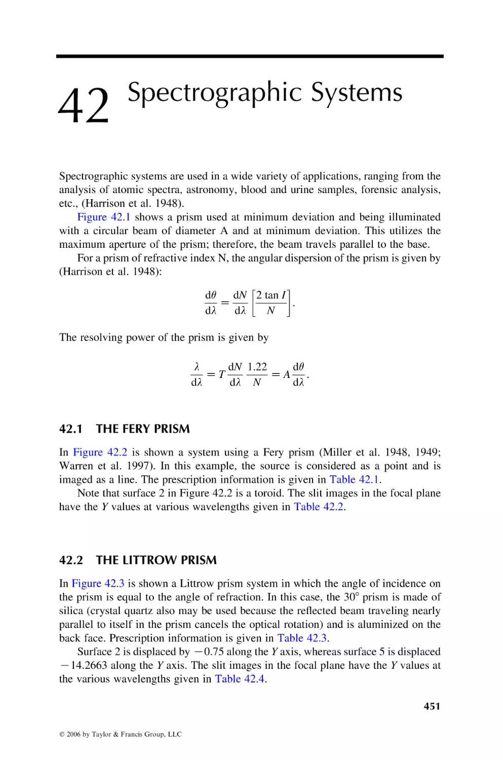
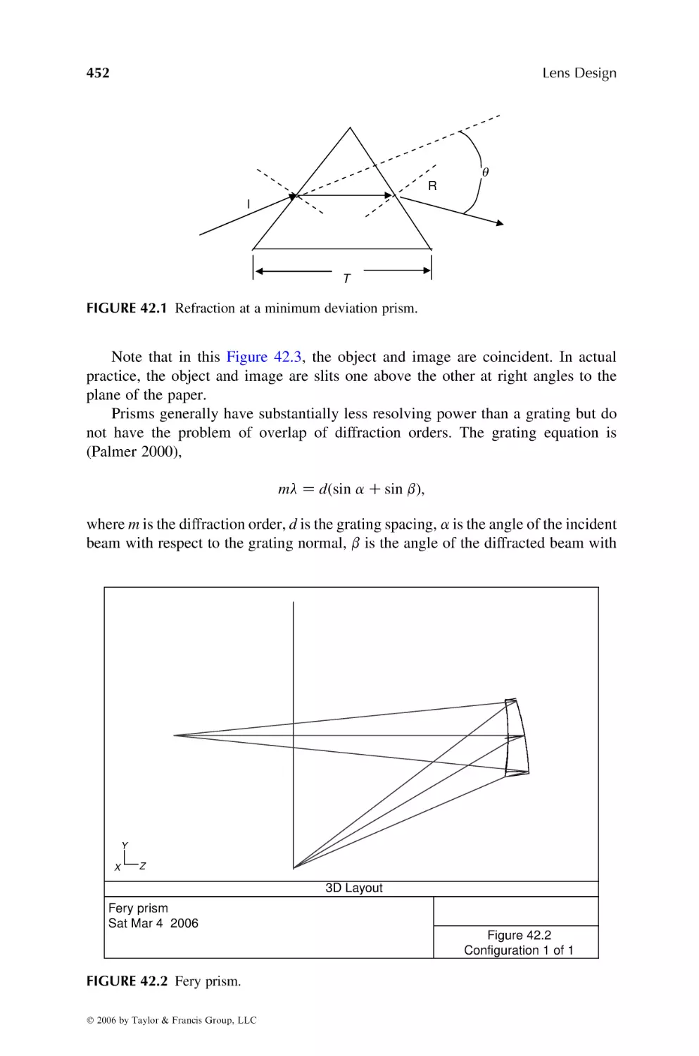
/


Текст
q 2006 by Taylor & Francis Group, LLC
q 2006 by Taylor & Francis Group, LLC
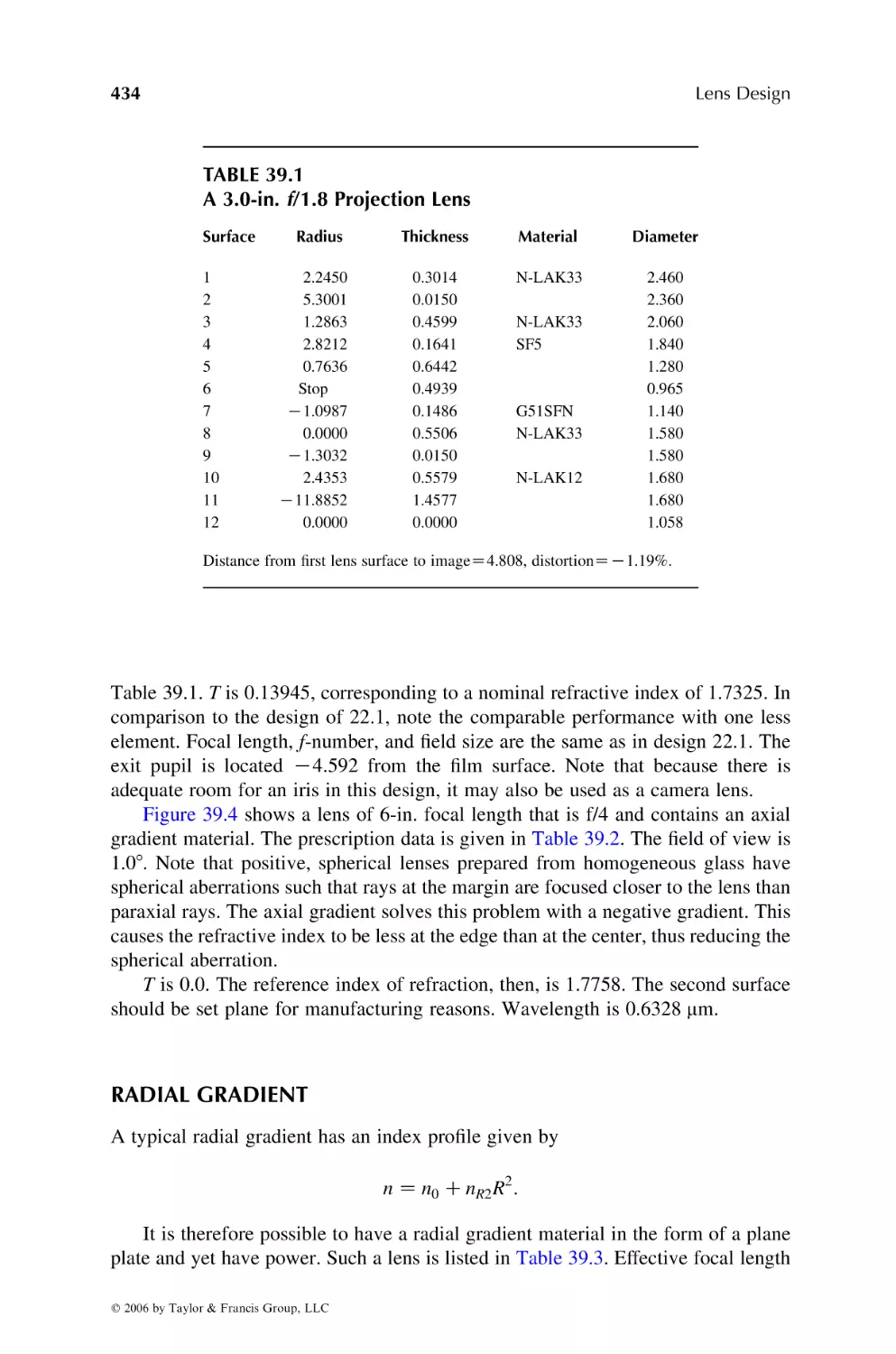
q 2006 by Taylor & Francis Group, LLC
q 2006 by Taylor & Francis Group, LLC
q 2006 by Taylor & Francis Group, LLC
q 2006 by Taylor & Francis Group, LLC
q 2006 by Taylor & Francis Group, LLC
q 2006 by Taylor & Francis Group, LLC
Dedication
This revised
and expanded edition
is dedicated to my wife, Pat
q 2006 by Taylor & Francis Group, LLC
q 2006 by Taylor & Francis Group, LLC
Preface
Of the several very fine texts on optical engineering, none gives detailed design
information or design procedures for a wide variety of optical systems. This text is
written as an aid for the practicing optical designer as well as for those aspiring to be
optical designers.
It is assumed that the reader is familiar with ray-tracing procedures, paraxial
data, and third-order aberrations. It is also assumed that the reader has access to a
computer lens design and analysis program. (See Appendix D for a list of
commercially available lens design programs.) As the personal computer has
increased in popularity and computing power, it exceeds, in its scientific computing
ability, the large computers of the 1960–1980 era. Many excellent programs are now
available for lens optimization, ray-trace analysis, lens plotting, modulation transfer
function (MTF) computations, etc. All of these programs, however, are optimization
programs; the designer must input a starting solution.
I have taught Introduction to Optical Engineering at the University of California
at Los Angeles for several years. I am often asked how I arrive at the starting design.
One of the purposes of this text is to answer just that question.
All optical glass listed in the designs are from the Schott glass catalog. (This
does not include the Ohara S-FPL53 element used in the designs shown in Figure 2.4
and Figure 7.5; the Ohara S-LAL18 (Figure 2.5) as well as the gradient index
materials of Chapter 39.) Other glass manufacturers (Ohara, Hoya, Chance,
Corning, Chengdu, etc.) make nearly equivalent types of glass. This was done for
convenience; I do not endorse any one glass manufacturer. In some of the
prescriptions, the material listed is SILICA. This is SiO2. CAF2 is calcium fluoride.
All lens prescription data, except for the human eye in Chapter 41, are given full
size in inches. This allows a practical system for presenting a particular application
(perhaps for a 35 mm reflex camera). The lens diameters have reasonable values of
edge thickness. The usual sign convention applies; thickness is an axial dimension to
the next surface and radius is C if the center of curvature is to the right of the
surface. Light travels left to right and from the long conjugate to the short. Lens
diameters are not necessarily clear apertures, but rather, the actual lens diameters as
shown in the lens diagrams.
All data for the visual region are centered at the e line and cover F 0 to C 0 . Two
infrared regions are considered; 8–14 mm (center at 10.2) and 3.2–4.2 mm (center at
3.63) that correspond to atmospheric windows. All data for the ultra-violet are
centered at 0.27 mm and cover 0.2–0.4 mm. (One needs to exercise caution here
because both calcium fluoride and fused silica show some absorption at these short
wavelengths. It is very important to select the correct grade.) Field of view (FOV) is
quoted in degrees and applies to the full field.
In the first edition of this book, all calculations for the fixed focal length designs
were performed using David Grey’s optical design and analysis programs. The
orthonormalization technique is described by Grey (1966) and the program by Walters
(1966). The use of orthogonal polynomials as aberration coefficients was later described
by Grey (1980). In this edition, all designs were re-optimized using the ZEMAX
q 2006 by Taylor & Francis Group, LLC
program (Moore 2006). This was necessary because there are now many changes to the
glasses that are available because of environmental requirements to remove lead,
cadmium, and arsenic. Perhaps most important, the ZEMAX program (like other
modern computer design programs listed in Appendix D) is a more comprehensive
program than the earlier GREY versions in that it can perform calculations on
decentered and tilted systems and gradient index as well as zoom systems in addition to
providing extensive graphical analysis.
In this edition, a CD containing two directories is included.
Lens. This contains all the lens prescriptions the same as listed in the text. By using
data directly from the computer, some of the prescription errors found in earlier
editions are eliminated. This is in a format RADIUS, THICKNESS, MATERIAL,
DIAMETER. Files correspond to the figures in the text (not table numbers).
Optics. This contains executable ZEMAX files corresponding to the figures in the
text. In the preliminary design of these systems, three wavelengths (except, of
course, for laser systems) and only a few rays were traced whereas more rays were
added to the merit function and, in most cases, five wavelengths were used. In the
presence of secondary color, the extra wavelengths give a realistic assessment of
MTF for the lens. Therefore, the prescriptions on the disk contain the added rays
and wavelengths. Under glass catalogs, PREFERED (note spelling error) is listed
for many of the designs. This is simply a list of Schott optical glass selected for its
reasonable price, availability, transmission, and stain resistance that the author
often uses. Simply substitute Schott_2000 for this catalog or load the file
PREFERED.AGF from the included disk into your glass catalogs. Unfortunately,
glass availability is changing as well as new glasses are sometimes developed. For
example, N-LLF6 used in design 4-1 as well as some other designs, is no longer
readily available, so OHARA S-TIL6 should be substituted. Likewise, for SK-18 in
design 14-4 is no longer readily available, so OHARA S-BSM 18 should be
substituted.
All plots in the figures were done with the ZEMAX program except for plots for
the zoom lens movements, secondary color chart, and anti-reflection films.
Regarding the zoom lens movement plots, the three curves on these plots represent
first-order relative movements of the two moving lens groups. Therefore, the
crossing of the curves (as in Figure 35.9b) does not mean that the moving groups
are interfering with each other. The crossing is simply a result of the presentation on
the plot. These plots are first-order calculations per the equations in Chapter 33 and
Chapter 34. Ten values were first computed and then fitted by a cubic spline equation
to do the actual plots.
For most of the systems, four plots for each lens are presented on a page
containing MTF, optical layout, ray fans, and RMS spot size. On the MTF plots,
the angle quoted is semi-field in degrees as seen from the first lens surface. (Or in
some cases, object or image heights.) The data are diffraction included MTF and
weighted as indicated in Table 1.2.
q 2006 by Taylor & Francis Group, LLC
Distortion is defined as
DZ
Y c Yg
;
Yg
where Yc is the actual image height at full field and Yg is the corresponding paraxial
image height. For a focal systems,
DZ
tan q 0 = tan q m
;
m
where q 0 is the emerging angle at full field, and m is the paraxial magnification
(Kingslake 1965).
Although I have taken a great deal of effort to assure accuracy, the user of any of
these designs should
† Carefully analyze the prescription to be sure that it meets his or her
particular requirements.
† Check the patent literature for possible infringement. Copies of patents are
available ($3.00 each) from Commissioner of Patents, P.O. Box 1450,
Alexandria, VA 22313-1450 (http://www.uspto.gov). Patent literature is a
valuable source of detail design data. Because patents are valid for 20
years after the application has been received by the patent office,
(previously 17 years after the patent was granted) older patents are now in
the public domain and may be freely used (US Patent Office 1999).
The Internet may be utilized to perform a search of the patent
literature. The patent office site is http://www.uspto.gov. Patents may
be searched by number or subject. Text and lens prescription are
given (only for patents issued after 1976), but no lens diagram or
other illustrations are provided. These illustrations are only available
in the printed version of the patent. In Optics and Photonics News,
Brian Caldwell discusses a patent design each month. There are also
patent reviews in Applied Optics.
† All data for the lens prescriptions (in this text, not on the CD) are
rounded. A very slight adjustment in back focal length (BFL) may be
necessary (particularly with lenses of low f number) if the reader
desires to verify the optical data.
This edition contains minor corrections to the previous editions as well as
presenting several new designs and sections on stabilized systems, the human eye,
spectrographic systems, and diffractive systems. Also, some of the glasses used in
the previous designs are now considered obsolete and were replaced.
Milton Laikin
q 2006 by Taylor & Francis Group, LLC
REFERENCES
Grey, D. S. (1966) Recent developments in orthonormalization of parameter space. In Lens
Design with Large Computers, Proceedings of the Conference, Institute of Optics,
Rochester, New York.
Grey, D. S. (1980) Orthogonal polynomials as lens aberration coefficients, International Lens
Design Conference, SPIE, Volume 237, p. 85.
Kidger, M. (2002) Fundamental Optical Design, SPIE Press, Bellingham, WA.
Kidger, M. (2004) Intermediate Optical Design, SPIE Press, Bellingham, WA.
Kingslake, R. (1965) Applied Optics and Optical Engineering, Volume 1, Academic Press,
New York.
Moore, K. (2006) ZEMAX Optical Design Program, User’s Guide, Zemax Development
Corporation, Belleview, WA.
US Patent Office (1999) General Information Concerning Patents, Available from US Govt.
Printing Office, Supt of Documents, Washington DC 20402.
Walters, R. M. (1966) Odds and ends from a Grey box. In Lens Design with Large Computers,
Proceedings of the Conference, Institute of Optics, Government Superintendent,
Rochester, New York.
q 2006 by Taylor & Francis Group, LLC
Contents
Chapter 1
The Method of Lens Design . . . . . . . . . . . . . . . . . . . . . . . . . . . . . . . . . . . . . . . . . . . . . . . . . . . 1
Chapter 2
The Achromatic Doublet . . . . . . . . . . . . . . . . . . . . . . . . . . . . . . . . . . . . . . . . . . . . . . . . . . . . . 41
Chapter 3
The Air-Spaced Triplet . . . . . . . . . . . . . . . . . . . . . . . . . . . . . . . . . . . . . . . . . . . . . . . . . . . . . . . 51
Chapter 4
Triplet Modifications . . . . . . . . . . . . . . . . . . . . . . . . . . . . . . . . . . . . . . . . . . . . . . . . . . . . . . . . . 61
Chapter 5
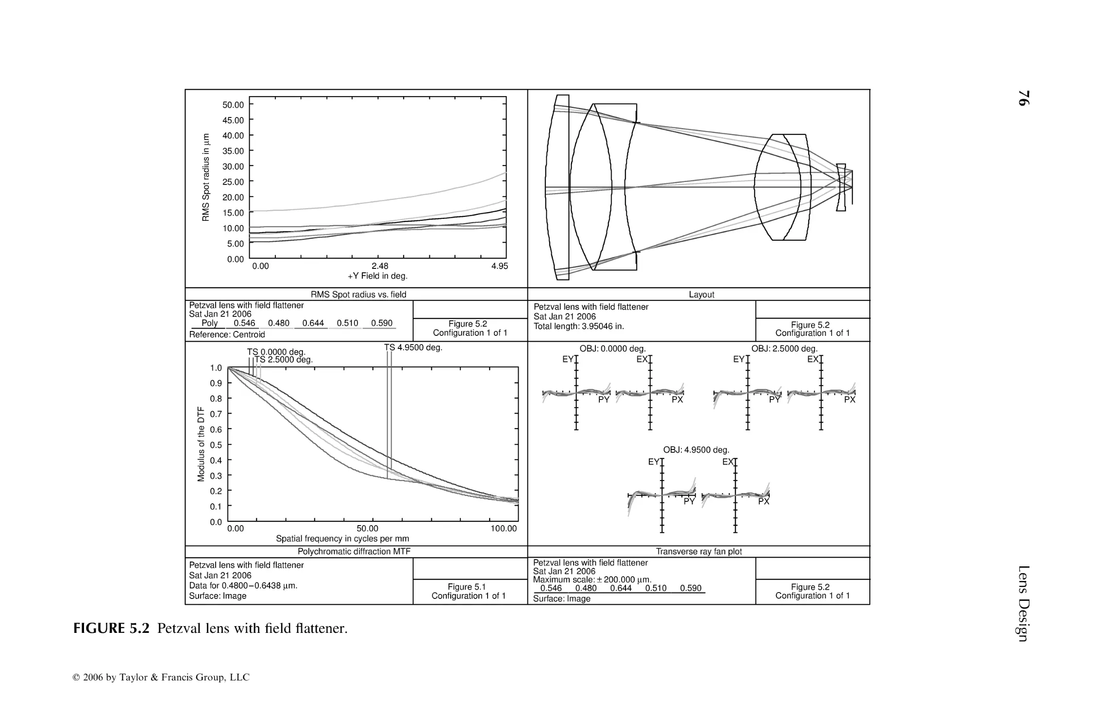
Petzval Lenses . . . . . . . . . . . . . . . . . . . . . . . . . . . . . . . . . . . . . . . . . . . . . . . . . . . . . . . . . . . . . . . 73
Chapter 6
Double Gauss and Near Symmetric Types . . . . . . . . . . . . . . . . . . . . . . . . . . . . . . . . . . . . 79
Chapter 7
Telephoto Lenses . . . . . . . . . . . . . . . . . . . . . . . . . . . . . . . . . . . . . . . . . . . . . . . . . . . . . . . . . . . . 87
Chapter 8
Inverted Telephoto Lens. . . . . . . . . . . . . . . . . . . . . . . . . . . . . . . . . . . . . . . . . . . . . . . . . . . . . . 99
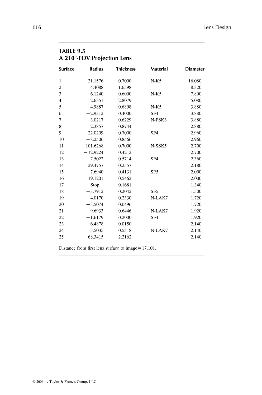
Chapter 9
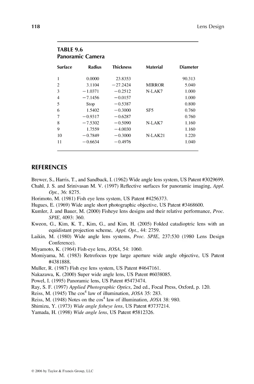
Very-Wide-Angle Lenses. . . . . . . . . . . . . . . . . . . . . . . . . . . . . . . . . . . . . . . . . . . . . . . . . . . 105
Chapter 10
Eyepieces . . . . . . . . . . . . . . . . . . . . . . . . . . . . . . . . . . . . . . . . . . . . . . . . . . . . . . . . . . . . . . . . . . 119
Chapter 11
Microscope Objectives . . . . . . . . . . . . . . . . . . . . . . . . . . . . . . . . . . . . . . . . . . . . . . . . . . . . . 131
Chapter 12
In-Water Lenses . . . . . . . . . . . . . . . . . . . . . . . . . . . . . . . . . . . . . . . . . . . . . . . . . . . . . . . . . . . 143
Chapter 13
Afocal Optical Systems . . . . . . . . . . . . . . . . . . . . . . . . . . . . . . . . . . . . . . . . . . . . . . . . . . . . 155
q 2006 by Taylor & Francis Group, LLC
Chapter 14
Relay Lenses . . . . . . . . . . . . . . . . . . . . . . . . . . . . . . . . . . . . . . . . . . . . . . . . . . . . . . . . . . . . . . 169
Chapter 15
Catadioptric and Mirror Optical Systems. . . . . . . . . . . . . . . . . . . . . . . . . . . . . . . . . . . . 183
Chapter 16
Periscope Systems . . . . . . . . . . . . . . . . . . . . . . . . . . . . . . . . . . . . . . . . . . . . . . . . . . . . . . . . . 211
Chapter 17
IR Lenses. . . . . . . . . . . . . . . . . . . . . . . . . . . . . . . . . . . . . . . . . . . . . . . . . . . . . . . . . . . . . . . . . . 219
Chapter 18
Ultraviolet Lenses and Optical Lithography . . . . . . . . . . . . . . . . . . . . . . . . . . . . . . . . . 233
Chapter 19
F-Theta Scan Lenses . . . . . . . . . . . . . . . . . . . . . . . . . . . . . . . . . . . . . . . . . . . . . . . . . . . . . . . 245
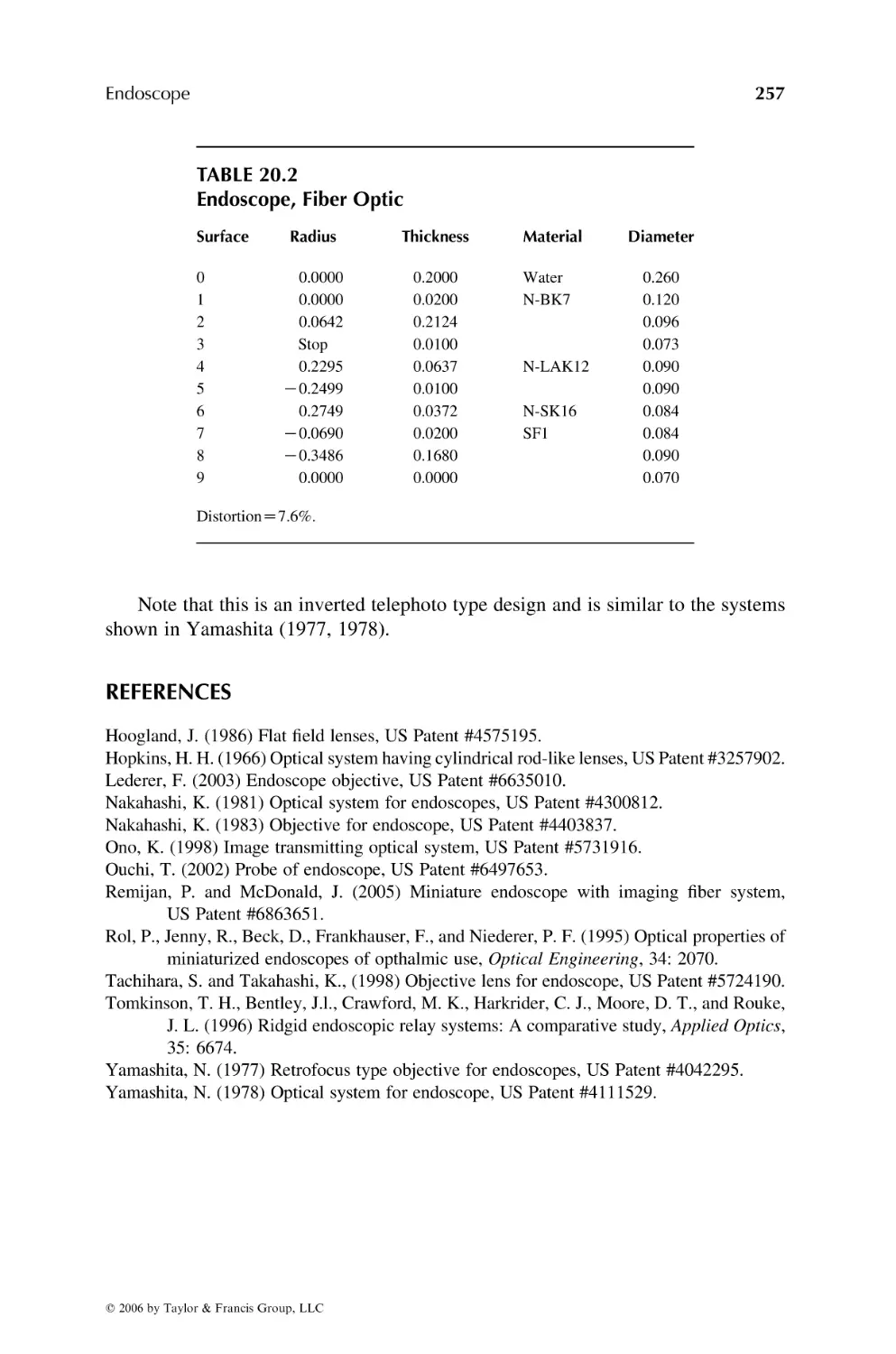
Chapter 20
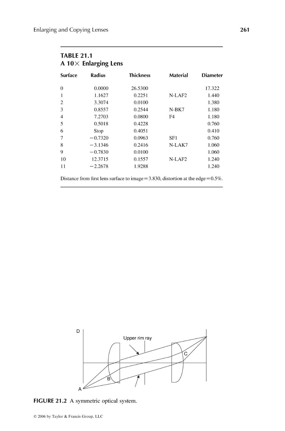
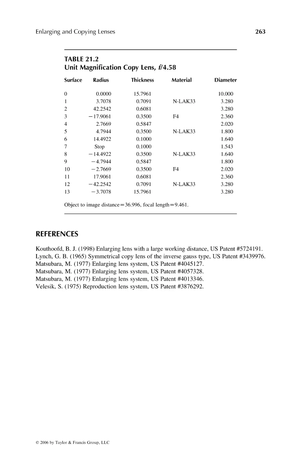
Endoscope . . . . . . . . . . . . . . . . . . . . . . . . . . . . . . . . . . . . . . . . . . . . . . . . . . . . . . . . . . . . . . . . . 253
Chapter 21
Enlarging and Copying Lenses . . . . . . . . . . . . . . . . . . . . . . . . . . . . . . . . . . . . . . . . . . . . . 259
Chapter 22
Projection Lenses . . . . . . . . . . . . . . . . . . . . . . . . . . . . . . . . . . . . . . . . . . . . . . . . . . . . . . . . . . 265
Chapter 23
Telecentric Systems . . . . . . . . . . . . . . . . . . . . . . . . . . . . . . . . . . . . . . . . . . . . . . . . . . . . . . . . 283
Chapter 24
Laser-Focusing Lenses (Optical Disc). . . . . . . . . . . . . . . . . . . . . . . . . . . . . . . . . . . . . . . 291
Chapter 25
Heads-Up Display Lenses . . . . . . . . . . . . . . . . . . . . . . . . . . . . . . . . . . . . . . . . . . . . . . . . . . 299
Chapter 26
The Achromatic Wedge . . . . . . . . . . . . . . . . . . . . . . . . . . . . . . . . . . . . . . . . . . . . . . . . . . . . 305
Chapter 27
Wedge-Plate and Rotary-Prism Cameras . . . . . . . . . . . . . . . . . . . . . . . . . . . . . . . . . . . . 309
q 2006 by Taylor & Francis Group, LLC
Chapter 28
Anamorphic Attachments. . . . . . . . . . . . . . . . . . . . . . . . . . . . . . . . . . . . . . . . . . . . . . . . . . . 317
Chapter 29
Illumination Systems . . . . . . . . . . . . . . . . . . . . . . . . . . . . . . . . . . . . . . . . . . . . . . . . . . . . . . . 325
Chapter 30
Lenses for Aerial Photography. . . . . . . . . . . . . . . . . . . . . . . . . . . . . . . . . . . . . . . . . . . . . . 333
Chapter 31
Radiation-Resistant Lenses . . . . . . . . . . . . . . . . . . . . . . . . . . . . . . . . . . . . . . . . . . . . . . . . . 343
Chapter 32
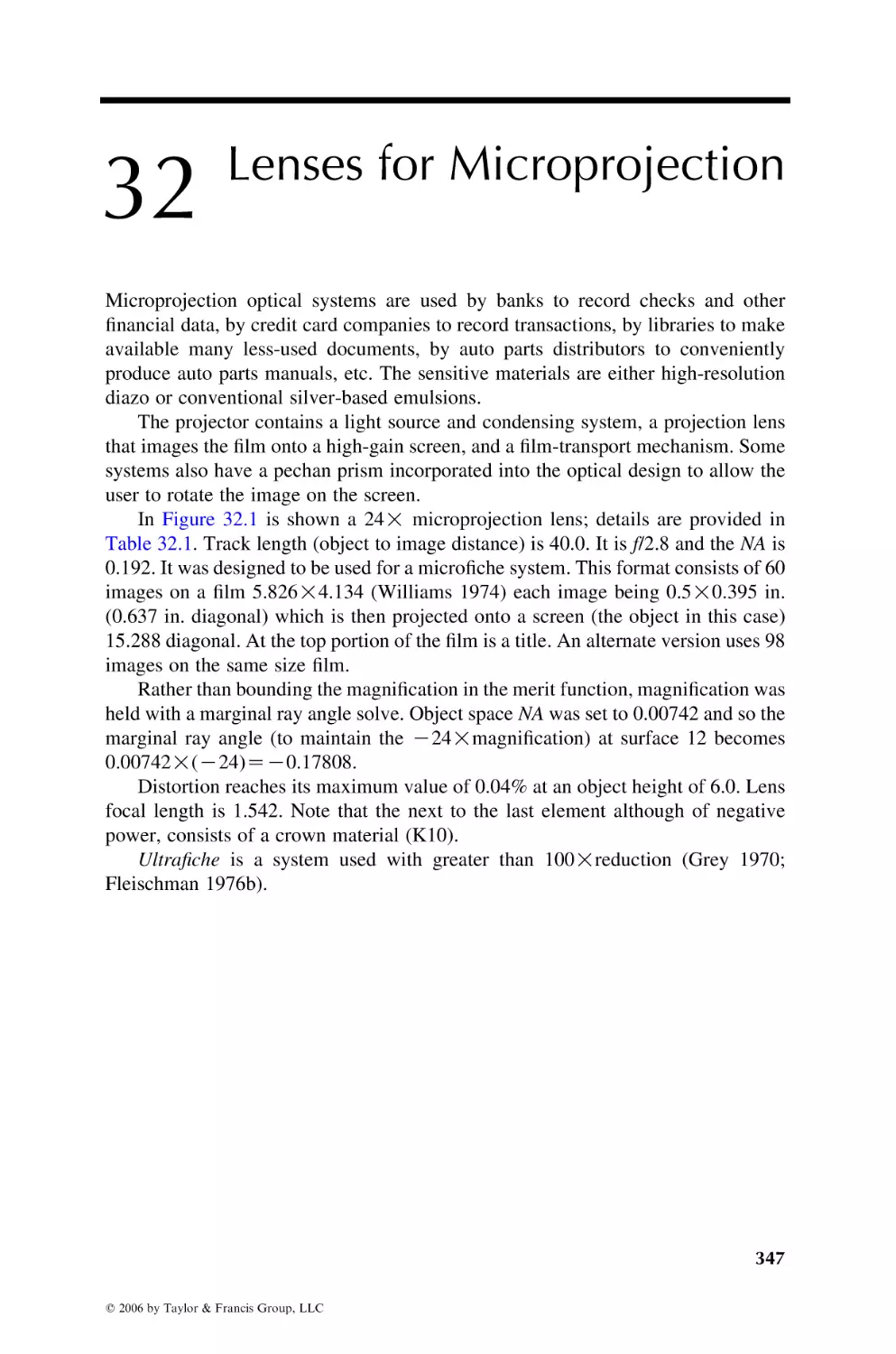
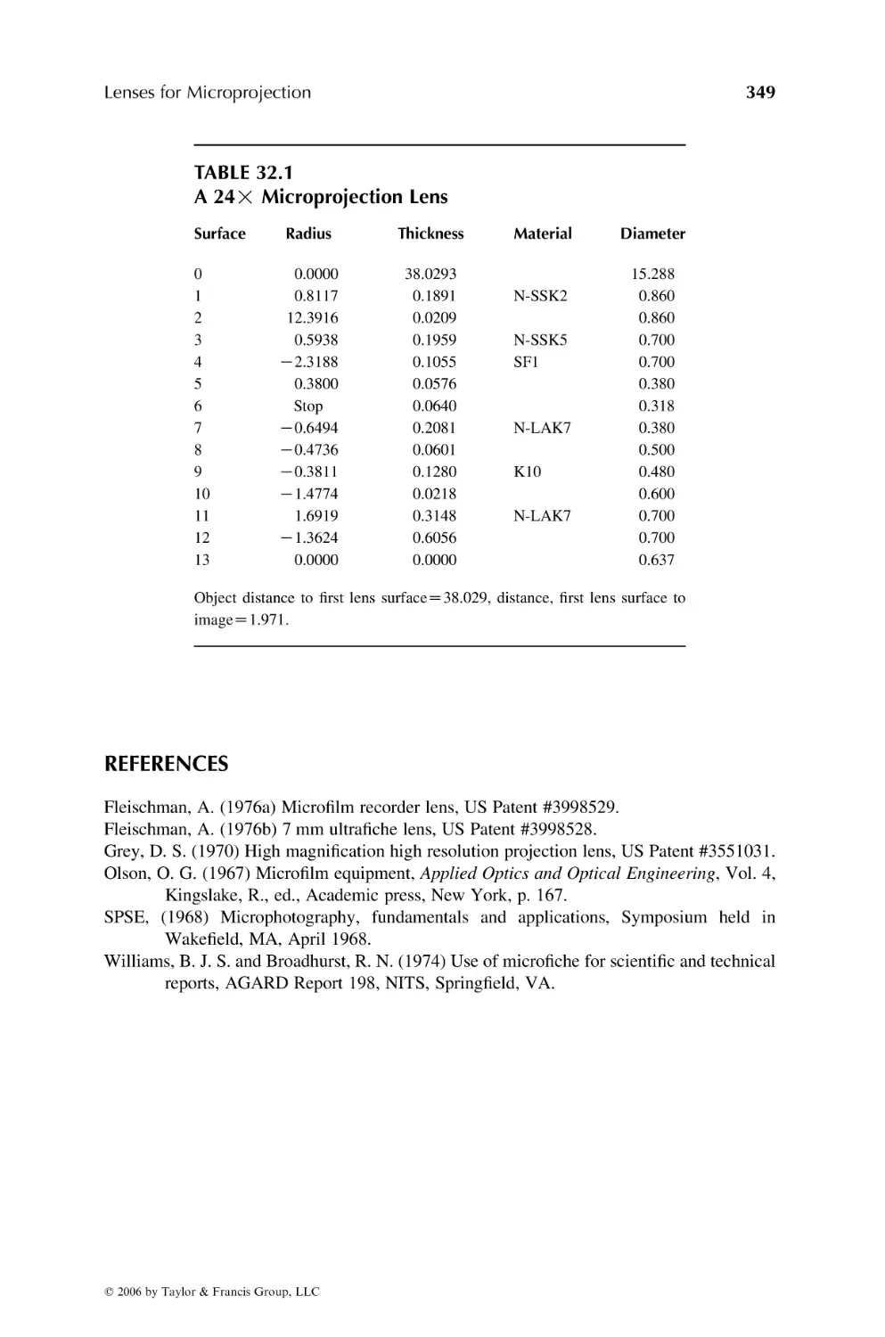
Lenses for Microprojection . . . . . . . . . . . . . . . . . . . . . . . . . . . . . . . . . . . . . . . . . . . . . . . . . 347
Chapter 33
First-Order Theory, Mechanically Compensated Zoom . . . . . . . . . . . . . . . . . . . . . . 351
Chapter 34
First Order Theory, Optically Compensated Zoom Lenses . . . . . . . . . . . . . . . . . . . 355
Chapter 35
Mechanically Compensated Zoom Lenses. . . . . . . . . . . . . . . . . . . . . . . . . . . . . . . . . . . 359
Chapter 36
Optically Compensated Zoom Lenses . . . . . . . . . . . . . . . . . . . . . . . . . . . . . . . . . . . . . . . 403
Chapter 37
Copy Lenses with Variable Magnification. . . . . . . . . . . . . . . . . . . . . . . . . . . . . . . . . . . 415
Chapter 38
Variable Focal Length Lenses . . . . . . . . . . . . . . . . . . . . . . . . . . . . . . . . . . . . . . . . . . . . . . 423
Chapter 39
Gradient-Index Lenses . . . . . . . . . . . . . . . . . . . . . . . . . . . . . . . . . . . . . . . . . . . . . . . . . . . . . 431
Chapter 40
Stabilized Optical Systems . . . . . . . . . . . . . . . . . . . . . . . . . . . . . . . . . . . . . . . . . . . . . . . . . 443
Chapter 41
The Human Emmetropic Eye . . . . . . . . . . . . . . . . . . . . . . . . . . . . . . . . . . . . . . . . . . . . . . . 447
q 2006 by Taylor & Francis Group, LLC
Chapter 42
Spectrographic Systems . . . . . . . . . . . . . . . . . . . . . . . . . . . . . . . . . . . . . . . . . . . . . . . . . . . . 451
Chapter 43
Diffractive Systems . . . . . . . . . . . . . . . . . . . . . . . . . . . . . . . . . . . . . . . . . . . . . . . . . . . . . . . . 459
Appendix A
Film and CCD Formats. . . . . . . . . . . . . . . . . . . . . . . . . . . . . . . . . . . . . . . . . . . . . . . . . . . . . 465
Appendix B
Flange Distances . . . . . . . . . . . . . . . . . . . . . . . . . . . . . . . . . . . . . . . . . . . . . . . . . . . . . . . . . . . 467
Appendix C
Thermal and Mechanical Properties. . . . . . . . . . . . . . . . . . . . . . . . . . . . . . . . . . . . . . . . . 469
Appendix D
Commercially Available Lens Design Programs . . . . . . . . . . . . . . . . . . . . . . . . . . . . . 471
q 2006 by Taylor & Francis Group, LLC
LIST OF DESIGNS
2-1
2-2
2-3
2-4
2-5
3-2
3-3
3-4
3-5
3-6
4-1
4-2
4-3
4-4
4-5
4-6
5-1
5-2
6-1
6-2
6-3
6-4
7-2
7-3
7-4
7-5
7-6
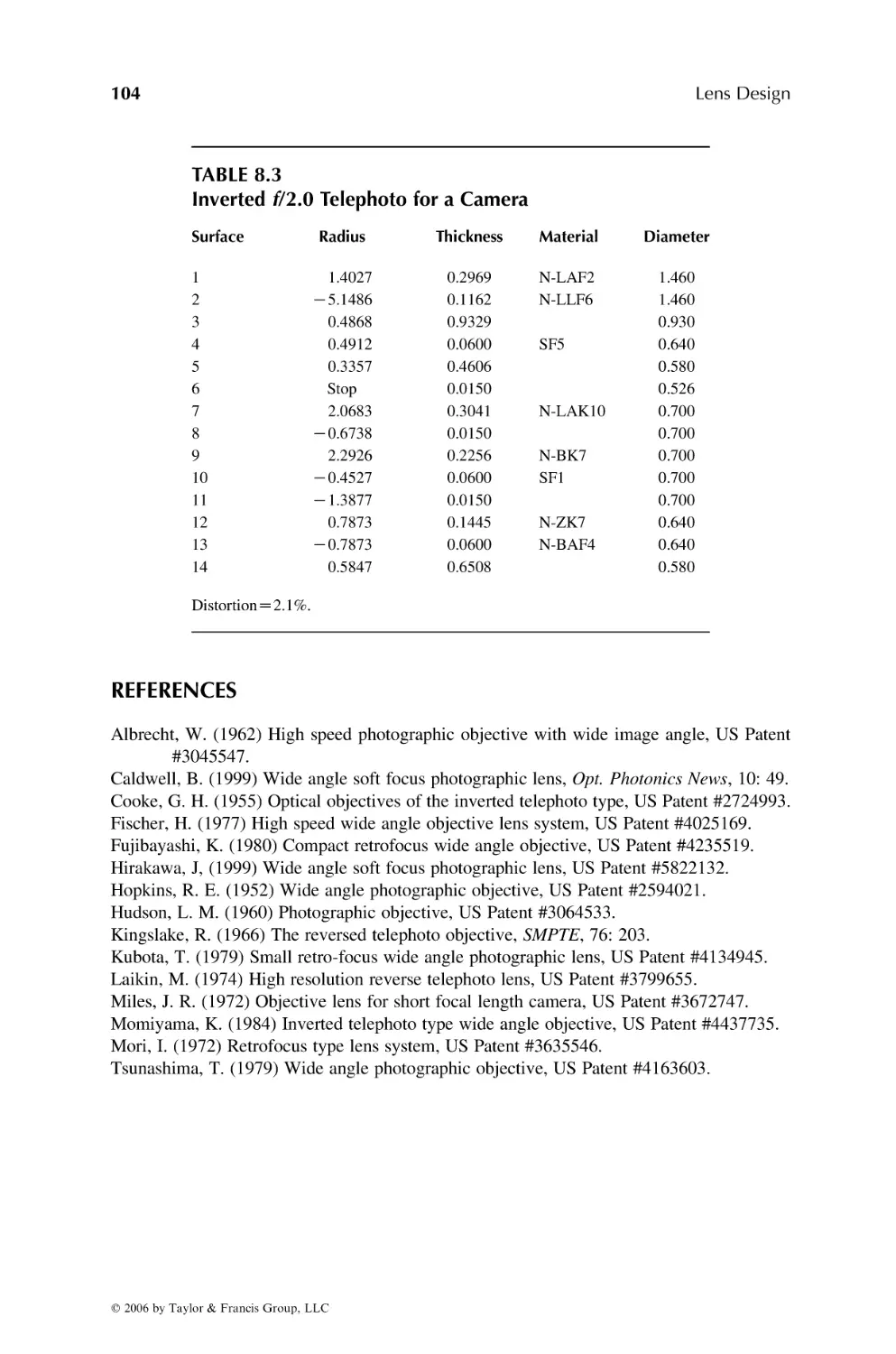
8-1
8-2
8-3
9-1
9-2
9-3
9-4
9-5
9-6
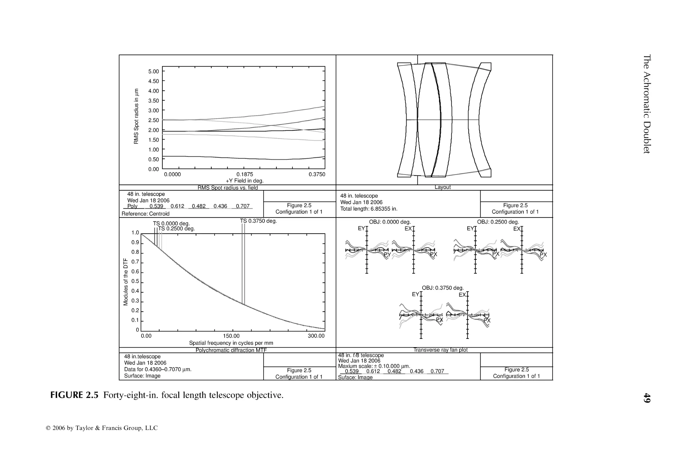
48 in. Focal Length Achromat
Cemented Achromat, 20 in. Focal Length
Cemented Achromat, 10 in. Focal Length
Cemented Apochromat
48 in. Focal Length Telescope Objective
5 in. Focal Length f/3.5 Triplet
IR Triplet 8-14 Micron
4 in. IR Triplet 3.2-4.2 Micron
50 in., f/8 Triplet
18 in., f/9 Triplet
Heliar f/5
Tessar Lens 4 in., f/4.5
Slide Projector Lens
Triplet with Corrector
100 mm f/2.8
10 mm f/2.8
Petzval Lens f/1.4
Petzval Lens with Field Flattener
Double Gauss f/2.5
50 mm f/1.8 SLR Camera Lens
f/1 5 deg. FOV Double Gauss
25 mm f/.85 Double Gauss
Telephoto f/5.6
f/2.8 180 mm Telephoto
400 mm f/4 Telephoto
1000 mm f/11 Telephoto
Cemented Achromat with 2X Extender
Inverted Telephoto f/3.5
10 mm Cinegon
Inverted Telephoto for Camera
100 deg. FOV Camera Lens
120 deg. f/2 Projection
160 deg. f/2 Projection
170 deg. f/1.8 Camera Lens
210 deg. Projection
Panoramic Camera
q 2006 by Taylor & Francis Group, LLC
10-2
10-3
10-4
10-5
10-6
11-1
11-2
11-3
11-4
11-5
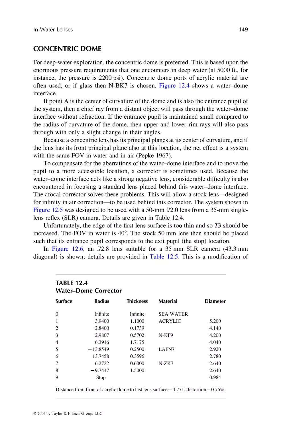
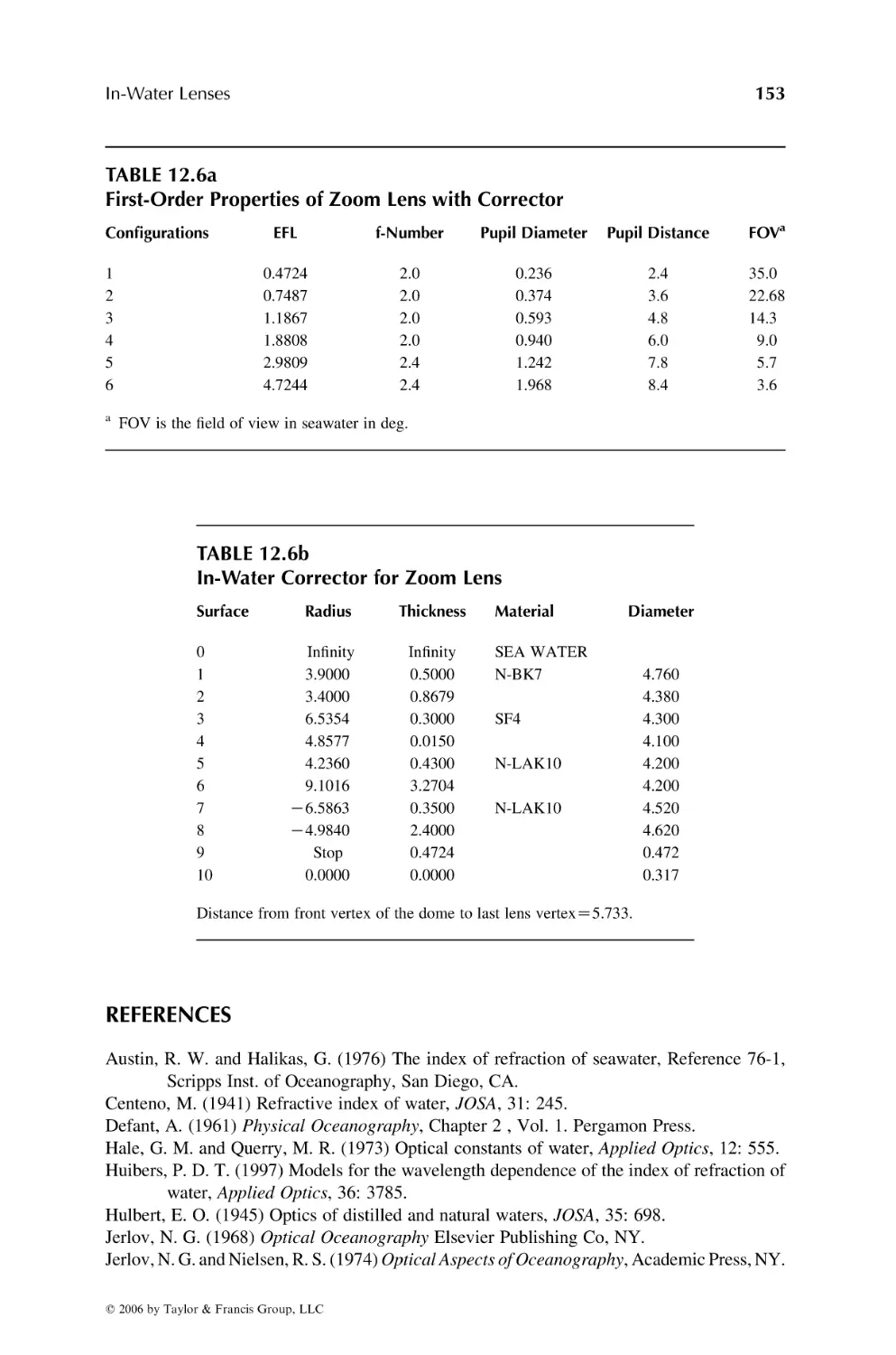
12-3
12-5
12-6
12-7
13-1
13-2
13-3
13-4
13-5
13-6
13-7
14-1
14-2
14-3
14-4
14-5
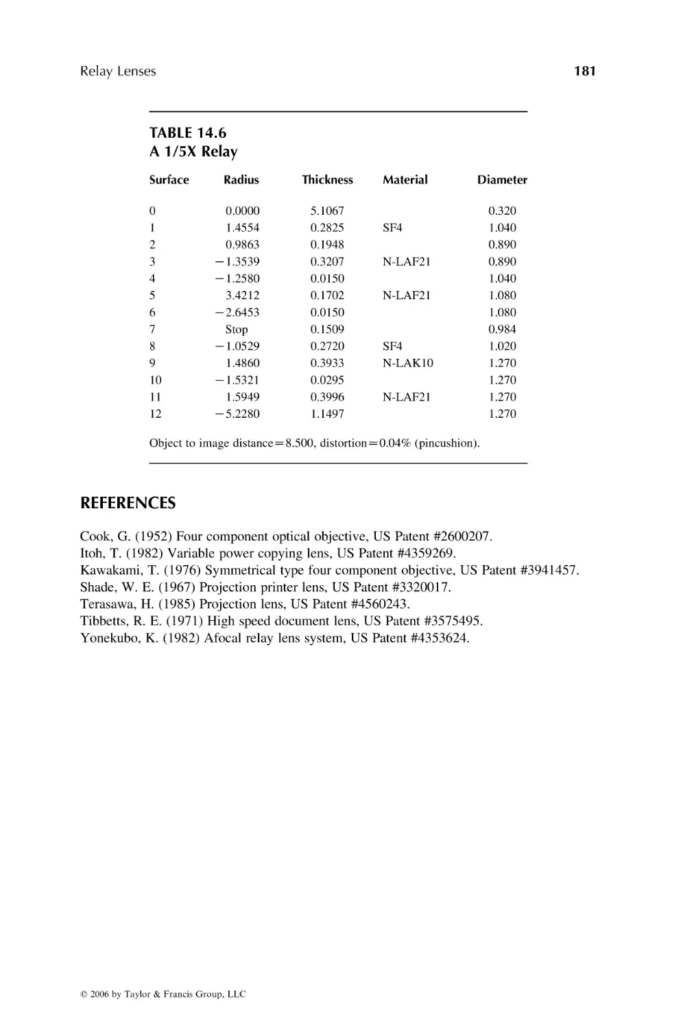
14-6
15-2
15-3
15-4
15-5
15-6
15-7
15-8
15-9
15-10
15-11
15-12
15-13
10 X Eyepiece
10 X Eyepiece, Long Eyerelief
Plossl Eyepiece
Erfle Eyepiece
25 mm Eyepiece with Internal Image
10X Microscope Objective
20X Microscope Objective
4 mm Apochromatic Microscope Objective
UV Reflecting Microscope Objective
98 X Oil Immersion Microscope Objective
Flat Port, 70 mm Camera Lens
Water Dome Corrector
In-water Lens with Dome
In-water Corrector for Zoom Lens
5 X Laser Beam Expander
5 X Gallean Beam Expander
50 X Laser Beam Expander
4 X Galilean Plastic Telescope
Power Changer
Albada View Finder
Door Scope
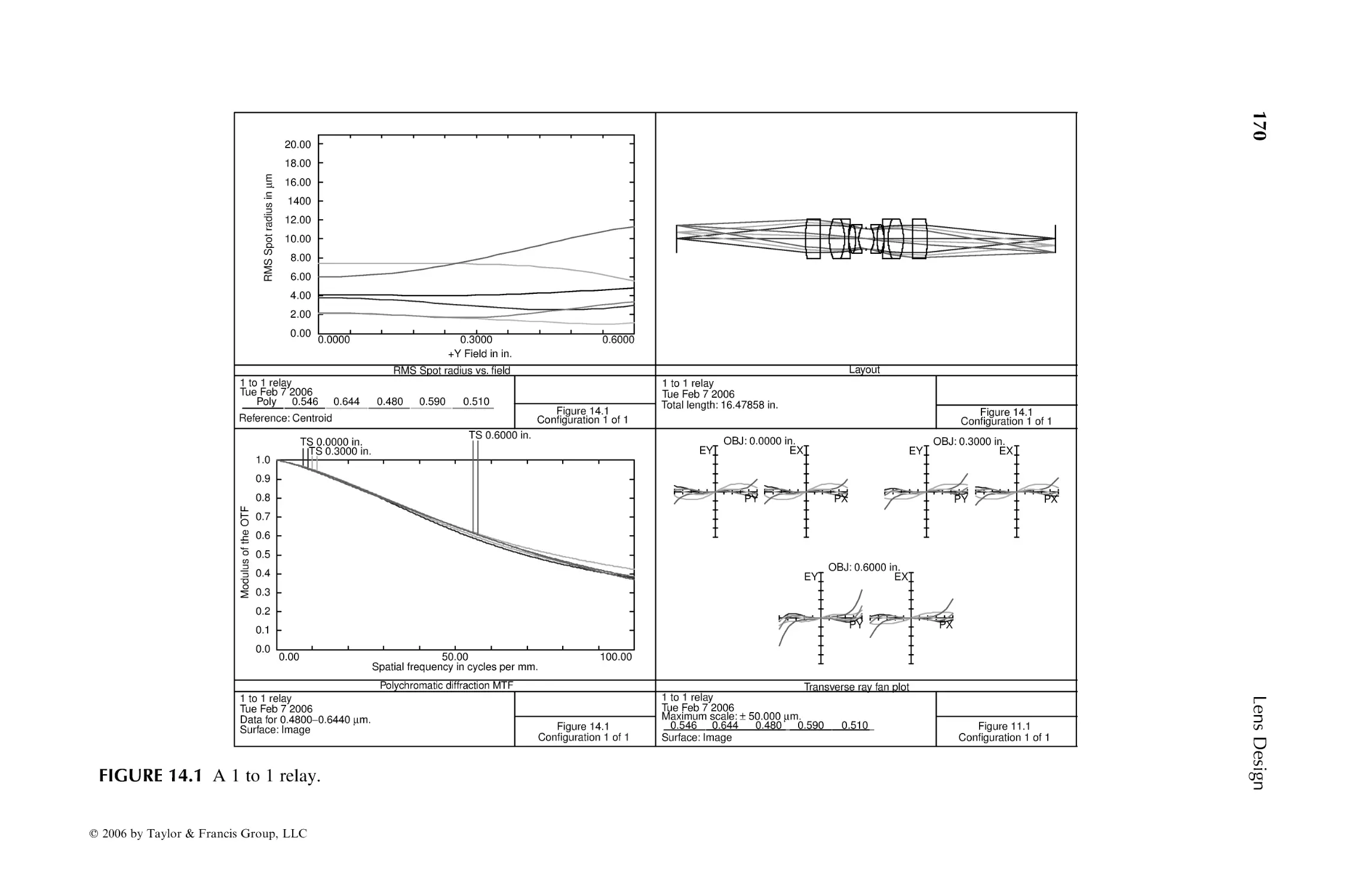
1 to 1 Relay
Unit Power Copy Lens
.6 X Copy Lens
Rifle Sight
Eyepiece Relay
1:5 Relay
Cassegrain Lens 3.2-4.2 mn
Starlight Scope Objective f/1.57
1000 mm Focal Length Cassegrain
50 in. Focal Length Telescope Objective
10 in. fl f/1.23 Cassegrain
Schmidt Objective
Reflecting Objective
250 in., f/10 Cassegrain
Ritchey-Chretien
Hubble Space Telescope
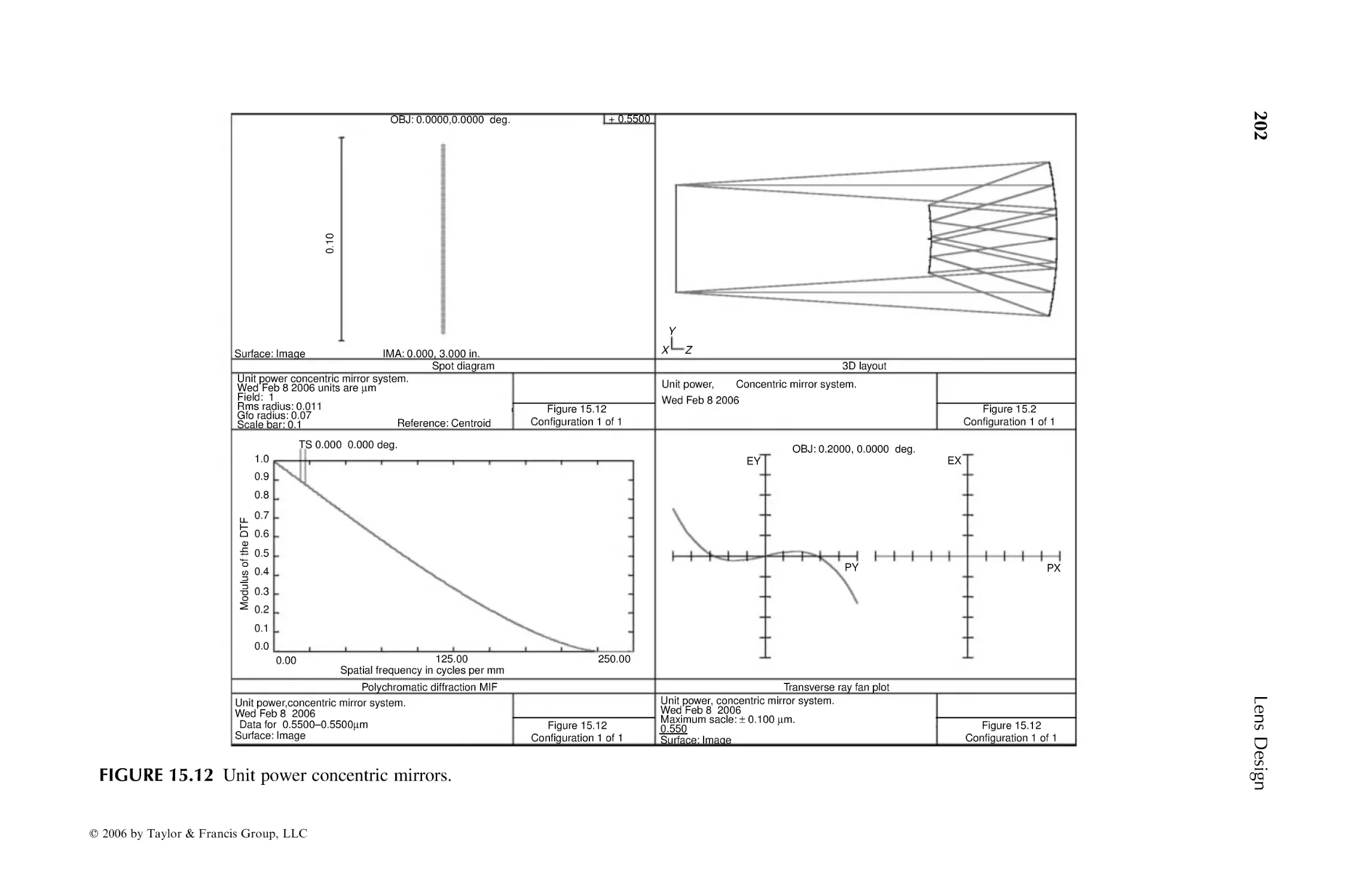
Unit Power Concentric Mirrors
Tilted Mirrors
q 2006 by Taylor & Francis Group, LLC
15-14
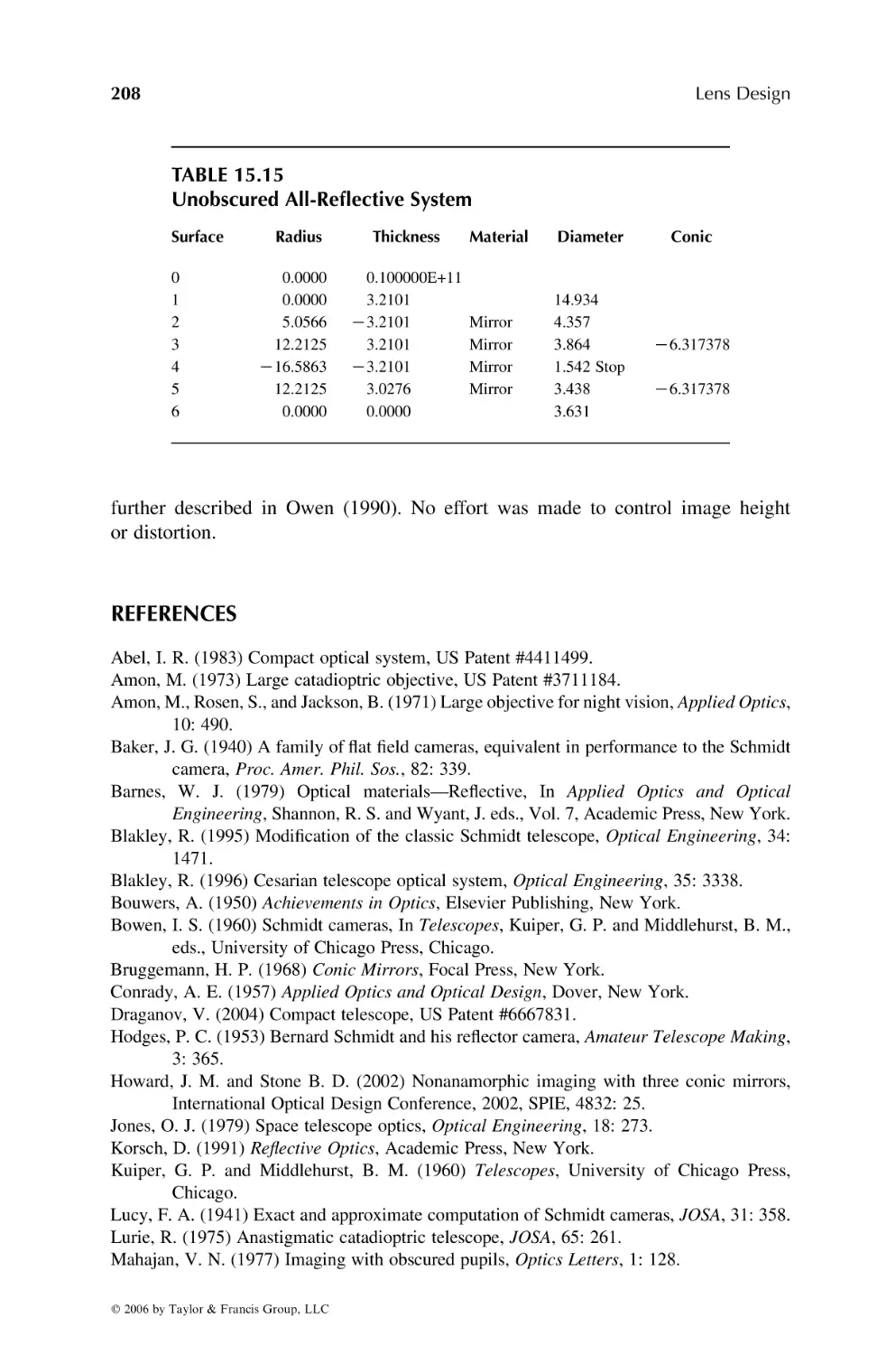
15-15
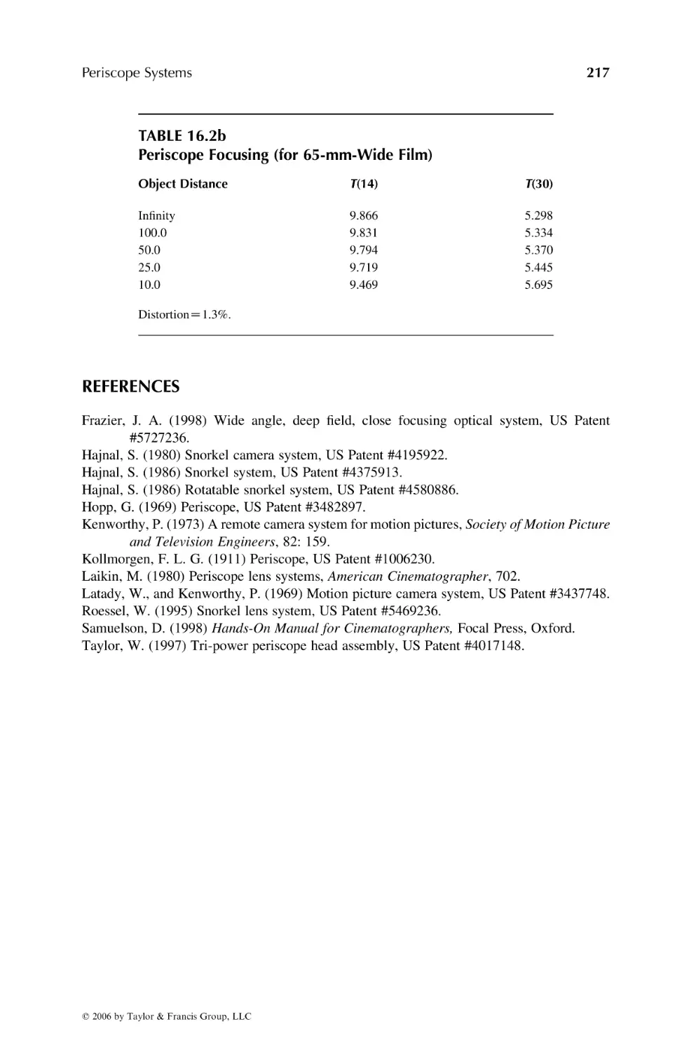
16-1
16-2
17-2
17-3
17-4
17-5
17-6
18-1
18-2
18-3
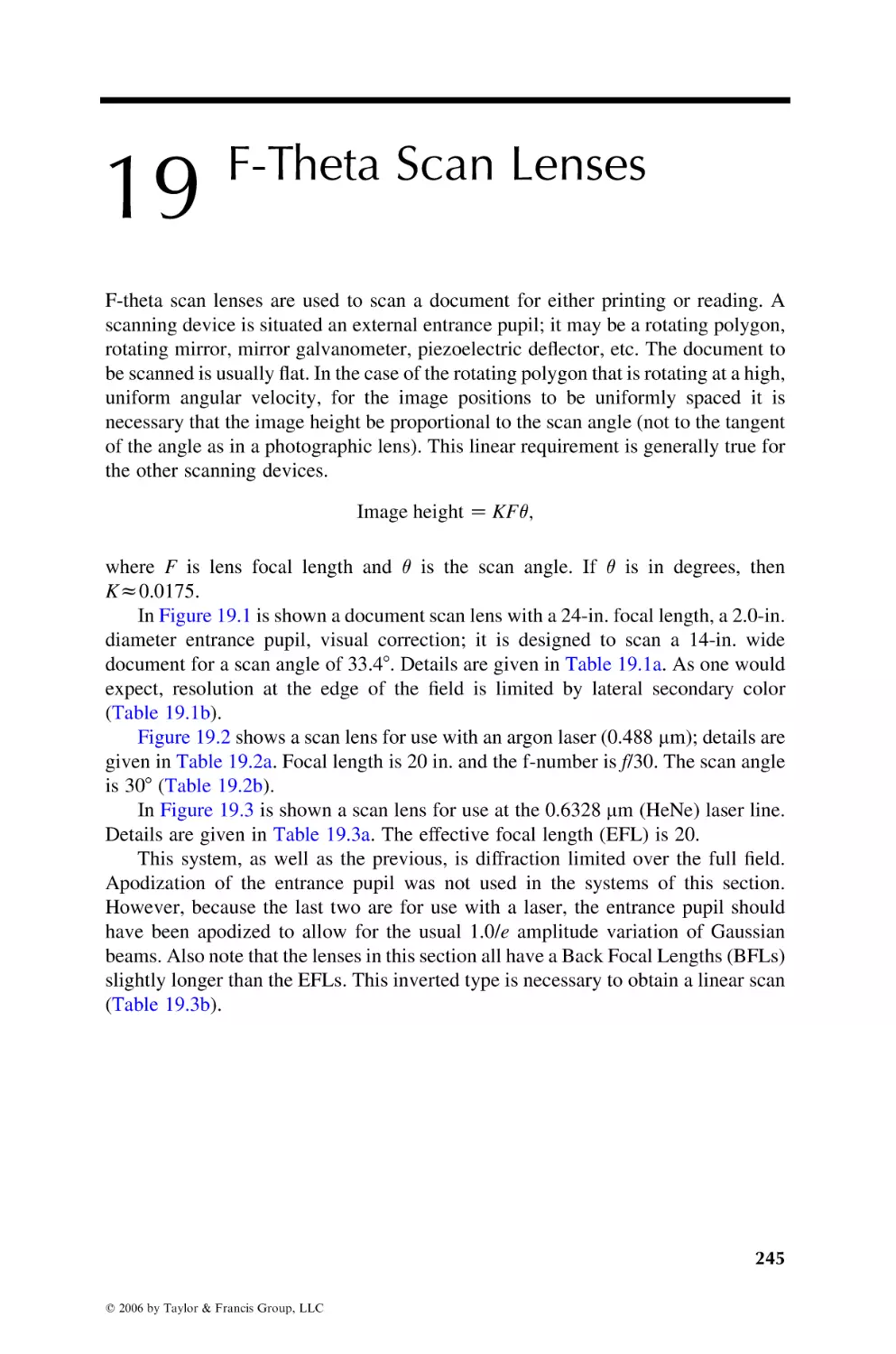
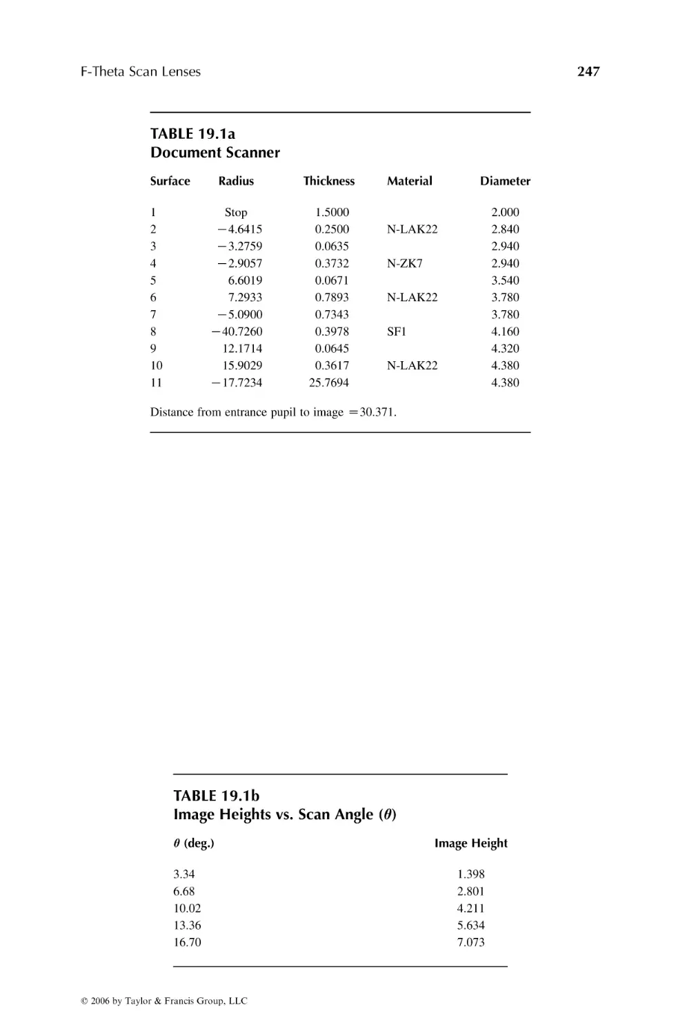
19-1
19-2
19-3
20-1
20-2
21-1
21-3
22-1
22-3
22-4
22-5
22-7
22-8
22-9
23-1
23-2
23-3
23-5
24-1
24-3
24-4
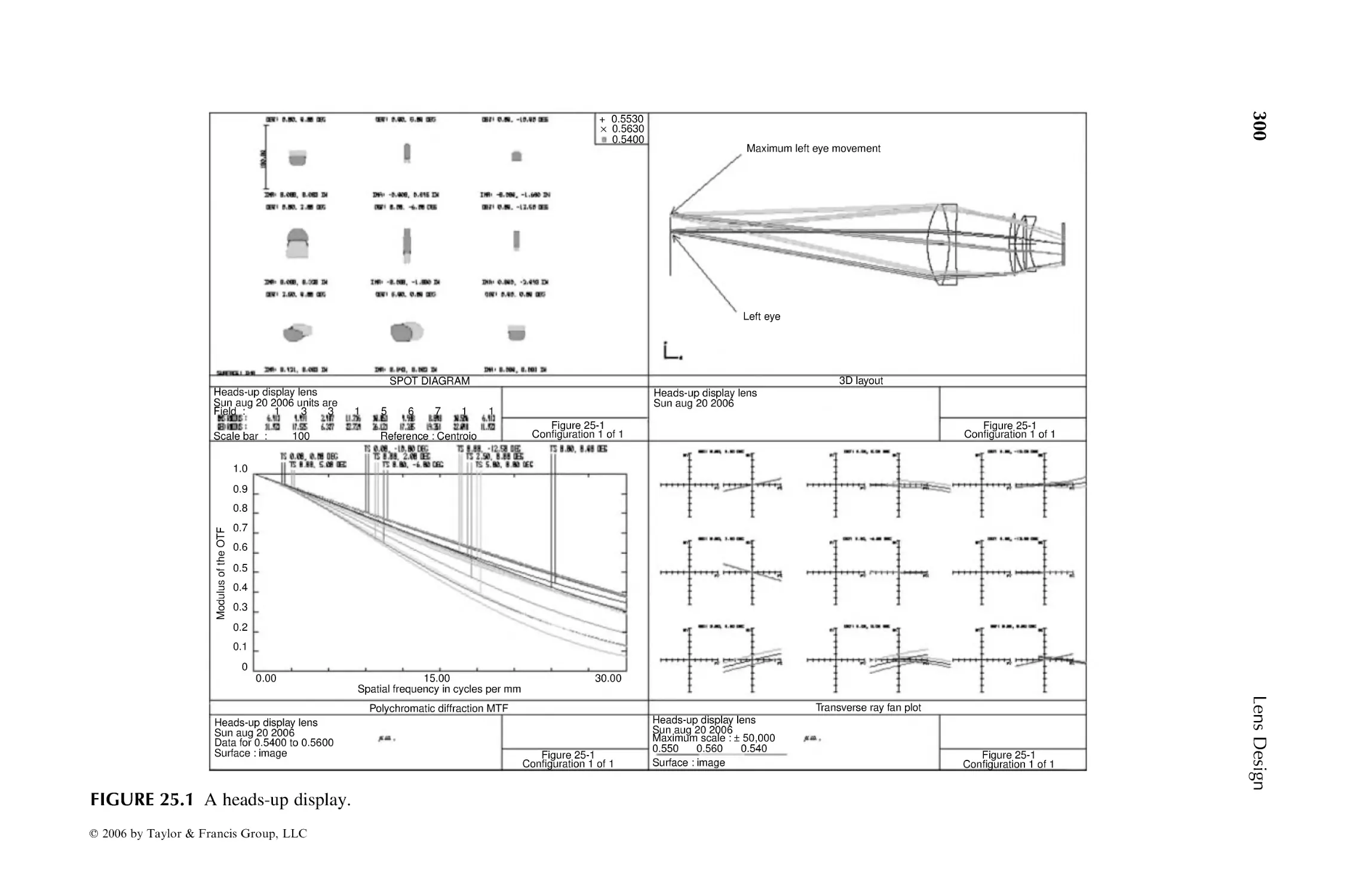
25-1
25-2
27-2
27-4
28-1
28-2
Compact Telescope
Unobscured, All Reflective Lens
25-mm Focal Length Periscope
65 mm Format Periscope
Dual Focal Length IR Lens System
IR Lens, 3.2 to 4.2 Micro
10X Beam Expander
Doublet, 1.8-2.2 mn
Long Wavelength IR Camera
UV Lens Silica, CaF2
Cassegrain Objective, All Fused Silica
Lithograph Projection
Document Scanner
Argon Laser Scanner Lens
Scan Lens 0.6328 mn
f/3. Endoscope, Rod Lens
Endoscope, Fiber Optic
65 mm f/4 10 X Enlarging Lens
Unit Magnification Copy Lens
f/1.8 Projection Lens
Projection Lens, 70 mm Film
70 deg. FOV Projection Lens, f/2
Plastic Projection Lens
2 in. FL LCD Projection
Wide Angle LCD Projection Lens
DLP Projection Lens
Profile Projector, 20 X
Telecentric Lens f/2.8
F/2 Telecentric
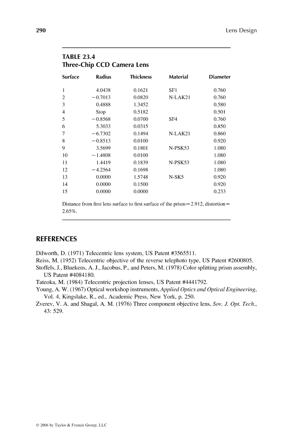
3 Chip CCD Camera Lens
Video Disk f/1
Laser Focusing Lens 0.308 m
Laser Focus Lens 0.6328m
Heads Up Display
BI-Ocular Lens
Wedge Plate
Lens for Rotary Prism Camera
2X Anamorphic Attachment, 35 mm Film
2X Anamorphic Attachment, 70 mm Film
q 2006 by Taylor & Francis Group, LLC
28-3
28-4
29-1
29-2
29-3
29-4
29-5
30-1
30-2
30-3
30-4
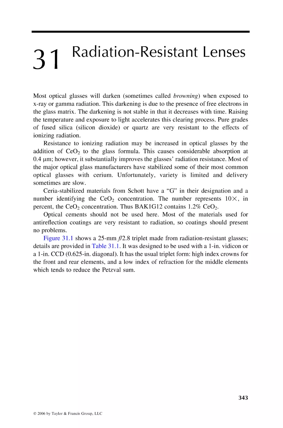
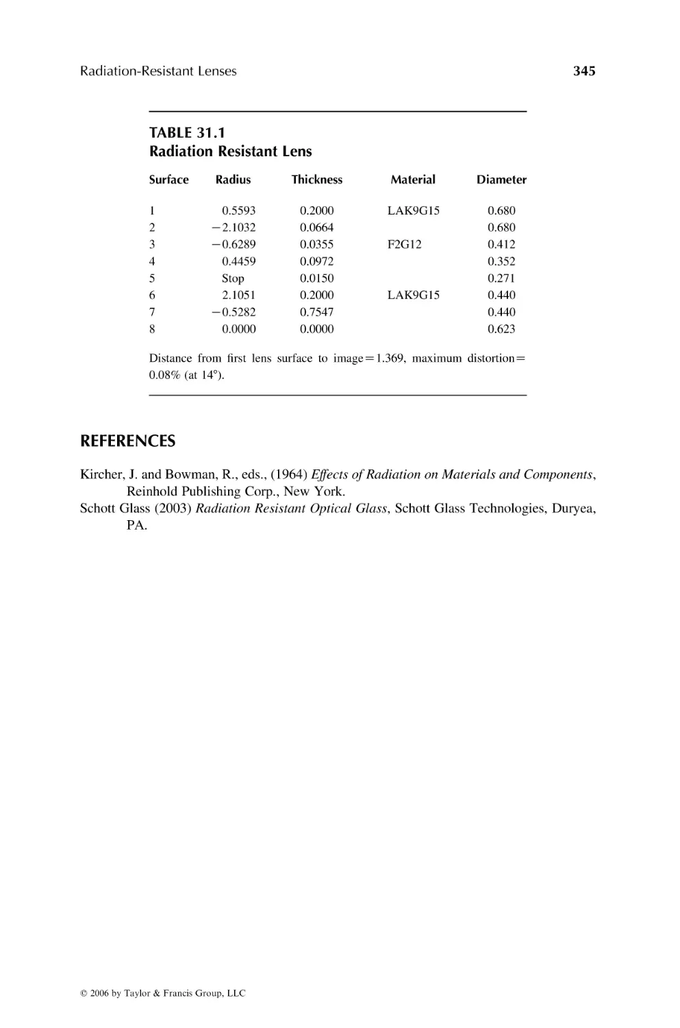
31-1
32-1
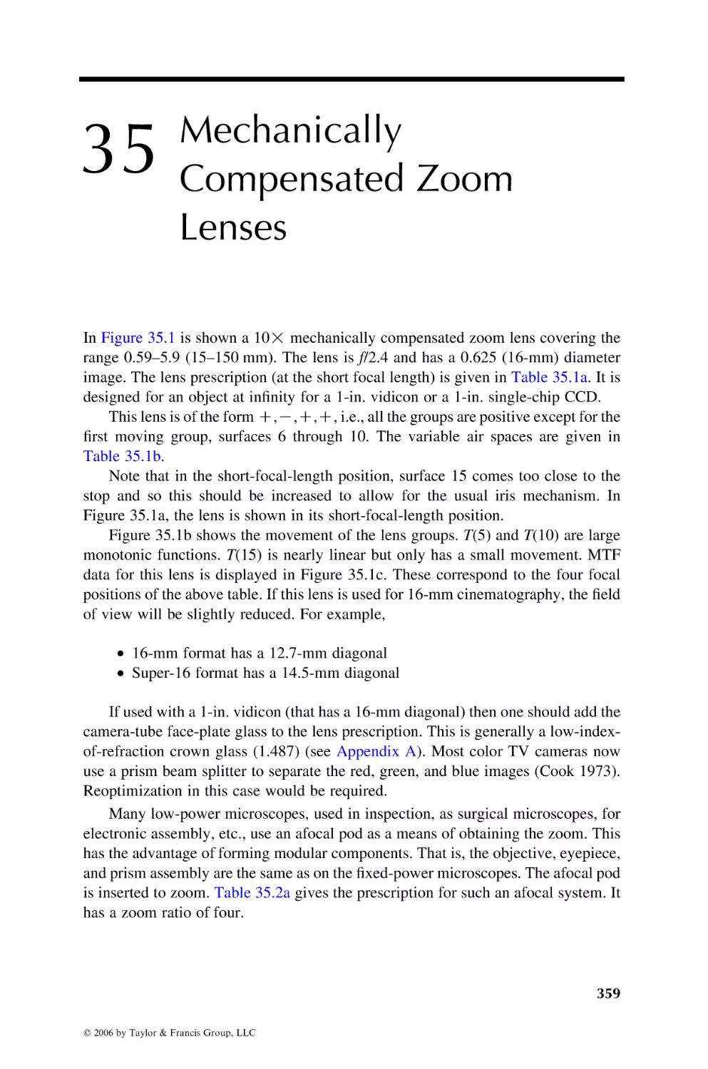
35-1
35-2
35-3
35-4
35-5
35-6
35-7
35-8
35-9
35-10
35-11
35-12
36-1
36-2
36-3
37-1
37-2
38-1
38-2
39-3
39-4
39-5
39-6
39-7
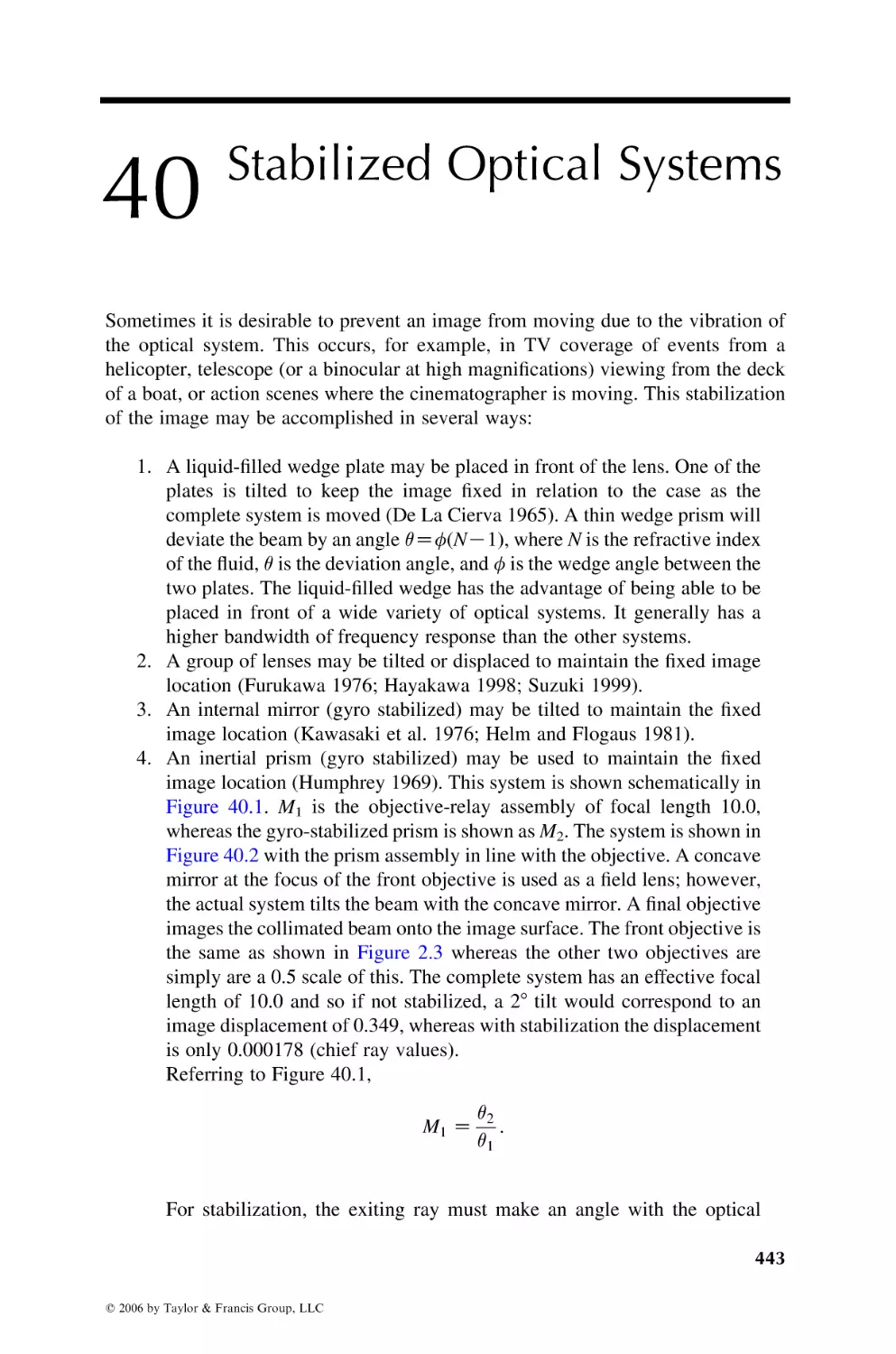
40-2
41-1
1.5X Anamorphic Expander
Anamorphic Prism Assembly
Fused Silica Condenser, 1 X
Fused Silica Condenser, 0.2 X
Pyrex Condenser
Condensor System For 10 X Projection
Xenon Arc Reflector
5 in. f/4 Aerial Camera Lens
12 in. f/4 Aerial Lens
18 in. f/3 Aerial Lens
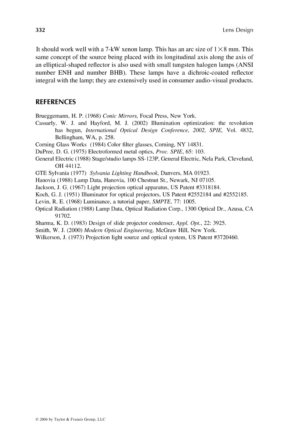
24 in. f/6 Aerial Lens
Radiation Resistant Lens 25mm f/2.8
24!Micro-Projection
10X Zoom Lens
Afocal Zoom for Microscope
Zoom Cassegrain
Zoom Rifle Scope
Stereo Zoom Microscope
Zoom Microscope
20 to 110 mm Zoom Lens
25 to 125 mm with Three Moving Groups
Zoom Lens for SLR Camera
12-234 mm TV Zoom Lens
40 to 20 mm Zoom Eyepiece
20 to 40 mm Focal Length Periscope
Optical Zoom, 100 to 200 mm EFL
SLR Optical Zoom 72 to 145 mm EFL
6.25 to 12.5X Optically Compensated Projection Lens
Xerographic Zoom
Copy Lens
Variable Focal Length Projection for SLR Camera
Variable Focal Length Motion Picture Projection Lens
3.0 in. f/1.8 Projection Lens, Axial Gradient
Laser Focusing Lens, Axial Gradient
Radial Gradient, 50 in. Focal Length
Selfoc Lens
Corning-GRIN Laser Focusing Lens
Stabilized Lens System
The Human Emmetropic Eye
q 2006 by Taylor & Francis Group, LLC
42-2
42-3
42-5
43-1
43-2
Fery Prism
Littrow Prism
Littrow Diffraction Grating
The Achromatic Singlet
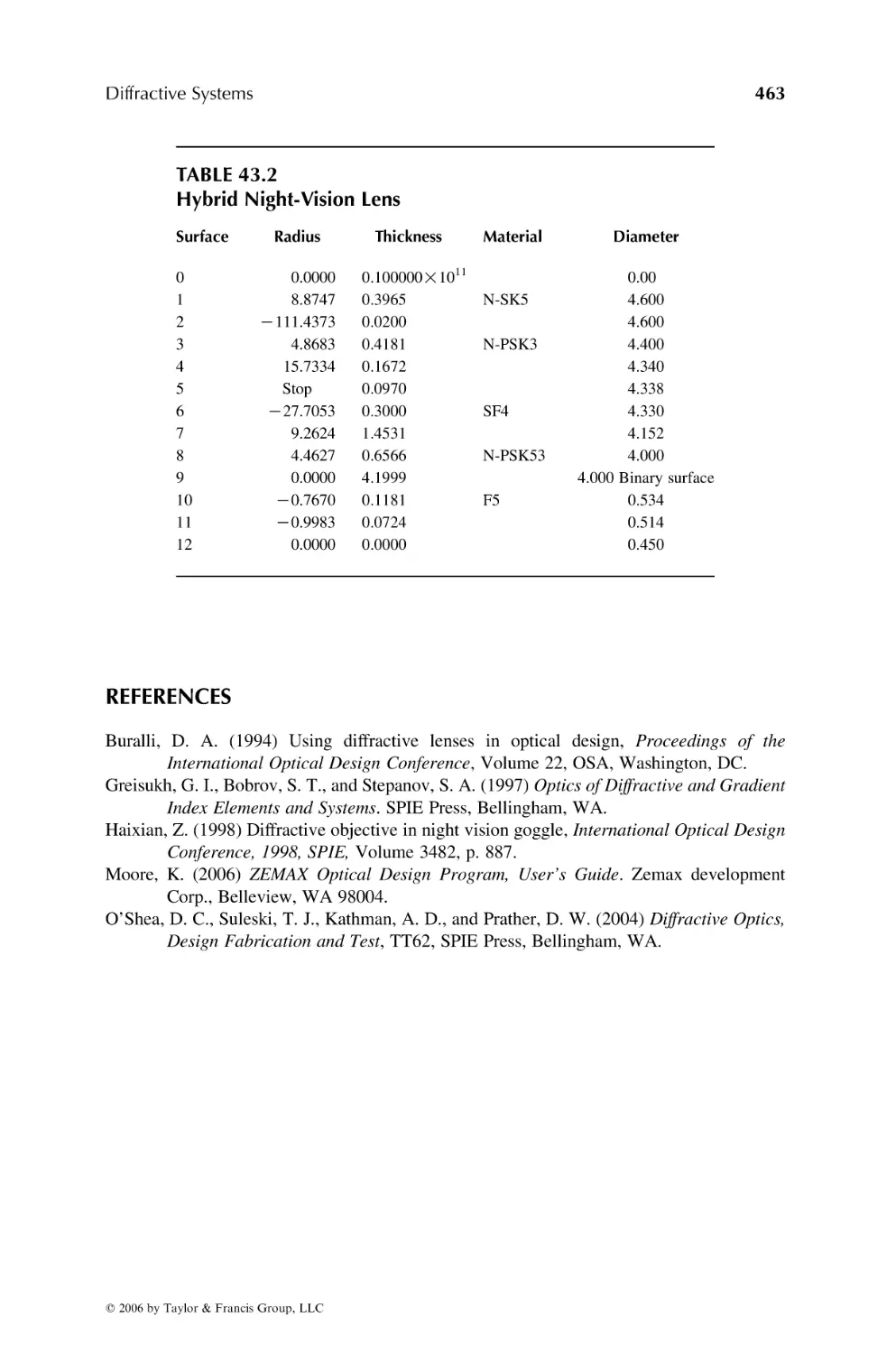
Hybrid Night Vision Lens
q 2006 by Taylor & Francis Group, LLC
q 2006 by Taylor & Francis Group, LLC
1
The Method of Lens Design
Given an object and image distance, the wavelength region and the degree of
correction for the optical system, it would at first appear that with the great progress
in computers and applied mathematics it would be possible to analytically determine
the radius, thickness, and other constants for the optical system. Neglecting very
primitive systems, such as a one- or two-mirror system, or a single-element lens,
such a technique is presently not possible.
The systematic method of lens design in use today is an iterative technique. By
this procedure, based upon the experience of the designer, a basic lens type is first
chosen. A paraxial thin lens and then a thick lens solution is next developed. In the
early days of computer optimization, the next step was often correcting for the
third-order aberrations (Hopkins et al. 1955). Now, with the relatively fast speed
of ray-tracing, this step is often skipped and one goes directly to optimization by
ray-trace.
In any automatic (these are really semi-automatic programs because the
designer must still exercise control) computer-optimization program, there must be a
single number that represents the quality of the lens. Because the concept of a good
lens vs. a bad lens is always open to discussion, there are thus several techniques for
creating this merit function (Feder 1957a,1957b; Brixner 1978). The ideal situation
is a merit function that considers the boundary conditions for the lens as well as the
image defects. These boundary conditions include such items as maintaining the
effective focal length (or magnification), f-number, center and edge spacings, overall
length, pupil location, element diameters, location on the glass map, paraxial angle
controls, paraxial height controls, etc. There should also be a means to change the
weights of these defects so that the axial image quality may be weighted differently
than the off-axis image, as well as means for changing the basic structure of the
image (core vs. flare, distortion, chromatic errors, etc.) (Palmer 1971). Some merit
functions also contain derivative data (Feder 1968).
Most optimization and analysis programs in use today evaluate the optical
system by means of ray tracing (Jamieson 1971). However, some compute the
aberration coefficients (third and higher orders) at each surface and then form the
sum (Buchdahl 1968).
In the early days of optical design, when the cost of tracing a ray was high (as
compared to today), a common technique to reduce the number of rays traced was to
only trace rays at the central wavelength and carry thru, at each surface, information
regarding path-length differences multiplied by the difference in dispersion (Feder
1952; Conrady 1960; Ginter 1990).
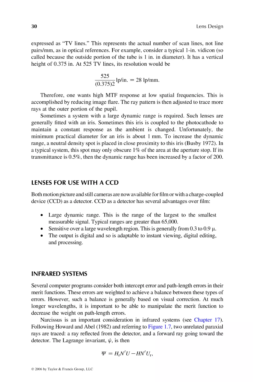
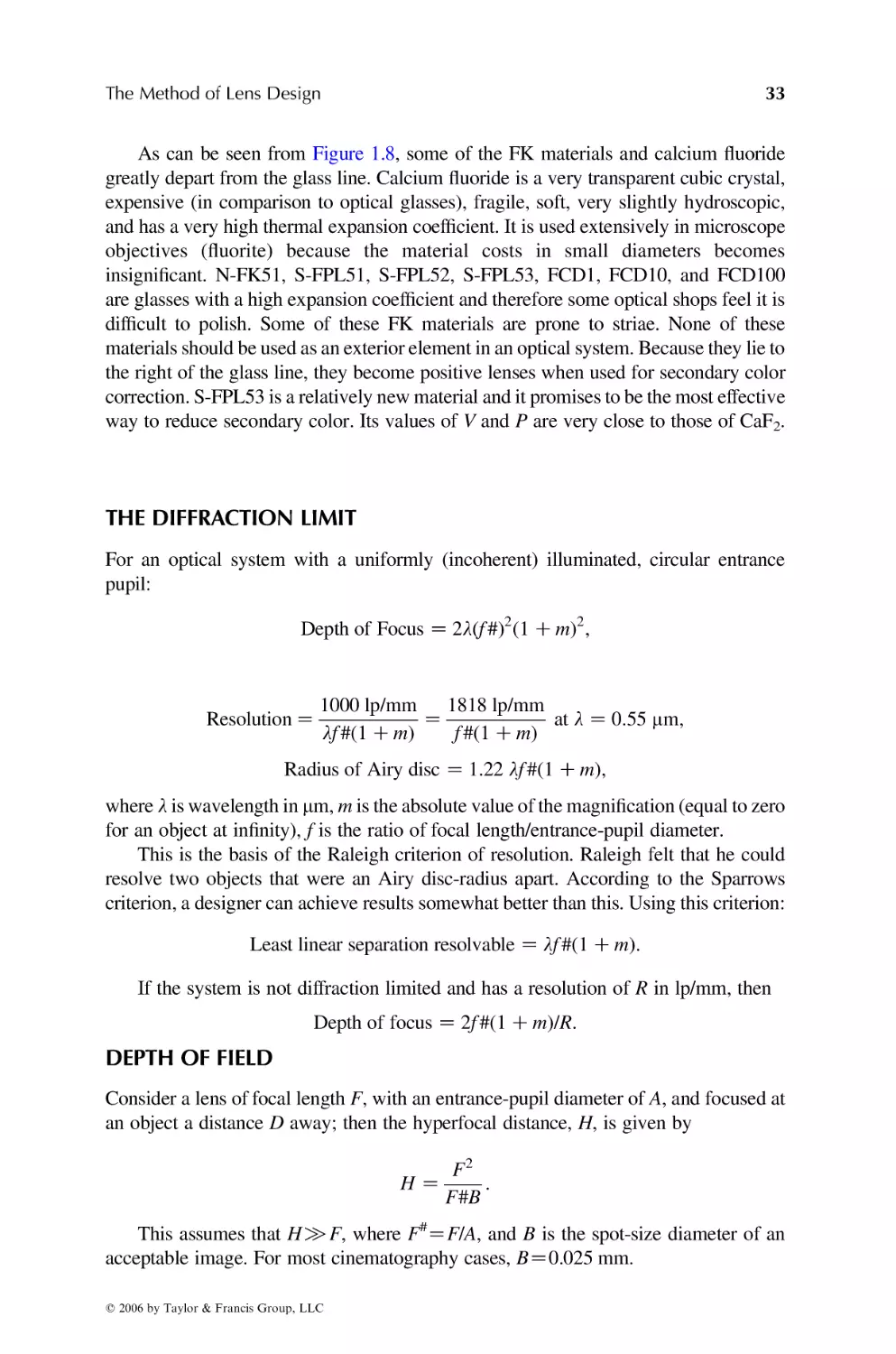
Let dI be the distance along the axis from surface I to surface IC1 and let DI be
the distance for an arbitrary ray from surface I to surface IC1. Then for a system of J
1
q 2006 by Taylor & Francis Group, LLC
2
Lens Design
surfaces, and (ND)I as the refractive index for the central wavelength following
surface I,
J
Σ DI ND
I =1
J
Σ dI ND
P
I =1
J
For a spherical wavefront centered at P,
J
X
ðDKdÞI ðND ÞI Z 0;
IZ1
and likewise for the extreme wavelengths, F and C, to be united at P. To be
achromatic,
J
X
ðDKdÞI ðNF KNC ÞI Z 0:
IZ1
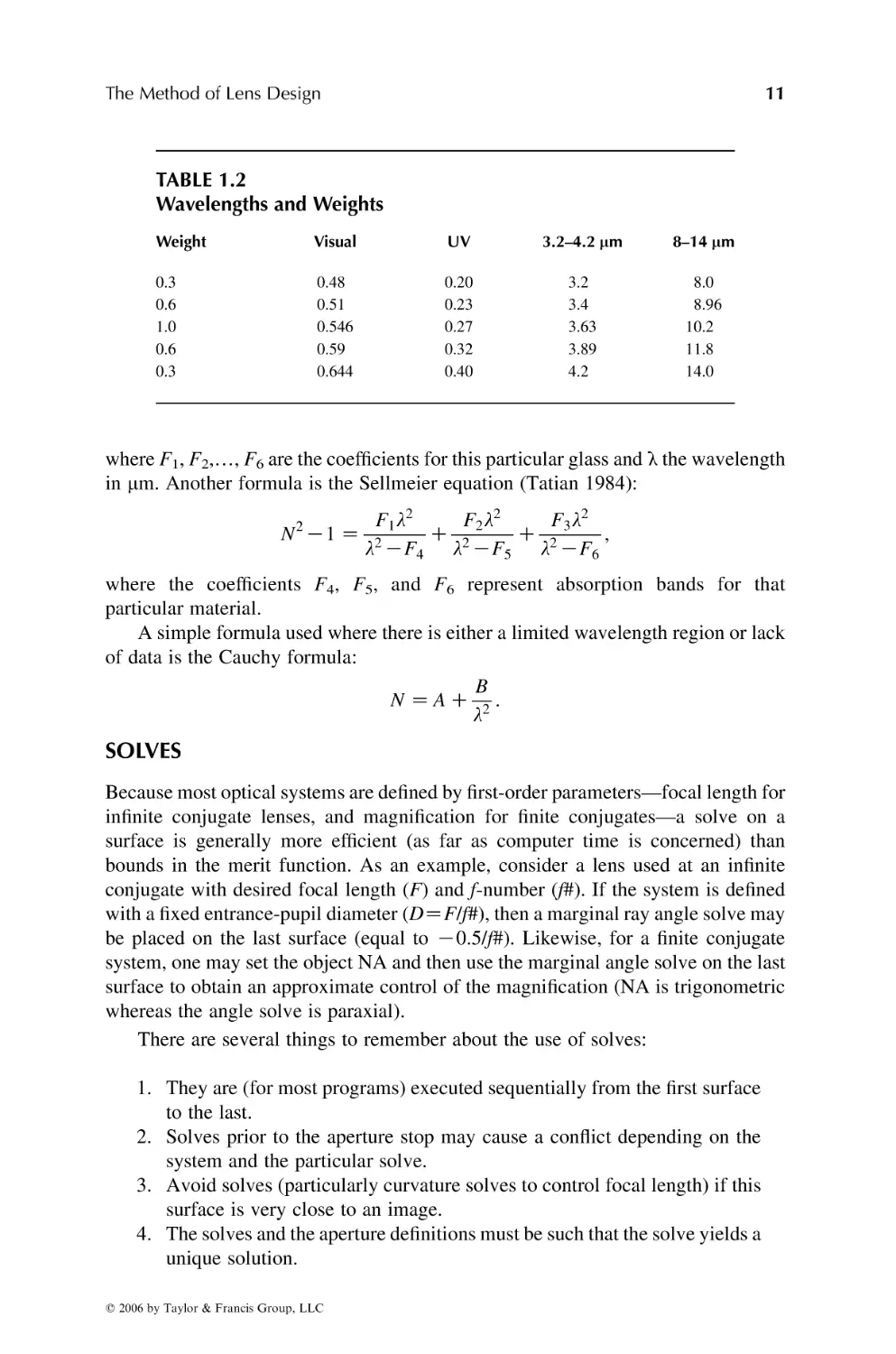
As an example of a merit function, let d be a defect item—the departure on the
image surface between the traced rays and its idealistic or Gaussian value (or other
means for determining the center of the image). Alternatively, one may use pathlength errors as a defect item. The ideal situation is to use a combination of both
intercept and path-length errors in the merit function because path-length errors may
be obtained with only a small amount of extra computing time, while the rays will be
traced.
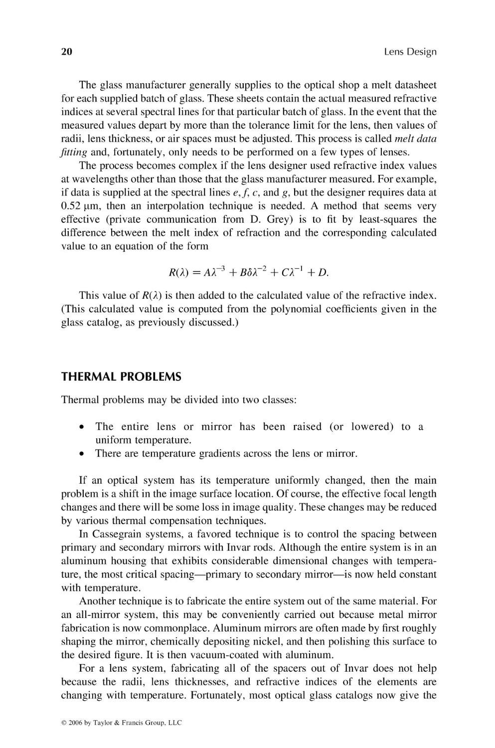
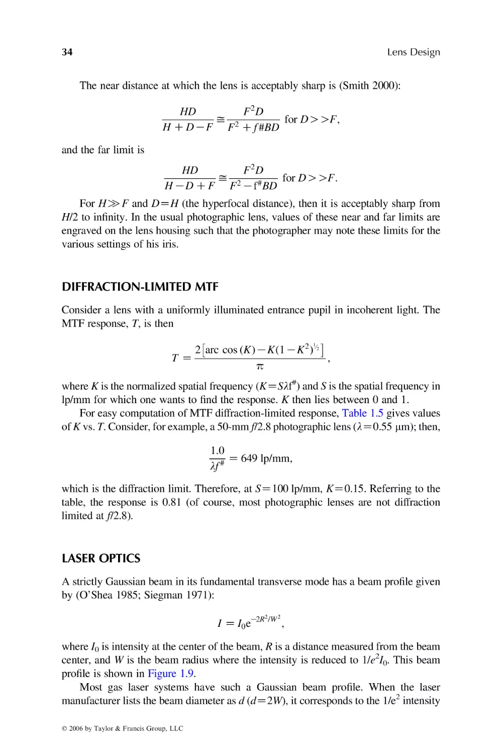
Wave front
Reference sphere
Wave front error
Δϕ
Last lens
surface
ΔY
Δϕ
q 2006 by Taylor & Francis Group, LLC
The Method of Lens Design
3
DY zkDf Z k !ðslope difference between the wavefront and the reference sphereÞ;
where k is a proportionally constant. The intercept errors are then approximately
proportional to the derivative of the path-length errors. It is also sometimes helpful
to add differential errors to the merit function. For example, if J rays are traced at a
particular field angle and wavelength, then
Differential error Z
PlðJÞKPlðJ K1Þ
;
PlðJ K1Þ
where Pl(J) is the path-length for the J ray. Because the major load in optimization is
the tracing of rays, these extra items improve the image while adding only slightly to
computer time. These defect items will be weighted by a factor W to permit us to
control the type of image we desire. If there are N defect items, then
Merit function Z
iZn
X
Wi di2 :
iZ1
Most merit functions are really “demerit” functions, i.e., they represent the sum
of squares of various image errors. Therefore, the larger the number, the worse the
image. The input system is ray traced, and the merit function is computed. One of the
permitted parameters is then changed, and a new value of the merit function is
calculated. A table is then created of merit function changes vs. parameter changes.
Then, usually by a technique of damped least-squares (or sometimes by
orthonormalization of aberrations) an improved system is created. There are four
important characteristics about this process that one should keep in mind:
1. The process finds a local minimum, i.e., a local minimum is reached in
respect to a multidimensional plot of all the permitted variables. Only by
past experience can one be certain that they have found a global
minimum. There are various “tricks” that designers have used to get out of
this local minimum and move the solution into a region where there is a
smaller local minimum of the merit function. This includes making a few
small changes to the lens parameters, changing merit-function weights,
and switching from ray-intercept to path-length errors in the merit
function (Bociort 2002). A trend in optimization programs is the inclusion
of a feature in which the program tries to find this global minimum (Jones
1992, 1994). It does this by making many perturbations of the original
system (Forbes 1991; Forbes and Jones 1992).
The orthonormalization process appears to sometimes penetrate these
potential barriers. A good procedure then is to first optimize in damped
least-squares mode, followed by orthonormalization.
2. The process finds an improvement, however small, wherever it may find
it. Thus, if one does not carefully provide bounds on lens thickness, thin
lenses of 1/50 lens diameter, or thick lenses (to solve for Petzval sum) of
12 in. could result. Likewise, when glasses are varied, a very small
improvement may result in a glass that is either very expensive, not
readily available, or has undesirable stain or transmission characteristics.
q 2006 by Taylor & Francis Group, LLC
4
Lens Design
These computer programs can trace rays through lenses with negative
lens thicknesses. Or, the lens system may be so long that it cannot fit into
the “box” that has been allocated to it. Therefore, a carefully thought
boundary control is vital.
3. Computer time is proportional to the product of the number of rays traced
and the number of parameters being varied. Inexperienced designer tend
to believe that they will obtain a better lens if they trace more rays;
instead, they achieve longer computer runs. The ideal situation is to trace
the minimum number of rays in the early stages. The number of rays and
field angles should only be increased at the end. Likewise, the image
errors should, in the early stages, be referenced to the chief ray for
computational speed. As the design progresses, the reference to centroid
may be changed. Due to the presence of coma, there is a difference in
image evaluation between the chief ray and the image centroid. In most of
the designs presented here, three wavelengths were used at the beginning
and five wavelengths were used at the end.
4. The program neither adds nor subtracts elements. Therefore, if one starts
with a six-element lens, it will always be a six-element lens. It is the art of
lens design to know when to add or remove elements.
The use of sine-wave response considering diffraction effects (MTF) is now
common in all lens evaluations. The main difficulty in using a sine-wave response as a
means of forming a merit function is the very large number of rays that need to be
traced, as well as the additional computation necessary to evaluate sine-wave
response. This would result in an excessively long computational run. The net result is
that diffraction-based criteria, particularly sine-wave response, have not been used as
a means of optimizing a lens, but has rather been limited to lens evaluation.
OPTIMIZATION METHODS
In the least-squares method, the above merit function is differentiated with respect to
the independent variables (construction parameters) and equated to zero. The
derivative is determined by actually incrementing a parameter and noting the change
in merit function. This results in N equations of the parameter increments. A matrix
method for solving these equations for the parameter increments is employed (Rosen
and Eldert 1954; Meiron 1959).
It has long been known that the least-squares method suffers from very slow
convergence (Feder 1957a,1957b). To speed convergence, the concept of a metric, M,
is introduced (Lavi and Vogl 1966:15). The gradient obtained from a least squares
technique is multiplied by M to speed convergence, although this is an
oversimplification of the technique. This step length computed on the basis of
linearity is usually too large, causing the process to oscillate. A damping factor is then
introduced into M that is large when the nonlinearity is large (Jamieson 1971).
The above method will rapidly improve a crude design. After a while, a balance of
aberrations will be reached. These residual aberrations vary only slowly when their
construction parameters are changed (Grey 1963). Thus, the construction parameters
have to be given an infinitesimal increment, which of course reduces the rate of
q 2006 by Taylor & Francis Group, LLC
The Method of Lens Design
5
convergence of the merit function. To avoid this problem, one must consider the rate
of change of each of the defect items with respect to the construction parameters. The
main difficulty in any automatic differential correction method lies not in the fact that
optical systems are nonlinear, but in the fact that every construction parameter affects
every defect item.
In the orthonormal method, a set of parameters are constructed that are
orthonormal to the construction parameters. This transformation matrix relating the
classical aberrations to its orthonormal counterpart is constructed at the beginning of
each pass. The merit function then is expressed as the sum of squares of certain
quantities, each of which is a linear combination of the classical aberration
coefficients. These are orthonormal aberration coefficients because the reduction of
any one of these reduces the value of the merit function no matter what the other
coefficients may be (Unvala 1966).
BOUNDARY VIOLATIONS
There are many physical constraints that must be imposed upon the optical system:
lens thickness, overall length of the assembly, maximum diameters, refractive index
range, minimum BFL, clearance between lens elements, etc. These are entered as
boundary controls by the designer and deviations from these bounds are entered into
the merit function. Therefore, if the lens is too long and will not fit into the required
envelope, this defect is added into the sum of image errors to be corrected. There are
several ways to handle these boundary errors:
1. Absolute control. With absolute control, a boundary error is not permitted.
If a parameter is changed such that it causes a boundary violation, that
parameter change is then not allowed. A problem with this method is that it
restricts optimization in that a better solution is often found when other
parameters are allowed to vary and thus remove this boundary violation.
2. Penalty control. With penalty control, a boundary violation is assigned a
penalty based upon the weightings that the designer has invoked. This
boundary violation is added into the merit function containing the image
errors. This is the most common method used in optimization programs.
3. Variable bounds. Variable bounds are a more complex method of boundary
control. Here, upper and lower bounds are assigned to all the boundary items.
As long as the bounded item remains within these bounds, no penalty is
added to the merit function. When the bounded item gets very close to the
edge of a bound, a penalty is added to the merit function, the bounds are moved
in slightly, and the penalty weight increased. Finally, when the bounded item
goes beyond the bounds, the weight is substantially increased. This has a
tendency to dampen the system and prevent large boundary violations.
RAY PATTERN
Because a ray may be regarded as the centroid of an energy bundle, it is convenient
to divide the entrance pupil into equal areas and to place a ray in the center of each
area (Table 1.1). For a centered optical system, one need only trace in one half of the
q 2006 by Taylor & Francis Group, LLC
6
Lens Design
TABLE 1.1
Entrance Pupil Fractions, Based on Equal Areas
NZ
2
3
4
5
6
7
8
0.866
0.500
0.913
0.707
0.408
0.353
0.316
0.935
0.791
0.612
0.548
0.500
0.289
0.948
0.837
0.707
0.645
0.598
0.463
0.957
0.866
0.764
0.707
0.661
0.559
0.964
0.886
0.802
0.750
0.968
0.901
0.829
0.267
0.433
0.250
entrance pupil. Likewise, for an axial object, only one quadrant need be traced. For
systems that lack symmetry, the full pupil needs to be traced.
When starting the design, always trace the minimum number of rays. A
reasonable value for the number of rays, N, might
be equal to 3.
pffiffiffiffiffiffiffiffiffiffiffiffiffiffiffiffiffiffiffiffiffiffiffiffiffiffiffiffiffiffiffiffiffiffiffi
In general, the value for the Jth value is ð2ðN KJÞC 1Þ=2N .
Today, most lens design programs automate this process. Generally, the pupil (or in
some cases the aperture stop) is divided into rings and the number of rays per ring. Thus,
the designer simply specifies the number of rings and the number of rays per ring.
For off-axis objects, a chief ray also needs to be traced as well as well as tracing to
both sides of the pupil. For systems that lack symmetry, the full pupil must be traced at
all fields. Most modern lens design programs today automate this process of ray
selection. The entrance pupil is divided into rings and each ring into sections.
Therefore, the designer only needs to specify the number of rings and the number of
rays in each ring. As the design progresses, the ray intercept plots should be carefully
monitored. If there is considerable flare, then additional rays should be added.
Likewise, if there are problems in the skew orientation, some skew rays should be
added. In a similar manner, the field angles should be such as to divide the image into
equal areas. The image height fractions are (the first field angle is axial, NZ1)
rffiffiffiffiffiffiffiffiffiffiffiffi
J
HðJÞ Z
N K1
NZ
2
3
4
5
6
H(1)
1.0
0.7071
0.5774
0.5
0.4472
1.0
0.8165
0.7071
0.6325
1.0
0.8660
0.7746
1.0
0.8944
H(2)
H(3)
H(4)
H(5)
q 2006 by Taylor & Francis Group, LLC
1.0
The Method of Lens Design
7
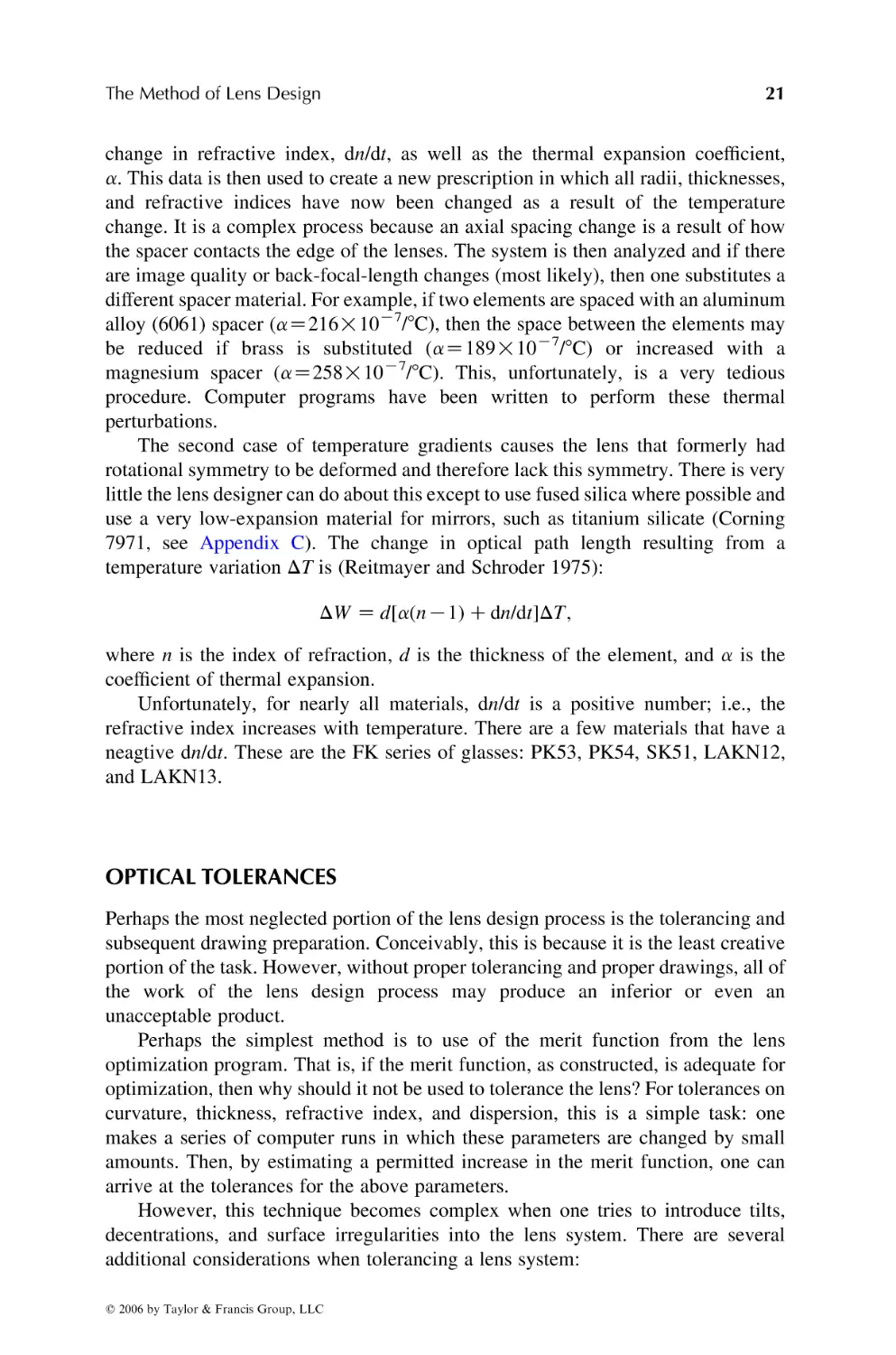
ASPHERIC SURFACES
Most modern computer programs have the ability to handle aspheric surfaces. For
mathematical convenience, surfaces are generally divided into three classes:
spheres, conic sections, and general aspheric. The aspheric is usually represented as
a tenth-order (or higher order) polynomial. Let X be the surface sag, Y the ray height,
and C the curvature of the surface at the optical axis; then
XZ
CY 2
pffiffiffiffiffiffiffiffiffiffiffiffiffiffiffiffiffiffiffiffiffiffiffiffiffiffiffiffiffiffiffiffiffi C AY 4 C A6 Y 6 C A8 Y 8 C A10 Y 10 :
1 C 1KY 2 C 2 ð1 C A2 Þ
This then represents the surface as a deviation from a conic section. A2 is the
conic coefficient and is equal to K32, where 3 is the eccentricity as given in most
geometry texts.
A2 Z 0
sphere
A2 !K1
hyperbola
A2 ZK1
parabola
K1! A2 ! 0
ellipse with foci on the optical axis
A2 O 0
ellipse with foci on a line normal to optic axis
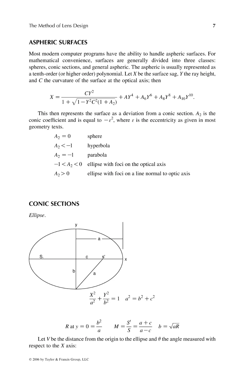
CONIC SECTIONS
Ellipse.
y
a
S.
c
b
s'
x
a
X2 Y 2
C 2 Z 1 a 2 Z b2 C c 2
a2
b
R at y Z 0 Z
b2
a
MZ
S0
a Cc
Z
S
aKc
pffiffiffiffiffiffi
b Z aR
Let V be the distance from the origin to the ellipse and q the angle measured with
respect to the X axis:
q 2006 by Taylor & Francis Group, LLC
8
Lens Design
cos2 q sin2 q
1
C 2 Z 2:
a2
b
V
Parabola.
Y
Focus
R/2
R/2
X
Y 2 Z 2RX
3 Z1
Radius of curvature Z
ðY 2 C R2 Þ3=2
Z R at Y Z 0
R2
Hyperbola.
Y
θ
a
X
f
C
K32 ZKtan2 qK1:
X2 Y 2
K Z 1:
A2 B 2
ðx C AÞ2 Y 2
K 2 Z 1:
A2
B
C 2 Z B2 C A 2
3 Z C=A
RZ
q 2006 by Taylor & Francis Group, LLC
B2
at Y Z 0:
A
The Method of Lens Design
9
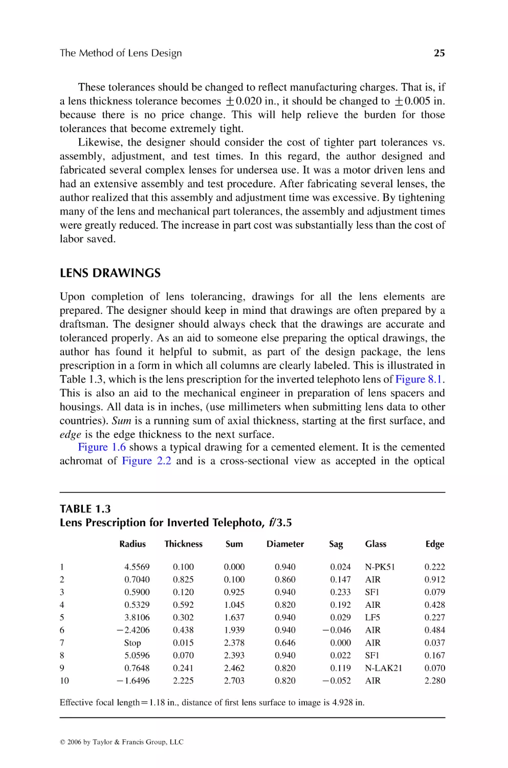
With present technology, it is possible to turn an aspheric surface with single
point diamond tooling. This is done with a numerical control system and is being
increasingly used for long wavelength infrared systems. In the visual and UV
regions, aspherics must be individually polished. The problem is twofold:
1. Most optical polishing machines have motions which tend to generate a
spherical surface. (Recently LOH Optical Machinery in Germantown,
WI, has made available machines to grind, polish, and test aspheric
surfaces.)
2. Aspheric surfaces are very difficult to test.
The best advice concerning aspherics is: unless absolutely necessary, do not use
an aspheric surface. Of course, if the lens is to be injection molded, then an aspheric
surface is a practical possibility. This is often done in the case of video disc lenses as
well as for low cost digital camera lenses (Yamaguchi et al. 2005).
As an aid in manufacturing and testing aspheric surfaces, the author has written
a computer program to calculate the surface coordinates as well as the coordinates
of a cutter to generate this surface. Let the aspheric surface have coordinates X, Y
and be generated by a cutter of diameter D. The coordinates of the center of this
cutter are U, V. The cutter is always tangent to the aspheric surface. Referring to
Figure 1.1:
y
Aspheric
section
Cutter
U
Radius
V
f
x
XN
FIGURE 1.1 Aspheric generation.
q 2006 by Taylor & Francis Group, LLC
10
Lens Design
tan f Z
2CY
pffiffiffiffiffiffiffiffiffiffiffiffiffi
1 C 1KC 2 Y 2 ð1 C A2 Þ
ð1 C A2 ÞC 3 Y 3
C 4A4 Y 3 C 6A6 Y 5
Ch
i2 pffiffiffiffiffiffiffiffiffiffiffiffiffi
pffiffiffiffiffiffiffiffiffiffiffiffiffi
2 2
2 2
1KC Y ð1 C A2 Þ
1 C 1KC Y ð1 C A2 Þ
C 8A8 Y C 10A10 Y ;
7
XZ
9
CY 2
pffiffiffiffiffiffiffiffiffiffiffiffiffiffiffiffiffiffiffiffiffiffiffiffiffiffiffiffiffiffiffiffiffi C A4 Y 4 C A6 Y 6 C A8 Y 8 C A10 Y 10 ;
1 C 1KY 2 C 2 ð1 C A2 Þ
U Z X C 0:5D cos fK0:5D;
V Z Y K0:5D sin f;
XN Z X C
radius Z
Y
;
tan f
pffiffiffiffiffiffiffiffiffiffiffiffiffiffiffiffiffiffiffiffiffiffiffiffiffiffiffiffiffiffiffi
Y 2 C ðXN KXÞ2 ;
where XN is the radius of curvature of the aspheric surface at the optical axis (the
paraxial radius of curvature).
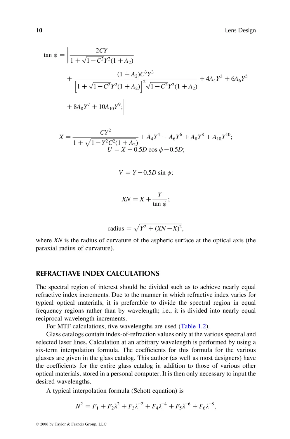
REFRACTIAVE INDEX CALCULATIONS
The spectral region of interest should be divided such as to achieve nearly equal
refractive index increments. Due to the manner in which refractive index varies for
typical optical materials, it is preferable to divide the spectral region in equal
frequency regions rather than by wavelength; i.e., it is divided into nearly equal
reciprocal wavelength increments.
For MTF calculations, five wavelengths are used (Table 1.2).
Glass catalogs contain index-of-refraction values only at the various spectral and
selected laser lines. Calculation at an arbitrary wavelength is performed by using a
six-term interpolation formula. The coefficients for this formula for the various
glasses are given in the glass catalog. This author (as well as most designers) have
the coefficients for the entire glass catalog in addition to those of various other
optical materials, stored in a personal computer. It is then only necessary to input the
desired wavelengths.
A typical interpolation formula (Schott equation) is
N 2 Z F1 C F2 l2 C F3 lK2 C F4 lK4 C F5 lK6 C F6 lK8 ;
q 2006 by Taylor & Francis Group, LLC
The Method of Lens Design
11
TABLE 1.2
Wavelengths and Weights
Weight
Visual
UV
3.2–4.2 mm
8–14 mm
0.3
0.6
1.0
0.6
0.3
0.48
0.51
0.546
0.59
0.644
0.20
0.23
0.27
0.32
0.40
3.2
3.4
3.63
3.89
4.2
8.0
8.96
10.2
11.8
14.0
where F1, F2,., F6 are the coefficients for this particular glass and l the wavelength
in mm. Another formula is the Sellmeier equation (Tatian 1984):
N 2 K1 Z
F1 l2
F2 l2
F3 l 2
C
C
;
l2 KF4 l2 KF5 l2 KF6
where the coefficients F4, F5, and F6 represent absorption bands for that
particular material.
A simple formula used where there is either a limited wavelength region or lack
of data is the Cauchy formula:
B
N ZAC 2 :
l
SOLVES
Because most optical systems are defined by first-order parameters—focal length for
infinite conjugate lenses, and magnification for finite conjugates—a solve on a
surface is generally more efficient (as far as computer time is concerned) than
bounds in the merit function. As an example, consider a lens used at an infinite
conjugate with desired focal length (F) and f-number (f#). If the system is defined
with a fixed entrance-pupil diameter (DZF/f#), then a marginal ray angle solve may
be placed on the last surface (equal to K0.5/f#). Likewise, for a finite conjugate
system, one may set the object NA and then use the marginal angle solve on the last
surface to obtain an approximate control of the magnification (NA is trigonometric
whereas the angle solve is paraxial).
There are several things to remember about the use of solves:
1. They are (for most programs) executed sequentially from the first surface
to the last.
2. Solves prior to the aperture stop may cause a conflict depending on the
system and the particular solve.
3. Avoid solves (particularly curvature solves to control focal length) if this
surface is very close to an image.
4. The solves and the aperture definitions must be such that the solve yields a
unique solution.
q 2006 by Taylor & Francis Group, LLC
12
Lens Design
In some of the examples in this text, bounds were placed on the focal length
whereas a solve on the last surface would probably have been a better choice.
GLASS VARIATION
Most modern lens optimization computer programs have the ability to vary the index
and dispersion of the material. This assumes a continuum of the so-called glass map.
This then generally precludes this variation in the UV or infrared regions. However,
in the visual region, it is a very powerful variable and should be utilized
wherever possible.
To be effective at glass variation, the computer program must be able to bound
the glasses to the actual regions of the map; i.e., if refractive index would be left as
an unfettered variable, a prescription with refractive index values of 10 would
be obtained.
However, not only must the designer carefully bound values of refractive index
and dispersion, the designer must also be careful as to the glass he or she chooses.
Consider, for example, N-LAK7 vs. N-SK15 (which are fairly close to each other on
the glass map). The former, in a grade-A slab, costs $63/pound whereas the latter
costs $29/pound (2002 prices). Therefore, for a large diameter lens, the price has
been greatly increased. Selecting an LASF-type glass can cost from $111/pound (NLASF45) to $648/pound (N-LASF31) for a grade-A slab.
Price is only the beginning. The designer must also check the catalog for:
† Availability. Some glasses are more available than others. These so-called
preferred glasses are indicated in the catalog. Due to environmental
pressures, particularly in Europe and Japan, some glasses (such as LAK6)
have been discontinued and others have been reformulated. Lead oxide is
being substituted with titanium oxide. This reduces the density and these
glasses have nearly the same index and dispersion as their predecessor
(SF6 and SFL6). Likewise, arsenic oxide and cadmium have been
eliminated.
† Transmission. Some glasses are very yellow, particularly the dense flints.
This is due to the lead oxide content. With the new versions of these
glasses, it is worse. For example, the old SF6 containing lead oxide has a
transmission of 73% for a 25-mm thickness at 0.4 mm, whereas SFL6 has
a transmission of 67%. Catalogs give transmission values at the various
wavelengths. In the so-called mini-catalog, a value for transmission at
0.4 mm thru a 25-mm path is given.
† Staining and weathering. Glass is affected in various ways when
contacted by aqueous solutions. Under certain conditions, the glass may
be leached. At first, when thin, it forms an interference coating. As it
thickens, it slowly turns white. Interactions with aqueous solutions,
particularly during the polishing operations, may cause surface staining.
Glasses that are particularly susceptible are listed in these glass catalogs.
Glasses that are susceptible to water vapor in the air (listed as climatic
resistance) should never be used as an exterior lens element.
q 2006 by Taylor & Francis Group, LLC
The Method of Lens Design
13
† Bubble. Some glasses, due to their chemical composition, are prone to
containing small bubbles. These glasses cannot be used near an
image surface.
† Striae. A few glass types are prone to fine striae (index of refraction
variations). These glasses should not be used in prisms or in thick
lenses.
When the glass is finally selected, the actual catalog values are then substituted
for the “fictitious glass” values. This is done by changing the surface curvatures to
maintain surface powers. Let F be the surface power at the Jth surface with
curvature C, and a fictitious refractive index N; then
F Z ðNJ KNJK1 ÞCJ Z ðN 0 KNJK1 ÞC 0 J;
where N 0 is the catalog value of the refractive index and C 0 is the adjusted value of
the curvature.
GLASS CATALOGS
All refractive index data was taken from the manufacturers’ catalogs. These catalogs
are included in most optical design programs and are kept current. As explained
above, many of these glasses, when used in the visual region, have poor transmission
in the blue region, are prone to staining, have striae or bubbles, or are very
expensive. Consequently, for these designs, the glass selection, where appropriate,
has been limited to some “prefered” glasses.
Material catalogs may be readily be obtained via the Internet. The following is a
listing for some of these materials.
Company
Internet Address
Material
Hoya optics
http://www.hoyaoptics.com
Optical glass
Schott glass technologies
http://www.us.schott.com
Optical glass
Ohara glass
http://www.oharacorp.com
Optical glass
Hikari glass
http://www.hikariglass.com
Optical glass
Heraeus
http://www.heraeus-quarzglas.
com
Fused silica
See also http://www.heraeusoptics.com
Fused silica
Corning
http://www.corning.com
Fused silica, Vycor, Pyrex
Morton
http://www.rohmhaas.com
Infrared materials
Dynasil
http://www.dynasil.com
Fused silica
Dow
http://www.dow.com/styron
Polystyrene
q 2006 by Taylor & Francis Group, LLC
14
Lens Design
CEMENTED SURFACES
Cement thickness is generally less than 0.001 in. Therefore, this cement layer is
generally ignored in the lens design process. Modern cements can withstand
temperature extremes from K628C to greater than 1008C (Summers 1991; Norland
1999). Because these cements have an index of refraction of about 1.55, there will be
some reflection loss at the interface. Nevertheless, the cement–glass interface is rarely
antireflection coated. For certain critical applications, a l/4 coating at each glass
surface prior to cementing will greatly reduce this reflection loss (Willey 1990).
Due to transmission problems with cements, their use is limited to the
visual region.
ANTIREFLECTION FILMS
For light striking at normal incidence on an uncoated surface, the reflectivity, R, is
given by
N0 KNS 2
;
RZ
N0 C NS
where light is in media N0 and is reflected from media of refractive index N1. For air,
N0 is 1; if NsZ1.5, then RZ4%.
Considering films whose optical thickness is l/4, then the reflectivity for a single
film of index N1 on a substrate of Ns is
h
i
N2 2
1K N1S
RZh
i ;
N2 2
1 C N1S
pffiffiffiffiffiffi
which becomes zero when N1 Z NS .
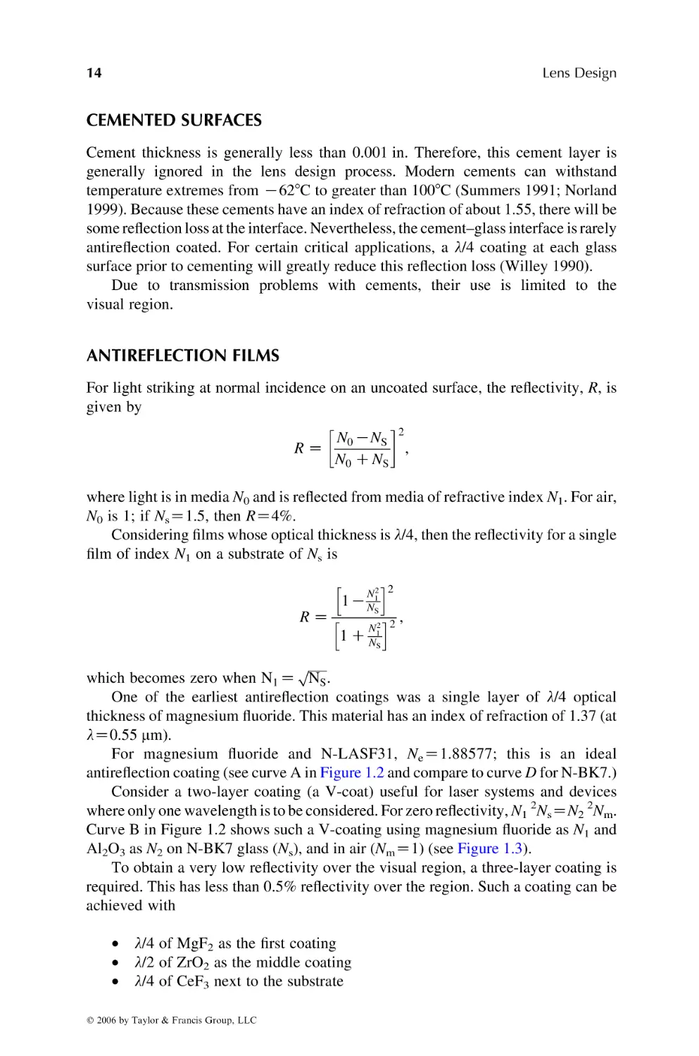
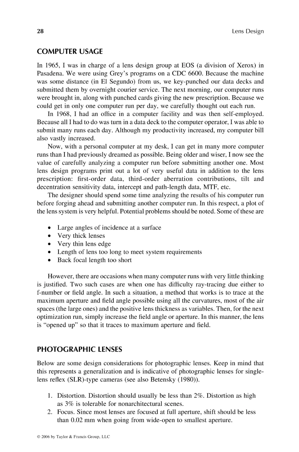
One of the earliest antireflection coatings was a single layer of l/4 optical
thickness of magnesium fluoride. This material has an index of refraction of 1.37 (at
lZ0.55 mm).
For magnesium fluoride and N-LASF31, NeZ1.88577; this is an ideal
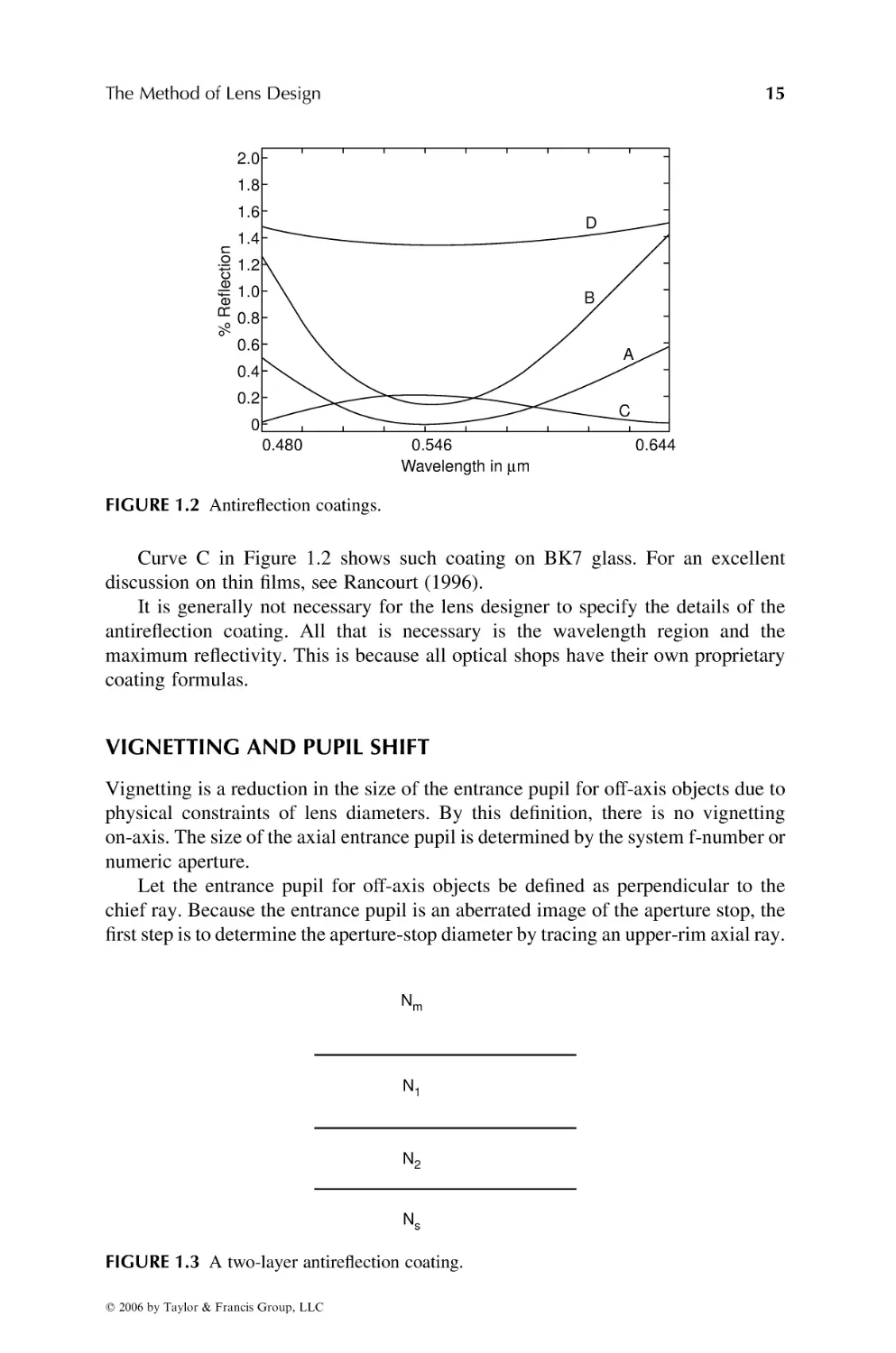
antireflection coating (see curve A in Figure 1.2 and compare to curve D for N-BK7.)
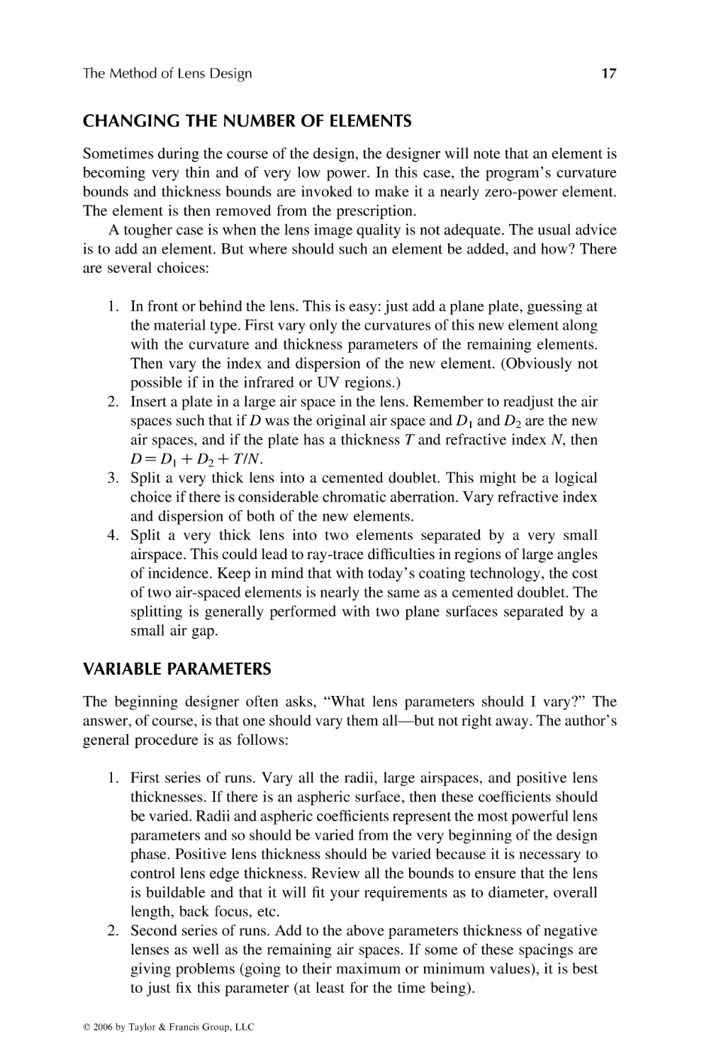
Consider a two-layer coating (a V-coat) useful for laser systems and devices
where only one wavelength is to be considered. For zero reflectivity, N1 2NsZN2 2Nm.
Curve B in Figure 1.2 shows such a V-coating using magnesium fluoride as N1 and
Al2O3 as N2 on N-BK7 glass (Ns), and in air (NmZ1) (see Figure 1.3).
To obtain a very low reflectivity over the visual region, a three-layer coating is
required. This has less than 0.5% reflectivity over the region. Such a coating can be
achieved with
† l/4 of MgF2 as the first coating
† l/2 of ZrO2 as the middle coating
† l/4 of CeF3 next to the substrate
q 2006 by Taylor & Francis Group, LLC
The Method of Lens Design
15
2.0
1.8
% Reflection
1.6
D
1.4
1.2
1.0
B
0.8
0.6
A
0.4
0.2
C
0
0.480
0.546
Wavelength in μm
0.644
FIGURE 1.2 Antireflection coatings.
Curve C in Figure 1.2 shows such coating on BK7 glass. For an excellent
discussion on thin films, see Rancourt (1996).
It is generally not necessary for the lens designer to specify the details of the
antireflection coating. All that is necessary is the wavelength region and the
maximum reflectivity. This is because all optical shops have their own proprietary
coating formulas.
VIGNETTING AND PUPIL SHIFT
Vignetting is a reduction in the size of the entrance pupil for off-axis objects due to
physical constraints of lens diameters. By this definition, there is no vignetting
on-axis. The size of the axial entrance pupil is determined by the system f-number or
numeric aperture.
Let the entrance pupil for off-axis objects be defined as perpendicular to the
chief ray. Because the entrance pupil is an aberrated image of the aperture stop, the
first step is to determine the aperture-stop diameter by tracing an upper-rim axial ray.
Nm
N1
N2
Ns
FIGURE 1.3 A two-layer antireflection coating.
q 2006 by Taylor & Francis Group, LLC
16
Lens Design
For this off-axis object, the size of the vignetted entrance pupil is determined by
iteratively tracing upper, lower, and chief rays to the aperture stop. For certain
systems, the full, unvignetted entrance pupil may not be traceable. In these
situations, this vignetting and pupil shift to the aperture stop; i.e., the ray coordinate
data is shifted and vignetted onto the aperture stop.
Vignetting is nearly the same for all wavelengths (at any particular field angle).
Therefore, for convenience, the above procedure only needs to be carried out at the
central wavelength. However, there is, in general, a different vignetting and pupil
shift for all off-axis field points and configurations (a zoom lens). In a typical
computer program, vignetting and pupil shift are handled as follows:
† VTT(J) is the vignetting for a particular field and configuration. It is
expressed as a fraction of the aberrated entrance-pupil diameter. It applies
only in the meridional direction (see Figure 1.4).
† VTS(J) is the same but in the sagittal direction. For a centered optical
system with rotational symmetry, these items are one.
† PST(J) is pupil shift for the vignetted pupil corresponding to the above.
† PSS(J) is the same but in the sagittal direction. For a centered optical
system with rotational symmetry, these items are zero.
† In the absence of any pupil shift or vignetting, all VTT(J) and VTS(S)
items are set equal to 1 and all PST(J) and PSS(J) are set equal to zero.
† To trace to the top of the pupil: PST(J)CVTT(J)Z1.
Entrance pupil coordinates are then shifted and multiplied by the appropriate
vignetting coefficient. This applies to all raytracing: MTF data, spot diagram, lens
drawings, etc. By this technique, accuracy in MTF and spot-diagram computations is
not compromised because the full number of rays is being traced in the presence of
vignetting. It also allows the designer to deliberately introduce vignetting into the
system when it is necessary to constrain lens diameters.
The lens designer must be cautioned that in systems with considerable
vignetting, care must be taken that there are lens diameters to limit the upper and
lower rim rays of the vignetted pupil. The aperture stop is now not the limiting
surface. Only rays that were traced in optimization must be able to pass through the
optical system.
(R)VTT(J)
PST(J )
S
R
Unvignetted
pupil
T
FIGURE 1.4 The vignetted entrance pupil.
q 2006 by Taylor & Francis Group, LLC
The Method of Lens Design
17
CHANGING THE NUMBER OF ELEMENTS
Sometimes during the course of the design, the designer will note that an element is
becoming very thin and of very low power. In this case, the program’s curvature
bounds and thickness bounds are invoked to make it a nearly zero-power element.
The element is then removed from the prescription.
A tougher case is when the lens image quality is not adequate. The usual advice
is to add an element. But where should such an element be added, and how? There
are several choices:
1. In front or behind the lens. This is easy: just add a plane plate, guessing at
the material type. First vary only the curvatures of this new element along
with the curvature and thickness parameters of the remaining elements.
Then vary the index and dispersion of the new element. (Obviously not
possible if in the infrared or UV regions.)
2. Insert a plate in a large air space in the lens. Remember to readjust the air
spaces such that if D was the original air space and D1 and D2 are the new
air spaces, and if the plate has a thickness T and refractive index N, then
DZ D1 C D2 C T=N.
3. Split a very thick lens into a cemented doublet. This might be a logical
choice if there is considerable chromatic aberration. Vary refractive index
and dispersion of both of the new elements.
4. Split a very thick lens into two elements separated by a very small
airspace. This could lead to ray-trace difficulties in regions of large angles
of incidence. Keep in mind that with today’s coating technology, the cost
of two air-spaced elements is nearly the same as a cemented doublet. The
splitting is generally performed with two plane surfaces separated by a
small air gap.
VARIABLE PARAMETERS
The beginning designer often asks, “What lens parameters should I vary?” The
answer, of course, is that one should vary them all—but not right away. The author’s
general procedure is as follows:
1. First series of runs. Vary all the radii, large airspaces, and positive lens
thicknesses. If there is an aspheric surface, then these coefficients should
be varied. Radii and aspheric coefficients represent the most powerful lens
parameters and so should be varied from the very beginning of the design
phase. Positive lens thickness should be varied because it is necessary to
control lens edge thickness. Review all the bounds to ensure that the lens
is buildable and that it will fit your requirements as to diameter, overall
length, back focus, etc.
2. Second series of runs. Add to the above parameters thickness of negative
lenses as well as the remaining air spaces. If some of these spacings are
giving problems (going to their maximum or minimum values), it is best
to just fix this parameter (at least for the time being).
q 2006 by Taylor & Francis Group, LLC
18
Lens Design
3. Third series of runs. Add to the above parameters index and dispersion of
glasses. Obviously, this is skipped if in the UV or IR regions. Then fix the
glasses. The author finds this the most “soul searching” part of lens design
because he must now make value decisions regarding glass prices and
availability, stain and bubble codes, and, of course, performance.
4. Fourth series of runs. With the glasses fixed, again vary all the parameters
(except obviously index and dispersion).
At several stages in the design process, it is wise to
1. Run MTF calculations to be sure that the design is meeting your image
quality requirements.
2. Check distortion.
3. Plot the lens to be sure that it is buildable.
4. Examine intercept and path-length error plots as well as third-order
surface aberration contributions. This often gives the designer an insight
into their design problems. Based upon this, the designer might want to
split a lens, add a lens, etc. (For a discussion on third-order aberrations,
see Born and Wolf (1965)).
BOUNDS ON EDGE AND CENTER THICKNESS
For the economical production of a lens element:
† Negative elements should have a diameter-to-center thickness ratio of
less than 10. This ratio is necessary to prevent the lens from distorting
when removed from the polishing block. Diameter-to-thickness ratios as
high as 30 are possible, but production costs increase. In the IR region,
where material is expensive and there is considerable absorption and
scattering, high thickness ratios are common.
† Positive elements should have at least 0.04-in. edge thickness on small
lenses less than 1 in. in diameter and at least 0.06-in. edge thickness for
larger lenses. This is necessary to prevent the lens from chipping while
being processed.
TEST GLASS FITTING
During the polishing process, all spherical surfaces are compared under a
monochromatic light source with a test glass (Malacara 1978:14). A test glass
consists of a pair of concave/convex spheres, generally made from Pyrex or
sometimes fused silica. When compared to the work in process, Newton rings are
seen that represent contours of half-wavelength deviations of the work from a
sphere. This is a crude, but yet very practical way to determine the accuracy and
irregularity of the work. One-fourth and one-eighth fringe deviations are readily
discernible. This technique has two disadvantages:
q 2006 by Taylor & Francis Group, LLC
The Method of Lens Design
19
1. The work surface is being contacted by the test glass and may be
scratched. Today, with the availability of the HeNe laser, various
interferometers are available (Zygo, for example) in which no surface
contact is made.
2. For every value of radius, one needs a pair of test glasses.
All optical shops have an extensive test-glass inventory. These lists are made
available to the designer in the hope that he will select values of radii from this list.
Cost of a test glass is approximately $400 per radius value. Therefore, total cost of a
prototype optic is vastly reduced if the designer can fit his design to the optical
shop’s list. It is unfortunate that all shops have a different list, and that there is no
such thing as a standardized list.
As a basis for such a list, one might consider a system where all radii are a
constant multiplier of the next smallest value, i.e., RjZcRjK1; for 100 values
between 1 and 10, cZ1.02329.
However, a rationalized system will never happen, and thus the designer must
contend with fitting his design to the irrational values of test glasses that are
available within his or her shop. The author uses a rather crude technique, as
follows:
1. The third-order aberration contributions at each surface are scanned and a
radius tolerance is estimated.
2. Any surface that lies within this tolerance limit of a test-glass value is then
actually set to the test-glass value.
3. The system is then optimized, of course keeping the test-glass-fitted
surfaces constant. (The other radii and thicknesses are varied.)
4. Steps 2 and 3 are then repeated. Values of radii that did not at first lie
within its tolerance for a test glass will often move to a new value with the
subsequent optimization and now can be fitted.
Other designers have advocated a different technique. They try to fit the most
sensitive radii first. They feel that the least-sensitive radii can always be fitted.
Regardless of the method, do not worry if you cannot fit every radius to
the test list. If you fit most of them, you will still have saved your client a
substantial sum.
MELT DATA FITTING
Some lenses, particularly long-focal-length, high-resolution types, are sensitive to
small changes in refractive index and dispersion of the actual material used as
compared to the nominal or catalog value. For materials such as quartz (fused silica),
calcium fluoride, silicon, germanium, etc., refractive index is an intrinsic property of
these compounds. However, for mixtures such as optical glass, there are slight
variations in refractive index from batch to batch. Refractive index is carefully
controlled by the glass manufacturer. Typical tolerances for glass as supplied are
NdG0.001 and VdG0.8%.
q 2006 by Taylor & Francis Group, LLC
20
Lens Design
The glass manufacturer generally supplies to the optical shop a melt datasheet
for each supplied batch of glass. These sheets contain the actual measured refractive
indices at several spectral lines for that particular batch of glass. In the event that the
measured values depart by more than the tolerance limit for the lens, then values of
radii, lens thickness, or air spaces must be adjusted. This process is called melt data
fitting and, fortunately, only needs to be performed on a few types of lenses.
The process becomes complex if the lens designer used refractive index values
at wavelengths other than those that the glass manufacturer measured. For example,
if data is supplied at the spectral lines e, f, c, and g, but the designer requires data at
0.52 mm, then an interpolation technique is needed. A method that seems very
effective (private communication from D. Grey) is to fit by least-squares the
difference between the melt index of refraction and the corresponding calculated
value to an equation of the form
RðlÞ Z AlK3 C Bdl2 C Cl1 C D:
This value of R(l) is then added to the calculated value of the refractive index.
(This calculated value is computed from the polynomial coefficients given in the
glass catalog, as previously discussed.)
THERMAL PROBLEMS
Thermal problems may be divided into two classes:
† The entire lens or mirror has been raised (or lowered) to a
uniform temperature.
† There are temperature gradients across the lens or mirror.
If an optical system has its temperature uniformly changed, then the main
problem is a shift in the image surface location. Of course, the effective focal length
changes and there will be some loss in image quality. These changes may be reduced
by various thermal compensation techniques.
In Cassegrain systems, a favored technique is to control the spacing between
primary and secondary mirrors with Invar rods. Although the entire system is in an
aluminum housing that exhibits considerable dimensional changes with temperature, the most critical spacing—primary to secondary mirror—is now held constant
with temperature.
Another technique is to fabricate the entire system out of the same material. For
an all-mirror system, this may be conveniently carried out because metal mirror
fabrication is now commonplace. Aluminum mirrors are often made by first roughly
shaping the mirror, chemically depositing nickel, and then polishing this surface to
the desired figure. It is then vacuum-coated with aluminum.
For a lens system, fabricating all of the spacers out of Invar does not help
because the radii, lens thicknesses, and refractive indices of the elements are
changing with temperature. Fortunately, most optical glass catalogs now give the
q 2006 by Taylor & Francis Group, LLC
The Method of Lens Design
21
change in refractive index, dn/dt, as well as the thermal expansion coefficient,
a. This data is then used to create a new prescription in which all radii, thicknesses,
and refractive indices have now been changed as a result of the temperature
change. It is a complex process because an axial spacing change is a result of how
the spacer contacts the edge of the lenses. The system is then analyzed and if there
are image quality or back-focal-length changes (most likely), then one substitutes a
different spacer material. For example, if two elements are spaced with an aluminum
alloy (6061) spacer (aZ216!10K7/8C), then the space between the elements may
be reduced if brass is substituted (aZ189!10K7/8C) or increased with a
magnesium spacer (aZ258!10K7/8C). This, unfortunately, is a very tedious
procedure. Computer programs have been written to perform these thermal
perturbations.
The second case of temperature gradients causes the lens that formerly had
rotational symmetry to be deformed and therefore lack this symmetry. There is very
little the lens designer can do about this except to use fused silica where possible and
use a very low-expansion material for mirrors, such as titanium silicate (Corning
7971, see Appendix C). The change in optical path length resulting from a
temperature variation DT is (Reitmayer and Schroder 1975):
DW Z d½aðnK1Þ C dn=dtDT;
where n is the index of refraction, d is the thickness of the element, and a is the
coefficient of thermal expansion.
Unfortunately, for nearly all materials, dn/dt is a positive number; i.e., the
refractive index increases with temperature. There are a few materials that have a
neagtive dn/dt. These are the FK series of glasses: PK53, PK54, SK51, LAKN12,
and LAKN13.
OPTICAL TOLERANCES
Perhaps the most neglected portion of the lens design process is the tolerancing and
subsequent drawing preparation. Conceivably, this is because it is the least creative
portion of the task. However, without proper tolerancing and proper drawings, all of
the work of the lens design process may produce an inferior or even an
unacceptable product.
Perhaps the simplest method is to use of the merit function from the lens
optimization program. That is, if the merit function, as constructed, is adequate for
optimization, then why should it not be used to tolerance the lens? For tolerances on
curvature, thickness, refractive index, and dispersion, this is a simple task: one
makes a series of computer runs in which these parameters are changed by small
amounts. Then, by estimating a permitted increase in the merit function, one can
arrive at the tolerances for the above parameters.
However, this technique becomes complex when one tries to introduce tilts,
decentrations, and surface irregularities into the lens system. There are several
additional considerations when tolerancing a lens system:
q 2006 by Taylor & Francis Group, LLC
22
Lens Design
1. Tolerances must be assigned to each parameter by some statistical method
(Koch 1978; Smith 1990). Everything subject to manufacture will depart
from the nominal design.
2. In addition to actual image-quality changes as a result of manufacture,
certain first-order parameters must often be maintained: effective focal
length (or magnification) and back focal length. In this regard, it is helpful
to have a printed table of the variation of these first-order parameters vs.
the lens parameters of curvature, thickness, and refractive index.
3. There is often a parameter that may be used to compensate for image or
first-order errors. The simplest case is a variation in back focal length.
This is often compensated by adjusting the mounting flange as the last
step in manufacture. Also, in telephoto lenses, the large air space between
the front and rear groups may used to maintain effective focal length.
4. Accuracy and irregularity tolerances: Accuracy represents the total number
of rings that the surface deviates from the test glass. Irregularity is the
difference in fringes as seen in two mutually perpendicular directions. This
irregularity causes astigmatism for an axial object. To detect irregularity,
the accuracy should not be greater than 4–6 times the irregularity.
However, the accuracy also is related to the radius tolerance, particularly in
cases where the radius is greater than 10 times the diameter.
Let Y be the semi-diameter, and Z the sag at the surface. Then, approximately,
ZZKY2/2R. Taking the derivative, DZZKY2/2R2 DR. As an example, for an
accuracy of four fringes, RZ100 mm, YZ5 mm, and DZZ1.1!10K3 mm. DR then
is 0.88 mm, which is probably greater than the radius tolerance (which might be
0.2 mm).
As discussed previously, should the lens be subject to refractive index or
dispersion variations of less than catalog values, then melt data fitting is employed.
When the designer prepares the lens drawings, the actual tolerances are a blend of
tolerances to maintain image quality and tolerances to maintain first-order
properties. Ginsberg (1981) discusses this overall tolerancing concept.
Figure 1.5a shows a decentered lens element of focal length F and refractive
index N. The optical axis contains the centers of curvatures of the lens surfaces.
However, the lens is actually centered about an axis indicated as the lens center.
Decenter (DEC) is the distance between the optical center and the center of the lens.
Image runout is the diameter of the circle made by the mutating image as the lens is
rotated (see Chapter 6 of Kimmel and Parks (1995)):
Image runout Z 2DEC;
DEC Z F deviation;
Edge variation Z E1 E2 Z
q 2006 by Taylor & Francis Group, LLC
DðdeviationÞ
Z TIRðtotal indicator runoutÞ:
N K1
The Method of Lens Design
23
E2
R(
DEC
1)
D
2)
R(
Lens center
Optical axis
TIR
(a)
E1
(b)
FIGURE 1.5 (a) Lens decentration and (b) centering (edging) an element.
This assumes that the part runs true on surface 2 and rotates about the lens center
axis. D is the clear aperture diameter of surface 1, and this is where the dial indicator
is placed to read TIR. As the lens is rotated, the image of a distant object will rotate
about a circle of diameter 2DEC.
Wedge (in radians) is the edge thickness difference divided by the lens diameter.
Figure 1.5b shows how a lens is setup for edging. On the left, a lens is waxed to a true
running spindle in preparation for edging (centering). Notice that the center of
curvature of the surface in contact with the spindle lies on the center of rotation of
the spindle. In the center figure, a bright object is seen as reflected from the external
surface of the lens. As the lens is rotated, the image tracks out a circle in space. With
the wax still soft (a little heat might be needed), the lens is pushed closer to the
centered position and the circle becomes smaller until no movement of the image
can be discerned. Alternatively, a dial indicator may be placed near the edge of the
external surface. (With this method, there is the possibility of scratching the polished
lens surface.) In the figure on the right, a beam of light (perhaps a laser) is
transmitted thru the lens and the deviation is noted. Again, the lens is adjusted until
no deviation can be detected. With the lens so centered on the spindle, a diamond
wheel then edges the lens to the proper diameter.
It is important to try to create a design that is not too sensitive to the construction
parameters. The usual method of optimization creates a lens that is in a local
q 2006 by Taylor & Francis Group, LLC
24
Lens Design
minimum with respect to the “centered” parameters: thickness, curvature, refractive
index, and dispersion (assuming that all these parameters were varied). However,
optimization does not create a system that is a minimum with respect to tilt and
decentrations. As a means of reducing these effects, the designer should try to avoid
large angles of incidence and large third-order surface contributions.
In POP, there is a bound (Grey 1970, 1978) whereby sensitivity to tilt and
decentration may be reduced. This, however, must be used with caution. The item
bounded is the RMS OPD (optical path difference) path-length error induced by tilt
or decentration (see the following discussion on wave front perturbations). In
addition, at the end of a computer run, there is a printout of lens tolerance data for
each surface and for each lens. This is RMS OPD (in mm) per 0.001-in. lateral
displacement, as well as TIR of 0.001-in. at the edge of the clear aperture. This alerts
the designer as to potential sensitive surfaces. Other lens optimization programs
have a similar feature.
MTF (modulation transfer function), or OTF (optical transfer function) is
presently regarded as the “best” way to evaluate an optical system. Therefore,
although most merit functions are not based on diffraction MTF, final analysis of the
lens is by diffraction-based MTF. Consequently, some tolerancing programs (for
example Code V, Appendix D) utilize a procedure for calculating the variation of
OTF with the construction parameters (Stark and Wise 1980). To reduce ray-trace
time, one procedure (Rimmer 1978) is to expand the OTF in a power series in the
parameters of interest. Another technique is to consider wavefront perturbations as a
function of parameter variations (Hopkins and Tiziani 1966). Let t be the path
length error produced by a perturbation:
t Z ðN cos I KN 0 cos RÞU;
where N and N 0 are refractive indices, I is the angle of incidence, R is the angle of
refraction, and O is the motion of surface normal to ray propagation.
Consider a lens of refractive index N in air with a surface irregularity thickness
of t. Then, at near-normal incidence, tZ(NK1)t, whereas for a mirror surface,
tZ2t.
Comparing a mirror system to a lens system of refractive index 1.5, the mirror is
four times as sensitive to effects of surface irregularity as the equivalent lens. One
starts by uniformly assigning tolerances, i.e.,
pffiffiffiffiffi
Wavefront error for each parameter Z 0:25l M ;
where M is the number of parameters that are subject to manufacturing errors.
The total wavefront error then will be
vffiffiffiffiffiffiffiffiffiffiffiffiffi
u M
uX
l
t
Ti2 Z ;
4
iZ1
where Ti is the wavefront error for the ith parameter. Most optical systems are not
diffraction limited and so the wavefront error for each parameter may be
accordingly increased.
q 2006 by Taylor & Francis Group, LLC
The Method of Lens Design
25
These tolerances should be changed to reflect manufacturing charges. That is, if
a lens thickness tolerance becomes G0.020 in., it should be changed to G0.005 in.
because there is no price change. This will help relieve the burden for those
tolerances that become extremely tight.
Likewise, the designer should consider the cost of tighter part tolerances vs.
assembly, adjustment, and test times. In this regard, the author designed and
fabricated several complex lenses for undersea use. It was a motor driven lens and
had an extensive assembly and test procedure. After fabricating several lenses, the
author realized that this assembly and adjustment time was excessive. By tightening
many of the lens and mechanical part tolerances, the assembly and adjustment times
were greatly reduced. The increase in part cost was substantially less than the cost of
labor saved.
LENS DRAWINGS
Upon completion of lens tolerancing, drawings for all the lens elements are
prepared. The designer should keep in mind that drawings are often prepared by a
draftsman. The designer should always check that the drawings are accurate and
toleranced properly. As an aid to someone else preparing the optical drawings, the
author has found it helpful to submit, as part of the design package, the lens
prescription in a form in which all columns are clearly labeled. This is illustrated in
Table 1.3, which is the lens prescription for the inverted telephoto lens of Figure 8.1.
This is also an aid to the mechanical engineer in preparation of lens spacers and
housings. All data is in inches, (use millimeters when submitting lens data to other
countries). Sum is a running sum of axial thickness, starting at the first surface, and
edge is the edge thickness to the next surface.
Figure 1.6 shows a typical drawing for a cemented element. It is the cemented
achromat of Figure 2.2 and is a cross-sectional view as accepted in the optical
TABLE 1.3
Lens Prescription for Inverted Telephoto, f/3.5
1
2
3
4
5
6
7
8
9
10
Radius
Thickness
Sum
Diameter
Sag
4.5569
0.7040
0.5900
0.5329
3.8106
K2.4206
Stop
5.0596
0.7648
K1.6496
0.100
0.825
0.120
0.592
0.302
0.438
0.015
0.070
0.241
2.225
0.000
0.100
0.925
1.045
1.637
1.939
2.378
2.393
2.462
2.703
0.940
0.860
0.940
0.820
0.940
0.940
0.646
0.940
0.820
0.820
0.024
0.147
0.233
0.192
0.029
K0.046
0.000
0.022
0.119
K0.052
Effective focal lengthZ1.18 in., distance of first lens surface to image is 4.928 in.
q 2006 by Taylor & Francis Group, LLC
Glass
Edge
N-PK51
AIR
SF1
AIR
LF5
AIR
AIR
SF1
N-LAK21
AIR
0.222
0.912
0.079
0.428
0.227
0.484
0.037
0.167
0.070
2.280
1
Radius
12.802
±.015
Accuracy
2
3
A
B
+0
3.410 −.002
1.
2.
3.
4.
5.
6.
7.
8.
9.
3
9.0623
±.010
37.655
±.03
Fringe
5 Fringe
4
Fringe
1 Fringe
2 Fringe
1
Fringe
4
Irregularity
1
2
26
Surface
Quality
60−40
80−50
60−40
Clear aperture
3.33
3.32
3.30
Break edges .03 face width max
Maximum edge thickness variation .0003
Fringes measured at .5461 μm
Blacken edge with waterproof ink.
All dimensions to be met after blackening
Effective focal length (.5461μm) 20.00
All dimensions are in in.
All dimensions without tolerance--reference only
Coat surface 1.3 with a high efficiency anti-reflection film:
maximum of .6% reflectivity over the visual region (.44 to .66 μm)
10. Optical glass striae class .Inhomogenity
Lens
A
BAK - 1
573575
Lens
B
SF - 8
689312
11. Cement surface 2 with summers labs M-62
12. Maximum power difference at surface 2.5 fringes
All specifications per 1SO 10110
±.005
0.321
±.005
0.434
Laikin optical
Date
9
4 1999
scale
1.000
Lens A/B
FIGURE 1.6 Lens drawing.
q 2006 by Taylor & Francis Group, LLC
Part number 1234
Lens Design
Telescope OBJ.
The Method of Lens Design
27
industry, (MIL-STD-34 and ISO standard 10110) not a true view as a mechanical
engineer would create.
A few comments concerning this drawing are in order. Some companies would
make this into three drawings: lens A, lens B, and a cemented assembly drawing.
However, most optical shops would prefer to work with the single drawing.
Diameter, center thickness, and radii are toleranced. Accuracy represents the total
number of fringes seen when a test glass is applied to the surface. Irregularity is the
difference in fringes between two perpendicular directions. All optical specifications
apply only within the clear aperture.
With a cemented assembly, some designers prefer to have the positive element
(the crown) somewhat smaller in diameter (perhaps 0.005–0.010) than the negative
element. The smaller crown lens can then be moved during the cementing process to
assure centration. The lens assembly is then located by the negative element. For this
illustration, both elements were made the same diameter. Several points should be
made concerning lens drawings:
1. All edges should have some break. This prevents chipping during
manufacture and subsequent assembly.
2. Maximum deviation in minutes of arc is sometimes given, or minutes of
arc maximum wedge.
3. Often, lenses are used at wavelengths other than the visual region (the
IR), and it is therefore important to define the wavelength at which the
accuracy and irregularity specification apply. Also, many shops are using
the HeNe laser (0.6328 mm) in their testing.
4. Edges are often blackened to reduce stray light (veiling glare) in the
system and prevent any edge build-up. For very high-energy laser
systems, this is often deleted.
5. This is to prevent any edge buildup, not necessary if an ink is used.
6. EFL is a handy bit of information. It is an aid in testing of the completed
element. It is a reference only, and is therefore not toleranced.
7. Most shops in the United States are on the inch system. If the lens is to be
made elsewhere, millimeters would probably be the correct choice.
8. Reference dimensions are very convenient for test and manufacturing
purposes. Sometimes lens edge thickness is indicated.
9. Coatings must be specified as to maximum reflectivity over some spectral
region. With modern coating technology, the single-layer antireflection
coating of a quarter wavelength of magnesium fluoride is now obsolete.
10. The six-digit code is per MIL-G174. Per this code, the first three digits
indicate refractive index and the next three indicate dispersion. For the A
lens, NdZ1.573 and VdZ57.5. If not an optical glass (quartz, calcium
fluoride, silicon, germanium, etc.) then more information as to the
material specification must be given. (See also ANSI (1980) for an
equivalent specification to MIL-O-13830.)
11. This is a thermosetting cement made by Summers Labs and Norland
Products.
12. A large power difference is to be avoided at the cemented interface.
q 2006 by Taylor & Francis Group, LLC
28
Lens Design
COMPUTER USAGE
In 1965, I was in charge of a lens design group at EOS (a division of Xerox) in
Pasadena. We were using Grey’s programs on a CDC 6600. Because the machine
was some distance (in El Segundo) from us, we key-punched our data decks and
submitted them by overnight courier service. The next morning, our computer runs
were brought in, along with punched cards giving the new prescription. Because we
could get in only one computer run per day, we carefully thought out each run.
In 1968, I had an office in a computer facility and was then self-employed.
Because all I had to do was turn in a data deck to the computer operator, I was able to
submit many runs each day. Although my productivity increased, my computer bill
also vastly increased.
Now, with a personal computer at my desk, I can get in many more computer
runs than I had previously dreamed as possible. Being older and wiser, I now see the
value of carefully analyzing a computer run before submitting another one. Most
lens design programs print out a lot of very useful data in addition to the lens
prescription: first-order data, third-order aberration contributions, tilt and
decentration sensitivity data, intercept and path-length data, MTF, etc.
The designer should spend some time analyzing the results of his computer run
before forging ahead and submitting another computer run. In this respect, a plot of
the lens system is very helpful. Potential problems should be noted. Some of these are
†
†
†
†
†
Large angles of incidence at a surface
Very thick lenses
Very thin lens edge
Length of lens too long to meet system requirements
Back focal length too short
However, there are occasions when many computer runs with very little thinking
is justified. Two such cases are when one has difficulty ray-tracing due either to
f-number or field angle. In such a situation, a method that works is to trace at the
maximum aperture and field angle possible using all the curvatures, most of the air
spaces (the large ones) and the positive lens thickness as variables. Then, for the next
optimization run, simply increase the field angle or aperture. In this manner, the lens
is “opened up” so that it traces to maximum aperture and field.
PHOTOGRAPHIC LENSES
Below are some design considerations for photographic lenses. Keep in mind that
this represents a generalization and is indicative of photographic lenses for singlelens reflex (SLR)-type cameras (see also Betensky (1980)).
1. Distortion. Distortion should usually be less than 2%. Distortion as high
as 3% is tolerable for nonarchitectural scenes.
2. Focus. Since most lenses are focused at full aperture, shift should be less
than 0.02 mm when going from wide-open to smallest aperture.
q 2006 by Taylor & Francis Group, LLC
The Method of Lens Design
29
3. Vignetting. Vignetting of 20% can be tolerated at full aperture. There
should be no vignetting at half the maximum aperture.
4. Veiling glare. Veiling glare of less than 1% is good, 3% is acceptable, and
6% is poor.
5. Spectral region. Due to the blue sensitivity of most films, it is important to
trace from the h line (0.4046 mm), to the long wavelength at C
(0.6563 mm) (Noffke et al. 2001). However, lenses for the graphic arts
industries are generally used with orthochromatic emulsion films (Kodak
#2556). A good choice would be h of 0.4047 mm, F 0 of 0.48 mm, and e of
0.5461 mm.
6. High contrast for the spatial frequencies of 10–40 cycles/mm.
7. Acceptable image quality when focused from infinity to 10 focal lengths.
Although MTF data for all “visual” lenses (as used in this text) have weights and
wavelengths as given previously (see Table 1.2), a better choice for strictly
photographic use (considering the blue sensitivity) would be those in Table 1.4
(Betensky 1980).
† Iris. All photographic lenses are fitted with an iris (in contrast to
projection lenses that have no iris). Sufficient clearance must be allowed:
generally about 0.12 in. on both sides.
† High contrast for spatial frequencies of 10 to 40 cycles/mm.
† Capable of focus (and maintaining a satisfactory image) from infinity to
12 focal lengths. For low f-number lenses, one often uses a “macro”
system in which a moving or “floating” element moves as the lens is
focused to reduce spherical and coma aberrations.
LENSES FOR USE WITH TV-TYPE SYSTEMS
These detectors are generally vidicon or charge-coupled devices. Because their
spectral response curves are often different than a “visual” or photographic system,
the designer should adjust the wavelength region accordingly.
Resolution for these types of systems are generally lower than for a
photographic system. Also note that in electronic datasheets, resolution is often
TABLE 1.4
Wavelength vs. Weight for Photographic Lens
Wavelength (mm)
0.4358
0.474
0.52
0.575
0.6438
q 2006 by Taylor & Francis Group, LLC
Weight
0.3
0.6
1.0
0.6
0.3
30
Lens Design
expressed as “TV lines.” This represents the actual number of scan lines, not line
pairs/mm, as in optical references. For example, consider a typical 1-in. vidicon (so
called because the outside portion of the tube is 1 in. in diameter). It has a vertical
height of 0.375 in. At 525 TV lines, its resolution would be
525
lp=in: Z 28 lp=mm:
ð0:375Þ2
Therefore, one wants high MTF response at low spatial frequencies. This is
accomplished by reducing image flare. The ray pattern is then adjusted to trace more
rays at the outer portion of the pupil.
Sometimes a system with a large dynamic range is required. Such lenses are
generally fitted with an iris. Sometimes this iris is coupled to the photocathode to
maintain a constant response as the ambient is changed. Unfortunately, the
minimum practical diameter for an iris is about 1 mm. To increase the dynamic
range, a neutral density spot is placed in close proximity to this iris (Busby 1972). In
a typical system, this spot may only obscure 1% of the area at the aperture stop. If its
transmittance is 0.5%, then the dynamic range has been increased by a factor of 200.
LENSES FOR USE WITH A CCD
Both motion picture and still cameras are now available for film or with a charge-coupled
device (CCD) as a detector. CCD as a detector has several advantages over film:
† Large dynamic range. This is the range of the largest to the smallest
measurable signal. Typical ranges are greater than 65,000.
† Sensitive over a large wavelength region. This is generally from 0.3 to 0.9 m.
† The output is digital and so is adaptable to instant viewing, digital editing,
and processing.
INFRARED SYSTEMS
Several computer programs consider both intercept error and path-length errors in their
merit functions. These errors are weighted to achieve a balance between these types of
errors. However, such a balance is generally based on visual correction. At much
longer wavelengths, it is important to be able to manipulate the merit function to
decrease the weight on path-length errors.
Narcissus is an important consideration in infrared systems (see Chapter 17).
Following Howard and Abel (1982) and referring to Figure 1.7, two unrelated paraxial
rays are traced: a ray reflected from the detector, and a forward ray going toward the
detector. The Lagrange invariant, j, is then
J Z Hr N 0 U KHN 0 Ur ;
q 2006 by Taylor & Francis Group, LLC
31
Z'
Z
The Method of Lens Design
I
C'
Re
fle
cte
d
C
I
I'
ray
FIGURE 1.7 Reflected ray in narcissus.
and because HrZH, then jZHN 0 [UKUr], and
Ur Z U C 2I 0 J ZKHN 0 2I 0 Z HN2I:
At the detector plane, jZHrN 0 U 0 . Thus, the radius of the circular ghost at the
detector plane, Hr, is
Hr Z
2HNI
:
N 0U 0
It is helpful to have the value of HNI printed out, on a surface-by-surface basis, to
determine if any surfaces will contribute to narcissus. This narcissus effect—the
reflection of the detector back upon itself—is only of importance for surfaces prior to
the scanning mirror. That is, a scanned reflection from a surface in front of the scanning
mirror causes an AC signal, whereas reflections from surfaces past the scanner only
cause a DC signal to be impressed upon the detector.
UV SYSTEMS
The comments above concerning path-length errors vs. intercept errors apply here, as
well. In this case, the weight on path-length errors should be increased (see Chapter 18).
SECONDARY COLOR
Perhaps the most difficult aberration to control is secondary color. This becomes acute
in long-focal-length, large-f# systems. In a typical visual system correction, the F 0 and
C 0 foci are united behind the e focus. This longitudinal distance is approximately (focal
length)/2000. The 2000 is a consequence of glass chemistry.
VZ
q 2006 by Taylor & Francis Group, LLC
Ne K1
;
Nf 0 KNc0
32
Lens Design
PZ
Nf 0 KNe
:
Nf 0 KNc0
If one plots all optical glasses for values of V vs. P, a near-straight line is obtained.
This is shown in Figure 1.8, which is a plot of the readily available optical glasses along
with some additional optical materials. To reduce secondary color, Conrady
(1960:158) showed that it is necessary to use a material that departs from this “glass
line.”
Unfortunately, there are only a few materials that depart from this glass line:
KZFS type glasses:
FK type glasses:
N-KZFS4
N-FK51 (Schott), S-FPL51, S-FPL52, S-FPL53
(Ohara), FCD1, FCD10 (Hoya), and calcium fluoride
(actually not a glass but a cubic crystal)
SF57
LAFN7
LF7
LASF3
BAFS1
P
.504 .507 .510 .513 .516 .519 .522 .525 .528 .531
Be careful when selecting some of these materials because they are not
always readily available, are fairly expensive, subject to stain, and have high thermal
expansion. To reduce secondary color with N-KZFS4 glass, it, like all materials to the
left of the glass line, should be a negative lens. Unfortunately, its departure from the
glass line is not great enough to be very effective in secondary color reduction.
Plexiglas
KZFSN4
LAK10
Ultran30
FPL52
FPL51
FK51
FK3
Water
28
36
44
FIGURE 1.8 Secondary color chart.
q 2006 by Taylor & Francis Group, LLC
52
60
v
FCD10
Quartz FK5
66
75
84
92
FPL53
The Method of Lens Design
33
As can be seen from Figure 1.8, some of the FK materials and calcium fluoride
greatly depart from the glass line. Calcium fluoride is a very transparent cubic crystal,
expensive (in comparison to optical glasses), fragile, soft, very slightly hydroscopic,
and has a very high thermal expansion coefficient. It is used extensively in microscope
objectives (fluorite) because the material costs in small diameters becomes
insignificant. N-FK51, S-FPL51, S-FPL52, S-FPL53, FCD1, FCD10, and FCD100
are glasses with a high expansion coefficient and therefore some optical shops feel it is
difficult to polish. Some of these FK materials are prone to striae. None of these
materials should be used as an exterior element in an optical system. Because they lie to
the right of the glass line, they become positive lenses when used for secondary color
correction. S-FPL53 is a relatively new material and it promises to be the most effective
way to reduce secondary color. Its values of V and P are very close to those of CaF2.
THE DIFFRACTION LIMIT
For an optical system with a uniformly (incoherent) illuminated, circular entrance
pupil:
Depth of Focus Z 2lðf #Þ2 ð1 C mÞ2 ;
Resolution Z
1000 lp=mm 1818 lp=mm
Z
at l Z 0:55 mm;
lf #ð1 C mÞ
f #ð1 C mÞ
Radius of Airy disc Z 1:22 lf #ð1 C mÞ;
where l is wavelength in mm, m is the absolute value of the magnification (equal to zero
for an object at infinity), f is the ratio of focal length/entrance-pupil diameter.
This is the basis of the Raleigh criterion of resolution. Raleigh felt that he could
resolve two objects that were an Airy disc-radius apart. According to the Sparrows
criterion, a designer can achieve results somewhat better than this. Using this criterion:
Least linear separation resolvable Z lf #ð1 C mÞ:
If the system is not diffraction limited and has a resolution of R in lp/mm, then
Depth of focus Z 2f #ð1 C mÞ=R:
DEPTH OF FIELD
Consider a lens of focal length F, with an entrance-pupil diameter of A, and focused at
an object a distance D away; then the hyperfocal distance, H, is given by
HZ
F2
:
F#B
This assumes that H[F, where F#ZF/A, and B is the spot-size diameter of an
acceptable image. For most cinematography cases, BZ0.025 mm.
q 2006 by Taylor & Francis Group, LLC
34
Lens Design
The near distance at which the lens is acceptably sharp is (Smith 2000):
HD
F2 D
y 2
for DOOF;
H C DKF F C f #BD
and the far limit is
HD
F2 D
y 2 #
for DOOF:
H KD C F F Kf BD
For H[F and DZH (the hyperfocal distance), then it is acceptably sharp from
H/2 to infinity. In the usual photographic lens, values of these near and far limits are
engraved on the lens housing such that the photographer may note these limits for the
various settings of his iris.
DIFFRACTION-LIMITED MTF
Consider a lens with a uniformly illuminated entrance pupil in incoherent light. The
MTF response, T, is then
1
2 arc cos ðKÞKKð1KK 2 Þ ⁄2
;
TZ
p
where K is the normalized spatial frequency (KZSlf#) and S is the spatial frequency in
lp/mm for which one wants to find the response. K then lies between 0 and 1.
For easy computation of MTF diffraction-limited response, Table 1.5 gives values
of K vs. T. Consider, for example, a 50-mm f/2.8 photographic lens (lZ0.55 mm); then,
1:0
Z 649 lp=mm;
lf #
which is the diffraction limit. Therefore, at SZ100 lp/mm, KZ0.15. Referring to the
table, the response is 0.81 (of course, most photographic lenses are not diffraction
limited at f/2.8).
LASER OPTICS
A strictly Gaussian beam in its fundamental transverse mode has a beam profile given
by (O’Shea 1985; Siegman 1971):
I Z I0 eK2R
2
=W 2
;
where I0 is intensity at the center of the beam, R is a distance measured from the beam
center, and W is the beam radius where the intensity is reduced to 1/e2I0. This beam
profile is shown in Figure 1.9.
Most gas laser systems have such a Gaussian beam profile. When the laser
manufacturer lists the beam diameter as d (dZ2W), it corresponds to the 1/e2 intensity
q 2006 by Taylor & Francis Group, LLC
The Method of Lens Design
35
TABLE 1.5
Diffraction-Limited MTF Response
K
0.02
0.04
0.06
0.08
0.10
0.12
0.14
0.16
0.18
0.20
0.22
0.24
0.26
0.28
0.30
0.32
0.34
0.36
0.38
0.40
0.42
0.44
0.46
0.48
0.50
0.52
0.54
0.56
0.58
0.60
0.62
0.64
0.66
0.68
0.70
0.72
0.74
0.76
0.78
0.80
0.82
0.84
0.86
T
0.97
0.95
0.92
0.90
0.87
0.85
0.82
0.80
0.77
0.75
0.72
0.70
0.67
0.65
0.62
0.60
0.58
0.55
0.53
0.50
0.48
0.46
0.44
0.41
0.39
0.37
0.35
0.33
0.31
0.28
0.26
0.24
0.23
0.21
0.19
0.17
0.15
0.14
0.12
0.10
0.09
0.07
0.06
(continued)
q 2006 by Taylor & Francis Group, LLC
36
Lens Design
Table 1.5
(Continued)
K
T
0.88
0.90
0.92
0.94
0.96
0.98
0.05
0.04
0.03
0.02
0.01
0.00
value (0.135). Within this diameter is 86% of the power. Within a diameter of 1.5d is
99% of the power. It is thus common practice to design laser optical systems (focusing
lenses, beam expanders, etc.) to accommodate this 1.5d. (For very high-power systems,
2d is often used; it then contains 99.97% of the total power.)
Within close proximity to the laser is the beam waist. Beyond this waist, the beam
expands (hyperbolic). The full angle beam divergence at a distance from this waist is
given by 1.27l/d (Kogelnik and Li 1966).
Some common laser lines are given in Table 1.6.
lo
W
I = lo = .135 lo
e2
d
Contains 86% of energy
Beam diameter
R
FIGURE 1.9 Intensity versus beam diameter for a Gaussian beam.
q 2006 by Taylor & Francis Group, LLC
The Method of Lens Design
37
TABLE 1.6
Some Common Laser Lines
Laser
F2
Xe2
ArF excimer
KrCl
KrF excimer
XeCl excimer
XeF excimer
Helium cadmium
Argon ion
Helium neon
Krypton ion
Ruby
Nd:YAG
Erbium fiber
Erbium/YAG
Carbon dioxide
Strongest Lines (mm)
0.157
0.172
0.1934
0.222
0.248
0.308
0.351
0.4416
0.4880, 0.5145 (lines from 0.45 to 0.53)
0.6328
0.6471, 0.6764 (lines from 0.46 to 0.68)
0.6943
1.064
1.550–1.567 tuneable
2.94
10.59
Source: Weber, M. J., Handbook of Laser Wavelengths, CRC Press, New York, 1998.
REFERENCES
American National Standards Institute (1980) Definitions, methods of testing, and specifications
for appearance of imperfections of optical elements and assemblies, PH3.617, American
National Standards Institute, New York.
Betensky, E. (1980) Photographic lenses, In Applied Optics and Optical Engineering, Volume 8
(R. Shannon and J. Wyant eds.) Academic Press, New York.
Bociort, F., Serebriakov, A., and Braat, J. (2002) Local optimization strategies to escape from
poor local minimum, International Lens Design Conference 2002, SPIE Volume 4832,
p. 218.
Born, M. and Wolf, E. (1965) Principles of Optics, Pergamon Press, New York.
Brixner, B. (1978) The merit function in lens design, Appl. Opt., 17: 715.
Buchdahl, H. A. (1968) Optical Aberration Coefficients, Dover Publications, New York.
Busby, E. S. (1972) Variable light transmitting filter for cameras, US Patent #3700314.
Conrady, A. E. (1960) Applied Optics and Optical Design, Part 2, Dover Publication, New York,
p. 659.
Cox, A. (1964) A System of Optical Design, Focal Press, London.
Eastman Kodak Co., Optical Formulas and Their Application, Kodak Publication AA-26,
Eastman Kodak.
Feder, D. (1957a) Automatic lens design methods, JOSA, 47: 902.
Feder, D. (1957b) Calculation of an optical merit function and its derivatives, JOSA, 47: 913.
Feder, D. (1962) Automatic lens design with a high speed computer, JOSA, 58: 1494.
Feder, D. (1968) Differentiation of ray traceing equations, JOSA, 52: 1494.
q 2006 by Taylor & Francis Group, LLC
38
Lens Design
Fischer, R. E., ed. (1978) Computer Aided Optical Design, Proc. SPIE, Volume 147,
Bellingham, WA.
Fischer, R. E., ed. (1980) International Lens Design Conference, Proc. SPIE, Volume 237,
Bellingham, WA.
Forbes, G. and Jones, A. (1991) Towards global optimization with adaptive simulated annealing,
SPIE, 1354: 144.
Forbes, G. and Jones, A. (1992) Global optimization in lens design, Opt. Photonics News, 3: 22.
Forbes, G. and Jones, A. (1995) An adaptive simulated annealing algorithm for global optimization
over continuous variables, J. Global Optim., 6: 1.
Ginsberg, R. H. (1981) An outline of tolerancing, Opt. Eng., 20: 175.
Ginter, H. (1990) An enhancement of Conrady’s D-d method, 1990 International Lens Design
Conference, Proc. SPIE, volume 1354, p. 97.
Grey, D. (1963) Aberration theories for semi-automatic lens design by electronic computers,
JOSA, 53: 672–680.
Grey, D. (1970) Tolerance sensitivity and optimization, Appl. Opt., 9: 523.
Grey, D. (1978) The inclusion of tolerance sensitivities in the merit function for lens
optimization, Proc. SPIE, 147: 63.
Herman, R. M. (1985) Diffraction and focusing of gausian beams, Appl. Opt., 24: 1346.
Hopkins, H. H. and Tiziani, H. J. (1966) A theoretical and experimental study of lens centering
errors, Br. J. Appl. Phys., 17: 33.
Hopkins, R., McCarthy, C. A., and Walters, R. M. (1955) Automatic correction of third order
aberrations, JOSA, 45: 365.
Howard, J. W. and Abel, I. R. (1982) Narcissus; reflections on retroreflections in thermal imaging
systems, Appl. Opt., 21: 3393.
Institute of Optics (1967) Lens Design with Large Computers, Proceedings of the Conference,
Rochester, NY.
International Lens Design Conference (1985) at Cherry Hill, NJ, Technical Digest SPIE,
Bellingham, WA.
ISO Standard 10110 (1995) American National Standards Institute, 11 West 42nd Street, New
York, NY 10036.
Jamieson, T. H. (1971) Optimization Techniques in Lens Design, American Elsevier, New York.
Kimmel, R. and Parks, R. E. (1995) ISO 10110, Optics and Optical Instruments, American
National Standards Institute, New York, NY 10036.
Kingslake, R. (1978) Lens Design Fundamentals. Academic Press, New York.
Kingslake, R. (1983) Optical System Design. Academic Press, New York.
Kingslake, R. (1989) History of the Photographic Lens, Academic Press, New York.
Koch, D. G. (1978) A statistical approach to lens tolerancing, Proc. SPIE, 147: 71.
Kodak, Optical Formulas and Their Application, Kodak Publication AA-26.
Kogelnik, H. and Li, T. (1966) Laser beams and resonators, Proc IEEE, 54: 1312; see also Appl.
Opt., 5: 1550.
Lavi, A. and Vogl, T. P. eds. (1966) Recent Advances in Optimization Techniques, Wiley,
New York.
Lawson, L. L. and Hanson, R. J. (1974) Solving Least Squares Problems, Prentice Hall,
Englewood Cliffs, NJ.
Malacara, D. (1978) Optical Shop Testing Wiley, New York.
Meiron, J. (1959) Automatic lens design by the least squares method, JOSA, 49: 293.
Military Standard, Preparation of Drawings for Optical Elements, MIL-STD-34.
Military Standardization Handbook, MIL HBK-141 (1962) Govt. Printing Office, Washington,
DC 20402.
q 2006 by Taylor & Francis Group, LLC
The Method of Lens Design
39
Noffke, J. W., Achtner, B., Gangler, D., and Schmidt, E. (2001) The new ultra-primes, Proc.
SPIE, 4441: 9
Norland Products Inc. (1999) Products catalog. New Brunscoick, NJ, Norland Products.
O’Shea, D. C. (1977) Introduction to Lasers and Their Application, Addison-Wesley, New York.
O’Shea, D. C. (1985) Elements of Modern Optical Design, Wiley Interscience, New York.
O’Shea, D. C. and Thompson, B. J. eds. (1988) Selected Papers on Optical Mechanical Design
Proc. SPIE, Volume 770, Bellingham, WA.
Palmer, J. M. (1971) Lens Aberration Data, American Elsevier Publishing, New York.
Rancourt, J. D. (1996) Optical Thin Films, User Handbook, SPIE, Bellingham, WA.
Reitmayer, F. and Schroder, H. (1975) Effect of temperature gradients on the wave aberration in a
thermal optical systems, Appl. Opt., 14: 716.
Rimmer, M. P. (1978) A tolerancing procedure based on modulation transfer function, Proc.
SPIE, 147: 66.
Rosen, S. and Eldert, C. (1954) Least squares method for optical correction, JOSA, 44: 250–252.
Siegman, A. E. (1971) Introduction to Lasers and Masers, McGraw-Hill, New York.
Smith, W. (1990) Fundamentals of optical tolerance budget, 1990 International Lens Design
Conference, Proc. SPIE, Volume 1354, p. 474.
Smith, W. (2000) Modern Optical Engineering. McGraw-Hill, New York.
Starke, J. P. and Wise, C. M. (1980) MTF based optical sensitivity and tolerancing programs,
Appl. Opt., 19: 1768.
Summers Laboratories. (1999) Summer Laboratories Catalog, Fort Washington, PA, Summer
Laboratories.
Tamagawa, Y. and Tajime, T. (1996) Expansion of an athermal chart into a multilens system,
Opt. Eng., 35: 3001.
Tamagawa, Y. and Wakabayashi, W. (1994) System with athermal chart, Appl. Opt., 33: 8009.
Tatian, B. (1984) Fitting refractive index data with the Sellmeier dispersion formula, Appl. Opt.,
23: 4477.
Tuchin, G. D. (1971) Summing of optical systems aberrations caused by decentering, Sov. J. Opt.
Technol., 38: 546.
Unvala, H. A. (1966) The orthonormalization of aberrations AD- 640395, Available from NTIS,
Springfield, VA.
Wang, J. (1972), Tolerance conditions for aberrations, JOSA, 62: 598.
Weber, M. J. (1998) Handbook of laser wavelengths, CRC Press, New York.
Welford, W.T (1986) Aberrations of Optical Systems, Adam Hilger, Bristol.
Willey, R. R. (1990) Anti-reflection coating for high index cemented doublets, Appl. Opt., 29:
4540.
Yamaguchi, S., Sato, H., Mori, N., and Kiriki, M. (2005) Recent technology and
usage of plastic lenses in image taking objectives, Proceedings of SPIE, Volume
5874, p. 58720E.
q 2006 by Taylor & Francis Group, LLC
q 2006 by Taylor & Francis Group, LLC
2
The Achromatic Doublet
Consider two thin lenses with a real and distant object with a combined effective
focal length of F. Let Fa be the focal length of the a lens (facing the long conjugate)
with a V value of Va, and likewise for the b lens. Then (Kingslake 1978:80),
Fa Z
ðVa KVb ÞF
Va
and
Fb Z
ðVb KVa ÞF
:
Vb
Using thin-lens G-sum formulae (Smith 2000:338; Ingalls 1953:208) to obtain a
lens system with zero third-order spherical aberration and coma, the following
algorithm for a thin lens achromatic doublet is obtained:
† Select materials: Va, Na, Vb, Nb, and system focal length F
† Determine Fa and Fb from above equations
† Ca Z Fa ðN1aK1Þ ; Cb Z Fb ðN1bK1Þ
H Z ðG8bÞðCb2 ÞKðG8aÞCa2 KðG7bÞCb =F
XI Z ðG5aÞCa =4; XK Z ðG5bÞCb =4
AZ ðG1aÞCa3 C ðG1bÞCb3 KðG3bÞCb2 =FC ðG6bÞCb =F 2
BZKðG2aÞCa2 ; EZ ðG4aÞCa ; XJ Z ðG4bÞCb
DZ ðG2bÞCb2 KðG5bÞCb =F; PZ AC HðXJ*H=XK KDÞ=XK
QZ BC XIð2XJ*H=XK KDÞ=XK; RZ EC XJðXI=XKÞ2
ROOTZ Q2 K4P*R ðCheck for negative rootÞ
pffiffiffiffiffiffiffiffiffiffi
† C1Z KQC2RROOT (King 1993)
†
†
†
†
†
†
†
† C4ZKðH CXI*C1Þ=XK;
C2Z C1KCa ;
C3Z Cb C C4
In the above equations, G1a is the G1 sum for the a lens, G8b is the G8 sum for
the b lens, etc. (see Smith [2000]); i.e., G8ZN(NK1)/2, etc. The symbol * denotes
multiplication as used in most of the programming languages. C1, C2, C3, and C4
are the surface curvatures. It is important to realize that various authors (Buchdahl
1985; Robb 1985; Sigler 1986) have provided data on selecting glasses for the
paraxial thin lens correction of chromatic aberration at several wavelengths. To
achieve this correction, it is required to use materials “off the glass line” such as
N-FK51. When one optimizes such solutions to obtain a reasonable correction over a
modest field and with actual lens thickness, the apochromatic correction is balanced
against the trigonometric aberrations.
This algorithm has been programmed on the author’s computer to rapidly arrive
at a thin lens, third-order solution as a start for lens optimization (Table 2.1). A
similar program is discussed by Reidl (1981). The ATMOS program by R. Massimo
41
q 2006 by Taylor & Francis Group, LLC
42
Lens Design
TABLE 2.1
Thin-Lens, Third-Order Solution for an Achromat
Na
4.0031
1.5187
1.5712
1.5749
1.4610
3.4313
2.2524
1.7125
Va
Nb
Vb
C1
C2
C3
C4
701.4
63.96
55.70
57.27
8.648
420.2
233.1
128.53
2.4054
1.6522
1.6241
1.6522
1.4980
4.0301
1.3572
1.5183
34.20
33.60
36.11
33.6
6.195
188.4
29.53
101.24
0.1005
0.1646
0.1573
0.1567
0.1726
0.1046
0.1123
0.2551
0.0655
K0.2415
K0.3405
K0.2642
K0.5921
0.0300
0.0209
K0.4058
K0.0378
K0.2404
K0.3376
K0.2631
K0.5835
0.0241
K0.0500
K0.4573
K0.0341
K0.0707
K0.0422
K0.0454
K0.0764
0.0509
K0.0094
0.2583
(Appendix D) provides a simple way to design a telescope objective. Several
examples are now given for a focal length of 10.
The first case is germanium and zinc selenide, 8–14-mm region. Then follows
three combinations for the visual region: N-BK7 and SF2 glass; N-BAK4 and F2
glass; N-BAK1 and SF2 glass. Next is a UV doublet with CaF2 and quartz (silica).
The next two cases are for the infrared region 3.2–4.2 mm; a silicon–germanium
combination, followed by IRTRAN2–IRTRAN1 doublet; last is SF4, N-BAK2 for
the 1.8–2.2-mm region. This last case was optimized and shown in Figure 17.5.
The second case was scaled to a focal length of 48 for an f/8 telescope objective
with a field of view of 1.58. It was optimized and is shown as Figure 2.1. The data for
this lens follows in Table 2.2.
Figure 2.2 shows a cemented achromat, f/6 of 20-in. focal length. Field of view
is 1.58. The data for this lens is given in Table 2.3.
In both of these designs, the entrance pupil is in contact with the first lens
surface. As is typical with such designs, the off-axis sagittal MTF is better than
tangential. Due to the small field of view and large f-number, the main aberrations
are secondary color and field curvature. Longitudinal secondary color is
approximately equal to focal length divided by 2000.
The radius of the Petzval surface (for a single thin lens) is equal to KNF.
However, in the above doublet case, RpZK1.45F. Due to the presence of
astigmatism, the best image surface radius is substantially shorter than this,
approximately 0.48 focal length.
These same equations may be used to obtain a lens of negative focal length, the
so called Barlow Lens (Ingalls 1953). For a focal length achromat of K10, simply
change the sign of the curvatures as given in Table 2.1. Figure 2.3 shows a 10-in.
focal length cemented achromat. It is f/5 and covers a 38 field of view. Data for this
lens is given in Table 2.4.
As discussed earlier, to reduce secondary color, a material that is off the glass
line must be selected. For three thin lenses in contact, the value
X 4i P i
Vi
q 2006 by Taylor & Francis Group, LLC
The Achromatic Doublet
43
Plot scale
1.00 2.00 3.00 4.00 5.00 6.00 7.00 8.00 9.00 10.0011.0012.0013.00
(a)
80
90
Lens MTF
60
50
40
10
20
30
% Response
70
Axial
TAN .75 deg.
SAS .75 deg.
(b)
10
20
30
40
50
60
70
80
1p/mm
FIGURE 2.1 48-in. focal length achromat.
must be zero, where 4i is the lens element power, and (Knetsch 1970)
q 2006 by Taylor & Francis Group, LLC
Vi Z
Ne K1
;
Nf KNc
Pi Z
Nf KNe
:
Nf KNc
90
100
44
Lens Design
TABLE 2.2
A 48-in. EFL, f/8 Telescope Objective
Surface
1
2
3
4
Radius
Thickness
29.32908
K20.06842
K20.08770
K66.54774
0.7000
0.0320
0.5780
47.3562
Material
Diameter
N-BK7
Air
SF2
Air
6.100
6.100
6.000
6.100
Distance from first lens surface to image Z48.666.
Plot scale
1.00 2.00 3.00 4.00 5.00 6.00 7.00 8.00 9.00 10.0011.0012.0013.00
(a)
80
90
Lens MTF
60
50
40
10
20
30
% Response
70
Axial
TAN .75 deg.
SAS .75 deg.
(b)
10
20
30
40
50
1p/mm
FIGURE 2.2 Cemented achromat, 20-in. focal length.
q 2006 by Taylor & Francis Group, LLC
60
70
80
90
100
The Achromatic Doublet
45
TABLE 2.3
Cemented Achromat, f/6, 20-in. Focal Length
Surface
1
2
3
Radius
Thickness
Material
Diameter
12.38401
K7.94140
K48.44396
0.4340
0.3210
19.6059
N-BAK1
SF2
Air
3.410
3.410
3.410
Distance from first lens surface to image Z20.361.
McCarthy (1955) shows an interesting way to greatly reduce secondary color
with only two ordinary glass types. The patent shows two cemented doublets
(N-BK7 and F4) separated by a large distance. The first doublet is nearly afocal,
whereas the second has all of the system power. The separation between the lenses is
the focal length of the rear doublet. Blakley (2003) discusses correction of lateral
color with dialyte systems.
Figure 2.4 is a cemented, three-element lens with greatly reduced secondary
color. The data for this lens is given in Table 2.5.
Entrance pupil is in contact with the first lens surface. Like the above achromat
(Figure 2.2), it is f/6, 20-in. focal length and has a field of view of 1.58. The
longitudinal secondary color is approximately one-third that of the design shown in
Figure 2.2. This greatly improves the axial MTF. However, the off-axis is limited by
astigmatism, which is about the same as for the above achromat (Figure 2.2).
Figure 2.5 shows a telescope objective suitable for amateur astronomy. It has a
48-in. focal length, is f/6, has a field of view of 0.758, and is very nearly diffraction
limited. To be useful for photography, it is corrected over the wavelength region
0.436–0.707 mm. The prescription for this is listed in Table 2.6.
Unfortunately, this lens is an expensive lens to build due to the large-diameter
calcium fluoride element. Surprisingly, an achromatic lens (actually a “pseudo”
achromat) may be made with only one type of glass.
Consider two thin lenses, F1 and F2, separated by a distance D. The back focal
length (BFL) is given by
TABLE 2.4
Cemented Achromat, f/6, 10-in. Focal Length
Surface
1
2
3
Radius
Thickness
Material
Diameter
6.4971
K4.9645
K17.2546
0.3500
0.2000
9.7267
N-BAK1
SF1
AIR
2.100
2.100
2.100
Distance from the first lens surface to image Z10.277.
q 2006 by Taylor & Francis Group, LLC
46
20.00
18.00
RMS Spot radius in μm
16.00
14.00
12.00
10.00
8.00
6.00
4.00
2.00
0.00
0.75
+Y Field in deg.
RMS Spot radius vs. field
10 in. focal length cemented achromat f /5
Wed Jan 18 2006
Poly
0.546 0.480
0.644
0.510
0.590
0.00
Reference: Centroid
1.0
TS 0.0000 deg.
TS 0.7500 deg.
1.50
Figure 2.3
Configuration 1 of 1
TS 1.5000 deg.
Layout
10 in. focal length cemented achromat f /5
Wed Jan 18 2006
Total length: 10. 27669 in.
EY
Figure 2.3
Configuration 1 of 1
OBJ: 0.0000 deg.
EX
EY
OBJ: 0.7500 deg.
EX
0.9
Modules of the DTF
0.8
0.7
PY
PX
PY
PX
0.6
0.5
0.4
EY
OBJ: 0.5000 deg.
EX
0.3
0.2
0.1
PY
PX
0
0.00
FIGURE 2.3 Cemented achromat, 10-in. focal length.
q 2006 by Taylor & Francis Group, LLC
Transverse ray fan plot
10 in. focal length cemented achromat f /5
Wed Jan 18 2006
Medium scale: ± 100.000 μm.
0.546
0.480
0.644
0.510
0.590
Surface: Image
Figure 2.3
Configuration 1 of 1
Lens Design
100.00
50.00
Spatial frequency in cycles per mm
Polychromatic diffraction MTF
10 in. focal length cemented achromat f /5
Wed Jan 18 2006
Data for 0.4800–0.6438 μm.
Figure 2.3
Surface: Image
Configuration 1 of 1
The Achromatic Doublet
20.00
18.00
RMS Spot radius in μm
16.00
14.00
12.00
10.00
8.00
6.00
4.00
2.00
0.00
0.3750
+Y Field in deg.
RMS Spot radius vs. field
0.0000
Cemented apochromat f /6.
Wed Jan 18 2006
Poly
0.546
0.640 0.480
Reference: Centroid
TS 0.0000 deg.
TS 0.3500 deg.
0.590
0.7500
Layout
0.515
Figure 2.4
Configuration 1 of 1
TS 0.7500 deg.
Cemented apochromat f /6.
Wed Jan 18 2006
Total Length: 1.71000 in.
EY
Figure 2.4
Configuration 1 of 1
OBJ: 0.0000 deg.
EX
EY
OBJ: 0.3500 deg.
EX
1.0
0.9
Modules of the DTF
0.8
PY
PX
PY
PX
0.7
0.6
0.5
0.4
EY
OBJ: 0.7500 deg.
EX
0.3
0.2
PY
0.1
0
0.00
50.00
Spatial frequency in cycles per mm
Polychromatic diffraction MTF
Cemented apochromat f /6
Wed Jan 18 2006
Data for 0.4800–0.6400 μm.
Surface: Image
q 2006 by Taylor & Francis Group, LLC
100.00
Figure 2.4
Configuration 1 of 1
Transverse ray fan plot
Cemented apochromat f /6.
Wed Jan 18 2006
Maxium scale: ± 100.000 μm.
0.546
0.640 0.480
0.590 0.515
Suface: Image
Figure 2.4
Configuration 1 of 1
47
FIGURE 2.4 Cemented apochromat.
PX
48
Lens Design
TABLE 2.5
Lens with Reduced Secondary Color
Surface
1
2
3
4
Radius
Thickness
Material
Diameter
0.4500
0.6600
0.6000
18.7923
N-SSN5
S-FPL53
N-BAK1
Air
3.400
3.400
3.400
3.400
7.28125
4.76851
K18.53124
K47.21180
Distance from first lens surface to image Z20.502.
BFL Z
ðF1 KDÞ
:
F1 C F2 KD
Differentiating to determine vBFL/vl and setting this to zero:
pffiffiffiffiffiffiffiffi
D Z F1 G KF1 F2 :
For example, if NZ1.5, F1Z20, and F2ZK10, then DZ5.8578, EFLZK48.284,
and BFLZK34.142. Note that this is not a true achromat because two wavelengths
are not united at a common focus. The BFL change with wavelength is now a
minimum, so this is only of value over a limited wavelength region. Also, the
negative EFL and BFL is a problem (see also Malacara and Malacara [1994]).
TABLE 2.6
A 48-in. Telescope Objective
Surface
0
1
2
3
4
5
6
7
8
9
10
Radius
0.0000
K12.7172
K18.5430
Stop
15.7580
K13.0390
K12.8310
K18.5430
9.8197
8.0010
0.0000
Thickness
0.100000EC11
0.8000
0.0148
0.0150
1.6701
0.0487
0.8000
1.1799
0.8000
44.3502
0.0000
Material
N-PSK3
CAF2
S-LAL18
N-SK16
Distance from first lens surface to image Z49.678.
q 2006 by Taylor & Francis Group, LLC
Diameter
0.00
7.960
8.400
8.181
8.400
8.400
8.240
8.400
8.400
7.320
0.629
The Achromatic Doublet
5.00
RMS Spot radius in μm
4.50
4.00
3.50
3.00
2.50
2.00
1.50
1.00
0.50
0.00
0.0000
0.1875
+Y Field in deg.
RMS Spot radius vs. field
48 in. telescope
Wed Jan 18 2006
Poly
0.539 0.612
Reference: Centroid
0.482
TS 0.0000 deg.
TS 0.2500 deg.
1.0
0.436
0.707
0.3750
Layout
Figure 2.5
Configuration 1 of 1
48 in. telescope
Wed Jan 18 2006
Total length: 6.85355 in.
TS 0.3750 deg.
EY
Figure 2.5
Configuration 1 of 1
OBJ: 0.0000 deg.
EX
EY
OBJ: 0.2500 deg.
EX
0.9
Modules of the DTF
0.8
PX
PX
PY
PX
0.7
0.6
0.5
0.4
EY
OBJ: 0.3750 deg.
EX
0.3
0.2
PX
0.1
PX
0
0.00
300.00
150.00
Spatial frequency in cycles per mm
Polychromatic diffraction MTF
48 in.telescope
Wed Jan 18 2006
Data for 0.4360–0.7070 μm.
Surface: Image
Figure 2.5
Configuration 1 of 1
q 2006 by Taylor & Francis Group, LLC
Figure 2.5
Configuration 1 of 1
49
FIGURE 2.5 Forty-eight-in. focal length telescope objective.
Transverse ray fan plot
48 in. f/8 telescope
Wed Jan 18 2006
Maxium scale: ± 0.10.000 μm.
0.539 0.612 0.482
0.436 0.707
Suface: Image
50
Lens Design
REFERENCES
Blakley, R. (2003) Dialyte refractor design for self-correcting lateral color, Opt. Eng., 42: 400.
Buchdahl, H. A. (1985) Many-color correction of thin doublets, Appl. Opt., 24: 1878.
Hariharan, P. (1997) Apochromatic lens combinations, Opt. Laser Technol., 4: 217.
Hastings, C. S. (1889) Telescope objective, US Patent #415040.
Hopkins, R. E. (1955) Automatic design of telescope objectives, JOSA, 45: 992.
Ingalls, A. G., ed., (1953) Amateur Telescope Making, Book 3, Scientific American,
New York, p. 208.
King, S. (1993) Personal correspondence. I would like to thank him for pointing out a subtle
error in the first edition.
Kingslake, R. (1978) Lens Design Fundamentals, Academic Press, New York.
Knetsch, G. (1970) Three Lens Objective with good correction of the secondary spectrum, US
Patent #3536379.
Kutsenko, N. I. (1975) The calculation of thin three lens cemented components, Sov. J. Opt.
Technol., 45: 82.
Lessing, N. W. (1957) Selection of optical glasses in apochromats, JOSA, 47: 955.
Malacara, D. and Malacara, Z. (1994) Achromatic aberration correction with only one glass,
Proc. SPIE, 2263: 81.
McCarthy, E. L. (1955) Optical system with corrected secondary spectrum, US Patent
#2698555.
Rayces, J. L. and Aguilar, M. R. (1999) Differential equation for normal glass dispersion,
Appl. Opt., 38: 2028.
Rayces, J. L. and Aguilar, M. R. (2001) Selection of glasses for achromatic doublets, Appl.
Opt., 40: 5663.
Reidl, M. (1981) The thin achromat, Electro-Opt. Syst. Des., Sept: 49.
Robb, P. N. (1985) Selection of optical glasses, 1: two materials, Appl. Opt., 24: 1864.
Sigler, R. D. (1986) Glass selection for air spaced apochromats using the Buchdahl dispersion
equation, Appl. Opt., 25: 4311.
Smith, W. (2000) Modern Optical Engineering, McGraw-Hill, New York.
Szulc, A. (1996) Improved solution for the cemented doublet, Appl. Opt., 35: 3548.
Uberhagen, F. (1970) Doublet which is partially corrected spherically, US Patent #3511558.
q 2006 by Taylor & Francis Group, LLC
3
The Air-Spaced Triplet
The air-spaced triplet is sometimes referred to as a Cooke triplet. It was developed
by Harold Dennis Taylor in 1894 (he worked for a company in York, England: T.
Cooke and Sons). There are enough degrees of freedom to design an anastigmat lens.
Referring to Figure 3.1, for a series of three thin lenses (note that although the lenses
are thin, the air spaces separating them are appreciable), the Petzval sum,
longitudinal chromatic, and lateral color are set to zero as system power is
controlled. Assume that the materials for the first and third lenses are the same that
the stop is at the second lens, and a distant object.
† FaZ1/Pa, where Pa is the power of the first lens, etc.
† TRZT2/T1
ðFa KT1 ÞFb KðFa C Fb KT1 ÞT2 Fc
† T3 Z
ðFa KT1 ÞFb C ðFa C Fb KT1 ÞðFc KT2 Þ
(3.1)
† XZT3PTR, where P is the power of the lens assembly
† Pb Z F1b ZKPc Nb XC1
Na
(3.2)
† Pa Z XPc
(3.3)
† PZ Pa C Pb C Pc KT1 Pa ðPb C Pc ÞKT2 Pc ðPa C Pb ÞC T1 T2 Pa Pb Pc (3.4)
1=XK
† Pc Z
qffiffiffiffiffiffiffiffiffiffiffiffiffiffiffiffiffiffiffiffiffiffiffiffiffiffiffiffiffiffiffiffiffiffiffiffiffiffiffiffiffiffiffiffiffiffiffiffiffiffiffiffiffiffiffiffiffiffiffiffiffiffiffiffiffiffiffiffiffiffiffiffiffiffiffiffiffiffiffiffiffiffiffi
ðX=TR2 C 1ÞVb Na =ðVb Na =ðVa XNb ðXC 1ÞÞÞ
T1
(3.5)
The algorithm becomes an iterative technique. Let E be a very small number (the
error of the iteration). Given values of Na, Va, Nb, Vb, TR, and system power P.
†
†
†
†
†
†
†
†
†
As a start, let T1Z0.1/P; XZ0.8
Then, T2ZTRT1
DO 7JZ1,10
From Equation 3.5, calculate Pc
From Equation 3.2, calculate Pb
From Equation 3.3, calculate Pa
From Equation 3.1, calculate T3
From Equation 3.4, calculate P
X1ZT3PTR
51
q 2006 by Taylor & Francis Group, LLC
52
Lens Design
Na /Va
Nb /Vb
Nc /Vc
B
A
T1
T2
C
T3
FIGURE 3.1 Triplet lens.
†
†
†
†
†
†
†
†
†
†
IF(ABS(X1KX)KE) if less than 0.0 go to 8 else go to 6
6 XZX1
7 CONTINUE
8 SZP/f
PaZPa/S
PbZPb/S
PcZPc/S
T1ZT1S
T3ZT3S
T2ZT1TR
This algorithm was programmed on the author’s computer and is routinely used
for triplet starting solutions.
Table 3.1 gives six such solutions, FZ100, and assumes that T2ZT1 (TRZ1).
The first three solutions are for the visual region, the next is for the UV region, and
the last two are for the IR region of 3.2–4.2 mm. This algorithm does not converge for
materials such as germanium and zinc selenide Vogel (1968). This table illustrates the
advantage of using this third order technique as preliminary design tool. Note that by
reducing the refractive index of the middle element of the second solution as
compared to the first, a more compact system with a longer BFL is obtained.
TABLE 3.1
Thin-Lens Triplet Starting Solutions
Pa
0.02244
0.03364
0.02088
0.03505
0.01873
0.00938
Pb
Pc
T1
T3
K0.04804
K0.06556
K0.04913
K0.07391
K0.05124
K0.03296
0.02556
0.03495
0.02514
0.03703
0.02490
0.04315
12.203
3.751
16.938
5.327
24.788
78.262
87.797
96.249
83.062
94.673
75.212
21.737
q 2006 by Taylor & Francis Group, LLC
Material
N-SK16, F2
N-SK16, N-LLF1
Plexiglas, polystyrene
CaF2, quartz
Silicon, germanium
IRTRAN2, IRTRAN3
The Air-Spaced Triplet
50.00
RMS Spot radius in μm
45.00
40.00
35.00
30.00
25.00
20.00
15.00
10.00
5.00
0.00
0.00
f/3.5 Triplet
Thu Jan 19 2006
Poly
0.546 0.640
Reference: Centroid
4.83
+Y Field in deg.
RMS Spot radius vs. field
0.480
0.600
TS 0.0000 deg.
TS 4.8330 deg.
9.67
Layout
0.515
Figure 3.2
Configuration 1 of 1
TS 9.6660 deg.
f/3.5 Triplet
Thu Jan 19 2006
Total length: 5.54310 in.
EY
Figure 3.2
Configuration 1 of 1
OBJ: 0.0000 deg.
EX
EY
OBJ: 4.8330 deg.
EX
1.0
0.9
Modulus of the DTF
0.8
PY
PY
PX
PX
0.7
0.6
0.5
OBJ: 9.6660 deg.
0.4
EY
EX
0.3
0.2
PY
0.1
0.0
0.00
25.00
Spatial frequency in cycles per mm
50.00
Polychromatic diffraction MTF
f/3.5 Triplet
Thu Jan 19 2006
Data for 0.4800–0.6400 μm.
Surface: Image
q 2006 by Taylor & Francis Group, LLC
Figure 3.2
Configuration 1 of 1
Transverse ray fan plot
f/3.5 Triplet
Thu Jan 19 2006
Maximum scale: ± 100.000 μm.
0.546
0.640
0.480
0.600
0.515
Surface: Image
Figure 3.2
Configuration 1 of 1
53
FIGURE 3.2 A 5-in. focal length, f/3.5 triplet.
PX
54
Lens Design
TABLE 3.2
An f/3.5 Triplet
Surface
1
2
3
4
5
6
7
Radius
Thickness
Material
Diameter
0.5250
0.0200
0.2541
0.1500
0.8056
0.2710
3.5174
N-SK16
AIR
AIR
F2
AIR
N-SK16
AIR
1.540
1.540
1.197
1.220
1.220
1.700
1.700
1.3214
0.0000
Stop
K3.5136
1.0975
3.0243
K4.5153
Distance from front lens vertex to imageZ5.543, distortionZ0.84%.
As a start in optimization, it is expedient to hold the powers and spacing of the
elements while bending the lenses to solve for spherical, coma, and astigmatism.
Next, thicken the elements and vary all the parameters. Optimizing the first solution
yields a design shown in Figure 3.2. It is f/3.5 and was designed to project 24!
36 mm2 film (EFLZ5). The prescription for this lens is given in Table 3.2.
To reduce the Petzval sum, designs of this type have glasses such that the front
and rear elements are made from a high-index crown, whereas the center element is
a low-index flint (Sharma 1982).
After a few small changes in Vogel’s prescription, and then an optimization, the
solution is obtained for an infrared lens (8–14 mm) as shown in Figure 3.3. The
prescription is given in Table 3.3.
The entrance pupil is in contact with the first lens surface. It is f/2, has a focal
length of 10 and a field of view of 88. It is interesting to note that the rear lens is
actually a negative lens and is therefore acting as a field flattener. Considering the
long wavelength, this lens is nearly diffraction limited.
TABLE 3.3
Infrared Triplet, 8–14 mm
Surface
1
2
3
4
5
6
Radius
10.4578
14.1079
K15.8842
K18.2105
2.5319
2.4308
Thickness
0.5901
4.3909
0.5900
5.6218
0.3918
1.3065
Material
Diameter
Germanium
Air
ZnSe
Air
Germanium
Air
5.100 Stop
5.000
3.800
3.900
2.400
2.100
Distance from first lens surface to imageZ12.891, distortionZ0.24%.
q 2006 by Taylor & Francis Group, LLC
The Air-Spaced Triplet
20.00
18.00
RMS Spot radius in μm
16.00
14.00
12.00
10.00
8.00
6.00
4.00
2.00
0.00
0.00
2.00
+Y Field in deg.
4.00
RMS Spot radius vs. field
Infrared triplet 8–14 μm
Thu Jan 19 2006
Poly
10.200 8.000
14.000
Reference: Centroid
TS 0.0000 deg.
TS 2.0000 deg.
9.000
Layout
11.800
Figure 3.3
Configuration 1 of 1
TS 4.0000 deg.
Infrared triplet 8 –14 μm
Thu Jan 19 2006
Total length: 12.89109 in.
Figure 3.3
Configuration 1 of 1
OBJ: 0.0000 deg.
EX
EY
OBJ: 2.0000 deg.
EY
EX
1.0
0.9
PY
Modulus of the DTF
0.8
PX
PY
PX
0.7
0.6
0.5
OBJ: 4.0000 deg.
0.4
EY
EX
0.3
0.2
PY
0.1
0.0
0.00
25.00
Spatial frequency in cycles per mm
50.00
Polychromatic diffraction MTF
Infrared triplet 8 –14 μm.
Thu Jan 19 2006
Data for 8.000 –14.000 μm.
Surface: Image
q 2006 by Taylor & Francis Group, LLC
Figure 3.3
Configuration 1 of 1
Transverse ray fan plot
Infrared triplet 8 –14 μm
Thu Jan 19 2006
Maximum scale: ± 50.000 μm.
10.200 8.000 14.000 9.000 11.800
Surface: Image
Figure 3.3
Configuration 1 of 1
55
FIGURE 3.3 An IR triplet, 8–14 mm.
PX
56
5.00
4.50
RMS Spot radius in μm
4.00
3.50
3.00
2.50
2.00
1.50
1.00
0.50
0.00
0.00
1.75
+Y Field in deg.
3.50
RMS Spot radius vs. field
4 in. IR triplet 3.2–4.2 μm f /4
Thu Jan 19 2006
Poly
3.630 4.200 3.200
Figure 3.3
Configuration 1 of 1
Reference: Centroid
TS
3.5000
deg.
TS 0.0000 deg.
TS 1.7500 deg.
1.0
Layout
4 in. IR triplet 3.2–4.2 μm f /4
Thu Jan 19 2006
Total length: 4.94530 in.
Figure 3.4
Configuration 1 of 1
OBJ: 0.0000 deg.
EY
EX
OBJ: 1.7500 deg.
EY
EX
0.9
Modulus of the DTF
0.8
PY
PX
PY
PX
0.7
0.6
0.5
OBJ: 3.5000 deg.
0.4
EY
EX
0.3
0.2
PY
0.1
0.0
0.00
FIGURE 3.4 A 4-in. IR triplet, 3.2–4.2 mm.
q 2006 by Taylor & Francis Group, LLC
50.00
Transverse ray fan plot
Figure 3.4
Configuration 1 of 1
4 in. IR triplet 3.2–4.2 μm f /4
Thu Jan 19 2006
Maximum scale: ± 10.000 μm.
3.630
4.200 3.200
Surface: Image
Figure 3.4
Configuration 1 of 1
Lens Design
25.00
Spatial frequency in cycles per mm
Polychromatic diffraction MTF
4 in. IR triplet 3.2–4.2 μm f /4
Thu Jan 19 2006
Data for 3.2000–4.2000 μm.
Surface: Image
PX
The Air-Spaced Triplet
57
TABLE 3.4
A 4-in. IR Triplet, 3.2–4.2-mm, f/4
Surface
1
2
3
4
5
6
7
Radius
2.0721
3.5488
Stop
13.7583
1.7491
0.0000
K3.5850
Thickness
0.1340
0.2392
0.6105
0.1000
0.8768
0.1462
2.8386
Material
Silicon
Air
Air
Germanium
Air
Silicon
Air
Diameter
1.120
1.120
0.830
0.720
0.680
1.180
1.180
Distance from first lens surface to imageZ4.945, distortionZ!0.17%.
Figure 3.4 is the result of an optimization of the fifth solution (silicon–
germanium, 3.2–4.2 mm), EFLZ4. The lens prescription is given in Table 3.4. This
lens is f/4 with a field of view of 78.
In Figure 3.5 is shown a 50-in. focal length, f/8 triplet that covers a 2.25!2.25
(3.18 diagonal) film format. It was designed to be used for photography by amateur
astronomers. The lens prescription is given in Table 3.5. Distortion is negligible.
The limiting aberration is longitudinal secondary color, which is 1.4 mm.
In Figure 3.6 is shown an f/9, 18-in. focal length triplet designed to project lettersized (8.5!11 in.) documents. The specifications are given in Table 3.6.
TABLE 3.5
A 50-in. EFL Triplet
Surface
1
2
3
4
5
6
7
Radius
11.4909
51.4450
Stop
K45.4740
12.3302
98.2327
K22.9598
Thickness
Material
Diameter
0.7006
0.1436
2.0023
0.6000
3.2981
0.6998
45.5079
N-SK16
AIR
AIR
LF5
AIR
N-SK16
AIR
6.320
6.320
6.066
5.800
5.700
6.180
6.180
Distance from first lens surface to imageZ52.952.
q 2006 by Taylor & Francis Group, LLC
58
50.00
RMS Spot radius in μm
45.00
40.00
35.00
30.00
25.00
20.00
15.50
10.00
5.00
0.00
0.00
0.91
+Y Field in deg.
1.82
RMS Spot radius vs. field
50 in. f /8 triplet
Thu Jan 19 2006
Poly
0.546 0.640
Reference: Centroid
0.480
TS 0.0000 deg.
TS 0.9100 deg.
1.0
0.590
0.515
Layout
Figure 3.5
Configuration 1 of 1
TS 1.8200 deg.
50 in. f /8 triplet
Thu Jan 19 2006
Total length: 52.95223 in.
Figure 3.5
Configuration 1 of 1
OBJ: 0.9100 deg.
EY
EX
OBJ: 0.0000 deg.
EY
EX
0.9
Modulus of the DTF
0.8
PY
PX
PY
PX
0.7
0.6
0.5
OBJ: 1.8200 deg.
0.4
EY
EX
0.3
0.2
PY
0.1
0.0
0.00
25.00
Spatial frequency in cycles per mm
Polychromatic diffraction MTF
FIGURE 3.5 A 50-in., f/8 triplet.
q 2006 by Taylor & Francis Group, LLC
50.00
Figure 3.5
Configuration 1 of 1
Transverse ray fan plot
50 in. f /8 triplet
Thu Jan 19 2006
Maximum scale: ± 100.000 μm.
0.546 0.640 0.480 0.590
0.515
Surface: Image
Figure 3.5
Configuration 1 of 1
Lens Design
50 in. f /8 triplet
Thu Jan 19 2006
Data for 0.4800–0.6400 μm.
Surface: Image
PX
The Air-Spaced Triplet
100.00
RMS Spot radius in μm
90.00
80.00
70.00
60.00
50.00
40.00
30.50
20.00
10.00
0.00
0.00
10.50
+Y Field in deg.
21.00
Layout
RMS Spot radius vs. field
f /9 18 in. EFL triplet
Thu Jan 19 2006
Poly
0.546 0.640
0.480
0.600
0.515
Reference: Centroid
TS 0.00 deg.
TS 5.00 deg.
1.0
Figure 3.6
Configuration 1 of 1
f /9 18 in. EFL triplet
Thu Jan 19 2006
Total length: 2.72188 in.
TS 10.00 deg.
TS 15.00 deg.
TS 21.00 deg.
EY
Figure 3.6
Configuration 1 of 1
OBJ: 5.00 deg.
OBJ: 0.00 deg.
EX
EY
EX
Modulus of the DTF
0.9
PY
0.8
PY
PX
PX
OBJ: 10.00 deg.
EX
EY
0.7
0.6
0.5
PY
0.4
PX
OBJ: 15.00 deg.
EY
EX
0.3
OBJ: 21.00 deg.
EY
EX
0.2
PY
0.1
0.0
0.00
5.00
Spatial frequency in cycles per mm
q 2006 by Taylor & Francis Group, LLC
PX
Figure 3.6
Configuration 1 of 1
Transverse ray fan plot
f /9 18 in. EFL triplet
Thu Jan 19 2006
Maximum scale: ± 200.000 μm.
0.546 0.640 0.480 0.600 0.515
Surface: Image
Figure 3.6
Configuration 1 of 1
59
FIGURE 3.6 An 18-in., f/9 triplet.
PY
10.00
Polychromatic diffraction MTF
f /9 18 in. EFL triplet
Thu Jan 19 2006
Data for 0.4800–0.6400 μm.
Surface: Image
PX
60
Lens Design
TABLE 3.6
An f/9, 18-in. EFL Triplet
Surface
0
1
2
3
4
5
6
7
8
Radius
0.0000
3.5121
4.3116
Stop
K9.0210
3.7834
5.6958
K6.5950
0.0000
Thickness
0.100000EC11
1.0035
0.1109
0.0382
0.3500
0.2192
1.0001
16.4135
0.0000
Material
Diameter
N-LAK33A
LF5
N-SK16
0.00
2.500
1.880
1.736
1.740
2.080
2.840
2.840
Distance from front surface to lens surfaceZ2.722, distortionZ0.45%.
REFERENCES
Ackroyd, M. D. (1968) Wide angle triplets, US Patent #3418040.
Ackroyd, M. D. (1969) Triplet type projection lens, US Patent #3443864.
Arai, Y. (1980), Achromatic objective lens, US Patent #4190324.
Conrad, L. H. (1972) Three element microphotographic objective lens, US Patent #3640606
and #3640607.
Eckhardt, S. K. (1997) Fixed focus triplet projection lens for overhead projectors, US Patent
#5596455.
Kallo, P. and Kovacs, G. (1993) Petzvzl sum in triplet design, Opt. Eng., 32: 2505.
Kingslake, R. (1968) Triplet covering a wide field, US Patent #3418039.
Kobayashi, K. (1969) Ultra-achromatic fluorite silica triplet, US Patent #3486805.
Sharma, K. D. (1982) Utility of low index high dispersion glasses for Cook triplet design,
Appl. Opt., 21: 1320.
Sharma, K. D. and Gopal, S. V. (1982) Significance of selection of Petzval curvature in triplet
design, Appl. Opt., 21: 4439.
Stephens, R. E. (1948) The design of triplet anastigmat lenses, JOSA, 38: 1032.
Tronnier, E. (1965) Three lens photographic objective, US Patent #3176582.
Vogel, T. (1968) Infrared optical System, US Patent #3363962.
q 2006 by Taylor & Francis Group, LLC
4
Triplet Modifications
To reduce the f-number, the front element is often split into two positive lenses.
Another modification involves the splitting of the rear element into a cemented
negative–positive lens. The Tessar lens is a modification in which both front and
rear elements are split into cemented negative–positive assemblies. The Heliar lens
is still another modification and is shown in Figure 4.1; details are given in
Table 4.1. The lens in the figure is f/5 with a 208 field of view (FOV), and has a focal
length of 10. Visual region. Figure 4.2 shows a 4-inch focal length, f/4.5 Tessar lens.
It covers an image field of 3.0 in diameter; details are given in Table 4.2.
In the above examples, note the use of a high index crown for front and rear
elements, and low index flint for the center element. Tessar-type lenses are often
used as enlarging lenses. This design is similar to the Velesik (1975) patent. In both
cases, the rear cemented assembly has a small Vd difference and a strong curvature
between the elements.
Figure 4.3 shows a lens for use with a slide projector for 35-mm SLR film; the
prescription is given in Table 4.3. From Appendix A, this has a diagonal of 1.703.
Because this lens has a focal length of 4.0, the FOV is 248. The lens is f/2.8.
If a target of 33 lp/mm was projected with this lens, the screen image of these lines
would subtend one minute of arc for an observer at the projection lens. Because an
observer cannot resolve one minute of arc (probably 2–3 minutes arc would be more
realistic) in a darkened room such as that in which slides would be projected, this lens
performance is excellent.
In Figure 4.4, a two-element field corrector has been added to the usual triplet
design. F-number and FOV are the same as in Figure 3.2; however, the resolution is
vastly improved due to the reduction of coma. The prescription is given in Table 4.4.
Figure 4.5 shows a 100-mm f/2.8 lens in which the spacing between the last two
elements has been substantially increased; details are given in Table 4.5. It resembles
a reversed form of the Tessar lens shown in Figure 4.2. The FOV is 15.248. It may be
used either as a camera lens or as a projection lens for 35-mm cinematography.
Figure 4.6 shows a 10-mm f/2.8 lens suitable as an objective for a CCD camera
with a 1/2-in. chip (8-mm diagonal); details are given in Table 4.6.
61
q 2006 by Taylor & Francis Group, LLC
62
20.00
18.00
RMS Spot radius in μm
16.00
14.00
12.00
10.00
8.00
6.00
4.00
2.00
0
5.00
+Y Field in deg.
0.00
10.00
Layout
RMS Spot radius vs. field
Heliar f/5
Fri Jan 20 2006
0.546
Poly
0.640
0.480
0.600
0.515
Reference: Centroid
TS 0.00 deg.
TS 5.00 deg.
Figure 4.1
Configuration 1 of 1
Heliar f/5
Fri Jan 20 2006
Total length: 12.13576 in.
TS 10.00 deg.
EY
OBJ: 0.00 deg.
EX
EY
Figure 4.1
Configuration 1 of 1
OBJ: 5.00 deg.
EX
1.0
0.9
Modulus of the DTF
0.8
PX
PY
PY
PX
0.7
0.6
0.5
0.4
EY
OBJ: 10.00 deg.
EX
0.3
0.2
PY
0.1
0
0.00
FIGURE 4.1 A Heliar f/5 les.
q 2006 by Taylor & Francis Group, LLC
100.00
Figure 4.1
Configuration 1 of 1
Transverse ray fan plot
Heliar f/5
Fri Jan 20 2006
Maximum scale: ± 100.000 μm.
0.546 0.640
0.480
0.600
0.515
Surface: Image
Figure 4.1
Configuration 1 of 1
Lens Design
Heliar f/5
Fri Jan 20 2006
Data for 0.4800–0.6400 μm.
Surface: Image
50.00
Spatial frequency in cycles per mm
Polychromatic diffraction MTF
PX
Triplet Modifications
63
TABLE 4.1
Heliar Lens, f/5
Surface
1
2
3
4
5
6
7
8
9
Radius
4.2103
K3.6208
29.1869
K3.1715
3.2083
Stop
43.0710
2.4494
K3.2576
Thickness
Material
Diameter
0.9004
0.2999
0.7587
0.2000
0.1264
0.2629
0.2500
0.8308
8.5066
N-SK16
N-LLF6
2.860
2.860
2.320
1.780
1.660
1.555
2.240
2.240
2.240
N-LLF6
N-LLF6
N-SK16
Distance of front lens surface to imageZ12.136, distortionZ0.12%.
TABLE 4.2
An f/4.5 Tessar Lens
Surface
1
2
3
4
5
6
7
8
Radius
1.3329
K9.9754
K2.0917
1.2123
Stop
K7.5205
1.3010
K1.5218
Thickness
Material
Diameter
0.2791
0.2054
0.0900
0.0709
0.1534
0.0900
0.3389
3.4025
N-SK15
1.400
1.400
0.940
0.820
0.715
1.260
1.260
1.260
F2
K10
N-SK15
Distance of first lens surface to imageZ4.630, distortionZ0.34%.
q 2006 by Taylor & Francis Group, LLC
64
50.00
RMS Spot radius in μm
45.00
40.00
35.00
30.00
25.00
20.00
15.00
10.00
5.00
0.00
0.00
10.25
+Y Field in deg.
20.50
Layout
RMS Spot radius vs. field
Tessar lens 4 in. f/4.5
Fri Jan 20 2006
Poly
0.546 0.640
0.480
0.590
0.515
Reference: Centroid
TS 0.00 deg.
TS 10.00 deg.
Figure 4.2
Configuration 1 of 1
Tessar lens 4 in. f/4.5
Fri Jan 20 2006
Total length: 4.63027 in.
TS 20.50 deg.
EY
1.0
Figure 4.2
Configuration 1 of 1
OBJ: 0.00 deg.
EX
EY
OBJ: 10.00 deg.
EX
0.9
0.8
PX
PY
0.7
PY
PX
0.6
0.5
0.4
EY
OBJ: 20.50 deg.
EX
0.3
0.2
0.1
0
0
PY
25.00
Spatial frequency in cycles per, mm
Polychromatic diffraction MTF
FIGURE 4.2 A Tessar lens, 4-in., f/4.5.
q 2006 by Taylor & Francis Group, LLC
Figure 4.2
Configuration 1 of 1
Transverse ray fan plot
Tessar lens 4 in. f /4.
Fri Jan 20 2006
Maximum scale: ± 200.000 μm.
0.546 0.640 0.480 0.590
0.515
Surface: Image
Figure 4.2
Configuration 1 of 1
Lens Design
Tessar lens 4 in. f/4.5
Fri Jan 20 2006
Data for 0.4800−0.6400 μm.
Surface: Image
PX
50.00
Triplet Modifications
50.00
RMS Spot Radius in μm
45.00
40.00
35.00
30.00
25.00
20.00
15.00
10.00
5.00
0.00
0.00
6.00
+Y Field in deg.
12.00
Layout
RMS Spot radius vs. field
Slide projector lens 4 in. f /2.8
Fri Jan 20 2006
0.546 0.640 0.480
Poly
0.590
0.515
Reference: Centroid
1.0
TS 0.00 deg.
TS 6.00 deg.
Figure 4.3
Configuration 1 of 1
Slide projector lens 4 in. f /2.8
Fri Jan 20 2006
Total length: 5.07988 in.
TS 12.00 deg.
Figure 4.3
Configuration 1 of 1
OBJ: 6.00 deg.
OBJ: 0.0000 deg.
EY
EX
EY
EX
0.9
Modulus of the DTF
0.8
PY
0.7
PX
PY
PX
0.6
0.5
0.4
EY
OBJ: 12.00 deg.
EX
0.3
0.2
PY
0.1
0.0
0.00
25.00
Spatial frequency in cycles per mm
Polychromatic diffraction MTF
Slide projector lens 4 in. f /2.8
Fri Jan 20 2006
Data for 0.4800−0.6400 μm.
Surface: Image
q 2006 by Taylor & Francis Group, LLC
50.00
Figure 4.3
Configuration 1 of 1
Transverse ray fan plot
Slide projector lens 4 in. f /2.8
Fri Jan 20 2006
Maximum scale: ± 100.000 μm.
0.546 0.640 0.480 0.590 0.515
Surface: Image
Figure 4.3
Configuration 1 of 1
65
FIGURE 4.3 A slide-projector lens.
PX
66
Lens Design
TABLE 4.3
Slide Projector Lens
Surface
1
2
3
4
5
6
7
8
9
Radius
Thickness
Material
Diameter
21.8985
K6.2473
1.5677
3.5212
K3.0936
1.2744
Stop
4.6891
K1.6590
0.2488
0.0239
0.5763
0.3969
0.1000
0.6424
0.0222
0.1740
2.8954
N-SK4
2.600
2.600
2.200
1.800
1.440
1.260
1.030
1.200
1.200
N-SK4
SF5
N-SK4
Distance of first lens surface to filmZ5.080, distortionZ0.08%.
TABLE 4.4
A 5-in. Focal Length, f/3.5 Lens with Field Corrector
Surface
1
2
3
4
5
6
7
8
9
10
11
Radius
Thickness
Material
Diameter
1.9863
6.2901
Stop
K2.5971
2.4073
5.8147
K2.1926
1.9071
2.3148
1.1907
0.9911
0.5000
0.4878
0.1016
0.1843
0.0719
0.3153
2.6845
0.5020
0.0150
0.2000
1.1590
N-SK16
1.860
1.640
1.134
1.280
1.340
1.460
1.460
2.000
1.840
2.000
1.680
q 2006 by Taylor & Francis Group, LLC
F5
N-SK16
N-SK16
N-SK4
Triplet Modifications
50.00
RMS Spot radius in μm
45.00
40.00
35.00
30.00
25.00
20.00
15.00
10.00
5.00
0.00
0.00
4.83
+Y Field in deg.
RMS Spot radius vs. field
5 in. EFL, f/3.5 19.32 deg. FOV
Fri Jan 20 2006
Poly
0.546 0.644 0.480 0.510 0.590
Reference: Centroid
TS 0.0000 deg.
TS 5.0000 deg.
9.65
Layout
Figure 4.4
Configuration 1 of 1
5 in. EFL, f/3.5 19.32 deg. FOV
Fri Jan 20 2006
Total length: 6.22138 in.
TS 9.6500 deg.
Figure 4.4
Configuration 1 of 1
OBJ: 5.0000 deg.
OBJ: 0.0000 deg.
EY
1.0
EX
EY
EX
0.9
Modulus of the DTF
0.8
PY
0.7
PY
PX
PX
0.6
0.5
OBJ: 9.6500 deg.
0.4
EY
EX
0.3
0.2
PY
0.1
0.0
0.00
50.00
Spatial frequency in cycles per mm
Polychromatic diffraction MTF
5 in. EFL, f/3.5 19.32 deg. FOV
Fri Jan 20 2006
Data for 0.4800−0.6438 μm.
Surface: Image
Figure 4.4
Configuration 1 of 1
Transverse ray fan plot
5 in. EFL, f/3.5 19.32 deg. FOV
Fri Jan 20 2006
Maximum scale: ± 100.000 μm.
0.546 0.644 0.480 0.510 0.590
Surface: Image
Figure 4.4
Configuration 1 of 1
67
FIGURE 4.4 Triplet with corrector. Distortion is 1.0%. Distance of first lens to image is 6.221.
q 2006 by Taylor & Francis Group, LLC
PX
100.00
68
50.00
RMS Spot radius in μm
45.00
40.00
35.00
30.00
25.00
20.00
15.00
10.00
5.00
0.00
0.00
7.65
3.81
+Y Field in deg.
RMS Spot radius vs. field
100 mm f/2.8 lens
Fri Jan 20 2006
0.546 0.640
Poly
Reference: Centroid
0.480
TS 0.0000 deg.
TS 3.8100 deg.
1.0
0.590
0.515
Layout
Figure 4.5
Configuration 1 of 1
100 mm f/2.8 lens
Fri Jan 20 2006
Total length: 4.463328 in.
TS 7.6200 deg.
Figure 4.5
Configuration 1 of 1
OBJ: 3.8100 deg.
OBJ: 0.0000 deg.
EY
EY
EX
EX
0.9
Modulus of the DTF
0.8
PY
0.7
PY
PX
PX
0.6
0.5
EY
0.4
OBJ: 7.6200 deg.
EX
0.3
0.2
PY
0.1
0.0
0.00
25.00
Spatial frequency in cycles per mm
50.00
Polychromatic diffraction MTF
FIGURE 4.5 A 100-mm f/2.8.
q 2006 by Taylor & Francis Group, LLC
Figure 4.5
Configuration 1 of 1
Transverse ray fan plot
100 mm f/2.8 lens
Fri Jan 20 2006
Maximum scale: ± 200.000 μm.
0.546 0.640 0.480 0.590 0.515
Surface: Image
Figure 4.5
Configuration 1 of 1
Lens Design
100 mm f/2.8 lens
Fri Jan 20 2006
Data for 0.4800−0.6400 μm.
Surface: Image
PX
Triplet Modifications
69
TABLE 4.5
A 100-mm f/2.8 Lens
Surface
1
2
3
4
5
6
7
8
Radius
Thickness
1.3502
K4.1565
0.0000
Stop
K1.7713
0.9780
2.0072
K2.0072
0.6245
0.2000
0.0200
0.4384
0.2000
0.4267
0.3199
2.2338
Material
Diameter
N-SK4
SF1
1.580
1.580
1.580
1.072
1.040
1.040
1.440
1.440
F5
N-SK4
Distance of first lens surface to imageZ4.463.
TABLE 4.6
A 10-mm f/2.8 Camera Lens
Surface
1
2
3
4
5
6
7
8
Radius
Thickness
Material
Diameter
0.1664
0.4557
K0.3066
K0.1459
0.1459
Stop
0.2829
K0.3529
0.0495
0.0215
0.0200
0.0200
0.0184
0.0027
0.0250
0.3063
N-LAK33
0.200
0.170
0.164
0.164
0.120
0.111
0.140
0.140
N-LAK33
F5
N-LAK33
Distance of first lens surface to image=0.463, distortion=0.95%.
q 2006 by Taylor & Francis Group, LLC
70
10.00
RMS Spot radius in μm
9.00
8.00
7.00
6.00
5.00
4.00
3.00
2.00
1.00
0.00
0.00
10.90
+Y Field in deg.
21.80
Layout
RMS Spot radius vs. field
10 mm f/2.8 Camera lens
Fri Jan 20 2006
Poly
0.546 0.480
0.644
Reference: Centroid
TS 0.00 deg.
TS 11.00 deg.
1.0
0.510
0.590
Figure 4.6
Configuration 1 of 1
TS 21.80 deg.
10 mm f/2.8 Camera lens
Fri Jan 20 2006
Total length: 0.46334 in.
EY
Figure 4.6
Configuration 1 of 1
OBJ: 0.00 deg.
EX
EY
OBT: 11.00 deg.
EX
0.9
Modulus of the DTF
0.8
PY
PX
PY
PX
0.7
0.6
0.5
0.4
EY
OBJ: 21.80 deg.
EX
0.3
0.2
PY
0.1
0.0
0.00
200.00
Figure 4.6
Configuration 1 of 1
Transverse ray fan plot
10 mm f/2.8 Camera lens
Fri Jan 20 2006
Maximum scale: ± 100.000 μm.
0.546 0.480 0.644 0.510 0.590
Surface: Image
FIGURE 4.6 A 10-mm f/2.8 lens. Distortion is 0.95%. Distance of first lens surface to the image is 0.463.
q 2006 by Taylor & Francis Group, LLC
Figure 4.6
Configuration 1 of 1
Lens Design
100.00
Spatial frequency in cycles per mm
Polychromatic diffraction MTF
10 mm f/2.8 Camera lens
Fri Jan 20 2006
Data for 0.480 −0.6438 μm.
Surface: Image
PX
Triplet Modifications
71
REFERENCES
Cook, G. H. (1950) Highly corrected three component objectives, US Patent #2502508.
Doi, Y. (1981) Rear stop lens system, US Patent #4298252.
Edwards, G. (1972) Four component objective, US Patent #3649104.
Eggert, J. (1965) Objective lens consisting of four lens units, US Patent #3212400.
Guenther, R. E. (1970) Four element photographic objective, US Patent #3517987.
Hopkins, R. E. (1965) Optical lens system design, AD 626844 Defense Documentation
Center.
Mihara, S. (1984) Compact camera lens system with a short overall length, US Patent
#4443069.
Sharma, K. D. (1979) Design of new 5 element Cook triplet derivative, Applied Optics, 18:
3933.
Sharma, K. D. (1980) Four element lens systems of the Cooke triplet family, Applied Optics,
19, 698.
Tateoka, M. (1983) Projection lens, US Patent #4370032.
Tronnier, A. W. (1937) Unsymmetrical photographic objective, US Patent #2084714.
Velesik, S. (1975) Reproduction lens system, US Patent #3876292.
q 2006 by Taylor & Francis Group, LLC
q 2006 by Taylor & Francis Group, LLC
5
Petzval Lenses
This class of lenses consists of two positive members separated by a large airspace of
perhaps half of the focal length of the lens. The system exhibits a large negative
Petzval sum, has an inward curving field, and so is only useable for small fields of
view. It is of economical construction and is capable of low f-number.
Figure 5.1 shows a basic f/1.4 projection lens for 16-mm motion picture film;
details are provided in Table 5.1. It has a 148 field of view and a focal length of 2;
there is considerable flare at the edge of the pupil.
In Figure 5.2 a modified Petzval-type lens is shown; details are provided in
Table 5.2. It is a modification of the Angenieux patent (Angenieux 1953). Because a
characteristic of these Petzval-type lenses have a strong inward curving field, a fieldflattening lens was placed just in front of the image surface. It is f/1.15 with a focal
length of 2.433 and covers a field of 9.98. This corresponds to an image diagonal of
0.42 in. and thus is suitable for use with a 0.67-in. CCD (11-mm diagonal).
73
q 2006 by Taylor & Francis Group, LLC
74
50.00
RMS Spot radius in μm
45.00
40.00
35.00
30.00
25.00
20.00
15.00
10.00
5.00
0.00
0.00
3.50
+Y Field in deg.
7.00
RMS Spot radius vs. field
Petzval lens f /1.4 14 Dec FOV
Sat Jan 21 2006
0.546 0.640
0.480
Poly
Reference: Centroid
TS 0.0000 deg.
TS 3.5000 deg.
1.0
0.600
Layout
0.515
Figure 5.1
Configuration 1 of 1
TS 7.0000 deg.
Petzval lens f /1.4 14 Dec FOV
Sat Jan 21 2006
Total length: 2.61413 in.
EY
Figure 5.1
Configuration 1 of 1
OBJ: 0.0000 deg.
EX
EY
OBJ: 3.5000 deg.
EX
0.9
Modulus of the DTF
0.8
PY
PX
PY
PX
0.7
0.6
0.5
0.4
EY
OBJ: 7.0000 deg.
EX
0.3
0.2
PY
0.1
0.0
0.00
FIGURE 5.1 Petzval lens f/1.4.
q 2006 by Taylor & Francis Group, LLC
50.00
Figure 5.1
Configuration 1 of 1
Transverse ray fan plot
Petzval lens f /1.4 14 Dec FOV
Sat Jan 21 2006
Maximum scale: ±100.000 μm.
0.546
0.640
0.480
0.600
0.515
Surface: Image
Figure 5.1
Configuration 1 of 1
Lens Design
25.00
Spatial frequency in cycles per mm
Polychromatic diffraction MTF
Petzval lens f /1.4 14 Dec FOV
Sat Jan 21 2006
Data for 0.4800 – 0.6400 μm.
Surface: Image
PX
Petzval Lenses
75
TABLE 5.1
An f/1.4 Petzval Lens
Surface
1
2
3
4
5
6
7
8
9
Radius
1.3265
K2.6919
K2.0028
5.4499
Stop
1.1724
K2.4602
K0.8615
3.0039
Thickness
Material
Diameter
0.4000
0.0600
0.1600
0.1000
0.8999
0.3000
0.2221
0.0800
0.3921
N-LAK12
1.560
1.560
1.380
1.220
1.087
1.040
1.040
0.740
0.700
SF4
N-LAK12
LF5
Distance from front lens surface to imageZ2.614, distortionZ0.17%.
TABLE 5.2
Modified Petzvzal-Type Lens with Field Flattener
Surf
1
2
3
4
5
6
7
8
9
10
11
Radius
4.6627
0.0000
2.0799
K2.6476
2.6476
Stop
1.1028
K1.1028
K3.3330
K1.0400
3.8085
Thickness
Material
Diameter
0.3000
0.0150
0.5391
0.1700
0.1470
1.5182
0.6000
0.1300
0.3712
0.0600
0.1000
N-LAK33
2.380
2.380
2.140
2.140
1.760
1.663
1.360
1.360
1.360
0.600
0.600
N-PSK3
F2
N-PSK3
F2
SF2
Distance from first surface to imageZ3.95, distortionZ0.12%.
q 2006 by Taylor & Francis Group, LLC
76
50.00
RMS Spot radius in μm
45.00
40.00
35.00
30.00
25.00
20.00
15.00
10.00
5.00
0.00
0.00
2.48
+Y Field in deg.
RMS Spot radius vs. field
Petzval lens with field flattener
Sat Jan 21 2006
0.546 0.480 0.644 0.510 0.590
Poly
Reference: Centroid
TS 0.0000 deg.
TS 2.5000 deg.
4.95
Layout
Figure 5.2
Configuration 1 of 1
Petzval lens with field flattener
Sat Jan 21 2006
Total length: 3.95046 in.
TS 4.9500 deg.
EY
Figure 5.2
Configuration 1 of 1
OBJ: 0.0000 deg.
EX
EY
OBJ: 2.5000 deg.
EX
1.0
0.9
Modulus of the DTF
0.8
PY
PX
PY
PX
0.7
0.6
0.5
0.4
EY
OBJ: 4.9500 deg.
EX
0.3
0.2
PY
0.1
0.0
0.00
50.00
Spatial frequency in cycles per mm
Polychromatic diffraction MTF
FIGURE 5.2 Petzval lens with field flattener.
q 2006 by Taylor & Francis Group, LLC
100.00
Figure 5.1
Configuration 1 of 1
Transverse ray fan plot
Petzval lens with field flattener
Sat Jan 21 2006
Maximum scale: ± 200.000 μm.
0.546
0.480
0.644
0.510
0.590
Surface: Image
Figure 5.2
Configuration 1 of 1
Lens Design
Petzval lens with field flattener
Sat Jan 21 2006
Data for 0.4800–0.6438 μm.
Surface: Image
PX
Petzval Lenses
77
REFERENCES
Angenieux, P. (1953) Large aperture photographic objective, US Patent #2649021.
Rogers, P. J. (1980) Modified petzval lens, US Patent #4232943.
Shade, W. (1951) Objectives of the petzval type with a high index collective lens, US Patent
#2541484.
Smith, W. J. (1966) Objective of the petzval type with field flattener, US Patent #3255664.
Werfeli, A. (1956) Photographic and projection objective of the petzval type, US Patent
#2744445.
q 2006 by Taylor & Francis Group, LLC
q 2006 by Taylor & Francis Group, LLC
6
Double Gauss and Near
Symmetric Types
This type of lens was derived from a telescope objective originally designed by
C. F. Gauss (Kingslake 1951). It is one of the basic forms of anastigmatic
photographic lenses and consists of a nearly symmetric arrangement of elements
about a central stop. Surrounding this stop are two achromats with the flint element
facing the stop (Brandt 1956), such that its surface is concave toward the stop. It can
be well corrected over a large aperture and moderately large field of view.
Apertures are generally f/2.8 or less, with fields of view of at least 308, and a BFL
of 0.5–0.9 EFL. It is the basic lens supplied (50-mm focal length) with 35-mm
single-lens reflex (SLR) cameras as well as motion-picture cameras. To reduce the
f-number, additional elements are generally added in the front and rear.
In Figure 6.1 is shown an f/2.5 double Gauss lens of 1.378 (35-mm) focal length
for use in a motion-picture camera (35-mm film). The prescription is given in
Table 6.1.
The use of the high-index-of-refraction lanthanum crown glass (N-LAK33) in
this design helps to reduce spherical aberration. Also note from the layout that there
is some vignetting at the full field which reduces the relative illumination at the edge
to about 80% (see comments for the lens shown in Figure 6.2).
Figure 6.2 shows a 50-mm f/1.8 SLR camera lens. It is the basic lens supplied
with 35-mm SLR cameras. The large back focal length required is to clear the
shutter and reflex mirror mechanism in the camera. A great deal of effort has been
spent in developing lenses for these cameras that are compact, lightweight, and have
good performance. See, for example, Wakamiya (1984).
This lens has some vignetting such that the relative illumination at 238 off-axis is
66% and 91% at 168 off-axis. There is no vignetting at f/4. Because focusing is
generally done at full aperture in the center of the field, then at the time of exposure
the lens is stopped down. Therefore, it is important to have relatively low spherical
aberration to prevent a focal shift as the lens is stopped down. The lens data for
Figure 6.2 is given in Table 6.2. This lens is a minor modification to Wakimoto
(1971). The patent description covers an f/1.4 lens.
Because this lens has vignetting, it is important that the designer adjust lens
diameters such that the system is physically realizable. This is because most
computer programs consider vignetting by appropriately adjusting the entrancepupil diameter at the various field positions to satisfy the designers vignetting
instruction. The lens diameters must be such that only those rays traced may actually
pass thru the lens. It is never a problem if there is no vignetting; the aperture stop
79
q 2006 by Taylor & Francis Group, LLC
80
50.00
RMS Spot radius in μm
45.00
40.00
35.00
30.00
25.00
20.00
15.00
10.00
5.00
0.00
0.00
11.94
+Y Field in deg.
23.88
Layout
RMS Spot radius vs. field
Double gauss lens f /2.5
Sat Jan 21 2006
0.546 0.640
Poly
Reference: Centroid
0.480
TS 0.00 deg.
TS 12.00 deg.
1.0
0.600
0.515
Figure 6.1
Configuration 1 of 1
TS 23.88 deg.
Double gauss lens f /2.5
Sat Jan 21 2006
Total length: 1.84923 in.
Figure 6.1
Configuration 1 of 1
OBJ: 0.00 deg.
EY
EX
OBJ: 12.00 deg.
EY
EX
Modulus of the DTF
0.9
0.8
PY
PX
PY
PX
0.7
0.6
0.5
OBJ: 23.88 deg.
0.4
EY
EX
0.3
0.2
PY
0.1
0.0
0.00
25.00
Spatial frequency in cycles per mm
50.00
Polychromatic diffraction MTF
FIGURE 6.1 A double Gauss f/2.5 lens.
q 2006 by Taylor & Francis Group, LLC
Figure 6.1
Configuration 1 of 1
Transverse ray fan plot
Double gauss lens f /2.5
Sat Jan 21 2006
Maximum scale: ±100.000 μm
0.546 0.640 0.480 0.600 0.515
Surface: Image
Figure 6.1
Configuration 1 of 1
Lens Design
Double gauss lens f /2.5
Sat Jan 21 2006
Data for 0.4800–0.6400 μm
Surface: Image
PX
Double Gauss and Near Symmetric Types
81
TABLE 6.1
An f/2.5 Double Gauss Lens
Surface
Radius
1
2
3
4
5
6
7
8
9
10
11
0.9377
2.3033
0.5241
0.9235
0.3714
Stop
K0.6206
1.5225
K0.9137
3.6353
K2.0103
Thickness
Material
Diameter
0.1258
0.0150
0.1185
0.0783
0.1466
0.1109
0.0600
0.1311
0.0175
0.2956
0.7500
N-LAK33
0.960
0.960
0.760
0.760
0.520
0.368
0.500
0.680
0.680
0.860
0.860
N-LAK33
SF1
F5
N-LAK33
N-LAK33
Distance from first lens surface to imageZ1.849, distortionZ1.6%.
prevents this. Referring to the lens diagram, note that the first lens limits the lower
rim ray at full and mid fields, whereas the last lens and surface 9 limit the upper
rim ray.
Figure 6.3 shows an f/1 lens of focal length 4. Field of view is 58. It is a minor
modification to what this author submitted at the 1980 Lens Design Conference.
(Juergens, 1980). Following is the lens data for Figure 6.3 (Table 6.3).
TABLE 6.2
A 50-mm f/1.8 Lens for SLR Cameras
Surface
Radius
1
2
3
4
5
6
7
8
9
10
11
12
13
1.3517
3.1073
1.0848
23.3464
0.6617
Stop
K0.6679
2.7336
K1.0096
0.0000
K2.3087
3.1206
27.5356
Thickness
Material
Diameter
0.1746
0.0150
0.2934
0.0800
0.2770
0.3652
0.0800
0.2911
0.0150
0.2358
0.0150
0.1318
1.3006
N-BASF2
1.480
1.420
1.260
1.260
0.900
0.772
0.940
1.260
1.260
1.520
1.520
1.620
1.620
N-LAK8
SF2
SF2
N-LAK33
N-LAK33
N-LAK8
Distance from first lens surface to imageZ3.275, distortionZ5%.
q 2006 by Taylor & Francis Group, LLC
82
100.00
RMS Spot radius in μm
90.00
80.00
70.00
60.00
50.00
40.00
30.00
20.00
10.00
0.00
0.00
11.50
+Y Field in deg.
RMS Spot radius vs. field
50 mm f /1.8 SLR Camera lens
Sat Jan 21 2006
0.546
0.640
0.480
Poly
0.590
Reference: Centroid
TS 0.00 deg.
TS 16.00 deg.
23.00
Layout
0.515
Figure 6.2
Configuration 1 of 1
TS 23.00 deg.
50 mm f /1.8 SLR Camera lens
Sat Jan 21 2006
Total length: 3.27454 in.
Figure 6.2
Configuration 1 of 1
OBJ: 0.00 deg.
EY
EX
OBJ: 16.00 deg.
EY
EX
1.0
0.9
Modulus of the DTF
0.8
PY
PX
PY
PX
0.7
0.6
0.5
0.4
EY
OBJ: 23.00 deg.
EX
0.3
0.2
PY
0.1
0.0
0.00
25.00
Spatial frequency in cycles per mm
50.00
Polychromatic diffraction MTF
FIGURE 6.2 A 50-mm f/1.8 SLR camera lens.
q 2006 by Taylor & Francis Group, LLC
Figure 6.2
Configuration 1 of 1
Transverse ray fan plot
50 mm f /1.8 SLR Camera lens
Sat Jan 21 2006
Maximum scale: ±100.000 μm.
0.546
0.640
0.480
0.590
0.515
Surface: Image
Figure 6.2
Configuration 1 of 1
Lens Design
50 mm f /1.8 SLR Camera lens
Sat Jan 21 2006
Data for 0.4800–0.6400 μm.
Surface: Image
PX
RMS Spot radius in μm
45.00
40.00
35.00
30.00
25.00
20.00
15.00
10.00
5.00
0.00
0.00
1.25
+Y Field in deg.
2.50
RMS Spot radius vs. field
f /1.5 Dec Fov Double gauss
Sat Jan 21 2006
Poly
0.546
0.644
0.480
0.590
0.510
Figure 6.3
Reference: Centroid
Configuration 1 of 1
TS 1.2500 deg.
TS 0.0000 deg.
TS 2.5000 deg.
1.0
Layout
f /1.5 Dec Fov Double gauss
Sat Jan 21 2006
Total length: 7.04246 in.
Figure 6.3
Configuration 1 of 1
OBJ: 0.0000 deg.
EY
EX
OBJ: 2.5000 deg.
EY
EX
Double Gauss and Near Symmetric Types
50.00
0.9
Modulus of the DTF
0.8
PY
PX
PY
PX
0.7
0.6
0.5
0.4
EY
OBJ: 1.2500 deg.
EX
0.3
0.2
PY
0.1
0.0
0.00
25.00
Spatial frequency in cycles per mm
50.00
Polychromatic diffraction MTF
f /1.5 Dec Fov Double gauss
Sat Jan 21 2006
Data for 0.4800–0.6400 μm.
Surface: Image
q 2006 by Taylor & Francis Group, LLC
Figure 6.3
Configuration 1 of 1
Transverse ray fan plot
f /1.5 Dec Fov Double gauss
Sat Jan 21 2006
Maximum scale: ±100.000 μm.
0.546
0.644
0.480
0.590
0.510
Surface: Image
Figure 6.3
Configuration 1 of 1
83
FIGURE 6.3 An f/1, 58 FOV double Gauss lens.
PX
84
Lens Design
TABLE 6.3
A 4.0 EFL f/1 Lens
Surface
1
2
3
4
5
6
7
8
9
10
11
Radius
3.5519
0.0000
1.7043
K16.2382
0.9860
Stop
K1.6424
1.8028
K2.3336
1.6593
14.4112
Thickness
Material
Diameter
1.3991
0.0088
0.9385
0.2522
0.4336
0.2777
0.2702
1.1586
0.4472
1.0438
0.8128
N-LAF2
4.440
4.440
2.960
2.960
1.660
1.654
1.660
2.080
2.080
1.880
1.880
N-PSK3
SF1
SF1
N-LAF2
N-LAF2
Distance from first lens surface to imageZ7.042, distortionZ0.3%.
TABLE 6.4
A 25-mm f/.85 Double Gauss Lens
Surface
1
2
3
4
5
6
7
8
9
10
11
12
13
14
15
16
17
Radius
K1.3208
K1.5870
1.9289
K14.4115
K13.5126
31.7442
0.6799
0.6526
0.4889
Stop
K1.0226
0.6805
K1.5009
0.8688
2.5004
1.1817
1.1430
Thickness
0.5000
0.0100
0.2672
0.0208
0.0900
0.0100
0.2000
0.0808
0.2791
0.1576
0.0600
0.4000
0.0100
0.5000
0.0100
0.5585
0.0603
Material
Diameter
N-LASF45
N-LASF43
SF6
N-LASF43
SF6
SF57
N-LASF31
N-LASF31
N-LASF43
Distance from first lens surface to imageZ3.214, distortionZ5.4%.
q 2006 by Taylor & Francis Group, LLC
1.680
1.920
1.760
1.760
1.700
1.760
1.200
1.040
0.840
0.788
0.840
1.080
1.080
1.140
1.140
0.900
0.480
RMS Spot radius in μm
18.00
16.00
14.00
12.00
10.00
8.00
6.00
4.00
2.00
0.00
0.00
12.00
6.00
+Y Field in deg.
Layout
RMS Spot radius vs. field
25 mm f /.85 Double gauss
Sat Jan 21 2006
Poly
0.546 0.640
Reference: Centroid
0.480
0.600
0.515
TS 0.00 deg.
TS 6.00 deg.
Figure 6.4
Configuration 1 of 1
25 mm f /.85 Double gauss
Sat Jan 21 2006
Total length: 3.51587 in.
TS 12.00 deg.
EY
OBJ: 0.00 deg.
EX
EY
Figure 6.4
Configuration 1 of 1
OBJ: 6.00 deg.
EX
Double Gauss and Near Symmetric Types
20.00
1.0
Modulus of the DTF
0.9
0.8
PY
PX
PY
PX
0.7
0.6
0.5
0.4
EY
OBJ: 12.00 deg.
EX
0.3
0.2
PY
0.1
0.0
0.00
50.00
Spatial frequency in cycles per mm
100.00
Polychromatic diffraction MTF
25 mm f /.85 Double gauss
Sat Jan 21 2006
Data for 0.4800–0.6400 μm.
Surface: Image
q 2006 by Taylor & Francis Group, LLC
Figure 6.4
Configuration 1 of 1
Transverse ray fan plot
25 mm f /.85 Double gauss
Sat Jan 21 2006
Maximum scale: ±100.000 μm.
0.546
0.644
0.480
0.600
0.515
Surface: Image
Figure 6.4
Configuration 1 of 1
85
FIGURE 6.4 A 25-mm f/0.85 double Gauss lens.
PX
86
Lens Design
Unfortunately, this lens has a few thick elements, a short back focal length, and
no room for an iris mechanism. However, considering its low f-number, it has
excellent image quality. See also the projection lens example of Figure 22.1.
Figure 6.4 shows a 25-mm f/0.85 lens. This is a modification of Kitahara (1999)
and reviewed by Caldwell (1999). The front meniscus element is acting as a coma
corrector to the system. Unfortunately, there is an abundance of high-refractiveindex glasses in this design. However, this is required for correction at large numeric
apertures. Also, the LASF glasses are expensive and show some absorption in the
blue (N-LASF45 has a transmission of 0.68 at 0.4 mm for a 25-mm thickness). It is
important when optimizing lenses of high numeric aperture like this to trace a
sufficient number of rays. In ZEMAX, the author used a ray pattern with six rays
on-axis covering half of the pupil (due to symmetry, see Table 1.1). The lens data for
this design are detailed in Table 6.4. The distortion of 5.4% is large considering the
small field angle.
REFERENCES
Brandt, H. M. (1956) The Photographic Lens, Focal Press, New York.
Caldwell, B. (1999) Fast double Gauss lens, Optics and Photonic News, 10, 38–39.
Fujioka, Y. (1984) Camera lens system with long back focal distance, US Patent #4443070.
Imai, T. (1983) Standard photographic lens system, US Patent #4396255.
Juergens, R. C. (1980) The sample problem: a comparative study of lens design programs and
users, 1980 International Lens Design Conference Proc. SPIE, 237: 348.
Kidger, M. J. (1967) Design of double Gauss systems, Applied Optics, 6, 553–563.
Kingslake, R. (1951) Lenses in Photography, Garden City Books, Garden City, NY.
Kitahara, Y. (1999) Fast double gauss lens, US Patent #5920436.
Mandler, W. (1980) Design of basic double Gauss lenses. Proc. SPIE, 237: 222.
Momiyama, K. (1982) Large aperture ratio photographic lens, US Patent #4364643.
Mori, I. (1983) Gauss type photographic lens, US Patent #4390252.
Mori, I. (1984) Gauss type photographic lens, US Patent #4426137.
Wakamiya, K. (1984) Great aperture ratio lens, US Patent #4448497.
Wakimoto, Z. and Yoshiyuki, S. (1971) Photographic lens having a large aperture,
US Patent #3560079.
q 2006 by Taylor & Francis Group, LLC
7
Telephoto Lenses
Telephoto lenses consist of a front positive (Fa) and a rear negative (Fb) group
separated by a distance T (see Figure 7.1). The telephoto ratio is defined as L/F
(Cooke 1965). Assuming thin lenses,
1
1
1
T
Z C K
;
F
F a Fb F a Fb
BFL Z
FðFa KTÞ
:
Fa
Solving the above equations gives
Fa Z
TF
;
FKL C T
and
Fb Z
TðT KLÞ
:
FKL
The absolute value of Fb is maximum at TZL/2.
Figure 7.2 shows a telephoto lens derived from that of Aklin (1945). It is f/5.6,
with a 208 field of view (FOV) and effective focal length (EFL) of 5.0. The data for
the lens is given in Table 7.1.
Figure 7.3 show an f/2.8 telephoto lens for use with a single-lens reflex (SLR)
camera (film size is 1.703 diagonal). The lens prescription is given in Table 7.2.
Figure 7.4 shows a 400-mm focal length f/4 telephoto lens for which the data is
given in Table 7.3. It covers an image diameter of 1.07 in. and is therefore useful for
35-mm motion-picture cinematography.
Internal focusing is generally used on relatively long lenses of this type. It has
the mechanical advantage of keeping the entire lens fixed to the camera, while only
moving an internal element. For examples of this, see Kreitzer (1982) or Sato
(1994). In this case, the last two cemented doublets are moved toward the film
plane when going from a distant object to a near one. Table 7.4 shows this focusing
movement.
This is accomplished with a computer program that can handle multiconfigurations. Since the aperture stop diameter should (preferably) remain fixed
as we focus, paraxial image height is used instead of field angle and f#. In this
case, thickness 7 is varied while holding the overall length constant for all the
configurations.
Figure 7.5 shows a 1000-mm f/11 telephoto lens for which the data is given in
Table 7.5. It covers a diameter of 1.704 in. and so may be used for an SLR camera.
87
q 2006 by Taylor & Francis Group, LLC
88
Lens Design
F
T
BFL
Fb
Fa
L
FIGURE 7.1 Telephoto lens groups.
Overall length is 20.00 and so its telephoto ratio is 0.508. Due to the thickness of the
middle element of the front triplet, this lens will be “front heavy.” The reader might
find it instructive to compare this design to the Cassegran lens of Figure 15.4.
Focusing is accomplished by moving the rear cemented doublet. As with the
previous design the aperture diameter is fixed while focusing at the different object
distances. Also, the overall length must be held while focusing. Details of the
focusing movement are given in Table 7.6.
Quite frequently, it is desirable to extend the focal length of an existing objective
(Fa) by adding a negative achromat (Fb) a distance T from this objective. In addition to
creating a telephoto lens, it may also be used as a dual-mode system, i.e., by inserting a
mirror between the objective and the negative achromat, a dual-focal-length system
may be attained. Consider the cemented achromat in Figure 2.2. If one wants to double
the focal length of this lens, then from the above equations with TZ8.0, a negative
achromat of focal length of K24.0 is required.
Using the same materials, N-BAK1 and SF2 as the objective, the thin-lens
achromat equations are used to arrive at a starting solution (refer to Table 2.1).
The system is then optimized by varying only the parameters of the negative lens.
Figure 7.6 shows the results of this. Effective focal length is 40 and FOV is 1.58. The
lens data for Figure 7.6 is detailed in Table 7.7. This system has considerable lateral
color that results in the nearly horizontal lines in the root mean square (RMS) spotsize plot.
q 2006 by Taylor & Francis Group, LLC
Telephoto Lenses
50.00
RMS Spot radius in mm
45.00
40.00
35.00
30.00
25.00
20.00
15.00
10.00
5.00
0.00
0.00
5.00
+Y Field in deg.
10.00
RMS Spot radius vs. field
Telephoto lens f /5.6
Sun Jan 22 2006
0.546 0.640
Poly
Reference: Centroid
0.480
TS 0.00 deg.
TS 5.00 deg.
1.0
0.600
Layout
0.515
Figure 7.2
Configuration 1 of 1
TS 10.00 deg.
Telephoto lens f /5.6
Sun Jan 22 2006
Total length: 4.17689 in.
EY
Figure 7.2
Configuration 1 of 1
OBJ: 0.00 deg.
EX
EY
OBJ: 5.00 deg.
EX
0.9
Modulus of the DTF
0.8
PY
PX
PY
PX
0.7
0.6
0.5
0.4
EY
OBJ: 10.00 deg.
EX
0.3
0.2
PY
0.1
0.0
0.00
Telephoto lens f /5.6
Sun Jan 22 2006
Data for 0.4800–0.6400 mm.
Surface: Image
q 2006 by Taylor & Francis Group, LLC
100.00
Figure 7.2
Configuration 1 of 1
Transverse ray fan plot
Telephoto lens f /5.6
Sun Jan 22 2006
Maximum scale: ±100.000 mm.
0.546 0.640 0.480 0.600 0.515
Surface: Image
Figure 7.2
Configuration 1 of 1
89
FIGURE 7.2 A telephoto f/5.6 lens.
50.00
Spatial frequency in cycles per mm
Polychromatic diffraction MTF
PX
90
20.00
RMS Spot radius in mm
18.00
16.00
14.00
12.00
10.00
8.00
6.00
4.00
2.00
0.00
0.00
3.43
+Y Field in deg.
6.85
Layout
RMS Spot radius vs. field
f /2.8 180 mm Telephoto lens 599
Sun Jan 22 2006
Poly
0.546 0.640 0.480 0.590 0.515
Reference: Centroid
TS 0.0000 deg.
TS 3.4000 deg.
Figure 7.3
Configuration 1 of 1
TS 6.8510 deg.
1.0
f /2.8 180 mm Telephoto lens 599
Sun Jan 22 2006
Total length: 6.76747 in.
Figure 7.3
Configuration 1 of 1
OBJ: 0.0000 deg.
EY
EX
OBJ: 3.4000 deg.
EY
EX
Modulus of the DTF
0.9
0.8
PY
PX
PY
PX
0.7
0.6
0.5
OBJ: 6.8510 deg.
0.4
EY
EX
0.3
0.2
PY
0.1
0.0
0.00
50.00
Spatial frequency in cycles per mm
100.00
Polychromatic diffraction MTF
FIGURE 7.3 A f/2.8 180-mm telephoto lens.
q 2006 by Taylor & Francis Group, LLC
Figure 7.3
Configuration 1 of 1
Transverse ray fan plot
f /2.8 180 mm Telephoto lens 599
Sun Jan 22 2006
Maximum scale: ±100.000 mm.
0.546 0.640 0.480 0.590 0.515
Surface: Image
Figure 7.3
Configuration 1 of 1
Lens Design
f /2.8 180 mm Telephoto lens 599
Sun Jan 22 2006
Data for 0.4800–0.6400 mm.
Surface: Image
PX
Telephoto Lenses
91
TABLE 7.1
An f/5.6 Telephoto Lens with EFL of 5.0
Surface
1
2
3
4
5
6
7
8
9
Radius
Thickness
Material
Diameter
0.8589
K2.6902
3.0318
Stop
K0.5715
K0.7423
K1.1433
K17.0388
K2.7695
0.2391
0.0900
0.0481
1.0347
0.0900
0.1005
0.0156
0.0793
2.4796
N-BK7
N-BASF2
1.020
1.020
0.880
0.766
0.860
1.000
1.080
1.100
1.100
N-ZK7
N-LAF33
SF1
Distance from first lens surface to imageZ4.177, distortionZ0.47%
(pincushion), telephoto ratioZ0.835.
TABLE 7.2
An f/2.8, 180-mm Telephoto Lens
Surface
1
2
3
4
5
6
7
8
9
10
11
12
13
14
15
16
Radius
Thickness
3.6349
K24.7282
K7.6566
41.9314
Stop
1.9097
4.5888
2.6494
4.8821
K11.3966
K2.1864
K1.4618
K3.1274
K1.4059
5.1640
K2.9315
0.3036
0.0895
0.2374
0.1000
0.1000
0.4879
0.2200
0.8101
0.3426
0.7696
0.2998
0.1500
0.7330
0.1600
0.2494
1.7146
Material
N-BK7
F5
N-BK10
SF1
N-KF9
K10
SF1
N-K5
SF5
Diameter
2.640
2.640
2.580
2.640
2.370
2.500
2.500
2.240
2.120
2.120
1.700
1.740
1.740
1.620
1.800
1.800
Distance from first lens surface to imageZ6.767, distortionZ0.57%
(pincushion), telephoto ratioZ0.955.
q 2006 by Taylor & Francis Group, LLC
92
50.00
RMS Spot radius in mm
45.00
40.00
35.00
30.00
25.00
20.00
15.00
10.00
5.00
0.00
0.00
0.2665
+Y Field in deg.
0.5330
RMS Spot radius vs. field
400 mm Telephoto lens f /4
Sun Jan 22 2006
Poly
0.546 0.644 0.480 0.600 0.515
Figure 7.4
Reference: Centroid
Configuration 1 of 1
TS 0.5330 in.
TS 0.0000 in.
TS 0.2700 in.
1.0
Layout
400 mm Telephoto lens f /4
Sun Jan 22 2006
Total length: 11.39181 in.
EY
Figure 7.4
Configuration 1 of 1
IMA: 0.0000 in.
EX
IMA: 0.2700 in.
EY
EX
Modulus of the DTF
0.9
0.8
PY
PX
PY
PX
0.7
0.6
0.5
0.4
EY
IMA: 0.5330 in.
EX
0.3
0.2
PY
0.1
0.0
0.00
50.00
Spatial frequency in cycles per mm
FIGURE 7.4 A 400-mm f/4 telephoto lens.
q 2006 by Taylor & Francis Group, LLC
100.00
Figure 7.4
Configuration 1 of 1
Transverse ray fan plot
400 mm Telephoto lens f /4
Sun Jan 22 2006
Maximum scale: ±100.000 mm.
0.546 0.644 0.480 0.600 0.515
Surface: Image
Figure 7.4
Configuration 1 of 1
Lens Design
Polychromatic diffraction MTF
400 mm Telephoto lens f /4
Sun Jan 22 2006
Data for 0.4800–0.6438 mm.
Surface: Image
PX
Telephoto Lenses
93
TABLE 7.3
A 400-mm f/4 Telephoto Lens
Surface
1
2
3
4
5
6
7
8
9
10
11
12
13
Radius
Thickness
Material
Diameter
16.2665
K19.9912
3.4920
K15.0735
K9.8613
9.7403
Stop
4.0679
K2.4971
1.8699
2.1187
1.5200
3.0828
0.3042
0.0150
0.7067
0.5468
0.3000
0.2610
2.6245
0.4635
0.2000
1.3277
0.2000
0.2011
4.2414
N-FK5
4.020
4.020
3.820
3.820
3.180
2.960
2.791
1.980
1.980
1.680
1.660
1.660
1.560
N-FK51
SF1
SF1
N-LAF3
SF1
N-FK5
Distance from first lens surface to imageZ11.392, distortionZ0.35%
(pincushion), telephoto ratioZ0.72.
TABLE 7.4
Focusing Movement for 400-mm Telephoto Lens
Object Distance
T(7)
T(13)
Infinity
1500
750
500
2.624
2.706
2.789
2.874
4.241
4.160
4.077
3.992
q 2006 by Taylor & Francis Group, LLC
94
20.00
RMS Spot radius in mm
18.00
16.00
14.00
12.00
10.00
8.00
6.00
4.00
2.00
0.00
0.00
0.4260
+Y Field in deg.
0.8520
RMS Spot radius vs. field
1000 mm Telephoto for SLR
Sun Jan 22 2006
Poly
0.546 0.640 0.480 0.590 0.515
Figure 7.5
Reference: Centroid
Configuration 1 of 4
TS
0.8520
in.
TS 0.0000 in.
TS 0.4500 in.
1.0
Layout
1000 mm Telephoto for SLR
Sun Jan 22 2006
Total length: 19.99984 in.
EY
Figure 7.5
Configuration 1 of 4
IMA: 0.0000 in.
EX
EY
IMA: 0.4500 in.
EX
0.9
Modulus of the DTF
0.8
PY
PY
PX
PX
0.7
0.6
0.5
0.4
EY
IMA: 0.8520 in.
EX
0.3
0.2
PY
0.1
0.0
0.00
50.00
Spatial frequency in cycles per mm
100.00
Polychromatic diffraction MTF
FIGURE 7.5 A 1000-mm f/11 telephoto lens.
q 2006 by Taylor & Francis Group, LLC
Figure 7.5
Configuration 1 of 4
Transverse ray fan plot
1000 mm Telephoto for SLR
Sun Jan 22 2006
Maximum scale: ±100.000 mm.
0.546 0.640 0.480 0.590 0.515
Surface: Image
Figure 7.5
Configuration 1 of 4
Lens Design
1000 mm Telephoto for SLR
Sun Jan 22 2006
Data for 0.4800–0.6400 mm.
Surface: Image
PX
Telephoto Lenses
95
TABLE 7.5
An Apochromat Telephoto for an SLR
Surface
1
2
3
4
5
6
7
8
9
10
11
12
13
14
15
16
Radius
2.6332
2.0674
K4.4324
K9.5362
K13.7333
62.0769
K2.3374
K13.6459
3.0957
2.6268
5.2901
48.8360
Stop
K2.9733
3.1113
K3.4606
Thickness
Material
Diameter
0.3730
1.7336
0.3730
1.1269
0.1976
0.3173
0.1980
0.0150
0.5227
0.1092
0.1876
0.9234
2.7584
0.1463
0.2491
10.7685
N-LAK12
S-FPL53
N-SK16
4.260
3.800
3.800
3.800
2.300
2.200
2.040
2.040
2.040
1.880
2.040
2.040
1.496
1.360
1.420
1.420
SF1
N-LAK10
S-FPL53
SF1
N-LAK10
F5
DistortionZC0.27% (pincushion).
TABLE 7.6
Focusing Movement for 1000-mm Telephoto Lens
Object Distance
T(13)
T(16)
Infinity
5000
2000
1000
2.758
2.847
2.983
3.216
10.768
10.680
10.544
10.311
q 2006 by Taylor & Francis Group, LLC
96
50.00
RMS Spot radius in mm
45.00
40.00
35.00
30.00
25.00
20.00
15.00
10.00
5.00
0.00
0.0000
0.3750
+Y Field in deg.
0.7500
Layout
RMS Spot radius vs. field
Cemented achromat with 2X. extender
Sun Jan 22 2006
0.546 0.640 0.480 0.590 0.515
Poly
Reference: Centroid
TS 0.0000 deg.
TS 0.7500 deg.
Figure 7.6
Configuration 1 of 1
TS 0.3750 deg.
Cemented achromat with 2X. extender
Sun Jan 22 2006
Total length: 32.00110 in.
Figure 7.6
Configuration 1 of 1
OBJ: 0.0000 deg.
EY
EX
OBJ: 0.7500 deg.
EY
EX
1.0
0.9
PY
Modulus of the DTF
0.8
PX
PY
PX
0.7
0.6
0.5
0.4
EY
OBJ: 0.3750 deg.
EX
0.3
0.2
PY
0.1
0.0
0.00
50.00
Spatial frequency in cycles per mm
100.00
Polychromatic diffraction MTF
FIGURE 7.6 A cemented achromat with a 2! extender.
q 2006 by Taylor & Francis Group, LLC
Figure 7.6
Configuration 1 of 1
Transverse ray fan plot
Cemented achromat with 2X. extender
Sun Jan 22 2006
Maximum scale: ±100.000 mm.
0.546 0.640 0.480 0.590 0.515
Surface: Image
Figure 7.6
Configuration 1 of 1
Lens Design
Cemented achromat with 2X. extender
Sun Jan 22 2006
Data for 0.4800–0.6400 mm.
Surface: Image
PX
Telephoto Lenses
97
TABLE 7.7
Cemented Achromat with 2! Extender
Surface
1
2
3
4
5
6
Radius
12.3840
K7.9414
K48.4440
17.9546
K32.0067
6.8946
Thickness
Material
Diameter
0.4340
0.3210
7.5706
0.2500
0.2500
23.1755
N-BAK1
SF2
3.410 Stop
3.410
3.410
2.320
2.320
2.240
SF2
N-BAK1
Distance from first lens surface to imageZ32.001, distortionZ0.02%.
REFERENCES
Aklin, G. (1945) Telephoto objective, US Patent #2380207.
Arai, Y. (1984) Large aperture telephoto lens, US Patent #4447137.
Cooke, G. H. (1965) Photographic Objectives, Applied Optics and Optical Engineering,
(R. Kingslake, ed.) 3: 104 Academic Press, NY.
Eggert, J. (1968) Photographic telephoto lenses of high telephoto power, US Patent #3388956.
Horikawa, Y. (1984) Telephoto lens system, US Patent #4435049.
Kreitzer, M. H. (1982) Internal focusing telephoto lens, US Patent #4359272.
Matsui, S. (1982) Telephoto lens system, US Patent #4338001.
Sato, S. (1994) Internal focusing telephoto lens, US Patent #5323270.
Tanaka, T. (1986) Lens system, US Patent #4575198.
q 2006 by Taylor & Francis Group, LLC
q 2006 by Taylor & Francis Group, LLC
8
Inverted Telephoto Lens
The inverted telephoto, or retrofocus, lens consists of a negative front lens group and
a rear positive lens group. It is characterized by having a long back focal length
(BFL) in relation to its effective focal length (EFL). This type of construction is then
extensively used in short-focal-length, wide-angle lenses for single-lens reflex
(SLR) cameras. Here, a long BFL is required to clear the moving mirror and shutter
mechanisms. It is thus important when setting up the merit function in the
optimization program to properly limit the minimum allowable back focal length.
Figure 8.1 shows an inverted telephoto. The requirements for this lens were that it
have a BFL of at least 1.8 F (Laikin 1974). Table 8.1 provides the lens data for
Figure 8.1.
Note that the lenses all have the same diameter and they may therefore be readily
assembled into a housing with the same inside diameter. Field of view is 28.58. Note
that the second element is meniscus and nearly concentric about the aperture stop. It
helps reduce spherical aberration of the assembly.
Figure 8.2 shows a wide angle inverted telephoto lens; the lens data is given in
Table 8.2. It is a modification of the Albrecht (1962) patent. It has a focal length of
10 mm, is f/2.5 with a 708 FOV and may therefore be used as a camera lens for
16-mm cinematography (0.500 diagonal).
This lens shows relatively little chromatic aberration. The main aberration is
oblique spherical. This causes the drop in tangential MTF response. However,
because the entrance pupil is enlarged at the edge of the field, relative illumination is
0.99 of the axial value. Also note that for a lens designed with vignetting, it is
important to mechanically limit the off axis bundle. This is accomplished here at
surfaces 1 and 12.
Figure 8.3 shows an inverted telephoto lens also suitable as a camera lens for
16-mm cinematography; the data is provided in Table 8.3. This covers a diagonal of
0.5 in. and has a focal length of 0.628 in. (16 mm). Overall length is 3.357. Field of
view is 43.288. This lens is a modification of the Miles (1972) patent.
An interesting variation of the inverted telephoto design is its use as a soft focus
photographic lens for portraiture. Since the portrait photographer does not want a
lens with extreme resolving power that would show the subjects facial blemishes, a
lens with spherical aberration is sometimes used. (Another trick is to use some
grease on the front element to soften the image.) Caldwell (1999) discusses such a
system in his patent review of the Hirakawa (1999) patent.
99
q 2006 by Taylor & Francis Group, LLC
100
10.00
RMS Spot radius in µm
9.00
8.00
7.00
6.00
5.00
4.00
3.00
2.00
1.00
0.00
0.00
7.12
+Y Field in deg.
14.24
RMS Spot radius vs. field
Inverted telephoto f/3.5
Mon Jan 23 2006
0.546 0.640
Poly
Reference: Centroid
0.480
TS 0.00 deg.
TS 7.12 deg.
0.600
0.515
Layout
Figure 8.1
Configuration 1 of 1
TS 14.24 deg.
Inverted telephoto f/3.5
Mon Jan 23 2006
Total length: 4.92847 in.
EY
1.0
Figure 8.1
Configuration 1 of 1
OBJ: 0.00 deg.
EX
OBJ: 7.12 deg.
EY
EX
0.9
Modulus of the DTF
0.8
PY
PX
PY
PX
0.7
0.6
0.5
0.4
EY
OBJ: 14.24 deg.
EX
0.3
0.2
PY
0.1
0.0
0.00
75.00
Spatial frequency in cycles per mm
Polychromatic diffraction MTF
FIGURE 8.1 An inverted telephoto, f/3.5.
q 2006 by Taylor & Francis Group, LLC
Figure 8.1
Configuration 1 of 1
Transverse ray fan plot
Inverted telephoto f/3.5
Mon Jan 23 2006
Maximum scale: ± 50.000 µm.
0.546 0.640 0.480 0.600 0.515
Surface: Image
Figure 8.1
Configuration 1 of 1
Lens Design
Inverted telephoto f/3.5
Mon Jan 23 2006
Data for 0.4800−0.6400 µm.
Surface: Image
PX
150.00
Inverted Telephoto Lens
101
TABLE 8.1
Inverted f/3.5 Telephoto Lens
Surface
1
2
3
4
5
6
7
8
9
10
Radius
Thickness
Material
Diameter
4.5569
0.7040
0.5900
0.5329
3.8106
K2.4206
Stop
5.0596
0.7648
K1.6496
0.1000
0.8254
0.1200
0.5916
0.3022
0.4382
0.0150
0.0695
0.2412
2.2253
N-PK51
0.940
0.860
0.940
0.820
0.940
0.940
0.647
0.940
0.820
0.820
SF1
LF5
SF1
N-LAK21
Distance from front lens to imageZ4.928, distortionZ2.39%, lens focal
lengthZ1.181.
TABLE 8.2
Wide-Angle Inverted Telephoto
Surface
1
2
3
4
5
6
7
8
9
10
11
12
13
14
15
Radius
Thickness
Material
Diameter
K3.6590
0.8260
K1.6509
1.0609
K1.7274
0.2416
Stop
K7.2279
0.7971
K0.6222
4.3097
K0.9908
0.9191
K0.6616
2.8942
0.0874
0.4851
0.2232
0.1716
0.0649
0.4439
0.1263
0.0604
0.2495
0.0150
0.1058
0.0150
0.1721
0.0600
0.6069
N-LAF2
N-PSK3
1.520
1.310
1.310
0.840
0.840
0.500
0.255
0.440
0.610
0.610
0.660
0.660
0.660
0.660
0.620
SF4
N-BK7
SF1
N-SK16
N-LAK12
N-PSK3
SF1
Distance from first lens surface to imageZ2.887, distortionZ10.5% (10%
vignetting).
q 2006 by Taylor & Francis Group, LLC
102
20.00
RMS Spot radius in mm
18.00
16.00
14.00
12.00
10.00
8.00
6.00
4.00
2.00
0.00
0.00
17.50
+Y Field in deg.
RMS Spot radius vs. field
10 mm Cinegon f/2.5
Mon Jan 23 2006
Poly
0.546 0.640
Reference: Centroid
0.480
TS 0.00 deg.
TS 18.00 deg.
1.0
0.600
35.00
Layout
0.515
Figure 8.2
Configuration 1 of 1
TS 35.00 deg.
10 mm Cinegon f/2.5
Mon Jan 23 2006
Total length: 2.96700 in.
EY
Figure 8.2
Configuration 1 of 1
OBJ: 0.00 deg.
EX
OBJ: 18.00 deg.
EY
EX
0.9
Modulus of the DTF
0.8
PY
PY
PX
PX
0.7
0.6
0.5
0.4
EY
OBJ: 36.00 deg.
EX
0.3
0.2
PY
0.1
0.0
0.00
75.00
Spatial frequency in cycles per mm
150.00
Polychromatic diffraction MTF
FIGURE 8. 2 A 10-mm Cinegon.
q 2006 by Taylor & Francis Group, LLC
Figure 8.2
Configuration 1 of 1
Transverse ray fan plot
10 mm Cinecon f/2.5
Mon Jan 23 2006
Maximum scale: ± 100.000 µm.
0.546 0.640 0.480 0.600
0.515
Surface: Image
Figure 8.2
Configuration 1 of 1
Lens Design
10 mm Cinegon f/2.5
Mon Jan 23 2006
Data for 0.4800−0.6400 µm.
Surface: Image
PX
Inverted Telephoto Lens
50.00
RMS Spot radius in µm
45.00
40.00
35.00
30.00
25.00
20.00
15.00
10.00
5.00
0.00
0.00
10.82
+Y Field in deg.
21.64
RMS Spot radius vs. field
Inverted telephoto for camera f/2.0
Mon Jan 23 2006
0.546 0.480 0.644 0.510 0.590
Poly
Figure 8.3
Configuration 1 of 1
Reference: Centroid
TS 21.64 deg.
TS 0.00 deg.
TS 10.00 deg.
1.0
Layout
Inverted telephoto for camera f/2.0
Mon Jan 23 2006
Total length: 3.35658 in.
Figure 8.3
Configuration 1 of 1
OBJ: 0.00 deg.
EY
EX
OBJ: 10.00 deg.
EY
EX
0.9
Modulus of the DTF
0.8
PY
PX
PY
PX
0.7
0.6
0.5
OBJ: 21.64 deg.
0.4
EY
EX
0.3
0.2
PY
0.1
0.0
0.00
50.00
Spatial frequency in cycles per mm
Polychromatic diffraction MTF
Inverted telephoto for camera f/2.0
Mon Jan 23 2006
Data for 0.4800−0.6438 µm.
Surface: Image
q 2006 by Taylor & Francis Group, LLC
Figure 8.3
Configuration 1 of 1
Transverse ray fan plot
Inverted telephoto for camera f/2.0
Mon Jan 23 2006
Maximum scale: ± 500.000 µm.
0.546 0.480 0.644 0.510 0.590
Surface: Image
Figure 8.3
Configuration 1 of 1
103
FIGURE 8. 3 An inverted telephoto for a camera.
PX
100.00
104
Lens Design
TABLE 8.3
Inverted f/2.0 Telephoto for a Camera
Surface
1
2
3
4
5
6
7
8
9
10
11
12
13
14
Radius
Thickness
Material
Diameter
1.4027
K5.1486
0.4868
0.4912
0.3357
Stop
2.0683
K0.6738
2.2926
K0.4527
K1.3877
0.7873
K0.7873
0.5847
0.2969
0.1162
0.9329
0.0600
0.4606
0.0150
0.3041
0.0150
0.2256
0.0600
0.0150
0.1445
0.0600
0.6508
N-LAF2
N-LLF6
1.460
1.460
0.930
0.640
0.580
0.526
0.700
0.700
0.700
0.700
0.700
0.640
0.640
0.580
SF5
N-LAK10
N-BK7
SF1
N-ZK7
N-BAF4
DistortionZ2.1%.
REFERENCES
Albrecht, W. (1962) High speed photographic objective with wide image angle, US Patent
#3045547.
Caldwell, B. (1999) Wide angle soft focus photographic lens, Opt. Photonics News, 10: 49.
Cooke, G. H. (1955) Optical objectives of the inverted telephoto type, US Patent #2724993.
Fischer, H. (1977) High speed wide angle objective lens system, US Patent #4025169.
Fujibayashi, K. (1980) Compact retrofocus wide angle objective, US Patent #4235519.
Hirakawa, J, (1999) Wide angle soft focus photographic lens, US Patent #5822132.
Hopkins, R. E. (1952) Wide angle photographic objective, US Patent #2594021.
Hudson, L. M. (1960) Photographic objective, US Patent #3064533.
Kingslake, R. (1966) The reversed telephoto objective, SMPTE, 76: 203.
Kubota, T. (1979) Small retro-focus wide angle photographic lens, US Patent #4134945.
Laikin, M. (1974) High resolution reverse telephoto lens, US Patent #3799655.
Miles, J. R. (1972) Objective lens for short focal length camera, US Patent #3672747.
Momiyama, K. (1984) Inverted telephoto type wide angle objective, US Patent #4437735.
Mori, I. (1972) Retrofocus type lens system, US Patent #3635546.
Tsunashima, T. (1979) Wide angle photographic objective, US Patent #4163603.
q 2006 by Taylor & Francis Group, LLC
9
Very-Wide-Angle Lenses
Very-wide-angle lenses have fields of view greater than 1008 and are of the inverted
telephoto design. Such large field angles result in very large distortion—so large that
a designer really should not even quote distortion as such. The lens, of course, has
focal length, but has little meaning considering the large distortion. According to the
cos4 law of illumination (Reiss 1945, 1948; Ray 1997), the illumination of optical
systems is given by EZ k cos4 q. However, this assumes no distortion and a constant
entrance-pupil diameter with field angle. Therefore, lenses obeying this “law” would
have no illumination past semi-field angles of 908.
If Y is the image height (measured from the optical axis to image centroid) and q
the semi-field angle, then for a distant object YZF tan q if there is no distortion. In
fisheye lenses, Yz0.015Fq (Laikin 1980). That is, image height is nearly a linear
function of the field angle.
With increasing field angle, the entrance pupil moves from inside the lens
toward the front of the lens and substantially increases in size. This pupil movement
is extremely apparent when examining such lenses. Pupil aberration must be
considered during the design; ray starting data must be constantly readjusted at the
various field angles. During analysis and MTF calculations, this starting data must
also be adjusted at the various wavelengths.
During the preliminary design phase, determining the initial pupil shift values is
a difficult task. In the ZEMAX program, as in other lens design programs, this
determination of pupil shift is done automatically. Also, the computer program
should allow the EFL to be varied at will, ignore the distortion, and maintain only
the image heights at various field angles.
Due to the very short focal length, axial secondary color will not be a problem.
However, the large field angle makes lateral secondary color impossible to
eliminate. Large distortion creates a unique problem: lens aberrations are sensitive
to object distance changes. For convenience, this author generally designs projection
lenses first at an infinite conjugate. Then, for the last few computer runs, finite
conjugate and screen curvature is introduced. However, all of the following
examples are presented for an infinite conjugate and are corrected over the visual
region.
Figure 9.1 shows a 1008-field-of-view (FOV) camera lens for which the data is
given in Table 9.1. It was designed to cover the 35-mm academy format (1.069
diagonal). Focal length is 0.656 and it is f/2.
Note from the ray diagram that this lens has a nearly telecentric exit pupil. As a
camera lens, this is immaterial; however, if this is to be used for projection, one must
either place a negative field lens between the film gate and the arc source to properly
105
q 2006 by Taylor & Francis Group, LLC
106
Lens Design
locate the arc image (see comments about exit-pupil location under Figure 9.3) or
redesign this for proper exit-pupil location.
This is an interesting design because only two common glasses are being used
and it does not contain any of the lanthanum types frequently used in some of the
other designs in this section.
Figure 9.2 shows an f/2 1208-FOV projection lens for 70-mm cinematography;
data is given in Table 9.2. The lens focal length is 1.123. It has the same glass types
as the above design, but the exit pupil is properly located for a normal projection
system.
The exit pupil is located at a distance of K5.32 from the film plane. This is the
position that the lamp source (an arc) should be imaged into.
Figure 9.3 shows an f/2 1608-FOV projection lens for 70-mm cinematography.
The lens data is provided in Table 9.3. The lens focal length is 0.943. It is a minor
modification of a projection lens designed for Omni Films International (Sarasota,
FL) for their Cinema 180 theaters. Notice that the second and third lenses are really
the same.
Because this lens was designed for high-power xenon arc projection (as was the
lenses shown in Figure 9.2 and Figure 9.5), the following must be maintained (see
also Chapter 22):
1. A BFL of at least 2 in. is required for film transport mechanism clearance.
2. Special optical cements must be used to withstand the high power
densities if cemented surfaces are used.
3. Exit pupil should be about 4–6 in. in front of the film gate. The arc is
imaged in this location for most projectors.
The reduced response at 808 off-axis as compared to axial is not really
detrimental in wide-field projection systems. The observer’s interest is mainly on the
center of the screen and his visual acuity is greatly reduced at his peripheral vision.
The limits of the normal visual field is 1608 horizontal and 1208 vertical. Note the
large diameters of the front lenses. As a practical matter, it is important to select
material that is economical and readily available—thus the choice for N-BK7 glass.
Fields of vision greater than this requires the observer to rotate his head (or entire
body).
Figure 9.4 shows a 1708 f/1.8 lens designed as a camera lens for 16-mm film
(0.500 diagonal). The data is provided in Table 9.4.
Note that the second surface is nearly a hemisphere. The computer program in
use should have a means for preventing this surface from becoming a hyperhemisphere. In some programs, the bound is the sag at the surface minus the semiclear aperture at this surface. In ZEMAX, one method to prevent a near hemisphere
is to form the product of lens diameter and curvature and then set a limit to
this operand.
Figure 9.5 shows a 2108-FOV, f/2 projection lens; lens details are given in
Table 9.5. It was designed to be used with a 10-perforation-frame, 70-mm film.
From Appendix A, note that this format is 1.912!1.808. The 2108 field corresponds
q 2006 by Taylor & Francis Group, LLC
Very-Wide-Angle Lenses
20.00
RMS Spot radius IN µm
18.00
16.00
14.00
12.00
10.00
8.00
6.00
4.00
2.00
0
0.00
50.00
25.00
+Y Field in deg.
RMS Spot radius vs. field
100 deg. FOV lens
Tue Jan 24 2006
Poly
0.546 0.640
Reference : Centroid
0.480
TS 0.00 deg.
TS 25.00 deg.
1.0
0.590
Layout
0.515
Figure 9.1
Configuration 1 of 1
100 deg. FOV lens
Tue jan 24 2006
Total length : 7.53331 in.
TS 50.00 deg.
EY
Figure 9.1
Configuration 1 of 1
OBJ: 0.00 deg.
EX
OBJ: 25.00 deg.
EY
EX
0.9
Modulus of the DTF
0.8
PY
PY
PX
PX
0.7
0.6
0.5
0.4
EY
OBJ: 50.00 deg.
EX
0.3
0.2
PY
0.1
0
0.00
25.00
Spatial frequency in cycles per mm
Polychromatic diffraction MTF
100 deg. FOV lens
Tue Jan 24 2006
Data for 0.4800–0.6400 µm.
Surface: Image
q 2006 by Taylor & Francis Group, LLC
Figure 9.1
Configuration 1 of 1
Transverse ray fan plot
100 Deg. FOV Lens
Tue Jan 24 2006
Maximum scale : ± 100.000 µm.
0.546
0.640
0.480
0.590
0.515
Surface: Image
Figure 9.1
Configuration 1 of 1
107
FIGURE 9.1 A 1008-FOV camera lens.
PX
50.00
108
Lens Design
TABLE 9.1
A 1008-FOV Camera Lens
Surface
1
2
3
4
5
6
7
8
9
10
11
12
13
14
15
16
17
18
19
Radius
8.0107
1.1856
1.6747
K7.5157
0.9411
K1.7688
K1.5531
K2.2281
Stop
13.6803
K3.4279
20.0257
K0.9258
K3.2233
10.3847
2.4272
K3.8828
3.3650
K14.7547
Thickness
0.2500
0.9613
0.3578
0.2136
0.4146
0.3333
0.3863
0.9842
0.1000
0.1400
0.0605
0.3332
0.4374
0.2679
0.1400
0.2609
0.0150
0.3167
1.5604
Material
N-SK4
SF1
N-SK4
SF1
N-SK4
N-SK4
N-SK4
SF1
SF1
N-SK4
N-SK4
Diameter
3.100
2.160
1.840
1.840
1.320
1.320
1.380
1.380
0.917
1.140
1.140
1.240
1.240
1.460
1.640
1.640
1.640
1.640
1.640
The distance from first lens surface to imageZ7.533.
to an image circle of 1.849. It was to be used to project vertically an image into a
spherical dome.
To prevent surfaces 2 and 4 from becoming a hyper-hemisphere, bounds were
placed on these surfaces as described for the design above. Also due the large
diameter of the front lens, an upper bound was placed on the diameter of the front
surface. The front two lenses are N-K5, which although not quite as economical as
N-BK7, is readily available and moderately priced. Unfortunately, the third lens
assembly is a cemented triplet which is used to improve the color correction at the
edge of the field.
Figure 9.6 shows a panoramic camera system (see also Powell (1995); Kweon
(2005) for similar systems); the details are given in Table 9.6. The first surface
shown (surface 2 in the prescription table) is p
a ffiffiffiffiffiffiffiffiffiffiffiffiffiffiffiffi
hyperbolic mirror with a conic
coefficient of K2.97286. The eccentricity, 3, is 2:97286 Z 1:7242:
Surface 1 is a reference surface. This forms a 3608 panoramic image in the form
of a donut. The outer diameter is 0.94 in., corresponding to objects 608 off-axis. The
inner diameter of this donut image is 0.20 in., corresponding to objects 208 off-axis.
The effective focal length of this system is 0.3075 in. and it is f/6.41.
q 2006 by Taylor & Francis Group, LLC
Very-Wide-Angle Lenses
50.00
RMS Spot radius in µm
45.00
40.00
35.00
30.00
25.00
20.00
15.00
10.00
5.00
0
0
30.00
+Y Field in deg.
60.00
Layout
RMS Spot radius vs. field
120 deg. FOV lens
Tue Jan 24 2006
Poly
0.546 0.640
Reference : Centroid
0.480
0.590
TS 0.00 deg.
TS 20.00 deg.
1.0
0.515
Figure 9.2
Configuration 1 of 1
TS 40.00 deg.
TS 60.00 deg.
120 deg. FOV lens
Tue Jan 24 2006
Total length : 12.04686 in.
EY
Figure 9.2
Configuration 1 of 1
OBJ : 0.00 deg.
EX
EY
OBJ : 20.00 deg.
EX
EY
OBJ : 60.00 deg.
EX
0.9
Modulus of the DTF
0.8
PY
PX
0.7
0.6
0.5
0.4
EY
OBJ : 40.00 deg.
EX
0.3
0.2
PY
0.1
0
0
25.00
Spatial frequency in cycles per mm
q 2006 by Taylor & Francis Group, LLC
PX
Figure 9.2
Configuration 1 of 1
Transverse ray fan plot
120 deg. FOV lens
Tue Jan 24 2006
Maximum scale : ± 200.000 µm.
0.546 0.640 0.480 0.590 0.515
Surface: Image
Figure 9.2
Configuration 1 of 1
109
FIGURE 9.2 A 1208-FOV f/2 projection lens.
PY
50.00
Polychromatic diffraction MTF
120 deg. FOV lens
Tue Jan 24 2006
Data for 0.4800–0.6400 µm.
Surface: Image
PX
110
Lens Design
TABLE 9.2
A 1208-FOV Projection Lens
Surface
1
2
3
4
5
6
7
8
9
10
11
12
13
14
15
16
17
18
19
20
21
22
23
24
Radius
28.2482
2.2027
2.7819
K10.4886
1.2417
K2.8768
K2.0989
K4.2448
8.4162
K1.6294
K4.5056
Stop
0.0000
K3.8691
K6.6827
K2.2167
K1.6444
K3.3466
K36.4599
5.3765
6.4204
K2.7537
5.1876
0.0000
Thickness
0.5000
1.4379
1.1174
0.3022
0.7247
0.5088
0.4998
0.0150
1.1279
0.2486
0.5412
0.0200
0.1689
0.1065
0.2007
0.2822
0.1827
0.0149
0.5235
0.0373
0.6243
0.0150
0.8475
2.0000
Material
N-SK4
SF1
N-SK4
SF1
N-SK4
N-SK4
SF1
N-SK4
N-SK4
SF1
SF1
N-SK4
N-SK4
Distance from first lens surface to imageZ12.047.
q 2006 by Taylor & Francis Group, LLC
Diameter
6.300
4.000
3.500
3.500
2.080
2.080
2.180
2.180
2.140
2.140
2.140
1.452
1.620
1.620
1.720
1.720
1.760
1.960
2.260
2.400
2.400
.400
2.500
2.500
Very-Wide-Angle Lenses
50.00
RMS Spot radius in µm
45.00
40.00
35.00
30.00
25.00
20.00
15.00
10.00
5.00
0.00
0.00
40.00
+Y Field in deg.
80.00
Layout
RMS Spot radius vs. field
160 deg. f/2
Tue Jan 24 2006
Poly
0.546 0.640
Reference : Centroid
0.480
0.600
TS 0.00 deg.
TS 40.00 deg.
1.0
0.515
Figure 9.3
Configuration 1 of 1
TS 56.00 deg.
TS 80.00 deg.
160 deg. f/2
Tue Jan 24 2006
Total length : 16.11031 in.
EY
Figure 9.3
Configuration 1 of 1
OBJ : 0.00 deg.
EX
OBJ : 40.00 deg.
EY
EX
0.9
Modulus of the DTF
0.8
PY
PX
PY
PX
0.7
0.6
0.5
0.4
EY
OBJ : 56.00 deg.
EX
EY
OBJ : 80.00 deg.
EX
0.3
0.2
PY
0.1
0.0
0.00
25.00
Spatial frequency in cycles per mm
Polychromatic diffraction MTF
160 deg. f/2
Tue Jan 24 2006
Data for 0.4800–0.6400 µm.
Surface : Image
q 2006 by Taylor & Francis Group, LLC
PY
PX
Figure 9.3
Configuration 1 of 1
Transverse ray fan plot
160 deg. f/2
Tue Jan 24 2006
Maximum scale : ± 200.000 µm.
0.546 0.640 0.480 0.600 0.515
Surface :Image
Figure 9.3
Configuration 1 of 1
111
FIGURE 9.3 A 1608-FOV f/2 projection lens.
PX
50.00
112
Lens Design
TABLE 9.3
An f/2 1608-FOV Projection Lens
Surface
1
2
3
4
5
6
7
8
9
10
11
12
13
14
15
16
17
18
19
Radius
38.9150
3.6152
0.0000
5.2515
K5.2515
0.0000
5.1075
K10.8385
2.3897
2.2789
Stop
K2.3536
2.7829
K2.8287
13.1578
K1.4944
K4.8082
4.3447
72.8673
Thickness
0.5459
1.6595
0.6927
1.4576
0.6927
4.1494
0.7000
0.0162
0.7443
0.1136
0.1040
0.7038
0.5423
0.2506
0.6350
0.2922
0.0668
0.5059
2.2376
Distance front lens surface to imageZ16.110.
q 2006 by Taylor & Francis Group, LLC
Material
N-BK7
N-BK7
N-BK7
SF4
SF4
SF1
N-LAK7
N-LAK7
SF4
N-LAK21
Diameter
10.000
6.080
6.200
4.720
4.720
6.200
2.520
2.520
2.100
1.400
1.333
1.400
2.100
2.100
2.300
2.300
2.680
2.680
2.580
Very-Wide-Angle Lenses
5.00
RMS Spot radius in µm
4.50
4.00
3.50
3.00
2.50
2.00
1.50
1.00
0.50
0.00
0.00
43.75
+Y Field in deg.
87.50
RMS Spot radius vs. field
170 deg. f/1.8 camera lens
Tue Jan 24 2006
Poly
0.546 0.640 0.480 0.590 0.515
Figure 9.4
Configuration 1 of 1
Reference : Centroid
TS 60.00 deg.
TS 0.00 deg.
TS 87.50 deg.
TS 30.00 deg.
1.0
Layout
170 deg. f/1.8 Camera lens
Tue Jan 24 2006
Total length : 7.76374 in.
EY
Figure 9.4
Configuration 1 of 1
OBJ : 0.00 deg.
EX
EY
OBJ : 30.00 deg.
EX
Modulus of the DTF
0.9
0.8
PY
PX
PY
PX
0.7
0.6
0.5
0.4
EY
OBJ : 60.00 deg.
EX
EY
OBJ : 87.50 deg.
EX
0.3
0.2
PY
0.1
0.0
0.00
50.00
Spatial frequency in cycles per mm
q 2006 by Taylor & Francis Group, LLC
PX
Figure 9.4
Configuration 1 of 1
Transverse ray fan plot
170 deg. f/1.8 Camera lens
Tue Jan 24 2006
Maximum scale : ± 200.000 µm.
0.546 0.640 0.480 0.590 0.515
Surface: Image
Figure 9.4
Configuration 1 of 1
113
FIGURE 9.4 A 1708-FOV f/1.8 camera lens.
PY
100.00
Polychromatic diffraction MTF
170 deg. f/1.8 camera lens
Tue Jan 24 2006
Data for 0.4800–0.6400 µm.
Surface: Image
PX
114
Lens Design
TABLE 9.4
A 1708-FOV, f/1.8 Camera Lens
Surface
1
2
3
4
5
6
7
8
9
10
11
12
13
14
15
16
17
Radius
6.0515
1.2087
K9.4697
1.0053
1.6634
K1.6712
1.1206
1.3895
0.5522
K0.8844
K0.8804
K2.1545
Stop
1.0354
K0.8443
K0.7386
K1.5285
Thickness
0.1796
0.9182
0.1939
0.6402
0.4518
0.1825
2.5272
0.2500
0.6047
0.0196
0.0800
0.1200
0.1200
0.4830
0.0546
0.1076
0.8308
Material
N-BK7
N-SK5
SF1
N-LAK9
N-LAK9
N-PSK3
SF1
N-PSK3
SF1
Diameter
4.400
2.300
2.260
1.620
1.600
1.600
1.220
1.060
1.060
1.060
0.780
0.820
0.684
0.820
0.820
0.700
0.820
Distance from first lens surface to imageZ7.764, lens focal lengthZ0.205.
q 2006 by Taylor & Francis Group, LLC
Very-Wide-Angle Lenses
20.00
RMS Spot radius in µm
18.00
16.00
14.00
12.00
10.00
8.00
6.00
4.00
2.00
0.00
0.00
52.50
+Y Field in deg.
105.00
RMS Spot radius vs. field
210 Dec FOV projection lens
Tue Jan 24 2006
Poly
0.546 0.640 0.480 0.600 0.515
Figure 9.5
Configuration 1 of 1
Reference : Centroid
TS 60.00 deg.
TS 0.00 deg.
TS 85.00 deg.
TS 30.00 deg.
TS 105.00 deg.
1.0
Layout
210 Dec FOV projection lens
Tue Jan 24 2006
Total length : 17.10149 in.
Figure 9.5
Configuration 1 of 1
OBJ : 30.00 deg.
EY
EX
OBJ : 0.00 deg.
EY
EX
0.9
PY
Modulus of the DTF
0.8
PY
PX
PX
OBJ : 60.00 deg.
EY
EX
0.7
0.6
0.5
PY
PX
OBJ : 85.00 deg.
EY
EX
0.4
0.3
OBJ : 105.00 deg.
EY
EX
0.2
PY
0.1
0.0
0.00
50.00
Spatial frequency in cycles per mm
q 2006 by Taylor & Francis Group, LLC
PX
Figure 9.5
Configuration 1 of 1
Transverse ray fan plot
210 Dec FOV projection lens
Tue Jan 24 2006
Maximum scale : ± 100.000 µm.
0.546 0.640 0.480 0.600 0.515
Surface :Image
Figure 9.5
Configuration 1 of 1
115
FIGURE 9.5 A 2108-FOV projection lens.
PY
100.00
Polychromatic diffraction MTF
210 Dec FOV projection lens
Tue Jan 24 2006
data for 0.4800–0.6400 µm.
Surface: Image
PX
116
Lens Design
TABLE 9.5
A 2108-FOV Projection Lens
Surface
1
2
3
4
5
6
7
8
9
10
11
12
13
14
15
16
17
18
19
20
21
22
23
24
25
Radius
21.1576
4.4088
6.1240
2.6351
K4.9887
K2.9312
K3.0217
2.3857
22.0209
K8.2506
101.6268
K12.9224
7.5022
29.4757
7.6940
19.1201
Stop
K3.7912
4.0170
K3.5074
9.6933
K1.6179
K6.4878
3.5035
K68.3415
Thickness
0.7000
1.6598
0.6000
2.8079
0.6898
0.4000
0.6229
0.8744
0.7000
0.8566
0.7000
0.4212
0.5714
0.2557
0.4131
0.5462
0.1681
0.2042
0.2330
0.0496
0.6446
0.2000
0.0150
0.5518
2.2162
Material
N-K5
N-K5
N-K5
SF4
N-PSK3
SF4
N-SSK5
SF4
SF5
SF5
N-LAK7
N-LAK7
SF4
N-LAK7
Distance from first lens surface to imageZ17.101.
q 2006 by Taylor & Francis Group, LLC
Diameter
16.080
8.320
7.800
5.080
3.880
3.880
3.880
2.880
2.960
2.960
2.700
2.700
2.360
2.180
2.000
2.000
1.340
1.500
1.720
1.720
1.920
1.920
2.140
2.140
2.140
Very-Wide-Angle Lenses
20.00
RMS Spot radius in µm
18.00
16.00
14.00
12.00
10.00
8.00
6.00
4.00
2.00
0.00
0.00
30.00
+Y Field in deg.
60.00
RMS Spot radius vs. field
Panoramic camera
Tue Jan 24 2006
Poly
0.546 0.480
Reference: Centroid
0.644
TS 20.00 deg.
TS 30.00 deg.
1.0
0.510
Layout
0.590
Figure 9.6
Configuration 1 of 1
TS 60.00 deg.
Panoramic camera
Tue Jan 24 2006
Total length : 35.09802 in.
Figure 9.6
Configuration 1 of 1
OBJ : 40.00 deg.
EY
EX
OBJ : 20.00 deg.
EY
EX
0.9
Modulus of the DTF
0.8
PY
PX
PY
PX
0.7
0.6
0.5
0.4
EY
OBJ : 60.00 deg.
EX
0.3
0.2
PY
0.1
0.0
0.00
50.00
Spatial frequency in cycles per mm
100.00
Polychromatic diffraction MTF
Panoramic camera
Tue Jan 24 2006
Data for 0.4800–0.6438 µm.
Surface : Image
q 2006 by Taylor & Francis Group, LLC
Figure 9.6
Configuration 1 of 1
Transverse ray fan plot
Panoramic camera
Tue Jan 24 2006
Maximum scale : ± 100.000 µm.
0.546 0.480 0.644 0.510 0.590
Surface: Image
Figure 9.6
Configuration 1 of 1
117
FIGURE 9.6 A panoramic camera lens.
PX
118
Lens Design
TABLE 9.6
Panoramic Camera
Surface
1
2
3
4
5
6
7
8
9
10
11
Radius
0.0000
3.1104
K1.0371
K7.1456
Stop
1.5402
K0.9317
K7.5302
1.7559
K0.7849
K0.6634
Thickness
23.8353
K27.2424
K0.2512
K0.0157
K0.5387
K0.3000
K0.6287
K0.5090
K4.0030
K0.3000
K0.4976
Material
MIRROR
N-LAK7
SF5
N-LAK7
N-LAK21
Diameter
90.313
5.040
1.000
1.000
0.800
0.760
0.760
1.160
1.160
1.220
1.040
REFERENCES
Brewer, S., Harris, T., and Sandback, I. (1962) Wide angle lens system, US Patent #3029699.
Chahl, J. S. and Srinivasan M. V. (1997) Reflective surfaces for panoramic imaging, Appl.
Opt., 36: 8275.
Horimoto, M. (1981) Fish eye lens system, US Patent #4256373.
Hugues, E. (1969) Wide angle short photographic objective, US Patent #3468600.
Kumler, J. and Bauer, M. (2000) Fisheye lens designs and their relative performance, Proc.
SPIE, 4093: 360.
Kweon, G., Kim, K. T., Kim, G., and Kim, H. (2005) Folded catadioptric lens with an
equidistant projection scheme, Appl. Opt., 44: 2759.
Laikin, M. (1980) Wide angle lens systems, Proc. SPIE, 237:530 (1980 Lens Design
Conference).
Miyamoto, K. (1964) Fish-eye lens, JOSA, 54: 1060.
Momiyama, M. (1983) Retrofocus type large aperture wide angle objective, US Patent
#4381888.
Muller, R. (1987) Fish eye lens system, US Patent #4647161.
Nakazawa, K. (2000) Super wide angle lens, US Patent #6038085.
Powel, I. (1995) Panoramic lens, US Patent #5473474.
Ray, S. F. (1997) Applied Photographic Optics, 2nd ed., Focal Press, Oxford, p. 120.
Reiss, M. (1945) The cos4 law of illumination, JOSA 35: 283.
Reiss, M. (1948) Notes on the cos4 law of illumination, JOSA 38: 980.
Shimizu, Y. (1973) Wide angle fisheye lens, US Patent #3737214.
Yamada, H. (1998) Wide angle lens, US Patent #5812326.
q 2006 by Taylor & Francis Group, LLC
10
Eyepieces
An eyepiece is a lens system with an external entrance pupil. The eye should be
placed at this entrance pupil location. The distance from the entrance pupil to the
first lens surface is called eye relief. Eye relief should be at least 10 mm (to obtain
adequate clearance for eyelashes), 15 mm to provide more comfortable viewing, and
20 mm for people wearing spectacles. In the case of eyepieces used for rifle sights,
the eye relief should be at least 3 in. to allow for rifle recoil (see Figure 14.4 and
Figure 35.4). For an example of a zoom eyepiece, see Figure 35.11 that shows an
eyepiece that zooms from 40 to 20-mm effective focal length.
The iris of the eye varies from 2-mm diameter (bright sunlight) to 8-mm
diameter (dark viewing). Its focal length is approximately 17 mm (Luizov 1984).
This iris diameter D (in mm) is approximated by the empirical expression:
DZ5.3K0.55 ln B (see also Equation 3 of Alpern (1987)), where B is the scene
brightness in ft. Lamberts. Some representative values of B are given in Table 10.1.
Typical eyepieces are designed to cover 3–6-mm diameter entrance pupil. If the
viewer is observing in a moving vehicle (as in military equipment), entrance pupils
as large as 10-mm diameter are sometimes used. This is to prevent the observer from
losing his field of view as his head moves from side to side.
The human eye can resolve (Ogle 1951) 1 min arc (central foveal cone vision),
about 3 min arc at 58 off-axis, and 10 min arc at 208 off-axis (rod vision). This is for
relatively high illumination levels—about 100 ft. Lamberts. Visual acuity drops as
the illumination level decreases.
When designing a binocular device, be sure to allow sufficient interpupillary
adjustment. This is typically 51–77 mm (could be as low as 45 mm for some small
children). Difference in binocular magnification (aniseikona) should be kept to
within 0.5%. The two systems should be aligned (disparity) as follows:
Horizontal:
Vertical:
8 min arc convergent
4 min arc divergent
4 min arc
Eyepieces should have the ability to move longitudinally (focus) thru 4 diopters.
From Newton’s formula, F2ZKXX 0 , where X is the apparent image distance,
and X 0 is the amount of eyepiece movement in inches (see Figure 10.1) and D is the
equivalent movement in diopters.
In most eyepieces, the distance from the eye to the principal plane is
approximately a focal length. Therefore, the eyepiece forms an image, a distance X,
119
q 2006 by Taylor & Francis Group, LLC
120
Lens Design
TABLE 10.1
Scene Brightness vs. Eye Pupil Diameter
Environment
Scene Brightness
(ft. Lamberts)
D (mm)
0.01
1.0
100.0
1000.0
7.8
5.3
2.7
1.5
Clear night
Dawn/dusk
Office
Sunny day
as shown in Figure 10.1, from the eye:
F2 Z
39:37 0
X:
D
The lens moves away from the eye for negative diopters, forming a virtual image
in front of the eye.
Eyepiece magnification, M, is the ratio of the apparent image size as viewed thru
the eyepiece to the object size. Because this object is generally imaged at a distance
of about 10 in. from the eye (the distance of most distinct vision, and thus the
distance that one normally holds his reading material),
MZ
Fe C 10
;
Fe
where Fe is the eyepiece effective focal length.
When an eyepiece is combined with a microscope objective (to form a
compound microscope) the resultant magnification is the product of objective
magnification and eyepiece magnification. Since the smallest object, Z, that may be
resolved is limited by diffraction (see chapter 11),
ZZ
X
F
0:61l
:
NA
X'
F
Object
Image
FIGURE 10.1 A positive diopter with focusing eyepiece.
q 2006 by Taylor & Francis Group, LLC
Eyepieces
100.00
RMS Spot radius in μm
90.00
80.00
70.00
60.00
50.00
40.00
30.00
20.00
10.00
0.00
0.00
10.00
+Y Field in deg.
20.00
Layout
RMS Spot radius vs. field
10X Eyepiece
Wed Jan 25 2006
Poly
0.546
0.640
0.480
0.600
0.515
Reference: Centroid
TS 0.00 deg.
TS 10.00 deg.
1.0
Figure 10.2
Configuration 1 of 1
TS 20.00 deg.
10X Eyepiece
Wed Jan 25 2006
Total length: 2.32408 in.
Figure 10.2
Configuration 1 of 1
OBJ: 0.00 deg.
EX
EY
OBJ: 10.00 deg.
EY
EX
Modulus of the DTF
0.9
0.8
PY
PY
PX
PX
0.7
0.6
0.5
0.4
EY
OBJ: 20.00 deg.
EX
0.3
0.2
PY
0.1
0.0
0.00
50.00
Spatial frequency in cycles per mm
100.00
Polychromatic diffraction MTF
10X Eyepiece
Wed Jan 25 2006
Data for 0.4800–0.6400 μm.
Surface: Image
q 2006 by Taylor & Francis Group, LLC
Figure 10.2
Configuration 1 of 1
Transverse ray fan plot
10X Eyepiece
Wed Jan 25 2006
Maximum scale: ± 100.000 μm.
0.546
0.640
0.480
0.600
0.515
Figure 10.2
Configuration 1 of 1
Surface: Image
121
FIGURE 10.2 A 10! eyepiece.
PX
122
Lens Design
TABLE 10.2
A 10! Eyepiece
Surface
1
2
3
4
5
6
Radius
Thickness
Stop
4.7709
K0.8585
1.1195
K0.7329
9.5115
0.9500
0.3058
0.0100
0.3024
0.1000
0.6558
Material
N-SK5
N-BK7
SF1
Diameter
0.197
0.960
0.960
0.960
0.960
0.960
Distance from first lens surface to imageZ1.374, distortionZ3.5%.
The minimum angular resolution as seen by the eyepiece, then, is
ZMo
:
Fe
Equating this to the limiting resolution of the eye of 1-min arc, note that the
system magnification, M, should be 216 (at lZ0.55 mm). Most observers usually
like to increase this to about 500. However, when used with an objective, Fo, to form
an afocal telescope, the angular magnification of this system is MZFo/Fe, and is
limited by diffraction such that the angular resolution is
Angular resolution Z
4:6 sec arc
:
D
This is Dawes’ rule, where D is the objective entrance pupil diameter in inches
and the wavelength is 0.55 mm (Smith 2000). This angular resolution is then
multiplied by the system magnification, M, and setting it to the angular resolution of
the eye, one determines that the system magnification should be at least 13 times the
diameter of the entrance pupil. However, due to sales appeal, low-cost refracting
telescope are available with system magnifications many times this value.
Because the general design procedure is to trace from long conjugate to short,
what is actually the system exit pupil (where the eye would be) is now called the
entrance pupil. The designer must then bound the exit pupil to correspond to the
telescope objective, relay, microscope objective, etc., location. This is typically a
positive distance of 5–30 in. Some wide-angle systems can have considerable pupil
aberration; it is then necessary to locate both the paraxial location of this exit pupil
as well as using a chief ray to locate this pupil. Also, one should remember that
because the eye-mind system always tries to bring the most important detail into the
center of the field, axial resolution then is much more important than off-axis (unlike
a photographic camera lens).
Figure 10.2 shows a 10! eyepiece with a 5-mm diameter entrance pupil and a
408 field of view (FOV). It is a modification of the usual Kellner form. Exit pupil is
located 25.2 from the image surface. Note from the layout that there is some
q 2006 by Taylor & Francis Group, LLC
Eyepieces
50.00
RMS Spot radius in μm
45.00
40.00
35.00
30.00
25.00
20.00
15.00
10.00
5.00
0.00
0.00
10.00
+Y Field in deg.
20.00
Layout
RMS Spot radius vs. field
10X Eyepiece, long eyerelief
Wed Jan 25 2006
Poly
0.546 0.640 0.480
Reference: Centroid
0.600
TS 0.00 deg.
TS 10.00 deg.
1.0
0.515
Figure 10.3
Configuration 1 of 1
TS 20.00 deg.
10X Eyepiece, long eyerelief
Wed Jan 25 2006
Total length: 3.17972 in.
Figure 10.3
Configuration 1 of 1
OBJ: 0.00 deg.
EY
EX
OBJ: 10.00 deg.
EY
EX
0.9
Modulus of the DTF
0.8
PY
PX
PY
PX
0.7
0.6
0.5
0.4
EY
OBJ: 20.00 deg.
EX
0.3
0.2
PY
0.1
0.0
0.00
50.00
Spatial frequency in cycles per mm
100.00
Polychromatic diffraction MTF
10X Eyepiece, long eyerelief
Wed Jan 25 2006
Data for 0.4800–0.6400 μm.
Surface: Image
q 2006 by Taylor & Francis Group, LLC
Figure 10.3
Configuration 1 of 1
Transverse ray fan plot
10X Eyepiece, long eyerelief
Wed Jan 25 2006
Maximum scale: ± 100.000 μm.
0.546 0.640 0.480 0.600 0.515
Surface: Image
Figure 10.3
Configuration 1 of 1
123
FIGURE 10.3 A 10! eyepiece, long eye relief.
PX
124
Lens Design
TABLE 10.3
A 10! Eyepiece with Long Eye Relief
Surface
1
2
3
4
5
6
7
8
9
10
Radius
Thickness
Stop
23.9176
0.9233
K2.1362
1.6039
K1.8755
0.9966
0.0000
K1.7120
0.9454
1.1583
0.1197
0.3421
0.1973
0.4801
0.0097
0.3906
0.1815
0.1122
0.1883
Material
SF1
N-SK16
N-PSK3
N-PSK3
SF1
Diameter
0.197
1.220
1.220
1.220
1.460
1.460
1.280
1.280
0.920
0.820
Distance first lens surface to imageZ2.022, distortionZ5.0%.
vignetting of the pupil at full field. The prescription for this eyepiece is given in
Table 10.2.
Figure 10.3 shows a 10! eyepiece with the same pupil diameter and field of
view as above, but with an increased eye relief (see Ludewig 1953). The eyepiece
details are provided in Table 10.3. Exit pupil is located 50.0 from the image surface.
Vignetting is the same as above. The ray intercept plot shows considerable coma at
the edge of the field.
This design is slightly superior to the Plossl or symmetric eyepiece that is shown
in Figure 10.4; details are given in Table 10.4. This design consists of two identical
cemented doublets with the crown elements facing each other. This is an advantage
in reducing production costs. It was designed for the same pupil diameter and field of
view as the above two designs. The poor sagittal MTF response at full field is due to
astigmatism as indicated by the ray fan plot.
TABLE 10.4
A Plossl Eyepiece
Surface
1
2
3
4
5
6
7
Radius
Thickness
Stop
2.1218
0.9042
K1.7701
1.7701
K0.9042
K2.1218
0.7610
0.1182
0.2783
0.0197
0.2783
0.1182
0.7246
Material
SF1
N-SK14
N-SK14
SF1
Diameter
0.197
0.980
0.980
0.980
0.980
0.980
0.980
Distance from first lens surface to imageZ1.537, distortionZ6.5%, exit pupil
is 31.88 from image surface.
q 2006 by Taylor & Francis Group, LLC
Eyepieces
50.00
RMS Spot radius in μm
45.00
40.00
35.00
30.00
25.00
20.00
15.00
10.00
5.00
0.00
0.00
10.00
+Y Field in deg.
20.00
RMS Spot radius vs. field
Plossl eyepiece
Wed Jan 25 2006
0.546
0.640
Poly
Reference: Centroid
0.480
TS 0.00 deg.
TS 10.00 deg.
1.0
0.590
0.515
Layout
Figure 10.4
Configuration 1 of 1
Plossl eyepiece
Wed Jan 25 2006
Total length: 2.29827 in.
TS 20.00 deg.
Figure 10.4
Configuration 1 of 1
OBJ: 10.00 deg.
EY
EX
OBJ: 0.00 deg.
EY
EX
Modulus of the DTF
0.9
0.8
PY
PY
PX
PX
0.7
0.6
0.5
0.4
EY
OBJ: 20.00 deg.
EX
0.3
0.2
PY
0.1
0.0
0.00
50.00
Spatial frequency in cycles per mm
100.00
Polychromatic diffraction MTF
Plossl eyepiece
Wed Jan 25 2006
Data for 0.4800–0.6400 μm.
Surface: Image
q 2006 by Taylor & Francis Group, LLC
Figure 10.4
Configuration 1 of 1
Transverse ray fan plot
Plossl eyepiece
Wed Jan 25 2006
Maximum scale: ± 100.000 μm.
0.546
0.640
0.480
0.600
0.515
Surface: Image
Figure 10.4
Configuration 1 of 1
125
FIGURE 10.4 A Plossl eyepiece.
PX
126
800.00
RMS Spot radius in μm
720.00
640.00
560.00
480.00
400.00
320.00
240.00
160.00
80.00
0.00
0.00
15.00
+Y Field in deg.
30.00
RMS Spot radius vs. field
Erfle eyepiece 60 deg FOV
Wed Jan 25 2006
0.546
0.640
0.480
0.600
0.515
Poly
Figure 10.5
Configuration 1 of 1
Reference: Centroid
TS 20.00 deg.
TS 0.00 deg.
TS 30.00 deg.
TS 10.00 deg.
1.0
Layout
Erfle eyepiece 60 deg FOV
Wed Jan 25 2006
Total length: 3.20712 in.
Figure 10.5
Configuration 1 of 1
OBJ: 0.00 deg.
EY
EX
EY
OBJ: 10.00 deg.
EX
Modulus of the DTF
0.9
0.8
PY
PY
PX
PX
0.7
0.6
0.5
0.4
EY
OBJ: 20.00 deg.
EX
EY
OBJ: 30.00 deg.
EX
0.3
0.2
PY
0.1
0.0
0.00
25.00
Spatial frequency in cycles per mm
q 2006 by Taylor & Francis Group, LLC
PX
Figure 10.5
Configuration 1 of 1
Transverse ray fan plot
Erfle eyepiece 60 deg FOV
Wed Jan 25 2006
Maximum scale: ± 200.000 μm.
0.546
0.640
0.480
0.600
0.515
Surface: Image
Figure 10.5
Configuration 1 of 1
Lens Design
FIGURE 10.5 An Erfle eyepiece.
PY
50.00
Polychromatic diffraction MTF
Erfle eyepiece 60 deg. FOV
Wed Jan 25 2006
Data for 0.4800–0.6400 μm.
Surface: Image
PX
Eyepieces
127
TABLE 10.5
Erfle Eyepiece with 608 FOV
Surface
1
2
3
4
5
6
7
8
9
Radius
Thickness
Stop
K1.6156
1.2630
K1.1748
2.5770
K1.7677
1.0852
K1.0511
1.2950
0.7000
0.0900
0.6500
0.0207
0.5911
0.0210
0.5843
0.1000
0.4500
Material
Diameter
0.197
0.840
1.400
1.400
1.760
1.760
1.460
1.460
1.180
SF1
N-SK14
N-LAK10
N-FK5
SF1
Distance from first lens surface to imageZ2.507, distortionZ6.0%.
Figure 10.5 shows an Erfle eyepiece with a 5-mm diameter entrance pupil and
608 FOV; details are given in Table 10.5. The exit pupil is located 10.0 from the
image surface.
This lens was optimized using four field angles: axial, 10, 20, and 308. As can be
seen from Figure 10.5, 50% vignetting was introduced and the pupil shifted such
that, for the full field case, only the bottom half of the pupil was being traced. The
ray fan plot shows considerable coma for this lens.
Figure 10.6 shows an eyepiece with an internal image. This is a modification of
the Nagler (1981) patent; details are given in Table 10.6. It has an internal image so
TABLE 10.6
Eyepiece with Internal Image
Surface
1
2
3
4
5
6
7
8
9
10
11
12
Radius
Thickness
Stop
K1.4468
K0.6358
K1.2325
2.4062
K1.5047
K2.4257
0.9430
0.9667
K2.5657
1.3208
11.2116
0.7720
0.3691
0.1979
0.2145
0.4744
0.2005
1.5926
0.8400
1.3622
0.1500
0.1400
K1.3001
Material
N-LAK22
SF1
N-ZK7
SF1
N-LAK22
N-SK16
SF1
Diameter
0.197
0.820
0.960
1.160
1.440
1.440
1.440
1.420
1.000
0.620
0.660
0.640
Distance from first lens surface to imageZ5.541, distortionZ1.0% (at 158).
q 2006 by Taylor & Francis Group, LLC
128
5.00
RMS Spot radius in μm
4.50
4.00
3.50
3.00
2.50
2.00
1.50
1.00
0.50
0.00
0.00
10.00
+Y Field in deg.
20.00
RMS Spot radius vs. field
25 mm FL Eyepiece with internal image
Fri Aug 18 2006
Poly
0.546
0.640
0.480
0.600
0.515
Figure 10.6
Configuration 1 of 1
Reference: Centroid
TS 20.00 deg.
TS 0.00 deg.
TS 10.00 deg.
1.0
Layout
25-mm £/5 Eyepiece with internal image
Fri Aug 18 2006
Total axial length: 5.01306 in.
EY
Figure 10.6
Configuration 1 of 1
EX
EY
EX
Modulus of the DTF
0.9
0.8
PY
PX
PY
PX
0.7
0.6
0.5
0.4
EY
OBJ: 20.00 deg.
EX
0.3
0.2
PY
0.1
0.0
0.00
50.00
Spatial frequency in cycles per mm
100.00
Polychromatic diffraction MTF
Figure 10.6
Configuration 1 of 1
FIGURE 10.6 25-mm f/5 eyepiece with an internal image/lens MTF.
q 2006 by Taylor & Francis Group, LLC
Transverse ray fan plot
25-mm £/5 Eyepiece with internal image
Fri Aug 18 2006
Maximum scale: ± 50.000 μm.
0.546
0.640
0.480
0.600
0.515
Surface: Image
Figure 10.6
Configuration 1 of 1
Lens Design
25 mm FL Eyepiece with internal image
Fri Aug 18 2006
Data for 0.4800–0.6400 μm.
Surface: Image
PX
Eyepieces
129
use is limited to systems where a reticle or grid is not required. It is also quite long
(5.541 from first lens surface to the last lens surface.) Note that this has the same
focal length (1.0) and FOV (408) as the first three designs in this section. However, it
exhibits superior performance. Distortion is 1% at 15 deg. and nearly zero at the
edge of the field.
REFERENCES
Abe, H. (1971) Wide angle eyepiece, US Patent #3586418.
Alpern, M. (1987) Eyes and vision, Handbook of Optics, McGraw Hill and the Optical Society
of America, New York.
Andreyev, L. N. (1968) Symmetric eyepieces with improved correction, Sov. J. Opt. Tech., 5:
303.
Bertele, L. (1929) Occular, US Patent #1699682.
Clark, T. L. (1983) Simple flat field eyepiece, Applied Optics, 22: 1807.
Dyer, A. (1993) Choosing eyepieces, Astronomy, June, 57.
Fedorova, N. S. (1980) Relation between MTF and visual resolution of a telescope, Sov.
J. Opt. Tech., 47: 1.
Fukumoto, S. (1996) Eyepiece, US Patent #5546237.
Giles, M. K. (1977) Aberration tolerances for visual optical systems, JOSA, 67: 634–643.
Kashima, S. (1993) Eyepieces, US Patent #5202795.
Koizumi, N. (1997) Wide field eyepiece with inside focus, US Patent #5612823.
Konig, A. (1940) Telescope eyepiece, US Patent #2206195.
Ludewig, M. (1953) Eyepiece for optical instruments, US Patent #2637245.
Luizov, A. V. (1984) Model of reduced eye, Sov. J. Opt. Tech., 51: 325.
MIL HDBK 141 (1962) Chapter 14, Optical Density, Military Standardization Handbook,
Defense Supply Agency.
Nagler, A. (1981) Ultra wide angle Flft field eyepiece, US Patent #4286844.
Nagler, A. (1987) Ultra wide angle eyepiece, US Patent #4747675.
Olge, K. N. (1951) On the resolving power of the human eye, JOSA, 41: 517.
Repinski, G. N. (1978) wide angle five lens eyepiece, Sov. J. Opt. Tech., 45: 287.
Rosen, S. (1965) Eyepiece and magnifiers, Chapter 9, Volume 3, Applied Optics and Optical
Engineering, Academic Press.
Skidmore, W. H. (1967) Eyepiece design providing a large eye relief, JOSA, 57: 700.
Skidmore, W. H. (1968) Wide angle eyepiece, US Patent #3390935.
Smith, W. (2000) Modern Optical Engineering, Section 6.10, McGraw Hill, NY.
Taylor, E. W. (1945) The evolution of the inverting eyepiece, J. Scientific. Inst., 22: 43.
Veno, Y. (1996) Eyepiece, US Patent #5557463.
Wald, G. (1945) The spectral sensitivity of the human eye, JOSA, 35: 187.
Wenz, J. B. (1989) Single eyepiece binocular microscope, US Patent #4818084.
q 2006 by Taylor & Francis Group, LLC
q 2006 by Taylor & Francis Group, LLC
11
Microscope Objectives
Microscope objective are essentially diffraction-limited optical devices. These
lenses are characterized by specimen magnification and NA. The image is generally
about 16 mm in diameter.
Most designs are based upon an old concept of 160-mm tube length. That is, the
distance from the image to a principal plane in the objective was 160 mm. This
corresponds to an object to image distance of about 180 mm. They were designed to
be mounted on a precision shoulder 35.68 mm from the specimen that was covered
by a 0.18-mm-thick glass. This cover glass is made either from fused silica (UV-type
objectives) or a chemically resistant soda lime glass. Because this type of glass is
reasonably close to N-K5, it is used in these designs. For an oil-immersion objective,
an additional thickness of 0.14 mm of oil is placed between the cover glass and the
first lens surface (generally a plane surface).
The objective thread is “Whitworth,” with a 558 included angle, 36 threads/in.,
0.796 major diameter. Typical laboratory microscopes have a shoulder-to-specimen
distance of 45 mm.
Several manufacturers have instituted infinity-corrected systems. This allows
greater flexibility in microscope design. Various beam splitters and other accessories
can now be readily inserted into the collimated beam. All designs shown here are
for 180 mm object-to-image distance with a 16-mm diameter image. Also note that,
although microscope magnification is listed as image diameter/specimen diameter,
the usual convention of tracing from the long conjugate is followed here; in this case,
it is from the 16-mm image diameter to the specimen. Thus magnification as
computed from these prescriptions is the reciprocal of the listed magnification.
According to the Raleigh criterion, the distance between two resolved images
is ZZ0.61l/NA, where Z is the separation of the images, l is the wavelength of
light, and NAZN sin q. N is the refractive index of the medium in which is the
image. Thus, to increase resolution, one needs to decrease the wavelength of the
illumination system (see Design 11.4, a UV objective) or increase the NA beyond 1.
This is accomplished by immersing the object in oil (see Design 11.5, a 98!
oil-immersion objective). Values of NA given in the following prescriptions are
paraxial, that is,
NA Z
Entrance pupil diameter
:
2:0ðFocal lengthÞ !ð1:0 C 1:0=magnificationÞ
In Figure 11.1 is shown a 10! microscope objective; details are provided
in Table 11.1. It consists of two widely spaced cemented doublets (Lister type).
131
q 2006 by Taylor & Francis Group, LLC
132
5.00
4.50
RMS spot radius in μm
4.00
3.50
3.00
2.50
2.00
1.50
1.00
0.50
0.00
0.0000
0.1575
+ Y Field in in.
0.3150
RMS Spot radius vs. field
10 X Microscope objective
Sun Feb 5 2006
Poly
0.546 0.640
0.480
0.600
0.515
Reference: Centroid
1.0
Layout
Figure 11.1
Configuration 1 of 1
10 X Microscope objective
Sun Feb 5 2006
Total length: 1.03709 in.
TS 0.3150 in.
TS 0.0000 in.
TS 0.1500 in.
EY
Figure 11.1
Configuration 1 of 1
OBJ : 0.000 in.
EX
EY
OBJ : 0.1500 in.
EX
0.9
Modulus of the DTF
0.8
PY
PX
PY
PX
0.7
0.6
0.5
0.4
EY
OBJ : 0.3150 in.
EX
0.3
0.2
PY
1.0
0
0.00
150.00
Spatial frequency in cycles per mm
Polychromatic diffraction MTF
FIGURE 11.1 A 10! microscope objective.
q 2006 by Taylor & Francis Group, LLC
Figure 11.1
Configuration 1 of 1
Transverse ray fan plot
10 X Microscope objective
Sun Feb 5 2006
Maximum scale : ± 20.000 μm.
0.546 0.640 0.480 0.600 0.515
Surface: Image
Figure 11.1
Configuration 1 of 1
Lens Design
10 X Microscope objective
Sun Feb 5 2006
Data for 0.4800–0.6400 μm.
Surface: Image
PX
300.00
Microscope Objectives
133
TABLE 11.1
A 10! Microscope Objective
Surface
0
1
2
3
4
5
6
7
8
Radius
Thickness
0.0000
Stop
0.5266
K0.3663
K2.5909
0.3892
K0.2326
K1.2163
0.0000
6.0503
0.0120
0.1204
0.0459
0.4463
0.1197
0.0383
0.2474
0.0070
Material
N-BK7
F5
N-BK7
F5
N-K5 cover glass
Diameter
0.630
0.303
0.390
0.390
0.390
0.310
0.310
0.310
0.070
Distance from first lens surface to imageZ5.013, distortionZ0.15%.
The NA is 0.22; the effective focal length (EFL) is 0.618. The object distance to the
aperture stop is 6.050. The last surface representsthe protective cover slip.
In Figure 11.2 is shown a 20! microscope objective for which NA is 0.49 and
EFL is 0.309; details are provided in Table 11.2. This lens has some primary color.
The ray plots show some flare at the edge of the pupil.
Figure 11.3 shows a 4-mm EFL apochromatic objective for which NA is 0.91
(the actual focal length is 3.76 mm). Details are provided in Table 11.3. There is
some flare at the edge of the pupil and a very small amount of primary color. Note
that the next to last lens surface (RZ0.09332) is nearly concentric about the image.
The spherical contribution at this surface is then zero. Magnification is 47.5.
Figure 11.4 shows a UV reflecting objective (UV spectral region, 0.2–0.4mm)
for which NA is 0.72 and magnification is 53. Details are given in Table 11.4. The
EFL is 0.129. The aperture stop is located at the secondary mirror which is bonded to
the calcium fluoride negative lens.
Near-diffraction-limited performance is obtained in the central portion of the
field. At the edge of the field, there is considerable flare. Because chromatic
aberration is very small for this type of design, the wavelength region may be
extended into the visual region. (Longitudinal chromatic aberration is considerable
at wavelengths below 0.24 mm.) The last surface in the above designs corresponds to
the protective cover slip. See Figure 15.8 for a reflecting objective design that may
be modified for microscope use.
Figure 11.5 shows a 98!oil-immersion microscope objective of NA 1.28 and
EFL of 0.0706. Details are provided in Table 11.5.
Note that a glass is listed for the material to the right of the image surface. If, as
usual, there is no material listed to the right of the image surface, most computer
programs insert NZ1.0 for the refractive index, which can cause ray-trace difficulties for very high numeric aperture systems such as this one. Setting the refractive
index to the same value as the previous surface prevents this.
q 2006 by Taylor & Francis Group, LLC
134
10.00
RMS Spot radius in μm
9.00
8.00
7.00
6.00
5.00
4.00
3.00
2.00
1.00
0.00
0.0000
20 X Microscope objective
Sun Feb 5 2006
Poly
0.546 0.640
0.1575
+ Y Field in in.
RMS Spot radius vs. field
0.480
0.590
0.515
Reference: Centroid
1.0
0.3150
Layout
Figure 11.2
Configuration 1 of 1
20 X Microscope objective
Sun Feb 5 2006
Total length: 0.89174 in.
TS 0.3150 in.
TS 0.0000 in.
TS 0.1600 in.
EY
Figure 11.2
Configuration 1 of 1
OBJ : 0.0000 in.
EX
EY
OBJ : 0.1600 in.
EX
0.9
Modulus of the OTF
0.8
PY
PX
PY
PX
0.7
0.6
0.5
0.4
EY
OBJ : 0.3150 in.
EX
0.3
0.2
PY
0.1
0
0.00
150.00
Spatial frequency in cycles per mm
300.00
Transverse ray fan plot
Polychromatic diffraction MTF
FIGURE 11.2 A 20! microscope objective.
q 2006 by Taylor & Francis Group, LLC
20 X Microscope objective
Sun Feb 5 2006
Maximum scale : ± 50.000 μm.
Figure 11.2
Configuration 1 of 1
0.546 0.640
Surface: Image
0.480
0.590
0.515
Figure 11.2
Configuration 1 of 1
Lens Design
20 X Microscope objective
Sun Feb 5 2006
Data for 0.4800–0.6400 μm.
Surface: Image
PX
Microscope Objectives
135
TABLE 11.2
A 20! Microscope Objective
Surface
0
1
2
3
4
5
6
7
8
9
10
11
Radius
Thickness
0.0000
K0.2352
K0.1968
K0.3251
0.5837
K0.9401
Stop
0.2077
K0.1686
0.4108
0.0000
0.0000
6.2679
0.0941
0.0413
0.0100
0.1115
0.0100
0.2236
0.2000
0.0250
0.0965
0.0070
0.0000
Material
N-SK16
SF4
N-SK16
N-SK16
SF4
N-K5
Diameter
0.630
0.340
0.380
0.420
0.420
0.420
0.375
0.280
0.280
0.173
0.088
0.034
Distance from object to first lens surfaceZ6.268, distance from first lens
surface to imageZ0.819, distortionZ0.21%.
q 2006 by Taylor & Francis Group, LLC
136
5.00
RMS Spot radius in μm
4.50
4.00
3.50
3.00
2.50
2.00
1.50
1.00
0.50
0.00
0.0000
4mm Apochromatic objective
Sun Feb 5 2006
Poly
0.546 0.640 0.480
Reference: Centroid
1.0
TS 0.0000 in.
TS 0.1600 in.
0.3150
0.1575
+ Y Field in in.
RMS Spot radius vs. field
0.600
0.515
Layout
Figure 11.3
Configuration 1 of 1
4mm Apochromatic objective
Sun Feb 5 2006
Total length: 0.45852 in.
TS 0.3150 in.
EY
Figure 11.3
Configuration 1 of 1
OBJ : 0.0000 in.
EX
EY
OBJ : 0.1600 in.
EX
0.9
Modulus of the OTF
0.8
PY
PX
PY
PX
0.7
0.6
0.5
0.4
EY
OBJ : 0.3150 in.
EX
0.3
0.2
PY
0.1
0
0.00
300.00
Figure 11.3
Configuration 1 of 1
Transverse ray fan plot
4mm Apochromatic objective
Sun Feb 5 2006
Maximum scale : ± 20.000 μm.
0.546 0.640 0.480 0.600 0.515
Surface: Image
FIGURE 11.3 A 4-mm apochromatic microscope objective.
q 2006 by Taylor & Francis Group, LLC
Figure 11.3
Configuration 1 of 1
Lens Design
4mm Apochromatic objective
Sun Feb 5 2006
data for 0.4800–0.6400 μm.
Surface: Image
150.00
Spatial frequency in cycles per mm
Polychromatic diffraction MTF
PX
Microscope Objectives
137
TABLE 11.3
A 4-mm Apochromatic Objective
Surface
0
1
2
3
4
5
6
7
8
9
10
11
12
13
14
Radius
Thickness
0.00000
0.23353
0.15292
K0.15292
1.54185
0.22209
K0.44781
Stop
0.15418
K0.15418
0.62418
0.09332
0.00000
0.00000
0.00000
6.6303
0.0220
0.1367
0.0220
0.0080
0.0795
0.0080
0.0080
0.0578
0.0150
0.0080
0.0783
0.0083
0.0070
0.0000
Material
N-LAK14
CAF2
N-LAK14
N-LAK14
CAF2
F2
N-SK5
N-K5
Diameter
0.630
0.260
0.240
0.240
0.260
0.260
0.260
0.196
0.170
0.170
0.140
0.120
0.120
0.060
0.015
Distance from first lens surface to imageZ0.4585, distortionZ0.15%.
q 2006 by Taylor & Francis Group, LLC
138
5.00
RMS Spot radius in μm
4.50
4.00
3.50
3.00
2.50
2.00
1.50
1.00
0.50
0.00
0.0000
0.1575
+ Y Field in in.
RMS Spot radius vs. field
UV Reflecting objective 53X
Sun Feb 5 2006
Poly 0.270 0.400 0.200
0.330
TS 0.0000 in.
TS 0.1500 in.
Layout
0.230
Figure 11.4
Configuration 1 of 1
Reference: Centroid
1.0
0.3150
UV Reflecting objective 53X
Sun Feb 5 2006
Total length: 1.46807 in.
TS 0.3150 in.
EY
Figure 11.4
Configuration 1 of 1
OBJ : 0.0000 in.
EX
EY
OBJ : 0.1500 in.
EX
0.9
Modulus of the OTF
0.8
PY
PX
PY
PX
0.7
0.6
0.5
0.4
EY
OBJ : 0.3150 in.
EX
0.3
0.2
PY
0.1
PX
0.0
0.00
500.00
Spatial frequency in cycles per mm
1000.00
Transverse ray fan plot
Polychromatic diffraction MTF
UV Reflecting objective 53X
Sun Feb 5 2006
Maximum scale : ± 20.000 μm.
Figure 11.4
Configuration 1 of 1
0.270
0.400
Surface: Image
FIGURE 11.4 A UV reflecting microscope objective.
q 2006 by Taylor & Francis Group, LLC
0.200
0.330
0.230
Figure 11.4
Configuration 1 of 1
Lens Design
UV Reflecting objective 53X
Sun Feb 5 2006
Data for 0.2000–0.4000 μm.
Surface: Image
Microscope Objectives
139
TABLE 11.4
A 53! UV Reflecting Objective
Surface
Radius
Thickness
0
1
2
3
4
5
6
7
8
9
10
11
12
0.0000
1.72300
2.90631
0.17783
0.72913
2.66996
0.48467
0.23767
8.64894
7.25758
0.44435
0.00000
0.00000
5.6198
0.0350
0.9731
K0.4995
0.5776
0.0427
0.0050
0.1861
0.0050
0.0588
0.0771
0.0071
0.0000
Material
SILICA
MIRROR
MIRROR
CAF2
CAF2
SILICA
SILICA
Diameter
0.630
0.284
0.284
0.161 Stop
1.082
0.580
0.500
0.420
0.320
0.300
0.196
0.042
0.042
Distance from first lens surface to imageZ1.468, distortionZ0.17%.
q 2006 by Taylor & Francis Group, LLC
140
5.00
RMS Spot radius in μm
4.50
4.00
3.50
3.00
2.50
2.00
1.50
1.00
0.50
0.00
0.0000
0.1575
+Y Field in in.
RMS Spot radius vs. field
98 X Oil immersion microscope objective
Sun Feb 5 2006
Poly
0.546 0.640 0.480 0.590 0.515
Reference: Centroid
1.0
TS 0.0000 in.
TS 0.1500 in.
0.3150
Layout
Figure 11.5
Configuration 1 of 1
98 X Oil immersion microscope objective
Sun Feb 5 2006
Total length: 0.27055 in.
TS 0.3150 in.
EY
OBJ: 0.0000 in.
EX
Figure 11.5
Configuration 1 of 1
EY
OBJ: 0.1500 in.
EX
0.9
Modulus of the OTF
0.8
PY
PX
PY
PX
0.7
0.6
0.5
0.4
EY
OBJ: 0.3150 in.
EX
0.3
0.2
PY
0.1
0.0
0.00
500.00
Spatial frequency in cycles per mm
100.00
Transverse ray fan plot
98 X Oil immersion microscope objective
Sun Feb 5 2006
Maximum scale: ± 20.00 μm.
Figure 11.5
Configuration 1 of 1
FIGURE 11.5 A 98! oil immersion microscope objective.
q 2006 by Taylor & Francis Group, LLC
0.546 0.640
Surface: Image
0.480
0.590
0.515
Figure 11.5
Configuration 1 of 1
Lens Design
Polychromatic diffraction MTF
98 X Oil immersion microscope objective
Sun Feb 5 2006
Data for 0.4800–0.6400 μm.
Surface: Image
PX
Microscope Objectives
141
TABLE 11.5
A 98! Oil-Immersion Microscope Objective
Surface
0
1
2
3
4
5
6
7
8
9
10
11
12
13
Radius
Thickness
0.00000
0.22369
K0.09757
K0.99257
Stop
0.21206
K0.18691
K0.17955
0.07585
0.11369
0.04570
0.00000
0.00000
0.00000
6.8186
0.0759
0.0224
0.0030
0.0030
0.0536
0.0214
0.0030
0.0200
0.0030
0.0527
0.0055
0.0071
0.0000
Material
Diameter
CAF2
F4
CAF2
N-PSK53
N-LAK21
N-BK7
TYPEA
N-K5
N-K5
0.630
0.166
0.166
0.166
0.163
0.168
0.168
0.168
0.124
0.116
0.088
0.036
0.036
0.006
Distance from first lens surface to imageZ0.2705, object distance to first lens
surfaceZ6.8186, distortionZ0.26%.
This type of design is sometimes called a semi-apochromatic or fluorite
objective. To be a true apochromat, a triplet should be added in the front. This
cemented triplet would have calcium fluoride as a middle element. The oil is a
microscope immersion oil (Cargille 1995) and has the following values for index
of refraction.
As evident from Table 11.6, this closely approximates the refractive properties
of N-BK7 (at the e line). The last element then is made of N-BK7 with the front
plano side not antireflection coated because it will be in contact with the immersion
oil. Such near-hemispheres are sometimes made by a ball-rolling process as are ball
bearings. That is, these small parts are not blocked as in conventional lens
manufacture, but are rolled between two parallel plates. A near-perfect sphere is
TABLE 11.6
Refractive Properties of Type-A Immersion Oil
Wavelength (mm)
0.4861
0.5461
0.5893
0.6563
q 2006 by Taylor & Francis Group, LLC
Index of Refraction
1.5239
1.5180
1.5150
1.5115
142
Lens Design
then obtained, and then these parts are conventionally blocked and the flat side
ground and polished.
The main off-axis aberration is coma, which severely limits performance at the
edge of the field. However, for the typical clinical application (examination of blood
cells, etc.) the primary interest is in the central portion of the field.
REFERENCES
Beck, J. L. (1969) A new reflecting microscope objective, Applied Optics, 8: 1503.
Benford, J. (1965) Microscope objectives, In Applied Optics and Optical Engineering,
Kingslake, R., ed., Volume 3, Academic Press, New York, pp. 145–182.
Benford, J. (1967) Microscopes, In Applied Optics and Optical Engineering, Volume 4,
Academic Press, New York, p. 31.
Cargille, R. P. (1995) Microscope immersion oils data sheet, IO-1260, Carbille Labs, Cedar
Grove, NJ.
Castro-Ramos, J., Cordero-Davila, A., Vazquex-Montiel, S., and Gale, D. (1998) Exact design
of aplanatic microscope objectives consisting of two conic mirrors, Applied Optics,
37: 5193.
Esswein, K. (1982) Achromatic objective, US Patent #4362365.
Grey, D. S. and Lee, P. H. (1949) A new series of microscope objectives, JOSA, 39: 727.
Martin, L. C. (1966) Theory of the Microscope, Blackie and Son, London.
Matsubara, M. (1977) Microscope objective, US Patent #4037934.
Rybicki, E. (1983) 40 ! Microscope objective, US Patent #4379623.
Sharma, K. (1985a) Medium power micro objective, Applied Optics, 24: 299.
Sharma, K. (1985b) High power micro objective, Applied Optics, 24: 2577.
Suzuki, T. (1997) Ultra high NA microscope objective, US patent #5659425.
Sussman, M. (1983) Microscope objective, US Patent #4376570.
q 2006 by Taylor & Francis Group, LLC
12
In-Water Lenses
Visibility in water is limited by scattering. Indeed, there are many places in the
world where a bather cannot see his own feet! Twenty feet in seawater could be
regarded as the limit of practical seeing. Figure 12.1 gives the transmission of 10 m
of seawater (from Smith and Baker 1981). Noting that most optical glasses show
considerable absorption at wavelengths below 0.4 mm, a reasonable wavelength
region for optimization would be 0.4–0.6 mm (this should also be modified by the
illumination and detector system sensitivity). However, designs discussed in this
section are for the normal visual region.
Using the Schott (also called a Laurent series formula) equation for refractive
index N:
N 2 Z F1 C F 2 l 2 C
F3 F4 F5 F6
C 4C 6C 8;
l2
l
l
l
where l is the wavelength in microns. Values for F1, F2, etc. for pure water (Centeno
1941) and seawater were fitted by a least squares fit (208C). Coefficients for pure
water and seawater are given in Table 12.1.
This yields the following refractive index values (Table 12.2):
Mobley (1995) and Huibers (1997) also lists index of refraction values for
seawater and pure water.
The increase in refractive index of seawater is due to salt concentration.
It increases approximately 0.00185 per 1% salt concentration. The above values
assume a salt concentration of 3.5%, which is the average salinity of the world ocean
(3.5 g of salt per 100 g water; oceanography texts refer to this concentration as 35%).
Index of refraction of water decreases 0.0001 per 8C at the above salt
concentration and over the temperature region 108C–208C (Quan and Fry 1995).
In general, for in-water systems, if F 0 is the distance from the second principal plane
to the image of a distant object, and F a like distance measured from the first principal
plane, then for an image in air: F 0 ZF/N, where N is the refractive index of the water.
Image height will be (in the absence of distortion) equal to NF tan q. The actual
optical system used depends upon the type of port required—usually a flat plate or
concentric dome.
FLAT PLATE PORT
The simplest type of port is, of course, a flat plate. This is encountered when looking
at fish in an aquarium or when using the usual face mask in a pool. Objects in water
143
q 2006 by Taylor & Francis Group, LLC
144
Lens Design
1.0
0.9
0.8
.811
.845
.763
0.6
0.5
Transmittance
0.7
.588
.523
0.4
0.3
.214
0.3
0.4
0.5
.03
86
.0
0.1
0
.002
0.2
0.6
0.7
FIGURE 12.1 The transmission of 10 m of seawater. (From Smith, R. and Baker, K., Applied
Optics, 20, 177–184, 1981.)
appear larger than they actually are. Figure 12.2 shows the relationship between
angle in water and its exit angle in air after passing thru a 0.5-in. thick Pyrexw flat
port. For small angles, the relationship is nearly linear and there is no distortion, only
a change in field of view (FOV). It thus appears that the focal length of the lens has
increased by a factor of the refractive index of the water. For large angles, the view
in water is compressed and therefore distortion is noted. Because most marine
TABLE 12.1
Coefficients in Dispersion Formula
F1
F2
F3
F4
F5
F6
q 2006 by Taylor & Francis Group, LLC
Pure Water
Sea Water
1.766499
K0.01484022
0.004454459
3.904621!10K4
K1.630518!10K5
4.134407!10K7
1.7836370
K0.01494094
0.004305215
4.634989!10K4
K2.155772!10K5
5.164058!10K7
In-Water Lenses
145
TABLE 12.2
Refractive Index Values for Water
Wavelength (mm)
Pure Water
Sea Water
1.34308
1.33914
1.33638
1.33434
1.33275
1.33145
1.34973
1.34569
1.34287
1.34078
1.33916
1.33785
0.40
0.45
0.50
0.55
0.60
0.65
scenes do not contain straight lines, this should not be a problem. The maximum
angle of view, q, in water for a flat port is
q Z arcsin
1:0
Z 48:58 :
1:334
Because all of this is wavelength dependent, considerable lateral color will be
seen and will be very noticeable on viewing fish (at large angles of incidence) in
an aquarium.
Angle in water (degrees)
56
48
Flat port
40
32
24
16
8
8
16
24
32
40
48
56
Angle at lens (in air, degrees)
64
72
FIGURE 12.2 The relationship between angle in water and its exit angle in air after passing
thru a 0.5-in.-thick Pyrexw flat port.
q 2006 by Taylor & Francis Group, LLC
146
20.00
RMS Spot radius in μm
18.00
16.00
14.00
12.00
10.00
8.00
6.00
4.00
2.00
0.00
0.00
13.75
+y Field in deg.
27.50
RMS Spot radius vs. field
Flat-port, 70 mm camera lens
Sun Feb 5 2006
0.515
0.590
0.640 0.480
0.546
Poly
Figure 12.3
Reference: Centroid
Configuration 1 of 1
27.50
deg.
TS
TS 0.00 deg.
TS13.00 deg.
1.0
Layout
Flat-port, 70 mm camera lens
Sun Feb 5 2006
Total length: 11.51911 in.
EY
Figure 12.3
configuration 1 of 1
OBJ: 0.00 deg.
EX
OBJ:13.00 deg.
EY
EX
0.9
PY
Modulus of the DTF
0.8
PX
PY
PX
0.7
0.6
0.5
0.4
EY
OBJ: 27.50 deg.
EX
0.3
0.2
PY
0.1
0.0
0.00
50.00
Spatial frequency in cycles per mm
FIGURE 12.3 A flat-port, 70-mm camera lens.
q 2006 by Taylor & Francis Group, LLC
100.00
Figure 12.3
Configuration 1 of 1
Transverse ray fan plot
Flat-port, 70 mm camera lens
Sun Feb 5 2006
Maximum scale: ±100.000
0.546 0.640 0.480
0.590 0.515
Surface: Image
Figure 12.3
configuration 1 of 1
Lens Design
Polychromatic diffraction MTF
Flat-port, 70 mm camera lens
Sun Feb 5 2006
Data for 0.4800–0.6400 μm.
Surface: Image
PX
In-Water Lenses
147
TABLE 12.3
Flat-Port 70-mm Camera Lens
Surface
0
1
2
3
4
5
6
7
8
9
10
11
12
13
Radius
Thickness
Infinite
0.0000
0.0000
K41.2230
2.3470
2.8049
K12.6884
Stop
K1.3876
25.7448
K6.5202
K1.5515
5.5285
K4.4786
Infinite
1.5000
0.2000
0.3000
2.7953
0.7012
0.9658
0.4386
0.1200
0.0603
0.3338
0.0150
0.2779
3.8112
Material
SEA WATER
PYREX
N-SK16
N-LAK7
SF4
N-BAF10
N-LAK14
Diameter
5.500
5.500
3.800
3.100
2.340
2.340
0.920
1.240
1.440
1.480
1.660
2.000
2.000
Distance from front of PYREXw port to image surfaceZ11.519, distortion is 6.9%.
Figure 12.3 shows an optical system designed for in-water photography using a
flat-port camera and 70-mm film. (This is a modification of a design by R. Altman.)
Details are given in Table 12.3.
This lens is f/3.9, has a focal length of 2.371, and was designed for a
camera using 70-mm film and having an image diagonal of 3.3. The FOV is 558
in water.
Water
Concentric dome
Air
A
FIGURE 12.4 A water–dome interface.
q 2006 by Taylor & Francis Group, LLC
148
Wavefront function
Water-dome corrector
Tue Mar 21 2006
0.5460 μm at 10.00 deg.
Peak to valley = 1.9356 waves
Surface: Image
Exit pupil diameter: 9.8425E-001 in. RMS = 0.3602 waves
Figure 12.5
configuration 1 of 1
Figure 12.5
configuration 1 of 1
TS 20.00 deg.
TS 0.00 deg.
TS 10.00 deg.
1.0
Layout
Water-dome corrector
Tue Mar 21 2006
Total length: 6.27121 in.
OBJ: 0.00 deg.
EX
EY
EY
OBJ: 0.00 deg.
EX
0.9
Modulus of the DTF
0.8
PY
PX
PX
PY
0.7
0.6
0.5
0.4
EY
OBJ: 0.00 deg.
EX
0.3
0.2
PY
0.1
PX
0.0
0.00
5.00
Angular frequency in cycles per MR
10.00
Polychromatic diffraction MTF
FIGURE 12.5 Water-dome corrector.
q 2006 by Taylor & Francis Group, LLC
Figure 12.5
configuration 1 of 1
Transverse ray fan plot
Water-dome corrector
Tue Mar 21 2006 maximum scale: ±1.00 MR
0.546
0.640
0.480
0.590
0.515
Surface: Image
Figure 12.5
configuration 1 of 1
Lens Design
Water-dome corrector
Tue Mar 21 2006 data for 0.4800 – 0.6400 μm.
Surface: Image
In-Water Lenses
149
CONCENTRIC DOME
For deep-water exploration, the concentric dome is preferred. This is based upon the
enormous pressure requirements that one encounters in deep water (at 5000 ft., for
instance, the pressure is 2200 psi). Concentric dome ports of acrylic material are
often used, or if glass then N-BK7 is chosen. Figure 12.4 shows a water–dome
interface.
If point A is the center of curvature of the dome and is also the entrance pupil of
the system, then a chief ray from a distant object will pass through the water–dome
interface without refraction. If the entrance pupil is maintained small compared to
the radius of curvature of the dome, then upper and lower rim rays will also pass
through with only a slight change in their angles.
Because a concentric lens has its principal planes at its center of curvature, and if
the lens has its front principal plane also at this location, the net effect is a system
with the same FOV in water and in air (Pepke 1967).
To compensate for the aberrations of the water–dome interface and to move the
pupil to a more accessible location, a corrector is sometimes used. Because the
water–dome interface acts like a strong negative lens, considerable difficulty is also
encountered in focusing a standard lens placed behind this water–dome interface.
The afocal corrector solves these problems. This will allow a stock lens—designed
for infinity in air correction—to be used behind this corrector. The system shown in
Figure 12.5 was designed to be used with a 50-mm f/2.0 lens from a 35-mm singlelens reflex (SLR) camera. Details are given in Table 12.4.
Unfortunately, the edge of the first lens surface is too thin and so T3 should be
increased. The FOV in water is 408. The stock 50 mm lens then should be placed
such that its entrance pupil corresponds to the exit pupil (the stop) location.
In Figure 12.6, an f/2.8 lens suitable for a 35 mm SLR camera (43.3 mm
diagonal) is shown; details are provided in Table 12.5. This is a modification of
TABLE 12.4
Water–Dome Corrector
Surface
0
1
2
3
4
5
6
7
8
9
Radius
Infinite
3.9400
2.8400
2.9807
6.3916
K13.8549
13.7458
6.2722
K9.7417
Stop
Thickness
Infinite
1.1000
0.1739
0.5702
1.7175
0.2500
0.3596
0.6000
1.5000
Material
SEA WATER
ACRYLIC
N-KF9
LAFN7
N-ZK7
Diameter
5.200
4.140
4.200
4.040
2.920
2.780
2.640
2.640
0.984
Distance from front of acrylic dome to last lens surfaceZ4.771, distortionZ0.75%.
q 2006 by Taylor & Francis Group, LLC
150
50.00
RMS Spot radius in μm
45.00
40.00
35.00
30.00
25.00
20.00
15.00
10.00
5.00
0.00
0.00
15.00
+Y Field in deg.
RMS Spot radius vs. field
In-water lens with dome
Sun Feb 5 2006
Poly
0.546 0.644
Reference: Centroid
0.480
TS 0.00 deg.
TS 15.00 deg.
0.590
0.515
30.00
Layout
Figure 12.6
configuration 1 of 1
TS 30.00 deg.
In-water lens with dome
Sun Feb 5 2006
Total length: 5.26539 in.
Figure 12.6
Configuration 1 of 1
OBJ: 15.00 deg.
EY
EX
OBJ: 0.00 deg.
EX
EY
1.0
0.9
Modulus of the DTF
0.8
PY
PX
PY
PX
0.7
0.6
0.5
0.4
EY
OBJ: 30.00 deg.
EX
0.3
0.2
PY
0.1
0.0
0.00
50.00
Spatial frequency in cycles per mm
Polychromatic diffraction MTF
FIGURE 12.6 In-water lens with dome.
q 2006 by Taylor & Francis Group, LLC
100.00
Figure 12.6
configuration 1 of 1
Transverse ray fan plot
In-water lens with dome
Sun Feb 5 2006
Maximum scale: ± 200.000 μm.
0.546 0.644 0.480 0.590 0.515
Surface: Image
FIgure 12.6
Configuration 1 of 1
Lens Design
In-water lens with dome
Sun Feb 5 2006
Data for 0.4800 – 0.6440 μm.
Surface: Image
PX
In-Water Lenses
151
TABLE 12.5
In-Water Lens with Dome
Surface
0
1
2
3
4
5
6
7
8
9
10
11
Radius
Infinite
2.0638
1.3115
1.2667
K4.5246
Stop
K0.8383
2.2706
K8.3424
K0.8589
K6.7938
K2.2992
Thickness
Infinite
0.2500
2.4606
0.4000
0.0150
0.1889
0.0700
0.0594
0.1500
0.0150
0.1000
1.5565
Material
Diameter
SEA WATER
N-BK7
N-LAF21
SF4
N-LAF21
N-LAF21
2.600
2.180
0.920
0.920
0.609
0.700
0.800
0.840
0.900
1.020
1.020
Distance from first lens surface to imageZ5.265, distortionZ3.7%.
Ohshita (1989). Note that the dome is not strictly concentric because it has some
negative power. This forms a retrofocus system, thus allowing a long back focal
length in relation to its focal length (1.105). A concentric dome is usually preferred
for structural reasons to better withstand the high pressures encountered at great
depths. Focusing is accomplished by moving the rear four elements in relation to the
dome. Even though N-LAF21 is an expensive glass, the diameters are not very large,
so this should not pose a problem.
An afocal, in-water corrector for use with a stock zoom lens is of special
interest because it allows for zooming capabilities in a remotely controlled vehicle
(Laikin 2002). To accomplish this, one uses the multiconfiguration capability of
the optical design program (Figure 12.7). This is necessary because the entrance
pupil of the stock zoom lens moves longitudinally with focal length and of course
changes its diameter. It is convenient to first create a table of the various first-order
parameters for this zoom system. This is shown in Table 12.6a for a 10:1 zoom
lens.
Unfortunately, the zoom lens manufacturer is reluctant to provide the necessary
pupil distance data. Fortunately, very accurate data for the zoom lens entrance pupil
location is not required and so may be determined by looking into the front of the
lens with the iris stopped down and illuminated from the rear. The image of the iris
(the entrance pupil) is then determined by its location in reference to the lens
housing. This system was designed for a zoom lens using a 0.5-in. CCD (8 mm
diagonal). Distortion is very low, less than 0.1% over the entire zoom range. The
lens system was optimized at the six configurations and listed in Table 12.6b. Note
the large amount of astigmatism at the corner of the field. To maintain a compact
design, the zoom lens manufacturer increased the f-number at the long focal length
positions. Entrance-pupil distances were measured as discussed above.
q 2006 by Taylor & Francis Group, LLC
152
2.00
RMS Spot radius in μm
1.80
1.60
1.40
1.20
1.00
0.80
0.60
0.40
0.20
0.00
0.00
8.75
+Y Field in deg.
17.50
RMS Spot radius vs. field
In water corrector for zoom lens
Sun Feb 5 2006
Poly
0.546
0.480
0.644
0.510
0.590
Reference: Centroid
TS 0.00 deg.
TS 15.00 deg.
1.0
Layout
Figure 12.7
Configuration 1 of 6
TS 0.00 deg.
TS 17.50 deg.
In water corrector for zoom lens
Sun Feb 5 2006
Total length: 8.6.0566 in.
EY
Figure 12.7
configuration 1 of 6
OBJ: 0.00 deg.
EX
EY
OBJ: 0.00 deg.
EX
0.9
Modulus of the DTF
0.8
PY
PX
PY
PX
0.7
0.6
0.5
0.4
EY
OBJ: 8.00 deg.
EX
EY
OBJ: 17.50 deg.
EX
0.3
0.2
PY
0.1
0.0
0.00
FIGURE 12.7 In-water corrector for zoom lens.
q 2006 by Taylor & Francis Group, LLC
PY
PX
200.00
Figure 12.7
Configuration 1 of 6
Transverse ray fan plot
In water corrector for zoom lens
Sun Feb 5 2006
Maximum scale: ±5.00 μm.
0.546
0.480
0.644
0.510
0.590
Surface: Image (0.5 in. vidicon)
Figure 12.7
Configuration 1 of 6
Lens Design
100.00
Spatial frequency in cycles per mm
Polychromatic diffraction MTF
In water corrector for zoom lens
Sun Feb 5 2006
Data for 0.4800 – 0.6438 μm.
Surface: Image (0.5 in. vidicon)
PX
In-Water Lenses
153
TABLE 12.6a
First-Order Properties of Zoom Lens with Corrector
Configurations
1
2
3
4
5
6
a
EFL
f-Number
Pupil Diameter
Pupil Distance
FOVa
0.4724
0.7487
1.1867
1.8808
2.9809
4.7244
2.0
2.0
2.0
2.0
2.4
2.4
0.236
0.374
0.593
0.940
1.242
1.968
2.4
3.6
4.8
6.0
7.8
8.4
35.0
22.68
14.3
9.0
5.7
3.6
FOV is the field of view in seawater in deg.
TABLE 12.6b
In-Water Corrector for Zoom Lens
Surface
0
1
2
3
4
5
6
7
8
9
10
Radius
Infinity
3.9000
3.4000
6.5354
4.8577
4.2360
9.1016
K6.5863
K4.9840
Stop
0.0000
Thickness
Infinity
0.5000
0.8679
0.3000
0.0150
0.4300
3.2704
0.3500
2.4000
0.4724
0.0000
Material
Diameter
SEA WATER
N-BK7
SF4
N-LAK10
N-LAK10
4.760
4.380
4.300
4.100
4.200
4.200
4.520
4.620
0.472
0.317
Distance from front vertex of the dome to last lens vertexZ5.733.
REFERENCES
Austin, R. W. and Halikas, G. (1976) The index of refraction of seawater, Reference 76-1,
Scripps Inst. of Oceanography, San Diego, CA.
Centeno, M. (1941) Refractive index of water, JOSA, 31: 245.
Defant, A. (1961) Physical Oceanography, Chapter 2 , Vol. 1. Pergamon Press.
Hale, G. M. and Querry, M. R. (1973) Optical constants of water, Applied Optics, 12: 555.
Huibers, P. D. T. (1997) Models for the wavelength dependence of the index of refraction of
water, Applied Optics, 36: 3785.
Hulbert, E. O. (1945) Optics of distilled and natural waters, JOSA, 35: 698.
Jerlov, N. G. (1968) Optical Oceanography Elsevier Publishing Co, NY.
Jerlov, N. G. and Nielsen, R. S. (1974) Optical Aspects of Oceanography, Academic Press, NY.
q 2006 by Taylor & Francis Group, LLC
154
Lens Design
Laikin, M. (2002) Design of an in-water corrector system, Applied Optics, 41: 3777.
Mertens, L. (1970) In-Water Photography, Wiley Interscience, New York.
Mobley, C. D. (1995) The optical properties of water, Handbook of Optics, Vol. 1, Chapter 3,
McGraw Hill, NY.
Ohshita, K. (1989) Photo taking lens for an underwater camera, US Patent #4856880.
Padgitt, H. R. (1965) Lens system having ultra-wide angle of view, US Patent #3175037.
Palmer, K. and Williams, D. (1974) Refractive index of water in the IR, JOSA, 64: 1107.
Pepke, M. H. (1967) Optical system for photographing objects in a liquid medium, US Patent
#3320018.
Quan, X. and Fry, E. S. (1995) Empirical equation for the index of refraction of seawater,
Applied Optics, 34: 3477.
Smith, R. and Baker, K. (1981) Optical properties of the clearest natural waters, Applied
Optics, 20: 177–184.
SPIE Seminar Proceedings, (1968) Underwater Photo-Optical Instrumentation, SPIE 12,
Bellingham, WA.
SPIE Seminar Proceedings, (1968) Ocean Optics, SPIE 637, Bellingham, WA.
q 2006 by Taylor & Francis Group, LLC
13
Afocal Optical Systems
Afocal optical systems are used for a variety of purposes, ranging from power
changers in microscopes, IR scanning or FLIR systems, laser beam expanders, and
view finders.
Some computer programs simply use a very large image distance for ray-trace
evaluation, whereas others use a “perfect lens” at the exit pupil. This converts
angular errors to intercept errors so that one may obtain the usual plots of intercept
and path-length errors, spot diagrams, and MTF analysis.
Figure 13.1 shows a 5 ! laser (HeNe, 0.6328 mm) beam expander; details are
given in Table 13.1. There is an intermediate image 0.465 to the right of the first
plano surface. A small aperture for mode selection is generally placed at this
location. Note that from the wavefront map and the ray plots, there is considerable
flare at the edge of the field.
Note that the MTF data presented here in Figure 13.1 through Figure 13.3, as
well as the other designs for laser systems, assumes a Gaussian distribution in the
entrance pupil. That is, the amplitude A, at a distance R from the optical axis is given
2
by AR Z eKGR . In these designs, G is equal to 1 and so the amplitude (A) at the edge
of the pupil is reduced to 0.3678 of the peak and the intensity is reduced to 0.135
of peak.
Because this design consists of two essentially thin lenses separated by a large
airspace, as a preliminary design, each lens is shaped for minimum spherical
aberration. For simplicity, a plano-convex form was chosen. Because the refractive
index for minimum spherical aberration is 1.686, N-SF8 glass comes closest to this
(1.68448). With this type of all positive lenses, spherical aberration adds.
Using a negative–positive system (a Galilean telescope) greatly reduces spherical
aberration and makes a more compact system, as shown in Figure 13.2 and detailed in
Table 13.2. However, a mode selection aperture is not possible. On the other hand, for
a very-high-power laser (not this HeNe laser), it might be preferred because there is
no focused spot and so less chance of ionization of air.
Both of the above systems were designed for a 0.2-in. (5-mm) diameter entrance
pupil. Note the superior performance of the Galilean-type system due to spherical
aberration canceling with the use of positive and negative components.
Figure 13.3 shows a Galilean-type beam expander of 50! magnification; details
are provided in Table 13.3. It was designed to accommodate a 0.08-in. (2-mm)
diameter input HeNe (0.6328-mm) laser beam.
Due to the large amount of spherical aberration present, the positive group was
split into two lenses. To provide more negative spherical aberration for the negative
component, a glass of lower refractive index was used, N-F2 (1.61656).
155
q 2006 by Taylor & Francis Group, LLC
156
Wavefront function
5 × Laser beam expander
Fri Mar 17 2006
0.6328 μm at 0.0000 deg.
Peak to valley = 8.4834 waves, RMS = 2.1997 waves
Surface: Image
Exit pupil diameter: 1.0600E + 000 in.
TS 0.0000 deg
TS 0.0500 deg.
1.0
Layout
5 × Laser beam expander
Fri Mar 17 2006
Total length: 4.31384 in.
Figure 13.1
Configuration 1 of 1
Figure 13.1
Configuration 1 of 1
0.9
Modulus of the DTF
0.8
EY
0.7
OBJ: 0.0000 deg.
EX
EY
OBJ: 0.0500 deg.
EX
0.6
0.5
PY
0.4
PX
PY
PX
0.3
0.2
0.1
0.0
0.0000
0.5000
Angular frequency in cycles per MR
1.0000
Transverse ray fan plot
Polychromatic diffraction MTF
FIGURE 13.1 A 5! laser beam expander.
q 2006 by Taylor & Francis Group, LLC
Figure 13.1
Configuration 1 of 1
5 × Laser beam expander
Fri Mar 17 2006
Maximum scale: ± 5.000 MR.
0.633
Surface: Image
Figure 13.1
Configuration 1 of 1
Lens Design
5 × Laser beam expander
Fri Mar 17 2006
Data for 0.6328–0.6328 μm.
Surface: Image
Afocal Optical Systems
157
TABLE 13.1
A 5! Laser Beam Expander
Surface
1
2
3
4
5
Radius
Thickness
Stop
0.3459
0.0000
0.0000
K1.7518
0.2000
0.0620
2.9018
0.1500
1.0000
Material
N-SF8
N-SF8
Diameter
0.200
0.260
0.260
1.120
1.120
Overall length of lensZ3.114.
TABLE 13.2
A 5! Galilean Beam Expander
Surface
1
2
3
4
5
Radius
Thickness
Stop
K0.3940
0.0000
0.0000
K1.9816
0.2000
0.0300
2.1984
0.1350
1.0000
Material
N-SF8
N-SF8
Diameter
0.200
0.240
0.280
1.100
1.100
Overall length of lensZ2.363.
TABLE 13.3
A 50! Laser Beam Expander
Surface
1
2
3
4
5
6
7
Radius
Thickness
Stop
0.1495
0.0626
K15.3924
K7.9626
0.0000
K16.1509
0.2000
0.0590
11.1143
0.4000
0.0300
0.4000
1.0000
Overall length of lensZ12.0.
q 2006 by Taylor & Francis Group, LLC
Material
N-F2
N-SF8
N-SF8
Diameter
0.080
0.130
0.120
5.600
5.600
5.600
5.600
158
Wavefront function
5 × Galilean beam expander
Tue Mar 21 2006 0.6328 μm at 0.0500 deg.
Peak to valley = 6.1832 waves, RMS = 1.2749 waves
Surface: Image
Exit pupil diameter: 9.5424E − 001 in.
Layout
Figure 13.2
Configuration 1 of 1
5 × Galilean beam expander
Tue Mar 21 2006
Total length: 3.56341 in.
Figure 13.2
Configuration 1 of 1
TS 0.0000 deg.
TS 0.0500 deg.
1.0
0.9
Modulus of the DTF
0.8
EY
0.7
OBJ: 0.0000 deg.
EX
EY
OBJ: 0.0500 deg.
EX
0.6
0.5
PY
PX
PY
PX
0.4
0.3
0.2
0.1
0.0
0.00
0.75
Angular frequency in cycles per MR
Polychromatic diffraction MTF
FIGURE 13.2 A 5! Gallean beam expander.
q 2006 by Taylor & Francis Group, LLC
Transverse ray fan plot
Figure 13.2
Configuration 1 of 1
5 × Galilean beam expander
Tue Mar 21 2006
Maximum scale: ± 2.000 MR.
0.633
Surface: Image
Figure 13.2
Configuration 1 of 1
Lens Design
5 × Galilean beam expander
Tue Mar 21 2006
Data for 0.6328–0.6328 μm.
Surface: Image
1.50
Afocal Optical Systems
Wavefront function
50 × Laser beam expander
Tue Mar 21 2006
0.6328 μm at 0.0500 deg.
Peak to valley = 4.3034 waves, RMS = 0.4120 waves
Surface: Image
Exit pupil diameter: 4.2269E + 000 in.
TS 0.0000 deg.
TS 0.0500 deg.
1.0
Layout
50 × Laser beam expander
Tue Mar 21 2006
Total length: 13.20332 in.
Figure 13.3
Configuration 1 of 1
Figure 13.3
Configuration 1 of 1
0.9
Modulus of the DTF
0.8
EY
0.7
OBJ: 0.0000 deg.
EX
EY
OBJ: 0.0500 deg.
EX
0.6
0.5
PY
0.4
PX
PY
PX
0.3
0.2
0.1
0.0
0.00
25.00
Angular frequency in cycles per MR
50.00
Transverse ray fan plot
Polychromatic diffraction MTF
50 × Laser beam expander
Tue Mar 21 2006
Data for 0.6328–0.6328 μm.
Surface: Image
q 2006 by Taylor & Francis Group, LLC
Figure 13.3
Configuration 1 of 1
159
FIGURE 13.3 A 50! laser beam expander.
Figure 13.3
Configuration 1 of 1
50 × Laser beam expander
Tue Mar 21 2006
Maximum scale: ± 0.500 MR.
0.633
Surface: Image
160
Wavefront function
4 × Binocular
Tue Mar 21 2006
0.5460 μm at 1.0000 deg.
Peak to valley = 12.3367 waves, RMS = 2.4097 waves
Surface: Image
Exit pupil diameter: 2.6000E − 001 in.
1.0
TS 0.0000 deg.
TS 1.0000 deg.
Layout
4 × Binocular
Tue Mar 21 2006
Total length: 4.37837 in.
Figure 13.4
Configuration 1 of 1
Figure 13.4
Configuration 1 of 1
TS 2.0000 deg.
EY
OBJ: 0.0000 deg.
EX
EY
OBJ: 1.0000 deg.
EX
0.9
Modulus of the DTF
0.8
PY
PX
PY
PX
0.7
0.6
0.5
0.4
EY
OBJ: 2.0000 deg.
EX
0.3
0.2
PY
0.1
0.0
0.0000
0.5000
Angular frequency in cycles per MR
Polychromatic diffraction MTF
FIGURE 13.4 A 4! Galilean plastic telescope.
q 2006 by Taylor & Francis Group, LLC
1.0000
Figure 13.4
Configuration 1 of 1
Transverse ray fan plot
4 X Binocular
Tue Mar 21 2006
Maximum scale: ± 20.000 MR.
0.546 0.640 0.480 0.590 0.515
Surface: Image
Figure 13.4
Configuration 1 of 1
Lens Design
4 × Binocular
Tue Mar 21 2006
Data for 0.4800–0.6400 μm.
Surface: Image
PX
Afocal Optical Systems
161
TABLE 13.4
Galilean 4! Plastic Telescope
Surface
1
2
3
4
5
Radius
Thickness
Material
Diameter
2.6370
K36.7252
K0.7379
2.8057
Stop
0.1500
3.6784
0.0500
0.5000
Acrylic
1.500
1.500
0.260
0.260
0.200
Acrylic
Overall length of lensZ3.878.
In Figure 13.4 is shown a simple Galilean 4! plastic telescope. Because the exit
pupil for such systems lie inside the telescope a positive value of 0.5 (corresponding
to a 12-mm eye relief and 5-mm pupil diameter) was nevertheless used. At 28 offaxis, the pupil is then vignetted by 50% and shifted, while at 18 off-axis, the pupil is
vignetted by 20% and also shifted up. Two of these units are often used to form a
low-cost binocular. The data for Figure 13.4 is given in Table 13.4. The ray plots
show considerable chromatic aberration which substantially contributes to the loss
in response at full field.
In Figure 13.5 is shown an afocal power changer for use in a microscope. It is
designed to rotate on a turret. A doublet is used with the usual microscope objective
such that collimated light emerges. This goes to the power changer and then to
another doublet that forms an image of the specimen to be viewed with an eyepiece.
The power-changer lenses are arranged such that light may pass through the two
lenses (unit power); the lenses may be rotated to the position shown (0.75!) or
rotated 1808 (1.333!). The lens data for Figure 13.5 is given in Table 13.5.
In Figure 13.6 is shown an Albada viewfinder. This is a simple viewfinder used
on some inexpensive cameras and on certain types of photometers. Table 13.6
contains lens data for Figure 13.6.
TABLE 13.5
A 0.75! Power Changer
Surface
1
2
3
4
5
6
7
Radius
Thickness
Stop
K6.8741
K0.9226
3.5381
K21.1430
1.4217
K2.7189
0.1000
0.1400
0.0600
0.7900
0.1100
0.3000
1.0000
Overall length of lens systemZ1.40.
q 2006 by Taylor & Francis Group, LLC
Material
LF5
N-SK16
LF5
N-SK16
Diameter
0.590
0.700
0.700
0.700
0.960
1.060
1.060
162
Wavefront function
Power changer 0.75 ×
Tue Mar 21 2006
0.5460 μm at 2.2000 deg.
Peak to valley = 0.3505 waves, RMS = 0.0775 waves
Surface: Image
Exit pupil diameter: 7.8653E − 001 in.
TS 0.0000 deg.
TS 2.2000 deg.
1.0
Layout
Power changer 0.75 ×
Tue Mar 21 2006
Total length: 2.50000 in.
Figure 13.5
Configuration 1 of 1
Figure 13.5
Configuration 1 of 1
TS 4.3600 deg.
EY
OBJ: 0.0000 deg.
EX
EY
OBJ: 2.2000 deg.
EX
0.9
Modulus of the DTF
0.8
PY
PY
PX
PX
0.7
0.6
0.5
0.4
EY
OBJ: 4.3600 deg.
EX
0.3
0.2
PY
0.1
0.0
0.00
15.00
Angular frequency in cycles per MR
Polychromatic diffraction MTF
FIGURE 13.5 Power change.
q 2006 by Taylor & Francis Group, LLC
30.00
Figure 13.5
Configuration 1 of 1
Transverse ray fan plot
Power changer 0.75 ×
Tue Mar 21 2006
Maximum scale: ± 100.000 MR.
0.546 0.640 0.480 0.590 0.515
Surface: Image
Figure 13.5
Configuration 1 of 1
Lens Design
Power changer 0.75 ×
Tue Mar 21 2006
Data for 0.4800–0.6400 μm.
Surface: Image
PX
Afocal Optical Systems
Layout
Wavefront function
Albada viewfinder
Sun Mar 26 2006
0.5460 μm at 4.2500 deg.
Peak to valley = 1.1404 waves, RMS = 0.2125 waves
Surface: Image
Exit pupil diameter: 2.5877E − 001 in.
TS 0.0000 deg.
TS 4.2500 deg.
1.0
Albada viewfinder
Sun Mar 26 2006
Total length: 2.74819 in.
Figure 13.6
Configuration 1 of 1
Figure 13.6
Configuration 1 of 1
TS 8.5000 deg.
EY
OBJ: 0.0000 deg.
EX
EY
OBJ: 4.2500 deg.
EX
Modulus of the DTF
0.9
0.8
PY
PX
PY
PX
0.7
0.6
0.5
0.4
EY
OBJ: 8.5000 deg.
EX
0.3
0.2
PY
0.1
0.0
0.00
2.50
Angular frequency in cycles per MR
5.00
Transverse ray fan plot
Polychromatic diffraction MTF
Albada viewfinder
Sun Mar 26 2006
Data for 0.4800–0.6400 μm.
Surface: Image
q 2006 by Taylor & Francis Group, LLC
Figure 13.6
Configuration 1 of 1
Albada viewfinder
Sun Mar 26 2006
Maximum scale: ± 2.000 MR.
0.546
0.640
0.480
0.590
Surface: Image
0.515
Figure 13.6
Configuration 1 of 1
163
FIGURE 13.6 Albada viewfinder.
PX
164
300.00
RMS Spot radius in μm
270.00
240.00
210.00
180.00
150.00
120.00
90.00
60.00
30.00
0.00
0.00
4.25
+Y Field in deg.
8.50
Layout
RMS Spot radius vs. field
Albada viewfinder
Tue Feb 7 2006
Poly
0.546
0.640
Reference: Centroid
0.480
TS 0.0000 deg.
TS 4.2500 deg.
1.0
0.590
0.515
Figure 13.6
Configuration 1 of 1
Albada viewfinder
Tue Feb 7 2006
Total length: 2.74819 in.
TS 8.5000 deg.
EY
Figure 13.6
Configuration 1 of 1
OBJ: 0.00 deg.
EX
EY
OBJ: 4.2500 deg.
EX
Modulus of the DTF
0.9
0.8
PY
PY
PX
0.6
0.5
OBJ: 8.5000 deg.
0.4
EY
EX
0.3
0.2
PY
0.1
0.0
0.00
2.50
Spatial frequency in cycles per mm
q 2006 by Taylor & Francis Group, LLC
Figure 13.6
Configuration 1 of 1
Transverse ray fan plot
Albada viewfinder
Tue Feb 7 2006
Maximum scale: ± 2000.000 μm.
0.546
0.640
0.480
0.590
0.515
Surface: Image
Figure 13.6
Configuration 1 of 1
Lens Design
(continued )
PX
5.00
Polychromatic diffraction MTF
Albada viewfinder
Tue Feb 7 2006
Data for 0.4800–0.6400 μm.
Surface: Image
FIGURE 13.6
PX
0.7
Afocal Optical Systems
Wavefront function
Door viewer
Sun Mar 26 2006
0.5460 μm at 25.00 deg.
Peak to valley = 2.5554 waves, RMS = 0.4393 waves
Figure 13.7
Surface: Image
Configuration 1 of 1
Exit pupil diameter: 1.9600E - 001 in.
TS 50.00 deg.
TS 0.00 deg.
TS 75.00 deg.
TS 25.00 deg.
1.0
Layout
Door viewer
Sun Mar 26 2006
Total length: 1.70031 in.
Figure 13.7
Configuration 1 of 1
EY
OBJ: 0.00 deg.
EX
EY
OBJ: 25.00 deg.
EX
Modulus of the DTF
0.9
0.8
PY
PY
PX
PX
0.7
0.6
0.5
0.4
EY
OBJ: 50.00 deg.
EX
EY
OBJ: 75.00 deg.
EX
0.3
0.2
PY
0.1
0.0
0.00
1.00
Angular frequency in cycles per MR
q 2006 by Taylor & Francis Group, LLC
PX
Transverse ray fan plot
Figure 13.7
Configuration 1 of 1
Door viewer
Sun Mar 26 2006
Maximum scale: ± 5.000 MR.
0.546
0.640
0.480
0.590
Surface: Image
0.515
Figure 13.7
Configuration 1 of 1
165
FIGURE 13.7 Door scope.
PY
2.00
Polychromatic diffraction MTF
Door viewer
Sun Mar 26 2006
data for 0.4800–0.6400 μm.
Surface: Image
PX
166
Lens Design
TABLE 13.6
Albada Viewfinder
Surface
1
2
3
4
5
Radius
Thickness
Stop
K5.8020
3.3010
K1.5970
K1.0320
0.6000
0.0820
0.9432
0.1230
1.0000
Material
N-K5
N-K5
Diameter
0.200
0.550
0.550
0.780
0.860
Overall length of lens systemZ1.148.
In place of the usual antireflection film, surface 4 (RZK1.597) is instead coated
with a quarter-wave thickness of ZnS. This has a reflectivity of approximately 30%.
The pattern to be projected is evaporated with chrome (or Nichrome) onto surface 3.
Looking through this view finder, it acts as a Galilean telescope of 1.29 power.
Because the chrome pattern is at the focus (as shown by the dashed lines in
Figure 13.6) of the optical system consisting of the first lens and the mirror of
surface 3 (EFLZ0.767), this pattern also appears as a bright image at infinity. The
MTF plot is for the view through the system. This, then, was designed by successive
iterations: optimization of the complete system, tracing from a distant object through
the first lens with reflection off surface 4 to the reticle pattern on surface 3, and
finally, tracing from the eye to surface 5, 4, and to the reticle pattern on surface 3.
For security reasons, it is desirable for a homeowner to be able to look through
a small hole in his door and see a wide field of view. It is obvious that a simple hole
in the door provides a narrow field of view. However, a reversed Galilean telescope
can provide the viewer with a wide field of view through a small door opening.
TABLE 13.7
Door Scope
Surface
1
2
3
4
5
6
7
8
9
Radius
Thickness
0.9939
0.4301
0.0000
0.2696
K0.2696
0.0000
0.9798
K0.9798
Stop
0.0600
0.1407
0.0400
0.1553
0.0400
0.6143
0.1500
0.5000
0.0000
Material
N-K5
N-K5
N-K5
N-K5
Distance from first surface to last surfaceZ1.20.
q 2006 by Taylor & Francis Group, LLC
Diameter
0.900
0.600
0.600
0.372
0.372
0.600
0.460
0.460
0.196
Afocal Optical Systems
167
Such door viewers are sold in hardware stores and are a common door accessory.
Figure 13.7 shows such a door viewer for which the data is given in Table 13.7. It has
a 1508 field of view and a 5-mm exit pupil 0.5 in. from the last lens surface. Of
course, if the observer moves his eye sideways, the field of view is thereby
increased. Following is lens data for Figure 13.7.
This system, like all wide angle optical systems, exhibits considerable shift of
the entrance pupil toward the front of the lens with field angle. It also suffers from
primary color, due to this simple construction with only one glass type. (Also see
Chapter 9 and design 17.4 for a 10! beam expander at 10.6 mm).
REFERENCES
Besenmatter, W. (2000) Recent progress in binocular design, Optics and Photonics News,
November 30–33.
Fraser, R. and McGrath, J. (1973) Folding camera viewfinder, US Patent #3710697.
Itzuka, Y. (1982) Inverted galilean finder, US Patent #4348090.
Neil, I. A. (1983) Collimation lens system, US Patent #4398786.
Neil, I. A. (1983) Afocal refractor telescopes, US Patent #4397520.
Ricco, L. D. (1945) Scanning lens, US Patent #2373815.
Rogers, P. J. (1983) Infra-red optical systems, US Patent #4383727.
Wetherell, W. B. (1987) Afocal Lenses, Applied Optics and Optical Engineering, Shannon,
R. and Wyant, J., eds., Chapter 3, Volume 10, Academic Press, New York.
Yanagimachi, M. (1979) Door scope, US Patent #4172636.
q 2006 by Taylor & Francis Group, LLC
q 2006 by Taylor & Francis Group, LLC
14
Relay Lenses
Relays are used to relay an image from one place to another. They are used in
rifle sights, periscope systems, microscopes, and military infrared imaging systems.
(This type of lens is also used for photocopy work.) Generally, a field lens is
required at an image plane to image the exit pupil of the previous group into the
entrance pupil of the next group. The designer should keep in mind that a
computer program, if allowed to vary the refractive index of this field lens, will select
a glass of high index and low dispersion. Very little is gained by using glasses of
refractive index greater than that of N-SK5. Also a material must be selected with a
low bubble code. Because this field lens is at an intermediate image, dirt, scratches,
and other imperfections are imaged onto the final image. It is thus advisable to slightly
move the field lens away from the intermediate image.
One to one imaging is desired because a completely symmetric lens may be
used. This means that all transverse aberrations (distortion, coma, and lateral color)
are zero. (See discussion under Figure 21.3 for a unit magnification copy lens.)
Figure 14.1 shows a symmetric one-to-one relay (without its field lens) for a 1.2diameter object; details are provided in Table 14.1. It was designed as a copy lens for
35-mm motion-picture film. The numeric aperture (NA) is
NA Z
0:5
Z 0:1:
f # ðM C 1Þ
The KZFSN4 elements help to reduce secondary color. Note that the lens is
completely symmetric about the stop; however, T17 is not quite the same as the
object distance due to field curvature and spherical aberration.
Figure 14.2 shows a lens used in photocopy work; the prescription is given in
Table 14.2. It images a 40-in. diameter object at unit magnification. Although, this
particular design is in the visual region, some of these lenses are designed to be used
with orthochromatic film and are therefore designed for a shorter wavelength region.
A general procedure in the graphic arts and printing trades is to create the various
articles and pictures as a “paste-up.” This is then photographed to make the actual
printing plate. A recent trend in the graphic arts is the use of a computer to directly
generate the printing plate.
This design is unusual in that the MTF at full field is better than at mid-field.
This is due to large sagittal errors at mid-field. This lens is f/11 and has a focal length
of 26.664. Copy lenses are generally fitted with an iris.
169
q 2006 by Taylor & Francis Group, LLC
170
20.00
RMS Spot radius in μm
18.00
16.00
1400
12.00
10.00
8.00
6.00
4.00
2.00
0.00
0.0000
0.3000
+Y Field in in.
0.6000
Layout
RMS Spot radius vs. field
1 to 1 relay
Tue Feb 7 2006
Poly 0.546
0.644
0.480
0.590
0.510
Reference: Centroid
TS 0.0000 in.
TS 0.3000 in.
1.0
Figure 14.1
Configuration 1 of 1
TS 0.6000 in.
1 to 1 relay
Tue Feb 7 2006
Total length: 16.47858 in.
Figure 14.1
Configuration 1 of 1
OBJ: 0.0000 in.
EY
EX
OBJ: 0.3000 in.
EY
EX
0.9
Modulus of the OTF
0.8
PY
PX
PY
PX
0.7
0.6
0.5
0.4
EY
OBJ: 0.6000 in.
EX
0.3
0.2
PY
0.1
0.0
0.00
50.00
Spatial frequency in cycles per mm.
100.00
Polychromatic diffraction MTF
FIGURE 14.1 A 1 to 1 relay.
q 2006 by Taylor & Francis Group, LLC
Figure 14.1
Configuration 1 of 1
Transverse ray fan plot
1 to 1 relay
Tue Feb 7 2006
Maximum scale: ± 50.000 μm.
0.546 0.644
0.480
0.590
0.510
Surface: Image
Figure 11.1
Configuration 1 of 1
Lens Design
1 to 1 relay
Tue Feb 7 2006
Data for 0.4800−0.6440 μm.
Surface: Image
PX
Relay Lenses
171
TABLE 14.1
A 1 to 1 Relay
Surface
0
1
2
3
4
5
6
7
8
9
10
11
12
13
14
15
16
17
18
Radius
0.0000
4.8569
0.0000
2.3595
K2.3595
2.9401
1.4406
K1.7750
0.9580
Stop
K0.9580
1.7750
K1.4406
K2.9401
2.3595
K2.3595
0.0000
K4.8569
0.0000
Thickness
5.6018
0.6499
0.3886
0.6586
0.1675
0.0150
0.3092
0.1209
0.3365
0.3365
0.1209
0.3092
0.0150
0.1675
0.6586
0.3886
0.6499
5.5840
0.0000
Material
N-LAK12
N-LAK12
N-BAF4
N-SSK2
KZFSN4
KZFSN4
N-SSK2
N-BAF4
N-LAK12
N-LAK12
Diameter
1.200
1.720
1.720
1.720
1.720
1.260
1.260
1.260
0.980
0.863
0.980
1.260
1.260
1.260
1.720
1.720
1.720
1.720
1.200
Lens focal lengthZ4.697, distance from first lens surface to imageZ10.876.
Figure 14.3 shows a copy lens for 0.6! magnification. It was designed to image
a 10-in. diameter object into a 6-in. diameter image. It is f/3.46 (NA is 0.0879). The
lens data for Figure 14.3 is given in Table 14.3.
These elements tend to be rather thick. This helps reduce the Petzval sum. There is
some flare at the edge of the pupil. Whenever a lens is to be fitted with an iris, be sure to
allow at least 0.12 on both sides of the stop location for this iris mechanism. (In this
case, the stop location should be moved a little to the right.)
Figure 14.4 shows a small three-element relay being used to create an erect image
in a rifle sight. The prescription is given in Table 14.4. In a rifle sight, unlike a
binocular, a long, in-line optical system is desired. This facilitates mounting on the
rifle. The front objective forms an image very close to the front surface of the field
lens. (This could cause a problem because dust and blemishes on this surface will be
visible.) The relay then images this onto the first surface of the field lens (surface 4). At
this image location, a cross-line is placed that may take the form of an actual wire
stretched over a frame or a photographic pattern on the lens. A more desirable
situation is to have this intermediate image on a thin glass plate just in front of the field
lens. This cross-line may be adjusted transversely to bore sight the scope to the rifle.
The eyepiece then forms a virtual image of this to the eye.
q 2006 by Taylor & Francis Group, LLC
172
100.00
RMS Spot radius in μm
90.00
80.00
70.00
60.00
50.00
40.00
30.00
20.00
10.00
0.00
0.00
1:1 copy lens f/11
Tue Feb 7 2006
Poly 0.546
0.640
10.00
+Y Field in in.
RMS Spot radius vs. field
0.480
Layout
0.515
Figure 14.2
Configuration 1 of 1
TS 14.00 in.
TS 20.00 in.
Reference: Centroid
TS 0.00 in.
TS 7.00 in.
1.0
0.600
20.00
1:1 copy lens f/11
Tue Feb 7 2006
Total length: 6.41028 in
Figure 14.2
Configuration 1 of 1
OBJ: 0.00 in.
EY
EX
EY
OBJ: 7.00 in.
EX
0.9
Modulus of the OTF
0.8
PY
PX
PY
PX
0.7
0.6
0.5
0.4
EY
OBJ: 14.00 in.
EX
EY
OBJ: 20.00 in.
EX
0.3
0.2
PY
0.1
0.0
0.00
12.50
Spatial frequency in cycles per mm.
q 2006 by Taylor & Francis Group, LLC
PX
Figure 14.2
Configuration 1 of 1
Transverse ray fan plot
1:1 copy lens f/11
Tue Feb 7 2006
Maximum scale: ±200.000 μm.
0.546 0.640
0.480
0.600 0.515
Surface: Image
Figure 14.2
Configuration 1 of 1
Lens Design
FIGURE 14.2 Unit power copy lens.
PY
25.00
Polychromatic diffraction MTF
1:1 copy lens f/11
Tue Feb 7 2006
Data for 0.4800−0.6400 μm.
Surface: Image
PX
Relay Lenses
173
TABLE 14.2
1:1 Copy Lens
Surface
0
1
2
3
4
5
6
7
8
9
10
11
12
Radius
0.0000
4.3332
48.4668
3.4936
5.8676
8.8510
Stop
K8.8510
K5.8676
K3.4936
K48.4668
K4.3332
0.0000
Thickness
50.0000
1.0025
0.3707
0.5698
0.3750
0.8872
0.8872
0.3750
0.5698
0.3707
1.0025
49.9925
0.0000
Material
N-PSK53
N-BALF4
N-FK51
N-FK51
N-BALF4
N-PSK53
Diameter
40.000
4.400
4.400
3.300
3.060
2.800
2.040
2.800
3.060
3.300
4.400
4.400
40.001
Distance from first lens surface to image isZ56.403.
Note that on the lens MTF plot, the abscissa (like all the afocal systems
discussed here) has units of cycles/mil radian. Three cycles/mil radian is
approximately 1 arc min, the limit of visual acuity.
Due to rifle recoil, a very large eye relief is required (3.92 in this case). To obtain
this long eye relief, the aperture stop of the system is located inside the relay. The
image of this by the eyepiece is the exit pupil. Magnification of the system is 4.0,
field of view is 5.08. Entrance pupil diameter is 16 mm.
Because a rifle sight is often exposed to rain, fog, snow, etc. it is important that
glass types used for front and rear lens surfaces be selected for high weather and
stain resistance. In the usual glass catalogues, the most resistant materials are
indicated with low numbers such as 0, 1, or 2, whereas glasses with poor stain and
weather resistance have codes of 4 or 5. In some of the glass catalogues, weather
resistance is termed climatic resistance and is a measure of the effect of water vapor
in the air on the glass. Staining is a result of the glass being in contact with slightly
acidic water—often due to a fingerprint.
At the edge of the field there is some primary lateral color. Figure 35.4 shows a
zoom rifle sight that might be of interest.
Figure 14.5 shows an eyepiece relay, similar to the above rifle sight. The
prescription is given in Table 14.5. It was designed to view a 16-mm diameter object
with a 4-mm diameter entrance pupil for a 16-mm film camera.
Note that this design features a relay composed of two identical cemented
doublets. Although this simple construction is economical to manufacture, it has the
usual astigmatism common to cemented doublets. This results in the image
degradation at the edge of the field.
Figure 14.6 shows a high numeric aperture (0.4) relay; details are provided in
Table 14.6. The object diameter is 0.32 and is imaged at a 1/5 reduction.
q 2006 by Taylor & Francis Group, LLC
174
100.00
RMS Spot radius in μm
90.00
80.00
70.00
60.00
50.00
40.00
30.00
20.00
10.00
0.00
0.00
0.6 X copy lens
Tue Feb 7 2006
Poly 0.546
0.640
10.00
+Y Field in in.
RMS Spot radius vs. field
0.480
0.600
0.515
Reference: Centroid
TS 0.0000 in.
TS 2.5000 in.
1.0
20.00
Layout
Figure 14.3
Configuration 1 of 1
0.6 X copy lens
Tue Feb 7 2006
Total length: 4.51007 in.
TS 5.0000 in.
EY
Figure 14.3
Configuration 1 of 1
OBJ: 0.0000 in.
EX
EY
OBJ: 2.5000 in.
EX
0.9
Modulus of the OTF
0.8
PY
PX
PY
PX
0.7
0.6
0.5
0.4
EY
OBJ: 5.0000 in.
EX
0.3
0.2
PY
0.1
0.0
0.00
25.00
Spatial frequency in cycles per mm
50.00
Polychromatic diffraction MTF
FIGURE 14.3 A 0.6! copy lens.
q 2006 by Taylor & Francis Group, LLC
Figure 14.3
Configuration 1 of 1
Transverse ray fan plot
0.6 X copy lens
Tue Feb 7 2006
Data for 0.4800−0.6400 μm.
0.546
0.640
0.480
0.590 0.515
Surface: Image
Figure 14.3
Configuration 1 of 1
Lens Design
0.6 X copy lens
Tue Feb 7 2006
Data for 0.4800−0.6400 μm.
Surface: Image
PX
Relay Lenses
175
TABLE 14.3
A 0.6! Copy Lens
Surface
0
1
2
3
4
5
6
7
8
9
10
11
12
13
14
Radius
0.0000
2.5180
K7.7191
K6.6004
1.6416
2.2888
3.8396
Stop
K4.0484
K2.4317
K1.6226
K13.9145
K21.7698
K2.3675
0.0000
Thickness
16.6667
0.8022
0.0481
0.5000
0.0984
0.7712
0.1008
0.2491
0.7500
0.1424
0.1900
0.0150
0.8429
8.7264
0.0000
Material
N-LAK12
LF5
N-LAK7
N-LAK7
LF5
N-LAK12
Diameter
10.000
2.920
2.920
2.620
1.870
1.920
1.420
1.344
1.540
1.980
1.940
2.360
2.360
2.760
6.093
Distance first lens surface to imageZ13.236, lens focal lengthZ7.076,
distortion is 0.5%.
q 2006 by Taylor & Francis Group, LLC
176
500.00
RMS Spot radius in μm
450.00
400.00
350.00
300.00
250.00
200.00
150.00
100.00
50.00
0.00
0.00
Rifle sight
Tue Feb 7 2006
Poly 0.546
0.640
1.25
+Y Field in in.
RMS Spot radius vs. field
0.480
Reference: Centroid
TS 0.0000 deg.
TS 1.2500 deg.
1.0
0.590
2.50
Layout
0.515
Figure 14.4
Configuration 1 of 1
TS 2.5000 deg.
Rifle sight
Tue Feb 7 2006
Total length: 15.34000 in.
EY
Figure 14.4
Configuration 1 of 1
OBJ: 1.2500 deg.
EY
EX
OBJ: 0.0000 deg.
EX
0.9
Modulus of the DTF
0.8
PY
PX
PY
PX
0.7
0.6
0.5
0.4
EY
OBJ: 2.5000 deg.
EX
0.3
0.2
PY
0.1
0.0
0.00
2.50
Spatial frequency in cycles per mm
5.00
Polychromatic diffraction MTF
FIGURE 14.4 Rifle sight.
q 2006 by Taylor & Francis Group, LLC
Figure 14.4
Configuration 1 of 1
Transverse ray fan plot
Rifle sight
Tue Feb 7 2006
Maximum scale: ± 500.000 μm.
0.546
0.640
0.480
0.590 0.515
Surface: Image
Figure 14.4
Configuration 1 of 1
Lens Design
Rifle sight
Tue Feb 7 2006
Data for 0.4800−0.6400 μm.
Surface: Image
PX
Relay Lenses
177
TABLE 14.4
Rifle Sight
Surface
1
2
3
4
5
6
7
8
9
10
11
12
13
14
15
16
17
Radius
1.8860
K2.0688
13.0679
0.4190
1.1764
0.2109
1.4389
Stop
K0.3619
0.1871
1.7273
K0.3147
K3.5888
0.8492
K1.4514
1.8328
K4.9786
Thickness
0.1635
0.1000
5.2726
0.1500
1.0074
0.0914
0.0293
0.0211
0.0322
0.1471
0.0956
2.7496
0.1783
0.4034
0.6778
0.3008
3.9200
Material
N-BK7
F2
N-BK7
N-SK18
F2
N-SK18
SF4
N-SK2
N-BAF3
Diameter
0.900
0.900
0.900
0.540
0.480
0.240
0.160
0.109
0.140
0.148
0.380
0.380
1.200
1.200
1.200
1.580
1.580
Distance from first surface to last surfaceZ11.42, distortionZ0.03%.
q 2006 by Taylor & Francis Group, LLC
178
100.00
RMS Spot radius in μm
90.00
80.00
70.00
60.00
50.00
40.00
30.00
20.00
10.00
0.00
0.00
Eyepiece relay
Tue Feb 7 2006
Poly 0.546
0.640
8.74
+Y Field in in.
RMS Spot radius vs. field
0.480
Reference: Centroid
TS 0.00 deg.
TS 2.5000 deg.
1.0
0.600
17.48
Layout
Eyepiece relay
Tue Feb 7 2006
Total length: 6.64000 in.
0.515
Figure 14.5
Configuration 1 of 1
TS 17.48 deg.
EY
Figure 14.5
Configuration 1 of 1
OBJ: 0.00 deg.
EX
OBJ: 8.74 deg.
EY
EX
0.9
Modulus of the OTF
0.8
PY
PX
PY
PX
0.7
0.6
0.5
0.4
EY
OBJ: 17.48 deg.
EX
0.3
0.2
PY
0.1
0.0
0.00
25.00
Spatial frequency in cycles per mm.
50.00
Polychromatic diffraction MTF
FIGURE 14.5 Eyepiece relay.
q 2006 by Taylor & Francis Group, LLC
Figure 14.5
Configuration 1 of 1
Transverse ray fan plot
Eyepiece relay
Tue Feb 7 2006
Maximum scale: – 200.000 μm.
0.546
0.640
0.480
0.590 0.515
Surface: Image
Figure 14.5
Configuration 1 of 1
Lens Design
Eyepiece relay
Tue Feb 7 2006
Data for 0.4800−0.6400 μm.
Surface: Image
PX
Relay Lenses
179
TABLE 14.5
Eyepiece Relay
Surface
1
2
3
4
5
6
7
8
9
10
11
12
Radius
Stop
K10.6581
0.5360
K0.7199
0.6937
6.1289
6.0463
0.7433
K1.2753
1.2753
K0.7433
K6.0463
Thickness
0.7170
0.0880
0.3246
0.0825
0.2735
2.6546
0.0808
0.1722
0.0150
0.1722
0.0808
1.9787
Material
SF1
N-BK7
N-BK7
SF2
N-SK5
N-SK5
SF2
Diameter
0.157
0.640
0.840
0.840
1.020
1.020
0.640
0.640
0.640
0.640
0.640
0.640
Distance from first lens surface to imageZ5.923, distortionZ1.73%.
q 2006 by Taylor & Francis Group, LLC
180
20.00
RMS Spot radius in μm
18.00
16.00
1400
12.00
10.00
8.00
6.00
4.00
2.00
0.00
0.0000
Relay lens 1/5X
Tue Feb 7 2006
Poly 0.546
0.644
0.0800
+Y Field in in.
RMS Spot radius vs. field
0.480
0.590
0.515
Reference: Centroid
TS 0.0000 in.
TS 0.0800 in.
1.0
0.1600
Layout
Relay lens 1/5X
Tue Feb 7 2006
Total length: 16.47858 in.
Figure 14.6
Configuration 1 of 1
Figure 14.6
Configuration 1 of 1
TS 0.1600 in.
OBJ: 0.0000 in.
EY
EX
EY
OBJ: 0.0800 in.
EX
0.9
Modulus of the OTF
0.8
PY
PX
PY
PX
0.7
0.6
0.5
0.4
EY
OBJ: 0.1600 in.
EX
0.3
0.2
PY
0.1
0.0
0.00
50.00
Spatial frequency in cycles per mm.
100.00
Polychromatic diffraction MTF
FIGURE 14.6 A 1/5X relay.
q 2006 by Taylor & Francis Group, LLC
Figure 14.6
Configuration 1 of 1
Transverse ray fan plot
Relay lens 1/5X
Tue Feb 7 2006
Maximum scale: ± 50.000 μm.
0.546 0.644
0.480
0.590
0.515
Surface: Image
Figure 14.6
Configuration 1 of 1
Lens Design
Relay lens 1/5X
Tue Feb 7 2006
Data for 0.4800−0.6400 μm.
Surface: Image
PX
Relay Lenses
181
TABLE 14.6
A 1/5X Relay
Surface
0
1
2
3
4
5
6
7
8
9
10
11
12
Radius
0.0000
1.4554
0.9863
K1.3539
K1.2580
3.4212
K2.6453
Stop
K1.0529
1.4860
K1.5321
1.5949
K5.2280
Thickness
5.1067
0.2825
0.1948
0.3207
0.0150
0.1702
0.0150
0.1509
0.2720
0.3933
0.0295
0.3996
1.1497
Material
Diameter
SF4
N-LAF21
N-LAF21
SF4
N-LAK10
N-LAF21
0.320
1.040
0.890
0.890
1.040
1.080
1.080
0.984
1.020
1.270
1.270
1.270
1.270
Object to image distanceZ8.500, distortionZ0.04% (pincushion).
REFERENCES
Cook, G. (1952) Four component optical objective, US Patent #2600207.
Itoh, T. (1982) Variable power copying lens, US Patent #4359269.
Kawakami, T. (1976) Symmetrical type four component objective, US Patent #3941457.
Shade, W. E. (1967) Projection printer lens, US Patent #3320017.
Terasawa, H. (1985) Projection lens, US Patent #4560243.
Tibbetts, R. E. (1971) High speed document lens, US Patent #3575495.
Yonekubo, K. (1982) Afocal relay lens system, US Patent #4353624.
q 2006 by Taylor & Francis Group, LLC
q 2006 by Taylor & Francis Group, LLC
15
Catadioptric and Mirror
Optical Systems
A mirror has substantially less spherical aberration than a lens of equivalent focal
length. In addition, the spherical aberration of a concave mirror is opposite in sign to
that of a positive lens. Therefore, several researchers (Maksutov 1944; Bowers 1950)
have proposed the use of a weak negative lens in conjunction with a concave mirror.
Schmidt (Hodges 1953) proposed a weak aspheric corrector at the center of curvature
of a spherical mirror.
In the Cassegrain system, two mirrors are required. The primary has a hole in it
and the smaller secondary is attached to (or is actually a part of) one of the front
corrector lenses. Due to vignetting, fields of view are generally limited to about 158.
The computer program must have the following features:
1. Surface radii, material, and thickness must be capable of being tied or set
equal to another surface.
2. Axial distances from one surface to another must be capable of
being bounded.
3. Beam diameter at the secondary mirror has to be limited.
4. Delete tracing of the chief ray and other rays that will ultimately be
blocked by the central obscuration. Most computer programs simply have
the user trace additional rays that are then deleted at the obscuration.
A more efficient way is to adjust the rays in the entrance pupil to allow for
this central obscuration.
Figure 15.1 shows a Cassegrain mirror system with a primary and secondary
mirror separated by a distance T, forming an image a distance B from the secondary.
Assuming a sign convention in which T and B are positive and Rp and Rs are negative
as shown, then
FZ
Rp Rs
Z Effective focal length:
2Rp K2Rs C 4T
Let H be the height ratio of a paraxial axial ray at the secondary mirror divided
by the height at the primary. If the object is at infinity then
HZ
Rp 2T
Rp
183
q 2006 by Taylor & Francis Group, LLC
184
Lens Design
T
B
Rs
Rp
FIGURE 15.1 Cassegrain mirror system.
and
BZ
2Rs T C Rs Rp
Z HF:
4T K2Rs C 2Rp
Most practical systems require that B should be at least as large as T (the image
is outside the primary mirror). Also, the obscuration by the secondary needs to be
minimized. Assigning a reasonable value for H of 0.3 and for a focal length, F, of
100 gives the data in Table 15.1 (B is obviously 30 for all values in this table).
If only two mirrors are used, then for a flat field (zero Petzval sum),
RpZRsZK140 with TZ49. However, to correct for other aberrations, it is necessary
to add some refractive elements as shown in the following examples. The below
table is useful in obtaining a starting solution.
The effect of obscuration must be considered in evaluating the image.
Diffraction, as a result of the obscuration, increases the energy in the outer portions
TABLE 15.1
Primary and Secondary Mirror Geometry FZ100
Rp
K171.428
K122.449
K95.238
K77.922
K65.934
K57.143
K50.420
K45.113
K40.816
K37.267
q 2006 by Taylor & Francis Group, LLC
Rs
T
K360.000
K94.737
K54.545
K38.298
K29.508
K24.000
K20.225
K17.476
K15.385
K13.740
60.000
42.857
33.333
27.273
23.077
20.000
17.647
15.789
14.286
13.043
Catadioptric and Mirror Optical Systems
50.00
RMS Spot radius in μm
45.00
40.00
35.00
30.00
25.00
20.00
15.00
10.00
5.00
0.00
0.00
0.57
+Y Field in in.
RMS Spot radius vs. field
Cassegrain lens 3.2–4.2 μm
Wed Feb 8 2006
Poly 3.630
4.200 3.200
3.890
Refrence: Centroid
1.0
TS 0.0000 deg.
TS 0.6000 deg.
1.15
Layout
3.400
Figure 15.2
Configuration 1 of 1
TS 0.1500 deg.
Cassegrain lens 3.2–4.2 μm
Wed Feb 8 2006
Total length: 5.72035 in.
Figure 15.2
Configuration 1 of 1
OBJ: 0.6000 deg.
EX
EY
OBJ: 0.000 deg.
EX
EY
0.9
Modulus of DTF
PX
PY
0.8
PY
PX
0.7
0.6
0.5
0.4
EY
OBJ: 1.1500 deg.
EX
0.3
0.2
PY
0.1
0.0
0.00
25.00
Spatial frequency in cycles per mm
Polychromatic diffraction MTF
Cassegrain lens 3.2–4.2 μm
Wed Feb 8 2006
Data for 0.2000–4.2000 μm.
Surface: Image
q 2006 by Taylor & Francis Group, LLC
50.00
Figure 15.2
Configuration 1 of 1
Transverse ray fan plot
Cassegrain lens 3.2–4.2 μm
Wed Feb 8 2006
Maximum scale : ± 200.000 μm.
3.630 4.200 3.200 3.890 3.400
Surface: Image
Figure 15.2
configuration 1 of 1
185
FIGURE 15.2 Cassegrain lens, 3.2–4.2 mm.
PX
186
Lens Design
of the image at the expense of the central bright spot. This reduces the MTF response
at low spatial frequencies, and increases the response at higher spatial frequencies
(Mahajan 1977).
For very short wavelength lithography (wavelengths less than 0.2 mm), mirror
systems are being developed. See for example the Wang and Pan patent in the
Chapter 18 references.
Figure 15.2 shows a 15-in. focal length, f/3.333 lens that covers the spectral region
3.2–4.2 mm. It has a 2.38 field of view (FOV). Details are provided in Table 15.2.
As an alternate, this design could have used zinc sulfide (ZnS) in place of the zinc
selenide (ZnSe). Note that for the system as shown, a ray may pass thru the front
corrector and go directly to the image. To prevent this from occurring, baffles are
required. This is accomplished with a lens extension tube placed in front of the lens
plus a tube in the hole of the primary mirror, as well as a shield at the secondary mirror.
Placing baffles to prevent these unwanted rays is a complex task (Song 2002).
Although computer programs are available to help the designer in this specific task,
a simple method is to make a large and careful layout showing the limiting rays.
Then, trace rays that would penetrate the system without making the necessary
reflections at primary and secondary mirrors. From this layout, the required baffles
may be determined.
Also note that the front lens is positive. However, in conjunction with the Mangin
primary mirror, the refractive elements have negative power.
Figure 15.3 shows a 4.0-in. focal length, f/1.57 Cassegrain with a 158 FOV for
the visual region. The prescription is given in Table 15.3. The front corrector is of
the usual negative form. Note that the secondary mirror has the same radius as the
front refracting surface. This is a manufacturing convenience because, with a mask,
a reflecting coating is first applied to the inside diameter (corresponding to the
secondary mirror) an antireflection coating applied to the entire surface and then the
mirror surface protected with a black paint.
TABLE 15.2
Cassegrain Lens, 3.2–4.2 mm
Surface
1
2
3
4
5
6
Radius
53.2907
0.0000
K11.4239
K13.5164
K11.4239
K10.1885
Thickness
Material
Diameter
0.3800
4.0000
0.5000
K0.5000
K3.8200
5.1603
ZnSe
5.280
5.280
4.460
4.660
4.460
1.548 Stop
ZnSe
Mirror
Mirror
Distance from first lens surface to imageZ5.720, distortionZ0.16%.
q 2006 by Taylor & Francis Group, LLC
Catadioptric and Mirror Optical Systems
50.00
RMS spot radius in μm
45.00
40.00
35.00
30.00
25.00
20.00
15.00
10.00
5.00
0.00
3.75
+Y Field in deg.
0.00
7.50
Layout
Rms spot radius vs. field
Starlight scope objective f /1.57
Wed Feb 8 2006
Poly
0.546
0.640
0.480
0.600
0.515
Figure 15.3
configuration 1 of 1
Refrence: Centroid
1.0
TS 0.000 deg.
TS 3.7500 deg.
TS 7.5000 deg.
Starlight scope objective f /1.57
Wed Feb 8 2006
Total length: 3.32171 in.
Figure 15.3
Configuration 1 of 1
OBJ: 3.7500 deg.
EY OBJ: 0.000 deg.EX
EX
EY
0.9
Modulus of the DTF
0.8
PY
PX
PY
PX
0.7
0.6
0.5
OBJ: 7.5000 deg.
0.4
EX
EY
0.3
0.2
PY
0.1
PX
0.0
0.00
15.00
Spatial frequency in cycles per mm
Sampling too low data inaccurate
Polychromatic diffraction MTF
Starlight scope objective f /1.57
Wed Feb 8 2006
Data for 0.4800–0.6400 μm.
Surface: image
q 2006 by Taylor & Francis Group, LLC
Figure 15.3
Configuration 1 of 1
Transverse ray fan plot
Starlight scope objective f /1.57
Wed Feb 8 2006
Maximum scale: ± 200.000 μm.
0.480
0.640
0.600
0.546
0.515
Surface: image
Figure 15.3
Configuration 1 of 1
187
FIGURE 15.3 Starlight scope objective, f/1.57.
30.00
188
Lens Design
TABLE 15.3
Starlight Scope Objective
Surface
1
2
3
4
5
6
7
8
9
10
11
Radius
K7.7618
K16.8186
K5.6768
K16.8186
K7.7618
K16.8186
K15.1741
0.0000
K2.7866
1.1320
1.4144
Thickness
Material
Diameter
0.2750
1.3662
K1.3662
K0.2750
0.2750
1.3662
0.1500
0.1846
0.3873
0.2469
0.5000
N-BK7
3.600
3.700
3.440
1.640
1.361 Stop
1.640
1.500
1.540
1.540
1.400
1.240
Mirror
N-BK7
Mirror
SF2
N-LAK7
N-SK16
Distance from first lens surface to imageZ3.110, distortionZnegligible.
Due to its compact form and low f-number, a variation of this design was
extensively used during the Korean War as a night-vision device. Excellent imagery
may be obtained to wavelengths as long as 0.85 mm. With an image intensifier tube
TABLE 15.4a
A 1000-mm Focal Length Cassegrain
Surface
0
1
2
3
4
5
6
7
8
9
10
11
12
13
14
15
Radius
0.0000
K7.4824
K10.3064
K13.0811
K6.8785
6.8720
K37.1174
K51.5664
K6.4233
K10.0893
K8.6473
44.1553
K3.3870
1.7302
13.9542
0.0000
Thickness
0.100000E+11
0.5000
4.5628
K4.3128
2.9218
0.2250
0.1358
0.2000
0.2000
0.5185
0.2000
4.2290
0.1300
0.2000
3.2912
0.0000
Material
0.00
N-BK7
MIRROR
MIRROR
N-SK16
SF4
N-SK16
SF4
N-LAK9
N-BALF4
Diameter
5.420
5.660
5.900
2.230 Stop
2.320
2.320
2.260
2.260
2.260
1.960
1.920
1.120
1.200
1.140
1.705
Distance from first lens surface to imageZ13.001, distortionZ1%.
q 2006 by Taylor & Francis Group, LLC
Catadioptric and Mirror Optical Systems
20.00
RMS Spot radius in μm
18.00
16.00
14.00
12.00
10.00
8.00
6.00
4.00
2.00
0.00
0.4230
+Y Field in in.
0.0000
0.8460
RMS Spot radius vs. field
1000 mm f /8 cassegarin objective
Wed Feb 8 2006
0.638
0.510 0.590
Poly 0.546 0.486
Refrence: Centroid
TS 0.000 deg.
TS 3.7500 deg.
1.0
Layout
Figure 15.4
Configuration 1 of 3
TS 7.5000 deg.
1000 mm f /8 cassegrain objective
Wed Feb 8 2006
Total length: 13.50938 in.
EY
Ima: 0.000 in.
Figure 15.4
Configuration 1 of 3
EX
EY
Ima: 0.4300 in.
EX
Modulus of the DTF
0.9
0.8
PY
PX
PY
PX
0.7
0.6
0.5
Ima: 0.8460 in.
0.4
EY
EX
0.3
0.2
PY
0.1
0.0
0.00
50.00
Spatial frequency in cycles per mm
Polychromatic diffraction mif
1000 mm f /8 cassegarin objective
Wed Feb 8 2006
Data for 0.4860–0.6380 μm.
Surface: Image
q 2006 by Taylor & Francis Group, LLC
Transverse ray fan plot
Figure 15.4
Configuration 1 of 3
1000 mm f /8 cassegarin objective
Wed Feb 8 2006
Maximum scale: ± 200.000 μm.
0.546
0.486 0.638
0.510
Surface: Image
0.590
Figure 15.4
Configuration 1 of 3
189
FIGURE 15.4 A 1000-mm focal length Cassegrain.
PX
100.00
190
Lens Design
TABLE 15.4b
Focus Movement
Object Distance
Infinite
5000
2500
T(6)
T(11)
0.1358
0.3404
0.5533
4.2290
4.0245
3.8115
and an eyepiece, it was fitted to a rifle to allow a soldier to function at night with the
aid only of “starlight.”
Figure 15.4 shows a 1,000-mm focal length, f/8.0 Cassegrain for use with a
35-mm single lens reflex (SLR) camera (visual region, 43-mm diagonal image).
Details are given in Table 15.4a. To reduce the diameter of the secondary mirror, it
was made the stop.
Although the system as shown has no vignetting, there may be a small amount
after one introduces the tubular baffle required around the lenses inside the primary
mirror. Long lenses like this are generally focused by moving an internal group of
lenses inside the lens barrel. Table 15.4b lists this focus movement.
Figure 15.5 shows a Cassegrain telescope objective with a 50-in. focal length. It
is f/14 with a 28 FOV; details are given in Table 15.5. This is a modification of a very
TABLE 15.5
A 50-in. Focal Length Telescope Objective
Surface
1
2
3
4
5
6
7
8
9
10
Radius
K23.0755a
K22.8578
K36.1813
K22.8578
K23.0755a
K22.8578
3.3580
2.1424
K3.3739
K3.0195
Thickness
Material
Diameter
0.6000
11.0000
K11.0000
K0.6000
0.6000
10.5000
0.2000
0.1968
0.2000
4.3068
Silica
5.060
5.140
4.740
5.140
1.298 Stop
5.140
1.460
1.360
1.360
1.460
Mirror
Silica
Mirror
N-BK7
SF1
Distance from the first lens surface to imageZ16.0004, distortion is 1.5%.
0:0433361Y 2
pffiffiffiffiffiffiffiffiffiffiffiffiffiffiffiffiffiffiffiffiffiffiffiffiffiffiffiffiffiffiffiffiffiffi K0:000302Y 4
This is an aspheric surface with the following relationship: XZ
1C 1C 0:0537045Y 2
C5:39681x10K6 Y 6 . This represents a surface with a deviation from a hyperbola.
a
q 2006 by Taylor & Francis Group, LLC
RMS Spot radius in mm
9.00
8.00
7.00
6.00
5.00
4.00
3.00
2.00
1.00
0.00
0.0000
0.5000
+Y Field in deg.
1.0000
Layout
RMS Spot radius vs. field
50 in. focal length telescope objective
Wed Feb 8 2006
Poly 0.546
0.640 0.480 0.600
0.515
Reference: Centroid
1.0
TS 0.0000 deg.
TS 3.7500 deg.
Figure 15.3
Configuration 1 of 1
TS 1.0000 deg.
50 in. focal length telescope objective
Wed Feb 8 2006
Total length: 16.14299 in.
EY
Figure 15.5
Configuration 1 of 1
OBJ: 0.5000 deg.
EY
EX
OBJ: 0.0000 deg.
EX
Catadioptric and Mirror Optical Systems
10.00
0.9
Modulus of the DTF
0.8
PY
PX
PY
PX
0.7
0.6
0.5
0.4
EY
OBJ: 1.000 deg.
EX
0.3
0.2
PY
0.1
0.0
0.00
50.00
Spatial frequency in cycles per mm
Polychromatic diffraction MTF
50 in. focal length telescope objective
Wed Feb 8 2006
Data for 0.4800–0.6400 mm.
Surface: Image
q 2006 by Taylor & Francis Group, LLC
100.00
Transverse ray fan plot
Figure 15.5
Configuration 1 of 1
50 in. focal length telescope objective
Wed Feb 8 2006
Maximum scale: ± 50.000 mm.
0.546
0.640
0.480
0.600
0.515
Surface: Image
Figure 15.5
Configuration 1 of 1
191
FIGURE 15.5 A 50-in. focal length telescope objective.
PX
192
20.00
RMS Spot radius in μm
18.00
16.00
14.00
12.00
10.00
8.00
6.00
4.00
2.00
0.00
0.0000
2.25
+Y Field in deg.
4.50
Rms Spot radius vs. field
10 in. focal length telescope objective
Wed feb 8 2006
Poly 0.546
0.640
0.480
Refrence: Centroid
1.0
TS 0.0000 deg.
TS 2.2500 deg.
0.600
Layout
0.515
Figure 15.6
Configuration 1 of 1
TS 4.5000 deg.
10 in. fl f /1.23 cassegrain lens
Wed Feb 8 2006
Total length:10.20819 in.
EY
Figure 15.6
Configuration 1 of 1
OBJ: 2.2500 deg.
EX
EY
OBJ: 0.0000 deg.
EX
0.9
Modulus of the DTF
0.8
PY
PX
PY
PX
0.7
0.6
0.5
0.4
EY
OBJ: 0.0000 deg.
EX
0.3
0.2
PY
0.1
PX
0.0
0.00
FIGURE 15.6 A 10-in. f/1.23 Cassegrain.
q 2006 by Taylor & Francis Group, LLC
100.00
Figure 15.6
Configuration 1 of 1
Transverse ray fan plot
10in. fl f /1.23 cassegrain lens
Wed Feb 8 2006
Maximum scale: ± 100.00 μm.
0.546 0.640
0.480
0.600 0.515
Surface: Image
Figure 15.6
Configuration 1 of 1
Lens Design
50.00
Spatial frequency in cycles per mm
Polychromatic diffraction MTF
10 in. fl f/1.23 cassegrain lens
Wed Feb 8 2006
Data for 0.4800–0.6400 μm.
Surface: Image
Catadioptric and Mirror Optical Systems
193
TABLE 15.6
A 10-in. Focal Length f/1.23 Cassegrain
Surface
1
2
3
4
5
6
7
8
9
10
11
12
Radius
Stop
21.8754
K58.9582
K11.2271
K26.6751
K9.0986
K11.0594
K12.0050
K11.0594
3.5312
3.2929
0.0000
Thickness
0.2000
0.8000
2.5484
0.5000
1.6572
0.6000
3.7677
K3.7677
2.4363
0.9663
0.5000
0.0000
Material
N-BK7
N-BK7
N-BK7
Mirror
Mirror
N-BK7
Diameter
8.129
8.400
8.400
8.100
8.400
8.360
8.800
9.420
4.334
2.540
2.000
1.569
Distance from first lens surface to imageZ10.208, distortion !0.41%.
popular commercially available telescope objective for SLR photography and
amateur astronomy.
Figure 15.6 shows a 10-in. focal length, f/1.23 Cassegrain. The prescription is
given in Table 15.6. It was designed for a 40-mm diameter image (FOVZ9.08). The
design is remarkable in that only one material is used; it nevertheless has negligible
chromatic aberration. Although designed for the visual region, it is useable over an
extended wavelength region (Shenker 1966).
Baffling may be accomplished with a cone surrounding the rear lens and a short
lens hood. Although the distortion is less than 0.41%, the central obscuration is
unfortunately large.
In 1930, Bernard Schmidt completed his famous camera. At the center of
curvature of a spherical mirror, he placed an aspheric plate with the flat side facing
the mirror. It was a concentric system with the image being formed halfway between
the corrector and the mirror. The image surface was spherical and of radius equal to
the focal length.
Schmidt manufactured his corrector plate by calculating the elastic deformation
of a plate held by a ring of known diameter. Using a vacuum pump, he then deformed
this plate the proper amount, ground one surface flat, and then released the vacuum,
allowing the plate to assume its proper aspheric shape. Palomar Observatory has two
Schmidt cameras, one with an 18-in. and the other with a 48-in. aperture. These are
used to map the entire night sky of the northern hemisphere.
Figure 15.7 shows a Schmidt objective. It is f/1.8 and covers a field of 78. Focal
length is 10. Details are given in Table 15.7.
q 2006 by Taylor & Francis Group, LLC
194
5.00
RMS Spot radius in μm
4.50
4.00
3.50
3.00
2.50
2.00
1.50
1.00
0.50
0.00
0.00
1.75
+Y Field in deg.
RMS Spot radius vs. field
3.50
Layout
Schmidt objective
Wed Feb 8 2006
Poly
0.546
0.640
0.480
Refrence: Centroid
TS 0.0000 deg.
TS 1.7500 deg.
0.600
0.515
Figure 15.7
Configuration 1 of 1
TS 3.5000 deg.
Schmidt objective
Wed feb 8 2006
Total length: 20.30433 in.
Figure 15.7
Configuration 1 of 1
OBJ: 1.7500 deg.
EX
EY
OBJ: 0.0000 deg.
EX
EY
1.0
0.9
Modulus of the DTF
0.8
PY
PX
PY
PX
0.7
0.6
0.5
OBJ: 3.5000 deg.
0.4
EY
EX
0.3
0.2
PY
0.1
0.0
0.00
100.00
Spatial frequency in cycles per mm
200.00
Transverse ray fan plot
Polychromatic diffraction MTF
FIGURE 15.7 Schmidt objective.
q 2006 by Taylor & Francis Group, LLC
Figure 15.7
Configuration 1 of 1
Schmidt objective
Wed feb 8 2006
Maximum scale: ± 50.000 μm.
0.546
0.640
Surface: Image
0.480
0.590
0.515
Figure 15.7
Configuration 1 of
Lens Design
Schmidt objective
Wed Feb 8 2006
Data for 0.4800–0.6400 μm.
Surface: Image
PX
Catadioptric and Mirror Optical Systems
195
TABLE 15.7
Schmidt Objective
Surface
1
2
3
4
Radius
0.0000
Stop
K20.0000
K9.8289
Thickness
Material
0.3000
20.0000
K9.9980
0.0000
Silica
Mirror
Diameter
5.660
5.556
8.141
1.222
Because the aspheric surface (surface 2) is plane, there is no conic term. The
equation for this surface is
X ZK4:406904 !10K5 Y 4 K9:213268 !10K6 Y 6 C 1:335688 !10K6 Y 8
K6:879200 !10K8 Y 10 :
The disadvantage of this system is the inconvenient position of the image inside the
objective as well as its curvature. Its advantage lies in simplicity of construction and
its ability to give excellent resolution over a large wavelength region and field of
view. A Cassegrain version has been proposed (Baker 1940). This requires an
aspheric primary mirror with a spherical secondary. Radii are the same, and
therefore a zero Petzval sum with a flat field is obtained. However, the author’s
experience with this modification has been disappointing. I found it far better to use
one of the all-spherical systems as given above.
All of the above systems (with perhaps the exception of the Schmidt system) are
telephoto lenses. That is, the overall length of the lens is much less than the effective
focal length. They also have relatively short (as a fraction of their focal length) back
TABLE 15.8
Reflecting Objective, f/2.5
Surface
1
2
3
4
5
6
7
8
Radius
0.0000
2.1332
3.6328
2.1332
1.5664
0.0000
K23.5725
0.0000
Thickness
1.7946
K1.7946
1.7946
0.3523
0.4190
0.1993
2.4867
0.0000
Material
Mirror
Mirror
N-K5
SF4
Diameter
1.018
0.802 Stop
2.360
1.600
1.380
1.360
1.360
0.201
Distance from the first surface to imageZ5.252, distortionZ0.11%.
q 2006 by Taylor & Francis Group, LLC
196
10.00
RMS Spot radius in μm
9.00
8.00
7.00
6.00
5.00
4.00
3.00
2.00
1.00
0.00
0.00
1.43
+Y Field in deg.
2.87
Layout
RMS Spot radius vs. field
Reflecting objective f /2.5
Wed Feb 8 2006
Poly
0.546 0.640
Refrence: Centroid
0.480
TS 0.0000 deg.
TS 1.4330 deg.
0.590
0.515
Figure 15.8
Configuration 1 of 1
Reflecting objective f /2.5
Wed Feb 8 2006
Total length: 5.25193 in.
TS 2.8660 deg.
EY
Figure 15.8
Configuration 1 of 1
OBJ: 0.0000 deg.
EX
EY
OBJ: 1.4330 deg.
EX
1.0
0.9
Modulus of the DTF
0.8
PY
PX
PY
PX
0.7
0.6
0.5
0.4
EY
OBJ: 2.8660 deg.
EX
0.3
0.2
PY
0.1
0.0
0.00
100.00
Spatial frequency in cycles per mm
200.00
Polychromatic diffraction MTF
FIGURE 15.8 Reflecting objective.
q 2006 by Taylor & Francis Group, LLC
Figure 15.8
Configuration 1 of 1
Transverse ray fan plot
Reflecting objective f /2.5
Wed Feb 8 2006
Maximum scale: ± 50.000 μm.
0.546 0.640 0.480 0.590
0.515
Surface: Image
Figure 15.8
Configuration 1 of 1
Lens Design
Reflecting objective f /2.5
Wed Feb 8 2006
Data for 0.4800–0.6400 μm.
Surface: Image
PX
RMS Spot radius in μm
0.9000
0.8000
0.7000
0.6000
0.5000
0.4000
0.3000
0.2000
0.1000
0.0000
0.0000
0.0975
0.1951
+Y Field in deg.
Layout
RMS Spot radius vs. field
250 in. f /10 cassegrain
Wed Feb 8 2006
Poly
0.546 0.644
0.480
0.590
0.515
Refrence: Centroid
1.0
TS 0.0000 deg.
TS 0.0967 deg.
Figure 15.9
Configuration 1 of 1
TS 0.1951 deg.
250 in. f /10 cassegrain
Wed Feb 8 2006
Total length: 56.16800 in.
Figure 15.9
Configuration 1 of 1
OBJ: 0.0000 deg.
EY
EX
Catadioptric and Mirror Optical Systems
1.0000
OBJ: 0.0976 deg.
EY
EX
0.9
Modulus of the DTF
0.8
PY
PX
PY
PX
0.7
0.6
0.5
0.4
EY
OBJ: 0.1951 deg.
EX
0.3
0.2
PY
0.1
0.0
0.00
100.00
Spatial frequency in cycles per mm
200.00
Polychromatic diffraction MTF
250 inch, f /10 cassegrain
Wed Feb 8 2006
Data for 0.4800–0.6400 μm.
Surface: Image
q 2006 by Taylor & Francis Group, LLC
Figure 15.9
Configuration 1 of 1
Transverse ray fan plot
250in. f /10 cassegrain
Wed Feb 8 2006
Maximum scale: ± 5.0000 μm.
0.546
0.640 0.480
0.590 0.515
Surface: Image
Figure 15.9
Configuration 1 of 1
197
FIGURE 15.9 A 250-in., f/10 Cassegrain.
PX
198
Lens Design
focal lengths. By reversing the role of primary and secondary mirrors, one may
obtain an inverted telephoto type of design. Here, the overall length will be
substantially longer than the effective focal length and the back focal length will be
longer than the effective focal length. This is a useful system for lenses of relatively
short focal length, where a long working distance is required. Such an inverted
telephoto type of design is shown in Figure 15.8. It is f/2.5 and has an image of 0.2
diameter. Details are provided in Table 15.8.
The computer program must have the ability to bound the ray heights at the
mirror surfaces. Because there is a hole in the large mirror (surface 2), the first mirror
surface must have sufficient curvature to cause the outer rim rays to strike the large
mirror outside of this hole. This lens would make an ideal long working distance
microscope objective (see Chapter 11). Surface 1 is a central obscuration to block all
rays with a height of less than 0.1.
In Figure 15.9 is shown a long effective focal length (250 in.) f/10 objective;
details are given in Table 15.9. Image size is 1.703, so it is suitable for a 35-mm SLR
camera. Both mirrors are hyperbolas, so this may be considered as a modified
Ritchey–Chretien design (Rutten 1988). The lens data is given in Table 15.9.
It should be noted here that the usual Cassegrain telescope has a paraboloid
primary mirror and a hyperboloid secondary. The Dall–Kirkham telescope has a
prolate ellipsoid primary mirror and a spherical secondary. The Richey–Chretien
telescope has a hyperboloid primary mirror and a hyperboloid secondary (Schroeder
2000).
Considerable baffling will be required in this system, as well as a spider
mechanism to hold the secondary mirror in place. Diffraction effects for this
mechanism are not considered in the MTF plot.
To illustrate the importance of the two cemented doublets in the rear, in
Figure 15.10 is shown a Ritchey–Chretien design with the same focal length,
TABLE 15.9
A 250-in. Cassegrain Objective
Surface
1
2
3
4
5
6
7
8
9
Radius
K102.3640
K35.3325
23.5556
97.0299
K8.4651
K6.0339
2.3002
8.5504
0.0000
Thickness
Material
Diameter
K37.8137
48.8327
0.2500
0.3600
0.3492
0.2500
0.5000
5.4581
0.0000
Mirror
Mirror
N-SK16
LF5
2.140
N-LLF1
LF5
1.900
1.705
25.060 Stop
6.910
2.140
2.140
1.980
2.140
Distance from secondary mirror to imageZ56.000 in., conic coefficient,
Surface 1ZK1.075613, conic coefficient, surface 2ZK3.376732.
q 2006 by Taylor & Francis Group, LLC
Catadioptric and Mirror Optical Systems
10.00
RMS Spot radius in μm
9.00
8.00
7.00
6.00
5.00
4.00
3.00
2.00
1.00
0.00
0.0000
0.0975
+Y Field in deg.
0.1951
Layout
Rms Spot radius vs. field
Ritchey-Chretien
Wed Feb 8 2006
Poly
0.550
Figure 15.10
Configuration 1 of 1
Reference: Centroid
Ritchey-Chretien
Wed Feb 8 2006
Total length: 82.64854 in.
Figure 15.10
Configuration 1 of 1
TS 0.0000 deg.
TS 0.1951 deg.
1.0
0.9
Modulus of the DTF
0.8
EY
0.7
OBJ: 0.0000 deg.
EX
EY
OBJ: 0.1951 deg.
EX
0.6
0.5
PY
PX
PY
PX
0.4
0.3
0.2
0.1
0.0
0.00
100.00
Spatial frequency in cycles per mm
200.00
Polychromatic diffraction MTF
Ritchey-Chretien
Wed Feb 8 2006
Data for 0.5500–0.5500 μm.
Surface: Image
q 2006 by Taylor & Francis Group, LLC
Figure 15.0
Configuration 1 of 1
Figure 15.10
Configuration 1 of 1
199
FIGURE 15.10 The Ritchey–Chretien system.
Transverse ray fan plot
Ritchey-Chretien
Wed Feb 8 2006
Maximum scale: ± 20.000 μm.
0.550
Surface: Image
200
Lens Design
TABLE 15.10
Ritchey–Chretien Design
Surface
1
2
3
Radius
K188.3465
K99.8005
0.0000
Thickness
Material
Diameter
K63.0701
82.5633
0.0000
Mirror
Mirror
1.703
26.400
8.260 Stop
Conic surface coefficient 1ZK1.159739, conic surface coefficient
2ZK6.877339.
f-number and field of view as the above design. However, it consists of only two
hyperbolic mirrors (Rutten 1988). The details of this design are given in Table 15.10.
Note that the design in Figure 15.9 has less obscuration by the secondary mirror.
The two doublets in the rear help to correct the off-axis aberrations: coma,
astigmatism, and field curvature. Another example of a Ritchey–Chretien system is
the Hubble Space Telescope (Jones 1979; Smith 1989). This has a 2.4-m diameter
primary mirror, an effective focal length of 57.6 m, is f/24, and has a field of view of
0.38. Note that this has an inward curving field and is analyzed on this curved surface.
It was launched on April 24, 1990. It circles the Earth every 97 min at an altitude of
600 km. This is shown in Figure 15.11. The prescription is given in Table 15.11.
It is often desired to use mirrors in an unobscured mode. To achieve this, the
object and image must be either tilted or displaced from each other. In Figure 15.12,
two concentric spherical mirrors are used to image a point source (perhaps a fiber).
The prescription for this mirror is given in Table 15.12. The object is displaced
upward by 3.0 from the optical axis and so the image is located 3.0 below the optical
axis. It forms an f/4.0 diffraction limited beam (Offner 1973; Korsch 1991).
Another method is the use of tilted mirrors. Rogers (2002) provides several
examples of unobscured mirror systems and compares them with the conventional
TABLE 15.11
Hubble Space Telescope
Surface
0
1
2
3
4
Radius
0.0000
0.0000
K434.6457
K53.1224
K25.0150
Thickness
Material
0.100000E+11
193.3071
K193.3071
Mirror
250.5983
Mirror
0.0000
Diameter
0.00
95.487
94.488 Stop
11.479
11.849
Conic surface coefficient 2ZK1.001152, conic surface coefficient
3ZK1.483014.
q 2006 by Taylor & Francis Group, LLC
RMS Spot radius in μm
45.00
40.00
35.00
30.00
25.00
20.00
15.00
10.00
5.00
0.00
0.0000
0.0750
+Y Field in deg.
RMS Spot radius vs. field
0.1500
Layout
Wed Feb 8 2006
Total length: 250, 90794 in.
Wed Feb 8 2006
Poly
0.550
Figure 15.11
Configuration 1 of 1
Reference: Centroid
TS 0.0000 deg.
TS 0.0750 deg.
1.0
TS 0.1500 deg.
Figure 15.11
Configuration 1 of 1
OBJ: 0.0000 deg.
EY
EX
Catadioptric and Mirror Optical Systems
50.00
OBJ: 0.0000 deg.
EY
EX
0.9
Modulus of the DTF
0.8
PY
PX
PY
PX
0.7
0.6
0.5
0.4
EY
OBJ: 1.500 deg.
EX
0.3
0.2
PY
0.1
0.0
0.00
25.00
Spatial frequency in cycles per mm
Polychromatic diffraction MTF
Wed Feb 8 2006
Data for 0.5500–0.5500 μm.
Surface: Image
q 2006 by Taylor & Francis Group, LLC
50.00
Transverse ray fan plot
Figure 15.11
configuration 1 of 1
Wed Feb 8 2006
Maximum scale: ± 100.000 μm.
0.550
Surface: Image
Figure 15.11
Configuration 1 of 1
201
FIGURE 15.11 The Hubble Space Telescope.
PX
202
+ 0.5500
0.10
OBJ: 0.0000,0.0000 deg.
Y
X
Surface: Image
IMA: 0.000, 3.000 in.
Spot diagram
Unit power concentric mirror system.
Wed Feb 8 2006 units are μm
Field: 1
Rms radius: 0.011
Gfo radius: 0.07
Reference: Centroid
Scale bar: 0.1
Z
3D layout
Unit power,
Figure 15.12
Configuration 1 of 1
Concentric mirror system.
Wed Feb 8 2006
Figure 15.2
Configuration 1 of 1
TS 0.000 0.000 deg.
OBJ: 0.2000, 0.0000 deg.
1.0
EX
EY
0.9
Modulus of the DTF
0.8
0.7
0.6
0.5
PY
0.4
PX
0.3
0.2
0.1
0.0
0.00
125.00
Spatial frequency in cycles per mm
FIGURE 15.12 Unit power concentric mirrors.
q 2006 by Taylor & Francis Group, LLC
250.00
Figure 15.12
Configuration 1 of 1
Transverse ray fan plot
Unit power, concentric mirror system.
Wed Feb 8 2006
Maximum sacle: ± 0.100 μm.
0.550
Surface: Image
Figure 15.12
Configuration 1 of 1
Lens Design
Polychromatic diffraction MIF
Unit power,concentric mirror system.
Wed Feb 8 2006
Data for 0.5500–0.5500μm
Surface: Image
Catadioptric and Mirror Optical Systems
203
TABLE 15.12
Unit Power Concentric Mirror
Surface
0
1
2
3
4
5
6
Radius
0.0000
0.0000
K21.2256
K14.2099
K21.2256
K14.2099
K21.2256
Thickness
Material
Diameter
21.2256
0.0000
K7.0157
7.0157
K7.0157
7.0157
K21.2256
0.000
0.000
Mirror
Mirror
Mirror
Mirror
Mirror
8.598
3.774
2.648 Stop
3.774
8.598
refractive system. Howard (2002) shows several examples of tilted conic mirrors.
This is demonstrated in the following figure. The first mirror is a torroid, the purpose
of which is to remove the astigmatism due to the tilted mirrors. Coma is now the
dominant aberration as indicated in the spot diagram for configuration 1. In
configuration 2, the beam is tilted downward, which nearly eliminates the coma as
shown in Figure 15.13. Both configurations are identical except for the tilt of the
second mirror: 108 up for configuration 1 and 108 down for configuration 2. Effective
focal length is 10.0 and the f-number is f/4. Details are provided in Table 15.13.
The above is for configuration 1 that has an RMS spot size of 112.6 mm. In
configuration 2 that has an RMS spot size of 10.3 mm, all the tilt angles are positive
and the Y displacement of the image is K1.07257. The reason for this large
reduction in coma for this second case is due to the fact that although the image
height for both systems after reflecting from the first mirror is positive, after
reflection from the second mirror the image height is positive for the first case and
negative for the second case.
Referring to the expression for the coma contribution for a thin lens passed
centrally by the oblique pencils as given in Conrady (1957):
TABLE 15.13
Tilted Mirrors
Surface
1
2
3
4
5
6
7
8
Radius
Stop
0.0000
K32.7249
0.0000
0.0000
32.0183
0.0000
0.0000
q 2006 by Taylor & Francis Group, LLC
Thickness Material
Diameter
0.0000
0.0000
0.0000
K6.1767
0.0000
6.1767
0.0000
0.0
2.500
0.000 108 tilt
2.547 RyZK31.36735
0.000 108 tilt
0.000 –108 tilt
1.573
0.000–108 tilt
Y Disp.Z1.07257
Mirror
Mirror
204
Y
X
Y
X
Z
Z
3D Layout
3D Layout
Tilted mirrors
Wed Feb 8 2006
Tilted mirrors
Wed Feb 8 2006
OBJ: 0.000, 0.0000 deg.
Surface: Image
FIGURE 15.13 Tilted mirrors.
q 2006 by Taylor & Francis Group, LLC
IMA: 0.000,0.005 in.
Spot diagram
Reference: Centroid
Surface: Image
Figure 15.13
Configuration 1 of 2
Tilted mirrors
Wed Feb 8 2006 units μm.
Field
RMSradius: 10.354
Geo radius: 30.463
Scale bar: 100
IMA: 0.000,0.000 in.
Spot diagram
Reference: Centroid
Figure 15.13
Configuration 2 of 2
Lens Design
Tilted mirrors
Wed Feb 8 2006 units μm.
Field
RMS radius: 112.661
Geo radius: 287.910
Scale bar : 1000
Figure 15.13
Configuration 2 of 2
0.5500
100.00
1000.00
OBJ: 0.000, 0.0000 deg.
Figure 15.13
Configuration 1 of 2
+0.5500
Catadioptric and Mirror Optical Systems
5.00
RMS Spot radius in μm
4.50
4.00
3.50
3.00
2.50
2.00
1.50
1.00
0.50
0.00
0.0000
0.1250
+Y Field in deg.
0.2500
Y
X
Z
RMS Spot radius vs. field
1.0
3D Layout
Compact telescope
Wed Feb 8 2006
Compact telescope
Wed Feb 8 2006
0.550
Poly
Reference: Centroid
Figure 15.14
Configuration 1 of 1
Figure 15.14
Configuration 1 of 1
TS 0.0000 deg.
TS 0.2500 deg.
0.9
Modulus of the DTF
0.8
EY
0.7
OBJ: 0.0000 deg.
EX
EY
OBJ: 0.2500 deg.
EX
0.6
0.5
0.4
PY
PX
PY
PX
0.3
0.2
0.1
0.0
0.00
50.00
Spatial frequency in cycles per mm
Polychromatic diffraction MTF
Compact telescope
Wed Feb 8 2006
Data for 0.5500–0.5500 μm.
Surface: Image
q 2006 by Taylor & Francis Group, LLC
Transverse ray fan plot
Figure 15.14
Configuration 1 of 1
Compact telescope
Wed Feb 8 2006
Maximum scale: ± 20.000 μm.
0.550
Surface: Image
Figure 15.14
Configuration 1 of 1
205
FIGURE 15.14 Compact telescope.
100.00
206
Lens Design
TABLE 15.14
Compact Telescope
Surfacea
0
1
2
3
4
5
a
Radius
0.0000
K16.4794
Stop
K5.2556
0.0000
0.0000
Thickness
Material
0.100000E+11
K5.5119
Mirror
5.9056
K5.9056
Mirror
9.2807
Mirror
0.0000
Diameter
0.00
7.619
2.607
3.014
1.803
0.344
Conic
K0.9774823
K0.4605796
Surfaces 1 and 3 are ellipses.
CC 0 Z Hk0 SA2 0:25G5 ðCÞðC1 ÞKG7 Cðv1 ÞKG8 C2 ;
where SA is the spherical aberration contribution of the mirror and noting that the
refractive index after reflection from a mirror is K1.0, thereby making G5Z0 and
G8Z1.0, the coma contributions become proportional to the image heights ðHk0 Þ for
each mirror. Therefore, in the first case, the coma contributions of the mirrors are
additive, whereas in the second case one subtracts from the other.
With regards to systems with tilted or decentered surfaces, it is important to
realize that there are essentially two methods of specifying the system: local
coordinates and global.
Local. In this method, the optical axis is tilted or displaced as required and all
subsequent surfaces are now referenced to this new axis. Some programs utilize a
dummy surface for this tilt and displacement. This surface does no refraction but
instead displaces and tilts the ray and path-length values at the surface. It has the
advantage of being generally easier to input the data because optics are generally
centered with respect to the new tilted or displaced axis. Bounds are required to limit
surface values in the global sense—generally in respect to the original axis.
Global. Here, all surface data is referenced to a common optical axis. When
lenses are tilted or displaced, the designer must calculate the surface location in
respect to the original optical axis to correctly input the system.
In Figure 15.14 is shown a novel version of a Gregorian telescope objective;
details are given in Table 15.14. As with all Gregorian systems, it has an
intermediate image and a concave secondary mirror, but the path is folded by means
of a flat mirror. It is an all-mirror system with an excellent image but a small field of
view of 0.58. This prescription is the same as that given in the patent (Draganov
2004) except for scaling to 1000-mm focal length and a minor adjustment of the
conic coefficients and back focal length. The system is f/5.0.
In Figure 15.15 is shown an all-reflective and unobscured system; details are
given in Table 15.15. Focal length is 1.972 with f/3.0 and covers field angles of
40–558 off-axis. Note that the large mirror (surfaces 3 and 5) is a hyperboloid. This is
q 2006 by Taylor & Francis Group, LLC
Catadioptric and Mirror Optical Systems
100.00
RMS Spot radius in μm
90.00
80.00
70.00
60.00
50.00
40.00
30.00
20.00
10.00
0.00
0.00
27.50
+Y Field in deg.
55.00
Layout
RMS Spot radius vs. field
Unobscured all-reflective
Wed Feb 8 2006
Poly 0.550
Reference: Centroid
Figure 15.15
Configuration 1 of 1
Unobscured all-reflective
Wed Feb 8 2006
Total length: 3.70337 in.
Figure 15.5
Configuration 1 of 1
TS 40.00 deg.
TS 55.00 deg.
1.0
0.9
Modulus of the DTF
0.8
EY
0.7
OBJ: 40.00 deg.
EX
EY
OBJ: 55.00 deg.
EX
0.6
0.5
PY
PX
PY
PX
0.4
0.3
0.2
0.1
0.0
0.00
25.00
Spatial frequency in cycles per mm
Polychromatic diffraction MTF
Unobscured all-reflective
Wed Feb 8 2006
Data for 0.5500–0.5500 μm.
Surface: image
q 2006 by Taylor & Francis Group, LLC
Transverse ray fan plot
Figure 15.15
Configuration 1 of 1
Unobscured all-reflective
Wed Feb 8 2006
Maximum scale: ± 100.000 μm.
0.5500
Surface: image
Figure 15.15
Configuration 1 of 1
207
FIGURE 15.15 Unobscured, all-reflective lens.
50.00
208
Lens Design
TABLE 15.15
Unobscured All-Reflective System
Surface
0
1
2
3
4
5
6
Radius
0.0000
0.0000
5.0566
12.2125
K16.5863
12.2125
0.0000
Thickness
0.100000E+11
3.2101
K3.2101
3.2101
K3.2101
3.0276
0.0000
Material
Diameter
Mirror
Mirror
Mirror
Mirror
14.934
4.357
3.864
1.542 Stop
3.438
3.631
Conic
K6.317378
K6.317378
further described in Owen (1990). No effort was made to control image height
or distortion.
REFERENCES
Abel, I. R. (1983) Compact optical system, US Patent #4411499.
Amon, M. (1973) Large catadioptric objective, US Patent #3711184.
Amon, M., Rosen, S., and Jackson, B. (1971) Large objective for night vision, Applied Optics,
10: 490.
Baker, J. G. (1940) A family of flat field cameras, equivalent in performance to the Schmidt
camera, Proc. Amer. Phil. Sos., 82: 339.
Barnes, W. J. (1979) Optical materials—Reflective, In Applied Optics and Optical
Engineering, Shannon, R. S. and Wyant, J. eds., Vol. 7, Academic Press, New York.
Blakley, R. (1995) Modification of the classic Schmidt telescope, Optical Engineering, 34:
1471.
Blakley, R. (1996) Cesarian telescope optical system, Optical Engineering, 35: 3338.
Bouwers, A. (1950) Achievements in Optics, Elsevier Publishing, New York.
Bowen, I. S. (1960) Schmidt cameras, In Telescopes, Kuiper, G. P. and Middlehurst, B. M.,
eds., University of Chicago Press, Chicago.
Bruggemann, H. P. (1968) Conic Mirrors, Focal Press, New York.
Conrady, A. E. (1957) Applied Optics and Optical Design, Dover, New York.
Draganov, V. (2004) Compact telescope, US Patent #6667831.
Hodges, P. C. (1953) Bernard Schmidt and his reflector camera, Amateur Telescope Making,
3: 365.
Howard, J. M. and Stone B. D. (2002) Nonanamorphic imaging with three conic mirrors,
International Optical Design Conference, 2002, SPIE, 4832: 25.
Jones, O. J. (1979) Space telescope optics, Optical Engineering, 18: 273.
Korsch, D. (1991) Reflective Optics, Academic Press, New York.
Kuiper, G. P. and Middlehurst, B. M. (1960) Telescopes, University of Chicago Press,
Chicago.
Lucy, F. A. (1941) Exact and approximate computation of Schmidt cameras, JOSA, 31: 358.
Lurie, R. (1975) Anastigmatic catadioptric telescope, JOSA, 65: 261.
Mahajan, V. N. (1977) Imaging with obscured pupils, Optics Letters, 1: 128.
q 2006 by Taylor & Francis Group, LLC
Catadioptric and Mirror Optical Systems
209
Maksutov, D. D. (1944) New catadioptric meniscus system, JOSA, 34: 270.
Maxwell, J. (1971) Catadioptric Imaging Systems, American Elsevier Publishing, New York.
Owen, R. C. (1990) International optical design conference, 1990, SPIE, 1354: 430.
Offner, A. (1973) Unit power imaging catoptic anastigmat, US patent #3748015.
Powell, J. (1988) Design of a 300 mm focal length f/3.6 spectrographic objective, Optical
Engineering, 27: 1042.
Puryayev, D. T. and Gontcharov, A. V. (1998) Aplanatic four-mirror system for optical
telescopes, Optical Engineering, 37: 2334.
Rayces, J. L. (1975) All spherical solid catadioptric system, US Patent #3926505.
Rogers, J. M. (2002) Unobscured mirror designs, International Optical Design Conference,
2002, SPIE, 4832: 33.
Rutten, H. and van Venrooij, M. (1988) Telsecope Optics, Willmann-Bell, Richmond, VA.
Shimizu, Y. (1972) Catadioptric telephoto objective lens, US Patent #3632190.
Shenker, M. (1966) High speed catadioptric objective, US Patent #3252373.
Schroeder, D. J. (2000) Astronomical Optics, Academic Press, New York.
Smith, R. W. (1989) The Space Telescope, Cambridge University Press, New York.
Song, N., Yin, Z., and Hu, F. (2002) Baffles design for an axial two-mirror telescope, Optical
Engineering, 41: 2353.
Stephens, R. E. (1948) Reduction of sphero-chromatic aberration in catadioptric systems,
Journal of Research of the National Bureau of Standards, 40: 467.
q 2006 by Taylor & Francis Group, LLC
q 2006 by Taylor & Francis Group, LLC
16
Periscope Systems
The periscope systems discussed here are not of the long submarine type; they are
instead an extended optical system used in special-effects cinematography. Such an
elongated lens system allows the cinematographer to get his very bulky camera into an
otherwise inaccessible place. Some cinematographers have erroneously concluded
that the depth of field is greater than that obtained from the usual depth-of-field tables
given in cinematography manuals (Samuelson 1998). One reason for the apparent
discrepancy is that these depth-of-field tables are measured from the lens front
principal plane (a nodal point). For periscope systems, this principal plane is usually
well within the body of the periscope, giving an apparently short near-depth-of-focus
distance. Another reason is that these systems generally have many lens surfaces and a
large distance between lens groups. Even with modern high-efficiency antireflection
coatings and threads and sand-blastes finishes on the interior walls, there is still
substantial veiling glare in the final image. This results in a loss of contrast that gives
the appearance of enhanced depth of field.
Such a device is shown in Figure 16.1 and detailed in Table 16.1a. A mirror is
placed at the front external entrance pupil. This allows the cinematographer to
scan the field in a vertical direction. (This assumes that the periscope tube is vertical
and that the axis of the front mirror is horizontal.) Behind the relay is a penta-roof
prism that deviates the beam 908 and yields an image of the correct orientation on the
film. This replaces the normal camera lens. Lens effective focal length is 1.0 and yet
the length from entrance pupil to image is 36.151. See Figure 35.12 for a zoom
version of this type of periscope.
The lens f-number is 4.5. Lens transmittance (considering the aluminized front
mirror and the silvered surfaces on the penta-roof prism) is 0.658. Unfortunately, the
glasses N-LAF34 and N-FK51 are expensive materials, but these are needed for
color correction due to the prism block.
f#
T # Z pffiffiffiffiffiffiffiffiffiffiffiffiffiffiffiffiffiffiffiffiffiffiffiffiffiffiffi Z 5:6:
transmittance
The rear group of lenses (surface 14.27) moves forward to focus from distant
objects to less than 2 in. in front of the front mirror. This mirror is located at the
entrance pupil that is 1.162 in. in front of the first lens surface. This type of internal
focusing is required when one realizes the large sizes of the periscope and camera.
It would be difficult, mechanically, to move the periscope in relation to the camera.
It is far simpler to move a lens group inside the periscope housing. This allows the
periscope to be rigidly attached to the camera (Table 16.1b).
211
q 2006 by Taylor & Francis Group, LLC
212
25.00
RMS Spot radius in μm
22.50
20.00
17.50
15.00
12.50
10.00
7.50
5.00
2.50
0.00
14.32
+Y Field in deg.
0.00
28.65
RMS Spot radius vs. field
Periscope lens
Tue Feb 14 2006
0.546
Poly
0.640
0.480
0.600
0.515
Reference: Centriod
Figure 16.1
Configuration 1 of 1
TS 28.65 deg.
TS 0.00 deg.
TS 15.00 deg.
1.0
Layout
Periscope lens
Tue Feb 14 2006
Total length: 36.15054 in.
EY
Figure 16.1
Configuration 1 of 1
OBJ: 0.00 deg.
EX
EY
OBJ: 15.00 deg.
EX
0.9
Modoulus of the DTF
0.8
PY
PX
PY
PX
0.7
0.6
0.5
OBJ: 28.65 deg.
0.4
EY
EX
0.3
0.2
PY
0.1
0.0
0.00
50.00
Spatial frequency in cycles per mm
100.00
Polychromatic diffraction MTF
FIGURE 16.1 A 25-mm focal length periscope.
q 2006 by Taylor & Francis Group, LLC
Figure 16.1
Configuration 1 of 1
Transverse ray fan plot
Periscope lens
Tue Feb 14 2006
Maximum scale: ± 50.000 μm
0.546
0.640
0.480
0.600
0.515
Surface: Image
Figure 16.1
Configuration 1 of 1
Lens Design
Periscope lens
Tue Feb 14 2006
Data for 0.4800–0.6400 μm
Surface: Image
PX
Periscope Systems
213
TABLE 16.1a
A 25-mm Focal Length Periscope
Surface
1
2
3
4
5
6
7
8
9
10
11
12
13
14
15
16
17
18
19
20
21
22
23
24
25
26
27
28
29
30
Radius
Thickness
0.0000
K3.8155
K1.7942
K1.4536
3.0089
8.7785
2.9643
23.2507
3.6454
3.0885
2.6251
4.7208
K47.6360
K1.6427
K1.1654
5.1913
4.0210
K1.3050
2.9370
Stop
K2.1993
8.4918
K2.2226
K6.5182
K3.4210
13.7066
K4.0663
0.0000
0.0000
0.0000
1.1621
0.1777
0.1524
1.7515
0.6650
4.3233
0.8370
0.1814
6.1202
0.4000
2.5001
0.7399
4.6346
0.3000
0.2769
0.1000
0.6155
0.1427
0.6588
0.2371
0.1472
0.3297
0.0166
0.5078
0.0153
0.2070
0.1008
5.3000
3.5500
0.0000
Material
N-LAK9
N-LAF2
N-LAK7
N-SK4
SF1
N-LAF34
LAFN7
N-FK51
LLF1
N-LAK22
SF5
SF5
N-LAK22
N-LAF2
N-LAF3
N-SK16
Diameter
0.537 Entrance pupil
1.480
1.540
1.640
2.680
2.600
3.520
3.520
3.180
3.360
3.120
3.540
3.540
1.140
1.180
1.100
1.140
1.140
1.060
1.103
1.240
1.540
1.540
1.560
1.760
1.840
1.840
1.760 Penta roof prism
1.760
1.083
DistortionZ1.0%.
In a previous edition of this book, this design had an intermediate image focused
very close to surface 9. This causes any scratches or dust on this surface to be in
focus. In this design, the intermediate image lies between surfaces 6 and 7. At this
location a field stop could be placed to help reduce stray light.
This design was optimized for infinity and then the focus movement determined.
As a consequence, performance is considerably degraded when focused at near
objects. Instead, one should optimize at various object distances with maximum
weight at an intermediate distance; perhaps 50 in.
q 2006 by Taylor & Francis Group, LLC
214
Lens Design
TABLE 16.1b
Periscope Focusing for 25-mm Focal Length Periscope
Object Distance
T(27)
T(13)
Infinity
100.0
50.0
25.0
10.0
0.1008
0.1151
0.1284
0.1545
0.2301
4.6346
4.6203
4.6070
4.5809
4.5053
The entire unit is fitted on a rotary mount such as to be able to scan 3608 in
azimuth. These lenses are generally equipped with motors such that the iris, focus,
front mirror, and rotary mount may be remotely controlled.
Figure 16.2 shows a periscope for use with 65-mm wide film. Referring to
Appendix A, this film format has a diagonal of 2.101. This periscope has a focal length
of 1.480, is f/8 and has an FOV of 71.48. The prescription is given in Table 16.2a.
The entire rear assembly, with the iris included, moves toward the film for
focusing. The following table gives the movements in Table 16.2b.
This periscope differs from the previous in that there is no erecting/folding prism.
The system is normally used in a vertical position. A mirror at the entrance pupil
deviates the beam 908. As in the above case, this mirror moves under motor control.
Between the iris and the film is another mirror to again deviate the beam 908. The
camera is then oriented “upside down” so that an erect image is obtained on the film.
Note that the iris is actually external to the lens system. This causes considerable
aberration of the entrance pupil. That is, the computer program must increase
the diameter of the entrance pupil (in the tangential orientation) such that the
diameter of the beam at the iris location is the same for the off-axis bundle as the
axial. The lens element of N-FK51 glass helps to reduce secondary color.
When computing the focusing movements for these periscopes (or any relay
systems) it is important to check magnification changes as the lens is focused. That is,
if the relay magnification is reduced during focusing from long conjugate to a close
distance, the final image may not fill the film frame. One then has to start with a larger
format to allow for this reduction in image size during focus.
Another type of cinematography periscope utilizes an available photographic
front objective coupled with a field lens and relay system. (Such systems are
commercially available from Century Precision, Panaviaion, Cine Magic, and
Roessel.) This has the advantage of excellent image quality, a relatively low
f-number, and, most importantly, the ability to use a wide variety of front objectives.
The field lens is chosen to operate over a limited range of exit-pupil locations.
Although this excludes some lenses (fisheye) there are still many available that fall
within the field lens correction. Its disadvantage is the diameter of the photographic
objective prevents the periscope from having its entrance pupil very close to the
ground.
q 2006 by Taylor & Francis Group, LLC
Periscope Systems
15.00
RMS Spot radius in μm
13.50
12.00
10.50
9.00
7.50
6.00
4.50
3.00
1.50
0.00
17.85
+Y Field in deg.
0.00
38.75
Layout
RMS Spot radius vs. field
65 mm format periscope
Tue Feb 14 2006
Poly
0.546 0.640
0.480
0.590
0.515
Reference: Centriod
TS 0.00 deg.
TS 18.00 deg.
1.0
Figure 16.2
Configuration 1 of 1
65 mm format periscope
Tue Feb 14 2006
Total length: 29.79181 in.
TS 35.70 deg.
EY
Figure 16.2
Configuration 1 of 1
OBJ: 0.00 deg.
EX
EY
OBJ: 15.00 deg.
EX
0.9
Modoulus of the DTF
0.8
PY
PX
PY
PX
0.7
0.6
0.5
0.4
EY
OBJ: 35.70 deg.
EX
0.3
0.2
PY
0.1
0.0
50.00
100.00
Spatial frequency in cycles per mm
Polychromatic diffraction MTF
65 mm format periscope
Tue Feb 14 2006
Data for 0.4800–0.6400 μm
Figure 16.2
Configuration 1 of 1
Surface: Image
PX
0.00
q 2006 by Taylor & Francis Group, LLC
Figure 16.2
Configuration 1 of 1
215
FIGURE 16.2 A 65-mm format periscope.
Transverse ray fan plot
65 mm periscope
Tue Feb 14 2006
Maximum scale: ± 50.000 μm
0.546 0.640 0.480 0.590
0.515
Surface: Image
216
Lens Design
TABLE 16.2a
A 65-mm Format Periscope
Surface
1
2
3
4
5
6
7
8
9
10
11
12
13
14
15
16
17
18
19
20
21
22
23
24
25
26
27
28
29
30
Radius
Thickness
0.0000
K2.5413
K1.0119
K1.8235
K29.6118
K4.8709
6.2988
K44.7760
3.9356
K20.9124
13.1605
K3.7687
20.1688
K7.0713
3.7174
K17.2857
361.2484
K2.6962
15.1835
1.2340
K24.4095
0.7068
K0.8258
2.0745
K1.1643
K2.4526
K1.9328
K6.0046
K2.7163
Stop
0.9000
0.4175
0.3603
0.7908
0.3465
2.0348
1.0012
0.3860
1.0011
0.2935
0.6668
0.2617
0.4529
9.8661
0.5447
0.6285
0.4070
0.1705
0.0933
0.5698
0.1537
0.8239
0.1545
0.4779
0.0192
0.5135
0.0292
0.7011
0.4280
5.2979
Distance from entrance pupil to image Z29.792.
q 2006 by Taylor & Francis Group, LLC
Material
N-LAF3
SF1
N-LAK12
N-LAK12
N-BK7
SF1
N-SK4
SF1
SF5
N-FK51
N-ZK7
N-LAK22
SF5
SF5
N-LAK22
N-LAF2
N-LAF3
Diameter
0.444 Entrance pupil
1.580
1.700
2.200
3.080
3.180
4.280
4.280
4.100
4.100
3.760
3.760
3.980
3.980
3.340
3.340
2.660
2.660
2.280
1.940
1.940
1.180
0.960
1.140
1.140
1.080
1.140
1.060
1.140
0.662
Periscope Systems
217
TABLE 16.2b
Periscope Focusing (for 65-mm-Wide Film)
Object Distance
T(14)
T(30)
Infinity
100.0
50.0
25.0
10.0
9.866
9.831
9.794
9.719
9.469
5.298
5.334
5.370
5.445
5.695
DistortionZ1.3%.
REFERENCES
Frazier, J. A. (1998) Wide angle, deep field, close focusing optical system, US Patent
#5727236.
Hajnal, S. (1980) Snorkel camera system, US Patent #4195922.
Hajnal, S. (1986) Snorkel system, US Patent #4375913.
Hajnal, S. (1986) Rotatable snorkel system, US Patent #4580886.
Hopp, G. (1969) Periscope, US Patent #3482897.
Kenworthy, P. (1973) A remote camera system for motion pictures, Society of Motion Picture
and Television Engineers, 82: 159.
Kollmorgen, F. L. G. (1911) Periscope, US Patent #1006230.
Laikin, M. (1980) Periscope lens systems, American Cinematographer, 702.
Latady, W., and Kenworthy, P. (1969) Motion picture camera system, US Patent #3437748.
Roessel, W. (1995) Snorkel lens system, US Patent #5469236.
Samuelson, D. (1998) Hands-On Manual for Cinematographers, Focal Press, Oxford.
Taylor, W. (1997) Tri-power periscope head assembly, US Patent #4017148.
q 2006 by Taylor & Francis Group, LLC
q 2006 by Taylor & Francis Group, LLC
17
IR Lenses
Infrared lenses differ from lenses designed for the visual region in several important
aspects:
† There are a lot less materials to choose from. Fortunately, available
materials have high index of refraction and low dispersion (germanium,
zinc selenide, etc.).
† Due to the high cost of these materials, and their relatively poor
transmission, thickness should be kept to a minimum. Many of these
materials are polycrystalline and exhibit some scattering; this is another
reason to keep the lenses thin.
† The long wavelength means a much lower resolution requirement.
† The walls of the housing are emitting radiation and therefore contribute to
the background.
† Detectors are often linear arrays, in contrast to film or the eye. These
detectors are usually cooled.
† One must check that the detector is not being imaged back onto itself in a
process known as narcissus; see Hudson (1969:275) and the discussion in
Chapter 1.
Absorption in our atmosphere by H2O, CO2, and N2O causes various
“windows” or regions of transmission. Water vapor is the principal absorber in
the 1- to 4-mm region whereas carbon dioxide absorbs significantly at 2.7 mm and is
also the main absorber between 4 and 5 mm. Therefore, the two main infrared
windows are 3.2–4.2 mm and the 8–14 mm region (Wolf 1985). Regarding the
refractive index of germanium, there are slight differences between the polycrystalline material and single crystal. The data used here is for the polycrystalline
material. Due to slight absorption at 14 mm, there is a little uncertainty as to the
refractive index.
Infrared systems are used for a wide variety of industrial and military
applications, including cancer detection (mammograms), discovery of electronic
problems in circuit boards, military night-vision systems, and detection of hot
bearings on railroad car wheels. Various detectors are used, some of which are given
below:
219
q 2006 by Taylor & Francis Group, LLC
220
Lens Design
Material
Wavelength Region (mm)
InGaAs (indium, gallium, arsenide)
0.9–1.7
Ge (germanium)
0.7–1.85
Si (silicon)
0.32–1.06
PbS (lead sulfide)
1.0–2.5
PbSe (lead selenide)
2.5–4.5
Hg:Cd:Te (mercury, cadmium, telluride)
0.8–2.5
Cooling increases the region of sensitivity for these detectors. These detectors
are available as arrays, so a scanning system would not be necessary. For the
8.0–14.0 mm infrared region, a scanning system is usually used as shown in
Figure 17.1.
Other than the infrared region, single-element lenses are rarely used by
themselves for imaging purposes. (The obvious exception is the meniscus lens used
in inexpensive box cameras. See also Chapter 24 for single-element laser focusing
lenses.) However, in the IR, the high refractive index of germanium (and the
generally lower resolution requirements of the IR) make the simple meniscus lens a
useful device.
Linear array of IR detectors
Scanning mirror
Vidicon
Objective
Linear array
of LED
Amplifier
FIGURE 17.1 Indicates how a FLIR (forward-looking infrared) system operates.
q 2006 by Taylor & Francis Group, LLC
IR Lenses
221
TABLE 17.1a
Minimum Spherical Aberration Lenses at 3.63 mm
R1
9.940
8.934
8.968
8.640
10.213
R2
T
BFL
16.640
23.994
23.645
27.486
15.249
0.146
0.180
0.179
0.190
0.137
9.896
9.882
9.883
9.878
9.899
Material
Silicon
As2S3
ZnSe
ZnS
Germanium
For a distant object and thin lens minimum spherical aberration (Riedl 1974):
R2
2N 2 C N
;
Z 2
R1
2N K4KN
where R1 and R2 are the front and rear lens radii.
In Table 17.1a and Table 17.1b, values of R1, R2, T (the center thickness), and
BFL are given for lenses of various materials. Effective focal length is 10, and
diameter is 3.0. Using the above formula, R1 and R2 were calculated and then a
thickness chosen as to yield a 0.1 edge thickness. (The lens then had to be scaled to
10.0 EFL.)
Figure 17.1 indicates how a forward-looking infrared (FLIR) system operates.
This system originated as a sensing system for fighter aircraft. In these early days,
they were large devices and were consequently placed in front of the aircraft facing
forward, hence forward looking. The objective forms an image onto a linear array of
IR detectors. The amplified output of each detector drives a corresponding lightemitting diode (LED). This array of LEDs is imaged, after reflection from the back
side of the scanning mirror, onto an image tube (vidicon). This, in turn, drives a
conventional cathode ray tube display. In this manner, a scanned infrared image is
converted into a visual image onto a “TV” screen. The system shown in Figure 17.1
is actually obsolete today because most modern infrared systems incorporate solidstate detectors. There is now a company that manufactures infrared cameras called
FLIR Systems.
TABLE 17.1b
Minimum Spherical Aberration Lenses at 10.2 mm
R1
10.203
8.920
8.524
R2
T
BFL
15.297
24.134
29.181
0.137
0.180
0.194
9.899
9.882
9.876
q 2006 by Taylor & Francis Group, LLC
Material
Germanium
ZnSe
ZnS
222
Lens Design
These systems operate in one of the “atmospheric windows” that are 3–5 or
8–12 mm. At these wavelengths, sun shining on polished metal will appear bright
to the eye, but black in infrared. Likewise, black anodized aluminum will appear
white on an infrared camera because it absorbs sunlight and becomes warm.
Figure 17.2 is a schematic of an infrared objective. The front four lenses
comprise an afocal telescope of magnification 9.357 that covers the spectral region
of 8–14 mm. Note from the ray fan plot that, although there is considerable
chromatic aberration due to the long wavelength, performance is still adequate. The
prescription is given in Table 17.2a.
To keep the diameter of the front lens to a minimum, the entrance pupil is placed
in contact with this front element. Pupil diameter is 9.0 and so the f-number is 2.777.
This system was designed to use an array of 160 detectors, 0.004 in. on centers. Thus
in the plane of the paper, the field of view is 1.478.
The vertical to horizontal aspect ratio of typical “TV” displays is 3/4. Horizontal
field of view of the objective then is 1.968. Because the effective focal length of the
lenses to the right of the scan mirror is 2.672, the scan mirror moves a total of 9.198.
The last two surfaces in the system represents a window which is used to protect the
cooled detector array.
To obtain a wide field of view, the three lenses in front of the scan mirror
(surfaces 4–9) are replaced as indicated in Table 17.2b to provide a wide field of
view of 3.668. The operator then may search the field in the wide FOV mode, and
when the target is located, switch to narrow FOV (Akram 2003).
Figure 17.3 shows an IR lens to be used in the 3.2–4.2 mm spectral region;
details are given in Table 17.3. It is f/1.5 and covers a 58 field. The EFL is 4.5 (at
3.63 mm). Detectors for the 3.2–4.2 mm region are often protected with a sapphire
window. This was not included in the above design.
Sometimes it is desirable to expand a laser beam. This has the additional
advantage of reducing the beam divergence by the magnification factor (see Chapter
13 on afocal systems). In Figure 17.4 is shown such a beam expander for use with a
CO2 laser at 10.6 mm; details are given in Table 17.4. The beam is expanded by a
factor of 10.0. Notice the excessive flare at the edge of the aperture.
In this case, the input beam intensity is assumed to have a Gaussian distribution
of the form
I Z I0 eK2
where I0 is the intensity in the center of the beam, I is the intensity at the edge of the
entrance pupil. The intensity at the edge has fallen to 13.5% of the center.
In the near IR region, 0.7 to 2.5 mm, ordinary glass may be used. Several very
dense flints with high refractive index (Schott N-SF57, Ohara S-NPH2, and Hoya
E-FDS1 for example) that show considerable absorption in the visual region are very
transparent here. In this spectral region, a very interesting thing occurs to the values
of V. At 1.2 mm, V values of many crowns and flints are the same, whereas at 2.2 mm,
V values of flints are often greater than the crowns.
Consider the region 1.8 to 2.2 mm, with center at 2.0 mm; then, N and V values
for N-BAK2 are 1.51833 and 101.238, respectively, whereas for SF4, N and V are
q 2006 by Taylor & Francis Group, LLC
IR Lenses
100.00
RMS Spot radius in μm
90.00
80.00
70.00
60.00
50.00
40.00
30.00
20.00
10.00
0.00
0.0000
0.3680
+Y Field in deg.
RMS Spot radius vs. field
Dual focal length IR system
Tue Feb 14 2006
Poly 10.200 8.000 14.000
Reference: Centroid
TS 0.0000 deg.
TS 0.3700 deg.
1.0
0.7360
Layout
Figure 17.2
Configuration 1 of 2
TS 0.7360 deg.
Dual focal length IR system
Tue Feb 14 2006
Total length: 16.31400 in.
EY
Figure 17.2
Configuration 1 of 2
OBJ: 0.0000 deg.
EX
EY
OBJ: 0.3700 deg.
EX
0.9
Modulus of the DTF
0.8
PY
PX
PY
PX
0.7
0.6
0.5
0.4
EY
OBJ: 0.7360 deg.
EX
0.3
0.2
PY
0.1
0.0
0.00
10.00
Spatial frequency in cycles per mm
FIGURE 17.2 Dual focal length IR lens system.
q 2006 by Taylor & Francis Group, LLC
20.00
Transverse ray fan plot
Figure 17.2
Configuration 1 of 2
Dual focal length IR system
Tue Feb 14 2006
Maximum scale: ± 100.000 μm.
10.200 8.000
14.000
Surface: Image
Figure 17.2
Configuration 1 of 2
223
Polychromatic diffraction MTF
Dual focal length IR system
Tue Feb 14 2006
Data for 8.0000–14.0000 μm.
Surface: Image
PX
224
Lens Design
TABLE 17.2a
Dual Focal Length IR Lens System, 25-in. Focal Length
Surface
0
1
2
3
4
5
6
7
8
9
10
11
12
13
14
15
16
17
18
19
Radius
0.0000
Stop
11.0025
15.8018
3.1701
3.1272
47.4227
20.9638
4.2229
1.8186
0.0000
20.1641
K15.2434
3.5941
3.5679
6.6340
6.7657
0.0000
0.0000
0.0000
Thickness
0.100000!1011
0.0000
0.6227
6.0193
0.2000
0.6158
0.2000
2.0310
0.1000
2.1415
1.2909
0.2000
0.0150
0.1500
1.5531
0.1920
0.6745
0.0400
0.2682
0.0000
Material
Germanium
Germanium
ZnSe
Germanium
Germanium
ZnSe
Germanium
Germanium
Diameter
0.00
9.000
9.100
8.880
3.700
3.480
3.380
3.240
1.320
1.220
1.780
2.180
2.180
2.080
1.980
1.280
1.180
0.860
0.860
0.648
Distance from first lens surface to imageZ16.314, effective focal lengthZ25.0
(at 10.2 mm), distortionZ0.09%.
TABLE 17.2b
A 10-in. Focal Length Conversion
Surface
Radius
Thickness
3
4
5
6
7
8
9
20.3250
10.9855
7.3959
5.8780
1.6078
1.3641
6.3916
0.2803
0.5844
0.1019
1.1364
0.2120
2.1415
DistortionZ0.43%.
q 2006 by Taylor & Francis Group, LLC
Material
Germanium
ZnSe
Germanium
Diameter
2.080
2.000
1.860
1.800
1.320
1.160
IR Lenses
10.00
RMS Spot radius in μm
9.00
8.00
7.00
6.00
5.00
4.00
3.00
2.00
1.00
0.00
0.00
1.25
+Y Field in deg.
2.50
RMS Spot radius vs. field
IR lens 3.2 to 4.2 μm
Tue feb 14 2006
Poly
3.630 4.200
Reference: Centroid
3.200
TS 0.0000 deg.
TS 1.2500 deg.
1.0
3.890
3.400
Layout
Figure 17.3
Configuration 1 of 1
TS 2.500 deg.
IR lens 3.2 to 4.2 μm
Tue Feb 14 2006
Total length: 6.09783 in.
Figure 17.3
Configuration 1 of 1
OBJ: 1.2500 deg.
EY
EX
OBJ: 0.0000 deg.
EY
EX
0.9
Modulus of the DTF
0.8
PY
PY
PX
PX
0.7
0.6
0.5
0.4
EY
OBJ: 2.5000 deg.
EX
0.3
0.2
PY
0.1
0.0
0.00
10.00
Spatial frequency in cycles per mm
20.00
Polychromatic diffraction MTF
IR lens 3.2 to 4.2 μm
Tue feb 14 2006
Data for 3.2000–4.2000 μm.
Surface: Image
q 2006 by Taylor & Francis Group, LLC
Figure 17.3
Configuration 1 of 1
Transverse ray fan plot
IR lens 3.2 to 4.2 μm
Tue feb 14 2006
Maximum scale: ± 50.000 μm.
3.630
4.200
3.200 3.890
3.400
Surface: Image
Figure 17.3
Configuration 1 of 1
225
FIGURE 17.3 IR lens, 3.2–4.2 mm.
PX
226
Lens Design
TABLE 17.3
IR Lens, 3.2–4.2 mm
Surface
1
2
3
4
5
6
7
8
9
Radius
3.6879
5.1177
13.1607
8.4938
Stop
2.3571
2.0207
3.2650
5.4889
Thickness
0.3250
0.1333
0.2050
0.1350
2.2867
0.1800
0.1148
0.2180
2.5000
Material
Diameter
Silicon
2.940
2.780
2.940
2.680
2.620
2.120
1.940
2.120
1.880
Germanium
Germanium
Silicon
Distance from first lens surface to imageZ6.098, distortionZ0.03%.
1.71253 and 128.533, respectively. Preliminary values of curvatures were taken
from Table 2.1 and optimized for a focal length of 10.0, f/8, and a 1.58 FOV. It is
shown in Figure 17.5; details are provided in Table 17.5.
Schott Glass (1992) has available a line of infrared transmitting glasses. These
glasses exhibit good transmission from 0.4 to 4 mm (5 mm in the case of IRG11).
Riedl (1996) presents a two element (both of germanium) lens for the 8–12 mm
region. It is a Petzval type of lens (the two elements have a large separation with the
rear element being close to the image). To correct for the residual spherical
aberration, the rear surface of the first element has a diffractive surface. This weak
diffractive surface also improves the chromatic correction.
In Figure 17.6 is shown a hyperbolic mirror imaging a wide field into a lens
system (see the panoramic camera of Figure 9.6). Details are provided in Table 17.6.
Field of view is 68–1128 from the optical axis and is f/1.75. A “donut-shaped” image
is thus formed with diameters of 0.208 on the inside and 0.472 on the outside.
TABLE 17.4
A 10! Laser-Beam Expander
Surface
1
2
3
4
5
6
7
Radius
Stop
K0.3107
0.0000
K2.3600
K1.7023
32.9071
K11.6462
q 2006 by Taylor & Francis Group, LLC
Thickness
0.5000
0.0500
1.2921
0.5000
0.0200
0.3100
1.0000
Material
ZNSE
ZNSE
ZNSE
Diameter
0.300
0.340
0.400
2.460
2.740
3.040
3.040
IR Lenses
Wavefront function
10× laser beam expander
Sun mar 26 2006
10.6000 μm at 0.0000 deg.
Peak to valley = 0.0023 waves, RMS = 0.0003 waves.
Surface: Image
Exit pupil diameter: 2.6671E+000 in.
Layout
Figure 17.4
Configuration 1 of 1
10× laser beam expander
Sun mar 26 2006
Total langth: 3.67210 in.
TS 0.0000 deg.
Figure 17.4
Configuration 1 of 1
OBJ: 0.0000 deg.
EY
1.0
EX
0.9
Modulus of the DTF
0.8
0.7
0.6
0.5
PY
0.4
PX
0.3
0.2
0.1
0.0
0.00
2.50
Angular frequency in cycles per MR
FIGURE 17.4 A 10! beam expander.
q 2006 by Taylor & Francis Group, LLC
Transverse ray fan plot
Figure 17.4
Configuration 1 of 1
10× laser beam expander
Sun mar 26 2006
Maximum scale: ± 0.020 MR.
10.600
Surface: Image
Figure 17.4
Configuration 1 of 1
227
Polychromatic diffraction MTF
10× laser beam expander
Sun mar 26 2006
Data for 10.6000 to 10.6000 μm.
Surface: Image
5.00
228
20.00
RMS Spot radius in μm
18.00
16.00
14.00
12.00
10.00
8.00
6.00
4.00
2.00
0.00
0.0000
0.3750
+Y Field in deg.
0.7500
RMS Spot radius vs. field
10 in. acromat, 1.8-2.2 μm
Mon feb 20 2006
Poly
2.000 1.800
2.200
Reference: Centroid
TS 0.0000 deg.
TS 0.4000 deg.
1.0
Layout
10 in. acromat, 1.8-2.2 μm
Mon Feb 20 2006
Total length: 0.43034 in.
Figure 17.5
Configuration 1 of 1
TS 0.7500 deg.
Figure 17.5
Configuration 1 of 1
OBJ: 0.0000 deg.
EY
EX
EY
OBJ: 0.4000 deg.
EX
0.9
Modulus of the DTF
0.8
PY
PX
PY
PX
0.7
0.6
0.5
0.4
EY
OBJ: 0.7500 deg.
EX
0.3
0.2
PY
0.1
0.0
25.00
Spatial frequency in cycles per mm
50.00
Transverse ray fan plot
Polychromatic diffraction MTF
10 in. acromat, 1.8-2.2 μm
Mon Feb 20 2006
Data for 1.8000 to 2.2000 μm.
Surface: Image
FIGURE 17.5 Doublet, 1.8–2.2 mm.
q 2006 by Taylor & Francis Group, LLC
Figure 17.5
Configuration 1 of 1
10 in. acromat, 1.8-2.2 μm
Mon Feb 20 2006
Maximum scale: ± 50.000 μm.
2.000
1.800
2.200
Surface: Image
Figure 17.5
Configuration 1 of 1
Lens Design
0.00
PX
IR Lenses
229
TABLE 17.5
A 10.0 Focal Length Achromat, 1.8–2.2 mm
Surface
1
2
3
4
5
Radius
Thickness
3.8202
K2.9282
K2.5421
3.8430
0.0000
0.2500
0.0300
0.1000
9.4260
0.0000
Material
Diameter
SF4
1.300 Stop
1.300
1.280
1.240
0.262
N-BAK2
TABLE 17.6
Long-Wavelength Infrared Camera
Surface
0
1
2
3
4
5
6
7
8
9
10
11
12
13
Radius
Thickness
0.0000
1.5360
0.4144
0.5736
K2.0255
5.2922
Stop
0.2631
0.5047
1.3151
1.0131
K0.5428
K0.6678
0.0000
0.100000!1011
K2.3750
K0.1301
K0.1578
K0.1081
K0.0640
K0.3629
K0.2428
K0.0647
K0.1321
K0.0197
K0.2066
K0.1331
0.0000
q 2006 by Taylor & Francis Group, LLC
Material
Mirror, conic coefficientZK2.073545
Germanium
Germanium
ZnSe
Germanium
Germanium
Diameter
0.00
5.140
0.380
0.460
0.380
0.380
0.229
0.380
0.700
0.780
0.880
0.880
0.690
0.472
230
+ 10.2030
8.9600
Spot diagram
LWIR camera Sat aug 19 2006 units are m m.
Field :
1
2
3
4
5
5.178
4.794
6.817
7.838 18.813
Figure 17-6
Geo radius : 11.589 15.432 18.542 16.833 35.212
Configuration 1 of 1
Scale bar :
100
Reference : Dentroio
Ts 90.00 deg
Ts 68.00 deg
Ts 101.00 deg
Ts 79.00 deg
Ts 112.00 deg
1.0
Layout
LWIR camera
Sat aug 19 2006
Total axial length :
−3.99676 in
Figure 17-6
Configuration 1 of 1
0.9
Modulus of the OTF
0.8
0.7
0.6
0.5
0.4
0.3
0.2
0.1
0.0
0.00
12.50
Spatial frequency in cycles per mm
FIGURE 17.6 Long wavelength IR camera.
q 2006 by Taylor & Francis Group, LLC
Transverse ray fan plot
Figure 17-6
Configuration 1 of 1
LWIR camera
Sat aug 19 2006
Maximum scale: ± 100.000 m m.
10.200 B.000 14.000 B.960
Surface: image
11.800
Figure 17-6
Configuration 1 of 1
Lens Design
Polychromatic diffration MTF
LWIR camera
Sat aug 19 2006
Data for B.0000 to 14.0000 m m.
Surface: image
25.00
IR Lenses
231
REFERENCES
Akram, M. N. (2003) Design of a multiple field of view optical system for 3 to 5 micron
infrared focal plane array, Optical Engineering, 42: 1704.
Fjeldsted, T. P. (1983) Four element infrared objective lens, US Patent #4380363.
Hudson, R. (1969) Infrared System Engineering, Wiley, New York.
Jamieson, T. H. (1976) Aplanatic anastigmatic two and three element objectives, Applied
Optics, 15: 2276.
Kirkpatrick, A. D. (1969) Far infrared lens, US Patent #3439969.
Kokorina, V. F. (1996) Glasses for Infrared Optics, CRC Press, Boca Raton, FL.
Lloyd, J. M. (1975) Thermal Imaging Systems, Plenum Press, New York.
Neil, I. A. (1985) Infrared objective lens system, US Patent #4505535.
Norrie, D. G. (1986) Catadioptric afocal telescopes for scanning infrared systems, Optical
Engineering, 25: 319.
NTIS, (1971) Engineering Design Handbook, Infrared Military Systems, AD 885227, NTIS,
Springfield, VA.
Optical materials for infrared instrumentation, IRIA, (1959) University of Michigan report
#2389 also supplement of 1961, Information and Analysis Center, Ann Arbor, MI.
Riedl, M. J. (1974) The single thin lens as an objective for IR imaging systems, ElectroOptical Sys Design, M. S. Kiver Publications, p. 58.
Riedl, M. J. (1996) Design example for the use of hybrid optical elements in the IR, OPN
Engineering and Laboratory Notes, SPIE, Bellingham, WA.
Rogers, P. J. (1977) Infrared lenses, US Patent #4030805.
Schott Glass, (1992) Data Sheet #3112e, Schott Glass Technologies, Durea, PA.
Sijgers, H. J. (1967) Four element infrared objective, US Patent #3321264.
Wolf, W., Ed. (1965) Handbook of Military Infrared Technology, Office of Naval Research,
Washington, DC.
Wolf, W. and Zissis, G. (1985) The Infrared Handbook, Research Institute of Michigan, Ann
Arbor, MI.
q 2006 by Taylor & Francis Group, LLC
q 2006 by Taylor & Francis Group, LLC
18
Ultraviolet Lenses and
Optical Lithography
Lenses for the UV spectral region are used in photo-mask printing, printing of
reticles onto a material with a photo-resist, microscope objective for fluorescence
studies (see Figure 11.4), forensic photography, optical lithography, etc.
As with the infrared spectral regions, a major problem is finding suitable
materials. For the spectral region, 0.2–0.4 mm, the most important materials are
fused silica and calcium fluoride. Although several glasses have been developed to
have reduced absorption below 0.4 mm, they have limited use because there is
considerable absorption even at 0.3 mm. Recently, Schott Glass Technologies (1992)
and Ohara Corp. (1993) have announced a new family of UV transmitting glasses
called their i-line glasses designed for high transmittance at 0.365 mm. These
materials have high chemical durability as well as being transparent over a large
wavelength region. Table 18.1 lists these new materials.
Schott, Inc. has developed a series of i-line glasses. These glasses have nearly
the same refractive index values as the regular glasses but are melted and tested to
have high transmittance at 0.365 mm. Table 18.2 contains a list of these glasses.
Table 18.3 details some of the properties of UV-transmitting materials Sapphire
and magnesium fluoride are often used as window materials for certain types of
detectors. Because these materials are birefringent, they cannot be used as lenses.
The first number in the thermal expansion column in the above table for these
materials represents the expansion parallel to the optic axis and the next value
is perpendicular.
To obtain high transmission at the UV wavelengths, fused silica is made from a
purified SiCl4. This is then directed into a hydrogen/oxygen flame to produce SiO2.
Due to its high melting temperature, it is difficult to obtain a homogeneous material and
also avoid contaminants that would reduce transmission at these short wavelengths.
Antireflection coatings are a problem due to the fact that some commonly used
coating materials are absorbing in this spectral region. The usual reflection curves,
which the coater presents, are not adequate here. Always insist on a transmission
curve as well. For the 0.157-mm lithography, antireflection coatings are a major
problem due to the lack of a variety of transparent materials (Chen et al. 2004).
A recent development is the Blu-ray project in which 27 gigabytes of
information may be recorded on a single 12-cm CD/DVD disk using a 0.405-mm
laser (conventional CDs and DVDs use 0.780- and 0.650-mm lasers, respectively).
Figure 18.1 shows a lens designed for this spectral region (0.2–0.4 mm with
center at 0.27 mm); details are given in Table 18.4. It is f/4.0 with a focal length of
233
q 2006 by Taylor & Francis Group, LLC
234
Lens Design
TABLE 18.1
Ohara New UV-Transmitting Glasses
Glass
S-FPL51Y
S-FSL5Y
BSL7Y
BAL15Y
BAL35Y
BASM51Y
PBL1Y
PBL6Y
PBL25Y
PBL26Y
PBM2Y
PBM8Y
a
Nd
Vd
Wavelengtha (mm)
1.4970
1.4875
1.5163
1.5567
1.5891
1.6031
1.5481
1.5317
1.5184
1.5673
1.6200
1.5955
81.1
70.2
64.1
58.7
61.2
60.7
45.9
49.0
40.8
42.9
36.3
39.3
0.310
0.302
0.315
0.323
0.318
0.320
0.319
0.316
0.336
0.337
0.345
0.339
For 70% transmittance and 25-mm thickness.
5.0 and a FOV of 108. It is a modification of Tibbets (1962). The main aberration is
primary chromatic color as can be seen from the RMS spot radius plot.
Figure 18.2 shows a Cassegrain lens system used to image an object 2.75
diameter at a magnification of 0.1 (0.2–0.4 mm with center at 0.27 mm). Details are
provided in Table 18.5.
TABLE 18.2
i-Line Glasses from Schott, Inc.
Glass
FK5HT
BK7HT
K5HT
K7HT
LLF1HT
LLF6HT
LF5HT
LF6HT
F2HT
F8HT
F14HT
q 2006 by Taylor & Francis Group, LLC
Nd
Vd
1.48756
1.51633
1.52245
1.51114
1.54814
1.53174
1.58148
1.56732
1.62004
1.59551
1.60139
70.56
64.14
59.53
60.47
45.89
48.97
40.91
42.85
36.37
39.18
38.28
Ultraviolet Lenses and Optical Lithography
235
TABLE 18.3
UV-Transmitting Materials
Material
Transmisison Region
(mm)
LiF
CaF2
BaF2
MgF2
Al2O3
SiO2
0.12–6.0
0.13–10.0
0.15–12.5
0.12–7.0
0.17–5.5
0.18–3.0
Density
(g/cm3)
Solubility
per 100 g
Water at
208C
Knoop
Hardness
Melting
Point (8C)
Thermal
Expansion
10L6/ K at
283 K
2.639
3.181
4.89
3.18
3.987
2.202
0.27
0.0016
0.12
0.0002
0.
0.
102
158.3
82
415
2000
522.
870
1423.
1280.
1585
2040
1600
37
18.85
18.1
13.7/8.9
5.6/5.0
0.55
Note that the secondary mirror (RZK2.9890) has a different radius than the
second surface of the corrector (RZK1.9288). This means that the corrector/secondary must be made in two sections with the secondary being aligned and
bonded to the corrector. For manufacturing reasons, this should be changed by
tying the curvature of surface 6 to surface 2. To keep the obscuration small, the
aperture stop is located at this secondary mirror. The primary mirror is a Mangin
type. In the visual region, silver (suitably protected with an overcoat of copper and
then painted) is generally used as a second surface mirror because of its higher
reflectivity than aluminum. However, in the 0.2–0.4 mm region, aluminum is the
preferred coating material because silver has reduced reflectivity below 0.38 mm
(Hass 1965).
Optical lithography is used in the production of computer chips (Mack 1996).
This typically involves a very high resolution lens operating at a single
UV wavelength.
For a circular, uniformly illuminated pupil, the radius of the airy disc is
RZ
0:61l
:
NA
Inside this radius is 84% of the energy. Thus, to increase resolving power, the
wavelength must be reduced and a high-NA lens system should be used. The depth
of focus becomes 0.5l/(NA)2. To obtain this high resolution, it is helpful to have a
single wavelength source. Many years ago, this was accomplished by the use of
one of the spectral lines (0.365 mm, 0.405 mm, and 0.436 mm) of a low-pressure
mercury arc lamp. To obtain higher resolution, it is necessary to use even shorter
wavelengths. Today, the preferred source is an excimer laser. Excimer is short for
excited dimer—a molecule consisting of two identical atoms such as He2 or Xe2
that exist only in the excited state. This term now includes ArF, KrCl, KrF, XeCl,
and XeF.
q 2006 by Taylor & Francis Group, LLC
236
50.00
RMS Spot radius in μm
45.00
40.00
35.00
30.00
25.00
20.00
15.00
10.00
5.00
0.00
0.00
2.50
+Y Field in deg.
5.00
RMS Spot radius vs. field
Fused silica - CaF2 lens
Mon Feb 20 2006
Poly
0.270
0.400
0.200
Reference: Centroid
TS 0.0000 deg.
TS 2.5000 deg.
0.330
Layout
0.330
Figure 18.1
Configuration 1 of 1
TS 5.0000 deg.
Fused silica - CaF2 lens
Mon Feb 20 2006
Total length: 6.79924 in.
Figure 18.1
Configuration 1 of 1
OBJ: 0.0000 deg.
EY
EX
OBJ: 2.5000 deg.
EY
EX
1.0
0.9
Modulus of the DTF
0.8
PY
PX
PY
PX
0.7
0.6
0.5
0.4
EY
OBJ: 5.0000 deg.
EX
0.3
0.2
PY
0.1
0.0
0.00
FIGURE 18.1 UV lens silica, CaF2.
q 2006 by Taylor & Francis Group, LLC
5.00
Figure 18.1
Configuration 1 of 1
Transverse ray fan plot
Fused silica - CaF2 lens
Mon Feb 20 2006
Maximum scale: ± 2000.000 μm.
0.270
0.400
0.200
0.330
0.230
Surface: Image
Figure 18.1
Configuration 1 of 1
Lens Design
2.50
Spatial frequency in cycles per mm
Polychromatic diffraction MTF
Fused silica - CaF2 lens
Mon Feb 20 2006
Data for 0.2000−0.4000 μm.
Surface: Image
PX
Ultraviolet Lenses and Optical Lithography
237
Laser
Wavelength (mm)
F2
ArF
KrCl
KrF
XeCl
XeF
0.15763
0.19339
0.222
0.248
0.308
0.350
The use of the excimer laser (F2) at 0.157 mm is under development. A highpower laser has been used to excite a supersonic stream of xenon gas to emit
radiation at 0.13 mm. To go to shorter wavelengths will require direct writing with an
electron beam.
Unfortunately, there are only a few materials that are transparent at
wavelengths below 0.35 mm. These are calcium fluoride, lithium fluoride,
magnesium fluoride, barium fluoride, strontium fluoride, sapphire, diamond, and
fused silica. Transmission at these short wavelengths is very dependent on material
purity. Damage threshold, index homogeneity, and fluorescence are additional
problems. Matsumoto and Takash (1998) discusses irradiation damage at 0.193 mm
and shorter wavelengths. Oxide and fluoride materials are usually “grown” in a
vacuum and then subsequently annealed to reduce stress birefringence. Calcium
fluoride exhibits slight birefringence at 0.157 mm (Burnett, Levine, and Shirley
2001). A catadioptric system minimizes this defect by placing most of the focusing
power in the mirror.
TABLE 18.4
Fused Silica–Calcium Fluoride Lens
Surface
0
1
2
3
4
5
6
7
8
9
10
11
12
Radius
Thickness
0.0000
2.9298
K46.0249
K2.3471
1.0880
1.1344
K10.8536
Stop
44.0565
K1.1589
K1.0150
K1.5764
0.0000
0.100000!1011
0.2285
1.0919
0.1312
0.0496
0.2224
0.1950
0.3086
0.2578
0.1175
0.2753
3.9216
0.0000
Material
Diameter
CaF2
Silica
CaF2
CaF2
Silica
Distance from first lens surface to imageZ6.799, distortion is negligible.
q 2006 by Taylor & Francis Group, LLC
0.00
1.700
1.700
1.157
1.112
1.140
1.140
1.020
1.220
1.220
1.140
1.220
0.883
238
10.00
RMS Spot radius in μm
9.00
8.00
7.00
6.00
5.00
4.00
3.00
2.00
1.00
0.00
0.00
0.69
+Y Field in in.
RMS Spot radius vs. field
Cassegrain objective all fused silica
Mon Feb 20 2006
Poly
0.270
0.400
0.200
0.320
0.230
Reference: Centroid
TS 0.0000 in.
TS 0.7000 in.
1.0
1.38
Layout
Figure 18.2
Configuration 1 of 1
Cassegrain objective all fused silica
Mon Feb 20 2006
Total length: 2.30645 in.
TS 1.3750 in.
EY
Figure 18.2
Configuration 1 of 1
OBJ: 0.0000 in.
EX
EY
OBJ: 0.7000 in.
EX
0.9
Modulus of the DTF
0.8
PY
PX
PY
PX
0.7
0.6
0.5
0.4
EY
OBJ: 1.3750 in.
EX
0.3
0.2
PY
0.1
0.0
0.00
FIGURE 18.2 Cassegrain objective, all fused silica.
q 2006 by Taylor & Francis Group, LLC
100.00
Figure 18.2
Configuration 1 of 1
Transverse ray fan plot
Cassegrain objective all fused silica
Mon Feb 20 2006
Maximum scale: ± 50.000 μm.
0.270
0.400
0.200
0.320
0.230
Surface: Image
Figure 18.2
Configuration 1 of 1
Lens Design
50.00
Spatial frequency in cycles per mm
Polychromatic diffraction MTF
Cassegrain objective all fused silica
Mon Feb 20 2006
Data for 0.2000−0.4000 μm.
Surface: Image
PX
Ultraviolet Lenses and Optical Lithography
239
TABLE 18.5
Cassegrain Objective, All Fused Silica
Surface
0
1
2
3
4
5
6
7
8
9
10
Radius
0.0000
K1.4667
K1.9288
K4.1223
K3.3439
K4.1223
K2.9890
K2.1435
K1.7957
0.8305
0.5479
Thickness
39.3700
0.1600
0.7869
0.1617
K0.1617
K0.7869
0.7869
0.1000
0.0200
0.0800
0.9591
Material
Silica
Silica
Mirror
Mirror
Silica
Silica
Diameter
2.750
1.480
1.580
1.620
1.680
1.620
0.700 Stop
0.540
0.580
0.580
0.480
Distance from first lens surface to imageZ2.106, distortionZ0.44%, image space
NAZ0.1644, magnificationZK0.1.
Extensive development is using optical lithography at the 0.193 mm line using a
high-index-refraction liquid immersion techniques to obtain line spacings of
0.03 mm.
To obtain even smaller image sizes, the trend is toward using source
wavelengths shorter than 0.193 mm (Kubiak and Kania 1996). Optical absorption
by air at these short wavelengths requires that the system be purged with either
helium or nitrogen.
Polishing of optics for high energy UV optics is also a problem. A l/10 surface
specification at 0.193 mm is nearly three times tighter than the same specification at
0.546 mm. Subsurface damage has also been identified. During the act of polishing
the surface, there is a layer of material that “flows” while the material is being
worked. This causes microfractures and other surface defects that under high
illumination levels eventually cause failure.
The manufacture of integrated circuits on a silicon substrate involves a step
and repeat process. This requires an optical system with very low distortion and
generally must be telecentric in both object and image space. Such a system is
shown in Figure 18.3 and detailed in Table 18.6. It was designed for use with a KrF
0.248mm source. Object is 0.145 in diameter and the magnification is K0.25 NA
is 0.56. This is a minor optimization from the Sasaya, Ushida, and Mercado
(1998) patent.
Maximum distortion occurs at about 0.7 of full field and is 0.00014% The
separation between the sagittal and tangential focii indicates that there is some small
astigmatism present.
Because resolution in an optical system is given by RZk1l/NA (Rothschild
2005) and the depth of focus is Gk2l/NA2, where the constants k1 and k2 are
q 2006 by Taylor & Francis Group, LLC
240
0.0100
RMS Spot radius in μm
0.0090
0.0080
0.0070
0.0060
0.0050
0.0040
0.0030
0.0020
0.0010
0.0000
0.0000
0.0363
+Y Field in in.
RMS Spot radius vs. field
Lithography projection lens
Mon Feb 20 2006
Poly
0.248
Reference: Centroid
1.0
TS 0.0000 in.
TS 0.0236 in.
0.0725
Layout
Figure 18.3
Configuration 1 of 1
TS 0.0472 in.
TS 0.0725 in.
Lithography projection lens
Mon Feb 20 2006
Total length: 1.57313 in.
EY
Figure 18.3
Configuration 1 of 1
OBJ: 0.0000 in.
EX
EY
OBJ: 0.0236 in.
EX
0.9
Modulus of the DTF
0.8
PY
PX
PY
PX
0.7
0.6
0.5
0.4
EY
OBJ: 0.0472 in.
EX
EY
OBJ: 0.0725 in.
EX
0.3
0.2
PY
0.1
0.0
0.00
2000.00
Spatial frequency in cycles per mm
Polychromatic diffraction MTF
FIGURE 18.3 Lithography projection.
q 2006 by Taylor & Francis Group, LLC
PY
PX
4000.00
Transverse ray fan plot
Figure 18.3
Configuration 1 of 1
Lithography projection lens
Mon Feb 20 2006
Maximum scale: ± 0.100 μm.
0.248
Surface: Image
Figure 18.3
Configuration 1 of 1
Lens Design
Lithography projection lens
Mon Feb 20 2006
Data for 0.2480−0.2480 μm.
Surface: Image
PX
Ultraviolet Lenses and Optical Lithography
241
TABLE 18.6
Lithography Projection Lens
Surface
0
1
2
3
4
5
6
7
8
9
10
11
12
13
14
15
16
17
18
19
20
21
22
23
24
25
26
27
28
29
30
31
32
33
34
35
36
37
38
39
40
41
42
43
Radius
Thickness
0.0000
K0.79639
K0.31776
0.31768
K0.90519
K1.53140
0.86996
K0.96937
0.30419
K4.54831
0.36328
K0.13317
0.83902
0.0000
K0.24698
0.97362
K0.34739
1.12092
K0.71734
0.82256
K1.18244
0.31346
1.42431
K2.67307
0.15590
K0.21770
1.01511
K0.11720
3.98510
K0.40426
K0.21818
K7.96203
K0.23180
1.01215
K0.50372
0.40042
3.75600
0.24527
0.49356
0.17401
0.11185
0.07661
0.18719
0.0000
0.1615
0.0418
0.0013
0.0247
0.0014
0.0138
0.1068
0.0138
0.0567
0.0179
0.0559
0.0179
0.0148
0.0581
0.0014
0.0653
0.0176
0.0447
0.0009
0.0323
0.0009
0.0345
0.1071
0.0138
0.0569
0.0171
0.0839
0.0176
0.0171
0.0339
0.0019
0.0650
0.0014
0.0411
0.0008
0.0441
0.0014
0.0429
0.0013
0.1101
0.0832
0.0263
0.0223
0.0000
Effective focal lengthZ10.644, object to image distanceZ1.573.
q 2006 by Taylor & Francis Group, LLC
Material
Silica
Silica
Silica
Silica
Silica
Silica
Silica
Silica
Silica
Silica
Silica
Silica
Silica
Silica
Silica
Silica
Silica
Silica
Silica
Silica
Silica
Diameter
0.145
0.189
0.197
0.198
0.198
0.196
0.199
0.171
0.169
0.176
0.180
0.185
0.240
0.273
0.273
0.330
0.330
0.342
0.342
0.332
0.332
0.300
0.296
0.187
0.162
0.154
0.154
0.161
0.183 Stop
0.193
0.214
0.246
0.265
0.289
0.289
0.287
0.281
0.267
0.267
0.233
0.139
0.082
0.065
0.036
242
Lens Design
TABLE 18.7
Future Lithography Lens Requirements
Wavelength
0.157 mm
(For extreme UV lithography, see the Kubiak and Kania (1996) and Wang and Pan (2001)
NA
0.85
Resolution
0.075 mm (assumes a value of k1Z0.4)
Magnification
5
Image size
31-mm diameter
functions of the lithography resist process (Levenson 2001), it is seen that increasing
the numeric aperture, although improving the resolution, also greatly reduces the
depth of focus. Therefore, the recent trend in lithography is to reduce the wavelength
(Hudyma 2002). Typical requirements for future lens development are listed in
Table 18.7 (additional future improvements would be in illumination systems and
phase shift masks).
REFERENCES
Betensky, E. I. (1967) Modified gauss type of optical objective, US Patent #3348896.
Burnett, J., Levine, Z., and Shirley, E. (2001) Photonics Spectra, December, 88.
Burnett, J., Levine, Z., and Shirley, E. (2002) The trouble with calcium fluoride, SPIE oe
Magazine, March, 23.
Chen, H.-L., Fan, W., Wang, T. J., Ko, F. H., Zhai, R. S., Hsu, C. K., and Chuang, T. J. (2004)
Optical-gradient antireflection coatings for the 157-nm optical lithography
applications, Applied Optics, 43: 2141–2145.
Elliott, D. J. and Shafer, D. (1996) Deep ultraviolet microlithography system, US Patent
#5488229.
Gupta, R., Burnett, J., Griesmann, U., and Walhout, M. (1998) Absolute refractive indices and
thermal coefficients of fused silica and calcium fluoride near 193 nm, Applied Optics,
37: 5964–5968.
Hass, G. (1965) Mirror Coatings, In Applied Optics and Optical Engineering, Volume 3,
Chapter 8, (R. Kingslake ed.) Academic Press, Newyork, p. 309.
Hudyma, R. (2002) An overview of optical systems for 30 nm resolution lithography at EUV
wavelengths, International Optical Design Conference, 2002, SPIE, Volume 4832,
pp. 137–148.
Hwang, S. (1994) Optimizing distortion for a large field submicron lens, Proceedings of SPIE,
2197: 882.
Kubiak, G. D. and Kania, D. R., Eds., (1996) Extreme Ultraviolet Lithography, Vol. 4 of OSA
Trends in Optics and Photonics, Optical Society of America, Washington, DC.
Levenson, H. J. (2001) Principles of Lithography, SPIE Press, Bellingham, WA.
Lowenthal, H. (1970) Lens system for use in the near ultraviolet, US Patent #3517979.
Mack, C. A. (1996) Trends in optical lithography, Optics and Photonics News, April 29–33.
Matsumoto, K. and Takash, M. (1998) International Optical Design Conference, 1998, SPIE,
Volume 3482, p. 362.
Ohara Corp. (1993) i-Line Glasses. Ohara Corp., Somerville, NJ.
Rothschild, M. (2005) Projection optical lithography, Materials Today, February 18–24.
q 2006 by Taylor & Francis Group, LLC
Ultraviolet Lenses and Optical Lithography
243
Sasaya, T., Ushida, K., and Mercado, R. (1998) All fused silica 0.248 nm lithographic
projection lens, US Patent #5805344, This patent is reviewed by Caldwell in Optics
and Photonics News, November 40.
Schott Glass Technologies (1993) Schott Glass Catalog, Schott Glass Technologies,
Durea, PA.
Sheats, J. R. and Smith, B. W., Eds., (1992) Microlithography: Science and Technology,
Marcel Dekker, New York.
Tibbetts, R. E. (1962) Ultra-violet lens, US Patent #3035490.
Wang, Z. and Pan, J. (2001) Reflective optical system for EUV lithography, US Patent
#6331710.
q 2006 by Taylor & Francis Group, LLC
q 2006 by Taylor & Francis Group, LLC
19
F-Theta Scan Lenses
F-theta scan lenses are used to scan a document for either printing or reading. A
scanning device is situated an external entrance pupil; it may be a rotating polygon,
rotating mirror, mirror galvanometer, piezoelectric deflector, etc. The document to
be scanned is usually flat. In the case of the rotating polygon that is rotating at a high,
uniform angular velocity, for the image positions to be uniformly spaced it is
necessary that the image height be proportional to the scan angle (not to the tangent
of the angle as in a photographic lens). This linear requirement is generally true for
the other scanning devices.
Image height Z KFq;
where F is lens focal length and q is the scan angle. If q is in degrees, then
Kz0.0175.
In Figure 19.1 is shown a document scan lens with a 24-in. focal length, a 2.0-in.
diameter entrance pupil, visual correction; it is designed to scan a 14-in. wide
document for a scan angle of 33.48. Details are given in Table 19.1a. As one would
expect, resolution at the edge of the field is limited by lateral secondary color
(Table 19.1b).
Figure 19.2 shows a scan lens for use with an argon laser (0.488 mm); details are
given in Table 19.2a. Focal length is 20 in. and the f-number is f/30. The scan angle
is 308 (Table 19.2b).
In Figure 19.3 is shown a scan lens for use at the 0.6328 mm (HeNe) laser line.
Details are given in Table 19.3a. The effective focal length (EFL) is 20.
This system, as well as the previous, is diffraction limited over the full field.
Apodization of the entrance pupil was not used in the systems of this section.
However, because the last two are for use with a laser, the entrance pupil should
have been apodized to allow for the usual 1.0/e amplitude variation of Gaussian
beams. Also note that the lenses in this section all have a Back Focal Lengths (BFLs)
slightly longer than the EFLs. This inverted type is necessary to obtain a linear scan
(Table 19.3b).
245
q 2006 by Taylor & Francis Group, LLC
246
50.00
RMS Spot radius in μm
45.00
40.00
35.00
30.00
25.00
20.00
15.00
10.00
5.00
0.00
8.35
+Y Field in deg.
0.00
16.70
RMS Spot radius vs. field
Document scanner
Mon Feb 20 2006
Poly
0.546 0.640
0.480
Reference: Centroid
1.0
TS 0.00 deg.
TS 5.570 deg.
0.600
0.515
Layout
Figure 19.1
Configuration 1 of 1
TS 11.13 deg.
TS 16.70 deg.
Document scanner
Mon Feb 20 2006
Total length: 4.60134 in.
EY
Figure 19.1
Configuration 1 of 1
OBJ: 0.00 deg.
EX
EY
OBJ: 5.57 deg.
EX
0.9
Modulus of the DTF
0.8
PY
PY
PX
PX
0.7
0.6
0.5
0.4
EY
OBJ: 11.03 deg.
EX
EY
OBJ: 16.70 deg.
EX
0.3
0.2
PY
0.1
0.0
0.00
FIGURE 19.1 Document scanner.
q 2006 by Taylor & Francis Group, LLC
PY
PX
100.00
Figure 19.1
Configuration 1 of 1
Transverse ray fan plot
Document scanner
Mon Feb 20 2006
maximum scale: ± 200.000 μm
0.546
0.640
0.480
0.600 0.515
Surface: Image
Figure 19.1
Configuration 1 of 1
Lens Design
Document scanner
Mon Feb 20 2006
Data for 0.4800–0.640 μm
Surface : Image
50.00
Spatial frequency in cycles per mm
Polychromatic diffraction MTF
PX
F-Theta Scan Lenses
247
TABLE 19.1a
Document Scanner
Surface
1
2
3
4
5
6
7
8
9
10
11
Radius
Thickness
Stop
K4.6415
K3.2759
K2.9057
6.6019
7.2933
K5.0900
K40.7260
12.1714
15.9029
K17.7234
1.5000
0.2500
0.0635
0.3732
0.0671
0.7893
0.7343
0.3978
0.0645
0.3617
25.7694
Material
Diameter
2.000
2.840
2.940
2.940
3.540
3.780
3.780
4.160
4.320
4.380
4.380
N-LAK22
N-ZK7
N-LAK22
SF1
N-LAK22
Distance from entrance pupil to image Z30.371.
TABLE 19.1b
Image Heights vs. Scan Angle (q)
q (deg.)
3.34
6.68
10.02
13.36
16.70
q 2006 by Taylor & Francis Group, LLC
Image Height
1.398
2.801
4.211
5.634
7.073
248
5.00
RMS Spot radius in μm
4.50
4.00
3.50
3.00
2.50
2.00
15.0
1.00
0.50
0.00
0.00
7.50
+Y Field in deg.
RMS Spot radius vs. field
Argon laser scan lens
Mon Feb 20 2006
Poly 0.488
Reference: Centroid
TS 0.00 deg.
TS 7.50 deg.
1.0
15.00
Figure 19.2
Configuration 1 of 1
TS 15.00 deg.
Layout
Argon laser scan lens
Mon Feb 20 2006
Total length: 2.30148 in.
Figure 19.2
Configuration 1 of 1
OBJ: 0.00 deg.
EY
EX
OBJ: 7.50 deg.
EX
EY
0.9
Modulus of the DTF
0.8
PY
PY
PX
PX
0.7
0.6
0.5
0.4
EY
OBJ: 15.00 deg.
EX
0.3
0.2
PY
0.1
0.0
0.00
FIGURE 19.2 Argon laser scanner lens.
q 2006 by Taylor & Francis Group, LLC
Transverse ray fan plot
Argo laser scan lens
Mon Feb 20 2006
Maximum scale: ± 20.000 μm
0.488
Surface: Image
Figure 19.2
Configuration 1 of 1
Lens Design
30.00
60.00
Spatial frequency in cycles per mm
Polychromatic diffraction MTF
Argon laser scan leans
Mon Feb 20 2006
Data for 0.4880–0.4880 μm
Figure 19.2
Surface : Image
Configuration 1 of 1
Px
F-Theta Scan Lenses
249
TABLE 19.2a
Argon Laser Scan Lens
Surface
1
2
3
4
5
6
7
Radius
Thickness
Stop
K3.5767
K68.8650
0.0000
K3.1420
K2.5242
K3.0566
1.0000
0.1300
0.6884
0.2242
0.0589
0.2000
23.4308
Material
Diameter
0.667
1.240
1.360
1.920
1.920
1.900
2.040
F2
SF1
SF1
Distance from entrance pupil to imageZ25.732.
TABLE 19.2b
Image Heights vs. Scan Angle (q)
q (deg.)
3.0
6.0
9.0
12.0
15.0
q 2006 by Taylor & Francis Group, LLC
Image Height
1.047
2.096
3.147
4.201
5.259
250
10.00
RMS Spot radius in μm
9.00
8.00
7.00
6.00
5.00
4.00
3.00
2.00
1.00
0.00
0.00
15.00
7.50
+Y Field in deg.
Layout
RMS Spot radius vs. field
Scanning lens for 0.6328 micron laser
Mon Feb 20 2006
Poly
0.633
Figure 19.3
Configuration 1 of 1
Reference: Centrotid
TS 0.00 deg.
TS 5.00 deg.
1.0
TS 10.00 deg.
TS 15.00 deg.
Scanning lens for 0.6328 micron laser
Mon Feb 20 2006
Total length: 11.12988 in.
EY
Figure 19.3
Configuration 1 of 1
OBJ: 0.00 deg.
EX
EY
OBJ: 5.00 deg.
EX
0.9
Modulus of the DTF
0.8
PY
PX
PY
PX
0.7
0.6
0.5
0.4
EY
OBJ: 10.00 deg.
EX
EY
OBJ: 15.00 deg.
EX
0.3
0.2
PY
0.1
0.0
0.00
7.50
Spatial frequency in cycles per mm
FIGURE 19.3 Scan lens 0.6328 mm.
q 2006 by Taylor & Francis Group, LLC
PY
PX
15.00
Figure 19.3
Configuration 1 of 1
Transverse ray fan plot
Scanning lens for 0. 6328 micron laser
Mon Feb 20 2006
Maximum scale: ± 50.000 μm
0.633
Surface: Image
Figure 19.3
Configuration 1 of 1
Lens Design
Polychromatic diffraction MTF
Scanning lens for 0. 6328 micron laser
Mon Feb 20 2006
Data for 0.4880–0.4880 μm
Surface: Image
PX
F-Theta Scan Lenses
251
TABLE 19.3a
Scanning Lens for 0.6328-mm Laser
Surface
1
2
3
4
5
6
7
Radius
Thickness
Stop
K2.2136
K2.6575
K5.5022
K3.8129
7.9951
8.3654
5.0000
0.3000
0.0200
0.5292
4.2927
0.5900
18.0014
Material
Diameter
0.200
2.720
3.040
3.160
3.400
5.180
5.100
SF57
SF57
SF57
Distance from entrance pupil to image surfaceZ28.733.
TABLE 19.3b
Image Heights vs. Scan Angle (q)
q (deg.)
3.0
6.0
9.0
12.0
15.0
q 2006 by Taylor & Francis Group, LLC
Image Height
1.047
2.095
3.143
4.190
5.234
252
Lens Design
REFERENCES
Beiser, L. (1974) Laser scanning systems, In Laser Applications, Volume 2, Chapter 2,
(M. Ross, ed.) Academic Press, New York.
Beiser, L. (1992) Laser Scanning Notebook, SPIE Press, Bellingham, WA.
Brixner, B. and Klein, M. M. (1992) Optimization to create a four-element laser scan lens
from a five element design, Optical Engineering, 31: 1257–1258.
Buzawa, M. J. and Hopkins, R. E. (1975) Optics for laser scanning, Proceedings of SPIE, 53: 9.
Cobb, J. M., LaPlante, M. J., Long, D. C., and Topolovec, F. (1995) Telecentric and
achromatic f-theta scan lens, US Patent #5404247.
Fisli, T. (1981) High efficiency symmetrical scanning optics, US Patent #4274703.
Gibbs, R. (2000) How to design a laser scanning system, Laser Focus World, 121.
Griffith, J. D. and Wooley, B. (1997) High resolution 2-D scan lens, US Patent #5633736.
Hopkins, R. (1987) Optical system requirements for laser scanning systems, Optics News, 11.
Maeda, H. (1983) An f-q lens system, US Patent #4401362.
Maeda, H. (1984) An f-q lens system, US Patent #4436383.
Marshall, G. (1985) Laser Beam Scanning, Marcel Dekker, New York.
Minami, S. (1987) Scanning optical system of the canon laser printer, Proceedings of SPIE,
741: 118.
Murthy, E. K. (1992) Elimination of the thick meniscus element in high-resolution scan
lenses, Optical Engineering, 31: 95–97.
Sakuma, N. (1987) F-q single lens, US Patent #4695132.
Starkweather, G. (1980) High speed laser printing systems, In Laser Applications, Volume 4,
(M. Ross, ed.) Academic Press, New York, p. 125.
q 2006 by Taylor & Francis Group, LLC
20
Endoscope
Endoscopes are very long and narrow optical relay systems designed to probe
interior parts of the body. The object medium is therefore water. Therefore, the front
element is usually flat, thereby permitting the endoscope to view objects in air or in
the body. Because endoscopes are used inside the body, they must be capable of
being sterilized either by being placed in an autoclave or being immersed in a
poisonous gas such as ethylene oxide. Because of their long and narrow
arrangement, endoscopes are also used in industry as a means of inspecting the
interior parts of deep bores. They are then called borescopes. A laparoscope is
an endoscope fitted with instruments such that the surgeon may perform surgery
while looking thru the endoscope.
In some systems, a front objective (the distal end of the probe) inside a small
diameter stainless steel tube followed by a series of relay/field lenses is used to
image the specimen onto a fiber optic bundle. This flexible bundle then transfers the
image to its opposite end (the proximal end of the probe) where it is viewed with an
eyepiece; alternatively, this image may be captured with a CCD to be conveniently
viewed on a monitor. A separate fiber optic bundle is also used to provide
illumination (Ouchi 2002). This provides a flexible system and is often preferred for
medical examinations. To minimize trauma to the patient, diameters of the front
rigid section are generally less than 3 mm (Remijan 2005).
In some medical applications it is desirable for the surgeon to be able to rotate
the endoscope so that the field is scanned inside the patient’s body. This is
accomplished by means of a deviation prism placed in front of the objective
(Lederer 2003).
Some of the earlier endoscopes were designed by separately designing the front
objective and a relay. Several identical relay units were then assembled with the
front objective to form a complete system. The problem with such a technique is that
each relay is not completely corrected. When four or more such units are assembled,
the aberrations are additive. All modern lens design programs have the ability to tie
surfaces together. Thus, the entire system may be designed as a complete system.
For example, in the following design, the curvature of surfaces 9, 15, and 21 were
tied together. In this mode, the curvature of surface 9 is an independent variable;
then curvatures 15 and 21 are set equal to it—likewise for surfaces 10, 16, and 22, as
well as for 11, 17, and 23.
In Figure 20.1 is shown an endoscope using rod lenses; data is provided in
Table 20.1. Such lens elements are very long in relation to their diameter. This helps
in the mounting and assembly of the instrument. The thick lens feature also helps to
reduce the Petzval sum (there is still an inward curving field) as well as spherical
aberration. It has a field of view in water of 508 and is f/3 (see Hopkins 1966).
253
q 2006 by Taylor & Francis Group, LLC
254
5.00
RMS Spot radius in μm
4.50
4.00
3.50
3.00
2.50
2.00
1.50
1.00
0.50
0.00
0.00
12.50
+Y Field in deg.
25.00
RMS Spot radius vs. field
Endoscope
Tue Feb 21 2006
Poly
0.546 0.640
Reference: Centroid
0.480
TS 0.00 deg.
TS 13.00 deg.
0.600
Layout
0.515
Figure 20.1
Configuration 1 of 1
TS 25.00 deg.
Endoscope
Tue Feb 21 2006
Total length: 8.20000 in.
EY
Figure 20.1
Configuration 1 of 1
OBJ: 0.00 deg.
EX
OBJ: 13.00 deg.
EY
EX
1.0
0.9
Modulus of the DTF
0.8
PY
PX
PY
PX
0.7
0.6
0.5
0.4
EY
OBJ: 25.00 deg.
EX
0.3
0.2
PY
0.1
0.0
0.00
50.00
Spatial frequency in cycles per mm
Polychromatic diffraction MTF
FIGURE 20.1 An f/3 endoscope, rod lens.
q 2006 by Taylor & Francis Group, LLC
100.00
Figure 20.1
Configuration 1 of 1
Transverse ray fan plot
Endoscope
Tue Feb 21 2006
Maximum scale: ±50.000 μm
0.546
0.640 0.480 0.600
0.515
Surface: Image
Figure 20.1
Configuration 1 of 1
Lens Design
Endoscope
Tue Feb 21 2006
Data for 0.4800−0.6400 μm.
Surface: Image
PX
Endoscope
255
TABLE 20.1
Endoscope, Rod Lens
Surface
0
1
2
3
4
5
6
7
8
9
10
11
12
13
14
15
16
17
18
19
20
21
22
23
24
25
26
Radius
Thickness
0.0000
0.0000
0.0284
Stop
K0.3742
K0.0965
0.7827
K0.0842
K0.3720
0.5158
K0.3939
K0.8018
0.5380
0.2073
K0.3509
0.5158
K0.3939
K0.8018
0.5380
0.2073
K0.3509
0.5158
K0.3939
K0.8018
0.5380
0.2073
K0.3509
Infinity
0.0310
0.0334
0.0080
0.1139
0.0050
0.1050
0.0321
0.4515
0.8304
0.1884
0.2429
0.0969
0.7971
0.3442
0.8304
0.1884
0.2429
0.0969
0.7971
0.4087
0.8304
0.1884
0.2429
0.0969
0.7971
0.2002
Material
Water
N-BK7
N-LAK12
SK16
SF4
N-LAF34
SF4
SF4
N-LAF34
N-LAF34
SF4
SF4
N-LAF34
N-LAF34
SF4
SF4
N-LAF34
Diameter
0.080
0.050
0.036
0.070
0.140
0.140
0.140
0.166
0.280
0.280
0.280
0.280
0.280
0.280
0.280
0.280
0.280
0.280
0.280
0.280
0.280
0.280
0.280
0.280
0.280
0.280
Distance from first lens surface to the imageZ8.20, effective focal lengthZK0.067, distortionZ3.0%.
Note that the rear section, surfaces 9 thru 26, is divided into three identical
modules: 9–14, 15–20, and 21–26. This is carried out in the optimization program by
tying curvatures and thickness of the groups, 14–20 and 21–26 to the corresponding
surfaces of the front section, surfaces 9–14. Also note the resemblance of the front
objective, surfaces 1–8 to the Tachihara (1998) patent.
In Figure 20.2 is shown an endoscope objective to image onto a 0.070 diameter
fiber-optic bundle. The object distance is 0.2 and the object is in water, which is a
close approximation to internal body fluids. The prescription is given in Table 20.2.
Note from the MTF plot that this system is nearly diffraction limited. Effective focal
length in air is 0.0658, with an f-number of 3.2; the overall length from object to the fiber
bundle is 0.741. The distortion of 7.6% should not be a problem because the main
function of this objective is the examination of the internal portions of the body.
q 2006 by Taylor & Francis Group, LLC
256
2.00
RMS Spot radius in μm
1.80
1.60
1.40
1.20
1.00
0.80
0.60
0.40
0.20
0.00
0.0000
0.0650
+Y Field in in.
0.1300
RMS Spot radius vs. field
Fiber optic imager
Tue Feb 21 2006
Poly
0.550 0.480
0.660
Reference: Centroid
TS 0.0000 in.
TS 0.0450 in.
1.0
Layout
Figure 20.2
Configuration 1 of 1
TS 0.0900 in.
TS 0.1300 in.
Fiber optic imager
Tue Feb 21 2006
Total length: 0.74129 in.
EY
Figure 20.2
Configuration 1 of 1
OBJ: 0.0000 in.
EX
EY
OBJ: 0.0450 in.
EX
0.9
Modulus of the DTF
0.8
PY
PX
PY
PX
0.7
0.6
0.5
0.4
EY
OBJ: 0.0900 in.
EX
EY
OBJ: 0.1300 in.
EX
0.3
0.2
PY
0.1
0.0
0.00
200.00
Spatial frequency in cycles per mm
Polychromatic diffraction MTF
FIGURE 20.2 An endoscope, fiber-optic.
q 2006 by Taylor & Francis Group, LLC
PY
PX
400.00
Transverse ray fan plot
Figure 20.2
Configuration 1 of 1
Fiber optic imager
Tue Feb 21 2006
Maximum scale: ±5.000 μm.
0.550
0.480
0.660
Surface: Image
Figure 20.2
Configuration 1 of 1
Lens Design
Fiber optic imager
Tue Feb 21 2006
Data for 0.4800−0.6400 μm.
Surface: Image
PX
Endoscope
257
TABLE 20.2
Endoscope, Fiber Optic
Surface
0
1
2
3
4
5
6
7
8
9
Radius
Thickness
0.0000
0.0000
0.0642
Stop
0.2295
K0.2499
0.2749
K0.0690
K0.3486
0.0000
0.2000
0.0200
0.2124
0.0100
0.0637
0.0100
0.0372
0.0200
0.1680
0.0000
Material
Water
N-BK7
N-LAK12
N-SK16
SF1
Diameter
0.260
0.120
0.096
0.073
0.090
0.090
0.084
0.084
0.090
0.070
DistortionZ7.6%.
Note that this is an inverted telephoto type design and is similar to the systems
shown in Yamashita (1977, 1978).
REFERENCES
Hoogland, J. (1986) Flat field lenses, US Patent #4575195.
Hopkins, H. H. (1966) Optical system having cylindrical rod-like lenses, US Patent #3257902.
Lederer, F. (2003) Endoscope objective, US Patent #6635010.
Nakahashi, K. (1981) Optical system for endoscopes, US Patent #4300812.
Nakahashi, K. (1983) Objective for endoscope, US Patent #4403837.
Ono, K. (1998) Image transmitting optical system, US Patent #5731916.
Ouchi, T. (2002) Probe of endoscope, US Patent #6497653.
Remijan, P. and McDonald, J. (2005) Miniature endoscope with imaging fiber system,
US Patent #6863651.
Rol, P., Jenny, R., Beck, D., Frankhauser, F., and Niederer, P. F. (1995) Optical properties of
miniaturized endoscopes of opthalmic use, Optical Engineering, 34: 2070.
Tachihara, S. and Takahashi, K., (1998) Objective lens for endoscope, US Patent #5724190.
Tomkinson, T. H., Bentley, J.l., Crawford, M. K., Harkrider, C. J., Moore, D. T., and Rouke,
J. L. (1996) Ridgid endoscopic relay systems: A comparative study, Applied Optics,
35: 6674.
Yamashita, N. (1977) Retrofocus type objective for endoscopes, US Patent #4042295.
Yamashita, N. (1978) Optical system for endoscope, US Patent #4111529.
q 2006 by Taylor & Francis Group, LLC
q 2006 by Taylor & Francis Group, LLC
21
Enlarging and Copying
Lenses
Enlarging and copying lenses all show some degree of symmetry and are used to
project film onto sensitized paper (or other photosensitive medium). The enlarging
lenses generally cover magnification ratios 2–8 or 8–16. The later case is for
enlarging 35-mm single-lens reflex (SLR) film to 8!10 or 11!14 in. prints.
F-numbers are usually f/2.8 or larger.
Due to the sensitivity of many photographic papers to wavelengths shorter than
0.4 mm, it is desirable to select glasses such that any energy below this wavelength is
absorbed. (It is also very difficult to correct lens aberrations at these shorter
wavelengths.) Conversely, the system must show high transmission at wavelengths
longer than 0.4 mm.
Figure 21.1 shows an enlarging lens designed for 10! magnification; details are
given in Table 21.1. It is designed to cover a 44-mm diagonal image (35-mm SLR
format). Focal length is 2.56.
This double-Gauss design would represent a “premium” lens for the
professional photographer. Note that from the MTF plot, resolution is more than
adequate at full aperture. A lower-priced lens would be a Tessar-type design (of
the type shown in Figure 4.2) or, for even lower cost, a three-element f/5.6.
This is the most popular type for amateur use. It yields best performance when
stopped down to f/8. Most enlarging lenses have an iris with a maximum
f-number of 32. Focal lengths longer than 150 mm generally have an iris to
cover the range f/5.6–f/45.
By using a completely symmetrical lens system, the transverse aberrations of
distortion, coma, and lateral color may be completely eliminated.
Figure 21.2 shows a symmetric optical system. Due to symmetry, the chief ray—
A, B, C, D—has a height at the object of H and a height at the image of H 0 ZH.
Because this is true for all obliquities and wavelengths, there is neither distortion nor
lateral color.
Again, by symmetry, the upper and lower rim rays in image space are identical
to their values in object space, thereby eliminating coma. Because each half of the
system is not necessarily coma corrected, the chief ray is not parallel to the upper
and lower rim rays at the aperture stop.
In Figure 21.3 is shown a copy lens for unit magnification; details are provided
in Table 21.2 It is completely symmetrical about the stop, thus removing the
transverse 14.1) aberrations of coma, distortion, and lateral color (see also the 1–1
relay of Figure 14.1).
259
q 2006 by Taylor & Francis Group, LLC
260
10.00
RMS Spot radius in μm
9.00
8.00
7.00
6.00
5.00
4.00
3.00
2.00
1.00
0.00
0.00
4.33
+Y Field in in.
8.66
Layout
RMS Spot radius vs. field
65 mm f /4 10 X enlarging lens
Tue Feb 21 2006
0.546 0.640 0.480 0.600 0.515
Poly
Reference: Centroid
TS 0.0000 in.
TS 4.3000 in.
Figure 21.1
Configuration 1 of 1
TS 8.6610 in.
65 mm f /4 10 X enlarging lens
Tue Feb 21 2006
Total length: 3.82980 in.
EY
Figure 21.1
Configuration 1 of 1
OBJ: 0.0000 in.
EX
EY
OBJ: 4.3000 in.
EX
1.0
0.9
Modulus of the DTF
0.8
PY
PX
PY
PX
0.7
0.6
0.5
0.4
EY
OBJ: 8.6610 in.
EX
0.3
0.2
PY
0.1
0.0
0.00
FIGURE 21.1 A 65-mm f/4 10! enlarging lens.
q 2006 by Taylor & Francis Group, LLC
200.00
Figure 21.1
Configuration 1 of 1
Transverse ray fan plot
65 mm f /4 10 X enlarging lens
Tue Feb 21 2006
Maximum scale: ± 50.000 μm.
0.546 0.640 0.480 0.600 0.515
Surface: Image
Figure 21.1
Configuration 1 of 1
Lens Design
100.00
Spatial frequency in cycles per mm
Polychromatic diffraction MTF
65 mm f /4 10 X enlarging lens
Tue Feb 21 2006
Data for 0.4800 to 0.6400 μm.
Surface: Image
PX
Enlarging and Copying Lenses
261
TABLE 21.1
A 10! Enlarging Lens
Surface
0
1
2
3
4
5
6
7
8
9
10
11
Radius
Thickness
0.0000
1.1627
3.3074
0.8557
7.2703
0.5018
Stop
K0.7320
K3.1346
K0.7830
12.3715
K2.2678
26.5300
0.2251
0.0100
0.2544
0.0800
0.4228
0.4051
0.0963
0.2416
0.0100
0.1557
1.9288
Material
N-LAF2
N-BK7
F4
SF1
N-LAK7
N-LAF2
Diameter
17.322
1.440
1.380
1.180
1.180
0.760
0.410
0.760
1.060
1.060
1.240
1.240
Distance from first lens surface to imageZ3.830, distortion at the edgeZ0.5%.
D
Upper rim ray
C
B
A
FIGURE 21.2 A symmetric optical system.
q 2006 by Taylor & Francis Group, LLC
262
50.00
RMS Spot radius in μm
45.00
40.00
.35.00
30.00
25.00
20.00
15.00
10.00
5.00
0.00
0.00
2.50
+Y Field in in.
RMS Spot radius vs. field
Unit magnification copy lens
Tue Feb 21 2006
Poly
0.546 0.640 0.480 0.600 0.515
Reference: Centroid
TS 0.0000 in.
TS 2.5000 in.
5.00
Layout
Figure 21.3
Configuration 1 of 1
Unit magnification copy lens
Tue Feb 21 2006
Total length: 5.40383 in.
TS 5.000 in.
EY
Figure 21.3
Configuration 1 of 1
OBJ: 0.0000 in.
EX
EY
OBJ: 2.5000 in.
EX
1.0
0.9
Modulus of the DTF
0.8
PY
PX
PY
PX
0.7
0.6
0.5
0.4
EY
OBJ: 5.0000 in.
EX
0.3
0.2
PY
0.1
0.0
0.00
FIGURE 21.3 Unit magnification copy lens.
q 2006 by Taylor & Francis Group, LLC
100.00
Figure 21.3
Configuration 1 of 1
Transverse ray fan plot
Unit magnification copy lens
Tue Feb 21 2006
Maximum scale: ± 200.000 μm.
0.546 0.640 0.480 0.600 0.515
Surface: Image
Figure 21.3
Configuration 1 of 1
Lens Design
50.00
Spatial frequency in cycles per mm
Polychromatic diffraction MTF
Unit magnification copy lens
Tue Feb 21 2006
Data for 0.4800 to 0.6400 μm.
Surface: Image
PX
Enlarging and Copying Lenses
263
TABLE 21.2
Unit Magnification Copy Lens, f/4.58
Surface
0
1
2
3
4
5
6
7
8
9
10
11
12
13
Radius
Thickness
0.0000
3.7078
42.2542
K17.9061
2.7669
4.7944
14.4922
Stop
K14.4922
K4.7944
K2.7669
17.9061
K42.2542
K3.7078
15.7961
0.7091
0.6081
0.3500
0.5847
0.3500
0.1000
0.1000
0.3500
0.5847
0.3500
0.6081
0.7091
15.7961
Material
N-LAK33
F4
N-LAK33
N-LAK33
F4
N-LAK33
Diameter
10.000
3.280
3.280
2.360
2.020
1.800
1.640
1.543
1.640
1.800
2.020
2.360
3.280
3.280
Object to image distanceZ36.996, focal lengthZ9.461.
REFERENCES
Kouthoofd, B. J. (1998) Enlarging lens with a large working distance, US Patent #5724191.
Lynch, G. B. (1965) Symmetrical copy lens of the inverse gauss type, US Patent #3439976.
Matsubara, M. (1977) Enlarging lens system, US Patent #4045127.
Matsubara, M. (1977) Enlarging lens system, US Patent #4057328.
Matsubara, M. (1977) Enlarging lens system, US Patent #4013346.
Velesik, S. (1975) Reproduction lens system, US Patent #3876292.
q 2006 by Taylor & Francis Group, LLC
q 2006 by Taylor & Francis Group, LLC
22
Projection Lenses
Although it is true that a camera lens can be used as a projection lens, a projection
lens does have several differences from a camera lens:
1. They must be able to withstand the high power densities encountered in
projection. (This assumes film projection. See discussion for Figure 22.6,
an liquid crystal display (LCD) projection lens.) This is particularly true
when a high-wattage xenon arc is being used. There is usually no problem
with coatings; the problem is with optical cements. Canada Balsam is
totally unsuitable and, fortunately, this is rarely used today. “Lens Bond,”
a thermosetting optical cement made by Summers Labs (Fort
Washington, PA) works very well. It is a polyester resin. Versions are
available for room-temperature curing, oven curing, and curing with a UV
lamp. They meet the requirements of MIL-A-3920 with NdZ1.55. A
similar material is made by Norland Optical (New Brunswick, NJ).
Epoxy cements are also sometimes used. These materials can withstand
very high temperatures. A material that the author has found to be very
useful is Hysol OSO-100. Parts must be cured overnight at 100 8C. Nd is
1.493. Lenses can withstand temperatures to 125 8C. Another useful
material is TRA-BOND F114, Tracon Inc., Medford, Massachusetts.
The Nd for this compound is 1.54. Useful over the temperature extremes
K608F to 1308F after a 24-h room-temperature cure.
2. An iris is not needed. These lenses have a fixed aperture stop.
3. Sufficient back focus must be provided to clear the film transport
mechanism. This generally eliminates a field-flattening lens near the film
plane ANSI (1982).
4. The lens exit pupil must correspond to a source image of the lamp. This is
typically 4.0 in. from the film plane for xenon arc 70-mm projectors.
About 2.2 in. are necessary for academy (35-mm) format projection.
5. Because the projection distance is always at least 100 focal lengths,
projection lenses are frequently designed for infinite conjugates. This can
sometimes be a dangerous mistake because, for wide-angle lenses with
appreciable distortion, the lens aberrations are strongly influenced by
conjugate distances. See comments regarding this in Chapter 9. All
designs in this section are presented for an infinite conjugate and the user
is advised to check performance at the actual conjugate distance.
6. The screen is generally a cylinder and curved toward the audience. This
radius is usually between 0.8 and 1.5 times the lens-to-screen distance. On
a first-order basis, the film should be on a radius same as the screen radius.
265
q 2006 by Taylor & Francis Group, LLC
266
20.00
RMS Spot radius in μm
18.00
16.00
14.00
12.00
10.00
8.00
6.00
4.00
2.00
0.00
0.00
5.10
+Y Field in deg.
10.20
RMS Spot radius vs. field
3.0 in. f /1.8 projection lens
Tue Feb 21 2006
Poly 0.480 0.510 0.546 0.590 0.644
Figure 22.1
Reference: Centroid
configuration 1 of 1
TS 10.20 deg.
TS 0.00 deg.
TS 6.00 deg.
1.0
Layout
3.0 in. f /1.8 projection lens
Tue Feb 21 2006
Total length: 5.18450 in.
EY
Figure 22.1
Configuration 1 of 1
OBJ: 6.00 deg.
OBJ: 0.00 deg.
EX
EY
EX
0.9
Modulus of the OTF
0.8
PX
PY
PY
PX
0.7
0.6
0.5
0.4
EY
OBJ: 00.20 deg.
EX
0.3
0.2
PY
0.1
0.0
PX
0.00
FIGURE 22.1 An f/1.8 projection lens.
q 2006 by Taylor & Francis Group, LLC
Transverse ray fan plot
3.0 in. f /1.8 projection lens
Tue Feb 21 2006
Maximum scale: ± 100.000 μm.
0.480
0.510 0.546 0.590 0.644
Surface: Image
Figure 22.1
Configuration 1 of 1
Lens Design
50.00
100.00
Spatial frequency in cycles per mm
Polychromatic diffraction MTF
3.0 in. f /1.8 projection lens
Tue Feb 21 2006
Data for 0.4800–0.6440 μm.
Figure 22.1
Surface: Image
Configuration 1 of 1
Projection Lenses
267
TABLE 22.1
A 3.0-in. f/1.8 Projection Lens
Surface
1
2
3
4
5
6
7
8
9
10
11
12
13
14
15
16
Radius
Thickness
4.4446
23.4433
2.0828
11.1061
K3.9104
1.4530
Stop
5.6967
K2.1597
2.1290
K20.2216
K6.0474
0.8242
0.8495
2.2429
0.0000
0.1958
0.0200
0.3770
0.4202
0.1201
0.9483
0.0206
0.7482
0.0200
0.4441
0.3497
0.1157
0.0223
0.1892
1.1932
0.0000
Material
N-SK4
N-LAK7
SF5
N-LAK7
N-LAK7
F2
N-SK4
Diameter
2.420
2.420
2.200
2.100
1.670
1.469
1.331
1.600
1.600
1.600
1.600
1.276
1.177
1.220
1.180
1.067
Distance from first lens surface to filmZ5.185, distortionZ1.1%.
However, because this radius is very long as compared to the film width, a
flat film surface is generally used.
Projectors made by Pioneer have a 50-in. cylindrical radius (center of
curvature is toward the arc). Likewise, the IMAX projector has a 18.78
cylindrical radius that requires a cylindrical field lens on the projection
lens side. Strong–Ballantine projectors have a flat gate.
Film center
Projection lens
D
S
H
Film plane
Screen
Screen center line
FIGURE 22.2 Displaced projection lens.
q 2006 by Taylor & Francis Group, LLC
268
25.00
RMS Spot radius in μm
22.50
20.00
17.50
15.00
12.50
10.00
7.50
5.00
2.50
0.00
0.00
8.79
17.58
+Y Field in deg.
RMS Spot radius vs. field
Projection lens for 70 mm film
Tue Feb 21 2006
Poly
0.546 0.480 0.644 0.510 0.590
Figure 22.3
Reference: Centroid
Configuration 1 of 1
TS 10.20 deg.
TS 0.00 deg.
TS 9.00 deg.
1.0
Y
Z
3D Layout
Projection lens for 70 mm film
Tue Feb 21 2006
EY
Figure 22.3
Configuration 1 of 1
OBJ: 9.00 deg.
OBJ: 0.00 deg.
EX
EY
EX
0.9
Modulus of the OTF
0.8
PX
PY
PY
PX
0.7
0.6
0.5
0.4
EY
OBJ: 17.68 deg.
EX
0.3
0.2
PY
0.1
0.0
0.00
50.00
Spatial frequency in cycles per mm
Polychromatic diffraction MTF
FIGURE 22.3 Projection lens, 70 mm film.
q 2006 by Taylor & Francis Group, LLC
Figure 22.3
configuration 1 of 1
Transverse ray fan plot
Projection lens for 70 mm film
Tue Feb 21 2006
Maximum scale: ± 100.000 μm.
0.546 0.480 0.644 0.510 0.590
Surface: Image
Figure 22.3
configuration 1 of 1
Lens Design
Projection lens for 70 mm film
Tue Feb 21 2006
Data for 0.4800–0.638 μm.
Surface : Image
PX
100.00
Projection Lenses
269
TABLE 22.2
Projection Lens for 70-mm Film
Surface
1
2
3
4
5
6
7
8
9
10
11
12
13
14
15
16
17
18
Radius
Thickness
5.4309
2.3942
K3.8629
K5.5409
K16.0642
K6.5538
4.3769
K4.1619
9.8038
Stop
K3.8829
5.4280
35.4552
K3.2140
3.2160
K36.2242
2.0680
1.6121
0.7220
1.2934
0.7140
0.0115
1.6219
0.0134
1.6521
0.4850
1.5399
0.5755
0.1769
0.0844
0.3503
0.0100
0.6218
0.0004
0.5136
2.3729
Material
N-FK5
SF5
N-LAK9
N-LAK10
F2
SF4
N-LAK10
N-LAK9
N-LAK9
Diameter
4.460
3.620
3.620
4.460
3.940
4.460
4.460
4.460
3.000
1.732
1.920
2.080
2.280
2.280
2.520
2.520
2.520
2.100
Distance from first lens surface to imageZ12.759, distortionZ1.4%.
7. ANSI 196M calls for 16 ft. Lamberts screen illuminance. Although the
eye resolves 1 min arc at 100 ft. Lamberts, its resolution drops to
2 min arc at 16 ft. Lamberts screen illuminance. If an observer was in the
rear of the theater (at the projector) his angular resolution, q, would be
qZ
1
;
RF
where R is the resolution at the film in lp/mm and F is the focal length of
the projection lens (in mm). This applies to an observer at the rear. At the
front of the theater, an observer will always see an aberrated image (if the
lens was perfect, he would see the magnified image of the film grain).
A compromise then is to achieve a resolution at the middle of the theater
of 2 min of arc. This is equivalent to 1 min arcZ1/RF at the center of the
field of the projection lens. At 308 off-axis (as seen by an observer at
the center of the theater), the resolution could be reduced to 5 min arc.
See SMPTE (1994) as a guide to projected image quality.
A very useful program (Theater Design Pro 2.1b from Schneider Optics) is
available as a download on the internet (http://www.schneideroptics.com).
q 2006 by Taylor & Francis Group, LLC
270
25.00
RMS Spot radius in μm
22.50
20.00
17.50
15.00
12.50
10.00
7.50
5.00
2.50
0.00
0.00
17.50
35.00
+Y Field in deg.
RMS Spot radius vs. field
70 degree fov f /2 projection lens
Tue Feb 21 2006
Poly 0.546 0.644 0.480 0.590 0.515
Figure 22.4
configuration 1 of 1
Reference: Centroid
TS 35.00 deg.
TS 0.00 deg.
TS 18.00 deg.
1.0
Layout
70 degree fov f /2 projection lens
Tue Feb 21 2006
Total length: 9.27576 in.
EY
Figure 22.4
configuration 1 of 1
OBJ: 18.00 deg.
OBJ: 0.00 deg.
EX
EY
EX
0.9
Modulus of the OTF
0.8
PY
PX
PY
PX
0.7
0.6
0.5
0.4
EY
OBJ: 35.00 deg.
EX
0.3
0.2
PY
0.1
0.0
FIGURE 22.4 A 708 FOV projection lens, f/2.
q 2006 by Taylor & Francis Group, LLC
Transverse ray fan plot
70 degree fov f /2. projection lens
Tue Feb 21 2006
Maximum scale: ± 100.000 μm.
0.546 0.644 0.480 0.590 0.515
Surface: Image
Figure 22.4
configuration 1 of 1
Lens Design
50.00
100.00
Spatial frequency in cycles per mm
Polychromatic diffraction MTF
70 degree fovf /2 projection lens
Tue Feb 21 2006
Data for 0.4800–0.644 μm.
Figure 22.4
Surface: Image
configuration 1 of 1
PX
0.00
Projection Lenses
271
TABLE 22.3
A 708 FOV, f/2 Projection Lens for 70-mm Film
Surface
1
2
3
4
5
6
7
8
9
10
11
12
13
14
15
16
17
18
Radius
Thickness
Material
Diameter
9.7275
K158.3779
8.6145
1.3766
43.1382
1.2346
2.9000
K13.0235
Stop
2.8503
K2.2679
19.4831
K1.2952
2.1446
25.7344
K2.7763
7.8016
K7.4907
0.6688
0.4966
0.2988
1.7130
0.4576
0.2277
0.6500
0.6425
0.0160
0.4583
0.0199
0.5086
0.1100
0.1754
0.2334
0.0322
0.3218
2.2454
N-SK14
5.400
5.400
3.540
2.440
2.000
1.720
1.780
1.780
1.528
1.780
1.780
1.780
1.780
1.660
1.780
1.780
1.920
1.920
SF2
N-FK5
SF6
N-LAF2
N-FK5
SF6
N-LAK9
N-LAK9
Distance from front lens surface to imageZ9.276, distortionZ4.7% (at full field).
Figure 22.1 shows a 3-in. Focal length (FL) f/1.8 lens designed to project 35-mm
motion-picture film (1.07-in. diagonal); details are given in Table 22.1. It is a
modification of Mittal, Gupta, and Sharma (1990).
The exit pupil is located K2.204 in. from the image surface. Note that this is a
seven-element lens whereas the lens shown in Figure 39.3 has similar performance
with one less element but one of the elements is a gradient index material.
In most movie theaters, the projector is nearly at the screen centerline. However,
there are times when the projector is substantially above the screen centerline. For
certain situations, having the projector above the audience allows a more efficient
theater design. Unfortunately, it causes keystone distortion: A square is projected as
a trapezoid. For some cases this may not be objectionable. It may be eliminated by
displacing the lens with respect to the film centerline. This is shown in Figure 22.2.
You will note that the lens is “dropped” a distance D below the film centerline:
DZ
FH
;
SKF
where F is the projection lens focal length.
This then images the film center into the screen center. Although this
arrangement has the desirable effect of eliminating keystone distortion, it means
q 2006 by Taylor & Francis Group, LLC
272
200.00
RMS Spot radius in μm
180.00
160.00
140.00
120.00
100.00
80.00
60.00
40.00
20.00
0.00
0.00
7.25
14.50
+Y Field in deg.
RMS Spot radius vs. field
Plastic projection lens 10 in. f /2
Tue Feb 21 2006
Poly
0.546 0.640 0.480 0.600 0.515
Figure 22.5
Reference: Centroid
Configuration 1 of 1
TS 14.50 deg.
TS 0.00 deg.
TS 7.25 deg.
1.0
Layout
Plastic projection lens 10 in. f /2
Tue Feb 21 2006
Total length: 10.78448 in.
EY
Figure 22.5
Configuration 1 of 1
OBJ: 0.00 deg.
EX
EY
OBJ: 7.25 deg.
EX
Modulus of the OTF
0.9
0.8
PX
PY
PY
PX
0.7
0.6
0.5
0.4
EY
OBJ: 14.50 deg.
EX
0.3
0.2
PY
0.1
0.0
FIGURE 22.5 Plastic projection lens.
q 2006 by Taylor & Francis Group, LLC
Transverse ray fan plot
Plastic projection lens 10 in. f /2
Tue Feb 21 2006
Maximum scale: ± 500.000 μm.
0.546 0.640 0.480 0.600 0.515
Surface: Image
Figure 22.5
Configuration 1 of 1
Lens Design
50.00
10.00
Spatial frequency in cycles per mm
Polychromatic diffraction MTF
Plastic projection lens 10 in. f /2
Tue Feb 21 2006
Data for 0.4800–0.6400 μm.
Figure 22.5
Surface: Image
Configuration 1 of 1
PX
0.00
Projection Lenses
273
TABLE 22.4
Plastic Projection Lens
Surface
1
2
3
4
5
6
7
8
9
10
11
Radius
Thickness
4.9281
0.0000
3.2798
10.0724
Stop
151.2944
2.5623
6.4575
3.5922
5.1956
K9.8660
0.9544
0.0100
1.3000
0.1770
0.0100
0.4995
0.4160
0.3534
1.2481
0.9839
4.8321
Material
Diameter
Acrylic
Acrylic
Polystyrene
Polystyrene
Acrylic
5.640
5.640
4.460
3.500
3.445
3.500
3.200
3.360
3.320
4.880
4.880
Distance from first lens surface to imageZ10.784.
that the projection lens must be designed for a larger field of view (FOV) than
normal. The Kodak 3D theater at the Epcot Center in Florida uses this principle. In
this case, two projectors 5.5 ft. (horizontal) apart are used to project 70-mm film.
Each projector has a Polaroid sheet in front of the lens and the viewers wear
Lamp
Blue object
Green object
Projection lens
Lamp
Red object
Lamp
FIGURE 22.6 LCD projection.
q 2006 by Taylor & Francis Group, LLC
274
20.00
RMS Spot radius in μm
18.00
16.00
14.00
12.00
10.00
8.00
6.00
4.00
2.00
0.00
0.00
Lens for LCD projection
Wed Feb 22 2006
Poly 0.546 0.640
12.50
+Y Field in deg.
RMS Spot radius vs. field
0.480
25.00
Layout
Figure 22.7
Configuration 1 of 1
TS 25.00 deg.
0.590 0.515
Reference: Centroid
TS 0.00 deg.
TS 13.00 deg.
1.0
Lens for LCD projection
Wed Feb 21 2006
Total length: 9.41404 in.
EY
Figure 22.7
Configuration 1 of 1
OBJ: 0.00 deg.
EX
EY
OBJ: 13.00 deg.
EX
0.9
Modulus of the OTF
0.8
PX
PY
PY
PX
0.7
0.6
0.5
0.4
EY
OBJ: 25.00 deg.
EX
0.3
0.2
PY
0.1
0.0
0.00
50.00
Spatial frequency in cycles per mm
Polychromatic diffraction MTF
FIGURE 22.7 A 2-in. FL LCD projection lens.
q 2006 by Taylor & Francis Group, LLC
Figure 22.7
Configuration 1 of 1
Transverse ray fan plot
Lens for LCD projection
Wed Feb 21 2006
Maximum scale: ± 100.000 μm.
0.546
0.640 0.480 0.590 0.515
Surface: Image
Figure 22.7
Configuration 1 of 1
Lens Design
Lens for LCD projection
Wed Feb 22 2006
Data for 0.4800–0.6400 μm.
Surface: Image
PX
100.00
Projection Lenses
275
TABLE 22.5
Lens for LCD Projection
Surface
1
2
3
4
5
6
7
8
9
10
11
12
13
14
15
Radius
Thickness
Material
Diameter
4.7221
1.1775
1.7742
Stop
K0.9642
K10.7044
K3.3891
K1.2436
K26.6036
K2.0923
6.4289
K3.4142
0.0000
0.0000
0.0000
0.3368
0.2929
1.8001
1.0330
0.1874
0.0858
0.2821
0.0175
0.3617
0.0486
0.9514
1.3166
2.5000
0.2000
0.0000
N-PSK3
SF4
2.360
1.880
1.780
0.449
1.240
1.740
1.680
1.740
2.260
2.260
2.560
2.560
2.220
2.220
1.751
SF1
N-PSK53
N-PSK53
N-PSK3
N-BK7
DistortionZ6.4%.
polarizing glasses. Both images must be accurately registered over the entire screen.
However, due to the projector separation, distortion at the edge of the field will be
different for each projector (See Figure 22.2).
S Z 1236
F Z 3:594
H Z 33
D Z 0:096:
Referring to Appendix A the standard for 65-mm film is 1.912!0.870. Due to
the lens displacement (in this case a horizontal displacement), the lens has to cover
an additional horizontal amount of 2D. This corresponds to a diagonal of 2.277. This
f/2 lens is shown in Figure 22.3 and detailed in Table 22.2.
The entrance pupil is 4.747 from the first lens surface. The exit pupil is K3.974
from the image (film) surface. Note that the diameters of the front lenses were made
the same as this simplifies the lens housing design.
Figure 22.4 shows a 708 FOV, f/2 projection lens for 70-mm film; details are
provided in Table 22.3. The effective focal length (EFL) is 1.5.
Exit pupil is K3.854 from the film. Referring to the root mean square (RMS)
spot size plot in Figure 22.4, note at 358 off-axis there is a RMS spot size of about
q 2006 by Taylor & Francis Group, LLC
276
20.00
RMS Spot radius in μm
18.00
16.00
14.00
12.00
10.00
8.00
6.50
4.00
2.00
0.00
0.00
42.25
+Y Field in in.
RMS Spot radius vs. field
Wide angle LCD projection lens
Wed Feb 22 2006
Poly 0.546 0.480 0.644 0.510 0.590
Reference : Centroid
TS 0.00 in.
TS 43.00 in.
1.0
84.50
Layout
Wide angle LCD projection lens
Figure 22.8
Configuration 1 of 1
Wed Feb 22 2006
Total length: 11.80461 in.
TS 84.50 in.
EY
Figure 22.8
configuration 1 of 1
OBJ: 0.00 in.
EX
EY
OBJ: 43.00 in.
EX
Modulus of the OTF
0.9
0.8
PY
PX
PY
PX
0.7
0.6
0.5
0.4
EY
OBJ: 84.50 in.
EX
0.3
0.2
PY
0.1
0.0
0.00
FIGURE 22.8 Wide-angle LCD projection lens.
q 2006 by Taylor & Francis Group, LLC
Transverse ray fan plot
Wide angle LCD projection lens
Wed Feb 22 2006
Maximum scale: ± 100.000 μm.
0.546 0.480 0.644 0.510 0.590
Surface: Image
Figure 22.8
configuration 1 of 1
Lens Design
50.00
100.00
Spatial frequency in cycles per mm
Polychromatic diffraction MTF
Wide angle LCD projection lens
Wed Feb 22 2006
Data for 0.4800–0.6438 μm.
Figure 22.8
Surface: Image
Configuration 1 of 1
PX
Projection Lenses
277
TABLE 22.6
Wide-Angle LCD Projection Lens
Surface
0
1
2
3
4
5
6
7
8
9
10
11
12
13
14
15
16
17
18
19
20
21
22
23
24
25
26
27
28
29
Radius
Thickness
0.0000
6.3798
28.0523
3.8816
1.5168
10.3990
1.4210
K6.3914
K2.9677
3.7015
1.3587
2.3754
12.5928
K3.7905
K1.6187
Stop
K18.6335
K1.8339
4.5565
K31.0074
K4.8505
15.7468
K4.6006
7.6608
K39.0266
8.1198
K5.5775
0.0000
0.0000
0.0000
120.0000
0.6603
0.0200
0.3529
0.5746
0.3532
0.5840
0.6299
0.0200
0.3541
0.1199
0.4096
0.4880
0.6745
0.0200
1.3945
0.4372
0.1180
0.2057
0.2169
0.0200
0.3374
0.0200
0.2685
0.0200
0.4054
0.4000
2.5000
0.2000
0.0000
Material
N-PSK53
N-SK16
N-SK16
N-LAK9
N-LLF6
SF1
N-PSK53
N-PSK53
SF4
N-SK11
N-PSK53
F2
N-PSK53
N-BK7
Diameter
169.000
4.480
4.200
3.420
2.460
2.460
1.940
1.900
1.960
1.820
1.560
1.600
1.460
1.260
1.320
1.141
1.800
1.880
2.060
2.160
2.280
2.540
2.540
2.700
2.700
2.740
2.740
2.520
2.520
1.852
Distance from first lens surface to imageZ11.805.
17 mm at the film. Someone in the rear of the theater would see an angular resolution
at the corner of the screen of
qZ
0:017
Z 0:00045 Z 1:5 min arc:
38:1
As discussed above, a patron in the center of the theater would have an angular
resolution of 3 min arc at the corner of the screen. This is adequate for
most applications.
q 2006 by Taylor & Francis Group, LLC
278
20.00
RMS Spot radius in μm
18.00
16.00
14.00
12.00
10.00
8.00
6.00
4.00
2.00
0.00
0.00
6.70
13.40
+Y Field in deg.
RMS Spot radius vs. field
Telecentric dlp projection lens
Wed Feb 22 2006
Poly 0.546 0.460 0.620 0.500 0.580
Figure 22.9
Configuration 1 of 1
Reference: Centroid
TS 13.40 deg.
TS 0.00 deg.
TS 6.70 deg.
1.0
Layout
Telecentric dlp projection lens
Wed Feb 22 2006
Total length: 10.97282 in.
EY
Figure 22.9
Configuration 1 of 1
OBJ: 6.70 deg.
OBJ: 0.00 deg.
EX
EY
EX
Modulus of the OTF
0.9
0.8
PY
PX
PY
PX
0.7
0.6
0.5
0.4
EY
OBJ: 13.40 deg.
EX
0.3
0.2
PY
0.1
0.0
0.00
FIGURE 22.9 DLP projection lens.
q 2006 by Taylor & Francis Group, LLC
Transverse ray fan plot
Telecentric dlp projection lens
Wed Feb 22 2006
Maximum scale: ± 100.000 μm.
0.546 0.460 0.620 0.500 0.580
Surface: Image
Figure 22.9
Configuration 1 of 1
Lens Design
50.00
100.00
Spatial frequency in cycles per mm
Polychromatic diffraction MTF
Telecentric dlp projection lens
Wed Feb 22 2006
data for 0.4600–0.6200 μm.
Figure 22.9
Surface: Image
Configuration 1 of 1
PX
Projection Lenses
279
TABLE 22.7
DLP Projection Lens
Surface
1
2
3
4
5
6
7
8
9
10
11
12
13
14
15
16
17
18
19
20
21
22
23
24
25
Radius
3.8544
2.1242
4.1824
K22.2563
15.4857
67.3299
K14.8143
1.1074
1.2006
Stop
2.5703
K2.4779
K2.8356
2.3240
K3.5648
K0.8775
K1.4332
K2.8313
K1.9252
3.8805
K7.9281
0.0000
0.0000
0.0000
0.0000
Thickness
Material
Diameter
0.1800
0.2966
0.2798
0.3072
0.1577
0.6293
0.1200
0.1575
0.7442
0.0200
0.6034
0.3775
0.1200
0.1836
0.5151
0.2473
0.5068
0.4021
0.0200
0.4084
0.5226
4.0354
0.1181
0.0200
0.0000
N-PSK53
2.400
2.200
2.300
2.300
1.940
1.940
1.400
1.300
1.300
1.158
1.420
1.420
1.340
1.380
1.380
1.560
1.900
2.260
2.440
2.580
2.580
2.300
2.300
2.300
1.185
N-LAF2
N-LASF44
N-PSK53
SF6
N-LASF44
SF6
N-FK51
N-LASF44
N-PSK53
N-PSK53
N-BK7
N-ZK7
Distance from first lens surface to prismZ6.800, distortionZ0.61%.
Figure 22.5 shows a plastic projection lens (10-in. focal length, f/2) designed to
project images from a 5-in. diameter CRT tube. Details are given in Table 22.4.
Plastic was chosen because the client wanted a lens that could be injection molded
for high-volume, low-cost production. Because of the relatively low power
densities, the use of plastics is not precluded.
The aperture stop is located between the second and third lenses. This is simply the
spacer between these two lenses. Distortion is very low; a maximum of 0.27% at 118,
and nearly zero at full field. Note from the layout that there is vignetting of the lower rim
ray at full field. This should cause only slight loss in illumination at full field.
The acrylic material is poly(methylmethacrylate) (PMMA) and is commercially
available as Plexiglasw made by Rhom; an equivalent, Lucitew, is made by Lucite
International. Both Plexiglasw and polystyrene are thermoplastic and are the most
q 2006 by Taylor & Francis Group, LLC
280
Lens Design
common materials used in injection molding. As discussed earlier under aspheric
surfaces, this type of injection-molded lens is an ideal candidate for aspheric
surfaces.
Figure 22.6 shows an arrangement to project a LCD Watanabe (1999) and Meuret
and De Visschere (2003) discusses other beam-splitting systems including a
polarizing cube. The dielectric coatings selectively reflect (and transmit the
complement) red, green, and blue images from the liquid crystal. Due to the
properties of the dichroic coatings of the beam combiner, the lens should be
nearly telecentric.
A lens suitable for LCD projection is shown in Figure 22.7 and detailed in
Table 22.5. Focal length is 2.0 in. and the lens is f/5. It is a modification of Taylor
(1980). It projects an image of 1.75 diameter. Length, first lens surface to image is
9.414 in.
Due to the fact that there are actually three light sources with their own object
surfaces, one may compensate for color differences in the three primary colors (red,
green, and blue) by moving the relative positions of these objects. In the above
design and the following designs, this was not done.
Because this lens and the next two are often used to project images from a
computer by projecting onto a screen, considerable keystone results. To prevent this,
these lenses are designed to cover a format larger than required so that the lens may
be shifted vertically and thus reduce the keystone effect. (See Figure 22.2 for a
theater version of this principal.)
In Figure 22.8 is shown a wide-angle LCD projection lens; details are provided
in Table 22.6. It uses the same glass block as the above lens, however in this
optimization, a finite conjugate distance was chosen of 120 in. Distortion is a
maximum at 0.8 field of 1.46% and drops to 1.03% at the edge of the field. It is f/2.5
and has a focal length of 1.356.
Texas Instruments has developed a digital micromirror device (DMD)
consisting of about a million small mirrors (each about 15 mm2, and 17 mm center
to center distance) on a semiconductor chip (Stupp and Brennesholtz 1999). Each
mirror represents one pixel of screen resolution and can be tilted toward or away
from the light to create a light or dark pixel. Because these pixels can be switched
several thousand times a second, one gets the impression of a continuous image.
To convert the monochrome image into full color, a rapidly spinning color
wheel is interposed between the light source and the chip. A more common method
of obtaining a full color image is the use of a three chip system in which separate
chips are used for each of the primary colors and combined together with a prism
(Dewald 2000). A two-chip system is also used in which one chip is continuously
illuminated with red light while the other chip is alternately illuminated with blue
and green light (see the Caldwell reference in Chapter 35). These projectors are
generally set on a table and projected upward; to avoid a keystone image, the lens is
shifted in relation to the image center (see Figure 22.2).
In Figure 22.9 is shown such a projection lens. Details are given in Table 22.7. It
has a focal length of 2.5 and is f/2.4. It is telecentric and has a FOV of 26.88.
q 2006 by Taylor & Francis Group, LLC
Projection Lenses
281
REFERENCES
ANSI (1982) Dimensions for 35 and 70 mm Projection Lenses, American National Standards
Institute, 1430 Broadway, New York.
ANSI (1986) Screen Illuminance and Viewing Vonditions, American National Standards
Institute, 1430 Broadway, New York.
Betensky, B. (1982) Projection lens, US Patent #4348081.
Buchroeder, R. A. (1978) Fisheye projection lens system for 35 mm motion pictures, US
Patent #4070098.
Caldwell, J. B. (1998) Compact wide-angle LCD projection lens, International Optical
Design Conference, 1998, SPIE Volume 3482, p. 269.
Clarke, J. A. (1988) Current trends in optics for projection TV, Opt. Eng., 27: 16.
Corbin, R. M. (1969) Motion picture equipment, In Applied Optics and Optical Engineering,
Volume 5, (R. Kingslake ed.) Academic Press, New York, p. 305.
Dewald, D. S. (2000) Using ZEMAX image analysis and userdefined surfaces for projection
lens design and evaluation for DLP systems, Opt. Eng., 39: 1802.
Meuret, Y. and De Visschere, P. (2003) Optical engines for high performance liquid crystal on
silicon projection systems, Opt. Eng., 42: 3551.
Mittal, M. K. and Gupta, B. (1994) Six element objective based on a new configuration, Opt.
Eng., 33: 1925.
Mittal, M. K. and Gupta, B., and Sharma, K. D. (1990) 35 mm Cinema projection lens, Appl.
Opt., 29: 2446.
Sharma, K. D. (1982) Better lenses for 35 mm projection, Appl. Opt., 21: 4443.
Sharma, K. D. (1983) Future lenses for 16 mm projection, Appl. Opt., 22: 1188.
Sharma, K. D. and Kumar, M. (1986), New lens for 35 mm cinematograph projector, Appl.
Opt., 25: 4609.
Schneider Optics, (2000) Schneider Theater Design Pro 2.1b, www.Schneideroptics.com.
SMPTE (1994) Engineering Guide EG 5-1994, SMPTE 595 W. Hartsdale Ave, White Plains,
NY, 10607.
Stupp, E. H. and Brennesholtz, M. S. (1999) Projection Displays, John Wiley, New York.
Taylor W. H. (1980) Wide angle telecentric projection lens, US Patent #4189211.
Watanabe, F. (1999) Telecentric projection lens system, US Patent #5905596.
Wheeler, L. J. (1969) Principles of Cinematography, Chapter 10, Fountain Press, Watford,
England.
q 2006 by Taylor & Francis Group, LLC
q 2006 by Taylor & Francis Group, LLC
23
Telecentric Systems
A telecentric optical system is one that has its exit pupil at infinity (the chief ray
emerges parallel to the optical axis). An example of use is in a contour projector
where one wants to accurately measure screw threads. Because the chief ray is
parallel to the optical axis, measurements are the same regardless of the image
location. The object can be placed anywhere within its depth of field. Systems have
also been developed that are telecentric in both object and image spaces. Another
use is in liquid crystal display (LCD) and digital light projector (DLP) projection
lenses where, due to the dichroic coatings, a telecentric system is required (see the
lenses in Figure 22.7 and Figure 22.8 in the previous section).
The computer program should have the ability to control the exit-pupil distance
from the last lens surface. However, for the telecentric feature, it is preferable to
instead bound the reciprocal of the exit-pupil distance. This is because most bounded
items are small numbers: lens thickness, refractive index, paraxial height ratios, etc.
Bounding the pupil to an infinitely large number would force the program to obey
this bound to the exclusion of all the other bounds. Reciprocal pupil distance solves
this problem and thus keeps all the bounds within the same magnitude. Another
method is to bound the chief ray angle for the various off-axis field angles after the
last lens surface.
Figure 23.1 shows a telecentric f/2.8 lens used as a 20! profile projection lens.
The data is given in Table 23.1.
Several mirrors are placed between the lens and the screen to make a compact
optical system. An erect image is obtained by the addition of a relay or prisms in
conjunction with the mirrors.
Figure 23.2 shows a variation of this lens; the object is now at infinity. The
aperture stop is immediately behind the first lens. The effective focal length (EFL) is
4.0; field of view is 208. The intercept ray plots show considerable flare at the edge of
the pupil. Note the long back focal length in relation to the effective focal length.
Details of this lens are provided in Table 23.2.
Figure 23.3 shows an f/2, 408 field of view telecentric lens for which Table 23.3
provides the details. The EFL is 1.0.
Cameras are now available with charge coupled devices (CCDs) rather than film.
Following is a lens suitable for such a camera. It uses a prism system as described by
Stoffels et al. (1978) with three, 1⁄3 -in. CCD chips (Figure 23.4). Each chip of 6-mm
diagonal corresponds to one of the primary colors of red, green, or blue. The lens has a
10-mm focal length and is f/1.8. This lens is shown in Figure 23.5; its prescription is
given in Table 23.4.
283
q 2006 by Taylor & Francis Group, LLC
284
25.00
RMS Spot radius in μm
22.50
20.00
17.50
15.00
12.50
10.00
7.50
5.00
2.50
0.00
0.00
5.00
+Y Field in in.
RMS Spot radius vs. field
20 X profile projector
Wed Feb 22 2006
Poly
0.546 0.640
Reference: Centroid
0.480
TS 0.00 in.
TS 5.00 in.
1.0
0.600
0.515
10.00
Layout
Figure 23.1
Configuration 1 of 1
20 X profile projector
Wed Feb 22 2006
Total length: 9.30197 in.
TS 10.00 in.
EY
Figure 23.1
Configuration 1 of 1
OBJ: 0.00 in.
EX
EY
OBJ: 5.00 in.
EX
Modulus of the OTF
0.9
0.8
PY
PY
PX
PX
0.7
0.6
0.5
0.4
EY
OBJ: 10.00 in.EX
0.3
0.2
PY
0.1
0.0
0.00
50.00
Spatial frequency in cycles per mm
Polychromatic diffraction MTF
FIGURE 23.1 Profile projector, 20!.
q 2006 by Taylor & Francis Group, LLC
Figure 23.1
Configuration 1 of 1
Transverse ray fan plot
20 X profile projector
Wed Feb 22 2006
Maximum scale: ± 50.000 μm.
0.546 0.640 0.480 0.600
0.515
Surface: Image
Figure 23.1
Configuration 1 of 1
Lens Design
20 X profile projector
Wed Feb 22 2006
Data for 0.4800− 0.6400 μm.
Surface: Image
PX
100.00
Telecentric Systems
285
TABLE 23.1
A 20! Profile Projector Lens
Surface
0
1
2
3
4
5
6
7
8
9
10
11
12
13
Radius
0.0000
3.1273
1.6504
2.7310
K4.4936
Stop
K1.4680
1.4563
5.2498
K1.6901
4.6960
1.4284
K4.9196
0.0000
Thickness
50.0000
0.2304
2.4245
0.3553
0.0150
1.0126
0.1290
0.6409
0.6963
0.0126
0.2144
0.8476
2.7236
0.0000
Material
Diameter
20.000
1.680
1.520
1.220
1.220
1.051
1.060
1.160
2.060
2.060
2.060
2.060
2.060
0.996
N-BK10
N-LAK12
F5
N-SK5
SF1
N-BALF4
Object (projection screen) to first lens surfaceZ50, first from lens surface to
imageZ9.302, distortionZ0.5%, image diameterZ1.0.
TABLE 23.2
Telecentric Lens, f/2.8
Surface
1
2
3
4
5
6
7
8
9
10
11
12
Radius
K9.8950
2.2296
Stop
K45.8969
K3.6443
K23.2708
K3.8903
0.0000
2.8151
3.7125
2.6748
K7.3325
Thickness
0.1956
0.9344
0.1272
0.4000
3.4945
0.3451
0.0150
0.3389
0.5361
0.3000
0.8362
5.3365
Material
Diameter
N-FK5
N-LAK33
N-LAK33
SF1
SF1
N-LAK12
Distance from first lens surface to imageZ12.860, distortionZ1.1%.
q 2006 by Taylor & Francis Group, LLC
1.820
1.740
1.799
1.940
2.060
3.160
3.200
3.100
3.000
3.400
3.400
3.400
286
25.00
22.50
RMS Spot radius in μm
20.00
17.50
15.00
12.50
10.00
7.50
5.00
2.50
0.00
0.00
5.00
+Y Field in deg.
10.00
Layout
RMS Spot radius vs. field
Telecentric lens f /2.8
Wed Feb 22 2006
Poly
0.546 0.640
Reference: Centroid
1.0
0.480
TS 0.00 deg.
TS 5.00 deg.
0.600
0.515
Figure 23.2
configuration 1 of 1
TS 10.00 deg.
Telecentric lens f /2.8
Wed Feb 22 2006
Total length: 12.90152 in.
OBJ: 0.00 deg.
EX
EY
EY
Figure 23.2
Configuration 1 of 1
OBJ: 5.00 deg.
EX
0.9
Modulus of the DTF
0.8
PY
PY
PX
PX
0.7
0.6
0.5
0.4
EY
OBJ: 10.00 deg.
EX
0.3
0.2
PY
0.1
0.0
0.00
25.00
Spatial frequency in cycles per mm
Polychromatic diffraction MTF
FIGURE 23.2 Telecentric lens, f/2.8.
q 2006 by Taylor & Francis Group, LLC
50.00
Figure 23.2
Configuration 1 of 1
Transverse ray fan plot
Telecentric lens f /2.8
Wed Feb 22 2006
Maximum scale: ± 100.000 μm.
0.546 0.640 0.480 0.600
0.515
Surface: Image
Figure 23.2
Configuration 1 of 1
Lens Design
Telecentric lens f /2.8
Wed Feb 22 2006
Data for 0.4800 −0.6400 μm.
Surface: Image
PX
Telecentric Systems
20.00
18.00
RMS Spot radius in μm
16.00
14.00
12.00
10.00
8.00
6.00
4.00
2.00
0.00
0.00
10.00
+Y Field in deg.
RMS Spot radius vs. field
Telecentric lens f /2. 40. deg. FOV
Wed Feb 22 2006
Poly
0.546 0.640 0.480
Reference: Centroid
1.0
TS 0.00 deg.
TS 5.00 deg.
0.600
0.515
20.00
Layout
Figure 23.3
Configuration 1 of 1
TS 20.00 deg.
Telecentric lens f /2. 40. deg. FOV
Wed Feb 22 2006
Total length: 5.55135 in
Figure 23.3
Configuration 1 of 1
OBJ: 0.00 deg.
EX
EY
EY
OBJ: 10.00 deg.
EX
0.9
Modulus of the OTF
0.8
PY
PY
PX
PX
0.7
0.6
0.5
0.4
EY
OBJ: 20.00 deg.
EX
0.3
0.2
PY
0.1
0.0
0.00
50.00
Spatial frequency in cycles per mm
Polychromatic diffraction MTF
Telecentric lens f /2. 40. deg. FOV
Wed Feb 22 2006
Data for 0.4800 − 0.6400 μm.
Surface: Image
q 2006 by Taylor & Francis Group, LLC
100.00
Figure 23.3
Configuration 1 of 1
Transverse ray fan plot
Telecentric lens f /2. 40. deg. FOV
Wed Feb 22 2006
Maximum scale: ± 50.000 μm.
0.546 0.640
0.480 0.600
0.515
Surface: Image
Figure 23.3
configuration 1 of 1
287
FIGURE 23.3 Telecentric lens, f/2.
PX
288
Lens Design
TABLE 23.3
Telecentric Lens, f/2 with 40.08 FOV
Surface
1
2
3
4
5
6
7
8
9
10
11
12
13
14
15
16
Radius
7.5636
1.5973
K5.7895
1.3118
1.2771
0.3826
Stop
K1.1379
1.0502
K0.7191
6.3867
K1.5146
1.8402
K2.4770
K3.1797
0.0000
Thickness
Material
Diameter
0.2495
1.0000
0.0150
0.8000
0.2006
0.5726
0.0239
0.1500
0.3262
0.0150
0.6082
0.4365
0.2538
0.1500
0.7500
0.0000
N-LAF21
N-BAF52
2.920
2.520
2.520
1.880
1.100
0.700
0.432
0.480
0.860
0.860
1.160
1.160
1.240
1.240
1.240
0.725
SF4
N-BAF10
SF4
N-SK16
N-LAK12
N-SK16
SF4
Distance from first lens surface to imageZ5.551, distortionZ1.0%.
Blue
Green
Red
FIGURE 23.4 Prism assembly for three-chip camera.
q 2006 by Taylor & Francis Group, LLC
Telecentric Systems
15.00
13.50
RMS Spot radius in μm
12.00
10.50
9.00
7.50
6.00
4.50
3.00
1.50
0.00
0.00
8.35
+Y Field in deg.
RMS Spot radius vs. field
Three-chip CCD camera lens
Wed Feb 22 2006
Poly
0.546 0.480 0.644
Reference: Centroid
1.0
0.510
TS 0.00 deg.
TS 8.00 deg.
0.590
16.70
Layout
Figure 23.5
Configuration 1 of 1
Three-chip CCD camera lens
Wed Feb 22 2006
Total length: 4.63696 in.
TS 16.70 deg.
Figure 23.5
Configuration 1 of 1
OBJ: 0.00 deg.
EY
OBJ: 8.00 deg.
EY
EX
EX
0.9
Modulus of the OTF
0.8
PY
PX
PY
PX
0.7
0.6
0.5
OBJ: 16.70 deg.
0.4
EY
EX
0.3
0.2
PY
0.1
0.0
0.00
50.00
Spatial frequency in cycles per mm
Polychromatic diffraction MTF
Three-chip CCD camera lens
Wed Feb 22 2006
Data for 0.4800− 0.6438 μm.
Surface: Image
q 2006 by Taylor & Francis Group, LLC
100.00
Figure 23.5
Configuration 1 of 1
Transverse ray fan plot
Three-chip CCD camera lens
Wed Feb 22 2006
Maximum scale: ± 50.000 μm.
0.546
0.480
0.644
0.510
0.590
Surface: Image
Figure 23.5
Configuration 1 of 1
289
FIGURE 23.5 Three-chip CCD camera lens.
PX
290
Lens Design
TABLE 23.4
Three-Chip CCD Camera Lens
Surface
1
2
3
4
5
6
7
8
9
10
11
12
13
14
15
Radius
4.0438
K0.7013
0.4888
Stop
K0.8568
5.3033
K6.7302
K0.8513
3.5699
K1.4808
1.4419
K4.2564
0.0000
0.0000
0.0000
Thickness
Material
Diameter
0.1621
0.0820
1.3452
0.5182
0.0700
0.0315
0.1494
0.0100
0.1801
0.0100
0.1839
0.1698
1.5748
0.1500
0.0000
SF1
N-LAK21
0.760
0.760
0.580
0.501
0.760
0.850
0.860
0.920
1.080
1.080
1.080
1.080
0.920
0.920
0.233
SF4
N-LAK21
N-PSK53
N-PSK53
N-SK5
Distance from first lens surface to first surface of the prismZ2.912, distortionZ
2.65%.
REFERENCES
Dilworth, D. (1971) Telecentric lens system, US Patent #3565511.
Reiss, M. (1952) Telecentric objective of the reverse telephoto type, US Patent #2600805.
Stoffels, J., Bluekens, A. J., Jacobus, P., and Peters, M. (1978) Color splitting prism assembly,
US Patent #4084180.
Tateoka, M. (1984) Telecentric projection lenses, US Patent #4441792.
Young, A. W. (1967) Optical workshop instruments, Applied Optics and Optical Engineering,
Vol. 4, Kingslake, R., ed., Academic Press, New York, p. 250.
Zverev, V. A. and Shagal, A. M. (1976) Three component objective lens, Sov. J. Opt. Tech.,
43: 529.
q 2006 by Taylor & Francis Group, LLC
24
Laser-Focusing Lenses
(Optical Disc)
Lenses for video and optical disc use are small, high-numeric aperture lenses
operating at a single laser wavelength. They cover a very small field, are diffraction
limited, and are nearly aplanatic.
Figure 24.1 shows an f/1 lens for video disc use for HeNe laser (0.6328 mm). The
details are provided in Table 24.1. The field of view (FOV) is 18. Effective focal
length (EFL) is 0.2. This design is based on the Minoura (1979) patent.
As can be seen from the MTF plot, it is diffraction limited for a FOV of 1.08.
A recent trend in the manufacture of these lenses is to injection mold in plastic or in
glass (Fitch 1991). This has the advantage of
† Light weight
† Low cost
† An aspheric surface may be used
Another technique is to replicate a thin layer of plastic onto a molded glass lens
(Saft 1994). It is true that mold costs are very high, but after these are made, lens cost
in large volume is very low. It has the added advantage that the spacers and
mounting means are molded into the lens.
Using conic sections, it is possible to have a single lens with zero spherical
aberration. Referring to Figure 24.2, for the flat hyperbola case, a plane wave front is
incident on the flat and is refracted at the hyperbolic surface such that a spherical
wave front emerges. If the lens has an index of refraction N, paraxial radius R, and
eccentricity 3 (A2ZK32 as used in the ZEMAX programs; see section on aspheric
surfaces), then
R ZKFðN K1Þ;
3 Z N:
For the ellipse/sphere case, FZNC1. For the ellipse,
RZ
N 2 K1
;
N
3Z
1
:
N
For the sphere, RZEFLKT.
291
q 2006 by Taylor & Francis Group, LLC
292
0.5000
RMS Spot radius in μm
0.4500
0.4000
0.3500
0.3000
0.2500
0.2000
0.1500
0.1000
0.0500
0.0000
0.0000
0.2500
+Y Field in deg.
0.5000
Layout
RMS Spot radius vs. field
f /1. Video disc lens
Thu Feb 23 2006
Poly
0.633
Reference: Centroid
Figure 24.1
Configuration 1 of 1
TS 0.0000 deg.
TS 0.2500 deg.
f /1. Video disc lens
Thu Feb 23 2006
Total length: 0.35514 in.
TS 0.5000 deg.
EY
Figure 24.1
Configuration 1 of 1
OBJ: 0.0000 deg.
EX
EY
OBJ: 0.2500 deg.
EX
1.0
0.9
Modulus of the DTF
0.8
PY
PX
PY
PX
0.7
0.6
0.5
0.4
EY
OBJ: 0.5000 deg.
EX
0.3
0.2
PY
0.1
0.0
0.00
500.00
Spatial frequency in cycles per mm
Polychromatic diffraction MTF
FIGURE 24.1 Video disc, f/1.
q 2006 by Taylor & Francis Group, LLC
1000.00
Transverse ray fan plot
Figure 24.1
Configuration 1 of 1
f /1. Video disc lens
Thu Feb 23 2006
Maximum scale: ±2.000 μm.
0.633
Surface: Image
Figure 24.1
Configuration 1 of 1
Lens Design
f /1. Video disc lens
Thu Feb 23 2006
Data for 0.6328–0.6328 μm.
Surface: Image
PX
Laser-Focusing Lenses (Optical Disc)
293
TABLE 24.1
An f/1 Video Disc Lens
Surface
1
2
3
4
5
6
7
Radius
Thickness
0.3752
K1.5787
K0.3499
K0.9344
0.1209
0.2966
0.0000
0.0500
0.0209
0.0500
0.0793
0.0500
0.1050
0.0000
Material
SF6
N-BK7
SF6
Distance first lens surface to imageZ0.355, distortionZ0.01%.
Hyperbola
Flat
F
Ellipse
Sphere
F
T
FIGURE 24.2 A single lens with zero spherical aberration.
q 2006 by Taylor & Francis Group, LLC
Diameter
0.240 Stop
0.240
0.220
0.240
0.180
0.140
0.003
294
2.00
RMS Spot radius in μm
1.80
1.60
1.40
1.20
1.00
0.80
0.60
0.40
0.20
0.00
0.0000
0.2500
+Y Field in deg.
0.5000
RMS Spot radius vs. field
Laser focusing lens 0.308 μm
Thu Feb 23 2006
Poly
0.308
Reference: Centroid
TS 0.0000 deg.
TS 0.2500 deg.
1.0
Layout
Figure 24.3
Configuration 1 of 1
TS 0.5000 deg.
Laser focusing lens 0.308 μm
Thu Feb 23 2006
Total length: 0.64824 in.
Figure 24.3
Configuration 1 of 1
OBJ: 0.0000 deg.
EY
EX
OBJ: 0.2500 deg.
EY
EX
0.9
Modulus of the DTF
0.8
PY
PX
PY
PX
0.7
0.6
0.5
0.4
EY
OBJ: 0.5000 deg.
EX
0.3
0.2
PY
0.1
0.0
0.00
300.00
Spatial frequency in cycles per mm
Polychromatic diffraction MTF
FIGURE 24.3 Laser focusing lens, 0.308 mm.
q 2006 by Taylor & Francis Group, LLC
600.00
Transverse ray fan plot
Figure 24.3
Configuration 1 of 1
Laser focusing lens 0.308 μm
Thu Feb 23 2006
Maximum scale: ±5.000 μm.
0.308
Surface: Image
Figure 24.3
Configuration 1 of 1
Lens Design
Laser focusing lens 0.308 μm
Thu Feb 23 2006
Data for 0.3080 – 0.3080 μm.
Surface: Image
PX
Laser-Focusing Lenses (Optical Disc)
295
TABLE 24.2
Laser Focusing Lens, 0.308 mm
Surface
0
1
2
3
4
Radius
0.00000
3.17381
K6.10489
K2.43609
K2.88562
Thickness
1.00000E+7
0.2592
0.1395
0.2496
4.6691
Material
Air
Silica
Air
Silica
Air
Diameter
1.100
1.100
0.960
1.100
Distance from first lens surface to imageZ5.317.
Both cases show diffraction limited performance on axis. Due to excessive
coma, performance is very poor, even 0.58 off-axis. For either of these cases to be
effective, the beam would have to be aligned to the lens optical axis to within a few
minutes of arc.
Figure 24.3 shows a lens used to focus an excimer laser (XeCl, 0.308 mm); lens
details are given in Table 24.2. It has a focal length of 5.0 and a 1.0 diameter
entrance pupil. The FOV is 1.08. This correction of coma means that the laser beam
does not have to be precisely aligned to the lens optical axis as with the above
conic lenses.
Figure 24.4 shows a laser focusing lens to be used with a HeNe laser
(0.6328 mm). Lens details are given in Table 24.3. It may be used as a bar-codereader lens.
EFL is 0.4833 and the lens is f/1. It is nearly diffraction limited for a FOV of
1.08. At 0.6328 mm, the refractive index of polystyrene is 1.58662. The first surface
is aspheric. Its equation is
XZ
3:316436Y 2
pffiffiffiffiffiffiffiffiffiffiffiffiffiffiffiffiffiffiffiffiffiffiffiffiffiffiffiffiffi K1:174228Y 4 K10:87748Y 6 K25:67630Y 8
1 C 1K7:01341Y 2
K721:13841Y 10 :
Plastic lenses may be antireflection coated, but due to their low transition
temperature as compared to glass, special techniques must be used (Bauer 2005;
Schulz 2005).
With the improvement of production technology for light-emitting diodes
(LEDs) at 0.405 mm, the Blu-ray disk system has been developed. ZEONEXw 340R
(Konishi 2005) has been developed as an ideal material for this application. It is a
cyclo-olefin polymer and may be injection molded; it has high transmission at this
short wavelength, with low water absorption and a stable refractive index.
q 2006 by Taylor & Francis Group, LLC
296
1.0000
RMS Spot radius in μm
0.9000
0.8000
0.7000
0.6000
0.5000
0.4000
0.3000
0.2000
0.1000
0.0000
0.0000
0.2500
+Y Field in deg.
0.5000
Layout
RMS Spot radius vs. field
Laser focus lens, Hene
Thu Feb 23 2006
0.633
Poly
Reference: Centroid
Figure 24.4
Configuration 1 of 1
Laser focusing lens, Hene
Thu Feb 23 2006
Total length: 0.57694 in.
Figure 24.4
Configuration 1 of 1
TS 0.0000 deg.
TS 0.5000 deg.
1.0
0.9
Modulus of the DTF
0.8
EY
0.7
OBJ: 0.0000 deg.
EX
EY
OBJ: 0.5000 deg.
EX
0.6
0.5
PY
0.4
PX
PY
PX
0.3
0.2
0.1
0.0
0.00
500.00
Spatial frequency in cycles per mm
Polychromatic diffraction MTF
FIGURE 24.4 Laser focus lens, 0.6328 mm.
q 2006 by Taylor & Francis Group, LLC
Transverse ray fan plot
Figure 24.4
Configuration 1 of 1
Laser focus lens, Hene
Thu Feb 23 2006
Maximum scale: ±5.000 μm.
0.633
Surface: Image
Figure 24.4
Configuration 1 of 1
Lens Design
Laser focus lens, Hene
Thu Feb 23 2006
Data for 0.6328 – 0.6328 μm.
Surface: Image
1000.00
Laser-Focusing Lenses (Optical Disc)
297
TABLE 24.3
Laser Focusing Lens, 0.6328 mm
Surface
0
1
2
Radius
Thickness
Material
Diameter
0.0000
0.30153
K3.4042
1.00000E+7
0.2300
0.3469
Air
Polystyrene
Air
0.500
0.500
REFERENCES
Bauer, T. (2005) Optical coatings on polymers, Proceeding of SPIE, Vol. 5872,
Goodman, T. D. ed., SPIE, 5872.
Binnie, T. D. (1994) Fast imaging micro lenses, Applied Optics, 33: 1170–1175.
Broome, B. G. (1992) Proceeding of Lens Design Conference, Vol. 3129, SPIE Press, Los
Angeles, p. 235.
Chirra, R. R. (1983) Wide aperture objective lens, US Patent #4368957.
Fitch, M. A. (1991) Molded optics, Photonics Spectra, October 1991, p. 23.
Isailovic, J. (1987) Videodisc Systems, Prentice Hall, Englewood Cliffs, NJ.
Konishi, Y., Sawaguchi, T., Kubomura, K., and Minami, K. (2005) High performance cyclo
olefin polymer ZEONEXw, Proceedings of SPIE, Vol. 5872, Goodman, T. D. ed.,
SPIE, 5872.
Minoura, K. (1979) Lens having high resolving power, US Patent #4139267.
Saft, H. W. (1994) Replicated optics, Photonics Spectra, February 1994.
Schulz, S., Munzert, P., Kaless, A., Lau, K., and Kaiser, N. (2005) Procedures to reduce
reflection on polymer surfaces, Proceedings of SPIE, Vol. 5872, Goodman, T, D. ed.,
SPIE, 587201.
U.S. Precision Lens (1973) The Handbook of Plastic Optics 3997, Cincinnati, OH 45245.
q 2006 by Taylor & Francis Group, LLC
q 2006 by Taylor & Francis Group, LLC
25
Heads-Up Display Lenses
This type of lens is used in the cockpit of an aircraft to image a cathode ray tube
(CRT) into the pilot’s eyes. It is similar to a huge eyepiece, with the exit pupil being
at the pilot’s eyes. This pupil should be large enough to encompass both eyes and
allow for some head movement. Typical specifications for such a system would be
Entrance pupil diameter
Pupil distance to lens
Angular resolution
Center
Edge
Field of view
Instantaneous field of view
Maximum distortion
6 in.
25 in.
1 min arc
3 min arc
258
208
5%
Singh (1996) gives additional requirements. For this system, one can assume
that there are two 8-mm-diameter pupils 65 mm apart. What one eye can see,
without moving one’s head, is referred to as “instantaneous field of view.” Due to
limitations on the size of the optics, one generally has to move one’s head slightly to
see the full CRT display.
Due to size limitations in the cockpit, an in-line system will not fit. The lens
therefore must be “folded” to fit into the crowded cockpit. Figure 25.1 shows a
typical heads-up display (see also Rogers 1980); details are given in Table 25.1a.
Because it was designed to be used with a 4.25-in. diameter CRT and have a field of
view of 258, the focal length becomes 9.585.
The space between the first and second lenses allows the insertion of a mirror to
fold the optical system for convenient packaging of the lens into the cockpit. The last
element of N-K5 glass is the CRT face plate. Due to the difficulty of chromatic
correction in these systems, they are generally designed to be used with a narrowband CRT phosphor (for example, P53 phosphor). In this case, the central
wavelength is 0.55 mm with the half-power points being at 0.54 and 0.56 mm. This
narrow bandwidth also has another advantage. These systems are generally
positioned such that the CRT image is reflected from the aircraft windshield into the
pilot’s eyes. To cause a minimum transmitted energy loss at the windshield, the
windshield (or a beam splitter very close to this windshield) is coated with a narrowband dielectric reflecting coating.
From the trace in Figure 25.1, notice that the 8-mm diameter pupil at the left eye
position can view 58 to the left and 108 to the right, and likewise for the right eye.
Therefore, they system is said to have an instantaneous field of view of 208. By
moving the head within a 6-in. diameter circle, the full 258 field will be visible.
299
q 2006 by Taylor & Francis Group, LLC
300
+ 0.5530
× 0.5630
0.5400
Maximum left eye movement
Left eye
3D layout
SPOT DIAGRAM
Heads-up display lens
Sun aug 20 2006 units are
Field :
1
3
3
Scale bar :
100
1
5
6
7
1
Heads-up display lens
Sun aug 20 2006
1
Reference : Centroio
Figure 25-1
Configuration 1 of 1
Figure 25-1
Configuration 1 of 1
1.0
0.9
Modulus of the OTF
0.8
0.7
0.6
0.5
0.4
0.3
0.2
0.1
0
0.00
15.00
Spatial frequency in cycles per mm
30.00
FIGURE 25.1 A heads-up display.
q 2006 by Taylor & Francis Group, LLC
Figure 25-1
Configuration 1 of 1
Heads-up display lens
Sun aug 20 2006
Maximum scale : ± 50,000
0.550
0.560
0.540
Surface : image
Figure 25-1
Configuration 1 of 1
Lens Design
Transverse ray fan plot
Polychromatic diffraction MTF
Heads-up display lens
Sun aug 20 2006
Data for 0.5400 to 0.5600
Surface : image
Heads-Up Display Lenses
301
TABLE 25.1a
Heads-Up Display
Surface
0
1
2
3
4
5
6
7
8
9
10
11
12
Radius
Thickness
0.0000
Stop
7.5799
K11.7458
160.7517
10.4450
212.3874
4.8956
13.6943
K67.4301
5.3371
0.0000
0.0000
0.100000E+11
25.0000
2.1001
0.7000
5.1618
0.5592
0.0200
0.7300
0.3398
0.3500
3.1451
0.1890
0.0000
Material
Diameter
0.00
6.000
7.860
7.860
7.860
5.960
5.960
5.540
5.400
5.360
4.820
4.220
4.220
N-SK16
SF6
N-SF6
N-LASF45
SF6
N-K5
Distance from first lens surface to imageZ13.295.
TABLE 25.1b
Pupil Shift vs. Field Angle for a Heads-Up Display
Field
1
2
3
4
5
6
7
8
9
DistortionZ2.2%.
q 2006 by Taylor & Francis Group, LLC
Pupil Shift (from Center)
Angle (deg.)
2.8425
2.8425
2.8425
2.8425
1.279
1.279
1.279
1.279
1.279
0.0
2.0
K6.0
K12.5
0.0
5.0
K10.0
2.5 sagittal
5.0 sagittal
302
+ 0.5461
× 0.4630
0.6438
0.5930
Spot diagram
Biocular lens
Sun aug 20 2006 units are
Field :
1
3
Scale bar :
1.0
3D layout
3
1
5
6
Figure 25-2
Configuration 1 of 1
Reference : dentroio
Ts 0.0000 −3.5600 deg
Ts 7.1300, 0.0000 deg
Ts 0.0000, 0.0000 deg
Ts 0.0000, −7.1300 deg
Ts 0.0000, 3.5600 deg
Ts 3.5600, 0.0000 deg
Biocular lens
Sun aug 20 2006
Figure 25-2
Configuration 1 of 1
100
0.9
Modulus of the OTF
0.8
0.7
0.6
0.5
0.4
0.3
0.2
0.1
0
0.00
15.00
Spatial frequency in cycles per mm
30.00
Biocular lens
Sun aug 20 2006
Data for 0.4800 to 0.6438
Surface : image
FIGURE 25.2 A biocular lens.
q 2006 by Taylor & Francis Group, LLC
Figure 25-2
Configuration 1 of 1
Biocular lens
Sun aug 20 2006
Maximum scale : ± 50.000
0.546
0.480
0.644
Surface : image
0.510
0.590
Figure 25-2
Configuration 1 of 1
Lens Design
Transverse ray fan plot
Polychromatic diffraction MTF
Heads-Up Display Lenses
303
TABLE 25.2a
Biocular Lens
Surface
1
2
3
4
5
6
7
8
9
Radius
Thickness
Stop
2.4675
6.6708
2.6344
1.2475
K11.3609
K1.8260
K1.7963
0.0000
2.0000
0.5716
0.0200
0.2680
1.3156
0.3275
0.5517
2.0912
0.0000
Material
N-PSK3
LAFN7
N-FK5
N-LLF6
Diameter
2.757
3.080
2.980
2.880
2.360
2.360
2.200
2.360
1.020
Distance first lens surface to imageZ5.146.
TABLE 25.2b
Field Angles for Biocular Lens
Field
1
2
3
4
5
6
Angle Y (deg.)
Angle X (deg.)
Displacement
0.0
3.56
K3.56
K7.13
0.0
0.0
0.0
0.0
0.0
0.0
3.56
7.13
1.28
1.28
1.28
1.28
1.28
1.28
Maximum distortionZ2.4%.
q 2006 by Taylor & Francis Group, LLC
304
Lens Design
Because the pupil is displaced, not only must the computer program have the
ability to displace the entrance pupil, but it must also be able to trace positive and
negative field angles in addition to field angles in the sagittal plane. In the above
example, nine field angles were used, seven in the tangential plane and two in the
sagittal plane. These field angles are presented in Table 25.1b.
Resolution in the central portion of the field is 1 min of arc. At the edge,
resolution is reduced due to astigmatism.
A bi-ocular lens is similar in many respects to a heads-up display. However, in a
bi-ocular system the user’s eyes are much closer to the lens than in a heads up
display. They are used in various types of viewing equipment where a relatively low
power eyepiece is required, and the convenience of viewing thru both eyes is
desired. As with the heads up display, the computer program must be able to shift the
entrance pupil and trace from objects in both tangential and sagittal planes.
Figure 25.2 shows a bi-ocular lens of 4.0 focal length; data is given in Table 25.2a
and Table 25.2b. From the formula for magnification in Chapter 10:
MZ
4 C 10
Z 3:5:
4
This lens has visual correction and covers an object diameter of 1.0. Rays were
traced for a 5-mm diameter pupil, 32.5 mm from the lens center line. It is interesting
that resolution off-axis is much better than the axial resolution.
REFERENCES
JEDEC Pub.# 16-C (1988) Optical Characteristics of cathode Ray Tubes, Electronic
Industries Association, 2001 Eye St, NW, Washington, DC 2006.
Rogers, P. J. (1980) Modified petzval lens, US Patent #4232943.
Singh, I., Kumar, A.., Singh, H. S., and Nijhawan, O. P. (1996) Optical design and
performance evaluation of a dual beam combiner HUD, Optical Engineering, 35:
813–818.
q 2006 by Taylor & Francis Group, LLC
26
The Achromatic Wedge
The achromatic wedge is a useful device to obtain a small angular deviation and still
preserve an achromatic image. It is limited to small deviation angles for two reasons:
1. Individual prism angles become excessively large for large
deviation angles.
2. Secondary color increases with deviation.
To prevent the introduction of coma and astigmatism into the axial image (see
Chapter 27) it is important that these wedges be used only in a collimated
light bundle.
Sometimes, prism deviation is measured by ophthalmic nomenclature:
1 Prism diopter Z
1 cm deviation
:
1 m distance
Figure 26.1 shows an incident beam normal to the first prism surface. After
refraction, the beam emerges with a deviation as shown. Smith (2000) gives useful
first-order formulas for calculating the prism angles. The author wrote a program
that traces a real ray through the prism assembly and, by a simple iterative scheme,
calculates the prism angles for an achromatic condition and to obtain the desired
deviation. (The deviation is calculated at the central wavelength; to be achromatic,
the deviation is to be the same at the extreme wavelengths.)
Consider an achromatic prism in the visual region. N-BK7 glass is used for the
first prism, and F2 is used for the second (Table 26.1).
Secondary refers to the angular difference between the deviation at the central
wavelength and the deviation at the short wavelength.
305
q 2006 by Taylor & Francis Group, LLC
306
Lens Design
1
DEV
IATIO
N
2
FIGURE 26.1 Achromatic prism.
TABLE 26.1
Achromatic Prism
Deviation
(deg)
1
2
3
4
5
6
7
8
9
10
q 2006 by Taylor & Francis Group, LLC
Angle 1
(deg)
Angle 2
(deg)
Secondary
(microradians)
4.419
8.781
13.031
17.127
21.032
24.719
28.176
31.393
34.374
37.124
2.071
4.098
6.040
7.865
9.546
11.070
12.430
13.625
14.663
15.554
10.0
19.0
29.0
38.0
48.0
58.0
68.0
78.0
89.0
99.0
The Achromatic Wedge
307
REFERENCES
Goncharenko, E. N. and Repinskii, G. N. (1975) Design of achromatic wedges, Sov. J. Opti.
Tech., 42: 445.
Sheinus, N. V. (1976) Design of a wedge scanner, Sov. J. Opti. Tech., 43: 473.
Smith, W. (2000) Modern Optical Engineering, McGraw Hill, New York.
q 2006 by Taylor & Francis Group, LLC
q 2006 by Taylor & Francis Group, LLC
27
Wedge-Plate and
Rotary-Prism Cameras
It is frequently necessary to place a beam splitter in a convergent beam. If a plate is
used, it will introduce coma and astigmatism into the axial image. This can be
reduced or eliminated by:
1. Use a pellicle. This is equivalent to a plate of zero thickness. Pellicles are
made by forming a nitrocellulose plastic over a flat frame. They are
extremely thin, typically about 5 mm. Limited types of coatings may be
applied to this rather fragile part. Glass pellicles of perhaps 0.005-in. thick
glass are also available. Although thicker than the plastic form, they are
more durable and a large variety of coatings may be applied.
2. Use a cube beam splitter. This is equivalent to a plane plate in the system
and they are easily accommodated in the optical design. They are bulky
and sometimes there is no way to incorporate them into the mechanical
package. In the IR region, a cube is out of the question.
3. Use a wedge plate. By this technique, axial coma and astigmatism may be
substantially reduced.
As seen in Figure 27.1, a plate of thickness T with a wedge angle of q is
in a converging beam. It is a distance P to the image. The plate is at an
angle b to a normal to the optical axis.
For zero astigmatism, De Lang (1957) gives the following value for the
wedge angle, q, in radians:
qZ
sin bðcos2 bÞT
:
2ðN 2 Ksin2 bÞP
Coma is also substantially reduced.
The author once incorporated a beam-splitter into a 10! microscope
objective system. The beam splitter had the following parameters:
N Z 1:51872ðN-BK7 glassÞ
B Z 458
T Z 0:04 in:
P Z 14:9473 in:
Using these values in the above equation gives a wedge angle, q equal
to 0.00026186 rad, or 54.0 sec. Using the ZEMAX optimization program,
309
q 2006 by Taylor & Francis Group, LLC
310
Lens Design
θ
T
P
β
FIGURE 27.1 A plate of thickness T with a wedge angle of q in a converging beam. It is a
distance P to the image. The plate is at an angle b to a normal to the optical axis.
and with a perfect lens (a paraxial lens in ZEMAX) of f/4 and effective
focal length (EFL) of 20.0, gives a wedge angle of 36.7 sec. Figure 27.2
shows the results of this by means of the spot diagram of the axial image.
For comparison, a spot diagram is also presented for a parallel plate. The
difference between this computed value and that given by the De Lang
formula is the formula is based on third-order theory, whereas the data
shown in Figure 27.2 is based upon exact ray tracing.
4. Use two beam-splitters oriented 908 to each other. That is, if an observer
looks along the optical axis, they will see two reflected beams at a 908
orientation to each other. A plane plate may be used to displace a beam
and is the basis of rotary prism cameras. In this type of camera, a plate is
coupled to the film movement such as to cause a displacement equal to the
film movement. The problem, in addition to aberrations of the plate, is
that this displacement is not a linear function of the plate rotation.
Referring to Figure 27.3 that shows the displacement of a plane plate of
thickness T and refractive index N,
sin I Z
DZ
q 2006 by Taylor & Francis Group, LLC
sin I 0
;
N
T sinðI KI 0 Þ
:
cos I 0
Wedge-Plate and Rotary-Prism Cameras
FIGURE 27.2 Wedge plate.
311
q 2006 by Taylor & Francis Group, LLC
312
Lens Design
I
D
I'
T
FIGURE 27.3 The displacement of a plane plate of thickness T and refractive index N.
For small angles of incidence,
DZ
TIðN K1Þ
:
N
Increasing the refractive index of the prism rotator from N-K5 to
N-LAK10 yields a thinner rotary prism, but with nearly the same nonlinear
function of displacement vs. rotation. Due to the nonlinear displacement of the
plate, a shutter is provided in rotary prism cameras to cutoff the beam to limit
TABLE 27.1a
A 35-mm f/2 Lens for Rotary Prism Camera
Surface
1
2
3
4
5
6
7
8
9
10
11
12
13
14
15
Radius
Thickness
0.6640
0.4632
0.6750
4.9569
0.5726
Stop
K0.8537
3.9727
K0.9634
1.4883
K0.8926
K2.8207
0.0000
0.0000
0.0000
0.3017
0.3151
0.1870
0.0689
0.0846
0.1769
0.1509
0.3807
0.2612
0.3680
0.1197
0.3500
0.4510
0.4500
0.0000
Material
SF1
LAF3
F2
F2
N-LAK33
N-LAK12
SF1
N-LAK10
Distance from first lens surface to imageZ3.666, distortionZ2.4%.
q 2006 by Taylor & Francis Group, LLC
Diameter
1.080
0.760
0.760
0.760
0.560
0.523
0.640
0.980
0.980
1.100
1.100
1.100
0.860
0.860
0.493
RMS Spot radius in μm
16.00
14.00
12.00
10.00
8.00
6.00
4.00
2.00
0.00
0.00
5.14
+Y Field in deg.
RMS Spot radius vs. field
35 mm f/2.0 lens for rotary prism camera
Fri Feb 24 2006
Poly
0.546 0.480
0.644
0.510 0.590
Reference: Centroid
y
x
z
3D Layout
35 mm f/2.0 lens for rotary prism camera
Fri Feb 24 2006
Figure 27.4
Configuration 1 of 1
Figure 27.4
Configuration 1 of 1
TS 10.28 deg.
TS 0.00 deg.
TS 5.00 deg.
1.0
10.28
EY
OBJ: 0.00 deg.
EX
EY
OBJ: 0.50 deg.
EX
Wedge-Plate and Rotary-Prism Cameras
20.00
18.00
0.9
Modulus of the DTF
0.8
PY
PX
PY
PX
0.7
0.6
0.5
0.4
EY
OBJ: 10.28 deg.
EX
0.3
0.2
PY
0.1
0.0
0.00
40.00
Spatial frequency in cycles per mm
Polychromatic diffraction MTF
35 mm f/2.0 lens for rotary prism camera
Fri Feb 24 2006
Data for 0.4800−0.6438 μm.
Surface: Image
q 2006 by Taylor & Francis Group, LLC
80.00
Figure 27.4
Configuration 1 of 1
Transverse ray fan plot
35 mm f/2.0 lens for rotary prism camera
Fri Feb 24 2006
Maximum scale: ±50.000 μm.
0.546
0.480
0.644 0.510 0.590
Surface: Image
Figure 27.4
Configuration 1 of 1
313
FIGURE 27.4 Lens for rotary camera.
PX
314
Lens Design
TABLE 27.1B
Image Displacement vs. Film Movement
Angle
Displacement
Film
Error
0.00330
0.00661
0.00992
0.01324
0.01656
0.01989
0.02323
0.02658
0.02995
0.03333
0.03674
0.04016
0.04360
0.04706
0.05055
0.05407
0.05762
0.06119
0.06480
0.06844
0.00333
0.00667
0.01000
0.01333
0.01667
0.02000
0.02333
0.02667
0.03000
0.03333
0.03667
0.04000
0.04333
0.04667
0.05000
0.05333
0.05667
0.06000
0.06333
0.06667
0.00003
0.00006
0.00008
0.00010
0.00011
0.00011
0.00010
0.00008
0.00005
0.00000
K0.00007
K0.00016
K0.00027
K0.00040
K0.00055
K0.00074
K0.00095
K0.00119
K0.00146
K0.00177
1
2
3
4
5
6
7
8
9
10
11
12
13
14
15
16
17
18
19
20
this displacement error. The example given is for a cube prism for a 16-mm
film camera. Using the above formula for N-LAK10 glass and D equal to 0.3,
one obtains a T value of 0.455.
Actual ray tracing indicates that the error is a monotonic increasing function.
Making the cube a little thinner (TZ0.451) yields a better compensated system.
A shutter is then provided that rotates with the cube and limits the angle of incidence
to G118. This of course, results in considerable light loss, but provides excellent
image movement compensation.
In Figure 27.4 is shown a lens for a rotary prism camera; the details are
given in Table 27.1a. To reduce the effects of astigmatism as the plate is
rotated, the lens is made nearly telecentric (Buckroeder 1997). Focal length is
1.378 in. (35 mm); the lens is f/2, and will cover the 16-mm film format (see
Appendix A). Table 27.1b shows the image displacement vs. the film movement
for this system.
Note that the error between the image displacement due to the prism
rotation and the film movement gets excessively large after 118; therefore, the
camera is fitted with a shutter to cut off the light at this point. This is a rotating
shutter attached to the prism.
q 2006 by Taylor & Francis Group, LLC
Wedge-Plate and Rotary-Prism Cameras
315
REFERENCES
Buckroeder, R. A. (1997) Rotating prism compensators Journal of SMPTE, 86: 431–438.
Howard, J. W. (1985) Formulas for the coma and astigmatism of wedge prisms in convergent
light, Applied Optics, 24: 4265.
De Lang, H. (1957) Compensation of aberrations caused by oblique plane parallel plates,
Philips Research Reports, 12: 131.
Sachteben, L. T., Parker, D. T., Allee, G. L., and Kornstein, E. (1952) Color television camera
system, RCA Review, 8: 27.
Shoberg, R. D. (1978) High speed movie camera, US Patent #4131343.
Whitley, E. M., Boyd, A. K., and Larsen, E. J. (1996) High speed motion picture camera, US
Patent #3259448.
q 2006 by Taylor & Francis Group, LLC
q 2006 by Taylor & Francis Group, LLC
28
Anamorphic Attachments
A recent trend in cinematography is to provide the audience with a wide field of
view. This, of course, may be accomplished by using a wider film (70 mm rather
than 35 mm). However, it is more economical and certainly more convenient to be
able to photograph and project using 35-mm film. Chretien (1931) was perhaps the
first to devise a process using anamorphic lenses.
Traditional 35 mm projection has a horizontal width-to-height ratio of 1.37. In
the CinemaScope process, a 2! anamorphic afocal attachment is placed in front of
the prime lens. This attachment has no effect in the vertical dimension but
compresses the horizontal image on the film. Although standard 35-mm film is used,
the vertical height on the film is slightly larger than standard (unsqueezed)
cinematography. The net result is an aspect ratio of 2.35 (Wheeler 1969, 76).
Projection is accomplished in the same manner: an afocal cylinder attachment is
placed in front of a standard projection lens. This expands the horizontal field by a
factor of two. SMPTE standard 195-2000 calls for a projected image area of 0.825!
0.690 that results after the 2! horizontal expansion of an aspect ratio of 2.40 and is
what is used here.
In Figure 28.1, such a projection attachment is shown; the details of the
attachment are given in Table 28.1. It was meant to be used with a 3.0-in. f/2
projection lens for 35-mm cinematography. This is an adaptation from Cook (1958).
All surfaces are cylinders, and the view is in the cylinder axis power plane. This lens
is a little too long; the large airspace should be reduced.
In Figure 28.2 is shown a 2! anamorphic attachment for use with 70-mm film
and a 4.0-in. focal length, f/2.4 projection lens. (View is in the cylinder axis power
plane, as for the above case.) Details are provided in Table 28.2.
These attachments are made in such a manner as to permit adjusting the airspace
for the actual lens to screen distance (usually 50–400 ft.). Because this is generally a
large distance, this adjustment creates no problems. However, in the studio, at short
close-up distances, the anamorphic ratio substantially changes and introduces
astigmatism. This has the effect in projection of making the actors fatter than they
actually are. This then proved to be a fatal flaw in the original Cinemascope system.
This was solved by Wallin and is now the basis of Panavision systems. Wallin
(1959) introduced two weak cylinder lenses that are rotated in opposite directions as
the attachment is focused. (Actually, the patent discusses astigmatism reduction.)
Another method, but not as convenient, is to place the anamorphic device in
convergent light between the prime lens and the image (Kingslake 1960). The prime
lens is moved to focus on the object. Because the rear anamorphic device does not
move, the anamorphic magnification remains constant.
317
q 2006 by Taylor & Francis Group, LLC
318
5.00
RMS Spot radius in μm
4.50
4.00
3.50
3.00
2.50
2.00
1.50
1.00
0.50
0.00
0.00
7.69
+Y Field in deg.
RMS Spot radius vs. field
2X Anamorphic front attachment for 35 mm film
Fri Feb 24 2006
0.546 0.480 0.644 0.510 0.590
Poly
Reference: Centroid
TS 0.00, 15.38 deg.
TS 0.00, 0.00 deg.
TS 3.00, 0.00 deg.
TS 0.00, 8.00 deg.
TS 6.56, 0.00 deg.
15.38
Y
X
Z
3D Layout
2X Anamorphic front attachment for 35 mm film
Fri Feb 24 2006
Figure 28.1
Configuration 1 of 1
Figure 28.1
Configuration 1 of 1
TS 5.00, 15.00 deg.
1.0
OBJ: 0.00, 0.00 deg.
OBJ: 0.00, 0.00 deg.
EY
EY
EX
EX
OBJ: 0.00, 15.30 deg.
EY
EX
Modulus of the DTF
0.9
PY
0.8
PX
PY
PX
PY
PX
0.7
0.6
0.5
0.4
OBJ: 3.00, 0.00 deg.
OBJ: 6.56, 0.00 deg.
0.3
EY
EY
EX
EX
OBJ: 5.00, 15.00 deg.
EY
EX
0.2
PY
0.1
0.0
0.00
25.00
Spatial frequency in cycles per mm
q 2006 by Taylor & Francis Group, LLC
PX
PY
PX
Figure 28.1
Configuration 1 of 1
Transverse ray fan plot
2X Anamorphic front attachment for 35 mm film
Fri Feb 24 2006
Maximum scale: ± 20.000 μm.
0.546 0.480 0.644 0.510 0.590
Surface: Image
Figure 28.1
Configuration 1 of 1
Lens Design
FIGURE 28.1 A 2! anamorphic attachment, 35-mm film.
PY
50.00
Polychromatic diffraction MTF
2X Anamorphic front attachment for 35 mm film
Fri Feb 24 2006
Data for 0.4800 − 0.6438 μm.
Surface: Image
PX
Anamorphic Attachments
319
TABLE 28.1
A 2! Anamorphic Front Attachment for Projection
Surface
1
2
3
4
5
6
7
Radius
Thickness
Material
Diameter
46.7204
K11.7061
3.2802
K11.9355
83.4516
K5.1488
Stop
0.3551
0.3000
7.9602
0.2006
0.2246
1.9000
3.0000
SF1
N-BK10
4.460
4.460
4.100
2.240
2.240
2.240
1.500
SF5
N-SK5
Distance from vertex to vertexZ9.040, distortion in horizontal planeZ1.7%.
A system of this type, a rear expander, is shown in Figure 28.3; details are
provided in Table 28.3. It was designed to be used with a camera lens that has an exit
pupil of 1.2 and forms an image 4.8 from this exit pupil. The distance from the
camera exit pupil (the aperture stop in this case) to the first lens surface is 1.5.
Distortion in the corner of the image is 1.9%. The lens is plotted in the power plane
(a vertical orientation). Note that this is a 1.5! expansion, not the usual 2! as in
commercial cinematography.
TABLE 28.2
A 2! Anamorphic Attachment for 70 mm Projection
Surface
1
2
3
4
5
6
7
8
9
10
11
12
13
Radius
Thickness
Material
Diameter
K112.0759
K11.9655
K17.5183
3.7247
K14.5527
K6.5908
K6.5937
K2.6759
K1.9715
K21.2689
K2.1337
Stop
0.0000
0.5598
0.0200
0.5930
2.0541
1.1097
5.3111
0.5071
0.3655
0.3000
0.5574
1.9320
4.0000
0.0000
N-SK14
6.660
6.700
6.240
5.080
5.060
5.240
3.000
3.060
2.600
2.860
2.860
1.667
1.827
N-SK14
SF1
N-KF9
N-LAF3
N-FK5
Distance from vertex to vertexZ11.378, distortion in tangential planeZ
1.4%.
q 2006 by Taylor & Francis Group, LLC
320
50.00
RMS Spot radius in μm
45.00
40.00
35.00
30.00
25.00
20.00
15.00
10.00
5.00
0.00
0.00
12.50
+Y Field in deg.
25.00
Y
X
RMS Spot radius vs. field
2X Anamorphic front attachment for 70 mm projection
Fri Feb 24 2006
Poly
0.546 0.480 0.644 0.510 0.590
Figure 28.2
Reference: Centroid
Configuration 1 of 1
TS 0.00, 25.00 deg.
TS
5.00,
20.00 deg.
TS 0.00, 0.00 deg.
TS 3.00, 0.00 deg.
TS 0.00, 12.00 deg.
TS 6.00, 0.00 deg.
1.0
Z
3D Layout
2X Anamorphic front attachment for 70 mm projection
Fri Feb 24 2006
Figure 28.2
Configuration 1 of 1
OBJ: 0.00, 0.00 deg.
EY
EX
OBJ: 0.00, 12.00 deg.
EY
EX
OBJ: 0.00, 25.00 deg.
EY
EX
Modulus of the DTF
0.9
0.8
PY
PX
PY
PX
PY
PX
0.7
0.6
0.5
0.4
OBJ: 3.00, 0.00 deg.
OBJ: 6.00, 0.00 deg.
0.3
EY
EY
EX
EX
OBJ: 5.00, 20.00 deg.
EY
EX
0.2
PY
0.1
0.0
0.00
25.00
Spatial frequency in cycles per mm
q 2006 by Taylor & Francis Group, LLC
PX
PY
PX
50.00
Figure 28.2
Configuration 1 of 1
FIGURE 28.2 A 2! anamorphic attachment, 70-mm film.
PY
Transverse ray fan plot
2X Anamorphic front attachment for 70 mm projection
Fri Feb 24 2006
Maximum scale: ± 50.000 μm.
0.546 0.480 0.644 0.510 0.590
Surface: Image
Figure 28.2
Configuration 1 of 1
Lens Design
Polychromatic diffraction MTF
2X Anamorphic front attachment for 70 mm projection
Fri Feb 24 2006
Data for 0.4800 − 0.6438 μm.
Surface: Image
PX
Anamorphic Attachments
20.00
RMS Spot radius in μm
18.00
16.00
14.00
12.00
10.00
8.00
6.00
4.00
Camera lens pupil
2.00
0.00
0.0000
0.1220
+Y Field in In.
0.2440
X
RMS Spot radius vs. field
1.5 X Anamorphic expander
Fri Feb 24 2006
Poly
0.546 0.480 0.644 0.510 0.590
Figure 28.3
Reference: Centroid
Configuration 1 of 1
TS 0.0000 0.2440 in.
TS 0.4300 0.2400 in
TS 0.0000, 0.0000 in.
TS 0.2160 0.0000 in.
TS 0.0000, 0.1220 in. TS 0.4330 0.0000 in.
1.0
Camera lens image
Y
Z
3D Layout
1.5 X Anamorphic expander
Fri Feb 24 2006
Figure 28.3
Configuration 1 of 1
OBJ: 0.0000, 0.0000 in.
EY
EX
OBJ: 0.0000, 0.1220 in.
EY
EX
OBJ: 0.0000, 0.2440 in.
EY
EX
Modulus of the DTF
0.9
0.8
PY
PX
PY
PX
PY
PX
0.7
0.6
0.5
0.4
OBJ: 0.2160, 0.0000 in.
EY
EX
0.3
OBJ: 0.1220, 0.0000 in.
EY
EX
OBJ: 0.4000, 0.2400 in.
EY
EX
0.2
PY
0.1
0.0 0.00
25.00
Spatial frequency in cycles per mm
q 2006 by Taylor & Francis Group, LLC
PX
PY
PX
Figure 28.3
Configuration 1 of 1
Transverse ray fan plot
1.5 X Anamorphic expander
Fri Feb 24 2006
Maximum scale: ± 50.000 μm.
0.546 0.480 0.644 0.510 0.590
Surface: Image
Figure 28.3
Configuration 1 of 1
321
FIGURE 28.3 A 1.5! anamorphic expander.
PY
50.00
Polychromatic diffraction MTF
1.5 X Anamorphic expander
Fri Feb 24 2006
Data for 0.4800 − 0.6438 μm.
Surface: Image
PX
322
Lens Design
TABLE 28.3
A 1.5! Rear Expander
Surface
0
1
2
3
4
5
6
7
8
9
10
11
12
13
14
15
Radius
Thickness
0.0000
Stop
1.3728
2.7094
2.4822
2.3885
1.3056
6.9781
K4.8145
K4.1143
K2.2806
1.7280
K0.8902
94.2111
K1.1919
0.0000
K4.8250
1.5000
0.1486
0.1180
0.0150
0.1111
0.9844
0.1245
0.0924
0.3723
0.0999
0.2756
0.1671
0.2172
0.9989
0.0000
Material
N-FK5
SF1
N-PSK53
N-FK5
SF1
N-FK5
N-PSK53
N-BAF52
Diameter
0.985
1.200
1.200
1.200
1.140
1.200
1.140
1.140
1.140
1.140
1.080
1.080
1.080
1.140
1.140
Distance first lens surface to imageZ3.725.
B
A
A
B
Y
X
Z
3D Layout
Anarmorphic prism assembly
Fri Feb 24 2006
Figure 28.4
Configuration 1 of 1
FIGURE 28.4 Anamorphic prism assembly.
q 2006 by Taylor & Francis Group, LLC
Anamorphic Attachments
323
Of course, one may also create anamorphic results by means of prisms
(Newcomer 1933). However, they are awkward to mount and the beam is displaced
from the lens axis.
In Figure 28.4 is shown such an anamorphic prism assembly. It consists of two
identical cemented prisms: prism angle A is 37.12468; prism angle B is 15.5548. The
first prism assembly deviates the beam 108. The second prism then has its first
surface tilted 108. As can be seen from the figure, the beam is displaced by 0.4991.
For an input beam diameter of 2.0, the output beam diameter is 1.7367, giving a
magnification of 1.15.
REFERENCES
American Cinematographer Manual (1993) American Society of Cinematographers, 1782 N
Orange Dr., Hollywood, CA 90028.
Betensky, E. I. (1977) Continuously variable anamorphic lens, US Patent #4017160.
Chretien, H. (1931) Process for taking or projecting photographic or cinematographic
panoramic views, US Patent #1829633.
Cook, G. H. (1958) Anamorphic attachments for optical systems, US Patent #2821110.
Kingslake, R. (1960) Anamorphic lens system for use in convergent light, US Patent
#2933017.
Larraburu, P. M. (1972) Anamorphic lens systems, US Patent #3644037.
Newcomer, H. S. (1933) Anamorphising prism objectives, US Patent #1931992.
Powell, J. (1983) Variable anamorphic lens, Appl. Opt., 22: 3249.
Raitiere, L. P. (1958) Wide angle optical system, US Patent #2822727.
Rosin, S. (1960) Anamorphic lens system, US Patent #2944464.
Schafter, P. (1961) Anamorphic attachment, US Patent #3002427.
Vetter, R. H. (1972) Focusing anamorphic optical system, US Patent #3682533.
Wallin, W. (1959) Anamorphosing system, US Patent #2890622.
Wheeler, L. J. (1969) Principles of Cinematography, Fountain Press, Argus Books, 14 St
James Rd., Watford, Herts, England.
q 2006 by Taylor & Francis Group, LLC
q 2006 by Taylor & Francis Group, LLC
29
Illumination Systems
A condensing lens transfers energy from the light source to the entrance pupil of the
projection lens. It must also provide uniform illumination at the film (or other object
that is to be illuminated). The assumption, of a circular uniformly illuminated pupil,
is imbedded in the usual illumination formulas given in texts (Smith 2000:241). The
illuminance produced at the image, E, is given by
EZ
TpB
;
4½f # ðm C 1Þ2
where T is system transmission, B is object brightness (luminance), f is the f-number
of the projection lens, and m is its absolute value of magnification. If A is the area of
the film, then for very large projection distances (M[1),
Flux at the screen Z
TpBA
lumens:
4ðf # Þ2
Therefore, for very large screen systems, the tendency is to use a large-format
film (see Appendix A for the various film formats).
Although the usual lens optimization program was designed to minimize image
aberrations, such a program may still be used in the design of a refractive condenser
system. There are several points to consider:
1. Locate the aperture at the film plane.
2. Provide a system magnification such that the source will fill the entrance
pupil of the projection lens.
3. Generally no vignetting.
4. Adjust the program for large emphasis on boundary violations and little
on image errors.
5. Due to the generally small source, two field angles should be adequate.
6. In tracing from long conjugate to source, pincushion distortion is
desirable. This is because an element of area at the edge of the entrance
pupil that is being illuminated should be a proportionately larger area of
the source than one in the center. Unfortunately, most sources have less
brightness at the edge than at the center.
7. Rarely are these systems made achromatic.
Recently, various computer programs have been developed to specifically
design illumination systems (Cassarly 2002). Most have the ability to model the
light source.
325
q 2006 by Taylor & Francis Group, LLC
326
Lens Design
T
T
Layout
Fused silica condenser 1X
Sun Feb 26 2006
Total length: 9.49163 in.
Figure 29.1
Configuration 1 of 1
FIGURE 29.1 Fused silica condenser, 1!.
Figure 29.1 shows a fused silica condenser at unit magnification. It fills a
projection lens pupil of 0.5 in. Details are given in Table 29.1. It has a NA of 0.25
and will cover a film of 2.0-in. diameter. Although it shows considerable spherical
aberration, it is a simple and effective condenser. Converting the spherical surfaces
into parabolas will considerably improve this.
TABLE 29.1
Fused Silica Condenser, 1!
Surface
0
1
2
3
4
5
6
Radius
Thickness
0.0000
0.0000
K2.2416
2.2416
0.0000
Stop
0.0000
4.5000
0.5300
0.0200
0.5300
0.2000
3.7116
0.0000
Material
Silica
Silica
Diameter
0.500
2.700
2.700
2.700
2.700
2.222
0.794
Distance from object (lamp) to first lens surfaceZ4.500, distance from object
(projection lens pupil) to sourceZ9.492, effective focal lengthZ2.441.
q 2006 by Taylor & Francis Group, LLC
Illumination Systems
327
Layout
Fused silica condenser 2X
Sun Feb 26 2006
Total length: 13.88577 in.
Figure 29.2
Configuration 1 of 1
FIGURE 29.2 Fused silica condenser, 0.2!.
Figure 29.2 shows a silica condenser at 0.2! magnification; details are given
in Table 29.2. It is also f/1 and will fill a 1.0-in. diameter projection lens entrance
pupil. This has less spherical aberration than the previous system. Making surface
4 (RZ1.3573) parabolic will reduce the spherical aberration.
TABLE 29.2
Fused Silica Condenser, 0.2!
Surface
0
1
2
3
4
5
6
Radius
Thickness
0.0000
Stop
3.6166
K3.6166
1.3573
5.9934
0.0000
11.0330
0.2000
0.4212
0.0200
0.4541
1.7575
0.0000
Material
Silica
Silica
Diameter
1.000
2.000
2.180
2.180
2.000
1.880
0.302
Distance from object (projection lens pupil) to sourceZ13.886, effective
focal lengthZ1.943.
q 2006 by Taylor & Francis Group, LLC
328
Lens Design
T
T
Layout
Pyrex condenser
Sun Feb 26 2006
Total length: 8.39225 in.
Figure 29.3
Configuration 1 of 1
FIGURE 29.3 Pyrex condenser.
In Figure 29.3 is shown an f/0.833 Pyrexe condenser consisting of three
spherical elements; details are given in Table 29.3 It has unit magnification and
will cover a film diameter of 1.8; adequate for a projector of 35 mm SLR film.
Focal length is 2.055.
TABLE 29.3
Pyrex Condenser
Surface
0
1
2
3
4
5
6
7
8
Radius
0.0000
0.0000
K2.6470
6.3189
K6.3189
2.6470
0.0000
Stop
0.0000
Thickness
3.6800
0.3500
0.0500
0.4000
0.0500
0.3500
0.2500
3.2623
0.0000
Material
Pyrex
Pyrex
Pyrex
Distance from object (projection lens pupil) to sourceZ8.392.
q 2006 by Taylor & Francis Group, LLC
Diameter
0.500
2.100
2.100
2.100
2.100
2.100
2.100
1.650
0.596
Illumination Systems
329
Note from the optical schematic that this last system is better corrected than the
previous two. Both of the unit magnification systems were traced from lamp to
projection lens pupil, whereas the 0.2! magnification system was traced from
projection lens to lamp filament.
Frequently, the lamp filament (or arc) is placed at the center of curvature of a
spherical mirror. This redirects energy that never would be collected by the
condenser back to the source. However, the author’s experience indicates these
mirrors only add a small amount to the illuminance. This is because in a modern
tungsten halogen lamp the filament coils are very tightly packed together. This
spherical mirror then images the filament onto itself; with little passing through.
Lamp number DYS is an example of a lamp with an open filament. It is a 600-W
lamp on a two-pin pre-focus base. The mirror should be adjusted such that the
filament image is a little above the lamp filament.
Some tungsten halogen lamps have these mirrors already built into the envelope.
An example is ANSI code BCK. This is a 500-W lamp common in many slide
projectors. It has a color temperature of 3250 K and a filament size of 0.425!
0.405 in.2
Pyrexe is a trade name of Corning Glass Works. A similar material is made by
Schott (Duran) and by Ohara (E-6). It is the preferred choice for condenser lenses for
use with lamps of moderate power. To remove excess infrared radiation, a heatabsorbing filter is often placed between the condensing lenses and the lamp. (Some
designs even split the lens system and place this heat absorber inside the lens group.)
Common heat filters are Schott KG series or Corning 1-58, 1-59, or 1-75. A recent
trend is to use a dichroic heat reflector between the lamp and the lens system in place
of the heat absorber. With modern coating technology, it has proven to be a more
efficient system. These heat reflectors are available as stock items on 0.125-in. thick
Pyrex material. They are used at normal incidence, or at 458 incidence (a cold
mirror). This latter case is generally more efficient and it has the advantage of
reflecting the heat outside of the optical system.
Figure 29.4 shows a condenser system designed to illuminate a transparency of
7.16-in. diameter; details are given in Table 29.4. This transparency is then projected
with a 9.54-in. focal length lens, f/8, at 10!. Because this condenser system has a
magnification of 2!, the source diameter is then
9:54
Z 0:596:
8ð2Þ
An ANSI number BCK lamp may thus be used here.
Given the focal length, the numerical aperture of this condenser then is 0.563 on
the source side. The transparancy to be projected is placed at the aperture stop of
the condenser.
For heat resistance and economy, the rear elements are made of Pyrex. However,
Pyrex (as well as Duran and other similar materials) has considerable striae, some
bubbles and inclusions. The front two elements, due to their proximity to the
q 2006 by Taylor & Francis Group, LLC
330
Lens Design
Source
Projection lens pupil
T
T
Layout
Condenser system for 10X projection
Sun Feb 26 2006
Total length: 33.99931 in.
Figure 29.4
Configuration 1 of 1
FIGURE 29.4 Condenser system for 10! projection.
TABLE 29.4
Condenser System for 10! Projection
Surface
0
1
2
3
4
5
6
7
8
9
10
11
12
Radius
Thickness
0.0000
Stop
0.0000
K9.2483
0.0000
K15.1872
24.3817
K24.3817
5.9643
17.2044
1.6901
2.6821
0.0000
10.5000
0.5000
1.2000
0.1100
1.0500
11.9400
0.8500
0.1100
1.1000
3.9593
0.9800
1.7000
0.0000
Material
N-BK7
N-BK7
Pyrex
Pyrex
Pyrex
Diameter
0.596
7.160
7.800
7.800
8.120
8.120
7.740
7.740
7.180
6.980
3.220
2.760
0.489
Distance from the object (projection lens exit pupil) to sourceZ33.999, focal
lengthZ69.613.
q 2006 by Taylor & Francis Group, LLC
Illumination Systems
331
Layout
Xenon arc reflector
Sun Feb 26 2006
Total length: 18.50000 in.
Figure 29.5
Configuration 1 of 1
FIGURE 29.5 Xenon arc reflector.
transparency, are made from N-BK7. The large air space between these elements
and the rear Pyrex lenses contains a folding cold mirror.
For very large xenon arc lamps (as in movie picture projection), a far more
efficient system uses a deep ellipsoidal mirror. The lamp is placed along the mirror
axis, with the arc being at one of the ellipsoid’s focii. Such a system is capable of
collecting far more energy than the above described refractive devices. They have
been made practical in recent years by the development of electroforming
technology. In this process, a steel master is first made. It is then electroplated
with nickel to perhaps a 2-mm thickness and then separated from the master. With
proper controls, a low-stress part is produced. The inner concave surface then is
aluminized.
Figure 29.5 shows an ellipsoidal reflector used with an arc source. Parameters
for this reflector are
Axial radius
Ecentricity (3)
Vertex to arc
Vertex to image
Magnification
q 2006 by Taylor & Francis Group, LLC
2.70641
0.853707, conic coefficientZK32ZK0.728815
1.46
18.50
12.67123
332
Lens Design
It should work well with a 7-kW xenon lamp. This has an arc size of 1!8 mm. This
same concept of the source being placed with its longitudinal axis along the axis of
an elliptical-shaped reflector is also used with small tungsten halogen lamps (ANSI
number ENH and number BHB). These lamps have a dichroic-coated reflector
integral with the lamp; they are extensively used in consumer audio-visual products.
REFERENCES
Brueggemann, H. P. (1968) Conic Mirrors, Focal Press, New York.
Cassarly, W. J. and Hayford, M. J. (2002) Illumination optimization: the revolution
has begun, International Optical Design Conference, 2002, SPIE, Vol. 4832,
Bellingham, WA, p. 258.
Corning Glass Works (1984) Color filter glasses, Corning, NY 14831.
DuPree, D. G. (1975) Electroformed metal optics, Proc. SPIE, 65: 103.
General Electric (1988) Stage/studio lamps SS-123P, General Electric, Nela Park, Cleveland,
OH 44112.
GTE Sylvania (1977) Sylvania Lighting Handbook, Danvers, MA 01923.
Hanovia (1988) Lamp Data, Hanovia, 100 Chestnut St., Newark, NJ 07105.
Jackson, J. G. (1967) Light projection optical apparatus, US Patent #3318184.
Koch, G. J. (1951) Illuminator for optical projectors, US Patent #2552184 and #2552185.
Levin, R. E. (1968) Luminance, a tutorial paper, SMPTE, 77: 1005.
Optical Radiation (1988) Lamp Data, Optical Radiation Corp., 1300 Optical Dr., Azusa, CA
91702.
Sharma, K. D. (1983) Design of slide projector condenser, Appl. Opt., 22: 3925.
Smith, W. J. (2000) Modern Optical Engineering, McGraw Hill, New York.
Wilkerson, J. (1973) Projection light source and optical system, US Patent #3720460.
q 2006 by Taylor & Francis Group, LLC
30
Lenses for Aerial
Photography
Aerial photography is used for a wide variety of applications, including military
reconnaissance, aerial mapping, forest surveys, pollution monitoring, and various
uses in oceanography. To record fine detail and to overcome the intrinsic grain size
in film, long focal length lenses are combined with large format films. Standard
widths of aerial films are 70 mm, 5.0 in., and 9.5 in. For dimensional stability, an
ester-based film is preferred.
To reduce the effects of atmospheric haze, a filter is generally used. The purpose
of this filter is to remove all short-wavelength radiation to which most films are very
sensitive. Ultraviolet and blue radiation is scattered more than green and red radiation
by water vapor and dust particles in the atmosphere. Typically used filters are
Wratten # 2A
Opaque to wavelengths shorter than 0:41 mm
3A
0:44 mm
4A
0:46 mm
Solid glass filters are also used. For a 3-mm thickness, the following apply:
GG420
Opaque to wavelengths shorter than 0:41 mm
GG455
0:44 mm
GG495
0:47 mm
To be useful for photogrammetry, these lenses have less than 0.1% distortion.
Figure 30.1 shows a 5-in. focal length, f/4 wide-angle aerial camera lens. It is a
modification of Rieche and Rische (1991). The distortion curve for this lens reaches
a maximum value of K0.13% at 0.7 of full field and has nearly zero distortion at full
field (Table 30.1).
Figure 30.2 shows a 12-in. focal length, f/4 aerial camera lens that covers a 4!
5 in. film format (6.4 in. diagonal) (Table 30.2).
Figure 30.3 shows an 18-in. focal length f/3 aerial lens of 108 field of view;
details are given in Table 30.3. It covers a 2.25-in. square format (70-mm film).
Axial secondary color is considerable in this design. It causes the best image surface
to move about 50 mm (away from the lens) from the image surface defined at
0.5461 mm.
Figure 30.4 shows a 24-in. focal length f/6 lens for use with the 9.5-in. wide film.
Image size is 9!4.5 in. This corresponds to a field of view of 23.668 (Table 30.4).
333
q 2006 by Taylor & Francis Group, LLC
334
50.00
RMS Spot radius in μm
45.00
40.00
35.00
30.00
25.00
20.00
15.00
10.00
5.00
0.00
0.00
22.50
+Y Field in deg.
45.00
RMS Spot radius vs. field
Wide angle aerial camera lens
Mon Feb 27 2006
Poly
0.546 0.480
0.644 0.510
0.590
Reference: Centroid
TS 0.00 deg.
TS 15.00 deg.
1.0
Layout
Figure 30.1
Configuration 1 of 1
TS 30.00 deg.
TS 45.00 deg.
Wide angle aerial camera lens
Mon Feb 27 2006
Total length: 13.88280 in.
EY
Figure 30.1
Configuration 1 of 1
OBJ: 0.00 deg.
EX
EY
OBJ: 15.00 deg.
EX
0.9
Modulus of the DTF
0.8
PY
PX
PY
PX
0.7
0.6
0.5
OBJ: 30.00 deg.
0.4
EY
OBJ: 46.00 deg.
EX
EY
EX
0.3
0.2
PY
0.1
0.0
0.00
FIGURE 30.1 A 5-in. f/4 aerial camera lens.
q 2006 by Taylor & Francis Group, LLC
PY
PX
100.00
Figure 30.1
Configuration 1 of 1
Transverse ray fan plot
Wide angle aerial camera lens
Mon Feb 27 2006
Maximum scale: ±100.000 μm.
0.546 0.480
0.644 0.510 0.590
Surface: Image
Figure 30.1
Configuration 1 of 1
Lens Design
50.00
Spatial frequency in cycles per mm
Polychromatic diffraction MTF
Wide angle aerial camera lens
Mon Feb 27 2006
Data for 0.4800 – 0.6438 μm.
Surface: Image
PX
Lenses for Aerial Photography
335
TABLE 30.1
Wide-Angle Aerial Camera Lens
Surface
1
2
3
4
5
6
7
8
9
10
11
12
13
14
15
16
17
18
19
Radius
Thickness
110.0451
3.6681
5.3757
13.0828
13.5841
4.8574
K4.8943
3.8957
7.8017
Stop
K37.7135
K1.3462
K2.5048
5.9923
10.2053
6.1582
K2.6805
K11.4269
0.0000
0.4604
0.9308
0.8631
0.4999
2.4301
0.8373
0.2449
1.3133
0.0886
0.2742
0.7134
0.9446
0.0125
0.3546
0.7098
2.0450
0.4604
0.7000
0.0000
Material
N-FK5
N-LAF3
N-K5
LAKN13
LLF1
LAKN13
N-FK51
SF4
SF4
N-LAK8
N-SK5
Distance from first lens surface to imageZ13.883.
q 2006 by Taylor & Francis Group, LLC
Diameter
9.260
6.580
6.600
6.600
0.100
3.690
3.690
2.620
1.360
1.167
1.720
2.060
3.140
4.300
4.300
4.200
4.620
6.720
9.985
336
20.00
RMS Spot radius in μm
18.00
16.00
14.00
12.00
10.00
8.00
6.00
4.00
2.00
0.00
0.00
7.50
+Y Field in deg.
RMS Spot radius vs. field
12 in f/4 aerial camera lens
Mon Feb 27 2006
Poly
0.546 0.640
0.480
Reference: Centroid
TS 0.00 deg.
TS 7.50 deg.
1.0
0.590
15.00
Layout
0.515
Figure 30.2
Configuration 1 of 1
TS 15.00 deg.
12 in f/4 aerial camera lens
Mon Feb 27 2006
Total length: 14.40644 in.
EY
Figure 30.2
Configuration 1 of 1
OBJ: 0.00 deg.
EX
EY
OBJ: 7.50 deg.
EX
0.9
Modulus of the DTF
0.8
PY
PY
PX
PX
0.7
0.6
0.5
0.4
EY
OBJ: 15.00 deg.
EX
0.3
0.2
PY
0.1
0.0
0.00
50.00
Spatial frequency in cycles per mm
Polychromatic diffraction MTF
FIGURE 30.2 A 12-in. f/4 aerial lens.
q 2006 by Taylor & Francis Group, LLC
Figure 30.2
Configuration 1 of 1
Transverse ray fan plot
12 in f/4 aerial camera lens
Mon Feb 27 2006
Maximum scale: ± 50.000 μm.
0.546 0.640
0.480 0.590 0.515
Surface: Image
Figure 30.2
Configuration 1 of 1
Lens Design
12 in f/4 aerial camera lens
Mon Feb 27 2006
Data for 0.4800 – 0.6400 μm.
Surface: Image
PX
100.00
Lenses for Aerial Photography
337
TABLE 30.2
A 12-in. f/4 Aerial Camera Lens
Surface
1
2
3
4
5
6
7
8
9
10
11
12
13
14
15
16
17
Radius
Thickness
Material
Diameter
6.6030
20.6605
4.4208
14.5008
22.6257
10.4384
3.5968
Stop
4.9032
6.1144
8.7324
K10.5815
K7.3027
K15.8894
K4.9302
K33.9319
0.0000
0.3762
0.0150
0.4698
0.0736
0.4095
0.4028
1.3792
3.0067
0.4500
1.7072
1.2023
0.6659
0.3612
1.8786
0.3607
1.6480
0.0000
N-SK16
4.700
4.700
4.280
4.280
4.280
3.700
3.200
0.281
4.500
4.440
5.160
5.160
4.960
5.080
5.040
5.460
6.433
N-SK16
N-LAK21
SF5
N-SK16
N-SK16
SF1
N-SK16
Distance from first lens surface to imageZ14.406, distortionZ0.13% (at
11.78), field of viewZ308.
TABLE 30.3
An 18-in. f/3.0 Aerial Lens
Surface
1
2
3
4
5
6
7
8
9
10
11
12
Radius
Thickness
Material
Diameter
10.7516
40.5183
5.6752
25.5110
3.6865
Stop
K4.0816
5.6748
K5.9607
26.7675
K10.4439
0.0000
2.2000
2.3449
2.2364
0.5397
0.4788
3.0863
0.8918
1.5000
0.4997
0.7500
10.6092
0.0000
N-SSK2
7.600
7.200
5.440
5.440
3.560
3.487
4.060
5.340
5.340
5.700
5.700
3.148
N-SSK2
SF1
N-KZFS4
N-SSK2
N-SSK2
Distance from first lens surface to imageZ25.137, distortionZ0.16%.
q 2006 by Taylor & Francis Group, LLC
338
50.00
RMS Spot radius in μm
45.00
40.00
35.00
30.00
25.00
20.00
15.00
10.00
5.00
0.00
0.00
22.50
+Y Field in deg.
45.00
Layout
RMS Spot radius vs. field
18 in. f/3 aerial lens
Mon Feb 27 2006
Poly
0.546 0.644
0.480
Reference: Centroid
TS 0.0000 deg.
TS 2.5000 deg.
1.0
0.590
0.510
Figure 30.3
Configuration 1 of 1
TS 5.0000 deg.
18 in. f/3 aerial lens
Mon Feb 27 2006
Total length: 25.13700 in.
EY
Figure 30.3
Configuration 1 of 1
OBJ: 0.0000 deg.
EX
EY
OBJ: 2.5000 deg.
EX
0.9
Modulus of the DTF
0.8
PY
PX
PY
PX
0.7
0.6
0.5
0.4
EY
OBJ: 5.0000 deg.
EX
0.3
0.2
PY
0.1
0.0
0.00
50.00
Spatial frequency in cycles per mm
Polychromatic diffraction MTF
FIGURE 30.3 An 18-in. f/3 aerial lens.
q 2006 by Taylor & Francis Group, LLC
100.00
Figure 30.3
Configuration 1 of 1
Transverse ray fan plot
18 in. f/3 aerial lens
Mon Feb 27 2006
Maximum scale: ±50.000 μm.
0.546 0.644
0.480 0.590 0.510
Surface: Image
Figure 30.3
Configuration 1 of 1
Lens Design
18 in. f/3 aerial lens
Mon Feb 27 2006
Data for 0.4800 – 0.6440 μm.
Surface: Image
PX
Lenses for Aerial Photography
50.00
RMS Spot radius in μm
45.00
40.00
35.00
30.00
25.00
20.00
15.00
10.00
5.00
0.00
0.00
5.92
+Y Field in deg.
11.83
Layout
RMS Spot radius vs. field
24 in. fl f/6 aerial lens
Mon Feb 27 2006
Poly
0.546 0.644
0.480
0.600
0.510
Figure 30.4
Configuration 1 of 1
Reference: Centroid
1.0
TS 11.83 deg.
TS 0.00 deg.
TS 5.92 deg.
24 in. fl f/6 aerial lens
Mon Feb 27 2006
Total length: 27.78088 in.
Figure 30.4
Configuration 1 of 1
OBJ: 0.00 deg.
EY
EX
EY
OBJ: 5.92 deg.
EX
0.9
Modulus of the DTF
0.8
PY
PX
PY
PX
0.7
0.6
0.5
0.4
EY
OBJ: 11.83 deg.
EX
0.3
0.2
PY
0.1
0.0
0.00
50.00
Spatial frequency in cycles per mm
100.00
Polychromatic diffraction MTF
24 in. fl f/6 aerial lens
Mon Feb 27 2006
Data for 0.4800 – 0.6440 μm.
Surface: Image
q 2006 by Taylor & Francis Group, LLC
Figure 30.4
Configuration 1 of 1
Transverse ray fan plot
24 in. fl f/6 aerial lens
Mon Feb 27 2006
Maximum scale: ± 50.000 μm.
0.546 0.644
0.480 0.600 0.510
Surface: Image
Figure 30.4
Configuration 1 of 1
339
FIGURE 30.4 A 24-in. f/6 aerial lens.
PX
340
Lens Design
TABLE 30.4
A 24-in. f/6 Aerial Lens
Surface
1
2
3
4
5
6
7
8
9
10
11
12
13
14
Radius
6.8535
143.1421
K194.9200
4.8982
6.3919
10.1724
Stop
K24.5739
K9.7198
K7.1689
13.7251
24.6558
K11.1244
0.0000
Thickness
Material
Diameter
1.7210
0.5270
0.5500
0.5611
1.1796
0.1398
0.1265
1.0250
0.3246
0.4000
1.0629
1.7000
18.4633
0.0000
N-LAK22
5.700
4.960
4.440
3.900
3.700
3.120
3.062
3.140
3.700
3.480
3.760
5.040
5.040
10.049
LF5
N-LAF3
N-LAK33
LF5
N-LAK12
Distance from first lens surface to imageZ27.780, distortionZ0.056%.
Aerial cameras are quite large and expensive. They usually have the following
features:
†
†
†
†
Interchangeable lenses.
Automatic exposure control.
Means of recording CRT data in a corner of the frame.
A focal plane shutter.
REFERENCES
Chicago Aerial Industries, (1960) Data Sheets on Aerial Cameras, Chicago Aerial Industries,
Barrington, IL.
Eastman Kodak Co., (1960) Kodak Wratten Filters, Pub. B-3, Eastman Kodak Co., Rochester,
NY.
Eastman Kodak Co., (1972) Kodak Aerial Films, Pub. M-57, Eastman Kodak Co., Rochester,
NY, 1972.
Eastman Kodak Co., (1974) Properties of Kodak Materials for Aerial Photography, Pub. M61, M-62, and M-63, Eastman Kodak Co., Rochester, NY.
Eastman Kodak Co., (1982) Kodak Data for Aerial Photography, Pub. M-29, Eastman Kodak
Co., Rochester, NY.
Hall, H. J. and Howell, H. K., eds., (1966) Photographic Considerations for aerospace, Itek
Corp., Lexington, MA.
Hoya Optics, (2004) Hoya Color Filter Glass Catalog, Hoya Optics, Fremont, CA.
q 2006 by Taylor & Francis Group, LLC
Lenses for Aerial Photography
341
Rieche, G. and Rische, G., (1991) Wide angle objective, US Patent #5056901.
Schott Glass Technologies, (1993) Schott Optical Glass Filters. Schott Glass Technologies,
Duryea, PA.
Thomas, W., ed, (1973) SPSE Handbook of Photographic Science and Engineering, Wiley,
New York.
q 2006 by Taylor & Francis Group, LLC
q 2006 by Taylor & Francis Group, LLC
31
Radiation-Resistant Lenses
Most optical glasses will darken (sometimes called browning) when exposed to
x-ray or gamma radiation. This darkening is due to the presence of free electrons in
the glass matrix. The darkening is not stable in that it decreases with time. Raising
the temperature and exposure to light accelerates this clearing process. Pure grades
of fused silica (silicon dioxide) or quartz are very resistant to the effects of
ionizing radiation.
Resistance to ionizing radiation may be increased in optical glasses by the
addition of CeO2 to the glass formula. This causes considerable absorption at
0.4 mm; however, it substantially improves the glasses’ radiation resistance. Most of
the major optical glass manufacturers have stabilized some of their most common
optical glasses with cerium. Unfortunately, variety is limited and delivery
sometimes are slow.
Ceria-stabilized materials from Schott have a “G” in their designation and a
number identifying the CeO2 concentration. The number represents 10!, in
percent, the CeO2 concentration. Thus BAK1G12 contains 1.2% CeO2.
Optical cements should not be used here. Most of the materials used for
antireflection coatings are very resistant to radiation, so coatings should present
no problems.
Figure 31.1 shows a 25-mm f/2.8 triplet made from radiation-resistant glasses;
details are provided in Table 31.1. It was designed to be used with a 1-in. vidicon or
a 1-in. CCD (0.625-in. diagonal). It has the usual triplet form: high index crowns for
the front and rear elements, and a low index of refraction for the middle elements
which tends to reduce the Petzval sum.
343
q 2006 by Taylor & Francis Group, LLC
344
50.00
RMS Spot radius in μm
45.00
40.00
35.00
30.00
25.00
20.00
15.00
10.00
5.00
0.00
0.00
8.68
+Y Field in deg.
RMS Spot radius vs. field
Radiation resistant lens 25-mm f /2.8
Mon Feb 27 2006
Poly
0.546 0.640 0.480 0.600 0.515
Reference: Centroid
1.0
TS 0.00 deg.
TS 8.68 deg.
17.35
Layout
Figure 31.1
Configuration 1 of 1
Radiation resistant lens 25-mm f /2.8
Mon Feb 27 2006
Total length: 1.36886 in.
TS 17.35 deg.
EY
OBJ: 0.00 deg.
EX
EY
Figure 31.1
Configuration 1 of 1
OBJ: 8.68 deg.
EX
Modulus of the OTF
0.9
0.8
PY
PX
PY
PX
0.7
0.6
0.5
OBJ: 17.36 deg.
0.4
EY
EX
0.3
0.2
PY
0.1
0.0
0.00
25.00
Spatial frequency in cycles per mm
FIGURE 31.1 Radiation resistant lens, 25-mm, f/2.8.
q 2006 by Taylor & Francis Group, LLC
50.00
Figure 31.1
Configuration 1 of 1
Transverse ray fan plot
Radiation resistant lens 25-mm f/2.8
Mon Feb 27 2006
Maximum scale: ±50.000 μm
0.546 0.640 0.480
0.600
0.515
Surface: Image
Figure 31.1
Configuration 1 of 1
Lens Design
Polychromatic diffraction MTF
Radiation resistant lens 25-mm f/2.8
Mon Feb 27 2006
Data for 0.4800−0.6400 μm.
Surface: Image
PX
Radiation-Resistant Lenses
345
TABLE 31.1
Radiation Resistant Lens
Surface
1
2
3
4
5
6
7
8
Radius
Thickness
Material
Diameter
0.5593
K2.1032
K0.6289
0.4459
Stop
2.1051
K0.5282
0.0000
0.2000
0.0664
0.0355
0.0972
0.0150
0.2000
0.7547
0.0000
LAK9G15
0.680
0.680
0.412
0.352
0.271
0.440
0.440
0.623
F2G12
LAK9G15
Distance from first lens surface to imageZ1.369, maximum distortionZ
0.08% (at 148).
REFERENCES
Kircher, J. and Bowman, R., eds., (1964) Effects of Radiation on Materials and Components,
Reinhold Publishing Corp., New York.
Schott Glass (2003) Radiation Resistant Optical Glass, Schott Glass Technologies, Duryea,
PA.
q 2006 by Taylor & Francis Group, LLC
q 2006 by Taylor & Francis Group, LLC
32
Lenses for Microprojection
Microprojection optical systems are used by banks to record checks and other
financial data, by credit card companies to record transactions, by libraries to make
available many less-used documents, by auto parts distributors to conveniently
produce auto parts manuals, etc. The sensitive materials are either high-resolution
diazo or conventional silver-based emulsions.
The projector contains a light source and condensing system, a projection lens
that images the film onto a high-gain screen, and a film-transport mechanism. Some
systems also have a pechan prism incorporated into the optical design to allow the
user to rotate the image on the screen.
In Figure 32.1 is shown a 24! microprojection lens; details are provided in
Table 32.1. Track length (object to image distance) is 40.0. It is f/2.8 and the NA is
0.192. It was designed to be used for a microfiche system. This format consists of 60
images on a film 5.826!4.134 (Williams 1974) each image being 0.5!0.395 in.
(0.637 in. diagonal) which is then projected onto a screen (the object in this case)
15.288 diagonal. At the top portion of the film is a title. An alternate version uses 98
images on the same size film.
Rather than bounding the magnification in the merit function, magnification was
held with a marginal ray angle solve. Object space NA was set to 0.00742 and so the
marginal ray angle (to maintain the K24!magnification) at surface 12 becomes
0.00742!(K24)ZK0.17808.
Distortion reaches its maximum value of 0.04% at an object height of 6.0. Lens
focal length is 1.542. Note that the next to the last element although of negative
power, consists of a crown material (K10).
Ultrafiche is a system used with greater than 100!reduction (Grey 1970;
Fleischman 1976b).
347
q 2006 by Taylor & Francis Group, LLC
348
5.00
RMS Spot radius in μm
4.50
4.00
3.50
3.00
2.50
2.00
1.50
1.00
0.50
0.00
0.00
3.82
+Y Field in in.
RMS Spot radius vs. field
24X microprojection
Mon Feb 27 2006
Poly
0.546 0.640
Reference: Centroid
0.480
0.590
TS 0.000 in.
TS 3.8000 in.
1.0
0.515
7.64
Layout
Figure 32.1
configuration 1 of 1
24X microprojection
Mon Feb 27 2006
Total length: 1.97153 in.
TS 7.6440 in.
EY
Figure 32.1
Configuration 1 of 1
OBJ: 0.0000 in.
EX
EY
PY
0.9
0.8
Modulus of the DTF
OBJ: 3.8000 in.
EX
PX
PX
PY
0.7
0.6
0.5
0.4
EY
OBJ: 7.64400 in.
EX
0.3
0.2
PY
0.1
0.0
0.00
200.00
Spatial frequency in cycles per mm
Polychromatic diffraction MTF
FIGURE 32.1 A 24! microprojection lens.
q 2006 by Taylor & Francis Group, LLC
400.00
Figure 32.1
Configuration 1 of 1
Transverse ray fan plot
24X microprojection
Mon Feb 27 2006
Maximum scale: ±10.000 μm.
0.546 0.640 0.480 0.590
0.515
Surface: Image
Figure 32.1
Configuration 1 of 1
Lens Design
24X microprojection
Mon Feb 27 2006
Data for 0.4800 − 0.6400 μm.
Surface: Image
PX
Lenses for Microprojection
349
TABLE 32.1
A 24! Microprojection Lens
Surface
0
1
2
3
4
5
6
7
8
9
10
11
12
13
Radius
Thickness
0.0000
0.8117
12.3916
0.5938
K2.3188
0.3800
Stop
K0.6494
K0.4736
K0.3811
K1.4774
1.6919
K1.3624
0.0000
38.0293
0.1891
0.0209
0.1959
0.1055
0.0576
0.0640
0.2081
0.0601
0.1280
0.0218
0.3148
0.6056
0.0000
Material
N-SSK2
N-SSK5
SF1
N-LAK7
K10
N-LAK7
Diameter
15.288
0.860
0.860
0.700
0.700
0.380
0.318
0.380
0.500
0.480
0.600
0.700
0.700
0.637
Object distance to first lens surfaceZ38.029, distance, first lens surface to
imageZ1.971.
REFERENCES
Fleischman, A. (1976a) Microfilm recorder lens, US Patent #3998529.
Fleischman, A. (1976b) 7 mm ultrafiche lens, US Patent #3998528.
Grey, D. S. (1970) High magnification high resolution projection lens, US Patent #3551031.
Olson, O. G. (1967) Microfilm equipment, Applied Optics and Optical Engineering, Vol. 4,
Kingslake, R., ed., Academic press, New York, p. 167.
SPSE, (1968) Microphotography, fundamentals and applications, Symposium held in
Wakefield, MA, April 1968.
Williams, B. J. S. and Broadhurst, R. N. (1974) Use of microfiche for scientific and technical
reports, AGARD Report 198, NITS, Springfield, VA.
q 2006 by Taylor & Francis Group, LLC
q 2006 by Taylor & Francis Group, LLC
33
First-Order Theory,
Mechanically
Compensated Zoom
In the discussions that follow, a zoom lens is an optical system in which the focal
length (or magnification) varies while the image plane remains stationary. For an
excellent compendium of zoom lens papers, see Mann (1993). (Variable focal length
lenses in which the image plane substantially moves are discussed in Chapter 38.)
All of these systems are rotationally symmetric.
It is desirable to divide the zoom region into logarithmically equal spaces: each
succeeding focal length (or magnification) is obtained by multiplying the previous
focal length by a constant. For example, for a 10! zoom lens and four positions, this
multiplier becomes the cube root of 10 (2.15443). In the data presented, this is only
approximately true because the desired value of focal length (or magnification) was
entered into the optimization program as a bounded item.
In Figure 33.1 is shown a four-component mechanically compensated zoom
system. Lens group A is the front group. It only moves for focusing purposes.
Therefore, the moving groups B and C always see a fixed virtual object for all
conjugate distances. Group D is fixed. It generally contains the iris (the aperture
stop) so that the image is always at a constant numerical aperture for all
zoom positions.
For purposes of this discussion, two paraxial rays will be traced from the object
to the image. For convenience, one ray is defined as emanating from an axial point;
the height it makes on a surfaceis labeled as H and its angle with the optical axis is
labeled U. The other ray will be a chief ray and has coordinates H and U (actually,
any two paraxial rays will suffice). As shown in Figure 33.1, U K is a negative
number because the ray is falling.
The Invarient, J, is given by
J Z HNU
KHNU:
Because J has the same value at each surface, it may be evaluated at the first lens
surface. At this surface, H is made zero; therefore, for a system in air, JZKH1 U 1 .
As a further simplification, the paraxial rays are traced such that H1Z1 and
U 1 Z 1.
Therefore, JZK1. The effective power of the B group is then given by
(Hopkins 1962).
351
q 2006 by Taylor & Francis Group, LLC
352
Lens Design
L
K
Hk
Uk Uk
M
N
U'L
Hk
P
'
UN
1'
1
2'
d
2
A
B
C
D
FIGURE 33.1 A four-component mechanically compensated zoom system.
Pb Z UK U 0 KU 0 U
0
L
Hanav and Hopkins (1962).
Likewise for the C group, Pc, and the complete system, P.
As discussed above, the A group creates a virtual object for the B group. This
distance from surface K is HK/UK. Likewise, the image distance after going through
group C from surface N is HN/UN0 .
The back focal length, BFL, of the B group is found by
K H L UK KHL U K
:
BFLb Z
Pb
The front focal length, FFL, of the B group is found by
H K UL0 KHK UL0
FFLb ZK
:
Pb
And, of course, the same is true for the C group.
The distance P of the principal plane from surface K is
PZ
1
C FFLb :
Pb
(FFLb is negative if image is to the left.) Therefore,
l1 ZK½HK =UK C 1=Pb C FFLb ;
because l1 is a negative number as shown.
The magnification of the B and C groups is MZ UK =UN0 . The separation
between the B and C groups, d, (measured between principal planes) is given by
dZ
Pb C Pc KPbc
1
1
Z TðLÞ C KBFLb K C FFLc :
Pb Pc
Pb
Pc
where PBC is the power of the B-C group.
Let S be the distance between object and image (minus the principal plane
separations) of the B and C group.
q 2006 by Taylor & Francis Group, LLC
First-Order Theory, Mechanically Compensated Zoom
353
S Z d C l20 C l1 :
This is to remain constant as the lens is zoomed. Following the nomenclature of
Clark (1973), the original positions are denoted by l and the new positions are
denoted by L.
The B and C lens groups are now moved to new positions. Their separation is D.
MZ
L10 Z L1 =ð1 C Pb L1 Þ;
(33.1)
L20 Z L2 =ð1 C Pc L2 Þ;
(33.2)
L10 L20
1
;
Z
L1 L2
ð1 C Pb L1 Þð1 C Pc L2 Þ
(33.3)
S ZKL1 C L10 KL2 C L20 :
(33.4)
Substituting Equation 33.1 and Equation 33.2 into Equation 33.4 gives
SZ
KPb L21
Pc L22
K
:
1 C Pb L1 1 C Pc L2
(33.5)
From Equation 33.3,
1
Z Mð1 C Pb L1 Þ:
1 C Pc L2
Substituting into Equation 33.5 results in
L2 Z
1KMð1 C Pb L1 Þ
MPc ð1 C Pb L1 Þ
(33.6)
Substituting Equation 33.6 into Equation 33.5 gives
Sð1 C Pb L1 Þ Z
KPb L21 K½1KMð1 C Pb L1 Þ2
:
MPc
Solving for L1,
1
Kb½b2 K4ac ⁄2
;
L1 Z
2a
where
a Z MPb Pc C M 2 P2b ;
b Z SMPb Pc K2MPb C 2M 2 Pb ;
and
c Z SMPc C M 2 K2M C 1:
q 2006 by Taylor & Francis Group, LLC
(33.7)
354
Lens Design
The sign for the square root term in Equation 33.7 is so chosen that it would
yield the starting solution values: L1Zl1. The value for the sign, then, is
2al1 C b
ffi;
pffiffiffiffiffiffiffiffiffiffiffiffiffiffiffiffi
b2 K4ac
which takes on of a value of G1.
From Equation 33.1, a new value of L10 may be found, and from Equation 33.5, a
new value of L2 may be found.
The separation between the B and C groups then becomes
D Z L10 KL2 :
Again, D is measured between principal planes of the B and C groups. Because these
principal planes do not change locations with respect to their groups as the lens
assembly zooms, the new zoom spacers become
TH1 Z TðK K1Þ C l1 KL1 ;
TH2 Z TðLÞ C DKd;
TH3 Z TðK K1Þ C TðLÞ C TðNÞKTH1KTH2;
where TH1 is the zoom space between the A and B groups. Likewise, TH2
corresponds to the B–C space and TH3 is for the C–D space.
Clark (1973) gives a different thin-lens analysis for this mechanically
compensated system. A great deal of effort has been made to reduce the size and
weight of commercially made zoom lenses for cameras (Masumoto 1998). Particular
emphasis has been placed upon the 35- to 105-mm zoom for single-lens reflex (SLR)
cameras and recently for the CCD compact camera. This has been helped by the
development of technology for the economic production of aspheric surfaces. All
examples shown in Chapter 35 are spherical solutions.
REFERENCES
Chunken, T. (1992) Design of a zoom system by the varifocal differential equation, Applied
Optics, 31: 2265.
Clark, A. D. (1973) Zoom Lenses, American Elsevier, New York.
Grey, D. S. (1973) Zoom lens design, Proceedings of SPIE, Volume 39, p. 223.
Hanau, R. and Hopkins, R. E. (1962) Optical Design, MIL-HDBK-141, Standardization
Division, Defense Supply Agency, Washington, DC.
Kingslake, R. (1960) the development of the zoom lens, JSMPTE, 69: 534.
Masumoto, H. (1982) Development of zoom lenses for cameras, International Optical Design
Conference, 1998, SPIE, Volume 3482, p. 202.
Yamaji, K. (1967) Design of Zoom Lenses, In Progress in Optics, Wolf, E., ed., Volume. 6,
Academic Press, New York.
q 2006 by Taylor & Francis Group, LLC
34
First Order Theory,
Optically Compensated
Zoom Lenses
In an optically compensated zoom lens, all of the moving lens groups, move in
unison, as if they were linked together on a common shaft. This is shown in
Figure 34.1. It has the distinct advantage that no cam is required. However, such
systems are generally longer than a comperable mechanically compensated system.
Most important, the image plane moves slightly with zoom. An object of the
designer is to make this movement less than the depth of focus.
Referring to Figure 34.1, lens groups A, C, and E are fixed while groups B and D
are linked together. Tracing a paraxial, axial ray, it makes an angle with the optical
axis after refraction at surface M of U 0 M and emerges at the last surface, K with an
angle U 0 k . Tracing a paraxial chief ray through the system is denoted by U 0 M etc.
The axial space between surfaces M and MC1 is T(M) Hanau and Hopkins (1962):
h
i.
dU 0 K
Z NU 0 M U 0 K U 0 M KU 0 K U 0 M j;
dTðMÞ
where j is the invarient equal to NHU KNHU ZKH0 U for an object in air.
The zoom ratio, Z, given by
ZZ
½U 0 K 1
;
½U 0 K 2
where subscript 1 denotes the system at its initial position and subscript 2 denotes
the system in its final zoom position. Since we are dealing with derivative changes,
the total change in U 0 k is the sum of these changes for all the variable air spaces.
As discussed above, the image moves with zoom. Wooters and Silvertooth
(1965) have shown that the maximum number of positions where the longitudinal
image motion is zero is equal to the number of moving air spaces. One must realize
that for a distant object, if the first group moves, this is not considered a variable air
space. Also this is the maximum number of crossing points; an actual system may
very well have fewer.
As an extreme example, we may consider a zoom lens with only one moving
element. Figure 34.2 shows such a thin lens arrangement for a distant object.
Paraxially, one obtains an effective focal length, EFL, and back focal length, BFL, of
355
q 2006 by Taylor & Francis Group, LLC
356
Lens Design
Plot scale
0.50
1.00
1.50
2.00
2.50
3.00
3.50
4.00
4.50
5.00
5.50
6.00
6.50
M
A
K
U'm
B
C
D
E
U k'
T(M)
FIGURE 34.1 Optically compensated zoom lenses.
EFL Z
F A FB
;
FA C FB KD
BFL Z
ðFA KDÞFB
:
FA C FB KD
For the image to be stationary, DCBFL is a constant.
If we move the B lens to a new position we obtain new values for EFL, BFL, and
of course D. Let the new EFL be noted as Z(EFL) Where Z then is the zoom ratio.
For the sum of DCBFL to be the same as previous value,
ZZ
FA2
:
EFL2
The new value of D would be;
Plot scale
.50 1.00 1.50 2.00 2.50 3.00 3.50 4.00 4.50 5.00 5.50 6.00 6.50
A
B
D
FIGURE 34.2 Zoom with one moving lens.
q 2006 by Taylor & Francis Group, LLC
BFL
First Order Theory, Optically Compensated Zoom Lenses
D2 Z FA C FB K
357
F A FB
:
ZðEFLÞ
The image would be in the same location at these two positions.
Johnson and Feng (1992) discuss an afocal, infrared lens system with one
moving group. They call it mechanically compensated. By this definition, it is
optically compensated since the image remains exactly stationary at only two
positions. However, if the cams are so arranged as to move both lens groups in
relation to the image plane, then obviously the image will remain stationary. See
Chapter 38 for variable focal length lenses.
REFERENCES
Back, F. G. and Lowen, H. (1954) The basic theory of varifocal lenses with linear movement
and optical compensation, JOSA 44: 684.
Bergstern, L. (1958) General theory of optically compensated varifocal systems, JOSA 48:
154.
Hanau, R. and Hopkins, R. E. (1962) Optical Design, MIL-HDBK-141, Defense Supply
Agency, Washington, DC.
Jamieson, T. H. (1970) Thin lens theory of zoom systems, Optica Acta, 17: 565.
Johnson, R. B. and Feng, C. (1992) Mechanically compensated zoom lenses with a single
moving element, Applied Optics, 31: 2274.
Mann, A. (1993) Selecter papers on zoom lenses, SPIE MS85. SPIE, Bellingham, WA.
Pegis, R. J. and Peck, W. G. (1962) First-order design theory for linearly compensated zoom
systems, JOSA 52: 905.
Wooters, G. and Silvertooth, E. W. (1965) Optically compensated zoom lens, JOSA 55: 347.
q 2006 by Taylor & Francis Group, LLC
q 2006 by Taylor & Francis Group, LLC
35
Mechanically
Compensated Zoom
Lenses
In Figure 35.1 is shown a 10! mechanically compensated zoom lens covering the
range 0.59–5.9 (15–150 mm). The lens is f/2.4 and has a 0.625 (16-mm) diameter
image. The lens prescription (at the short focal length) is given in Table 35.1a. It is
designed for an object at infinity for a 1-in. vidicon or a 1-in. single-chip CCD.
This lens is of the form C,K,C,C, i.e., all the groups are positive except for the
first moving group, surfaces 6 through 10. The variable air spaces are given in
Table 35.1b.
Note that in the short-focal-length position, surface 15 comes too close to the
stop and so this should be increased to allow for the usual iris mechanism. In
Figure 35.1a, the lens is shown in its short-focal-length position.
Figure 35.1b shows the movement of the lens groups. T(5) and T(10) are large
monotonic functions. T(15) is nearly linear but only has a small movement. MTF
data for this lens is displayed in Figure 35.1c. These correspond to the four focal
positions of the above table. If this lens is used for 16-mm cinematography, the field
of view will be slightly reduced. For example,
† 16-mm format has a 12.7-mm diagonal
† Super-16 format has a 14.5-mm diagonal
If used with a 1-in. vidicon (that has a 16-mm diagonal) then one should add the
camera-tube face-plate glass to the lens prescription. This is generally a low-indexof-refraction crown glass (1.487) (see Appendix A). Most color TV cameras now
use a prism beam splitter to separate the red, green, and blue images (Cook 1973).
Reoptimization in this case would be required.
Many low-power microscopes, used in inspection, as surgical microscopes, for
electronic assembly, etc., use an afocal pod as a means of obtaining the zoom. This
has the advantage of forming modular components. That is, the objective, eyepiece,
and prism assembly are the same as on the fixed-power microscopes. The afocal pod
is inserted to zoom. Table 35.2a gives the prescription for such an afocal system. It
has a zoom ratio of four.
359
q 2006 by Taylor & Francis Group, LLC
360
Lens Design
Layout
10X zoom lens
Tue Feb 28 2006
Total length: 12.25023 in.
Figure 35.1a
Configuration 1 of 4
4.57
5.91
(a)
3.54
10X zoom lens
.591
.763
.985
1.27
EFL in.
1.64 2.12
2.74
T (5)
T (10)
T (15)
(b)
Lens movement
FIGURE 35.1 (a) Layout, (b) Lens movement, (c) MTF plots.
q 2006 by Taylor & Francis Group, LLC
Modulus of the OTF
1.0
TS 28.07 deg.
1.0
0.9
0.9
0.8
0.8
0.7
0.7
0.6
0.6
0.5
0.5
0.5
0.5
0.3
0.3
0.2
0.2
15 mm
0.1
0.0
0.00
25.00
Spatial frequency in cycles per mm
Polychromatic diffraction MTF
TS 0.0000 deg.
TS 3.2880 deg.
Modulus of the OTF
1.0
50.00
Figure 35.1c
Configuration 1 of 4
TS 6.5550 deg.
0.00
0.9
0.8
0.8
0.7
0.7
0.6
0.6
0.5
0.5
0.5
0.5
0.3
25.00
Spatial frequency in cycles per mm
Polychromatic diffraction MTF
10 x Zoom lens
Tue Feb 28 2006
Data for 0.4800–0.6440 μm.
Surface: Image
TS 0.0000 deg.
TS 1.5280 deg.
1.0
50.00
Figure 35.1c
Configuration 2 of 4
TS 3.0530 deg.
0.3
0.2
69.6 mm
0.1
150 mm
0.1
0.00
10 x Zoom lens
Tue Feb 28 2006
Data for 0.4800– 0.6440 μm.
Surface: Image
(continued )
q 2006 by Taylor & Francis Group, LLC
25.00
Spatial frequency in cycles per mm
Polychromatic diffraction MTF
50.00
Figure 35.1c
Configuration 3 of 4
0.0
0.00
10 x Zoom lens
Tue Feb 28 2006
Data for 0.4800–0.6440 μm.
Surface: Image
25.00
Spatial frequency in cycles per mm
Polychromatic diffraction MTF
50.00
Figure 35.1c
Configuration 4 of 4
361
FIGURE 35.1
0.0
0.9
0.2
(c)
32.3 mm
0.1
10 x Zoom lens
Tue Feb 28 2006
Data for 0.4800–0.6440 μm.
Surface: Image
0.0
TS 13.90 deg.
TS 0.00 deg.
TS 7.05 deg.
Mechanically Compensated Zoom Lenses
TS 0.00 deg.
TS 14.93 deg.
362
Lens Design
TABLE 35.1a
A 10! Zoom Lens
Surface
1
2
3
4
5
6
7
8
9
10
11
12
13
14
15
16
17
18
19
20
21
22
23
24
25
Radius
Thickness
Material
Diameter
10.0697
K6.2327
15.1603
6.0741
12.9033
41.2877
1.7269
K3.8953
1.2599
K43.9995
3.4298
K4.9794
1.6004
0.7220
6.9314
Stop
K1.2083
K2.8138
1.9740
K2.5527
K0.8716
1.9698
K0.7692
K3.7908
0.0000
1.2211
0.2360
0.0150
0.4336
0.0903
0.1400
0.4613
0.1400
0.5386
5.7197
0.3125
0.0150
0.1698
0.4947
0.0090
0.2934
0.1191
0.0984
0.0659
0.3367
0.0200
0.2970
0.1000
0.9232
0.0000
N-LAK9
SF5
5.800
5.800
5.380
5.260
5.200
2.420
2.000
2.000
1.960
1.960
1.800
1.800
1.680
1.380
1.380
0.639
0.660
0.700
0.700
0.700
0.860
0.880
0.880
0.880
0.589
N-LAF21
N-LAK9
N-LAK9
SF5
N-LAK9
SF1
N-LAK9
N-LAK8
SF1
N-SF8
N-BAK4
SF1
TABLE 35.1b
Focal Length, Spacings, and Distortion
EFL
0.591
1.272
2.741
5.905
T(5)
T(10)
T(15)
Distortion (%)
0.0903
2.4124
4.0081
5.1199
5.7197
3.2501
1.4376
0.0100
0.0090
0.1566
0.3733
0.6891
K8.5
K0.6
1.73
2.95
Distance from first lens surface to imageZ12.250
q 2006 by Taylor & Francis Group, LLC
Mechanically Compensated Zoom Lenses
363
TABLE 35.2a
Afocal Zoom for Microscope
Surface
1
2
3
4
5
6
7
8
9
10
11
12
13
14
15
16
17
18
19
20
Radius
Thickness
Stop
1.2388
9.3542
1.3062
0.6690
2.4729
2.6233
0.2835
0.9740
K0.6347
3.7396
K1.7308
0.6212
2.3140
38.9045
1.5054
K2.5537
5.2888
K1.7936
0.0000
K2.3622
0.1504
0.0234
0.0787
0.1145
0.6310
0.0709
0.1794
0.3496
0.0606
0.3475
0.0492
0.1614
0.1352
0.0789
0.1923
0.0362
0.2755
0.0000
39.3700
Material
K10
SF1
N-PSK3
N-SK16
N-SSK5
N-SK16
N-SK16
SF1
SF1
N-PSK3
N-BK7
Diameter
0.400
0.760
0.760
0.700
0.700
0.600
0.460
0.460
0.360
0.320
0.320
0.400
0.500
0.440
0.880
0.880
0.880
0.880
0.880
0.785
The system is shown in Figure 35.2a in the MZ2 power position. Distance from
the first to last surface is 2.935. MTF data is presented in Figure 35.2b. Zoom
movement and distortion data are presented in Table 35.2b.
As discussed previously, the zoom region is
into four equally spaced
ffi
pffiffidivided
(logarithmically) divisions; the factor becomes 3 4Z1:5874.
Note that a paraxial trace of the above system yields an angular magnification of
1.955 at the first zoom position. The semi field angle is represented by q, measured in
degrees of the entering beam. The above zoom movements are plotted in
Figure 35.2c. From this, we note that T(14) moves in a nearly linear fashion,
whereas T(11) reverses direction at about 0.78 magnification.
In Figure 35.3a is shown an infrared Cassegrain zoom lens. It has an
intermediate image inside the primary mirror. It was designed to cover the
wavelength region of 3.2 mm–4.2 mm. The relative weightings are given in
Table 35.3a. The prescription is given in Table 35.3b. Table 35.3c gives the focal
lengths, spacings and distortion.
The entrance pupil has a constant 3.937 diameter and is located 23.164 to the
right of the first lens surface. This places the aperture stop in contact with the
secondary mirror that has the effect of minimizing the diameter required (and hence
the obscuration) of the secondary mirror. Image diameter is 0.157 (4 mm).
q 2006 by Taylor & Francis Group, LLC
364
Lens Design
Afocal zoom for microscope
Tue Feb 28 2006
Total length: 2.93462 in.
Figure 35.2a
Configuration 1 of 4
(a)
FIGURE 35.2 (a) An afocal zoom for a microscope.
Angle in Table 35.3c is the semi-field angle for the full field corresponding to the
image height of 0.0785. The movement of these lens groups is plotted in
Figure 35.3b. MTF data at the focal lengths indicated in the above table is plotted in
Figure 35.3c.
Rifle sights and binoculars are afocal devices. However, they differ from the
afocal pods used in microscopy in that it is not a component, but rather the complete
system. For use as a rifle sight, it must have very long eye relief to allow for the
recoil of the rifle. Also, long length is desirable because this length allows easy
mounting on the rifle.
In Figure 35.4a, such a zoom rifle scope is shown in the low-magnification
position; the prescription is provided in Table 35.4a. The power will change from
TABLE 35.2b
Zoom Movement and Distortion Data
Magnification
2.0
1.259
0.7937
0.5
q
T(6)
T(11)
T(14)
Distortion (%)
3.500
2.205
1.389
0.875
0.6310
0.4967
0.2548
0.0083
0.3475
0.1863
0.2369
0.4534
0.1352
0.4306
0.6219
0.6520
0.86
0.005
K0.07
K0.03
q 2006 by Taylor & Francis Group, LLC
0.9
Modulus of the OTF
0.9
2 × Magnification
0.8
0.7
0.6
0.6
0.5
0.5
0.4
0.4
0.3
0.3
0.2
0.2
0.1
0.1
0.00
5.00
Angular frequency in cycles per mm
10.00
0.0
0.00
5.00
Angular frequency in cycles per mm
Polychromatic diffraction MTF
Afocal zoom for microscope
Sun Mar 26 2006
Data for 0.4799–0.6438 μm.
Surface: Image
TS 0.0000 deg.
TS 0.6945 deg.
Modulus of the OTF
1.0
Figure 35.2b
Configuration 1 of 4
TS 1.3890 deg.
0.9
0.8
0.8
0.7
0.7
0.6
0.6
0.5
0.5
Figure 35.2b
Configuration 2 of 4
TS 0.8750 deg.
0.4
0.4
0.7937 × Magnification
0.3
0.5 × Magnification
0.3
0.2
0.1
0.1
0.00
Afocal zoom for microscope
Sun Mar 26 2006
Data for 0.4799–0.6438 μm.
Surface: Image
(continued )
q 2006 by Taylor & Francis Group, LLC
5.00
Angular frequency in cycles per mm
Polychromatic diffraction MTF
10.00
Figure 35.2b
Configuration 3 of 4
0.0
0.00
25.00
Angular frequency in cycles per mm
Polychromatic diffraction MTF
Afocal zoom for microscope
Sun Mar 26 2006
Data for 0.4799–0.6438 μm.
Surface: Image
50.00
Figure 35.2b
Configuration 4 of 4
365
FIGURE 35.2
TS 0.0000 deg.
TS 0.4375 deg.
1.0
0.2
(b)
10.00
Polychromatic diffraction MTF
Afocal zoom for microscope
Sun Mar 26 2006
Data for 0.4799–0.6438 μm.
Surface: Image
0.9
0.0
TS 2.2050 deg.
1.259 × Magnification
0.8
0.7
0.0
TS 0.0000 deg.
TS 1.1025 deg.
1.0
Mechanically Compensated Zoom Lenses
TS 3.5000 deg.
TS 0.0000 deg.
TS 1.7500 deg.
1.0
Lens Design
Afocal zoom for microscope
.665
.570
.489
366
.905
1.06
1.96
1.68
1.44
1.23
Magnification
.776
T (5)
T (11)
T (14)
(c)
Lens movement
FIGURE 35.2 (continued )
2.35 to 8.0. The entrance pupil is in contact with the first lens surface. Focusing for
the individual shooter is accomplished by moving the eyepiece, and the front
objective is moved to focus at various object distances. Eye relief is 3.543 (90 mm).
This system suffers from considerable astigmatism, particularly in the lowmagnification position.
The objective images the distant target onto the first surface of the reticle
(surface 7) by means of a paraxial thickness solve on surface 6. This is often a
tapered cross line and is adjusted to the boresight of the rifle. Because the zoom
action occurs after the reticle, any misalignment as a result of the moving lenses will
not affect the aiming accuracy.
Zoom movements are plotted in Figure 35.4b.
MTF data at the four zoom positions are given in Figure 35.4c. Note that this
data applies to the emerging ray bundle—what the eye sees. Thus, 3 cycles/
milliradian corresponds to ray angles of 1/3000Z1 min arc. Also note that
resolution on-axis is more than adequate at all zoom positions. At the full field angle,
resolution is seriously degraded for the sagittal component of the MTF. However,
because the shooter’s main interest is in the center of the field, this is not a
significant defect.
In Figure 35.5a is shown (in the low magnification position) a system suitable as
a stereo microscope. Zimmer (1998) illustrates the Greenough microscope as well as
q 2006 by Taylor & Francis Group, LLC
Mechanically Compensated Zoom Lenses
367
Layout
Zoom cassegrain
Tue Feb 28 2006
Total length: 10.41722 in.
Figure 35.3a
Configuration 1 of 4
11.8 13.5 15.5 17.8 20.5 23.5 25.9 30.9 35.4
EFL in.
(a)
T (10)
T (14)
T (18)
(b)
Lens movement
FIGURE 35.3 (a) Layout, (b) Lens movement, (c) MTF plots.
q 2006 by Taylor & Francis Group, LLC
Modulus of the OTF
TS 0.3820 deg.
0.9
0.9
0.8
0.8
0.7
0.7
0.6
0.6
0.5
0.5
0.3
0.3
EFL = 11.774 in.
0.1
0.1
0.00
15.00
Spatial frequency in cycles per mm
Polychromatic diffraction MTF
Zoom cassegrain
Tue Feb 28 2006
Data for 3.2000–4.2000 μm
Surface: Image
TS 0.0000 deg.
TS 0.0918 deg.
1.0
Modulus of the OTF
EFL = 16.985 in.
0.2
0.2
30.00
Figure 35.3c
Configuration 1 of 4
TS 0.1836 deg.
0.0
0.00
TS 0.0000 deg.
TS 0.0637 deg.
1.0
0.9
0.8
0.8
0.7
0.7
0.6
0.6
0.5
0.5
0.5
0.4
30.00
15.00
Spatial frequency in cycles per mm
Polychromatic diffraction MTF
Zoom cassegrain
Tue Feb 28 2006
Data for 3.2000–4.2000 μm
Surface: Image
0.9
Figure 35.3c
Configuration 2 of 4
TS 0.1274 deg.
0.3
0.3
EFL = 24.497 in.
0.2
0.2
0.1
0.1
0.0
0.0
0.00
Zoom cassegrain
Tue Feb 28 2006
Data for 3.2000–4.2000 μm
Surface: Image
FIGURE 35.3 (continued)
q 2006 by Taylor & Francis Group, LLC
15.00
Spatial frequency in cycles per mm
Polychromatic diffraction MTF
30.00
Figure 35.3c
Configuration 3 of 4
EFL = 35.304 in.
0.00
15.00
Spatial frequency in cycles per millimeter
Polychromatic diffraction MTF
Zoom cassegrain
Tue Feb 28 2006
Data for 3.2000 to 4.2000 μm
Surface: Image
30.00
Figure 35.3c
Configuration 4 of 4
Lens Design
(c)
TS 0.2648 deg.
0.4
0.4
0.0
TS 0.0000 deg.
TS 0.1324 deg.
1.0
368
TS 0.0000 deg.
TS 0.1910 deg.
1.0
Mechanically Compensated Zoom Lenses
369
TABLE 35.3a
Relative Weight vs. Wavelength
Wavelength (mm)
Weight
3.2
3.4
3.63
3.89
4.2
0.3
0.6
1.0
0.6
0.3
TABLE 35.3b
Infrared Zoom Cassegrain
Surface
1
2
3
4
5
6
7
8
9
10
11
12
13
14
15
16
17
18
19
20
21
22
23
24
25
Radius
Thickness
Material
Diameter
42.1589
0.0000
K9.9461
K12.1094
K9.9461
K6.7765
K5.7918
K1.8406
K9.9278
2.1043
1.7317
14.8150
K2.4479
K15.8495
1.1474
0.8076
0.9050
1.8909
0.0000
1.4949
2.2105
K1.0808
K0.6794
K1.2931
0.0000
0.3797
3.9956
0.5500
K0.5500
K3.8239
3.2207
0.1000
0.0225
0.1000
3.2548
0.1514
0.2912
0.0800
0.8080
0.1181
0.0240
0.2204
0.2410
0.0788
0.3357
0.1000
0.0445
0.1000
0.5747
0.0000
ZnSe
4.360
4.360
3.660
3.780
3.660
1.054 Stop
0.420
0.420
0.420
0.420
1.180
1.180
0.780
0.820
0.600
0.540
0.600
0.480
0.360
0.300
0.360
0.360
0.300
0.360
0.156
Distance from front lens vertex to imageZ10.417.
q 2006 by Taylor & Francis Group, LLC
ZnSe
Mirror
Mirror
Germanium
Silicon
Silicon
Germanium
Germanium
Silicon
Silicon
Silicon
Germanium
370
Lens Design
TABLE 35.3c
Focal Lengths, Spacings, and Distortion
EFL
Angle
T(10)
T(14)
T(18)
Distortion (%)
K11.774
K16.985
K24.497
K35.304
0.3820
0.2648
0.1836
0.1274
3.2548
2.6799
2.3033
2.1683
0.8080
0.9496
0.7351
0.2936
0.2410
0.6743
1.2654
1.8419
K1.04
0.23
0.89
1.22
the common objective type of microscopes (shown in Figure 35.6d). It has a zoom
range of three with the effective focal length varying from 0.591 to 1.773
(15–45 mm). Table 35.5a gives the prescription when in the long focal length (low
magnification) position.
These first lenses (surfaces 1–6) are a Plossl eyepiece with a focal length of
0.836. It forms an intermediate image 0.684 from surface 6. A glass block of N-BK7
(surfaces 7–8) is actually a roof prism (Hopkins 1962) that inverts and reverts the
image. It also deviates the beam so that the eyepiece assembly is 608 from the
vertical axis. This makes for convenient viewing. A 608 deviation prism is shown in
Figure 35.5d. Surface 9 is the aperture and is fixed in location and so is part of the A
group. This means that the eye position remains fixed as the lens is zoomed. Surfaces
10–12 are the B moving group and 13–15 are the C group. Table 35.5b provides data
for the various zoom positions.
Magnification for the eyepiece portion is given by
Magnification Z
EFL C 10
Z 12:96:
EFL
For the complete system, the magnification varies from 6.64 to 17.92. The zoom
movements are plotted in Figure 35.5b. MTF data at the various zoom settings is
shown in Figure 35.5c.
Determining the axial resolution from these graphs and then dividing by the
focal length gives a nearly constant angular resolution, as seen by the eye, of
0.0005 rad over the field. This corresponds to about 1.6 min arc.
In Figure 35.6a is shown a zoom microscope with magnification changing from
11 to 51. It is shown is the low-magnification position. The prescription is given in
Table 35.6a. Data for the zoom positions is given in Table 35.6b. These lens
movements are plotted in Figure 35.6b.
Notice that surface 13 is the aperture stop of the system which has a fixed
diameter over the zoom region. Because it is part of a moving group, the entrance
pupil moves slightly with zoom, and should not be objectionable. Surface 6 is a field
stop. It has a fixed diameter of 0.397, which yields a fixed field of view for all zoom
positions of 208.
MTF data is shown in Figure 35.6c.
q 2006 by Taylor & Francis Group, LLC
Mechanically Compensated Zoom Lenses
371
Layout
Zoom rifle scope
Tue Feb 28 2006
Total length: 16.54327 in.
Figure 35.4a
Configuration 1 of 4
Zoom rifle scope
6.02
6.90
7.90
(a)
4.59
4.00
2.32
2.66
3.05
3.49
Magnification
5.25
T (8)
T (11)
T (14)
(b)
Lens movement
FIGURE 35.4 (a) Layout, (b) Lens movement, (c) MTF plots.
q 2006 by Taylor & Francis Group, LLC
Modulus of the OTF
0.9
TS 3.7000 deg.
0.9
2.35 × Magnification
0.8
0.8
0.7
0.7
0.6
0.6
0.5
0.5
0.4
0.4
0.3
0.3
0.2
0.2
0.1
0.1
0.0
0.00
3.00
1.50
Angular frequency in cycles per mr
Polychromatic diffraction MTF
Zoom rifle scope
Sun Mar 6 2006
Data for 0.4799–0.6438 μm.
Surface: Image
TS 0.0000 deg.
TS 0.8200 deg.
Figure 35.4c
Configuration 1 of 4
TS 1.6350 deg.
Modulus of the OTF
0.9
3.535 × Magnification
0.00
3.00
1.50
Angular frequency in cycles per mr
Polychromatic diffraction MTF
Zoom rifle scope
Sun Mar 6 2006
Data for 0.4799–0.6438 μm.
Surface: Image
TS 0.0000 deg.
TS 0.5400 deg.
0.9
5.318 × magnification
0.8
0.8
0.7
0.7
0.6
0.6
0.5
0.5
0.4
0.4
0.3
0.3
0.2
0.2
0.1
0.1
0.00
Figure 35.4c
Configuration 2 of 4
TS 1.0870 deg.
(c)
(continued )
q 2006 by Taylor & Francis Group, LLC
1.50
Angular frequency in cycles per mr
Polychromatic diffraction MTF
3.00
Figure 35.4c
Configuration 3 of 4
0.0
8.0 × Magnification
0.00
1.50
Angular frequency in cycles per mr
Polychromatic diffraction MTF
Zoom rifle scope
Sun Mar 6 2006
Data for 0.4799–0.6438 μm.
Surface: Image
3.00
Figure 35.4c
Configuration 4 of 4
Lens Design
Zoom rifle scope
Sun Mar 6 2006
Data for 0.4799–0.6438 μm.
Surface: Image
FIGURE 35.4
0.0
TS 2.4600 deg.
1.0
1.0
0.0
TS 0.0000 deg.
TS 1.2300 deg.
1.0
372
TS 0.0000 deg.
TS 1.8500 deg.
1.0
Mechanically Compensated Zoom Lenses
373
Layout
Stereo microscope
Wed Mar 1 2006
Total length: 12.20000 in.
Figure 35.5a
Configuration 1 of 4
EFL in.
1.77 1.57 1.39 1.23 1.09 .963 .853 .755 .668 .591
(a)
(b)
Stereo zoom microscope
T (9)
T (12)
T (15)
Lens movement
FIGURE 35.5 (a) Layout, (b) Lens movement, (c) MTF plots, (d) 608 deviation prism.
q 2006 by Taylor & Francis Group, LLC
TS 6.0000 deg.
0.9
Modulus of the OTF
0.7
0.6
0.6
0.5
0.5
0.4
0.4
0.3
0.3
0.2
0.2
0.1
0.1
0.00
100.00
50.00
Spatial frequency in cycles per mm
Polychromatic diffraction MTF
Stereo microscope
Wed Mar 1 2006
Data for 0.4799–0.6438 μm.
Surface: Image
TS 0.0000 deg.
TS 3.0000 deg.
Figure 35.5c
Configuration 1 of 4
TS 6.0000 deg.
0.9
Modulus of the OTF
0.00
100.00
50.00
Spatial frequency in cycles per mm
Polychromatic diffraction MTF
Stereo microscope
Wed Mar 1 2006
Data for 0.4799–0.6438 μm.
Surface: Image
TS 0.0000 deg.
TS 3.0000 deg.
Figure 35.5c
Configuration 2 of 4
TS 6.0000 deg.
0.9
M = 12.74 ×
0.8
M = 17.92 ×
0.8
0.7
0.7
0.6
0.6
0.5
0.5
0.4
0.4
0.3
0.3
0.2
0.2
0.1
0.1
0.00
Stereo microscope
Wed Mar 1 2006
Data for 0.4799–0.6438 μm.
Surface: Image
(continued)
q 2006 by Taylor & Francis Group, LLC
50.00
Spatial frequency in cycles per mm
Polychromatic diffraction MTF
100.00
Figure 35.5c
Configuration 3 of 4
0.0
0.00
Stereo microscope
Wed Mar 1 2006
Data for 0.4799–0.6438 μm.
Surface: Image
50.00
Spatial frequency in cycles per mm
Polychromatic diffraction MTF
100.00
Figure 35.5c
Configuration 4 of 4
Lens Design
FIGURE 35.5
0.0
1.0
1.0
(c)
M = 9.14 ×
0.8
0.7
0.0
TS 6.0000 deg.
0.9
M = 6.64 ×
0.8
0.0
TS 0.0000 deg.
TS 3.0000 deg.
1.0
374
TS 0.0000 deg.
TS 3.0000 deg.
1.0
Mechanically Compensated Zoom Lenses
375
60°
(d)
60° deviation prism
Figure 35.5 (continued )
Note that both of these zoom microscope systems use separate front objectives.
This has the advantage of allowing each arm to be inclined to the work. Another
method (Murty et al. 1997) uses a large front objective that is common to both
sides. This has two advantages: construction is simpler and it may readily be
TABLE 35.4a
Zoom Rifle Scope
Surface
1
2
3
4
5
6
7
8
9
10
11
12
13
14
15
16
17
18
19
Radius
Thickness
Material
Diameter
2.5318
K4.0666
K2.7909
0.0000
0.4969
0.4930
0.0000
0.0000
4.9915
0.9644
K1.1026
1.0412
0.4661
K1.6318
K3.0451
1.7937
K1.5693
3.1051
K3.8889
0.2667
0.3455
0.2002
4.2990
0.1969
0.2708
0.1181
0.9504
0.0787
0.1821
1.8568
0.0787
0.3800
2.8169
0.1378
0.5002
0.0200
0.3013
3.5433
N-SK14
1.640 Stop
1.640
1.400
1.640
0.820
0.680
0.700
0.700
0.740
0.740
0.740
0.580
0.580
0.580
1.100
1.340
1.340
1.380
1.380
Distance from first surface to last surfaceZ13.0.
q 2006 by Taylor & Francis Group, LLC
SF1
N-K5
N-K5
SF4
N-SSK2
SF4
N-SSK2
SF4
N-SSK2
N-PSK53
376
Lens Design
TABLE 35.4b
Zoom Movements for Rifle Scope
Magnification
2.350
3.535
5.318
8.000
a
b
a
Entrance
Pupil
Angleb
(degs.)
T(8)
T(11)
T(14)
Distortion (%)
0.4629
0.6964
1.0476
1.5760
3.700
2.460
1.635
1.087
0.9504
0.3758
0.4361
0.5843
1.8568
1.6389
1.0693
0.4024
2.8169
3.6093
4.1186
4.6373
K0.3
K1.0
0.4
0.9
Angular magnification.
Full field semi-field angle.
TABLE 35.5a
Stereo Microscope
Surface
1
2
3
4
5
6
7
8
9
10
11
12
13
14
15
16
17
18
19
20
21
Radius
Thickness
Material
Diameter
1.7902
0.8492
K1.6068
1.6068
K0.8492
K1.7902
0.0000
0.0000
Stop
1.0343
0.6173
K3.2953
K0.7848
0.3149
0.4628
3.3521
8.3774
1.4869
0.8089
K2.1363
0.0000
0.1017
0.1220
0.0200
0.1220
0.1017
6.1873
0.9843
0.6890
0.9058
0.1451
0.1609
1.5102
0.0750
0.2500
0.4542
0.0800
0.0200
0.0906
0.1803
7.0000
0.0000
SF1
N-SK14
0.330
0.330
0.330
0.330
0.330
0.330
0.400
0.400
0.394
0.520
0.520
0.520
0.350
0.380
0.380
0.800
0.760
0.800
0.800
0.800
0.371
Distance from the eye (the entrance pupil) to first lens surfaceZ0.787.
q 2006 by Taylor & Francis Group, LLC
N-SK14
SF1
N-BK7
SF1
N-FK5
K7
SF4
N-FK5
SF4
K7
Mechanically Compensated Zoom Lenses
377
TABLE 35.5b
Zoom Positions and Distortion
EFL
K1.773
K1.229
K0.852
K0.591
Object Dia.
T(9)
T(12)
T(15)
Distortion (%)
0.363
0.258
0.179
0.124
0.9058
0.5403
0.4714
0.6080
1.5102
1.3934
1.1783
0.8639
0.4542
0.9366
1.2206
1.3984
K0.60
K0.69
K0.75
K0.82
Distance from first lens surface to imageZ19.20.
TABLE 35.6a
Zoom Microscope
Surface
1
2
3
4
5
6
7
8
9
10
11
12
13
14
15
16
17
18
19
20
21
22
23
24
25
Radius
Thickness
K4.2467
K0.6793
1.1768
K1.0717
2.1570
0.0000
K49.0372
K2.0457
K1.9622
3.6080
0.8135
10.0962
Stop
K2.4607
K0.4319
K0.3686
K0.3401
2.0289
18.9348
1.2857
K1.1690
1.1690
K1.2857
K18.9348
0.0000
0.1020
0.0200
0.2000
0.0591
0.8836
3.6602
0.1200
0.1200
0.0200
0.1049
0.2000
4.2320
0.0050
0.0601
0.0528
0.0200
0.0393
0.0222
0.0787
0.2003
0.2000
0.2003
0.0787
2.0000
0.0000
Distance from first lens surface to imageZ12.679.
q 2006 by Taylor & Francis Group, LLC
Material
N-SK5
N-SK5
SF1
SF1
N-SK5
SF1
N-SK5
SF1
N-SK5
F5
F4
N-BK10
N-BK10
F4
Diameter
0.500
0.500
0.500
0.500
0.500
0.397
1.020
1.080
1.080
1.080
1.080
0.960
0.200
0.220
0.280
0.280
0.240
0.240
0.520
0.620
0.620
0.620
0.620
0.520
0.344
378
Lens Design
TABLE 35.6b
Zoom Positions and Distortion
EFL
K0.9836
K0.5764
K0.3385
K0.1985
Entrance
Pupil Dia.
%
Eye Relief
T(6)
T(12)
T(18)
Distortion (%)
0.0912
0.0766
0.0566
0.0352
0.8753
0.9288
0.8963
0.9013
3.6602
2.7529
1.4706
0.0204
4.2320
4.1750
5.0013
6.3518
0.0222
0.9865
1.4425
1.5422
K0.96
K2.35
K2.75
K2.41
changed to change the overall magnification of the zoom system. This is shown in
Figure 35.6d.
In Figure 35.7a, a zoom lens suitable for use with a vidicon, CCD, or 16-mm
film camera (16-mm diameter image) is shown. It is f/2 and varies in focal length
from 0.787 to 4.33 (20–110 mm). This design is a modification of the Kato et al.
(1989) patent. Note that for the usual video camera usage, a glass block should be
added to the rear of the lens system (as in the patent). Unlike the above zoom camera
lens designs, the iris is located between the two moving groups. Moving the iris into
the forward portion of the lens tends to reduce the front lens diameters; this is
particularly important at the wide-field position. The iris also moves, which causes
an increased complexity in the mechanical construction. Figure 35.7a shows the lens
in its 0.787-in. focal length position. Additional clearance between the iris and
surface 12 should be added. The lens prescription (short focal length setting) is given
in Table 35.7a.
Movement of the lens groups is tabulated in Table 35.7b. Note that the
movement of the C group (surfaces 12–14) reverses direction. MTF data is plotted in
Figure 35.7c.
In Figure 35.8a is shown a 25- to 125-mm focal length zoom lens for 35-mm
motion picture (Academy format, 1.069 diagonal) cinematography. The lens is f/4.
This system differs from the previous examples in that it has three moving groups.
Although only two moving groups are required to change focal length and maintain
a fixed image plane, the additional moving group is used to for aberration control.
This design is a modification of Cook’s and Laurent (1972) patent. As discussed
in this patent, focusing is accomplished by moving the doublet and singlet
(surfaces 5–9) following the front two singlets. The overall length of the lens then
does not change with focus as it does in most zoom lenses. Another advantage with
this system is that a nearly constant angular field of view is obtained as one focuses
from distant to near objects. Table 35.8a lists the lens prescription for a distant object
at the short focal length setting. To focus on near objects, T4 is decreased.
Table 35.8b gives the zoom positions and distortion data.
MTF data is plotted in Figure 35.8b.
q 2006 by Taylor & Francis Group, LLC
Mechanically Compensated Zoom Lenses
379
Layout
Zoom microscope
Wed Mar 1 2006
Total length: 12.68663 in.
Figure 35.6a
Configuration 1 of 4
.237
.199
(a)
.283
Zoom microscope
.404
.483
0.984 0.923 .689
.577
EFL in.
.338
T (6)
T (12)
T (18)
(b)
Lens movement
FIGURE 35.6 (a) Layout, (b) Lens movement, (c) MTF plots, (d) Stereo microscope with
common front objective.
q 2006 by Taylor & Francis Group, LLC
0.9
Modulus of the OTF
0.9
M = 11.16 ×
0.8
0.7
0.6
0.6
0.5
0.5
0.4
0.4
0.3
0.3
0.2
0.2
0.1
0.1
0.00
60.00
Spatial frequency in cycles per mm
M = 18.35 ×
0.8
0.7
0.0
120.00
0.0
0.00
60.00
Spatial frequency in cycles per mm
Zoom microscope
Wed Mar 1 2006
Data for 0.4799–0.6438 μm
Surface: Image
Modulus of the OTF
Figure 35.6c
Configuration 1 of 4
TS 10.00 deg.
TS 0.00 deg.
TS 5.00 deg.
1.0
Zoom microscope
Wed Mar 1 2006
Data for 0.4799–0.6438 μm.
Surface: Image
0.9
0.8
0.8
0.7
0.7
0.6
0.6
0.5
0.5
0.4
0.4
0.3
M = 30.54 ×
0.2
M = 51.38 ×
0.2
0.1
0.1
0.00
60.00
Spatial frequency in cycles per mm
120.00
0.0
0.00
60.00
Spatial frequency in cycles per mm
FIGURE 35.6
Zoom microscope
Wed Mar 1 2006
Data for 0.4799–0.6438 μm.
Surface: Image
(continued)
q 2006 by Taylor & Francis Group, LLC
120.00
Polychromatic diffraction MTF
Figure 35.6c
Configuration 3 of 4
Zoom microscope
Wed Mar 1 2006
Data for 0.4799–0.6438 μm.
Surface: Image
Figure 35.6c
Configuration 4 of 4
Lens Design
Polychromatic diffraction MTF
(c)
Figure 35.6c
Configuration 2 of 4
TS 10.00 deg.
TS 0.00 deg.
TS 5.00 deg.
1.0
0.9
0.3
120.00
Polychromatic diffraction MTF
Polychromatic diffraction MTF
0.0
TS 10.00 deg.
TS 0.00 deg.
TS 5.00 deg.
1.0
380
TS 10.00 deg.
TS 0.00 deg.
TS 5.00 deg.
1.0
Mechanically Compensated Zoom Lenses
381
Eyepiece
Erecting prism
Zoom module
Objective
Common front objective
(d)
Figure 35.6 (continued )
In Figure 35.9a is plotted a 2! zoom lens designed for a single-lens reflex
(SLR) camera (43-mm diagonal). The prescription data is given in Table 35.9a. Data
for the focal length and zoom movements is given in Table 35.9b. The lens is f/2.8
and zooms from 75 to 150 mm. Lens length from front surface to the image is 9.555,
which is a little too long for a commercial product.
In Figure 35.10 is shown a lens suitable for TV usage. The focal length can be
made to vary from 12 to 234 mm. It was designed for use with a 0.5-in. CCD
(6.4!4.8 mm). The lens prescription in the short-focal-length configuration is given
in Table 35.10a. Data on focal length and zoom movements are given in Table 35.10b.
q 2006 by Taylor & Francis Group, LLC
382
Lens Design
TABLE 35.7a
A 20–110 mm Zoom
Surface
1
2
3
4
5
6
7
8
9
10
11
12
13
14
15
16
17
18
19
20
21
22
23
24
25
26
Radius
Thickness
Material
Diameter
14.2226
4.6570
0.0000
4.1686
10.0881
7.7040
1.4669
K4.3993
1.7272
0.0000
Stop
4.6496
K2.2132
K7.4574
4.3730
K6.9907
0.0000
1.6248
2.1437
1.2756
0.8345
1.3775
2.9995
1.1583
1.4237
0.0000
0.2300
1.0785
0.0200
0.6582
0.0514
0.1181
0.6133
0.1500
0.9000
6.8756
0.0147
0.4542
0.1500
1.1543
0.6820
0.1600
0.0200
0.6112
0.4645
0.1575
0.1774
0.1604
0.0200
0.2231
0.7800
0.0000
SF6
N-LAK33
6.300
5.840
5.840
5.320
5.180
2.640
2.140
2.120
2.140
2.140
1.323
2.140
2.140
2.220
2.520
2.520
2.520
2.300
1.940
1.640
1.360
1.400
1.320
1.300
1.140
0.619
N-LAK33
N-LAF3
N-LAK33
SF6
N-BAK2
SF1
N-LAK33
SF6
N-PSK53
SF6
N-FK5
N-LAK14
Distance from first lens surface to imageZ15.924.
TABLE 35.7b
Zoom Positions and Distortion
EFL
0.787
1.411
2.404
4.331
T(5)
T(10)
T(11)
T(14)
Iris Dia.
Distortion (%)
0.0514
1.7889
2.5665
3.0294
6.8756
4.0586
3.0433
0.6762
0.0146
2.2387
2.1218
2.4796
1.1543
0.0098
0.3644
1.9108
1.3226
1.0034
1.0298
1.0384
K2.02
K1.01
K0.77
0.70
q 2006 by Taylor & Francis Group, LLC
Mechanically Compensated Zoom Lenses
383
Layout
20 to 110 mm zoom lens, 16 mm image
Wed Mar 1 2006
Total length: 15.92440 in.
Figure 35.7a
Configuration 1 of 4
20 – 110 mm zoom
T (6)
T (10)
T (14)
EFL in.
.787 .951 1.15 1.39 .1.68 2.03 2.45
2.96 3.58 4.33
(a)
(b)
Lens movement
FIGURE 35.7 (a) Layout, (b) Lens movement, (c) MTF plots.
q 2006 by Taylor & Francis Group, LLC
TS 21.81 deg.
1.0
Modulus of the OTF
0.9
0.8
0.7
0.7
0.6
0.6
0.5
0.5
0.4
0.4
0.3
0.3
0.2
0.2
0.1
0.1
0.0
50.00
Spatial frequency in cycles per mm
Polychromatic diffraction MTF
20 to 110 mm zoom lens, 16 mm image
Wed Mar 1 2006
Data for 0.4799–0.6438 μm
Surface: Image
TS 0.0000 deg.
TS 3.6000 deg.
1.0
Modulus of the OTF
100.00
Figure 35.7c
configuration 1 of 4
0.0
0.00
0.8
0.7
0.6
0.6
0.5
0.5
0.4
0.4
0.3
0.3
0.2
0.2
0.1
0.1
FIGURE 35.7 (continued)
q 2006 by Taylor & Francis Group, LLC
100.00
Figure 35.7c
Configuration 3 of 4
0.0
0.00
50.00
Spatial frequency in cycles per mm
Polychromatic diffraction MTF
20 to 110 mm zoom lens, 16 mm image
Wed Mar 1 2006
Data for 0.4799–0.6438 μm
Surface: Image
F = 4.331 in.
100.00
Figure 35.7c
Configuration 4 of 4
Lens Design
(c)
Figure 35.7c
Configuration 2 of 4
TS 4.1600 deg.
0.9
0.7
50.00
Spatial frequency in cycles per mm
Polychromatic diffraction MTF
20 to 110 mm zoom lens, 16 mm image
Wed Mar 1 2006
Data for 0.4799–0.6438 μm
Surface: Image
100.00
1.0
F = 2.404 in.
0.00
50.00
Spatial frequency in cycles per mm
TS 0.0000 deg.
TS 2.100 deg.
0.8
0.0
F = 1.411 in.
Polychromatic diffraction MTF
20 to 110 mm zoom lens, 16 mm image
Wed Mar 1 2006
Data for 0.4799–0.6438 μm
Surface: Image
TS 7.3200 deg.
0.9
TS 12.77 deg.
0.9
F = 0.787 in.
0.8
0.00
TS 0.00 deg.
TS 6.20 deg.
384
TS 0.00 deg.
TS 11.10 deg.
1.0
Mechanically Compensated Zoom Lenses
385
TABLE 35.8a
A 25- to 125-mm Zoom
Surface
1
2
3
4
5
6
7
8
9
10
11
12
13
14
15
16
17
18
19
20
21
22
23
24
25
26
27
28
29
30
31
32
33
34
35
36
37
Radius
Thickness
Material
Diameter
5.5424
4.1535
14.7730
5.9532
K44.3038
K5.8326
10.5241
K5.3900
K12.0046
0.0000
9.4247
K6.9815
9.2390
5.2032
K17.1406
4.1080
28.2663
9.1064
1.6703
K2.3807
2.1988
K22.1102
24.5962
2.3534
K2.8580
2.7941
K6.1514
Stop
K2.1692
1.4544
27.2549
K5.8483
K2.1041
10.8462
1.3856
K3.3962
0.0000
0.4481
0.5225
0.3177
0.9787
0.7062
0.5362
0.5108
0.3000
0.5744
0.3000
0.5950
0.0200
0.2676
0.6130
0.0200
0.5135
0.0295
0.1600
1.0266
0.1500
0.6872
3.3140
0.1500
0.4365
0.0200
0.2955
0.0266
0.1053
0.1000
0.4000
0.4372
0.2541
0.4358
0.1000
0.2850
3.1133
0.0000
N-LAK21
5.120
4.540
4.560
4.160
3.800
3.880
3.400
3.420
3.660
3.920
3.920
3.920
4.040
4.040
4.040
3.940
3.840
2.120
1.800
1.620
1.860
1.860
1.920
1.920
1.920
1.860
1.860
0.950
0.980
1.100
1.060
1.160
1.260
1.280
1.280
1.280
1.013
Distance from front surface to imageZ18.750.
q 2006 by Taylor & Francis Group, LLC
N-LAK21
SF6
F5
N-LAK10
SF6
N-SK16
SF6
N-LAK21
N-LAK21
N-LAK21
N-LAF3
SF6
SF6
N-SSK5
N-FK5
N-LAF3
SF6
N-BK7
SF6
N-SK5
386
Lens Design
TABLE 35.8b
Zoom Positions and Distortion
EFL
0.984
1.682
2.877
4.921
T(9)
T(17)
T(22)
T(27)
Distortion (%)
0.5744
0.6175
0.5005
0.01213
0.2950
1.0434
1.8946
2.7063
3.3140
1.9653
0.8880
0.0200
0.0266
0.3184
0.6614
1.1969
K5.62
K0.10
1.25
1.54
Note that the f-number increases as one zooms from short to long focal length,
and consequently the stop diameter changes with zoom. This was done to reduce the
size of the front group. The N-SK5 block at the rear of the lens is part of the CCD
array (see Figure 23.4 for details of this beam-splitting arrangement). To yield even
illumination at the CCD array, this lens is nearly telecentric. (Exit pupil is located
K17.27 from the image.) It is a modification of the Enomoto and Ito (1998) patent.
MTF data is plotted in Figure 35.10c.
In Figure 35.11a is shown a zoom eyepiece which was designed to work with an
f/5.0 objective of 80-in. effective focal length. The prescription information is given
in Table 35.11a; focal length and zoom movements are given in Table 35.11b. With
Layout
25 to 125 mm (3 moving groups)
Wed Mar 1 2006
Total length: 18.75040 in.
(a)
Figure 35.8a
Configuration 1 of 4
FIGURE 35.8 (a) A 25- to 125-mm zoom lens with three moving groups, (b) 25 to
125mm zoom no plot of Lens movements.
q 2006 by Taylor & Francis Group, LLC
Modulus of the OTF
1.0
TS 20.51 deg.
TS 0.00 deg.
TS 8.80 deg.
1.0
0.9
0.9
0.8
0.8
0.7
0.7
0.6
0.6
0.5
0.5
0.4
0.4
0.3
0.3
0.2
0.2
F = 0.984 in.
0.0
0.00
50.00
Spatial frequency in cycles per mm
Polychromatic diffraction MTF
25 to 125 mm (3 moving groups)
Wed Mar 1 2006
Data for 0.4799–0.6438 μm
Surface: Image
Modulus of the OTF
TS 0.00 deg.
TS 5.26 deg.
100.00
Figure 35.8b
Configuration 1 of 4
1.0
0.9
0.8
0.8
0.7
0.7
0.6
0.6
0.5
0.5
0.4
0.4
0.3
0.2
TS 0.0000 deg.
TS 3.1000 deg.
Figure 35.8b
Configuration 2 of 4
TS 6.1990 deg.
0.2
F = 4.921 in.
0.1
100.00
Figure 35.8b
Configuration 3 of 4
0.0
0.00
50.00
Spatial frequency in cycles per mm
Polychromatic diffraction MTF
25 to 125 mm (3 moving groups)
Wed Mar 1 2006
Data for 0.4799–0.6438 μm
Surface: Image
100.00
Figure 35.8b
Configuration 4 of 4
387
q 2006 by Taylor & Francis Group, LLC
100.00
0.3
F = 2.877in.
50.00
Spatial frequency in cycles per mm
Polychromatic diffraction MTF
25 to 125 mm (3 moving groups)
Wed Mar 1 2006
Data for 0.4799–0.6438 μm
Surface: Image
(continued )
50.00
Spatial frequency in cycles per mm
Polychromatic diffraction MTF
25 to 125 mm (3 moving groups)
Wed Mar 1 2006
Data for 0.4799–0.6438 μm
Surface: Image
0.9
0.0
0.00
FIGURE 35.8
0.0
0.00
TS 10.52 deg.
0.1
(b)
F = 1.682 in.
0.1
0.1
1.0
TS 17.62 deg.
Mechanically Compensated Zoom Lenses
TS 0.00 deg.
TS 14.25 deg.
388
Lens Design
Layout
SLR Zoom lens f /2.8
Wed Mar 1 2006
Total length: 9.55514 in.
Figure 35.9a
Configuration 1 of 4
SLR zoom lens
5.06
5.47
5.91
(a)
2.95
3.19
3.44
3.72
EFL in.
4.02 4.34
4.69
T (5)
T (10)
T (13)
(b)
Lens movement
FIGURE 35.9 (a) Layout, (b) Lens movement, (c) MTF plots.
q 2006 by Taylor & Francis Group, LLC
Modulus of the OTF
TS 13.26 deg.
TS 16.10 deg.
1.0
0.9
0.9
0.8
0.8
0.7
0.7
0.6
0.6
0.5
0.5
0.4
0.4
0.3
0.3
0.2
0.2
F = 2.9527
0.1
0.0
0.00
50.00
Spatial frequency in cycles per mm
Polychromatic diffraction MTF
TS 0.00 deg.
TS 5.99 deg.
Modulus of the OTF
F = 3.710 in.
100.00
0.0
0.00
50.00
Spatial frequency in cycles per mm
100.00
Polychromatic diffraction MTF
Figure 35.9C
Configuration 1 of 4
TS 8.44 deg.
TS 10.30 deg.
SLR Zoom lens f /2.8
Wed Mar 1 2006
Data for 0.4800–0.6438 μm
Surface: Image
1.0
0.9
0.9
0.8
0.8
0.7
0.7
0.6
0.6
0.5
0.5
0.4
0.4
TS 0.0000 deg.
TS 4.7600 deg.
Figure 35.9C
Configuration 2 of 4
TS 6.7200 deg.
TS 8.2130 deg.
0.3
0.3
0.2
0.2
F = 4.677
0.1
0.1
0.0
0.0
0.00
0.00
50.00
Spatial frequency in cycles per mm
Polychromatic diffraction MTF
SLR Zoom lens f /2.8
Wed Mar 1 2006
Data for 0.4800–0.6438 μm
Surface: Image
(continued)
q 2006 by Taylor & Francis Group, LLC
100.00
Figure 35.9C
Configuration 3 of 4
F = 5.905
50.00
Spatial frequency in cycles per mm
Polychromatic diffraction MTF
SLR Zoom lens f /2.8
Wed Mar 1 2006
Data for 0.4800–0.6438 μm
Surface: Image
100.00
Figure 35.9C
Configuration 4 of 4
389
(c)
FIGURE 35.9
TS 10.59 deg.
TS 12.90 deg.
0.1
SLR Zoom lens f /2.8
Wed Mar 1 2006
Data for 0.4800–0.6438 μm
Surface: Image
1.0
TS 0.00 deg.
TS 7.53 deg.
Mechanically Compensated Zoom Lenses
TS 0.00 deg.
TS 9.46 deg.
1.0
390
Lens Design
Layout
TV Zoom, 12 to 234 mm
Thu Mar 2 2006
Total length: 11.94475 in.
Figure 35.10a
Configuration 1 of 4
EFL inches
.476 .662 .921 1.28 1.78 2.48 3.45 4.80 6.67 9.28
(a)
(b)
TV zoom, 12 to 234 mm
T ( 5)
T (12)
T (15)
Lens movement
FIGURE 35.10 (a) A 12- to 234-mm TV zoom lens, (b) 12- to 234-mm TV zoom, (c) MTF
plots.
q 2006 by Taylor & Francis Group, LLC
Modulus of the OTF
TS 18.44 deg.
0.8
0.7
0.7
0.6
0.6
0.5
0.5
0.4
0.4
0.3
0.3
0.2
F
= 0.4724 in.
0.2
0.1
0.00
50.00
Spatial frequency in cycles per mm
Polychromatic diffraction MTF
TS 0.0000 deg.
TS 1.3000 deg.
Modulus of the OTF
1.0
100.00
Figure 35.10c
Configuration 1 of 4
TS 2.6340 deg.
= 1.242 in.
0.9
0.8
0.8
0.7
0.7
0.6
0.6
0.5
0.5
0.4
0.4
0.3
F
0.00
TS 0.00 deg.
TS 0.5000 deg.
0.2
50.00
Spatial frequency in cycles per mm
Polychromatic diffraction MTF
TV Zoom, 12–234 mm
Thu Mar 2 2006
Data for 0.4800–0.6438 μm
Surface: Image
q 2006 by Taylor & Francis Group, LLC
Figure 35.10c
Configuration 2 of 4
TS 0.9793 deg.
F
100.00
Figure 35.10c
Configuration 3 of 4
0.0
0.00
= 9.2126 in.
50.00
Spatial frequency in cycles per mm
Polychromatic diffraction MTF
TV Zoom, 12–234 mm
Thu Mar 2 2006
Data for 0.4800–0.6438 μm
Surface: Image
100.00
Figure 35.10c
Configuration 4 of 4
391
(continued )
100.00
0.3
= 3.401 in.
0.1
0.00
50.00
Spatial frequency in cycles per mm
Polychromatic diffraction MTF
TV Zoom, 12–234 mm
Thu Mar 2 2006
Data for 0.4800–0.6438 μm
Surface: Image
1.0
0.1
FIGURE 35.10
0.0
0.9
0.2
(c)
F
0.1
TV Zoom, 12–234 mm
Thu Mar 2 2006
Data for 0.4800–0.6438 μm
Surface: Image
0.0
TS 7.0600 deg.
0.9
0.8
0.0
TS 0.0000 deg.
TS 3.5000 deg.
1.0
Mechanically Compensated Zoom Lenses
TS 0.00 deg.
TS 9.20 deg.
1.0
0.9
392
Lens Design
TABLE 35.9a
Zoom Lens for SLR Camera
Surface
1
2
3
4
5
6
7
8
9
10
11
12
13
14
15
16
17
18
19
20
21
22
23
24
25
26
Radius
Thickness
Material
Diameter
5.0954
0.0000
4.4902
K69.5957
5.1582
K7.2570
1.6608
K4.3110
1.8731
11.9465
3.2456
1.7322
K9.3690
Stop
1.7769
0.0000
2.4665
K1.8183
1.6176
17.8559
K1.6574
K1.3171
K5.9934
3.6479
6.3874
0.0000
0.6914
0.1013
0.6299
0.1772
0.2229
0.1769
0.4048
0.1500
0.5752
1.5086
0.2710
0.2933
0.2942
0.0500
0.2471
0.0185
0.3370
0.1500
0.7093
0.2993
0.2518
0.1500
0.0175
0.1734
1.6543
0.0000
N-LAK7
4.840
4.840
4.160
4.160
3.520
2.180
1.880
1.880
1.940
1.940
1.640
1.640
1.640
1.295
1.460
1.460
1.440
1.440
1.300
1.540
1.540
1.420
1.540
1.580
1.540
1.648
T5
T10
T13
Distortion (%)
0.2229
0.8699
1.3818
1.7839
1.5086
1.1241
0.6358
0.0200
0.2492
0.0318
0.0083
0.2219
3.50
1.52
0.15
1.53
N-LAK7
SF4
F5
N-FK5
SF6
SF6
N-BALF4
N-SK14
N-SK14
N-LAF2
N-LAK7
N-LAK7
N-LAK9
TABLE 35.9b
Focal Length and Zoom Movements
EFL
2.953
3.710
4.677
5.905
q 2006 by Taylor & Francis Group, LLC
Mechanically Compensated Zoom Lenses
393
TABLE 35.10a
A 12–234 mm TV Zoom Lens
Surface
1
2
3
4
5
6
7
8
9
10
11
12
13
14
15
16
17
18
19
20
21
22
23
24
25
26
27
28
29
30
Radius
Thickness
Material
Diameter
6.7727
4.1151
0.0000
4.2186
9.3181
3.7889
1.2639
1.9633
K1.9633
1.8669
K2.2435
5.7477
K1.3500
K24.7601
Stop
17.5201
K2.2770
K3.8408
K2.2202
2.1127
K1.4969
8.2419
3.7216
K2.3913
1.2780
0.7513
4.8498
0.0000
0.0000
0.0000
0.3000
0.8508
0.0200
0.7482
0.0200
0.0900
0.1296
0.4635
0.0900
0.2466
0.0900
3.6347
0.1000
0.6937
0.0946
0.1538
0.0200
0.1781
0.0200
0.2842
0.0700
0.9469
0.4998
0.0200
0.0945
0.2856
0.3000
1.5000
0.0000
0.0000
SF6
N-PSK53
4.860
4.640
4.640
4.380
4.100
2.080
1.760
1.800
1.800
1.380
1.360
1.320
0.840
0.880
1.060
1.220
1.220
1.220
1.280
1.280
1.280
1.220
1.380
1.380
1.300
1.140
1.100
0.940
0.940
0.309
N-FK51
F2
SF6
N-LAF2
N-LAK8
N-LAK33
SF6
N-LAK9
N-FK5
SF6
N-FK5
LAFN7
N-PSK3
N-SK5
Distance from first surface to imageZ11.945.
TABLE 35.10b
Focal Length and Zoom Movements
EFL
0.4724
1.2420
3.4010
9.2126
T5
T12
T14
f#
Distortion (%)
Stop Dia.
0.0200
2.0741
3.4211
4.1838
3.6347
1.4353
0.1305
0.1206
0.6937
0.8390
0.7967
0.0404
1.6
1.6
2.0
2.8
K3.00
K1.00
K0.53
0.10
1.06
1.06
0.85
0.60
q 2006 by Taylor & Francis Group, LLC
394
Lens Design
Layout
Zoom eyepiece 40 – 20 mm focal length
Thu Mar 2 2006
Total length: 7.89876 in.
Figure 35.11a
Configuration 1 of 4
Zoom eyepiece 40–20 mm
T (4)
T (10)
T (13)
EFL in.
1.57 1.46 1.35 1.25 1.16 1.07 .991
.918 .850 .787
(a)
(b)
Lens movement
FIGURE 35.11 A 40- to 20-mm zoom eyepiece, (b) zoom eyepiece enclosed, (c) MTF
plots.
q 2006 by Taylor & Francis Group, LLC
Modulus of the OTF
0.9
0.9
0.8
0.8
0.7
0.7
0.6
0.6
0.5
0.5
0.4
0.4
0.3
EFL = 40 mm
0.2
0.1
Modulus of the OTF
0.00
0.0
50.00
25.00
Spatial frequency in cycles per mm
Polychromatic diffraction MTF
Zoom eyepiece 40 to 20 mm focal length
Thu Mar 2 2006
Data for 0.4799–0.6438 μm.
Figure 35.12c
Surface: Image
Configuration 2 of 4
TS 14.00 deg.
TS 0.00 deg.
TS 25.00 deg.
TS 10.00 deg.
1.0
0.9
0.9
0.8
0.8
0.7
0.7
0.6
0.6
0.5
0.5
0.4
0.4
0.00
0.3
0.3
0.2
0.2
EFL = 25.2 mm
0.1
(c)
EFL = 31.7 mm
0.1
50.00
25.00
Spatial frequency in cycles per mm
Polychromatic diffraction MTF
Zoom eyepiece 40 to 20 mm focal length
Thu Mar 2 2006
Data for 0.4800–0.6438 μm.
Figure 35.11c
Surface: Image
Configuration 1 of 4
TS 14.00 deg.
TS 0.00 deg.
TS 25.00 deg.
TS 7.00 deg.
1.0
0.0
TS 14.00 deg.
TS 25.00 deg.
0.3
0.2
0.0
TS 0.00 deg.
TS 7.00 deg.
1.0
Mechanically Compensated Zoom Lenses
TS 14.00 deg.
TS 25.00 deg.
TS 0.00 deg.
TS 7.00 deg.
1.0
EFL = 20 mm
0.1
0.00
40.00
Spatial frequency in cycles per mm
Polychromatic diffraction MTF
Zoom eyepiece 40 to 20 mm focal length
Thu Mar 2 2006
Data for 0.4800–0.6438 μm.
Surface: Image
q 2006 by Taylor & Francis Group, LLC
Figure 35.11c
Configuration 3 of 4
0.0
0.00
25.00
50.00
Spatial frequency in cycles per mm
Polychromatic diffraction MTF
Zoom eyepiece 40 to 20 mm focal length
Thu Mar 2 2006
Data for 0.4800–0.6438 μm.
Figure 35.11c
Surface: Image
Configuration 4 of 4
395
FIGURE 35.11 (continued)
80.00
396
Lens Design
Layout
20-40 mm f /6 Periscope 496
Thu Mar 2 2006
Total length: 43 .79089 in.
Figure 35.12a
Configuration 1 of 5
20 – 40 mm F/6 periscope
.069
.074
.080
(a)
.040
.043
.047
.051
Magnification
.055 .059 .064
T (19)
T (27)
T (34)
(b)
Lens movement
FIGURE 35.12 A 20- to 40-mm focal-length periscope.
q 2006 by Taylor & Francis Group, LLC
Modulus of the OTF
TS 37.88 deg.
1.0
1.0
0.9
0.9
0.8
0.8
0.7
0.7
0.6
0.6
0.5
0.5
0.4
0.4
0.3
0.1
0.00
40.00
Spatial frequency in cycles per mm
Polychromatic diffraction MTF
20-40 mm f /6 periscape 496
Thu Mar 2 2006
Data for 0.4800–0.6440 μm.
Surface: Image
TS 0.00 deg.
TS 14.00 deg.
Modulus of the OTF
1.0
80.00
Figure 35.12c
Configuration 1 of 5
0.0
0.00
TS 27.41 deg.
0.9
0.9
0.8
0.8
0.7
0.7
0.6
0.6
0.5
0.5
0.4
0.4
0.3
40.00
Spatial frequency in cycles per mm
Polychromatic diffraction MTF
20-40 mm f /6 periscape 496
Thu Mar 2 2006
Data for 0.4799–0.6438 μm
Surface: Image
TS 0.00 deg.
TS 10.00 deg.
1.0
80.00
Figure 35.12c
Configuration 2 of 5
TS 21.25 deg.
0.3
0.2
0.2
F = 1.182 in.
0.1
F = 1.573 in.
0.1
0.0
0.00
40.00
Spatial frequency in cycles per mm
Polychromatic diffraction MTF
20 - 40 mm f /6 periscape 496
Thu Mar 2 2006
Data for 0.4800–0.6440 μm
Surface: Image
(continued)
q 2006 by Taylor & Francis Group, LLC
80.00
Figure 35.12c
Configuration 3 of 5
0.0
0.00
20-40 mm f /6 periscape 496
Thu Mar 2 2006
Data for 0.4800–0.6440 μm
Surface: Image
40.00
Spatial frequency in cycles per mm
Polychromatic diffraction MTF
80.00
Figure 35.12c
Configuration 5 of 5
397
FIGURE 35.12
F = 0.9861 in.
0.2
F = 0 .7941 in.
0.1
(c)
TS 31.89 deg.
0.3
0.2
0.0
TS 0.005 deg.
TS 16.00 deg.
Mechanically Compensated Zoom Lenses
TS 0.00 deg.
TS 20.00 deg.
398
Lens Design
TABLE 35.11a
A 40- to 20-mm Zoom Eyepiece
Surface
0
1
2
3
4
5
6
7
8
9
10
11
12
13
14
15
16
17
18
Radius
Thickness
0.0000
0.0000
K1.3231
K0.6449
K1.0733
2.9747
K6.4343
1.7009
K1.7498
10.4877
0.0000
K4.8561
K1.2384
1.6068
K4.8069
1.4821
K34.0438
Stop
0.0000
0.100000!1011
0.7874
0.4986
0.1181
1.2716
0.5017
1.3233
0.7283
0.1575
0.0836
0.0939
0.2627
0.1181
1.3866
0.1575
0.4100
78.7402
K80.7087
0.0000
Material
N-SK5
SF1
N-SK16
N-LAK9
SF4
SF4
N-BAF4
N-BAF4
SF1
Diameter
0.00
0.375
1.022
1.213
1.454
2.600
2.600
2.060
2.060
1.682
1.633
1.613
1.602
1.378
1.225
1.230
1.230
15.748
1.369
only minor modifications it should work well with any f/5.0 telescope objective. It
zooms from 40 to 20 mm effective focal length. It is shown for the 40 mm focal
length case.
Notice that the entrance-pupil diameter changes with the zoom focal length.
This is a result of system magnification and pupil magnification. Surface 17, the
objective exit pupil, is the system stop; in the absence of pupil aberration, the
TABLE 35.11b
Focal Length and Zoom Movements
EFL
1.575
1.248
0.992
0.787
T4
T10
T13
Distortion
(%)
Entrance Pupil Dia.
1.2715
1.0629
0.6721
0.1323
0.0939
0.7109
1.4100
2.1833
1.3866
0.9782
0.6699
0.4365
K6.8
K5.4
K5.5
K5.3
0.375
0.398
0.326
0.240
q 2006 by Taylor & Francis Group, LLC
Mechanically Compensated Zoom Lenses
399
TABLE 35.12a
A 20–40 mm f/6 Periscope
Surface
0
1
2
3
4
5
6
7
8
9
10
11
12
13
14
15
16
17
18
19
20
21
22
23
24
25
26
27
28
29
30
31
32
33
34
35
36
37
38
39
40
41
42
Radius
Thickness
0.0000
0.0000
K1.8490
11.0597
K1.6883
K10.2578
K4.1241
16.8226
K8.2947
9.3114
2.8763
9.0304
3.6047
0.0000
1.6678
1.7580
K3.0143
K3.4251
K5.8472
2.2262
0.0000
K6.2969
3.8501
4.8645
3.4260
8.3274
K3.2017
K9.0770
38.2970
10.2122
28.1989
K3.7724
0.0000
K6.7739
K29.4443
1.9608
K3.1032
1.5418
Stop
K1.8725
K3.1113
K1.7943
5.8585
20.0000
1.1320
0.1904
0.6944
0.0100
0.2979
0.0100
0.6167
0.0100
0.3984
1.1931
1.6682
1.2066
1.0742
0.4471
0.8985
0.7014
0.0100
0.3227
7.4314
0.4368
0.0101
0.6269
0.5309
6.3575
0.7054
0.3930
0.0200
0.1516
0.1531
0.0784
0.2059
0.0462
0.2210
1.8610
0.2983
0.1358
0.7146
0.6720
0.1691
0.4325
0.0166
0.2077
Material
SF1
N-SSK5
N-LAK21
N-LAK21
N-LAF3
N-LAK21
SF1
SF4
SF4
N-LAK21
N-SSK8
SF4
N-LAK8
N-LAK21
SF1
N-LAK21
SF5
N-LAK21
SF5
N-LAK21
SF5
SF5
N-LAK22
LAFN7
Diameter
30.830 Object
0.512 Mirror
1.710
2.480
2.480
2.900
3.020
3.400
3.400
3.520
3.520
3.480
4.340
4.340
2.940
2.640
2.640
2.940
2.440
2.220
3.940
3.940
3.840
3.840
3.260
3.300
3.300
3.300
1.560
1.560
1.440
1.440
1.440
1.420
1.440
1.260
1.260
1.100
1.082
1.340
1.460
1.640
1.740
(continued)
q 2006 by Taylor & Francis Group, LLC
400
Lens Design
Table 35.12a
Surface
43
44
45
46
(Continued)
Radius
Thickness
K14.0066
0.0000
0.0000
0.0000
0.5525
6.3074
4.1740
0.0000
Material
Diameter
1.740
1.740 Penta roof prism
1.740
1.219
N-SK16
TABLE 35.12b
Focal Length and Zoom Movements
EFL
0.794
0.986
1.182
1.378
1.573
T19
T27
T34
Distortion (%)
7.4314
6.3863
5.8065
5.3657
5.0113
0.0200
1.4497
2.5390
3.4735
4.2939
1.8610
1.4763
0.9668
0.4732
0.0072
2.0
0.86
0.68
0.65
0.64
entrance-pupil diameter would be given by
Feye
D1
1:5748
D1
:
Z
Z
Z
D17
Fobj
15:748
80
and so the entrance pupil diameter, D1, would vary from 0.310 in. diameter (the
40-mm focal length case) to 0.155 in. (the 20-mm focal length case).
In Figure 35.11c is shown the MTF for the four zoom positions, 40- to 20-mm
focal lengths.
In Figure 35.12a is shown a zoom periscope, 20–40 mm focal length and is
shown in the 20-mm focal-length setting. (See Figure 16.1 for a 25-mm focal-length
periscope.) This was optimized for an object distance of 20 in. The lens prescription
is given in Table 35.12a.
Surfaces 44–45 represent a penta-roof prism to deviate the beam 908, whereas
the first surface (the entrance pupil) consists of a mirror to deviate the incoming
beam 908 nominal. Thus, the camera is facing forward and the camera operator sees
in his viewfinder a normal, erect image. The f-number is 6 throughout the zoom.
The object distance was chosen to be 20 in. because it is to be used to
photograph miniature objects. Focusing is accomplished by moving the D group,
surfaces 35–43. Focal length and zoom movement data is given in Table 35.12b.
A plot of these zoom movements is shown in Figure 35.12b.
q 2006 by Taylor & Francis Group, LLC
Mechanically Compensated Zoom Lenses
401
REFERENCES
Betensky, E. (1992) Zoom lens principles and types, Lens Design, SPIE Critical Review,
Volume. CR31, p. 88.
Caldwell, J. B. and Betensky, E. I. (1998) Compact, wide range, telecentric zoom lens for
DMD projectors, International Optical Design Conference, 1998, SPIE, Vol. 3482,
p. 229.
Cook, G. H. (1959) Television zoom lenses, J. SMPTE, 68: 25.
Cook, G. H. (1973) Recent developments in television optics, Royal Television Society
Journal, 158.
Cook, G. H. and Laurent, F.R. (1972) Objectives of variable focal length, US Patent
#3682534.
Enomoto, T. and Ito, T. (1998) Zoom lens having a high zoom ratio, US Patent #5815322.
Hopkins, R. E. (1962) Optical Design, Standardization Division, Defense Supply Agency,
Washington, DC, MIL-HDBK-141, pp. 13–47.
Jamerson, T. H. (1971) Zoom lenses for the 8–13 micron region, Opt. Acta, 18: 17.
Johnson, R. B. (1990) All reflective four element zoom telescope, International Lens Design
Conference, Monterey, p. 669.
Kanai, M. (2004) Zoom eyepiece optical system, US Patent #6735019.
Kato, M., Tsuji, S., Sugiura, M., and Tanaka, K. (1989) Compact zoom lens, US Patent
#4854681.
Kojima, T. (1970) Zoom objective lens system with highly reduced secondary chromatic
aberration, US Patent #3547523.
Kolzumi, N. (1997) Eyepiece zoom lens system, US Patent #5663834.
Macher, K. (1970) High speed varifocal objective system, US Patent #3549235.
Macher, K. (1974) High speed varifocal objective, US Patent #3827786.
Mann, A. (1992) Infrared zoom lenses in the 1980’s and beyond, Opt. Eng., 31: 1064.
Murty, A. S. et al. (1997) Design of a high resolution stereo zoom microscope, Opt. Eng., 36:
201.
Nothnagle, P. E. and Rosenberger, H. D. (1969) Zoom lens system for microscopy, US Patent
#3421807.
Rah, S. Y. and Lee, S. S. (1989) Spherical mirror zoom telescope satisfying the aplanatic
condition, Opt. Eng., 28: 1014.
Schuma, R. F. (1962) Variable magnification optical system, US Patent #3057259.
Yahagi, S. (2000) Zoom lens for a digital camera, US Patent #6014268.
Zimmer, K.-P. (1998) Optical design of stereo microscopes, International Optical Design
Conference, 1998, SPIE, Vol. 3482, p. 690.
q 2006 by Taylor & Francis Group, LLC
36
Optically Compensated
Zoom Lens
In Figure 36.1a is shown an optically compensated zoom lens with two moving
groups. It zooms from 3.94 to 7.87 (100–200 mm) focal length and covers the full
frame 35-mm motion-picture format (1.225 diagonal). It is shown in the long focal
length position. Table 36.1a gives the lens prescription at this long focal length.
There are two moving lens groups: surfaces 4–6 and surfaces 12–16, which are
tied together and move as a group. In the optimization program, this is accomplished
by adjusting T(11) to maintain a constant value for all the zoom positions as
measured from surface 6 and adjusting T(16) to maintain a constant value for all the
zoom positions as measured from surface 3. Lens positions, focal lengths, and
distortion are given in Table 36.1b.
In Figure 36.1b is plotted the zoom movement indicated as T(3) vs. the paraxial
back focal length, BFL, shift, whereas the BFL values in the above table are actual
values. Depth of focus is given by
2f #
;
R
where R is the resolution in line pairs/mm and f is the f-number. Assuming that for
this system R is 150 lp/mm, then d is 0.0026 in. Therefore, the variation in BFL is
well within the depth of focus. The system as shown has no vignetting and is f/5
throughout the zoom. Distortion is fairly small.
Figure 36.1c shows the MTF for the above four focal settings. Note that although
the paraxial BFL varies slightly with focal length, this MTF data is plotted on a
common image surface as indicated in Table 36.1a.
In Figure 36.2a is shown an optically compensated zoom lens (shown in its
short-focal-length position) suitable for use with a single-lens reflex (SLR) camera
(43.3 mm diagonal). Focal length varies from 2.835 (72 mm) to 5.709 (145 mm). It
is f/4.5 throughout the zoom range. Table 36.2a details the lens prescription in the
short-focal-length position. It is a modification of the design of Ikemori (1980). The
distance from the first lens surface to the image varies from 9.704 (short-focal length
position) to 11.431 (long-focal-length position). The focal lengths, spacings, and
distortion are given in Table 36.2b.
MTF data is shown in Figure 36.2c. The lens movements and variation in back focal
length is plotted in Figure 36.2b. Note that additional clearance should be allowed for
the iris. Also, as a consumer product for a single lens reflex camera, most photographers
would feel that this lens is too long. Mechanical compensation, although having the
complexity of a cam, does provide a substantially more compact lens system.
dZ
403
q 2006 by Taylor & Francis Group, LLC
404
Lens Design
Layout
Ozoom 100-200 mm EFL full frame 35
Fri Mar 3 2006
Total length: 14.43285 in.
Figure 36.1a
Configuration 1 of 4
EFL in.
7.87 7.29 6.75 6.25 5.79 5.36 4.96 4.59 4.25
3.94
(a)
(b)
10 to 200 mm zoom lens
T (3)
T (25)
Lens movement
Variation in BFL
FIGURE 36.1 (a) System layout, (b) zoom movements, and (c) MTF plots.
q 2006 by Taylor & Francis Group, LLC
Modulus of the DTF
TS 4.4315 deg.
0.9
0.9
0.8
0.8
0.7
0.7
0.6
0.6
0.5
0.5
0.4
0.4
0.3
0.1
0.0
0.00
50.00
Spatial frequency in cycles per mm
100.00
Polychromatic diffraction MTF
Ozoom 100 - 200 mm EFL full frame 35
Mon Sep 25 2006
Data for 0.4799–0.6438 μm.
Surface: Image
Figure 36-1c
Configuration 1 of 4
TS
7.0136
deg.
TS 0.000 deg.
TS 3.5000 deg.
1.0
Modulus of the DTF
EFl = 6.249 in.
0.2
0.1
0.0
0.9
0.8
0.7
0.7
0.6
0.6
0.5
0.5
0.4
0.4
0.3
EFl = 4.960 in.
0.2
25.00
Spatial frequency in cycles per mm
TS 0.000 deg.
TS 4.4000 deg.
1.0
0.8
0.3
0.00
100.00
Polychromatic diffraction MTF
Ozoom 100 - 200 mm EFL full frame 35
Mon Sep 25 2006
Data for 0.4799–0.6438 μm.
Surface: Image
0.9
Figure 36-1c
Configuration 3 of 4
TS 8.8107 deg.
EFl = 3.937 in.
0.2
0.1
0.1
0.00
50.00
Spatial frequency in cycles per mm
100.00
Polychromatic diffraction MTF
Ozoom 100 - 200 mm EFL full frame 35
Mon Sep 25 2006
Data for 0.4799–0.6438 μm.
Surface: Image
Figure 36.1c
Configuration 3 of 4
FIGURE 36.1 (continued)
q 2006 by Taylor & Francis Group, LLC
0.0
0.00
50.00
Spatial frequency in cycles per mm
100.00
Polychromatic diffraction MTF
Ozoom 100 - 200 mm EFL full frame 35
Mon Sep 25 2006
Data for 0.4799–0.6438 μm.
Surface: Image
Figure 36.1c
Configuration 4 of 4
405
(c)
TS 5.5769 deg.
0.3
EFl = 7.874 in.
0.2
0.0
TS 0.000 deg.
TS 2.6000 deg.
1.0
Optically Compensated Zoom Lens
TS 0.000 deg.
TS 2.2100 deg.
1.0
406
Lens Design
TABLE 36.1a
Lens Prescription, 100–200-mm Focal Length, Optical Zoom
Surface
Radius
1
2
3
4
5
6
7
8
9
10
11
12
13
14
15
16
17
18
19
20
21
22
23
24
25
26
7.8887
4.7233
5.9991
5.0160
2.3243
K24.2009
K9.2215
2.8425
K4.1789
2.3193
31.6131
54.0708
K3.2619
3.6571
K2.9031
0.0000
Stop
K2.1185
7.6501
2.8668
K6.3400
K27.9533
2.3426
11.1843
K2.5766
0.0000
Thickness
Material
Diameter
0.3238
0.5496
1.4933
0.2568
0.5055
1.5342
0.1634
0.2440
0.1633
0.2800
0.1318
0.5507
0.1952
0.3857
0.1619
1.2227
0.1707
0.1053
0.1212
0.1538
0.5338
0.1053
0.0881
0.1569
4.8360
0.0000
LF5
N-LAK8
3.200
3.200
2.940
2.780
2.600
2.600
1.780
1.700
1.700
1.800
1.800
1.840
1.840
1.840
1.840
1.840
1.044
1.080
1.240
1.240
1.240
1.240
1.300
1.300
1.300
1.234
SF4
N-BAF10
N-SK14
N-SK14
SF4
N-SK14
N-SK14
SF4
N-BAF4
N-BASF2
SF2
N-LAK8
Distance from first lens surface to image Z14.433.
TABLE 36.1b
Lens Positions, Focal Lengths, and Distortion
EFL
3.937
4.960
6.249
7.874
T(3)
T(6)
T(11)
T(16)
BFL
Distortion %
2.6169
2.2322
1.8431
1.4933
0.0500
0.5583
1.0464
1.5342
1.6160
1.1077
0.6195
0.1318
0.0991
0.4838
0.8729
1.2227
4.8357
4.8348
4.8341
4.8348
K0.65
0.10
0.60
0.94
q 2006 by Taylor & Francis Group, LLC
Optically Compensated Zoom Lens
407
Layout
SLR ozoom
Fri Mar 3 2006
Total length: 9.70394 in.
Figure 36.2a
Configuration 1 of 4
EFL in.
2.84 3.06 3.31 3.57 3.86 4.17 4.50 4.86 5.25 5.67
(a)
(b)
SLR ozoom
Lens movement
T (3)
T (22)
Variation in BFL
FIGURE 36.2 (a) System layout, (b) zoom movements, and (c) MTF plots.
q 2006 by Taylor & Francis Group, LLC
0.9
0.9
0.8
0.8
0.7
0.6
0.5
0.4
0.3
0.2
0.5
0.4
0.3
EFL = 3.580 in.
0.1
0.0
0.0
0.00
0.00
50.00
Spatial frequency in cycles per mm
100.00
Polychromatic diffraction MTF
TS 0.00 deg.
TS 5.00 deg.
1.0
Modulus of the DTF
0.6
0.2
EFL = 2.835 in.
Figure 36.2c
Configuration 1 of 4
50.00
Spatial frequency in cycles per mm
Polychromatic diffraction MTF
SLR ozoom
Fri Mar 3 2006
Data for 0.4800− 0.6438 μm.
Surface: Image
TS 10.67 deg.
1.0
0.9
0.9
0.8
0.8
0.7
0.7
0.6
0.6
0.5
TS 13.38 deg.
0.7
0.1
SLR ozoom
Fri Mar 3 2006
Data for 0.4800−0.6438 μm.
Surface: Image
TS 0.000 deg.
TS 4.2000 deg.
100.00
Figure 36.2c
Configuration 2 of 4
TS 8.4851 deg.
0.5
0.4
0.4
0.3
0.3
0.2
0.2
EFL = 4.521 in.
0.1
EFL = 5.709 in.
0.1
0.0
0.00
50.00
Spatial frequency in cycles per mm
Polychromatic diffraction MTF
SLR ozoom
Fri Mar 3 2006
Data for 0.4800−0.6438 μm.
Surface: Image
FIGURE 36.2 (continued)
q 2006 by Taylor & Francis Group, LLC
100.00
Figure 36.2c
Configuration 3 of 4
0.0
0.00
50.00
Spatial frequency in cycles per mm
Polychromatic diffraction MTF
SLR ozoom
Fri Mar 3 2006
Data for 0.4800−0.6438 μm.
Surface: Image
100.00
Figure 36.2c
Configuration 4 of 4
Lens Design
(c)
TS 0.00 deg.
TS 6.50 deg.
1.0
Modulus of the DTF
Modulus of the DTF
TS 16.72 deg.
408
TS 0.00 deg.
TS 8.00 deg.
1.0
Optically Compensated Zoom Lens
409
TABLE 36.2a
Optically Compensated Zoom Lens for SLR Camera
Surface
1
2
3
4
5
6
7
8
9
10
11
12
13
14
15
16
17
18
19
20
21
22
23
Radius
Thickness
Material
Diameter
8.7447
3.1234
K22.7398
K3.8212
7.0240
K6.5778
2.4341
15.3932
K4.0346
K2.6814
3.7272
K3.7272
K18.0137
Stop
11.8022
1.7815
1.6730
K6.9770
K1.6225
3.5322
K14.6996
K1.6066
0.0000
0.3000
0.8196
0.5217
0.1824
0.1641
0.1614
0.2930
1.9516
0.3393
0.0200
0.3415
0.0900
0.0080
0.0500
0.0750
0.0203
0.1870
0.2743
0.0750
0.2398
0.2054
3.3846
0.0000
SF4
N-LAF3
4.100
3.800
3.800
2.060
2.000
2.000
2.060
2.060
1.960
2.060
1.940
1.940
1.940
0.864
1.000
0.950
1.000
1.000
0.980
1.020
1.140
1.240
1.603
N-SK14
N-SK14
SF4
N-SK14
N-SK14
SF4
N-BAK2
N-LAK33
SF2
N-LAK9
TABLE 36.2b
Focal Length, Spacings, and Distortion for Zoom Lens for SLR Camera
EFL
2.835
3.580
4.521
5.709
T(3)
T(8)
T(13)
Distortion %
Length
0.5217
1.1110
1.6839
2.2491
1.9516
1.3623
0.7894
0.2242
0.0080
0.5973
1.1702
1.7354
K6.06
K2.66
K0.37
1.16
9.704
10.293
10.866
11.431
q 2006 by Taylor & Francis Group, LLC
410
Lens Design
Layout
Projector 6.25− 12.5x
Fri Mar 3 2006
Total length: 26.02975 in.
Figure 36.3a
Configuration 1 of 4
.148
.160
(a)
.101 .109
.118 .127
T (13)
T (33)
.080
.086 .093
Magnification
.137
Projection lens
(b)
Lens movement
Variation in BFL
FIGURE 36.3 (a) System layout, (b) zoom movements, and (c) MTF plots.
q 2006 by Taylor & Francis Group, LLC
Modulus of the DTF
0.9
0.9
0.8
0.8
0.7
0.7
0.6
0.6
0.5
0.5
0.4
0.4
0.3
0.2
M = 12.5x
0.1
M = 9.804x
0.1
0.0
0.00
25.00
Spatial frequency in cycles per mm
50.00
Polychromatic diffraction MTF
Projector 6.25 − 12.5x
Fri Mar 3 2006
Data for 0.4800 to 0.6438 μm.
Surface: Image
TS 0.000 in.
TS 2.0000 in.
1.0
Modulus of the DTF
TS 4.0000 in.
0.3
0.2
0.0
0.00
25.00
Spatial frequency in cycles per mm
100.00
Polychromatic diffraction MTF
Figure 36.3c
Configuration 1 of 4
Projector 6.25 − 12.5x
Fri Mar 3 2006
Data for 0.4800 − 0.6438 μm.
Surface: Image
TS 4.0000 in.
TS 0.000 in.
TS 2.0000 in.
1.0
0.9
0.9
0.8
0.8
0.7
0.7
0.6
0.6
0.5
0.5
0.4
0.4
0.3
Figure 36.3c
Configuration 2 of 4
TS 4.0000 in.
0.3
0.2
0.2
M = 7.874x
0.1
0.0
TS 0.000 in.
TS 2.0000 in.
1.0
Optically Compensated Zoom Lens
TS 4.0000 in.
TS 0.000 in.
TS 2.0000 in.
1.0
M = 6.25x
0.1
0.00
25.00
Spatial frequency in cycles per mm
Projector 6.25 − 12.5x
Fri Mar 3 2006
Data for 0.4800 −0.6438 μm.
Surface: Image
(c)
q 2006 by Taylor & Francis Group, LLC
Polychromatic diffraction MTF
0.0
0.00
25.00
Spatial frequency in cycles per mm
50.00
Polychromatic diffraction MTF
Figure 36-3c
Configuration 3 of 4
Projector 6.25 − 12.5x
Fri Mar 3 2006
Data for 0.4800 − 0.6438 μm.
Surface: Image
Figure 36.3c
Configuration 4 of 4
411
FIGURE 36.3 (continued)
50.00
412
Lens Design
TABLE 36.3a
Prescription for a 6.25–12.5 OZOOM Projector
Surface
0
3
2
3
4
5
6
7
8
9
10
11
12
13
14
15
16
17
18
19
20
21
22
23
24
25
26
27
28
29
30
31
32
33
34
Radius
Thickness
0.0000
6.4421
K13.2202
2.1033
3.3309
1.0715
Stop
K0.9040
2.3249
K1.7977
K4.3055
K0.9975
3.7164
K12.7012
K10.1125
K1.5456
2.1324
1.3114
2.5650
K3.4714
K1.0916
6.1375
20.9579
K1.0523
K1.6450
0.4877
0.5258
1.8312
9.6178
K1.3403
7.0546
1.0689
2.2313
K1.9815
0.0000
30.0000
0.5639
0.2251
0.7964
0.2000
6.3259
0.4225
0.0500
0.0996
0.0195
0.0993
4.0246
0.4401
4.7729
0.1949
0.2072
0.2000
0.7434
0.1561
0.0556
0.1500
0.0315
0.2501
0.1564
0.1000
0.0289
0.2107
0.5616
0.1806
0.8075
0.1506
0.5067
0.2519
3.0460
0.0000
Material
N-LAK21
N-LAK21
F2
F2
N-LAK21
N-LAK21
N-LAK21
N-LAK21
F2
N-LAK21
SF1
SF5
N-LAK14
N-LAK21
N-LAK21
F2
N-LAK21
Diameter
8.000
3.640
3.640
2.920
2.920
1.820
0.185
0.340
0.440
0.440
0.400
0.480
1.280
1.280
1.240
1.240
1.060
0.920
0.760
0.760
0.660
0.700
0.700
0.700
0.540
0.520
0.580
0.500
0.580
0.580
0.700
0.660
1.160
1.160
0.629
Distance from first lens surface to imageZ26.030.
In Figure 36.3a is shown an optically compensated lens used to project an
image onto an 8-in. diameter screen. Distance from the screen to the first lens
surface Z30 in. Table 36.3a gives the lens prescription when the lens is in the
12.5! magnification position. The zoom movements, distortion, and magnification
are given in Table 36.3b.
q 2006 by Taylor & Francis Group, LLC
Optically Compensated Zoom Lens
413
TABLE 36.3b
Zoom Movements, Distortion, and Magnification
Magnification
T(13)
T(19)
T(27)
T(33)
Distortion (%)
12.50
9.804
7.874
6.250
4.7729
4.5801
4.4129
4.2343
0.0556
0.2484
0.4156
0.5942
0.5616
0.3688
0.2106
0.0230
3.0460
3.2388
3.4060
3.5846
K1.94
K0.66
0.26 at mid-field
K0.52 0.41 at mid-field
To maintain constant screen brightness over the zoom region, the system has a
fixed NA at the screen of 0.004 (tracing from the screen to the “image”). MTF data is
shown in Figure 36.3c. The main aberrations are color with coma dominating at the
low magnification position.
Note that the main objection to the optically compensated zoom lens (as
contrasted to the mechanically compensated) is its long length. As used in a
projector, this extra length is not nearly as objectionable as it would be for a camera
lens. Also note the considerable variation in back focal length with zoom, requiring
some focus adjustment as one zooms.
REFERENCES
Back, F. (1963) Zoom projection lens, US Patent #3094581.
Grey, D. (1974) Compact eight element zoom lens with optical compensation, US Patent
#3848968.
Hiroshi, T. (1983) Bright and compact optical compensation zoom, US Patent #4377325.
Ikemori, K. (1980) Optically compensated zoom lens, US Patent #4232942.
Macher, K. (1969) Optically compensated varifocal objective, US Patent #3451743.
q 2006 by Taylor & Francis Group, LLC
q 2006 by Taylor & Francis Group, LLC
37
Copy Lenses with Variable
Magnification
In a xerographic copying machine and similar applications, the object and image is
fixed and the lens is allowed to move to obtain various magnifications. Such a copy
lens is shown (high-magnification position) in Figure 37.1a. The aperture stop
(surface 10) is just to the left of the next to the last lens. It was designed to cover an
image size of 13.9 diagonal, corresponding to standard 8.5 ! 11 in. paper. Object to
image distance is fixed at 54.134 in. Prescription data for this lens is given in
Table 37.1a. The variable spacing and distortion data is given in Table 37.1b.
MTF data at the above magnifications is given in Figure 37.1b.
This lens system has considerable longitudinal chromatic aberration. At the high
magnification position, this is 1.49 mm (green to red). Note that this type of lens,
although mechanically compensated in the sense that the moving groups operate
under cam control, changes its overall length. However, object-to-image distance
remains constant.
In Figure 37.2 is shown a variable magnification copy lens. Prescription
information is given in Table 37.2a. Lens spacing and distortion data is given in
Table 37.2b. The lens has a fixed object-to-image distance of 46 in. and covers a
13.9 in. diameter object. The lens is symmetrical about the stop. It is a modification
of the Yamakawa (1997) patent. MTF plots are shown in Figure 37.2b.
415
q 2006 by Taylor & Francis Group, LLC
416
Lens Design
Layout
Xerographic zoom
Fri Mar 3 2006
Total length: 5.65838 in.
(a)
FIGURE 37.1 Xerographic zoom (a) layout, (b) MTF plots.
q 2006 by Taylor & Francis Group, LLC
Figure 37.1a
Configuration 1 of 4
Modulus of the DTF
TS 5.5600 in.
TS 0.0000 in.
TS 3.2200 in.
1.0
0.9
0.9
0.8
0.8
0.7
0.7
0.6
0.6
0.5
0.5
0.4
0.4
0.3
0.3
0.2
0.2
M = 1.25X
0.1
M = 1.077X
0.1
0.0
0.0
0.00
15.00
Spatial frequency in cycles per mm
30.00
0.00
15.00
Spatial frequency in cycles per mm
Polychromatic diffraction MTF
Xerographic zoom
Fri Mar 3 2006
Data for 0.4799−0.6438 μm.
Surface: Image
TS 0.0000 in.
TS 3.7400 in.
Modulus of the DTF
1.0
Figure 37.1b
Configuration 1 of 4
TS 7.4890 in.
Xerographic zoom
Fri Mar 3 2006
Data for 0.4799−0.6438 μm.
Surface: Image
TS 0.0000 in.
TS 4.3400 in.
1.0
0.9
0.8
0.8
0.7
0.7
0.6
0.6
0.5
0.5
0.4
0.4
Figure 37.1b
Configuration 2 of 4
TS 8.6870 in.
0.3
0.3
0.2
0.2
M = 0.927X
M = 0.8X
0.1
0.1
0.00
15.00
Spatial frequency in cycles per mm
30.00
0.0
0.00
Polychromatic diffraction MTF
(b)
30.00
Polychromatic diffraction MTF
0.9
0.0
TS 6.4530 in.
Copy Lenses with Variable Magnification
TS 0.0000 in.
TS 2.7800 in.
1.0
Xerographic zoom
Fri Mar 3 2006
Data for 0.4799−0.6438 μm.
Surface: Image
q 2006 by Taylor & Francis Group, LLC
30.00
Polychromatic diffraction MTF
Figure 37.1b
Configuration 3 of 4
Xerographic zoom
Fri Mar 3 2006
Data for 0.4799−0.6438 μm.
Surface: Image
Figure 37.1b
Configuration 4 of 4
417
FIGURE 37.1 (continued)
15.00
Spatial frequency in cycles per mm
418
Lens Design
TABLE 37.1a
Xerographic Zoom Copy Lens (High Magnification
Position)
Surface
0
1
2
3
4
5
6
7
8
9
10
11
12
13
14
15
Radius
Thickness
0.0000
8.4626
47.0276
8.9304
0.0000
K21.7334
K3.6312
55.5291
K5.9960
5.2889
Stop
99.3279
0.0000
40.0443
K5.1653
0.0000
21.2744
0.3154
0.0200
0.3228
1.8457
0.1933
0.2381
0.1612
0.1544
0.8885
0.0372
0.2502
0.8984
0.3333
27.2012
0.0000
Material
N-SK16
N-SK16
N-SK16
LF5
LF5
N-SK16
N-SK16
Diameter
11.120
4.560
4.560
4.360
4.360
2.160
2.160
1.880
1.780
1.640
1.051
1.300
1.300
2.220
2.220
13.905
TABLE 37.1b
Variable Spacings and Distortion vs. Magnification
Mag
T(0)
T(4)
T(9)
T(14)
Distortion %
0.800
0.927
1.077
1.250
27.273
25.424
23.399
21.274
1.7890
1.7463
1.7640
1.8457
0.9394
0.8395
0.8238
0.8885
21.208
23.200
25.223
27.201
0.39
0.33
0.23
0.10
q 2006 by Taylor & Francis Group, LLC
Copy Lenses with Variable Magnification
419
Layout
Copier lens
Fri Mar 3 2006
Total length: 2.74655 in.
(a)
FIGURE 37.2 Copy lens (a) layout, (b) MTF plots.
q 2006 by Taylor & Francis Group, LLC
Figure 37.2a
Configuration 1 of 4
1.0
0.9
0.9
0.8
0.8
0.7
Modulus of the DTF
Modulus of the DTF
TS 6.9500 in.
0.6
0.5
0.4
0.3
0.2
0.1
0.0
0.00
15.00
Spatial frequency in cycles per mm
Polychromatic diffraction MTF
TS 0.0000 in.
TS 3.5000 in.
1.0
0.5
0.4
0.3
M = 1.030X
0.0
0.00
30.00
15.00
Spatial frequency in cycles per mm
Figure 37.2b
Configuration 1 of 4
TS 6.9500 in.
1.0
0.9
0.9
0.8
0.8
0.7
0.6
0.5
0.4
0.3
TS 0.0000 in.
TS 3.5000 in.
Figure 37.2b
Configuration 2 of 4
TS 6.9500 in
0.7
0.6
0.5
0.4
0.3
0.2
0.2
M = 0.8498X
0.1
0.00
0.1
15.00
Spatial frequency in cycles per mm
30.00
0.0
0.00
M = 0.7X
15.00
Spatial frequency in cycles per mm
Copier lens
Fri Mar 3 2006
Data for 0.4800–0.6438 μm.
Surface: Image
FIGURE 37.2 (continued)
q 2006 by Taylor & Francis Group, LLC
30.00
Polychromatic diffraction MTF
Figure 37.2b
Configuration 3 of 4
Copier lens
Fri Mar 3 2006
Data for 0.4800–0.6438 μm.
Surface: Image
Figure 37.2b
Configuration 4 of 4
Lens Design
Polychromatic diffraction MTF
(b)
30.00
Polychromatic diffraction MTF
Copier lens
Fri Mar 3 2006
Data for 0.4800–0.6438 μm.
Surface: Image
Modulus of the DTF
Modulus of the DTF
0.6
0.1
Copier lens
Fri Mar 3 2006
Data for 0.4800–0.6438 μm.
Surface: Image
0.0
TS 6.9500 in
0.7
0.2
M = 1.25X
TS 0.0000 in.
TS 3.5000 in.
420
TS 0.0000 in.
TS 3.5000 in.
1.0
Copy Lenses with Variable Magnification
421
REFERENCES
Arai, Y. and Minefuji, N. (1989) Zoom lens for copying, US Patent #4832465.
Harper, D. C., McCrobie, G. L., and Ritter, J. A. (1975) Zoom lens for fixed conjugates, US
Patent #3905685.
Yamakawa, H. (1997) Zoom lens system in finite conjugate distance, US Patent #5671094.
q 2006 by Taylor & Francis Group, LLC
q 2006 by Taylor & Francis Group, LLC
38
Variable Focal Length
Lenses
Variable focal length lenses pre-date true zoom lenses. It was realized some time ago
that for a lens system consisting of positive and negative groups, varying the air
space between these groups would change the effective focal length. For projection,
this is a handy feature because by a simple adjustment and then refocusing, the
image may be made to fit the screen.
In Figure 38.1a is shown a variable focal length lens suitable to project film from
a 35-mm single-lens reflex (SLR) camera (18!24 mm format). Table 38.1a
contains its lens prescription in the short-focal-length position, 1.417 (36.0 mm).
The spacing and focal length data is given in Table 38.2b.
Figure 38.1b displays the MTF at the above focal lengths. This lens system is a
modification of the Sato (1988) patent. As with previous examples of projection
lenses, an infinite object distance is used. It is recommended that a final computer
run be made at a typical finite conjugate. Note that the exit pupil moves with the
focal length changes and so the projection condenser system may have to be adjusted
(Table 38.1b).
In Figure 38.2a is shown a variable focal length projection lens (see Angenieux
1958) to project 35-mm film (1.069 diagonal). The prescription is given in
Table 38.2a. Table 38.2b gives focal lengths vs. lens movements. Unlike the above
example, the length of the lens does not change with changing focal length. The
inner lens group moves to vary the focal length from 1.772 (45 mm) to 2.165
(55 mm). The lens is f/3.80 at the short-focal-length position.
Note that the back focal length (BFL) increases with focal length. Also, for
theatrical motion-picture projection, the f-number should be reduced to obtain
sufficient screen illumination.
423
q 2006 by Taylor & Francis Group, LLC
424
Lens Design
Layout
Variable focal length projection
Sat Mar 4 2006
Total length: 9.20564 in.
(a)
Figure 38.1a
Configuration 1 of 4
FIGURE 38.1 Variable focal length projection for SLR camera (a) layout, (b) MTF plots.
q 2006 by Taylor & Francis Group, LLC
Modulus of the DTF
1.0
0.9
0.9
0.8
0.8
0.7
0.7
0.6
0.6
0.5
0.5
0.4
0.4
0.3
0.3
0.2
0.2
0.1
0.0
0.00
Modulus of the DTF
80.00
Figure 38.1b
Configuration 1 of 4
TS 14.20 deg.
TS 21.37 deg.
TS 0.000 deg.
TS 7.10 deg.
1.0
EFL = 1.756 in.
0.1
EFL = 1.417 in.
40.00
Spatial frequency in cycles per mm
Polychromatic diffraction MTF
Variable focal length projection
Sat Mar 4 2006
Data for 0.4800–0.6439 μm.
Surface: Image
0.0
40.00
Spatial frequency in cycles per mm
Polychromatic diffraction MTF
Variable focal length projection
Sat Mar 4 2006
Data for 0.4800–0.6439 μm.
Surface: Image
1.0
0.9
0.9
0.8
0.8
0.7
0.7
0.6
0.6
0.5
0.5
0.4
0.4
0.3
0.3
0.2
0.00
TS 0.00 deg.
TS 6.00 deg.
0.00
40.00
Spatial frequency in cycles per mm
0.1
80.00
0.0
Figure 38.b
Configuration 2 of 4
TS 12.00 deg.
TS 17.52 deg.
EFL = 2.697 in.
0.00
40.00
Spatial frequency in cycles per mm
Polychromatic diffraction MTF
(b)
80.00
0.2
EFL = 2.176 in.
0.1
0.0
TS 17.20 deg.
TS 25.87 deg.
TS 0.00 deg.
TS 8.60 deg.
1.0
Variable Focal Length Lenses
TS 20.00 deg.
TS 31.00 deg.
TS 0.00 deg.
TS 10.00 deg.
Variable focal length projection
Sat Mar 4 2006
Data for 0.4800–0.6439 μm.
Surface: Image
q 2006 by Taylor & Francis Group, LLC
Figure 38.1b
Configuration 3 of 4
Variable focal length projection
Sat Mar 4 2006
Data for 0.4800–0.6439 μm.
Surface: Image
Figure 38.1b
Configuration 4 of 4
425
FIGURE 38.1 (continued)
80.00
Polychromatic diffraction MTF
426
Lens Design
TABLE 38.1a
Variable Focal Length Projection Lens
Surface
1
2
3
4
5
6
7
8
9
10
11
12
13
14
15
Radius
Thickness
3.0383
1.9289
6.5000
1.2770
2.0978
Stop
1.8348
6.4015
1.1214
4.1292
K7.5735
0.9410
4.1515
K1.8098
0.0000
0.2000
0.4277
0.2000
0.4162
4.6266
0.0000
0.0768
0.0095
0.0864
0.3231
0.1743
0.0535
0.0994
2.5122
0.0000
Material
Diameter
SF4
3.100
2.680
2.700
2.240
2.180
0.512
0.620
0.560
0.620
0.580
0.600
0.620
0.700
0.700
1.638
N-BAF10
SF4
N-LAK33
N-SSK5
SF4
N-BAF3
TABLE 38.1b
Spacings vs. Focal Length
Focal
Length
1.417
1.756
2.176
2.697
a
b
c
qa
(degrees)
31.002
25.869
21.371
17.522
Length
Distortionc
(%)
T(5)
BFL
f#
Exit Pupil
9.2056
8.4790
8.0182
7.7837
K4.02
K1.83
K0.61
0.02
4.6266
3.6388
2.8594
2.2210
2.5122
2.7734
3.0920
3.4960
7.00
7.58
8.30
9.22
K3.11
K3.37
K3.69
K4.09
b
Full field semi-field angle.
Length of the lens system, from front lens vertex to image.
Distortion at full field.
q 2006 by Taylor & Francis Group, LLC
Variable Focal Length Lenses
427
Layout
(a)
V. F. lens, motion picture projection
Sat Mar 4 2006
Total length: 9.00020 in.
Figure 38.2a
Configuration 1 of 4
FIGURE 38.2 Variable focal length motion picture projection lens (a) layout, (b) MTF
plots.
q 2006 by Taylor & Francis Group, LLC
Modulus of the DTF
0.9
0.9
0.8
0.8
0.7
0.7
0.6
0.6
0.5
0.5
0.4
0.3
0.2
0.1
0.00
50.00
Spatial frequency in cycles per mm
Polychromatic diffraction MTF
V.F. lens, motion picture projection
Sat Mar 4 2006
Data for 0.4800–0.6400 μm.
Surface: Image
Modulus of the DTF
TS 0.00 deg.
TS 7.40 deg.
100.00
Figure 38.2b
Configuration 1 of 4
TS 14.79 deg.
50.00
Spatial frequency in cycles per mm
Polychromatic diffraction MTF
V.F. lens, motion picture projection
Sat Mar 4 2006
Data for 0.4800–0.6400 μm.
Surface: Image
1.0
0.9
0.9
0.8
0.8
0.7
0.7
0.6
0.6
0.5
0.5
0.4
0.00
TS 0.00 deg.
TS 6.90 deg.
100.00
Figure 38.2b
Configuration 2 of 4
TS 13.87 deg.
0.4
0.3
0.3
EFL = 2.0252 in.
EFL = 2.1653 in.
0.2
0.1
0.1
0.00
50.00
Spatial frequency in cycles per mm
Polychromatic diffraction MTF
V.F. lens, motion picture projection
Sat Mar 4 2006
Data for 0.4800–0.6400 μm.
Surface: Image
(continued)
q 2006 by Taylor & Francis Group, LLC
100.00
Figure 38.2b
Configuration 3 of 4
0.0
0.00
50.00
Spatial frequency in cycles per mm
Polychromatic diffraction MTF
V.F. lens, motion picture projection
Sat Mar 4 2006
Data for 0.4800–0.6400 μm.
Surface: image
100.00
Figure 38.2b
Configuration 4 of 4
Lens Design
FIGURE 38.2
0.0
1.0
0.2
(b)
EFL = 1.8940 in.
0.2
0.1
0.0
TS 15.76 deg.
0.4
EFL = 1.7716 in.
0.3
0.0
TS 0.000 deg.
TS 7.90 deg.
1.0
428
TS 16.79 deg.
TS 0.00 deg.
TS 8.30 deg.
1.0
Variable Focal Length Lenses
429
TABLE 38.2a
Variable Focal Length Projection Lens
Surface
1
2
3
4
5
6
7
8
9
10
11
12
13
14
15
16
17
18
19
20
Radius
K4.6286
8.3461
2.2419
3.4666
K10.5167
K3.2300
K3.9679
5.2746
2.5992
3.9967
Stop
4.2640
K7.4193
K7.7031
1.7286
K2.3943
1.0825
1.2714
2.8182
0.0000
Thickness
Material
Diameter
0.2000
0.1500
0.8863
0.2276
0.0951
0.1500
0.0100
0.2247
0.1191
3.1424
0.0200
0.1500
0.1500
0.0200
0.5532
0.1547
0.1053
0.1500
2.4074
0.0000
N-LAK7
SF1
1.760
1.760
1.760
1.900
1.900
1.800
1.760
1.760
1.680
1.680
0.900
1.040
1.040
1.080
1.080
1.080
0.940
1.000
0.960
1.002
N-LAF2
F5
N-LAK12
SF1
N-BASF2
N-LAK12
N-LAK14
SF1
N-LAK14
Distance from first lens surface to imageZ8.916.
TABLE 38.2b
Focal Lengths vs. Lens Movements
EFL
1.7716
1.8940
2.0252
2.1653
T(5)
T(10)
BFL
Distortion %
Exit Pupil
0.0951
1.0819
1.9536
2.7285
3.1424
2.1555
2.0252
0.5090
2.4074
2.4715
2.5391
2.6111
K6.58
K5.77
K5.00
K4.27
K3.144
K3.208
K3.275
K3.348
q 2006 by Taylor & Francis Group, LLC
430
Lens Design
REFERENCES
Angenieux, P. (1958) Variable focal length objective, US Patent #2847907.
Nasu, S., and Tada, E. (2004) Variable-focus lens system, US Patent #6683730.
Sato, S. (1988) Zoom lens, US Patent #4792215.
q 2006 by Taylor & Francis Group, LLC
39
Gradient-Index Lenses
In the previous chapters, it has been assumed that the refractive index and dispersion
of the medium was the same for all locations in the lens. Here, lens systems are
discussed in which the refractive index has been made to vary depending upon its
location in the lens. There are basically two types to consider: axial gradients and
radial gradients.
AXIAL-GRADIENT LENSES
In a lens with an axial gradient, the refractive index varies according to its position
along the optical axis. A typical equation describing this is (Marchand 1978)
n Z n0 C f ðzÞ
where n0 is the refractive index at starting position Z0, and f(z) is an index function
referenced from this starting position. Ray tracing is accomplished by dividing up
the lens into small slices (DZ). As the ray passes through the lens, the value of Z is
determined at each slice, and the refractive index at that location computed. This is
illustrated in Figure 39.1. Large slices are taken for the preliminary system and
reduced as the design progresses. Therefore, the designer has as a variable for any
given material—the value of T—which is the distance of the lens vertex from Z0.
This value of T must be indicated on the lens drawing. Unlike conventional glass
blocks, this blank cannot be reversed by the optical shop. Hunter and Walters (1998)
lists some of the items that should be specified on drawings for axial gradient lenses.
ZEMAXe, as well as most comprehensive lens design programs, provide
the designer with several types of axial-gradient functions. One such type is the
GRADIUMe surface (Lightpath 1996; Hunter et al. 1989). Figure 39.2 shows
the index profile for one such material. In converting an existing design to one using a
GRADIUMe material, one should keep in mind that all of these materials are “flint”
type materials—glasses with a high refractive index and large dispersion. Each type
comes in two versions: P-type that goes from high refractive to low refractive, and
N-type that goes from low to high. Figure 39.2 is an example of N type.
The design procedure should be for the designer to first plot the ray intercept
curves. Then, he or she should examine the existing design and decide which “flint”
element should be converted to a gradient index material and whether it should be an
N- or a P-type material. This is done by an examination of the ray intercepts and
noting if the upper rim rays are above or below the optical axis. Wang and Moore
(1990) present a systematic method for determining a starting solution.
In Figure 39.3 is shown a 3.0-in. f/1.8 projection lens containing an axial
gradient material (GRADIUM G51SFN). The prescription information is given in
431
q 2006 by Taylor & Francis Group, LLC
432
Lens Design
ΔZ
T
Z
Zo
FIGURE 39.1 Tracing through a lens with an axial gradient.
Gradium profile: G51SFN
1.7500
1.7440
Index of refraction
1.7380
1.7320
1.7260
1.7200
1.7140
1.7080
1.7020
1.6960
1.6900
0.000
7.400
Z Position in mm
Index of refraction vs. delta Z
Sat Mar 4 2006
Wavelength: 0.5876
FIGURE 39.2 Index of refraction vs. delta Z.
q 2006 by Taylor & Francis Group, LLC
14.800
Figure 39.2
Configuration 1 of 1
0.5460
0.6400
0.4800
0.6000
0.5150
100.00
OBJ: 0.00 5.05 deg.
Gradient-Index Lenses
OBJ: 0.00 0.00 deg.
IMA: 0.000 0.000 in.
IMA: 0.000 0.264 in.
OBJ: 0.00 10.10 deg.
Y
Surface: IMA
IMA: 0.000 0.528 in.
X
Z
Spot diagram
3.0 in. f /1.8 projection lens,
Tue Feb 21 2006 Units are μm.
Fielo
:
1
2
3
RMS Radius : 6.127 5.693 9.194
GEO Radius : 14.731 18.892 31.617
Scale bar
: 100
1.0
TS 0.00 0.00 deg.
TS 0.00 5.05 deg.
3D Layout
3.0 in. f /1.8 projection lens
Tue Feb 21 2006
Figure 39.3
Configuration 1 of 1
Reference: Centroid
TS 0.00 10.10 deg.
Figure 39.3
Configuration 1 of 1
OBJ: 0.00 0.00 deg.
EY
EX
OBJ: 0.00 5.05 deg.
EY
EX
Modulus of the DTF
0.9
0.8
PY
PX
PY
PX
0.7
0.6
0.5
OBJ: 0.00 10.10 deg.
0.4
EY
EX
0.3
0.2
PY
0.1
0.0
0.00
50.00
Spatial frequency in cycles per mm
100.00
Polychromatic diffraction MTF
3.0 in. f /1.8 projection lens
Tue Feb 21 2006
Data for 0.4800 to 0.6400 μm.
Surface: Image
Figure 39.3
Configuration 1 of 1
q 2006 by Taylor & Francis Group, LLC
Transverse ray fan plot
3.0 inch f /1.8 projection lens
Tue Feb 21 2006
Maximum scale: ± 100.000 μm.
0.546
0.640
0.480
0.600
0.515
Surface: Image
Figure 39.3
Configuration 1 of 1
433
FIGURE 39.3 A 3.0-in. f/1.8 projection lens, axial gradient.
PX
434
Lens Design
TABLE 39.1
A 3.0-in. f/1.8 Projection Lens
Surface
1
2
3
4
5
6
7
8
9
10
11
12
Radius
2.2450
5.3001
1.2863
2.8212
0.7636
Stop
K1.0987
0.0000
K1.3032
2.4353
K11.8852
0.0000
Thickness
Material
Diameter
0.3014
0.0150
0.4599
0.1641
0.6442
0.4939
0.1486
0.5506
0.0150
0.5579
1.4577
0.0000
N-LAK33
2.460
2.360
2.060
1.840
1.280
0.965
1.140
1.580
1.580
1.680
1.680
1.058
N-LAK33
SF5
G51SFN
N-LAK33
N-LAK12
Distance from first lens surface to imageZ4.808, distortionZK1.19%.
Table 39.1. T is 0.13945, corresponding to a nominal refractive index of 1.7325. In
comparison to the design of 22.1, note the comparable performance with one less
element. Focal length, f-number, and field size are the same as in design 22.1. The
exit pupil is located K4.592 from the film surface. Note that because there is
adequate room for an iris in this design, it may also be used as a camera lens.
Figure 39.4 shows a lens of 6-in. focal length that is f/4 and contains an axial
gradient material. The prescription data is given in Table 39.2. The field of view is
1.08. Note that positive, spherical lenses prepared from homogeneous glass have
spherical aberrations such that rays at the margin are focused closer to the lens than
paraxial rays. The axial gradient solves this problem with a negative gradient. This
causes the refractive index to be less at the edge than at the center, thus reducing the
spherical aberration.
T is 0.0. The reference index of refraction, then, is 1.7758. The second surface
should be set plane for manufacturing reasons. Wavelength is 0.6328 mm.
RADIAL GRADIENT
A typical radial gradient has an index profile given by
n Z n0 C nR2 R2 :
It is therefore possible to have a radial gradient material in the form of a plane
plate and yet have power. Such a lens is listed in Table 39.3. Effective focal length
q 2006 by Taylor & Francis Group, LLC
Gradient-Index Lenses
0.6328
OBJ: 0.0000 0.5000 deg.
100.00
OBJ: 0.0000 0.0000 deg.
IMA: 0.000 0.000 in.
IMA: 0.000 0.053 in.
Y
Surface: IMA
X
Z
Spot diagram
Laser focus lens, Hene
Sat Mar 4 2006, Units are μm.
Fielo
:
1
2
RMS Radius : 7.176
6.745
GEO Radius : 22.878 23.978
Scale bar
: 100
1.0
3D Layout
Laser focus lens, Hene
Sat Mar 4 2006
Reference: Centroid
Figure 39.4
Configuration 1 of 1
Figure 39.4
Configuration 1 of 1
TS 0.0000 0.0000 deg.
TS 0.0000 0.5000 deg.
Modulus of the DTF
0.9
OBJ: 0.0000 0.0000 deg.
0.8
EY
0.7
OBJ: 0.0000 0.5000 deg.
EX
EY
EX
0.6
0.5
PY
PX
PY
PX
0.4
0.3
0.2
0.1
0.0
0.00
150.00
Spatial frequency in cycles per mm
300.00
Transverse ray fan plot
Polychromatic diffraction MTF
Laser focus lens, Hene
Sat Mar 4 2006
Data for 0.6328 to 0.6328 μm.
Surface: Image
q 2006 by Taylor & Francis Group, LLC
Figure 39.4
Configuration 1 of 1
435
FIGURE 39.4 Laser focusing lens, axial gradient.
Figure 39.4
Configuration 1 of 1
Laser focus lens, Hene
Sat Mar 4 2006
Maximum scale: ± 10.000 μm.
0.633
Surface: Image
436
Lens Design
TABLE 39.2
6 Inch f/4, Laser Focus Lens
Surface
0
1
2
3
Radius
Thickness
Material
0.100000!1011
0.1705
5.9069
0.0000
0.0000
4.4701
123.6921
0.0000
Diameter
G23SFN
0.00
1.500
1.485
0.107
(at 0.55 mm) is 50.0. The material (Radial) is per the above equation with N0Z1.7
and NR2ZK0.05. The lens is shown in Figure 39.5.
Long rod lenses, using a radial gradient index profile, may be made by an ionexchange process. Such devices are used in making long and very small diameter
borescopes for medical and industrial inspection purposes (Gradient Lens Corp.,
1999). Such a device is shown in Figure 39.6. This has eight intermediate images
inside the scope. It may be combined with a front objective to obtain an erect image
when viewed with an eyepiece (Table 39.4).
The radial gradient material is made by NSG America (1999). Its index profile is
given by
A 2
n Z n0 1:0K r ;
2
where A and N0 are functions of wavelength:
K1 K2 2
AðlÞ Z K0 C 2 C 4 ;
l
l
TABLE 39.3
Data for 50-in. Focal Length Lens with Radial Gradient
Surface
Radius
Thickness
0
0.0000
1
2
3
4
Stop
0.0000
0.0000
0.0000
0.100000
!1011
0.0000
0.2000
49.9592
0.0000
q 2006 by Taylor & Francis Group, LLC
Material
Diameter
0.00
Radial Grad., N0Z1.7, NR2ZK0.05
2.000
2.000
2.000
0.874
Gradient-Index Lenses
0.5500
OBJ: 0.5000 deg.
IMA: 0.000 in.
IMA: 0.437 in.
40.00
OBJ: 0.0000 deg.
Y
X
Z
Surface: IMA
3D Layout
Spot diagram
Radial gradient lens
Sat Mar 4 2006 Units are μm.
Fielo
:
1
2
RMS Radius : 2.743 4.863
GEO Radius : 5.520 13.942
Scale bar
: 40
TS 0.0000 deg.
TS 0.5000 deg.
1.0
Radial gradient lens
Sat Mar 4 2006
Reference: Centroid
Figure 39.5
Configuration 1 of 1
Figure 39.5
Configuration 1 of 1
0.9
OBJ: 0.0000 deg.
Modulus of the DTF
0.8
EY
0.7
OBJ: 0.5000 deg.
EX
EY
EX
0.6
0.5
PY
PX
PY
PX
0.4
0.3
0.2
0.1
0.0
0.00
25.00
Spatial frequency in cycles per mm
Polychromatic diffraction MTF
Radial gradient lens
Sat Mar 4 2006
Data for 0.5500 to 0.5500 μm.
Surface: Image
q 2006 by Taylor & Francis Group, LLC
Transverse ray fan plot
Figure 39.5
Configuration 1 of 1
Radial gradient lens
Sat Mar 4 2006
Maximum scale: ± 10.000 μm.
0.550
Surface: Image
Figure 39.5
Configuration 1 of 1
437
FIGURE 39.5 Radial gradient, 50-in. focal length.
50.00
438
0.5461
0.4800
0.6438
0.5100
0.5900
DBJ :0.0000 0.0100 in.
1000.00
DBJ :0.0000 0.0000 in.
IMA: 0.000 0.000 in.
IMA: –0.000 –0.005 in.
Y
X
Surface: IMA
Z
3D Layout
Spot diagram
Selfoc lens
Sat Mar 4 2006 Units are μm.
Field
:
1
2
RMS Radius : 93.136 95.419
GEO Radius: 210.471 355.702
Scale Bar
: 1000
Reference: Centroid
TS 0.0000. 0.0000 in.
TS 0.0000. 0.0100 in.
1.0
Selfoc lens
Sat Mar 4 2006
Figure 39.6
Configuration 1 of 1
Figure 39.6
Configuration 1 of 1
0.9
OBJ: 0.000 0.100 in.
OBJ: 0.000 0.000 in.
EY
EX
0.8
EY
EX
Modulation
0.7
0.6
0.5
PY
PX
PY
PX
0.4
0.3
0.2
0.1
0.0
0.00
5.00
Spatial frequency in cycles per mm
Polychromatic geometric MTF
FIGURE 39.6 Selfoc lens.
q 2006 by Taylor & Francis Group, LLC
Figure 39.6
Configuration 1 of 1
Transverse ray fan plot
Selfoc lens
SAT Mar 4 2006
Maximum Scale: ± 500.000 μm.
0.546
0.480 0.644
0.510 0.590
Surface : Image
Figure 39.6
Configuration 1 of 1
Lens Design
Selfoc lens
SAT Mar 4 2006
MTF for 0.4800–0.6438 μm.
10.00
Gradient-Index Lenses
439
TABLE 39.4
SELFOC Lens
Surface
Radius
Thickness
0
1
2
3
0.0000
Stop
0.0000
0.0000
0.0800
2.0546
0.0255
0.0000
n0 Z B C
Material
SLS-1.0
Diameter
0.020
0.040
0.040
0.024
C
:
l2
Figure 39.6 shows the geometric MTF of this system (geometric MTF was used
due to the relatively low resolution.) Changing the front surface from a plane to a
curve improves performance slightly.
Corning has recently developed a line of radial gradient index lenses for use in
fiber optics systems at 1.55 mm featuring low chromatic dispersion (Corning 2003).
This wavelength was chosen because glass fibers typically have their minimum loss
at this wavelength and it is near the region of minimum dispersion (Hecht 1999).
Also, the rare earth erbium laser may be used to amplify the signal for long-length
fibers (Table 39.5).
A single mode fiber of 10-mm diameter is placed 0.0053 in. from the lens.
Figure 39.7 shows some of the aspects of this lens. In the upper left of the
figure is a plot of refractive index as measured from the center (NZ1.537 at the
center). The diffraction-encircled energy plot shows near-diffraction-limited
performance with about 87% of the energy going into the 10-mm fiber. The
lens NA (numeric aperture) is 0.286.
TABLE 39.5
Corning-GRIN (Gradient Index Material) Laser Focusing Lens
Surface
Radius
0
1
2
3
0.0000
0.0000
0.0000
0.0000
q 2006 by Taylor & Francis Group, LLC
Thickness
0.100000!1011
0.2000
0.0053
0.0000
Material
Corning-GRIN
Diameter
0.00
0.050 Stop
0.002
0.001
440
Surface: 1
1.54000
1.52600
Index of refraction
1.51200
1.49800
1.48400
1.47000
1.45600
1.44200
1.42800
1.41400
1.40000
y
0.025
Y Coordinate in in.
0.000
0.050
X
z
3D Layout
Index of refraction Vs. y
Sat Mar 4 2006
Z Coordinate: 0. 00000000e+000
X Coordinate: 0. 00000000e+000
Wavelength: 1. 5500 μm.
Figure 39.7
Configuration 1 of 1
Corning quantum focus
Sat Mar 4 2006
Figure 39.7
Configuration 1 of 1
Diff. Limit
0.0000 0.0000 deg.
Ts 0.000 0.0000 deg.
1.0
1.0
0.9
0.9
Modulus of the DTF
0.8
0.8
0.7
0.7
0.6
0.6
0.5
0.5
0.4
0.4
0.3
0.3
0.2
0.2
0.1
0.1
0.0
0.0
0.00
150.00
Spatial frequency in cycles per mm
Polychromatic diffraction MTF
Figure 39.7
Configuration 1 of 1
Corning quantum focus
Sat Mar 4 2006
Wavelength: polychromatic
Surface: image
FIGURE 39.7 Corning-GRIN (Gradient Index Material) laser focusing lens.
q 2006 by Taylor & Francis Group, LLC
5.000
Radius from centroid in μm
Fft diffraction enctrcled energy
10.000
Figure 39.7
Configuration 1 of 1
Lens Design
Corning quantum focus
Sat Mar 4 2006
Data for 1.5500 to 1.5500 μm.
Surface: image
0.000
300.00
Gradient-Index Lenses
441
REFERENCES
Corning (2003) Low Chromatic Dispersion of Quantum focus Q Gradient Index Lens,
Corniong Photonic Materials, corning, NY.
Gradient Lens Corp. (1999) Data Sheet. Gradient Lens Corp., Rochester, NY.
Greisukh, G. I. and Stepanovm, S. A. (1998) Design of a cemented, radial gradient-index
triplet, Applied Optics, 37: 2687–2690.
Greisukh, G. I., Bobrov, S. T., and Stepanov, S. A. (1997) Optics of Diffractive and Gradient
Index Elements and Systems, SPIE Press, Bellingham, WA.
Hecht, J. (1999) Understanding Fiber Optics, Prentice Hall, Upper Saddle river, NJ.
Hunter, B. V. and Walters, B. (1998) How to design and tolerance with GRADIUMw glass,
International Optical Design Conference, 1998, SPIE, Volume 3482, p. 801.
Hunter, B. V., Tyagi, V., Tinch, D. A., and Fournier, P. (1989) Current developments in
GRADIUMw glass technology, International Optical Design Conference, 1989,
SPIE, Volume 3482, p. 789.
Krishna, K. S. R. and Sharma, A. (1996a) Chromatic abberrations of radial gradient-index
lenses I, Applied Optics, 35: 1032–1036.
Krishna, K. S. R. and Sharma, A. (1996b) Chromatic abberrations of radial gradient-index
lenses I, Applied Optics, 35: 1037–1040.
Krishna, K. S. R. and Sharma, A. (1996c) Chromatic abberrations of radial gradient-index
lenses I, Applied Optics, 35: 5636–5641.
Lightpath Technologies Data Sheet, Lightpath Technologies, albuquerque, NM.
Manhart, P. K. (1997) Gradient refractive index lens elements, US Patent #5617252.
Marchand, E. W. (1978) Gradient index optics. Academic Press, New York.
NSG America Data Sheet, NSG America, Sommerset, NJ. (1999).
Rouke, J. L., Crawford, M. K., Fisher, D. J., Harkrider, C. J., Moore, D. T., and Tomkinson,
T. H. (1998) Design of a three element night-vision goggle, Applied Optics, 37:
622–626.
Wang, D. Y. H. and Moore, D. T. (1990) Systematic approach to axial gradient lens design,
International Lens Design Conference, 1990, SPIE, Volume 1354, p. 599.
q 2006 by Taylor & Francis Group, LLC
q 2006 by Taylor & Francis Group, LLC
40
Stabilized Optical Systems
Sometimes it is desirable to prevent an image from moving due to the vibration of
the optical system. This occurs, for example, in TV coverage of events from a
helicopter, telescope (or a binocular at high magnifications) viewing from the deck
of a boat, or action scenes where the cinematographer is moving. This stabilization
of the image may be accomplished in several ways:
1. A liquid-filled wedge plate may be placed in front of the lens. One of the
plates is tilted to keep the image fixed in relation to the case as the
complete system is moved (De La Cierva 1965). A thin wedge prism will
deviate the beam by an angle qZf(NK1), where N is the refractive index
of the fluid, q is the deviation angle, and f is the wedge angle between the
two plates. The liquid-filled wedge has the advantage of being able to be
placed in front of a wide variety of optical systems. It generally has a
higher bandwidth of frequency response than the other systems.
2. A group of lenses may be tilted or displaced to maintain the fixed image
location (Furukawa 1976; Hayakawa 1998; Suzuki 1999).
3. An internal mirror (gyro stabilized) may be tilted to maintain the fixed
image location (Kawasaki et al. 1976; Helm and Flogaus 1981).
4. An inertial prism (gyro stabilized) may be used to maintain the fixed
image location (Humphrey 1969). This system is shown schematically in
Figure 40.1. M1 is the objective-relay assembly of focal length 10.0,
whereas the gyro-stabilized prism is shown as M2. The system is shown in
Figure 40.2 with the prism assembly in line with the objective. A concave
mirror at the focus of the front objective is used as a field lens; however,
the actual system tilts the beam with the concave mirror. A final objective
images the collimated beam onto the image surface. The front objective is
the same as shown in Figure 2.3 whereas the other two objectives are
simply are a 0.5 scale of this. The complete system has an effective focal
length of 10.0 and so if not stabilized, a 28 tilt would correspond to an
image displacement of 0.349, whereas with stabilization the displacement
is only 0.000178 (chief ray values).
Referring to Figure 40.1,
M1 Z
q2
:
q1
For stabilization, the exiting ray must make an angle with the optical
443
q 2006 by Taylor & Francis Group, LLC
444
Lens Design
q1
q2
M2(q2−q1)
M2
FIGURE 40.1 Case stabilization.
axis that is the same as before the tilt:
q1 KM2 ðq2 Kq1 Þ Z 0:0
q1 KM2 ðq1 M1 Kq1 Þ Z 0:0
M2 ðM1 K1:0Þ Z 1:0
Because M2 has an odd number of reflections, M2Z1.0 (as per the above
sign convention) and M1Z2.0.
The following system is shown for an axial beam only (Table 40.1).
The significance of some of these surfaces is noted below:
† Surfaces 1, 9, and 19 are used to test the system for stabilization
(rotate M1).
† Surfaces 2–4 have a front objective of focal length 10.0.
Final image
Stabilizing prism
Concave mirror
Objective f = 5.0
Objective f =10.0
Y
X
Z
3D Layout
Stabilized
Sat Mar 4 2006
FIGURE 40.2 Stabilized lens system.
q 2006 by Taylor & Francis Group, LLC
Figure 40.2
Configuration 1 of 1
Stabilized Optical Systems
445
TABLE 40.1
Case-Stabilized System
Surface
0
1
2
3
4
5
6
7
8
9
10
11
12
13
14
15
16
17
18
19
20
21
22
23
Radius
0.0000
0.0000
6.4971
K4.9645
K17.2546
K6.6660
K8.6273
K2.4823
3.2486
0.0000
0.0000
0.0000
0.0000
0.0000
0.0000
0.0000
0.0000
0.0000
0.0000
0.0000
3.2486
K2.4823
K8.6273
0.0000
Thickness
0.1000E+11
0.0000
0.3500
0.2000
9.7267
K4.8663
K0.1000
K0.1750
K0.5000
0.0000
K0.5000
0.0000
0.5517
0.0000
K0.7779
0.0000
0.5517
0.0000
0.5000
0.0000
0.1750
0.1000
4.8610
0.0000
Material
N-BAK1
SF1
Mirror
SF1
N-BAK1
N-BK7
Mirror
Mirror
Mirror
N-BAK1
SF1
Diameter
0.000
0.000
2.000 Stop
2.020
2.002
0.040
1.022
1.031
1.041
0.000
1.040
0.000
1.144
0.000
1.596
0.000
1.144
0.000
1.046
0.000
1.046
1.036
1.027
0.001
† Surface 5 is the concave mirror functioning as a field lens.
† Surfaces 6–8 comprise a collimating lens of 5.0 focal length.
† Surfaces 10–18 is the stabilized prism, M2.
† Surfaces 20–22 comprise the final imaging lens of 5.0 focal length.
† Surface 23 is the final image that is then viewed with an eyepiece.
5. Hydrostatic compensation may be used (Humphrey 1970). In this method,
the line of sight is reflected off of a plane mirror in a fluid-filled chamber
that will not follow motions of the housing. The output beam then remains
stable for accidental motion of the housing.
REFERENCES
De La Cierva, J. (1965) Image motion compensator, US Patent #3212420.
Furukawa, H. (1976) Image stabilizing optical element, US Patent #3953106.
Hayakawa, S. (1998) Design of image stabilizing optical systems, Proceedings of SPIE,
Volume 3482, p. 240.
q 2006 by Taylor & Francis Group, LLC
446
Lens Design
Helm, D. B. and Flogaus, W. S. (1981) Optical scanning system using folding mirrors and
with stabilization, US Patent #4249791.
Humphrey, W. E. (1969) Accidental-motion compensation for optical devices, US Patent
#3473861.
Humphrey, W. E. (1970) Hydrostatically supported optical stabilizer, US Patent #3532409.
Kawasaki, A. K., Machida, K. H., Furukawa, H., and Ichiyangi, T. (1976) Image stabilized
zoom lens system, US Patent #3944324.
Suzuki, K. (1999) Wide angle lens with image stabilizing function, US Patent #5917663.
q 2006 by Taylor & Francis Group, LLC
41
The Human Emmetropic
Eye
Following is a description of the most important optical device: our own eye.
Because the eye is a fluid very similar to water, it is difficult to take one apart and
measure its parameters. Various researchers have measured the curvature of the
cornea in live people as well as measuring frozen sections of eyes from cadavers.
Curvatures and positions of the internal surfaces of the eye also may be measured
with a telescope and the image position of the surface in question may be noted.
Making an assumption for the refractive index for the medium, the actual location of
the surface is calculated. The most comprehensive work was done by Gullstrand
(1924). This analysis is based on that data. This is also presented as Table 1 in
Charman (1995) as well as in Emsley (1953).
Because most ophthalmic work is reported in millimeters, this section departs
from the rest of the other designs in that all lens data is given in millimeters.
Gullstrands data was modified to include dispersion data for the lens, cornea, and
aqueous to be similar to water. Also, the anterior cornea surface was modified to be
aspheric (Lotmar 1971). This model is a little shorter than that presented by Blaker
(1983) (Table 41.1).
This data is for an emmetropic eye—an eye focused at a distant object. Focusing
at close objects is done by means of ciliary muscles that increase the curvature of the
lens. Entrance-pupil diameter is controlled by muscle fibers of the iris. In total
darkness, the iris is about 8 mm in diameter, whereas in bright light it is reduced to
2 mm in diameter (Figure 41.1).
The above plot is for a 3 mm diameter pupil.
Aspreric data for the cornea:
ConicZK0.5917424
A4Z1.10551!10K4
A6ZK9.17369!10K6
A8Z1.000623!10K6
A10ZK6.31872!10K9
According to the Stiles–Crawford effect (Stiles 1933), rays passing through the
outer portion of the entrance pupil are not as effective in retinal response as rays
passing thru the center of the pupil. This is due to the rods and cones in the retina
acting as fiber-optic conduits to the nerve endings. Accordingly, the entrance pupil
2
was apodized according to the relation AðrÞZ eKGr , where G is the apodization
447
q 2006 by Taylor & Francis Group, LLC
448
Lens Design
TABLE 41.1
The Human Emmetropic Eye
Surface
0
1
2
3
4
5
6
7
8
Radius
0.0000
7.7000
6.8000
10.0000
10.0000
7.9110
K5.7600
K6.0000
K11.36431
Thickness
0.100000 E!1011
0.5000
3.1000
0.2730
0.2730
2.4190
0.6350
16.6424
0.0000
Material
Diameter
Cornea
Aqueous
Aqueous
Aqueous
Eyelens
Aqueous
Aqueous
Aqueous
8.200 Aspheric
7.600
6.000
5.000 Stop
7.000
7.000
7.000
12.000
factor and r is the normalized pupil coordinate. A value for G of 0.34 was used to
yield an intensity of 0.507 at the edge of an 8-mm pupil as compared to the center.
Because the index of refraction of the lens is 1.406 (at 0.5876 mm) in the central
portion and reduces to 1.386 at the edge of the lens, a radial gradient (Blaker 1980)
formula was used for this, listed as Eyelens in the above lens prescription. A
photopic wavelength and weightings were used. The equation to account for
dispersion in Eyelens is
N00 Z 1:406K0:034 !10K8 l2 ;
where l is in nanometers.
Because the refractive index for the vitreous material (between the lens and the
retina) is nearly the same as that between the cornea and the lens, aqueous data was
used for both materials. The refractive index for the cornea and the aqueous was
fitted using a Conrady (1960) formula:
N Z N0 C A=l C B=l3:5 :
q 2006 by Taylor & Francis Group, LLC
The Human Emmetropic Eye
Aqueous
50.00
RMS Spot radius in mm
45.00
40.00
3 mm Pupil
35.00
30.00
25.00
Lens
20.00
15.00
Vitreous
10.00
5.00
0.00
0.00
10.50
+Y Field in degree
RMS Spot radius vs field
The human emmetropic eye
Mon Mar 6 2006
Poly
0.588 0.486 0.656
Reference : Centroid
1.0
TS 0.00 deg
TS 7.00 deg
21.00
Cornea
Layout
Figure 41-1
Configuration 1 of 1
TS 14.00 deg
TS 21.00 deg
The human emmetropic eye
Mon Mar 6 2006
Total length : 23.90467 mm
EY
Figure 41-1
Configuration 1 of 1
OBJ: 0.00 deg
EX
EY
OBJ: 7.00 deg
EX
0.9
Modulus of the DTF
0.8
PY
PY
PX
PX
0.7
0.6
0.5
0.4
EY
OBJ: 14.00 deg
EX
EY
OBJ: 21.00 deg
EX
0.3
0.2
0.1
PY
PX
PY
PX
0
0.00
25.00
50.00
Spatial frequency in cycles per millimeter
Polychromatic diffraction MTF
The human emmetropic eye
Mon Mar 6 2006
Data for 0.4860 to 0.6560 mm.
Surface: Image (Retina)
Figure 41-1
Configuration 1 of 1
q 2006 by Taylor & Francis Group, LLC
Figure 41-1
Configuration 1 of 1
449
FIGURE 41.1 The human emmetropic eye.
Transverse ray fan plot
The human emmetropic eye
Mon Mar 6 2006
Maximum scale : ± 100.000 mm.
0.588 0.486 0.656
Surface: Image (Retina)
450
Lens Design
This yields a value of 1.336 at 0.5876 mm for the aqueous and 1.376 for the cornea.
Material
N0
A
B
Aqueous
1.32420
0.0048714
0.00054201
Cornea
1.26536
0.0883011
K0.00616611
Effective focal length (EFL) is 16.63 mm. Goss (2002) lists a focal length of
16.5 mm. Note that from the root mean square (RMS) spot radius plot for a 3-mm
pupil, the spot radius on axis is 5 mm. Then
tan q Z
0:005
Z 0:0003
16:63
and so qZ1.0 min arc, and at 218 off-axis, the spot radius increases to 25 mm,
yielding a resolution of qZ5.0 min arc.
Our eyes suffer from longitudinal chromatic aberration (see Figure 11 of
Charman (1995)), the same as for a simple lens made of water. Correcting this
chromatic aberration would not help because the limit is actually the diameters of
the cones in the fovea.
REFERENCES
Blaker, J. W. (1980) Towards an adaptive model of the human eye, JOSA, 70: 220.
Blaker, J. W. (1983) Applied Optics and Optical Engineering, Volume 9, Chapter 7,
Opthalmic Optics.
Charman, W. N. (1995) Optics of the eye, Handbook of Optics, Volume 1, Chapter 24,
McGraw Hill, New York.
Conrady, A. E. (1960) Applied Optics and Optical Design, Part 2, Dover, New York, p. 659.
Emsley, H. H. (1953) Visual Optics, Volume 1: Optics of vision, Butterworths, London.
Goss, D. A. and West, R. W. (2002) Introduction to the Optics of the Eye. ButterworthHeinemann, NY.
Gullstrand, A. (1924) Helmoholtz’s Treatise on Physiological Optics, Optical Society of
America, Washington, DC.
Lotmar, W. (1971) Theoretical eye model with aspherics, JOSA, 61: 1522.
Stiles, W. S. and Crawford, B. H. (1933) The luminous efficiency of rays entering the eye
pupil at different points, Proc. R. Soc. Lond., B, 112: 428.
q 2006 by Taylor & Francis Group, LLC
42
Spectrographic Systems
Spectrographic systems are used in a wide variety of applications, ranging from the
analysis of atomic spectra, astronomy, blood and urine samples, forensic analysis,
etc., (Harrison et al. 1948).
Figure 42.1 shows a prism used at minimum deviation and being illuminated
with a circular beam of diameter A and at minimum deviation. This utilizes the
maximum aperture of the prism; therefore, the beam travels parallel to the base.
For a prism of refractive index N, the angular dispersion of the prism is given by
(Harrison et al. 1948):
dq dN 2 tan I
Z
:
dl
dl
N
The resolving power of the prism is given by
l
dN 1:22
dq
ZT
ZA :
dl
dl N
dl
42.1 THE FERY PRISM
In Figure 42.2 is shown a system using a Fery prism (Miller et al. 1948, 1949;
Warren et al. 1997). In this example, the source is considered as a point and is
imaged as a line. The prescription information is given in Table 42.1.
Note that surface 2 in Figure 42.2 is a toroid. The slit images in the focal plane
have the Y values at various wavelengths given in Table 42.2.
42.2 THE LITTROW PRISM
In Figure 42.3 is shown a Littrow prism system in which the angle of incidence on
the prism is equal to the angle of refraction. In this case, the 308 prism is made of
silica (crystal quartz also may be used because the reflected beam traveling nearly
parallel to itself in the prism cancels the optical rotation) and is aluminized on the
back face. Prescription information is given in Table 42.3.
Surface 2 is displaced by K0.75 along the Y axis, whereas surface 5 is displaced
K14.2663 along the Y axis. The slit images in the focal plane have the Y values at
the various wavelengths given in Table 42.4.
451
q 2006 by Taylor & Francis Group, LLC
452
Lens Design
q
R
I
T
FIGURE 42.1 Refraction at a minimum deviation prism.
Note that in this Figure 42.3, the object and image are coincident. In actual
practice, the object and image are slits one above the other at right angles to the
plane of the paper.
Prisms generally have substantially less resolving power than a grating but do
not have the problem of overlap of diffraction orders. The grating equation is
(Palmer 2000),
ml Z dðsin a C sin bÞ;
where m is the diffraction order, d is the grating spacing, a is the angle of the incident
beam with respect to the grating normal, b is the angle of the diffracted beam with
Y
X
Z
3D Layout
Fery prism
Sat Mar 4 2006
Figure 42.2
Configuration 1 of 1
FIGURE 42.2 Fery prism.
q 2006 by Taylor & Francis Group, LLC
Spectrographic Systems
453
TABLE 42.1
Fery Prism System
Surface
0
1
2
3
4
Radius
Thickness
0.0000
K14.0335
K17.4844
K14.0335
0.0000
20.0000
1.0000
K1.0000
K12.8739
0.0000
Material
Silica
Mirror
Diameter
0.000
3.991 Stop
4.327
4.579
15.977
R2 in XZK16.89774, surface 2 is tilted K108 to the optical axis.
respect to the grating normal. The above equation assumes that the incident beam is
perpendicular the groove faces (Figure 42.4).
Differentiating the above equation with respect to l gives the angular dispersion
(Loewen 1997):
db sin a C sin b
m
Z
Z
:
dl
l cos b
d cos b
The resolving power, R, becomes
RZ
l
Z Nm:
Dl
For a Littrow configuration (aZb) (Figure 42.5), and Table 42.5.
db 2 tan b
Z
;
dl
l
2 sin a Z
(42.1)
ml
:
d
TABLE 42.2
Image Heights vs. Wavelengths for a Fery
Prism
Wavelength (mm)
Image Height
0.4
0.5
0.6
K7.987
K7.931
K7.900
q 2006 by Taylor & Francis Group, LLC
454
Lens Design
Y
X
Z
3D Layout
Littrow prism
Sat Mar 4 2006
Figure 42.3
Configuration 1of 1
FIGURE 42.3 Littrow prism.
TABLE 42.3
Littrow Prism System
Surface
0
1
2
3
4
5
6
Radius
Thickness
0.0000
K40.0000
0.0000
0.0000
0.0000
K40.0000
0.0000
20.0000
K20.0000
K1.0000
1.1450
13.4387
K19.9100
0.0000
Tilt are values in degrees about the X axis.
q 2006 by Taylor & Francis Group, LLC
Material
Mirror
Silica
Mirror
Mirror
Diameter
Tilt
0.000
2.000 Stop
3.790 Prism
2.784
3.216
2.414
2.369
K3.0
K50.0
30.0
K30.0
50.0
Spectrographic Systems
455
TABLE 42.4
Image Heights vs. Wavelengths for a Littrow Prism
Wavelength (mm)
Image Height
0.4
0.5
0.6
1.1799
1.0546
0.8250
With respect to the above grating equation, note that there is an overlap of orders,
i.e., at a wavelength of l and order, m, of 1, there would be the same diffracted angle
of l/2 at order 2. The free spectral range is given by (Loewen 1997)
Dl Z
l
:
m
This overlap of orders may be eliminated with a prism as a pre-dispersion
arrangement, or by the use of filters. Because the sample is often in a solvent, a
double-beam system is sometimes used (Hollas 2005). In this case, the sample with
its solvent is in one beam, and the other beam contains the solvent. Recording is the
ratio of the two beams.
Referring to the angular dispersion equation given above Eq. (42.1), and noting
that the diffracted ray angle at 0.5 mm is 4.301 degrees, the angular dispersion then
becomes 300.846/mm, or 0.300846/mm. Because the concave mirror has a focal
length of 20, and for a Dl of 0.1 mm, a difference in image height of 0.6017 is
obtained, which agrees with the values in Table 42.6.
Incident
a
b
d
FIGURE 42.4 Diffraction from a plane grating.
q 2006 by Taylor & Francis Group, LLC
Diffracted
456
Lens Design
Diffraction grating
Concave mirror
Y
Z
X
3D Layout
Littrow grating
Sat Mar 4 2006
Figure 42.5
Configuration 1 of 1
FIGURE 42.5 Littrow diffraction grating.
TABLE 42.5
Littrow Grating System
Surface
0
1
2
3
4
Radius
Thickness
Material
0.0000
K40.0000
0.0000
K40.0000
0.0000
20.0000
K20.0000
20.0000
K19.9328
0.0000
Mirror
Mirror
Mirror
Diameter
Tilt
0.000
2.000 Stop
3.410 Grating
5.991
1.421
K2.0
4.301
K2.0
TABLE 42.6
Image Heights vs. Wavelengths for a Littrow Diffraction
Grating System
Wavelength (mm)
0.4
0.5
0.6
q 2006 by Taylor & Francis Group, LLC
Image Height
K0.498
0.103
0.705
Spectrographic Systems
457
REFERENCES
Harrison, G. R., Lord, R. C., and Loofbourow, J. R. (1948) Practical Spectroscopy, Prentice
Hall, New York.
Hollas, J. M. (2005) Modern Spectroscopy, John Wiley, NY.
Loewen, E. G. and Popov, E. (1997) Diffraction Gratings and Applications, Marcel Dekker,
NY.
Miller, W. C., Hare, G. G., George, K. P., Strain, D. C., and Stickney, N. E. (1948) A new
spectrophotometer employing a glass Fery prism, JOSA 38: 1102.
Miller, W. C., Hare, G. G., George, K. P., Strain, D. C., and Stickney, N. E. (1949) A new
spectrophotometer employing a glass Fery prism, JOSA 39: 377.
Palmer, C. (2000), Diffraction Grating Handbook, Richardson Grating Laboratory, Rochester,
NY.
Warren, D. and Hackwell, A. (1992) Compact prism spectrograph, US Patent #5127728.
Warren, D., Hackwell, A., and Gutierrez, D. J. (1997) Compact prism spectrographs based on
aplanatic principles, Optical Engineering, 36: 1174.
q 2006 by Taylor & Francis Group, LLC
q 2006 by Taylor & Francis Group, LLC
43
Diffractive Systems
A diffractive optical element can be considered as a very thin device that changes the
phase of the emerging wavefront. The simplest type is a binary optic that has a
discrete number of these phase altering steps. These steps either add zero or p phase
difference to the wavefront. Such diffractive surfaces may be applied to a lens to aid
in color and other aberration correction (O’Shea et al. 2004). The paraxial power of
such surfaces is a linear function of wavelength, i.e.:
nZ
l0
;
lshort Kllong
consequently, this value is negative and its absolute value is much smaller than
“flint” glasses (Buralli 1994). This, therefore, is very effective for correcting
chromatic aberration. It also does not increase the Petzval sum.
In the ZEMAX computer program (Moore 2006), a binary optic diffractive surface is modeled by a polynomial expansion for the added phase to the
surface:
fZM
N
X
Ai r2i ;
iZ1
where M is the diffraction order, N is the number of polynomial coefficients, Ai is the
coefficient, and r is the normalized radial aperture coordinate.
In Figure 43.1, a binary surface is applied to the rear surface of a simple positive
lens to form an achromat; prescription data is given in Table 43.1. Because this lens
has a focal length of 20 in., is f/6 and has a field of view of 1.58, it may be compared
to the cemented achromat doublet as shown in Figure 2.2. Performance is nearly the
same. If one compares the longitudinal chromatic aberration of these two designs, he
or she will note that the cemented achromat exhibits the classic chromatic correction
with the median wavelength focusing closest to the lens and the extreme
wavelengths focusing farthest from the lens. However, this diffractive lens is just
the opposite due to the extreme dispersion of the diffractive surface. The diffractive
order, M, is 1.
The binary surface coefficients for a normalized radius of 1 are:
K400:01846
for P 2 term
9:6866789
for P 4 term
K0:0514924
for P 6 term
459
q 2006 by Taylor & Francis Group, LLC
460
0.6438
0.6274
Wavelength in μm
0.6111
0.5947
0.5783
0.5619
0.5455
0.5291
0.5128
0.4964
0.4800
–1270.000
0.000
Focal shift in μm
1270.000
Chromatic focal shift
Achromatic singlet
Thu Mar 9 2006
Maximum focal shift range: 1180.2390 μm
Figure 43.1
Diffraction limited range: 78.784 μm
Pupil zone: 0.0000
Configuration 1 of 1
TS 0.7500 deg.
TS 0.0000 deg.
Layout
Achromatic singlet
Thu Mar 9 2006
Total length: 20.16682 in.
EY
TS 0. 3750 deg.
Figure 43.1
Configuration 1 of 1
OBJ: 0.0000 deg.
EX
EY
OBJ: 0.3750 deg.
EX
1.0
0.9
Modulus of the DTF
PX
PY
0.8
PY
PX
0.7
0.6
0.5
0.4
EY
OBJ: 0.7500 deg.
EX
0.3
0.2
PY
0.1
0.0
0.00
25.00
PX
50.00
Spatial frequency in cycles per mm
Polychromatic diffraction MTF
FIGURE 43.1 The achromatic singlet.
q 2006 by Taylor & Francis Group, LLC
Figure 43.1
Configuration 1 of 1
Transverse ray fan plot
Achromatic singlet
Thu Mar 9 2006
Maximum scale: ± 100.000 μm.
0.480
0.546
0.644
0.510 0.590
Surface: Image
Figure 43.1
Configuration 1 of 1
Lens Design
Achromatic singlet
Thu Mar 9 2006
Data for 0.4800–0.6400 μm.
Surface: Image
Diffractive Systems
461
TABLE 43.1
Achromatic Singlet
Surface
Radius
Thickness
0
1
2
3
0.0000
10.9831
0.0000
0.0000
0.100000!1011
0.4000
19.7668
0.0000
Material
N-BK7
Diffractive
Diameter
0.00
3.400 Stop
3.400
0.529
Due to this large dispersion, the positive lens should have a very large n value.
However, the image is only slightly improved as one proceeds from N-BK7 to
N-FK5 and finally to N-FK51.
In Figure 43.2 is shown a Petzval-type lens used as a night vision objective; the
prescription information is given in Table 43.2. It is f/1.4, 6.39 in. focal length with a
field of view of 48. Because it is meant for night vision use, it covers the wavelength
region from 0.48 to 0.863 mm. It is a modification of a system described by Haixian
(1998).
Coefficients for the binary surface are:
q 2006 by Taylor & Francis Group, LLC
K437:57506
for P 2 term
14:675909
for P 4 term
5:153380
for P 6 term
K0:659243
for P 8 term
462
20.00
RMS Spot radius in μm
18.00
16.00
14.00
12.00
10.00
8.00
6.00
4.00
2.00
0.00
0.00
1.00
2.00
+Y Field in deg.
Y
X
Z
3D Layout
RMS Spot radius vs. field
Sat Mar 4 2006
Poly
0.480
Sat Mar 4 2006
0.563
0.681
1.0
0.863
Figure 43.2
Configuration 1 of 1
TS 2.0000 deg.
Refrence: Centroid
TS 0.0000 deg.
TS 1.0000 deg.
EY
Figure 43.2
Configuration 1 of 1
OBJ: 1.0000 deg.
EY
EX
OBJ: 0.0000 deg.
EX
0.9
PY
Modulus of the DTF
0.8
PX
PY
PX
0.7
0.6
0.5
0.4
EY
OBJ: 2.0000 deg.
EX
0.3
0.2
PY
0.1
0.0 0.00
75.00
Spatial frequency in cycles per mm
150.00
Transverse ray fan plot
Polychromatic diffraction MTF
FIGURE 43.2 Hybrid night-vision lens.
q 2006 by Taylor & Francis Group, LLC
Figure 43.2
Configuration 1 of 1
Sat Mar 4 2006
Maximum scale: ± 100.000 μm.
0.863
0.480
0.563 0.681
Surface: Image
Figure 43.2
Configuration 1 of 1
Lens Design
Sat Mar 4 2006
Data for 0.4800–0.8630 μm.
Surface: Image
PX
Diffractive Systems
463
TABLE 43.2
Hybrid Night-Vision Lens
Surface
0
1
2
3
4
5
6
7
8
9
10
11
12
Radius
0.0000
8.8747
K111.4373
4.8683
15.7334
Stop
K27.7053
9.2624
4.4627
0.0000
K0.7670
K0.9983
0.0000
Thickness
0.100000!1011
0.3965
0.0200
0.4181
0.1672
0.0970
0.3000
1.4531
0.6566
4.1999
0.1181
0.0724
0.0000
Material
N-SK5
N-PSK3
SF4
N-PSK53
F5
Diameter
0.00
4.600
4.600
4.400
4.340
4.338
4.330
4.152
4.000
4.000 Binary surface
0.534
0.514
0.450
REFERENCES
Buralli, D. A. (1994) Using diffractive lenses in optical design, Proceedings of the
International Optical Design Conference, Volume 22, OSA, Washington, DC.
Greisukh, G. I., Bobrov, S. T., and Stepanov, S. A. (1997) Optics of Diffractive and Gradient
Index Elements and Systems. SPIE Press, Bellingham, WA.
Haixian, Z. (1998) Diffractive objective in night vision goggle, International Optical Design
Conference, 1998, SPIE, Volume 3482, p. 887.
Moore, K. (2006) ZEMAX Optical Design Program, User’s Guide. Zemax development
Corp., Belleview, WA 98004.
O’Shea, D. C., Suleski, T. J., Kathman, A. D., and Prather, D. W. (2004) Diffractive Optics,
Design Fabrication and Test, TT62, SPIE Press, Bellingham, WA.
q 2006 by Taylor & Francis Group, LLC
q 2006 by Taylor & Francis Group, LLC