/


Текст
Г Wiley Trader’s Advantage
WILEY
MESH and Trading
Market Cycles
FORECASTING
AND TRADING
STRATEGIES FROM
THE CREATOR ’
5
John F. Ehlers
Series Editor. Perry J. Kaufman
The Wiley Trader’s Advantage is
a new series of concise, highly
focused books designed to keep
savvy futures, options, stocks,
bonds, and commodities traders
abreast of the latest, successful
strategies and techniques used by
the keenest minds in the business.
Each title delivers timely, cutting-
edge guidance on a key aspect of
trading, including trading sys-
tems portfolio management
methods, computerized forecast-
ing, and systems optimization.
In MESA and leading Market
Cycles, John Ehlers provides
traders and professional specula-
tors with (he first full4ength, de-
finitive treatment on using MESA
(Maximum Entropy Spectral
Analysis)—the author’s well-
known and highly respected
computerized trading system—
and cyclical analysis to create and
execute highly profitable fore-
casting and trading strategies.
This practical book first validates
the existence of market cycles
by using analogies to physical
phenomena and direct measure-
ment. It then profiles the basic
characteristics of cycles, and fully
describes traditional moving
averages, momentum functions,
and indicators from the cyclic
perspective. From here, the au-
thor focuses on MESA, explain-
ing how it works, how it compares
to Fast Fourier Transform, and
how traders can use its high-
resolution spectral estimates to
consistently pinpoint and exploit
market cycles and trends.
For maximum advantage, MESA
and Trading Market Cycles walks
readers through realistic trading
examples that demonstrate the
(continued on back flap)
WILEY TRADER’S ADVANTAGE SERIES
-John I Ehlers, MESA and Trading Market Cycles
Robert Pardo, Design Testing, ana Optimization of Systems
MESH and Trading
Market tildes
John F. Ehlers
Series Editor Perry J Kaufman
John Wiley & Sons, Inc.
New York • Chichester • Brisbane • Toronto • Singapore
In recognition of the importance of preserving w hat has been
written, it is a policy of John Wiley & Sons, Inc., to have
hooks of enduring value published in the United Slates
printed on acid-free paper, and we exert our best efforts
to that end.
Copyright © 1992 by John F. Ehlers
Published by John Wiley & Sons, Inc.
All rights reserved. Published simultaneously in Canada.
Reproduction or translation of any part of this work
beyond that permitted by Section 107 or 108 of the
1976 United States Copyright Act without the permission
of the copyright owner is unlawful. Requests for
permission or further information should be addressed to
the Permissions Department, John Wiley & Sons, Inc.
'Phis publication is designed to provide accurate and
authoritative information in regard to the subject
matter covered. It is sold with the understanding that
the publisher is not engaged in rendering legal, accounting,
or other professional services. If legal advice or other
expert assistance is required, the services of a competent
professional person should be sought, from a Ireclaratujn
of Principles jointly adopted by a Committee of the
American Bar Association and a Committee of Publishers.
Library of Congress Cataloging-in-Publication Data
Ehlers, John F., 1933
MFSA and trading market cycles / by John F Ehlers,
p. cm. — (Wiley trader's library : 1919)
Includes index.
ISBN 0-471-54943-6 (cloth)
1 MF.SA (Computer program) 2. Futures—Computer programs.
3. Options (Finance)—Computer programs. -1 Business cycles—
Computer programs I. Title 11. Senes,
HG6024 A3E43 1992
332.63'2'0285—dc20 91-40274
Printed in the United States of America
10 98765432 1
Printed and bound by Courier Companies, Inc.
To Elizabeth
Acknowledgments
My thanks to Dr Alexander Elder for encouraging me to focus
my engineering talent and research n the area of cycles in the
market and to Perry Kaufman for helping me present the re
suits in a format useful to traders.
• vii •
The Trader’s Advantage
Series Preface
The Trader’s Advantage senes is a new concept in publishing for
traders ar.d analysts of futures, options, equity and generally
all world economic markets. Books in the series present single
ideas with only that background information needed to under-
stand the content. No long intrcduct ions, no defimf ions of the
futures contract, clearing house and order entry Focused.
The Futures and Options Industry is no longer in its in-
fancy From its role as an agricultural vehicle it has become the
alterego of the most active world markets The use of EFP's (Ex-
change for Physicals) in currency markets makes the selection of
physical or futures markets transparent, in tne same way the
futures markets evolved mto the official pricing vehicle for world
gram VV ith a single telephone Cal I a trader or investment man-
ager can hedge a stock portfolio, set a crossrate, perform a swap,
or buy the protection of an inflation index. The classic regimes
can no 1 anger be clearly separated.
And this is just the beginning. Automated exchanges are
репе.rating traditional open outcry markets Even now, from
the time the trancaction is completed in ‘he pit, everything else
X
THE TRADER'S ADVANTAGE SERIES PREFACE
is electronic. “Program trading” is the automated response to
the analysis of a computerized ticker tape, and just the t ip of the
inevitable evolutionary process. Soon the executions will he
comput erized and then we won’t be able to call anyone to com-
plain about a fill Perhaps we won’t even have to place an order
to get a fill.
Market literature has also evolved. Many of the books writ-
ten on trading are introductory. Even those intended for more
advanced audiences often include a review of contract specifica-
tions and market mechanics. There are very few books specifi-
cally targeted for the experienced and professional traders and
analysts. The Trader's Advantage series changes all that.
This senes presents contributions by established profes-
sionals and exceptional research analysts. The authors’ highly-
specialized talents have been applied primarily to futures, cash
and equity markets, (but are often general in applicable to price
forecasting) across all markets. Topics in the senes will include
trading systems and individual techniques, all are a necessary
part of the development process which is intrinsic to improving
price forecasting and trading.
These works are creative, often state-of-the art They offer
new techniques, in depth analysis of current trading methods,
or innovative and enlightening ways of looking at still unsolved
problems The ideas are explained in a clear, straightforward
manner with frequent examples and illustrations. Because they
do not contain unnecessary background material t hey are short
and to the point They require careful reading, study and con-
sideration In exchange, they contribute knowledge to help build
an unparalleled understanding of all areas of market analysis
and forecasting.
MESA
John Ehlers is the consummate technical analyst. Eminently
qualified, highly experienced and deeply committed, he is willing
THE TRADER'S ADVANTAGE SERIES PREFACE . xi
to share the method behind his efforts. MESA (Maximum En
tropy Spectral Analysis) is primarily the identification of short
term cycles for trading Bui it is taken much further
Cycles alone are an interesting application of pr ce analy-
sis because they forecast rather than explain, price movement
The goal of explaining price action is to be able to say what
prices are doing now, in context of the interval of observation.
Forecasting attempts to predict what prices will do at some
future time Explaining always includes a lag, while forecasting
d< ies not.
Ehlers does even more MESA forecasts only short-term
cycles Trading based on this faster movement can reduce risk
and be more responsive to changing situations.
The complete method also provides a surprisingly practical
approach to trading by specifying when trading signals should
follow the short term cycles and when a trend is the dominant
factor. It is a very intriguing way of distinguishing sideways
from trending markets—and of profiting from them.
Ehlers’ presentation is rigorous and parts of the descrip-
tion will require a modest but working knowledge of mathemat
ics or statistics. But it is not necessary to solve the formulas in
order to benefit from the method Once the principle is under-
stood, the solution may he found using statistical software
packages or MESA itself, both commercially available.
Perry J. Kaufman
Bermuda
May 199a
Foreword
Modern computers, available to every trader, have dramatically
altered the way technical analysts study the marxet. The stud
ies are not only more complex and detnded but also broader.
The studies are broader because greater understanding of un-
derlying principles and insight have resulted from the overview
enabled by the greater сотри tat tonal power.
Cycle analysis is one of the elements that have been pro-
foundly affected by computers because these studies are сотри -
rationally intensive. The very accomplishment of the calculations
has led to a greater appreciation that the market is dynamic
rather than st auc. Through the use of cycle analysis, traders can
now model the market and use the model to adapt strateg’es to
rhe current market conditions.
This book establishes a philosophical basis for the existence
of cycles in the market and describes the ba‘ ic characteristics of
cycles. Traditional moving axerages, momentum functions, and
indicators arc describe 1 again from rhe cyclic perspective to es-
tablish effects in the dynamic market All the prirc pies are
brought together in t radi ng examples to show how trading s rat -
egy can be alte red to improve the probability of est ablishing suc-
cessful trades.
John F Ehlers
Goleta. California
April 1992
• xui •
Contents
Chapter 1
Why Cycles Exist in the Market 1
Historical Perspective 2
What Is a Cycle? 4
Components of the Market 5
Random Walk 6
Diffusion Equation 6
Telegrapher’s Equation 10
Conclusions 13
Chapter 2
Cycle Basics 15
Frequency 16
Phase 1 ?
Amplitude 19
Chapter 3
Principles of Cycles 21
Principle of Proportionality 21
Prim iple of Superposition 23
Principle of Resonance 26
Synthesized Chart Patterns 28
Trading Channels 28
Head and Shoulders 30
Double Top 32
xv
xvi • CONTENTS
Flags and Pennants 33
For Further Study 36
Chapter 4
Effects of Moving Averages 37
Simple Moving Averages 37
Movi ng Averages as Filters 40
Exponential Moving Averages 42
Chapter 5
Effects of Momentum 47
Moment um Defined 47
Momen1 um Leading Phase 49
Minimizing Momentum Noise 50
CiiapterG
How Cycles Help Trading 53
Indicators 53
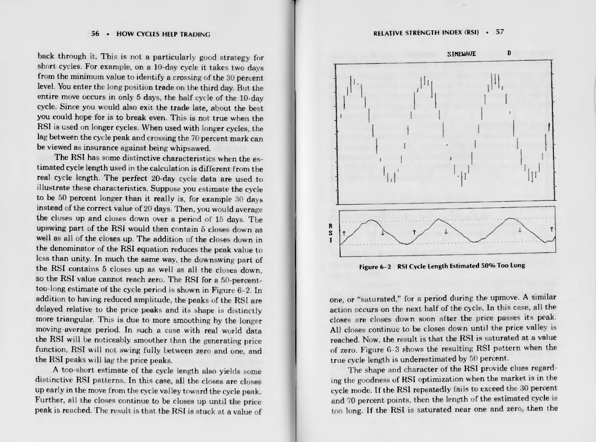
Relative Strength Index (RSI) 54
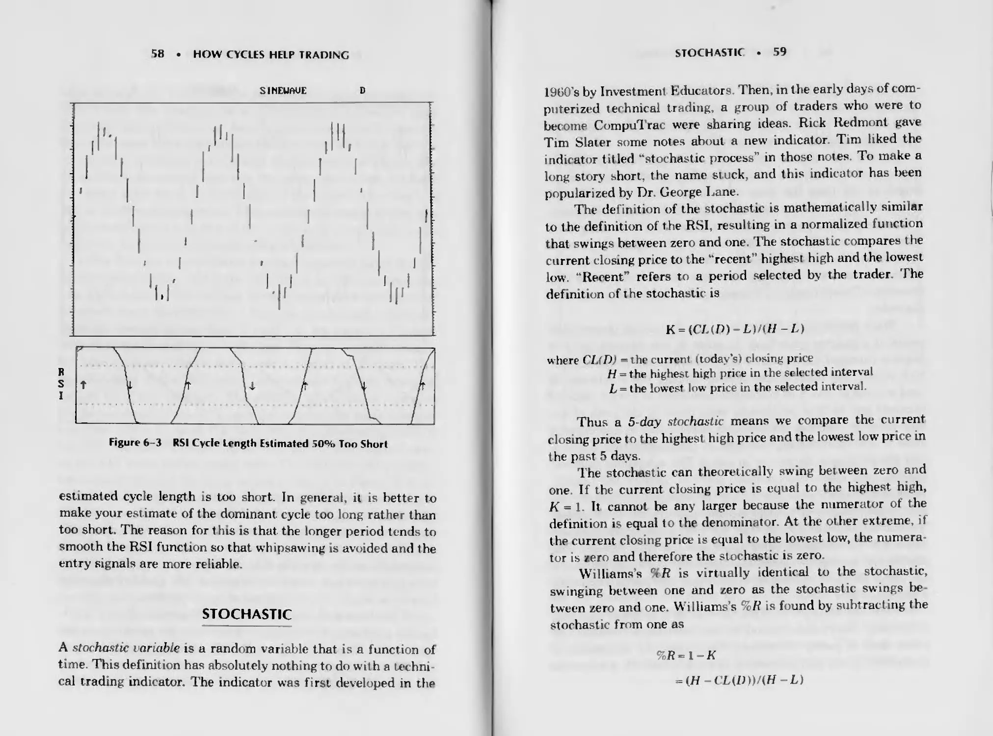
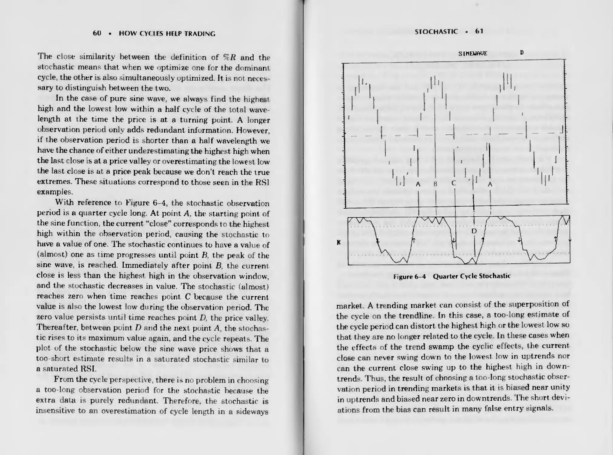
Stochastic 58
Using RSI and Stochastic to Read the Market 62
Mewing Average Convergence/
Divergence (MACD) 62
Leading Indicators 64
Chapier 7
Setting Stops 71
Key Stop Elements 71
The Initial Stop-Loss Placement 72
Acceleration 73
Chapter 8
Cycle Measurement 77
Cycle Finders 78
Fast Fourier Transforms (FFT) 78
Maximum Entropy Spectral Analysis (MESA) 81
CONTENTS . xvii
Chapter 9
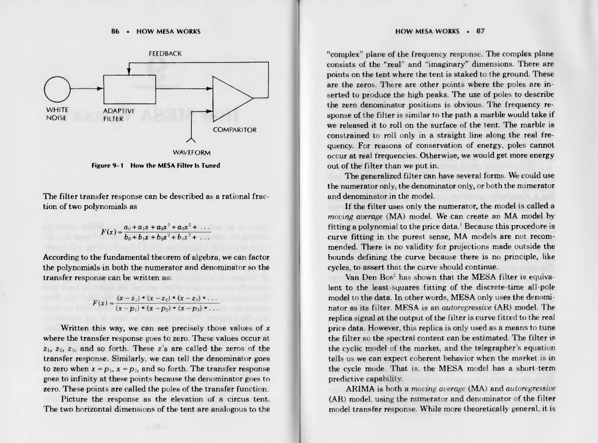
How MESA Works 85
Data length 88
Predictions 90
Chapter 10
Using the Spectrum to Identify Cycles
and Trends 93
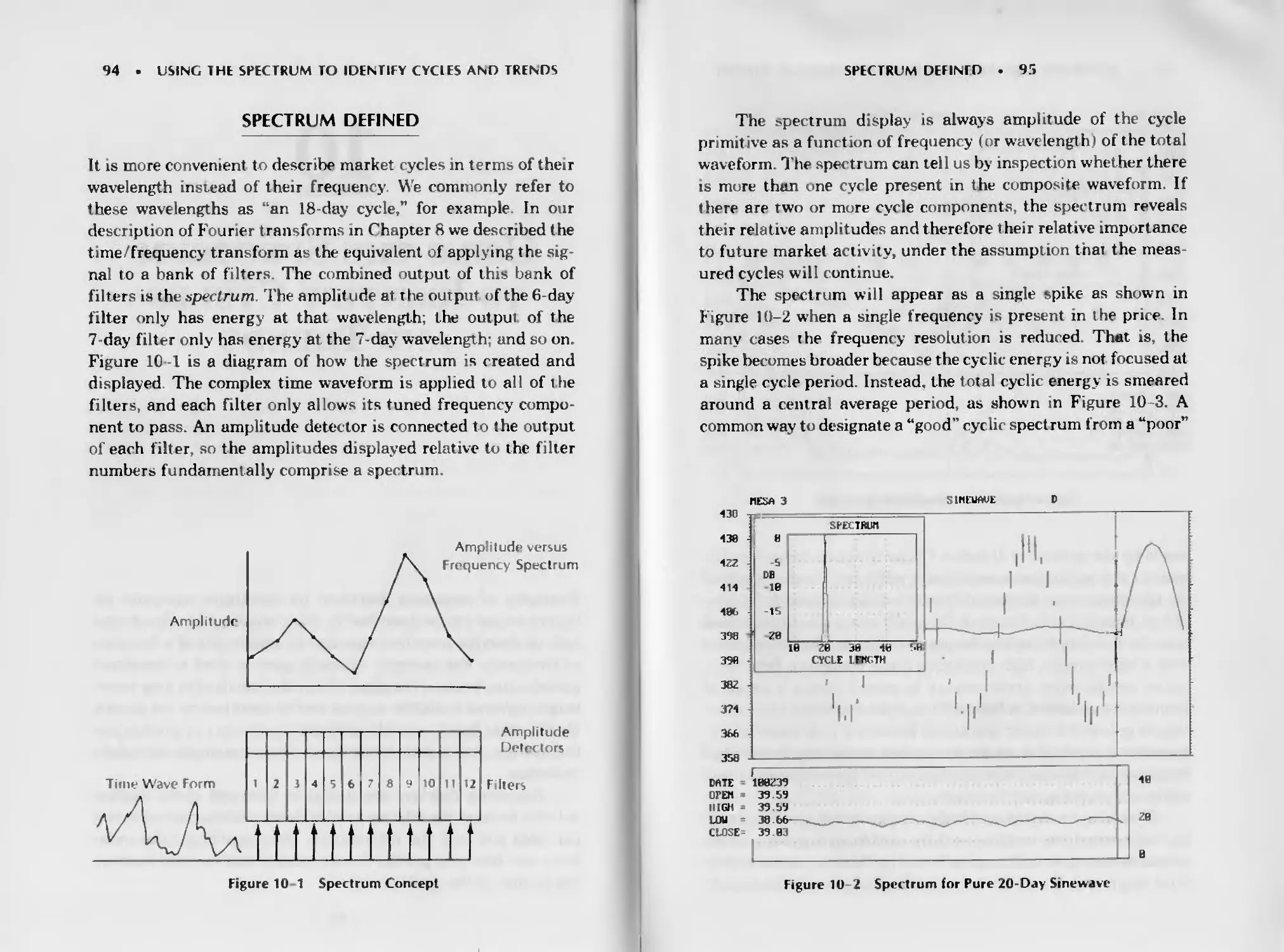
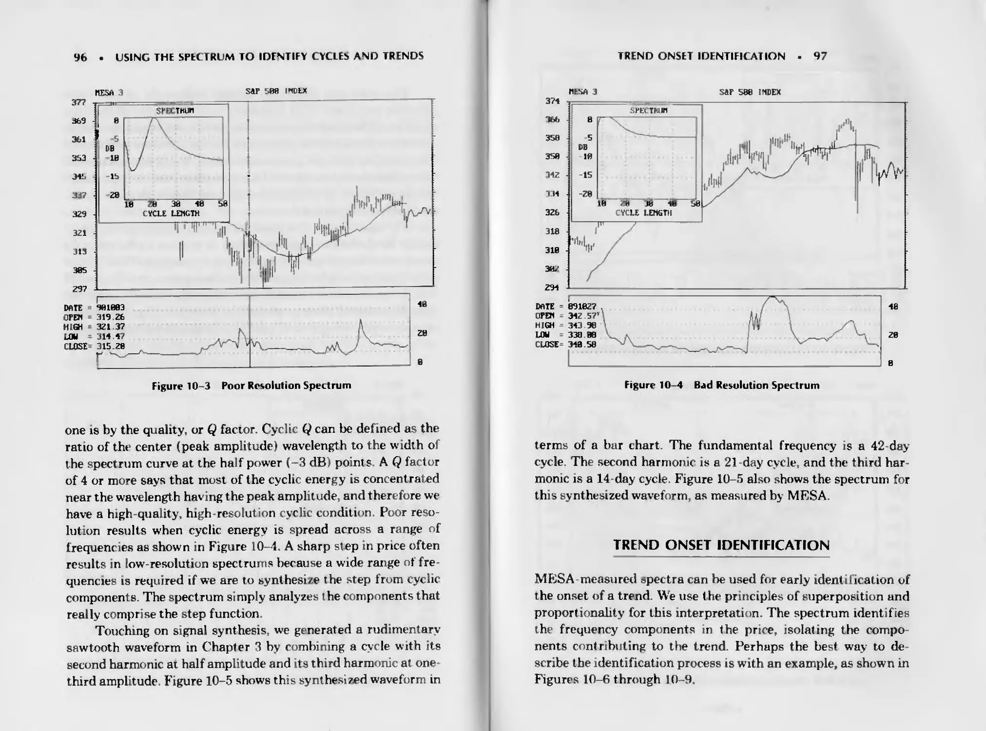
Spectrum Defined 94
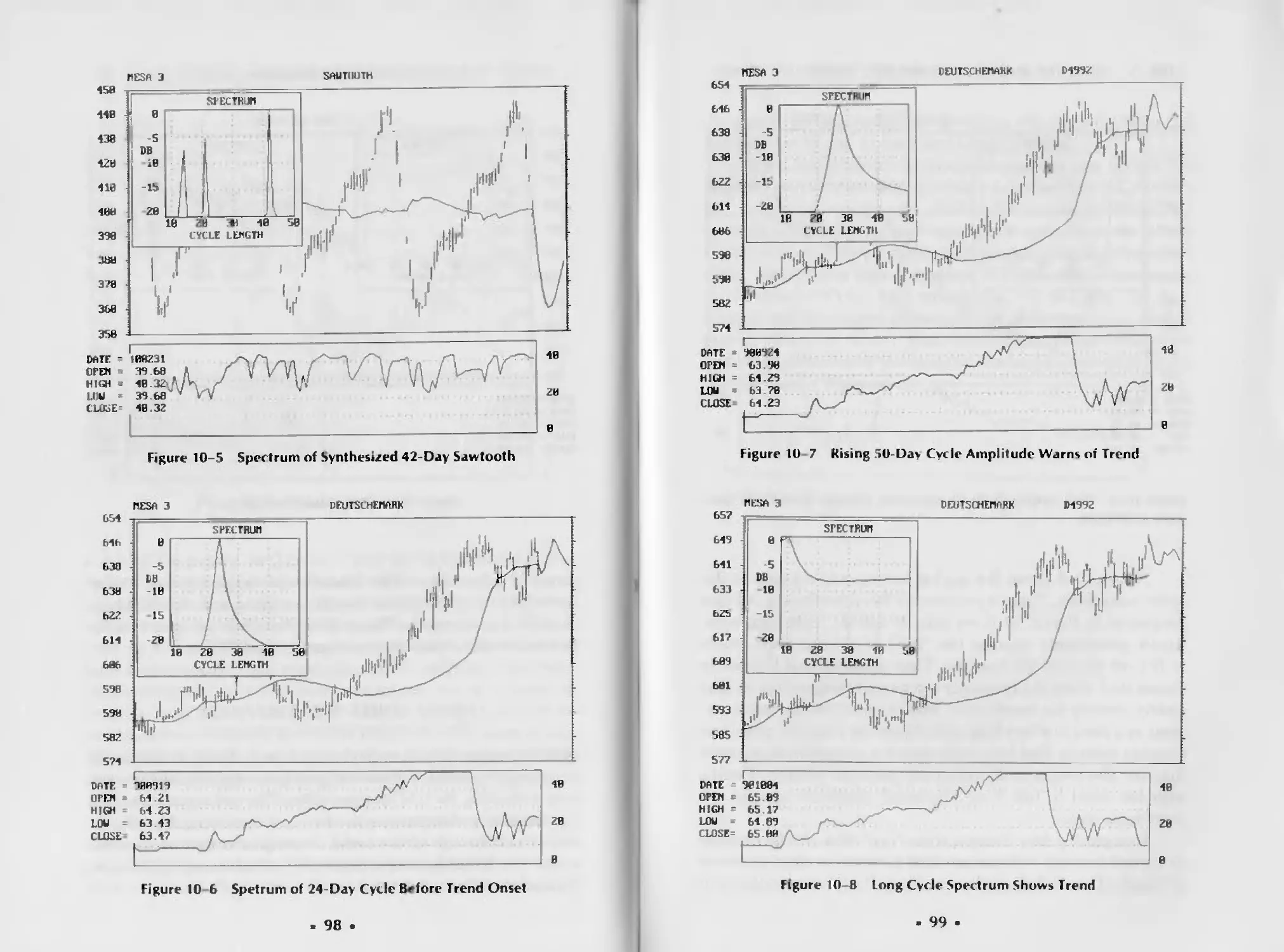
Trend Onset Identification 97
Chapter 11
Putting It All Together 103
Models Suit Miire Than Clothes 103
Role Models Show the Way 104
A Spectrum of Suppi >rt 106
“It Is Difficult to Make Forecasts, Especially
about the Future” 110
Adapt and Survive! 111
Chapter 12
Trading with MESA 113
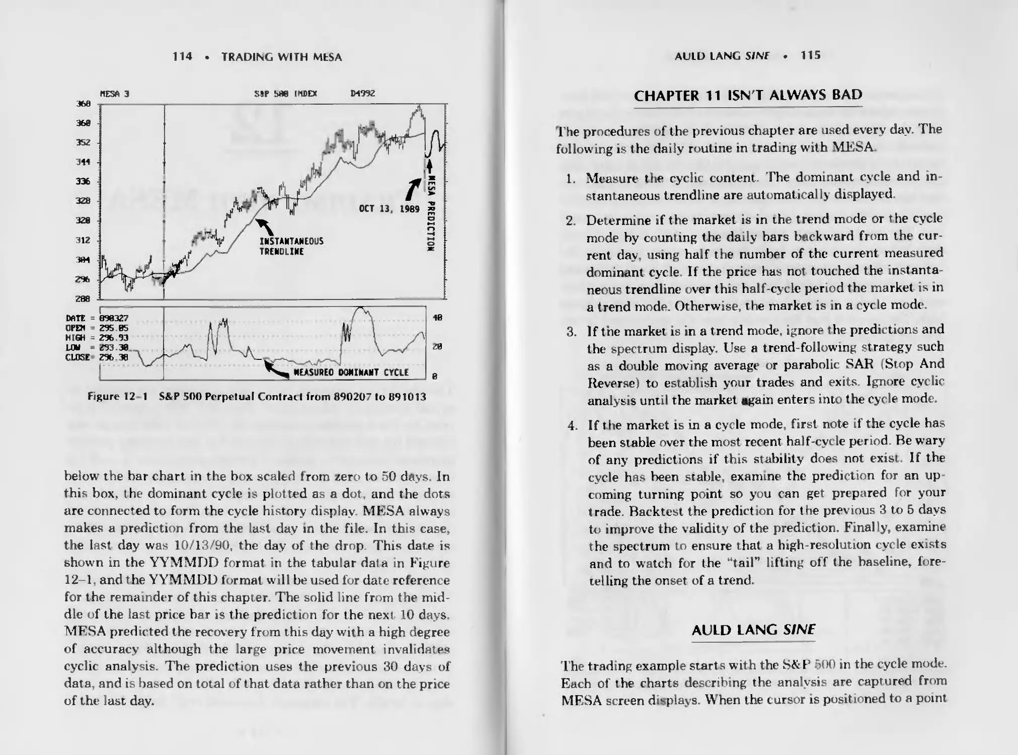
Chapter 11 Isn’t Always Rad 115
Auld Lang Sine 115
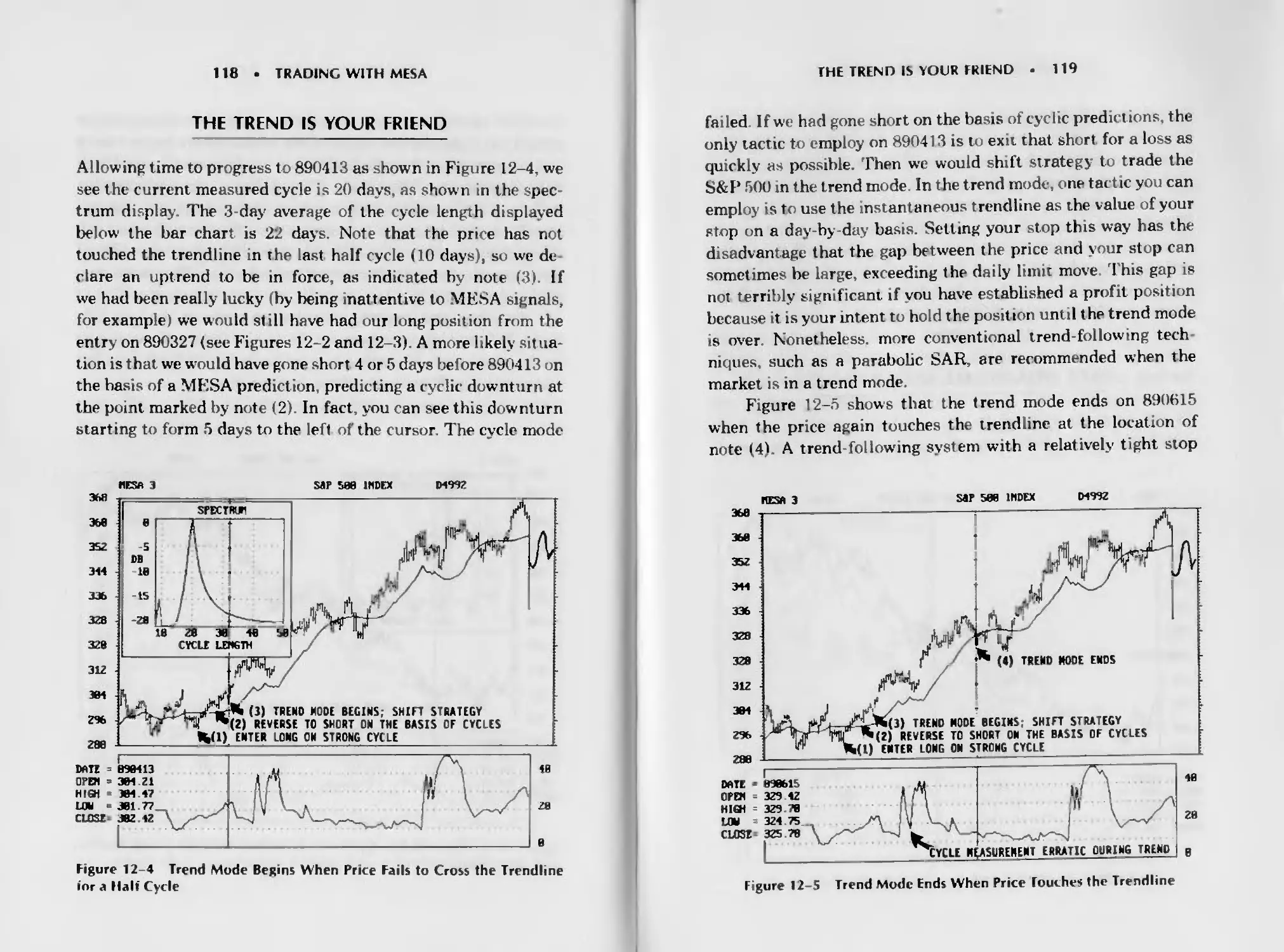
The Trend Is Your Friend 118
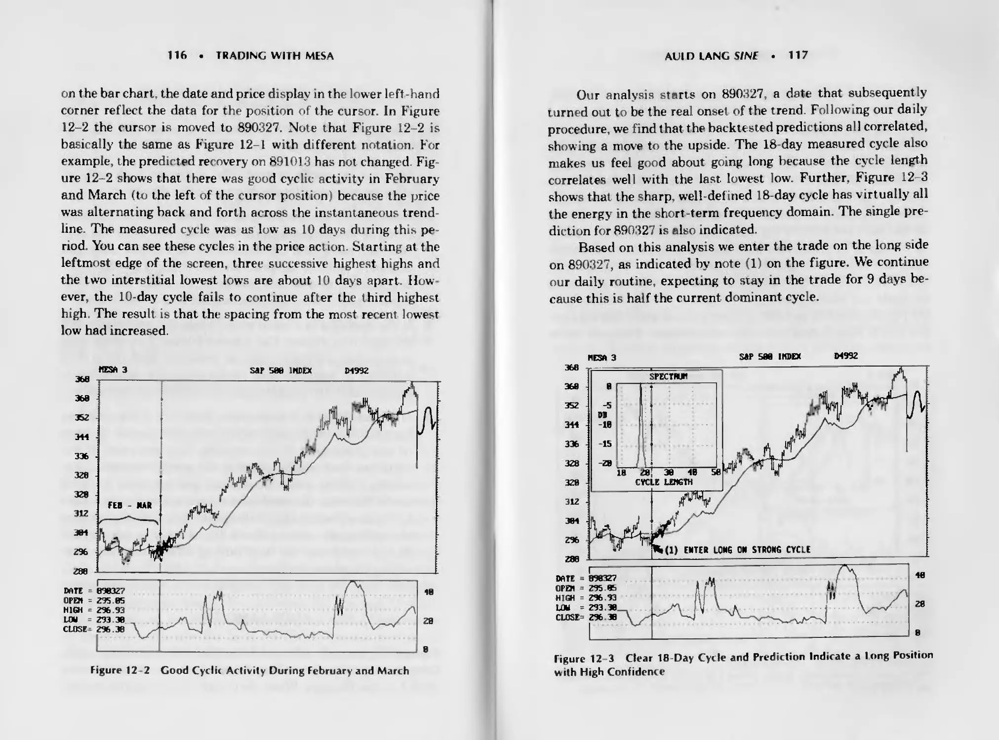
“h’s Deja Vu All Over Again’ 120
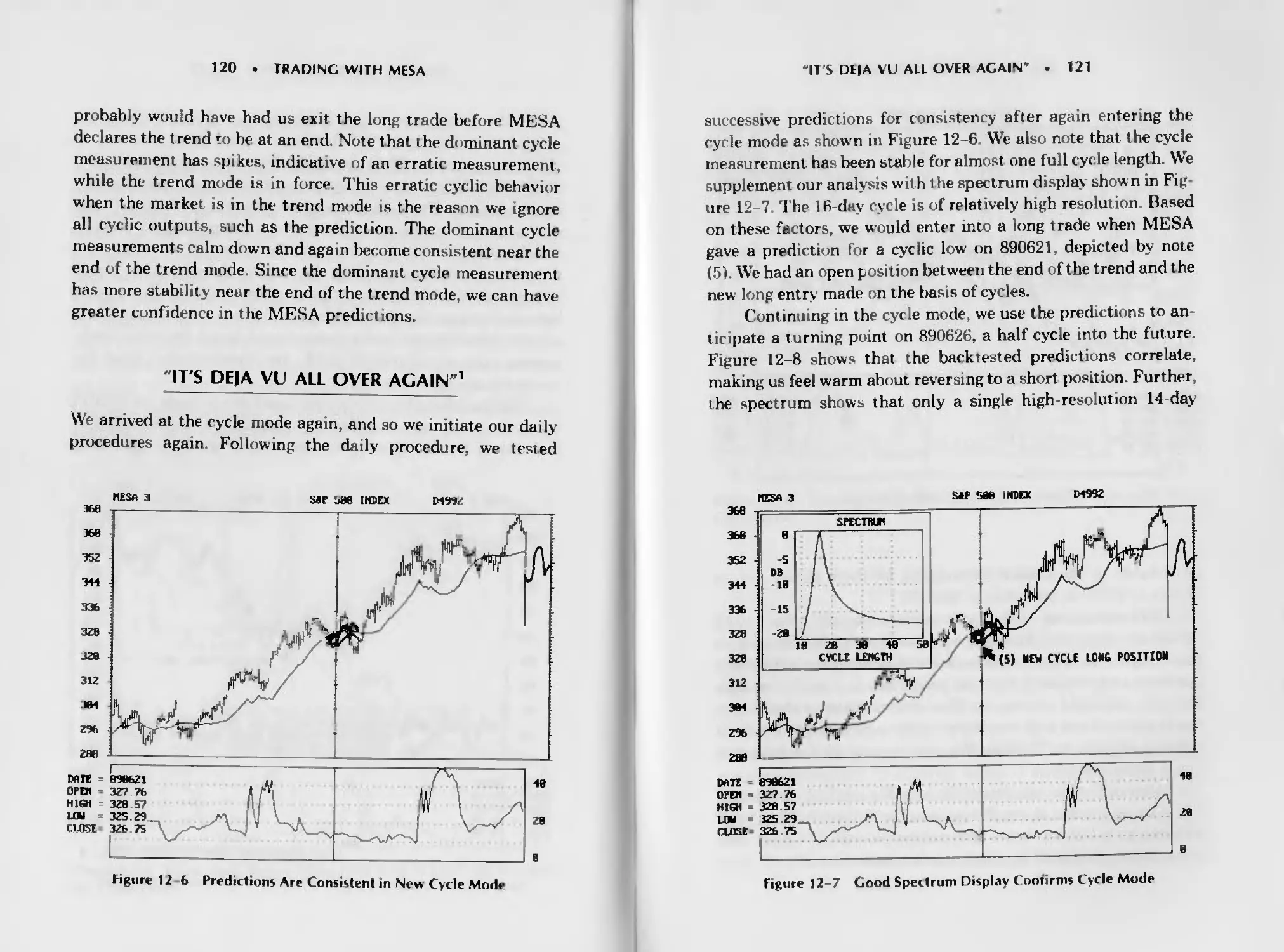
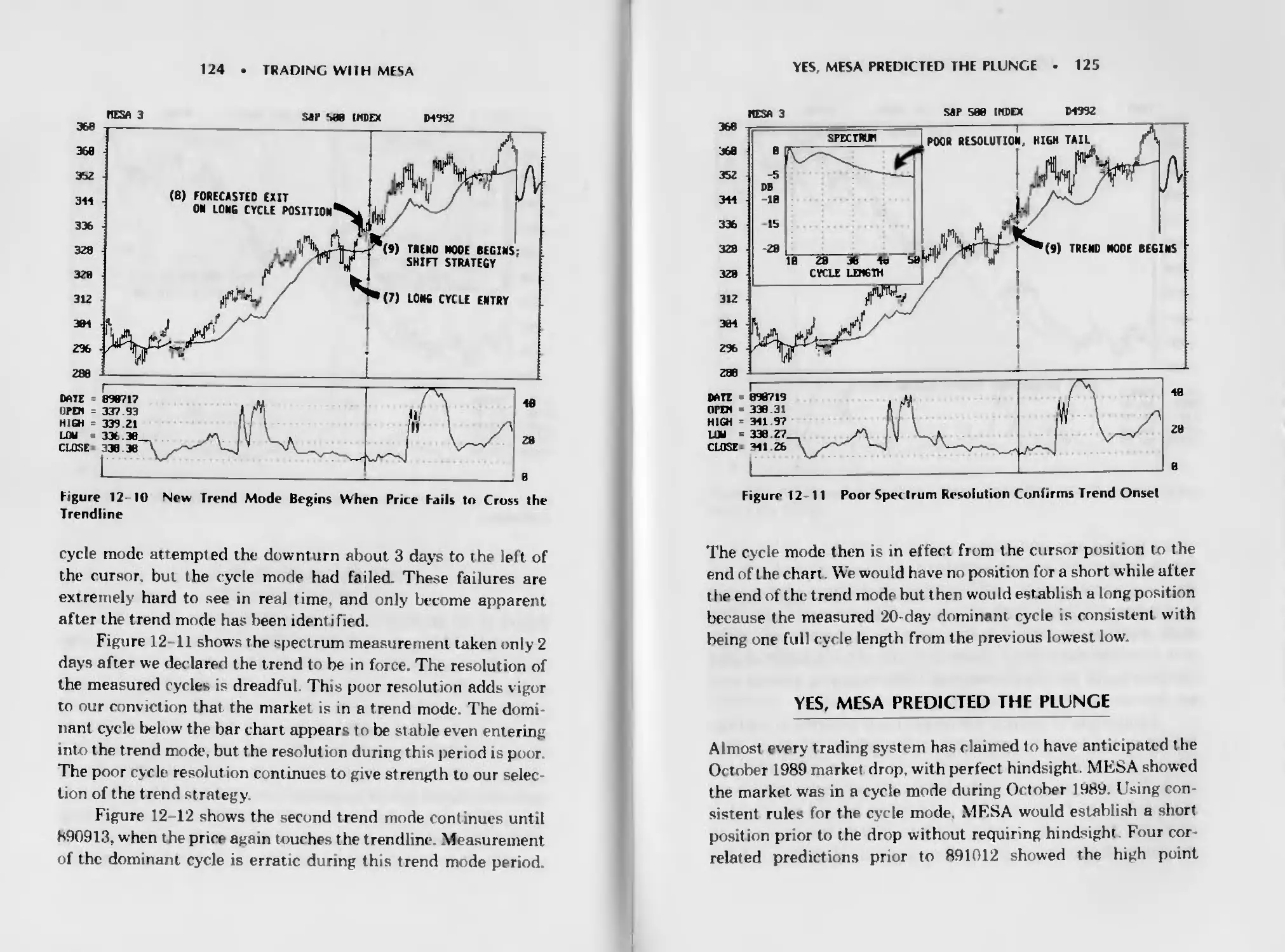
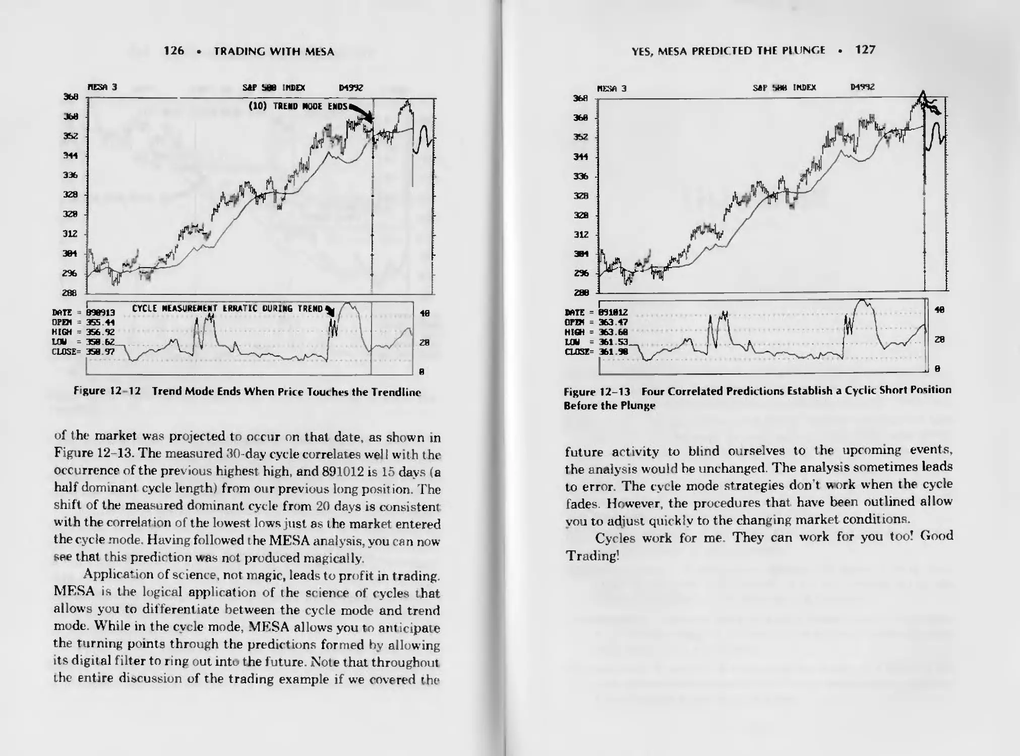
The Friend Returns 123
Yes, MESA Predicted the Plunge 125
Glossary 129
Endnotes 135
Index
137
1
Why Cycles Exist
in the Market
Technical analysis of the market is successful because the mar
ket is not always efficient. Discernible events that occur in
chart patterns, such as double tops and Elliott waves, enable
trading to be guided by technical analysis. Cycles are one of
these discernible events that occur and are identifiable by di-
rect measurement. Identification of cycles does not take a life-
time of experience or an expert system. Cycles can be measured
directly, either by a simple system such as measuring the dis
tance between successive lows or by a sophisticated computer
software program such as MESA.
The fact that cycles exist does not imply that they exist
all the time. Cycles come and go External events sometimes
dominate and obscure existing cycles. Experience shows that
cycles useful for t rading are present only about 15 to 30 percent
of the time This corresponds remarkably with J M. Hurst's
statement that “23% of all price motion is oscillatory in nature
and semi predictable ’’ It is analogous to the problems of the
1
2
WHY CYCLES EXIST IN THE MARKET
trend-follower, who finds that the markets “trend” only a
small percentage of the time.
HISTORICAL PERSPECTIVE
Cyclic recurring processes observed in natural phenomena by
humans since the earliest times have embedded the basic con-
cepts used in modern spectral estimation. Ancient cixiLza
tions were able to design calendars and time measures from
t heir observations of the periodicities in the length of da>, the
length of the year, the seasonal changes, the phases of the
moon, and the motion of the planets and stars. Pythagoras
developed a relationship between the periodicity of musical
notes produced by a f ixed tension string and a number repre
sent.ng the length of the string in the sixth century B.( Ht
believed that the essence of harmony was inherent in the num
bers Pythagoras extended the relat ionship to describe t he har-
monic motion of heavenly bodies, describing the motion as the
“music of the spheres.”
Sir Isaac Newton provided the mat hematical basis for mod-
ern spectral analysis. In the seventeenth century he discovered
that sunlight passing t hrough a glass prism expanded into a band
of manv colors. He determined that each color represented a
particular wavelength of light and that the white light of the sun
contained all wavelengths. He invented the word spectrum as a
scientific term to describe the band of light colors.
Daniel Rournoulh developed the solution to the wave
equation for the vibrating musical string in 1738. Later, in
1822, the French Engineer Jean Baptiste Joseph Fourier ex-
tended the wave equat .on results by assert.ng that any function
could be represented as an infinite summation of sine and
cosine terms. The mathematics of such representation has be
come known as harmonic analysis due to the harmonic rela-
tionship between the sine and cosine terms. Fourier transforms
HISIORICAL PERSPECTIVE
3
the frequency description of time domain events (and vice
versa) have been named in his honor
Norbert Wiener provided the major turning point for the
theory of spectral analysis in 1930, when he published his clas-
sic paper “Generalized Harmonic Analysis.” Among his contn
but ions were precise statist ical definit ions of autocorrelation
and power spectral density for stationary random processes. The
use of Fourier transforms, rather than the Fourier scries of tra-
ditional harmonic analysis, enabled Wiener to define spectra in
terms of a continuum of frequencies rather than as discrete
harmonic f requencies.
John Tukey is the pioneer of modern empirical spectral
analysis. In 1949 he provided the foundation for spectral esti-
mation using correlation estimates produced from finite time
sequences. Many of the terms of modern spectral estimation
(such as aliasing, windowing, prewhitening, tapering, smooth-
ing. and decimation) are attributed to Tukey. In 1965 he collab-
orated with Jim Cooley to describe an efficient algorithm for
digital computation of the Fourier transform. This fast Fourier
transform (FFT) unfortunately is not suitable for analysis of
market data, as we will develop in later chapters.
The work of John Burg was the prime impetus for the cur
rent interest m high-resolution spectral estimation from limited
time sequences He described his high-resolution spectral esti-
mate in terms of a maximum entropy formalism in his 1975
doctoral thesis and has been instrumental in the development of
modeling approaches to high-resolution spectral estimation
Burg’s approach was initially applied to the geophysical explo-
ration for oil and gas through the analysis of seismic waves. The
approach is also applicable for technical market analysis I if cause
it produces high-resolution spectral estimates using minimal
data. This is important because the short term market cycles
are always shifting. Another benefit of the approach is that is
maximally responsive to the selected data length and is not sub
ject to distortions due to end effects at the ends of the data. The
4
WHY CYCLES EXIST IN THE MARKET
trading program, MESA, is an acronym for maximum entropy
spectral analysis.
WHAT IS A CYCLE?
The dictionary definition of a cycle is that it is “an interval or
space of time in which is completed one round of events or
phenomena that recur regularly and in the same sequence.”
In the market, we consider a classic cycle exists when the price
starts low, nses smoothly to a high over a length of time, and
then smoothly falls back to the original price over the same
length of time The t ime required to complete the cycle is called
the period of the cycle or the cycle length
Cycles certainly exist in the market. Many times they
are justified on the basis of fundamental considerations. The
clearest is the seasonal change for agricultural prices (lowest at
harvest), or the decline in real estate prices in the winter Tele-
vision analysts are always talking about the rate of inflation
being “seasonally adjusted” bj the governmeni But the sea-
sonal is a specific case of the cycle always being 12 months
Oxher fundamentals-related cycles can originate from the 18
month cattle breeding cycle or the monthly cold-storage report
on pork bellies.
Business cycles are not as clear, but they exist. Business
cycles vary with interest rates. The government sets objectives
for economic growth based on its ability to hold inflation to rea-
sonable levels. This growl h is increased or decreased by adding or
withdrawing funds from the economy and by changing the rate at
which government lends money to banks. Easing of rates encour
ages business: tightening of rates inhibits it. Inevitably this proc-
ess alternates, causing what we see as a business cycle. Although
in practice this cycle may repeat in the same number of years,
the exact repetition of the period is not necessary. The business
cycle is limited on the upside by the amount of growth the govern-
ment will allow (usually 3%) and on the downside by moderate
COMPONENTS ОТ THE MARKET
5
negative growth (about -1%), which indicates a recession. The
range of the cycle from +3% to -1% is called its amplitude
COMPONENTS OF THE MARKET
Statisticians and economists have identified four important
characteristics of price movement. Ail price forecasts and analy-
ses deal with each of these elements:
1 A trend, or a tendency to move in one direction for a speci-
fied time period.
2. A seasonal factor, a pattern related to the calendar
3. A cycle (other than seasonal) that may exist due to govern-
ment action, the lag in starting up and winding down of
business, or crop estimate announcements.
4. Other unaccountable price movement, often called noise.
Since points 2 and 3 are both cycles, it is clear that cycles
are a significant and accepted part of all price movement
When trading using cycles, one key question is the desired
time span of the trade. At one ext reme, the 54-year Kondratieff
economic cycle (not without its critics) could be considered.
A cattle rancher might prefer the 18-month breeding cycle,
while a grain farmer probably hedges on the basis of the annual
harvest Speculators often work over a short (sometimes very
short) time span.
Behavioral cycles in prices have been most popular in
Elliotts’ wave theory and more recently in the works of Gann.
But these methods have a large element of interpretation and
subjectivity.
Short-term cycles can exist even within the definition of
point 4, “noise.” A casual glance at almost any bar chart show's,
in retrospect, that, short-term cycles ebb and flow. The ability to
isolate and use market phenomena, such as cycles, is related
6
WHY CYCLES EXIST IM THE MARKET
to the awareness of its existence and the tools available. Many
forecasting methods were not practical until the computer be
came popular. Now these methods can be used by nearly every
one. The philosophical foundation for these short term cycles is
derived from random walk theory and is developed so you will
feel more comfortable dealing with cycles within the constraint^
of point 4
RANDOM WALK
Randomness in the market results from a large number of
traders exercising their prerogatives with different motivations
of profit, loss, greed, fear and entertainment; it is complicated
by different perspectives of time. Market movement can there-
fore be analyzed in terms of random variables. One such analy-
sis is the random walk Imagine an atom of oxygen in a plastic
box containing nothing but air. The path of this atom is erratic
as it bounces from one molecule to another. Brownian motion is
used to describe the way the atom moves. Its path is described as
a three dimensional random walk. Following such a random
walk, the position of that atom is just as likely to be at any one
location in that box as at any other
Another form of the random walk is more appropriate for
describing the motion of the market. This form is a two-dimen-
sional random walk, called the “drunkard’s walk.” The two-
dimensional structure is appropriate for the market because the
prices can only go up or down m one dimension The other
dimension, time, can only move forward. These are similar to
the way a drunkard’s walk is described.
DIFFUSION EQUATION
The drunkard’s walk is formulated by allow .ng the drunkard to
step to either the right or left randomly with each step forward
DIFFUSION EQUATION
7
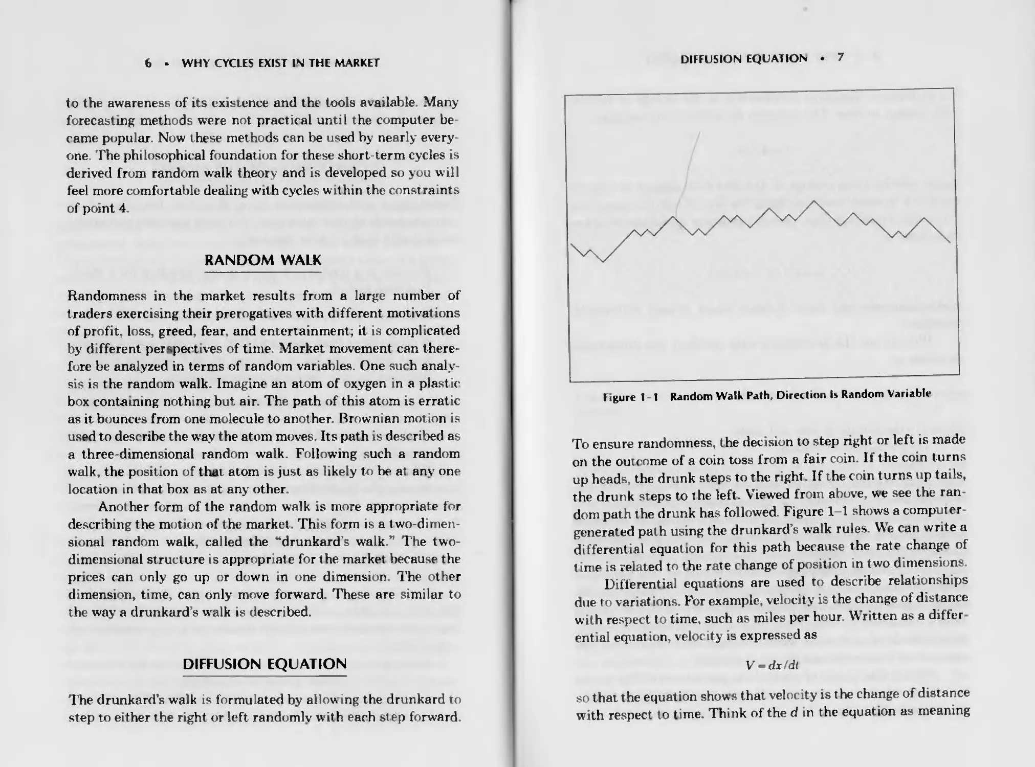
Figure I 1 Random Walk Path, Direction Is Random Variable
To ensure randomness, the decision to step right or left is made
on the outcome of a coin toss from a fair coin. If the coin turns
up heads, the drunk steps to the right. If the coin turns up tails,
the drunk steps to the left. Viewed from above, we see the ran
dom path the drunk has followed. Figure 1-1 shows a computer-
generated path using the drunkard’s walk rules. We can write a
differential equation for this path because the rate change of
time is related to the rate change of position in two dimensions.
Differential equations are used to describe relationships
due to variations. For example, velocity is the change of distance
with respect to time, such as miles per hour Written as a differ
ential equation, velocity is expressed as
V-dx/dt
so that the equation shows that velocity is the change of distance
with respect to time. Think of the d in the equation as meaning
8
WHY CYCIFS EXISl IN THE MARKET
the difference. Similarly, acceleration is the change of velocity
with respect to time. The equation for acceleration becomes
a -dV/dt
Since velocity is the change of distance with respect to time we
can think of acceleration as being t he second rate change of dis-
tance with respect to time. Now the equation for acceleration can
be written as
a =dV/dt -d x/dr
Mathematicians use these formats when writing differential
equations.
Writing out the drunkard's walk problem, the differential
equation is
dP/dt = D * d2P/dx2
where P the position in time and space
D = the diffusion constant.
This relatively famous differential equation (among mathemati-
cians, at least) is known as the diffusion equation. In words, this
equation states that the change of position with respect to time is
proportional to t he second rate change of position with respect to
space. It describes many natural phenomena; for example, the
way heat travels up a silver spoon when it’s placed in a hot cup of
coffee A better analogy to the way the market works is that
the diffusion equation can describe the plume of smoke coming
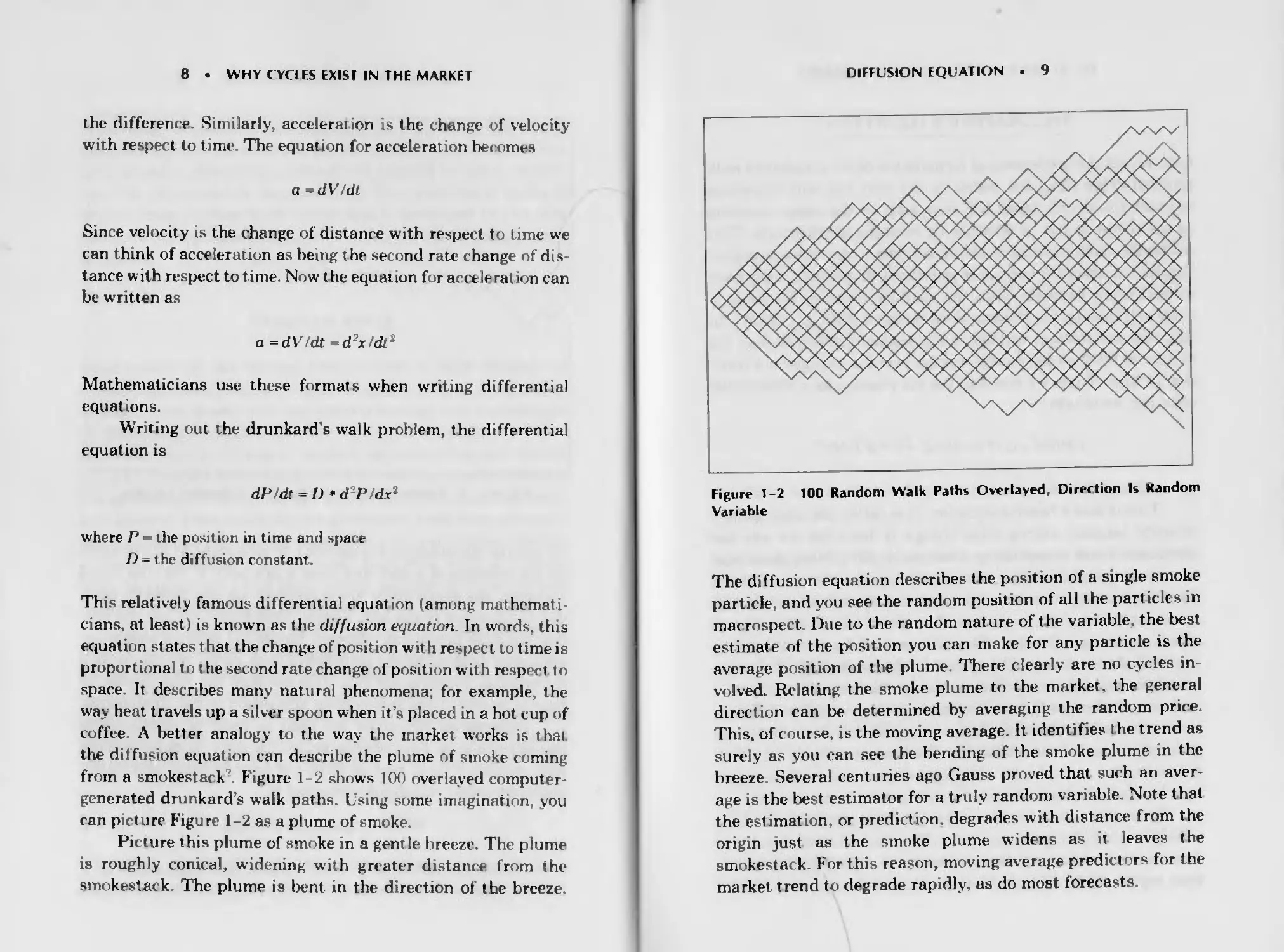
from a smokestack Figure 1-2 shows 100 overlayed computer-
generated drunkard’s walk paths. Using some imagination, you
can picture Figure 1-2 as a plume of smoke.
Picture this plume of smoke in a gentle breeze. The plume
is roughly conical, widening with greater distance from the
smokestack The plume is bent in the direction of the breeze.
DIFFUSION EQUATION . 9
Figure 1-2 100 Random Walk Paths Overlayed, Direction Is Random
Variable
The diffusion equation describes the position of a single smoke
particle, and you see the random position of all the pari icles in
macrospect Due to the random nature of the variable, the best
estimate of the position you can make for any particle is the
average position of the plume There clearly are no cycles in-
volved. Relating the smoke plume to the market, the general
direction can be determined by averaging the random price.
This, of course, is the moving average. It identifies the trend as
surely as you can see the bending of the smoke plume in the
breeze Several centuries ago Gauss proved that such an aver-
age is the best estimator for a truly random variable. Note that
the estimation, or prediction, degrades with distance from the
origin just as the smoke plume widens as it leaves the
smokestack. For this reason, moving average predictors for the
market trend to degrade rapidly, as do most forecasts.
10
WHY CYCl.ES EXIST IN IHE MARKET
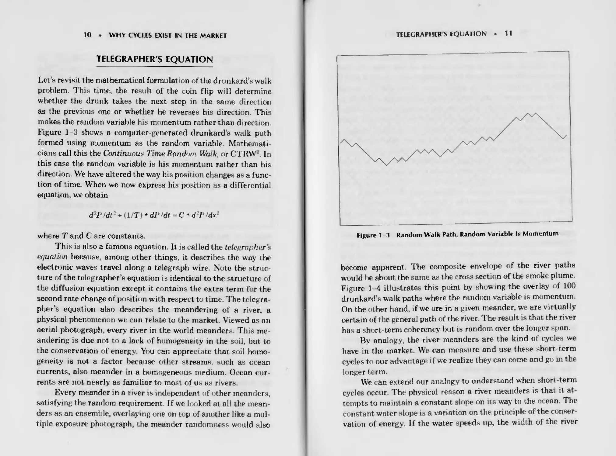
TELEGRAPHER'S EQUATION
Let’s revisit the mathematical formula! ion of the drunkard’s walk
problem This time, the result of the coin flip will determine
whether the drunk takes the next step in rhe same direction
as the previous one or whether he reverses his direction. This
make* the random variable his momentum rather than direct ion.
Figure 1-3 shows a computer-generated drunkard’s walk path
formed using momentum as the random variable. Mathemati
mans call this the Continuous Time Random Walk, or C-TRW In
this case the random variable is his momentum rather than his
direction. We have altered the way his position changes as a func-
tion of time. When we now express his position as a differential
equation, we obtain
d2P/dt~ + (l/T) • dP/dt = C * d2P/dx2
where T and C are constants.
This is also a famous equation It is called the telegrapher’s
equation because, among other things, it describes the way the
electronic waves travel along a telegraph wire. Note the struc-
ture of the telegrapher’s equat ion is identical to the structure of
the diffusion equation except it contains the extra term for the
second rate change of position wit h respect to time. The telegra
pher’s equation also describes the meandering of a river, a
physical phenomenon we can relate to the market. Viewed as an
aerial photograph, every river in the world meanders. This me
andering is due not to a lack of homogeneity in the soil, but to
the conservation of energy. You can appreciate that soil homo
geneity is not a factor because other streams such as ocean
currents, also meander in a homogeneous medium. Ocean cur-
rents are not nearly as fami liar to most of us as rivers.
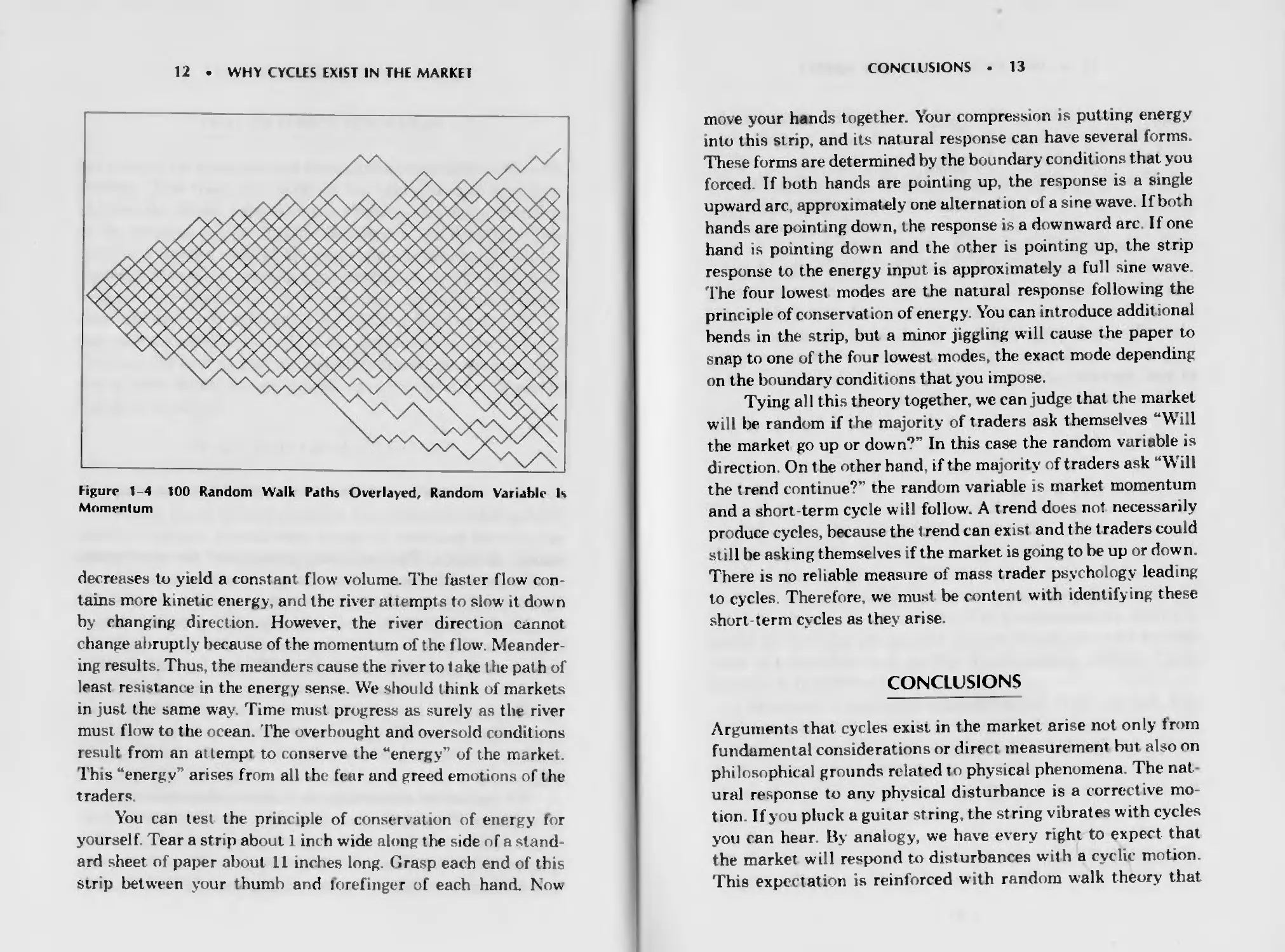
Every meander in a river is independent of other meanders,
satisfying the random requirement If we looked at all the mean-
ders as an ensemble, overlaying one on top of another like a mul-
tiple exposure photograph, the meander randomness would also
TELEGRAPHER S EQUATION . 11
Figure 1-3 Random Walk Path, Random Variable Is Momentum
become apparent. The composite envelope of the river paths
would he about the same as the cross section of the smoke plume.
Figure 1 4 illustrates this point by showing the overlay of 100
drunkard’s walk paths where the random variable is momentum.
On the other hand, if we are in a given meander, we are virtual ly
certain of the general path of the river The result is that the river
has a short-term coherency but is random over the longer span.
By analogy, the river meanders are the kind of cycles we
have in the market. We can measure and use these short-term
cycles to our advantage if we realize they can come and go in the
longer term.
We can extend our analogy to understand when short-term
cycles occur. The physical reason a river meanders is that it at-
tempts to maintain a constant slope on its way to the ocean. The
constant water slope is a variation on the principle of the conser-
vation of energy. If the water speeds up, the width of the river
12
WHY CYCLES EXIST IN THE MARKEl
Figure 1-4 100 Random Walk Paths Overlayed, Random Variable Is
Momentum
decreases to yield a constant flow volume. The faster flow con
tains more kinetic energy, and the river attempts to slow it down
by changing direction. However, the river direction cannot
change abruptly because of the momentum of the flow'. Meander-
ing resul ts. Thus, the meanders cause the river to t ake t he pat h of
least resistance in the energy sense. We should think of markets
in just the same wray. Time must progress as surely as the river
must flow to the ocean. The overbought and oversold conditions
result from an attempt to conserve the “energy” of the market.
This “energy” arises from all the fear and greed emotions of the
traders
You can test the principle of conservation of energy for
yourself. Tear a strip about 1 inch wide along the side of a stand
ard sheet of paper about 11 inches long. Grasp each end of this
strip between your thumb and forefinger of each hand. Now
CONCLUSIONS
13
move your hands together. Your compression is putting energy
into this strip, and its natural response can have several forms.
These forms are determined by the boundary conditions that you
forced If both hands are pointing up, the response is a single
upward arc, approximately one alternation of a sine wave. If both
hands are pointing down, t he response is a downward arc. If one
hand is pointing down and the other is pointing up, the strip
response to the energy input is approximately a full sine wave.
The four lowest modes are the natural response following the
principle of conservation of energy. You can introduce additional
bends in the strip, but a minor jiggling will cause the paper to
snap to one of the four lowest modes, the exact mode depending
on the boundary conditions that you impose.
Tying all this theory together, we can judge that the market
will be random if the majority of traders ask themselves “Will
the market go up or down?” In this case the random variable is
direction. On the other hand, if the majority of traders ask “Will
the trend continue?” the random variable is market momentum
and a short-term cycle will follow'. A trend does not necessarily
produce cycles, because the trend can exist and the traders could
still be asking themselves if the market is going to be up or down
There is no reliable measure of mass trader psychology leading
to cycles. Therefore, we must be content with identifying these
short term cycles as they arise.
CONCLUSIONS
Arguments that, cycles exist in the market arise not only from
fundamental considerations or direct measurement but also on
philosophical grounds related to physical phenomena The nat-
ural response to any physical disturbance is a corrective mo-
tion If you pluck a guitar string, the string vibrates with cycles
you can hear. By analogy, we have every right to expect that
the market will respond to disturbances with a cyclic motion.
This expectation is reinforced with random walk theory that
14
WHY CYCIFS EXIST IN THE MARF.EE
suggests there are tunes the market prices can be described by
the dif fusion equation and other times when the market prices
can be described by the telegrapher’s equation
The challenge for technical traders is to recognize when the
short term cycles are present and to trade them in a logical and
consistent manner so these cycles can contribute profitably to
the bottom line
In the chapters that follow I will define the basics of cycles
and how to manipulate them to tune the momentum and moving
average functions—components of every technical trading indi-
cator. Cycle primitives will even be related to traditional chart-
ing patterns, perhaps giving these patterns a whole new meaning
to you. Perhaps most importantly, I will discuss when to use
cycles for trading and when to avoid their use.
2
Cycle Basics
The one thing on which market technicians agree is that the
market varies. Precisely how it varies is the matter of the con-
tinuous debate. Each oi the technical trading techniques, from
classical chart patterns to Elliott’s wave, construct a simplified
model of the market. Each technique describes the market in
terms of the model parameters The parameters are then ad-
justed to describe the current market conditions and further
used to extrapolate and predict future market activity. Cycle
analysis is no different.
Cycles are a simplified technical model of the market. 1'he
model is at least as complex as most ot her models because sev-
eral cycles can coexist; cycles are often mixed with noise, and
all the cycles ebb and flow with time. The primitive component
of complex cycles is the sine wave The sine wave is the natural
cycle primitive for several reasons:
1. The sine wave is the mathematically smoothest waveform
describing a cycle and harmonic motion
15
16
CYCLE BASICS
2 More complicated forms of waves are made up of the sums
of simple sine waves.
3. Sine and cosine waves form an independent parameter set
for advanced analyses such as Pourier transforms.
Just as with any model, we must define the parameters of
the components so that we can assemble them into the logical
complex model The cycle parameters are frequency, phase, and
amplitude.
FREQUENCY
A cycle is any process where a point of observation returns to its
origin One example is a clock pendulum. The pendulum swings
with such regularity that it has been used for centuries as the
time standard for the clock. Thus, a prime charac teristic of a
cycle is frequency. The rotation of an automobile engine is
cyclic. The frequency is the number of revolutions per minute
the crankshaft makes. The term 2000 FU’M should be familiar
to most motorists RPM is the acronym for revolutions per
minute Each rotation is a cycle, and the period of such a cycle is
1/2000 of a minute Thai is, the period of the cycle is the recip
rocal of its frequency. In trading we commonly refer to cycles in
terms of their period rather than their frequency. For example,
the frequency of a 10 day cycle is 0 1 cycles per day.
Think of the automobile eng ne crankshaft. We will pic-
ture a cycle as being generated bj a rotating arrow', or vector,
connected to the crankshaft. This arrow is called a phasor. The
cycle is complete when the tip of the phasor has completed a full
rotation to the origin We can generate the fundamental cycle
bui Idmg block, or primitive, from our rotating arrow Imagine
the t.p of the arrow casting a shadow on the vertical axis as if it
were illuminated from the right and left by flashlights. The
PHASE
17
amplitude of this shadow rises and falls as a sine wave with
respect to time
Alternating current generators creating electricity operate
much like our phasor. The copper wires on the rotating anna
ture first move parallel to the magnetic lines of the fixed pole
pieces, transitioning to cutting across the magnetic lines as the
armature rotates. The copper wires moving through the mag-
netic field create the electric current flow The resulting voltage
and current wave shapes are sine waves. In the United States
the AC frequency is standardized at 60 cycles per second.
Frequency is a uniquely singular measurable parameter of
a cycle. A simple sine wave can have only one frequency. A sine
wave is a primitive because we can add sine waves of different
frequencies, phases, and amplitudes to create complex wave
shapes. A sine wave can be described mathematically in terms of
an infinite power series as
sin(x) - x - x:,/3! + xb/5! - x7/7! +
where ’ denotes the factorial. That is, 5! = 1 *2*3*4* 5.
The simplified description of the sine wave relative to a
power series expansion is another reason to consider it to Im* a
prumtive function.
PHASE
Phase relationships of the cycle primitive are important for the
understanding of moving average and momentum functions.
Moving averages cause lagging phase relationships, and mo-
mentum produces leading phases. We will show later how these
relationships are combined to form useful indicators.
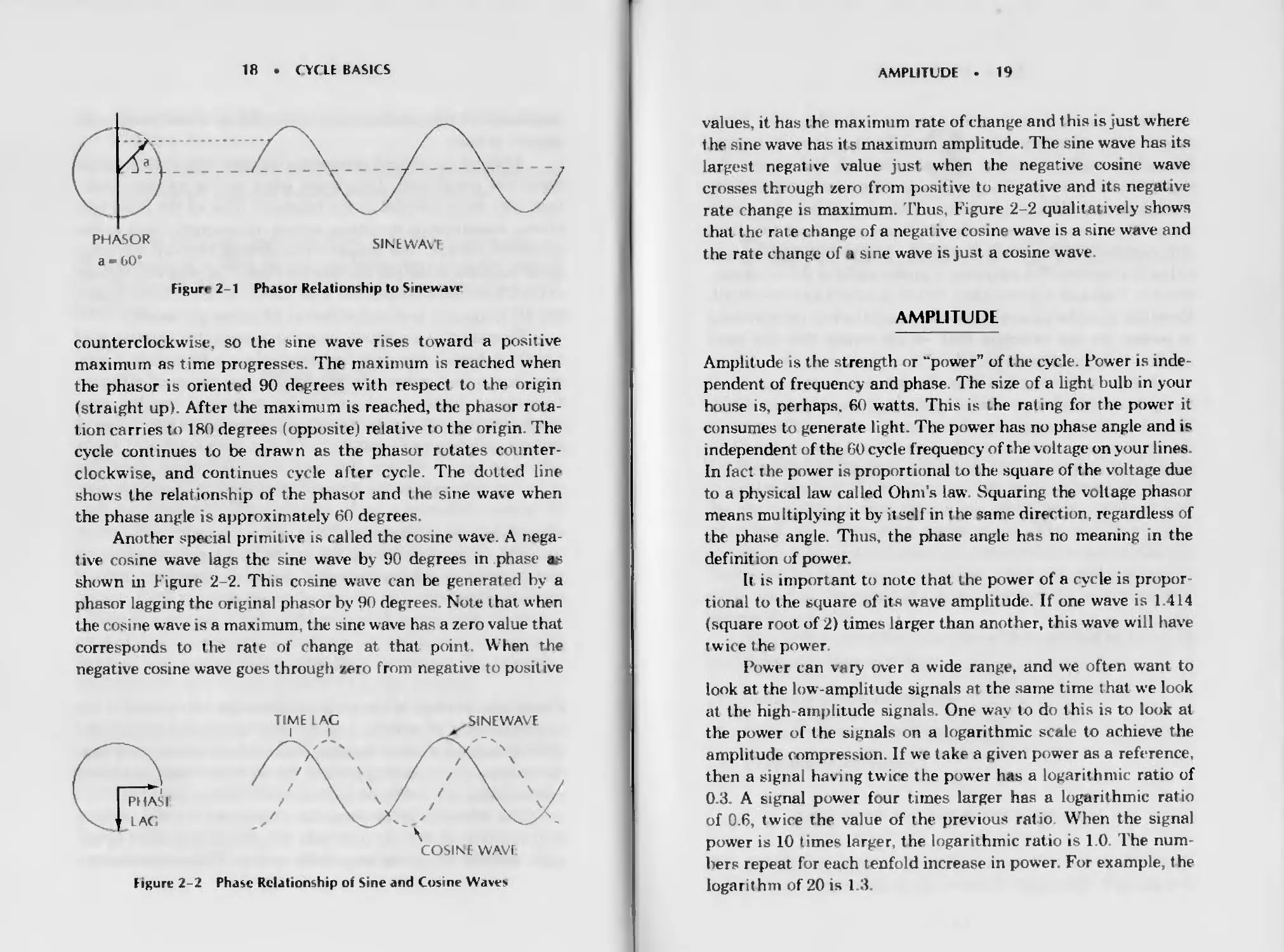
The relationship between the phasor and the sine wave is
showm in Figure 2-1 At time zero the phasor is pointed to the
right and the sine wave amplitude is zero. The phasor rotates
18
CYCLE BASICS
Figure 2-1 Phasor Relationship to Sinewavc
counterclockwise, so the sine wave rises toward a positive
maximum as time progresses. The maximum is reached when
the phasor is oriented 90 degrees with respect to the origin
(straight up). After the maximum is reached, the phasor rota-
tion carries to 180 degrees (opposite) relative to the origin The
cycle continues to be drawn as the phasor rotates counter-
clockwise, and continues cycle after cycle. The dotted line
shows the relationship of the phasor and the sine wave when
the phase angle is approximately 60 degrees.
Another special primitive is called the cosine wave. A nega-
tive cosine wave lags the sine wave by 90 degrees in phase as
shown m Figure 2-2. This cosine wave can be generated by a
phasor lagging the original phasor by 90 degrees. Note that when
the cosine wave is a maximum, the sine wave has a zero value that
corresp«»nds to the rate of change at that point. When the
negative cosine wave goes through zero from negative to positive
Figure 2-2 Phase Relationship of Sine and Cosine Waves
AMPLITLDF
19
values, it has lhe max inium rate of change and this is just where
the sine wave has it s maximum amplitude The sine wave has its
largest negative value just when the negative cosine wave
crosses through zero from positive to negative and its negative
rate change is maximum. Thus, Figure 2-2 qualitatively shows
that the rate change of a negat ive cosine wave is a sine wave and
the rate change of a sine wave is just a cosine wave.
AMPLITUDE
Amplitude is the strength or “power” of the cycle. Power is inde
pendent of frequency and phase The size of a light bulb in your
house is. perhaps. 60 watts. This is lhe rating for the power it
consumes to generate light. The power has no phase angle and is
independent of the 60 cycle f requency of the voltage on your lines
In fact lhe power is proportional to the square of the voltage due
to a physical law called Ohm's law Squaring the voltage phasor
means multiplying it by itself in lhe same direction, regardless of
the phase angle. Thus, the phase angle has no meaning in the
definition of power.
It is important to note that the power of a cycle is propor
tional to the square of its wave amplitude. If one wave is 1 414
(square root of 2) times larger than another, this wave wnl have
twice the power.
Power can vary over a wide range, and we often want to
look at the low-amplitude signals at the same time that we look
at the high-amplitude signals. One way to do this is to look at
the power of the signals on a logarithmic scale to achieve the
amplitude compression. If we take a given power as a reference,
then a signal having twice the power has a logarithmic ratio of
0.3. A signal power four times larger has a logarithmic ratio
of 0.6, twice rhe value of the previous ratio When the signal
power is 10 times larger, the logarithmic ratio is 1 0 The num-
bers repeat for each tenfold increase in power. For example, the
logarithm of 20 is 1 3.
20
CYC’Lt BASICS
Power is often expressed in terms of deciBels. The Bel is
named after Alexander Graham Bell for the research he per-
formed on audio power to help the deaf A Bel is just the
logarithm of a power ratio. Deci- is a prefix meaning one tenth
Therefore, a deciBel is one tenth of the logarithm of a power
ratio. The power ratios can be both larger and smaller than
unity. If the power ratio is less than one, the sign of the loga-
rithm is negative. For example, a power ratio of 0.5 is equiva-
lent to -3 dB and a power ratio of 0.01 is equivalent to -20 dB
Recalling that the square of the wave amplitude is proportional
to power, we can calculate that 6 dB means that the wave
amplitude is half the amplitude of the reference wave.
It is common practice in spectrum analysis to compare all
the cycle amplitudes with the amplitude of the strongest signal.
Therefore, the strongest signal has a power of zero dB because it
is being compared with itself ( the logarithm of 1 is zero), and all
other signals have powers measured in negative deciBels.
3
Principles of Cycles
Traditional charting is an analytical technique that is difficult
to master because of the large number of rules associated with
the chart patterns. The charts are laboriously prepared and
often look as if thev were works of art. The beauty of cycle
analysis is that it cuts through all these rules by describing the
market action in terms of primitives. Once you understand the
cyclic activity, the result of combinations of the primitives will
become clear to you
All market chart formations can be described in terms of
only three principles of cycles:
1. Principle of proportionality
2 Principle oi superposition
«3. Principle of resonance.
PRINCIPLE OF PROPORTIONALITY
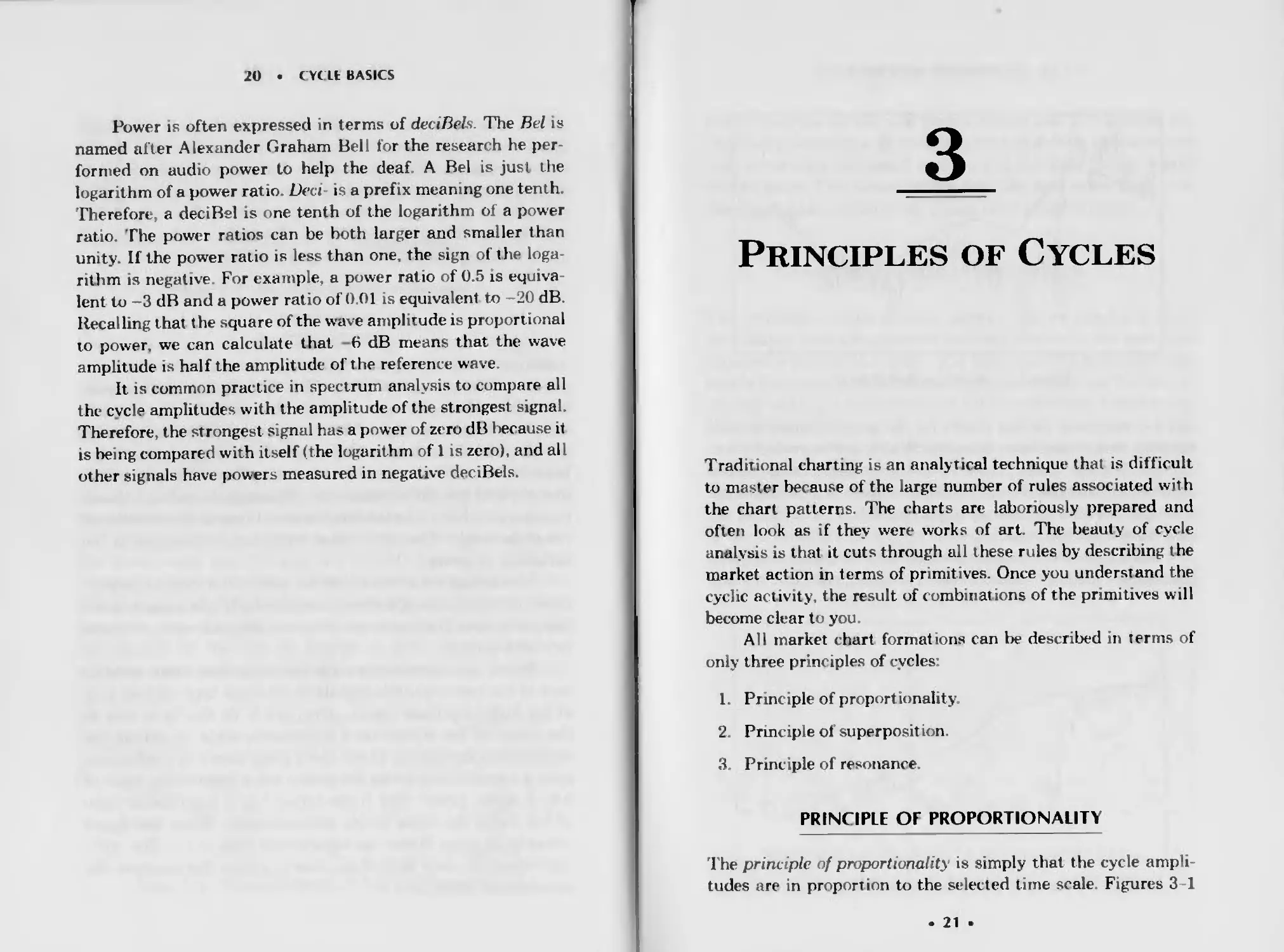
The principle of proportionality is simply that t he cycle amph
tudes are in proportion to the selected time scale Figures 3 1
. 21 •
22
PRINCIPIES OP CYCLES
Figure 3-1 Weekly or Daily Chart?
and 3-2 represent the bar charts for the same commodity with
the time and price scales removed. Which is the weekly chart
and which is the da*ly chart? You simply can t tell by casual
observation because of the principle of proportionality. This
principle has also become an important factor in the more re-
cent fractal mathematics.
Another way to convince yourself that the principle of pro-
portionality holds is to assume that it doesn’t, and then test the
Figure 3-2 Weekly or Daily Chart?
PRINCIPLE OF SUPERPOSITION
23
result. Suppose we had w ild hour! у swings that far exceeded the
day-to day variations. If that were true, the daily charts would
have a virtually horizontal average and the daily ranges would
fill the chart This clearly is not the case, and so the failure of
the assumption validates t he principle of proportionality
PRINCIPLE OF SUPERPOSITION
The principle of superposition asserts that we can build com-
plex shapes from the primitive building blocks If you have ever
watched waves on the water, you have seen the total wave ac-
tion is the summation of waves from several sources. For exam-
ple, the wake of a hoat combines with wind-driven waves to lap
at the dock.
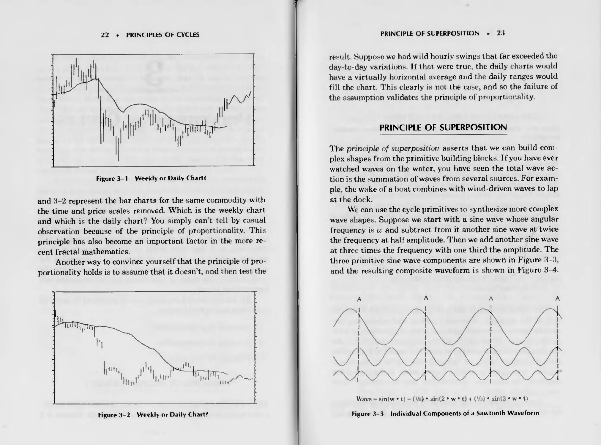
We can use the cycle pr.mit ives to synthesize more complex
wave shapes Suppose wre start with a sine wave whose angular
frequency is iv and subtract from it another sine wave at twice
the frequency at half amplitude Then we add another sine wave
at three times the frequency with one third the amplitude. The
three primitive sine wave components are shown in Figure 3-3,
and the resulting composite waveform is shown in Figure 3 4.
Wave - sin(w • t) (V«) » sin(2 * w • i) + (Уз) • sin(3 * w * О
Figure 3-3 Individual < omponents of a Sawtooth Waveform
24
PRINCIPLES OF CYCLtS
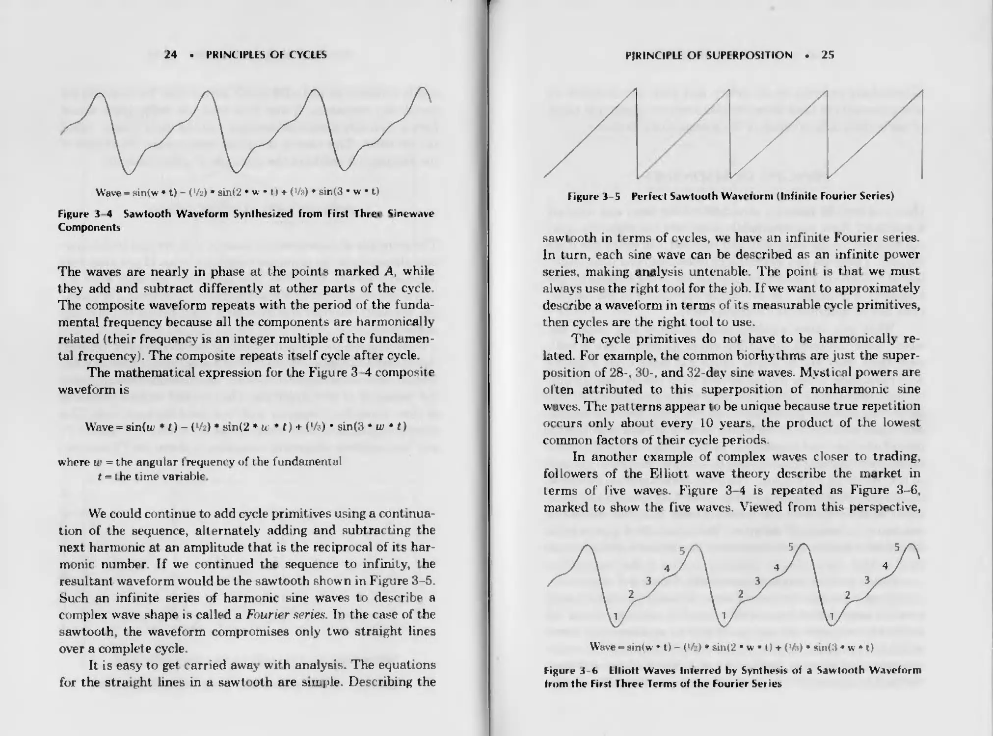
Wave - sin(w • t) - (>/2) * sin 12 * w • 1) + (>/») ♦ sin(3 • w • t)
Figure 3- 4 Sawtooth Waveform Synthesized from First Three Sinewave
Components
The waves are nearly ir. phase at the points marked Д w'hile
they add and subtract differently at other parts of the cycle
The composite waveform repeats with the period of the funtla
mental frequency because ail the components are harmonically
related 1thei г freqi ency is an integer multiple of the fundamen-
tal frequency). The composite repeats itself cvc e after cycle.
The matnemat ical expression for tne Figure 3 4 composite
waveform is
Wave = sin(u? ♦ t)- (*/2) * sin(2 ♦ w * t) + (‘A) • sin(3 * w * t)
where w = t he angular Tequency of 1 he fundamental
t = 1 he t irne variable.
We could continue to add cycle pnm_tives using a continue
tiun of the sequence, alternately adding and subtracting the
next harmonic at an amplitude that is the reciprocal oi its har-
monic numbei If we continued the sequence to infinity, the
resultant waveform would be the sawtooth shown in F .gore 3 -5
Such an infinite series of harmonic sine waves to describe a
complex wrave *»hape is called a Fourier series. In the case of the
sawtooth the waveform compromises only two straight lines
over a complete cycle.
It is easy to get carried away wrh analysis The equabons
for the straight lines in a sawtooth are simple. Describing the
PRINCIPLE OF SUPERPOSITION
25
figure 3-5 Perfect Sawtooth Wavetorm (Infinite Fourier Series)
sawt ooth tn terms of cycles, we have an infinite Courier series.
In turn, each s.ne wave can be described as an inf nite power
series, making analysis untenable The point is that we mu4
always use the t ight tool for the job. If we want to approximately
desenbe a waveform in terms of its measurable cycle primitives,
then cycles are the right tool to use.
The cycle primitives do not have to be harmonically re
lated. For example, the common biorhythms are just the super-
position of 28-, 30-, and 32 -dav sine waves. Mystical powers are
often attributed to this superposition of nonharmonic sine
waves. The patt erns appear to be unique because true repetition
occurs only about every 10 years, the product of the lowest
common factors of their cycle periods
In another example of complex waves closer to trading,
followers of tne Elliott wave theory describe the market in
terms of five waves Figure 3-4 is repeated as Figure 3-6,
marked to show the five waves. Viewed from this perspective,
Wave - sin(w • t) - (l/j I • sin(2 • w t) + (V ) » sin(3 • w * t)
Figure 3 < Elliott Waves Inferred bv Synthesis of a Sawtooth Waveform
from the First Three Terms of the Fourier Sei ies
26
PRINCIPLES ОГ CYCLES
Elliotticians embrace cycle theory and even the principle of
proport ionaiity in their more complex analyses 1 prefer to think
of the market only in terms of the measurable primitives.
PRINCIPLE OF RESONANCE
Have you ever strummed a stretched rubber band and watched
it oscillate? Have you ever held a ruler over the edge of a desk,
pulled down on the loose end, and released it to watch the ruler
vibrate? 'lhese are two examples of resonance. The items osc.il
late at a frequency determined by the restoring forces and the
boundary conditions. The maximum excursions of the oscilla-
tions can be described as a standing wave.
When you throw a pebble into a pond of still water, the
waves travel outward until they strike an object like a wall,
whereupon they are reflected. Much the same thing happens
with resonance When you deflect the ruler you put energy into
it. The wave travels down the ruler when you release it, but
there is no place for the energy to go w'hen the wave reaches the
desk, and so the wave is reflected back. The wave now' travels
toward the free end, causing it to move. But when the wave
reaches the free end there is no place for the energy to go, and
so it is reflected back again. The process continues with waves
traveling in both directions on the ruler. The forward and back
waves combine to form the standing wave that you see as the
maximum excursion of the ruler, lhe same effect occurs with
the rubber band except the boundary conditions hold both ends
fixed so that the maximum excursion occurs at the center
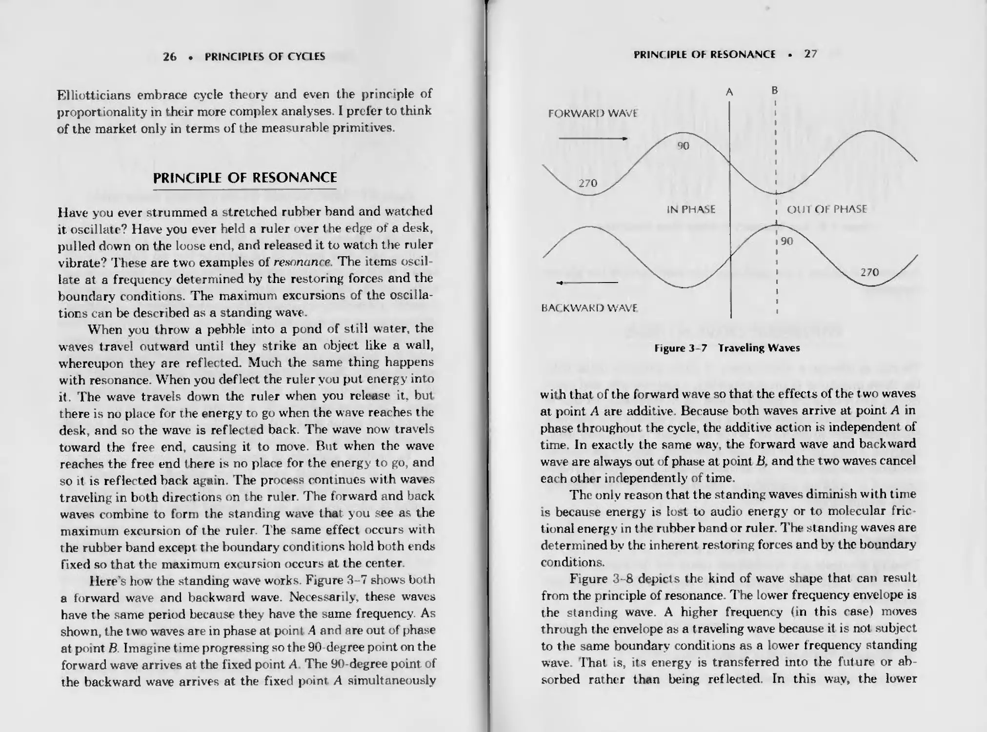
Here’s how the standing wave works. Figure 3-7 shows both
a forward wave and backward wave. Necessarily, these waves
have the same period because they have the same frequency As
shown, the two waves are in phase at point .4 and are out of phase
at point В Imagine t ime progressing so the 90 degree point on the
forward wave arrives at the fixed point A The 9O-degree point of
the backward wrave arrives at the fixed point A simultaneously
PRINCIPLE OF RESONANCE
27
Figure 3-7 Traveling Waves
with that of the forward wave so that the effects of the t wo waves
at point A are additive. Because both waves arrive at point A in
phase throughout the cycle, the additive action is independent of
time. In exactly the same way, the forward wave and backward
wave are always out of phase at pcmt B. and the two waves cancel
each other independently of time
The only reason that the standing waves diminish with time
is because energy is lost to audio energy or to molecular fric-
tional energy in the rubber band or ruler. The standing waves are
determined by the inherent restoring forces and by the boundary
conditions.
Figure 3-8 depicts the kind of wave shape that can result
from the principle of resonance The lower frequency envelope is
the standing wave. A higher frequency (in this rase) moves
through the envelope as a traveling wave because it is not subject
to the same boundary conditions as a lower frequency standing
wave. That is, its energy is transferred into the future or ab-
sorbed rather than being reflected, In this way, the lower
28 • PRINCIPLES OF CYCLES
Figure 3-8 Low Frequency Standing Wave Modulation
frequency standing wave modulates the amplitude of rhe higher
frequency
SYNTHESIZED CHART PATTERNS
We can synthesize a wide variety of chart patterns using only
the three principles of proportionality, superposition, and reso
nance. Analysis is the inverse operation of synthesis, so that if
we understand synthesis we have a greater insight into analysis
techniques and procedures. While synthesis is relatively easy,
analysis is very diff ’cult because of t he wide range of parameter
combinations that must be accommodated. We often perform
analysis by making simplifying assumptions and then testing
these assumptions.
Trading Channels
Trading channels are synthesized using the principles of pro-
portionality and superposition. We use the following three
primitives:
1 Trend (a piece of a large ampbtude long cycle)
2 Medium length cycle of medium amplitude.
3 . Short-term cycle of small amplitude.
SYNIHESIZED CHART PATTERNS
13
MAGNITUDE
Figure 3 10 Head and-Shoulders Pattern
30
PRINCIPLES OF CYCLES
When we add these three coinponente, the resultant is the wave
form shown in Figure 3-9, The trading channels are simply t he
maximum and minimum excursions of the short-term cycle
when it s combined with the other two cycle components. In
this case the ‘"channel” is bent with the medium-length cycle
rather than being constructed from straight lines.
Head and Shoulders
One of the favorite formations of the chartists s the class.c
head-and-shoulders pattern showm in Figure 3-10. Each of the
chan characteristics are noted on the figure. Conventional m
terpret ation would have the downside break through the sloping
neckline confirming the trend reversal called by the previous
breakthrough of the uptrend line Even the return move fol-
lowed by further downside activity is indicated.
Figure 3 11 Cyclic Components of Head-and-Shoulders Pa’.tern
SYNTHESIZED CHART PATTERNS • 31
Now, let’s see how we synthesized that head-and-shoulders
pattern. Figure 3-11 shows the primitive components of the
composite wave shape We simply used the principle of superpo-
sition and added a trend line (a segment of a very long cycle), a
medium-length cycle, and a short term cycle at half the ampli-
tude and four tunes the frequi ncy The short-term cycle and the
medium length cycle phase together at. theii peaks to form the
head. The two shoulders are formed basically by the short cycle
adding to the medi am-length cycle at its midpoint.
Knowing the cyclic components makes analysis far easier.
We would establish the long term trend directly. The medium
trend and its breakpoint are established by the medium-length
cycle. The short-term cycle gives 'he best entry points for trades
to be made in the direction of the medium-length trend. It is
clear that the probability of a profitable trade is best if you
enter using the short-term cycle with the trade in the direction
figure 3 12 Relative Phase of Shifted Short Cy< le
32
PRINCIPLES OF CYCIFS
of the medium cycle Trades where the two cycles conflict m
direction should be avoided That’s about all there is to it, using
the primitives. No complicated rules to learn, just trade the
cycles you measure.
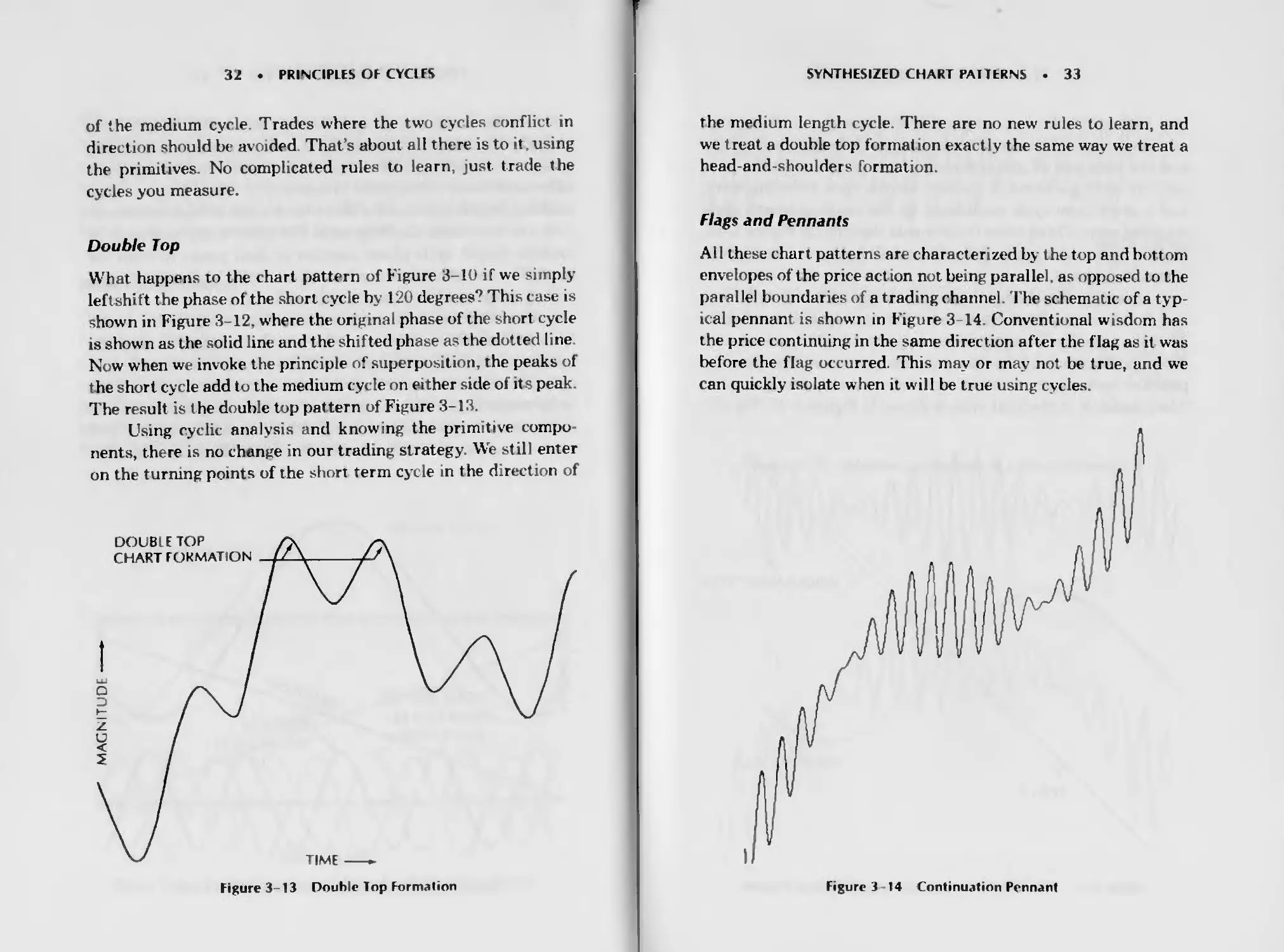
Double Top
What happens to the chart pattern of Figure 3-10 if we simply
left shift the phase of the short cycle by 120 degrees? This case is
shown in Figure 3-12, where the original phase of the short cycle
is shown as the solid line and the shifted phase as the dotted line
Now when we invoke the principle of superposition, the peaks of
the short cycle add to the medium cycle on either side of its peak.
The result is the double top pattern of Figure 3-13.
Using cyclic analysis and knowing the primitive compo-
nents, there is no change in our trading strategy. We still enter
on the turning points of the short term cycle in the direction of
Figure 3-13 Double Top Formation
SYNTHESIZED CHART PATTERNS . 33
the medium length cycle. There are no new rules to learn, and
we treat a double top formation exactly the same way we treat a
head-and-shoulders formation.
Flags and Pennants
All these chart patterns are characterized by the top and bottom
envelopes of the price act ion not being parallel, as opposed to the
parallel boundaries of a trading channel. The. schematic of a typ-
ical pennant is shown in Figure 3 14 Conventional wisdom has
the price continuing in the same direction after the flag as it was
before the flag occurred. This may or may not be true, and we
can quickly isolate when it will be true using cycles.
Figure 3 14 Continuation Pennant
34
PRINCIPIES OF CYCLES
Figure 3 8 shows a nonparallel envelope due to the princi-
ple of resonance. If we now .nvoke the principle of superposition
and the principle of proportionality, we can generate the pen
nant by adding a trend, a medium-length cycle traveling wave,
and a short term cycle modulated by the medium length cycle
standing wave. Using these components depicted in Figure 3-15,
the conventional w.sdom prevails and the price rise continues
after the pennant.
However, if we double the length of the medium-length cycle
and double its amplitude (principle of proportionality) andelim
inate the t rendline, the primit ive components of the pennant are
shown in Figure 3-16. In this case, the price reverses after the
pennant because the trend is replaced with the stronger cycle.
The schematic of the total price is shown in Figure 3-17. We still
Figure 3 -15 Primitive Components of a Continuation Pennant
SYNTHESIZED CHART PATTERNS
35
Figure 3-17 Reversal Pennant
36
PRINCIPLES OF CYCLES
have v irtually the same pennant we had in Figure 3-14, hut read-
ing the pennant as a continuation signal is dead wrong. Had we
known the cycle primitives, the price direction at the end of the
flag could have easily been predicted.
FOR FURTHER STUDY
The relationship between chart patterns and cycles has enough
variations that this topic can be the basis of an entire book by
itself. The goal in this chapter was only to make you aware that
the relationships exist and that you can use cycles to aid your
charting analysis J M. Hurst is recommended for further
reading on the subject.
Effects of
Moving Averages
SIMPLE MOVING AVERAGES
Several hundred years ago Karl Friedrich Gauss proved that the
average is the best est.mator of a random variable. As a result,
in statistics the mean is always the nominal forecast This best
estimator is certainly true for the market in the case where the
diffusion equation applies The best estimate of the location of
the smoke plume is tne center of the plume, the average across
its widl h This is probably the reason moving averages are heav-
ily used by te< bnical traders—they want the best estimator of
the random variable.
An N-day simple average is ft>rmed by adding the prices over
xV days and dividing by N. The simple average becomes a moving
average by adding the next day s weighted price to the sum and
dropping off the weighted first day’s price Thus the simple aver-
age “moves” from day to day.
Lets look at how simple moving averages (SMA) behave
with cycles With reference to Figure 4 1, we will take an average
• 37
38
EFFECTS ОТ MOVING AVtKAGES
WINDOW A
Figure 4-1 Half ( vcle Average Window
of all the sampled points of the sine wave in window A W indow
A covers half a cycle. If t he window were wider, it would include
some negative values of the sine wave and the peak value of the
moving average would be reduced. On the other hand, if the win-
dow were narrower, all values in the positive alternation would
not be included in the window. Therefore, a simple moving aver-
age of half the cycle length has special significance.
Referenc ing the moving average to t he right-hand side of the
window, the moving average is maximum at point A m Figure 4-2.
As we move the window to the right in our mind’s eye, we start to
include some negative values of the sine wave in the moving aver
age. Therefore, the moving average amplitude declines. When the
right -hand edge of the window reaches position B. t here are just
as many negative values inside the window as positive values The
result is that the moving average has a zero value at position В
We can continue to move the window, creating the moving aver
age shown as the dashed line.
We can make some observations about a half-cycle moving
average of a sine wave First, the shape ot t he moving average is a
negative eosine wave. From the phasor discussion in Chapter 2,
vou recognize that the halt-cycle moving average lags the sine
wave by exactly 90 degrees The trendline for the sine wave is
zero, so we can observe that the sine wave price function reaches
SIMPLE MOVING AVERAGES . 39
its maximum just as the half-cyc le moving average crosses the
trendline from bottom to top Similarly, the price function just
reaches its valley as the half-cycle moving average crosses the
trendline from top to bottom
Another special simple moving average is one taken over
the full period of lhe cycle. In this case there are just as many
positive values in the window as negative values. The result is
that this moving average is always zero, regardless of the phase
angle position of the window If the price consists of a t rendline
plus the sine wave, the full-cycle moving average removes the
cycle part and retains the trendline.
The action of the half-cycle and full-cycle moving averages
suggests a trading system. You would sell when the half-cycle
moving average crosses the full-cycle moving average from hot
tom to lop because this is where the sine wave has its peak value.
You would buy when the half-cycle moving average crosses the
full cycle moving average from top to bottom because this is
where the sine wave has its lowest value Note that these trading
rules are exactly the opposite of the rules for short and long
moving averages m trend-following systems.
40
EFFECTS OF MOVING AVERAGES
MOVING AVERAGES AS FILTERS
A moving average is basically a Zoic pass filter. That is, the aver-
aging smooths the input data. Th.s smoothing means that the
higher frequency wiggles (noise) arc removed and only the lower
frequency components (bigger moves) are allowed to pass. The
smoothing action uses historical data so that the filtered output
is always delayed in phase relative to the input. We have already
examined the filter characteristic of two special low pass filters,
the half-cycle moving average and the full-cycle moving average.
We can establish a more general picture of the passband and
delay characteristics of the moving average.
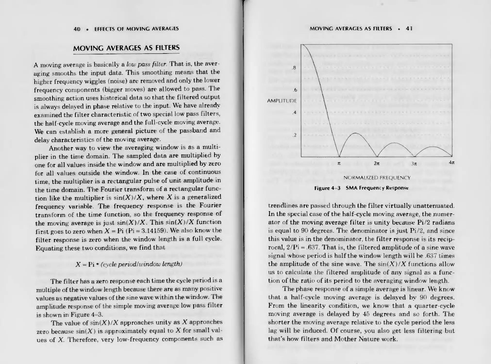
Another way to view the averaging window is as a multi-
plier in the time domain. The sampled data are multiplied by
one for all values inside the window and are multiplied by zero
for all values outside the window. In the case of continuous
time the multiplier is a rectangular pulse of unit amplitude in
the time domain. The Fourier transform of a rectangular func
tion like the multiplier is sin(X)/X, where X is a generalized
frequency variable The frequency response is the Fourier
transform of the tune function, so the frequency response of
the moving average is just sin(X)/X. This sin(X)/X function
first goes to zero when X = Pi (Pi = 3.14159). We also know the
filter response is zero when the window length is a full cycle.
Equating these two conditions, we find that
X = Pi * (cycle period/window length)
The filter has a zero response each t ime the cycle period is a
multiple of the window length because there are as many positive
values as negative values of the sine wave within the window. The
amplitude response of the simple moving average low pass filter
is shown in Figure 4 3.
The value of sin(X)/X approaches unity as X approaches
zero because sin(X) is approximately equal to X for small val-
ues of X Therefore, very low-frequency components such as
MOVING AVERAGES AS FILTERS
41
trendlines are passed through the filter virtually unattenuated
In the special case of the half-cycle moving average, the numer-
ator of the moving average filter is unity because Pi/2 radians
is equal to 90 degrees. The denominator is just Pi/2. and since
this value is in the denominator, the filter response is its recip
rocal, 2/Pi = .637. That is, the filtered amplitude of a sine wave
signal whose period is half the window length will be .637 times
the amplitude of the sine wave. The sin(X)/X functions allow
us to calculate the filtered amplitude of any signal as a func-
tion of the ratio of its period to the averaging window length
The phase response of a simple average is linear We know
that a half-cycle moving average is delayed by 90 degrees.
From the linearity condition, we know that a quarter-cycle
moving average is delayed by 45 degrees and so forth The
shorter the moving average relative to the cycle period the less
lag will be induced. Of course, you also get less filtering but
that’s how filters and Mother Nature work
42
EFFECTS OF MOVING AVERAGES
Filters can be designed to have a much sharper frequency
cutoff than the sin(X)/X response of the simple moving a\ erage.
Higher order filters can be designed1: however, the use of these
filters is discouraged- The amount of delay experienced by a fil-
ter is directly related to the order of the filter In general the
phase response is more important to traders than the frequency
attenuation response Therefore, these higher order filters are
not very useful for traders.
EXPONENTIAL MOVING AVERAGES
The exponential moving average (EMA) is a way of recursively
calculating the average, emphasizing most recent data more
than older data. The EMA by the way , is a mathemat ical real-
ization of real filters. Simple averages can only be calculated,
they cannot be generated in physically realizable filters. The
equation for the EMA is
NEW EMA - (1 - (X) * (OLD EMA) + К * (NEW SAMPLE)
where К is a constant < 1.
In words, this equation says that today’s EMA is formed by
taking a fraction of today’s data and adding it to the compli-
ment of the fraction multiplving yesterday’s EMA. 1'he equa
tion is convergent when К is less than one because if the data
input becomes constant, the value of the EMA approaches that
constant Consider the case where all the new samples are unity
The EMA starts with a zero value and gradually builds up to
almost unity When this occurs the equation for the NEW EMA
is approximately
NEW EMA - (1 - К) + К = 1
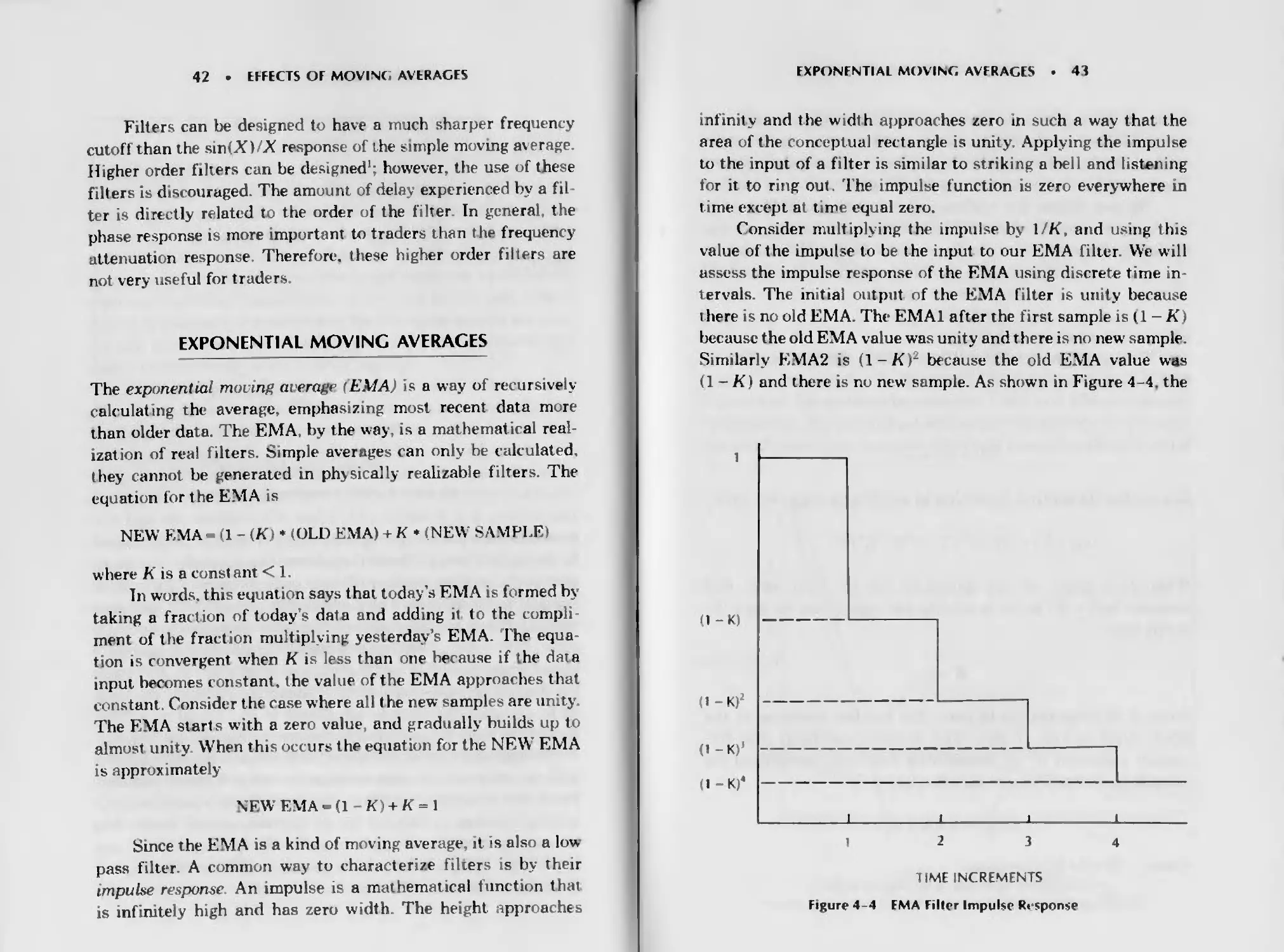
Since the EMA is a kind of moving average, it is also a low
pass filter. A common way to characterize filters is by their
impulse response An impulse is a mathematical function that
is infinitely high and has zero width The height approaches
EXPONENTIAL MOVING AVFRAGES
43
infinity and the width approaches zero in such a way that the
area of the conceptual rectangle is unity. Applying the impulse
to the input of a filter is similar to striking a bell and listening
for it to ring out. The impulse function is zero everywhere in
time except at time equal zero.
Consider multiplying the impulse by l/K, and using this
value of the impulse to be the input to our EMA filter We will
assess the impulse response of the FMA using discrete time in
tervals. The initial output of the EMA filter is unity because
i here is no old EMA. The EM Al after the first sample is (1 - K)
because the old EMA value was unity and there is no new sample.
Similarly EMA2 is (1-K)~ because the old EMA value was
(1 - К1 and there is no new sample. As shown in Figure 4 -4, the
(1-K)
(1 - K)2
(l-K)’
(I -K)‘
TIME INCREMENTS
Figure 4-4 EMA Filter Impulse Response
44
EFFECTS OF MOVING AVERAGES
decay of lhe response to the impulse falls as the exponent of
the trial That is, the EMA has an exponential decay. Now it’s
easy to see how the exponential moving average got its name.
The rate of the decay depends on the К factor.
We can derive the equivalence between an FMA and a
SMA using a specific value of K. To do this, we first equate the
finite impulse response to an exponential for the Nth sample as
(1 - К )л - exp (-a * N )
where a is a constant to be found.
'Гаking the natural logarithm of both sides of this equa
tion, we have
jV ♦ Inti - K) - -a • A
Ind - A) = -a
Expanding the natural logarithm to an infinite series we have
ln(l -K) = -K-K3/2- KV3-KV4-.
When К is small, we can ignore all but the first term, and
equating Inf 1 - K) in the preceding two equations, we have the
result that
A-a
Since N is proportional to time, the impulse response of lhe
EMA filter is just The Fourier transform (the fre-
quency response! of an exponential function, normalized for
unity t ransfer response at zero frequency, is
HdV) = K/(K+;W)
where W - 2 • Pi ♦ frequency
j »imaginary operator, a 90-degree shift
H(W9=l/(l+jVV/K).
EXPONENTIAL MOVING AVERAGES . 45
We note that the X in the sin(X)/X SMA function is Pi
times the frequency times the SMA period. In the EMA fre-
quency response the variable is 2 ♦ Pi times the frequency nor-
malized to K. Equating the frequency variables, we have
Pi • F * Window = 2 ♦ Pi ♦ F/K
Performing the algebra, we obtain the result that
К = 2/W ndow
The amplitude response of the EMA as a function of fre-
quency is compared with the amplitude response of the SMA in
Figure 4-5. Equivalence between the SMA and EMA is subject
to definition. For example, if we force the amplitude response of
the two filters to be the same when half the cycle period is equal
NORMALIZED FREQUENCY
Figure 4-5 FMA/SMA Frequency Response Comparison
4Ь
EFFECTS OF MOVING AVERAGES
to the window length, then the relationship for the EMA К
factoi is approximately
К =2.5/Window
Hutson derived the relationship between the EMA К fac-
tor and the SMA w indow length as
К = 2/\ Window + 1)
This definition is based on the average age of each Note that
this definition is substantially the same as the first definit ion
derived except for the shortest wmduw lengths.
Examination of the HijW) freq uency response gives in-
sight into the pnase delay of an FMA. When the frequency is
near zero.jW/K is much smaller than unity and can he ignored.
In this case the output is almost the same as the input, and
there is no phase delay. On the other hand, when the frequency
approaches infinity, j W/K is much larger than unity and the
unity factor in the denominator can be ignored. When this is
done, the denominator has a 90 degree phase shirt due to tne
maginary operator. An interest ng result is that the phase lag
of an EMA is never more than 90 degrees at any frequency.
Since the phase lag of an EMA is always less t han the phase lag
of an SMA, the FMA is the preferred type of moving a\ erage in
many applicat ions
5
Effects of Momentum
MOMENTUM DEFINED
In the jargon of technical analysis, momentum is the rate of
change, usually applied to price. It has nothing to do w’th the
length of time to bring a moving bi >dv to rest under constant force
(the mechanical definition) Nor does the momentum of technical
traders imply mpetus, as used in the common vernacular
The summat ions of moving averages can be viewed as paral-
lels to integrals in the calculus, Since momentum functions are
rate of change they can be viewed as denvauves n the calculus
using the same parallels. While not rigorous, thic viewpoint al-
lows us to think of momentum as the opposite of moving aver
ages For example, when moving averages cause a pha^e delay,
momentum functions can introduce a phase lead. We can use this
viewpoint to manipulate combinations of moving averages and
momentums tc generate indicators that will perform to our
specifications That is, we gain an msighi on how to adapt
our tools to the current market conditions.
While 1 he prospect of a leading phase function can be ex-
citing because of predictive properties for cyclic behavior,
. 47 .
48
EFFECTS OF MOMENTUM
Mother Nature strikes again and does not allow us this luxury
without some difficulty. The price data that technical analysts
use are noisy. Momentum amplifies this noise, often so much
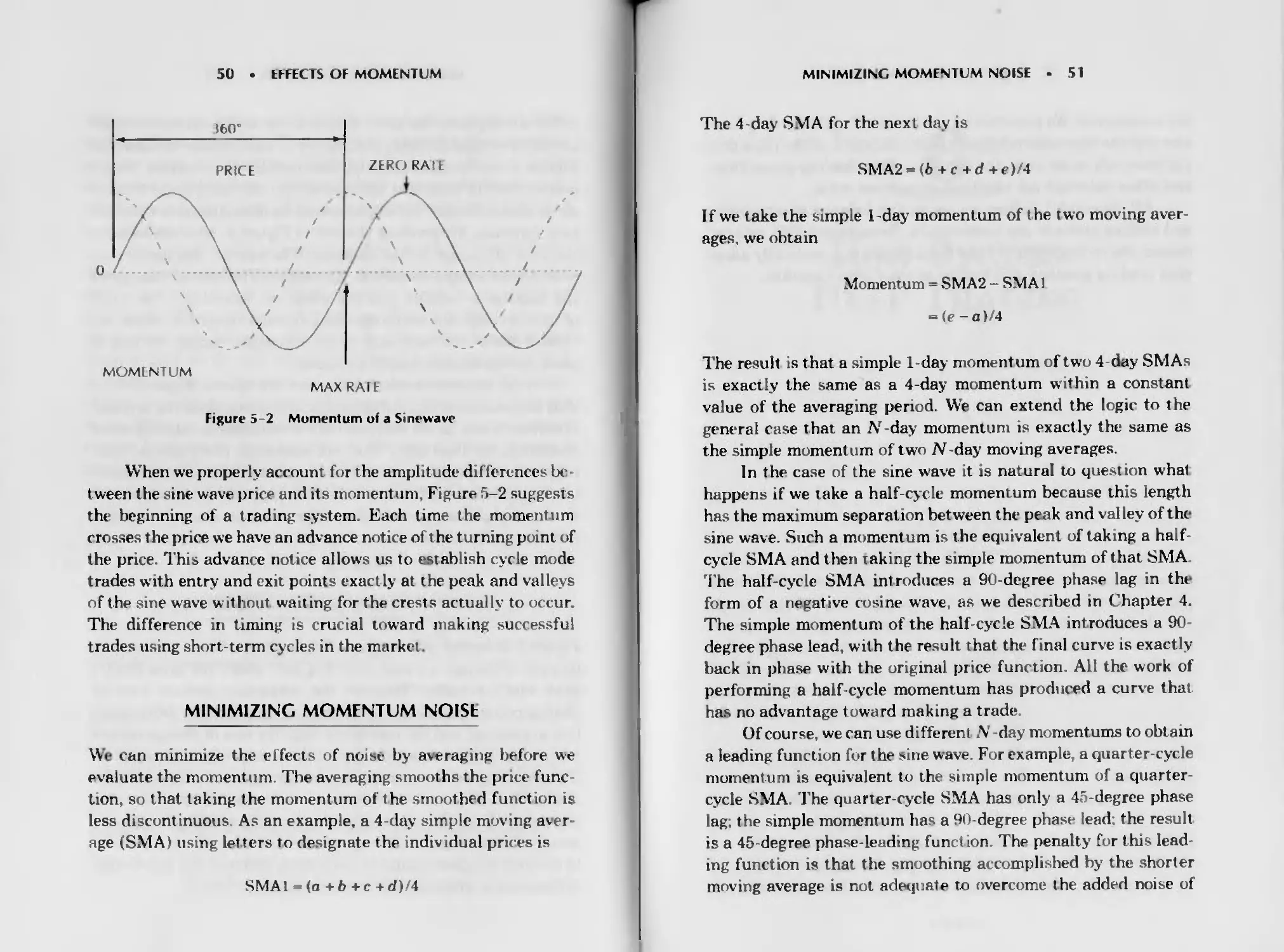
that useful indications are completely obscured. Figure 5- 1,
showing successive rates of change, demonstrates why the noise
is amplified.
The initial curve is a ramp and is shown in Figure 5-la.
The “origin" is at the center, so the ramp has a zero slope to the
left of the origin and a finite constant slope to the right of
the origin. When we take the rate ol change of the ramp, we
ohta n the step function, Figure 5-lb. The rate change of the
ramp is zero to the left of the origin and instantly jumps to a
constant value to the right of the origin, producing the step.
Notice that the step appears to be more discontinuous than the
ramp. When we take the rate of the step, it has a zero rate of
change both to the right and left of the origin. There is only a
change exactly at the origin, and this change is infinite because
it occurs over a zero horizontal span. This infinite change is
ORIGIN
Figure 5-1 Successive Momentum Functions
MOMENTUM LEADING PHASE • 49
called an impulse, the same function we used with exponential
moving averages (EMAs) in Chapter 4 The impulse is shown as
Figure 5-lc Mathematically, the impulse has infinite height
and zero width such that the area within this theoretical rectan
gle is unity. Clearly, the impulse is more discontinuous than the
step function. We produce the jerk of Figure 5 Id when we take
the rate of change of the impulse. The rate of change is zero
everywhere except exactly at the origin. The rate of change of
the impulse is infinite positive when we “travel up” the front
of the conceptual rectangle and infinite negative when we
“travel down” the back side of the rectangle. Again, the jerk is
more discontinuous than the impulse
What becomes evident from the example of Figure 5-1 is
that momentum is always more discontinuous than the original
function. Noise in the original data is manifest in the degree of
discontinuity. Less noisy data are smoother. If we use momen-
tum without consideration of the impact on noise. wre can easily
be disappointed in the result. However, properly implemented,
we can exploit the phase leading characteristic when the market
is in the cyclic mode.
MOMENTUM LEADING PHASE
Figure 5-2 depicts price as the solid sine wave. When we examine
its rate of change, we note that it is zero where the price has its
peak and its valley. Further, the maximum positive rate of
change occurs just as the price crosses through zero from nega-
tive to posit ive, and the maximum negative rate of change occurs
just as the price crosses through zero from positive to negative.
The resulting momentum of the sine wave price is shown as the
dashed line. Figure 5-2 shows that the momentum of the sine
wave price leads the price by 90 degrees We would get approxi-
mately the same result if we quantized the continuous sine wave
in discrete samples similar to daily data, and took the day-to-day
differences to generate the momentum.
50
EFFECTS OF MOMENTUM
Figure 5-2 Momentum ot a Sine wave
When we properly account for the amplitude differences be-
tween the sine wave price and its momentum, Figure 5-2 suggests
the beginning of a trading system Each time the momentum
crosses the price we have an advance notice of the turning point of
the price. This advance notice allows us to establish cycle mode
trades with entry and exit points exactly at the peak and valleys
of the sine wave without waiting for the crests actually to occur.
The difference in timing is crucial toward making successful
trades using short-term cycles in the market.
MINIMIZING MOMENTUM NOISE
We can minimize the effects of noise by averaging before we
evaluate the momentum. The averaging smooths the price tunc
lion, so that taking the momentum of the smoothed function is
less discontinuous As an example, a 4-day simple moving aver-
age (SMA) using letters to designate the mdividual prices is
SMA1 - (a + b + c + d)/4
MINIMIZING MOMENTUM NOISE • 51
The 4-day SMA for the next day is
SMA2 (Ь + c + d + e )/4
If we take the simple 1-day momentum of the two moving aver-
ages, we obtain
Momentum = SMA2 - SMA1
= (e - a)/4
The result is that a simple 1-day momentum of two 4 day SMAs
is exactly the same as a 4-day momentum within a constant
value of the averaging period. We can extend the logic to the
general case that an Ar-day momentum is exactly the same as
the simple momentum of two TV-day moving averages.
In the case of the sine w'ave it is natural to question what
happens if we take a half-cycle momentum because this length
has the maximum separation between the peak and valley of the
sine wave. Such a momentum is the equivalent of taking a half
cycle SMA and then raking the simple momentum of that SMA
The half-cycle SMA introduces a 90-degree phase lag in the
form of a negative cosine wave, as we described in Chapter 4.
The simple momentum of the half-cycle SMA introduces a 90-
degree phase lead, with the result that the final curve is exactly
back in phase with the original price function. All the work of
performing a half-cycle momentum has produced a curve that
has no advantage toward making a trade.
Of course, we can use different Л’-day momentums to obtain
a leading function for the sine wave. For example, a quarter-cycle
moment uni is equivalent to the simple momentum of a quarter
cycle SMA The quarter-cycle SMA has only a 45-degree phase
lag; the simple momentum has a 90-degree phase lead; the result
is a 45 degree phase-leading function. The penalty for this lead-
ing function is that the smoothing accomplished by the shorter
moving average is not adequate to overcome the added noise of
52 • EFFECTS OF MOMENTUM
the momentum. We therefore have a trade-off of the leading func
tion and the increased noisiness of that function. If the price data
are relatively noise-free, the benefits of the leading-phase func-
tion often outweigh the negatives of increase noise.
All successful indicators weigh the balance of smoothing
and leading phase in their generation. Recognizing this, you can
dissect the indicators and tune them so you can optimally adapt
your trading strategy and tact ics to the current market.
6
How Cycles
Help Trading
INDICATORS
Some of the more popular trading indicators examine specific
aspects of the price function, using combinations of moving
average and momentum functions These indicators usually in-
clude the time parameter in their specific names, such as a
“14-day RSI” or a “5 period stochastic.” The character of the
market is always changing and therefore no single fixed indica-
tor best fits all market conditions.
We can classify the varying market by the measured cycles.
Since we have an appreciation of 1 he effects of moving average
and momentum functions on the phase lead and lag of cycles,
the cycle perspective can be used to adapt the indicators to the
current market conditions.
The sections that follow discuss how best to adapt RSI
(relative strength index), stochastics, and MACD (moving aver-
age convergence-divergence) to market cyclic conditions.
. 53 .
54
HOW CYCLES HELP TRADING
RELATIVE STRENGTH INDEX (RSI)
J. Welles Wilder describes the relative strength index (RSI) in
his book New Concepts in Technical Trading Systems 1 as
RSI -1- 1/(1 + RS)
where R.S - CU/CD
= (14 day averages of closes upj/(14-day average of
closes down)
With a little algebra this simplifies to
RSI-RS/(I + RS)
-CUHCU + CD)
The “closes up” and “closes down” are simple momentums
of successive closing prices. 'The original definition of RSI took
the observation period over 14 days. This rigid def inition of RSI
is what attracted me to investigate technical analysis with the
perspective of adapting the indicators to market conditions.
Since cycles are one of the few things about market price that
can be measured and that can have a short term predictive
capability, I decided cycles would be the focus of my technical
analysis research
In the case of a perfect sine wave of closing prices, the
“closes up" would have a maximum value near the center point
of the upswing of the cycle and the “closes down” would have a
maximum value near the center point of the downswing (see
Figure 5-2), Both the “closes up” and “closes down” have a zero
value near the peak and valley of the sine wave price Thus, each
of the components has a 90 degree leading characteristic. When
these components are averaged over some period, the average
introduces phase lag. If the averaging period is exactly a half
cycle of the sine wave, the “closes up" and “closes down” are
RELATIVE STRENGTH INDEX (RSI) . 55
both exactly in phase with the sine wave price. Since all compo-
nents of the RSI are in phase with price when the averaging
period is a half cycle, the RSI is also exactly in phase with the
price under this condition. The RSI swings between zero and
one as a perfect sine wave, as shown in Figure 6-1. VVe can see
the logic of this because at the end of the half-cycle upswing
there are no closes down, and the value of the RSI is one. At the
end of the half-cycle downswing there are no closes up. and the
value of the RSI is zero.
The most simple BUY indication from the RSI is when the
RSI swings below- 30 percent and crosses back up through
the 30 percent level. Conversely, the SELL indication occurs
when the RSI swings above the 70 percent level and then crosses
Figure 6-1 RSI lor a 20 Day Sinewave Price
56 • HOW CYCLES HELP TRADING
back through it. This is not a particularly good strategy for
short cycles For example, on a 10-day cycle it takes two days
from the minimum value to ident ify a crossing of the 30 percent
level. You enter the long position trade on the third day. But the
entire move occurs in only 5 days, the half cycle of the 10 day
cycle. Since you would also exit the trade late, about the best
you could hope for is to break even. This is not true when the
RSI is used on longer cycles. When used with longer cycles, the
lag between the cycle peak and crossing the 70 percent mark can
be viewed as insurance against being whipsawed
The RSI has some distinctive characteristics when the es-
timated cycle length used in the calculation is different from the
real cycle length. The perfect 20-day cycle data are used to
illustrate these characteristics. Suppose you estimate the cycle
to lie 50 percent longer than it really is, for example 30 days
instead of the correct value of 20 days. Then, you would average
the closes up and closes down over a period of 15 days. The
upswing part of the RSi would then contain 5 closes down as
well as all of the closes up. The addition of the closes down in
the denominator of the RSI equation reduces the peak value to
less than unity. In much the same way, the downswing part of
the RSI contains 5 closes up as well as all the closes down,
so the RSI value cannot reach zero. The RSI for a 50-percent-
too-long estimate of the cycle period is shown in Figure 6-2. In
addition to having reduced amplitude, the peaks of the RSI are
delayed relative to the price peaks and its shape is distinctly
more triangular. This is due to more smoothing by the longer
moving average period. In such a case with real world data
the RSI will be noticeably smoother than the generating price
function, RSI will not swing fully between zero and one, and
the RSI peaks will lag the price peaks.
A too-short estimate of the cycle length also yields some
distinctive RSI patterns In this case, all the closes are closes
up early in the move from the cycle valley toward the cycle peak
Further, all the closes continue to be closes up until the price
peak is reached The result is that the RSI is stuck at a value of
RELATIVE STRENGTH INDEX (RSI) • 57
Figure 6-2 RSI Cycle Length Estimated 50% Too Long
one, or “saturated,” for a period during the upmove A similar
action occurs on the next half of the cycle. In this case, all the
closes are closes down soon after the price passes its peak
All closes continue to be closes down until the price valley is
reached. Now. the result is that the RSI is saturated at a value
of zero. Figure G- 3 shows the resulting RSI pattern when the
true cycle length is underestimated by 50 percent.
The shape and character of the RSI provide clues regard
ing the goodness of RSI optimization when the market is in the
cycle mode. If the RSI repeatedly fails to exceed the 30 percent
and 70 percent points, then the length of the estimated cycle is
too long. If the RSI is saturated near one and zero, then the
58
HOW CYCLES HELP TRADING
Figure 6-3 RSI Cycle Length Estimated 50% Too Short
estimated cycle length is too short. In general, it is better to
make your estimate of the dominant cycle too long rather than
too short. The reason for this is that the longer period tends to
smooth the RSI function so that whipsawing is avoided and the
entry signals are more reliable
STOCHASTIC
A stochastic variable is a random variable that is a function of
time. This definition has absolutely nothing to do with a techni-
cal trading indicator. The indicator was first developed in the
STOCHASTIC
59
1960’s by Investment Educators. Then, in the early days of com-
puterized technical trading, a group of traders who were to
become CompuTrac were sharing ideas. Rick Redmont gave
Tim Slater some notes about a new indicator. Tim liked the
indicator titled "stochastic process” in those notes To make a
long story short, the name stuck, and this indicator has been
popularized by Dr George Lane.
The definition of the stochastic is mathematically similar
to the definition of the RSI, resulting in a normalized function
that swings between zero and one. The stochastic compares the
current closing price to the "recent” highest high and the lowest
low. “Recent” refers to a period selected by the trader The
definition of t he stochastic is
K = (CL(P)-L)/(W-L)
where CL(D) - the current (today’s) closing price
H = the highest high price in the selected interval
L= the lowest low price in the selected interval.
Thus a 5~day stochastic means we compare the current
closing price to the highest high price and the lowest low price in
the past 5 days.
The stochastic can theoretically swing between zero and
one If the current closing price is equal to the highest high,
К = 1. It cannot be any larger because the numerator of the
definition is equal to the denominator. At the other extreme, if
the current closing price is equal to the lowest low, the numera
tor is zero and therefore the stochastic is zero
Williams’s is virtually identical to the stochastic,
swinging between one and zero as the stochastic swings be-
tween zero and one. Williams’s %R is found by subtracting the
stochastic from one as
= (H -L)
60
HOW CY( IFS HELP TRADING
The close similarity between the definition of %R and the
stochastic means that when we optimize one for the dominant
cycle, the other is also simultaneously optimi zed. It is not neces-
sary to distinguish between the two.
In the case of pure sine w'ave, we always find the highest
high and the lowest low within a half cycle of the total wave-
length at the time the price is at a turning point. A longer
observation period only adds redundant information However,
if the observation period is shorter than a half wavelength we
have the chance of either underestimating the highest high when
the last close is at a price valley or overestimating the lowest low
t he last close is at a price peak because we don’t reach the true
extremes. These situations correspond to those seen in the RSI
examples.
With reference to Figure 6-4, the stochastic observation
period is a quarter cycle long. At point A, the starting point of
the sine function, the current “close” corresponds to the highest
high within the observation period, causing the stochastic to
have a value of one The stochastic continues to have a value of
(almost) one as lime progresses until point B, the peak of the
sine wave, is reached. Immediately after point B, the current
close is less than the highest high in the observation window,
and the stochastic decreases in value. The stochastic (al most)
reaches zero when time reaches point C because the current
value is also the lowest low' during the observation period. The
zero value persists until time reaches point I), the price valley.
Thereafter, between point D and the next point A. the stochas-
tic rises to its maximum value again, and the cycle repeats. The
plot of the stochastic below the sine wave price shows that a
too-short estimate results in a saturated stochastic similar to
a saturated RSI
From the cycle perspective, there is no problem in choosing
a too-long observation period for the stochastic because the
extra data is purely redundant Therefore, the stochastic is
insensitive to an overestimation of cycle length in a sideways
STOCHASTIC
61
SIMEUAUE D
Figure 6-4 Quarter Cycle Stochastic
market A trending market can consist of the superposition of
the cycle on the trendline In this case, a too-long estimate of
the cycle period can distort the highest high or the lowest low so
that they are no longer related to the cycle In these cases when
the effects of the trend swamp the cyclic effects, the current
close can never swing down to the lowest low in uptrends nor
can the current close swing up to the highest high in down-
trends. Thus, the result of choosing a too-long stochastic ohser
vat ion period in trending markets is that it is biased near unity
in uptrends and biased near zero m downtrends. The short devi-
ations from the bias can result in manv false entry signals.
62
HOW CYCLES HELP TRADING
USING RSI AND STOCHASTIC
TO READ THE MARKET
You can use a comparison of the RSI and the stochastic to
assess the market condition and to optimize your indicator
parameters. Both swing as normalized sine waves in phase with
a sine wave generating function. Both become saturated when a
too-short estimate of the dominant cycle is made. However, the
dif ference between their characteristics when the estimal ed cy
cle length is too long can be exploited.
If the est imated cycle length is too long and the market is
in a sideways move, the overestimation will have no effect on
the stochastic because the extra data beyond a half wavelength
are redundant On the other hand, a length estimate longer than
a half wavelength decreases the peak to-peak swings of the RSI
because the extra information makes the RSI less likely to have
all the closes up or all the closes down within the observation
period. In trending markets the stochastic tends to be stuck
near one limit or the other while the RSI tends to be desensi-
tized and doesn’t vary too far from its central value
Using these clues, the methodology to read 1 he market is to
observe RSI and stochastic concurrently, varying the observa-
tion period. When the period is less than a half cycle, both will
look similar as saturated square waves. Near the half-cycle
length both will look sinusoidal. However, as the observation
length continues to be increased, the RSI is desensitized and
changes its appearance relative to the stochastic. When this
occurs, you know too much smoothing is being used and your
indicator signals are bound to be too slow
MOVING AVERAGE
CONVERGENCE/D1VERGENCE (MACD)
MACD was .nvented by Gerry Appel for the stock market be
cause he noted significant market cycles of 12 to 13 weeks and
MOVING AVERAGE CONVERGENCE/DIVERGENCE (MACD)
63
24 to 28 weeks. Although developed for weekly markets, MACD
has been used with the constants unchanged for daily commod-
ity markets! This must be a truly robust indicator since there is
no guarantee that there are 13- or 26-day cycles in commodities.
A dtuergena occurs when the line drawn between succes-
sive significant highs of the indicator have a slope opposite t hat
of the line drawn between significant highs of the price. Diver-
gence can also occur between the lines drawn between the sig-
nificant lows of the indicator and the price. Convergence occurs
when these lines have the same slope, allowing the indicator to
reinforce the direction of the price move I must confess a per-
sonal trading weakness. I cannot see convergences and diver-
gences as they develop m real time. When concentrating on
trading and trying to estimate what the future will bring, I
cannot def ine to my own satisfaction what constitutes a signifi-
cant high (or low). Of course, the definition of a significant high
is very clear and the convergence or divergence is easy to see in
retrospect Because of this personal weakness, I completely ig
note all convergences and divergences in arriving at my trading
strategies. I even ignore them in MACD, where they are part of
the name.
I was originally attracted to MACD in much the same way I
was attracted to RSI The t ime constants were rigidly defined,
with no apparent adaptat ion to current market conditions ('ycle
theory can also be applied to MACD to improve its efficacy and,
m fact, to provide leading signals for cyclic turns
The traditional MACD starts with a 13-day exponential
moving average (EMA), whose smoothing constant is 2Лз= .15
(see Chapter 4 for the significance of this conversion rule). A
26-day EMA is calculated next using a smoothing constant of
.075 (2/w-.O75 approximately). The MACD signal is obtained
by subtracting the 26-day EMA from the 13-day EMA The
MACD signal is then smoothed by a 10-day EMA (smoothing
constant is 2/io= 2). Ignoring the convergence/divergence inter
pretations, trading signals are obtained when the MACD signal
crosses its function, delayed by EMA smoothing. Before we
64
HOW CYCLES HELP TRADING
apply cyclic variability te MACD, let’s examines some charai t.er-
istics. It is probably significant that the second EMA i& exactly
twice the length of the first EMA There is no special reason to
use a 10-dav smoothing EMA. so why not smooth wit h a similar
13-day FMA? Having the th rd E MA equal to the first EMA is
easier to remember, and ’here is continuity rationale for use
with leading indicators.
LEADING INDICATORS
An opt imum pred ctive filter can be derived for a message source
having a Poisson probability distribution for its waveform IA
Poisson distribution describes the probability of zero crossings
within a given interval for a waveform having a zero mean and
swinging between positive and negative values.) Skipping all the
heavy math and applying the optimum predictive filter to t-ad
ing, th.s filter turns out to bi basically the pnci less its FMA if
the price function is modified to have a zero mean. It’s surprising
that such a simple relationship can have predictive capabilities,
but this relationship is fruitful when applied to, MACD because
MAC D comprises a combination of EMAs.
Dealing with the nonlinear phase lag of FMAs can be a
little complicated, so the idea of creating leading indicators us-
ing simple moving averages (SMA) can perhaps be more easily
understood. This is because SMAs have a linear phase relat ion-
ship as a function of the averaging period From Chapter 4 you
recall that tne amplitude iranster response of an SMA is
sin(X) !X. When the penod is a half cycle, X is Pi/2. The result
is that the half-cycle SMA lags rhe sine wave price by Pi /2 or 90
degrees in phase, and is 2/Pi = .637 of its amplitude. Because
X = Pi'4 for the quarter cycle SMA, its phase delay is 45 de
grees and its amplitude is .900. The phasors for the original sine
wave price at the dominant cycle and the half cycle and quarter-
cycle SMAs are shown in Figure 6-5a We perform the vector
auhtra'tion of the half-cycle SMA from the quarter-cvcle SMA
I fading INDICATORS • 65
Figure 6- 5a Phasor Diagram for the Quarter-Cvcle and Half-Cyi!e SMAs
by reversing its direction and then doing a vector addition The
results of the vector subtraction ot the two SMAs are shown in
Figure 6-5b.
The amazing conclusion is that the difference of the
quarter-cycle SMA and the half-cycle SMA at the dominant
cycle is another sine wave almost exactly in phase with the
original sine wave price function! Of course, this result does
not occur at all frequencies When the frequency is very low,
both SMAs have very little attenuation and phase shift. There-
fore, the difference between the two SMAs is almost zero. The
result is that the price is detrended by the SMA difference
because the trend can he viewed as a very low-frequency cycle
component. At higher frequencies, the SMAs are lai ger frac-
tions of the wavelength and both moving average components
66
HOW CYCLES HELP 1 RADING
figure 6-5b SMA Phasor Construction of Synthetic Price
are attenuated. (We actually prefer EM As because at these
higher frequencies the phase shift cannot exceed 90 degrees so
the two components can never add vectonally. Further, the
amplitude functions are smooth so that there is always an
amplitude difference.) Since the low frequency trend is re
moved since the in-phase dominant cycle exists, and since the
high frequency components are attenuated by the moving av
erage filters, I like to think of the difference of the two moving
averages as a detrended synthetic price.
The detrended synthetic price result is even more surpris-
ing when we reflect that the in-phase difference is generated
from two functions that both lagged the original sine wave price.
Recognizing this, and recalling the structure of the optimum
predictive filter, if we take a quarter-cycle SMA of the detrended
synthetic price and subtract this SMA from the synthetic price
as in the phasor diagram of Figure 6 6, we see that the resulting
LEADING INDICATORS • 67
Figure 6 6 SMA Phasor Construction of a leading Function
function leads the synthetic pr ce (and hence the original price)
by approximately 60 degrees The relationship of the synthetic
price and the leading function in the time domain is shown in
Figure 6-7.
Figure 6- 7 suggests a trading methodology using the leading
indicator. When the indicator crosses the synthetic price from the
top, sell on the next period because that period will occur very
near the cycle peak. Conversely, buy when the indicator crosses
the synthetic price from the bottom. 1 have immodestly dubbed
this indicator the ELI, as an acronym for the Ehlers leading
Indicator ELI is clearly a specialized formulation of the MACD
momentum based on the optimum predictive filter But being
related to both MACD and the optimum predictive filter, ELI is
best formulated using EMAs rather than SMAs
68
HOW CYCLES HEIP TRADING
SELL
SELI
Figure 6- 7 Leading Function in the Time Domain
Instead of a half-cycle SMA, wr use an EMA whose smooth-
ing function is 3/(dominant cvcle) Il s amplitude response is .436,
and its phase lag is approximately 60.5 degrees. Instead of a
quarter-cycle SMA we use an EMA whose smoothing function is
twice the value of the first ЕМЛ The amplitude response of this
second EMA is .702 and its phase lag is approx.mately 43 degrees.
Figure 6-8a shows the phasor differencing of these two EMAs to
obtain the detrended synthetic price It turns out that the phase
of the deb ended synthetic price lags the dominant tycle price
funct'on by approximately 17 degrees We could be closer to the
desired zero phase lag, but the EMA smoothing constants would
be harder to remember, and any improvement would be negligible
(1 day of a 10 day cycle corresponds to 36 degrees). Figure 6 8b
shows the phasor differencing of the synthetic pr.ee and its EMA
using the value of the second smoolh’ng function In this case.
ELI leads the synthetic price by about 44 5 degrees. The ELI
amplitude is 682 times the amplitude of the synthetic price It is
desirable to have the ELI and synthetic price have the same am
plitude for data being at the dominant cycle. (Other frequency
LEADING INDICATORS
69
Figure 6 Hb EMA Phasor Construction of Synthetic Price and ELI
70 • HOW CYCLES HELP TRADING
components will have varving amplitudes because of different tai
filter attenuation.) All we need do is to divide ELI by 6ft2 to
produce this amplitude normalization
When we use the MACD as it relates to cycles, we trade
sruipiy on the crossing of lhe ELI and the detrended synthetic
price. All convergences and divergences are ignored My experi-
ence is that this is a very robust trading sysl em when the mar-
ket is n the cyclic mode
Setting Stops
Technical trading seems to put extreme emphasis on finding thr
right entry point for a trade, and scant attention is paid to
techniques to exit a trade. There are t mes when it would not be
hard to convince me that a trade can be entered almost any-
where and overall profitability would really be established by
the way the trades wrere exited. The purpose of this chapter is to
establish a logical and coherent method of stop-loss placement
using cycle information.
KEY STOP ELEMENTS
An effectwe stop loss system must allow sufficient risk to give
the trade a chance to “breathe.” The system also must include
features that minimize loss of profit after the expected movement
has occurred. Using these criteria, the key elements of the stop
system are settmg the uw al value of the stop and ,ken using a
method to accelerate, or tighten the stop as t one progresses.
. 71 .
72
SETTING STOPS
THfc INITIAL STOP-LOSS PLACEMEN’
The average value of price can have a measurable short rerm
cycle, These cycles can have a high-frequency pru e action that
can be treated as super1 mposed noise unrelated io tht cycle. For
example, the intraday activity can be considered “poise” on a
daily bar chart If we want to allow enough risk for our trade to
breathe and accommodate the noise variations, we must set the
stop-loss so the noise will not erroneously take us out of a
desirable trade. The obvious solution is to use the average daily
trading range, or volatility, as a key to setting the stop on a
daily basis.
Using daily volatility is a logical method of setting the initial
stop-loss so the stop-loss adapts to the current market condi
tions. Daily volatility is just the difference between the high and
low pr ce for the day. Averaging the dady volatility over the Iasi
half cycle of prices provides a reasonable measure of the curreni
noise level. This average volatility is subtracted from the low
price of the day of entry (for a long position ) to establish the stop
for the next day’s trad ng. Of course, the average volatility is
added to the entry day’s hrgh price to place t he stop for a short
position.
Using this system, an entry is made a1 the opening pr ce
based on the ELI leading indicator or by stop and reverse (SAR)
from a previous stop-loss value. There is no stop placed on the
day of entry This is because there is no clear-cut way to establish
this stop. For example, entry into the position could occur from a
previous stop-and-reverse strategy In such a system the ftop
may not be touched, and it is not possible to place a stop on a
position you have not already established. In many cases you
don’t even know in a timely manner if your stop has been touched.
T he average volati’ity almost requires a limit move to tr gger the
initial stop in many cases, and no stop can protect against a limit
move.
In any event, lhe first key element of stop loss placement
is that the initial stop is placed a distance equal to the average
daily trading range below the low (or above the high) of the day
ACCELERATION
73
of entry. The average is taken over a period equal to half the
dominant cycle.
ACCELERATION
The purpose of introducing an acceleration factor into stop
placement is to successively tighten the stop to preserve accumu-
lated profits when the price makes a sicmfu ant reversal. We can
use the dominant cycle to establish Lhe criteria for a sign ficant
reversal. If we know the length of the short-term price cycle, we
know the opt'muni dural ion of the traoe is half the cycle period.
Thi best long position phase of the half cycle takes us from the
valley of t he price tn it s peak The best short position phase takes
us from the peak to the valley Knowing this, we will derive the
acceleration term so that a trade reversal occurs every half cycle
of a theoret cal pure sine wave price
The stop-loss stratf gy is to remove a fraction of the differ-
ence between the previous day’s low price and its stop value (for a
long position). This fraction increases linearly as the age of the
trade increase» so that by the time the trade age reaches the
period of the half cycle, the entire difference is removed to set
the stop for the next day. This accelerat'ng stop strategy allows
the trade to mature gracefully. * ery little difference between the
day’s low pr-ce and its stop is removed in setting the stop for
the next day’s trading early in the 1 rade. Nonet heless, profits are
protected because the next day’s stop is raised if today’s low is
h gher than before When the age of the trade reaches the length
of half the dominant cycle, remnv ing t he ent.re difference means
the price would have to increase dramatically to avoid touching
the stop on the next day.
The equation for setti ng the long position stop for the next
trading period is
Stop <D + J) = Low (D)-(l -2 * Age/DC) » (Low (D) - Stop CD))
where D= Today
D + 1 ” Tomorrow
DC = Dominant cycle length (in days).
74
SETTING STOPS
When the age of the trade is zero at the entry of the t rade,
the equation reduces to
Stop (D + 1) = Low (D) - (Low (D) - Stop iD))
= Stop (D)
In this case, the next stop is equal to the previous stop. By t he
time the age of the trade reaches half the dominant cycle length,
the term (1 - 2 * Age/DC) reduces to »ero so that the next stop
is exactly the current low price As the age of the trade exceeds
half the dominant cycle, the (1 - 2 ‘ Age/DC) term becomes
negative canceling the negative sign preceding it. The current
stop must always be below the current low price otherwise lhe
trade would be stopped out Thus, for the case of the age exceed-
ing the half dominant cycle length, the next stop will be higher
than the previous low price The price must accelerate rapidly
to avoid being slopped out for longer and longer trade ages.
The basic idea of the accelerating stop can be seen with
reference t o Figure 7-1, where the solid line is the history of the
Figure 7 1 Stop Acceleration Optimally Set for Sinewave Price in Noi^e
ACCELERATION
75
stop \ allies relative to a sine wave price with superimposed
noise. If we o\erestimate the cycle length, the stop does not
accelerate as fast, and the cyclic price tends to collapse back
toward the stop before the trade exited The effects of a too-long
estimate of the dominant cycle is shown in Figure 7-2 Although
some profit is sacrificed, the system is still workable. On the
other hand, if the estimated cycle length is too short, the stop
accelerates very rapidly, intersecting the price while the price is
still making its move Figure 7-3 shows how the too short esti-
mate of cycle length can introduce whipsaw trades These whip
saw trades must be avoided because they can consume profit in
a hurry In general it is preferable to make a too-long estimate
of the dominant cycle rather than a too-short estimate when
using this stop strategy.
The basic idea of the stop system can be modified several
ways to produce enhanced performance. For example, the
(1 - 2 * Age/7)C) term can be changed to (1 - Age/(K * DC)). К
can be some number larger than 0.5, for example, 0.7. If К is
0 7 and you input the true dominant cycle, then the entire gap
Figure 7 2 Overestimation of Cycle Length blows Acceleration Reducing
Profit (Stop-Loss Is Solid Line)
76 • SETTING STOPS
Figure 7-3 Underestimated Cycle Length Speeds Stop Acceleration—
Resulting Whipsaws Severely Reduce Profits (Stop-Loss Is Solid Line)
between the current low price and the cur'eni stop will not be
removed ifhul the age of the trade is 70% of the dominant cycle
This var anon ensures that you will err on the long side of your
cycle input to compute the stops, result ng n fewer whipsaw re
versals. You can also make the Age/(K * DC) term nonlinear by
multiplying it by itself one or more times, w ith t he result that the
term is square, cubed, and so foith hen you do this, the factor
becomes much smaller when the ratio is less than one and much
larger when the ratio is greater than one, thereby making it more
nonlinear. Another variant on the stop system is to multiply the
measured average daily volatility by a constant to e.ther decrease
or increase the initial risk. Providing flexibility m setting rhe risk
can alter the overall profits of the system.
I have a high regard for this stop loss system This stop
system, combined w th rhe ELI indicator described in Chapter 6.
are the heart of the EPOCH PRO trad.ng program.
8
Cycle Measurement
Cycles in the market can be measured in a variety of ways I hat
involve a range of complexity, with resulting accuracy d ffer
ences. In this cnapter we discuss the most commonly used ap-
proaches. The most commonly u -ed measurement techniques are
cycle finders, Fast Fourier Transforms (FFT), and Maximum
Entropy Spectral Analysis (MESA).
I do not think FFTs are appropriate for the measurement
of short-term market cycles. The practical application of FFTs
leaves much to be desired because some of the fundamental
constraints are ignored when looking at the market. Cycle find
ers are nice for historical research, but if cycles are apparent in
real-time trading the r existence will be obvious to many
traders. If the majority of traders establish positions on the
basis of the cycle, the cycle is extinguished. As an example,
seasonals are most often di counted at the t me the contract
begi ns trading.
. 77 •
78
CYCLE MEASUREMENT
CYCIE FINDERS
The basic idea of cycle finders is to measure the distance be
tween the same phase on successive cycles The resultant meas-
urement is necessarily the cycle length of a simple cycle Any
constant phase point on the cycle can be used, hut the measure-
ment is usually made between cycle lows. Cycle low's are used
not only because they are easy to identify but because they tend
to be sharper than cycle highs.
A cycle finder can be as simple as a ruler or dividers that
measure lengths on printed charts. The Ehrlich Cycle Finder
named after inventor Stan Ehrlich, is basically a pantograph that
allow's you mechanically to correlate successive cycles and to
scale cycle periods in the search for more complicated patterns
Cycle finders are also found on most Toolbox trading
programs such as CompuTrac, TV-Squared Computing, and
MetaStock. Typical operation involves piacing the screen cur-
sor at a critical time position of interest. When the cycle finder
tool is called, a vertical line is drawn at the cursor position ard
other vertical lines are repeated every cycle period to the right
and left of the critical position. The up arrow and dow'n-arrow
keys typically adjust the cycle length the length hemg the
spacing between vertical lines. The left-arrow and righl arrow
keys typically control the time position of all the lines by mov-
ing them together
Cycle finders are handy devices for a quick inspection of
cyclic activity and estimation of the next cyclic turn of the
market. What the cycle finders have in speed and simpbcily is
compromised by their inability to address all but the most obvi-
ous cases.
FAST FOURIER TRANSFORMS (FFT)
A Fourier transform is a procedure to find the frequency re-
ponse of a function whose 1 me domain characterist ic is known.
FAST FOL'klER TRANSFORMS (FFT) • 79
As it. relates to the market, a Fourier transform measures the
cycles from the bar chart where time is the horizontal axis and
the price is scaled along the vertical axis. The transform pro
duces a spectragram (see Figure 8-1) where the cycle amplitudes
are displayed as a function of Irequency. Engineers and sc en-
lists usually prefer the transform to be displayed in terms of
frequency rather than period (cycle length). A fast Fourier trans-
form (FFT) is an algorithm used to speed the calculation because
a large number of mathematical operations are required *n taK
ing the transform The FFT has particular application when the
length of the data are long.
Fourier transforms are the equivalent of applying the time
data to a bank of filters. Energy input to his bank of filters can
have components at all frequencies Conceptually, one of these
filters could be tuned to output energy only for a 6-day cycle and
FRFOI ENCY
Figure 8-1 Spectragram of a Complex Signal
80
CYCLE MEASUREMENT
rejecting all other energy Another f ilter could be tuned to 7 days,
a third filter could be tuned to 8 days, and so forth Then the
frequency response of the complex input data is computed by
comparing the amplitude of the energy at the output of each of
the filters in the bank. If we stacked the filters from left to right
so that the X-axis is the cycle frequency and plotted the output
energy of each filter parallel to the У-axis, the result would be a
discrete spectrum in terms of the cycle frequency. By simple ex-
amination of the spectrum we could see which filter has the
strongest output and therefore what is the dominant cycle in the
data. We could also easny spot secondary cycles of lower ampli-
tude if they were present
Fourier transforms do this filtering mathematically. If the
input data is multiplied by a sine wave and the product of all the
discrete points are added over exactly a complete cycle, only
energy at the frequency of the sine wave results. The energy is
additive over multiple complete cycles. If the input data is also
multiplied by a cosine wave and the product of all the discrete
points are added, another energy term is obtained only for the
frequency of the cosine wave. Adding the two energy terms to
gether recovers the entire energy in the input data at the fre
quency of the sine wave That is, we have mathematically
accomplished t he equivalent of filtering
A very important constraint in the Fourier transform is
that the data must be taken only over an integer number of
cycles.
When taking a Fourier transform, the user obtains a sample
of data to satisfy the integer number of cycle constraint. In the-
ory, this sample of data is perfectly representative of all data
extending in both directions to infinity. That is. data in the win -
dow is replicated over and over again in the complete picture.
A final constraint of the sampled dale system is the
Nyquist sampling criterion The Nyquist criterion states that the
shortest cycle must have at least two samples per cycle. There
fore, the shortest cycle that can be measured using daily data is
a 2-day cycle
MAXIMUM ENTROPY SPECTRAL ANALYSIS (MESA)
81
Let’s see where these constraints lead us if we analyze the
market with a 64-sample FFT. Each sample can be a day’s data,
so we are using about 13 weeks of data on a daily basis. The
longest cycle that fits in this sample window is 64 days. The next
longest cycle fitting an integer number of times is a 32-day cycle.
The next longest cycle is 64/3, or 21.3 days. The fourth longest
cycle is 64/4, or 16 days. Note there is a gap, or lack of resolution
of more than 5 days just in the region we wish to examine for
trading short-term cycles We have a di lemma We cannot meas-
ure an J 8-day cycle and still have the Fourier transform be valid.
The only way to increase the resolution is to increase the size of
the data window Suppose we increased the data window to 256
samples (days). Now there are 14 cycles of a signal whose period
is 18.29 davs and 15 cycles of a signal whose period is 17.07 days.
We have achieved an approximate 1-day resolution with the 256
data samples, but the penalty is severe.
The only way we can get the FFT resolution we need is to
use more than one year’s data. The short-term 18-day cycle can
only be identified if it has been occurring consistently for the
last 14 or 15 cycles! If we accept the drunkard’s walk formula-
tion as the basis for chart activity, the data-lengt h requirement
is unacceptable The requirement is similar to demanding that
14 river meanders m a row all be identical to pred ct the occur-
rence of the next meander. This is so unlikely that the possibil-
ity should be dismissed out of hand.
FFTs lack resolution when the data window is short.
Longer data bases force an unlikely requirement on continued
existence of the cycle. For these reasons we should reject FFTs
for the identification of short-term cycles m the market.
MAXIMUM ENTROPY SPECTRAL ANALYSIS (MESA)
MESA is an outgrowth of the predictive deconvolut ion filtering
techniques developed by geophysicists for oil exploration. Its
specific goal is to obtain high resolution measurements from
82
CYC IE MEASUREMENT
minimum length data—precisely the requirement for the identi-
fication of short term cycles in the market.
If we have a frequency source followed by a filter, I he output
of the filter is just those frequency components of the filter that
were allowed to pass through the filter. This is mathematically
expressed as the product of the frequency source and the lilter in
the frequency domain. We can find the Fourier series (not to be
confused with the Fourier transform) for both the source and the
filter to obtain a description m the t ime domain The process of
taking the product of the two Fourier series is called convolution.
Convolution is the equivalent of slid ing the filter time response
past the source time response, taking the product at each time
increment, and summing all the products.
The maximum entropy approach to spectral analysis is a
variation of deconvolution filtering techniques. A deconvolution
filter whitens the spectrum of the Signal on which it operates;
that is, when convolved with the or.g’nal signal it outputs a new
signal with a constant spectrum A constant spectrum signal is
called white noise because it contains energy at all frequencies.
This approach to spectral analysis is also known as the Markov
spectrum or the autoregressive spectrum. Burg realized that this
approach yields the spectrum having the “maximum entropy” of
all possible spectra that are consistent with the measured auto-
correlation function. Entropy is a term first used >n thermody-
namics to describe the degree of disorder and has more recently
been used as a quantitative term in information theory There
fore, “maximum entropy” is a case having the least amount of
information, and deconvolution filtering produces an output
having the least amount of information
The advantage of deconvolution filtering is immediately
obvious. Finding the frequency spectrum does nut involve a
convolution in the frequency domain with a cumbersome win-
dowspectrum (the FFT period) that unavoidably destroys spec-
tral resolution. The convolution has already taken place in the
time domain between the input signal and the digital filter
Therefore, no window sidelobes or serious end effects exist with
MAXIMUM ENTROPY SPECTRAL ANALYSIS (MESA) • 83
the FFT The truncation of the data set is important only to the
extent that enough data must be available to allow the building
of an efficient whitening filter that can reduce the output data
to a random series. This is routinely done using only about one
cycle’s worth of input data
The maximum entropy estimate is the optimal choice for
measuring cycles because it is maximally noncommittal with
regard to any missing data and is simultaneously constrained to
be consistent with all available data. The “correct” length of
data to be used for analysis is perhaps the most critical aspect
of using MESA. In any event, the fact that MESA attains its
high-resolution measurement with a short amount of data
makes its use ideal for the market where current measurements
are mandatory for relevant results.
9
How MESA Works
There is an easier way to understand how MESA works by
relating its operation to the circuit diagram of Figure 9-1 In-
stead of putting a signal into the filter and getting white noise
out, as we described in the previous chapter, we turn the process
around That is, we start with a white noise source (containing
all frequencies at uniform amplitudes) and apply it to a tunable
fi Iter. Bv turning the problem around, we expect to see a time
domain signal at the output of the filter. We take this filter
output and compare it with the real time domain data we input
into the program The comparison is done in the comparitor
circuit The output of the comparitor is used to tune the filter
Filter tuning continues until the output of the comparitor is as
close to zero as we can gel in the RMS (Root Mean Square)
sense. That is, the filter is tuned to be maximally consistent
with the input data.
When the filter is tuned we have a replica of the data we
input However, there is now a major difference. We have de-
scribed the data in terms of the transfer response of the filter
In other words, we have created an accurate model of the data.
. 85 .
8Ь
HOW MESA WORKS
The filter transfer response can be described as a rational frac-
tion of two polynomials as
FU) =
ч я
a,j + op: + a.x‘+ a.,x +
Ьо + feiX + b>x2 + b^x +
According to the fundamental theorem of algebra, we can factor
the polynomials in both the numerator and denominator so the
transfer response can be written as
(x-zj • (x-z2) * (x-23) •
Их) = -----—7-----т~.-----T----
(x-pO’tx-p -(x-p<)».
Written this way, we can see precisely those values of x
where the transfer response goes to zero. These values occur at
2>, z2, 23, and so forth. These z’s are called the zeros of the
transfer response. Similarly, we can tell the denominator goes
to zero when x = pu x = p2, and so forth. The transfer response
goes to infinity at these points because the denominator goes to
zero. These points are called the poles of the transfer function.
Picture the response as the elevation of a circus tent.
The two horizontal dimensions of the tent are analogous to the
HOW MtSA WORKS
87
“complex” plane of the frequency response. The complex plane
consists of the ‘"real” and “imaginary” dimensions. There are
points on the tent where the tent is staked to the ground. These
are the zeros. There are other points where the poles are in-
serted to produce the high peaks. The use of poles to describe
the zero denominator positions is obvious. The frequency re-
sponse of the filler is simi lar to the path a marble would take if
we released it to roll on the surface of the tent. The marble is
constrained to roll only m a straight line along the real fre-
quency. For reasons of conservation of energy, poles cannot
occur at real frequencies Otherwise, we would get more energy
out of the filter than we put in.
The generalized filter can have several forms. We could use
the numerator only, the denominator only, or both the numerator
and denominator in the model.
If the filter uses only the numerator, the model is called a
moving average (MA) model. We can create an MA model by
fitting a polynomial to t he price data.' Because this procedure is
curve fitting in the purest sense, MA models are not recom
mended. There is no validity for projections made outside the
bounds defining the curve because there is no principle, like
cycles, to assert that the curve should continue.
Van Den Ros has shown that the MESA filter is equiva
lent to the least-squares fitting of the discrete-time all-pole
model to the data In other words MESA only uses the denonu
nator as its filter MESA is an autoregressive (AR> model, l he
replica signal at the output of the filter is curve fitted to the real
price data. However, this replica is only used as a means to tune
the filter so the spectral content can be estimated The filler is
the cyclic model of the market, and the telegrapher’s equation
tells us we can expect coherent behavior when the market is in
the cycle mode. That is. the MESA model has a short term
predictive capability.
ARIMA is both a moving average (MA) and autoregressive
(AR) model, using the numerator and denominator of the filter
model transfer response W’hile more theoretically general, it is
88
HOW MESA WORKS
not preferred to MESA because of its tendency to produce spu-
rious filter responses. These spurious responses occur when the
filter is overspecified in terms of the order of the polynomials.
When overspecified, the filter attempts to reduce to the order of
the filter by providing a zero to cancel a pole. If the cancel lation
is not exact, the misalignment of the stake and the pole in the
tent surface can cause the marble to roil much differently than
if neither existed Since there is no real wav to determine the
correct order of the filter, ARIMA models have a tendency to
ward spurious responses when the order of the filter is kept high
to obtain the desired frequency resolution.
Of the three kinds of models that can be formed from the
rational filter transfer response, MESA is preferred because it
has the least tendency toward spurious responses and because it
has a short-term predictive capability Scient.fic research is
continuing to improve the spectral estimate m the presence
of noise.
DATA LENGTH
The most critical decision to be made using MESA is the length
of data to be used for the analysis. One of the major applications
of a filter is to eliminate the noise in order to clarify the action of
the cyclic s.gnal. Early versions of MESA maximized the output
signal-to-noise ratio to establish the “correct” length of data to be
used for analysis On a given day the analysis was repeated using
different data lengths, and the data length that produced the
highest signal to noise ratio was finally used as the output.
The cycle measurement made usmg this criteria was basi-
cally a “snapshot” for the given day. The cycle measurement
made on the next day was a completely independent snapshot
While fine in theory, this approach led to difficulties in interpre-
tation Basically, the trader tried to string the snapshots together
to make a “movie” under the assumption that the cycle activity-
does not change dramatically from day to day Unfortunately, the
DATA LENGTH • 89
independent measurements produced a “movie” that was so jerky
that interpretation of cycle activity was difficult.
Interpretation of the market cyclic activity was improved
by changing the criterion for the length of data to use for analy-
sis. The new criterion emphasizes continuity Knowing that
MESA requires only about one cycle’s worth of data to make a
measurement, the data length used for “today s measurement
is “yesterday’s” cycle lengt h This algorithm tends to preclude
the preference for a longer cycle when MESA has already fo-
cused on a shorter cycle. For example, assume a 10 day cycle is
currently in force as the dominant cycle and a 40-day cycle
is also present. Using a longer data sample. MESA would prob-
ably jump to the 40-day cycle length on the basis of having t he
maximum signal-to-noise ratio. MESA wrould select the longer
cycle length because the 10-day cycle would have to be present
for the entire 40 day span to compete with the 40 day cycle
The 10-day cycle would also confront the principle of propor-
tionality—the 40-day cycle amplitude is probably larger By
using a shorter data length when a shorter cycle has previously
been measured, the bias to the longer cycle lengths is removed
and MESA has greater inertia, avoiding jerky day- to day meas-
urements. The continuity resulting from using the previous
dominant cycle period as the new data length allows the meas-
urements to move smoothly between short dominant cycles and
longer dominant cycles and back as these cycles ebb and flowr
Sometimes, when tradable cycles are not present, the cycle
length measurement is erratic.
Jerkiness in the cyclic measurement can, in fact, aid inter
pretation of market activity Cyclic measurements are most er-
ratic when the market is in a trend mode and there is little
useful cyclic activity. Therefore, when the MESA cycle meas-
urements are erratic, you should avoid trading on the basis of
cycles. One of the key uses of MESA is to detect when the
market is in the cycle mode and when it is in the trend mode. Ry
identification of these modes you know when to shift your trad
ing strategy to fit the current market conditions
90
HOW MESA WORKS
PREDICTIONS
The MESA filter outputs data in the time domain that is a true
replica of the real data The big difference between the real data
and the filter is that the filter is a model of the price function
and has the ability to produce predictions. The predictions are
based on the assumpt ion that the cycles measured in the recent
past u ill continue into the future.
One simple example of a predictor is a crystal goblet an
opera singer tries to break with her voice. The opera singer
adjusts the pitch of her voice to the resonant frequency of the
goblet and the goblet starts to ring. If the singer suddenly stops,
the goblet continues to ring and is a predictor of the note the
singer would have made In this simple example the goblet is a
single pole filter with only one resonant frequency. Moreover,
the singer had to adjust to the filter rather than the filter ad
justing to the singer. But. the point is that when a filter pole is
excited, it continues to ring for a short while just as if the input
energy were still present. This ringing is still true even when
the filter is complex and has a larger number of poles
The MESA digital filter has been tuned to all the cycles
between ft and 50 days. By allowing t he digital clock to run into
the future, a prediction is formed by combining all the measured
cycles in their measured amplitudes and phases. The pred iction
is made by projecting the ringing one day into the future Then
this dav is taken to be “ real” data so that another prediction can
be made one more day forward. T he prediction is therefore sub
ject to cumulative error buildup the further the prediction is
carried into the future. The prediction is therefore limited to 10
periods to avoid accumulation of large errors
MESA makes cycle measurements throughout the entire
contract. The “fearless forecast” made by the prediction is easy
to backrest. Greater confidence can be placed in the timing of
the predicted turning points bv backtesting the prediction for
several days and seeing if the predicted turning point remains
stationary. There is no definitive way to measure the accuracy
PREDICTIONS
91
of the prediction because it spans a 10-day period. The defim
tion of accuracy can vary over t hat period. Here are some exam
pies for which accuracy is sought: How well does MESA call the
direction of the next day’s trading? How accurately does MESA
call the timing of the turning point? How accurately does
MESA call the level at which a turn is made?
My answers to these questions are qualitative and are based
on using the program over the years. First MESA works best
when the market is in the cycle mode. The cycle mode generally
occurs when the market is otherwise described as in a trading
range or in a sideways movement. MESA predictions can be used
simply to call the direction of the next day’s move. MESA pre-
dictions can be used as a timing device to anticipate turning
points hut. are just, aw'ful in predicting the level at which the
turns will be made. These are simply observations, and I have no
rat ionale to justify them Cycles certainly exist when the market
is in the trend mode, but it is generally unwise to take a position
against the trend because the slope of the trend can cancel the
contraslope of the cycle. On the other hand, the predicted cycle
turning point can be used to pick an advantageous entry po.nt
for trades in the direction of the trend.
MESA predictions are most valid when the measured cycle
has been stable in recent history, a period on the order of a half-
cycle length. The longer the stability the better, but short term
cycles seldom remain stable for several cycle lengths If the recent
cycle measurement shows a changing from one cycle length to
another, the historical data record contains old cycle informal ion
that distorts the prediction from representing the current domi-
nant cycle. Greater confidence can be placed on the prediction of
a turning point if that turning point prediction remains consist
ent over several successive predictions.
10
Using the Spectrum
to Identify Cycles
and Trends
Examples of responses desci .bed by spectrums surround us.
Colors wc see can be described by their wavelengths. Spectrums
help us describe transfer responses as amplitudes of a function
of frequency. For example, common glass is used to construct
greenhouses bee ause the glass allows the (relatively) long wave
lengin infrared radiation to pass and be absorbed by rhe plants.
On the other hand, you will never ge t a sunburn m a greenhouse
because the glass panels block the shorter wavelength ultraviolet
radiat ion
Spectrum displays are useful to nterpret cyclic market
ac tivity because the relative amplitude of combinations of cycles
can help you sort the information. Your resulting interpreta
tions can help you predict future market activity and improve
the quality of the predictions
. 93 .
94
USING THE SPECTRUM TO IDENTIFY CYCIES AND TRENDS
SPECTRUM DEFINED
It is more convenient to describe market cycles in terms of their
wavelength instead of their frequency We commonly refer to
these wavelengths as “an 18-day cycle,” for example In our
description of Ft iurier t ransforms in Chapter 8 we described the
time/frequency transform as the equivalent of applying the sig-
nal to a bank of filters. The combined output of this bank of
filters is the spectrum The amplitude at the output of the 6-day
filter only has energy at that wavelength; the output of the
7 day filter only has energy at the 7-day wavelength; and so on.
Figure 10 -1 is a diagram of how the spectrum is created and
displayed The complex time waveform is applied to all of the
filters, and each filter only allows its tuned frequency compo-
nent to pass. An amplitude detector is connected to the output
of each filter, so the amplitudes displayed relative to the filter
numbers fundament ally comprise a spectrum.
Figure 10 1 Spectrum Concept
SPECTRUM DEFINED
95
The spectrum display is always amplitude of the cycle
primitive as a function of frequency (or wavelength) of the total
waveform The spectrum can tell us by inspection whether there
is more than one cycle present in the composite waveform. If
there are two or more cycle components, the spectrum reveals
their relative amplitudes and therefore their relative importance
to future market activity, under the assumption tnai the meas
ured cycles will continue.
The spectrum will appear as a single spike as shown in
Figure 10-2 when a single frequency is present in the price In
many cases ihe frequency resolution is reduced That is, the
spike becomes broader because the cyclic energy is not focused at
a single cycle period. Instead, the total cyclic energy is smeared
around a central average period, as shown in Figure 10-3. A
common way to designate a “good" cyclic spectrum from a “poor”
Figure 10 2 Spectrum for Pure 20-Day Sinewave
чь
USING THE SPECTRUM TO IDENTIFY CYCLES AND TRENDS
one is by the quality, or Q factor. Cyclic Q can be defined as the
ratio of the center (peak amplitude) wavelength to the width of
the spectrum curve at the half power (-3 dB) points A Q factor
of 4 or more says that most of the cyclic energy is concentrated
near the wavelength having the peak amplitude, and therefore we
have a high-quality, high-resolution cyclic condition. Poor reso-
lution results when cyclic energy is spread across a range of
frequencies as shown in Figure 10-4. A sharp step in price often
results in low-resolution spectrums because a wide range of fre-
quencies is required if we are to synthesize the step from cyclic
components. The spectrum simply analyzes the components that
really comprise the step function
Touching on signal synthesis, we generated a rudimentary
sawtooth waveform in Chapter 3 by combining a cycle with its
second harmonic at half amplitude and its third harmonic at one
third amplitude Figure 10-5 shows this synthesized waveform in
TREND ONSET IDENTIFICATION . 97
Figure 10-4 Bad Resolution Spectrum
terms of a bar chart The fundamental frequency is a 42 day
cycle The second harmonic is a 21 day cycle, and the third har-
monic is a 14 day cycle. Figure 10-5 also shows the spectrum for
this synthesized waveform, as measured by MESA.
TREND ONSET IDENTIFICATION
MESA measured spectra can be used for early identification of
the onset of a trend. We use the principles of superposition and
proportionality for this interpretation. The spectrum identifies
the frequency components in the price, isolating the compo-
nents contributing to the trend. Perhaps the best way to de
scribe the identification process is with an example, as shown in
Figures 10-6 through 10-9.
MESO 3
SrtUTUUTH
Figure 10-5 Spectrum of Synthesized 42-Day Sawtooth
Figure 10 6 Spetrum of 24 Day Cycle Before Trend Onset
. 98 •
rasfi i
rajrxhtwiHK
М5Э7
Figure Id 7 Rising 50-Dav Cycle Amplitude Warns of Trend
Figure 10-В long Cycle Spectrum Shows Trend
. Q9 •
100
USING THE SPECTRUM TO IDENTIFY CYCLES AND TRENDS
Figure 10-9 High Amplitude Trend Amplitude Swamps Short Cycle Spe<
trum Amplitudes
Figure 10-6 shows the market having only a single 24 day
cyclic component. There is no hint of a trend developing. As time
progresses to Figure 10-7, we start to see low level long wave-
length components because the "tail” of the spectrum starts
to lift off lhe -20 dB baseline. Time progress still further m
Figure 10-8 where the frequency components longer than 50 days
clearly identify the trend onset. MESA identifies the trend seg
ment as a piece of a very long cycle. Since the principle of propor-
tionality prevails, that long-term cycle has an amplitude stronger
than the short-term cycle within the spectrum window. Finally,
with the trend in full force, the trend amplitude swamps the
short-term cycle.
Recognizing how the spectrum “tail” lifts off the baseline
as a trend develops helps us use such patterns as early warnings
of trends. The reading works equally w'ell at the termination of
TREND ONSET IDENTIFICATION
101
the trend. We can watch the spectrum tail drop down to the
baseline day by das as the trend is extinguished.
Trend identification is important because now MESA not
only can help us trade during cyclic market activity but also can
help us bet trading strategy—shifting from cycle mode strategy
to trend mode strategy and back Cycle analysis is one of the
lastest wrays to 'dent ify trend characteristics because the onset
of the trend results from the failure of a cycle Cycle failure can
he identified within a half cycle of the full period in the time
domain, and the unique characteristics of the spectrum display
provide clues even sooner. Fast identification of the trend onset
and exhaustion allows you to capture a larger percentage of the
move without w'hipsaws.
11
Putting It All
Together
Previous chapters have addressed various concepts and theories
without part icular attention for application to trading. All the
theories in rhe world are of no benefit unless they have a practi-
cal application Thats the purpose of this chapter. We will tie
the concepts together in a coordinated way to create a trading
methodology In the next chapter we show how this methodol-
ogy is used in a practic al example.
MODELS SUIT MORE THAN CLOTHES
Since the market consists of several distinctive modes such as
trends, seasonals, random, and short-term cycles, the first goal
is tn identity the current market mode. We do this by tirst
< reat*ng a simple model of the market. Tins model consists of a
trend plus a dominant cycle The model is a first -order model
because complex combinations of cycles are not considered.
. 103
104
PUTTING IT ALL TOGETHFR
Also, seasonal variations are lumped together with trends, and
both are considered the trend for the moment. The simple model
also does not directly consider the sideways random market,
where additional interpretation is required.
The simple model only has two components—the cycle and
the trend. If we know one of these components, we automatically
know t he other because we know the total market If we know 1 he
dominant cycle, we can obtain the trend simply by subtracting
the cyclic component from the total market. Mathematically, if
we know two components of an equation we can solve for the
third component. That’s exactly what MESA does. MESA first
accurately measures the cycles in the market and identifies the
dominant cycle among al I the measured cycles. MESA also takes
a simple average equal to the length of the dominant cycle This
average removes the dominant cycle component, as explained in
Chapter 4. This average is a point, when plotted on i he bar chart,
positioned at the day the simple average was taken This point
has been stripped of the dominant cycle component If we repeat
this each day, taking different averages as the dominant cycle
changes, we can connect the points to form an “instantaneous
trendline.” Quotation marks are used for the instantaneous
trendline because a trendline is recovered only for the simplistic
model. In actual practice the instantaneous trendline contains
seasonals, secondary cycles, and other components that are ig
nored by the model.
Although imperfect, the mathematical model puts the mar-
ket on display in a way that we traders can understand.
ROLE MODELS SHOW THE WAY
We next examine the price action of the market relative to the
instantaneous trendline. When the market is in a cycle mode, the
price alternates back and forth across the trendline every half
cycle. This alternation was schematically shown in Figures 2 1
and 3-9, for example. This is the fundamental definition of the
ROIF MODELS SHOW THE WAY • 105
cycle mode On the other hand, when the market breaks into a
trend the price stays on one side of the trendline This is the
same action a trending market takes with any moving average
The difference is that the instantaneous trendline is a very spe-
cial kind of moving average. The special characteristic is that the
period of the moving average is adapted to the current market
conditions It enables one of the earliest identifications of the
onset of a trend
Trend identification is straightforward. If the price range
fails to touch the .nstantaneous trendline within a half cycle of
the measured dominant cycle, a trend is declared to be m force.
This is one of the quickest ways to detect the onset of the trend
mode because the trend is established by inference from the
measured cycle instead of being measured directly. The usual
lag accompanying conventional moving averages is avoided. The
cycle mode fails because the trend overwhelms the cycle ampli
tude, holduig the price in the direction of the trend. As a result,
the price fails to cross the instantaneous trendline. Cycle failure
in the time domain can be reinforced w'ith observations regard-
ing the spectrum shape, as we discussed in Chapter 10
The instantaneous trendline can be curved This is a natu-
ral result of including the seasonals and secondary cycles in the
definition of a trend A typical MESA trendline is shown in Fig
ure 1 l-l as the solid line. MESA indicates the concurrent meas-
ure dominant cycle, recalculated dady below the bar chart on the
same time scale, with the vertical scale running from zero to 50
davs. On any given day, the onset of the trend is determined by
count ing backward half the number of days, as indicated on the
dominant cycle display. The cursor location in Figure 11-1 is at
the onset of a trend on 10/23/90. (The date is in the YYMMDD
format in the tabular data on the chart). On this date the meas-
ured dommant cj cle was 14 days as shown on the cycle display.
Counting backward, and including the current day. the price has
not touched the instantaneous trendline m the past 7 days (half
the measured dominant cycle). Therefore, we declare the onset of
the trend to have occurred on this date. The trend continues in
106
PUTTING IT ALL TOGFTHFR
Figure 11-1 MFSA Identifies Trend Onset by Cycle Failure
force until the price again touches the trendline. It is possible for
the price to dip d< iwn and touch the trendline for a day or two,
such as at point A, hefon resuming the trend In such cases,
declaring the trend still to be _n t *rce is a judgment call
The simplified model and lhe accurate MESA cycle meas-
urement enable you to as >ess the current role, or mode, of the
market. From this, you can adjust your tradii ig st rategy accord
ingly. You should use a trend-follow.ng strategy when the mar
ket is in the trend mode and a strategy exploiting the rapid
turning points when the market is in the cycle mode
A SPECTRUM OF SUPPORT
The quality and resolution of the cycle measurement can be
determined from the spectrum display. A sin-pie spike in thf
A SPFC TRUM OF SUPPORT
107
spectrum window indicates that only a single, well-defined domi -
nan,( cycle is present. If the d'splay is a mushy bell-shaped curve,
the cyclic energy is spread over a range of cycle periods. You
should be ess inclined to trade on the basis of cycles if the spec-
trum indicates this poor resolution of a dominant cycle The poor
resolution means that there is a low confidence that, a single
useful cycle exists. The spectrum also indicates the existence of
several simultaneous cycles when they occur. The relat we amph
tudes and phasing of multiple cycles can make interpretat ons of
market action more diffic uh Multiple cycles can add together in
a complicated way, like biorhythms, to make forecasting more
problematical.
The spectrum can be used to anticipate the onset of a trend
using the print iple of proportions lifcy ME&A considers a trend as
a segment of a very lot g cycle. The principle of proportionality
Figure 112 Sper.'rum Display Lifli Oil the Baseline Near the Beginn.ng
of a Trend
108
PUITING IT ALL TOGETHER
asserts that the longer cycles have a much larger amplitude than
short-term cycles. MESA displays cycle periods up to 50 days on
its spectrum display. Longer cycles are out of scale, so the dis-
play only catches a piece of the skirt of the bell-shaped spectrum.
With reference to Figure 11-2, when the trend begins we only see
the short term cycle in the spectrum Figure 11 -3 shows the
spectrum further into the trend. In this case we start to see the
skirt of the long-term cycle ttrend) as the spectrum display lifts
off the baseline near the right-hand side Progressing in time,
Figure 11-3 shows the development of the trend and the impact
on the spectrum display. The spectrum is still further oft the
baseline, showing the trend is gaining strength. Finally, Figure
11-4 shows the trend well in force and the spectrum implying
there is a very strong dominant cycle with a period much longer
Figure 11-3 Further Lifting of the Spectrum from the Baseline Confirms
Trend Development
A SPECTRUM OF SUPPORT
109
Figure 11-4 Skirt of the trend Spectrum Swamp*- the Short-Term Cycle
than 50 days The trend stays in force until the price next touches
the instantaneous trendline.
A good spectrum does not necessarily imply that the pre
diction will be good. This is because the spectrum is formed
from historical data while the prediction deals with the immedi
ate future. For example, if the market has had several high
quality cycles, the spectrum will have high resolution. As we
approach the cyclic peak, the prediction correctly predicts the
expected downturn Bui if an uptrend really has started, the
prediction is dead wrong. The predicted direction for the next
several days continues to be a downturn while the spectrum is
still looking good and the uptrend is roaring off. Finally, the
inertia of the historical data is overcome, and the predicted
direction snaps to follow the trend. This snap often comes
too late, on the order of three days after the trend has been
110 • PUTTING IT ALL TOGETHER
declared, by using the failurertp-cross-the-trendlipe method. It
is good practice to abandon trading using cyclic strategy imme-
diately when ihe price fa..s to touch the trendline over the last
half dominant cycle.
IT IS DIFFICULT TO MAKE FORECASTS,
ESPECIALLY ABOUT THE FUTURE'1
The MESA prediction has the greatest validity when the market
is in the cycle mode and the measured dominant cycle has been
stable for at least a half cycle. The expectation is t hat this stable
dommant cycle will continue into the future The prediction re-
flects this expectation, and add tionally factors in the contribu-
tion of all the other measured cyclic component. The MESA
Figure 11-5 Successive Correlated Predictions Indicate a Cyclic Turning
Point on 9/4/90
ADAPT AND SURVIVE!
Ill
prediction is more successful predicting the timing of turning
points rather than the level at which the turning point s occur.
The accuracy of the prediction can be enhanced by Ьаск testing
the prediction over the previous 3 to 5 days. Greater credibility
can be given to predict ions if they all reflect the same timing of
the turning point For example, Figure 11 5 shows the hack-
tested predictions for the 9 days preceding 9/4/90. Note the
measured cycle was relatively stable during this period, and all
the predictions consistently indicated the turning point with
pre< ision
ADAPT AND SURVIVE!
Don’t be a dinosaur with your trading strategy. The most impor-
tant overall aspect of all these rules and t.ps is that you adapt to
he market and take what the market gives you. Be flexible.
Trade the trend mode using trend-following techniques when
you have ident.fied this m**de is in force. You should be able to
switch strategy ba* k to cycle mode trading with equal facility.
Chapter 12 provides an example of how this switching is done.
Trading with MESA
The theoretical concepts previously discussed are applied to
actual trading in this chapter The S&P 500 perpetual con-
tract for the 6 months preceding the October 1989 plunge was
selected for this example because it has two trending periods
interlaced with cyclic modes A perpetual contract is used for
illustration to obtain a single contiguous example wuth repre-
sentative daily ranges over the entire time span Actual con-
tracts are often thinly traded early in their existence and the
chosen span would have necessarily included such cases if an
actual contract were used. The MESA picture for this period is
shown in Figure 12-1.
Figure 12-1 is representative of a typical MESA display
The daily price bars are plotted in the conventional manner, run
ning from the low of the day to the high of the day A tick on the
left of the bar denotes the open ing price and the tick on the right
of the bar indicates the closing price for that day. The instanta-
neous t rendline is overlaid on the price history so you can relate
the price action to this trendline. We will discuss this relation-
ship at length. The measured dominant cycle length is shown
113
114 . TRADISG WITH MtSA
Figure 12 1 S&P SOO Perpetual Contrail from 890207 to 891013
below lhe bar chart in the box scaled from zero to 50 days. In
this box, t he dominant cycle is plotted as a dot, and the dots
are connected to form the cycle history display. MESA always
makes a prediction from the last day in the file. In this case,
the last day was 10/13/90, the day of the drop This date is
shown in the YYMMDD format in the tabular data in Figure
12-1 and the YYMMDD format will be u»ed for date reference
for the remainder of this chapter. The solid line from the mid-
dle of the last price bar is the prediction for the next 10 days.
MESA predicted the recovery from this day with a high degree
of accuracy although the large price movement invalidates
cyclic analysis. The prediction uses the previous 30 days of
data, and is based on total of that data rather than on the price
of the last day.
AULD LANG S/M
115
CHAPTER 11 ISN'T ALWAYS BAD
The procedures of the previous chapter are used every day. The
following is the daily routine in trading with MESA
1. Measure the cyclic content The dominant cycle and in-
stantaneous trendline are automatically displayed
2. Determine if the market is in the trend mode or the cycle
mode by counting the daily bars backward from the cur-
rent day, using half the number of the current measured
dominant cycle. If the price has not touched the instanta-
neous trendline over this half-cycle period the market is in
a trend mode. Otherwise, the market is in a cycle mode.
3. If the market is in a trend mode, ignore the predictions and
the spectrum display. Use a trend-following strategy such
as a double moving average or parabolic SAR (Stop And
Reverse) to establish your trades and exits. Ignore cyclic
analysis until the market again enters into the cycle mode.
4. If the market is in a cycle mode, first note if the cycle has
been stable over the most recent half-cycle period Re wary
of any predictions if this stability does not exist If the
cycle has been stable, examine the prediction for an up
coming turning point so you can get prepared for your
trade. Racktest the prediction for the previous 3 to 5 days
to improve the validity of the prediction. Finally, examine
the spectrum to ensure that a high-resolution cycle exists
and to watch for the “tail” lifting off the baseline, fore-
telling the onset of a trend.
AULD LANG SINE
The trading example starts with the S& P 500 in the cycle mode.
Each of the charts describing the analysis are captured from
MESA screen displays. When the cursor is positioned to a point
116
TRADING WITH MESA
on the bar chart the date and price display in the lower left-hand
corner reflect the data for the position of the cursor. In Figure
12-2 the cursor is moved to 890327. Note that Figure 12-2 is
basically the same as Figure 12-1 with different notation For
example, the predicted recovery on 891013 has not changed. Fig
ure 12-2 shows that there was good cyclic activity in February
and March (to the left of the cursor position) because the price
was alternating back and forth across the instantaneous trend
line. The measured cycle was as low as 10 days during this pe
nod You can see these cycles in the price action. Starting at the
leftmost edge of the screen, three successive highest highs and
the tw'o interstitial lowest lows are about 10 days apart. How-
ever, the 10-day cycle fails to continue after the third highest
high. The result is that the spacing from the most recent lowest
low had increased.
Figure 12 2 Good Cyclic Aclivity During February and March
AVI D LANG S/NE
117
Our analysis starts on 890327, a date that subsequently
turned out to be the real onset of the trend. Following our daily
procedure, we find that the backtested predictions all correlated,
showing a move to the upside. The 18-day measured cycle also
makes us feel good about going long because the cycle length
correlates well with the last lowest low. Further, Figure 12-3
shows that the sharp, well-defined 18-day cycle has virtually all
the energy in the short-term frequency domain. The single pre-
diction for 890327 is also indicated.
Based on this analysis we enter the trade on the long side
on 890327, as indicated by note (1) on the figure. We continue
our daily routine, expecting to stay in the trade for 9 days be-
cause this is half the current dominant cycle.
figure 12 3 Clear 18 Day Cycle and Prediction Indicate a long Position
with High Confidence
118
TRADING WITH MESA
THE TREND IS YOUR FRIEND
Allowing time to progress to 890413 as shown in Figure 12-4, we
see the current measured cycle is 20 days, as shown tn the spec
trum display. The 3-day average of the cycle length displayed
below the bar chart, is 22 days. Note that the price has not
touched the trendline tn the last half cycle (10 days), so we de
ciare an uptrend to be in force, as indicated by note (3). If
we had been really lucky (by being inattentive to MESA signals,
for example) we would still have had our long position from the
entry on 890327 (see Figures 12-2 and 12-3) A more likely sit na-
tion is that we wrould have gone short 4 or 5 days before 890413 on
the basis of a MESA prediction, predicting a cyclic downturn at
the point marked by note (2). In fact, you can see this downturn
starting to form 5 days to the left of the cursor. The cycle mode
Figure 12-4 Trend Mode Begins When Price Fails to Cross the Trendline
for л Halt Cycle
THE TREND IS YOUR FRIEND • 119
failed If we had gone short on the basis of cyclic predictions, the
only lactic to employ on 890413 is to exit that short for a loss as
quickly as possible. Then we would shift strategy to trade the
S&F’ 500 in the trend mode In the trend mode, one tactic you can
employ is to use the instantaneous trendline as the value of your
stop on a day-by-day basis. Setting your stop this way has the
disadvantage that the gap between the price and your stop can
sometimes be large, exceeding the daily limit move This gap is
not terribly significant if you have established a profit position
because it is your intent to hold the position until the trend mode
is over Nonetheless, more conventional trend-following tech
niques, such as a parabolic SAR, are recommended when the
market is in a trend mode.
Figure 12-5 shows that the trend mode ends on 890615
when the price again touches the trendline at the location of
note (4). A trend-follow'ing system with a relatively tight stop
Figure 12-5 Trend Mode Ends When Price Touches the Trendline
120
TRADING WITH MESA
probably would have had us exit the long trade before MESA
declares the trend io be at an end Note that the dominant cycle
measurement has spikes, indicative of an erratic measurement,
while the trend mode is in force. This erratic cyclic behavior
when the market is in the trend mode is the reason we ignore
all cyclic outputs, such as the prediction. The dominant cycle
measurements calm down and again become consistent near the
end of the trend mode Since the dominant cycle measurement
has more stability near the end of the trend mode, we can have
greater confidence in the MESA p'edictions.
"IT'S DE|A VU ALL OVER AGAIN '1
We arrived at the cycle mode again, and so we initiate our daily
procedures again. Following the daily procedure, we tested
Figure 12 6 Predictions Are Consistent in Ness Cycle Mode
“IT'S Dfc|A VU ALL OVER AGAIN’
121
successive predictions for consistency after again entering the
cycle mode as shown in Figure 12-6 We also note that the cycle
measurement has been stable for almost one full cycle length. We
supplement our analysis with the spectrum display shown m Fig-
ure 12-7. The 16-day cycle is of relatively high resolution. Based
on these factors, we would enter into a long trade when MESA
gave a prediction for a cyclic low on 890621, depicted by note
(5). We had an open position between the end of the trend and the
new long entry made on the basis of cycles.
Continuing in the cycle mode, we use the predictions to an
ticipate a turning point on 890626, a half cycle into the future.
Figure Г2-8 shows that the backtested predictions correlate,
making us feel warm about reversing to a short position. Further,
the spectrum shows that only a single high resolution 14 day
Figure 12-7 Good Spectrum Display Coofirms Cycle Mode
122
TRADING WITH MESA
Figure 12 8 Cycle Mode Continues
cycle exists at the current time Using all these signals, we go
short on 890626 as indicated by note (6).
Still continuing in the cycle mode, a turning point to the
upside is anticipated for 890705 on the basis of MESA predic-
tions. Figure 12 9 shows the backtested predictions correlate to
improve the probability that the prediction is a good one. with
the entry depicted at note (7). The spectrum shows that meas-
ured cycle still has high resolution and the cycle length has been
reduced slightly to 12 days We now reverse to the long side
based on this analysis.
Also note that the predictions in Figure 12-9 indicate a
cyclic turning point about 6 days into the future. At this point
we anticipate staying in the long position for about 6 days, half
the current, measured dominant cycle length
THE FRIEND RETURNS
123
Figure 12-9 Correlated Predictions Indicate a Long Entry with High
Confidence
THE FRIEND RETURNS
Figure 12-10 displays the cursor at 890717, 8 days after the cur-
sor position of Figure 12-9. The cycle measurement remains sta-
ble. MESA had predicted a downturn 3 days prior io this point,
and we would be in a short position on the basis of the predicted
cyclic turning point, as indicated at note (8). However, the price
has not touched the trendline in the past 5 days Five days is half
the measured dominant cycle at this time Therefore, an uptrend
is again declared to be in force. Being in a short position due to
cycles, we should exit this position immediately and switch strat
egy back to trend mode strategy. We should now be on the long
side of the trade entering into t he trend inode, as depicted by
note (9). Careful examination of Figure 12-10 shows that the
124
TRADING WHH MESA
Figure 12 10 New Trend Mode Begins When Price Fails to Cross the
Trendline
cycle mode attempted the downturn about 3 days to the left of
the cursor, but the cycle mode had failed. These failures are
extremely hard to see in real time, and only become apparent
after the trend mode has been identified.
Figure 12-11 shows the spectrum measurement taken only 2
days after we declared the trend to be in force. The resolution of
the measured cycles is dreadful. This poor resolution adds vigor
to our conviction that the market is in a trend mode. The domi-
nant cycle below the bar chart appears to be stable even entering
into the trend mode, but the resolution during this period is poor.
The poor cycle resolution continues to give strength to our selec-
tion of the trend strategy.
Figure 12-12 shows the second trend mode continues until
H90913, when the price again touches the trendline. Measurement
of the dominant cycle is erratic during this trend mode period.
YES, MFSA PREDICTED THE PLUNGE • 125
366
368
352
344
336
328
328
312
304
236
288
HESA 3
sar see index
M932
Figure 12 11 Poor Spot trum Resolution Confirms Trend Onset
The cycle mode then is in effect from the cursor position to the
end of the chart We would have no position for a short while after
the end of the trend mode but then would establish a long position
because the measured 20-day dominant cycle is consistent with
being one full cycle length from the previous lowest low
YES, MESA PREDICTED THE PLUNGE
Almost every trading system has claimed to have anticipated the
October 1989 market drop, with perfect hindsight. MESA showed
the market wras in a cycle mode during October 1989. Using con
sistent rules for the cycle mode. MESA would establish a short
position prior to the drop without requiring hindsight Four cor
related predictions prior to 891012 showed the high point
126
TRADING WITH MfcSA
of the marKet was projected to occur on that date, as shown in
Figure 12-13. The measured 30-day cycle correlate? wel I with the*
occurrence of the previous highest high, and 891012 is 15 days (a
half dominant cycle length) from our previous long position. The
shift of the measured dominant cycle from 20 days is consistent
w'ith the correlation of the lowest lows just as the market entered
the cyc le mode. Having followed i he MESA analysis, you ca n now-
see that this prediction was not produced magically
Application of science, not magic, leads to profit in trading.
MESA is the logical application of the science of cycles hat
allows у ju to ditferentiate between the cycle mode and trend
mode. While in the cycle mode, MESA allows you to anticipate
the turning points through the predictions formed by allowing
its digital filter to i mg out inti the future. Note that throughout
the entire discussion of the trading example if we covered ’he
YES. MESA PREDICTED THE PLUNGE
127
Figure 12-13 Four Correlated Predictions Establish a Cyclic Short Position
Before the Plunge
future activity to blind ourselves to the upcoming events,
the analysis would be unchanged. The analysis sometimes leads
to error The cycle mode strategies don t work when the cycle
fades. However, the procedures that have been outlined allow
you to adjust quickly to the changing market conditions.
Cycles work for me They can work for you too! flood
T rading!
Glossary
Aliasing False reconstruction of a signal resulting from sampling at
a rate below the Nyquist sampling criterion. Stagecoach wheels
appearing to turn backward in a movie is an example of aliasing.
Ampliti de The size of the cycle swing. Usually expressed as half
the difference between the peak value and minimum value of the
cycle function. Amplitude is the length of the cycle phasor
Autocorrelation A function measuring the correlation of a wave
shape in the time domain with itself shifted over a range of lag
periods For example, a sine wave is perfectly correlated with
itself when shilled by exactly one cycle
BEL Fhe logarithm of a power ratio. Named after Alexander Graham
Bell for his work in audio research.
Brow man motion Random three-dimensional motion. Can lie visu-
alized as the path of a molecule of air in a vacuum jar in the
absence of electrostatic or gravitational influences.
Convergence Situation when the rate of change of price is the same
as the rate of change of an indicator, for example, when both price
and momentum are increasing.
Convolution A method of computing the output of a filter in the
time domain using the time domain input waveform and the time-
folded impulse response of the filter.
. 129 .
130
GLOSSARY
CV'i к A motion where the element returns to the point of origin
after a period of time
DEC J A pref x meaning one tenth.
DeciBei. One tenth fhe logai ithm of a power ratio.
Decimat ion Lit erally means taking every tenth, but in practice it
usually means taking every second one of a set. Experimenters
sometimes take a long history of closely spaced samples to obtain
the high-frequency components by analysis without aliasing.
Samples can be removed to compute the lower frequency compo-
nents to reduce computation time.
Detrended synthetic pkic e A function t hat is in phase with the
dominant cycle of real price data. It is computed by subtracting
t he half-dominant-cycle SMA from the quarter-dominant-cycle
SMA (or equivalent EMAs).
DiFFtsio.N EQi'Anoh A differential equation describing the way heat
travels up a spoon when placed m a hot cup of coffee or the path of
particles in a smoke plume leaving a smokestack. By analogy, it
can describe market acl ion under conditions satisfying the drunk-
ard’s walk.
DlVERGEhX ь When the rate of change of price is opposite Lhe rate of
change of an indicator. Fur example, pr ce is inc leasing and mo-
mentum is de creasing.
Ehlers leading indicator An indicator giving an advance indica-
tion of a cyclic turning point II is computed by subtracting the
quarter-dominant cycle SMA tor EMA equivalent) f rom the de-
trended synthetic price. BUY and SF1 ,L signals arise when this
indicator crosses the detrended synthetic price.
ELI Acronym for Ehlers Leading Indicator.
FMA Acronym for exponential moving averagi
Entropy A measure of unavailable energy, or disorder I feed hot h n
thermodynamics and information theory. Coined from the Greek
language to mean “transformation.”
Exponential moving average A recursive calculation for a mov-
ing average accomplished by adding a fraction times current data
to the product of the complement of that fraction and the previ-
ous exponential moving average value. Somet:mes called an
infinite impulse response (HR) filter. The time response to an
impulse input is an exponential decay of amplitude
GLOSSARY
131
Fast FOURIER transform A method for calculat ing Fourier coeffi-
cient я hy reducing the calculations to the order of \*log(N),
where N is the sample length.
First order A term meaning a simple approximation The term is
derived from using only the first term of an Nth-order power
series expansion of a funct ion as an approximat ion.
Fqurier sf rif-S The theory that any arbitrary waveform can be
synthesized, or described by an infinite senes of sines and cosi-
nes. Each 'erm in the series can have an independent amplitude
and phase.
Fourier TRANSFORM A symmetrical process to describe a function in
the frequency doma.i. gwen its tfrne, domain response or to de
scribe the function in the time domain, given its frequency do-
main response.
Fri :qu i-'.nc 1 The rate at vbich cycles occur For example, 2000 rew
lotions p&r minute is a 1 rtq-iency.
I.mpi i).sE A mathemat ical function that exists only at the origin The
impulse has an mfin te height and zero width, such that the area
within the impulse is unity
JlRK The derivative, or rate of change of an impulse Can be visual-
ized as comprising a positive impulse and a negative impulse.
Kinetic energy The energy attributed to a mass due to its motion.
Low pass filter A filter that allows only low-frequency compo-
nents of a signal to pass to the output, blocking high frequency
components. Often used as a smoothing filter
Maximum entropy A formalism describing optimal calculation
procedures. For example if all the informal on is extracted from
a signal the residual is left wth maximum entropy The residual
can be tested for information content to see if, in fact, it has
maximum entropy.
Maxi mi7Л ENTROPY SPEUTRAi analysis A method of spectral esti-
mation generated by Dr. John Parker Hurg.
MESA Tne name of a cycles based trading program and the com
pany produc.ng this program MESA is an acronym for maxi-
mum entropy spectral analysis
Moment’ m 1 MF' h ank ai .) The property of a moving body t hat de-
termines the amount of t me to bring it to rest under the at tinn
132
CIOSSARY
of a constant force. In the market, it usually means taking the
difference between prices at a fixed interval.
\c ISE Al I functions that do not contain informal in bratic hiss from
a radio is an example of noise The only information this hiss
contains is that the radio is turned on.
Nvqi :.чт Sampling limitation Any band-limited function can be
faithfully reproduced from sample . taken at least twice per cycle.
PERIOD rhe length of a cycle. Peuod is the reciprocal of frequency.
Phase The relative position within a cycle. Phase is usually ex-
pressed as an angle referenced to 1 he origin. There are 360 degrees
of pnase in a cycle.
Phasor A rotating vector depicting the relative phase in a cycle
Pl The ratio of the circumference to the radius of a circle,
3.1415926.
Power SPEC TEAL DENSITY A continuous function describing the
power function in the frequency domain. It is the discrete-time
Fourier transform of the autocorrelation sequence of a sampled
function.
Pri *л Hi’iT NiN't Removing known frequency components prior to
analysis.
Primitive A primary function, not derived Used here, sine waves
are prim lives from which complex waveforms can be synthe-
sized See Fourier series.
R AMP A function having a constant slope beginning at the origin.
Random variable A variable that can take on values at random
from a continuum of possible values
Relative strength index A normalized trading indicator formed
by the ratio of lhe sum of the closes up to the sum of the closes up
plus Lhe sum of the closes down over a selei ted period of t.ine.
Resonance A condition where oscillation is allowed at <>ne fre-
quency only.
RSI The acronym for rc lative strength index.
Seasonal A pattern that repeats over any 12 month period.
Simple Moving A vERAGE A simple average of N samples is the sum
of the samples, each weighted by N. This average becomes a
moving average by simultaneously adding a new weighted sample
and dropping off the oldest weighted sample.
GLOSSARY
133
six<X»/X A mathematical function where X is expressed in radians.
This is the Foui ier t ransform of a pulse with uniform amphtude.
Si.ope A rate of change.
SMA Acronym for simple moving average.
Smoothing The process of removing high-frequency variations by
low pass filtering Smoothing is always accompanied bv time delay
Step FUNCTION A function having an abrupt discontinuity at lhe
origin and uniform amplitude everywhere else
Stochastic indk ator A normalized indicator where the difference
lietween the recent highest high and the current closing price is
divided by the difference between the recent highest high and the
rec ent lowest low. “Re-.ent” is a t.me space chosen by the techni-
cal analyst
Stochastic variable The outcome in an experiment having an ex-
hausl ive s^t of mutually exclusive events and a set of probabil.t.es
of occurrences, so-called because taking any one of the possible
val ies is a matter of chance.
Synthetic price A function that is in phase with the domh ant
cycle of real price data. It is compul ed by subtracting the half-
dominant-cycle bMA from the quarter-dominant -cycle SMA (or
equivalent EMAs).
Taperinc A weighting multiplier used to shape the data within a
sample window Tapering is used to reduce the sidelobe responses
such as m the sin (X)/X function that re_sult from the Fourier
transform of a rectangular window
Telegrapher's equation A differential equation that describes
the waves traveling on a pair of telegraph wires By analogy, it
describes the market when the market is m the cycle mode
Trend A general linear rate of change. In the market, trends are
often identified by drawing lines between successive highest
highs or successive lowest lows.
Windowing Taking a sample of data representative of the longei
data stream Mathematically, this is equivalent to multiply-
ing the data by one within the window' length and multiplying
by zero outside t he window. Rei tangular windowing results in a
sin (X)/X Fourier transform response being superimposed on
lhe Fourier transform of the real signal
Endnotes
CHAPTER 1
1. J D. Hurst, The Profit Magic of Stock Transaction Timing (Prentice
Hall, 1970). p. 31.
2 G 1. Taylow, •"Diffusion bv Continuous Movements,” Prix London
Math Soc 20 (192O> 197-212. Proceedings of the London Mathematical
Society.
3. G. H. Weiss and R. J Rubin. “Random Walks Theory and Se.ected
Applications,” Advances in Chi mica! Physics, Volume 52 John W’ley & Sons.
1983.
CHAPTER 3
1. J.M Hurst The Profit Magic of Stock Transaction Timing (Prentice-
Hail, 1970) p. 51 67
CHAPTER 4
1. J Ehlers. “Moving Averages and Smoothing Filters,” Technical Ana1
ytsis of Stocks and Commodities (March 1989) p 42
2 J К Hutson, “Mo ng Averages versus Expcnen’ial Moving Aver
ages ” Technical Analysis of Stocks and ( immodit es <May/June 1984). p 107.
• 135 •
136
ENDNOTES
CHAPTER 6
1 J. Ve>les Wilder Jr “New Concepts in Techr.a al Trading Systems,”
7rnnd Research (1978), Section VI.
2. Gerald Appel, The Major Trend Power Index. Copyright by Scientific
Investment Systems, Inc.. 6* Wellesley Street West, Toronto C anada
3. Y. W Lee, Statistical Theory of Communicat in (John W ,ley & Sons,
196^), Chapter 15
CHAPTER 8
1 Sian Ehi li. h, Ehrlich Commodity Futu’es, 1683 Novato Blvd. Suite
2A, Novato ( A 94947.
2. J P. Burg, Maximum Entropy Spectral Analysis (Paper presented at
the 3"th Annual Meeting, Society of Exploration Geophysicists. Oklahoma
City. OK. 31 October 1967).
3. J. P Burg, Maximum En'ropy Spectral Analys.s (Doctoral disserta-
tion, electrical engineering, Stanford University, Stanford. € A. 1975).
CHAPTER 9
1. W. G. Hood, “Polynomial Curve F.tter," BYTE (June 1987): 135.
2 A Van Den Воз, Alternat.ve Interpretation of Maximum Entropy-
Spectrum Analysis,” IEEE Transactions Information Theory (1971): IT-17,
493. 1971.
3. R L Miller, “A New Cycle Analysis Trading Technique,” Technical
Analysis of Stocks & Commodities (May 1989 r 22
CHAPTER 11
1. Attributed to Samuel Goldwyn,
CHAPTER 12
1 Atlribu'ed to Yogi Вета.
Index
Acceleration, 8, 73
Amplitude, 5, 16, 17, 19. 23 28 3ft,
40, 41, 4Я, 50, 105
Analysis, 2ft, 31
Appel, Gerald. 62
ARJMA, 87. 88
Attenuation, 42
Autocoi relation, 3
Autoregressive spei trum, 82
Autoregressive. 87
Averaging, 50
Backward wave, 26, 27
Bar chart, 114.116, 124
Bel 20
Bioi hythms, 25 107
Brownian motion 6
Burg, John, 3
Chart patterns, 1 36
C omparitor, 85
Components, 24, 30, 31
Conservation of energy, 10. 12
Continuous Time Random Walk, 10
Cunvergence 63
Convoluticn, 82
C ooley, Jim, 3
Correlation, 3
Cosine wave, 2. 16, 18, 19, 3ft, ftO
CTRW, 10
Cycle analysis, 15, 21
Cycle failure, 101
Cycle finder, 77, 78
Cycle length. 38. 75. 89. 117,122
Cycle mode. 91,105, 115, 120. 121
124. 125, 126, 127
Cycle period, 78
Cycle primitive, 36, 9-5
Cycle, 1,4. 5, 15, 16 18 19,24,28,
30, 34. 36,37,39, 53, 71. 73. 77,
78 81.89. 9(1. 91 95, 103, 1V4,
105, 116, 117 117. 122, 123,
Cycle, behavioral, 5
Cycle, business 4
Cycle, medium, 32, 33, 34
Cycle, short. 6, 31. 32
Cyclic analysis, 114 115
Cyclic component, 31. 100
Cyclic content, 115
Cyclic, 2,13,47,53,61,89,95,110,120
137
138 • INDEX
Daily chart, 22
dB, 20
Deci-, 20
Dec.iBd. 20
Deconvolut ion filtering, 82
Deconvolution, 82
Detrended synthetic price, 66, 68
Diffusion equation, 8. 9, 10, 1 4, 37
Divergence, 63
Dominant cycle, 58, 62, 66, 73, 74,
75, 76, 108, 110,117,120, 124,
126
Double moving average 115
Double top 1, 32
Drunkard’s walk, 6 8, 10,11.81
Ehlers Leading Indicator, 67
Ehrlich, Stan, 78
ELI. 67.68. 70. 72, 76
Elliott wave. 1, 5,15, 25
EMA, 42, 44, 45, 49, 63, 64. 66, 67, 68
Energy, 12. 27, 80
EPOCH PRO. 76
Estimator. 37
Exponential moving average, 42 49
Fast. Fourier transform, 3, 77, 78 79
FFT 3, 77. 78. 79.81,83
Filter. 85, 87. 90. 90 94
Filtering, 80
Flag. 33
Forward wave, 26, 27
Fourier series, 3. 24. 25. 82
Fourier transform, 2, 3, 16,40, 44,
78, 79, 80, 81, 82, 94
Fourier, Jean Baptiste Joseph, 2
Frequency response, 46
Frequency, 3, 16, 17,19, 23, 24 26.
31, 44. 93, 95
Full cycle, 39, 121
Full-cycle moving average, 40
Fundamental, 4
Gaues, Karl Friedrich, 9, 37
Half dominant cycle 126
Half wavelength, 62
Half cycle moving average, 40
Half-cycle, 38, 39, 51. 55
Harmonic motion. 2, 15
Head and shoulders, 30. 31
High resolution, 3, 83, 109, 121
122
High-resolution cycle, 115
Hurst, J M.. 1, 36
Hutson, Jack. 46
Impulse response. 42
Impute, 43, 44 49
In phase, 55, 66
Instantaneous trendline, 104,
115
Jerk, 49
Kinetic energy, 12
Kondratieff. economic, cycle, 5
Lane. Dr George, 59
Leading indicator, 64
Logarithm, 44
Logarithmic scale, 19
Low pass filter 40
MACD, 53, 62. 63. 64. 67. 70,
Maximum Entropy Spectral
Anaisysis, 4, 77, 81
Maximum entropy, 3, 82, 83
Meander 10. 11 12
MESA. 1, 4. 77, 81, 83, 85, 87-91, 97,
100 101, 104. 105 110,113-116,
118,120 123,125- 126
Minimum length data, 82
Model. 103 101
Momentum, 12.17 47-51, 53
Moving Average
Convergence-Divergence, 63
Moving average, 17 38, 39, 47, 51,
53, 87, 105
INDEX
139
Newton, Sir Isaac, 2
Noise, 5, 48, 72
Noisy, 49
Nyquist sampling criterion 80
Optimum predictive filter. 64
Oscillate 26
Parabolic SAR. 119
Pennant. 33, >4, 36
Period, 4,16, 39. 73, 79
Phase angle, 18. 19
Phase Ing, 46, 64
Phase response, 42
Phase, 16-19, 32, 41, 47
Phasor, 16-19. 38
Poisson probability distribution, 64
Pole, 86,88
Power rat io. 20
Power spectral density, 3
Power, 19
Prediction, 90, 91 110, 111, 114,115,
118. 119, 121,122,126
Predictors. 9
Primitive component, 32, 34
Primitive, 14, 15, 16. 17, 21, 23, 24,
25. 26, 31
Proportionality, 21, 22, 34. 107
Pythagoras, 2
Q factor, 96
Quarter cycle, 60
Ramp 48
Random variable. 13
Random walk, 6. 13
Random, 103, 104
Randomness. 6
Relative strength index 53
Resolution. 81
Resonance, 21, 26, 34
River, 11
RMS, 85
RSI, 53, 54, 55, 56. 57, 59, 60, 62
SAR, 115
Sawtooth, 24
Seasonal, 5, 103, 104
Second harmonic, 96. 97
Secondary cycle, 104
Short-term cycles, 108
Simple moving average, 37, 38, 40,
41. 50
Sine wave 2, 13, 15, 16, 17. 18, 19,
23, 38. 41.49, 50, 51, 55, 62. 75,
80
Slater, Tim, 59
SMA. 37. 44. 45. 50, 51,64, 67
SMA, half-cycle, 51. 64, 65, 68
SMA, quarter-cycle, 51, 64- 65,66,
68
Smoke plume. 8. 9
Spectra) analysis. 3
Spectral estimate, 3
Spectrum, 80. 82, 93, 94, 95, 97, 100.
106, 107, 108, 109, 118, 121, 122
Spurious response. 88
Standing wave, 26, 27. 28, 34
Stationary random process, 3
Step function, 48
Stochastic variable, 58
Stochastic, 53, 58. 59. 60, 60, 61, 62
Stop, 72, 74. 76, 119
Stop-loss, 71-73
Superposition, 21, 23, 31, 32, 34
Synthesis, 28
Synthet ic price, 67
Technical market analysis, 3
Telegrapher's equation, 10, 14
Third harmonic. 96, 97
Time domain, 3
Trading channel, 28, 30
Trend mode 115, 119. 124
Trend, 2, 5. 28, 31, 34, 61 97, 100,
101, 103. 104, 105, 109, 115, 118,
120
Trend follower, 2
Trend-following 39, 106, 119
i40 •
Trendline, 31, 34, 38. 39, 40, 104.
105, 123
Tukey John, 3
Vector addition, 65
Velocity, 7
Volatility, 72
Wave equation, 2
Waveform, 23, 24
INDIA
Waveiengi h, 2, 93, 95
Waves 16,27.27
Weekly chart, 22
White noise, 82, 85
Wiener. Norbert, 3
Wilder, J Welles. 54
William' %R. 59
W ifldow 38, 40 45 46
Zero. 86,88
(continuedfrom front (lap)
precision and utility of MESA
under widely vary'ng market
conditions. Throughout, it sup-
plies proiessionak-level guidance
on;
* liming momentum and mov ing
average functions to measured
cycles
• Relating cycle primitives to
traditional charting patterns
and imbuing them with new
meaning
• Deciding when to use cycles for
trading and when to avoid them
• Differentiating between trade-
able cyclic content, trending
activity and seasonal factors
The first book to combine cycles
techwcal analysis, and MESA,
this vital guide shows results-
driven traders in the futures, op-
tions, and stock markets how to
boost the nrobabi i ity of establish
ing successful trades and pn >fit-
ably increase their bottom line.
About the author
JOHN F. EHLERS, the creator
of the highly acclaimed MESA
and EPOCH trading programs is
an acknowledged expert in the
use of cycles in technical traamg
Currents a systems consultant
tor commodity trading advisors
and other finan. ial prolessionals,
he also publishes and lectures
extensively on the application of
cycles to trad mg
About the Series Editor
PERRY J. К AL! IM AN is a spe-
cial 1st in systems design for deriv-
ative products. He is the author of
five books, including The New
Commodity Trading Sy stems and
Methods Mr. Kaufman is the
Managing Director of Com rand
Limited, Bermuda.
A proven strategy to increase your chances
of correctly predicting trends and
making successful trades...
MESA a well-known computerized analysis tool designed to
trade market cycles, has proven profitable for many traders in
the futures, options, and stock markets since its introduction
in 1978, Now its creator shows you how to use MESA to
improve the probability of making successful trades. Plus, he
shows you how to adapt your own trading system to include
MESA elements.
• The nrst comprehensive work describing MESA and Ehler’s
successful approach to trading the markets using cycles
• How to measure cycles and use MESA to identify cycles
and trends
• Shows how MESA can be applied to any trading technique
using moving averages and momentum signals
• Demonstrates the key elements in setting stops
• Explains when to use cycles for trading and when to
avoid them
• Presents true-todife trading examples that apply the
principles of cycles, technical analysis, and MESA
«Ын» V ifey X. Sontv, Inc.
Frofesstoiu'. Reference and Trade (iroup
'•( 6 Third Avcnui Nev, York. NA 1О158-(Ю12
Neu ChkHester Brisbane • Toronto
Singapore