/


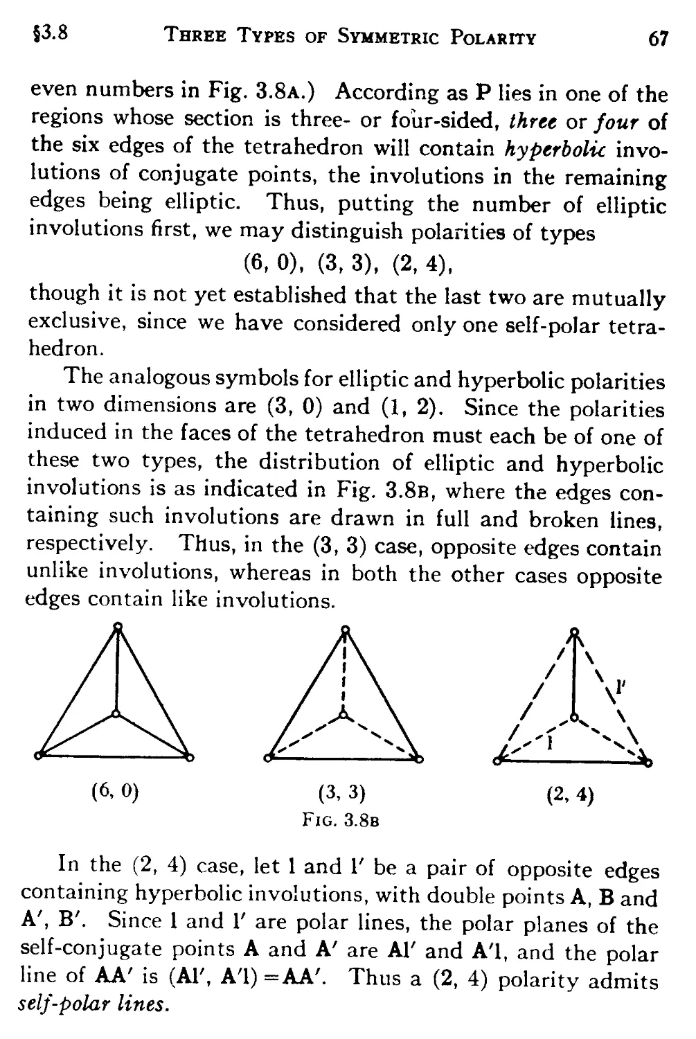


Текст
Copyright, Canada, 1942, 1947, 1957
First Edition 1942
Second Edition 1947
Third Edition 1957
Fourth Edition 1961
Fifth Edition 1965
Sixth Edition 1998
By the Same Author
REGULAR POLYTOPES
Dover, New York
THE REAL PROJECTIVE PLANE
Springer-Verlag, New York
INTRODUCTION TO GEOMETRY
Wiley, New York
PROJECTIVE GEOMETRY
Spring-Verlag, New York
TWELVE GEOMETRIC ESSAYS
Southern Illinois University Press
Copyright © 1998 by
The Mathematical Association of America (Incorporated)
Library of Congress Catalog Card Number 98-85640
ISBN 0-88385-522-4
Printed in the United States of America
NON-EUCLIDEAN
GEOMETRY
H. S. M. COXETER, C.C., F.R.S., F.R.S.C.
PROFESSOR EMERITUS OF MATHEMATICS
UNIVERSITY OF TORONTO
SIXTH EDITION
THE MATHEMATICAL ASSOCIATION OF AMERICA
Washington, D.C. 20036
PREFACE TO THE SIXTH EDITION
I am grateful to the Mathematical Association of America for
rescuing my book from oblivion by agreeing to publish this new
edition. I particularly appreciate Elaine Pedreira's careful editing
and advice.
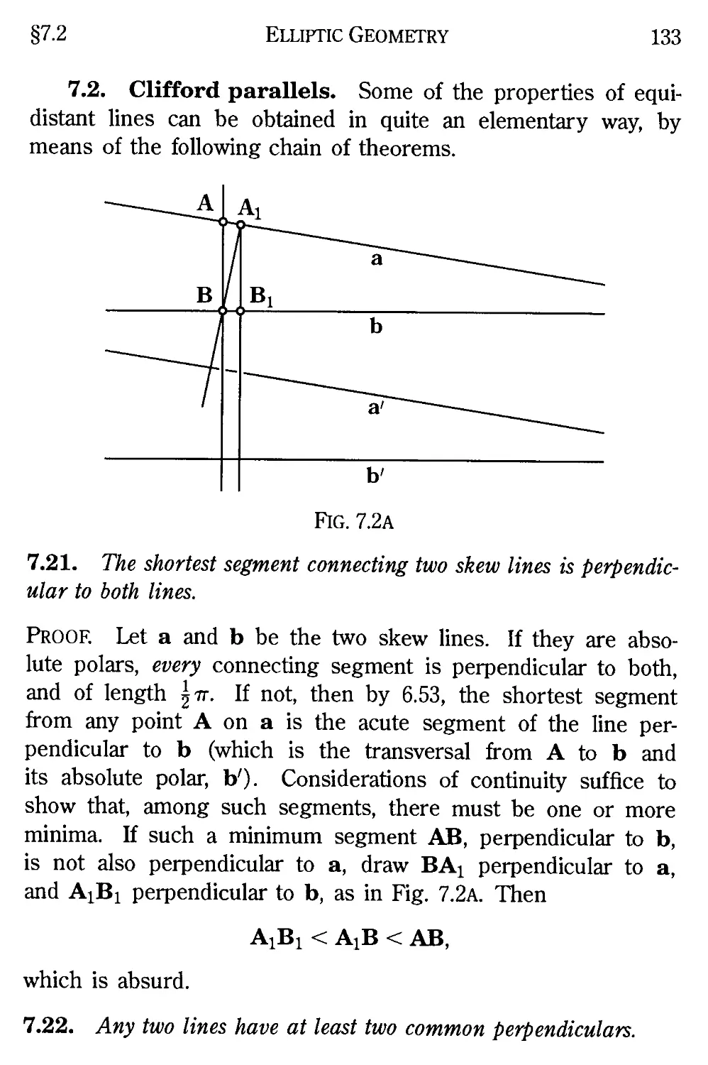
I welcome the opportunity to correct FlG. 7.2A on page 133
and to make other small improvements and especially to add
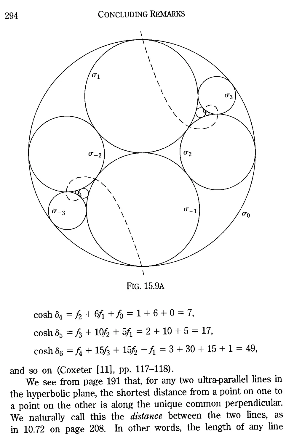
the new §15.9. That section contains, in particular, an 'abso-
'absolute' sequence of circles (Fig. 15.9a) which involves a surprising
application of Fibonacci numbers A5.94). For further discus-
discussion of inversive geometry, the reader may like to look at "The
inversive plane and hyperbolic space," Abhandlungen aus dem
Mathematischen Seminar der Universitdt Hamburg, 28 A965), pp.
217-242. The subject of §15.7 has been extended by E. B. Vin-
berg in his paper, "The volume of polyhedra on a sphere and in
Lobachevsky space," American Mathematical Society Translations
B), 148 A991), pp. 15-27. Vinberg draws attention to W. P.
Thurston, "Three-dimensional manifolds, Kleinian groups and hy-
hyperbolic geometry," Bulletin of the American Mathematical Society,
6 A986), pp. 357-382. When Hamlet exclaims (in Act II, Scene
II) "/ could be bounded in a nutshell, and count myself a king of
infinite space," he is providing a poetic anticipation of Poincare's
inversive model of the infinite hyperbolic plane, using a circular
"nutshell" for the Absolute. In fact, the hyperbolic plane can be
filled with infinitely many congruent equilateral triangles, seven
at each vertex, to form the regular tessellation {3, 7}. One ac-
acquires an intuitive feeling for hyperbolic geometry by packing a
disc with a multitude of curvilinear triangles, becoming smaller
and smaller as they approach the peripheral circle, which rep-
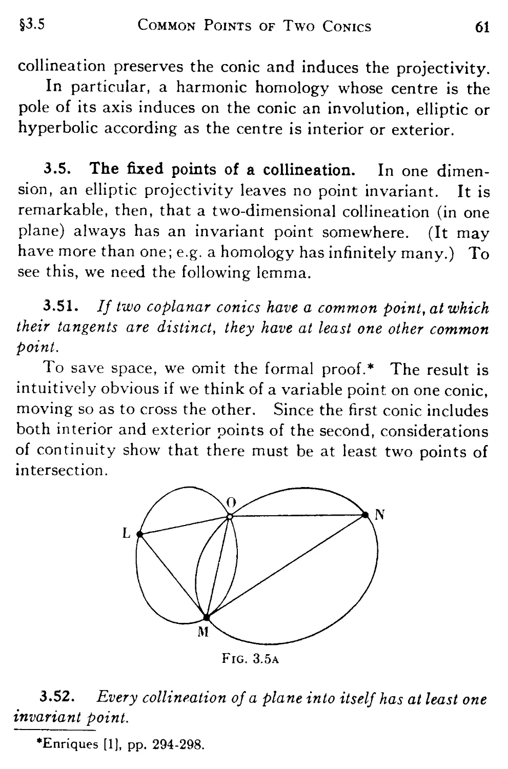
IX
x Preface
resents the Absolute. This book's cover design shows the 63
largest of these triangular tiles, systematically coloured so that
any two of them which are coloured alike are entirely disjoint,
having no common vertex. In other words, every vertex belongs
to seven or fewer triangles, all differently coloured.
H.S.M.C.
June, 1998.
Preface to the Third Edition
Apart from a simplification of p. 206, most of the changes
are additions. Accordingly, it has seemed best to put the ex-
extra material together as a new chapter (XV). This includes a
description of the two families of "mid-lines" between two given
lines, an elementary derivation of the basic formulae of spherical
trigonometry and hyperbolic trigonometry, a computation of the
Gaussian curvature of the elliptic and hyperbolic planes, and a
proof of Schafli's remarkable formula for the differential of the
volume of a tetrahedron.
I gratefully acknowledge the help of L. J. Mordell and Frans
Handest in the preparation of §15.6 (on quadratic forms) and
§15.8 (on problems of construction), respectively.
H.S.M.C.
December, 1956.
Preface xi
Preface to the First Edition
The name non-Euclidean was used by Gauss to describe a
system of geometry which differs from Euclid's in its properties
of parallelism. Such a system was developed independently by
Bolyai in Hungary and Lobatschewsky in Russia, about 120 years
ago. Another system, differing more radically from Euclid's,
was suggested later by Riemann in Germany and Schlafli in
Switzerland. The subject was unified in 1871 by Klein, who gave
the names parabolic, hyperbolic, and elliptic to the respective
systems of Euclid, Bolyai-Lobatschewsky, and Riemann-Shlafli.
Since then, a vast literature has accumulated, and it is with some
diffidence that I venture to add a fresh exposition.
After a historical introductory chapter (which can be omitted
without impairing the main development), I devote three chap-
chapters to a survey of real projective geometry. Although many
text-books on that subject have appeared, most of those in En-
English stress the connection with Euclidean geometry. Moreover,
it is customary to define a conic and then derive the relation
of pole and polar, whereas the application to non-Euclidean ge-
geometry makes it more desirable to define the polarity first and
then look for a conic (which may or may not exist)! This treat-
treatment of projective geometry, due to von Staudt, has been found
satisfactory in a course of lectures for undergraduates (Coxeter
t6]).
In Chapters VIII and K, the Euclidean and hyperbolic geome-
geometries are built up axiomatically as special cases of a more general
"descriptive geometry." Following Veblen, I develop the proper-
properties of parallel lines (§8.9) before introducing congruence. For the
introduction of ideal elements, such as points at infinity, I employ
the method of Pasch and F. Schur. In this manner, hyperbolic
geometry is eventually identified with the geometry of Klein's
projective metric as applied to a real conic or quadric (Cayley's
Absolute, §§8.1, 9.7). This elaborate process of identification is
xii Preface
unnecessary in the case of elliptic geometry. For, the axioms of
real projective geometry (§2.1) can be taken over as they stand.
Any axioms of congruence that might be proposed would quickly
lead to the absolute polarity, and so are conveniently replaced by
the simple statement that one uniform polarity is singled out as
a means for defining congruence.
Von Staudfs extension of real space to complex space is
logically similar to Pasch's extension of descriptive space to pro-
projective space, but is far harder for students to grasp; so I prefer
to deal with real space alone, expressing distance and angle in
terms of real cross ratios. I hope this restriction to real space
will remove some of the mystery that is apt to surround such
concepts as Clifford parallels (§§7.2, 7.5). But Klein's complex
treatment is given as an alternative (at the end of Chapters
rv-vii).
In order to emphasize purely geometrical ideas, I introduce
the various geometries synthetically. But coordinates are used
for the derivation of trigonometrical formulae in Chapter xii.
Roughly speaking, the chapters increase in difficulty to the
middle of the book. (Chapter VII may well be omitted on first
reading, although it is my own favourite). Then they become
progressively easier. For a rapid survey of the subject, just read
the first and the last two.
For reading various parts of the manuscript in preparation,
and making valuable suggestions for its improvement, I offer cor-
cordial thanks to my colleagues on the Editorial Board, especially
Richard Brauer and G. de B. Robinson; also to N. S. Mendelsohn
of the Department of Mathematics, to S. H. Gould of the Depart-
Department of Classics, and to A W. Tucker of Princeton University.
H.S.M. Coxeter
The University of Toronto,
May, 1942.
CONTENTS
I. THE HISTORICAL DEVELOPMENT OF
NON-EUCLIDEAN GEOMETRY
SECTION PAGE
1.1 Euclid 1
1.2 Saccheri and Lambert 5
1.3 Gauss, Wachter, Schweikart, Taurinus 7
1.4 Lobatschewsky 8
1.5 Bolyai 10
1.6 Riemann 11
1.7 Klein 13
II. REAL PROJECTIVE GEOMETRY: FOUNDATIONS
2.1 Definitions and axioms 16
2.2 Models 23
2.3 The principle of duality 26
2.4 Harmonic sets 28
2.5 Sense 31
2.6 Triangular and tetrahedral regions 34
2.7 Ordered correspondences 35
2.8 One-dimensional projectivities 40
2.9 Involutions 44
III. REAL PROJECTIVE GEOMETRY: POLARITIES,
CONICS AND QUADRICS
3.1 Two-dimensional projectivities 48
3.2 Polarities in the plane 52
xni
xiv CONTENTS
SECTION PAGE
3.3 Conies 55
3.4 Projectivities on a conic 59
3.5 The fixed points of a collineation 61
3.6 Cones and reguli 62
3.7 Three-dimensional projectivities 63
3.8 Polarities in space 65
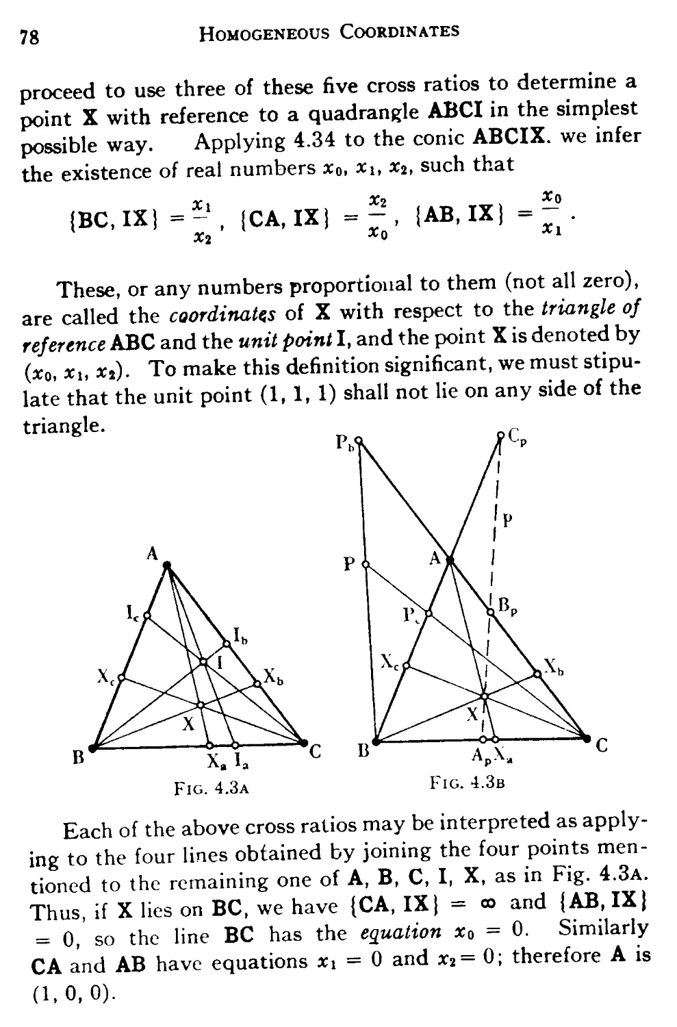
IV. HOMOGENEOUS COORDINATES
4.1 The von Staudt-Hessenberg calculus of points 71
4.2 One-dimensional projectivities 74
4.3 Coordinates in one and two dimensions 76
4.4 Collineations and coordinate transformations 81
4.5 Polarities 85
4.6 Coordinates in three dimensions 87
4.7 Three-dimensional projectivities 90
4.8 Line coordinates for the generators of a quadric 93
4.9 Complex projective geometry 94
V. ELLIPTIC GEOMETRY IN ONE DIMENSION
5.1 Elliptic geometry in general 95
5.2 Models 96
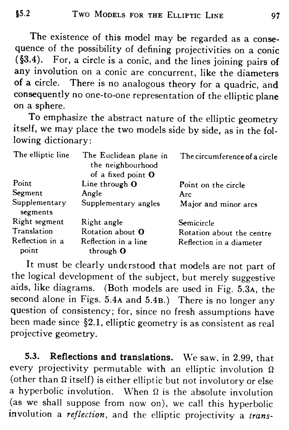
5.3 Reflections and translations 97
5.4 Congruence 100
5.5 Continuous translation 101
5.6 The length of a segment 103
5.7 Distance in terms of cross ratio 104
5.8 Alternative treatment using the complex line 106
VI. ELLIPTIC GEOMETRY IN TWO DIMENSIONS
6.1 Spherical and elliptic geometry 109
6.2 Reflection 110
6.3 Rotations and angles Ill
6.4 Congruence 113
Contents xv
section page
6.5 Circles 115
6.6 Composition of rotations 118
6.7 Formulae for distance and angle 120
6.8 Rotations and quaternions 122
6.9 Alternative treatment using the complex plane 126
VII. ELLIPTIC GEOMETRY IN THREE DIMENSIONS
7.1 Congruent transformations 128
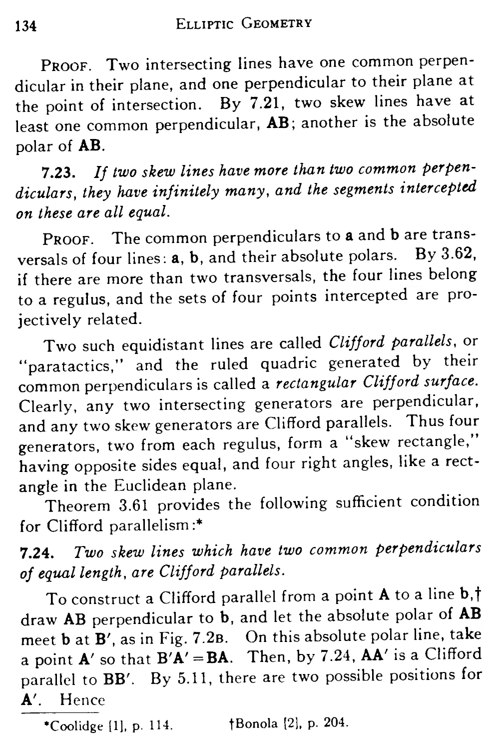
7.2 Clifford parallels 133
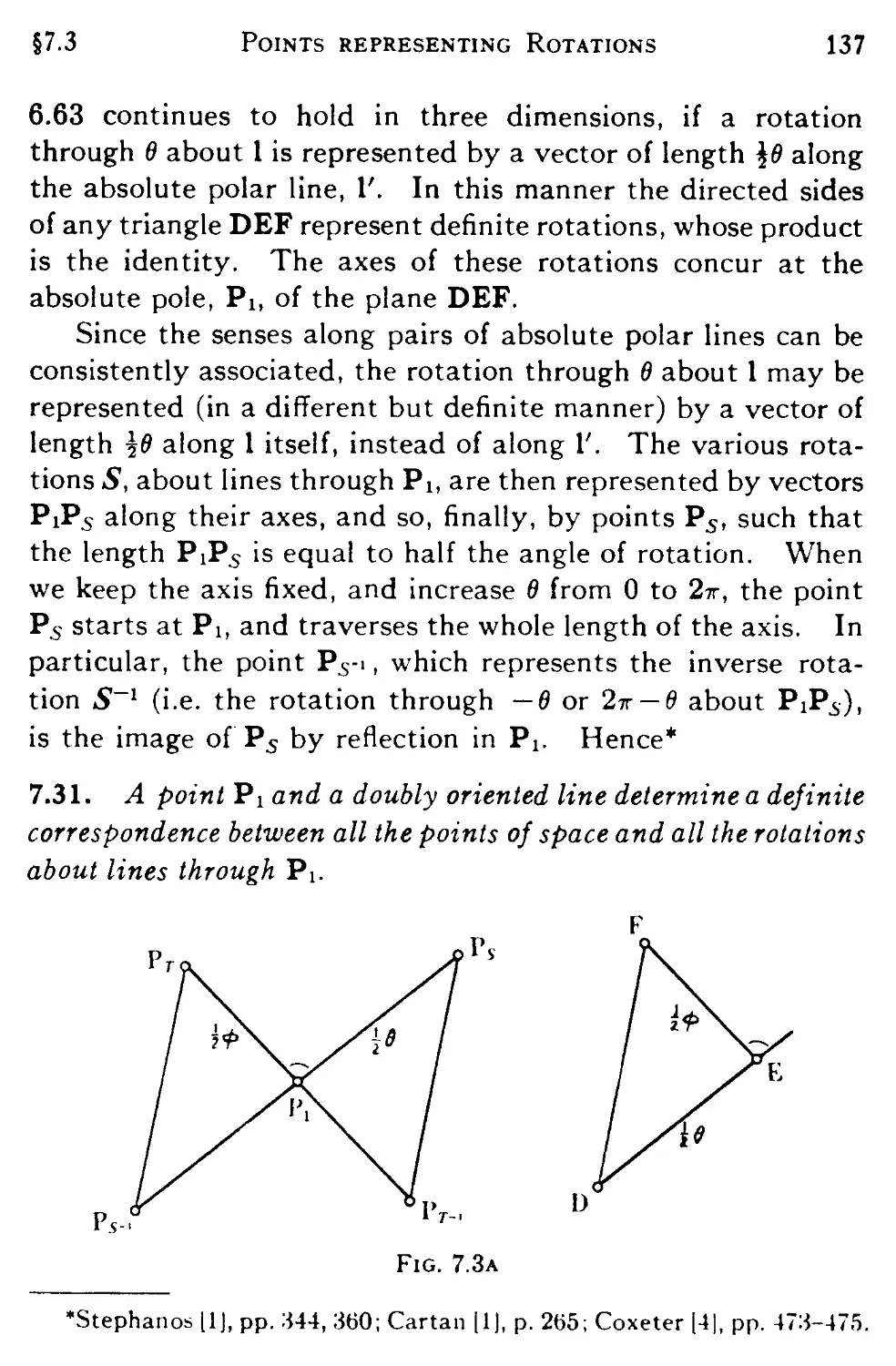
7.3 The Stephanos-Cartan representation of rotations by points 136
7.4 Right translations and left translations 138
7.5 Right parallels and left parallels 141
7.6 Study's representation of lines by pairs of points 146
7.7 Clifford translations and quaternions 148
7.8 Study's coordinates for a line 151
7.9 Complex space 153
VIII. DESCRIPTIVE GEOMETRY
8.1 Klein's projective model for hyperbolic geometry 157
8.2 Geometry in a convex region 159
8.3 Veblen's axioms of order 161
8.4 Order in a pencil 162
8.5 The geometry of lines and planes through a fixed point . . 164
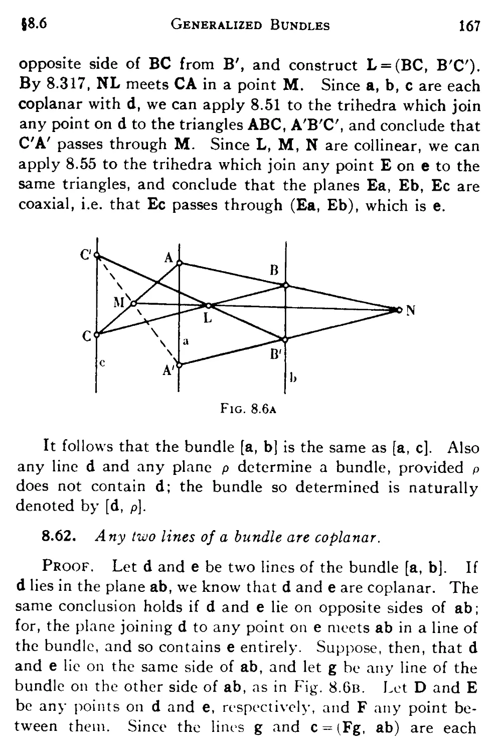
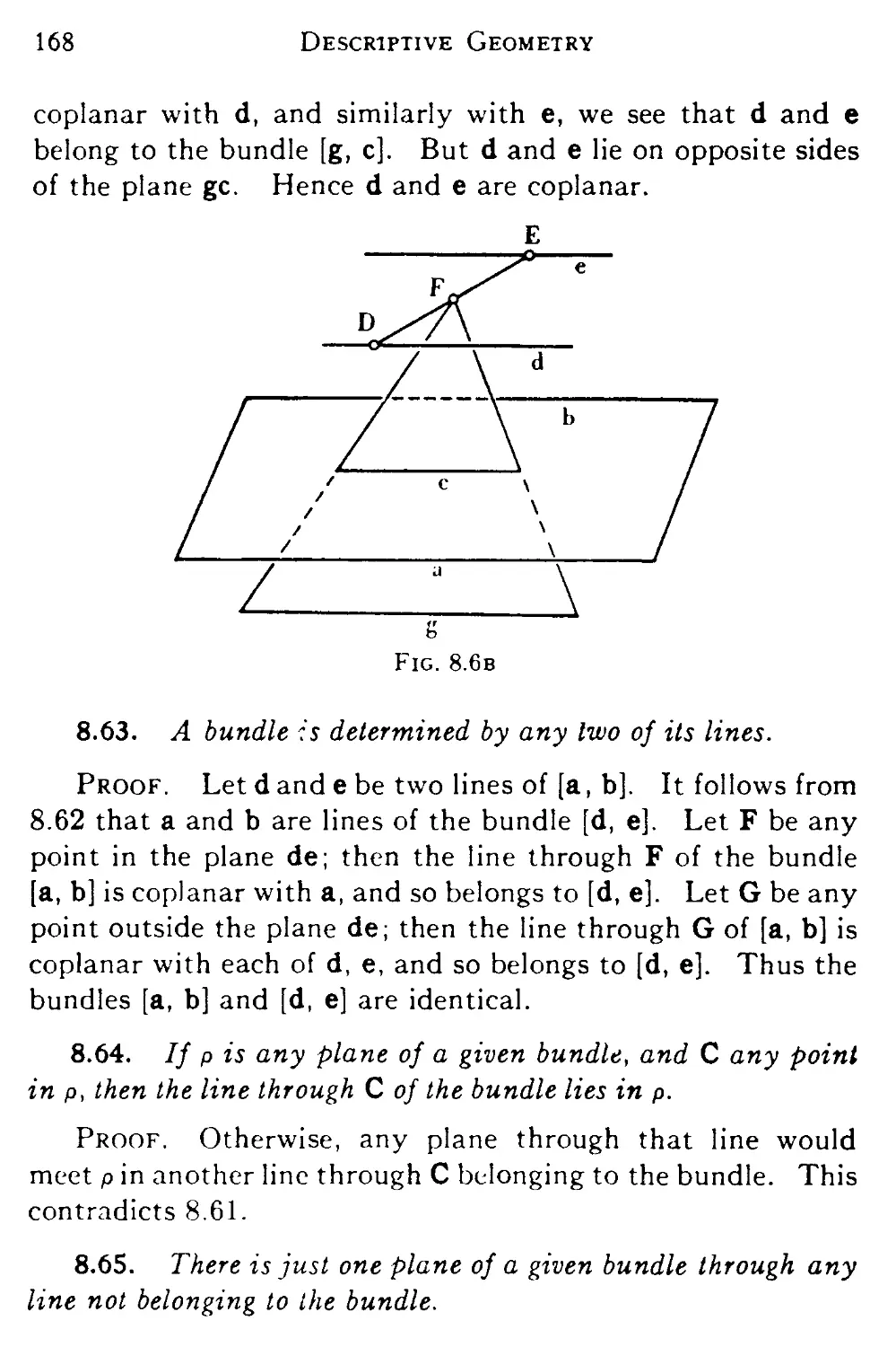
8.6 Generalized bundles and pencils 165
8.7 Ideal points and lines 171
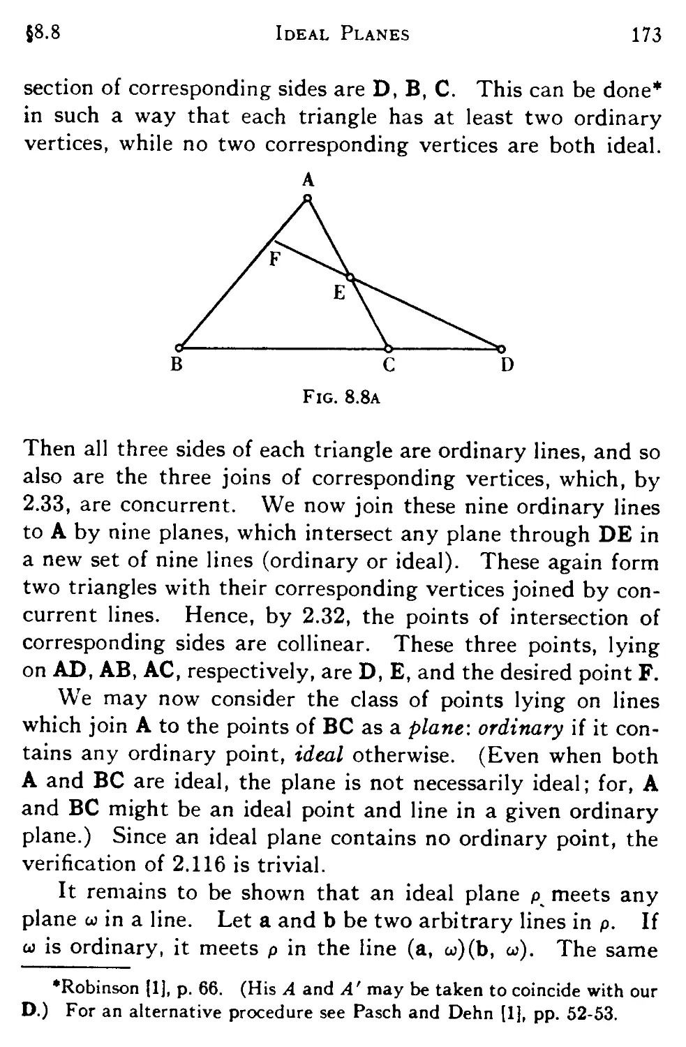
8.8 Verifying the projective axioms 172
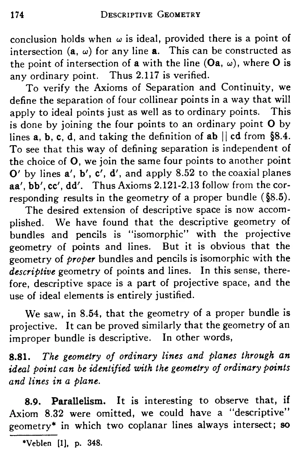
8.9 Parallelism 174
IX. EUCLIDEAN AND HYPERBOLIC GEOMETRY
9.1 The introduction of congruence 179
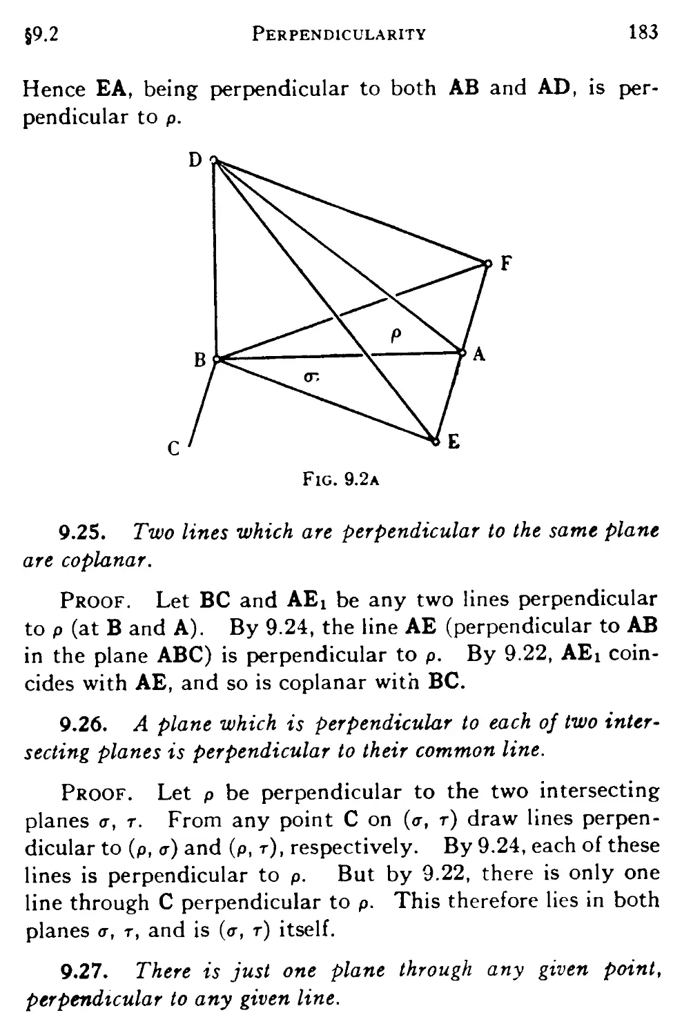
9.2 Perpendicular lines and planes 181
9.3 Improper bundles and pencils 184
9.4 The absolute polarity 185
xvi Contents
SECTION PAGE
9.5 The Euclidean case 186
9.6 The hyperbolic case 187
9.7 The Absolute 192
9.8 The geometry of a bundle 197
X. HYPERBOLIC GEOMETRY IN TWO DIMENSIONS
10.1 Ideal elements 199
10.2 Angle-bisectors 200
10.3 Congruent transformations 201
10.4 Some famous constructions 204
10.5 An alternative expression for distance 206
10.6 The angle of parallelism 207
10.7 Distance and angle in terms of poles and polars 208
10.8 Canonical coordinates 209
10.9 Euclidean geometry as a limiting case 211
XI. CIRCLES AND TRIANGLES
11.1 Various definitions for a circle 213
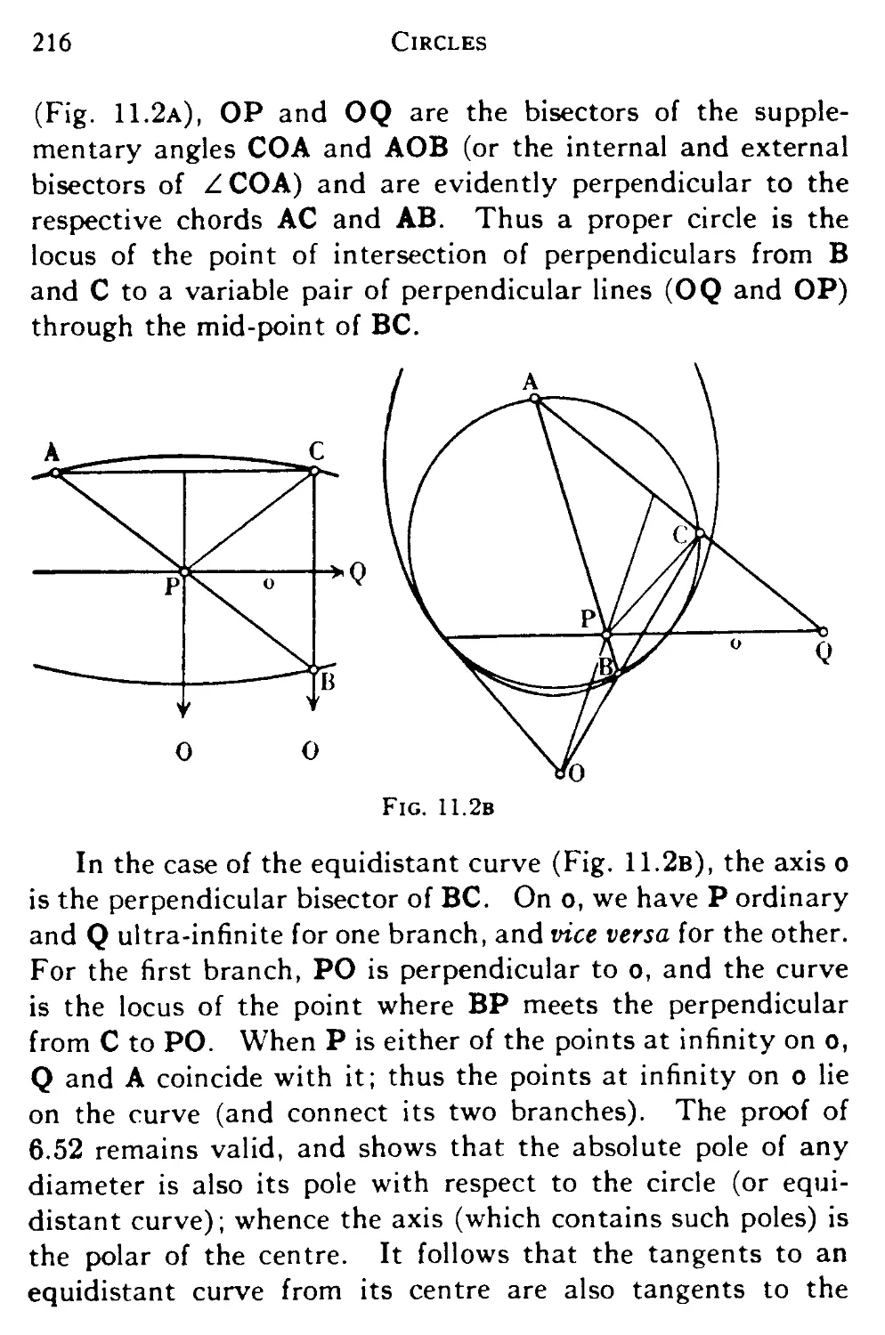
11.2 The circle as a special conic 215
11.3 Spheres 218
11.4 The in- and ex-circles of a triangle 220
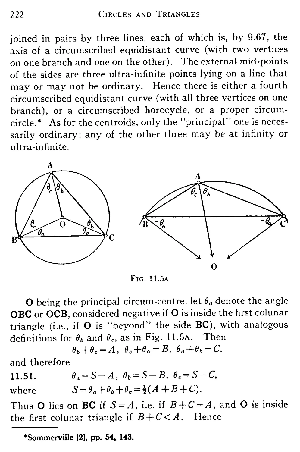
11.5 The circum-circles and centroids 221
11.6 The polar triangle and the orthocentre 223
XII. THE USE OF A GENERAL TRIANGLE
OF REFERENCE
12.1 Formulae for distance and angle 224
12.2 The general circle 226
12.3 Tangential equations 228
12.4 Circum-circles and centroids 229
12.5 In- and ex-circles 231
12.6 The orthocentre 231
12.7 Elliptic trigonometry 232
Contents xvii
SECTION PAGE
12.8 The radii 235
12.9 Hyperbolic trigonometry 237
XIII. AREA
13.1 Equivalent regions 241
13.2 The choice of a unit 241
13.3 The area of a triangle in elliptic geometry 242
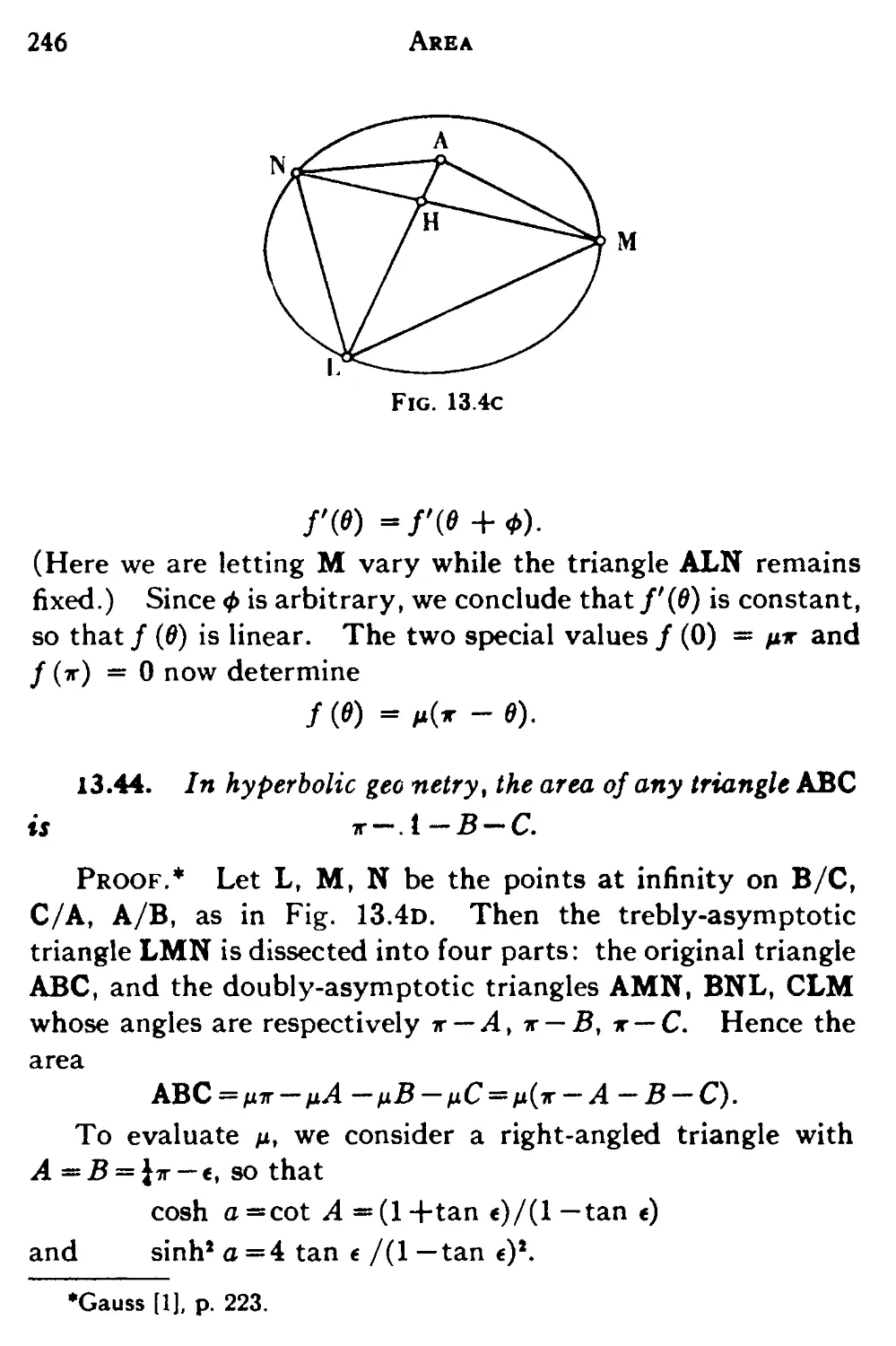
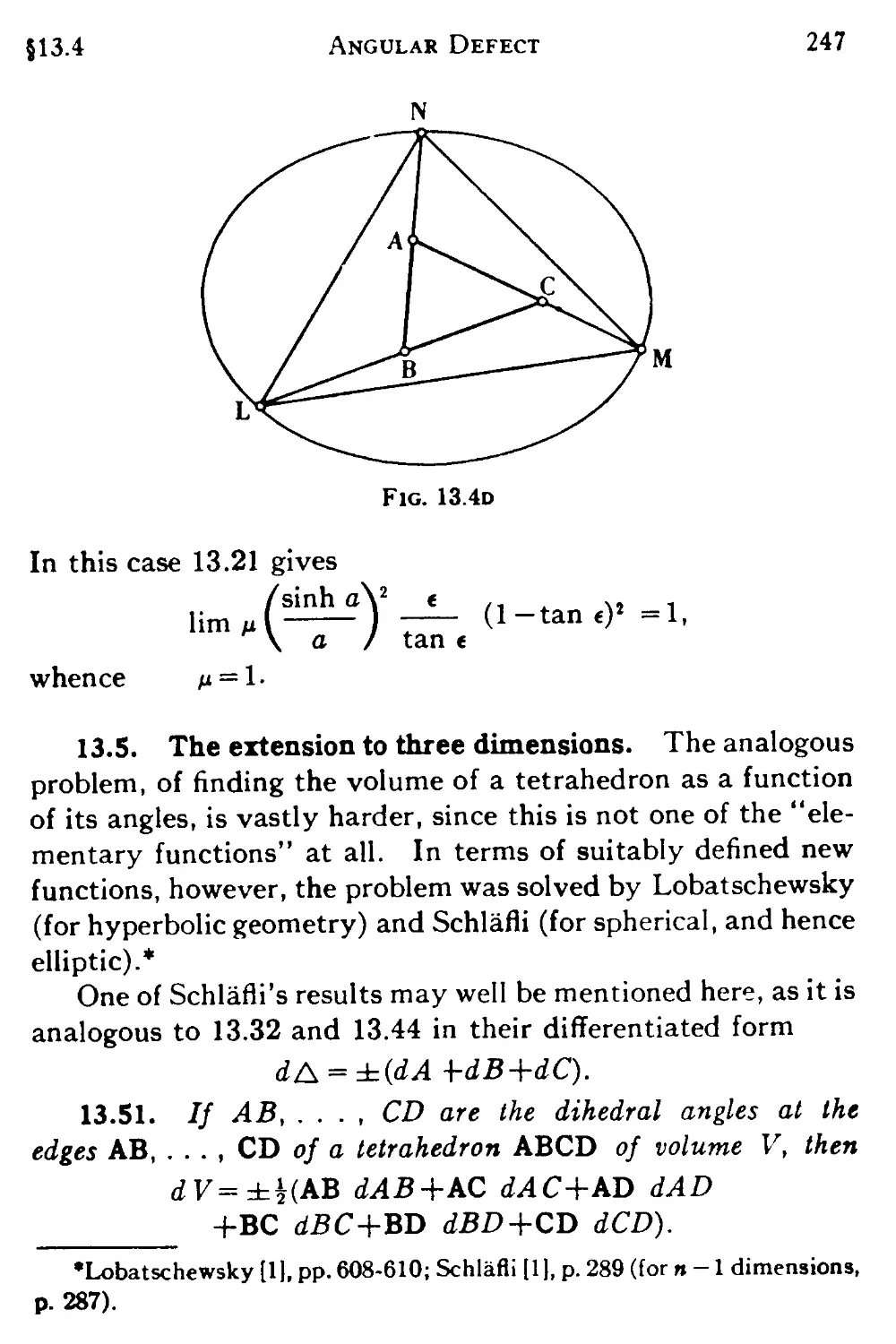
13.4 Area in hyperbolic geometry 243
13.5 The extension to three dimensions 247
13.6 The differential of distance 248
13.7 Arcs and areas of circles 249
13.8 Two surfaces which can be developed on the Euclidean
plane 251
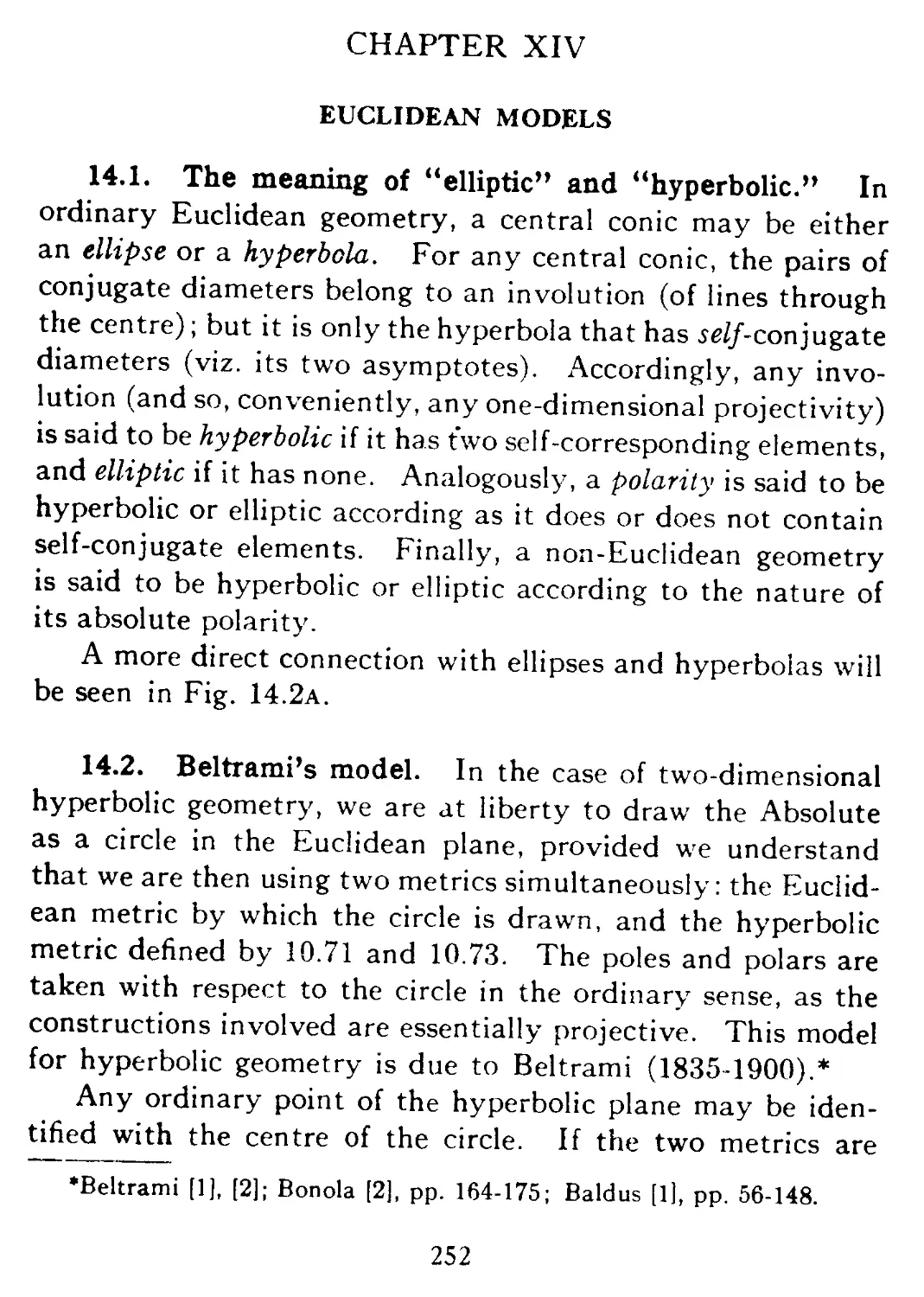
XIV. EUCLIDEAN MODELS
14.1 The meaning of "elliptic" and "hyperbolic" 252
14.2 Beltrami's model 252
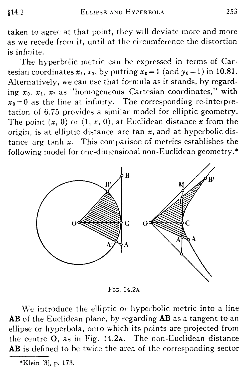
14.3 The differential of distance 254
14.4 Gnomonic projection 255
14.5 Development on surfaces of constant curvature 256
14.6 Klein's conformal model of the elliptic plane 258
14.7 Klein's conformal model of the hyperbolic plane 260
14.8 Poincare's model of the hyperbolic plane 263
14.9 Conformal models of non-Euclidean space 264
XV. CONCLUDING REMARKS
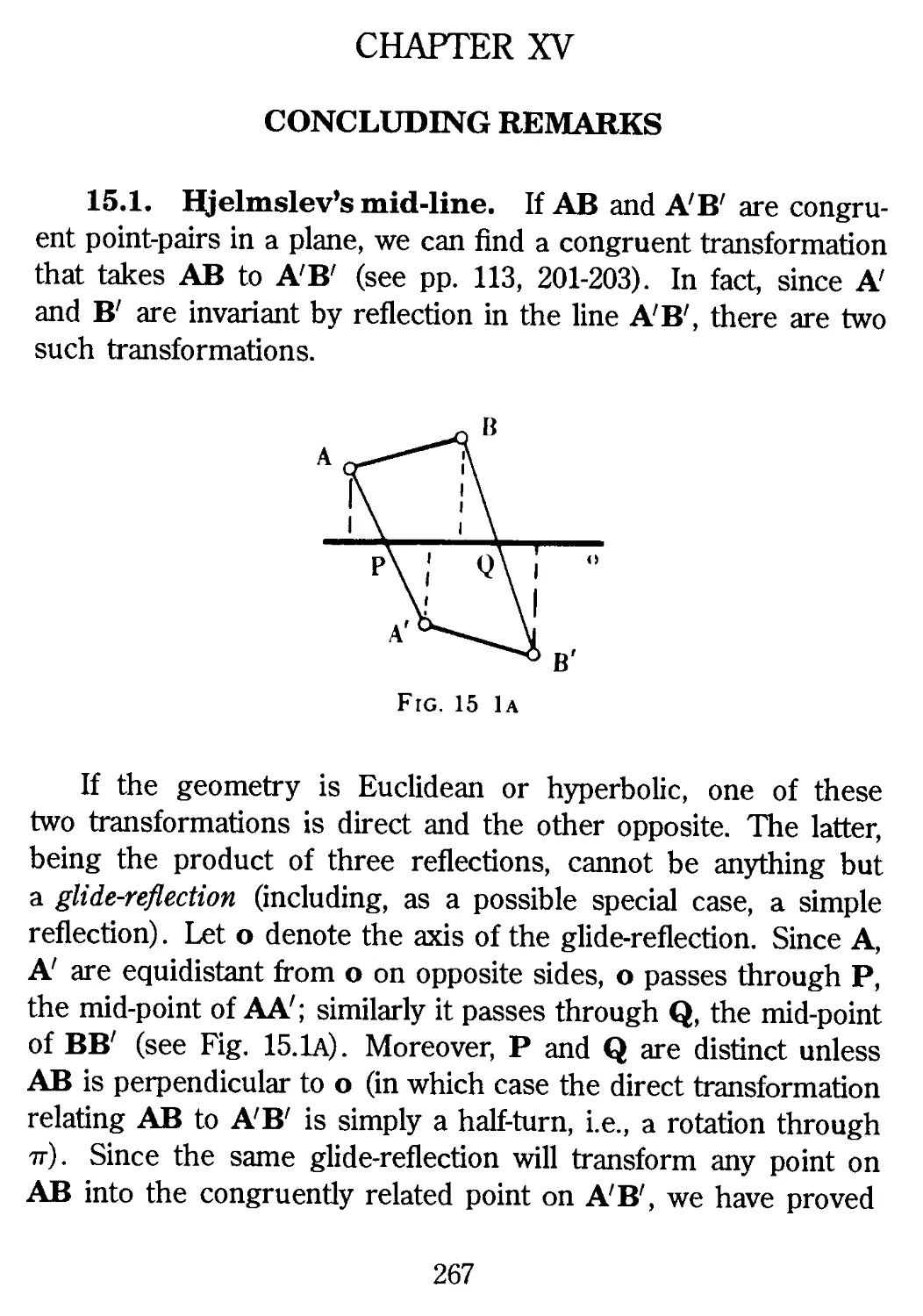
15.1 Hjelmslev's mid-line 267
15.2 The Napier chain 273
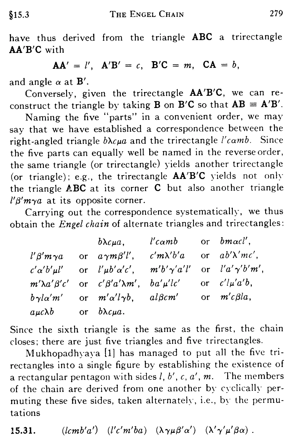
15.3 The Engel chain 277
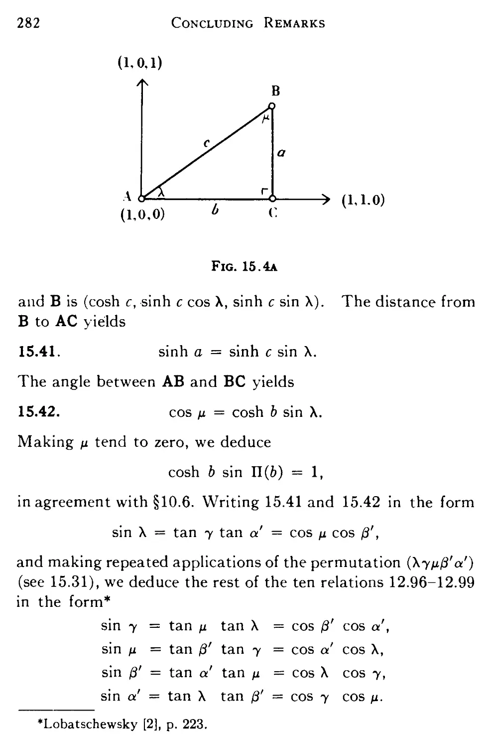
15.4 Normalized canonical coordinates 281
15.5 Curvature 283
15.6 Quadratic forms 284
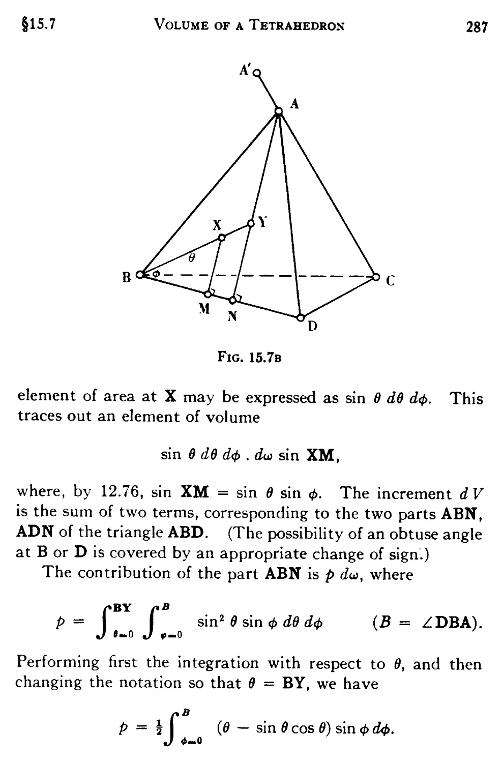
15.7 The volume of a tetrahedron 285
xviii Contents
SECTION PAGE
15.8 A brief historical survey of construction problems .... 289
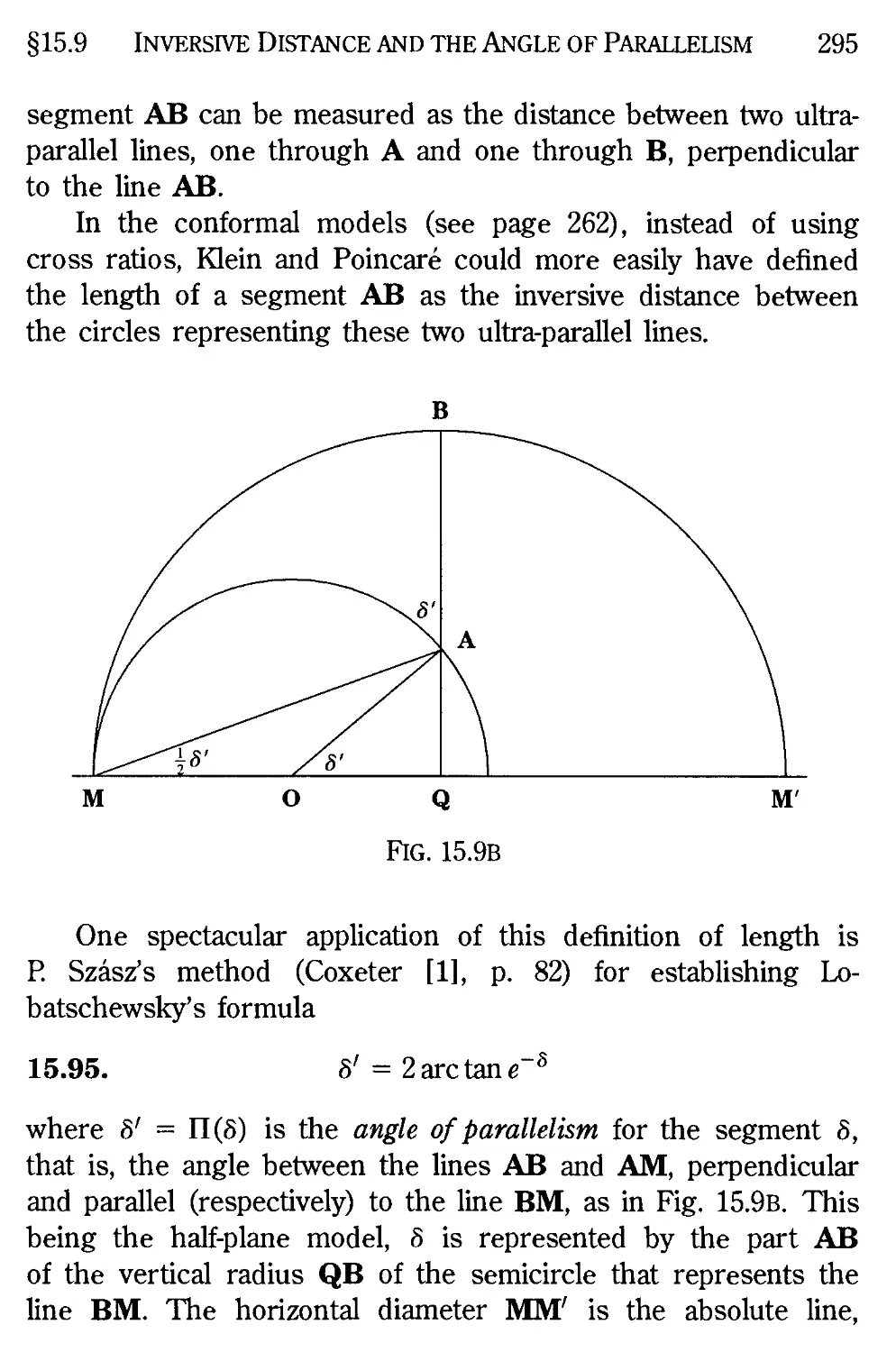
15.9 Inversive distance and the angle of parallelism 292
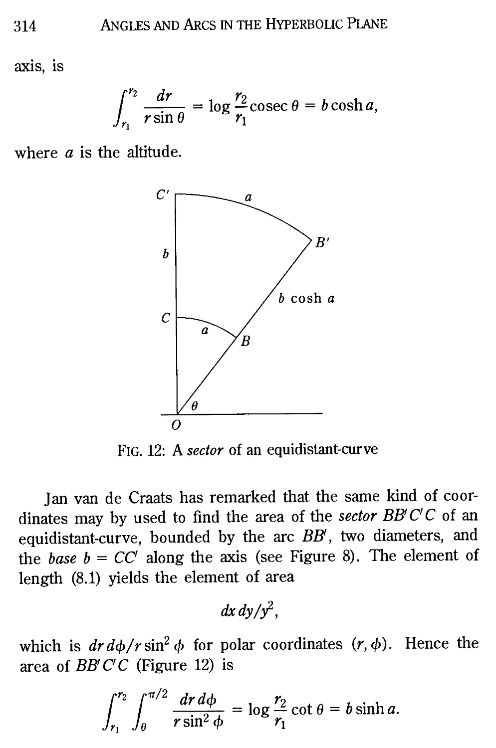
Appendix: Angles and Arcs in the Hyperbolic Plane 299
Bibliography 317
Index 327
CHAPTER I
THE HISTORICAL DEVELOPMENT OF NON-EUCLIDEAN
GEOMETRY
1.1. Euclid. Geometry, as we see from its name, began
as a practical science of measurement. As such, it was used
in Egypt about 2000 B.C. Thence it was brought to Greece
by Thales F40-546 B.C.), who began the process of abstraction
by which positions and straight edges are idealized into points
and lines. Much progress was made by Pythagoras and his
disciples. Among others, Hippocrates attempted a logical
presentation in the form of a chain of propositions based on a
few definitions and assumptions. This was greatly improved
by Euclid (about 300 B.C.), whose Elements became one of the
most widely read books in the world. The geometry taught
in high school today is essentially a part of the Elements, with
a few unimportant changes.
According to the best editions, Euclid's basic assumptions
consist of five "common notions" concerning magnitudes, and
the following five Postulates:
I. A straight line may be drawn from any one point to any
other point.
II. A finite straight line may be produced to any length in a
straight line.
III. A circle may be described with my centre at any distance
from that centre.
IV. All right angles are equal.
V. // a straight line meet two other straight lines, so as to make
the two interior angles on one side of it together less than two right
angles, the other straight lines will meet if produced on that side
on which the angles are less than two right angles.
2 Historical Development
According to the modern view, these postulates are incom-
incomplete and somewhat misleading. (For the rigorous axioms that
replace them, see §§ 8.3, 9.1, 9.5.) Still, they give some idea
of the kind of assumptions that have to be made, and are of
interest historically.
Postulate I is generally regarded as implying that any two
points determine a unique line, Postulate II that a line is of
infinite length. Euclid showed the great strength of his genius
by introducing Postulate V, which is not self-evident like the
others. (Moreover, his reluctance to introduce it provides a
case for calling him the first non-Euclidean geometer!) Between
his time and our own, hundreds of people, finding it compli-
complicated and artificial, have tried to deduce it as a proposition.
But they only succeeded in replacing it by various equivalent
assumptions, such as the following five:
1.11. Two parallel lines are equidistant. (Posidonius, first
century B.C.)
1.12. If a line intersects one of two parallels, it also intersects
the other. (Proclus, 410-485 A.D.)
1.13. Given a triangle, we can construct a similar triangle of any
size whatever. (Wallis, 1616-1703.)
1.14. The sum of the angles of a triangle is equal to two right
angles. (Legendre, 1752-1833.)
1.15. Three non-collinear points always lie on a circle. (Bolyai
Farkas,* 1775-1856.)
According to Euclid's definition, two lines are parallel if
they are coplanar without intersecting. (Following Gauss and
Lobatschewsky, we shall modify this definition later.) The
*In Hungarian, the surname is put first. The " in "Bolyai" is mute.
§1-1
Playfair's Axiom
existence of such pairs of lines follows from Euclid I, 27, which
depends on Postulate II but not on Postulate V.
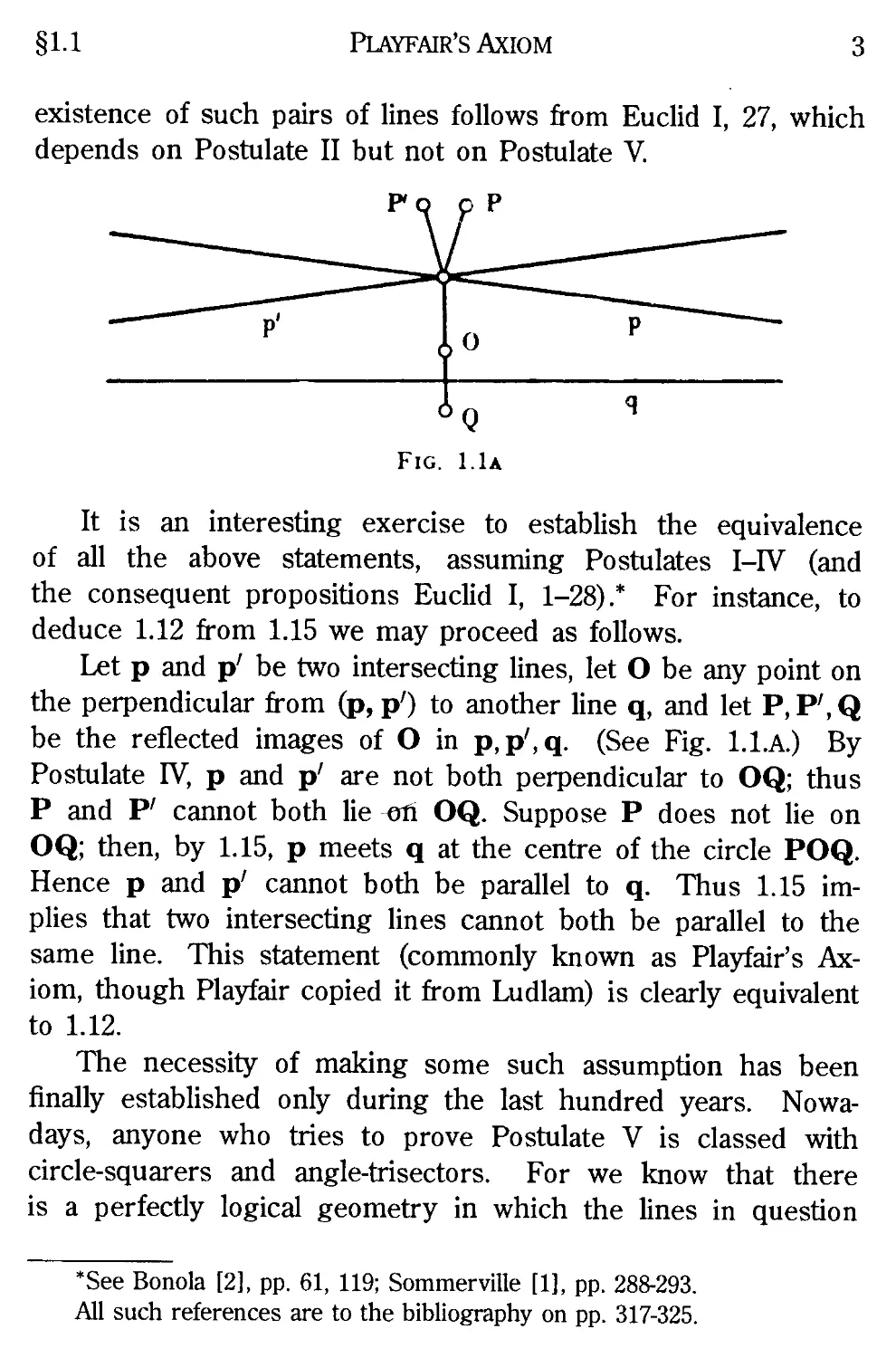
Fig. 1.1a
It is an interesting exercise to establish the equivalence
of all the above statements, assuming Postulates I-IV (and
the consequent propositions Euclid I, 1-28).* For instance, to
deduce 1.12 from 1.15 we may proceed as follows.
Let p and p' be two intersecting lines, let O be any point on
the perpendicular from (p, p') to another line q, and let P, P', Q
be the reflected images of O in p, p',q. (See Fig. I.I.A.) By
Postulate IV, p and p' are not both perpendicular to OQ; thus
P and P' cannot both lie on OQ. Suppose P does not lie on
OQ; then, by 1.15, p meets q at the centre of the circle POQ.
Hence p and p' cannot both be parallel to q. Thus 1.15 im-
implies that two intersecting lines cannot both be parallel to the
same line. This statement (commonly known as Playfair's Ax-
Axiom, though Playfair copied it from Ludlam) is clearly equivalent
to 1.12.
The necessity of making some such assumption has been
finally established only during the last hundred years. Nowa-
Nowadays, anyone who tries to prove Postulate V is classed with
circle-squarers and angle-trisectors. For we know that there
is a perfectly logical geometry in which the lines in question
*See Bonola [2], pp. 61, 119; Sommerville [1], pp. 288-293.
All such references are to the bibliography on pp. 317-325.
4 Historical Development
may fail to meet, even when the interior angles are quite small.
This remark is so easy to make today that we are apt to forget
what a heresy it seemed to a generation brought up in the
belief that Euclid's was the only true geometry. We now
learn of many different geometries, but for historical reasons
we reserve the name non-Euclidean for two special kinds:
hyperbolic geometry, in which all the "self-evident" postu-
postulates I-IV are satisfied though Postulate V is denied, and
elliptic geometry, in which the traditional interpretation of
Postulate II is modified so as to allow the total length of a line
to be infinite.
As a first glimpse of hyperbolic geometry, here are the
statements that replace 1.11-1.15: Two lines cannot be equi-
equidistant; a line may intersect one of two parallels without inter-
intersecting the other; similar triangles are necessarily congruent;
the sum of the angles of a triangle is less than two right angles;
three points may be neither collinear nor concyclic. In elliptic
geometry, on the other hand, any two coplanar lines intersect,
so there are no parallels in Euclid's sense, and no equidistant
lines in a plane. (We shall see, however, that equidistant lines
are possible in space.)
Each of these geometries, Euclidean and non-Euclidean, is
consistent, in the sense that the assumptions imply no contra-
contradiction. But which geometry is valid in physical space? It is
important to realize that this question is meaningless until we
have assigned physical equivalents for the geometrical con-
concepts. Even the notion of a point, "position without magni-
magnitude," can only be realized by a process of approximation.
Then, what is the physical counterpart for a straight line?
The two most obvious answers are: a taut string, and a ray of
light. According to recent developments in physics, these are
not precisely the same! But the discrepancy is due to the
presence of matter, and so a theoretical geometry of empty
space remains significant. Consider, then, two rays of light,
§1.2
Playfair's Axiom
perpendicular to one plane. Certainly they remain equidistant
according to all terrestrial experiments; but it is quite conceivable
that they might ultimately diverge (as in hyperbolic geometry)
or converge (as in elliptic).
1.2. Saccheri and Lambert. The most elaborate attempt
to prove the "parallel postulate" was that of the Jesuit Saccheri
A667-1733), who based his work on an isosceles birectangle, i.e.
a quadrangle ABED with AD = BE and right angles at D and
E. It is obvious that the angles at A and B are equal. He
considered the three hypotheses that they are obtuse, right,
or acute, and showed that the assumption of any one of these
hypotheses for a single isosceles birectangle implies the same
for every isosceles birectangle. It was his intention to establish
the hypothesis of the right angle by showing that either of the
other hypotheses leads to a contradiction. He found that the
hypothesis of the obtuse angle implies Postulate V, which in turn
implies the hypothesis of the right angle. From the hypothesis
of the acute angle he made many interesting deductions, always
hoping for an eventual contradiction. We know now that his hope
could never have been realized (without his making a mistake);
but in the attempt he was unwittingly discovering many of the
theorems of what was later to be known as hyperbolic geometry.
B
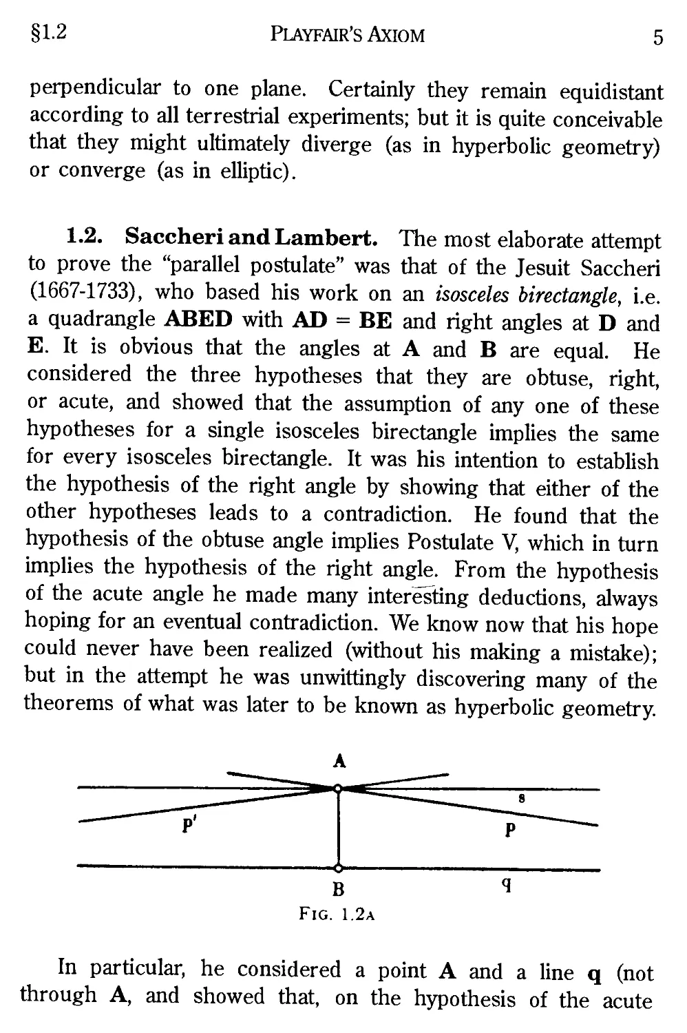
Fig. 1.2a
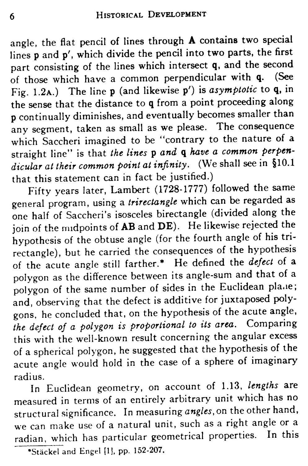
In particular, he considered a point A and a line q (not
through A, and showed that, on the hypothesis of the acute
6 Historical Development
angle, the flat pencil of lines through A contains two special
lines p and p', which divide the pencil into two parts, the first
part consisting of the lines which intersect q, and the second
of those which have a common perpendicular with q. (See
Fig. 1.2a.) The line p (and likewise p') is asymptotic to q, in
the sense that the distance to q from a point proceeding along
p continually diminishes, and eventually becomes smaller than
any segment, taken as small as we please. The consequence
which Saccheri imagined to be "contrary to the nature of a
straight line" is that the lines p and q have a common perpen-
perpendicular at their common point at infinity. (We shall see in §10.1
that this statement can in fact be justified.)
Fifty years later, Lambert A728-1777) followed the same
general program, using a trirectangle which can be regarded as
one half of Saccheri's isosceles birectangle (divided along the
join of the midpoints of AB and DE). He likewise rejected the
hypothesis of the obtuse angle (for the fourth angle of his tri-
trirectangle), but he carried the consequences of the hypothesis
of the acute angle still farther.* He defined the defect of a
polygon as the difference between its angle-sum and that of a
polygon of the same number of sides in the Euclidean pla.ie;
and, observing that the defect is additive for juxtaposed poly-
polygons, he concluded that, on the hypothesis of the acute angle,
the defect of a polygon is proportional to its area. Comparing
this with the well-known result concerning the angular excess
of a spherical polygon, he suggested that the hypothesis of the
acute angle would hold in the case of a sphere of imaginary
radius.
In Euclidean geometry, on account of 1.13, lengths are
measured in terms of an entirely arbitrary unit which has no
structural significance. In measuring angles, on the other hand,
we can make use of a natural unit, such as a right angle or a
radian, which has particular geometrical properties. In this
"Stackel and Engel [1], pp. 152-207.
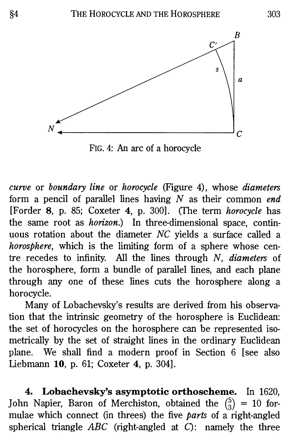
A.3 The Horosphere 7
sense we may say that Euclidean lengths are relative, whereas
angles are absolute. Lambert made the notable discovery that,
when Postulate V is denied, angles are still absolute, but
lengths are absolute too. In fact, for every segment there is a
corresponding angle, e.g. the angle of an equilateral triangle
based on the given segment.
1.3. Gauss, Wachter, Schweikart, Taurinus. Gauss
A777-1855) was the first to take the modern point of view,
that a geometry denying Postulate V should be developed for
its intrinsic interest, without expecting any contradiction to
arise. But, fearing ridicule, he kept these revolutionary ideas
to himself until others had published them independently.
From 1792 to 1813, he too tried to prove the parallel postulate;
but after 1813 his letters show that he had overcome the cus-
customary prejudice, and developed an "anti-Euclidean" or "njon-
Euclidean" geometry, which is in fact the geometry of Sac-
cheri's hypothesis of the acute angle. He discussed this with
his pupil Wachter A792-1817), who remarked in 1816 that the
limiting form assumed by a sphere as its radius becomes infinite
is a surface on which all the propositions of Euclid (including
Postulate V) are valid; or, as we should say nowadays, that
the intrinsic geometry of a horosphere is Euclidean.
Independently of Gauss, Schweikart A780-1859) developed
what he called "astral" geometry, in which the angle-sum of a
triangle is less than two right angles and (consequently) di-
diminishes as the area increases. In a Memorandum dated 1818
he observed that "the altitude of an isosceles right-angled
triangle continually grows, as the sides increase, but it can
never become greater than a certain length, which I call the
Constant." Gauss complimented Schweikart on his results,
and remarked that, if the Constant is called k log(l +-s/2), the
area of a triangle has the upper bound irk"-.
Thus encouraged, Schweikart persuaded his nephew
8 Historical Development
Taurinus A794-1874) to devote himself to the subject; and it was
in a letter written to this young man in 1824 that Gauss gave
the fullest account of his own discoveries. Taurinus developed
a "logarithmic-spherical" geometry by writing ik for the radius k
in the formulae of spherical trigonometry. (Compare Lambert's
suggestion about an imaginary sphere.) Thus, for a triangle with
angles A, B,C and sides a, b, c, he found
1.31. cosC = sin.Asin5cosh(c/&) - cos^4cos5,
whence cos C > — cos (A + B), and
1.32. A + B + C < tt.
For the circumference and area of a circle of radius r, he ob-
obtained
2tt& sinh - and 2tt&2 (cosh - - 1) ,
k \ k )
and for the surface and volume of a sphere,
4tt&2 sinh2 - and 2tt&3 (sinh - cosh - - - )
k \ k k k)
(Notice that, if k tends to oo, these tend to the usual expressions
in Euclidean geometry.)
1.4. Lobatschewsky. Formulae equivalent to these were
derived rigorously (and quite independently) by the Russian
mathematician Lobatschewsky A793-1856), who shares with
Gauss and the younger Bolyai the honour of having made the
first really systematic study of what we now call hyperbolic
geometry. His earliest paper was read in 1826, published in
1830, and a number of others followed.* Like Gauss, he defined
parallelism in such a way that there are just two lines through a
given point A parallel to a given line q (Fig. 1.2a), these being
'Lobatschewsky [1].
§1.4 The Angle of Parallelism 9
asymptomatic to q, as Saccheri had already shown. Drawing AB
perpendicular to q, he defined the angle of parallelism II(AB)
as the (acute) angle between AB and either of the parallels.
In terms of a convenient form of the absolute unit of length
(Taurinus's k = 1), he found that the angle of parallelism for the
distance AB = c is
II(c) = 2arctane~c = arc cot(sinhc) = arc cos(tanhc),
which decreases from \tt to 0 as c increases from 0 to oo. The
same result, in the form sin II (c) cosh c = 1, could have been
obtained by Taurinus also, if he had put A = U(c), B = \tt,
C = 0, k = 1 in 1.31.
Lobatschewsky derived his trigonometrical formulae from a
study of the horocycle (circle of infinite radius) and horosphere
(sphere of infinite radius), in the course of which he rediscov-
rediscovered Wachter's theorem that the geometry of horocycles on a
horosphere is identical with the geometry of straight lines in the
Euclidean plane. Having also rediscovered Lambert's formula
7T - A - B - C for the area of a triangle ABC, he proceeded to
calculate the volume of a tetrahedron,* expressing the result in
terms of his famous transcendental function
f*
L(x) = / log sec ydy.
Observing that the trigonometrical formulae of Euclidean
geometry are valid in the infinitesimal neighbourhood of a
point in the new geometry, Lobatschewsky considered the
possibility that his geometry might replace Euclid's in the ex-
exploration of astronomical space. The crucial experiment would
consist in finding a positive lower bound for the parallax of
stars. For, if c is a diameter of the Earth's orbit, measured
in terms of the (unknown) absolute unit, the parallax of any
star should exceed \tt — II(c). But this remains an open ques-
question, since such a lower bound, if it exists, is smaller than the
*Cf. Schlafli [1], p. 97; Richmond [1]; Coxeter [1].
10 Historical Development
allowance for experimental error. The failure of the experi-
experiment merely tells us that, if space is in fact hyperbolic, the
absolute unit must be many millions of times as long as the
diameter of the Earth's orbit.
In this connection we must bear in mind that, although a
geometry may seem more interesting if we can compare it
with the real world, its validity as a logical structure is not
affected, but depends only on its internal consistency. In order
to show that his "imaginary" geometry or "pangeometry" is
as consistent as Euclidean geometry, Lobatschewsky pointed
out that it is all based on his formulae for a triangle, which
lead to the familiar formulae for a spherical triangle when the
sides a, b, c are replaced by ia, ib, ic. Any inconsistency in the
new geometry could be "translated" into an inconsistency in
spherical geometry (which is part of Euclidean geometry).
Thus, after two thousand years of doubt, the independence of
Euclid's Postulate V was finally established.
1.5. Bolyai. Many of the same results were discovered
about the same time by Bolyai Janos A802-1860), who wrote
to his father, Bolyai Farkas, in 1823: "I have resolved to
publish a work on the theory of parallels, as soon as I shall
have put the material in order. . . . The goal is not yet reached,
but I have made such wonderful discoveries that I have been
almost overwhelmed by them. . . . I have created a new universe
from nothing."
Bolyai Farkas expressed the wish to insert his son's dis-
discoveries in his own book, as an Appendix.* In making this
offer, he remarked, more appropriately than he realized, that
"many things have an epoch, in which they are found at the
same time in several places, just as the violets appear on every
side in spring."
The younger Bolyai's speciality was the "absolute science
'Bolyai [1], [2].
jl.6 The Unboundedness of Space 11
of space" (or absolute geometry), consisting of those proposi-
propositions which are independent of Postulate V, so that they hold
in both Euclidean and hyperbolic geometry. For instance, he
expressed the "sine rule" for a triangle ABC in the form
Oa : Ob : Oc :: sin A : sin B : sin C,
where Oa denotes the circumference of a circle of radius a. He
observed that such formulae hold also in spherical geometry.
1.6. Riemann. The full recognition that spherical geome-
geometry is itself a kind of non-Euclidean geometry, without paral-
parallels, is due to Riemann A826-1866). He realized that Saccheri's
hypothesis of the obtuse angle becomes valid as soon as Pos-
Postulates I, II and V are modified to read:
I. Any two points determine at least one line.
II. A line is unbounded.
V. Any two lines in a plane will meet.
For a line to be unbounded and yet of finite length, it mere-
merely has to be re-entrant, like a circle. The great circles on a sphere
provide a model for the finite lines on a finite plane, and, when
so interpreted, satisfy the modified postulates. But if a line
and a plane can each be finite and yet unbounded, why not also
an n-dimensional manifold, and in particular the three-dimen-
three-dimensional space of the real world? In Riemann's words of 1854:
"The unboundedness of space possesses a greater empirical
certainty than any other external experience. But its infinite
extent by no means follows from this; on the other hand, if we
assume independence of bodies from position, and therefore
ascribe to space constant curvature, it must necessarily be finite
provided this curvature has ever so small a positive value."*
According to the General Theory of Relativity, astro-
astronomical space has positive curvature locally (wherever there
is matter), but we cannot tell whether the curvature of
"Riemann [1], p. 36.
12 Historical Development
"empty" space is exactly zero or has a very small positive or
negative value. In other words, we still cannot decide whether
the real world is approximately Euclidean or approximately
non-Euclidean.
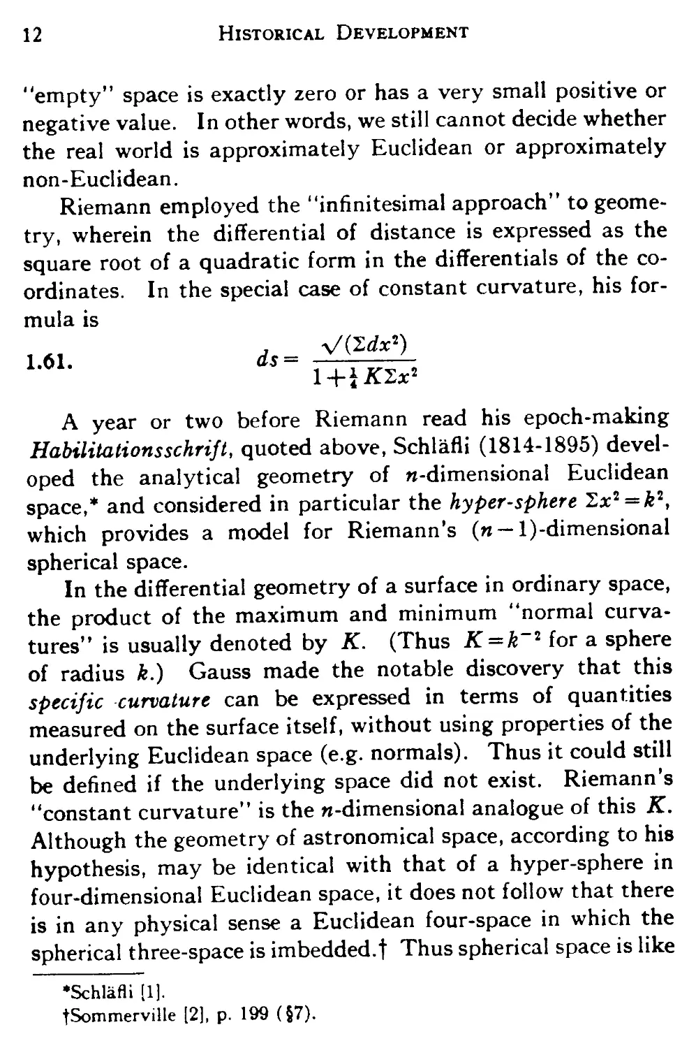
Riemann employed the "infinitesimal approach" to geome-
geometry, wherein the differential of distance is expressed as the
square root of a quadratic form in the differentials of the co-
coordinates. In the special case of constant curvature, his for-
formula is
1.01. as=
A year or two before Riemann read his epoch-making
Habilitationsschrift, quoted above, Schlafii A814-1895) devel-
developed the analytical geometry of n-dimensional Euclidean
space,* and considered in particular the hyper-sphere I,xi = k*,
which provides a model for Riemann's (n — l)-dimensional
spherical space.
In the differential geometry of a surface in ordinary space,
the product of the maximum and minimum "normal curva-
curvatures" is usually denoted by K. (Thus K = k~2 for a sphere
of radius k.) Gauss made the notable discovery that this
specific curvature can be expressed in terms of quantities
measured on the surface itself, without using properties of the
underlying Euclidean space (e.g. normals). Thus it could still
be defined if the underlying space did not exist. Riemann's
"constant curvature" is the n-dimensional analogue of this K.
Although the geometry of astronomical space, according to his
hypothesis, may be identical with that of a hyper-sphere in
four-dimensional Euclidean space, it does not follow that there
is in any physical sense a Euclidean four-space in which the
spherical three-space is imbedded.t Thus spherical space is like
¦Schlafli [1].
fSommerville [2], p. 199 (§7).
§1.7 Elliptic Geometry 13
the substance of a balloon with an extra dimension; but the
simile breaks down if we seek a meaning for the air inside or
outside the balloon.
1.7. Klein. Riemann developed the differential geometry
of spherical space. On the other hand, Cayley A821-1895)
considered space "in the large," defining distance in terms of
homogeneous coordinates. But it was Klein A849-1925) who
first saw clearly how to rid spherical geometry of its one
blemish: the fact that two coplanar lines (being two great
circles of a sphere) have not just one but Iwo common points.
Since every point determines a unique antipodal point, and
every figure is thus duplicated at the antipodes, he realized
that nothing would be lost, but much gained, by abstractly
identifying each pair of antipodal points, i.e. by changing the
meaning of the word "point" so as to call such a pair one point.
The word "line" will then be used for a great circle with
every pair of diametrically opposite points identified (or a
great semicircle with its two ends identified). So also, the
word "plane" will be used for a great sphere with every pair
of antipodal points identified, and analogous definitions can
be made in any number of dimensions. With this meaning for
the words, any two points determine a unique line; for, anti-
antipodal points are no longer two but one. Thus the traditional
form of Postulate I is restored. As for Postulate II, a line is
still unbounded, though finite, its length being half that of the
great circle. Right angles retain their ordinary meaning, but
a circle appears as a pair of antipodal circles.
It was to this modification of spherical geometry that Klein
gave the name elliptic geometry. It is in many ways simpler
than either spherical or Euclidean geometry, and can be de-
developed quite independently. The geometry of pairs of anti-
antipodal points is merely a model for it, a convenient representa-
representation in terms of more familiar concepts. Another model is
14 Historical Development
obtained by considering the diameters which join such pairs
of points. In this manner the points and lines in elliptic space
of n dimensions are represented by the lines and planes
through a fixed point O in Euclidean space of n-fl dimensions.
In particular, elliptic geometry of two dimensions is represented
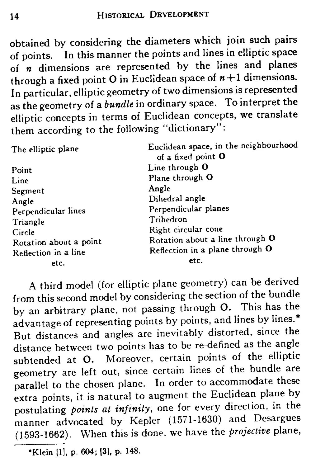
as the geometry of a bundle in ordinary space. To interpret the
elliptic concepts in terms of Euclidean concepts, we translate
them according to the following "dictionary":
The elliptic plane Euclidean space, in the neighbourhood
of a fixed point O
Point Line through O
Line Plane through O
Segment Angle
Angle Dihedral angle
Perpendicular lines Perpendicular planes
Triangle Trihedron
Circle Right circular cone
Rotation about a point Rotation about a line through O
Reflection in a line Reflection in a plane through O
etc. etc.
A third model (for elliptic plane geometry) can be derived
from this second model by considering the section of the bundle
by an arbitrary plane, not passing through 0. This has the
advantage of representing points by points, and lines by lines.*
But distances and angles are inevitably distorted, since the
distance between two points has to be re-defined as the angle
subtended at O. Moreover, certain points of the elliptic
geometry are left out, since certain lines of the bundle are
parallel to the chosen plane. In order to accommodate these
extra points, it is natural to augment the Euclidean plane by
postulating points at infinity, one for every direction, in the
manner advocated by Kepler A571-1630) and Desargues
A593-1662). When this is done, we have the projective plane,
'Klein [1], p. 604; [3], p. 148.
$1.7 The Plane at Infinity 15
in which every two lines intersect (either at an ordinary point
or at infinity). Thus, if metrical ideas are left out of consider-
consideration, elliptic geometry is the same as real projective geometry.
Conversely, real projective geometry (which we shall de-
develop in Chapters II, III, IV) contains certain correspondences
which enable us to define the elliptic metric in the whole space
(see Chapters v, vi, vii), and to define either the Euclidean or
the hyperbolic metric in a suitable part of space (Chapter ix).
The study of elliptic geometry is almost forced upon us as
soon as we have added points and lines at infinity to Euclidean
space. For, such points and lines form a plane—the plane at
infinity—whose intrinsic geometry is elliptic. (See §9.5.)
To sum up, the metrical geometries with which we are
concerned are Euclidean, hyperbolic, spherical, and elliptic. Our
preoccupation with these four, as against all other continuous
geometries, is justified by the fact that only in these cases is
space completely isotropic, in the sense that all the lines
through each point are alike. It is an interesting result in
differential geometry that, if space is continuous and isotropic,
it is also homogeneous or, as Riemann would say, of constant
curvature.
CHAPTER II
REAL PROJECTIVE GEOMETRY: FOUNDATIONS
2.1. Definitions and axioms. In any geometry, logically
developed, each definition of an entity or relation involves
other entities and relations; therefore certain particular entities
and relations must remain undefined. Similarly, the proof of
each proposition uses other propositions; therefore certain
particular propositions must remain unproved; these are the
axioms. We take for granted the machinery of logical deduc-
deduction, and the primitive concept of a class (or "set of all").
Unless the contrary is stated, the word correspondence will
be used in the sense of one-to-one correspondence. Thus a set
of entities is said to correspond to another set if every entity in
each set is associated with a unique entity in the other set. In
geometry the entities are usually points or lines, and the set
of entities is called a figure. Thus we speak of a correspondence
between two figures. It is often convenient to regard the cor-
correspondence as an operation which changes the first figure into
the second. (Familiar instances are rotation, reflection, inver-
inversion, and reciprocation.) The general technique for discussing
correspondences belongs properly to the theory of groups; but
the following outline will suffice for our purposes.
We shall find it convenient to denote a correspondence by
a capital Greek letter, such as 9, writing F9 = F' to mean that
9 relates the figure F to F' (or that the figure corresponding to
F is F'). If a second correspondence 3> relates the figure F' to
Fj, we write F'3> = Fp or F93> = Fi, and say that the product
9$ relates F to Fi. The trivial correspondence that relates
every entity to itself is called the identity, and is denoted by 1
(since its product with 9 is 9 itself). If 9$ = 1, we call $ the
16
52.1 Klein's Erlanger Programm 17
inverse of 0, writing <t> = 0~'. (Thus the relation F0 = F' is
equivalent to F =F'0~'.) Some authors write 0(F) instead of
F0, so as to exhibit it as a function of F. (Note that, in one of
the accepted notations, we write x=sin~V when sin x = x'.)
If a correspondence 0 relates F to F', while another corres-
correspondence <t> relates the pair of figures (F, F') to (Fi, Fi), we say
that $ transforms 0 into the correspondence between Fi and
F[. Since
[
this transformed correspondence is ^"'G*. It may happen that
0 itself relates Fi to Fj, so that <i> transforms 9 into itself. We
then say that 0 is invariant under transformation by <J>. Since
the relation 3>~10<t> = 0 may be written 04>=<J>9, an equivalent
statement is that 0 and $ are permutable. (As a familiar
example of correspondences which are not permutable, con-
consider the reflections in two planes not perpendicular to one
another.)
According to Klein, the character of any geometry is deter-
determined by the type of correspondence under which its relations
are invariant; e.g. Euclidean geometry is invariant under
"similarity transformations."* The title of this book refers
strictly to just two geometries, elliptic and hyperbolic; but
certain others are so closely interwoven with these as to compel
our attention. The concept of similarity, which plays such a
vital role in Euclidean geometry, has no analogue in either of
the non-Euclidean geometries. On the other hand, the concept
of parallelism (for lines in one plane) belongs to both Euclidean
and hyperbolic geometry, but is lacking in elliptic. Bolyai
Janos (§1.5) gave the name absolute geometry to the large body
of propositions common to Euclidean and hyperbolic geometry.
Some of these propositions will be used in Chapter IX, before
•Veblen and Young [2], I, pp. 64-68; II, pp. 78, 119.
18 Real Projective Geometry
we split absolute geometry into its two parts by affirming or
denying the uniqueness of parallelism (or Postulate V).
The contrast between absolute and elliptic geometry is
clearly seen in the theory of order.* In either geometry we can
describe a "four point" order, saying that four collinear points
fall into two pairs which separate each other. In absolute
geometry this can be derived from the stronger "three point"
order, in which we say that one of three collinear points lies
between the other two. But in elliptic geometry all lines are
closed, and so the notion of order does not specialize one of
three points: order is no longer "serial" but "cyclic."
Throughout the ages, from the ancient Egyptians and
Euclid to Poncelet and Steiner, geometry has been based on
the concept of measurement, which is defined in terms of the
relation of congruence. It was von Staudt A798-1867) who
first saw the possibility of constructing a logical geometry
without this concept. Since his time there has been an increas-
increasing tendency to focus attention on the much simpler relation
of incidence,^ which is expressed by such phrases as "The point
A lies on the line p" or "The line p passes through the point A."
Euclidean geometry with congruence left out is called affine
geometry. As so many figures in Euclidean geometry are
denned in terms of congruence (e.g. equilateral triangle, circle,
conic section), it might seem that in affine geometry there
would be little left to talk about. It is true that the content
of affine geometry is less rich than that of Euclidean, but it is
still possible to define conies, for example, and to distinguish
the three types: ellipse, parabola, hyperbola. Postulate V,
in its non-metrical form 1.12, allows us to define an attenuated
kind of congruence, by which we can compare certain segments
(namely those which are parallel to one another) and measure
area.J But the notion of "perpendicularity" is entirely lack-
•Vailati [1]. See also Veblen and Young [2], II, p. 44, and Russell [1],
IV. fPieri [1]: Baker [1], I, p. 4. fHeffter and Koehler [1], I, p. 219.
§2.1 A Geometrical Genealogy 19
ing. By suitably defining perpendicularity, we can restore the
whole of Euclidean geometry. By modifying the definition,
we can derive instead Minkowskian geometry,* the four-
dimensional case of which is used in the Special Theory of
Relativity.
Similarly, elliptic geometry with congruence left out is real
projective geometry. This was developed (qua Euclidean
geometry augmented by points at infinity) long before elliptio
geometry itself, and is still widely studied for its own interest.
It excels affine geometry in the symmetry of its propositions
of incidence, which occur in pairs in accordance with the "prin-
"principle of duality." Moreover, it includes all the other geome-
geometries that have been mentioned. For. by suitably defining
perpendicularity we can restore the metrical properties of
elliptic geometry, and by modifying the definition we can
derive instead hyperbolic geometry. Again, by specializing a
plane (in the three-dimensional case) or a line (in the two-
dimensional), we can derive affine geometry, and thence either
Euclidean or Minkowskian.
In the following "genealogy," each geometry (save the
first) is derived from its parent by some kind of specialization:
Projective
Elliptic Affine Hyperbolic
Euclidean Minkowskian
In view of the above remarks, we shall set aside all metrical
considerations till Chapter v, and survey the foundations of
real projective geometry, using the axioms of Pieri, Vailati,
and Dedekind. In this case there are two undefined entities,
•Minkowski [1]; Robb [1].
20 Real Projective Geometry
point and line; two undefined relations, incidence and separa-
separation.
AXIOMS OF INCIDENCE
2.111. There are at least two points.
2.112. Any two points are incident with just one line.
The line thus determined by two points A and B is said to
join the points, and is denoted by AB.
2.113. The line AB is incident with at least one point besides
A and B.
Points incident with a line are said to lie on the line, or to
be collinear. The class of points on a line is called a range.
2.114. There is at least one point not incident with the
line AB.
Lines incident with a point are said to pass through the
point, or to be concurrent. Two such lines are said to meet or
intersect. By joining the points of a range to a point C, not
belonging to this range, we obtain a flat pencil of lines, with
centre C. A plane is the class of points on the lines of a fiat
pencil, together with the class of lines joining pairs of these
points.
2.115. If A, B, C are three non-collinear points, and D is a
point on BC distinct from B and C, while E is a point on CA
distinct from C and A, then there is a point F on AB such that
D, E, F are collinear. (See Fig. 8.8a on page 173.)
It follows that a plane contains all the points on each of its
lines, and can be denned equally well by any pencil contained
in it. In terms of three non-collinear points, or a non-incident
point and line, we denote a plane by ABC or Ap. Points or
lines in one plane are said to be coplanar.
2.116. There is at least one point not in the plane ABC.
2.117. Any two planes intersect in a line.
So far, we may appear to have been underlining the obvious. Every
student of elementary geometry is familiar with the terms just used. But
the real importance of the foregoing remarks lies less in what we have said
§2.1 Perspectivity 21
than in what we have not said. We have not mentioned the possibility of
the distance AB being equal to the distance CD; we shall never make such
a remark as long as we are dealing with projective geometry only.
From the above axioms it is possible to deduce all the pro-
propositions of incidence for points, lines, and planes. If lines p
and q intersect, we denote their common point by (p, q) and
their plane by pq. Two lines which do not intersect are said
to be skew. Planes incident with a line are said to pass through
the line, or to be coaxial. The class of planes through a line p
is called an axial pencil, with axis p. The class of lines and
planes through a point O is called a bundle (or sheaf, or star),
with centre O.
By considering "degrees of freedom" we are led to speak
of a point as having no dimension, a line one dimension, and a
plane two dimensions. The lines of a flat pencil, and likewise
the planes of an axial pencil, correspond (by incidence) to the
points of a range, which is the section of the pencil by a line.
For this reason, ranges and pencils together are described as
one-dimensional primitive forms. Similarly, planes and bundles
are two-dimensional forms, the points and lines of a plane being
sections of the lines and planes of a bundle; and the whole
space is three-dimensional.
One of the most important correspondences in projective
geometry is perspectivity. This is the correspondence estab-
established between two coplanar lines, or two planes, by regarding
them as different sections of the same flat pencil or bundle,
respectively. In the case of lines, we say that the flat pencil
projects the one range into the other, and the two ranges are
said to be in perspective. (See Fig. 2.1a, where O is the centre
of the pencil.) Corresponding points are indicated by for-
formulae such as
ABC... = A'B'C .. ., or ABC...? ABC ....
A A
22
Real Projective Geometry
Fig. 2.1a
Fig. 2.1b
Our second undefined relation refers to two pairs of points
on a line. Following Vailati, we use the symbol AB || CD to
mean that A and B separate C and D. (The significance of this
relation is most clearly seen by representing the line as a circle.
See Fig. 2.1b.)
AXIOMS OF SEPARATION
2.121. If A, B, C are three collinear points, there is at least
one point D such that AB || CD.
2.122. //AB || CD, then A, B, C, D are collinear and distinct.
2.123. //AB || CD, then AB || DC.
2.124. If A, B, C, D are four collinear points, then either
AB || CD or AC || BD or AD || BC.
2.125. //AB || CD and AD || BX, then AB || CX.
2.126. //AB || CD and ABCD ^ A'B'C'D', then A'B' || CD'.
From the last of these axioms we can deduce* that the relation
AB||CD implies CD||AB. Putting C for X in 2.125, and using 2.122,
we see that the relation AB || CD excludes AC || BC. The existence-axiom
2.121 has been inserted as the most natural way to secure an infinity of points.
*Robinson [1], p. 119 (second footnote). Following Veblen, Robinson uses
the symbol A for the combination of several perspectives. Following von
Staudt, who invented that symbol, I prefer to define it differently, though later
the two definitions will be seen to be equivalent (in real geometry).
§2.2 MODELS 23
Accordingly, the above axioms differ slightly from those given by Vailati (and
quoted by Veblen and Russell).
If A, B, C are three collinear points, we define the segment
AB/C as the class of points X for which AB || CX. Thus the
segment AB/C does not contain C. The segment with its end
points A and B is called an interval, and is denoted by AB/C.
If X and Y belong to AB/C, the interval XY/C is said to
be interior to AB/C, and a point D lies between X and Y in
AB/C if it belongs to XY/C, i.e. if XY||CD. (Either X or Y
may coincide with either A or B. In other cases we have either
AX || BY or AY || BX.) Thus "three point" order becomes valid
when we restrict consideration to an interval, or to a segment.
AXIOM OF CONTINUITY
2.13. For every partition of all the points of a segment into two
non-vacuous sets, such that no point of either lies between two points
of the other, there is a point of one set which lies between every other
point of that set and every point of the other set.
This final axiom will be used in §2.7.
2.2. Models. When we say that a system of axioms is
consistent, we mean that no two theorems, logically deduced
from them, can be contradictory (like the statements "All right
angles are equal" and "Some lines are self-perpendicular").
Clearly, there is no direct test for consistency, since we cannot
follow up the infinite number of possible chains of deduction to
see whether any two of them lead to a contradiction. For an
indirect test we use a model, which is a set of objects satisfy-
satisfying the same axioms as the undefined entities of the original
system. Any contradiction implied by the original system would
be represented by a contradiction in the model, and this can-
cannot occur so long as the objects unquestionably exist. These
objects may be (defined or undefined) entities in another ab-
24 Real Projective Geometry
stract system whose consistency is taken for granted, or they
may be physical objects whose reality is accepted for reasons
outside the domain of mathematics. In the former case the
assumption of consistency can only be justified by means of a
model of the model; so it may well be argued that every ques-
question of consistency is ultimately based on properties of the
physical world as interpreted by our senses. (For those who
dislike this materialistic conclusion, a possible loophole is
offered by the recent attempts to prove the consistency of
arithmetic in a direct fashion.*)
We give here three models for real projective geometry.
The first is in terms of affine geometry, whose consistency is
usually established by means of Cartesian coordinates (the
"model of the model"). The second refers directly to the
number system. The third is in terms of absolute geometry,
which, being based on the "self-evident" postulates I—IV, is
amenable to direct comparison with physical space.
To construct the first model, we define axial pencils and
bundles in affine (or, if preferred, Euclidean) space, in such a
way as to include pencils and bundles of parallels, and then set
up a "dictionary," as follows:
Real projective space Affine space
Point Bundle
Line Axial pencil
A point lies on a line The planes of a bundle include those
of a pencil
Two points determine a line The common planes of two bundles
form a pencil
Setting up this model is effectively equivalent to the classi-
classical derivation of projective space from affine (or Euclidean)
space by adding the "ideal" points and lines of a postulated
*Hilbert and Bernays [1].
§2.2
Geometry as Consistent as Arithmetic
25
"plane at infinity." For, such points arise as centres of bun-
bundles of parallel lines, and such lines arise as axes of pencils of
parallel planes.
The direct appeal to arithmetic is made by using homo-
homogeneous coordinates. The appropriate dictionary this time is
as follows:
Real projective space
Point A
Line p
Point A lies on line p
Line AB
AB II CD
The real number system
The class of ordered tetrads of real
numbers, proportional to a given tetrad
(aa, a\, at, <ij)
The class of ordered hexads of real
numbers, proportional to a given hexad
{Pit. P.i, Pit, Poi, Poi, Pos( satisfying the
equation PuPoi + PtiPoi+PnPoi=0
(For convenience we define P,j etc., so
that P^= —PM, and therefore P,t=0)
aoPov+aiPir+aiPiv+atPtt^O for two
(and therefore all four) values of v
\ajb\-aibo, aabt—atbo, aobi — aibo,
The o's, and likewise the b's, c's, and
d's, satisfy two independent linear homo-
homogeneous equations; and the respective
ratios a^/a,, c^/c,, b^/b,, d^/d,, or some
cyclic permutation thereof, are in strictly
ascending order of magnitude for at least
one choice of ^ and v
For further details of this model, see §4.6. The verification of
all the axioms is an interesting exercise.
If we are content to consider the two-dimensional projec-
projective geometry of a single plane, a third model consists of the
lines and planes through one point in ordinary space (as in
§1.7, but without the metrical concepts):
26 Real Projective Geometry
The real projective plane Euclidean or non-Euclidean space, in
the neighbourhood of a fixed point O
Point A Line a through O
Line AB Plane ab
Range Flat pencil
Flat pencil Axial pencil
Triangle Trihedron
Conic Quadric cone
This has the advantage of symmetry, which the first model
lacks. Moreover, the geometry of a bundle can be developed
without using "Postulate V"; in fact a bundle is essentially
the same thing in absolute geometry as in projective. But in
order to adapt this model to three dimensions, we would have
to consider the "hyper-bundle" of lines and planes through a
point in four dimensions—which is quite satisfactory for any-
anyone who has become familiar with the properties of absolute
(or Euclidean) hyper-space.
2.3. The principle of duality. Three non-collinear points
A, B, C are called the vertices of a triangle ABC; its sides are the
three lines BC, CA, AB. Analogously, four non-coplanar points
A, B, C, D are the vertices of a tetrahedron ABCD; its edges and
faces are the six lines AD, BD, CD, BC, CA, AB, and the four
planes BCD, CDA, DAB, ABC.
The principle of duality in the plane affirms that every
definition remains significant, and every theorem remains true,
when we interchange "point" and "line," and make a few
consequent alterations in wording. This means that the
geometry of lines forms a model for the geometry of points.
The following definition provides an example:
§2.3
Dual Configurations
27
Four coplanar points, A, B, G,
D, of which no three are collinear,
are the vertices of a complete
quadrangle* ABCD, with the six
lines AD, BD, CD, BG, CA, AB
for sides. The points of inter-
intersection of "opposite" sides, namely
(AD, BC), (BD, CA), (CD, AB).
are called diagonal points, and are
the vertices of the diagonal tri-
triangle.
The principle of duality in space allows the analogous inter-
interchange of "point" and "plane." Thus 2.117 is the space-dual
of 2.112. Here is another example:
Four coplanar lines a, b, c, d,
of which no three are concurrent,
are the sides of a complete quadri-
quadrilateral* abed, with the six points
(a, d), (b,d), (c.d), (b,c), (c,a),
(a, b) for vertices. The joins
of "opposite" vertices, namely
(a,d)(b,c),(b,d)(c,a),(c,d)(a,b),
are called diagonal lines, and are
the sides of the diagonal triangle.
Five points A, B, C, D, E, of
which no four are coplanar, are
the vertices of a complete penta-
pentagon ABCDE, with the ten lines
AB, . . . , DE for edges, and the
ten planes ABC CDE for
faces. Each edge lies in three
faces.
Five planes a, /9, y, 8, e, of which
no four are concurrent, are the
faces of a complete pentahedron
afiybt, with the ten lines (a, |3),
...,(?,<) for edges, and the ten
points (a, j3, 7), . . . , G, 5, e) for
vertices. Each edge contains three
vertices.
To justify the principle of duality, we observe that the
axioms imply their own duals. For instance, 2.115 enables us
to prove the plane-dual of 2.112, namelyf
2.31. Any two coplanar lines intersect.
(This is the result that most clearly distinguishes projective
geometry from affine geometry. It rules out the possibility of
parallels.)
Having proved a theorem, we can state the space-dual
theorem without more ado; for a proof could in fact be written
down mechanically by dualizing every step in the proof of the
'When there is no danger of confusion, we shall omit the word "com-
"complete."
fVeblen and Young [2], I, p. 19.
28 Real Projective Geometry
original theorem. The same remark applies to the plane-dual
of any theorem which can be proved without using points
outside the plane. Consider, however, Desargues1 Theorem
and its converse (which are easily proved with the help of
2.116):
2.32. If the vertices of 2.33. If the sides of two
two coplanar triangles cor- coplanar triangles correspond
respond in such a way that in such a way that the in-
the joins of corresponding tersections of corresponding
vertices are concurrent, then sides are collinear, then the
the intersections of corres- joins of corresponding ver-
ponding sides are collinear. tices are concurrent.
Either of these dual theorems can be deduced from the other,
without leaving the plane;* but it is not legitimate to invoke
the principle of duality in the plane for this purpose, since the
initial proof is essentially three-dimensional.
To obtain a sufficient set of axioms for projective geometry
in two dimensions, we can replace 2.115—2.117 by 2.31 and
2.32 (omitting the word coplanar). The principle of duality will
then hold without reservation.
2.4. Harmonic sets. A large part of our investigation
(e.g. Chapter v) will be concerned with the geometry jf points
on a single line, where there is no scope for incidences. This
deficiency is compensated by the possibility of defining the
harmonic conjugate of a given point with respect to two given
points. (We think of this as a one-dimensional concept, even
though it requires incidences in two dimensions for its con-
construction and in three dimensions for the proof of its unique-
uniqueness.) We shall use the abbreviation H(AB, CD) for the state-
*See, for instance, Baker [1] I, p. 181, or Robson [1), p. 211. Cf.
Veblen and Young [2], I, p. 41.
§2.4 Harmonic Separation 29
ment that D is the harmonic conjugate of C with respect to
A and B, which means* that there is a quadrangle IJKL such
that one pair of opposite sides intersect at A, and a second pair
at B, while the third pair meet AB at C and D. This relation
is clearly symmetrical between A and B, and between C and D.
Given three collinear points A, B, C, we can obtain D by
taking two points I, J, collinear with C, and constructing the
intersections K = (AJ, BI), L = (AI, BJ), D = (AB, KL). It is a
simple consequence of 2.32 and 2.33 that the position of D is
independent of the choice of I and J. But can we be sure that
D is distinct from C? (This is important for certain applica-
applications.) The following proof is due to Enriques.
P
By 2.121 and 2.123, we can take a point S such that
AK 11 SJ, as in Fig. 2.4a. Let IS meet AB at X, and KL at O;
let JO meet AB at Y, and AI at P. Then
AKSJ
ABXC, AKSJ ALIpaBCY, AKSJ°ADXY.
By 2.126, we therefore have AB || XC, AB || CY, AD || XY.
*De la Hire [1], lib. i, prop, xx; Enriques [1], p. 51.
flf X happens to coincide with D, the argument ends here; for then
the given relation AK ISJ implies ABIIDC.
30
Real Proiective Geometry
Thus both X and Y are in the segment AB/C, and D lies be-
between them. In other words,
2.41. H(AB, CD) implies AB || CD.
By applying the plane-dual of the above construction for
the fourth harmonic point of three collinear points, we obtain
a unique "fourth harmonic line" for any three lines of a flat
pencil. The figure involved is almost the same as before; in
fact ID is the harmonic conjugate of IC with respect to IA and
IB. Thus a harmonic set of points is joined to any external
point by a harmonic set of lines. Dually, any section of a
harmonic set of lines is a harmonic set of points. Hence
2.42. // H (AB, CD) and ABCD = A'B'C'D', then H (A'B', CD).
Two-dimensional geometry admits three alternative ana-
analogues for harmonic conjugacy. One of these, which plays an
Important part in the introduction of coordinates (§4.3), is the
so-called trilinear polarity. (The other two are the harmonic
homology of §3.1, and the true polarity of §3.2.) The trilinear
pole of a line g, with respect to a triangle ABC, is constructed
as follows.
N
Let the sides of ABC meet g in L. M, N. and let G^G^G, be
the triangle formed by the lines AL, BM, CN. By 2.33, the
three lines AGa, BG6, CGC are concurrent; their common point
G is the trilinear pole of g. These lines meet the sides of the
§2.4 Trilinear Polarity 31
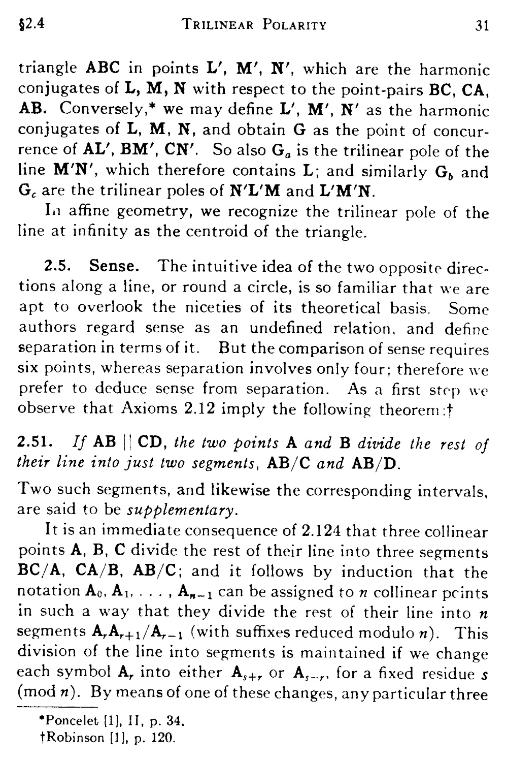
triangle ABC in points I/, M', N', which are the harmonic
conjugates of L, M, N with respect to the point-pairs BC, CA,
AB. Conversely,* we may define L', M', N' as the harmonic
conjugates of L, M, N, and obtain G as the point of concur-
concurrence of AL', BM', CN'. So also Go is the trilinear pole of the
line M'N', which therefore contains L; and similarly G6 and
Gc are the trilinear poles of N'L'M and L'M'N.
In affine geometry, we recognize the trilinear pole of the
line at infinity as the centroid of the triangle.
2.5. Sense. The intuitive idea of the two opposite direc-
directions along a line, or round a circle, is so familiar that we are
apt to overlook the niceties of its theoretical basis. Some
authors regard sense as an undefined relation, and define
separation in terms of it. But the comparison of sense requires
six points, whereas separation involves only four; therefore we
prefer to deduce sense from separation. As a first step we
observe that Axioms 2.12 imply the following theorem :f
2.51. // AB i| CD, the two points A and B divide the rest of
their line into just two segments, AB/C and AB/D.
Two such segments, and likewise the corresponding intervals,
are said to be supplementary.
It is an immediate consequence of 2.124 that three collinear
points A, B, C divide the rest of their line into three segments
BC/A, CA/B, AB/C; and it follows by induction that the
notation Ao, Ai, . . . , An_j can be assigned to n collinear prints
in such a way that they divide the rest of their line into n
segments ArAr+1/Ar_1 (with suffixes reduced modulo n). This
division of the line into segments is maintained if we change
each symbol Ar into either As+r or As_r, for a fixed residue 5
(mod n). By means of one of these changes, any particular three
•Poncelet [1], II, p. 34.
fRobinson [1], p. 120.
32 Real Projective Geometry
of the n points may be named Aq.Aj.Ac, where 0 < b < c < n.
This notation facilitates the definition of one-dimensional sense.
Let ABC and DEF be two triads of distinct points on one
line. (Any of D, E, F may happen to coincide with any of
A, B, C.) Let the distinct points of this set be named Aq, Ai, ...,
A,,-! (n = 3, 4, 5, or 6) in such a way that A - Aq, B = Ab,
C = Ac, with b < c. Suppose that then D = A^, E = A*,, F = A/.
If d < e < f or e < f < d or / < d < e, we say that the two
triads have the same sense, and write
S(DEF) = S(ABC).
If, on the other hand, f<e<d or d<f<e or e<d<f, we
say that the two triads have opposite senses, and write
S(DEF) # S(ABC).
(The arithmetical ideas employed here do not involve any fresh
assumptions, but merely avoid separate consideration of the 228
possible ways of distributing D, E, F among A, B, C.)
We easily verify that the relation of having the same sense
is reflective, symmetric, and transitive, and that
S(ABC) = S(BCA) = S(CAB) * S(ACB).
All triads which have the same sense as ABC are said to belong
to the sense-class S(ABC). It follows that
2.52. There are two sense-classes in the line:
S(ABC) and S(ACB).
In other words, the line is orientable.
The direct connection between sense and separation is given
by the following theorem:
2.53. The relation AB || CD is equivalent to S(ABC) # S(ABD).
Proof. If AB||CD, the line is divided into four segments
AD/C, DB/A, BC/D, CA/B, which enable us to write (as
above, with n = 4):
§2.5 Orientability 33
A = Ao, D = A1; B = A2, C = A3
Hence S(ABC) = S(ADB) # S(ABD). Conversely, given
S(ABC) =? S(ABD), we can reverse the argument and deduce
AB||CD.
It is now easy to justify the intuitive consequence of us-
using circular diagrams such as Fig. 2.1b, where clockwise and
counter-clockwise senses can be indicated by an arrow pointing
one way or the other.
In virtue of 2.126, all of the above theory of sense in one
dimension can be applied to the lines or planes of a pencil:
three lines of a flat pencil determine two sense-classes S(abc)
and S(acb), and three planes of an axial pencil determine two
sense-classes S(aj3y) and S(ay/3). Moreover, the notion of sense
can be extended from one to two dimensions, where a sense-
class is defined by the vertices of a quadrangle. (This is roughly
equivalent to the statement that a sense of rotation is defined
by the centre of a circle and three points on its circumfer-
circumference.) But the conclusion is different: *all quadrangles in the
plane have the same sense, so there is only one sense-class;
the plane is non-orientable.
The projective plane, with its single sense-class, is not very easy to
visualize. In ordinary space a non-orientable surface is "one-sided," and
must cross itself if unbounded. But the impossibility of distinguishing two
senses of rotation is easily seen in the geometry of a bundle (which is
the "third model" of §2.2). For, any rotation about a line of the bundle
(i.e. about a point of the projective plane) is clockwise when we look along
the line in one direction, and counter-clockwise when we look along it in
the opposite direction.
In projective geometry of three dimensions, we might de-
define a sense-class by means of the vertices of a complete
pentagon, but it is easier to use Veblen's notion of a doubly
*Veblen and Young [2], II, pp. 67, 422; Klein [3], pp. 12-17.
34 Real Projective Geometry
oriented line (ABC, aj3y). This is a line associated with one
sense-class S(ABC) among the points on it and one sense-
class S(aj3y) among the planes through it. Thus the line AB
provides four doubly oriented lines: (ABC,aj3y), (ACB, ay/3),
(ABC, ay/3), (ACB, a/3y). Two doubly oriented lines are said
to be doubly perspective if they can be named (ABC,aj3y)
and (A'B'Ca'jS'V) in such a way that A,B,C,A',B',C lie
on a',j3',y,a,j3,y, respectively. Two doubly oriented lines
are said to be similarly oriented if they are related by a se-
sequence of such "double perspectivities." It can be proved^ that
(ABC,a/3y) is similarly oriented with (ACB, ay/3), but not with
(ABC,ayj3), and that
2.54. There are just two classes of doubly oriented lines, such that
any two doubly oriented lines are similarly oriented if and only if
they belong to the same class.
Intuitively, this is the distinction between right-handed and left-handed
screws. The general result is that a projective space is orientable or non-
orientable according as its number of dimensions is odd or even.
2.6. Triangular and tetrahedral regions. The plane-
dual and space-dual of 2.51 may be stated as follows:
Two coplanar lines (or two planes) divide the rest of their
plane (or of space) into two classes of points, such that two
points in different classes are separated by the points in which
their join meets the given lines (or planes), whereas two points
in the same class are not so separated.
Such classes of points are called regions* A third line (or
plane) will in general subdivide each region. Hence
2.61. The sides of a triangle ABC divide the rest of the plane
ABC into four regions.
and Young [2], II, p. 449. Cf. Russell [1], p. 232.
"Veblen and Young [2], II, pp. 51-54, 385-400.
§2.6
Convex Regions
35
Fig. 2.6a
To distinguish one of these, we may proceed as follows. A
line p, not passing through any of A, B, C, is divided by BC,
CA, AB into three segments, lying respectively in three of the
four regions. The remaining region, to which p is exterior, is
then denoted by ABC/p, as in Fig. 2.6A.
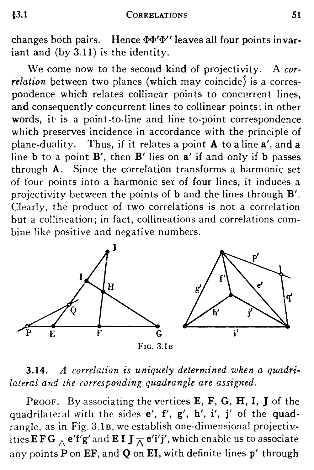
So also, three non-coaxial planes divide the rest of space into
four regions, each of which will be subdivided by a fourth plane
(not concurrent with the others). Hence
2.62. The faces of a tetrahedron ABCD divide the rest of space
into eight regions.
We distinguish any one of these as ABCD/trr, where m is an
exterior plane.
The above results become quite obvious when we apply
them to affine space with ideal elements, taking one side of
the triangle (or one face of the tetrahedron) to be the line (or
plane) at infinity, then 2.61 describes the four "quadrants," and
2.62 the eight "octants."
2.7. Ordered correspondences. A correspondence be-
between two ranges is said to be ordered if it preserves the
relation of separation. The points of the second range which
correspond to A,B... in the first will be denoted by A',B',
Thus the correspondence is ordered if A'B' || CD' whenever
36 Real Projective Geometry
AB || CD. If the two ranges are on the same line ("super-
("superposed"), the correspondence is said to be direct or opposite
according as it preserves or reverses sense, i.e. according as
S(ABC) =or#S(A'B'C). A point which corresponds to itself
(A' = A) is called a double point. As a particular direct corres-
correspondence, we include the identity, in which every point is a
double point. Direct and opposite correspondences are easily
seen to combine like positive and negative numbers; e.g. the
product of two opposite correspondences is direct. These
notions extend in an obvious manner to correspondences be-
between any kind of one-dimensional primitive forms; e.g., in a
correspondence between two flat pencils, a line which corres-
corresponds to itself is called a double line.
Our first application of the Axiom of Continuity is in
proving the following lemma* (which we shall need several
times, notably in 2.84, where we enumerate the double points
of a projectivity):
2.71. // an ordered correspondence relates an interval AB/C to
an interior interval A'B'/C, then the latter interval contains a
double point M, such that there is no double point between A and
M (in AB/C).
Proof. It is convenient to say, of points X and Y in
AB/C, that X precedes Y (and Y follows X) if S(XYC) =S(ABC).
If A' coincides with A, then A is itself the desired point M. If
B coincides with B', while every other point of AB/C precedes
its corresponding point, then B is the desired point M. Setting
aside these two extreme cases, we divide the segment AB/C
into two sets of points:
(i) Points P such that every point H which precedes P
precedes its corresponding point H',
(ii) Points Q which follow at least one point K which does
not precede its corresponding point K'.
*Kiirique- [1], pp. 71-75. See <t!-o Coxeter |(.|, pp. HiK 17A (§10.til.
§2.7
Enriques' Lemma
37
We are assuming the existence of such a point K; the second
set includes every point between this and B. To see that the
first set likewise contains some points, we observe that every
point between A and B, and in particular every point between
A and A', is related to a point between A' and B'. Hence, if
the correspondence is direct, so that A' precedes B' (as in
Fig. 2.7a), the first set certainly contains A'. If, on the other
hand, the correspondence is opposite, so that A' follows B' (as
in Fig. 2.7c), consider any point P between A and B. If P
precedes (or coincides with) its corresponding point P', then
every point which precedes P is related to a point which follows
P'; hence the first set contains this P. But if P follows P', then
P' precedes its corresponding point P", and by the same argu-
argument the first set contains this P'.
Fig. 2.7a
Fig. 2.7b
Fig. 2.7c
Clearly, every point of the first set precedes every point of
the second. Hence, by 2.13, there is a point M such that
every point which precedes M belongs to the first set, while
every point which follows M belongs to the second. (Actually,
M itself belongs to the first.) By (i), every point H which
precedes M precedes its corresponding point H'; hence there
is no double point preceding M. To see that M itself is a
double point, we again consider the two types of correspon-
correspondence separately.
If the correspondence is direct, suppose if possible that M
is not a double point. If M follows M', then M' follows M",
38 Real Projective Geometry
contradicting (i). But if M precedes M', as in Fig. 2.7a, then
every point H between M and M' precedes its corresponding
point H' (which follows M'); this makes M' belong to the first
set, which is absurd.
If, on the other hand, the correspondence is opposite, every
point Q of the second set follows its corresponding point Q\
since Q' precedes the point K' of (ii). Let H be a fixed point
between A and M, and P a variable point between H and M,
as in Fig. 2.7b. Then, the correspondence being opposite, H'
follows P\ which follows P. Thus H' follows every point which
precedes M, and so either follows or coincides with M. Simi-
Similarly, for any point K between B and M, the corresponding
point K' either precedes or coincides with M. If M' precedes
M, as in Fig. 2.7c, then every point H' between M and M',
being also between A' and M', corresponds to a point H be-
between A and M, which is absurd. Similarly, it is absurd to
suppose that M' follows M.
Hence, finally, M is a double point.
Although this rigorous proof (due to Enriques) is quite subtle, the
result is intuitively obvious when we think of a correspondence between
moving points. On a circular race-track, Tom runs from A to B while
Dick runs (over part of the same ground) from A' to B'; M is the place
where Tom first passes Dick.
In the case when the correspondence is opposite, we easily
see that M is the only double point in AB/C. By applying the
same theorem to the inverse correspondence, we deduce that
there is likewise just one double point in the supplementary
interval. Conversely, every opposite correspondence relates
a pair of intervals, one containing the other; tor, if A' is related
to A" (which may or may not coincide with A), then the two
intervals AA' are related to the two intervals A'A'', one of
which is interior. Hence
§2.7 Opposite Correspondences 39
2.72. Every opposite correspondence has exactly two double
points.
We shall see, in §4.1, that the points of a line can be represented by
the real numbers and °° . The relation xf ¦» x~* is an example of an opposite
correspondence; its two double points are ±1. On the other hand, the
direct correspondence x7"** has four double points: 0, °° , ±1. In fact,
a direct correspondence may have any number of double points, from none
to infinitely many.
By 2.126, a perspectivity is an ordered correspondence; so
also is the result of any sequence of perspectivities. Thus, if
A, B, I, K in Fig. 2.4a are fixed, the correspondence between
C and D is ordered, since it is given by the sequence of per-
perspectivities
ABC^AKJ = AIL*ABD.
By 2.41 and 2.53, this correspondence reverses sense. In other
words,
2.73. The correspondence between harmonic conjugates with
respect to two fixed points is opposite.
If H(AB, CD) and H(AB, CiDi), so that dDi is another
pair in the same correspondence, we have S(CDCi) j^S(DCDi),
i.e.
S(CDCi)=S(CDDi).
By 2.53, this means that Ci and Di do not separate C and D.
Hence
2.74. // two pairs of points on a line are each harmonic con-
conjugates with respect to a third pair, they do not separate each
other.
By applying 2.71 to the product of two correspondences of
the kind just considered, it is easy to prove* the converse
theorem (which plays an important part in the theory of
projectivities):
•Enriques [1], p. 77; Holgate [1], p. 36.
40 Real Projective Geometry
2.75. // two pairs of points on a line do not separate each other,
there is ai least one pair of points which are harmonic conjugates
with respect to each of the given pairs.
2.8. One-dimensional projectivities. Following von
Staucit, we define a projectivity between two ranges (or two
pencils, or a range and a pencil) as a correspondence which
preserves the harmonic relation,* so that H(A'B\ CD') when-
whenever H(AB, CD); and we indicate corresponding elements by
formulae such as
ABC . . .^A'B'C
This relation is clearly reflexive, symmetric, and transitive.
(The analogous two- and three-dimensional correspondences
will constitute the main topic of Chapter in.)
By 2.42, every perspectivity is a projectivity; so also is
any product of perspectivities. We shall see (in 2.86) that,
conversely, every projectivity can be constructed as a product
of perspectivities; but for the present we shall be content to
treat such a product as a special case of a projectivity. In this
manner it is easily verified that, for any four collinear points,
2.81. ABCD^BADC.
This means that there is at least one projectivity which inter-
interchanges A with B, and C with D. Hence
ABCD^BADC^DCBA^CDAB.
In particular,
2.82. H(AB, CD) implies H(CT>, AB).
2.83. Every projectivity is an ordered correspondence.
Proof. Given AB CD^A'B'CD', where AB || CD, we
have to show that A'B' || CD'. Suppose, if possible, that this
•Von Staucit [1], pp. 49, 5^; Enriques [1], pp. 78, 81, 84, 89, 101, 108.
§2.8 von Staudt's Projectivity 41
were not the case. Then, by 2.75, the second range would
contain points M' and N\ such that H(A'B', M'N') and
H(C'D\ M'N'). These would correspond to points M and N
in the first range, such that H(AB, MN) and H(CD, MN). By
2.74 and 2.82, this contradicts our hypothesis that AB||CD.
In particular, a projectivity between the points of one line
is either direct or opposite. However, in contrast to the general
ordered correspondence, this special kind has the following
property:
Fig. 2.8a
2.84. A projectivity which has more than two double points is
the identity.
Proof. Suppose, if possible, that we can have a non-
trivial projectivity with three double points A, B, C, so that
for some point P,
ABCP^ABCP'
with P' distinct from P. (Fig. 2.8a.) Since the double points
were named arbitrarily, we may suppose that AB 11 CP. Then,
by 2.83, AB || CP'; and there is no loss of generality in sup-
supposing that, in the interval AB/C, P' lies between P and B.
Since the projectivity relates the interval PB/C to the interior
interval P'B/C, 2.71 reveals the presence of a double point M,
such that there is no double point between P and M. Applying
the same theorem to the inverse projectivity, which relates
42 Real Projective Geometry
P'A/C to PA/C, we find another double point N, such that
there is no double point between P' and N. Since the segments
PM/C and PTJ/C overlap, there is no double point in MN/C.
But the harmonic conjugate of C with respect to M and N is
clearly a double point, and lies in MN/C. Thus we have proved
the theorem by reductio ad absurdum.
The following has been called the Fundamental Theorem
of Projective Geometry:
2.85. A projectivity between two ranges is uniquely determined
when we are given three points of one and the corresponding three
points of the other.
Proof. A product of perspectivities by which ABC^
A'B'C can be chosen in many ways, such as the following. If
the two ranges are on distinct lines, as in Fig. 2.8b, take any
point Co on AB', and use centres Oi = (BB\ CC0), O2 = (AA\
C0C). Then
Oi O2
ABC=AB'C0 = A'B'C
A A
If AB and A'B' are skew lines, this construction may be de-
described more simply by saying that the related ranges are
traced out by a pencil of planes (with axis OiO2). If the two
ranges are on one line, a range related to one of them can be
obtained by applying an arbitrary perspectivity, and then we
proceed as before (thus using three perspectivities in all).
Denote this product of perspectivities (in either case) by 4>,
and let 0 be any projectivity having the same effect on A, B, C.
Then, since
and similarly for B and C, the "quotient" projectivity Q$~l has
three double points. By 2.84, 0* = 1, and 0 =*. Thus the
projectivity is unique.
§2.8
Poncelet's Projectivity
43
As an immediate corollary, we have
2.86. Every projectivity can be constructed as the product of two
or three perspectivities.
In one important case, a single perspectivity suffices:
2.87. // a projectivity between the points of two distinct lines has
a double point, it is a perspectivity.
Proof. By 2.85, there is only one projectivity by which
ABC^A B'C'. (See Fig. 2.8c.) Using the centre O = (BB',
CC), we have A B C = A B'C.
A projectivity in one line is said to be elliptic, parabolic, or
hyperbolic, according as the number of double points is 0, 1,
or 2 (these being the numbers of points at infinity on the three
types of conic in Euclidean geometry). As a special case of
2.72, we have
2.88. Every opposite projectivity is hyperbolic.
Therefore every elliptic or parabolic projectivity is direct. On
the other hand,
2.89. A hyperbolic projectivity is opposite or direct according
as the double points do or do not separate a pair of corresponding
points.
44 Real Projective Geometry
Proof. Let M, N be the double points, and AA' any pair
of corresponding points. We merely have to compare S(MNA)
with S(MNA'), using 2.53.
2.9. Involutions. We now consider a concept which will
be seen to have a fundamental bearing on the subject of non-
Euclidean geometry. By its aid we shall define coordinates
in Chapter iv, and metrical notions in Chapter v. An invo-
involution* is a projectivity of period two F2 = 1), i.e. a non-
trivial projectivity which is its own inverse F-1 = 6?^1). From
2.81 and 2.85 we easily deduce
2.91. Any projectivity which has one doubly-corresponding pair
(A A' -^ A'A) is an involution.
A A' C
Fig 2.9a
By a further application of 2.81, we obtain the relation
AA'BC^A A'C'B'
as a necessary and sufficient condition for the pairs AA', BB',
CC to belong to an involution. Three such pairs of points are
said to form a "quadrangular set," for the following reason.
Let O denote the diagonal point (IL, JK) of a quadrangle
IJKL, whoso sides meet a line in points A, B, C, A', B', C, as
in Fig. 2.9a. Then
I L
AA'BC = AOKJ = A A'C'B'.
A A
•Von Staudt [1], pp. 118-122; Enriques [1J, pp. 124-129, 138.
§2.9 Quadrangular Set 45
Hence
2.92. The pairs of opposite sides of a quadrangle meet any
coplanar line {not through a vertex) in three pairs of an invo-
involution.
An involution may be elliptic or hyperbolic; but it cannot
be parabolic, as the following theorem shows:
2.93. // an involution has one double point it has another, and
any two corresponding points ¦ are harmonic conjugates with
respect to the two double points.
Proof. Let AA' be any pair of an involution in which M
is a double point. Then the harmonic conjugate of M with
respect to A and A', being also the harmonic conjugate of M
with respect to A' and A, is a second double point.
The following two corollaries are easily deduced:
2.94. // a hyperbolic projectivity has a pair of corresponding
points which are harmonic conjugates with respect to the double
points, it is an involution.
2.95. The relation M N A A' ^ M N A'A is equivalent to
H(MN, AA').
By 2.88, every opposite involution is hyperbolic. By 2.73,
every hyperbolic involution is opposite. Hence
2.96. An involution is elliptic or hyperbolic according as it is
direct or opposite.
If the involution determined by pairs AA' and BB' is
elliptic, and so direct, we have S(AA'B) = S(A'AB') ^S(AA'B'),
and AA' || BB'. Similarly, if the involution is hyperbolic we
have S(AA'B) =S(AA'B'). Hence
2.97. An involution is elliptic or hyperbolic according as two of
its pairs do or do not separate each other.
If 6 and $ are two involutions in one line, we have 8-1 = 6,
*~1 =*, and (9*) =4>-1e~1 =*0. Hence
46 Real Projective Geometry
2.98. Two involutions are permutable if and only if their product
is an involution.
We are now ready to prove a theorem which will enable us
to define reflections and translations in Chapter v:
2.99. Given two points A and B, and an elliptic involution ft in
the line AB, there are just two projectivities which are permutable
with ft and relate A to B. One of these is a hyperbolic involution,
and the other is elliptic {but is not an involution unless A and B
are a pair in ft, in which case it coincides with ft).
Proof. If A and B are not a pair in ft, we define A' = Aft,
B'=Bft. If there is a hyperbolic or parabolic projectivity <?,
such that ft<t> = <I>ft and A$> = B, suppose that it has a double
point M, and define M' =Mft. Then
M'* = Mft$ = M$ft = Mft = M'
is another double point, and 4> is hyperbolic (not parabolic).
Since
M$ft = M' and M'$ft = M,
the product $ft is an involution (by 2.91). Hence
and $ is itself an involution
Since A'* = B', the only possible involution which is per-
permutable with ft, and relates A to B, is that determined by the
pairs AB, A'B'. Conversely, the involution <? so defined is in
fact permutable with ft; for, since
A$ft = Bft=B' and B'$ft=A'ft = A,
"fcft is an involution. Moreover, $ is in fact hyperbolic; for, by
2.97, AA' II BB', and therefore A and B do not separate A'
and B'.
If there is a non-involutory (and therefore elliptic) pro-
projectivity *, such thatftS['=*ftandA^'=B, we define C =
C = Cft. Then C'? =A', and A'* =B'. Thus
A A'C C A B B'A A' ^ A'A B'B,
§2.9 Permutable Projectivities 47
AA', CB', BC are three pairs of an involution, and
AA'CB^ A'A B'C A A A'B C.
(The last projectivity used here is 0.) It follows, by 2.95, that
H(AA', BC). Thus ? is determined as the projectivity by
which A A'C /^ BB'A, where C is the harmonic conjugate of B
with respect to A and A'. Conversely, the projectivity ^ so
denned is in fact permutable with 0; for, OSf and SfO have the
same effect on each of three points, namely
(AA'C)O* = (A'AC)* = (B'BA') = (BB'A)O = (AA'C)*O.
If, on the other hand, A and B are a pair in 0 (so that A'
coincides with B, and the previous construction breaks down),
let 0 be a projectivity such that 00 = 00 and A0 = B. Then,
since
B0 = AO0 = A0O = B0 = A,
0 must be an involution. Since A and B are interchanged by
both 0 and 0, they are unchanged by the product S20. Hence
either 00 = 1, in which case 0 = ft, or Q0 is the hyperbolic
involution with double points A and B, in which case 0 is itself
hyperbolic, by 2.96.
CHAPTER III
REAL PROJECTIVE GEOMETRY: POLARITIES, CONICS
AND OUADRICS
3.1. Two-dimensional projectivities. The history of
conies begins about 430 B.C., when Hippocrates of Chios ex-
expressed the "duplication of the cube" as a problem which his
followers could solve by means of intersecting curves. Some
seventy years later, Menaechmus showed that these curves
can be defined as sections of a right circular cone by a plane
perpendicular to a generator. Their metrical properties (such
as the theorem regarding the ratio of the distances to focus
and directrix) were described in great detail by Aristaeus,
Euclid, and Apollonius.* Apollonius introduced the names
ellipse, parabola, and hyperbola, and discovered the harmonic
property of pole and polar. But the earliest genuinely non-
metrical property is the theorem of Pascal A623-1662), who
obtained it at the age of sixteen. (See 3.35.) A hundred years
later, Maclaurin used similar ideas in one of his constructions
for the conic through five given points.t The first systematic
account of projective properties is due to Steiner" A796-1863).
But his definition in terms of related pencils C.34) lacks sym-
symmetry, as it specializes two points on the conic (the centres of
the pencils); moreover, several steps have to be taken before
the self-duality of a conic becomes apparent. Von Staudt
A798-1867) made the important discovery that the relation
which a conic establishes between poles and polars is really
more fundamental than the conic itself, and can be set up
independently (§3.2). This "polarity" can then be used to
define the conic, in a manner that is perfectly symmetrical and
•See Zeuthen [lj. fMaclaurin [1], p. 350.
48
§3.1 COLLINEATIONS 49
immediately self-dual: a conic is simply the locus of points
which lie on their polars, or the envelope of lines which pass
through their poles. Von Staudt's treatment of quadrics is
analogous, in three dimensions.
We shall find projectivities easier to define in two or three
dimensions than in one (as there is no need to mention the
preservation of harmonic sets). But we have to distinguish
two kinds: collineations and correlations.
A collineation between two planes (which may coincide) is
a correspondence which relates collinear points to collinear
points, and consequently concurrent lines to concurrent lines;
in other words, it is a point-to-point and line-to-line corres-
correspondence preserving incidence. Since this transforms a quad-
quadrangle into a quadrangle, it automatically preserves the har-
harmonic relation; and the correspondence "induced" between
two corresponding ranges is a one-dimensional projectivity.
3.11. Any collineation which leaves a quadrangle or quadri-
quadrilateral invariant is the identity.
Proof. If the four sides of a quadrilateral are invariant,
so arc its six vertices. Since then three points on each side are
invariant, 2.84 shows that every point on each side is invar-
invariant. Hence every line in the plane (joining points on two
distinct sides) is invariant, and so also every point. The dual
argument establishes the same result for a quadrangle.
In other words, any collineation which leaves four inde-
independent points (or lines) invariant is the identity.
3.12. A collineation is uniquely determined when a pair of
corresponding quadrangles or quadrilaterals is assigned.
Proof. Such a collineation is easily constructed by means
50
Real Projective Geometry
of a sequence of perspectivities* (three or four, according as
the two planes are distinct or coincident). Its uniqueness fol-
follows from 3.11.
It can be proved that the only involutory collineations in a
plane are harmonic homologies, having any given point O as
centre and any line o, not through O, as axis. Such a corres-
correspondence relates each point A in the plane to its harmonic
conjugate with respect to the two points O and (o, OA), and
consequently relates each line a to its harmonic conjugate with
respect to the two lines o and O(o, a).
3.13. The product of three harmonic homologies, whose
centres and axes are the vertices and sides of a triangle, is the
identity.
Proof. Let <?, <*>', $>" be the homologies, with centres
O, O\ O" and axes O'O", O"O, 00'. Take four points, A, B,
A', B', such that H(OO", AB) and H(O'O", A'B'), as in Fig.
3.1a. Then <? interchanges A and B, leaving the other points
invariant; similarly <?' interchanges A' and B'; but <J>" inter-
•Robinson [1], pp. 133-137. Cf. von Staudt [1], pp. 60-66, 125.
53.1
Correlations
51
changes both pairs. Hence $$'$•" leaves all four points invar-
invariant and (by 3.11) is the identity.
We come now to the second kind of projectivity. A cor-
correlation between two planes (which may coincide) is a corres-
correspondence which relates collinear points to concurrent lines,
and consequently concurrent lines to collinear points; in other
words, it- is a point-to-line and line-to-point correspondence
whith preserves incidence in accordance with the principle of
plane-duality. Thus, if it relates a point A to a line a', and a
line b to a point B', then B' lies on a' if and only if b passes
through A. Since the correlation transforms a harmonic set
of four points into a harmonic sec of four lines, it induces a
projectivity between the points of b and the lines through B'.
Clearly, the product of two correlations is not a correlation
but a collineation; in fact, collineations and correlations com-
combine like positive and negative numbers.
J
3.14. A correlation is uniquely determined when a quadri-
quadrilateral and the corresponding quadrangle are assigned.
Proof. By associating the vertices E, F, G, H, I, J of the
quadrilateral with the sides e', f, g\ h\ i', j' of the quad-
quadrangle, as in Fig. 3.1b, we establish one-dimensional projectiv-
ities E F G ^ e'f'g' and EI J ^ e'i'j', which enable us to associate
any points P on EF, and Q on El, with definite lines p' through
52 Real Projective Geometry
(e',f), and q' through (e', i'). In this way we obtain a definite
point (p', q') corresponding to any line PQ. Let (pi, qi),
(P2. lOi (P3. q3) be the points corresponding to three con-
concurrent lines PiQx, P2Q2, PsQ3- Then
^E P!P2P3 = E Q1Q2Q3^e
Hence, by the plane-dual of 2.87, these three points are col-
linear. This shows that the correspondence we have set up is
in fact a correlation. It is unique since, if F and I" were two
such, we would have rT~1 = l, by 3.11. (We could have proved
3.12 similarly, without using a sequence of perspectivities.)
3.2. Polarities in the plane. A polarity is a correlation
of period two, i.e. a correlation which is its own inverse, so that
if it relates any point A to a line a, it also relates a to the same
point A. We call A the pole of a, and a the polar of A. If B
lies on a, its polar, b, passes through A. We call A and B
conjugate points, a and b conjugate lines. The polarity induces
an involution of conjugate points on any line which is not
self-conjugate, and an involution of conjugate lines through
any point which is not self-conjugate.*
We shall see in §3.8 that, in certain three-dimensional polarities, every
point is self-conjugate. However, there are no such "null" polarities in
two dimensions; in fact, it is impossible for a line to contain more than two
self-conjugate points, f
A polarity is a correlation, a correlation is a correspondence, and we
consistently use this last word in the strict sense of "one-to-one corres-
correspondence." Thus, in the definition of a correlation between two planes,
we mean that every point in the first has a definite corresponding line in
the second, and that every line in the second corresponds to a definite point
in the first. The "trilinear polarity" of §2.4 is not a correspondence in this
sense (for, the trilinear pole of a side of the triangle is partially indeter-
indeterminate). Moreover, it does not relate concurrent lines to collinear points.
Thus it is not a true polarity, and to that extent its name is unfortunate.
¦Von Staudt [1], pp. 131-136.
fEnriques [1], pp. 184-185.
§3.2 Hesse's Theorem 53
Several theorems, originally stated for conies, are really
properties of polarities; e.g.*
3.21. Hesse's Theorem. // two pairs of opposite sides of a
quadrangle are pairs of conjugate lines in a given polarity, so is
the third pair.
Proof. Let the sides of the quadrangle IJKL meet the
polar of L in the points A, B, C, A', B', C, as in Fig. 2.9a. If
the sides IL and JL are respectively conjugate to JK and IK,
their poles are A and B. Hence the involution of conjugate
points on the polar of L contains the pairs AA', BB', which
suffice to determine it. By 2.92, it also contains the pair CC.
Hence KL is the polar of C, and is conjugate to IJ.
By considering the triangle formed by the poles of JK, KI,
IJ, we immediately deduce
3.22. Chasles's Theorem. If the vertices of one triangle are the
poles of the sides of another, the joins of corresponding vertices are
concurrent (as in 2.32).
The two-dimensional analogue of the one-dimensional
theorem 2.91 is as follows:
3.23. Any correlation which transforms each vertex of one tri-
triangle into the opposite side is a polarity.
Proof. Let the vertices and opposite sides be A, B, C and
a, b, c. A correlation which transforms B into b, and C into c,
also transforms BC =a into (b, c) =A, and so interchanges the
vertices with the opposite sides. Let P be any point not on
a side, so that the corresponding line p does not pass through
a vertex. By 3.14, ABCP and abep suffice to determine the
correlation. Construct the six points
*Hesse [1], p. 301; Chasles [2], p. 98.
54
Real Projective Geometry
Pa = (AP, a), Pb = (BP, b), PC = (CP, c),
Ap = (a, p), Bp = (b,p), Cp = (c, p).
For each point D on a, there is a corresponding line d through
A, and the correlation induces in a a projectivity between
points D and (d, a). This projectivity, in which BCPa ^
CBAp, is an involution, and so transforms Ap into Pa. Thus,
when D is Ap, d is APa or AP; similarly the line corresponding
to Bp is BP. Hence the correlation transforms p=ApBp into
P = (AP, BP), and is a polarity.
Ph
Pc
Fig. 3.2a
Given ABC, P, and p, the polarity is determined. Such
a triangle ABC is said to be self-polar. Any two vertices or
sides are conjugate. A given polarity has infinitely many self-
polar triangles; for, A and B may be any two points which are
conjugate, but neither self-conjugate, and then C is deter-
determined as (a, b).
A polarity is said to be hyperbolic or elliptic according as it
does or does not admit a self-conjugate point (i.e. a point
which lies on its own polar). The following theorem shows
that both types exist:
3.24. // p is a line not through any vertex of a self-polar triangle
§3.2 Elliptic and Hyperbolic Polarities 55
ABC, and P is its pole, the polarity is elliptic or hyperbolic accord-
according as P lies in the region ABC/p or in one of the other three
regions determined by the triangle.
Proof. If P lies in ABC/p, as in Fig. 3.2a, we have
BC||PaAp, CA||PbBp, AB||PCCP,
and the involutions of conjugate points on the sides of the
triangle are all elliptic (by 2.97). Hence, if we take a new
position for p, the same separations must hold, and again P
lies in ABC/p. Since it is then impossible for P to lie on p, the
polarity is elliptic. But if P lies in one of the other regions,
as in Fig. 3.2b, two of the above separations cease to hold,
and two of the three involutions are hyperbolic. The double
points of these involutions being self-con jugate, the polarity
is hyperbolic.
3.3. Conies. With reference to a given polarity, a non-
self-con jugate line (or point) is said to be elliptic or hyperbolic
according to the nature of the involution of conjugate points
on it (or lines through it). Thus, if the polarity is elliptic, all
lines and points are elliptic; but if it is hyperbolic, every self-
polar triangle has one elliptic side and vertex, two hyperbolic
sides and vertices, as in Fig. 3.3a. Hence, in the latter case,
every point on an elliptic line is hyperbolic, and likewise
56 Real Projective Geometry
every line through an elliptic point. But every hyperbolic
line contains two self-conjugate points, which separate* its
elliptic points from its hyperbolic points; and every hyperbolic
point lies on two self-conjugate lines, which separate the
elliptic and hyperbolic lines through it. On the other hand,
the only self-conjugate point on a self-conjugate line is its
pole, and the only self-conjugate line through a self-conjugate
point is its polar.
Following von Staudt, we define a conic as the class of self-
conjugate points and lines in a hyperbolic polarity. The points
are said to lie on the conic, and the lines are called tangents.
The pole of a tangent is its point of contact. Hyperbolic lines
(each containing two points on the conic) are called secants.
Hyperbolic points (each lying on two tangents) and elliptic
lines (containing no points on the conic) are said to be exterior.
Elliptic points (through which no tangent passes) are said to
be interior.
(These notions are particularly relevant to the subject of
this book, since the interior of a conic provides the most im-
important model for hyperbolic geometry.)
The polar of an exterior point P joins the points of contact
of the two tangents through P. For, if these tangents are m
and n, with points of contact M and N, then MN is the polar
of (m, n) = P. (See Fig. 3.3b.)
The polar of an interior or exterior point C contains the
harmonic conjugate of C with respect to the two points in
which any secant through C meets the conic. For, these two
points are the double points of the involution of conjugate
points on the secant. It follows that the conic (as a whole) is
invariant under any harmonic homology whose centre is the
pole of its axis, and that the diagonal triangle of an inscribed
•Strictly, this separation needs further discussion. See Enriques [1],
p. 262.
§3.3 Seydewitz's Theorem 57
quadrangle (or of a circumscribed quadrilateral) is self-polar.*
P
Fig. 3.3b
3.31. A definite conic is determined when two tangents, their
points of contact, and a pair of conjugate points are given.
Proof. Let MP and NP be given as the tangents at M
and N, let A and B be the given conjugate points, and let C
be the harmonic conjugate of C = (AP, MN) with respect to
M and N, as in Fig. 3.3b. Consider the definite correlation
which transforms M, N, P, A into MP, NP, MN, BC, and
consequently transforms MN into P, PA into C, and C into
PC. This induces in MN a projectivity which relates C to C
and has double points M and N. By 2.94, the projectivity is
an involution; so the correlation transforms C into PC. We
can now apply 3.23 to the triangle PCC.
3.32. Seydewitz's Theorem. If a triangle is inscribed
in a conic, any line conjugate to one side meets the other two sides
in conjugate points.
Proof. Let the sides LM and LN of the inscribed triangle
LMN meet the tangents at N and M in N' and M' respectively,
as in Fig. 3.3c. For every point A on LM, there is a conjugate
point A' = (a, LN) on LN. Since the range of points A is pro-
jective with the pencil of polars a, this correspondence between
A and A' is a projectivity, and is determined by LMN'X
¦Von Staudt [1], pp. 137-143.
58 Real Projective Geometry
L M'N. By 2.87, the projectivity is a perspectivity with
centre P = (MM', NN'). Hence the pairs of conjugate points
on LM and LN (respectively) are cut out by the pencil of lines
through P, the pole of MN.
Fig. 3.3c
3.33. Steiner's Theorem.* By joining all the points on a
conic to any two fixed points on the conic, we obtain two projec-
tively related pencils.
Proof. Let M and N be the two fixed points, and L a
variable point on the conic. On any fixed line conjugate to
MN, the lines ML and NL of the two pencils determine a pair
of conjugate points, A and A', as in Fig. 3.3c. Since such pairs
of points belong to an involution, the pencils are projectively
related. In particular, the lines MN and MP of the first
pencil are related to the lines NP and NM of the second.
Conversely,
3.34. The points of intersection of corresponding lines of two
projectively related pencils in one plane, with distinct centres
M and N, are the points on a conic through M and N, provided
MN is not a double line in the projectivity.
¦Steiner [1], p. 139.
§3.4 Projectivities on a Conic 59
Proof. Suppose the lines MN, MP, ML of the first pencil
are related to the lines NP, NM, NX of the second. Then the
desired conic is determined by the polarity in which L is self-
conjugate while the polars of M, N, P are MP, NP, MN. (Use
3.31, with the conjugate points coincident.)
Most text-books on Projective Geometry give 3.34 as the
definition of a conic. Steiner's Theorem reconciles the two
alternative treatments, and allows us to use the customary
proof* for the dual theorems of Pascal and Brianchon:
3.35. Pascal's Theorem. 3.36. Brianchon's Theorem.
// L, M', N, L', M, N' are If 1, m', n, 1', m, n' are
any six points on a conic, the any six tangents to a conic,
three points (M'N, MN'), the three lines (m', n) (m, n'),
(N'L, NL'), (L'M, LM') are (n', 1) (n, 1'), A', m) A, m') are
collinear. concurrent.
3.4. Projectivities on a conic. Since the two pencils of
3.33 are in ordered correspondence, any such pencil defines a
definite order for all the points on the conic. Thus the Axioms
of Separation hold for points on a conic, as well as for points
on a line. Accordingly, we extend the meaning of the word
range to include such a class of points, and say that two ranges
on the conic are projectively related if the pencils joining them
to any fixed point on the conic are projectively related.f Any
such projectivity, relating pairs of points on the conic, carries
with it a projectivity relating pairs of tangents (the polars of
the points). A projectivity on a conic, as on a line, may be
direct or opposite, elliptic or parabolic or hyperbolic, and it is
an involution if it admits a doubly-corresponding pair.
'Cremona [1], p. 121, or Robinson [1], p. 39.
tSimilarly, we can define projectivities between two distinct conies.
See Bellavitis [1], p. 270; von Staudt [1], pp. 149, 158.
60 Real Projective Geometry
It is a simple consequence of 3.35 that every projectivity
on a conic has an axis, which contains the intersection o( "cross-
joins" of any two pairs of corresponding points, as in Fig. 3.4a.
The double points, if any exist, lie on the axis; therefore the
projectivity is hyperbolic, parabolic, or elliptic, according as
its axis is a secant, a tangent, or an exterior line. A hyperbolic
projectivity may be opposite or direct, as in 2.89.
By applying the polarity which defines the conic, we deduce
that the projectivity of tangents has a centre, which lies on the
join of "cross-intersections" of any two pairs of corresponding
tangents.
N ^—i —^ N1
Fig. 3.4a
3.41. Any projectivity on a conic determines a collineation
of the whole plane.
Proof. If the projectivity is given byLMN^ L'M'N',
let P and P' be the poles of MN and M'N'. By 3.12, the quad-
quadrangles LMNP and L'M'N'P' are related by a definite collin-
collineation, which transforms the given conic, as determined by
points L, M, N and tangents PM, PN, into the same conic as
determined by I/, M', N', P'M', P'N'. In other words, this
§3.5 Common Points of Two Conics 61
collineation preserves the conic and induces the projectivity.
In particular, a harmonic homology whose centre is the
pole of its axis induces on the conic an involution, elliptic or
hyperbolic according as the centre is interior or exterior.
3.5. The fixed points of a collineation. In one dimen-
dimension, an elliptic projectivity leaves no point invariant. It is
remarkable, then, that a two-dimensional collineation (in one
plane) always has an invariant point somewhere. (It may
have more than one; e.g. a homology has infinitely many.) To
see this, we need the following lemma.
3.51. // two coplanar conics have a common point, at which
their tangents are distinct, they have at least one other common
point.
To save space, we omit the formal proof.* The result is
intuitively obvious if we think of a variable point on one conic,
moving so as to cross the other. Since the first conic includes
both interior and exterior points of the second, considerations
of continuity show that there must be at least two points of
intersection.
3.52. Every collineation of a plane into itself has at least one
invariant point.
*Enriques [1], pp. 294-298.
62 Real Projective Geometry
Proof. If the collineation has two invariant lines, their
point of intersection is an invariant (i.e. self-corresponding)
point. If not, let L be a point not lying on any invariant line,
so that, if L is transformed into M, and M into N, the line LM
is distinct from MN, as in Fig. 3.5a. The collineation induces
a projectivity between the lines through L and M, and between
the lines through M and N. Since LM and MN are not
invariant, the loci of points of intersection of corresponding
lines are conies: one through L and M touching MN, and one
through M and N touching ML. These two conies, having
distinct tangents at their common point M, have at least one
other common point, say O. The collineation transforms LO
into MO, and MO into NO; therefore O is an invariant point.
The two conies may have four common points. Then the
collineation has three invariant points.
3.6. Cones and reguli. By applying space-duality to
§§ 3.2 and 3.3, we obtain the analogous theory of polarities in
a bundle, i.e., of involutory correspondences between lines and
planes through one fixed point. Such a polarity may be elliptic
or hyperbolic, and in the latter case its self-conjugate lines and
planes are the generators and tangent planes of a quadric cone.
Every property of conies leads to a corresponding property of
cones; e.g. the space-dual of Brianchon's Theorem 3.36 is the
following: If 1, m', n, 1', m, n' are any six generators of a cone,
the three lines (m'n, mn'), (n'l, nl'), (I'm, lm') are coplanar.
A more interesting system of lines may be defined as fol-
follows.* A regulus is the ciass of lines which meet each of three
skew lines a, b, c. The lines are again called generators.
Every plane through c meets a and b in two points whose
join, AB, is a transversal of the three skew lines. The generator
AB, meeting c at C, may also be described as the intersection
¦Enriques [1], p. 333.
§3.6 Associated Reguli 63
of planes Ca, Cb. Thus the regulus is a self-dual figure, each
generator being both the join of corresponding points of pro-
projectively related ranges on a and b, and also the intersection
of corresponding planes of projectively related axial pencils
through a and b.
The transversal to two generators AB and A'B', from any
point D" on a third generator A"B", determines points D and
D', such that ABCD^A'B'C'D'. By 2.85, the projectivity
thus established between AB and A'B' is independent of the
choice of A"B". Hence the given regulus determines another
associated regulus, such that every generator of either regulus
meets every generator of the other. (The generators of the
associated regulus include the original lines a, b, c.)
The above remarks suffice to prove the following theorem:
3.61. If four skew lines have two transversals on which they
determine projectively related ranges, they belong to a regulus, and
so have an infinity of transversals.
The remaining possibilities for four skew lines are as follows:
3.62. If four skew lines do not belong to a regulus, the number
of their transversals may be 0, 1, or 2.
Proof. The regulus determined by three of the four skew
lines is generated .by corresponding planes of two axial pencils,
which meet the fourth line in projectively related ranges. There
will be a transversal for each double point in this projectivity
(i.e., for each point in which the fourth line meets the regulus).
3.7. Three-dimensional projectivities. In space, a col-
lineation can again be defined as a correspondence which re-
relates collinear points to collinear points; it consequently relates
flat pencils to fiat pencils, and planes to planes. It clearly
induces a collineation between any two corresponding planes,
64 Real Projective Geometry
and a projectivity between any two corresponding lines or
pencils.
3.71. Any collineation which leaves a complete pentagon or
pentahedron invariant is the identity.
Proof. If the five faces of a complete pentahedron are
invariant, so are its ten edges and ten vertices. Since then
three points on each edge are invariant, 2.84 shows that every
point on each edge is invariant. Hence every plane (joining
points on three distinct edges) is invariant, and so also every
line and point. The dual argument establishes the same result
for a complete pentagon.
Any given point O and plane u, not incident, are the centre
and axial plane of a harmonic homology, which relates each
point A to its harmonic conjugate with respect to the points
O and («, OA).
3.72. The product of four harmonic homologies, whose cen-
centres and axial planes are the vertices and faces of a tetrahedron, is
the identity.
Proof. Let <?, $', 3>", $"' be the homologies, with centres
O, O', O", O"'. Take six points A, B, A', B', A", B", such that
H(OO', AB), H(O'O", A'B'), H(O"O"', A"B"). Then A and
B are interchanged by $ and again by $', A' and B' by <?' and
again by 3>", A" and B" by <?" and again by <?'". Hence
$&$"&" = 1, preserving all six points, of which five form a
complete pentagon (ABA'A"B" or ABB'A"B").
In three dimensions, as in one dimension, we can distin-
distinguish two kinds of collineation: direct (preserving sense) and
opposite (reversing sense). For, by the definition of a "double
perspectivity" on p. 34, any collineation preserves similarity of
orientation (for a pair of doubly oriented lines). In other
§3.7 Harmonic Homology 65
words, to see whether a given collineation is direct or opposite,
we merely have to test its effect on one doubly oriented line.
Consider, for instance, the harmonic homology <!> and the
doubly oriented line (OAB, a/Sy), where B is the harmonic
homologue of A. This is transformed into (OBA, a/Sy). Hence
3.73. A harmonic homology is an opposite collineation.
A correlation in space is a correspondence which relates
collinear points to coaxial planes, and so preserves incidence
in accordance with the principle of space-duality. It clearly
induces a projectivity between the points of a line and the
planes through the corresponding line. Theorem 3.14 is readily
extended as follows:*
3.74. A correlation is uniquely determined when we are given a
complete pentahedron and the corresponding complete pentagon.
3.8. Polarities in space. A polarity is a correlation of
period two, so that if it relates any point A to a plane a, it also
relates a to A. We call A the pole of a, and a the polar plane
of A. If B lies on a, its polar plane,/3, passes through A. We
call A and B conjugate points, a and /3 conjugate planes. Since
AB lies in the polar plane of any point on (a, /3), two such lines
are symmetrically related; we call them polar lines (of each
other). Two lines are said to be conjugate if either meets the
polar line of the other. If there is a plane a which is not self-
conjugate, the polar planes and polar lines of the points and
lines in a will meet a in lines and points according to a plane
polarity, which we say is induced by the polarity in space.
Similarly, an involution is induced in any line which is neither
self-conjugate nor self-polar. If BCD is a self-polar triangle
for the polarity induced in the polar plane of a non-self-con-
non-self-conjugate point A, the tetrahedron ABCD is said to be self-polar.
Any two vertices or faces are conjugate; any two opposite
edges are polar lines.
¦Von Staudt [1], pp. 60-69.
66
Real Projective Geometry
Arguments similar to those used in proving 3.23 and 3.24
suffice for the following analogous theorems:*
3.81. Any correlation which transforms each vertex of one tetra-
tetrahedron into the opposite face is a polarity.
3.82. If m is a plane not through any vertex of a self-polar tetra-
tetrahedron ABCD, and P is its pole, the polarity does not or does
admit a self-conjugate point, according as P lies in the region
ABCD/ur or in one of the other seven regions determined by the
tetrahedron.
In the former case the polarity is said to be uniform (or
elliptic), since the involution of conjugate points on any line
is elliptic; there are no self-conjugate points, lines, or planes,
and no self-polar lines. In the latter case there are still two
alternative possibilities, since "the other seven regions" consist
of four of one kind and three of another. In fact, the four faces
of the tetrahedron meet the plane w in a quadrilateral, thereby
dividing the rest of the plane into seven regions (which are
Fig. 3.8a
sections of the seven regions in space); of these plane regions,
four are three-sided and three four-sided. (See the odd and
•Von Staudt [11, pp. 190-196.
§3.8
Three Types of Symmetric Polarity
67
even numbers in Fig. 3.8a.) According as P lies in one of the
regions whose section is three- or four-sided, three or four of
the six edges of the tetrahedron will contain hyperbolic invo-
involutions of conjugate points, the involutions in the remaining
edges being elliptic. Thus, putting the number of elliptic
involutions first, we may distinguish polarities of types
F, 0), C, 3), B, 4),
though it is not yet established that the last two are mutually
exclusive, since we have considered only one self-polar tetra-
tetrahedron.
The analogous symbols for elliptic and hyperbolic polarities
in two dimensions are C, 0) and A, 2). Since the polarities
induced in the faces of the tetrahedron must each be of one of
these two types, the distribution of elliptic and hyperbolic
involutions is as indicated in Fig. 3.8b, where the edges con-
containing such involutions are drawn in full and broken lines,
respectively. Thus, in the C, 3) case, opposite edges contain
unlike involutions, whereas in both the other cases opposite
edges contain like involutions.
\ II
'1
F,0)
C,3)
Fig. 3.8b
B,4)
In the B, 4) case, let 1 and 1' be a pair of opposite edges
containing hyperbolic involutions, with double points A, B and
A', B'. Since 1 and 1' are polar lines, the polar planes of the
self-conjugate points A and A' are AT and A'l, and the polar
line of AA' is (AT, A'l) =AA'. Thus a B, 4) polarity admits
self-polar lines.
68 Real Projective Geometry
Conversely, if a polarity admits a self-polar line and a non-
self-conjugate point (or plane), it is of type B, 4) with respect
to every self-polar tetrahedron. For, since every non-self-
conjugate plane contains a self-conjugate point (where it
meets the self-polar line), the polarity induced in such a plane
is necessarily hyperbolic; thus every face of any self-polar
tetrahedron is of type A, 2), and the tetrahedron itself is of
type B, 4). It follows that a B, 4) polarity cannot be also a
C, 3) polarity. Hence
3.83. // a polarity admits a self-conjugate point and a non-self-
conjugate point, it is of type B, 4) or C, 3) according as it does
or does not admit a self-polar line.
We define a quadric as the class of self-conjugate points and
planes in such a polarity: in the B, 4) case, a ruled (or ring-
shaped) quadric; and in the C, 3) case, an oval (or non-ruled)
quadric. The self-conjugate points are said to lie on the
quadric, their polar planes are called tangent planes, the self-
conjugate lines are called tangent lines, and, in the B, 4)
case, the self-polar lines are called generators.
A tangent line t, whose polar line is t', meets the quadric
only at its point of contact (t, t'), whose polar plane is the
tangent plane tt'. In each tangent plane, the flat pencil of
tangent lines contains an involution of such pairs. In the case
of the ruled quadric, this involution is hyperbolic, its double
lines being two generators. Lines which are neither tangents
nor generators fall into two categories, according as the invo-
involutions of conjugate points on them are elliptic or hyperbolic:
exterior lines, which do not meet the quadric at all; and secant
lines, which meet it twice.
The properties of an oval quadric are closely analogous to
those of a conic. Such a quadric divides the points of space,
and so also the planes, into three categories, as follows:
}3.8 Null Polarity 69
(i) Interior points, through (i) Exterior planes, which do
which no tangents pass; not meet the quadric;
(ii) Points on the quadric, (ii) Tangent planes, each
each the centre of a flat containing a flat pencil of
pencil of tangent lines; tangent lines;
(iii) Exterior points, the tan- (iii) Secant planes, each
gent lines through each form- meeting the quadric in a
ing a cone; conic.
3.84. The generators of a ruled quadric form two associated
reguli.
Proof. Let a and b be two skew generators of the quadric.
The polar plane of each point A on a meets b in a point B whose
polar plane is Ab. Since the range of points A is projectively
related to the range of points B, their joins form a regulus of
self-polar lines (i.e. generators of the quadric). Similarly,
relating the points on any two of these generators, say m and n,
we infer that also the generators of the associated regulus be-
belong to the quadric. These account for all the generators of the
quadric, since the two generators in any tangent plane 7, whose
pole (or point of contact) is C, may be described as (Ca, 7^ and
(Cm, 7).
Returning to the general classification of polarities, we still
have to consider the possibility that every point (and every
plane) is self-conjugate, so that there is no self-polar tetra-
tetrahedron, and the only appropriate type-symbol is @, 0). Then
we have what is known as a null polarity (or null system), and
the class of self-polar lines is called a linear complex. Clearly,
every plane contains a flat pencil of such lines, with its centre
at the pole of the plane; and conversely, a polarity which
admits a flat pencil of self-polar lines can only be a null
polarity.
70
Real Projective Geometry
The following theorem establishes the existence of such a
polarity :*
3.85. The correlation which transforms the vertices of a complete
pentagon ABCDE into the respective planes EAB, ABC, BCD,
CDE, DEA is a null polarity.
Proof. The given correlation transforms the plane EAB
into the point (DEA, EAB, ABC) =A, and so is the same as its
inverse; i.e., it is a polarity. Each of the lines AB, BC, CD,
DE, EA is self-polar; e.g. DE = (CDE, DEA). The polar plane
of P = (ABC, DE) is BDE; therefore the line BP = (ABC, BDE)
is self-polar. The flat pencil of lines through B in ABC is trans-
transformed into itself according to a projectivity with three double
lines: BA, BC, BP. Hence, by the plane-dual of 2.84, every
line of the pencil is self-polar.
The following summary gives, in the customary notation,
the number of points and lines which play a special role in the
four types of polarity.
Polarity
Type-symbol
Self-conjugate points
(or planes)
Self-conjugate lines
Self-polar lines
Uniform
F.0)
0
0
0
With respect
to an oval
quadric
C,3)
.»'
CD1
0
With respect
to a ruled
quadric
B,4)
oo1
oo1
2oo'
Null
@.0)
CD1
0
oo1
*Von Staudt [l], p. 194.
CHAPTER IV
HOMOGENEOUS COORDINATES
4.1. The von Staudt-Hessenberg calculus of points.
Projective geometry might well be described as "What we can
do with an ungraduated straight edge or ruler, without
compasses." It is hoped that Chapters II and in have shown
what a wealth of elegant theorems can be obtained without
any appeal to measurement. It is one of von Staudt's greatest
discoveries that even such apparently metrical notions as co-
coordinates and cross ratios can be introduced non-metrically.
The following is a brief outline of his method, as revised by
Hessenberg,* and a summary of the standard results in analy-
analytical projective geometry.
We saw, in §2.9, that an involution cannot be parabolic.
It is sometimes convenient, however, to extend the meaning
of the word "involution" so as to admit the relation which
associates every point on a line with one particular point on
the same line. We call this a degenerate involution. It enables
us to omit the proviso (in parentheses) in 2.92.
Let (AA')(BB') denote the involution determined by the
pairs AA' and BB'. Then if A^B, (AM)(BM) is the degen-
degenerate involution with double point M.
Let Po, Pi, Poo be any three fixed collinear points, and
X, Y, Z variable points on the same line. We define the sum
X+Y as the point corresponding to Po in (XY)(PCOP00), and
the difference Z —Y as the point corresponding to Y in
and if X^Pco, XdbPco=Pco- Also Po — X is the harmonic
¦Von Staudt [2], pp. 15-18, 166-176, 256-283; Hessenberg [1]; Robinson
[1], pp. 90-104.
71
72 Homogeneous Coordinates
conjugate of X with respect to Po and P^. By means of inci-
incidences in a plane,* it is easily proved that
4.11. X + (Y+Z) = (X+Y)+Z.
Accordingly, if we define P2 = Pi+Pi, P*=Px_i+Pi, and
P_,:=Po — P», we shall have PjiPj, = P*±y for all integers x
and y.
Next, we define the product XY as the point corresponding
to Pi in (XY)(P0PQO), and the quotient Z:Y as the point
corresponding to Y in (ZP1)(PoPQO). Thus
XY = YX, (Z:Y) Y=Z, XP1 = X = X.P1,
XP0 = Po = X:PQO (if X^Pco), and
X-.Po^Pco^XP^ (if X^Po).
The associative law for multiplication, namely X (Y Z) =
(X-Y)-Z, can be proved in the same manner as the associative
law for addition, 4.11. But the distributive law can be proved
"in one dimension," as follows.
By the definition of XY, we have
4.12. PQOPoPiYAP0Pco(X-Y)X,
whence, by 2.81,
4.13. P^PoPiY APQOP0X(XY).
This last projectivity, which is the same for all positions of Y,
transforms the involution (YZ)(PQOPQO) into (XYX Z)(PQOPQO).
But Po is paired with Y+Z in the former involution, and with
XY + X Z in the latter. Hence
X-(Y+Z) = X-Y + X-Z.
It follows that, if we define Px=Pn:Pd for all rational
numbers x = n/d, we shall have
P 4-P — P . P—P=P
x I l^x y * l-4-y, ^ z ^y ^z — y,
P. p __p P . p _p
I Xy i I]/, *2 . Xy Xj/y.
*Veblen and Young [2], I, pp. 143, 146.
}4.1 Net of Rationality 73
Such points Px, along with P^, are said to form a net of ration-
rationality in the line.
Let * be any rational number other than 0. Since Pm+y —
P^+Pj,, P2j is the point corresponding to Po in (P,PJ)(PCOP00);
hence H(P00PJ, PoP2X), and PcoPx || PcP2x- We can now prove
by induction that
PcoP»l|PoP«x
for all integers m> 1. For, by the definition of X+Y,
PooPoXY AP00(X+Y)YX.
In particular, P^ PoPxP(m_i)x ^ Pco Pm*P(m-i)XP». Hence the
separation PooPx||PoP(m-i)x implies PcoP(m_i),||PmxP,, which
(by 2.123 and 2.125) implies P^P, || P0Pmx.
Thus the points Px, PJx> P3x, . . .occur in order in one of the
two segments Po Pa,. Replacing * by — x, we see that the same
holds for P_x, P_2X, P_3x Moreover, these lie in the other
segment P0Pco> since H(P0Poo, PXP_X). Hence all the points
• • • > * — SXi * — 2n * — x> » Oi * xi xi • • • i * oo
occur in order. In other words, if m and n are any integers,
while d is a positive integer, we have S(PmxPnxPco) = S(P0Pd,Poo)
if and only if m <n. Writing \/d for x, and observing that any
two rational numbers can be expressed as m/d and n/d (in
terms of a "common denominator"), we deduce that
S(PoP6Pco)=S(P0P1Poo)
if and only if a < b. Hence*
4.14. The order of the points Px of a net of rationality agrees
with the order of the rational numbers x.
The step from a net of rationality to the whole line is made
by means of Axiom 2.13.' Let y be any real number, which we
first suppose to be positive. We divide all the points of the
¦Veblen and Young [1], p. 368.
74 Homogeneous Coordinates
"
positive" segment Po Poo/P_i into two sets: (i) all points
which lie between Po and every "rational" point Px with x>y,
and (ii) the rest of the segment. The point determined by this
dichotomy is denoted by Pv. For a negative y, we treat the
"negative" segment Po Pc/Pi similarly. Thus
4.15. There is a defirMe point for every real number, the order
of the points agreeing with the order of the numbers.
Conversely, every point of the line can be so numbered.
For, any point divides the numbered points, and thence the
real numbers, into two sets, to which we can apply the arith-
arithmetical axiom of Dedekind. The real number x is called the
abscissa of the point Pz.
4.2. One-dimensional projectivities. Since PO_X=PO—Px,
the above definition for the difference of two points may be
expressed in the form
Poo Po Po Px ~^ Poo Po Po Po— !•
Replacing x by — x, and applying the involution (PoPo) (Poo Poo) i
we deduce that
» oo* —o* 0* x ~K * co"o* o* o+i-
Considering Pz as a variable point, we thus see that the trans-
transformation
4.21. x' = a + x
defines a projectivity between points Px and Pz/.
By 4.12 and 4.13, we have
Poo PoPlP* /\ PoPoo PlPl/»
and PcoPoPiPz7\PcoPoPoPo,.
Thus the transformations
4.22. x'-l/x,
4.23. x' = ax
define two further projectivities.
§4.2 Linear Fractional Transformation 75
It follows that the combined transformation
4,4.
-\
t+X
likewise defines a projectivity. Moreover, the values oo, 0, 1
for x give for x' the values 0+y/8, P+y/E+l/t), p+y/{d +
l/(« + l)}, which may be arbitrarily assigned, provided they
are distinct. Hence, by 2.85,
The general one-dimensional projectivity is given by the linear
fractional transformation
4.25. x' = (px+q)/(rx+s) (ps-qr^O)
¦or by the bilinear relation
4.26. axx'+bx+cx'+d^O (ad-bc^0).
By observing their effect on the points Po, Pi, Poo« we see
that the projectivities 4.21 and 4.22 are direct and opposite,
respectively, while 4.23 is direct or opposite according as a is
positive or negative. Hence 4.24, 4.25, and 4.26 are direct or
opposite according to the sign of
y =ps — qr =ad— be.
By considering the discriminant of the quadratic equation
we see that the projectivity 4.26 is elliptic, parabolic, or hyper-
hyperbolic according as ad — be is greater than, equal to, or less than
\{b — cJ. The projectivity is an involution if it is symmetrical
with respect to * and x', i.e. if b =c. (Cf. 2.88 and 2.96.)
Any involution can be expressed in the form xx'+d = Q, by
assigning the symbols Po and Poo to one of its pairs. For any
non-vanishing number c, we can change the notation by assign-
assigning the symbol Pz to the point previously called Pex. The given
involution then becomes c2xx'+d = 0. Finally, takingc = y/\d\,
76 Homogeneous Coordinates
Any elliptic or hyperbolic involution can be expressed in the
' 'canonical form''
4.27. **'±l=0.
The hyperbolic involution **' —1=0 has double points
P±i. More generally, for any unequal finite numbers 5 and t,
(P.P.)(P|Pi) is
4.28. xx'-l(s+t)(x+x')+st = 0;
for, this relation becomes (x — s)(x — t) = 0 when we put x' —x.
On the other hand, (P,P,)(PooPoo) is
4.29. x+x'=2s.
4.3. Coordinates in one and two dimensions. The sum,
difference, product, and quotient of points (§4.1) depends on
our choice of Po, Pi, Poo. The transformation 4.25 enables us
to get rid of this particular choice by using the symbol Pz to
denote the point previously called Pz».
The interpretation of 4.25 when * = oo requires a little care.
Such difficulties are avoided if we replace the abscissae * by
pairs of homogeneous coordinates Xo, *i, such that Xi/xq— x.
Then if Xoj^O, (x0, *i) denotes the point Pj,/Io, but @, 1) de-
denotes Pa,. Thus every ordered pair of real numbers, not both
zero, defines a point on the line, but each point is equally well
defined by every pair (pXo, p*i), where p?^0; hence "homo-
"homogeneous." In particular, the harmonic conjugate of (x0, *i)
with respect to A, 0) and @, 1) is ( — x0, *i) or (x0, — *i).
By the fundamental theorem 2.85, any three collinear
points are projectively related to any other three collinear
points. But the case of four collinear points is different, as
some tetrads are harmonic while others are not. Accordingly,
we seek a number which will distinguish a given tetrad from
all unrelated tetrads.
For any four collinear points Px, Pv, P,, Pt, not necessarily
distinct, we define the cross ratio
§4.3 Cross Ratio 77
4.3i. {p,p,, p.p,} = (*
The former expression (in terms of abscissae) is convenient to
use when the point P^ is not involved. The cross ratio is
clearly unchanged by each of the transformations 4.21, 4.22,
4.23, and is therefore a projective invariant. In other words,
the relation ABCD^ A'B'C'D' is equivalent to the equation
{AB, CD} = {A'B', CD'}. But there is no projective invariant
depending on fewer than four points. (The simple ratio
AC/BC, which occurs in affine geometry, has no place in
the present theory, though it can actually be derived from
{AB, CD} by calling D the "point at infinity.")
Clearly
{AB, CD} = {BA, DC} = {CD, AB} = {DC, BA},
in agreement with 2.81. In particular,
{AB, AD}={BA, DA}=0,
{AA, CD} = {CD, AA}=1,
{AB, CA}={BA, AC} =oo.
Also
4.32. {AB,DC} ={AB, CD}, {AC, BD} =1 - {AB, CD}.
Another useful formula is
4.33. {P,Pv,PoPco }=*/?,
which shows that the relation H(AB, CD) is equivalent to
{AB, CD} = -1. By 4.33 again, we have
{PVP., PoP^} {P.P., PoPoo} {P,Pv PoPool=l.
Thus, for any five points A, B, C, I, X, on a line or conic,
4.34. {BC, IX} {CA, IX} {AB, IX} = 1.
By 3.12, any four coplanar points, no three collinear, are
related (by a collineation) to any other such set of four points.
On the other hand, each of five coplanar points is joined to the
remaining four by lines which have a definite cross ratio. We
78
Homogeneous Coordinates
proceed to use three of these five cross ratios to determine a
point X with reference to a quadrangle ABCI in the simplest
possible way. Applying 4.34 to the conic ABCIX. we infer
the existence of real numbers Xo, X\, Xi, such that
{BC.IX} = *', {CA.IX} =-, {AB.IXJ =-.
X2 Xq xl
These, or any numbers proportional to them (not all zero),
are called the coordinates of X with respect to the triangle of
reference ABC and the unit point I, and the point X is denoted by
(xo, xi, xj). To make this definition significant, we must stipu-
stipulate that the unit point A, 1, 1) shall not lie on any side of the
triangle.
Each of the above cross ratios may be interpreted as apply-
applying to the four lines obtained by joining the four points men-
mentioned to the remaining one of A, B, C, I, X, as in Fig. 4.3a.
Thus, if X lies on BC, we have (CA, IX) = 00 and {AB.IX}
= 0, so the line BC has the equation x0 = 0. Similarly
CA and AB have equations Xi = 0 and Xt= 0; therefore A is
A,0,0).
§4-3 Coordinates for a Point or a Line 79
Similarly B and C are @, 1, 0) and @, 0, 1). It is important to
notice that the point (x0, xy, 0) on AB has one-dimensional
coordinates Xo, xlt referred to Po =A, P^ =B, Pi =IC. The line
joining C to (y0, yi, 0) evidently has the equation xjxo—yi/yo
To see that a line not through any vertex of the triangle
has likewise a linear equation, consider such a line p (as in
Fig. 3.2b) and let P = (po, pi, Pt) be its trilinear pole. In
other words, defining Pb and Pc so that H(PbBp, CA) and
H(PCCP, AB), let P be the point where BPb meets CPC. (See
Fig. 4.3b.) Then, for any point X on p, we have
B C
Since the points Xb, X,., Bp, Cp are respectively
(xo, 0, x,), (x0, xu 0), (-po, 0, pi), (po, -Pi, 0),
we easily calculate the cross ratios
, {BA,CPXC} = -
Hence the line p has the equation
Po Pi Pi
Thus every point, and likewise every line, is represented
by an ordered set of three real numbers: a point by its co-
coordinates (or "point coordinates") x0, xlt xj, and a line by its
tangential coordinates (or "line coordinates") Xo, Xi, Xi,
which are the coefficients of x0, x\, x2 in its equation. Any three
real numbers, not all zero, are the coordinates of a definite
point, and of a definite line; but the same point (x0, xi, Xj) or
line [Xo, Xlf X2] is represented when the three coordinates are
all multiplied by the same non-vanishing number.
If (x0, Xi, Xj) is the trilinear pole of [Xo, Xi, Xi], we have
80
Homogeneous Coordinates
On the other hand, the condition for (x0, xx, xi) and
o, Xy, Xt] to be incident is
The expression on the left is conveniently abbreviated to {x X},
and we say that the condition for the point (x) and line [ X] to
be incident is {xX} =0. If we regard [ X] as a fixed line and
(x) as a variable point, this relation is the equation of the line,
being the condition satisfied by all points which lie on it.
Dually, if we regard (x) as a fixed point and [X] as a variable
line, the same relation is the tangential equation of the point,
being the condition satisfied by all lines which pass through it.
Thus the coordinates of a point are the coefficients of Xo, Xi, Xj
in its tangential equation. In particular, the vertices A, 0, 0),
@, 1,0), @, 0, 1) of the triangle of reference have equations
Xll = 0 (m=0, 1, 2). Dually, the sides, having equations xM = 0,
are [1, 0, 0], [0, 1, 0], [0, 0, 1].
To find the condition for three points (x), (y), (z) to be
collinear, we eliminate Xo, X\, Xj between the equations
[xX\ =0, \yX) =0, {zX\ =0, obtaining
X0 Xl Xj
yo yi yi
Zq Z\ Z%
Thus the line joining (y) and (z) is
0.
Dually, the condition for three lines [X], [Y], [Z] to be con-
concurrent is
Yo Yx F2
Zq Z\ Zi
0,
and the point of intersection of [ Y] and [Z] is
§4.4 Harmonic Homology 81
It is easily seen that any point collinear with (y) and (z) may
be expressed in the form
or briefly (my-\-nz), and that its harmonic conjugate with
respect to (y) and (z) is (my — nz).
The triangle of reference divides the plane into four regions
(§2.6), any one of which may be chosen as the interior region
by taking the unit point in that region. (The fact that we
intuitively designate a particular region of a triangle as interior
serves to emphasize the difference between projective and
Euclidean geometr)'.) In the interior region all three coordi-
coordinates of a point have the same sign, but in the other three
regions one coordinate differs in sign from the other two.
The same distinction can be made as to the signs of the
tangential coordinates of a line. If Xo, Xu X2 are all of the
same sign, and (ilj =0, then xQ, x\, x2 are certainly not all
of the same sign. Hence the lines whose coordinates are all of
the same sign are exterior to the triangle of reference. The
trilinear pole of an exterior line is an interior point.
4.4. Collineations and coordinate transformations. Be-
Before considering the general collineation, let us take an impor-
important special case: the harmonic homology (§3.1) with centre
(m) and axis [?/]. Let (/) be the point where the line joining
any point (x) to (u) meets [?/]. Since (x) is collinear with (t)
and (m), we may write
xl,=mtll+null,
and the harmonic homologue is (xr) where
= mtp — nuli=xli —
But, since (/) lies on [U],
\xU\ =m{tU}+n{uU\ =n{uU\.
Hence the harmonic homology is given by
4.41. x'll=xll-2u>l{xU}/{uU}.
82 Homogeneous Coordinates
In terms of homogeneous coordinates, the one-dimensional
projectivity 4.25 takes the form
Xo fXy + SXo
or ('
Analogously in two dimensions,
4.42. The general collineation is given by the linear transforma-
transformation
(V=0, 1, 2),
the coefficients being any nine real numbers whose determinant
7= Cio ?11 ?12
^0 ^21 ?22
is not zero.
Proof. Whenever there is no danger of confusion, the
factor of proportionality p will be omitted or "absorbed."
Since 75^0, we can solve the equations
r -r -4- r -r -4- r -r =y' (ii=n 1 \
/*0 0 I fx 1 1 I /i22 m ^" ">At™/i
obtaining x, = C0,Xq+ClxXi+C2,X2 (v = 0, 1, 2),
where the numbers C,,, are proportional to the co-factors of cM,
in the determinant 7. Hence the transformation is a point-
to-point correspondence; and since any linear function of the
xy is a linear function of the xM, this correspondence is a col-
collineation. Conversely, every collineation is expressible in this
form. For, in order to transform the four particular points
4.43. A,0,0), @, 1,0), @,0, 1), A, 1, 1)
into the four general points
§4.4 General Collineation 83
4.44. (z0,, xu,x») (v = 0, 1,2,3),
we merely have to take cli,=xlirwr, where w0, W\, w2 are given
by the simultaneous equations
xltowo + x^iwi + xll2wI=x)li (m = 0, 1, 2),
which have a non-vanishing solution provided no three of the
four points 4.44 are collinear. Thus any matrix (cM>,) for which
7 5^0 determines a collineation, and conversely the collineation
determines the matrix (apart from a scalar factor).
The above proof shows also that (x') is the point whose
coordinates are xy when referred to the triangle and unit point
4.44 instead of 4.43. Thus the transformation plays a double
role: it can be regarded either as a collineation which relates
one point to another, or as a transformation of coordinates,
enabling us to use a new triangle of reference and unit point.*
It is convenient to borrow from tensor calculus the con-
convention whereby any term involving a repeated suffix is under-
understood to be summed for the possible values of that suffix (in the
present case, the values 0, 1, 2). In this notation the trans-
transformation 4.42 takes the form
4.45. x'*=c^l, (M = 0,1,2)
or
4.46. *, = CM,*; (, = 0,1,2).
The connection between these two equations becomes clearer
when we use the "Kronecker delta" 8X)l, which is equal to 1 or
0 according as the two suffixes are the same or different. In
fact, if we define CM, so that the co-factor of c^ in y is precisely
r, the theory of determinants shows that
Hence 4.46 implies cx^ = cXkCm,x^ = hXlix'll =x'h, which is 4.45;
and similarly 4.45 implies 4.46.
¦Mobius [1), p. 304.
84 Homogeneous Coordinates
The corresponding transformation of tangential coordinates
must be such that the incidence-condition {xX} = 0 is equiv-
equivalent to {x'X1} = 0. Disregarding a factor of proportionality,
we equate these expressions, obtaining
Since this must hold for every point (x), we equate coefficients
of xv, and find
4.47. X^c^ {v = 0,1,2).
Similarly, since ^X'^ = xvXv = C^^Xv, we have
4.48. X'IL = CtLVXv 0* = 0,1,2).
A'
The advantage of being able to transform the coordinates
to any triangle of reference is well illustrated by the following
self-dual definition of cross ratio. Let A, B, a, b, or (x), (y),
[X], [Y], be any two points and two lines in one plane. (See
Fig. 4.4A.) Defining their cross ratio by the formula*
we observe that this expression does not depend on the arbi-
arbitrary factors in the coordinates of the points and lines, nor
on the choice of the coordinate system. Accordingly, we may
suppose the triangle of reference to be formed by the lines
b, a, AB, so that [X] is [0,1,0], [Y] is [1,0,0], and
*Heffter and Koehler [1], I, pp. 120, 136.
§4.5 General Correlation 85
ib} = ^oAo^i-
Denoting by A' and B' the points where a and b meet AB, we
see that this agrees with the value of {AB^'B'} as given by
4.33.
4.5. Polarities. Since the product of any two correlations
is a coUineation, and the inverse of a correlation is a corre-
correlation, we see that every correlation can be regarded as the
product of any particular correlation and a suitable coUineation.
The simplest particular correlation is clearly that which re-
relates each point (x) to the line [x]. (Incidentally, this also
relates the line [X] to the point (X), and so is a polarity.)
We have seen that the general coUineation is given by
v1 = r r Yl = C Y (i, = ft 1 9\
Hence
4.51. The general correlation is given by
y — C Y1 Y — r y1 /„ -01 9^
Interchanging x and xf, X and X', ju, and v, we find that, in
the inverse correlation, X'^ — c^vxv. The correlation is a polarity
if it is the same as its inverse, i.e. if c^v = mc^. Since this
implies c^ = mcVfl, we must have m2 = 1. But m — -1 would
imply
0 C01 ~C20
c20 ~C12 0
Therefore m — 1, and cVfl = c^. Moreover, no confusion can
now be caused by writing x for x1 and X for X'. Hence
4.52. The general polarity is given by
X = r x = C X (n = n \ 7)
where cVfX = c^v and C\vCp,v = 8^.
86 Homogeneous Coordinates
This last condition implies that the co-factor of cM, in the
determinant -y=det (cM,) is yC^,, that the co-factor of C^ in
T =det (CM,) is Tc^, and that -yr = 1. Clearly, the condition
for points (x) and (y) to be conjugate is
and the condition for lines [X] and [F] to be conjugate is
CM,XM7, = 0.
By transforming to a self-polar triangle of reference, we ob-
obtain the polarity in a remarkably simple form. In fact, since
each pair of vertices is now a pair of conjugate points, we
have Ci2=C2o = cOi = O, and the polarity is given by
4.53. Xo = CooXot Xi=zcuXi, Xt = cttXt,
where CqqCuCm^O- Since the order in which the new co-
coordinates are numbered 0, 1, 2 is arbitrary, and since the
polarity is not altered when the coefficients are all multiplied
by the same constant (which may be negative), there is no
loss of generality in assuming that cu and c« are positive.
A "change of scale," which preserves the triangle of refer-
reference while changing the unit point, is achieved by writing
xo/co, xi/cu x2/c2 for x0, xit x2, and CoXo, C\Xi, C2X2 for
Xo, Xi, X2. The relations 4.53 then become
Taking co = \/|cool, Ci = \Zcn, Ci — y/cn, we thus reduce the
polarity to its canonical form
4.54. Xo = ±xo, Ii = xi, Jfj = x,.
Since this relates the interior point A, 1, 1) to the exterior
or interior line [±1, 1, 1], the polarity is elliptic or hyperbolic
according as the upper or lower sign is taken. In 4.52, the
condition for the point (x) to be self-conjugate is ^^^, = 0;
hence the polarity is elliptic or hyperbolic according as c^yX^x,
is a definite or indefinite quadratic form, i.e. according as the
three numbers Coo, en, y are or are not all of the same sign.*
¦Veblen and Young [2], II, p. 205.
§4.5 Polarities and Conics 87
In the hyperbolic case, the locus of self-conjugate points,
and the envelope of self-conjugate lines, is the conic
4.55. cM^Mx, = 0, CM,XMX, = 0,
or, in canonical form,
4.56. -Xo'+xf+xf^O, -X02+X!2+X22=0.
The line [1, 0, 0] or Xo = 0 does not meet the conic 4.56. Hence,
by considerations of continuity, all lines [X] for which
are exterior to this conic, while those for which
are secants. Applying the polarity 4.54, we deduce that the
point (x) is interior or exterior according as — xj+xf+xf is
negative or positive.
4.6. Coordinates in three dimensions. The above results
are easily extended to three-dimensional space.* The point (x)
now has a fourth coordinate x», and the tangential coordinates
[X]or[X0, Xi, X2, Xt] represent a plane. The condition for
the point (x) and plane [X] to be incident is {*X} —0 or
xMXM=0, which now means
This can be interpreted either as the ordinary equation of a
fixed plane [X], or as the tangential equation of a fixed point
(x). In particular, the tetrahedron of reference has faces zM — 0
G*=0, 1, 2, 3) and vertices XM = 0.
Since the relations x^X^y^X^—0 imply (mxM+«yM) X^ 0,
every plane through (x) and (y) contains the point
(mxo+nyo, mxi+nyu mxt+nyit mXi+ny*),
or briefly (mx+ny). This point is therefore collinear with (x)
and (y). The plane through three non-collinear points (x),
(y), (z) is [X], where
•Instead of the conic ABCIX we now use the twisted cubic ABCDIX.
Cf. Robinson [1], pp. 104-106; Pliicker [1], [2].
88
Homogeneous Coordinates
3*1
*1
x0
1
^2
*\
3*3
*3
*3
3*3
, *3 = ~
Jo
*O
*0
yl
*2
XX
y\
3*3
*3
*2
3*2
Xo =
The point of intersection of three planes is given by the same
formulae with small and capital letters interchanged.
Pliicker's coordinates for a line are defined by closely analo-
analogous formulae:
The line joining points (x)
and (y) is {/>} or
xv
The line of intersection of
planes [X] and [Y] is
where
so that
Yv
P = —P
\i.V
where
PflV =
so that
Pv\x. ~ ~P\t.v
and Poo=Pu~p22-Pa — 0- and Poo = P\\-P22-P33= 0-
In order to identify these two sets of six coordinates, we
observe that, if both the points (x) and (y) lie in both the planes
[X] and [Y], so that {xX} = \yX] = {xY} - {yY} = 0, then
¦y^QC^-Y^)
- xKYIL{yX] - yxX^xY) + y^Y^xX] = 0.
If A # /a, two of the four terms implied by the expression
, vanish identically. We thus have twelve relations such as
+ P02P32 = 0, which are equivalent to
Pol PO2 PO3 P23 P31 P\2
§4.6 Plucker's Line Coordinates 89
Since the p^ and P^ are homogeneous coordinates, we may
write simply
4 g-, -P23 - />oi> P31 - Po2> P12 = Poz<
¦Pbl = P23> Pq2 - Pzi> Pq3 ~ P\2-
To find the condition which six numbers pQ\, p02, P03, p23>
Psi> P12 must satisfy in order to be the coordinates of a line, we
put A = n = 0 in the relation p^P^ = 0, obtaining PqvPqv = 0
or
4.62. ^01^23 + ^02^31 + ^03^12 = 0.
To find the condition for two lines {/>} and {/>'} to intersect,*
let (x) and (y) be two points on the former, [X] and [Y] two
planes through the latter, so that
= 2{xX]{yY}-2{xY){yX).
If the lines intersect at (x), we have {xX} = {xY} = 0, and
therefore p^P'^v ~ 0- Conversely, if this relation holds, we can
choose [Y] so that (x) lies on it and thus {xY} = 0. Then the
relation p^F^ = 0 yields either {xX} = 0 or {y Y] = 0. In the
former case, (x) lies on both lines; in the latter, [Y] contains
both lines. Thus the necessary and sufficient condition for
{/>} and {/>'} to intersect is
4.63. poip'22 + P02P3I + P(Qp'l2 + ^23^01 + ^31^02 + ^12^03 = °-
To find conditions for the line {/>} to lie in the plane [X], let
{/>} be given as the join of points (x) and (y), so that, for any
plane [X],
p^vXv = (x^ - yllxv)Xv = x^lyX} - y^xX}.
Then the four relations
4.64. PvlvXv=*0 (/x, = 0,1,2,3)
hold whenever [X] passes through {/>}. For each value of /a,
Tartan [1], p. 120.
90 Homogeneous Coordinates
the relation 4.64, being linear in the Xv, is the tangential equation
of a point, viz. the point (x^y-y^x), collinear with (x) and (y).
Since there is no term in X^, this is the point in which the
line meets the plane x^ = 0. Thus the four conditions 4.64 are
sufficient to make {/>} lie in [X]. The dual argument shows that
the four relations
4.65. P,,vxv = 0 (^ = 0,1,2,3)
(which are the equations of the planes joining the line to the
points X^ — 0) are necessary and sufficient conditions for the
line {/>} to pass through the point (x).
4.7. Three-dimensional projectivities. The results of
§4.4 continue to hold in three dimensions if we make the
obvious changes, replacing lines by planes, triangles by tetra-
hedra, and extending the range of the suffixes to 0, 1, 2, 3.
Thus a linear transformation of coordinates will enable us
to take the tetrahedron of reference (and the unit point) in
any convenient position. For any two points and two planes
A,B, a,p, or (x), (y), [X], [Y], we define the cross ratio*
The convenient tetrahedron of reference is formed by /3, a, and
any two planes through AB. Then [X] is [0,1,0,0], [Y] is
[1,0,0,0], and
{AB, a/3} = x1yo/xoy1 = {AB, A'B'},
A' and B' being the points where a and /3 meet AB.
The general collineation is given by
^ = c^vxv, Z; - C^XV Gu = 0,1,2,3)
xv = C^, Xv = c^X'^ (v = 0,1,2,3).
Combining this with the special polarity which relates the point
*Heffter and Koehler [1], II, pp. 76, 95.
§4.7 Polarities in Space 91
(x) to the plane [x], and the plane [X] to the point (X), we
obtain the general correlation
X^ = c^pXp, x^ = C^VXV \[i = 0,1,2,3),
xv = C^, Xv = c^ (v = 0,1,2,3).
The condition for this to be a polarity is again cVfl = mc^, where
m = ±1; but now both values of m are available. Hence
4.72. The general polarity is given by
Xfi = c^vxv, x^ = L,^VXV \[Xj — 0,1, Z, o),
where cV[l = ±c^v and ckvC^v = 8V.
The implications of this last condition are the same as in the
case of 4.52, save that now the determinants y and F each have
four rows and columns instead of three.
When cVfl - c^v, so that the determinants are symmetric, we
have an ordinary polarity, which admits non-self-conjugate points.
By referring the coordinates to a self-polar tetrahedron,* we can
reduce this to the canonical form
Xo - CqXq, Zi = CyXx, X2 = C2X2, X3 = C3*3.
(A proper choice of the unit point would enable us to put cv =
±1; but it is convenient to postpone this last step.) The condition
for a point (x) to be self-conjugate is now cvx\ = 0. Hence the
polarity is uniform, i.e. of type F,0), if the cv all have the same
sign.
If a line {/>} joins points (x) and (y), its polar line is the
intersection of the polar planes
[co*o,ci*i, ?2*2,^3*3] and
namely
4.73. {c2C3p23, C3cl/>31> Clc2pl2, cOclPoi>
In particular, the polar line of {/>} in the uniform polarity Xv = xv
is {P}, or
Teblen and Young [2], II, p. 263.
92 Homogeneous Coordinates
4.74. {pu, psu Pitt pou pot, P03} •
A line {p} is self-polar if it is the same as 4.73, i.e. if
n _ C3C1P31 _ C\Cipxi _ CoCipoi _ C0C2P02 _ C0C3P03
_
~~~ 7/7' j
poi P01 P03 Pn pu pn
where m2 = CoCiCt*~3. This cannot happen if one of the cv differs
in sign from the other three, but it can if two differ in sign from
the other two. Hence, by 3.83, these distributions of sign give
polarities of types C, 3) and B, 4), respectively. In particular,
the quadric
is oval or ruled according as the upper or lower sign is taken.
On the other hand, when ^ — —c^, so that the deter-
determinants are skew-symmetric, we have a null polarity. For,
smce _ —if 1 1 _n
every point in space is self-conjugate. Two distinct points,
(x) and (y), are conjugate if cltPxllyr=0. Since this relation is
equivalent to curxlly,+crilxryl,=0 or cliy(xllyr — Xyyll)=O, the
condition for a line [p\ to join two conjugate points is
4.75. <WV=0.
But the join of two conjugate points, being the line of inter-
intersection of their polar planes, is self-polaf. Hence 4.75 is the
equation of a linear complex.
When c,M = — cMK, we easily verify that
7 = (CoiCa3+ C02C31 + C03C12J.
Thusif Co1c23+Co2C3i+Co3C12 = 0, the lines which satisfy 4.75 are
not the self-polar lines in a polarity. Instead, they are all
the lines that meet the particular line {en, c31, c12, c01, C02, cOj}.
They form what is called a special linear complex.
The common lines of two linear complexes, say bllvpliy = O
and cliypll,=0, are said to form a linear congruence. Clearly,
they belong to the linear complex (nblir+cllv)pll, = 0, for all
values of n.
§4.8 Generators of a Quadric 93
This is a special linear complex if n satisfies the quadratic
equation
) =0.
If the roots are real and distinct, they provide two lines
called directrices, and the congruence consists of all lines which
meet these two. If the directrices are skew, the congruence
is said to be hyperbolic, in contrast with the elliptic congruence*
for which the above quadratic equation has no real root. By
solving the equations b^p^ = cltPpltv = 0, along with three of the
equations 4.65, we obtain a definite line of the congruence
through a given point (x) of general position. For a hyperbolic
congruence, this line is simply the transversal from (x) to the
two directrices, and so is no longer definite when (x) lies on
either of the directrices. But an elliptic congruence has no
directrices, and in that case the line is definite for every
point (x).
4.8. Line coordinates for the generators of a quadric.
Consider the quadric CyXy2 = 0. If Coc1c2c3> 0, we can simplify
4.73 by the following device, due to P. W. Wood. Multiplying
the c, by the constant (co/cic2c3)\ and changing the notation
so as to call the new coefficients cy again, we obtain the same
quadric in a "normalized" form, with Co = CiCiC3. Then the
polar line of {p\ is
{p2sAl, p3l/c2, P12/C3, CipOl, C2p02, C3p03J-
If one of cu c2, c3 differs in sign from the other two, the
quadric is ruled. If, further,
¦Veblen and Young [2], I, p. 315.
94 Homogeneous Coordinates
4.81. p2j
the line {p} is self-polar. Thus a typical generator of one
regulus of the quadric
CiCiC3Xo2+CiXit + C&2t+CiXii -0
is {Pu P2, pz, Cipi, c2ps, c3pi\,
where, by 4.62,
A typical generator of the other regulus is obtained by rever-
reversing the signs of cu c2, c3.
4.9. Complex projective geometry. An alternative pro-
procedure (of great theoretical importance, since it identifies the
consistency of the axioms with the consistency of the real
number field) is to define a point as an ordered set of four real
numbers, a line as an ordered set of six real numbers satisfying
4.62, and soon. (See p. 25.) Then every axiom about points
and lines is replaced by a theorem about numbers, and most
of these theorems are quite easy to prove.
Two possible generalizations immediately present them-
themselves. First, instead of four numbers, we may take n + 1, so
as to obtain n-dimensional geometry.* Secondly, instead of
real numbers, we may take elements of any field, e.g. the field
of complex numbers.f Defining a projectivity as a linear
transformation, we find, in this last case, that every polarity
has self-con jugate points, and that every quadric has gen-
generators.
Axiomatically, complex geometry is derived from real
geometry by denying 2.124, while retaining all the other axioms
and adding an "axiom of closure" (to rule out more extensive
fields), t
*Schoute [1], pp. 187-219; Sommerville [3], pp. 59-72.
tCartan [1].
JVeblen and Young [2], II, p. 30: "Assumption I." See also Young [1].
CHAPTER V
ELLIPTIC GEOMETRY IN ONE DIMENSION
5.1. Elliptic geometry in general. As we saw in §1.7,
Klein's elliptic geometry is a metrical geometry in which two
coplanar lines always have a single point of intersection. One
method of approaching this geometry is to introduce an un-
undefined relation of congruence, satisfying certain axioms such
as the following:
5.11. From any point D on a given line, we can lay off two
segments, CD and DE, each congruent to a given segment AB.
We can then develop a chain of propositions similar to Euclid I,
1-15, and conclude* that all lines are finite and equal. A line
being finite, any two points determine two "supplementary"
segments. If these are equal, each is a "right" segment, and
the two points are said to be "conjugate." All the lines per-
perpendicular to a given plane are found to concur at a definite
point, conjugate to every point in the plane. Conversely, the
locus of points conjugate to a given point is a plane. There is
thus a definite correspondence between points and planes, of
the kind that was called a uniform polarity in §3.8.
This brings us to the alternative treatment which is fol-
followed in the present book. Observing that every axiom of
real projective geometry is valid in elliptic geometry, we simply
adopt the axioms of §2.1, and agree to specialize a uniform
polarity. This absolute polarity, having once been arbitrarily
chosen, is kept fixed, and a congruent transformation is defined
as a collineation which transforms this polarity into itself. All
the axioms of congruence then become theorems which can be
¦Sommerville [2], p. 88.
95
96 Elliptic Geometry
proved. The gain in simplicity is considerable, especially as
those axioms are more complicated than in Euclidean geome-
geometry (where a segment is uniquely determined by its two ends).
Moreover, all the theorems of real projective geometry
(Chapters II, in, iv) necessarily hold also in elliptic geometry,
and form a substantial basis for the deduction of further
theorems. (Another name for "congruent transformation" is
isometry.)
If we wish to develop elliptic geometry in two dimensions
only, we begin with the real projective plane, and specialize
an elliptic polarity (§3.2). This will be done in Chapter vi;
but in the present chapter we are still less ambitious, being
content to consider the geometry of a single line. Instead of
an absolute polarity we now have an absolute involution. This
is initially any elliptic involution in the real projective line;
but when once chosen it is retained throughout the whole dis-
discussion. By definition, its pairs are conjugate points, which
divide the line into right segments.
Analogously, we can derive Euclidean from "affine" geometry* by
specializing an elliptic polarity (or involution) in the plane at infinity (or
line at infinity). In fact, the geometry of points and lines in the plane at
infinity of affine space is projective, whereas the geometry of points and
lines in the plane at infinity of Euclidean space is elliptic.
5.2. Models. In §1.7 we illustrated two-dimensional
elliptic geometry by a model consisting of a bundle of lines
and planes in Euclidean space. The analogous model for one-
dimensional elliptic geometry consists of a flat pencil in the
Euclidean plane, conjugate points being represented by per-
perpendicular lines. But in this one-dimensional case, excep-
exceptionally, another simpler model is available. In fact, the
geometry of the elliptic line is identical with the geometry of
an ordinary circle, points being "conjugate" when they are
diametrically opposite.
*Robinson U], Chapter IV.
55.2
Two Models for the Elliptic Line
97
The existence of this model may be regarded as a conse-
consequence of the possibility of denning projectivities on a conic
(§3.4). For, a circle is a conic, and the lines joining pairs of
any involution on a conic are concurrent, like the diameters
of a circle. There is no analogous theory for a quadric, and
consequently no one-to-one representation of the elliptic plane
on a sphere.
To emphasize the abstract nature of the elliptic geometry
itself, we may place the two models side by side, as in the fol-
following dictionary:
The elliptic line
Point
Segment
Supplementary
segments
Right segment
Translation
Reflection in a
point
The Euclidean plane in
the neighbourhood
of a fixed point O
Line through O
Angle
Supplementary angles
Right angle
Rotation about O
Reflection in a line
through O
The circumference of a circle
Point on the circle
Arc
Major and minor arcs
Semicircle
Rotation about the centre
Reflection in a diameter
It must be clearly understood that models are not part of
the logical development of the subject, but merely suggestive
aids, like diagrams. (Both models are used in Fig. 5.3a, the
second alone in Figs. 5.4a and 5.4b.) There is no longer any
question of consistency; for, since no fresh assumptions have
been made since §2.1, elliptic geometry is as consistent as real
projective geometry.
5.3. Reflections and translations. We saw, in 2.99, that
every projectivity permutable with an elliptic involution Q
(other than Q itself) is either elliptic but not involutory or else
a hyperbolic involution. When SI is the absolute involution
(as we shall suppose from now on), we call this hyperbolic
involution a reflection, and the elliptic projectivity a trans-
98
Elliptic Geometry
lation. The same theorem tells us that, for any two points
A and B, there is a unique reflection a^Bi and a. unique trans-
translation A*B. each taking A to B. In the special case when A
and B are conjugate, A^B—U.
The remarkable power of Theorem 2.99 is apparent in the
ease with which the following important results can be deduced.
The product of two projectivities, each permutable with ft, is
itself permutable with ft. (In detail, ft00'=0ft0'= 00'ft.)
Hence, by 2.96, the product of two reflections, or of two trans-
translations, is a translation; but the product of a reflection and a
translation is a reflection. In symbols, for any three points
A, B, C on the line, we have
A*B B*C = A*C = A*B B*C,
A*B B*C = A*C = A*B B*C-
It is therefore natural to extend the notation so as to
include
a*a = 1,
in agreement with the obvious fact that a^b = b^a- But A4>A
is the involution whose double points are A and Aft; we call
this the reflection in A (or in Aft). Since a'J'b interchanges
A and B, it is the same as b4>a-
If 4> is any reflection, and ^ any translation, we have
% =3>-$^, where ^ is a reflection. Hence
5.31. Every translation is the product of two reflections, one of
which may be chosen arbitrarily.
D
Fig. 5.3a
§5.3 Reflection and Translation 99
Again, since $V, being a reflection, is of period two, we have
5.32. *<*>* = <*>.
Thus, if A*=B and B<J> = C, then A* = A^**=B$^ = C^.
Calling this last point D, as in Fig. 5.3a, we deduce the following
theorem (which justifies the definition that we shall adopt for
congruent segments):
5.33. The relations A^B — q^d and b*c =a*d o.re equivalent.
Since the second relation is symmetrical between B and C,
another equivalent relation is A^c = b^d-
Our use of the words "reflection" and "translation" is
explained by the fact that the above theorems hold also in
Euclidean geometry; but the method of proof is quite different,
since the Euclidean line admits no absolute involution, no
conjugate points. In Euclidean geometry, any two trans-
translations are permutable, but no two reflections are permutable
(in one dimension). We now investigate the corresponding
results in elliptic geometry.
Let ^ and SP' be two translations, and A any point. Define
B=A^, C=A^', T>=CV. Then, since the relation A^B=C^D
(=*) is equivalent to B^D =A^C( =*'). we nave B*'=D.
Thus A**' = D=A*'*,
and therefore *Sff'=ASf'D=Sf''>I'. Hence
5.34. Any two translations are permutable.
On the other hand, if reflections A<t>B and b'I'c are permu-
permutable, we have
A^C^A^B B*C=B*C A*B=C*B B*A=C*A-
By 5.33 (with C for B, and A for D), this implies c$c =A$X.
Thus, if A and C are distinct, they are conjugate, and A^c =fi-
Hence
5.35. // two reflections are permutable, their product is the abso-
absolute involution.
100
Elliptic Geometry
5.4. Congruence. Since we are considering a single line,
we are free to make a convention whereby one of the two
sense-classes is distinguished as "positive" or "left to right."
If the triad ABC belongs to the positive sense-class, the seg-
segment AB/C is denoted by AB, and the supplementary segment
by BA. When A and B are conjugate, AB and BA are right
segments.
Two segments, AB and CD, are said to be congruent if
a*b = c*d (or 8*0= a*d- or A*c = b*d) ; and we write
AB=CD. We see at once that this implies AC=BD.
The relation of congruence is reflexive, symmetric, and
transitive. It is also "additive," in the following sense. If
AB=DE and BC=EF, as in Fig. 5.4a, we have a^d = b^e =
C*F, and therefore AC=DF.
Fig. 5.4a
Fig. 5.4b
To construct the segments CD and DE of 5.11, we merely
have to apply b^d ar>d a^d. in turn. (See Fig. 5.4b.)
If AB and CD are right segments, A^B =fi = c^d- Thus all
right segments are congruent.
We define the mid-points of the segments AB and BA as the
double points of the hyperbolic involution A$B. Thus A$B
may be described as the reflection in the mid-point of AB (or
of BA). Since the two double points are a pair in ft, the mid-
midpoints of supplementary segments are conjugate.
§5.4 Congruent Segments 101
Let O be the mid-point of AB. Then A<t>B = 0*0. and
therefore
AO=sOB.
The translation A^g is the product of reflections in A and O;
for,
A*A O*O = A<J)A A*B =A*B-
5.5. Continuous translation. The following considera-
considerations enable us to define any power of a translation. For any
n + 1 points A, B, C, . . . , G, H, we have
A*H=A*B B*C • • • G^H ¦
In particular, if ABh=BC== . . . ==GH, so that A^B = b^c = . . .
— g^h = *. say, we obtain
A*H = *"¦
This notion of a power of SF can be extended to fractional
values of n, as follows. If O is the mid-point of AB, we write
A*O = *1/2,
observing that (V/2J=A^O o^b =a^b =*• By repeated
bisection* we define Vl/\ ^1/8, . . . , and deduce ^n where n
is any terminating "decimal" in the scale of 2, e.g.
vjr0.1011 _ ^1/2^1/8^1/16
Now, if n is any number between 0 and 1, the l's in its
binary expansion determine a sequence of points Ar; e.g.,
« =0.1011 . . . gives
A,=A*1/2, A2=A!*1/8, A,=A,*1/14, ... ;
and we can apply axiom 2.13 to the segment AB, taking as one
set all points which lie in at least one segment AAr, and as the
other the remaining points of AB. If M is the point deter-
determined by this "Dedekind cut," we write
*Veblen and Young [2], II, pp. 151-154; Enriques [1], p. 393.
102 Elliptic Geometry
The extension to values of n which are negative or greater
than 1 presents no difficulty.
We proceed to prove that, conversely, any translation can
be expressed as a power of any other. In particular,
.5.51. Every translation is a power of Q.
Proof. We shall see that, for any segment AB, there is a
number n, between 0 and 2, such that AVB =H". In fact, the
following process leads to a binary expansion
,01,02,03,
n = ao.a1a2a3... = ao+—+—+— + ....
We put a0 = 0 or 1 according as B lies in the segment AA' or A'A
(where A'=Afi). We then bisect the segment thus selected,
and put Ci =0 or 1 according as B lies in the left or right half.
And so on. If at any stage a point of bisection coincides with
B, we write ar — \, and the "decimal" terminates. In any case,
a definite number n is obtained; and this power of ft, inter-
interpreted as above, is precisely a^b- We can include the case
when B coincides with A by defining ft° = l.
To express any translation as a power of any other, we
merely have to observe that ftm = (ftn)m/M.
As defined in §5.3, a translation is a "sudden" transfor-
transformation, relating every point to another point. But since the
translation ft" can be obtained by a gradual increase of the
exponent of ft from 0 to n, there is another aspect of it as a
"deformation," gradually displacing every point to a new
position. According to the first aspect, we have ft2 = l; but
according to the second, we can distinguish ft2 as a displace-
displacement over the whole line in the positive sense. Thus any
segment AB determines an infinity of translations fiM+2r, r
being an arbitrary integer (positive, zero, or negative). We can
select a definite one of these by making the exponent lie be-
between 0 and 2.
A reflection, on the other hand, is essentially."sudden."
§5.6 Length and Distance 103
In the language of the theory of groups, the class of trans-
translations is a continuous abelian group, and is a subgroup of
index two (by 5.31) in the non-abelian group of translations
and reflections.
5.6. The length of a segment. To define the length of a
segment, we seek a property which is invariant under con-
congruent transformation, and additive for juxtaposed segments,
i.e.
AB+BC=AC
whenever B lies in the segment AC. Since A^B b^c = a*c» we
consider the power to which the translation ft must be raised
in order to transform A into B. To be precise, if A^B=Qn
@<n<2),the segment AB is said to be of length nX, where X
is an arbitrary constant depending on the unit of length; and
we write
AB=nX.
(No confusion need result from using the same symbol AB for
a segment and its length. The context always shows which
meaning is intended.) It follows immediately that two seg-
segments are congruent if and only if they have the same length.
If A and B are conjugate, we have AB=X, and the length
of the whole line is obtained by juxtaposing two such segments:
AB+BA = 2X.
Of course AB-f-BA is the whole line even if A and B are not
conjugate, in which case the shorter segment is said to be
acute, and the longer obtuse. The length of the acute segment
is called the distance between A and B.
The choice of a unit has not the same kind of arbitrariness
here that it has in Euclidean geometry, since the distance X
plays a special role. In fact, we shall find that a judicious
choice of X greatly simplifies the appearance of certain for-
formulae.
104 Elliptic Geometry
5.7. Distance in terms of cross ratio. We saw, in §4.1,
that the points of the line can be represented continuously by
the real numbers and co, these being the values of a non-
homogeneous coordinate or abscissa, x. By 4.27, the simplest
form for an elliptic involution is
5.71. xx' + l=0.
Let the fundamental points Po, Pi, Poo be so chosen that this
is the absolute involution ft.
Then the abscissae of a typical pair of conjugate points
are t and — t~l. By 4.28, the involution which has these for
double points is
5.72. xx'-\{t-rl){x+x')-l = Q.
This, therefore, is the general reflection; but, by 4.29, the
reflection in Po is
x+x'=Q.
Combining these two reflections, by putting — x for x in 5.72,
we obtain the general translation in the form
5.73. xxt-$(t-rl)(x-xt) + l=0
or
This can be simplified by a trigonometrical substitution. In
fact, putting x = tan ?, x' = tan ?', Z = tan \d, we obtain
tan (?' — ?) =tan 0, whence
5.74. ?'=?+0 (modTr).
It need hardly be pointed out that the tangent function, though
commonly denned in terms of Euclidean geometry, can just as well be
dy
denned analytically, say by means of the differential equation —- =1+3'*
(with y = 0 when x = 0).
For any number ?, with 0:2 ?<tt, there is a definite point (?)
whose abscissa is tan ?. As ? increases steadily from 0 through
\tr to 7r, tan ? increases from 0 to co and then through negative
values back to 0. Meanwhile, the point (?) describes the line
§5.7 Cross Ratio 105
by means of the continuous translation fi", where n increases
steadily from 0 to 2. If fin and fim translate the origin @) to
(?) and @) respectively, the combination fin+m translates @)
to (?+0), in accordance with 5.74. Hence ? and n increase
proportionately, and fin translates @) to {\-nn). In other
words, the length of the segment from @) to (?), or of the equal
segment from @) to (?+0), is proportional to ?; in the notation
of §5.6, it is precisely 2?\/tt.
In terms of 0, the translation 5.73 takes the more familiar
form
xx' + (x-x') cot 0 + 1=0
or
,.,_,. ,_ xcos0+sin0
— a: sin 0+cos0
To obtain a formula for length which is independent of the
choice of fundamental points, we calculate the cross ratio that
the ends of a given segment make with their respective con-
conjugates. Consider a segment AB, whose ends are (?) and (y).
The conjugate points A' and B' are (?±j7r) and (r}±%Tr). The
abscissae of these four points are tan f, tan rj, —cot f, —cot y.
Hence, by 4.31,
lAA' BB'} = (tan ?-*an g)(-cot ?+cot y)
(tan ?+cot 77) ( — cot ? — tan 17)
' ,_tan,( p.
J
In other words, if AB is a segment of length 29\/tt, we have
{AA\ BB'} =-tan20,
and therefore, by 4.32,
{AA', B'B} = -cot20, {AB', A'B} =cosec20,
{AB', BA'} =sin20, {AB, B'A'} =cos20,
{AB, A'B'}=sec20.
106 Elliptic Geometry
Selecting a convenient one of these cross ratios, we express
the length itself as
5.76. AB = - arc cos (± V {AB, B'A'}),
where the ambiguous sign is determined by the sense of the
triad ABA'.
Our measure of length agrees with the radian measure of
angle or arc (§5.2) if we take X = |ir in the first model, and
X = tt in the second. Then the length of the whole line is -k or
2tt, respectively.
5.8. Alternative treatment using the complex line. Many
of the above considerations are formally simplified if we regard
the real projective line as a subspace of the complex projective
line (§4.9). Then the involution ft has two conjugate imag-
imaginary double points, say M and N. A projectivity permutable
with ft must either interchange M and N, in which case it is
an involution, or leave both M and N invariant, in which case
it cannot be an involution unless it is ft itself. Hence the
reflection A$B is the involution (AB)(MN), and the translation
a^b is the projectivity in which A M N^ B M N.
It is thus possible to define the elliptic line as the complex
projective line with two conjugate imaginary absolute points
specialized, or rather as the real part of such a complex line.
From this aspect, conjugate points are harmonic conjugates
with respect to M and N, and two segments AB and CD are
congruent if
ABMN^CDMN.
When the elliptic line is regarded as the line at infinity of
the Euclidean plane, M and N are recognized as Poncelet's
circular points at infinity. For, as Chasles observed in 1850,
two lines in the Euclidean plane are perpendicular if (and only
§5.8 The Absolute Points 107
if) their points at infinity are harmonic conjugates with respect
to the circular points.* Extending this result, Laguerre showed
in 1853 that the angle between any two lines is proportional to
the logarithm of the cross ratio which their points at infinity form
with the circular points.
The recognition of this as a theorem in one-dimensional
elliptic geometry is due to Klein.f He saw that it can be
derived from the relation
{AB, MN} {BC, MN} = {AC, MN} ,
which holds for any five collinear points. (See 4.34.) If M
and N are the absolute points, the cross ratio {AB, MN} is the
same for AB as for any congruent segment; it is therefore a
function of the length AB, say/(AB), and satisfies the func-
functional equation
/(AB) -/(BC)=/(AB+BC)
or/(«) •/(») =/(«+»). Since/(f) tends to {BB, MN} =1 ast
tends to zero, f(u) is continuous. Hence
for some constant k. But f{u) must be periodic, with period
2X; therefore
5.81. K-iri/\.
Representing each point of the complex line by a complex
abscissa x, we observe that M and N, being the double points
of the absolute involution 5.71, have abscissae ±». Let x and
y be the abscissae of A and B. Then
5.82. e"AB={AB,MN} - {
Formula 5.76 may be verified (in the case when AB = X) as
follows:
•Poncelet [1], I, p. 48; Chasles [1], p. 425; Laguerre [1], p. 64.
fKlein [3], pp. 146, 164.
108 Elliptic Geometry
cos (tAB/2X)=cos (kAB/2i)
= cosh (icAB/2)
,
/
(x+i) (y-t) y (x
+») (y-0\
-i) (y+i)/
2V(x+i)V(x-i)V(y+i)V(y-i)
xy + l
/
V
= V{AB,B'A'}'.
CH\PTER VI
ELLIPTIC GEOMETRY IN TWO DIMENSIONS
6.1. Spherical and elliptic geometry. As we saw in §1.7,
a convenient model for the elliptic plane can be obtained by
abstractly identifying every pair of antipodal points on an
ordinary sphere. The reflections and rotations which we shall
define in §§6.2 and 6.3 are represented on the sphere by reflec-
reflections in diametral planes and rotations about diameters.
In elliptic plane geometry, every reflection is a rotation.
This rather startling result is a consequence of the fact that
the product of the reflection in any diametral plane and the
rotation through t about the perpendicular diameter is the
central inversion (or point-reflection in the centre of the
sphere), which interchanges antipodal points and so corres-
corresponds to the identity in elliptic geometry. In any orientable
space (§2.5), a reflection reverses sense, whereas a rotation
preserves sense. Thus the above remarks are closely as-
associated with the non-orientability of the real protective plane
(in which elliptic geometry operates). On a sphere, corres-
corresponding rotations about antipodal points have opposite senses;
so the identification of such points abolishes the distinction
of sense.
It was shown by Euler in 1776 that every displacement of
a sphere (keeping the centre fixed) can be obtained as a rota-
rotation. In elliptic geometry we have the stronger statement
that every congruent transformation can be obtained as a rota-
rotation. The problem of combining two rotations of a sphere
was investigated between 1840 and 1850 by Rodrigues, Cayley,
Sylvester, Hamilton, and Donkin. Their results are imme-
109
110 Elliptic
diately applicable to elliptic geometry, which, in turn, provides
alternative proofs for them (§§6.6, 6.8).
Every diametral plane of the sphere determines a perpen-
perpendicular diameter. In other words, every great circle has a pair
of poles, which are antipodal points. This correspondence
represents the absolute polarity of elliptic geometry. For the
reasons given in §5.1, instead of basing our investigation on
the notion of congruence, we shall take over the axioms of real
projective geometry, and define all the metrical concepts in
terms of this absolute polarity, which is an arbitrarily chosen
elliptic polarity.
If we chose to single out a hyperbolic polarity instead, the
result would be hyperbolic geometry (with "ideal elements";
see §8.1).
6.2. Reflection. Two points, or two lines, will be said
to be perpendicular if they are conjugate in the absolute polar-
polarity. Thus any line through a point A is perpendicular to the
absolute polar of A, and every point on a line a is perpendicular
to the absolute pole of a. Two perpendicular lines, and the
absolute polar of their point of intersection, form a self-polar
triangle, of which every two sides are perpendicular, and like-
likewise every two vertices. The geometry of points on any line
is the one-dimensional elliptic geometry described in Chapter
v, its absolute involution being induced by the absolute polar-
polarity. We now speak of perpendicular points rather than con-
conjugate points, because the dual concept of perpendicular lines
is closely analogous to the concept so named in Euclidean
geometry. For the same reason, we fix the unit of length by
writing X =\ic, so that the length of a right segment is §tt, and
the length of a whole line is tt. (When more than one line is
involved, we naturally have to abandon the convention
whereby the two segments terminated by A and B were dis-
distinguished as AB and BA.)
§6.2
Reflection
111
Let o be any line, and O its absolute pole. If we define
the reflection in o (or in O) as the harmonic homology with
axis o and centre O (§3.1), we find that it has all the properties
commonly associated with the idea of reflecting in a line (or
in a point). This transformation is involutory; and, being
invariant with respect to the absolute polarity, it relates per-
perpendicular lines (or points) to perpendicular lines (or points).
The fact that a reflection is permutable with the absolute
polarity may be seen in greater detail as follows. Let A be a
general point of the plane, B its reflected image, O' the point
(o, AB), and a, b, o' the absolute polars of A, B, O\ as in Fig.
6.2a (where the lines are drawn as arcs of circles, so as to
allow angles to be represented without distortion). Then
H(AB, OO'); therefore H(ab, oo'), and b is the reflected image
of a.
By 3.13, the product of reflections in the three sides of a
self-polar triangle is the identity. Hence
6.21. The product of reflections in two perpendicular lines is
the reflection in the common perpendicular of the two lines.
0"
R
6.3. Rotations and angles. A rotation about a point O
may be defined as the product of reflections in two lines
through O. The point O is transformed into itself; so also is
112 Elliptic Geometry
its absolute polar, o. With every segment PQ of o, we as-
associate the product of reflections in OP and OQ. (See Fig.
6.3a.) This rotation induces in o the one-dimensional trans-
translation
where R is the image of P by reflection in Q. When Q is
perpendicular to P (so that PQ is a right segment), the rotation
reduces to the reflection in o, by 6.21. In this case R coincides
with P, but the two supplementary segments OP are inter-
interchanged. We denote this involutory rotation by Q, regarding
it as the absolute involution of the one-dimensional elliptic
geometry whose "points" are right segments emanating from
O, and whose "translations" are rotations about O. We define
fl" for all real numbers n, as in §5.5. In order to agree with
the ordinary radian measure of angles, we take the unit of
length in this one-dimensional geometry to be such that X = x.
Then segments OP and OR are said to form an angle Z POR =6
if OR is derived from OP by applying the rotation 08/r, which
we describe as a rotation through angle 6. (Cf. §5.6.) This
rotation induces in o a translation of length PR = 0, but the
"associated" segment PQ is of length \d. Thus the total angle
at a point is 2tt, although the total length of a line is only x.
(If we wish to extend the principle of duality to metrical con-
concepts, we must take, as the dual of length, the measure of a
"directed angle" or "cross,"* instead of an ordinary angle.)
A convention of "positive" sense enables us to distinguish
two angles ZPOR and ZROP, whose sum is 2w. Since OP
may mean either of two supplementary right segments, we
make this distinction precise by taking an arbitrary point A
in the segment under discussion, and similarly a point C in the
segment OR, and writing ZAOC for the angle between the
directed (or oriented) lines OAP and OCR.
•Johnson [1], [2]; Picken [1]; Forder [1], p. 120.
§6.3 Supplementary Angles 113
If A and A' lie respectively in supplementary segments OP,
we have ZAOA' = ZA'OA = tt (a "straight angle"). (Thus
6.21 asserts that reflection in o is equivalent to rotation through ir
about O.) Two angles ZAOB and ZBOA', whose sum is ir,
are said to be supplementary. If OA and OB are perpendicu-
perpendicular, so that these angles are equal, each is a right angle ( = 57r).
Most of the one-dimensional theorems about segments can
immediately be interpreted as theorems about angles at one
point. For instance, if Z AOB = ZCOD, so that the rotation
which takes OA to OB also takes OC to OD, then ZAOC =
ZBOD. This happens, in particular, when Z AOB and ZCOD
are (positive) right angles.
The convention which distinguishes ZBOA from ZAOB
can to a limited extent be applied to angles at distinct points,
by continuous variation within such a region as the interior
of a triangle. But it cannot be applied universally, since the
projective plane is not orientable. In general, therefore, the
symbol ZAOB may mean either of two angles whose sum is
2tt, just as AB may mean either of two segments whose sum
is 7r. If the context does not indicate otherwise, we shall take
the smaller value. For instance, we say that any two lines
determine two supplementary angles, respectively equal to the
lengths of the two supplementary segments formed by their
absolute poles.
6.4. Congruence. In §§5.4 and 5.6 we defined con-
congruence in terms of translation, and showed that congruent
segments have equal lengths. In two-dimensional geometry
we can take advantage of the one-dimensional determination
of length, and define a congruent transformation as a point-to-
point correspondence which preserves length. Since a line is
the locus of points distant \ir from its absolute pole, such a
correspondence is a collineation. Since it preserves the rela-
relation of pole and polar, it is permutable with the absolute
114 Elliptic Geometry
polarity. A congruent transformation could alternatively
be defined as a coUineation which is permutable with the abso-
absolute polarity, the preservation of length being a consequence
of the one-dimensional theory.
Thus a reflection is a congruent transformation (and there-
therefore, so also is a rotation). Conversely,
6.41. Any congruent transformation which preserves two dis-
distinct points is a reflection (if it is not the identity).
Proof. If the two points, say O and A (Fig. 6.2a), are not
perpendicular, the congruent transformation preserves also
the absolute polar o, and the point O' where o meets OA.
Hence, by 2.84, it preserves every point on OA. The projec-
tivity induced in o is either the identity or the one-dimensional
reflection in O'. In the former case, the whole transformation
is the identity, by 3.11. In the latter, it is the reflection in
OA; for, its product with that reflection preserves every point
on o, as well as every point on OA.
If, on the other hand, the two given fixed points are O and
O', it may happen that every point on 00' is preserved, as
before; but another possibility is that the projectivity induced
in OO' is the one-dimensional reflection in O. In that case the
whole transformation is the reflection in either o or o'; for, its
product with the reflection in o preserves every point on 00',
and so is either the identity or the reflection in 00'.
We are now ready for the important theorem
6.42. Every congruent transformation (of the plane) is a
rotation.
Proof. By 3.52, any coUineation preserves at least one
point. In view of 6.41 and 6.21, it will suffice to consider a
congruent transformation which preserves only one point, say
O. This induces, in the absolute polar o, an elliptic projec-
projectivity permutable with the absolute involution, i.e., a trans-
§6.4 Congruent Figures 115
lation. This translation, of length 6, say, could have been
induced by a rotation through angle 6 about O. Consider the
product of the given transformation with the inverse of this
rotation. This product, preserving every point on o, must
be either the identity or the reflection in o, which is the rota-
rotation through angle w about O. Hence the given transforma-
transformation is a rotation through either angle 6 or 6-\-ir about O.
Two figures are said to be congruent if one can be derived
from the other by a congruent transformation, i.e., by a
rotation.
This definition is easily seen to satisfy the familiar properties of
congruence. Consider, for instance, the theorem (Euclid I, 4) that two
triangles ABC and A'B'C are congruent if two sides and the included
angle of the one are respectively equal to two sides and the included angle
of the other. By a suitable rotation about the absolute pole of AA', we
obtain a triangle ABiCi, congruent to A'B'C. If we are given AB = A'B',
a suitable rotation about A carries ABiCi to ABC2. If we are also given
ZBAC= ZB'A'C and AC = A'C, the point Cj either coincides with C
or is its image by reflection in AB. (This is essentially Euclid's own proof,
with the superposition of a triangle replaced by a congruent transformation
of the whole plane.) By 6.42, the various transformations used could be
combined into a single rotation.
On page 17 we mentioned the standpoint of Klein's
Erlanger Programm, where the various geometries are distin-
distinguished by the groups of transformations under which their
properties are invariant. We conclude from the results of
Chapter in that the group for projective geometry consists
of all collineations and all correlations. We see now that the
group for elliptic geometry is a subgroup of this, consisting of
those collineations and correlations which are permutable with
a given uniform polarity. In the two-dimensional case, these
collineations are just the rotations, and the correlations are
derived irom them by applying the absolute polarity itsell.*
6.5. Circles. A circle with centre O may be defined as
*Co\eter [7], p. C.
116 Elliptic Geometry
the locus of a point under continuous rotation about O, or as
the locus of a point whose distance from O is constant, say R,
the radius. Since no distance can be greater than %w, we have
/?^§tt. The rotation through tt gives us two "diametrically
opposite" points of the circle, which are images of one another
by reflection in the absolute polar of O, say o, the axis. A
circle of radius \-k is merely the axis itself, described twice over.
In the following investigation, we suppose that R<\it.
Fig. 6.5a
Given two diametrically opposite points B and C, and a
variable point A on the circle, let OP (with P on o) be the
perpendicular bisector of CA, as in Fig. 6.5a. Then trie rota-
rotation which carries C to A is the product of reflections in OC
and OP. The former reflection has no effect on C. The latter
is the harmonic homology with axis OP and centre Q, the abso-
absolute pole of OP. If BC meets o at O', we have H(BC, 00');
therefore BP, the reflected image of CP, contains A. Hence
the circle may be constructed as the locus of (BP, CQ), where
P and Q are a variable pair of perpendicular points on the
axis o. But P and Q trace projectively related ranges on o.
Hence, by 3.34,
§6.5 Circles 117
6.51. Every circle is a conic.
It is interesting to observe that the same reasoning applies in Euclidean
geometry, if we replace o by the line at infinity. Then Z BAC is a right
angle; but in elliptic geometry it is obtuse.
When P coincides with O', Q coincides with O", the abso-
absolute pole of BC. Thus CO", perpendicular to BC, is the tan-
tangent at C. Hence
6.52. Any tangent to a circle is perpendicular to the diameter
through its point of contact.
It follows also that O", besides being the absolute pole of
BC, is the pole of BC with respect to the circle. The axis o,
containing no point on the circle, is an exterior line; hence the
centre, its pole, is an interior point. But an arbitrary point D
on the tangent at C is an exterior point. By considering the
right-angled triangle ODC, we deduce that
6.53. The hypotenuse of an acute-sided right-angled triangle is
longer than either of the other sides.
In other words, the shortest distance from a point to a line
is along the perpendicular line. We naturally call this the
distance from the point to the line; it is the "complement" of
the distance from the point to the absolute pole of the line.
Thus a circle of radius R is the envelope of a variable line
distant R from the centre, and also the locus of a variable point
distant \v — R from the axis. Since ZCO"O' =CO' =\ic-R,
the same circle is the envelope of a variable line making a
constant angle with the axis.* These remarks reveal the circle
as a self-dual figure.
Since diametrically opposite points are images of one another by
reflection in o, we have the paradox that the circle, continuously described,
remains at a constant distance from o "on one side" and later reappears
¦Coolidge [1], p. 131.
118 Elliptic Geometry
at the same distance "on the other side." The explanation is that the
two sides of a line can only be denned locally, since the whole line does
not divide the protective plane into two regions. When R approaches its
maximum value, \ir, the circle resembles the periphery of the familiar
Mobius band, which may be modelled by joining the ends of a long strip
of paper after making a half-twist. The line bisecting the width of the
strip represents o. It is now easy to see how, in the limiting case when
R — \v, the circle reduces to the line o described twice over; so that its
total length, or circumference, is then 2ir, in agreement with the total
angle at its centre.
6.6. Composition of rotations. Since the product of two
rotations is a congruent transformation, 6.42 shows at once
that
6.61. The product of two rotations is a rotation.
We proceed to determine the centre and angle of the
rotation which thus arises from two given rotations, with
centres C and A, say. By 5.31, any rotation about C is the
product of reflections in two lines through C, one of which may
be chosen arbitrarily. Hence there is a point B, such that the
given rotation about C is the product of reflections in CB and
CA, while the given rotation about A is the product of reflec-
reflections in AC and AB. Then, since the reflection in CA cancels
out, the product of the two rotations is the product of the
reflections in CB and AB, which is a rotation about B.
Thus, to obtain the product of rotations through angles y
and a about C and A, we draw CB and AB so as to make
ZBCA = ^7, zCAB = |a. The resultant rotation is then
through 2/CBA about B. The special case when -y = a = 7r
and CA = |x has already been considered in 6.21. The general
case may be expressed as follows:*
6.62. The product of rotations through angles 2A, 25, 2C about
the three vertices of a triangle ABC is the identity.
'Sylvester [1], p. 441.
§6.6 Donkin's Theorem 119
In §6.3 we found it convenient to represent a rotation
through angle 6 about O by a segment of length \d of the
absolute polar, o (along which the rotation induces a trans-
translation of length 0). Since the starting-point of this directed
segment is immaterial (provided it remains on o), we may call
it a vector of length \6 along o. By considering the polar tri-
triangle of ABC, whose vertices D, E, F are the absolute poles of
BC, CA, AB, we see that 6.62 is equivalent to
6.63. Donkin's Theorem.* If DEF is any triangle, the
product of rotations represented by vectors EF, FD, DE is the
identity.
Fig. 6.6a
Donkin's own proof is delightfully perspicuous. It consists
in observing the effect of the three rotations on the triangle
marked 1 in Fig. 6.6a.
By applying 5.35 to the one-dimensional geometry of right
segments emanating from O, we see that two reflections cannot
be permutable unless their axes are perpendicular. By 5.34,
two rotations are permutable if they have a common centre.
The condition for two rotations with distinct centres to be
*Donkin [2]. See also Hamilton [4], p. 330.
120 Elliptic Geometry
permutable may be found as follows. From the construction
which led to 6.62, it is clear that the product of the same rota-
rotations in the reverse order is a rotation about the image of B by
reflection in CA. If this image coincides with B, B must be
the absolute pole of CA; then AB and BC are perpendicular to
CA, and 7=a = 7r. We now have the product of reflections in
BC and AB, and the product of reflections in AB and BC, which
cannot be the same unless these lines are perpendicular, in
which case ABC is a self-polar triangle. Hence*
6.64. If two rotations about distinct points are permutable, they
are rotations through w about perpendicular points.
In §2.1, we considered the principle of transformation in
general. By applying this to rotations, we see that, if ^ is a
rotation through d about O, and 9 is any other rotation, then
G^'S^G is a rotation through 0 about the point OG. This result
may be verified in detail by performing the rotation through d
about OG in three stages, as follows. We first apply the
rotation 6-1, which takes OG to O, then the rotation ^ about
this transformed centre, and finally the rotation G, which
restores the centre of rotation to its original position.
6.7. Formulae for distance and angle. Putting X = \-k in
5.76, we see that the lengths of the two segments determined
by points A and B are given by
AB=arccos (±V{AB, B'A'}),
A' and B' being the points where the line AB meets the absolute
polars a and b. The upper sign refers to the acute segment
AB/A', and gives the distance AB. There is some advantage
in using the "mixed" cross ratio, of two points and two lines
D.49), so that
6.71. AB=arc cos (±V{AB, ba}).
•Stephanos [1], p. 357.
§6.7 Distance and Angle 121
The angles between a and b, having these same values,
may be expressed in the dually corresponding form
6.72. Z(ab)=arccos (±\/{ab,BA}).
According to the definition which was justified by 6.53, the
distance from the point A to the line b is
AB'=arccos V{AB', BA'}
6.73. =arc cos y/\ Ab, Ba} =arc sin \/{ AB, ba}.
In terms of coordinates, if A, B, a, b are (x), (y), [X], [Y],
we have . w .
where {xY] =xoYo+XiYi+X2Yi, and so on. If we take the
absolute polarity in its canonical form
6.74. *„=*„
(see 4.54), this can just as well be written in any of the fol-
following ways:
{AB,ba} =¦
{xx\{yy} {xx}{YY\ {XX} { YY} '
where [xx] = xoi+Xi'2+X22, and so on. Thus
cos AB = ± . '*yi r , cos Z (ab) = ± —?—^X > •
V{xx}V{yy] V{XX}V{YY]
In particular, A and B are perpendicular points if {xy} =0, and
a and b are perpendicular lines if {^F} =0.
If we suppose the coordinates of B to be derived from those
of A by continuous variation along the intended segment AB,
we can take the upper sign in the above expression for cos AB.
But the choice of sign in the expression for cos Z (ab) is less
obvious. Of the two supplementary angles between a and b,
the one usually preferred is that which contains some standard
point, such as A, 1, 1). For two lines whose coordinates differ
122 Elliptic Geometry
sufficiently little, this will in general be the obtuse angle; we
therefore take the lower sign.
On this understanding, the segment between points (x) and
(y), the angle between lines [X] and [Y], and the distance from
(x) to [Y], are respectively
\xy\ -\XY}
6.75. arc cos —;—' ' , r , arc cos —; L; r r .
V[xx}V{yy\ V{XX}V{YY]
\{*Y}\
arc sin —r-LL-.—V r.
V{xx}V{YY\
It follows that the circle of radius /? with centre B) has the
ordinary equation
6.76. {zx}2 = \zz\ \xx) cos2/?
and the tangential equation
{zX}2 = \zz) {XX} sin2/?.
It is sometimes convenient to normalize the coordinates
Xo, X\, X2, replacing them by such multiples that {xx\ =1.
Homogeneity is then lost, although (x) and (— x) are still the
same point. (We have here the analytical form of the model
described in §6.1.) The normalized equation of the circle is
simply
6.77. {zx}=cos/?.
When the centre is A, 0, 0), this reduces to
6.78. x0=cos R,
and the general point on the circle is (cos /?, x\, X2), where
6.79. x,2+*22=sin2 R.
6.8. Rotations and quaternions. Quaternions were in-
invented by W. R. Hamilton in 1843, and were soon applied, by
Cayley and others, to the analytical geometry of rotations.*
The basic ideas are as follows.
'Hamilton [1], [2], [3]; Cayley [1]; Boole [1); Donkin [1].
§6.8 Orthogonal Transformation 123
Quaternions are generalized numbers, consisting of ordered
tetrads of real numbers, for which addition and multiplication
are defined by special rules. If the quaternion consisting of
the real numbers a, b, c, d is written as
a + bi + cj + dk,
the rules are those of ordinary arithmetic, excluding the com-
commutative law of multiplication, together with
These clearly imply jk = — kj = i, ki = — ik = j, ij — — ji = k.
For a quaternion u = a + bi + cj -\- dk, we define the con-
conjugate u = a — bi — cj — dk, the scalar part ^(u+ w) = a, the
norm uu =uu = a2+b'2+c2 + d2, and the reciprocal u~l =
u/uu. By examining the conjugates of ii, ij, etc., we easily
verify that
~UV = V U,
whence the norm of a product equals the product of norms:
UV UV = V UU V = UU VV
(The real number uu commutes with the quaternion v.)
If the scalar part vanishes the quaternion is said to be pure.
Then u = - u, and u! = —UU. Thus any pure quaternion of
unit norm is a square root of —1. The scalar part of the
product of two pure quaternions u and v is
\{uv + uv) = %(uv + vu).
Before applying these ideas to geometry, let us obtain the
analytical expression for a rotation. The collineation 4.45 or
4.48 is a rotation if it commutes with the absolute polarity
6.74, i.e., if
CpV ^fiy
Since cx>iCKv=b^, this condition is equivalent to
6.81. c\Mcxi. = hfit,,
which makes the transformation x'u=cuyxr "orthogonal." By
124 Elliptic Geometry
this transformation wehave {x'x'} = xxx'x = cXlixucXyxy =
But \xx\ =xyxw = 8lll,xtixy. Thus the relation 6.81 is a conse-
consequence of {x'x'} — {xx}, and we deduce the following theorem:
6.82. If a linear transformation leaves the quadratic form {xx}
invariant, it represents a rotation.
Consider the linear transformation
6.83. x'0i+x'j+x'2k =s~l(xoi+xJ+Xik)s,
where s is a quaternion. Since
- \x'x'\ =
this transformation represents a rotation. Clearly, there will
be no loss of generality in supposing s to be a quaternion of
unit norm.
With any line [u], or \ux } = 0, normalized so that {mm } = 1,
we may associate a pure quaternion u = uoi + uxj + u-Jl of
unit norm. Since the scalar part of the product
(tt0* + uj + u2k) (voi + vj + vtk)
is — {uv}, the cosine of the angle between two such lines [m]
and [v] is {uv\ = — \{uv + vu). (This choice of sign makes
the angle vanish when u = v. In 6.75 we employed the
opposite convention.)
The reflection in the line [«], being the harmonic homology
with axis [u] and centre («) (see 4.41), is
As a transformation of the quaternion x= xoi +
this takes the form
x' = x — 2u I ux } = x + u(ux + xu)
= uxu
(since U2 = —1).
Now, every transformation *' = S~lxs is a rotation, every
rotation is expressible as the product of two reflections, and
the product of reflections in lines [u] and [v] is
x' = vuxuv.
§6.8 The Quaternion of a Rotation 125
Since {uv)~l = v~xU~x = (- v) (- u) = vu, this transforma-
transformation may be identified with 6.83 by setting s = — uv. (It
would have been formally simpler to set s = +uv, but the
minus sign has the advantage of making 5 = 1 when u — v.)
If this is a rotation through 6, the angle between [m] and [v]
must be %8, so
cos \6 = -\{uv + vu),
which is the scalar part of s. For a reason that will appear
in a moment, let us write the non-scalar part of s as z sin §0,
where z = zoi + Zij + z2k. Then s = cos %6 — z sin \d, and
cos2 {Q — z'1 sin2 \Q = ss = 1; therefore — Z2= 1, and z is a
pure quaternion of unit norm. Since s commutes with z, we
have z = s~lzs, so the point (z) is left invariant by the rota-
rotation *' = s~lxs. We have now proved Cayley's remarkable
theorem
6.85. The rotation through 6 about the point B), where {22} = 1,
is given by the transformation
where 5= cos hd + (z0i+Zij-\-z2k) sin \d.
In particular, the rotation through d about A, 0, 0) is
given by
XqI+XJ+XiR
= (cos %6 — i sin ^)(*0i+*ii+*2At)(cos \B+i sin \B)
sin $0J
xik) sin 8,
or
xo=xo,
6.86. -I x\ =Xi cos 0+X2 sin 8,
\ x2 = —X! sin 0+^2 cos B,
which agrees with 5.75 when we put x =xl/x2-
To combine two given rotations, we merely have to mul-
multiply the corresponding quaternions. For, the effect of trans-
transforming by s, and then by t, is to transform by St. However,
the correspondence between rotations and quaternions (of unit
126 Elliptic Geometry
norm) is not one-to-one but one-to-two, since s and — s have the
same effect.
The advantage of the quaternion notation is also seen in
its conciseness. The general rotation of 6.85, when written
in full (with s = a + bi + cj + dk), takes the far less elegant
form*
x'q = (a2 + b2 - c2 - d2)x0 + 2(bc + ad)xl + 2(db - ac)x2,
*i = 2 (be- ad)x0 + (a2 - b2 + c2 - d2)x± + 2(cd + ab)x2,
xr2 = 2(db + ac)x0 + 2(cd - ab)xl + (a2 - b2 - c2 + d2)x2.
6.9. Alternative treatment using the complex plane.
The expressions for distance and angle in terms of coordinates
(§6.7) were obtained by Cayley in 1859. His derivation of them
will be described later (§12.1). The idea of expressing dis-
distance in terms of cross ratio is due to Klein.t Both Cayley
and Klein regarded the real projective plane as a subspace of
the complex projective plane, and defined the absolute polarity
by means of a conic, called the Absolute. A congruent trans-
transformation is then a collineation which preserves the Absolute,
and may be described (by 3.41) as a projectivity on the conic
itself.
The tangents to the Absolute are self-perpendicular lines, and
the points on the Absolute are self-perpendicular points. Thus
the points in which any real line meets the Absolute are the
"absolute points" for that line. By 5.81, our chosen unit of length
is such that k = 2i. Hence, by 5.82, if the line AB meets the
Absolute at M and N, the two segments AB are given by
«2?AB={AB,MN}±1,
and the distance AB is
6.91. log{AB,MN}
2i
"Klein [3], p. 102.
t Cayley [3], pp. 88-89; Klein [1], p. 574.
§6.9 Double Contact with the Absolute 127
The acute angle between the absolute polar lines a and b,
being equal to this distance, may be expressed in the dually
corresponding form
log{ab, mn}
2i
where m and n are the tangents to the Absolute from the point
(a,b).
In both these expressions, the logarithm is a "principal
value." The other values would give the same distance or
angle plus an arbitrary multiple of tt.
By 6.52, the tangents to a circle from its centre are self-
perpendicular, i.e. they are tangents also to the Absolute.
Since the centre has the same polar with respect to the circle
and the Absolute, the points of contact of these tangents are
the same in both cases. Hence
6.92. A circle is a conic which has double contact with the
Absolute.
This is also clear from the form of 6.76, since the Absolute has
the equation {xx} = 0.
CHAPTER VII
ELLIPTIC GEOMETRY IN THREE DIMENSIONS
7.1. Congruent transformations. In the present section
we describe those properties of perpendicularity, congruence,
distance, angle, etc., which closely resemble their two-dimen-
two-dimensional analogues. We mention also certain other properties
which more closely resemble their one-dimensional analogues,
because projective spaces of odd dimension are orientable.
In contrast to 6.42, we find various kinds of congruent trans-
transformation: reflections, rotations, rotatory reflections, and
double rotations. The last of these resembles the one-dimen-
one-dimensional translation in leaving no point invariant. A special case
of it, known as a Clifford translation,* is intimately associated
with the existence of pairs of skew lines which are parallel in
the sense of 1.11. Most of this chapter is concerned with
various devices for the elucidation of this fascinating idea,
which is quite different from the hyperbolic parallelism de-
described in §1.4.
As in two dimensions, so in three, we begin with real pro-
projective geometry, and introduce metrical concepts by singling
out an arbitrarily chosen uniform (or elliptic) polarity, calling
it the absolute polarity. Then every point A has an absolute
polar plane a, every line AB has an absolute polar line (a, /3),
and every plane a has an absolute pole A. Every point of a
is perpendicular to A, and every plane through A is perpen-
perpendicular to a. The relation between two absolute polar lines is
symmetrical: every point on the one is perpendicular to every
point on the other, and every plane through the one is per-
perpendicular to every plane through the other. Two perpen-
•Clifford [1].
128
§7.1 Absolute Polar Lines 129
dicular planes through each of two such lines form a self-polar
tetrahedron, such that any two opposite edges are absolute
polar lines.
In any plane (or line), we have an elliptic geometry whose
absolute polarity (or involution) is induced by the absolute
polarity in space. Thus lengths can be measured as in §5.6.
The dihedral angles formed by two planes a and /3 can be
measured as ordinary angles by taking their section by any
plane, y, perpendicular to the line (a, /3). The result is inde-
independent of our choice of y, since any such plane contains the
absolute polar line AB, and the angles in question are equal
to the lengths of the two supplementary segments AB.
7.11. The angles between two intersecting lines are equal to
the angles between the respective absolute polar lines.
Proof. Let 1 and m be the lines, intersecting at D and
lying in y. Then the absolute polar lines, 1' and m', lie in the
absolute polar plane 5, and intersect at the absolute pole C.
Since CD is perpendicular to y, the angles between 1 and m
are equal to the angles between the planes Cl and Cm, and so
are equal to the segments formed by the absolute poles of
these planes, which are the points where 1' and m' meet y.
The orientability of space (§2.5) enables us to associate, in
either of two definite ways, the senses along each line with the
senses along the absolute polar line. We can thus improve
7.11 by distinguishing the two supplementary angles formed
by the two lines. The distinction is made by considerations
of continuity, beginning with the case when the angle is zero.
The result is as follows:
7.12. The angle between two directed intersecting lines is equal
to the angle between the correspondingly directed absolute polar
lines.
The reflection in any plane w (or in its absolute pole, O) is
130 Elliptic Geometry
defined as the harmonic homology with centre O and axial
plane oo. There are two reflections which will interchange two
given points A and B, namely those in which O is the mid-
midpoint of either segment AB. It is easy to see, as in §6.2, that
a reflection is permutable with the absolute polarity. By 3.72,
the product of reflections in all four faces of a self-polar tetrahedron
is the identity.
Corresponding to the two-dimensional rotation through
angle 8 about a point O in a plane a, we have a three-dimen-
three-dimensional rotation through the same angle about the line AO,
perpendicular to a. When the former rotation is expressed as
the product of reflections in lines OP and OQ, the latter is the
product of reflections in the planes AOP and AOQ, whose line
of intersection is the axis of the rotation. The three-dimen-
three-dimensional rotation preserves every point on its axis, AO, and
induces a translation of length 6 in the absolute polar line.
This translation reduces to the identity in the special case
when d = r; the rotation is then the product of reflections in
two perpendicular planes. Thus it is the same as the product
of reflections in two other planes which form with the first two
a self-polar tetrahedron, and it may therefore be regarded
indifferently as a rotation through -k about either of two abso-
absolute polar lines. Any line which intersects both axes is rotated
into itself.
As in §6.4, we may define a congruent transformation either
as a point-to-point correspondence preserving distance or as a
collineation which is permutable with the absolute polarity.
Any reflection or rotation is a congruent transformation, but
there are other kinds as well. The possibilities, however, are
limited by the following theorem:
7.13. Every congruent transformation is the product of at most
four reflections.
Proof. Let any given congruent transformation ^ relate
§7.1 Congruent Transformations 131
A to B, and let <J> be one of the two reflections which interchange
A and B. Then the product V& leaves A invariant, and induces,
in the absolute polar plane a, a certain two-dimensional con-
congruent transformation, which, by 6.42, is a rotation about some
point O. Let 0 denote the corresponding three-dimensional
rotation about the line AO. Then 9~llJ'<I>, preserving every
point of a, is either the identity or the reflection in a, say <J>'.
(This follows from 3.71, since the projectivity induced in AO
is either the identity or the one-dimensional reflection in A.)
Thus ^ is either 9$ or 9<J>'<J>. Since 0 is the product of two
reflections, * is now expressed as the product of three or four
reflections.
By 5.31, when a rotation is expressed as the product of two
reflections, one of the reflecting planes may be any plane
through the axis, and so can be chosen to pass through a given
point, or to be perpendicular to a given plane. Thus, in the
product of three reflections, we can choose the first two in such
a way that the plane of the second is perpendicular to that of
the third. Then (if necessary) we can modify the second and
third so as to make the plane of the second perpendicular to
that of the first. We now have a product <J>$'4>", where both
<? and <?" are permutable with <?'. This can be expressed as
9$', where the rotation G=<J>4>" is permutable with the reflec-
reflection <?', the axis of 9 being perpendicular to the plane of <?>'.
In other words,
7.14. The product of three reflections is a rotatory reflection.
It follows from 7.13 that any congruent transformation
which leaves no point invariant is expressible (in many ways)
as the product of four reflections, or of two rotations. We shall
see, in 7.49, that the axes of the two rotations can be chosen
so as to be absolute polars; then the rotations are permutable,
and we are justified in calling their product a double rotation.
By 3.73, a congruent transformation is direct or opposite
132 Elliptic Geometry
according as it is the product of an even or odd number of
reflections. Hence
7.15. A direct congruent transformation is either a rotation or a
double rotation, and an opposite congruent transformation is either
a reflection or a rotatory reflection.
Two figures are again said to be congruent if one can be
derived from the other by a congruent transformation. The
congruence may be either direct or opposite (as between left
and right hands).
In terms of cross ratio D.71), the lengths of the two segments
AB are
arccos(±x/{AB,j8a}),
where a and j3 are the absolute polar planes of A and B.
(Cf. §6.71.) These are the same as the angles between a and j3,
and as such may be written in the form
arc cos(±y/{aj3,BA}).
The distance from the point A to the plane j3 is
arc cosy^AjS.Ba} = arc siny^AB, j3a}.
In terms of coordinates, if A, B, a, j3 are (x), (y), [X], [Y],
we have
where now {xY} — xqYq + %iY\ + X2Y2 + x^Y^, and so on. If
we take the absolute polarity in its canonical form, and make
the proper conventions for selecting one of the two supplemen-
supplementary lengths or angles, we deduce the following expressions
for the segment between points (x) and (y), the angle between
planes [X] and [Y], and the distance from the point (x) to the
plane [Y]:
{xy} -{XY}
arc cos—; ;—, arc cos
\{*Y}\
arc sin
y/{xx}y/{YY}'
§7.2
Elliptic Geometry
133
7.2. Clifford parallels. Some of the properties of equi-
equidistant lines can be obtained in quite an elementary way, by
means of the following chain of theorems.
Fig. 7.2a
7.21. The shortest segment connecting two skew lines is perpendic-
perpendicular to both lines.
Proof. Let a and b be the two skew lines. If they are abso-
absolute polars, every connecting segment is perpendicular to both,
and of length \tt. If not, then by 6.53, the shortest segment
from any point A on a is the acute segment of the line per-
perpendicular to b (which is the transversal from A to b and
its absolute polar, b'). Considerations of continuity suffice to
show that, among such segments, there must be one or more
minima. If such a minimum segment AB, perpendicular to b,
is not also perpendicular to a, draw BA} perpendicular to a,
and AxBi perpendicular to b, as in Fig. 7.2a. Then
< AjB < AB,
which is absurd.
7.22. Any two lines have at least two common perpendiculars.
134 Elliptic Geometry
Proof. Two intersecting lines have one common perpen-
perpendicular in their plane, and one perpendicular to their plane at
the point of intersection. By 7.21, two skew lines have at
least one common perpendicular, AB; another is the absolute
polar of AB.
7.23. If two skew lines have more than two common perpen-
perpendiculars, they have infinitely many, and the segments intercepted
on these are all equal.
Proof. The common perpendiculars to a and b are trans-
transversals of four lines: a, b, and their absolute polars. By 3.62,
if there are more than two transversals, the four lines belong
to a regulus, and the sets of four points intercepted are pro-
jectively related.
Two such equidistant lines are called Clifford parallels, or
"paratactics," and the ruled quadric generated by their
common perpendiculars is called a rectangular Clifford surface.
Clearly, any two intersecting generators are perpendicular,
and any two skew generators are Clifford parallels. Thus four
generators, two from each regulus, form a "skew rectangle,"
having opposite sides equal, and four right angles, like a rect-
rectangle in the Euclidean plane.
Theorem 3.61 provides the following sufficient condition
for Clifford parallelism :*
7.24. Two skew lines which have two common perpendiculars
of equal length, are Clifford parallels.
To construct a Clifford parallel from a point A to a line b,f
draw AB perpendicular to b, and let the absolute polar of AB
meet b at B', as in Fig. 7.2b. On this absolute polar line, take
a point A' so that B'A' =BA. Then, by 7.24, AA' is a Clifford
parallel to BB'. By 5.11, there are two possible positions for
A'. Hence
•Coolidge [1), p. 114. fBonola [2], p. 204.
§7.2
Clifford Parallels
135
7.25. Two Clifford parallels to a given line can be drawn through
a given point of general position.
The two parallels reduce to one if the point lies on the line
or on its absolute polar.
Fig. 7.2b
A Clifford translation may be defined as the product of
rotations through equal angles 8 about two absolute polar lines.
Each rotation leaves one of these lines pointwise invariant,
and induces a one-dimensional translation in the other; thus
the product induces equal translations in the two lines. We
proceed to investigate its effect on an arbitrary point C.
Let AA' be the transversal from C to the two lines (i.e., the
perpendicular from C to either of the lines). Suppose the
Clifford translation takes AA' to BB', and C to D. Then the
segments AB and A'B' are equal, and the line BB' is a Clifford
parallel to AA'. By varying 0, we obtain an infinity of lines
BB', which generate a rectangular Clifford surface. The gen-
generators of the regulus that includes AA' are permuted by the
Clifford translation; the generators of the other regulus, in-
including AB and A'B', are translated along themselves. Hence
D is the point where the generator through C of this second
regulus meets BB'.
Since the senses along AB and its absolute polar can be
associated in either of two ways, there are two possible posi-
positions for B', given A, B, and A'. Hence
136 Elliptic Geometry
7.26. For any two points A and B, there are just two Clifford
translations which will take A to B.
Since the point C was chosen arbitrarily, we see that a
Clifford translation of length (or angle) 6 moves every point
of space through a distance 6 along a line which is preserved
by being translated along itself. Conversely,
7.27. Any congruent transformation which moves every point
through the same distance, and preserves the line which joins each
point to its transform, is a Clifford translation.
Proof. If such a congruent transformation takes A to B,
let A' be any point on the absolute polar of AB, and suppose
the transformation takes A' to B\ so that A'B'=AB. Then
the line AB is invariant; its absolute polar, being likewise
invariant, contains B', and is A'B'.
The invariant lines of a Clifford translation are called its
axes; the same translation can be regarded as the product of
rotations through 8 about any one of them and its absolute
polar. Clearly, every power of the Clifford translation has
the same axes, and any two axes are Clifford parallels. Since
two Clifford parallel lines whose distance apart is \ir are abso-
absolute polars,
7.28. A Clifford translation of length \ir transforms any line
perpendicular to an axis into its absolute polar line.
A Clifford translation of length tt, being the product of
rerlections in the faces of a self-polar tetrahedron, is the
identity.
7.3. The Stephanos-Cartan representation of rotations by
points. A rotation about a line 1 induces, in any plane per-
perpendicular to 1, a rotation through the same angle about the
point where this plane meets 1. Therefore Donkin's Theorem
§7.3
Points representing Rotations
137
6.63 continues to hold in three dimensions, if a rotation
through 0 about 1 is represented by a vector of length \6 along
the absolute polar line, I'. In this manner the directed sides
of any triangle DEF represent definite rotations, whose product
is the identity. The axes of these rotations concur at the
absolute pole, Pi, of the plane DEF.
Since the senses along pairs of absolute polar lines can be
consistently associated, the rotation through 6 about 1 may be
represented (in a different but definite manner) by a vector of
length \6 along 1 itself, instead of along I'. The various rota-
rotations S, about lines through Pi, are then represented by vectors
PiP5 along their axes, and so, finally, by points P5, such that
the length P1P5 is equal to half the angle of rotation. When
we keep the axis fixed, and increase d from 0 to 2tt, the point
P5 starts at Pi, and traverses the whole length of the axis. In
particular, the point P5-1, which represents the inverse rota-
rotation S (i.e. the rotation through -6 or 2t-6 about P1P5),
is the image of P5 by reflection in P:. Hence*
7.31. A point Pi and a doubly oriented line determine a definite
correspondence between all the points of space and all the rotations
about lines through Pi.
Pr
•Stephanos il), pp. 344, 360; Cartan |1), p. 265; Coxeter |4|, pp. 47S-475.
138 Elliptic Geometry
Consider two rotations S and T, through angles 6 and <t>,
about lines P1P5 and PiPr- We seek the point P5r which
represents their product. Let DE and EF (Fig. 7.3a) be vec-
vectors of lengths \Q and \<t> along the absolute polars of PiPs
and PiPr (so that E is the absolute pole of the plane PiPsPt-).
By 7.12, the angle between the vectors P1P5 and PiPr is equal
to the angle between the vectors DE and EF, which is the
supplement of the angle E of the triangle DEF. Thus triangles
DEF and Ps-'PlPr are congruent, the sides DE, EF, and angle
E of the former being equal to the corresponding sides and
angle of the latter. By Donkin's Theorem, Psr lies on the
absolute polar of DF, at distance DF from Pi. Thus
Transforming the rotation ST by S, we see that TS is a
rotation through the same angle. Hence
P1Prs=P1P5r = PsPr.
Replacing S by S~l,
7.32. P1Prs.=P1Ps.r = PsPr.
Thus the length P5Pr is equal to half the angle of either of the
rotations TS~l, S~lT.
It follows readily that both the segments PsrPtr ar>d
P*s Prt are congruent to P5Pr.
7.4. Right translations and left translations. Consider
the group of all rotations about lines through Pi, and the cor-
corresponding set of all points of space. The effect of multiplying
all the rotations by any one of them, say R, on the right or on
the left, is to permute the representative points according to
a certain correspondence, AR or AR, so that, for every point P5,
we have p a -P P A -P
§7.4 Clifford Translations 139
By the remark at the end of §7.3, AR and AR preserve the
distance between any two points, and so are congruent trans-
transformations. Let us call them right and left translations. In
order to identify them with the Clifford translations defined in
§7.2, we shall apply the criterion 7.27, after establishing the
following lemma:
7.41. Any line may be expressed as the locus of a point P^'s,
or of a point T?svy, where Ps is an arbitrary point on the line, U
and V are rotations through arbitrary angles about definite axes,
and x and y vary over a sufficient range of real numbers.
Proof. Since the various powers of a rotation all have
the same axis, the general point on the line Pi P^ is P^1. Ap-
Applying the right translation A5, we deduce that the general
point on PsPys is Pt/*s- Similarly, the general point on Ps^sv
is PSvy- Since any line P5Pr may be expressed as P5Pt/s or
as PSP5K, the desired result follows.
Since PsP/?s =PiPR =P5P5k, Ar and AR translate every
point Ps through the same distance PiP/j. By 7.41, the line
PsPrs is preserved by AR, and P5Psk by AR. Hence
7.42. // R is a rotation through d (about a line through Pi), AR
and AR are Clifford translations of length \6, each having PiP/?
as an axis.
Given two points, Ps and Pr, there is a unique left trans-
translation A7-5-', and a unique right translation A5-'7-, which will
take Ps to Pr.* Hence, by 7.26,
7.43. Every Clifford translation is either a left translation or a
right translation.
Since VSAU&V=1PUSV =Vs&vAu (for every point P5),
7.44. Any left translation is permutable with any right trans-
translation.
•Klein [3], p. 236.
140 Elliptic Geometry
Since AyAy —Ayy and A{/Ay =^-vu<
7.45. The product of two right (or left) translations is a right (or
left) translation.*
Thus, in the language of group-theory, the class of right
(or left) translations is a continuous group, simply isomorphic
with the group of rotations about lines through Pi.
We come now to the most important theorem on Clifford
translations:
7.46. Every direct congruent transformation is uniquely expres-
expressible as the product of a left translation and a right translation.
Proof. A rotation through 6 about any line whatever may
be regarded as the product of two equal rotations through \Q
about this line and two inverse rotations through \0 about the
absolute polar line in opposite senses. It is then expressed as
the product of a left translation and a right translation, each
of length \6. Hence, by 7.44 and 7.45, the product of any two
rotations, being the product of two left and two right trans-
translations, is also the product of one left and one right translation.
By 7.15, this is the most general direct congruent transformation.
Finally, if this expression were not unique, we could find
a left translation (other than the identity) which was also a
right translation, say A5=Ar- This would imply SR = RT for
every R, including R = 1; hence S = T, and SR = RS. By 6.64,
this is impossible.
The last three theorems may be summarized in group-
theoretic terms, as follows:
7.47. The group of all direct congruent transformations, being
the direct product of the group of left translations and the group
of right translations, is simply isomorphic with the direct square
of the group of all rotations about lines through a fixed point.
¦Klein [3], p. 23G.
§7.4 Double Rotations 141
From the above proof of 7.46, it is seen that, when a rota-
rotation through 9 about any line 1 is expressed as A^Ay, the Clifford
translations Av and Av are of equal length \Q. Therefore, by
7.42, V and V are rotations through equal angles 6 about two
lines through Pi. The effect of replacing I/or Av by its inverse
is to change the rotation through 9 about 1 into a rotation
through 6 about the absolute polar line. Hence
7.48. // U and V are rotations through equal angles about two
lines through Pi, then AVAV and A^-'Ay are rotations through
equal angles about two lines which are absolute polars of each
other.
In particular, since any R transforms any S into R~lSR,
we have n
R=AR-iAR,
for a rotation through 2PiPR about the line PiPr. Putting
for R, and transforming by A5, we obtain the expression
As-'T for a rotation through 2PsPr about the line PsPr-
The rotations about absolute polar lines (in 7.48) can be
re-combined to form Clifford translations, as follows:
AvAy Ay-'Ay =AV,, AuAv(Au^Av)~l = AUi.
More generally,
7.49. Every direct congruent transformation is the product of
rotations about two absolute polar lines.
Proof. Since any two rotations about lines through Pi
may be expressed as Uz and V, where U and V are rotations
through equal angles, the general direct congruent trans-
transformation is
7.5. Right parallels and left parallels. By 7.25, there are,
in general, two Clifford parallels to a given line through a given
point. These may be distinguished as follows. Two lines
142
Elliptic Geometry
which occur among the axes of a right (or left) translation are
said to be right (or left) parallels. It follows at once that
right (or left) parallelism is transitive, and that two lines which
are both right and left parallels must be absolute polars.
us*
If V and V are any two rotations about distinct lines
through Pi, the skew quadrangle PiPj/Pj/yPy is called a Clifford
parallelogram.* (See Fig. 7.5a.) The opposite sides PiP^ and
PrPf/r. being axes of Av, are left parallels; the opposite sides
PiP^ and P^Pf/y, being axes of Ay, are right parallels. The
former two opposite sides are both of length half the angle of
the rotation U, and the latter two are both of length half the
angle of V. Since A^ takes PiPv to PU'PUV, and translatesPiP^
along itself, the external angle at PLr is equal to the internal
angle at P). Proceeding similarly with Av, we see that the four
internal angles are equal or supplementary, just like those of
a Euclidean parallelogram; their sum is exactly 2ir. For
simplicity, we have taken one vertex at Pi; but similar
results evidently hold for the general Clifford parallelogram
"^s^us^usv^sv- Since A^ translates the line PSP5^ to
, while Av translates PSPUS to PsvPt,SK, we have
7.51. Two lines which are derived from one another by a left (or
right) translation are right (or left) parallels.
•Klein [3], p. 235.
§7.5 Clifford Parallelograms 143
It is now clear that the problem of representing the product
of two given rotations (§7.3) amounts to completing a Clifford
parallelogram. Fig. 7.5b indicates the representative points
of three rotations R, S, T whose product is the identity (so that
the inverse of each is the product of the other two, in cyclic
order). Six Clifford parallelograms are easily picked out.
The following theorem enables us to define a generalization
of the surface considered in §7.2:
7.52. Given any two intersecting lines, the left parallel to one
through any point of the other meets the right parallel to the latter
through any point of the former, so as to form a Clifford paral-
parallelogram.
Proof. Since any point Ps can be translated (by As-' or
A5-1) to Pi, there is no loss of generality in taking the two inter-
intersecting lines to be PiPy and PiP^. as in Fig. 7.5c. Then Pvz
is the general point of the former, and Pyyoi the latter. The
point VVxVy lies on both the left parallel to PiPy through Pvy
and the right parallel to PJP^ through Py*.
The quadric generated by the above systems of lines is
called a Clifford surface.* Given three parallel lines and a
transversal, we can apply 7.52 and obtain
•Sommerville [21, pp. 105-114.
144 Elliptic Geometry
7.53. The quadric determined by any three left (or right) paral-
parallels is a Clifford surface.
Clearly, any two left parallel generators and any two right
parallel generators form a Clifford parallelogram of angle
\f/= ZPyP^^. By a famous theorem of Gauss, the "total
curvature" of a geodesic polygon on any surface is measured
by its angular excess (as compared with a Euclidean polygon
of the same number of sides). Since a Clifford surface is cov-
covered with a network of Clifford parallelograms, as small as we
please, it follows that this surface has zero curvature every-
everywhere, which means that it can be mapped without distortion
on a suitable region of the Euclidean plane.* (This will be seen
more clearly in §13.8.) To put the matter picturesquely, a
small creature whose world was a Clifford surface would find
his practical geometry to be Euclidean, until he explored so
far as to discover that his "fiat earth" was finite (though un-
unbounded). In other words, after cutting the Clifford surface
along any two intersecting generators, we can "develop" it on
the Euclidean plane, just as we can unroll a cylinder. The
Clifford parallelograms will then become ordinary parallelo-
parallelograms, and the whole surface will appear as the interior of a
rhombus of side w and angle \f/. (Thus its total area is w2 sin ^.)
The general point of the Clifford surface being "Pyxyy, the
numbers x and y serve as intrinsic coordinates, which resemble
affine coordinates in the Euclidean plane, save that they are
periodic (since every generator is of length tt). Along each of
the right parallel generators, x is constant; and along each of
the left parallel generators, y is constant. Linear equations
involving both x and y define curves called geodesies, which
develop into straight lines. If U and V are rotations through
angles 6 and <t>, we have
•Klein [31, pp. 243-247.
§7.5 Clifford Surfaces 145
The coordinates x and y will be proportional to actual distances
(like oblique Cartesian coordinates) if we choose the points
Pv and Pv to be equidistant from Pi, so that 6 = 4>. In this case
the surface, consisting of points Vvxvy, is preserved by every
power of either of the rotations A^A^ and A^-'Ap. Hence
7.54. A Clifford surface is a surface of revolution in two distinct
ways.
It follows that the geodesies x — y =c are circles (of the same
radius for all values of c), and likewise the geodesies x+y =c.
When the surface is developed on the Euclidean plane, two
such circles, one of each kind, appear as diagonals of the
rhombus. Hence, by Euclidean trigonometry, their circum-
circumferences are 2tt sin \\f/ and 27r cos \yp. In the special case of a
rectangular Clifford surface, the rhombus is a square, and the
circles are equal.
If we had taken the two intersecting lines of 7.52 to be PSPC s
andPsP5r, the general point of the Clifford surface would have
been Pv*svy (and the angle ^= ZPUSPSPSV = ZPs-'usPiPv).
The loci of points PvxSMyy for various values of z are a family
of "coaxal" Clifford surfaces. The numbers x, y, z could be
used as coordinates for the whole elliptic space.*
A Clifford surface, being closed and uniform like a sphere,
developable like a cylinder, and ring-shaped like a torus, is
not easy to visualize. Unlike a sphere, it has zero curvature;
moreover, in the rectangular case, its "inside" and "outside"
are congruent. Unlike a cylinder, it is finite, and has two
systems of generating lines.
*A treatment closely resembling the above § §7.3-7.5 was worked out
independently by W. S. Morris (The Geometry of the Rotation Group,
Princeton Junior Paper, 1936) under the direction of Professor A. W.
Tucker. Morris considers the abstract space whose "points" are rotations
about a point in ordinary space. He defines the "motions" of this space
146 Elliptic Geometry
7.6. Study's representation of lines by pairs of points.
Any line determines a unique pair of lines through the arbitrary
fixed point P^ one left parallel and one right parallel. These
meet the absolute polar plane of Pi in a definite pair of "rep-
"representative" points. Any other line represented by the same
pair of points (in the same order) is both left and right par-
parallel to the first line, and so can only be the absolute polar
line. Clearly, point-pairs such as (A, B) and (A, D) represent
left parallel lines, while pairs such as (A, D) and (C,D) rep-
represent right parallel lines. In particular, (A, A) represents the
line Pi A (and its absolute polar).
7.61. If U and V are rotations through it about lines through
Pi,A[/Ay is the rotation through it about either of the lines repre-
represented by the point-pair (P[/,
Proof. The two absolute polar lines represented by (P^, PF),
being left parallel to P{Pu and right parallel to P{Py, are axes
of both the Clifford translations A^ and Av. Therefore either of
them can be regarded as the axis of the rotation
7.62, The general direct congruent transformation ASAT is repre-
represented by independent rotations S and T, applied respectively to
the first and second representative points of a line. *
PROOF. A5A7 transforms the rotation Af/Ap into
(AsAr)A[/AF(AsAr) = As
to be the transformations that we have called AyAp, the "lines" to be the
one-dimensional subgroups Vy (V fixed) and their cosets SVy (cf. 7.41), the
"distance" from S to T to be proportional to the angle of the rotation S~XT
(cf. 7.32), the "polar plane" of S to be the class of rotations T for which
S~XT is of angle it, and a "Clifford surface" to be the product of two one-
dimensional subgroups. He shows that these definitions are consistent, and
that the properties of the space so constructed are those of elliptic space.
*Study [1], pp. 121-123.
§7.6 Point-pairs Representing Lines 147
and thus replaces the point-pair (Pu,Pv) by (Psus-1>^t-1vt)-
7.63. A necessary and sufficient condition for two lines, repre-
represented by point-pairs (A, B) and (C, D), to be either intersecting or
perpendicular, is AC = BD.
Proof. If the two lines intersect at an angle i//(< \tt)> the
respective left parallels through Pi make this same angle, and
therefore AC = i//. Similarly BD = i//. If, on the other hand,
the two lines are perpendicular (i.e. conjugate in the absolute
polarity), one intersects the absolute polar of the other, and
again AC = BD. Conversely, if we are given AC = BD, we can
find a two-dimensional rotation (in the absolute polar plane of Pi)
which takes A to B, and C to D. Let T be the corresponding
three-dimensional rotation (about a line through Pi). By 7.62,
a right translation affects the second representative point alone.
Thus AT transforms the point-pairs (A, A) and (C,C), which
represent lines through Pi, into (A, B) and (C, D).
In the above theorem, the word "perpendicular" is used in
a wider sense than in 7.22, where the "common perpendiculars"
of two lines were understood to intersect the two lines. If
lines represented by (A, B) and (E, F) are perpendicular in this
stricter sense, we have AE = BF = \ir. Hence
7.64. If two non-parallel lines are represented by point-pairs (A, B)
and (C, D), their two common perpendiculars are represented to-
together by (E, F) where E and F are the absolute poles of the lines
AC and BD (in the plane of the representation).
The bundle of lines through Pi is represented by all pairs
of coincident points (A,A). Applying AT, we deduce that the
bundle of lines through any point PT is represented by all
pairs (A,Ar), where A is arbitrary. In other words, the point
PT is represented by the rotation T. In this sense, Study's
representation is just the inverse of the Stephanos-Cartan repre-
representation.
148 Elliptic Geometry
By 7.54, the reguli of a Clifford surface are the loci of two
intersecting lines, say 1 and r, by continuous rotation about
either of the two lines which are left parallel to I and right
parallel to r. Suppose that 1 and r are represented by (A, B)
and (C, D), where AC =BD = \p. Then the two axes of rotation
are represented together by (A, D). Thus the Clifford surface
is represented by two equal circles, with centres D and A, in
the following manner. The left parallel generators are repre-
represented by point-pairs (A, B), where A is fixed and B describes
the circle with centre D and radius \p; and the right parallel
generators by point-pairs (C, D), where C describes the circle
with centre A and the same radius.
In the special case when \p= \ir, the circles reduce to lines.
In every other case, a second Clifford surface, whose generators
are the absolute polars of those of the first, is automatically
represented at the same time. Both surfaces belong to the
coaxal system which is obtained by varying \f/ while keeping A
and D fixed. If \p = AD, one of the surfaces passes through Pi.
Three left parallel lines, represented by (A, B), (a, C),
(A, D), determine a Clifford surface which is represented by
the circle BCD and an equal circle with centre A. (Cf. 7.53.)
7.7. Clifford translations and quaternions. Let us choose
our canonical coordinate system so that the point Pi is
A,0,0,0). A rotation about a line through A, 0, 0, 0) induces,
in the perpendicular plane xo = O, a rotation through the same
angle about the point where this plane meets the line. By
6.85, if this point is @, Zi, z2, z3), where Zj-f-Zj-f-Zj = 1, such a
rotation S, through angle 8, leaves x<, unchanged, and trans-
transforms xi, xit Xz according to the formula
where
7.71. 5=cos %6 + (zii+Zij+z3k) sin %6.
In other words, the rotation through 6 about the line
§7.7 Points, Rotations, and Quaternions 149
7 7? *!_**_ X*
I.I*,. — —
Z\ *t 2«
is given by the transformation
or, in brief,
7.73. x'=s~lxs.
We naturally call 5 the quaternion of the rotation, observing
that quaternions combine by multiplication in the same manner
as the corresponding rotations.
The Stephanos-Cartan representative point P5, distant \B
from A, 0, 0, 0) along the line 7.72, is
(cos \6, Z\ sin \d, z% sin \6, z3 sin \d).
These coordinates being the constituents of s, we have
7.74. The point (s) represents the rotation whose quaternion
is s.
For a given point (s), there are two quaternions of unit
norm: ±s/-\/{ss\. These correspond to values of d which
differ by 2ir, and so give essentially the same rotation.
If u and v are the quaternions of rotations U and V, the
effect of multiplying all rotations on the left by U, and on the
right by V, is to multiply the corresponding quaternions on
the left by u and on the right by v. Thus the transformation
AyAy is*
7.75. x' = uxv.
In particular, the Clifford translations A^ and Av are, respec-
respectively,
X =U X,
or
x'o =
Xrt =
x'=x v,
or
'o =v 0*0 — v i*i — c»x» —
'l =l/iXo +
t =t/2X0 —
•Cayley [2\, p. 812.
150 Elliptic Geometry
By 6.86 (with x0 for xlt and then x3 for xx), the product of
rotations through given angles 0 and <j> about two opposite
edges of the tetrahedron of reference is*
x'0=x0 cos 6 — Xi sin 0,
x[=x0 sin d+xi cos 6,
t cos <t> — xt sin
x\=xi sin <j>+xs cos
(Cf. 7.49.) This may be expressed in the form 7.75 by taking
U and V to be rotations through respective angles d±4> about
the line x2=;c3 = 0, so that
sin ^W+*»'+**¦>+*•*>
cos +
(
(c
= (cos 0+1 sin 0)(xo+Xi/) + (cos <? + isi
= (*o cos 0—*i sin fl) + (s:o sin fl+*i cos B)i
+ (xi cos ^ — 3:3 sin <t>)j+(xt sin ^+a:«cos <^>) k.
By 7.46, 7.75 is the general direct transformation of elliptic
space. To obtain the general opposite transformation, it is
sufficient to combine this with a particular opposite trans-
transformation, such as the reflection in x0=0, which merely re-
reverses the sign of x0. Hence
7.76. The general congruent transformation {direct or opposite
according as we take the upper or lower sign for x0) is
3 k =
As in §4.6, we define the PI ticker coordinates of the line
joining two points {x) and (y) by the formula pll,=xlly,—yMx,.
If (y) is derived from (x) by applying A^, we multiply both
sides of the equation ux = y on the right by x0 — Xii — xtj — xtk,
obtaining llll
*Goursat [1), p. 36.
§7.7 Congruences of Clifford Parallels 151
If, on the other hand, (y) is derived from (x) by applying Av,
the equation x v = y gives similarly
Comparing the coefficients of i, j, k, we deduce that the axes
of A[/ and Av form the linear congruences
p0l+p23
7.77.
Ml «2
Vi V2 l>3
Hence*
7.78. A necessary and sufficient condition for two lines to be
left (or right) parallel is that the sums (or differences) of comple-
complementary Pliicker coordinates for one line be proportional to the
corresponding sums (or differences) for the other.
7.8. Study's coordinaces for a line. The linear congru-
congruences 7.77 are elliptic, in the sense of p. 93, since there is just
one axis through each point of space. If a line [p] belongs
to both of them, its left and right parallels through A, 0, 0, 0)
{«!, m2, «3, 0, 0, 0} and \ti, v2, v3, 0, 0, Oj ;
therefore the points of Study's representative pair are
7.81. @, Mi, MS, u3), @, vu vi, v3).
Since the coordinates are homogeneous, we may write
whence
782
*Coolidge [1), p. 125.
152 Elliptic Geometry
The line is specified by its "Study coordinates"* u\, mj, u%,
f i. ^2, fa, just as well as by its Pliicker coordinates^,. We then
speak of "the line {«; i>}." The identical relation 4.62 is re-
replaced by
7.83. ul+ul+ul=vl+vl+vl
and the condition 4.63 for two lines to intersect becomes
7.84. Wi«[-f W2W2+W3W3 =vlv[+viv'i+V3v'3.
By 4.74, the absolute polar of {«; v} is {«; — v\, which olearly
has the samp representative point-pair. Two lines \u;v\ and
{«';t/| are perpendicular (without necessarily intersecting) if
one intersects the absolute polar of the other, i.e. if
«i«i +«2«2 +U3U3 +V iV 1 + V 2V 2 +V 3V 3 = 0.
These results resemble 7.63, but are slightly stronger in that
they distinguish between intersection and perpendicularity.
By 7.78, two lines are left parallel if their «'s are propor-
proportional, and right parallel if their v's are proportional. Since
the line \u;v} is represented by the point-pair 7.81, 7.62 implies
the following theorem:
7.85. As a transformation of Study coordinates, A5Ar is
where s and t are the quaternions of the rotations S and T.
To illustrate the use of these coordinates, let us apply them
to a Clifford surface. We saw, at the end of §7.6, that the
right parallel generators of a Clifford surface of angle \p are
represented by a circle of radius \p and centre A, paired with a
fixed point D. By applying suitable left and right translations,
we can make A and D coincide at @, 1, 0, 0). By 6.79, a
typical point of the circle is then
•Study [1], p. 119.
§7.8 Equation for a Clifford Surface 153
@, cos \j/, ut, ut), where uii+u\=sini \j/.
Hence a typical generator (of the right parallel regulus) is
{cos^, «,, «,; 1, 0, 0}.
By 7.82, the same line in Plucker coordinates is
{2 cos2 to, uit ut, —2 sin2 \$, «,, «,}.
Comparing this with 4.81, we see that Ci = — tan2 to and
cs = c3 = 1. Thus the Clifford surface is
;?) tan3 2J
or (*02 +«i2) sin1 to = (x,2 +*,2) cos2 to,
or*
7.86. x\+x\ - x\ - x\ = {xx} cos *.
In particular, the rectangular Clifford surface is simply
x\+x\=x\+x\.
7.9. Complex space. When the real projective space of
elliptic geometry is regarded as a subspace of complex projec-
projective space, the locus of self-perpendicular points and the en-
envelope of self-perpendicular planes is a quadric, called the
Absolute. Klein's formulae for distance and dihedral anglef
are precisely analogous to his formulae for distance and angle
in the plane (§6.9).
A congruent transformation, being a collineation which
preserves the Absolute, either preserves each of the two reguli
or interchanges them. Consider, in particular, a reflection.
Let L be the point where the reflecting plane meets an arbi-
arbitrary generator 1. Since L reflects into itself, the reflected
generator 1' passes through L. Thus 1 and 1' intersect, and
belong to different reguli. Hence a reflection interchanges the
two reguli, and, by 7.15,
*Klein [3], p. 241.
tKlein [1], p. 621.
154 Elliptic Geometry
7.91. A congruent transformation is direct or opposite, according
as it preserves each regulus of the Absolute, or interchanges the
two reguli.
Since there are no real points on the Absolute, its gener-
generators are imaginary lines of the second kind,* and occur in
conjugate imaginary pairs which, being skew, belong to one
regulus. Any real line meets the Absolute in two conjugate
imaginary points, and the two generators through one of these
points are conjugate imaginary to the two generators through
the other. Thus any real line which meets a particular gener-
generator also meets the conjugate imaginary generator.
L N L1 y
Fig. 7.9a
7.92. Two real lines which meet the same generator of the
Absolute are Clifford parallels.^
Proof. Let KL and MN be two real lines which meet
both the conjugate imaginary generators KM and LN. Since
generators are self-polar, the respective polar lines K'L' and
M'N' will meet the same generators, as in Fig. 7.9a. Now,
the polar planes of K, M, K', M' are KK'L', MM'N', K'KL,
M'MN, which meet LN in L', N', L, N, respectively. Hence
K M K'M' ^ L'N'L N^LN L'N',
and, by 3.61 and 7.23, KL and MN are Clifford parallels.
*Klein [3], p. 79; Robinson [1], p. 147.
tKlein [31, p. 234; Study [1], p. 133.
§7.9 Generators of the Absolute 155
This theorem enables us to recognize each pair of conjugate
imaginary generators as the directrices of a linear congruence
of left or right parallels. Accordingly, Study distinguishes the
two reguli as consisting of left and right generators, respec-
respectively. The opposite convention would perhaps be more
natural, since the left generators (which intersect all right
generators) belong to every congruence of right parallels, and
vice versa.
7.93. A real collineation which preserves each right {or left)
generator is a left (or right) translation.
Proof. Since such a collineation preserves the Absolute,
it is a congruent transformation, in fact (by 7.91) a direct
congruent transformation. It transforms the left (or right)
generators according to a certain projectivity having two self-
corresponding elements. There are thus two conjugate imag-
imaginary left (or right) generators of which every point is invar-
invariant. The Clifford parallels which are transversals of these
two generators are consequently invariant, and the trans-
transformation is a left (or right) translation having these trans-
transversals for axes.
Theorem 7.92 suggests the possibility of defining a Clifford
surface without mentioning parallels. This can be done by
means of 7.53. The result is as follows:*
7.94. A real quadric which has four generators in common with
the Absolute is a Clifford surface.
In other words, a Clifford surface may be denned as a real
quadric which has quadruple contact with the Absolute.
Comparison with 6.92 emphasizes the analogy between a circle
and a Clifford surface, though a more obvious analogue of the
circle is a sphere (which can be shown to have "ring contact"
with the Absolute).
•Klein [3], p. 241.
156 Elliptic Geometry
To close this chapter, let us express some of the above
results in terms of coordinates.
The Absolute, being the locus of self-perpendicular points,
has the equation {xx} = 0, or
To obtain the generators, it is easiest to use Study coordinates.
Since the polar line of {«;t} is {«;— t), or { — m; i>}, a self-
polar line has either vanishing v's or vanishing «'s. Thus the
generators are
[pu pt, pt\ 0,0,0} and {0,0,0; pu p,, p3},
where, by 7.83,
p\+p1+p\=o.
Since {p; 0} belongs to every congruence of right parallels,
and JO; p] to every congruence of left parallels, these are left
and right generators, respectively. The same lines in PI ticker
coordinates are
{pu p2, pi, \
in agreement with §4.8 (which is valid in complex space with-
without any restriction on the signs of C\, c2, Ci).
The Clifford surface 7.86 meets the Absolute where
x\ +x\=x\ +x\ = 0.
This locus, being the intersection of the planes xQ±ixi =0 with
the planes i2±«3 = 0, consists of four lines
{0, 1, ±i, 0, 1, ±i], [0, 1, ±i, 0, -1, =Fi],
in agreement with 7.94.
CHAPTER VIII
DESCRIPTIVE GEOMETRY
8.1. Klein's projective model for hyperbolic geometry.
The two chief ways of approaching non-Euclidean geometry
are that of Gauss, Lobatschewsky, Bolyai, and Riemann, who
began with Euclidean geometry and modified the postulates,
and that of Cayley and Klein, who began with projective
geometry and singled out a polarity.
In Klein's treatment, two lines are perpendicular if they
are conjugate in the absolute polarity, and the geometry is
elliptic or hyperbolic according to the nature of this polarity.
We have considered the elliptic case exhaustively in the pre-
preceding three chapters; the null polarity is easily seen to be
unsuitable. Setting these aside, we are left with a polarity of
the kind that determines a conic or quadric: "the Absolute."
If we accept Postulate IV (§1.1), which rules out the possibility
of self-perpendicular lines, we find that the Absolute cannot
be a ruled quadric, and we are led to consider points interior
to a conic in the plane, or to an oval quadric in space.*
Defining a congruent transformation as a collineation which
preserves the Absolute, Klein showed, as in §5.8, that if a line
AB meets the Absolute at M and N, then the length AB is given
by the formula
eKAB = {AB, MNJ ,
where « is a real constant depending on the unit of length.
Taking * to be positive, we find that this formula makes AB
positive or negative according as AM 11 BN or AN || BM. In
either case the distance AB is
•Veblen and Young [2], II, pp. 350-370.
157
158 Hyperbolic Geometry
| log {AB, MN} |
K
In particular, AM = 00; so we speak of the points on the
Absolute as points at infinity.
N
Fig. 8.1a
We easily see that this geometry of the interior of a conic
or quadric has all the properties of Lobatschewsky's "imagi-
"imaginary geometry." Consider, for instance, a flat pencil with
centre A, and a line q in the same plane, as in Figs. 1.2a and
8.1a. The parallels p and p' join A to the points at infinity
on q, and divide the pencil into two parts. The "second" part
consists of lines which meet q outside the Absolute, so that,
from the standpoint of hyperbolic geometry, they do not meet
q at all.
The ideal points, on and exterior to the Absolute, will be
found very useful; e.g. the polar of an exterior point is the
common perpendicular of any two lines through it. But since
all the ordinary points of hyperbolic geometry are interior to
the absolute, it is by no means obvious that these other points
can still be defined when we approach hyperbolic geometry in
the classical manner, as a modification of Euclidean geometry.
Klein indicated a method for achieving this extension of hyper-
§8.2 Descriptive Geometry 159
bolic space. The details were worked out by Pasch. The
adjunction of points at infinity to affine or Euclidean space
appears as a special case.
It is natural enough that metrical notions are irrelevant.
What is more startling is that nothing need be said as to the
number of lines, parallel to a given line, that can be drawn
through a given point. We are thus dealing with a more gen-
general geometry, which includes both Euclidean and hyperbolic.
8.2. Geometry in a convex region. When we described
real projective geometry as "What can be done with an un-
graduated straight edge," we ignored the practical difficulty
that a complicated construction is apt to involve pairs of lines
whose desired point of intersection is outside the sheet of paper
we are using.* We can take account of this familiar trouble
by asking what becomes of real projective geometry when we
restrict consideration to a convex region (i.e. to a region which
does not include the whole of any line but includes the whole
of one of the two segments determined by any two points
within it). The only axioms that are violated are 2.115 and
2.117. (Two lines, or two planes, are said not to meet at all
if they do not meet within the chosen region.) The resulting
descriptive geometry is of theoretical as well as practical inter-
interest, since the loss of the principle of duality is compensated by
the fact that two points now determine a unique segment.
Consequently the relations of incidence and separation, instead
of being undefined, are both expressible in terms of the single
relation of "three point" order, or intermediacy. In fact, the
collinearity of three points is tested by seeing whether one of
them lies between the other two, just as in practical surveying.
The name "descriptive geometry," which commonly refers
to something quite different (namely, the technique of repre-
•Robinson [1], p. 68.
160 Descriptive Geometry
senting a solid figure by projections on planes), was adopted
by Russell and Whitehead as a convenient abbreviation for
"the geometry of serial order." Possibly a better name for it
would be ordered geometry (as in Coxeter [9]).
A set of axioms for descriptive geometry will be given in
§8.3. The geometry of a convex region then serves as a model.
But the variety of possible convex regions shows that descrip-
descriptive geometry is not categorical; in other words, it is strictly not
one geometry but a family of geometries. The two most useful
regions (in the two-dimensional case) are the interior of a conic,
and the whole projective plane with the exception of one line;
these give hyperbolic geometry and affine geometry, respec-
respectively. But there are other possibilities. For instance, we
might use a triangular region and the corresponding trilinear
polarity; however, the metrical properties are then quite
bizarre, as perpendicularity is no longer a symmetric relation.
Descriptive geometry, being high school geometry with
congruence and parallelism left out, is more familiar than
projective geometry. It is therefore interesting that the
former provides a model for the latter, as well as vice versa.
In fact, this happens in two distinct ways. We shall see in
§8.5 that the lines and planes through a point in descriptive
space form a model for the points and lines in the real projec-
projective plane. More generally, the lines and planes through a
point in n-dimensional descriptive space form a model for the
points and lines in real projective (n — l)-space. Secondly, fol-
following Klein's suggestion as elaborated by Pasch, we shall see
in §§8.6-8.8 that certain classes of lines and planes in descrip-
descriptive space form a model for the points and lines in real pro-
projective space of the same number of dimensions. In effect this
means that, given a descriptive space, we can construct a
projective space of which the descriptive space is a part,
namely a convex region.
§8.3 Veblen's Axioms 161
8.3. Veblen's axioms of order. After giving a sufficient
set of axioms for descriptive geometry, we shall save space by
omitting most of the consequent elementary theorems, as they
are intuitively obvious and have been elegantly proved else-
elsewhere.*
In Veblen's treatment there is one undefined entity, a
point, and one undefined relation, intermediacy. Following
Forder, we use the symbol [ABC] to express this relation in the
form "B lies between A and C" or "the three points A, B, C are
in the order ABC."
AXIOMS FOR DESCRIPTIVE GEOMETRY
8.311. There are at least two points.
8.312. If A and B are two points, there is at least one point C
such that [ABC].
8.313. // [ABC], then A and C are distinct.
8.314. // [ABC], then [CBA] but not [BCA].
If A and B are any two points, the segment AB is the class
of points X such that [AXB], the half-line or ray A/B is the
class of points Y such that [BAY], the interval AB consists of
the segment AB together with its end-points A and B, and the
line AB consists of the interval AB together with the rays A/B
and B/A, as in Fig. 8.3a. The ray A/B is said to emanate from
A. Points are said to lie on a segment, ray, interval, or line,
if they belong to the respective class. Several other words,
such as collinear, will be used in the same sense as in §2.1.
A/B 1 AB x B/A
V A X B
Fig. 8.3a
8.315. // C and D are two points on the line AB, then A is
on the line CD.
•Veblen [1], pp. 353-370.
162 Descriptive Geometry
8.316. There is at least one point not on the line AB.
8.317. If A, B, C are three non-collinear points, and D and
E are such that [BCD] and [CEA], then there is a point F on the
line DE with [AFB]. (See Fig. 8.8a.)
If A, B, C are non-collinear, the plane ABC is the class of
points collinear with pairs of points on the intervals BC, CA,
AB. It can be deduced* that the plane contains the line
joining any two of its points.
8.318. There is at least one point not in the plane ABC.
8.319. Two planes which have one common point have
another.
8.32. For every partition of all the points of a line into two
non-vacuous sets, such that no point of either lies between two
points of the other, there is a point of one set which lies between
every other point of that set and every point of the other set.
This last axiomf differs from 2.13 only in the substitution
of "line" for "segment." There would be no harm in using
2.13 itself, although we could not conversely use 8.32 in pro-
jective geometry (where it would be meaningless).
8.4. Order in a pencil. A convex region is slightly easier
to define in descriptive geometry than in projective; in fact
it is simply a set of points which includes the whole of the
segment bounded by any two points within it. In particular,
segments and rays are convex regions.
For any three collinear points A, B, C, we have either
[ABC] or [BCA] or [CAB]. In the first two cases we say that
B and C are on the same side of A (on the line considered), and
in the third case that they are on opposite sides of A. Thus the
points on either side of A form a ray emanating from A. Two
such rays (which are "halves of one line") are said to be supple-
*Veblen [1], p. 360; Forder [1], p. 59.
tDedekind [1], §3.
58.4 Rays and Angles 163
mentary. Analogously,* if a is any line through A, and a any
plane through a, then a divides the rest of a into two convex
regions called supplementary half-planes. Points B and C are
said to be on the same side of a (in a) if they belong to the
same half-plane, i.e. if the segment BC contains no point of a.
Again the plane a divides the rest of space into two convex
regions called supplementary half-spaces, which determine
whether two points are on the same side of a or on opposite
sides.
Two rays ai, bi, emanating from a point O, along with O
itself, are said to form the angle aibi. Another ray xj, eman-
emanating from O in the same plane, is said to lie within the angle
aibi, or between ai and bi, if and only if there are points
A, B, X, on ai, bi, xi, with [AXB]. There is a precisely analo-
analogous condition for a half-plane to lie within the dihedral angle
oijJi, where ai and /3i are two half-planes bounded by a common
line.
Let a.i and a2 denote the two rays into which a point O
divides a line a (through O). Then two lines a and b through
O divide the rest of the plane into four convex regionsf bounded
by the angles aibi, bia2, a2b2, bjai. A ray Ci within the angle
divides it into two angles aiCi, cibi, and the supplementary
•Forder [1], p. 68.
fVeblen [1], p. 365; Forder [1], p. 82.
164 Descriptive Geometry
ray c2 effects a corresponding division of a2b2. In this manner
we see that n coplanar lines through O divide the rest of the
plane into 2m convex regions. In particular, the notation a, b, c, d
can be assigned to four concurrent and coplanar lines in such a
way that the eight regions are bounded by the angles
aici. cibi, bidi, d^, a2c2, c2b2, b2d2, d2a1;
as in Fig. 8.4A. We then say that a and b separate c and d,
writing
ab || cd.
The separation a/31| yS for four coaxial planes can be defined in
an analogous manner, since n coaxial planes divide the rest of
space into 2m convex regions bounded by dihedral angles.
8.5. The geometry of lines and planes through a fixed
point. The following definition will be needed soon. A trihe-
trihedron consists of three concurrent but non-coplanar lines a,b, c
(its edges) and their joining planes be, ca, ab (its faces).
In §2.2 we asserted that the "third model" for real pro-
jective geometry can be set up in Euclidean or non-Euclidean
space. More generally, it can be set up in descriptive space.
This is proved in detail by taking the axioms of real projec-
tive geometry in two dimensions, namely 2.111-2.114, 2.31, 2.32,
2.121-2.126, 2.13, and translating them into provable theorems in
the geometry of lines and planes through a fixed point. For
instance, the translations of 2.32, 2.126, 2.13 are as follows:
8.51. If the edges of two covertical trihedra correspond in such a
way that the planes joining corresponding edges are coaxial, then the
lines of intersection of corresponding faces are coplanar.
8.52. If abed and a'b'c'd' are two plane sections of a set of four
coaxial planes, and ab || cd, then also a'b' || c'd'.
8.53. For every partition of all the rays within an angle into two
non-vacuous sets, such that no ray of either lies between two rays of
§8.5 The Geometry of a Proper Bundle 165
the other, there is a ray of one set which lies between every other ray
of that set and every ray of the other set.
The deduction of these theorems from Axioms 8.311-8.32 is
left to the reader. The particularly significant theorem 8.51 is
due to Reyes y Prosper.* The final result is as follows:
8.54. The descriptive geometry of lines and planes through a point
can be identified with the real projective geometry of points and lines
in a plane.
In other words, the properties of a bundle are the same in
descriptive geometry as in real projective geometry. In particular,
there is a principle of duality between lines and planes of a
bundle. Using this, or applying 8.54 to 2.33, we obtain the
bundle-dual of 8.51, which is also its converse:
8.55. If the faces of two covertical trihedra correspond in such a
way that the lines of intersection of corresponding faces are coplanar,
then the planes joining corresponding edges are coaxial.
8.6. Generalized bundles and pencils. Given two
coplanar lines a and b, which fail to meet within a certain
convex region of projective space (or as drawn on an ordi-
ordinary sheet of paper), the problem of constructing another line
through their inaccessible point of intersection can be solved
by means of 2.33. But it can be solved more elegantly as
follows: Join a and b by planes to a point E outside ab. Then
lines of the desired kind are coplanar with the line (Ea, Eb).
(It will be proved in 8.61 that the result is independent of
the choice of E.) Essentially, instead of the inaccessible point
(a, b) we are using the bundle of lines and planes through it.
From the standpoint of the convex region, or of the correspond-
corresponding descriptive geometry, we cannot call this a bundle without
•Reyes y Prosper [1]; Robinson [1], pp. 59-60.
166 Descriptive Geometry
extending the meaning of that word. Let us call it an improper
bundle, in contrast to the proper bundle whose centre is an
accessible or ordinary point. The following definition applies
equally well to either kind.*
If a and b are any two coplanar lines, we define the bundle
[a, b] as a class of lines and planes, consisting of all lines of
intersection of planes through a and planes through b, together
with all planes through every such line, and all lines of inter-
intersection of such planes with the plane ab. If a and b intersect
in a point O, we have a proper bundle, consisting of all the lines
and planes through the centre O. We shall see that an im-
improper bundle has many of the same properties.
The common planes of two bundles are said to form a
pencil.^ If the two bundles contain a common line o, we have
a proper (axial) pencil, consisting of all the planes through the
axis o. The essential properties of these generalized bundles
and pencils are developed in the following theorems.
8.61. There is just one line of a given bundle through any
point {other than the centre, in case the bundle is proper).
Proof. Let [a, b] be the bundle, and C the point. When
C is outside the plane ab, the unique line through it is (Ca, Cb).
The theorem is again obvious when C lies on a or b. Suppose,
then, that C lies in ab, but not on a or b. Let d and e be any
two lines of the bundle outside ab. What we have to prove is
that the line c = (Cd, ab) could just as well be constructed as
(Ce, ab), or that C and e are coplanar. Since this is obvious
when a and b intersect, we shall suppose that they do not.
Let A, A' be two points on a, as in Fig. 8.6a. Take a point
N, in the plane ab, on the other side of b, and construct
B = (AN, b), B' = (A'N, b). Take a point C on c, on the
•Pasch and Dehn [1], pp. 33-36; Schur [1], pp. 16-18; Whitehead 12],
pp. 18-22; Baker [1], pp. 110-114; Robinson [1], pp. 61-67.
fVeblen [1], p. 372.
(8.6
Generalized Bundles
167
opposite side of BC from B', and construct L = (BC, B'C).
By 8.317, NL meets CA in a point M. Since a, b, c are each
coplanar with d, we can apply 8.51 to the trihedra which join
any point on d to the triangles ABC, A'B'C, and conclude that
CA' passes through M. Since L, M, N are collinear, we can
apply 8.55 to the trihedra which join any point E on e to the
same triangles, and conclude that the planes Ea, Eb, Ec are
coaxial, i.e. that Ec passes through (Ea, Eb), which is e.
Fig. 8.6a
It follows that the bundle [a, b] is the same as [a, c]. Also
any line d and any plane p determine a bundle, provided p
does not contain d; the bundle so determined is naturally
denoted by [d, p].
8.62. Any two lines of a bundle are coplanar.
Proof. Let d and e be two lines of the bundle [a, b]. If
d lies in the plane ab, we know that d and e are coplanar. The
same conclusion holds if d and e lie on opposite sides of ab;
for, the plane joining d to any point on e meets ab in a line of
the bundle, and so contains e entirely. Suppose, then, that d
and e lie on the same side of ab, and let g be any line of the
bundle on the other side of ab, as in Fig. 8.6b. Let D and E
be any points on d and e, respectively, and F any point be-
between them. Since the lines g and c = (Fg, ab) are each
168 Descriptive Geometry
coplanar with d, and similarly with e, we see that d and e
belong to the bundle [g, c]. But d and e lie on opposite sides
of the plane gc. Hence d and e are coplanar.
D
/ /
/
/—
c
.1
\
\
\
7"-
d
\
\
\
\
e
/
\
Fig. 8.6b
8.63. A bundle is determined by any two of its lines.
Proof. Let d and e be two lines of [a, b]. It follows from
8.62 that a and b are lines of the bundle [d, e]. Let F be any
point in the plane de; then the line through F of the bundle
[a, b] is coplanar with a, and so belongs to [d, e]. Let G be any
point outside the plane de; then the line through G of [a, b] is
coplanar with each of d, e, and so belongs to [d, e]. Thus the
bundles [a, b] and [d, e] are identical.
8.64. // p is any plane of a given bundle, and C any point
in p, then the line through C of the bundle lies in p.
Proof. Otherwise, any plane through that line would
meet p in another line through C belonging to the bundle. This
contradicts 8.61.
8.65. There is just one plane of a given bundle through any
line not belonging to the bundle.
§8.6 Generalized Pencils 169
Proof. Let AB be the given line, and BC the line through
B of the bundle. Then ABC is the required plane. It is
unique since, if two planes of a bundle intersect, their common
line belongs to the bundle.
8.66. There is just one plane of a given pencil through any
point (not on the axis, in case the pencil is proper).
Proof. Let 1 and m be the lines, through the given point
O, of the two bundles which determine the pencil. Then lm,
belonging to both bundles, is the required plane. Any other
plane through O of the pencil would meet lm in a line belonging
to both bundles; the pencil would then consist of all the planes
through this line, its axis.
<r
Fig. 8.6c
8.67. Any two planes belong to a unique pencil.
Proof. A pencil containing two given planes p and a is
determined by two bundles [1, p] and [m, p], where 1 and m are
two intersecting lines in a whose common point O does not lie
in p. To establish the uniqueness of this pencil, we shall show
that any other bundle which contains p and a also contains
every common plane of [1, p] and [m, p].
Let [n, p] be such a bundle, n being its line through O. By
170 Descriptive Geometry
8.64, n lies in a. Take any two points A, A' in p, any point C
on the line (Am, p), any point B' on (A'n, p), and construct
a = OA, b = (An, Cl), c = OC,
a'=OA', b'=OB\ c' = (A'm, B'l),
as in Fig. 8.6c. By 8.55, since 1, m, n are coplanar, the three
planes aa', bb', cc' pass through one line o. Let d be any
point on neither of the planes p, a. Let h, mi, ni, Oi be the
lines through Ox of the respective bundles [1, p], [m, p], [n, p],
[o, p], and construct
ax=O1A, b1 = (An1, Clx), cx = O1C,
ai'-CA', bx^OxB', Ci' = (A'mi, B'U).
Now, the bundle [b, p] contains the planes An, Cl, which meet
p in the lines through A, C of the respective bundles [n, p],
[1, p]. But [bi, p], containing the same lines through A and C,
is the same bundle. Hence the planes bb' and bibi' (through
B') are coaxial with p. Similarly, cc' and CiCi' (through C)
are coaxial with p. Thus the three planes aiai', bibi', Cid'
belong to the bundle [o, p], and pass through the line Oi. By
8.51, applied to the trihedra axbiCi and ai'bi'c/, the three lines
h, nix, ni are coplanar. Thus any plane belonging to both
bundles [1, p] and [m, p] belongs also to [n, p],
8.68. Any three planes, not belonging to a pencil, belong
to a unique bundle.
Proof. Let p, a, r be the three planes, and O any point
in t. Let w be the plane through O of the pencil determined
by p and a. Then w meets r in a line through O, say 1. The
bundle [1, p], containing the planes u and p of the pencil, con-
contains a also, by 8.67. This bundle is unique, since two such
would determine a pencil.
8.69. If two pencils contain a common plane, they belong to
one bundle.
§8.7 Ideal Points and Lines 171
Proof. Let each pencil be determined by the common
plane and one other plane, and apply 8.68.
8.7. Ideal points and lines. In this section and the next,
we shall establish the validity of the "first model" for real
projective geometry, by translating the above theorems
according to the dictionary on page 24, and deducing the
axioms 2.111-2.13. Proper and improper bundles (or pencils)
will be translated as ordinary and ideal points (or lines). It is
natural to identify the ordinary points and lines with the centres
and axes of the proper bundles and pencils, and to think of the
ideal points and lines as centres and axes of improper bundles
and pencils.*
An analogous change of meaning occurs several times
in arithmeticf For instance, we derive the field of
rational numbers from the ring of integers by defining a
rational number as the class of "equivalent" pairs of integers
n/d, the criterion for equivalence of such pairs being nd' =dn'.
We then observe that certain classes of pairs (namely those in
which d divides n) are isomorphic to the integers themselves.
Therefore we agree to include the integers among the rational
numbers, identifying the integer n with the class of pairs
equivalent to n/1. It is to be clearly understood, however,
that the use of such devices in mathematics is psychological
rather than logical. They aid our thinking in much the same
way as diagrams do in the discovery of geometrical theorems.
Returning to geometry, we say that a point and a line
(ordinary or ideal) are incident if the bundle contains the pencil.
In particular, an ordinary line passes through an ideal point
if it belongs to the corresponding improper bundle. Similarly,
we say that a given plane passes through an ideal point or line
•Pasch and Dehn [1], pp. 40-49; Schur [1], pp. 18-20; Bonola [1], pp.
110-116; Veblen [1], pp. 373-376; Whitehead [2], pp. 22-29.
tRobinson [1], pp. 77, 86.
172 Descriptive Geometry
if it belongs to the corresponding improper bundle or pencil.
Thus Theorems 8.61-8.69 are translated as follows:
An ideal point is joined to an ordinary point by an ordinary
line.
Any two ordinary lines through an ideal point are coplanar.
If two ordinary lines lie in a plane, they meet in a point
(ordinary or ideal).
Any plane containing an ideal point and an ordinary point
contains their join.
An ideal point (or line) is joined to an ordinary line (or
point) by a plane.
Any two planes meet in a line (ordinary or ideal).
Any three non-coaxial planes meet in a point (ordinary or
ideal).
Any two coplanar lines (ordinary or ideal) meet in a point.
It is easily deduced that an ideal line meets a plane (not
containing it) in an ideal point. (Naturally, every point on
an ideal line is ideal.) Such results become quite obvious
when we think of the ordinary points and lines as interior
points and "secants" of a convex region, such as a sphere.
This model forms a suggestive guide, but we have not yet
completed its justification.
8.8. Verifying the projective axioms. Clearly, Axioms
2.111-2.114 present no difficulty. Before considering the next,
it is useful to remark that we can prove Desargues' Theorem
2.32, and its converse 2.33, by joining the vertices and sides
of the given triangles to an ordinary point outside their plane,
and applying 8.51 or 8.55 to the consequent trihedra.
Axiom 2.115 (Fig. 8.8a) is easily verified whenever at least
one of A, B, C is an ordinary point; but it is no longer obvious
when all these points are ideal. To establish it we construct,
in any plane through BC, two triangles whose points of inter-
§8.8 Ideal Planes 173
section of corresponding sides are D, B, C. This can be done*
in such a way that each triangle has at least two ordinary
vertices, while no two corresponding vertices are both ideal.
A
Then all three sides of each triangle are ordinary lines, and so
also are the three joins of corresponding vertices, which, by
2.33, are concurrent. We now join these nine ordinary lines
to A by nine planes, which intersect any plane through DE in
a new set of nine lines (ordinary or ideal). These again form
two triangles with their corresponding vertices joined by con-
concurrent lines. Hence, by 2.32, the points of intersection of
corresponding sides are collinear. These three points, lying
on AD, AB, AC, respectively, are D, E, and the desired point F.
We may now consider the class of points lying on lines
which join A to the points of BC as a plane: ordinary if it con-
contains any ordinary point, ideal otherwise. (Even when both
A and BC are ideal, the plane is not necessarily ideal; for, A
and BC might be an ideal point and line in a given ordinary
plane.) Since an ideal plane contains no ordinary point, the
verification of 2.116 is trivial.
It remains to be shown that an ideal plane p meets any
plane w in a line. Let a and b be two arbitrary lines in p. If
u is ordinary, it meets p in the line (a, w)(b, w). The same
•Robinson [1], p. 66. (His A and A' may be taken to coincide with our
D.) For an alternative procedure see Pasch and Dehn [1], pp. 52-53.
174 Descriptive Geometry
conclusion holds when w is ideal, provided there is a point of
intersection (a, w) for any line a. This can be constructed as
the point of intersection of a with the line (Oa, w), where O is
any ordinary point. Thus 2.117 is verified.
To verify the Axioms of Separation and Continuity, we
define the separation of four collinear points in a way that will
apply to ideal points just as well as to ordinary points. This
is done by joining the four points to an ordinary point O by
lines a, b, c, d, and taking the definition of ab || cd from §8.4.
To see that this way of defining separation is independent of
the choice of O, we join the same four points to another point
O' by lines a', b', c\ d', and apply 8.52 to the coaxial planes
aa', bb', cc', dd'. Thus Axioms 2.121-2.13 follow from the cor-
corresponding results in the geometry of a proper bundle (§8.5).
The desired extension of descriptive space is now accom-
accomplished. We have found that the descriptive geometry of
bundles and pencils is "isomorphic" with the projective
geometry of points and lines. But it is obvious that the
geometry of proper bundles and pencils is isomorphic with the
descriptive geometry of points and lines. In this sense, there-
therefore, descriptive space is a part of projective space, and the
use of ideal elements is entirely justified.
We saw, in 8.54, that the geometry of a proper bundle is
projective. It can be proved similarly that the geometry of an
improper bundle is descriptive. In other words,
8.81. The geometry of ordinary lines and planes through an
ideal point can be identified with the geometry of ordinary points
and lines in a plane.
8.9. Parallelism. It is interesting to observe that, if
Axiom 8.32 were omitted, we could have a "descriptive"
geometry* in which two coplanar lines always intersect; so
•Veblen [1], p. 348.
§8.9 Parallel Lines 175
that all bundles (and pencils) are proper, and the projective
axioms (except 2.13) can be deduced without extending the
space. The manner in which continuity provides non-
intersecting lines will be seen in the proof of the following
theorem :*
8.91. Every line contains at least one ideal point.
Proof. Suppose, if possible, that a certain line q contains
no ideal point, so that it is a projective line whose points are
all ordinary. Take points B, C, D on q, such that [BCD], and
apply 2.13 to the partition of the segment BD/C into the two
rays B/C and D/C. The dividing point E belongs to one of
these rays, say the latter. By 8.312, this ray contains a point
F such that [DEF]. But by 2.13, such a point F belongs to the
other ray; so we have a contradiction, and our theorem is
proved.
In order to define parallelism, we consider once more a flat
pencil with centre A, and a line BC or q in the same plane, as
in Fig. 1.2a. The pencil includes all the lines that join A to
ordinary points on q. By 8.91, it contains at least one more
line, say s. If (q, s) is the only ideal point on q, we say (with
Euclid) that s is parallel to q.
But if q contains more than one ideal point, let R and S be
two, such that BR 11 CS. Then, by 2.13 applied to the segment
CS/B, the ray C/B contains & first ideal point M, such that all
points between C and M are ordinary, while all points "beyond"
M are ideal. Similarly, the supplementary ray C/D contains
a first ideal point N. We now say (with Gauss and Lobat-
schewsky) that both AM and AN are parallel to q.
Without making a further assumption, we cannot say
whether q contains just one ideal point or more than one. In
other words, we cannot say whether one or two lines parallel
•Veblen [1], pp. 369-370.
176 Descriptive Geometry
to q can be drawn through A. We may combine these alter-
alternatives by using rays instead of lines, thus:
A ray pi, emanating from A, is said to be parallel to a
ray qi if it joins A to the first ideal point on qu It is then also
said to be parallel to the line q which contains qi.
According to this definition, there are always two rays
from A parallel to q. If q contains only one ideal point, these
two rays are supplementary (and the word "first" in the defini-
definition is superfluous). The rays are again supplementary if A
lies on q, any ray being parallel to itself. When A does not lie
on q, the parallels from A separate every ray that meets q
(in an ordinary point) from every other ray that fails to do so.
If the ray pi is parallel to q, so also is any ray proceeding in
the same sense along the line p which contains pi. Thus the
position of A on p is immaterial,* and we can define the paral-
parallelism of two lines as follows:
A line p is said to be parallel to a line q if it contains the
first ideal point on q in either sense. Hence, if there is only
one ideal point on q, there is only one line parallel to q through
any point A; but if there are two (and so infinitely many) ideal
points on q, then there are two lines parallel to q through any
point A not lying on q.
The relation of parallelism, as defined above, is obviously
reflexive. We shall now prove that it is also symmetric and
transitive, f
8.92. If pi is parallel to qi, then qi is parallel to pi.
Proof. Take any points A,. B, on p, q, respectively, and
A' on A/B (or "BA produced"), as in Fig. 8.9a. From A',
•Gauss [1], p. 203.
tGauss gave a metrical proof of 8.92, and a descriptive proof of 8.93.
Lobatschewsky's treatment is somewhat simpler, but still metrical. (See
Carslaw [1], p. 45.) Our descriptive proof of 8.92 was suggested by Gauss's
proof of 8.93.
§8.9
Parallel Rays
177
draw ri parallel to qi. Then any ray from A' within the angle
between A'B and ri meets qi, say at C. It is a consequence of
Axioms 8.311-8.317 that* if a line coplanar with A', B, C meets
the segment A'B and does not pass through C, it meets one of
the segments A'C, BC. Hence p, not meeting BC, must meet
A'C. Since this property of A'C applies to every ray between
A'B and ri, ri is parallel to pi. Let M be the first ideal point
on qi, so that pi is AM and ri is A'M. Then, since n is parallel
to pi, M is the first ideal point on pi, and qi (or BM) is likewise
parallel to pi.
M
Thus parallelism is symmetric, and we may say that two
rays are parallel (to one another) if and only if they have the
same first ideal point. Hence
8.93. Two rays which are parallel to the same ray are parallel
to one another, and
8.94. The lines parallel to a given ray form an improper bundle.
We naturally call this a bundle of parallels, and the corres-
corresponding ideal point a point at infinity. Moreover, any line and
plane of the bundle are said to be parallel (to one another).
Thus two lines, or a line and a plane, are parallel if and only
if they have a common point at infinity.
•Forder [11, p. 58.
178 Descriptive Geometry
The following theorem will enable us to distinguish two
kinds of point at infinity:
8.95. // there is a line containing only one ideal point, then
every parallel line contains only one ideal point.
Proof. Let q be such a line, and p any parallel line.
Choose A' as in Fig. 8.9a. Since q contains only one ideal
point, the rays from A parallel to q, and likewise those from
A', are supplementary. But the latter pair of rays are parallel
also to p. Hence p contains only one ideal point.
It follows that every point at infinity is of one of two kinds.
Every ordinary line through a point of the first kind contains
no other ideal point; but every line through a point of the
second kind contains an infinity of ideal points.
If every point at infinity is of the first kind, then every
ordinary plane contains just one ideal line (its line at infinity),
and there is just one ideal plane (the plane at infinity). This
geometry is affine (see §2.1), and can be metricized by singling
out an elliptic or hyperbolic polarity in the plane at infinity.
We thus obtain three-dimensional Euclidean or Minkowskian
geometry, respectively.
In hyperbolic geometry, which may now be considered as
the geometry of points interior to an oval quadric, every point
at infinity is of the second kind. But this is not the only such
case: the locus of points at infinity may be any convex surface,
not necessarily a quadric. The geometry can then be con-
considered as a "distorted" hyperbolic geometry.
Between these extremes we have many geometries in which
points at infinity of the two kinds coexist. The most obvious
case is a Euclidean half-space,* wherein any line parallel to
the bounding plane contains only one ideal point, but any
other line contains infinitely many (in the supplementary half-
space). Another instance is the interior of a cone (in real
projective space); here the vertex alone is of the first kind.
*Forder [I], p. 303.
CHAPTER IX
EUCLIDEAN AND HYPERBOLIC GEOMETRY
9.1. The introduction of congruence. In Chapters v-vn
we introduced the elliptic metric into real projective geometry
by means of the "absolute polarity," and observed the equiva-
equivalence of two alternative definitions for a congruent trans-
transformation: a point-to-point transformation preserving dis-
distance, and a collineation permutable with the absolute polar-
polarity. It is quite easy to introduce the hyperbolic metric simi-
similarly (see §8.1). But in order to follow the historical develop-
development more closely, we prefer to reverse the process, introducing
congruence into descriptive geometry as a second undefined
relation, and stating its properties in the form of axioms. The
propositions of Bolyai's "absolute geometry" can then be
deduced in a straightforward manner. After imbedding the
descriptive space in a real projective space by the method of
Chapter vm, we shall find a definite polarity which is per-
permutable with every congruent transformation.
The relation of congruence applies initially to point-pairs,
and we write AB = CD to mean that the point-pair AB is con-
congruent to the point-pair CD. But since every point-pair deter-
determines a unique segment, no confusion will be caused by reading
the same formula as "the segment AB is congruent to the
segment CD."
The idea of introducing congruence axiomatically is due
to Pasch. His axioms were simplified by Hilbert and R. L.
Moore.* For the sake of reducing the number of axioms to a
minimum, it should be noticed that 9.11 makes 8.312 super-
superfluous. Accordingly, we begin with the single undefined
¦Pasch and Dehn [1], pp. 92-101; Hilbert [1], pp. 9-19; Moore [1].
179
180 Absolute Geometry
entity, a point, the two undefined relations of intermediacy and
congruence, the "descriptive" axioms 8.311, 8.313-8.32, and the
following five
AXIOMS OF CONGRUENCE
9.11. If A and B are distinct points, then on any ray C/E
there is just one point D such that AB = CD.
9.12. J/AB = CD_an<f CD^EF, then AB = E?.
9.13. AB = BA. (Therefore AB^AB.)
9.14. // [ABC] and [A'B'C] and ABsA'B' and BC = B'C,
ihen AC = A'C.
9.15. // ABC and A'B'C are two triads of non-collinear
points, with BC=B'C, CA = C'A', AB = A'B', while D and D'
are two further points, such that [BCD], [B'C'D'], and BDsB'D',
then AD=A'D'.
It is easily deduced that the relation of congruence is not
only reflexive and transitive but also symmetric* Moreover,
this relation is readily extended from point-pairs or segments
to figures of any kind. The only really complicated axiom is
9.15, wbrjch may be roughly described as ensuring the rigidity
of "a triangle with a tail."
The detailed deduction of elementary theorems would take
too much space, so we shall be content to mention some of the
most important steps. Axioms 9.11-9.14 enable us to define
the length of a segment (or of an interval), and then 8.32 shows
that lengths form a continuous set of magnitudes. In par-
particular, every interval has a mid-point. After defining con-
congruent angles in the natural manner, we can deducef that if
piqi is any angle, and ai any ray, there are not more than two
rays bi, in a plane through ai, such that aibi = piqi.
If ai and a2 are supplementary rays, and bi emanates from
¦Forder [1], p. 92.
fForder [I], p. 132. Hilbert took this as an axiom, instead of 9.15.
§9.1 Congruence 181
the same vertex, the angles ajbi and ajbi are said to be sup-
supplementary. If aibi^ajbi, then the rays ai and bi, or the
lines a and b which contain them, are said to be perpendicular,
and the angle aibi is called a right angle.
The statement AB = CD for segments is clearly equivalent
to the statement AB = CD for lengths, so no confusion arises
from using the same symbol for a segment and its length. A
similar remark applies to angles, although there the situation
is slightly more complicated.*
The circle with centre O and radius OP is defined as the
class of points X, in a plane through O, such that OX = OP
(or OX = OP). A point Q such that OQ>OP is said to be
outside the circle. Points neither on nor outside the circle are
said to be inside. It can be provedf that if a circle with
centre A has a point inside and a point outside a circle with
centre C, in the same plane, then the two circles meet in at
least one point on each side of AC. It then follows that any
two right angles are congruent, and we have reached Euclid's
starting-point (with Postulates I-IV). Accordingly, we accept
Euclid's propositions I, 1-28, with the word "parallel" replaced
by "non-intersecting." We shall also adopt the customary
notation Z BAC for the angle formed by the rays from A that
contain B and C, respectively.
9.2. Perpendicular lines and planes. In Chapter vm we
saw how to extend descriptive space by defining ideal elements,
and found that the result is real projective space. The method
used has the advantage that no new axioms are needed, as the
ideal elements are sets of things already defined. Our purpose
in the present chapter is to show that the effect of introdu-
introducing congruence into the descriptive space is to single out an
absolute polarity, either in one ideal plane or in the whole pro-
¦Forder [1], pp. 113-115.
fForder [1], pp. 308, 13L, 133.
182 Absolute Geometry
jective space. In other words, the treatment of Cayley and
Klein will be derived from that of Bolyai and Lobatschewsky.
As a first step we shall obtain, in §9.3, a metrical description
for the bundles and pencils which determine the various kinds
of ideal element, beginning with the following chain of theo-
theorems about perpendicularity. (Until §9.4, all points, lines,
and planes considered are ordinary.)
9.21. A line which is perpendicular to each of two intersec-
intersecting lines at their common point A, is perpendicular to every
line through A in the plane of the two lines.
Euclid's proof (XI, 4) is valid. Such a line and plane are
said to be perpendicular (to one another).
9.22. There is just one line through any given point, per-
perpendicular to any given plane.
Euclid's constructions (XI, 11 and 12) give such a line.
(But his proof of the former has to be modified* to avoid using
parallels.) The uniqueness follows (as in Euclid XI, 13) by
considering the plane that two such lines would determine.
9.23. // a plane cr contains a line r perpendicular to a
plane p, then p contains a line s perpendicular to a.
This follows easily from 9.21. Two planes such as p and a
are said to be perpendicular. (Cf. Euclid XI, 18.)
9.24. // p and a are perpendicular planes, any line in a
which is perpendicular to the line (p, a-) is perpendicular to p.
Proof. Let a- contain the line BC perpendicular to p, and
p contain the line BD perpendicular to a. (See Fig. 9.2a.)
Let AE be any line in a perpendicular to (p, a) or BA. On A/E,
take F so that AFs=;AE. By considering pairs of congruent
triangles (as in Euclid's proof of XI, 6), we deduce in turn that
that DE = DF, and that DA is perpendicular to EA.
¦Forder [U, p 123.
§9.2
Perpendicularity
183
Hence EA, being perpendicular to both AB and AD, is per-
perpendicular to p.
Fig. 9.2a
9.25. Two lines which are perpendicular to the same plane
are coplanar.
Proof. Let BC and AEi be any two lines perpendicular
to p (at B and A). By 9.24, the line AE (perpendicular to AB
in the plane ABC) is perpendicular to p. By 9.22, AEi coin-
coincides with AE, and so is coplanar with BC.
9.26. A plane which is perpendicular to each of two inter-
intersecting planes is perpendicular to their common line.
Proof. Let p be perpendicular to the two intersecting
planes a, r. From any point C on (<r, r) draw lines perpen-
perpendicular to (p, o-) and (p, t), respectively. By 9.24, each of these
lines is perpendicular to p. But by 9.22, there is only one
line through C perpendicular to p. This therefore lies in both
planes a, t, and is (a, r) itself.
9.27. There is just one plane through any given point,
perpendicular to any given line.
184 Absolute Geometry
Proof. In the plane of the given point A and given line r
(or, if r contains A, in any plane through r) draw the line t
perpendicular to r through A. Let s be the line through A
perpendicular to the plane rt. Then st is the required plane
(by 9.24 with p =st, a =rt). The uniqueness can be established
(as in Euclid XI, 14) by considering the section which two
such planes would make on rt.
9.3. Improper bundles and pencils. We now consider
two kinds of bundle and two kinds of pencil, without saying
that they are necessarily different.
9.31. The lines and planes perpendicular to a given plane
form an improper bundle.
Proof. Let a and b be any two lines perpendicular to the
given plane p. By 9.25, these are coplanar. All the planes
through a or b, all the lines of intersection of pairs of these
planes, all planes through each of these lines, and all lines of
intersection of such planes with ab, are perpendicular to p (by
9.23 and 9.26). These lines and planes form the bundle [a, b],
which is improper by 9.22.
9.32. The planes perpendicular to a given line form an
improper pencil.
Proof. Take any two planes p, a, through the given line,
and consider the bundles perpendicular to p and a, respec-
respectively. The common planes of these bundles form a pencil.
Being perpendicular to both p and a, they are perpendicular
to the given line. Conversely, every plane perpendicular to
the given line is perpendicular to both p and a, and so belongs
to the pencil. The pencil is improper, by 9.27.
By 8.94, there is a "bundle of parallels" consisting of all
lines and planes parallel to a given ray. Let p be any plane
{9.4 Poles and Polars 185
of such a bundle. Then those planes of the bundle which are
perpendicular to p, being the common planes of two bundles,
form a pencil, called a pencil of parallels. (This pencil is im-
improper. For otherwise, by 9.26, its axis would intersect p; but
it would also be parallel to p.) Any two planes of such a pencil
are said to be parallel (to one another).
9.4. The absolute polarity. The ideal point R, defined
by the bundle perpendicular to a plane p, is called the absolute
pole of p; it lies on every line or plane perpendicular to p. The
ideal line RS, defined by the pencil of planes perpendicular to
a line (p, a), is called the absolute polar line of (p, a); it lies on
every plane perpendicular to (p, a).
9.41. The absolute poles of the planes through an ordinary
line 1 are the points of its absolute polar line V.
Proof. Let « and wi be any two planes perpendicular to
1, so that 1' is (w, wi). Since all planes through 1 are perpen-
perpendicular to w and «i, their absolute poles lie on 1'. Conversely,
if R is any given point on 1', there is a plane through 1 whose
absolute pole is R, namely the plane through 1 perpendicular
toRl.
9.42. The absolute poles of the planes through an ordinary
point A are the points of an ideal plane a.
Proof. Let 1 be any line through A, and p any plane
through A but not through 1. Let 1' be the absolute polar line
of 1, and R the absolute pole of p. By 9.41, R does not lie on
1'. The planes through 1 meet p in a flat pencil of lines, whose
absolute polar lines join R to the points of 1'. Hence the planes
through the lines of the flat pencil (i.e. the planes through A)
have for absolute poles the points of the plane a=Rl'. This
plane is ideal, as every point in it is the absolute pole of an
ordinary plane.
We call a the absolute polar plane of A.
186 Euclidean Geometry
Thus every ordinary point, line, or plane has a definite
absolute polar plane, line, or point (pole), with incidences
corresponding dually.* But we must not assume that every
ideal element is the pole or polar of an ordinary element.
We saw, in §8.9, that a line may contain one ideal point or
more than one. By the Axioms of Congruence, any line is
congruent to every line; hence either every line contains just
one ideal point, or every line contains infinitely many ideal
points. In other words, these axioms exclude the coexistence
of the two kinds of point at infinity defined on page 178.
Accordingly, we make our geometry categorical by stating one
further axiom, either affirming or denying the existence of a
unique parallel to a given line through a given point.
9.5. The Euclidean case. One of the alternative state-
statements is: f
THE EUCLIDEAN AXIOM OF PARALLELISM
9.51. There is at least one line q and at least one point A, not
on q, such that not more than one line can be drawn through A
coplanar with but not meeting q.
This implies that one (and so every) ordinary line contains
just one ideal point, its "point at infinity." Hence the join of
two such points must be an ideal line. An ordinary plane con-
contains only one ideal line (since two such would meet an ordin-
ordinary line in two ideal points); hence the plane determined by
two such "lines at infinity" must be an ideal plane. Similarly,
there is only one ideal plane (in three-dimensional space).
This "plane at infinity" contains every ideal point, and is the
absolute polar plane of every ordinary point. Thus the "abso-
"absolute polarity" does not operate uniformly throughout the whole
projective space, but is degenerate.
*Pasch and Dehn [1], p. 147.
fMoore [1], p. 489; Forder [1], p. 307.
§9.5 The Plane at Infinity 187
Let A, Ai be two ordinary points, and p, p\ the planes per-
perpendicular to AA! through A, Ai, respectively. Then p and pi
have the same absolute pole, namely the point at infinity on
AAi; and every line perpendicular to p is also perpendicular to
Pi. Hence the absolute polar line of any such line is (p, pi),
and every ordinary plane through the line at infinity in p is
perpendicular to every ordinary line through the point at
infinity on AAi. In other words, we have an improper pencil
of ("horizontal") planes perpendicular to an improper bundle
of ("vertical") lines.
This correspondence between pencils and bundles can be
regarded as a two-dimensional polarity in the plane at infinity,
two ordinary lines (or planes) being perpendicular if their
points (or lines) at infinity are conjugate in this polarity. Since
self-perpendicular lines are excluded, the polarity is elliptic,
and we have the projective definition for Euclidean geometry.
Since every ideal point is now a point at infinity, the lines
and planes perpendicular to any given plane form a bundle of
parallels, and the planes perpendicular to any given line form
a pencil of parallels.
A large part of the above theory can be developed without using
continuity, provided we insert some extra axioms of congruence. However,
we must then abandon the theory of parallelism as developed in §8.9, and
the above deductions from it. In fact, Dehn has developed a "semi-
Euclidean geometry" in which all ordinary points have the same absolute
polar plane, although ideal points exist outside this plane.*
9.6. The hyperbolic case. The other alternative is:f
THE HYPERBOLIC AXIOM OF PARALLELISM
9.61. There is at least one line q and at least one point A, such
that two distinct lines can be drawn through A coplanar with but
not meeting q.
*Dehn [1], pp. 436-438; Forder [I], pp. 337-338.
fMoore [1], p. 503.
188 Hyperbolic Geometry
This implies that one (and so every) ordinary line contains
two (and so infinitely many) ideal points. We shall deduce,
in §9.7, that in this case the absolute polarity is non-degen-
non-degenerate, i.e. that every point, ideal as well as ordinary, has a
definite polar plane. In preparation for this, we shall prove
some of the classical theorems of two-dimensional hyperbolic
geometry,* culminating in the famous result about the angle-
sum of a triangle A.32, 9.66).
By 9.61, the two rays that can be drawn from A parallel to
q are. not supplementary, and a ray from A meets q if and only
if it lies within the angle formed by these particular rays. In
other words, the flat pencil of lines through A in Aq contains
two special lines, p and p\ which separate all other lines not
meeting q from all lines which meet q. (See Fig. 1.2a.) Accord-
According to our definition, the lines p and p' are parallel to q. It is
convenient to describe the "other lines not meeting q" as ultra-
parallel to q; they lie in the "external" angle formed by the
two parallels.
The figure consisting of two parallel lines with a transversal
AB may be regarded as a triangle ABM with M at infinity; it
is therefore called a singly-asymptotic triangle. Similarly, a
triangle with two or three vertices at infinity is said to be
doubly- or trebly-asymptotic. The analogy with ordinary
triangles is exemplified in 9.62 and 9.64, which are adapted
from Euclid I, 26 and 16.
Fig. 9.6a
*CarsIaw [1], pp. 48-54.
§9.6
9.62.
thatAB =
The Angle of Parallelism
189
Two singly-asymptotic triangles ABM, A'B'M', such
= A'B' and Z ABM = Z A'B'M', are congruent.
Proof. If the angles at A and A' are unequal, suppose the
former to be the greater. Draw a ray AD so that Z BAD =
Z B'A'M', and let D be the point where this ray meets BM, as
in Fig. 9.6a. On B'M', take a point D' so that B'D'=BD.
Then the triangles ABD and A'B'D' are congruent. Therefore
Z B'A'D' = Z BAD = Z B'A'M',
which is absurd. Hence in fact ZBAM = Z B'A'M'.
Applying this theorem to the singly-asymptotic triangles
ABM and ABN, where AM and AN are the parallels from
A to q, and AB is perpendicular to q (as in Fig. 1.2a), we con-
conclude that ZBAM and ZBAN are equal, and therefore acute.
Their common value (which, by 9.62; is a function of the dis-
distance AB) is called the angle of parallelism for AB, and is
denoted by II(AB). (This is Lobatschewsky's notation.) It
follows also that the Line through A perpendicular to AB is
ultra-parallel to q. Thus
9.63. Two lines which are perpendicular to the same line are
ultra-parallel to one another.
M
Fig. 9.6b
9.64. In a singly-asymptotic triangle ABM, the external
angle at A is greater than the internal angle at B.
190
Hyperbolic Geometry
Proof. Produce BA to G, and draw AF so that Z FAG =
ZMBA, as in Fig. 9.6b. Then the perpendicular to BM from
the mid-point of AB is also perpendicular to AF. By 9.63, AF
is ultra-parallel to BM, and ZFAG < ZMAG; that is,
Z MAG > Z MBA.
Our next theorem concerns Saccheri's isosceles birectangle.
9.65. If a simple quadrangle ABED has right angles at D and
E, while AD=BE, then the angles at A and B are equal acute
angles.
Proof. By constructing pairs of congruent triangles, we
easily see that the angles at A and B are equal. To show that
they are acute, we draw AM and BM parallel to D/E, as in
Fig. 9.6c, and apply 9.62 to the triangles BEM, ADM. Since
BE=AD, while the angles at E and D are equal, we conclude
that Z EBM = Z DAM. By 9.64, we have Z MBA < Z MAG,
where G is any point on A/B. Hence
ZBAD= ZEBA<ZDAG,
and ZBAD is acute.
We now come to the theorem which Gauss used in his
unsuccessful attempt to determine the nature of physical space,
when he set up theodolites on three mountain peaks.
G
M
Fig. 9.6c
§9.6 The Angle-sum of a Triangle 191
9.66. The sum of the angles of any triangle is less than two right
angles.
Proof. By Euclid I, 17, the triangle cannot have two
angles that are right or obtuse; in other words, at least two of
the three angles must be acute. Let ABC be any triangle with
acute angles at A and B. Let I and J be the mid-points of BC
and CA, as in Fig. 9.6d. Draw AD, BE, CF, perpendicular to
IJ. Then the right-angled triangles ADJ, CFJ are congruent;
so also are BEI, CFI. Hence
9.67. AD=CF = BE,
and Z ACB = Z JCF + Z FCI = Z JAD + Z EBI.
The angle-sum of the triangle ABC is
ZBAC+ ZACB-f ZCBA = ZBAJ+ Z JAD+ ZEBI+ ZlBA
= ZBAD+ZEBA.
By 9.65, these last angles are both acute. Thus the angle-sum
is less than two right angles. (Cf. 1.14.)
Since any simple quadrangle can be dissected into two
triangles, it follows that the angle-sum of a quadrangle is less
than four right angles. In particular, there are no rectangles:
9.68. Two coplanar lines cannot have two common perpen-
perpendiculars.
We saw, in 9.63, that two coplanar lines which have a
common perpendicular are ultra-parallel. Conversely,
9.69. A ny two ultra-parallel lines have a common perpendicular.
Construction.* Let r and s be two ultra-parallel lines.
From any two points A and C on s, draw AB and CB' perpen-
perpendicular to r. If it happens that AB =CB', the desired common
perpendicular joins the mid-points of AC and BB' (by the
symmetry of the isosceles birectangle ACB'B). If not, suppose
AB <CB'. Take A' on CB' so that A'B' = AB, as in Fig. 9.6e.
•Hilbert [1], p. 149.
192
Hyperbolic Geometry
Through A' draw a line s', making the same angle with A'B'
that s makes with AB. Then (as we shall prove) s meets s' in
an ordinary point D. Take a point D' on A/C so that AD' =
A'D. Then the perpendicular bisector of DD' is also per-
perpendicular to r.
Fig. 9.6k
Proof. Let L, M, M' be the points at infinity on r, s, s',
on the same side of CB' as A. Draw the parallels BM, B'M,
B'M'. By 9.62, the singly-asymptotic triangles ABM, A'B'M'
are congruent. By 9.64,
Z LB'M < Z LBM = Z LB'M'.
Hence B'M', lying within ZMB'C, must meet CM; so also
must A'M'. This gives D, and we have constructed D' in such
a way that D and D' are two vertices of an isosceles birectangle
with its base on r. The desired result now follows easily.
9.7. The Absolute. We now return to three-dimensional
geometry, extended by the postulation of ideal elements: a
point at infinity for each bundle of parallels, a line at infinity
for each pencil of parallels, an ultra-infinite point for each
bundle of ultra-parallels (9.31), an ultra-infinite line for each
pencil of ultra-parallels (9.32), and an ideal plane determined
by any ideal point and line that do not determine an ordinary
plane. Assuming 9.61, we obtain the following important
theorem (which does not hold in Euclidean geometry):
g9.7 Reciprocal Pencils of Planes 193
9.71. Any two ordinary planes have distinct absolute poles.
Proof. If two ordinary planes p and pi had the same
absolute pole, every line perpendicular to p would be perpen-
perpendicular to pi. Two such lines would form, with the sections of
p and pi by their plane, a rectangle, contradicting 9.68.
It follows that the planes perpendicular to any two planes
p and a, being the common planes of two distinct bundles,
form a pencil, whose axis joins the absolute poles of p and a.
The planes perpendicular to any two planes of this pencil form
a second pencil, which includes p and a and so consists of all
the planes through (p, a). Hence each plane of the second
pencil is perpendicular not merely to two planes of the first,
but to all. Two such pencils are said to be reciprocal. They
include as special cases the pencils whose axes are absolute
polar lines, as defined in §9.4. In other cases (namely, when
both axes are ideal), they provide a definition for absolute polar
lines. Thus two lines (one or both ideal) are absolute polars
if the ordinary planes through one are perpendicular to the
ordinary planes through the other. In this sense every line,
ordinary or ideal, has a definite absolute polar line. Conse-
Consequently, every point has an absolute polar plane, whose lines
are polar to the lines through the point; and similarly every
plane has an absolute pole.
9.72. The absolute polarity is of type C, 3).
Proof. Of the four possible types of polarity (§3.8), two
are ruled out immediately: this cannot be a null polarity, since
an ordinary plane does not contain its pole; and it cannot be
of type B, 4), since the plane joining an ordinary point to a
self-polar line would be self-perpendicular.
194
Hyperbolic Geometry
Fig. 9.7a
To exclude the remaining possibility, of a uniform or F,0)
polarity, consider the involution of conjugate points on the line
HD in Fig. 9.7A. Here ADHK is a simple quadrangle with
right angles at D,H, K, and therefore an acute angle at A.
(We may take H and K to be the mid-points of DE and AB
in Fig. 9.6c.) The absolute polarity in space induces a two-
dimensional polarity in the plane of this "trirectangle." Thus the
ideal point R = (KA,HD) is the pole of KH. Let S be the
pole of AD, and M the point at infinity on D/H. Then ZDAR,
/IDAS, and zJDAM are respectively obtuse, right, and acute.
Hence
S(RSM) * S(HDM)
and the order of the ordinary points on HD is opposite to that
of their ideal conjugates. By 2.96, the involution of conjugate
points is hyperbolic, and has two (ideal) double points, one of
which will later be identified with M. Thus the absolute polarity
admits self-conjugate points, and is not of type F,0).
The above proof depends essentially on 9.65, which tells us that the
fourth angle of a trirectangle is acute. This, in turn, depends on the prop-
properties of parallelism, and so ultimately on the Axiom of Continuity. By
denying continuity, Dehn has developed a "non-Legendrian geometry" in
which pairs of coplanar lines may still have no ordinary intersection al-
although the absolute polarity is uniform (from which it follows that the
fourth angle of a trirectangle is obtuse, and the angle-sum of a triangle is
greater than two right angles). Following a different procedure, Hilbert
rules out this possibility (without assuming continuity) by strengthening
9.61.*
§9.7 The Absolute 195
By 9.72, there is an oval quadric, the Absolute, whose points
are self-conjugate; but we have not yet identified these points
with the points at infinity determined by bundles of parallels.
9.73. The points on the Absolute are the points at infinity.
PROOF. By 9.69, every improper bundle is either a bundle of
parallels or else the class of lines and planes perpendicular to a
plane. Hence every ideal point which is not a point at infinity
has an ordinary polar plane. Also, by 9.42, every ordinary point
has an ideal polar plane. Thus, on an ordinary line, whose points
at infinity are M and N, all the ordinary points are conjugate
to ideal points, and all the ideal points except M and N are
conjugate to ordinary points. Hence M and N, which separate
the two classes of points, are the double points of the involution
of conjugate points; i.e. they are self-conjugate. Conversely, any
self-conjugate point can be joined to an ordinary point by an
ordinary line, and occurs as one of the points at infinity on that
line.
Hence, also, the interior and exterior points of the Absolute
are the ordinary and ultra-infinite points, respectively, and its
secant lines and planes are the ordinary lines and planes. Thus
any two points at infinity are joined by an ordinary line; in other
words, the common planes of two bundles of parallels form a
proper pencil.
9.74. The tangent lines of the Absolute are the lines at infinity.
Proof. A "line at infinity," being the axis of a pencil of
parallels, is an ideal line which contains a point at infinity;
Dehn [1], pp. 431-436; Forder [1], p. 338; Hilbert [1], p. 147.
196 Hyperbolic Geometry
i.e. it is a tangent line of the Absolute. Conversely, if m is
any tangent, its polar line m' is another tangent having the
same point of contact. The reciprocal pencils determined by
these lines both belong to the same bundle of parallels, and
each is a pencil of parallels (as defined in §9.3). Hence m and
m' are lines at infinity.
It follows that the lines and planes through a point A,
parallel to a plane p (not through A), are the generators and
tangent planes of a cone, which joins A to the section of the
Absolute by p.
By a natural extension of the above terminology, we define
a plane at infinity as a tangent plane of the Absolute, or as the
polar plane of a point at infinity. Thus a plane at infinity is
traced out by the lines at infinity in the planes of a bundle of
parallels. Other ideal planes are said to be ultra-infinite; they
are the polar planes of ordinary points.
The points at infinity on an ordinary plane form a conic,
which separates ordinary (interior) points from ultra-infinite
points. Secants of the conic are ordinary lines, tangents are
lines at infinity, and exterior lines are ultra-infinite. A plane
at infinity contains just one point at infinity, namely its pole
(point of contact), and contains a flat pencil of lines at infinity.
Its other points and lines are ultra-infinite. Finally, an ultra-
infinite plane consists solely of ultra-infinite points and lines.
Thus the pairs of polar elements may be summarized as follows:
Ordinary points Ultra-infinite planes
Points at infinity Planes at infinity
Ultra-infinite points Ordinary planes
Ordinary iines Ultra-infinite lines
Lines at infinity Lines at infinity
This completes the proof that hyperbolic geometry is both
consistent and categorical. It is categorical (or unique), since
Axioms 8.3, 9.1, 9.61 suffice for the construction of Cayley's
§9.8 The Geometry of a Bundle 197
Absolute (§8.1); and it is consistent, since the Cayley-Klein
model satisfies these axioms (as the reader can easily verify).
We have seen also that Euclidean geometry can be based on
Axioms 8.3, 9.1, 9.51. Hence either axiom of parallelism is
independent of the axioms of order, continuity, and congru-
congruence. This means that Euclid is vindicated: his decision to
include "Postulate V" among his basic assumptions is entirely
justified.
9.8. The geometry of a bundle. It is interesting to see
how Theorems 8.54 and 8.81 are affected by the introduction
of congruence. The absolute polarity induces a two-dimen-
two-dimensional polarity in any bundle whose centre is not self-conjugate.
This polarity will be hyperbolic or elliptic according as the
bundle does or does not contain self-conjugate lines (tangents
of the Absolute), i.e., according as the centre is exterior or
interior to the Absolute. Hence
9.81. The geometry of lines and planes through an ordinary
point can be identified with the elliptic geometry of points and
lines in a plane, and
9.82. The geometry of lines and planes through an ultra-infinite
point can be identified with the hyperbolic geometry of points and
lines in an ordinary plane.
In 9.81, the elliptic polarity is the correspondence between
perpendicular lines and planes through the given point. In
both cases, perpendicular planes are represented by perpen-
perpendicular lines. In 9.82, the given lines and planes are all per-
perpendicular to one ordinary plane (the polar of the ultra-infinite
point), and can be represented on that plane by their sections.
Analogously,
9.83. The geometry of lines and planes through a point at infin-
infinity can be identified with the Euclidean geometry of points and
lines in a plane.
198 "Parabolic" Geometry
Proof. Let M be the given point at infinity, and m its
polar plane. Apart from n, all the planes through M are
ordinary. In n itself, the pairs of polar lines through M con-
constitute an absolute involution, which establishes a Euclidean
metric in the bundle of parallels.
This result is remarkable, as showing that every theorem
of Euclidean plane geometry has its counterpart in hyperbolic
solid geometry. For instance, the counterpart of 9.51 is:*
9.84. // a plane p is parallel to a line 1, there is only one plane
through 1 which does not meet p in an ordinary line.
This unique parallel plane is, of course, lm, where m is the line
in which p meets the polar plane of the point at infinity A, p).
In other words, it is the plane through 1 perpendicular to a,
where a is the plane through 1 perpendicular to p.
It is interesting to notice that 9.81, 9.83, and 9.84 hold also
for Euclidean geometry, and 9.81 for elliptic geometry. To
sum up, the geometry of a bundle is elliptic, or Euclidean, or
hyperbolic, according as the bundle is proper, or a bundle of
parallels, or a bundle of ultra-parallels.
¦Sommerville B), p. 50.
CHAPTER X
HYPERBOLIC GEOMETRY IN TWO DIMENSIONS
10.1. Ideal elements. As a sufficient set of axioms for
plane hyperbolic geometry (based on point, intermediacy, and
congruence) we may take 8.311, 8.313-8.317, 8.32, 9.11-9.15,
and 9.61 (along with the denial of 8.318). It is, of course,
possible to prove such theorems as 8.92 and 9.69 without using
ideal elements.* But the advantage of points at infinity has
already been seen, and the reader will find that many pro-
propositions can be handled very expeditiously with the aid of the
powerful machinery of projective geometry.
By considering flat pencils of parallels (namely, lines par-
parallel to a given ray) and flat pencils of ultra-parallels (namely,
lines perpendicular to a given line) it is possible to introduce
ideal points into the plane, and to distinguish certain classes
of them as forming ideal lines.f But the three-dimensional
treatment of Chapters vm and IX is more satisfactory, as it
allows all kinds of point, ordinary and ideal, to be covered by
a single definition (§§8.6, 8.7). Accordingly, we have used
Axioms 8.318, 8.319, and defined the absolute polarity in terms
of reciprocal pencils of planes (§9.7), obtaining an oval quadric
as the locus of points at infinity. When we restrict considera-
consideration to a single ordinary plane, the points at infinity that
remain form a conic (the section of the quadric by the plane).
From now on, we shall reserve the name Absolute for this conic,
as we shall be concerned almost entirely with two-dimensional
geometry.
Two ordinary lines are perpendicular if and only if they
*See, for instance, Carslaw [1], pp. 45, 55.
tBonola [2], p. 231. Cf. Owens [1].
199
200 Hyperbolic Geometry
are conjugate with respect to the Absolute. The lines per-
perpendicular to an ordinary line r form a flat pencil whose centre
is an ultra-infinite point R, the pole of r. Conversely, any two
ultra-parallel lines (through R, say) have a common perpen-
perpendicular (namely r). The poles of the lines through an ordinary
point A are the points of an ultra-infinite line a, the polar of A.
The poles of the lines of a flat pencil of parallels (i.e., of the
lines through a point at infinity, M) are the points of a line at
infinity (namely the polar, m). Each line at infinity, being a
tangent to the Absolute, contains its pole, while the rest of its
points are ultra-infinite. Thus the pairs of polar elements
(cf. page 196) are as follows:
Ordinary points Ultra-infinite lines
Points at infinity Lines at infinity
Ultra-infinite points Ordinary lines
10.2. Angle-bisectors. As a striking instance of the
difference between the classical and projective methods, let us
take the familiar theorem which gives a triangle an in-centre,
and show that this is Brianchon's Theorem in disguise.
10.21. The internal angle-bisectors of a triangle are concurrent.
Classical Proof. By considering congruent triangles, we
see that every point on the bisector of an angle is equidistant
from the two arms of the angle. Hence the point of intersection
of two (internal) angle-bisectors of a triangle is equidistant
from all three sides, and so lies on the third angle-bisector too.
Projective Proof. Since the two parallels to a line
through a point are equally inclined to the perpendicular, the
internal bisector of an angle NAM, -with M and N at infinity,
is perpendicular to MN, and so joins A to the pole of MN,
which is the point of intersection of the tangents at M and N
to the Absolute. (See frontispiece.) Hence the angle-bisectors
J10.2 Brianchon's Theorem 201
of a triangle ABC are the diagonals of the simple hexagon
whose sides are the polars of the six points at infinity on the
three sides of the triangle. Their concurrence now follows
from 3.36.*
10.3. Congruent transformations. We have seen that
the ordinary and ultra-infinite points on an ordinary line are
separated bytwo points at infinity,sayM and N (p.175),which
are the double points of the involution of conjugate points on
the line (see 9.73). In other words, conjugate points (such as
H, R, or D, S, in Fig. 9.7a) are merely harmonic conjugates
with respect to M and N. A one-dimensional congruent trans-
transformation is thus a projectivity which either preserves or
interchanges M and N, as in §5.8 (only now these are real
points). The translation a^b. taking A to B, is the projec-
projectivity by which A M N^B M N, and the reflection A$B is the
involution (A B)(M N). This aspect of translation shows at
once that two segments AB and CD are congruent if
ABMN^CDMN.
It follows (see §8.1) that the distance AB is proportional to
| log {AB, MN\\. In order that our unit of measurement may
agree with Lobatschewsky's, we choose the factor of propor-
proportionality to be k = 2, so that
10.31. AB= \ | log {AB, MN} |.
We turn now to the consideration of two-dimensional
transformations. In marked contrast to 6.42, which shows
that there is essentially only one kind of congruent trans-
transformation in the elliptic plane, there are four kinds in the hyper-
hyperbolic plane:
(i) Rotation,
(ii) Parallel displacement,
(iii) Translation,
(iv) Glide-reflection.
*For a similar treatment of external angle-bisectors, see Coxeter [8|,
p. 13.
202 Hyperbolic Geometry
Each of these can be expressed as a product of reflections, the
reflection in a line OO' being the transformation that preserves
every point on this line, but replaces every other point A by a
different point B, such that AOO' and BOO' are congruent
triangles. A rotation is, as usual, the product of reflections
in two intersecting lines. A parallel displacement is the pro-
product of reflections in two parallel lines; it can be regarded as
a rotation whose centre is at infinity, since it shifts the lines
of a pencil of parallels just as an ordinary rotation shifts those
of a proper pencil. A translation is the product of reflections
in two ultra-parallel lines; it induces a one-dimensional trans-
translation in the common perpendicular of the two lines, which is
called the axis of the translation. A glide-reflection is the
product of a translation with the reflection in its axis. The
reflection itself can be regarded as the special case when the
extent of the component translation reduces to zero. Being
composed of an even number of reflections, (i), (ii), (iii) are
direct transformations; but (iv) is opposite.
The only essential difference in Euclidean geometry is that
there the lines perpendicular to a given line form a pencil of
parallels, so that the distinction between a translation and a
parallel displacement is lost, and a translation has infinitely
many "axes" instead of only one.
The following projective considerations suffice to show that
the above list is exhaustive. Since a congruent transformation
is a collineation which preserves the Absolute, it is completely
determined by the projectivity it induces in the Absolute
itself.* (The transform of any line is determined by the trans-
transforms of its two points at infinity.) We saw, in §3.4, that any
projectivity on a conic has a centre and an axis (which are pole
and polar), and that in the hyperbolic case the projectivity is
opposite or direct according as two corresponding points do or
*Veblen and Young [2], II, pp. 353, 355.
§10.3 Point-pairs representing Lines 203
do not separate the double points. Hence the various possi-
possibilities, in the same order as above, are as follows:
(i) Elliptic projectivity,
(ii) Parabolic projectivity,
(iii) Direct hyperbolic projectivity,
(iv) Opposite hyperbolic projectivity.
In the first case the centre is an ordinary point; in the second,
both centre and axis are at infinity; in the last two the axis is
an ordinary line. Thus Fig. 3.4a illustrates a glide-reflection.
We saw, in §3.3, that'a conic is preserved by any harmonic
homology whose centre is the pole of its axis. When the conic
is the Absolute, such a homology is a congruent transformation
of period two, namely the reflection in a point or in a line
according as the centre is ordinary or ultra-infinite. (See §3.4.)
Thus again, as in §6.2, a reflection is a harmonic homology.*
This may be seen directly in Fig. 3.1a, if we take B and B' to
be the images of A and A' by reflection in OO' (so that the
angles at O and O' are right angles, and O" is the pole of OO').
The above remarks provide a one-dimensional projective
model for two-dimensional hyperbolic geometry, congruent
transformations of the hyperbolic plane being represented by
projectivities on a conic, or on a line. Among these pro-
jectivities, any involution, elliptic or hyperbolic, represents
the reflection in a point or in a line, respectively. In this
sense, points and lines are themselves represented by involu-
involutions, and the condition for incidence is that the involutions
be permutable. We may say alternatively that each line is
represented by a pair of points, the double points of a hyper-
hyperbolic involution. Essentially, we are representing a line by
its two points at infinity, and then transforming the Absolute
into a line by "stereographic projection."
•Ibid., p. 352.
204
Hyperbolic Geometry
10.4. Some famous constructions. In 9.69 we considered
Hilbert's construction for the common perpendicular to two
ultra-parallel lines. We may now describe this more simply
by observing that s' is derived from s by applying a translation
with axis r, while D' is derived from D by applying the inverse
translation. The following three problems are concerned with
drawing lines parallel to a given ray.
B
Fig. 10.4a
10.41. Given a point A and a line q, construct the parallels
to q through A.
Construction.* Through A draw r perpendicular to q, and
s perpendicular to r. (See Fig. 10.4a.) Through any point C
on q, draw t perpendicular to s. On t, locate D and D' so that
AD=AD'=BC, where B is (q, r). Then AD and AD' are
parallel to q.
Proof.f Let M and N be the points at infinity on q, and
M' and N' the remaining points at infinity on AN and AM.
•Bolyai [21, §34.
fBaldus [1], p. 102. Mohrmann [1], p. 108.
§10.4
The Common Parallel to Two Rays
205
Construct R = (MN, M'N') and S = (MM', NN'). Then AS,
the polar of R, is r; and AR, the polar of S, is s. Being perpen-
perpendicular to s, t passes through S; and the points where t meets
AM and AN satisfy the relations
N'ADM ^ NAD'M' ^ NBCM,
which are the projective equivalent of AD =AD' =BC. These
points, therefore, are the same as the D and D' previously
obtained by drawing a circle arc and A.
10.42. Given two non-parallel rays, p and p', construct
their common parallel.
Construction.* Let M be the point at infinity on p, and
N on p'. Through any point A on p, draw AN parallel to p'.
Through any point B on p', draw BM parallel to p. (See Fig.
10.4b.) Then the bisectors of ZNAM and ZNBM are ultra-
parallel, and their common perpendicular is the desired
line MN.
M
Fig. 10.4b
Proof. We have already seen (in the frontispiece) that
the bisector of an angle NAM is AQ, where Q is the pole of MN.
Hence the bisectors of ZNAM and ZNBM meet in the ultra-
infinite point Q, and MN is their common perpendicular.
•Cf. Hiibert [1], p. 151.
206 Hyperbolic Geometry
10.43. Given a ray p and a line r which is neither parallel
nor perpendicular to p, construct the line which is parallel to
p and perpendicular to r.
Construction.* Draw p', the image of p by reflection in
r. Then, clearly, the desired line is the common parallel to p
and p'.
10.5. An alternative expression for distance. It is some-
sometimes convenient to replace 10.31 by a formula resembling
5.76 instead of 6.91. Such a formula can most easily be
obtained by using abscissae, with the involution of conjugate
points in the form
x + x' = 0
(which is 4.29 with .v = 0), so that the points at infinity, M
and N, have abscissae 0 and <» , while ordinary points have
positive abscissae. Let x and y be the abscissae of A and B,
so that —x and — y are those of their respective conjugates,
A' and B'. Then, in terms of Lobatschewsky's unit of
measurement, we have, by 4.33,
= (AB, MN) =
y
whence
cosh AB = K«AB + «"AB)
= x + y
~ 2V(xy)
= /(* +y) (y+*)
V (x + x) (y + y)
= V{AB, B'A'} .
•Carslaw [1], p. 76.
§10.6
The Angle of Parallelism
207
This is, of course, the same as the expression for cos AB in
elliptic geometry. In fact, every metrical formula of elliptic
geometry leads to a corresponding formula for hyperbolic
geometry when we multiply each distance by i. There is
nothing surprising in this principle, which arises because both
these geometries are special cases of the complex non-Euclidean
geometry whose Absolute is the general quadric in complex
projective space.
By 9.81 and 5.76, the angles between two intersecting lines
a and b are given by
10.52. cos Z(ab) = ±\/{ab, b'a'} ,
where a' and b' are the respective perpendiculars through the
point (a, b) in the plane ab.
10.6. The angle of parallelism. Problem 10.41 enables
us to construct the angle U(c) for a given segment of length c.
Conversely, 10.43 provides the length corresponding to a given
(acute) angle. The functional relation between c and U(c)
may be found as follows.
B
Fig. 10.6a
Let AM or p be one of the parallels from a point A to a
line q. Through A, draw r perpendicular to q, s perpendicular
to r, and o perpendicular to p, as in Fig. 10.6a. Then a, the
polar of A, meets p, q, r, o in O, R, S, P (the poles of o, r, s, p).
208 Hyperbolic Geometry
The polar of M contains P, and meets r in Q (the pole of q).
Hence
ABQS^ORPS^psor.
Since S and Q are conjugate to A and B, respectively, we have
cosh2AB = {AB,QS}.
Since o and s are perpendicular to p and r, respectively, we
have
cos2 L (pr) = {pr, so}, sin2 L (pr) = {ps, ro},
and cosec2Zl(pr) = {ps,or}.
Hence the relation between the distance c = AB and its angle of
parallelism d = II (c) = Z.(pr) is
coshc = cosecc7,
or sinhc = cote1, or tanhc = cose1. Another form of the same
relation is coshc - sinhc = cosecc' - cote', or
e~c - tanjc7.
Thus*
n(c) = 2 arc tane~c.
10.7. Distance and angle in terms of poles and polars.
If a and b are the polars of A and B, we may put 10.51 into a
form analogous to 6.71, namely
10.71. AB - arg cosh y/{AB, ba},
Since the shortest distance from a point A to a line q is
along the perpendicular AQ, it is
arc cosh y^Aq, Qa} = arg sinh y^-jAQ, qa}).
Similarly, the distance between two ultra-parallel lines q and s,
measured along their common perpendicular, is
10.72. arg cosh y^qs, SQ}.
For the angle between two intersecting lines, 6.72 can be
carried over in the form
10.73. Z. (pr) = arc cos (± y^pr, RP}).
*Lobatschewsky [1], p. 633.
§10.8 Hyperbolic Geometry 209
10.8. Canonical coordinates. The simplest coordi-
coordinates, for most purposes, are given by taking the Absolute
in its canonical form 4.56, so that the polar of (xq,Xi,x2) is
[—.%*i>*2]> an(i the condition for lines [X] and [Y] to be
perpendicular is
XqYq = X\Y\ + X2Y2.
Then the point (x) is ordinary, at infinity, or ultra-infinite, accord-
according as
0 12
is positive zero, or negative; and the nature of the line [X]
depends similarly on the sign of — Xq + Xf + X%. Since these
coordinates are homogeneous, there is no loss of generality in
assuming that x$ a 0; then x0 is positive for every ordinary point.
By 10.71, the distance between (x) and (y) is*
10.81. argcosh
{xX}{yY}
= argcosh
The condition for this expression to vanish is
(%Vo -xxyx -x2y2f = {xl -x\ -x\)(yl -y\ -y\),
or - (*uy2 - *2:yiJ + (x2yo - x$2J + (*Wi - *iJ>oJ = 0.
This can happen either when (x) and (y) coincide, or when their
join is a line at infinity. The latter possibility (which suggests the
alternative name "null lines" for lines at infinity) is not so para-
paradoxical as it looks, when we remember that it involves applying
10.81 to the ideal region, where distance has not hitherto been
defined.^
Similarly, the distance from (x) to [Y] is
* Klein [3], p. 185.
Schilling [2]. Physicists will recognize this ideal region as a two-
dimensional de Sitter's world, whose time-like and space-like lines are our
ordinary and ultra-infinite lines.
210 Hyperbolic Geometry
1O.S,
= arg sinh
This vanishes only when (x) lies on [Y].
The distance between non-intersecting lines [X] and [Y] is
10.83. arg cosh
— argcosh
y(-xo2+x2+x2V(-^
which vanishes if
10.84. (XxFa - X2YXJ - (X2F0 - X0Y2J
i.e., ?/ #*e /mes are parallel. Hence, when a variable line, ultra-
parallel to a fixed line and passing through a fixed point, rotates
towards either of the positions of parallelism, the distance be-
between the lines tends to zero. In other words, parallel lines
approach one another asymptotically.*
Finally, the acute angle between intersecting lines [X] and
[Y] ist
10.85. arccos,/j™
= arc cos
For instance, this is zero for two parallel lines and is [1, ±1,1].*
Hence, when two parallel lines arise as the limiting form of two
intersecting lines whose point of intersection recedes to infinity,
the angle between the lines tends to zero. Thus a singly-, doubly-,
or trebly-asymptotic triangle may be regarded as having one, two,
or three zero angles.
"This is one of Saccheri's theorems. See Carslaw [1], pp. 56-58.
t Kline [3], p. 185.
*Bonola [2], p. 171.
§10.9 Canonical Coordinates 211
10.9. Euclidean geometry as a limiting case. The for-
formulae of §§6.7 and 10.8 can be unified by inserting a parameter
K, which takes the value 1 for elliptic geometry and —1 for
hyperbolic (cf. § 15.5). Then the distance between points (x) and
(y) is
10.91.
.
Kx\+ Kx*)y/<y> + Ky\ + Kyj)
- x0y2J
the distance from (x) to [Y] is
10.92. —r- arc sin
and the acute angle between lines [X] and [Y] is
10.93. arccos-^ \KXQYQ+XlYj+X2Y2\
y/{KX$ + X\ + XI) J{KY% + Y$ +
There is no harm in giving K other positive or negative
values. This merely means changing the "unit point" of the
coordinate system, so that the absolute polarity takes the form
Xq — KXq, Xi — X\, x2 — X2.
By making K tend to zero* we obtain Euclidean geometry
with Cartesian coordinates Xi/xq,x2/xq. For, the above expres-
expressions become, respectively,
0 0
\XXYX+X2Y2\
and arc cos
*Bonola [2], p. 162; Klein [3], p 190.
212 Parabolic Geometry
The factor l/y/K in 10.91 and 10.92 indicates an infinite
magnification of scale as K approaches zero. Our conclusion
may therefore be expressed as follows:
10.94. The geometry of an infinitesimal region is Euclidean.
The analogous results in three dimensions are the same,
save that [X] is now a plane and the formulae acquire extra
terms involving the fourth coordinate. When K tends to zero,
the absolute polarity
Xo~KXo, X\=X\, X2—X2, X3=Xz
degenerates in the manner described in §9.5, so that every
plane has its absolute pole in the plane at infinity x0 = 0.
There is thus a continuous transition from hyperbolic
geometry to elliptic, with Euclidean (or "parabolic") geometry
occurring instantaneously on the way. The absolute quadric
XXoHIi' + XiHX^ 0
disappears when K ceases to be negative. But if we enlarge
our space by including complex points, we may say that the
quadric degenerates into an imaginary conic in the plane at
infinity when 2C = 0, and becomes an imaginary quadric when
K>0. (See §7.9.)
CHAPTER XI
CIRCLES AND TRIANGLES
11.1. Various definitions for a circle. We have seen
that both elliptic geometry and hyperbolic geometry can be
derived from real projective geometry by singling out a
polarity. In the present chapter, so far as is possible, we
give the definitions and theorems in such a form as to apply
equally well in either of these non-Euclidean geometries.
In §8.6 we generalized the concepts "bundle" and "axial
pencil" (§2.1) in such a way that any line and plane belong
to a bundle, any two planes to a pencil. Those lines of a bundle
which lie in a plane of the bundle are said to form aflat pencil
(§10.1). Thus any two coplanar lines determine a flat pencil.
In the proof of 8.61, we saw that any flat pencil can be con-
constructed as a plane section of an axial pencil. We now make
the analogous generalization of the concept "circle."
A circle is the class of images of a point by reflection in the
lines of a flat pencil.* The lines are called diameters, their
common point the centre, and the absolute polar of this point
the axis. In elliptic geometry this will be seen to agree with
our previous definition (§6.5). But in hyperbolic geometry
we have to distinguish three cases: a proper circle (the "circle"
of §9.1) has an ordinary centre and an ultra-infinite axis; a
horocycle has parallel diameters, so that its centre and axis are
at infinity; and an equidistant curve has ultra-parallel diame-
diameters, all perpendicular to the axis, while the centre is ultra-
infinite. (Some authors use the distinctive word cycle for the
general circle in hyperbolic geometry, and distinguish the
three kinds as a circle, a horocycle, and a hypercycle.)
•Baldus [1], p. 140.
213
214 Circles
Since the product of reflections in two diameters is a dis-
displacement which can vary continuously, an alternative
definition for a circle in elliptic geometry, or for a proper circle
in hyperbolic, is the locus of a point under continuous rotation
about the centre. So also a horocycle or an equidistant curve
is the locus of a point under continuous parallel displacement
or translation, respectively. (See §10.3.) It follows that a
proper circle is the locus of a point whose distance from the
centre is constant, say R, while an equidistant curve is the
locus of a point whose distance from the axis is constant, say
D. According to this description, a circle in elliptic geometry
is both a proper circle and an equidistant curve, with R + D =
\-n, and "diametrically opposite" points are images of one
another by reflection in the axis.
In hyperbolic geometry, on the other hand, an equidistant
curve is not obviously symmetrical by reflection in its axis.
To achieve this desirable symmetry, we have to combine the
reflections in two conjugate diameters, one of which is neces-
necessarily ultra-infinite. When this is done, the curve is seen to
have two separate branches, like a Euclidean hyperbola (or,
better, like the two parallel lines that can arise from an ellipse
by making the eccentricity tend to 1). It consists of the points
distant D from the axis on both sides. Returning to our first
definition, we can describe the second branch as the class of
images of the same point by reflection in the points of the axis
(which is the common perpendicular of all the diameters).
Thus a circle of any kind meets each diameter twice,
though in the case of the horocycle one of the points of inter-
intersection is the centre (at infinity). In this respect the horocycle
resembles the Euclidean parabola.
Since a circle is symmetrical by reflection in any diameter,
the diameters through two points A and B on the circle make
equal angles with the "chord" AB. Conversely, this property
§11.1
Corresponding Points on Two Lines
21S
is sometimes used to define a circle.* After Gauss, points A
and B on lines AA' and BB' are said to correspond when
ZA'AB = Z ABB'. If the lines intersect (in an ordinary point),
this means that A and B are equidistant from the point of
intersection. If they are ultra-parallel, it means that A and B
are equidistant from the common perpendicular. But the
definition remains significant in the "intermediate" case when
the lines are parallel; for it is still truef that the property of
correspondence is transitive for points on all lines of the con-
consequent pencil of parallels. Thus in all three cases, the locus
of corresponding points on the lines of a pencil is a circle.
P
Fig. 11.2a
11.2. The circle as a special conic. Many properties of
a circle are easily deduced from the fact that every circle is a
conic.% This was proved for elliptic geometry in 6.51, where
we obtained the circle as the locus of A = (BP, CQ), P and Q
being a variable pair of conjugate points on the axis. The
same proof can be applied to a proper circle in hyperbolic
geometry, and to an equidistant curve. In the former case
•Bonola B], p. 74.
tGauss [1], p. 207; Bolyai [2], §§8-12; Carslaw [1], pp. 69-71, 80.
JKlein [3], p. 177.
216
Circles
(Fig. 11.2a), OP and OQ are the bisectors of the supple-
supplementary angles COA and AOB (or the internal and external
bisectors of ZCOA) and are evidently perpendicular to the
respective chords AC and AB. Thus a proper circle is the
locus of the point of intersection of perpendiculars from B
and C to a variable pair of perpendicular lines (OQ and OP)
through the mid-point of BC.
Fig. 11.2b
In the case of the equidistant curve (Fig. 11.2b), the axis o
is the perpendicular bisector of BC. On o, we have P ordinary
and Q ultra-infinite for one branch, and vice versa for the other.
For the first branch, PO is perpendicular to o, and the curve
is the locus of the point where BP meets the perpendicular
from C to PO. When P is either of the points at infinity on o,
Q and A coincide with it; thus the points at infinity on o lie
on the curve (and connect its two branches). The proof of
6.52 remains valid, and shows that the absolute pole of any
diameter is also its pole with respect to the circle (or equi-
equidistant curve); whence the axis (which contains such poles) is
the polar of the centre. It follows that the tangents to an
equidistant curve from its centre are also tangents to the
jll.2
The Horocycle
217
Absolute (i.e. lines at infinity). Hence
11.21. An equidistant curve has double contact* with the
Absolute.
(In complex geometry, the same statement can be made
for a proper circle. Cf. 6.92.)
The horocycle has to be treated differently, since in this
case B and P coincide with the centre O, at infinity. As before,
let C and A be two points on the curve, fixed and variable
respectively. Let N and L be the remaining points at infinity
on OC and OA, as in Fig. 11.2c. Then the reflection that
carries C to A is a harmonic homology whose centre, Q, lies
on the axis o, as well as on CA and NL. Since O, N, C are fixed
points, we can apply 3.33 to the Absolute, obtaining the pro-
jectively related pencils
OL^NQ^CQ.
Hence, by 3.34, the horocycle is a conic.
N
Fig. 11.2c
•Chasles B), p. 324.
218 Circles
One line of the pencil OL is o, the tangent at O to the
Absolute. The corresponding line of the pencil CQ is CO.
Hence o is the tangent at O to the horocycle also. In any
other position, OL is an ordinary line, and A an ordinary point.
Thus the horocycle has only the point O in common with the
Absolute.
When OL coincides with ON, NQ is the tangent at N to the
Absolute, and CQ is the tangent at C to the horocycle. Thus
6.52 continues to hold, and the contact of the horocycle with
the Absolute is such that each point on their common tangent
has the same polar with respect to both conies. Two conies
so related are said to have contact of the third order * This is
the limiting form of double contact when the two points of
contact become coincident. The horocycle is thus exhibited
as a limiting form of an equidistant curve. It is obviously also
a limiting form of a proper circle, when the centre recedes to
infinity. In fact Lobatschewsky sometimes called it simply
the limiting-curve.
11.3. Spheres. The extension of the above results from
two to three dimensions presents no serious difficulty. A sphere
is defined as the class of images of a point by reflection in the
planes of a bundle. Its axial plane is the absolute polar of its
centre (which is the centre of the bundle). la hyperbolic
geometry, a proper sphere has an ordinary centre (from which
all its points are distant R, say), a horosphere has its centre and
axial plane at infinity, and an equidistant surface has an ordin-
ordinary axial plane (from which all its points are distant D, say)
and consists of two separate sheets.
To show that a proper sphere or an equidistant surface is
a quadric, we consider it as the locus of (BP, Cp), where B and
C are two fixed diametrically opposite points, P is a variable
¦Veblen and Young [2], I, pp. 133-134.
§11.3 Spheres 219
point on the axial plane co, and p is the line in which co meets
the absolute polar plane of P.
In the case of a proper sphere, we have a variable line OP
through the centre O, and a plane Op which varies in such a
way as to remain perpendicular to OP. Then BP is the line
through B perpendicular to Op, and Cp is the plane through C
perpendicular to OP.
In the case of the equidistant surface, co is the perpendicular
bisector of BC. On co, we have P ordinary and p ultra-infinite
for one sheet, and vice versa for the other. For the first sheet,
PO is perpendicular to co, and the surface is the locus of the
point where BP meets the plane through C perpendicular toPO.
For the second sheet, pO is perpendicular to co, and the surface
is the locus of the point where Cp meets the line through B
perpendicular to pO.
In either case, BP and Cp trace correlated bundles.* There-
Therefore the locus of their point of intersection is a quadric accord-
according to Seydewitz's definition, which can be reconciled with von
Staudt's by means of a chain of theorems analogous to 3.31-
3.34.
As for the horosphere, let C and A be two points on it, fixed
and variable respectively, as in Fig. 11.2c. Let O be the
centre, N and L the remaining points at infinity on OC and
OA, and S the absolute pole of the plane OCA. Then the
reflection that carries C to A is a harmonic homology whose
centre, Q = (CA, NL), lies in the axial plane. Since the
Absolute is a quadric through the fixed points O, N, and the
variable point L, the analogue of Steinef's Theorem shows
that the plane OSL and line NL trace correlated bundles. But
the latter bundle is collineated with that traced by CQ. Hence
OSL and CQ (which meet at A) trace correlated bundles, and
the horosphere is a quadric.
¦Seydewitz [1], p. 158; Reye [1], pp. 26-38.
220 Triangles
The diameters of a horosphere are the lines of a bundle of
parallels. Any plane of the bundle meets the other planes in
a flat pencil of parallels. Hence the section of the horosphere
by any "diametral plane" is a horocycle. Theorem 9.83 now
gives
11.31. The geometry of points and horocycles on a horosphere
can be identified with the Euclidean geometry of points and lines
in a plane.
This theorem, due to Wachter (§1.3), was rediscovered by
both Lobatschewsky and Bolyai, and is fundamental in their
treatment of hyperbolic trigonometry.*
11.4. The in- and ex-circles of a triangle. In discussing
the general triangle we shall use the customary terminology
and notation, letting a, b, c denote the sides, A, B, C the
angles, ha, hb, hc the altitudes, r the in-radius, and ra, rb, rc,
R, Ra, Rb, Rc the three ex-radii and four circum-radii (when
they exist).
We have seen B.61) that three lines BC, CA, AB decompose
the real projective plane into four regions, any one of which
can be singled out as "the triangle ABC" by naming an exterior
line (or an interior point). The remaining three are then called
the associated or colunar triangles.f In elliptic geometry, the
colunar triangle that has the same side a has for its other two
sides iT — b and tt — c, while its angles are A, tt — B, tt—C. In
hyperbolic geometry, we take A, B, C to be ordinary points,
and consider the one triangle ABC whose interior points are all
ordinary (i.e., the triangle ABC/p, where p is any ideal line).
The internal and external bisectors of the angles A, B, C,
are the loci of points equidistant from pairs of sides. In elliptic
geometry, they accordingly concur in sets of three at four
points, each of which is equidistant from all three sides. One
*Bolyai [2], §21; Klein [3], p. 252.
tM^Clelland and Preston [1], I, p. 15.
§11.5 ClRCUM-CENTRES AND CENTROIDS 221
of these, being interior to the triangle, is called the in-centre, I.
The distance of this point from any side is called the in-radius,
r, since it is the radius of the inscribed circle. The rest of the
four points are the three ex-centres, Io> I&, Id their distances
from a side are the ex-radii, ra, rb, re. The escribed circles are
the inscribed circles of the colunar triangles.
Most of these definitions remain valid in hyperbolic geom-
geometry. But some pairs of external angle-bisectors may be par-
parallel or ultra-parallel. In such a case the triangle has an
escribed horocycle or equidistant curve, whose tangents are
the images of any side by reflection in the lines of the pencil
determined by those two angle-bisectors.
It is easily proved, as in Euclidean geometry,* that the
lengths of the tangents from A to the inscribed and escribed,
circles are respectively
s — a, s, s — c, s — b,
where s = \{a-\-b-\-c).
11.5. The circum-circles and centroids. The above re-
results can be dualized, as follows. The internal and external
mid-points of the sides a, b, c, are the envelopes of lines equi-
equidistant from pairs of vertices. In elliptic geometry, they
accordingly lie by threes on four lines, each of which is equi-
equidistant from all three vertices. The "trilinear poles" of these
four lines, being the points of concurrency of the medians, are
the centroids G, Ga, Gb, Gc. (See Fig. 2.4b.) The absolute
poles of the same four lines are called circum-centres, since each
is the centre of a circumscribed circle. One of the lines is
exterior to the triangle, and the corresponding circle is called
the principal circum-circle. Similarly, there is a principal
centroid.
In hyperbolic geometry, the mid-points of BC, CA, AB are
•See, e.g., Johnson [2], p. 184.
222
Circles and Triangles
joined in pairs by three lines, each of which is, by 9.67, the
axis of a circumscribed equidistant curve (with two vertices
on one branch and one on the other). The external mid-points
of the sides are three ultra-infinite points lying on a line that
may or may not be ordinary. Hence there is either a fourth
circumscribed equidistant curve (with all three vertices on one
branch), or a circumscribed horocycle, or a proper circum-
circle.* As for the centroids, only the "principal" one is neces-
necessarily ordinary; any of the other three may be at infinity or
ultra-infinite.
Fig. 11.5a
O being the principal circum-centre, let 8a denote the angle
OBC or OCB, considered negative if O is inside the first colunar
triangle (i.e., if O is "beyond" the side BC), with analogous
definitions for db and dc, as in Fig. 11.5a. Then
6b+6e = A, dc+da = B, da+db = C,
and therefore
11.51. 9a = S-A, 9b = S-B, 8C = S-C,
where S =
Thus O lies on BC if S = A, i.e. if B+C = A, and O is inside
the first colunar triangle if B + C<A. Hence
¦Sommerville [2], pp. 54, 143.
§11.6 Concurrence of Altitudes 223
11.52. The principal circum-centre is interior to the triangle
ABC if and only if each of the angles A, B, C is less than the sum
of the other two.
11.6. The polar triangle and the orthocentre. In elliptic
geometry, the absolute polars of the points A, B, C intersect
in pairs at the absolute poles of BC, CA, AB, forming four new
triangles. One of these, having sides w — A, tt — B, w — C, and
angles w — a, v — b, tr — c, is called the polar triangle of ABC.
Clearly, its in-radius and principal circum-radius are \ir — R
and jv — r. The relation between the original triangle and
its polar triangle is symmetrical. The in- and ex-centres of
either are the circum-centres of the other.* The same definition
can be applied in hyperbolic geometry; but then, of course, the
polar triangle is entirely ultra-infinite.
By Hesse's Theorem C.21), if the respective perpendiculars
from A and B to BC and CA meet at H, then CH will be per-
perpendicular to AB. In other words, the "altitude lines" (which
join A, B, C to the corresponding vertices of the polar triangle,
as in 3.22) concur at a point H, called the orthocentre. In
hyperbolic geometry, the orthocentre of an obtuse-angled
triangle may be ordinary, at infinity, or ultra-infinite.
*McClelland and Preston [1], I, p. 27; II, p. 8.
CHAPTER XII
THE USE OF A GENERAL TRIANGLE OF REFERENCE
12.1. Formulae for distance and angle. For many pur-
purposes, such as the development of trigonometry, it is desirable
to take the absolute polarity in its general form 4.52, namely
12.11. Xll=cli,x,, xll = CliyX, (m=0, 1. 2),
where cM, = cvil and cXi,Cmj,=5Xm.
We shall find it convenient to make the abbreviations*
so that the hyperbolic Absolute is the conic (xx) — 0 or [ X X] = 0.
Since the polarity is not changed by reversing the signs of
all the cM, and CMV, there is no loss of generality in assuming
that (xx)>0 for one ordinary point, and therefore (by con-
continuous variation) for all ordinary points. In hyperbolic
geometry this implies that (xx) < 0 for all ultra-infinite points.
Let [X] and [ Y] be the respective polars of (x) and (y), so
that, besides 12.11, we have a similar relation between the
Vs and y's. Then since
<W»~X»Y» and Cll,XllY,=x,Y,,
we have
12.12. (xy) = {xY}=[XY]={Xy}.
Factors of proportionality have been suppressed in 12.11, and
so also here. This makes no confusion, provided we keep our
equations homogeneous in the coordinates of each point or
line.
In particular, [XY]=0 is the condition for lines [X] and
[ Y] to be perpendicular, and (xy) =0 is the condition for points
*In the notation of Klein [3], pp. 167-169, these arcft,, and *,,,.
224
§12.1 Distance and Angle 225
(x) and (y) to be perpendicular (or conjugate). More gener-
generally, the squared cosine of the angle between lines [X] and
in is
{xY\\yX} _
ixX}{yY} [XX)[YY]
and the cosine (or hyperbolic cosine) of the distance between
points (x) and (y) is
{xY} {yX\ \(xy)\
\xX\ \yY)
In elliptic geometry we have [ X X] = (xx) > 0 for every line;
in fact both (xx) and [ATX] are positive definite forms. In
hyperbolic geometry we have [ X X] = (xx) > 0 for the polar of
any ordinary point, i.e. for any ultra-infinite line; therefore
[XX]<0 for every ordinary line. Hence, according to the
convention of §6.7, the "internal" angle between intersecting
lines [X] and [Y] is
,,,, ~[XY] [XY]
12.13. arc cos - or arc cos
V[XXW[YY] V([XX][YY])
in the two geometries respectively. Also the distance from the
point (x) to the line [ Y] is
ILyll |{*y}|
12.14. arc sin U '-> or are sinh LJ U
V(xx)V[YY] * V(xx)V(~[YY])
and, as we have already remarked, the distance between points
(x) and (y) is
\(xy)\ \(xy)\
12.15. arc cos —y—r—77—: or arg cosh —77 —77 : .
V(xx)V(yy) V(xx)\/(yy)
Finally, by 10.72, the distance between ultra-parallel lines
[X]and[F]is
\[XY)\
12.16. arg cosh
V([XX][YY])
226
Homogeneous Coordinates
It is interesting to see how 12.15 was obtained before KJein
had defined distance in terms of cross ratio. Cayley shewed
that this expression has the additive property for juxtaposed
segments, by observing that the relation
(*y)
arc cos
V(yy)
4- arc cos
arc cos
V(yy)
(*«)
V(xx)
implies the vanishing of the determinant
(xx)
(yx)
(zx)
(xy)
(yy)
(zy)
(xz)
(yz)
(zz)
=
xX
yx
zX
xY
yY
zY
xZ
yZ
zZ
Xq
y<>
2o
Xi
yi
Zl
Xi
y*
Zi
Xq
X,
xt
Fo
F,
F,
Zo
z,
Zi
which is the condition for the points (x), (y), (z) to be col-
linear* (or for the lines [X], [Y], [Z] to be concurrent, which
amounts to the same thing).
12.2. The general circle. To obtain the equation for a
circle, we use the first definition of §11.1, reflecting the fixed
point (y) in the variable line [U] through the centre B). If (m)
is the absolute pole of [U], so that (uz) = { Uz\ =0, 4.41 gives
the circle as the locus of (x) where
12.21. xll=yll-2ull{yU}/{uU} =yll-2u,(yu)/(uu),
and similarly yll=xl, — 2ul,(xu)/(uu).
Multiplying the first of these relations by cMrx,, the second by
c^y,, and either of them by c^z,, we deduce
(xx) = (xy)-2(xu)(yu)/(uu) = (yy), and (zx) = (zy).
These lead to the single homogeneous equation
(A factor of proportionality may be appended to xM in 12.21
•Cayley [31, pp. 69, 81.
512.2 The General Circle 227
if desired. Then the final step consists in eliminating it.)
Hence the circle through (y) with centre (z) has the equation*
12.22. (»)»«*'(**),
where g' = (zy^/iyy).
In other words, the circle through (y) with axis [Z] has the
equation
12.23. \Zx}*-g(xx),
where g= \Zy\ *l{yy).
In hyperbolic geometry, the above equations represent a
proper circle, horocycle, or equidistant curve, according as
(zz)=[ZZ] is positive, zero, or negative. Applying 12.15 to
(y) and (z), and 12.14 to (y) and [Z], we see that
g' = B2) cos2/? or (zz) cosh2/? (for a proper circle)
and g = [ZZ] sin2/) or — [ZZ] sinh2Z? (for an equidistant curve).
No such expression for g' or g can be looked for in the case of a
horocycle. The form of equation 12.23 is clearly in agreement
with 6.92 and 11.21, the chord of contact being the axis
\Zx\ = 0.
In particular, when the absolute polarity is expressed in
its canonical form, a proper circle with centre A, 0, 0) is
12.24. Xo = (xo+*?+*j)cos2Z? or x\ = (x\-x\ -x\) cosh2/?;
the horocycle through A, 0, 0) with centre A, 0, 1) is
12.25. (*o-*sJ = *o-*l-4
which may alternatively be expressed as
and an equidistant curve with axis [0, 0, 1] is
12.26. x\ = {x\ -x\ -x\) sinh2 D.
As an example of the use of general coordinates, consider
the familiar theorem that the polar of a point with respect to a
*Sommerville [2), p. 136.
228 Homogeneous Coordinates
circle is perpendicular to the diameter through the point. This
can be proved (for all kinds of circle at once) as follows. The
polar of the point {w) with respect to the conic 12.23 is the line
{Zw} \Zx] =g(wx).
From the form of its equation, we see that this is concurrent
with the lines \Zx\ = 0 and (wx) = 0, namely the axis of the
circle and the absolute polar of (w). Hence its absolute polar
is collinear with the centre of the circle and (w) itself. The
desired result is now evident.
12.3. Tangential equations. The harmonic homology
with centre (u) and axis [U] may be expressed as a trans-
transformation of tangential coordinates by dualizing the steps that
led to 4.41. The result is
This enables us to dualize the derivation of 12.22, so that the
circle touching [ Y] with axis [Z] has the tangential equation
12.31. [ZXY=G'[XX],
where G' =[ZYf/[ YY].
In other words, the circle touching [ Y] with centre (z) has the
tangential equation
12.32. \zX}*=G[XX],
where G = \zY}2/[ YY].
Applying 12.13 or 12.16 to [Z] and [ Y], and 12.14 to B) and
[Y], we see that
G' = [ZZ]cosW or [ZZ] cosh'D (for an equidistant curve)
and G =(zz) sin2/? or —B2) sinh2i? (for a proper circle).
Thus, in both geometries, G+g' = (zz) and g+G' =[ZZ\. In
fact, we could verify directly that the tangents to the conic
12.23 satisfy the equation [ZX]* = ([ZZ]-g)[X X}.
§12.4 The Signs of the Coefficients 229
12.4. Circum-circles and centroids. There are two pos-
possible ways of applying coordinates to the study of the general
triangle. One* is to take the absolute polarity in its canonical
form, letting the vertices of the triangle be three general points
(*)» (y)< (z)- The other, preferred here, is to take the absolute
polarity in its general form 12.11 and to study the triangle of
reference, whose sides and angles are definite functions of the
coefficients c^.
In elliptic geometry, (xx) and [X.Y] being positive definite
forms, the "diagonal" coefficients cOo, Cn, C22. Coo> ^n- Cm are
positive, and we shall find it convenient to denote their posi-
positive square roots by
Co, C\, ci, Co. C1, 62-
The reciprocal determinants y and F are positive also.
In hyperbolic geometry, the vertices and sides of the
triangle of reference being ordinary points and lines, we have
Coo, en, C22 positive, and Coo, Cu, C22 negative; accordingly we
write
Co~ *VCoo, Co = V I Coo I ,
and so on. The absolute polars of the vertices, namely the
lines
[coo, cio. 620L (coi, Cn, C21], [cO2, C12, C22] ,
are ultra-infinite, and so external; hence the c^ are all positive.
The points at infinity on the side x0==0 are given by the
quadratic equation
CuX\+2cnXiX2+Caxl =0;
hence yCoo = ^11^22 — cl-> <0, and 7 is again positive.
Since the coefficient of xi in (xx) is cQ0 or c'Q, the general
circle 12.23 passes through the point A, 0, 0) if Z'o = gc:0, and
*Coolidge [1], p. 102; Sommerville [2], p. 139.
230 Homogeneous Coordinates
through the other two vertices if Z\ =gc\ andZ\ = gc\. Hence
the four circum-circles are
12.41.
and their axes (the absolute polars of the circum-centres) are
12.42. [c0, C\, c2], [ — Co, c\, c2], [c0, —C\, c2], [c0, C\, — c2].
Thus the principal circum-centre is [cX] = 0, or
(?>0 CM' ^Ml CM' ^M* Cm)'
In hyperbolic geometry, there is a proper circum-circle if
the axis [c0, Ci, d] is ultra-infinite, i.e. if [cc]> 0; and there is a
circumscribed horocycle if [cc]=0. In the former case the
circum-radius R, being the distance from A, 0, 0) to the circum-
centre, is given by
%/cooVM
Since co,Cli,clx=Solicli=co, this reduces to
12.43. i?=arg cosh [cc]-*,
In elliptic geometry the principal circum-radius is found
more easily. Since %ir — R is the distance from the point
A, 0, 0) to the line [c0, ci, C2], we have
sin (\tv — R) =co/VcooV[cc],
so that
12.44. R = arc cos [cc}~*.
The centroids, being the trilinear poles of the lines 12.42, are
In hyperbolic geometry, the last three are not necessarily
ordinary points; e.g. the fourth is ultra-infinite if
12.46. Ill + i!l _ i?L > A .
C1C2 CjCq CqCi 2
§12.5 In- and Ex-Circles 231
12.5. In- and ex-circles. The circle 12.32 touches the
line [1, 0, 0] if z\ =GC00 = \G\C\, and also the other two sides if
2* = ((SjCi and z\ = \G\C\. (In hyperbolic geometry, G is
negative.) Hence the in-circle and ex-circles are
12.51. (C0tfo±Ci.X'i±Ci.X'«)*=|[**ll.
and their centres are
12.52. (Co, Cu CO, (-Co, d, C2), (Co, -Ci, &), (Co, d, -C,).
The in-radius, being the distance from (Co, C\, Cj) to
[1, 0, 0], is
12.53. r = arc sin {CC)-k or arg sinh {CC)~k.
12.6. The orthocentre. The vertices of the polar triangle
of the triangle of reference, being the absolute poles of the
sides [1, 0, 0], [0, 1, 0], [0, 0, 1], are
(Coo, Cio, Cjo), (Coi, Cn, Cji), (Cos, Cu, Cjj).
These are joined to the corresponding vertices of the original
triangle by the altitude-lines
[0, Cjo, —Cio], [~Cji, 0, COi], [Cit, ~Cot, 0],
which concur at the orthocentre (C20C01, C0iCu, CuC»0). If
, this is simply
12.61.
(-¦-•-)
\Cij C20 Coi/
If one of Cu, Cjo, Coi vanishes, the triangle is right-angled,
and the orthocentre coincides with a vertex. If more than one
of them vanishes, the triangle has two (or three) right angles,
and the orthocentre is indeterminate. If one of Cu, C»o, COi
differs in sign from the other two, the orthocentre is exterior.
(This is, of course, the case of an obtuse-angled triangle.)
In hyperbolic geometry, the orthocentre is ultra-infinite if
?00 , ^11 , Cjt , 2cu 2foi 2fo; .
Cu Cji) Uoi V^JO L-OI *^01 <--12 Ll2(-20
232 Elliptic Trigonometry
Since cOo = 7(CiiCjj —d22) and ci2=7(C2oCOi —COoCi2), this
condition is equivalent to
n i Wl Cjt . CjJ Coo | Coo Cn
f. 2 • -~ 2
Ojo t-'Ol
2CooCu 2C11C20 2C2J
C20C01 C01C12 C12C20
/Col _ ClA /C20 _ C22\ / Cu _ C22\/Col _ Coo\
\C2o C12/ \Coi C12/ VCol C20/ \Ci2 Cjo/
__9 - __A C^i2 _ ?Ll\ < 0
Cij Coi/ \C20 Col/
C20 Col , Coi C12 C12 C20 . «
Cjo C12 C01C12 C01C20 C12C20 Cl2Coi C20C0I
or
12 62 ^ao Cqi Cqi Ct2 , C12 C20
C12 C20 Coi
12.7. Elliptic trigonometry. By considering the model of
§6.1, we see that the formulae of elliptic trigonometry must be
identical with the familiar formulae of spherical trigonometry.*
Nevertheless, it is interesting to derive them differently.
When the points (jc) and (y) of 12.15 are @, 1, 0) and
@, 0, 1), we have (xx)=cn, Ory)=ci2, (;y;y)=C22. Hence, in
elliptic geometry, the sides of the triangle of reference are
given byf
12.71. cos a = — , cos b = —^- , cos c = -^- •
Since C\iCa — i
sin a =
C\Ct
-122 = Coo7>
C0V7
C1C2
it
sin
C2C0
follows that
b Cl^y
u >
C2C0
C0C1
C2V7
q, n r —
C0C1
¦See, e.g., McClelland and Preston [1], I, pp. 36-39, 50, 58.
fBaker [1], II, p. 205.
§12.7 The General Triangle 233
Similarly, when the lines [X] and [7] of 12.13 are [0, 1 0]
and [0, 0, 1], we have [XX] = Clu [XY] = Cii, [YY] = Clt.
Hence the angles are given by
12.72.
a Cu _, Cjo .-, Coi
cos A = — , cos B = — , cos C — —
i Cj Cj Co
Since CnC2» — Cj = cOor, it follows that
sin A = , sin 5 = , sin C—
Ci C2 C2 Co Co Ci
To obtain the three colunar triangles, we merely have to
reverse the signs of two of c0, C\, c%, and of the corresponding
two of Co, Cu Ci. To obtain the polar triangle, we interchange
cM, and ?„„, 7 and F.
When the point (jc) and line [ Y] of 12.14 are A, 0, 0) and
[1, 0, 0], we have (xx)=c00, {xY} =1, [ YY] = C00. Hence the
altitudes are given by
cosec Aa = coCo, cosec Jn = CiCi, cosec
Thus sin a sin Aa = sin b sin At=sin c sin he =
sin A sin ha = sin 5 sin Aj = sin C sin Ae =
and we have the famous "rule of sines":
sin a _ sin b _ sine
sin ^4 sin 5 sin C
To express the angle C in terms of the three sides, we have
the formula
sin a sin b cos C= —Coiy/ciC2iCo — (ciiCoi — CuCio)/ciCttCQ
12.74. =cos c — cos a cos b.
Again, to express the side c in terms of the three angles, we
have
sin A sin B cos c = c
12.75. =cos C+cos A cos B.
234 Elliptic Trigonometry
From each such formula we can derive others by permuting
a, b, c, and simultaneously A, B, C; e.g. 12.75 gives
sin B sin C cos a =cos A +cos B cos C.
In a similar manner we may prove that
cot c sin a—cot C sin B — cos a cos B —c^C^/ciCtCtCo^O,
cot a sin 6—cot .4 sin C—cos 6 cos C = 0,
and so on.
By putting C = \ir, we derive the following formulae for a
right-angled triangle:
sin a/sin .4 =sin 6/sin S=sin c,
0=cos c—cos a cos 6,
sin A sin B cos c=cos A cos B,
sin B cos a =cos .4,
cot c sin a —cos a cos B = 0,
cot a sin 6 —cot .4 =0.
Collecting these into a more convenient form, we have
12.76. sin o=sin c sin A, sin 6= sin c sin B,
12.77. cos c = cos a cos 6 =cot .4 cot B,
12.78. cos A =cos a sin B, cos B =cos 6 sin A,
tan a = tan c cos B=sin b tan .4,
12.79.
^ tan 6 =tan c cos ^4 =sin a tan B.
It was noticed by Napier that the formulae for a right-
angled triangle are permuted among themselves by cyclic
permutation of the five "parts" A, |ir—a, c, \tc—b, B. If we
remember this rule, we can deduce all the ten formulae from
12.77. By drawing the absolute polars of the vertices A and
B, Gauss showed that the five "parts" in the above order are
the supplements of the angles of a pentagon whose five pairs
of alternate sides are perpendicular.* They are also the halves
*For a nicely illustrated description of this pentagramma mirificum, see
Mohrmann [1], p. 72.
§12.7
Pentagramma Mirificum
235
of the angles of a hyperbolic pentagon whose five pairs of
alternate sides are parallel.*
The result of using a general unit of length, as in 5.76,
would be to replace 12.74 by
ire ira xb , . wa . wb ~
cos — = cos — cos — + sin — sin — cos C,
2X 2X 2X 2X 2X
where X is the length of a "right segment." Making X tend
to infinity, we obtain the familiar formula
ci=ai+bi-2abcos C.
This provides an alternative proof for 10.94 (in the elliptic
case).
Fig. 12.8a
Fig. 12.8b
12.8. The radii. Continuing our investigation of the
elliptic geometry of the general triangle ABC, let Z and Z' be
the points of contact of the side AB with the in-circle and the
first ex-circle, so that the triangles AIZ and AIOZ' are right-
angled at Z and Z', as in Fig. 12.8a. Also let M be the internal
mid-point of BC, so that the triangle OBM is right-angled at
M, as in Fig. 12.8b. Applying 12.79 to these triangles, we
have, in the notation of §§11.4 and 11.5,f
12.81. tan r =sin (s — a) tan \A,
12.82. tan ra=sin s tan \A,
and tan |a = tan R cos E—^4), whence
¦See §15.2.
fMcCIelland and Preston [1], II, pp. 4-12.
236 Elliptic Trigonometry
12.83. cot R = cos (S-A) cot \a.
Formula 12.82 could have been obtained by applying 12.81
to the colunar triangle whose sides are a, *¦ — b, v—c; we merely
have to replace s — a by *¦ — s. Similarly, replacing S — A by
rr— S, we deduce from 12.83,
12.84. cot Re = —cos 5 cot \a.
(This expression is positive, since 5 is obtuse.)
Alternatively, 12.83 and 12.84 could have been obtained
by applying 12.81 and 12.82 to the polar triangle, whose sides,
angles, and circum-radii are
ir —A, rr —5, rr — C, rr —a, rr — b, ir — c,
\tc — r, \ir — ra, $t — ri, \ir — re.
By permuting a, b, c, and A, B, C, we derive alternative
formulae for r and R, and analogous formulae for rt, re, R^, Rc.
Since a triangle is determined by its three sides, we lose no
generality by putting either C0 = Ci = Cj = l or co = ci = ct = l.
In the former case we deduce
Cit = —cos A, Cjo = —cos B, Cm = —cos C,
12.85. T = 1 - cos2 A - cos2 B - cos2 C - 2 cos A cos B cos C,
and sin B sin C sin a = %/r.
By 12.44, we have
T sec2 R = V (c*o+c11+cl+2Ciic1ci+2CioCiCo+2CoiCocI)
= sin2 A +sin2 B+sin2 C — 2 cos yl sin J5 sin C
— 2 cos 5 sin C sin A — 2 cos C sin /I sin J3,
whence T tan2 #=2+2 cos D +J5 + C) = 4 cos2 S. But cos 5<0;
hence
12.86. tan R=-2T~i cos 5.
Moreover, the in-centre, orthocentre, and (principal) centroid
are now
A, 1, 1), (sec A, sec B, sec C), (cosec A, cosec B, cosec C),
§12.8 Trilinear and Areal Coordinates 237
precisely as in Euclidean trilinear coordinates.* In fact, we
can derive Euclidean geometry by making F tend to zero.
(Cf. §10.9.)
The analogue of areal coordinates* is obtained by making
the alternative specialization co = ci=Cj = l, whence
Cit=cos a, Cto — cosb, Coi=cos c,
12.87. 7 = 1 —cos2 a — cos2 b —cos* c-f-2 cos a cos b cos c,
andf sin b sin c sin A = Vy-
From 12.53 we readily deduce
12.88. cot r=2y~* sin 5.
The coordinates of any point are the same as in the previous
case, only multiplied respectively by sin A, sin B, sin C (or by
sin a, sin b, sin c). The principal circum-circle, in the form
(CiCt -Cxt)XiXt + (CtCt, ~ Ci(,)XtX0 + (CqCi - C0l)*oXi = 0,
reduces to
(sin2 $a)xi*s + (sin2 $&)x2jto + (sin* $c)xoXi=O.
This time we derive Euclidean geometry! by making 7 tend to
zero. (Since we have made two different specializations, we
no longer have 7F = 1.)
12.9. Hyperbolic trigonometry. By applying the methods
of §12.7 to hyperbolic geometry, we obtain the sides, angles,
and altitudes of the triangle of reference in the form
12.91. cosh a= — , etc., sinh a =
12.92.
cos A = —— , etc., sin A - ^— , etc.,
C C C C
•Sommerville D], p. 19.
fThus 7 and T are the 4n« and 4JV* of McClelland and Preaton W. I,
pp. 42, 55.
{Milne [1], p. 106.
238 Hyperbolic Trigonometry
cosech hB =c0C0, etc.,
and deduce*
._ _, sinh a _ sin-h b _ sinh c
sin A sin B sin C
12.94. sinh b sinh c cos A =cosh b cosh c — cosh a, e/c,
12.95. sin B sin C cosh a =cos B cos C+cos .4, etc.
For a right-angled triangle (with C = \ir), we have
12.96. sinh a = sinh c sin A, sinh &=sinh c sin B,
12.97. cosh c = cosh a cosh b =cot .4 cot B,
12.98. cos A =cosha*sin B, cos 5= cosh b sin A,
jtanh a = tanh c cos 5= sinh b tan .4,
Uanh & =tanh c cos A =sinh a tan S.
All these formulae were discovered by Lobatschewsky.
But he preferred to express them in terms of angles of paral-
parallelism; e.g., he wrote 12.98 in the form
sin B = sin H(a) cos A, sin A =sin II(&) cos B.
The result of using a general unit of length, as in §8.1,
would be to replace 12.94 by
cosh ^»ca=cosh \n.b cosh \kc — sinh \nb sinh \kc cos A.
Making k tend to zero, we see again that the geometry of an
infinitesimal region is Euclidean. On the other hand, putting
K = 2i instead of 2, we obtain die elliptic formula
cos a=cos b cos c4-sin b sin c cos A.
Conversely,f hyperbolic formulae can be derived from elliptic
formulae by multiplying each symbol for distance (such as a
or ha) by t.
We find, as in §12.8, that the radii of the general triangle
are given by
•Lobatschewsky [1], pp. 633-638.
fThis is the device used by Taurinus; see $1.3.
$12.9 The Circum-radius and In-radius 239
tanh r =sinhE—a) tan $A,
tanh ro = sinh s tan \A, etc.,
coth R-cos(S-A) coth \a.
The condition for a proper ex-circle beyond the side BC (or
for a real r0)* is found to be
cos \A < sin \B + sin \C.
Thus the conditions for three escribed horocycles are
A = B = C = 2 arc tan \ = arc tan 4,
implying!
a = b ¦= c — arg cosh f .
By putting COo = Cii = Cjj = — 1, so that Cu=cos 4, e<c,
we find the hyperbolic analogue of 12.86 to be
tanh R = 2T~* cos S,
where F = — 1 -fcos2 A -fcos2 B +cos* C+2 cos A cos B cos C.
Similarly, the analogue of 12.88 is
coth r = 2y~* sinh s,
where y = 1 — cosh2 a — cosh2 b — cosh2 c+2 cosh a cosh b cosh c.
The condition 12.46 for the fourth centroid Gc to be ultra-
infinite is clearly equivalent to
cosh a+cosh b—cosh c>?.
Thus all three centroids are at infinity if a=6=c=arg cosh4-
In this case there are three escribed horocycles; for, it follows
from 12.91 that any triangle whose principal centroid and
in-centre coincide is equilateral, and that then the other
centroids coincide with the ex-centres.
By 12.92, an obtuse-angled triangle has CiiC»oCoi<0.
Hence, by 12.62, the condition for the orthocentre of an
obtuse-angled triangle to be ultra-infinite is
*Coxeter 13].
tSommerville [2], p. &"> (Example 13).
240 Hyperbolic Trigonometry
or sech a tan .4 -f-sech b tan 5+sech c tan C > 0,
or tanh a sec .4 +tanh h sec 5-f-tanh c sec C > 0.
We can study a triangle that is singly-, doubly-, or trebly-
asymptotic by making one or more of c0, cu ct tend to zero.
Thus a trebly-asymptotic triangle has
and y=2citCiocQi—2CoCiCiyi/2. In fact, the Absolute takes
the form
C + C + C—0 or
For such a triangle, 12.53 gives
cosech1 r = (CQ =2c
=3.
Thus* the in-radius of a trebly-asymptotic triangle is i log 3.
More simply, it is geometrically evident that II(r) = $t, whence
r = log cot i*.
•Sommerville [2], p. 85 (Example 10).
CHAPTER XIII
AREA
13.1. Equivalent regions. Two polygonal regions in a
plane are said to be equivalent if they can be dissected into
parts which are respectively congruent.* For instance, in
Fig. 9.6d, the triangle ABC is equivalent to the isosceles birect-
angle ABED, since the parts CFJ and CFI of the former are
congruent to the parts AD J and BEI of the latter. That the
relation of equivalence is transitive may be seen by super-
superposing two dissections to make a finer dissection. Regions
bounded by curves can be treated similarly, by regarding them
as limiting cases of polygonal regions.
This notion enables us to define the area of any region in
terms of a standard unit region, as follows. A region is said
to be of area 1/ra (where n is a positive integer) if the unit
region can be dissected into n parts each equivalent to the
given region; and a region is said to be of area m/n if it is
equivalent to m juxtaposed replicas of a region of area 1/n.
By a natural limiting process, we obtain a real number as the
area of any given region.
13.2. The choice of a unit. In Euclidean geometry the
unit of area is the square of unit side. In non-Euclidean
geometry there is no square, but only a "regular quadrangle"
whose angles are not right. By drawing the diagonals of this
*For the further refinements required when continuity is not assumed,
see Hilbert [1], pp. 58-60; Carslaw [1], pp. 84-90. It is remarkable that
the above simple definition for equivalence cannot be extended to three-
dimensjonal space. Two polyhedral regions may have equal volume
without being equivalent by dissection into a finite number of parts.
241
242 Area
figure, we dissect it into four isosceles right-angled triangles
(whose base-angles differ from Jir). For such a triangle ABC,
with A=B, formulae 12.77 and 12.97 give
cose =cos2a = cot2 A (elliptic),
cosh c = cosh2 a = cot2 A (hyperbolic).
If we make a tend towards zero, this more and more closely
resembles a Euclidean triangle with c2 = 2a2 and A —\ir. (See
10.9<.) Accordingly, we adjust our unit so as to make the
area A of the non-Euclidean triangle satisfy
13.21. lim — = 1.
We shall see later that, in elliptic geometry, our unit is in
fact the area of a birectangular triangle whose third angle is
one radian (or whose base is of unit length), while in hyper-
hyperbolic geometry it is the area of a horocyclic sector of unit arc.
(The latter figure has the disadvantage 61 extending to infinity,
but can easily be replaced by other figures that are entirely
accessible.)
13.3. The area of a triangle in elliptic geometry. Two
lines decompose the real projective plane into two angular
regions called lunes. (Such a lune has two sides but only one
vertex, unlike a lune on a sphere.) In elliptic geometry, the
two supplementary lunes are congruent if the lines are perpen-
perpendicular. By repeated bisection of such a right-angled lune,
we see that the area of a lune is proportional to its angle.
If nB is the area of a lune of angle 6, the area of the whole
plane is
Let A, Ao. Aj>, Ac denote the areas of any triangle ABC and
its colunar triangles. (See Fig. 2.6a on page 35.) Then
§13.3 Angular Excess 243
and A+Aa+Ak+Ac=M*--
Hence* 2A =n(A +B + C-*).
This argument provides the simplest proof of the famous
inequality
13.31. A+B + Ott,
which can alternatively be deduced from 12.75 (just as 1.32
was deduced from 1.31).
To evaluate n, we consider a right-angled triangle with
A =B = \TT+e, so that
cos c=cot A =A — tan e)/(l +tan <)
and sin2 a=4 tan «/(I+tan eJ.
The ratio of the area of this triangle to that of a Euclidean
right-angled triangle with equal sides a is
Mi=M/sin_aV_1_
\a> 2 \ c / tan e
The limit, as a and t tend to zero, is n/2. Hence n=2, and
13.32. In elliptic geometry, the area of any triangle ABC is
A+B + C-ir.
13.4. Area in hyperbolic geometry. The corresponding
result in hyperbolic geometry does not come so easily. Since
the plane is now infinite, our only hope of an analogous method
will be to work within some region whose area is known to be
finite. The main steps in the argument are given by the
following chain of theorems.
13.41. A horocyclic sector has a finite area.
Proof.f Let H, Hi, H2, H3, ... be points evenly spaced
along a line HM. Let these be joined to corresponding points
on a parallel line AM by horocyclic arcs HA, H1A1, H2A2, H3A3,
¦Klein [3], pp. 200-201.
fSuggested by Carslaw [1], p. 120. See also Coxeter [9], p. 295.
244
Area
II
H,
M
H, H,
Fig. 13.4a
. . . , with centre M (at infinity). On the arc HA, take points
B, C, D, . . . , so that
HB =H1A1, HC =H2A2, HD =H3A3> ....
and let the parallel lines BM, CM, DM, . . . meet the other arcs
at points Br, Cr, Dr, . . . , as in Fig. 13.4a. Then the trans-
translation along HM that takes H to Hi (and Hr to Hr+i) takes
BBiB2 ... to A1A2A3 . . ., CCjC2 ... to B1B2B3. . ., and so on.*
Thus the "curvilinear rectangles" ABi, BCi, CDi, . . . are re-
respectively congruent to the curvilinear rectangles ABi, A^,
A2B3, . . . , which together make up the horocyclic sector ABM.
By a natural limiting process, we deduce that this horocyclic
sector is equivalent to the curvilinear rectangle AHi. The area
of the given sector AHM, being greater than that of ABM in
the ratio of the arcs AH:AB, is still finite.
13.42. A trebly-asymptotic triangle has a finite area.
Proof. Let LMN be a trebly-asymptotic triangle. Draw
LH perpendicular to MN, HK perpendicular to LM, and let
the horocycle through H with centre M meet LM at A, as in
Fig. 13.4b. By 13.41, the sector AHM has a finite area; a
fortiori, so has the singly-asymptotic triangle KHM. By
reflection in HK, the area of the doubly-asymptotic triangle
LHM is twice that of KHM. Finally, doubling again by
reflection in LH, the area of LMN is still finite.
*We see in this manner that all horocycles arc congruent.
§13.4 Trebly-asymptotic Triangles 245
IS
Fig. 13.4b
Since any three points at infinity can be transformed into
any other three points at infinity by a projectivity in the
Absolute, i.e. by a congruent transformation, we see that all
trebly-asymptotic triangles are congruent. Accordingly, we let
far denote the area of such a triangle, n being a constant which
remains to be calculated. (The n is inserted for convenience.)
It follows that the area of a right-angled doubly-asymptotic
triangle, such as LHM, is
13.43. The area of a doubly-asymptotic triangle of angle
6 is n(r-e).
Proof.* Let H be any point on the "doubly infinite" side
MN of the doubly-asymptotic triangle AMN, and let L be the
point at infinity on the ray H/A, as in Fig. 13.4c. Then the
areas of the various triangles combine as follows:
ALM+ALN=AMN+LMN.
Hence, letting f(8) denote the area of a doubly-asymptotic
triangle of angle 6, we have
/(») + /(«) =/(* +0) +»*¦
Differentiating with respect to 6, while keeping 0 constant, we
obtain
•Cf. Liebmann [1], p. 44; Schilling [11, II, p. 198.
246 Area
N
(Here we are letting M vary while the triangle ALN remains
fixed.) Since 4> is arbitrary, we conclude that/'@) is constant,
so that / @) is linear. The two special values / @) = p* and
/ (ir) = 0 now determine
13.44. In hyperbolic gee netry, the area of any triangle ABC
M r-A-B-C.
Proof.* Let L, M, N be the points at infinity on B/C,
C/A, A/B, as in Fig. 13.4d. Then the trebly-asymptotic
triangle LMN is dissected into four parts: the original triangle
ABC, and the doubly-asymptotic triangles AMN, BNL, CLM
whose angles are respectively ir — A, r — B, t — C. Hence the
area
To evaluate m. we consider a right-angled triangle with
A —B = \ir — t, so that
cosh c=cot A =(l+tan «)/(l — tan «)
and sinh1 a =4 tan e /(I — tan «)*.
•Gauss [1], p. 223.
§13.4 Angular Defect 247
Fig. 13.4d
In this case 13.21 gives
/sinh cV « ,-, ^ \, i
limM( ) (l-tane)J=l,
\ a / tan <
whence
13.5. The extension to three dimensions. The analogous
problem, of finding the volume of a tetrahedron as a function
of its angles, is vastly harder, since this is not one of the "ele-
"elementary functions" at all. In terms of suitably denned new
functions, however, the problem was solved by Lobatschewsky
(for hyperbolic geometry) and Schlafli (for spherical, and hence
elliptic).*
One of Schlafli's results may well be mentioned here, as it is
analogous to 13.32 and 13.44 in their differentiated form
13.51. // AB, . . . , CD are the dihedral angles at the
edges AB, . . . , CD of a tetrahedron ABCD of volume V, then
dF=±HAB dAB+AC dAC+AB dAD
+BC dBC+BD dBD+CD dCD).
•Lobatschewsky [11, pp. 608-610; Schlafli [11, p. 289 (for n -1 dimensions,
p. 287).
248 Area
A proof of this remarkable theorem will be given in §15.7.
13.6. The differential of distance. A continuous curve
may be defined as the locus of a point whose coordinates are
continuous functions of a parameter t. We assume further that
the functions have continuous derivatives. If As is the distance
between points (x) and (x + A.x), whose parameters are t and
t + A.t, we consider the curve as the limit of a sequence of broken
lines, or polygons, formed by smaller and smaller chords, and
define its length* to be
s= lim y^As= lim Y^—A? = / sdt,
a?o^^ a?o^^AJ J
a?—o^-^AJ Jti
where s = lim(As/A0-
For purposes of differential geometry, it is convenient to nor-
normalize the coordinates by making (xx) = 1, so that the distance
between (x) and (y) is simply
arc cos (xy) or argcosh(ry).
(Cf. page 122.)
13.61. In terms of normalized coordinates, the differential of dis-
distance along any continuous curve is given by
ds2 = ±(dxdx) = ±ciLVdxiLdxv,
with the upper sign for elliptic geometry, the lower for hyperbolic.
Proof. In elliptic geometry, the distance from (*) to (x + Ax) is
given byt
cos As = (xx + A.x) = (xx) + (xA.x) = 1 + (xA.x).
Since (x + A.xx + A.x) = 1 = (xx), we have 2(xAx) + (A^A*) = 0,
and therefore
4sin2 ^As = 2A - cosAs) = -2(xAx) = (AxA*).
*Hein [3], p. 245.
tCoolidge [1], p. 187.
§13.6 The Line Element 249
Dividing by A.t2 and passing to the limit, we find s2 = (xx), or
in the notation of differentials
ds2 = (dxdx).
In hyperbolic geometry, we have similarly
cosh As = 1 + (xkx),
4sinh2 ±As = 2(coshAs - 1) = 2(xAx) = -(A*A*),
and ds2 = -(dxdx).
Thus, in terms of normalized coordinates with the absolute
polarity in canonical form, we have
13.62. ds2 = ±dxl + dxj + dxj
in the plane, and
ds2 = ±dx\ + dx\ + dx\ + dxj
in space.
13.7. Arcs and areas of circles. The circle 12.24, in the
form
x\ + x\ = sin2 R or sinh2 R
(cf. 6.79), has the parametric representation
Xq = cosR, *i = sin R cos t, x2 = sin R sin t
or x0 = coshi?, xx = sinh R cos t, x2 = sinh R sin t
(in the two geometries, respectively). Hence
*0 = 0, xl = -x2, x2 = xh
and
= sini? or sinhi?.
Integrating from t = 0 to t = 6, we deduce that an arc of angle 6
of a circle of radius R is of length*
13.71. s(R) = dsmR or d sinhi?.
Theorem 10.94 enables us to calculate areas by integration,
as in Euclidean geometry. Thus a sector of angle 6 of a circle of
radius R has area
*Carslaw [1], p. 118. See also Coxeter [5], p. 268, [13], p. 24.
250 Area
r*
13.72. s(r)dr = 0A-cos R) or 0(cosh R-l).
Jo
In particular,* a circle of radius R has circumference
2ir sin R or 2ir sinh R
and area
13.73. 2ir(l-cosi?) or 2ir(cosh R-l).
Putting R = $ir, we deduce that the area of the elliptic plane is
2ir, in agreement with §13.3.
By 13.71 and 13.72, the area of a sector of arc s (in hyper-
hyperbolic geometry) is
j(cosh i?-l)/sinh R=s tanh §2?.
Making R tend to infinity, we deduce that
13.74. The area of a horocyclic sector is equal to its arc.
(Cf. 13.41.) In other words, our chosen unit is the area of a
horocyclic sector of unit arc.
In terms of normalized coordinates, the horocycle 12.25
may be expressed as
whence dxo=dxt and
ds =dx\.
It follows that a horocyclic arc of length s goes from A, 0, 0) to
The diameter through the latter point meets the line x2 = 0 at
(l,j,0). But this line is the tangent at A,0,0). Putting s = l,
we deduce the following characterization for a horocyclic arc
of unit length: the tangent at one end is parallel to the diameter
through the other.] Thus, in Fig. 13.4b, AH is a horocyclic
arc of unit length, and AHM is a horocyclic sector of unit
area.
•Bolyai [2], §§30, 32 (IV).
tCarslaw [1], p. 119.
§13.8 Developable Surfaces 251
13.8. Two surfaces which can be developed on the Euclid-
Euclidean plane. Analogously, the horosphere through A, 0, 0, 0)
with centre A, 0, 0, 1) has the equation
or
In terms of normalized coordinates, this becomes
X0 — Xi = 1,
whence dxo = dx3 and
13.81. ds^dxS+dxt*.
Since x3 = %(xii+xt2) and xo = l+x3, all four coordinates are
expressible in terms of xt and x^. Thus 13.81 provides an
alternative proof that the intrinsic geometry of a horosphere
is Euclidean. (See 11.31.)
The corresponding proof of the same result for a Clifford
surface G.86) is as follows. The obvious representation in
terms of parameters ? and rj is
xo =cos \$ cos ?, xi =cos \ty sin ?,
Xj = sin \ty cos 77, x3 = sin \ty sin 77,
whence
dxo= — Xxd?, dxi=Xod?, dxi= —x3dr],
and
ds2= \dxdx) =
= cos2 ty d? + sin2 \+ dr,2.
This can be put into the "Euclidean" form ds2=dx2+dy2 by
taking new parameters
In comparing these two "developables," the one hyper-
hyperbolic and the other elliptic, it is important to notice that,
whereas the horosphere can be mapped on the whole Euclidean
plane, the corresponding map of the Clifford surface covers
only a finite portion of the plane, namely a rhombus of side ir
and angle \j/. (See §7.5.)
CHAPTER XIV
EUCLIDEAN MODELS
14.1. The meaning of "elliptic" and "hyperbolic." In
ordinary Euclidean geometry, a central conic may be either
an ellipse or a hyperbola. For any central conic, the pairs of
conjugate diameters belong to an involution (of lines through
the centre); but it is only the hyperbola that has self-con jugate
diameters (viz. its two asymptotes). Accordingly, any invo-
involution (and so, conveniently, any one-dimensional projectivity)
is said to be hyperbolic if it has two self-corresponding elements,
and elliptic if it has none. Analogously, a polarity is said to be
hyperbolic or elliptic according as it does or does not contain
self-conjugate elements. Finally, a non-Euclidean geometry
is said to be hyperbolic or elliptic according to the nature of
its absolute polarity.
A more direct connection with ellipses and hyperbolas will
be seen in Fig. 14.2a.
14.2. Beltrami's model. In the case of two-dimensional
hyperbolic geometry, we are at liberty to draw the Absolute
as a circle in the Euclidean plane, provided we understand
that we are then using two metrics simultaneously: the Euclid-
Euclidean metric by which the circle is drawn, and the hyperbolic
metric defined by 10.71 and 10.73. The poles and polars are
taken with respect to the circle in the ordinary sense, as the
constructions involved are essentially protective. This model
for hyperbolic geometry is due to Beltrami A835-1900).*
Any ordinary point of the hyperbolic plane may be iden-
identified with the centre of the circle. If the two metrics are
¦Beltrami [1], [2]; Bonola [2], pp. 164-175; Baldus [1], pp. 56-148.
252
§14.2
Ellipse and Hyperbola
253
taken to agree at that point, they will deviate more and more
as we recede from it, until at the circumference the distortion
is infinite.
The hyperbolic metric can be expressed in terms of Car-
Cartesian coordinates x\, x-i, by putting x0 = 1 (and y0 = 1) in 10.81.
Alternatively, we can use that formula as it stands, by regard-
regarding x0, Xu *2 as "homogeneous Cartesian coordinates," with
xo = O as the line at infinity. The corresponding re-interpre-
re-interpretation of 6.75 provides a similar model for elliptic geometry.
The point (x, 0) or A, x, 0), at Euclidean distance x from the
origin, is at elliptic distance arc tan x, and at hyperbolic dis-
distance arg tanh x. This comparison of metrics establishes the
following model for one-dimensional non-Euclidean geometry.*
Fig. 14.2a
We introduce the elliptic or hyperbolic metric into a line
AB of the Euclidean plane, by regarding AB as a tangent to an
ellipse or hyperbola, onto which its points are projected from
the centre O, as in Fig. 14.2a. The non-Euclidean distance
AB is defined to be twice the area of the corresponding sector
•Klein [3], p. 173.
254 Euclidean Models
OA'B'. Thus the elliptic length of the whole line is finite,
being just the area of the ellipse; but the hyperbolic distance
AM, to a point on either asymptote, is infinite. For simplicity
we may take the ellipse "to be a circle, and the hyperbola to be
rectangular* with AB as the tangent at the vertex, C. Then,
if x, xt, x\ are the Euclidean, elliptic, and hyperbolic distances
CB, we have
xe = arc tan x, :*;>,= arg tanh x,
as above.
Note that the two kinds of trigonometrical functions have to be called
circular and hyperbolic, the name "elliptic functions" being already used
in another connection. In fact, the latter functions arise when we consider
the arc-length of an ellipse (or hyperbola), and this is not proportional
to the area of the corresponding sector unless the ellipse reduces to a circle.
14.3. The differential of distance. In Beltrami's model
we represented the point with canonical coordinates (x0, X\, x2)
by the point with Cartesian coordinates (xi/x0, x2/x0). Putting
xo = l, we have the expressions
arc cos
sin
and
l—xiyx — x2y2
arg cosh
arg
for the elliptic and hyperbolic distances between points
(x\,'X2), (yi, yi). Thus the elliptic distance between (xi, x2)
and (jci+Axi,X2 +Ax2) is given by
•Hobson [1], p. 329.
§14.3 The Line Element 255
sin2 As= -
and the differential of elliptic distance is given by
14.31. ds2 =
Similarly* for hyperbolic distance we have
.. „„ ,, dx
14.3Z. as =
A-*,«-*,*)»
A -x2i)dx12+2x1x2dxidx2
(l-xf-x,*)*
Analogous formulae for three-dimensional space are readily
obtained. The hyperbolic absolute is then represented by a
sphere, and planes by secant planes. This modelf provides
the earliest satisfactory proof that hyperbolic geometry is
consistent (so that Euclid's Postulate V cannot possibly be
deduced from his other assumptions).
14.4. Gnomonic projection. In the elliptic case, the above
results have a very simple interpretation in the geometry of a
bundle (§1.7). In fact, we may consider (x0, xu jc2) as Car-
Cartesian coordinates in three dimensions, lines through the origin
representing points of the elliptic plane. Then the result of
putting xa = 1 is to take the section of the bundle by a plane
In other words, if we represent the points of the elliptic
plane by pairs of antipodal points of the sphere
•Beltrami [2], pp. 287, 307.
fBeltrami [3].
256 Euclidean Models
we can make a gnomonic projection* onto the plane x — 1, with
the result that the antipodal points (x, y, z) and ( — x, —y, — z)
project into the single point A, xu x2), where
1 x,
x — ± , y = ±
Z=db
Then 14.31 may be obtained by substitution in the familiar
formula
The same analysis can be made to include a derivation of
14.32 as well. For, we can change the normalized canonical
coordinates of 13.62 into homogeneous canonical coordinates
by writing x,,/\/(*o2±*i2±*22) for x^, and then we can derive
Beltrami's model by putting xo = l. But in order to interpret
14.32 in terms of a bundle or gnomonic projection, we would
have to use a three-dimensional space that is Minkowskian
instead of Euclidean. (See page 178.)
14.5. Development on surfaces of constant curvature.
Since the elliptic plane can be developed (i.e. represented
without distortion) on a sphere, it is natural to seek a corres-
corresponding development of the hyperbolic plane on some kind
of "pseudo-sphere." This should be a surface in Euclidean
space, such that all distances measured on the surface itself are
related like distances in the hyperbolic plane.f In particular,
the lines of the hyperbolic plane should be represented by
geodesies (i.e. shortest paths, like great circles on a sphere).
The point-to-point homogeneity of the hyperbolic plane re-
*Klein [3], p. 294.
fMinding [2], p. 324. For a very enjoyable account of this aspect
of non-Euclidean geometry, see Lieber [1].
§14.5 The Pseudo-sphere 257
quires constant specific curvature K for the surface. (Cf. §1.6.)
Gauss proved that, for a triangle ABC formed by geodesic
arcs on a surface of area S, the total curvature is
In the case where K is constant, this means that the area of
the geodesic triangle is (A+B + C — w)/K, which agrees with
13.32 and 13.44 when the unit of length is generalized as in
§10.9. Thus a pseudo-sphere is a surface of constant negative
curvature.
Such surfaces were studied by Minding A806-1885).* The
simplest example is the horn-shaped tractroid, a surface of
revolution for which cylindrical coordinates r and z are expres-
expressible in terms of a parameter t, thus:
r = sech /, z=t — tanht.
This model for hyperbolic geometry is inferior to the
spherical model for elliptic geometry in two respects. First,
although the maximum and minimum normal curvatures at a
point on the surface have the constant product K= — 1, they
vary from one point to another, whereasevery normal section of
the unit sphere has curvature 1. Second, the tractroid does not
represent the whole hyperbolic plane, but only a restricted
region, namely a horocyclic sector (Fig. 13.4a). For, the meri-
meridians of the tractroid, being geodesies which approach one
another asymptotically, represent parallel lines; and the circles
orthogonal to them represent arcs of concentric horocycles,
one of which, representing the "rim" (/=0) of the tractroid,
is of length 2t. The horocyclic sector is "wrapped around"
the tractroid so that its two bounding diameters coincide with
*Minding [1], pp. 379-380. For good pictures of these surfaces, see
Klein [3], p. 286. For an easy proof that the tractroid has constant curva-
curvature, see Sommervtile [2], pp. 168-170..
258 Euclidean Models
one meridian. We easily verify that the total area of the
surface is 2ir, in agreement with 13.74.
Beltrami suspected, and it is now known,* that there is no
smooth surface in ordinary space which provides an undis-
torted representation for the whole hyperbolic plane.
14.6. Klein's conformal model of the elliptic plane. The
various ways of representing a sphere on the Euclidean plane
have a practical application in mapping the surface of the
Earth, and it is convenient to use the terminology suggested
by that application. Thus stereographic projection^ may be
described geographically as the projection from the "north
pole" onto the "equatorial plane" (or, in some treatments,
onto the tangent plane at the "south pole," which gives a
similar result). Using Cartesian coordinates, we project the
general point (x0, *i. x2) of the unit sphere xo2+*i2+X22 = l
from the point A, 0, 0) onto the plane x0=0, obtaining the
point @, «i, uz) for which
X\ Xi 1— Xo
so that
14.61. xo^ ' "J — , xi =
These equations take the slightly simpler form
uu — 1 u-\-u . u — u
14.62. xo=-^—. X\=—= , 1x2=—=
+ l + 1
UU + l UU + 1 Mtt
in terms of the complex number u—u\-\-iu%. Conversely, we
have here a representation of complex numbers by points of a
sphere, known as the Neumann sphere. The geodesic dis-
•Lutkemeyer [1].
fNeumann [1], p. 52; Klein [31, p. 295.
§14.6 Circles Bisecting a Fixed Circle 259
tance 8 between two such points (x) and (y), corresponding to
complex numbers u and v, is given by
cos 8=xoyo+xiyi+x2yt
_ (uu — l)(w — l) + (u-\-u)(v+v) — (u — u)(v — v)
so that
cos2 AS = (uv
5 (?
This is the cross ratio* of the four complex numbers
u, v, — v~l, —u~l. Hence, if A, B, B', A' are the points in the
u-plane which represent these complex numbers, we have
..,, , ls „ ls, \u+'v~l\ . \v+u'l\ AB'-BA'
14.63. cos2 ^5= cos- §5 = =—'—¦ =—! = .
\u+u~l\ . \v + v-l\ AA' -BB'
We thus have a simple expression for the "spherical distance
AB" in terms of the Euclidean distances between A, B, and
their "negative inverse" points A', B'. (If u=re>e, then
— u~l =r~xel{e+w). Thus A and A'are at reciprocal distances
from the origin in opposite directions.)
By 14.61, every linear relation among x0, xit x2 is equivalent
to a linear relation among wr+w22, uu u2. In other words,
every circle on the sphere projects into a circle (or line) in the
plane. In particular, a "meridian" (lying in the plane
X1X1+ X2x2 = 0, say) projects into a line through the origin,
but any other great circle (such as that in the plane
xo+ AT 1*1 + ^2*2 = 0) projects into a circle of the form
«,2+«22+2A'1m1+2X2m2-1 =0,
for which the power of the origin is — 1. Such a circle meets
the "equator" w12+w22 —1=0 in two diametrically opposite
points (of the latter).f
This representation of spherical geometry on the Euclidean
•Cf. Sommerville [2], pp. 182-185.
fCarslaw [1], pp. 171-174.
260 Euclidean Models
plane is due to Klein. "Lines" of the spherical geometry,
being great circles of the sphere, are represented by circles and
lines which meet a fixed circle at the ends of a diameter. To
derive the corresponding representation for elliptic geometry,
we merely have to identify each pair of "negative inverse"
points, or equally well to restrict consideration to the inside
of the fixed circle, identifying each pair of diametrically oppo-
opposite points of that circle.
Since circles are represented by circles, the above trans-
transformation (from the spherical or elliptic plane to the Euclidean
plane) is conformal,* i.e., angles are represented without any
distortion. For distances, on the other hand, we have from
14.62 the formula
14.64. as2 =axo2+oxi2+axj — —=
(
14.7. Klein's conformal model of the hyperbolic plane.
To obtain a representation of two-dimensional hyperbolic
geometry on a sphere in Euclidean space, we take Beltrami's
model in the equatorial plane, with the equator for Absolute,
and project orthogonally.f Then every ordinary point of the
hyperbolic plane is represented by two points on the sphere,
one in the northern hemisphere and one in the southern, while
the equator represents points at infinity. Lines of the hyper-
hyperbolic plane are represented by circles orthogonal to the
equator. Any circle on the sphere which intersects the
equator projects orthogonally into an ellipse which has double
contact with the equator, and so represents an equidistant
*The preservation of circles is a sufficient condition for conformality.
See Sommerville [2], p. 237.
fFor beautiful drawings of this construction, see Klein [3], p. 296.
Note that we are using the equatorial plane instead of the tangent plane
at the south pole. The advantage is that points at infinity now have the
¦ame representatives in both models.
§14.7 Circles Orthogonal to a Fixed Circle 261
curve. We shall not be surprised, therefore, to find that this
representation on the sphere is conformal. Finally, we go
back to the equatorial plane by stereographic projection from
the north (or south) pole. The result is a representation of
the hyperbolic plane on the Euclidean plane, lines being repre-
represented by circles which cut a fixed circle orthogonally, te. by
circles for which the centre of the fixed circle has power 1.
Since two such circles meet once inside and once outside
the fixed circle, each point of the hyperbolic plane is repre-
represented by two points which are inverses with respect to this
circle, or equally well by one of these alone, say that which lies
inside the circle.
A flat pencil is represented by a system of coaxal circles
(orthogonal to the fixed circle). In the case of a proper pencil,
these will of course be intersecting circles. For a pencil of
parallels, they will touch one another at a point on the fixed
circle, their common tangent being a diameter. For a pencil
of ultra-parallels, they will be non-intersecting circles, namely
the system of circles orthogonal to two given intersecting circles.
In each case, the "complementary" system of coaxal circles,
which are the orthogonal trajectories of the system just de-
described, will represent the system of concentric circles (or
horocycles, or equidistant curves) whose diameters are the
lines of the given flat pencil. In particular, a horocycle is
represented by a circle touching the fixed circle.
We must remember that the points outside the fixed circle
merely represent the ordinary points over again. Ultra-
infinite points are not represented by points at all (unless we
extend the Euclidean plane so as to include complex points).
If we restrict consideration to the inside of the fixed circle, we
must say that an equidistant curve is represented by a figure
consisting of two arcs which cut the fixed circle at supple-
supplementary angles. This shows clearly that an equidistant curve
262 Euclidean Models
may meet a proper circle (or a horocycle, or another equidistant
curve) in as many as four points.
We have seen that lines are represented by circular arcs
joining pairs of points on the fixed circle. To return to
Beltrami's model, we merely have to replace these arcs by
their chords.
Analytically, if x0 = 0 is the equatorial plane of the sphere
14.71. xo'+xi'+xj^l,
the point @, x\, x2) of Beltrami's model projects orthogonally
into the two points (± Vl — Xi2 — x22, Xi, x2) on the sphere. If
the point ( —Vl — Xi2 —x22, X\, x2) in the southern hemisphere
projects stereographically into @, u\, Ut), we have
Xi =
l+M12+«22
with «i2+m22<1. In terms of complex numbers x=;
and u = ul+iu2, these relations become
x = 2m/A+mm).
By 10.81, the hyperbolic distance 5 between points x and y
(in Beltrami's model) or u and v (in the conformal model) is
given by
coshi= i-^+y*). =
\/(l —xx)\/(l —yy) A—mm)A—t
whence
, 2 5 A — uv){\— vu) _ (u — i;)(t; — u~l)
This cross ratio can again be expressed as
AB'
AA' BB'
(cf. 14.63), where A and B are the points in the M-planc which
represent the complex numbers u and v; only now A' and B'
§14.8
Circles Orthogonal to a Fixed Line
263
(representing u 1 and v l) are their ordinary inverses with
respect to the circle uu = l.
14.8. Poincare's model of the hyperbolic plane. There
is clearly a very close analogy between the models described
in §14.6 and §14.7. It is instructive to place corresponding
results side by side; e.g., Fig. 14.8a illustrates the fact that the
angle-sum of a triangle is greater than r in elliptic geometry,
less than tt in hyperbolic.
Fig. 14.8a
Since circles are represented by circles, and (consequently)
angles are preserved, it is clear that reflections are represented
by inversions. Hence any inversion, applied once for all to the
whole system, will produce another conformal representation.
A distinction between the elliptic and hyperbolic cases
arises here, since the property of cutting a circle orthogonally
is maintained by inversion, whereas the property of cutting a
circle diametrally is not. Thus, in the hyperbolic case, a suit-
suitable inversion will replace the "fixed circle" by a straight line,
and we have Poincare's representation of the hyperbolic plane
on a Euclidean half-plane, lines being represented by semi-
semicircles based on the bounding line.* When this line is taken
*Poincare [1], p. 8.
264 Euclidean Models
to be «2 = 0, or u = u, the inversion in a circle orthogonal to it
is expressible in the form
where b and c are real.
Since a semicircle is determined by its diameter, we have
incidentally represented the lines in the hyperbolic plane by
pairs of points on a line, as at the end of §10.3.
Klein made the interesting observation that Poincare's
model can be derived from Beltrami's by projection without
inversion. His procedure* is equivalent to the following.
Given Beltrami's model in the plane x0 = 0, we project ortho-
orthogonally onto the sphere 14.71, and then stereographically from
the point @, 0, 1) onto the plane x2 = 0 (perpendicular to the
equatorial plane). Thus the equator projects into the xi-axis,
and the lines of the hyperbolic plane are represented by circles
orthogonal to this line.
14.9. Conformal models of non-Euclidean space. Apart
from the use of complex numbers, which was convenient but
not essential, all the ideas of §§14.6-14.8 can readily be ex-
extended to space of three or more dimensions. Instead of a
sphere we must use a hyper-sphere, but that hardly demands
an apology nowadays.
The planes of three-dimensional "spherical space" are
represented by the planes and spheres that meet a fixed sphere
in great circles (of the latter). The spherical distance AB is
still expressible in terms of "negative inverse" points A' and
B', as in 14.63. Elliptic space can then be derived by iden-
identifying pairs of negative inverse points, or by restricting con-
consideration to the inside of the fixed sphere and identifying
pairs of antipodal points of that sphere.
*Klein [3], p. 300.
§14.9 The Inversive Plane 265
In a somewhat analogous manner, the planes of hyper-
hyperbolic space are represented by the planes and spheres ortho-
orthogonal to a fixed sphere or plane u (Poincare [2]) or by the
circles that are the sections of these planes and spheres by w
(Liebmann [1]). Since w represents the Absolute (p. 195), we
have here a representation of the planes of hyperbolic space by
their absolute conies, which are sections' of the absolute
quadric. By regarding u as a sphere or (inversive) plane,
instead of a general oval quadric, we have the advantage of a
conformal representation: the two supplementary dihedral
angles between two intersecting planes are equal to the two
supplementary angles between the corresponding intersecting
circles.
Stereographic projection makes it natural to regard the
inversive plane (Coxeter [9], pp. 83, 91, 146) as the Euclidean
plane completed by the postulation of a single point at infinity,
so that a line is a circle through this point and two parallel
lines are two circles that touch each other there. Three non-
coaxal circles belong to a bundle of circles which contains, with
every two of its members, the coaxal pencil to which they
belong. The bundle is said to be hyperbolic, parabolic or elliptic
according as its circles have a common orthogonal circle, a
common point, or neither. Two non-intersecting circles have
an inversive distance which can be defined as log(i?/r), where
R and r (with R > r) are the radii of two concentric circles into
which the given circles can be inverted. Any two circles are
interchanged by inversion in a mid-circle (or "circle of anti-
similitude"). In the case of intersecting circles, there are two
mid-circles bisecting the supplementary angles of intersection;
in the case of non-intersecting circles, there is just one mid-
circle, bisecting the inversive distance. A product of inversions
is called a homography or an antihomography according as the
number of inversions is even or odd. In particular, the product
of inversions in two orthogonal circles is a Mobius involution,
266
Euclidean Models
and the product of inversions in three mutually orthogonal circles
is an anti-inversion (or "elliptic anti-involution"). The correspond-
corresponding product of reflections in three mutually orthogonal planes is
a central inversion (or "reflection in a point").
These remarks enable us to exhibit Liebmann's representa-
representation in the form of a "dictionary," as follows:
The inversive plane
Circles and point pairs
Tangent circles
The angles between two intersecting
circles, and the mid-circles that bi-
bisect these angles
The inversive distance between two
non-intersecting circles, and the
mid-circle that bisects it
Two orthogonal pencils of tangent cir-
circles
A pencil of intersecting circles and
the orthogonal pencil of non-
intersecting circles
The limiting points of the pencil con-
containing two non-intersecting circles
A hyperbolic bundle of circles
A parabolic bundle of circles
An elliptic bundle of circles
Three mutually orthogonal circles
Inversion in a circle
Homographies and anti-
homographies
Mbbius involutions and other elliptic
homographies
Parabolic and hyperbolic homogra-
homographies
Anti-inversions and other elliptic anti-
homographies
Parabolic and hyperbolic anti-
homographies
Loxodromic homographies
Hyperbolic space
Planes and lines
Parallel planes
Dihedral angles, and the planes that
bisect these angles
The distance between two ultra-
parallel planes, and the mid-plane
that bisects it
Two reciprocal pencils of parallel
planes
An axial pencil of planes and the
reciprocal pencil of ultraparallel
planes
The common perpendicular of two ul-
ultraparallel planes
The planes perpendicular to one plane
The planes parallel to one ray
A point (or the planes through it)
Three mutually perpendicular planes
Reflection in a plane
Congruent transformations, direct
and opposite
Half-turns and other rotations
Parallel displacements and transla-
translations
Central inversions and other rotatory-
reflections
Parallel-reflections and glide-
reflections
Screw displacements or twists
CHAPTER XV
CONCLUDING REMARKS
15.1. Hjelmslev's mid-line. If AB and A'B' are congru-
congruent point-pairs in a plane, we can find a congruent transformation
that takes AB to A'B' (see pp. 113, 201-203). In fact, since A'
and B' are invariant by reflection in the line A'B', there are two
such transformations.
A'
Frc. 15 U
If the geometry is Euclidean or hyperbolic, one of these
two transformations is direct and the other opposite. The latter,
being the product of three reflections, cannot be anything but
a glide-reflection (including, as a possible special case, a simple
reflection). Let o denote the axis of the glide-reflection. Since A,
A' are equidistant from o on opposite sides, o passes through P,
the mid-point of AA'; similarly it passes through Q, the mid-point
of BB' (see Fig. 15.1a). Moreover, P and Q are distinct unless
AB is perpendicular to o (in which case the direct transformation
relating AB to A'B' is simply a half-turn, i.e., a rotation through
tt). Since the same glide-reflection will transform any point on
AB into the congruently related point on A'B', we have proved
267
268 Concluding Remarks
HJELMSLEV'STHEOREM.* IfX-^X' is any congruent mapping
of one line on another, then the mid-points of the segments XX' are
distinct and collinear or else they all coincide.
The line o, which is the axis of the glide-reflection, is called
the mid-line (or Hjelmslev line) of the congruent mapping.
If the geometry is elliptic, the two transformations relat-
relating AB to A'B' are both rotations, but it is possible to re-
regard them as glide-reflections whose axes are the polars of
their centres. Thus in the elliptic plane we have two mid-lines,
the loci of the two mid-points of XX' (see p. 100).
By varying the segment A'B' on its line, and allowing its
sense to be reversed, we obtain two continuously-infinite families
of mid-lines belonging to the two given lines AB and A'B'.
In the elliptic plane, the centre of a rotation relating two
lines, being equidistant from the lines, lies on one of their angle-
bisectors. Since the mid-lines are the polars of these centres of
rotation, the two families are two pencils, namely all the lines
through the pole of either angle-bisector. In other words, they
are the lines perpendicular to either angle-bisector.
In the Euclidean or hyperbolic plane, the axis of a glide-
reflection relating two lines is equidistant from the lines or else
makes equal angles with them. Hence, for two intersecting
lines, the two families of mid-lines are (as before) the lines
perpendicular to either angle-bisector. In the Euclidean case they
are pencils of parallels; in the hyperbolic, pencils of ultra-parallels
(see p. 199).
The above families of mid-lines may be described as the
joins AA' of corresponding points (see p. 215) on the two given
lines. Such a description remains valid (for one family of mid-
lines) when the two given lines (in the Euclidean or hyperbolic
"Hjelmslev [1], p. 458. He denoted this glide-reflection by W, and ex-
expressed it as the product of the half-turn about P and the reflection in a line
perpendicular to o. What particularly interested him was the fact that this is a
substantial theorem not requiring any assumption about parallelism.
§15.1 The Mid-Line in a Plane 269
plane) do not intersect. In the case of parallel lines in the
hyperbolic plane, every point between A and A', on such a
mid-line, is the mid-point of some segment XX' (such that A'X'
is congruent to AX). In the case of ultra-parallel lines, the
locus of mid-points of segments XX' is restricted to a segment
in the middle of AA', cut off by the parallels to the given
lines through their symmetry point,* which is the mid-point of
their common perpendicular. In particular, when AA' is this
common perpendicular, the symmetry point is the mid-point of
every segment XX'. In the case of parallel lines in the Euclidean
plane, this reduction of the locus to a single point occurs for
every pair AA' of corresponding points.
In all these cases, the congruent segments AX and A'X', on
the given parallel or ultra-parallel lines, are oppositely directed.
A second family of mid-lines (having only one member in the
Euclidean case) arises when the senses of AX and A'X' agree.
Now the locus of mid-points of segments XX' covers the whole
mid-line; the mid-line lies between the two given lines and is
parallel or ultra-parallel to both. In the case of parallel lines in
the hyperbolic plane, this second family of mid-lines consists of
all the (parallel) lines between them. In the case of ultra-parallel
lines, it consists of part of the pencil of lines through their
symmetry point, namely, those lines through the symmetry point
which are ultra-parallel to the given lines.
This last remark provides a neat construction for the sym-
symmetry point of two given ultra-parallel lines. Take two adja-
adjacent segments AB, BC on one line, both congruent to A'B'
on the other (with senses agreeing, so that B and B' are on
the same side of AA'). Then the symmetry point lies on the
join of mid-points of AA', BB' and also on the join of the
mid-points of BA',CB'.
Since the symmetry point lies on the common perpendicular,
this construction supersedes Hilbert's (pp. 191-192).
*Busemann and Kelly [1], p. 200.
270
Concluding Remarks
If AB and A'B' are congruent point-pairs in three-di-
three-dimensional space (elliptic, Euclidean, or hyperbolic), one con-
congruent transformation taking AB to A'B' is a half-twist about
the line PQ joining the mid-points of AA' and BB'. To see
this, let Bi, B/ be the orthogonal projections of B, B' on the
plane AA'Q, as in Fig. 15.1b.
Fig. 15 1b
The congruent right-angled triangles QBBj, QB'B/ show
that B and B' are equidistant from the plane AA'Q on opposite
sides, and that Q is the mid-point of BiB/. The congruent
right-angled triangles ABB^ ABB/ show that ABj s A'B/.
Hence PQ is the mid-line of ABi and A'B/, i.e., it is the axis
of the glide-reflection that relates AB! to A'B/. Regarding
the reflection in the line PQ as a half-turn about that line, we
have, instead of the glide-reflection, a half-twist (the pro-
product of the half-turn with the same translation that was used
in the glide-reflection). Since this half-twist interchanges
the two sides of the plane AA'Q, it not only takes B! to B/
but also B to B', as desired.
Since the same half-twist will transform any point on
AB into the congruently related point on A'B', we see that
Hjelmslev's Theorem continues to hold for point-pairs on
skew lines.*
*Liebmann [1|, p. IS.
§15.1 The Mid-line in Space 271
As before, the different congruent mappings between two
given lines yield two continuously-infinite families of mid-
lines. In Euclidean space, each half-twist interchanges two
parallel planes, namely the plane through each line parallel
to the other; therefore the mid-lines of the given lines are the
same as those of the respectively parallel lines through their
symmetry point (the mid-point of their common perpen-
perpendicular), namely two perpendicular pencils of parallels. But
In elliptic or hyperbolic 3-space, the two families of mid-lines
of two skew lines are generators of a ruled quadric.
We shall prove this by showing that two mid-lines intersect
or are skew according as they belong to opposite families or
to the same family (see pp. 62, 69).
Consider the mid-lines of two congruent mappings X jr X'
and X -r X", where X is a variable point on the first line li
while X' or X" is the congruently related point on the second
line U. Suppose first that the two mid-lines belong to opposite
families. Then, on 12, the congruent transformation X'vX",
being opposite, is simply the reflection in a point A' = A"
(see p. 98). Thus the two given mappings have a common
pair of corresponding points AA', and the mid-point of AA'
lies on both mid-lines. (In the elliptic case there is the slight
complication that each congruent mapping yields a pair of
mid-lines. The two mid-points of AA' lie on one pair of mid-
lines from each family; therefore both mid-lines of one family
meet both mid-lines of the other.)
Two mid-lines of the same family cannot intersect. For,
their point of intersection would be a mid-point of some pair
AA' related by the first mapping and also a mid-point of
another pair BB" related by the second. (These two pairs
must be distinct, since the congruent transformation X' -r X",
being direct, is a translation, which has no double point.)
Thus the lines li = AB and I2 = A'B" would be coplanar,
whereas we are assuming them to be skew.
272
Concluding Remarks
In hyperbolic space, the ruled quadric may be described
very simply in terms of the common parallels of the given
skew lines li, 12. Naming their points at infinity, suppose
li = MiN], 12 = M2N2, and let p, q denote the common
perpendiculars of MiM2 and NiN2, MiN2 and M2Ni, as in
Fig. 15.1c. Then one regulus consists of lines meeting M1M2,
NiN2, q, while the other consists of lines meeting MiN2,
M2Ni, p.
q
M, 4
Fig. 15.1c
In fact, a limiting case of the mapping X x X' will relate
Mi on li to an ordinary point M' on 12, and an ordinary point
N on li to N2 on 12. Since the mid-points of MiM' and NN2
are Mi and N2, one of the mid-lines is the common parallel
MiN2. Similarly, others are MiM2, M2Nb N,N2. Moreover,
p is the mid-line for the mapping M1O1N1 — M2O2N2, where
OiO2 is the common perpendicular of li and 12. For, in this
case the half-twist reduces to a simple half-turn. Similarly,
q is the mid-line for M1O1N1 x N2O2M2.
II. Cj. Forder has pointed out thai lljelmslev's Theorem
may be extended as follows:
§15.1 The Mid-plane 273
// X yr X' is any congruent mapping of one plane on an-
another, then the mid-points of the segments XX' are distinct and
coplanar or else they all coincide.
In fact, one of the two congruent transformations relating
two congruent triangles ABC, A'B'C is a rotatory reflection
(p. 131) whose plane, joining the mid-points of AA', BB', CC,
is the "mid-plane" of the congruent mapping.
15.2. The Napier chain. The formulae connecting the
sides and angles of a triangle in the elliptic plane (p. 234) are,
of course, the same as the classical formulae for a spherical
triangle on a sphere of unit radius in Euclidean 3-space. The
sides of such a spherical triangle ABC are arcs of three great
circles whose planes form a trihedral angle at the centre P» of
the sphere. This trihedral angle may be regarded as one
corner of a special kind of tetrahedron P0P1P2PS whose opposite
face is perpendicular to P0A, as in Fig. 15.2a.
This is called a quadri-rectangular tetrahedron or ortho-
scheme, because all its faces PiP3P2, P0P3P2, P0P2P1, P0P3P1
are right-angled triangles (with each right-angle at the point
named last). Since these Euclidean triangles have respec-
respectively an angle A at Pi, and angles a, b, c at Po, those formulae
which do not involve B may be deduced immediately; e.g.,
P2P3 P1P3 P2P3 • • .
sin a = = = sin c sin A.
P0P3 P0P3 P1P3
The rest follow by Napier's rule, to the effect that any formula
connecting
15.21. A, \* - a, c, \v - b, B
remains valid when these five quantities are cyclically per-
permuted. (To be historically accurate, Napier used the "alter-
"alternate" cycle
274 Concluding Remarks
15.22. ^t — a, B, c, A, \ir — b\
but either rule implies the other.)
C P,
Fig. 15.2a
One way to establish Napier's rule is to draw another unit
sphere, with its centre at P3 instead of Po, so as to obtain a
triangle A'B'C whose vertices lie on P3P0, P3P2, P3P1, as in
Fig. 15.2a. Since the dihedral angle at the edge P0P3 appears
as the angle B of ABC and as the angle A' of A'B'C, we have
A' = B.
Since the two acute angles of a Euclidean right-angled triangle
are complementary,
\t - a' = A, c' = \t - a, \-k - b' = c, B' = \ir - b.
Thus we pass from ABC to A'B'C by a cyclic permutation.
In other words, these are the first two of a cycle of five related
right-angled spherical triangles, known as the Napier chain.
An alternative procedure is to consider a certain set of five
§15.2
Pentagramma Mirificum
275
Fig. 15.2b
planes through Po, namely three faces of the orthoscheme, one
plane parallel to the fourth face, and one perpendicular to
the longest edge P0P3. These five planes cut out from the
sphere round Po a rectangular pentagram* (Gauss's penta-
pentagramma mirificum) whose sides
\-k -f- a. t — B, w — c, w — A, \-k + b
are the supplements of Napier's cycle 15.22.
A third way is to use G. T. Bennett's diagramf (Fig. 15.2b)
based on four collinear points Xo, Xi, X2, X3 in the Euclidean
plane, so arranged that
XoX! = PoPi2, X1X2 = PiPz2, X2X3 =-¦ P2P32
and consequently (by Pythagoras)
X0X2 = P0P22, X0X3 = P0P32, XiXs = P1P32.
Semicircles and lines are drawn orthogonal to the line of the
*Sommerville [2], p. 118.
fit was stated (Coxeter [2], p. 123) that Dr. Bennett would publish this
in greater detail elsewhere. But he did not live to do so.
276
Concluding Remarks
Fig. 15.2c
X's. Comparing the two parts of Fig. 15.2c, in which YX2Y'
is a chord perpendicular to the diameter XiX2X3, we have
X1X2 X1X2 X2Y
/P1P2V =
Vp2p3/
X2X3
X>Y
X2Y
Since PiPjP2 and X1YX2 are similar triangles, the angle be-
between the line X2Y and the arc YX3 is 2A. Similarly, the
triangles PoP3P2, P0P2P1, P0P3P1 yield angles 2a, 2b, 2c, as
indicated in Fig. 15.2b. Performing an arbitrary inversion,
and calling the centre of inversion X4, we obtain Fig. 15.2d,
which shows that, since 2a and 2b are interchanged by naming
X0X1X2X3X4 in the reverse order, the angle indicated between
X0X2 and X1X3 is 25.
Thus the arcs XnX2, XiX:), X2X4, X3X0, X4X1, orthogonal to
form a curvilinear pentagon whose
the circle
angles
X0X1X2X3X4,
2A, r - 2a, 2c, x - 2b, 2B
are the doubles of those in the cycle 15.21. Regarding
the interior of the circle as a conformal model of the hyper-
§15.2
Bennett's Diagram
277
Fig. 15. 2d
bolic plane (p. 261), we may say that these are the angles of
a pentagon whose alternate sides are parallel.
15.3. The Engel chain. Let the angles of parallelism for
lengths a, b, c, I, m be denoted by the corresponding Greek
letters a, C, y, X, n, and let a', b', c', /', m' denote the lengths
whose angles of parallelism are the complements a' = \tc — a,
n' = §tt - n. By §10.6,
sinh a = cot a,
sinh a' = cot a' = tan a,
tanh a — cos a,
tanh a' = cos a' = sin a,
and so on. This notation is useful for discussing a remarkable
connection that Lobatschewsky* discovered between the
*Lobathchewsky's treatment was trigonometrical. Kngel [1] estab-
established the correspondence from purely geometrical considerations, using
three-dimensional space. Liebmann ([1), pp. 37-42) gave a synthetic proof
in the plane. The simpler treatment gi\en here was inspired by Lieb-
mann's pruof of Bolyai's parallel construction (Liebmann |1], p. 30).
278
Concluding Remarks
M
M'
Fig. 15.3a
general trirectangle (p. 194) and the genera' right-angled
triangle. Writing X and n for A and B, we may express his
result by saying that the right-angled triangle ABC corresponds
to a trirectangle with sides /', c, m, b, the second and third
sides enclosing the single acute angle, which is a.
Given ABC (right-angled at C, as in Fig. 15.3a), draw AA'
of length /' perpendicular to MAC on the same side as B, so
that A'M', parallel to AB, is perpendicular to AA'. By Bolyai's
parallel construction (p. 204), A'M' meets CB produced in a
point B' such that A'B' = AB. Since these congruent seg-
segments are on parallel lines, their mid-line PQM' (§15.1)
belongs to the same pencil of parallels. The half-turn about
P interchanges AM and A'M'. The half-turn about Q trans-
transforms C into a point C such that CM', parallel to AB, is
perpendicular to CB. Since the acute angle at B is n, we have
B'C = BC = m;
and since B'C = BC = a, the acute angle at B' is a. We,
§15.3 The Engel Chain 279
have thus derived from the triangle ABC a trirectangle
AA'B'C with
AA' = /', A'B' = c, B'C = m, CA = b,
and angle a at B'.
Conversely, given the trirectangle AA'B'C, we can re-
reconstruct the triangle by taking B on B'C so that AB = A'B'.
Naming the five "parts" in a convenient order, we may
say that we have established a correspondence between the
right-angled triangle bXcua and the trirectangle Vcamb. Since
the five parts can equally well be named in the reverse order,
the same triangle (or trirectangle) yields another trirectangle
(or triangle); e.g., the trirectangle AA'B'C yields not only
the triangle ABC at its corner C but also another triangle
l'0'mya at its opposite corner.
Carrying out the correspondence systematically, we thus
obtain the Engel chain of alternate triangles and trirectangles:
l'0'mya
c'a'b'nl'
m'Xa'P'c'
byla'm'
a/xcXb
or
or
or
or
or
bXcixa,
aymfr'V,
I'lib'a'c',
c'P'a'Xm',
m'a'lyb,
bXcua.
I camb
c'mX'b'a
m'b'y'a'l'
ba'ii'lc'
alficm'
or
or
or
or
or
bmacl ,
ab'X'mc',
I'a'y'b'm',
c'lu'a'b,
m'cftta,
Since the sixth triangle is the same as the first, the chain
closes; there are just five triangles and five trirectangles.
Mukhopadhyaya [l] has managed to put all the five tri-
trirectangles into a single figure by establishing the existence of
a rectangular pentagon with sides /, b', c, a', m. The members
of the chain are derived from one another by cyclically per-
permuting these five sides, taken alternately, i.e., by the permu-
permutations
15.31. (Icmb'a1) (I'c'm'ba) (Xyrf'a') (X'y'p'fia) .
280 Concluding Remarks
R. (\ Bose [1] has proved directly that, in a rectangular penta-
pentagon, the hyperbolic cosine of any side is equal to the product
of the hyperbolic cotangents of the adjacent sides,* and equal
to the product of the hyperbolic sines of the remaining sides.
Thus
cosh c = coth a' coth b' = sinh / sinh ra,
i.e.,
cosh c = cosh a cosh b = cot X cot n,
in agreement with 12.97 (p. 238). The rest of the ten formulae
for the right-angled hyperbolic triangle can be derived from
these two by means of the above permutations (i.e., by
applying Bose's rule to other sides of the rectangular penta-
pentagon).
Lobatschewsky described a correspondence between spher-
spherical and hyperbolic trianglesf whereby the Engel chain may
be derived from the Napier chain (§ 15.2). Regarding the
orthoscheme P(,PiP2P:i of Fig. 15.2 \ as being in hyperbolic
space instead of Euclidean, we take the plane PiP2P:( (perpen-
(perpendicular to PoA) to be parallel to PoP.i, so that P:i is a point at
infinity and the tetrahedron is "singh -as\ mptotic." To give
the sides of the spherical triangle ABC their proper values, we
may take the radius of the sphere round Po to be arg sinh 1
(see 13.71). Thus
a = ri(PoP2), c = II(P,P,), A = n(P,P2) .
On the other hand, instead of another sphere round P:! we
now have a horosphere, so that A'B'C is a horospherical
triangle, which is indistinguishable from a Euclidean triangle
(see 11.31). Thus
B = A' = \* - B' = \* -
This was anticipated by White-head in his Universal Algebra (Cam-
(Cambridge, 1898), p. «».
fLobatschewsky |2J, p. 18; [:*], p. 30.
§15.3 Napier and Engel 281
Since also b — ZP1P0P2, we have expressed the five parts of
the spherical triangle ABC in terms of the five parts of the
hyperbolic triangle P2P0Pi. Changing the notation so as to
identify P2PoPi with the hyperbolic triangle ABC of our earlier
discussion, we may say that the corresponding spherical
triangle has hypotenuse II(a) = a and catheti 7, 11 opposite
to its angles /3, X'. In other words, the hyperbolic triangle
b\c/j.a corresponds to a spherical triangle nfiaX'y. The ten
formulae 12.96-12.99 now follow from the ten formulae 12.76-
12.79, and Napier's cycle 15.22 yields the cycle G'X' a /3/i'),
which is the inverse of Engel's (X' 7' // /3 a) (see 15.31).
15.4. Normalized canonical coordinates. Another approach
to hyperbolic trigonometry is the use of canonical coordinates
(§10.8), normalized so that
x0 > 0, x02 - .-ci2 - x22 = 1, Xo2 - Xx2 - X22 = -1.
This normalization simplifies the formulae in a striking manner.
The distance between (x) and (y) is
arg cosh (xnyn — Xiyi - x2;y2) ,
the distance from (x) to [ Y] is
arg sinh | x0 Fo + Xi Y\ -f x2 Y2 \ ,
and the angle between intersecting lines [X] and [Y] is
arc cos | ~X0 Yo + Xl 7, + X2 Y2 \ .
For a right-angled triangle ABC with A at A,0,0) and AC
along [0,0,1], as in Fig. 15.4a, we see at once that
C is (cosh b, sinh b, 0) ,
BC is [sinh b, —cosh b, 0] ,
AB is [0, —sin X, cos X] ,
282
Concluding Remarks
A,0,1)
/
V <
r
B
a
A,0,0)
A,1.0)
Fig. 15.4a
and B is (cosh c, sinh c cos X, sinh c sin X). The distance from
B to AC yields
15.41. sinh a = sinh c sin X.
The angle between AB and BC yields
15.42. cos n = cosh b sin X.
Making n tend to zero, we deduce
cosh b sin 11F) = 1,
in agreement with §10.6. Writing 15.41 and 15.42 in the form
sin X = tan y tan a' = cos y. cos /3',
and making repeated applications of the permutation (Xynfi'a')
(see 15.31), we deduce the rest of the ten relations 12.96-12.99
in the form*
sin 7 = tan y. tan X = cos /3' cos a ,
sin fi = tan /3' tan y = cos a cos X,
sin j3' = tan a' tan fi = cos X cos y,
sin a' = tan X tan /3' = cos y cos //.
*Lobatschewsky [2], p. 223.
§15.5 Curvature 283
15.5. Curvature. Instead of the normalized canonical
coordinates x0, X\, *2 used in 6.77, 13.62 and §§14.3, 15.4, it is
sometimes convenient to use isometric coordinates U\, Ui,
given by
Xa = P — 1, Xi = pui, Xz = pu2,
where, since x02 ± (xi2 + x22) = 1 (with the upper or lower
sign according as the geometry is elliptic or hyperbolic),
P =
(cf. pp. 258, 262). Since dp = ^p2{uydui + pidui), it follows
that
ds2 = ± dxa2 + dxi2 + dx22 = p2(du12 + du22)
{1 ±(u,2 + «22)}2
as in 14.64 and §14.9. Comparing this with the formula
ds2 = gM, d^ du, = E dui2 + 2Fduidu2 + Gdui1
of classical differential geometry, we have E = G = p2,
F = 0, so that the curvature K (of the elliptic or hyper-
hyperbolic plane, with the classical unit of measurement) is given by*
d /I dp\ d (\ dp\
I H ( ~ — ) =
dui \p dui/ du2 \p dui/
\/G du2 }
V2 log p
= - V2 log{1 ±(«i2 + u22)} =
We thus verify that K = ±1, in agreement with p. 211.
¦Struik [1], p. 113.
284 Concluding Remarks
Still more simply, we may use polar coordinates r, 8, so that
ds2 = dr2 + g dd\
where g = sinV or sinh2r (see 13.71). Then*
K = - _L ?V« = ±i
(since s/g = sin r or sinh r).
15.6. Quadratic forms. From the remarks on p. 225,
we see that the expression
(xyJ
(xx) (yy)
is ^ 1 or ^ 1 according as the geometry is elliptic or hyperbolic,
i.e., according as the signature of the quadratic form
(xx) = c^^x,
is { + + + ...} or |H ...}. L. J. Mordell has kindly
supplied a proof for the corresponding algebraic theorem:
(i) // (xx) is positive definite, (xyJ ^ (xx) (yy) .
(ii) // (xx) is indefinite, of signature {H •••}, then
for values of (y) satisfying (yy) > 0,
(xyJ Z (xx) (yy) .
Working in projective (n — l)-space, so that (xx) is an
n-ary form, we may assume (x) and (y) to be two distinct
points and then choose n — 2 further points to form a simplex
(x) (y) . . .(z), so that
0.
xnyn . . . zn
*Struik [1], p. 138.
§15.6 Quadratic Forms 285
These n independent points determine a coordinate trans-
transformation
&. = x? + ytf + . . . + zj (n terms),
from (?,, f, ?„) to ({, ij, . . . , f) (cf. p. 83). Applying
this transformation to the form (??), we obtain
= (xx)? + 2(xy)h + (yy)r,2 + . • • •
(i) If (xx) is positive definite, so is (??), and so is
15.61. (xx)? + 2{xy)Z-o + (yy)v2-
Hence (xx) (yy) — (xyJ > 0.
(ii) If (xx) is of signature {-\ . . .}, so is (??). There-
Therefore the binary form 15.61 is either indefinite or negative
definite; if (yy) > 0, it can only be indefinite, i.e.,
(xx) (yy) — (xyJ < 0.
15.7. The volume of a tetrahedron. A proof of 13.51,
simpler than Schlafli's, was given in 1903 by H. W. Rich-
Richmond [1]. But his presentation is so highly condensed that a
full account seems desirable. Following him, we work in
elliptic space; but the corresponding proof for hyperbolic
space may be derived by making the appropriate changes
from circular to hyperbolic functions.
We begin with a lemma concerning a spherical (or elliptic)
triangle ABC: For a small displacement of A along CA produced,
15.71. dA — —cos c dB (a and C constant).
To prove this, draw AH perpendicular to BA' as in
Fig. 15.7a, so as to form an infinitesimal right-angled triangle
A'AH in which, by 13.71, AH = dB sin c, and therefore
dc = A'H = dB sin c cot A.
By 12.73, sin c sin A = sin a sin C = const., whence
286 Concluding Remarks
sin c cos A dA = —cos c sin A dc
= —cos c sin c cos A dB,
as desired.
We proceed to prove that the differential of the volume V
of an elliptic tetrahedron A6CD is
15.72. dV = %Zld\,
where / is the length of an edge at which the dihedral angle is X,
and the summation is taken over the six edges.
It is clearly sufficient to consider the effect of varying just
one vertex. Since any small displacement of A may be decom-
decomposed into small displacements along the three edges at that
corner, we may simply suppose A to be displaced to A' on CA
produced, as in Fig. 15.7b. Let w denote the dihedral angle
at the edge BD, so that dw is the angle between the planes
ABD and A'BD.
Draw XM and AN perpendicular to BD, taking Y any-
anywhere on AN, and X on BY. Set 0 = BX, </> = ZDBX. An
§15.7
Volume of a Tetrahedron
287
Fig. 15.7b
element of area at X may be expressed as sin 8 dd d<t>. This
traces out an element of volume
sin 6 dd d<f> . du sin XM,
where, by 12.76, sin XM = sin 8 sin <f>. The increment d V
is the sum of two terms, corresponding to the two parts ABN,
ADN of the triangle ABD. (The possibility of an obtuse angle
at B or D is covered by an appropriate change of sign.)
The contribution of the part ABN is p du, where
JBY pB
«-0 J p-0
sin2 6 sin <f> dd d<f>
(B = ZDBA).
Performing first the integration with respect to 8, and then
changing the notation so that 6 — BY, we have
P ~ i I (8 — sin d cos 8) sin <t> d<t>.
288 Concluding Remarks
Applying 12.79 to the triangle YBN, we obtain
tan 6 cos </> = tan BN,
whence
sin 6 cos 6 sin </> d<p = cos <p dd
and
p = \ j @ sin </> tf</> - cos </> cW) = - \\ 6 cos </>
- BA cos B) .
Similarly, the contribution of the part ADN is q du, where
q = §(ND - DA cos D) (D = ZBDA).
By addition,
dV = pdu + qdu = |(BD - BA cos B - DA cos D)du
du + BA(-cos B dw) + DA(-cos Ddu)}.
Applying 15.71 to the trihedral angle at the corner D of
the tetrahedron, we see that d\ for the edge DA is —cos D du.
Similarly, d\ for the edge BA is —cos B du. Also d\ for the
edge BD is du itself. Hence
d V = \ Z ld\,
summed over the three edges BD, BA, DA whose dihedral
angles vary. For the reasons given above, this suffices to
establish 15.72 in its full generality.
The computation of V itself is most readily performed by
dissecting the tetrahedron into orthoschemes (Fig. 15.2a) and
then employing the formulae of Coxeter [1] (where 15.72 is
used on p. 25). In the hyperbolic case the explicit formula,
though complicated, is elegant: If V is the volume of an
orthoscheme P0P1P2P3 in which the dihedral angles at the
edges P0P1, P0P3, P2P3 are |ir —a, /3, \ir — 7 (while the re-
§15.7 The Lobatschewsky Function 289
maining three are right angles), then, as Lobatschewsky
proved by an entirely different method,
4 V = Lib + a) + L{b - a) - L(S + 0) - L(S - 0)
+ Lib + y) + Lib - y) - 2Lib) ,
where
. sin a sin y
o = arc cos
\/(sin2a — sin2/?
and
Lix) = f
log sec 6 dd .
15.8. A brief historical survey of construction problems.
In §10.4, we saw some famous constructions in hyperbolic
geometry performed by means of ruler and compasses. The
construction of a line parallel to a given ray is shown in 10.41,
•and the construction of a line perpendicular to one line and
parallel to another in 10.43. The latter can also be obtained
as the altitude of infinite length passing through the inter-
intersection of the two altitudes of finite length in a singly-asymp-
singly-asymptotic triangle having the two given lines as intersecting sides.*
In 1927, Mordoukhay-Boltovskoy [1] proved a theorem
which may be stated as follows :f
15.81. By means of ruler and compasses we are able to
construct, from a given point on a given line, all segments of
length r, where sinh r belongs to the rational field extended by
extraction of square roots.
Since the proper circle is only one of the three "cycles"
(§11.1), it is reasonable to consider, along with the compasses,
two more instruments, namely the hypercompass for drawing
¦Gerard [1]; Liebmann [1], p. 34.
fCf. Jessen [1J.
290 Concluding Remarks
a hypercycle (or equidistant curve) with a given axis and a
given distance (p. 214) and a horocompass for drawing a horo-
cycle with a given diameter and passing through a given
point. Nestorowitsch [1;2] has proved that no further con-
constructions are obtained by adding either or both of these new
instruments. Later, Nestorowitsch [3; 4] proved that the
three kinds of compasses are of equal efficacy in conjunction
with a ruler. Hence
15.82. Any construction that can be performed by means
of ruler, compasses, horocompass and hypercompass can be
performed by means of ruler and compasses or ruler and horo-
horocompass or ruler and hypercompass.
A further restriction on the use of the instruments
can be made without reducing their efficacy. Hjelmslev
(see Forder [2], [3]) and Handest [1] proved:
15.83. Any construction that can be performed by means
of ruler and compasses can still be performed if the compasses
have a fixed adjustment, or if the compasses are replaced by a
hypercompass with a fixed adjustment.
Steiner [2] proved in Euclidean geometry that a fixed circle
with its centre and a ruler have the same efficacy as the ruler
and compasses. This is not quite the case in hyperbolic
geometry, but:
15.84. Any construction that can be performed by means
of ruler and compasses can be performed with a ruler alone if
there is drawn somewhere in the plane: either a circle with its
centre and two parallel lines, or a horocycle with one diameter
and two parallel lines with their common end not at the centre
of the horocycle, or a hypercycle with its axis and two parallel
lines with their common end not on the axis*
¦Handest [1].
§15.8 Construction Problems 291
Actually, the circle with its centre and two parallel lines
may be replaced by a circle of radius arg sinh 1 with its centre.
For, since the angle of parallelism for this radius is \r, the
ruler yields a pair of parallel lines.
Quite another instrument has the same effect, namely a
parallel-ruler, which is an instrument for drawing a line
through a given point parallel to a given ray.*
In elliptic geometry f 15.81 is valid if we write sin r instead
of sinh r. But the theorems concerning new instruments are,
of course, meaningless.
Georg Mohr [1] proved in 1672 (and independently of him,
Mascheroni in 1797) that all the constructions in Euclidean
geometry that can be performed by means of ruler and com-
compasses can be performed with the compasses alone. (A line
is then said to be constructed if two points on it are con-
constructed.) In 1935, Fog [1] proved that in elliptic geometry
the compasses alone are as effective as the ruler and compasses
if two perpendicular points are given. In 1951, Smogor-
schevsky [1] proved that in hyperbolic geometry the three
kinds of compasses together have the same effect as the ruler
and ordinary compasses. Finally, in 1953, Mokriscev [1J
proved:
15.85. Any hyperbolic construction that can be performed
by means of ruler and compasses can be performed by means of
compasses and horocompass or by means of the {adjustable)
hypercompass alone.
*Handest [1].
fBonnesen [1]; cf. Jessen [1].
292 Concluding Remarks
15.9. Inversive distance and the angle of parallelism.
Consider, in the Euclidean plane, two circles with radii o, b and
centres A, B. Suppose AB = c. If each of a, b, c is less than the
sum of the other two, the circles have two common points; let
C be one of them. Then ABC is a triangle whose angle at C,
is given by
15.91. cos C = (a2 + b2 - c2) /2ab,
is one of the two supplementary angles of intersection of the
circles. Since angles are preserved by inversion, the expression
on the right of 15.91 is an inversive invariant for all values of
a,b,c.
If a + b = c or \a — b\ = c, the circles are 'tangent', that is, in
contact, internally or externally, and C = 0 or tt.
If a + b < c or \a - b\ > c, the circles are disjoint, so there is
no real point C. Instead, there is a real number S, invariant for
inversion, such that
15.92. cosS = |a2 + b2 - c2\/2ab.
This S, like C, is zero when the two circles are tangent; it
becomes infinite when one of the circles shrinks to a point.
Accordingly we call S the inversive distance between the two
disjoint circles.
In particular, if the circles are concentric, so that c = 0, we
have
ab b a
Thus, if a > b,
Since any two disjoint circles can be inverted into concentric
circles (Coxeter and Greitzer [1], p. 121), this expression for S
§ 15.9 Inversive Distance and the Angle of Parallelism 293
justifies the definition for inversive distance proposed on page 265
(see also Coxeter [10]).
Consider, in Euclidean space, a uniform triangular prism.
A sphere which touches all the nine edges at their midpoints
contains the incircles of all the 3 + 2 faces. By stereographic
projection, these incircles yield three mutually tangent circles
and two disjoint circles tangent to each of those three. The
inversive distance between the two disjoint circles is easily seen
to be
15.93. S = 21ogB + y/l) = argcosh7
(Coxeter and Greitzer [1], p. 125 with n = 3).
More interestingly, consider a 'loxodromic' sequence of tan-
tangent circles
• •• ,«¦_!, ctq, cri,cr2>- ¦¦
(Coxeter [11], pp. 112, 176-177) such that every four consecutive
members are mutually tangent, as in Fig. 15.9A. Let Sv denote
the inversive distance between cr0 and crv (or between ar^ and
cr^+j, for any (x). Then it can be proved that cosh 8V is always
an integer. In terms of the Fibonacci numbers
/-I = l,fo = ®,fn =fn-l
we have
b/2]
15.94. hS J2
Thus
COsh §!=/_! = 1,
coshS2 =/o+/-i = 0 + l = 1,
cosh S3 = fx + 3/0 = 1 + 0 = 1,
294
Concluding Remarks
Fig. 15.9a
cosh S4 = f2 + 6/i +/0 = 1 + 6 + 0 = 7,
cosh S5 = /3 + 10/2 + 5/i = 2 + 10 + 5 = 17,
cosh S6 = /4 + 15/3 + 15/2 +A = 3 + 30 + 15 + 1 = 49,
and so on (Coxeter [11], pp. 117-118).
We see from page 191 that, for any two ultra-parallel lines in
the hyperbolic plane, the shortest distance from a point on one to
a point on the other is along the unique common perpendicular.
We naturally call this the distance between the two lines, as
in 10.72 on page 208. In other words, the length of any line
§ 15.9 Inversive Distance and the Angle of Parallelism 295
segment AB can be measured as the distance between two ultra-
parallel lines, one through A and one through B, perpendicular
to the line AB.
In the conformal models (see page 262), instead of using
cross ratios, Klein and Poincare could more easily have defined
the length of a segment AB as the inversive distance between
the circles representing these two ultra-parallel lines.
M'
One spectacular application of this definition of length is
P. Szasz's method (Coxeter [1], p. 82) for establishing Lo-
batschewsky's formula
15.95.
5' = 2arctane
where 5' = 11E) is the angle of parallelism for the segment S,
that is, the angle between the lines AB and AM, perpendicular
and parallel (respectively) to the line BM, as in Fig. 15.9b. This
being the half-plane model, S is represented by the part AB
of the vertical radius QB of the semicircle that represents the
line BM. The horizontal diameter MM' is the absolute line,
296
Concluding Remarks
whose points are 'at infinity'. The line AM, parallel to BM, is
represented by another semicircle, with centre O and radii OM
and OA. The angle of parallelism appears as the angle at A in
the curvilinear triangle BAM, and again as ziQOA. Since S is
the inversive distance between concentric circles with radii QB
and QA (the latter not drawn), we have
es = ^ =
QA
which is equivalent to 15.95.
cosh 8
sinh S
FIG. 15.9C
The right-angled triangle AOQ suggests a useful mnemonic
(Fig 15.9c) for the six circular (i.e. trigonometrical) functions
of 5' which are equal, in a peculiar order, to the six hyperbolic
functions of S (see pages 9, 208, 277): the sides of the triangle
illustrate the theorem of Pythagoras in the form
1 + sinh2 S = cosh2 S,
and the angle opposite to the side of length 1 is 8'.
Comparing the projective and inversive aspects of hyperbolic
geometry, we may declare that the hyperbolic plane is part of
the real projective plane with a metric introduced by an 'absolute'
conic, and it is also part of the real inversive plane with a
different metric introduced by an 'absolute' circle (or line, since,
§ 15.9 Inversive Distance and the Angle of Parallelism 297
in the vocabulary of inversive geometry, a line is simply another
circle). Although we have found it convenient to describe the real
inversive plane, with its points and circles, in terms of Euclidean
distance, a purely axiomatic treatment is feasible (Ewald [1],
p. 357; Mirsky [1], p. 40). Orthogonality can be defined by
declaring two circles to be orthogonal if one of them belongs to
a triad of mutually tangent circles while the other is determined
by the three points of contact. Then inversion can be defined by
saying that two points are inverse with respect to a circle a if
they are the intersection of two distinct circles orthogonal to o\
Consider, in the Euclidean plane, a sequence of concentric
circles whose radii are in geometric progression. Each circle, in-
interchanging its two neighbours by inversion, is the mid-circle of
those neighbours. From the inversive standpoint, the circles are
evenly spaced with respect to inversive distance, and this prop-
property is invariant for inversion (Coxeter [1], p. 4). Thus repeated
inversions enable one to multiply a given inversive distance by
any whole number. The mid-circle (see page 265), which halves
the inversive distance between any two disjoint circles, can be
constructed as the locus of the point of contact of a variable pair
of tangent circles which touch both the given circles. Repeated
bisection, followed (if necessary) by a limiting process, will mul-
multiply the inversive distance by any real number, and the circle
so obtained will be coaxal with the original pair of circles. Thus,
to obtain a purely inversive definition for inversive distance, all
that we still need is a special pair of circles whose inversive
distance is precisely known. In Euclidean geometry, such a unit
is provided by a pair of concentric circles with radii 1 and e; the
simplest possible hyperbolic choice seems to be 15.93.
These ideas, including the above description of a loxodromic
sequence (Fig. 15.9a and equation 15.94) belong to hyperbolic
geometry as well as to Euclidean: they are 'absolute' in the
sense of Bolyai (see page 17) and so are valid also on a sphere,
like the sphere that led to 15.93.
298 Concluding Remarks
The Euclidean plane, on which Fig. 15.9A is drawn, must be
regarded as having been rendered inversive by the adjunction
of a single point at infinity which lies on both the upper and
lower parts of the curve (drawn as a broken line) which passes
through the points of contact of a^ and a^+x for all values of /a.
This curve begins and ends at the two points of accumulation
where the circles seem to become infinitesimal (although from
the standpoint of inversive geometry they are all alike)! By
applying two suitable inversions we can place this arrangement
of circles on a geographical sphere in such a position that the two
'points of accumulation' are antipodal, say at the north and south
poles. Now the curve becomes a loxodrome (or 'rhumb line')
cutting all the meridians at the same angle </>, approximately
64°37' (Coxeter [11], pp. 115-116), and still passing through the
points of contact of consecutive pairs of circles. Any one of the
circles can be named <tq, but it is natural to choose the circle
whose centre lies on the equator. Then the remaining circles
ov have their centres in the northern or southern hemisphere
according to the sign of v.
APPENDIX
ANGLES AND ARCS IN THE
HYPERBOLIC PLANE
H.S.M. Coxeter
Dedicated to H.G. Forder on his 90th birthday
1. Introduction. This essay may be regarded as a se-
sequel to Chapter V of H.G. Forder's charming little book, Geom-
Geometry [Forder 8*, pp. 80-95], which is summarized in Sections 2
and 3. Section 4 gives a fuller account of Lobachevsky's ap-
approach to hyperbolic trigonometry. Section 5 contains a simple
proof that the natural unit of measurement is the length of a
horocyclic arc such that the tangent at one end is parallel to the
diameter at the other end. Section 6 frees Poincare's half-plane
model from its dependence on cross-ratio, by introducing a more
natural concept: the inversive distance between two disjoint cir-
circles. Section 7 shows how an equidistant-curve of altitude a is
represented by lines crossing the absolute line at angles ±U(a).
Finally, Section 8 provides an easy deduction of Poincare's for-
formula \dz\/y for the hyperbolic line-element.
Math. Chronicle 9 A980) 17-33.
*See page 316.
299
300
Angles and Arcs in the Hyperbolic Plane
b
n(o)
N
M
Fig. 1: Parallel rays
2. Asymptotic triangles. Felix Klein once said that
"non-Euclidean geometry...forms one of the few parts of math-
mathematics which...is talked about in wide circles, so that any
teacher may be asked about it at any moment" [Klein 9, p. 135].
The richest kind of non-Euclidean geometry is the one discov-
discovered independently about 1826 by J. Bolyai A802-1860) and N.I.
Lobachevsky A793-1856). After 1858, when B. Riemann and
L. Schlafli had discovered another kind, Klein named the old
kind hyperbolic. This geometry shares with Euclid the first 28
propositions and many more. The first departure occurs when
we consider a line ? and a point B not on it (see Figure 1). In
the plane BZ, the pencil of rays going out from B includes some
that intersect the infinitely long line -€ and others that do not.
The two special rays that separate those intersecting -? from all
the rest are said to be parallel to ?. In Euclid's geometry they
are the two halves of a single line, but in hyperbolic geometry
they form an angle. This angle is bisected by the perpendicular
BC from B to -?. Lobachevsky called either half the angle of
parallelism corresponding to the distance a = BC, and denoted
it by n(o).
After proving that parallelism is an equivalence relation it
becomes natural to describe the two rays parallel to ? as BM
and BN where M and N are ideal points: the infinitely distant
§2
Asymptotic Triangles
301
ends of the line ? = MN. (It was D. Hilbert who first called
them ends.) We speak of asymptotic triangles BCM, BCN, and
call BMN a doubly asymptotic triangle. The limiting form of
BMN when B recedes from C towards the end L of the ray
CB is the trebly asymptotic triangle LMN (Figure 2): a triangle
whose three angles are all zero while its three sides are all
infinitely long!
Fig. 2: A trebly asymptotic triangle
Gauss, in his famous letter of March 1832 to Bolyai's father,
gave an extremely elegant proof that the area of any triangle
ABC is proportional to its angular defect it - A - B — C [see
Coxeter 4, pp. 297-299]. The second of the seven numbered
steps in this proof is the statement that a trebly asymptotic
triangle has a finite area. Admirers of Lewis Carroll [Dodgson
6, p. 14] must face the sad fact that he rejected the possibility
of hyperbolic geometry because he found it unthinkable that a
triangle (or quadrangle) could retain a finite area when its sides
were indefinitely lengthened.
302
Angles and Arcs in the Hyperbolic Plane
This gap in Gauss's proof was finally closed in 1905 by
Liebmann [10, p. 54; see also Coxeter 4, p. 295]. For Liebmann
saw how to dissect a finite quadrangle into an infinite sequence
of small pieces that can be reassembled to form an asymptotic
triangle.
3. The horocycle and the horosphere. Lobachevsky
announced his newly discovered world in a lecture at Kazan
on the 12th of February, 1826, which he published later as a
little book, Geometric investigations on the theory of parallel lines.
The Dover edition of Bonola's Non-Euclidean Geometry [Bonola
1] includes, as an Appendix, G.B. Halsted's translation of that
little book. There we can see how cleverly Lobachevsky derived
hyperbolic trigonometry from spherical trigonometry (which is
independent of considerations of parallel lines).
B
C'
FIG. 3: An arc of a circle
Figure 3 shows an arc s = CO of a circle of radius b =
AC = AC When C stays fixed while b tends to infinity, so
that the centre A tends to the end N of the ray CA, the limit-
limiting form of the circle is an interesting curve called a limiting
§4
The Horocycle and the Horosphere 303
B
C'
Fig. 4: An arc of a horocycle
curve or boundary line or horocycle (Figure 4), whose diameters
form a pencil of parallel lines having N as their common end
[Forder 8, p. 85; Coxeter 4, p. 300]. (The term horocycle has
the same root as horizon.) In three-dimensional space, contin-
continuous rotation about the diameter NC yields a surface called a
horosphere, which is the limiting form of a sphere whose cen-
centre recedes to infinity. All the lines through N, diameters of
the horosphere, form a bundle of parallel lines, and each plane
through any one of these lines cuts the horosphere along a
horocycle.
Many of Lobachevsky's results are derived from his observa-
observation that the intrinsic geometry of the horosphere is Euclidean:
the set of horocycles on the horosphere can be represented iso-
metrically by the set of straight lines in the ordinary Euclidean
plane. We shall find a modern proof in Section 6 [see also
Liebmann 10, p. 61; Coxeter 4, p. 304].
4. Lobachevsky's asymptotic orthoscheme. In 1620,
John Napier, Baron of Merchiston, obtained the C) = 10 for-
formulae which connect (in threes) the five parts of a right-angled
spherical triangle ABC (right-angled at Q: namely the three
304
Angles and Arcs in the Hyperbolic Plane
sides a, b, c and the acute angles A, B. For instance:
cose = cose cos6 = cot-A cotB
[Donnay 7, p. 40]. What Lobachevsky did was to base a special
kind of asymptotic tetrahedron BCAN on a hyperbolic triangle
ABC by erecting a ray AN perpendicular to the plane ABC and
completing the tetrahedron with parallel rays BN and CN so that
the three edges BC, CA, AN are mutually perpendicular, BC is
perpendicular to the plane ACN, and
B
n(c)
B
N
Fig. 5: An orthoscheme BCAN with AT at infinity
This tetrahedron BCAN (Figure 5) is called an asymptotic
orthoscheme [Coxeter 4, p. 156].
Lobachevsky observed that the three planes, NBC, NCA,
NAB, whose lines of intersection are parallel, cut out, from any
§4 LOBACHEVSKY'S ASYMPTOTIC ORTHOSCHEME 305
horosphere with centre N, a horospherical triangle which is iso-
isometric to a Euclidean triangle. Since the first two of these three
planes are perpendicular, this triangle is right-angled; therefore
its two acute angles, which are the dihedral angles along the
edges NA and NB of the orthoscheme, are complementary. But
the dihedral angle along NA is equal to the angle A of the hy-
hyperbolic triangle ABC; therefore the dihedral angle along NB is
\tt-A.
It follows that the three planes BCA, BAN, BNC cut out,
from a suitable sphere with centre B, a right-angled spherical
triangle with sides B, U(c), Il(a) and acute angles \-n-A, U(b).
In this way, Napier's ten spherical formulae (which remain valid
in hyperbolic space) yield a corresponding set of ten hyperbolic
formulae. For instance, Napier's
yields
D.1)
cose
cos II (a)
= cot A cot B
= tan A cotr
At this stage, n (x) remains an unknown function of #, decreasing
from 11@) = g v to II(oo) = 0, but after some rather formidable
work Lobachevsky finds
D.2) tan \ Ii{x) = e~\
At first he allows this e to be any positive number, but then he
chooses a natural unit of measurement by identifying e with the
base of Naperian logarithms.
Many simpler proofs of this famous formula have been discov-
discovered since Lobachevsky's time [for instance, Carslaw 2, p. 109;
Coxeter 4, p. 453, Figure 16.7a; 5, p. 395]. It obviously implies
cosn(#) = tanh#, cotll(#) = sinh#;
306
Angles and Arcs in the Hyperbolic Plane
hence D.1) becomes, in modern notation,
D.3) tanh a = tan A sinh b,
analogous to Napier's spherical formula tana = tanA sinb.
Fig. 6: A polygon and its incircle
5. The unit horocyclic arc. With this background, we
can pass easily to some further results concerning circles and
horocycles.
Consider (in the hyperbolic plane) a regular w-gon with centre
A and an inscribed circle of radius b = AC, as in Figure 6. A
typical vertex B forms, with A and C, a right-angled triangle
ABC in which the side a = BC is half a side of the polygon. By
D.3), in the form
tanh a = tan(ir/H) sinh b,
the perimeter of the w-gon is
_ _ a tan(ir/«) • r_,
2na = 2tt—-. / sinhfr.
tanh a tt/m
§5 The Unit Horocyclic Arc 307
We may now make a tend to zero and n to infinity (while fixing
b) and deduce that the circumference of a circle of radius b is
2ir sinh b.
Consequently the area of a circle of radius r is
f ? r
2ir / sinhb db = 2ir(coshr - 1) = 4irsinh -.
Jo ^
Restricting attention to what happens inside the angle A, as
in Figure 3, we deduce that a circular arc of radius b subtending
an angle A has length
E.1) s
and that a sector of radius b and angle A has area
E.2) 24 sinh2 ^ =stanh^
Li Ci
We see from D.3) and E.1) that
s = -—7 tanh a.
tan A
Keeping BC fixed while pushing A away from C (to the end N,
as in Figure 4) so that b tends to infinity and A to zero, we
deduce that, for a horocyclic arc with tangent a,
E.3) s = tanha.
Also E.2) shows that the area of a horocyclic sector is equal to its
arc [Coxeter 5, p. 250].
Keeping NC fixed while pushing B away from C (to the end
L, as in Figure 7) so that a tends to infinity and tanh a to 1, we
deduce that a horocyclic arc CO has length 1 when the tangent at
C is parallel to the diameter through C [Carslaw 2, p. 119; Coxeter
308 Angles and Arcs in the Hyperbolic Plane
L
Fig. 7: A horocyclic arc of length 1
3, p. 250]. Also the area of this horocyclic sector NCC is equal
to 1. (An amusing consequence is that the curvilinear triangle
formed by three mutually tangent horocyclic arcs of length 1 has
area tt - 3.)
6. Circles and cycles. Along with circles and horocycles,
it is natural to consider also hypercycles or equidistant-curves. Such
a curve is the locus of a point B at a constant distance a from a
fixed line Z. We call a the altitude of the equidistant-curve, and
Z the axis. Since B may be on either side of the axis, this curve
(like a hyperbola) has two separate branches. However, since
the isosceles birectangle BB'C'C in Figure 8 has acute angles
at B and B', both branches are concave as seen from any point
between them. By varying a while keeping ? fixed, we obtain
a pencil of coaxial equidistant-curves, which may be described
as the orthogonal trajectories of the pencil of ultraparallel lines
perpendicular to ? [Coxeter 4, p. 300]. Analogously, concentric
horocycles having a common centre N (at infinity) are the or-
orthogonal trajectories of the pencil of parallel lines through N,
and concentric circles are the orthogonal trajectories of a pencil
of intersecting lines.
§6
Circles and Cycles
B _— _ B'
309
Fig. 8: An equidistant-curve of altitude a
The investigation of these cycles is facilitated by using one
of Poincare's Euclidean models for the hyperbolic plane. In this
model the ends appear as the points of a horizontal line SI, and
the hyperbolic lines are represented by the circles and lines
orthogonal to SI, that is, by the circles with their centres on SI,
and the vertical lines. Since this model is conformal, the angles
between two intersecting lines of the hyperbolic plane agree with
the angles of intersection of the representative circles. The point
of intersection of the two lines thus appears as a pair of points
which are images of each other by reflection in SI, or as a single
point in the upper half-plane (if we choose to disregard the lower
half-plane and represent lines by semicircles and vertical rays).
The length of a hyperbolic line-segment AB can be measured
as the distance between lines through A and B perpendicular to
AB, and this is the inversive distance between the representative
circles: the natural logarithm of the ratio of the radii (greater
to smaller) of any two concentric circles into which these repre-
representative circles can be inverted [Coxeter 4, pp. 90, 303]. The
310 Angles and Arcs in the Hyperbolic Plane
inversive distance tends to zero when the circles approach tan-
gency, and tends to infinity when one of the circles shrinks
to a point, which is what happens when A (or B) becomes
an end.
A coaxial pencil of disjoint circles having ft for radical axis,
being orthogonal to a pencil of intersecting circles with their
centres on ft, represents a pencil of concentric circles of the
hyperbolic plane. As a limiting case, a coaxial pencil of tangent
circles, touching ft at a point N, being orthogonal to the pen-
pencil of circles touching the vertical line through N, represents a
pencil of concentric horocycles. Inverting the Euclidean plane in
a circle with centre N, we see that another pencil of concen-
concentric horocycles is represented by the pencil of lines parallel to
ft (in the Euclidean sense), that is, by all the horizontal lines
except ft itself. The vertical lines, being the diameters of these
horocycles, are parallel in the hyperbolic sense as well as in
the Euclidean sense. (The reader may wonder how their com-
common end can lie on ft; but we must remember that the plane
of the representation, which we have called Euclidean, is more
precisely an inversive plane, which is the Euclidean plane aug-
augmented by just one point at infinity, lying on every line, horizontal
or vertical or oblique.) All the horocycles are symmetrical by
reflection in each of these diameters; therefore any discrete set
of vertical lines, evenly spaced, represents a set of diameters
cutting out a set of points evenly spaced on any one of the
horocycles. It follows that distances along the horocycle are pro-
proportional to the corresponding distances along the representative
Euclidean line.
Figure 9 shows the Poincare model for Figure 7. OCCL is
a square of side 1 with O and L on ft; the arc LC is a quadrant
of a circle with centre O. As we have seen, the horizontal line
CC represents a horocycle. Since the arc LC, representing the
tangent at C, touches the line C'L, which represents the diam-
diameter at C, this tangent and diameter are parallel. Hence, by
§7
y = 0
Circles and Cycles
N N
311
o L
Fig. 9: Poincare's version of Figure 7
Carslaw's theorem which was quoted near the end of Section 5,
the horocyclic arc CO is of length 1, so that, on this particu-
particular horocycle, hyperbolic distance is not merely proportional to
Euclidean distance but equal to it. Rotating the whole figure
continuously about the vertical line OC, we deduce the isometric
representation of the horosphere on a Euclidean plane, which is
Lobachevsky's observation mentioned at the end of Section 3.
7. The altitude of an equidistant-curve. A coaxial
pencil of intersecting circles through two points M and N on
SI, being orthogonal to the pencil of disjoint circles having
M and N for limiting points, represents a pencil of coaxial
equidistant-curves whose axis is represented by the circle on
MN as diameter. Inverting in a circle with centre N, we see that
another pencil of coaxial equidistant-curves is represented by an
ordinary pencil of lines, all passing through M', the inverse of
312
Angles and Arcs in the Hyperbolic Plane
M. Thus any oblique line T, along with its image by reflection
in SI (see Figure 10) represents an equidistant-curve [Siegel 12,
p. 25].
Fig. 10: Poincare's version of Figure 8
It is natural to ask how the acute angle 0 between SI and
F is related to the altitude a of the equidistant-curve. For this
purpose, let any circle through M, with its centre on SI, meet T
again in B, so that M'B is a chord, and let the circle through B
with centre M meet the vertical line through M in C. The two
arcs M'B and BC obviously form an angle 0 at their intersection
B. Comparing Figure 10 with Figure 1, we see that
G.1)
0 = n(fl).
This shows that a is independent of the position of B on F, in
agreement with our definition of the equidistant-curve.
8. The hyperbolic line-element. Taking SI to be the
#-axis of Cartesian coordinates, as in Figure 9 or Figure 11, we
may represent any hyperbolic line Z by the ^axis, any point on
this line by @,y), and a neighbouring point by @,y + dy). Circles
§8
The Hyperbolic Line-Element
313
0 y- 0
Fig. 11: An application of concentric circles
(or semicircles) with centre O represent lines perpendicular to
¦?, and the hyperbolic distance ds from @,y) to @,y + dy) can
be measured as the inversive distance between these two circles.
Since the circles are concentric, and dy is infinitesimal, this
inversive distance is simply the logarithm of the ratio of their
radii:
, , y + dy , (A dy\ dy
ds = log = log 1 + — = — .
y V yJ y
Since Poincare's model is conformal, local measurements are the
same in all directions. We have thus obtained his famous formula
(8.1)
ds=
+ df/y
[Poincare 11, p. 7; Liebmann 10, p. 149]. In particular, along
the horocycle y = 1,
ds = dx;
and along the equidistant-curve with polar equation G.1), the arc
from 0*1,0) to (r2,0), corresponding to a distance b along the
314
Angles and Arcs in the Hyperbolic Plane
axis, is
f1 dr r-)
I —:—- = log— cosecfl = 6 cosh a,
Jr r sin 6 t\
where a is the altitude.
cosh a
0
Fig. 12: A sector of an equidistant-curve
Jan van de Craats has remarked that the same kind of coor-
coordinates may by used to find the area of the sector BB'C'C of an
equidistant-curve, bounded by the arc BB', two diameters, and
the base b = CO along the axis (see Figure 8). The element of
length (8.1) yields the element of area
dxdy/y*,
which is dr d(j>/r sin2 (j> for polar coordinates (r, (/>). Hence the
area of BB'C'C (Figure 12) is
•r2 i-rt/2
n
Jr, Je
drdd)
r2 , . ,
= log — cot 0 = o sinh a.
rx
§8
The Hyperbolic Line-Element
315
N 0 M
Fig. 13: A trebly asymptotic triangle
At the end of Section 2 we tried to deal with Gauss's as-
assumption that a trebly asymptotic triangle has a finite area.
Coordinates provide a quick verification if we represent such
a triangle by the strip LMN above the circle r = 1, bounded by
the ordinates x = ±1 (see Figure 13). Thus the area is
dxdy
=
References
1. Roberto Bonola, Non-Euclidean Geometry, Dover, New York, 1955.
2. H.S. Carslaw, The Elements of Non-Euclidean Plane Geometry and
Trigonometry, Longmans-Green, London, 1916.
3. H.S.M. Coxeter, Non-Euclidean Geometry, 5th ed., University of
Toronto Press, 1965.
4. H.S.M. Coxeter, Introduction to Geometry, 2nd ed., Wiley, New
York, 1969.
316 References for the Appendix
5. H.S.M. Coxeter, Parallel lines, Canad. Math. Bulletin, 21.4 A978),
385-397.
6. C.L Dodgson, Curiosa Mathematica, 3rd ed., London, 1890.
7. J.D.H. Donnay, Spherical Trigonometry, Interscience, New York,
1945.
8. H.G. Forder, Geometry, Hutchinson, London, 1950.
9. Felix Klein, Elementary Mathematics from an Advanced Stand-
Standpoint, vol. 2, Macmillan, New York, 1939.
10. Heinrich Liebmann, Nichteuklidische Geometrie, 2nd ed., Goschen,
Berlin and Leipzig, 1912.
11. Henri Poincare, Theorie des groupes fuchsiens, Acta Math. 1, A883),
1-62.
12. C.L. Siegel, Topics in complex function theory, vol. 2, Wiley-
Interscience, New York, 1971.
University of Toronto
BIBLIOGRAPHY (FOR THE WHOLE BOOK)
Baker [1]. Principles of Geometry: vol. I, Cambridge, England, 1929;
vol II, 1930.
Baldus [1]. Nichteuklidische Geometrie, Leipzig, 1927.
Bellavitis [1]. "Saggio di geometria derivata," Nuovi Saggi dell' Ac-
cademia di Padova, 4 A838).
Beltrami [1]. "Risoluzione del problema di riportare i punti di una su-
perficie sopra un piano in modo che le linee geodetiche vengano
rappresentate da linee rette," Annali di Matematica A), 7 A866),
pp. 185-204.
[2]. "Saggio di interpretazione della geometria noneuclidea."
Giornale di Matematiche, 6 A868), pp. 284-312.
[3]. 'Teoria fondamentale degli spazii di curvatura costante,"
Annali di Matematica B), 2 A868), pp. 232-255.
Bolyai [1]. Tentamen juventutem studiosam in elementa matheseos
purae, elementaris ac sublimioris methodo intuitiva evidentiaque
huic propria, introducendi, Maros-Vasarhelyini, 1832.
[2]. Appendix scientiam spatii absolute veram exhibens: a ver-
itate aut falsitate Axiomatis XI Euclidei (a priori hand unquam
decidenda) independentem, translated into English by G. B. Hal-
sted, Austin, Texas, 1891.
Bonnesen [1]. "Geometriske konstruktioner pa kuglefladen." Nyt
Tidsskrift for Matematik, afd. B, 10 A899), pp. 1-13, 25-35.
Bonola [1]. "Sulla introduzione degli enti improprii in geometria
proiettiva," Giornale di Matematiche, 38 A900), pp. 105-116.
[2]. La geometria non-euclidea, Bologna, 1906. References are
made to the English translation by H. S. Carslaw, Chicago, 1912.
Boole [1]. "Notes on quaternions," Philosophical Magazine C), 33
A848), pp. 278-280.
Bose [1]. "On a new derivation of the fundamental formulae of
hyperbolic geometry." Tohoku Mathematical Journal, 34 A931),
pp. 291-294.
Busemann and Kelly [1]. Protective Geometry and Projective Metrics,
New York, 1953.
317
318 Bibliography
Carslaw [1]. The Elements of Non-Euclidean Plane Geometry and
Trigonometry, London, 1916.
Cartan [1]. Lecons sur la Geometrie Projective Complexe, Paris, 1931.
Cayley [1]. "On certain results relating to quaternions," Philosophical
Magazine C), 26 A845), pp. 141-145.
[2]. "Recherches ulterieures sur les determinants gaudies,"
Journal fur die reine und angewandte Mathematik, 50 A855), pp.
299-313.
[3]. "A sixth memoir upon quantics," Philosophical Transactions
of the Royal Society of London, 149 A859), pp. 61-90.
[4]. Presidential Adress, British Association for the Advance-
Advancement of Science, 53 (Southport, 1883), pp. 3-37.
Chasles [1]. Traite de Geometrie Superieure (second edition), Paris,
1880.
[2]. Traite des Sections Coniques, Paris, 1865.
Clifford [1]. "Preliminary sketch of biquaternions," Proceedings of the
London Mathematical Society, 4 A873), pp. 381-395.
Coolidge [1]. The Elements of Non-Euclidean Geometry, Oxford, 1910.
Coxeter [1]. "The functions of Schlafli and Lobatschefsky," Quarterly
Journal of Mathematics, 6 A935), pp. 13-29.
[2]. "On Schlafli's generalization of Napier's Pentagramma
Mirificum," Bulletin of the Calcutta Mathematical Society, 28
A936), pp. 123-144.
[3]. "Excenter in hyperbolic geometry," American Mathemat-
Mathematical Monthly, 51 A944), pp. 600-601.
[4]. "Regular honeycombs in elliptic space," Proceedings of
the London Mathematical Society C), 4 A954), pp. 471-501.
[5]. "Arrangement of equal spheres in non-Euclidean spaces,"
Ada Mathematica Academiae Scientiarum Hungaricae, 5 A954),
pp. 263-274.
[6]. The Real Projective Plane (third edition), New York, 1992.
[7]. "The affine plane," Scripta Mathematica, 21 A955), pp.
5-14.
Bibliography 319
Coxeter [8]. "Hyperbolic triangles," Scripta Mathematica, 22 A956),
pp. 5-13.
[9]. Introduction to Geometry, (second edition) New York
1969.
[10]. "Inversive distance," Annali di Matematica D), 71
A966), pp. 73-83.
[11]. "Loxodromic sequences of tangent spheres," Aequa-
tiones Mathematicae, 1 A968), pp. 104-121.
[12]. "Mid-circles and loxodromes," Mathematical Gazette, 52
A968), pp. 1-8.
[13]. "Angles and arcs in the hyperbolic plane," Mathematics
Chronicle, 9 A980), pp. 17-33.
Cremona [1]. Elements of Protective Geometry, London, 1913.
Dedekind [1]. Stetigkeit und irrationalen Zahlen, Braunschweig, 1872.
(There is an English translation by W. W. Beman, Chicago, 1901.)
Dehn [1]. "Die Legendre'schen Satze iiber die Winkelsumme im
Dreieck," Mathematische Annalen, 53 A900), pp. 404-439.
Donkin [1]. "On the geometrical interpretation of quaternions," Philo-
Philosophical Magazine C), 36 A850), pp. 489-503.
[2]. "On the geometrical theory of rotation," Philosophical
Magazine D), 1 A851), pp. 187-192.
Engel [1]. "Zur nichteuklidischen Geometrie," Bericht uber die
Verhandlungen der Koniglich sdchsischen Gesellschaft der Wis-
senschaften zu Leipzig, Math.-Naturwiss. Classe, 50 A898), pp.
181-191.
Enriques [1]. Lezioni di Geometria Proiettiva, Bologna, 1904. Ref-
References are made to the French translation by Paul Laberenne,
Paris, 1930.
Ewald [1]. "Axiomatischer Aufbau der Kreisgeometrie," Mathematis-
Mathematische Annalen, 131 A956), pp. 354-371.
Fog [1]. "Om Konstruktion med Passeren alene," Matematisk
TidsskriftA A935), pp. 16-24.
Forder [1]. The Foundations of Euclidean Geometry, Cambridge, Eng-
England, 1927.
320 Bibliography
[2]. "On gauge constructions," Mathematical Gazette, 23
A939), pp. 465-467.
Forder [3]. "On gauge constructions and a letter of Hjelmslev,"
Mathematical Gazette, 37 A953), pp. 203-205.
Gauss [1]. Werke, vol. VIII, Gbttingen, 1900.
Goursat [1]. "Sur les substitutions orthogonales et les divisions
regulieres de l'espace," Annales Scientifiques de I'tcole Normale
Superieure C), 6 A889), pp. 9-102.
Hamilton [1]. "A new species of imaginary quantities," Proceedings of
the Royal Irish Academy, 2 A843), pp. 424-434.
[2]. "On quaternions; or, on a new system of imaginaries in
algebra," Philosophical Magazine C), 25 A844), pp. 490-495.
[3]. "Researches respecting quaternions," Transactions of
the Royal Irish Academy, 21 A848), pp. 199-296.
[4]. Lectures on Quaternions, Dublin, 1853.
Handest [1]. "Constructions in hyperbolic geometry," Canadian Jour-
Journal of Mathematics, 8 A956), pp. 389-394.
Heffter and Koehler [1]. Lehrbuch der analytischen Geometrie: vol. I,
Leipzig, 1905; vol. II (by Heffter alone), 1923.
Hesse [1]. "De curvis et superficiebus secundi ordinis," Journal fiir
die reine und angewandte Mathematik, 20 A840), pp. 285-308.
Hessenberg [1]. "Ueber einen geometrischen Calciil," Ada Mathe-
matica, 29 A905), pp. 1-23.
Hilbert [1]. Grundlagen der Geometrie, Leipzig, 1913.
Hilbert and Bernays [1]. Grundlagen der Mathematik, vol. I, Berlin,
1934.
De la Hire [1]. Sectiones conicae, Paris. 1685.
Hjelmslev [1]. "Neue Begrundung der ebenen Geometrie," Mathema-
tische Annalen, 64 A907), pp. 449-474.
Hobson [1]. A Treatise on Plane Trigonometry, Cambridge, England,
1925.
Holgate [1]. Projective Pure Geometry, New York, 1934.
Jessen [1]. "Ora Konstruktion med Passer og Lineal," Matematisk
TidsskriftA A944), pp. 25-44.
Bibliography 321
Johnson [1]. "Directed angles in elementary geometry," American
Mathematical Monthly, 24 A917), pp. 101-105.
Johnson [2]. Modern Geometry, Cambridge, Mass., 1929.
Klein [1]. "Ueber die sogenannte Nicht-Euklidische Geometrie," Math-
ematische Annalen, 4 A871), pp. 573-625.
[2]. "Ueber die sogenannte..." (Zweiter Aufsatz), Mathematis-
che Annalen, 6 A873), pp. 112-145.
[3]. Vorlesungen uber Nicht-Euklidische Geometrie, Berlin, 1928.
Laguerre [1]. "Note sur la theorie des foyers," Nouvelles Annales de
Mathematiques, 12 A853), pp. 57-66.
Lieber [1]. Non-Euclidean Geometry, or Three Moons in Mathesis,
Lancaster, Pa., 1940.
Liebmann [1]. Nichteuklidische Geometrie, Leipzig, 1923.
Lobatschewsky [1]. Collection complete des ceuvres geometriques de
N.J. Lobatcheffsky, Kazan, 1886.
[2]. Zwei geometrische Abhandlungen, Leipzig, 1898.
[3]. Geometrical Researches on the Theory of Parallels,
translated into English by G. B. Halsted, Chicago, 1914.
Liitkemeyer [1]. Ueber den analytischen Charakter der Integrate von
partiellen Differentialgleichungen, Gbttingen, 1902.
McClelland and Preston [1]. A Treatise on Spherical Trigonometry:
vol. I, London, 1890; vol. II, 1886.
McClintock [1]. "On the non-Euclidean geometry," Bulletin of the New
York Mathematical Society, 2 A893), pp. 21-33.
Maclaurin [1]. A Treatise of Algebra, London, 1761.
Milne [1]. Homogeneous Coordinates, London, 1924.
Minding [1]. "Wie sich entscheiden lasst, ob zwei gegebene
krumme Flachen auf einander abwickelbar sind oder nicht;
nebst Bemerkungen uber die Flachen vn unveranderlichen
Krummungsmaasse," Journal fur die reine und angewandte Math-
ematik, 19 A839), pp. 370-387.
[2]. "Beitrage zur Theorie der kiirzesten Linien auf krummen
Flachen," ibid., 20 A840), pp. 323-327.
322 Bibliography
Minkowski [1]. "Space and Time," Bulletin of the Calcutta Mathemat-
Mathematical Society, 1 A909), pp. 135-141.
Mtibius [1]. Der barycentrische Calcul, ein neues Hulfsmittel zur ana-
lytischen Behandlung der Geometrie, Leipzig, 1827.
Mohr [1]. Euclides Danicus, Copenhagen, 1928.
Mohrmann [1]. Einfuhrung in die Nicht-Euklidische Geometrie,
Leipzig, 1930.
Mokriscev [1]. "On the solvability of construction problems of second
degree in the Lobatschewsky plane by means of hypercompass
or compasses and horocompass," Doklady Akademiya Nauk SSSR,
91 A953), pp. 453-456.
Moore [1]. "Sets of metrical hypotheses for geometry," Transactions
of the American Mathematical Society, 9 A908), pp. 487-512.
Mordoukhay-Boltovskoy [1]. In memoriam Lobatschewsky II, Kazan,
1927.
Mukhopadhyaya [1]. "Geometrical investigations on the corre-
correspondences between a right-angled triangle, a three-right-angled
quadrilateral and a rectangular pentagon in hyperbolic geome-
geometry," Bulletin of the Calcutta Mathematical Society, 13 A923), pp.
211-216.
Nestorowitsch [1]. "Sur l'equivalence par rapport a la construction du
complexe MB et du complexe E," Comptes Rendus (Doklady) de
lAcademie des Sciences de I'URSS, 22 A939), pp. 224-227.
[2]. "Sur la puissance constructive d'un complexe E sur
le plan de Lobatchevski," Comptes Rendus (Doklady) de lAcademie
des Sciences de I'URSS, 43 A944), pp. 186-188.
[3]. "Geometrical constructions with horocompass and
rule in the Lobatschewsky plane," Doklady Akademii Nauk SSSR,
66 A949), pp. 1047-1050.
[4]. "On the equivalence of a hypercycle to an ordi-
ordinary circle in constructions in the Lobatschewsky plane," Doklady
Akademii Nauk SSSR, 69 A949), pp. 731-735.
Neumann [1]. Vorlesungen u'ber Riemann's Theorie der Abel'schen
Integrate, Leipzig, 1884.
Bibliography 323
Owens [1]. "The introduction of ideal elements and a new definition
of projective M-space," Transactions of the American Mathematical
Society, 11 A910), p. 141-171.
Pasch and Dehn [1]. Vorlesungen uber neuere Geometrie, Berlin, 1926.
Picken [1]. "Euclidean geometry of angle," Proceedings of the London
Mathematical Society, B), 23 A925), pp. 45-55.
Pieri [1]. "I principii della geometria di posizione, composti in sistema
logico deduttivo," Memorie dell'Accademia Reale di Torino B), 48
A898), pp. 1-62.
Pliicker [1]. System der Geometrie des Raumes, Diisseldorf, 1846.
[2]. Neue Geometrie des Raumes, Leipzig, 1868.
Poincare [1]. "Theorie des groupes fuchsiens," Ada Mathematica, 1
A882), pp. 1-62.
[2]. "Les geometries non-euclidiennes," Revue Generate des
Sciences, 2 A891), No. 23; English translation in Nature, 45
A892), pp. 404-407.
Poncelet [1]. Traite des Proprietes Projectives des Figures, Paris, 1865.
Reye [1]. Die Geometrie der Lage, vol. II, Hannover, 1868.
Reyes y Prosper [1]. "Sur les proprietes graphiques des figures
centriques," Mathematische Annalen, 32 A888), pp. 157-158.
Richmond [1]. "The volume of a tetrahedron in elliptic space," Quar-
Quarterly Journal of Mathematics, 34 A903), pp. 175-177.
Riemann [1]. "Ueber die Hypothesen, welche der Geometrie zu
Grunde liegen," Abhandlungen der Koniglichen Gesellschaft der
Wissenschaften zu Gottingen, 13 A866), pp. 254-268. References
are made to the English translation by W. K. Clifford, Nature, 8
A873), pp. 14-17, 36-37.
Robb [1]. Geometry of Time and Space, Cambridge, England, 1936.
Robinson [1]. The Foundations of Geometry (Mathematical Exposi-
Expositions, No. 1), Toronto, 1940.
Robson [1]. An Introduction to Analytical Geometry, vol. I, Cambridge,
England, 1940.
Russell [1]. Principles of Mathematics, London, 1937.
Schilling [1]. Projektive und nichteuklidische Geometrie, Leipzig, 1931.
324 BIBLIOGRAPHY
[2]. "Die Extremaleigenschaften der ausserhalb des abso-
luten Kegelschnittes gelegenen Strecken in der projektiven Ebene
mit hyperbolischer Geometrie," Deutsche Mathematik, 6 A941),
pp. 33-49.
Schlafli [1]. "On the mutiple integral f" dxdy...dz, whose limits
are p\ = a\X + b^y + ¦ ¦ ¦ + h\z > 0, p2 > 0,... ,pn > 0; and
x2 +/ + ••¦ +z2 < 1," Quarterly Journal of Mathematics, 2 A858),
pp. 269-301, and 3 A860), pp. 54-68, 97-108.
Schoute [1]. Mehrdimensionale Geometrie, vol I, Leipzig, 1902.
Schur [1]. Grundlagen der Geometrie, Leipzig, 1909.
Seydewitz [1]. "Konstruktion und Klassiflkation der Flachen zweiten
Grades," Archiv fur Mathematik und Physik, 9 A848) pp. 102-158.
Smogorschevsky [1]. Geometrical constructions in the Lobatschewsky
plane, Moscow and Leningrad, 1951.
Sommerville [1]. Bibliography of Non-Euclidean Geometry, London,
1911.
[2]. The Elements of Non-Euclidean Geometry, London,
1914.
[3]. An Introduction to the Geometry of n Dimensions,
London, 1929.
[4]. "Metrical coordinates in non-Euclidean geometry,"
Proceedings of the Edinburgh Mathematical Society B), 3 A932),
pp. 16-25.
Stackel and Engel [1]. Die Theorie der Parallellinien von Euklid bis
auf Gauss, Leipzig, 1895.
von Staudt [1]. Geometrie der Lage, Niirnberg, 1847.
[2]. Beitrdge zur Geometrie der Lage, Niirnberg, 1856.
Steiner [1]. Systematische Entwickelung der Abha'ngigkeit geometrischer
Gestalten von einander, Berling, 1832.
[2]. Die geometrischen Konstruktionen ausgefuhrt mittels der
geraden Linie und eines festen Kreises, Leipzig, 1913.
Stephanos [1]. "Memoire sur la representation des homographies
binaires par des points de l'espace avec application a Petude
des rotations spheriques," Mathematische Annalen, 22 A883), pp.
299-367.
Bibliography 325
Struik [1]. Lectures on Classical Differential Geometry, Cambridge,
Mass., 1950.
Study [1]. "Beitrage zur nichteuklidische Geometrie," American Jour-
Journal of Mathematics, 29 A907), pp. 101-167.
Sylvester [1]. "On the rotation of a rigid body about a fixed point,"
Philosophical Magazine C), 37 A850), pp. 440-444.
Vailati [1]. "Sulle relizioni di posizione tra punti d'una linea chiusa" and
"Sulle proprieta caratteristiche delle varieta a una dimensione,"
Rivista di Matematica, 5 A895), pp. 75-78, 183-185.
Veblen [1]. "A system of axioms for geometry," Transactions of the
American Mathematical Society, 5 A904), pp. 343-384.
Veblen and Young [1]. "A set of assumptions for projective geometry,"
American Journal of Mathematics, 30 A908), pp. 347-380.
[2]. Projective Geometry: vol. I, Boston, 1910; vol.
II (by Veblen alone), 1918.
Whitehead [1]. The Axioms of Projective Geometry, Cambridge, Eng-
England, 1906.
[2]. The Axioms of Descriptive Geometry, Cambridge, Eng-
England, 1907.
Young [1]. "The geometry of chains on a complex line," Annals of
Mathematics B), 11 A909), pp. 33-48.
Zeuthen [1]. Die Lehre von den Kegelschnitten im Altertum, Kopen-
hagen, 1886.
INDEX
Abscissa, 74, 104, 107, 206
Absolute, ix, 126, 153-157, 195, 199,
207, 224, 252; geometry, 11, 17, 26,
179-185; involution, 96, 104, 198;
points, 106; polarity, 95, 110, 128,
157, 181, 185, 193, 211, 212, 224,
252, 296
Acute-angle hypothesis, 5
Acute segment, 103
Addition of points, 71
Affine geometry, 18, 24, 31, 35, 77,
96, 159, 178
Altitudes of a triangle, 220, 223, 231,
233, 289
Analytical geometry, 71-94, 121-127,
132, 148-153, 156, 209-212, 224-
231, 253-265, 281-285
Angle, descriptive, 163, 180; metrical,
6, 14, 107, 112, 127, 129, 132, 207-
211, 225, 260; of parallelism, 9, 189,
208, 239, 277, 295-296, 300, 305,
312
Angle-bisector, 200, 220
Angle-sum of a triangle, 2, 7, 191, 243,
263
Appendix, 2^\) ^l-z
Apollonius of Perga, 48
Arc, 249, 303, 307
Area, 6, 18, 241, 253; of a circle, 8,
250; of the elliptic plane, 242, 250;
of a horocyclic sector, 243, 250,
258; of a triangle, 7, 9, 243-247,
257
Areal coordinates, 237
ARISTAEUS, 48
Associated reguli, 63, 69, 272
Associative law, 72
Astral geometry, 7
Astronomy, 9
Asymptotic approach of parallel lines,
6, 210, 257, 301
Axial pencil, 21; see also Pencil, gen-
generalized
Axiom, 16; Pasch's, 20 B.115), 162
(8.317); Playfair's, 3, 186
Axioms of congruence, 180; of con-
continuity, 23, 36, 162, 174, 194; of
descriptive geometry, 161; of inci-
incidence, 20; of parallelism, 186, 187,
197; of plane hyperbolic geometry,
199; of plane projective geometry,
28; of plane inversive geometry,
297; of separation, 22, 174
Axis of a circle, 116, 213; of an
equidistant curve, 213; of a pencil
of planes, 21; of a projectivity, 60;
of a rotation, 130; of a translation,
136, 202
BAKER, H. F., 18, 28, 166-171, 232-233
BALDUS, Richard, 204, 213, 252
BELLAVITIS, Giusto, 59
BELTRAMI, Eugenio, 252, 255-258,
260, 262, 264
BERNAYS, Paul, 24
Between, 18, 23, 159
Bibliography, 317-325
Bilinear relation, 75
Binary expansion, 101
Birectangle, isosceles, 5, 190, 241,
308-309
Bisection, 100, 200, 268, 297
BOLYAI, Farkas, 2, 10, 301
BOLYAI, Janos, 10, 17, 157, 179, 204,
215, 220, 250, 277, 298, 300
327
328
Index
Bolyai's parallel construction, 204
BONOLA, Roberto, 3, 134, 171, 199,
210, 211, 215, 252, 302, 315
Boole, George, 122
BRIANCHON, C. J., 59, 62, 200
Bundle (of lines and planes), 14, 21;
generalized, 166-171, 184, 197, 213,
218; of parallels, 24, 177, 184, 187,
195
Bundles, correlated, 219
Canonical form for a conic, 87, 209;
for an involution, 76; for a polarity,
86, 91, 249; for a quadric, 92
Carroll, Lewis, 301
CARSLAW, H. S., 176, 188, 199, 206,
210, 215, 241, 244, 249, 250, 259,
267
CARTAN, Elie, 89, 94, 137
Cartesian coordinates, 24, 211, 253-
256, 258-260, 262, 312
Categorical, 160, 186, 196
CAYLEY, Arthur, 13, 109, 122, 125, 126,
149, 157, 182, 196, 226, 266
Central projection, 256
Centre of a bundle, 21; of a circle,
1, 213; of a (flat) pencil, 20; of a
projectivity, 60, 203; of a rotation,
111, 202
Centroid, 31, 221, 230, 236, 239
CHASLES, Michel, 53, 106, 217
Circle, 1, 2, 14, 115-117, 122, 181,
213-218, 221-222, 226-231, 237,
252, 259-264; see also Arc, Area,
Circumference, Coaxal
Circular points at infinity, 106
Circum-centres, 221, 223, 230
Circumferences, 8, 11, 250
Circum-radius R, 230, 236, 239
Circumscribed circles (or Circum-
circles), 221, 230, 237
Class, 16
Clifford, W. K., 128, 270
Clifford parallel, 134, 151, 154; par-
parallelogram, 142; surface, 143-145,
148, 153, 155, 251; translation, 135-
142, 149, 155
Coaxal circles, 261; Clifford surfaces,
145
Coaxial planes, 21
Collinear, 20, 80
Collineation, 49, 60-63, 82, 90
Colours, ix
Colunar triangles, 220, 233
Common parallel, 205; perpendicular,
133, 147, 158, 191, 204, 272
Complex, linear, 69, 92
complex geometry, Euclidean, 106,
261; non-Euclidean, 207, 212, 217;
projective, 94, 106, 126, 153, 207
Complex number, 94, 107, 258, 262
Composition of rotations, 118-120,
125
Cone, quadric, 26, 62, 178; right cir-
circular, 14, 48
Conformal mapping, 258-265, 295
Congruence, linear, 92, 151, 155
Congruence (relation), 18, 95, 100,
103, 106, 115, 132, 179, 201,
241
Congruent transformation, 95, 113,
126, 130-132, 139-141, 150, 154,
179, 201-203, 245; see also Direct,
Opposite
Conic, 26, 48, 56-62, 87, 117,126,196,
199, 215
Conjugate lines, 52, 65, 86, 252;
planes, 65; points, 52, 65, 86, 95,
96, 106; quaternions, 123
Index
329
Consistency of axioms, 4, 10, 23, 97,
197, 255
Construction for a common parallel,
205; for a common perpendicular,
191; for parallels to a given line,
204, 289-291
Contact, see Double, Quadruple, Ring,
Third order
Continuity, 23, 74, 101, 162, 174, 187,
194, 201
Convex region, 159, 162
COOLIDGE, J. L, 117, 134, 151, 229,
248
Coordinates, see Areal, Cartesian,
Homogeneous, Non-homogeneous,
Pliicker, Study, Trilinear
Coordinate transformation, 76, 83
Coplanar, 20
Correlation, 51, 65, 85, 91, 219
Correspondence, 16, 52, 215; see also
Direct, Ordered
Cosh, 206
COXETER, H. S. M., 9, 201, 275, 288,
293-295
CRAATS, Jan van de, 314
Cremona, Luigi, 59
Cross (angle), 112
Cross ratio, 76, 84, 90, 105, 107, 120,
126-132, 259, 262, 299
Curvature, Gaussian (or Specific), 12,
144, 211, 257; of space, 11, 212
Curve, 248
Cycle, 213, 309
Cyclic order on a line, 18
DEDEKIND, Richard, 19, 74, 101, 162
Defect, angular, 6, 246, 301
Degenerate involution, 71; polarity,
186, 212
DEHN, Max, 166-173, 179, 187, 194
DE LA HIRE, Philippe, 29
DESARGUES, Girard, 14, 28, 172
Descriptive geometry, 159-178
de Sitter, Willem, 209
Developable surfaces, 144, 220, 251
Diagonal triangle, 27, 56
Diameter, 213, 252
Dictionary, 14, 24-26, 97, 266
Differential geometry, 12, 15, 247-
251, 255-257, 260, 265, 283
Dihedral angle, 129, 163
Dimensions, 21
Direct collineation, 64; congruent
transformation, 132, 140, 141, 146,
154, 202; correspondence, 36; pro-
jectivity, 43
Directed angle, 112
Directrices of a congruence, 93, 155
Distance, 225; see also Elliptic, Hyper-
Hyperbolic
Distributive law, 72
DODGSON, C. L, 301
DONKIN, W. E, 109, 119, 122, 136-
138
DONNAY, J. D. H., 304
Double contact, 127, 217, 260; per-
spectivity, 34; point, 36; rotation,
131, 141, 150
Doubly-asymptotic triangle, 188, 210,
245, 301
Doubly oriented line, 34, 137
Duality, 19, 26, 51, 62, 165
Dummy suffix convention, 83
Duplication of the cube, 48
Elements of Euclid, 1, 115, 181-184,
188, 191
Ellipse, 18, 48, 252-254
330
Index
Elliptic 0inear) congruence, 93, 151,
155
Elliptic distance, 14, 103, 117, 120-
122, 126, 132, 254-255; geometry,
4, 13-15, 95-156, 207, 220-223, 242,
252-255, 260, 264-266; involution,
45-47, 96, 104, 252; line, 55, 96-
108, 112, 253; point, 55; polarity,
54, 66, 86, 96, 110, 157, 252; pro-
jectivity, 43, 75, 203; trigonometry,
232-238, 272
ENGEL, Friedrich, 6, 277
ENRIQUES, Federigo, 29, 36-45, 54-56,
61-63, 101
Equidistant curve, 213-217, 222, 227,
260, 309, 312; surface, 218
Equivalent regions, 241
Erlanger Programm, 17, 115
Escribed circles (or Ex-circles), 221,
231, 239
EUCLID, 1, 18, 48, 175, 181, 197; see
also Elements, Postulates
Euclidean geometry, 6, 9, 17, 96, 99,
106, 117, 144, 178, 186-187, 197,
202, 220, 251-266, 297-298; as a
limiting case, 8, 212, 235, 237, 242
EULER, Leonhard, 109
EWALD, Gunther, 297
Factor of proportionality, 82
Fibonacci numbers, 293
Finite but unbounded space, 11, 301
Fixed points of a collineation, 61
Flat pencil (of lines), 6, 20, 158, 175;
generalized, 199, 213, 261
FORDER, H. G., 112,162,163,177-182,
186, 187, 195, 272, 299
Forms, primitive, 21
Four-dimensional space, 12, 26
Fractional linear transformation, 75
Fundamental Theorem of Projective
Geometry, 42, 76
GAUSS, C. F, 2, 7, 8, 144, 157, 175,
176, 190, 215, 234, 247, 257, 275,
301-322
Genealogy of geometries, 19
Generators of a quadric, 62, 68, 94; of
the Absolute, 153-156
Geodesies, 144, 256-257
Geographical sphere, 298
Glide-reflection, 201-203, 267
Gnomonic projection, 256
GOURSAT, Edouard, 150
GREITZER, S. L, 292
Group, 16, 103, 115, 138, 140, 145
H(AB, CD), 28
Half-plane, 163, 263, 299
Half-space, 163, 178, 302
HALSTED, G. B., 267
Hamilton, Sir W. R, 109,119,122
Hamlet, ix
Harmonic conjugate, 28, 39, 42, 45,
76, 81, 107; homology, 50, 64, 65,
81, 116, 203, 228; set of lines, 30,
51; set of points, 28, 40, 51
HEFFTER, Lothar, 18, 84, 90
Hesse, L O., 53, 223
HESSENBERG, Gerhard, 71
Hexagon, 59, 201
HILBERT, David, 24, 179, 180, 191,
194, 195, 205, 241, 301
HIPPOCRATES of Chios, 1, 48
HIRE, Philippe de la, 29
History, 1-15, 48, 226, 277, 289-291
HOBSON, E. W., 254
Index
331
HOLGATE, T. E, 39
Homogeneous coordinates, 25, 76-94,
121, 124-127, 132, 148-153, 156,
209-212, 224-233, 236, 240, 253;
space, 15, 256
Homography, 265, 266
Homology, see Harmonic
Horocycle, 9, 213, 214, 217-222, 227,
239, 244, 250, 257, 290, 303, 308
Horosphere, 7, 9, 218-220, 251, 280,
311
Hyperbola, 18, 48, 252-254
Hyperbolic, ix; cosine, 206; distance,
157, 201, 206-211, 254-255, 294-
295; functions, 206, 254, 292-296;
geometry, 4-11, 157, 178, 187-210,
213-223, 243-247, 252-258, 260-
266, 300; involution, 45, 76, 252;
line, 55, 201, 253; point, 55; polar-
polarity, 54, 56, 86, 110, 157, 252; pro-
jectivity, 43, 75, 203; trigonometry,
220, 237-240, 277-282
Hypercycle, see Equidistant curve
Hyperosculation, 218
Hyper-space, 12, 14, 26, 94, 160, 265
Hyper-sphere, 12, 264
Ideal line, 171, 185, 199, 209; plane,
173, 185; point, 158, 171-178, 185,
199, 209, 300; see also line at Infin-
Infinity, Ultra-infinite
Imaginary geometry, 10, 158
Improper bundle, 166, 174, 184
In-centre, 200, 221, 231, 236
Incidence, 18, 20, 80, 171, 203
Infinitesimal, 9, 212, 235, 238, 298
Infinity, ix, see Point, Line, Plane
In-radius r, 221, 231, 235, 237, 239
Inscribed circle (or In-circle), 221, 231
Interior of a conic, 56, 87; of an inter-
interval, 23, 36-38, 41
Intermediacy, 159
Intersection condition for lines, 89,
152, 271
Interval, 23, 36-38, 41, 161
Invariant, 17, 77; see also Fixed
Inverse correspondence, 17
Inversion, 259, 263, 276, 297
Inversive distance, 265, 292, 296, 299,
313
Involution, 44, 61, 76, 203, 252; see
also Absolute, Degenerate, Elliptic,
Hyperbolic
Involutory collineation, 50
Isosceles birectangle, 5, 190, 241,
308-309
Isotropic space, 15
Johnson, R A., 112, 221
K, see Curvature
KEPLER (or Keppler), Johann, 14
KLEIN, Felix, 13, 14, 17, 33, 95, 107,
115, 126, 139-144, 153-160, 182,
209-212, 215, 220, 224-226, 243,
248, 252-264, 295, 300
Klein's conformal model, 258-263,
266; projective model, 157
Kronecker, Leopold, 83
LAGUERRE, Edmond, 107
Lambert, J. H., 6
Left generator, 155; parallel, 142, 146,
155; translation, 139, 146, 149, 155
LEGENDRE, A M, 2, 194
Length, 6, 103, 106, 157, 180, 248
332
Index
LIEBER, H. G., and L R, 256
LIEBMANN, Heinrich, 245, 270, 277,
313
Light-ray, 4
Line, 1,4,14, 20, 24,161; see also Dou-
Doubly oriented, Elliptic, Hyperbolic,
Ideal, Projective; at infinity, 24, 31,
106, 117, 178, 186, 192, 195, 200,
209, 217, 253; coordinates, see Tan-
Tangential, Plucker; element, 12, 248,
255, 260, 265, 299, 313
Linear complex, 69, 92; congruence,
92, 151,155; transformation, 75, 82,
90, 124, 285
LOBATSCHEWSKY, N. I., 2, 8-10, 158,
175, 176, 182, 201, 206-208, 218,
220, 238, 247, 277, 280, 282, 289,
299
Logarithmic-spherical geometry, 8
Loxodrome, 298
Loxodromic sequence of tangent cir-
circles, 293
LUDLAM, William, 3
Lune, 242
McClelland, W. J., 220, 223, 232-237
McCLINTOCK, Emory, 266
MACLAURIN, Colin, 48
Matrix of a linear transformation, 83
Measuring-rod, variable, 265
Medians, 221
MENAECHMUS, 48
Metric, see Distance, Elliptic, Hyper-
Hyperbolic
Mid-circle, 265-266, 297
Mid-line, 267-273
Mid-point, 100, 180, 268
Milne, W. P., 237
MINDING, Ferdinand, 256-257
MlNKOWSKI, Hermann, 19
Minkowskian geometry, 178, 256
Model, 13, 23, 97, 157, 203, 253; see
also Beltrami, Conformal, Poincare
MOBIUS, A. E, 83, 118
Mdbius involution, 265-266
MOHRMANN, Hans, 204, 234
Moore, R L, 179, 186, 187
Morris, W. S., 145
Multiplication of points, 72
NAPIER, John, 234, 274, 303
M-dimensional geometry, 12, 14, 94,
160, 247, 265, 284
Net of rationality, 73
Neumann, Carl, 258
Non-Euclidean geometry, 4, 7, 252
Non-homogeneous coordinates, 12,
122, 144, 145, 248, 251, 283
Non-Legendrian geometry, 194
Norm (of a quaternion), 123
Normalized coordinates, 122, 248
Null polarity, 52, 69, 70, 92
Number, see Complex, Rational, Real
Nutshell, ix
Obtuse-angle hypothesis, 5, 11
One-dimensional geometry, see Ellip-
Elliptic line, Hyperbolic line, Projective
line
One-sided, 33
Opposite congruent transformation,
132, 150, 154, 202; see also Direct
Ordered correspondence, 35-40
Order on a conic, 59; on a line, 18,
73, 159; in a pencil, 164
Ordinary, see Ideal
Orientability, 32-34, 109, 113, 129
Index
333
Orthocentre, 223, 231, 236, 239
Orthogonal circles, 297; projection,
260, 264; transformation, 123
Oval quadric, 68, 92, 157, 195, 219
Owens, F. W., 199
Pangeometry, 10
Parabola, 18, 48
Parabolic geometry, 197, 212; projec-
tivity, 43, 75, 203
Parallax, 9
Parallel displacement, 201-203, 214;
line and plane, 177; lines, 2, 8, 17,
134, 136, 141-144, 151, 154, 175-
178; planes, 185; rays, 176, 300
Parallelism, see Angle, Axioms, Sym-
Symmetry, Transitivity
Paratactic, 134
Pascal, Blaise, 48, 59
Pasch, Moritz, 159, 166-173, 179, 186
Pencil, axial, 21; flat, 6, 20, 58, 158,
175, 199, 213; generalized (axial),
166, 169-171, 184, 193, 213; of par-
parallels, 24, 185, 187, 195, 199, 308
Pentagon, complete, 27, 64, 70; sim-
simple, 234, 235
Pentagramma mirificum, 234, 275
Pentahedron, complete, 27, 64
Permutable correspondences, 17,115;
involutions, 46, 203; quaternions,
123; reflections, 99, 119; rotations,
120; translations, 99, 139
Perpendicular line and plane, 182;
lines, 18, 110, 121, 133, 147, 157,
181, 224; planes, 128, 182; points,
110, 121, 128
Perspectivity, 21, 22, 39, 40, 43; dou-
double, 34
Physics, 4, 24, 209
PICKEN, D. K, 112
PIERI, Mario, 18
Plane, 20, 162; see also Ideal; at infin-
infinity, 15, 25, 178, 186, 196, 212
PLAYFAIR, John, 3
Plucker, Julius, 87, 88, 150, 153
POINCARE, Henri, ix, 263-265, 295,
299, 309, 313
Point, 1, 4, 14, 20, 24, 161; see also
Double, Ideal; at infinity, 6, 14, 19,
77, 106, 158, 177, 186, 192, 195-
206, 239, 296, 298; of contact, 56
Polarity in a bundle, 62; in a plane,
52, 85, 187; in space, 65, 70, 91; see
also Absolute, Degenerate, elliptic,
Hyperbolic, Null, Trilinear
Polar coordinates, 314; line, 52, 65,91,
128, 193, 227; plane, 65; triangle,
53, 119, 223, 231, 233, 236
Pole, 52, 65, 117
PONCELET, J. V., 18, 31, 106
POSIDONIUS, 2
Postulates of Euclid, 1, 11, 13, 181,
197, 255
Power of a point, 259, 261
PRESTON, Thomas, 220, 223, 232-237
Primitive forms, 21
Proclus, 2
Product of correspondences, 16; of
points, 72; of rotations, 118, 141
Projection, 21; see also Gnomonic, Or-
Orthogonal, Stereographic
Projective geometry, 14; see also Com-
Complex, Real
Projective line, 28, 31-33, 35-47, 71-
77
Projectivities, one-dimensional, 40-
47, 58-61, 75, 126, 201-203; two-
dimensional, 49-52
Prosper, Reyes y, 165
334
Index
Pseudo-sphere, 256
Pythagoras, 1, 275, 296
Quadrangle, complete, 27, 29, 49, 51,
53; simple, 5, 6, 190, 194, 241
Quadrangular set, 44, 72
Quadratic form, 86, 124, 284
Quadric, 68, 94, 207; see also Cone,
Oval, Ruled
Quadrilateral, complete, 27, 49, 51
Quadruple contact, 155
Quaternions, 122-126, 148-152
R, r, see Circum-radius, In-radius
Radian measure, 6, 106, 112
Range, 20, 59
Ratio, 77; see also Cross ratio
Rationality, net of, 73
Rational number, 72, 171
Ray, 161
Real number, 25, 73, 94; projective
geometry, 15, 19-94, 203, 296
Reciprocal pencils of planes, 193
Rectangular Clifford surface, 134,
153; hyperbola, 254
Reflection, 3, 14, 97, 104, 106, 111,
129, 153, 201-203, 213, 263
Regions, 34, 159, 162, 241; eight de-
determined by a tetrahedron, 35, 66;
four determined by a triangle, 34,
55, 81, 220; seven determined by a
quadrilateral, 66
Regulus, 62, 94, 134, 272; see also
Associated
Relativity, 11, 19
Representation of lines by point-pairs,
146-148, 203; of rotations by points,
136-149
REYE, Theodor, 219
Reyes y Prosper, Ventura, 165
Richmond, H. W., 9, 285
RlEMANN, Bernhard, 11, 157, 265
Right angle, 1, 13, 113, 181
Right-angled triangle, 117, 231, 234,
238, 272-282, 296
Right segment, 95, 96; translation,
etc., see Left
Ring contact, 155
ROBB, A A., 19
Robinson, G. de B., 22, 31, 50, 59, 71,
78, 87, 96, 154, 159, 165-173
ROBSON, Alan, 28
RODRIGUES, Olinde, 109
Rotation, 14, 111-114, 118-120, 122-
126, 130, 136-150, 214; see also
Double
Rotatory reflection, 131, 273
Ruled quadric, 68, 92-94, 134, 144,
153, 271
Rhumb line, 298
RUSSELL, Bertrand, 18, 23, 34, 160
S(ABC), 32
SACCHERI, Gerolamo, 5, 11, 190, 210
Schilling, Friedrich, 209, 245
SCHLAFLI, Ludwig, 9, 12, 247
SCHOUTE, E H., 94
SCHUR, Friedrich, 166-173
SCHWEIKART, F K, 7
Secant, 56, 68, 87
Sector, 249, 250
Segment, 23, 161; shortest, 133
Self-duality, 48, 117
Self-perpendicular, 126
Self-polar lines, 67-70; tetrahedron,
65, 91, 129; triangle, 53-57, 86, 110
Semi-Euclidean geometry, 187
Index
335
Sense, 31, 100
Separation, 18, 22, 31, 164, 174
SEYDEWITZ, E, 57, 219
SlEGEL, C. L, 312
Sine rule, 11, 233, 238
Singly-asymptotic triangle, 188, 189,
210
Sitter, Willem de, 209
Skew lines, 21, 42, 63, 133-134, 270
SOMMERVILLE, D. M. Y., 3, 12, 94, 95,
143, 198, 222, 227, 229, 237-240,
257-260, 275
Space, see Curvature, Finite, Homo-
Homogeneous
Special linear complex, 92
Sphere, 218, 255, 258
Spherical geometry, 6, 10-13, 259,
264; trigonometry, 8, 232, 273-276
STACKEL, Paul, 6
STAUDT, G. K C. von, 18, 22, 40, 44,
48-66, 70-77, 219
STEINER, Jacob, 18, 48, 58, 219
Stephanos, Cyparissos, 120, 237
Stereographic projection, 258, 264,
293
STUDY, Eduard, 146, 151-156
Subtraction of points, 71
Summation convention, 83
Supplementary angles, 113, 181; rays,
162; segments, 31, 100
Sylvester, J. J., 109,118
Symmetry of parallelism, 176
SZASZ, Paul, 295
Tangential coordinates, 79, 87; equa-
equations, 80, 122, 228
Tangent circles, 297; line, 56, 68, 117,
126, 195, 221; plane, 62, 68
TAURINUS, E A, 8, 238
Tessellation, ix
Tetrahedron, 26, 35; see also Self-
polar, Volume; of reference, 87, 91
THALES, 1
Third order contact, 218
Tractroid, 257
Transformation, 17, 120; see also Con-
Congruent, Coordinate, Fractional, Lin-
Linear, Orthogonal
Transitivity of parallelism, 177
Translation, 97, 104-106, 112, 135-
142, 149, 155, 201-204; continuous,
101-103, 214
Trebly asymptotic, 188, 210, 240, 244,
245, 301, 315
Triangle, ix, 34, 57, 200, 220-
223, 257; see also Angle-bisector,
Angle-sum, Area, Colunar, Diag-
Diagonal, Doubly-asymptotic, Polar,
Right-angled, Self-polar, Singly-
asymptotic, Trebly-asymptotic; of
reference, 78, 86, 229-240
Triangular prism, 293
Trigonometry, 8, 104; see also Elliptic,
Hyperbolic
Trihedron, 14, 164, 274
Trilinear coordinates, 237; polarity,
30, 52, 79, 160, 221, 230
Trirectangle, 6, 194, 277
Tucker, A W., 145
Types of polarity, 67-69
Ultra-infinite, 192, 195, 200, 225, 239
Ultra-parallel lines, 188, 191, 199, 204,
268, 295
Uniform polarity, 66, 91, 95, 128, 194
Unit of measurement, 6,103, 201, 206,
241-242, 250, 265, 299
Unit point, 78
336 Index
VAILATI, Giovanni, 18, 22
VEBLEN, Oswald, 17, 18, 22, 23, 27,
31-34, 72-74, 86, 91-94, 101-103,
157, 161-175, 202, 203, 218
Vector (localized), 119, 137
Volume of a tetrahedron, 9, 247, 285-
289
VON STAUDT, G.K.C., see Staudt
WACHTER, F. L, 7, 220
WALLIS, John, 2
WHITEHEAD, A. N., 160, 166-173
Wood, P. W., 93
Young, J. W., 17, 27, 31, 72-74, 93,
94, 218
ZEUTHEN, H. G., 48