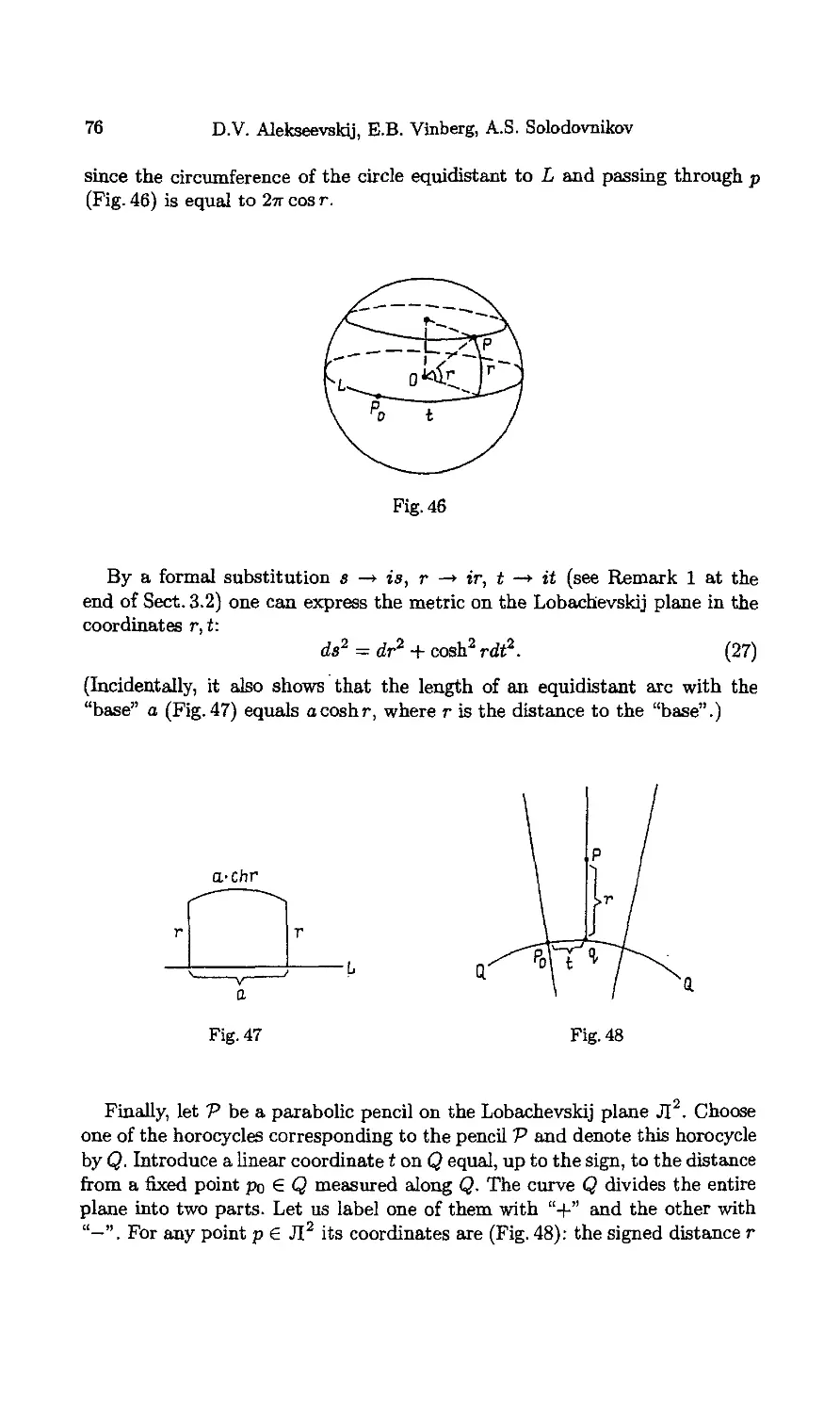
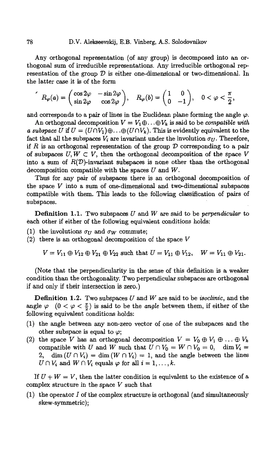
/


Автор: Alekseevskij D.V. Vinberg E.B. Solodovnikov A.S.
Теги: mathematics geometry
ISBN: 3-540-51999-8
Год: 1993

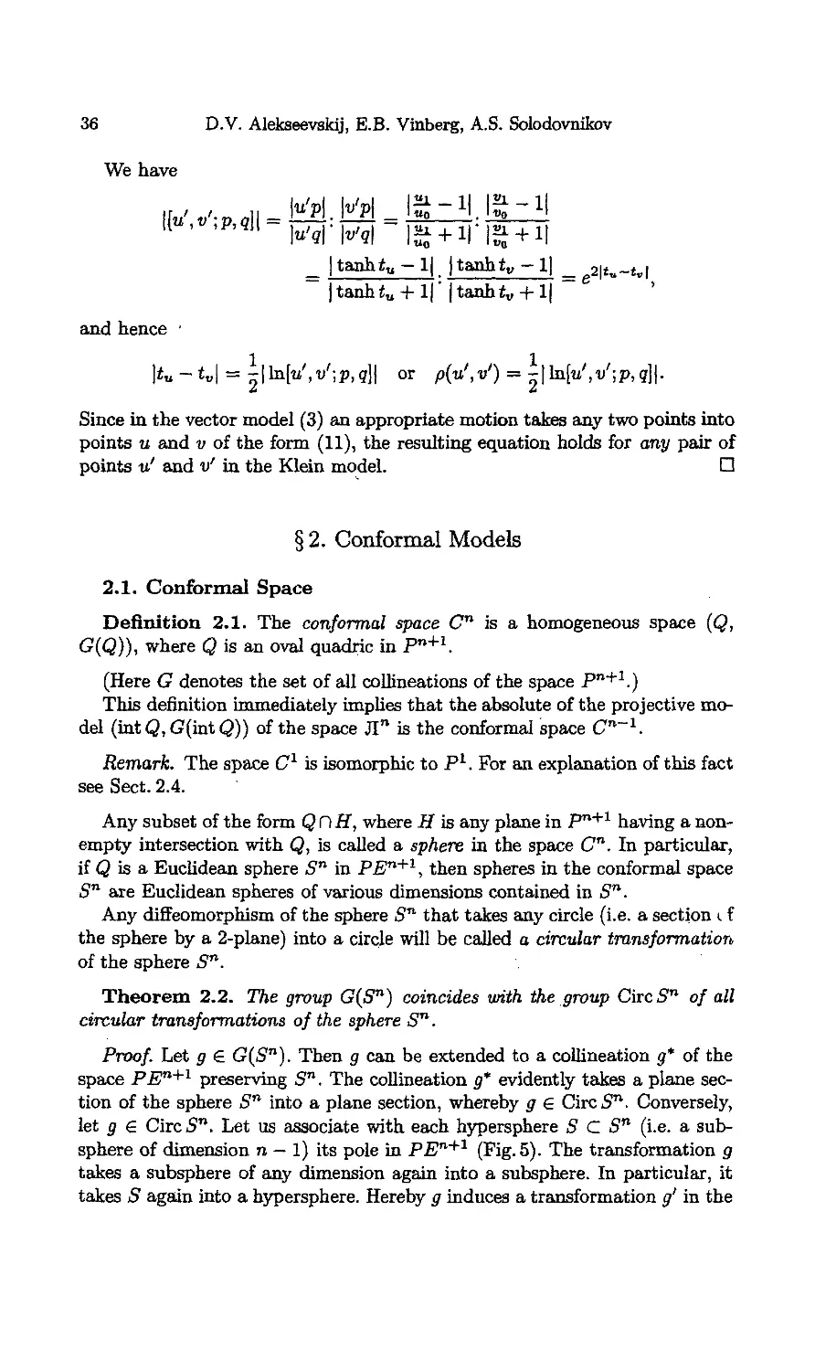
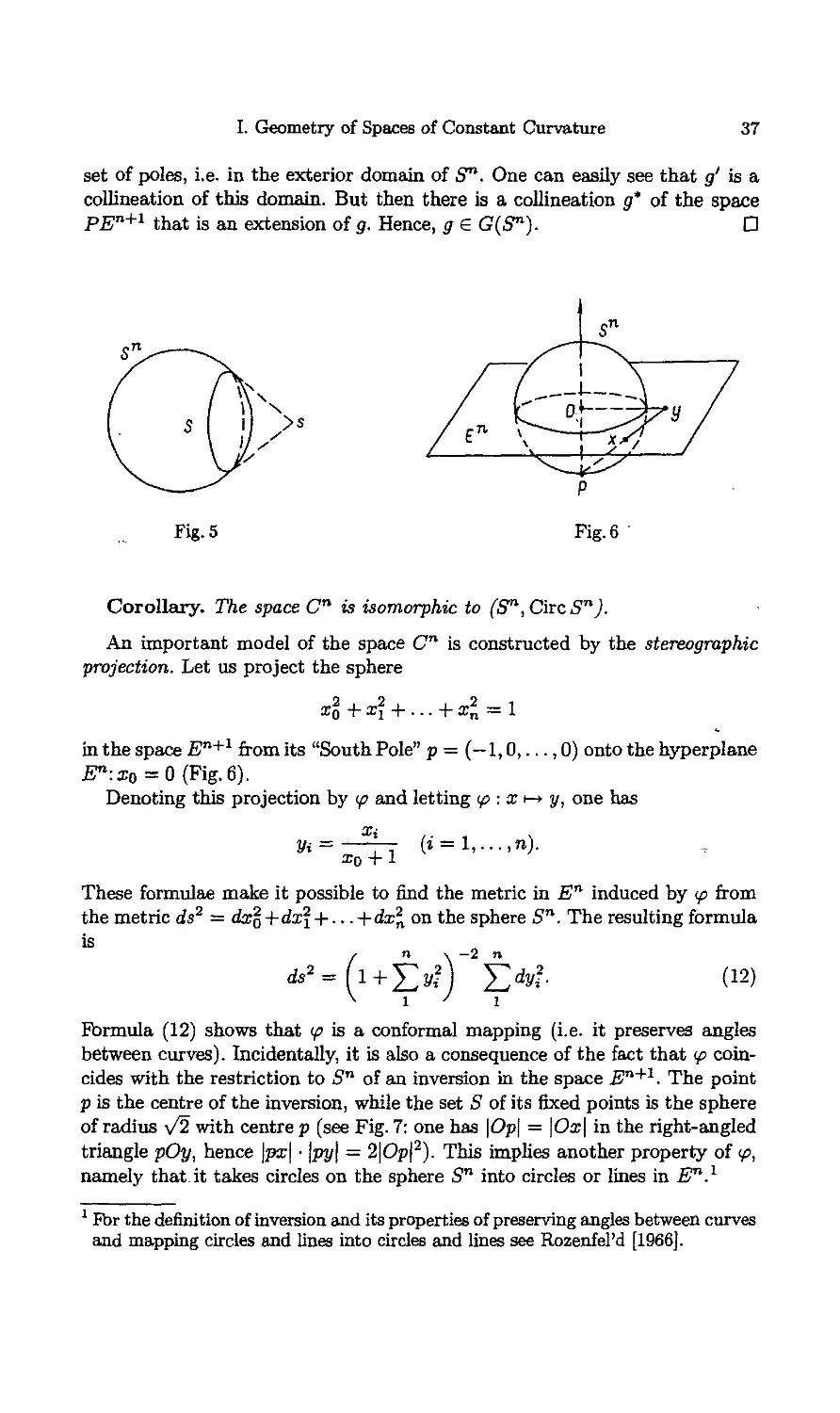
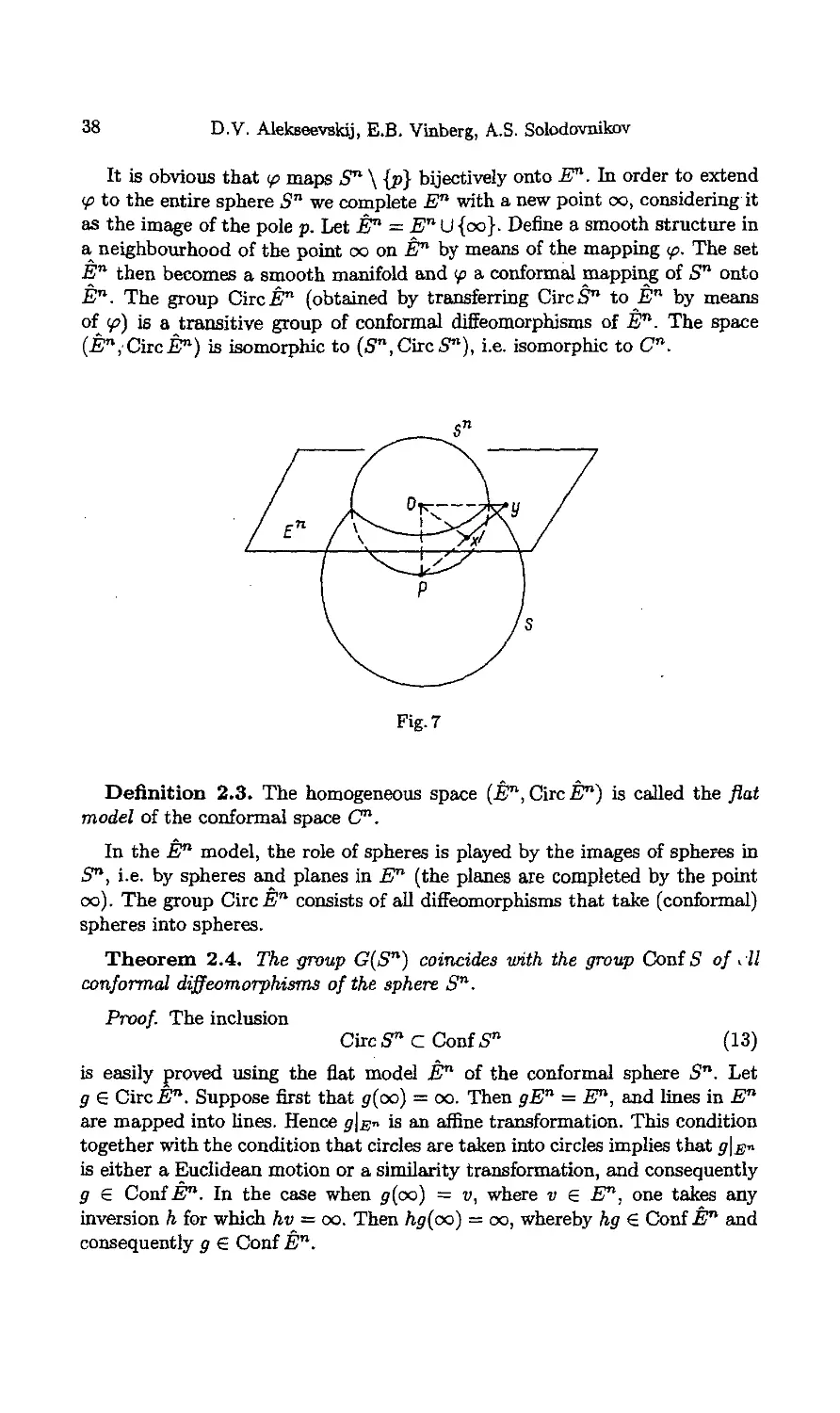
Текст
I. Geometry of Spaces
of Constant Curvature
D.V. Alekseevskij, E.B. Vinberg,
A.S. Solodovnikov
Translated from the Russian
by V. Minachin
Contents
Preface 6
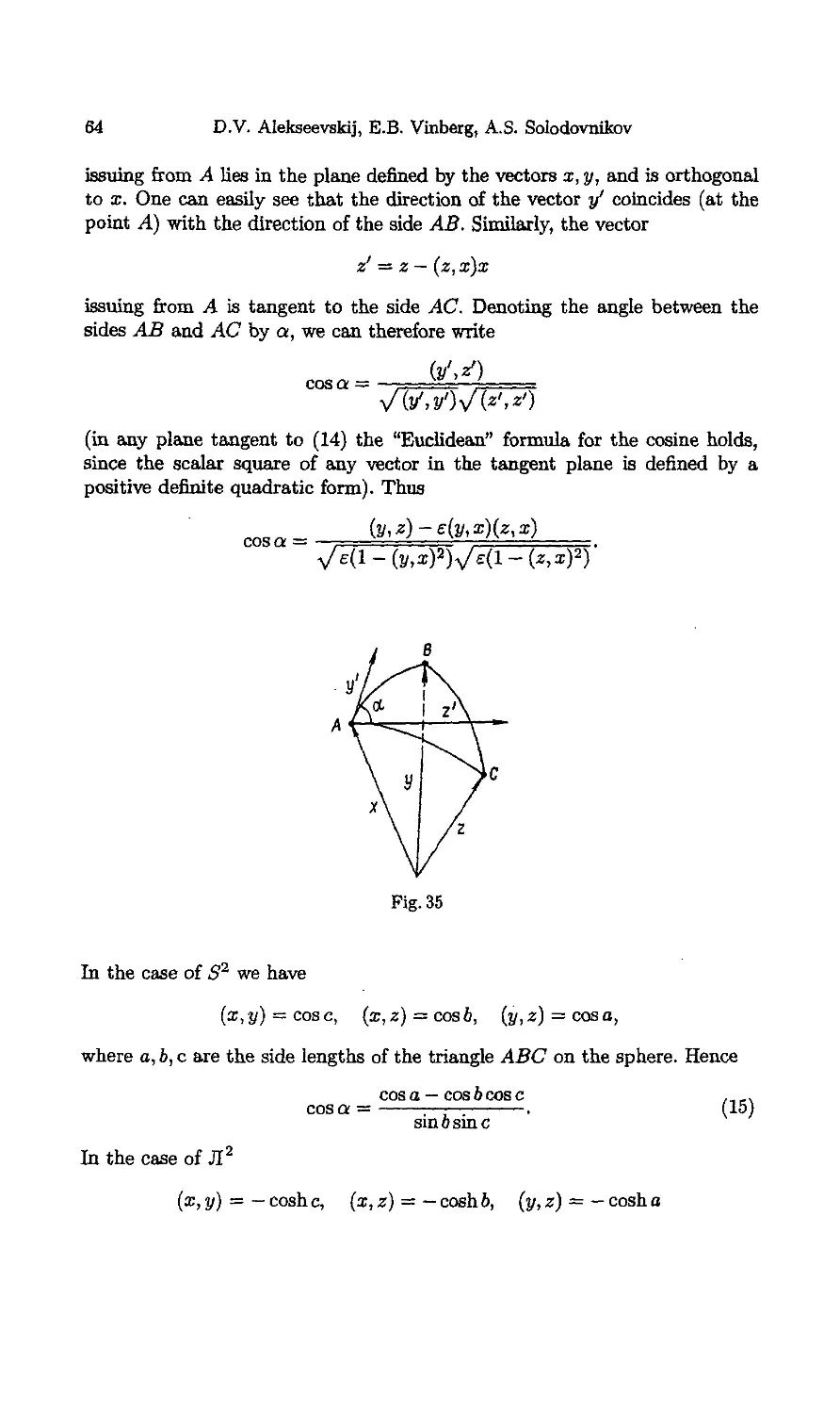
Chapter 1. Basic Structures 8
§ 1. Definition of Spaces of Constant Curvature 8
1.1. Lie Groups of Transformations 8
1.2. Groups of Motions of a Riemannian Manifold 9
1.3. Invariant Riemannian Metrics on Homogeneous Spaces 10
1.4. Spaces of Constant Curvature 11
1.5. Three Spaces 11
1.6. Subspaces of the Space R"'1 14
§ 2. The Classification Theorem 15
2.1. Statement of the Theorem 15
2.2. Reduction to Lie Algebras 16
2.3. The Symmetry 16
2.4. Structure of the Tangent Algebra of the Group of Motions . . 17
2.5. Riemann Space 19
§ 3. Subspaces and Convexity 20
3.1. Involutions 20
3.2. Planes 21
3.3. Half-Spaces and Convex Sets 23
3.4. Orthogonal Planes 24
2 D.V. Alekseevskij, E.B. Vinberg, A.S. Solodovnikov
§ 4. Metric 26
4.1. General Properties 26
4.2. Formulae for Distance in the Vector Model 26
4.3. Convexity of Distance 27
Chapter 2. Models of Lobachevskij Space 29
§ 1. Projective Models 29
1.1. Homogeneous Domains 29
1.2. Projective Model of Lobachevskij Space 29
1.3. Projective Euclidean Models. The Klein Model 31
1.4. "Affine" Subgroup of the Group of Automorphisms of a
Quadric 32
1.5. Riemannian Metric and Distance Between Points in the
Projective Model 33
§ 2. Conformal Models 36
2.1. Conformal Space 36
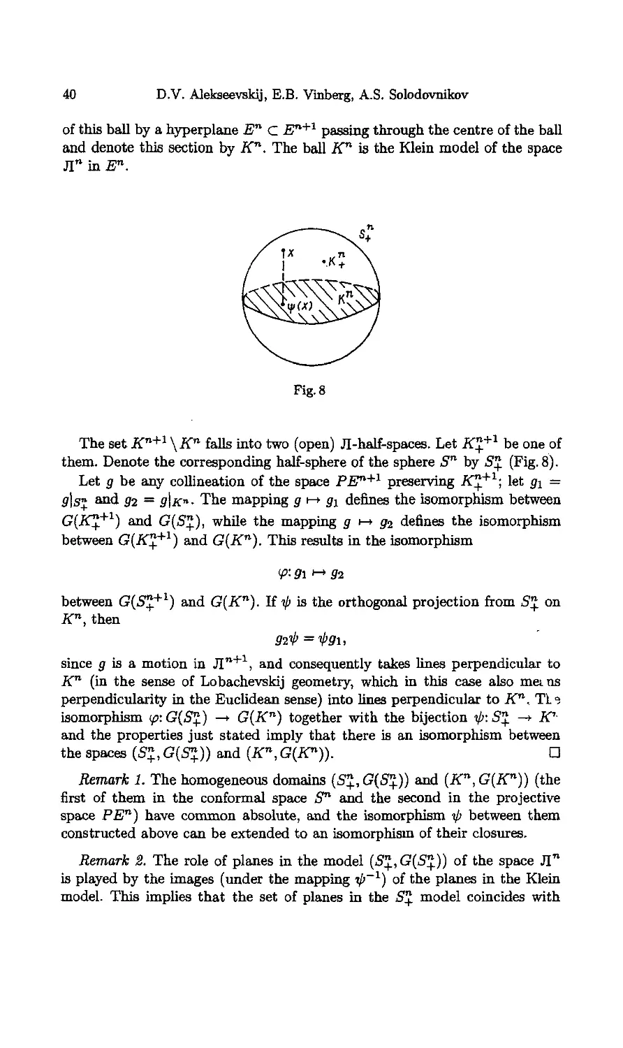
2.2. Conformal Model of the Lobachevskij Space 39
2.3. Conformal Euclidean Models 42
2.4. Complex Structure of the Lobachevskij Plane 46
§ 3. Matrix Models of the Spaces Л2 and Л3 47
3.1. Matrix Model of the Space Л2 47
3.2. Matrix Model of the Space Л3 48
Chapter 3. Plane Geometry 50
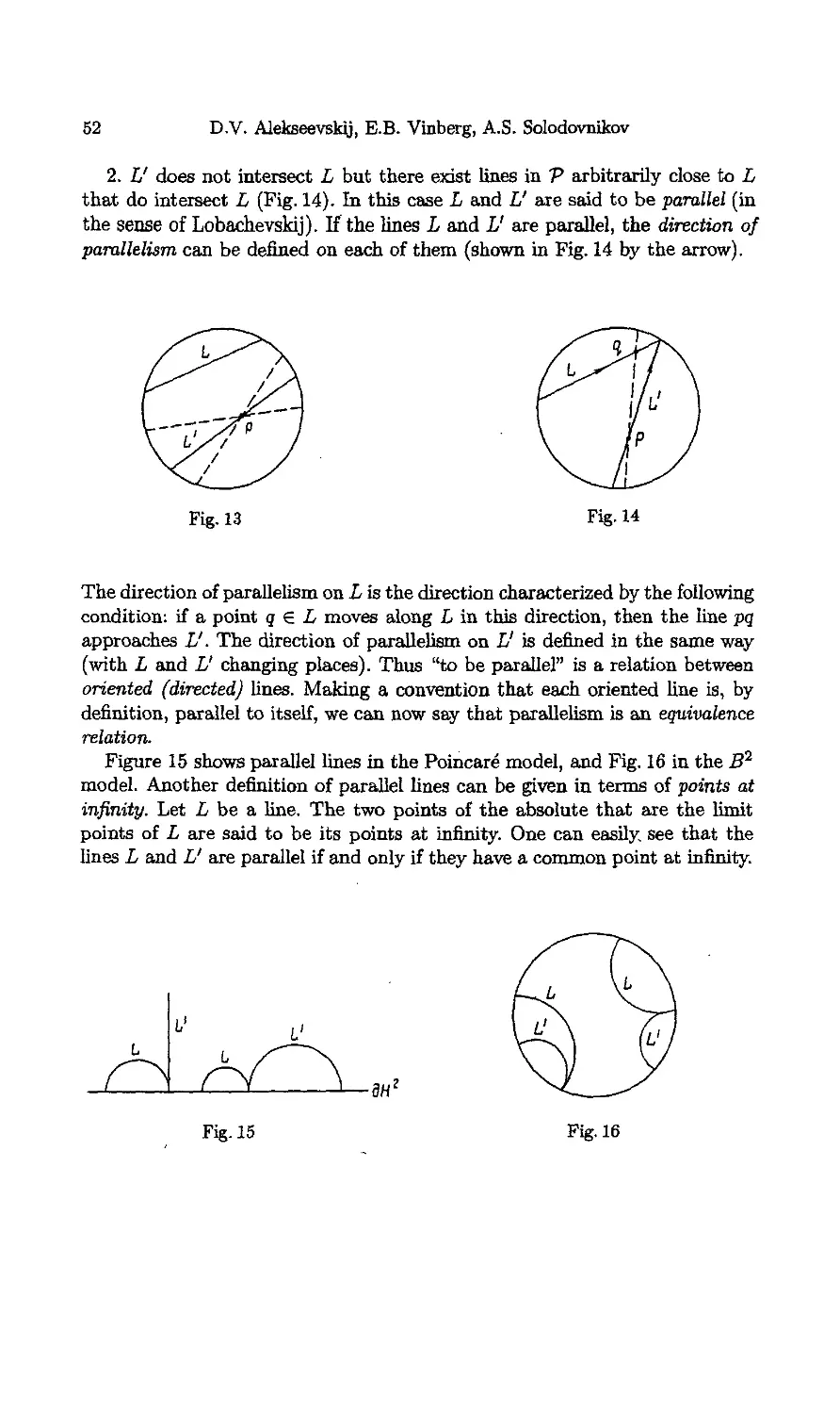
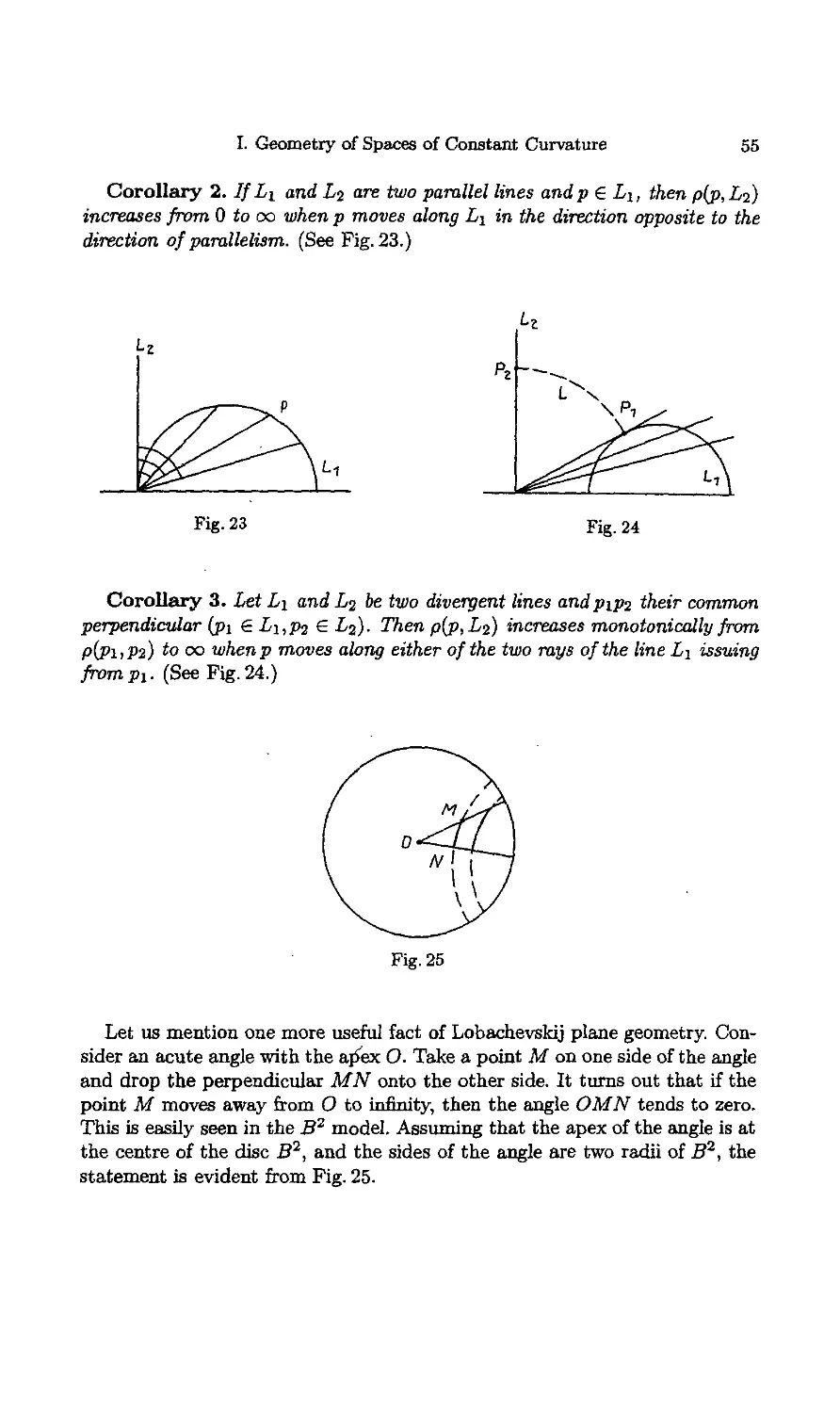
§ 1. Lines 51
1.1. Divergent and Parallel Lines on the Lobachevskij Plane .... 51
1.2. Distance Between Points of Different Lines 54
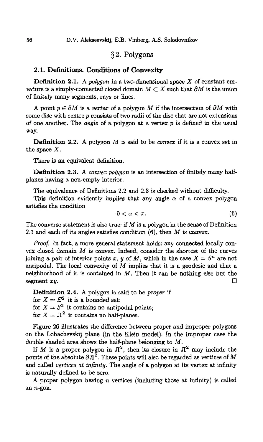
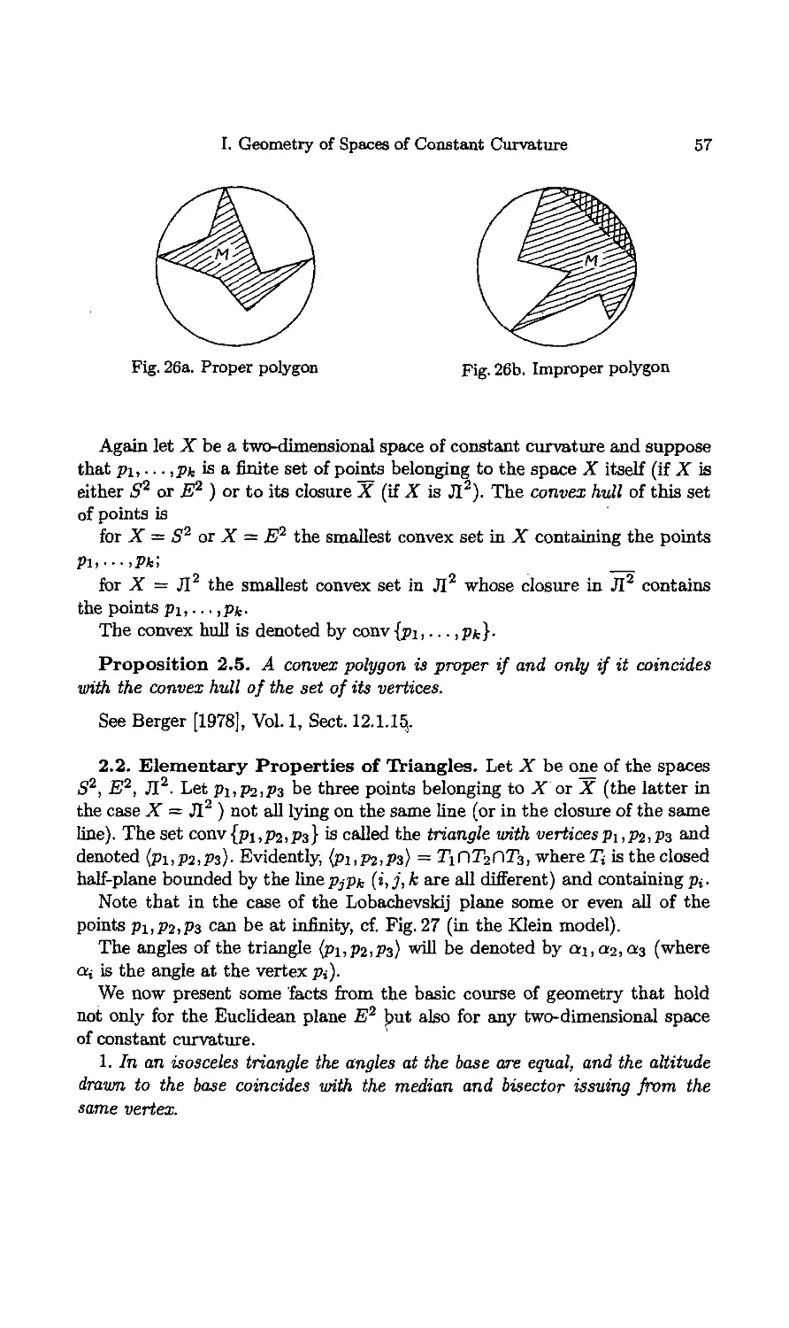
§ 2. Polygons 5*5
2.1. Definitions. Conditions of Convexity 56
2.2. Elementary Properties of Triangles 57
2.3. Polar Triangles on the Sphere 59
2.4. The Sum of the Angles in a Triangle 59
2.5. Existence of a Convex Polygon with Given Angles 60
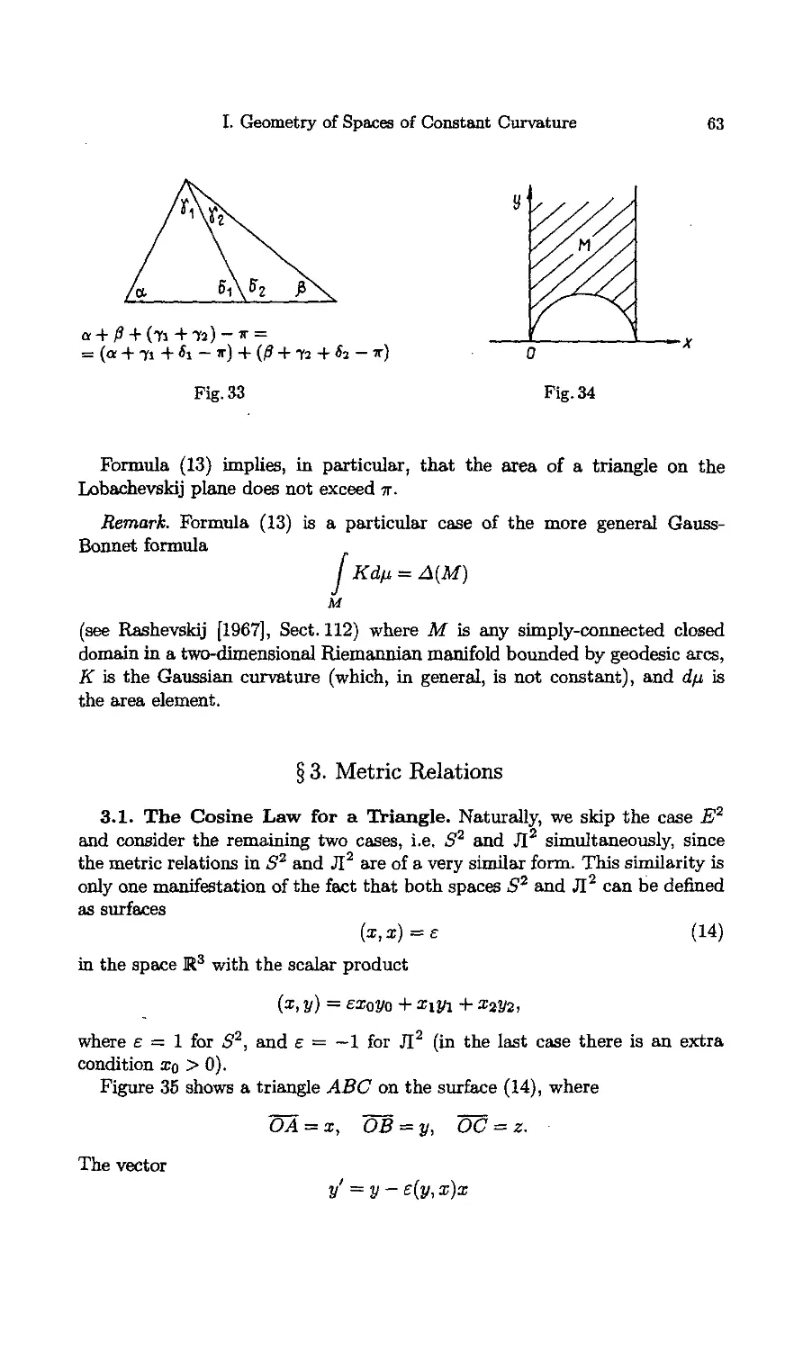
2.6. The Angular Excess and the Area of a Polygon 62
§ 3. Metric Relations 63
3.1. The Cosine Law for a Triangle 63
3.2. Other Relations in a Triangle 65
3.3. The Angle of Parallelism 67
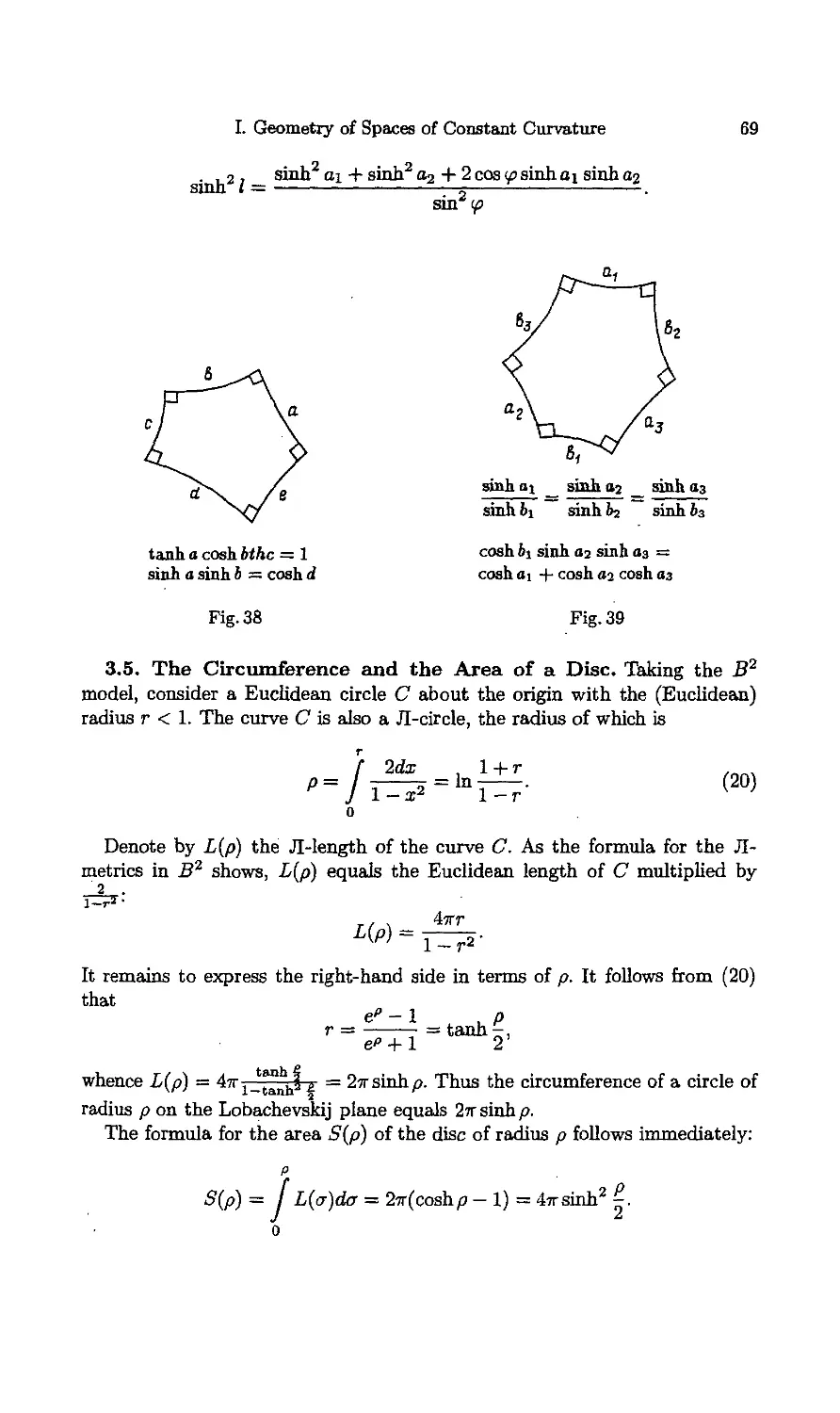
3.4. Relations in Quadrilaterals, Pentagons, and Hexagons 68
3.5. The Circumference and the Area of a Disk 69
§ 4. Motions and Homogeneous Lines 70
4.1. Classification of Motions of Two-Dimensional Spaces of
Constant Curvature 70
I. Geometry of Spaces of Constant Curvature 3
4.2. Characterization of Motions of the Lobachevskij Plane in
the Poincare Model in Terms of Traces of Matrices 71
4.3. One-Parameter Groups of Motions of the Lobachevskij
Plane and Their Orbits 72
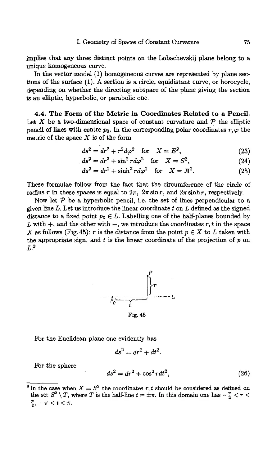
4.4. The Form of the Metric in Coordinates Related to a Pencil . 75
Chapter 4. Planes, Spheres, Horospheres and Equidistant Surfaces ... 77
§ 1. Relative Position of Planes 77
1.1. Pairs of Subspaces of a Euclidean Vector Space 77
1.2. Some General Notions 79
1.3. Pairs of Planes on the Sphere 79
1.4. Pairs of Planes in the Euclidean Space 80
1.5. Pseudo-orthogonal Transformations 80
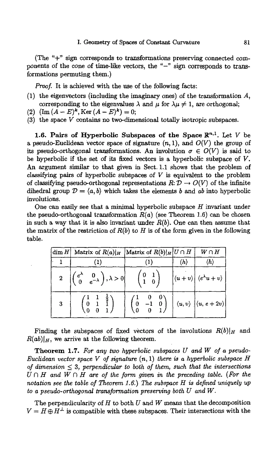
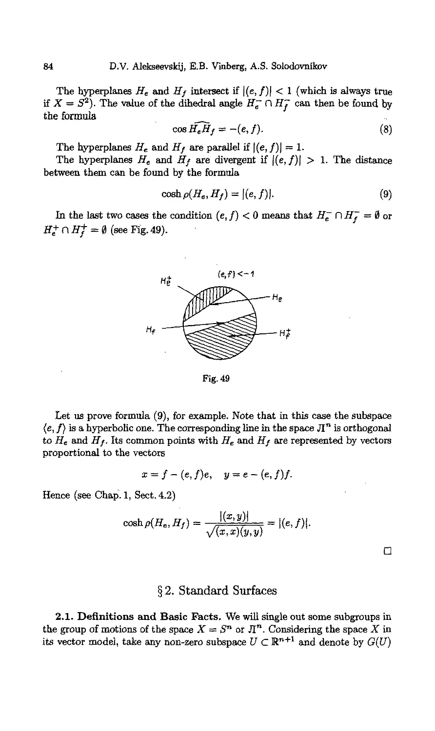
1.6. Pairs of Hyperbolic Subspaces of the Space R"'1 81
1.7. Pairs of Planes in the Lobachevskij Space 82
1.8. Pairs of Lines in the Lobachevskij Space 82
1.9. Pairs of Hyperplanes 83
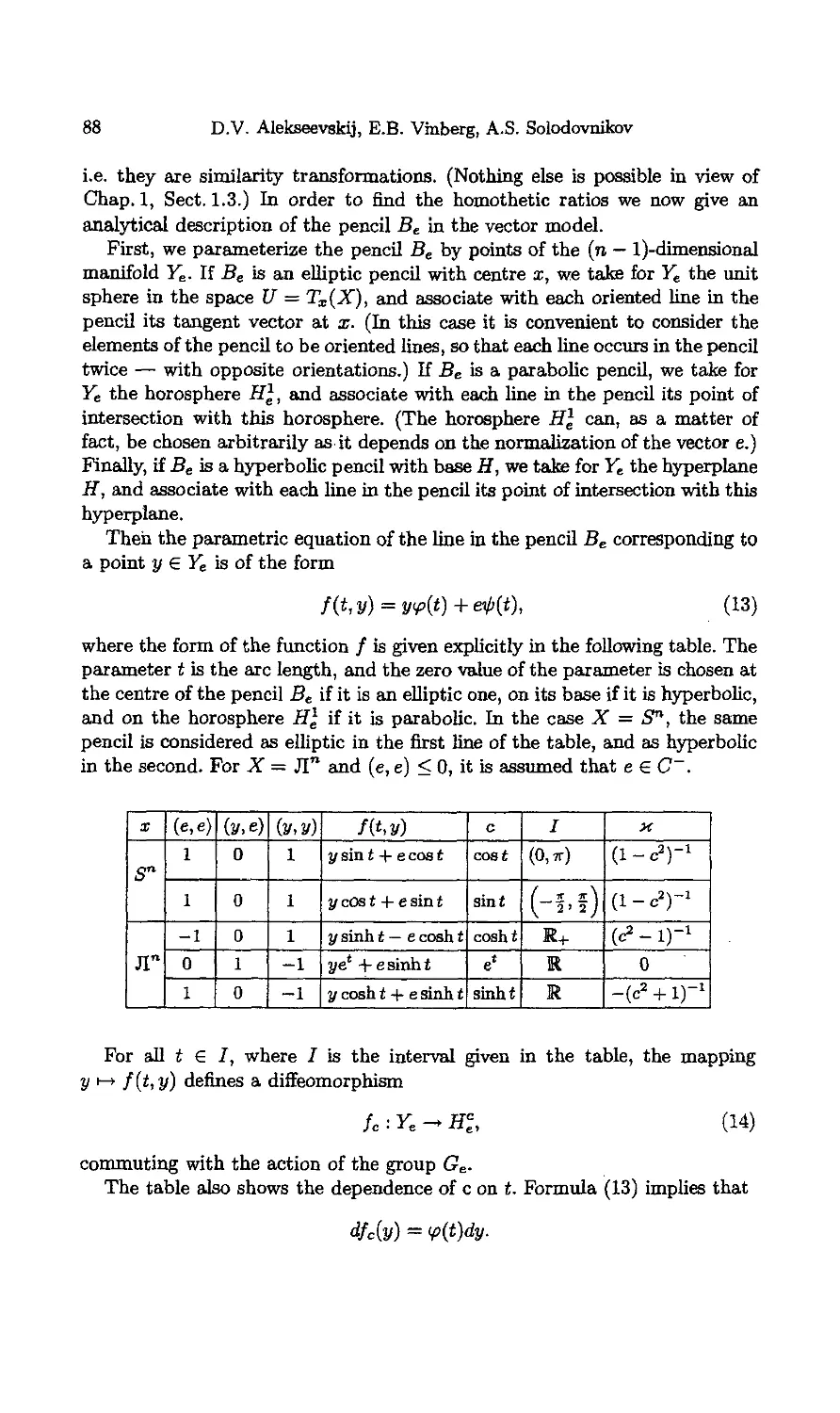
§ 2. Standard Surfaces 84
2.1. Definitions and Basic Facts 84
2.2. Standard Hypersurfaces 86
2.3. Similarity of Standard Hypersurfaces 87
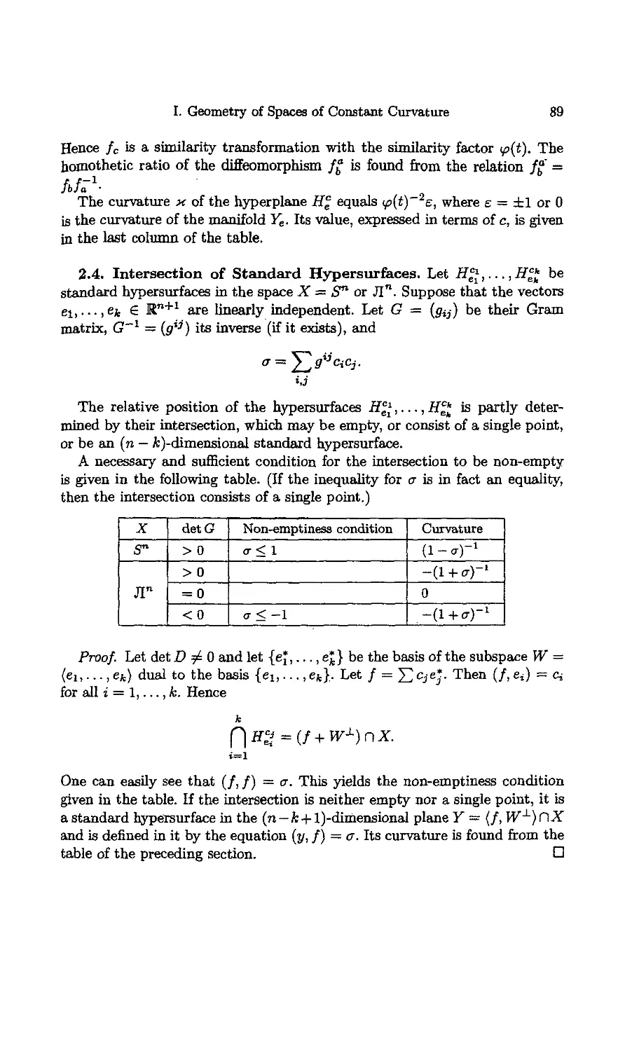
2.4. Intersection of Standard Hypersurfaces 89
§ 3. Decompositions into Semi-direct Products 90
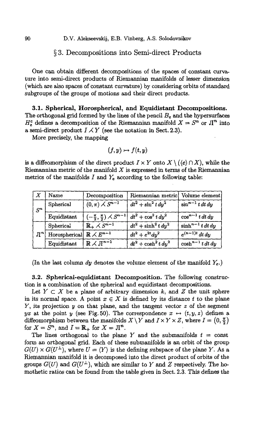
3.1. Spherical, Horospherical, and Equidistant Decompositions . . 90
3.2. Spherical-equidistant Decomposition 90
Chapter 5. Motions 92
§ 1. General Properties of Motions 92
1.1. Description of Motions 92
1.2. Continuation of a Plane Motion 92
1.3. Displacement Function 93
§ 2. Classification of Motions 94
2.1. Motions of the Sphere 94
2.2. Motions of the Euclidean Space 95
2.3. Motions of the Lobachevskij Space 95
2.4. One-parameter Groups of Motions 97
§ 3. Groups of Motions and Similarities 98
3.1. Some Basic Notions 98
3.2. Criterion for the Existence of a Fixed Point 99
3.3. Groups of Motions of the Sphere 99
3.4. Groups of Motions of the Euclidean Space 100
3.5. Groups of Similarities 101
3.6. Groups of Motions of the Lobachevskij Space 101
4 D.V. Alekseevskvj, E.B. Vinberg, A.S. Solodovnikov
Chapter 6. Acute-angled Polyhedra
§ 1. Basic Properties of Acute-angled Polyhedra
1.1. General Information on Convex Polyhedra
1.2. The Gram Matrix of a Convex Polyhedron
1.3. Acute-angled Families of Half-spaces and Acute-angled
Polyhedra
1.4. Acute-angled Polyhedra on the Sphere and in Euclidean
Space
1.5. Simplicity of Acute-angled Polyhedra
§ 2. Acute-angled Polyhedra in Lobachevskij Space
2.1. Description in Terms of Gram Matrices
2.2. Combinatorial Structure
2.3. Description in Terms of Dihedral Angles
Chapter 7. Volumes
§ 1. Volumes of Sectors and Wedges
1.1. Volumes of Sectors
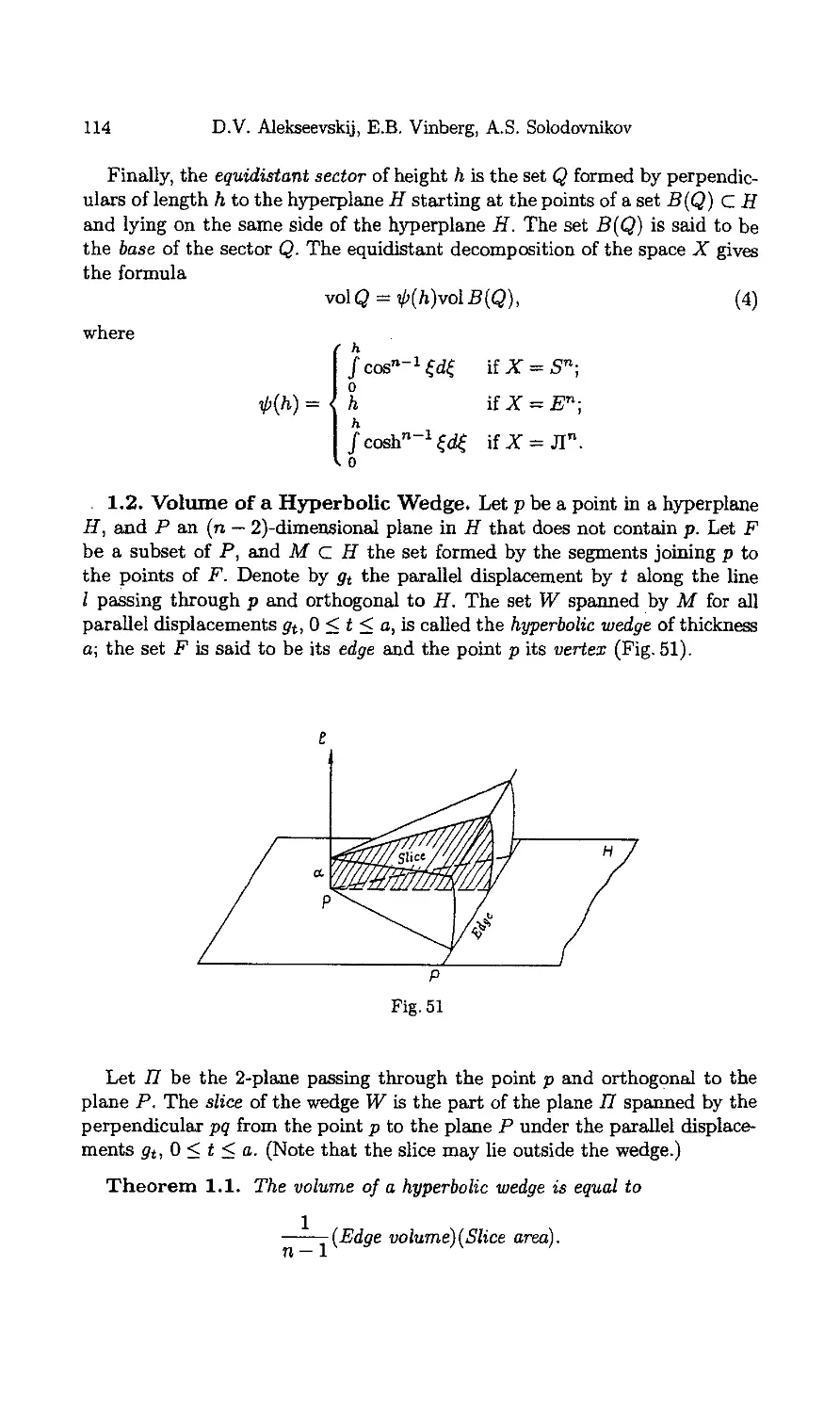
1.2. Volume of a Hyperbolic Wedge
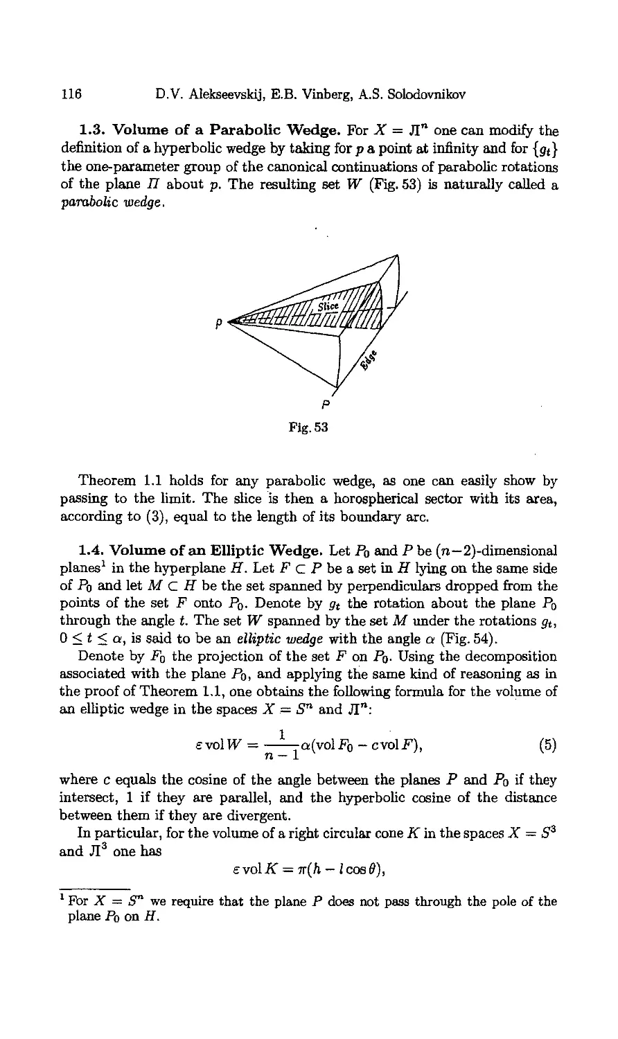
1.3. Volume of a Parabolic Wedge
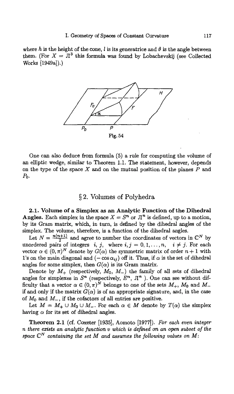
1.4. Volume of an Elliptic Wedge
§ 2. Volumes of Polyhedra
2.1. Volume of a Simplex as an Analytic Function of the
Dihedral Angles -
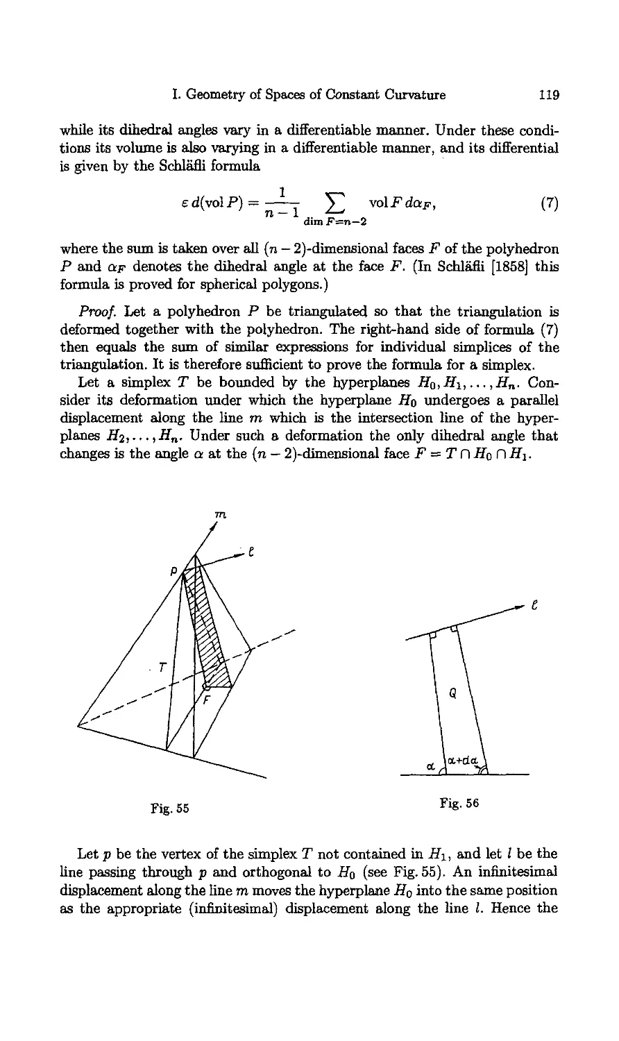
2.2. Volume Differential
2.3. Volume of an Even-dimensional Polyhedron. The Poincare
and Schlafii Formulae
2.4. Volume of an Even-dimensional Polyhedron. The
Gauss-Bonnet Formula
§ 3. Volumes of 3-dimensional Polyhedra '
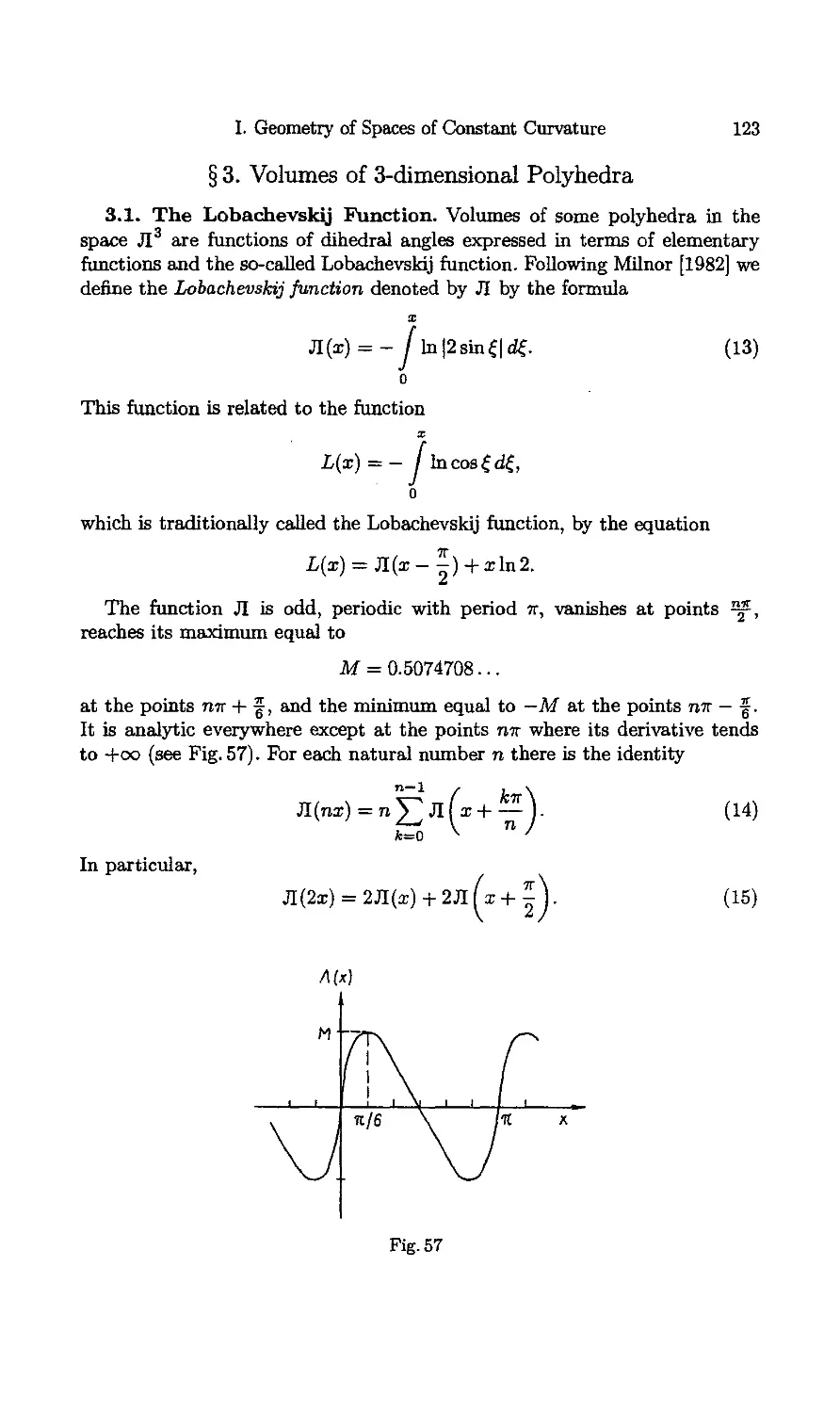
3.1. The Lobachevskij Function
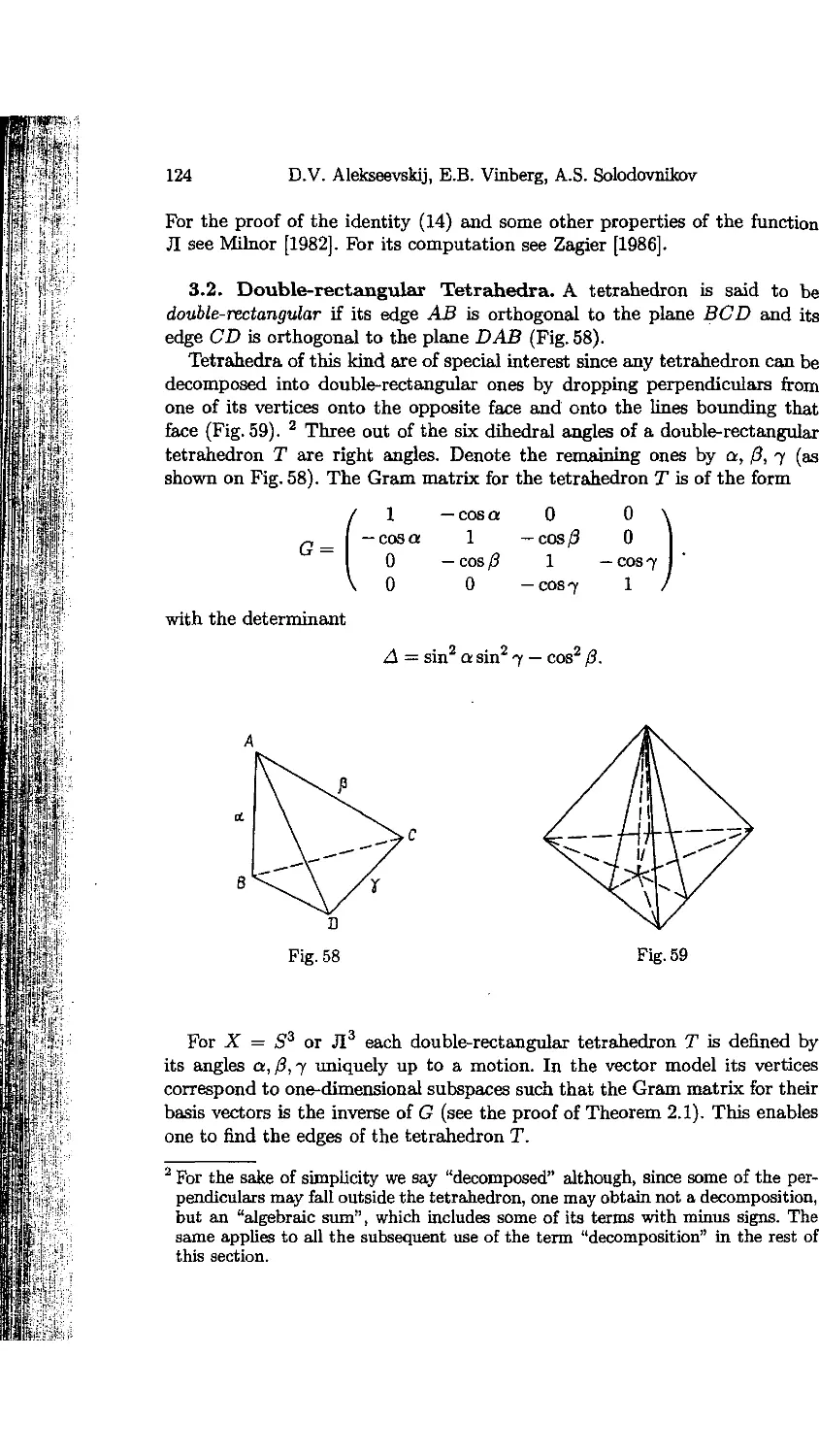
3.2. Double-rectangular Tetrahedra
3.3. Volume of a Double-rectangular Tetrahedron. The
Lobachevskij Formula
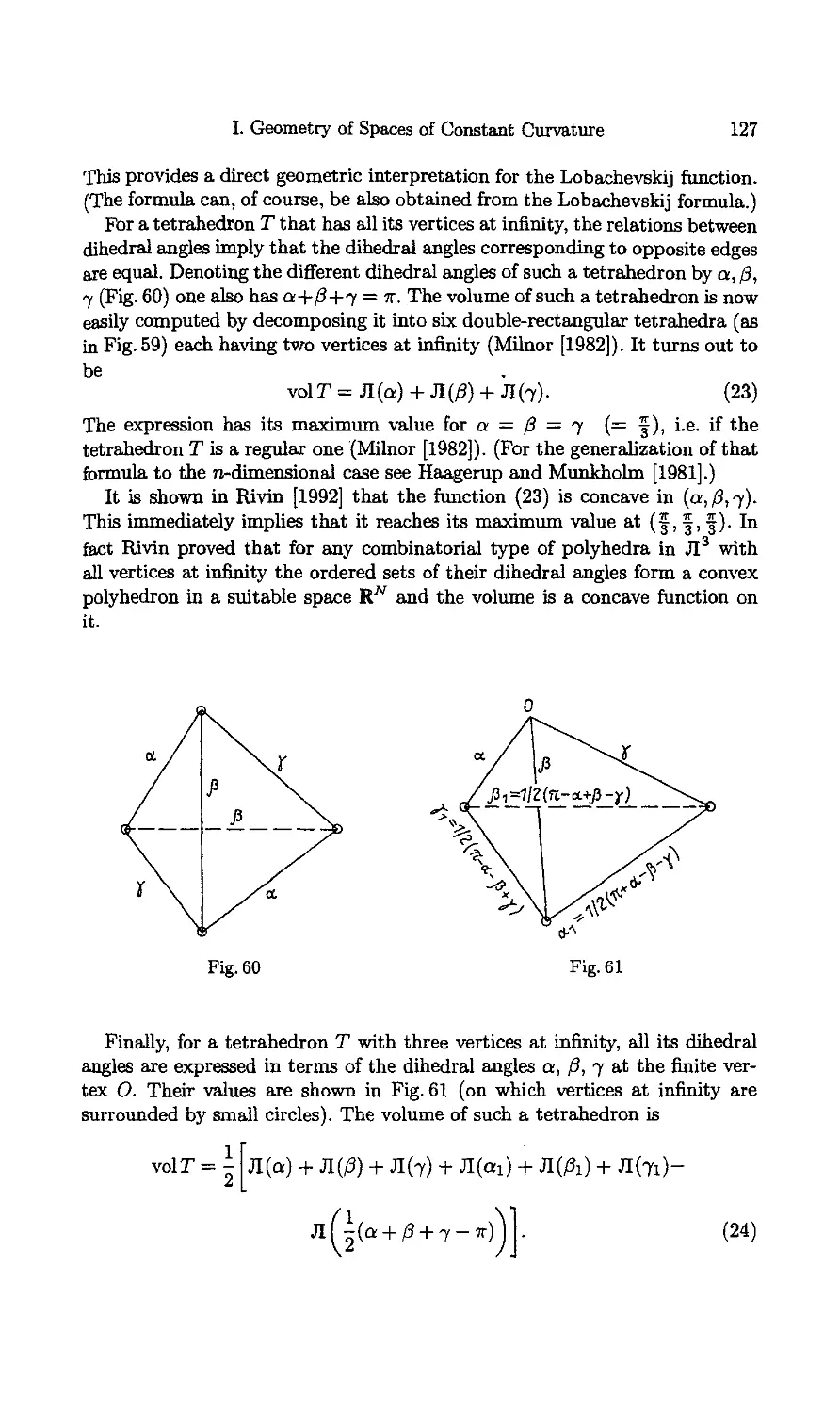
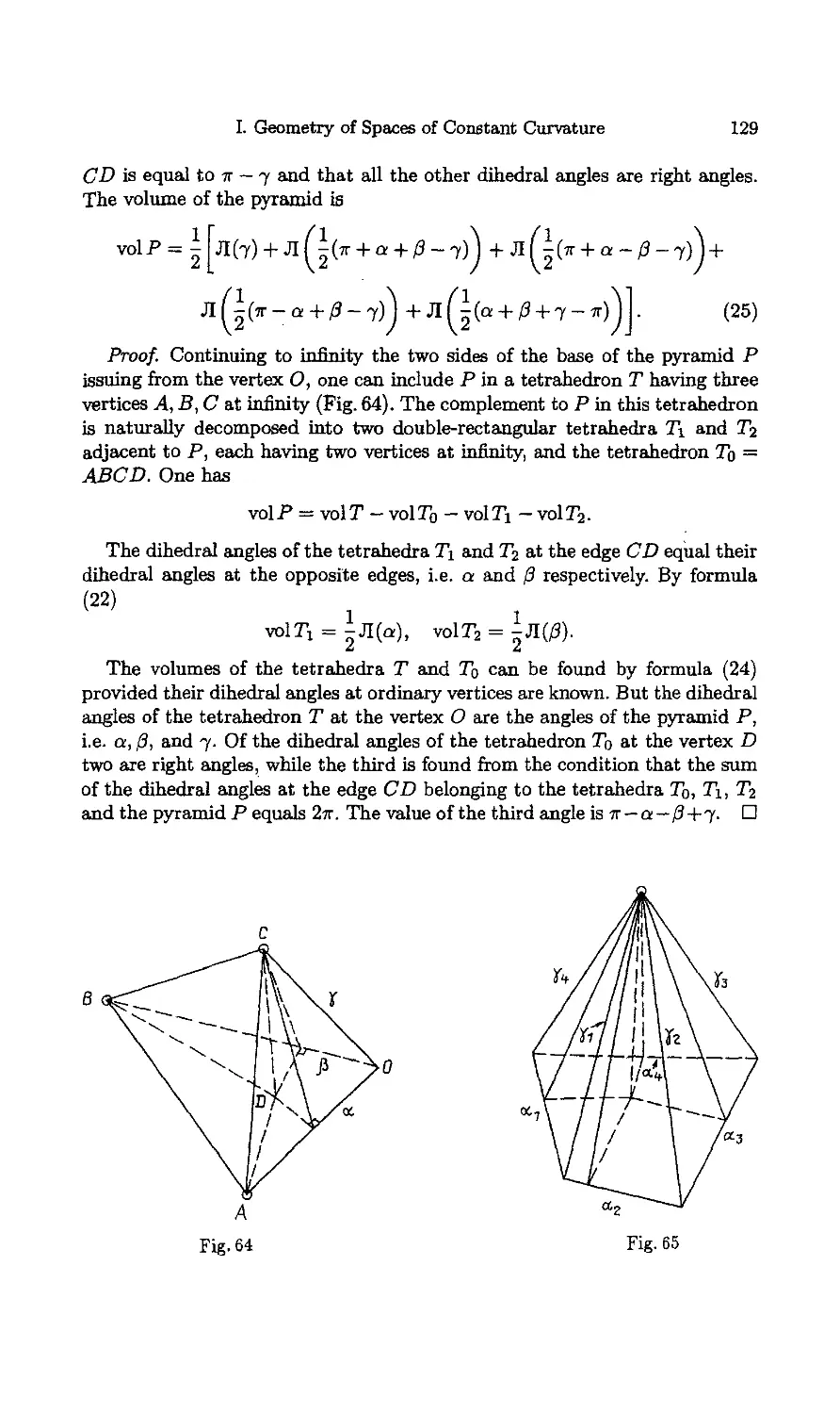
3.4. Volumes of Tetrahedra with Vertices at Infinity
3.5. Volume of a Pyramid with the Apex at Infinity
Chapter 8. Spaces of Constant Curvature as Riemannian Manifolds
1.1. Exponential Mapping
1.2. Parallel Translation
1.3. Curvature
1.4. Totally Geodesic Submanifolds
I I. Geometry of Spaces of Constant Curvature
104 I 1.5. Hypersurfaces
1 1.6. Projective Properties
104 '_ 1.7. Conformal Properties
104 з 1.8. Pseudo-Riemannian Spaces of Constant Curvature
104 ;
References
106 l
107 a
108 i
108 j
108 . I
109 |
110 1
112
113
113
114
116
116
117
117
118
120
122
123
123
124
125
126
128
130
130
131
131
132
D.V. Alekseevskij, E.B. Vinberg, A.S. Solodovnikov
Preface
Spaces of constant curvature, i.e. Euclidean space, the sphere, and Loba-
chevskij space, occupy a special place in geometry. They are most accessible to
our geometric intuition, making it possible to develop elementary geometry
in a way very similar to that used to create the geometry we learned at
school. However, since its basic notions can be interpreted in different ways,
this geometry can be applied to objects other than the conventional physical
space, the original source of our geometric intuition.
Euclidean geometry has for a long time been deeply rooted in the human
mind. The same is true of spherical geometry, since a sphere can naturally be
embedded into a Euclidean space. Lobachevskij geometry, which in the first
fifty years after its discovery had been regarded only as a logically feasible
by-product appearing in the investigation of the foundations of geometry, has
even now, despite the fact that it has found its use in numerous applications,
preserved a kind of exotic and even romantic element. This may probably be
explained by the permanent cultural and historical impact which the proof of
the independence of the Fifth Postulate had on human thought.
Nowadays modern research trends call for much more businesslike use of
Lobachevskij geometry. The traditional way of introducing Lobachevskij ge-
geometry, based on a kind of Euclid-Hilbert axiomatics, is ill suited for this
purpose because it does not enable one to introduce the necessary analytical
tools from the very beginning. On the other hand, introducing Lobachevskij
geometry starting with some specific model also leads to inconveniences since
different problems require different models. The most reasonable approach
should, in our view, start with an axiomatic definition, but it should be based
on a well-advanced system of notions and make it possible either to refer to
any model or do without any model at all.
Their name itself provides the description of the property by which spaces
of constant curvature are singled out among Riemannian manifolds. However,
another characteristic property is more important and natural for them — the
property of maximum mobility. This is the property on which our exposition
is based.
The reader should realize that our use of the term "space of constant cur-
curvature" does not quite coincide with the conventional one. Usually one under-
understands it as describing any Riemannian manifold of constant curvature. Under
our definition (see Chap. 1, Sect. 1) any space of constant curvature turns out
to be one of the three spaces listed at the beginning of the Preface.
Although Euclidean space is, of course, included in our exposition as a
special case, we have no intention of introducing the reader to Euclidean
geometry. On the contrary, we make free use of its basic facts and theorems.
We also assume that the reader is familiar with the basics of linear algebra
and affine geometry, the notion of a smooth manifold and Lie group, and the
elements of Riemannian geometry.
I. Geometry of Spaces of Constant Curvature
For the history of non-Euclidean geometry and the development
the reader is referred to relevant chapters in the books of Klein [19
[1949, 1956], Coxeter [1957], and Efimov [1978].
D.V. AlekseevsHj, E.B. Vinberg, A.S. Solodovnikov
Chapter 1
Basic Structures
§ 1. Definition of Spaces of Constant Curvature
This chapter provides the definition of spaces of constant curvature and of
their basic structures, and describes their place among homogeneous spaces
on the one hand and Riemannian manifolds on the other. If the reader's main
aim is just to study Lobachevskij geometry, no great damage will be done if
he skips Theorems 1.2 and 1.3 and the proof of Theorem 2.1.
1.1. Lie Groups of Transformations. We assume that the reader is
familiar with the notions of a (real) smooth manifold and of a (real) Lie
group. The word "smooth" (manifold, function, map etc.) always means that
the corresponding structure is C°°. All smooth manifolds are assumed to have
a countable base of open subsets. By TX{X) we denote the tangent space to a
manifold X at a point x, and by dxg the differential of the map g at a point
x. If no indication of the point is necessary the subscript is omitted.
We now recall some basic definitions of Lie group theory. (For more details
see, e.g. Vinberg and Onishchik [1988].)
A group G of transformations1 of a smooth manifold X endowed with a Lie
group structure is said to be a Lie group of transformations of the manifold
X if the map
GxX-+X, (g, x) к-> gx,
is smooth, which means that the (local) coordinates of the point gx are smooth
functions of the coordinates of the element g and the point x. Then the sta-
stabilizer
Gx = {g ? G: gx = x}
of any point islisa (closed) Lie subgroup of the group G. Its linea-
representation g i-* dxg in the space Tx (X) is called the isotropy representation
and the linear group dxGx is called the isotropy group at the point x.
The stabilizers of equivalent points x and у = gx (g € (?) are conjugate
in G, i.e.
Gy = gG^g-1.
The corresponding isotropy groups are related in the following way:
= (dxg)(dxGx)(dx9y1.
In other words, if tangent spaces TX(X) and Ty(Y) are identified by the iso-
isomorphism dxg, then the group dxGx coincides with the group dyGy.
1 By a group of transformations we understand an effective group of transformations,
i.e. we assume that different transformations correspond to different elements of
the group.
I. Geometry of Spaces of Constant Curvature 9
If G is a transitive Lie group of transformations of a manifold X, then for
each point x € X the map
G/Gx — X, gGx <-* gx
is a diffeomorphism commuting with the action of the group G. (The group
G acts on the manifold G/Gx of left cosets by left shifts.) In this case the
manifold X together with the action of G on it can be reconstructed from the
pair (G, Gx).
Definition 1.1. A smooth manifold X together with a given transitive
Lie group G of its transformations is said to be a homogeneous space.
We denote a homogeneous space by (X, G), or simply X.
A homogeneous space (X, G) is said to be connected or simply-connected2
if the manifold X has this property.
1.2. Group of Motions of a Riemannian Manifold. A Riemanniari
metric is said to be defined on a smooth manifold X if a Euclidean metric is
defined in each tangent space TX(X), and if the coefficients of this metric are
smooth functions in the coordinates of x. A diffeomorphism g of a Riemannian
manifold X is called a motion (or an isometry) if for each point x ? X the
linear map
dxg : TX{X) - Tgx(X)
is an isometry. The set of all motions is evidently a group.
Each motion g takes a geodesic into a geodesic, and therefore commutes
with the exponential map, i.e.
for all ? € T(X). Hence each motion g of a connected manifold X is uniquely
defined by the image gx of some point x € X and the differential dxg at that
point. This enables us to introduce coordinates into the group of motions,
turning it into a Lie group. To be more precise, the following theorem holds.
Theorem 1.2 (Kobayashi and Nomizu [1981]). The group of motions of a
Riemannian manifold X is uniquely endowed with a differentiable structure,
which turns it into a Lie group of transformations of the manifold X.
If the group of motions of a Riemannian manifold X is transitive, then X
is complete. Indeed, in this case there exists e > 0, which does not depend
on x, such that for any point x € X and for any direction at that point there
exists a geodesic segment of length e issuing from x in that direction. This
implies that each geodesic can be continued indefinitely in any direction.
A Riemannian manifold X is said to have constant curvature с if at each
point its sectional curvature along any plane section equals с
' We assume that any simply-connected space is, by definition, connected.
10 D.V. Alekeeevskij, E.B. Vinberg, A.S. Solodovnikov
Simply-connected complete Riemannian manifolds of constant curvature
admit a convenient characterization in terms of the group of motions.
Theorem 1,3 (Wolf [1972]). A simply-connected complete Riemannian
manifold is of constant curvature if and only if for any pair of points x, у 6 X
and for any isometry <p : TX(X) —> Ty(X) there exists a (unique) motion g
such that gx = у and dxg = tp.
The first part of the statement follows immediately from the fact that
motions preserve curvature and that any given two-dimensional subspace of
the space TX(X) can, by an appropriate isometry, be taken into any given
two-dimensional subspace of the space TV(X). For the proof of the converse
statement see Chap. 8, Sect. 1.3.
1.3. Invariant Riemannian Metrics on Homogeneous Spaces. Let
(X, G) be a homogeneous space. A Riemannian metric on X is said to be
invariant (with respect to (?) if all transformations in G are motions with
respect to that metric. An invariant Riemannian metric can be reconstructed
from the Euclidean metric it defines on any tangent space TX(X). This Eu-
Euclidean metric is invariant under the isotropy group dxGx. Conversely, if a
Euclidean metric is defined in the space TX(X) and is invariant under the
isotropy group, then it can be moved around by the action of the group G
thus yielding an invariant Riemannian metric on X. Thus, an invariant Rie-
Riemannian metric on X exists if and only if there is a Euclidean metric in the
tangent space invariant under the isotropy group.
We now consider the question of when such a metric is unique.
A linear group H acting in a vector space V is said to be irreducible if
there is no non-trivial subspace U CV invariant under H.
Lemma 1.4. Let H be a linear group acting in a real vector space V.' If
H is irreducible, then up to a (positive) scalar multiple there is at most one
Euclidean metric in the space V invariant under H.
Proof. Consider any invariant Euclidean metric (if such a metric exists,
turning V into a Euclidean space. Then each invariant Euclidean metric q
on У is of the form q(x) = (Ax,x), where A is a positive definite symmetric
operator commuting with all operators in H. Let с be any eigenvalue of A. The
corresponding eigenspace is invariant under H, and consequently coincides
with V. This implies that A = cE, i.e. q(x) = c(x,x). О
The Lemma implies that if the isotropy group of a homogeneous space is
irreducible, then there exists, up to a (positive) scalar multiple, at most one
invariant Riemannian metric.
If a homogeneous space X is connected and admits an invariant Riemannian
metric, then the isotropy representation is faithful at each point x € X, since
each element of the stabilizer of x, being a motion, is uniquely defined by its
differential at that point.
I. Geometry of Spaces of Constant Curvature 11
1.4. Spaces of Constant Curvature
Definition 1.5. A simply-connected homogeneous space is said to be a
space of constant curvature if its isotropy group (at each point) is the group
of all orthogonal transformations with respect to some Euclidean metric.
The last condition is called the maximum mobility axiom. For the possibil-
possibility of giving up the condition that the space is simply connected see Sect. 2.5.
Let (X, G) be a space of constant curvature. The maximum mobility axiom
immediately implies that there is a unique (up to a scalar multiple) invariant
Riemannian metric on X. With respect to this metric X is a Riemannian
manifold of constant curvature (the trivial part of Theorem 1.3). The fact that
G is a transitive group implies that X is a complete Riemannian manifold.
Note also that G is the group of all its motions. Indeed, for each motion g and
for each point x € X, there exist an element g\ € G such that gx = g\X, i.e.
(gilg)x = x, and an element рг € Gx such that dx(g^ 1p) = dxg2- But then
9гг9 = 92 and g = g-^92 € G.
Conversely, by Theorem 1.3, any simply-connected complete Riemannian
manifold X of constant curvature satisfies the conditions of Definition 1.5 if
one takes for G the group of all its motions.
Thus, spaces of constant curvature (in the sense of the above definition)
are simply-connected complete Riemannian manifolds of constant curvature
considered up to change of scale, which explains their name. However, below
in presenting the geometry of these spaces the fact that they are of constant
Riemannian curvature is never used directly, and it is quite sufficient for the
reader to be familiar with the simplest facts of Riemannian geometry (in-
(including the notion of a geodesic but excluding that of parallel translation or
curvature).
Let (X, G) be a space of constant curvature. Since the manifold X is simply-
connected, firstly it is orientable, and secondly each connected component of
the group G contains exactly one connected component of the stabilizer (of
each point). Since the isotropy representation is faithful, the stabilizer is iso-
morphic to the orthogonal group. The orthogonal group consists of two con-
connected components, one including all orthogonal transformations with deter-
determinant 1, the other including all orthogonal transformations with determinant
—1. Hence the group of motions of a space of constant curvature consists of
two connected components, one of which includes all the motions preserving
orientation (proper motions) and the other includes all motions reversing it
(improper motions).
1.5. Three Spaces. For each n > 2 there are at least three n-dimensional
spaces of constant curvature.
1. Euclidean Space En. Denoting the coordinates in the space R" by
Xi,..., xn> we define the scalar product by the formula
12 D.V. Alekseevskij, E.B. Vinberg, A.S. Solodovnikov
(x,y) = Х1У1 + ... + xnyn,
thus turning Rn into a Euclidean vector space.
Let
X = Rn, G = Tn X On (semidirect product),
where Tn is the group of parallel translations (isomorphic to Rn) and On is
the group of orthogonal transformations of Rn.
For any parallel translation ta along a vector о € Rn and any orthogonal
transformation tp 6 On one has
<ptaip~l = tv(a),
which shows that G is indeed a group. Evidently, G acts transitively on X.
For each x € X the tangent space TX(X) is naturally identified with the
space Kn. The isotropy group then coincides with the group On.
Thus (X, G) is a space of constant curvature. It is called the n-dimensional
Euclidean space, and denoted by ЕГ1.
The Riemannian metric on the space E™ is induced by the Euclidean metric
on the space Rn, i.e. it is of the form
ds2 = dxl + ... + dx2n.
Its curvature is 0.
2. Sphere Sn. Denoting the coordinates in the space Rn+1 by x0, xi,..., xn,
we introduce a scalar product in Mn+1 by the formula
(x, у) = Ж02/0 + Xiyi + ...
which turns Mn+1 into a Euclidean vector space.
Let
For each x € X the tangent space TX(X) is naturally identified witi the
orthogonal complement to the vector x in the space Rn+1. If {ei,..., en} ib an
orthonormal basis in the space TX{X), then {x, ei,..., en} is an orthonormal
basis in the space Mn+1.
Since each orthonormal basis in the space Rn+1 can, by an appropriate or-
orthogonal transformation, be taken into any other orthonormal basis, the group
G acts transitively on X, and the isotropy group at each point x coincides
with the group of all orthogonal transformations of the space TX(X).
For n > 2 the manifold X is simply-connected and hence (X, G) is a space
of constant curvature. It is called the n-dimensional sphere and denoted by
Sn.
The Riemannian metric on the space Sn is induced by the Euclidean metric
on Mn+1, i.e. it is of the form
ds2 = dxl + dxl + ¦ ¦ ¦ +
I. Geometry of Spaces of Constant Curvature 13
(Remember that the coordinate functions Xo, x\,..., xn are not independent
on Sn.) The curvature of this metric is 1.
3. Lobachevskij Space JI". Denoting the coordinates in the space Rn+1 by
xo,xi,... ,xn, we introduce a scalar product in Rn+1 by the formula
(x, у) = -ХоУо + XiV! + ... + Xnyn,
which turns Rn+1 into a pseudo-Euclidean vector space, denoted by R™'1.
Each pseudo-orthogonal (i.e. preserving the above scalar product) trans-
transformation of Rn>1 takes an open cone of time-like vectors
consisting of two connected components
C+ = {x € С : xo > 0}, С = {x 6 С : xQ < 0}
onto itself.
Denote by On,i the group of all pseudo-orthogonal transformations of the
space Kn>1, and by O'nl its subgroup of index 2 consisting of those pseudo-
orthogonal transformations which map each connected component of the cone
С onto itself. Let
X = {x € K"'1 : -xl + x\ + ... +x2n = -l,z0 > 0}, G = <Уп>1.
A basis {eo,ei,..., en} is said to be orthonormal if (eo, e0) = —1, (e*,ej) =
1 for i ф 0 and (ei, ej) = 0 for г ф j. For example, the standard basis is
orthonormal.
For any x & X the tangent space TX(X) is naturally identified with the
orthogonal complement of the vector x in the space Rn>1, which is an n-
dimensional Euclidean space (with respect to the same scalar product). If
{ei,..., en} is an orthonormal basis in it, then {x, ei,..., en} is an orthonor-
orthonormal basis in the space Rn>1. It follows then (in the same way as for the sphere)
that the group G acts transitively on X and the isotropy group coincides with
the group of all orthogonal transformations of the tangent space.
The manifold X has a diffeomorphic projection onto the subspace Xq =
0, and is therefore simply-connected. Hence (X, G) is a space of constant
curvature. It is called the n-dimensional Lobachevskij space (or hyperbolic
space) and denoted by JI™.
The Riemannian metric on the space JIn is induced by the pseudo-
Euclidean metric on the space R™'1, i.e. it is of the form
ds2 = -dx2, + dxl + ... + dx^.
Its curvature is —1.
Remark 1. For the sake of uniformity the procedure of embedding in Rn+1
can also be applied to the Euclidean space En. Its motions are then induced
14 D.V. Alekseevsldj, E.B. Vinberg, A.S. Solodovnikov
by linear transformations in the following way. Let xo,xi,...,xn be coordi-
coordinates in R™+1, and let En С Rn+1 be the subspace defined by the equation
Xo = 0. The space E*1 can then be identified with the hyperplane Xi — 1, its
motions being induced by linear transformations of the space Rn+1 preserv-
preserving xo and inducing orthogonal transformations in Rn (with respect to the
standard Euclidean metric). Note that under this interpretation the subspace
Rn may naturally be regarded as a tangent space of En (at any point).
Remark 2. All the above constructions can also be carried out in a
coordinate-free form. For example, the sphere Sn can be defined as the set of
vectors of square 1 in the (n + l)-dimensional Euclidean vector space, and its
group of motions as the group of orthogonal transformations of that space.
The space JIn can be defined as the connected component of the set of vec-
vectors of square —1 in the (n -f- l)-dimensional pseudo-Euclidean vector space
of signature (n, 1), and its group of motions as the index 2 subgroup of the
group of pseudo-orthogonal transformations of that space which consists of
transformations preserving each connected component of the cone of tune-
like vectors. Another approach is to consider a coordinate system in which
the scalar product is not written in the standard way (but has the right sig-
signature).
Remark 3. For n = 1 and 0 the above constructions define the following
homogeneous spaces:
E1 ~ Л1 (Euclidean line),
S1 (circle),
E° ~ Л0 (point),
5° (double point).
The spaces E1 ~ Л1 and E° ~ Л0 are spaces of constant curvature while,
under our definition, the spaces S1 and 5° do not belong to this class as they
are not simply connected.
The models of Sn and Лп constructed above together with the me del of
.E™ given in Remark 1 will be called vector models, while the model c° E™
described at the beginning of this section will be referred to as the ajjine
model. When there is a reason to indicate that a model under discussion is
related to a coordinate system in the above manner we will refer to it as a
standard vector (affine) model.
Unless otherwise stated we will assume that the Riemannian metric in Sn
and Лп is normalized as in this section. If the Riemannian metric is divided
by к > 0, the curvature is multiplied by k2.
1.6. Subspaces of the Space Mn>1. In view of the extensive use below
of the vector model of the Lobachevskij space we now present the classifi-
classification of subspaces of the pseudo-Euclidean vector space Rn>1. A subspace
U С Rn>1 is said to be elliptic (respectively, parabolic, hyperbolic) if the re-
restriction of the scalar product in R™'1 to U is positive definite (respectively,
positive semi-definite and degenerate, indefinite). Subspaces of each type can
I. Geometry of Spaces of Constant Curvature
15
be characterized by their position with respect to the cone С of time-like
vectors (Fig. 1).
Fig.l
Any two subspaces of the same type and dimension can, by the Witt The-
Theorem (see, e.g., Berger [1984]), be mapped onto one another by a pseudo-
orthogonal transformation.
The orthogonal complement U1- to an elliptic (respectively, parabolic, hy-
hyperbolic) subspace U. is a hyperbolic (respectively, parabolic, elliptic) sub-
space.
§ 2. The Classification Theorem
2.1. Statement of the Theorem. Two homogeneous spaces (X\,G2)
and (Х2,<?2) are said to be isomorphic if there exist a diffeomorphism / :
Xi —* X2, and an isomorphism of Lie groups ip : G\ —> (З2 such that
f(gx) = <p(g)f(x)
for all x 6 Xi,g € Gx.
Theorem 2.1. Any space of constant curvature is isomorphic to one of
the spaces ?", Sn, JIn.
(These spaces have been described in Sect. 1.5.)
Note that for n > 2 the spaces ?"*, Sn, and JIn are not isomorphic, since
they have different curvature. Incidentally, this is also a consequence of nu-
numerous differences in their elementary geometry, which will be considered
below.
The proof of Theorem 2.1 will be given in Sect. 2.2-2.4.
16 D.V. Alekseevskij, E.B. Vinberg, A.S. Solodavnikov
2.2. Reduction to Lie Algebras. A homogeneous space (X, G) is unique-
uniquely (up to ал isomorphism) defined by the pair (G,K), where К = Gx is the
stabilizer of a point x e X (see Sect. 1.1).
Let g and I be the tangent algebras of the Lie groups G and K, respectively.
If the group G is connected and the manifold X is simply-connected, then
the pair (G, K) is uniquely denned by the pair (fl, i) (see, e.g. Gorbatsevich
and Onishchik [1988]). However, the groups of motions of spaces of constant
curvature are not connected, so this argument cannot be applied directly.
Nevertheless, one can prove the foEowing lemma.
Lemma 2.2. Any space (X,G) of constant curvature is uniquely (up to
an isomorphism) defined by the pair (g, I).
Proof. The fact that the manifold X is connected implies that the con-
connected component G+ of the group G acts transitively on X, which means
that the above reasoning can be applied to the homogeneous space (X, G+).
What remains to be shown is that the group G (as a group of transformations
of the manifold X) can be reconstructed from G+.
With that goal in mind, note that the isotropy group of the homogeneous
space (X, G+) at a point x e X coincides with the connected component of
the group dxGx, which is the special orthogonal group of the space TX(X).
One can easily see that the action of the group SOn in R", as well as that
of the larger group On, is irreducible. Lemma 1.4 now implies that the G-
invariant Riemannian metric on X is the unique (up to a scalar multiple)
G+-invariant Riemannian metric, and is therefore uniquely denned by the
group G+. The group G is then reconstructed from G+ as the group of all
motions with respect to this metric. D
The proof of the theorem will be completed if we show that for each n there
are at most three non-isomorphic pairs (g, i) corresponding to n-dimensional
spaces of constant curvature.
2.3. The Symmetry. Let (X, G) be a space of constant curvatu. ч.
The maximum mobility axiom implies that for each x ? X there is a
(unique) motion ax S G satisfying the condition
axx = x, dxa — —id.
This motion is called the symmetry about the point x.
The existence of symmetry leads to the following consequences.
First, it is evident that
gaxg~x - agx
for all g ? G. In particular, all elements of Gx commute with ax.
In geodesic coordinates in a neighbourhood of each point x the symmetry ax
coincides with multiplication by —1, which implies that in this neighbourhood
x is the only fixed point. Hence there is a neighbourhood of unity in the group
G in which all elements commuting with ax belong to the subgroup Gx.
I. Geometry of Spaces of Constant Curvature 17
Therefore the centralizer of the symmetry crx in G contains the subgroup
Gx as an open subgroup, so Gx may differ from it only by other connected
components.
Fix a point x e X and let Gx = K,crx = a. Denote by s the inner auto-
automorphism of G defined by the element a, and by S the corresponding auto-
automorphism des = Ado- (where Ad is the adjoint representation of the group
(?) of the tangent algebra g of the group G.
The subalgebra of fixed points of the automorphism S is the tangent algebra
of the subgroup of fixed points of the automorphism s and, as shown above,
coincides with the tangent algebra t of the subgroup K. Now, since S2 =
id, the algebra g is decomposed, as a vector space, into the direct sum of
eigenspaces of the automorphism S corresponding to the eigenvalues 1 and
The first of them is t, and the second we denote by tn. Since S is an
automorphism of the algebra g, the decomposition
6 = eero (i)
has the following properties:
Met, [*.ro]Cm, MC«. B)
Now, since a commutes with all elements in K, the element S = Ad a com-
commutes with all elements in Ad K. Therefore, both terms in the decomposition
A) are invariant under Ad K.
2.4. Structure of the Tangent Algebra of the Group of Motions.
Under the assumptions and notation of the preceding section we fix an in-
invariant Riemannian metric on X. (Recall that it is defined up to a scalar
multiple.)
This defines a Euclidean metric in the space V = TX{X). Denote by O(V)
the group of orthogonal transformations of the space V and by so(V) its
tangent algebra consisting, as is well known, of all skew-symmetric transfor-
transformations.
The definition of a space of constant curvature implies that the mapping
к i—> dxk is an isomorphism of the group К onto the group O(V). Being
smooth, it is an isomorphism of Lie groups, and consequently its differential is
a Lie algebra isomorphism between 6 and so(V). These isomorphisms identify
the group К with the group O(V), and its tangent algebra I with the Lie
algebra so(V). This defines the first term in the decomposition A) and the
adjoint action of the group К on it.
The second term in A) is naturally identified with the space V. Namely,
consider the map
a : G —* X, pi-» gx.
Since the group G acts transitively on X, the differential dea maps g onto V in
such a way that its kernel is the tangent algebra to the stabilizer of the point
18 d.V. Alekseevskij, E,B. Vinberg, A.S. Solodovnikov
x, i.e. the subalgebra t (see, e.g. Vinberg and Onishchik [1988]). Therefore,
dea maps m isomorphically onto V. This isomorphism identifies m with V.
One has, therefore,
K = O(V), t=so(V), m = F. C)
Assuming that К acts on G by inner automorphisms, one can easily see that
a commutes with this action. Therefore, its differential dea also commutes
with the action of К (we assume that К acts on g by differentials of inner
automorphisms, i.e. by the adjoint representation). This implies that under
our identification the adjoint action of the group К on m coincides with the
natural action of the group O(V) on V :
(Ad C)i/ = C4> {CeO(V) = K, veV = m). D)
Hence it follows that the adjoint action of the algebra t on m coincides with
the natural action of the algebra so(V) on V:
[A,v] = Av (Aeso(V) = t, veV = m). E)
This defines commutators of elements of t with elements of in.
To complete the definition of the algebra g one has to specify the commu-
commutation law for any two elements in m. This law can be written in the form
[u,v]=T(u,v) (u,v?V = m, T(u,v)eso(V) = i) F)
where Г:УхУ-> so(V) is a skew-symmetric bilinear map.
Applying the operator AdC, where С e O{V) = K, to F) and using the
fact that Ad С is an automorphism of the algebra g and the above description
of its action on I and m, one has
T{Cu,Cv) = CT{u,v)C-1. ' G)
The last relation holds for each С € O(V) and makes it possible to define
the map T almost uniquely. Indeed, let w be a vector orthogonal ti и and v.
Taking for С the reflection in the hyperplane orthogonal to w and > pplying
relation G) to w we have T(u, v)w = — CT(u, v)w, i.e. T(u, v)w = aw, where
a e R. Since T(u, v) is a skew-symmetric operator, one has a — 0, and con-
consequently T(u, v)w = 0. Thus the operator T(u, v) acts non-trivially only in
the subspace spanned by the vectors и and v.
Now let и and г; be orthogonal unit vectors. One has
T(u, v)u = pv, T(u, v)v = —pu,
where p is a real number. Formula G) implies that p does not depend on и
and v since any pair of orthogonal unit vectors can be taken into any other
such pair by an appropriate orthogonal transformation.
Under the same assumptions on и and v, this implies that for each vector
w
I. Geometry of Spaces of Constant Curvature 19
T(u, v)w = p[(u, w)v — (v, w)u]. (8)
Since both sides of this formula are linear and skew-symmetric in и and v,
relation (8) holds for all и and г;. Formulae F) and (8) define a commutation
law in m (for a given p).
Thus, the pair (g, t) is completely determined by p.
If р ф 0, then by an appropriate choice of scale one can get p = ±1.
Therefore, there are at most three possibilities for the pair (g, t), which implies
the statement of the Theorem.
A direct verification shows that for p = 0, 1, and —1 one obtains the spaces
E", 5", and JIn, respectively. For n — 1 there is only one such space, as in
this case p is not defined.
2.5. Riemarm Space. Let us now replace the condition included in Defi-
Definition 1.5 that a space of constant curvature must be simply-connected by the
weaker condition that it should be connected. New possibilities arise which,
however, can be described without much difficulty. They include firstly the
circle S1 and secondly the n-dimensional Riemann space (or the elliptic space)
Rn obtained from the sphere Sn by identifying antipodal points. The space
Л" is the n-dimensional real projective space endowed with the Riemannian
metric induced by the metric on the sphere.
Proof. Let (X, G) be a connected homogeneous space satisfying the maxi-
maximum mobility axiom.
Consider a simply-connected covering p : X —> X of the manifold X.
It is known that for each diffeomorphism / : X —» X and each pair of
points x\,X2 ? X satisfying the condition f(p(xi)) = р(гг) there exists a
unique diffeomorphism / : X —> X satisfying the conditions f(?i) — %2 and
P(/(*)) = /(p(z)) for all x ? X. The diffeomorphism / is said to cover the
diffeomorphism /. The set of all diffeomorphisms of the manifold X covering
diffeomorphisms in G is a group. Denote it by G. The map tp:G-+G associ-
associating with each diffeomorphism in G the diffeomorphism in G which it covers,
is a group epimorphism. The kernel Г of this epimorphism is nothing else but
the covering group of the covering p.
The group G acquires a Lie group structure under which its action on X
and the homomorphism <p are smooth and the subgroup Г is discrete. As
a discrete normal subgroup of a Lie group, the group Г is contained in the
centralizer Z(G+) of the connected component G+ of the group G.
One can easily see that the group G acts transitively on X and that the
homogeneous space {X, G) satisfies the maximum mobility axiom. Since, by
assumption, this space is simply-connected, it is isomorphic to one of the
spaces E*1, Sn, JIn.
Suppose that the covering p is non-trivial, i.e, Г ф е. A detailed analysis of
groups of motions of the spaces of constant curvature shows that Z(G+) ф е
only if X ~ E1 or Sn. In the first case Z(G+) = G+ ~ R, Г ~ Z, and
20 D.V. Alekseevskij, E.B. Vinberg, A.S. Solodovnikov
X - Х/Г с- 51. In the second case Г = Z(G+) = ±id and X = 5n/±id is
the Riemann space for which G = On+i/±id = POn+i- Q
§ 3. Subspaces and Convexity
In the rest of this chapter we consider a fixed n-dimensional space (X, G)
of constant curvature. The word "point" then means "point of the space X",
the word "motion" means "motion of the space X", etc.
3.1. Involutions. A remarkable feature of the spaces of constant curvature
is that they have many "subspaces" of the same type (the meaning of the
word "many" is explained in Sect. 3.2). Prom the point of view of Riemannian
geometry subspaces are totally geodesic submaaifolds. It is, however, much
more convenient to define them in terms of the group of motions, namely, as
the sets of fixed points of involutions.
The fact that motions commute with the exponential map implies that for
each motion g the set Xs of its stable points is a totally geodesic submanifold
and that for all a; € X9 the tangent space TX(X9) coincides with the subspace
of invariant vectors of the linear operator dxg.
A motion a is said to be an involution if a2 = id. The differential of an
involution a at a point x 6 X" is the orthogonal reflection in the subspace
TX(X"). This implies that any involution a is uniquely defined by the sub-
manifold Xa provided this submanifold is not empty. It is also evident that
gXa = Xsas'X (9)
for any motion g. In particular, the submanifold Xa is invariant under g if
and only if g commutes with a (provided Xa is not empty).
For each involution a, denote by G" the group of motions of the manifold
X" induced by those transformations in G that commute with a. This group is
naturally isomorphic to the quotient group of the centralizer of the invoi. 'tion
a in the group G with respect to the subgroup of motions acting identically
on Xa.
Theorem 3.1. The submanifold X" is not empty for any involution a 6 G
with the exception of the case X = 5", a = —id. For each k = 0,l,...,n there
is an involution a = G for which dimX^ = k. Moreover,
A) all such involutions are conjugate in the group G ;
B) the group G" acts transitively on X"';
C) the homogeneous space (Xa, G") is the space of constant curvature of the
same type as (X, G) except for the cases when X — Sn and к = 1 or
0; in these cases (XCT, G") is either the circle S1 or the double point S°,
respectively.
I. Geometry of Spaces of Constant Curvature 21
Proof. The proof can be obtained with the use of the explicit description of
involutions in the vector model of the space X (see Sect. 1.5). In this model,
each involution a e G is induced by an involutory linear transformation of
the space Rn+1, which will also be denoted by a. A well-known statement of
linear algebra yields
Rn+1 = V+{a)®V-(a), A0)
where V+{o) and V~(cr) are the eigenspaces of <r corresponding to the eigen-
eigenvalues 1 and —1, respectively.
The condition a € G means that
for X = En: V+(a) С R" and V~{a) П Rn is orthogonal to V~{a);
for X = S": the spaces V+(a) and V~(a) are orthogonal with respect to
the Euclidean metric in the space Rn+1;
for X = Л": the spaces V+(cr) and V~{a) are orthogonal with respect to
the pseudo-Euclidean metric in the space Rn+1, and V~(a) is an elliptic
subspace.
Under this notation, one has X" = X П V+{cr), so that if V+{a) ф 0, then
Xa ф 0 and dimX" = dim V+{ff) - 1. Evidently, V+(cr) = 0 only if X = Sn
and a = —id.
The properties of the decomposition A0) imply that it is completely
determined by the subspace V+(a). For involutions O\ and a2 such that
dimV+(cri) = dimF+(cr2) there exists a linear transformation g € G such
that gV+{ai) = V+(a2), and consequently дсг-уд'1 = аъ-
The subspace V+{a) inherits the type of its structure from the space Rn+1,
i.e.
for X = En: a distinguished subspace of codimension 1 (= V+(a) П Rn)
and a Euclidean metric on it;
for X = Sn: a Euclidean metric;
for X — Jln: a pseudo-Euclidean metric together with a distinguished
connected component (= V+(a) П C+) of the time-like cone.
These structures are invariant under all linear transformations g ? G com-
commuting with a. Conversely, each linear transformation of the space V+{a)
preserving the corresponding structure can be extended to a linear transfor-
transformation g ? G commuting with a: one simply sets g\v-{a) — id •
This implies the statement of the theorem. ?
3.2. Planes
Definition 3.2. A non-empty set Y С X is said to be a plane if it is the
set of fixed points for an involution a 6 G. The homogeneous space {Y, Gff) is
then called a subspace of the space (X, G) and the involution a is called the
reflection in the plane Y.
The reflection in the plane У will be denoted by ay.
In the vector model, a fc-dimensional plane У in the space X is a non-empty
intersection of a (k + l)-dimensional subspace U of the space Rn+1 with X.
22 D.V. Alekseevskij, E.B. Vinberg, A.S. Solodovnikov
The condition that it is non-empty means, for X = E", that the subspace U
is not contained in Kn, and for X = JI", that U is hyperbolic. The subspace
U is called the defining subspace for the plane Y, It is evident that U = (Y).
For X = Sn and JIn the tangent space of the plane У at a point у is
identified with the orthogonal subspace of (y) in U, and for X = i?" with
[/Tltn. For X = Sn or JIn, its orthogonal subspace in Ty{X) is naturally
identified with L/-1, and for X = .?" with the orthogonal subspace of U ПК"
in Rn. This subspace of Rn+1 (which does not depend on the point у € У) is
said to be the normal space of the plane У and is denoted by N(Y).
For any motion the set of its fixed points is a plane (provided it is non-
nonempty). A non-empty intersection of any family of planes is also a plane.
Relation (9) implies that any motion takes a plane into a plane.
A O-dimensional plane is a point for X = E" or Л", and a double point
for X = Sn (i.e. a pair of antipodal points on the sphere). A one-dimensional
plane is called a (straight) line, and an (n — l)-dimensional plane is called a
hyperplane.
Note that our notion of a plane, as we have just defined it in the affine model
of the Euclidean space, coincides with that in the sense of affine geometry.
The next two theorems provide a description of the set of planes. For the
Euclidean space, they are weD-known facts of affine geometry.
Theorem 3.3. For any point and any k-dimensional direction there is ex-
exactly one k-dimensional plane passing through the point in the given direction.
Proof. It follows from the maximum mobility axiom that there is a (unique)
involution for which the differential at the given point is the reflection in the
given fc-dimensional subspace of the tangent space. The submanifold of fixed
points of this involution is the required plane. D
Corollary. (Straight) lines are geodesies in the sense of Riemannian ge-
geometry.
Proof. Any line is a geodesic as a subset of fixed points for an involution.
Conversely, since for any point and any direction there is exactly one geodesic
passing through the point in the given direction, any geodesic is a (straig.4)
line. D
Theorem 3.4. For any set ofk+1 points there exists a plane of dimension
< к passing through all of them.
Proof. Let xq,xi,. .. ,Xk denote the given points. In the vector model of
the space X the required plane is the intersection of X with the subspace of
Rn+1 spanned by the vectors Xq, X\,..., Xk- ?
The points Xq,Xi, ... ,Xk are said to be in general position if they are not
contained in any plane of dimension < k. The theorem we have just proved
implies that for any set of к + 1 points in general position there is exactly
one fc-dimensional plane passing through them. Indeed, if the points lie in two
I. Geometry of Spaces of Constant Curvature 23
different fc-dimensional planes, then they also lie in their intersection, which
is a plane of dimension < k.
3.3. Half-Spaces and Convex Sets. According to Theorem 3.4, for any
pair of distinct points x, у (which, if X = Sn, are not antipodal) there exists
a unique line I passing through them. The segment joining x to у (denoted
by xy) is the segment of the line / with end-points a: and у if I ~ El, or the
shorter of the two arcs with end-points x and у if I ^ S1. Prom the point
of view of Riemannian geometry the segment xy is the unique shortest curve
joining x to y. If x — y, the segment consists, by definition, of a single point
x.
Definition 3.5. A set P С X is said to be convex if for any pair of points
x, у С Р (which, if X = 5"*, are not antipodal) it contains the segment xy.
Any intersection of convex sets is evidently also a convex set.
A plane is a convex set, since together with any pair of its points (which,
if X = 5", are not antipodal) it contains not just the segment but the whole
line passing through them.
In the vector model the set P С X is convex if and only if the set R+P =
{ax : x € P, a > 0} is a convex cone in the vector space Kn+1.
In the affine model convex sets of a Euclidean space are convex sets in the
sense of affine geometry.
Theorem 3.6. LetP be a (k—1)-dimensional plane andQ a k-dimensional
plane (k > 0) containing P. The set Q\P consists of two connected compo-
components both of which, as well as their unions with the plane P, are convex
sets.
Proof. Let L and M be the defining subspaces for the planes P and Q
respectively. One has L С М. Take a linear function / on Kn+1 which vanishes
on L but does not vanish on M. Then
Q\P = {xeQ: f{x) > 0} U {x 6 Q : f(x) < 0}
provides the decomposition of Q \ P into two non-intersecting convex subsets,
which are its connected components. Their unions with the plane P are defined
by the inequalities f(x) > 0 and f(x) < 0, respectively, and are evidently also
convex. D
Definition 3.7. In the notation of Theorem 3.6 the connected components
of the set Q \ P (respectively, their unions with the plane P) are said to be
open (respectively, closed) half-planes into which the plane P divides the
plane Q.
Below, unless otherwise stated, "half-plane" always means a closed half-
plane.
In particular,, each hyperplane H divides the whole space X into two half-
spaces, which the reflection ац takes into each other. They are said to be
24 D.V. Alekseevskij, E.B. Vinberg, A.S. Solodovnikov
bounded by the hyperplane H, and are denoted by H+ and H~. A choice
of one of them (the "positive" one, denoted by H+) is an orientation of the
hyperplane H.
Theorem 3.8. Any closed convex set is an intersection of half-spaces.
Proof. Denote the set in question by P. The proof is obtained in the vector
model by applying the analogous theorem of affme geometry (see, e.g., Berger
[1978]) to the closure of the convex cone R+P in the ambient vector space of
the model. ?
It seems quite natural, in the light of this theorem, to consider those convex
sets which are intersections of finitely many half-spaces.
Definition 3.9. A convex polyhedron is an intersection of finitely many
half-spaces, having a non-empty interior3.
3.4. Orthogonal Planes
Definition 3.10. Two planes У and Z are said to be orthogonal if their
intersection is a O-dimensional plane and if at each point where they intersect
their tangent spaces are orthogonal.
In the vector model of the spaces X — S" and Л", the orthogonality of
the planes Y and Z means that
A) the intersection of their defining subspaces (У) and (Z) is a one-dimen-
one-dimensional subspace of the form (y), where у € X (i.e. any one-dimensional
subspace if X = Sn, and a hyperbolic one-dimensional subspace if X =
Лп);
B) the sections of the subspaces (У) and (Z) by the orthogonal subspace of
(y) (which, as we remember, is identified with the tangent space Ty{X))
are orthogonal to each other.
For the statement of the next theorem we introduce a notion concerning
planes on a sphere. Let У С Sn be any plane. The set of points mapped by
the reflection ay into the points antipodal to them coincides, in the \ xtor
model, with the intersection of the sphere with the orthogonal subspace {/}-L
of the subspace (У), and is therefore a plane of dimension n — 1 — dimy.
This plane is said to be the polar plane of the plane У and denoted by Y*.
Evidently, (У*)* = Y. The polar plane of a point is a hyperplane, and vice
versa.
3 The alternative term is convex polytope. It is however more appropriate to apply
that name to a convex hull of finitely many points and not to an intersection of
finitely many half-spaces. By the Weyl-Minkowski theorem, a convex hull of finitely
many points is a bounded convex polyhedron. In the case of Lobachevskij space the
notion of a convex polytope may also include convex polyhedra of finite volume in
view of the fact that they are convex hulls of finitely many points, either ordinary
or at infinity.
I. Geometry of Spaces of Constant Curvature 25
Theorem 3.11. Let Y be a k-dimensional plane and let x be a point. If
(in the case of the sphere) x fi Y*, then there is a unique (n - k)-dimensional
plane L passing through x and orthogonal to Y. If the extra condition x $ Y
is satisfied, then there is a unique line I passing through x and orthogonal to
Y; moreover I C L.
Proof. Leaving out the well-known case X = Е™, consider the vector model
of the space X = Sn or JIn. Note that x ф (УI (for X = Sn it is implied
by the hypothesis, and for X = JIn it follows from the fact that (Y) -1 is an
elliptic subspace).
There Is a unique decomposition
x = y' + z' (y'€(Y), «'е(У)-1-, vVO).
According to the above description of orthogonal planes in the vector model,
the defining subspace for each plane Z С X passing through x and orthogonal
to Y is of the form
(Z) = (у1) Ф U,
where U С (YI- is a subspace of dimension equal to dim Z. If dim if = n — к,
one has U = (YI. If dimZ = 1 and x $ Y, one has z' ф 0, and therefore
U = (z1). This implies the statement of the theorem. D
If X = Sn and x € Y*, each line passing through x is orthogonal to Y.
Definition 3.12. The projection (more precisely, the orthogonal projec-
projection) of a point юпа plane Y is the point у at which the line I passing
through x and orthogonal to Y intersects the plane Y. For X = S" one takes
the intersection point nearest to x, and if x € Y* the projection is not defined.
If x € Y, then its projection is defined to be the point a; itself.
The segment xy is called the perpendicular dropped from the point x on
the plane Y.
The proof of Theorem 3.10 implies that, for X = Sn or Л" in the vector
model, the projection у of a point x on the plane Y is represented by a vector
which is a scalar multiple of the orthogonal projection y' of the vector x on
the subspace (Y), the scalar being a positive real number. For X = Sn it is
a consequence of the inequalities (x, y) > 0 and (x, y') = (x, x) > 0, and for
X = Л" it follows from the inequalities (x, y) < 0 and (a;, y') = (x, x) < 0.
The map associating with each point its projection on the plane Y (pro-
(provided it is defined) is called the projection (more precisely, the orthogonal
projection) on the plane Y, denoted by тгу.
This description of the projection on a plane in the vector model easily
yields the following "theorem on three perpendiculars" for the spaces 51" and
Лп.
Theorem 3.13. If a plane Z is contained in a plane Y, then
26 D.V. Alekseevskij, E.B. Vinberg, A.S. Solodovnikov
§4. Metric
4.1. General Properties. In a space of constant curvature X, as in any
complete Riemanman manifold, for any pair of points x, у there is a shortest
curve joining them (which is automatically a geodesic). Its length is said to
be the distance between the points x and y, denoted by p(x, y). As noted in
Sect. 3.3, if (in the case of the sphere) the points x and у axe not antipodal,
such a curve is unique and coincides with the segment xy of the line passing
through x and y. If X = 5", and the points x and у are antipodal, then one
can take for such a curve any half-line joining x to y. In this case p(x, у) = тг
(the largest possible distance between any two points on the sphere).
A space X equipped with a distance p is a metric space. In particular, the
triangle inequality holds:
p(x,z)< p(x,y) + p(y,z).
The equality holds if and only if the segments xy and yz lie on the same line
so that each of them extends the other and (in the case of the sphere) their
total length does riot exceed half of this line.
The distance p agrees with the topology of the space X and, in particular,
is continuous in both arguments. Any bounded closed subset in X is compact.
The distance p(A, B) between two sets А, В С X is defined as the infimum
of distances between their points. If the sets A and В are closed, and at least
one of them is compact, then p{A, B) = p(x, y) for some points x € А, у € В.
If В is a submanifold and p(A, B) = p(x, y) for some points x € А, у € В,
then a simple argument of Riemannian geometry shows that the segment xy is
orthogonal to В (at the point y). In particular, this implies that the distance
from the point x to the plane У is equal to the length of the perpendicular
from x to the plane Y, with the exception of the case when X = Sn and
x 6 Y*. In the latter case all the segments connecting x with the points of
the plane Y are orthogonal to Y and have the same length equal to тг/2, so
that p(x,Y) = тг/2 (the largest possible distance from a point to a p.'ane on
the sphere).
4.2. Formulae for Distance in the Vector Model. In the vector model
of the space X = Sn or Л", the distance between points and the distance from
a point to a hyperplane can be computed by the following simple formulae:
cosp(x,y) = (x,y)
sinp(x,Hc) = |(я,е)|
Х = Л"
cosh p(x, y) = -(x,y)
smhp(x,He) = \(x,e)\
Here e is a vector satisfying the condition (e, e) = 1, and He is the hyper-
hyperplane which it defines, i.e.
I. Geometry of Spaces of Constant Curvature 27
He = {xeX:{x,e) = 0}. A1)
(The vector e is defined by the hyperplane He up to multiplication by — 1.)
Proof. Let us prove the first formula for X = JIn. Since both sides of the
formula are invariant under motions, we can assume that in the standard
coordinate system in Rn>1 the line passing through the points x and у is
defined by the parametric equations
xq = coshi, a;i=sinht, x, = 0 (*'= 2,...,n),
where the point x corresponds to t = 0 and the point у to some t = T > 0.
Then on the one hand {x,y) = — coshT, and on the other hand one has
ds2 = -dx% + dx2 = (- sinh2 t + cosh2 t)dt2 = dt2
along this line, so that ds — dt, and the length of the segment xy equals T.
The second formula is proved as follows. One has
p(x,He)=p(x,y),
where у is the projection of the point x on the hyperplane He. According to
Sect. 3.4, у = су', where у1 is the orthogonal projection of the vector x on the
subspace (He) — (e) and с is a positive real number. Evidently,
y' = x~ (x,e)e.
The coefficient с is defined by the condition (у, у) = —1. The distance is then
found from the first formula. D
For a similar formula giving the distance between disjoint hyperplanes in
Lobachevskij space see Chap. 4, Sect. 1.9.
4.3. Convexity of Distance. We recall that a continuous function / on
the real line is said to be convex if
for all s, t € R. This condition is known to imply a more general inequality
<pf(s)+qf(t) for p,q>l, p + q = l. A3)
If the function / is twice differentiable, then its convexity is equivalent to the
fact that /"(?) > 0 for all t € R. A function / is said to be strictly convex
if A2) is a strict inequality for all s ф t. In this case A3) is also a strict
inequality for all s Ф t and p, q > 0.
Definition 4.1. A function / defined on the space X = E" or JIn is
said to be convex if its restriction to any line in the space X is a convex
28 D.V. Alekseevsky, E.B. Vinberg, A.S. Solodovnikov
function of the natural parameter on that line (i.e. the parameter providing
its isomorphism with E1).
Theorem 4.2. The function f(y) = p(x,y) in the space X = En, or Jln
is convex for all x € X, and its restriction to any line not passing through x
is strictly convex.
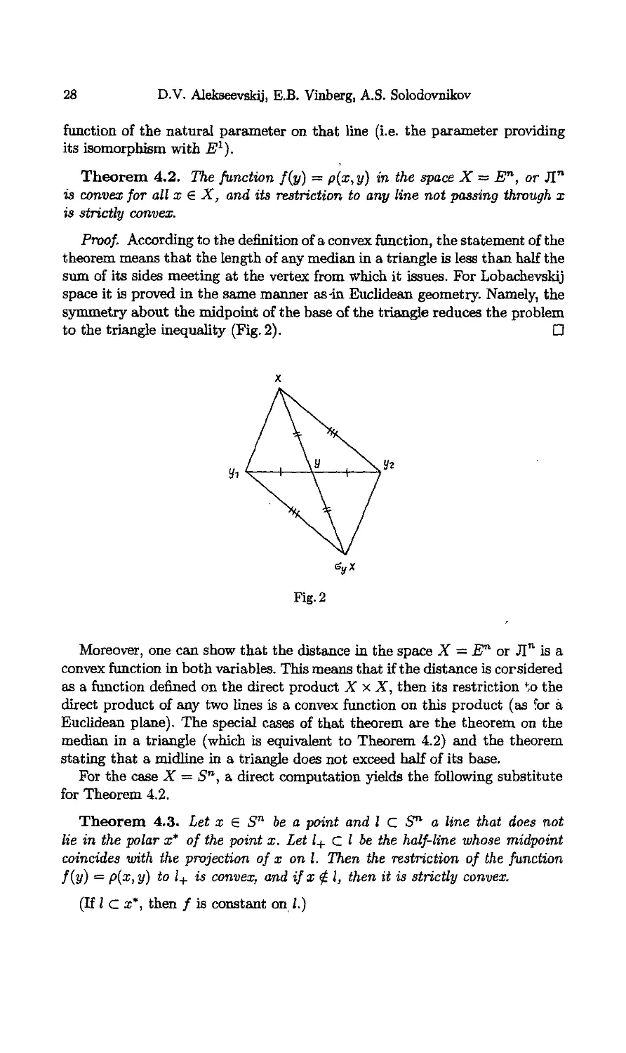
Proof According to the definition of a convex function, the statement of the
theorem, means that the length of any median in a triangle is less than half the
sum of its sides meeting at the vertex from which it issues. For Lobachevskij
space it is proved in the same manner as-in Euclidean geometry. Namely, the
symmetry about the midpoint of the base of the triangle reduces the problem
to the triangle inequality (Fig. 2). D
Moreover, one can show that the distance in the space X = E* or JIn is a
convex function in both variables. This means that if the distance is corsidered
as a function defined on the direct product X x X, then its restriction f,o the
direct product of any two lines is a convex function on this product (as for a
Euclidean plane). The special cases of that theorem are the theorem on the
median in a triangle (which is equivalent to Theorem 4.2) and the theorem
stating that a midline in a triangle does not exceed half of its base.
For the case X = Sn, a direct computation yields the following substitute
for Theorem 4.2.
Theorem 4.3. Let x 6 Sn be a point and I C Sn a line that does not
lie in the polar x* of the point x. Let 1+ Ql be the half-line whose midpoint
coincides with the projection of x on I. Then the restriction of the function
f(y) = p(x, y) to l+ is convex, and if x $1, then it is strictly convex.
(If l С x*, then / is constant on I.)
I. Geometry of Spaces of Constant Curvature 29
Chapter 2
Models of Lobachevskij Space
§ 1. Projective Models
1.1. Homogeneous Domains. Along with the vector model introduced
in Chap. 1 there are other models of the Lobachevskij space JIn. The most
interesting among them are covered by the notion of a homogeneous domain.
Let (X, G) be a homogeneous space. We introduce the following notation:
A) If M С X and Я С G are such that EM С М, then Н\м denotes the
set of transformations of M induced by the transformations from H.
B) If М С X, then Gm denotes the subgroup of G consisting of all g С G
such that gM = M. Evidently the group Gm takes each of the sets dM
and M onto itself.
C) If M С X, then G(M) denotes the group Gm \m of transformations of
the set M.
Now let M be an open subset in X. The subgroup Gm is closed in G.
Indeed, if gM ф M for some g € Gm, then there is a point x $ M such
that either gx € M or g~lx € M, which means that the same holds for some
g' € Gm- Thus for any open subset M the subgroup Gm is a Lie subgroup.
Definition 1.1. If M is a domain in X, and the group G(M) acts tran-
transitively on M, then the homogeneous space (M,G(M)) (or the domain M
itself) is said to be a homogeneous domain in the homogeneous space (X, G).
Let M be a homogeneous domain.
Definition 1.2. The pair_(#M, GM\dM) is called the boundary or the ab-
absolute of M, and the pair (M, Gm\~m) is called its closure. The same names
are also given to the sets dM and M.
Hereafter we consider only those cases where Gm\&m — G{dM) and
m
It seems quite natural to construct and study models of the Lobachev-
Lobachevskij space as homogeneous domains in some well-known homogeneous spaces.
For such an ambient space X one can take, e.g., the real projective space Pn,
whose points are one-dimensional subspaces in Rn+1. Its transformation group
is PGLn+i(R), the quotient of the full linear group GLn+i(R) with respect
to the subgroup {A.E|A € R \ {0}}. Models of this type are called projective.
1.2. Projective Model of Lobachevskij Space. We now recall some
facts and notions of projective geometry (in the form convenient for what
follows).
Let U and U' be two domains in the projective space Pn, n > 2. A diffeo-
morphism fofU onto V is said to be a collineation if it takes any subset of
30 D.V. Alekseevskij, E.B. Vmberg, A.S. Solodovnikov
the form V П I, where I is a line in P", onto a subset U' П11, where V is also
a line. Any collineation from U onto U' can be extended to a collineation of
the entire space P™.
Let Qo be the set of generatrices of the cone
-x2o + x2l + ... + x2n = O A)
in Kn+1. The set Qo is a hypersurface in Pn. The set Pn\Q0 evidently consists
of two connected components such that one and only one of them contains no
lines. This component is the set of generatrices of the cone
-xl + xl + ...+x2n<0 B)
(or, more precisely, the cone obtained by adding the origin to the set defined
by B)). It is said to be the inner domain of Qo, and denoted by int Qo- It is
clear that any collineation of the space P™ preserving Qo takes int Qo onto
intQo.
Definition 1.3. An oval guadric in the space P" is any hypersurface pro-
jectively equivalent to Qo-
Following the notation of Sect. 1.1, we denote the group of all projective
transformations of the space P" by G.
Theorem 1.4. The homogeneous space (intQ, G(intQ)), where Q is an
oval quadric in Pn, is isomorphic to the Lobachevskij space Л".
Proof. We begin with the standard vector model of the Lobachevskij space
JIn, realized as the hypersurface
-x\ + x\ + ... + a? = -l, a;0>0 C)
in the pseudo-Euclidean vector space K"'1 equipped with the metric — dx\ +
dx\ + ... + dXn- Associating with each point x of the model C) the one-
dimensional subspace {Aa:|A e K} in Kn>1, one obtains a bijection if the
hyperspace C) onto the domain int Qo- Its group of motions then goes ;nto
G{mtQo). Indeed, in the vector model C) motions are the transformations
induced by the group O'nV This group can be described as the group of all
linear transformations in K"'1 with determinant ±1 taking the cone B) into
itself and preserving the condition го > 0. This means that the group of
transformations in P" induced by that group is the group of all collineations
of the space P" preserving Qo- D
Note that planes in the int Qo model are images of planes in the vector
model C). Since planes in the vector model are non-empty intersections of
the hypersurface C) with subspaces in K"'1, planes in the intQo model are
non-empty intersections of int Qo with planes in P". In particular, straight
lines in the int Qo are non-empty intersections of int Qo with lines in P".
I. Geometry of Spaces of Constant Curvature 31
Corollary. Any diffeomorphism of the Lobachevskij space Л" that takes
lines into lines is a motion.
Definition 1.5. A homogeneous domain (int Q, G(mt Q) ), where Q is ал
oval quadric in P", is called a protective model of the space Л".
The absolute for the projective model is (Q,G(Q)). Note that the group
G(Q) acts transitively on Q. For example, if Q is a sphere in a Euclidean
space whose completion is Pn, then G(Q) includes all rotations of the sphere.
1.3. Projective Euclidean Models. The Klein Model. Denote by
PE" the model of the projective space Pn obtained by adding points at
infinity to the Euclidean space En.
Let Q be an oval quadric in PEn. As we have just proved, the homogeneous
space (int Q, G(int Q)) can be considered as a model of the Lobachevskij space
Л". Models that can be represented in this form will be called projective Eu-
Euclidean models of the space Л" (in the space PE"). Of course, all of them are
projectively equivalent. However, from the affine point of view these models
fan into three classes depending on the type of the set Q П En. A model of
that kind can be an ellipsoid, an elliptic paraboloid, or a hyperboloid of two
sheets. The difference between the three cases can also be characterized by the
position of the surface Q with respect to the improper hyperplane H of the
space PE". In the first case, the set Q !~)En is empty. In the second, it consists
of a single point (the point at which H is tangent to Q), in the third, it is
an oval quadric in H. Representatives of each of the three classes are called
projective models of the space Л" in an ellipsoid, paraboloid, or hyperboloid,
respectively.
Now we note some general properties of such models. Let us agree that if
Г is a Л-plane (i.e., a plane in the sense of Lobachevskij geometry) in such
a model, then Г* denotes the corresponding plane in PE" (i.e., the plane for
A) Let Г be a Л-plane, and L a Л-line in the model. Then L and Г are
orthogonal (in the sense of Lobachevskij geometry) if and only if L* contains
the pole pr- of the plane Г* with respect to the absolute (Fig. 3).
Proof. Consider a collineation g of the space PEn which in our model
induces the reflection in Г. Since gQ = Q and дГ = Г, one has gpr* — p,
and consequently gL* — L*, where L* is any line in PEn passing through
Pi*. Q
B) If two points pi and pi are Л-symmetric with respect to the hyperplane
Г, and p is the Л-midpoint of the segment P1P2, then the cross-ratio of the
(ordered) 4-tuple pi, P2, ргт, Р equals —1.
Proof. Denote the cross-ratio [pi, рг; Pr-, p] by A. If g is a collineation of the
space PE", which in our model induces the reflection in the hyperplane pass-
passing through p perpendicular to P1P2, then g takes the 4-tuple pi, p%, pr-, p into
the 4-tuplep2,Pi,pr*,P, whence \p\,P2\pr-,p] = \P2,Pi;Pr-,p] aad therefore
32 D.V. Alekseevskij, E.B. Vinberg, A.S. Solodovnikov
A2 = 1. Since, evidently, each of the pairs pi,pi and pr-,P separates the other
one (pr* lies outside Q), we have Л = — 1. D
Fig.3
The most convenient protective Euclidean model is that in the unit ball,
known as the Klein model, and denoted by Kn. Thus, the Klein model is
the ball in the Euclidean space En in which the motions are defined as those
collineations of the space PE11 that take the ball onto itself. The absolute in
the Klein model is the (homogeneous) space (Sn~1,G(Sn~1)).
1.4. "Affine" Subgroup of the Group of Automorphisms of a
Quadric. Let (intQ, G(intQ)) be a projective Euclidean model of the space
JT" (in PEn). Consider collineations of the space PEn preserving not only
Q but also the improper hyperplane H of the space PE", or, equivalently,
preserving both Q and the point рн, the pole of H with respect to Q. Such
collineations constitute a group of affine transformations in PE"'. The restric-
restriction of this group to int Q is naturally called the "affine" subgroup of the group
G(intQ). Denote this subgroup by AG(mbQ). There are three possiWities.
A) Q is an ellipsoid. Then H С extQ (where extQ is the exterior vf Q),
and ря € int Q, more precisely, ря is the centre О of Q. Therefore AG(mb Q)
is the group of all JI-motions that preserve the point O, i.e., the group of all
Jl-rotations about O.
Note that if Q is a sphere then affine transformations preserving Q are
ordinary Euclidean rotations about its centre O. Thus, for the Klein model,
Jl-rotations about the centre О are represented by ordinary Euclidean rota-
rotations about O. This implies, in particular, that if in the Klein model Г is
a hyperplane passing through the centre of Q, then JI-reflection in Г is an
ordinary Euclidean reflection.
B) Q П En is a hyperboloid of two sheets. Then H intersects int Q along
a JI-hyperplane. One has pjj 6 extQ, moie precisely, ря is the vertex of
the asymptotic cone for Q. The group AG(iat Q) consists of all JI-motions
preserving the JI-hyperplane H П int Q.
I. Geometry of Spaces of Constant Curvature 33
C) Qd J5" is a paraboloid. Then H is tangent to Q at the point pjj (the im-
improper point of the paraboloid). In that case (unlike the two preceding cases)
the group AG(ix& Q) acts transitively on int Q. Moreover, it also contains a
subgroup whose action on int Q is simply-transitive.
Proof. Let int Q be denned by the inequality
in > vl + ¦ ¦ ¦ + vl-
Consider the set of affine transformations fe,\ of the form
2 7, Г) + (С, С),
where F = (j/a, ...,yn), С = (с2,.. .,е„), (С, Y) = c2y2 + ... + Cnyn and
A is any nonzero real number. One can easily check that each of the transfor-
transformations fc,\ preserves intQ and that they constitute a group with simply-
transitive action on int Q. Note also that for A = 1, С ф 0 the transformation
fc,a has only one fixed point in PE71, while for А ф 1 it has two fixed points
(ря and one more point on the paraboloid). ?
The fact that for a paraboloid the group AG(int Q) acts transitively has
the following invariant meaning: the group of all collineations of the projective
space P" preserving a given oval quadric Q and a given point g e Q (or,
equivalently, preserving Q and the tangent hyperplane to Q at the point q)
acts transitively on int Q.
1.5. Riemannian Metric and Distance Between Points in the Pro-
Projective Model
Proposition 1.6. Let <p — 0 be the equation of an oval quadric Q in PEn,
where <p is a polynomial of degree 2 in Cartesian coordinates. Then, in the
projective model, the Lobachevskij metric in int Q is given by the formula
Proof. We first consider the case of the Klein model.
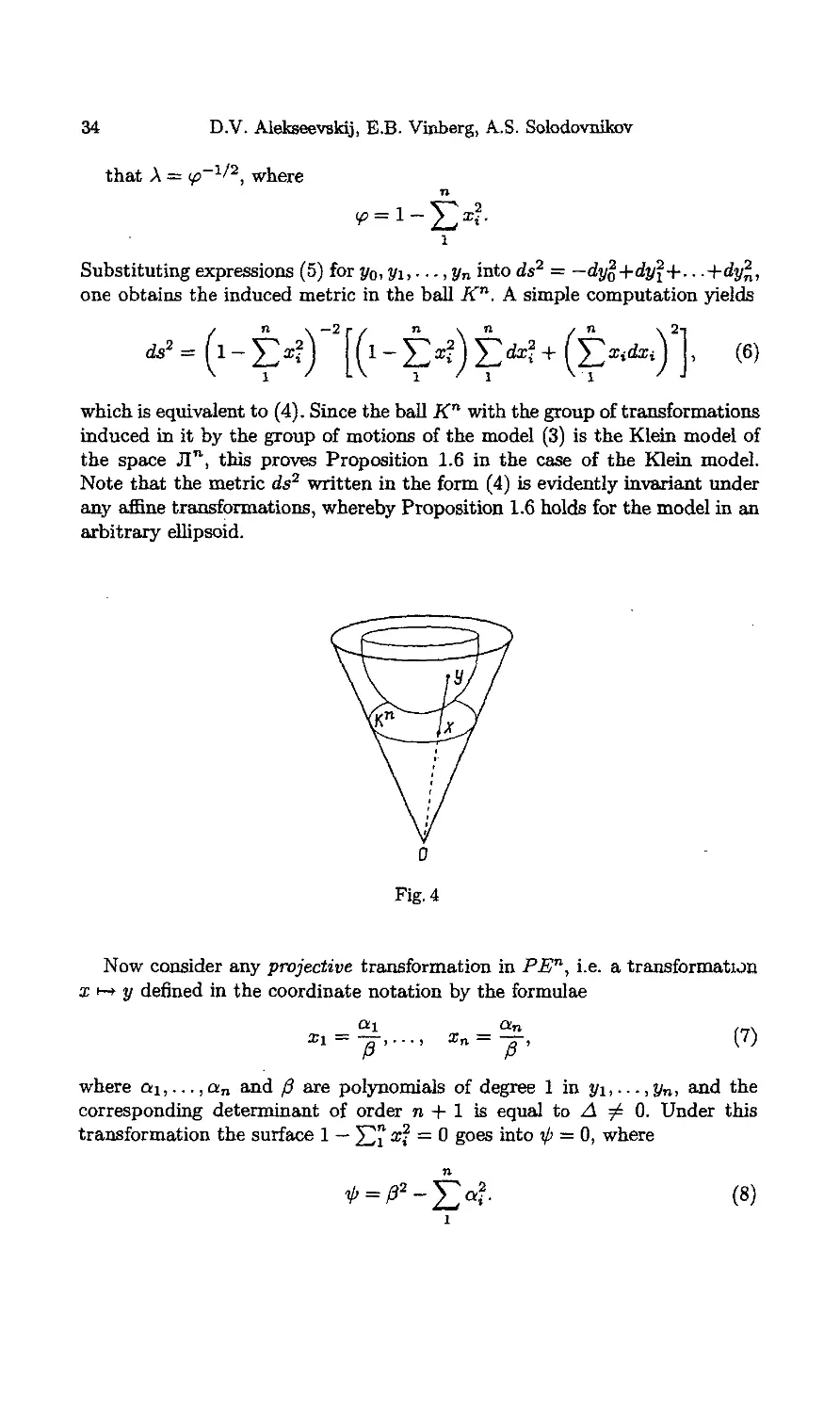
Fig. 4 shows the vector model C), the cone B) corresponding to it, and its
section by the plane E71 : Xo — 1, i.e. the ball
Taking into account that -y% + yf + ... + y% = -1, one can easily deduce
from the relation у = \х, which in the coordinate notation means
2/o = A, yi = \xi, ...,у„ = Аж„, E)
34 D.V. Alekseevskij, E.B. Vinberg, A.S. Solodovnikov
that A = <р~г/2, where
n
Substituting expressions E) for y0, уг,..., yn into ds2 = —dy2+dy2+.. •
one obtains the induced metric in the ball Kn. A simple computation yields
F)
which is equivalent to D). Since the ball Kn with the group of transformations
induced in it by the group of motions of the model C) is the Klein model of
the space JIn, this proves Proposition 1.6 in the case of the Klein model.
Note that the metric ds2 written in the form D) is evidently invariant under
any affine transformations, whereby Proposition 1.6 holds for the model in an
arbitrary ellipsoid.
Now consider any projective transformation in PEn, i.e. a transformation
а; н-» у defined in the coordinate notation by the formulae
x, - ^1 x -— \1\
¦cl — a ' '' " > n — a ' \ '
where a\,...,an and 0 are polynomials of degree 1 in yi,...,yn, and the
corresponding determinant of order n + 1 is equal to Л Ф 0. Under this
transformation the surface 1 — 52™ x2 = 0 goes into ф — 0, where
l/- = /?2-f>,2. (8)
I. Geometry of Spaces of Constant Curvature 35
A direct computation shows that the transformation G) takes the metric F)
into
Remark. The determinant of the metric form F) is equal to A—^" ж?
hence, in the Klein model, the volume element is of the form
Fbr the metric (9), where ¦ф is defined by (8), the volume element is given by
the expression ^~("+1)/2di/i... dyn.
Proposition 1.7. The distance between points x and у in the protective
model (int Q, G(int Q)) is given by the formula
p{x,y) = -\\n{x,y;p,q]\, A0)
where p and q are the points at which the line xy intersects the absolute Q (in
PE71), and [x,y;p,q] denotes the cross-ratio of the 4-tuple.
Proof. Since the right-hand side in A0) has an invariant projective mean-
meaning, one need consider only the case of the Klein model.
Let
u=(uo,ui,0,...,0), v = (vo,vlt0,...,0) A1)
be two points in the vector model C), and L the Л-line passing through
them and defined by the equations X2 = ¦ ¦ ¦ = xn = 0. The parametric
representation of the line L can be written in the form
xq = cosh t, xi = sinh t, x% = ... = xn — 0.
Therefore, one has ds2 = dt2 (along L), and consequently
p(u,v) = \tu-tv\.
Taking the projections of the points и and v from the origin on the plane
x0 = 1, we get the points
«'=A,^,0. -,0), «/ = A,21,0, -,0)
in the Klein model. The line u'v' intersects the absolute Sn~1 at the points
p=(l,l,0,...,0), « = A,-1,0,....0).
36 D.V. Alekaeevskij, E.B. Vinberg, A.S. Solodovnikov
We have
and hence
Since in the vector model C) ал appropriate motion takes any two points into
points и and v of the form A1), the resulting equation holds for any pair of
points u' and v' in the Klein model. ?
§ 2. Conformal Models
2.1. Conformal Space
Definition 2.1. The conformal space C" is a homogeneous space (Q,
G(Q)), where Q is an oval quadric in Pn+1.
(Here G denotes the set of all collineations of the space Pn+1.)
This definition immediately implies that the absolute of the projective mo-
model (intQ,G(intQ)) of the space JIn is the conformal space C".
Remark. The space C1 is isomorphic to P1. For an explanation of this fact
see Sect. 2.4.
Any subset of the form QnH, where H is any plane in Р™+1 having a non-
nonempty intersection with Q, is called a sphere in the space Cn. In particular,
if Q is a Euclidean sphere Sn in PEn+1, then spheres in the conformal space
Sn are Euclidean spheres of various dimensions contained in Sn.
Any diffeomorphism of the sphere 5™ that takes any circle (i.e. a section «. f
the sphere by a 2-plane) into a circle will be called о circular transformation
of the sphere Sn.
Theorem 2.2. The group G(Sn) coincides with the group CircS" of all
circular transformations of the sphere Sn.
Proof. Let g ? G(Sn). Then g can be extended to a collineation g* of the
space PE"+1 preserving S". The collineation g* evidently takes a plane sec-
section of the sphere Sn into a plane section, whereby g € Circ5n. Conversely,
let g e Circ Sn. Let us associate with each hypersphere S С Sn (i.e. a sub-
sphere of dimension n — 1) its pole in PEn+1 (Fig. 5). The transformation g
takes a subsphere of any dimension again into a subsphere. In particular, it
takes S again into a hypersphere. Hereby g induces a transformation g' in the
I. Geometry of Spaces of Constant Curvature
37
set of poles, i.e. in the exterior domain of 5". One can easily see that g' is a
collineation of this domain. But then there is a collineation g* of the space
PEn+1 that is an extension of g. Hence, g e GE"). D
Fig. 5
Corollary. The space Cn is isomorphic to (S71, CacSn).
An important model of the space Cn is constructed by the stereographic
projection. Let us project the sphere
x\ + x\ + ... + xl = 1
in the space En+1 from its "South Pole" p = (-1,0,..., 0) onto the hyperplane
En:xo=0 (Fig. 6).
Denoting this projection by (f and letting ip : x t-> y, one has
These formulae make it possible to find the metric in En induced by <p from
the metric ds2 = dx%+dx\ + .. -+dx2n on the sphere Sn. The resulting formula
is
Formula A2) shows that у is a conformal mapping (i.e. it preserves angles
between curves). Incidentally, it is also a consequence of the fact that <p coin-
coincides with the restriction to Sn of an inversion in the space En+1. The point
p is the centre of the inversion, while the set S of its fixed points is the sphere
of radius \/2 with centre p (see Fig. 7: one has \Op\ = \Ox\ in the right-angled
triangle pOy, hence \px\ ¦ \py\ = 2\Op\2). This implies another property of <p,
namely that it takes circles on the sphere Sn into circles or lines in E".1
1 Fbr the definition of inversion and its properties of preserving angles between curves
and mapping circles and lines into circles and lines see Rozenfel'd [1966].
38 D.V. Alekseevskij, E.B. Vinberg, A.S. Solodovnikov
It is obvious that <p maps S™ \ {p} bijectively onto E*. In order to extend
<p to the entire sphere Sn we complete E" with a new point oo, considering it
as the image of the pole p. Let Ё" = En U {oo}. Define a smooth structure in
a neighbourhood of the point oo on Ё" by means of the mapping <p. The set
En then becomes a smooth manifold and tp a conformal mapping of S" onto
?". The group CircE1" (obtained by transferring CircS" to En by means
of (p) is a transitive group of conformal diffeomorphisms of En. The space
(?"*, CircE") is isomorphic to (Sn,CircSn), i.e. isomorphic to C"\
Fig. 7
Definition 2.3. The homogeneous space (.Ё", Circ ?") is called the flat
model of the conformal space C".
In the E" model, the role of spheres is played by the images of spheres in
5", i.e. by spheres and planes in E™ (the planes are completed by the point
oo). The group CircEn consists of all diffeomorphisms that take (conformal)
spheres into spheres.
Theorem 2.4. The group G(Sn) coincides with the group Conf S of >7/
conformal diffeomorphisms of the sphere Sn.
Proof. The inclusion
Circ5ncConf5" A3)
is easily proved using the flat model Ё™ of the conformal sphere Sn. Let
g 6 CircjB". Suppose first that g{oo) = со. Then gEn = E", and lines in E"
are mapped into lines. Hence g\s" is an affine transformation. This condition
together with the condition that circles are taken into circles implies that g\s-°-
is either a Euclidean motion or a similarity transformation, and consequently
g e ConfE™. In the case when g(oo) = v, where v e E", one takes any
inversion h for which hv = oo. Then hg(oo) = oo, whereby hg € Conf En and
consequently g € Conf En.
I. Geometry of Spaces of Constant Curvature 39
The reverse inclusion
Con?Sn cCiicS" A4)
for n = 2 is a well-known fact of complex analysis (any conformal diffeo-
morphism of the extended complex plane is either a linear fractional map
or a composition of a linear fractional map with complex conjugation). For
n > 2 the proof of A4) is more complicated. We refer the reader to Berger
[1978], Vol. 1, Sect. 9.5.4, where the following version of the Liouville theorem
is proved: for n > 2 any diffeomorphism of the complex plane of the class Cfc,
к > 4, that maps a domain U С E™ conformally onto a domain U' € En, is
a composition of inversions and reflections (which does not hold for E2). The
fact that any conformal diffeomorphism U —* U' belongs to the class C4 is a
very subtle one (see references therein). ?
We should mention that only the first of inclusions A3) and A4) will be
used below.
Corollary. The space C" is isomorphic to E",Conf Sn).
This explains the term "conformal space".
Let M be a smooth manifold and g a Riemannian metric on M. Its confor-
conformal class {g} is the set of all metrics of the form tpg where ip is any positive
smooth function on M. We say that an angular measure is defined on M if a
conformal class of metrics is chosen on M; then one can associate with each
pair ?, r\ 6 TP(M) (p € M) the number cos (?, tj), defined (in the usual way)
by any metric belonging to this class.
If M is the sphere 541 in En+l , then the unique conformal class invariant
under the action of the group of motions of Sn is {go}, where g0 is the Rie-
Riemannian metric induced by the inclusion of 51™ in En+1. This class is also
invariant under CircS™, since CircS С ConfS". Thus, for the group CircS
(for which, evidently, there are no invariant Riemannian metrics on Sn) there
exists a unique invariant conformal class on Sn. This implies that the confor-
conformal space has a unique angular measure.
2.2. Conformal Model of the Lobachevskij Space. Consider again
the conformal space C" = (Q, G(Q)), where Q is an oval quadric in Pn+1.
Choose a subspace P" С Pn+1 passing through a point lying in the interior
of Q. The intersection Q П Pn is a hypersurface in Q. From the point of view
of conformal geometry of the space C" this hypersurface is a hypersphere.
The set Q \ (Q П P") evidently consists of two connected components.
Denote one of them by Q+ (a "half-space" in Q ) and consider the group
Theorem 2.5. The group G(Q+) acts transitively on Q+. The homoge-
homogeneous domain (Q+,G(Q+)) in the space C" is isomorphic to the space JI".
Proof. Suppose that Q is the sphere 5" С En+l. Consider the Klein model
of the space JI"+1 in the unit ball Kn+1 with boundary 5". Consider a section
40 D.V. Alekseevskij, E.B. Vinberg, A.S. Solodovnikov
of this ball by a hyperplane En С ?™+1 passing through the centre of the ball
and denote this section by Kn. The ball K™ is the Klein model of the space
Лп in En.
Fig. 8
The set Kn+1 \Kn falls into two (open) Л-half-spaces. Let K^+1 be one of
them. Denote the corresponding half-sphere of the sphere Sn by S? (Fig. 8).
Let g be any collineation of the space РЯ"+1 preserving IC^+1; let gi =
g\Sn and 32 = д\кп ¦ The mapping g i-> gi defines the isomorphism between
G(K!l+1) and GE"), while the mapping g i-> g-i. defines the isomorphism
between G(K^+1) and G(Kn). This results in the isomorphism
4>'- 9\ >-» 92
between G(S^_+1) and G(Kn). If ф is the orthogonal projection from S? on
Kn, then
since g is a motion in JIn+1, and consequently takes lines perpendicular to
Kn (in the sense of Lobachevskij geometry, which in this case also met ns
perpendicularity in the Euclidean sense) into lines perpendicular to Kn, Ti?
isomorphism <p: G{S^) -> G{Kn) together with the bijection ф: 5J -*¦ K1
and the properties just stated imply that there is an isomorphism between
the spaces (S?, G(S$)) and (Kn, G(Jf")). П
Remark 1. The homogeneous domains (SJ, G{S%)) and (Kn, G(Kn)) (the
first of them in the conformal space S™ and the second in the projective
space PEn) have common absolute, and the isomorphism ф between them
constructed above can be extended to an isomorphism of their closures.
Remark 2. The role of planes in the model E+,G(S+)) of the space JIn
is played by the images (under the mapping ф~г) of the planes in the Klein
model. This implies that the set of planes in the 5™ model coincides with
I. Geometry of Spaces of Constant Curvature 41
the set of all Euclidean hemispheres contained in 5" and orthogonal to 95",
or, equivalently, intersections of 5" with the spheres of the conformal space
5™ orthogonal to 95". In particular, lines in the 5? model are Euclidean
semicircles lying in 5™ and orthogonal to 95™.
As we have shown in Sect. 1.2, any collineation of the space Л" is a motion
(see Corollary to Theorem 1.4). The same result holds for conformal transfor-
transformations, namely, the group Conf JIn coincides with the group Isom JIn.
Proof. The case n = 2 will be considered later (see Theorem 2.12 of
Sect. 2.4). For n > 2, take the realization of Л" in the form of a hemisphere
5™ used in the proof of Theorem 2.5. Any transformation g 6 Conf 5" can
be extended to g* 6 Conf 5™ (see the end of the proof of Theorem 2.5) which
implies that g* e G(Sn), and consequently g e GEJ) = Isom Л". D
Definition 2.6. The homogeneous domain (Q+, G(Q+)) in the conformal
space Cn is called the conformed model of the Lobachevskij space Л".
The distinctive feature of this model, which explains its name, is the fact
that if the space Cn is realized in the form En, G(Sn)), then the group of
motions of the model is a subgroup of the group Conf Sn, and consequently
angular measures on the model coincide with Euclidean angular measures in
Sn (i.e., one can "see" the angles on the model).
Proposition 2.7. Any isomorphism between the prvjective and the confor-
conformal models of the space JIn can be extended to their closures. In particular,
the absolutes of both models are isomorphic.
Proof. It is evident that any two conformal models of the space JI" are
isomorphic and that this isomorphism can be extended to their closures. The
statement of the Proposition is then implied by the Remark to Theorem 2.5.
D
Proposition 2.8. If Г is a hyperplane in JI", then дГ is a hypersphere
in the conformal space dJln. The angle between two hyperplanes Г\ and Г2 in
the space JI" coincides with the angle between the hyperspheres дГ\ and дГ^
in the space dJln.
Proof. One has Г = TnQ+, where T is a hyperplane in Pn+1 (Fig. 9). This
implies that дГ = Т П dQ+, i.e. дГ is a hypersphere in Cn~l. The second
part of the proposition follows from the fact that if a motion g of the space
Л™ takes a pair А,Лг into a pair Г[,Г2, tnen *be motion g* of the space
С1 takes the pair дГх,дГ2 into the pair ЭГ^дГ^. (The motions g and g*
are restrictions of one and the same collineation of Pn+1 to Q+ and dQ+,
respectively.) D
This proposition is especially useful if Л" is realized as the Klein model,
since in that case dJln is a Euclidean sphere with the ordinary angular mea-
measure.
42 D.V. Alekseevskij, E.B. Vinberg, A.S..Solodovnikov
Fig. 9
Note that the vector model of the space JI" in R™'1 (considered earlier) is,
in fact, one of its conformed models. It is obtained if one takes for Pn+1 the
space PEn+1, for Q the surface -x% + x\ H 1- x\ = -1 (more precisely, its
closure in PIS"*1 ), and for Q+ one of the "halves" (defined by the condition
xq > 0) into which Q is divided by the improper hyperplane H of the space
PEn+1 (the second "half' is defined by the condition x0 < 0). The motions
in the model are collineations preserving both Q and H, i.e. transformations
of the group O'nl. The absolute of this model is QnH.
2.3. Conformed Euclidean Models. Consider the flat model (Bn,Circ
En) of the conformal space C1. Any hypersphere in this model is either a hy-
persphere in E", or a hyperplane in En completed by the point oo. Therefore,
up to a Euclidean similarity, there are exactly three conformal models of the
space JIn in Ё" :
A) the unit ball Bn С E" :
l A5)
with the group Cn(Bn), where2 Cn = Circ j?n;
B) the exterior domain of the sphere, i.e. the domain
completed by the point со, with a similar group;
C) the half-space Hn :
Vn > 0, A6)
with the group Cn(Hn).
Models A) and B) are taken into one another by inversion with respect
to the unit sphere dBn, so we consider only the models 1 and 3. The model
(Bn, CniB")) is called the conformal model of the space Л" in the unit ball,
and the model (Hn,Cn(Hn)) is called the model in the half-space or the
2 In Sect. 1 the unit ball has been denoted by Kn. The two kinds of notation (Kn or
Bn) are used depending on which of the models of the space Л" is considered (the
Klein model, or the conformal model). We also remind the reader that Cn(Bn)
denotes tbe restriction to Bn of the subgroup of C" preserving B".
I. Geometry of Spaces of Constant Curvature 43
Poincare model. Below we refer to them simply as the Bn model and the Hn
model, although following the lines of Sect. 1.2 they should be called "confor-
mal Euclidean" models of the space Л".
We now find the Шетапшап metric for each of these models,naturally
taking the Cartesian coordinates yi,...,yn in En.
Proposition 2.9. The Riemannian metric of the model Bn is given by the
formula
ds* = 4A -Ы2Г2Х>?, A7)
l
where ly\ = (J2"yfI/2.
Proof. We take the conformal model 5™ used in the proof of Theorem
2.5, i.e. a hemisphere in En+l. Under the stereographic projection <p de-
described in Sect. 2.1 the model 5+ goes into the model Bn. To each point
x = (xq, Xi, ..., xn) 6 5"™ there correspond two points in the plane En {xq =
0): the point ф(х) with coordinates х\,...,хп and the point ip(x) with coor-
coordinates 3/i,..., yn (Fig. 10). It is easily computed that they are related by the
formulae
X = (i = 1n)
where \y\ = (yf H f- y^I^2. The Lobachevskij metric in 5", expressed in
coordinates X\,..., xn, is of the form F). Substituting A8) for Xi,..., xn one
gets the expression of the metric in terms of yj,..., yn, which coincides with
A7). ?
Note the following obvious property of the Bn model: any rotation of the
model about the point O:y\ = ... = yn = 0 (the centre of the ball Bn ) is a
usual Euclidean rotation about O.
Proposition 2.10. The Riemannian metric of the model Hn is of the
form
^ A9)
Proof. We use the inversion a with respect to the hypersphere S С Еп
with centre s = @,..., 0, —1) and radius \/5, applying it to the model Bn (as
defined by formulae A5) and A7)) (Fig. 11). Under this transformation, the
ball Bn goes into the half-space yn > 0. Letting а: у н-> z, one can write
z^f ««l,...,n-l), *, + ! = &!,
where p2 = y2 + ... + y\_x + (yn + IJ. The metric A7) then goes into the
metric
44
D.V. Alekseevskij, E.B. Vinberg, A.S. Solodovnikov
defined on the half-space zn > 0.
n-1
Fig. 11
For the reader's convenience we now collect the formulae related to the Bn
and Hn models into a single table:
Model
Domain in E™
2M>0
Metric
ds2=A(l-\y\2)-2Zyd^
ds2 = y;2YZdy?
Volume element
dv = 2n(l-\y\2)-ndyi...dyn
dv = yn"dyi ,..dyn
We now present some other facts concerning confonnal Euclidean models
of the Lobachevskij space JI". In the statements of Properties 1 and 2 below,
X denotes any of the models Bn or Hn.
A) A plane in the model X is a non-empty intersection of X with a split *e
in Cn (i.e. either with a Euclidean sphere or a Euclidean plane) orthogonal to
dX. This follows from the characterization of planes in the model 5" given
in Remark 2 to Theorem 2.5 and from the fact the isomorphism between the
models 5™ and Bn is established by the mapping (p. In particular, lines in
the model Bn are either diameters of the ball Bn or Euclidean circular arcs
orthogonal to dBn. Lines in Hn are either Euclidean semicircles or half-lines
orthogonal to dHn.
B) Let Г be a hyperplane in the model X and Г* the corresponding
Euclidean sphere or hyperplane (so that Г is Г* П X). Let g be the Euclidean
inversion with respect to Г* if Г* is a sphere, or the Euclidean reflection in
Г* if Г* is a hyperplane. Then in the model X one has gX = X and g\x is
the reflection in Г.
I. Geometry of Spaces of Constant Curvature 45
Since Jl-reflections in hyperplanes generate the entire group Isom Л", any
motion of the model x can be described as a composition of finitely many
inversions with respect to Euclidean hyperspheres orthogonal to dX.
There is a simple formula for distances in each of the conformal Euclidean
models. First, note that the "cross-ratio" of any four points u, v, p, q in Ё"
*«'•*-&& <20)
(where \up\ denotes the Euclidean distance between и and p) is invariant under
inversions and reflections in En (see Berger [1978], Vol. 2, Sect. 18.10.7).
Proposition 2.11. In the conformal Euclidean model.(i.e. either Bn or
the Jl-distance between points и and v is given by the formula
v;p,q}}\, B1)
where p and q are boundary points of the Jl-line uv.
Proof. Let и and v be two arbitrary points belonging to the hemisphere
5™ used in the proof of Theorem 2.5 (Fig. 12), and let p and q be boundary
points of the Л-line uv. Let u' = i>{u), v' = i>(v). According to Proposition
1.7, p(u, v) = \\ ln[u, v;p, q]\. One can easily check (see Fig. 12) that
whence
p(u,v) = \]n[[u,v;p,q]]\.
As we have already mentioned, the stereographic projection <p taking 5" into
Bn is a restriction to 5" of an inversion in the space En+1. But an inversion
does not change the "cross-ratio" B1). This implies formula B1) for the Bn
model. Since Hn is obtained from Bn by an inversion, the same formula holds
for Hn as well. ?
p u.'
Fig. 12
In the Hn model a special case should be noted, namely when the points
и and v lie on the same Euclidean perpendicular to dHn. Then one of the
points p and q (say q) is oo, and formula B1) takes the form
46 D.V. Alekseevskij, Б.В. Vinberg, A.S. Solodovnikov
M
p{u,v)
In
M
2.4. Complex Structure of the Lobachevskij Plane. Consider the
Poincare model Я2 of the plane Л2. We shall interpret Я2 as the upper half-
plane Im z > 0 of the complex plane. It is well known that Hoi H2 (the group
of all holomorphic diffeomorphisms of H2) consists of all transformations of
the form
az + b
cz + d
where a, b, c, d e R, ad - be > 0 (Shabat [1985], Sect. 11). For each pair of
tangent directions to H2 (a tangent direction is determined by a point p € Я2
and a vector ? 6 TP(H2) defined up to a positive scalar multiple) there exists
a unique mapping g € Hoi Я2 taking the first direction into the second.
This implies that any antiholomorphic diffeomorphism of H2 is of the form
az + b
Z t-> ;,
cz + d
where a, b, c, d 6 R, ad — be < 0.
Theorem 2.12. The group of motions of the model H2 coincides with the
group of all holomorphic and antiholomorphic diffeomorphisms of the half-
plane H2.
Proof. Denote by Isom+ H2 the group of all proper (i.e. preserving the
orientation) isometries of the model H2. Since each isometry is a conformal
mapping, one has Ьопц. Я2 С Hoi Я2. But the group Ьопц. Я2 is transitive
on the set of tangent directions. Therefore Ьот+Я2 = Hoi Я2. It only re-
remains to note that the mapping z —» 1/z is a motion of H2. ?
Theorem 2.12 makes it possible to describe the plane Л2 as a Riemann
surface (i.e., a one-dimensional complex manifold) which is conformally equiv-
equivalent to a half-plane. The corresponding group of motions consists of ьЧ its
holomorphic and antiholomorphic diffeomorphisms.
Two other two-dimensional spaces of constant curvature (S2 and E2) can
also be considered as Riemann surfaces whose groups of motions are realized
as sets of holomorphic and antiholomorphic diffeomorphisms. However, unlike
Л2, for both of them the group Isom.)- is strictly less than the corresponding
Hoi group. For example, the group Hoi E2 consists of diffeomorphisms of the
form z —» az + /?, where a and /3 are any complex numbers such that a ^ 0,
while the group Isom+ E2 is defined by the additional condition \a\ = 1.
Note that by the Poincare-Koebe uniformization theorem the Riemann
surfaces (Л2, S2, E2) are the only possible conformally non-equivalent simply-
connected Riemann surfaces.
Remark. The absolute of the model Я2 is the one-dimensional manifold
R = R U {oo} with the induced transformation group of the form
I. Geometry of Spaces of Constant Curvature 47
ax + b
cx + d
(a,b,c,d€R, ad-bc^Q).
This implies that the absolute is isomorphic to the projective line P1. On
the other hand, the absolute of the conformal model for JI2 is isomorphic
to the absolute of the projective model (Proposition 2.7), i.e. to the one-
dimensional conformal space C1. Thus the spaces C1 and P1 are isomorphic
(as homogeneous spaces).
§ 3. Matrix Models of the Spaces Л2 and JI3
Models of two- and three-dimensional Lobachevskij spaces are especially
important due to their numerous applications in algebra, complex analysis,
differential equations, number theory, etc. In particular, for the problems re-
related to quadratic forms, the matrix models are useful.
3.1. Matrix Model of the Space JI2. Let 5r*L2(R) be the group of
all real 2 x 2-matrices with determinant ±1, and Mi the vector space of all
real symmetric 2 x 2-matrices. A representation of the group 5*Ьг(К) can be
defined in Mi by associating with each A 6 S*Li (R) the linear transformation
4>{A): Mi —» M2 by the formula
. <p{A)V = AVAT,
where
In fact, <p(A) is the transformation law for the quadratic form
px2 + 2qxy + ry2
when the variables x and у undergo the linear transformation denned by the
matrix A.
Obviously, any <p(A) preserves the form
Pr-q\ B2)
Introducing (instead of p and q) new coordinates s and t into Mi such that
p — s + t, r = s — t, one obtains the following form for the right hand side of
B2):
s2-f-q2. B3)
Thus we have constructed a representation of the group S*L2(R) in the vector
space Mi expressed in the coordinates s, t, g and preserving the form B3), i.e.
48 D.V. Alekseevskij, E.B. Vinberg, A.S. Solodovnikov
a representation by matrices from 02, i- Note that for some A the determinant
of tp(A) is equal to — 1, e.g.
¦((i -0)=
This implies that ip(S*L2(R)) consists (like the group 5*2/2(K) itself) of two
components. Both of them belong to 0'21, since they preserve the cone of
positive definite matrices.
Since the dimension of the group S*L2(R) coincides with that of (У21 and
the kernel of the mapping A i-> <p(A) consists of the matrices E and — E, we
conclude that A t-f tp{A) is an isomorphism of the group S*L2(M)/{E, — E}
onto the group 02>i-
Consider the orbit of the point
°^eM2
0
(for this point one has p = r = l,g = 0ors = l, t = 0, g = 0) with respect to
the group (p(S*Lz(R)), i.e. with respect to the group O'iv It is the "upper"
sheet of the hyperboloid
S2-t2-g2 = l,
which provides a model for JI2. We can therefore conclude that the homoge-
homogeneous space of positive definite real symmetric 2 x 2-matrices with determinant
1 considered with the action of the group ip(S*L2{&)) is isomorphic to the
Lobachevskij plane JI2.
Let us also find the stabilizer of the point Vq. The quadratic form corre-
corresponding to Vq is x2 + y2. Therefore ip(A)Vo = Vq if and only if Л 6 O2.
Taking into account that both of the matrices E and — E belong to 02, one
gets the following result: the space JI2 is isomorphic to 5*Хг(К)/02-
3.2. Matrix Model of the Space JI3. This model is constructed in he
same way as the matrix model for JI2. Denote by 1*2 the set of all Hermitiaj
2 x 2-matrices, i.e. matrices of the form
Z q
q Г
where p, r ? R, q 6 С The elements of T2 can be interpreted as binary
Hermitian forms
pxx + qxy 4- qyx + ryy.
The formula
ф(А)У = AVAT,
I. Geometry of Spaces of Constant Curvature 49
where A € SL2 (C), V 6 T2, defines a representation ф of the group 5?-г(С)
in the space T2. All transformations ф(А) as well as the complex conjugation
V '-* V preserve the form
P Я
q r
r-qq. B4)
Introducing the (real) coordinates s, t, u, v into T2, where
p = s + t, r = s — t, q = u + iv,
one can write the form B4) as
Now, in complete analogy with the preceding section, one obtains the following
result.
The homogeneous space of positive definite Hermitian 2 x 2-matrices with
determinant 1, considered with the action of the group i/)(S2/2(C)) extended
by the operation of complex conjugation, is isomorphic to the Lobachevskij
space Л3. The group ip(SL2(C)) then corresponds to the group Isom+ Л3 of
proper motions of the space Л3.
Consider, as in the preceding case, the point
The corresponding Hermitian form is xx+yy, and consequently ф(А)(Ц,) = Vq
if and only if Л 6 Ui- Therefore the space (Л3,Ьот+ Л3) is isomorphic to
SL2(C)/SU2.
The same result can be obtained from different considerations using the
Poincare model H3. Here is a brief outline of the argument.
The boundary of the half-space Я3 is the plane E2 defined by the equation
j/3 = 0. Consider it as the complex plane z = yi + гуг- There is a unique
isomorphism <p between the groups bom H3 and Conf E2 (roughly speaking,
(p is the natural isomorphism between G(int Q) and G(Q), see Sect. 2.1). Thus
there is an isomorphism tp: Isom+ H3 ^ SL2(C)/{E, —E}. One can show that
under this homomorphism the stabilizer of the point @,0,1) 6 H3 corresponds
to the group SU2/{E, -E}.
50 D.V. Alekseevskij, E.B. Vinberg, A.S. Solodovnikov
Chapter 3
Plane Geometry
This chapter considers (from the same point of view whenever possible)
geometric properties of two-dimensional spaces of constant curvature, i.e. the
sphere S2, the Euclidean plane E2, and the Lobachevskij plane Л2. For the
realizations of S2 and E2 we take the vector model and the affine model,
respectively. For Л2 four models will be used. First, we use the vector model,
i.e. the realization of Л2 in the form of the surface
-xl + x\ + x\ = -1, x0 > 0 A)
in the pseudo-Euclidean space R2>1 with the pseudo-Riemannian metric
—dx% -f dx\ + dx2,. The three other models of Л2 are:
1. The Poincare model
H* = {(x,y)\y>0}
with the metric
which below, for brevity sake, is referred to as the UH2 model".
2. The conformal model in the unit disc
with the metric
called below the "?2 model".
3. The Klein model, i.e. the unit disc with the metric
A-х2 - y2J
called the "K2 model".
A description of motions and lines for each of these models has been given
in Chap. 2. We reiterate that the H2 and B2 models are considered as subsets
of the conformal plane E2 = E2 П {со} and the K2 model as a subset of the
projective plane PE2.
Most of our attention will be directed to the Lobachevskij plane, since it
has a "richer" geometry compared to that of the sphere or the Euclidean plane
and is (of all the three geometries 52, E2, and Л2) the least known among
the general audience.
The isomorphism between the H2 and B2 models is established by the
mapping
I. Geometry of Spaces of Constant Curvature 51
z — i
z + i
which takes the upper half-plane onto the unit disc and the metric B) into
C). The isomorphism between B2 and K2 is achieved by the mapping
22
which takes the unit disc onto itself and the metric C) into D).
For each of the models H2, B2, and K2 (see Sect. 1.1 and Proposition 2.7 in
Chap. 2) its closure is called the extended Lobachevskij plane and sometimes
denoted by Л2. From the topological point of view Л2 is a disc. If Л2 is
realized by the Poincare model, the boundary of the disc is the real axis
completed by the point со, while in the B2 and K2 models the boundary is
the unit circle. As a homogeneous space, the boundary is isomorphic to C1 or
P1, and the transformation induced by an appropriate motion of the model
can take any three points lying on it into any other three points.
For a more detailed exposition (as compared to this Chapter) of the two-
dimensional Lobachevskij geometry we refer the reader to Beardon [1983],
Chap. 7 and the references therein. The spherical geometry is considered in
more detail in Berger [1978]. For the axiomatic construction of Lobachevskij
geometry see, e.g. Efimov [1978].
§1. Lines
1.1; Divergent and Parallel Lines on the Lobachevskij Plane. Any
pair of lines on the sphere S2 has exactly two common points. Two lines on
the Euclidean plane E2 or the Lobachevskij plane Л2 may have either one
common point or none. This, of course, makes a sharp difference between the
geometry of S2 on the one hand, and the geometries of E2 and Л2 on the
other. At the same time, there are great differences between the geometries
of #2 and Л2.
For any given line L in the space E2 and any point p not lying on L there
is a unique line L' through p that does not intersect L (i.e. is parallel to it).
The position of I/ relative to 2/is completely determined by the distance from
p to L .
In the space Л2 the situation is more complicated (and more interesting).
Denote by V the pencil of lines with centre p. One can easily see (e.g. by
taking the Klein model) that there are two possibilities:
1. L' does not intersect L, and all lines in V that are close to V also do not
intersect L (Fig. 13). In that case the lines L and L' are said to be divergent1.
Two divergent lines have a unique common perpendicular (see below) the
length of which evidently characterizes the relative position of L and L'.
1 The terms ultra-parallel and disjoint are also in use.
52
D.V. Alekseevskij, E.B. Vinberg, A.S. Solodovnikov
2. V does not intersect L but there exist lines in V arbitrarily close to L
that do intersect L (Fig. 14). In this case L and U are said to be parallel (in
the sense of Lobachevskij). If the lines L and V are parallel, the direction of
parallelism can be defined on each of them (shown in Fig. 14 by the arrow).
Fig. 13
Fig. 14
The direction of parallelism on L is the direction characterized by the following
condition: if a point q € L moves along L in this direction, then the line pq
approaches L'. The direction of parallelism on I/ is defined in the same way
(with L and L' changing places). Thus "to be parallel" is a relation between
oriented (directed) lines. Making a convention that each oriented line is, by
definition, parallel to itself, we can now say that parallelism is an equivalence
relation.
Figure 15 shows parallel lines in the Poincare model, and Fig. 16 in the B2
model. Another definition of parallel lines can be given in terms of points at
infinity. Let L be a line. The two points of the absolute that are the limit
points of L are said to be its points at infinity. One can easily see that the
lines L and L' are parallel if and only if they have a common point at infinity.
-дНг
Fig. 15
Pig. 16
I. Geometry of Spaces of Constant Curvature
53
The angle between two parallel lines L and L' is, by definition, equal to
zero. This definition is motivated by the fact that if a point p € L' is fixed and
a point q € L moves to infinity in the direction of parallelism, then the angle
ip between the lines L and pq tends to zero. (See Fig. 17, where the situation
is shown in the B2 model).
Proposition 1.1. If a line Li is parallel to L[, L4 is parallel to L'2, and
L\ ф L\, L2 ф L'2l then there is a motion taking Li into L2> and L[ into L'2.
Proof. Figure 18 shows the lines Li, L[, L2, L'2 in the B2 model. The
motion under which zi i-» vi\, z% i-+ w2, z% >-* w^ is the desired one. D
Pig-17
Fig. 18
Proposition 1.2. Two lines L and L' are divergent if and only if they
have a common perpendicular. Such a perpendicular is unique.
Proof. Take the model К2 С РЕ2. The lines in P?2 extending the chords
L and V intersect at some point и (Fig. 19). The lines uv and uw are tan-
tangent to the absolute. The chord T connecting v with w is the common Л-
perpendicular to L and L' (see Chap. 2, Sect. 1.3). The common perpendicular
is unique, since the extension of the chord representing it in the model passes
through the poles of the lines L and U. D
The existence of the two types of pairs of non-intersecting lines on the
Lobachevskij plane (i.e. divergent and parallel) is responsible for some facts
on the Lobachevskij plane that look paradoxical. For example, any angle con-
contains an entire line inside it (Fig. 20). Another apparent paradox is that there
are triangles that cannot be inscribed in a circle, etc. Some of the most im-
important and significant of these facts will be considered below. One cannot
hope to master Lobachevskij geometry without getting used to these facts and
developing a proper intuition different from the Euclidean one.
54
D.V. Alekseevskij, E.B. Vinberg, A.S. Solodovnikov
Fig. 20
1.2. Distance Between Points of Different Lines. Let L be a lin
and p a point on the Lobachevskij plane. We now derive a useful formula fo
p(p, L) in the H2 model.
Taking for L the positive half of the ordinate axis, one can write
p(p,L)=p(p,q),
where q 6 L, \Op\ = \Oq\ (Fig. 21). Hence
+ dy*
У
where the integral is taken along the Euclidean circular arc connecting p with
q and orthogonal to L . Letting в = ZpOq, we have
ri in-nUn 1 /я- в\ 1 1 + tanf
. - tan §
Thus, p(p, L) is defined merely by the angle в. The distance increases from 0
to oo when в changes from 0 to тг/2.
Fig. 21
L-г
Fig. 22
Corollary 1. If L\ and Li are two intersecting lines, then the distance
between the point p € L\ and the line Li increases monotonically from 0 to oo
whenp moves away from the intersection point of L\ and L^. (See Fig. 22.)
I. Geometry of Spaces of Constant Curvature
55
Corollary 2. If Li and L% are two parallel lines andp € L\, then p(p,L2)
increases from 0 to 00 when p moves along L\ in the direction opposite to the
direction of parallelism. (See Fig. 23.)
Fig. 23
Fig. 24
Corollary 3. Let L\ and Li be two divergent lines andpipi their common
perpendicular (pi € Li,p2 ? -^2)- Then p(p,L2) increases monotonically from
p(j>i,P2) to 00 whenp moves along either of the two rays of the line L\ issuing
frompi. (See Fig. 24.)
Fig. 25
Let us mention one more useful fact of Lobachevskij plane geometry. Con-
Consider an acute angle with the aplex O. Take a point M on one side of the angle
and drop the perpendicular MN onto the other side. It turns out that if the
point M moves away from О to infinity, then the angle OMN tends to zero.
This is easily seen in the B2 model. Assuming that the apex of the angle is at
the centre of the disc J52, and the sides of the angle are two radii of B2, the
statement is evident from Fig. 25.
56 D.V. Alekseevskij, E.B. Vinberg, A.S. Solodovnikov
§ 2. Polygons
2.1. Definitions. Conditions of Convexity
Definition 2.1. A polygon in a two-dimensional space X of constant cur-
curvature is a simply-connected closed domain M С X such that дМ is the union
of finitely many segments, rays or lines.
A point p € дМ is a vertex of a polygon M if the intersection of дМ with
some disc with centre p consists of two radii of the disc that are not extensions
of one another. The angle of a polygon at a vertex p is defined in the usual
way.
Definition 2.2. A polygon M is said to be convex if it is a convex set in
the space X.
There is an equivalent definition.
Definition 2.3. A convex polygon is an intersection of finitely many half-
planes having a non-empty interior.
The equivalence of Definitions 2.2 and 2.3 is checked without difficulty.
This definition evidently implies that any angle a of a convex polygon
satisfies the condition
0 < a < ж. F)
The converse statement is also true: if M is a polygon in the sense of Definition
2.1 and each of its angles satisfies condition F), then M is convex.
Proof. In fact, a more general statement holds: any connected locally con-
convex closed domain M is convex. Indeed, consider the shortest of the curves
joining a pair of interior points x, у of M, which in the case X = Sn are not
antipodal. The local convexity of M implies that it is a geodesic and that a
neighborhood of it is contained in M. Then it can be nothing else but the
segment xy. О
Definition 2.4. A polygon is said to be proper if
for X — E2 it is a bounded set;
for X = S2 it contains no antipodal points;
for X = Л2 it contains no half-planes.
Figure 26 illustrates the difference between proper and improper polygons
on the Lobachevskij plane (in the Klein model). In the improper case the
double shaded area shows the half-plane belonging to M.
If M is a proper polygon in JI2, then its closure in JI2 may include the
points of the absolute дЛ2. These points will also be regarded as vertices of M
and called vertices at infinity. The angle of a polygon at its vertex at infinity
is naturally defined to be zero.
A proper polygon having я vertices (including those at infinity) is called
an n-gon.
I. Geometry of Spaces of Constant Curvature 57
Fig. 26a. Proper polygon pig. 26b. Improper polygon
Again let X be a two-dimensional space of constant curvature and suppose
that pi,... ,pk is a finite set of points belonging to the space X itself (if X is
either S^orS2) or to its closure X (if X is Л2). The convex hull of this set
of points is
for X = S2 or X = E2 the smallest convex set in X containing the points
Pi,---,Pk;
for X = Л2 the smallest convex set in Л2 whose closure in Л2 contains
the points pi,...,pk.
The convex hull is denoted by conv{pi,... ,pk}-
Proposition 2.5. A convex polygon is proper if and only if it coincides
with the convex hull of the set of its vertices.
See Berger [1978], Vol. 1, Sect. 12.1.Ц.
2.2. Elementary Properties of Triangles. Let X be one of the spaces
S2, E2, Л2. Let Pi,P2,P3 be three points belonging to lor X (the latter in
the case X = Л2 ) not all lying on the same line (or in the closure of the same
line). The set conv{pj,pz,p3} is called the triangle with verticesPi,P2,P3 and
denoted (рьрг.Рз)- Evidently, 1р\,р2,рз) = Т1ПТ2ПТ3, where Tt is the closed
half-plane bounded by the line pjPk (i, j, к are all different) and containing pi.
Note that in the case of the Lobachevskij plane some or even all of the
points pi,P2,P3 can be at infinity, cf. Fig. 27 (in the Klein model).
The angles of the triangle (р1,Р2,Рз) will be denoted by 01,02,0:3 (where
сц is the angle at the vertex pi).
We now present some facts from the basic course of geometry that hold
not only for the Euclidean plane E2 but also for any two-dimensional space
of constant curvature.
1. In an isosceles triangle the angles at the base are equal, and the altitude
drawn to the base coincides with the median and bisector issuing from the
same vertex.
58
D.V. Alekseevskij, E.B. Vinberg, A.S. Solodovnikov
Pig. 27
2. Congruence criteria2 for (ordinary) triangles:
(SAS) "by two sides and the included angle";
(ASA) "by a side and the two angles adjacent to it";
(SSS) "by the three sides".
Below we establish one more congruence criterion for triangles which holds
only in the spaces S2 and Л2:
(AAA) "by the three angles".
There is no such criterion in Euclidean geometry, since triangles there may
be similar but non-congruent.
3. In any triangle the greatest angle lies opposite the greatest side.
A well-known proof of this proposition invokes the theorem about an ex-
exterior angle of a triangle, which does not hold for S2. However, a weaker
assumption is sufficient, namely
7Г —
G)
This means that an exterior angle is greater than the difference of the two
interior angles not adjacent to it. The desired statement is now easily deduced
by applying G) to the triangle shown by braces in Fig. 28. In the case of the
sphere, inequality G) will be proved in the next section.
Fig. 28
2 As usual, two figures are said to be congruent if they can be taken into one another
by a motion.
I. Geometry of Spaces of Constant Curvature 59
4. The length of any side of a triangle is less than the total length of its
other two sides.
Note that a corollary to this fact is the following statement: the total length
of all three sides of a spherical triangle is less than 2ж. Indeed, for any triangle
(pi,P2iPz) on the sphere S2 we have
where q is the point of the sphere antipodal to px (Fig. 29).
2.3. Polar Triangles on the Sphere. To each triangle A on a sphere
there corresponds a triangle A' polar to A, which is defined as follows. If
A = {Р1>Р2,Рз), then A' is the intersection of three hemispheres Si,S2,S3,
where Si (i = 1,2,3) is the hemisphere bounded by the plane passing through
О perpendicular to the vector Opi, and containing p* (Fig. 30). Denoting the
vertices of the triangle A' by pi,p'2,P3 and setting ж» = Opt, x\ = Op^, one
can define A' by the following set of conditions:
(хих^)>0, (xi,x'j) = 0, where i,j = 1,2,3, i^j.
Hence it follows that if A' is polar to A, then A is polar to A', i.e. the relation
of polarity between triangles on a sphere is symmetric.
Proposition 2.6. The lengths a^a^a^ of the sides of the triangle A' are
related to the angles 0-1,02,03 of the triangle A by the following formulae:
а; + а< = 1г (t = 1,2,3),
Proof. The side aj corresponds to the angle between the vectors Opj, and
Oj/k (where i,j,k are all different), which is equal to the difference between
7Г and the angle between the planes (O,pt,pj) and (O,pi,pk) (orthogonal to
these vectors). Hence oj = тг — a. D
Corollary. Inequality G) holds for the angles 01,012,03 of any spherical
triangle A.
Proof. Write inequality a[ + a'2 > a'3 for the polar triangle A'. Then one
gets G) by replacing each of the numbers a\ (i = 1,2,3) by 7г - а*. ?
2.4. The Sum of the Angles in a Triangle. Again let X be a two-
dimensional space of constant curvature. How can one determine the sign of
its curvature? One way is to take any triangle and compare the sum of its
angles with ж.
Theorem 2.7. The sum of the angles of any triangle on the sphere is
greater than it, on the Euclidean plane it is equal to ж, and on the Lobachevskij
plane it is less than тг.
60
D.V. Alekseevskij, E.B. Vinberg, A.S. Solodovnikov
Proof. The cases to be considered are those of the sphere and the Lobachev-
skij plane.
For S2 the statement of the theorem follows from Proposition 2.6 and the
fact that the sum of the sides of a spherical triangle is less than 2тг (see the
end of Sect. 2.2).
In the case of JI2 let us use the conformal B2 model. One can assume that
one of the vertices of the triangle is the centre of the disc B2, so the two sides
meeting at this point are actually parts of two radii. The rest is evident from
Fig. 31. D
Fig. 30
Fig. 31
2.5. Existence of a Convex Polygon with Given Angles- The theo-
theorem on the sum of the angles in a triangle implies that the sum of the angles
in any convex n-gon on a Lobachevskij plane is less than (n — 2)тг, on a Eu-
Euclidean plane it is equal to this value, and on a sphere it is greater. This is
easily proved by cutting the n-gon into n — 2 triangles with diagonals issuing
from the same vertex.
Theorem 2.8. For any numbers ац,... ,an satisfying the conditions
0<ft;<7T (i~ l,...,n), (8)
a1 + ... + an<(n- 2)ir, V9)
there exists a (bounded) convex n-gon with the angles ati,..., an in Л2 or E2.
Proof. Denote the sum ai + ¦• ¦ + an by a. The following two cases are
possible:
a < (n - 2)я; A0)
a = (n - 2)тг; A1)
Consider the case A0) first. Then, naturally, the desired polygon M is to
be constructed in Л2. We shall look for M in the class of polygons admitting
an inscribed circle.
Fix a positive number d and construct for each angle сц the quadrilateral
Qi shown in Fig. 32. If we can choose d in such a way that
I. Geometry of Spaces of Constant Curvature 61
n
X>=7r- A2)
l
the problem is solved: one can simply lay the quadrilaterals Qi,...,Qn one
beside the other, successively joining them along the sides equal to d, the
resulting n-gon being the desired one.
Fig. 32
For small d the difference between tpf and f — ^ is also small, so the
difference between 5Ц™ 4>i an(i
is small as well. By condition A0), the last value is greater than тг. On the
other hand, each of the angles щ tends to zero as d —* oo (see the end of
Sect. 1), so 53 'fit als0 tends to zero. Since the function Yl ft (which depends
on d) is continuous and among the values it assumes are those greater than
я- as well as those less than тг, there is an intermediate value of d for which
, is equal to n.
In the case A1) one looks for the desired polygon M in E2. Then the
construction we have just described yields A2) for all values of d, thus solving
the problem. П
Remark 1. For the Lobachevskij plane, condition (8) can be replaced by a
more general condition:
0<а;<тг (i = 1, ...,n),
(8')
The same argument as above proves that there is a convex n-gon in Л with
the angles сц,..., an (provided, of course, that и < (n — 2)тг). The vertices
of the polygon for which a,- = 0 are at infinity.
62 D.V. Alekseevskij, E.B. Vinberg, A.S. Solodovnikov
Remark 2. One can show that the n-gon with n given angles ai,...,an
depends, up to a motion, on n — 3 parameters for Л , and on n — 2 parameters
for E2.
Corollary to Theorem 2.8. For any three angles with the sum less than
7Г there is a triangle on the Lobachevskij plane having precisely these angles.
As we shall see below, such a triangle is unique up to a motion of the plane.
One can show that for the existence of a spherical triangle with the angles
ai, a2, a3 @ < a, < тг, г = 1,2,3) the following conditions are necessary and
sufficient:
fti + а2 + а3 > тг,
-ai + oi2 + «з < т,
ati — а2 + аз < л-,
ai 4- OC2 — осз < тг.
(For necessity see G).) As will be shown below, such a spherical triangle is
unique up to a motion.
2.6. The Angular Excess and the Area of a Polygon. Denote by
a(M) the sum of the angles in a proper polygon M in a two-dimensional
space of constant curvature.
Definition 2.9. The angular excess of a proper n-gon M is the number
A{M) = a(M) - (n - 2)tt.
In particular, the angular excess of a triangle is the difference between the
sum of its angles and тт.
Theorem 2.10. In each of the spaces S2 and Л2 the area S(M) of a
proper polygon M equals the absolute value of its angular excess:
S{M) = \A{M)\. A3).
Proof. The function A(M) is evidently invariant under any motion. One
can show without much difficulty that A(M) is additive: if M — U"Mj, where
no two polygons Mi and Mj have common interior points, then A(M) equals
the sum of A(Mi),..., A(Mn) (see Fig. 33 for an illustration). Since A(M) is
both invariant and additive, one has S(M) = \\A(M)\, where A =const. To
show that A = 1 let us find the area of some specific polygon. In the case of
S2 we can take, for example, the triangle having three right angles. Its area is
1/8 of the total area of the sphere. In the case of Л2 one can take the triangle
shown in Fig. 34 (in the H2 model). It has |4(M)| = n and
S(M) = f f
J Jm
dxdy
— 7Г.
Jm У2
For details see, e.g. Berger [1978], Sect. 18.3 and Sect. 19.5. D
I. Geometry of Spaces of Constant Curvature
63
+ ? + Gi+72)
(a + 71 + «l - *) + (/? + 72 + Si - t)
Pig. 33
Г -4
— X
Fig. 34
Formula A3) implies, in particular, that the area of a triangle on the
Lobachevskij plane does not exceed тт.
Remark. Formula A3) is a particular case of the more general Gauss-
Bonnet formula
[ Кйц = А(М)
м
(see Rashevskij [1967], Sect. 112) where M is any simply-connected closed
domain in a two-dimensional Riemannian manifold bounded by geodesic arcs,
К is the Gaussian curvature (which, in general, is not constant), and d/j, is
the area element.
§ 3. Metric Relations
3.1. The Cosine Law for a Triangle. Naturally, we skip the case E2
and consider the remaining two cases, i.e. S2 and Л2 simultaneously, since
the metric relations in S2 and Л2 are of a very similar form. This similarity is
only one manifestation of the fact that both spaces S2 and Л2 can be defined
as surfaces
(x,x) = e A4)
in the space R3 with the scalar product
(x, y) = eXOyO
+ 222/2,
where e = 1 for S2, and e = — 1 for Л2 (in the last case there is an extra
condition xo > 0).
Figure 35 shows a triangle ABC on the surface A4), where
The vector
О А = х, ОВ = у, ОС = z.
y' = y- e(y, x)x
64
D.V. Alekseevskij, E.B. Vinberg, A.S. Solodovnikov
issuing from A lies in the plane defined by the vectors x, y, and is orthogonal
to x. One can easily see that the direction of the vector y' coincides (at the
point A) with the direction of the side AB. Similarly, the vector
z' — z— (z, x)x
issuing from A is tangent to the side AC. Denoting the angle between the
sides AB and AC by a, we can therefore write
cos a = —
(in any plane tangent to A4) the "Euclidean" formula for the cosine holds,
since the scalar square of any vector in the tangent plane is defined by a
positive definite quadratic form). Thus
cos a =
(V,z)-e{y,x)(z,x)
Fig. 35
In the case of S2 we have
(x, y) = cos c, (x, z) = cos 6, (y, z) = cos a,
where a, b, с are the side lengths of the triangle ABC on the sphere. Hence
cosa — cosbcosc
cos a =
sin b sin с
A5)
In the case of Л2
(x, y) — — cosh c, (x, z) — — cosh 6, (y, z) = — cosh a
I. Geometry of Spaces of Constant Curvature 65
(see Chap. 1, Sect. 4.2), whereby
— cosh a + cosh 6 cosh с . „
cosa = , . . A6)
sinh b smh с
Formulae A5) and A6) provide the so-called Cosine Law. Let us rewrite it in
the following way.
The Cosine Law for S2
cosa = cos ft cos с 4-sin ft sine-cosa. (C+)
The Cosine Law for Л2
cosh a = cosh b cosh c — sinh 6 sinh с • cos a. {C-)
Corollary. If an angle a in a triangle increases, while the lengths of the
sides b and с do not change, then the side a also increases.
Proof. For S2 and Л2 the corollary follows from (C+) and (C-), while for
E2 it is a consequence of the usual (Euclidean) Cosine Law. ?
3.2. Other Relations in a Triangle. Formulae (C+) and (C_) imply a
number of other important formulae relating the sides and angles in a triangle.
The most important are the Sine Law and the Dual Cosine Law.
The Sine Law for S2:
sin a sin/? sin7 „ .
The
Sine
Law
for
Л2:
sin a
sin a
sini
sin/?
sine
sin 7
• (S-)
sinh a sinhb sinh с
The Dual Cosine Law for S2:
cosa = — cos/3cos7 + sin/3sin7- cosa. (C+)
The Dual Cosine Law for Л2:
cosa= —cos/? cos 7 +sin/? sin 7 • cosh a. (C-)
Formula (S+) is proved very easily. It follows from (C+) that
sin2 a sin2 b sin2 с — (cos a 4- cos b cos cJ
sin2 a sin2 a sin2 b sin2 с
and one has only to note that the expression
1 — cos2 a — cos2 6 — cos2 с — 2 cos a cos b cos с
appearing in the numerator is symmetric in a, 6, с Formula E_) is proved in
the same way.
66
D.V. Alekseevskij, E.B. Vinberg, A.S. Solodovnikov
Formulae (C'+), and (C'_) can also be obtained from (C+) and (C_) by
simple transformations. Incidentally, formula (C'+) is also a direct consequence
of (C-j.) and Proposition 2.6.
A special note should be made of the laws (C'+) and (Cl). They have no
analogues in Euclidean geometry, since they imply that the sides of a triangle
on the sphere or the Lobachevskij plane are uniquely determined by its angles!
This yields the (AAA) congruence criterion "by the three angles" for triangles
in S2 and JI2 (see Sect. 2.2 of this chapter).
In the particular case of a right triangle G = f), the laws (C+) and (C_)
imply that
cos с = cos a cos 6 for S2, A7)
cosh с = cosh a cos b for Л2.
A8)
These are non-Euclidean analogues of the Pythagoras theorem.
The laws given above make it possible to derive all the relations between
the sides and the angles in a triangle. The following table provides a list of
formulae which, for a right triangle, given any two of the elements a, /?, a, ft,
с G = f )> enables one to find any third element:
forS2
cosc = cosacosb
sin 6 = sin с sin/?
tana = tanccos/?
cos с = cot a cot f3
cos a = cosasin/3
tana = sin b tan a
cosh с = cosh a cosh 6
sinh b = sinh с sin 0
tanh a = tanh с cos 0
cosh с = cot a cot 0
cos a = cosh 0 sin /?
tan 0 = sinh b tan a
In addition, we also give formulae expressing the area S of a triangle on
the sphere or the Lobachevskij plane in terms of the sides of the triangle (a
formula expressing S in terms of the angles is provided by Theorem 2.10):
p — a
,5 p p a p b
tan — = tan - tan —-— tan —-— tan
tanh2 —= tanh | tanh Z
p — b
-
tanh 1
p — с
—-—
tanh ^
for b ,
^ for Л2,
where p = |(a + b + c). For E2 there is the well-known Heron formula
S2=p{j>-a)(i>~b)(p-c).
Remark 1. The reader has probably already noted that the relations
between the sides and angles in a spherical triangle turn into their ana-
analogues on the Lobachevskij plane if one replaces a, b, с with ia, ib, ic (since
cosiz = coshz, siniz = г sinh z). It comes as no great surprise if one recalls
that the spaces S2 and Л2 can be denned in a similar way (see the beginning
I. Geometry of Spaces of Constant Curvature 67
of the present section). The fact the trigonometric formulae in Л2 look like
those in spherical trigonometry with every linear expression a; replaced by ix
(as if they were trigonometric formulae on a sphere with an imaginary radius)
was already noted by Lobachevskij himself (Lambert mentioned an imaginary
sphere back in the 18th century). Lobachevskij even considered this fact as a
kind of evidence — unfortunately, it was not enough to be a conclusive one
— supporting the claim that his geometry was non-contradictory.
Remark 2. All the formulae given above refer to the "canonical" metrics in
S2 and JI2, i.e. the invariant Riemannian metrics with curvature 1 and —1,
respectively. If the "canonical" metric is multiplied by any scalar к~г > 0,
one gets an invariant metric with the curvature k2 and — k2, respectively.
This would incur only one change for the above formulae — all the linear
expressions must be multiplied by k. For example, formula A8) turns into
cosh kc = cosh ka cosh kb. A9)
Suppose that к —> 0 and the values a, b, с depend on к in such a way that
lima = ao, Iim6 = ?>oi limc = co
as к —> 0.
As follows from A9),
or
where dots replace the terms of degree greater than 2 in k. Dividing the last
equality by k2 and taking the limit as к -+ 0, one gets
which is the ordinary Pythagoras theorem.
A similar argument can be applied to any formula of Lobachevskij or spher-
spherical geometry. The general conclusion is that Euclidean geometry is the limit
of Lobachevskij geometry or spherical geometry as its curvature tends to zero.
3.3. The Angle of Parallelism. Consider a triangle in Л2 with one angle
equal to \ and another angle equal to 0. Up to a motion, such a triangle is
uniquely defined by its side x opposite to the zero angle (Fig. 36).
In particular, the third angle is a function of x. It is denoted by IJ{x) and
called the angle of parallelism (corresponding to the side x).
The formula cos a = cosh d sin /?, which we have already mentioned above,
implies that
1 = cosh a; sin IJ(x),
68 D.V. Alekseevskij, E.B. Vinberg, A.S. Solodovnikov
and a simple calculation yields
The trigonometric functions of the angle of parallelism П(х) are expressed
in terms of the hyperbolic functions of a; as follows:
siniTfa;) = —;—, cosiTfa;) = tanha:, П(х) =-
4 ' cosha: v ' > w si
cosha:
If x increases from zero to infinity, the function П(х) decreases from \ to 0.
3.4. Relations in Quadrilaterals, Pentagons, and Hexagons. Figure
37 shows a quadrilateral in JI2 with the largest possible number (three) of right
angles. A set of independent relations between 0,1,0.2,0.3 is provided.
Fig. 36
smh 01 sinh 02 = cos (p
cosh 01 = cosh bi sin tp
Fig. 37
Figures 38 and 39 depict a pentagon and a hexagon all the angles of
which are right angles. For a derivation of the formulae see Beardon [1983],
Sect. 7.17-7.19. Note that these relations can be considered as the analytical
continuations of metric relations in a triangle when one, two, or all three of
its vertices go beyond the absolute. In that case the role of the cosine of the
angle between the corresponding sides is played by the hyperbolic cosine of
the distance between them.
Keeping the remaining notation of Fig. 37, we now consider the case when
the angle between the sides ai and 02 is not necessarily a right angle denoting
it by ф. Then
cos tp = sinh ai sinh o2 — cos ф cosh a\ cosh a?.
The length of the diagonal I joining the vertices of the angles tp and ф can be
found by the formula
sinhz г =
I. Geometry of Spaces of Constant Curvature
sinh ai + sinh2 a2 + 2 cos tpsinh ai sinh a.4
sin2
69
tanh a cosh bthc = 1
sinh a sinh i = cosh d
Fig. 38
sinh 01 _ sinh 02 _ sinh аз
sinh b\ sinh 62 sinh Ьз
cosh 61 sinh a2 sinh аз =
cosh 01 •+- cosh a2 cosh аз
Fig. 39
3.5. The Circumference and the Area of a Disc. Taking the B2
model, consider a Euclidean circle С about the origin with the (Euclidean)
radius r < 1. The curve С is also a Л-circle, the radius of which is
2dx
1 + r
B0)
Denote by Z(p) the Л-length of the curve C. As the formula for the Л-
metrics in B2 shows, L(p) equals the Euclidean length of С multiplied by
Tl \ 47ГГ
L{p) = T=is-
It remains to express the right-hand side in terms of p. It follows from B0)
that
e" - 1 ,p
r — = tanh-,
e" + l 2'
whence L(p) = 4т jit^^t = 27rsinh/>. Thus the circumference of a circle of
radius p on the Lobachevskij plane equals 27r sinh p.
The formula for the area S(p) of the disc of radius p follows immediately:
p
S(p) = / L(a)da = 27r(cosh/7 - 1) = 47rsinh2 |.
70 D.V. Alekseevskij, E.B. Vinberg, A.S. Solodovnikov
In the case of the sphere S2 the circumference and the area of the disc are
given by the formulae
L(p) = 2тг sin p, S[p) = 4тг sin2 |,
respectively.
§ 4. Motions and Homogeneous Lines
4.1. Classification of Motions of Two-Dimensional Spaces of Con-
Constant Curvature. A proper (i.e. preserving orientation) motion g is said to
be
(a) a rotation about a point P through an angle a if gp = p and the angle
between the lines pq and p(gq) (where q is an arbitrary point) equals a;
(b) a parallel displacement by d along the line L if gL = L and p(j>, gp) — d
for all p € L.
The existence and uniqueness of the rotation through any angle a and of
the parallel displacement by any distance d > 0 follows from the definition of
a space of constant curvature.
One can easily see that in the case of the sphere S2 any parallel displace-
displacement along any line L is also a rotation about some point (namely, either of
the poles of the Hne L in S2).
A well-known fact of Euclidean geometry is that any proper motion of the
sphere or the Euclidean plane is either a rotation or a parallel displacement.
On the contrary, on the Lobachevskij plane there are proper motions that
have neither fixed points nor invariant lines.
In order to verify this we use the Poincare model H2. Then any proper
motion g is of the form
az+b
where a, 6, c, d € R, ad — be = 1. Consider the fixed points of the transfor-
transformation g on the extended complex plane Ё2 = E2 U {oo}. There can be at
most two such points, and if gz — z, then qz — z. Thus there are only three
possibilities:
A) g has two fixed points u + iv and и — iv, where v Ф 0. Let us assume that
v > 0. Then g is a Л-rotation about the point и + iv;
B) g has two fixed points щ and 112, where «1,1*2 € R U {oo}, «! ф it2-
Denote by L the Л-line with the points щ and иг at infinity. Clearly,
gL = L, so g is a parallel displacement along the Л-line L. Note that g
has no other invariant lines;
C) g has a single fixed point v. e R U {oo}. Replacing g by a conjugate
transformation (in the group of all motions) if necessary, one can assume
that и — oo. Then
I. Geometry of Spaces of Constant Curvature 71
g(z) = z + b, beR. B2)
Evidently the transformation g has neither fixed points, nor invariant
lines in H2.
A motion g having a single fixed point и (belonging to R U {oo}) in Ё2 is
called a rotation about the point и at infinity or a parabolic rotation. For the
motion written in the form B2) we have и = oo.
The set of Euclidean half-lines of the form {xo+iy | у € К, у > 0}, oriented
in the direction of the increase of y, is a pencil of parallel lines in the H2 model
denoted by V. Under the motion B2) this pencil goes into itself, and
A) for any pair of lines L\ and L2 in V there exists a unique motion of the
form B2) sending L\ into L2;
B) if pi € L, P2 € I<2 and g(j>i) = рг> then the segment p\Pi forms equal
interior angles with the lines Li and L2 (Fig. 40) and is called a secant of
equal slope to the lines L\ and L2.
The above considerations imply the following theorem.
Theorem 4.1. Any proper motion g of the Lobachevskij plane is a rotation
about a point, or a a parallel displacement along a line, or a parabolic rotation.
For any two oriented parallel lines L\ and L2 there is a unique parabolic
rotation sending L\ into L2.
Now let g be an improper motion. If g has an invariant line L, then g is a
composition of two transformations: a reflection in L and a parallel displace-
displacement along L. Such a motion is called a glide-reflection in L. A particular
case of a glide-reflection is the ordinary reflection in a line.
Theorem 4.2. In a two-dimensional space of constant curvature any im-
improper motion g is a glide-reflection.
Proof. In the cases of the sphere and the Euclidean plane the statement
is a well-known fact of elementary geometry. The Lobachevsky plane is best
treated in this case in the Poincare model. One has
, . az + b
9{Z) = UTd'
where a,b, c, d € R and ad — be — — 1. The equation g(z) = z defines two
distinct points in R U {00} for a + d ф 0, and either a circle or a half-line
orthogonal to dH2 for о + d = 0. In the first case g is a glide-reflection, and
in the second case it is an ordinary reflection in a line. D
4.2.- Characterization of Motions of the Lobachevskij Plane in the
Poincare Model in Terms of Traces of Matrices. Any proper motion g
of the model H2 is of the form B1), and is therefore defined by a matrix
bd)eSL2(R).
72 D.V. Alekseevskij, E.B. Vinberg, A.S. Solodovnikov
Theorem 4.3. In the model Я2 о matrix A € S2/2(R), А ф ±Е, corre-
corresponds to
a rotation about a point if |tr A\ < 1;
a. parallel displacement along a line if |tr A\ > 2;
о parabolic rotation if |tr A\ = 2.
Proof Any rotation g is conjugate to a rotation about the point i, which,
in turn, is described by the pair of matrices
f
I sin ip cos y> J
with the traces 2cosy> and — 2cosy>. In this case one has |tr^4| < 2 (provided
that g ф id).
A parallel displacement along any line is conjugate to a parallel displace-
displacement along the line x = 0, у > 0, i.e. to a transformation of the form
z i-> a2z (a > 0). The (two) corresponding matrices have the traces a + i
and — (a + ^). Hence (provided that g ф id) one has |tr j4| > 2.
Finally, any parabolic rotation is conjugate to a transformation of the form
z >—> z + b, which is described by (two) matrices with the traces 2 and —2. ?
Fig. 40 ' Fig. 41
4.3. One-Parameter Groups of Motions of the Lobachevskij Plane
and Their Orbits. Let G be a one-parameter group of motions in JI2. Con-
Consider any motion go € G different from id. One has g^g = ggo for any g € G.
There are three possibilities.
A) go is a rotation about a point p. Then gp — gogp, and since p is the
only fixed point for g0 we have gp = p. Hence G is the group of rotations
about p. Its orbits are circles with centre p, while the orthogonal trajectories
to the orbits form a pencil of lines with centre p. A set of lines in L2 having
a common point p is said to be an elliptic pencil with centre p.
The dotted lines in Fig. 41 show an elliptic pencil of lines in the H2 model.
The solid lines depict the orthogonal trajectories of the pencil, i.e. JI2-circles
I. Geometry of Spaces of Constant Curvature
73
with common centre p. Since the H2 model is a conformal one, these circles
are also circles in the Euclidean sense.
B) go is a parallel displacement along a line L. Then gL = gogL, and
since L is the only line invariant under go one has gL = L. Therefore G is
the group of parallel displacements along L. Its orbits are curves described
by the condition that all points of such a curve are positioned at the same
distance from L. They are said to be equidistant curves with the base line
L (i.e. the curves "equally distanced" from L), The line L itself is evidently
also an equidistant curve. The orthogonal trajectories to orbits are JI-lines
perpendicular to L. The set of lines in Л2 perpendicular to a given line L is
called a hyperbolic pencil.
Figure 42 shows equidistant curves in the H2 model. The left-hand side of
the figure depicts the case when L is represented by a Euclidean ray orthogonal
to L, and the drawing on the right shows the case when L is represented
by a Euclidean semicircle orthogonal to dH2. In the first case equidistant
curves are represented (see formula E) in Sect. 1.2) by the Euclidean rays
lying in H2 and issuing from the same point as the ray L. In the second case
equidistant curves are Euclidean circular arcs having the same end-points as
L. The corresponding hyperbolic pencil is shown by dotted lines.
Fig. 42
C) go is a parabolic rotation. Since go has neither fixed points nor invariant
lines, the same holds for any g € G,g -ф id. Hence each g G G is a parabolic
rotation. The fact that the fixed point (at infinity) of the motion go is preserved
by any g G G implies that G is the group of all parabolic rotations about the
common point at infinity.
The left-hand side of Fig. 43 shows orbits (solid lines) and their orthogonal
trajectories (dotted lines) for the one-parameter group
gtz = z +1 (t e R)
of motions in the H2 model. The orbits are represented by the Euclidean lines
parallel to dH2, while the orthogonal trajectories to them form a pencil of
JI-lines with centre oo. The right-hand side of the figure shows the orbits and
74
D.V. Alekseevskij, E.B. Vinberg, A.S. Solodovnikov
their orthogonal trajectories for the group of rotations about the point p at
infinity lying on dH2.
Fig. 43
The set of all oriented lines in JI2 parallel to a given oriented line is said
to be a parabolic pencil. The orthogonal trajectories of a parabolic pencil
are called horocycles. In the Poincare model, horocycles are represented by
Euclidean lines parallel to dH2, or Euclidean circles tangent to dH2.
Note that a horocycle is often called a Л-circle with centre at infinity.
Fixing a line L on the plane Л2 and a point po € L, consider the circle with
centre p € L passing through p0 (Fig. 44). When the point p moves along the
line L to infinity in either direction (the chosen direction is marked by the
arrow in the figure) the circle will approach some limiting line Q which is the
horocycle with "centre" at one of the two points at infinity of the line L.
Fig. 44
For brevity, orbits of one-parameter groups will be called homogeneous
lines. The above statements about circles, equidistant curves, and horocycles
in the Poincare model lead to a unified characterization of these lines in the
conformal model as curves of the form H2 П C, where ? is any Euclidean
line or circle having a non-empty intersection with H2. Incidentally, this also
I. Geometry of Spaces of Constant Curvature 75
implies that any three distinct points on the Lobachevskij plane belong to a
unique homogeneous curve.
In the vector model A) homogeneous curves are represented by plane sec-
sections of the surface A). A section is a circle, equidistant curve, or horocycle,
depending on whether the directing subspace of the plane giving the section
is an elliptic, hyperbolic, or parabolic one.
4.4. The Form of the Metric in Coordinates Related to a Pencil.
Let X be a two-dimensional space of constant curvature and V the elliptic
pencil of lines with centre po- In the corresponding polar coordinates r, ip the
metric of the space X is of the form
for X = E2, B3)
for X = 52, B4)
ds2 = dr2 + swh2 rdtp2 for X = Л2. B5)
These formulae follow from the fact that the circumference of the circle of
radius r in these spaces is equal to 2тг, 27rsinr, and 27rsinhr, respectively.
Now let V be a hyperbolic pencil, i.e. the set of lines perpendicular to a
given line L. Let us introduce the linear coordinate t on L defined as the signed
distance to a fixed point po € L. Labelling one of the half-planes bounded by
L with +, and the other with —, we introduce the coordinates r, t in the space
X as follows (Fig. 45): r is the distance from the point p € X to L taken with
the appropriate sign, and t is the linear coordinate of the projection of p on
L?
For
For
the
the
Euclidean
sphere
plane
one
a
ds2
ь
J L
t
Fig. 45
evidently has
Is2 = dr2 + dt2.
= dr2 + cos2 rdt2,
B6)
3 In the case when X = S2 the coordinates r, t should be considered as defined on
the set S2 \ T, where T is the half-line t = int. In this domain one has — | < r <
f, -it < t < it.
76
D.V. Alekseevskij, Б.В. Vmberg, A.S. Solodovnikov
since the circumference of the circle equidistant to L and passing through p
(Fig. 46) is equal to 2тг cos r.
Fig. 46
By a formal substitution s —* is, r —¦ ir, t —¦ it (see Remark 1 at the
end of Sect. 3.2) one can express the metric on the Lobachevskij plane in the
coordinates r,t:
ds1 = dr2 + cosh2 rdt2. B7)
(Incidentally, it also shows that the length of an equidistant arc with the
"base" a (Fig. 47) equals a cosh r, where r is the distance to the "base".)
a-chr
a
Fig. 47
Fig. 48
Finally, let V be a parabolic pencil on the Lobachevskij plane JI2. Choose
one of the horocycles corresponding to the pencil V and denote this horocycle
by Q. Introduce a linear coordinate t on Q equal, up to the sign, to the distance
from a fixed point щ € Q measured along Q. The curve Q divides the entire
plane into two parts. Let us label one of them with "+" and the other with
"—". For any point p € JI2 its coordinates are (Fig. 48): the signed distance r
I. Geometry of Spaces of Constant Curvature 77
from p to Q, i.e. r = ±p(p, q), where q is the point at which Q intersects the
line of the pencil passing through p, and the linear coordinate t of the point
q on Q. Clearly,
ds2 = dr2 + ip(r)dt2.
In order to find the function ip let us consider, in the Poincare model H2,
the parabolic pencil with centre oo (Fig. 48). Take for Q the line у = 1. The
metric in H2 is of the form
ds2=y-2(dx2+dy2),
which implies that dt = dx, whence x = t, and dr = ^, whereby у = er.
Thus
ds2 = dr2 + е~2г<Й2. B8)
Since the result is invariant, formula B8) clearly holds for any parabolic pencil
¦P.
Chapter 4
Planes, Spheres, Horospheres and
Equidistant Surfaces
§ 1. Relative Position of Planes
1.1. Pairs of Subspaces of a Euclidean Vector Space. Let V be a
Euclidean vector space, and O(V) the group of its orthogonal transformations.
Any subspaee U of the space V is the set of fixed points of an involution
аи ? O(V), the orthogonal reflection in U. The correspondence U <-> a\j
between subspaces and involutions is bijective.
Let а,т € O(V) be two involutions and a = та. Then the following rela-
relations are satisfied:
a2 — id, aaa~l = a~l.
The mapping R: a —* a, b —> a defines an orthogonal representation of the
infinite dihedral group
V = (o, b | b2 = e, bob'1 = a~l).
Conversely, any such representation R defines a pair of involutions a =
R(b), т = R(ab). Thus the classification of pairs of subspaces of the space
V is equivalent to the classification of orthogonal representations of the group
V in the space V.
78 D.V. Alekseevskij, E.B. Vinberg, A.S. Solodovnikov
Any orthogonal representation (of any group) is decomposed into an or-
orthogonal sum of irreducible representations. Any irreducible orthogonal rep-
representation of the group T> is either one-dimensional or two-dimensional. In
the latter case it is of the form
0
and corresponds to a pair of lines in the Euclidean plane forming the angle (p.
An orthogonal decomposition V = Vi®.. -Ф14 is said to be compatible with
a subspace U if U = (UC\Vi)®.. .®(UC\Vk). This is evidently equivalent to the
fact that all the subspaces Vi are invariant under the involution аи- Therefore,
if Л is an orthogonal representation of the group V corresponding to a pair
of subspaces U, W С V, then the orthogonal decomposition of the space V
into a sum of J?(Z?)-invariant subspaces is none other than the orthogonal
decomposition compatible with the spaces U and W.
Thus for any pair of subspaces there is an orthogonal decomposition of
the space V into a sum of one-dimensional and two-dimensional subspaces
compatible with them. This leads to the following classification of pairs of
subspaces.
Definition 1.1. Two subspaces U and W are said to be perpendicular to
each other if either of the foUowing equivalent conditions holds:
A) the involutions аи and aw commute;
B) there is an orthogonal decomposition of the space V
V = Vu 0 Fi2 Ф V2i Ф V22 such that U = Vn Ф V12, W = Vu ® V21.
(Note that the perpendicularity in the sense of this definition is a weaker
condition than the orthogonality. Two perpendicular subspaces are orthogonal
if and only if their intersection is zero.)
Definition 1.2. Two subspaces U and W are said to be isoclinic, and the
angle if @ < if < f) is said to be the angle between them, if either of the
following equivalent conditions holds:
A) the angle between any non-zero vector of one of the subspaces and the
other subspace is equal to tp;
B) the space V has an orthogonal decomposition V = Vo © Vi © ... Ф 14
compatible with U and W such that U nV0 ~W nV0 = 0, dim Vt =
2, dim (U П Vi) = dim (W П Vi) = 1, and the angle between the lines
U П V; and W П Vi equals ip for all i = 1,..., it.
If U + W = V, then the latter condition is equivalent to the existence of a
complex structure in the space V such that
A) the operator / of the complex structure is orthogonal (and simultaneously
skew-symmetric);
I. Geometry of Spaces of Constant Curvature 79
B) {U,IU) = 0;
C) W= (E cos <p +1 sin ip)U.
Theorem 1.3. For any two subspaces U and W of a Euclidean vector
space V there is a unique orthogonal decomposition
v = v0 e Vi e... ф vk
compatible with them such that
A) the subspaces Щ = U П Vo and Wo = W П Vo are perpendicular;
B) for i = 1,..., к the subspaces Ui = UnVi and W( = W HVi are isoclinic,
generate the entire space Vi and form the angle ipi;
C) the angles ipi,..., <pk are different.
The angles <Р1,...,(рь are called stationary angles of the pair {U, W}.
The number dim Ui = dim Wi is called the multiplicity of the stationary
angle ifi. The angles <px,...,<pk are critical values of the angular function
<PV,W- UxW —*№. associating with each pair of non-zero vectors v. € U, w €
W the angle between them. (Other critical values of this function are тг —
(^.....тг-рь andO if Uf\W^0,ox f if Uo, Wo ф U f\W.)
A practical way of finding stationary angles is the following. Let {ei,..., ej}
and {/i,..., /i} be orthonormal bases in the subspaces U and W respectively,
and G = ((ei, fj)) their Gram matrix. Then the numbers cos2 <px,...,cos2 ip^
taken with their respective multiplicities, and 1 taken with the multiplicity
equal to dim (UC\W), are non-zero eigenvalues of the symmetric matrix GGT
(or GTG). ,
1.2. Some General Notions. We now introduce some general notions
describing the relative position of a pair of planes in a space of constant
curvature.
Definition 1.4. Two planes Y and Z are said to be perpendicular if the
reflections ay and <?z in these planes commute.
(This is a weaker condition than the orthogonality.)
Both in Euclidean space and Lobachevskij space any two perpendicular
planes Y and Z intersect. Indeed, the midpoint of the interval connecting any
point z € Z with the point ay(z) belongs to Y П Z. Two intersecting planes
are perpendicular if and only if the tangent spaces to them at each common
point are perpendicular.
Definition 1.5. Two sets Y and Z (e.g. planes) are said to be mutually
equidistant if the distance of any point of each of these sets to the other set
is constant (and equal to p(Y, Z)).
1.3, Pairs of Planes on the Sphere. The description of the relative
"position of a pair of planes У, Z in the sphere Sn is reduced to the description
j||f the relative position of their defining subspaces (Y), (Z) in the Euclidean
80
D.V. Alekseevskij, E.B. Vinberg, A.S. Solodovnikov
vector space Rn+1. The planes Y and Z are perpendicular if and only if the
subspaces (Y) and (Z) are perpendicular, and are mutually equidistant if and
only if the subspaces (Y) and (Z) are isoclinie or orthogonal. In particular,
any two mutually equidistant planes the distance between which is less than
\ are of the same dimension.
1.4. Pairs of Planes in the Euclidean Space. A plane Y С Еп is
defined by any of its points and the directing (i.e. the tangent) subspace U of
the Euclidean vector space V associated with En.
Any two planes Y, Z С E* with the directing subspaces U, W have a
common perpendicular, which is defined uniquely up to a parallel displacement
along a vector from UflW. (If the planes Y and Z intersect, then their common
perpendicular is defined as the segment xx, where x is any common point of
Y and Z.) The length of a common perpendicular is equal to the distance
p(Y, Z) between Y and Z. The relative position of the planes У and Z is
characterized by the distance between them and the relative position of their
directing subspaces U and W.
The planes Y and Z are mutually equidistant if and only if U = W.
1.5. Pseudo-orthogonal Transformations. In order to develop a classi-
classification of pairs of planes (as well as motions) in Lobachevskij space we need a
description of pseudo-orthogonal transformations of a pseudo-Euclidean vec-
vector space V of signature (n, 1).
If Л is a pseudo-orthogonal transformation and H the hyperbolic subspace
invariant under it, then H1- is an invariant elliptic subspace, and V = H ©
H1-. The restriction of the transformation A to H1- is the usual orthogonal
transformation. Thus in order to describe pseudo-orthogonal transformations
it is sufficient to describe their restrictions to a minimal invariant hyperbolic
subspace.
Theorem 1.6. For any pseudo-orthogonal transformation A of a pseudo-
Euclidean vector space V of signature (n, 1), any minimal invariant hyper-
hyperbolic subspace H has dimension < 3. It is defined uniquely up to a pseudo-
orthogonal transformation commuting with A. The restriction of A to H is
given in the following table.
dim Я
1
2
3
Basis in H
{h}
{u,v}
{u, e, v}
Grain matrix of this basis
(-1)
u -»)
(s; -o1)
\-l 0 0/
Matrix of A\h
±(i)
*(o Л0.»>о
/1 1 l/2\
±01 1
Vo о \ }
I. Geometry of Spaces of Constant Curvature
81
(The "+" sign corresponds to transformations preserving connected com-
components of the cone of time-like vectors, the "-" sign corresponds to trans-
transformations permuting them.)
Proof. It is achieved with the use of the following facts:
A) the eigenvectors (including the imaginary ones) of the transformation A,
corresponding to the eigenvalues A and цготХцф 1, are orthogonal;
B) Am (A - E)k, Kei (A-E)k) = 0;
C) the space V contains no two-dimensional totally isotropic subspaces.
1.6. Pairs of Hyperbolic Subspaces of the Space R™-1. Let V be
a pseudo-Euclidean vector space of signature (n, 1), and O(V) the group of
its pseudo-orthogonal transformations. An involution a € O(V) is said to
be hyperbolic if the set of its fixed vectors is a hyperbolic subspace of V.
An argument similar to that given in Sect. 1.1 shows that the problem of
classifying pairs of hyperbolic subspaces of У is equivalent to the problem
of classifying pseudo-orthogonal representations R: V —> O(V) of the infinite
dihedral group V = (a, 6) which takes the elements b and ab into hyperbolic
involutions.
One can easily see that a minimal hyperbolic subspace H invariant under
the pseudo-orthogonal transformation R(a) (see Theorem 1.6) can be chosen
in such a way that it is also invariant under R(b). One can then assume that
the matrix of the restriction of R(b) to Я is of the form given in the following
table.
dim Я
- 1
2
3
Matrix of R(а) \н
(!)
Vo о \)
Matrix of R{b)\H
A)
(!!)
/1 0 0\
0 -1 0
Vo о i)
ипн
(h)
{u + v)
WDH
(h)
(eAu + v)
(и, е + 2v)
Finding the subspaces of fixed vectors of the involutions Л(Ь)|я and
, we arrive at the following theorem.
Theorem 1.7. For any two hyperbolic subspaces U and W of a pseudo-
Euclidean vector space V of signature (n, 1) there is a hyperbolic subspace H
of dimension < 3, perpendicular to both of them, such that the intersections
U П H and W П H are of the form given in the preceding table. (For the
notation see the table of Theorem 1.6.) The subspace H is defined uniquely up
to a pseudo-orthogonal transformation preserving both U and W.
The perpendicularity of Я to both U and W means that the decomposition
V = HfBH1- is compatible with these subspaces. Their intersections with the
82 D.V. Alekseevskij, E.B. Vinberg, A.S. Solodovnikov
elliptic subspace Hx are described by Theorem 1.3. Note that the subspace
U П W is hyperbolic for dim H = 1, elliptic for dim Я = 2, and parabolic for
dimH = 3. In the second case the subspace H is the sum of eigenspaces of
the operator aw^u-, and is therefore defined uniquely.
1.7. Pairs of Planes in the Lobachevskij Space. The classification of
pairs of planes in the Lobachevskij space Л" is equivalent to the classification
of pairs of hyperbolic subspaces of the space Rn>1 given in the preceding
section. In the context of Lobachevskij geometry, however, one can make its
geometric meaning more clear, and this is what we are now about to do.
Definition 1.8. A perpendicular secant of a pair of planes У and Z is a
minimal plane П perpendicular to both У and Z.
It follows from the results of the preceding section that dimi7 < 2, and
that the plane П is defined uniquely up to a motion preserving both У and
Z, and if dim 27 = 1, then it is defined uniquely.
Consider all the three possible cases separately.
Condition dim Л = 0 means that the planes У and Z intersect.
Condition dim П = 1 means that the planes У and Z have a unique com-
common perpendicular yoZo (yo ? У, -го ? Z, yo ф zq). In that case the planes
are said to be divergent. The length of the common perpendicular is equal
to the length p(Y, Z) between У and Z. In the notation of the table given in
Sect. 1.6 one has
)
Condition dim IT = 2 means that the planes У and Z do not intersect, but
have a common point p at infinity. In this case they are said to be parallel (in
the sense of Lobachevskij). The plane П intersects У and Z in parallel lines
passing through the point p.
In each of the three cases consider the subspaces
NY(II) = <У> П ЩП) = Ty(Y) П ЩП) (y € Y Л Я),
Nz(n) = (Z) П N(n) = TZ(Z) ПN(II) (zeZnП).
in the normal subspace N(IT) of the plane IT (see Chap. 1, Sect. 3.2). The
relative position of the planes У and Z is characterized by the number dim П,
i.e. by whether these planes intersect, are divergent, or parallel; by the distance
p(Y, Z) if they are divergent; and by the relative position of the subspaces
Ny{n) and Nz(II) in the Euclidean vector space N(II).
1.8. Pairs of Lines in the Lobachevskij Space. A line / in the space
Л" is defined by its points p, q at infinity. Let u, v € dC+ be isotropic vectors
representing these points. Under the condition that (it, v) = —2, the formula
*(*) = ^(е*и + е-*1/) A)
I. Geometry of Spaces of Constant Curvature 83
defines a line I parametrized by the arc length. The vectors и and v are defined
up to a transformation of the form и >—^ Ли, v >—^ X~1v (A > 0).
The orthogonal projection of the point x on the line I is equal to a:(A),
where
2 (x,u)
and the distance p(x, I) is found by the formula
cosh p(x, I) = \J(x, u)(x, v).
Let us now use these terms to characterize the relative position of two
lines. Let I1 be another line, and u1, v' the corresponding isotropic vectors.
The non-negative numbers
a = (u,u')(v,v'), p = (u,v')(v,u'), B)
defined up to permutation, are invariants of the pair of lines, and satisfy the
inequalities
2 - v/o/3 < 2Lt? < 2 + V^/3, C)
where equality on the left corresponds to the case of intersecting (and therefore
lying in the same plane) lines, while equality on the right corresponds to
the case of divergent lines lying in the same plane. The two equalities hold
simultaneously if and only if the lines are parallel.
The distance p between the lines I and I' is found by the formula
2 cosh2 р=^±1 + ^ф, D)
and the angle <p between them by the formula
\/^- E)
1.9. Pairs of Hyperplanes. In the vector model, any hyperplane H of
the space X = Sn or Л" is of the form
He = {xeX:(x,e) = 0}, F)
where e € Rn+1, (e, e) = 1. The vector e is defined by the hyperplane H
uniquely up to the sign. Its choice is equivalent to the choice of an orientation
of the hyperplane H, i.e. to specifying which of the half-spaces bounded by it
is the "positive" one. We shall assume that
Я+ = {x ? X: (x, e) > 0}, H~ = {x € X: (x, e) < 0}. G)
We now describe the relative position of two oriented hyperplanes He and
Hf in terms of the vectors e and /.
84 D.V. Alekseevskij, E.B. Vinberg, A.S. Solodovnikov
The hyperplanes He and Hf intersect if |(e, /)| < 1 (which is always true
if X = S2). The value of the dihedral angle H~ П HJ can then be found by
the formula
cos HeHf = -(e,f). (8)
The hyperplanes He and Hf are parallel if j(e, /)j = 1.
The hyperplanes He and Hf are divergent if |(e,/)j > 1. The distance
between them can be found by the formula
co8hp(He,Hf) = \(e,f)). (9)
In the last two cases the condition (e, /) < 0 means that H~ П HJ = 0 or
/ = 0(seeFig.49).
Fig. 49
Let us prove formula (9), for example. Note that in this case the subspace
(e, /} is a hyperbolic one. The corresponding line in the space JIn is orthogonal
to He and Hf. Its common points with He and Hf are represented by vectors
proportional to the vectors
Hence (see Chap. 1, Sect. 4.2)
coshp(He,Hf) = ' L= = |(e,/)|.
D
§ 2. Standard Surfaces
2.1. Definitions and Basic Facts. We will single out some subgroups in
the group of motions of the space X = Sn or JIn. Considering the space X in
its vector model, take any non-zero subspace U С Kn+1 and denote by G(U)
Г I- Geometry of Spaces of Constant Curvature 85
,the group of motions arising from pseudo-orthogonal transformations of the
apace Rn+1 that are the identity on Ux (and consequently preserve U).
• Proposition 2.1. The orbits of the group G(U) are the intersections of X
with linear manifolds of the form x + U- If x $. U^, then the tangent space to
the orbit G(U)x at the point x is
and the homogeneous space (G(U)x, G(U)) satisfies the maximum mobility
axiom {see Chap. 1, Sect. 1.4) with respect to the induced Riemannian metric.
(Ifx € U-1, then the orbit G(U)x consists of a single point.)
Proof. Evidently G{U)x С x + U. Conversely, if и € U and у = x + и ? X,
then the linear mapping (x, U^) —>• {y, U^) that takes x into у and is the
identity on U1- is an isometric one. By Witt's theorem it can be extended to
a pseudo-orthogonal transformation of the space Rn+1. Hence у е G(U)x.
Now one has
G(U)x =
where Q С U is a submanifold defined by the equation
(u,u) + 2(u,a:) = 0 A0)
and if X = Л" by the condition x + u e C+. If x ? Ux, equation A0) defines
a quadric with the tangent space Ux at the point 0.
In order to verify the maximum mobility axiom, note that any orthogonal
transformation of the space Ux can be extended to a pseudo-orthogonal trans-
transformation of the space Kn+1 that is the identity on U^ = {x, Ux). The last
transformation defines a motion belonging to the group G(U) and preserving
the point x. ?
Definition 2.2. The subgroups of the form G(U) are said to be the stan-
standard subgroups of the group of motions of the space X. The orbits of the group
G(U) that do not lie in [/¦*¦ are called the standard surfaces associated with
the subspace U.
The subspace U is uniquely defined by any standard surface associated
with it, as the tangent subspace of its affine hull in Kn+1. If the intersection
of (arbitrary) standard surfaces associated with the subspaces U\,..., Щ is
not empty and does not consist of a single point, then it is a standard surface
associated with the subspace Z7i П... П Щ.
For x e U the standard surface (x + U)nX coincides with the plane UC\X,
and for x ^ U it is a standard hypersurface (a standard surface of codimension
1) in the plane ,{x,U) П X. Therefore the study of standard surfaces can be
reduced to the study of standard hypersurfaces.
If Y = U П X Ф 0, then the standard subgroup G(U) has an intrinsic
description as the group of motions preserving the plane Y and acting trivially
on its normal space. In this case one of its orbits is the plane Y. If Z =
86 D.V. Alekseevskij, E.B. Vinberg, A.S. Solodovnikov
UXC\X ф 0, then G(U) consists of motions that are the identity on the plane
Z. In this case, from the point of view of the intrinsic geometry of the space
X, those of its orbits that do not lie in Z are spheres (with centres in Z)
belonging to the planes of complementary dimension orthogonal to Z.
For X = Sn one always has Y ф 0, and provided that U ф Rn+1 we also
have Z ф 0.
For X = JIn the subspace U may be a hyperbolic, an elliptic, or a parabolic
one. In the first case Y ф 0, in the second Y = 0, Z ф 0, and in the third
Y = Z = <b.
For X = En one can naturally define two types of standard subgroups.
The first consist of motions preserving some plane Y and acting trivially on
its normal space, and the second consists of motions that are the identity on
some plane Z. The orbits of the standard groups of the first type are planes
parallel to Y, while those of the standard groups of the second type are spheres
in the planes of complementary dimension orthogonal to Z. These surfaces are
naturally called standard surfaces in the Euclidean space.
2.2. Standard Hypersurfaces. The standard hypersurfaces in the space
X = Sn or JIn are associated with n-dimensional subspaces of Mn+1 and are
obtained as the sections of the space X by hyperplanes of Rn+1.
Any n-dimensional subspace U of Kn+1 is defined by a non-zero vector e
orthogonal to it. The standard hypersurfaces associated with U are of the
form
Щ = {хеХ:(х,е) = с}. A1)
The vector e is chosen up to a scalar multiple. Evidently Щ = Hj?.
The homogeneity considerations imply that for a fixed e and different с the
hypersurfaces Щ are mutually equidistant (see Definition 1.5). The distance
between them can be measured along any curve orthogonal to them. These
curves turn out to be straight lines. Indeed, the hypersurface HI is orthogonal
to all lines whose defining subspaces contain the vector e. There is exactly one
such line passing through any point of the space X not contained in (e) (i.e.
with the exception of at most two points). The set of all such lines is called
the pencil of lines associated with the vector e and is denoted below by Be.
Pencils of lines, and consequently standard hypersurfaces can be described
in terms of the geometry of the space X.
If the intersection (e) ПХ contains at least one point x, the pencil Be is said
to be elliptic with centre x, and is simply the set of all lines passing through
the point x. In this case the hypersurfaces Щ are spheres with centre x.
If the intersection (e)-1 DZ is not empty, it is a hypersurface H of the
space X. The pencil Be is then said to be hyperbolic with base H, and is the
set of all lines orthogonal to H. The hypersurfaces Щ in this case are called
equidistant hypersurfaces with base H. Each of them is a connected component
of the set of all points lying at a fixed (but depending on c) distance from H.
(The entire set is the union of Щ and H~c.)
I. Geometry of Spaces of Constant Curvature 87
For X = Sn any pencil Be is both elliptic and hyperbolic, and each hyper-
plane H? is both a sphere and an equidistant hypersurface.
For X = JIn the pencil Be is elliptic if (e, e) < 0, and hyperbolic if (e, e) >
0. In the case (e, e) = 0, the pencil Be is said to be parabolic with centre at the
point p = (e) at infinity, and is the set of all lines passing through that point.
In this case the hypersurfaces Щ are said to be horospheres with centre p.
Theorem 2.3. Any standard hypersurface of the sphere Sn is isomorphic,
as a homogeneous space, to Sn~1. In the Lobachevskij space JIn any sphere is
isomorphic to Sn~1, any horosphere to En~1, and any equidistant hypersur-
hypersurface to Л".
Thus any standard hypersurface, and thereby any standard surface in a
space of constant curvature, is a space of constant curvature with the trivial
exceptions of the circle S1 and the double point S°.
The fact that a horosphere in a Lobachevskij space is isomorphic to a
Euclidean space is justly considered as one of the most remarkable facts of
Lobachevskij geometry. It was established independently by N. I. Lobachevskij
and J. Bolyai.
Proof. For a sphere with centre x the required isomorphism is established
by associating with each of its points у the unit tangent vector of the seg-
segment xy at the point x, and for an equidistant hypersurface with base H by
projecting it on the hyperplane H.
In the case of the horosphere Я| С JIn with centre at the point p = (e) at
infinity, its isomorphism with the space En~x is established in the following
way. Let U = (eI-, R" = Kn+1/(e), JR" = U/(e). The group G(U), which
acts naturally in the space Kn, preserves the subspace Kn~l and the Euclidean
metric induced on it. The horosphere Щ is projected diffeomorphically on
the hyperplane of the space Kn parallel to R", so this hyperplane can be
considered as a vector model of the Euclidean space En~l. ?
In the conformal model of the space JIn, any sphere, horosphere, or equidis-
equidistant hypersurface is an intersection of a sphere of the conformal space with
Лп.
Proof. Indeed, the vector model of the space Л" can be considered as its
conformal model on the hyperboloid (Chap. 2, Sect. 2.2), and the statement
follows from the fact that any intersection of the hyperboloid with a hyper-
hyperplane is a sphere in the conformal space. ?
2.3. Similarity of Standard Hypersurfaces. Let e € Mn+1 (e ф
0), U = {e)x, Ge = G(U). Projections along lines of the pencil Be define
diffeomorphisms
П-.Щ^ВЦ, A2)
commuting with the action of the group Ge. However, these diffeomorphisms
do not preserve the Riemannian metric, but multiply it by a scalar factor,
88
D.V. Alekseevskij, E.B. Vmberg, A.S. Solodovnikov
i.e. they are similarity transformations. (Nothing else is possible in view of
Chap. 1, Sect. 1.3.) In order to find the homothetic ratios we now give an
analytical description of the pencil Be in the vector model.
First, we parameterize the pencil Be by points of the (n — l)-dimensional
manifold Ye. If Be is an elliptic pencil with centre x, we take for Ye the unit
sphere in the space U = TX(X), and associate with each oriented line in the
pencil its tangent vector at x. (In this case it is convenient to consider the
elements of the pencil to be oriented lines, so that each line occurs in the pencil
twice — with opposite orientations.) If Be is a parabolic pencil, we take for
Ye the horosphere Щ, and associate with each line in the pencil its point of
intersection with this horosphere. (The horosphere H\ can, as a matter of
fact, be chosen arbitrarily as it depends on the normalization of the vector e.)
Finally, if Be is a hyperbolic pencil with base H, we take for Ye the hyperplane
H, and associate with each line in the pencil its point of intersection with this
hyperplane.
Then the parametric equation of the line in the pencil Be corresponding to
a point у € Ye is of the form
where the form of the function / is given explicitly in the following table. The
parameter t is the arc length, and the zero value of the parameter is chosen at
the centre of the pencil Be if it is an elliptic one, on its base if it is hyperbolic,
and on the horosphere Hi if it is parabolic. In the case X = 5n, the same
pencil is considered as elliptic in the first line of the table, and as hyperbolic
in the second. For X = Л" and (e, e) < 0, it is assumed that eeC~.
X
Лп
(e,e)
1
1
-1
0
1
B/,e)
0
0
0
1
0
(y, v)
1
1
1
-1
-1
j/smt + ecost
у cos t + e sin t
ysmht— ecosht
2/e* -t-esinht
у cosh t + e sinh t
с
cost
sini
cosht
e*
sinht
/
(О,*)
("I'?)
R+
R
К
A-е2)
A-е2)-1
(с2-!)
0
-(c' + l)-1
For all t e I, where / is the interval given in the table, the mapping
у i-> f(t,y) defines a diffeomorphism
fc '-Ye.—> Щ,
A4)
commuting with the action of the group GB.
The table also shows the dependence of с on t. Formula A3) implies that
dfdy) = <p(t)dy.
I. Geometry of Spaces of Constant Curvature
89
Hence /c is a similarity transformation with the similarity factor ip(t). The
homothetic ratio of the diffeomorphism /? is found from the relation /?' =
л/»-1-
The curvature x of the hyperplane Щ equals ip(t) 2e, where e = ±1 or 0
is the curvature of the manifold Ye. Its value, expressed in terms of c, is given
in the last column of the table.
2.4. Intersection of Standard Hypersurfaces. Let #?,...,#? be
standard hypersurfaces in the space X = Sn or Л". Suppose that the vectors
ei,...,ejfc € Rn+1 are linearly independent. Let G = (gy) be their Gram
matrix, G~x = (gli) its inverse (if it exists), and
The relative position of the hypersurfaces H%\,...,Щ* is partly deter-
determined by their intersection, which may be empty, or consist of a single point,
or be an (n — A)-dimensional standard hypersurface.
A necessary and sufficient condition for the intersection to be non-empty
is given in the following table. (If the inequality for a is in fact an equality,
then the intersection consists of a single point.)
X
S"
лп
detG
>0
> 0
= 0
<0
Non-emptiness condition
<T<1
ст<-1
Curvature
A-a)-1
-(l + ff)-
0
-(l+ff)-*
Proof. Let det D Ф 0 and let {e?,..., e?} be the basis of the subspace W =
(ei,..., в*} dual to the basis {ei,..., e^}. Let f = J2ciej- Then (/, e,) = Cj
for all г = 1,..., к. Hence
One can easily see that (/, /) = a. This yields the non-emptiness condition
given in the table. If the intersection is neither empty nor a single point, it is
a standard hypersurface in the (n-A; + l)-dimensional plane Y - (/, W^nX
and is defined in it by the equation (y, f) = a. Its curvature is found from the
table of the preceding section. П
90 D.V. Alekseevskij, E.B. Vinberg, A.S. Solodovnikov
§ 3. Decompositions into Semi-direct Products
One can obtain different decompositions of the spaces of constant curva-
curvature into semi-direct products of Riemannian manifolds of lesser dimension
(which are also spaces of constant curvature) by considering orbits of standard
subgroups of the groups of motions and their direct products.
3.1. Spherical, Horospherical, and Equidistant Decompositions.
The orthogonal grid formed by the lines of the pencil Be and the hypersurfaces
Щ defines a decomposition of the Riemannian manifold X = Sn or JIn into
a semi-direct product I AY (see the notation in Sect. 2.3).
More precisely, the mapping
is a diffeomorphism of the direct product I xY onto X \ ((e) П X), while the
Riemannian metric of the manifold X is expressed in terms of the Riemannian
metrics of the manifolds I and Ye according to the following table:
X
sn
Л"
Name
Spherical
Equidistant
Spherical
Horospherical
Equidistant
Decomposition
(O.tOXS"*-1
(-f.f)XS-1
R+ X S—1
RXS"-1
кхл"-1
Riemannian metric
A2 + sin2 tdy2
dt2 + cos21 dy2
dt2 + sinh2 tdy2
df + e^dy2
dt2 + cosh2 tdy2
Volume element
sin" tdtdy
cos" tdtdy
sinh" tdtdy
e^-^dtdy
cosh" tdtdy
(In the last column dy denotes the volume element of the manifold Ye.)
3.2. Spherical-equidistant Decomposition. The following construc-
construction is a combination of the spherical and equidistant decompositions.
Let Y С X be a plane of arbitrary dimension k, and Z the unit sphere
in its normal space. A point x € X is defined by its distance t to the plane
Y, its projection у on that plane, and the tangent vector z of the segment
yx at the point у (see Fig. 50). The correspondence x <-> (t,y, z) defines a
diffeomorphism between the manifolds X\Y and TxY x Z, where I = @, ^)
for X = Sn, and / = R+ for X = Л".
The lines orthogonal to the plane Y and the submanifolds t = const
form an orthogonal grid. Each of these submanifolds is an orbit of the group
G(U) x G(UX), where U = (Y) is the defining subspace of the plane Y. As a
Riemannian manifold it is decomposed into the direct product of orbits of the
groups G(U) and G(UX), which are similar to Y and Z respectively. The ho-
mothetic ratios can be found from the table given in Sect. 2.3. This defines the
I. Geometry of Spaces of Constant Curvature 91
decomposition of the Riemannian manifold X \ Y into a semi-direct product
IA(YxZ).
Pig. 50
For X = Sn this gives the decomposition
S" \ Sk = (o, |^ X (Sk x 5"-*-1). A5)
The Riemannian metric is of the form
dx2 = dt2 + cos21 dy2 + sin21 dz2, A6)
with the volume element
dx = cos* * sin""* * dt dy dz. A7)
For X = JI" one gets the decomposition
Л" \ Л* = R+ X (Л* x 5"-*-1). A8)
The Riemannian metric is of the form
<iE2 = dt2+CMh2idi/2 + sinh2id-22, A9)
with the volume element
dx = cosh* t sinh"-* * dt dy dz. B0)
92 D.V. Alekseevskij, E.B. Vinberg, A.S. Solodovnikov
Chapter 5
Motions
In this chapter we establish the main properties of motions in spaces of
constant curvature. We also give the classification of motions and describe
the structure of the groups of motions.
We denote by G the entire group of motions of a space of constant curvature
X, and by G+ its connected component.
§ 1. General Properties of Motions
1.1. Description of Motions. Let x, у be two points, and e = {ei,...,
en}, / = {/i,..., /„} two bases in the tangent spaces at these points having
the same Gram matrix, i.e. (e<, e,-) = (ft, fj). The definition of a space of con-
constant curvature implies that there is a unique motion g &G taking the point x
into the point y, and the basis e into the basis /. The following proposition is
an analogue of this statement for the "reference frames" consisting of directed
intervals of the space X.
Proposition 1.1. Let (xo,Xi,.. .,х„) and (yo,Vi,- ¦ ¦,yn) be two sets of
points in general position (see ChapA, Sect.3.2). If p(Xi,Xj) =¦ p{yi,yj) for
all i, j = 0,1,..., n, then there is a unique motion taking the first set into the
second.
Proof. We consider only the case of X = 5™ or JIn. In terms of the vector
model both sets can be considered as two bases in the ambient vector space
R"+1 having the same Gram matrices. Such bases can evidently be taken into
one another by a (pseudo)-orthogonal transformation. D
Note that the position of any point x € X is uniquely defined by its dis-
distances to n. + 1 points Xo, Xi,..., xn in general position. Indeed, in the vector
model of the space X = Sn or Л" these distances define the scalar products
of the vector x & X С Rn+1 with the vectors Xo,xi,... ,xn forming a basis in
the space Rn+1.
1.2. Continuation of a Plane Motion. Let У be a ^-dimensional plane,
and N(Y) its normal space.
Definition 1.2. A motion g € G is said to be a glide along the plane Y if
it leaves the plane Y invariant and acts identically on its normal space N(Y).
The group of all glides along the plane Y will be denoted by G(Y), and its
connected component containing unity by G+(Y).
Since R"+1 = (Y) Ф N(Y), any motion g of the plane Y can be uniquely
continued to a glide g along Y. This glide is called the canonical continuation
I. Geometry of Spaces of Constant Curvature 93
of the motion g. The glide g leaves any plane containing Y invariant, and takes
any point x 6 X into the point gx described by the following conditions:
A) the point gx lies in the (k + l)-dimensional plane spanned by x and Y on
the same side of Y as the point x\
B) the projection of the point gx on Y coincides with gy, where у is the
projection of the point x on Y.
Definition 1.3. A motion preserving all the points of the plane Y is called
a rotation about the plane Y.
The group of all rotations about Y will be denoted by GY. Evidently GY a
O(N(Y)).
Proposition 1.4. The group Gy of all motions of the space X preserving
Hie plane Y is decomposed into the direct product
GY = G(Y) xGY.
1.3. Displacement Function
Definition 1.5. The function pg(x) = p(x,gx) on X is said to be the
displacement function of the motion g.
The formula for the distance between points implies that the displacement
function is differentiable at any point x such that gx ф х, and in the case of
the sphere, gx ф —х, where —x is the point antipodal to x.
Denote by M? the set of critical points of the displacement function with
the critical value Л. (Recall that critical points for a function are those points
where the differential of the function either equals zero or does not exist.)
In particular, Mfj is the set of fixed points of the motion g, and in the case
of the sphere MJ is the set of points mapped into their antipodes.
Theorem 1.6. Let g be a motion of the space X.
A) Any non-empty critical set Mg is a g-invariant plane. If X > 0, and in
the case of the sphere, if A < тг, then for any point x & Mg there is a
g-invariant line lying in Mg and passing through x.
B) For X = E71 the displacement function pg has exactly one critical value
A, which is the absolute minimum. The motion g induces a parallel trans-
translation in Mg.
C) ForX — JIn the displacement function pg has at most one critical value X,
which is necessarily the absolute minimum. For X > 0 the corresponding
critical set Mg is a line.
Proof. In terms of the vector model of the space X — Sn or Jln the critical
set Mg is the set of critical points of the quadratic form F(x) = (x, gx) on
the surface (x, x) = const = ±1. This set is defined by the equation
(da;, gx) + (x, gdx) = 2ц(х, dx),
94 D.V. Alekseevskij, E.B. Vinberg, A.S. Solodovnikov
i.e. it is the intersection of X with the eigenspace of a symmetric linear trans-
transformation g + g~x. Hence M^ is a plane for X = Sn or JIn. The case X = E"-
is treated in the same way. If x ? M?, then the subspace (x,gx) is invari-
invariant under g because g2x = 2цдх — x. This proves A). To prove B) and C)
it is enough to note that the distance between any two (/-invariant lines is
bounded. There are no such lines in the Lobachevskij space, while in the Eu-
Euclidean space such lines are parallel. D
Definition 1.7. The non-empty critical set Mg of the displacement func-
function pg is said to be the axis of the motion g.
The preceding results imply the following corollaries.
Corollary 1.8. A) Any motion of the Euclidean space has a unique axis.
B) Any motion of the sphere Sn has an axis, the number of axes does not
exceed [n/2].
C) Any motion of the Lobachevskij space has at most one axis. If a motion
has no fixed points and has an axis, then its axis is a line.
Definition 1.9. A motion g having a constant displacement function
pg{x) = A = const is called a Clifford translation. The number Л is said
to be the displacement value.
It follows from Theorem 1.6 that Clifford translations in En are parallel
displacements, and that there are no non-identical Clifford translations in Л™.
Clifford translations on the sphere are described in Section 2.1.
§ 2. Classification of Motions
2.1. Motions of the Sphere. It is a known fact of linear algebra that any
orthogonal transformation of a Euclidean vector space can, in an appropriate
orthonormal basis, be expressed in the form
g = diag A,..., 1, -1,..., -1, i%>,),..., ДЫ),
where R(ip) = I . I is the matrix of rotation through an angle
K^' \ sin tp cos ip )
ip, 0 < ip < ж.
Denote by Ve the eigenspace of g corresponding to the eigenvalue e = 1, — 1,
respectively, and by V(ip) the direct sum of the subspaces corresponding to
the diagonal blocks R(ipi) with ipt — ip. The transformation g induces in
each subspace V(ip) a complex structure operator / acting in each ^-invariant
two-dimensional subspace U С V(tp) as the rotation through | in the same
direction as g\u- The restriction of g to the subspace V(ip) is of the form
9\v(<p) = E cos tp + I sin Lp
I. Geometry of Spaces of Constant Curvature 95
and induces a Clifford translation in the plane V(ip) П Sn of the sphere with
the displacement value tp. The subspaces Ve, V(<pi) are denned uniquely, and
yield the orthogonal decomposition
r"+! = Vi e v-i ф v(<pi) e... e v(<pk).
The planes VE П Sn, V(tfi) П Sn are the axes of g, and the respective critical
values of the displacement function equal 0 for Vi П S71, ж for V_i П Sn, and
ipi for V((pi)nSn. This leads to the following result.
Theorem 2.1» Let g be a motion of the sphere, and Mi,... ,Mi its axes.
A) The motion g induces a Clifford translation gi = д\щ on each axis, and is
decomposed into a product of commuting glides along the axes Mi induced
by these translations.
B) A motion is defined by the critical values of the displacement function and
the dimension of the corresponding axis uniquely up to conjugacy in the
group of motions.
Corollary 2.2. Clifford translations of the sphere Sn with the displacement
value A, 0 < Л < я-, are in one-to-one correspondence with orthogonal complex
structures in the ambient space Rn+1. A complex structure I corresponds to
the Clifford translation </j = I? cos A + I sin A. In particular, on an even-
dimensional sphere there are just two Clifford translations, namely ±id.
Since any Clifford translation g$, A < тг, is contained in a one-parameter
group of Clifford translations gj, t ? R, whose trajectories are g|-invariant
lines, one has another corollary.
Corollary 2.3. The Clifford translation gf, 0 < A < n, defines a foliation
of the sphere into mutually equidistant g$-invariant lines {g\x}.
2.2. Motions of the Euclidean Space
Theorem 2.4. Any motion g of the Euclidean space has the unique axis
M (corresponding to the absolute minimum of the displacement function), and
is the product of a rotation about M and a parallel translation along a vector
lying in M.
Note that parallel translations can be described as those motions (or Clif-
Clifford translations) the axes of which coincide with the entire space, and rota-
rotations as those motions for which the critical value of the displacement function
vanishes.
2.3. Motions of the Lobachevskij Space
Definition 2.5. A motion of the Lobachevskij space JI™ is said to be
elliptic (or a rotation) if it has a fixed point in JI™, hyperbolic if it has no
fixed points in JI™ but has an invariant line, and parabolic if it has neither
fixed points nor invariant lines but has a fixed point at infinity.
96 D.V. Alekseevskij, E.B. Vinberg, A.S. Solodovnikov
An example of a hyperbolic motion is a parallel displacement along a
line I, the canonical continuation of a proper motion of the line. An exam-
example of a parabolic motion is given by a parabolic translation along a two-
dimensional plane, the canonical continuation of a parabolic rotation of the
two-dimensional plane.
In the vector model these motions are described as follows.
Let / be an oriented line with the defining subspace U = (u, v), where u,v
are isotropic vectors representing points at infinity of the line / and normalized
by the condition (u, v) = — 1. With respect to the direct decomposition R™'1 =
Ru®Rv®I/x, a parallel displacement along the line I is denned by a diagonal
transformation
diag(e~\ e\ id).
The line I is the axis of this parallel displacement, and the corresponding
critical value of the displacement function equals Л.
Let Y be a two-dimensional plane, and {u,e,v} a basis of its denning
subspace U with the Gram matrix
G =
This basis defines a parabolic translation S along the plane Y. The restric-
restriction of the corresponding pseudo-orthogonal transformation to U, in the basis
{u, e, v}, is given by the matrix
The isotropic vector и is the unique (up to a scalar multiple) fixed isotropic
vector of this transformation. The S-invariant point p = (u) at infinity corre-
corresponding to it is referred to as the centre of the parabolic translation S. The
displacement function of a parabolic translation has no critical points.
Theorem 2.6. A) Any motion of a Lobachevskij space is an elliptic, hy-
hyperbolic or parabolic one.
B) Any hyperbolic motion g is uniquely decomposed into the product of a
parallel displacement along a line I and a rotation about this line. The line I
is the unique axis of the motion g.
C) Any parabolic motion g is uniquely decomposed into the product of a
parabolic translation S along a two-dimensional, plane Y and a rotation R
about this plane. A parabolic motion has no axes.
Remark. In the last case, if the rotation axis R does not coincide with Y
a plane Y is not defined uniquely.
I. Geometry of Spaces of Constant Curvature 97
Proof. The proof follows from Theorem 1.6 of Chapter 4, which describes
the canonical form of a pseudo-orthogonal transformation in the space R™'1.
A pseudo-orthogonal transformation A induces ал elliptic, hyperbolic, or
parabolic motion if the dimension of the minimal A-invariant hyperbolic sub-
space H equals 1, 2, or 3, respectively. D
2.4. One-parameter Groups of Motions. The above classification of
motions implies that any proper motion of a space of constant curvature can
be included in a one-parameter group of motions.
Let us now describe the form of one-parameter groups of parallel displace-
displacements along lines and parabolic translations in a Lobachevskij space.
Denote by aAb the skew-symmetric transformation of the space Rn>1 given
by the formula x ь-» (b,x)a - (a,x)b, x € R"'1, a,b € Rn>1. The transforma-
transformation aAb generates a one-parameter group expt(aЛ 6) of pseudo-orthogonal
transformations, and therefore of motions of the space JIn. In the notation of
Sect. 2.3 the one-parameter group of motions along a line L with the defining
space U = (и, v) is of the form exp t(u A v). Its restriction to U is given in the
basis {и, и} by the matrix
diag(e-',e*).
The one-parameter group of parabolic translations along a plane Y with
the denning subspace U = (u, e, v) is of the form exp t(u Л е). Its restriction
to U is given in the basis {u, e, v} by the matrix
Let {</t}i {ht} be two one-parameter groups of motions the elements of
which commute. Then their product {gtht} is also a one-parameter group of
motions.
The results of Sect. 2.1 imply that any one-parameter group of motions of
the sphere can be decomposed into a product of commuting one-parameter
groups, which are the canonical continuations of the one-parameter groups
Eexist + Isint of Clifford translations of some mutually polar planes. This
provides a description of one-parameter groups of rotations in any space of
constant curvature.
The structure of one-parameter groups in En and JI" with no fixed points
is described by the following theorem.
Theorem 2.7. A) Any one-parameter group of motions of the Euclidean
space En having no fixed points is either the group of parallel translations along
vectors of the form tv, t € R, or the product of such group by a one-parameter
group of rotations about a line with the direction vector v.
B) Any one-parameter group of hyperbolic motions of the Lobachevskij
space is either the group of parallel displacements along a certain line I, or
98 D.V. Alekseevskij, E.B. Vinberg, A.S. Solodovnikov
the product of this group by a one-parameter group of rotations about the line
I.
C) Any one-parameter group of parabolic motions of the Lobachevskij
space is either the one-parameter group of parabolic translations along a two-
dimensional plane Y, or the product of this group by a one-parameter group
of rotations about the plane Y.
§ 3. Groups of Motions and Similarities
Throughout this section we mean by a "group of motions" a closed sub-
subgroup of the full group of motions G of a space X of constant curvature; We
take the vector model and consider the group G as a linear group.
3.1. Some Basic Notions
Definition 3.1. A group of motions H is said to be reducible if it has an
invariant plane Y. Otherwise H is said to be irreducible.
Note that this definition does not conform to the usual definition of an
irreducible linear group.
According to the definition, a reducible group is contained in a group Gy
which is the direct product of the group G(Y) of glides along the plane Y and
the group GY a O(N(Y)) of rotations about Y.
A linear group H is said to be algebraic if it can be singled out in the full
linear group by a system of polynomial equations in the matrix elements. A
subgroup of finite index in an algebraic group is said to be quasi-algebraic.
The groups of all motions of the sphere and the Euclidean space are al-
algebraic, while the group of all motions of the Lobachevskij space is quasi-
algebraic. (It is a subgroup of index 2 of the algebraic group On>i.)
A linear group H is said to be reductive (respectively, diagonal, unipotent)
if it is completely reducible (can be written, in some basis, by diagonal or
unitriangular matrices, respectively).
Definition 3.2. A decomposition G = K- A-N of a linear Lie group G into
a product of Lie subgroups K, A, N is said to be an Iwasawa decomposition
if
A) G = К x Ax N ase. manifold;
B) if is a compact subgroup, N is a unipotent subgroup, and A is a connected
diagonal subgroup normalizing N.
In this case K, A, N are automatically maximal compact, connected diag-
diagonal and unipotent subgroups, respectively.
It is a known fact that any quasi-algebraic linear group has an Iwasawa
decomposition and that any two such decompositions are conjugate by an
inner automorphism. Any quasi-algebraic subgroup G% of a quasi-algebraic
I. Geometry of Spaces of Constant Curvature 99
group G has an Iwasawa decomposition Gi = K\ • A\ ¦ N1 compatible with
some Iwasawa decomposition G = К ¦ A- N of the group G in the sense that
N1=NDG1.
3.2. Criterion for the Existence of a Fixed Point
Theorem 3.3. Suppose that a group of motions H of the space X has a
compact orbit K. If X is the sphere, suppose also that the orbit К lies in
an open half-space. Then the group H has a fixed point (and is consequently
compact).
Corollary 1. Any compact group of motions of the space X = En or JI"
has a fixed point, and is therefore reducible.
Corollary 2. All maximal compact subgroups of the full group of motions
are, conjugate.
The theorem is implied by the following lemma.
Lemma 3.4. Let К С X be a compact set contained in an open half-space.
Then there is a unique closed ball of minimal radius containing K.
The centre of such a minimal ball containing the compact orbit К of the
group H is evidently a fixed point of the group H.
Proof. In order to prove the lemma it is enough to check that the intersec-
intersection of two balls of radius r with centres at points A,5eXis contained in
the ball of radius r' < r with centre at the point О which is the midpoint of
the segment AB. In the case of the sphere one can also assume that г < f. Let
a point С belong to the intersection of the balls. Then in the triangle ABC
the sides AC and ВС are not greater than r. Hence it follows (Theorems 4.2
and 4.3 of Chap. 1) that the median CO is less than r. ?
Remark. Theorem 3.3 and Lemma 3.4 can be generalized to the case when
X is an arbitrary complete Riemannian manifold if one modifies the statement
by replacing an open half-space by a geodesically convex domain.
3.3. Groups of Motions of the Sphere. The full group G = On+i of
motions of the sphere S™ is compact. This fact is responsible for a number of
special features of the group of motions of the sphere as compared with the
groups of motions of other spaces of constant curvature. Note that there are
many irreducible groups of motions of the sphere: any irreducible orthogonal
representation <p : H —» On+\ of an arbitrary compact group H defines an
irreducible group tp{H) of motions of Sn. On the other hand, there are, up to
conjugacy in the group G, only finitely many connected transitive groups H of
motions of the sphere Sn (Gorbatsevich and Onishchik, 1988). All of them are
listed in the following table which also includes the stabilizer Hx of a point of
the sphere in the group H and the decomposition of its isotropy representation
100
D.V. Alekseevskij, Б.В. Vinberg, A.S. Solodovnikov
into irreducible components. The trivial Дг-module of dimension к is denote
by Uk, and the irreducible #x-module of dimension к by Vk.
n
m — 1
2m-I
2m- 1
4m-1
4m-1
4m-1
15
7
6
Я
som
um
sum
Spi ¦ Spm
SO2 ¦ Spm
Spm
Spins
Spiny
G2
Stabilizer
S0m-1
Um-i
SUm-\
Spi ¦ Spm-l
SO2 ¦ Spm-l
Sprn-1
Spinr
G2
SUi
Isotropy
representation
ym-l
Vl ф уЦт-1)
и1 © v2im-v
уЗ ф уЦт-1)
и1 е^фИ"1
цЗ е уЦт-1)
Уф Vе
V7
Vе
Corollary I. The groups SOm, Spiny, G2 are the only transitive groups
of motions of the sphere with the irreducible isotropy representation.
Corollary 2. The group SO2 of motions of S1 and the group SU2 of mo-
motions of S3 are the only simply transitive groups of motions of the sphere.
3.4. Groups of Motions of the Euclidean Space. The full group G of
motions of the Euclidean space En has a normal subgroup of parallel displace-
displacements, which may be considered as the vector group of the Euclidean vector
space V associated with E™. Each point x € E™ defines the isomorphism
Vx'-O(V) —> Gx of the orthogonal group O(V) with the stabilizer Gx of the
point x under which ip(A) is a motion with the linear part A. The group Gx is
a maximal compact subgroup of the group G, and V is its (unique) maximal
unipotent subgroup. The Iwasawa decomposition of the group G is of the form
G = GXV. This implies (see Sect. 3.1) that any algebraic subgroup H of the
group G is of the form H — К ¦ U, where К is a subgroup of some stabilizer
Gx and U С V is a icT-invariant subspace. For non-algebraic subgroups this
is not necessarily the case, but, taking the algebraic closures, one obtains the
following results.
Theorem 3.5 (see, e.g. Alekseevskij [1975]). Let H be a connected group
of motions of the Euclidean space En.
A) If the group H is irreducible, then it acts transitively in En. In the general
case it has an orbit which is a plane.
B) If the group H is reductive, then it preserves some point, and is therefore
compact.
C) The group H has a decomposition H = К ¦ F, where К is a compact
subgroup, and F is a metabelian normal subgroup which acts freely. In
particular, if H is transitive, then F is simply transitive.
I. Geometry of Spaces of Constant Curvature 101
The structure of simply transitive groups of motions is described as follows.
Let V = U®W be an orthogonal decomposition of the space V. Any homomor-
phism ф-.U —* O(W) defines a commutative group U^ = {<рх(ф(и))и: и ?U}
of helical motions, and a simply transitive group F = U^W. Any simply tran-
transitive group can be constructed in this way. Arbitrary groups of motions acting
freely are described in a similar manner.
3.5. Groups of Similarities. A peculiar feature of the Euclidean space,
which makes its position so special not only among other spaces of constant
curvature but among all complete Riemannian manifolds, is that it has essen-
essential similarities, i.e. transformations changing the distances between points by
a factor A, where A = const ф 1. Any essential similarity g of the Euclidean
space has a unique fixed point x, and can be decomposed into the product of
a homothetic transformation with centre a; and a rotation about x.
A group of similarities which is not a group of motions is said to be es-
essential. A connected essential group of similarities P admits a decomposition
P = A- H, where Л is a one-parameter group of essential similarities, and H
a normal subgroup consisting of motions.
Theorem 3.6. A connected essential group of similarities P of the Eu-
Euclidean space admits a decomposition
P = A-K-F,
where A is a one-parameter group of essential similarities preserving some
point x, К is a group of rotations about x commuting with A, and F is a
normal subgroup acting freely. The normal subgroup H — К ¦ F consists of all
motions of the group P, and the orbit Px of the point x is the plane on which
the group F acts simply transitively.
Proof. The desired decomposition is constructed from the decomposition
P = A ¦ H of the group P given above and the decomposition H = К ¦ F of
the subgroup of motions described in Section 3.5. The possibility of choosing
the group A in such a way that it commutes with К follows from the fact that
the compact group К is completely reducible. D
3.6. Groups of Motions of the Lobachevskij Space. Let G г± О'п1 be
the group of motions of the Lobachevskij space JIn considered in the vector
model, and Ga the stabilizer of an arbitrary vector а ф 0 of the space R71'1.
The group Ga is isomorphic to On, On~i -Rn, or O'n_1<1 if (a, a) > 0, (a, a) = 0,
or (a, a) < 0, respectively. The orbits of the group Ga in the space Л" that are
not points are standard hypersurfaces, i.e. hyperplanes, spheres, horospheres,
or equidistant hypersurfaces (see Chap. 4). If the vector о is not isotropic,
then the group Gf = Ga nlsom+JIn is a maximal connected subgroup of G.
For an isotropic vector и the group G+ is contained in a unique maximal
connected subgroup of G. This subgroup is of the form G* == Gp nlsom+JIn,
where the group Gp consists of all motions g e G preserving the point at
102 D.V. Alekseevskij, E.B. Vinberg, A.S. Solodovnikov
infinity p = (u) € дЛп. The group Gv acts transitively in the space JIn, and
the orbits of its normal subgroup Gu are horospheres H° on which the group
Gu acts as the full group of motions (with respect to the induced Euclidean
metric). Denote by Np the normal subgroup of the group Gp acting on horo-
horospheres as the group of parallel displacements. The group Np is called the
horospherical subgroup of G associated with the point p at infinity.
The Iwasawa decomposition of the group G is defined by a choice of an
oriented line I and a point x € I and is of the form
G = GxAr Np,
where p ? дЛп is the point at infinit}' of the line I, and Ai the one-parameter
group of parallel displacements along I. This decomposition induces an Iwa-
Iwasawa decomposition of the maximal subgroup Gp:
Gp = Gl-Ai- Np,
where Gl ~ On-i is the group of rotations about the line I. The group Gl
coincides with the centralizer of the group Ai in the group Gx, and the horo-
horospherical subgroup Np ~ Rn-1 is a normal subgroup of the group Gp.
The tangent Lie algebras L(H) of the Lie groups H defined above are
described as follows.
Let u, v be isotropic vectors representing points at infinity of the line I such
that (u, v) = —1, and U = (u,v)x. Then, in the notation of Sect. 2.4, one has
L(Gl) = so(U), L(GP) = L(Gl) + L(At) + L(NP).
Let us describe the action of the group G and of its maximal subgroups on
the absolute. Recall (see Chap. 2) that a conformal structure (i.e. a conformal
class of Riemannian metrics) is defined on the absolute, and the group G acts
on it as the full group of conformal transformations. Since the stabilizer of a
point p ? dJln is the group Gp, the absolute is identified with the quotient
space G/Gp. The complement Ep of the point p in dJln can be considered as a
Euclidean space. The Euclidean metric in Ep (defined up to a scalar multiple)
is induced by the metric on the horosphere H^, p = (it) under the projection
/: H^ —> Ep along the lines of the parabolic pencil Bu (see Fig. 43). The group
Gp (respectively, Gu) acts transitively in the Euclidean space Ep as the full
group of similarities (respectively, motions), and the horospherical group Np
acts as the group of parallel displacements.
Now consider the group Ge preserving a vector e with (e,e) = 1. It has
three orbits on the absolute дЛп: a closed orbit S of codimension one, and
open orbits M+, M~. The orbit S is a hypersphere in the conformal space
dJln and consists of all points at infinity of each of the equidistants H?, с €
R. The group Ge acts on S as the full group of conformal transformations.
The orbits M+, M~ are hemispheres bounded by S. The projection of the
I. Geometry of Spaces of Constant Curvature 103
sjjiyperplane He along lines of the hyperbolic pencil Be defines diffeomorphisms
р±:Не —* M± commuting with the action of the group Ge. Therefore, these
sorbits (as homogeneous spaces of the group Ge) are spaces of constant negative
curvature.
Finally, the stabilizer Gx of the point i ? JI" acts transitively on the
absolute dJln. The central projection / of a sphere with centre at the point
x on the absolute dJln along the lines of the pencil Bx commutes with the
action of the group Gx. Therefore, as a homogeneous space of the group Gx,
the absolute is a space of constant positive curvature.
Remark. Denote by 77C7) the GE-invariant metric of constant curvature 1
on the absolute induced by the metric of the sphere H^ under the diffeomor-
phism /. The mapping x н-» т)(х) defines a one-to-one correspondence between
points of the Lobachevskij space and Riemannian metrics of constant curva-
curvature 1 on the absolute compatible with the conformal structure.
We now describe the structure of arbitrary connected groups of motions of
the Lobachevskij space JIn.
Theorem 3.7. A) Any connected reductive group H of motions of the
space Л" is of the form H = G+ (Y)xK, where G+ (Y) is the group of proper
glides along some plane Y, and К is a connected group of rotations about Y.
B) Any non-reductive group H of motions of the space JIn preserves some
point p at infinity and is consequently contained in the group Gp isomorphic
to the group of similarities of the Euclidean space En~1.
Corollary. Let H be a proper connected subgroup of the group G.
A) The group H is irreducible if and only if it preserves a point p at infinity
and-acts transitively on the Euclidean space Ep = дЛп \ {p}.
B) The group H is transitive if and only if it preserves a point p at in-
infinity and acts on the Euclidean space Ep as the transitive essential group of
similarities. In particular, any transitive group of motions is irreducible.
Proof. Statement A) follows from a general theorem proved by Karpelevich
[1953]. Now let H be a non-reductive group. The group H leaves invariant
a parabolic subspace in R*1'1, and consequently its kernel, which is a one-
dimensional isotropic subspace p = (u). This proves B). ?
104 D.V. Alekseevskij, Б.В. Vinberg, A.S. Solodovnikov
Chapter 6
Acute-angled Polyhedra
Acute-angled polyhedra have been the object of study in connection with
discrete groups generated by reflections (see Part 2, Chap. 6 of the present
volume). However, the completeness of results obtained in this area makes
it possible to organize them into a separate theory in which the peculiar
character of Lobachevskij geometry manifests itself very brightly.
§ 1. Basic Properties of Acute-angled Polyhedra
1.1. General Information on Convex Polyhedra. According to the
definition (see Definition 3.8 of Chap. 1), each convex polyhedron P is an
intersection of finitely many half-spaces:
Р=Г\НГ- (i)
1=1
(Here H~ is a half-space bounded by the hyperplane Щ.) It may always be
assumed that none of the half-spaces H^ contains the intersection of all the
others. In what follows we assume this without special mention. Under this
condition the half-spaces H~ are uniquely determined by the polyhedron P.
Each of the hyperplanes Щ is said to bound the polyhedron P.
In the Klein model Kn of the Lobachevskij space Л" any convex polyhedron
P С Jln is the intersection of a convex polyhedron P, lying in the ambient
Euclidean space and bounded by the same number of hyperplanes, with the
ball Kn. A polyhedron P is bounded (respectively, has finite volume) in the
space JIn if and only if P С Kn (respectively, P С Кп). These considerations
make it possible to automatically transfer a number of theorems on convex
polyhedra in Euclidean space to convex polyhedra in Lobachevskij space.
In particular, by the Weyl-Minkowski theorem, any bounded convex poly-
polyhedron in a Euclidean space is the convex hull of finitely many points and vice
versa. Hence it follows that bounded convex polyhedra (respectively, convex
polyhedra of finite volume) in the Lobachevskij space are convex hulls of finite
sets of points (respectively, finite sets of points, either ordinary or at infinity).
A convex polyhedron is said to be degenerate if it is a cone with the apex at
an ordinary point or (in the case X = JIn) a point at infinity, or if the bound-
bounding hyperplanes are perpendicular to the same hyperplane. Non-degeneracy of
a spherical polyhedron means that it contains no antipodes. Any convex poly-
polyhedron of finite volume in Euclidean or Lobachevskij space is non-degenerate.
1.2. The Gram Matrix of a Convex Polyhedron. One can associate
a matrix with each convex polyhedron ? in an n-dimensional space X of
I. Geometry of Spaces of Constant Curvature 105
constant curvature, which for X ¦=¦ Sn or JI", as a rule, characterizes the
polyhedron P uniquely up to a motion, thus providing a useful algebraic tool
for studying convex polyhedra.
Denote by V one of the following vector spaces:
for X = E" the Euclidean space Rn of the affine model of E";
for X = Sn the Euclidean space Rn+l of the vector model of Sn;
for X = JI™ the pseudo-Euclidean space Kn>1 of the vector model of JI™.
Let us assume that the polyhedron P is represented in the form A), and
consider for each i the unit vector et of the space V orthogonal to the hyper-
plane Щ and directed away from P. For X = 5" or JIn this means that the
polyhedron P is the intersection in the space V of the convex polyhedral cone
{хеУ:(х,е<)<0, » = l,....,e} B)
with X.
Definition 1.1. The Gram matrix of the system of vectors {ei,..., es} is
said to be the Gram matrix of the polyhedron P, denoted by G(P).
The diagonal elements of the matrix G(P) are equal to 1, while those off
the main diagonal are, in accordance with Sect. 1.9 of Chap. 4, defined by the
relative position of the half-spaces iff,..., H~.
For X = En the matrix G(P) is positive semi-definite of rank < n. A
polyhedron P is non-degenerate if and only if rk G(P) = n. The matrix G(P)
defines the system of vectors {ei,..., e3} up to an orthogonal transformation,
and therefore the polyhedron P up to a motion and parallel displacement of
the bounding hyperplanes.
For X = Sn the matrix G(P) is positive semi-definite of rank < n +
1. A polyhedron P is non-degenerate if and only if rk G(P) = n + 1. The
matrix G(P) defines the system of vectors {ei,..., es} up to an orthogonal
transformation, and therefore the polyhedron P up to a motion.
For X = JI" the matrix G(P) is either indefinite of rank < n + 1 (with the
negative index of inertia 1), or positive semi-definite of rank < n. A polyhedron
P is non-degenerate if and only if rkG(P) = n + 1. With the exception of the
case when the matrix G(P) is positive semi-definite and degenerate, it defines
the system of vectors {ег,..., e3] up to a pseudo-orthogonal transformation,
and therefore the polyhedron P up to a motion or replacing the polyhedron
with another one bounded by the same hyperplanes but contained in the
intersection of the opposite half-spaces, provided such a polyhedron exists.
(The last alternative is due to the fact that the group of motions of JI" does
not coincide with the group of all pseudo-orthogonal transformations of the
space V but with its subgroup of index 2.) In particular, if a polyhedron P has
finite volume, the Gram matrix defines it (in the class of all convex polyhedra)
unambiguously up to a motion.
106 D.V. Alekseevskij, E.B. Vinberg, A.S. Solodovnikov
1.3. Acute-angled Families of Half-spaces and Acute-angled Poly,
hedra
Definition 1.2. A family of half-spaces {Щ,..., H~ } is said to be acute-
angled if for any distinct i,j either the hyperplanes Hi and Hj intersect and
the dihedral angle HJ П HJ does not exceed \, or Hf П H* = 0. A convex
polyhedron A) is said to be acute-angled if {H^,..., H~} is an acute-angled
family of half-spaces.
The following "inheritance" properties hold.
Theorem 1.3. If {HJ,... ,H~} is an acute-angled family of half-spaces,,
then for all ii,... ,it the intersections of the half-spaces Jiff,..., H~ with the
plane Y = Нг1П.. .ПЩ( that are different from Y form an acute-angled family
of half-spaces in the space Y such that the angle between any two intersecting
hyperplanes Hj П Y and Hд. П Y of the space Y does not exceed the angle
between Hj and H^. If P = C\\=lH~ has a non-empty interior in X, then
P C\Y has a non-empty interior in Y.
Proof. An inductive reasoning reduces the proof to the case t = 1. Let
Y = Щ, and let Hj П Щ and Hk ПHi be intersecting hyperplanes of the space
Hi. We now prove that the angle between them (in the space Hi) does not
exceed the angle between Hj and Hk. With that in mind, consider the section
of Hi by the three-dimensional plane orthogonal to Hi ПЯ^ПЯ^. The desired
statement is equivalent to the fact that a plane angle of an acute-angled
trihedral angle in a three-dimensional space does not exceed the dihedral
angle opposite to it, which is a simple consequence of formulae of spherical
trigonometry.
The last statement of the theorem in the case У = Hi is implied by the
evident fact that the projection of P on Hi is contained in P (it is sufficient
to verify this for s = 2). D
By definition, a convex polyhedron A) is acute-angled if for any distinct
indices i,j for which the hyperplanes Я, and Hj intersect, the dihedral angle
HJHHJ does not exceed |. This does not necessarily refer just to the dihedral
angles at (n — 2)-dimensional faces of the polyhedron P, as one cannot a
priori exclude the situation when the hyperplanes Hi and Hj intersect but
the (n — l)-dimensional faces Fi = Ht П P and Fj = HjHP are not adjacent.
However, the preceding theorem shows that for acute-angled polyhedra such
a situation is in fact impossible.
A question arises, whether it is enough to mention just the dihedral angles
at (n — 2)-dimensional faces in the definition of acute-angled polyhedra. The
affirmative answer is provided by the following theorem, which the reader can,
however, ignore since it is not essential for what follows.
Theorem 1.4 (Andreev [1970c]). // the dihedral angles at all (n - 2)-
dimensional faces of a convex polyhedron P do not exceed |, then the hy-
I, Geometry of Spaces of Constant Curvature 107
perplanes of its non-adjacent (n — 1)-dimensional faces do not intersect, and
consequently the polyhedron P is an acute-angled one.
Theorem 1.3 shows that each face of an acute-angled polyhedron P is also
an acute-angled polyhedron, the dihedral angles of which do not exceed the
respective dihedral angles of the polyhedron P.
1.4. Acute-angled Polyhedra on the Sphere and in the Euclidean
Space
Theorem 1.5. Any поп-degenerate acute-angled polyhedron P on the
sphere Sn (respectively, in the Euclidean space En) is a simplex (respectively,
a direct product of a number of simplices and a simplicial cone).
The last statement means that the space E71 can be decomposed into the
direct product E x EHl x ...ЕПк (щ > 0, п\,...,пк > 0, n0 + Пг +
... + njfe = я) in such a way that P = Pq x Pi x ... x P^, where Pq is a
simplicial cone in the space E™0, and Pi,..., Pj. are simplices in the spaces
E™1,.-.,ЕПк, respectively.
This theorem is implied by the following simple lemma (for the proof see,
e.g. Bourbaki [1969]).
Lemma 1.6. Any system of vectors {ei,...,es} in a Euclidean vector
space satisfying the condition
(ei,ej)<0 for i^j
is a union of finitely many subsystems which are orthogonal to each other,
and each of them is either linearly independent or satisfies a unique (up to a
scalar multiple) linear condition with positive coefficients.
A simplicial cone in En cuts on the sphere Sn~1 (with centre at the apex
of the cone) a simplex having the same dihedral angles. Therefore a complete
description of all acute-angled polyhedra on the sphere and in a Euclidean
space can also be achieved by describing acute-angled simplices. A convenient
way to do that is in terms of their Gram matrices.
A square matrix A is said to be decomposable if by some permutation of
the rows and the same permutation of the columns it can be brought to the
form ( -1 . I, where A* and At are square matrices. One can easily see
that the Gram matrix of a Euclidean simplex is not decomposable.
Theorem 1.7. Any positive definite (respectively, degenerate indecompos-
indecomposable positive semi-definite) symmetric matrix with 1 's on the diagonal and
non-positive entries off it is the Gram matrix of a spherical (respectively, Eu-
Euclidean) simplex which is defined uniquely up to a motion (respectively, up to
a similarity transformation).
108 D.V. Alekseevskij, E.B. Vmberg, A.S. Solodovnikov
Proof. The proof follows immediately from Lemma 1.6 and the fact that
any positive semi-definite symmetric matrix is the Gram matrix for some
system of vectors in a Euclidean vector space. D
1.5. Simplicity of Acute-angled Polyhedra. The fact that any non-
degenerate acute-angled spherical polyhedron is a simplex implies a restriction
on the combinatorial structure of an acute-angled polyhedron in any space of
constant curvature.
A convex polyhedron P is said to be simple in its (n — k)-dimensional
face F if this face is contained in exactly к (i.e. the least possible number of)
(n — l)-dimensional faces. Then it is also simple in any face containing F. A
polyhedron P is said to be simple if it is simple in each of its faces. Evidently,
for a bounded polyhedron, simplicity in its vertices is sufficient.
Theorem 1.8. Any acute-angled polyhedron P is simple.
Proof. Let, e.g., p be a vertex of the polyhedron P. Consider the intersec-
intersection of P with a sufficiently small sphere with centre p. This intersection is a
non-degenerate acute-angled spherical polyhedron, and hence a simplex. The
last statement means that the polyhedron P is simple at the vertex p. ?
§ 2. Acute-angled Polyhedra in Lobachevskij Space
2.1. Description in Terms of Gram Matrices. The combinatorial
structure of an acute-angled polyhedron in Lobachevskij space can be rather
complicated, so its description in terms of Gram matrices requires a separate
study of systems of linear inequalities of a special kind.
A system of hyperplanes is said to be indecomposable if it cannot be de-
decomposed into two non-empty subsystems perpendicular to one another, and
поп-degenerate if these hyperplanes have no point in common (either ordinary
or at infinity), and are not perpendicular to a single hyperplane.
Theorem 2.1. Let {Jiff,..., H~} be an acute-angled family of half-spaces
of the space Л™ such that the family of hyperplanes {Hi,..., H3} is indecom-
indecomposable and non-degenerate. Let
Then one of the following statements holds:
A) P~ has a non-empty interior, and P+ is empty,
B) P+ has a non-empty interior, and P~ is empty.
Proof. Taking the vector model, consider the unit vectors ej,..., ea ?
such that
Я: = {1€Лп;A,е;) < 0}.
I. Geometry of Spaces of Constant Curvature 109
?,et G = (gij) be their Gram matrix. By hypothesis, it is indecomposable
and of rank n + 1, and consequently has signature (n, 1). Let A > 0 be its
smallest eigenvalue. Then 1 —A is the greatest eigenvalue of the matrix E-G,
•which has only non-negative entries. By the Perron-Probenius theorem (see,
e.g. Gantmakher [1967]) this eigenvalue corresponds to an eigenvector с =
(ci, • • • c3) with positive components. Consider the vector
One has
(v, e{) = ^2 QijCj = Xci < 0 for all i,
3=1
whereby either v € C+ and r/o = .? is an interior point of the set P~,
Vl(««)l
V
or v € C~ and no is an interior point of the set P+. Suppose the former case
holds, and let x € P+. Then
which is impossible since v, x € C+. Hence P+ = 0. ?
We say that a convex polyhedron in the space JIn is indecomposable if the
family of hyperplanes bounding it is indecomposable, or, which is the same,
that its Gram matrix is indecomposable. For a non-degenerate polyhedron,
this is equivalent to the fact that none of its faces is perpendicular to all its
other (n — l)-dimensional faces not containing it. Any convex polyhedron of
finite volume is indecomposable.
Theorem 2.1 implies (see Sect. 1.2) the following theorem.
Theorem 2.2. Any indecomposable symmetric matrix of signature (n, 1)
with 1 's along the main diagonal and non-positive entries off it is the Gram
matrix for some convex polyhedron in the space Jln. This polyhedron is defined
uniquely up to a motion.
2.2. Combinatorial Structure. Let P С Л" be a convex polyhedron.
We associate with each face F of P the submatrix GF of the matrix G(P)
formed by the rows and columns corresponding to the (n — l)-dimensional
faces of the polyhedron P containing F. The last statement of Theorem 1.3
implies the following theorem.
Theorem 2.3. If P is a convex polyhedron, then the mapping F i-> GF
establishes a one-to-one correspondence between the set of all faces of the
110 D.V. Alekseevskij, Б.В. Vinberg, A.S. Solodovnikov
polyhedron P and the set of all positive definite principal submatrices of the
matrix G(P).
Thus, the principal submatrices of G(P) corresponding to the faces of the
polyhedron P are characterized by their intrinsic properties. A similar char-
characterization can be obtained for the principal submatrices corresponding (in
the same sense) to vertices at infinity.
Definition 2.4. A point at infinity p € dJln is a vertex at infinity of
a convex polyhedron P С Лп if p € P and the intersection of P with a
sufficiently small horosphere Sp with centre p is a bounded subset of this
horosphere regarded as an (n — l)-dimensional Euclidean space.
The polyhedron Pf~\Sp is evidently convex, and its dihedral angles are equal
to the respective dihedral angles of the polyhedron P. In particular, if P is an
acute-angled polyhedron, then so is P П Sp, and hence it is a direct product
of simplices. Thus the combinatorial structure of an acute-angled polyhedron
in a neighbourhood of any of its vertices at infinity is that of a cone over a
direct product of simplices.
A symmetric matrix with non-positive elements off the diagonal is said to
be parabolic if by some permutation of the rows and the same permutation of
the columns it can be brought to the form
Aj 0
A2
0 Akt
where Ax,..., Ak are degenerate indecomposable positive semi-definite matri-
matrices.
The preceding statements imply that if P is an acute-angled polyhedron
and p is its vertex at infinity, then the matrix Gp is a parabolic one.
Theorem 2.5. If P is an acute-angled polyhedron, then the mapping p >—»
Gp establishes a one-to-one correspondence between the set of all vertices at
infinity of the polyhedron P and the set of all parabolic principal submatrices
of rank n — 1 of the matrix G(P).
For the proof see, e.g., Vinberg [1985].
2.3. Description in Terms of Dihedral Angles. A convex fc-gon
with the angles «i,..., од (in particular, an acute-angled one) exists on the
Lobachevskij plane if and only if
(see Chap. 3, Sect. 2.5), and depends (up to a motion) on к — 3 parameters.
The situation is completely different in spaces of larger dimension.
I. Geometry of Spaces of Constant Curvature 111
A combinatorial type of convex polyhedra of finite volume in the space Л™
is the set of all polyhedra whose closures in Л™ are combinatorially isomorphic
to a given bounded convex polyhedron Q in the space E™. The combinatorial
type is said to be simple if the polyhedron Q is simple, and almost simple if
the combinatorial structure of Q in a neighbourhood of each of its vertices is
that of a cone over a direct product of simplices.
Theorem 2.6 (Andreev [1970a]). A bounded acute-angled polyhedron in
the space Л™ for n > 3 is defined by its combinatorial type and dihedral
angles uniquely up to a motion.
The proof of this theorem is easily reduced to the three-dimensional case,
where it is proved in the same way as the Cauchy theorem about the unique-
uniqueness of a bounded Euclidean polyhedron with a given development. Theorem
2.6 can also be considered as the statement dual (for acute-angled polyhedra)
to the hyperbolic counterpart of the Cauchy theorem. It is quite remarkable
that there is no Euclidean counterpart of Theorem 2.6.
Theorem 2.6 probably also holds for unbounded polyhedra of finite volume.
We now consider the problem of the existence of an acute-angled polyhe-
polyhedron with given dihedral angles. A satisfactory solution is known only in the
two- and three-dimensional cases, where the existence conditions are expressed
by simple inequalities.
Theorem 2.7 (Andreev [1970a]). A bounded acute-angled polyhedron of
a given simple combinatorial type, different from that of a tetrahedron or a
triangular prism, and having given dihedral angles exists in the space Л if
and only if the following conditions are satisfied:
A) if three faces meet at a vertex, then the sum of dihedral angles between
them is greater than it;
B) if three faces are pairuri.se adjacent, but not concurrent, then the sum of
the dihedral angles between them is less than it;
C) if four faces are "cyclically" adjacent {like the lateral faces of a quadri-
quadrilateral prism), then at least one of the dihedral angles between them is
different from %.
For a triangular prism an extra condition is necessary, namely that at least
one of the angles formed by the lateral faces with the bases must be different
from \, and for a tetrahedron that the determinant of the Gram matrix (which
in this case is completely determined by the dihedral angles) must be negative.
The necessity of these conditions is almost evident. If a desired polyhedron
exists, then the dihedral angles referred to in the first (respectively, second)
condition are equal to the angles of the triangle cut by the planes of the
three faces on the sphere (respectively, plane) orthogonal to all three of them,
and therefore the sum of these angles is greater (respectively, less) than ж.
If all the dihedral angles referred to in the third condition equal |, then the
principal submatrix of the Gram matrix corresponding to the four faces under
consideration is of the form
112 D.V. Alekseevskij, E.B. Vinberg, A.S. Solodovnikov
and its negative index of inertia equals 2, which is impossible.
The sufficiency of the conditions can be considered as a theorem, dual
(in the case of acute-angled polyhedra) to the hyperbolic covmterpart of the
A.D.Aleksandrov [1950] theorem on the existence of a bounded Euclidean
polyhedron with a given development. The proof utilizes the basic ideas of
the proof of Aleksandrov's theorem as well as some additional considerations.
Theorem 2.8 (Andreev [1970b]). An acute-angled polyhedron of finite vol-
volume having a given almost simple combinatorial type other than that of a
tetrahedron or a triangular prism and having given dihedral angles exists in
the space Л3 if and only if the following conditions are satisfied:
A) if three faces meet at a vertex, then the sum of the dihedral angles between
them is at least -к;
B) if four faces meet at a vertex, then all dihedral angles between them equal
C) if three faces are pairwise adjacent but not concurrent at a vertex, then
the sum of the dihedral angles between them is less than it;
D) if a face Ft is adjacent to faces Fj and Fk, while Fj and F^ are not
adjacent but have a common vertex not in Fit then at least one of the
angles formed by Fi with Fj and with Fk is different from |;
E) if four faces are "cyclically" adjacent but do not meet at a vertex, then at
least one of the dihedral angles between them is different from ^.
The extra conditions for the cases of a tetrahedron and a triangular prism
are the same as those for bounded polyhedra.
A generalization of these results to arbitrary (not necessarily acute-angled)
polyhedra in JI3 see in Hodgson, Rivin, and Smith [1992].
Chapter 7
Volumes
All the results now known on the volumes of solids on the sphere and
in Lobachevskij space have either already appeared in the classical works of
Lobachevskij (see Collected Works [1949a, 1949b]) and Schlafli [1858] or are
based on their ideas. (Of the more recent works on this subject we note the
papers by Coxeter [1935] and Milnor [1982].)
In the present chapter our intention is to present these results in their final
form and to provide a choice of proofs the ideas of which are the simplest.
W I. Geometry of Spaces of Constant Curvature ИЗ
I
Following the lines of the preceding chapters we assume, unless otherwise
"stated, that the action is unfolding in an n-dimensional space of constant
curvature denoted by X. The parameter e used in a number of formulae is
set, by definition, to be 1 for X = Sn and -1 for X = JI™.
In this chapter the director cone of a set M at a point p is defined as
the cone CV[M) С TV{M) formed by the tangent rays to segments px for all
x&M.
The angular measure of a cone in a Euclidean vector space V is the volume
of its intersection with the unit sphere. For a cone С its angular measure is
denoted by cr(C). In particular, o-(V) is the volume of the unit sphere in the
: space V. We remind the reader that the volume of the unit sphere in the
(n + l)-dimensional Euclidean space is given by
For a convex cone С С V the dual cone C* is the convex cone
C* = {x € V: (x, y)>0 for all у € С}.
§ 1. Volumes of Sectors and Wedges
1.1. Volumes of Sectors. Let В be a ball of radius r. A spherical sector
is a subset Q of В containing with each of its points the whole radius of В
passing through this point. The central angle of a spherical sector Q is the
cone C(Q) = CP(Q) С TP(X), where p is the centre of the ball В (for notation
see the introduction to the present chapter).
With the use of the spherical decomposition of the space X (Chap. 4,
Sect. 3.1) one easily obtains the following formula for the volume of a spherical
sector:
B)
where
V?(r) =
l о
For the Lobachevskij space JI" a horospherical sector is a subset of the
horoball В containing with each of its points the radius of the horoball passing
through this point. Let P(Q) be the intersection of the horospherical sector Q
with the horosphere S = dB. The horospherical decomposition of the space
X yields the formula
volQ = —Ц- vol P(Q). C)
n — 1
112 D.V. Alekseevskij, E.B. Vinberg, A.S. Solodovnikov
a,b> 1,
1 -a 0
-a 1 0
0 0 1-6
0 0 -b
and its negative index of inertia equals 2, which is impossible.
The sufficiency of the conditions can be considered as a theorem dual
(in the case of acute-angled polyhedra) to the hyperbolic covmterpart of the
A.D.Aleksandrov [1950] theorem on the existence of a bounded Euclidean
polyhedron with a given development. The proof utilizes the basic ideas of
the proof of Aleksandrov's theorem as well as some additional considerations.
Theorem 2.8 (Andreev [1970b]). An acute-angled polyhedron of finite vol-
volume having a given almost simple combinatorial type other than that of a
tetrahedron or a triangular prism and having given dihedral angles exists in
the space JI3 if and only if the following conditions are satisfied:
A) if three faces meet at a vertex, then the sum of the dihedral angles between
them is at least ir,
B) if four faces meet at a vertex, then all dihedral angles between them equal
— •
?'
C) if three faces are pairwise adjacent but not concurrent at a vertex, then
the sum of the dihedral angles between them is less than ir;
D) if a face Fj is adjacent to faces Fj and Fk, while Fj and Fk are not
adjacent but have a common vertex not in Fi, then at least one of the
angles formed by Ft with Fj and with Fk is different from §;
E) if four faces are "cyclically" adjacent but do not meet at a vertex, then at
least one of the dihedral angles between them is different from |.
The extra conditions for the cases of a tetrahedron and a triangular prism
are the same as those for bounded polyhedra.
A generalization of these results to arbitrary (not necessarily acute-angled)
polyhedra in JI3 see in Hodgson, Rivin, and Smith [1992].
Chapter 7
Volumes
All the results now known on the volumes of solids on the sphere and
in Lobachevskij space have either already appeared in the classical works of
Lobachevskij (see Collected Works [1949a, 1949b]) and Schlafli [1858] or are
based on their ideas. (Of the more recent works on this subject we note the
papers by Coxeter [1935] and Milnor [1982].)
In the present chapter our intention is to present these results in their final
form and to provide a choice of proofs the ideas of which are the simplest.
Р I. Geometry of Spaces of Constant Curvature ИЗ
'; Following the lines of the preceding chapters we assume, unless otherwise
"itated, that the action is unfolding in an n-dimensional space of constant
curvature denoted by X. The parameter e used in a number of formulae is
set, by definition, to be 1 for X = Sn and -1 for X = Л™.
In this chapter the director cone of a set Mat a point p is defined as
the cone CP{M) С Тр{М) formed by the tangent rays to segments px for all
xeM.
The angular measure of a cone in a Euclidean vector space V is the volume
of its intersection with the unit sphere. For a cone С its angular measure is
denoted by <r(C). In particular, a(V) is the volume of the unit sphere in the
¦< space V. We remind the reader that the volume of the unit sphere in the
(n + l)-dimensional Euclidean space is given by
if n = :
For a convex cone С С V the dual cone C* is the convex cone
C* ={xe V: (x,y) > 0 for all у € С}.
§ 1. Volumes of Sectors and Wedges
1.1. Volumes of Sectors. Let В be a ball of radius r. A spherical sector
is a subset Q of В containing with each of its points the whole radius of В
passing through this point. The central angle of a spherical sector Q is the
cone C(Q) = CP(Q) С TP(X), where p is the centre of the ball В (for notation
see the introduction to the present chapter).
With the use of the spherical decomposition of the space X (Chap. 4,
Sect. 3.1) one easily obtains the following formula for the volume of a spherical
sector:
where
V?(r) =
For the Lobachevskij space Л" a horospherical sector is a subset of the
horoball В containing with each of its points the radius of the horoball passing
through this point. Let P(Q) be the intersection of the horospherical sector Q
with the horosphere S — dB. The horospherical decomposition of the space
X yields the formula
volQ = —Ц- volP(Q). C)
n — 1
114
D.V. Alekseevskij, E.B. Vinberg, A.S. Solodovnikov
Finally, the equidistant sector of height h is the set Q formed by perpendic-
perpendiculars of length h to the hyperplane H starting at the points of a set B(Q) С Н
and lying on the same side of the hyperplane H. The set B(Q) is said to be
the base of the sector Q. The equidistant decomposition of the space X gives
the formula
where
1.2. Volume of a Hyperbolic Wedge. Let p be a point in a hyperplane
H, and P an (n — 2)-dimensional plane in H that does not contain p. Let F
be a subset of P, and M С Н the set formed by the segments joining p to
the points of F. Denote by gt the parallel displacement by t along the line
I passing through p and orthogonal to H. The set W spanned by M for all
parallel displacements gt, 0 < t < a, is called the hyperbolic wedge of thickness
a; the set F is said to be its edge and the point p its vertex (Fig. 51).
P
Fig. 51
Let П be the 2-plane passing through the point p and orthogonal to the
plane P. The slice of the wedge W is the part of the plane П spanned by the
perpendicular pq from the point p to the plane P under the parallel displace-
displacements gt, 0 < t < a. (Note that the slice may lie outside the wedge.)
Theorem 1.1. The volume of a hyperbolic wedge is equal to
i
(Edge volume)(Slice area).
n-1
I. Geometry of Spaces of Constant Curvature
115
(The statement of this theorem is due to E.B.Vinberg, but a very close
statement for X = S" was proved by Schlafli [1858].)
Proof. It is sufficient to prove the statement for an infinitesimal wedge of
thickness dt the edge of which is an infinitesimal element dP of the plane P
(Fig. 52). Consider the decomposition of the space X associated with the line
I For X — Л" this decomposition is of the form Л" = R+ X (Sn~2 x Jl1) and
the volume of the wedge is equal to
dV =
n-2 .
cosh$dt\(T(dC)dt= - _ .
sinh" г ¦ <r(dC) dt,
where г is the distance from the point p to the edge dP and dC — Cp(dP) С
Гр(#) is the director cone of the set dP. However, sinh"~2 r a{dC) is nothing
else but the volume of the projection of the edge dP on the sphere of radius r
with centre at the point p in the hyperplane P. This volume equals sin a vol
dP, where a is the angle between the plane P and the segment px, x € dP
(see Fig. 52). Hence
dV =
n-1
sinh г sin a vol dP dt =
n-1
sinh a vol dP dt,
where a is the length of the perpendicular pq. It only remains to note that
smhadt is the area of, the slice, which is an equidistant sector (shaded in
Fig. 52) of the plane П.
Fig. 52
In the case X = 5™ the computation is carried out in a similar way with
the hyperbolic functions replaced by their trigonometric counterparts. For
X = EJ™ any wedge is a right prism and the statement of the theorem is easily
verified in a straightforward manner. ?
116 D.V. Alekseevskij, E.B. Vinberg, A.S. Solodovnikov
1.3. Volume of a Parabolic Wedge. For X = JI" one can modify the
definition of a hyperbolic wedge by taking for p a point at infinity and for {gt}
the one-parameter group of the canonical continuations of parabolic rotations
of the plane П about p. The resulting set W (Fig. 53) is naturally called a
parabolic wedge.
Theorem 1.1 holds for any parabolic wedge, as one can easily show by
passing to the limit. The slice is then a horospherical sector with its area,
according to C), equal to the length of its boundary arc.
1.4. Volume of an Elliptic Wedge. Let Po and P be (n—2)-dimensional
planes1 in the hyperplane H. Let F с P be a set in H lying on the same side
of Po and let M С Н be the set spanned by perpendiculars dropped from the
points of the set F onto Po. Denote by gt the rotation about the plane Po
through the angle t. The set W spanned by the set M under the rotations gt,
0 < t < a, is said to be an elliptic wedge with the angle a (Fig. 54).
Denote by Fo the projection of the set F on Po- Using the decomposition
associated with the plane Po, and applying the same kind of reasoning as in
the proof of Theorem 1.1, one obtains the following formula for the volume of
an elliptic wedge in the spaces X .= Sn and Л":
evoiW = —!—a(volFo - cvdlF), E)
71 — 1
where с equals the cosine of the angle between the planes P and Po if they
intersect, 1 if they are parallel, and the hyperbolic cosine of the distance
between them if they are divergent.
In particular, for the volume of a right circular cone К in the spaces X = S3
and Л3 one has
1 For X = Sn we require that the plane P does not pass through the pole of the
plane Po on H.
I. Geometry of Spaces of Constant Curvature 117
where h is the height of the cone, I is its generatrice and в is the angle between
them. (For X = JI3 this formula was found by Lobachevskij (see Collected
Works [1949a]).)
P
Fig. 54
One can also deduce from formula E) a rule for computing the volume of
an elliptic wedge, similar to Theorem 1.1. The statement, however, depends
on the type of the space X and on the mutual position of the planes P and
§ 2. Volumes of Polyhedra
2.1. Volume of a Simplex as an Analytic Function of the Dihedral
Angles. Each simplex in the space X = Sn or JI" is denned, up to a motion,
by its Gram matrix, which, in turn, is defined by the dihedral angles of the
simplex. The volume, therefore, is a function of the dihedral angles.
Let N = "(n2+1) and agree to number the coordinates of vectors in C-^ by
unordered pairs of integers i, j, where i,j = 0,l,...,n, i Ф j. For each
vector a € @, тг)^ denote by G(a) the symmetric matrix of order n + 1 with
l's on the main diagonal and (— cos ay) off it. Thus, if a is the set of dihedral
angles for some simplex, then G(a) is its Gram matrix.
Denote by M+ (respectively, Mo, M_) the family of all sets of dihedral
angles for simplexes in Sn (respectively, E", JI" ). One can see without dif-
difficulty that a vector a € @, ir)N belongs to one of the sets M+, Mo and M_
if and only if the matrix G(a) is of an appropriate signature, and, in the case
of Mo and M_, if the cofactors of all entries are positive.
Let M = M+ U Mo U M_. For each a € M denote by T(a) the simplex
having a for its set of dihedral angles.
Theorem 2.1 (cf. Coxeter [1935], Aomoto [1977]). For each even integer
n there exists an analytic function v which is defined on an open subset of the
space CN containing the set M and assumes the following values on M:
118 D.V. Alekseevskij, E.B. Vinberg, A.S. Solodovnikov
volT(a)
0
(-l)ivolT(a)
if
if
if
а
а
а
€
€
€
M+;
Mo;
М_.
For each odd integer n there exists a two-valued analytic function v which
is defined on an open subset of the space CN containing the set M, ramifies
on the set det G(a) — 0, and assumes the following values on M:
( ±volT(a) if а € M+;
v{a) = I 0 if а € Mo;
[±ivolT(a) if a€M_.
Proof. For each a € M+ U M_ we compute the volume of the simplex
Г(а) using the vector model for the spaces X = 5" and JI". Let K(a) be
the simplicial cone in the ambient (pseudo) Euclidean vector space Rn+1 cor-
corresponding to the simplex T(a), and let /i be the canonical measure on the
space Rn+1. Then
( e-^'^nidx) = cvolT(a), F)
K(a)
where
Let eo, ej,..., en be the unit vectors orthogonal to the n-dimensional faces
of the cone К (a) and directed outside. Their Gram matrix is G(a). The edges
of the cone K(a) go along vectors eg^i,. ..,e?, denned by the conditions
(e{, e*j) = — 8ij. Their Gram matrix is the inverse of the matrix G(a). Denote
by g*j (a) the cofactors of the elements of the matrix G(a). In the coordinate
system fo>fii ¦ • ¦ jfn, defined by the vectors ej, e*,... e*, the integral F) takes
the form
= |detG(a)|* J
Ь<%0<%1 ¦¦¦<%„¦
For the desired analytic function v one can take
v{a) = c~1 (det<5(a))? /"
fthfl fn>0
2.2. Volume Differential. Let a convex polyhedron in the space X = Sn
or Л" be deformed in such a way that its combinatorial structure is preserved
I. Geometry of Spaces of Constant Curvature
119
while its dihedral angles vary in a differentiable manner. Under these condi-
conditions its volume is also varying in a differentiable manner, and its differential
is given by the Schlafli formula
ed(volP) =
n-1
volFdap,
G)
dim F=n—2
where the sum is taken over all (n — 2)-dimensional faces F of the polyhedron
P and ttf denotes the dihedral angle at the face F. (In Schlafli [1858] this
formula is proved for spherical polygons.)
Proof. Let a polyhedron P be triangulated so that the triangulation is
deformed together with the polyhedron. The right-hand side of formula G)
then equals the sum of similar expressions for individual simplices of the
triangulation. It is therefore sufficient to prove the formula for a simplex.
Let a simplex T be bounded by the hyperplanes Ho,Hi,...,Hn. Con-
Consider its deformation under which the hyperplane Ho undergoes a parallel
displacement along the line m which is the intersection line of the hyper-
hyperplanes #2,...,#n. Under such a deformation the only dihedral angle that
changes is the angle a at the (n — 2)-dimensional face F = T Л Щ Л Hi.
Fig. 55
Fig. 56
Let p be the vertex of the simplex T not contained in Hi, and let I be the
line passing through p and orthogonal to Щ (see Fig. 55). An infinitesimal
displacement along the line m moves the hyperplane Ho into the same position
as the appropriate (infinitesimal) displacement along the line 2. Hence the
120 D.V. Alekseevskij, E.B. Vinberg, A.S. Solodovnikov
volume differential for the simplex T equals the volume of an infinitesimal
hyperbolic wedge having the edge F and the vertex p and lying between the
original position of the hyperplane Щ and its new position. The area of the
slice of this wedge equals the area of the quadrilateral Q shaded in Fig. 55
and shown separately in Fig. 56. (The quadrilateral lies in the 2-plane passing
through the point p and orthogonal to the plane of the face F.)
As shown in Fig. 56 the angular excess of the quadrilateral Q equals da, so
its area is sda and, by Theorem 1.1, one has
e dvolT = vol Fda. P
n — 1
2.3. Volume of an Even-dimensional Polyhedron. The Poincare
and Schlafli Formulae. For an even integer n the volume of a polyhedron
in the space X = Sn or Л" can be expressed in terms of the volumes of
polyhedra of lesser dimension.
We define the necessary notation.
For a cone С in a Euclidean vector space V its relative angular measure
fi(G) is denned as the portion of the full angle it occupies, i.e.
^ (n = dimV>2).
For n = 1 and 0 we use the following convention: the relative angular measure
of the full space is 1 (as for n > 2), and the relative angular measure for a ray
in the 1-dimensional space is |.
Now let P be a convex polyhedron. The angle of the polyhedron Pat a
fc-dimensional face F is defined as follows. Let x be an interior point of the
face F, and let П be the (n — fc)-dimensional plane passing through p and
orthogonal to the plane Y of the face F. Now recall that the tangent space
ТХ(П) is nothing else but the normal space N(Y) of the plane Y (see Chap. 1,
Sect. 3.2). The angle of the polyhedron P at the face F is the director cone of
the section P П П at the point x. It is a convex polyhedral cone in the space
N(Y), which does not depend on the choice of the point x. This cone will be
denoted by P/F.
Under this notation the volume of a (bounded) convex polyhedron P in
the space X — Sn or JIn for even n may be computed by the formula
?3VolP = ian?(-l)dim^(P/n (8)
F
where the sum is taken over all faces F of the polyhedron P (including the
polyhedron itself). Formula (8) is also known as the Poincare formula.
Proof. One can easily see that if the polyhedron P is triangulated, the right-
hand side of formula (8) equals the sum of similar expressions for individual
simplices of the triangulation. Hence it is sufficient to verify the formula for
I. Geometry of Spaces of Constant Curvature 121
a simplex. Each simplex is defined by its dihedral angles, and Theorem 2.1
implies that the relative angular measure of the angle at each of its faces is
an analytic function of the dihedral angles. Hence, by the same theorem, it is
sufficient to verify formula (8) for a spherical simplex.
Now let the simplex Г С 5° be formed by the intersection of half-spaces
Hq,H^,...,H~, and let <Po,<p\,¦ ¦ ¦ ,<pn be the characteristic functions of
these subspaces. One has
volT = I(vo<pi...<pn),
where I(ip) denotes the integral of the function <p over the sphere Sn. Since
the intersection of the half-spaces H$,H*,...,Я+ is the simplex antipodal
to T, one also has
volT = /(A - po)(l - <рг)... A - Vn)) =
k=0
E I(Vi1.-<Pi,.)-I(vo<Pi-<Pn),
and consequently
volT =!?(-!)* E '(№•••?>*)•
*=0 »i<...<t*
It only remains to note that
!{<Pii ¦ ¦ ¦ Vik) = vol (H- П ... Г) НГ) = <jnfi(T/Fh...ik),
where -Fti...tt is the (n — A;)-dimensional face of the simplex T, cut out by the
hyperplanes H^,...,Hik. О
An application of Theorem 2.1 also shows that for a Euclidean polyhedron
0. (9)
Similar considerations for odd n prove formula (9) for all three spaces.
The summands in the formula (8) corresponding to the faces of odd co-
dimension are expressible in terms of the volumes of even-dimensional spher-
spherical polyhedra and may be dropped out by means of similar formulae. This
yields the formula
F:dim F even
where k(F) is a rational coefficient depending only on the combinatorial struc-
structure of the face F. (For spherical polyhedra this formula was found and in-
investigated by Schlafli in his 1858 paper.)
122 D.V. Alekseevskij, E.B. Vinberg, A.S. Solodovnikov
For some even-dimensional polyhedra we can give the values of this com-
combinatorial invariant. For the n-simplex Tn one has
K(Tn) = An- —-^ Bn+2,
where B^B^,... are the Bernoulli numbers. In particular,
1 17
Ao = 1, A2 = --, 44 = 1, A6 = -—, A8 = 31.
For an n-dimensional simple polyhedron P (see Chap. 6, Sect. 1.5)
Jfc=0
where <Ji(P) is the number of i-dimensional faces of the polyhedron P. (In
particular, for an m-gon one has к = 1 — у.)
2.4. Volume of an Even-dimensional Polyhedron. The Gauss-
Bonnet Formula. A different approach to the problem of calculating vol-
volumes of even-dimensional polyhedra involves the use of the generalized Gauss-
Bonnet formula obtained for arbitrary curved polyhedra on Riemannian man-
manifolds by Allendoerfer and Weil [1943]. (See also Chern [1944]). For a convex
polyhedron P in the space X = 5™ or Л" this formula takes the form
? ? ^ = i, (и)
k=0 F-.dim F=2k 2k
where the sum is taken over all faces F of even dimension. For even n it
includes the volume of the polyhedron P itself, making it possible to express
it in terms of the volumes of polyhedra of lesser dimension. The cone (P/F)*
dual to the angle P/F of the polyhedron P at the face F can be viewed as a
generalization of the exterior angle of a polygon.
For a polyhedron P in the Euclidean space formula A1) is reduced to the
equality
F: dim F=0
generalizing the well-known fact that the sum of all exterior angles of a Eu-
Euclidean polygon equals 2тг.
I. Geometry of Spaces of Constant Curvature
§ 3. Volumes of 3-dimensional Polyhedra
123
3.1. The Lobachevsky Function. Volumes of some polyhedra in the
space Л3 are functions of dihedral angles expressed in terms of elementary
functions and the so-called Lobachevskij function. Following Milnor [1982] we
define the Lobachevskij function denoted by Л by the formula
X
Л(х) = - /"ln|2si
A3)
This function is related to the function
X
L(x) = - f]ncos?d?,
о
which is traditionally called the Lobachevskij function, by the equation
The function Л is odd, periodic with period тг, vanishes at points sf,
reaches its maximum equal to
M = 0.5074708...
at the points птг + f, and the minimum equal to — M at the points nir — f.
It is analytic everywhere except at the points птг where its derivative tends
to +00 (see Fig. 57). For each natural number n there is the identity
n-l
R(nx) = n"
k=0
In particular,
— J.
И
A4)
A5)
Fig. 57
11!
ill
124
' .
it
Щ
it и
D.V. Alekseevskij, E.B. Vinberg, A.S. Solodovnikov
For the proof of the identity A4) and some other properties of the function
Л see Milnor [1982]. For its computation see Zagier [1986].
3.2. Double-rectangular Tetrahedra. A tetrahedron is said to be
double-rectangular if its edge AB is orthogonal to the plane BCD and its
edge CD is orthogonal to the plane DAB (Fig. 58).
Tetrahedra of this kind are of special interest since any tetrahedron can be
decomposed into double-rectangular ones by dropping perpendiculars from
one of its vertices onto the opposite face and onto the lines bounding that
face (Fig. 59). 2 Three out of the six dihedral angles of a double-rectangular
tetrahedron T are right angles. Denote the remaining ones by a, /3, 7 (as
shown on Fig. 58). The Gram matrix for the tetrahedron T is of the form
G =
with the determinant
1
— cos a
0
0
— cos a
1
— cos/3
0
0
-cos/3
1
— cos 7
0
0
— cos 7
1
Л = sin2 a sin2 7 - cos2 /3.
Fig. 59
For X = S3 or Л3 each double-rectangular tetrahedron T is defined by
its angles a, /3,7 uniquely up to a motion. In the vector model its vertices
correspond to one-dimensional subspaces such that the Gram matrix for their
basis vectors is the inverse of G (see the proof of Theorem 2.1). This enables
one to find the edges of the tetrahedron T.
2 For the sake of simplicity we say "decomposed" although, since some of the per-
perpendiculars may fall outside the tetrahedron, one may obtain not a decomposition,
but an "algebraic sum", which includes some of its terms with minus signs. The
same applies to all the subsequent use of the term "decomposition" in the rest of
this section.
I. Geometry of Spaces of Constant Curvature 125
In particular, denote by a, b, с the edges for which the corresponding di-
dihedral angles are a, /?,7 respectively. Then for X = S3 one has
tana tana = tanЬ tan( в) = tan с tan7 = , A6)
42 ' cos a cos 7
and for X = Л3
tanha tana = tanhb tan(— — в) = tanhc tan7 = . A7)
V2 ' cosacos7
3.3. Volume of a Double-rectangular Tetrahedron. The Lobachev-
skij Formula. Let X = Л3. With the notation above one can find the (acute)
angle 6 from the equation
^A A8)
cos a cos 7
Then the volume of the tetrahedron T may be calculated from the following
formula due to Lobachevskij (which he derived in one of the papers included
in his Collected Works [1949b]):
^ - /3 -
A9)
(In Lobachevskij's work /3 is expressed in terms of other elements of the
tetrahedron. The fact that it actually represents a dihedral angle of the tetra-
tetrahedron has been realized by Coxeter [1935].) For the geometrical meaning of
the angle 8 see Maier [1954].
Proof. Relations A7) and A8) easily imply that
_ 1 sin(a + 6) _ 1 sinG + 6)
a~2sin{a-S)' C~ 2 sinG-5)'
Let us now contract the tetrahedron into a point in such a way that it
remains double-rectangular and the value of S does not change. Formula A7)
shows that each of the angles a, § — /3, and 7 then tends to f. According to
G)
d(vol T) = - (ada + bdfi + cdry).
Substituting B0) into the last expression and integrating, one obtains A9)
(following simple transformations involving formula A5)), ?
126 D.V. Alekseevskij, E.B. Vinberg, A.S. Solodovnikov
One can only admire Lobachevskij who found this truly remarkable formula
alone, making his way from the very beginnings of non-Euclidean geometry!
If the vertex A of a double-rectangular tetrahedron T С Л3 goes beyond
the absolute, one can truncate it by a plane orthogonal to all its faces pass-
passing through A. The same applies to the vertex С Interestingly, the volume
of the resulting "truncated double-rectangular tetrahedron" is also given by
the Lobachevskij formula (Kellerhals [1989]). This formula also holds if both
vertices are truncated but the edge AC contains points of the space Л3. If the
entire edge AC goes beyond the absolute, the volume of the truncated poly-
polyhedron, called the Lambert cube, is given by a somewhat different formula
(similar to Lobachevskij's) which can also be found in Kellerhals [1989].
Analytic continuation makes it possible to apply the Lobachevskij formula
to the computation of volumes of spherical double-rectangular tetrahedra.
With that problem in mind, continue the Lobachevskij function from the
interval @, тг) to the strip 0 < Re г < тг on the complex plane using the
formula
z
Л(г) = - /*lnB sin()d(, B1)
о
where the integral is taken along an arbitrary path within that strip. For a
sufficiently small spherical double-rectangular tetrahedron for which
cos2 a + cos2/3 + cos2y > 1,
there exists a purely imaginary S satisfying equation A8). Then the right-hand
side of formula A9) makes sense, and by Theorem 2.1 equals ±ivolT.
The volumes of non-Euclidean polyhedra of odd dimension n > 5 can
apparently be expressed in terms of the Lobachevskij functions of higher order
connected to polylogarithms in the same way as the ordinary Lobachevskij
-function is connected to dilogarithms. At any rate, this is the case for n = 5,
see B6hm and Hertel [1981] and Kellerhals [1991].
3.4. Volumes of Tetrahedra with Vertices at Infinity. The volume
formula for a tetrahedron in Л3 is greatly simplified if the latter has one or
more of its vertices at infinity.
First we note that for a vertex at infinity the sum of the dihedral angles
between the faces meeting at this vertex equals тг (as the sum of angles of the
Euclidean triangle cut out by the tetrahedron on the horosphere having its
centre at this vertex).
For a double-rectangular tetrahedron T = ABCD (Fig. 58) having two ver-
vertices at infinity A and С one has a = f—/3 = 7. The volume of this tetrahedron
is easily computed in the Poincare model (Milnor [1982]) by straightforward
integration and turns out to be
^(a). B2)
I. Geometry of Spaces of Constant Curvature
127
This provides a direct geometric interpretation for the Lobachevskij function.
(The formula can, of course, be also obtained from the Lobachevskij formula.)
For a tetrahedron T that has all its vertices at infinity, the relations between
dihedral angles imply that the dihedral angles corresponding to opposite edges
are equal. Denoting the different dihedral angles of such a tetrahedron by a, /3,
7 (Fig. 60) one also has а+/?+7 = тт. The volume of such a tetrahedron is now
easily computed by decomposing it into six double-rectangular tetrahedra (as
in Fig. 59) each having two vertices at infinity (Milnor [1982]). It turns out to
be
voir= Л(а) + Л(/3) + ЛG)- B3)
The expression has its maximum value for a = /3 = 7 (= f), i.e. if the
tetrahedron T is a regular one (Milnor [1982]). (For the generalization of that
formula to the n-dimensional case see Haagerup and Munkholm [1981].)
It is shown in Rivin [1992] that the function B3) is concave in (a,/3,7).
This immediately implies that it reaches its maximum value at (f, f, f )• In
fact Rivin proved that for any combinatorial type of polyhedra in Л3 with
all vertices at infinity the ordered sets of their dihedral angles form a convex
polyhedron in a suitable space RN and the volume is a concave function on
it.
Fig. 60
Finally, for a tetrahedron T with three vertices at infinity, all its dihedral
angles are expressed in terms of the dihedral angles a, /?, 7 at the finite ver-
vertex O. Their values are shown in Fig. 61 (on which vertices at infinity are
surrounded by small circles). The volume of such a tetrahedron is
volT = i Гл(а) + Л 09) + ЛG) + Щаг) + Л (ft) + Л(тп)-
л:>
B4)
128
D.V. Alekseevskij, E.B. Vinberg, A.S. Solodovnikov
Proof. Indeed, by continuing the edges of the tetrahedron Г to infinity one
obtains six points at infinity, which can be considered as the vertices of an
octahedron. Continuing the faces of the tetrahedron T one cuts this octahe-
octahedron into eight tetrahedra such that for each of them there is another one
symmetric to it with respect to their common vertex О (Fig. 62). One of them
is T itself (in Fig. 62 it may, for example, be represented by the tetrahedron
О ABC). Each of these tetrahedra has three vertices at infinity and its di-
dihedral angles at the vertex О coincide either with the dihedral angles of the
tetrahedron T or with the angles adjacent to them. Hence, all its dihedral
angles can be expressed in terms of the dihedral angles of the tetrahedron T.
Any two adjacent tetrahedra of the decomposition form a tetrahedron hav-
having all its vertices at infinity. Their volumes may be computed by formula
B3). On the other hand, one can, without great difficulty, find their linear
combination equal to T. For example, let T± and Tz be two tetrahedra of the
decomposition adjacent to T, and let Т'г be the tetrahedron symmetric to T2.
Then
2volT = vol (T U 7\) + vol (T U Г2) - vol G\ ufj). D
Fig. 62
Fig. 63
3.5. Volume of a Pyramid with the Apex at Infinity. The formulae
of the preceding section are, in fact, specializations of the formula for the
volume of a pyramid with the apex at infinity.
We begin by considering a quadrilateral pyramid P with the apex С at
infinity, the side edge CD orthogonal to the base, and the sides of the base
issuing from D forming right angles with two other sides. Denote the dihedral
angles at the vertex О of the base opposite to D by a, /3,7 as shown in
Fig. 63. Considering the Euclidean quadrilateral cut out by the pyramid P on
the horosphere with centre C, one finds that the dihedral angle at the edge
I. Geometry of Spaces of Constant Curvature
129
CD is equal to тг — 7 and that all the other dihedral angles are right angles.
The volume of the pyramid is
+ Л Q
B5)
Proof. Continuing to infinity the two sides of the base of the pyramid P
issuing from the vertex O, one can include P in a tetrahedron T having three
vertices А, В, С at infinity (Fig. 64). The complement to P in this tetrahedron
is naturally decomposed into two double-rectangular tetrahedra T\ and T2
adjacent to P, each having two vertices at infinity, and the tetrahedron To =
ABCD. One has
volP == volT - volTo - volTi - volTb.
The dihedral angles of the tetrahedra T\ and T2 at the edge CD equal their
dihedral angles at the opposite edges, i.e. a and /3 respectively. By formula
B2) i
volTi = -Л(а), vo\T2 = -Л(/3).
2 2
The volumes of the tetrahedra T and To can be found by formula B4)
provided their dihedral angles at ordinary vertices are known. But the dihedral
angles of the tetrahedron T at the vertex О are the angles of the pyramid P,
i.e. a, /3, and 7. Of the dihedral angles of the tetrahedron To at the vertex D
two are right angles, while the third is found from the condition that the sum
of the dihedral angles at the edge CD belonging to the tetrahedra ТЬ, Т\, Т2
and the pyramid P equals 2тг. The value of the third angle is тг — a—/3+y. ?
h
Fig. 65
130
D.V. Alekseevskij, E.B. Vinberg, A.S. Solodovnikov
An arbitrary n-sided pyramid P with the apex at infinity can be decom-
decomposed into n quadrilateral pyramids of the above type by dropping perpen-
perpendiculars from its apex onto its base and onto the lines bounding the base
(Fig. 65). Hence the volume of this pyramid is
volP = i
ЛМ + Л (^
+Л ( - (ж + oti - ai+l -
+л -
+
Л I - (ж - on
+ ai+1 - 7i)
B6)
where oi,...,an are the dihedral angles at the base, an+i = ai, and
7i,..., 7n axe the dihedral angles at the side edges. (The formulae B4), B5)
and B6) and the proofs given above are due to E.B.Vinberg [1991]. A partial
case of formula B5) for 7 = \ can be found in Lobachevskij's works (see his
Collected Works [1949b]).)
Chapter 8
Spaces of Constant Curvature
as Riemannian Manifolds
In this chapter we assume that the reader has a good command of the
foundations of Riemannian geometry.
1.1. Exponential Mapping. In the vector model of the space X = Sn
or Л" the exponential mapping expx: TX{X) —> X at a point i6Xis denned
by the formula
. A)
where the functions с and s are given by the following table:
X
5"
Л"
c(t)
cost
coshf
s(t)
sint
t
sinfat
t
In the case X = Л" the mapping expx is a diffeomorphism of the tangent
space ТЦЛ") onto the space Л", and in the case X = Sn it is a diffeomor-
diffeomorphism of the ball of radius ж in Tx(Sn) onto the punctured sphere Sn \ {—#}¦
I. Geometry of Spaces of Constant Curvature 131
On the orthogonal subspace of | the differential of the exponential mapping
is defined by the formula
(d(expx)(v) = s(\t\)v for K,i/) = 0. B)
Since ^f^ < 1 (respectively, ^^ > 1) for all t, the exponential mapping in
5^ (respectively, JIn) does not increase (respectively, does not decrease) the
lengtE of tangent vectors, and consequently does not increase (respectively,
does not decrease) the distance between points. Hence, for example, given two
sides and the included angle in a spherical (respectively, hyperbolic) triangle,
the length of the third side is less (respectively, greater) than in the Euclidean
one. Incidentally, these properties of the exponential mapping are not related
to the fact that the sectional curvature is constant, but only to the fact that
its sign is constant. The same results hold for any Riemannian manifolds of
non-negative (respectively, non-positive) curvature.
The mapping expx transfers the Cartesian coordinates from the space
TX{X) into the space X yielding the so-called normal or geodesic coordi-
coordinates in X. Expressed in these coordinates, the Riemannian metric is of the
form 2
L^lfe\ , C)
where r = i/^x?, anc^ *ne volume element is of the form
dx = s(r)n-1dx1...dxn. D)
1.2. Parallel Translation. A parallel translation along a (geodesic) line
I in a space of constant curvature X is the differential of a displacement along
I (see Chap. 5, Sect. 1.2, 2.3). Thus, under the canonical identification of the
orthogonal subspace of Tx(l) in TX(X) for x € I with the normal space N{1)
of the line I (Chap. 1, Sect. 3.2), a parallel translation along I induces the
identical transformation of the space N(l). Hence a parallel translation along
any curve lying in a plane Y induces the identical transformation of the space
N(Y). This defines an absolute parallelism in the normal bundle over any
plane Y.
The holonomy groups of Sn and Л" coincide with SOn. This, together
with the theory of invariants of the group SOn, implies that all parallel tensor
fields in these spaces are obtained from the metric tensor, its inverse, and the
discriminant tensor by the operations of tensor multiplication and contraction.
1.3. Curvature. It is known that if a Riemannian manifold X has constant
sectional curvature x at some point, then its curvature tensor at this point is
of the form
Ri}№ = x{gikgji - gugjk)- E)
In other words, if the curvature tensor is considered as a linear operator in
the space of bivectors, then this operator is a homothetic transformation with
the homothetic ratio x.
132 D.V. Alekseevskij, E.B. Vinberg, A.S. Solodovnikov
We now give an outline of the proof that any simply-connected complete
Riemannian manifold X of constant curvature is isometric to one of the spaces
En, Sn, Л" (cf. Chap. 1, Theorem 1.3).
Let x1,..., xn be the normal coordinates with centre at a point x € X,
Consider the restrictions of the components of the metric tensor g = (</y) to
the geodesic xl = f?*, where | = (?*) is a unit vector in the space TX(X).
They satisfy the differential equations of Herglotz:
$ + 2t-% ~ l^iikUji + 2R*jitk? = 0, F)
where (gxi) is the inverse of the metric tensor, and g1 denotes the derivative
of g with respect to t. If the manifold X has a constant curvature x, then,
substituting the components of the curvature tensor E) into F), one gets the
system of ordinary differential equations with respect to the functions дц in
the variable t. Together with the initial conditions
9ij = 8ij, g'ij =0 for t = 0,
this system defines the metric tensor uniquely.
Since all values x of the curvature can be realized in the spaces IP1, Sn, JIn,
this argument implies that a Riemannian manifold of constant curvature is
locally isometric to one of these spaces. If it is also complete and simply-
connected, a local isometry can be extended to a global one.
1.4. Totally Geodesic Submanifolds. Since the planes in a space of
constant curvature X are totally geodesic submanifolds, for any fc-dimensional
direction at a point x of the space X there is a it-dimensional totally geodesic
submanifold passing through x in this direction. The following theorem shows
that this is a characteristic property of spaces of constant curvature.
Theorem 1.1 (Cartan [1928]). Let X be a complete Riemannian manifold
of dimension n > 3 and x € X. The following conditions are equivalent:
A) there is an integer к, 2 < к < n, such that for any k-dimensional direction
at the point x a totally geodesic submanifold passes through x in this
direction;
B) for any к-dimensional (where к > 2) direction at the point x a totally
geodesic submanifold passes through x in this direction;
C) any orthogonal transformation of the tangent space TX(X) is the differ-
differential of a motion preserving the point x.
Corollary. Let X be a simply-connected complete Riemannian manifold of
dimension n > 3, and к a fixed integer, 2 < к < n. If for any k-dimensional
direction at any point x of the space X a totally geodesic submanifold passes
through x in this direction, then X is a space of constant curvature.
In fact, a weaker condition is sufficient, namely that this property holds for
a pair of non-conjugate points of the manifold X (Cartan [1928]).
I. Geometry of Spaces of Constant Curvature 133
1.5. Hypersurfaces. Let У be a hypersurface in a space of constant cur-
curvature X. The second fundamental form of the hypersurface Y describing the
principal part of its deviation from the tangent plane at the point у € Y de-
defines a symmetric operator A in the space Ty(Y) called the Peterson operator.
The curvature tensor S of the hypersurface Y, considered as a linear operator
in the space of bivectors, is expressed in terms of the Peterson operator by
the Gauss formula (Kobayashi and Nomizu [1963 and 1969])
G)
where x is the curvature of the space X and (Л2А) (? Л 7?) = A? А Ац for
Hence the curvature x(?, fj.) of the hypersurface Y along the two-dimen-
two-dimensional direction defined by a pair of orthogonal unit vectors |, /i is
In particular, if the hypersurface Y is convex, then the operator A is either
positive or negative definite, and consequently x(?, fj.) > x.
A hypersurface is said to be umbilical if at each point its Peterson op-
operator is a scalar one. The isotropy considerations show that each standard
hypersurface is umbilical.
Theorem 1.2 (Kobayashi and Nomizu [1963 and 1969]). Any connected
umbilical hypersurface in a space of constant curvature of dimension n > 3 is
an open subset of a standard hypersurface.
As follows from formula (8), any umbilical hypersurface has constant cur-
curvature. If dimX = n > 4 and rkA > 1, the reverse statement is also true.
For all n > 3 any hypersurface of constant curvature for which rkA = 1 is
developable, i.e. can be obtained by bending a domain D of some hyperplane
Y along a one-parameter family of (n — 2)-dimensional planes Zt С Y, no
two of which have common points inside the domain D. Any complete devel-
developable hypersurface in Sn is a hyperplane (Borisenko [1981]), and in En it is
a cylinder (Kobayashi and Nomizu [1963 and 1969]). Complete developable
hypersurfaces in JIn are obtained in the Klein model Kn as intersections
of Kn with developable hypersurfaces in the ambient space En having their
singularities outside Kn.
In a three-dimensional space of constant curvature there are non-develop-
non-developable non-umbilical surfaces of constant curvature. Examples of such surfaces
are given by pseudo-spheres in E3 and analogous surfaces in JI3, as well as
by Clifford surfaces (i.e. orbits of a maximal torus of the group of motions)
in S3. The classification of connected complete surfaces of constant curvature
in three-dimensional spaces of constant curvature is a difficult problem of
geometry in the large. It is known (see, e.g., Kobayashi and Nomizu [1963
and 1969]) that any such surface in the Euclidean space is either a sphere or
a cylinder (which means, in particular, that there are no complete surfaces of
134 D.V. Alekseevskij, Б.В. Vinberg, A.S. Solodovnikov
constant negative curvature). Any complete non-umbilical surface of constant
curvature in S3 is a Clifford surface (Borisenko [1974]). In the space Л3 there
are no complete non-umbilical surfaces of constant positive or null curvature
(Volkov and Vladimirova [1971]).
1.6. Projective Properties. A Riemannian manifold is said to be pro-
projectively flat if any of its points has a neighborhood projectively isomorphic to
a domain in the Euclidean space. The Klein model of the Lobachevskij space
and the central projection of a hemisphere on the tangent space show that
the spaces of constant curvature are projectively flat. The converse statement
is also true.
Theorem 1.3 (Rashevskij [1967]). Any simply-connected complete projec-
projectively flat Riemannian manifold is a space of constant curvature.
Since any projective isomorphism between domains in the projective space
can be extended to a global projective transformation (see Sect. 1.2, Chap. 2),
any projective automorphism of the Lobachevskij space is a motion. Projec-
Projective automorphisms of the Euclidean space are affine transformations. Finally,
from the projective point of view, the sphere is nothing else but a two-sheeted
covering of the projective space, and its group of projective automorphisms is
a two-sheeted covering of the projective group. Thus, the spaces En and Sn
admit projective automorphisms that are not motions. The following theorem
shows that this is largely an exclusive property of these two spaces.
Theorem 1.4 (Solodovnikov [1969]). A simply connected complete ana-
analytic Riemannian manifold X admitting a one-parameter group H of projec-
projective automorphisms not contained in the group of motions is either X = Sn
or X = En x Y, where Y is a Riemannian manifold. In the latter case the
group H consists of affine automorphisms.
1.7. Conformal Properties. A Riemannian manifold is said to be con-
conformally flat if each of its points has a neighbourhood conformally isomorphic
to a domain in Euclidean space. All spaces of constant curvature are confor-
conformally flat. There are many other simply-connected complete conformally flat
Riemannian manifolds, but the following theorem holds.
Theorem 1.5 (Kuiper [1949]). Any simply connected compact conformally
flat Riemannian manifold is conformally isomorphic to the sphere.
Any conformal automorphism of Lobachevskij space is a motion (Chap. 2,
Sect. 2.2). However, this holds neither for Euclidean space nor the sphere. The
group of conformal automorphisms of the space En is the group of similarities,
while the group of conformal automorphisms of the sphere Sn is the conformal
group isomorphic to O'n+ll (Chap. 2, Sect. 2.1).
Theorem 1.6 (Alekseevskij [1973]). Any connected Riemannian manifold
X admitting a conformal automorphism that is not a motion of a Riemannian
I. Geometry of Spaces of Constant Curvature 135
manifold conformally isomorphic to X is conformally isomorphic to either the
Euclidean space or the sphere.
1.8. Pseudo-Riemannian Spaces of Constant Curvature. The no-
notion of a space of constant curvature can be transferred to the pseudo-
Riemannian case. A pseudo-Riemannian space of constant curvature is defined
in group terms as a simply-connected homogeneous space with the isotropy
group Ok,i, and in the framework of pseudo-Riemannian geometry as a simply-
connected complete pseudo-Riemannian manifold of signature (k, I) having
constant sectional curvature. The equivalence of the two definitions is proved
in the same way as in the Riemannian case.
An argument similar to that of Chap. 1, Sect. 2 leads to a classification of
pseudo-Riemannian spaces of constant curvature of arbitrary signature (A;, I).
Foxk>l>0 they are the spaces (Rk+l\Ok,i)/Ok,i, Ok+hi/Ok,h Ok.i+i/Ok,i,
the curvature of which equals 0,1, and —1, respectively. The only reservation is
that, instead of the space Ok,i/Ok,i whose fundamental group is isomorphic
to Z, one has to take its simply-connected covering Ok,2/Ok>i. (The other
spaces are simply-connected.)
In particular, the pseudo-Riemannian spaces of constant curvature with sig-
signature C,1) are the flat Minkowski space, which provides the geometric basis
of special relativity, and the two de Sitter spaces 04д/Озд and О
used as cosmological models in general relativity.
References"
Aleksandrov, A.D. A950): Convex Polyhedra. Gostekhizdat, Moscow. German
transl.: Akademie Verlag, Berlin 1958, Zbl.41,509
Alekseevskij, D.V. A973): S" and E" are the only Riemannian spaces admitting an
essentially conformal transformation. Usp. Mat. Nauk 28, No. 5, 225-226 (Rus-
(Russian), Zbl.284.53035
Alekseevskij, D.V. A975): Homogeneous Riemannian spaces of negative curvature.
Mat. Sb., Nov. Ser. 96, 93-117. English transl.: Math. USSR, Sb. 25 A975), 87-
109 A976)
Allendoerfer, C.B., Weil A. A943): The Gauss-Bonnet theorem for Riemannian poly-
polyhedra. Trans. Am. Math. Soc. 53, 101-129, Zbl.60,381
Andreev, E.M. A970a): On convex polyhedra in Lobachevsky spaces. Mat. Sb.,
Nov. Ser &7A23), 445-478. English transl.: Math. USSR, Sb. 10, 413-440 A970),
Zbl. 194,234
'For the convenience of the reader, references to reviews in Zentralblatt fur
Mathematik (Zbl.), compiled using the MATH database, and Jahrbuch iiber die
Fortschritte der Mathematik (Jbuch) have, as far as possible, been included in this
bibliography.
134 D.V. Alekseevskij, E.B. Vinberg, A.S. Solodovnikov
constant negative curvature). Any complete non-umbilical surface of constant
curvature in S3 is a Clifford surface (Borisenko [1974]). In the space Л there
are no complete non-umbilical surfaces of constant positive or null curvature
(Volkov and Vladimirova [1971]).
1.6. Projective Properties. A Riemannian manifold is said to be pro-
projectively flat if any of its points has a neighborhood projectively isomorphic to
a domain in the Euclidean space. The Klein model of the Lobachevskij space
and the central projection of a hemisphere on the tangent space show that
the spaces of constant curvature are projectively flat. The converse statement
is also true.
Theorem 1.3 (Rashevskij [1967]). Any simply-connected complete projec-
projectively flat Riemannian manifold is a space of constant curvature.
Since any projective isomorphism between domains in the projective space
can be extended to a global projective transformation (see Sect. 1.2, Chap. 2),
any projective automorphism of the Lobachevskij space is a motion. Projec-
Projective automorphisms of the Euclidean space are affine transformations. Finally,
from the projective point of view, the sphere is nothing else but a two-sheeted
covering of the projective space, and its group of projective automorphisms is
a two-sheeted covering of the projective group. Thus, the spaces En and Sn
admit projective automorphisms that are not motions. The following theorem
shows that this is largely an exclusive property of these two spaces.
Theorem 1.4 (Solodovnikov [1969]). A simply connected complete ana-
analytic Riemannian manifold X admitting a one-parameter group H of projec-
projective automorphisms not contained in the group of motions is either X = Sn
or X = E™ x Y, where Y is a Riemannian manifold. In the latter case the
group H consists of affine automorphisms.
1.7. Conformal Properties. A Riemannian manifold is said to be con-
conformally flat if each of its points has a neighbourhood conformally isomorphic
to a domain in Euclidean space. All spaces of constant curvature are confor-
maJly flat. There are many other simply-connected complete conformally flat
Riemannian manifolds, but the following theorem holds.
Theorem 1.5 (Kuiper [1949]). Any simply connected compact conformally
flat Riemannian manifold is conformally isomorphic to the sphere.
Any conformal automorphism of Lobachevskij space is a motion (Chap. 2,
Sect. 2.2). However, this holds neither for Euclidean space nor the sphere. The
group of conformal automorphisms of the space En is the group of similarities,
while the group of conformal automorphisms of the sphere Sn is the conformal
group isomorphic to O'n+ll (Chap. 2, Sect. 2.1).
Theorem 1.6 (Alekseevskij [1973]). Any connected Riemannian manifold
X admitting a conformal automorphism that is not a motion of a Riemannian
I. Geometry of Spaces of Constant Curvature 135
manifold conformally isomorphic to X is conformally isomorphic to either the
Euclidean space or the sphere.
1.8. Pseudo-Riemannian Spaces of Constant Curvature. The no-
notion of a space of constant curvature can be transferred to the pseudo-
Riemannian case. A pseudo-Riemannian space of constant curvature is defined
in group terms as a simply-connected homogeneous space with the isotropy
group Ok,i, and in the framework of pseudo-Riemannian geometry as a simply-
connected complete pseudo-Riemannian manifold of signature (A;, I) having
constant sectional curvature. The equivalence of the two definitions is proved
in the same way as in the Riemannian case.
An argument similar to that of Chap. 1, Sect. 2 leads to a classification of
pseudo-Riemannian spaces of constant curvature of arbitrary signature (A;, I).
Fork>l>0 they are the spaces (Rk+t\Okj)/Ok,i, Ok+U/Ok,u Okii+1/Ok,t,
the curvature of which equals 0,1, and —1, respectively. The only reservation is
that, instead of the space Ok^lOkti whose fundamental group is isomorphic
to Z, one has to take its simply-connected covering Ok^.IOk>\. (The other
spaces are simply-connected.)
In particular, the pseudo-Riemannian spaces of constant curvature with sig-
signature C,1) are the fiat Minkowski space, which provides the geometric basis
of special relativity, and the two de Sitter spaces O^\jO^\ and 0з,2/Озд,
used as cosmological models in general relativity.
References"
Aleksandrov, A.D. A950): Convex Polyhedra. Gostekhizdat, Moscow. German
transl.: Akademie Verlag, Berlin 1958, Zbl.41,509
Alekseevskij, D.V. A973): S" and E" are the only Riemannian spaces admitting an
essentially conformal transformation. Usp. Mat. Nauk 28, No. 5, 225-226 (Rus-
(Russian), Zbl.284.53035
Alekseevskij, D.V. A975): Homogeneous Riemannian spaces of negative curvature.
Mat. Sb., Nov. Sex. 96, 93-117. English transl.: Math. USSR, Sb. 25 A975), 87-
109 A976)
Allendoerfer, C.B., Weil A. A943): The Gauss-Bonnet theorem for Riemannian poly-
polyhedra. Trans. Am. Math. Soc. 53, 101-129, Zbl.60,381
Andreev, E.M. A970a): On convex polyhedra in Lobachevsky spaces. Mat. Sb.,
Nov. Ser «A23), 445-478. English transl.: Math. USSR, Sb. 10, 413-440 A970),
Zbl.194,234
* For the convenience of the reader, references to reviews in Zentralblatt fur
Mathematik (Zbl.), compiled using the MATH database, and Jahrbuch iiber die
Fortschritte der Mathematik (Jbuch) have, as far as possible, been included in this
bibliography.
136 D.V. Alekseevskij, E.B. Vinberg, A.S. Solodovnikov
Andreev, Б.М. A970b): On convex polyhedra of finite volume in Lobachevsky
spaces. Mat. Sb., Nov. Ser. 55A25), 256-260. English transl.: Math. USSR, Sb
12, 255-259 A971), Zbl.203,549
Andreev, E.M. A970c): Intersection of plane boundaries of acute-angled polyhe-
polyhedra. Mat. Zametki 8, 521-527. English transl.: Math. Notes 8, 761-764 A971),
Zbl.209,265
Aomoto, K. A977): Analytic structure of Schlafli function. Nagoya Math.J. 68,1-16,
Zbl.382.33010
Beardon, A.P. A983): The Geometry of Discrete Groups. Springer, New York Berlin
Heidelberg, Zbl.528.30001
Berger, M. A978): Geometrie, vols. 1-5. CEDIC/Pernand Nathan, Paris, Zbl.382.
51011, Zbl.382.51012, Zbl.423,51001, Zbl.423.51002, Zbl.423.51003
Bohm, J., Hertel, E. A981): Polyedergeometrie in n-dimensionalen Raumen kon-
stanter Krummung. Birkhauser, Basel
Borisenko, A.A. A974): On complete surfaces in spaces of constant curvature. Ukr.
Geom. Sb. 15, 8-15 (Russian), Zbl.312,53042
Borisenko, A.A. A981): On surfaces of non-positive exterior curvature in spaces of
constant curvature. Mat. Sb. ii^A56), 339-354. English transl.: Math. USSR,
Sb. 42, 297-310 A982), Zbl.473.53049
Bourbaki, N. A969): Groupes et algebres de Lie. Chap. 4-6. Hermann, Paris,
Zbl.186,330
Busemann, H., Kelly P.J A953): Projective Geometry and Projective Metrics. Aca-
Academic Press, New York, Zbl.52,373
Cartan, E. A928): Lecons sur la geometrie des espaces de Riemann. Gauthier-Vfflars,
Paris, Jbuch 54,755
Cheeger, J., Ebin, D.G. A975): Comparison Theorems in Riemannian Geometry,
North-Holland, Amsterdam
Chern, S. A944): A simple intrinsic proof of the Gauss-Bonnet formula for closed
Riemannian manifolds. Ann. Math., II. Ser, 45, 747-752, Zbl.60,381
Coxeter, H.S.M. A934): Discrete groups generated by reflections. Ann. Math., II.
Ser. 35, 588-621, Zbl.10,11
Coxeter, H.S.M. A935): The functions of Schlafli and Lobatchevsky. Q. J. Math.,
Oxf., Ser 6, 13-29, Zbl.11,170
Coxeter, H.S.M. A957): Non-Euclidean Geometry, 3rd edition. University of Toronto
Press, Toronto, Zbl.60,328
Dubrovin, B.A., Novikov, S.P, Fomenko, A.T. A979): Modern Geometry. Nauka,
Moscow. English transl.: Springer, New York Berlin Heidelberg 1984, Zbl.433.
53001
Efimov, N.V. A978): Higher Geometry. Nauka, Moscow. English transl.: Mir,
Moscow 1990, Zbl.457.51001
Fenchel, W. A989): Elementary Geometry in Hyperbolic Spaces. Walter de Gruyter,
Berlin New York
Gantmakher, F.R. A967): Theory of Matrices, 2nd. ed. Nauka, Moscow. French
transl.: Dunod, Paris 1966, Zbl.50,248; Zbl. 145,36
Gorbatsevich, V.V., Onishchik, A.L. A988): Lie groups of transformations. Itogi
Nauki Tekh., Ser. Sovrem. Probl. Mat., Fundam. Napravleniya 20, 103-240. En-
English transl. in: Encycl. Math. Sci. 20. Springer, Berlin Heidelberg New York
Tokyo (in preparation), Zbl.65622003
Gromoll, D., Klingenberg, W., Meyer, W. A968): Riemannsche Geometrie im
Grossen. Springer, Berlin Heidelberg New York, Zbl. 155,307
Giinther, P. A960): Einige Satze iiber das Volumenelement eines Riemannschen
Raumes. Publ. Math., Debrecen 7, 78-93, Zbl.97,373
Haagerup, U., Munkholm, H.D. A981): Simplices of maximal volume in hyperbolic
n-space. Acta Math. Ц7, 1-11, Zbl.493.51016
I. Geometry of Spaces of Constant Curvature 137
Hodgson, CD., Rivin, I., Smith, W.D. A992): A characterization of convex hyper-
hyperbolic polyhedra and of convex polyhedra inscribed in the sphere. Bull. Am. Math.
Soc. 2Л, 246-251
Kagan, V.F. A949): Foundations of Geometry, part 1. Gostekhizdat, Moscow Le-
Leningrad (Russian), Zbl.49,380
Kagan, V.F. A956): Foundations of Geometry, part 2. Gostekhizdat, Moscow Le-
Leningrad (Russian), Zbl.49,380
Karpelevich, F.I. A953): Surfaces of transitivity of a semi-simple subgroup of the
group of motions of a symmetric space. Dokl. Akad. Nauk SSSR 93, 401-404
(Russian), Zbl.52,389
Kellerhals, R. A989): On the volume of hyperbolic polyhedra. Math. Ann. 285,
541-569, Zbl.664.51012
Kellerhals, R. A991): On the volumes of hyperbolic 5-orthoschemes and the trilog-
arithm. Preprint. Max-Planck-Institut fur Mathematik. Bonn
Klein, F. A928): Vorlesungen fiber Nicht-Euklidische Geometrie. Verlag von J.Sprin-
ger, Berlin.Jbuch 54,593
Kobayashi, Sh., Nomizu, K. A963): Foundations of Differential Geometry. Vol.1.
Interscience Publishers, New York London Sydney, Zbl. 119,375
Kobayashi, Sh., Nomizu, K. A969): Foundations of Differential Geometry. Vol.2.
Interscience Publishers, New York London Sydney, Zbl. 175,485
Kuiper, N.H. A949): On conformally fiat spaces in the large. Ann. Math., II. Ser:
50, 916-924, Zbl.41,93
Lobachevskij, N.I. A949a): Imaginary Geometry. Complete Works. Vol.1. Moscow
Leningrad, 16-70 (Russian)
Lobachevskij, N.I. A949b): Applications of Imaginary Geometry to Certain Inte-
Integrals. Complete Works. Vol.3. Moscow Leningrad, 181-294 (Russian)
Maier, W. A954): Inhaltsmessung im K3 fester Krummung. Ein Beitrag zur ima-
ginaren Geometrie. Arch. Math. 5, 266-273, Zbl.55,381
Milnor, J. A982): Hyperbolic geometry: the first 150 years. Bull. Am. Math. Soc,
New Ser. 6, 9-24, Zbl.486.01006
Rashevskij, P.K. A967): Riemannian Geometry and Tensor Calculus, 2nd ed. Nauka,
Moscow. German transl.: VEB Deutscher Verlag der Wissenschaften, Berlin 1959,
Zbl.52,388, Zbl.92,392, Zbl. 152,390'
Rivin, I. A992): Some applications of Lobachevsky's volume formula. Preprint. NEC
Research Institute and Mathematics Department, Princeton University
Rozenfel'd, B.A. A966): Multi-Dimensional Spaces. Nauka, Moscow (Russian),
Zbl. 143,438
Rozenfel'd, B.A. A969): Non-Euclidean Spaces. Nauka, Moscow (Russian), Zbl.176,
189
Schlafli, L. A858): On the multiple integral / /... / dxdy.. .dz whose limits are
pi = a1x + bxy + ...+h1z> 0, p2 > 0 pn > 0 and x2 + y2 + ... + z2 < 1.
Q. J. Math. 2, 269-300
Schlafli, L. A860): On the multiple integral J j... j dxdy ...dz whose limits are
pi = сцх + biy + .... + hiz > 0, p2 > 0,... ,р„ > 0 and x2 + y2 + ... + z2 < 1.
Q. J. Math. 3, 54-68; 97-108
Shabat, B.V. A985): Introduction to Complex Analysis, Vol. 1-2. Nauka, Moscow.
French transl.: Mir, Moscow 1990, Zbl.574.30001, Zbl.578.32001
Shirokov, P.A. A983): A Short Outline of the Foundations of Lobachevskij Geome-
Geometry, 2nd ed. Nauka, Moscow. English transl.: P. Nordhoff Ltd., Groningen 1964,
Zbl.68,142
Solodovnikov, A.S. A969): The group of projective transformations in a complete
analytic Riemannian space. Dokl. Akad. Nauk SSSR 186, 1262-1265. English
transl.: Sov. Math., Dokl. 10, 750-753 A969), Zbl.188,540
138 D.V. Alekseevskij, E.B. Vinberg, A.S. Solodovnikov
Vinberg, E.B. A985): Hyperbolic reflection groups. Usp. Mat. Nauk. 40, No. 1,
29-66. English transl.: Russ. Math. Surv. 40, No. 1, 31-75 A985), Zbl.579.51015
Vinberg, E.B. A991): The volume of polyhedra on a sphere and in Lobachevsky
space. Proc. First Siberian Winter School "Algebra and Analysis" (Kemerovo,
1987). Amer. Math. Soc. Transl. 148, 15-18
Vinberg, E.B., Onishchik A.L. A988): Foundations of the theory of Lie groups. Itogi
Nauki Tekh., Ser. Sovrem. Probl. Mat. Fundam. Napravleniya 20, 5-102. English
transl. in: Encycl. Math. Sci. 20. Springer, Berlin Heidelberg New York Tokyo (in
preparation), Zbl.656.22002
Volkov, Yu.A., Vladimirova, S.M. A971): Isometric immersions of a Euclidean plane
in Lobachevsky space. Mat. Zametki 10, 327-332. English transl.: Math. Notes
10, 619-622, Zbl.235.53041
Wolf, J.A. A967): Spaces of Constant Curvature. McGraw-Hill, New York, Zbl.162,
533
Zagier, D. A986): Hyperbolic manifolds and special values of Dedekind zeta-
functions. Invent. Math. 83, 285-301, Zbl.591.12014
II. Discrete Groups of Motions
of Spaces of Constant Curvature
E.B. Vinberg, O.V. Shvaxtsman
Translated from the Russian
by V. Minachin
Contents
Preface 143
Chapter 1. Introduction 144
§ 1. Basic Notions 144
1.1. Definition of Discrete Groups of Motions 144
1.2. Quotient Spaces 145
1.3. Fundamental Domains 146
1.4. The Dirichlet Domain 148
1.5. Commensurable Groups 150
§ 2. Origins of Discrete Groups of Motions 152
2.1. Symmetry Groups 152
2.2. Arithmetic Groups 156
2.3. Fundamental Groups of Space Forms 156
Chapter 2. Fundamental Domains 159
§ 1. Description of a Discrete Group in Terms of a Fundamental
Domain 159
1.1. Normalization of a Fundamental Domain 159
1.2. Generators 160
1.3. Defining Relations 161
1.4. Points of a Fundamental Domain at Infinity 162
248 E.B. Vinberg, O.V. Shvartsman
Vinberg, E.B. A975a): Some arithmetical discrete groups in Lobachevskij spaces. In:
Proc. Int. Coll. on Discrete Subgroups of Lie Groups, Appl. Moduli, Pap. Bombay
Colloq. 1973, 323-348, Zbl.316.10013
Vinberg, E.B. A975b): On the Schoenflies-Bieberbach theorem. Dokl. Akad. Nauk
SSSR 221, 1013-1015. English transl.: Sov. Math., Dokl. 16, 440-442 A975),
Zbl.336.20037
Vinberg, E.B. A983): The two most algebraic КЗ surfaces. Math. Ann. 265, 1-21,
Zbl.537.14025
Vinberg, E.B. A984a): Discrete Reflection groups in Lobachevskij spaces. In: Proc.
Int. Congr. Math., Warszawa, 1983, Vol. 1, 593-601, Zbl.563.51011
Vinberg, E.B. A984b): The absence of crystallographic groups of reflections in
Lobachevskij spaces of large dimension. Tr. Mosk. Mat. 0-va 4-1, 68-102. English
transl.: Trans. Mosc. Math. Soc. 1985, 75-112 A985), Zbl.593.2207
Vinberg, E.B. A985): Hyperbolic reflection groups. Usp. Mat. Nauk. 40, 29-64.
English transl.: Russ. Math. Surv. 40, No. 1, 31-75 A985), Zbl.579.51015
Vinberg, E.B. A987): Subgroups of reflections in Bianchi groups. In: Vopr. Teor.
Grupp Gomologicheskoj Algebry 7, 121-127. English transl.: Sel. Math. Sov. 9,
No.4, 309-314 A990), Zbl.708.20016
Vinberg, E.B., Kaplinskaya, I.M. A978): On the groups Oi8,i(Z) and Oi9,i (Z). Dokl.
Akad. Nauk SSSR 238, 1273-1275. English transl.: Sov. Math., Dokl. 19, 194-197
A978), Zbl.402.20034
Vinberg, Б.В., Gorbatsevich, V.V., Shvartsman, O.V. A988): Discrete subgroups of
Lie groups. Itogi Nauki Tekh., Ser. Sovrem. Probl. Mat., Fundam. Napravleniya
21, 5-120, Zbl.656.2204. English transl. in: Encycl. Math. Sc. 21, Springer, Berlin
Heidelberg New York (in preparation)
Vinberg, E.B., Shvartsman, O.V. A978): Riemann surfaces. Itogi Nauki Tekh., Ser.
Algebra. Topologija Geom. 16, 191-245. English transl.: J. Sov. Math. Ц, 985-
1002 A980), Zbl.401.30035
Wang, H.-C. A972): Topics on totally discontinuous groups. In: Symmetric spaces.
Courses pres. at Washington Univ., Pure Appl. Math. 8, 459-487, Zbl.232.22018
Weyl, H. A952): Symmetry. Princeton Univ. Press, Zbl.46,4
Wielenberg, N.J. A977): Discrete Mobius groups: fundamental polyhedra and con-
convergence. Am. J. Math. 99, 861-877, Zbl.373.57024
Wolf, J. A972): Spaces of Constant Curvature. 4th ed. Publish or Perish, Berkeley,
Zbl.281.53034; Zbl.162.533
Wong, C.K. A971): A uniformization theorem for arbitrary Riemann surfaces with
signature. Proc. Am. Math. Soc. 28, 489-495, Zbl.218.30020
Zhuk, I.K. A983): Fundamental tetrahedra in Euclidean and Lobachevskij spaces.
Dokl. Akad. Nauk SSSR 270, 35-37. English transl.: Sov. Math., Dokl. 27, 540-543
A983), Zbl.568.51030
Zieschang, H. A981): Finite Groups of Mapping Classes of Surfaces. Lect. Notes
Math. 575, Zbl.472.57006
Zieschang, H., Vogt, E., Coldewey, H.D. A980): Surfaces and Planar Discontinuous
Groups. Lect. Notes Mat. 835, Zbl.438.57001; Zbl.204,240
Author Index
Abels, H. 159
Aleksandrov, A.D. 112,159
Allendoerfer, C.B. 122
Andreev, E.M. 106, 111, 112, 204,237
Apanasov, B.N. 173
Baer, R. 194
Bernoulli, J. 122
Bianchi, L. 220
Bieberbach, L. 151,170,174
Bolyai, J. 87
Bonnet, O. 63,122
Borcherds, R. 224
Bravais, A. 180
Cauchy, A. Ill
Charlap, L. 181,182
Chabauty, G. 191
Clifford, W.K. 94,133,156
Coxeter, H.S.M 112,125,198,201, 214
Dehn, M. 195, 235
Delone, B.N. 182
Dirichlet, P.G.L. 148,173
Dyck, W. 204
Efremovich, V.A.
Euclid 6
231
Fedorov, E.S. 155,180
Fibonacci 167
Fricke, R. 156
Frobenius, G. 109, 219
Galois, E. 184
Garland, H. 232
Gauss, C.F. 63,122
Gram, J.P. 79,104
Gromov, M. 228,232
Helling, H. 167
Herglotz, G. 131
Hilbert, D. 6,180
Iwasawa, K. 98
J0rgensen, Т. 167,170
van Kampen, E.R. 186
Karpelevich, F.I. 103
Kazhdan, D.A. 170
Kerckhoff, S.P. 197
Killing, W. 156
Kim, A.C. 167
Klein, F. 32,156, 208
Koebe, P. 46,196
Lambert, J.H. 67
banner, G. 204
Leech, J. 224
Lie, S. 8
Liouville, J. 39
Lobachevskij, N.I. 6,87,113,
126,130
Lobell, F. 158,204
Makarov, V.S. 204,209, 227
Marden, A. 167
Margulis, G.A. 170, 226, 231,
Maskit, B. 159
Mennicke, J.L. 167
Milnor, J. 112,123
Millson, J.J. 239
Minkowski, H. 104,135
Mobius, A. 181
Mostow, G. 232
Nielsen, J. 190,197
Nikulin, V.V. 225
Perron, O. 109
Peterson, K.M. 132
Piatetski-Shapiro, I.I. 228
Poincare, H. 43, 46,120,157,
204
Prasad, G. 231
250
Author Index
Raghunathan, M.S. 232
Riemann, B. 19
Sandakova, N.N. 182
Satake, I. 171
Schlaffl, L. 112,115,118,120,121,152,
212
Schlegel, V. 215
Schoenflies, A. 151,170,174,180
Seifert, H. 159,172
Selberg, A. 151
de Sitter, W. 135
Teichmuller, O. 191,192,196
Threlfall, W. 172
Thurston, W.P. 158,194,197,232,235
Tikhomirova, E.S. 231
Venkov, B.A. 156, 218
Vinberg, E.B. 115,130,210, 225,226
Weil, A. 191,232
Weyl, H. 104,153
Witt, E. 15
Wolf, J. 157
Zariski, O. 230
Zassenhaus, H. 178
Zhuk, I.K. 167
Subject Index
Absolute 29
Adjacency transformation 160
Angle of a polyhedron at a face 120
- of parallelism 67
Angular excess 62
Angular measure of a cone 113
- of a cone, relative 120
Axiom of maximum mobility 11
Axis of motion 94
Boundary element of a planar group
187
Boundary of a homogeneous domain
29
Canonical system of generators of a
planar group 186
Centre of a parabolic translation 96
Chabauty topology 191
Circular transformation 36
Class 178
- , arithmetic 178
- , conformal (of a metric) 39
Clifford translation 94
Closure of a homogeneous domain 29
Collineation 29
Commensurator 238
Commensurable groups 150
Cocycle, 1- 177
Cone, director 113
- , dual 113
Continuation of a motion, canonical
92-93
Convex hull 57
Convex set 23
Cosine law 65
- , dual 65
Covolume of a discrete group 239
Crystal structure 153
Criterion of arithmeticity of a reflection
group 226
- of geometrical finiteness 172
Curve, homogeneous 74
Decomposition 146
- , compatible with a subspace 78
- , homogeneous 167
- , Iwasawa 98
- , normal 159
Defining subspace (of a plane) 22
Dehn-Thurston surgery 235,237
Dehn's twist 195
Determinant of a scheme 201
Developable hypersurface ' 133
Direction of parallelism 52
Dirichlet domain 148
Distance 26
Domain, fundamental (of a discrete
group) 146
- , homogeneous 29
Equidistant curve 73
Equidistant hypersurface 86
Euler characteristic of a planar group
187
False faceting 159
Family, locally finite 144
- of half-spaces, acute angled 106
- of hyperplanes, indecomposable 108
- hyperplanes, non-degenerate 108
Field of definition of an arithmetic
group 218
Flag of a polyhedron 211
Formula, Gauss-Bonnet 63,122
- , Lobachevskij 125
- , Poincare 120
- , Riemann-Hurwitz 188
- , Schlafli 119,121
Free action of a group 145
Function, convex 27
- , displacement 93
- , Lobachevskij 123
Galois covering 184
General position, points in
Glide along a plane 92
Glide-reflection 71
22
252
Subject Index
Gram matrix of a convex polyhedron
105
Group, Bravais 180
— , dihedral infinite 77
— , discrete irreducible 98
-- , reducible 98
— , reflection 200
— , elementary 169
— , finite 176
— , Puchsian 183
— , arithmetic 222
-- , maximal 197
— , of the first kind 190
— , of the second kind 190
— , Galois (of a covering) 184
— , H1 cohomology 177
— , isotropy 8
— , banner 205
— , Lie (of transformations) 8
— , linear algebraic 98
— , diaonal 98
— , quasi-algebraic 98
— , reductive 98
— , unipotent 98
— , modular 192
— , Kleinian 144
— of motions 9
— motions, arithmetic of simplest type
218
— motions, arithmetic of the space JI2
219
— motions, arithmetic of the space Л
220
— motions, arithmetic of the space
JI3, universal 158
— motions, arithmetic of the space JI7
222
— motions, arithmetic of the space JIn
221
— motions, crystallographic of the
space En 174
— motions, crystallographic of the
space JIn, arithmetic 156
— motions, crystallographic of the
space JIn, non-arithmetic 231
— motions, crystallographic of the,
reflective 222
— motions, crystallographic, split
(symmorphic) 177
— motions, discrete 144
— motions, discrete arithmetic 156
— motions, discrete crystallographic
145
— motions, discrete geometrically
finite 168
— motions, discrete of compact type
169
— motions, discrete uniform 145
— motions, discrete of divergent type
232
— , planar 186
— of compact type 187
— of finite type 186
— of non-compact type 187
— , quasi-banner 205
— , reflection 198
— , uniformization 185
Half-plane 23
Half-space 23
Hilbert's 18th problem 180
Holohedry (syngony) 180
— , arithmetic 180
Honeycomb 215
Horosphere 87
Horocylce 74
Hyperplane 22
Hypersurface, standard 85
Inertia index of a scheme 201
Involution of a Riemann manifold 20
Isometry 9
Isomorphism of a homogeneous space
15
Isotropy representation 8
J0rgensen's inequality 170
Leech lattice 224
Lemma, Margulis 170
— , Selberg 151
Limit point, conical 172
— , cuspidal 172
— , parabolic 163
— , quasi-parabolic 163
Limit set 169
Line 22
Lines, divergent 51
— , parallel in the sense of Lobachevskij
52
Manifold, conformally flat 134
— , of constant curvature 9
— , projectively flat 134
— , Riemannian flat 181
Matrix, decomposable 107
— , parabolic 110
Subject Index
Metric, Riemaimian invariant 10
Millson's property 239
Model, affine 14
- , standard 14
- , conformal 41
- , Euclidean 41
- , fiat (of a conformal space) 38
- , Klein 32
- , matrix 44
- , Poincare 43
- , projective 29
- , Euclidean 31
- , vector 14
- , standard 14
Motion 9
- , elliptic 95
- , hyperbolic 95
- , improper 11
- , parabolic 95
- , proper 11
Mutually equidistant sets 79
Nielsen's conjecture 197
Nielsen's domain 190
Normal coordinates 131
Orbifold 158
Orientation of a hyperplane
Ornament 152
23
Pair of pants 194
Parallel displacement along a line 71,
96
Parallelohedron 182
Pencil of lines 51, 86
- lines, elliptic 72,86
- lines, hyperbolicl 73,86
- lines, parabolic 74,87
Perpendicular 25
Perpendicular secant for a pair of planes
82
Peterson operator 133
Plane 21
- , Lobachevskij extended 51
Planes 85
- , mutually equidistant 79
- , orthogonal 24
- , parallel (in the sense of
Lobachevskij) 82
- , perpendicular 79
- , polar 24
Poincare's method 164
Poincare's relation 161
РлЬгоглп Kfi
- , convex 56
- , proper 56
- , fundamental canonical 187
- , regular 214
Polyhedron, acute-angled 106
- , convex 24
- , acute-angled 106
- , indecomposable 109
- , non-degenerate 104
- , Coxeter 199
- , fundamental 159
- , normal 159
- , regular 211
Projection (orthogonal) 25
- , stereographic 37
Quadric, oval 30
Quaternion algebra 218
Quotient space with respect to the
action of a discrete group 145
Ramification index 184
Ramifiend covering 184
Rank of a scheme 201
Reflection 21
Rotation about a plane 93
Rotation, parabolic 71
Satake compactification 171
Scheme 201
- , Coxeter 201
- , parabolic 201
- , banner 205
- , elliptic 201
- of an acute-angled polyhedron 2
- , quasi-Lanner 205
Schlafli symbol of a honeycomb 21
- of a regular polyhedron 212
Secant of equal slope 71
Sector, equidistant 114
- , horospherical 113
- , spherical 113
Segment 23
Signature 184
- , carrier of 184
- , maximal 197
Simplex with ideal vertices 209
Sine law 65
- , dual 65
Space, conformal 36
- , dodecahedral spherical 157
- , Euclidean 12
- , homogeneous 9
254
Subject Index
- , moduli 191
- , normal (to a plane) 22
- , of constant curvature 11
- , Riemann (elliptic) 19
- , tangent (to a plane) 22
- , Teichmuller (of a compact surface
with boundary) 194
- , (of a planar group) 196
- , (of an abstract group) 191
- , (of the fundamental group for a
closed surface) 192
Space form 157
- , Euclidean 157
- , hyperbolic 157
-- , spherical 157
Sphere 12
- in a conformal space 36
Stationary angles of a pair of subspaces
79
Stereohedron 168
Subscheme 201
Subgroup, horospherical 102
- , standard 85
Subspace, elliptic 15
- , hyperbolic 15
- of a space of constant curvature 21
- , parabolic 15
Subspaces, isoclinic 78
- , perpendicular 78
Surface 183
- , Clifford 134
- , Riemann 196
- , standard 85
- , umbilical 133
- with signature 185
Symmetry in a point 16
Syngony (holohedry) 180
Tetrahedron, double-rectangular 124
Theorem of A.D. Aleksandrov 112
— Schoenflies-Bieberbach 151,178
— on analytic uniformization 196
— strong rigidity 23
— three perpendiculars 25
— topological uniformization 185
Thurston'i conjecture 158
Translation, parabolic 96
Triangle 57
— , polar 59
Tape, almost simple 111
— , Bravais 180
— , combinatorial 111
— , simple 111
Uniformization of a surface with
signature, analytic 197
— a surface with signature, topological
184
Universality property of analytic
uniformization 197
— of topological uniformization 186
Vertex of a polygon 56
— a polygon at infinity 56
— of a polyhedron at infinity
— a polyhedron, ideal 208
Wall of a polyhedron 199
Wedge, elliptic 116
— , hyperbolic 114
— , parabolic 116
110
Volume 28: R.V.Gamkrelidze (Ed.)
Geometry I
Basic Ideas and Concepts
of Differential Geometry
1991. VII, 264 pp. 62 figs. ISBN 3-540-51999-8
Volume 29: E.B.Vinberg (Ed.)
Geometry II
Geometry of Spaces
of Constant Curvature
1993. Approx. 260 pp. ISBN 3-54О-52ООО-7
Volume 48: Yu.D.Burago, V.A.ZalgaUer (Eds.)
Geometry III
Theory of Surfaces
1992. Approx. 270 pp. ISBN 3-540-53377-X
Volume 70: Yu.G.Reshetnyak (Ed.)
Geometry IV
Nonregular Rlemannian Geometry
1993. Approx. 270 pp. ISBN 3-54О-547О1-О
Volume 23:1.R.Sha&revich (Ed.)
Algebraic Geometry I
Algebraic Curves. Algebraic Manifolds
and Schemes
1993. Approx. 300 pp. ISBN 3-540-51995-5
Volume 35:I.R.Shaferevich (Ed.)
Algebraic Geometry II
Cohomological Methods In Algebra.
Geometric Applications to Algebraic
Surfaces
1995. Approx. 270 pp. ISBN 3-540-54680-4
Volume 36: A.N.Parshin, LR.Shafarevich (Eds.)
Algebraic Geometry III
Complex Algebraic Manifolds
1995. Approx. 270 pp. ISBN 3-540-54681-2
Volume 55: A.N.Parshin, LR.Shaferevich (Eds.)
Algebraic Geometry IV
Linear Algebraic Groups.
Invariant Theory
1993- Approx. 310 pp. ISBN 3-540-54682-0
Volume 49: A.N.Parshin, I.R.Shafarevich (Eds.)
Number Theory I
Fundamental Problems, Ideas and
Theories
1993. Approx. 340 pp. 16 figs.
ISBN 3-540-53384-2
Volume 62: A.N.Parshin, LR.Shafarevich (Eds.)
Number Theory II
Algebraic Number Theory
1992. VI, 269 pp. ISBN 3-540-53386-9
Volume 60: S.Lang
Number Theory III
Dlophantlne Geometry
1991. XIII, 296 pp. 1 fig. ISBN 3-540-53004-5
Springer